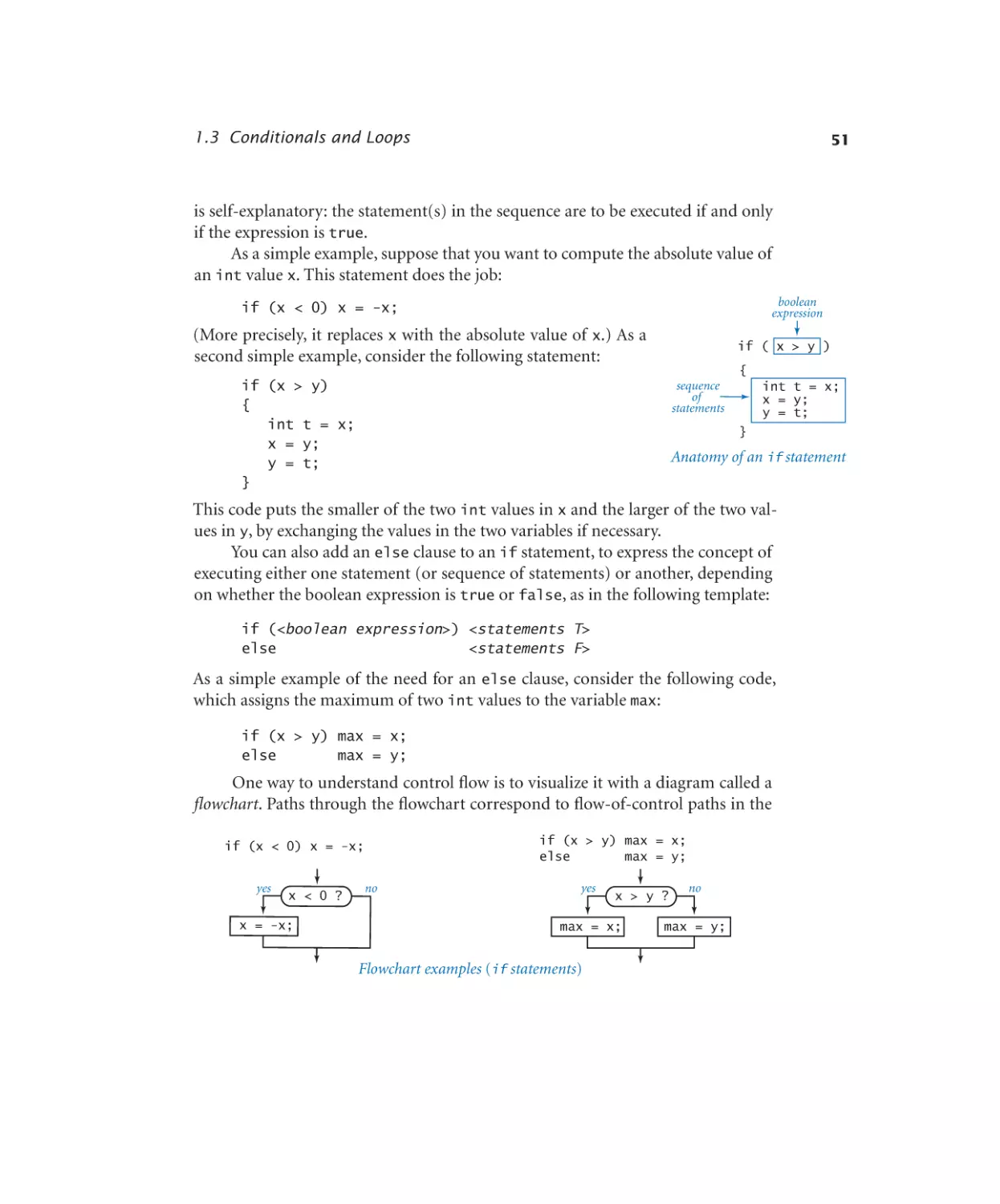
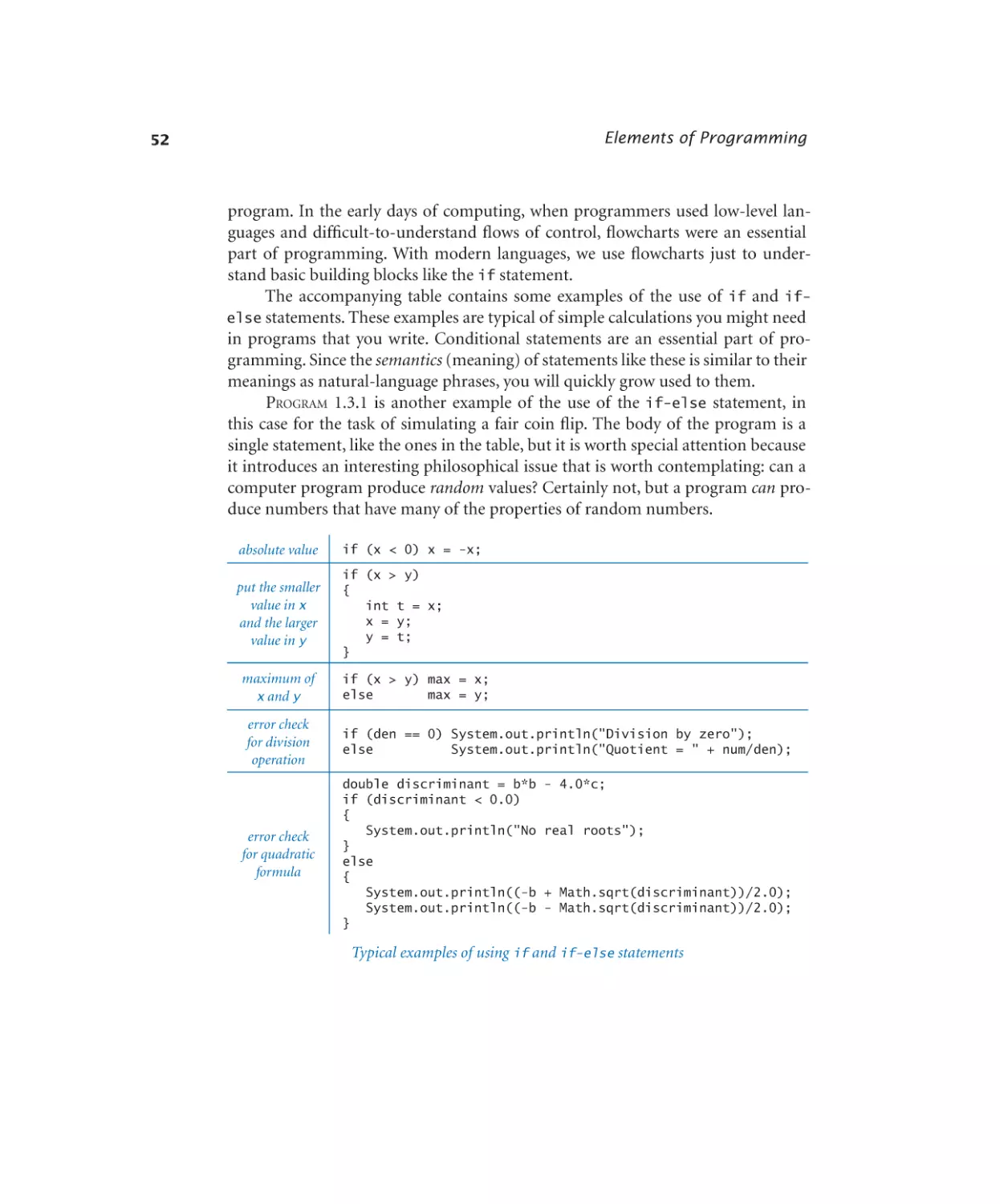
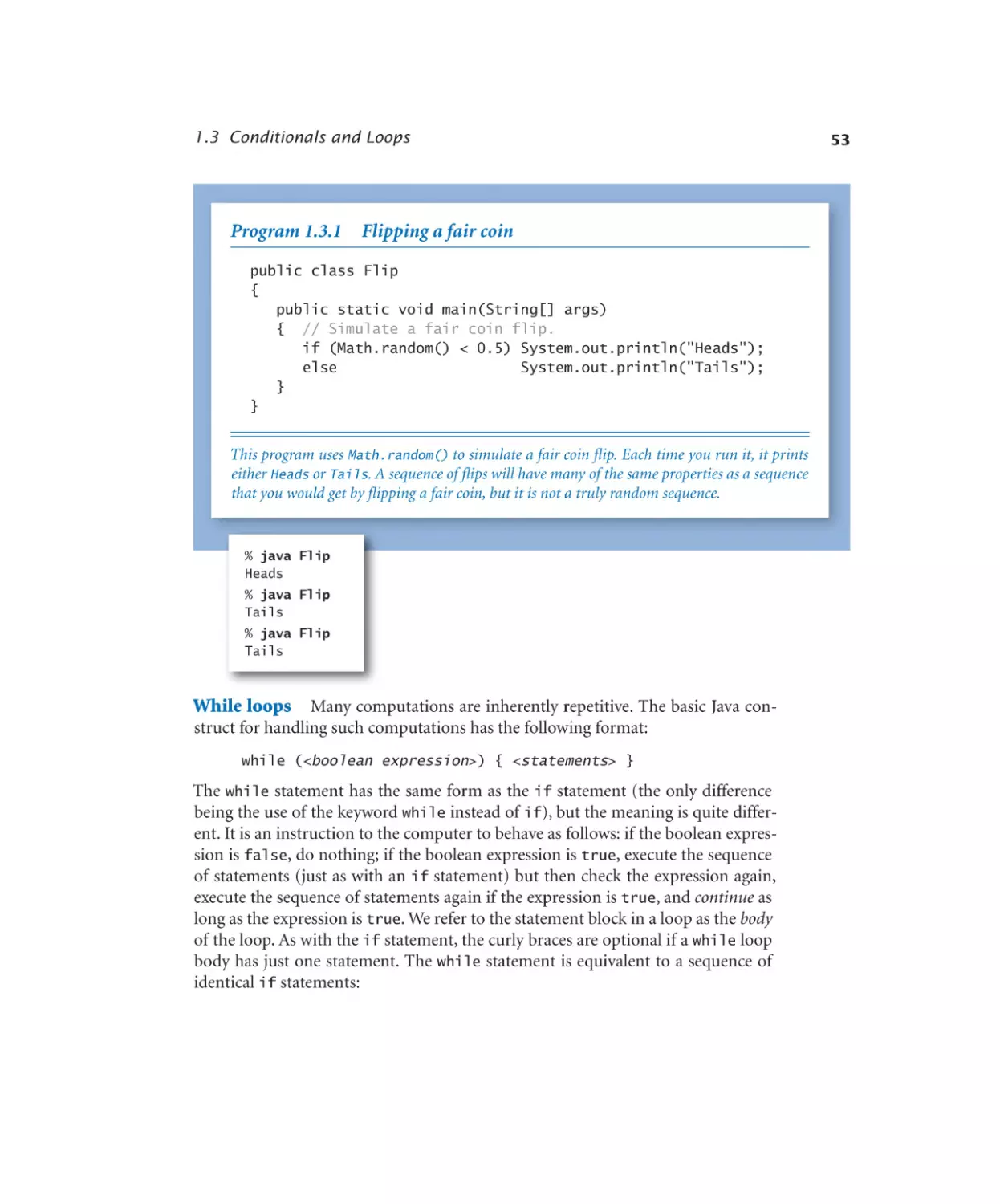
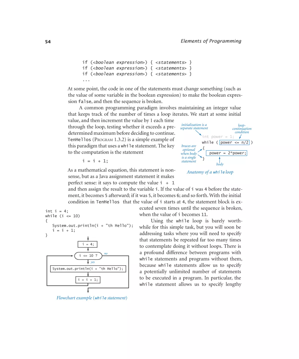
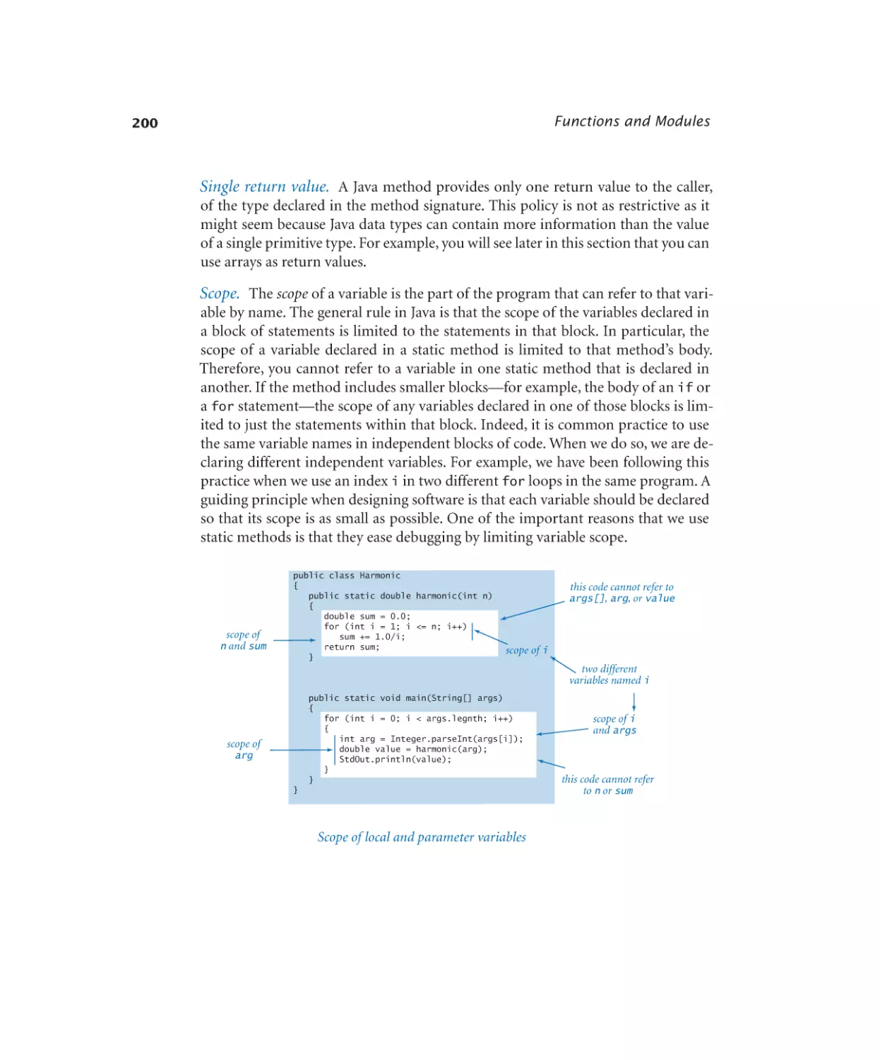
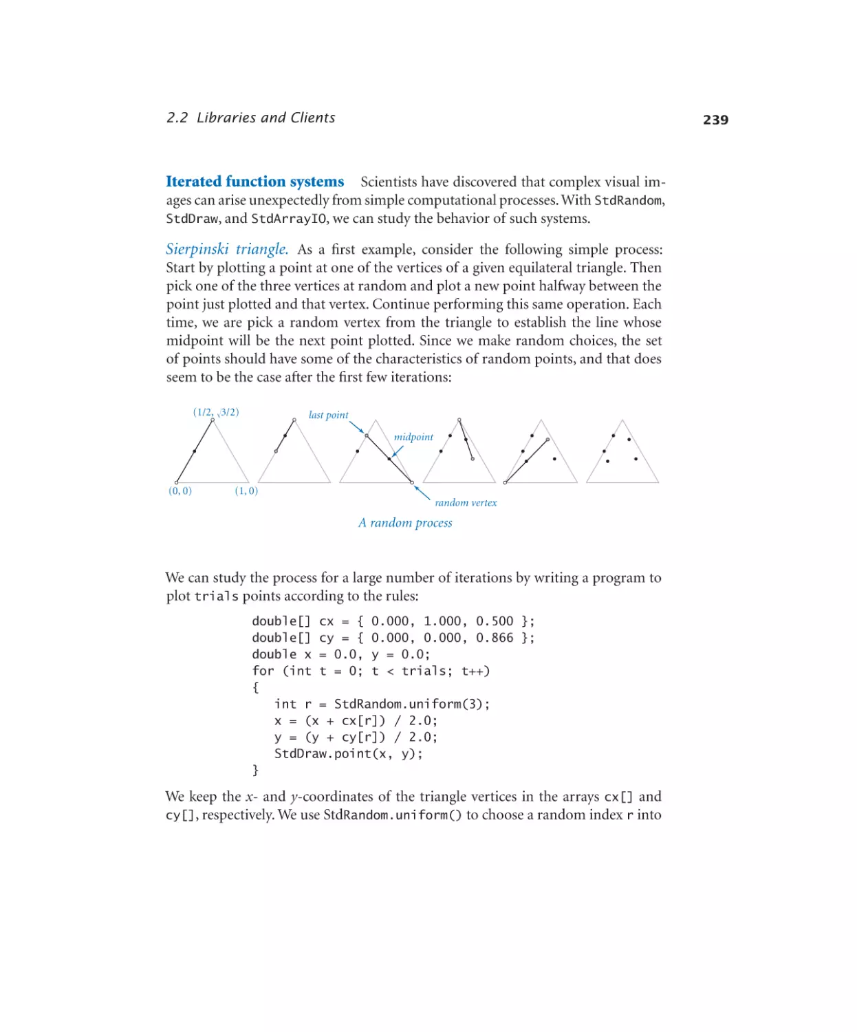
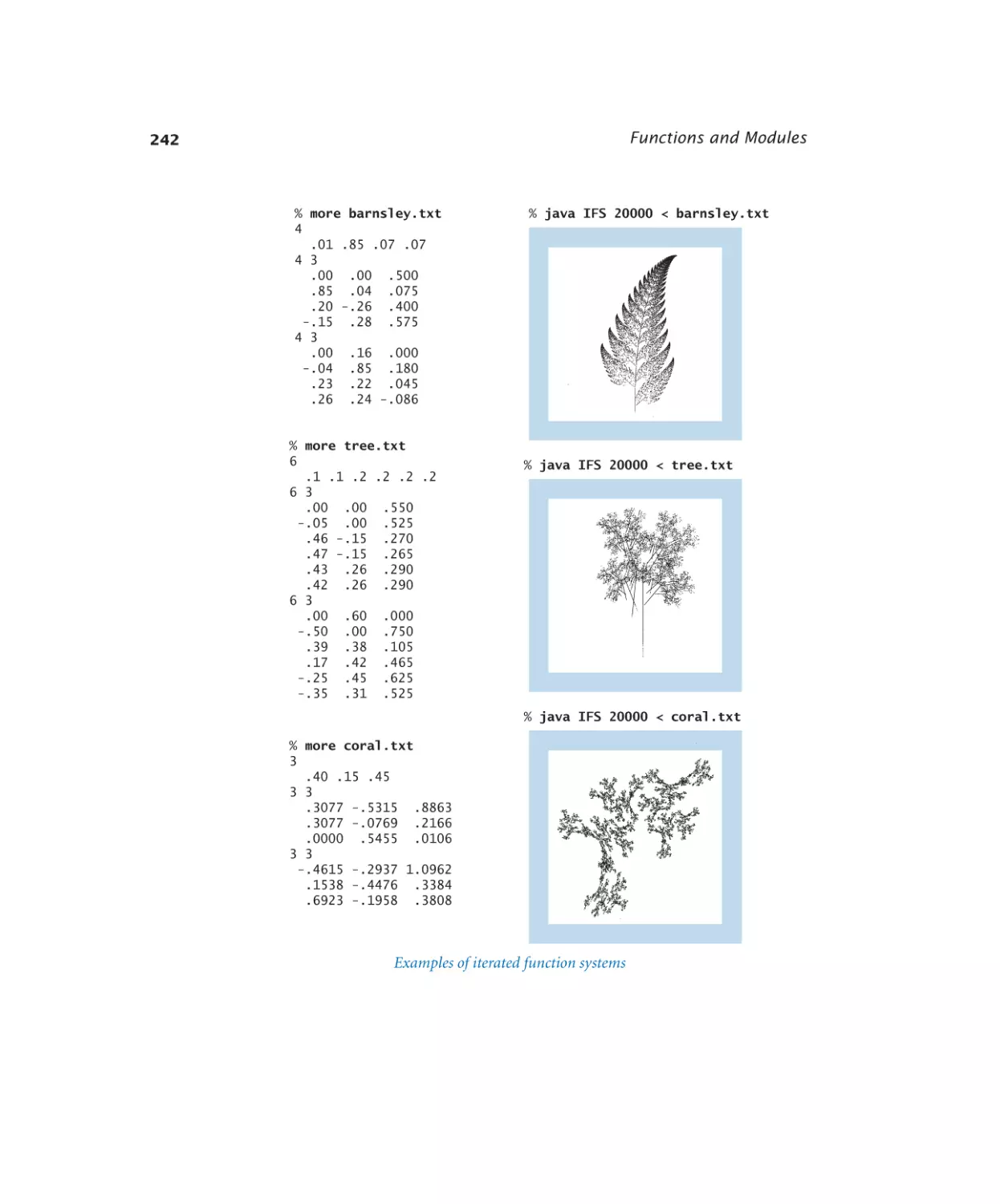
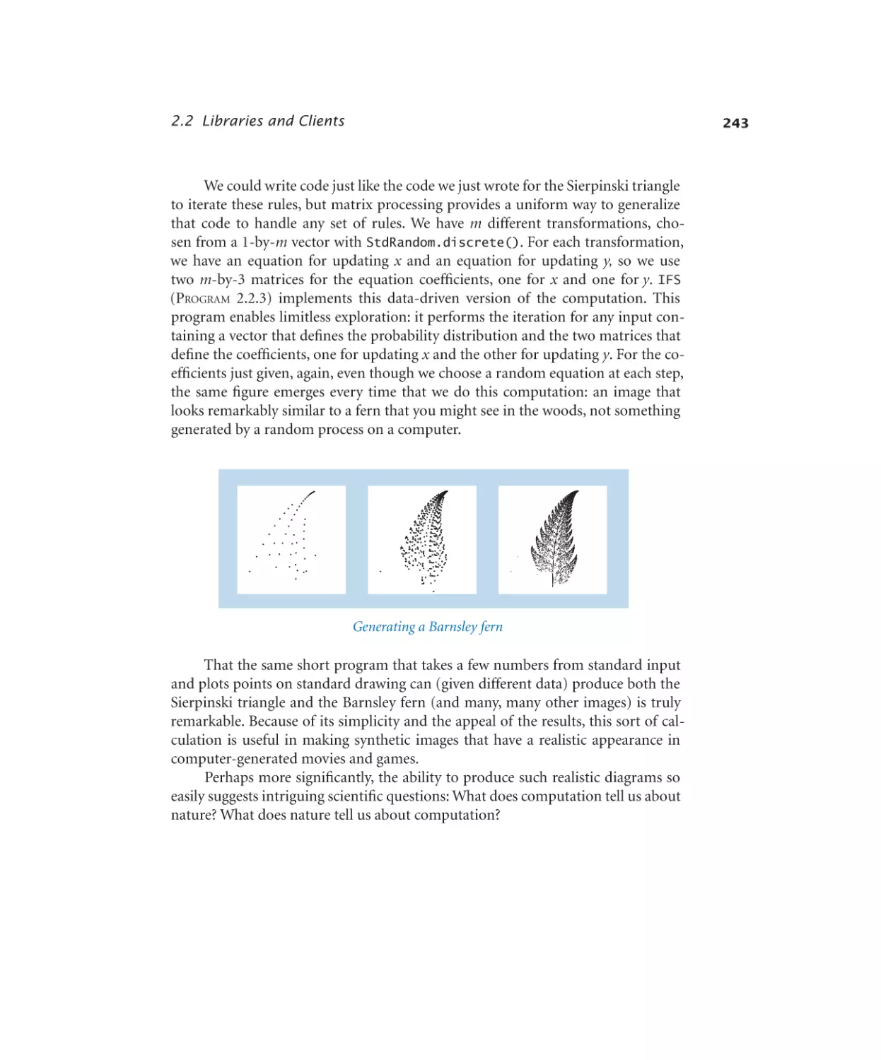
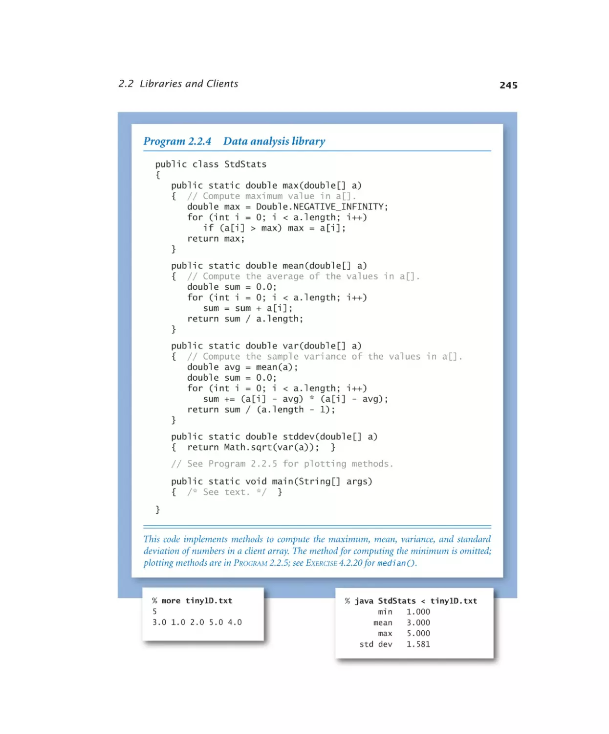
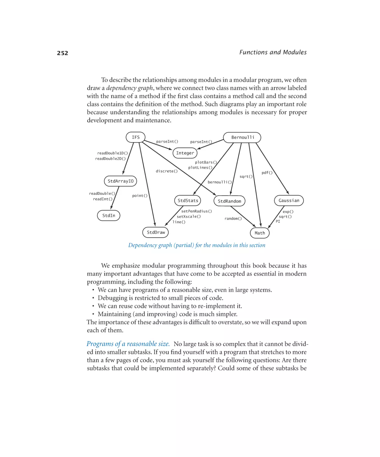
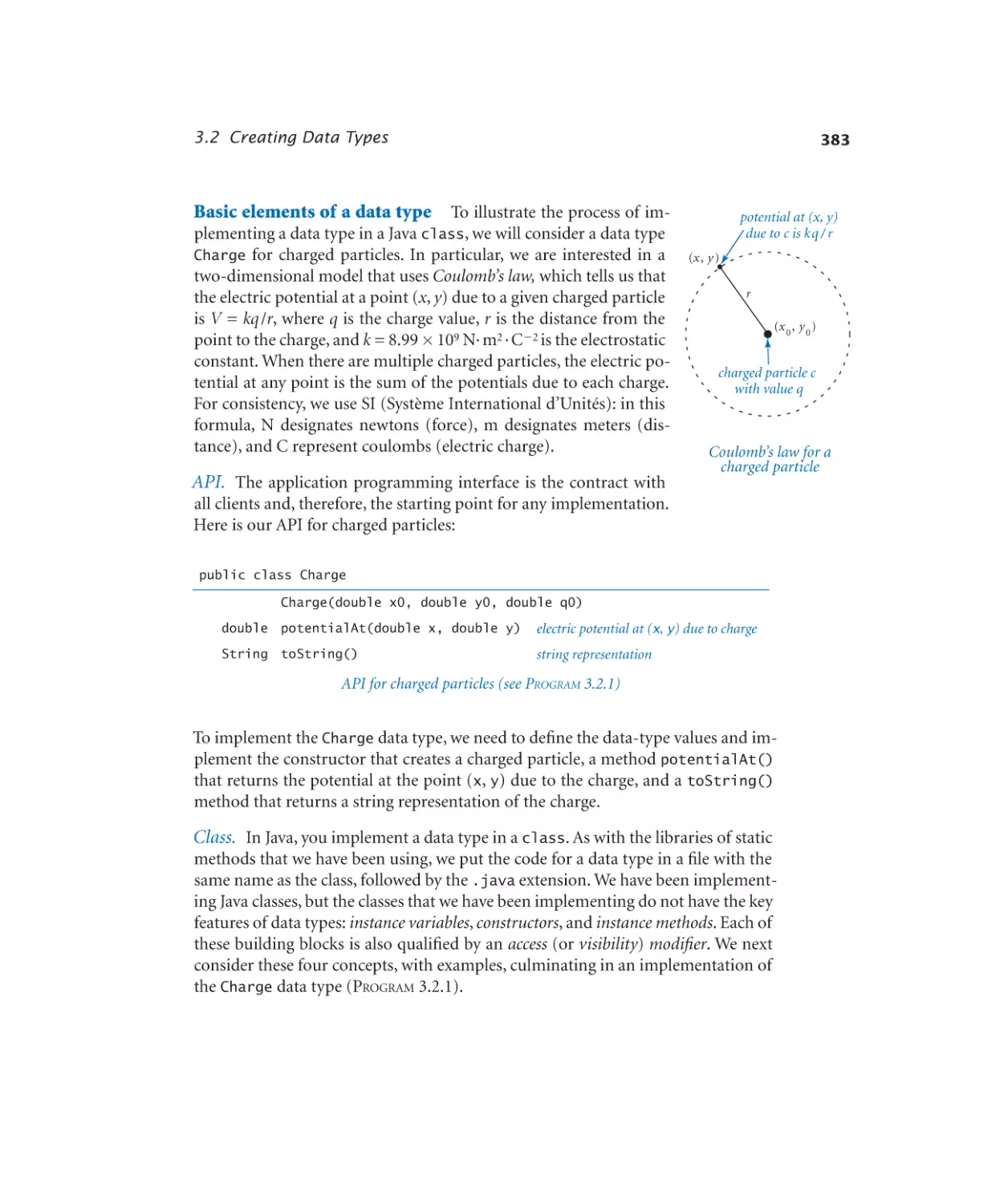
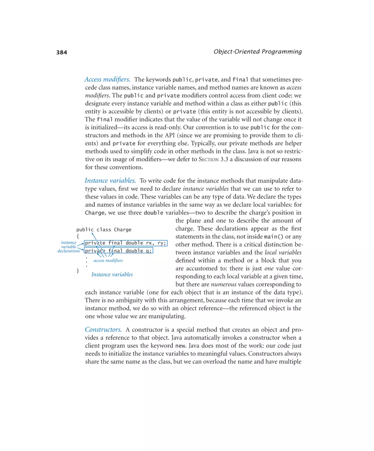
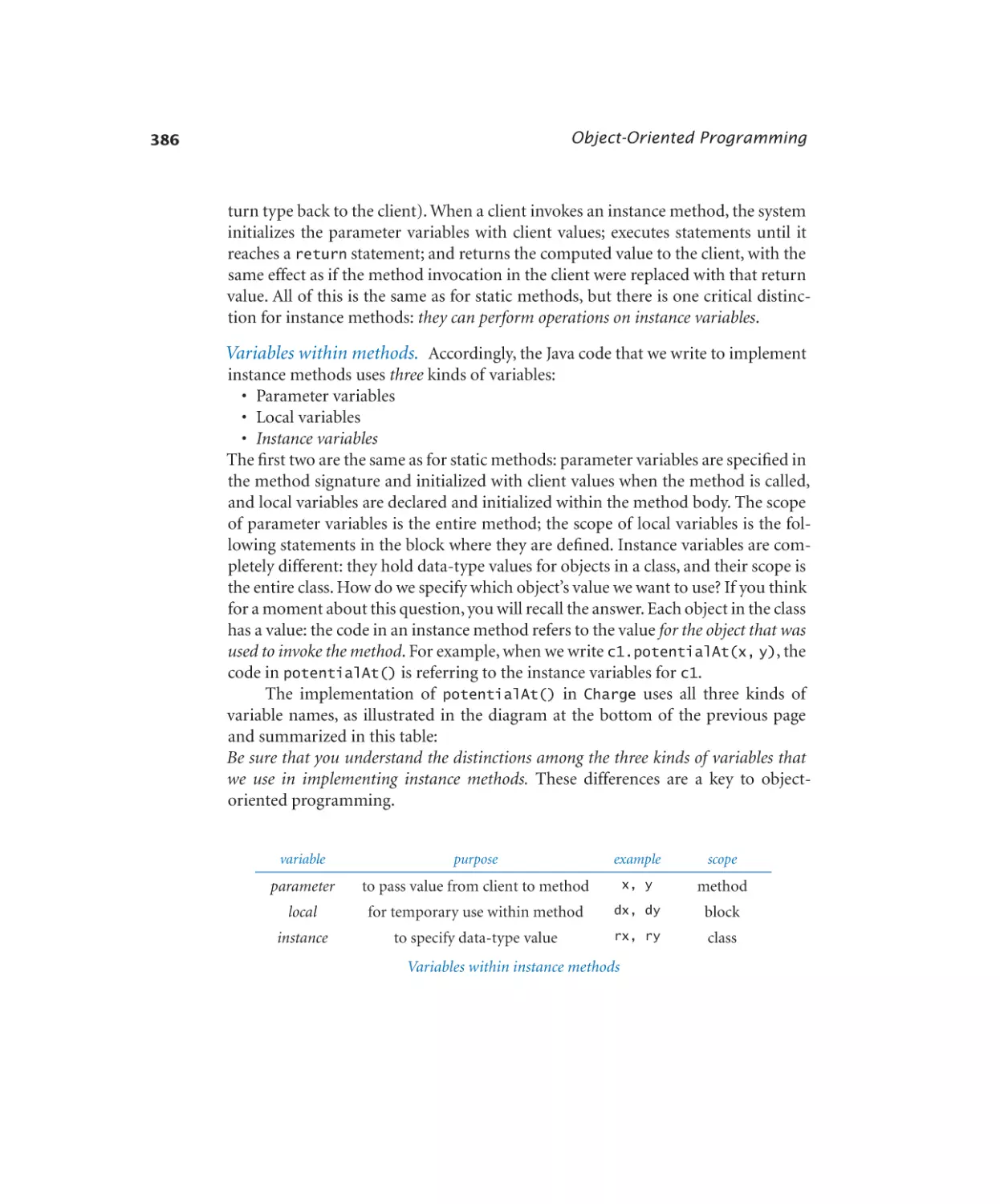
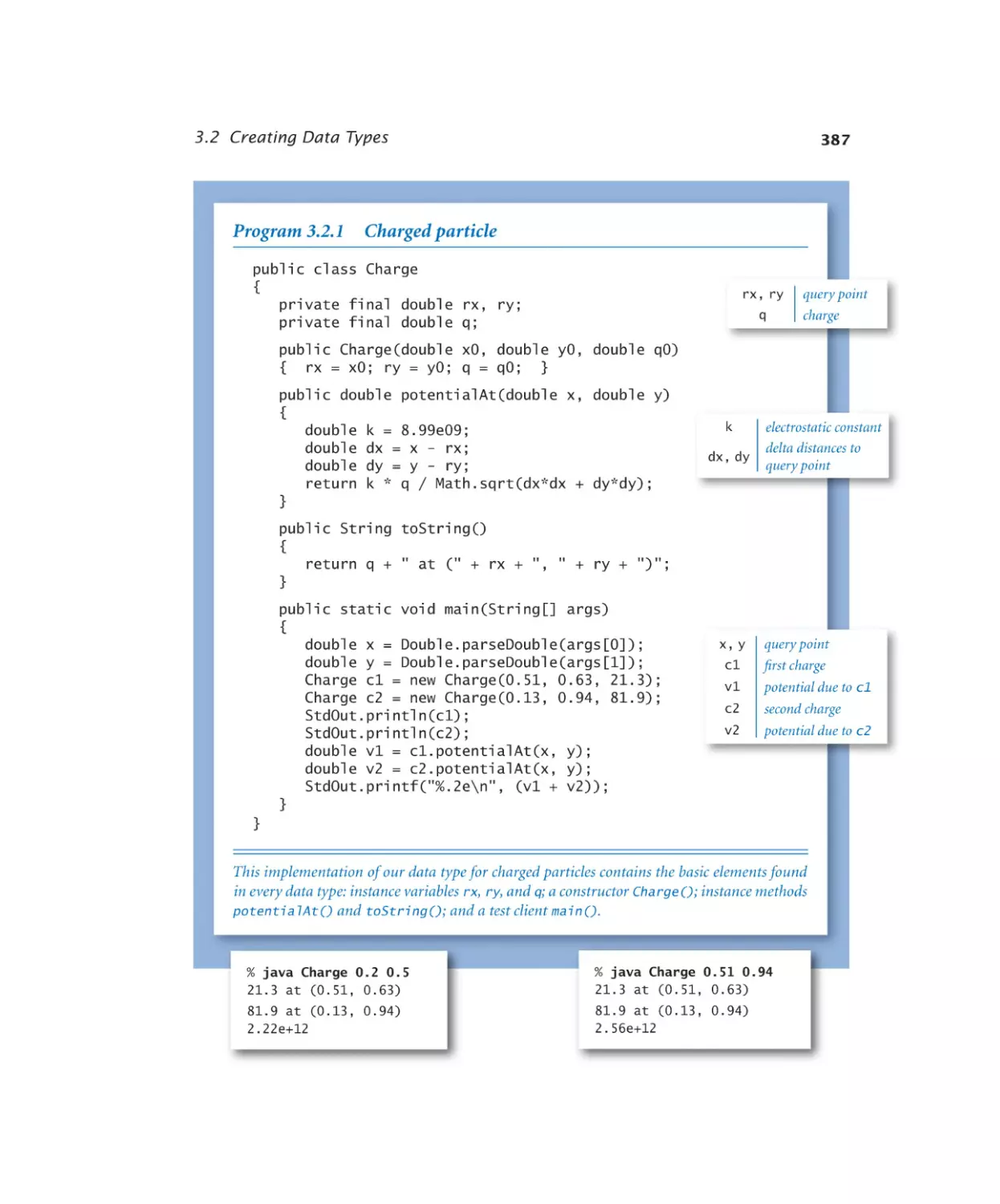
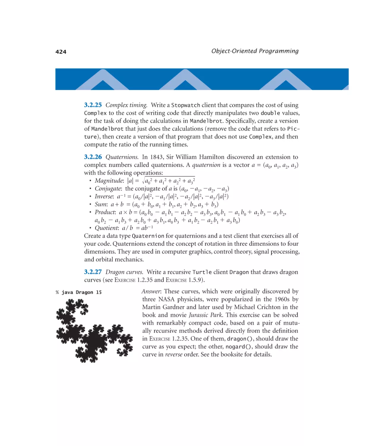
/


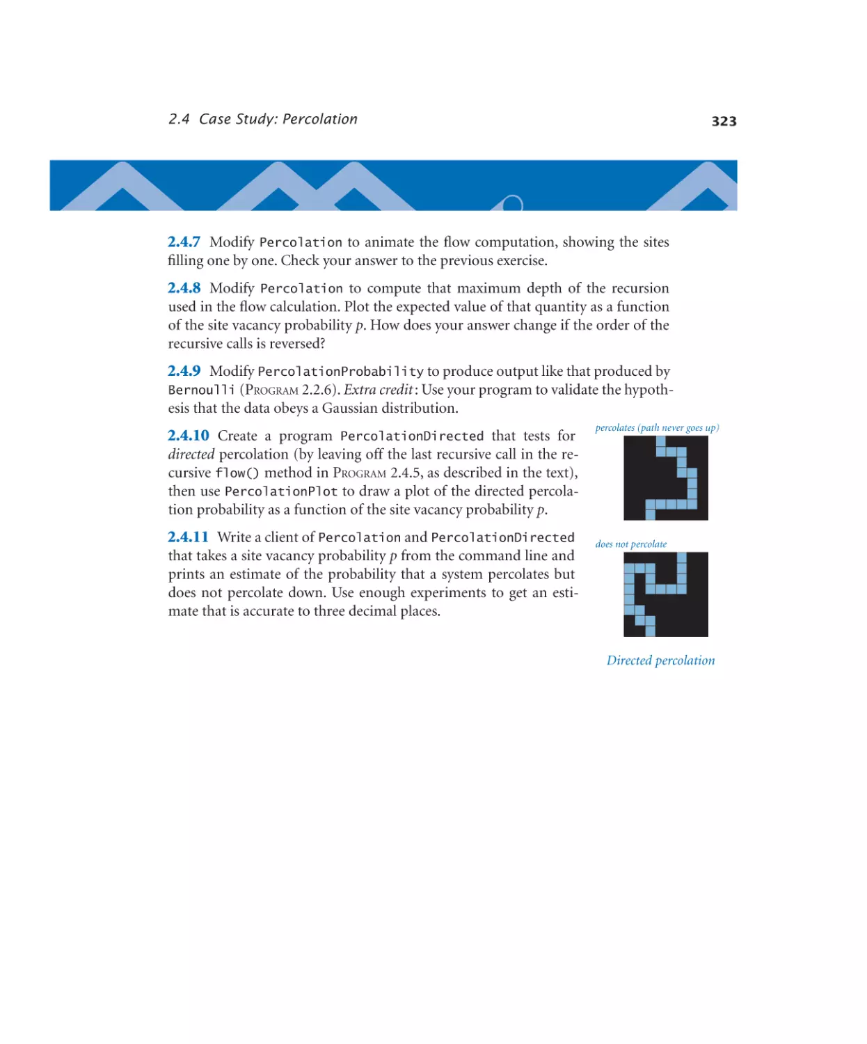

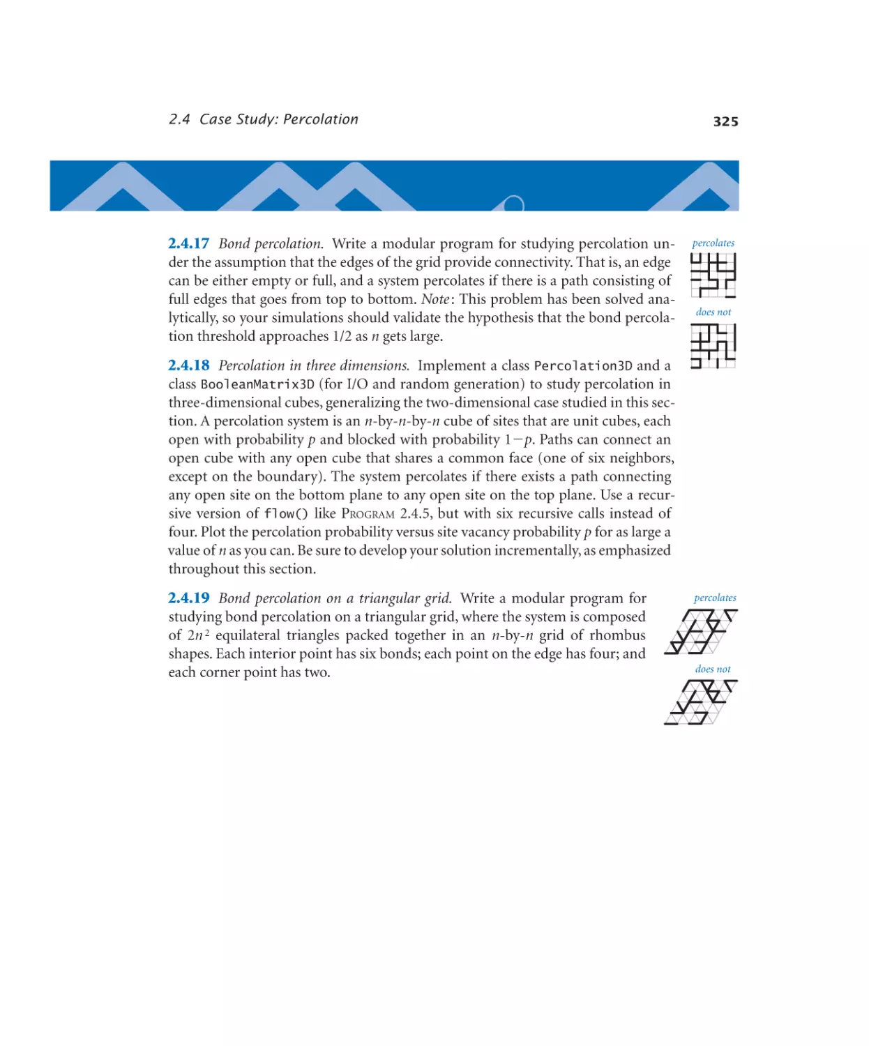
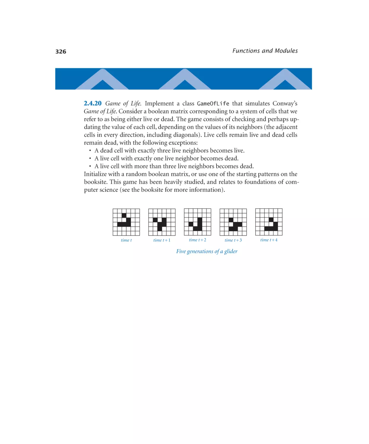


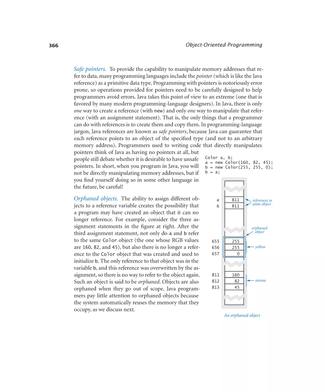


Автор: Sedgewick Robert Wayne Kevin
Теги: programming computer science
ISBN: 978-0-13-407642-3
Год: 2017


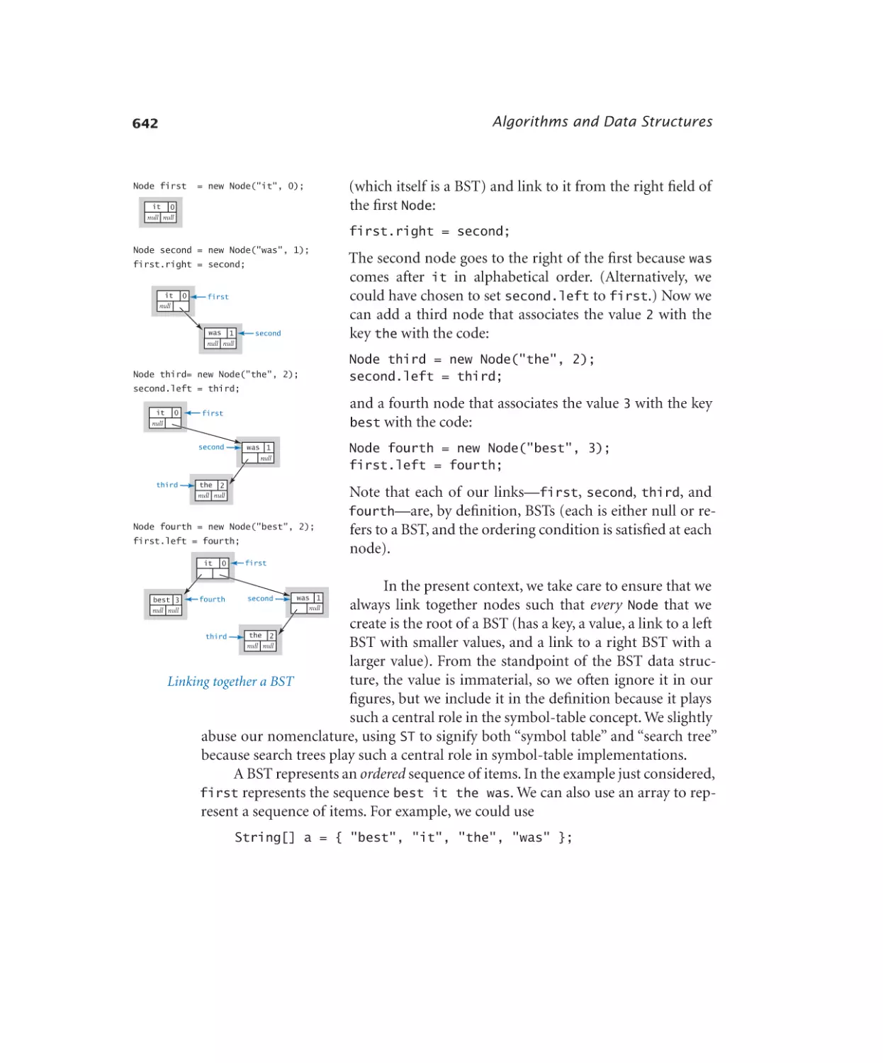
Текст
Computer
Science
This page intentionally left blank
Computer
Science
An Interdisciplinary Approach
Robert Sedgewick
Kevin Wayne
Princeton University
Boston • Columbus • Indianapolis • New York • San Francisco • Amsterdam • Cape Town
Dubai • London • Madrid • Milan • Munich • Paris • Montreal • Toronto • Delhi • Mexico City
Sāo Paulo • Sydney • Hong Kong • Seoul • Singapore • Taipei • Tokyo
Many of the designations used by manufacturers and sellers to distinguish their products are claimed
as trademarks. Where those designations appear in this book, and the publisher was aware of a trademark claim, the designations have been printed with initial capital letters or in all capitals.
The authors and publisher have taken care in the preparation of this book, but make no expressed
or implied warranty of any kind and assume no responsibility for errors or omissions. No liability is
assumed for incidental or consequential damages in connection with or arising out of the use of the
information or programs contained herein.
For information about buying this title in bulk quantities, or for special sales opportunities (which
may include electronic versions; custom cover designs; and content particular to your business, training goals, marketing focus, or branding interests), please contact our corporate sales department at
corpsales@pearsoned.com or (800) 382-3419.
For government sales inquiries, please contact governmentsales@pearsoned.com.
For questions about sales outside the United States, please contact intlcs@pearson.com.
Visit us on the Web: informit.com/aw
Library of Congress Control Number: 2016936496
Copyright © 2017 Pearson Education, Inc.
All rights reserved. Printed in the United States of America. This publication is protected by copyright, and permission must be obtained from the publisher prior to any prohibited reproduction,
storage in a retrieval system, or transmission in any form or by any means, electronic, mechanical,
photocopying, recording, or likewise. For information regarding permissions, request forms, and the
appropriate contacts within the Pearson Education Global Rights & Permissions Department, please
visit www.pearsoned.com/permissions/.
ISBN-13: 978-0-13-407642-3
ISBN-10: 0-13-407642-7
2
16
______________________________
To Adam, Andrew, Brett, Robbie,
Henry, Iona, Rose, Peter,
and especially Linda
______________________________
______________________________
To Jackie, Alex, and Michael
______________________________
Contents
Preface . . . . . . . . . . . . . . . . . . . . xiii
1—Elements of Programming . . . . . . . . . . . . 1
1.1 Your First Program
2
1.2 Built-in Types of Data
14
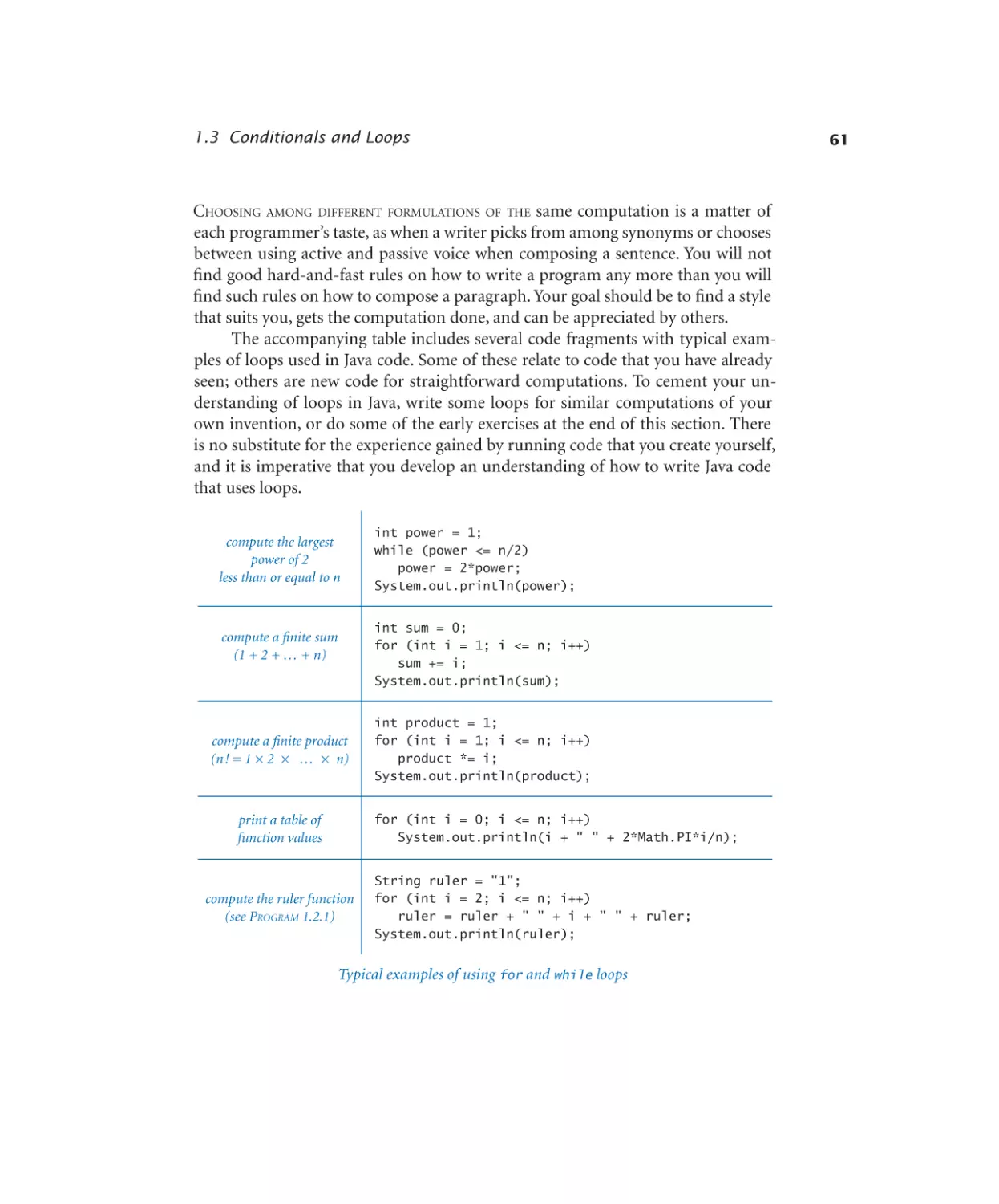
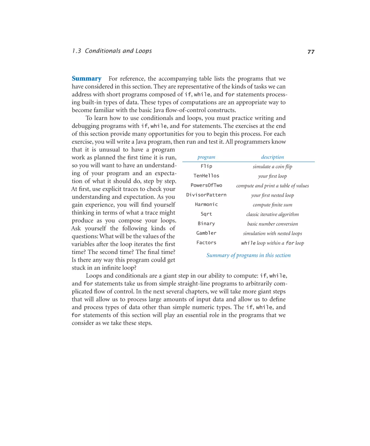
1.3 Conditionals and Loops
50
1.4 Arrays
90
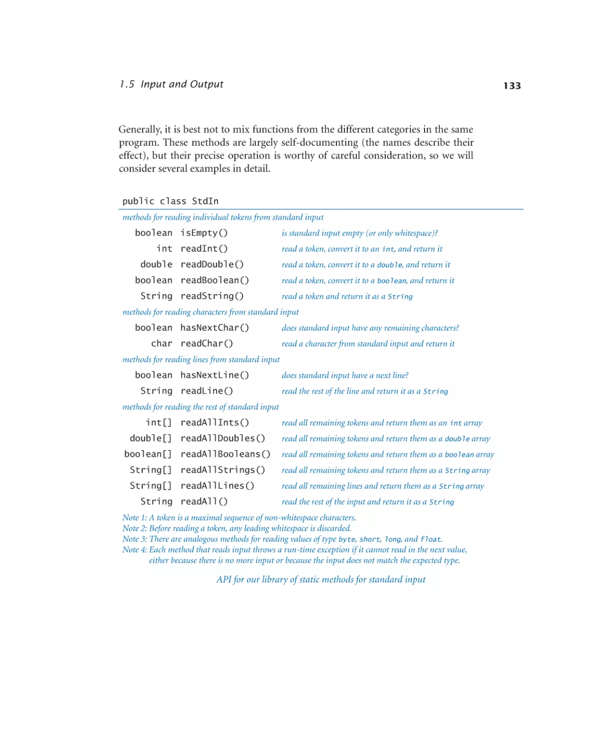
1.5 Input and Output
126
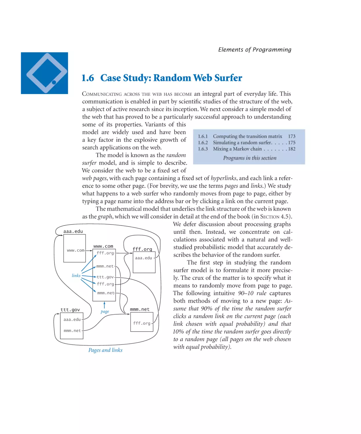
1.6 Case Study: Random Web Surfer
170
2—Functions and Modules . . . . . . . . . . . .
2.1 Defining Functions
192
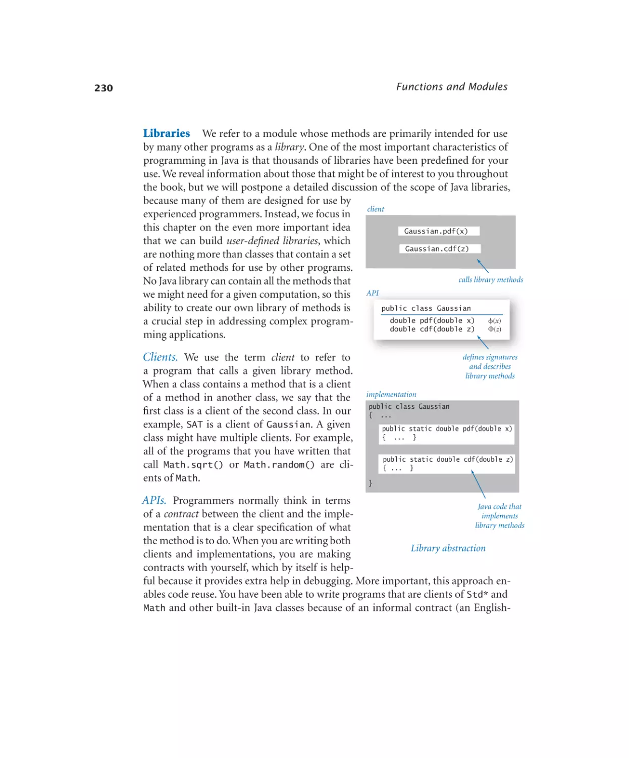
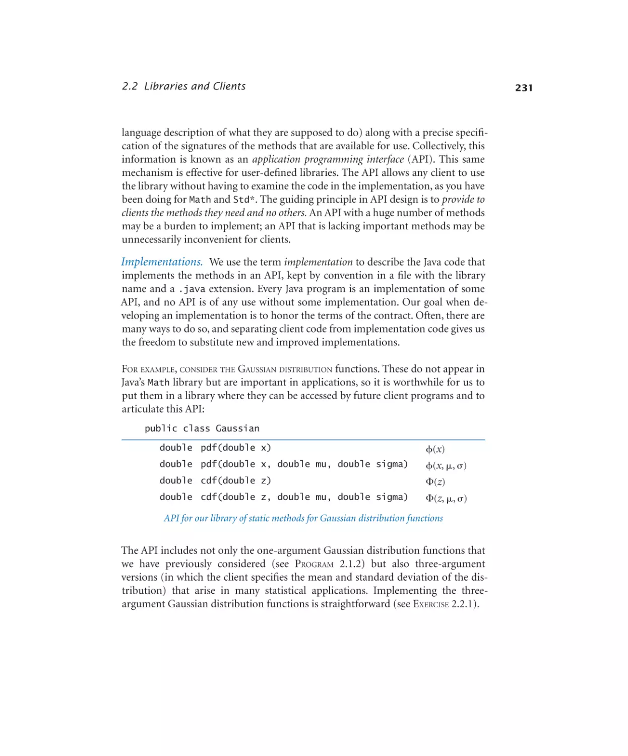
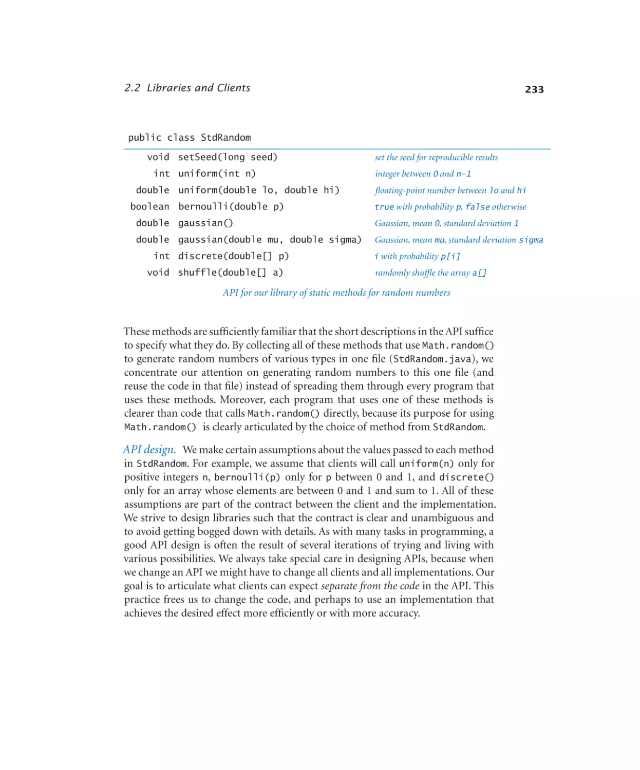
2.2 Libraries and Clients
226
2.3 Recursion
262
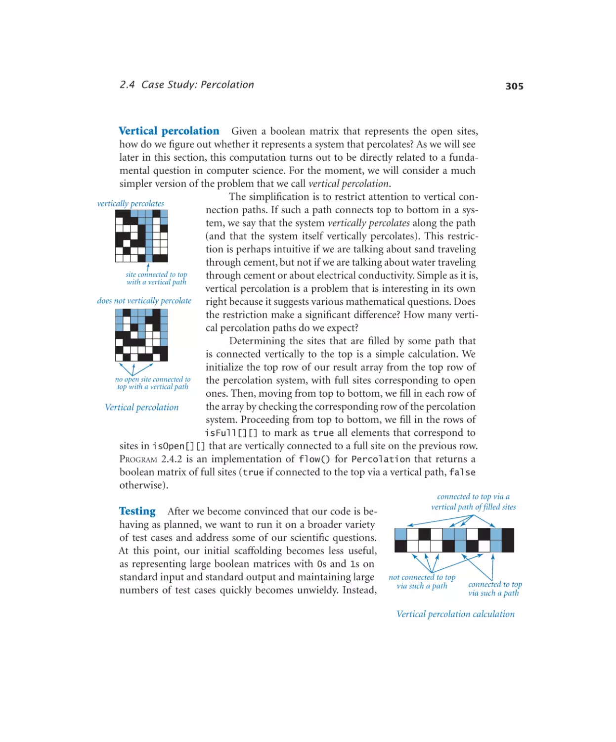
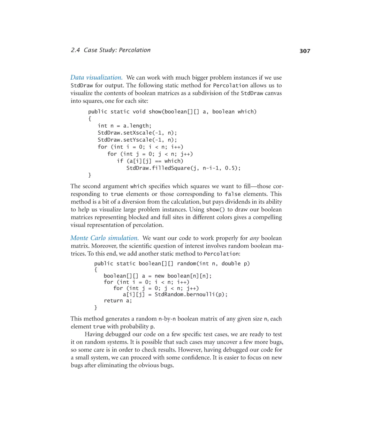
2.4 Case Study: Percolation
300
191
3—Object-Oriented Programming . . . . . . . . .
3.1 Using Data Types
330
3.2 Creating Data Types
382
3.3 Designing Data Types
428
3.4 Case Study: N-Body Simulation
478
329
4—Algorithms and Data Structures . . . . . . . . . 493
4.1 Performance
494
4.2 Sorting and Searching
532
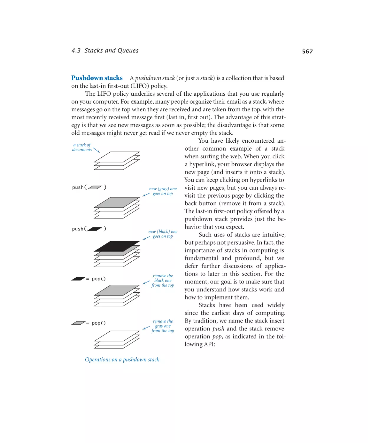
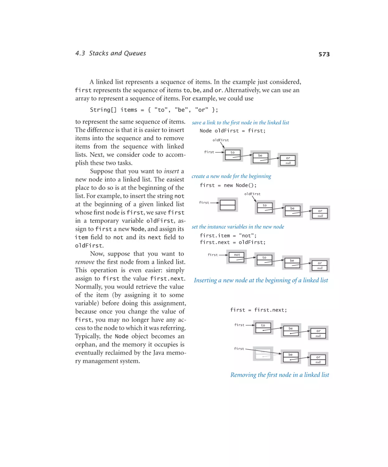
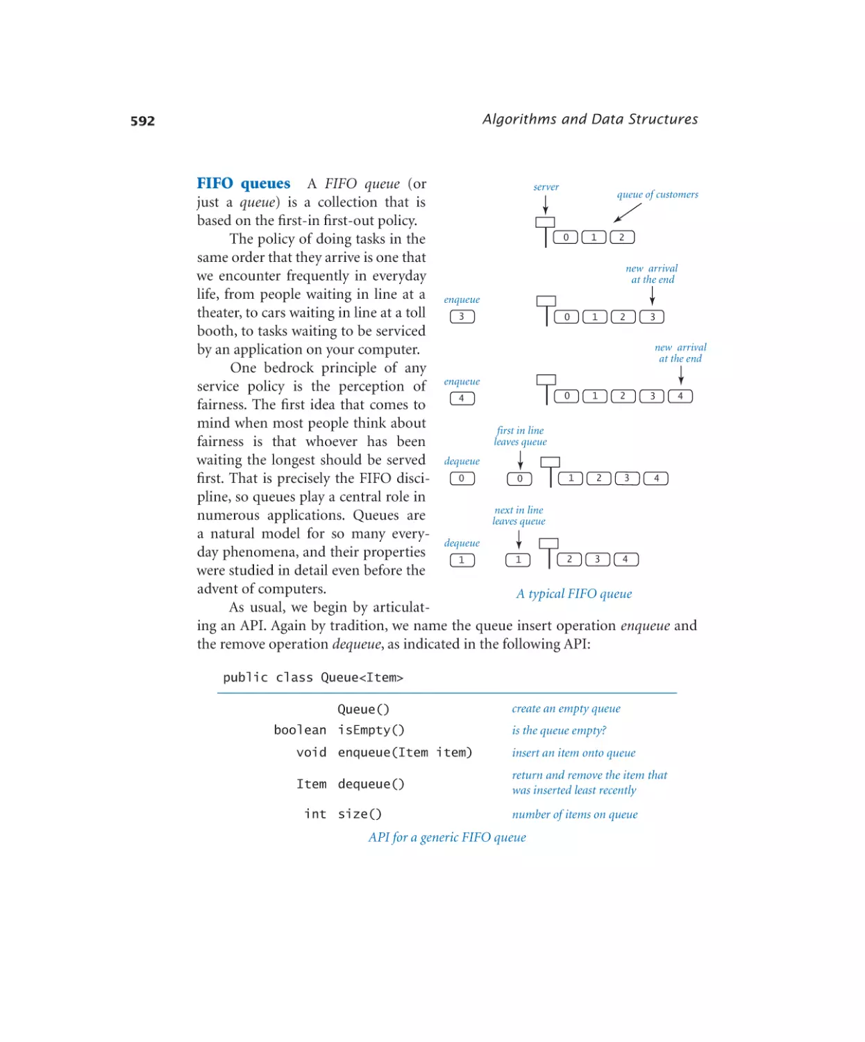
4.3 Stacks and Queues
566
4.4 Symbol Tables
624
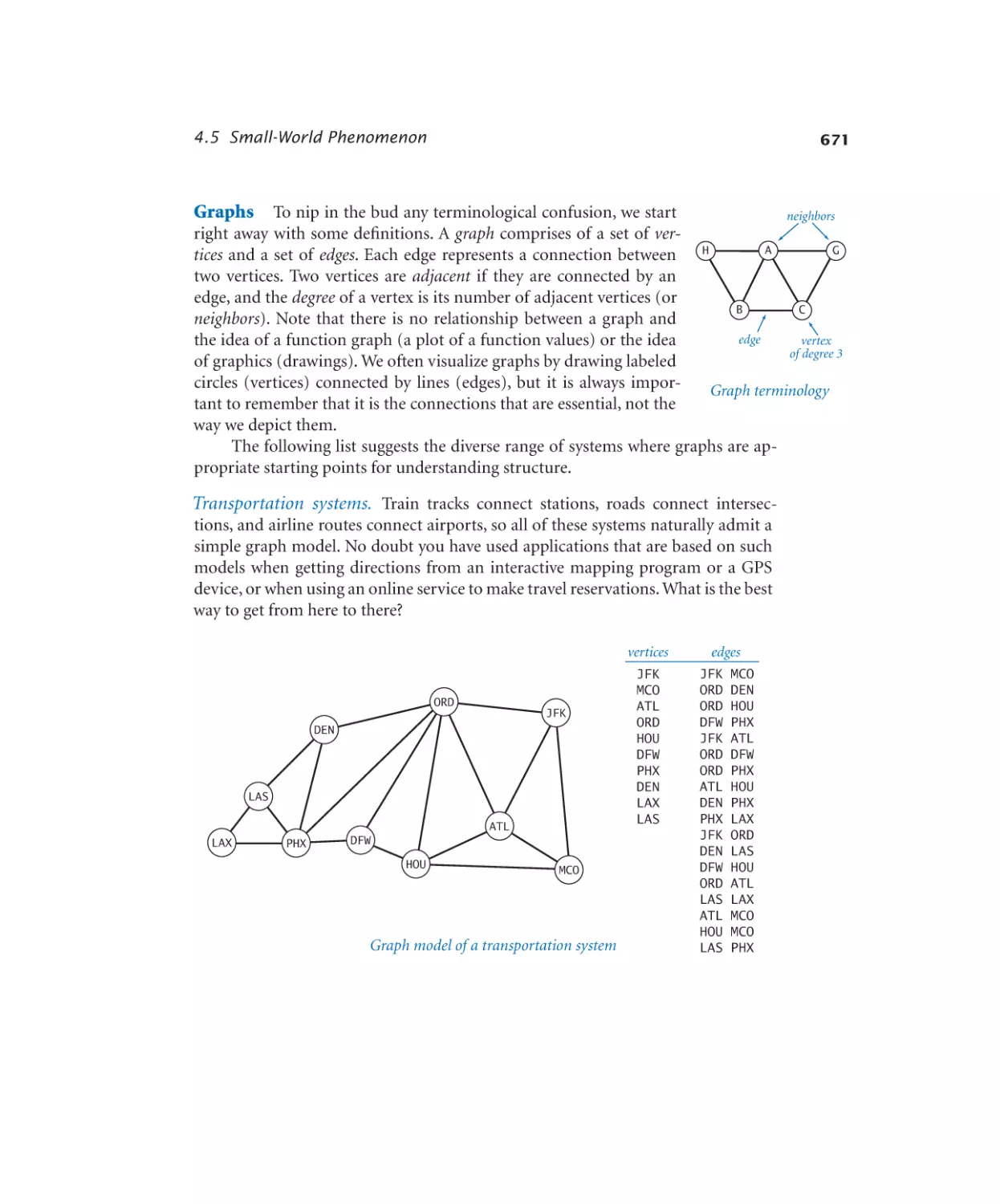
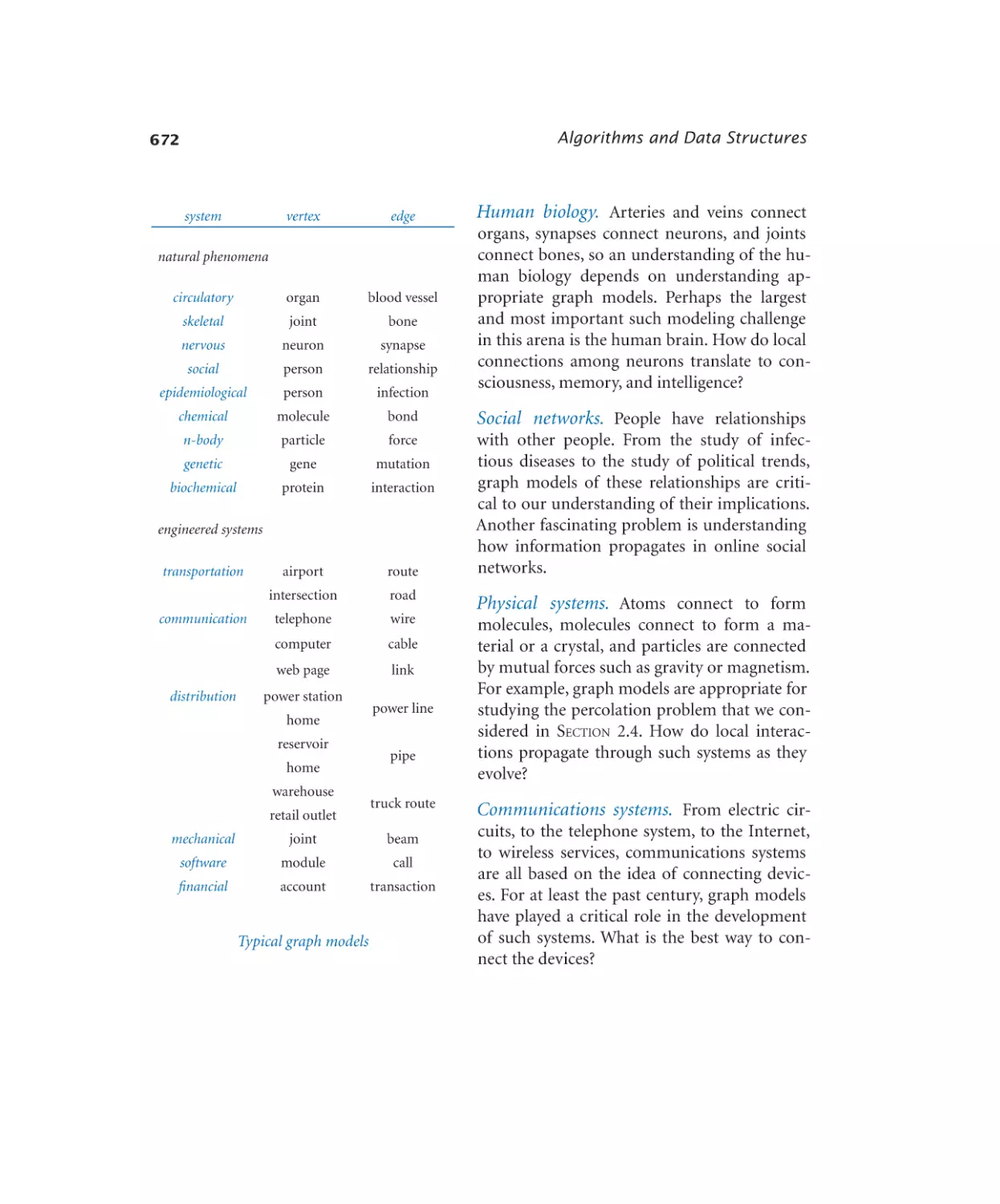
4.5 Case Study: Small-World Phenomenon
670
vi
5—Theory of Computing . . . . . . . . . . . . . 715
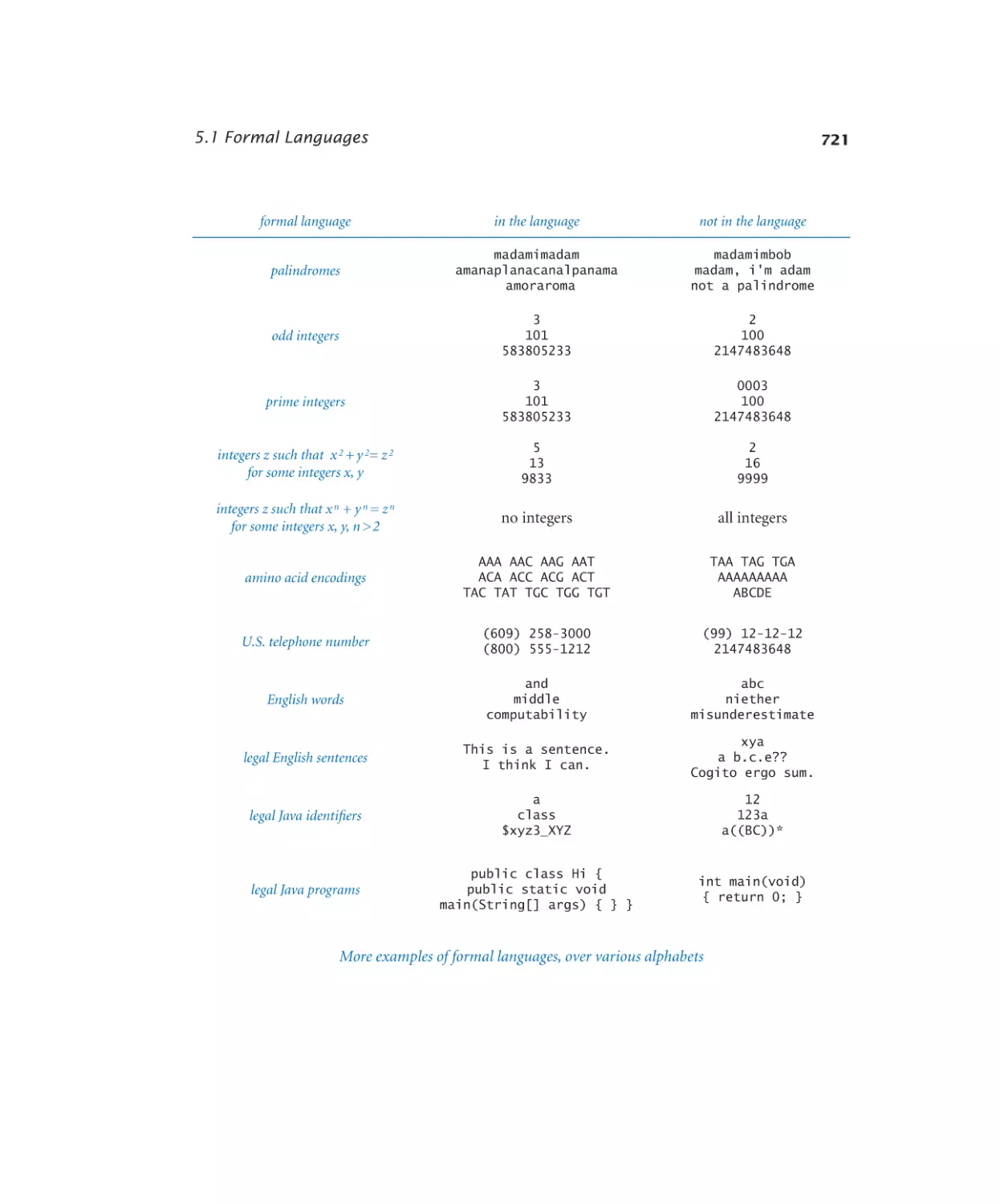
5.1 Formal Languages
718
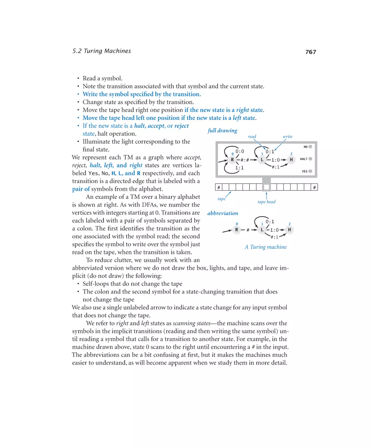
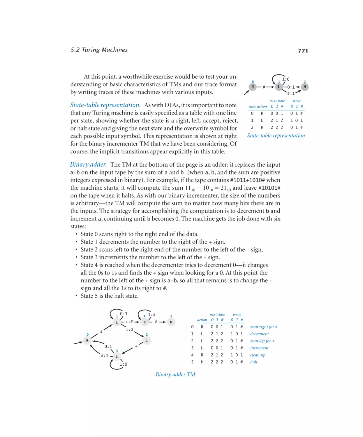
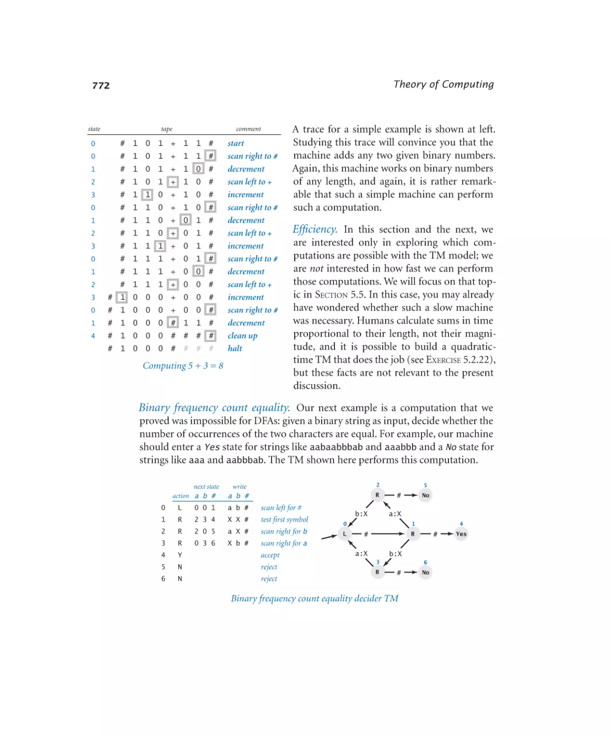
5.2 Turing Machines
766
5.3 Universality
786
5.4 Computability
806
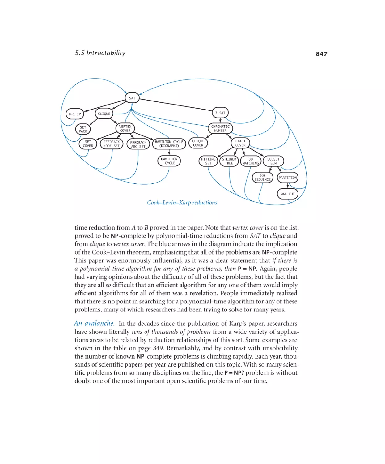
5.5 Intractability
822
6—A Computing Machine. . . . . . . . . . . . . 873
6.1 Representing Information
874
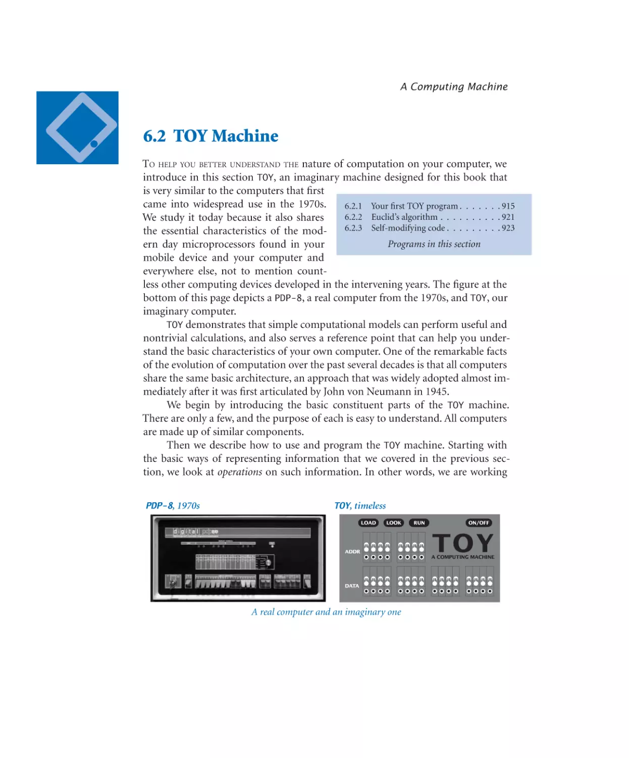
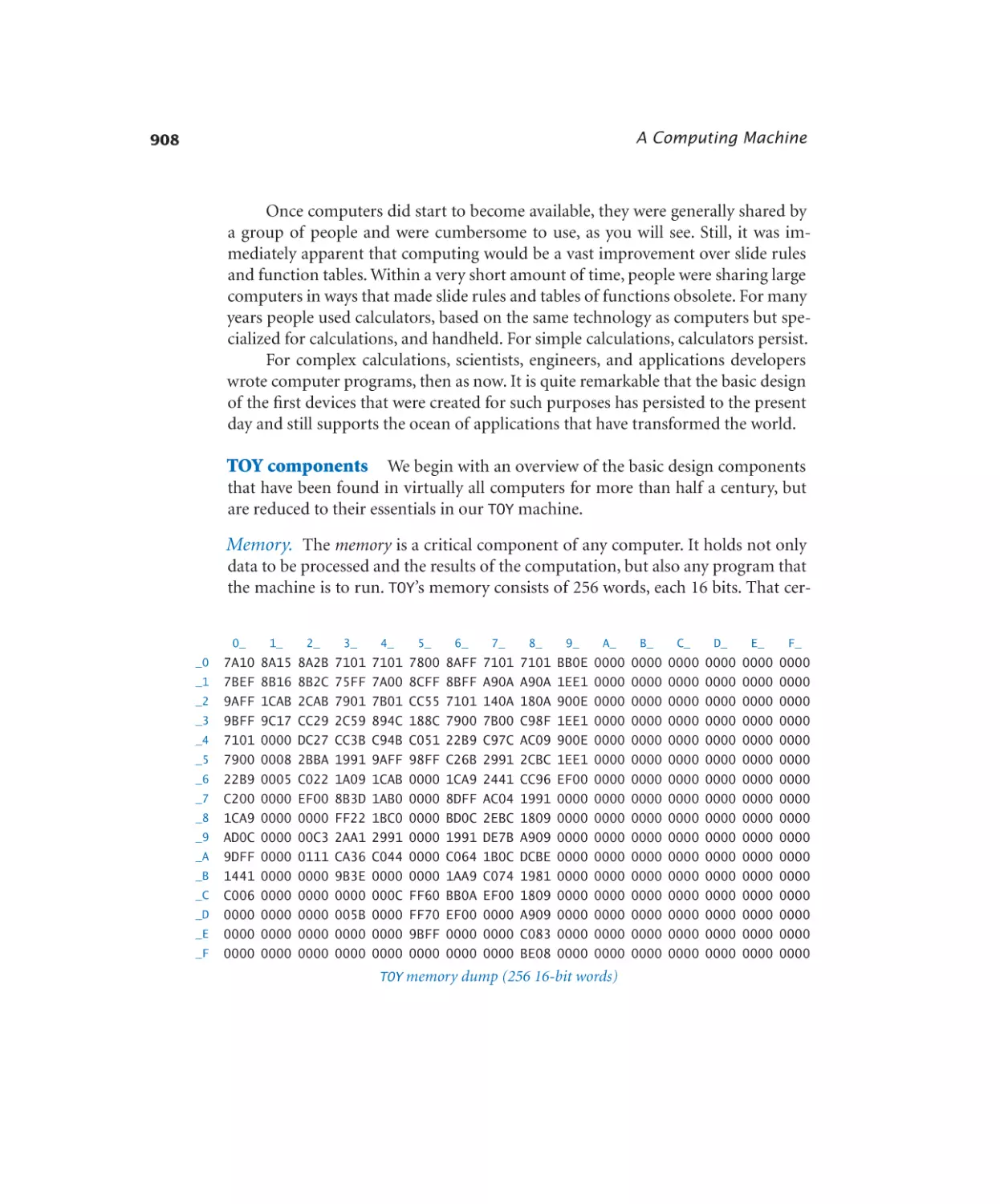
6.2 TOY Machine
906
6.3 Machine-Language Programming
930
6.4 TOY Virtual Machine
958
7—Building a Computing Device . . . . . . . . . . 985
7.1 Boolean Logic
986
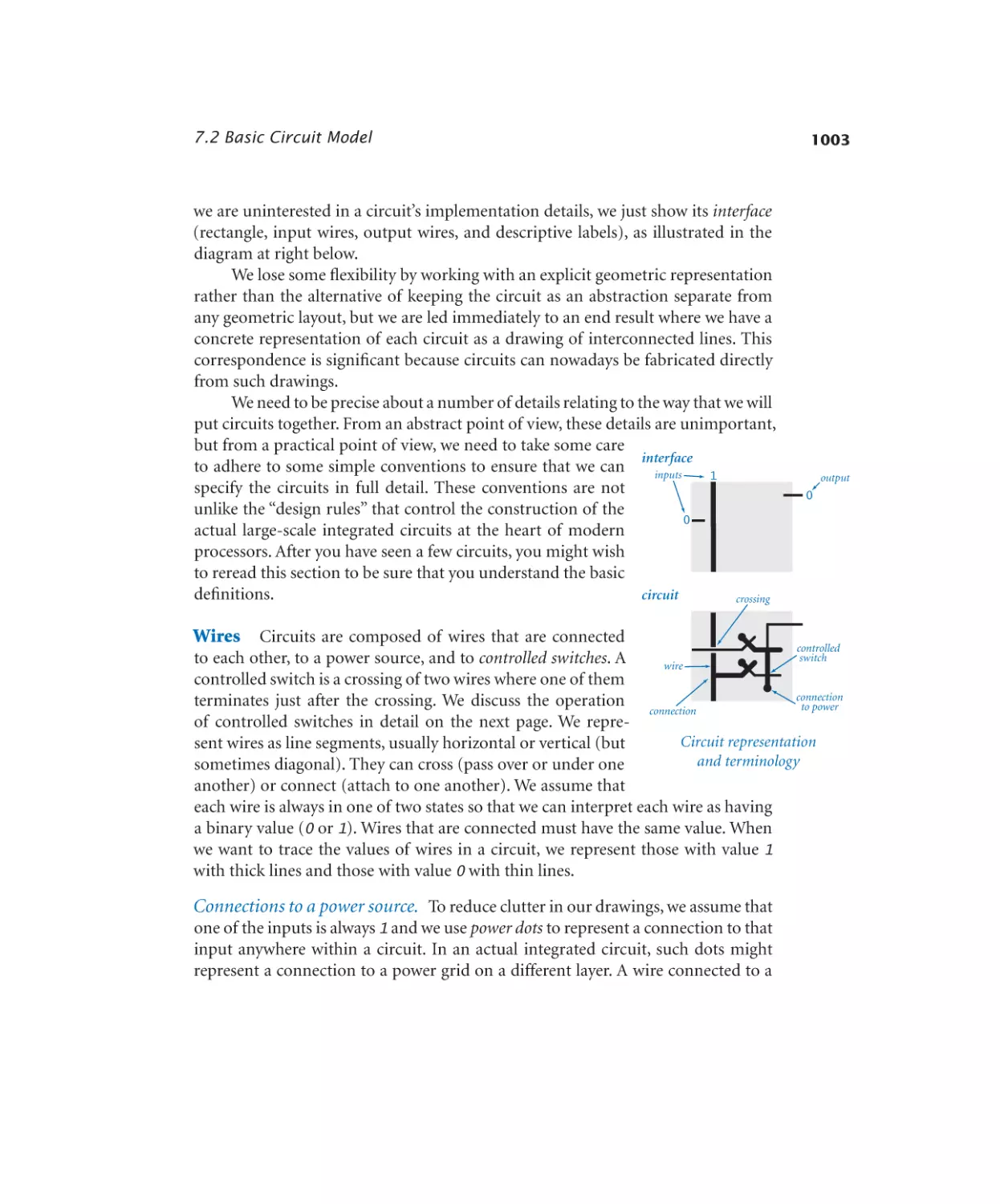
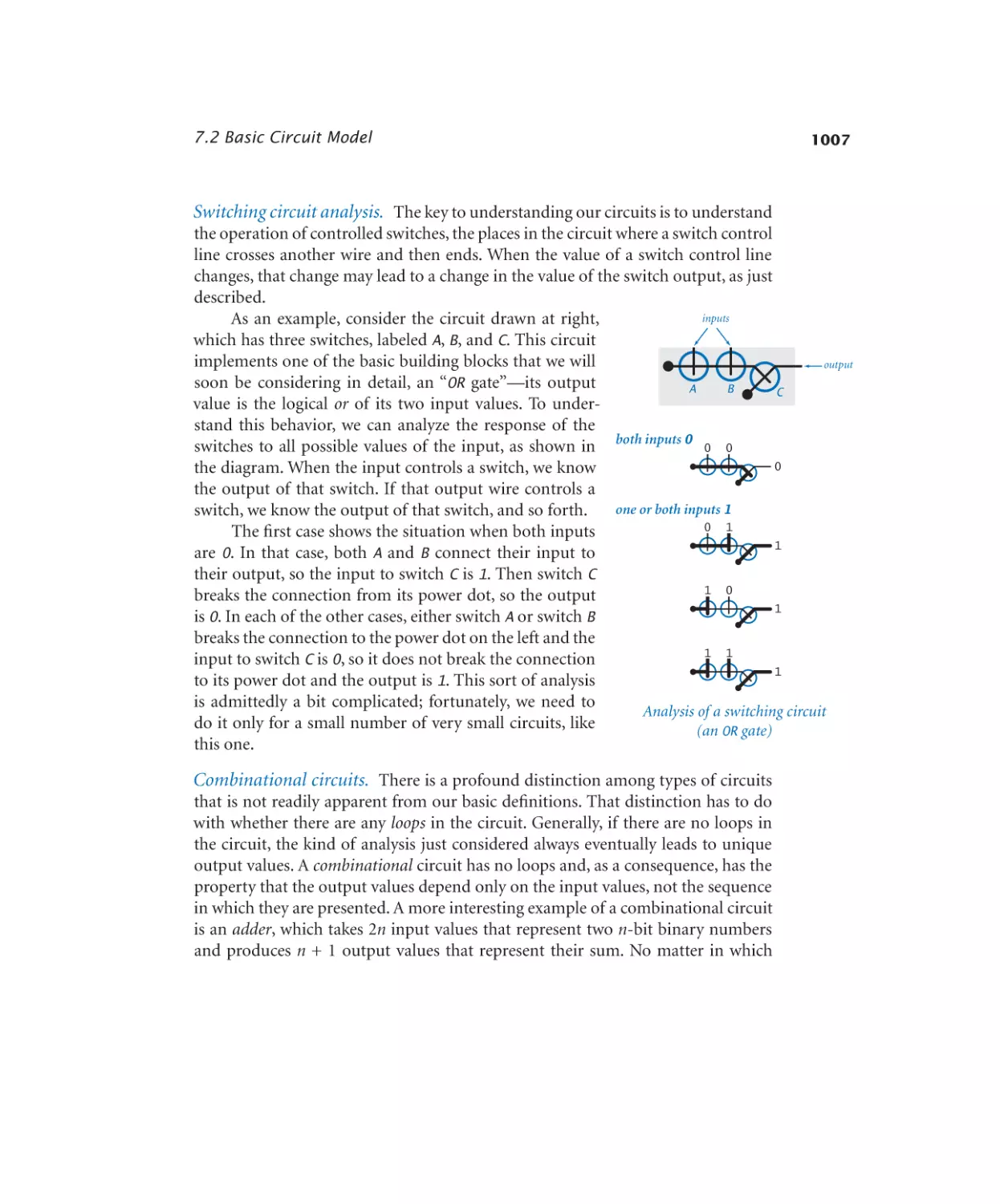
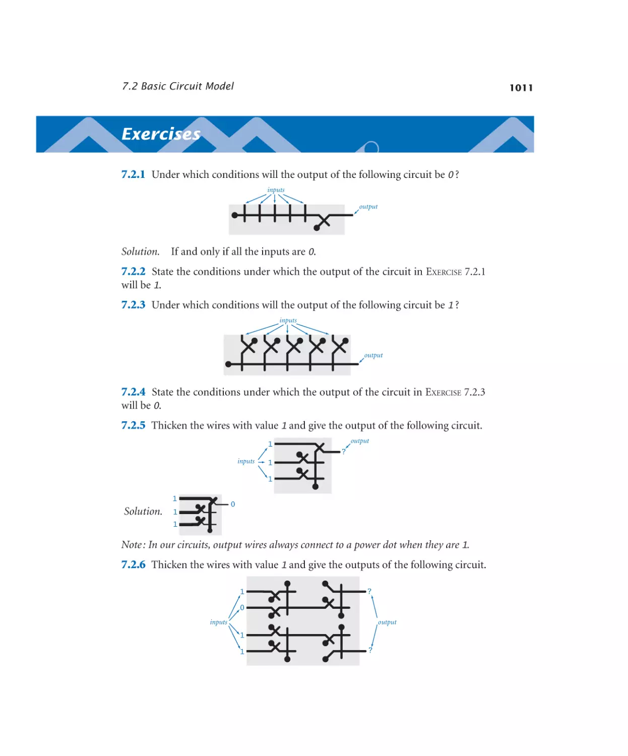
7.2 Basic Circuit Model
1002
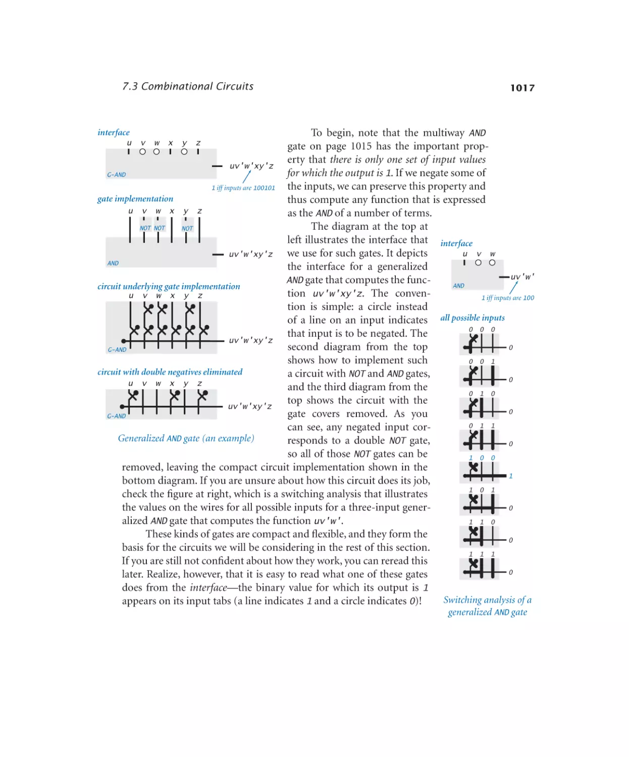
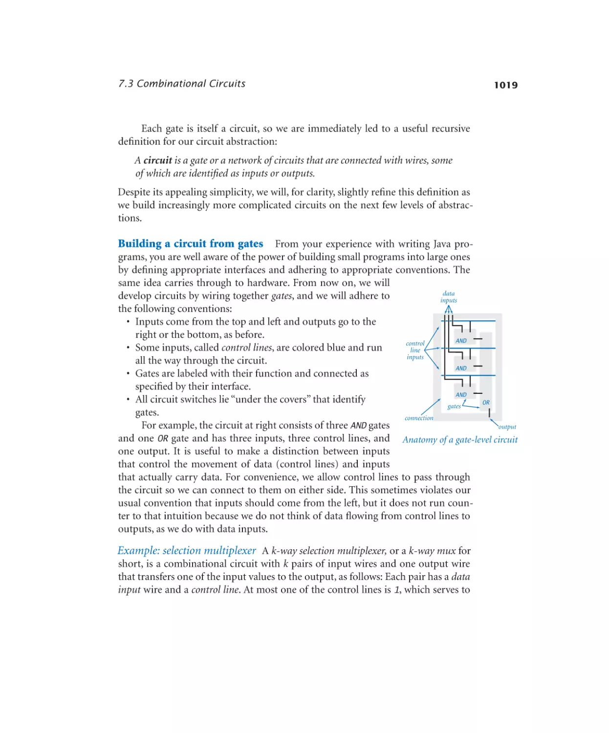
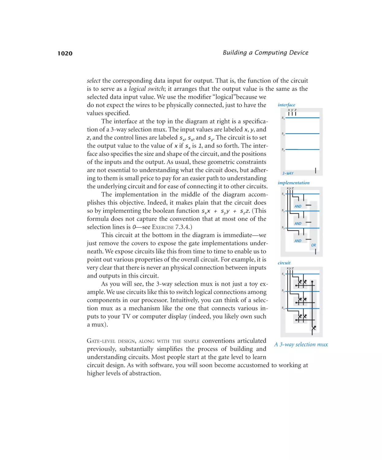
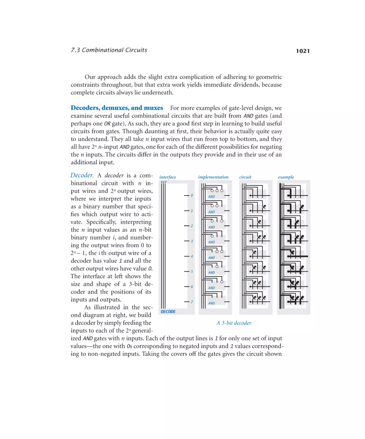
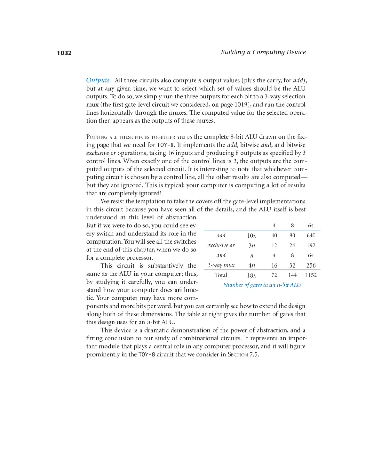
7.3 Combinational Circuits
1012
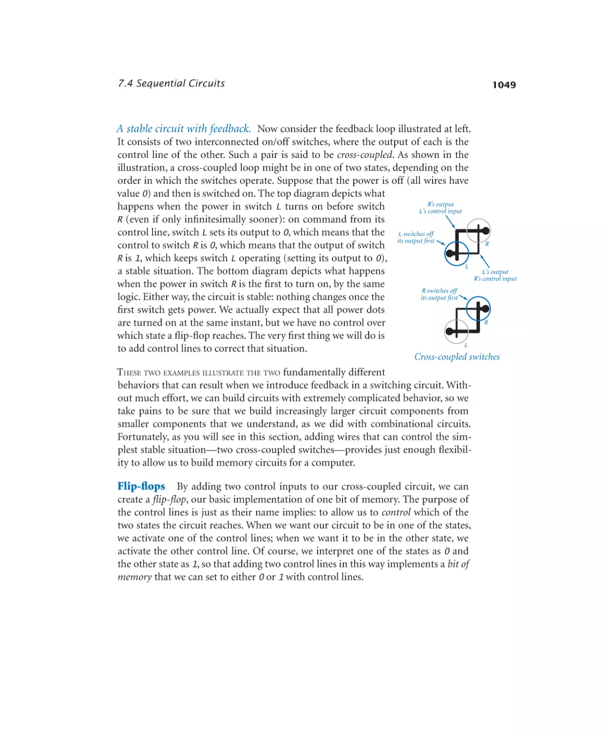
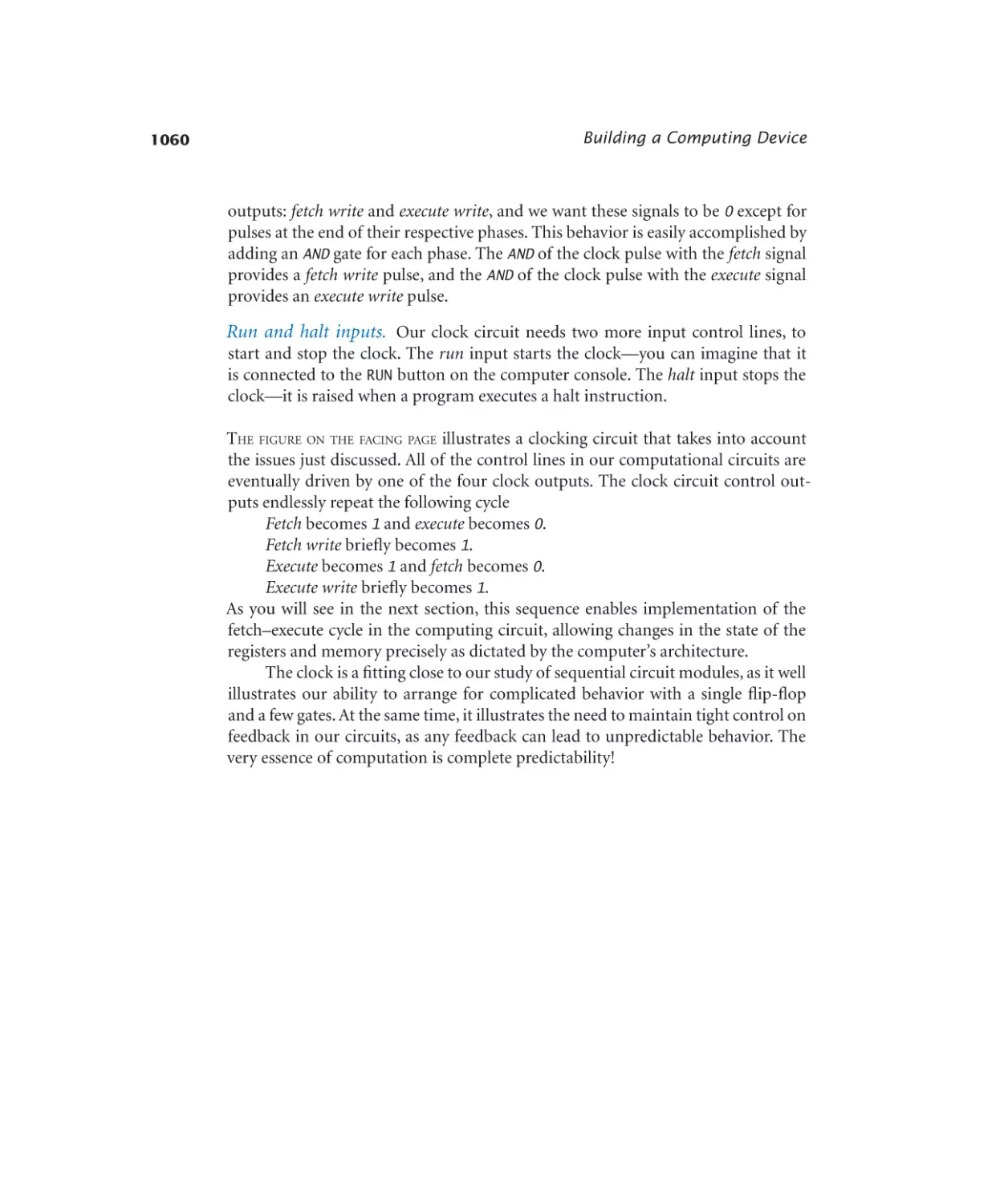
7.4 Sequential Circuits
1048
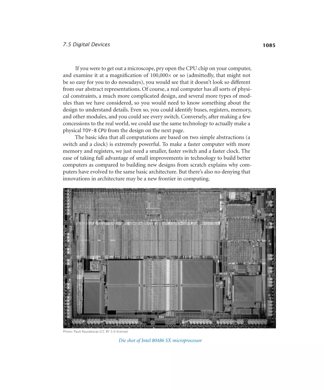
7.5 Digital Devices
1070
Context. . . . . . . . . . . . . . . . . . . 1093
Glossary . . . . . . . . . . . . . . . . . .
1097
Index . . . . . . . . . . . . . . . . . . . . 1107
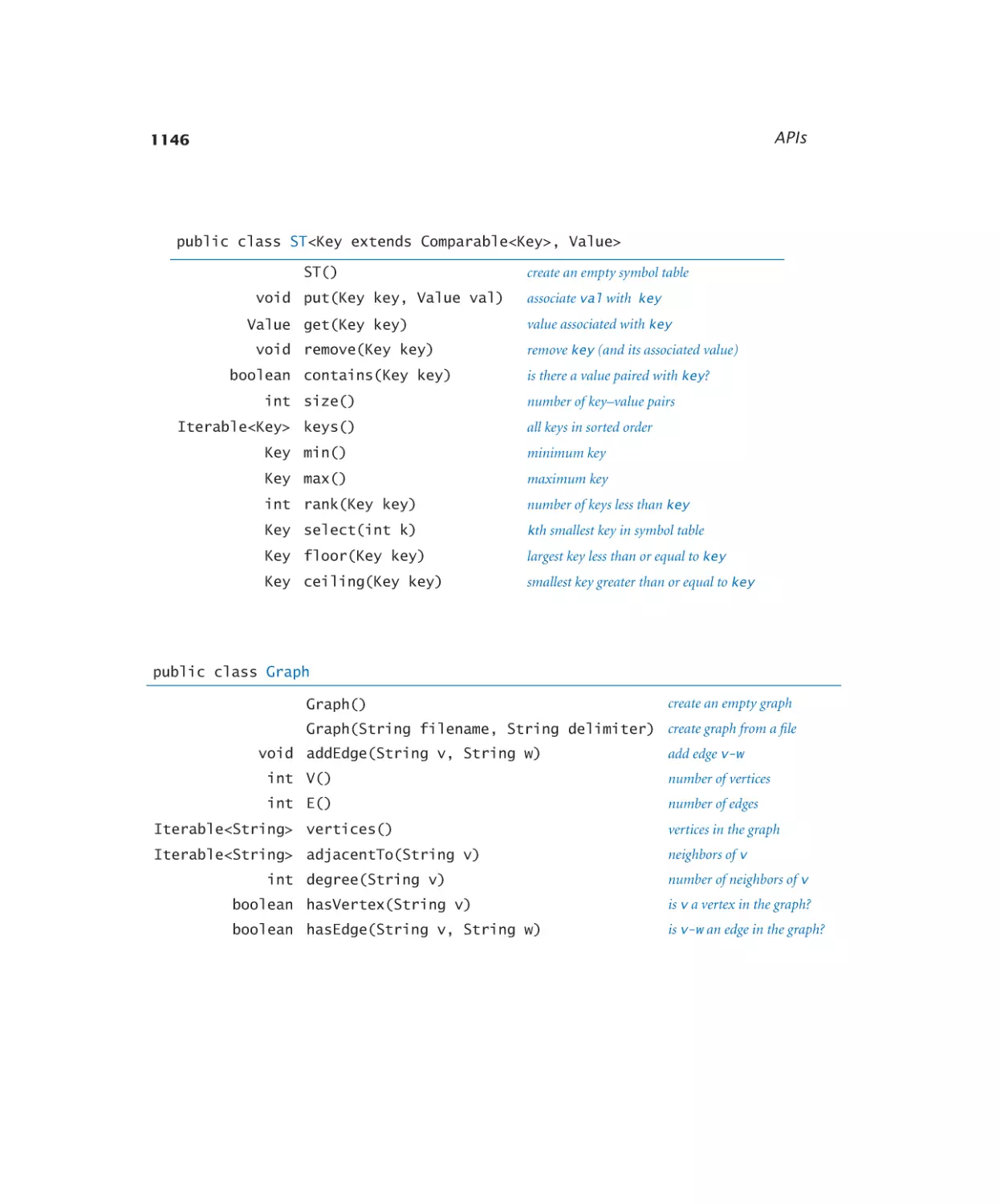
APIs . . . . . . . . . . . . . . . . . . . . 1139
vii
Programs
Elements of Programming
Functions and Modules
Your First Program
Defining Functions
1.1.1 Hello, World. . . . . . . . . . . 4
1.1.2 Using a command-line argument . 7
Built-in Types of Data
1.2.1
1.2.2
1.2.3
1.2.4
1.2.5
String concatenation . . . . . . . 20
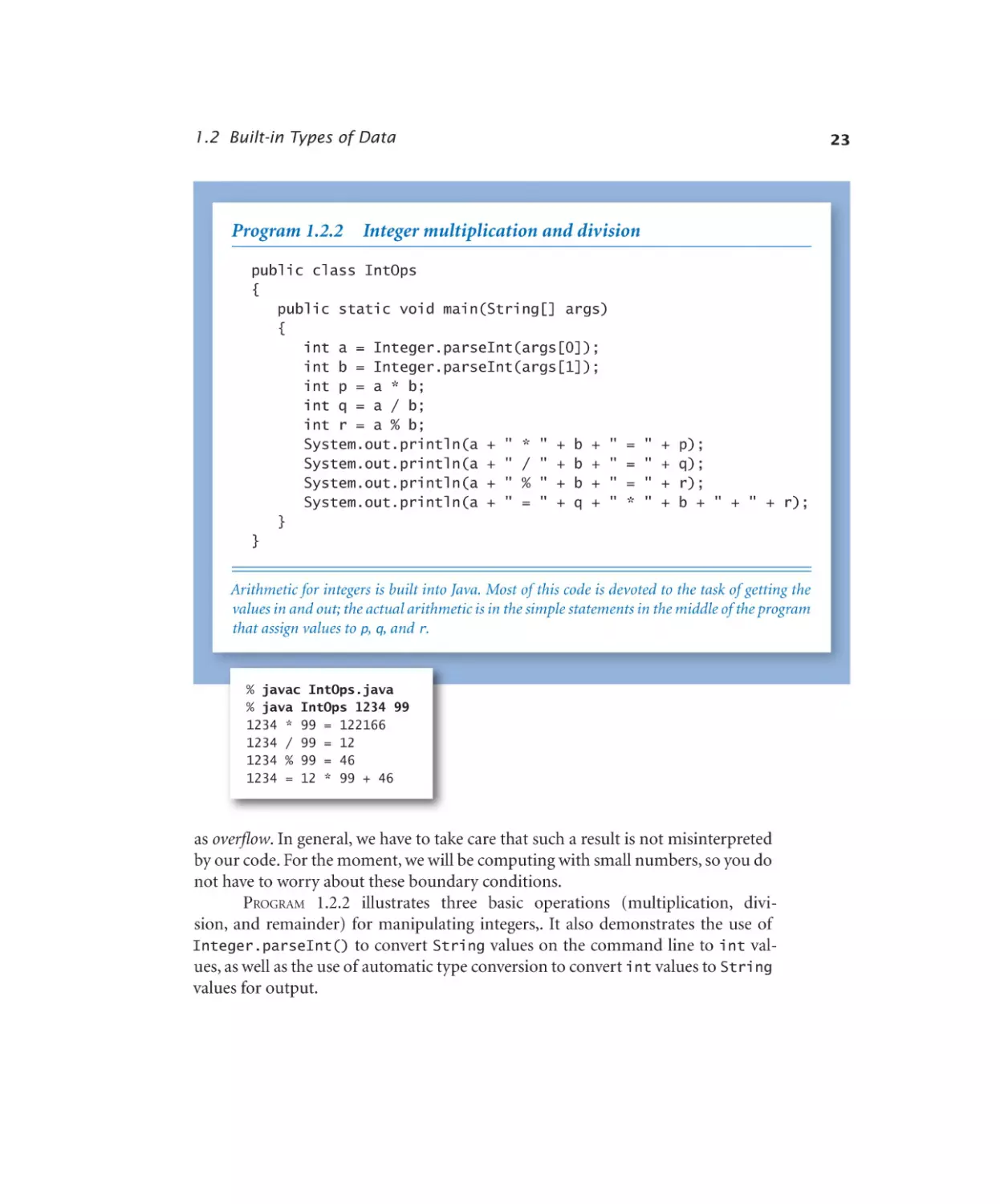
Integer multiplication and division.23
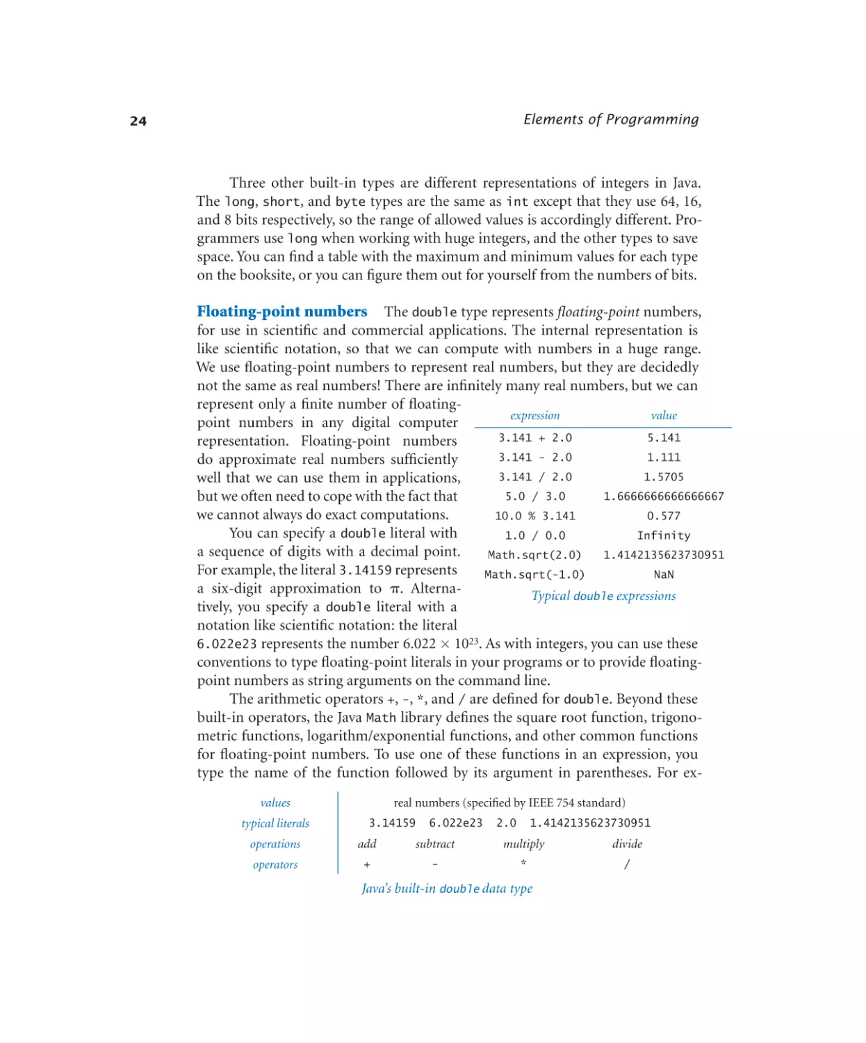
Quadratic formula. . . . . . . . 25
Leap year . . . . . . . . . . . 28
Casting to get a random integer. . 34
Conditionals and Loops
1.3.1
1.3.2
1.3.3
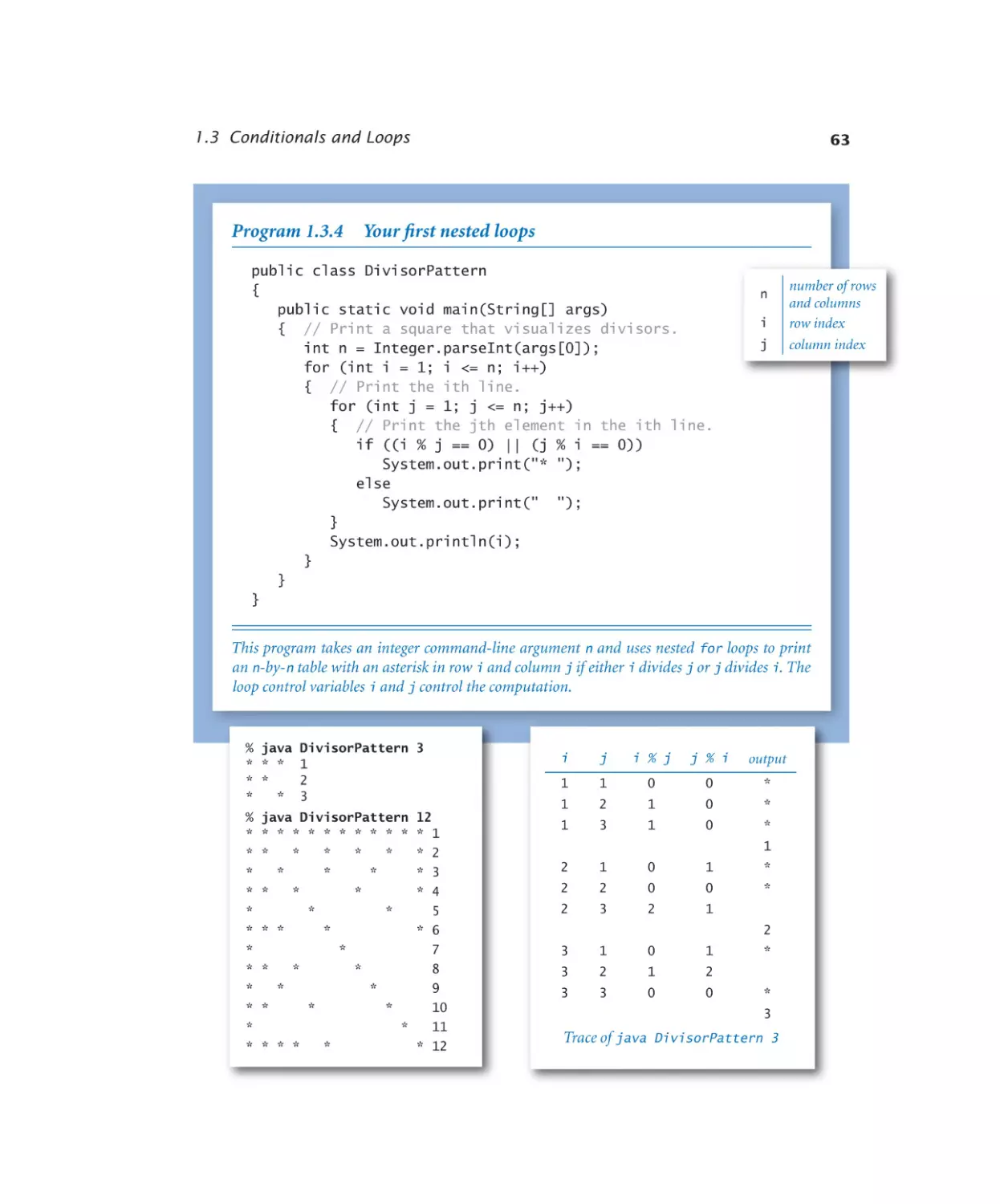
1.3.4
1.3.5
1.3.6
1.3.7
1.3.8
1.3.9
Flipping a fair coin . . . . . . . 53
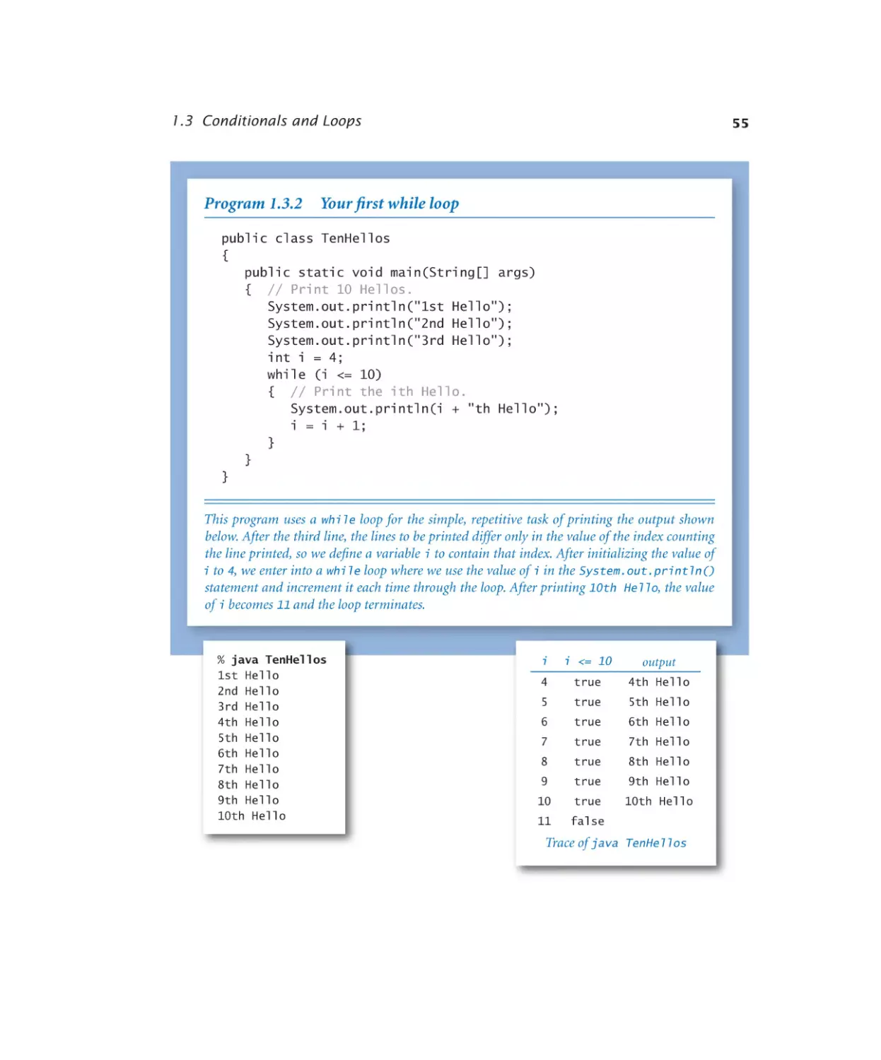
Your first while loop. . . . . . . 55
Computing powers of 2 . . . . . 57
Your first nested loops. . . . . . 63
Harmonic numbers. . . . . . . 65
Newton’s method. . . . . . . . 66
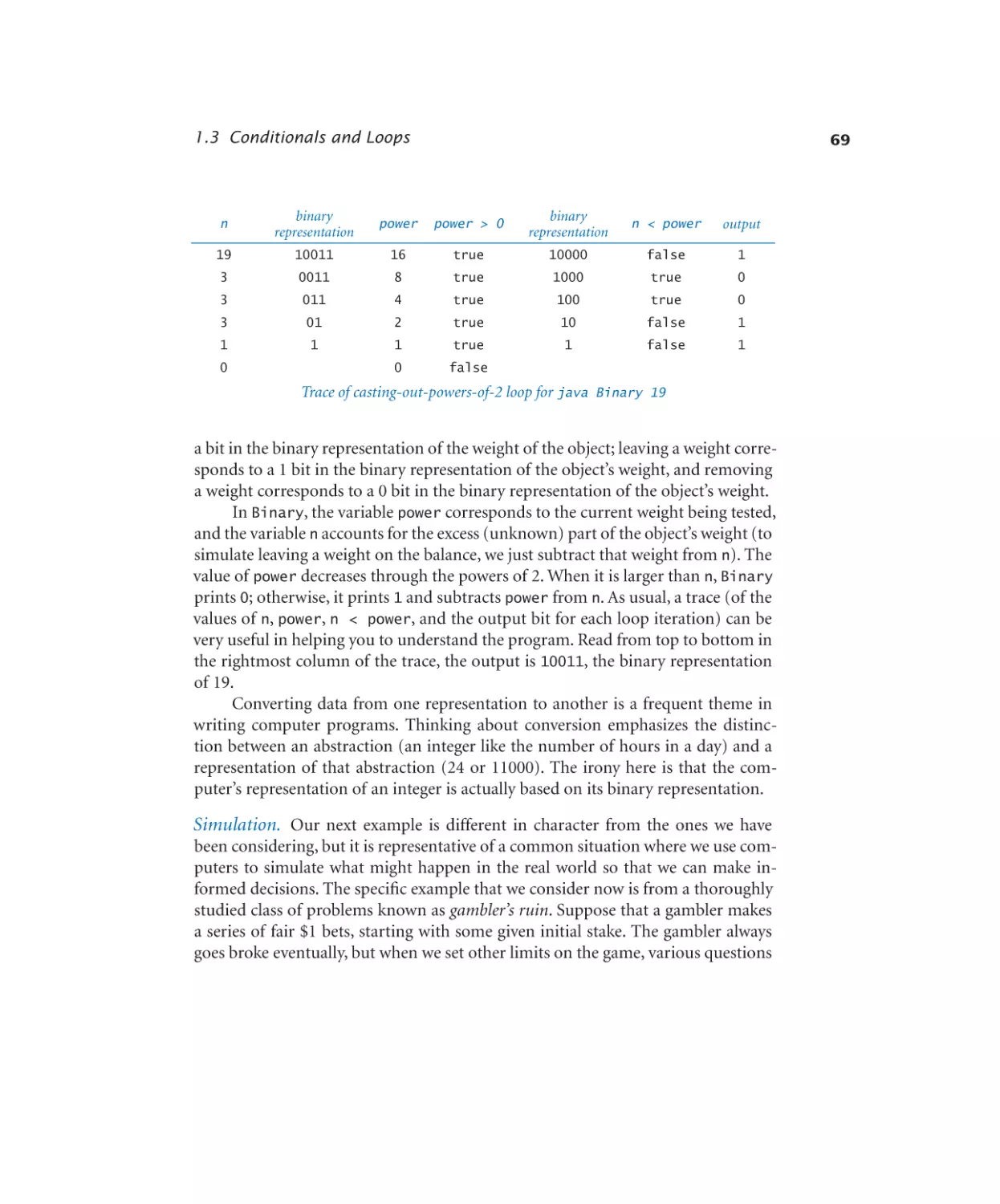
Converting to binary. . . . . . . 68
Gambler’s ruin simulation . . . . 71
Factoring integers. . . . . . . . 73
Arrays
1.4.1
1.4.2
1.4.3
1.4.4
Generating a random sequence . 128
Interactive user input. . . . . . 136
Averaging a stream of numbers . 138
A simple filter. . . . . . . . . 140
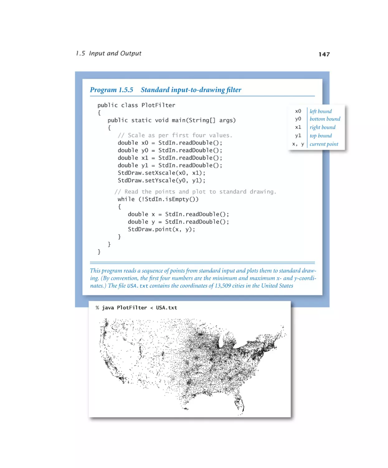
Standard input-to-drawing filter. 147
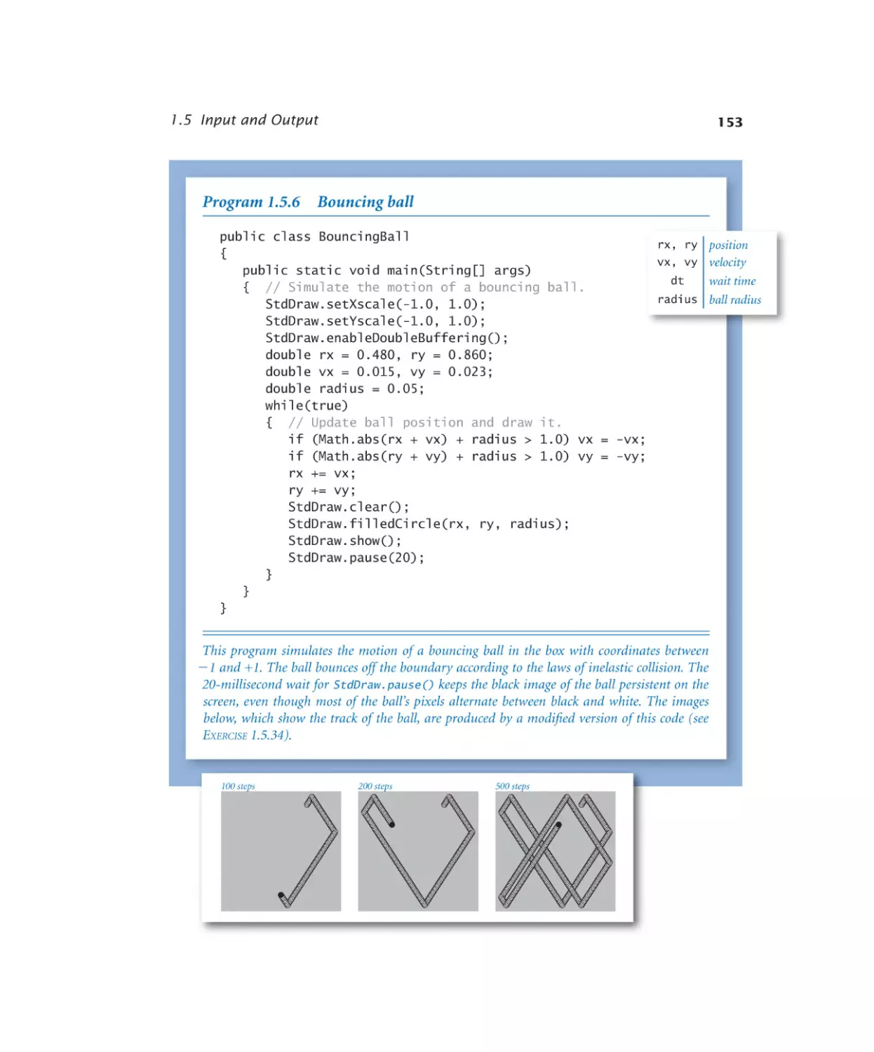
Bouncing ball. . . . . . . . . 153
Digital signal processing . . . . . 158
Case Study: Random Web Surfer
viii
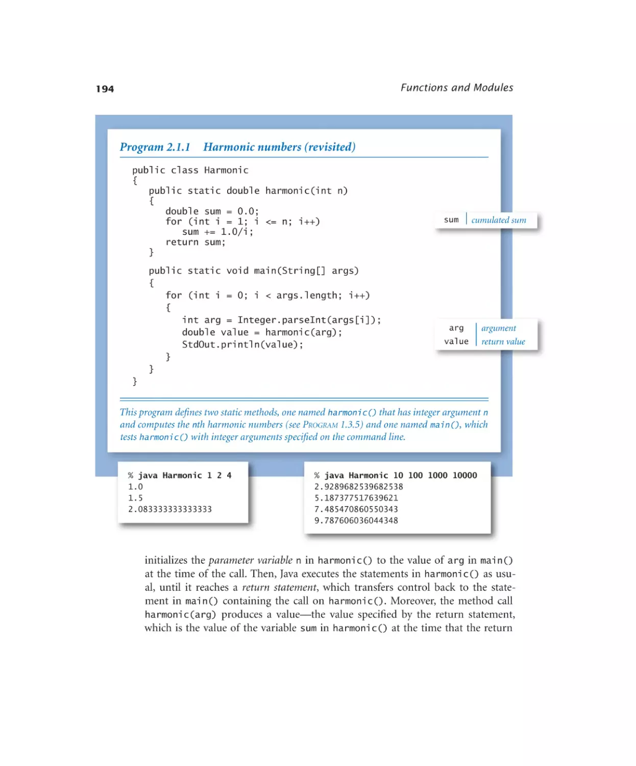
Harmonic numbers (revisited) . 194
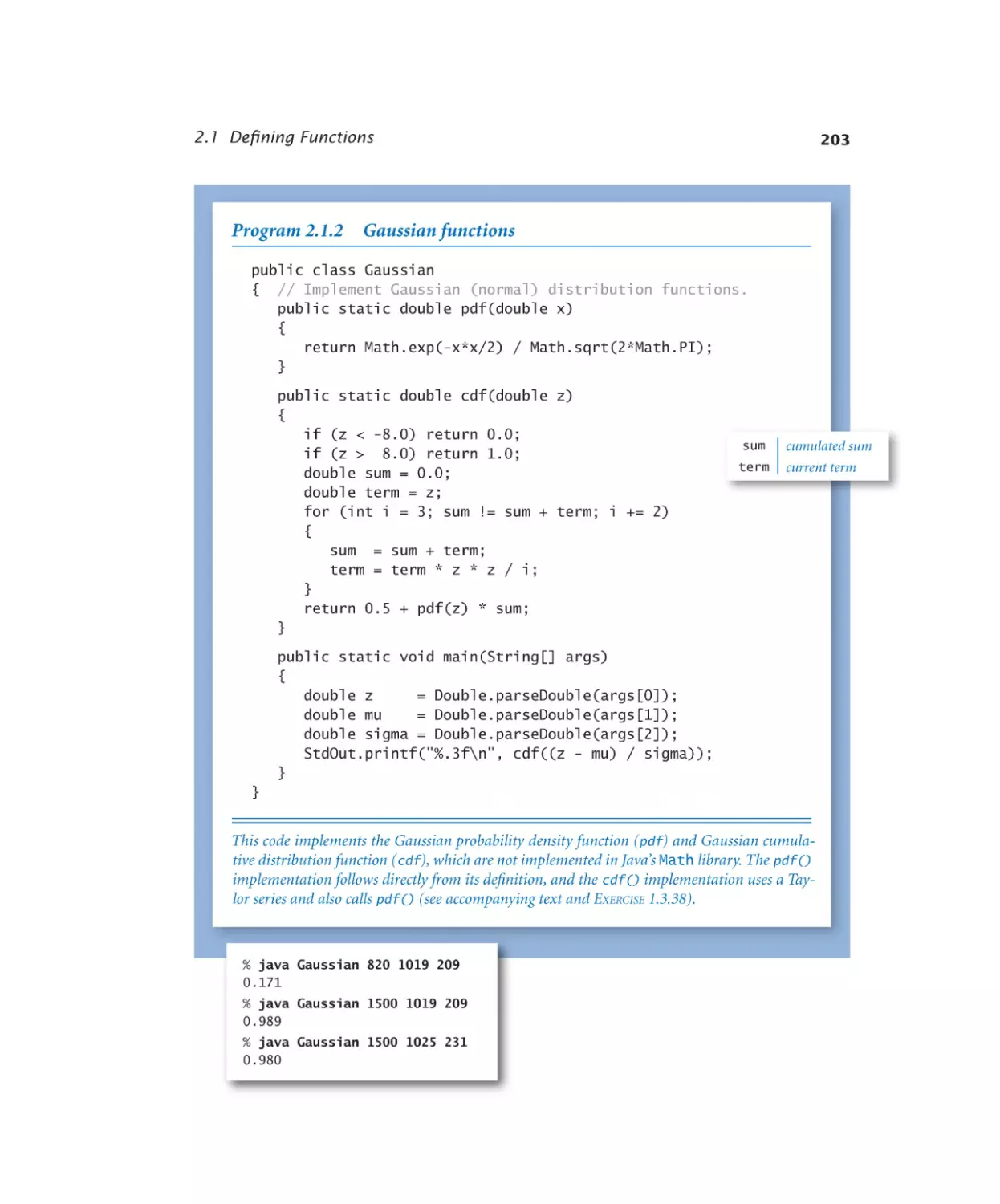
Gaussian functions. . . . . . . 203
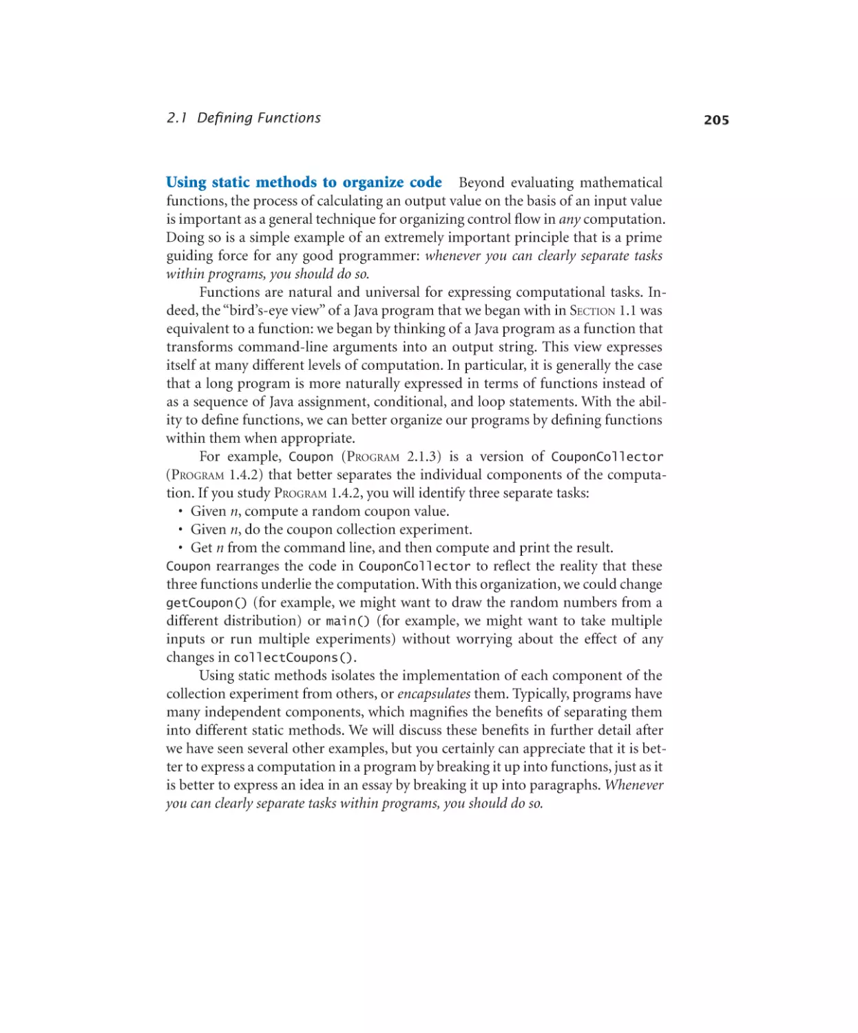
Coupon collector (revisited) . . . 206
Play that tune (revisited). . . . . 213
Libraries and Clients
2.2.1
2.2.2
2.2.3
2.2.4
2.2.5
2.2.6
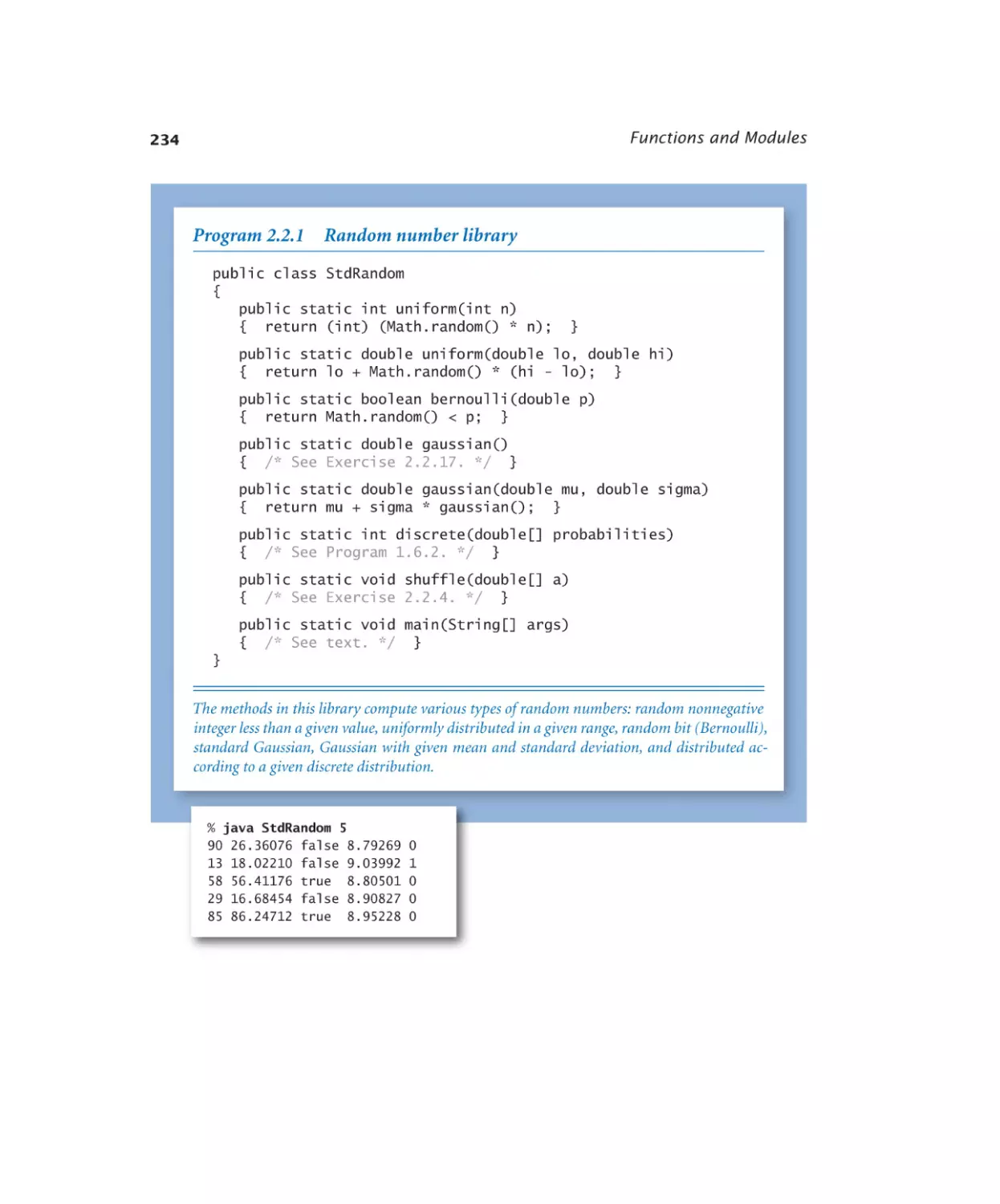
Random number library. . . . . 234
Array I/O library. . . . . . . . 238
Iterated function systems. . . . . 241
Data analysis library. . . . . . . 245
Plotting data values in an array . 247
Bernoulli trials . . . . . . . . . 250
Recursion
2.3.1
2.3.2
2.3.3
2.3.4
2.3.5
2.3.6
Euclid’s algorithm. . . . . . . 267
Towers of Hanoi . . . . . . . . 270
Gray code . . . . . . . . . . . 275
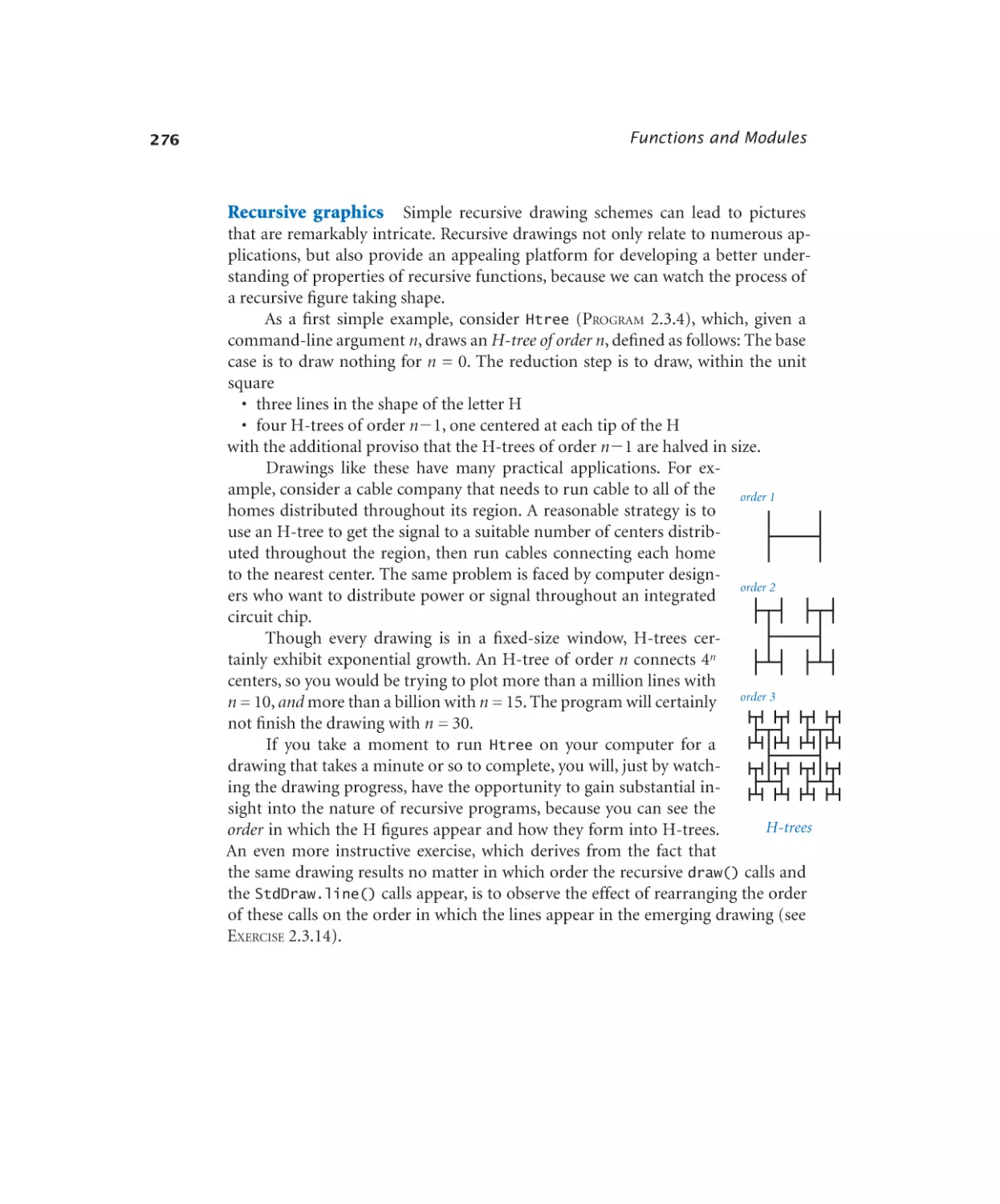
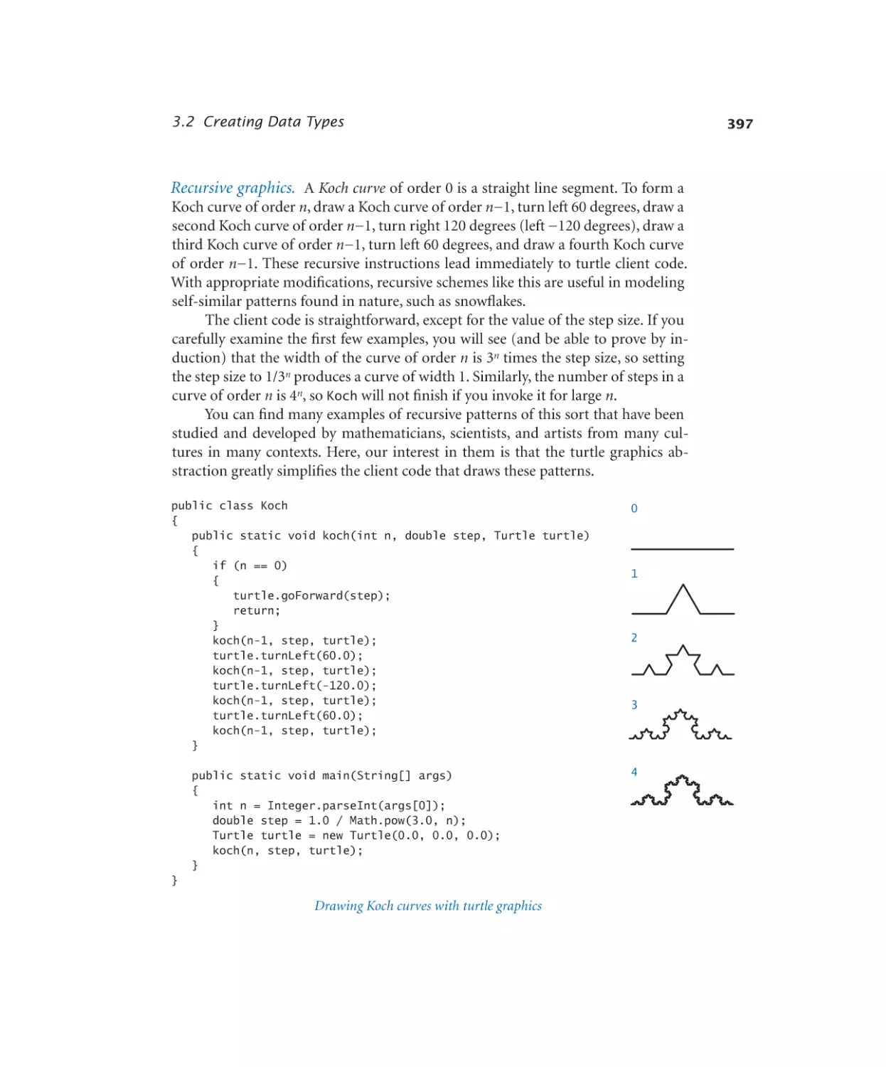
Recursive graphics. . . . . . . 277
Brownian bridge. . . . . . . . 279
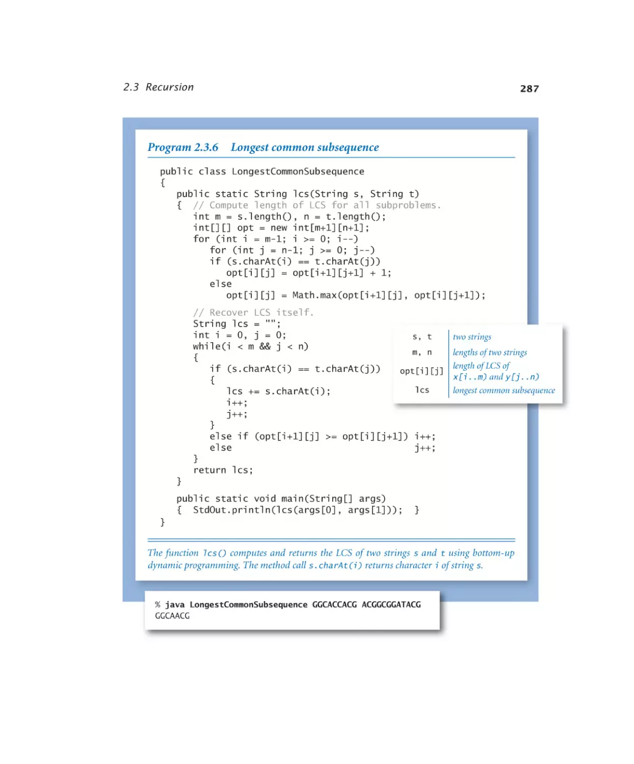
Longest common subsequence . 287
Case Study: Percolation
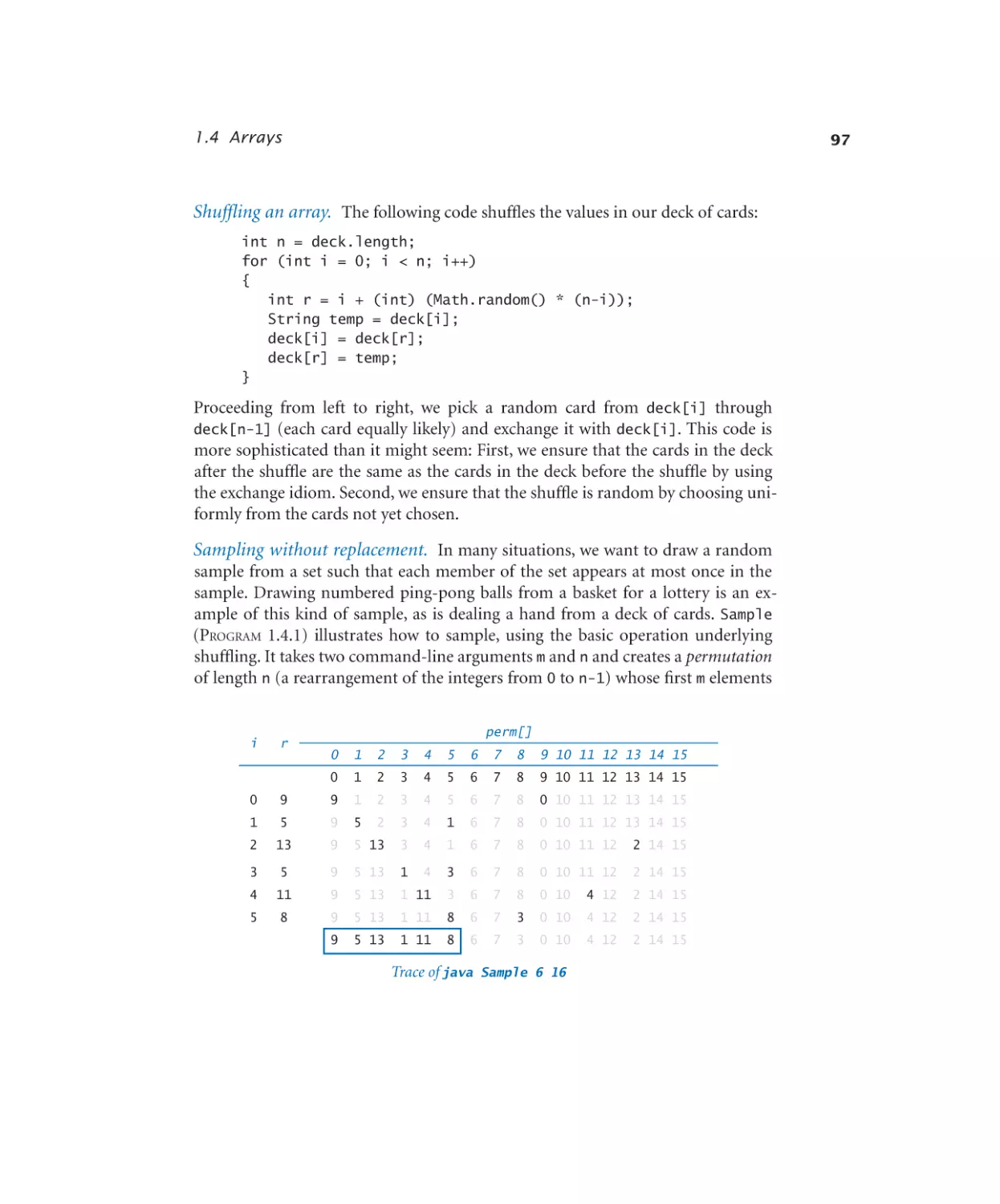
Sampling without replacement. . 98
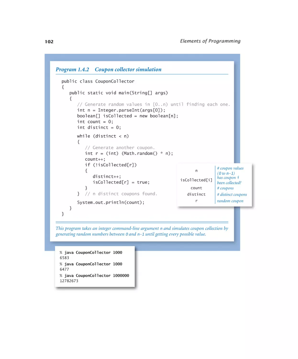
Coupon collector simulation . . . 102
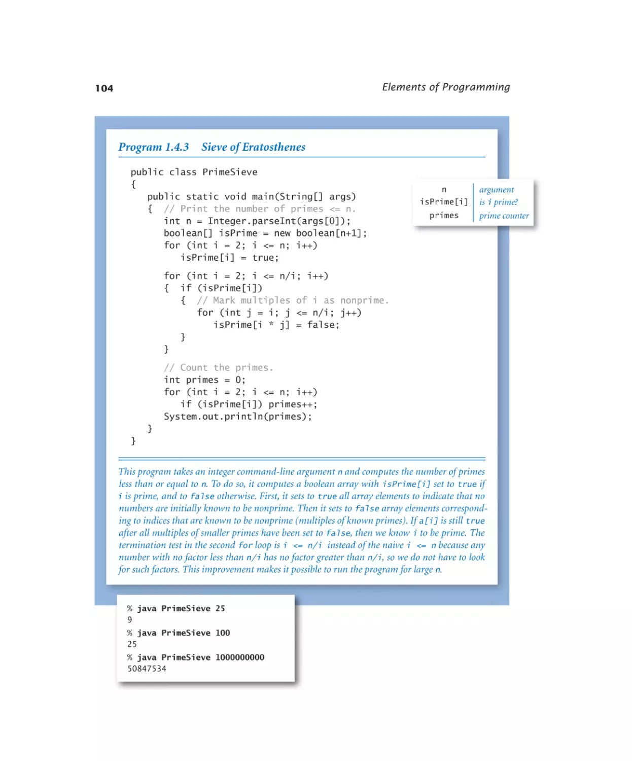
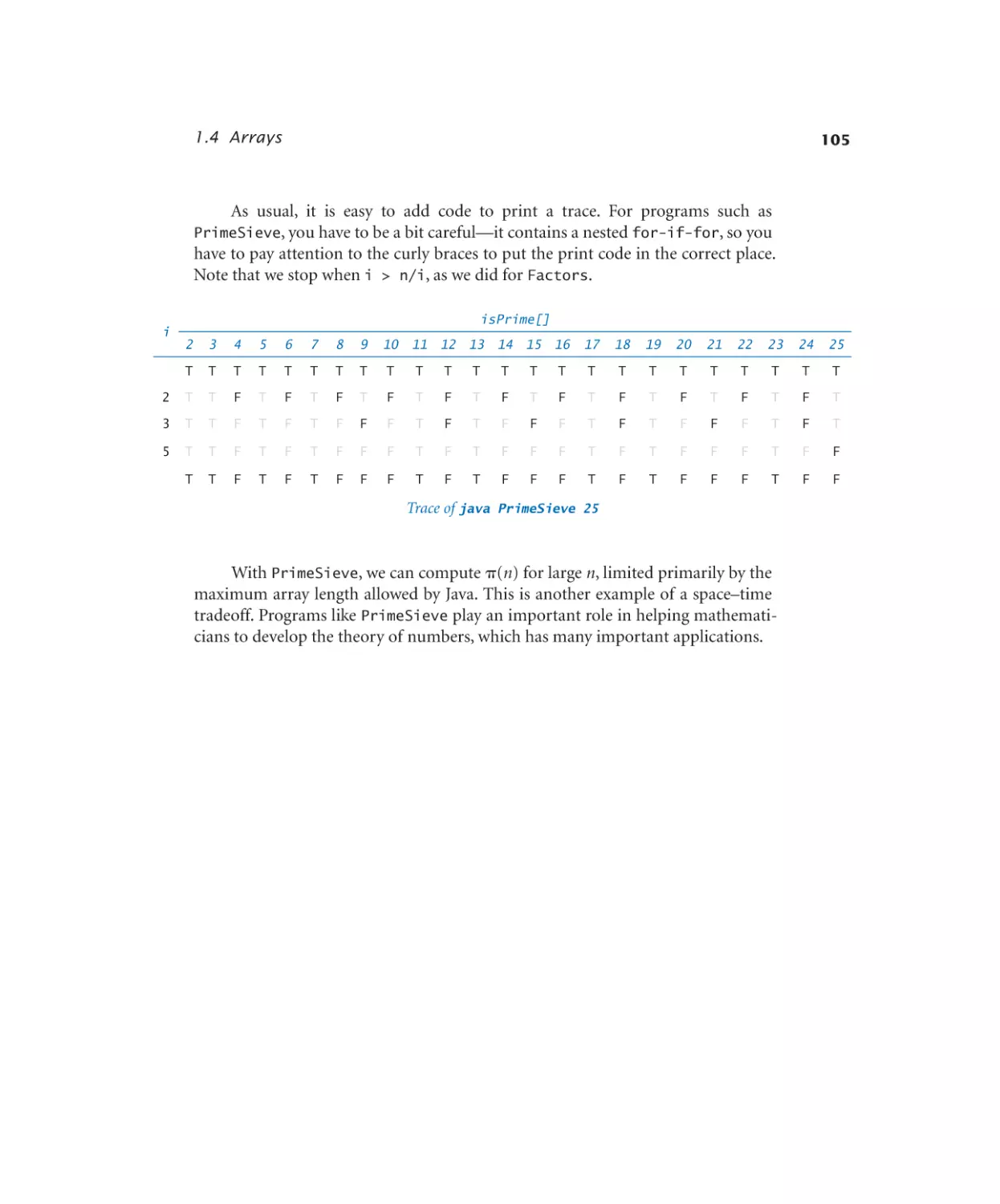
Sieve of Eratosthenes. . . . . . 104
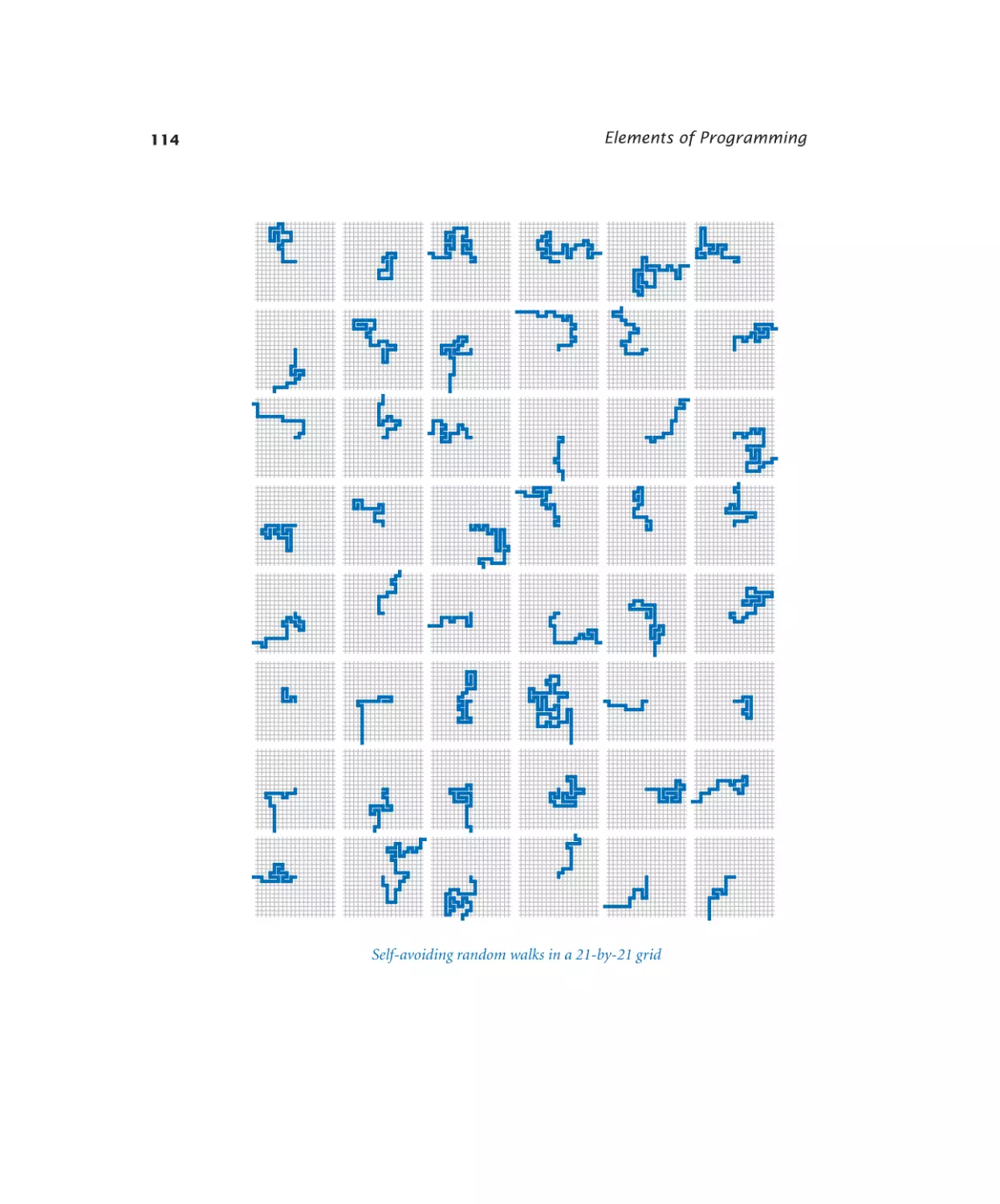
Self-avoiding random walks. . . 113
Input and Output
1.5.1
1.5.2
1.5.3
1.5.4
1.5.5
1.5.6
1.5.7
2.1.1
2.1.2
2.1.3
2.1.4
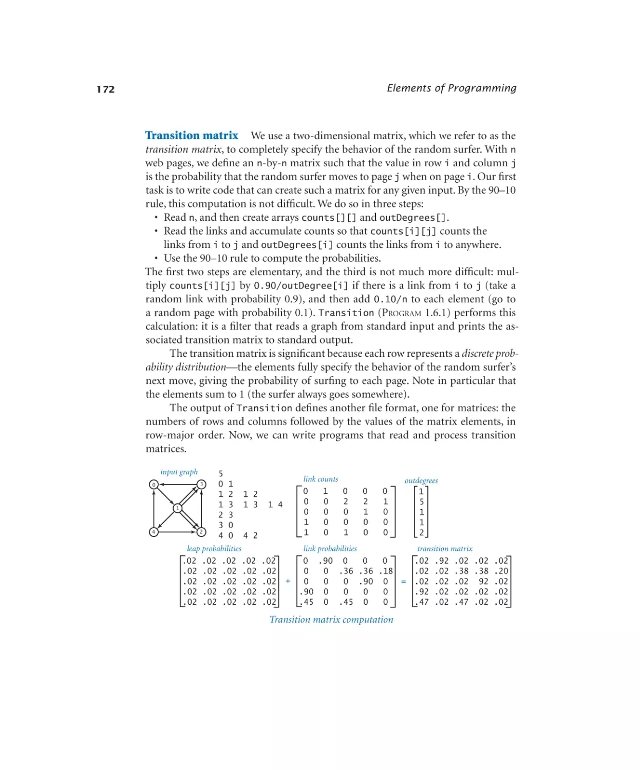
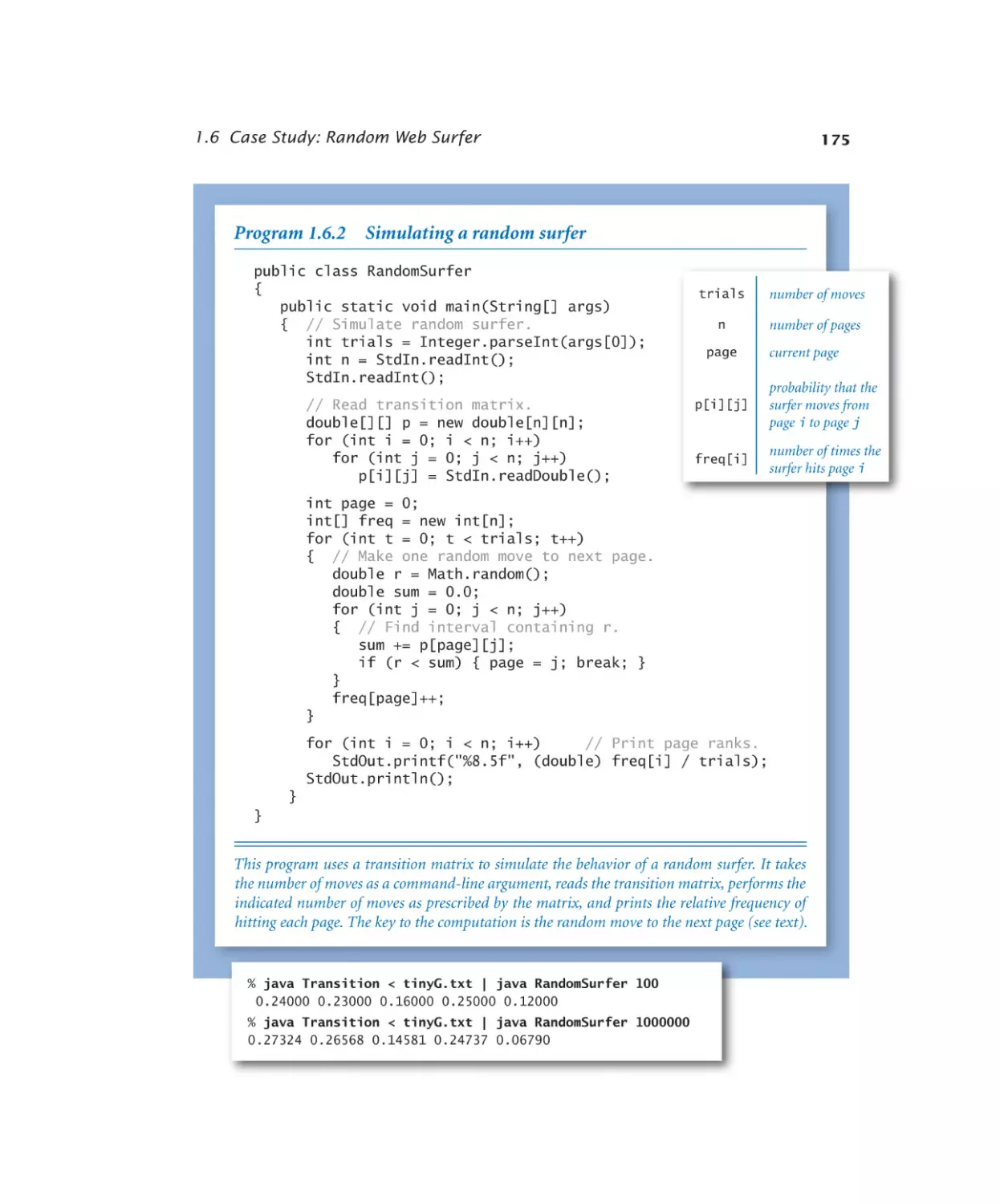
1.6.1 Computing the transition matrix. 173
1.6.2 Simulating a random surfer . . . 175
1.6.3 Mixing a Markov chain. . . . . 182
2.4.1
2.4.2
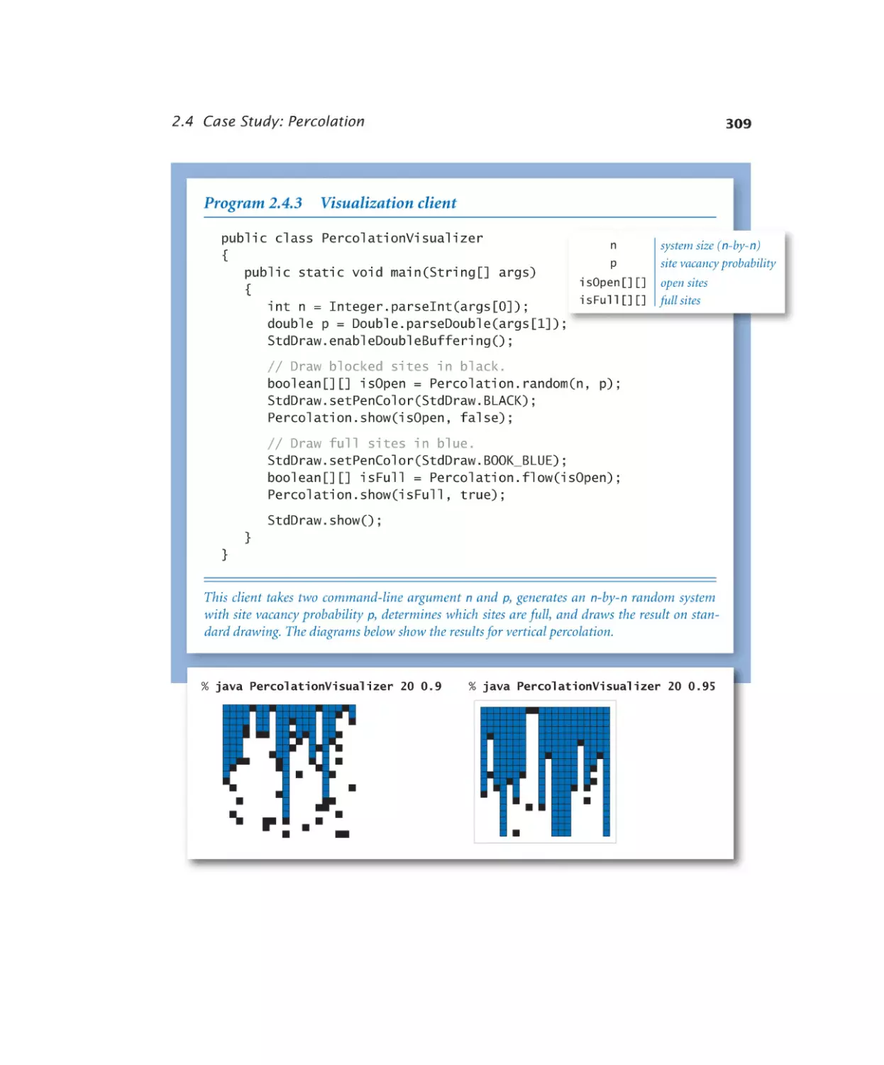
2.4.3
2.4.4
2.4.5
2.4.6
Percolation scaffolding. . . . . 304
Vertical percolation detection. . . 306
Visualization client . . . . . . . 309
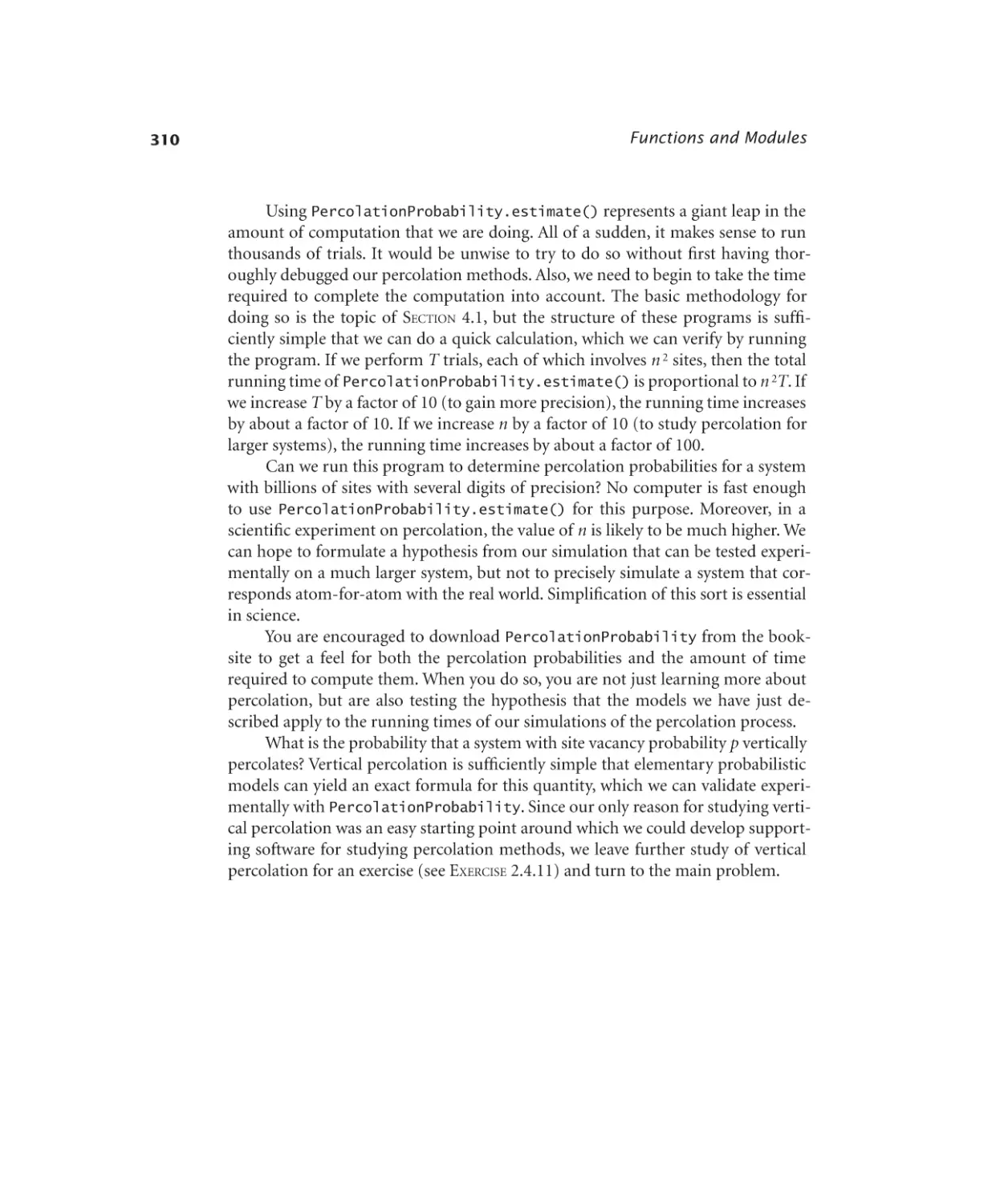
Percolation probability estimate .311
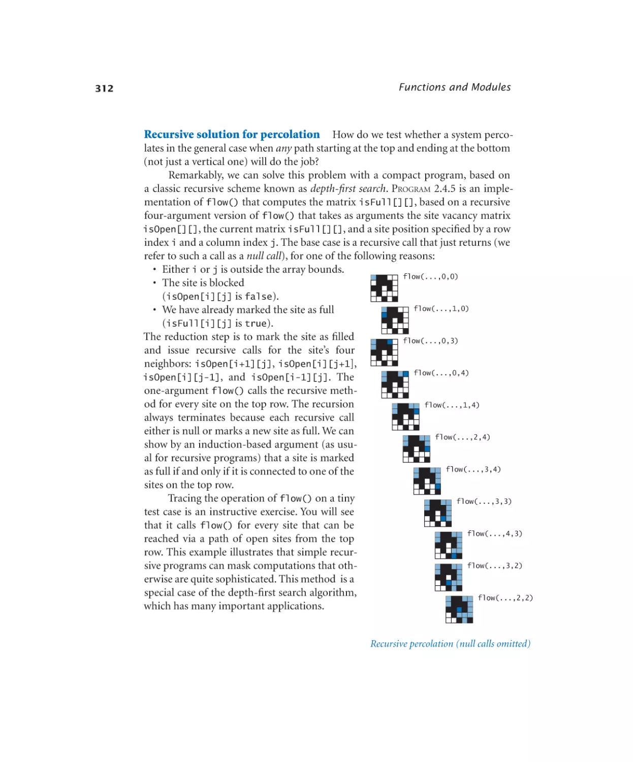
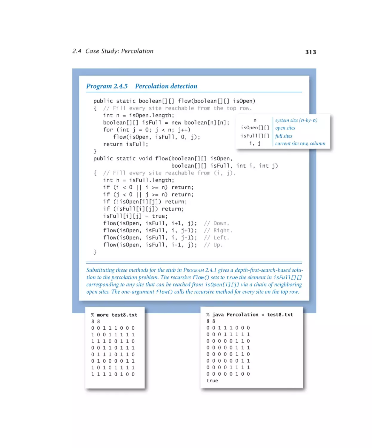
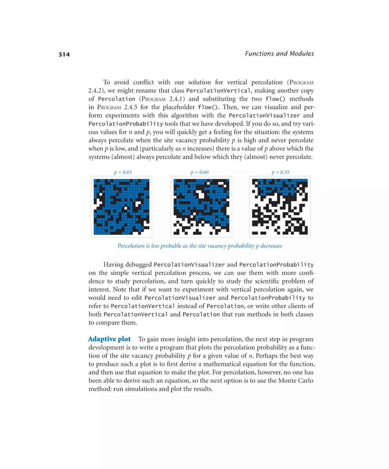
Percolation detection . . . . . . 313
Adaptive plot client . . . . . . . 316
Object-Oriented Programming
Algorithms and Data Structures
Using Data Types
Performance
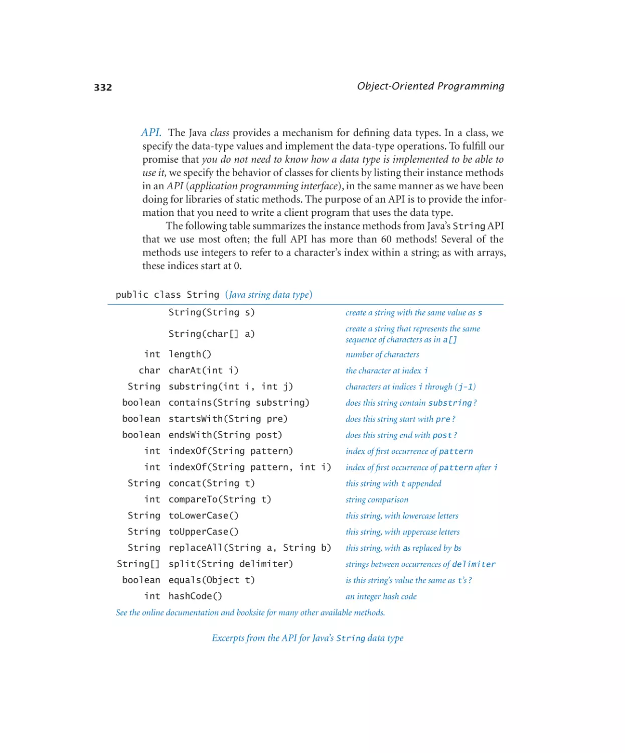
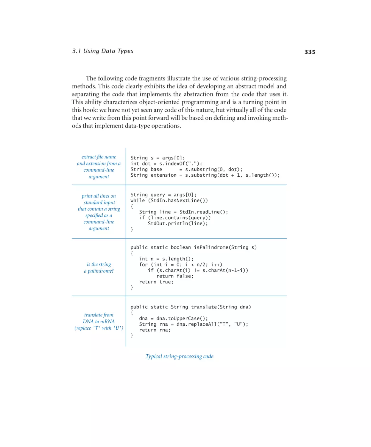
3.1.1 Identifying a potential gene . . . 337
3.1.2 Albers squares . . . . . . . . . 342
3.1.3 Luminance library . . . . . . . 345
3.1.4 Converting color to grayscale. . . 348
3.1.5 Image scaling . . . . . . . . . 350
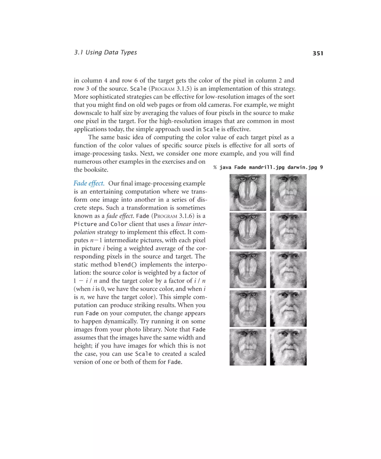
3.1.6 Fade effect. . . . . . . . . . . 352
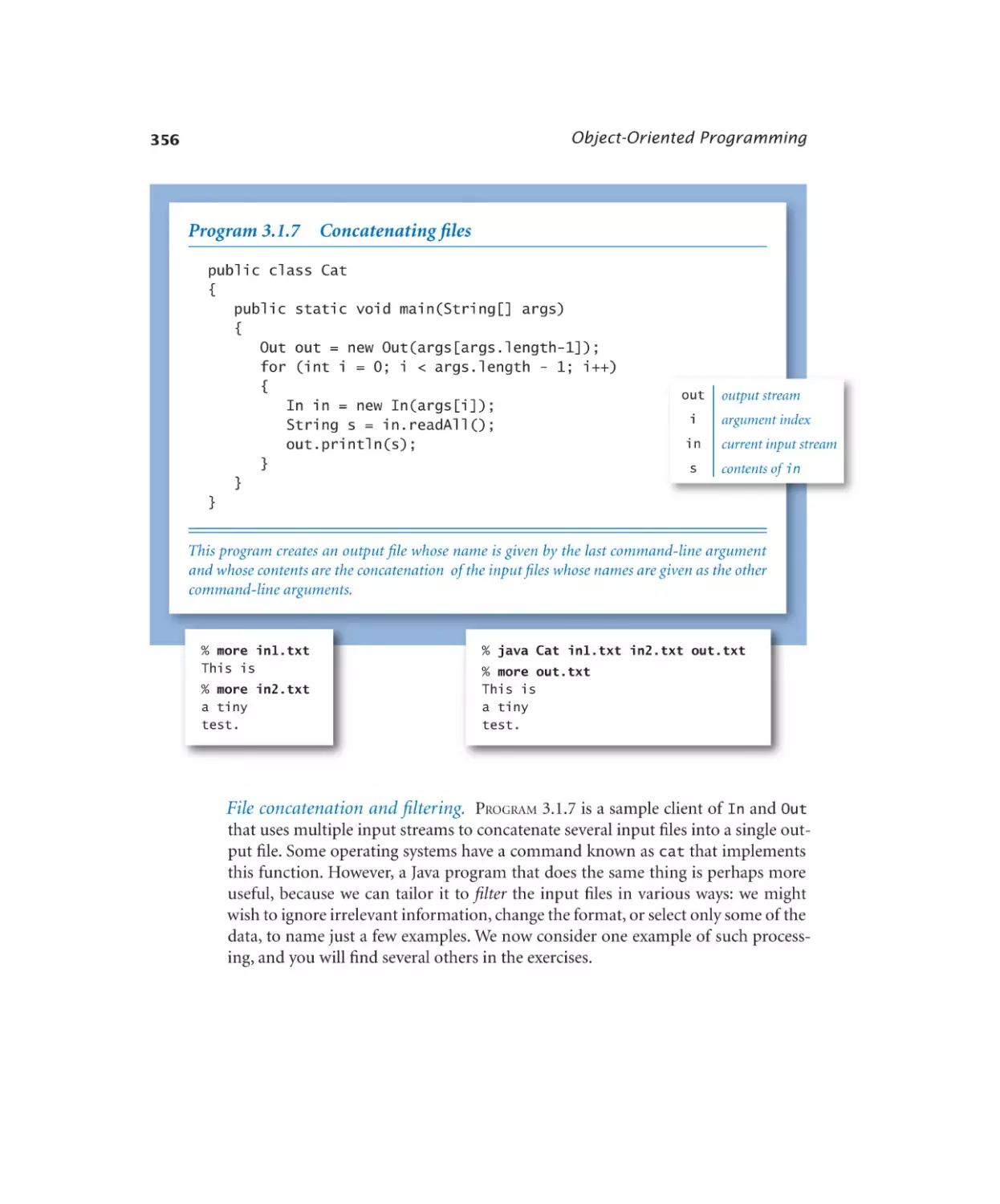
3.1.7 Concatenating files. . . . . . . 356
3.1.8 Screen scraping for stock quotes . 359
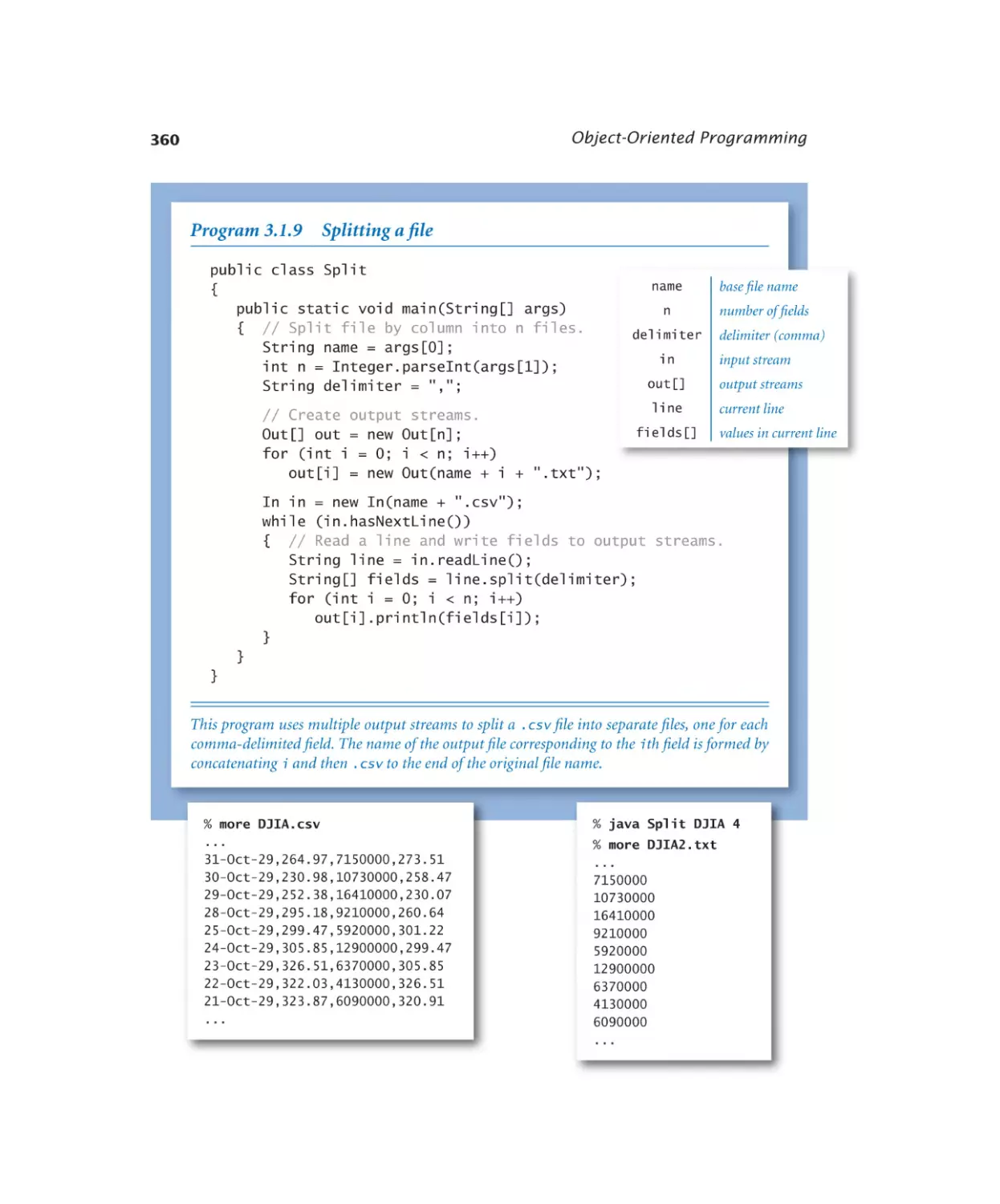
3.1.9 Splitting a file . . . . . . . . . 360
Creating Data Types
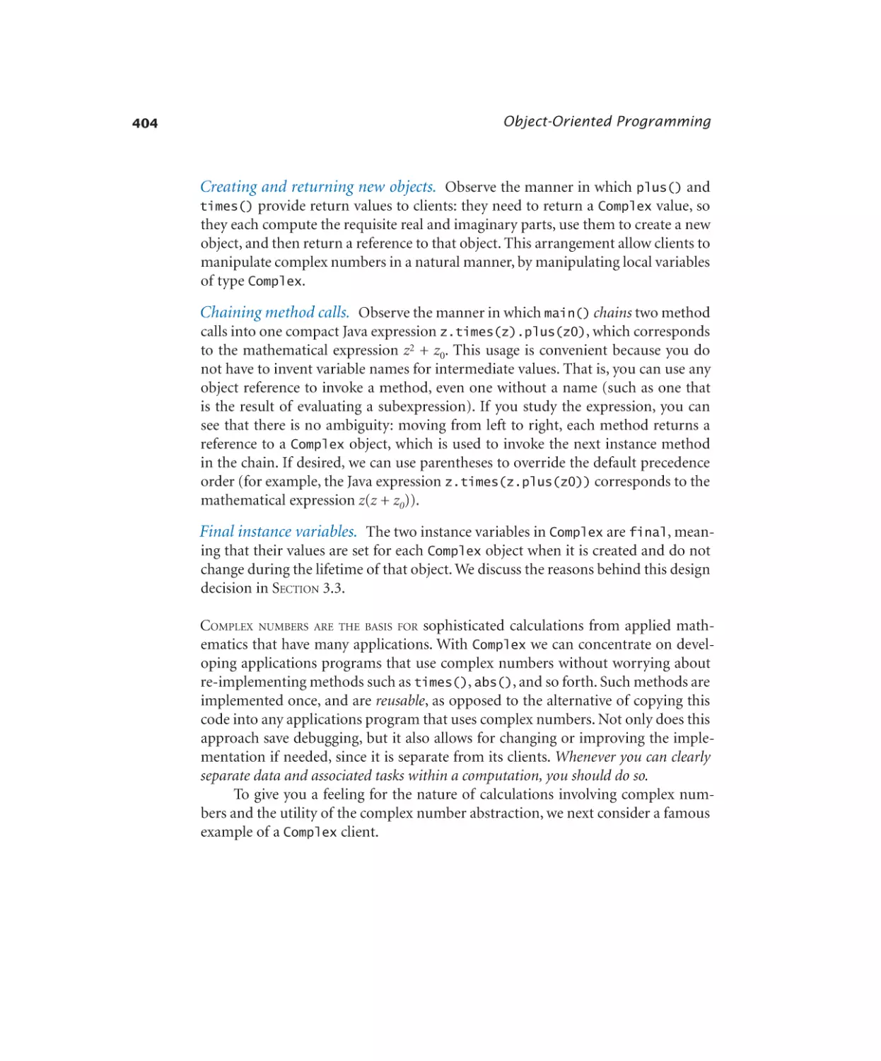
3.2.1
3.2.2
3.2.3
3.2.4
3.2.5
3.2.6
3.2.7
3.2.8
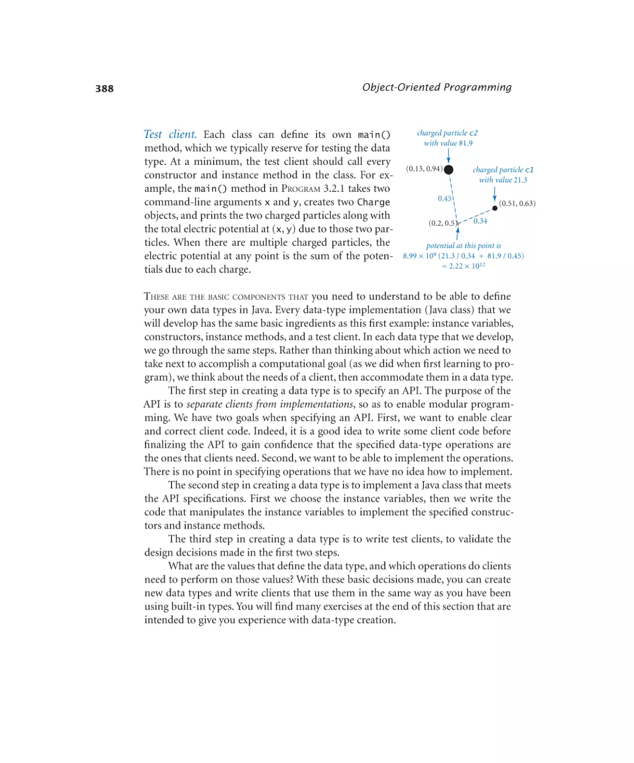
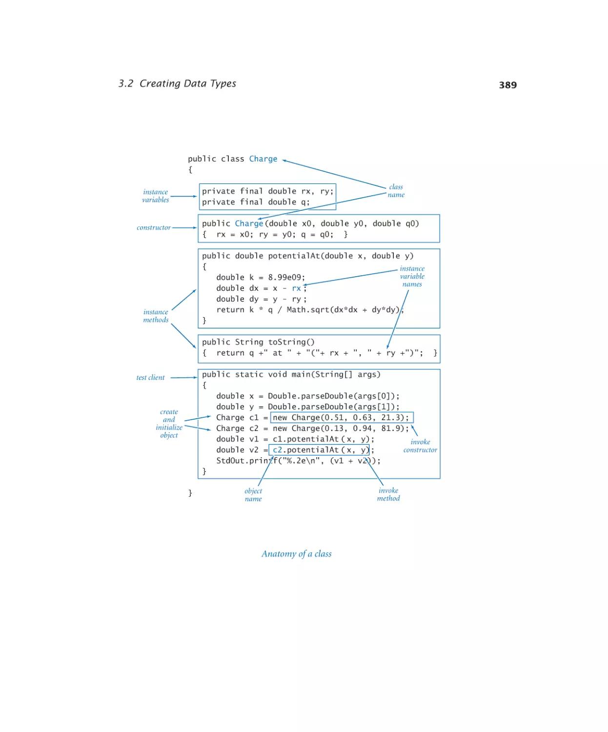
Charged particle . . . . . . . . 387
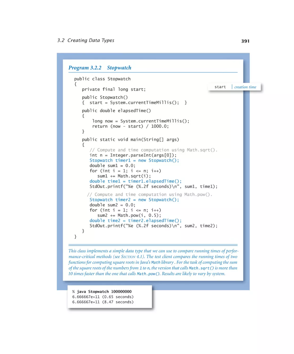
Stopwatch. . . . . . . . . . . 391
Histogram. . . . . . . . . . . 393
Turtle graphics. . . . . . . . . 396
Spira mirabilis. . . . . . . . . 399
Complex number. . . . . . . . 405
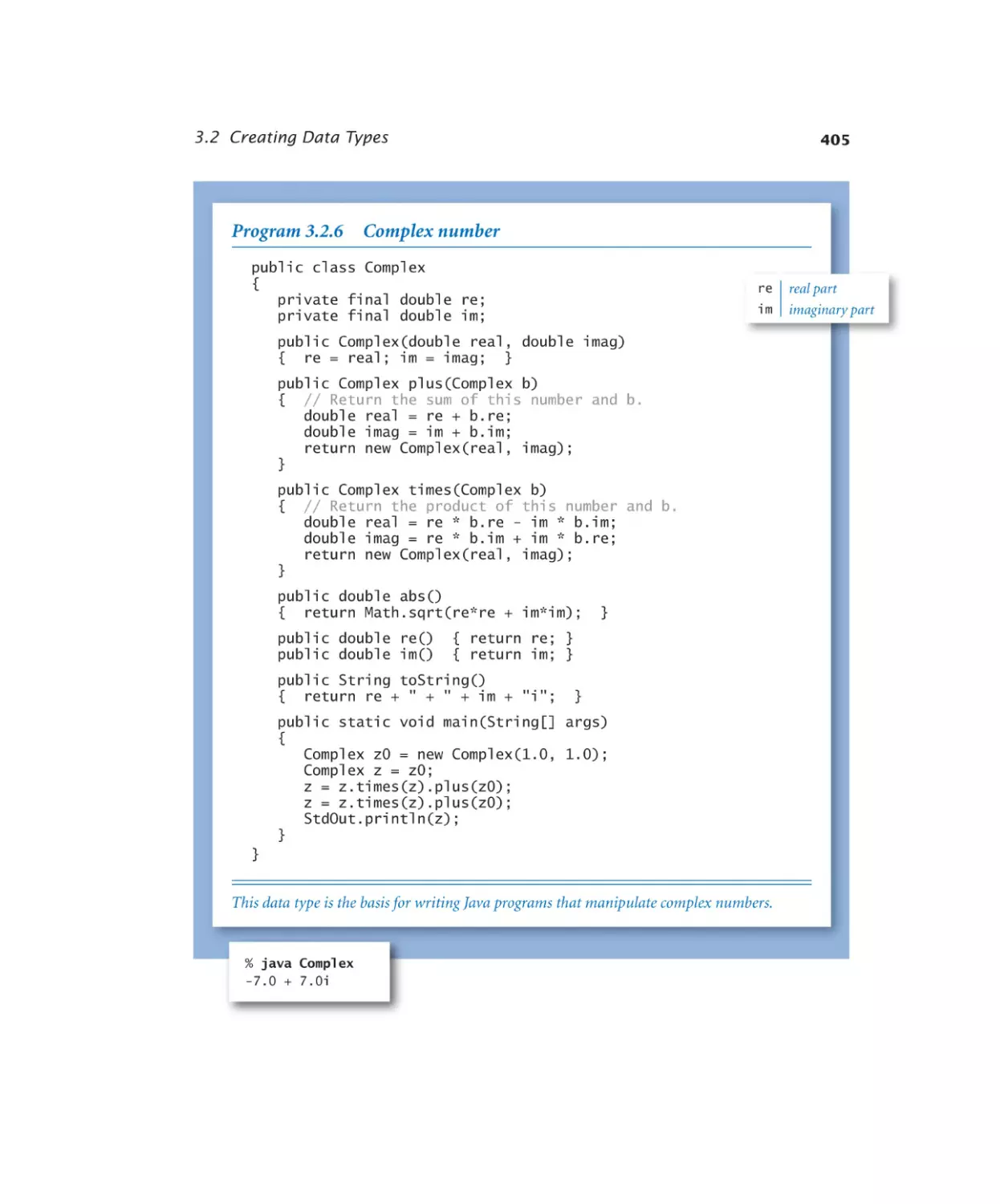
Mandelbrot set. . . . . . . . . 409
Stock account. . . . . . . . . 413
Designing Data Types
3.3.1
3.3.2
3.3.3
3.3.4
3.3.5
Complex number (alternate) . . . 434
Counter. . . . . . . . . . . . 437
Spatial vectors . . . . . . . . . 444
Document sketch. . . . . . . . 461
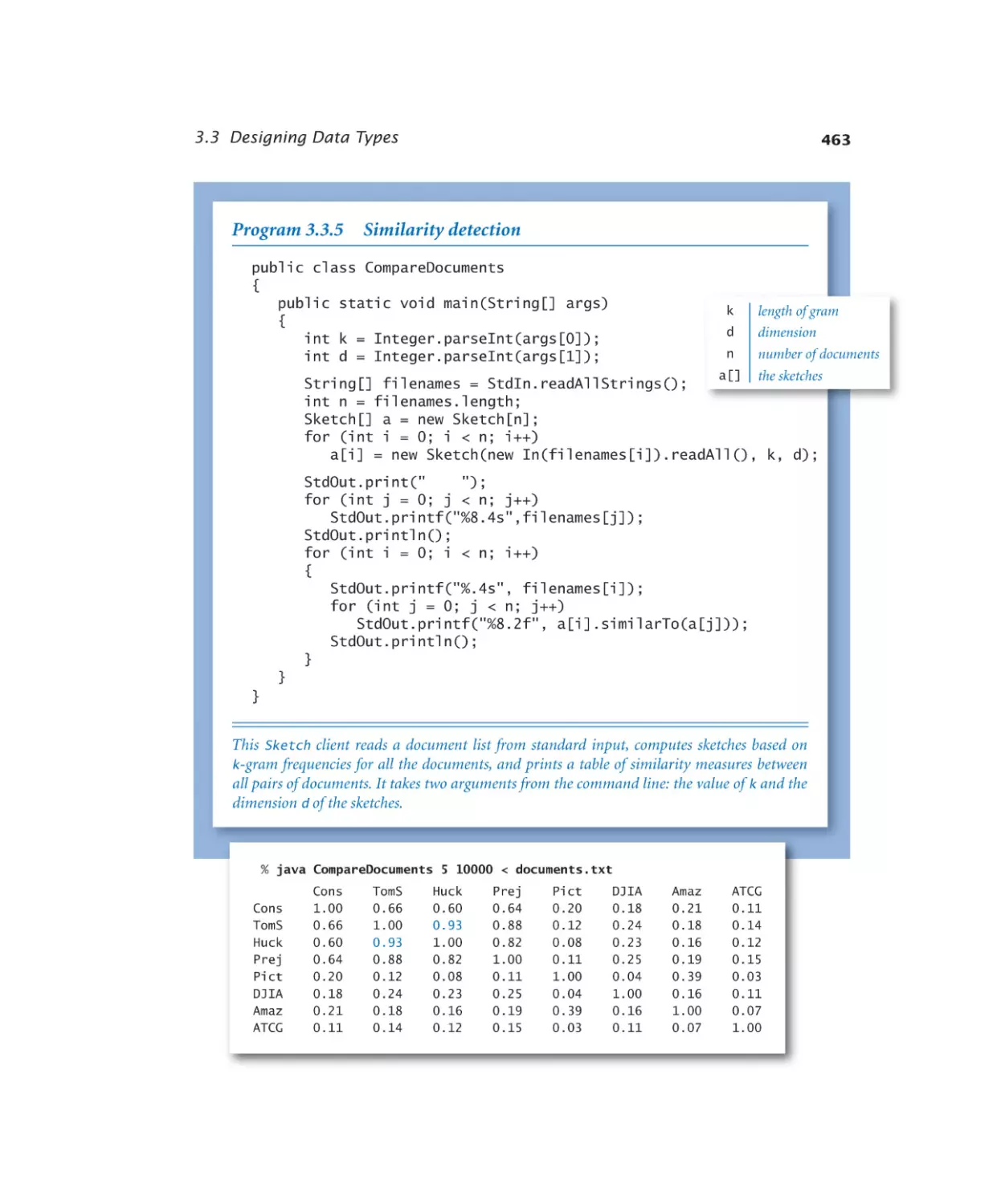
Similarity detection. . . . . . . 463
Case Study: N-Body Simulation
3.4.1
3.4.2
Gravitational body . . . . . . . 482
N-body simulation. . . . . . . 485
4.1.1 3-sum problem. . . . . . . . . 497
4.1.2 Validating a doubling hypothesis. 499
Sorting and Searching
4.2.1
4.2.2
4.2.3
4.2.4
4.2.5
4.2.6
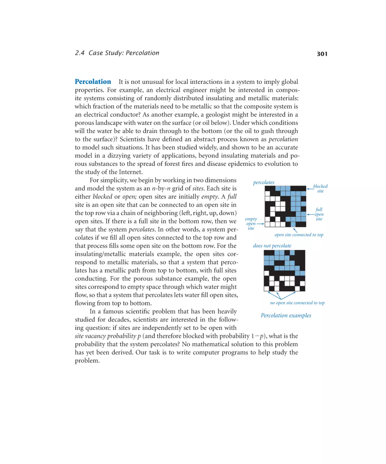
4.2.7
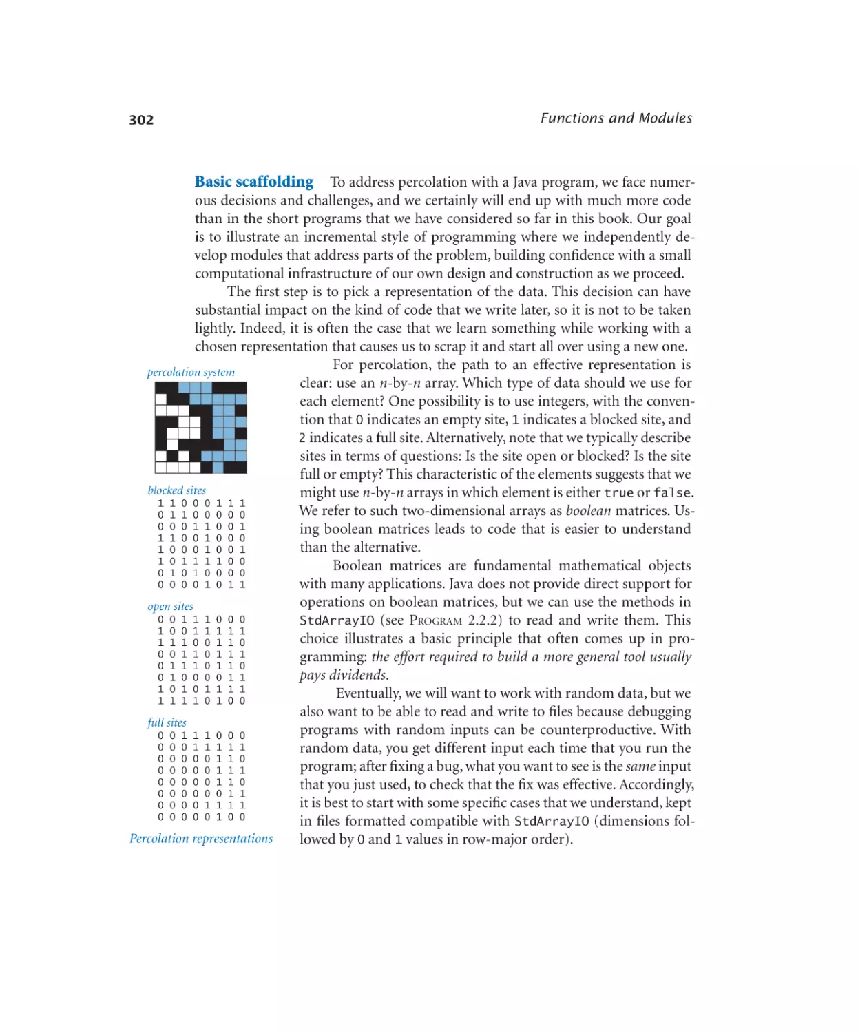
Binary search (20 questions). . . 534
Bisection search . . . . . . . . 537
Binary search (sorted array). . . 539
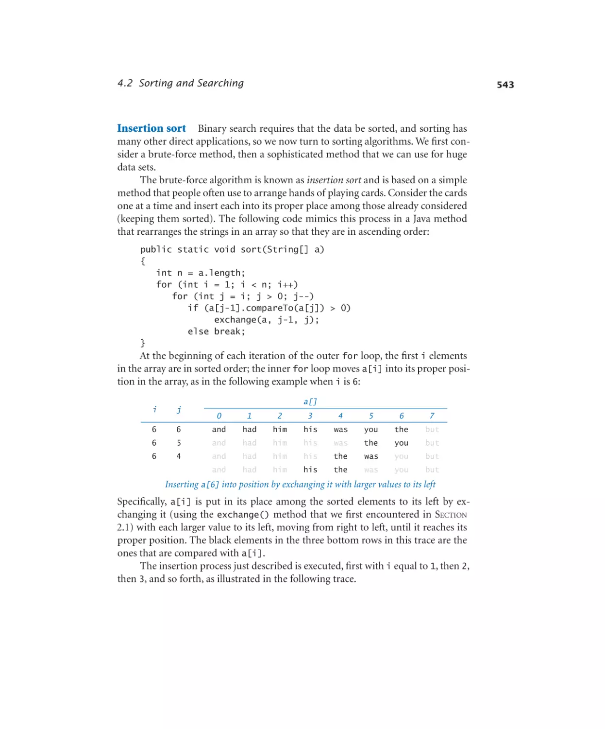
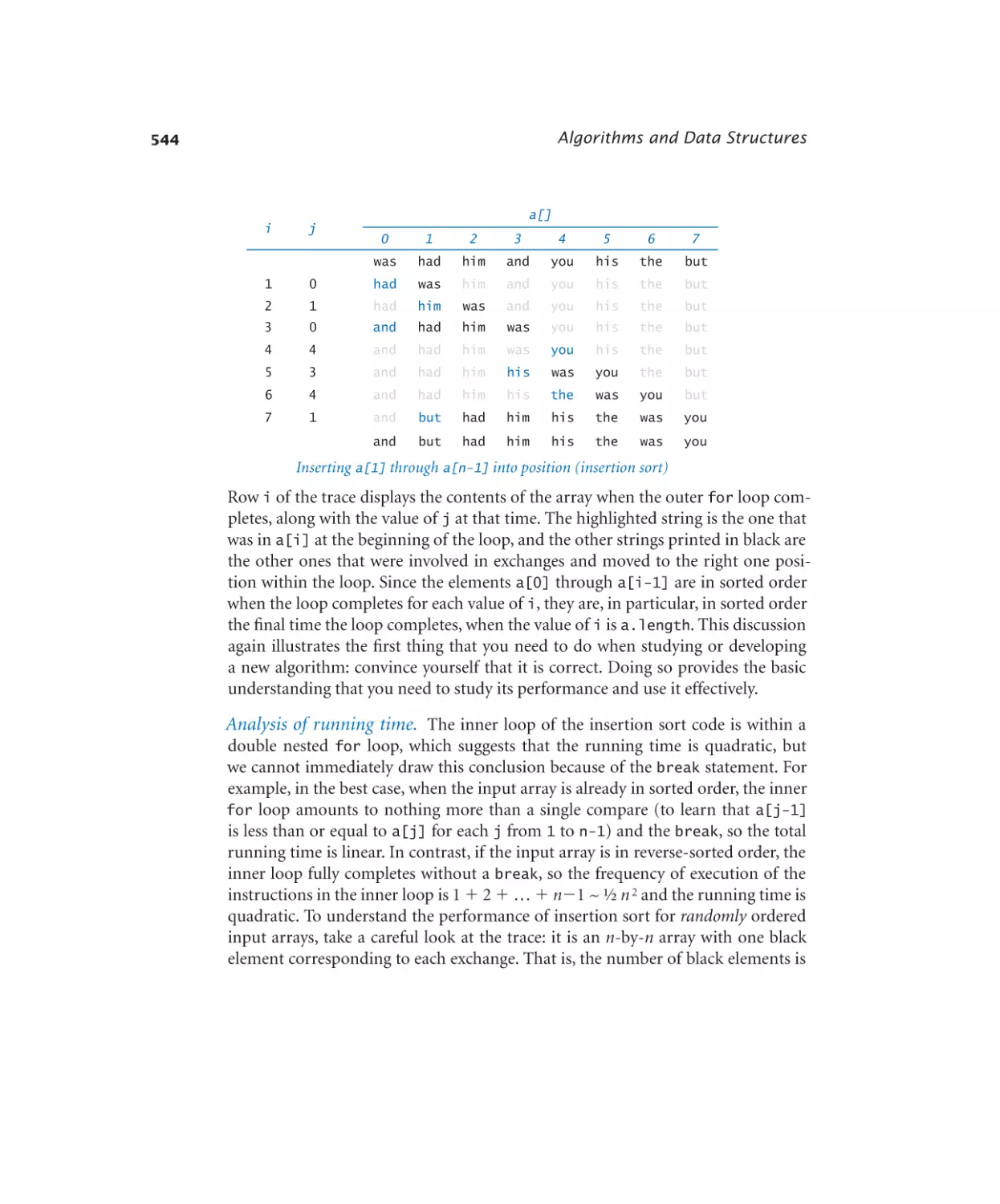
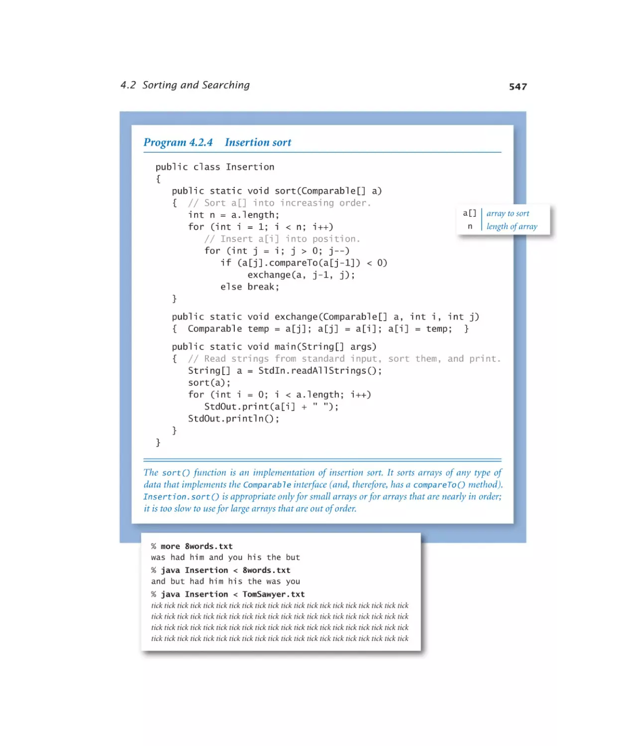
Insertion sort . . . . . . . . . 547
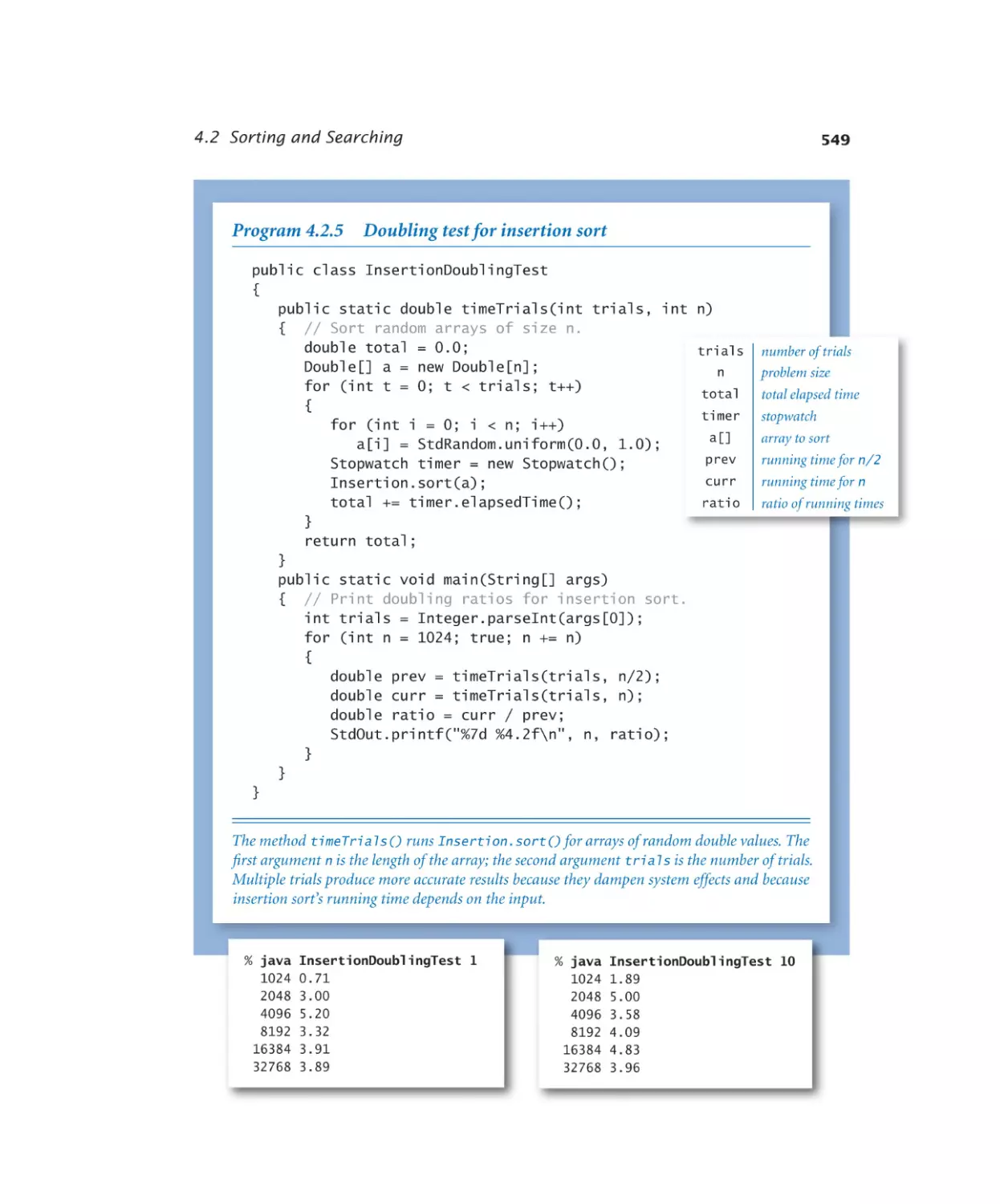
Doubling test for insertion sort .549
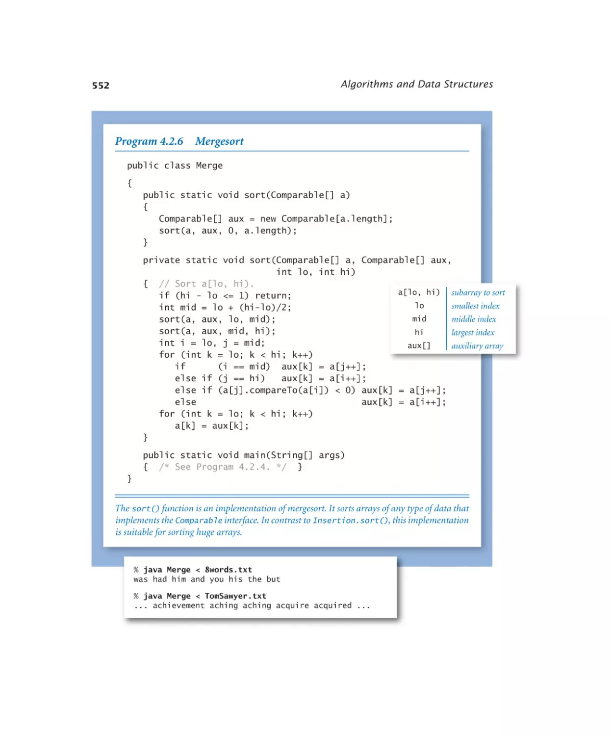
Mergesort . . . . . . . . . . . 552
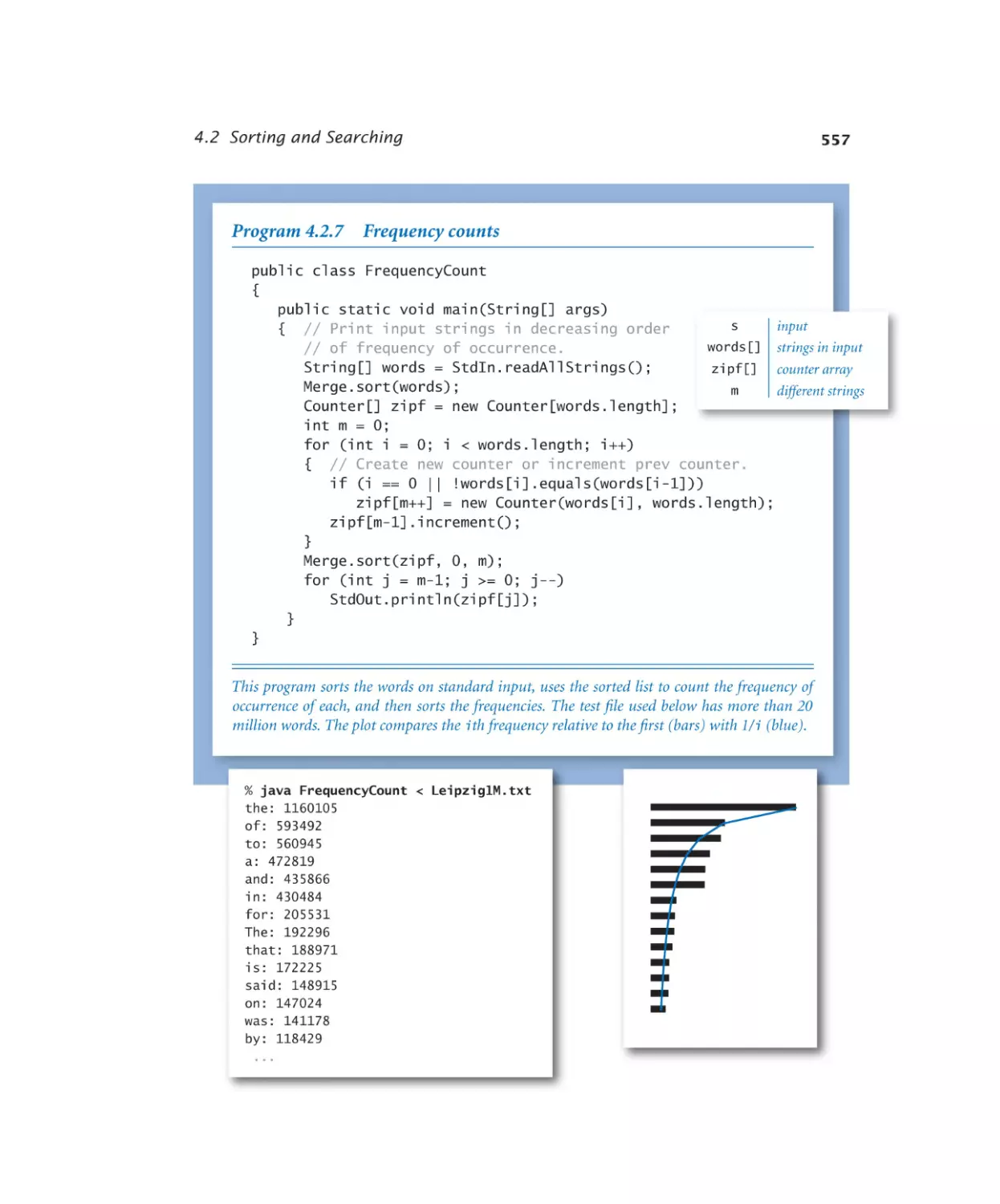
Frequency counts. . . . . . . . 557
Stacks and Queues
4.3.1
4.3.2
4.3.3
4.3.4
4.3.5
4.3.6
4.3.7
4.3.8
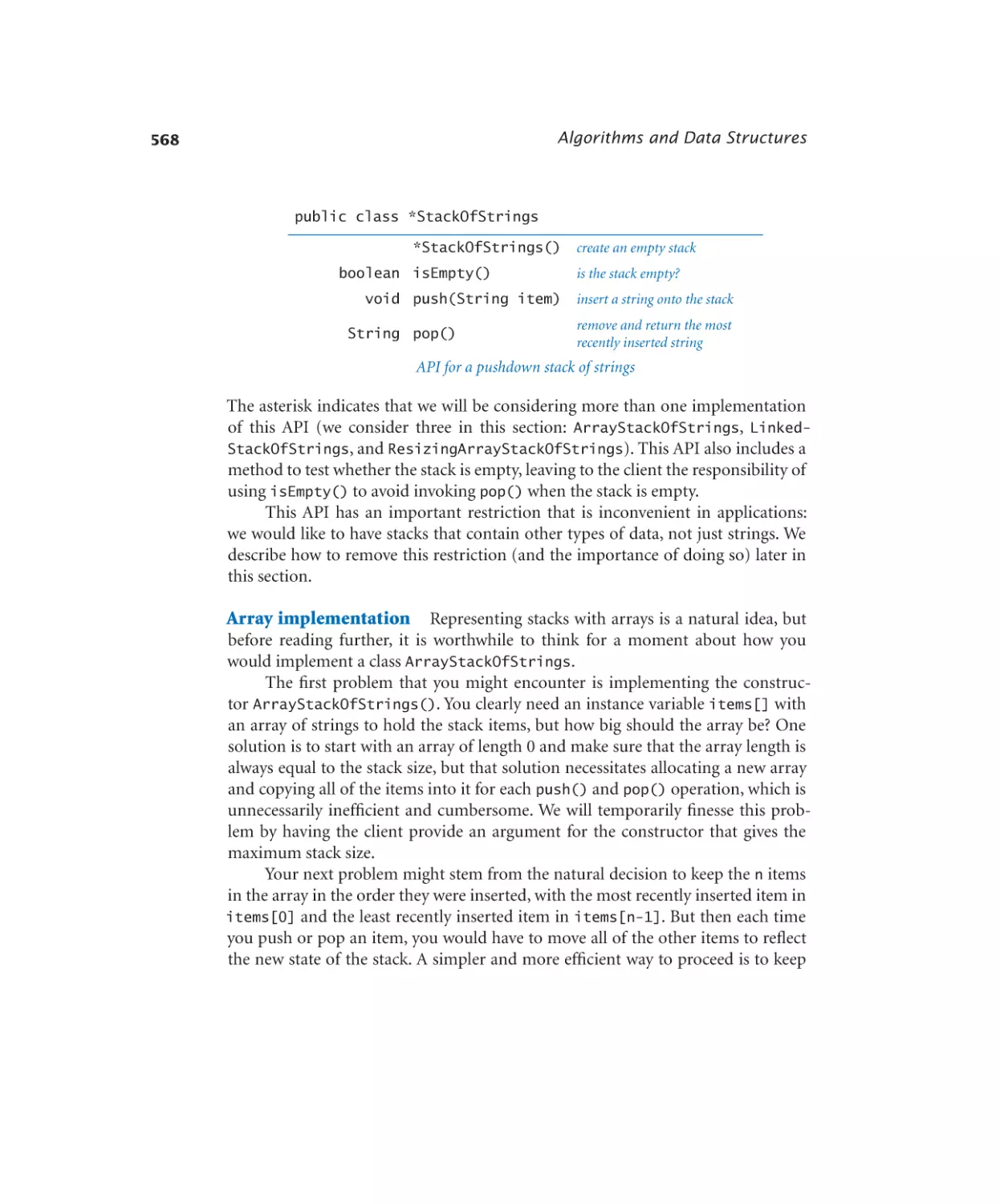
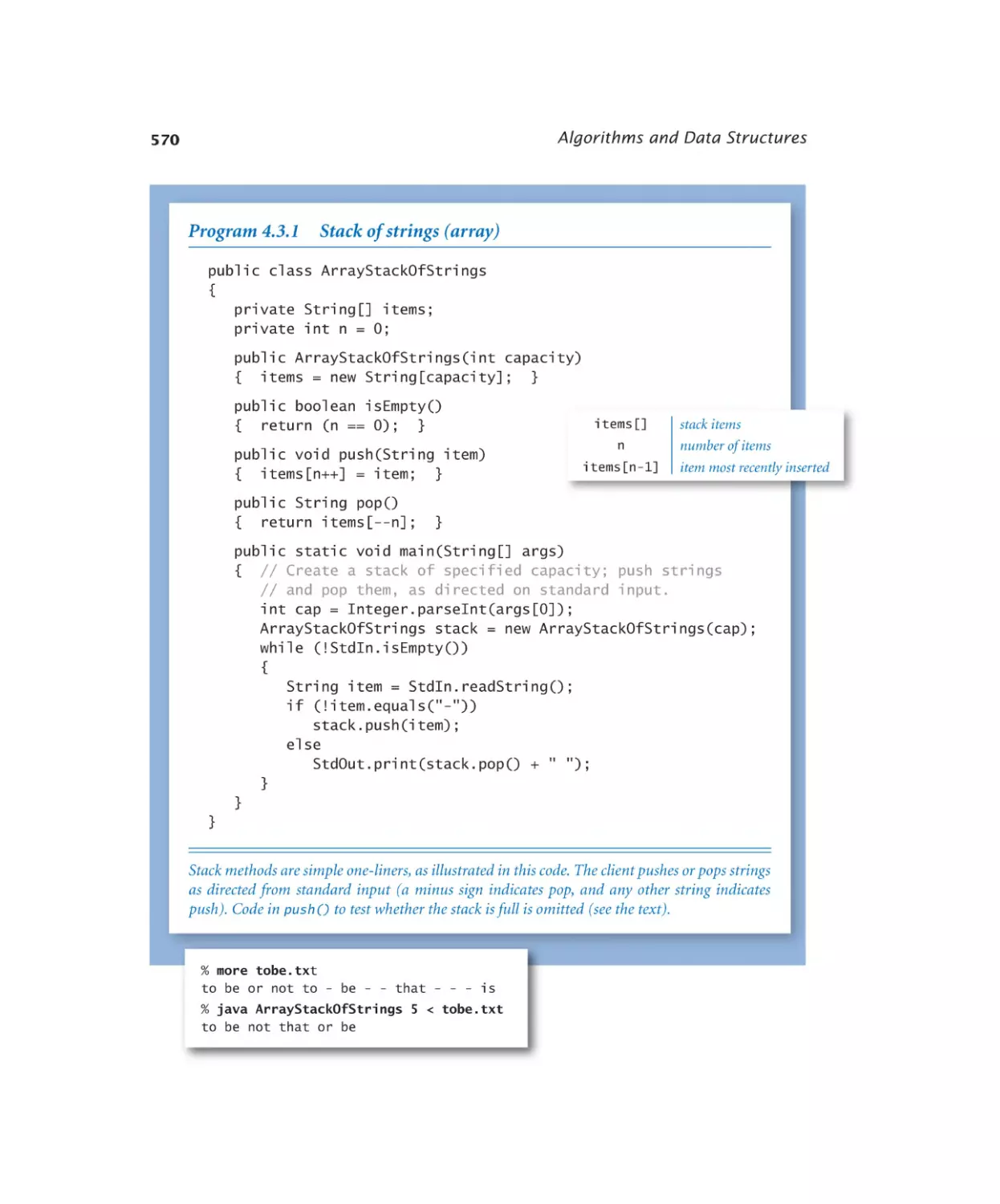
Stack of strings (array). . . . . 570
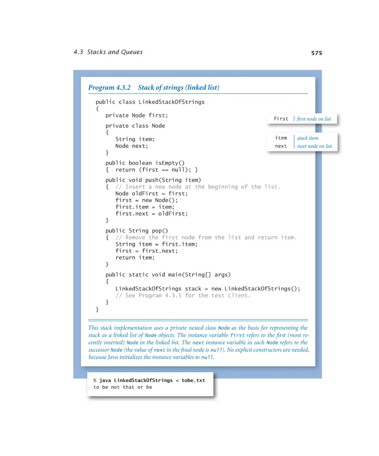
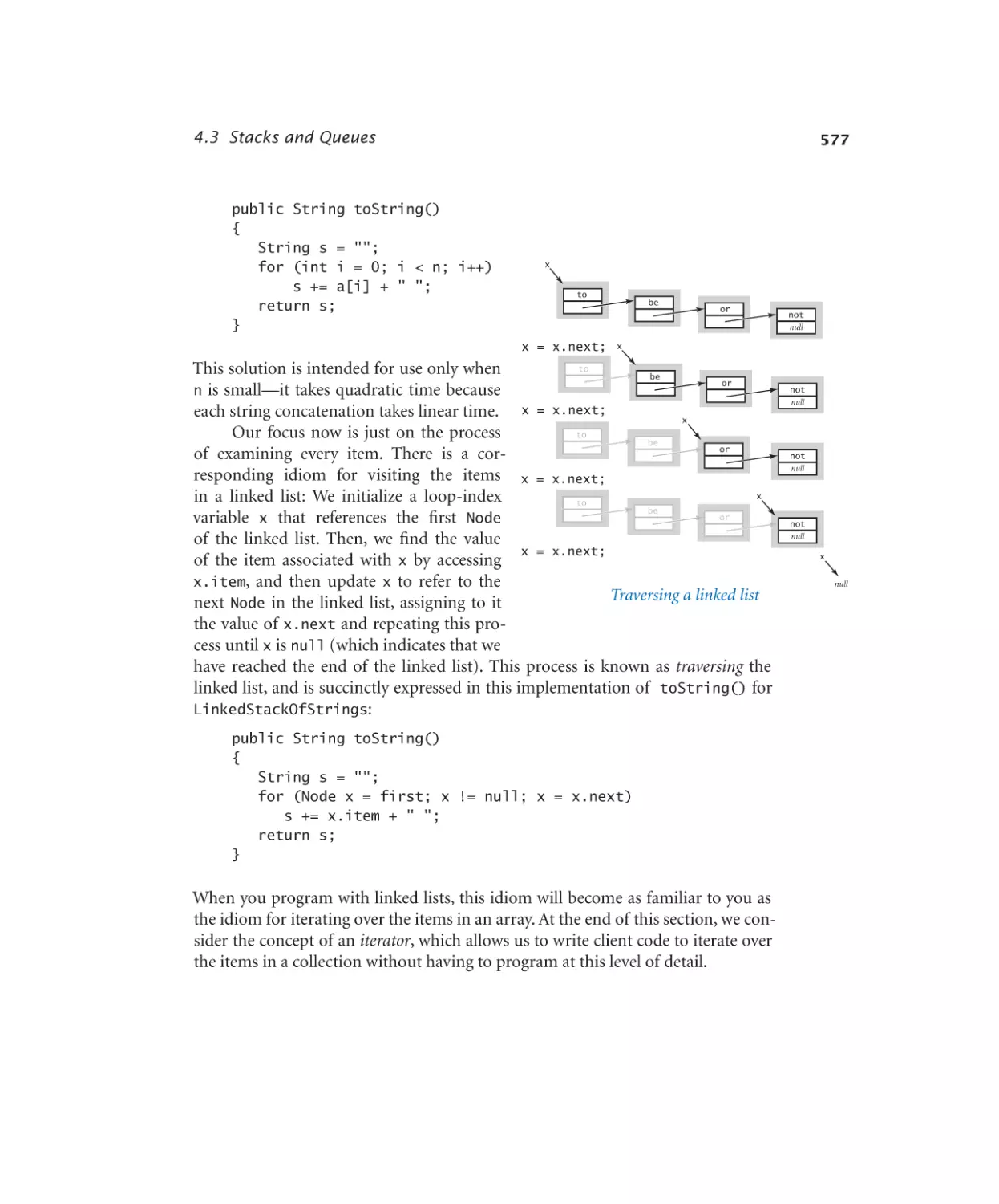
Stack of strings (linked list). . . . 575
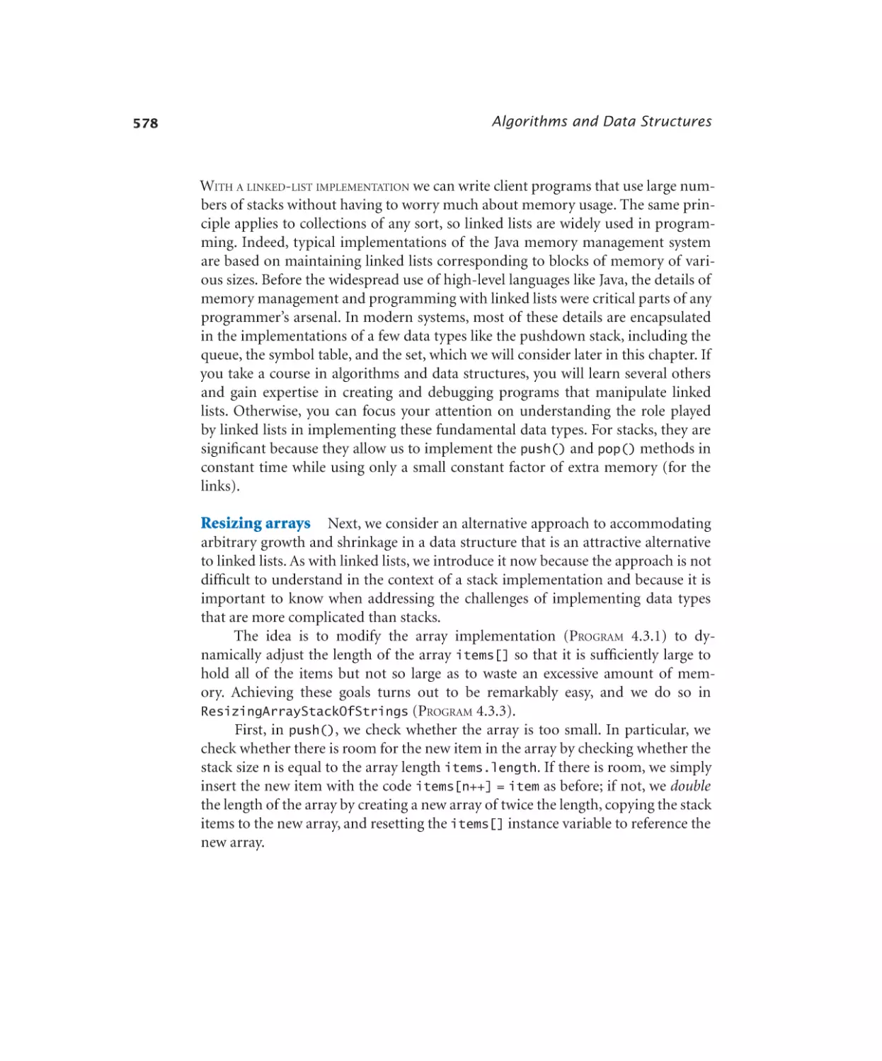
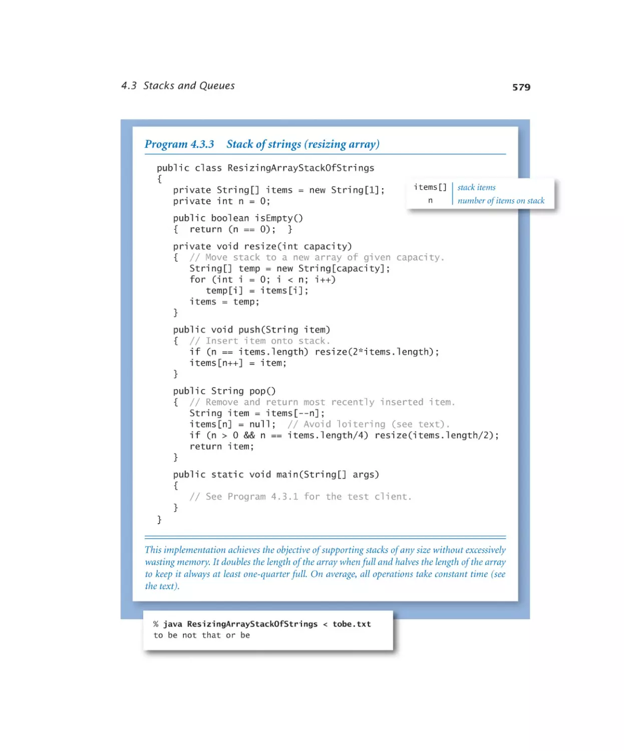
Stack of strings (resizing array) . 579
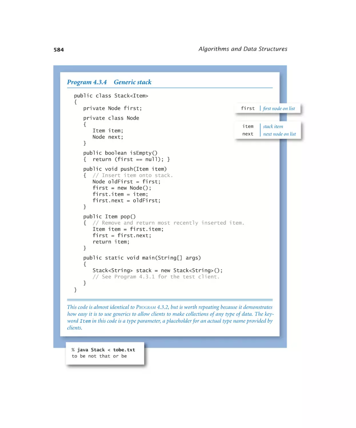
Generic stack . . . . . . . . . 584
Expression evaluation . . . . . . 588
Generic FIFO queue (linked list). 594
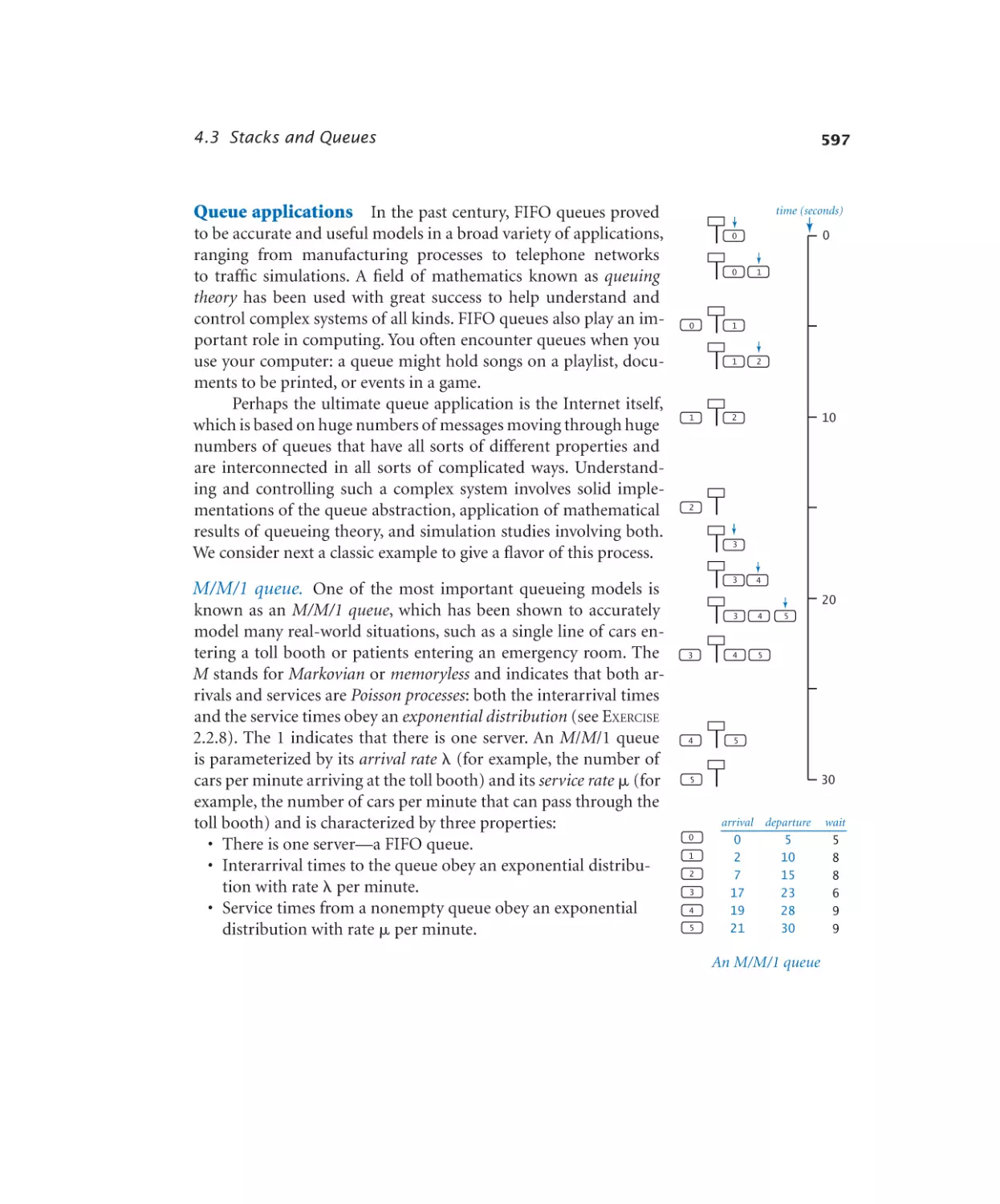
M/M/1 queue simulation . . . . 599
Load balancing simulation . . . . 607
Symbol Tables
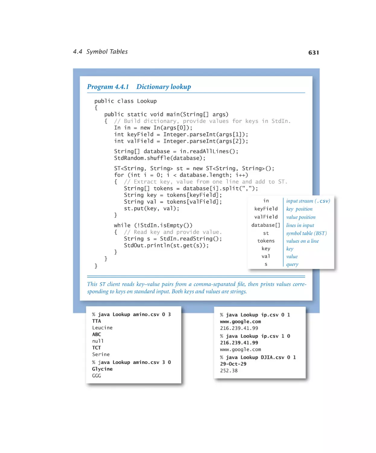
4.4.1
4.4.2
4.4.3
4.4.4
4.4.5
Dictionary lookup. . . . . . . 631
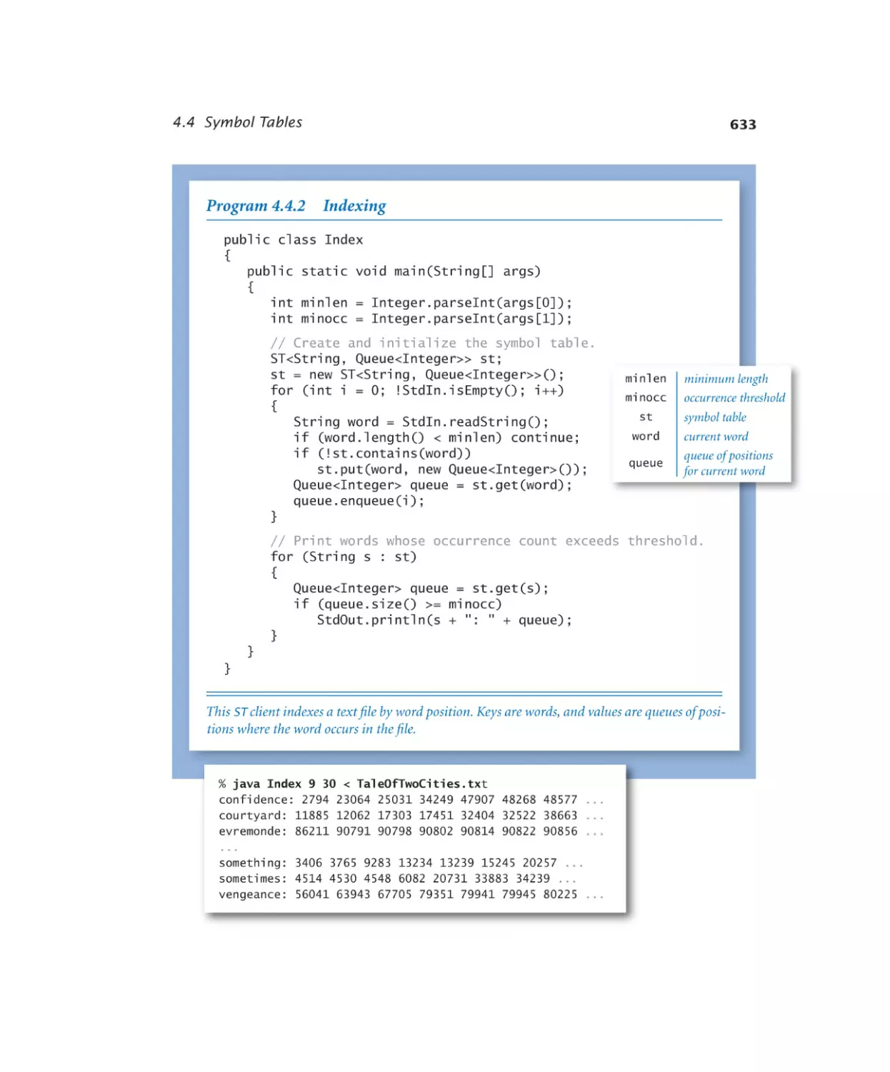
Indexing. . . . . . . . . . . 633
Hash table. . . . . . . . . . . 638
Binary search tree. . . . . . . . 646
Dedup filter. . . . . . . . . . 653
Case Study: Small-World Phenomenon
4.5.1
4.5.2
4.5.3
4.5.4
4.5.5
4.5.6
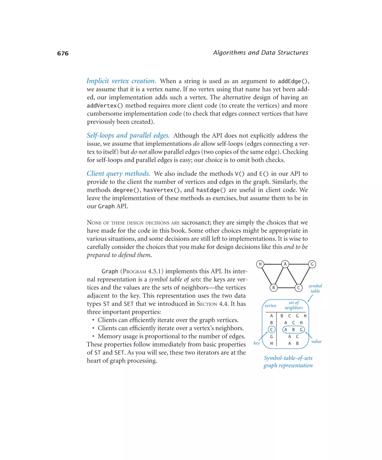
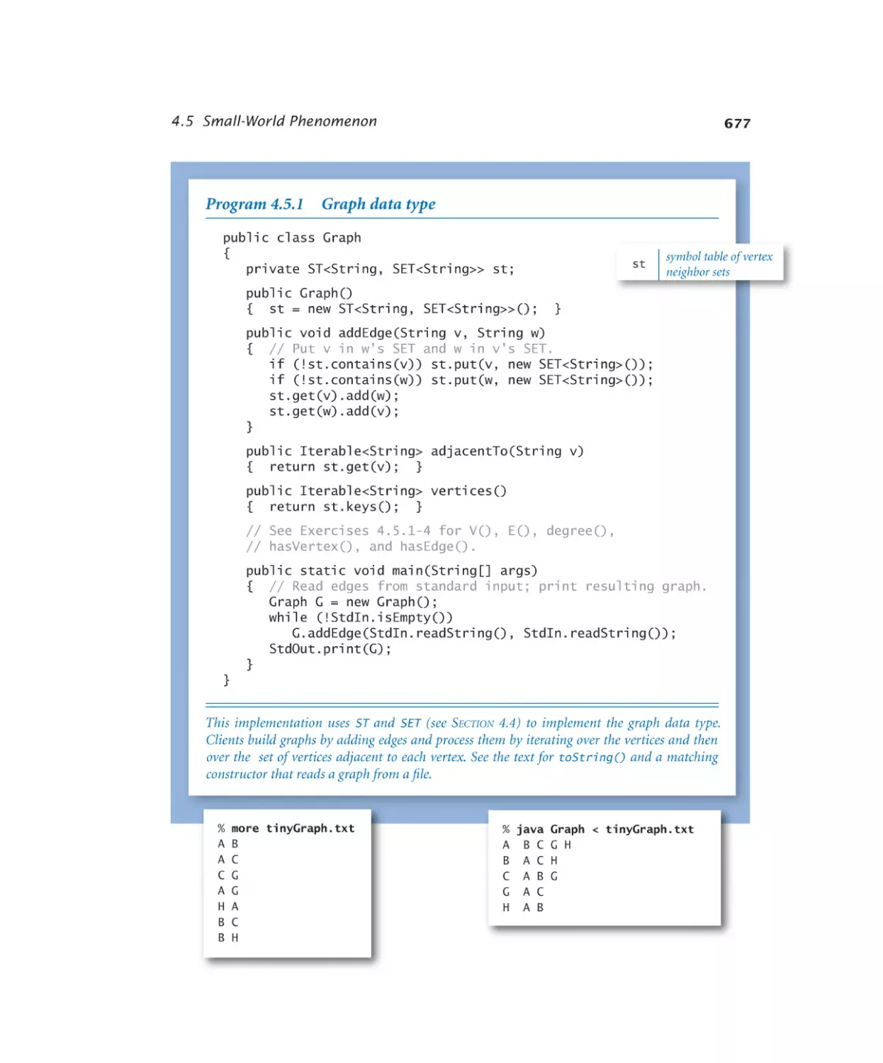
Graph data type . . . . . . . . 677
Using a graph to invert an index . 681
Shortest-paths client . . . . . . 685
Shortest-paths implementation .691
Small-world test. . . . . . . . 696
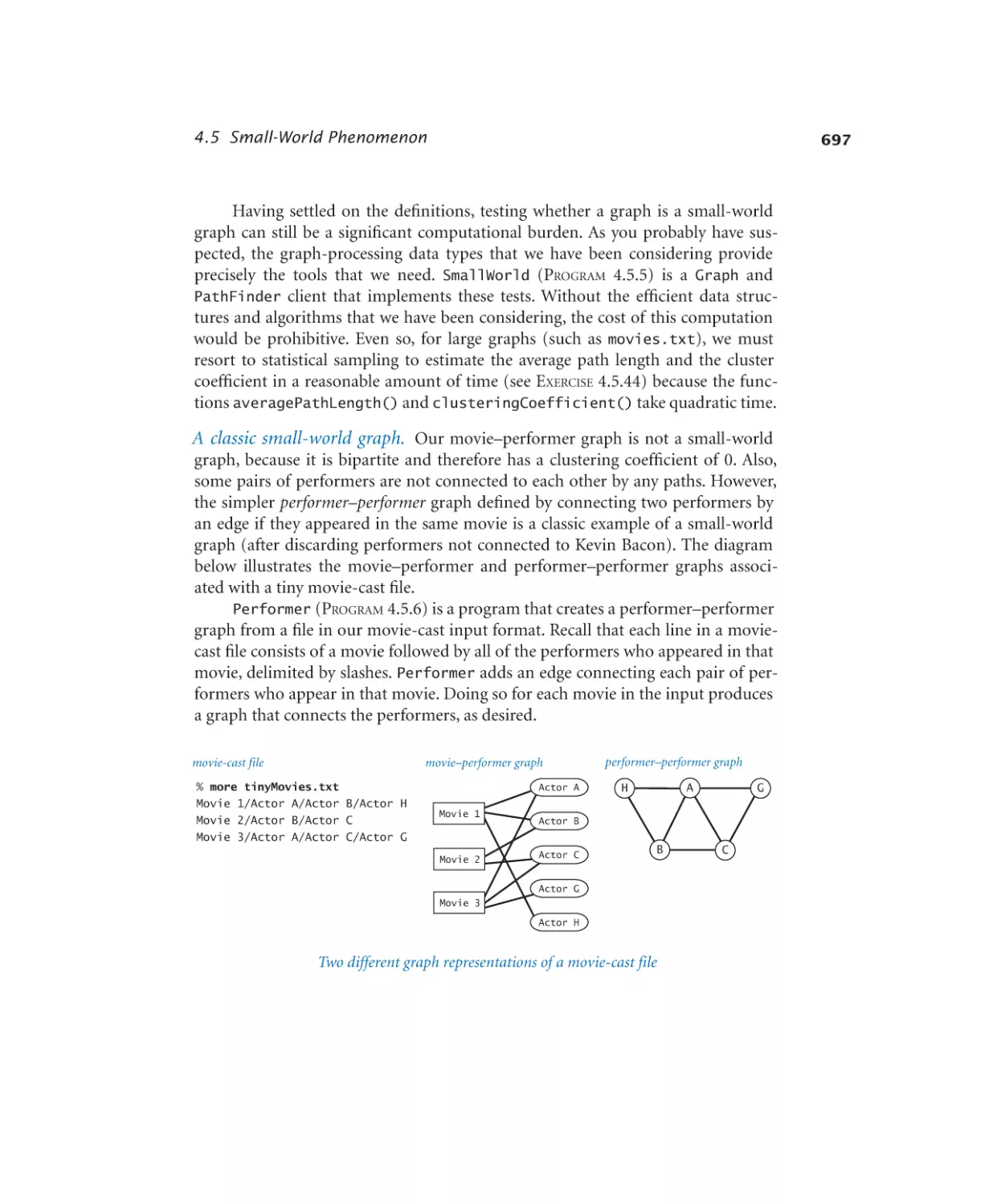
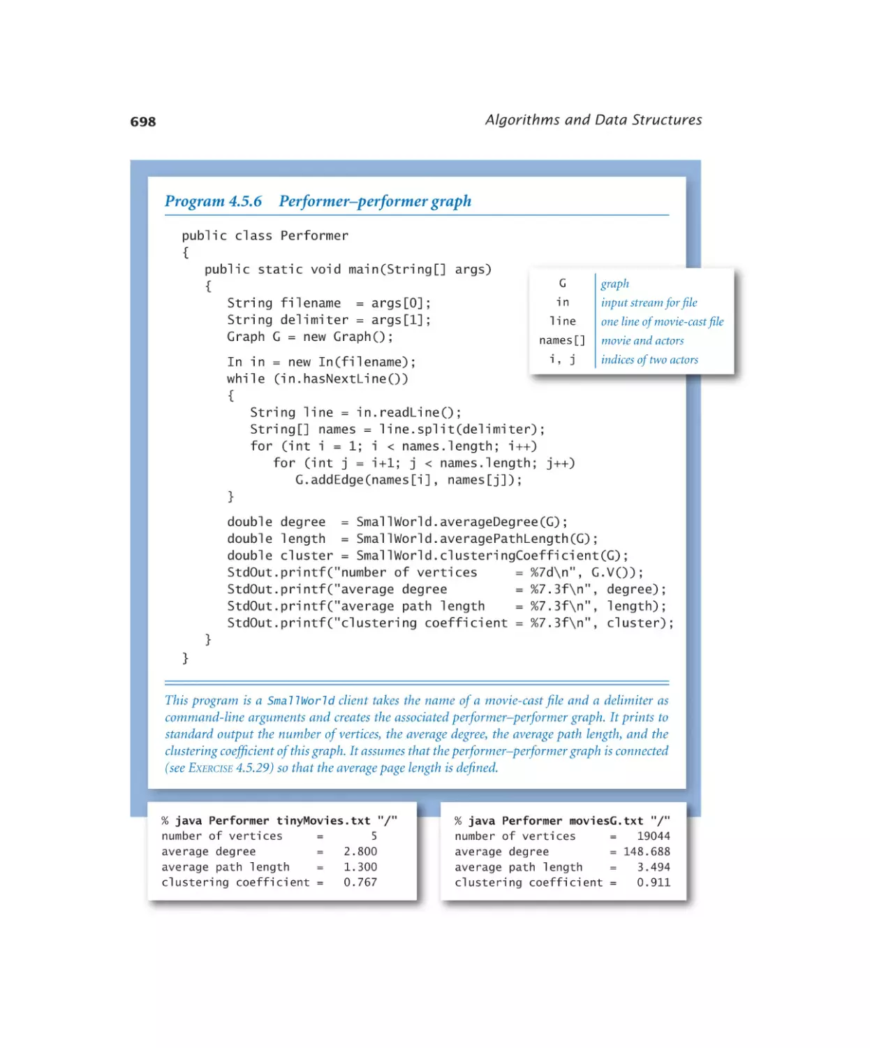
Performer–performer graph . . . 698
ix
Theory of Computing
A Computing Machine
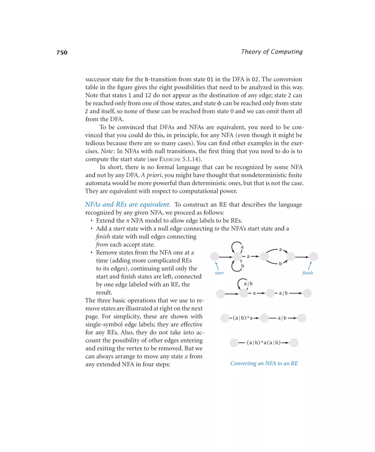
Formal Languages
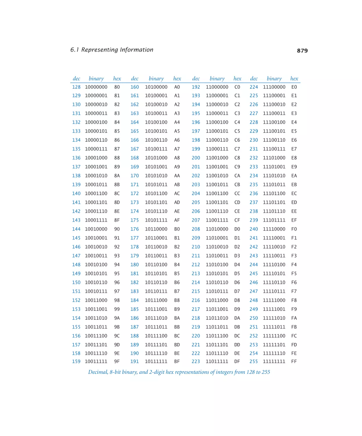
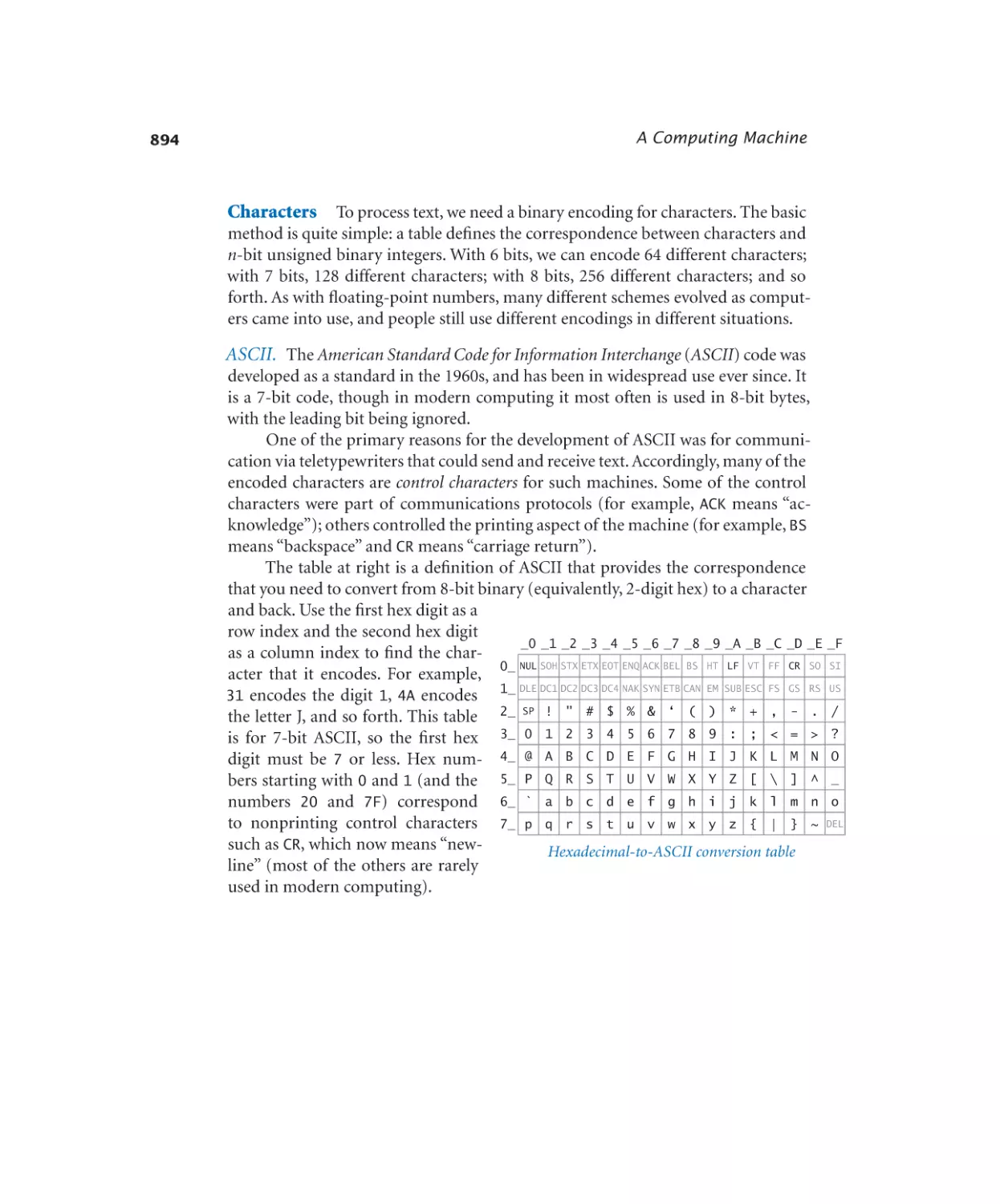
Representing Information
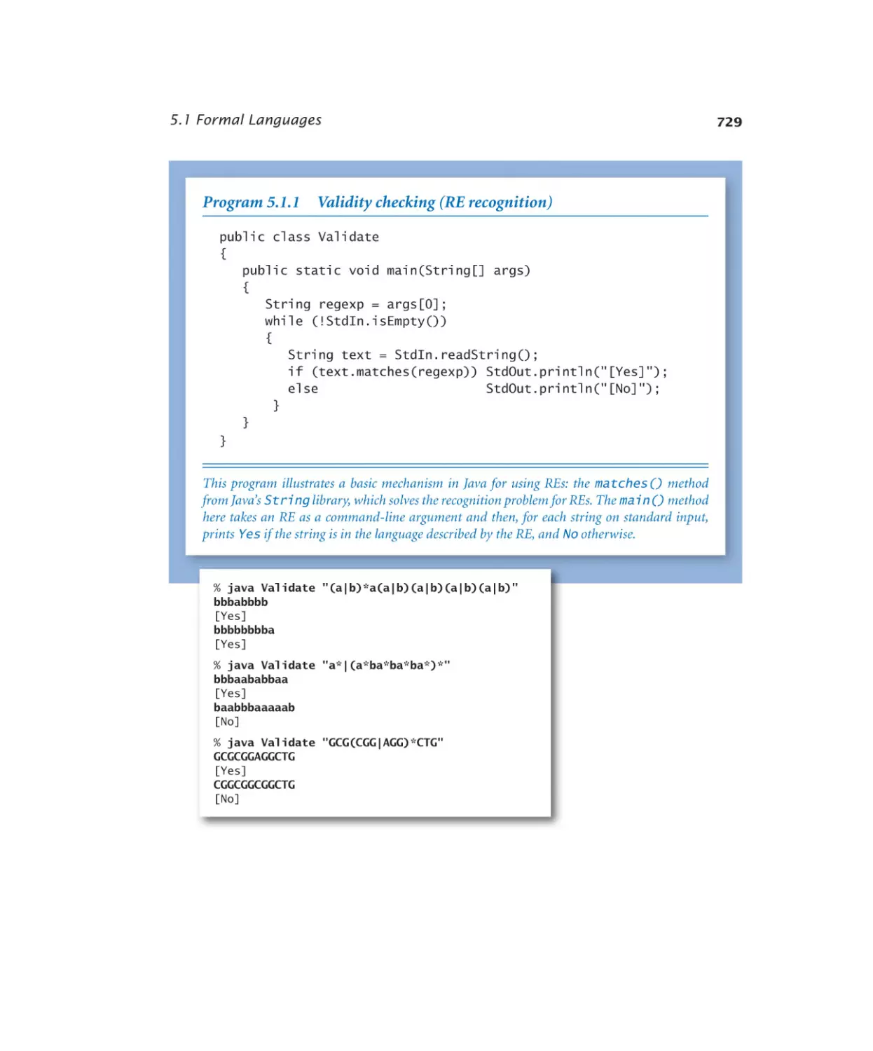
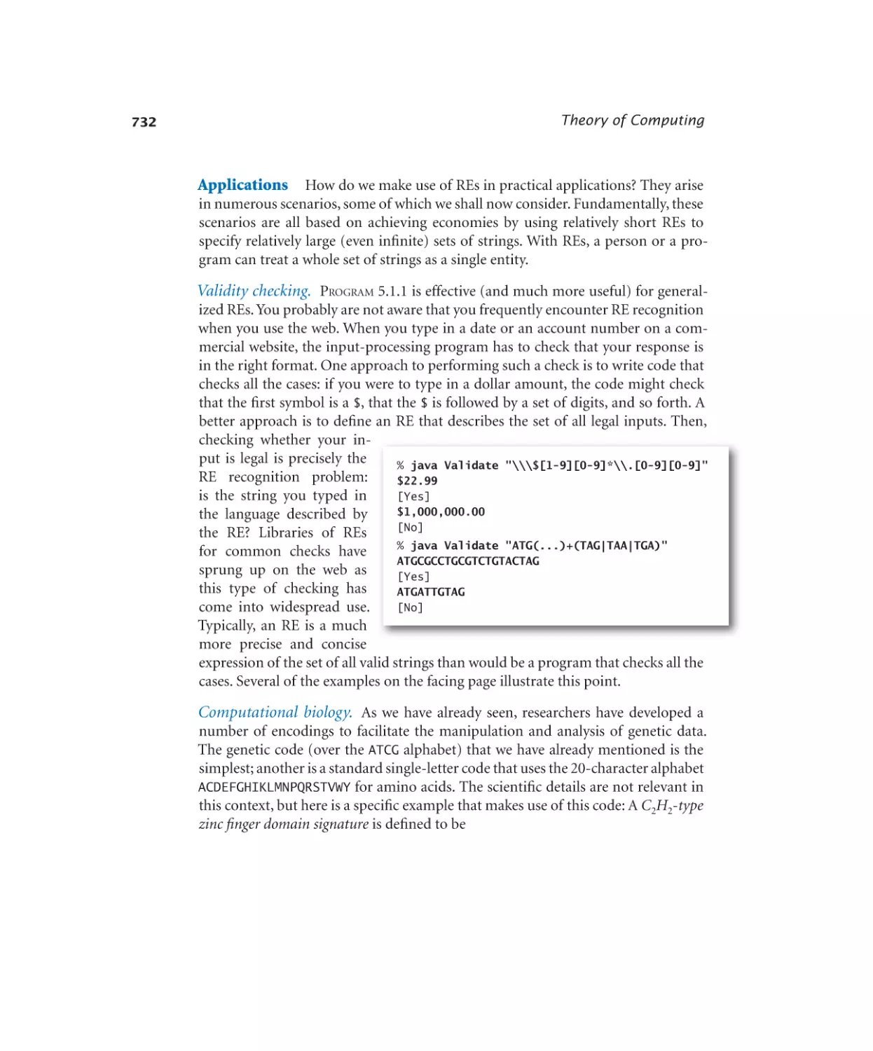
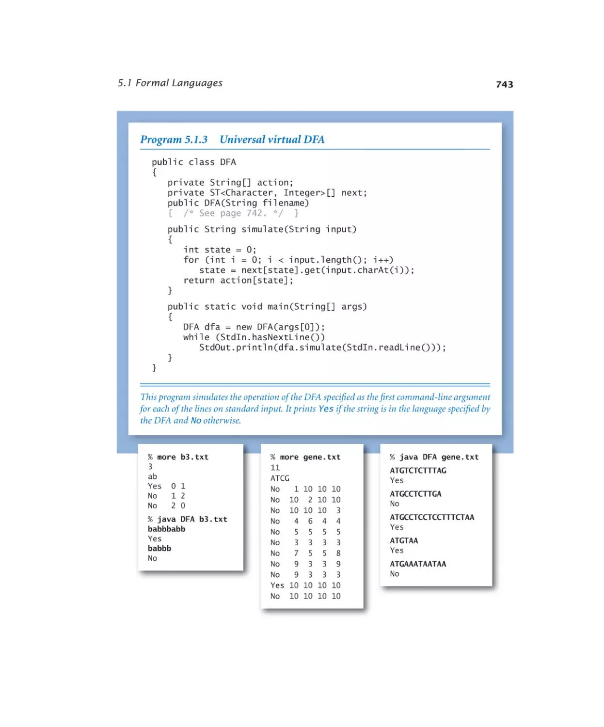
5.1.1 RE recognition. . . . . . . . . 729
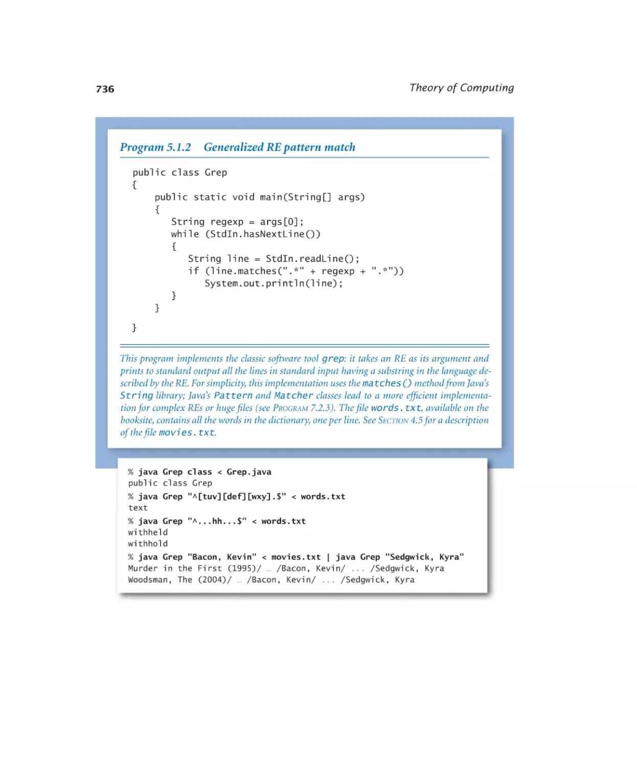
5.1.2 Generalized RE pattern match . 736
5.1.3 Universal virtual DFA . . . . . . 743
Turing Machines
5.2.1 Virtual Turing machine tape . . . 776
5.2.2 Universal virtual TM. . . . . . 777
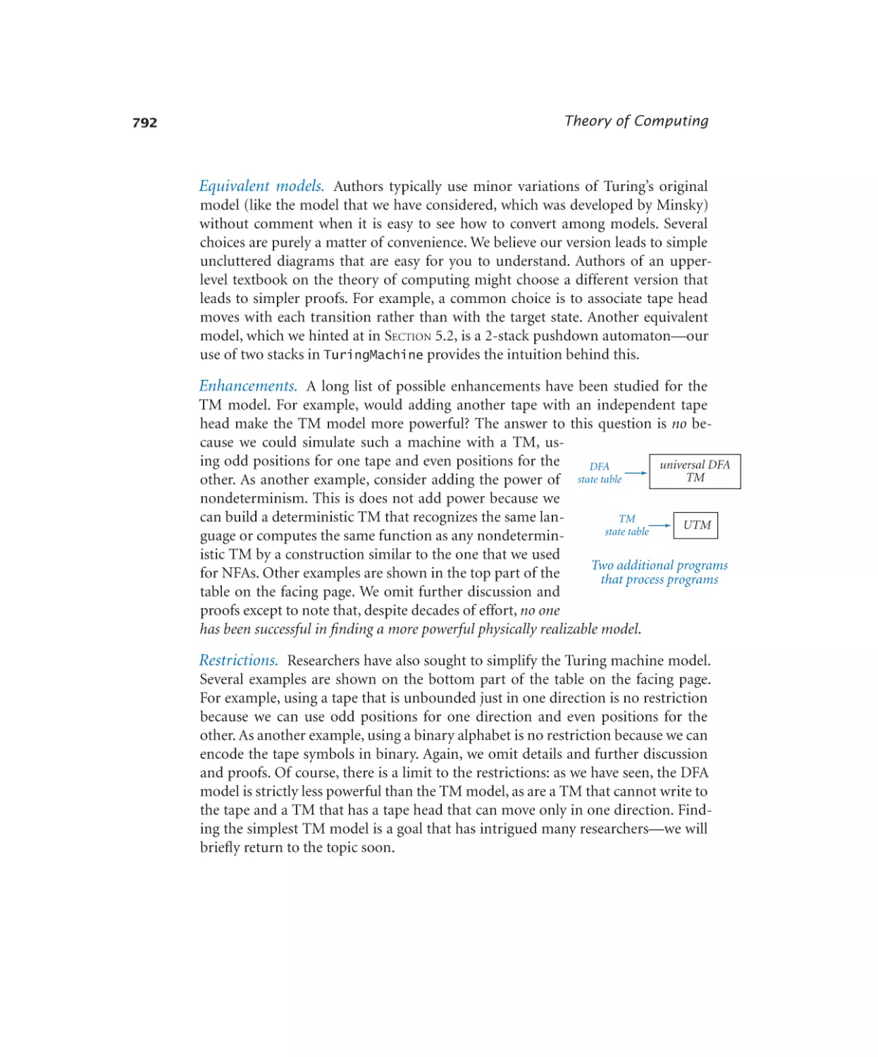
Universality
Computability
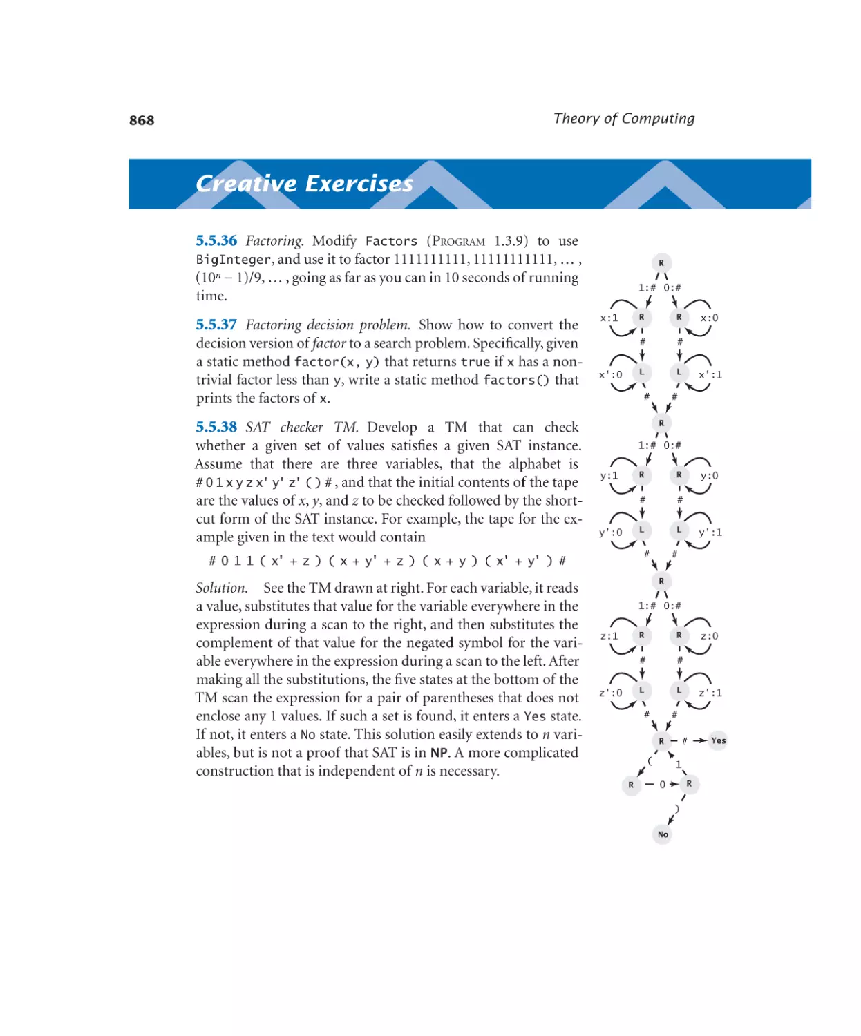
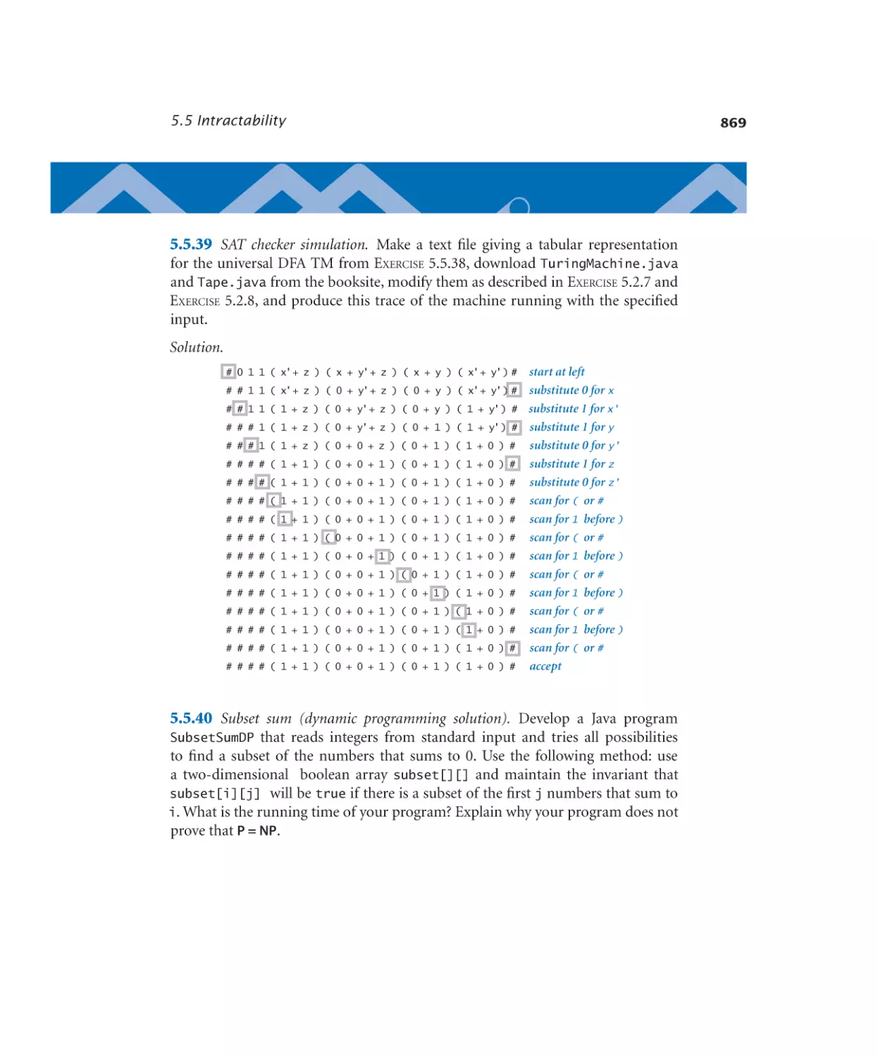
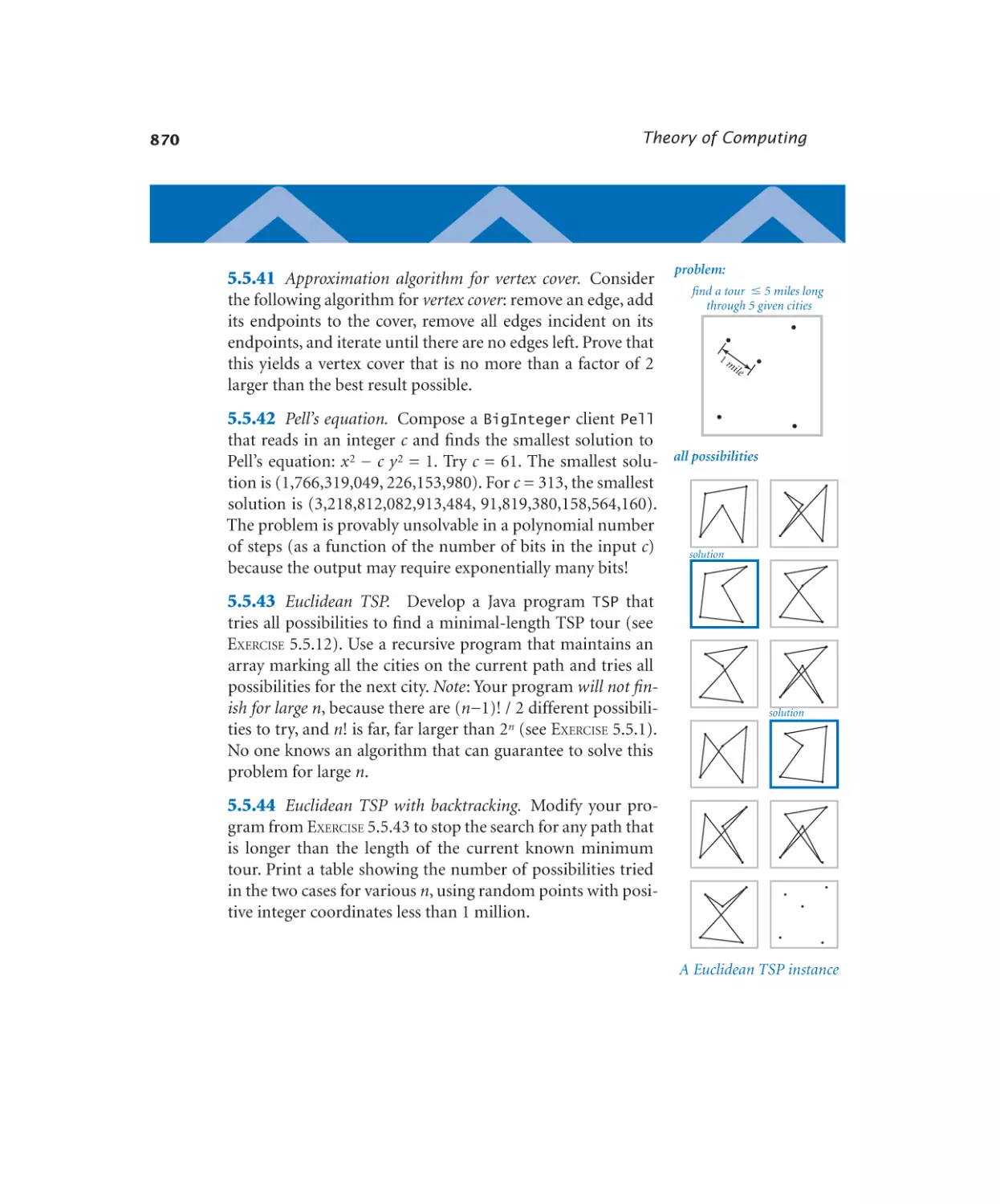
Intractability
5.5.1 SAT solver . . . . . . . . . . 855
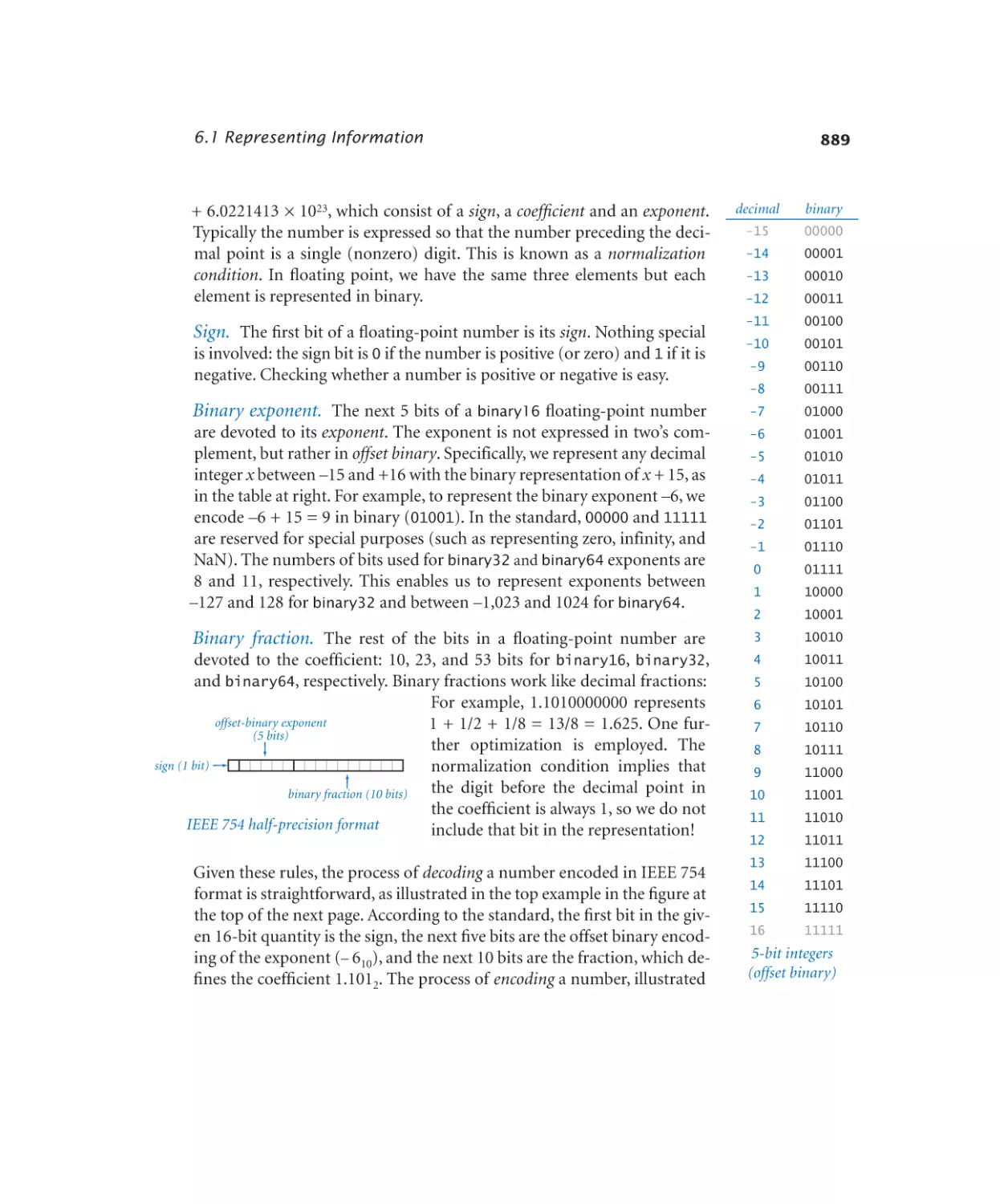
6.1.1
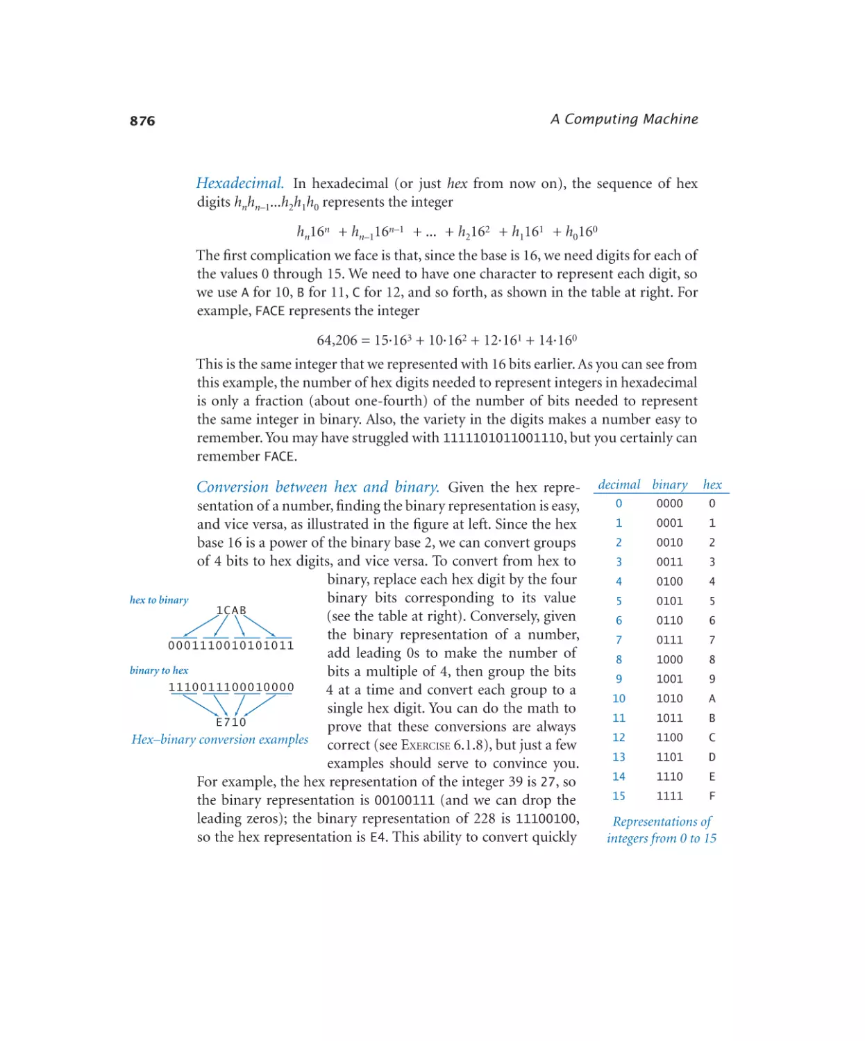
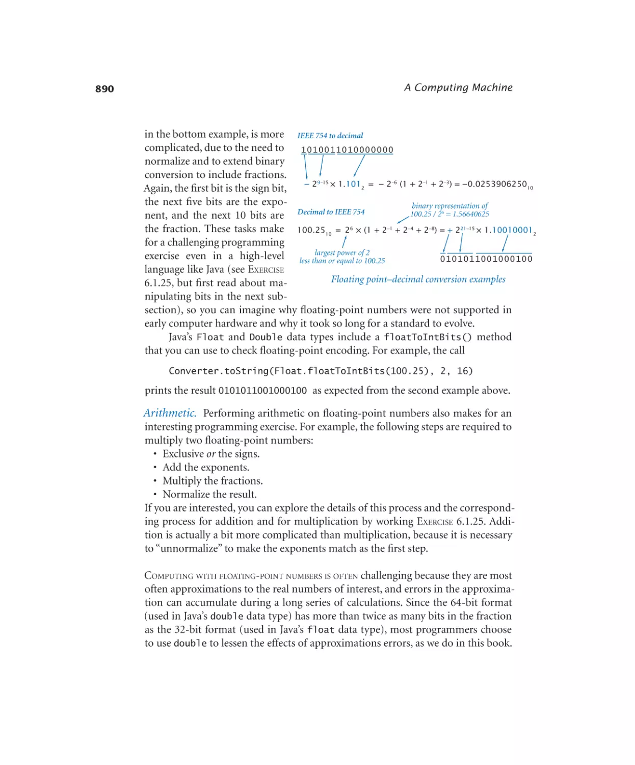
6.1.2
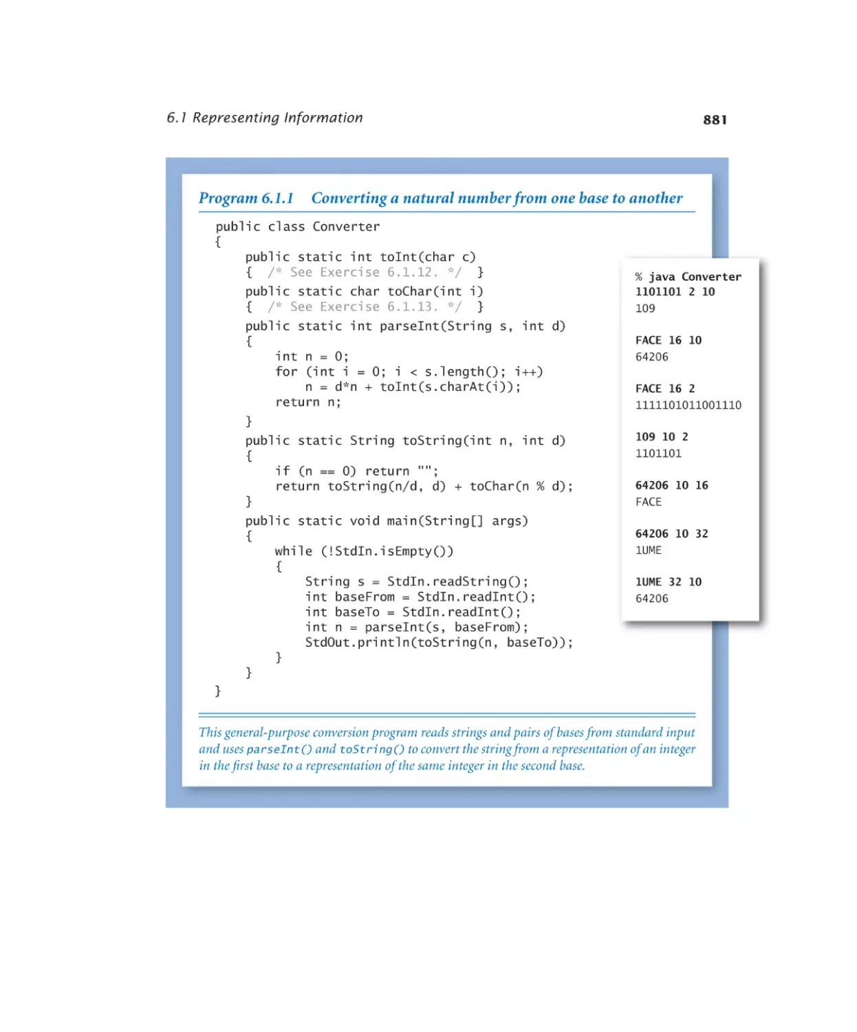
Number conversion. . . . . . . 881
Floating-point components . . . 893
TOY Machine
6.2.1 Your first TOY program. . . . . 915
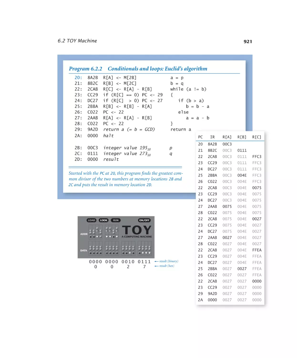
6.2.2 Conditionals and loops. . . . . 921
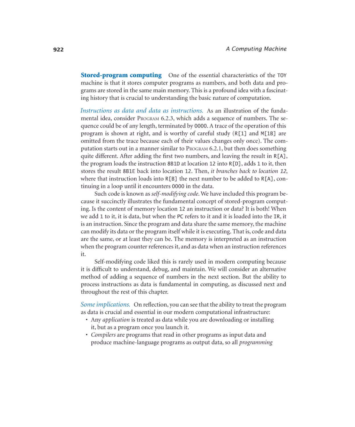
6.2.3 Self-modifying code. . . . . . . 923
Machine-Language Programming
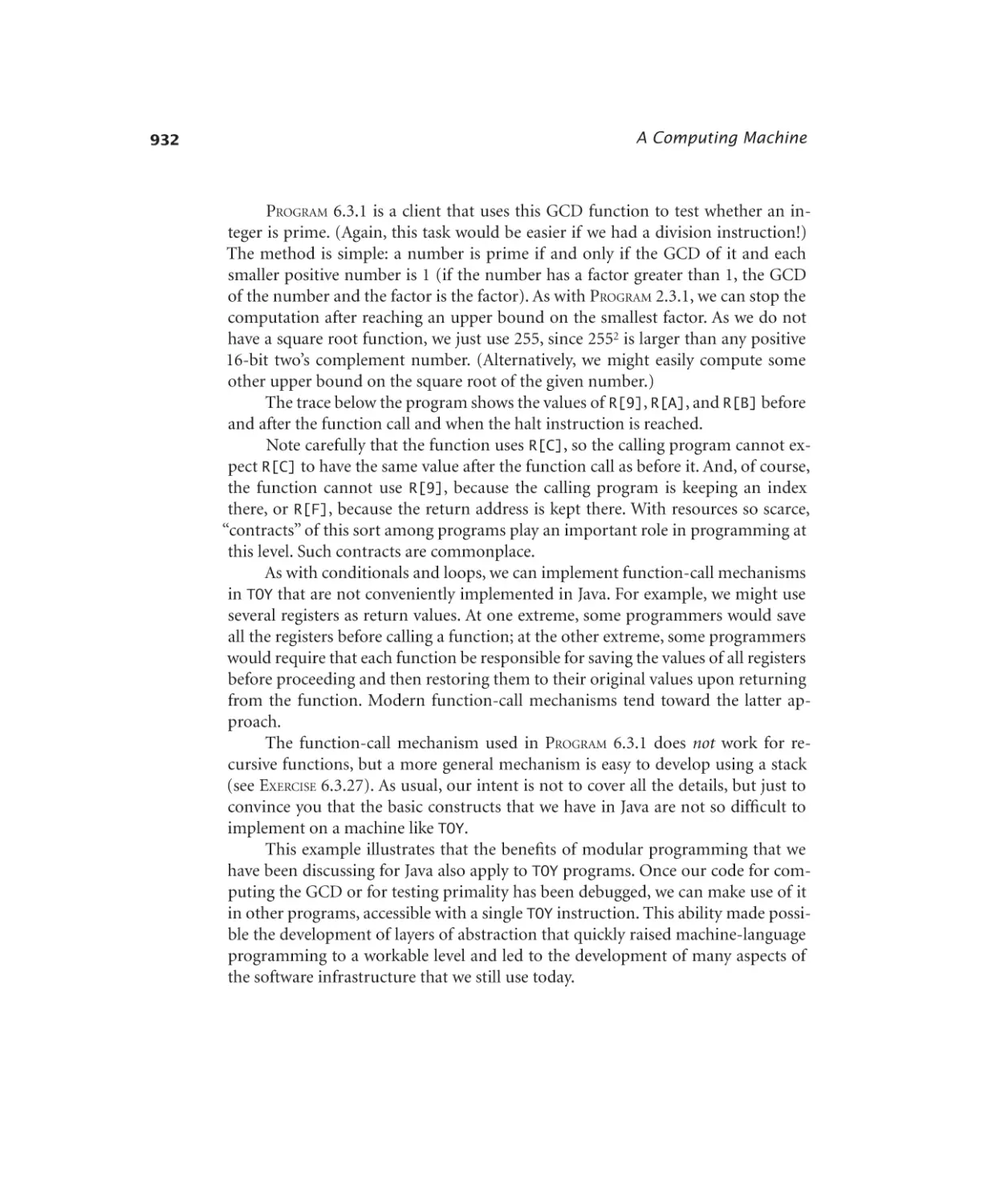
6.3.1 Calling a function . . . . . . . 933
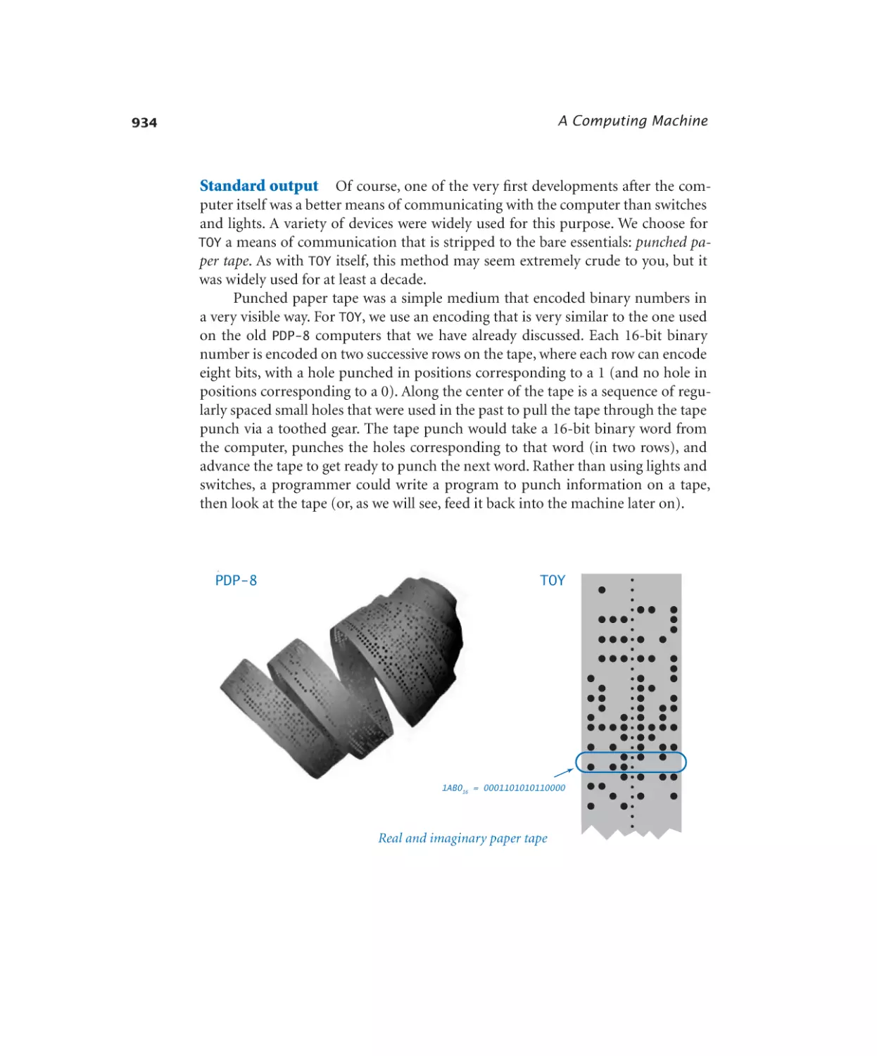
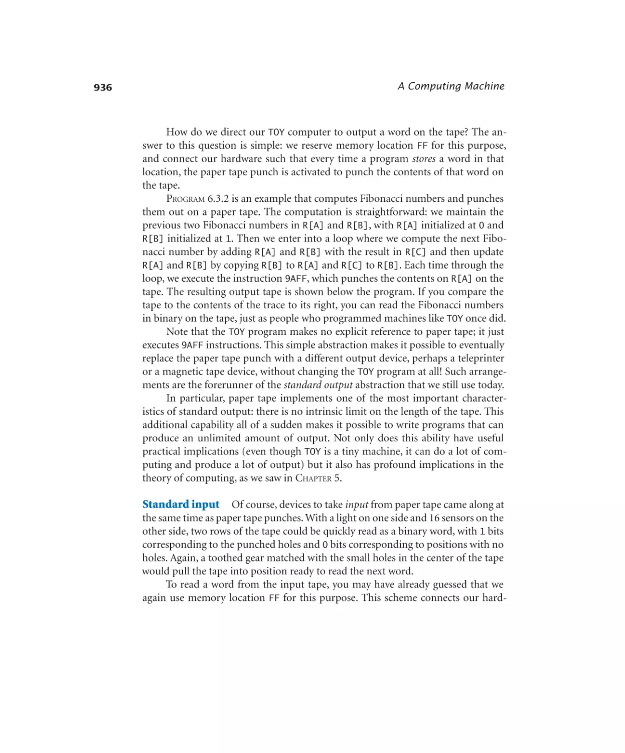
6.3.2 Standard output. . . . . . . . 935
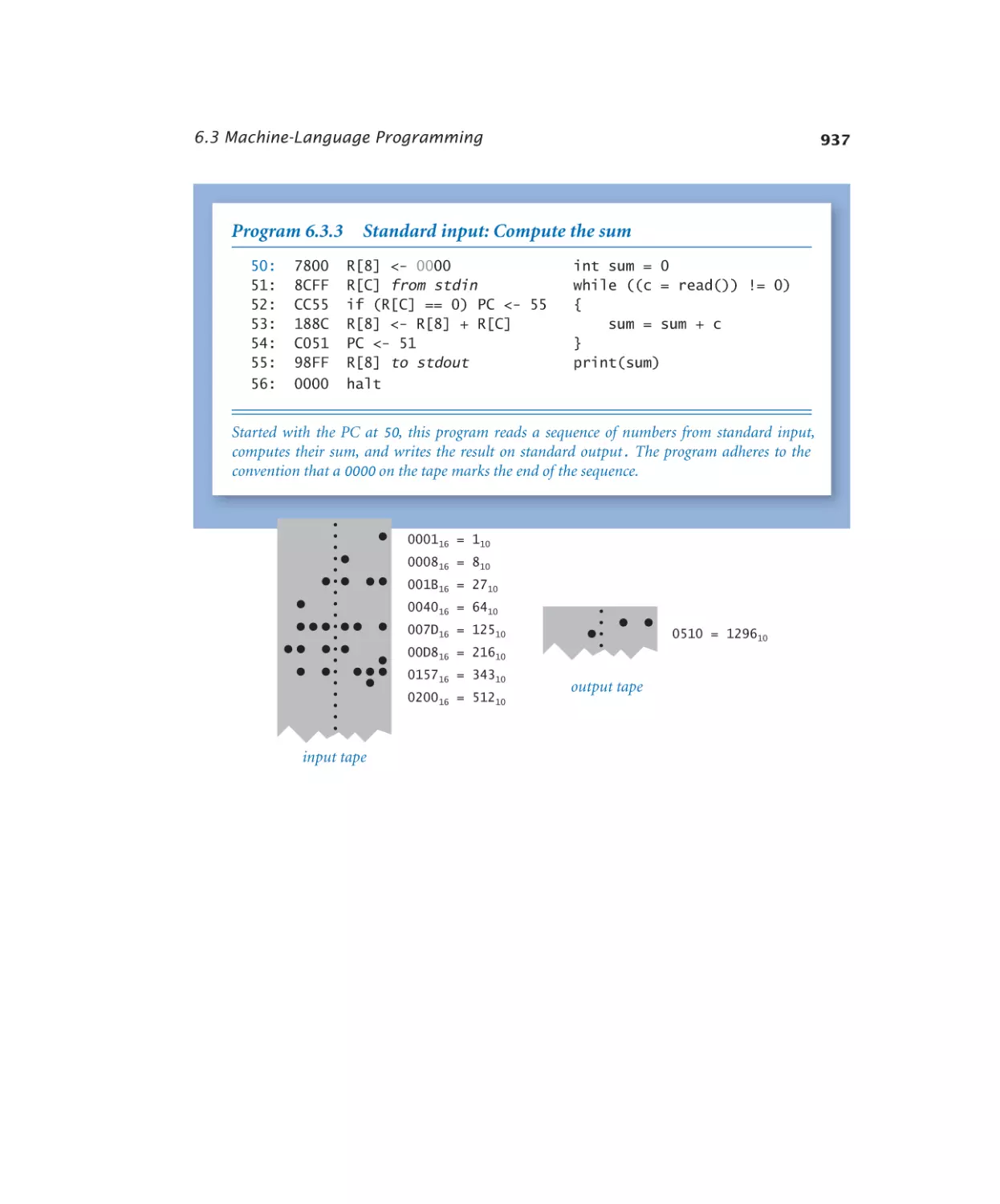
6.3.3 Standard input. . . . . . . . . 937
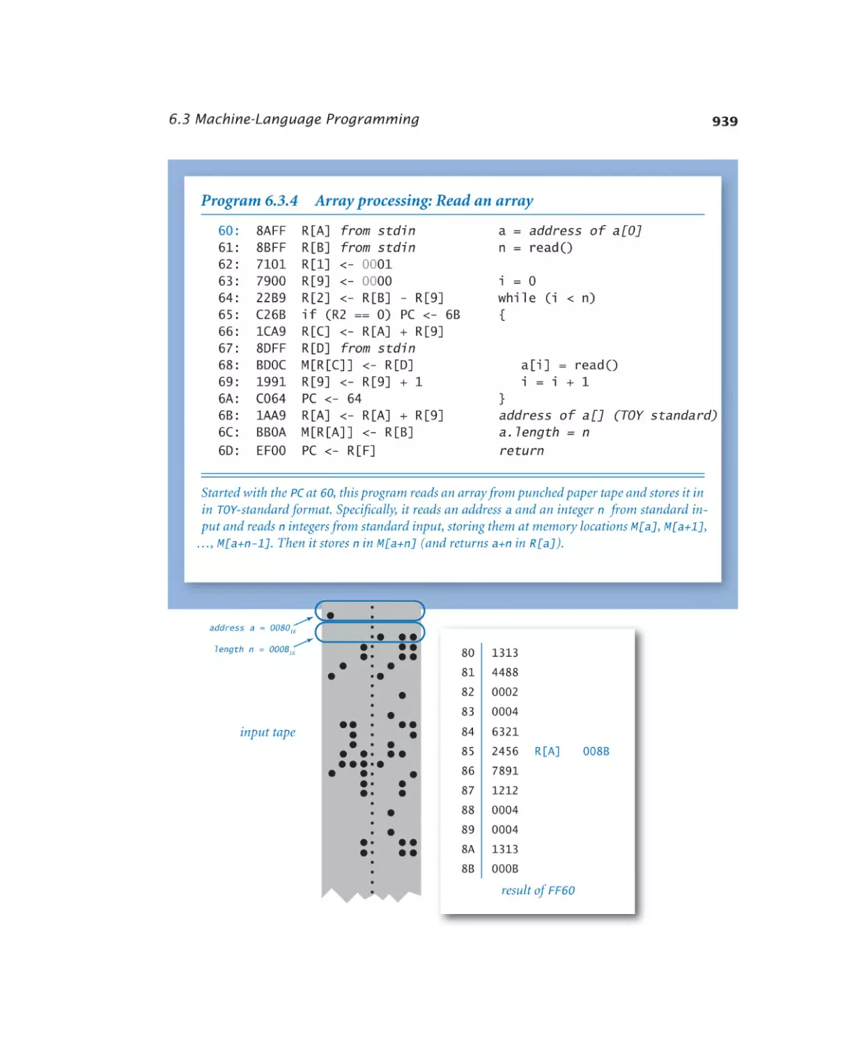
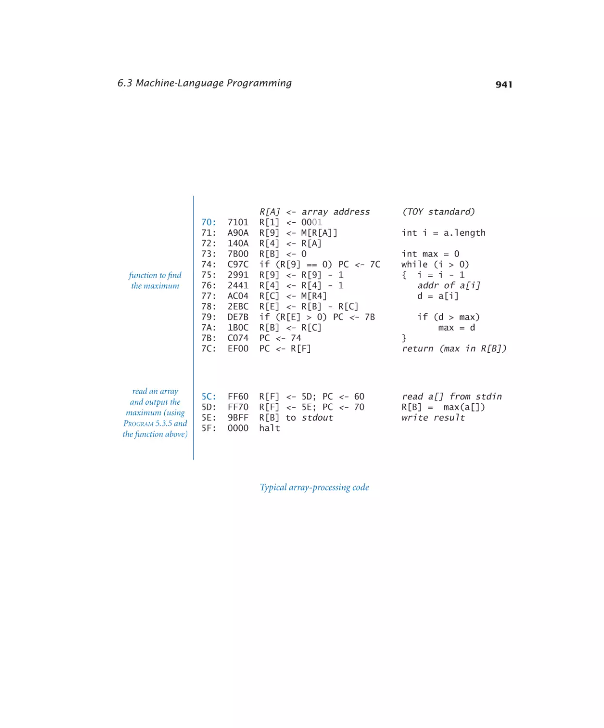
6.3.4 Array processing . . . . . . . . 939
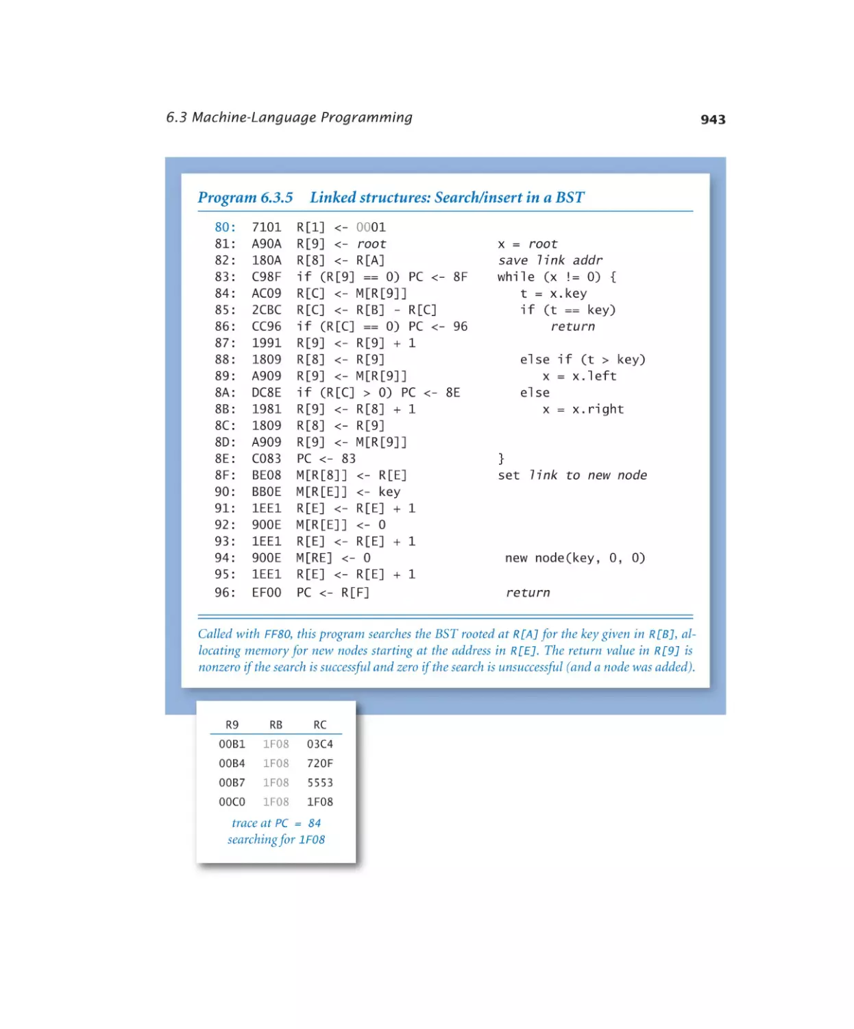
6.3.5 Linked structures. . . . . . . . 943
TOY Virtual Machine
6.4.1
x
TOY virtual machine. . . . . . 967
Circuits
Building a Computing Device
Boolean Logic
Basic Circuit Model
Combinational Circuits
Basic logic gates. . . . . . . . . . . 1014
Selection multiplexer. . . . . . . . 1024
Decoder. . . . . . . . . . . . . . 1021
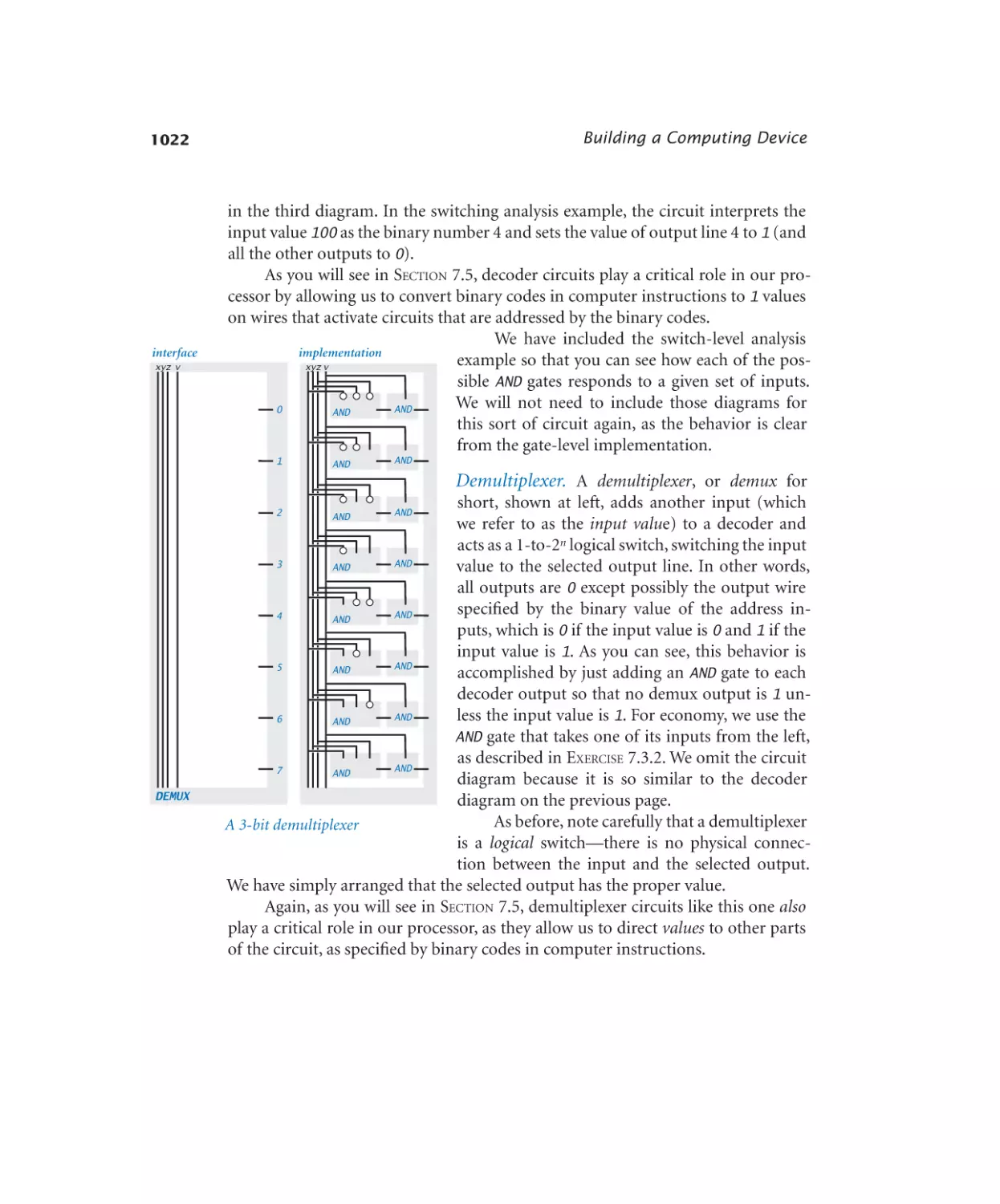
Demultiplexer. . . . . . . . . . . 1022
Multiplexer . . . . . . . . . . . . 1023
XOR . . . . . . . . . . . . . . . 1024
Majority. . . . . . . . . . . . . . 1025
Odd parity. . . . . . . . . . . . . 1026
Adder. . . . . . . . . . . . . . . 1029
ALU . . . . . . . . . . . . . . . 1033
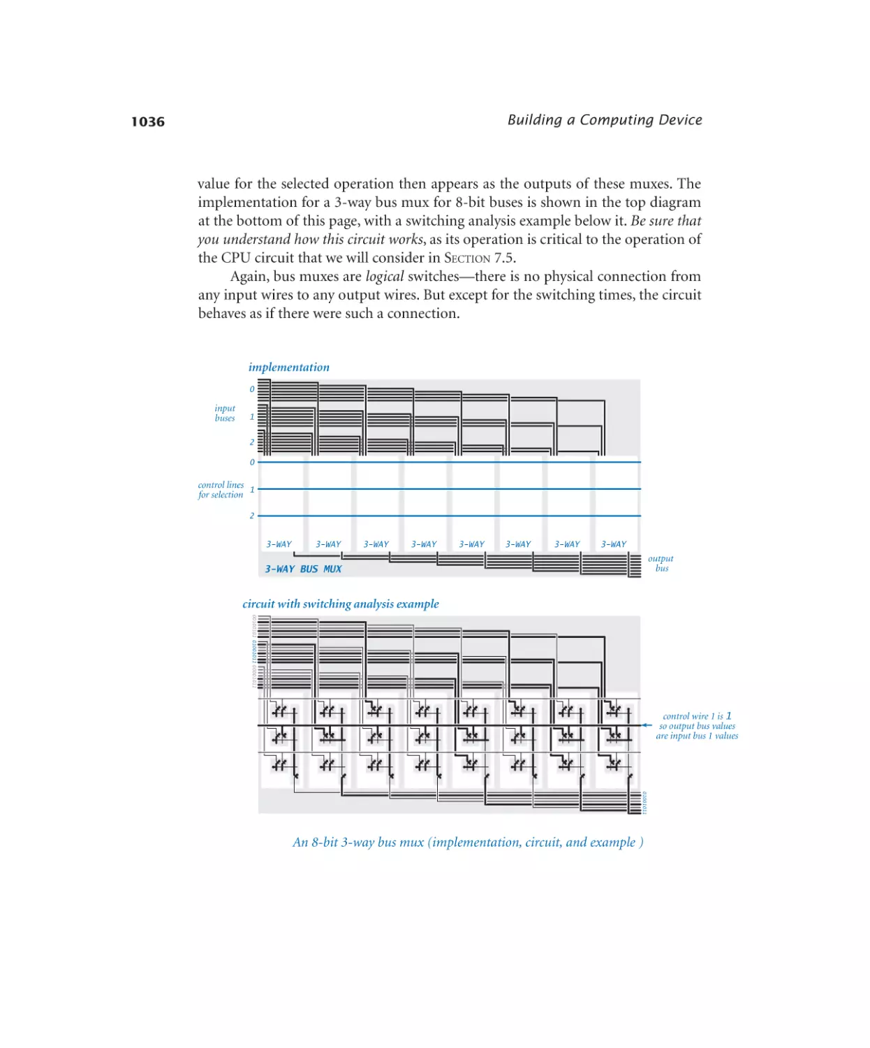
Bus multiplexer. . . . . . . . . . . 1036
Sequential Circuits
SR flip-flop . . . . . . . . . . . . 1050
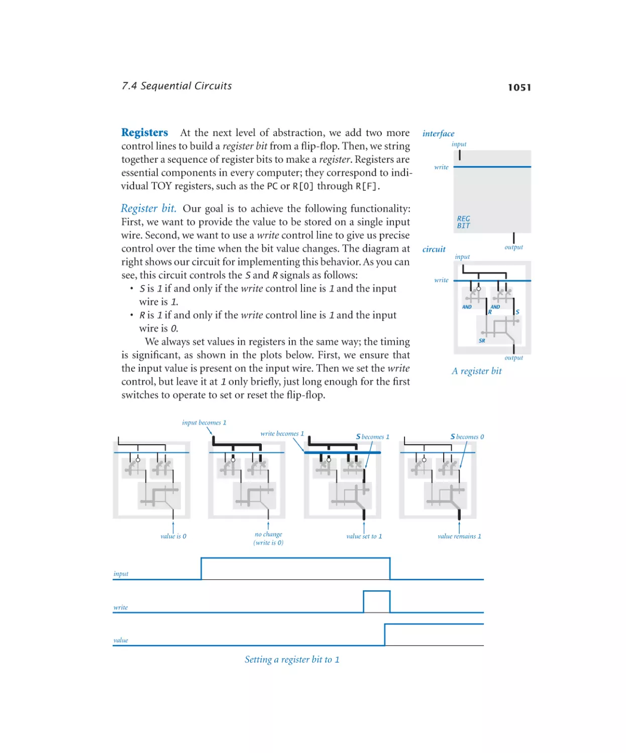
Register bit. . . . . . . . . . . . . 1051
Register. . . . . . . . . . . . . . 1052
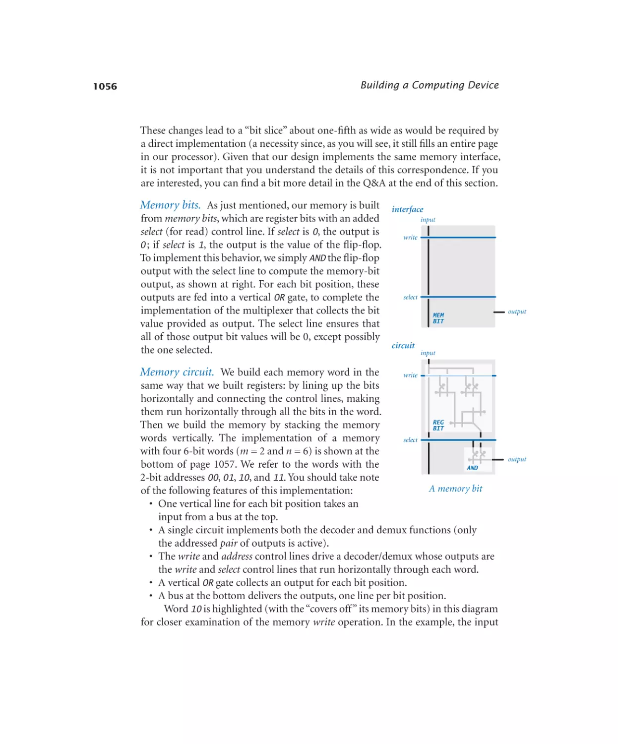
Memory bit. . . . . . . . . . . . 1056
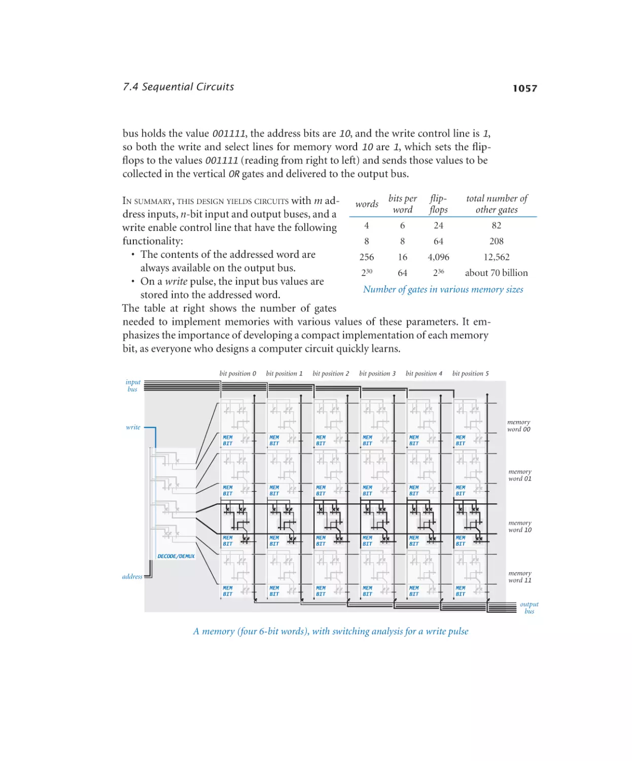
Memory. . . . . . . . . . . . . . 1057
Clock . . . . . . . . . . . . . . . 1061
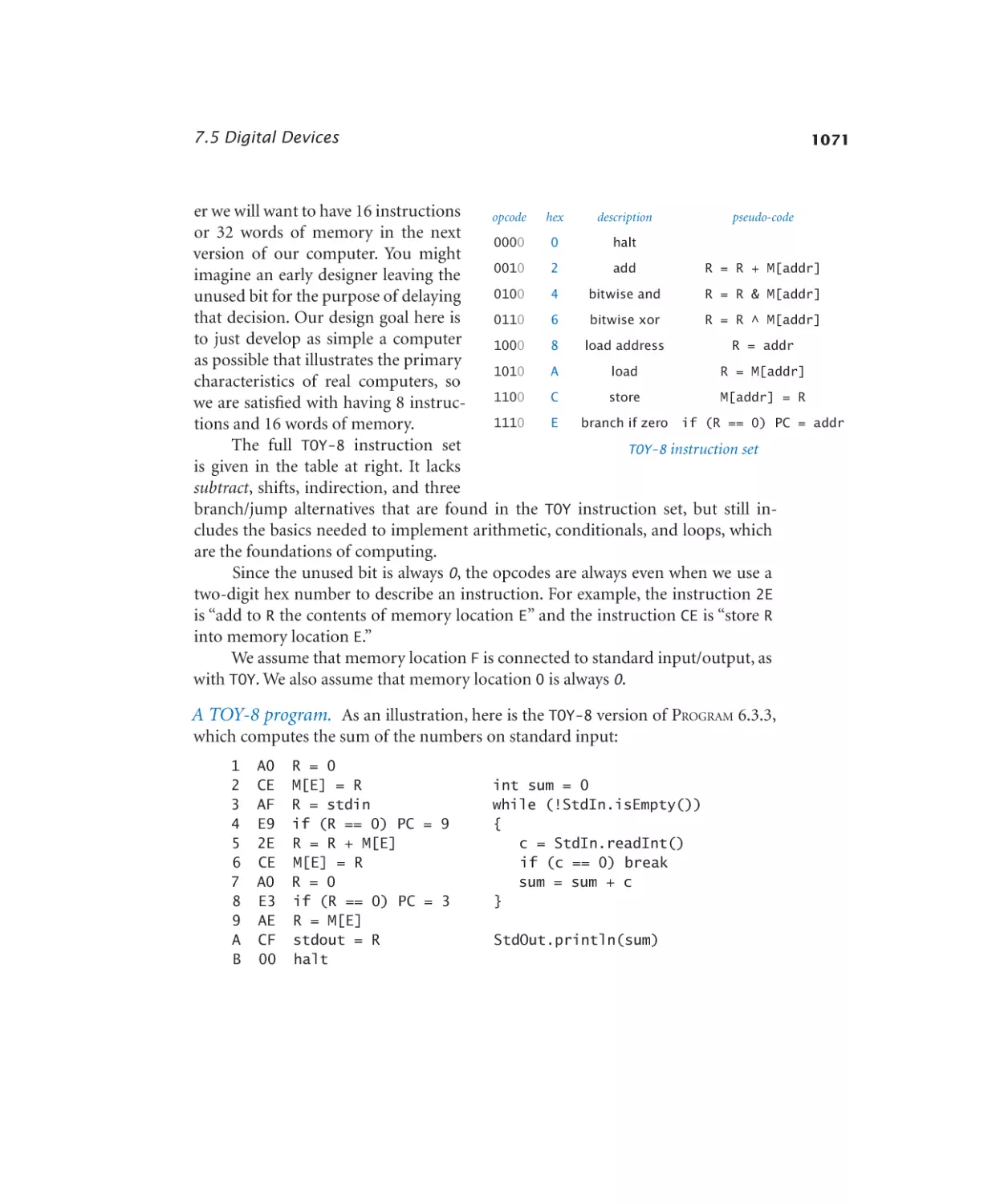
Digital Devices
Program counter. . . . . . . . . . 1074
Control. . . . . . . . . . . . . . 1081
CPU . . . . . . . . . . . . . . . 1086
xi
This page intentionally left blank
Preface
T
he basis for education in the last millennium was “reading, writing, and arithmetic”; now it is reading, writing, and computing. Learning to program is an
essential part of the education of every student in the sciences and engineering.
Beyond direct applications, it is the first step in understanding the nature of computer science’s undeniable impact on the modern world. This book aims to teach
programming to those who need or want to learn it, in a scientific context.
Our primary goal is to empower students by supplying the experience and
basic tools necessary to use computation effectively. Our approach is to teach students that composing a program is a natural, satisfying, and creative experience.
We progressively introduce essential concepts, embrace classic applications from
applied mathematics and the sciences to illustrate the concepts, and provide opportunities for students to write programs to solve engaging problems. We seek
also to demystify computation for students and to build awareness about the substantial intellectual underpinnings of the field of computer science.
We use the Java programming language for all of the programs in this book.
The first part of the book teaches basic skills for computational problem solving
that are applicable in many modern computing environments, and it is a selfcontained treatment intended for people with no previous experience in programming. It is about fundamental concepts in programming, not Java per se. The second
part of the book demonstrates that there is much more to computer science than
programming, but we do often use Java programs to help communicate the main
ideas.
This book is an interdisciplinary approach to the traditional CS1 curriculum,
in that we highlight the role of computing in other disciplines, from materials science to genomics to astrophysics to network systems. This approach reinforces for
students the essential idea that mathematics, science, engineering, and computing
are intertwined in the modern world. While it is a CS1 textbook designed for any
first-year college student, the book also can be used for self-study.
xiii
Preface
xiv
Coverage
The first part of the book is organized around three stages of learning
to program: basic elements, functions, object-oriented programming, and algorithms. We provide the basic information that readers need to build confidence
in composing programs at each level before moving to the next level. An essential
feature of our approach is the use of example programs that solve intriguing problems, supported with exercises ranging from self-study drills to challenging problems that call for creative solutions.
Elements of programming include variables, assignment statements, built-in
types of data, flow of control, arrays, and input/output, including graphics and
sound.
Functions and modules are the students’ first exposure to modular programming. We build upon students’ familiarity with mathematical functions to
introduce Java functions, and then consider the implications of programming
with functions, including libraries of functions and recursion. We stress the fundamental idea of dividing a program into components that can be independently
debugged, maintained, and reused.
Object-oriented programming is our introduction to data abstraction. We
emphasize the concept of a data type and its implementation using Java’s class
mechanism. We teach students how to use, create, and design data types. Modularity, encapsulation, and other modern programming paradigms are the central
concepts of this stage.
The second part of the book introduces advanced topics in computer science:
algorithms and data structures, theory of computing, and machine architecture.
Algorithms and data structures combine these modern programming paradigms with classic methods of organizing and processing data that remain effective
for modern applications. We provide an introduction to classical algorithms for
sorting and searching as well as fundamental data structures and their application,
emphasizing the use of the scientific method to understand performance characteristics of implementations.
Theory of computing helps us address basic questions about computation,
using simple abstract models of computers. Not only are the insights gained invaluable, but many of the ideas are also directly useful and relevant in practical
computing applications.
Machine architecture provides a path to understanding what computation
actually looks like in the real world—a link between the abstract machines of the
theory of computing and the real computers that we use. Moreover, the study of
Preface
machine architecture provides a link to the past, as the microprocessors found in
today’s computers and mobile devices are not so different from the first computers
that were developed in the middle of the 20th century.
Applications in science and engineering are a key feature of the text. We motivate each programming concept that we address by examining its impact on
specific applications. We draw examples from applied mathematics, the physical
and biological sciences, and computer science itself, and include simulation of
physical systems, numerical methods, data visualization, sound synthesis, image
processing, financial simulation, and information technology. Specific examples
include a treatment in the first chapter of Markov chains for web page ranks and
case studies that address the percolation problem, n-body simulation, and the
small-world phenomenon. These applications are an integral part of the text. They
engage students in the material, illustrate the importance of the programming concepts, and provide persuasive evidence of the critical role played by computation in
modern science and engineering.
Historical context is emphasized in the later chapters. The fascinating story of
the development and application of fundamental ideas about computation by Alan
Turing, John von Neumann, and many others is an important subtext.
Our primary goal is to teach the specific mechanisms and skills that are
needed to develop effective solutions to any programming problem. We work with
complete Java programs and encourage readers to use them. We focus on programming by individuals, not programming in the large.
Use in the Curriculum
This book is intended for a first-year college course
aimed at teaching computer science to novices in the context of scientific applications. When such a course is taught from this book, college student will learn to
program in a familiar context. Students completing a course based on this book
will be well prepared to apply their skills in later courses in their chosen major and
to recognize when further education in computer science might be beneficial.
Prospective computer science majors, in particular, can benefit from learning
to program in the context of scientific applications. A computer scientist needs the
same basic background in the scientific method and the same exposure to the role
of computation in science as does a biologist, an engineer, or a physicist.
Indeed, our interdisciplinary approach enables colleges and universities to
teach prospective computer science majors and prospective majors in other fields
in the same course. We cover the material prescribed by CS1, but our focus on
xv
Preface
xvi
applications brings life to the concepts and motivates students to learn them. Our
interdisciplinary approach exposes students to problems in many different disciplines, helping them to choose a major more wisely.
Whatever the specific mechanism, the use of this book is best positioned early
in the curriculum. First, this positioning allows us to leverage familiar material
in high school mathematics and science. Second, students who learn to program
early in their college curriculum will then be able to use computers more effectively
when moving on to courses in their specialty. Like reading and writing, programming is certain to be an essential skill for any scientist or engineer. Students who
have grasped the concepts in this book will continually develop that skill throughout their lifetimes, reaping the benefits of exploiting computation to solve or to
better understand the problems and projects that arise in their chosen field.
Prerequisites
This book is suitable for typical first-year college students. That
is, we do not expect preparation beyond what is typically required for other entrylevel science and mathematics courses.
Mathematical maturity is important. While we do not dwell on mathematical
material, we do refer to the mathematics curriculum that students have taken in
high school, including algebra, geometry, and trigonometry. Most students in our
target audience automatically meet these requirements. Indeed, we take advantage
of their familiarity with the basic curriculum to introduce basic programming
concepts.
Scientific curiosity is also an essential ingredient. Science and engineering students bring with them a sense of fascination with the ability of scientific inquiry to
help explain what goes on in nature. We leverage this predilection with examples
of simple programs that speak volumes about the natural world. We do not assume
any specific knowledge beyond that provided by typical high school courses in
mathematics, physics, biology, or chemistry.
Programming experience is not necessary, but also is not harmful. Teaching
programming is one of our primary goals, so we assume no prior programming
experience. But composing a program to solve a new problem is a challenging intellectual task, so students who have written numerous programs in high school
can benefit from taking an introductory programming course based on this book.
The book can support teaching students with varying backgrounds because the
applications appeal to both novices and experts alike.
Preface
Experience using a computer is not necessary, but also is not a problem. College students use computers regularly—for example, to communicate with friends
and relatives, listen to music, process photos, and as part of many other activities.
The realization that they can harness the power of their own computer in interesting and important ways is an exciting and lasting lesson.
In summary, virtually all college students are prepared to take a course based
on this book as a part of their first-semester curriculum.
Goals What can instructors of upper-level courses in science and engineering
expect of students who have completed a course based on this book?
We cover the CS1 curriculum, but anyone who has taught an introductory
programming course knows that expectations of instructors in later courses are
typically high: each instructor expects all students to be familiar with the computing
environment and approach that he or she wants to use. A physics professor might
expect some students to design a program over the weekend to run a simulation;
an engineering professor might expect other students to use a particular package
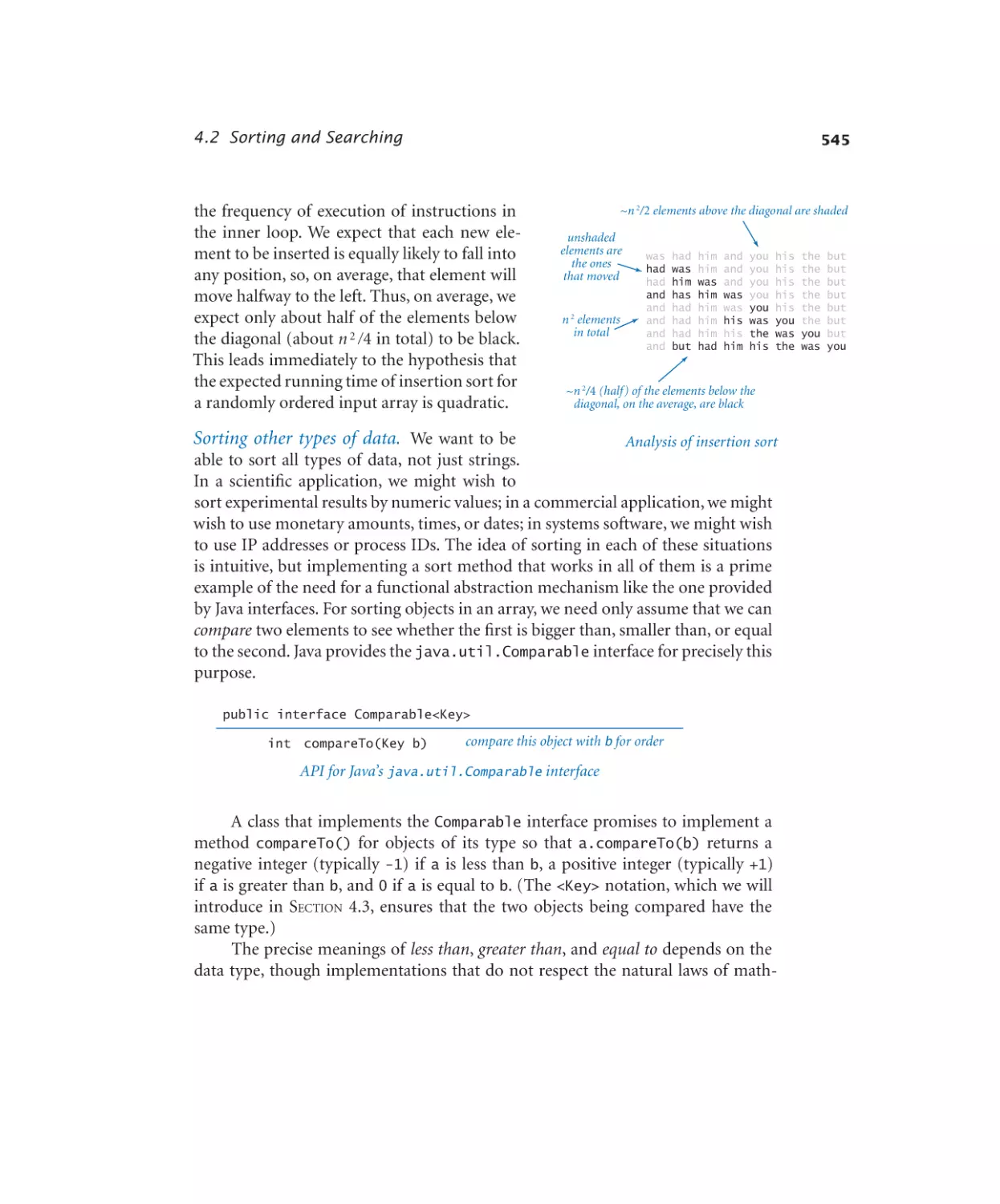
to numerically solve differential equations; or a computer science professor might
expect knowledge of the details of a particular programming environment. Is it
realistic for a single entry-level course to meet such diverse expectations? Should
there be a different introductory course for each set of students?
Colleges and universities have been wrestling with such questions since computers came into widespread use in the latter part of the 20th century. Our answer
to them is found in this common introductory treatment of programming, which
is analogous to commonly accepted introductory courses in mathematics, physics,
biology, and chemistry. Computer Science strives to provide the basic preparation
needed by all students in science and engineering, while sending the clear message
that there is much more to understand about computer science than programming.
Instructors teaching students who have studied from this book can expect that they
will have the knowledge and experience necessary to enable those students to adapt
to new computational environments and to effectively exploit computers in diverse
applications.
What can students who have completed a course based on this book expect to
accomplish in later courses?
Our message is that programming is not difficult to learn and that harnessing the power of the computer is rewarding. Students who master the material in
this book are prepared to address computational challenges wherever they might
xvii
Preface
xviii
appear later in their careers. They learn that modern programming environments,
such as the one provided by Java, help open the door to any computational problem they might encounter later, and they gain the confidence to learn, evaluate, and
use other computational tools. Students interested in computer science will be well
prepared to pursue that interest; students in science and engineering will be ready
to integrate computation into their studies.
Online lectures A complete set of studio-produced videos that can be used in
conjunction with this text are available at
http://www.informit.com/store/computer-science-videolectures-20-part-lecture-series-9780134493831
These lectures are fully coordinated with the text, but also include examples and
other materials that supplement the text and are intended to bring the subject to
life. As with traditional live lectures, the purpose of these videos is to inform and
inspire, motivating students to study and learn from the text. Our experience is
that student engagement with the material is significantly better with videos than
with live lectures because of the ability to play the lectures at a chosen speed and to
replay and review the lectures at any time.
Booksite An extensive amount of other information that supplements this text
may be found on the web at
http://introcs.cs.princeton.edu/java
For economy, we refer to this site as the booksite throughout. It contains material
for instructors, students, and casual readers of the book. We briefly describe this
material here, though, as all web users know, it is best surveyed by browsing. With
a few exceptions to support testing, the material is all publicly available.
One of the most important implications of the booksite is that it empowers
teachers, students, and casual readers to use their own computers to teach and
learn the material. Anyone with a computer and a browser can delve into the study
of computer science by following a few instructions on the booksite.
For teachers, the booksite is a rich source of enrichment materials and material
for quizzes, examinations, programming assignments, and other assessments. Together with the studio-produced videos (and the book), it represents resources for
teaching that are sufficiently flexible to support many of the models for teaching
that are emerging as teachers embrace technology in the 21st century. For example,
at Princeton, our teaching style was for many years based on offering two lectures
Preface
xix
per week to a large audience, supplemented by “precepts” each week where students met in small groups with instructors or teaching assistants. More recently, we
have evolved to a model where students watch lectures online and we hold class
meetings in addition to the precepts. These class meetings generally involve exams,
exam preparation sessions, tutorials, and other activities that previously had to be
scheduled outside of class time. Other teachers may work completely online. Still
others may use a “flipped” model involving enrichment of each lecture after students watch it.
For students, the booksite contains quick access to much of the material in the
book, including source code, plus extra material to encourage self-learning. Solutions are provided for many of the book’s exercises, including complete program
code and test data. There is a wealth of information associated with programming
assignments, including suggested approaches, checklists, FAQs, and test data.
For casual readers, the booksite is a resource for accessing all manner of extra information associated with the book’s content. All of the booksite content provides
web links and other routes to pursue more information about the topic under consideration. There is far more information accessible than any individual could fully
digest, but our goal is to provide enough to whet any reader’s appetite for more
information about the book’s content.
Our goal in creating these materials is to provide complementary approaches to
the ideas. People may learn a concept through careful study in the book, an engaging example in an online lectures, browsing on the booksite, or perhaps all three.
Acknowledgments This project has been under development since 1992, so far
too many people have contributed to its success for us to acknowledge them all here.
Special thanks are due to Anne Rogers, for helping to start the ball rolling; to Dave
Hanson, Andrew Appel, and Chris van Wyk, for their patience in explaining data
abstraction; to Lisa Worthington and Donna Gabai, for being the first to truly relish the challenge of teaching this material to first-year students; and to Doug Clark
for his patience as we learned about building Turing machines and circuits. We also
gratefully acknowledge the efforts of /dev/126; the faculty, graduate students, and
teaching staff who have dedicated themselves to teaching this material over the past
25 years here at Princeton University; and the thousands of undergraduates who
have dedicated themselves to learning it.
Robert Sedgewick and Kevin Wayne
Princeton, NJ, December 2016
Chapter One
Elements of Programming
1.1 Your First Program . . . . . . . . . . . . 2
1.2 Built-in Types of Data . . . . . . . . . 14
1.3 Conditionals and Loops . . . . . . . . 50
1.4 Arrays . . . . . . . . . . . . . . . . . . . 90
1.5 Input and Output . . . . . . . . . . . .126
1.6 Case Study: Random Web Surfer . . .170
O
ur goal in this chapter is to convince you that writing a program is easier than
writing a piece of text, such as a paragraph or essay. Writing prose is difficult:
we spend many years in school to learn how to do it. By contrast, just a few building blocks suffice to enable us to write programs that can help solve all sorts of
fascinating, but otherwise unapproachable, problems. In this chapter, we take you
through these building blocks, get you started on programming in Java, and study
a variety of interesting programs. You will be able to express yourself (by writing
programs) within just a few weeks. Like the ability to write prose, the ability to program is a lifetime skill that you can continually refine well into the future.
In this book, you will learn the Java programming language. This task will be
much easier for you than, for example, learning a foreign language. Indeed, programming languages are characterized by only a few dozen vocabulary words and
rules of grammar. Much of the material that we cover in this book could be expressed in the Python or C++ languages, or any of several other modern programming languages. We describe everything specifically in Java so that you can get
started creating and running programs right away. On the one hand, we will focus
on learning to program, as opposed to learning details about Java. On the other
hand, part of the challenge of programming is knowing which details are relevant
in a given situation. Java is widely used, so learning to program in this language
will enable you to write programs on many computers (your own, for example).
Also, learning to program in Java will make it easy for you to learn other languages,
including lower-level languages such as C and specialized languages such as Matlab.
1
Elements of Programming
1.1 Your First Program
In this section, our plan is to lead you into the world of Java programming by taking you through the basic steps required to get a simple program running. The
Java platform (hereafter abbreviated Java) is a collection of applications, not unlike
many of the other applications that you
are accustomed to using (such as your
1.1.1 Hello, World . . . . . . . . . . . . . . 4
word processor, email program, and web
1.1.2 Using a command-line argument . . . 7
browser). As with any application, you
Programs in this section
need to be sure that Java is properly installed on your computer. It comes preloaded on many computers, or you can download it easily. You also need a text
editor and a terminal application. Your first task is to find the instructions for installing such a Java programming environment on your computer by visiting
http://introcs.cs.princeton.edu/java
We refer to this site as the booksite. It contains an extensive amount of supplementary information about the material in this book for your reference and use while
programming.
Programming in Java To introduce you to developing Java programs, we
break the process down into three steps. To program in Java, you need to:
• Create a program by typing it into a file named, say, MyProgram.java.
• Compile it by typing javac MyProgram.java in a terminal window.
• Execute (or run) it by typing java MyProgram in the terminal window.
In the first step, you start with a blank screen and end with a sequence of typed
characters on the screen, just as when you compose an email message or an essay.
Programmers use the term code to refer to program text and the term coding to refer to the act of creating and editing the code. In the second step, you use a system
application that compiles your program (translates it into a form more suitable for
the computer) and puts the result in a file named MyProgram.class. In the third
step, you transfer control of the computer from the system to your program (which
returns control back to the system when finished). Many systems have several different ways to create, compile, and execute programs. We choose the sequence given here because it is the simplest to describe and use for small programs.
1.1 Your First Program
3
Creating a program. A Java program is nothing more than a sequence of characters, like a paragraph or a poem, stored in a file with a .java extension. To create
one, therefore, you need simply define that sequence of characters, in the same way
as you do for email or any other computer application. You can use any text editor
for this task, or you can use one of the more sophisticated integrated development
environments described on the booksite. Such environments are overkill for the
sorts of programs we consider in this book, but they are not difficult to use, have
many useful features, and are widely used by professionals.
Compiling a program. At first, it might seem that Java is designed to be best understood by the computer. To the contrary, the language is designed to be best
understood by the programmer—that’s you. The computer’s language is far more
primitive than Java. A compiler is an application that translates a program from the
Java language to a language more suitable for execution on the computer. The compiler takes a file with a .java extension as input (your program) and produces a
file with the same name but with a .class extension (the computer-language version). To use your Java compiler, type in a terminal window the javac command
followed by the file name of the program you want to compile.
Executing (running) a program. Once you compile the program, you can execute (or run) it. This is the exciting part, where your program takes control of your
computer (within the constraints of what Java allows). It is perhaps more accurate
to say that your computer follows your instructions. It is even more accurate to say
that a part of Java known as the Java Virtual Machine (JVM, for short) directs your
computer to follow your instructions. To use the JVM to execute your program,
type the java command followed by the program name in a terminal window.
use any text editor to
create your program
editor
type javac HelloWorld.java
to compile your program
type java HelloWorld
to execute your program
compiler
JVM
HelloWorld.java
your program
(a text file)
HelloWorld.class
computer-language
version of your program
Developing a Java program
"Hello, World"
output
Elements of Programming
4
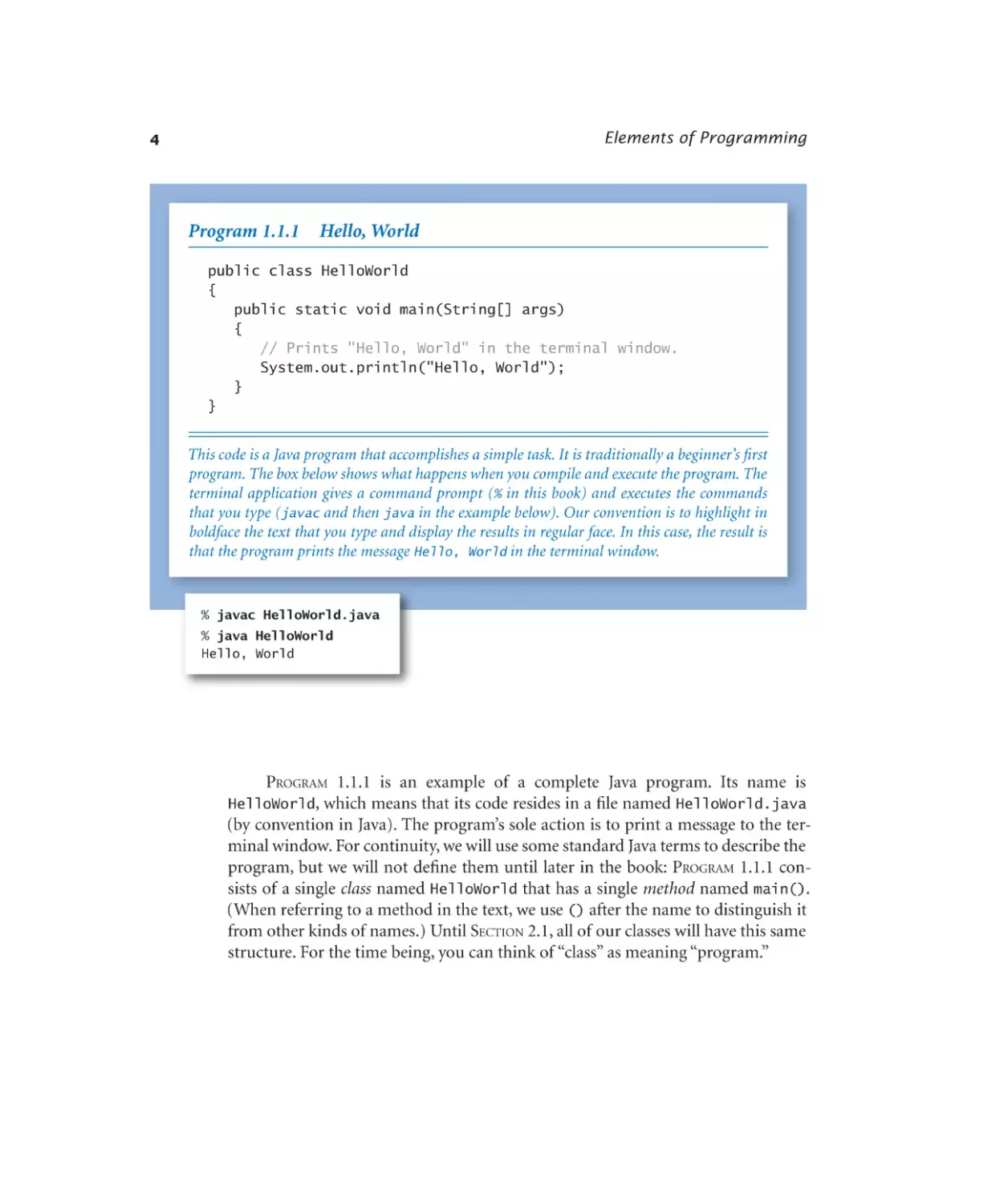
Program 1.1.1
Hello, World
public class HelloWorld
{
public static void main(String[] args)
{
// Prints "Hello, World" in the terminal window.
System.out.println("Hello, World");
}
}
This code is a Java program that accomplishes a simple task. It is traditionally a beginner’s first
program. The box below shows what happens when you compile and execute the program. The
terminal application gives a command prompt (% in this book) and executes the commands
that you type (javac and then java in the example below). Our convention is to highlight in
boldface the text that you type and display the results in regular face. In this case, the result is
that the program prints the message Hello, World in the terminal window.
% javac HelloWorld.java
% java HelloWorld
Hello, World
Program 1.1.1 is an example of a complete Java program. Its name is
means that its code resides in a file named HelloWorld.java
(by convention in Java). The program’s sole action is to print a message to the terminal window. For continuity, we will use some standard Java terms to describe the
program, but we will not define them until later in the book: Program 1.1.1 consists of a single class named HelloWorld that has a single method named main().
(When referring to a method in the text, we use () after the name to distinguish it
from other kinds of names.) Until Section 2.1, all of our classes will have this same
structure. For the time being, you can think of “class” as meaning “program.”
HelloWorld, which
1.1 Your First Program
5
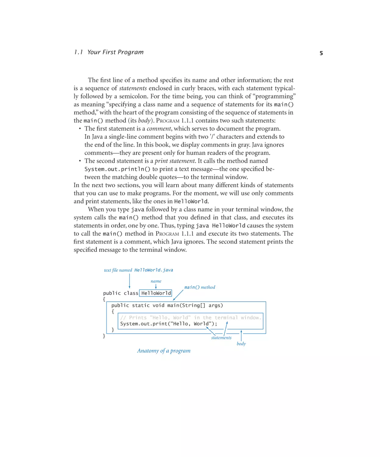
The first line of a method specifies its name and other information; the rest
is a sequence of statements enclosed in curly braces, with each statement typically followed by a semicolon. For the time being, you can think of “programming”
as meaning “specifying a class name and a sequence of statements for its main()
method,” with the heart of the program consisting of the sequence of statements in
the main() method (its body). Program 1.1.1 contains two such statements:
• The first statement is a comment, which serves to document the program.
In Java a single-line comment begins with two '/' characters and extends to
the end of the line. In this book, we display comments in gray. Java ignores
comments—they are present only for human readers of the program.
• The second statement is a print statement. It calls the method named
System.out.println() to print a text message—the one specified between the matching double quotes—to the terminal window.
In the next two sections, you will learn about many different kinds of statements
that you can use to make programs. For the moment, we will use only comments
and print statements, like the ones in HelloWorld.
When you type java followed by a class name in your terminal window, the
system calls the main() method that you defined in that class, and executes its
statements in order, one by one. Thus, typing java HelloWorld causes the system
to call the main() method in Program 1.1.1 and execute its two statements. The
first statement is a comment, which Java ignores. The second statement prints the
specified message to the terminal window.
text file named HelloWorld.java
name
main() method
public class HelloWorld
{
public static void main(String[] args)
{
// Prints "Hello, World" in the terminal window.
System.out.print("Hello, World");
}
}
statements
body
Anatomy of a program
6
Elements of Programming
Since the 1970s, it has been a tradition that a beginning programmer’s first
program should print Hello, World. So, you should type the code in Program
1.1.1 into a file, compile it, and execute it. By doing so, you will be following in the
footsteps of countless others who have learned how to program. Also, you will be
checking that you have a usable editor and terminal application. At first, accomplishing the task of printing something out in a terminal window might not seem
very interesting; upon reflection, however, you will see that one of the most basic
functions that we need from a program is its ability to tell us what it is doing.
For the time being, all our program code will be just like Program 1.1.1, except with a different sequence of statements in main(). Thus, you do not need to
start with a blank page to write a program. Instead, you can
• Copy HelloWorld.java into a new file having a new program name of
your choice, followed by .java.
• Replace HelloWorld on the first line with the new program name.
• Replace the comment and print statements with a different sequence of
statements.
Your program is characterized by its sequence of statements and its name. Each
Java program must reside in a file whose name matches the one after the word
class on the first line, and it also must have a .java extension.
Errors. It is easy to blur the distinctions among editing, compiling, and executing
programs. You should keep these processes separate in your mind when you are
learning to program, to better understand the effects of the errors that inevitably
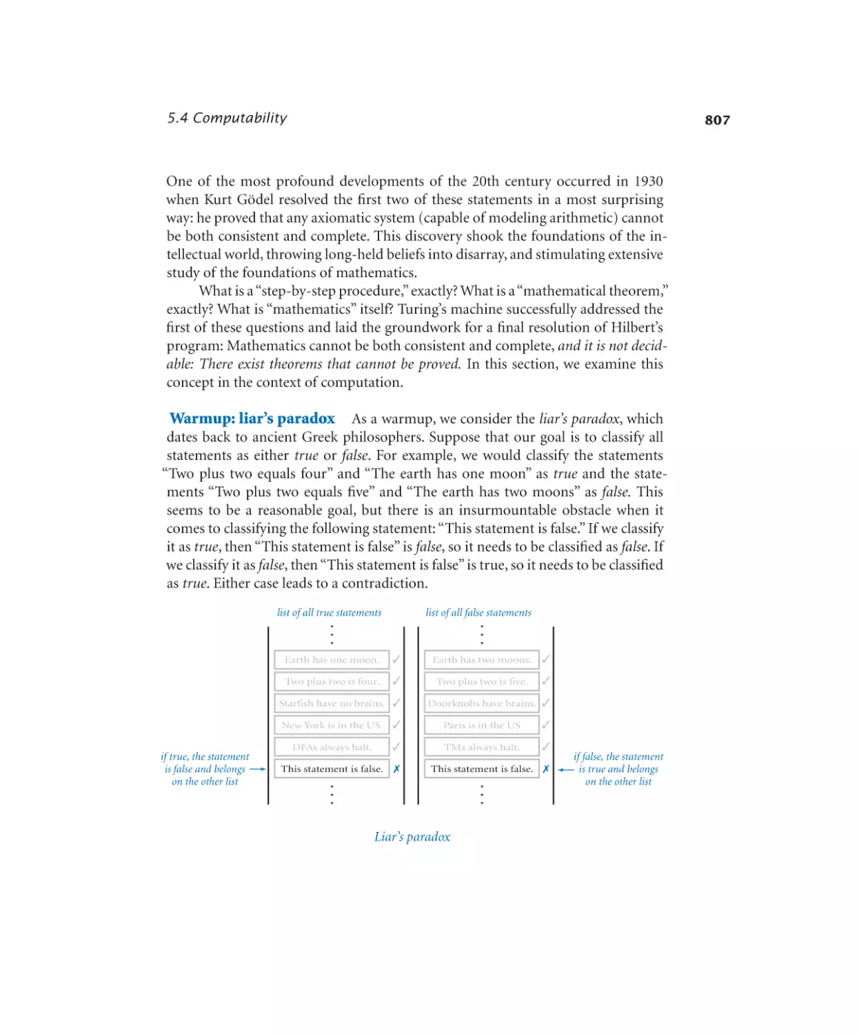
arise.
You can fix or avoid most errors by carefully examining the program as you
create it, the same way you fix spelling and grammatical errors when you compose
an email message. Some errors, known as compile-time errors, are identified when
you compile the program, because they prevent the compiler from doing the translation. Other errors, known as run-time errors, do not show up until you execute
the program.
In general, errors in programs, also commonly known as bugs, are the bane of
a programmer’s existence: the error messages can be confusing or misleading, and
the source of the error can be very hard to find. One of the first skills that you will
learn is to identify errors; you will also learn to be sufficiently careful when coding,
to avoid making many of them in the first place. You can find several examples of
errors in the Q&A at the end of this section.
1.1 Your First Program
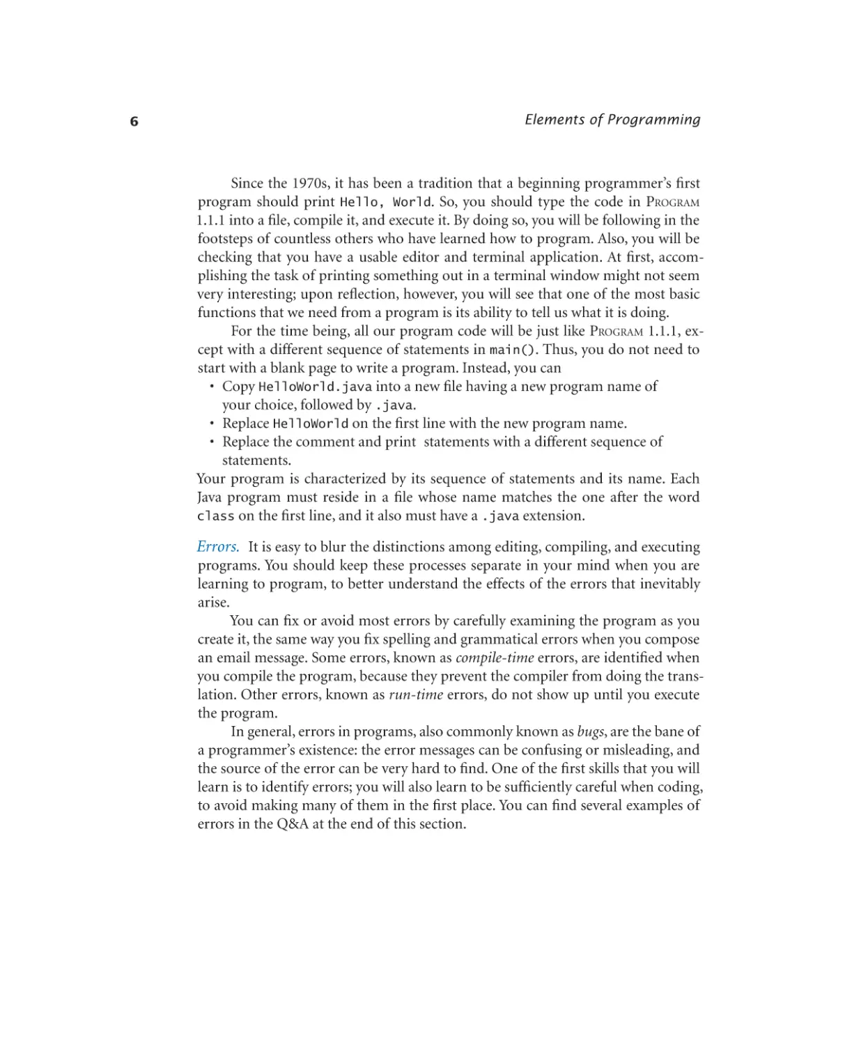
Program 1.1.2
Using a command-line argument
public class UseArgument
{
public static void main(String[] args)
{
System.out.print("Hi, ");
System.out.print(args[0]);
System.out.println(". How are you?");
}
}
This program shows the way in which we can control the actions of our programs: by providing
an argument on the command line. Doing so allows us to tailor the behavior of our programs.
% javac UseArgument.java
% java UseArgument Alice
Hi, Alice. How are you?
% java UseArgument Bob
Hi, Bob. How are you?
Input and output Typically, we want to provide input to our programs—that
is, data that they can process to produce a result. The simplest way to provide input data is illustrated in UseArgument (Program 1.1.2). Whenever you execute the
program UseArgument, it accepts the command-line argument that you type after
the program name and prints it back out to the terminal window as part of the
message. The result of executing this program depends on what you type after the
program name. By executing the program with different command-line arguments,
you produce different printed results. We will discuss in more detail the mechanism
that we use to pass command-line arguments to our programs later, in Section 2.1.
For now it is sufficient to understand that args[0] is the first command-line argument that you type after the program name, args[1] is the second, and so forth.
Thus, you can use args[0] within your program’s body to represent the first string
that you type on the command line when it is executed, as in UseArgument.
7
Elements of Programming
8
In addition to the System.out.println() method, UseArgument calls the
method. This method is just like System.out.println(),
but prints just the specified string (and not a newline character).
Again, accomplishing the task of getting a program to print back out what we
type in to it may not seem interesting at first, but upon reflection you will realize
that another basic function of a program is its ability to respond to basic information from the user to control what the program does. The simple model that
UseArgument represents will suffice to allow us to consider Java’s basic programming mechanism and to address all sorts of interesting computational problems.
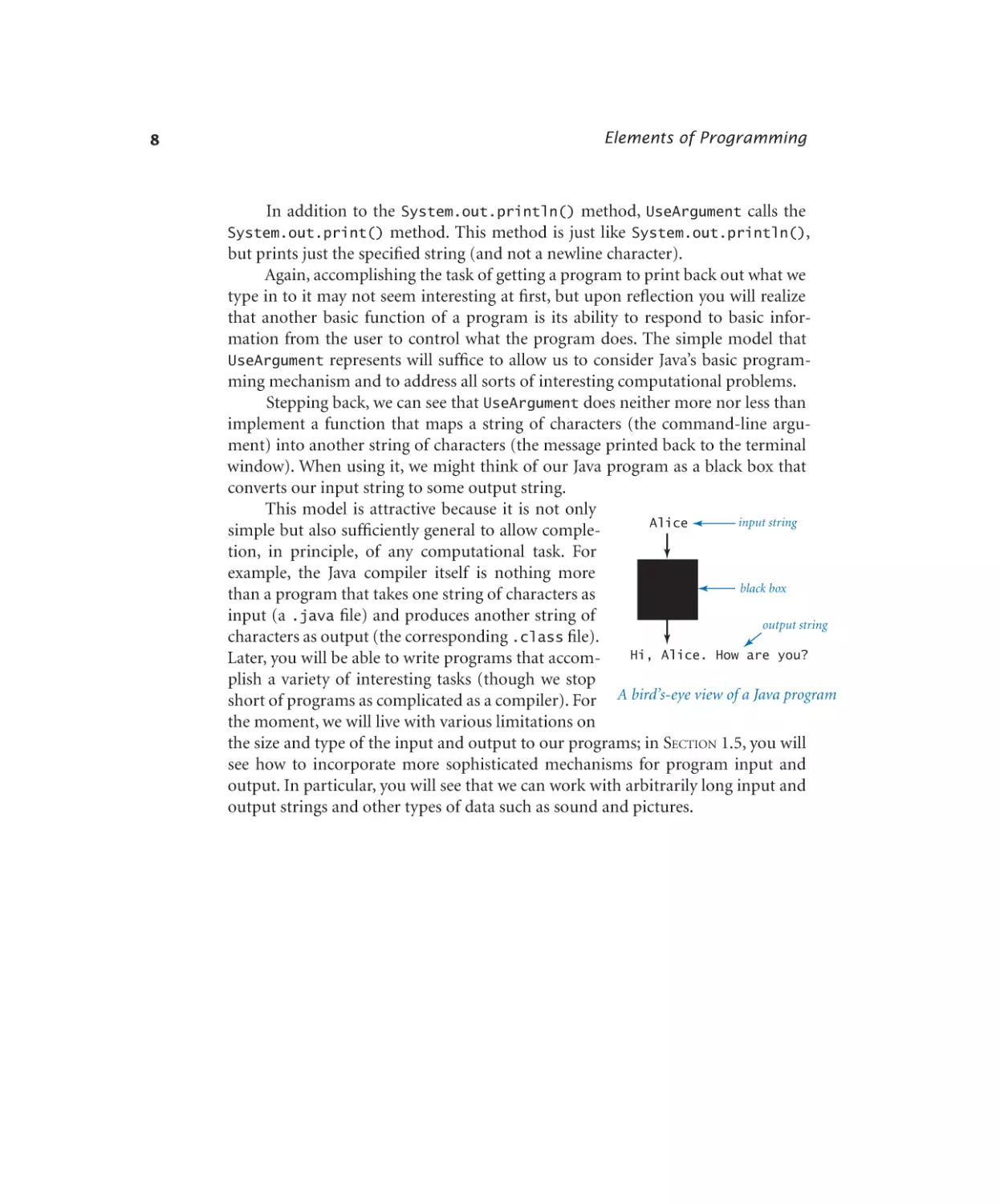
Stepping back, we can see that UseArgument does neither more nor less than
implement a function that maps a string of characters (the command-line argument) into another string of characters (the message printed back to the terminal
window). When using it, we might think of our Java program as a black box that
converts our input string to some output string.
This model is attractive because it is not only
input string
Alice
simple but also sufficiently general to allow completion, in principle, of any computational task. For
example, the Java compiler itself is nothing more
black box
than a program that takes one string of characters as
input (a .java file) and produces another string of
output string
characters as output (the corresponding .class file).
Hi, Alice. How are you?
Later, you will be able to write programs that accomplish a variety of interesting tasks (though we stop
short of programs as complicated as a compiler). For A bird’s-eye view of a Java program
the moment, we will live with various limitations on
the size and type of the input and output to our programs; in Section 1.5, you will
see how to incorporate more sophisticated mechanisms for program input and
output. In particular, you will see that we can work with arbitrarily long input and
output strings and other types of data such as sound and pictures.
System.out.print()
1.1 Your First Program
Q&A
Q. Why Java?
A. The programs that we are writing are very similar to their counterparts in several other languages, so our choice of language is not crucial. We use Java because
it is widely available, embraces a full set of modern abstractions, and has a variety
of automatic checks for mistakes in programs, so it is suitable for learning to program. There is no perfect language, and you certainly will be programming in other
languages in the future.
Q. Do I really have to type in the programs in the book to try them out? I believe
that you ran them and that they produce the indicated output.
A. Everyone should type in and run
HelloWorld. Your understanding will be
you also run UseArgument, try it on various inputs, and modi-
greatly magnified if
fy it to test different ideas of your own. To save some typing, you can find all of the
code in this book (and much more) on the booksite. This site also has information
about installing and running Java on your computer, answers to selected exercises,
web links, and other extra information that you may find useful while programming.
Q. What is the meaning of the words public, static, and void?
A. These keywords specify certain properties of main() that you will learn about
later in the book. For the moment, we just include these keywords in the code (because they are required) but do not refer to them in the text.
Q. What is the meaning of the //, /*, and */ character sequences in the code?
A. They denote comments, which are ignored by the compiler. A comment is either
text in between /* and */ or at the end of a line after //. Comments are indispensable because they help other programmers to understand your code and even
can help you to understand your own code in retrospect. The constraints of the
book format demand that we use comments sparingly in our programs; instead
we describe each program thoroughly in the accompanying text and figures. The
programs on the booksite are commented to a more realistic degree.
9
Elements of Programming
10
Q. What are Java’s rules regarding tabs, spaces, and newline characters?
A. Such characters are known as whitespace characters. Java compilers consider all whitespace in program text to be equivalent. For example, we could write
HelloWorld as follows:
public class HelloWorld { public static void main ( String
[] args) { System.out.println("Hello, World")
; } }
But we do normally adhere to spacing and indenting conventions when we write
Java programs, just as we indent paragraphs and lines consistently when we write
prose or poetry.
Q. What are the rules regarding quotation marks?
A. Material inside double quotation marks is an exception to the rule defined in
the previous question: typically, characters within quotes are taken literally so that
you can precisely specify what gets printed. If you put any number of successive
spaces within the quotes, you get that number of spaces in the output. If you accidentally omit a quotation mark, the compiler may get very confused, because it
needs that mark to distinguish between characters in the string and other parts of
the program.
Q. What happens when you omit a curly brace or misspell one of the words, such
as public or static or void or main?
A. It depends upon precisely what you do. Such errors are called syntax errors and
are usually caught by the compiler. For example, if you make a program Bad that is
exactly the same as HelloWorld except that you omit the line containing the first
left curly brace (and change the program name from HelloWorld to Bad), you get
the following helpful message:
% javac Bad.java
Bad.java:1: error: '{' expected
public class Bad
^
1 error
1.1 Your First Program
From this message, you might correctly surmise that you need to insert a left curly
brace. But the compiler may not be able to tell you exactly which mistake you made,
so the error message may be hard to understand. For example, if you omit the second left curly brace instead of the first one, you get the following message:
% javac Bad.java
Bad.java:3: error: ';' expected
public static void main(String[] args)
^
Bad.java:7: error: class, interface, or enum expected
}
^
2 errors
One way to get used to such messages is to intentionally introduce mistakes into a
simple program and then see what happens. Whatever the error message says, you
should treat the compiler as a friend, because it is just trying to tell you that something is wrong with your program.
Q. Which Java methods are available for me to use?
A. There are thousands of them. We introduce them to you in a deliberate fashion
(starting in the next section) to avoid overwhelming you with choices.
Q. When I ran UseArgument, I got a strange error message. What’s the problem?
A. Most likely, you forgot to include a command-line argument:
% java UseArgument
Hi, Exception in thread “main”
java.lang.ArrayIndexOutOfBoundsException: 0
at UseArgument.main(UseArgument.java:6)
Java is complaining that you ran the program but did not type a command-line argument as promised. You will learn more details about array indices in Section 1.4.
Remember this error message—you are likely to see it again. Even experienced programmers forget to type command-line arguments on occasion.
11
Elements of Programming
12
Exercises
1.1.1 Write a program that prints the Hello, World message 10 times.
1.1.2 Describe what happens if you omit the following in HelloWorld.java:
a.
b.
c.
d.
public
static
void
args
1.1.3 Describe what happens if you misspell (by, say, omitting the second letter)
the following in HelloWorld.java:
a. public
b. static
c. void
d. args
1.1.4 Describe what happens if you put the double quotes in the print statement
of HelloWorld.java on different lines, as in this code fragment:
System.out.println("Hello,
World");
1.1.5 Describe what happens if you try to execute UseArgument with each of the
following command lines:
a. java UseArgument java
b. java UseArgument @!&^%
c. java UseArgument 1234
d. java UseArgument.java Bob
e. java UseArgument Alice Bob
1.1.6 Modify UseArgument.java to make a program UseThree.java that takes
three names as command-line arguments and prints a proper sentence with the
names in the reverse of the order given, so that, for example, java UseThree Alice
Bob Carol prints Hi Carol, Bob, and Alice.
This page intentionally left blank
Elements of Programming
1.2 Built-in Types of Data
When programming in Java, you must always be aware of the type of data that your
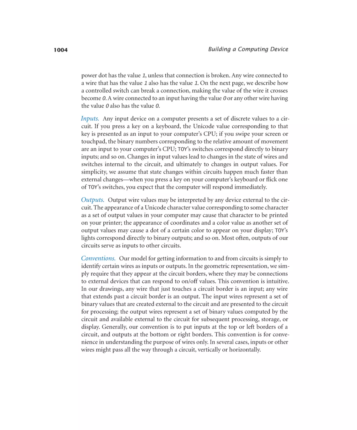
program is processing. The programs in Section 1.1 process strings of characters,
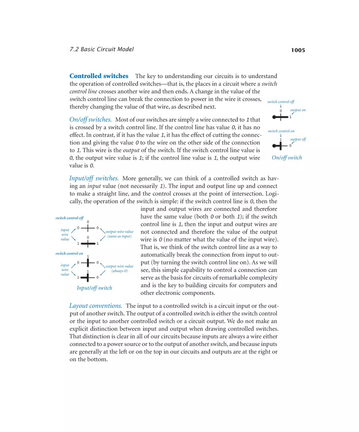
many of the programs in this section process numbers, and we consider numerous other types later in the book. Understanding the distinctions among them is
1.2.1 String concatenation . . . . . . . . . 20
so important that we formally define the
1.2.2 Integer multiplication and division. 23
1.2.3 Quadratic formula. . . . . . . . . . . 25
idea: a data type is a set of values and a set
1.2.4 Leap year. . . . . . . . . . . . . . . . 28
of operations defined on those values. You
1.2.5 Casting to get a random integer . . . 34
are familiar with various types of numPrograms in this section
bers, such as integers and real numbers,
and with operations defined on them,
such as addition and multiplication. In
mathematics, we are accustomed to thinking of sets of numbers as being infinite;
in computer programs we have to work with a finite number of possibilities. Each
operation that we perform is well defined only for the finite set of values in an associated data type.
There are eight primitive types of data in Java, mostly for different kinds of
numbers. Of the eight primitive types, we most often use these: int for integers;
double for real numbers; and boolean for true–false values. Other data types are
available in Java libraries: for example, the programs in Section 1.1 use the type
String for strings of characters. Java treats the String type differently from other
types because its usage for input and output is essential. Accordingly, it shares some
characteristics of the primitive types; for example, some of its operations are built
into the Java language. For clarity, we refer to primitive types and String collectively as built-in types. For the time being, we concentrate on programs that are
based on computing with built-in types. Later, you will learn about Java library
data types and building your own data types. Indeed, programming in Java often
centers on building data types, as you shall see in Chapter 3.
After defining basic terms, we consider several sample programs and code
fragments that illustrate the use of different types of data. These code fragments
do not do much real computing, but you will soon see similar code in longer programs. Understanding data types (values and operations on them) is an essential
step in beginning to program. It sets the stage for us to begin working with more
intricate programs in the next section. Every program that you write will use code
like the tiny fragments shown in this section.
1.2 Built-in Types of Data
15
type
set of values
common operators
sample literal values
int
integers
+ - * / %
99 12 2147483647
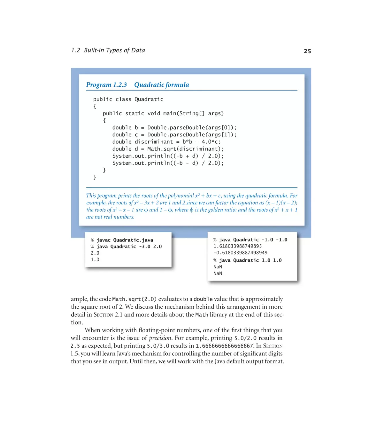
double
floating-point numbers
+ - * /
3.14 2.5 6.022e23
boolean
boolean values
&& || !
char
characters
String
sequences of characters
true false
'A' '1' '%' '\n'
+
"AB" "Hello" "2.5"
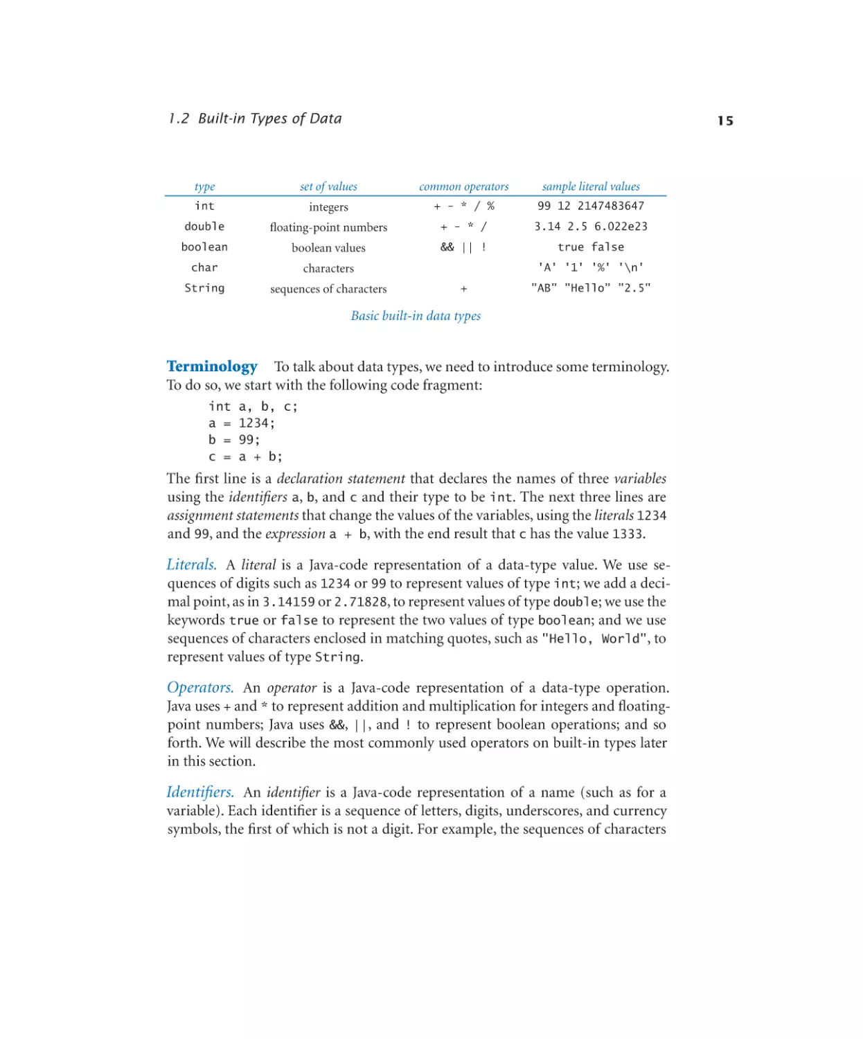
Basic built-in data types
Terminology To talk about data types, we need to introduce some terminology.
To do so, we start with the following code fragment:
int
a =
b =
c =
a, b, c;
1234;
99;
a + b;
The first line is a declaration statement that declares the names of three variables
using the identifiers a, b, and c and their type to be int. The next three lines are
assignment statements that change the values of the variables, using the literals 1234
and 99, and the expression a + b, with the end result that c has the value 1333.
Literals. A literal is a Java-code representation of a data-type value. We use sequences of digits such as 1234 or 99 to represent values of type int; we add a decimal point, as in 3.14159 or 2.71828, to represent values of type double; we use the
keywords true or false to represent the two values of type boolean; and we use
sequences of characters enclosed in matching quotes, such as "Hello, World", to
represent values of type String.
Operators. An operator is a Java-code representation of a data-type operation.
Java uses + and * to represent addition and multiplication for integers and floatingpoint numbers; Java uses &&, ||, and ! to represent boolean operations; and so
forth. We will describe the most commonly used operators on built-in types later
in this section.
Identifiers. An identifier is a Java-code representation of a name (such as for a
variable). Each identifier is a sequence of letters, digits, underscores, and currency
symbols, the first of which is not a digit. For example, the sequences of characters
Elements of Programming
16
abc, Ab$, abc123, and a_b
are all legal Java identifiers, but Ab*, 1abc, and a+b are
not. Identifiers are case sensitive, so Ab, ab, and AB are all different names. Certain
reserved words—such as public, static, int, double, String, true, false, and
null—are special, and you cannot use them as identifiers.
Variables. A variable is an entity that holds a data-type value, which we can refer
to by name. In Java, each variable has a specific type and stores one of the possible
values from that type. For example, an int variable can store either the value 99
or 1234 but not 3.14159 or "Hello, World". Different variables of the same type
may store the same value. Also, as the name suggests, the value of a variable may
change as a computation unfolds. For example, we use a variable named sum in several programs in this book to keep the running sum of a sequence of numbers. We
create variables using declaration statements and compute with them in expressions,
as described next.
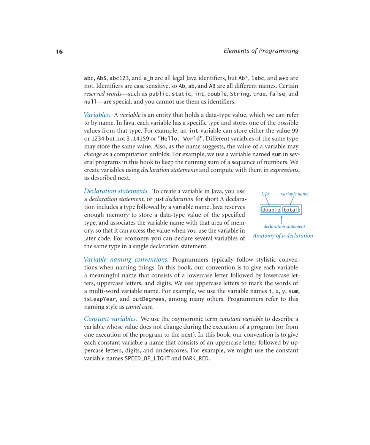
Declaration statements. To create a variable in Java, you use
type
variable name
a declaration statement, or just declaration for short A declaration includes a type followed by a variable name. Java reserves
double total;
enough memory to store a data-type value of the specified
type, and associates the variable name with that area of memdeclaration statement
ory, so that it can access the value when you use the variable in
later code. For economy, you can declare several variables of Anatomy of a declaration
the same type in a single declaration statement.
Variable naming conventions. Programmers typically follow stylistic conventions when naming things. In this book, our convention is to give each variable
a meaningful name that consists of a lowercase letter followed by lowercase letters, uppercase letters, and digits. We use uppercase letters to mark the words of
a multi-word variable name. For example, we use the variable names i, x, y, sum,
isLeapYear, and outDegrees, among many others. Programmers refer to this
naming style as camel case.
Constant variables. We use the oxymoronic term constant variable to describe a
variable whose value does not change during the execution of a program (or from
one execution of the program to the next). In this book, our convention is to give
each constant variable a name that consists of an uppercase letter followed by uppercase letters, digits, and underscores. For example, we might use the constant
variable names SPEED_OF_LIGHT and DARK_RED.
1.2 Built-in Types of Data
17
Expressions. An expression is a combination of literals, variables,
operands
and operations that Java evaluates to produce a value. For primi(and expressions)
tive types, expressions often look just like mathematical formulas,
using operators to specify data-type operations to be performed on
4 * ( x - 3 )
one more operands. Most of the operators that we use are binary
operators that take exactly two operands, such as x - 3 or 5 * x.
operator
Each operand can be any expression, perhaps within parentheses. Anatomy of an expression
For example, we can write 4 * (x - 3) or 5 * x - 6 and Java will
understand what we mean. An expression is a directive to perform
a sequence of operations; the expression is a representation of the resulting value.
Operator precedence. An expression is shorthand for a sequence of operations:
in which order should the operators be applied? Java has natural and well defined
precedence rules that fully specify this order. For arithmetic operations, multiplication and division are performed before addition and subtraction, so that a - b * c
and a - (b * c) represent the same sequence of operations. When arithmetic operators have the same precedence, the order is determined by left associativity, so that
a - b - c and (a - b) - c represent the same sequence of operations. You can use
parentheses to override the rules, so you can write a - (b - c) if that is what you
want. You might encounter in the future some Java code that depends subtly on
precedence rules, but we use parentheses to avoid such code in this book. If you are
interested, you can find full details on the rules on the booksite.
Assignment statements. An assignment statement associates a data-type value
with a variable. When we write c = a + b in Java, we are not expressing mathematical equality, but are instead expressing an action: set the
declaration statement
value of the variable c to be the value of a plus the value
of b. It is true that the value of c is mathematically equal
int a, b;
literal
to the value of a + b immediately after the assignment variable name
a = 1234 ;
statement has been executed, but the point of the stateassignment
b = 99;
statement
ment is to change (or initialize) the value of c. The leftint c = a + b;
hand side of an assignment statement must be a single
variable; the right-hand side can be any expression that inline initialization
statement
produces a value of a compatible type. So, for example,
both 1234 = a; and a + b = b + a; are invalid statements
Using a primitive data type
in Java. In short, the meaning of = is decidedly not the
same as in mathematical equations.
Elements of Programming
18
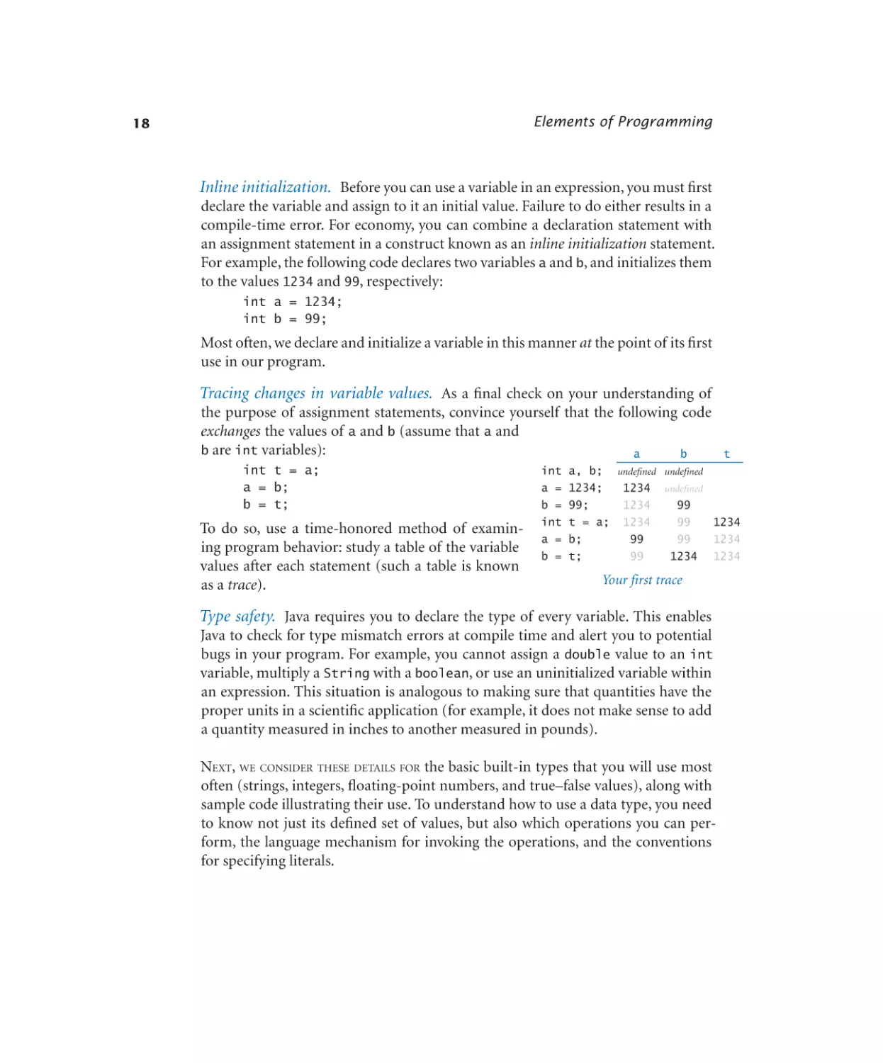
Inline initialization. Before you can use a variable in an expression, you must first
declare the variable and assign to it an initial value. Failure to do either results in a
compile-time error. For economy, you can combine a declaration statement with
an assignment statement in a construct known as an inline initialization statement.
For example, the following code declares two variables a and b, and initializes them
to the values 1234 and 99, respectively:
int a = 1234;
int b = 99;
Most often, we declare and initialize a variable in this manner at the point of its first
use in our program.
Tracing changes in variable values. As a final check on your understanding of
the purpose of assignment statements, convince yourself that the following code
exchanges the values of a and b (assume that a and
b are int variables):
a
b
int t = a;
a = b;
b = t;
To do so, use a time-honored method of examining program behavior: study a table of the variable
values after each statement (such a table is known
as a trace).
int
a =
b =
int
a =
b =
t
a, b; undefined undefined
1234;
1234 undefined
99;
1234
99
t = a; 1234
99
1234
b;
99
99
1234
t;
99
1234 1234
Your first trace
Type safety. Java requires you to declare the type of every variable. This enables
Java to check for type mismatch errors at compile time and alert you to potential
bugs in your program. For example, you cannot assign a double value to an int
variable, multiply a String with a boolean, or use an uninitialized variable within
an expression. This situation is analogous to making sure that quantities have the
proper units in a scientific application (for example, it does not make sense to add
a quantity measured in inches to another measured in pounds).
Next, we consider these details for the basic built-in types that you will use most
often (strings, integers, floating-point numbers, and true–false values), along with
sample code illustrating their use. To understand how to use a data type, you need
to know not just its defined set of values, but also which operations you can perform, the language mechanism for invoking the operations, and the conventions
for specifying literals.
1.2 Built-in Types of Data
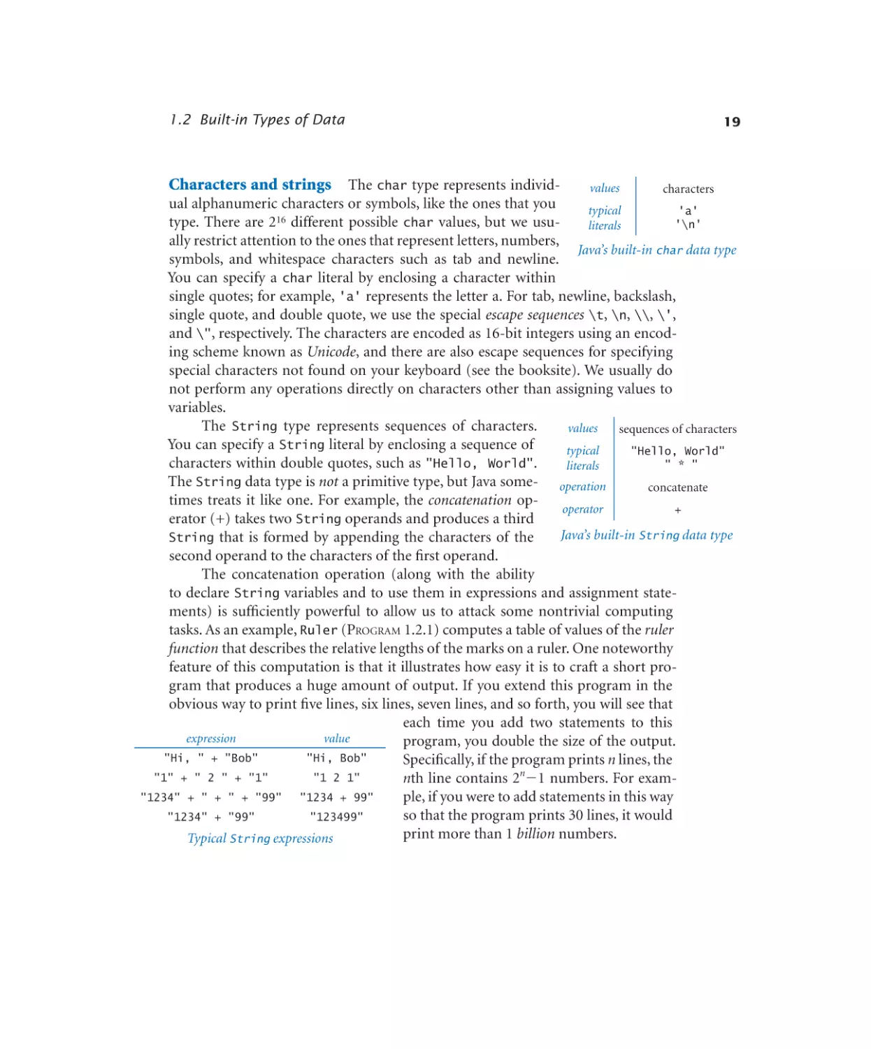
Characters and strings The char type represents individ-
19
values
characters
ual alphanumeric characters or symbols, like the ones that you
typical
'a'
type. There are 216 different possible char values, but we usu'\n'
literals
ally restrict attention to the ones that represent letters, numbers,
Java’s built-in char data type
symbols, and whitespace characters such as tab and newline.
You can specify a char literal by enclosing a character within
single quotes; for example, 'a' represents the letter a. For tab, newline, backslash,
single quote, and double quote, we use the special escape sequences \t, \n, \\, \',
and \", respectively. The characters are encoded as 16-bit integers using an encoding scheme known as Unicode, and there are also escape sequences for specifying
special characters not found on your keyboard (see the booksite). We usually do
not perform any operations directly on characters other than assigning values to
variables.
The String type represents sequences of characters.
values
sequences of characters
You can specify a String literal by enclosing a sequence of
typical
"Hello, World"
characters within double quotes, such as "Hello, World".
" * "
literals
The String data type is not a primitive type, but Java some- operation
concatenate
times treats it like one. For example, the concatenation opoperator
+
erator (+) takes two String operands and produces a third
Java’s built-in String data type
String that is formed by appending the characters of the
second operand to the characters of the first operand.
The concatenation operation (along with the ability
to declare String variables and to use them in expressions and assignment statements) is sufficiently powerful to allow us to attack some nontrivial computing
tasks. As an example, Ruler (Program 1.2.1) computes a table of values of the ruler
function that describes the relative lengths of the marks on a ruler. One noteworthy
feature of this computation is that it illustrates how easy it is to craft a short program that produces a huge amount of output. If you extend this program in the
obvious way to print five lines, six lines, seven lines, and so forth, you will see that
each time you add two statements to this
expression
value
program, you double the size of the output.
"Hi, " + "Bob"
"Hi, Bob"
Specifically, if the program prints n lines, the
"1" + " 2 " + "1"
"1 2 1"
nth line contains 2n1 numbers. For exam"1234" + " + " + "99"
"1234 + 99"
ple, if you were to add statements in this way
so that the program prints 30 lines, it would
"1234" + "99"
"123499"
print more than 1 billion numbers.
Typical String expressions
Elements of Programming
20
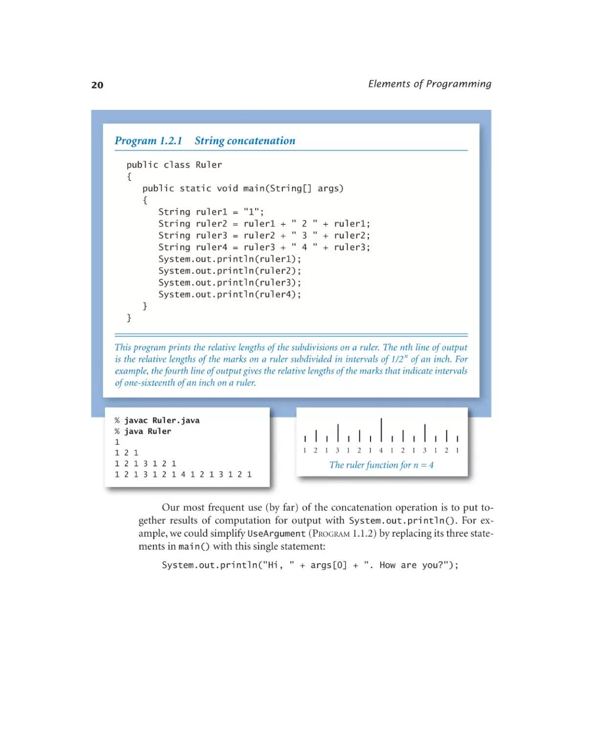
Program 1.2.1
String concatenation
public class Ruler
{
public static void main(String[] args)
{
String ruler1 = "1";
String ruler2 = ruler1 + " 2 " + ruler1;
String ruler3 = ruler2 + " 3 " + ruler2;
String ruler4 = ruler3 + " 4 " + ruler3;
System.out.println(ruler1);
System.out.println(ruler2);
System.out.println(ruler3);
System.out.println(ruler4);
}
}
This program prints the relative lengths of the subdivisions on a ruler. The nth line of output
is the relative lengths of the marks on a ruler subdivided in intervals of 1/2 n of an inch. For
example, the fourth line of output gives the relative lengths of the marks that indicate intervals
of one-sixteenth of an inch on a ruler.
%
%
1
1
1
1
javac Ruler.java
java Ruler
2 1
2 1 3 1 2 1
2 1 3 1 2 1 4 1 2 1 3 1 2 1
1 2 1 3 1 2 1 4 1 2 1 3 1 2 1
The ruler function for n = 4
Our most frequent use (by far) of the concatenation operation is to put together results of computation for output with System.out.println(). For example, we could simplify UseArgument (Program 1.1.2) by replacing its three statements in main() with this single statement:
System.out.println("Hi, " + args[0] + ". How are you?");
1.2 Built-in Types of Data
21
We have considered the String type first precisely because we need it for output (and command-line arguments) in programs that process not only strings but
other types of data as well. Next we consider two convenient mechanisms in Java
for converting numbers to strings and strings to numbers.
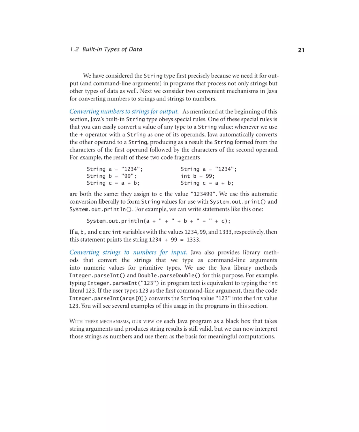
Converting numbers to strings for output. As mentioned at the beginning of this
section, Java’s built-in String type obeys special rules. One of these special rules is
that you can easily convert a value of any type to a String value: whenever we use
the + operator with a String as one of its operands, Java automatically converts
the other operand to a String, producing as a result the String formed from the
characters of the first operand followed by the characters of the second operand.
For example, the result of these two code fragments
String a = "1234";
String b = "99";
String c = a + b;
String a = "1234";
int b = 99;
String c = a + b;
are both the same: they assign to c the value "123499". We use this automatic
conversion liberally to form String values for use with System.out.print() and
System.out.println(). For example, we can write statements like this one:
System.out.println(a + " + " + b + " = " + c);
If a, b, and c are int variables with the values 1234, 99, and 1333, respectively, then
this statement prints the string 1234 + 99 = 1333.
Converting strings to numbers for input. Java also provides library methods that convert the strings that we type as command-line arguments
into numeric values for primitive types. We use the Java library methods
Integer.parseInt() and Double.parseDouble() for this purpose. For example,
typing Integer.parseInt("123") in program text is equivalent to typing the int
literal 123. If the user types 123 as the first command-line argument, then the code
Integer.parseInt(args[0]) converts the String value "123" into the int value
123. You will see several examples of this usage in the programs in this section.
With these mechanisms, our view of each Java program as a black box that takes
string arguments and produces string results is still valid, but we can now interpret
those strings as numbers and use them as the basis for meaningful computations.
Elements of Programming
22
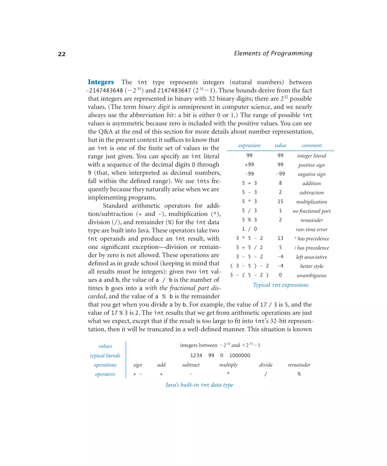
Integers
The int type represents integers (natural numbers) between
–2147483648 (2 31) and 2147483647 (2 311). These bounds derive from the fact
that integers are represented in binary with 32 binary digits; there are 232 possible
values. (The term binary digit is omnipresent in computer science, and we nearly
always use the abbreviation bit : a bit is either 0 or 1.) The range of possible int
values is asymmetric because zero is included with the positive values. You can see
the Q&A at the end of this section for more details about number representation,
but in the present context it suffices to know that
expression
value
comment
an int is one of the finite set of values in the
99
99
integer literal
range just given. You can specify an int literal
+99
99
with a sequence of the decimal digits 0 through
positive sign
9 (that, when interpreted as decimal numbers,
-99
-99
negative sign
fall within the defined range). We use ints fre5 + 3
8
addition
quently because they naturally arise when we are
5 - 3
2
subtraction
implementing programs.
5 * 3
15
multiplication
Standard arithmetic operators for addi5 / 3
1
no fractional part
tion/subtraction (+ and -), multiplication (*),
5 % 3
2
remainder
division (/), and remainder (%) for the int data
1 / 0
run-time error
type are built into Java. These operators take two
3 * 5 - 2
13
* has precedence
int operands and produce an int result, with
one significant exception—division or remain3 + 5 / 2
5
/ has precedence
der by zero is not allowed. These operations are
3 - 5 - 2
-4
left associative
defined as in grade school (keeping in mind that
( 3 - 5 ) - 2
-4
better style
all results must be integers): given two int val- 3 - ( 5 - 2 ) 0
unambiguous
ues a and b, the value of a / b is the number of
Typical int expressions
times b goes into a with the fractional part discarded, and the value of a % b is the remainder
that you get when you divide a by b. For example, the value of 17 / 3 is 5, and the
value of 17 % 3 is 2. The int results that we get from arithmetic operations are just
what we expect, except that if the result is too large to fit into int’s 32-bit representation, then it will be truncated in a well-defined manner. This situation is known
integers between 2 31 and 2 311
values
1234
typical literals
99
0
1000000
operations
sign
add
subtract
multiply
divide
remainder
operators
+ -
+
-
*
/
%
Java’s built-in int data type
1.2 Built-in Types of Data
Program 1.2.2
23
Integer multiplication and division
public class IntOps
{
public static void main(String[] args)
{
int a = Integer.parseInt(args[0]);
int b = Integer.parseInt(args[1]);
int p = a * b;
int q = a / b;
int r = a % b;
System.out.println(a + " * " + b + "
System.out.println(a + " / " + b + "
System.out.println(a + " % " + b + "
System.out.println(a + " = " + q + "
}
}
=
=
=
*
"
"
"
"
+
+
+
+
p);
q);
r);
b + " + " + r);
Arithmetic for integers is built into Java. Most of this code is devoted to the task of getting the
values in and out; the actual arithmetic is in the simple statements in the middle of the program
that assign values to p, q, and r.
% javac IntOps.java
% java IntOps 1234 99
1234 * 99 = 122166
1234 / 99 = 12
1234 % 99 = 46
1234 = 12 * 99 + 46
as overflow. In general, we have to take care that such a result is not misinterpreted
by our code. For the moment, we will be computing with small numbers, so you do
not have to worry about these boundary conditions.
Program 1.2.2 illustrates three basic operations (multiplication, division, and remainder) for manipulating integers,. It also demonstrates the use of
Integer.parseInt() to convert String values on the command line to int values, as well as the use of automatic type conversion to convert int values to String
values for output.
Elements of Programming
24
Three other built-in types are different representations of integers in Java.
The long, short, and byte types are the same as int except that they use 64, 16,
and 8 bits respectively, so the range of allowed values is accordingly different. Programmers use long when working with huge integers, and the other types to save
space. You can find a table with the maximum and minimum values for each type
on the booksite, or you can figure them out for yourself from the numbers of bits.
Floating-point numbers The double type represents floating-point numbers,
for use in scientific and commercial applications. The internal representation is
like scientific notation, so that we can compute with numbers in a huge range.
We use floating-point numbers to represent real numbers, but they are decidedly
not the same as real numbers! There are infinitely many real numbers, but we can
represent only a finite number of floatingexpression
value
point numbers in any digital computer
3.141 + 2.0
5.141
representation. Floating-point numbers
3.141
2.0
1.111
do approximate real numbers sufficiently
3.141 / 2.0
1.5705
well that we can use them in applications,
5.0 / 3.0
1.6666666666666667
but we often need to cope with the fact that
we cannot always do exact computations.
10.0 % 3.141
0.577
You can specify a double literal with
1.0 / 0.0
Infinity
a sequence of digits with a decimal point.
Math.sqrt(2.0)
1.4142135623730951
For example, the literal 3.14159 represents
Math.sqrt(-1.0)
NaN
a six-digit approximation to . AlternaTypical double expressions
tively, you specify a double literal with a
notation like scientific notation: the literal
6.022e23 represents the number 6.022 1023. As with integers, you can use these
conventions to type floating-point literals in your programs or to provide floatingpoint numbers as string arguments on the command line.
The arithmetic operators +, -, *, and / are defined for double. Beyond these
built-in operators, the Java Math library defines the square root function, trigonometric functions, logarithm/exponential functions, and other common functions
for floating-point numbers. To use one of these functions in an expression, you
type the name of the function followed by its argument in parentheses. For exvalues
typical literals
real numbers (specified by IEEE 754 standard)
3.14159
6.022e23
2.0
1.4142135623730951
operations
add
subtract
multiply
divide
operators
+
-
*
/
Java’s built-in double data type
1.2 Built-in Types of Data
Program 1.2.3
25
Quadratic formula
public class Quadratic
{
public static void main(String[] args)
{
double b = Double.parseDouble(args[0]);
double c = Double.parseDouble(args[1]);
double discriminant = b*b - 4.0*c;
double d = Math.sqrt(discriminant);
System.out.println((-b + d) / 2.0);
System.out.println((-b - d) / 2.0);
}
}
This program prints the roots of the polynomial x2 + bx + c, using the quadratic formula. For
example, the roots of x2 – 3x + 2 are 1 and 2 since we can factor the equation as (x – 1)(x – 2);
the roots of x2 – x – 1 are and 1 – , where is the golden ratio; and the roots of x2 + x + 1
are not real numbers.
% javac Quadratic.java
% java Quadratic -3.0 2.0
2.0
1.0
% java Quadratic -1.0 -1.0
1.618033988749895
-0.6180339887498949
% java Quadratic 1.0 1.0
NaN
NaN
ample, the code Math.sqrt(2.0) evaluates to a double value that is approximately
the square root of 2. We discuss the mechanism behind this arrangement in more
detail in Section 2.1 and more details about the Math library at the end of this section.
When working with floating-point numbers, one of the first things that you
will encounter is the issue of precision. For example, printing 5.0/2.0 results in
2.5 as expected, but printing 5.0/3.0 results in 1.6666666666666667. In Section
1.5, you will learn Java’s mechanism for controlling the number of significant digits
that you see in output. Until then, we will work with the Java default output format.
Elements of Programming
26
The result of a calculation can be one of the special values Infinity (if the
number is too large to be represented) or NaN (if the result of the calculation is
undefined). Though there are myriad details to consider when calculations involve
these values, you can use double in a natural way and begin to write Java programs
instead of using a calculator for all kinds of calculations. For example, Program
1.2.3 shows the use of double values in computing the roots of a quadratic equation using the quadratic formula. Several of the exercises at the end of this section
further illustrate this point.
As with long, short, and byte for integers, there is another representation
for real numbers called float. Programmers sometimes use float to save space
when precision is a secondary consideration. The double type is useful for about
15 significant digits; the float type is good for only about 7 digits. We do not use
float in this book.
Booleans The
type represents truth valvalues
true or false
ues from logic. It has just two values: true and false.
literals
true false
These are also the two possible boolean literals. Every
operations
and
or
not
boolean variable has one of these two values, and evoperators
&&
||
!
ery boolean operation has operands and a result that
takes on just one of these two values. This simplicity Java’s built-in boolean data type
is deceiving—boolean values lie at the foundation of
computer science.
The most important operations defined for booleans are and (&&), or (||),
and not (!), which have familiar definitions:
• a && b is true if both operands are true, and false if either is false.
• a || b is false if both operands are false, and true if either is true.
• !a is true if a is false, and false if a is true.
Despite the intuitive nature of these definitions, it is worthwhile to fully specify
each possibility for each operation in tables known as truth tables. The not function
has only one operand: its value for each of the two possible values of the operand is
boolean
a
!a
a
b
a && b
a || b
true
false
false
false
false
false
false
true
false
true
false
true
true
false
false
true
true
true
true
true
Truth-table definitions of
boolean operations
1.2 Built-in Types of Data
27
specified in the second column. The and and or functions each have two operands:
there are four different possibilities for operand values, and the values of the functions for each possibility are specified in the right two columns.
We can use these operators with parentheses to develop arbitrarily complex
expressions, each of which specifies a well-defined boolean function. Often the
same function appears in different guises. For example, the expressions (a && b)
and !(!a || !b) are equivalent.
a
b
a && b
!a
!b
!a || !b
!(!a || !b)
false
false
false
true
true
true
false
false
true
false
true
false
true
false
true
false
false
false
true
true
false
true
true
true
false
false
false
true
Truth-table proof that a
&& b
and
!(!a || !b) are identical
The study of manipulating expressions of this kind is known as Boolean logic.
This field of mathematics is fundamental to computing: it plays an essential role in
the design and operation of computer hardware itself, and it is also a starting point
for the theoretical foundations of computation. In the present context, we are interested in boolean expressions because we use them to control the behavior of
our programs. Typically, a particular condition of interest is specified as a boolean
expression, and a piece of program code is written to execute one set of statements
if that expression is true and a different set of statements if the expression is false.
The mechanics of doing so are the topic of Section 1.3.
Comparisons
Some mixed-type operators take operands of one type and produce a result of another type. The most important operators of this kind are the
comparison operators ==, !=, <, <=, >, and >=, which all are defined for each primitive numeric type and produce a boolean result. Since operations are defined only
with respect to data types, each of these symbols stands for many operations, one
for each data type. It is required that both operands be of the same type.
non-negative discriminant?
(b*b - 4.0*a*c) >= 0.0
beginning of a century?
(year % 100) == 0
legal month?
(month >= 1) && (month <= 12)
Typical comparison expressions
Elements of Programming
28
Program 1.2.4
Leap year
public class LeapYear
{
public static void main(String[] args)
{
int year = Integer.parseInt(args[0]);
boolean isLeapYear;
isLeapYear = (year % 4 == 0);
isLeapYear = isLeapYear && (year % 100 != 0);
isLeapYear = isLeapYear || (year % 400 == 0);
System.out.println(isLeapYear);
}
}
This program tests whether an integer corresponds to a leap year in the Gregorian calendar. A
year is a leap year if it is divisible by 4 (2004), unless it is divisible by 100 in which case it is not
(1900), unless it is divisible by 400 in which case it is (2000).
% javac LeapYear.java
% java LeapYear 2004
true
% java LeapYear 1900
false
% java LeapYear 2000
true
Even without going into the details of number representation, it is clear that
the operations for the various types are quite different. For example, it is one thing
to compare two ints to check that (2 <= 2) is true, but quite another to compare two doubles to check whether (2.0 <= 0.002e3) is true. Still, these operations are well defined and useful to write code that tests for conditions such as
(b*b - 4.0*a*c) >= 0.0, which is frequently needed, as you will see.
1.2 Built-in Types of Data
29
The comparison operations have lower precedence than arithmetic operators
and higher precedence than boolean operators, so you do not need the parentheses
in an expression such as (b*b - 4.0*a*c) >= 0.0, and you could write an expression such as month >= 1 && month <= 12 without parentheses to test whether
the value of the int variable month is between 1 and 12. (It is better style to use the
parentheses, however.)
true
meaning
false
Comparison operations, to- operator
gether with boolean logic, provide
==
2 == 2
2 == 3
equal
the basis for decision making in Java
3 != 2
2 != 2
!=
not equal
programs. Program 1.2.4 is an ex2 < 13
2 < 2
<
less than
ample of their use, and you can find
<=
2 <= 2
3 <= 2
less than or equal
other examples in the exercises at the
13 > 2
2 > 13
>
greater than
end of this section. More importantly,
3
>=
2
2 >= 3
>=
greater than or equal
in Section 1.3 we will see the role that
boolean expressions play in more soComparisons with int operands and a boolean result
phisticated programs.
Library methods and APIs As we have seen, many programming tasks involve using Java library methods in addition to the built-in operators. The number
of available library methods is vast. As you learn to program, you will learn to use
more and more library methods, but it is best at the beginning to restrict your attention to a relatively small set of methods. In this chapter, you have already used
some of Java’s methods for printing, for converting data from one type to another,
and for computing mathematical functions (the Java Math library). In later chapters, you will learn not just how to use other methods, but how to create and use
your own methods.
For convenience, we will consistently summarize the library methods that
you need to know how to use in tables like this one:
void System.out.print(String s)
void System.out.println(String s)
void System.out.println()
print s
print s, followed by a newline
print a newline
Note: Any type of data can be used as argument (and will be automatically converted to String).
Java library methods for printing strings to the terminal
Elements of Programming
30
Such a table is known as an application programming interface (API ). Each method is described by a line in the API
public class Math
that specifies the information you need to know to use the
. . .
method name
method. The code in the tables is not the code that you type
signature
to use the method; it is known as the method’s signature.
double sqrt(double a)
The signature specifies the type of the arguments, the methreturn type
argument type
od name, and the type of the result that the method computes (the return value).
. . .
In your code, you can call a method by typing its name
Anatomy of a method signature
followed by arguments, enclosed in parentheses and separated by commas. When Java executes your program, we
say that it calls (or evaluates) the method with the given arguments and that the
method returns a value. A method call is an
expression, so you can use a method call in
library name
method name
the same way that you use variables and literdouble d = Math.sqrt(b*b - 4.0*a*c);
als to build up more complicated expressions.
return type
argument
For example, you can write expressions like
Math.sin(x) * Math.cos(y) and so on. An
Using a library method
argument is also an expression, so you can
write code like Math.sqrt(b*b - 4.0*a*c)
and Java knows what you mean—it evaluates the argument expression and passes
the resulting value to the method.
The API tables on the facing page show some of the commonly used methods
in Java’s Math library, along with the Java methods we have seen for printing text to
the terminal window and for converting strings to primitive types. The following
table shows several examples of calls that use these library methods:
library name
method call
library
return type
value
Integer.parseInt("123")
Integer
int
123
Double.parseDouble("1.5")
Double
double
1.5
Math.sqrt(5.0*5.0 - 4.0*4.0)
Math
double
3.0
Math.log(Math.E)
Math
double
1.0
Math.random()
Math
double
random in [0, 1)
Math.round(3.14159)
Math
long
3
Math.max(1.0, 9.0)
Math
double
9.0
Typical calls to Java library methods
1.2 Built-in Types of Data
31
public class Math
double abs(double a)
absolute value of a
double max(double a, double b) maximum of a and b
double min(double a, double b) minimum of a and b
Note 1: abs(), max(), and min() are defined also for int, long, and float.
double sin(double theta)
sine of theta
double cos(double theta)
cosine of theta
double tan(double theta)
tangent of theta
Note 2: Angles are expressed in radians. Use toDegrees() and toRadians() to convert.
Note 3: Use asin(), acos(), and atan() for inverse functions.
double exp(double a)
exponential (e a)
double log(double a)
natural log (loge a, or ln a)
double pow(double a, double b) raise a to the bth power (ab )
long round(double a)
round a to the nearest integer
double random()
random number in [0, 1)
double sqrt(double a)
square root of a
double E
value of e (constant)
double PI
value of (constant)
See booksite for other available functions.
Excerpts from Java’s Math library
void System.out.print(String s)
void System.out.println(String s)
print s
print s, followed by a newline
void System.out.println()
print a newline
Java library methods for printing strings to the terminal
int Integer.parseInt(String s)
double
Double.parseDouble(String s)
long Long.parseLong(String s)
convert s to an int value
convert s to a double value
convert s to a long value
Java library methods for converting strings to primitive types
Elements of Programming
32
With three exceptions, the methods on the previous page are pure—given
the same arguments, they always return the same value, without producing any
observable side effect. The method Math.random() is impure because it returns potentially a different value each time it is called; the methods System.out.print()
and System.out.println() are impure because they produce side effects—printing strings to the terminal. In APIs, we use a verb phrase to describe the behavior
of a method that produces side effects; otherwise, we use a noun phrase to describe
the return value. The keyword void designates a method that does not return a
value (and whose main purpose is to produce side effects).
The Math library also defines the constant values Math.PI (for ) and
Math.E (for e), which you can use in your programs. For example, the value of
Math.sin(Math.PI/2) is 1.0 and the value of Math.log(Math.E) is 1.0 (because
Math.sin() takes its argument in radians and Math.log() implements the natural logarithm function).
These APIs are typical of the online documentation that is the standard in modern
programming. The extensive online documentation of the Java APIs is routinely
used by professional programmers, and it is available to you (if you are interested)
directly from the Java website or through our booksite. You do not need to go to
the online documentation to understand the code in this book or to write similar
code, because we present and explain in the text all of the library methods that we
use in APIs like these and summarize them in the endpapers. More important, in
Chapters 2 and 3 you will learn in this book how to develop your own APIs and to
implement methods for your own use.
Type conversion
One of the primary rules of modern programming is that you
should always be aware of the type of data that your program is processing. Only by
knowing the type can you know precisely which set of values each variable can have,
which literals you can use, and which operations you can perform. For example,
suppose that you wish to compute the average of the four integers 1, 2, 3, and 4.
Naturally, the expression (1 + 2 + 3 + 4) / 4 comes to mind, but it produces
the int value 2 instead of the double value 2.5 because of type conversion conventions. The problem stems from the fact that the operands are int values but it is
natural to expect a double value for the result, so conversion from int to double
is necessary at some point. There are several ways to do so in Java.
1.2 Built-in Types of Data
33
Implicit type conversion. You can use an int value wherever a double value is
expected, because Java automatically converts integers to doubles when appropriate. For example, 11*0.25 evaluates to 2.75 because 0.25 is a double and both
operands need to be of the same type; thus, 11 is converted to a double and then
the result of dividing two doubles is a double. As another example, Math.sqrt(4)
evaluates to 2.0 because 4 is converted to a double, as expected by Math.sqrt(),
which then returns a double value. This kind of conversion is called automatic
promotion or coercion. Automatic promotion is appropriate because your intent is
clear and it can be done with no loss of information. In contrast, a conversion that
might involve loss of information (for example, assigning a double value to an int
variable) leads to a compile-time error.
Explicit cast. Java has some built-in type conversion conventions for primitive
types that you can take advantage of when you are aware that you might lose information. You have to make your intention to do so explicit by using a device
expression expression
expression
type
value
called a cast. You cast an expression
from one primitive type to another
(1 + 2 + 3 + 4) / 4.0
double
2.5
by prepending the desired type name
Math.sqrt(4)
double
2.0
within parentheses. For example, the
"1234" + 99
String
"123499"
expression (int) 2.71828 is a cast
11 * 0.25
double
2.75
from double to int that produces
(int) 11 * 0.25
double
2.75
an int with value 2. The conversion
11 * (int) 0.25
int
0
methods defined for casts throw away
(int) (11 * 0.25)
int
2
information in a reasonable way (for a
(int) 2.71828
int
2
full list, see the booksite). For example,
Math.round(2.71828)
long
3
casting a floating-point number to
(int)
Math.round(2.71828)
int
3
an integer discards the fractional part
Integer.parseInt("1234")
int
1234
by rounding toward zero. RandomInt
Typical type conversions
(Program 1.2.5) is an example that
uses a cast for a practical computation.
Casting has higher precedence than arithmetic operations—any cast
is applied to the value that immediately follows it. For example, if we write
int value = (int) 11 * 0.25, the cast is no help: the literal 11 is already an
integer, so the cast (int) has no effect. In this example, the compiler produces
a possible loss of precision error message because there would be a loss
Elements of Programming
34
Program 1.2.5
Casting to get a random integer
public class RandomInt
{
public static void main(String[] args)
{
int n = Integer.parseInt(args[0]);
double r = Math.random();
// uniform between 0.0 and 1.0
int value = (int) (r * n); // uniform between 0 and n-1
System.out.println(value);
}
}
This program uses the Java method Math.random() to generate a random number r between
0.0 (inclusive) and 1.0 (exclusive); then multiplies r by the command-line argument n to get
a random number greater than or equal to 0 and less than n; then uses a cast to truncate the
result to be an integer value between 0 and n-1.
% javac RandomInt.java
% java RandomInt 1000
548
% java RandomInt 1000
141
% java RandomInt 1000000
135032
of precision in converting the resulting value (2.75) to an int for assignment to
value. The error is helpful because the intended computation for this code is likely
(int) (11 * 0.25), which has the value 2, not 2.75.
Explicit type conversion. You can use a method that takes an argument of one
type (the value to be converted) and produces a result of another type. We have
already used the Integer.parseInt() and Double.parseDouble() library methods to convert String values to int and double values, respectively. Many other
methods are available for conversion among other types. For example, the library
1.2 Built-in Types of Data
35
method Math.round() takes a double argument and returns a long result: the
nearest integer to the argument. Thus, for example, Math.round(3.14159) and
Math.round(2.71828) are both of type long and have the same value (3). If you
want to convert the result of Math.round() to an int, you must use an explicit cast.
Beginning programmers tend to find type conversion to be an
annoyance, but experienced programmers know that paying
careful attention to data types is a key to success in programming. It may also be a key to avoiding failure: in a famous incident in 1985, a French rocket exploded in midair because of
a type-conversion problem. While a bug in your program may
not cause an explosion, it is well worth your while to take the
time to understand what type conversion is all about. After you
have written just a few programs, you will see that an understanding of data types will help you not only compose compact
code but also make your intentions explicit and avoid subtle
bugs in your programs.
Summary
Photo: ESA
Explosion of Ariane 5 rocket
A data type is a set of values and a set of operations on those values.
Java has eight primitive data types: boolean, char, byte, short, int, long, float,
and double. In Java code, we use operators and expressions like those in familiar
mathematical expressions to invoke the operations associated with each type. The
boolean type is used for computing with the logical values true and false; the
char type is the set of character values that we type; and the other six numeric
types are used for computing with numbers. In this book, we most often use boolean, int, and double; we do not use short or float. Another data type that we
use frequently, String, is not primitive, but Java has some built-in facilities for
Strings that are like those for primitive types.
When programming in Java, we have to be aware that every operation is defined only in the context of its data type (so we may need type conversions) and
that all types can have only a finite number of values (so we may need to live with
imprecise results).
The boolean type and its operations—&&, ||, and !—are the basis for logical
decision making in Java programs, when used in conjunction with the mixed-type
comparison operators ==, !=, <, >, <=, and >=. Specifically, we use boolean expressions to control Java’s conditional (if) and loop (for and while) constructs, which
we will study in detail in the next section.
36
Elements of Programming
The numeric types and Java’s libraries give us the ability to use Java as an extensive mathematical calculator. We write arithmetic expressions using the built-in
operators +, -, *, /, and % along with Java methods from the Math library.
Although the programs in this section are quite rudimentary by the standards
of what we will be able to do after the next section, this class of programs is quite
useful in its own right. You will use primitive types and basic mathematical functions extensively in Java programming, so the effort that you spend now in understanding them will certainly be worthwhile.
1.2 Built-in Types of Data
Q&A (Strings)
Q. How does Java store strings internally?
A. Strings are sequences of characters that are encoded with Unicode, a modern
standard for encoding text. Unicode supports more than 100,000 different characters, including more than 100 different languages plus mathematical and musical
symbols.
Q. Can you use < and > to compare String values?
A. No. Those operators are defined only for primitive-type values.
Q. How about == and != ?
A. Yes, but the result may not be what you expect, because of the meanings these
operators have for nonprimitive types. For example, there is a distinction between
a String and its value. The expression "abc" == "ab" + x is false when x is a
String with value "c" because the two operands are stored in different places in
memory (even though they have the same value). This distinction is essential, as
you will learn when we discuss it in more detail in Section 3.1.
Q. How can I compare two strings like words in a book index or dictionary?
A. We defer discussion of the
String data type and associated methods until
Section 3.1, where we introduce object-oriented programming. Until then, the
string concatenation operation suffices.
Q. How can I specify a string literal that is too long to fit on a single line?
A. You can’t. Instead, divide the string literal into independent string literals and
concatenate them together, as in the following example:
String dna = "ATGCGCCCACAGCTGCGTCTAAACCGGACTCTG" +
"AAGTCCGGAAATTACACCTGTTAG";
37
Elements of Programming
38
Q&A (Integers)
Q. How does Java store integers internally?
A. The simplest representation is for small positive integers, where the binary
number system is used to represent each integer with a fixed amount of computer
memory.
Q. What’s the binary number system?
A. In the binary number system, we represent an integer as a sequence of bits. A bit
is a single binary (base 2) digit—either 0 or 1—and is the basis for representing
information in computers. In this case the bits are coefficients of powers of 2. Specifically, the sequence of bits bnbn–1…b2b1b0 represents the integer
bn2n + bn–12n–1 + … + b222 + b121 + b020
For example, 1100011 represents the integer
99 = 1· 64 + 1· 32 + 0· 16 + 0· 8 + 0· 4 + 1· 2 +1· 1
The more familiar decimal number system is the same except that the digits are
between 0 and 9 and we use powers of 10. Converting a number to binary is an
interesting computational problem that we will consider in the next section. Java
uses 32 bits to represent int values. For example, the decimal integer 99 might be
represented with the 32 bits 00000000000000000000000001100011.
Q. How about negative numbers?
A. Negative numbers are handled with a convention known as two’s complement,
which we need not consider in detail. This is why the range of int values in Java
is –2147483648 (–231) to 2147483647 (231 – 1). One surprising consequence of
this representation is that int values can become negative when they get large and
overflow (exceed 2147483647). If you have not experienced this phenomenon, see
Exercise 1.2.10. A safe strategy is to use the int type when you know the integer
values will be fewer than ten digits and the long type when you think the integer
values might get to be ten digits or more.
Q. It seems wrong that Java should just let
ints
Shouldn’t Java automatically check for overflow?
overflow and give bad values.
1.2 Built-in Types of Data
39
A. Yes, this issue is a contentious one among programmers. The short answer for
now is that the lack of such checking is one reason such types are called primitive
data types. A little knowledge can go a long way in avoiding such problems. Again,
it is fine to use the int type for small numbers, but when values run into the billions, you cannot.
Q. What is the value of Math.abs(-2147483648)?
A.
-2147483648. This strange (but true) result is a typical example of the effects of
integer overflow and two’s complement representation.
Q. What do the expressions 1
/ 0 and 1 % 0
evaluate to in Java?
A. Each generates a run-time exception, for division by zero.
Q. What is the result of division and remainder for negative integers?
A. The quotient a / b rounds toward 0; the remainder a % b is defined such that
(a / b) * b + a % b is always equal to a. For example, -14 / 3 and 14 / -3 are both
-4, but -14 % 3 is -2 and 14 % -3 is 2. Some other languages (including Python)
have different conventions when dividing by negative integers.
Q. Why is the value of 10
^ 6 not 1000000 but 12?
A. The ^ operator is not an exponentiation operator, which you must have been
thinking. Instead, it is the bitwise exclusive or operator, which is seldom what you
want. Instead, you can use the literal 1e6. You could also use Math.pow(10, 6) but
doing so is wasteful if you are raising 10 to a known power.
Elements of Programming
40
Q&A (Floating-Point Numbers)
Q. Why is the type for real numbers named double?
A. The decimal point can “float” across the digits that make up the real number. In
contrast, with integers the (implicit) decimal point is fixed after the least significant
digit.
Q. How does Java store floating-point numbers internally?
A. Java follows the IEEE 754 standard, which supported in hardware by most
modern computer systems. The standard specifies that a floating-point number
is stored using three fields: sign, mantissa, and exponent. If you are interested,
see the booksite for more details. The IEEE 754 standard also specifies how special floating-point values—positive zero, negative zero, positive infinity, negative
infinity, and NaN (not a number)—should be handled. In particular, floatingpoint arithmetic never leads to a run-time exception. For example, the expression
-0.0/3.0 evaluates to -0.0, the expression 1.0/0.0 evaluates to positive infinity,
and Math.sqrt(-2.0) evaluates to NaN.
Q. Fifteen digits for floating-point numbers certainly seems enough to me. Do I
really need to worry much about precision?
A. Yes, because you are used to mathematics based on real numbers with infinite
precision, whereas the computer always deals with finite approximations. For example, the expression (0.1 + 0.1 == 0.2) evaluates to true but the expression
(0.1 + 0.1 + 0.1 == 0.3) evaluates to false! Pitfalls like this are not at all unusual in scientific computing. Novice programmers should avoid comparing two
floating-point numbers for equality.
Q. How can I initialize a double variable to NaN or infinity?
A. Java has built-in constants available for this purpose:
Double.NaN,
Double.POSITIVE_INFINITY, and Double.NEGATIVE_INFINITY.
Q. Are there functions in Java’s
Math library for other trigonometric functions,
such as cosecant, secant, and cotangent?
1.2 Built-in Types of Data
A. No, but you could use Math.sin(), Math.cos(), and Math.tan() to compute
them. Choosing which functions to include in an API is a tradeoff between the
convenience of having every function that you need and the annoyance of having to find one of the few that you need in a long list. No choice will satisfy all
users, and the Java designers have many users to satisfy. Note that there are plenty
of redundancies even in the APIs that we have listed. For example, you could use
Math.sin(x)/Math.cos(x) instead of Math.tan(x).
Q. It is annoying to see all those digits when printing a double. Can we arrange
System.out.println() to print just two or three digits after the decimal point?
A. That sort of task involves a closer look at the method used to convert from
to String. The Java library function System.out.printf() is one way
to do the job, and it is similar to the basic printing method in the C programming
language and many modern languages, as discussed in Section 1.5. Until then, we
will live with the extra digits (which is not all bad, since doing so helps us to get
used to the different primitive types of numbers).
double
41
Elements of Programming
42
Q&A (Variables and Expressions)
Q. What happens if I forget to declare a variable?
A. The compiler complains when you refer to that variable in an expression. For
example, IntOpsBad is the same as Program 1.2.2 except that the variable p is not
declared (to be of type int).
% javac IntOpsBad.java
IntOpsBad.java:7: error: cannot find symbol
p = a * b;
^
symbol:
variable p
location: class IntOpsBad
IntOpsBad.java:10: error: cannot find symbol
System.out.println(a + " * " + b + " = " + p);
^
symbol:
variable p
location: class IntOpsBad
2 errors
The compiler says that there are two errors, but there is really just one: the declaration of p is missing. If you forget to declare a variable that you use often, you will
get quite a few error messages. A good strategy is to correct the first error and check
that correction before addressing later ones.
Q. What happens if I forget to initialize a variable?
A. The compiler checks for this condition and will give you a variable
might
error message if you try to use the variable in an
expression before you have initialized it.
not have been initialized
Q. Is there a difference between the = and == operators?
A. Yes, they are quite different! The first is an assignment operator that changes
the value of a variable, and the second is a comparison operator that produces a
boolean result. Your ability to understand this answer is a sure test of whether you
understood the material in this section. Think about how you might explain the
difference to a friend.
1.2 Built-in Types of Data
Q. Can you compare a double to an int?
A. Not without doing a type conversion, but remember that Java usually does the
requisite type conversion automatically. For example, if x is an int with the value
3, then the expression (x < 3.1) is true—Java converts x to double (because 3.1
is a double literal) before performing the comparison.
Q. Will the statement a = b = c = 17; assign the value 17 to the three integer
variables a, b, and c?
A. Yes. It works because an assignment statement in Java is also an expression (that
evaluates to its right-hand side) and the assignment operator is right associative. As
a matter of style, we do not use such chained assignments in this book.
Q. Will the expression (a
test whether the values of three integer variables a, b, and c are in strictly ascending order?
< b < c)
A. No, it will not compile because the expression a
< b produces a boolean value,
which would then be compared to an int value. Java does not support chained
comparisons. Instead, you need to write (a < b && b < c).
Q. Why do we write (a
A. Java also has an
&
&& b) and not (a & b)?
operator that you may encounter if you pursue advanced
programming courses.
Q. What is the value of Math.round(6.022e23)?
A. You should get in the habit of typing in a tiny Java program to answer such
questions yourself (and trying to understand why your program produces the result that it does).
Q. I’ve heard Java referred to as a statically typed language. What does this mean?
A. Static typing means that the type of every variable and expression is known at
compile time. Java also verifies and enforces type constraints at compile time; for
example, your program will not compile if you attempt to store a value of type
double in a variable of type int or call Math.sqrt() with a String argument.
43
Elements of Programming
44
Exercises
1.2.1 Suppose that a and b are int variables. What does the following sequence
of statements do?
int t = a; b = t; a = b;
1.2.2 Write a program that uses Math.sin() and Math.cos() to check that the
value of cos2 + sin2 is approximately 1 for any entered as a command-line argument. Just print the value. Why are the values not always exactly 1?
1.2.3 Suppose that a and b are boolean variables. Show that the expression
(!(a && b) && (a || b)) || ((a && b) || !(a || b))
evaluates to true.
1.2.4 Suppose that a and b
(!(a < b) && !(a > b)).
are int variables. Simplify the following expression:
1.2.5 The exclusive or operator ^ for boolean operands is defined to be true if
they are different, false if they are the same. Give a truth table for this function.
1.2.6 Why does 10/3 give 3 and not 3.333333333?
Solution. Since both 10 and 3 are integer literals, Java sees no need for type conversion and uses integer division. You should write 10.0/3.0 if you mean the numbers
to be double literals. If you write 10/3.0 or 10.0/3, Java does implicit conversion
to get the same result.
1.2.7 What does each of the following print?
a. System.out.println(2 + "bc");
b. System.out.println(2 + 3 + "bc");
c. System.out.println((2+3) + "bc");
d. System.out.println("bc" + (2+3));
e. System.out.println("bc" + 2 + 3);
Explain each outcome.
1.2.8 Explain how to use Program 1.2.3 to find the square root of a number.
1.2 Built-in Types of Data
45
1.2.9 What does each of the following print?
a. System.out.println('b');
b. System.out.println('b' + 'c');
c. System.out.println((char) ('a' + 4));
Explain each outcome.
1.2.10 Suppose that a variable a is declared as int
a = 2147483647
(or equiva-
lently, Integer.MAX_VALUE). What does each of the following print?
a. System.out.println(a);
b. System.out.println(a+1);
c. System.out.println(2-a);
d. System.out.println(-2-a);
e. System.out.println(2*a);
f. System.out.println(4*a);
Explain each outcome.
1.2.11 Suppose that a variable a is declared as double
a = 3.14159. What does
each of the following print?
a. System.out.println(a);
b. System.out.println(a+1);
c. System.out.println(8/(int) a);
d. System.out.println(8/a);
e. System.out.println((int) (8/a));
Explain each outcome.
1.2.12 Describe what happens if you write sqrt instead of Math.sqrt in Program
1.2.3.
1.2.13 Evaluate the expression (Math.sqrt(2) * Math.sqrt(2) == 2).
1.2.14 Write a program that takes two positive integers as command-line
arguments and prints true if either evenly divides the other.
Elements of Programming
46
1.2.15 Write a program that takes three positive integers as command-line
arguments and prints false if any one of them is greater than or equal to the sum
of the other two and true otherwise. (Note : This computation tests whether the
three numbers could be the lengths of the sides of some triangle.)
1.2.16 A physics student gets unexpected results when using the code
double force = G * mass1 * mass2 / r * r;
to compute values according to the formula F = Gm1m2 r 2. Explain the problem
and correct the code.
1.2.17 Give the value of the variable a after the execution of each of the following
sequences of statements:
int
a =
a =
a =
a
a
a
a
=
+
+
+
1;
a;
a;
a;
boolean a = true;
a = !a;
a = !a;
a = !a;
int
a =
a =
a =
a
a
a
a
=
*
*
*
2;
a;
a;
a;
1.2.18 Write a program that takes two integer command-line arguments x and y
and prints the Euclidean distance from the point (x, y) to the origin (0, 0).
1.2.19 Write a program that takes two integer command-line arguments a and b
and prints a random integer between a and b, inclusive.
1.2.20 Write a program that prints the sum of two random integers between 1 and
6 (such as you might get when rolling dice).
1.2.21 Write a program that takes a double command-line argument t and prints
the value of sin(2t) sin(3t).
1.2.22 Write a program that takes three double command-line arguments x0, v0,
and t and prints the value of x0 v0t − g t 2 2, where g is the constant 9.80665. (Note :
This value is the displacement in meters after t seconds when an object is thrown
straight up from initial position x0 at velocity v0 meters per second.)
1.2.23 Write a program that takes two integer command-line arguments
d and prints true if
m and
day d of month m is between 3/20 and 6/20, false otherwise.
1.2 Built-in Types of Data
47
Creative Exercises
1.2.24 Continuously compounded interest. Write a program that calculates and
prints the amount of money you would have after t years if you invested P dollars
at an annual interest rate r (compounded continuously). The desired value is given
by the formula Pe rt.
1.2.25 Wind chill. Given the temperature T (in degrees Fahrenheit) and the wind
speed v (in miles per hour), the National Weather Service defines the effective temperature (the wind chill) as follows:
w = 35.74 0.6215 T (0.4275 T 35.75) v 0.16
Write a program that takes two double command-line arguments temperature
and velocity and prints the wind chill. Use Math.pow(a, b) to compute ab. Note :
The formula is not valid if T is larger than 50 in absolute value or if v is larger than
120 or less than 3 (you may assume that the values you get are in that range).
1.2.26 Polar coordinates. Write a program that converts from Cartesian
to polar coordinates. Your program should accept two double commandline arguments x and y and print the polar coordinates r and . Use the
method Math.atan2(y, x) to compute the arctangent value of y/x that is
in the range from to .
1.2.27 Gaussian random numbers. Write a program
x
r
Polar coordinates
RandomGaussian
that prints a random number r drawn from the Gaussian distribution. One way to
do so is to use the Box–Muller formula
r = sin(2 v) (2 ln u)1/2
where u and v are real numbers between 0 and 1 generated by the Math.random()
method.
1.2.28 Order check. Write a program that takes three
command-line
arguments x, y, and z and prints true if the values are strictly ascending or descending ( x < y < z or x > y > z ), and false otherwise.
double
y
Elements of Programming
48
1.2.29 Day of the week. Write a program that takes a date as input and prints the
day of the week that date falls on. Your program should accept three int commandline arguments: m (month), d (day), and y (year). For m, use 1 for January, 2 for
February, and so forth. For output, print 0 for Sunday, 1 for Monday, 2 for Tuesday,
and so forth. Use the following formulas, for the Gregorian calendar:
y0 = y (14 m) / 12
x = y0 y0 / 4 y0 / 100 y0 / 400
m0 = m 12 ((14 m) / 12) 2
d0 = (d x (31 m0) / 12) % 7
Example:
On which day of the week did February 14, 2000 fall?
y0 =
x =
m0 =
d0 =
Answer :
2000 1 = 1999
1999 1999 / 4 1999 / 100 1999 / 400 = 2483
2 12 1 2 = 12
(14 2483 (31 12) / 12) % 7 = 2500 % 7 = 1
Monday.
1.2.30 Uniform random numbers. Write a program that prints five uniform random numbers between 0 and 1, their average value, and their minimum and maximum values. Use Math.random(), Math.min(), and Math.max().
1.2.31 Mercator projection. The Mercator projection is a conformal (anglepreserving) projection that maps latitude and longitude to rectangular coordinates (x, y). It is widely used—for example, in nautical charts and in the maps that
you print from the web. The projection is defined by the equations x 0 and
y 1/2 ln ((1 sin ) (1 sin )), where 0 is the longitude of the point in the
center of the map. Write a program that takes 0 and the latitude and longitude of
a point from the command line and prints its projection.
1.2.32 Color conversion. Several different formats are used to represent color. For
example, the primary format for LCD displays, digital cameras, and web pages,
known as the RGB format, specifies the level of red (R), green (G), and blue (B)
on an integer scale from 0 to 255. The primary format for publishing books and
magazines, known as the CMYK format, specifies the level of cyan (C), magenta
1.2 Built-in Types of Data
49
(M), yellow (Y), and black (K) on a real scale from 0.0 to 1.0. Write a program
RGBtoCMYK that converts RGB to CMYK. Take three integers—r, g, and b—from
the command line and print the equivalent CMYK values. If the RGB values are all
0, then the CMY values are all 0 and the K value is 1; otherwise, use these formulas:
w max ( r / 255, g / 255, b / 255 )
c (w ( r / 255)) w
m (w ( g / 255)) w
y (w ( b / 255)) w
k 1 w
1.2.33 Great circle. Write a program
GreatCircle that takes four double
command-line arguments—x1, y1, x2, and y2—(the latitude and longitude, in de-
grees, of two points on the earth) and prints the great-circle distance between them.
The great-circle distance (in nautical miles) is given by the following equation:
d = 60 arccos(sin(x1) sin(x2) cos(x1) cos(x2) cos(y1 y2))
Note that this equation uses degrees, whereas Java’s trigonometric functions use radians. Use Math.toRadians() and Math.toDegrees() to convert between the two.
Use your program to compute the great-circle distance between Paris (48.87° N
and 2.33° W) and San Francisco (37.8° N and 122.4° W).
1.2.34 Three-sort. Write a program that takes three integer command-line arguments and prints them in ascending order. Use Math.min() and Math.max().
1.2.35 Dragon curves. Write a program to print the instructions for drawing the
dragon curves of order 0 through 5. The instructions are strings of F, L, and R
characters, where F means “draw line while moving 1 unit
F
forward,” L means “turn left,” and R means “turn right.” A
FLF
dragon curve of order n is formed when you fold a strip
of paper in half n times, then unfold to right angles. The
key to solving this problem is to note that a curve of order
FLFLFRF
n is a curve of order n1 followed by an L followed by a
curve of order n1 traversed in reverse order, and then
FLFLFRFLFLFRFRF
to figure out a similar description for the reverse curve.
Dragon curves of order 0, 1, 2, and 3
Elements of Programming
1.3 Conditionals and Loops
In the programs that we have examined to this point, each of the statements in the
program is executed once, in the order given. Most programs are more complicated
because the sequence of statements and the number of times each is executed can
vary. We use the term control flow to refer to statement sequencing in a program.
1.3.1 Flipping a fair coin. . . . . . . . . . . 53
In this section, we introduce statements
1.3.2 Your first while loop. . . . . . . . . . 55
that allow us to change the control flow,
1.3.3 Computing powers of 2. . . . . . . . 57
using logic about the values of program
1.3.4 Your first nested loops. . . . . . . . . 63
1.3.5 Harmonic numbers . . . . . . . . . . 65
variables. This feature is an essential
1.3.6 Newton’s method . . . . . . . . . . . 66
component of programming.
1.3.7 Converting to binary . . . . . . . . . 68
Specifically, we consider Java state1.3.8 Gambler’s ruin simulation . . . . . . 71
ments that implement conditionals,
1.3.9 Factoring integers . . . . . . . . . . . 73
where some other statements may or may
Programs in this section
not be executed depending on certain
conditions, and loops, where some other
statements may be executed multiple times, again depending on certain conditions.
As you will see in this section, conditionals and loops truly harness the power of the
computer and will equip you to write programs to accomplish a broad variety of
tasks that you could not contemplate attempting without a computer.
If statements
Most computations require different actions for different inputs.
One way to express these differences in Java is the if statement:
if (<boolean expression>) { <statements> }
This description introduces a formal notation known as a template that we will
use to specify the format of Java constructs. We put within angle brackets (< >)
a construct that we have already defined, to indicate that we can use any instance
of that construct where specified. In this case, <boolean expression> represents
an expression that evaluates to a boolean value, such as one involving a comparison operation, and <statements> represents a statement block (a sequence of Java
statements). This latter construct is familiar to you: the body of main() is such a sequence. If the sequence is a single statement, the curly braces are optional. It is possible to make formal definitions of <boolean expression> and <statements>,
but we refrain from going into that level of detail. The meaning of an if statement
1.3 Conditionals and Loops
51
is self-explanatory: the statement(s) in the sequence are to be executed if and only
if the expression is true.
As a simple example, suppose that you want to compute the absolute value of
an int value x. This statement does the job:
boolean
expression
if (x < 0) x = -x;
(More precisely, it replaces x with the absolute value of x.) As a
second simple example, consider the following statement:
if ( x > y )
{
if (x > y)
{
int t = x;
x = y;
y = t;
}
int t = x;
x = y;
y = t;
sequence
of
statements
}
Anatomy of an if statement
This code puts the smaller of the two int values in x and the larger of the two values in y, by exchanging the values in the two variables if necessary.
You can also add an else clause to an if statement, to express the concept of
executing either one statement (or sequence of statements) or another, depending
on whether the boolean expression is true or false, as in the following template:
if (<boolean expression>) <statements T>
else
<statements F>
As a simple example of the need for an else clause, consider the following code,
which assigns the maximum of two int values to the variable max:
if (x > y) max = x;
else
max = y;
One way to understand control flow is to visualize it with a diagram called a
flowchart. Paths through the flowchart correspond to flow-of-control paths in the
if (x > y) max = x;
else
max = y;
if (x < 0) x = -x;
yes
x < 0 ?
x = -x;
no
yes
x > y ?
max = x;
Flowchart examples (if statements)
no
max = y;
Elements of Programming
52
program. In the early days of computing, when programmers used low-level languages and difficult-to-understand flows of control, flowcharts were an essential
part of programming. With modern languages, we use flowcharts just to understand basic building blocks like the if statement.
The accompanying table contains some examples of the use of if and ifelse statements. These examples are typical of simple calculations you might need
in programs that you write. Conditional statements are an essential part of programming. Since the semantics (meaning) of statements like these is similar to their
meanings as natural-language phrases, you will quickly grow used to them.
Program 1.3.1 is another example of the use of the if-else statement, in
this case for the task of simulating a fair coin flip. The body of the program is a
single statement, like the ones in the table, but it is worth special attention because
it introduces an interesting philosophical issue that is worth contemplating: can a
computer program produce random values? Certainly not, but a program can produce numbers that have many of the properties of random numbers.
absolute value
if (x < 0) x = -x;
put the smaller
value in x
and the larger
value in y
if (x > y)
{
int t = x;
x = y;
y = t;
}
maximum of
x and y
error check
for division
operation
error check
for quadratic
formula
if (x > y) max = x;
else
max = y;
if (den == 0) System.out.println("Division by zero");
else
System.out.println("Quotient = " + num/den);
double discriminant = b*b
if (discriminant < 0.0)
{
System.out.println("No
}
else
{
System.out.println((-b
System.out.println((-b
}
- 4.0*c;
real roots");
+ Math.sqrt(discriminant))/2.0);
- Math.sqrt(discriminant))/2.0);
Typical examples of using if and if-else statements
1.3 Conditionals and Loops
Program 1.3.1
Flipping a fair coin
public class Flip
{
public static void main(String[] args)
{ // Simulate a fair coin flip.
if (Math.random() < 0.5) System.out.println("Heads");
else
System.out.println("Tails");
}
}
This program uses Math.random() to simulate a fair coin flip. Each time you run it, it prints
either Heads or Tails. A sequence of flips will have many of the same properties as a sequence
that you would get by flipping a fair coin, but it is not a truly random sequence.
% java Flip
Heads
% java Flip
Tails
% java Flip
Tails
While loops Many computations are inherently repetitive. The basic Java construct for handling such computations has the following format:
while (<boolean expression>) { <statements> }
The while statement has the same form as the if statement (the only difference
being the use of the keyword while instead of if), but the meaning is quite different. It is an instruction to the computer to behave as follows: if the boolean expression is false, do nothing; if the boolean expression is true, execute the sequence
of statements (just as with an if statement) but then check the expression again,
execute the sequence of statements again if the expression is true, and continue as
long as the expression is true. We refer to the statement block in a loop as the body
of the loop. As with the if statement, the curly braces are optional if a while loop
body has just one statement. The while statement is equivalent to a sequence of
identical if statements:
53
Elements of Programming
54
if (<boolean expression>) { <statements> }
if (<boolean expression>) { <statements> }
if (<boolean expression>) { <statements> }
...
At some point, the code in one of the statements must change something (such as
the value of some variable in the boolean expression) to make the boolean expression false, and then the sequence is broken.
A common programming paradigm involves maintaining an integer value
that keeps track of the number of times a loop iterates. We start at some initial
value, and then increment the value by 1 each time
initialization is a
loopthrough the loop, testing whether it exceeds a pre- separate
statement
continuation
condition
determined maximum before deciding to continue.
int power = 1;
TenHellos (Program 1.3.2) is a simple example of
while ( power <= n/2 )
this paradigm that uses a while statement. The key braces are {
optional
to the computation is the statement
power = 2*power;
when body
i = i + 1;
is a single
statement
}
body
As a mathematical equation, this statement is nonAnatomy of a while loop
sense, but as a Java assignment statement it makes
perfect sense: it says to compute the value i + 1
and then assign the result to the variable i. If the value of i was 4 before the statement, it becomes 5 afterward; if it was 5, it becomes 6; and so forth. With the initial
condition in TenHellos that the value of i starts at 4, the statement block is executed seven times until the sequence is broken,
int i = 4;
when
the value of i becomes 11.
while (i <= 10)
{
Using the while loop is barely worthSystem.out.println(i + "th Hello"); while for this simple task, but you will soon be
i = i + 1;
addressing tasks where you will need to specify
}
that statements be repeated far too many times
i = 4;
to contemplate doing it without loops. There is
a profound difference between programs with
no
i <= 10 ?
while statements and programs without them,
yes
because while statements allow us to specify
System.out.println(i + "th Hello");
a potentially unlimited number of statements
to
be executed in a program. In particular, the
i = i + 1;
while statement allows us to specify lengthy
Flowchart example (while statement)
1.3 Conditionals and Loops
Program 1.3.2
55
Your first while loop
public class TenHellos
{
public static void main(String[] args)
{ // Print 10 Hellos.
System.out.println("1st Hello");
System.out.println("2nd Hello");
System.out.println("3rd Hello");
int i = 4;
while (i <= 10)
{ // Print the ith Hello.
System.out.println(i + "th Hello");
i = i + 1;
}
}
}
This program uses a while loop for the simple, repetitive task of printing the output shown
below. After the third line, the lines to be printed differ only in the value of the index counting
the line printed, so we define a variable i to contain that index. After initializing the value of
i to 4, we enter into a while loop where we use the value of i in the System.out.println()
statement and increment it each time through the loop. After printing 10th Hello, the value
of i becomes 11 and the loop terminates.
% java TenHellos
1st Hello
2nd Hello
3rd Hello
4th Hello
5th Hello
6th Hello
7th Hello
8th Hello
9th Hello
10th Hello
i
i <= 10
output
4
true
4th Hello
5
true
5th Hello
6
true
6th Hello
7
true
7th Hello
8
true
8th Hello
9
true
9th Hello
10
true
10th Hello
11
false
Trace of java
TenHellos
56
Elements of Programming
computations in short programs. This ability opens the
door to writing programs for tasks that we could not
contemplate addressing without a computer. But there
is also a price to pay: as your programs become more
sophisticated, they become more difficult to understand.
PowersOfTwo (Program 1.3.3) uses a while loop to
print out a table of the powers of 2. Beyond the loop control counter i, it maintains a variable power that holds
the powers of 2 as it computes them. The loop body contains three statements: one to print the current power of
2, one to compute the next (multiply the current one by
2), and one to increment the loop control counter.
There are many situations in computer science
where it is useful to be familiar with powers of 2. You
should know at least the first 10 values in this table and
you should note that 210 is about 1 thousand, 220 is about
1 million, and 230 is about 1 billion.
PowersOfTwo is the prototype for many useful
computations. By varying the computations that change
the accumulated value and the way that the loop control
variable is incremented, we can print out tables of a variety of functions (see Exercise 1.3.12).
It is worthwhile to carefully examine the behavior of programs that use loops by studying a trace of
the program. For example, a trace of the operation of
PowersOfTwo should show the value of each variable
before each iteration of the loop and the value of the
boolean expression that controls the loop. Tracing the
operation of a loop can be very tedious, but it is often
worthwhile to run a trace because it clearly exposes what
a program is doing.
PowersOfTwo is nearly a self-tracing program,
because it prints the values of its variables each time
through the loop. Clearly, you can make any program produce a trace of itself by adding appropriate
System.out.println() statements. Modern program-
i
power
i <= n
0
1
true
1
2
true
2
4
true
3
8
true
4
16
true
5
32
true
6
64
true
7
128
true
8
256
true
9
512
true
10
1024
true
11
2048
true
12
4096
true
13
8192
true
14
16384
true
15
32768
true
16
65536
true
17
131072
true
18
262144
true
19
524288
true
20
1048576
true
21
2097152
true
22
4194304
true
23
8388608
true
24
16777216
true
25
33554432
true
26
67108864
true
27
134217728
true
28
268435456
true
29
536870912
true
30
1073741824
false
Trace of java
PowersOfTwo 29
1.3 Conditionals and Loops
Program 1.3.3
57
Computing powers of 2
public class PowersOfTwo
{
public static void main(String[] args)
{ // Print the first n powers of 2.
int n = Integer.parseInt(args[0]);
int power = 1;
int i = 0;
while (i <= n)
{ // Print ith power of 2.
System.out.println(i + " " + power);
power = 2 * power;
i = i + 1;
}
}
}
n
i
power
loop termination value
loop control counter
current power of 2
This program takes an integer command-line argument n and prints a table of the powers of 2
that are less than or equal to 2 n. Each time through the loop, it increments the value of i and
doubles the value of power. We show only the first three and the last three lines of the table; the
program prints n+1 lines.
%
0
1
2
3
4
5
java PowersOfTwo 5
1
2
4
8
16
32
% java PowersOfTwo 29
0 1
1 2
2 4
...
27 134217728
28 268435456
29 536870912
ming environments provide sophisticated tools for tracing, but this tried-and-true
method is simple and effective. You certainly should add print statements to the
first few loops that you write, to be sure that they are doing precisely what you
expect.
Elements of Programming
58
There is a hidden trap in PowersOfTwo, because the largest integer in Java’s
data type is 231 – 1 and the program does not test for that possibility. If you
invoke it with java PowersOfTwo 31, you may be surprised by the last line of
output printed:
int
...
1073741824
-2147483648
The variable power becomes too large and takes on a negative value because of the
way Java represents integers. The maximum value of an int is available for us to
use as Integer.MAX_VALUE. A better version of Program 1.3.3 would use this value
to test for overflow and print an error message if the user types too large a value,
though getting such a program to work properly for all inputs is trickier than you
might think. (For a similar challenge, see Exercise 1.3.16.)
As a more complicated example, suppose that we
want to compute the largest power of 2 that is less than
or equal to a given positive integer n. If n is 13, we want
int power = 1;
the result 8; if n is 1000, we want the result 512; if n is 64,
we want the result 64; and so forth. This computation is
power <= n/2 ?
simple to perform with a while loop:
int power = 1;
while (power <= n/2)
power = 2*power;
no
yes
power = 2*power;
It takes some thought to convince yourself that this simple piece of code produces the desired result. You can do
so by making these observations:
Flowchart for the statements
• power is always a power of 2.
int power = 1;
• power is never greater than n.
while (power <= n/2)
power = 2*power;
• power increases each time through the loop, so the
loop must terminate.
• After the loop terminates, 2*power is greater than n.
Reasoning of this sort is often important in understanding how while loops work.
Even though many of the loops you will write will be much simpler than this one,
you should be sure to convince yourself that each loop you write will behave as you
expect.
The logic behind such arguments is the same whether the loop iterates just a
few times, as in TenHellos, or dozens of times, as in PowersOfTwo, or millions of
1.3 Conditionals and Loops
59
times, as in several examples that we will soon consider. That leap from a few tiny
cases to a huge computation is profound. When writing loops, understanding how
the values of the variables change each time through the loop (and checking that
understanding by adding statements to trace their values and running for a small
number of iterations) is essential. Having done so, you can confidently remove
those training wheels and truly unleash the power of the computer.
For loops
As you will see, the
loop allows us to write prodeclare and initialize
another a loop control variable
grams for all manner of applica- initialize
loopvariable in a
continuation
separate
tions. Before considering more
increment
condition
statement
int power = 1;
examples, we will look at an alterfor (int i = 0; i <= n; i++ )
nate Java construct that allows us
{
even more flexibility when writing
System.out.println(i + " " + power);
programs with loops. This alterpower = 2*power;
nate notation is not fundamental}
body
ly different from the basic while
Anatomy of a for loop (that prints powers of 2)
loop, but it is widely used because
it often allows us to write more
compact and more readable programs than if we used only while statements.
while
For notation. Many loops follow this scheme: initialize an index variable to some
value and then use a while loop to test a loop-continuation condition involving
the index variable, where the last statement in the while loop increments the index
variable. You can express such loops directly with Java’s for notation:
for (<initialize>; <boolean expression>; <increment>)
{
<statements>
}
This code is, with only a few exceptions, equivalent to
<initialize>;
while (<boolean expression>)
{
<statements>
<increment>;
}
Elements of Programming
60
Your Java compiler might even produce identical results for the two loops. In truth,
and <increment> can be more complicated statements, but we
nearly always use for loops to support this typical initialize-and-increment programming idiom. For example, the following two lines of code are equivalent to the
corresponding lines of code in TenHellos (Program 1.3.2):
<initialize>
for (int i = 4; i <= 10; i = i + 1)
System.out.println(i + "th Hello");
Typically, we work with a slightly more compact version of this code, using the
shorthand notation discussed next.
Compound assignment idioms. Modifying the value of a variable is something
that we do so often in programming that Java provides a variety of shorthand notations for the purpose. For example, the following four statements all increment
the value of i by 1:
i = i+1;
i++;
++i;
i += 1;
You can also say i-- or --i or i -= 1 or i = i-1 to decrement that value of i by
1. Most programmers use i++ or i-- in for loops, though any of the others would
do. The ++ and -- constructs are normally used for integers, but the compound assignment constructs are useful operations for any arithmetic operator in any primitive numeric type. For example, you can say power *= 2 or power += power instead
of power = 2*power. All of these idioms are provided for notational convenience,
nothing more. These shortcuts came into widespread use with the C programming
language in the 1970s and have become standard. They have survived the test of
time because they lead to compact, elegant, and easily understood programs. When
you learn to write (and to read) programs that use them, you will be able to transfer
that skill to programming in numerous modern languages, not just Java.
Scope. The scope of a variable is the part of the program that can refer to that
variable by name. Generally the scope of a variable comprises the statements that
follow the declaration in the same block as the declaration. For this purpose, the
code in the for loop header is considered to be in the same block as the for loop
body. Therefore, the while and for formulations of loops are not quite equivalent:
in a typical for loop, the incrementing variable is not available for use in later statements; in the corresponding while loop, it is. This distinction is often a reason to
use a while loop instead of a for loop.
1.3 Conditionals and Loops
Choosing among different formulations of the same computation is a matter of
each programmer’s taste, as when a writer picks from among synonyms or chooses
between using active and passive voice when composing a sentence. You will not
find good hard-and-fast rules on how to write a program any more than you will
find such rules on how to compose a paragraph. Your goal should be to find a style
that suits you, gets the computation done, and can be appreciated by others.
The accompanying table includes several code fragments with typical examples of loops used in Java code. Some of these relate to code that you have already
seen; others are new code for straightforward computations. To cement your understanding of loops in Java, write some loops for similar computations of your
own invention, or do some of the early exercises at the end of this section. There
is no substitute for the experience gained by running code that you create yourself,
and it is imperative that you develop an understanding of how to write Java code
that uses loops.
compute the largest
power of 2
less than or equal to n
compute a finite sum
(1 + 2 + … + n)
compute a finite product
(n ! = 1 × 2 × … × n)
int power = 1;
while (power <= n/2)
power = 2*power;
System.out.println(power);
int sum = 0;
for (int i = 1; i <= n; i++)
sum += i;
System.out.println(sum);
int product = 1;
for (int i = 1; i <= n; i++)
product *= i;
System.out.println(product);
for (int i = 0; i <= n; i++)
System.out.println(i + " " + 2*Math.PI*i/n);
print a table of
function values
compute the ruler function
(see Program 1.2.1)
String ruler = "1";
for (int i = 2; i <= n; i++)
ruler = ruler + " " + i + " " + ruler;
System.out.println(ruler);
Typical examples of using for and while loops
61
Elements of Programming
62
Nesting The if, while, and for statements have the same status as assignment
statements or any other statements in Java; that is, we can use them wherever a
statement is called for. In particular, we can use one or more of them in the body
of another statement to make compound statements. As a first example, DivisorPattern (Program 1.3.4) has a for loop whose body contains a for loop (whose
body is an if-else statement) and a print statement. It prints a pattern of asterisks
where the ith row has an asterisk in each position corresponding to divisors of i
(the same holds true for the columns).
To emphasize the nesting, we use indentation in the program code. We refer
to the i loop as the outer loop and the j loop as the inner loop. The inner loop iterates all the way through for each iteration of the outer loop. As usual, the best way
to understand a new programming construct like this is to study a trace.
DivisorPattern has a complicated control flow, as you can see from its flowchart. A diagram like this illustrates the importance of using a limited number of
simple control flow structures in programming. With nesting, you can compose
loops and conditionals to build programs that are easy to understand even though
they may have a complicated control flow. A great many useful computations can
be accomplished with just one or two levels of nesting. For example, many programs in this book have the same general structure as DivisorPattern.
i = 1;
i++;
i <= n ?
no
yes
j = 1;
j++;
yes
j <= n ?
yes
no
(i % j == 0) || (j % i == 0) ?
System.out.print("* ");
no
System.out.print("
System.out.println(i);
Flowchart for DivisorPattern
");
1.3 Conditionals and Loops
Program 1.3.4
63
Your first nested loops
public class DivisorPattern
{
public static void main(String[] args)
{ // Print a square that visualizes divisors.
int n = Integer.parseInt(args[0]);
for (int i = 1; i <= n; i++)
{ // Print the ith line.
for (int j = 1; j <= n; j++)
{ // Print the jth element in the ith line.
if ((i % j == 0) || (j % i == 0))
System.out.print("* ");
else
System.out.print(" ");
}
System.out.println(i);
}
}
}
n
i
j
number of rows
and columns
row index
column index
This program takes an integer command-line argument n and uses nested for loops to print
an n-by-n table with an asterisk in row i and column j if either i divides j or j divides i. The
loop control variables i and j control the computation.
% java DivisorPattern 3
* * * 1
* *
2
*
* 3
%
*
*
*
*
*
*
*
*
*
*
*
*
java DivisorPattern
* * * * * * * * * *
*
*
*
*
*
*
*
*
*
*
*
*
*
* *
*
*
*
*
*
*
*
*
*
*
*
* * *
*
12
* 1
* 2
* 3
* 4
5
* 6
7
8
9
10
11
* 12
i
j
i % j
j % i
output
1
1
0
0
*
1
2
1
0
*
1
3
1
0
*
1
2
1
0
1
*
2
2
0
0
*
2
3
2
1
2
3
1
0
1
3
2
1
2
3
3
0
0
*
*
3
Trace of java
DivisorPattern 3
Elements of Programming
64
As a second example of nesting, consider the following program fragment,
which a tax preparation program might use to compute income tax rates:
if
else
else
else
else
else
else
else
if
if
if
if
if
if
(income
(income
(income
(income
(income
(income
(income
<
0) rate =
<
8925) rate =
< 36250) rate =
< 87850) rate =
< 183250) rate =
< 398350) rate =
< 400000) rate =
rate =
0.00;
0.10;
0.15;
0.23;
0.28;
0.33;
0.35;
0.396;
In this case, a number of if statements are nested to test from among a number
of mutually exclusive possibilities. This construct is a special one that we use often.
Otherwise, it is best to use curly braces to resolve ambiguities when nesting if
statements. This issue and more examples are addressed in the Q&A and exercises.
Applications The ability to program with loops immediately opens up the full
world of computation. To emphasize this fact, we next consider a variety of examples. These examples all involve working with the types of data that we considered in Section 1.2, but rest assured that the same mechanisms serve us well for
any computational application. The sample programs are carefully crafted, and by
studying them, you will be prepared to write your own programs containing loops.
The examples that we consider here involve computing with numbers. Several of our examples are tied to problems faced by mathematicians and scientists
throughout the past several centuries. While computers have existed for only 70
years or so, many of the computational methods that we use are based on a rich
mathematical tradition tracing back to antiquity.
Finite sum. The computational paradigm used by
PowersOfTwo is one that
you will use frequently. It uses two variables—one as an index that controls
a loop and the other to accumulate a computational result. HarmonicNumber
(Program 1.3.5) uses the same paradigm to evaluate the finite
1
sum Hn = 1 + 1/2 + 1/3 + ... + 1/n . These numbers, which are
known as the harmonic numbers, arise frequently in discrete
mathematics. Harmonic numbers are the discrete analog of
the logarithm. They also approximate the area under the curve
y = 1/x. You can use Program 1.3.5 as a model for computing the
values of other finite sums (see Exercise 1.3.18).
1/2
1/3
1/4
1/5
1.3 Conditionals and Loops
Program 1.3.5
65
Harmonic numbers
public class HarmonicNumber
{
public static void main(String[] args)
{ // Compute the nth harmonic number.
int n = Integer.parseInt(args[0]);
double sum = 0.0;
for (int i = 1; i <= n; i++)
{ // Add the ith term to the sum.
sum += 1.0/i;
}
System.out.println(sum);
}
}
n
number of terms in sum
loop index
sum cumulated sum
i
This program takes an integer command-line argument n and computes the value of the nth
harmonic number. The value is known from mathematical analysis to be about ln(n) + 0.57721
for large n. Note that ln(1,000,000) + 0.57721 14.39272.
% java HarmonicNumber 2
1.5
% java HarmonicNumber 10000
7.485470860550343
% java HarmonicNumber 10
2.9289682539682538
% java HarmonicNumber 1000000
14.392726722864989
Computing the square root. How are functions in Java’s Math library, such as Math.sqrt(), implemented? Sqrt (Program 1.3.6)
illustrates one technique. To compute the square root of a positive
number, it uses an iterative computation that was known to the
Babylonians more than 4,000 years ago. It is also a special case
of a general computational technique that was developed in the
17th century by Isaac Newton and Joseph Raphson and is widely
known as Newton’s method. Under generous conditions on a given
function f (x), Newton’s method is an effective way to find roots
y = f(x)
root
ti+2
ti+1
ti
Newton’s method
Elements of Programming
66
Program 1.3.6
Newton’s method
public class Sqrt
{
public static void main(String[] args)
{
double c = Double.parseDouble(args[0]);
double EPSILON = 1e-15;
double t = c;
while (Math.abs(t - c/t) > EPSILON * t)
{ // Replace t by the average of t and c/t.
t = (c/t + t) / 2.0;
}
System.out.println(t);
}
}
c
EPSILON
t
argument
error tolerance
estimate of
square root of c
This program takes a positive floating-point number c as a command-line argument and computes the square root of c to 15 decimal places of accuracy, using Newton’s method (see text).
% java Sqrt 2.0
1.414213562373095
% java Sqrt 2544545
1595.1630010754388
iteration
t
c/t
2.0000000000000000
1.0
1
1.5000000000000000
1.3333333333333333
2
1.4166666666666665
1.4117647058823530
3
1.4142156862745097
1.4142114384748700
4
1.4142135623746899
1.4142135623715002
5
1.4142135623730950
1.4142135623730951
Trace of java
Sqrt 2.0
(values of x for which the function is 0). Start with an initial estimate, t0. Given the
estimate ti , compute a new estimate by drawing a line tangent to the curve y = f (x)
at the point (ti , f (ti)) and set ti+1 to the x-coordinate of the point where that line hits
the x-axis. Iterating this process, we get closer to the root.
1.3 Conditionals and Loops
Computing the square root of a positive number c
is equivalent to finding the positive root of the function
f (x) = x 2 – c. For this special case, Newton’s method
amounts to the process implemented in Sqrt (see Exercise 1.3.19). Start with the estimate t = c. If t is equal
to c / t, then t is equal to the square root of c, so the
computation is complete. If not, refine the estimate by
replacing t with the average of t and c / t. With Newton’s
method, we get the value of the square root of 2 accurate to 15 decimal places in just 5 iterations of the loop.
Newton’s method is important in scientific computing because the same iterative approach is effective for finding the roots of a broad class of functions,
including many for which analytic solutions are not
known (and for which the Java Math library is no help).
Nowadays, we take for granted that we can find whatever values we need of mathematical functions; before
computers, scientists and engineers had to use tables
or compute values by hand. Computational techniques
that were developed to enable calculations by hand
needed to be very efficient, so it is not surprising that
many of those same techniques are effective when we
use computers. Newton’s method is a classic example of
this phenomenon. Another useful approach for evaluating mathematical functions is to use Taylor series expansions (see Exercise 1.3.37 and Exercise 1.3.38).
67
greater than 16
1????
16
>16
less than 16 + 8
10???
<24
16 8
less than 16 4
100??
<20
16
4
greater than 16 2
1001?
16
2
>18
Number conversion.
Binary (Program 1.3.7) prints
the binary (base 2) representation of the decimal number typed as the command-line argument. It is based
on decomposing a number into a sum of powers of 2.
For example, the binary representation of 19 is 10011,
which is the same as saying that 19 = 16 + 2 + 1. To
compute the binary representation of n, we consider
the powers of 2 less than or equal to n in decreasing order to determine which belong in the binary decomposition (and therefore correspond to a 1 bit in the binary
equal to 16 + 2 + 1
10011
16
21
10000+10+1
=19
=
10011
Scale analog to binary conversion
Elements of Programming
68
Program 1.3.7
Converting to binary
public class Binary
{
public static void main(String[] args)
{ // Print binary representation of n.
int n = Integer.parseInt(args[0]);
int power = 1;
while (power <= n/2)
power *= 2;
// Now power is the largest power of 2 <= n.
n
power
integer to convert
current power of 2
while (power > 0)
{ // Cast out powers of 2 in decreasing order.
if (n < power) { System.out.print(0);
}
else
{ System.out.print(1); n -= power; }
power /= 2;
}
System.out.println();
}
}
This program takes a positive integer n as a command-line argument and prints the binary
representation of n, by casting out powers of 2 in decreasing order (see text).
% java Binary 19
10011
% java Binary 100000000
101111101011110000100000000
representation). The process corresponds precisely to using a balance scale to
weigh an object, using weights whose values are powers of 2. First, we find the largest weight not heavier than the object. Then, considering the weights in decreasing
order, we add each weight to test whether the object is lighter. If so, we remove the
weight; if not, we leave the weight and try the next one. Each weight corresponds to
1.3 Conditionals and Loops
n
binary
representation
power
19
10011
3
0011
3
3
1
0
69
power > 0
binary
representation
n < power
output
16
true
10000
false
1
8
true
1000
true
0
011
4
true
100
true
0
01
2
true
10
false
1
1
1
true
1
false
1
0
false
Trace of casting-out-powers-of-2 loop for java
Binary 19
a bit in the binary representation of the weight of the object; leaving a weight corresponds to a 1 bit in the binary representation of the object’s weight, and removing
a weight corresponds to a 0 bit in the binary representation of the object’s weight.
In Binary, the variable power corresponds to the current weight being tested,
and the variable n accounts for the excess (unknown) part of the object’s weight (to
simulate leaving a weight on the balance, we just subtract that weight from n). The
value of power decreases through the powers of 2. When it is larger than n, Binary
prints 0; otherwise, it prints 1 and subtracts power from n. As usual, a trace (of the
values of n, power, n < power, and the output bit for each loop iteration) can be
very useful in helping you to understand the program. Read from top to bottom in
the rightmost column of the trace, the output is 10011, the binary representation
of 19.
Converting data from one representation to another is a frequent theme in
writing computer programs. Thinking about conversion emphasizes the distinction between an abstraction (an integer like the number of hours in a day) and a
representation of that abstraction (24 or 11000). The irony here is that the computer’s representation of an integer is actually based on its binary representation.
Simulation. Our next example is different in character from the ones we have
been considering, but it is representative of a common situation where we use computers to simulate what might happen in the real world so that we can make informed decisions. The specific example that we consider now is from a thoroughly
studied class of problems known as gambler’s ruin. Suppose that a gambler makes
a series of fair $1 bets, starting with some given initial stake. The gambler always
goes broke eventually, but when we set other limits on the game, various questions
Elements of Programming
70
goal
stake
0
goal
stake
0
arise. For example, suppose that the gambler decides
ahead of time to walk away after reaching a certain
goal. What are the chances that the gambler will win?
How many bets might be needed to win or lose the
game? What is the maximum amount of money that
the gambler will have during the course of the game?
Gambler (Program 1.3.8) is a simulation that
can help answer these questions. It does a sequence
of trials, using Math.random() to simulate the sequence of bets, continuing until either the gambler
is broke or the goal is reached, and keeping track of
the number of times the gambler reaches the goal
Gambler simulation sequences
and the number of bets. After running the experiment for the specified number of trials, it averages and prints the results. You might
wish to run this program for various values of the command-line arguments, not
necessarily just to plan your next trip to the casino, but to help you think about the
following questions: Is the simulation an accurate reflection of what would happen in real life? How many trials are needed to get an accurate answer? What are
the computational limits on performing such a simulation? Simulations are widely
used in applications in economics, science, and engineering, and questions of this
sort are important in any simulation.
In the case of Gambler, we are verifying classical results from probability theory, which say the probability of success is the ratio of the stake to the goal and that
the expected number of bets is the product of the stake and the desired gain (the difference between the goal and the stake). For example, if you go to Monte Carlo to try
to turn $500 into $2,500, you have a reasonable (20%) chance of success, but you
should expect to make a million $1 bets! If you try to turn $1 into $1,000, you have
a 0.1% chance and can expect to be done (ruined, most likely) in about 999 bets.
Simulation and analysis go hand-in-hand, each validating the other. In practice, the value of simulation is that it can suggest answers to questions that might
be too difficult to resolve with analysis. For example, suppose that our gambler,
recognizing that there will never be enough time to make a million bets, decides
ahead of time to set an upper limit on the number of bets. How much money can
the gambler expect to take home in that case? You can address this question with
an easy change to Program 1.3.8 (see Exercise 1.3.26), but addressing it with mathematical analysis is not so easy.
win
1.3 Conditionals and Loops
Program 1.3.8
71
Gambler’s ruin simulation
public class Gambler
stake
{
goal
public static void main(String[] args)
trials
{ // Run trials experiments that start with
bets
// $stake and terminate on $0 or $goal.
wins
int stake = Integer.parseInt(args[0]);
cash
int goal
= Integer.parseInt(args[1]);
int trials = Integer.parseInt(args[2]);
int bets = 0;
int wins = 0;
for (int t = 0; t < trials; t++)
{ // Run one experiment.
int cash = stake;
while (cash > 0 && cash < goal)
{ // Simulate one bet.
bets++;
if (Math.random() < 0.5) cash++;
else
cash--;
} // Cash is either 0 (ruin) or $goal (win).
if (cash == goal) wins++;
}
System.out.println(100*wins/trials + "% wins");
System.out.println("Avg # bets: " + bets/trials);
}
}
initial stake
walkaway goal
number of trials
bet count
win count
cash on hand
This program takes three integers command-line arguments stake, goal, and trials. The
inner while loop in this program simulates a gambler with $stake who makes a series of $1
bets, continuing until going broke or reaching $goal. The running time of this program is proportional to trials times the average number of bets. For example, the third command below
causes nearly 100 million random numbers to be generated.
% java Gambler 10 20 1000
50% wins
Avg # bets: 100
% java Gambler 50 250 100
19% wins
Avg # bets: 11050
% java Gambler 10 20 1000
51% wins
Avg # bets: 98
% java Gambler 500 2500 100
21% wins
Avg # bets: 998071
Elements of Programming
72
Factoring. A prime number is an integer greater than 1 whose only positive divi-
factor
2
3
4
5
6
7
8
9
10
11
12
13
14
15
16
17
18
19
20
sors are 1 and itself. The prime factorization of an integer is the multiset of primes
whose product is the integer. For example, 3,757,208 = 2 2 2 7 13 13 397.
Factors (Program 1.3.9) computes the prime factorization of any given positive
integer. In contrast to many of the other programs that we have seen (which we
could do in a few minutes with a calculator or even a pencil and paper), this computation would not be feasible without a computer. How would you go about trying to find the factors of a number like 287994837222311? You might find the
factor 17 quickly, but even with a calculator it would take you quite a while to find
1739347.
Although Factors is compact, it certainly will take some thought to convince
yourself that it produces the desired result for any given integer. As usual, following a trace that shows the values of the variables at the beginning of each iteration
of the outer for loop is a good way to understand the computation. For the case
where the initial value of n is 3757208, the inner while loop iterates three times
when factor is 2, to remove the three factors of 2; then zero
n
output
times when factor is 3, 4, 5, and 6, since none of those
numbers divides 469651; and so forth. Tracing the program
3757208
2 2 2
for a few example inputs reveals its basic operation. To con469651
vince
ourselves that the program will behave as expected for
469651
all
inputs,
we reason about what we expect each of the loops
469651
to do. The while loop prints and removes from n all factors
469651
of factor, but the key to understanding the program is to
469651
7
see that the following fact holds at the beginning of each
67093
iteration of the for loop: n has no factors between 2 and
67093
factor-1. Thus, if factor is not prime, it will not divide
67093
n; if factor is prime, the while loop will do its job. Once
67093
we know that n has no divisors less than or equal to factor,
67093
we also know that it has no factors greater than n/factor,
67093
13 13
so we need look no further when factor is greater than n/
397
factor.
397
In a more naïve implementation, we might simply
have used the condition (factor < n) to terminate the for
397
loop. Even given the blinding speed of modern computers,
397
such a decision would have a dramatic effect on the size of
397
the numbers that we could factor. Exercise 1.3.28 encour397
ages you to experiment with the program to learn the ef397
397
Trace of java
Factors 3757208
1.3 Conditionals and Loops
Program 1.3.9
73
Factoring integers
public class Factors
n
{
factor
public static void main(String[] args)
{ // Print the prime factorization of n.
long n = Long.parseLong(args[0]);
for (long factor = 2; factor <= n/factor; factor++)
{ // Test potential factor.
while (n % factor == 0)
{ // Cast out and print factor.
n /= factor;
System.out.print(factor + " ");
} // Any factor of n must be greater than factor.
}
if (n > 1) System.out.print(n);
System.out.println();
}
}
unfactored part
potential factor
This program takes a positive integer n as a command-line argument and prints the prime
factorization of n. The code is simple, but it takes some thought to convince yourself that it is
correct (see text).
% java Factors 3757208
2 2 2 7 13 13 397
% java Factors 287994837222311
17 1739347 9739789
fectiveness of this simple change. On a computer that can do billions of operations
per second, we could factor numbers on the order of 109 in a few seconds; with
the (factor <= n/factor) test, we can factor numbers on the order of 1018 in a
comparable amount of time. Loops give us the ability to solve difficult problems,
but they also give us the ability to construct simple programs that run slowly, so we
must always be cognizant of performance.
In modern applications in cryptography, there are important situations where
we wish to factor truly huge numbers (with, say, hundreds or thousands of digits).
Such a computation is prohibitively difficult even with the use of a computer.
74
Elements of Programming
Other conditional and loop constructs To more fully cover the Java language, we consider here four more control-flow constructs. You need not think
about using these constructs for every program that you write, because you are
likely to encounter them much less frequently than the if, while, and for statements. You certainly do not need to worry about using these constructs until you
are comfortable using if, while, and for. You might encounter one of them in a
program in a book or on the web, but many programmers do not use them at all
and we rarely use any of them outside this section.
Break statements. In some situations, we want to immediately exit a loop without
letting it run to completion. Java provides the break statement for this purpose.
For example, the following code is an effective way to test whether a given integer
n > 1 is prime:
int factor;
for (factor = 2; factor <= n/factor; factor++)
if (n % factor == 0) break;
if (factor > n/factor)
System.out.println(n + " is prime");
There are two different ways to leave this loop: either the break statement is executed (because factor divides n, so n is not prime) or the loop-continuation condition is not satisfied (because no factor with factor <= n/factor was found
that divides n, which implies that n is prime). Note that we have to declare factor
outside the for loop instead of in the initialization statement so that its scope extends beyond the loop.
Continue statements. Java also provides a way to skip to the next iteration of a
loop: the continue statement. When a continue statement is executed within the
body of a for loop, the flow of control transfers directly to the increment statement
for the next iteration of the loop.
Switch statements. The if and if-else statements allow one or two alternatives
in directing the flow of control. Sometimes, a computation naturally suggests more
than two mutually exclusive alternatives. We could use a sequence or a chain of ifelse statements (as in the tax rate calculation discussed earlier in this section), but
the Java switch statement provides a more direct solution. Let us move right to a
typical example. Rather than printing an int variable day in a program that works
with days of the weeks (such as a solution to Exercise 1.2.29), it is easier to use a
switch statement, as follows:
1.3 Conditionals and Loops
switch (day)
{
case 0: System.out.println("Sun");
case 1: System.out.println("Mon");
case 2: System.out.println("Tue");
case 3: System.out.println("Wed");
case 4: System.out.println("Thu");
case 5: System.out.println("Fri");
case 6: System.out.println("Sat");
}
75
break;
break;
break;
break;
break;
break;
break;
When you have a program that seems to have a long and regular sequence of if
statements, you might consider consulting the booksite and using a switch statement, or using an alternate approach described in Section 1.4.
Do–while loops. Another way to write a loop is to use the template
do { <statements> } while (<boolean expression>);
The meaning of this statement is the same as
while (<boolean expression>) { <statements> }
except that the first test of the boolean condition is omitted. If the boolean condition initially holds, there is no difference. For an example in which do-while is
useful, consider the problem of generating points that are randomly distributed in
the unit disk. We can use Math.random() to generate x- and y-coordinates independently to get points that are randomly distributed in the 2-by-2 square centered
on the origin. Most points fall within the unit disk, so we just reject those that do
not. We always want to generate at least one point, so a do-while loop is ideal for
this computation. The following code sets x and y such that the point (x, y) is randomly distributed in the unit disk:
do
{ // Scale x and y to be random in (-1, 1).
x = 2.0*Math.random() - 1.0;
y = 2.0*Math.random() - 1.0;
} while (x*x + y*y > 1.0);
Since the area of the disk is and the area of the square is 4, the expected number of times the loop is iterated is 4/ (about 1.27).
y
(1, 1)
in
x
(0, 0)
out
Elements of Programming
76
Infinite loops
Before you write programs that use loops, you need to think
about the following issue: what if the loop-continuation condition in a while loop
is always satisfied? With the statements that you have learned so far, one of two bad
things could happen, both of which you need to learn to cope with.
First, suppose that such a loop calls System.out.println(). For example, if
the loop-continuation condition in TenHellos were (i > 3) instead of (i <= 10),
it would always be true. What happens? Nowadays, we use print as an abstraction
to mean display in a terminal window and the result of attempting to display an
unlimited number of lines in a terminal window is dependent on operating-system
conventions. If your system is set up to have print mean print characters on a piece of
paper, you might run out of paper or have to unplug the printer.
In a terminal window, you need a stop printing operation. Bepublic class BadHellos
fore running programs with loops on your own, you make sure
...
int i = 4;
that you know what to do to “pull the plug” on an infinite loop
while (i > 3)
of System.out.println() calls and then test out the strategy
{
by making the change to TenHellos indicated above and trying
System.out.println
to stop it. On most systems, <Ctrl-C> means stop the current
(i + "th Hello");
program, and should do the job.
i = i + 1;
Second, nothing might happen. If your program has an
}
infinite
loop that does not produce any output, it will spin
...
through the loop and you will see no results at all. When you
find yourself in such a situation, you can inspect the loops to
% java BadHellos
make sure that the loop exit condition always happens, but the
1st Hello
2nd Hello
problem may not be easy to identify. One way to locate such
3rd Hello
a bug is to insert calls to System.out.println() to produce
5th Hello
a trace. If these calls fall within an infinite loop, this strategy
6th Hello
reduces the problem to the case discussed in the previous para7th Hello
graph, but the output might give you a clue about what to do.
...
You might not know (or it might not matter) whether a
An infinite loop
loop is infinite or just very long. Even BadHellos eventually
would terminate after printing more than 1 billion lines because of integer overflow. If you invoke Program 1.3.8 with arguments such as java
Gambler 100000 200000 100, you may not want to wait for the answer. You will
learn to be aware of and to estimate the running time of your programs.
Why not have Java detect infinite loops and warn us about them? You might
be surprised to know that it is not possible to do so, in general. This counterintuitive fact is one of the fundamental results of theoretical computer science.
1.3 Conditionals and Loops
Summary
77
For reference, the accompanying table lists the programs that we
have considered in this section. They are representative of the kinds of tasks we can
address with short programs composed of if, while, and for statements processing built-in types of data. These types of computations are an appropriate way to
become familiar with the basic Java flow-of-control constructs.
To learn how to use conditionals and loops, you must practice writing and
debugging programs with if, while, and for statements. The exercises at the end
of this section provide many opportunities for you to begin this process. For each
exercise, you will write a Java program, then run and test it. All programmers know
that it is unusual to have a program
program
description
work as planned the first time it is run,
so you will want to have an understandFlip
simulate a coin flip
ing of your program and an expectaTenHellos
your first loop
tion of what it should do, step by step.
PowersOfTwo
compute and print a table of values
At first, use explicit traces to check your
DivisorPattern
your first nested loop
understanding and expectation. As you
Harmonic
compute finite sum
gain experience, you will find yourself
thinking in terms of what a trace might
Sqrt
classic iterative algorithm
produce as you compose your loops.
Binary
basic number conversion
Ask yourself the following kinds of
Gambler
simulation with nested loops
questions: What will be the values of the
Factors
while loop within a for loop
variables after the loop iterates the first
time? The second time? The final time?
Summary of programs in this section
Is there any way this program could get
stuck in an infinite loop?
Loops and conditionals are a giant step in our ability to compute: if, while,
and for statements take us from simple straight-line programs to arbitrarily complicated flow of control. In the next several chapters, we will take more giant steps
that will allow us to process large amounts of input data and allow us to define
and process types of data other than simple numeric types. The if, while, and
for statements of this section will play an essential role in the programs that we
consider as we take these steps.
Elements of Programming
78
Q&A
Q. What is the difference between = and ==?
A. We repeat this question here to remind you to be sure not to use = when you
mean == in a boolean expression. The expression (x = y) assigns the value of y to
x, whereas the expression (x == y) tests whether the two variables currently have
the same values. In some programming languages, this difference can wreak havoc
in a program and be difficult to detect, but Java’s type safety usually will come to
the rescue. For example, if we make the mistake of typing (cash = goal) instead
of (cash == goal) in Program 1.3.8, the compiler finds the bug for us:
javac Gambler.java
Gambler.java:18: incompatible types
found : int
required: boolean
if (cash = goal) wins++;
^
1 error
Be careful about writing if (x = y) when x and y are boolean variables, since this
will be treated as an assignment statement, which assigns the value of y to x and
evaluates to the truth value of y. For example, you should write if (!isPrime)
instead of if (isPrime = false).
Q. So I need to pay attention to using == instead of = when writing loops and conditionals. Is there something else in particular that I should watch out for?
A. Another common mistake is to forget the braces in a loop or conditional with a
multi-statement body. For example, consider this version of the code in Gambler:
for (int t = 0; t < trials; t++)
for (cash = stake; cash > 0 && cash < goal; bets++)
if (Math.random() < 0.5) cash++;
else
cash--;
if (cash == goal) wins++;
The code appears correct, but it is dysfunctional because the second if is outside
both for loops and gets executed just once. Many programmers always use braces
to delimit the body of a loop or conditional precisely to avoid such insidious bugs.
1.3 Conditionals and Loops
Q. Anything else?
A. The third classic pitfall is ambiguity in nested if statements:
if <expr1> if <expr2> <stmntA> else <stmntB>
In Java, this is equivalent to
if <expr1> { if <expr2> <stmntA> else <stmntB> }
even if you might have been thinking
if <expr1> { if <expr2> <stmntA> } else <stmntB>
Again, using explicit braces to delimit the body is a good way to avoid this pitfall.
Q. Are there cases where I must use a for loop but not a while, or vice versa?
A. No. Generally, you should use a for loop when you have an initialization, an
increment, and a loop continuation test (if you do not need the loop control variable outside the loop). But the equivalent while loop still might be fine.
Q. What are the rules on where we declare the loop-control variables?
A. Opinions differ. In older programming languages, it was required that all variables be declared at the beginning of a block, so many programmers are in this
habit and a lot of code follows this convention. But it makes a great deal of sense
to declare variables where they are first used, particularly in for loops, when it is
normally the case that the variable is not needed outside the loop. However, it is
not uncommon to need to test (and therefore declare) the loop-control variable
outside the loop, as in the primality-testing code we considered as an example of
the break statement.
Q. What is the difference between ++i and i++?
A. As statements, there is no difference. In expressions, both increment i, but ++i
has the value after the increment and i++ the value before the increment. In this
book, we avoid statements like x = ++i that have the side effect of changing variable values. So, it is safe to not worry much about this distinction and just use i++
79
Elements of Programming
80
in for loops and as a statement. When we do use ++i in this book, we will call attention to it and say why we are using it.
Q. In a for loop, <initialize> and <increment> can be statements more complicated than declaring, initializing, and updating a loop-control variable. How can
I take advantage of this ability?
A. The <initialize> and <increment> can be sequences of statements, separated
by commas. This notation allows for code that initializes and modifies other variables besides the loop-control variable. In some cases, this ability leads to compact
code. For example, the following two lines of code could replace the last eight lines
in the body of the main() method in PowersOfTwo (Program 1.3.3):
for (int i = 0, power = 1; i <= n; i++, power *= 2)
System.out.println(i + " " + power);
Such code is rarely necessary and better avoided, particularly by beginners.
Q Can I use a double variable as a loop-control variable in a for loop?
A It is legal, but generally bad practice to do so. Consider the following loop:
for (double x = 0.0; x <= 1.0; x += 0.1)
System.out.println(x + " " + Math.sin(x));
How many times does it iterate? The number of iterations depends on an equality
test between double values, which may not always give the result that you expect
because of floating-point precision.
Q. Anything else tricky about loops?
A. Not all parts of a
for loop need to be filled in with code. The initialization
statement, the boolean expression, the increment statement, and the loop body can
each be omitted. It is generally better style to use a while statement int power = 1;
while (power <= n/2)
empty increment
than null statements in a for loop.
power *= 2;
statement
In the code in this book, we avoid
for (int power = 1; power <= n/2; )
such empty statements.
power *= 2;
for (int power = 1; power <= n/2; power *= 2)
;
empty loop body
Three equivalent loops
1.3 Conditionals and Loops
81
Exercises
1.3.1 Write a program that takes three integer command-line arguments and
prints equal if all three are equal, and not equal otherwise.
1.3.2 Write a more general and more robust version of Quadratic (Program
1.2.3) that prints the roots of the polynomial ax2 + bx + c, prints an appropriate
message if the discriminant is negative, and behaves appropriately (avoiding division by zero) if a is zero.
1.3.3 What (if anything) is wrong with each of the following statements?
a.
b.
c.
d.
if (a > b) then c = 0;
if a > b { c = 0; }
if (a > b) c = 0;
if (a > b) c = 0 else b = 0;
1.3.4 Write a code fragment that prints true if the double variables x and y are
both strictly between 0 and 1, and false otherwise.
1.3.5 Write a program RollLoadedDie that prints the result of rolling a loaded
die such that the probability of getting a 1, 2, 3, 4, or 5 is 1/8 and the probability of
getting a 6 is 3/8.
1.3.6 Improve your solution to Exercise 1.2.25 by adding code to check that the
values of the command-line arguments fall within the ranges of validity of the formula, and by also adding code to print out an error message if that is not the case.
1.3.7 Suppose that i and j are both of type int. What is the value of j after each
of the following statements is executed?
a. for (i = 0, j = 0; i < 10;
b. for (i = 0, j = 1; i < 10;
c. for (j = 0; j < 10; j++) j
d. for (i = 0, j = 0; i < 10;
1.3.8 Rewrite
i++)
j += i;
i++)
j += j;
+= j;
i++) j += j++;
to make a program Hellos that takes the number of
lines to print as a command-line argument. You may assume that the argument is
less than 1000. Hint: Use i % 10 and i % 100 to determine when to use st, nd, rd, or
th for printing the ith Hello.
TenHellos
Elements of Programming
82
1.3.9 Write a program that, using one for loop and one if statement, prints the
integers from 1,000 to 2,000 with five integers per line. Hint: Use the % operation.
1.3.10 Write a program that takes an integer command-line argument n, uses
Math.random() to print n uniform random values between 0 and 1, and then
prints their average value (see Exercise 1.2.30).
1.3.11 Describe what happens when you try to print a ruler function (see the table
on page 57) with a value of n that is too large, such as 100.
1.3.12 Write a program FunctionGrowth that prints a table of the values log n, n,
n loge n, n 2, n 3, and 2 n for n = 16, 32, 64, ... , 2,048. Use tabs (\t characters) to align
columns.
1.3.13 What are the values of m and n after executing the following code?
int n = 123456789;
int m = 0;
while (n != 0)
{
m = (10 * m) + (n % 10);
n = n / 10;
}
1.3.14 What does the following code fragment print?
int f = 0, g = 1;
for (int i = 0; i <= 15; i++)
{
System.out.println(f);
f = f + g;
g = f - g;
}
Solution. Even an expert programmer will tell you that the only way to understand a program like this is to trace it. When you do, you will find that it prints the
values 0, 1, 1, 2, 3, 5, 8, 13, 21, 34, 55, 89, 134, 233, 377, and 610. These numbers are
the first sixteen of the famous Fibonacci sequence, which are defined by the following formulas: F0 = 0, F1 = 1, and Fn = Fn-1 + Fn-2 for n > 1.
1.3 Conditionals and Loops
83
1.3.15 How many lines of output does the following code fragment produce?
for (int i = 0; i < 999; i++);
{ System.out.println("Hello");
}
Solution. One. Note the spurious semicolon at the end of the first line.
1.3.16 Write a program that takes an integer command-line argument
n and
prints all the positive powers of 2 less than or equal to n. Make sure that your program works properly for all values of n.
1.3.17 Expand your solution to Exercise 1.2.24 to print a table giving the total
amount of money you would have after t years for t = 0 to 25.
1.3.18 Unlike the harmonic numbers, the sum 1/12 + 1/22 + ... + 1/n2 does converge to a constant as n grows to infinity. (Indeed, the constant is 2/6, so this
formula can be used to estimate the value of .) Which of the following for loops
computes this sum? Assume that n is an int variable initialized to 1000000 and sum
is a double variable initialized to 0.0.
a. for (int i = 1; i <= n; i++) sum += 1 / (i*i);
b. for (int i = 1; i <= n; i++) sum += 1.0 / i*i;
c. for (int i = 1; i <= n; i++) sum += 1.0 / (i*i);
d. for (int i = 1; i <= n; i++) sum += 1 / (1.0*i*i);
1.3.19 Show that Program 1.3.6 implements Newton’s method for finding the
square root of c. Hint : Use the fact that the slope of the tangent to a (differentiable)
function f (x) at x = t is f (t) to find the equation of the tangent line, and then use
that equation to find the point where the tangent line intersects the x-axis to show
that you can use Newton’s method to find a root of any function as follows: at each
iteration, replace the estimate t by t f (t) / f (t).
1.3.20 Using Newton’s method, develop a program that takes two integer command-line arguments n and k and prints the kth root of n (Hint : See Exercise 1.3.19).
1.3.21 Modify
Binary to get a program Kary that takes two integer commandline arguments i and k and converts i to base k. Assume that i is an integer in Java’s
long data type and that k is an integer between 2 and 16. For bases greater than 10,
use the letters A through F to represent the 11th through 16th digits, respectively.
Elements of Programming
84
1.3.22 Write a code fragment that puts the binary representation of a positive
integer n into a String variable s.
Solution. Java has a built-in method Integer.toBinaryString(n) for this job,
but the point of the exercise is to see how such a method might be implemented.
Working from Program 1.3.7, we get the solution
String s = "";
int power = 1;
while (power <= n/2) power *= 2;
while (power > 0)
{
if (n < power) { s += 0;
}
else
{ s += 1; n -= power; }
power /= 2;
}
A simpler option is to work from right to left:
String s = "";
for (int i = n; i > 0; i /= 2)
s = (i % 2) + s;
Both of these methods are worthy of careful study.
1.3.23 Write a version of Gambler that uses two nested while loops or two nested
for loops instead of
a while loop inside a for loop.
1.3.24 Write a program GamblerPlot that traces a gambler’s ruin simulation by
printing a line after each bet in which one asterisk corresponds to each dollar held
by the gambler.
1.3.25 Modify Gambler to take an extra command-line argument that specifies
the (fixed) probability that the gambler wins each bet. Use your program to try to
learn how this probability affects the chance of winning and the expected number
of bets. Try a value of p close to 0.5 (say, 0.48).
1.3.26 Modify Gambler to take an extra command-line argument that specifies
the number of bets the gambler is willing to make, so that there are three possible
1.3 Conditionals and Loops
ways for the game to end: the gambler wins, loses, or runs out of time. Add to the
output to give the expected amount of money the gambler will have when the game
ends. Extra credit : Use your program to plan your next trip to Monte Carlo.
1.3.27 Modify Factors to print just one copy each of the prime divisors.
1.3.28 Run quick experiments to determine the impact of using the termination
condition (factor <= n/factor) instead of (factor < n) in Factors in Program
1.3.9. For each method, find the largest n such that when you type in an n-digit
number, the program is sure to finish within 10 seconds.
1.3.29 Write a program Checkerboard that takes an integer command-line argument n and uses a loop nested within a loop to print out a two-dimensional n-by-n
checkerboard pattern with alternating spaces and asterisks.
1.3.30 Write a program GreatestCommonDivisor that finds the greatest common
divisor (gcd) of two integers using Euclid’s algorithm, which is an iterative computation based on the following observation: if x is greater than y, then if y divides x,
the gcd of x and y is y; otherwise, the gcd of x and y is the same as the gcd of x % y
and y.
1.3.31 Write a program
RelativelyPrime that takes an integer command-line
argument n and prints an n-by-n table such that there is an * in row i and column
j if the gcd of i and j is 1 (i and j are relatively prime) and a space in that position
otherwise.
1.3.32 Write a program PowersOfK that takes an integer command-line argument
and prints all the positive powers of k in the Java long data type. Note : The constant Long.MAX_VALUE is the value of the largest integer in long.
k
1.3.33 Write a program that prints the coordinates of a random point (a, b, c) on
the surface of a sphere. To generate such a point, use Marsaglia’s method: Start by
picking a random point (x, y) in the unit disk using the method described at the
end of this section. Then, set a to 2 x 1 – x2 – y2 , b to 2 1 – x2 – y2 , and c to
1– 2 (x2 + y2).
85
Elements of Programming
86
Creative Exercises
1.3.34 Ramanujan’s taxi. Srinivasa Ramanujan was an Indian mathematician
who became famous for his intuition for numbers. When the English mathematician G. H. Hardy came to visit him one day, Hardy remarked that the number of
his taxi was 1729, a rather dull number. To which Ramanujan replied, “No, Hardy!
No, Hardy! It is a very interesting number. It is the smallest number expressible as
the sum of two cubes in two different ways.” Verify this claim by writing a program
that takes an integer command-line argument n and prints all integers less than or
equal to n that can be expressed as the sum of two cubes in two different ways. In
other words, find distinct positive integers a, b, c, and d such that a3 + b3 = c3 + d3.
Use four nested for loops.
1.3.35 Checksum. The International Standard Book Number (ISBN) is a 10-digit
code that uniquely specifies a book. The rightmost digit is a checksum digit that
can be uniquely determined from the other 9 digits, from the condition that
d1 + 2d2 +3d3 + ... + 10d10 must be a multiple of 11 (here di denotes the ith digit
from the right). The checksum digit d1 can be any value from 0 to 10. The ISBN
convention is to use the character 'X' to denote 10. As an example, the checksum
digit corresponding to 020131452 is 5 since 5 is the only value of x between 0 and
10 for which
10·0 + 9·2 + 8·0 + 7·1 + 6·3 + 5·1 +4·4 +3·5 + 2·2 + 1·x
is a multiple of 11. Write a program that takes a 9-digit integer as a command-line
argument, computes the checksum, and prints the ISBN number.
1.3.36 Counting primes. Write a program
PrimeCounter that takes an integer
command-line argument n and finds the number of primes less than or equal to n.
Use it to print out the number of primes less than or equal to 10 million. Note : If
you are not careful, your program may not finish in a reasonable amount of time!
1.3.37 2D random walk. A two-dimensional random walk simulates the behavior
of a particle moving in a grid of points. At each step, the random walker moves
north, south, east, or west with probability equal to 1/4, independent of previous
moves. Write a program RandomWalker that takes an integer command-line argument n and estimates how long it will take a random walker to hit the boundary of
a 2n-by-2n square centered at the starting point.
1.3 Conditionals and Loops
1.3.38 Exponential function. Assume that x is a positive variable of type double.
Write a code fragment that uses the Taylor series expansion to set the value of sum
to e x = 1 + x + x2/2! + x3/3! + . . . .
Solution. The purpose of this exercise is to get you to think about how a library
function like Math.exp() might be implemented in terms of elementary operators.
Try solving it, then compare your solution with the one developed here.
We start by considering the problem of computing one term. Suppose that x
and term are variables of type double and n is a variable of type int. The following code fragment sets term to x n / n ! using the direct method of having one loop
for the numerator and another loop for the denominator, then dividing the results:
double num = 1.0, den = 1.0;
for (int i = 1; i <= n; i++) num *= x;
for (int i = 1; i <= n; i++) den *= i;
double term = num/den;
A better approach is to use just a single for loop:
double term = 1.0;
for (i = 1; i <= n; i++) term *= x/i;
Besides being more compact and elegant, the latter solution is preferable because
it avoids inaccuracies caused by computing with huge numbers. For example, the
two-loop approach breaks down for values like x = 10 and n = 100 because 100! is
too large to represent as a double.
To compute ex , we nest this for loop within another for loop:
double term = 1.0;
double sum = 0.0;
for (int n = 1; sum != sum + term; n++)
{
sum += term;
term = 1.0;
for (int i = 1; i <= n; i++) term *= x/i;
}
The number of times the loop iterates depends on the relative values of the next
term and the accumulated sum. Once the value of the sum stops changing, we leave
87
Elements of Programming
88
the loop. (This strategy is more efficient than using the loop-continuation condition (term > 0) because it avoids a significant number of iterations that do not
change the value of the sum.) This code is effective, but it is inefficient because the
inner for loop recomputes all the values it computed on the previous iteration of
the outer for loop. Instead, we can make use of the term that was added in on the
previous loop iteration and solve the problem with a single for loop:
double term = 1.0;
double sum = 0.0;
for (int n = 1; sum != sum + term; n++)
{
sum += term;
term *= x/n;
}
1.3.39 Trigonometric functions. Write two programs,
and Cos, that
compute the sine and cosine functions using their Taylor series expansions
sin x = x x 3/3! + x 5/5! ... and cos x = 1 x 2/2! + x 4/4! . . . .
Sin
1.3.40 Experimental analysis. Run experiments to determine the relative costs of
and the methods from Exercise 1.3.38 for computing e x : the direct
method with nested for loops, the improvement with a single for loop, and the
latter with the loop-continuation condition (term > 0). Use trial-and-error with
a command-line argument to determine how many times your computer can perform each computation in 10 seconds.
Math.exp()
1.3.41 Pepys problem. In 1693 Samuel Pepys asked Isaac Newton which is more
likely: getting 1 at least once when rolling a fair die six times or getting 1 at least
twice when rolling it 12 times. Write a program that could have provided Newton
with a quick answer.
1.3.42 Game simulation. In the game show Let’s Make a Deal, a contestant is presented with three doors. Behind one of them is a valuable prize. After the contestant
chooses a door, the host opens one of the other two doors (never revealing the prize,
of course). The contestant is then given the opportunity to switch to the other
unopened door. Should the contestant do so? Intuitively, it might seem that the
1.3 Conditionals and Loops
contestant’s initial choice door and the other unopened door are equally likely to
contain the prize, so there would be no incentive to switch. Write a program MonteHall to test this intuition by simulation. Your program should take a commandline argument n, play the game n times using each of the two strategies (switch or
do not switch), and print the chance of success for each of the two strategies.
1.3.43 Median-of-5. Write a program that takes five distinct integers as commandline arguments and prints the median value (the value such that two of the other
integers are smaller and two are larger). Extra credit : Solve the problem with a
program that compares values fewer than 7 times for any given input.
1.3.44 Sorting three numbers. Suppose that the variables a, b, c, and t are all of the
type int. Explain why the following code puts a, b, and c in ascending order:
if (a > b) { t = a; a = b; b = t; }
if (a > c) { t = a; a = c; c = t; }
if (b > c) { t = b; b = c; c = t; }
1.3.45 Chaos. Write a program to study the following simple model for population growth, which might be applied to study fish in a pond, bacteria in a test tube,
or any of a host of similar situations. We suppose that the population ranges from
0 (extinct) to 1 (maximum population that can be sustained). If the population at
time t is x, then we suppose the population at time t + 1 to be r x (1x), where the
argument r, known as the fecundity parameter, controls the rate of growth. Start
with a small population—say, x = 0.01—and study the result of iterating the model, for various values of r. For which values of r does the population stabilize at
x = 1 1/r ? Can you say anything about the population when r is 3.5? 3.8? 5?
1.3.46 Euler’s sum-of-powers conjecture. In 1769 Leonhard Euler formulated a
generalized version of Fermat’s Last Theorem, conjecturing that at least n nth powers are needed to obtain a sum that is itself an nth power, for n > 2. Write a program
to disprove Euler’s conjecture (which stood until 1967), using a quintuply nested
loop to find four positive integers whose 5th power sums to the 5th power of another positive integer. That is, find a, b, c, d, and e such that a 5 b 5 c 5 d 5 e 5.
Use the long data type.
89
Elements of Programming
1.4 Arrays
In this section, we introduce you to the idea of a data structure and to your first
data structure, the array. The primary purpose of an array is to facilitate storing
and manipulating large quantities of data.
Arrays play an essential role in many data
1.4.1 Sampling without replacement. . . . 98
processing tasks. They also correspond
1.4.2 Coupon collector simulation. . . . 102
to vectors and matrices, which are widely
1.4.3 Sieve of Eratosthenes . . . . . . . . 104
used in science and in scientific program1.4.4 Self-avoiding random walks . . . . 113
ming. We will consider basic properties
Programs in this section
of arrays in Java, with many examples illustrating why they are useful.
A data structure is a way to organize data in a computer (usually to save time
or space). Data structures play an essential role in computer programming—indeed, Chapter 4 of this book is devoted to the study of classic data structures of all
sorts.
A one-dimensional array (or array) is a data structure that stores a se- a
a[0]
quence of values, all of the same type. We refer to the components of an ara[1]
ray as its elements. We use indexing to refer to the array elements: If we have
a[2]
n elements in an array, we think of the elements as being numbered from
a[3]
0 to n-1 so that we can unambiguously specify an element with an integer
a[4]
index in this range.
a[5]
A two-dimensional array is an array of one-dimensional arrays. Wherea[6]
as the elements of a one-dimensional array are indexed by a single integer,
a[7]
the elements of a two-dimensional array are indexed by a pair of integers:
the first index specifies the row, and the second index specifies the column.
An array
Often, when we have a large amount of data to process, we first put all
of the data into one or more arrays. Then we use indexing to refer to individual elements and to process the data. We might have exam scores, stock prices,
nucleotides in a DNA strand, or characters in a book. Each of these examples involves a large number of values that are all of the same type. We consider such applications when we discuss input/output in Section 1.5 and in the case study that
is the subject of Section 1.6. In this section, we expose the basic properties of arrays by considering examples where our programs first populate arrays with values
computed from experimental studies and then process them.
1.4 Arrays
91
Arrays in Java Making an array in a Java program involves three distinct steps:
• Declare the array.
• Create the array.
• Initialize the array elements.
To declare an array, you need to specify a name and the type of data it will contain.
To create it, you need to specify its length (the number of elements). To initialize it,
you need to assign a value to each of its elements. For example, the following code
makes an array of n elements, each of type double and initialized to 0.0:
double[] a;
a = new double[n];
for (int i = 0; i < n; i++)
a[i] = 0.0;
// declare the array
// create the array
// initialize the array
The first statement is the array declaration. It is just like a declaration of a variable
of the corresponding primitive type except for the square brackets following the
type name, which specify that we are declaring an array. The second statement
creates the array; it uses the keyword new to allocate memory to store the specified
number of elements. This action is unnecessary for variables of a primitive type,
but it is needed for all other types of data in Java (see Section 3.1). The for loop
assigns the value 0.0 to each of the n array elements. We refer to an array element
by putting its index in square brackets after the array name: the code a[i] refers to
element i of array a[]. (In the text, we use the notation a[] to indicate that variable a is an array, but we do not use a[] in Java code.)
The obvious advantage of using arrays is to define many variables without
explicitly naming them. For example, if you wanted to process eight variables of
type double, you could declare them with
double a0, a1, a2, a3, a4, a5, a6, a7;
and then refer to them as a0, a1, a2, and so forth. Naming dozens of individual variables in this way is cumbersome and naming millions is untenable. Instead, with arrays, you can declare n variables with the statement double[] a = new double[n]
and refer to them as a[0], a[1], a[2], and so forth. Now, it is easy to define
dozens or millions of variables. Moreover, since you can use a variable (or other expression computed at run time) as an array index, you can process arbitrarily many
elements in a single loop, as we do above. You should think of each array element as
an individual variable, which you can use in an expression or as the left-hand side
of an assignment statement.
Elements of Programming
92
As our first example, we use arrays to represent vectors. We consider vectors in
detail in Section 3.3; for the moment, think of a vector as a sequence of real numbers. The dot product of two vectors (of the same length) is the sum of the products
of their corresponding elements. The dot product of two vectors that are represented as one-dimensional arrays x[] and y[], each of length 3, is the expression
x[0]*y[0] + x[1]*y[1] + x[2]*y[2]. More generally, if each array is of length
n, then the following code computes their
dot product:
i
x[i]
y[i]
x[i]*y[i]
sum
double sum = 0.0;
for (int i = 0; i < n; i++)
sum += x[i]*y[i];
The simplicity of coding such computations makes the use of arrays the natural
choice for all kinds of applications.
0.00
0
0.30
0.50
0.15
0.15
1
0.60
0.10
0.06
0.21
2
0.10
0.40
0.04
0.25
0.25
Trace of dot product computation
The table on the facing page has many examples of array-processing code, and we
will consider even more examples later in the book, because arrays play a central
role in processing data in many applications. Before considering more sophisticated examples, we describe a number of important characteristics of programming
with arrays.
Zero-based indexing. The first element of an array a[] is a[0], the second element is a[1], and so forth. It might seem more natural to you to refer to the first
element as a[1], the second element as a[2], and so forth, but starting the indexing with 0 has some advantages and has emerged as the convention used in most
modern programming languages. Misunderstanding this convention often leads
to off-by one-errors that are notoriously difficult to avoid and debug, so be careful!
Array length. Once you create an array in Java, its length is fixed. One reason that
you need to explicitly create arrays at run time is that the Java compiler cannot
always know how much space to reserve for the array at compile time (because its
length may not be known until run time). You do not need to explicitly allocate
memory for variables of type int or double because their size is fixed, and known
at compile time. You can use the code a.length to refer to the length of an array
a[]. Note that the last element of an array a[] is always a[a.length-1]. For convenience, we often keep the array length in an integer variable n.
1.4 Arrays
create an array
with random values
93
double[] a = new double[n];
for (int i = 0; i < n; i++)
a[i] = Math.random();
print the array values,
one per line
for (int i = 0; i < n; i++)
System.out.println(a[i]);
find the maximum of
the array values
double max = Double.NEGATIVE_INFINITY;
for (int i = 0; i < n; i++)
if (a[i] > max) max = a[i];
compute the average of
the array values
reverse the values
within an array
copy a sequence of
values to another array
double sum = 0.0;
for (int i = 0; i < n; i++)
sum += a[i];
double average = sum / n;
for (int i = 0; i < n/2; i++)
{
double temp = a[i];
a[i] = a[n-1-i];
a[n-i-1] = temp;
}
double[] b = new double[n];
for (int i = 0; i < n; i++)
b[i] = a[i];
Typical array-processing code (for an array a[] of n double values)
Default array initialization. For economy in code, we often take advantage of
Java’s default array initialization to declare, create, and initialize an array in a single
statement. For example, the following statement is equivalent to the code at the top
of page 91:
double[] a = new double[n];
The code to the left of the equals sign constitutes the declaration; the code to the
right constitutes the creation. The for loop is unnecessary in this case because Java
automatically initializes array elements of any primitive type to zero (for numeric
types) or false (for the type boolean). Java automatically initializes array elements of type String (and other nonprimitive types) to null, a special value that
you will learn about in Chapter 3.
Elements of Programming
94
Memory representation. Arrays are fundamental data struc-
tures in that they have a direct correspondence with memory 000
systems on virtually all computers. The elements of an array are
stored consecutively in memory, so that it is easy to quickly access any array value. Indeed, we can view memory itself as a giant
a
array. On modern computers, memory is implemented in hard123
523
ware as a sequence of memory locations, each of which can be
124
8
quickly accessed with an appropriate index. When referring to
computer memory, we normally refer to a location’s index as its
a.length
address. It is convenient to think of the name of the array—say,
a—as storing the memory address of the first element of the array a[0]. For the purposes of illustration, suppose that the com- 523
a[0]
524
a[1]
puter’s memory is organized as 1,000 values, with addresses from
a[2]
000 to 999. (This simplified model bypasses the fact that array el- 525
a[3]
ements can occupy differing amounts of memory depending on 526
527
a[4]
their type, but you can ignore such details for the moment.) Now,
528
a[5]
suppose that an array of eight elements is stored in memory loca- 529
a[6]
tions 523 through 530. In such a situation, Java would store the
530
a[7]
memory address (index) of the first array element somewhere
else in memory, along with the array length. We refer to the address as a pointer and think of it as pointing to the referenced
memory location. When we specify a[i], the compiler generates
code that accesses the desired value by adding the index i to the
999
memory address of the array a[]. For example, the Java code
a[4] would generate machine code that finds the value at memory location 523 + 4 = 527. Accessing element i of an array is an Memory representation
efficient operation because it simply requires adding two integers
and then referencing memory—just two elementary operations.
Memory allocation. When you use the keyword
new to create an array, Java reserves sufficient space in memory to store the specified number of elements. This
process is called memory allocation. The same process is required for all variables
that you use in a program (but you do not use the keyword new with variables of
primitive types because Java knows how much memory to allocate). We call attention to it now because it is your responsibility to create an array before accessing
any of its elements. If you fail to adhere to this rule, you will get an uninitialized
variable error at compile time.
1.4 Arrays
Bounds checking. As already indicated, you must be careful when programming with arrays. It is your responsibility to use valid indices when referring
to an array element. If you have created an array of length n and use an index
whose value is less than 0 or greater than n-1, your program will terminate with
an ArrayIndexOutOfBoundsException at run time. (In many programming
languages, such buffer overflow conditions are not checked by the system. Such unchecked errors can and do lead to debugging nightmares, but it is also not uncommon for such an error to go unnoticed and remain in a finished program. You
might be surprised to know that such a mistake can be exploited by a hacker to
take control of a system, even your personal computer, to spread viruses, steal personal information, or wreak other malicious havoc.) The error messages provided
by Java may seem annoying to you at first, but they are small price to pay to have a
more secure program.
Setting array values at compile time. When we have a small number of values
that we want to keep in array, we can declare, create, and initialize the array by listing the values between curly braces, separated by commas. For example, we might
use the following code in a program that processes playing cards:
String[] SUITS = { "Clubs", "Diamonds", "Hearts", "Spades" };
String[] RANKS =
{
"2", "3", "4", "5", "6", "7", "8", "9", "10",
"Jack", "Queen", "King", "Ace"
};
Now, we can use the two arrays to print a random card name, such as Queen of
Clubs, as follows:
int i = (int) (Math.random() * RANKS.length);
int j = (int) (Math.random() * SUITS.length);
System.out.println(RANKS[i] + " of " + SUITS[j]);
This code uses the idiom introduced in Section 1.2 to generate random indices and
then uses the indices to pick strings out of the two arrays. Whenever the values of
all array elements are known (and the length of the array is not too large), it makes
sense to use this method of initializing the array—just put all the values in curly
braces on the right-hand side of the equals sign in the array declaration. Doing so
implies array creation, so the new keyword is not needed.
95
Elements of Programming
96
Setting array values at run time. A more typical situation is when we wish to
compute the values to be stored in an array. In this case, we can use an array name
with indices in the same way we use a variable names on the left-hand side of an
assignment statement. For example, we might use the following code to initialize
an array of length 52 that represents a deck of playing cards, using the two arrays
just defined:
String[] deck = new String[RANKS.length * SUITS.length];
for (int i = 0; i < RANKS.length; i++)
for (int j = 0; j < SUITS.length; j++)
deck[SUITS.length*i + j] = RANKS[i] + " of " + SUITS[j];
After this code has been executed, if you were to print the contents of deck[] in
order from deck[0] through deck[51], you would get
2 of Clubs
2 of Diamonds
2 of Hearts
2 of Spades
3 of Clubs
3 of Diamonds
...
Ace of Hearts
Ace of Spades
Exchanging two values in an array. Frequently, we wish to exchange the values of
two elements in an array. Continuing our example with playing cards, the following code exchanges the cards at indices i and j using the same idiom that we traced
as our first example of the use of assignment statements in Section 1.2:
String temp = deck[i];
deck[i] = deck[j];
deck[j] = temp;
For example, if we were to use this code with i equal to 1 and j equal to 4 in the
deck[] array of the previous example, it would leave 3 of Clubs in deck[1] and
2 of Diamonds in deck[4]. You can also verify that the code leaves the array unchanged when i and j are equal. So, when we use this code, we are assured that we
are perhaps changing the order of the values in the array but not the set of values
in the array.
1.4 Arrays
97
Shuffling an array. The following code shuffles the values in our deck of cards:
int n = deck.length;
for (int i = 0; i < n; i++)
{
int r = i + (int) (Math.random() * (n-i));
String temp = deck[i];
deck[i] = deck[r];
deck[r] = temp;
}
Proceeding from left to right, we pick a random card from deck[i] through
(each card equally likely) and exchange it with deck[i]. This code is
more sophisticated than it might seem: First, we ensure that the cards in the deck
after the shuffle are the same as the cards in the deck before the shuffle by using
the exchange idiom. Second, we ensure that the shuffle is random by choosing uniformly from the cards not yet chosen.
deck[n-1]
Sampling without replacement. In many situations, we want to draw a random
sample from a set such that each member of the set appears at most once in the
sample. Drawing numbered ping-pong balls from a basket for a lottery is an example of this kind of sample, as is dealing a hand from a deck of cards. Sample
(Program 1.4.1) illustrates how to sample, using the basic operation underlying
shuffling. It takes two command-line arguments m and n and creates a permutation
of length n (a rearrangement of the integers from 0 to n-1) whose first m elements
i
r
0
9
1
2
3
perm[]
0
1
2
3
4
5
6
7
8
9 10 11 12 13 14 15
0
1
2
3
4
5
6
7
8
9 10 11 12 13 14 15
9
1
2
3
4
5
6
7
8
0 10 11 12 13 14 15
5
9
5
2
3
4
1
6
7
8
0 10 11 12 13 14 15
13
9
5 13
3
4
1
6
7
8
0 10 11 12
2 14 15
5
9
5 13
1
4
3
6
7
8
0 10 11 12
2 14 15
4
11
9
5 13
1 11
3
6
7
8
0 10
4 12
2 14 15
5
8
9
5 13
1 11
8
6
7
3
0 10
4 12
2 14 15
9
5 13
1 11
8
6
7
3
0 10
4 12
2 14 15
Trace of java
Sample 6 16
Elements of Programming
98
Program 1.4.1
Sampling without replacement
public class Sample
{
public static void main(String[] args)
{ // Print a random sample of m integers
// from 0 ... n-1 (no duplicates).
int m = Integer.parseInt(args[0]);
int n = Integer.parseInt(args[1]);
int[] perm = new int[n];
// Initialize perm[].
for (int j = 0; j < n; j++)
perm[j] = j;
m
sample size
range
perm[] permutation of 0 to n-1
n
// Take sample.
for (int i = 0; i < m; i++)
{ // Exchange perm[i] with a random element to its right.
int r = i + (int) (Math.random() * (n-i));
int t = perm[r];
perm[r] = perm[i];
perm[i] = t;
}
// Print sample.
for (int i = 0; i < m; i++)
System.out.print(perm[i] + " ");
System.out.println();
}
}
This program takes two command-line arguments m and n and produces a sample of m of the
integers from 0 to n-1. This process is useful not just in state and local lotteries, but in scientific applications of all sorts. If the first argument is equal to the second, the result is a random
permutation of the integers from 0 to n-1. If the first argument is greater than the second, the
program will terminate with an ArrayOutOfBoundsException.
% java Sample 6 16
9 5 13 1 11 8
% java Sample 10 1000
656 488 298 534 811 97 813 156 424 109
% java Sample 20 20
6 12 9 8 13 19 0 2 4 5 18 1 14 16 17 3 7 11 10 15
1.4 Arrays
comprise a random sample. The accompanying trace of the contents of the perm[]
array at the end of each iteration of the main loop (for a run where the values of m
and n are 6 and 16, respectively) illustrates the process.
If the values of r are chosen such that each value in the given range is equally
likely, then the elements perm[0] through perm[m-1] are a uniformly random
sample at the end of the process (even though some values might move multiple
times) because each element in the sample is assigned a value uniformly at random
from those values not yet sampled. One important reason to explicitly compute
the permutation is that we can use it to print a random sample of any array by using the elements of the permutation as indices into the array. Doing so is often an
attractive alternative to actually rearranging the array because it may need to be in
order for some other reason (for instance, a company might wish to draw a random sample from a list of customers that is kept in alphabetical order).
To see how this trick works, suppose that we wish to draw a random poker
hand from our deck[] array, constructed as just described. We use the code in
Sample with n = 52 and m = 5 and replace perm[i] with deck[perm[i]] in the
System.out.print() statement (and change it to println()), resulting in output such as the following:
3 of Clubs
Jack of Hearts
6 of Spades
Ace of Clubs
10 of Diamonds
Sampling like this is widely used as the basis for statistical studies in polling, scientific research, and many other applications, whenever we want to draw conclusions
about a large population by analyzing a small random sample.
Precomputed values. One simple application of arrays is to save values that you
have computed for later use. As an example, suppose that you are writing a program that performs calculations using small values of the harmonic numbers (see
Program 1.3.5). An efficient approach is to save the values in an array, as follows:
double[] harmonic = new double[n];
for (int i = 1; i < n; i++)
harmonic[i] = harmonic[i-1] + 1.0/i;
99
Elements of Programming
100
Then you can just use the code harmonic[i] to refer to the ith harmonic number.
Precomputing values in this way is an example of a space–time tradeoff: by investing in space (to save the values), we save time (since we do not need to recompute
them). This method is not effective if we need values for huge n, but it is very effective if we need values for small n many different times.
Simplifying repetitive code. As an example of another simple application of arrays, consider the following code fragment, which prints the name of a month
given its number (1 for January, 2 for February, and so forth):
if
else
else
else
else
else
else
else
else
else
else
else
if
if
if
if
if
if
if
if
if
if
if
(m
(m
(m
(m
(m
(m
(m
(m
(m
(m
(m
(m
== 1) System.out.println("Jan");
== 2) System.out.println("Feb");
== 3) System.out.println("Mar");
== 4) System.out.println("Apr");
== 5) System.out.println("May");
== 6) System.out.println("Jun");
== 7) System.out.println("Jul");
== 8) System.out.println("Aug");
== 9) System.out.println("Sep");
== 10) System.out.println("Oct");
== 11) System.out.println("Nov");
== 12) System.out.println("Dec");
We could also use a switch statement, but a much more compact alternative is to
use an array of strings, consisting of the names of each month:
String[] MONTHS =
{
"", "Jan", "Feb", "Mar", "Apr", "May", "Jun",
"Jul", "Aug", "Sep", "Oct", "Nov", "Dec"
};
System.out.println(MONTHS[m]);
This technique would be especially useful if you needed to access the name of a
month by its number in several different places in your program. Note that we intentionally waste one slot in the array (element 0) to make MONTHS[1] correspond
to January, as required.
With these basic definitions and examples out of the way, we can now consider two
applications that both address interesting classical problems and illustrate the fundamental importance of arrays in efficient computation. In both cases, the idea of
using an expression to index into an array plays a central role and enables a computation that would not otherwise be feasible.
1.4 Arrays
101
Coupon collector Suppose that you have a deck of cards and you turn
♣ ♠ ♣
♥ ♥ ♣
♠ ♦
up cards uniformly at random (with replacement) one by one. How many
cards do you need to turn up before you have seen one of each suit? How
many cards do you need to turn up before seeing one of each value? These
Coupon collection
are examples of the famous coupon collector problem. In general, suppose
that a trading card company issues trading cards with n different possible
cards: how many do you have to collect before you have all n possibilities, assuming
that each possibility is equally likely for each card that you collect?
Coupon collecting is no toy problem. For example, scientists often want to
know whether a sequence that arises in nature has the same characteristics as a
random sequence. If so, that fact might be of interest; if not, further investigation may be warranted to look for patterns that might be of importance. For example, such tests are used by scientists to decide which parts of genomes are worth
studying. One effective test for whether a sequence is truly random is the coupon
collector test : compare the number of elements that need to be examined before
all values are found against the corresponding number for a uniformly random
sequence. CouponCollector (Program 1.4.2) is an example program that simulates this process and illustrates the utility of arrays. It takes a command-line argument n and generates a sequence of random integers between 0 and n-1 using the
code (int) (Math.random() * n)—see Program 1.2.5. Each integer represents a
card: for each card, we want to know if we have seen that card before. To maintain that knowledge, we use an array isCollected[], which uses the card as an
index; isCollected[i] is true if we have seen
isCollected[]
a card i and false if we have not. When we
r
distinct
count
0 1 2 3 4 5
get a new card that is represented by the integer
F F F F F F
0
0
r, we check whether we have seen it before by
2
F
F
T
F
F
F
1
1
accessing isCollected[r]. The computation
0
T F T F F F
2
2
consists of keeping count of the number of distinct cards seen and the number of cards gen4
T F T F T F
3
3
erated, and printing the latter when the former
0
T F T F T F
3
4
reaches n.
1
T T T F T F
4
5
As usual, the best way to understand a
2
T T T F T F
4
6
program is to consider a trace of the values
5
T T T F T T
5
7
of its variables for a typical run. It is easy to
add code to CouponCollector that produces a
0
T T T F T T
5
8
trace that gives the values of the variables at the
1
T T T F T T
5
9
3
T T T T T T
6
Trace for a typical run of
java CouponCollector 6
10
Elements of Programming
102
Program 1.4.2
Coupon collector simulation
public class CouponCollector
{
public static void main(String[] args)
{
// Generate random values in [0..n) until finding each one.
int n = Integer.parseInt(args[0]);
boolean[] isCollected = new boolean[n];
int count = 0;
int distinct = 0;
while (distinct < n)
{
// Generate another coupon.
int r = (int) (Math.random() * n);
count++;
if (!isCollected[r])
{
distinct++;
isCollected[r] = true;
}
} // n distinct coupons found.
System.out.println(count);
n
isCollected[i]
count
distinct
r
# coupon values
(0 to n-1)
has coupon i
been collected?
# coupons
# distinct coupons
random coupon
}
}
This program takes an integer command-line argument n and simulates coupon collection by
generating random numbers between 0 and n-1 until getting every possible value.
% java CouponCollector 1000
6583
% java CouponCollector 1000
6477
% java CouponCollector 1000000
12782673
1.4 Arrays
end of the while loop. In the accompanying figure, we use F for the value false
and T for the value true to make the trace easier to follow. Tracing programs that
use large arrays can be a challenge: when you have an array of length n in your program, it represents n variables, so you have to list them all. Tracing programs that
use Math.random() also can be a challenge because you get a different trace every
time you run the program. Accordingly, we check relationships among variables
carefully. Here, note that distinct always is equal to the number of true values
in isCollected[].
Without arrays, we could not contemplate simulating the coupon collector
process for huge n; with arrays, it is easy to do so. We will see many examples of
such processes throughout the book.
Sieve of Eratosthenes Prime numbers play an important role in mathematics
and computation, including cryptography. A prime number is an integer greater
than 1 whose only positive divisors are 1 and itself. The prime counting function
(n) is the number of primes less than or equal to n. For example, (25) = 9 since
the first nine primes are 2, 3, 5, 7, 11, 13, 17, 19, and 23. This function plays a central
role in number theory.
One approach to counting primes is to use a program like Factors (Program
1.3.9). Specifically, we could modify the code in Factors to set a boolean variable
to true if a given number is prime and false otherwise (instead of printing out
factors), then enclose that code in a loop that increments a counter for each prime
number. This approach is effective for small n, but becomes too slow as n grows.
PrimeSieve (Program 1.4.3) takes a command-line integer n and computes
the prime count using a technique known as the Sieve of Eratosthenes. The program
uses a boolean array isPrime[] to record which integers are prime. The goal is
to set isPrime[i] to true if the integer i is prime, and to false otherwise. The
sieve works as follows: Initially, set all array elements to true, indicating that no
factors of any integer have yet been found. Then, repeat the following steps as long
as i <= n/i:
• Find the next smallest integer i for which no factors have been found.
• Leave isPrime[i] as true since i has no smaller factors.
• Set the isPrime[] elements for all multiples of i to false.
When the nested for loop ends, isPrime[i] is true if and only if integer i is prime.
With one more pass through the array, we can count the number of primes less
than or equal to n.
103
Elements of Programming
104
Program 1.4.3
Sieve of Eratosthenes
public class PrimeSieve
{
public static void main(String[] args)
{ // Print the number of primes <= n.
int n = Integer.parseInt(args[0]);
boolean[] isPrime = new boolean[n+1];
for (int i = 2; i <= n; i++)
isPrime[i] = true;
n
isPrime[i]
primes
argument
is i prime?
prime counter
for (int i = 2; i <= n/i; i++)
{ if (isPrime[i])
{ // Mark multiples of i as nonprime.
for (int j = i; j <= n/i; j++)
isPrime[i * j] = false;
}
}
// Count the primes.
int primes = 0;
for (int i = 2; i <= n; i++)
if (isPrime[i]) primes++;
System.out.println(primes);
}
}
This program takes an integer command-line argument n and computes the number of primes
less than or equal to n. To do so, it computes a boolean array with isPrime[i] set to true if
i is prime, and to false otherwise. First, it sets to true all array elements to indicate that no
numbers are initially known to be nonprime. Then it sets to false array elements corresponding to indices that are known to be nonprime (multiples of known primes). If a[i] is still true
after all multiples of smaller primes have been set to false, then we know i to be prime. The
termination test in the second for loop is i <= n/i instead of the naive i <= n because any
number with no factor less than n/i has no factor greater than n/i, so we do not have to look
for such factors. This improvement makes it possible to run the program for large n.
% java PrimeSieve 25
9
% java PrimeSieve 100
25
% java PrimeSieve 1000000000
50847534
1.4 Arrays
105
As usual, it is easy to add code to print a trace. For programs such as
PrimeSieve, you have to be a bit careful—it contains a nested for-if-for, so you
have to pay attention to the curly braces to put the print code in the correct place.
Note that we stop when i > n/i, as we did for Factors.
i
isPrime[]
2
3
4
5
6
7
8
9
10
11
12
13
14
15
16
17
18
19
20
21
22
23
24
25
T
T
T
T
T
T
T
T
T
T
T
T
T
T
T
T
T
T
T
T
T
T
T
T
2
T
T
F
T
F
T
F
T
F
T
F
T
F
T
F
T
F
T
F
T
F
T
F
T
3
T
T
F
T
F
T
F
F
F
T
F
T
F
F
F
T
F
T
F
F
F
T
F
T
5
T
T
F
T
F
T
F
F
F
T
F
T
F
F
F
T
F
T
F
F
F
T
F
F
T
T
F
T
F
T
F
F
F
T
F
T
F
F
F
T
F
T
F
F
F
T
F
F
Trace of java
PrimeSieve 25
With PrimeSieve, we can compute (n) for large n, limited primarily by the
maximum array length allowed by Java. This is another example of a space–time
tradeoff. Programs like PrimeSieve play an important role in helping mathematicians to develop the theory of numbers, which has many important applications.
Elements of Programming
106
Two-dimensional arrays In many applications, a convenient way to store information is to use a table of numbers organized in a rectangle and refer to rows and
columns in the table. For example, a teacher might need to maintain a table with
rows corresponding to students and columns corresponding to exams, a scientist
might need to maintain a table of experimental data with rows corresponding to
experiments and columns corresponding to various outcomes,
or a programmer might want to prepare an image for display
a[1][2]
by setting a table of pixels to various grayscale values or colors.
99 85 98
The mathematical abstraction corresponding to such
98 57 78
row 1
tables is a matrix; the corresponding Java construct is a two92 77 76
dimensional array. You are likely to have already encountered
94 32 11
many applications of matrices and two-dimensional arrays,
99 34 22
90 46 54
and you will certainly encounter many others in science, engi76 59 88
neering, and computing applications, as we will demonstrate
92 66 89
with examples throughout this book. As with vectors and one97 71 24
dimensional arrays, many of the most important applications
89 29 38
involve processing large amounts of data, and we defer considcolumn 2
ering those applications until we introduce input and output,
in Section 1.5.
Anatomy of a
Extending Java array constructs to handle two-dimen- two-dimensional array
sional arrays is straightforward. To refer to the element in row
i and column j of a two-dimensional array a[][], we use
the notation a[i][j]; to declare a two-dimensional array, we add another pair of
square brackets; and to create the array, we specify the number of rows followed
by the number of columns after the type name (both within square brackets), as
follows:
double[][] a = new double[m][n];
We refer to such an array as an m-by-n array. By convention, the first dimension
is the number of rows and the second is the number of columns. As with onedimensional arrays, Java initializes all elements in arrays of numbers to zero and in
boolean arrays to false.
Default initialization. Default initialization of two-dimensional arrays is useful
because it masks more code than for one-dimensional arrays. The following code
is equivalent to the single-line create-and-initialize idiom that we just considered:
1.4 Arrays
107
double[][] a;
a = new double[m][n];
for (int i = 0; i < m; i++)
{ // Initialize the ith row.
for (int j = 0; j < n; j++)
a[i][j] = 0.0;
}
This code is superfluous when initializing the elements of a two-dimensional array
to zero, but the nested for loops are needed to initialize the elements to some other
value(s). As you will see, this code is a model for the code that we use to access or
modify each element of a two-dimensional array.
Output. We use nested for loops for many two-dimensional array-processing operations. For example, to print an m-by-n array in the tabular format, we can use
the following code:
for (int i = 0; i < m; i++)
{ // Print the ith row.
for (int j = 0; j < n; j++)
System.out.print(a[i][j] + " ");
System.out.println();
}
If desired, we could add code to embellish the output
with row and column indices (see Exercise 1.4.6). Java
programmers typically tabulate two-dimensional arrays with row indices running top to bottom from 0
and column indices running left to right from 0.
a[][]
a[0][0] a[0][1] a[0][2]
a[1][0] a[1][1] a[1][2]
a[2][0] a[2][1] a[2][2]
a[3][0] a[3][1] a[3][2]
Memory representation. Java represents a two-dimensional array as an array of arrays. That is, a two-dimensional array with m rows and n columns is actually
an array of length m, each element of which is a onedimensional array of length n. In a two-dimensional
Java array a[][], you can use the code a[i] to refer to
row i (which is a one-dimensional array), but there is
no corresponding way to refer to column j.
a[4][0] a[4][1] a[4][2]
a[5]
a[5][0] a[5][1] a[5][2]
a[6][0] a[6][1] a[6][2]
a[7][0] a[7][1] a[7][2]
a[8][0] a[8][1] a[8][2]
a[9][0] a[9][1] a[9][2]
A 10-by-3 array
Elements of Programming
108
Setting values at compile time. The Java method
for initializing an array of values at compile time
follows immediately from the representation. A
two-dimensional array is an array of rows, each row
initialized as a one-dimensional array. To initialize a
two-dimensional array, we enclose in curly braces a
list of terms to initialize the rows, separated by commas. Each term in the list is itself a list: the values
for the array elements in the row, enclosed in curly
braces and separated by commas.
Spreadsheets. One familiar use of arrays is a spread-
double[][]
{
{ 99.0,
{ 98.0,
{ 92.0,
{ 94.0,
{ 99.0,
{ 80.0,
{ 76.0,
{ 92.0,
{ 97.0,
{ 89.0,
{ 0.0,
};
a =
85.0,
57.0,
77.0,
62.0,
94.0,
76.5,
58.5,
66.0,
70.5,
89.5,
0.0,
98.0,
79.0,
74.0,
81.0,
92.0,
67.0,
90.5,
91.0,
66.5,
81.0,
0.0,
0.0
0.0
0.0
0.0
0.0
0.0
0.0
0.0
0.0
0.0
0.0
},
},
},
},
},
},
},
},
},
},
}
sheet for maintaining a table of numbers. For examCompile-time initialization of a
ple, a teacher with m students and n test grades for
of an 11-by-4 double array
each student might maintain an (m +1)-by-(n +1)
array, reserving the last column for each student’s
average grade and the last row for the average test grades. Even though we typically
do such computations within specialized applications, it is worthwhile to study the
underlying code as an introduction to array processing. To compute the average
grade for each student (average values for each row), sum the elements for each
row and divide by n. The row-by-row order in which this code processes the matrix
elements is known as row-major order. Similarly, to compute the average test grade
(average values for each column), sum the elements for each column and divide by
m. The column-by-column order in which this code processes the matrix elements
is known as column-major order.
n=3
m = 10
99.0
98.0
92.0
94.0
99.0
80.0
76.0
92.0
97.0
89.0
91.6
85.0
57.0
77.0
62.0
94.0
76.5
58.5
66.0
70.5
89.5
73.6
98.0
79.0
74.0
81.0
92.0
67.0
90.5
91.0
66.5
81.0
82.0
85 + 57 + ... + 89.5
10
row averages
in column n
94.0 92 + 77 + 74
3
78.0
81.0
79.0
95.0
74.5
75.0
83.0
78.0
86.5
column
averages
in row m
Compute row averages
for (int i = 0; i < m; i++)
{ // Compute average for row i
double sum = 0.0;
for (int j = 0; j < n; j++)
sum += a[i][j];
a[i][n] = sum / n;
}
Compute column averages
for (int j = 0; j < n; j++)
{ // Compute average for column j
double sum = 0.0;
for (int i = 0; i < m; i++)
sum += a[i][j];
a[m][j] = sum / m;
}
Typical spreadsheet calculations
1.4 Arrays
109
Matrix operations. Typical applications in science and engineering involve representing matrices as two-dimensional arrays and
then implementing various mathematical operations with matrix
operands. Again, even though such processing is often done within
specialized applications, it is worthwhile for you to understand the
underlying computation. For example, you can add two n-by-n matrices as follows:
double[][] c = new double[n][n];
for (int i = 0; i < n; i++)
for (int j = 0; j < n; j++)
c[i][j] = a[i][j] + b[i][j];
a[][]
.70 .20 .10
.30 .60 .10
.50 .10 .40
a[1][2]
b[][]
b[1][2]
.20 .30 .50
.10 .20 .10
.10 .30 .40
c[][]
.90 .50 .60
.40 .80 .20
.60 .40 .80
c[1][2]
Similarly, you can multiply two matrices. You may have
Matrix addition
learned matrix multiplication, but if you do not recall or are not
familiar with it, the Java code below for multiplying two square matrices is essentially the same as the mathematical definition. Each element c[i][j]
in the product of a[][] and b[][] is computed by taking the dot product of row i
of a[][] with column j of b[][].
double[][] c = new double[n][n];
for (int i = 0; i < n; i++)
{
for (int j = 0; j < n; j++)
{
// Dot product of row i and column j.
for (int k = 0; k < n; k++)
c[i][j] += a[i][k]*b[k][j];
}
}
b[][]
a[][]
.70 .20 .10
.30 .60 .10
.50 .10 .40
row 1
column 2
.20 .30 .50
.10 .20 .10
.10 .30 .40
c[1][2] =
+
c[][]
+
.17 .28 .41
=
.13 .24 .25
.15 .29 .42
Matrix multiplication
0.3 * 0.5
0.6 * 0.1
0.1 * 0.4
0.25
Elements of Programming
110
Special cases of matrix multiplication. Two special cases of matrix multiplication
are important. These special cases occur when one of the dimensions of one of the
matrices is 1, so it may be viewed as a vector. We have matrix–vector multiplication,
where we multiply an m-by-n matrix by a column vector (an n-by-1 matrix) to
get an m-by-1 column vector result (each element in the result is the dot product
of the corresponding row in the Matrix–vector multiplication a[][]*x[] = b[]
matrix with the operand vector).
for (int i = 0; i < m; i++)
The second case is vector–matrix
{ // Dot product of row i and x[].
for (int j = 0; j < n; j++)
multiplication, where we multiply
b[i] += a[i][j]*x[j];
a row vector (a 1-by-m matrix) by
}
an m-by-n matrix to get a 1-by-n
a[][]
b[]
row vector result (each element
94
99 85 98
in the result is the dot product of
77
98 57 78
81
92 77 76
x[]
the operand vector with the cor45
94 32 11
responding column in the matrix).
.33
51
99 34 22
row
.33
63
averages
90 46 54
These operations provide a
.33
74
76 59 88
succinct way to express numerous
82
92 66 89
64
97 71 24
matrix calculations. For example,
52
89 29 38
the row-average computation for
such a spreadsheet with m rows
and n columns is equivalent to Vector–matrix multiplication y[]*a[][] = c[]
a matrix–vector multiplication
for (int j = 0; j < n; j++)
where the column vector has n el{ // Dot product of y[] and column j.
for (int i = 0; i < m; i++)
ements all equal to 1/n. Similarly,
c[j] += y[i]*a[i][j];
the column-average computation
}
in such a spreadsheet is equivalent
y[] [ .1 .1 .1 .1 .1 .1 .1 .1 .1 .1 ]
to a vector–matrix multiplication
a[][] 99 85 98
where the row vector has m ele98 57 78
92 77 76
ments all equal to 1/m. We return
94 32 11
to vector–matrix multiplication in
99 34 22
90 46 54
the context of an important appli76 59 88
cation at the end of this chapter.
92 66 89
c[]
97
89
71
29
24
38
[92
55
57]
column
averages
Matrix–vector and vector–matrix multiplication
1.4 Arrays
Ragged arrays. There is actually no requirement that all rows in a two-dimensional array have the same length—an array with rows of nonuniform length is known
as a ragged array (see Exercise 1.4.34 for an example application). The possibility of
ragged arrays creates the need for more care in crafting array-processing code. For
example, this code prints the contents of a ragged array:
for (int i = 0; i < a.length; i++)
{
for (int j = 0; j < a[i].length; j++)
System.out.print(a[i][j] + " ");
System.out.println();
}
This code tests your understanding of Java arrays, so you should take the time to
study it. In this book, we normally use square or rectangular arrays, whose dimension are given by the variable m or n. Code that uses a[i].length in this way is a
clear signal to you that an array is ragged.
Multidimensional arrays. The same notation extends to allow us to write code
using arrays that have any number of dimensions. For instance, we can declare and
initialize a three-dimensional array with the code
double[][][] a = new double[n][n][n];
and then refer to an element with code like a[i][j][k], and so forth.
Two-dimensional arrays provide a natural representation for matrices, which are
omnipresent in science, mathematics, and engineering. They also provide a natural way to organize large amounts of data—a key component in spreadsheets and
many other computing applications. Through Cartesian coordinates, two- and
three-dimensional arrays also provide the basis for models of the physical world.
We consider their use in all three arenas throughout this book.
111
Elements of Programming
112
Example: self-avoiding random walks
Suppose that you leave your dog in
the middle of a large city whose streets form a familiar grid pattern. We
dead end
assume that there are n north–south streets and n east–west streets all
regularly spaced and fully intersecting in a pattern known as a lattice.
Trying to escape the city, the dog makes a random choice of which way
to go at each intersection, but knows by scent to avoid visiting any place
previously visited. But it is possible for the dog to get stuck in a dead
end
where there is no choice but to revisit some intersection. What is the
escape
chance that this will happen? This amusing problem is a simple example
of a famous model known as the self-avoiding random walk, which has
important scientific applications in the study of polymers and in statistical mechanics, among many others. For example, you can see that
this process models a chain of material growing a bit at a time, until no
growth is possible. To better understand such processes, scientists seek to
Self-avoiding walks
understand the properties of self-avoiding walks.
The dog’s escape probability is certainly dependent on the size of
the city. In a tiny 5-by-5 city, it is easy to convince yourself that the dog is certain
to escape. But what are the chances of escape when the city is large? We are also
interested in other parameters. For example, how long is the dog’s path, on the average? How often does the dog come within one block of escaping? These sorts of
properties are important in the various applications just mentioned.
SelfAvoidingWalk (Program 1.4.4) is a simulation of this situation that uses
a two-dimensional boolean array, where each element represents an intersection.
The value true indicates that the dog has visited the intersection; false indicates
that the dog has not visited the intersection. The path starts in the center and takes
random steps to places not yet visited until getting stuck or escaping at a boundary. For simplicity, the code is written so that if a random choice is made to go to a
spot that has already been visited, it takes no action, trusting that some subsequent
random choice will find a new place (which is assured because the code explicitly
tests for a dead end and terminates the loop in that case).
Note that the code depends on Java initializing all of the array elements to
false for each experiment. It also exhibits an important programming technique
where we code the loop exit test in the while statement as a guard against an illegal
statement in the body of the loop. In this case, the while loop-continuation condition serves as a guard against an out-of-bounds array access within the loop. This
corresponds to checking whether the dog has escaped. Within the loop, a successful
dead-end test results in a break out of the loop.
1.4 Arrays
113
Program 1.4.4
Self-avoiding random walks
public class SelfAvoidingWalk
{
public static void main(String[] args)
{
n
lattice size
# trials
# trials resulting in
deadEnds
a dead end
a[][]
intersections visited
x, y
current position
r
random number in (0, 1)
trials
// Do trials random self-avoiding
// walks in an n-by-n lattice.
int n = Integer.parseInt(args[0]);
int trials = Integer.parseInt(args[1]);
int deadEnds = 0;
for (int t = 0; t < trials; t++)
{
boolean[][] a = new boolean[n][n];
int x = n/2, y = n/2;
while (x > 0 && x < n-1 && y > 0 && y < n-1)
{ // Check for dead end and make a random move.
a[x][y] = true;
if (a[x-1][y] && a[x+1][y] && a[x][y-1] && a[x][y+1])
{ deadEnds++; break; }
double r = Math.random();
if
(r < 0.25) { if (!a[x+1][y]) x++; }
else if (r < 0.50) { if (!a[x-1][y]) x--; }
else if (r < 0.75) { if (!a[x][y+1]) y++; }
else if (r < 1.00) { if (!a[x][y-1]) y--; }
}
}
System.out.println(100*deadEnds/trials + "% dead ends");
}
}
This program takes command-line arguments n and trials and computes trials self-avoiding
walks in an n-by-n lattice. For each walk, it creates a boolean array, starts the walk in the center,
and continues until either a dead end or a boundary is reached. The result of the computation
is the percentage of dead ends. Increasing the number of experiments increases the precision.
% java SelfAvoidingWalk 5 100
0% dead ends
% java SelfAvoidingWalk 5 1000
0% dead ends
% java SelfAvoidingWalk 20 100
36% dead ends
% java SelfAvoidingWalk 20 1000
32% dead ends
% java SelfAvoidingWalk 40 100
80% dead ends
% java SelfAvoidingWalk 40 1000
70% dead ends
% java SelfAvoidingWalk 80 100
98% dead ends
% java SelfAvoidingWalk 80 1000
95% dead ends
114
Elements of Programming
Self-avoiding random walks in a 21-by-21 grid
1.4 Arrays
As you can see from the sample runs on the facing page, the unfortunate truth
is that your dog is nearly certain to get trapped in a dead end in a large city. If you
are interested in learning more about self-avoiding walks, you can find several suggestions in the exercises. For example, the dog is virtually certain to escape in the
three-dimensional version of the problem. While this is an intuitive result that is
confirmed by our tests, the development of a mathematical model that explains
the behavior of self-avoiding walks is a famous open problem; despite extensive research, no one knows a succinct mathematical expression for the escape probability,
the average length of the path, or any other important parameter.
Summary
Arrays are the fourth basic element (after assignments, conditionals,
and loops) found in virtually every programming language, completing our coverage of basic Java constructs. As you have seen with the sample programs that we
have presented, you can write programs that can solve all sorts of problems using
just these constructs.
Arrays are prominent in many of the programs that we consider, and the basic operations that we have discussed here will serve you well in addressing many
programming tasks. When you are not using arrays explicitly (and you are sure to
do so frequently), you will be using them implicitly, because all computers have a
memory that is conceptually equivalent to an array.
The fundamental ingredient that arrays add to our programs is a potentially
huge increase in the size of a program’s state. The state of a program can be defined
as the information you need to know to understand what a program is doing. In a
program without arrays, if you know the values of the variables and which statement is the next to be executed, you can normally determine what the program
will do next. When we trace a program, we are essentially tracking its state. When
a program uses arrays, however, there can be too huge a number of values (each of
which might be changed in each statement) for us to effectively track them all. This
difference makes writing programs with arrays more of a challenge than writing
programs without them.
Arrays directly represent vectors and matrices, so they are of direct use in
computations associated with many basic problems in science and engineering. Arrays also provide a succinct notation for manipulating a potentially huge amount
of data in a uniform way, so they play a critical role in any application that involves
processing large amounts of data, as you will see throughout this book.
115
Elements of Programming
116
Q&A
Q. Some Java programmers use int a[] instead of int[] a to declare arrays.
What’s the difference?
A. In Java, both are legal and essentially equivalent. The former is how arrays are
declared in C. The latter is the preferred style in Java since the type of the variable
integers.
int[] more clearly indicates that it is an array of
Q. Why do array indices start at 0 instead of 1?
A. This convention originated with machine-language programming, where the
address of an array element would be computed by adding the index to the address
of the beginning of an array. Starting indices at 1 would entail either a waste of
space at the beginning of the array or a waste of time to subtract the 1.
Q. What happens if I use a negative integer to index an array?
A. The same thing as when you use an index that is too large. Whenever a program
attempts to index an array with an index that is not between 0 and the array length
minus 1, Java will issue an ArrayIndexOutOfBoundsException.
Q. Must the entries in an array initializer be literals?
A. No. The entries in an array initializer can be arbitrary expressions (of the specified type), even if their values are not known at compile time. For example, the
following code fragment initializes a two-dimensional array using a command-line
argument theta:
double theta = Double.parseDouble(args[0]);
double[][] rotation =
{
{ Math.cos(theta), -Math.sin(theta) },
{ Math.sin(theta), Math.cos(theta) },
};
Q. Is there a difference between an array of characters and a String?
A. Yes. For example, you can change the individual characters in a char[] but not
in a String. We will consider strings in detail in Section 3.1.
1.4 Arrays
Q. What happens when I compare two arrays with (a
117
== b)?
A. The expression evaluates to true if and only if a[] and b[] refer to the same
array (memory address), not if they store the same sequence of values. Unfortunately, this is rarely what you want. Instead, you can use a loop to compare the corresponding elements.
Q. When happens when I use an array in an assignment statement like a
= b?
A. The assignment statement makes the variable a refer to the same array as b—it
does not copy the values from the array b to the array a, as you might expect. For
example, consider the following code fragment:
int[] a = { 1, 2, 3, 4 };
int[] b = { 5, 6, 7, 8 };
a = b;
a[0] = 9;
After the assignment statement a = b, we have a[0] equal to 5, a[1] equal to 6, and
so forth, as expected. That is, the arrays correspond to the same sequence of values.
However, they are not independent arrays. For example, after the last statement, not
only is a[0] equal to 9, but b[0] is equal to 9 as well. This is one of the key differences between primitive types (such as int and double) and nonprimitive types
(such as arrays). We will revisit this subtle (but fundamental) distinction in more
detail when we consider passing arrays to functions in Section 2.1 and reference
types in Section 3.1.
Q. If
a[] is an array, why does System.out.println(a)
@f62373, instead of the sequence of values in the array?
print something like
A. Good question. It prints the memory address of the array (as a hexadecimal
integer), which, unfortunately, is rarely what you want.
Q. Which other pitfalls should I watch out for when using arrays?
A. It is very important to remember that Java automatically initializes arrays when
you create them, so that creating an array takes time proportional to its length.
Elements of Programming
118
Exercises
1.4.1 Write a program that declares, creates, and initializes an array a[] of length
1000 and accesses a[1000]. Does your program compile? What happens when you
run it?
1.4.2 Describe and explain what happens when you try to compile a program with
the following statement:
int n = 1000;
int[] a = new int[n*n*n*n];
1.4.3 Given two vectors of length
that are represented with one-dimensional
arrays, write a code fragment that computes the Euclidean distance between them
(the square root of the sums of the squares of the differences between corresponding elements).
n
1.4.4 Write a code fragment that reverses the order of the values in a onedimensional string array. Do not create another array to hold the result. Hint : Use
the code in the text for exchanging the values of two elements.
1.4.5 What is wrong with the following code fragment?
int[] a;
for (int i = 0; i < 10; i++)
a[i] = i * i;
1.4.6 Write a code fragment that prints the contents of a two-dimensional boolean array, using * to represent true and a space to represent false. Include row
and column indices.
1.4.7 What does the following code fragment print?
int[] a = new int[10];
for (int i = 0; i < 10; i++)
a[i] = 9 - i;
for (int i = 0; i < 10; i++)
a[i] = a[a[i]];
for (int i = 0; i < 10; i++)
System.out.println(a[i]);
1.4 Arrays
119
1.4.8 Which values does the following code put in the array a[]?
int n = 10;
int[] a = new int[n];
a[0] = 1;
a[1] = 1;
for (int i = 2; i < n; i++)
a[i] = a[i-1] + a[i-2];
1.4.9 What does the following code fragment print?
int[] a = { 1, 2, 3 };
int[] b = { 1, 2, 3 };
System.out.println(a == b);
1.4.10 Write a program Deal that takes an integer command-line argument n and
prints n poker hands (five cards each) from a shuffled deck, separated by blank lines.
1.4.11 Write a program HowMany that takes a variable number of command-line
arguments and prints how many there are.
1.4.12 Write a program DiscreteDistribution that takes a variable number of
integer command-line arguments and prints the integer i with probability proportional to the ith command-line argument.
1.4.13 Write code fragments to create a two-dimensional array
that is a
copy of an existing two-dimensional array a[][], under each of the following assumptions:
a. a[][] is square
b. a[][] is rectangular
c. a[][] may be ragged
Your solution to b should work for a, and your solution to c should work for both b
and a, and your code should get progressively more complicated.
b[][]
Elements of Programming
120
1.4.14 Write a code fragment to print the transposition (rows and columns exchanged) of a square two-dimensional array. For the example spreadsheet array in
the text, you code would print the following:
99
85
98
98
57
78
92
77
76
94
32
11
99
34
22
90
46
54
76
59
88
92
66
89
97
71
24
89
29
38
1.4.15 Write a code fragment to transpose a square two-dimensional array in place
without creating a second array.
1.4.16 Write a program that takes an integer command-line argument n and creates an n-by-n boolean array a[][] such that a[i][j] is true if i and j are relatively prime (have no common factors), and false otherwise. Use your solution to
Exercise 1.4.6 to print the array. Hint: Use sieving.
1.4.17 Modify the spreadsheet code fragment in the text to compute a weighted
average of the rows, where the weights of each exam score are in a one-dimensional
array weights[]. For example, to assign the last of the three exams in our example
to be twice the weight of the first two, you would use
double[] weights = { 0.25, 0.25, 0.50 };
Note that the weights should sum to 1.
1.4.18 Write a code fragment to multiply two rectangular matrices that are not
necessarily square. Note: For the dot product to be well defined, the number of columns in the first matrix must be equal to the number of rows in the second matrix.
Print an error message if the dimensions do not satisfy this condition.
1.4.19 Write a program that multiplies two square boolean matrices, using the or
operation instead of + and the and operation instead of *.
1.4.20 Modify SelfAvoidingWalk (Program 1.4.4) to calculate and print the average length of the paths as well as the dead-end probability. Keep separate the
average lengths of escape paths and dead-end paths.
1.4.21 Modify SelfAvoidingWalk to calculate and print the average area of the
smallest axis-aligned rectangle that encloses the dead-end paths.
1.4 Arrays
Creative Exercises
1.4.22 Dice simulation. The following code computes the exact probability distribution for the sum of two dice:
int[] frequencies = new int[13];
for (int i = 1; i <= 6; i++)
for (int j = 1; j <= 6; j++)
frequencies[i+j]++;
double[] probabilities = new double[13];
for (int k = 1; k <= 12; k++)
probabilities[k] = frequencies[k] / 36.0;
The value probabilities[k] is the probability that the dice sum to k. Run experiments that validate this calculation by simulating n dice throws, keeping track of
the frequencies of occurrence of each value when you compute the sum of two
uniformly random integers between 1 and 6. How large does n have to be before
your empirical results match the exact results to three decimal places?
1.4.23 Longest plateau. Given an array of integers, find the length and location
of the longest contiguous sequence of equal values for which the values of the elements just before and just after this sequence are smaller.
1.4.24 Empirical shuffle check. Run computational experiments to check that our
shuffling code works as advertised. Write a program ShuffleTest that takes two
integer command-line arguments m and n, does n shuffles of an array of length m
that is initialized with a[i] = i before each shuffle, and prints an m-by-m table such
that row i gives the number of times i wound up in position j for all j. All values
in the resulting array should be close to n / m.
1.4.25 Bad shuffling. Suppose that you choose a random integer between 0 and
n-1 in our shuffling code instead of one between i and n-1. Show that the resulting
order is not equally likely to be one of the n! possibilities. Run the test of the previ-
ous exercise for this version.
1.4.26 Music shuffling. You set your music player to shuffle mode. It plays each of
the n songs before repeating any. Write a program to estimate the likelihood that
you will not hear any sequential pair of songs (that is, song 3 does not follow song
2, song 10 does not follow song 9, and so on).
121
Elements of Programming
122
1.4.27 Minima in permutations. Write a program that takes an integer commandline argument n, generates a random permutation, prints the permutation, and
prints the number of left-to-right minima in the permutation (the number of
times an element is the smallest seen so far). Then write a program that takes two
integer command-line arguments m and n, generates m random permutations of
length n, and prints the average number of left-to-right minima in the permutations generated. Extra credit : Formulate a hypothesis about the number of left-toright minima in a permutation of length n, as a function of n.
1.4.28 Inverse permutation. Write a program that reads in a permutation of the
integers 0 to n-1 from n command-line arguments and prints the inverse permutation. (If the permutation is in an array a[], its inverse is the array b[] such that
a[b[i]] = b[a[i]] = i.) Be sure to check that the input is a valid permutation.
1.4.29 Hadamard matrix. The n-by-n Hadamard matrix H(n) is a boolean matrix
with the remarkable property that any two rows differ in exactly n / 2 values. (This
property makes it useful for designing error-correcting codes.) H(1) is a 1-by-1
matrix with the single element true, and for n > 1, H(2n) is obtained by aligning
four copies of H(n) in a large square, and then inverting all of the values in the lower
right n-by-n copy, as shown in the following examples (with T representing true
and F representing false, as usual).
H(1)
H(2)
H(4)
T
T T
T T T T
T F
T F T F
T T F F
T F F T
Write a program that takes an integer command-line argument n and prints H(n).
Assume that n is a power of 2.
1.4 Arrays
123
1.4.30 Rumors. Alice is throwing a party with n other guests, including Bob. Bob
starts a rumor about Alice by telling it to one of the other guests. A person hearing this rumor for the first time will immediately tell it to one other guest, chosen
uniformly at random from all the people at the party except Alice and the person
from whom they heard it. If a person (including Bob) hears the rumor for a second
time, he or she will not propagate it further. Write a program to estimate the probability that everyone at the party (except Alice) will hear the rumor before it stops
propagating. Also calculate an estimate of the expected number of people to hear
the rumor.
1.4.31 Counting primes. Compare PrimeSieve with the method that we used to
demonstrate the break statement, at the end of Section 1.3. This is a classic example of a space–time tradeoff: PrimeSieve is fast, but requires a boolean array
of length n; the other approach uses only two integer variables, but is substantially
slower. Estimate the magnitude of this difference by finding the value of n for which
this second approach can complete the computation in about the same time as
java PrimeSeive 1000000.
1.4.32 Minesweeper. Write a program that takes three command-line arguments
m, n, and p and produces an m-by-n boolean array where each element is occupied
with probability p. In the minesweeper game, occupied cells represent bombs and
empty cells represent safe cells. Print out the array using an asterisk for bombs
and a period for safe cells. Then, create an integer two-dimensional array with the
number of neighboring bombs (above, below, left, right, or diagonal).
* * . . .
. . . . .
. * . . .
* * 1 0 0
3 3 2 0 0
1 * 1 0 0
Write your code so that you have as few special cases as possible to deal with, by
using an (m2)-by-(n2) boolean array.
124
Elements of Programming
1.4.33 Find a duplicate. Given an integer array of length n, with each value between 1 and n, write a code fragment to determine whether there are any duplicate
values. You may not use an extra array (but you do not need to preserve the contents of the given array.)
1.4.34 Self-avoiding walk length. Suppose that there is no limit on the size of the
grid. Run experiments to estimate the average path length.
1.4.35 Three-dimensional self-avoiding walks. Run experiments to verify that the
dead-end probability is 0 for a three-dimensional self-avoiding walk and to compute the average path length for various values of n.
1.4.36 Random walkers. Suppose that n random walkers, starting in the center
of an n-by-n grid, move one step at a time, choosing to go left, right, up, or down
with equal probability at each step. Write a program to help formulate and test a
hypothesis about the number of steps taken before all cells are touched.
1.4.37 Bridge hands. In the game of bridge, four players are dealt hands of 13
cards each. An important statistic is the distribution of the number of cards in each
suit in a hand. Which is the most likely, 5–3-3–2, 4–4-3–2, or 4–3–3–3?
1.4.38 Birthday problem. Suppose that people enter an empty room until a pair
of people share a birthday. On average, how many people will have to enter before
there is a match? Run experiments to estimate the value of this quantity. Assume
birthdays to be uniform random integers between 0 and 364.
1.4.39 Coupon collector. Run experiments to validate the classical mathematical
result that the expected number of coupons needed to collect n values is approximately n Hn, where Hn in the nth harmonic number. For example, if you are observing the cards carefully at the blackjack table (and the dealer has enough decks
randomly shuffled together), you will wait until approximately 235 cards are dealt,
on average, before seeing every card value.
1.4 Arrays
125
1.4.40 Riffle shuffle. Compose a program to rearrange a deck of n cards using the
Gilbert–Shannon–Reeds model of a riffle shuffle. First, generate a random integer r
according to a binomial distribution: flip a fair coin n times and let r be the number
of heads. Now, divide the deck into two piles: the first r cards and the remaining
n r cards. To complete the shuffle, repeatedly take the top card from one of the
two piles and put it on the bottom of a new pile. If there are n1 cards remaining in
the first pile and n2 cards remaining in the second pile, choose the next card from
the first pile with probability n1 / (n1 + n2) and from the second pile with probability
n2 / (n1 + n2). Investigate how many riffle shuffles you need to apply to a deck of 52
cards to produce a (nearly) uniformly shuffled deck.
1.4.41 Binomial distribution. Write a program that takes an integer commandline argument n and creates a two-dimensional ragged array a[][] such that a[n]
[k] contains the probability that you get exactly k heads when you toss a fair coin n
times. These numbers are known as the binomial distribution: if you multiply each
element in row i by 2 n, you get the binomial coefficients—the coefficients of x k in
(x+1)n—arranged in Pascal’s triangle. To compute them, start with a[n][0] = 0.0
for all n and a[1][1] = 1.0, then compute values in successive rows, left to right,
with a[n][k] = (a[n-1][k] + a[n-1][k-1]) / 2.0.
Pascal’s triangle
binomial distribution
1
1
1 1
1/2
1/2
1 2 1
1/4
1/2
1/4
1 3 3 1
1/8
3/8
3/8
1/8
1 4 6 4 1
1/16 1/4
3/8
1/4
1/16
Elements of Programming
1.5 Input and Output
In this section we extend the set of simple abstractions (command-line arguments
and standard output) that we have been using as the interface between our Java
programs and the outside world to include standard input, standard draw1.5.1 Generating a random sequence. . . 128
ing, and standard audio. Standard input
1.5.2 Interactive user input . . . . . . . . 136
1.5.3 Averaging a stream of numbers. . . 138
makes it convenient for us to write pro1.5.4 A simple filter . . . . . . . . . . . . 140
grams that process arbitrary amounts of
1.5.5 Standard input-to-drawing filter. . 147
input and to interact with our programs;
1.5.6 Bouncing ball . . . . . . . . . . . . 153
standard drawing makes it possible for us
1.5.7 Digital signal processing . . . . . . 158
to work with graphical representations of
Programs in this section
images, freeing us from having to encode
everything as text; and standard audio
adds sound. These extensions are easy to use, and you will find that they bring you
to yet another new world of programming.
The abbreviation I/O is universally understood to mean input/output, a collective term that refers to the mechanisms by which programs communicate with
the outside world. Your computer’s operating system controls the physical devices
that are connected to your computer. To implement the standard I/O abstractions,
we use libraries of methods that interface to the operating system.
You have already been accepting arguments from the command line and
printing strings in a terminal window; the purpose of this section is to provide
you with a much richer set of tools for processing and presenting data. Like the
System.out.print() and System.out.println() methods that you have been
using, these methods do not implement pure mathematical functions—their purpose is to cause some side effect, either on an input device or an output device.
Our prime concern is using such devices to get information into and out of our
programs.
An essential feature of standard I/O mechanisms is that there is no limit on
the amount of input or output, from the point of view of the program. Your programs can consume input or produce output indefinitely.
One use of standard I/O mechanisms is to connect your programs to files on
your computer’s external storage. It is easy to connect standard input, standard
output, standard drawing, and standard audio to files. Such connections make it
easy to have your Java programs save or load results to files for archival purposes or
for later reference by other programs or other applications.
1.5 Input and Output
Bird’s-eye view
The conventional model that we have been using for Java programming has served us since Section 1.1. To build context, we begin by briefly
reviewing the model.
A Java program takes input strings from the command line and prints a string
of characters as output. By default, both command-line arguments and standard
output are associated with the application that takes commands (the one in which
you have been typing the java and javac commands). We use the generic term
terminal window to refer to this application. This model has proved to be a convenient and direct way for us to interact with our programs and data.
Command-line arguments. This mechanism, which we have been using to provide input values to our programs, is a standard part of Java programming. All of
our classes have a main() method that takes a String array args[] as its argument.
That array is the sequence of command-line arguments that we type, provided to
Java by the operating system. By convention, both Java and the operating system
process the arguments as strings, so if we intend for an argument to be a number,
we use a method such as Integer.parseInt() or Double.parseDouble() to convert it from String to the appropriate type.
Standard output. To print output values in our programs, we have been using the
system methods System.out.println() and System.out.print(). Java puts the
results of a program’s sequence of these method calls into the form of an abstract
stream of characters known as standard output. By default, the operating system
connects standard output to the terminal window. All of the output in our programs so far has been appearing in the terminal window.
For reference, and as a starting point, RandomSeq (Program 1.5.1) is a program
that uses this model. It takes a command-line argument n and produces an output
sequence of n random numbers between 0 and 1.
Now we are going to complement command-line arguments and standard output with three additional mechanisms that address their limitations and provide
us with a far more useful programming model. These mechanisms give us a new
bird’s-eye view of a Java program in which the program converts a standard input
stream and a sequence of command-line arguments into a standard output stream,
a standard drawing, and a standard audio stream.
127
Elements of Programming
128
Program 1.5.1
Generating a random sequence
public class RandomSeq
{
public static void main(String[] args)
{ // Print a random sequence of n real values in [0, 1)
int n = Integer.parseInt(args[0]);
for (int i = 0; i < n; i++)
System.out.println(Math.random());
}
}
This program illustrates the conventional model that we have been using so far for Java programming. It takes a command-line argument n and prints n random numbers between 0.0
and 1.0. From the program’s point of view, there is no limit on the length of the output sequence.
% java RandomSeq 1000000
0.2498362534343327
0.5578468691774513
0.5702167639727175
0.32191774192688727
0.6865902823177537
...
Standard input. Our class
StdIn is a library that implements a standard input
abstraction to complement the standard output abstraction. Just as you can print a
value to standard output at any time during the execution of your program, so you
can read a value from a standard input stream at any time.
Standard drawing. Our class StdDraw allows you to create drawings with your
programs. It uses a simple graphics model that allows you to create drawings consisting of points and lines in a window on your computer. StdDraw also includes
facilities for text, color, and animation.
Standard audio. Our class StdAudio allows you to create sound with your programs. It uses a standard format to convert arrays of numbers into sound.
1.5 Input and Output
129
To use both command-line arguments and standard output, you have been using
built-in Java facilities. Java also has built-in facilities that support abstractions like
standard input, standard drawing, and standard audio, but they are somewhat more
complicated to use, so we have developed a simpler interface to them in our StdIn,
StdDraw, and StdAudio libraries. To logically complete our programming model,
we also include a StdOut library. To use these libraries, you must make StdIn.java,
StdOut.java, StdDraw.java, and StdAudio.java available to Java (see the Q&A
at the end of this section for details).
The standard input and standard output
command-line
standard input
arguments
abstractions date back to the development of
the Unix operating system in the 1970s and are
found in some form on all modern systems. Although they are primitive by comparison to varistandard output
ous mechanisms developed since then, modern
programmers still depend on them as a reliable
way to connect data to programs. We have destandard audio
veloped for this book standard drawing and
standard audio in the same spirit as these earlier
standard drawing
abstractions to provide you with an easy way to
A bird’s-eye view of a Java program (revisited)
produce visual and aural output.
Standard output
Java’s System.out.print() and System.out.println()
methods implement the basic standard output abstraction that we need. Nevertheless, to treat standard input and standard output in a uniform manner (and
to provide a few technical improvements), starting in this section and continuing
through the rest of the book, we use similar methods that are defined in our StdOut
library. StdOut.print() and StdOut.println() are nearly the same as the Java
methods that you have been using (see the booksite for a discussion of the differences, which need not concern you now). The StdOut.printf() method is a main
topic of this section and will be of interest to you now because it gives you more
control over the appearance of the output. It was a feature of the C language of the
early 1970s that still survives in modern languages because it is so useful.
Since the first time that we printed double values, we have been distracted by excessive precision in the printed output. For example, when we use
System.out.print(Math.PI) we get the output 3.141592653589793, even
though we might prefer to see 3.14 or 3.14159. The print() and println()
Elements of Programming
130
public class StdOut
void print(String s)
print s to standard output
void println(String s)
print s and a newline to standard output
void println()
print a newline to standard output
void printf(String format, ... )
print the arguments to standard output,
as specified by the format string format
API for our library of static methods for standard output
methods present each number to up to 15 decimal places even when we would
be happy with only a few. The printf() method is more flexible. For example, it
allows us to specify the number of decimal places when converting floating-point
numbers to strings for output. We can write StdOut.printf("%7.5f", Math.PI)
to get 3.14159, and we can replace System.out.print(t) with
StdOut.printf("The square root of %.1f is %.6f", c, t);
in Newton (Program 1.3.6) to get output like
The square root of 2.0 is 1.414214
Next, we describe the meaning and operation of these statements, along with extensions to handle the other built-in types of data.
Formatted printing basics. In its simplest form, printf() takes two arguments.
The first argument is called the format string. It contains a conversion specification
that describes how the second argument is to be converted to a string for output. A
conversion specification has the form %w.pc, where w and p are integers and c is a
character, to be interpreted as follows:
• w is the field width, the number of characters that should be written. If the
number of characters to be written exceeds (or equals) the field width, then
the field width is ignored; otherwise, the output is padded with spaces on
the left. A negative field width indicates that the output instead should be
padded with spaces on the right.
• .p is the precision. For floating-point numbers, the precision is the number
of digits that should be written after the decimal point; for strings, it is the
number of characters of the string that should be printed. The precision is
not used with integers.
1.5 Input and Output
131
• c is the conversion code. The conversion codes
format
string
number to print
that we use most frequently are d (for decimal
values from Java’s integer types), f (for floatStdOut.printf(" % 7 . 5 f " , Math.PI)
ing-point values), e (for floating-point values
conversion
field width
using scientific notation), s (for string values),
precision specification
and b (for boolean values).
The field width and precision can be omitted, but
Anatomy of a formatted print statement
every specification must have a conversion code.
The most important thing to remember about using printf() is that the
conversion code and the type of the corresponding argument must match. That is, Java
must be able to convert from the type of the argument to the type required by the
conversion code. Every type of data can be converted to String, but if you write
StdOut.printf("%12d", Math.PI) or StdOut.printf("%4.2f", 512), you will
get an IllegalFormatConversionException run-time error.
Format string. The format string can contain characters in addition to those for
the conversion specification. The conversion specification is replaced by the argument value (converted to a string as specified) and all remaining characters are
passed through to the output. For example, the statement
StdOut.printf("PI is approximately %.2f.\n", Math.PI);
prints the line
PI is approximately 3.14.
Note that we need to explicitly include the newline character \n in the format string
to print a new line with printf().
Multiple arguments. The printf() method can take more than two arguments.
In this case, the format string will have an additional conversion specification for
each additional argument, perhaps separated by other characters to pass through
to the output. For example, if you were making payments on a loan, you might use
code whose inner loop contains the statements
String formats = "%3s $%6.2f
$%7.2f
$%5.2f\n";
StdOut.printf(formats, month[i], pay, balance, interest);
to print the second and subsequent lines in a table like this (see Exercise 1.5.13):
Elements of Programming
132
Jan
Feb
Mar
...
payment
$299.00
$299.00
$299.00
balance
$9742.67
$9484.26
$9224.78
interest
$41.67
$40.59
$39.52
Formatted printing is convenient because this sort of code is much more compact
than the string-concatenation code that we have been using to create output strings.
We have described only the basic options; see the booksite for more details.
type
code
typical
literal
int
d
512
double
f
e
String
boolean
sample
format strings
converted string
values for output
"%14d"
"%-14d"
"
"512
512"
"
1595.1680010754388
"%14.2f"
"%.7f"
"%14.4e"
"
1595.17"
"1595.1680011"
"
1.5952e+03"
s
"Hello, World"
"%14s"
"%-14s"
"%-14.5s"
" Hello, World"
"Hello, World "
"Hello
"
b
true
"%b"
"true"
Format conventions for printf() (see the booksite for many other options)
Standard input Our StdIn library takes data from a standard input stream that
may be empty or may contain a sequence of values separated by whitespace (spaces,
tabs, newline characters, and the like). Each value is a string or a value from one of
Java’s primitive types. One of the key features of the standard input stream is that
your program consumes values when it reads them. Once your program has read a
value, it cannot back up and read it again. This assumption is restrictive, but it reflects the physical characteristics of some input devices. The API for StdIn appears
on the facing page. The methods fall into one of four categories:
• Those for reading individual values, one at a time
• Those for reading lines, one at a time
• Those for reading characters, one at a time
• Those for reading a sequence of values of the same type
1.5 Input and Output
133
Generally, it is best not to mix functions from the different categories in the same
program. These methods are largely self-documenting (the names describe their
effect), but their precise operation is worthy of careful consideration, so we will
consider several examples in detail.
public class StdIn
methods for reading individual tokens from standard input
boolean isEmpty()
int readInt()
is standard input empty (or only whitespace)?
read a token, convert it to an int, and return it
double readDouble()
read a token, convert it to a double, and return it
boolean readBoolean()
read a token, convert it to a boolean, and return it
String readString()
read a token and return it as a String
methods for reading characters from standard input
boolean hasNextChar()
does standard input have any remaining characters?
char readChar()
read a character from standard input and return it
methods for reading lines from standard input
boolean hasNextLine()
String readLine()
does standard input have a next line?
read the rest of the line and return it as a String
methods for reading the rest of standard input
int[] readAllInts()
read all remaining tokens and return them as an int array
double[] readAllDoubles()
read all remaining tokens and return them as a double array
boolean[] readAllBooleans()
read all remaining tokens and return them as a boolean array
String[] readAllStrings()
read all remaining tokens and return them as a String array
String[] readAllLines()
read all remaining lines and return them as a String array
String readAll()
read the rest of the input and return it as a String
Note 1: A token is a maximal sequence of non-whitespace characters.
Note 2: Before reading a token, any leading whitespace is discarded.
Note 3: There are analogous methods for reading values of type byte, short, long, and float.
Note 4: Each method that reads input throws a run-time exception if it cannot read in the next value,
either because there is no more input or because the input does not match the expected type.
API for our library of static methods for standard input
Elements of Programming
134
Typing input. When you use the java command to invoke a Java program from
the command line, you actually are doing three things: (1) issuing a command to
start executing your program, (2) specifying the command-line arguments, and (3)
beginning to define the standard input stream. The string of characters that you
type in the terminal window after the command line is the standard input stream.
When you type characters, you are interacting with your program. The program
waits for you to type characters in the terminal window.
For example, consider the program AddInts, which takes a command-line
argument n, then reads n numbers from standard input, adds them, and prints the
result to standard output. When you type java AddInts 4, after the program
takes the command-line argument, it calls the method StdIn.readInt() and
waits for you to type an integer. Suppose that you want 144 to be the first value. As
you type 1, then 4, and then 4, nothing happens, because StdIn does not know that
you are done typing the integer. But when you then type <Return> to signify the
end of your integer, StdIn.readInt() immediately returns the value 144, which
your program adds to sum and then calls StdIn.readInt() again. Again, nothing happens until you type the second value: if you type 2, then 3, then 3, and
then <Return> to end the number, StdIn.readInt() returns the value 233, which
your program again adds to sum. After you have typed four numbers in this way,
AddInts expects no more input and prints the sum, as desired.
public class AddInts
{
public static void main(String[] args)
{
int n = Integer.parseInt(args[0]);
int sum = 0;
parse commandfor (int i = 0; i < n; i++)
line argument
{
int value = StdIn.readInt();
read from
sum += value;
standard input stream
}
StdOut.println("Sum is " + sum);
}
print to
standard output stream
}
command-line
argument
command line
% java AddInts 4
144
233
377
standard input stream
1024
Sum is 1778
standard output stream
Anatomy of a command
1.5 Input and Output
Input format. If you type abc or 12.2 or true when StdIn.readInt() is expecting an int, it will respond with an InputMismatchException. The format for each
type is essentially the same as you have been using to specify literals within Java
programs. For convenience, StdIn treats strings of consecutive whitespace characters as identical to one space and allows you to delimit your numbers with such
strings. It does not matter how many spaces you put between numbers, or whether
you enter numbers on one line or separate them with tab characters or spread them
out over several lines, (except that your terminal application processes standard
input one line at a time, so it will wait until you type <Return> before sending all of
the numbers on that line to standard input). You can mix values of different types
in an input stream, but whenever the program expects a value of a particular type,
the input stream must have a value of that type.
Interactive user input.
TwentyQuestions (Program 1.5.2) is a simple example
of a program that interacts with its user. The program generates a random integer
and then gives clues to a user trying to guess the number. (As a side note, by using binary search, you can always get to the answer in at most 20 questions. See
Section 4.2.) The fundamental difference between this program and others that
we have written is that the user has the ability to change the control flow while the
program is executing. This capability was very important in early applications of
computing, but we rarely write such programs nowadays because modern applications typically take such input through the graphical user interface, as discussed in
Chapter 3. Even a simple program like TwentyQuestions illustrates that writing
programs that support user interaction is potentially very difficult because you
have to plan for all possible user inputs.
135
Elements of Programming
136
Program 1.5.2
Interactive user input
public class TwentyQuestions
secret secret value
{
guess user’s guess
public static void main(String[] args)
{ // Generate a number and answer questions
// while the user tries to guess the value.
int secret = 1 + (int) (Math.random() * 1000000);
StdOut.print("I'm thinking of a number ");
StdOut.println("between 1 and 1,000,000");
int guess = 0;
while (guess != secret)
{ // Solicit one guess and provide one answer.
StdOut.print("What's your guess? ");
guess = StdIn.readInt();
if (guess == secret) StdOut.println("You win!");
if (guess < secret) StdOut.println("Too low ");
if (guess > secret) StdOut.println("Too high");
}
}
}
This program plays a simple guessing game. You type numbers, each of which is an implicit
question (“Is this the number?”) and the program tells you whether your guess is too high or
too low. You can always get it to print You win! with fewer than 20 questions. To use this
program, you StdIn and StdOut must be available to Java (see the first Q&A at the end of
this section).
% java TwentyQuestions
I’m thinking of a number between 1 and 1,000,000
What’s your guess? 500000
Too high
What’s your guess? 250000
Too low
What’s your guess? 375000
Too high
What’s your guess? 312500
Too high
What’s your guess? 300500
Too low
...
1.5 Input and Output
Processing an arbitrary-size input stream. Typically, input streams are finite:
your program marches through the input stream, consuming values until the
stream is empty. But there is no restriction of the size of the input stream, and some
programs simply process all the input presented to them. Average (Program 1.5.3)
is an example that reads in a sequence of floating-point numbers from standard
input and prints their average. It illustrates a key property of using an input stream:
the length of the stream is not known to the program. We type all the numbers that
we have, and then the program averages them. Before reading each number, the
program uses the method StdIn.isEmpty() to check whether there are any more
numbers in the input stream. How do we signal that we have no more data to type?
By convention, we type a special sequence of characters known as the end-of-file
sequence. Unfortunately, the terminal applications that we typically encounter on
modern operating systems use different conventions for this critically important
sequence. In this book, we use <Ctrl-D> (many systems require <Ctrl-D> to be
on a line by itself); the other widely used convention is <Ctrl-Z> on a line by itself.
Average is a simple program, but it represents a profound new capability in programming: with standard input, we can write programs that process an unlimited
amount of data. As you will see, writing such programs is an effective approach for
numerous data-processing applications.
Standard input is a substantial step up from the command-line-arguments model
that we have been using, for two reasons, as illustrated by TwentyQuestions and
Average. First, we can interact with our program—with command-line arguments,
we can provide data to the program only before it begins execution. Second, we can
read in large amounts of data—with command-line arguments, we can enter only
values that fit on the command line. Indeed, as illustrated by Average, the amount
of data can be potentially unlimited, and many programs are made simpler by that
assumption. A third raison d’être for standard input is that your operating system
makes it possible to change the source of standard input, so that you do not have
to type all the input. Next, we consider the mechanisms that enable this possibility.
137
Elements of Programming
138
Program 1.5.3
Averaging a stream of numbers
public class Average
n
count of numbers read
{
sum
cumulated sum
public static void main(String[] args)
{ // Average the numbers on standard input.
double sum = 0.0;
int n = 0;
while (!StdIn.isEmpty())
{ // Read a number from standard input and add to sum.
double value = StdIn.readDouble();
sum += value;
n++;
}
double average = sum / n;
StdOut.println("Average is " + average);
}
}
This program reads in a sequence of floating-point numbers from standard input and prints
their average on standard output (provided that the sum does not overflow). From its point of
view, there is no limit on the size of the input stream. The commands on the right below use redirection and piping (discussed in the next subsection) to provide 100,000 numbers to average.
% java Average
10.0 5.0 6.0
3.0
7.0 32.0
<Ctrl-D>
Average is 10.5
% java RandomSeq 100000 > data.txt
% java Average < data.txt
Average is 0.5010473676174824
% java RandomSeq 100000 | java Average
Average is 0.5000499417963857
1.5 Input and Output
139
Redirection and piping
For many applications, typing input data as a standard input stream from the terminal window is untenable because our program’s
processing power is then limited by the amount of data that we can type (and
our typing speed). Similarly, we often want to save the information printed on the
standard output stream for later use. To address such limitations, we next focus on
the idea that standard input is an abstraction—the program expects to read data
from an input stream but it has no dependence on the source of that input stream.
Standard output is a similar abstraction. The power of these abstractions derives
from our ability (through the operating system) to specify various other sources
for standard input and standard output, such as a file, the network, or another program. All modern operating systems implement these mechanisms.
Redirecting standard output to a file. By adding a simple directive to the command that invokes a program, we can redirect its standard output stream to a file,
either for permanent storage or for input to another program at a later time. For
example,
% java RandomSeq 1000 > data.txt
specifies that the standard output stream is not to be printed in the terminal
window, but instead is to be written to a text file named data.txt. Each call to
System.out.print() or System.out.println() appends text at the end of that
file. In this example, the end result is a file that contains 1,000 random values. No
output appears in the terminal window: it goes directly into the file named after the > symbol. Thus, we can save away information
% java RandomSeq 1000 > data.txt
for later retrieval. Note that we do not have to change
RandomSeq (Program 1.5.1) in any way for this mechRandomSeq
anism to work—it uses the standard output abstracdata.txt
tion and is unaffected by our use of a different implestandard output
mentation of that abstraction. You can use redirection
to save output from any program that you write. Once
Redirecting standard output to a file
you have expended a significant amount of effort to
obtain a result, you often want to save the result for
later reference. In a modern system, you can save some information by using cutand-paste or some similar mechanism that is provided by the operating system, but
cut-and-paste is inconvenient for large amounts of data. By contrast, redirection is
specifically designed to make it easy to handle large amounts of data.
Elements of Programming
140
Program 1.5.4
A simple filter
public class RangeFilter
{
public static void main(String[] args)
{ // Filter out numbers not between lo and hi.
int lo = Integer.parseInt(args[0]);
int hi = Integer.parseInt(args[1]);
while (!StdIn.isEmpty())
{ // Process one number.
int value = StdIn.readInt();
if (value >= lo && value <= hi)
StdOut.print(value + " ");
}
StdOut.println();
}
}
lo
lower bound of range
upper bound of range
value current number
hi
This filter copies to the output stream the numbers from the input stream that fall inside the
range given by the command-line arguments. There is no limit on the length of the streams.
% java RangeFilter 100 400
358 1330 55 165 689 1014 3066 387 575 843 203 48 292 877 65 998
358 165 387 203 292
<Ctrl-D>
Redirecting from a file to standard input. Similarly, we can redirect the standard
input stream so that StdIn reads data from a file instead of the terminal window:
% java Average < data.txt
This command reads a sequence of numbers from the file data.txt and computes
their average value. Specifically, the < symbol is a directive that tells the operating
system to implement the standard input stream
% java Average < data.txt
by reading from the text file data.txt instead
data.txt
of waiting for the user to type something into
standard input
Average
Redirecting from a file to standard input
1.5 Input and Output
141
the terminal window. When the program calls StdIn.readDouble(), the operating system reads the value from the file. The file data.txt could have been created
by any application, not just a Java program—many applications on your computer
can create text files. This facility to redirect from a file to standard input enables us
to create data-driven code where you can change the data processed by a program
without having to change the program at all. Instead, you can keep data in files and
write programs that read from the standard input stream.
Connecting two programs. The most flexible way to implement the standard input and standard output abstractions is to specify that they are implemented by
our own programs! This mechanism is called piping. For example, the command
% java RandomSeq 1000 | java Average
specifies that the standard output stream for RandomSeq and the standard input
stream for Average are the same stream. The effect is as if RandomSeq were typing
the numbers it generates into the terminal window while Average is running. This
example also has the same effect as the following sequence of commands:
% java RandomSeq 1000 > data.txt
% java Average < data.txt
In this case, the file data.txt is not created. This difference is profound, because it
removes another limitation on the size of the input and output streams that we can
process. For example, you could replace 1000 in the example with 1000000000, even
though you might not have the space
to save a billion numbers on our com- % java RandomSeq 1000 | java Average
puter (you, however, do need the time
RandomSeq
to process them). When RandomSeq
calls System.out.println(), a string
standard input
standard output
is added to the end of the stream; when
Average
Average calls StdIn.readInt(), a
string is removed from the beginning
of the stream. The timing of precisely Piping the output of one program to the input of another
what happens is up to the operating system: it might run RandomSeq until it produces some output, and then run
Average to consume that output, or it might run Average until it needs some
input, and then run RandomSeq until it produces the needed input. The end result
is the same, but your programs are freed from worrying about such details because
they work solely with the standard input and standard output abstractions.
Elements of Programming
142
Filters. Piping, a core feature of the original Unix system of the early 1970s, still
survives in modern systems because it is a simple abstraction for communicating
among disparate programs. Testimony to the power of this abstraction is that many
Unix programs are still being used today to process files that are thousands or millions of times larger than imagined by the programs’ authors. We can communicate
with other Java programs via method calls, but standard input and standard output
allow us to communicate with programs that were written at another time and,
perhaps, in another language. With standard input and standard output, we are
agreeing on a simple interface to the outside world.
For many common tasks, it is convenient to think of each program as a filter
that converts a standard input stream to a standard output stream in some way,
with piping as the command mechanism to connect programs together. For example, RangeFilter (Program 1.5.4) takes two command-line arguments and
prints on standard output those numbers from standard input that fall within the
specified range. You might imagine standard input to be measurement data from
some instrument, with the filter being used to throw away data outside the range
of interest for the experiment at hand.
Several standard filters that were designed for Unix still survive (sometimes
with different names) as commands in modern operating systems. For example,
the sort filter puts the lines on standard input in sorted order:
% java RandomSeq 6 | sort
0.035813305516568916
0.14306638757584322
0.348292877655532103
0.5761644592016527
0.7234592733392126
0.9795908813988247
We discuss sorting in Section 4.2. A second useful filter is grep, which prints the
lines from standard input that match a given pattern. For example, if you type
% grep lo < RangeFilter.java
you get the result
// Filter out numbers not between lo and hi.
int lo = Integer.parseInt(args[0]);
if (value >= lo && value <= hi)
1.5 Input and Output
Programmers often use tools such as grep to get a quick reminder of variable
names or language usage details. A third useful filter is more, which reads data from
standard input and displays it in your terminal window one screenful at a time. For
example, if you type
% java RandomSeq 1000 | more
you will see as many numbers as fit in your terminal window, but more will wait
for you to hit the space bar before displaying each succeeding screenful. The term
filter is perhaps misleading: it was meant to describe programs like RangeFilter
that write some subsequence of standard input to standard output, but it is now
often used to describe any program that reads from standard input and writes to
standard output.
Multiple streams. For many common tasks, we want to write programs that take
input from multiple sources and/or produce output intended for multiple destinations. In Section 3.1 we discuss our Out and In libraries, which generalize StdOut
and StdIn to allow for multiple input and output streams. These libraries include
provisions for redirecting these streams not only to and from files, but also from
web pages.
Processing large amounts of information plays an essential role in many applications of computing. A scientist may need to analyze data collected from a series of
experiments, a stock trader may wish to analyze information about recent financial
transactions, or a student may wish to maintain collections of music and movies. In these and countless other applications, data-driven programs are the norm.
Standard output, standard input, redirection, and piping provide us with the capability to address such applications with our Java programs. We can collect data
into files on our computer through the web or any of the standard devices and use
redirection and piping to connect data to our programs. Many (if not most) of the
programming examples that we consider throughout this book have this ability.
143
Elements of Programming
144
Standard drawing Up to this point, our input/output abstractions have focused exclusively on text strings. Now we introduce an abstraction for producing
drawings as output. This library is easy to use and allows us to take advantage of a
visual medium to work with far more information than is possible with mere text.
As with StdIn and StdOut, our standard drawing abstraction is implemented
in a library StdDraw that you will need to make available to Java (see the first Q&A
at the end of this section). Standard drawing is very simple. We imagine an abstract
drawing device capable of drawing lines and points on a two-dimensional canvas.
The device is capable of responding to the commands that our programs issue in
the form of calls to methods in StdDraw such as the following:
public class StdDraw (basic drawing commands)
void line(double x0, double y0, double x1, double y1)
void point(double x, double y)
(1, 1)
Like the methods for standard input and standard
output, these methods are nearly self-document(x0, y0)
ing: StdDraw.line() draws a straight line segment connecting the point (x0 , y0) with the point
(x1 , y1) whose coordinates are given as arguments.
StdDraw.point() draws a spot centered on the
(x1, y1)
point (x, y) whose coordinates are given as arguments. The default scale is the unit square (all
x- and y-coordinates between 0 and 1). StdDraw
(0, 0)
displays the canvas in a window on your computStdDraw.line(x0, y0, x1, y1);
er’s screen, with black lines and points on a white
background. The window includes a menu option
to save your drawing to a file, in a format suitable for publishing on paper or on
the web.
Your first drawing. The HelloWorld equivalent for graphics programming with
StdDraw is to draw an equilateral triangle with a point inside. To form the triangle,
we draw three line segments: one from the point (0, 0) at the lower-left corner to
the point (1, 0), one from that point to the third point at (1/2, 3/2), and one from
that point back to (0, 0). As a final flourish, we draw a spot in the middle of the
triangle. Once you have successfully compiled and run Triangle, you are off and
1.5 Input and Output
running to write your own programs that
draw figures composed of line segments and
points. This ability literally adds a new dimension to the output that you can produce.
When you use a computer to create
drawings, you get immediate feedback (the
drawing) so that you can refine and improve
your program quickly. With a computer
program, you can create drawings that you
could not contemplate making by hand. In
particular, instead of viewing our data as
merely numbers, we can use pictures, which
are far more expressive. We will consider other graphics examples after we discuss a few
other drawing commands.
145
public class Triangle
{
public static void main(String[] args)
{
double t = Math.sqrt(3.0)/2.0;
StdDraw.line(0.0, 0.0, 1.0, 0.0);
StdDraw.line(1.0, 0.0, 0.5,
t);
StdDraw.line(0.5,
t, 0.0, 0.0);
StdDraw.point(0.5, t/3.0);
}
}
Control commands. The default canvas size
is 512-by-512 pixels; if you want to change
it, call setCanvasSize() before any drawing
commands. The default coordinate system
Your first drawing
for standard drawing is the unit square, but
we often want to draw plots at different scales.
For example, a typical situation is to use coordinates in some range for the x-coordinate, or the y-coordinate, or both. Also, we often want to draw line segments of
different thickness and points of different size from the standard. To accommodate
these needs, StdDraw has the following methods:
public class StdDraw (basic control commands)
void setCanvasSize(int w, int h)
create canvas in screen window of
width w and height h (in pixels)
void setXscale(double x0, double x1)
reset x-scale to (x0 , x1)
void setYscale(double y0, double y1)
reset y-scale to (y0 , y1)
void setPenRadius(double radius)
set pen radius to radius
Note: Methods with the same names but no arguments reset to default values the unit square for
the x- and y-scales, 0.002 for the pen radius.
Elements of Programming
146
For example, the two-call sequence
int n = 50;
StdDraw.setXscale(0, n);
StdDraw.setYscale(0, n);
for (int i = 0; i <= n; i++)
StdDraw.line(0, n-i, i, 0);
(n, n)
(0, 0)
Scaling to integer coordinates
StdDraw.setXscale(x0, x1);
StdDraw.setYscale(y0, y1);
sets the drawing coordinates to be within a bounding box
whose lower-left corner is at (x0, y0) and whose upperright corner is at (x1, y1). Scaling is the simplest of the
transformations commonly used in graphics. In the applications that we consider in this chapter, we use it in a
straightforward way to match our drawings to our data.
The pen is circular, so that lines have rounded
ends, and when you set the pen radius to r and draw a
point, you get a circle of radius r. The default pen radius
is 0.002 and is not affected by coordinate scaling. This
default is about 1/500 the width of the default window,
so that if you draw 200 points equally spaced along a
horizontal or vertical line, you will be able to see individual circles, but if you draw 250 such points, the result will look like a line. When you issue the command
StdDraw.setPenRadius(0.01), you are saying that
you want the thickness of the line segments and the size
of the points to be five times the 0.002 standard.
Filtering data to standard drawing. One of the simplest applications of standard drawing is to plot data, by filtering it from standard input to standard drawing. PlotFilter (Program 1.5.5) is such a filter: it reads from standard input a
sequence of points defined by (x, y) coordinates and draws a spot at each point.
It adopts the convention that the first four numbers on standard input specify
the bounding box, so that it can scale the plot without having to make an extra
pass through all the points to determine the scale. The graphical representation of
points plotted in this way is far more expressive (and far more compact) than the
numbers themselves. The image that is produced by Program 1.5.5 makes it far
easier for us to infer properties of the points (such as, for example, clustering of
population centers when plotting points that represent city locations) than does a
list of the coordinates. Whenever we are processing data that represents the physical world, a visual image is likely to be one of the most meaningful ways that we
can use to display output. PlotFilter illustrates how easily you can create such
an image.
1.5 Input and Output
Program 1.5.5
147
Standard input-to-drawing filter
public class PlotFilter
{
public static void main(String[] args)
{
// Scale as per first four values.
double x0 = StdIn.readDouble();
double y0 = StdIn.readDouble();
double x1 = StdIn.readDouble();
double y1 = StdIn.readDouble();
StdDraw.setXscale(x0, x1);
StdDraw.setYscale(y0, y1);
x0
left bound
bottom bound
x1
right bound
y1
top bound
x, y current point
y0
// Read the points and plot to standard drawing.
while (!StdIn.isEmpty())
{
double x = StdIn.readDouble();
double y = StdIn.readDouble();
StdDraw.point(x, y);
}
}
}
This program reads a sequence of points from standard input and plots them to standard drawing. (By convention, the first four numbers are the minimum and maximum x- and y-coordinates.) The file USA.txt contains the coordinates of 13,509 cities in the United States
% java PlotFilter < USA.txt
148
Elements of Programming
Plotting a function graph. Another important use of standard drawing is to plot
experimental data or the values of a mathematical function. For example, suppose
that we want to plot values of the function y = sin(4x) sin(20x) in the interval
[0, ]. Accomplishing this task is a prototypical example of sampling: there are an
infinite number of points in the interval but we have to make do with evaluating
the function at a finite number of such points. We sample the function by choosing a set of x-values, then computing y-values by evaluating the function at each
of these x-value. Plotting the function by connecting successive points with lines
produces what is known as a
piecewise linear approximation.
double[] x = new double[n+1];
The simplest way to proceed
double[] y = new double[n+1];
is to evenly space the x-values.
for (int i = 0; i <= n; i++)
First, we decide ahead of time
x[i] = Math.PI * i / n;
on a sample size, then we space
for (int i = 0; i <= n; i++)
y[i] = Math.sin(4*x[i]) + Math.sin(20*x[i]);
the x-values by the interval size
StdDraw.setXscale(0,
Math.PI);
divided by the sample size. To
StdDraw.setYscale(-2.0, 2.0);
make sure that the values we
for (int i = 1; i <= n; i++)
plot fall in the visible canvas,
StdDraw.line(x[i-1], y[i-1], x[i], y[i]);
we scale the x-axis correspondn = 20
n = 200
ing to the interval and the yaxis corresponding to the maximum and minimum values
of the function within the interval. The smoothness of the
curve depends on properties
Plotting a function graph
of the function and the size of
the sample. If the sample size is
too small, the rendition of the
function may not be at all accurate (it might not be very smooth, and it might miss
major fluctuations); if the sample is too large, producing the plot may be timeconsuming, since some functions are time-consuming to compute. (In Section 2.4,
we will look at a method for plotting a smooth curve without using an excessive
number of points.) You can use this same technique to plot the function graph of
any function you choose. That is, you can decide on an x-interval where you want
to plot the function, compute function values evenly spaced within that interval,
determine and set the y-scale, and draw the line segments.
1.5 Input and Output
Outline and filled shapes.
149
StdDraw also includes methods to draw circles, squares,
rectangles, and arbitrary polygons. Each shape defines an outline. When the method name is the name of a shape, that outline is traced by the drawing pen. When
the name begins with filled, the named shape is filled solid, not traced. As usual,
we summarize the available methods in an API:
public class StdDraw (shapes)
void circle(double x, double y, double radius)
void filledCircle(double x, double y, double radius)
void square(double x, double y, double r)
void filledSquare(double x, double y, double r)
void rectangle(double x, double y, double r1, double r2)
void filledRectangle(double x, double y, double r1, double r2)
void polygon(double[] x, double[] y)
void filledPolygon(double[] x, double[] y)
The arguments for circle() and filledCircle() define a circle of radius r centered at (x, y); the arguments for square() and filledSquare() define a square of
side length 2r centered at (x, y); the arguments for rectangle() and filledRectangle() define a rectangle of width 2r1 and height 2r2, centered at (x, y); and the
arguments for polygon() and filledPolygon() define a sequence of points that
are connected by line segments, including one from the last point to the first point.
(x0, y0)
r
(x1, y1)
r
r
(x, y)
(x, y)
StdDraw.circle(x, y, r);
StdDraw.square(x, y, r);
(x3, y3)
(x2, y2)
double[] x = {x0, x1, x2, x3};
double[] y = {y0, y1, y2, y3};
StdDraw.polygon(x, y);
Elements of Programming
150
Text and color. Occasionally, you may wish to annotate or highlight various elements in your drawings. StdDraw has a method for drawing text, another for setting parameters associated with text, and another for changing the color of the ink
in the pen. We make scant use of these features in this book, but they can be very
useful, particularly for drawings on your computer screen. You will find many examples of their use on the booksite.
public class StdDraw (text and color commands)
void text(double x, double y, String s)
void setFont(Font font)
void setPenColor(Color color)
In this code, Font and Color are nonprimitive types that you will learn about in
Section 3.1. Until then, we leave the details to StdDraw. The available pen colors are
BLACK, BLUE, CYAN, DARK_GRAY, GRAY, GREEN, LIGHT_GRAY, MAGENTA, ORANGE, PINK,
RED, WHITE, YELLOW, and BOOK_BLUE, all of which are defined as constants within
StdDraw. For example, the call StdDraw.setPenColor(StdDraw.GRAY) changes
the pen to use gray ink. The default ink color is
StdDraw.square(.2, .8, .1);
BLACK. The default font in StdDraw suffices for most
StdDraw.filledSquare(.8, .8, .2);
of the drawings that you need (you can find inforStdDraw.circle(.8, .2, .2);
mation
on using other fonts on the booksite). For
double[] xd = { .1, .2, .3, .2 };
example,
you might wish to use these methods to
double[] yd = { .2, .3, .2, .1 };
annotate function graphs to highlight relevant valStdDraw.filledPolygon(xd, yd);
StdDraw.text(.2, .5, "black text");
ues, and you might find it useful to develop similar
StdDraw.setPenColor(StdDraw.WHITE);
methods to annotate other parts of your drawings.
StdDraw.text(.8, .8, "white text");
Shapes, color, and text are basic tools that you
can use to produce a dizzying variety of images, but
you should use them sparingly. Use of such artifacts usually presents a design challenge, and our
StdDraw commands are crude by the standards of
modern graphics libraries, so that you are likely to
need an extensive number of calls to them to produce the beautiful images that you may imagine. By
comparison, using color or labels to help focus on
important information in drawings is often worthwhile, as is using color to represent data values.
white text
black text
Shape and text examples
1.5 Input and Output
151
Double buffering and computer animations.
StdDraw supports a powerful com-
puter graphics feature known as double buffering. When double buffering is enabled
by calling enableDoubleBuffering(), all drawing takes place on the offscreen canvas. The offscreen canvas is not displayed; it exists only in computer memory. Only
when you call show() does your drawing get copied from the offscreen canvas to
the onscreen canvas, where it is displayed in the standard drawing window. You
can think of double buffering as collecting all of the lines, points, shapes, and text
that you tell it to draw, and then drawing them all simultaneously, upon request.
Double buffering enables you to precisely control when the drawing takes place.
One reason to use double buffering is for efficiency when performing a
large number of drawing commands. Incrementally displaying a complex drawing while it is being created can be intolerably inefficient on many computer systems. For example, you can dramatically speed up Program 1.5.5 by adding a call
to enableDoubleBuffering() before the while loop and a call to show() after the
while loop. Now, the points appear all at once (instead of one at a time).
Our most important use of double buffering is to produce computer animations, where we create the illusion of motion by rapidly displaying static drawings.
Such effects can provide compelling and dynamic visualizations of scientific phenomenon. We can produce animations by repeating the following four steps:
• Clear the offscreen canvas.
• Draw objects on the offscreen canvas.
• Copy the offscreen canvas to the onscreen canvas.
• Wait for a short while.
In support of the first and last of these steps, StdDraw provides three additional
methods. The clear() methods clear the canvas, either to white or to a specified
color. To control the apparent speed of an animation, the pause() method takes
an argument dt and tells StdDraw to wait for dt milliseconds before processing
additional commands.
public class StdDraw (advanced control commands)
void enableDoubleBuffering()
enable double buffering
void disableDoubleBuffering()
disable double buffering
void show()
copy the offscreen canvas to the onscreen canvas
void clear()
clear the canvas to white (default)
void clear(Color color)
clear the canvas to color color
void pause(double dt)
pause dt milliseconds
152
Elements of Programming
Bouncing ball. The “Hello, World” program for animation is to produce a
black ball that appears to move around on the canvas, bouncing off the boundary according to the laws of elastic collision. Suppose that the ball is at position
(rx , ry) and we want to create the impression of moving it to a nearby position, say,
(rx 0.01, ry 0.02). We do so in four steps:
• Clear the offscreen canvas to white.
• Draw a black ball at the new position on the offscreen canvas.
• Copy the offscreen canvas to the onscreen canvas.
• Wait for a short while.
To create the illusion of movement, we iterate these steps for a whole sequence
of positions of the ball (one that will form a straight line, in this case). Without
double buffering, the image of the ball will rapidly flicker between black and white
instead of creating a smooth animation.
BouncingBall (Program 1.5.6) implements these steps to create the illusion
of a ball moving in the 2-by-2 box centered at the origin. The current position of
the ball is (rx , ry), and we compute the new position at each step by adding vx to
rx and vy to ry. Since (vx , vy) is the fixed distance that the ball moves in each time
unit, it represents the velocity. To keep the ball in the standard drawing window,
we simulate the effect of the ball bouncing off the walls according to the laws of
elastic collision. This effect is easy to implement: when the ball hits a vertical wall,
we change the velocity in the x-direction from vx to –vx , and when the ball hits a
horizontal wall, we change the velocity in the y-direction from vy to –vy . Of course,
you have to download the code from the booksite and run it on your computer to
see motion. To make the image clearer on the printed page, we modified BouncingBall to use a gray background that also shows the track of the ball as it moves
(see Exercise 1.5.34).
Standard drawing completes our programming model by adding a “picture is worth
a thousand words” component. It is a natural abstraction that you can use to better
open up your programs to the outside world. With it, you can easily produce the
function graphs and visual representations of data that are commonly used in science and engineering. We will put it to such uses frequently throughout this book.
Any time that you spend now working with the sample programs on the last few
pages will be well worth the investment. You can find many useful examples on
the booksite and in the exercises, and you are certain to find some outlet for your
creativity by using StdDraw to meet various challenges. Can you draw an n-pointed
star? Can you make our bouncing ball actually bounce (by adding gravity)? You
may be surprised at how easily you can accomplish these and other tasks.
1.5 Input and Output
Program 1.5.6
153
Bouncing ball
public class BouncingBall
rx, ry position
{
vx, vy velocity
public static void main(String[] args)
dt
wait time
{ // Simulate the motion of a bouncing ball.
radius
ball radius
StdDraw.setXscale(-1.0, 1.0);
StdDraw.setYscale(-1.0, 1.0);
StdDraw.enableDoubleBuffering();
double rx = 0.480, ry = 0.860;
double vx = 0.015, vy = 0.023;
double radius = 0.05;
while(true)
{ // Update ball position and draw it.
if (Math.abs(rx + vx) + radius > 1.0) vx = -vx;
if (Math.abs(ry + vy) + radius > 1.0) vy = -vy;
rx += vx;
ry += vy;
StdDraw.clear();
StdDraw.filledCircle(rx, ry, radius);
StdDraw.show();
StdDraw.pause(20);
}
}
}
This program simulates the motion of a bouncing ball in the box with coordinates between
1 and +1. The ball bounces off the boundary according to the laws of inelastic collision. The
20-millisecond wait for StdDraw.pause() keeps the black image of the ball persistent on the
screen, even though most of the ball’s pixels alternate between black and white. The images
below, which show the track of the ball, are produced by a modified version of this code (see
Exercise 1.5.34).
100 steps
200 steps
500 steps
Elements of Programming
154
This API table summarizes the StdDraw methods that we have considered:
public class StdDraw
drawing commands
void line(double x0, double y0, double x1, double y1)
void point(double x, double y)
void circle(double x, double y, double radius)
void filledCircle(double x, double y, double radius)
void square(double x, double y, double radius)
void filledSquare(double x, double y, double radius)
void rectangle(double x, double y, double r1, double r2)
void filledRectangle(double x, double y, double r1, double r2)
void polygon(double[] x, double[] y)
void filledPolygon(double[] x, double[] y)
void text(double x, double y, String s)
control commands
void setXscale(double x0, double x1)
reset x-scale to (x0 , x1)
void setYscale(double y0, double y1)
reset y-scale to (y0 , y1)
void setPenRadius(double radius)
set pen radius to radius
void setPenColor(Color color)
set pen color to color
void setFont(Font font)
set text font to font
void setCanvasSize(int w, int h)
set canvas size to w-by-h
void enableDoubleBuffering()
enable double buffering
void disableDoubleBuffering()
disable double buffering
void show()
copy the offscreen canvas to
the onscreen canvas
void clear(Color color)
clear the canvas to color color
void pause(int dt)
pause dt milliseconds
void save(String filename)
save to a .jpg or .png file
Note: Methods with the same names but no arguments reset to default values.
API for our library of static methods for standard drawing
1.5 Input and Output
155
Standard audio
As a final example of a basic abstraction for output, we consider StdAudio, a library that you can use to play, manipulate, and synthesize sound.
You probably have used your computer to process music. Now you can write programs to do so. At the same time, you will learn some concepts behind a venerable
and important area of computer science and scientific computing: digital signal
processing. We will merely scratch the surface of this fascinating subject, but you
may be surprised at the simplicity of the underlying concepts.
Concert A. Sound is the perception of the vibration of molecules—in particular,
the vibration of our eardrums. Therefore, oscillation is the key to understanding
sound. Perhaps the simplest place to start is to consider the musical note A above
middle C, which is known as concert A. This note is nothing more than a sine wave,
scaled to oscillate at a frequency of 440 times per second. The function sin(t) repeats itself once every 2 units, so if we measure t in seconds and plot the function
sin(2t 440), we get a curve that oscillates 440 times per second. When you play
an A by plucking a guitar string, pushing air through a trumpet, or causing a small
cone to vibrate in a speaker, this sine wave is the prominent part of the sound that
you hear and recognize as concert A. We measure frequency in hertz (cycles per second). When you double or halve the frequency, you move up or down one octave
on the scale. For example, 880 hertz is one octave above concert A and 110 hertz is
two octaves below concert A. For reference, the frequency range of human hearing
is about 20 to 20,000 hertz. The amplitude (y-value) of a sound corresponds to the
volume. We plot our curves between 1 and 1 and assume that any devices that
record and play sound will scale as appropriate, with further scaling controlled by
you when you turn the volume knob.
1
0 2
4
3
6
5
9 11
7
8 10 12
♩♩♩♩♩♩♩♩
note
i
frequency
A
0
1
2
3
4
5
6
7
8
9
10
11
12
440.00
466.16
493.88
523.25
554.37
587.33
622.25
659.26
698.46
739.99
783.99
830.61
880.00
A♯ or B♭
B
C
C♯ or D♭
D
D♯ or E♭
E
F
F♯ or G♭
G
G♯ or A♭
A
440 2i/12
Notes, numbers, and waves
156
Elements of Programming
Other notes. A simple mathematical formula characterizes the other notes on the
chromatic scale. There are 12 notes on the chromatic scale, evenly spaced on a
logarithmic (base 2) scale. We get the i th note above a given note by multiplying its
frequency by the (i /12)th power of 2. In other words, the frequency of each note
in the chromatic scale is precisely the frequency of the previous note in the scale
multiplied by the twelfth root of 2 (about 1.06). This information suffices to create
music! For example, to play the tune Frère Jacques, play each of the notes A B C# A
by producing sine waves of the appropriate frequency for about half a second each,
and then repeat the pattern. The primary method in the StdAudio library, StdAudio.play(), allows you to do exactly this.
Sampling. For digital sound, we represent a curve by sampling it at regular intervals, in precisely the same manner as when we plot function graphs. We sample
sufficiently often that we have an accurate representation of the curve—a widely
used sampling rate for digital sound is 44,100 samples per second. For concert A,
that rate corresponds to plotting each cycle of the sine wave by sampling it at about
100 points. Since we sample at regular intervals, we only need to compute the ycoordinates of the sample points. It is that simple: we represent sound as an array of
real numbers (between 1 and 1). The method StdAudio.play() takes an array
as its argument and plays the sound represented by that array on your computer.
For example, suppose that you want to play concert A for 10 seconds. At
44,100 samples per second, you need a double array of length 441,001. To fill in
the array, use a for loop that samples the function sin(2t 440) at t = 0/44,100,
1/44,100, 2/44,100, 3/44,100, …, 441,000/44,100. Once we fill the array with these
values, we are ready for StdAudio.play(), as in the following code:
int SAMPLING_RATE = 44100;
// samples per second
int hz = 440;
// concert A
double duration = 10.0;
// ten seconds
int n = (int) (SAMPLING_RATE * duration);
double[] a = new double[n+1];
for (int i = 0; i <= n; i++)
a[i] = Math.sin(2 * Math.PI * i * hz / SAMPLING_RATE);
StdAudio.play(a);
This code is the “Hello, World” of digital audio. Once you use it to get your computer to play this note, you can write code to play other notes and make music!
The difference between creating sound and plotting an oscillating curve is nothing
1.5 Input and Output
157
more than the output device. Indeed, it is instructive and entertaining to send the
same numbers to both standard drawing and standard audio (see Exercise 1.5.27).
Saving to a file. Music can take up a lot of space on your
computer. At 44,100 samples per second, a four-minute
song corresponds to 4 60 44100 = 10,584,000 numbers. Therefore, it is common to represent the numbers
corresponding to a song in a binary format that uses less
space than the string-of-digits representation that we use
for standard input and output. Many such formats have
been developed in recent years—StdAudio uses the .wav
format. You can find some information about the .wav
format on the booksite, but you do not need to know the
details, because StdAudio takes care of the conversions
for you. Our standard library for audio allows you to read
.wav files, write .wav files, and convert .wav files to arrays
of double values for processing.
1/40 second (various sample rates)
5,512 samples/second, 137 samples
11,025 samples/second, 275 samples
22,050 samples/second, 551 samples
44,100 samples/second, 1,102 samples
(Program 1.5.7) is an example that
shows how you can use StdAudio to turn your computer
into a musical instrument. It takes notes from standard in- 44,100 samples/second (various times)
put, indexed on the chromatic scale from concert A, and
1/40 second, 1,102 samples
plays them on standard audio. You can imagine all sorts
of extensions on this basic scheme, some of which are addressed in the exercises.
PlayThatTune
1/1000 second
We include standard audio in our basic arsenal of programming tools because sound processing is one important application of scientific computing that is certainly familiar
to you. Not only has the commercial application of digital
signal processing had a phenomenal impact on modern
society, but the science and engineering behind it combine physics and computer science in interesting ways. We
will study more components of digital signal processing in
some detail later in the book. (For example, you will learn
in Section 2.1 how to create sounds that are more musical
than the pure sounds produced by PlayThatTune.)
1/200 second, 220 samples
1/1000 second
1/1,000 second, 44 samples
Sampling a sine wave
Elements of Programming
158
Program 1.5.7
Digital signal processing
public class PlayThatTune
pitch
distance from A
{
duration
note play time
public static void main(String[] args)
hz
frequency
{ // Read a tune from StdIn and play it.
n
number of samples
int SAMPLING_RATE = 44100;
while (!StdIn.isEmpty())
a[]
sampled sine wave
{ // Read and play one note.
int pitch = StdIn.readInt();
double duration = StdIn.readDouble();
double hz = 440 * Math.pow(2, pitch / 12.0);
int n = (int) (SAMPLING_RATE * duration);
double[] a = new double[n+1];
for (int i = 0; i <= n; i++)
a[i] = Math.sin(2*Math.PI * i * hz / SAMPLING_RATE);
StdAudio.play(a);
}
}
}
This data-driven program turns your computer into a musical instrument. It reads notes
and durations from standard input and plays a pure tone corresponding to each note for the
specified duration on standard audio. Each note is specified as a pitch (distance from concert
A). After reading each note and duration, the program creates an array by sampling a sine
wave of the specified frequency and duration at 44,100 samples per second, and plays it using
StdAudio.play().
%
7
6
7
6
7
2
5
3
0
more elise.txt
0.25
0.25
0.25
0.25
0.25
0.25
0.25
0.25
0.50
% java PlayThatTune < elise.txt
1.5 Input and Output
159
The API table below summarizes the methods in StdAudio:
public class StdAudio
void play(String filename)
play the given .wav file
void play(double[] a)
play the given sound wave
void play(double x)
play sample for 1/44,100 second
void save(String filename, double[] a) save to a .wav file
double[] read(String filename)
read from a .wav file
API for our library of static methods for standard audio
Summary
I/O is a compelling example of the power of abstraction because
standard input, standard output, standard drawing, and standard audio can be tied
to different physical devices at different times without making any changes to programs. Although devices may differ dramatically, we can write programs that can
do I/O without depending on the properties of specific devices. From this point
forward, we will use methods from StdOut, StdIn, StdDraw, and/or StdAudio in
nearly every program in this book. For economy, we collectively refer to these libraries as Std*. One important advantage of using such libraries is that you can
switch to new devices that are faster, are cheaper, or hold more data without changing your program at all. In such a situation, the details of the connection are a matter to be resolved between your operating system and the Std* implementations.
On modern systems, new devices are typically supplied with software that resolves
such details automatically both for the operating system and for Java.
Elements of Programming
160
Q&A
Q. How can I make StdIn, StdOut, StdDraw, and StdAudio available to Java?
A. If you followed the step-by-step instructions on the booksite for installing Java,
these libraries should already be available to Java. Alternatively, you can copy the
files StdIn.java, StdOut.java, StdDraw.java, and StdAudio.java from the
booksite and put them in the same directory as the programs that use them.
Q. What does the error message Exception in thread "main" java.lang.NoClassDefFoundError: StdIn mean?
A. The library StdIn is not available to Java.
Q. Why are we not using the standard Java libraries for input, graphics, and sound?
A. We are using them, but we prefer to work with simpler abstract models. The Java
libraries behind StdIn, StdDraw, and StdAudio are built for production programming, and the libraries and their APIs are a bit unwieldy. To get an idea of what they
are like, look at the code in StdIn.java, StdDraw.java, and StdAudio.java.
Q. So, let me get this straight. If I use the format %2.4f for a double value, I get two
digits before the decimal point and four digits after, right?
A. No, that specifies 4 digits after the decimal point. The first value is the width of
the whole field. You want to use the format %7.2f to specify 7 characters in total,
4 before the decimal point, the decimal point itself, and 2 digits after the decimal
point.
Q. Which other conversion codes are there for printf()?
A. For integer values, there is
for octal and x for hexadecimal. There are also
numerous formats for dates and times. See the booksite for more information.
o
Q. Can my program reread data from standard input?
A. No. You get only one shot at it, in the same way that you cannot undo a
println() command.
1.5 Input and Output
Q. What happens if my program attempts to read data from standard input after it
is exhausted?
A. You will get an error. StdIn.isEmpty() allows you to avoid such an error by
checking whether there is more input available.
Q. Why does StdDraw.square(x, y, r) draw a square of width 2*r instead of r?
A. This makes it consistent with the function StdDraw.circle(x, y, r), in which
the third argument is the radius of the circle, not the diameter. In this context, r is
the radius of the biggest circle that can fit inside the square.
Q. My terminal window hangs at the end of a program using StdAudio. How can
I avoid having to use <Ctrl-C> to get a command prompt?
A. Add a call to
System.exit(0) as the last line in main(). Don’t ask why.
Q. Can I use negative integers to specify notes below concert A when making input
files for PlayThatTune?
A. Yes. Actually, our choice to put concert A at 0 is arbitrary. A popular standard,
known as the MIDI Tuning Standard, starts numbering at the C five octaves below
concert A. By that convention, concert A is 69 and you do not need to use negative
numbers.
Q. Why do I hear weird results on standard audio when I try to sonify a sine wave
with a frequency of 30,000 hertz (or more)?
A. The Nyquist frequency, defined as one-half the sampling frequency, represents
the highest frequency that can be reproduced. For standard audio, the sampling
frequency is 44,100 hertz, so the Nyquist frequency is 22,050 hertz.
161
Elements of Programming
162
Exercises
1.5.1 Write a program that reads in integers (as many as the user enters) from
standard input and prints the maximum and minimum values.
1.5.2 Modify your program from the previous exercise to insist that the integers
must be positive (by prompting the user to enter positive integers whenever the
value entered is not positive).
1.5.3 Write a program that takes an integer command-line argument n, reads n
floating-point numbers from standard input, and prints their mean (average value)
and sample standard deviation (square root of the sum of the squares of their differences from the average, divided by n-1).
1.5.4 Extend your program from the previous exercise to create a filter that reads n
floating-point numbers from standard input, and prints those that are further than
1.5 standard deviations from the mean.
1.5.5 Write a program that reads in a sequence of integers and prints both the
integer that appears in a longest consecutive run and the length of that run. For
example, if the input is 1 2 2 1 5 1 1 7 7 7 7 1 1, then your program should
print Longest run: 4 consecutive 7s.
1.5.6 Write a filter that reads in a sequence of integers and prints the integers,
removing repeated values that appear consecutively. For example, if the input is
your program should print
1 2 2 1 5 1 1 7 7 7 7 1 1 1 1 1 1 1 1 1,
1 2 1 5 1 7 1.
1.5.7 Write a program that takes an integer command-line argument n, reads in
n-1 distinct integers between 1 and n, and determines the missing value.
1.5.8 Write a program that reads in positive floating-point numbers from standard input and prints their geometric and harmonic means. The geometric mean
of n positive numbers x1, x2, ..., xn is (x1 x2 ... xn)1/n. The harmonic mean is
n / (1/x1 + 1/x2 + ... + 1/xn). Hint : For the geometric mean, consider taking logarithms to avoid overflow.
1.5.9 Suppose that the file input.txt contains the two strings F and F. What does
the following command do (see Exercise 1.2.35)?
1.5 Input and Output
% java Dragon < input.txt | java Dragon | java Dragon
public class Dragon
{
public static void main(String[] args)
{
String dragon = StdIn.readString();
String nogard = StdIn.readString();
StdOut.print(dragon + "L" + nogard);
StdOut.print(" ");
StdOut.print(dragon + "R" + nogard);
StdOut.println();
}
}
1.5.10 Write a filter
TenPerLine that reads from standard input a sequence of
integers between 0 and 99 and prints them back, 10 integers per line, with columns
aligned. Then write a program RandomIntSeq that takes two integer commandline arguments m and n and prints n random integers between 0 and m-1. Test your
programs with the command java RandomIntSeq 200 100 | java TenPerLine.
1.5.11 Write a program that reads in text from standard input and prints the number of words in the text. For the purpose of this exercise, a word is a sequence of
non-whitespace characters that is surrounded by whitespace.
1.5.12 Write a program that reads in lines from standard input with each line
containing a name and two integers and then uses printf() to print a table with a
column of the names, the integers, and the result of dividing the first by the second,
accurate to three decimal places. You could use a program like this to tabulate batting averages for baseball players or grades for students.
1.5.13 Write a program that prints a table of the monthly payments, remaining
principal, and interest paid for a loan, taking three numbers as command-line
arguments: the number of years, the principal, and the interest rate (see Exercise 1.2.24).
163
Elements of Programming
164
1.5.14 Which of the following require saving all the values from standard input (in
an array, say), and which could be implemented as a filter using only a fixed number
of variables? For each, the input comes from standard input and consists of n real
numbers between 0 and 1.
• Print the maximum and minimum numbers.
• Print the sum of the squares of the n numbers.
• Print the average of the n numbers.
• Print the median of the n numbers.
• Print the percentage of numbers greater than the average.
• Print the n numbers in increasing order.
• Print the n numbers in random order.
1.5.15 Write a program that takes three
command-line arguments x, y,
and z, reads from standard input a sequence of point coordinates (xi, yi, zi), and
prints the coordinates of the point closest to (x, y, z). Recall that the square of the
distance between (x , y , z) and (xi , yi , zi ) is (x xi )2 + (y yi )2 + (z zi )2. For efficiency, do not use Math.sqrt().
double
1.5.16 Given the positions and masses of a sequence of objects, write a program
to compute their center-of-mass, or centroid. The centroid is the average position of
the n objects, weighted by mass. If the positions and masses are given by (xi , yi, mi ),
then the centroid (x, y, m) is given by
m = m1 + m2 + ... + mn
x = (m1 x1 + ... + mn xn) / m
y = (m1 y1 + ... + mn yn ) / m
1.5.17 Write a program that reads in a sequence of real numbers between 1 and
1 and prints their average magnitude, average power, and the number of zero
crossings. The average magnitude is the average of the absolute values of the data
values. The average power is the average of the squares of the data values. The number of zero crossings is the number of times a data value transitions from a strictly
negative number to a strictly positive number, or vice versa. These three statistics
are widely used to analyze digital signals.
1.5 Input and Output
165
1.5.18 Write a program that takes an integer command-line argument n and plots
an n-by-n checkerboard with red and black squares. Color the lower-left square red.
1.5.19 Write a program that takes as command-line arguments an integer n and
a floating-point number p (between 0 and 1), plots n equally spaced points on the
circumference of a circle, and then, with probability p for each pair of points, draws
a gray line connecting them.
16 0.125
16 0.25
16 0.5
16 1.0
1.5.20 Write code to draw hearts, spades, clubs, and diamonds. To draw a heart,
draw a filled diamond, then attach two filled semicircles to the upper left and upper
right sides.
1.5.21 Write a program that takes an integer command-line argument n and plots
a rose with n petals (if n is odd) or 2n petals (if n is even), by plotting the polar
coordinates (r, ) of the function r = sin(n ) for ranging from 0 to 2 radians.
4
5
8
9
1.5.22 Write a program that takes a string command-line argument s and displays
it in banner style on the screen, moving from left to right and wrapping back to the
beginning of the string as the end is reached. Add a second command-line argument to control the speed.
Elements of Programming
166
1.5.23 Modify
to take additional command-line arguments that
control the volume (multiply each sample value by the volume) and the tempo
(multiply each note’s duration by the tempo).
PlayThatTune
1.5.24 Write a program that takes the name of a
.wav file and a playback rate
r as command-line arguments and plays the file at the given rate. First, use
StdAudio.read() to read the file into an array a[]. If r = 1, play a[]; otherwise,
create a new array b[] of approximate size r times the length of a[]. If r < 1, populate b[] by sampling from the original; if r > 1, populate b[] by interpolating from
the original. Then play b[].
1.5.25 Write programs that uses StdDraw to create each of the following designs.
1.5.26 Write a program Circles that draws filled circles of random radii at random positions in the unit square, producing images like those below. Your program
should take four command-line arguments: the number of circles, the probability
that each circle is black, the minimum radius, and the maximum radius.
200 1 0.01 0.01
100 1 0.01 0.05
500 0.5 0.01 0.05
50 0.75 0.1 0.2
1.5 Input and Output
Creative Exercises
1.5.27 Visualizing audio. Modify PlayThatTune to send the values played to standard drawing, so that you can watch the sound waves as they are played. You will
have to experiment with plotting multiple curves in the drawing canvas to synchronize the sound and the picture.
1.5.28 Statistical polling. When collecting statistical data for certain political polls,
it is very important to obtain an unbiased sample of registered voters. Assume that
you have a file with n registered voters, one per line. Write a filter that prints a uniformly random sample of size m (see Program 1.4.1).
1.5.29 Terrain analysis. Suppose that a terrain is represented by a two-dimensional grid of elevation values (in meters). A peak is a grid point whose four neighboring cells (left, right, up, and down) have strictly lower elevation values. Write a
program Peaks that reads a terrain from standard input and then computes and
prints the number of peaks in the terrain.
1.5.30 Histogram. Suppose that the standard input stream is a sequence of double
values. Write a program that takes an integer n and two real numbers lo and hi as
command-line arguments and uses StdDraw to plot a histogram of the count of the
numbers in the standard input stream that fall in each of the n intervals defined by
dividing (lo , hi) into n equal-sized intervals.
1.5.31 Spirographs. Write a program that takes three double command-line arguments R, r, and a and draws the resulting spirograph. A spirograph (technically,
an epicycloid) is a curve formed by rolling a circle of radius r around a larger fixed
circle of radius R. If the pen offset from the center of the rolling circle is (ra), then
the equation of the resulting curve at time t is given by
x(t ) = (R + r ) cos (t ) (r + a ) cos ((R + r )t /r)
y(t ) = (R + r ) sin (t ) (r + a ) sin ((R + r )t /r)
Such curves were popularized by a best-selling toy that contains discs with gear
teeth on the edges and small holes that you could put a pen in to trace spirographs.
167
Elements of Programming
168
1.5.32 Clock. Write a program that displays an animation of the second, minute,
and hour hands of an analog clock. Use the method StdDraw.pause(1000) to
update the display roughly once per second.
1.5.33 Oscilloscope. Write a program that simulates the output of an oscilloscope
and produces Lissajous patterns. These patterns are named after the French physicist, Jules A. Lissajous, who studied the patterns that arise when two mutually perpendicular periodic disturbances occur simultaneously. Assume that the inputs are
sinusoidal, so that the following parametric equations describe the curve:
x(t ) = Ax sin (wx t + x)
y(t ) = A y sin (wy t + y)
Take the six arguments Ax ,, wx ,, x , Ay ,, wy , and y from the command line.
1.5.34 Bouncing ball with tracks. Modify BouncingBall to produce images like
the ones shown in the text, which show the track of the ball on a gray background.
1.5.35 Bouncing ball with gravity. Modify BouncingBall to incorporate gravity
in the vertical direction. Add calls to StdAudio.play() to add a sound effect when
the ball hits a wall and a different sound effect when it hits the floor.
1.5.36 Random tunes. Write a program that uses StdAudio to play random tunes.
Experiment with keeping in key, assigning high probabilities to whole steps, repetition, and other rules to produce reasonable melodies.
1.5.37 Tile patterns. Using your solution to Exercise 1.5.25, write a program
TilePattern that takes an integer command-line argument n and draws an n-by-n
pattern, using the tile of your choice. Add a second command-line argument that
adds a checkerboard option. Add a third command-line argument for color selection. Using the patterns on the facing page as a starting point, design a tile floor.
Be creative! Note: These are all designs from antiquity that you can find in many
ancient (and modern) buildings.
1.5 Input and Output
169
Elements of Programming
1.6 Case Study: Random Web Surfer
Communicating across the web has become an integral part of everyday life. This
communication is enabled in part by scientific studies of the structure of the web,
a subject of active research since its inception. We next consider a simple model of
the web that has proved to be a particularly successful approach to understanding
some of its properties. Variants of this
model are widely used and have been
1.6.1 Computing the transition matrix .173
a key factor in the explosive growth of
1.6.2 Simulating a random surfer. . . . . 175
search applications on the web.
1.6.3 Mixing a Markov chain . . . . . . . 182
The model is known as the random
Programs in this section
surfer model, and is simple to describe.
We consider the web to be a fixed set of
web pages, with each page containing a fixed set of hyperlinks, and each link a reference to some other page. (For brevity, we use the terms pages and links.) We study
what happens to a web surfer who randomly moves from page to page, either by
typing a page name into the address bar or by clicking a link on the current page.
The mathematical model that underlies the link structure of the web is known
as the graph, which we will consider in detail at the end of the book (in Section 4.5).
We defer discussion about processing graphs
aaa.edu
until then. Instead, we concentrate on calculations associated with a natural and wellwww.com
studied probabilistic model that accurately defff.org
www.com
fff.org
scribes the behavior of the random surfer.
aaa.edu
The first step in studying the random
mmm.net
surfer model is to formulate it more preciselinks
ttt.gov
ly. The crux of the matter is to specify what it
fff.org
means to randomly move from page to page.
mmm.net
The following intuitive 90–10 rule captures
both methods of moving to a new page: Assume
that 90% of the time the random surfer
mmm.net
ttt.gov
page
clicks
a
random link on the current page (each
aaa.edu
fff.org
link chosen with equal probability) and that
mmm.net
10% of the time the random surfer goes directly
to a random page (all pages on the web chosen
with equal probability).
Pages and links
1.6 Case Study: Random Web Surfer
171
You can immediately see that this model has flaws, because you know from
your own experience that the behavior of a real web surfer is not quite so simple:
• No one chooses links or pages with equal probability.
• There is no real potential to surf directly to each page on the web.
• The 90–10 (or any fixed) breakdown is just a guess.
• It does not take the back button or bookmarks into account.
Despite these flaws, the model is sufficiently rich that computer scientists have
learned a great deal about properties of the web by studying it. To appreciate the
model, consider the small example on the previous page. Which page do you think
the random surfer is most likely to visit?
Each person using the web behaves a bit like the random surfer, so understanding the fate of the random surfer is of intense interest to people building
web infrastructure and web applications. The model is a tool for understanding
the experience of each of the billions of web users. In this section, you will use the
basic programming tools from this chapter to study the model and its implications.
Input format
We want to be able to study the behavior of the random surfer
on various graphs, not just one example. Consequently,
% more tiny.txt
we want to write data-driven code, where we keep data
5
n
in files and write programs that read the data from stan- 0
3
0 1
dard input. The first step in this approach is to define an
1 2 1 2
1
input format that we can use to structure the informa1 3 1 3 1 4
tion in the input files. We are free to define any conve2 3
2
4
3 0
nient input format.
links
4 0 4 2
Later in the book, you will learn how to read web
pages in Java programs (Section 3.1) and to convert
Random surfer input format
from names to numbers (Section 4.4) as well as other
techniques for efficient graph processing. For now, we
assume that there are n web pages, numbered from 0 to n-1, and we represent links
with ordered pairs of such numbers, the first specifying the page containing the
link and the second specifying the page to which it refers. Given these conventions,
a straightforward input format for the random surfer problem is an input stream
consisting of an integer (the value of n) followed by a sequence of pairs of integers
(the representations of all the links). StdIn treats all sequences of whitespace characters as a single delimiter, so we are free to either put one link per line or arrange
them several to a line.
Elements of Programming
172
Transition matrix We use a two-dimensional matrix, which we refer to as the
transition matrix, to completely specify the behavior of the random surfer. With n
web pages, we define an n-by-n matrix such that the value in row i and column j
is the probability that the random surfer moves to page j when on page i. Our first
task is to write code that can create such a matrix for any given input. By the 90–10
rule, this computation is not difficult. We do so in three steps:
• Read n, and then create arrays counts[][] and outDegrees[].
• Read the links and accumulate counts so that counts[i][j] counts the
links from i to j and outDegrees[i] counts the links from i to anywhere.
• Use the 90–10 rule to compute the probabilities.
The first two steps are elementary, and the third is not much more difficult: multiply counts[i][j] by 0.90/outDegree[i] if there is a link from i to j (take a
random link with probability 0.9), and then add 0.10/n to each element (go to
a random page with probability 0.1). Transition (Program 1.6.1) performs this
calculation: it is a filter that reads a graph from standard input and prints the associated transition matrix to standard output.
The transition matrix is significant because each row represents a discrete probability distribution—the elements fully specify the behavior of the random surfer’s
next move, giving the probability of surfing to each page. Note in particular that
the elements sum to 1 (the surfer always goes somewhere).
The output of Transition defines another file format, one for matrices: the
numbers of rows and columns followed by the values of the matrix elements, in
row-major order. Now, we can write programs that read and process transition
matrices.
input graph
3
0
1
4
2
5
0
1
1
2
3
4
1
2
3
3
0
0
link counts
1 2
1 3
0
0
0
1
1
1 4
4 2
leap probabilities
.02 .02 .02 .02
.02 .02 .02 .02
.02 .02 .02 .02
.02 .02 .02 .02
.02 .02 .02 .02
.02
.02
.02
.02
.02
+
1
0
0
0
0
0
2
0
0
1
0
2
1
0
0
0
1
0
0
0
outdegrees
1
5
1
1
2
link probabilities
transition matrix
0 .90 0
0
0
.02 .92 .02 .02
0
0 .36 .36 .18
.02 .02 .38 .38
= .02 .02 .02 92
0
0
0 .90 0
.90 0
0
0
0
.92 .02 .02 .02
.45 0 .45 0
0
.47 .02 .47 .02
Transition matrix computation
.02
.20
.02
.02
.02
1.6 Case Study: Random Web Surfer
Program 1.6.1
173
Computing the transition matrix
public class Transition
{
public static void main(String[] args)
{
int n = StdIn.readInt();
int[][] counts = new int[n][n];
int[] outDegrees = new int[n];
while (!StdIn.isEmpty())
{ // Accumulate link counts.
int i = StdIn.readInt();
int j = StdIn.readInt();
outDegrees[i]++;
counts[i][j]++;
}
n
number of pages
counts[i][j]
count of links from
page i to page j
outDegrees[i]
count of links from
page i to anywhere
p
transition probability
StdOut.println(n + " " + n);
for (int i = 0; i < n; i++)
{ // Print probability distribution for row i.
for (int j = 0; j < n; j++)
{ // Print probability for row i and column j.
double p = 0.9*counts[i][j]/outDegrees[i] + 0.1/n;
StdOut.printf("%8.5f", p);
}
StdOut.println();
}
}
}
This program is a filter that reads links from standard input and produces the corresponding
transition matrix on standard output. First it processes the input to count the outlinks from
each page. Then it applies the 90–10 rule to compute the transition matrix (see text). It assumes
that there are no pages that have no outlinks in the input (see Exercise 1.6.3).
%
5
0
1
1
2
3
4
more tinyG.txt
1
2
3
3
0
0
1 2
1 3
4 2
1 4
% java Transition < tinyG.txt
5 5
0.02000 0.92000 0.02000 0.02000
0.02000 0.02000 0.38000 0.38000
0.02000 0.02000 0.02000 0.92000
0.92000 0.02000 0.02000 0.02000
0.47000 0.02000 0.47000 0.02000
0.02000
0.20000
0.02000
0.02000
0.02000
Elements of Programming
174
Simulation
Given the transition matrix, simulating the behavior of the random
surfer involves surprisingly little code, as you can see in RandomSurfer (Program
1.6.2). This program reads a transition matrix from standard input and surfs according to the rules, starting at page 0 and taking the number of moves as a command-line argument. It counts the number of times that the surfer visits each page.
Dividing that count by the number of moves yields an estimate of the probability
that a random surfer winds up on the page. This probability is known as the page’s
rank. In other words, RandomSurfer computes an estimate of all page ranks.
One random move. The key to the computation is the random move, which is
specified by the transition matrix. We maintain a variable page whose value is the
current location of the surfer. Row page of the matrix gives, for each j, the probability that the surfer next goes to j. In other words, when the surfer is at page, our
task is to generate a random integer between 0 and n-1 according to the distribution
given by row page in the transition maj
0
1
2
3
4
trix. How can we accomplish this task?
probabilities p[page][j] .47 .02 .47 .02 .02
We use a technique known as roulette.47 .49 .96 .98 1.0
cumulated sum values
wheel selection. We use Math.random()
generate .71, return 2
to generate a random number r between
0 and 1, but how does that help us get to
a random page? One way to answer this
question is to think of the probabilities
0.0
0.47 0.49
0.96 0.98 1.0
in row page as defining a set of n interGenerating a random integer from a discrete distribution vals in (0, 1), with each probability corresponding to an interval length. Then
our random variable r falls into one of the intervals, with probability precisely
specified by the interval length. This reasoning leads to the following code:
double sum = 0.0;
for (int j = 0; j < n; j++)
{ // Find interval containing r.
sum += p[page][j];
if (r < sum) { page = j; break; }
}
The variable sum tracks the endpoints of the intervals defined in row page, and
the for loop finds the interval containing the random value r. For example, suppose that the surfer is at page 4 in our example. The transition probabilities are
0.47, 0.02, 0.47, 0.02, and 0.02, and sum takes on the values 0.0, 0.47, 0.49, 0.96,
1.6 Case Study: Random Web Surfer
Program 1.6.2
175
Simulating a random surfer
public class RandomSurfer
{
public static void main(String[] args)
{ // Simulate random surfer.
int trials = Integer.parseInt(args[0]);
int n = StdIn.readInt();
StdIn.readInt();
// Read transition matrix.
double[][] p = new double[n][n];
for (int i = 0; i < n; i++)
for (int j = 0; j < n; j++)
p[i][j] = StdIn.readDouble();
trials
number of moves
n
number of pages
page
current page
p[i][j]
probability that the
surfer moves from
page i to page j
freq[i]
number of times the
surfer hits page i
int page = 0;
int[] freq = new int[n];
for (int t = 0; t < trials; t++)
{ // Make one random move to next page.
double r = Math.random();
double sum = 0.0;
for (int j = 0; j < n; j++)
{ // Find interval containing r.
sum += p[page][j];
if (r < sum) { page = j; break; }
}
freq[page]++;
}
for (int i = 0; i < n; i++)
// Print page ranks.
StdOut.printf("%8.5f", (double) freq[i] / trials);
StdOut.println();
}
}
This program uses a transition matrix to simulate the behavior of a random surfer. It takes
the number of moves as a command-line argument, reads the transition matrix, performs the
indicated number of moves as prescribed by the matrix, and prints the relative frequency of
hitting each page. The key to the computation is the random move to the next page (see text).
% java Transition < tinyG.txt | java RandomSurfer 100
0.24000 0.23000 0.16000 0.25000 0.12000
% java Transition < tinyG.txt | java RandomSurfer 1000000
0.27324 0.26568 0.14581 0.24737 0.06790
176
Elements of Programming
0.98, and 1.0. These values indicate that the probabilities define the five intervals
(0, 0.47), (0.47, 0.49), (0.49, 0.96), (0.96, 0.98), and (0.98, 1), one for each page.
Now, suppose that Math.random() returns the value 0.71 . We increment j from 0
to 1 to 2 and stop there, which indicates that 0.71 is in the interval (0.49, 0.96), so
we send the surfer to page 2. Then, we perform the same computation start at page
2, and the random surfer is off and surfing. For large n, we can use binary search
to substantially speed up this computation (see Exercise 4.2.38). Typically, we are
interested in speeding up the search in this situation because we are likely to need
a huge number of random moves, as you will see.
Markov chains. The random process that describes the surfer’s behavior is known
as a Markov chain, named after the Russian mathematician Andrey Markov, who
developed the concept in the early 20th century. Markov chains are widely applicable and well studied, and they have many remarkable and useful properties. For
example, you may have wondered why RandomSurfer starts the random surfer at
page 0—you might have expected a random choice. A basic limit theorem for Markov chains says that the surfer could start anywhere, because the probability that a
random surfer eventually winds up on any particular page is the same for all starting pages! No matter where the surfer starts, the process eventually stabilizes to a
point where further surfing provides no further information. This phenomenon is
known as mixing. Though this phenomenon is perhaps counterintuitive at first, it
explains coherent behavior in a situation that might seem chaotic. In the present
context, it captures the idea that the web looks pretty much the same to everyone
after surfing for a sufficiently long time. However, not all Markov chains have this
mixing property. For example, if we eliminate the random leap from our model,
certain configurations of web pages can present problems for the surfer. Indeed,
there exist on the web sets of pages known as spider traps, which are designed to
attract incoming links but have no outgoing links. Without the random leap, the
surfer could get stuck in a spider trap. The primary purpose of the 90–10 rule is to
guarantee mixing and eliminate such anomalies.
Page ranks. The RandomSurfer simulation is straightforward: it loops for the indicated number of moves, randomly surfing through the graph. Because of the
mixing phenomenon, increasing the number of iterations gives increasingly accurate estimates of the probability that the surfer lands on each page (the page ranks).
How do the results compare with your intuition when you first thought about the
question? You might have guessed that page 4 was the lowest-ranked page, but did
1.6 Case Study: Random Web Surfer
177
you think that pages 0 and 1 would rank higher than page 3? If we want to know
which page is the highest rank, we need more precision and more accuracy. RandomSurfer needs 10n moves to get answers precise to n decimal places and many
more moves for those answers to stabilize to an accurate value. For our example, it
takes tens of thousands of iterations to get answers accurate to two decimal places
and millions of iterations to get answers accurate to three places (see Exercise 1.6.5).
The end result is that page 0 beats page 1 by 27.3% to 26.6%. That such a tiny difference would appear in such a small problem is quite surprising: if you guessed that
page 0 is the most likely spot for the surfer to end up, you were lucky!
Accurate page rank estimates for the web are valuable in practice for many
reasons. First, using them to put in order the pages that match the search criteria
for web searches proved to be vastly more in line with people’s expectations than
previous methods. Next, this measure of confidence and reliability led to the investment of huge amounts of money in web advertising based on
page ranks. Even in our tiny example, page ranks might be used
3
0
to convince advertisers to pay up to four times as much to place
an ad on page 0 as on page 4. Computing page ranks is math1
ematically sound, an interesting computer science problem, and
2
4
big business, all rolled into one.
0 0.273
1
3
2
4
0.266
0.146
0.247
0.068
Visualizing the histogram. With
StdDraw, it is also easy to
create a visual representation that can give you a feeling for how
the random surfer visit frequencies converge to the page ranks.
If you enable double buffering; scale the x- and y-coordinates
appropriately; add this code
Page ranks with histogram
StdDraw.clear();
for (int i = 0; i < n; i++)
StdDraw.filledRectangle(i, freq[i]/2.0, 0.25, freq[i]/2.0);
StdDraw.show();
StdDraw.pause(10);
to the random move loop; and run RandomSurfer for a large number of trials,
then you will see a drawing of the frequency histogram that eventually stabilizes
to the page ranks. After you have used this tool once, you are likely to find yourself
using it every time you want to study a new model (perhaps with some minor adjustments to handle larger models).
Elements of Programming
178
Studying other models.
RandomSurfer and Transition are excellent examples of
data-driven programs. You can easily define a graph by creating a file like tiny.txt
that starts with an integer n and then specifies pairs of integers between 0 and n-1
that represent links connecting pages. You are encouraged to run it for various data
models as suggested in the exercises, or to make up some graphs of your own to
study. If you have ever wondered how web page ranking works, this calculation is
your chance to develop better intuition about what causes one page to be ranked
more highly than another. Which kind of page is likely to be rated highly? One that
has many links to other pages, or one that has just a few links to other pages? The
exercises in this section present many opportunities to study the behavior of the
random surfer. Since RandomSurfer uses standard input, you can also write simple
programs that generate large graphs, pipe their output through both Transition
and RandomSurfer, and in this way study the random surfer on large graphs. Such
flexibility is an important reason to use standard input and standard output.
Directly simulating the behavior of a random surfer to understand the structure
of the web is appealing, but it has limitations. Think about the following question:
could you use it to compute page ranks for a web graph with millions (or billions!)
of web pages and links? The quick answer to this question is no, because you cannot
even afford to store the transition matrix for such a large number of pages. A matrix for millions of pages would have trillions of elements. Do you have that much
space on your computer? Could you use RandomSurfer to find page ranks for a
smaller graph with, say, thousands of pages? To answer this question, you might
run multiple simulations, record the results for a large number of trials, and then
interpret those experimental results. We do use this approach for many scientific
problems (the gambler’s ruin problem is one example; Section 2.4 is devoted to
another), but it can be very time-consuming, as a huge number of trials may be
necessary to get the desired accuracy. Even for our tiny example, we saw that it takes
millions of iterations to get the page ranks accurate to three or four decimal places.
For larger graphs, the required number of iterations to obtain accurate estimates
becomes truly huge.
1.6 Case Study: Random Web Surfer
179
Mixing a Markov chain It is important to remember that the page ranks are a
property of the transition matrix, not any particular approach for computing them.
That is, RandomSurfer is just one way to compute page ranks. Fortunately, a simple
computational model based on a well-studied area of mathematics provides a far
more efficient approach than simulation to the problem of computing page ranks.
That model makes use of the basic arithmetic operations on two-dimensional matrices that we considered in Section 1.4.
Squaring a Markov chain. What is the probability that the random surfer will
move from page i to page j in two moves? The first move goes to an intermediate page k, so we calculate the probability of moving from i to k and then from
k to j for all possible k and add up the results. For our example, the probability
of moving from 1 to 2 in two moves is the probability of moving from 1 to 0 to 2
(0.02 0.02), plus the probability of moving from 1 to 1 to 2 (0.02 0.38), plus
the probability of moving from 1 to 2 to 2 (0.38 0.02), plus the probability of
moving from 1 to 3 to 2 (0.38 0.02), plus the probability of moving from 1 to
4 to 2 (0.20 0.47), which adds up to a grand total of 0.1172. The same process
works for each pair of pages. This calculation is
3
0
one that we have seen before, in the definition of
matrix multiplication: the element in row i and
1
column j in the result is the dot product of row i
probability of
and column j in the original. In other words, the
2
4
surfing from i to 2
result of multiplying p[][] by itself is a matrix
in one move
where the element in row i and column j is the p
.02 .92 .02 .02 .02
probability that the random surfer moves from
.02 .02 .38 .38 .20
page i to page j in two moves. Studying the ele.02 .02 .02 .92 .02
ments of the two-move transition matrix for our
probability of
surfing from 1 to i
.92 .02 .02 .02 .02
example is well worth your time and will help
in one move
you better understand the movement of the ran.47 .02 .47 .02 .02
dom surfer. For instance, the largest value in the p 2
square is the one in row 2 and column 0, reflect.05 .04 .36 .37 .19
probability of
ing the fact that a surfer starting on page 2 has
.45 .04 .12 .37 .02 surfing from 1 to 2
only one link out, to page 3, where there is also
in two moves
.86 .04 .04 .05 .02
only one link out, to page 0. Therefore, by far the
(dot product)
.05 .85 .04 .05 .02
most likely outcome for a surfer starting on page
.05 .44 .04 .45 .02
2 is to end up in page 0 after two moves. All of the
other two-move routes involve more choices and
Squaring a Markov chain
are less probable. It is important to note that this
Elements of Programming
180
is an exact computation (up to the limitations of Java’s floating-point precision);
in contrast, RandomSurfer produces an estimate and needs more iterations to get
a more accurate estimate.
The power method. We might then calculate the probabilities for three moves
by multiplying by p[][] again, and for four moves by multiplying by p[][] yet
again, and so forth. However, matrix–matrix multiplication is expensive, and we
are actually interested in a vector–matrix multiplication. For our example, we start
with the vector
[1.0 0.0 0.0 0.0 0.0 ]
which specifies that the random surfer starts on page 0. Multiplying this vector by
the transition matrix gives the vector
[.02 .92 .02 .02 .02 ]
which is the probabilities that the surfer winds up on each of the pages after one
step. Now, multiplying this vector by the transition matrix gives the vector
[.05 .04 .36 .37 .19 ]
which contains the probabilities that the surfer winds up on each of the pages after
two steps. For example, the probability of moving from 0 to 2 in two moves is the
probability of moving from 0 to 0 to 2 (0.02 0.02), plus the probability of moving from 0 to 1 to 2 (0.92 0.38), plus the probability of moving from 0 to 2 to 2
(0.02 0.02), plus the probability of moving from 0 to 3 to 2 (0.02 0.02), plus
the probability of moving from 0 to 4 to 2 (0.02 0.47), which adds up to a grand
total of 0.36. From these initial calculations, the pattern is clear: the vector giving the
probabilities that the random surfer is at each page after t steps is precisely the product
of the corresponding vector for t 1 steps and the transition matrix. By the basic limit
theorem for Markov chains, this process converges to the same vector no matter
where we start; in other words, after a sufficient number of moves, the probability that the surfer ends up on any given page is independent of the starting point.
Markov (Program 1.6.3) is an implementation that you can use to check convergence for our example. For instance, it gets the same results (the page ranks accurate to two decimal places) as RandomSurfer, but with just 20 matrix–vector multiplications instead of the tens of thousands of iterations needed by RandomSurfer.
Another 20 multiplications gives the results accurate to three decimal places, as
compared with millions of iterations for RandomSurfer, and just a few more give
the results to full precision (see Exercise 1.6.6).
1.6 Case Study: Random Web Surfer
ranks[]
first move
181
newRanks[]
p[][]
.02 .92 .02 .02 .02
.02 .02 .38 .38 .20
[ 1.0 0.0 0.0 0.0 0.0 ] *
.02 .02 .02 .92 .02
.92 .02 .02 .02 .02
.47 .02 .47 .02 .02
.02 .92 .02 .02 .02
.02 .02 .38 .38 .20
[ .02 .92 .02 .02 .02 ] *
probabilities of surfing
from 0 to i in one move
probabilities of surfing
from i to 2 in one move
second move
probabilities of surfing
from 0 to i in one move
= [ .02 .92 .02 .02 .02 ]
.02 .02 .02 .92 .02
.92 .02 .02 .02 .02
.47 .02 .47 .02 .02
probability of surfing from 0 to 2
in two moves (dot product)
= [ .05 .04 .36 .37 .19 ]
probabilities of surfing
from 0 to i in two moves
third move
probabilities of surfing
from 0 to i in two moves
.02 .92 .02 .02 .02
.02 .02 .38 .38 .20
[ .05 .04 .36 .37 .19 ] *
.02 .02 .02 .92 .02
.92 .02 .02 .02 .02
.47 .02 .47 .02 .02
20th move
probabilities of surfing
from 0 to i in 19 moves
= [ .44 .06 .12 .36 .03 ]
probabilities of surfing
from 0 to i in three moves
.
.
.
.02 .92 .02 .02 .02
.02 .02 .38 .38 .20
[ .27 .26 .15 .25 .07 ] *
.02 .02 .02 .92 .02
.92 .02 .02 .02 .02
.47 .02 .47 .02 .02
= [ .27 .26 .15 .25 .07 ]
probabilities of surfing
from 0 to i in 20 moves
(steady state)
The power method for computing page ranks (limit values of transition probabilities)
Elements of Programming
182
Program 1.6.3
Mixing a Markov chain
public class Markov
{ // Compute page ranks after trials moves.
public static void main(String[] args)
{
int trials = Integer.parseInt(args[0]);
int n = StdIn.readInt();
StdIn.readInt();
// Read transition matrix.
double[][] p = new double[n][n];
for (int i = 0; i < n; i++)
for (int j = 0; j < n; j++)
p[i][j] = StdIn.readDouble();
trials
number of moves
n
number of pages
p[][]
transition matrix
ranks[]
newRanks[]
page ranks
new page ranks
// Use the power method to compute page ranks.
double[] ranks = new double[n];
ranks[0] = 1.0;
for (int t = 0; t < trials; t++)
{ // Compute effect of next move on page ranks.
double[] newRanks = new double[n];
for (int j = 0; j < n; j++)
{ // New rank of page j is dot product
// of old ranks and column j of p[][].
for (int k = 0; k < n; k++)
newRanks[j] += ranks[k]*p[k][j];
}
for (int j = 0; j < n; j++)
ranks[j] = newRanks[j];
// Update ranks[].
}
for (int i = 0; i < n; i++)
// Print page ranks.
StdOut.printf("%8.5f", ranks[i]);
StdOut.println();
}
}
This program reads a transition matrix from standard input and computes the probabilities
that a random surfer lands on each page (page ranks) after the number of steps specified as
command-line argument.
% java Transition < tinyG.txt | java Markov 20
0.27245 0.26515 0.14669 0.24764 0.06806
% java Transition < tinyG.txt | java Markov 40
0.27303 0.26573 0.14618 0.24723 0.06783
1.6 Case Study: Random Web Surfer
183
25
34
0
7
10
19
29
41
2
40
33
15
49
8
44
45
28
1
14
48
22
39
18
21
6
42
13
23
47
31
11
32
12
30
26
27
5
37
9
16
43
4
24
38
3
17
35
36
46
20
6
22
Page ranks with histogram for a larger example
0
1
2
3
4
5
6
7
8
9
10
11
12
13
14
15
16
17
18
19
20
21
22
23
24
25
26
27
28
29
30
31
32
33
34
35
36
37
38
39
40
41
42
43
44
45
46
47
48
49
0.00226
0.01681
0.00909
0.00279
0.00572
0.01586
0.06644
0.02092
0.01718
0.03978
0.00200
0.02770
0.00638
0.04452
0.01793
0.02582
0.02309
0.00508
0.02308
0.02562
0.00352
0.03357
0.06288
0.04268
0.01072
0.00473
0.00559
0.00774
0.03738
0.00251
0.03705
0.02340
0.01772
0.01349
0.02363
0.01934
0.00330
0.03144
0.01162
0.02343
0.01677
0.02108
0.02120
0.01627
0.02270
0.00578
0.02343
0.02368
0.01948
0.01579
184
Elements of Programming
Markov chains are well studied, but their impact on the web was not truly felt
until 1998, when two graduate students—Sergey Brin and Lawrence Page—had
the audacity to build a Markov chain and compute the probabilities that a random
surfer hits each page for the whole web. Their work revolutionized web search and
is the basis for the page ranking method used by Google, the highly successful web
search company that they founded. Specifically, their idea was to present to the user
a list of web pages related to their search query in decreasing order of page rank. Page
ranks (and related techniques) now predominate because they provide users with
more relevant web pages for typical searches than earlier techniques (such as ordering pages by the number of incoming links). Computing page ranks is an enormously time-consuming task, due to the huge number of pages on the web, but
the result has turned out to be enormously profitable and well worth the expense.
Lessons Developing a full understanding of the random surfer model is beyond
the scope of this book. Instead, our purpose is to show you an application that
involves writing a bit more code than the short programs that we have been using
to teach specific concepts. Which specific lessons can we learn from this case study?
We already have a full computational model. Primitive types of data and strings,
conditionals and loops, arrays, and standard input/output/drawing/audio enable
you to address interesting problems of all sorts. Indeed, it is a basic precept of theoretical computer science that this model suffices to specify any computation that
can be performed on any reasonable computing device. In the next two chapters,
we discuss two critical ways in which the model has been extended to drastically
reduce the amount of time and effort required to develop large and complex programs.
Data-driven code is prevalent. The concept of using the standard input and output streams and saving data in files is a powerful one. We write filters to convert
from one kind of input to another, generators that can produce huge input files for
study, and programs that can handle a wide variety of models. We can save data for
archiving or later use. We can also process data derived from some other source and
then save it in a file, whether it is from a scientific instrument or a distant website.
The concept of data-driven code is an easy and flexible way to support this suite of
activities.
1.6 Case Study: Random Web Surfer
Accuracy can be elusive. It is a mistake to assume that a program produces accurate answers simply because it can print numbers to many decimal places of
precision. Often, the most difficult challenge that we face is ensuring that we have
accurate answers.
Uniform random numbers are only a start. When we speak informally about
random behavior, we often are thinking of something more complicated than the
“every value equally likely” model that Math.random() gives us. Many of the problems that we consider involve working with random numbers from other distributions, such as RandomSurfer.
Efficiency matters. It is also a mistake to assume that your computer is so fast
that it can do any computation. Some problems require much more computational
effort than others. For example, the method used in Markov is far more efficient
than directly simulating the behavior of a random surfer, but it is still too slow to
compute page ranks for the huge web graphs that arise in practice. Chapter 4 is devoted to a thorough discussion of evaluating the performance of the programs that
you write. We defer detailed consideration of such issues until then, but remember
that you always need to have some general idea of the performance requirements
of your programs.
Perhaps the most important lesson to learn from writing programs for complicated
problems like the example in this section is that debugging is difficult. The polished
programs in the book mask that lesson, but you can rest assured that each one is
the product of a long bout of testing, fixing bugs, and running the programs on
numerous inputs. Generally we avoid describing bugs and the process of fixing
them in the text because that makes for a boring account and overly focuses attention on bad code, but you can find some examples and descriptions in the exercises
and on the booksite.
185
Elements of Programming
186
Exercises
1.6.1 Modify
to take the leap probability as a command-line argument and use your modified version to examine the effect on page ranks of switching to an 80–20 rule or a 95–5 rule.
Transition
1.6.2 Modify Transition to ignore the effect of multiple links. That is, if there
are multiple links from one page to another, count them as one link. Create a small
example that shows how this modification can change the order of page ranks.
1.6.3 Modify Transition to handle pages with no outgoing links, by filling rows
corresponding to such pages with the value 1/n, where n is the number of columns.
1.6.4 The code fragment in RandomSurfer that generates the random move fails
if the probabilities in the row p[page] do not add up to 1. Explain what happens
in that case, and suggest a way to fix the problem.
1.6.5 Determine, to within a factor of 10, the number of iterations required by
RandomSurfer to compute page ranks accurate to 4 decimal places and to 5 decimal
places for tiny.txt.
1.6.6 Determine the number of iterations required by Markov to compute page
ranks accurate to 3 decimal places, to 4 decimal places, and to ten 10 places for
tiny.txt.
1.6.7 Download the file
from the booksite (which reflects the 50page example depicted in this section) and add to it links from page 23 to every
other page. Observe the effect on the page ranks, and discuss the result.
medium.txt
1.6.8 Add to medium.txt (see the previous exercise) links to page 23 from every
other page, observe the effect on the page ranks, and discuss the result.
1.6.9 Suppose that your page is page 23 in medium.txt. Is there a link that you
could add from your page to some other page that would raise the rank of your
page?
1.6.10 Suppose that your page is page 23 in medium.txt. Is there a link that you
could add from your page to some other page that would lower the rank of that
page?
1.6 Case Study: Random Web Surfer
1.6.11 Use Transition and RandomSurfer to determine the page ranks for the
eight-page graph shown below.
1.6.12 Use
Transition
page graph shown below.
3
0
5
1
4
7
2
Eight-page example
6
and Markov to determine the page ranks for the eight-
187
Elements of Programming
188
Creative Exercises
1.6.13 Matrix squaring. Write a program like Markov that computes page ranks
by repeatedly squaring the matrix, thus computing the sequence p, p 2, p 4, p 8, p 16,
and so forth. Verify that all of the rows in the matrix converge to the same values.
1.6.14 Random web. Write a generator for Transition that takes as commandline arguments a page count n and a link count m and prints to standard output n
followed by m random pairs of integers from 0 to n-1. (See Section 4.5 for a discussion of more realistic web models.)
1.6.15 Hubs and authorities. Add to your generator from the previous exercise a
fixed number of hubs, which have links pointing to them from 10% of the pages,
chosen at random, and authorities, which have links pointing from them to 10% of
the pages. Compute page ranks. Which rank higher, hubs or authorities?
1.6.16 Page ranks. Design a graph in which the highest-ranking page has fewer
links pointing to it than some other page.
1.6.17 Hitting time. The hitting time for a page is the expected number of moves
between times the random surfer visits the page. Run experiments to estimate the
hitting times for tiny.txt, compare hitting times with page ranks, formulate a
hypothesis about the relationship, and test your hypothesis on medium.txt.
1.6.18 Cover time. Write a program that estimates the time required for the random surfer to visit every page at least once, starting from a random page.
1.6.19 Graphical simulation. Create a graphical simulation where the size of the
dot representing each page is proportional to its page rank. To make your program
data driven, design a file format that includes coordinates specifying where each
page should be drawn. Test your program on medium.txt.
This page intentionally left blank
Chapter Two
Functions and Modules
2.1
2.2
2.3
2.4
Defining Functions . . . . . . . . . . .192
Libraries and Clients . . . . . . . . . .226
Recursion . . . . . . . . . . . . . . . . 262
Case Study: Percolation . . . . . . . . 300
T
his chapter centers on a construct that has as profound an impact on control
flow as do conditionals and loops: the function, which allows us to transfer control back and forth between different pieces of code. Functions (which are known
as static methods in Java) are important because they allow us to clearly separate
tasks within a program and because they provide a general mechanism that enables
us to reuse code.
We group functions together in modules, which we can compile independently. We use modules to break a computational task into subtasks of a reasonable size.
You will learn in this chapter how to build modules of your own and how to use
them, in a style of programming known as modular programming.
Some modules are developed with the primary intent of providing code that
can be reused later by many other programs. We refer to such modules as libraries.
In particular, we consider in this chapter libraries for generating random numbers,
analyzing data, and providing input/output for arrays. Libraries vastly extend the
set of operations that we use in our programs.
We pay special attention to functions that transfer control to themselves—a
process known as recursion. At first, recursion may seem counterintuitive, but it
allows us to develop simple programs that can address complex tasks that would
otherwise be much more difficult to carry out.
Whenever you can clearly separate tasks within programs, you should do so. We
repeat this mantra throughout this chapter, and end the chapter with a case study
showing how a complex programming task can be handled by breaking it into
smaller subtasks, then independently developing modules that interact with one
another to address the subtasks.
191
Functions and Modules
2.1 Defining Functions
The Java construct for implementing a function is known as the static method. The
modifier static distinguishes this kind of method from the kind discussed in
Chapter 3—we will apply it consistently for now and discuss the difference then.
You have actually been using static methods since the beginning of this book,
2.1.1 Harmonic numbers (revisited). . . 194
from mathematical functions such as
2.1.2 Gaussian functions . . . . . . . . . 203
Math.abs() and Math.sqrt() to all of
2.1.3 Coupon collector (revisited) . . . . 206
the methods in StdIn, StdOut, StdDraw,
2.1.4 Play that tune (revisited). . . . . . 213
and StdAudio. Indeed, every Java proPrograms in this section
gram that you have written has a static
method named main(). In this section,
you will learn how to define your own static methods.
In mathematics, a function maps an input value of one type (the domain) to
an output value of another type (the range). For example, the function f (x) = x 2
maps 2 to 4, 3 to 9, 4 to 16, and so forth. At first, we work with static methods that
implement mathematical functions, because they are so familiar. Many standard
mathematical functions are implemented in Java’s Math library, but scientists and
engineers work with a broad variety of mathematical functions, which cannot all
be included in the library. At the beginning of this section, you will learn how to
implement such functions on your own.
Later, you will learn that we can do more with static methods than implement
mathematical functions: static methods can have strings and other types as their
range or domain, and they can produce side effects such as printing output. We
also consider in this section how to use static methods to organize programs and
thus to simplify complicated programming tasks.
Static methods support a key concept that will pervade your approach to programming from this point forward: whenever you can clearly separate tasks within
programs, you should do so. We will be overemphasizing this point throughout this
section and reinforcing it throughout this book. When you write an essay, you break
it up into paragraphs; when you write a program, you will break it up into methods.
Separating a larger task into smaller ones is much more important in programming than in writing, because it greatly facilitates debugging, maintenance, and reuse, which are all critical in developing good software.
2.1 Defining Functions
193
Static methods As you know from using Java’s Math library, the use of static
methods is easy to understand. For example, when you write Math.abs(a-b) in a
program, the effect is as if you were to replace that code with the return value that
is produced by Java’s Math.abs() method when passed the expression a-b as an
argument. This usage is so intuitive that we have hardly needed to comment on
it. If you think about what the system has to do to create this effect, you will see
that it involves changing a program’s control flow. The implications of being able
to change the control flow in this way are as profound as doing so for conditionals
and loops.
You can define static methods other than main() in a .java file by specifying a method signature, followed by a sequence of statements that constitute the
method. We will consider the details shortly, but we begin with a simple example—
Harmonic (Program 2.1.1)—that illustrates how methods affect control flow. It
features a static method named harmonic() that takes an integer argument n and
returns the nth harmonic number (see Program 1.3.5).
Program 2.1.1 is superior to our original implementation for computing harmonic numbers (Program 1.3.5) because it clearly separates the two primary tasks
performed by the program: calculating harmonic numbers and interacting with
the user. (For purposes of illustration, Program 2.1.1 takes several command-line
arguments instead of just one.) Whenever you
can clearly separate tasks within programs, you
public class Harmonic
{
should do so.
Control flow. While
appeals to our
familiarity with mathematical functions, we will
examine it in detail so that you can think carefully about what a static method is and how it
operates. Harmonic comprises two static methods: harmonic() and main(). Even though
harmonic() appears first in the code, the first
statement that Java executes is, as usual, the
first statement in main(). The next few statements operate as usual, except that the code
harmonic(arg), which is known as a call on the
static method harmonic(), causes a transfer of
control to the first line of code in harmonic(),
each time that it is encountered. Moreover, Java
public static double harmonic(int n)
{
double sum = 0.0;
for (int i = 1; i <= n; i++)
sum += 1.0/i;
return sum;
}
Harmonic
public static void main(String[] args)
{
for (int i = 0; i < args.length; i++)
{
int arg = Integer.parseInt(args[i]);
double value = harmonic(arg);
StdOut.println(value);
}
}
}
Flow of control for a call on a static method
Functions and Modules
194
Program 2.1.1
Harmonic numbers (revisited)
public class Harmonic
{
public static double harmonic(int n)
{
double sum = 0.0;
for (int i = 1; i <= n; i++)
sum += 1.0/i;
return sum;
}
public static void main(String[] args)
{
for (int i = 0; i < args.length; i++)
{
int arg = Integer.parseInt(args[i]);
double value = harmonic(arg);
StdOut.println(value);
}
}
sum
cumulated sum
arg
value
argument
return value
}
This program defines two static methods, one named harmonic() that has integer argument n
and computes the nth harmonic numbers (see Program 1.3.5) and one named main(), which
tests harmonic() with integer arguments specified on the command line.
% java Harmonic 1 2 4
1.0
1.5
2.083333333333333
% java Harmonic 10 100 1000 10000
2.9289682539682538
5.187377517639621
7.485470860550343
9.787606036044348
initializes the parameter variable n in harmonic() to the value of arg in main()
at the time of the call. Then, Java executes the statements in harmonic() as usual, until it reaches a return statement, which transfers control back to the statement in main() containing the call on harmonic(). Moreover, the method call
harmonic(arg) produces a value—the value specified by the return statement,
which is the value of the variable sum in harmonic() at the time that the return
2.1 Defining Functions
195
statement is executed. Java then assigns this return value to the variable value. The
end result exactly matches our intuition: The first value assigned to value and
printed is 1.0—the value computed by code in harmonic() when the parameter
variable n is initialized to 1. The next value assigned to value and printed is 1.5—
the value computed by harmonic() when n is initialized to 2. The same process is
repeated for each command-line argument, transferring control back and forth
between harmonic() and main().
Function-call trace. One simple approach to following the
control flow through function calls is to imagine that each
function prints its name and argument value(s) when it is
called and its return value just before returning, with indentation added on calls and subtracted on returns. The result
enhances the process of tracing a program by printing the
values of its variables, which we have been using since Section 1.2. The added indentation exposes the flow of the control, and helps us check that each function has the effect that
we expect. Generally, adding calls on StdOut.println() to
trace any program’s control flow in this way is a fine way to
begin to understand what it is doing. If the return values
match our expectations, we need not trace the function code
in detail, saving us a substantial amount of work.
For the rest of this chapter, your programming will center
on creating and using static methods, so it is worthwhile to
consider in more detail their basic properties. Following that,
we will study several examples of function implementations
and applications.
i = 0
arg = 1
harmonic(1)
sum = 0.0
sum = 1.0
return 1.0
value = 1.0
i = 1
arg = 2
harmonic(2)
sum = 0.0
sum = 1.0
sum = 1.5
return 1.5
value = 1.5
i = 2
arg = 4
harmonic(4)
sum = 0.0
sum = 1.0
sum = 1.5
sum = 1.8333333333333333
sum = 2.083333333333333
return 2.083333333333333
value = 2.083333333333333
Function-call trace for
java Harmonic 1 2 4
Terminology. It is useful to draw a distinction between abstract concepts and Java mechanisms to implement them (the Java if statement
implements the conditional, the while statement implements the loop, and so
forth). Several concepts are rolled up in the idea of a mathematical function, and
there are Java constructs corresponding to each, as summarized in the table at the
top of the next page. While these formalisms have served mathematicians well for
centuries (and have served programmers well for decades), we will refrain from
considering in detail all of the implications of this correspondence and focus on
those that will help you learn to program.
Functions and Modules
196
concept
Java construct
description
function
static method
mapping
input value
argument
input to function
output value
return value
output from function
formula
method body
function definition
independent variable
parameter variable
symbolic placeholder for input value
When we use a symbolic name in a formula that defines a mathematical function
(such as f (x) = 1 + x + x2), the symbol x is a placeholder for some input value that
will be substituted into the formula to determine the output value. In Java, we use
a parameter variable as a symbolic placeholder and we refer to a particular input
value where the function is to be evaluated as an argument.
Static method definition. The first line of a static method definition, known as the
signature, gives a name to the method and to each parameter variable. It also specifies the type of each parameter variable and the return type of the method. The
signature consists of the keyword public; the keyword static; the return type; the
method name; and a sequence of zero or more parameter variable types and names,
separated by commas and enclosed in parentheses. We will discuss the meaning of
the public keyword in the next section and the meaning of the static keyword
in Chapter 3. (Technically, the signature in Java includes only the method name
and parameter types, but we leave that distinction for experts.) Following the signature is the body of the method,
argument parameter
method
return
enclosed in curly braces. The body signature
type
name
type
variable
consists of the kinds of statements
we discussed in Chapter 1. It also
public static double harmonic ( int n )
can contain a return statement,
{
which transfers control back to
double sum = 0.0;
local
the point where the static method variable
for (int i = 1; i <= n; i++)
was called and returns the result of
method
sum += 1.0/i;
body
return sum;
the computation or return value.
}
The body may declare local varireturn statement
ables, which are variables that are
Anatomy of a static method
available only inside the method
in which they are declared.
2.1 Defining Functions
Function calls. As you have already seen, a
197
for (int i = 0; i < args.length; i++)
static method call in Java is nothing more
{
than the method name followed by its arguarg = Integer.parseInt(args[i]);
ments, separated by commas and enclosed
double value = harmonic( arg );
in parentheses, in precisely the same form as
StdOut.prinln(value);
is customary for mathematical functions. As
argument
function call
}
noted in Section 1.2, a method call is an expression, so you can use it to build up more
Anatomy of a function call
complicated expressions. Similarly, an argument is an expression—Java evaluates the expression and passes the resulting value to the method. So, you can write code like
Math.exp(-x*x/2) / Math.sqrt(2*Math.PI) and Java knows what you mean.
Multiple arguments. Like a mathematical function, a Java static method can take
on more than one argument, and therefore can have more than one parameter
variable. For example, the following static method computes the length of the hypotenuse of a right triangle with sides of length a and b:
public static double hypotenuse(double a, double b)
{ return Math.sqrt(a*a + b*b); }
Although the parameter variables are of the same type in this case, in general they
can be of different types. The type and the name of each parameter variable are
declared in the function signature, with the declarations for each variable separated
by commas.
Multiple methods. You can define as many static methods as you want in a .java
file. Each method has a body that consists of a sequence of statements enclosed in
curly braces. These methods are independent and can appear in any order in the
file. A static method can call any other static method in the same file or any static
method in a Java library such as Math, as illustrated with this pair of methods:
public static double square(double a)
{ return a*a; }
public static double hypotenuse(double a, double b)
{ return Math.sqrt(square(a) + square(b)); }
Also, as we see in the next section, a static method can call static methods in other
files (provided they are accessible to Java). In Section 2.3, we consider the
ramifications of the idea that a static method can even call itself.
.java
Functions and Modules
198
Overloading. Static methods with different signatures are different static methods. For example, we often want to define the same operation for values of different
numeric types, as in the following static methods for computing absolute values:
public static int abs(int x)
{
if (x < 0) return -x;
else
return x;
}
public static double abs(double x)
{
if (x < 0.0) return -x;
else
return x;
}
These are two different methods, but are sufficiently similar so as to justify using the
same name (abs). Using the same name for two static methods whose signatures
differ is known as overloading, and is a common practice in Java programming. For
example, the Java Math library uses this approach to provide implementations of
Math.abs(), Math.min(), and Math.max() for all primitive numeric types. Another common use of overloading is to define two different versions of a method:
one that takes an argument and another that uses a default value for that argument.
Multiple return statements. You can put return statements in a method wherever you need them: control goes back to the calling program as soon as the first
statement is reached. This primality-testing function is an example of a
function that is natural to define using multiple return statements:
return
public static boolean isPrime(int n)
{
if (n < 2) return false;
for (int i = 2; i <= n/i; i++)
if (n % i == 0) return false;
return true;
}
Even though there may be multiple return statements, any static method returns a
single value each time it is invoked: the value following the first return statement
encountered. Some programmers insist on having only one return per method,
but we are not so strict in this book.
2.1 Defining Functions
absolute value of an
int value
public static int abs(int x)
{
if (x < 0) return -x;
else
return x;
}
absolute value of a
double value
public static double abs(double x)
{
if (x < 0.0) return -x;
else
return x;
}
public static boolean isPrime(int n)
{
if (n < 2) return false;
for (int i = 2; i <= n/i; i++)
if (n % i == 0) return false;
return true;
}
primality test
public static double hypotenuse(double a, double b)
{ return Math.sqrt(a*a + b*b); }
hypotenuse of
a right triangle
harmonic number
public static double harmonic(int n)
{
double sum = 0.0;
for (int i = 1; i <= n; i++)
sum += 1.0 / i;
return sum;
}
uniform random
integer in [0, n )
public static int uniform(int n)
{ return (int) (Math.random() * n);
draw a triangle
199
}
public static void drawTriangle(double x0, double y0,
double x1, double y1,
double x2, double y2 )
{
StdDraw.line(x0, y0, x1, y1);
StdDraw.line(x1, y1, x2, y2);
StdDraw.line(x2, y2, x0, y0);
}
Typical code for implementing functions (static methods)
Functions and Modules
200
Single return value. A Java method provides only one return value to the caller,
of the type declared in the method signature. This policy is not as restrictive as it
might seem because Java data types can contain more information than the value
of a single primitive type. For example, you will see later in this section that you can
use arrays as return values.
Scope. The scope of a variable is the part of the program that can refer to that variable by name. The general rule in Java is that the scope of the variables declared in
a block of statements is limited to the statements in that block. In particular, the
scope of a variable declared in a static method is limited to that method’s body.
Therefore, you cannot refer to a variable in one static method that is declared in
another. If the method includes smaller blocks—for example, the body of an if or
a for statement—the scope of any variables declared in one of those blocks is limited to just the statements within that block. Indeed, it is common practice to use
the same variable names in independent blocks of code. When we do so, we are declaring different independent variables. For example, we have been following this
practice when we use an index i in two different for loops in the same program. A
guiding principle when designing software is that each variable should be declared
so that its scope is as small as possible. One of the important reasons that we use
static methods is that they ease debugging by limiting variable scope.
scope of
n and sum
public class Harmonic
{
public static double harmonic(int n)
{
double sum = 0.0;
for (int i = 1; i <= n; i++)
sum += 1.0/i;
return sum;
}
this code cannot refer to
args[], arg, or value
scope of i
two different
variables named i
public static void main(String[] args)
{
for (int i = 0; i < args.legnth; i++)
{
int arg = Integer.parseInt(args[i]);
double value = harmonic(arg);
StdOut.println(value);
}
}
scope of
arg
}
Scope of local and parameter variables
scope of i
and args
this code cannot refer
to n or sum
2.1 Defining Functions
Side effects. In mathematics, a function maps one or more input values to some
output value. In computer programming, many functions fit that same model: they
accept one or more arguments, and their only purpose is to return a value. A pure
function is a function that, given the same arguments, always returns the same value,
without producing any observable side effects, such as consuming input, producing
output, or otherwise changing the state of the system. The functions harmonic(),
abs(), isPrime(), and hypotenuse() are examples of pure functions.
However, in computer programming it is also useful to define functions that
do produce side effects. In fact, we often define functions whose only purpose is to
produce side effects. In Java, a static method may use the keyword void as its return
type, to indicate that it has no return value. An explicit return is not necessary in
a void static method: control returns to the caller after Java executes the method’s
last statement.
For example, the static method StdOut.println() has the side effect of
printing the given argument to standard output (and has no return value). Similarly, the following static method has the side effect of drawing a triangle to standard drawing (and has no specified return value):
public static void drawTriangle(double x0, double y0,
double x1, double y1,
double x2, double y2)
{
StdDraw.line(x0, y0, x1, y1);
StdDraw.line(x1, y1, x2, y2);
StdDraw.line(x2, y2, x0, y0);
}
It is generally poor style to write a static method that both produces side effects
and returns a value. One notable exception arises in functions that read input. For
ex-ample, StdIn.readInt() both returns a value (an integer) and produces a side
effect (consuming one integer from standard input). In this book, we use void
static methods for two primary purposes:
• For I/O, using StdIn, StdOut, StdDraw, and StdAudio
• To manipulate the contents of arrays
You have been using void static methods for output since main() in HelloWorld,
and we will discuss their use with arrays later in this section. It is possible in Java to
write methods that have other side effects, but we will avoid doing so until Chapter
3, where we do so in a specific manner supported by Java.
201
202
Functions and Modules
Implementing mathematical functions Why not just use the methods that
are defined within Java, such as Math.sqrt()? The answer to this question is that
we do use such implementations when they are present. Unfortunately, there are an
unlimited number of mathematical functions that we may wish to use and only a
small set of functions in the library. When you encounter a mathematical function
that is not in the library, you need to implement a corresponding static method.
As an example, we consider the kind of code required for a familiar and important application that is of interest to many high school and college students in
the United States. In a recent year, more than 1 million students took a standard
college entrance examination. Scores range from 400 (lowest) to 1600 (highest) on
the multiple-choice parts of the test. These scores play a role in making important
decisions: for example, student athletes are required to have a score of at least 820,
and the minimum eligibility requirement for certain academic scholarships is 1500.
What percentage of test takers are ineligible for athletics? What percentage are eligible for the scholarships?
Two functions from statistics enable us to compute
probability density function
accurate answers to these questions. The Gaussian (nor1
mal) probability density function is characterized by the
familiar bell-shaped curve and defined by the formula
(x) ex 2 2 2 . The Gaussian cumulative distribution
function F(z) is defined to be the area under the curve de
(x)
fined by f(x) above the x-axis and to the left of the vertical
area is (z0)
line x = z. These functions play an important role in science,
engineering, and finance because they arise as accurate
x
0
z0
models throughout the natural world and because they are
essential in understanding experimental error.
cumulative distribution function
In particular, these functions are known to accurately
1
describe the distribution of test scores in our example, as a
function of the mean (average value of the scores) and the
standard deviation (square root of the average of the sum
of the squares of the differences between each score and the
mean), which are published each year. Given the mean
(z0)
and the standard deviation of the test scores, the percentage of students with scores less than a given value z is closely
z
0
approximated by the function ((z )/). Static methz0
ods to calculate and are not available in Java’s Math
Gaussian probability functions
library, so we need to develop our own implementations.
2.1 Defining Functions
Program 2.1.2
203
Gaussian functions
public class Gaussian
{ // Implement Gaussian (normal) distribution functions.
public static double pdf(double x)
{
return Math.exp(-x*x/2) / Math.sqrt(2*Math.PI);
}
public static double cdf(double z)
{
if (z < -8.0) return 0.0;
if (z > 8.0) return 1.0;
double sum = 0.0;
double term = z;
for (int i = 3; sum != sum + term; i += 2)
{
sum = sum + term;
term = term * z * z / i;
}
return 0.5 + pdf(z) * sum;
}
sum
term
cumulated sum
current term
public static void main(String[] args)
{
double z
= Double.parseDouble(args[0]);
double mu
= Double.parseDouble(args[1]);
double sigma = Double.parseDouble(args[2]);
StdOut.printf("%.3f\n", cdf((z - mu) / sigma));
}
}
This code implements the Gaussian probability density function (pdf) and Gaussian cumulative distribution function (cdf), which are not implemented in Java’s Math library. The pdf()
implementation follows directly from its definition, and the cdf() implementation uses a Taylor series and also calls pdf() (see accompanying text and Exercise 1.3.38).
% java Gaussian 820 1019 209
0.171
% java Gaussian 1500 1019 209
0.989
% java Gaussian 1500 1025 231
0.980
204
Functions and Modules
Closed form. In the simplest situation, we have a closed-form mathematical formula defining our function in terms of functions that are implemented in the library. This situation is the case for —the Java Math library includes methods to
compute the exponential and the square root functions (and a constant value for
), so a static method pdf() corresponding to the mathematical definition is easy
to implement (see Program 2.1.2).
No closed form. Otherwise, we may need a more complicated algorithm to compute function values. This situation is the case for —no closed-form expression
exists for this function. Such algorithms sometimes follow immediately from Taylor series approximations, but developing reliably accurate implementations of
mathematical functions is an art that needs to be addressed carefully, taking advantage of the knowledge built up in mathematics over the past several centuries. Many
different approaches have been studied for evaluating . For example, a Taylor
series approximation to the ratio of and turns out to be an effective basis for
evaluating the function:
F(z) 12 f(z) ( z z 3 3 z 5 (35) z 7 (357) . . . )
This formula readily translates to the Java code for the static method cdf() in
Program 2.1.2. For small (respectively large) z, the value is extremely close to 0
(respectively 1), so the code directly returns 0 (respectively 1); otherwise, it uses the
Taylor series to add terms until the sum converges.
Running Gaussian with the appropriate arguments on the command line
tells us that about 17% of the test takers were ineligible for athletics and that only
about 1% qualified for the scholarship. In a year when the mean was 1025 and the
standard deviation 231, about 2% qualified for the scholarship.
Computing with mathematical functions of all kinds has always played a central
role in science and engineering. In a great many applications, the functions that
you need are expressed in terms of the functions in Java’s Math library, as we have
just seen with pdf(), or in terms of Taylor series approximations that are easy to
compute, as we have just seen with cdf(). Indeed, support for such computations
has played a central role throughout the evolution of computing systems and programming languages. You will find many examples on the booksite and throughout
this book.
2.1 Defining Functions
Using static methods to organize code
Beyond evaluating mathematical
functions, the process of calculating an output value on the basis of an input value
is important as a general technique for organizing control flow in any computation.
Doing so is a simple example of an extremely important principle that is a prime
guiding force for any good programmer: whenever you can clearly separate tasks
within programs, you should do so.
Functions are natural and universal for expressing computational tasks. Indeed, the “bird’s-eye view” of a Java program that we began with in Section 1.1 was
equivalent to a function: we began by thinking of a Java program as a function that
transforms command-line arguments into an output string. This view expresses
itself at many different levels of computation. In particular, it is generally the case
that a long program is more naturally expressed in terms of functions instead of
as a sequence of Java assignment, conditional, and loop statements. With the ability to define functions, we can better organize our programs by defining functions
within them when appropriate.
For example, Coupon (Program 2.1.3) is a version of CouponCollector
(Program 1.4.2) that better separates the individual components of the computation. If you study Program 1.4.2, you will identify three separate tasks:
• Given n, compute a random coupon value.
• Given n, do the coupon collection experiment.
• Get n from the command line, and then compute and print the result.
Coupon rearranges the code in CouponCollector to reflect the reality that these
three functions underlie the computation. With this organization, we could change
getCoupon() (for example, we might want to draw the random numbers from a
different distribution) or main() (for example, we might want to take multiple
inputs or run multiple experiments) without worrying about the effect of any
changes in collectCoupons().
Using static methods isolates the implementation of each component of the
collection experiment from others, or encapsulates them. Typically, programs have
many independent components, which magnifies the benefits of separating them
into different static methods. We will discuss these benefits in further detail after
we have seen several other examples, but you certainly can appreciate that it is better to express a computation in a program by breaking it up into functions, just as it
is better to express an idea in an essay by breaking it up into paragraphs. Whenever
you can clearly separate tasks within programs, you should do so.
205
Functions and Modules
206
Program 2.1.3
Coupon collector (revisited)
public class Coupon
{
public static int getCoupon(int n)
{ // Return a random integer between 0 and n-1.
return (int) (Math.random() * n);
}
public static int collectCoupons(int n)
{ // Collect coupons until getting one of each value
// and return the number of coupons collected.
boolean[] isCollected = new boolean[n];
int count = 0, distinct = 0;
while (distinct < n)
{
n
# coupon values (0 to n-1)
int r = getCoupon(n);
isCollected[i] has coupon i been collected?
count++;
count
# coupons collected
if (!isCollected[r])
distinct
# distinct coupons collected
distinct++;
r
random coupon
isCollected[r] = true;
}
return count;
}
public static void main(String[] args)
{ // Collect n different coupons.
int n = Integer.parseInt(args[0]);
int count = collectCoupons(n);
StdOut.println(count);
}
}
This version of Program 1.4.2 illustrates the style of encapsulating computations in static methods. This code has the same effect as CouponCollector, but better separates the code into its
three constituent pieces: generating a random integer between 0 and n-1, running a coupon
collection experiment, and managing the I/O.
% java Coupon 1000
6522
% java Coupon 10000
105798
% java Coupon 1000
6481
% java Coupon 1000000
12783771
2.1 Defining Functions
Passing arguments and returning values Next, we examine the specifics of
Java’s mechanisms for passing arguments to and returning values from functions.
These mechanisms are conceptually very simple, but it is worthwhile to take the
time to understand them fully, as the effects are actually profound. Understanding argument-passing and return-value mechanisms is key to learning any new
programming language.
Pass by value. You can use parameter variables anywhere in the code in the body
of the function in the same way you use local variables. The only difference between a parameter variable and a local variable is that Java evaluates the argument
provided by the calling code and initializes the parameter variable with the resulting value. This approach is known as pass by value. The method works with the
value of its arguments, not the arguments themselves. One consequence of this
approach is that changing the value of a parameter variable within a static method
has no effect on the calling code. (For clarity, we do not change parameter variables in the code in this book.) An alternative approach known as pass by reference,
where the method works directly with the calling code’s arguments, is favored in
some programming environments.
A static method can take an array as an argument or return an array to the caller.
This capability is a special case of Java’s object orientation, which is the subject of
Chapter 3. We consider it in the present context because the basic mechanisms
are easy to understand and to use, leading us to compact solutions to a number of
problems that naturally arise when we use arrays to help us process large amounts
of data.
Arrays as arguments. When a static method takes an array as an argument, it
implements a function that operates on an arbitrary number of values of the same
type. For example, the following static method computes the mean (average) of an
array of double values:
public static double mean(double[] a)
{
double sum = 0.0;
for (int i = 0; i < a.length; i++)
sum += a[i];
return sum / a.length;
}
207
Functions and Modules
208
We have been using arrays as arguments since our first program. The code
public static void main(String[] args)
defines main() as a static method that takes an array of strings as an argument and
returns nothing. By convention, the Java system collects the strings that you type
after the program name in the java command into an array and calls main() with
that array as argument. (Most programmers use the name args for the parameter
variable, even though any name at all would do.) Within main(), we can manipulate that array just like any other array.
Side effects with arrays. It is often the case that the purpose of a static method
that takes an array as argument is to produce a side effect (change values of array
elements). A prototypical example of such a method is one that exchanges the values at two given indices in a given array. We can adapt the code that we examined
at the beginning of Section 1.4:
public static void exchange(String[] a, int i, int j)
{
String temp = a[i];
a[i] = a[j];
a[j] = temp;
}
This implementation stems naturally from the Java array representation. The parameter variable in exchange() is a reference to the array, not a copy of the array
values: when you pass an array as an argument to a method, the method has an
opportunity to reassign values to the elements in that array. A second prototypical
example of a static method that takes an array argument and produces side effects is one that randomly shuffles the values in the array, using this version of the
algorithm that we examined in Section 1.4 (and the exchange() and uniform()
methods considered earlier in this section):
public static void shuffle(String[] a)
{
int n = a.length;
for (int i = 0; i < n; i++)
exchange(a, i, i + uniform(n-i));
}
2.1 Defining Functions
find the maximum
of the array values
dot product
exchange the values of
two elements
in an array
public static double max(double[] a)
{
double max = Double.NEGATIVE_INFINITY;
for (int i = 0; i < a.length; i++)
if (a[i] > max) max = a[i];
return max;
}
public static double dot(double[] a, double[] b)
{
double sum = 0.0;
for (int i = 0; i < a.length; i++)
sum += a[i] * b[i];
return sum;
}
public static void exchange(String[] a, int i, int j)
{
String temp = a[i];
a[i] = a[j];
a[j] = temp;
}
print a onedimensional array
(and its length)
public static void print(double[] a)
{
StdOut.println(a.length);
for (int i = 0; i < a.length; i++)
StdOut.println(a[i]);
}
read a 2D array
of double values
(with dimensions)
in row-major order
public static double[][] readDouble2D()
{
int m = StdIn.readInt();
int n = StdIn.readInt();
double[][] a = new double[m][n];
for (int i = 0; i < m; i++)
for (int j = 0; j < n; j++)
a[i][j] = StdIn.readDouble();
return a;
}
Typical code for implementing functions with array arguments or return values
209
210
Functions and Modules
Similarly, we will consider in Section 4.2 methods that sort an array (rearrange its
values so that they are in order). All of these examples highlight the basic fact that
the mechanism for passing arrays in Java is call by value with respect to the array
reference but call by reference with respect to the array elements. Unlike primitivetype arguments, the changes that a method makes to the elements of an array are
reflected in the client program. A method that takes an array as its argument cannot change the array itself—the memory location, length, and type of the array are
the same as they were when the array was created—but a method can assign different values to the elements in the array.
Arrays as return values. A method that sorts, shuffles, or otherwise modifies an
array taken as an argument does not have to return a reference to that array, because it is changing the elements of a client array, not a copy. But there are many
situations where it is useful for a static method to provide an array as a return value.
Chief among these are static methods that create arrays for the purpose of returning multiple values of the same type to a client. For example, the following static
method creates and returns an array of the kind used by StdAudio (see Program
1.5.7): it contains values sampled from a sine wave of a given frequency (in hertz)
and duration (in seconds), sampled at the standard 44,100 samples per second.
public static double[] tone(double hz, double t)
{
int SAMPLING_RATE = 44100;
int n = (int) (SAMPLING_RATE * t);
double[] a = new double[n+1];
for (int i = 0; i <= n; i++)
a[i] = Math.sin(2 * Math.PI * i * hz / SAMPLING_RATE);
return a;
}
In this code, the length of the array returned depends on the duration: if the given
duration is t, the length of the array is about 44100*t. With static methods like this
one, we can write code that treats a sound wave as a single entity (an array containing sampled values), as we will see next in Program 2.1.4.
2.1 Defining Functions
Example: superposition of sound waves As discussed in Section 1.5, the
simple audio model that we studied there needs to be embellished to create sound
that resembles the sound produced by a musical instrument. Many different embellishments are possible; with static methods we can systematically apply them to
produce sound waves that are far more complicated than the simple sine waves that
we produced in Section 1.5. As an illustration of the effective use of static methods
to solve an interesting computational problem, we consider a program that has essentially the same functionality as PlayThatTune (Program 1.5.7), but adds harmonic tones one octave above and one octave below each note to produce a more
realistic sound.
Chords and harmonics. Notes like concert A have a pure sound that is not very
musical, because the sounds that you are accustomed to hearing have many other
components. The sound from the guitar string echoes off the wooden part of the
instrument, the walls of the room that
A
440.00
you are in, and so forth. You may think of
C♯
554.37
E
such effects as modifying the basic sine
659.26
wave.
For example, most musical instruA major chord
ments produce harmonics (the same note
in different octaves and not as loud), or
A
you might play chords (multiple notes
440.00
A
220.00
at the same time). To combine multiple
A
880.00
sounds, we use superposition: simply
concert A with harmonics
add the waves together and rescale to
make sure that all values stay between
1 and 1. As it turns out, when we suSuperposing waves to make composite sounds
perpose sine waves of different frequencies in this way, we can get arbitrarily
complicated waves. Indeed, one of the triumphs of 19th-century mathematics was
the development of the idea that any smooth periodic function can be expressed as
a sum of sine and cosine waves, known as a Fourier series. This mathematical idea
corresponds to the notion that we can create a large range of sounds with musical instruments or our vocal cords and that all sound consists of a composition of
various oscillating curves. Any sound corresponds to a curve and any curve corresponds to a sound, and we can create arbitrarily complex curves with superposition.
211
Functions and Modules
212
Weighted superposition. Since we represent sound waves by arrays of numbers
that represent their values at the same sample points, superposition is simple to
implement: we add together the values at each sample point to produce the combined result and then rescale. For greater control, we specify a relative weight for
each of the two waves to be added, with the property that the weights are positive
and sum to 1. For example, if we want the first sound to have three times the effect
of the second, we would assign the first a weight of 0.75 and the second a weight of
0.25. Now, if one wave is in an array a[] with relative weight awt and the other is
in an array b[] with relative weight bwt, we compute their weighted sum with the
following code:
double[] c = new double[a.length];
for (int i = 0; i < a.length; i++)
c[i] = a[i]*awt + b[i]*bwt;
The conditions that the weights are positive and sum to 1 ensure that this operation preserves our convention of keeping the values of all of our waves between 1
and 1.
0.982
lo = tone(220, 1.0/220.0)
lo[44] = 0.982
hi = tone(880, 1.0/220.0)
hi[44] = -0.693
-0.693
harmonics = superpose(lo, hi, 0.5, 0.5)
harmonics[44]
= 0.5*lo[44] + 0.5*hi[44]
= 0.5*0.982 + 0.5*0.693
= 0.144
0.144
concertA = tone(440, 1.0/220.0)
0.374
concertA[44] = 0.374
superpose(harmonics, concertA, 0.5, 0.5)
0.259
0.5*harmonics[44] + 0.5*concertA[44])
= 0.5*.144 + 0.5*0.374
= 0.259
44
Adding harmonics to concert A (1/220 second at 44,100 samples/second)
2.1 Defining Functions
Program 2.1.4
213
Play that tune (revisited)
public class PlayThatTuneDeluxe
{
public static double[] superpose(double[] a, double[] b,
double awt, double bwt)
{ // Weighted superposition of a and b.
hz
frequency
double[] c = new double[a.length];
a[] pure tone
for (int i = 0; i < a.length; i++)
c[i] = a[i]*awt + b[i]*bwt;
hi[] upper harmonic
return c;
lo[] lower harmonic
}
h[] tone with harmonics
public static double[] tone(double hz, double t)
{ /* see text */ }
public static double[] note(int pitch, double t)
{ // Play note of given pitch, with harmonics.
double hz = 440.0 * Math.pow(2, pitch / 12.0);
double[] a = tone(hz, t);
double[] hi = tone(2*hz, t);
double[] lo = tone(hz/2, t);
double[] h = superpose(hi, lo, 0.5, 0.5);
return superpose(a, h, 0.5, 0.5);
}
public static void main(String[] args)
{ // Read and play a tune, with harmonics.
while (!StdIn.isEmpty())
{ // Read and play a note, with harmonics.
int pitch = StdIn.readInt();
double duration = StdIn.readDouble();
double[] a = note(pitch, duration);
StdAudio.play(a);
}
}
}
This code embellishes the sounds produced by Program 1.5.7 by using static methods to create
harmonics, which results in a more realistic sound than the pure tone.
% more elise.txt
7 0.25
6 0.25
7 0.25
6 0.25
...
% java PlayThatTuneDeluxe < elise.txt
214
Functions and Modules
Program 2.1.4 is an implementation that applies these concepts to produce a more
realistic sound than that produced by Program 1.5.7. To do so, it makes use of functions to divide the computation into four parts:
• Given a frequency and duration, create a pure tone.
• Given two sound waves and relative weights, superpose them.
• Given a pitch and duration, create a note with harmonics.
• Read and play a sequence of pitch/duration pairs from standard input.
These tasks are each amenable to
implementation as a function, with
public class PlayThatTuneDeluxe
all of the functions then depend{
public static double[] superpose
ing on one another. Each function
(double[] a, double[] b,
double awt, double bwt)
{
is well defined and straightforward
double[] c = new double[a.length];
for (int i = 0; i < a.length; i++)
to implement. All of them (and
c[i] = a[i]*awt + b[i]*bwt;
return c;
StdAudio) represent sound as a se}
quence of floating-point numbers
kept in an array, corresponding to
public static double[] tone(double hz, double t)
{
int RATE = 44100;
sampling a sound wave at 44,100
int n = (int) (RATE * t);
double[] a = new double[n+1];
samples per second.
for (int i = 0; i <= n; i++)
a[i] = Math.sin(2 * Math.PI * i * hz / RATE);
Up to this point, the use
return a;
}
of functions has been somewhat
of a notational convenience. For
public static double[] note(int pitch, double t)
{
example, the control flow in
double hz = 440.0 * Math.pow(2, pitch / 12.0);
double[] a = tone(hz, t);
Program 2.1.1–2.1.3 is simple—
double[] hi = tone(2*hz, t);
each function is called in just one
double[] lo = tone(hz/2, t);
place in the code. By contrast,
double[] h = superpose(hi, lo, .5, .5);
PlayThatTuneDeluxe
(Program
return superpose(a, h, .5, .5);
2.1.4) is a convincing example of
}
the effectiveness of defining funcpublic static void main(String[] args)
tions to organize a computation
{
while (!StdIn.isEmpty())
because the functions are each
{
int pitch = StdIn.readInt();
called multiple times. For examdouble duration = StdIn.readDouble();
double[] a = note(pitch, duration);
ple, the function note() calls the
StdAudio.play(a);
}
function tone() three times and
}
the function sum() twice. With}
out functions methods, we would
need multiple copies of the code in
Flow of control among several static methods
2.1 Defining Functions
and sum(); with functions, we can deal directly with concepts close to the
application. Like loops, functions have a simple but profound effect: one sequence
of statements (those in the method definition) is executed multiple times during
the execution of our program—once for each time the function is called in the
control flow in main().
tone()
Functions (static methods) are important because they give us the ability to extend
the Java language within a program. Having implemented and debugged functions such as harmonic(), pdf(), cdf(), mean(), abs(), exchange(), shuffle(),
isPrime(), uniform(), superpose(), note(), and tone(), we can use them almost as if they were built into Java. The flexibility to do so opens up a whole new
world of programming. Before, you were safe in thinking about a Java program
as a sequence of statements. Now you need to think of a Java program as a set of
static methods that can call one another. The statement-to-statement control flow
to which you have been accustomed is still present within static methods, but programs have a higher-level control flow defined by static method calls and returns.
This ability enables you to think in terms of operations called for by the application,
not just the simple arithmetic operations on primitive types that are built into Java.
Whenever you can clearly separate tasks within programs, you should do so. The
examples in this section (and the programs throughout the rest of the book) clearly
illustrate the benefits of adhering to this maxim. With static methods, we can
• Divide a long sequence of statements into independent parts.
• Reuse code without having to copy it.
• Work with higher-level concepts (such as sound waves).
This produces code that is easier to understand, maintain, and debug than a long
program composed solely of Java assignment, conditional, and loop statements. In
the next section, we discuss the idea of using static methods defined in other programs, which again takes us to another level of programming.
215
Functions and Modules
216
Q&A
Q. What happens if I leave out the keyword static when defining a static method?
A. As usual, the best way to answer a question like this is to try it yourself and
see what happens. Here is the result of omitting the static modifier from
harmonic() in Harmonic:
Harmonic.java:15: error: non-static method harmonic(int)
cannot be referenced from a static context
double value = harmonic(arg);
^
1 error
Non-static methods are different from static methods. You will learn about the
former in Chapter 3.
Q. What happens if I write code after a return statement?
A. Once a return statement is reached, control immediately returns to the caller,
so any code after a return statement is useless. Java identifies this situation as a
compile-time error, reporting unreachable code.
Q. What happens if I do not include a return statement?
A. There is no problem, if the return type is
void. In this case, control will return to the caller after the last statement. When the return type is not void, Java
will report a missing return statement compile-time error if there is any path
through the code that does not end in a return statement.
Q. Why do I need to use the return type void? Why not just omit the return type?
A. Java requires it; we have to include it. Second-guessing a decision made by a
programming-language designer is the first step on the road to becoming one.
Q. Can I return from a void function by using return? If so, which return value
should I use?
A. Yes. Use the statement return; with no return value.
2.1 Defining Functions
Q. This issue with side effects and arrays passed as arguments is confusing. Is it
really all that important?
A. Yes. Properly controlling side effects is one of a programmer’s most important
tasks in large systems. Taking the time to be sure that you understand the difference
between passing a value (when arguments are of a primitive type) and passing a
reference (when arguments are arrays) will certainly be worthwhile. The very same
mechanism is used for all other types of data, as you will learn in Chapter 3.
Q. So why not just eliminate the possibility of side effects by making all arguments
pass by value, including arrays?
A. Think of a huge array with, say, millions of elements. Does it make sense to copy
all of those values for a static method that is going to exchange just two of them?
For this reason, most programming languages support passing an array to a function without creating a copy of the array elements—Matlab is a notable exception.
Q. In which order does Java evaluate method calls?
A. Regardless of operator precedence or associativity, Java evaluates subexpressions (including method calls) and argument lists from left to right. For example,
when evaluating the expression
f1() + f2() * f3(f4(), f5())
Java calls the methods in the order f1(), f2(), f4(), f5(), and f3(). This is most
relevant for methods that produce side effects. As a matter of style, we avoid writing code that depends on the order of evaluation.
217
Functions and Modules
218
Exercises
2.1.1 Write a static method max3() that takes three int arguments and returns
the value of the largest one. Add an overloaded function that does the same thing
with three double values.
2.1.2 Write a static method odd() that takes three boolean arguments and returns
true if
an odd number of the argument values are true, and false otherwise.
2.1.3 Write a static method majority() that takes three boolean arguments and
returns true if at least two of the argument values are true, and false otherwise.
Do not use an if statement.
2.1.4 Write a static method eq() that takes two int arrays as arguments and returns true if the arrays have the same length and all corresponding pairs of of elements are equal, and false otherwise.
2.1.5 Write a static method areTriangular() that takes three double arguments
and returns true if they could be the sides of a triangle (none of them is greater
than or equal to the sum of the other two). See Exercise 1.2.15.
2.1.6 Write a static method
sigmoid() that takes a double argument x and returns the double value obtained from the formula 1 (1 + ex).
2.1.7 Write a static method sqrt() that takes a double argument and returns the
square root of that number. Use Newton’s method (see Program 1.3.6) to compute
the result.
2.1.8 Give the function-call trace for java
Harmonic 3 5
2.1.9 Write a static method lg() that takes a double argument n and returns the
base-2 logarithm of n. You may use Java’s Math library.
2.1.10 Write a static method lg() that takes an int argument n and returns the
largest integer not larger than the base-2 logarithm of n. Do not use the Math library.
2.1.11 Write a static method signum() that takes an int argument n and returns
-1 if n is less than 0, 0 if n is equal to 0, and +1 if n is greater than 0.
2.1 Defining Functions
2.1.12 Consider the static method duplicate() below.
public static String duplicate(String s)
{
String t = s + s;
return t;
}
What does the following code fragment do?
String s = "Hello";
s = duplicate(s);
String t = "Bye";
t = duplicate(duplicate(duplicate(t)));
StdOut.println(s + t);
2.1.13 Consider the static method cube() below.
public static void cube(int i)
{
i = i * i * i;
}
How many times is the following for loop iterated?
for (int i = 0; i < 1000; i++)
cube(i);
Answer : Just 1,000 times. A call to cube() has no effect on the client code. It changes the value of its local parameter variable i, but that change has no effect on the i
in the for loop, which is a different variable. If you replace the call to cube(i) with
the statement i = i * i * i; (maybe that was what you were thinking), then
the loop is iterated five times, with i taking on the values 0, 1, 2, 9, and 730 at the
beginning of the five iterations.
219
Functions and Modules
220
2.1.14 The following checksum formula is widely used by banks and credit card
companies to validate legal account numbers:
d0 f (d1) d2 f (d3) d4 f (d5) … = 0 (mod 10)
The di are the decimal digits of the account number and f (d) is the sum of the
decimal digits of 2d (for example, f (7) = 5 because 2 7 = 14 and 1 4 = 5). For
example, 17,327 is valid because 1 + 5 + 3 + 4 + 7 = 20, which is a multiple of
10. Implement the function f and write a program to take a 10-digit integer as a
command-line argument and print a valid 11-digit number with the given integer
as its first 10 digits and the checksum as the last digit.
2.1.15 Given two stars with angles of declination and right ascension (d1, a1) and
(d2, a2), the angle they subtend is given by the formula
2 arcsin((sin2(d/2) + cos (d1)cos(d2)sin2(a/2))1/2)
where a1 and a2 are angles between 180 and 180 degrees, d1 and d2 are angles
between 90 and 90 degrees, a = a2 a1, and d = d2 d1. Write a program to take
the declination and right ascension of two stars as command-line arguments and
print the angle they subtend. Hint : Be careful about converting from degrees to
radians.
2.1.16 Write a static method scale() that takes a double array as its argument
and has the side effect of scaling the array so that each element is between 0 and
1 (by subtracting the minimum value from each element and then dividing each
element by the difference between the minimum and maximum values). Use the
max() method defined in the table in the text, and write and use a matching min()
method.
2.1.17 Write a static method reverse() that takes an array of strings as its argument and returns a new array with the strings in reverse order. (Do not change the
order of the strings in the argument array.) Write a static method reverseInplace()
that takes an array of strings as its argument and produces the side effect of reversing the order of the strings in the argument array.
2.1 Defining Functions
221
2.1.18 Write a static method
readBoolean2D() that reads a two-dimensional
boolean matrix (with dimensions) from standard input and returns the resulting
two-dimensional array.
2.1.19 Write a static method
histogram() that takes an int array a[] and an
integer m as arguments and returns an array of length m whose ith element is the
number of times the integer i appeared in a[]. Assuming the values in a[] are
all between 0 and m-1, the sum of the values in the returned array should equal
a.length.
2.1.20 Assemble code fragments in this section and in Section 1.4 to develop a
program that takes an integer command-line argument n and prints n five-card
hands, separated by blank lines, drawn from a randomly shuffled card deck, one
card per line using card names like Ace of Clubs.
2.1.21 Write a static method multiply() that takes two square matrices of the
same dimension as arguments and produces their product (another square matrix
of that same dimension). Extra credit : Make your program work whenever the
number of columns in the first matrix is equal to the number of rows in the second
matrix.
2.1.22 Write a static method
that takes a boolean array as its argument
and returns true if any of the elements in the array is true, and false otherwise.
Write a static method all() that takes an array of boolean values as its argument
and returns true if all of the elements in the array are true, and false otherwise.
any()
2.1.23 Develop a version of getCoupon() that better models the situation when
one of the coupons is rare: choose one of the n values at random, return that value
with probability 1 /(1,000n), and return all other values with equal probability. Extra credit : How does this change affect the expected number of coupons that need
to be collected in the coupon collector problem?
2.1.24 Modify PlayThatTune to add harmonics two octaves away from each note,
with half the weight of the one-octave harmonics.
Functions and Modules
222
Creative Exercises
2.1.25 Birthday problem. Develop a class with appropriate static methods for
studying the birthday problem (see Exercise 1.4.38).
2.1.26 Euler’s totient function. Euler’s totient function is an important function
in number theory: (n) is defined as the number of positive integers less than or
equal to n that are relatively prime with n (no factors in common with n other than
1). Write a class with a static method that takes an integer argument n and returns
(n), and a main() that takes an integer command-line argument, calls the method
with that argument, and prints the resulting value.
2.1.27 Harmonic numbers. Write a program Harmonic that contains three static
methods harmoinc(), harmoincSmall(), and harmonicLarge() for computing the harmonic numbers. The harmonicSmall() method should just compute
the sum (as in Program 1.3.5), the harmonicLarge() method should use the approximation Hn = loge(n ) 1/(2n ) 1/(12n 2) 1/(120n 4) (the number
= 0.577215664901532... is known as Euler’s constant), and the harmonic() method should call harmonicSmall() for n < 100 and harmonicLarge() otherwise.
2.1.28 Black–Scholes option valuation. The Black–Scholes formula supplies
the theoretical value of a European call option on a stock that pays no dividends, given the current stock price s, the exercise price x, the continuously compounded risk-free interest rate r, the volatility , and the time (in years) to maturity t. The Black–Scholes value is given by the formula s F(a) x e r t F(b),
where F(z) is the Gaussian cumulative distribution function, a = (ln(s x)
(r 2 2) t) / (t), and b = a t. Write a program that takes s, r, , and t from
the command line and prints the Black–Scholes value.
2.1.29 Fourier spikes. Write a program that takes a command-line argument n
and plots the function
(cos(t) cos(2 t) cos(3 t) … + cos(n t)) / n
for 500 equally spaced samples of t from 10 to 10 (in radians). Run your program
for n 5 and n 500. Note : You will observe that the sum converges to a spike
(0 everywhere except a single value). This property is the basis for a proof that any
smooth function can be expressed as a sum of sinusoids.
2.1 Defining Functions
223
2.1.30 Calendar. Write a program
Calendar that takes two integer commandline arguments m and y and prints the monthly calendar for month m of year y, as
in this example:
% java Calendar 2
February 2009
S M Tu W Th F
1 2 3 4 5 6
8 9 10 11 12 13
15 16 17 18 19 20
22 23 24 25 26 27
2009
S
7
14
21
28
Hint: See LeapYear (Program 1.2.4) and Exercise 1.2.29.
2.1.31 Horner’s method. Write a class
Horner with a method evaluate() that
takes a floating-point number x and array p[] as arguments and returns the result
of evaluating the polynomial whose coefficients are the elements in p[] at x:
p(x) = p0 p1x1 p2 x2 … pn2 xn2 pn1 xn1
Use Horner’s method, an efficient way to perform the computations that is suggested by the following parenthesization:
p(x) = p0 x (p1 x (p2 … x (pn2 x pn1)) . . . )
Write a test client with a static method exp() that uses evaluate() to compute
an approximation to e x, using the first n terms of the Taylor series expansion
e x = 1 + x + x 2/2! + x 3/3! + .... Your client should take a command-line argument x
and compare your result against that computed by Math.exp(x).
2.1.32 Chords. Develop a version of
PlayThatTune that can handle songs with
chords (including harmonics). Develop an input format that allows you to specify
different durations for each chord and different amplitude weights for each note
within a chord. Create test files that exercise your program with various chords and
harmonics, and create a version of Für Elise that uses them.
Functions and Modules
224
2.1.33 Benford’s law. The American astronomer Simon Newcomb observed a
quirk in a book that compiled logarithm tables: the beginning pages were much
grubbier than the ending pages. He suspected that scientists performed more computations with numbers starting with 1 than with 8 or 9, and postulated that, under
general circumstances, the leading digit is much more likely to be 1 (roughly 30%)
than the digit 9 (less than 4%). This phenomenon is known as Benford’s law and is
now often used as a statistical test. For example, IRS forensic accountants rely on
it to discover tax fraud. Write a program that reads in a sequence of integers from
standard input and tabulates the number of times each of the digits 1–9 is the leading digit, breaking the computation into a set of appropriate static methods. Use
your program to test the law on some tables of information from your computer or
from the web. Then, write a program to foil the IRS by generating random amounts
from $1.00 to $1,000.00 with the same distribution that you observed.
2.1.34 Binomial distribution. Write a function
public static double binomial(int n, int k, double p)
to compute the probability of obtaining exactly k heads in n biased coin flips (heads
with probability p) using the formula
f (n, k, p) = pk(1p)nk n! (k!(nk)!)
Hint : To stave off overflow, compute x = ln f (n, k, p) and then return ex. In main(),
take n and p from the command line and check that the sum over all values of k
between 0 and n is (approximately) 1. Also, compare every value computed with
the normal approximation
f (n, k, p) (np, np(1p))
(see Exercise 2.2.1).
2.1.35 Coupon collecting from a binomial distribution. Develop a version of
getCoupon() that uses binomial() from the previous exercise to return coupon
values according to the binomial distribution with p = 1/2. Hint : Generate a uniformly random number x between 0 and 1, then return the smallest value of k for
which the sum of f (n, j, p) for all j < k exceeds x. Extra credit : Develop a hypothesis
for describing the behavior of the coupon collector function under this assumption.
2.1 Defining Functions
225
2.1.36 Postal bar codes. The barcode used by the U.S. Postal System to route mail
is defined as follows: Each decimal digit in the ZIP code is encoded using a sequence
of three half-height and two full-height bars. The barcode starts and ends with a
full-height bar (the guard rail) and includes a checksum digit (after the five-digit
ZIP code or ZIP+4), computed by summing up the original digits modulo 10. Implement the following functions
• Draw a half-height or full-height bar on StdDraw.
08540
• Given a digit, draw its sequence of bars.
0 8 5 4 0 7
guard
• Compute the checksum digit.
rail
checksum
Also implement a test client that reads in a five- (or nine-)
digit
digit ZIP code as the command-line argument and draws
the corresponding postal bar code.
guard
rail
Functions and Modules
2.2 Libraries and Clients
Each program that you have written so far consists of Java code that resides in a
single .java file. For large programs, keeping all the code in a single file in this way
is restrictive and unnecessary. Fortunately,
it is very easy in Java to refer to a method
2.2.1 Random number library . . . . . . 234
in one file that is defined in another. This
2.2.2 Array I/O library. . . . . . . . . . . 238
2.2.3 Iterated function systems. . . . . . 241
ability has two important consequences
2.2.4 Data analysis library. . . . . . . . . 245
on our style of programming.
2.2.5 Plotting data values in an array. . . 247
First, it enables code reuse. One pro2.2.6 Bernoulli trials. . . . . . . . . . . . 250
gram can make use of code that is already
Programs in this section
written and debugged, not by copying the
code, but just by referring to it. This ability to define code that can be reused is an essential part of modern programming. It
amounts to extending Java—you can define and use your own operations on data.
Second, it enables modular programming. You can not only divide a program
up into static methods, as just described in Section 2.1, but also keep those methods in different files, grouped together according to the needs of the application.
Modular programming is important because it allows us to independently develop,
compile, and debug parts of big programs one piece at a time, leaving each finished
piece in its own file for later use without having to worry about its details again. We
develop libraries of static methods for use by any other program, keeping each library in its own file and using its methods in any other program. Java’s Math library
and our Std* libraries for input/output are examples that you have already used.
More importantly, you will soon see that it is very easy to define libraries of your
own. The ability to define libraries and then to use them in multiple programs is a
critical aspect of our ability to build programs to address complex tasks.
Having just moved in Section 2.1 from thinking of a Java program as a sequence of statements to thinking of a Java program as a class comprising a set of
static methods (one of which is main()), you will be ready after this section to
think of a Java program as a set of classes, each of which is an independent module
consisting of a set of methods. Since each method can call a method in another
class, all of your code can interact as a network of methods that call one another, grouped together in classes. With this capability, you can start to think about
managing complexity when programming by breaking up programming tasks into
classes that can be implemented and tested independently.
2.2 Libraries and Clients
227
Using static methods in other programs
To refer to a static method in one
class that is defined in another, we use the same mechanism that we have been using to invoke methods such as Math.sqrt() and StdOut.println():
• Make both classes accessible to Java (for example, by putting them both in
the same directory in your computer).
• To call a method, prepend its class name and a period separator.
For example, we might wish to write a simple client SAT.java that takes an SAT
score z from the command line and prints the percentage of students scoring less
than z in a given year (in which the mean score was 1,019 and its standard deviation
was 209). To get the job done, SAT.java needs to compute F((z1,019) 209), a
% java SAT 1019 209
...
%
Gaussian.java
public class Gaussian
{
SAT.java
public class SAT
{
public static double cdf(double z)
{
if (z < -8.0) return 0.0;
if (z > 8.0) return 1.0;
double sum = 0.0;
double term = z;
for (int i = 3; sum != sum + term; i += 2)
{
sum = sum + term;
term = term * z * z / i;
}
return 0.5
+
pdf(z)
* sum;
}
public static void main(String[] args)
{
double z = Double.parseDouble(args[0]);
double v = Gaussian.cdf((z - 1019)/209);
StdOut.println(v);
}
}
Math.java
public class Math
{
public static double exp(double x)
{
...
}
public static double pdf(double x)
{
return Math.exp(-x*x/2) /
Math.sqrt(2*Math.PI);
}
public static void main(String[] args)
{
double z
= Double.parseDouble(args[0]);
double mu
= Double.parseDouble(args[1]);
double sigma = Double.parseDouble(args[2]);
StdOut.println(cdf((z - mu) / sigma));
}
public static double sqrt(double x)
{
...
}
}
}
Flow of control in a modular program
Functions and Modules
228
task perfectly suited for the cdf() method in Gaussian.java (Program 2.1.2). All
that we need to do is to keep Gaussian.java in the same directory as SAT.java
and prepend the class name when calling cdf(). Moreover, any other class in
that directory can make use of the static methods defined in Gaussian, by calling Gaussian.pdf() or Gaussian.cdf(). The Math library is always accessible
in Java, so any class can call Math.sqrt() and Math.exp(), as usual. The files
Gaussian.java, SAT.java, and Math.java implement Java classes that interact
with one another: SAT calls a method in Gaussian, which calls another method in
Gaussian, which then calls two methods in Math.
The potential effect of programming by defining multiple files, each an independent class with multiple methods, is another profound change in our programming style. Generally, we refer to this approach as modular programming. We independently develop and debug methods for an application and then utilize them at
any later time. In this section, we will consider numerous illustrative examples to
help you get used to the idea. However, there are several details about the process
that we need to discuss before considering more examples.
The
public keyword. We have been identifying every static method as public
since HelloWorld. This modifier identifies the method as available for use by any
other program with access to the file. You can also identify methods as private
(and there are a few other categories), but you have no reason to do so at this point.
We will discuss various options in Section 3.3.
Each module is a class. We use the term module to refer to all the code that we
keep in a single file. In Java, by convention, each module is a Java class that is kept
in a file with the same name of the class but has a .java extension. In this chapter,
each class is merely a set of static methods (one of which is main()). You will
learn much more about the general structure of the Java class in Chapter 3.
The
.class file. When you compile the program (by typing javac followed by
the class name), the Java compiler makes a file with the class name followed by
a .class extension that has the code of your program in a language more suited
to your computer. If you have a .class file, you can use the module’s methods in
another program even without having the source code in the corresponding .java
file (but you are on your own if you discover a bug!).
2.2 Libraries and Clients
Compile when necessary. When you compile a program, Java typically compiles
everything that needs to be compiled in order to run that program. If you call
in SAT, then, when you type javac SAT.java, the compiler will
also check whether you modified Gaussian.java since the last time it was compiled (by checking the time it was last changed against the time Gaussian.class
was created). If so, it will also compile Gaussian.java! If you think about this approach, you will agree that it is actually quite helpful. After all, if you find a bug in
Gaussian.java (and fix it), you want all the classes that call methods in Gaussian
to use the new version.
Gaussian.cdf()
Multiple
main()
methods. Another subtle point is to note that more than one
class might have a main() method. In our example, both SAT and Gaussian have
their own main() method. If you recall the rule for executing a program, you will
see that there is no confusion: when you type java followed by a class name, Java
transfers control to the machine code corresponding to the main() method defined
in that class. Typically, we include a main() method in every class, to test and debug
its methods. When we want to run SAT, we type java SAT; when we want to debug
Gaussian, we type java Gaussian (with appropriate command-line arguments).
If you think of each program that you write as something that you might want to
make use of later, you will soon find yourself with all sorts of useful tools. Modular
programming allows us to view every solution to a computational problem that we
may develop as adding value to our computational environment.
For example, suppose that you need to evaluate F for some future application.
Why not just cut and paste the code that implements cdf() from Gaussian? That
would work, but would leave you with two copies of the code, making it more difficult to maintain. If you later want to fix or improve this code, you would need to
do so in both copies. Instead, you can just call Gaussian.cdf(). Our implementations and uses of our methods are soon going to proliferate, so having just one copy
of each is a worthy goal.
From this point forward, you should write every program by identifying a
reasonable way to divide the computation into separate parts of a manageable size
and implementing each part as if someone will want to use it later. Most frequently,
that someone will be you, and you will have yourself to thank for saving the effort
of rewriting and re-debugging code.
229
Functions and Modules
230
Libraries We refer to a module whose methods are primarily intended for use
by many other programs as a library. One of the most important characteristics of
programming in Java is that thousands of libraries have been predefined for your
use. We reveal information about those that might be of interest to you throughout
the book, but we will postpone a detailed discussion of the scope of Java libraries,
because many of them are designed for use by
client
experienced programmers. Instead, we focus in
this chapter on the even more important idea
Gaussian.pdf(x)
that we can build user-defined libraries, which
Gaussian.cdf(z)
are nothing more than classes that contain a set
of related methods for use by other programs.
calls library methods
No Java library can contain all the methods that
API
we might need for a given computation, so this
public class Gaussian
ability to create our own library of methods is
double pdf(double x)
(x)
a crucial step in addressing complex programdouble cdf(double z)
(z)
ming applications.
Clients. We use the term client to refer to
a program that calls a given library method.
When a class contains a method that is a client
of a method in another class, we say that the
first class is a client of the second class. In our
example, SAT is a client of Gaussian. A given
class might have multiple clients. For example,
all of the programs that you have written that
call Math.sqrt() or Math.random() are clients of Math.
APIs. Programmers normally think in terms
defines signatures
and describes
library methods
implementation
public class Gaussian
{ ...
public static double pdf(double x)
{ ... }
public static double cdf(double z)
{ ... }
}
Java code that
of a contract between the client and the impleimplements
library methods
mentation that is a clear specification of what
the method is to do. When you are writing both
Library abstraction
clients and implementations, you are making
contracts with yourself, which by itself is helpful because it provides extra help in debugging. More important, this approach enables code reuse. You have been able to write programs that are clients of Std* and
Math and other built-in Java classes because of an informal contract (an English-
2.2 Libraries and Clients
231
language description of what they are supposed to do) along with a precise specification of the signatures of the methods that are available for use. Collectively, this
information is known as an application programming interface (API). This same
mechanism is effective for user-defined libraries. The API allows any client to use
the library without having to examine the code in the implementation, as you have
been doing for Math and Std*. The guiding principle in API design is to provide to
clients the methods they need and no others. An API with a huge number of methods
may be a burden to implement; an API that is lacking important methods may be
unnecessarily inconvenient for clients.
Implementations. We use the term implementation to describe the Java code that
implements the methods in an API, kept by convention in a file with the library
name and a .java extension. Every Java program is an implementation of some
API, and no API is of any use without some implementation. Our goal when developing an implementation is to honor the terms of the contract. Often, there are
many ways to do so, and separating client code from implementation code gives us
the freedom to substitute new and improved implementations.
For example, consider the Gaussian distribution functions. These do not appear in
Java’s Math library but are important in applications, so it is worthwhile for us to
put them in a library where they can be accessed by future client programs and to
articulate this API:
public class Gaussian
double pdf(double x)
f(x)
double pdf(double x, double mu, double sigma)
f(x, , )
double cdf(double z)
(z)
double cdf(double z, double mu, double sigma)
(z, , )
API for our library of static methods for Gaussian distribution functions
The API includes not only the one-argument Gaussian distribution functions that
we have previously considered (see Program 2.1.2) but also three-argument
versions (in which the client specifies the mean and standard deviation of the distribution) that arise in many statistical applications. Implementing the threeargument Gaussian distribution functions is straightforward (see Exercise 2.2.1).
Functions and Modules
232
How much information should an API contain? This is a gray area and a hotly
debated issue among programmers and computer-science educators. We might try
to put as much information as possible in the API, but (as with any contract!) there
are limits to the amount of information that we can productively include. In this
book, we stick to a principle that parallels our guiding design principle: provide
to client programmers the information they need and no more. Doing so gives us
vastly more flexibility than the alternative of providing detailed information about
implementations. Indeed, any extra information amounts to implicitly extending
the contract, which is undesirable. Many programmers fall into the bad habit of
checking implementation code to try to understand what it does. Doing so might
lead to client code that depends on behavior not specified in the API, which would
not work with a new implementation. Implementations change more often than
you might think. For example, each new release of Java contains many new implementations of library functions.
Often, the implementation comes first. You might have a working module
that you later decide would be useful for some task, and you can just start using
its methods in other programs. In such a situation, it is wise to carefully articulate
the API at some point. The methods may not have been designed for reuse, so it is
worthwhile to use an API to do such a design (as we did for Gaussian).
The remainder of this section is devoted to several examples of libraries and
clients. Our purpose in considering these libraries is twofold. First, they provide
a richer programming environment for your use as you develop increasingly sophisticated client programs of your own. Second, they serve as examples for you to
study as you begin to develop libraries for your own use.
Random numbers
We have written several programs that use Math.random(),
but our code often uses particular idioms that convert the random double values
between 0 and 1 that Math.random() provides to the type of random numbers that
we want to use (random boolean values or random int values in a specified range,
for example). To effectively reuse our code that implements these idioms, we will,
from now on, use the StdRandom library in Program 2.2.1. StdRandom uses overloading to generate random numbers from various distributions. You can use any
of them in the same way that you use our standard I/O libraries (see the first Q&A
at the end of Section 2.1). As usual, we summarize the methods in our StdRandom
library with an API:
2.2 Libraries and Clients
233
public class StdRandom
void setSeed(long seed)
int uniform(int n)
double uniform(double lo, double hi)
boolean bernoulli(double p)
set the seed for reproducible results
integer between 0 and n-1
floating-point number between lo and hi
true with probability p, false otherwise
double gaussian()
Gaussian, mean 0, standard deviation 1
double gaussian(double mu, double sigma)
Gaussian, mean mu, standard deviation sigma
int discrete(double[] p)
void shuffle(double[] a)
i with probability p[i]
randomly shuffle the array a[]
API for our library of static methods for random numbers
These methods are sufficiently familiar that the short descriptions in the API suffice
to specify what they do. By collecting all of these methods that use Math.random()
to generate random numbers of various types in one file (StdRandom.java), we
concentrate our attention on generating random numbers to this one file (and
reuse the code in that file) instead of spreading them through every program that
uses these methods. Moreover, each program that uses one of these methods is
clearer than code that calls Math.random() directly, because its purpose for using
Math.random() is clearly articulated by the choice of method from StdRandom.
API design. We make certain assumptions about the values passed to each method
in StdRandom. For example, we assume that clients will call uniform(n) only for
positive integers n, bernoulli(p) only for p between 0 and 1, and discrete()
only for an array whose elements are between 0 and 1 and sum to 1. All of these
assumptions are part of the contract between the client and the implementation.
We strive to design libraries such that the contract is clear and unambiguous and
to avoid getting bogged down with details. As with many tasks in programming, a
good API design is often the result of several iterations of trying and living with
various possibilities. We always take special care in designing APIs, because when
we change an API we might have to change all clients and all implementations. Our
goal is to articulate what clients can expect separate from the code in the API. This
practice frees us to change the code, and perhaps to use an implementation that
achieves the desired effect more efficiently or with more accuracy.
Functions and Modules
234
Program 2.2.1
Random number library
public class StdRandom
{
public static int uniform(int n)
{ return (int) (Math.random() * n);
}
public static double uniform(double lo, double hi)
{ return lo + Math.random() * (hi - lo); }
public static boolean bernoulli(double p)
{ return Math.random() < p; }
public static double gaussian()
{ /* See Exercise 2.2.17. */ }
public static double gaussian(double mu, double sigma)
{ return mu + sigma * gaussian(); }
public static int discrete(double[] probabilities)
{ /* See Program 1.6.2. */ }
public static void shuffle(double[] a)
{ /* See Exercise 2.2.4. */ }
public static void main(String[] args)
{ /* See text. */ }
}
The methods in this library compute various types of random numbers: random nonnegative
integer less than a given value, uniformly distributed in a given range, random bit (Bernoulli),
standard Gaussian, Gaussian with given mean and standard deviation, and distributed according to a given discrete distribution.
% java StdRandom 5
90 26.36076 false 8.79269
13 18.02210 false 9.03992
58 56.41176 true 8.80501
29 16.68454 false 8.90827
85 86.24712 true 8.95228
0
1
0
0
0
2.2 Libraries and Clients
Unit testing. Even though we implement
235
without reference to any
particular client, it is good programming practice to include a test client main()
that, although not used when a client class uses the library, is helpful when debugging and testing the methods in the library. Whenever you create a library, you
should include a main() method for unit testing and debugging. Proper unit testing
can be a significant programming challenge in itself (for example, the best way of
testing whether the methods in StdRandom produce numbers that have the same
characteristics as truly random numbers is still debated by experts). At a minimum,
you should always include a main() method that
• Exercises all the code
• Provides some assurance that the code is working
• Takes an argument from the command line to allow more testing
Then, you should refine that main() method to do more exhaustive testing as you
use the library more extensively. For example, we might start with the following
code for StdRandom (leaving the testing of shuffle() for an exercise):
StdRandom
public static void main(String[] args)
{
int n = Integer.parseInt(args[0]);
double[] probabilities = { 0.5, 0.3, 0.1, 0.1 };
for (int i = 0; i < n; i++)
{
StdOut.printf(" %2d " , uniform(100));
StdOut.printf("%8.5f ", uniform(10.0, 99.0));
StdOut.printf("%5b " , bernoulli(0.5));
StdOut.printf("%7.5f ", gaussian(9.0, 0.2));
StdOut.printf("%2d " , discrete(probabilities));
StdOut.println();
}
}
When we include this code in StdRandom.java and invoke this method as illustrated in Program 2.2.1, the output includes no surprises: the integers in the first
column might be equally likely to be any value from 0 to 99; the numbers in the
second column might be uniformly spread between 10.0 and 99.0; about half of
the values in the third column are true; the numbers in the fourth column seem to
average about 9.0, and seem unlikely to be too far from 9.0; and the last column
seems to be not far from 50% 0s, 30% 1s, 10% 2s, and 10% 3s. If something seems
Functions and Modules
236
amiss in one of the columns, we can type java StdRandom 10 or 100 to see many
more results. In this particular case, we can (and should) do far more extensive
testing in a separate client to check that the numbers have many of the same properties as truly random numbers drawn from the cited distributions (see
Exercise 2.2.3). One effective approach is to write test clients that use StdDraw, as
data visualization can be a quick indication that a program is behaving as intended.
For example, a plot of a large number of points whose x- and y-coordinates are
both drawn from various distribupublic class RandomPoints
tions
often produces a pattern that
{
gives direct insight into the imporpublic static void main(String[] args)
{
tant properties of the distribution.
int n = Integer.parseInt(args[0]);
More important, a bug in the random
for (int i = 0; i < n; i++)
number generation code is likely to
{
double x = StdRandom.gaussian(.5, .2);
show up immediately in such a plot.
double y = StdRandom.gaussian(.5, .2);
StdDraw.point(x, y);
}
}
}
Stress testing. An extensively used li-
brary such as StdRandom should also
be subjected to stress testing, where
we make sure that it does not crash
when the client does not follow the
contract or makes some assumption
that is not explicitly covered. Java libraries have already been subjected
to such stress testing, which requires
carefully examining each line of code
and questioning whether some condition might cause a problem. What
should discrete() do if the array elements
do not sum to exactly 1? What
A StdRandom test client
if the argument is an array of length
0? What should the two-argument
uniform() do if one or both of its arguments is NaN? Infinity? Any question that
you can think of is fair game. Such cases are sometimes referred to as corner cases.
You are certain to encounter a teacher or a supervisor who is a stickler about corner
cases. With experience, most programmers learn to address them early, to avoid an
unpleasant bout of debugging later. Again, a reasonable approach is to implement
a stress test as a separate client.
2.2 Libraries and Clients
237
Input and output for arrays We have seen—and will continue to see—many
examples where we wish to keep data in arrays for processing. Accordingly, it is
useful to build a library that complements StdIn and StdOut by providing static
methods for reading arrays of primitive types from standard input and printing
them to standard output. The following API provides these methods:
public class StdArrayIO
double[] readDouble1D()
read a one-dimensional array of double values
double[][] readDouble2D()
read a two-dimensional array of double values
void print(double[] a)
print a one-dimensional array of double values
void print(double[][] a) print a two-dimensional array of double values
Note 1. 1D format is an integer n followed by n values.
Note 2. 2D format is two integers m and n followed by m × n values in row-major order.
Note 3. Methods for int and boolean are also included.
API for our library of static methods for array input and output
The first two notes at the bottom of the table reflect the idea that we need to settle
on a file format. For simplicity and harmony, we adopt the convention that all values appearing in standard input include the dimension(s) and appear in the order
indicated. The read*() methods expect input in this format; the print() methods produce output in this format. The third note at the bottom of the table indicates that StdArrayIO actually contains 12 methods—four each for int, double,
and boolean. The print() methods are overloaded (they all have the same name
print() but different types of arguments), but the read*() methods need different names, formed by adding the type name (capitalized, as in StdIn) followed by
1D or 2D.
Implementing these methods is straightforward from the array-processing code that we have considered in Section 1.4 and in Section 2.1, as shown in
StdArrayIO (Program 2.2.2). Packaging up all of these static methods into one
file—StdArrayIO.java—allows us to easily reuse the code and saves us from having to worry about the details of reading and printing arrays when writing client
programs later on.
Functions and Modules
238
Program 2.2.2
Array I/O library
public class StdArrayIO
{
public static double[] readDouble1D()
{ /* See Exercise 2.2.11. */ }
public static double[][] readDouble2D()
{
int m = StdIn.readInt();
int n = StdIn.readInt();
double[][] a = new double[m][n];
for (int i = 0; i < m; i++)
for (int j = 0; j < n; j++)
a[i][j] = StdIn.readDouble();
return a;
}
public static void print(double[] a)
{ /* See Exercise 2.2.11. */ }
% more tiny2D.txt
4 3
0.000 0.270 0.000
0.246 0.224 -0.036
0.222 0.176 0.0893
-0.032 0.739 0.270
% java StdArrayIO < tiny2D.txt
public static void print(double[][] a)
4 3
{
0.00000
int m = a.length;
0.24600
int n = a[0].length;
0.22200
System.out.println(m + " " + n);
-0.03200
for (int i = 0; i < m; i++)
{
for (int j = 0; j < n; j++)
StdOut.prinf("%9.5f ", a[i][j]);
StdOut.println();
}
StdOut.println();
}
0.27000
0.22400
0.17600
0.73900
0.00000
-0.03600
0.08930
0.27000
// Methods for other types are similar (see booksite).
public static void main(String[] args)
{ print(readDouble2D()); }
}
This library of static methods facilitates reading one-dimensional and two-dimensional
arrays from standard input and printing them to standard output. The file format includes
the dimensions (see accompanying text). Numbers in the output in the example are truncated.
2.2 Libraries and Clients
239
Iterated function systems
Scientists have discovered that complex visual images can arise unexpectedly from simple computational processes. With StdRandom,
StdDraw, and StdArrayIO, we can study the behavior of such systems.
Sierpinski triangle. As a first example, consider the following simple process:
Start by plotting a point at one of the vertices of a given equilateral triangle. Then
pick one of the three vertices at random and plot a new point halfway between the
point just plotted and that vertex. Continue performing this same operation. Each
time, we are pick a random vertex from the triangle to establish the line whose
midpoint will be the next point plotted. Since we make random choices, the set
of points should have some of the characteristics of random points, and that does
seem to be the case after the first few iterations:
(1/2, 3/2)
last point
midpoint
(0, 0)
(1, 0)
random vertex
A random process
We can study the process for a large number of iterations by writing a program to
plot trials points according to the rules:
double[] cx = { 0.000, 1.000, 0.500 };
double[] cy = { 0.000, 0.000, 0.866 };
double x = 0.0, y = 0.0;
for (int t = 0; t < trials; t++)
{
int r = StdRandom.uniform(3);
x = (x + cx[r]) / 2.0;
y = (y + cy[r]) / 2.0;
StdDraw.point(x, y);
}
We keep the x- and y-coordinates of the triangle vertices in the arrays cx[] and
cy[], respectively. We use StdRandom.uniform() to choose a random index r into
Functions and Modules
240
these arrays—the coordinates of the chosen vertex are (cx[r], cy[r]). The x-coordinate of the midpoint of the line from (x, y) to that vertex is given by the expression (x + cx[r])/2.0, and a similar calculation gives the y-coordinate. Adding a
call to StdDraw.point() and putting this code in a loop completes the implementation. Remarkably, despite the randomness, the same figure always emerges after
a large number of iterations! This figure is known as the Sierpinski triangle (see
Exercise 2.3.27). Understanding why such a regular figure should arise from such a
random process is a fascinating question.
A random process?
Barnsley fern. To add to the mystery, we can produce pictures of remarkable
diversity by playing the same game with different rules. One striking example is
known as the Barnsley fern. To generate it, we use the same process, but this time
driven by the following table of formulas. At each step, we choose the formulas to
use to update x and y with the indicated probability (1% of the time we use the first
pair of formulas, 85% of the time we use the second pair of formulas, and so forth).
probability
1%
85%
7%
7%
x-update
x=
0.500
x = 0.85x 0.04y 0.075
x = 0.20x 0.26y 0.400
x = 0.15x 0.28y 0.575
y-update
y=
0.16y
y = 0.04x 0.85y 0.180
y = 0.23x 0.22y 0.045
y = 0.26x 0.24y 0.086
2.2 Libraries and Clients
Program 2.2.3
241
Iterated function systems
public class IFS
{
public static void main(String[] args)
{ // Plot trials iterations of IFS on StdIn.
trials
int trials = Integer.parseInt(args[0]);
dist[]
double[] dist
= StdArrayIO.readDouble1D();
cx[][]
double[][] cx
= StdArrayIO.readDouble2D();
cy[][]
double[][] cy
= StdArrayIO.readDouble2D();
x, y
double x = 0.0, y = 0.0;
for (int t = 0; t < trials; t++)
{ // Plot 1 iteration.
int r = StdRandom.discrete(dist);
double x0 = cx[r][0]*x + cx[r][1]*y + cx[r][2];
double y0 = cy[r][0]*x + cy[r][1]*y + cy[r][2];
x = x0;
y = y0;
StdDraw.point(x, y);
}
}
}
iterations
probabilities
x coefficients
y coefficients
current point
This data-driven client of StdArrayIO, StdRandom, and StdDraw iterates the function system
defined by a 1-by-m vector (probabilities) and two m-by-3 matrices (coefficients for updating x and y, respectively) on standard input, plotting the result as a set of points on standard
drawing. Curiously, this code does not need to know the value of m, as it uses separate methods to create and process the matrices.
% more sierpinski.txt
3
.33 .33 .34
3 3
.50 .00 .00
.50 .00 .50
.50 .00 .25
3 3
.00 .50 .00
.00 .50 .00
.00 .50 .433
% java IFS 10000 < sierpinski.txt
Functions and Modules
242
% more barnsley.txt
4
.01 .85 .07 .07
4 3
.00 .00 .500
.85 .04 .075
.20 -.26 .400
-.15 .28 .575
4 3
.00 .16 .000
-.04 .85 .180
.23 .22 .045
.26 .24 -.086
% more tree.txt
6
.1 .1 .2 .2 .2 .2
6 3
.00 .00 .550
-.05 .00 .525
.46 -.15 .270
.47 -.15 .265
.43 .26 .290
.42 .26 .290
6 3
.00 .60 .000
-.50 .00 .750
.39 .38 .105
.17 .42 .465
-.25 .45 .625
-.35 .31 .525
% java IFS 20000 < barnsley.txt
% java IFS 20000 < tree.txt
% java IFS 20000 < coral.txt
% more coral.txt
3
.40 .15 .45
3 3
.3077 -.5315 .8863
.3077 -.0769 .2166
.0000 .5455 .0106
3 3
-.4615 -.2937 1.0962
.1538 -.4476 .3384
.6923 -.1958 .3808
Examples of iterated function systems
2.2 Libraries and Clients
243
We could write code just like the code we just wrote for the Sierpinski triangle
to iterate these rules, but matrix processing provides a uniform way to generalize
that code to handle any set of rules. We have m different transformations, chosen from a 1-by-m vector with StdRandom.discrete(). For each transformation,
we have an equation for updating x and an equation for updating y, so we use
two m-by-3 matrices for the equation coefficients, one for x and one for y. IFS
(Program 2.2.3) implements this data-driven version of the computation. This
program enables limitless exploration: it performs the iteration for any input containing a vector that defines the probability distribution and the two matrices that
define the coefficients, one for updating x and the other for updating y. For the coefficients just given, again, even though we choose a random equation at each step,
the same figure emerges every time that we do this computation: an image that
looks remarkably similar to a fern that you might see in the woods, not something
generated by a random process on a computer.
Generating a Barnsley fern
That the same short program that takes a few numbers from standard input
and plots points on standard drawing can (given different data) produce both the
Sierpinski triangle and the Barnsley fern (and many, many other images) is truly
remarkable. Because of its simplicity and the appeal of the results, this sort of calculation is useful in making synthetic images that have a realistic appearance in
computer-generated movies and games.
Perhaps more significantly, the ability to produce such realistic diagrams so
easily suggests intriguing scientific questions: What does computation tell us about
nature? What does nature tell us about computation?
Functions and Modules
244
Statistics Next, we consider a library for a set of mathematical calculations and
basic visualization tools that arise in all sorts of applications in science and engineering and are not all implemented in standard Java libraries. These calculations
relate to the task of understanding the statistical properties of a set of numbers.
Such a library is useful, for example, when we perform a series of scientific experiments that yield measurements of a quantity. One of the most important challenges facing modern scientists is proper analysis of such data, and computation is
playing an increasingly important role in such analysis. These basic data analysis
methods that we will consider are summarized in the following API:
public class StdStats
double
max(double[] a)
largest value
double
min(double[] a)
smallest value
double
mean(double[] a)
average
double var(double[] a)
sample variance
double stddev(double[] a)
sample standard deviation
double
median
median(double[] a)
void plotPoints(double[] a)
plot points at (i, a[i])
void plotLines(double[] a)
plot lines connecting points at (i, a[i])
void plotBars(double[] a)
plot bars to points at (i, a[i])
Note: Overloaded implementations are included for other numeric types.
API for our library of static methods for data analysis
Basic statistics. Suppose that we have n measurements x0, x1, …, xn1. The average
value of those measurements, otherwise known as the mean, is given by the formula ( x0 x1 … xn1 ) n and is an estimate of the value of the quantity.
The minimum and maximum values are also of interest, as is the median (the value
that is smaller than and larger than half the values). Also of interest is the sample
variance, which is given by the formula
2 ( ( x0 )2 ( x1 )2 … ( xn1 )2 ) ( n1 )
2.2 Libraries and Clients
Program 2.2.4
245
Data analysis library
public class StdStats
{
public static double max(double[] a)
{ // Compute maximum value in a[].
double max = Double.NEGATIVE_INFINITY;
for (int i = 0; i < a.length; i++)
if (a[i] > max) max = a[i];
return max;
}
public static double mean(double[] a)
{ // Compute the average of the values in a[].
double sum = 0.0;
for (int i = 0; i < a.length; i++)
sum = sum + a[i];
return sum / a.length;
}
public static double var(double[] a)
{ // Compute the sample variance of the values in a[].
double avg = mean(a);
double sum = 0.0;
for (int i = 0; i < a.length; i++)
sum += (a[i] - avg) * (a[i] - avg);
return sum / (a.length - 1);
}
public static double stddev(double[] a)
{ return Math.sqrt(var(a)); }
// See Program 2.2.5 for plotting methods.
public static void main(String[] args)
{ /* See text. */ }
}
This code implements methods to compute the maximum, mean, variance, and standard
deviation of numbers in a client array. The method for computing the minimum is omitted;
plotting methods are in Program 2.2.5; see Exercise 4.2.20 for median().
% more tiny1D.txt
5
3.0 1.0 2.0 5.0 4.0
% java StdStats < tiny1D.txt
min
1.000
mean
3.000
max
5.000
std dev
1.581
246
Functions and Modules
and the sample standard deviation, the square root of the sample variance. StdStats
(Program 2.2.4) shows implementations of static methods for computing these
basic statistics (the median is more difficult to compute than the others—we will
consider the implementation of median() in Section 4.2). The main() test client
for StdStats reads numbers from standard input into an array and calls each of
the methods to print the minimum, mean, maximum, and standard deviation, as
follows:
public static void main(String[] args)
{
double[] a = StdArrayIO.readDouble1D();
StdOut.printf("
min %7.3f\n", min(a));
StdOut.printf("
mean %7.3f\n", mean(a));
StdOut.printf("
max %7.3f\n", max(a));
StdOut.printf("
std dev %7.3f\n", stddev(a));
}
As with StdRandom, a more extensive test of the calculations is called for (see
Exercise 2.2.3). Typically, as we debug or test new methods in the library, we adjust
the unit testing code accordingly, testing the methods one at a time. A mature and
widely used library like StdStats also deserves a stress-testing client for extensively
testing everything after any change. If you are interested in seeing what such a
client might look like, you can find one for StdStats on the booksite. Most experienced programmers will advise you that any time spent doing unit testing and
stress testing will more than pay for itself later.
Plotting. One important use of StdDraw is to help us visualize data rather than relying on tables of numbers. In a typical situation, we perform experiments, save the
experimental data in an array, and then compare the results against a model, perhaps a mathematical function that describes the data. To expedite this process for
the typical case where values of one variable are equally spaced, our StdStats library contains static methods that you can use for plotting data in an array. Program
2.2.5 is an implementation of the plotPoints(), plotLines(), and plotBars()
methods for StdStats. These methods display the values in the argument array at
evenly spaced intervals in the drawing window, either connected together by line
segments (lines), filled circles at each value (points), or bars from the x-axis to
the value (bars). They all plot the points with x-coordinate i and y-coordinate
a[i] using filled circles, lines through the points, and bars, respectively. In addition,
2.2 Libraries and Clients
Program 2.2.5
247
Plotting data values in an array
public static void plotPoints(double[] a)
{ // Plot points at (i, a[i]).
int n = a.length;
StdDraw.setXscale(-1, n);
StdDraw.setPenRadius(1/(3.0*n));
for (int i = 0; i < n; i++)
StdDraw.point(i, a[i]);
}
public static void plotLines(double[] a)
{ // Plot lines through points at (i, a[i]).
int n = a.length;
StdDraw.setXscale(-1, n);
StdDraw.setPenRadius();
for (int i = 1; i < n; i++)
StdDraw.line(i-1, a[i-1], i, a[i]);
}
public static void plotBars(double[] a)
{ // Plot bars from (0, a[i]) to (i, a[i]).
int n = a.length;
StdDraw.setXscale(-1, n);
for (int i = 0; i < n; i++)
StdDraw.filledRectangle(i, a[i]/2, 0.25, a[i]/2);
}
This code implements three methods in StdStats (Program 2.2.4) for plotting data. They
plot the points (i, a[i]) with filled circles, connecting line segments, and bars, respectively.
plotPoints(a);
int n = 20;
double[] a = new double[n];
for (int i = 0; i < n; i++)
a[i] = 1.0/(i+1);
(0.0, 1.0)
(9.0, 0.1)
plotLines(a);
plotBars(a);
Functions and Modules
248
they all rescale x to fill the drawing window (so that the points are evenly spaced
along the x-coordinate) and leave to the client scaling of the y-coordinates.
These methods are not intended to be a general-purpose plotting package,
but you can certainly think of all sorts of things that you might want to add: different types of spots, labeled axes, color, and many other artifacts are commonly
found in modern systems that can plot data. Some situations might call for more
complicated methods than these.
Our intent with StdStats is to introduce you to data analysis while showing
you how easy it is to define a library to take care of useful tasks. Indeed, this library
has already proved useful—we use these plotting methods to produce the figures in
this book that depict function graphs, sound waves, and experimental results. Next,
we consider several examples of their use.
Plotting function graphs. You can use
int n = 50;
the StdStats.plot*() methods to draw double[] a = new double[n+1];
a plot of the function graph for any func- for (int i = 0; i <= n; i++)
a[i] = Gaussian.pdf(-4.0 + 8.0*i/n);
tion at all: choose an x-interval where StdStats.plotPoints(a);
you want to plot the function, compute StdStats.plotLines(a);
function values evenly spaced through
that interval and store them in an array,
determine and set the y-scale, and then
call StdStats.plotLines() or another
plot*() method. For example, to plot a
sine function, rescale the y-axis to cover
Plotting a function graph
values between 1 and 1. Scaling the xaxis is automatically handled by the StdStats methods. If you do not know the range, you can handle the situation by
calling:
StdDraw.setYscale(StdStats.min(a), StdStats.max(a));
The smoothness of the curve is determined by properties of the function and by
the number of points plotted. As we discussed when first considering StdDraw, you
have to be careful to sample enough points to catch fluctuations in the function.
We will consider another approach to plotting functions based on sampling values
that are not equally spaced in Section 2.4.
2.2 Libraries and Clients
Plotting sound waves. Both the
249
library StdDraw.setYscale(-1.0, 1.0);
and the StdStats plot methods work with arrays that double[] hi;
contain sampled values at regular intervals. The dia- hi = PlayThatTune.tone(880, 0.01);
StdStats.plotPoints(hi);
grams of sound waves in Section 1.5 and at the beginning of this section were all produced by first scaling
the y-axis with StdDraw.setYscale(-1, 1), then
plotting the points with StdStats.plotPoints().
As you have seen, such plots give direct insight into
Plotting a sound wave
processing audio. You can also produce interesting effects by plotting sound waves as you play them with
StdAudio, although this task is a bit challenging because of the huge amount of
data involved (see Exercise 1.5.23).
StdAudio
Plotting experimental results. You can put multiple plots on the same drawing.
One typical reason to do so is to compare experimental results with a theoretical model. For example, Bernoulli (Program 2.2.6) counts the number of heads
found when a fair coin is flipped n times and compares the result with the predicted
Gaussian probability density function. A famous result from probability theory is
that the distribution of this quantity is the binomial distribution, which is extremely
well approximated by the Gaussian distribution with mean n/2 and standard deviation n/2. The more trials we perform, the more accurate the approximation.
The drawing produced by Bernoulli is a succinct summary of the results of the
experiment and a convincing validation of the theory. This example is prototypical
of a scientific approach to applications programming that we use often throughout
this book and that you should use whenever you run an experiment. If a theoretical
model that can explain your results is available, a visual plot comparing the experiment to the theory can validate both.
These few examples are intended to suggest what is possible with a well-designed library of static methods for data analysis. Several extensions and other ideas are explored in the exercises. You will find StdStats to be useful for basic plots, and you
are encouraged to experiment with these implementations and to modify them or
to add methods to make your own library that can draw plots of your own design.
As you continue to address an ever-widening circle of programming tasks, you will
naturally be drawn to the idea of developing tools like these for your own use.
Functions and Modules
250
Program 2.2.6
Bernoulli trials
public class Bernoulli
{
public static int binomial(int n)
{ // Simulate flipping a coin n times; return # heads.
int heads = 0;
for (int i = 0; i < n; i++)
if (StdRandom.bernoulli(0.5)) heads++;
return heads;
}
public static void main(String[] args)
{ // Perform Bernoulli trials, plot results and model.
int n = Integer.parseInt(args[0]);
int trials = Integer.parseInt(args[1]);
n
number of flips per trial
int[] freq = new int[n+1];
trials number of trials
for (int t = 0; t < trials; t++)
freq[] experimental results
freq[binomial(n)]++;
double[] norm = new double[n+1];
for (int i = 0; i <= n; i++)
norm[i] = (double) freq[i] / trials;
StdStats.plotBars(norm);
norm[]
phi[]
normalized results
Gaussian model
double mean
= n / 2.0;
double stddev = Math.sqrt(n) / 2.0;
double[] phi = new double[n+1];
for (int i = 0; i <= n; i++)
phi[i] = Gaussian.pdf(i, mean, stddev);
StdStats.plotLines(phi);
}
}
This StdStats, StdRandom, and Gaussian client provides visual evidence that the number of
heads observed when a fair coin is flipped n times obeys a Gaussian distribution.
% java Bernoulli 20 100000
2.2 Libraries and Clients
251
Modular programming The library implementations that we have developed
illustrate a programming style known as modular programming. Instead of writing
a new program that is self-contained within its own file to address a new problem,
we break up each task into smaller, more manageable subtasks, then implement
and independently debug code that addresses each subtask. Good libraries facilitate modular programming by allowing us to define and provide solutions for important subtasks for future clients. Whenever you can clearly separate tasks within a
program, you should do so. Java supports such separation by allowing us to independently debug and later use classes in separate files. Traditionally, programmers use
the term module to refer to code that can be compiled and run independently; in
Java, each class is a module.
IFS (Program 2.2.3) exemplifies modular programming. This relatively sophisticated computation is implemented with several relatively small modules, developed independently. It uses StdRandom and StdArrayIO, as well as the methods
from Integer and StdDraw that we
are accustomed to using. If we were
API
description
to put all of the code required for
Gaussian
Gaussian distribution functions
IFS in a single file, we would have a
StdRandom
random numbers
large amount of code on our hands
StdArrayIO
input and output for arrays
to maintain and debug; with modular
programming, we can study iterated
IFS
client for iterated function systems
function systems with some confiStdStats
functions for data analysis
dence that the arrays are read properly
Bernoulli
client for Bernoulli trials
and that the random number generator will produce properly distributed
Summary of classes in this section
values, because we already implemented and tested the code for these
tasks in separate modules.
Similarly, Bernoulli (Program 2.2.6) exemplifies modular programming. It
is a client of Gaussian, Integer, Math, StdRandom, and StdStats. Again, we can
have some confidence that the methods in these modules produce the expected
results because they are system libraries or libraries that we have tested, debugged,
and used before.
Functions and Modules
252
To describe the relationships among modules in a modular program, we often
draw a dependency graph, where we connect two class names with an arrow labeled
with the name of a method if the first class contains a method call and the second
class contains the definition of the method. Such diagrams play an important role
because understanding the relationships among modules is necessary for proper
development and maintenance.
IFS
parseInt()
parseInt()
Integer
readDouble1D()
readDouble2D()
discrete()
plotBars()
plotLines()
sqrt()
StdArrayIO
readDouble()
readInt()
Bernoulli
pdf()
bernoulli()
point()
StdStats
setPenRadius()
setXscale()
line()
StdIn
StdDraw
Gaussian
StdRandom
exp()
sqrt()
PI
random()
Math
Dependency graph (partial) for the modules in this section
We emphasize modular programming throughout this book because it has
many important advantages that have come to be accepted as essential in modern
programming, including the following:
• We can have programs of a reasonable size, even in large systems.
• Debugging is restricted to small pieces of code.
• We can reuse code without having to re-implement it.
• Maintaining (and improving) code is much simpler.
The importance of these advantages is difficult to overstate, so we will expand upon
each of them.
Programs of a reasonable size. No large task is so complex that it cannot be divided into smaller subtasks. If you find yourself with a program that stretches to more
than a few pages of code, you must ask yourself the following questions: Are there
subtasks that could be implemented separately? Could some of these subtasks be
2.2 Libraries and Clients
logically grouped together in a separate library? Could other clients use this code
in the future? At the other end of the range, if you find yourself with a huge number of tiny modules, you must ask yourself questions such as these: Is there some
group of subtasks that logically belong in the same module? Is each module likely
to be used by multiple clients? There is no hard-and-fast rule on module size: one
implementation of a critically important abstraction might properly be a few lines
of code, whereas another library with a large number of overloaded methods might
properly stretch to hundreds of lines of code.
Debugging. Tracing a program rapidly becomes more difficult as the number of
statements and interacting variables increases. Tracing a program with hundreds
of variables requires keeping track of hundreds of values, as any statement might
affect or be affected by any variable. To do so for hundreds or thousands of statements or more is untenable. With modular programming and our guiding principle of keeping the scope of variables local to the extent possible, we severely restrict the number of possibilities that we have to consider when debugging. Equally
important is the idea of a contract between client and implementation. Once we
are satisfied that an implementation is meeting its end of the bargain, we can debug
all its clients under that assumption.
Code reuse. Once we have implemented libraries such as StdStats and StdRandom,
we do not have to worry about writing code to compute averages or standard deviations or to generate random numbers again—we can simply reuse the code that
we have written. Moreover, we do not need to make copies of the code: any module
can just refer to any public method in any other module.
Maintenance. Like a good piece of writing, a good program can always be improved, and modular programming facilitates the process of continually improving your Java programs because improving a module improves all of its clients.
For example, it is normally the case that there are several different approaches to
solving a particular problem. With modular programming, you can implement
more than one and try them independently. More importantly, suppose that while
developing a new client, you find a bug in some module. With modular programming, fixing that bug essentially fixes bugs in all of the module’s clients.
253
254
Functions and Modules
If you encounter an old program (or a new program written by an old programmer!), you are likely to find one huge module—a long sequence of statements,
stretching to several pages or more, where any statement can refer to any variable
in the program. Old programs of this kind are found in critical parts of our computational infrastructure (for example, some nuclear power plants and some banks)
precisely because the programmers charged with maintaining them cannot even
understand them well enough to rewrite them in a modern language! With support
for modular programming, modern languages like Java help us avoid such situations by separately developing libraries of methods in independent classes.
The ability to share static methods among different files fundamentally extends our programming model in two different ways. First, it allows us to reuse
code without having to maintain multiple copies of it. Second, by allowing us to
organize a program into files of manageable size that can be independently debugged and compiled, it strongly supports our basic message: whenever you can
clearly separate tasks within a program, you should do so.
In this section, we have supplemented the Std* libraries of Section 1.5 with
several other libraries that you can use: Gaussian, StdArrayIO, StdRandom, and
StdStats. Furthermore, we have illustrated their use with several client programs.
These tools are centered on basic mathematical concepts that arise in any scientific
project or engineering task. Our intent is not just to provide tools, but also to illustrate that it is easy to create your own tools. The first question that most modern programmers ask when addressing a complex task is “Which tools do I need?”
When the needed tools are not conveniently available, the second question is “How
difficult would it be to implement them?” To be a good programmer, you need to
have the confidence to build a software tool when you need it and the wisdom to
know when it might be better to seek a solution in a library.
After libraries and modular programming, you have one more step to learn
a complete modern programming model: object-oriented programming, the topic
of Chapter 3. With object-oriented programming, you can build libraries of functions that use side effects (in a tightly controlled manner) to vastly extend the Java
programming model. Before moving to object-oriented programming, we consider in this chapter the profound ramifications of the idea that any method can call
itself (in Section 2.3) and a more extensive case study (in Section 2.4) of modular
programming than the small clients in this section.
2.2 Libraries and Clients
Q&A
Q. I tried to use StdRandom, but got the error message Exception in thread
"main" java.lang.NoClassDefFoundError: StdRandom. What’s wrong?
A. You need to make StdRandom accessible to Java. See the first Q&A at the end of
Section 1.5.
Q. Is there a keyword that identifies a class as a library?
A. No, any set of public methods will do. There is a bit of a conceptual leap in this
viewpoint because it is one thing to sit down to create a .java file that you will
compile and run, quite another thing to create a .java file that you will rely on
much later in the future, and still another thing to create a .java file for someone
else to use in the future. You need to develop some libraries for your own use before engaging in this sort of activity, which is the province of experienced systems
programmers.
Q. How do I develop a new version of a library that I have been using for a while?
A. With care. Any change to the API might break any client program, so it is best
to work in a separate directory. When you use this approach, you are working with
a copy of the code. If you are changing a library that has a lot of clients, you can
appreciate the problems faced by companies putting out new versions of their software. If you just want to add a few methods to a library, go ahead: that is usually
not too dangerous, though you should realize that you might find yourself in a
situation where you have to support that library for years!
Q. How do I know that an implementation behaves properly? Why not automatically check that it satisfies the API?
A. We use informal specifications because writing a detailed specification is not
much different from writing a program. Moreover, a fundamental tenet of theoretical computer science says that doing so does not even solve the basic problem,
because generally there is no way to check that two different programs perform the
same computation.
255
Functions and Modules
256
Exercises
2.2.1 Add to Gaussian (Program 2.1.2) an implementation of the three-argument
static method pdf(x, mu, sigma) specified in the API that computes the Gaussian
probability density function with a given mean and standard deviation , based
on the formula (x, , ) = f(( x ) / )/. Also add an implementation of the
associated cumulative distribution function cdf(z, mu, sigma), based on the formula (z, , ) = ((z ) / ).
2.2.2 Write a library of static methods that implements the hyperbolic functions
based on the definitions sinh(x) = (e x ex) / 2 and cosh(x) = (e x ex) / 2, with
tanh(x), coth(x), sech(x), and csch(x) defined in a manner analogous to standard
trigonometric functions.
2.2.3 Write a test client for both StdStats and StdRandom that checks that the
methods in both libraries operate as expected. Take a command-line argument n,
generate n random numbers using each of the methods in StdRandom, and print
their statistics. Extra credit : Defend the results that you get by comparing them to
those that are to be expected from analysis.
2.2.4 Add to StdRandom a method shuffle() that takes an array of double values
as argument and rearranges them in random order. Implement a test client that
checks that each permutation of the array is produced about the same number of
times. Add overloaded methods that take arrays of integers and strings.
2.2.5 Develop a client that does stress testing for StdRandom. Pay particular attention to discrete(). For example, do the probabilities sum to 1?
2.2.6 Write a static method that takes double values ymin and ymax (with ymin
strictly less than ymax), and a double array a[] as arguments and uses the StdStats
library to linearly scale the values in a[] so that they are all between ymin and ymax.
2.2.7 Write a Gaussian and StdStats client that explores the effects of changing
the mean and standard deviation for the Gaussian probability density function.
Create one plot with the Gaussian distributions having a fixed mean and various
standard deviations and another with Gaussian distributions having a fixed standard deviation and various means.
2.2 Libraries and Clients
257
2.2.8 Add a method exp() to StdRandom that takes an argument and returns a
random number drawn from the exponential distribution with rate . Hint: If x is a
random number uniformly distributed between 0 and 1, then ln x / is a random
number from the exponential distribution with rate .
2.2.9 Add to StdRandom a static method maxwellBoltzmann() that returns a random value drawn from a Maxwell–Boltzmann distribution with parameter . To
produce such a value, return the square root of the sum of the squares of three
random numbers drawn from the Gaussian distribution with mean 0 and standard
deviation . The speeds of molecules in an ideal gas obey a Maxwell–Boltzmann
distribution.
2.2.10 Modify Bernoulli (Program 2.2.6) to animate the bar graph, replotting it
after each experiment, so that you can watch it converge to the Gaussian distribution. Then add a command-line argument and an overloaded binomial() implementation to allow you to specify the probability p that a biased coin comes up
heads, and run experiments to get a feeling for the distribution corresponding to a
biased coin. Be sure to try values of p that are close to 0 and close to 1.
2.2.11 Develop a full implementation of StdArrayIO (implement all 12 methods
indicated in the API).
2.2.12 Write a library Matrix that implements the following API:
public class Matrix
double dot(double[] a, double[] b)
vector dot product
double[][] multiply(double[][] a, double[][] b)
matrix–matrix product
double[][] transpose(double[][] a)
transpose
double[] multiply(double[][] a, double[] x)
matrix–vector product
double[] multiply(double[] x, double[][] a)
vector–matrix product
(See Section 1.4.) As a test client, use the following code, which performs the same
calculation as Markov (Program 1.6.3):
Functions and Modules
258
public static void main(String[] args)
{
int trials = Integer.parseInt(args[0]);
double[][] p = StdArrayIO.readDouble2D();
double[] ranks = new double[p.length];
rank[0] = 1.0;
for (int t = 0; t < trials; t++)
ranks = Matrix.multiply(ranks, p);
StdArrayIO.print(ranks);
}
Mathematicians and scientists use mature libraries or special-purpose matrix-processing languages for such tasks. See the booksite for details on using such libraries.
2.2.13 Write a
Matrix client that implements the version of Markov described
in Section 1.6 but is based on squaring the matrix, instead of iterating the vector–
matrix multiplication.
2.2.14 Rewrite
RandomSurfer
(Program 1.6.2) using the StdArrayIO and
StdRandom libraries.
Partial solution.
...
double[][] p = StdArrayIO.readDouble2D();
int page = 0; // Start at page 0.
int[] freq = new int[n];
for (int t = 0; t < trials; t++)
{
page = StdRandom.discrete(p[page]);
freq[page]++;
}
...
2.2 Libraries and Clients
Creative Exercises
2.2.15 Sicherman dice. Suppose that you have two six-sided dice, one with faces
labeled 1, 3, 4, 5, 6, and 8 and the other with faces labeled 1, 2, 2, 3, 3, and 4. Compare the probabilities of occurrence of each of the values of the sum of the dice with
those for a standard pair of dice. Use StdRandom and StdStats.
2.2.16 Craps. The following are the rules for a pass bet in the game of craps. Roll
two six-sided dice, and let x be their sum.
• If x is 7 or 11, you win.
• If x is 2, 3, or 12, you lose.
Otherwise, repeatedly roll the two dice until their sum is either x or 7.
• If their sum is x, you win.
• If their sum is 7, you lose.
Write a modular program to estimate the probability of winning a pass bet. Modify
your program to handle loaded dice, where the probability of a die landing on 1
is taken from the command line, the probability of landing on 6 is 1/6 minus that
probability, and 2–5 are assumed equally likely. Hint : Use StdRandom.discrete().
2.2.17 Gaussian random values. Implement the no-argument gaussian() function in StdRandom (Program 2.2.1) using the Box–Muller formula (see Exercise
1.2.27). Next, consider an alternative approach, known as Marsaglia’s method, which
is based on generating a random point in the unit circle and using a form of the
Box–Muller formula (see the discussion of do-while at the end of Section 1.3).
public static double gaussian()
{
double r, x, y;
do
{
x = uniform(-1.0, 1.0);
y = uniform(-1.0, 1.0);
r = x*x + y*y;
} while (r >= 1 || r == 0);
return x * Math.sqrt(-2 * Math.log(r) / r);
}
For each approach, generate 10 million random values from the Gaussian distribution, and measure which is faster.
259
Functions and Modules
260
2.2.18 Dynamic histogram. Suppose that the standard input stream is a sequence
of double values. Write a program that takes an integer n and two double values
and hi from the command line and uses StdStats to plot a histogram of the
count of the numbers in the standard input stream that fall in each of the n intervals defined by dividing (lo , hi) into n equal-sized intervals. Use your program to
add code to your solution to Exercise 2.2.3 to plot a histogram of the distribution
of the numbers produced by each method, taking n from the command line.
lo
2.2.19 Stress test. Develop a client that does stress testing for
StdStats.
Work
with a classmate, with one person writing code and the other testing it.
2.2.20 Gambler’s ruin. Develop a StdRandom client to study the gambler’s ruin
problem (see Program 1.3.8 and Exercise 1.3.24–25). Note : Defining a static method for the experiment is more difficult than for Bernoulli because you cannot
return two values.
2.2.21 IFS. Experiment with various inputs to IFS to create patterns of your own
design like the Sierpinski triangle, the Barnsley fern, or the other examples in the
table in the text. You might begin by experimenting with minor modifications to
the given inputs.
2.2.22 IFS matrix implementation. Write a version of
IFS that uses the static
method multiply() from Matrix (see Exercise 2.2.12) instead of the equations
that compute the new values of x0 and y0.
2.2.23 Library for properties of integers. Develop a library based on the functions
that we have considered in this book for computing properties of integers. Include
functions for determining whether a given integer is prime; determining whether
two integers are relatively prime; computing all the factors of a given integer; computing the greatest common divisor and least common multiple of two integers;
Euler’s totient function (Exercise 2.1.26); and any other functions that you think
might be useful. Include overloaded implementations for long values. Create an
API, a client that performs stress testing, and clients that solve several of the exercises earlier in this book.
2.2 Libraries and Clients
2.2.24 Music library. Develop a library based on the functions in PlayThatTune
(Program 2.1.4) that you can use to write client programs to create and manipulate
songs.
2.2.25 Voting machines. Develop a
StdRandom client (with appropriate static
methods of its own) to study the following problem: Suppose that in a population of 100 million voters, 51% vote for candidate A and 49% vote for candidate
B. However, the voting machines are prone to make mistakes, and 5% of the time
they produce the wrong answer. Assuming the errors are made independently and
at random, is a 5% error rate enough to invalidate the results of a close election?
What error rate can be tolerated?
2.2.26 Poker analysis. Write a StdRandom and StdStats client (with appropriate
static methods of its own) to estimate the probabilities of getting one pair, two pair,
three of a kind, a full house, and a flush in a five-card poker hand via simulation.
Divide your program into appropriate static methods and defend your design decisions. Extra credit : Add straight and straight flush to the list of possibilities.
2.2.27 Animated plots. Write a program that takes a command-line argument m
and produces a bar graph of the m most recent double values on standard input.
Use the same animation technique that we used for BouncingBall (Program 1.5.6):
erase, redraw, show, and wait briefly. Each time your program reads a new number,
it should redraw the whole bar graph. Since most of the picture does not change as
it is redrawn slightly to the left, your program will produce the effect of a fixed-size
window dynamically sliding over the input values. Use your program to plot a huge
time-variant data file, such as stock prices.
2.2.28 Array plot library. Develop your own plot methods that improve upon
those in StdStats. Be creative! Try to make a plotting library that you think will be
useful for some application in the future.
261
Functions and Modules
2.3 Recursion
The idea of calling one function from another immediately suggests the possibility
of a function calling itself. The function-call mechanism in Java and most modern
programming languages supports this possibility, which is known as recursion. In
this section, we will study examples of
elegant and efficient recursive solutions
2.3.1 Euclid’s algorithm. . . . . . . . . . 267
to a variety of problems. Recursion is a
2.3.2 Towers of Hanoi. . . . . . . . . . . 270
powerful programming technique that
2.3.3 Gray code. . . . . . . . . . . . . . . 275
we use often in this book. Recursive pro2.3.4 Recursive graphics. . . . . . . . . . 277
grams are often more compact and easier
2.3.5 Brownian bridge. . . . . . . . . . . 279
2.3.6 Longest common subsequence. . . 287
to understand than their nonrecursive
counterparts. Few programmers become
Programs in this section
sufficiently comfortable with recursion
to use it in everyday code, but solving a
problem with an elegantly crafted recursive program is a satisfying experience that
is certainly accessible to every programmer (even you!).
Recursion is much more than a programming technique. In many
settings, it is a useful way to describe the natural world. For example, the
recursive tree (to the left) resembles a real tree, and has a natural recursive description. Many, many phenomena are well explained by recursive
models. In particular, recursion plays a central role in computer science. It
provides a simple computational model that embraces everything that can
be computed with any computer; it helps us to organize and to analyze
programs; and it is the key to numerous critically important computational applications, ranging from combinatorial search to tree data strucA recursive model
of the natural world tures that support information processing to the fast Fourier transform
for signal processing.
One important reason to embrace recursion is that it provides a straightforward way to build simple mathematical models that we can use to prove important
facts about our programs. The proof technique that we use to do so is known as
mathematical induction. Generally, we avoid going into the details of mathematical
proofs in this book, but you will see in this section that it is worthwhile to understand that point of view and make the effort to convince yourself that recursive
programs have the intended effect.
2.3 Recursion
263
Functions and Modules
Functions and Modules
2.3 Recursion
Functions and Modules
THE IDEA OF CALLING ONE FUNCTION from another immediately suggests the possibility
of a function calling itself. The function-call mechanism in Python and in most
modern programming languages supports this possibility, which is known as recursion. In this section, we will study examples of elegant and efficient recursive so2.3.1 Euclid’s algorithm . . . . . . . . . . 295
lutions to a variety of problems. Once
2.3.2 Towers of Hanoi . . . . . . . . . . . 298
you get used to the idea, you will see that
2.3.3 Gray code . . . . . . . . . . . . . . 303
recursion is a powerful general-purpose
2.3.4 Recursive graphics . . . . . . . . . 305
2.3.5 Brownian bridge . . . . . . . . . . 307
programming technique with many attractive properties. It is a fundamental
Programs in this section
tool that we use often in this
book. Recursive programs are
often more compact and easier to understand than their nonrecursive
counterparts. Few programmers become sufficiently comfortable with
recursion to use it in everyday code, but solving a problem with an elegantly crafted recursive program is a satisfying experience that is certainly accessible to every programmer (even you!).
Recursion is much more than a programming technique. In many
settings, it is a useful way to describe the natural world. For example, the
A recursive model
recursive tree (to the left) resembles a real tree, and has a natural recurof the natural world
sive description. Many, many phenomena are well explained by recursive
models. In particular, recursion plays a central role in computer science.
It provides a simple computational model that embraces everything that can be
computed with any computer; it helps us to organize and to analyze programs; and
it is the key to numerous critically important computational applications, ranging
from combinatorial search to tree data structures that support information processing to the fast Fourier transform for signal processing.
One important reason to embrace recursion is that it provides a straightforward way to build simple mathematical models that we can use to prove important
facts about our programs. The proof technique that we use to do so is known as
mathematical induction. Generally, we avoid going into the details of mathematical
proofs in this book, but you will see in this section that it is worthwhile to understand that point of view and to make the effort to convince yourself that recursive
programs have the intended effect.
2.3 Recursion
THE IDEA OF CALLING ONE FUNCTION from another immediately suggests the possibility
of a function calling itself. The function-call mechanism in Python and in most
modern programming languages supports this possibility, which is known as recursion. In this section, we will study examples of elegant and efficient recursive so2.3.1 Euclid’s algorithm . . . . . . . . . . 295
lutions to a variety of problems. Once
2.3.2 Towers of Hanoi . . . . . . . . . . . 298
you get used to the idea, you will see that
2.3.3 Gray code . . . . . . . . . . . . . . 303
recursion is a powerful general-purpose
2.3.4 Recursive graphics . . . . . . . . . 305
2.3.5 Brownian bridge . . . . . . . . . . 307
programming technique with many attractive properties. It is a fundamental
Programs in this section
tool that we use often in this
book. Recursive programs are
often more compact and easier to understand than their nonrecursive
counterparts. Few programmers become sufficiently comfortable with
recursion to use it in everyday code, but solving a problem with an elegantly crafted recursive program is a satisfying experience that is certainly accessible to every programmer (even you!).
Recursion is much more than a programming technique. In many
settings, it is a useful way to describe the natural world. For example, the
A recursive model
recursive tree (to the left) resembles a real tree, and has a natural recurof the natural world
sive description. Many, many phenomena are well explained by recursive
models. In particular, recursion plays a central role in computer science.
It provides a simple computational model that embraces everything that can be
computed with any computer; it helps us to organize and to analyze programs; and
it is the key to numerous critically important computational applications, ranging
from combinatorial search to tree data structures that support information processing to the fast Fourier transform for signal processing.
One important reason to embrace recursion is that it provides a straightforward way to build simple mathematical models that we can use to prove important
facts about our programs. The proof technique that we use to do so is known as
mathematical induction. Generally, we avoid going into the details of mathematical
proofs in this book, but you will see in this section that it is worthwhile to understand that point of view and to make the effort to convince yourself that recursive
programs have the intended effect.
seludoM dna snoitcnuF
noisruceR 3.2
ytilibissop eht stseggus yletaidemmi rehtona morf NOITCNUF ENO GNILLAC FO AEDI EHT
tsom ni dna nohtyP ni msinahcem llac-noitcnuf ehT .flesti gnillac noitcnuf a fo
-rucer sa nwonk si hcihw ,ytilibissop siht stroppus segaugnal gnimmargorp nredom
-maxe yduts lliw ew ,noitces siht nI .nois
-os evisrucer tneicfife dna tnagele fo selp
ecnO .smelborp fo yteirav a ot snoitul
taht ees lliw uoy ,aedi eht ot desu teg uoy
esoprup-lareneg lufrewop a si noisrucer
-ta ynam htiw euqinhcet gnimmargorp
latnemadnuf a si tI .seitreporp evitcart
noitces siht ni smargorP
siht ni netfo esu ew taht loot
era smargorp evisruceR .koob
evisrucernon rieht naht dnatsrednu ot reisae dna tcapmoc erom netfo
htiw elbatrofmoc yltneicfifus emoceb sremmargorp weF .strapretnuoc
-ele na htiw melborp a gnivlos tub ,edoc yadyreve ni ti esu ot noisrucer
-niatrec si taht ecneirepxe gniyfsitas a si margorp evisrucer detfarc yltnag
.)!uoy neve( remmargorp yreve ot elbissecca yl
ynam nI .euqinhcet gnimmargorp a naht erom hcum si noisruceR
eht ,elpmaxe roF .dlrow larutan eht ebircsed ot yaw lufesu a si ti ,sgnittes
ledom evisrucer A
-rucer larutan a sah dna ,eert laer a selbmeser )tfel eht ot( eert evisrucer
dlrow larutan eht fo
evisrucer yb denialpxe llew era anemonehp ynam ,ynaM .noitpircsed evis
.ecneics retupmoc ni elor lartnec a syalp noisrucer ,ralucitrap nI .sledom
eb nac taht gnihtyreve secarbme taht ledom lanoitatupmoc elpmis a sedivorp tI
dna ;smargorp ezylana ot dna ezinagro ot su spleh ti ;retupmoc yna htiw detupmoc
gnignar ,snoitacilppa lanoitatupmoc tnatropmi yllacitirc suoremun ot yek eht si ti
-orp noitamrofni troppus taht serutcurts atad eert ot hcraes lairotanibmoc morf
.gnissecorp langis rof mrofsnart reiruoF tsaf eht ot gnissec
-rofthgiarts a sedivorp ti taht si noisrucer ecarbme ot nosaer tnatropmi enO
tnatropmi evorp ot esu nac ew taht sledom lacitamehtam elpmis dliub ot yaw draw
sa nwonk si os od ot esu ew taht euqinhcet foorp ehT .smargorp ruo tuoba stcaf
lacitamehtam fo sliated eht otni gniog diova ew ,yllareneG .noitcudni lacitamehtam
-rednu ot elihwhtrow si ti taht noitces siht ni ees lliw uoy tub ,koob siht ni sfoorp
evisrucer taht flesruoy ecnivnoc ot troffe eht ekam ot dna weiv fo tniop taht dnats
.tceffe dednetni eht evah smargorp
592 . . . . . . . . . . mhtirogla s’dilcuE 1.3.2
892 . . . . . . . . . . . ionaH fo srewoT 2.3.2
303 . . . . . . . . . . . . . . edoc yarG 3.3.2
503 . . . . . . . . . scihparg evisruceR 4.3.2
703 . . . . . . . . . . egdirb nainworB 5.3.2
Functions and Modules
2.3 Recursion
seludoM dna snoitcnuF
THE IDEA OF CALLING ONE FUNCTION from another immediately suggests the possibility
of a function calling itself. The function-call mechanism in Python and in most
modern programming languages supports this possibility, which is known as recursion. In this section, we will study examples of elegant and efficient recursive so2.3.1 Euclid’s algorithm . . . . . . . . . . 295
lutions to a variety of problems. Once
2.3.2 Towers of Hanoi . . . . . . . . . . . 298
you get used to the idea, you will see that
2.3.3 Gray code . . . . . . . . . . . . . . 303
recursion is a powerful general-purpose
2.3.4 Recursive graphics . . . . . . . . . 305
2.3.5 Brownian bridge . . . . . . . . . . 307
programming technique with many attractive properties. It is a fundamental
Programs in this section
tool that we use often in this
book. Recursive programs are
often more compact and easier to understand than their nonrecursive
counterparts. Few programmers become sufficiently comfortable with
recursion to use it in everyday code, but solving a problem with an elegantly crafted recursive program is a satisfying experience that is certainly accessible to every programmer (even you!).
Recursion is much more than a programming technique. In many
settings, it is a useful way to describe the natural world. For example, the
A recursive model
recursive tree (to the left) resembles a real tree, and has a natural recurof the natural world
sive description. Many, many phenomena are well explained by recursive
models. In particular, recursion plays a central role in computer science.
It provides a simple computational model that embraces everything that can be
computed with any computer; it helps us to organize and to analyze programs; and
it is the key to numerous critically important computational applications, ranging
from combinatorial search to tree data structures that support information processing to the fast Fourier transform for signal processing.
One important reason to embrace recursion is that it provides a straightforward way to build simple mathematical models that we can use to prove important
facts about our programs. The proof technique that we use to do so is known as
mathematical induction. Generally, we avoid going into the details of mathematical
proofs in this book, but you will see in this section that it is worthwhile to understand that point of view and to make the effort to convince yourself that recursive
programs have the intended effect.
noisruceR 3.2
seludoM dna snoitcnuF
noisruceR 3.2
ytilibissop eht stseggus yletaidemmi rehtona morf NOITCNUF ENO GNILLAC FO AEDI EHT
tsom ni dna nohtyP ni msinahcem llac-noitcnuf ehT .flesti gnillac noitcnuf a fo
-rucer sa nwonk si hcihw ,ytilibissop siht stroppus segaugnal gnimmargorp nredom
-maxe yduts lliw ew ,noitces siht nI .nois
-os evisrucer tneicfife dna tnagele fo selp
ecnO .smelborp fo yteirav a ot snoitul
taht ees lliw uoy ,aedi eht ot desu teg uoy
esoprup-lareneg lufrewop a si noisrucer
-ta ynam htiw euqinhcet gnimmargorp
latnemadnuf a si tI .seitreporp evitcart
noitces siht ni smargorP
siht ni netfo esu ew taht loot
era smargorp evisruceR .koob
evisrucernon rieht naht dnatsrednu ot reisae dna tcapmoc erom netfo
htiw elbatrofmoc yltneicfifus emoceb sremmargorp weF .strapretnuoc
-ele na htiw melborp a gnivlos tub ,edoc yadyreve ni ti esu ot noisrucer
-niatrec si taht ecneirepxe gniyfsitas a si margorp evisrucer detfarc yltnag
.)!uoy neve( remmargorp yreve ot elbissecca yl
ynam nI .euqinhcet gnimmargorp a naht erom hcum si noisruceR
eht ,elpmaxe roF .dlrow larutan eht ebircsed ot yaw lufesu a si ti ,sgnittes
ledom evisrucer A
-rucer larutan a sah dna ,eert laer a selbmeser )tfel eht ot( eert evisrucer
dlrow larutan eht fo
evisrucer yb denialpxe llew era anemonehp ynam ,ynaM .noitpircsed evis
.ecneics retupmoc ni elor lartnec a syalp noisrucer ,ralucitrap nI .sledom
eb nac taht gnihtyreve secarbme taht ledom lanoitatupmoc elpmis a sedivorp tI
dna ;smargorp ezylana ot dna ezinagro ot su spleh ti ;retupmoc yna htiw detupmoc
gnignar ,snoitacilppa lanoitatupmoc tnatropmi yllacitirc suoremun ot yek eht si ti
-orp noitamrofni troppus taht serutcurts atad eert ot hcraes lairotanibmoc morf
.gnissecorp langis rof mrofsnart reiruoF tsaf eht ot gnissec
-rofthgiarts a sedivorp ti taht si noisrucer ecarbme ot nosaer tnatropmi enO
tnatropmi evorp ot esu nac ew taht sledom lacitamehtam elpmis dliub ot yaw draw
sa nwonk si os od ot esu ew taht euqinhcet foorp ehT .smargorp ruo tuoba stcaf
lacitamehtam fo sliated eht otni gniog diova ew ,yllareneG .noitcudni lacitamehtam
-rednu ot elihwhtrow si ti taht noitces siht ni ees lliw uoy tub ,koob siht ni sfoorp
evisrucer taht flesruoy ecnivnoc ot troffe eht ekam ot dna weiv fo tniop taht dnats
.tceffe dednetni eht evah smargorp
592 . . . . . . . . . . mhtirogla s’dilcuE 1.3.2
892 . . . . . . . . . . . ionaH fo srewoT 2.3.2
303 . . . . . . . . . . . . . . edoc yarG 3.3.2
503 . . . . . . . . . scihparg evisruceR 4.3.2
703 . . . . . . . . . . egdirb nainworB 5.3.2
ytilibissop eht stseggus yletaidemmi rehtona morf NOITCNUF ENO GNILLAC FO AEDI EHT
tsom ni dna nohtyP ni msinahcem llac-noitcnuf ehT .flesti gnillac noitcnuf a fo
-rucer sa nwonk si hcihw ,ytilibissop siht stroppus segaugnal gnimmargorp nredom
-maxe yduts lliw ew ,noitces siht nI .nois
-os evisrucer tneicfife dna tnagele fo selp
592 . . . . . . . . . . mhtirogla s’dilcuE 1.3.2
ecnO .smelborp fo yteirav a ot snoitul
892 . . . . . . . . . . . ionaH fo srewoT 2.3.2
taht ees lliw uoy ,aedi eht ot desu teg uoy
303 . . . . . . . . . . . . . . edoc yarG 3.3.2
esoprup-lareneg lufrewop a si noisrucer
503 . . . . . . . . . scihparg evisruceR 4.3.2
703 . . . . . . . . . . egdirb nainworB 5.3.2
-ta ynam htiw euqinhcet gnimmargorp
latnemadnuf a si tI .seitreporp evitcart
noitces siht ni smargorP
siht ni netfo esu ew taht loot
era smargorp evisruceR .koob
evisrucernon rieht naht dnatsrednu ot reisae dna tcapmoc erom netfo
htiw elbatrofmoc yltneicfifus emoceb sremmargorp weF .strapretnuoc
-ele na htiw melborp a gnivlos tub ,edoc yadyreve ni ti esu ot noisrucer
-niatrec si taht ecneirepxe gniyfsitas a si margorp evisrucer detfarc yltnag
.)!uoy neve( remmargorp yreve ot elbissecca yl
ynam nI .euqinhcet gnimmargorp a naht erom hcum si noisruceR
eht ,elpmaxe roF .dlrow larutan eht ebircsed ot yaw lufesu a si ti ,sgnittes
ledom evisrucer A
-rucer larutan a sah dna ,eert laer a selbmeser )tfel eht ot( eert evisrucer
dlrow larutan eht fo
evisrucer yb denialpxe llew era anemonehp ynam ,ynaM .noitpircsed evis
.ecneics retupmoc ni elor lartnec a syalp noisrucer ,ralucitrap nI .sledom
eb nac taht gnihtyreve secarbme taht ledom lanoitatupmoc elpmis a sedivorp tI
dna ;smargorp ezylana ot dna ezinagro ot su spleh ti ;retupmoc yna htiw detupmoc
gnignar ,snoitacilppa lanoitatupmoc tnatropmi yllacitirc suoremun ot yek eht si ti
-orp noitamrofni troppus taht serutcurts atad eert ot hcraes lairotanibmoc morf
.gnissecorp langis rof mrofsnart reiruoF tsaf eht ot gnissec
-rofthgiarts a sedivorp ti taht si noisrucer ecarbme ot nosaer tnatropmi enO
tnatropmi evorp ot esu nac ew taht sledom lacitamehtam elpmis dliub ot yaw draw
sa nwonk si os od ot esu ew taht euqinhcet foorp ehT .smargorp ruo tuoba stcaf
lacitamehtam fo sliated eht otni gniog diova ew ,yllareneG .noitcudni lacitamehtam
-rednu ot elihwhtrow si ti taht noitces siht ni ees lliw uoy tub ,koob siht ni sfoorp
evisrucer taht flesruoy ecnivnoc ot troffe eht ekam ot dna weiv fo tniop taht dnats
.tceffe dednetni eht evah smargorp
Functions and Modules
Functions and Modules
2.3 Recursion
THE IDEA OF CALLING ONE FUNCTION from another immediately suggests the possibility
of a function calling itself. The function-call mechanism in Python and in most
modern programming languages supports this possibility, which is known as recursion. In this section, we will study examples of elegant and efficient recursive so2.3.1 Euclid’s algorithm . . . . . . . . . . 295
lutions to a variety of problems. Once
2.3.2 Towers of Hanoi . . . . . . . . . . . 298
you get used to the idea, you will see that
2.3.3 Gray code . . . . . . . . . . . . . . 303
recursion is a powerful general-purpose
2.3.4 Recursive graphics . . . . . . . . . 305
2.3.5 Brownian bridge . . . . . . . . . . 307
programming technique with many attractive properties. It is a fundamental
Programs in this section
tool that we use often in this
book. Recursive programs are
often more compact and easier to understand than their nonrecursive
counterparts. Few programmers become sufficiently comfortable with
recursion to use it in everyday code, but solving a problem with an elegantly crafted recursive program is a satisfying experience that is certainly accessible to every programmer (even you!).
Recursion is much more than a programming technique. In many
settings, it is a useful way to describe the natural world. For example, the
A recursive model
recursive tree (to the left) resembles a real tree, and has a natural recurof the natural world
sive description. Many, many phenomena are well explained by recursive
models. In particular, recursion plays a central role in computer science.
It provides a simple computational model that embraces everything that can be
computed with any computer; it helps us to organize and to analyze programs; and
it is the key to numerous critically important computational applications, ranging
from combinatorial search to tree data structures that support information processing to the fast Fourier transform for signal processing.
One important reason to embrace recursion is that it provides a straightforward way to build simple mathematical models that we can use to prove important
facts about our programs. The proof technique that we use to do so is known as
mathematical induction. Generally, we avoid going into the details of mathematical
proofs in this book, but you will see in this section that it is worthwhile to understand that point of view and to make the effort to convince yourself that recursive
programs have the intended effect.
seludoM dna snoitcnuF
noisruceR 3.2
seludoM dna snoitcnuF
noisruceR 3.2
ytilibissop eht stseggus yletaidemmi rehtona morf NOITCNUF ENO GNILLAC FO AEDI EHT
tsom ni dna nohtyP ni msinahcem llac-noitcnuf ehT .flesti gnillac noitcnuf a fo
-rucer sa nwonk si hcihw ,ytilibissop siht stroppus segaugnal gnimmargorp nredom
-maxe yduts lliw ew ,noitces siht nI .nois
-os evisrucer tneicfife dna tnagele fo selp
ecnO .smelborp fo yteirav a ot snoitul
taht ees lliw uoy ,aedi eht ot desu teg uoy
esoprup-lareneg lufrewop a si noisrucer
-ta ynam htiw euqinhcet gnimmargorp
latnemadnuf a si tI .seitreporp evitcart
noitces siht ni smargorP
siht ni netfo esu ew taht loot
era smargorp evisruceR .koob
evisrucernon rieht naht dnatsrednu ot reisae dna tcapmoc erom netfo
htiw elbatrofmoc yltneicfifus emoceb sremmargorp weF .strapretnuoc
-ele na htiw melborp a gnivlos tub ,edoc yadyreve ni ti esu ot noisrucer
-niatrec si taht ecneirepxe gniyfsitas a si margorp evisrucer detfarc yltnag
.)!uoy neve( remmargorp yreve ot elbissecca yl
ynam nI .euqinhcet gnimmargorp a naht erom hcum si noisruceR
eht ,elpmaxe roF .dlrow larutan eht ebircsed ot yaw lufesu a si ti ,sgnittes
ledom evisrucer A
-rucer larutan a sah dna ,eert laer a selbmeser )tfel eht ot( eert evisrucer
dlrow larutan eht fo
evisrucer yb denialpxe llew era anemonehp ynam ,ynaM .noitpircsed evis
.ecneics retupmoc ni elor lartnec a syalp noisrucer ,ralucitrap nI .sledom
eb nac taht gnihtyreve secarbme taht ledom lanoitatupmoc elpmis a sedivorp tI
dna ;smargorp ezylana ot dna ezinagro ot su spleh ti ;retupmoc yna htiw detupmoc
gnignar ,snoitacilppa lanoitatupmoc tnatropmi yllacitirc suoremun ot yek eht si ti
-orp noitamrofni troppus taht serutcurts atad eert ot hcraes lairotanibmoc morf
.gnissecorp langis rof mrofsnart reiruoF tsaf eht ot gnissec
-rofthgiarts a sedivorp ti taht si noisrucer ecarbme ot nosaer tnatropmi enO
tnatropmi evorp ot esu nac ew taht sledom lacitamehtam elpmis dliub ot yaw draw
sa nwonk si os od ot esu ew taht euqinhcet foorp ehT .smargorp ruo tuoba stcaf
lacitamehtam fo sliated eht otni gniog diova ew ,yllareneG .noitcudni lacitamehtam
-rednu ot elihwhtrow si ti taht noitces siht ni ees lliw uoy tub ,koob siht ni sfoorp
evisrucer taht flesruoy ecnivnoc ot troffe eht ekam ot dna weiv fo tniop taht dnats
.tceffe dednetni eht evah smargorp
592 . . . . . . . . . . mhtirogla s’dilcuE 1.3.2
892 . . . . . . . . . . . ionaH fo srewoT 2.3.2
303 . . . . . . . . . . . . . . edoc yarG 3.3.2
503 . . . . . . . . . scihparg evisruceR 4.3.2
703 . . . . . . . . . . egdirb nainworB 5.3.2
Functions and Modules
2.3 Recursion
seludoM dna snoitcnuF
THE IDEA OF CALLING ONE FUNCTION from another immediately suggests the possibility
of a function calling itself. The function-call mechanism in Python and in most
modern programming languages supports this possibility, which is known as recursion. In this section, we will study examples of elegant and efficient recursive so2.3.1 Euclid’s algorithm . . . . . . . . . . 295
lutions to a variety of problems. Once
2.3.2 Towers of Hanoi . . . . . . . . . . . 298
you get used to the idea, you will see that
2.3.3 Gray code . . . . . . . . . . . . . . 303
recursion is a powerful general-purpose
2.3.4 Recursive graphics . . . . . . . . . 305
2.3.5 Brownian bridge . . . . . . . . . . 307
programming technique with many attractive properties. It is a fundamental
Programs in this section
tool that we use often in this
book. Recursive programs are
often more compact and easier to understand than their nonrecursive
counterparts. Few programmers become sufficiently comfortable with
recursion to use it in everyday code, but solving a problem with an elegantly crafted recursive program is a satisfying experience that is certainly accessible to every programmer (even you!).
Recursion is much more than a programming technique. In many
settings, it is a useful way to describe the natural world. For example, the
A recursive model
recursive tree (to the left) resembles a real tree, and has a natural recurof the natural world
sive description. Many, many phenomena are well explained by recursive
models. In particular, recursion plays a central role in computer science.
It provides a simple computational model that embraces everything that can be
computed with any computer; it helps us to organize and to analyze programs; and
it is the key to numerous critically important computational applications, ranging
from combinatorial search to tree data structures that support information processing to the fast Fourier transform for signal processing.
One important reason to embrace recursion is that it provides a straightforward way to build simple mathematical models that we can use to prove important
facts about our programs. The proof technique that we use to do so is known as
mathematical induction. Generally, we avoid going into the details of mathematical
proofs in this book, but you will see in this section that it is worthwhile to understand that point of view and to make the effort to convince yourself that recursive
programs have the intended effect.
noisruceR 3.2
seludoM dna snoitcnuF
noisruceR 3.2
ytilibissop eht stseggus yletaidemmi rehtona morf NOITCNUF ENO GNILLAC FO AEDI EHT
tsom ni dna nohtyP ni msinahcem llac-noitcnuf ehT .flesti gnillac noitcnuf a fo
-rucer sa nwonk si hcihw ,ytilibissop siht stroppus segaugnal gnimmargorp nredom
-maxe yduts lliw ew ,noitces siht nI .nois
-os evisrucer tneicfife dna tnagele fo selp
ecnO .smelborp fo yteirav a ot snoitul
taht ees lliw uoy ,aedi eht ot desu teg uoy
esoprup-lareneg lufrewop a si noisrucer
-ta ynam htiw euqinhcet gnimmargorp
latnemadnuf a si tI .seitreporp evitcart
noitces siht ni smargorP
siht ni netfo esu ew taht loot
era smargorp evisruceR .koob
evisrucernon rieht naht dnatsrednu ot reisae dna tcapmoc erom netfo
htiw elbatrofmoc yltneicfifus emoceb sremmargorp weF .strapretnuoc
-ele na htiw melborp a gnivlos tub ,edoc yadyreve ni ti esu ot noisrucer
-niatrec si taht ecneirepxe gniyfsitas a si margorp evisrucer detfarc yltnag
.)!uoy neve( remmargorp yreve ot elbissecca yl
ynam nI .euqinhcet gnimmargorp a naht erom hcum si noisruceR
eht ,elpmaxe roF .dlrow larutan eht ebircsed ot yaw lufesu a si ti ,sgnittes
ledom evisrucer A
-rucer larutan a sah dna ,eert laer a selbmeser )tfel eht ot( eert evisrucer
dlrow larutan eht fo
evisrucer yb denialpxe llew era anemonehp ynam ,ynaM .noitpircsed evis
.ecneics retupmoc ni elor lartnec a syalp noisrucer ,ralucitrap nI .sledom
eb nac taht gnihtyreve secarbme taht ledom lanoitatupmoc elpmis a sedivorp tI
dna ;smargorp ezylana ot dna ezinagro ot su spleh ti ;retupmoc yna htiw detupmoc
gnignar ,snoitacilppa lanoitatupmoc tnatropmi yllacitirc suoremun ot yek eht si ti
-orp noitamrofni troppus taht serutcurts atad eert ot hcraes lairotanibmoc morf
.gnissecorp langis rof mrofsnart reiruoF tsaf eht ot gnissec
-rofthgiarts a sedivorp ti taht si noisrucer ecarbme ot nosaer tnatropmi enO
tnatropmi evorp ot esu nac ew taht sledom lacitamehtam elpmis dliub ot yaw draw
sa nwonk si os od ot esu ew taht euqinhcet foorp ehT .smargorp ruo tuoba stcaf
lacitamehtam fo sliated eht otni gniog diova ew ,yllareneG .noitcudni lacitamehtam
-rednu ot elihwhtrow si ti taht noitces siht ni ees lliw uoy tub ,koob siht ni sfoorp
evisrucer taht flesruoy ecnivnoc ot troffe eht ekam ot dna weiv fo tniop taht dnats
.tceffe dednetni eht evah smargorp
592 . . . . . . . . . . mhtirogla s’dilcuE 1.3.2
892 . . . . . . . . . . . ionaH fo srewoT 2.3.2
303 . . . . . . . . . . . . . . edoc yarG 3.3.2
503 . . . . . . . . . scihparg evisruceR 4.3.2
703 . . . . . . . . . . egdirb nainworB 5.3.2
ytilibissop eht stseggus yletaidemmi rehtona morf NOITCNUF ENO GNILLAC FO AEDI EHT
tsom ni dna nohtyP ni msinahcem llac-noitcnuf ehT .flesti gnillac noitcnuf a fo
-rucer sa nwonk si hcihw ,ytilibissop siht stroppus segaugnal gnimmargorp nredom
-maxe yduts lliw ew ,noitces siht nI .nois
-os evisrucer tneicfife dna tnagele fo selp
592 . . . . . . . . . . mhtirogla s’dilcuE 1.3.2
ecnO .smelborp fo yteirav a ot snoitul
892 . . . . . . . . . . . ionaH fo srewoT 2.3.2
taht ees lliw uoy ,aedi eht ot desu teg uoy
303 . . . . . . . . . . . . . . edoc yarG 3.3.2
esoprup-lareneg lufrewop a si noisrucer
503 . . . . . . . . . scihparg evisruceR 4.3.2
703 . . . . . . . . . . egdirb nainworB 5.3.2
-ta ynam htiw euqinhcet gnimmargorp
latnemadnuf a si tI .seitreporp evitcart
noitces siht ni smargorP
siht ni netfo esu ew taht loot
era smargorp evisruceR .koob
evisrucernon rieht naht dnatsrednu ot reisae dna tcapmoc erom netfo
htiw elbatrofmoc yltneicfifus emoceb sremmargorp weF .strapretnuoc
-ele na htiw melborp a gnivlos tub ,edoc yadyreve ni ti esu ot noisrucer
-niatrec si taht ecneirepxe gniyfsitas a si margorp evisrucer detfarc yltnag
.)!uoy neve( remmargorp yreve ot elbissecca yl
ynam nI .euqinhcet gnimmargorp a naht erom hcum si noisruceR
eht ,elpmaxe roF .dlrow larutan eht ebircsed ot yaw lufesu a si ti ,sgnittes
ledom evisrucer A
-rucer larutan a sah dna ,eert laer a selbmeser )tfel eht ot( eert evisrucer
dlrow larutan eht fo
evisrucer yb denialpxe llew era anemonehp ynam ,ynaM .noitpircsed evis
.ecneics retupmoc ni elor lartnec a syalp noisrucer ,ralucitrap nI .sledom
eb nac taht gnihtyreve secarbme taht ledom lanoitatupmoc elpmis a sedivorp tI
dna ;smargorp ezylana ot dna ezinagro ot su spleh ti ;retupmoc yna htiw detupmoc
gnignar ,snoitacilppa lanoitatupmoc tnatropmi yllacitirc suoremun ot yek eht si ti
-orp noitamrofni troppus taht serutcurts atad eert ot hcraes lairotanibmoc morf
.gnissecorp langis rof mrofsnart reiruoF tsaf eht ot gnissec
-rofthgiarts a sedivorp ti taht si noisrucer ecarbme ot nosaer tnatropmi enO
tnatropmi evorp ot esu nac ew taht sledom lacitamehtam elpmis dliub ot yaw draw
sa nwonk si os od ot esu ew taht euqinhcet foorp ehT .smargorp ruo tuoba stcaf
lacitamehtam fo sliated eht otni gniog diova ew ,yllareneG .noitcudni lacitamehtam
-rednu ot elihwhtrow si ti taht noitces siht ni ees lliw uoy tub ,koob siht ni sfoorp
evisrucer taht flesruoy ecnivnoc ot troffe eht ekam ot dna weiv fo tniop taht dnats
.tceffe dednetni eht evah smargorp
A recursive image
Functions and Modules
264
Your first recursive program The “Hello, World” for recursion is the factorial
function, defined for positive integers n by the equation
n ! = n (n1) (n2) … 2 1
In other words, n! is the product of the positive integers less than or equal to n. Now,
n! is easy to compute with a for loop, but an even easier method is to use the following recursive function:
public static long factorial(int n)
{
if (n == 1) return 1;
return n * factorial(n-1);
}
This function calls itself. The implementation clearly produces the desired effect.
You can persuade yourself that it does so by noting that factorial() returns 1 =
1! when n is 1 and that if it properly computes the value
(n1) ! = (n1) (n2) … 2 1
then it properly computes the value
n ! = n (n1)!
= n (n1) (n2) … 2 1
factorial(5)
To compute factorial(5), the recursive funcfactorial(4)
factorial(3)
tion multiplies 5 by factorial(4); to compute
factorial(2)
factorial(4), it multiplies 4 by factorial(3);
factorial(1)
and so forth. This process is repeated until calling
return 1
return 2*1 = 2
factorial(1), which directly returns the value 1.
return 3*2 = 6
We can trace this computation in precisely the same
return 4*6 = 24
return 5*24 = 120
way that we trace any sequence of function calls.
Since we treat all of the calls as being independent
copies of the code, the fact that they are recursive is Function-call trace for factorial(5)
immaterial.
Our factorial() implementation exhibits the two main components
that are required for every recursive function. First, the base case returns a value without making any subsequent recursive calls. It does this for one or more
special input values for which the function can be evaluated without recursion.
For factorial(), the base case is n = 1. Second, the reduction step is the central
2.3 Recursion
265
part of a recursive function. It relates the value of the function
1 1
2 2
at one (or more) arguments to the value of function at one (or
3 6
more) other arguments. For factorial(), the reduction step is
4 24
5 120
n * factorial(n-1). All recursive functions must have these
6 720
two components. Furthermore, the sequence of argument values
7 5040
must converge to the base case. For factorial(), the value of n
8 40320
9 362880
decreases by 1 for each call, so the sequence of argument values
10 3628800
converges to the base case n = 1.
11 39916800
Tiny programs such as factorial() perhaps become 12 479001600
slightly clearer if we put the reduction step in an else clause. 13 6227020800
14 87178291200
However, adopting this convention for every recursive program 15 1307674368000
would unnecessarily complicate larger programs because it 16 20922789888000
355687428096000
would involve putting most of the code (for the reduction step) 17
18 6402373705728000
within curly braces after the else. Instead, we adopt the conven- 19 121645100408832000
tion of always putting the base case as the first statement, end- 20 2432902008176640000
ing with a return, and then devoting the rest of the code to the
Values of n! in long
reduction step.
The factorial() implementation itself is not particularly
useful in practice because n! grows so quickly that the multiplication will overflow
a long and produce incorrect answers for n > 20. But the same technique is effective for computing all sorts of functions. For example, the recursive function
public static double harmonic(int n)
{
if (n == 1) return 1.0;
return harmonic(n-1) + 1.0/n;
}
computes the nth harmonic numbers (see Program 1.3.5) when n is small, based
on the following equations:
Hn = 1 + 1/2 + … + 1/n
= (1 + 1/2 + … + 1/(n1)) + 1/n
= Hn1 + 1/n
Indeed, this same approach is effective for computing, with only a few lines of code,
the value of any finite sum (or product) for which you have a compact formula.
Recursive functions like these are just loops in disguise, but recursion can help us
better understand the underlying computation.
266
Functions and Modules
Mathematical induction Recursive programming is directly related to mathematical induction, a technique that is widely used for proving facts about the natural numbers.
Proving that a statement involving an integer n is true for infinitely many
values of n by mathematical induction involves the following two steps:
• The base case: prove the statement true for some specific value or values of
n (usually 0 or 1).
• The induction step (the central part of the proof): assume the statement to
be true for all positive integers less than n, then use that fact to prove it true
for n.
Such a proof suffices to show that the statement is true for infinitely many values of
n: we can start at the base case, and use our proof to establish that the statement is
true for each larger value of n, one by one.
Everyone’s first induction proof is to demonstrate that the sum of the positive
integers less than or equal to n is given by the formula n (n + 1) / 2. That is, we wish
to prove that the following equation is valid for all n 1:
1 + 2 + 3 … + (n1) + n = n (n + 1) / 2
The equation is certainly true for n = 1 (base case) because 1 = 1(1 + 1) / 2. If we
assume it to be true for all positive integers less than n, then, in particular, it is true
for n1, so
1 + 2 + 3 … + (n1) = (n1) n / 2
and we can add n to both sides of this equation and simplify to get the desired
equation (induction step).
Every time we write a recursive program, we need mathematical induction to
be convinced that the program has the desired effect. The correspondence between
induction and recursion is self-evident. The difference in nomenclature indicates
a difference in outlook: in a recursive program, our outlook is to get a computation done by reducing to a smaller problem, so we use the term reduction step; in
an induction proof, our outlook is to establish the truth of the statement for larger
problems, so we use the term induction step.
When we write recursive programs we usually do not write down a full formal
proof that they produce the desired result, but we are always dependent upon the
existence of such a proof. We often appeal to an informal induction proof to convince ourselves that a recursive program operates as expected. For example, we just
discussed an informal proof to become convinced that factorial() computes the
product of the positive integers less than or equal to n.
2.3 Recursion
Program 2.3.1
267
Euclid’s algorithm
public class Euclid
{
public static int gcd(int p, int q)
{
if (q == 0) return p;
return gcd(q, p % q);
}
public static void main(String[] args)
{
int p = Integer.parseInt(args[0]);
int q = Integer.parseInt(args[1]);
int divisor = gcd(p, q);
StdOut.println(divisor);
}
}
p, q
divisor
arguments
greatest common divisor
% java Euclid 1440 408
24
% java Euclid 314159 271828
1
This program prints the greatest common divisor of its two command-line arguments, using a
recursive implementation of Euclid’s algorithm.
Euclid’s algorithm
The greatest common divisor (gcd) of two positive integers
is the largest integer that divides evenly into both of them. For example, the greatest
common divisor of 102 and 68 is 34 since both 102 and 68 are multiples of 34, but
no integer larger than 34 divides evenly into 102 and 68. You may recall learning
about the greatest common divisor when you learned to reduce fractions. For example, we can simplify 68/102 to 2/3 by dividing both numerator and denominator
by 34, their gcd. Finding the gcd of huge numbers is an important problem that
arises in many commercial applications, including the famous RSA cryptosystem.
We can efficiently compute the gcd using the following property, which holds
for positive integers p and q:
If p > q, the gcd of p and q is the same as the gcd of q and p % q.
268
Functions and Modules
To convince yourself of this fact, first note that the gcd of p and q is the same as the
gcd of q and pq, because a number divides both p and q if and only if it divides
both q and pq. By the same argument, q and p2q, q and p3q, and so forth have
the same gcd, and one way to compute p % q is to subtract q from p until getting a
number less than q.
The static method gcd() in Euclid (Program 2.3.1) is a compact recursive
function whose reduction step is based on this property. The base case is when q
is 0, with gcd(p, 0) = p. To see that the reduction step converges to the base case,
observe that the second argument value strictly decreases
in each recursive call since p % q < q. If p < q, the gcd(1440, 408)
gcd(408, 216)
first recursive call effectively switches the order of the two
gcd(216, 192)
gcd(192, 24)
arguments. In fact, the second argument value decreases
gcd(24, 0)
by at least a factor of 2 for every second recursive call, so
return 24
the sequence of argument values quickly converges to the
return 24
return 24
base case (see Exercise 2.3.11). This recursive solution to
return 24
the problem of computing the greatest common divisor is
return 24
known as Euclid’s algorithm and is one of the oldest known Function-call trace for gcd()
algorithms—it is more than 2,000 years old.
Towers of Hanoi No discussion of recursion would be complete without the
ancient towers of Hanoi problem. In this problem, we have three poles and n discs
that fit onto the poles. The discs differ in size and are initially stacked on one of
the poles, in order from largest (disc n) at the bottom to smallest (disc 1) at the top.
The task is to move all n discs to another pole, while obeying the following rules:
• Move only one disc at a time.
• Never place a larger disc on a smaller one.
One legend says that the world will end when a certain group of monks accomplishes this task in a temple with 64 golden discs on three diamond needles. But
how can the monks accomplish the task at all, playing by the rules?
To solve the problem, our goal is to issue a sequence of instructions for moving the discs. We assume that the poles are arranged in a row, and that each instruction to move a disc specifies its number and whether to move it left or right.
If a disc is on the left pole, an instruction to move left means to wrap to the right
pole; if a disc is on the right pole, an instruction to move right means to wrap
to the left pole. When the discs are all on one pole, there are two possible moves
(move the smallest disc left or right); otherwise, there are three possible moves
2.3 Recursion
269
(move the smallest disc left or right, or make the one legal
move involving the other two poles). Choosing among these
possibilities on each move to achieve the goal is a challenge
that requires a plan. Recursion provides just the plan that
we need, based on the following idea: first we move the top
n1 discs to an empty pole, then we move the largest disc
to the other empty pole (where it does not interfere with the
smaller ones), and then we complete the job by moving the
n1 discs onto the largest disc.
TowersOfHanoi (Program 2.3.2) is a direct implementation of this recursive strategy. It takes a command-line
argument n and prints the solution to the towers of Hanoi
problem on n discs. The recursive function moves() prints
the sequence of moves to move the stack of discs to the
left (if the argument left is true) or to the right (if left
is false). It does so exactly according to the plan just described.
Function-call trees To better understand the behav-
1
start position
move n–1 discs to the right (recursively)
move largest disc left (wrap to rightmost)
move n–1 discs to the right (recursively)
Recursive plan for towers of Hanoi
ior of modular programs that have multiple recursive calls
(such as TowersOfHanoi), we use a visual representation known as a function-call
tree. Specifically, we represent each method call as a tree node, depicted as a circle
labeled with the values of the arguments for that call. Below each tree node, we
draw the tree nodes corresponding to each call in that use of the method (in order
from left to right) and lines connecting to them. This diagram contains all the information we need to understand the behavior of the program. It contains a tree
node for each function call.
We can use function-call trees to understand the behavior of any modular
program, but they are particularly useful in exposing the behavior of recursive
programs. For example, the tree
corresponding to a call to move()
4
in TowersOfHanoi is easy to con3
3
struct. Start by drawing a tree
node labeled with the values of
2
2
2
2
the command-line arguments.
1
1
1
1
1
1
1
The first argument is the number
Function-call tree for moves(4,
true) in TowersOfHanoi
Functions and Modules
270
Program 2.3.2
Towers of Hanoi
public class TowersOfHanoi
{
public static void moves(int n, boolean left)
{
if (n == 0) return;
moves(n-1, !left);
if (left) StdOut.println(n + " left");
else
StdOut.println(n + " right");
moves(n-1, !left);
}
public static void main(String[] args)
{ // Read n, print moves to move n discs left.
int n = Integer.parseInt(args[0]);
moves(n, true);
}
}
The recursive method moves() prints the
true) or to the right (if left is false).
% java TowersOfHanoi 1
1 left
%
1
2
1
java TowersOfHanoi 2
right
left
right
%
1
2
1
3
1
2
1
java TowersOfHanoi 3
left
right
left
left
left
right
left
n
left
number of discs
direction to move pile
moves needed to move n discs to the left (if left is
%
1
2
1
3
1
2
1
4
1
2
1
3
1
2
1
java TowersOfHanoi 4
right
left
right
right
right
left
right
left
right
left
right
right
right
left
right
2.3 Recursion
271
of discs in the pile to be moved (and the label of the disc to actually be moved);
the second is the direction to move the disc. For clarity, we depict the direction (a
boolean value) as an arrow that points left or right, since that is our interpretation
of the value—the direction to move the piece. Then draw two tree nodes below
with the number of discs decremented by 1 and the direction switched, and continue doing so until only nodes with labels corresponding
moves(4, true)
to a first argument value 1 have no nodes below them.
moves(3, false)
moves(2, true)
These nodes correspond to calls on moves() that do
moves(1, false)
1 right
not lead to further recursive calls.
Take a moment to study the function-call tree
2 left
depicted earlier in this section and to compare it with
moves(1, false)
1 right
the corresponding function-call trace depicted at right.
When you do so, you will see that the recursion tree is
3 right
moves(2, true)
just a compact representation of the trace. In particumoves(1, false)
lar, reading the node labels from left to right gives the
1 right
moves needed to solve the problem.
2 left
Moreover, when you study the tree, you probably
moves(1, false)
notice several patterns, including the following two:
1 right
• Alternate moves involve the smallest disc.
3 discs moved right
• That disc always moves in the same direction.
4 left
These observations are relevant because they give a
disc 4 moved left
moves(3, false)
solution to the problem that does not require recurmoves(2, true)
sion (or even a computer): every other move involves
moves(1, false)
1 right
the smallest disc (including the first and last), and each
intervening move is the only legal move at the time
2 left
not involving the smallest disc. We can prove that this
moves(1, false)
1 right
approach produces the same outcome as the recursive
program, using induction. Having started centuries
3 right
moves(2, true)
ago without the benefit of a computer, perhaps our
moves(1, false)
1 right
monks are using this approach.
Trees are relevant and important in understand2 left
ing recursion because the tree is a quintessential recurmoves(1, false)
sive object. As an abstract mathematical model, trees
1 right
play an essential role in many applications, and in
3 discs moved right
Chapter 4, we will consider the use of trees as a compuFunction-call trace for moves(4, true)
tational model to structure data for efficient processing.
272
Functions and Modules
Exponential time One advantage of using recursion is that often we can develop mathematical models that allow us to prove important facts about the behavior of recursive programs. For the towers of Hanoi problem, we can estimate the
amount of time until the end of the world (assuming that the legend is true). This
exercise is important not just because it tells us that the end of the world is quite far
off (even if the legend is true), but also because it provides insight that can help us
avoid writing programs that will not finish until then.
The mathematical model for the towers of Hanoi problem is simple: if we
define the function T(n) to be the number of discs moved by TowersOfHanoi to
solve an n-disc problem, then the recursive code implies that T(n) must satisfy the
following equation:
T(n) = 2 T(n1) 1 for n > 1, with T(1) = 1
Such an equation is known in discrete mathematics as a recurrence relation. Recurrence relations naturally arise in the study of recursive programs. We can often use
them to derive a closed-form expression for the quantity of interest. For T(n), you
may have already guessed from the initial values T(1) = 1, T(2) = 3, T(3), = 7, and
T(4) = 15 that T(n) = 2 n 1. The recurrence relation provides a way to prove this
to be true, by mathematical induction:
• Base case : T(1) = 2n 1 = 1
• Induction step: if T(n1)= 2n1 1, T(n) = 2 (2n1 1) 1 = 2n 1
Therefore, by induction, T(n) = 2n 1 for all n > 0. The minimum possible
number of moves also satisfies the same recurrence (see Exercise 2.3.11).
(30, 230)
Knowing the value of T(n), we can estimate the amount of time required to perform all the moves. If the monks move discs at the rate of one
per second, it would take more than one week for them to finish a 20-disc
problem, more than 34 years to finish a 30-disc problem, and more than
348 centuries for them to finish a 40-disc problem (assuming that they do
not make a mistake). The 64-disc problem would take more than 5.8 billion centuries. The end of the world is likely to be even further off than
that because those monks presumably never have had the benefit of using
Program 2.3.2, and might not be able to move the discs so rapidly or to
figure out so quickly which disc to move next.
Even computers are no match for exponential growth. A computer
that can do a billion operations per second will still take centuries to do 264
(20, 220)
1,000
operations, and no computer will ever do 2
operations, say. The lesson
is profound: with recursion, you can easily write simple short programs
Exponential
growth
2.3 Recursion
273
that take exponential time, but they simply will not run to completion when you
try to run them for large n. Novices are often skeptical of this basic fact, so it is
worth your while to pause now to think about it. To convince yourself that it is true,
take the print statements out of TowersOfHanoi and run it for increasing values of
n starting at 20. You can easily verify that each time you increase the value of n by 1,
the running time doubles, and you will quickly lose patience waiting for it to finish.
If you wait for an hour for some value of n, you will wait more than a day for n + 5,
more than a month for n + 10, and more than a century for n + 20 (no one has that
much patience). Your computer is just not fast enough to run every short Java program that you write, no matter how simple the program might seem! Beware of
programs that might require exponential time.
We are often interested in predicting the running time of our programs. In
Section 4.1, we will discuss the use of the same process that we just used to help
estimate the running time of other programs.
Gray codes
The towers of Hanoi problem is no toy. It is intimately related to
basic algorithms for manipulating numbers and discrete objects. As an example,
we consider Gray codes, a mathematical abstraction with numerous applications.
The playwright Samuel Beckett, perhaps best known for Waiting for Godot,
wrote a play called Quad that had the following property: starting with an empty
stage, characters enter and exit one at a time so that each subset of characters on
the stage appears exactly once. How did Beckett generate the stage directions for
this play?
One way to represent a subset of n discrete objects is to
code
subset
empty
use a string of n bits. For Beckett’s problem, we use a 4-bit 0 0 0 0
0
0
0
1
1
string, with bits numbered from right to left and a bit value of 1 0 0 1 1
2 1
indicating the character onstage. For example, the string 0 1 0 0 0 1 0
2
3 2
1 corresponds to the scene with characters 3 and 1 onstage. This 0 1 1 0
0 1 1 1
3 2 1
representation gives a quick proof of a basic fact: the number 0 1 0 1
3 1
3
different subsets of n objects is exactly 2 n. Quad has four charac- 0 1 0 0
1 1 0 0
4 3
4
ters, so there are 2 = 16 different scenes. Our task is to generate 1 1 0 1 4 3 1
1 1 1 1 4 3 2 1
the stage directions.
1 1 1 0
4 3 2
n
An n-bit Gray code is a list of the 2 different n-bit binary 1 0 1 0
4 2
numbers such that each element in the list differs in precisely 1 0 1 1 4 2 1
4 1
one bit from its predecessor. Gray codes directly apply to Beck- 11 00 00 10
4
ett’s problem because changing the value of a bit from 0 to 1
move
enter
enter
exit
enter
enter
exit
exit
enter
enter
enter
exit
exit
enter
exit
exit
Gray code representations
1
2
1
3
1
2
1
4
1
2
1
3
1
2
1
274
Functions and Modules
corresponds to a character entering the subset onstage; changing a bit from 1 to 0
corresponds to a character exiting the subset.
How do we generate a Gray code? A recursive plan that is very similar to the
one that we used for the towers of Hanoi problem is effective. The n-bit binaryreflected Gray code is defined recursively as follows:
• The (n1) bit code, with 0 prepended to each word, followed by
• The (n1) bit code in reverse order, with 1 prepended to each word
The 0-bit code is defined to be empty, so the 1-bit code is 0 followed by 1. From this
recursive definition, we can verify by induction that the n-bit binary reflected Gray
code has the required property: adjacent codewords differ in one bit position. It is
true by the inductive hypothesis, except possibly for the last codeword in the first
half and the first codeword in the second half: this pair differs only in their first bit.
The recursive definition leads, after some
1-bit code
3-bit code
careful thought, to the implementation in Beckett
(Program 2.3.3) for printing Beckett’s stage direc- 2-bit 0 0
4-bit 0 0 0 0
0 1
tions. This program is remarkably similar to Tow0 0 0 1
1 1
0 0 1 1
ersOfHanoi. Indeed, except for nomenclature, the
1 0
0 0 1 0
only difference is in the values of the second argu1-bit code
0 1 1 0
(reversed)
0 1 1 1
ments in the recursive calls!
0 1 0 1
2-bit code
As with the directions in TowersOfHanoi, the
0 1 0 0
1 1 0 0
enter and exit directions are redundant in Beckett, 3-bit 0 0 0
1 1 0 1
0 0 1
since exit is issued only when an actor is onstage,
1 1 1 1
0 1 1
1 1 1 0
0 1 0
and enter is issued only when an actor is not on1 0 1 0
1 1 0
stage. Indeed, both Beckett and TowersOfHanoi
1 0 1 1
1 1 1
1 0 0 1
1 0 1
directly involve the ruler function that we consid1 0 0 0
1 0 0
ered in one of our first programs (Program 1.2.1).
3-bit code
Without the printing instructions, they both imple2-bit code
(reversed)
(reversed)
ment a simple recursive function that could allow
2-, 3-, and 4-bit Gray codes
Ruler to print the values of the ruler function for
any value given as a command-line argument.
Gray codes have many applications, ranging
from analog-to-digital converters to experimental design. They have been used in
pulse code communication, the minimization of logic circuits, and hypercube architectures, and were even proposed to organize books on library shelves.
2.3 Recursion
Program 2.3.3
275
Gray code
public class Beckett
{
public static void moves(int n, boolean enter)
{
if (n == 0) return;
moves(n-1, true);
if (enter) StdOut.println("enter " + n);
else
StdOut.println("exit " + n);
moves(n-1, false);
}
n
enter
number of actors
stage direction
public static void main(String[] args)
{
int n = Integer.parseInt(args[0]);
moves(n, true);
}
}
This recursive program gives Beckett’s stage instructions (the bit positions that change in a
binary-reflected Gray code). The bit position that changes is precisely described by the ruler
function, and (of course) each actor alternately enters and exits.
% java Beckett 1
enter 1
% java Beckett 2
enter 1
enter 2
exit 1
% java Beckett 3
enter 1
enter 2
exit 1
enter 3
enter 1
exit 2
exit 1
% java Beckett 4
enter 1
enter 2
exit 1
enter 3
enter 1
exit 2
exit 1
enter 4
enter 1
enter 2
exit 1
exit 3
enter 1
exit 2
exit 1
276
Functions and Modules
Recursive graphics Simple recursive drawing schemes can lead to pictures
that are remarkably intricate. Recursive drawings not only relate to numerous applications, but also provide an appealing platform for developing a better understanding of properties of recursive functions, because we can watch the process of
a recursive figure taking shape.
As a first simple example, consider Htree (Program 2.3.4), which, given a
command-line argument n, draws an H-tree of order n, defined as follows: The base
case is to draw nothing for n = 0. The reduction step is to draw, within the unit
square
• three lines in the shape of the letter H
• four H-trees of order n1, one centered at each tip of the H
with the additional proviso that the H-trees of order n1 are halved in size.
Drawings like these have many practical applications. For example, consider a cable company that needs to run cable to all of the order 1
homes distributed throughout its region. A reasonable strategy is to
use an H-tree to get the signal to a suitable number of centers distributed throughout the region, then run cables connecting each home
to the nearest center. The same problem is faced by computer designorder 2
ers who want to distribute power or signal throughout an integrated
circuit chip.
Though every drawing is in a fixed-size window, H-trees certainly exhibit exponential growth. An H-tree of order n connects 4n
centers, so you would be trying to plot more than a million lines with
n = 10, and more than a billion with n = 15. The program will certainly order 3
not finish the drawing with n = 30.
If you take a moment to run Htree on your computer for a
drawing that takes a minute or so to complete, you will, just by watching the drawing progress, have the opportunity to gain substantial insight into the nature of recursive programs, because you can see the
H-trees
order in which the H figures appear and how they form into H-trees.
An even more instructive exercise, which derives from the fact that
the same drawing results no matter in which order the recursive draw() calls and
the StdDraw.line() calls appear, is to observe the effect of rearranging the order
of these calls on the order in which the lines appear in the emerging drawing (see
Exercise 2.3.14).
2.3 Recursion
Program 2.3.4
277
Recursive graphics
public class Htree
{
public static void draw(int n, double size, double x, double y)
{ // Draw an H-tree centered at x, y
n
depth
// of depth n and given size.
size line length
if (n == 0) return;
x, y center
double x0 = x - size/2, x1 = x + size/2;
double y0 = y - size/2, y1 = y + size/2;
StdDraw.line(x0, y, x1, y);
StdDraw.line(x0, y0, x0, y1);
StdDraw.line(x1, y0, x1, y1);
(x0, y1)
(x1, y1)
draw(n-1, size/2, x0, y0);
draw(n-1, size/2, x0, y1);
(x, y)
draw(n-1, size/2, x1, y0);
size
draw(n-1, size/2, x1, y1);
}
public static void main(String[] args)
{
int n = Integer.parseInt(args[0]);
draw(n, 0.5, 0.5, 0.5);
}
(x0, y0)
}
The function draw() draws three lines, each of length size, in the shape of the letter H, centered at (x, y). Then, it calls itself recursively for each of the four tips, halving the size argument in each call and using an integer argument n to control the depth of the recursion.
% java Htree 3
% java Htree 4
% java Htree 5
(x1, y0)
Functions and Modules
278
Brownian bridge
An H-tree is a simple example of a fractal: a geometric shape
that can be divided into parts, each of which is (approximately) a reduced-size copy
of the original. Fractals are easy to produce with recursive programs, although scientists, mathematicians, and programmers study them from many different points
of view. We have already encountered fractals several times in this book—for example, IFS (Program 2.2.3).
The study of fractals plays an important and lasting role in artistic expression,
economic analysis, and scientific discovery. Artists and scientists use fractals to
build compact models of complex shapes that arise in nature and resist description
using conventional geometry, such as clouds, plants, mountains, riverbeds, human
skin, and many others. Economists use fractals to model function graphs of economic indicators.
Fractional Brownian motion is a mathematical model for creating realistic
fractal models for many naturally rugged shapes. It is used in computational finance and in the study of many natural phenomena, including ocean flows and
nerve membranes. Computing the exact fractals specified by the model can be a
difficult challenge, but it is not difficult to compute approximations with recursive
programs.
Brownian (Program 2.3.5) produces a function graph that approximates a
simple example of fractional Brownian motion known as a Brownian bridge and
closely related functions. You can think of this graph as
a random walk that connects the two points (x0, y0) and
(x m , y m + )
(x1, y1), controlled by a few parameters. The implemen(x 1 , y 1 )
tation is based on the midpoint displacement method,
random
which is a recursive plan for drawing the plot within displacement
(x m , y m )
the x-interval [x0, x1]. The base case (when the length
of the interval is smaller than a given tolerance) is to
(x 0 , y 0 )
draw a straight line connecting the two endpoints. The
reduction case is to divide the interval into two halves,
Brownian bridge calculation
proceeding as follows:
• Compute the midpoint (xm, ym) of the interval.
• Add to the y-coordinate ym of the midpoint a random value , drawn from
the Gaussian distribution with mean 0 and a given variance.
• Recur on the subintervals, dividing the variance by a given scaling factor s.
The shape of the curve is controlled by two parameters: the volatility (initial value
of the variance) controls the distance the function graph strays from the straight
2.3 Recursion
Program 2.3.5
279
Brownian bridge
public class Brownian
{
public static void curve(double x0, double y0,
x0, y0
double x1, double y1,
x1, y1
double var, double s)
xm, ym
{
if (x1 - x0 < 0.01)
delta
{
var
StdDraw.line(x0, y0, x1, y1);
return;
hurst
}
double xm = (x0 + x1) / 2;
double ym = (y0 + y1) / 2;
double delta = StdRandom.gaussian(0, Math.sqrt(var));
curve(x0, y0, xm, ym + delta, var/s, s);
curve(xm, ym+delta, x1, y1, var/s, s);
}
public static void main(String[] args)
{
double hurst = Double.parseDouble(args[0]);
double s = Math.pow(2, 2*hurst);
curve(0, 0.5, 1.0, 0.5, 0.01, s);
}
}
left endpoint
right endpoint
middle
displacement
variance
Hurst exponent
By adding a small, random Gaussian to a recursive program that would otherwise plot a
straight line, we get fractal curves. The command-line argument hurst, known as the Hurst
exponent, controls the smoothness of the curves.
% java Brownian 1
% java Brownian 0.5
% java Brownian 0.05
Functions and Modules
280
line connecting the points, and the Hurst exponent controls the smoothness of
the curve. We denote the Hurst exponent by H and divide the variance by 22H at
each recursive level. When H is 1/2 (halved at each level), the curve is a Brownian bridge—a continuous version of the gambler’s ruin problem (see Program
1.3.8). When 0 < H < 1/2, the displacements tend to increase, resulting in a rougher
curve. Finally, when 2 > H > 1/2, the displacements tend to decrease, resulting in
a smoother curve. The value 2 H is known as the fractal dimension of the curve.
The volatility and initial endpoints of the interval have to do with scale and
positioning. The main() test client in Brownian allows you to experiment with
the Hurst exponent. With values larger than 1/2, you get plots that look something
like the horizon in a mountainous landscape; with values smaller than 1/2, you get
plots similar to those you might see for the value of a stock index.
Extending the midpoint displacement method to two dimensions yields fractals known as plasma clouds. To draw a rectangular plasma cloud, we use a recursive
plan where the base case is to draw a rectangle of a given color and the reduction
step is to draw a plasma cloud in each of the four quadrants with colors that are
perturbed from the average with a random Gaussian. Using the same volatility
and smoothness controls as in Brownian, we can produce synthetic clouds that are
remarkably realistic. We can use the same code to produce synthetic terrain, by interpreting the color value as the altitude. Variants of this scheme are widely used in
the entertainment industry to generate background scenery for movies and games.
1
2
3
4
8
5
6
7
Plasma clouds
2.3 Recursion
Pitfalls of recursion
By now, you are perhaps persuaded that recursion can
help you to write compact and elegant programs. As you begin to craft your own
recursive programs, you need to be aware of several common pitfalls that can arise.
We have already discussed one of them in some detail (the running time of your
program might grow exponentially). Once identified, these problems are generally
not difficult to overcome, but you will learn to be very careful to avoid them when
writing recursive programs.
Missing base case. Consider the following recursive function, which is supposed
to compute harmonic numbers, but is missing a base case:
public static double harmonic(int n)
{
return harmonic(n-1) + 1.0/n;
}
If you run a client that calls this function, it will repeatedly call itself and never
return, so your program will never terminate. You probably already have encountered infinite loops, where you invoke your program and nothing happens (or perhaps you get an unending sequence of printed output). With infinite recursion,
however, the result is different because the system keeps track of each recursive call
(using a mechanism that we will discuss in Section 4.3, based on a data structure
known as a stack) and eventually runs out of memory trying to do so. Eventually,
Java reports a StackOverflowError at run time. When you write a recursive program, you should always try to convince yourself that it has the desired effect by an
informal argument based on mathematical induction. Doing so might uncover a
missing base case.
No guarantee of convergence. Another common problem is to include within a
recursive function a recursive call to solve a subproblem that is not smaller than the
original problem. For example, the following method goes into an infinite recursive loop for any value of its argument (except 1) because the sequence of argument
values does not converge to the base case:
public static double harmonic(int n)
{
if (n == 1) return 1.0;
return harmonic(n) + 1.0/n;
}
281
Functions and Modules
282
Bugs like this one are easy to spot, but subtle versions of the same problem can be
harder to identify. You may find several examples in the exercises at the end of this
section.
Excessive memory requirements. If a function calls itself recursively an excessive
number of times before returning, the memory required by Java to keep track of
the recursive calls may be prohibitive, resulting in a StackOverflowError. To get
an idea of how much memory is involved, run a small set of experiments using our
recursive function for computing the harmonic numbers for increasing values of n:
public static double harmonic(int n)
{
if (n == 1) return 1.0;
return harmonic(n-1) + 1.0/n;
}
The point at which you get StackOverflowError will give you some idea of how
much memory Java uses to implement recursion. By contrast, you can run Program
1.3.5 to compute Hn for huge n using only a tiny bit of memory.
Excessive recomputation. The temptation to write a simple recursive function to
solve a problem must always be tempered by the understanding that a function
might take exponential time (unnecessarily) due to excessive recomputation. This
effect is possible even in the simplest recursive functions, and you certainly need to
learn to avoid it. For example, the Fibonacci sequence
0, 1, 1, 2, 3, 5, 8, 13, 21, 34, 55, 89, 144, 233, 377, …
is defined by the recurrence Fn = Fn1 + Fn2 for n 2 with F0 = 0 and F1 = 1. The
Fibonacci sequence has many interesting properties and arise in numerous applications. A novice programmer might implement this recursive function to compute
numbers in the Fibonacci sequence:
// Warning: this function is spectacularly inefficient.
public static long fibonacci(int n)
{
if (n == 0) return 0;
if (n == 1) return 1;
return fibonacci(n-1) + fibonacci(n-2);
}
2.3 Recursion
fibonacci(8)
fibonacci(7)
fibonacci(6)
fibonacci(5)
fibonacci(4)
fibonacci(3)
fibonacci(2)
fibonacci(1)
return 1
fibonacci(0)
return 0
return 1
fibonacci(1)
return 1
return 2
fibonacci(2)
fibonacci(1)
return 1
fibonacci(0)
return 0
return 1
return 3
fibonacci(3)
fibonacci(2)
fibonacci(1)
return 1
fibonacci(0)
return 0
return 1
fibonacci(1)
return 1
return 2
return 5
fibonacci(4)
fibonacci(3)
fibonacci(2)
.
.
.
Wrong way to compute Fibonacci numbers
283
However, this function is spectacularly inefficient! Novice programmers often refuse to
believe this fact, and run code like this expecting that the computer is certainly fast enough
to crank out an answer. Go ahead; see if your
computer is fast enough to use this function to
compute fibonacci(50). To see why it is futile to do so, consider what the function does to
compute fibonacci(8) = 21. It first computes
fibonacci(7) = 13 and fibonacci(6) = 8. To
compute fibonacci(7), it recursively computes
fibonacci(6) = 8 again and fibonacci(5) = 5.
Things rapidly get worse because both times it
computes fibonacci(6), it ignores the fact
that it already computed fibonacci(5), and
so forth. In fact, the number of times this program computes fibonacci(1) when computing fibonacci(n) is precisely Fn (see Exercise
2.3.12). The mistake of recomputation is
compounded exponentially. As an example,
fibonacci(200) makes F200 > 1043 recursive
calls to fibonacci(1)! No imaginable computer will ever be able to do this many calculations.
Beware of programs that might require exponential time. Many calculations that arise and find
natural expression as recursive functions fall
into this category. Do not fall into the trap of
implementing and trying to run them.
Next, we consider a systematic technique known
as dynamic programming, an elegant technique
for avoiding such problems. The idea is to avoid
the excessive recomputation inherent in some
recursive functions by saving away the previously computed values for later reuse, instead of
constantly recomputing them.
Functions and Modules
284
Dynamic programming
A general approach to implementing recursive programs, known as dynamic programming, provides effective and elegant solutions to
a wide class of problems. The basic idea is to recursively divide a complex problem
into a number of simpler subproblems; store the answer to each of these subproblems; and, ultimately, use the stored answers to solve the original problem. By solving each subproblem only once (instead of over and over), this technique avoids a
potential exponential blow-up in the running time.
For example, if our original problem is to compute the nth Fibonacci number,
then it is natural to define n + 1 subproblems, where subproblem i is to compute
the ith Fibonacci number for each 0 i n. We can solve subproblem i easily if
we already know the solutions to smaller subproblems—specifically, subproblems
i1 and i2. Moreover, the solution to our original problem is simply the solution
to one of the subproblems—subproblem n.
Top-down dynamic programming. In top-down dynamic programming, we
store or cache the result of each subproblem that we solve, so that the next time we
need to solve the same subproblem, we can use the cached values instead of solving
the subproblem from scratch. For our Fibonacci example, we use an array f[] to
store the Fibonacci numbers that have already been computed. We accomplish this
in Java by using a static variable, also known as a class variable or global variable,
that is declared outside of any method. This allows us to save information from one
function call to the next.
public class TopDownFibonacci
cached values
{
private static long[] f = new long[92];
static variable
(declared outside
of any method)
}
public static long fibonacci(int n)
{
return cached value
(if previously computed)
if (n == 0) return 0;
if (n == 1) return 1;
if (f[n] > 0) return f[n];
f[n] = fibonacci(n-1) + fibonacci(n-2);
return f[n];
}
compute and cache value
Top-down dynamic programming approach for computing Fibonacci numbers
Top-down dynamic programming is also known as memoization because it avoids
duplicating work by remembering the results of function calls.
2.3 Recursion
Bottom-up dynamic programming. In bottom-up dynamic programming, we
compute solutions to all of the subproblems, starting with the “simplest” subproblems and gradually building up solutions to more and more complicated subproblems. To apply bottom-up dynamic programming, we must order the subproblems
so that each subsequent subproblem can be solved by combining solutions to subproblems earlier in the order (which have already been solved). For our Fibonacci
example, this is easy: solve the subproblems in the order 0, 1, and 2, and so forth.
By the time we need to solve subproblem i, we have already solved all smaller subproblems—in particular, subproblems i1 and i2.
public static long fibonacci(int n)
{
long[] f = new int[n+1];
f[0] = 0;
f[1] = 1;
for (int i = 2; i <= n; i++)
f[i] = f[i-1] + f[i-2];
return f[n];
}
When the ordering of the subproblems is clear, and space is available to store all the
solutions, bottom-up dynamic programming is a very effective approach.
Next, we consider a more sophisticated application of dynamic programming,
where the order of solving the subproblems is not so clear (until you see it). Unlike the problem of computing Fibonacci numbers, this problem would be much
more difficult to solve without thinking recursively and also applying a bottom-up
dynamic programming approach.
Longest common subsequence problem. We consider a fundamental string-processing problem that arises in computational biology and other domains. Given
two strings x and y, we wish to determine how similar they are. Some examples
include comparing two DNA sequences for homology, two English words for spelling, or two Java files for repeated code. One measure of similarity is the length of
the longest common subsequence (LCS). If we delete some characters from x and
some characters from y, and the resulting two strings are equal, we call the resulting
string a common subsequence. The LCS problem is to find a common subsequence
of two strings that is as long as possible. For example, the LCS of GGCACCACG and
ACGGCGGATACG is GGCAACG, a string of length 7.
285
Functions and Modules
286
Algorithms to compute the LCS are used in data comparison programs like
the diff command in Unix, which has been used for decades by programmers
wanting to understand differences and similarities in their text files. Similar algorithms play important roles in scientific applications, such as the Smith–Waterman
algorithm in computational biology and the Viterbi algorithm in digital communications theory.
Longest common subsequence recurrence. Now we describe a recursive formulation that enables us to find the LCS of two given strings s and t. Let m and n be the
lengths of s and t, respectively. We use the notation s[i..m) to denote the suffix
of s starting at index i, and t[j..n) to denote the suffix of t starting at index j.
On the one hand, if s and t begin with the same character, then the LCS of x and
y contains that first character. Thus, our problem reduces to finding the LCS of the
suffixes s[1..m) and t[1..n). On the other hand, if s and t begin with different
characters, both characters cannot be part of a common subsequence, so we can
safely discard one or the other. In either case, the problem reduces to finding the
LCS of two strings—either s[0..m) and t[1..n) or s[1..m) and t[0..n)—one
of which is strictly shorter. In general, if we let opt[i][j] denote the length of the
LCS of the suffixes s[i..m) and t[j..m), then the following recurrence expresses
opt[i][j] in terms of the length of the LCS for shorter suffixes.
opt[i][j] =
0
opt[i+1, j+1] + 1
max(opt[i, j+1], opt[i+1, j])
Dynamic programming solution.
if i = m or j = n
if s[i] = t[j]
otherwise
LongestCommonSubsequence (Program 2.3.6)
begins with a bottom-up dynamic programming approach to solving this recurrence. We maintain a two-dimensional array opt[i][j] that stores the length of
the LCS of the suffixes s[i..m) and t[j..n). Initially, the bottom row (the values
for i = m) and the right column (the values for j = n) are 0. These are the initial
values. From the recurrence, the order of the rest of the computation is clear: we
start with opt[m][n]. Then, as long as we decrease either i or j or both, we know
that we will have computed what we need to compute opt[i][j], since the two
options involve an opt[][] entry with a larger value of i or j or both. The method
lcs() in Program 2.3.6 computes the elements in opt[][] by filling in values in
rows from bottom to top (i = m-1 to 0) and from right to left in each row (j = n-1
to 0). The alternative choice of filling in values in columns from right to left and
2.3 Recursion
Program 2.3.6
287
Longest common subsequence
public class LongestCommonSubsequence
{
public static String lcs(String s, String t)
{ // Compute length of LCS for all subproblems.
int m = s.length(), n = t.length();
int[][] opt = new int[m+1][n+1];
for (int i = m-1; i >= 0; i--)
for (int j = n-1; j >= 0; j--)
if (s.charAt(i) == t.charAt(j))
opt[i][j] = opt[i+1][j+1] + 1;
else
opt[i][j] = Math.max(opt[i+1][j], opt[i][j+1]);
// Recover LCS itself.
String lcs = "";
int i = 0, j = 0;
s, t
while(i < m && j < n)
m, n
{
if (s.charAt(i) == t.charAt(j))
opt[i][j]
{
lcs
lcs += s.charAt(i);
i++;
j++;
}
else if (opt[i+1][j] >= opt[i][j+1]) i++;
else
j++;
}
return lcs;
two strings
lengths of two strings
length of LCS of
x[i..m) and y[j..n)
longest common subsequence
}
public static void main(String[] args)
{ StdOut.println(lcs(args[0], args[1]));
}
}
The function lcs() computes and returns the LCS of two strings s and t using bottom-up
dynamic programming. The method call s.charAt(i) returns character i of string s.
% java LongestCommonSubsequence GGCACCACG ACGGCGGATACG
GGCAACG
Functions and Modules
288
from bottom to top in each row would work as well. The diagram at the bottom
of this page has a blue arrow pointing to each entry that indicates which value was
used to compute it. (When there is a tie in computing the maximum, both options
are shown.)
The final challenge is to recover the longest common subsequence itself, not
just its length. The key idea is to retrace the steps of the dynamic programming
algorithm backward, rediscovering the path of choices (highlighted in gray in the
diagram) from opt[0][0] to opt[m][n]. To determine the choice that led to
opt[i][j], we consider the three possibilities:
• The character s[i] equals t[j]. In this case, we must have opt[i][j] =
opt[i+1][j+1] + 1, and the next character in the LCS is s[i] (or t[j]), so
we include the character s[i] (or t[j]) in the LCS and continue tracing
back from opt[i+1][j+1].
• The LCS does not contain s[i]. In this case, opt[i][j] = opt[i+1][j]
and we continue tracing back from opt[i+1][j].
• The LCS does not contain t[j]. In this case, opt[i][j] = opt[i][j+1]
and we continue tracing back from opt[i][j+1].
We begin tracing back at opt[0][0] and continue until we reach opt[m][n]. At
each step in the traceback either i increases or j increases (or both), so the process
terminates after at most m + n iterations of the while loop.
j
0
1
2
3
4
5
6
7
8
9 10 11 12
s[j] A
C
G
G
C
G
G
A
T
A
C
G
-
i t[i]
0
G
7
7
7
6
6
6
5
4
3
3
2
1
0
1
G
6
6
6
6
5
5
5
4
3
3
2
1
0
2
C
6
5
5
5
5
4
4
4
3
3
2
1
0
3
A
6
5
4
4
4
4
4
4
3
3
2
1
0
4
C
5
5
4
4
4
3
3
3
3
3
2
1
0
5
C
4
4
4
4
4
3
3
3
3
3
2
1
0
6
A
3
3
3
3
3
3
3
3
3
3
2
1
0
7
C
2
2
2
2
2
2
2
2
2
2
2
1
0
8
G
1
1
1
1
1
1
1
1
1
1
1
1
0
9
-
0
0
0
0
0
0
0
0
0
0
0
0
0
Longest common subsequence of G G C A C C A C G and A C G G C G G A T A C G
2.3 Recursion
Dynamic programming is a fundamental algorithm design paradigm, intimately
linked to recursion. If you take later courses in algorithms or operations research,
you are sure to learn more about it. The idea of recursion is fundamental in computation, and the idea of avoiding recomputation of values that have been computed before is certainly a natural one. Not all problems immediately lend themselves
to a recursive formulation, and not all recursive formulations admit an order of
computation that easily avoids recomputation—arranging for both can seem a bit
miraculous when one first encounters it, as you have just seen for the LCS problem.
Perspective Programmers who do not use recursion are missing two opportunities. First recursion leads to compact solutions to complex problems. Second,
recursive solutions embody an argument that the program operates as anticipated.
In the early days of computing, the overhead associated with recursive programs
was prohibitive in some systems, and many people avoided recursion. In modern
systems like Java, recursion is often the method of choice.
Recursive functions truly illustrate the power of a carefully articulated abstraction. While the concept of a function having the ability to call itself seems
absurd to many people at first, the many examples that we have considered are
certainly evidence that mastering recursion is essential to understanding and exploiting computation and in understanding the role of computational models in
studying natural phenomena.
Recursion has reinforced for us the idea of proving that a program operates
as intended. The natural connection between recursion and mathematical induction is essential. For everyday programming, our interest in correctness is to save
time and energy tracking down bugs. In modern applications, security and privacy
concerns make correctness an essential part of programming. If the programmer
cannot be convinced that an application works as intended, how can a user who
wants to keep personal data private and secure be so convinced?
Recursion is the last piece in a programming model that served to build much
of the computational infrastructure that was developed as computers emerged to
take a central role in daily life in the latter part of the 20th century. Programs built
from libraries of functions consisting of statements that operate on primitive types
of data, conditionals, loops, and function calls (including recursive ones) can solve
important problems of all sorts. In the next section, we emphasize this point and
review these concepts in the context of a large application. In Chapter 3 and in
Chapter 4, we will examine extensions to these basic ideas that embrace the more
expansive style of programming that now dominates the computing landscape.
289
Functions and Modules
290
Q&A
Q. Are there situations when iteration is the only option available to address a
problem?
A. No, any loop can be replaced by a recursive function, though the recursive version might require excessive memory.
Q. Are there situations when recursion is the only option available to address a
problem?
A. No, any recursive function can be replaced by an iterative counterpart. In
Section 4.3, we will see how compilers produce code for function calls by using a
data structure called a stack.
Q. Which should I prefer, recursion or iteration?
A. Whichever leads to the simpler, more easily understood, or more efficient code.
Q. I get the concern about excessive space and excessive recomputation in recursive code. Anything else to be concerned about?
A. Be extremely wary of creating arrays in recursive code. The amount of space
used can pile up very quickly, as can the amount of time required for memory
management.
2.3 Recursion
Exercises
2.3.1 What happens if you call factorial() with a negative value of n? With a
large value of, say, 35?
2.3.2 Write a recursive function that takes an integer n as its argument and returns
ln (n !).
2.3.3 Give the sequence of integers printed by a call to ex233(6):
public static void ex233(int n)
{
if (n <= 0) return;
StdOut.println(n);
ex233(n-2);
ex233(n-3);
StdOut.println(n);
}
2.3.4 Give the value of ex234(6):
public static String ex234(int n)
{
if (n <= 0) return "";
return ex234(n-3) + n + ex234(n-2) + n;
}
2.3.5 Criticize the following recursive function:
public static String ex235(int n)
{
String s = ex235(n-3) + n + ex235(n-2) + n;
if (n <= 0) return "";
return s;
}
Answer : The base case will never be reached because the base case appears after
the reduction step. A call to ex235(3) will result in calls to ex235(0), ex235(-3),
ex235(-6), and so forth until a StackOverflowError.
291
Functions and Modules
292
2.3.6 Given four positive integers a, b, c, and d, explain what value is computed by
gcd(gcd(a, b), gcd(c, d)).
2.3.7 Explain in terms of integers and divisors the effect of the following Euclidlike function:
public static boolean gcdlike(int p, int q)
{
if (q == 0) return (p == 1);
return gcdlike(q, p % q);
}
2.3.8 Consider the following recursive function:
public static int mystery(int a, int b)
{
if (b == 0) return 0;
if (b % 2 == 0) return mystery(a+a, b/2);
return mystery(a+a, b/2) + a;
}
What are the values of mystery(2, 25) and mystery(3, 11)? Given positive
integers a and b, describe what value mystery(a, b) computes. Then answer the
same question, but replace + with * and return 0 with return 1.
2.3.9 Write a recursive program Ruler to plot the subdivisions of a ruler using
StdDraw, as in Program 1.2.1.
2.3.10 Solve the following recurrence relations, all with T(1) = 1. Assume n is a
power of 2.
• T(n) = T(n/2) + 1
• T(n) = 2T(n/2) + 1
• T(n) = 2T(n/2) + n
• T(n) = 4T(n/2) + 3
2.3.11 Prove by induction that the minimum possible number of moves needed
to solve the towers of Hanoi satisfies the same recurrence as the number of moves
used by our recursive solution.
2.3 Recursion
293
2.3.12 Prove by induction that the recursive program given in the text makes exactly Fn recursive calls to fibonacci(1) when computing fibonacci(n).
2.3.13 Prove that the second argument to gcd() decreases by at least a factor of
2 for every second recursive call, and then prove that gcd(p, q) uses at most
2 log2 n + 1 recursive calls where n is the larger of p and q.
2.3.14 Modify
(Program 2.3.4) to animate the drawing of the H-tree.
Next, rearrange the order of the recursive calls (and the base case), view the resulting animation, and explain each outcome.
20%
Htree
40%
60%
80%
100%
Functions and Modules
294
Creative Exercises
2.3.15 Binary representation. Write a program that takes a positive integer n (in
decimal) as a command-line argument and prints its binary representation. Recall,
in Program 1.3.7, that we used the method of subtracting out powers of 2. Now, use
the following simpler method: repeatedly divide 2 into n and read the remainders
backward. First, write a while loop to carry out this computation and print the bits
in the wrong order. Then, use recursion to print the bits in the correct order.
2.3.16 A4 paper. The width-to-height ratio of paper in the ISO format is the
square root of 2 to 1. Format A0 has an area of 1 square meter. Format A1 is A0 cut
with a vertical line into two equal halves, A2 is A1 cut with a horizontal line into two
halves, and so on. Write a program that takes an integer command-line argument
n and uses StdDraw to show how to cut a sheet of A0 paper into 2n pieces.
2.3.17 Permutations. Write a program Permutations that takes an integer command-line argument n and prints all n ! permutations of the n letters starting at a
(assume that n is no greater than 26). A permutation of n elements is one of the
n ! possible orderings of the elements. As an example, when n = 3, you should get
the following output (but do not worry about the order in which you enumerate
them):
bca cba cab acb bac abc
2.3.18 Permutations of size k. Modify Permutations from the previous exercise
so that it takes two command-line arguments n and k, and prints all P(n , k) =
n ! / (nk)! permutations that contain exactly k of the n elements. Below is the
desired output when k = 2 and n = 4 (again, do not worry about the order):
ab ac ad ba bc bd ca cb cd da db dc
2.3.19 Combinations. Write a program Combinations that takes an integer command-line argument n and prints all 2n combinations of any size. A combination is
a subset of the n elements, independent of order. As an example, when n = 3, you
should get the following output:
a ab abc ac b bc c
Note that your program needs to print the empty string (subset of size 0).
2.3 Recursion
2.3.20 Combinations of size k. Modify
Combinations from the previous exercise so that it takes two integer command-line arguments n and k, and prints all
C(n, k) = n ! / (k !(nk)!) combinations of size k. For example, when n = 5 and k = 3,
you should get the following output:
abc abd abe acd ace ade bcd bce bde cde
2.3.21 Hamming distance. The Hamming distance between two bit strings of
length n is equal to the number of bits in which the two strings differ. Write a program that reads in an integer k and a bit string s from the command line, and prints
all bit strings that have Hamming distance at most k from s. For example, if k is 2
and s is 0000, then your program should print
0011 0101 0110 1001 1010 1100
Hint : Choose k of the bits in s to flip.
2.3.22 Recursive squares. Write a program to produce each of the following recursive patterns. The ratio of the sizes of the squares is 2.2:1. To draw a shaded square,
draw a filled gray square, then an unfilled black square.
2.3.23 Pancake flipping. You have a stack of n pancakes of varying sizes on a griddle. Your goal is to rearrange the stack in order so that the largest pancake is on
the bottom and the smallest one is on top. You are only permitted to flip the top k
pancakes, thereby reversing their order. Devise a recursive scheme to arrange the
pancakes in the proper order that uses at most 2n 3 flips.
295
Functions and Modules
296
2.3.24 Gray code. Modify Beckett (Program 2.3.3) to print the Gray code (not
just the sequence of bit positions that change).
2.3.25 Towers of Hanoi variant. Consider the following variant of the towers of
Hanoi problem. There are 2n discs of increasing size stored on three poles. Initially
all of the discs with odd size (1, 3, ..., 2n-1) are piled on the left pole from top to bottom in increasing order of size; all of the discs with even size (2, 4, ..., 2n)
are piled on the right pole. Write a program to provide instructions for order 1
moving the odd discs to the right pole and the even discs to the left pole,
obeying the same rules as for towers of Hanoi.
2.3.26 Animated towers of Hanoi. Use StdDraw to animate a solution to
the towers of Hanoi problem, moving the discs at a rate of approximately
1 per second.
order 2
2.3.27 Sierpinski triangles. Write a recursive program to draw Sierpinski triangles (see Program 2.2.3). As with Htree, use a command-line
argument to control the depth of the recursion.
order 3
2.3.28 Binomial distribution. Estimate the number of recursive calls
that would be used by the code
public static double binomial(int n, int k)
{
if ((n == 0) && (k == 0)) return 1.0;
if ((n < 0) || (k < 0))
return 0.0;
return (binomial(n-1, k) + binomial(n-1, k-1))/2.0;
}
Sierpinski
triangles
to compute binomial(100, 50). Develop a better implementation that is based
on dynamic programming. Hint : See Exercise 1.4.41.
2.3.29 Collatz function. Consider the following recursive function, which is related to a famous unsolved problem in number theory, known as the Collatz problem,
or the 3n+1 problem:
2.3 Recursion
297
public static void collatz(int n)
{
StdOut.print(n + " ");
if (n == 1) return;
if (n % 2 == 0) collatz(n / 2);
else
collatz(3*n + 1);
}
For example, a call to collatz(7) prints the sequence
7 22 11 34 17 52 26 13 40 20 10 5 16 8 4 2 1
as a consequence of 17 recursive calls. Write a program that takes a command-line
argument n and returns the value of i < n for which the number of recursive
calls for collatz(i) is maximized. The unsolved problem is that no one knows
whether the function terminates for all integers (mathematical induction is no help,
because one of the recursive calls is for a larger value of the argument).
2.3.30 Brownian island. B. Mandelbrot asked the famous question How long is
the coast of Britain? Modify Brownian to get a program BrownianIsland that plots
Brownian islands, whose coastlines resemble that of Great Britain. The modifications are simple: first, change curve() to add a random Gaussian to the x-coordinate as well as to the y-coordinate; second, change main() to draw a curve from the
point at the center of the canvas back to itself. Experiment with various values of
the parameters to get your program to produce islands with a realistic look.
Brownian islands with Hurst exponent of 0.76
Functions and Modules
298
2.3.31 Plasma clouds. Write a recursive program to draw plasma clouds, using the
method suggested in the text.
2.3.32 A strange function. Consider McCarthy’s 91 function:
public static int mcCarthy(int n)
{
if (n > 100) return n - 10;
return mcCarthy(mcCarthy(n+11));
}
Determine the value of mcCarthy(50) without using a computer. Give the number
of recursive calls used by mcCarthy() to compute this result. Prove that the base
case is reached for all positive integers n or find a value of n for which this function
goes into an infinite recursive loop.
2.3.33 Recursive tree. Write a program Tree that takes a command-line argument
n and produces the following recursive patterns for n equal to 1, 2, 3, 4, and 8.
1
2
3
4
8
2.3.34 Longest palindromic subsequence. Write a program LongestPalindromicSubsequence that takes a string as a command-line argument and determines the
longest subsequence of the string that is a palindrome (the same when read forward
or backward). Hint : Compute the longest common subsequence of the string and
its reverse.
2.3 Recursion
2.3.35 Longest common subsequence of three strings. Given three strings, write a
program that computes the longest common subsequence of the three strings.
2.3.36 Longest strictly increasing subsequence. Given an integer array, find the
longest subsequence that is strictly increasing. Hint : Compute the longest common subsequence of the original array and a sorted version of the array, where any
duplicate values are removed.
2.3.37 Longest common strictly increasing subsequence. Given two integer arrays,
find the longest increasing subsequence that is common to both arrays.
2.3.38 Binomial coefficients. The binomial coefficient C(n, k) is the number of
ways of choosing a subset of k elements from a set of n elements. Pascal’s identity
expresses the binomial coefficient C(n, k) in terms of smaller binomial coefficients:
C(n, k) = C(n1, k1) + C(n1, k), with C(n, 0) = 1 for each integer n. Write a
recursive function (do not use dynamic programming) to computer C(n, k). How
long does it take to computer C(100, 15)? Repeat the question, first using top-down
dynamic programming, then using bottom-up dynamic programming.
2.3.39 Painting houses. Your job is to paint a row of n houses red, green, or blue
so as to minimize total cost, where cost(i, color) = cost to pain house i the specified color. You may not paint two adjacent houses the same color. Write a program
to determine an optimal solution to the problem. Hint : Use bottom-up dynamic
programming and solve the following subproblems for each i = 1, 2, …, n:
• red(i) = min cost to paint houses 1, 2, …, i so that the house i is red
• green(i) = min cost to paint houses 1, 2, …, i so that the house i is green
• blue(i) = min cost to paint houses 1, 2, …, i so that the house i is blue
299
Functions and Modules
2.4 Case Study: Percolation
The programming tools that we have considered to this point allow us to attack all
manner of important problems. We conclude our study of functions and modules
by considering a case study of developing a program to solve an interesting scientific problem. Our purpose in doing so is to review the basic elements that we have
covered, in the context of the various
challenges that you might face in solv2.4.1 Percolation scaffolding . . . . . . . 304
2.4.2 Vertical percolation detection. . . . 306
ing a specific problem, and to illustrate
2.4.3 Visualization client . . . . . . . . . 309
a programming style that you can apply
2.4.4 Percolation probability estimate . . 311
broadly.
2.4.5 Percolation detection. . . . . . . . 313
Our example applies a widely appli2.4.6 Adaptive plot client. . . . . . . . . 316
cable computational technique known as
Programs in this section
Monte Carlo simulation to study a natural
model known as percolation. The term
“Monte Carlo simulation” is broadly used to encompass any computational technique that employs randomness to estimate an unknown quantity by performing
multiple trials (known as simulations). We have used it in several other contexts already—for example, in the gambler’s ruin and coupon collector problems. Rather
than develop a complete mathematical model or measure all possible outcomes of
an experiment, we rely on the laws of probability.
In this case study we will learn quite a bit about percolation, a model which
underlies many natural phenomena. Our focus, however, is on the process of developing modular programs to address computational tasks. We identify subtasks that
can be independently addressed, striving to identify the key underlying abstractions and asking ourselves questions such as the following: Is there some specific
subtask that would help solve this problem? What are the essential characteristics
of this specific subtask? Might a solution that addresses these essential characteristics be useful in solving other problems? Asking such questions pays significant
dividend, because they lead us to develop software that is easier to create, debug,
and reuse, so that we can more quickly address the main problem of interest.
2.4 Case Study: Percolation
Percolation
301
It is not unusual for local interactions in a system to imply global
properties. For example, an electrical engineer might be interested in composite systems consisting of randomly distributed insulating and metallic materials:
which fraction of the materials need to be metallic so that the composite system is
an electrical conductor? As another example, a geologist might be interested in a
porous landscape with water on the surface (or oil below). Under which conditions
will the water be able to drain through to the bottom (or the oil to gush through
to the surface)? Scientists have defined an abstract process known as percolation
to model such situations. It has been studied widely, and shown to be an accurate
model in a dizzying variety of applications, beyond insulating materials and porous substances to the spread of forest fires and disease epidemics to evolution to
the study of the Internet.
For simplicity, we begin by working in two dimensions
percolates
blocked
and model the system as an n-by-n grid of sites. Each site is
site
either blocked or open; open sites are initially empty. A full
site is an open site that can be connected to an open site in
full
the top row via a chain of neighboring (left, right, up, down)
open
site
open sites. If there is a full site in the bottom row, then we empty
open
say that the system percolates. In other words, a system per- site
open site connected to top
colates if we fill all open sites connected to the top row and
does not percolate
that process fills some open site on the bottom row. For the
insulating/metallic materials example, the open sites correspond to metallic materials, so that a system that percolates has a metallic path from top to bottom, with full sites
conducting. For the porous substance example, the open
sites correspond to empty space through which water might
flow, so that a system that percolates lets water fill open sites,
no open site connected to top
flowing from top to bottom.
In a famous scientific problem that has been heavily
Percolation examples
studied for decades, scientists are interested in the following question: if sites are independently set to be open with
site vacancy probability p (and therefore blocked with probability 1p), what is the
probability that the system percolates? No mathematical solution to this problem
has yet been derived. Our task is to write computer programs to help study the
problem.
302
Functions and Modules
Basic scaffolding To address percolation with a Java program, we face numerous decisions and challenges, and we certainly will end up with much more code
than in the short programs that we have considered so far in this book. Our goal
is to illustrate an incremental style of programming where we independently develop modules that address parts of the problem, building confidence with a small
computational infrastructure of our own design and construction as we proceed.
The first step is to pick a representation of the data. This decision can have
substantial impact on the kind of code that we write later, so it is not to be taken
lightly. Indeed, it is often the case that we learn something while working with a
chosen representation that causes us to scrap it and start all over using a new one.
For percolation, the path to an effective representation is
percolation system
clear: use an n-by-n array. Which type of data should we use for
each element? One possibility is to use integers, with the convention that 0 indicates an empty site, 1 indicates a blocked site, and
2 indicates a full site. Alternatively, note that we typically describe
sites in terms of questions: Is the site open or blocked? Is the site
full or empty? This characteristic of the elements suggests that we
blocked sites
might use n-by-n arrays in which element is either true or false.
1 1 0 0 0 1 1 1
We refer to such two-dimensional arrays as boolean matrices. Us0 1 1 0 0 0 0 0
0 0 0 1 1 0 0 1
ing boolean matrices leads to code that is easier to understand
1 1 0 0 1 0 0 0
than the alternative.
1 0 0 0 1 0 0 1
1 0 1 1 1 1 0 0
Boolean matrices are fundamental mathematical objects
0 1 0 1 0 0 0 0
0 0 0 0 1 0 1 1
with many applications. Java does not provide direct support for
operations on boolean matrices, but we can use the methods in
open sites
0 0 1 1 1 0 0 0
StdArrayIO (see Program 2.2.2) to read and write them. This
1 0 0 1 1 1 1 1
choice illustrates a basic principle that often comes up in pro1 1 1 0 0 1 1 0
0 0 1 1 0 1 1 1
gramming: the effort required to build a more general tool usually
0 1 1 1 0 1 1 0
pays
dividends.
0 1 0 0 0 0 1 1
1 0 1 0 1 1 1 1
Eventually, we will want to work with random data, but we
1 1 1 1 0 1 0 0
also want to be able to read and write to files because debugging
full sites
programs with random inputs can be counterproductive. With
0 0 1 1 1 0 0 0
0 0 0 1 1 1 1 1
random data, you get different input each time that you run the
0 0 0 0 0 1 1 0
program; after fixing a bug, what you want to see is the same input
0 0 0 0 0 1 1 1
0 0 0 0 0 1 1 0
that you just used, to check that the fix was effective. Accordingly,
0 0 0 0 0 0 1 1
it is best to start with some specific cases that we understand, kept
0 0 0 0 1 1 1 1
0 0 0 0 0 1 0 0
in files formatted compatible with StdArrayIO (dimensions folPercolation representations
lowed by 0 and 1 values in row-major order).
2.4 Case Study: Percolation
When you start working on a new problem that involves several files, it is
usually worthwhile to create a new folder (directory) to isolate those files from
others that you may be working on. For example, we might create a folder named
percolation to store all of the files for this case study. To get started, we can implement and debug the basic code for reading and writing percolation systems, create
test files, check that the files are compatible with the code, and so forth, before
worrying about percolation at all. This type of code, sometimes called scaffolding,
is straightforward to implement, but making sure that it is solid at the outset will
save us from distraction when approaching the main problem.
Now we can turn to the code for testing whether a boolean matrix represents
a system that percolates. Referring to the helpful interpretation in which we can
think of the task as simulating what would happen if the top were flooded with water (does it flow to the bottom or not?), our first design decision is that we will want
to have a flow() method that takes as an argument a boolean matrix isOpen[][]
that specifies which sites are open and returns another boolean matrix isFull[][]
that specifies which sites are full. For the moment, we will not worry at all about
how to implement this method; we are just deciding how to organize the computation. It is also clear that we will want client code to be able to use a percolates()
method that checks whether the array returned by flow() has any full sites on the
bottom.
Percolation (Program 2.4.1) summarizes these decisions. It does not perform any interesting computation, but after running and debugging this code we
can start thinking about actually solving the problem. A method that performs no
computation, such as flow(), is sometimes called a stub. Having this stub allows us
to test and debug percolates() and main() in the context in which we will need
them. We refer to code like Program 2.4.1 as scaffolding. As with scaffolding that
construction workers use when erecting a building, this kind of code provides the
support that we need to develop a program. By fully implementing and debugging
this code (much, if not all, of which we need, anyway) at the outset, we provide a
sound basis for building code to solve the problem at hand. Often, we carry the
analogy one step further and remove the scaffolding (or replace it with something
better) after the implementation is complete.
303
Functions and Modules
304
Program 2.4.1
Percolation scaffolding
public class Percolation
{
public static boolean[][] flow(boolean[][] isOpen)
{
int n = isOpen.length;
boolean[][] isFull = new boolean[n][n];
// The isFull[][] matrix computation goes here.
return isFull;
}
public static boolean percolates(boolean[][] isOpen)
{
boolean[][] isFull = flow(isOpen);
int n = isOpen.length;
for (int j = 0; j < n; j++)
n
if (isFull[n-1][j]) return true;
isFull[][]
return false;
isOpen[][]
}
system size (n-by-n)
full sites
open sites
public static void main(String[] args)
{
boolean[][] isOpen = StdArrayIO.readBoolean2D();
StdArrayIO.print(flow(isOpen));
StdOut.println(percolates(isOpen));
}
}
To get started with percolation, we implement and debug this code, which handles all the
straightforward tasks surrounding the computation. The primary function flow() returns a
boolean matrix giving the full sites (none, in the placeholder code here). The helper function
percolates() checks the bottom row of the returned matrix to decide whether the system
percolates. The test client main() reads a boolean matrix from standard input and prints the
result of calling flow() and percolates() for that matrix.
%
5
0
0
1
1
0
more test5.txt
5
1 1 0 1
0 1 1 1
1 0 1 1
0 0 0 1
1 1 1 1
% java Percolation < test5.txt
5 5
0 0 0 0 0
0 0 0 0 0
0 0 0 0 0
0 0 0 0 0
0 0 0 0 0
false
2.4 Case Study: Percolation
305
Vertical percolation Given a boolean matrix that represents the open sites,
how do we figure out whether it represents a system that percolates? As we will see
later in this section, this computation turns out to be directly related to a fundamental question in computer science. For the moment, we will consider a much
simpler version of the problem that we call vertical percolation.
The simplification is to restrict attention to vertical convertically percolates
nection paths. If such a path connects top to bottom in a system, we say that the system vertically percolates along the path
(and that the system itself vertically percolates). This restriction is perhaps intuitive if we are talking about sand traveling
through cement, but not if we are talking about water traveling
site connected to top
through cement or about electrical conductivity. Simple as it is,
with a vertical path
vertical percolation is a problem that is interesting in its own
does not vertically percolate
right because it suggests various mathematical questions. Does
the restriction make a significant difference? How many vertical percolation paths do we expect?
Determining the sites that are filled by some path that
is connected vertically to the top is a simple calculation. We
initialize the top row of our result array from the top row of
no open site connected to
the percolation system, with full sites corresponding to open
top with a vertical path
ones. Then, moving from top to bottom, we fill in each row of
the array by checking the corresponding row of the percolation
Vertical percolation
system. Proceeding from top to bottom, we fill in the rows of
isFull[][] to mark as true all elements that correspond to
sites in isOpen[][] that are vertically connected to a full site on the previous row.
Program 2.4.2 is an implementation of flow() for Percolation that returns a
boolean matrix of full sites (true if connected to the top via a vertical path, false
otherwise).
Testing After we become convinced that our code is behaving as planned, we want to run it on a broader variety
of test cases and address some of our scientific questions.
At this point, our initial scaffolding becomes less useful,
as representing large boolean matrices with 0s and 1s on
standard input and standard output and maintaining large
numbers of test cases quickly becomes unwieldy. Instead,
connected to top via a
vertical path of filled sites
not connected to top
via such a path
connected to top
via such a path
Vertical percolation calculation
Functions and Modules
306
Program 2.4.2
Vertical percolation detection
public static boolean[][] flow(boolean[][] isOpen)
{ // Compute full sites for vertical percolation.
int n = isOpen.length;
boolean[][] isFull = new boolean[n][n];
n
for (int j = 0; j < n; j++)
isFull[][]
isFull[0][j] = isOpen[0][j];
isOpen[][]
for (int i = 1; i < n; i++)
for (int j = 0; j < n; j++)
isFull[i][j] = isOpen[i][j] && isFull[i-1][j];
return isFull;
}
system size (n-by-n)
full sites
open sites
Substituting this method for the stub in Program 2.4.1 gives a solution to the vertical-only
percolation problem that solves our test case as expected (see text).
%
5
0
0
1
1
0
more test5.txt
5
1 1 0 1
0 1 1 1
1 0 1 1
0 0 0 1
1 1 1 1
% java Percolation < test5.txt
5 5
0 1 1 0 1
0 0 1 0 1
0 0 0 0 1
0 0 0 0 1
0 0 0 0 1
true
we want to automatically generate test cases and observe the operation of our code
on them, to be sure that it is operating as we expect. Specifically, to gain confidence
in our code and to develop a better understanding of percolation, our next goals
are to:
• Test our code for large random boolean matrices.
• Estimate the probability that a system percolates for a given p.
To accomplish these goals, we need new clients that are slightly more sophisticated
than the scaffolding we used to get the program up and running. Our modular programming style is to develop such clients in independent classes without modifying
our percolation code at all.
2.4 Case Study: Percolation
Data visualization. We can work with much bigger problem instances if we use
StdDraw for output. The following static method for Percolation allows us to
visualize the contents of boolean matrices as a subdivision of the StdDraw canvas
into squares, one for each site:
public static void show(boolean[][] a, boolean which)
{
int n = a.length;
StdDraw.setXscale(-1, n);
StdDraw.setYscale(-1, n);
for (int i = 0; i < n; i++)
for (int j = 0; j < n; j++)
if (a[i][j] == which)
StdDraw.filledSquare(j, n-i-1, 0.5);
}
The second argument which specifies which squares we want to fill—those corresponding to true elements or those corresponding to false elements. This
method is a bit of a diversion from the calculation, but pays dividends in its ability
to help us visualize large problem instances. Using show() to draw our boolean
matrices representing blocked and full sites in different colors gives a compelling
visual representation of percolation.
Monte Carlo simulation. We want our code to work properly for any boolean
matrix. Moreover, the scientific question of interest involves random boolean matrices. To this end, we add another static method to Percolation:
public static boolean[][] random(int n, double p)
{
boolean[][] a = new boolean[n][n];
for (int i = 0; i < n; i++)
for (int j = 0; j < n; j++)
a[i][j] = StdRandom.bernoulli(p);
return a;
}
This method generates a random n-by-n boolean matrix of any given size n, each
element true with probability p.
Having debugged our code on a few specific test cases, we are ready to test
it on random systems. It is possible that such cases may uncover a few more bugs,
so some care is in order to check results. However, having debugged our code for
a small system, we can proceed with some confidence. It is easier to focus on new
bugs after eliminating the obvious bugs.
307
308
Functions and Modules
With these tools, a client for testing our percolation code on a much larger set of
trials is straightforward. PercolationVisualizer (Program 2.4.3) consists of just
a main() method that takes n and p from the command line and displays the result
of the percolation flow calculation.
This kind of client is typical. Our eventual goal is to compute an accurate
estimate of percolation probabilities, perhaps by running a large number of trials, but this simple tool gives us the opportunity to gain more familiarity with the
problem by studying some large cases (while at the same time gaining confidence
that our code is working properly). Before reading further, you are encouraged to
download and run this code from the booksite to study the percolation process.
When you run PercolationVisualizer for moderate-size n (50 to 100, say) and
various p, you will immediately be drawn into using this program to try to answer
some questions about percolation. Clearly, the system never percolates when p is
low and always percolates when p is very high. How does it behave for intermediate
values of p? How does the behavior change as n increases?
Estimating probabilities The next step in our program development process
is to write code to estimate the probability that a random system (of size n with
site vacancy probability p) percolates. We refer to this quantity as the percolation
probability. To estimate its value, we simply run a number of trials. The situation
is no different from our study of coin flipping (see Program 2.2.6), but instead of
flipping a coin, we generate a random system and check whether it percolates.
PercolationProbability (Program 2.4.4) encapsulates this computation
in a method estimate(), which takes three arguments n, p, and trials and returns an estimate of the probability that an n-by-n system with site vacancy probability p percolates, obtained by generating trials random systems and calculating the fraction of them that percolate.
How many trials do we need to obtain an accurate estimate? This question
is addressed by basic methods in probability and statistics, which are beyond the
scope of this book, but we can get a feeling for the problem with computational
experience. With just a few runs of PercolationProbability, you can learn that
if the site vacancy probability is close to either 0 or 1, then we do not need many
trials, but that there are values for which we need as many as 10,000 trials to be
able to estimate it within two decimal places. To study the situation in more detail,
we might modify PercolationProbability to produce output like Bernoulli
(Program 2.2.6), plotting a histogram of the data points so that we can see the distribution of values (see Exercise 2.4.9).
2.4 Case Study: Percolation
Program 2.4.3
309
Visualization client
public class PercolationVisualizer
n
{
p
public static void main(String[] args)
isOpen[][]
{
isFull[][]
int n = Integer.parseInt(args[0]);
double p = Double.parseDouble(args[1]);
StdDraw.enableDoubleBuffering();
system size (n-by-n)
site vacancy probability
open sites
full sites
// Draw blocked sites in black.
boolean[][] isOpen = Percolation.random(n, p);
StdDraw.setPenColor(StdDraw.BLACK);
Percolation.show(isOpen, false);
// Draw full sites in blue.
StdDraw.setPenColor(StdDraw.BOOK_BLUE);
boolean[][] isFull = Percolation.flow(isOpen);
Percolation.show(isFull, true);
StdDraw.show();
}
}
This client takes two command-line argument n and p, generates an n-by-n random system
with site vacancy probability p, determines which sites are full, and draws the result on standard drawing. The diagrams below show the results for vertical percolation.
% java PercolationVisualizer 20 0.9
% java PercolationVisualizer 20 0.95
310
Functions and Modules
Using PercolationProbability.estimate() represents a giant leap in the
amount of computation that we are doing. All of a sudden, it makes sense to run
thousands of trials. It would be unwise to try to do so without first having thoroughly debugged our percolation methods. Also, we need to begin to take the time
required to complete the computation into account. The basic methodology for
doing so is the topic of Section 4.1, but the structure of these programs is sufficiently simple that we can do a quick calculation, which we can verify by running
the program. If we perform T trials, each of which involves n 2 sites, then the total
running time of PercolationProbability.estimate() is proportional to n 2T. If
we increase T by a factor of 10 (to gain more precision), the running time increases
by about a factor of 10. If we increase n by a factor of 10 (to study percolation for
larger systems), the running time increases by about a factor of 100.
Can we run this program to determine percolation probabilities for a system
with billions of sites with several digits of precision? No computer is fast enough
to use PercolationProbability.estimate() for this purpose. Moreover, in a
scientific experiment on percolation, the value of n is likely to be much higher. We
can hope to formulate a hypothesis from our simulation that can be tested experimentally on a much larger system, but not to precisely simulate a system that corresponds atom-for-atom with the real world. Simplification of this sort is essential
in science.
You are encouraged to download PercolationProbability from the booksite to get a feel for both the percolation probabilities and the amount of time
required to compute them. When you do so, you are not just learning more about
percolation, but are also testing the hypothesis that the models we have just described apply to the running times of our simulations of the percolation process.
What is the probability that a system with site vacancy probability p vertically
percolates? Vertical percolation is sufficiently simple that elementary probabilistic
models can yield an exact formula for this quantity, which we can validate experimentally with PercolationProbability. Since our only reason for studying vertical percolation was an easy starting point around which we could develop supporting software for studying percolation methods, we leave further study of vertical
percolation for an exercise (see Exercise 2.4.11) and turn to the main problem.
2.4 Case Study: Percolation
Program 2.4.4
311
Percolation probability estimate
public class PercolationProbability
{
public static double estimate(int n, double p, int trials)
{ // Generate trials random n-by-n systems; return empirical
// percolation probability estimate.
int count = 0;
for (int t = 0; t < trials; t++)
{ // Generate one random n-by-n boolean matrix.
boolean[][] isOpen = Percolation.random(n, p);
if (Percolation.percolates(isOpen)) count++;
}
return (double) count / trials;
n
system size (n-by-n)
}
p
site vacancy probability
public static void main(String[] args)
trials
number of trials
{
int n = Integer.parseInt(args[0]);
double p = Double.parseDouble(args[1]);
int trials = Integer.parseInt(args[2]);
double q = estimate(n, p, trials);
StdOut.println(q);
isOpen[][]
q
open sites
percolation probability
}
}
The method estimate() generates trials random n-by-n systems with site vacancy probability p and computes the fraction of them that percolate. This is a Bernoulli process, like coin
flipping (see Program 2.2.6). Increasing the number of trials increases the accuracy of the
estimate. If p is close to 0 or to 1, not many trials are needed to achieve an accurate estimate.
The results below are for vertical percolation.
% java PercolationProbability 20 0.05 10
0.0
% java PercolationProbability 20 0.95 10
1.0
% java PercolationProbability 20 0.85 10
0.7
% java PercolationProbability 20 0.85 1000
0.564
% java PercolationProbability 40 0.85 100
0.1
312
Functions and Modules
Recursive solution for percolation How do we test whether a system percolates in the general case when any path starting at the top and ending at the bottom
(not just a vertical one) will do the job?
Remarkably, we can solve this problem with a compact program, based on
a classic recursive scheme known as depth-first search. Program 2.4.5 is an implementation of flow() that computes the matrix isFull[][], based on a recursive
four-argument version of flow() that takes as arguments the site vacancy matrix
isOpen[][], the current matrix isFull[][], and a site position specified by a row
index i and a column index j. The base case is a recursive call that just returns (we
refer to such a call as a null call), for one of the following reasons:
• Either i or j is outside the array bounds.
flow(...,0,0)
• The site is blocked
(isOpen[i][j] is false).
flow(...,1,0)
• We have already marked the site as full
(isFull[i][j] is true).
The reduction step is to mark the site as filled
flow(...,0,3)
and issue recursive calls for the site’s four
neighbors: isOpen[i+1][j], isOpen[i][j+1],
flow(...,0,4)
isOpen[i][j-1], and isOpen[i-1][j]. The
one-argument flow() calls the recursive method for every site on the top row. The recursion
flow(...,1,4)
always terminates because each recursive call
either is null or marks a new site as full. We can
flow(...,2,4)
show by an induction-based argument (as usual for recursive programs) that a site is marked
flow(...,3,4)
as full if and only if it is connected to one of the
sites on the top row.
Tracing the operation of flow() on a tiny
flow(...,3,3)
test case is an instructive exercise. You will see
that it calls flow() for every site that can be
flow(...,4,3)
reached via a path of open sites from the top
row. This example illustrates that simple recurflow(...,3,2)
sive programs can mask computations that otherwise are quite sophisticated. This method is a
special case of the depth-first search algorithm,
flow(...,2,2)
which has many important applications.
Recursive percolation (null calls omitted)
2.4 Case Study: Percolation
Program 2.4.5
313
Percolation detection
public static boolean[][] flow(boolean[][] isOpen)
{ // Fill every site reachable from the top row.
int n = isOpen.length;
n
system size (n-by-n)
boolean[][] isFull = new boolean[n][n];
isOpen[][]
open sites
for (int j = 0; j < n; j++)
isFull[][] full sites
flow(isOpen, isFull, 0, j);
i, j
current site row, column
return isFull;
}
public static void flow(boolean[][] isOpen,
boolean[][] isFull, int i, int j)
{ // Fill every site reachable from (i, j).
int n = isFull.length;
if (i < 0 || i >= n) return;
if (j < 0 || j >= n) return;
if (!isOpen[i][j]) return;
if (isFull[i][j]) return;
isFull[i][j] = true;
flow(isOpen, isFull, i+1, j); // Down.
flow(isOpen, isFull, i, j+1); // Right.
flow(isOpen, isFull, i, j-1); // Left.
flow(isOpen, isFull, i-1, j); // Up.
}
Substituting these methods for the stub in Program 2.4.1 gives a depth-first-search-based solution to the percolation problem. The recursive flow() sets to true the element in isFull[][]
corresponding to any site that can be reached from isOpen[i][j] via a chain of neighboring
open sites. The one-argument flow() calls the recursive method for every site on the top row.
%
8
0
1
1
0
0
0
1
1
more test8.txt
8
0 1 1 1 0 0 0
0 0 1 1 1 1 1
1 1 0 0 1 1 0
0 1 1 0 1 1 1
1 1 1 0 1 1 0
1 0 0 0 0 1 1
0 1 0 1 1 1 1
1 1 1 0 1 0 0
% java Percolation < test8.txt
8 8
0 0 1 1 1 0 0 0
0 0 0 1 1 1 1 1
0 0 0 0 0 1 1 0
0 0 0 0 0 1 1 1
0 0 0 0 0 1 1 0
0 0 0 0 0 0 1 1
0 0 0 0 1 1 1 1
0 0 0 0 0 1 0 0
true
Functions and Modules
314
To avoid conflict with our solution for vertical percolation (Program
2.4.2), we might rename that class PercolationVertical, making another copy
of Percolation (Program 2.4.1) and substituting the two flow() methods
in Program 2.4.5 for the placeholder flow(). Then, we can visualize and perform experiments with this algorithm with the PercolationVisualizer and
PercolationProbability tools that we have developed. If you do so, and try various values for n and p, you will quickly get a feeling for the situation: the systems
always percolate when the site vacancy probability p is high and never percolate
when p is low, and (particularly as n increases) there is a value of p above which the
systems (almost) always percolate and below which they (almost) never percolate.
p = 0.65
p = 0.60
p = 0.55
Percolation is less probable as the site vacancy probability p decreases
Having debugged PercolationVisualizer and PercolationProbability
on the simple vertical percolation process, we can use them with more confidence to study percolation, and turn quickly to study the scientific problem of
interest. Note that if we want to experiment with vertical percolation again, we
would need to edit PercolationVisualizer and PercolationProbability to
refer to PercolationVertical instead of Percolation, or write other clients of
both PercolationVertical and Percolation that run methods in both classes
to compare them.
Adaptive plot
To gain more insight into percolation, the next step in program
development is to write a program that plots the percolation probability as a function of the site vacancy probability p for a given value of n. Perhaps the best way
to produce such a plot is to first derive a mathematical equation for the function,
and then use that equation to make the plot. For percolation, however, no one has
been able to derive such an equation, so the next option is to use the Monte Carlo
method: run simulations and plot the results.
2.4 Case Study: Percolation
315
Immediately, we are faced with numerous decisions. For how many values of
p should we compute an estimate of the percolation probability? Which values of p
should we choose? How much precision should we aim for in these calculations?
These decisions constitute an experimental design problem. Much as we might like
to instantly produce an accurate rendition of the curve for any given n, the computation cost can be prohibitive. For example, the first thing that comes to mind is to
plot, say, 100 to 1,000 equally spaced points, using StdStats (Program 2.2.5). But,
as you learned from using PercolationProbability, computing a sufficiently
precise value of the percolation probability for each point might take several seconds or longer, so the whole plot might take minutes or hours or even longer.
Moreover, it is clear that a lot of this computation time is completely wasted, because we know that values for small p are 0 and values for large p are 1. We might
prefer to spend that time on more precise computations for intermediate p. How
should we proceed?
PercolationPlot (Program 2.4.6) implements a
(x m , f(x m ))
recursive approach with the same structure as Brownian
(Program 2.3.5) that is widely applicable to similar prob(x 1 , y 1 )
error
lems. The basic idea is simple: we choose the maximum distolerance
tance that we wish to allow between values of the x-coordi(x m , y m )
nate (which we refer to as the gap tolerance), the maximum
gap tolerance
known error that we wish to tolerate in the y-coordinate (x 0 , y 0 )
(which we refer to as the error tolerance), and the number
of trials T per point that we wish to perform. The recursive
Adaptive plot tolerances
method draws the plot within a given interval [x0, x1], from
(x0, y0) to (x1, y1). For our problem, the plot is from (0, 0) to
(1, 1). The base case (if the distance between x0 and x1 is less than the gap tolerance,
or the distance between the line connecting the two endpoints and the value of the
function at the midpoint is less than the error tolerance) is to simply draw a line
from (x0, y0) to (x1, y1). The reduction step is to (recursively) plot the two halves of
the curve, from (x0, y0) to (xm, f (xm)) and from (xm, f (xm)) to (x1, y1).
The code in PercolationPlot is relatively simple and produces a goodlooking curve at relatively low cost. We can use it to study the shape of the curve
for various values of n or choose smaller tolerances to be more confident that the
curve is close to the actual values. Precise mathematical statements about quality
of approximation can, in principle, be derived, but it is perhaps not appropriate
to go into too much detail while exploring and experimenting, since our goal is
simply to develop a hypothesis about percolation that can be tested by scientific
experimentation.
Functions and Modules
316
Program 2.4.6
Adaptive plot client
public class PercolationPlot
{
public static void curve(int n,
double x0, double y0,
double x1, double y1)
{ // Perform experiments and plot results.
double gap = 0.01;
double err = 0.0025;
int trials = 10000;
double xm = (x0 + x1)/2;
double ym = (y0 + y1)/2;
double fxm = PercolationProbability.estimate(n,
if (x1 - x0 < gap || Math.abs(ym - fxm) < err)
{
StdDraw.line(x0, y0, x1, y1);
return;
}
curve(n, x0, y0, xm, fxm);
StdDraw.filledCircle(xm, fxm, 0.005);
curve(n, xm, fxm, x1, y1);
}
n
system size
x0, y0
left endpoint
x1, y1
right endpoint
xm, trials);
xm, ym
midpoint
fxm
value at midpoint
gap
gap tolerance
err
error tolerance
trials
number of trials
public static void main(String[] args)
{ // Plot experimental curve for n-by-n percolation system.
int n = Integer.parseInt(args[0]);
curve(n, 0.0, 0.0, 1.0, 1.0);
}
}
This recursive program draws a plot of the percolation probability (experimental observations)
against the site vacancy probability p (control variable) for random n-by-n systems.
% java PercolationPlot 20
% java PercolationPlot 100
1
1
percolation
probability
percolation
probability
0
0
0.593
1
site vacancy probability p
0
0.593
1
site vacancy probability p
2.4 Case Study: Percolation
317
Indeed, the curves produced by PercolationPlot immediately confirm the
hypothesis that there is a threshold value (about 0.593): if p is greater than the
threshold, then the system almost certainly percolates; if p is less than the threshold,
then the system almost certainly does not percolate.
PercolationPlot.curve()
As n increases, the curve approaches a step function
PercolationProbability.estimate()
Percolation.random()
that changes value from 0 to 1 at the threshold. This
StdRandom.bernoulli()
.
phenomenon, known as a phase transition, is found in
. n times
.
many physical systems.
StdRandom.bernoulli()
return
The simple form of the output of Program 2.4.6
Percolation.percolates()
masks the huge amount of computation behind it. For
flow()
return
example, the curve drawn for n = 100 has 18 points,
return
.
each the result of 10,000 trials, with each trial involv. T times
.
ing n 2 sites. Generating and testing each site involves
Percolation.random()
StdRandom.bernoulli()
a few lines of code, so this plot comes at the cost of
.
. n times
executing billions of statements. There are two lessons
.
StdRandom.bernoulli()
to be learned from this observation. First, we need
return
Percolation.percolates()
to have confidence in any line of code that might be
flow()
executed billions of times, so our care in developing
return
return
and debugging code incrementally is justified. Second,
return
.
although we might be interested in systems that are
. once for each point
.
much larger, we need further study in computer sciPercolationProbability.estimate()
Percolation.random()
ence to be able to handle larger cases—that is, to deStdRandom.bernoulli()
.
velop faster algorithms and a framework for knowing
. n times
.
their performance characteristics.
StdRandom.bernoulli()
return
With this reuse of all of our software, we can
Percolation.percolates()
flow()
study all sorts of variants on the percolation problem,
return
just by implementing different flow() methods. For
return
.
.
example, if you leave out the last recursive call in the
. T times
Percolation.random()
recursive flow() method in Program 2.4.5, it tests
StdRandom.bernoulli()
.
for a type of percolation known as directed percola. n times
.
tion, where paths that go up are not considered. This
StdRandom.bernoulli()
return
model might be important for a situation like a liqPercolation.percolates()
uid percolating through porous rock, where gravity
flow()
return
might play a role, but not for a situation like electrical
return
connectivity. If you run PercolationPlot for both
return
return
methods, will you be able to discern the difference
(see Exercise 2.4.10)?
Function-call trace for PercolationPlot
2
2
2
2
Functions and Modules
318
To model physical situations such as water flowing through porous substances,
we need to use three-dimensional arrays. Is there a similar threshold in the threedimensional problem? If so, what is its value? Depth-first search is effective for
studying this question, though the addition of another dimension requires that
we pay even more attention to the computational cost of determining whether a
system percolates (see Exercise 2.4.18). Scientists also study more complex lattice
structures that are not well modeled by multidimensional arrays—we will see how
to model such structures in Section 4.5.
Percolation is interesting to study via in silico experimentation because no
one has been able to derive the threshold value mathematically for several natural
models. The only way that scientists know the value is by using simulations like
Percolation. A scientist needs to do experiments to see whether the percolation
model reflects what is observed in nature, perhaps through refining the model (for
example, using a different lattice structure). Percolation is an example of an increasing number of problems where computer science of the kind described here is
an essential part of the scientific process.
Lessons
We might have approached the problem of studying percolation by sitting down to design and implement a single program, which probably would run
to hundreds of lines, to produce the kind of plots that are drawn by Program 2.4.6.
In the early days of computing, programmers had little choice but to work with
such programs, and would spend enormous amounts of time isolating bugs and
correcting design decisions. With modern programming tools like Java, we can
do better, using the incremental modular style of programming presented in this
chapter and keeping in mind some of the lessons that we have learned.
Expect bugs. Every interesting piece of code that you write is going to have at least
one or two bugs, if not many more. By running small pieces of code on small test
cases that you understand, you can more easily isolate any bugs and then more
easily fix them when you find them. Once debugged, you can depend on using a
library as a building block for any client.
2.4 Case Study: Percolation
319
Keep modules small. You can focus attention on at most a few dozen lines of code
at a time, so you may as well break your code into small modules as you write it.
Some classes that contain libraries of related methods may eventually grow to contain hundreds of lines of code; otherwise, we work with small files.
Limit interactions. In a well-designed modular program, most modules should
depend on just a few others. In particular, a module that calls a large number of
other modules needs to be divided
Percolation
Percolation
into smaller pieces. Modules that are
StdDraw
Visualizer
Plot
called by a large number of other modules (you should have only a few) need
StdRandom
special attention, because if you do
need to make changes in a module’s
Percolation
API, you have to reflect those changes
in all its clients.
Develop code incrementally. You
StdOut
should run and debug each small
Percolation
module as you implement it. That way,
Probability
StdArrayIO
you are never working with more than
a few dozen lines of unreliable code
at any given time. If you put all your
StdIn
code in one big module, it is difficult
to be confident that any of it is free Case study dependency graph (not including system calls)
from bugs. Running code early also
forces you to think sooner rather than later about I/O formats, the nature of problem instances, and other issues. Experience gained when thinking about such issues
and debugging related code makes the code that you develop later in the process
more effective.
Solve an easier problem. Some working solution is better than no solution, so it is
typical to begin by putting together the simplest code that you can craft that solves
a given problem, as we did with vertical percolation. This implementation is the
first step in a process of continual refinements and improvements as we develop a
more complete understanding of the problem by examining a broader variety of
test cases and developing support software such as our PercolationVisualizer
and PercolationProbability classes.
Functions and Modules
320
Consider a recursive solution. Recursion is an indispensable tool in modern programming that you should learn to trust. If you are not already convinced of this
fact by the simplicity and elegance of Percolation and PercolationPlot, you
might wish to try to develop a nonrecursive program for testing whether a system
percolates and then reconsider the issue.
Build tools when appropriate. Our visualization method
show() and random
boolean matrix generation method random() are certainly useful for many other
applications, as is the adaptive plotting method of PercolationPlot. Incorporating these methods into appropriate libraries would be simple. It is no more difficult
(indeed, perhaps easier) to implement general-purpose methods like these than it
would be to implement special-purpose methods for percolation.
Reuse software when possible. Our
StdIn, StdRandom, and StdDraw libraries all simplified the process of developing the code in this section, and we were
also immediately able to reuse programs such as PercolationVisualizer,
PercolationProbability, and PercolationPlot for percolation after developing them for vertical percolation. After you have written a few programs of this
kind, you might find yourself developing versions of these programs that you can
reuse for other Monte Carlo simulations or other experimental data analysis problems.
The primary purpose of this case study is to convince you that modular programming will take you much further than you could get without it. Although no approach to programming is a panacea, the tools and approach that we have discussed in this section will allow you to attack complex programming tasks that
might otherwise be far beyond your reach.
The success of modular programming is only a start. Modern programming
systems have a vastly more flexible programming model than the class-as-a-libraryof-static-methods model that we have been considering. In the next two chapters,
we develop this model, along with many examples that illustrate its utility.
2.4 Case Study: Percolation
Q&A
Q. Editing PercolationVisualizer and PercolationProbability to rename
Percolation to PercolationVertical or whatever method we want to study
seems to be a bother. Is there a way to avoid doing so?
A. Yes, this is a key issue to be revisited in Chapter 3. In the meantime, you can
keep the implementations in separate subdirectories, but that can get confusing.
Advanced Java mechanisms (such as the classpath) are also helpful, but they also
have their own problems.
Q. That recursive flow() method makes me nervous. How can I better understand
what it’s doing?
A. Run it for small examples of your own making, instrumented with instructions
to print a function-call trace. After a few runs, you will gain confidence that it always marks as full the sites connected to the start site via a chain of neighboring
open sites.
Q. Is there a simple nonrecursive approach to identifying the full sites?
A. There are several methods that perform the same basic computation. We will
revisit the problem in Section 4.5, where we consider breadth-first search. In the
meantime, working on developing a nonrecursive implementation of flow() is
certain to be an instructive exercise, if you are interested.
Q. PercolationPlot (Program 2.4.6) seems to involve a huge amount of computation to produce a simple function graph. Is there some better way?
A. Well, the best would be a simple mathematical formula describing the function,
but that has eluded scientists for decades. Until scientists discover such a formula,
they must resort to computational experiments like the ones in this section.
321
Functions and Modules
322
Exercises
2.4.1 Write a program that takes a command-line argument n and creates an
n-by-n boolean matrix with the element in row i and column j set to true if i and
j are relatively prime, then shows the matrix on the standard drawing (see Exercise
1.4.16). Then, write a similar program to draw the Hadamard matrix of order n
(see Exercise 1.4.29). Finally, write a program to draw the boolean matrix such that
the element in row n and column j is set to true if the coefficient of x j in (1 + x)i
(binomial coefficient) is odd (see Exercise 1.4.41). You may be surprised at the pattern formed by the third example.
2.4.2 Implement a print() method for Percolation that prints 1 for blocked
sites, 0 for open sites, and * for full sites.
2.4.3 Give the recursive calls for flow() in Program 2.4.5 given the following input:
3
1
0
1
3
0 1
0 0
1 0
2.4.4 Write a client of
Percolation like PercolationVisualizer that does a
series of experiments for a value of n taken from the command line where the site
vacancy probability p increases from 0 to 1 by a given increment (also taken from
the command line).
2.4.5 Describe the order in which the sites are marked when Percolation is used
on a system with no blocked sites. Which is the last site marked? What is the depth
of the recursion?
2.4.6 Experiment with using
PercolationPlot to plot various mathematical
call PercolationProbability.estimate() with
functions (by replacing the
a different expression that evaluates a mathematical function). Try the function
f(x) = sin x + cos 10x to see how the plot adapts to an oscillating curve, and come
up with interesting plots for three or four functions of your own choosing.
2.4 Case Study: Percolation
323
2.4.7 Modify Percolation to animate the flow computation, showing the sites
filling one by one. Check your answer to the previous exercise.
2.4.8 Modify
Percolation to compute that maximum depth of the recursion
used in the flow calculation. Plot the expected value of that quantity as a function
of the site vacancy probability p. How does your answer change if the order of the
recursive calls is reversed?
2.4.9 Modify PercolationProbability to produce output like that produced by
Bernoulli (Program 2.2.6). Extra credit : Use your program to validate the hypothesis that the data obeys a Gaussian distribution.
2.4.10 Create a program
that tests for
directed percolation (by leaving off the last recursive call in the recursive flow() method in Program 2.4.5, as described in the text),
then use PercolationPlot to draw a plot of the directed percolation probability as a function of the site vacancy probability p.
PercolationDirected
2.4.11 Write a client of Percolation and PercolationDirected
that takes a site vacancy probability p from the command line and
prints an estimate of the probability that a system percolates but
does not percolate down. Use enough experiments to get an estimate that is accurate to three decimal places.
percolates (path never goes up)
does not percolate
Directed percolation
Functions and Modules
324
Creative Exercises
2.4.12 Vertical percolation. Show that a system with site vacancy probability p vertically percolates with probability 1 (1 p n)n, and use PercolationProbability
to validate your analysis for various values of n.
2.4.13 Rectangular percolation systems. Modify the code in this section to allow
you to study percolation in rectangular systems. Compare the percolation probability plots of systems whose ratio of width to height is 2 to 1 with those whose
ratio is 1 to 2.
2.4.14 Adaptive plotting. Modify PercolationPlot to take its control parameters
(gap tolerance, error tolerance, and number of trials) as command-line arguments.
Experiment with various values of the parameters to learn their effect on the quality
of the curve and the cost of computing it. Briefly describe your findings.
2.4.15 Nonrecursive directed percolation. Write a nonrecursive program that tests
for directed percolation by moving from top to bottom as in our vertical percolation code. Base your solution on the following
connected to top via a path of
computation: if any site in a contiguous subfilled sites that never goes up
row of open sites in the current row is connected to some full site on the previous row,
then all of the sites in the subrow become full.
2.4.16 Fast percolation test. Modify the re-
not connected to top
connected to top
cursive flow() method in Program 2.4.5 so
(by such a path)
that it returns as soon as it finds a site on the
Directed percolation calculation
bottom row (and fills no more sites). Hint: Use
an argument done that is true if the bottom
has been hit, false otherwise. Give a rough estimate of the performance improvement factor for this change when running PercolationPlot. Use values of n for
which the programs run at least a few seconds but not more than a few minutes.
Note that the improvement is ineffective unless the first recursive call in flow() is
for the site below the current site.
2.4 Case Study: Percolation
2.4.17 Bond percolation. Write a modular program for studying percolation under the assumption that the edges of the grid provide connectivity. That is, an edge
can be either empty or full, and a system percolates if there is a path consisting of
full edges that goes from top to bottom. Note : This problem has been solved analytically, so your simulations should validate the hypothesis that the bond percolation threshold approaches 1/2 as n gets large.
325
percolates
does not
2.4.18 Percolation in three dimensions. Implement a class Percolation3D and a
class BooleanMatrix3D (for I/O and random generation) to study percolation in
three-dimensional cubes, generalizing the two-dimensional case studied in this section. A percolation system is an n-by-n-by-n cube of sites that are unit cubes, each
open with probability p and blocked with probability 1p. Paths can connect an
open cube with any open cube that shares a common face (one of six neighbors,
except on the boundary). The system percolates if there exists a path connecting
any open site on the bottom plane to any open site on the top plane. Use a recursive version of flow() like Program 2.4.5, but with six recursive calls instead of
four. Plot the percolation probability versus site vacancy probability p for as large a
value of n as you can. Be sure to develop your solution incrementally, as emphasized
throughout this section.
2.4.19 Bond percolation on a triangular grid. Write a modular program for
percolates
studying bond percolation on a triangular grid, where the system is composed
of 2n 2 equilateral triangles packed together in an n-by-n grid of rhombus
shapes. Each interior point has six bonds; each point on the edge has four; and
each corner point has two.
does not
Functions and Modules
326
2.4.20 Game of Life. Implement a class GameOfLife that simulates Conway’s
Game of Life. Consider a boolean matrix corresponding to a system of cells that we
refer to as being either live or dead. The game consists of checking and perhaps updating the value of each cell, depending on the values of its neighbors (the adjacent
cells in every direction, including diagonals). Live cells remain live and dead cells
remain dead, with the following exceptions:
• A dead cell with exactly three live neighbors becomes live.
• A live cell with exactly one live neighbor becomes dead.
• A live cell with more than three live neighbors becomes dead.
Initialize with a random boolean matrix, or use one of the starting patterns on the
booksite. This game has been heavily studied, and relates to foundations of computer science (see the booksite for more information).
time t
time t + 1
time t + 2
time t + 3
Five generations of a glider
time t + 4
This page intentionally left blank
Chapter Three
Object-Oriented Programming
3.1
3.2
3.3
3.4
Using Data Types . . . . . . . . . . . .330
Creating Data Types . . . . . . . . . .382
Designing Data Types . . . . . . . . . 428
Case Study: N-Body Simulation . . . 478
Y
our next step in programming effectively is conceptually simple. Now that you
know how to use primitive types of data, you will learn in this chapter how to
use, create, and design higher-level data types.
An abstraction is a simplified description of something that captures its essential elements while suppressing all other details. In science, engineering, and
programming, we are always striving to understand complex systems through abstraction. In Java programming, we do so with object-oriented programming, where
we break a large and potentially complex program into a set of interacting elements,
or objects. The idea originates from modeling (in software) real-world entities such
as electrons, people, buildings, or solar systems and readily extends to modeling
abstract entities such as bits, numbers, colors, images, or programs.
A data type is a set of values and a set of operations defined on those values.
The values and operations for primitive types such as int and double are predefined by Java. In object-oriented programming, we write Java code to define new
data types. An object is an entity that holds a data-type value; you can manipulate
this data-type value by applying one of the object’s data-type operations.
This ability to define new data types and to manipulate objects holding datatype values is also known as data abstraction, and leads us to a style of modular programming that naturally extends the procedural programming style for primitive
types that was the basis for Chapter 2. A data type allows us to isolate data as well
as functions. Our mantra for this chapter is this: whenever you can clearly separate
data and associated tasks within a computation, you should do so.
329
Object-Oriented Programming
3.1 Using Data Types
Organizing data for processing is an essential step in the development of a computer program. Programming in Java is largely based on doing so with data types
known as reference types that are designed to support object-oriented programming, a style of programming that facilitates
organizing and processing data.
3.1.1 Identifying a potential gene. . . . . 337
The eight primitive data types
3.1.2 Albers squares. . . . . . . . . . . . 342
3.1.3 Luminance library. . . . . . . . . . 345
(boolean, byte, char, double, float, int,
3.1.4 Converting color to grayscale. . . . 348
long, and short) that you have been using
3.1.5 Image scaling. . . . . . . . . . . . . 350
are supplemented in Java by extensive librar3.1.6 Fade effect . . . . . . . . . . . . . . 352
ies of reference types that are tailored for a
3.1.7 Concatenating files . . . . . . . . . 356
3.1.8 Screen scraping for stock quotes . . 359
large variety of applications. The String
3.1.9 Splitting a file. . . . . . . . . . . . . 360
data type is one such example that you have
Programs in this section
already used. You will learn more about the
String data type in this section, as well as
how to use several other reference types for
image processing and input/output. Some of them are built into Java (String and
Color), and some were developed for this book (In, Out, Draw, and Picture) and
are useful as general resources.
You certainly noticed in the first two chapters of this book that our programs
were largely confined to operations on numbers. Of course, the reason is that Java’s
primitive types represent numbers. The one exception has been strings, a reference
type that is built into Java. With reference types you can write programs that operate not just on strings, but on images, sounds, or any of hundreds of other abstractions that are available in Java’s libraries or on our booksite.
In this section, we focus on client programs that use existing data types, to
give you some concrete reference points for understanding these new concepts
and to illustrate their broad reach. We will consider programs that manipulate
strings, colors, images, files, and web pages—quite a leap from the primitive types
of Chapter 1.
In the next section, you will take another leap, by learning how to define your
own data types to implement any abstraction whatsoever, taking you to a whole
new level of programming. Writing programs that operate on your own types of
data is an extremely powerful and useful style of programming that has dominated
the landscape for many years.
3.1 Using Data Types
Basic definitions
A data type is a set of values and a set of operations defined on
those values. This statement is one of several mantras that we repeat often because
of its importance. In Chapter 1, we discussed in detail Java’s primitive data types.
For example, the values of the primitive data type int are integers between 231
and 231 1; the operations defined for the int data type include those for basic
arithmetic and comparisons, such as +, *, %, <, and >.
You also have been using a data type that is not primitive—the String data
type. You know that values of the String data type are sequences of characters and
that you can perform the operation of concatenating two String values to produce
a String result. You will learn in this section that there are dozens of other operations available for processing strings, such as finding a string’s length, extracting
individual characters from the string, and comparing two strings.
Every data type is defined by its set of values and the operations defined on
them, but when we use the data type, we focus on the operations, not the values.
When you write programs that use int or double values, you are not concerning
yourself with how they are represented (we never did spell out the details), and the
same holds true when you write programs that use reference types, such as String,
Color, or Picture. In other words, you do not need to know how a data type is
implemented to be able to use it (yet another mantra)
The String data type. As a running example, we will revisit Java’s String data
type in the context of object-oriented programming. We do so for two reasons.
First, you have been using the String data type since your first program, so it is a
familiar example. Second, string processing is critical to many computational applications. Strings lie at the heart of our ability to compile and run Java programs
and to perform many other core computations; they are the basis of the information-processing systems that are critical to most business systems; people use them
every day when typing into email, blog, or chat applications or preparing documents for publication; and they have proved to be critical ingredients in scientific
progress in several fields, particularly molecular biology.
We will write programs that declare, create, and manipulate values of type
String. We begin by describing the String API, which documents the available
operations. Then, we consider Java language mechanisms for declaring variables,
creating objects to hold data-type values, and invoking instance methods to apply
data-type operations. These mechanisms differ from the corresponding ones for
primitive types, though you will notice many similarities.
331
Object-Oriented Programming
332
API. The Java class provides a mechanism for defining data types. In a class, we
specify the data-type values and implement the data-type operations. To fulfill our
promise that you do not need to know how a data type is implemented to be able to
use it, we specify the behavior of classes for clients by listing their instance methods
in an API (application programming interface), in the same manner as we have been
doing for libraries of static methods. The purpose of an API is to provide the information that you need to write a client program that uses the data type.
The following table summarizes the instance methods from Java’s String API
that we use most often; the full API has more than 60 methods! Several of the
methods use integers to refer to a character’s index within a string; as with arrays,
these indices start at 0.
public class String
(Java string data type)
String(String s)
create a string with the same value as s
String(char[] a)
create a string that represents the same
sequence of characters as in a[]
int length()
char charAt(int i)
String substring(int i, int j)
number of characters
the character at index i
characters at indices i through (j-1)
boolean contains(String substring)
does this string contain substring ?
boolean startsWith(String pre)
does this string start with pre ?
boolean endsWith(String post)
does this string end with post ?
int indexOf(String pattern)
index of first occurrence of pattern
int indexOf(String pattern, int i)
index of first occurrence of pattern after i
String concat(String t)
int compareTo(String t)
this string with t appended
string comparison
String toLowerCase()
this string, with lowercase letters
String toUpperCase()
this string, with uppercase letters
String replaceAll(String a, String b)
this string, with as replaced by bs
String[] split(String delimiter)
boolean equals(Object t)
int hashCode()
strings between occurrences of delimiter
is this string’s value the same as t’s ?
an integer hash code
See the online documentation and booksite for many other available methods.
Excerpts from the API for Java’s String data type
3.1 Using Data Types
333
The first entry, with the same name as the class and no return type, defines a
special method known as a constructor. The other entries define instance methods
that can take arguments and return values in the same manner as the static methods that we have been using, but they are not static methods: they implement operations for the data type. For example, the instance method length() returns
the number of characters in the string and charAt() returns the character at a
specified index.
Declaring variables. You declare variables of a reference type in precisely the
same way that you declare variables of a primitive type, using a declaration statement consisting of the data type name followed by a variable name. For example,
the statement
String s;
declares a variable s of type String. This statement does not create anything; it just
says that we will use the variable name s to refer to a String object. By convention, reference types begin with uppercase letters and primitive types begin with
lowercase letters.
Creating objects. In Java, each data-type value is
declare a variable (object name)
stored in an object. When a client invokes a coninvoke a constructor to create an object
structor, the Java system creates (or instantiates)
String s;
an individual object (or instance). To invoke a constructor, use the keyword new; followed by the class s = new String("Hello, World") ;
name; followed by the constructor’s arguments, char c = s .charAt(4) ;
enclosed in parentheses and separated by commas,
object name
invoke an instance method
in the same manner as a static method call. For exthat operates on the object’s value
ample, new String("Hello, World") creates a
Using a reference data type
new String object corresponding to the sequence
of characters Hello, World. Typically, client code
invokes a constructor to create an object and assigns it to a variable in the same line
of code as the declaration:
String s = new String("Hello, World");
You can create any number of objects from the same class; each object has its own
identity and may or may not store the same value as another object of the same
type. For example, the code
Object-Oriented Programming
334
String s1 = new String("Cat");
String s2 = new String("Dog");
String s3 = new String("Cat");
creates three different String objects. In particular, s1 and s3 refer to different
objects, even though the two objects represent the same sequence of characters.
Invoking instance methods. The most important difference between a variable of
a reference type and a variable of a primitive type is that you can use reference-type
variables to invoke the methods that implement data-type operations (in contrast
to the built-in syntax involving
String a = new String("now is");
operators such as + and * that
String b = new String("the time");
String c = new String(" the");
we used with primitive types).
Such methods are known as
instance method call return type
return value
instance methods. Invoking (or
6
int
a.length()
calling) an instance method is
'i'
char
a.charAt(4)
similar to calling a static meth"w i"
String
a.substring(2, 5)
od in another class, except that b.startsWith("the") boolean
true
4
a.indexOf("is")
int
an instance method is associ"now is the"
a.concat(c)
String
ated not just with a class, but
b.replace("t", "T")
"The Time"
String
also with an individual object.
a.split(" ")
{ "now", "is"
String[]
Accordingly, we typically use
b.equals(c)
false
boolean
an object name (variable of the
given type) instead of the class
Examples of String data-type operations
name to identify the method.
For example, if s1 and s2 are variables of type String as defined earlier, then
s1.length() returns the integer 3, s1.charAt(1) returns the character 'a', and
s1.concat(s2) returns a new string CatDog.
String shortcuts. As you already know, Java provides special language support for
the String data type. You can create a String object using a string literal instead
of an explicit constructor call. Also, you can concatenate two strings using the
string concatenation operator (+) instead of making an explicit call to the concat() method. We introduced the longhand version here solely to demonstrate the
syntax you need for other data types; these two shortcuts are unique to the String
data type.
shorthand
longhand
String s = "abc";
String t = r + s;
String s = new String("abc");
String t = r.concat(s);
}
3.1 Using Data Types
335
The following code fragments illustrate the use of various string-processing
methods. This code clearly exhibits the idea of developing an abstract model and
separating the code that implements the abstraction from the code that uses it.
This ability characterizes object-oriented programming and is a turning point in
this book: we have not yet seen any code of this nature, but virtually all of the code
that we write from this point forward will be based on defining and invoking methods that implement data-type operations.
extract file name
and extension from a
command-line
argument
String s = args[0];
int dot = s.indexOf(".");
String base
= s.substring(0, dot);
String extension = s.substring(dot + 1, s.length());
print all lines on
standard input
that contain a string
specified as a
command-line
argument
String query = args[0];
while (StdIn.hasNextLine())
{
String line = StdIn.readLine();
if (line.contains(query))
StdOut.println(line);
}
is the string
a palindrome?
translate from
DNA to mRNA
(replace 'T' with 'U')
public static boolean isPalindrome(String s)
{
int n = s.length();
for (int i = 0; i < n/2; i++)
if (s.charAt(i) != s.charAt(n-1-i))
return false;
return true;
}
public static String translate(String dna)
{
dna = dna.toUpperCase();
String rna = dna.replaceAll("T", "U");
return rna;
}
Typical string-processing code
Object-Oriented Programming
336
String-processing application: genomics
To give you more experience
with string processing, we will give a very brief overview of the field of genomics
and consider a program that a bioinformatician might use to identify potential
genes. Biologists use a simple model to represent the building blocks of life, in
which the letters A, C, G, and T represent the four bases in the DNA of living organisms. In each living organism, these basic building blocks appear in a set of long
sequences (one for each chromosome) known as a genome. Understanding properties of genomes is a key to understanding the processes that manifest themselves
in living organisms. The genomic sequences for many living things are known, including the human genome, which is a sequence of about 3 billion bases. Since the
sequences have been identified, scientists have begun composing computer programs to study their structure. String processing is now one of the most important
methodologies—experimental or computational—in molecular biology.
Gene prediction. A gene is a substring of a genome that represents a functional
unit of critical importance in understanding life processes. A gene consists of a
sequence of codons, each of which is a sequence of three bases that represents one
amino acid. The start codon ATG marks the beginning of a gene, and any of the stop
codons TAG, TAA, or TGA marks the end of a gene (and no other occurrences of any
of these stop codons can appear within the gene). One of the first steps in analyzing a genome is to identify its potential genes, which is a string-processing problem
that Java’s String data type equips us to solve.
PotentialGene (Program 3.1.1) is a program that serves as a first step. The
isPotentialGene() function takes a DNA string as an argument and determines
whether it corresponds to a potential gene based on the following criteria: length
is a multiple of 3, starts with the start codon, ends with a stop codon, and has
no intervening stop codons. To make the determination, the program uses a variety of string instance methods: length(), charAt(), startsWith(), endsWith(),
substring(), and equals().
Although the rules that define genes are a bit more complicated than those
we have sketched here, PotentialGene exemplifies how a basic knowledge of programming can enable a scientist to study genomic sequences more effectively.
In the present context, our interest in the String data type is that it illustrates
what a data type can be—a well-developed encapsulation of an important abstraction that is useful to clients. Before proceeding to other examples, we consider a few
basic properties of reference types and objects in Java.
3.1 Using Data Types
Program 3.1.1
337
Identifying a potential gene
public class PotentialGene
{
public static boolean isPotentialGene(String dna)
{
// Length is a multiple of 3.
if (dna.length() % 3 != 0) return false;
// Starts with start codon.
if (!dna.startsWith("ATG")) return false;
// No intervening stop codons.
for (int i = 3; i < dna.length() - 3;
{
if (i % 3 == 0)
{
String codon = dna.substring(i,
if (codon.equals("TAA")) return
if (codon.equals("TAG")) return
if (codon.equals("TGA")) return
}
}
//
if
if
if
i++)
dna
codon
string to analyze
3 consecutive bases
i+3);
false;
false;
false;
Ends with a stop codon.
(dna.endsWith("TAA")) return true;
(dna.endsWith("TAG")) return true;
(dna.endsWith("TGA")) return true;
return false;
}
}
The isPotentialGene() function takes a DNA string as an argument and determines whether it corresponds to a potential gene: length is a multiple of 3, starts with the start codon (ATG),
ends with a stop codon (TAA or TAG or TGA), and has no intervening stop codons. See Exercise
3.1.19 for the test client.
% java PotentialGene ATGCGCCTGCGTCTGTACTAG
true
% java PotentialGene ATGCGCTGCGTCTGTACTAG
false
338
Object-Oriented Programming
Object references. A constructor creates an object and returns to the client a reference to that object, not the object itself (hence the name reference type). What is an
object reference? Nothing more than a mechanism for accessing an object. There
are several different ways for Java to implement references, but we do not need to
know the details to use them. Still, it is worthwhile to have a mental model of one
common implementation. One approach is for new to assign one object
memory space to hold the object’s current data-type value
and return a pointer (memory address) to that space. We rereference
fer to the memory address associated with the object as the
c1
459
object’s identity.
Why not just process the object itself? For small objects,
length
it might make sense to do so, but for large objects, cost be- 459
3
460
C
comes an issue: data-type values can consume large amounts
characters
461
A
of memory. It does not make sense to copy or move all of its
462
T
data every time that we pass an object as an argument to a
method. If this reasoning seems familiar to you, it is because
we have used precisely the same reasoning before, when talking about passing arrays as arguments to static methods in
Section 2.1. Indeed, arrays are objects, as we will see later in two objects
this section. By contrast, primitive types have values that are
natural to represent directly in memory, so that it does not
c1
459
make sense to use a reference to access each value.
c2
611
We will discuss properties of object references in more
identity
of c1
detail after you have seen several examples of client code that
use reference types.
459
3
Using objects. A variable declaration gives us a variable
name for an object that we can use in code in much the same
way as we use a variable name for an int or double:
• As an argument or return value for a method
• In an assignment statement
• In an array
We have been using String objects in this way ever since
HelloWorld: most of our programs call StdOut.println()
with a String argument, and all of our programs have a
main() method that takes an argument that is a String
460
461
462
C
A
T
identity
of c2
611
612
613
614
3
D
O
G
Object representation
3.1 Using Data Types
array. As we have already seen, there is one critically important addition to this list
for variables that refer to objects:
• To invoke an instance method defined on it
This usage is not available for variables of a primitive type, where operations are
built into the language and invoked only via operators such as +, -, *, and /.
Uninitialized variables. When you declare a variable of a reference type but do
not assign a value to it, the variable is uninitialized, which leads to the same behavior as for primitive types when you try to use the variable. For example, the code
String bad;
boolean value = bad.startsWith("Hello");
leads to the compile-time error variable bad might not have been initialized because it is trying to use an uninitialized variable.
Type conversion. If you want to convert an object from one type to another, you
have to write code to do it. Often, there is no issue, because values for different data
types are so different that no conversion is contemplated. For instance, what would
it mean to convert a String object to a Color object? But there is one important
case where conversion is very often worthwhile: all Java reference types have a special instance method toString() that returns a String object. The nature of the
conversion is completely up to the implementation, but usually the string encodes
the object’s value. Programmers typically call the toString() method to print
traces when debugging code. Java automatically calls the toString() method in
certain situations, including with string concatenation and StdOut.println().
For example, for any object reference x, Java automatically converts the expression
"x = " + x to "x = " + x.toString() and the expression StdOut.println(x) to
StdOut.println(x.toString()). We will examine the Java language mechanism
that enables this feature in Section 3.3.
Accessing a reference data type. As with libraries of static methods, the code that
implements each class resides in a file that has the same name as the class but carries a .java extension. To write a client program that uses a data type, you need to
make the class available to Java. The String data type is part of the Java language,
so it is always available. You can make a user-defined data type available either by
placing a copy of the .java file in the same directory as the client or by using Java’s
classpath mechanism (described on the booksite). With this understood, you will
next learn how to use a data type in your own client code.
339
Object-Oriented Programming
340
Distinction between instance methods and static methods. Finally, you are
ready to appreciate the meaning of the modifier static that we have been using
since Program 1.1.1—one of the last mysterious details in the Java programs that
you have been writing. The primary purpose of static methods is to implement
functions; the primary purpose of instance (non-static) methods is to implement
data-type operations. You can distinguish between the uses of the two types of
methods in our client code, because a static method call typically starts with a class
name (uppercase, by convention) and an instance method call typically starts with
an object name (lowercase, by convention). These differences are summarized in
the following table, but after you have written some client code yourself, you will
be able to quickly recognize the difference.
instance method
static method
sample call
s.startsWith("Hello")
Math.sqrt(2.0)
invoked with
object name (or object reference)
class name
parameters
reference to invoking object and argument(s)
argument(s)
primary purpose
manipulate object’s value
compute return value
Instance methods versus static methods
The basic concepts that we have just covered are the starting point for objectoriented programming, so it is worthwhile to briefly summarize them here. A data
type is a set of values and a set of operations defined on those values. We implement
data types in independent modules and write client programs that use them. An
object is an instance of a data type. Objects are characterized by three essential properties: state, behavior, and identity. The state of an object is a value from its data
type. The behavior of an object is defined by the data type’s operations. The identity
of an object is the location in memory where it is stored. In object-oriented programming, we invoke constructors to create objects and then modify their state by
invoking their instance methods. In Java, we manipulate objects via object references.
To demonstrate the power of object orientation, we next consider several
more examples. First, we consider the familiar world of image processing, where
we process Color and Picture objects. Then, we revisit our input/output libraries
in the context of object-oriented programming, enabling us to access information
from files and the web.
3.1 Using Data Types
341
Color. Color is a sensation in the eye from electromagnetic radiation. Since we
want to view and manipulate color images on our computers, color is a widely used
abstraction in computer graphics, and Java provides a Color data type. In professional publishing, in print, and on the web, working with color is a complex task.
For example, the appearance of a color image depends in a significant way on the
medium used to present it. The Color data type separates the creative designer’s
problem of specifying a desired color from the system’s problem of faithfully reproducing it.
Java has hundreds of data types in its libraries, so we need to explicitly list
which Java libraries we are using in our program to avoid naming conflicts. Specifically, we include the statement
import java.awt.Color;
at the beginning of any program that uses Color. (Until now, we have been using
standard Java libraries or our own, so there has been no need to import them.)
To represent color values, Color uses the RGB color model
where a color is defined by three integers (each between 0 and 255) red green blue
that represent the intensity of the red, green, and blue (respective- 255 0
0
red
ly) components of the color. Other color values are obtained by
255
0
green
0
mixing the red, green, and blue components. That is, the data-type
0
255
blue
0
values of Color are three 8-bit integers. We do not need to know
0
0
black
0
whether the implementation uses int, short, or char values to 100 100 100 dark gray
represent these integers. With this convention, Java is using 24 bits 255 255 255 white
yellow
to represent each color and can represent 2563 224 16.7 mil- 255 255 0
0
255 magenta
255
lion possible colors. Scientists estimate that the human eye can dis90
166 this color
9
tinguish only about 10 million distinct colors.
The Color data type has a constructor that takes three integer
Some color values
arguments. For example, you can write
Color red
= new Color(255,
Color bookBlue = new Color( 9,
0,
0);
90, 166);
to create objects whose values represent pure red and the blue used to print this
book, respectively. We have been using colors in StdDraw since Section 1.5, but
have been limited to a set of predefined colors, such as StdDraw.BLACK, StdDraw.
RED, and StdDraw.PINK. Now you have millions of colors available for your use.
AlbersSquares (Program 3.1.2) is a StdDraw client that allows you to experiment
with them.
Object-Oriented Programming
342
Program 3.1.2
Albers squares
import java.awt.Color;
public class AlbersSquares
{
public static void main(String[] args)
{
int r1 = Integer.parseInt(args[0]);
int g1 = Integer.parseInt(args[1]);
int b1 = Integer.parseInt(args[2]);
Color c1 = new Color(r1, g1, b1);
int r2 =
int g2 =
int b2 =
Color c2
Integer.parseInt(args[3]);
Integer.parseInt(args[4]);
Integer.parseInt(args[5]);
= new Color(r2, g2, b2);
StdDraw.setPenColor(c1);
StdDraw.filledSquare(.25,
StdDraw.setPenColor(c2);
StdDraw.filledSquare(.25,
StdDraw.setPenColor(c2);
StdDraw.filledSquare(.75,
StdDraw.setPenColor(c1);
StdDraw.filledSquare(.75,
r1, g1, b1
c1
RGB values
first color
r2, g2, b2
RGB values
c2
second color
0.5, 0.2);
0.5, 0.1);
0.5, 0.2);
0.5, 0.1);
}
}
This program displays the two colors entered in RGB representation on the command line in
the familiar format developed in the 1960s by the color theorist Josef Albers, which revolutionized the way that people think about color.
% java AlbersSquares 9 90 166
100 100 100
3.1 Using Data Types
343
As usual, when we address a new abstraction, we are introducing you to Color
by describing the essential elements of Java’s color model, not all of the details. The
API for Color contains several constructors and more than 20 methods; the ones
that we will use are briefly summarized next.
public class java.awt.Color
Color(int r, int g, int b)
int getRed()
red intensity
int getGreen()
green intensity
int getBlue()
blue intensity
Color brighter()
brighter version of this color
Color darker()
darker version of this color
String toString()
string representation of this color
String equals(Object c)
is this color’s value the same as c ?
See the online documentation and booksite for other available methods.
Excerpts from the API for Java’s Color data type
Our primary purpose is to use Color as an example to illustrate object-oriented programming, while at the same time developing a few useful tools that we
can use to write programs that process colors. Accordingly, we choose one color
property as an example to convince you that writing object-oriented code to process abstract concepts like color is a convenient and useful approach.
Luminance. The quality of the images on modern displays such as LCD monitors,
plasma TVs, and cellphone screens depends on an understanding of a color property known as monochrome luminance, or effective brightness. A standard formula
for luminance is derived from the eye’s sensitivity to red, green, and blue. It is a
linear combination of the three intensities: if a color’s red, green, and blue values
are r, g, and b, respectively, then its monochrome luminance Y is defined by this
equation:
Y = 0.299 r + 0.587g + 0.114b
Since the coefficients are positive and sum to 1, and the intensities are all integers
between 0 and 255, the luminance is a real number between 0 and 255.
Object-Oriented Programming
344
Grayscale. The RGB color model has the prop-
red
green
blue
erty that when all three color intensities are the
same, the resulting color is on a grayscale that
ranges from black (all 0s) to white (all 255s). To
print a color photograph in a black-and-white
newspaper (or a book), we need a function to
convert from color to grayscale. A simple way
to convert a color to grayscale is to replace the
color with a new one whose red, green, and blue
values equal its monochrome luminance.
9
90
166
this color
74
74
74
grayscale version
0
0
0
black
0.299 * 9 + 0.587 * 90 + 0.114 * 166 = 74.445
Grayscale example
Color compatibility. The monochrome luminance is also crucial in determining whether two colors are compatible, in the sense
that printing text in one of the colors on a background in the other color will be
readable. A widely used rule of thumb is that the difference between the luminance
of the foreground and background colors should be at least 128. For example, black
text on a white background has a luminance difference of 255, but black text on a
(book) blue background has a luminance difference of only 74. This rule is important in the design of advertising, road signs, websites, and many other applications.
Luminance (Program 3.1.3) is a library of static methods that we can use to convert
a color to grayscale and to test whether
two colors are compatible. The static luminance
difference
methods in Luminance illustrate the util0
232
compatible
ity of using data types to organize infor74
158
mation. Using Color objects as argucompatible
ments and return values substantially
232
74
not compatible
simplifies the implementation: the alternative of passing around three intensity
Compatibility example
values is cumbersome and returning
multiple values is not possible without
reference types.
Having an abstraction for color is important not just for direct use, but also in
building higher-level data types that have Color values. Next, we illustrate this
point by building on the color abstraction to develop a data type that allows us to
write programs to process digital images.
3.1 Using Data Types
Program 3.1.3
345
Luminance library
import java.awt.Color;
public class Luminance
{
public static double intensity(Color color)
{ // Monochrome luminance of color.
int r = color.getRed();
int g = color.getGreen();
int b = color.getBlue();
return 0.299*r + 0.587*g + 0.114*b;
}
public static Color toGray(Color color)
{ // Use luminance to convert to grayscale.
int y = (int) Math.round(intensity(color));
Color gray = new Color(y, y, y);
return gray;
}
r, g, b
y
RGB values
luminance of color
public static boolean areCompatible(Color a, Color b)
{ // True if colors are compatible, false otherwise.
return Math.abs(intensity(a) - intensity(b)) >= 128.0;
}
public static void main(String[] args)
{ // Are the two specified RGB colors compatible?
int[] a = new int[6];
for (int i = 0; i < 6; i++)
a[]
a[i] = Integer.parseInt(args[i]);
Color c1 = new Color(a[0], a[1], a[2]);
c1
Color c2 = new Color(a[3], a[4], a[5]);
c2
StdOut.println(areCompatible(c1, c2));
}
int values of args[]
first color
second color
}
This library comprises three important functions for manipulating color: monochrome luminance, conversion to grayscale, and background/foreground compatibility.
% java Luminance 232 232 232
true
% java Luminance
9 90 166
true
% java Luminance
9 90 166
false
0
0
0
232 232 232
0
0
0
Object-Oriented Programming
346
Digital image processing You are familiar with the concept of a photograph.
Technically, we might define a photograph as a two-dimensional image created
by collecting and focusing visible wavelengths of electromagnetic radiation that
constitutes a representation of a scene at a point in time. That technical definition
is beyond our scope, except to note that the history of photography is a history of
technological development. During the last century, photography was based on
chemical processes, but its future is now based in computation. Your camera and
your cellphone are computers with lenses and light-sensitive devices capable of
capturing images in digital form, and your computer has photo-editing software
that allows you to process those images. You can crop them, enlarge and reduce
them, adjust the contrast, brighten or darken them, remove redeye, or perform
scores of other operations. Many such operations are remarkably easy to implement, given a simple basic data type that captures the idea of a digital image, as you
will now see.
Digital images. Which set of values do we need to process digital images, and
pixel
(0, 0)
row
height
which operations do we need to perform on those values? The basic abstraction for
computer displays is the same one that is used for digital photographs and is very
simple: a digital image is a rectangular grid of pixels (picture elements), where the
color of each pixel is individually defined. Digital images are sometimes referred
to as raster or bitmapped images. In contrast, the types of images that we produce
with StdDraw (which involve geometric objects such as points, lines, circles, and
squares)are referred to as vector images.
Our class Picture is a data type for digital images whose
pixels are
references to
definition follows immediately from the digital image abstracColor objects
column
tion. The set of values is nothing more than a two-dimensional matrix of Color values, and the operations are what you
might expect: create a blank image with a given width and
height, load an image from a file, set the value of a pixel to a
given color, return the color of a given pixel, return the width
or the height, show the image in a window on your computer
screen, and save the image to a file. In this description, we intentionally use the word matrix instead of array to emphasize
that we are referring to an abstraction (a matrix of pixels), not
a specific implementation (a Java two-dimensional array of
Color objects). You do not need to know how a data type is
width
Anatomy of a digital image
3.1 Using Data Types
347
implemented to be able to use it. Indeed, typical images have so many pixels that
implementations are likely to use a more efficient representation than an array of
Color objects. In any case, to write client programs that manipulate images, you
just need to know this API:
public class Picture
Picture(String filename)
create a picture from a file
Picture(int w, int h)
create a blank w-by-h picture
int width()
return the width of the picture
int height()
return the height of the picture
Color get(int col, int row)
return the color of pixel (col, row)
void set(int col, int row, Color c)
set the color of pixel (col, row) to c
void show()
display the picture in a window
void save(String filename)
save the picture to a file
API for our data type for image processing
By convention, (0, 0) is the upper-leftmost pixel, so the image is laid as in the
customary order for two-dimensional arrays (by contrast, the convention for
StdDraw is to have the point (0,0) at the lower-left corner, so that drawings are
oriented as in the customary manner for Cartesian coordinates). Most imageprocessing programs are filters that scan through all of the pixels in a source image
and then perform some computation to determine the color of each pixel in a target image. The supported file formats for the first constructor and the save()
method are the widely used PNG and JPEG formats, so that you can write programs to process your own digital photos and add the results to an album or a
website. The show() window also has an interactive option for saving to a file.
These methods, together with Java’s Color data type, open the door to image processing.
Grayscale. You will find many examples of color images on the booksite, and all of
the methods that we describe are effective for full-color images, but all our example
images in this book will be grayscale. Accordingly, our first task is to write a program that converts images from color to grayscale. This task is a prototypical
image-processing task: for each pixel in the source, we set a pixel in the target to a
Object-Oriented Programming
348
Program 3.1.4
Converting color to grayscale
import java.awt.Color;
picture
public class Grayscale
col, row
{
color
public static void main(String[] args)
gray
{ // Show image in grayscale.
Picture picture = new Picture(args[0]);
for (int col = 0; col < picture.width(); col++)
{
for (int row = 0; row < picture.height(); row++)
{
Color color = picture.get(col, row);
Color gray = Luminance.toGray(color);
picture.set(col, row, gray);
}
}
picture.show();
}
}
image from file
pixel coordinates
pixel color
pixel grayscale
This program illustrates a simple image-processing client. First, it creates a Picture object initialized with an image file named by the command-line argument. Then it converts each pixel
in the picture to grayscale by creating a grayscale version of each pixel’s color and resetting the
pixel to that color. Finally, it shows the picture. You can perceive individual pixels in the picture
on the right, which was upscaled from a low-resolution picture (see “Scaling” on the next page).
% java Grayscale mandrill.jpg
% java Grayscale darwin.jpg
3.1 Using Data Types
349
different color. Grayscale (Program 3.1.4) is a filter that takes a file name from the
command line and produces a grayscale version of that image. It creates a new
Picture object initialized with the color image, then sets the color of each pixel to
a new Color having a grayscale value computed by applying the toGray() method
in Luminance (Program 3.1.3) to the color of the corresponding pixdownscaling
el in the source.
source
Scaling. One of the most common image-processing tasks is to
make an image smaller or larger. Examples of this basic operation,
known as scaling, include making small thumbnail photos for use in
a chat room or a cellphone, changing the size of a high-resolution
photo to make it fit into a specific space in a printed publication or
on a web page, and zooming in on a satellite photograph or an image produced by a microscope. In optical systems, we can just move
target
a lens to achieve a desired scale, but in digital imagery, we have to do
more work.
In some cases, the strategy is clear. For example, if the target image is to be half the size (in each dimension) of the source image, we
simply choose half the pixels, say, by deleting half the rows and half upscaling
the columns. This technique is known as sampling. If the target image
source
is to be double the size (in each dimension) of the source image, we
can replace each source pixel by four target pixels of the same color.
Note that we can lose information when we downscale, so halving
an image and then doubling it generally does not give back the same
target
image.
A single strategy is effective for both downscaling and upscaling. Our goal is to produce the target image, so we proceed through
the pixels in the target, one by one, scaling each pixel’s coordinates to
identify a pixel in the source whose color can be assigned to the target.
If the width and height of the source are ws and hs (respectively) and
the width and height of the target are wt and ht (respectively), then we
scale the column index by ws /wt and the row index by hs /ht. That is,
Scaling a digital image
we get the color of the pixel in column c and row r and of the target
from column cws /wt and row rhs /ht in the source. For example,
if we are halving the size of an image, the scale factors are 2, so the pixel in column
3 and row 2 of the target gets the color of the pixel in column 6 and row 4 of the
source; if we are doubling the size of the image, the scale factors are 1/2, so the pixel
Object-Oriented Programming
350
Program 3.1.5
Image scaling
public class Scale
{
public static void main(String[] args)
w, h
target dimensions
{
source
source image
int w = Integer.parseInt(args[1]);
int h = Integer.parseInt(args[2]);
target
target image
Picture source = new Picture(args[0]);
colT, rowT target pixel coords
Picture target = new Picture(w, h);
colS, rowS source pixel coords
for (int colT = 0; colT < w; colT++)
{
for (int rowT = 0; rowT < h; rowT++)
{
int colS = colT * source.width() / w;
int rowS = rowT * source.height() / h;
target.set(colT, rowT, source.get(colS, rowS));
}
}
source.show();
target.show();
}
}
This program takes the name of an image file and two integers (width w and height h) as
command-line arguments, scales the picture to w-by-h, and displays both images.
% java Scale mandrill.jpg 800 800
600 300
200 400
200 200
3.1 Using Data Types
351
in column 4 and row 6 of the target gets the color of the pixel in column 2 and
row 3 of the source. Scale (Program 3.1.5) is an implementation of this strategy.
More sophisticated strategies can be effective for low-resolution images of the sort
that you might find on old web pages or from old cameras. For example, we might
downscale to half size by averaging the values of four pixels in the source to make
one pixel in the target. For the high-resolution images that are common in most
applications today, the simple approach used in Scale is effective.
The same basic idea of computing the color value of each target pixel as a
function of the color values of specific source pixels is effective for all sorts of
image-processing tasks. Next, we consider one more example, and you will find
numerous other examples in the exercises and on
% java Fade mandrill.jpg darwin.jpg
the booksite.
Fade effect. Our final image-processing example
is an entertaining computation where we transform one image into another in a series of discrete steps. Such a transformation is sometimes
known as a fade effect. Fade (Program 3.1.6) is a
Picture and Color client that uses a linear interpolation strategy to implement this effect. It computes n1 intermediate pictures, with each pixel
in picture i being a weighted average of the corresponding pixels in the source and target. The
static method blend() implements the interpolation: the source color is weighted by a factor of
1 i / n and the target color by a factor of i / n
(when i is 0, we have the source color, and when i
is n, we have the target color). This simple computation can produce striking results. When you
run Fade on your computer, the change appears
to happen dynamically. Try running it on some
images from your photo library. Note that Fade
assumes that the images have the same width and
height; if you have images for which this is not
the case, you can use Scale to created a scaled
version of one or both of them for Fade.
9
Object-Oriented Programming
352
Program 3.1.6
Fade effect
import java.awt.Color;
public class Fade
{
public static Color blend(Color c1, Color c2, double alpha)
{ // Compute blend of colors c1 and c2, weighted by alpha.
double r = (1-alpha)*c1.getRed()
+ alpha*c2.getRed();
double g = (1-alpha)*c1.getGreen() + alpha*c2.getGreen();
double b = (1-alpha)*c1.getBlue() + alpha*c2.getBlue();
return new Color((int) r, (int) g, (int) b);
}
public static void main(String[] args)
{ // Show m-image fade sequence from source to target.
Picture source = new Picture(args[0]);
Picture target = new Picture(args[1]);
int n = Integer.parseInt(args[2]);
int width = source.width();
int height = source.height();
Picture picture = new Picture(width, height);
for (int i = 0; i <= n; i++)
n
number of pictures
{
for (int col = 0; col < width; col++)
picture current picture
{
i
picture counter
for (int row = 0; row < height; row++)
c1
source color
{
Color c1 = source.get(col, row);
c2
target color
Color c2 = target.get(col, row);
color
blended color
double alpha = (double) i / n;
Color color = blend(c1, c2, alpha);
picture.set(col, row, color);
}
}
picture.show();
}
}
}
To fade from one picture into another in n steps, we set each pixel in picture i to a weighted average of the corresponding pixel in the source and destination pictures, with the source getting
weight 1 i / n and the destination getting weight i / n. An example transformation is shown
on the facing page.
3.1 Using Data Types
Input and output revisited In Section 1.5 you learned how to read and write
numbers and text using StdIn and StdOut and to make drawings with StdDraw.
You have certainly come to appreciate the utility of these mechanism in getting
information into and out of your programs. One reason that they are convenient is
that the “standard” conventions make them accessible from anywhere within a program. One disadvantage of these conventions is that they leave us dependent upon
the operating system’s piping and redirection mechanism for access to files, and
they restrict us to working with just one input file, one output file, and one drawing
for any given program. With object-oriented programming, we can define mechanisms that are similar to those in StdIn, StdOut, and StdDraw but allow us to work
with multiple input streams, output streams, and drawings within one program.
Specifically, we define in
input streams
this section the data types In,
Out, and Draw for input streams,
output streams, and drawings,
respectively. As usual, you must
make these classes accessible to
command-line
standard input
Java
(see the Q&A at the end of
arguments
Section 1.5).
pictures
These data types give us the
flexibility that we need to address
many common data-processing
output streams
tasks within our Java programs.
Rather than being restricted to
just one input stream, one outdrawings
put stream, and one drawing,
we can easily define multiple
standard output
objects of each type, connecting
the streams to various sources
and destinations. We also get
the flexibility to assign such obA bird’s-eye view of a Java program (revisited again)
jects to variables, pass them as
arguments or return values from
methods, and create arrays of them, manipulating them just as we manipulate objects of any type. We will consider several examples of their use after we have presented the APIs.
353
Object-Oriented Programming
354
Input stream data type. Our In data type is a more general version of StdIn that
supports reading numbers and text from files and websites as well as the standard
input stream. It implements the input stream data type, with the API at the bottom
of this page. Instead of being restricted to one abstract input stream (standard
input), this data type gives you the ability to directly specify the source of an input
stream. Moreover, that source can be either a file or a website. When you call the
constructor with a string argument, the constructor first tries to find a file in the
current directory of your local computer with that name. If it cannot do so, it assumes the argument is a website name and tries to connect to that website. (If no
such website exists, it generates a run-time exception.) In either case, the specified
file or website becomes the source of the input for the input stream object thus created, and the read*() methods will read input from that stream.
public class In
In()
create an input stream from standard input
In(String name)
create an input stream from a file or website
instance methods that read individual tokens from the input stream
boolean isEmpty()
int readInt()
double readDouble()
is standard input empty (or only whitespace)?
read a token, convert it to an int, and return it
read a token, convert it to a double, and return it
...
instance methods that read characters from the input stream
boolean hasNextChar()
does standard input have any remaining characters?
char readChar()
read a character from standard input and return it
instance methods that read lines from the input stream
boolean hasNextLine()
String readLine()
does standard input have a next line?
read the rest of the line and return it as a String
instance methods that read the rest of the input stream
int[] readAllInts()
read all remaining tokens; return as array of integers
double[] readAllDoubles()
read all remaining tokens; return as array of doubles
...
Note: All operations supported by StdIn are also supported for In objects.
API for our data type for input streams
3.1 Using Data Types
355
This arrangement makes it possible to process multiple files within the same
program. Moreover, the ability to directly access the web opens up the whole web
as potential input for your programs. For example, it allows you to process data
that is provided and maintained by someone else. You can find such files all over
the web. Scientists now regularly post data files with measurements or results of experiments, ranging from genome and protein sequences to satellite photographs to
astronomical observations; financial services companies, such as stock exchanges,
regularly publish on the web detailed information about the performance of stock
and other financial instruments; governments publish election results; and so forth.
Now you can write Java programs that read these kinds of files directly. The In data
type gives you a great deal of flexibility to take advantage of the multitude of data
sources that are now available.
Output stream data type. Similarly, our Out data type is a more general version
of StdOut that supports printing text to a variety of output streams, including
standard output and files. Again, the API specifies the same methods as its StdOut
counterpart. You specify the file that you want to use for output by using the oneargument constructor with the file’s name as the argument. Out interprets this
string as the name of a new file on your local computer, and sends its output there.
If you use the no-argument constructor, then you obtain the standard output
stream.
public class Out
Out()
create an output stream to standard output
Out(String name)
create an output stream to a file
void print(String s)
print s to the output stream
void println(String s)
print s and a newline to the output stream
void println()
print a newline to the output stream
void printf(String format, ...)
print the arguments to the output stream,
as specified by the format string format
API for our data type for output streams
Object-Oriented Programming
356
Program 3.1.7
Concatenating files
public class Cat
{
public static void main(String[] args)
{
Out out = new Out(args[args.length-1]);
for (int i = 0; i < args.length - 1; i++)
{
In in = new In(args[i]);
String s = in.readAll();
out.println(s);
}
}
}
out
i
in
s
output stream
argument index
current input stream
contents of in
This program creates an output file whose name is given by the last command-line argument
and whose contents are the concatenation of the input files whose names are given as the other
command-line arguments.
% more in1.txt
This is
% more in2.txt
a tiny
test.
% java Cat in1.txt in2.txt out.txt
% more out.txt
This is
a tiny
test.
File concatenation and filtering. Program 3.1.7 is a sample client of In and Out
that uses multiple input streams to concatenate several input files into a single output file. Some operating systems have a command known as cat that implements
this function. However, a Java program that does the same thing is perhaps more
useful, because we can tailor it to filter the input files in various ways: we might
wish to ignore irrelevant information, change the format, or select only some of the
data, to name just a few examples. We now consider one example of such processing, and you will find several others in the exercises.
3.1 Using Data Types
357
Screen scraping. The combination of the In data type (which allows us to create an input stream from any page on the web) and the String data type (which
provides powerful tools for processing text strings) opens up the entire web to direct access by our Java programs, without any direct dependence on the operating
system or browser. One paradigm is known as screen scraping: the goal is to extract
some information from a web page with a program, rather than having to browse
to find it. To do so, we take advantage of the fact that many web pages are defined
with text files in a highly structured format (because they are created by computer
programs!). Your browser has a mechanism that allows you to examine the source
code that produces the web page that you are ...
viewing, and by examining that source you can (GOOG)</h2> <span class="rtq_
often figure out what to do.
exch"><span class="rtq_dash">-</span>
Suppose that we want to take a stock trad- NMS </span><span class="wl_sign">
ing symbol as a command-line argument and </span></div></div>
print that stock’s current trading price. Such in- <div class="yfi_rt_quote_summary_rt_top
formation is published on the web by financial sigfig_promo_1"><div>
service companies and Internet service provid- <span class="time_rtq_ticker">
<span id="yfs_l84goog">1,100.62</span>
ers. For example, you can find the stock price
</span> <span class="down_r time_rtq_
of a company whose symbol is goog by brows- content"><span id="yfs_c63_goog">
ing to http://finance.yahoo.com/q?s=goog. ...
Like many web pages, the name encodes an
HTML code from the web
argument (goog), and we could substitute any
other ticker symbol to get a web page with financial information for any other company.
Also, like many other files on the web, the referenced file is a text file, written in a
formatting language known as HTML. From the point of view of a Java program, it
is just a String value accessible through an In object. You can use your browser to
download the source of that file, or you could use
% java Cat "http://finance.yahoo.com/q?s=goog" goog.html
to put the source into a file goog.html on your local computer (though there is no
real need to do so). Now, suppose that goog is trading at $1,100.62 at the moment.
If you search for the string "1,100.62" in the source of that page, you will find the
stock price buried within some HTML code. Without having to know details of
HTML, you can figure out something about the context in which the price appears.
In this case, you can see that the stock price is enclosed between the substrings
<span id=”yfs_l84goog”> and </span>.
358
Object-Oriented Programming
With the String data type’s indexOf() and substring() methods, you easily can grab this information, as illustrated in StockQuote (Program 3.1.8). This
program depends on the web page format used by http://finance.yahoo.com;
if this format changes, StockQuote will not work. Indeed, by the time you read
this page, the format may have changed. Even so, making appropriate changes is
not likely to be difficult. You can entertain yourself by embellishing StockQuote
in all kinds of interesting ways. For example, you could grab the stock price on a
periodic basis and plot it, compute a moving average, or save the results to a file
for later analysis. Of course, the same technique works for sources of data found all
over the web, as you can see in examples in the exercises at the end of this section
and on the booksite.
Extracting data. The ability to maintain multiple input and output streams gives
us a great deal of flexibility in meeting the challenges of processing large amounts
of data coming from a variety of sources. We consider one more example: Suppose
that a scientist or a financial analyst has a large amount of data within a spreadsheet
program. Typically such spreadsheets are tables with a relatively large number of
rows and a relatively small number of columns. You are not likely to be interested
in all the data in the spreadsheet, but you may be interested in a few of the columns.
You can do some calculations within the spreadsheet program (this is its purpose,
after all), but you certainly do not have the flexibility that you have with Java programming. One way to address this situation is to have the spreadsheet export the
data to a text file, using some special character to delimit the columns, and then
write a Java program that reads that file from an input stream. One standard practice is to use commas as delimiters: print one line per row, with commas separating
column entries. Such files are known as comma-separated-value or .csv files. With
the split() method in Java’s String data type, we can read the file line-by-line
and isolate the data that we want. We will see several examples of this approach
later in the book. Split (Program 3.1.9) is an In and Out client that goes one step
further: it creates multiple output streams and makes one file for each column.
These examples are convincing illustrations of the utility of working with text files,
with multiple input and output streams, and with direct access to web pages. Web
pages are written in HTML precisely so that they are accessible to any program that
can read strings. People use text formats such as .csv files rather than data formats
that are beholden to particular applications precisely to allow as many people as
possible to access the data with simple programs like Split.
3.1 Using Data Types
Program 3.1.8
359
Screen scraping for stock quotes
public class StockQuote
{
private static String readHTML(String symbol)
{ // Return HTML corresponding to stock symbol.
In page = new In("http://finance.yahoo.com/q?s=" + symbol);
return page.readAll();
}
symbol stock symbol
public static double priceOf(String symbol)
page
{ // Return current stock price for symbol.
String html = readHTML(symbol);
int p
= html.indexOf("yfs_l84", 0);
int from = html.indexOf(">", p);
int to
= html.indexOf("</span>", from);
String price = html.substring(from + 1, to);
return Double.parseDouble(price.replaceAll(",", ""));
}
public static void main(String[] args)
{ // Print price of stock specified by symbol.
String symbol = args[0];
double price = priceOf(symbol);
StdOut.println(price);
}
input stream
html
contents of page
p
yfs_184 index
from
to
price
> index
</span> index
current price
}
This program accepts a stock ticker symbol as a command-line argument and prints to standard output the current stock price for that stock, as reported by the website http://finance.
yahoo.com. It uses the indexOf(), substring(), and replaceAll() methods from String.
% java StockQuote goog
1100.62
% java StockQuote adbe
70.51
Object-Oriented Programming
360
Program 3.1.9
Splitting a file
public class Split
{
public static void main(String[] args)
{ // Split file by column into n files.
String name = args[0];
int n = Integer.parseInt(args[1]);
String delimiter = ",";
name
n
delimiter
in
out[]
// Create output streams.
Out[] out = new Out[n];
for (int i = 0; i < n; i++)
out[i] = new Out(name + i + ".txt");
line
fields[]
base file name
number of fields
delimiter (comma)
input stream
output streams
current line
values in current line
In in = new In(name + ".csv");
while (in.hasNextLine())
{ // Read a line and write fields to output streams.
String line = in.readLine();
String[] fields = line.split(delimiter);
for (int i = 0; i < n; i++)
out[i].println(fields[i]);
}
}
}
This program uses multiple output streams to split a .csv file into separate files, one for each
comma-delimited field. The name of the output file corresponding to the ith field is formed by
concatenating i and then .csv to the end of the original file name.
% more DJIA.csv
...
31-Oct-29,264.97,7150000,273.51
30-Oct-29,230.98,10730000,258.47
29-Oct-29,252.38,16410000,230.07
28-Oct-29,295.18,9210000,260.64
25-Oct-29,299.47,5920000,301.22
24-Oct-29,305.85,12900000,299.47
23-Oct-29,326.51,6370000,305.85
22-Oct-29,322.03,4130000,326.51
21-Oct-29,323.87,6090000,320.91
...
% java Split DJIA 4
% more DJIA2.txt
...
7150000
10730000
16410000
9210000
5920000
12900000
6370000
4130000
6090000
...
3.1 Using Data Types
Drawing data type. When using the Picture data type that we considered earlier
in this section, we could write programs that manipulated multiple pictures, arrays of pictures, and so forth, precisely because the data type provides us with the
capability for computing with Picture objects. Naturally, we would like the same
capability for computing with the kinds of geometric objects that we create with
StdDraw. Accordingly, we have a Draw data type with the following API:
public class Draw
Draw()
drawing commands
void line(double x0, double y0, double x1, double y1)
void point(double x, double y)
void circle(double x, double y, double radius)
void filledCircle(double x, double y, double radius)
...
control commands
void setXscale(double x0, double x1)
void setYscale(double y0, double y1)
void setPenRadius(double radius)
...
Note: All operations supported by StdDraw are also supported for Draw objects.
As for any data type, you can create a new drawing by using new to create a
object, assign it to a variable, and use that variable name to call the methods
that create the graphics. For example, the code
Draw
Draw draw = new Draw();
draw.circle(0.5, 0.5, 0.2);
draws a circle in the center of a window on your screen. As with Picture, each
drawing has its own window, so that you can address applications that call for displaying multiple different drawings at the same time.
361
Object-Oriented Programming
362
Properties of reference types
Now that you have seen several examples of
reference types (Charge, Color, Picture, String, In, Out, and Draw) and client
programs that use them, we discuss in more detail some of their essential properties. To a large extent, Java protects novice programmers from having to know these
details. Experienced programmers, however, know that a firm understanding of
these properties is helpful in writing correct, effective, and efficient object-oriented
programs.
A reference captures the distinction between a thing and its name. This distinction is a familiar one, as illustrated in these examples:
type
typical object
typical name
website
our booksite
http://introcs.cs.princeton.edu
person
father of computer science
Alan Turing
planet
third rock from the sun
Earth
building
our office
35 Olden Street
ship
superliner that sank in 1912
RMS Titanic
number
circumference/diameter of a circle
Picture
new Picture("mandrill.jpg")
picture
A given object may have multiple names, but each object has its own identity. We
can create a new name for an object without changing the object’s value (via an
assignment statement), but when we change an object’s value (by invoking an instance method), all of the object’s names refer to the changed object.
The following analogy may help you keep this crucial distinction clear in your
mind. Suppose that you want to have your house painted, so you write the street
address of your house in pencil on a piece of paper and give it to a few house painters. Now, if you hire one of the painters to paint the house, it becomes a different
color. No changes have been made to any of the pieces of paper, but the house that
they all refer to has changed. One of the painters might erase what you’ve written
and write the address of another house, but changing what is written on one piece
of paper does not change what is written on another piece of paper. Java references
are like the pieces of paper: they hold names of objects. Changing a reference does
not change the object, but changing an object makes the change apparent to everyone having a reference to it.
3.1 Using Data Types
The famous Belgian artist René Magritte captured this
same concept in a painting where he created an image of a pipe
along with the caption ceci n’est pas une pipe (this is not a pipe)
below it. We might interpret the caption as saying that the image is not actually a pipe, just an image of a pipe. Or perhaps
Magritte meant that the caption is neither a pipe nor an image
of a pipe, just a caption! In the present context, this image reinforces the idea that a reference to an object is nothing more
than a reference; it is not the object itself.
363
© 2015 C. Herscovici / Artists Rights Society (ARS), New York
This is a picture of a pipe
Aliasing. An assignment statement with a reference type creates a second copy of
the reference. The assignment statement does not create a new object, just another
reference to an existing object. This situation is known as aliasing: both variables
refer to the same object. Aliasing also arises when passing an object reference to a
method: The parameter variable becomes another reference to the corresponding
object. The effect of aliasing is a bit unexpected, because it is different from that
for variables holding values of a primitive type. Be sure that you understand the difference. If x and y are variables of a primitive type, then the
a;
assignment statement x = y copies the value of y to x. For Color
a = new Color(160,
reference types, the reference is copied (not the value).
Color b = a;
Aliasing is a common source of bugs in Java programs,
as illustrated by the following example:
Picture a = new Picture("mandrill.jpg");
Picture b = a;
a.set(col, row, color1); // a updated
b.set(col, row, color2); // a updated again
After the second assignment statement, variables a and b
both refer to the same Picture object. Changing the state
of an object impacts all code involving aliased variables referencing that object. We are used to thinking of two different variables of primitive types as being independent, but
that intuition does not carry over to reference objects. For
example, if the preceding code assumes that a and b refer to
different Picture objects, then it will produce the wrong result. Such aliasing bugs are common in programs written by
people without much experience in using reference objects
(that’s you, so pay attention here!).
a
b
811
812
813
811
811
160
82
45
Aliasing
82, 45);
references to
same object
sienna
364
Object-Oriented Programming
Immutable types. For this very reason, it is common to define data types whose
values cannot change. An object from a data type is immutable if its data-type value
cannot change once created. An immutable data type is one in which all objects of
that type are immutable. For example, String is an immutable data type because
there are no operations available to clients that change a string’s characters. In contrast, a mutable data type is one in which objects of that type have values that are
designed to change. For example, Picture is mutable data type because we can
change pixel colors. We will consider immutability in more detail in Section 3.3.
Comparing objects. When applied to reference types, the
== operator checks
whether the two object references are equal (that is, whether they point to the same
object). That is not the same as checking whether the objects have the same value.
For example, consider the following code:
Color a = new Color(160, 82, 45);
Color b = new Color(160, 82, 45);
Color c = b;
Now (a == b) is false and (b == c) is true, but when you are thinking about
equality testing for Color, you probably are thinking that you want to test whether
their values are the same—you might want all three of these to test as equal. Java
does not have an automatic mechanism for testing the equality of object values,
which leaves programmers with the opportunity (and responsibility) to define it
for themselves by defining for any class a customized method named equals(), as
described in Section 3.3. For example, Color has such a method, and a.equals(c)
is true in our example. String also contains an implementation of equals() because we often want to test whether two String objects have the same value (the
same sequence of characters).
Pass by value. When you call a method with arguments, the effect in Java is as if
each argument were to appear on the right-hand side of an assignment statement
with the corresponding argument name on the left-hand side. That is, Java passes a
copy of the argument value from the caller to the method. If the argument value is
a primitive type, Java passes a copy of that value; if the argument value is an object
reference, Java passes a copy of the object reference. This arrangement is known as
pass by value.
One important consequence of this arrangement is that a method cannot directly change the value of a caller’s variable. For primitive types, this policy is what
3.1 Using Data Types
365
we expect (the two variables are independent), but each time that we use a reference type as a method argument, we create an alias, so we must be cautious. For
example, if we pass an object reference of type Picture to a method, the method
cannot change the caller’s object reference (for example, make it refer to a different
Picture), but it can change the value of the object, such as by invoking the set()
method to change a pixel’s color.
Arrays are objects. In Java, every value of any nonprimitive type is an object. In
particular, arrays are objects. As with strings, special language support is provided
for certain operations on arrays: declarations, initialization, and indexing. As with
any other object, when we pass an array to a method or use an array variable on the
right-hand side of an assignment statement, we are making a copy of the array reference, not a copy of the array. Arrays are mutable objects—a convention that is appropriate for the typical case where we expect the method to be able to modify the
array by rearranging the values of its elements, as in, for example, the exchange()
and shuffle() methods that we considered in Section 2.1.
Arrays of objects. Array elements can be of any type, as we have
already seen on several occasions, from args[] (an array of strings)
in our main() implementations, to the array of Out objects in
Program 3.1.9. When we create an array of objects, we do so in two
steps:
• Create the array by using new and the square bracket syntax
for array creation
• Create each object in the array, by using new to call a constructor
For example, we would use the following code to create an array of
two Color objects:
Color[] a = new Color[2];
a[0] = new Color(255, 255, 0);
a[1] = new Color(160, 82, 45);
Naturally, an array of objects in Java is an array of object references,
not the objects themselves. If the objects are large, then we gain efficiency by not having to move them around, just their references.
If they are small, we lose efficiency by having to follow a reference
each time we need to get to some information.
a
123
124
323
2
a.length
a[0]
323
324
459
611
459
460
461
255
255
0
yellow
611
612
613
160
82
45
sienna
a[1]
An array of objects
366
Object-Oriented Programming
Safe pointers. To provide the capability to manipulate memory addresses that refer to data, many programming languages include the pointer (which is like the Java
reference) as a primitive data type. Programming with pointers is notoriously error
prone, so operations provided for pointers need to be carefully designed to help
programmers avoid errors. Java takes this point of view to an extreme (one that is
favored by many modern programming-language designers). In Java, there is only
one way to create a reference (with new) and only one way to manipulate that reference (with an assignment statement). That is, the only things that a programmer
can do with references is to create them and copy them. In programming-language
jargon, Java references are known as safe pointers, because Java can guarantee that
each reference points to an object of the specified type (and not to an arbitrary
memory address). Programmers used to writing code that directly manipulates
pointers think of Java as having no pointers at all, but
people still debate whether it is desirable to have unsafe Color a, b;
a = new Color(160, 82, 45);
pointers. In short, when you program in Java, you will b = new Color(255, 255, 0);
not be directly manipulating memory addresses, but if b = a;
you find yourself doing so in some other language in
the future, be careful!
Orphaned objects. The ability to assign different objects to a reference variable creates the possibility that
a program may have created an object that it can no
longer reference. For example, consider the three assignment statements in the figure at right. After the
third assignment statement, not only do a and b refer
to the same Color object (the one whose RGB values
are 160, 82, and 45), but also there is no longer a reference to the Color object that was created and used to
initialize b. The only reference to that object was in the
variable b, and this reference was overwritten by the assignment, so there is no way to refer to the object again.
Such an object is said to be orphaned. Objects are also
orphaned when they go out of scope. Java programmers pay little attention to orphaned objects because
the system automatically reuses the memory that they
occupy, as we discuss next.
a
b
811
811
references to
same object
orphaned
object
655
656
657
255
255
0
yellow
811
812
813
160
82
45
sienna
An orphaned object
3.1 Using Data Types
Memory management. Programs tend to create huge numbers of objects but
have a need for only a small number of them at any given point in time. Accordingly, programming languages and systems need mechanisms to allocate memory
for data-type values during the time they are needed and to free the memory when
they are no longer needed (for an object, sometime after it is orphaned). Memory
management is easier for primitive types because all of the information needed
for memory allocation is known at compile time. Java (and most other systems)
reserves memory for variables when they are declared and frees that memory when
they go out of scope. Memory management for objects is more complicated: Java
knows to allocate memory for an object when it is created (with new), but cannot
know precisely when to free the memory associated with that object because the
dynamics of a program in execution determine when the object is orphaned.
Memory leaks. In many languages (such as C and C++), the programmer is
responsible for both allocating and freeing memory. Doing so is tedious and
notoriously error prone. For example, suppose that a program deallocates the
memory for an object, but then continues to refer to it (perhaps much later in the
program). In the meantime, the system may have reallocated the same memory
for another use, so all kinds of havoc can result. Another insidious problem occurs
when a programmer neglects to ensure that the memory for an orphaned object is
deallocated. This bug is known as a memory leak because it can result in a steadily
increasing amount of memory devoted to orphaned objects (and therefore not
available for use). The effect is that performance degrades, as if memory were
leaking out of your computer. Have you ever had to reboot your computer because
it was gradually getting less and less responsive? A common cause of such behavior
is a memory leak in one of your applications.
Garbage collection. One of Java’s most significant features is its ability to automatically manage memory. The idea is to free the programmer from the responsibility of managing memory by keeping track of orphaned objects and returning
the memory they use to a pool of free memory. Reclaiming memory in this way is
known as garbage collection, and Java’s safe pointer policy enables it to do this efficiently and automatically. Programmers still debate whether the overhead of automatic garbage collection justifies the convenience of not having to worry about
memory management. The same conclusion that we drew for pointers holds: when
you program in Java, you will not be writing code to allocate and free memory, but
if you find yourself doing so in some other language in the future, be careful!
367
368
Object-Oriented Programming
For reference, we summarize the examples that we have considered in this section
in the table below. These examples are chosen to help you understand the essential
properties of data types and object-oriented programming.
A data type is a set of values and a set of operations defined on those values. With
primitive data types, we worked with a small and simple set of values. Strings, colors, pictures, and I/O streams are high-level data types that indicate the breadth of
applicability of data abstraction. You do not need to know how a data type is implemented to be able to use it. Each data type (there are hundreds in the Java libraries,
and you will soon learn to create your own) is characterized by an API (application
programming interface) that provides the inAPI
description
formation that you need to use it. A client program creates objects that hold data-type values
Color
colors
and invokes instance methods to manipulate
Picture
digital images
those values. We write client programs with
String
character strings
the basic statements and control constructs
In
input streams
that you learned in Chapters 1 and 2, but now
Out
output streams
have the capability to work with a vast variety of data types, not just the primitive ones
Draw
drawings
to which you have grown accustomed. With
Summary of data types in this section
greater experience, you will find that this ability opens up new horizons in programming.
When properly designed, data types lead to client programs that are clearer,
easier to develop, and easier to maintain than equivalent programs that do not take
advantage of data abstraction. The client programs in this section are testimony
to this claim. Moreover, as you will see in the next section, implementing a data
type is a straightforward application of the basic programming skills that you have
already learned. In particular, addressing a large and complex application becomes
a process of understanding its data and the operations to be performed on it, then
writing programs that directly reflect this understanding. Once you have learned to
do so, you might wonder how programmers ever developed large programs without using data abstraction.
3.1 Using Data Types
Q&A
Q. Why the distinction between primitive and reference types?
A. Performance. Java provides the wrapper reference types Integer, Double, and
so forth that correspond to primitive types and can be used by programmers who
prefer to ignore the distinction (for details, see Section 3.3). Primitive types are
closer to the types of data that are supported by computer hardware, so programs
that use them usually run faster and consume less memory than programs that use
the corresponding reference types.
Q. What happens if I forget to use new when creating an object?
A. To Java, it looks as though you want to call a static method with a return value
of the object type. Since you have not defined such a method, the error message is
the same as when you refer to an undefined symbol. If you compile the code
Color sienna = Color(160, 82, 45);
you get this error message:
cannot find symbol
symbol : method Color(int,int,int)
Constructors do not provide return values (their signature has no return type)—
they can only follow new. You get the same kind of error message if you provide the
wrong number of arguments to a constructor or method.
Q. Why can we print an object x with the function call StdOut.println(x), as
opposed to StdOut.println(x.toString())?
A. Good question. That latter code works fine, but Java saves us some typing by
automatically invoking the toString() method in such situations. In Section 3.3,
we will discuss Java’s mechanism for ensuring that this is the case.
Q. What is the difference between =, ==, and equals()?
A. The single equals sign (=) is the basis of the assignment statement—you certainly are familiar with that. The double equals sign (==) is a binary operator for
checking whether its two operands are identical. If the operands are of a primitive
type, the result is true if they have the same value, and false otherwise. If the op-
369
Object-Oriented Programming
370
erands are object references, the result is true if they refer to the same object, and
otherwise. That is, we use == to test object identity equality. The data-type
method equals() is included in every Java type so that the implementation can
provide the capability for clients to test whether two objects have the same value.
Note that (a == b) implies a.equals(b), but not the other way around.
false
Q. How can I arrange to pass an array as an argument to a function in such a way
that the function cannot change the values of the elements in the array?
A. There is no direct way to do so—arrays are mutable. In Section 3.3, you will
see how to achieve the same effect by building a wrapper data type and passing an
object reference of that type instead (see Vector, in Program 3.3.3).
Q. What happens if I forget to use new when creating an array of objects?
A. You need to use new for each object that you create, so when you create an array
of n objects, you need to use new n + 1 times: once for the array and once for each
of the n objects. If you forget to create the array:
Color[] colors;
colors[0] = new Color(255, 0, 0);
you get the same error message that you would get when trying to assign a value to
any uninitialized variable:
variable colors might not have been initialized
colors[0] = new Color(255, 0, 0);
^
In contrast, if you forget to use new when creating an object within the array and
then try to use it to invoke a method:
Color[] colors = new Color[2];
int red = colors[0].getRed();
you get a NullPointerException. As usual, the best way to answer such questions
is to write and compile such code yourself, then try to interpret Java’s error message.
Doing so might help you more quickly recognize mistakes later.
3.1 Using Data Types
371
Q. Where can I find more details on how Java implements references and garbage
collection?
A. One Java system might differ completely from another. For example, one natural scheme is to use a pointer (machine address); another is to use a handle (a
pointer to a pointer). The former gives faster access to data; the latter facilitates
garbage collection.
Q. Why red, green, and blue instead of red, yellow, and blue?
A. In theory, any three colors that contain some amount of each primary would
work, but two different color models have evolved: one (RGB) that has proven
to produce good colors on television screens, computer monitors, and digital
cameras, and the other (CMYK) that is typically used for the printed page (see
Exercise 1.2.32). CMYK does include yellow (cyan, magenta, yellow, and black).
Two different color models are appropriate because printed inks absorb color; thus,
where there are two different inks, there are more colors absorbed and fewer reflected. Conversely, video displays emit color, so where there are two different-colored
pixels, there are more colors emitted.
Q. What exactly is the purpose of an import statement?
A. Not much: it just saves some typing. For example, in Program 3.1.2, it enables
you to abbreviate java.awt.Color with Color everywhere in your code.
Q. Is there anything wrong with allocating and deallocating thousands of
Color
objects, as in Grayscale (Program 3.1.4)?
A. All programming-language constructs come at some cost. In this case the cost
is reasonable, since the time to allocate Color objects is tiny compared to the time
to draw the image.
Object-Oriented Programming
372
Q. Why does the String method call s.substring(i,
j) return the substring of
s starting at index i and ending at j-1 (and not j)?
A. Why do the indices of an array a[] go from 0 to a.length-1 instead of from
to length? Programming-language designers make choices; we live with them.
One nice consequence of this convention is that the length of the extracted substring is j-i.
1
Q. What is the difference between pass by value and pass by reference?
Q. With pass by value, when you call a method with arguments, each argument
is evaluated and a copy of the resulting value is passed to the method. This means
that if a method directly modifies an argument variable, that modification is not
visible to the caller. With pass by reference, the memory address of each argument is
passed to the method. This means that if a method modifies an argument variable,
that modification is visible to the caller. Technically, Java is a purely pass-by-value
language, in which the value is either a primitive-type value or an object reference.
As a result, when you pass a primitive-type value to a method, the method cannot
modify the corresponding value in the caller; when you pass an object reference to
a method, the method cannot modify the object reference (say, to refer to a different object), but it can change the underlying object (by using the object reference
to invoke one of the object’s methods). For this reason, some Java programmers
use the term pass by object reference to refer to Java’s argument-passing conventions
for reference types.
Q. I noticed that the argument to the equals() method in String and Color is of
type Object. Shouldn’t the argument be of type String and Color, respectively?
A. No. In Java, the
equals() method is a special and its argument type should
always be Object. This is an artifact of the inheritance mechanism that Java uses to
support the equals() method, which we consider on page 454. For now, you can
safely ignore the distinction.
Q. Why is the image-processing data type named Picture instead of Image?
A. There is already a built-in Java library named Image.
3.1 Using Data Types
Exercises
3.1.1 Write a static method reverse() that takes a string as an argument and returns a string that contains the same sequence of characters as the argument string
but in reverse order.
3.1.2 Write a program that takes from the command line three integers between
0 and 255 that represent red, green, and blue values of a color and then creates and
shows a 256-by-256 Picture in which each pixel has that color.
3.1.3 Modify AlbersSquares (Program 3.1.2) to take nine command-line arguments that specify three colors and then draws the six squares showing all the Albers
squares with the large square in each color and the small square in each different
color.
3.1.4 Write a program that takes the name of a grayscale image file as a
command-line argument and uses StdDraw to plot a histogram of the frequency of
occurrence of each of the 256 grayscale intensities.
3.1.5 Write a program that takes the name of an image file as a command-line
argument and flips the image horizontally.
3.1.6 Write a program that takes the name of an image file as a command-line
argument, and creates and shows three Picture objects, one that contains only the
red components, one for green, and one for blue.
3.1.7 Write a program that takes the name of an image file as a command-line
argument and prints the pixel coordinates of the lower-left corner and the upperright corner of the smallest bounding box (rectangle parallel to the x- and y-axes)
that contains all of the non-white pixels.
3.1.8 Write a program that takes as command-line arguments the name of an
image file and the pixel coordinates of a rectangle within the image; reads from
standard input a list of Color values (represented as triples of int values); and
serves as a filter, printing those color values for which all pixels in the rectangle are
background/foreground compatible. (Such a filter can be used to pick a color for
text to label an image.)
373
Object-Oriented Programming
374
3.1.9 Write a static method isValidDNA() that takes a string as its argument and
returns true if and only if it is composed entirely of the characters A, T, C, and G.
3.1.10 Write a function complementWatsonCrick() that takes a DNA string as
its argument and returns its Watson–Crick complement: replace A with T, C with G,
and vice versa.
3.1.11 Write a function
isWatsonCrickPalindrome() that takes a DNA string
as its input and returns true if the string is a Watson–Crick complemented palindrome, and false otherwise. A Watson–Crick complemented palindrome is a DNA
string that is equal to the reverse of its Watson–Crick complement.
3.1.12 Write a program to check whether an ISBN number is valid (see Exercise
1.3.35), taking into account that an ISBN number can have hyphens inserted at
arbitrary places.
3.1.13 What does the following code fragment print?
String string1 = "hello";
String string2 = string1;
string1 = "world";
StdOut.println(string1);
StdOut.println(string2);
3.1.14 What does the following code fragment print?
String s = "Hello World";
s.toUpperCase();
s.substring(6, 11);
StdOut.println(s);
Answer: "Hello World". String objects are immutable—string methods each return a new String object with the appropriate value (but they do not change the
value of the object that was used to invoke them). This code ignores the objects
returned and just prints the original string. To print "WORLD", replace the second
and third statements with s = s.toUpperCase() and s = s.substring(6, 11).
3.1 Using Data Types
3.1.15 A string s is a circular shift of a string t if it matches when the characters of
one string are circularly shifted by some number of positions. For example, ACTGACG is a circular shift of TGACGAC, and vice versa. Detecting this condition is important in the study of genomic sequences. Write a function isCircularShift()
that checks whether two given strings s and t are circular shifts of one another.
Hint : The solution is a one-liner with indexOf() and string concatenation.
3.1.16 Given a string that represents a domain name, write a code fragment to
determine its top-level domain. For example, the top-level domain of the string
cs.princeton.edu is edu.
3.1.17 Write a static method that takes a domain name as its argument and returns the reverse domain name (reverse the order of the strings between periods).
For example, the reverse domain name of cs.princeton.edu is edu.princeton.
cs. This computation is useful for web log analysis. (See Exercise 4.2.36.)
3.1.18 What does the following recursive function return?
public static String mystery(String s)
{
int n = s.length();
if (n <= 1) return s;
String a = s.substring(0, n/2);
String b = s.substring(n/2, n);
return mystery(b) + mystery(a);
}
3.1.19 Write a test client for PotentialGene (Program 3.1.1) that takes a string as
a command-line argument and reports whether it is a potential gene.
3.1.20 Write a version of
PotentialGene (Program 3.1.1) that finds all potential genes contained as substrings within a long DNA string. Add a command-line
argument to allow the user to specify the minimum length of a potential gene.
3.1.21 Write a filter that reads text from an input stream and prints it to an output
stream, removing any lines that consist only of whitespace.
375
Object-Oriented Programming
376
3.1.22 Write a program that takes a start string and a stop string as commandline arguments and prints all substrings of a given string that start with the first,
end with the second, and otherwise contain neither. Note: Be especially careful of
overlaps!
3.1.23 Modify StockQuote (Program 3.1.8) to take multiple symbols on the command line.
3.1.24 The example file DJIA.csv used for Split (Program 3.1.9) lists the date,
high price, volume, and low price of the Dow Jones stock market average for every
day since records have been kept. Download this file from the booksite and write a
program that creates two Draw objects, one for the prices and one for the volumes,
and plots them at a rate taken from the command line.
3.1.25 Write a program Merge that takes a delimiter string followed by an arbitrary number of file names as command-line arguments; concatenates the corresponding lines of each file, separated by the delimiter; and then prints the result to
standard output, thus performing the opposite operation of Split (Program 3.1.9).
3.1.26 Find a website that publishes the current temperature in your area, and
write a screen-scraper program Weather so that typing java Weather followed by
your ZIP code will give you a weather forecast.
3.1.27 Suppose that a[] and b[] are both integer arrays consisting of millions of
integers. What does the following code do, and how long does it take?
int[] temp = a; a = b; b = temp;
Solution. It swaps the arrays, but it does so by copying object references, so that it
is not necessary to copy millions of values.
3.1.28 Describe the effect of the following function.
public void swap(Color a, Color b)
{
Color temp = a;
a = b;
b = temp;
}
3.1 Using Data Types
Creative Exercises
3.1.29 Picture file format. Write a library of static methods RawPicture with
read() and write() methods for saving and reading pictures from a file. The
write() method takes a Picture and the name of a file as arguments and writes
the picture to the specified file, using the following format: if the picture is w-byh, write w, then h, then w × h triples of integers representing the pixel color values,
in row-major order. The read() method takes the name of a picture file as an
argument and returns a Picture, which it creates by reading a picture from the
specified file, in the format just described. Note: Be aware that this will use up much
more disk space than necessary—the standard formats compress this information
so that it will not take up so much space.
3.1.30 Sound visualization. Write a program that uses StdAudio and Picture to
create an interesting two-dimensional color visualization of a sound file while it is
playing. Be creative!
3.1.31 Kamasutra cipher. Write a filter KamasutraCipher that takes two strings
as command-line argument (the key strings), then reads strings (separated by
whitespace) from standard input, substitutes for each letter as specified by the key
strings, and prints the result to standard output. This operation is the basis for one
of the earliest known cryptographic systems. The condition on the key strings is
that they must be of equal length and that any letter in standard input must appear in exactly one of them. For example, if the two keys are THEQUICKBROWN and
FXJMPSVLAZYDG, then we make the table
T H E Q U I C K B R O W N
F X J M P S V L A Z Y D G
which tells us that we should substitute F for T, T for F, H for X, X for H, and so
forth when filtering standard input to standard output. The message is encoded
by replacing each letter with its pair. For example, the message MEET AT ELEVEN is
encoded as QJJF BF JKJCJG. The person receiving the message can use the same
keys to get the message back.
377
Object-Oriented Programming
378
3.1.32 Safe password verification. Write a static method that takes a string as an
argument and returns true if it meets the following conditions, false otherwise:
• At least eight characters long
• Contains at least one digit (0–9)
• Contains at least one uppercase letter
• Contains at least one lowercase letter
• Contains at least one character that is neither a letter nor a number
Such checks are commonly used for passwords on the web.
3.1.33 Color study. Write a program that
displays the color study shown at right, which
gives Albers squares corresponding to each of
the 256 levels of blue (blue-to-white in rowmajor order) and gray (black-to-white in column-major order) that were used to print this
book.
3.1.34 Entropy. The Shannon entropy measures the information content of an input
string and plays a cornerstone role in information theory and data compression. Given a
string of n characters, let fc be the frequency
of occurrence of character c. The quantity
A color study
pc = fc n is an estimate of the probability that
c would be in the string if it were a random
string, and the entropy is defined to be the sum of the quantity pc log2 pc , over all
characters that appear in the string. The entropy is said to measure the information
content of a string: if each character appears the same number times, the entropy is
at its minimum value among strings of a given length. Write a program that takes
the name of a file as a command-line argument and prints the entropy of the text
in that file. Run your program on a web page that you read regularly, a recent paper
that you wrote, and the fruit fly genome found on the website.
3.1 Using Data Types
379
3.1.35 Tile. Write a program that takes the name of an image file and two integers
m and n as command-line arguments and creates an m-by-n tiling of the image.
3.1.36 Rotation filter. Write a program that takes two command-line ar-
rotate 30 degrees
guments (the name of an image file and a real number ) and rotates the
image degrees counterclockwise. To rotate, copy the color of each pixel (si ,
s j) in the source image to a target pixel (ti , t j) whose coordinates are given
by the following formulas:
ti = (si ci)cos (sj cj)sin ci
tj = (si ci)sin (sj cj)cos cj
swirl filter
where (c i, c j) is the center of the image.
3.1.37 Swirl filter. Creating a swirl effect is similar to rotation, except that
the angle changes as a function of distance to the center of the image. Use
the same formulas as in the previous exercise, but compute as a function
of (si , s j), specifically /256 times the distance to the center.
wave filter
3.1.38 Wave filter. Write a filter like those in the previous two exercises
that creates a wave effect, by copying the color of each pixel (si , s j) in the
source image to a target pixel (ti , t j), where ti = si and tj = sj 20 sin(2 sj / 64).
Add code to take the amplitude (20 in the accompanying figure) and the
frequency (64 in the accompanying figure) as command-line arguments.
Experiment with various values of these parameters.
glass filter
3.1.39 Glass filter. Write a program that takes the name of an image file as
a command-line argument and applies a glass filter: set each pixel p to the
color of a random neighboring pixel (whose pixel coordinates both differ
from p’s coordinates by at most 5).
Image filters
Object-Oriented Programming
380
3.1.40 Slide show. Write a program that takes the
% java Zoom boy.jpg 1 .5 .5
names of several image files as command-line arguments and displays them in a slide show (one every
two seconds), using a fade effect to black and a fade
from black between images.
3.1.41 Morph. The example images in the text for
do not quite line up in the vertical direction
(the mandrill’s mouth is much lower than Darwin’s).
Modify Fade to add a transformation in the vertical
dimension that makes a smoother transition.
Fade
3.1.42 Digital zoom. Write a program
that
takes the name of an image file and three numbers
s, x, and y as command-line arguments, and shows
an output image that zooms in on a portion of the
input image. The numbers are all between 0 and 1,
with s to be interpreted as a scale factor and (x, y) as
the relative coordinates of the point that is to be at
the center of the output image. Use this program to
zoom in on a relative or pet in some digital photo on
your computer. (If your photo came from an old cell
phone or camera, you may not be able to zoom in too
close without having visible artifacts from scaling.)
© 2014 Janine Dietz
% java Zoom boy.jpg .5 .5 .5
Zoom
% java Zoom boy.jpg .2 .48 .5
Digital zoom
This page intentionally left blank
Object-Oriented Programming
3.2 Creating Data Types
In principle, we could write all of our programs using only the eight built-in primitive types. However, as we saw in the last section, it is much more convenient to
write programs at a higher level of abstraction. Thus, a variety of data types are
built into the Java language and libraries. Still, we certainly cannot expect Java to
contain every conceivable data type that we might ever wish to use, so we need
to be able to define our own. This section
explains how to build data types with the
3.2.1 Charged particle. . . . . . . . . . . 387
familiar Java class.
3.2.2 Stopwatch . . . . . . . . . . . . . . 391
Implementing a data type as a Java
3.2.3 Histogram. . . . . . . . . . . . . . 393
class is not very different from imple3.2.4 Turtle graphics. . . . . . . . . . . . 396
menting a library of static methods. The
3.2.5 Spira mirabilis. . . . . . . . . . . . 399
primary difference is that we associate
3.2.6 Complex number . . . . . . . . . . 405
3.2.7 Mandelbrot set. . . . . . . . . . . . 409
data with the method implementations.
3.2.8 Stock account . . . . . . . . . . . . 413
The API specifies the constructors and
Programs in this section
instance methods that we need to implement, but we are free to choose any convenient representation. To cement the basic concepts, we begin by considering an implementation of a data type for charged
particles. Next, we illustrate the process of creating data types by considering a
range of examples, from complex numbers to stock accounts, including a number
of software tools that we will use later in the book. Useful client code is testimony
to the value of any data type, so we also consider a number of clients, including one
that depicts the famous and fascinating Mandelbrot set.
The process of defining a data type is known as data abstraction. We focus on
the data and implement operations on that data. Whenever you can clearly separate
data and associated operations within a program, you should do so. Modeling physical objects or familiar mathematical abstractions is straightforward and extremely
useful, but the true power of data abstraction is that it allows us to model anything
that we can precisely specify. Once you gain experience with this style of programming, you will see that it helps us address programming challenges of arbitrary
complexity.
3.2 Creating Data Types
383
Basic elements of a data type To illustrate the process of implementing a data type in a Java class, we will consider a data type
Charge for charged particles. In particular, we are interested in a
two-dimensional model that uses Coulomb’s law, which tells us that
the electric potential at a point (x, y) due to a given charged particle
is V = kq /r, where q is the charge value, r is the distance from the
point to the charge, and k = 8.99 109 N· m2 · C2 is the electrostatic
constant. When there are multiple charged particles, the electric potential at any point is the sum of the potentials due to each charge.
For consistency, we use SI (Système International d’Unités): in this
formula, N designates newtons (force), m designates meters (distance), and C represent coulombs (electric charge).
API. The application programming interface is the contract with
potential at (x, y)
due to c is k q / r
(x, y)
r
(x 0 , y 0 )
charged particle c
with value q
Coulomb’s law for a
charged particle
all clients and, therefore, the starting point for any implementation.
Here is our API for charged particles:
public class Charge
Charge(double x0, double y0, double q0)
double
potentialAt(double x, double y)
electric potential at (x, y) due to charge
String
toString()
string representation
API for charged particles (see Program 3.2.1)
To implement the Charge data type, we need to define the data-type values and implement the constructor that creates a charged particle, a method potentialAt()
that returns the potential at the point (x, y) due to the charge, and a toString()
method that returns a string representation of the charge.
Class. In Java, you implement a data type in a class. As with the libraries of static
methods that we have been using, we put the code for a data type in a file with the
same name as the class, followed by the .java extension. We have been implementing Java classes, but the classes that we have been implementing do not have the key
features of data types: instance variables, constructors, and instance methods. Each of
these building blocks is also qualified by an access (or visibility) modifier. We next
consider these four concepts, with examples, culminating in an implementation of
the Charge data type (Program 3.2.1).
384
Object-Oriented Programming
Access modifiers. The keywords public, private, and final that sometimes precede class names, instance variable names, and method names are known as access
modifiers. The public and private modifiers control access from client code: we
designate every instance variable and method within a class as either public (this
entity is accessible by clients) or private (this entity is not accessible by clients).
The final modifier indicates that the value of the variable will not change once it
is initialized—its access is read-only. Our convention is to use public for the constructors and methods in the API (since we are promising to provide them to clients) and private for everything else. Typically, our private methods are helper
methods used to simplify code in other methods in the class. Java is not so restrictive on its usage of modifiers—we defer to Section 3.3 a discussion of our reasons
for these conventions.
Instance variables. To write code for the instance methods that manipulate datatype values, first we need to declare instance variables that we can use to refer to
these values in code. These variables can be any type of data. We declare the types
and names of instance variables in the same way as we declare local variables: for
Charge, we use three double variables—two to describe the charge’s position in
the plane and one to describe the amount of
charge. These declarations appear as the first
public class Charge
{
statements in the class, not inside main() or any
instance
private final double rx, ry;
other method. There is a critical distinction bevariable
declarations private final double q;
tween instance variables and the local variables
.
defined within a method or a block that you
. access modifiers
.
are accustomed to: there is just one value cor}
Instance variables
responding to each local variable at a given time,
but there are numerous values corresponding to
each instance variable (one for each object that is an instance of the data type).
There is no ambiguity with this arrangement, because each time that we invoke an
instance method, we do so with an object reference—the referenced object is the
one whose value we are manipulating.
Constructors. A constructor is a special method that creates an object and provides a reference to that object. Java automatically invokes a constructor when a
client program uses the keyword new. Java does most of the work: our code just
needs to initialize the instance variables to meaningful values. Constructors always
share the same name as the class, but we can overload the name and have multiple
3.2 Creating Data Types
access
modifier
instance
variable
names
385
no return constructor name
(same as class name)
type
parameter
variables
public Charge ( double x0 , double y0 , double q0 )
{
rx = x0;
signature
body of
ry = y0;
constructor
q = q0;
}
Anatomy of a constructor
constructors with different signatures, just as with static methods. To the client,
the combination of new followed by a constructor name (with arguments enclosed
within parentheses) is the same as a function call that returns an object reference
of the specified type. A constructor signature has no return type, because constructors always return a reference to an object of its data type (the name of the type,
the class, and the constructor are all the same). Each time that a client invokes a
constructor, Java automatically
• Allocates memory for the object
• Invokes the constructor code to initialize the instance variables
• Returns a reference to the newly created object
The constructor in Charge is typical: it initializes the instance variables with the
values provided by the client as arguments.
Instance methods. To implement instance methods, we write code that is precisely like the code that we learned in Chapter 2 to implement static methods
(functions). Each method has a signature (which specifies its return type and the
types and names of its parameter variables) and a body (which consists of a sequence of statements, including a return statement that provides a value of the reaccess
modifier
return
type
method
name
parameter
variables
public double potentialAt( double x, double y)
{
double k
local
variables
= 8.99e09;
double dx = x - rx;
parameter variable name
signature
instance variable name
double dy = y - ry;
return k * q
}
/ Math.sqrt(dx*dx + dy* dy) ;
call on a static method
Anatomy of an instance method
local variable name
Object-Oriented Programming
386
turn type back to the client). When a client invokes an instance method, the system
initializes the parameter variables with client values; executes statements until it
reaches a return statement; and returns the computed value to the client, with the
same effect as if the method invocation in the client were replaced with that return
value. All of this is the same as for static methods, but there is one critical distinction for instance methods: they can perform operations on instance variables.
Variables within methods. Accordingly, the Java code that we write to implement
instance methods uses three kinds of variables:
• Parameter variables
• Local variables
• Instance variables
The first two are the same as for static methods: parameter variables are specified in
the method signature and initialized with client values when the method is called,
and local variables are declared and initialized within the method body. The scope
of parameter variables is the entire method; the scope of local variables is the following statements in the block where they are defined. Instance variables are completely different: they hold data-type values for objects in a class, and their scope is
the entire class. How do we specify which object’s value we want to use? If you think
for a moment about this question, you will recall the answer. Each object in the class
has a value: the code in an instance method refers to the value for the object that was
used to invoke the method. For example, when we write c1.potentialAt(x, y), the
code in potentialAt() is referring to the instance variables for c1.
The implementation of potentialAt() in Charge uses all three kinds of
variable names, as illustrated in the diagram at the bottom of the previous page
and summarized in this table:
Be sure that you understand the distinctions among the three kinds of variables that
we use in implementing instance methods. These differences are a key to objectoriented programming.
variable
purpose
example
scope
parameter
to pass value from client to method
x, y
method
for temporary use within method
dx, dy
block
to specify data-type value
rx, ry
class
local
instance
Variables within instance methods
3.2 Creating Data Types
Program 3.2.1
387
Charged particle
public class Charge
{
private final double rx, ry;
private final double q;
rx, ry
q
query point
charge
public Charge(double x0, double y0, double q0)
{ rx = x0; ry = y0; q = q0; }
public double potentialAt(double x, double y)
{
double k = 8.99e09;
double dx = x - rx;
double dy = y - ry;
return k * q / Math.sqrt(dx*dx + dy*dy);
}
k
dx, dy
electrostatic constant
delta distances to
query point
public String toString()
{
return q + " at (" + rx + ", " + ry + ")";
}
public static void main(String[] args)
{
double x = Double.parseDouble(args[0]);
double y = Double.parseDouble(args[1]);
Charge c1 = new Charge(0.51, 0.63, 21.3);
Charge c2 = new Charge(0.13, 0.94, 81.9);
StdOut.println(c1);
StdOut.println(c2);
double v1 = c1.potentialAt(x, y);
double v2 = c2.potentialAt(x, y);
StdOut.printf("%.2e\n", (v1 + v2));
}
x, y
c1
query point
first charge
v1
potential due to c1
c2
second charge
v2
potential due to c2
}
This implementation of our data type for charged particles contains the basic elements found
in every data type: instance variables rx, ry, and q; a constructor Charge(); instance methods
potentialAt() and toString(); and a test client main().
% java Charge 0.2 0.5
21.3 at (0.51, 0.63)
% java Charge 0.51 0.94
21.3 at (0.51, 0.63)
81.9 at (0.13, 0.94)
2.22e+12
81.9 at (0.13, 0.94)
2.56e+12
Object-Oriented Programming
388
Test client. Each class can define its own
main()
method, which we typically reserve for testing the data
type. At a minimum, the test client should call every
constructor and instance method in the class. For example, the main() method in Program 3.2.1 takes two
command-line arguments x and y, creates two Charge
objects, and prints the two charged particles along with
the total electric potential at (x, y) due to those two particles. When there are multiple charged particles, the
electric potential at any point is the sum of the potentials due to each charge.
charged particle c2
with value 81.9
(0.13, 0.94)
charged particle c1
with value 21.3
0.45
(0.2, 0.5)
(0.51, 0.63)
0.34
potential at this point is
8.99 × 10⁹ (21.3 / 0.34 + 81.9 / 0.45)
= 2.22 × 10¹²
These are the basic components that you need to understand to be able to define
your own data types in Java. Every data-type implementation (Java class) that we
will develop has the same basic ingredients as this first example: instance variables,
constructors, instance methods, and a test client. In each data type that we develop,
we go through the same steps. Rather than thinking about which action we need to
take next to accomplish a computational goal (as we did when first learning to program), we think about the needs of a client, then accommodate them in a data type.
The first step in creating a data type is to specify an API. The purpose of the
API is to separate clients from implementations, so as to enable modular programming. We have two goals when specifying an API. First, we want to enable clear
and correct client code. Indeed, it is a good idea to write some client code before
finalizing the API to gain confidence that the specified data-type operations are
the ones that clients need. Second, we want to be able to implement the operations.
There is no point in specifying operations that we have no idea how to implement.
The second step in creating a data type is to implement a Java class that meets
the API specifications. First we choose the instance variables, then we write the
code that manipulates the instance variables to implement the specified constructors and instance methods.
The third step in creating a data type is to write test clients, to validate the
design decisions made in the first two steps.
What are the values that define the data type, and which operations do clients
need to perform on those values? With these basic decisions made, you can create
new data types and write clients that use them in the same way as you have been
using built-in types. You will find many exercises at the end of this section that are
intended to give you experience with data-type creation.
3.2 Creating Data Types
389
public class Charge
{
private final double rx, ry;
private final double q;
instance
variables
class
name
public Charge(double x0, double y0, double q0)
{ rx = x0; ry = y0; q = q0; }
constructor
public double potentialAt(double x, double y)
{
instance
variable
double k = 8.99e09;
names
double dx = x - rx ;
double dy = y - ry ;
return k * q / Math.sqrt(dx*dx + dy*dy);
}
instance
methods
public String toString()
{ return q +" at " + "("+ rx + ", " + ry +")";
}
public static void main(String[] args)
{
double x = Double.parseDouble(args[0]);
double y = Double.parseDouble(args[1]);
Charge c1 = new Charge(0.51, 0.63, 21.3);
Charge c2 = new Charge(0.13, 0.94, 81.9);
double v1 = c1.potentialAt ( x, y);
invoke
constructor
double v2 = c2.potentialAt ( x, y);
StdOut.printf("%.2e\n", (v1 + v2));
}
test client
create
and
initialize
object
}
object
name
Anatomy of a class
invoke
method
Object-Oriented Programming
390
Stopwatch
One of the hallmarks of object-oriented programming is the idea
of easily modeling real-world objects by creating abstract programming objects.
As a simple example, consider Stopwatch (Program 3.3.2), which implements the
following API:
public class Stopwatch
double
Stopwatch()
create a new stopwatch and start it running
elapsedTime()
return the elapsed time since creation, in seconds
API for stopwatches (see Program 3.2.2)
In other words, a Stopwatch is a stripped-down version of an old-fashioned stopwatch. When you create one, it starts running, and you can ask it how long it has
been running by invoking the method elapsedTime(). You might imagine adding
all sorts of bells and whistles to Stopwatch, limited only by your imagination. Do
you want to be able to reset the stopwatch? Start and stop it? Include a lap timer?
These sorts of things are easy to add (see Exercise 3.2.12).
The implementation of Stopwatch uses the Java system method
System.currentTimeMillis(), which returns a long value giving
the current time in milliseconds (the number of milliseconds since
midnight on January 1, 1970 UTC). The data-type implementation
could hardly be simpler. A Stopwatch saves its creation time in an instance variable, then returns the difference between that time and the
current time whenever a client invokes its elapsedTime() method. A
Stopwatch itself does not actually tick (an internal system clock on
Old-fashioned
your computer does all the ticking); it just creates the illusion that it
stopwatch
does for clients. Why not just use System.currentTimeMillis() in
clients? We could do so, but using the Stopwatch leads to client code
that is easier to understand and maintain.
The test client is typical. It creates two Stopwatch objects, uses them to measure the running time of two different computations, then prints the running times.
The question of whether one approach to solving a problem is better than another
has been lurking since the first few programs that you have run, and plays an essential role in program development. In Section 4.1,we will develop a scientific
approach to understanding the cost of computation. Stopwatch is a useful tool in
that approach.
3.2 Creating Data Types
Program 3.2.2
391
Stopwatch
public class Stopwatch
{
private final long start;
public Stopwatch()
{ start = System.currentTimeMillis();
start
creation time
}
public double elapsedTime()
{
long now = System.currentTimeMillis();
return (now - start) / 1000.0;
}
public static void main(String[] args)
{
// Compute and time computation using Math.sqrt().
int n = Integer.parseInt(args[0]);
Stopwatch timer1 = new Stopwatch();
double sum1 = 0.0;
for (int i = 1; i <= n; i++)
sum1 += Math.sqrt(i);
double time1 = timer1.elapsedTime();
StdOut.printf("%e (%.2f seconds)\n", sum1, time1);
// Compute and time computation using Math.pow().
Stopwatch timer2 = new Stopwatch();
double sum2 = 0.0;
for (int i = 1; i <= n; i++)
sum2 += Math.pow(i, 0.5);
double time2 = timer2.elapsedTime();
StdOut.printf("%e (%.2f seconds)\n", sum2, time2);
}
}
This class implements a simple data type that we can use to compare running times of performance-critical methods (see Section 4.1). The test client compares the running times of two
functions for computing square roots in Java’s Math library . For the task of computing the sum
of the square roots of the numbers from 1 to n, the version that calls Math.sqrt() is more than
10 times faster than the one that calls Math.pow(). Results are likely to vary by system.
% java Stopwatch 100000000
6.666667e+11 (0.65 seconds)
6.666667e+11 (8.47 seconds)
Object-Oriented Programming
392
Histogram Now, we consider a data type to visualize data using a familiar plot
known as a histogram. For simplicity, we assume that the data consists of a sequence of integer values between 0 and n 1. A histogram counts the number of
times each value appears and plots a bar for each value (with height proportional
to its frequency). The following API describes the operations:
public class Histogram
double
void
Histogram(int n)
create a histogram for the integer values 0 to n-1
addDataPoint(int i)
add an occurrence of the value i
draw()
draw the histogram to standard drawing
API for histograms (see Program 3.2.3)
To implement a data type, you must first determine which instance variables to use. In this case, we need to use an array as an instance variable. Specifically, Histogram (Program 3.2.3) maintains an instance variable freq[] so that
freq[i] records the number of times the data value i appears in the data, for
each i between 0 and n-1. Histogram also includes an integer instance variable
max that stores the maximum frequency of any of the values (which corresponds
to the height of the tallest bar). The instance method draw() method uses the
variable max to set the y-scale of the standard drawing window and calls the method StdStats.plotBars() to draw the histogram of values. The main() method
is a sample client that performs Bernoulli trials. It is substantially simpler than
Bernoulli (Program 2.2.6) because it uses the Histogram data type.
By creating a data type such as Histogram, we reap the benefits of modular
programming (reusable code, independent development of small programs, and so
forth) that we discussed in Chapter 2, with the additional benefit that we separate
the data. Without Histogram, we would have to mix the code for creating the histogram with the code for the managing the data of interest, resulting in a program
much more difficult to understand and maintain than the two separate programs.
Whenever you can clearly separate data and associated operations within a program,
you should do so.
3.2 Creating Data Types
Program 3.2.3
393
Histogram
public class Histogram
{
private final double[] freq;
private double max;
freq[]
max
frequency counts
maximum frequency
public Histogram(int n)
{ // Create a new histogram.
freq = new double[n];
}
public void addDataPoint(int i)
{ // Add one occurrence of the value i.
freq[i]++;
if (freq[i] > max) max = freq[i];
}
public void draw()
{ // Draw (and scale) the histogram.
StdDraw.setYscale(0, max);
StdStats.plotBars(freq);
}
% java Histogram 50 1000000
public static void main(String[] args)
{ // See Program 2.2.6.
int n = Integer.parseInt(args[0]);
int trials = Integer.parseInt(args[1]);
Histogram histogram = new Histogram(n+1);
StdDraw.setCanvasSize(500, 200);
for (int t = 0; t < trials; t++)
histogram.addDataPoint(Bernoulli.binomial(n));
histogram.draw();
}
}
This data type supports simple client code to create histograms of the frequency of occurrence of
integers values between 0 and n-1. The frequencies are kept in an instance variable that is an
array. An integer instance variable max tracks the maximum frequency (for scaling the y-axis
when drawing the histogram). The sample client is a version of Bernoulli (Program 2.2.6),
but is substantially simper because it uses the Histogram data type.
Object-Oriented Programming
394
Turtle graphics
Whenever you can clearly separate tasks within a program, you
should do so. In object-oriented programming, we extend that mantra to include
data (or state) with the tasks. A small amount of state can be immensely valuable
in simplifying a computation. Next, we consider turtle graphics, which is based on
the data type defined by this API:
public class Turtle
Turtle(double x0, double y0, double a0)
create a new turtle at (x0, yo) facing a0
degrees counterclockwise from the x-axis
void
turnLeft(double delta)
rotate delta degrees counterclockwise
void
goForward(double step)
move distance step, drawing a line
API for turtle graphics (see Program 3.2.4)
Imagine a turtle that lives in the unit square and draws lines as it moves. It can
move a specified distance in a straight line, or it can rotate left (counterclockwise)
a specified number of degrees. According to the API, when we create a turtle, we
place it at a specified point, facing a specified direction. Then, we create drawings
by giving the turtle a sequence of goForward() and turnLeft() commands.
For example, to draw an equilateral triangle, we create a Turtle at (0.5, 0)
facing at an angle of 60 degrees counterdouble x0 = 0.5;
clockwise from the origin, then direct it double y0 = 0.0;
to take a step forward, then rotate 120 double a0 = 60.0;
degrees counterclockwise, then take an- double step = Math.sqrt(3)/2;
Turtle turtle = new Turtle(x0, y0,
other step forward, then rotate another turtle.goForward(step);
120 degrees counterclockwise, and then
take a third step forward to complete the
triangle. Indeed, all of the turtle clients
that we will examine simply create a turtle, then give it an alternating sequence
step
of step and rotate commands, varying
the step size and the amount of rotation.
As you will see in the next several pages,
this simple model allows us to create ara0
bitrarily complex drawings, with many
(x0 , y0)
important applications.
A turtle’s first step
a0);
3.2 Creating Data Types
Turtle (Program 3.2.4) is an implementation of this
API that uses StdDraw. It maintains three instance variables:
the coordinates of the turtle’s position and the current direction it is facing, measured in degrees counterclockwise from
the x-axis. Implementing the two methods requires changing
the values of these variables, so
they are not final. The neces(x0 + d cos , y0 + d sin )
sary updates are straightforward: turnLeft(delta) adds
d
delta to the current angle, and
d sin
goForward(step) adds the step
size times the cosine of its argument to the current x-coordinate
d cos
(x0 , y0)
and the step size times the sine
Turtle trigonometry
of its argument to the current ycoordinate.
The test client in Turtle takes an integer command-line
argument n and draws a regular polygon with n sides. If you
are interested in elementary analytic geometry, you might enjoy
verifying that fact. Whether or not you choose to do so, think
about what you would need to do to compute the coordinates
of all the points in the polygon. The simplicity of the turtle’s
approach is very appealing. In short, turtle graphics serves as a
useful abstraction for describing geometric shapes of all sorts.
For example, we obtain a good approximation to a circle by taking n to a sufficiently large value.
You can use a Turtle as you use any other object. Programs can create arrays of Turtle objects, pass them as arguments to functions, and so forth. Our examples will illustrate
these capabilities and convince you that creating a data type like
Turtle is both very easy and very useful. For each of them, as
with regular polygons, it is possible to compute the coordinates
of all the points and draw straight lines to get the drawings, but
it is easier to do so with a Turtle. Turtle graphics exemplifies
the value of data abstraction.
395
turtle.goForward(step);
turtle.turnLeft(120.0);
turtle.goForward(step);
turtle.turnLeft(120.0);
turtle.goForward(step);
Your first turtle
graphics drawing
Object-Oriented Programming
396
Program 3.2.4
Turtle graphics
public class Turtle
{
private double x, y;
private double angle;
x, y
angle
position (in unit square)
direction of motion (degrees,
counterclockwise from x-axis)
public Turtle(double x0, double y0, double a0)
{ x = x0; y = y0; angle = a0; }
public void turnLeft(double delta)
{ angle += delta; }
public void goForward(double step)
{ // Compute new position; move and draw line to it.
double oldx = x, oldy = y;
x += step * Math.cos(Math.toRadians(angle));
y += step * Math.sin(Math.toRadians(angle));
StdDraw.line(oldx, oldy, x, y);
}
public static void main(String[] args)
{ // Draw a regular polygon with n sides.
int n = Integer.parseInt(args[0]);
double angle = 360.0 / n;
double step = Math.sin(Math.toRadians(angle/2));
Turtle turtle = new Turtle(0.5, 0.0, angle/2);
for (int i = 0; i < n; i++)
{
turtle.goForward(step);
turtle.turnLeft(angle);
}
}
}
This data type supports turtle graphics, which often simplifies the creation of drawings.
% java Turtle 3
% java Turtle 7
% java Turtle 1000
3.2 Creating Data Types
397
Recursive graphics. A Koch curve of order 0 is a straight line segment. To form a
Koch curve of order n, draw a Koch curve of order n−1, turn left 60 degrees, draw a
second Koch curve of order n−1, turn right 120 degrees (left −120 degrees), draw a
third Koch curve of order n−1, turn left 60 degrees, and draw a fourth Koch curve
of order n−1. These recursive instructions lead immediately to turtle client code.
With appropriate modifications, recursive schemes like this are useful in modeling
self-similar patterns found in nature, such as snowflakes.
The client code is straightforward, except for the value of the step size. If you
carefully examine the first few examples, you will see (and be able to prove by induction) that the width of the curve of order n is 3n times the step size, so setting
the step size to 1/3n produces a curve of width 1. Similarly, the number of steps in a
curve of order n is 4n, so Koch will not finish if you invoke it for large n.
You can find many examples of recursive patterns of this sort that have been
studied and developed by mathematicians, scientists, and artists from many cultures in many contexts. Here, our interest in them is that the turtle graphics abstraction greatly simplifies the client code that draws these patterns.
public class Koch
{
public static void koch(int n, double step, Turtle turtle)
{
if (n == 0)
{
turtle.goForward(step);
return;
}
koch(n-1, step, turtle);
turtle.turnLeft(60.0);
koch(n-1, step, turtle);
turtle.turnLeft(-120.0);
koch(n-1, step, turtle);
turtle.turnLeft(60.0);
koch(n-1, step, turtle);
}
public static void main(String[] args)
{
int n = Integer.parseInt(args[0]);
double step = 1.0 / Math.pow(3.0, n);
Turtle turtle = new Turtle(0.0, 0.0, 0.0);
koch(n, step, turtle);
}
}
Drawing Koch curves with turtle graphics
0
1
2
3
4
Object-Oriented Programming
398
Spira mirabilis. Perhaps the turtle is a bit tired after taking 4n steps to draw a
Koch curve. Accordingly, imagine that the turtle’s step size decays by a tiny constant
factor each time that it takes a step. What happens to our drawings? Remarkably,
modifying the polygon-drawing test client in Program 3.2.4 to answer this question leads to a geometric shape known as a logarithmic spiral, a curve that is found
in many contexts in nature.
Spiral (Program 3.2.5) is an implementation of this curve. It takes n and the
decay factor as command-line arguments and instructs the turtle to alternately step
and turn until it has wound around itself 10 times. As you can see from the four examples given with the program, if the decay factor is greater than 1, the path spirals
into the center of the drawing. The argument n controls the shape of the spiral. You
are encouraged to experiment with Spiral yourself to develop an understanding
of the way in which the parameters control the behavior of the spiral.
The logarithmic spiral was first described by René Descartes in 1638. Jacob
Bernoulli was so amazed by its mathematical properties that he named it the spira
mirabilis (miraculous spiral) and even asked to have it engraved on his tombstone.
Many people also consider it to be “miraculous” that this precise curve is clearly
present in a broad variety of natural phenomena. Three examples are depicted
below: the chambers of a nautilus shell, the arms of a spiral galaxy, and the cloud
formation in a tropical storm. Scientists have also observed it as the path followed
by a hawk approaching its prey and as the path followed by a charged particle moving perpendicular to a uniform magnetic field.
One of the goals of scientific enquiry is to provide simple but accurate models
of complex natural phenomena. Our tired turtle certainly passes that test!
nautilus shell
spiral galaxy
storm clouds
Photo: Chris 73 (CC by-SA license)
Photo: NASA and ESA
Photo: NASA
Examples of the spira mirabilis in nature
3.2 Creating Data Types
Program 3.2.5
399
Spira mirabilis
public class Spiral
{
public static void
{
int n
=
double decay =
double angle =
double step
=
Turtle turtle =
step
main(String[] args)
decay
angle
turtle
Integer.parseInt(args[0]);
Double.parseDouble(args[1]);
360.0 / n;
Math.sin(Math.toRadians(angle/2));
new Turtle(0.5, 0, angle/2);
step size
decay factor
rotation amount
tired turtle
for (int i = 0; i < 10 * 360 / angle; i++)
{
step /= decay;
turtle.goForward(step);
turtle.turnLeft(angle);
}
}
}
This code is a modification of the test client in Program 3.2.4 that decreases the step size at
each step and cycles around 10 times. The angle controls the shape; the decay controls the
nature of the spiral.
% java Spiral 3 1.0
% java Spiral 1440 1.00004
% java Spiral 3 1.2
% java Spiral 1440 1.0004
Object-Oriented Programming
400
Brownian motion. Or perhaps the turtle has had one too many. Accordingly,
imagine that the disoriented turtle (again following its standard alternating turnand-step regimen) turns in a random direction before each step. Again, it is easy to
plot the path followed by such a turtle for millions of steps, and again, such paths
are found in nature in many contexts. In 1827, the botanist Robert Brown observed
through a microscope that tiny particles ejected from pollen grains seemed to move
about in just such a random fashion when immersed in water. This process, which
later became known as Brownian motion, led to Albert Einstein’s insights into the
atomic nature of matter.
Or perhaps our turtle has friends, all of whom have had one too many. After
they have wandered around for a sufficiently long time, their paths merge together
and become indistinguishable from a single path. Astrophysicists today are using
this model to understand observed properties of distant galaxies.
Turtle graphics was originally developed by Seymour Papert at MIT in the 1960s as
part of an educational programming language, Logo, that is still used today in toys.
But turtle graphics is no toy, as we have just seen in numerous scientific examples.
Turtle graphics also has numerous commercial applications. For example, it is the
basis for PostScript, a programming language for creating printed pages that is
used for most newspapers, magazines, and books. In the present context, Turtle
is a quintessential object-oriented programming example, showing that a small
amount of saved state (data abstraction using objects, not just functions) can vastly
simplify a computation.
public class DrunkenTurtle
{
% java DrunkenTurtle 10000 0.01
public static void main(String[] args)
{
int trials = Integer.parseInt(args[0]);
double step = Double.parseDouble(args[1]);
Turtle turtle = new Turtle(0.5, 0.5, 0.0);
for (int t = 0; t < trials; t++)
{
turtle.turnLeft(StdRandom.uniform(0.0, 360.0));
turtle.goForward(step);
}
}
}
Brownian motion of a drunken turtle (moving a fixed distance in a random direction)
3.2 Creating Data Types
public class DrunkenTurtles
{
public static void main(String[] args)
{
int n = Integer.parseInt(args[0]);
// number of turtles
int trials = Integer.parseInt(args[1]);
// number of steps
double step = Double.parseDouble(args[2]); // step size
Turtle[] turtles = new Turtle[n];
for (int i = 0; i < n; i++)
{
double x = StdRandom.uniform(0.0, 1.0);
double y = StdRandom.uniform(0.0, 1.0);
turtles[i] = new Turtle(x, y, 0.0);
}
for (int t = 0; t < trials; t++)
{ // All turtles take one step.
for (int i = 0; i < n; i++)
{ // Turtle i takes one step in a random direction.
turtles[i].turnLeft(StdRandom.uniform(0.0, 360.0));
turtles[i].goForward(step);
}
}
}
}
% java DrunkenTurtles 20 5000 0.005
20 500 0.005
20 1000 0.005
Brownian motion of a bale of drunken turtles
401
Object-Oriented Programming
402
Complex numbers
A complex number is a number of the form x + iy, where x
and y are real numbers and i is the square root of 1. The number x is known as
the real part of the complex number, and the number y is known as the imaginary
part. This terminology stems from the idea that the square root of 1 has to be an
imaginary number, because no real number can have this value. Complex numbers
are a quintessential mathematical abstraction: whether or not one believes that it
makes sense physically to take the square root of 1, complex numbers help us
understand the natural world. They are used extensively in applied mathematics
and play an essential role in many branches of science and engineering. They are
used to model physical systems of all sorts, from circuits to sound waves to electromagnetic fields. These models typically require extensive computations involving
manipulating complex numbers according to well-defined arithmetic operations,
so we want to write computer programs to do the computations. In short, we need
a new data type.
Developing a data type for complex numbers is a prototypical example of
object-oriented programming. No programming language can provide implementations of every mathematical abstraction that we might need, but the ability to
implement data types gives us not just the ability to write programs to easily manipulate abstractions such as complex numbers, polynomials, vectors, and matrices, but also the freedom to think in terms of new abstractions.
The operations on complex numbers that are needed for basic computations
are to add and multiply them by applying the commutative, associative, and distributive laws of algebra (along with the identity i 2 = 1); to compute the magnitude; and to extract the real and imaginary parts, according to the following equations:
• Addition: (x + iy) + (v + iw) = (x + v) + i(y + w)
• Multiplication: (x + iy) (v + iw) = (xv yw) + i(yv + xw)
• Magnitude: |x + iy | = x 2 + y 2
• Real part: Re(x + iy) = x
• Imaginary part: Im(x + iy) = y
For example, if a = 3 + 4i and b =2 + 3i, then a +b = 1 + 7i, a b = 18 + i,
Re(a) = 3, Im(a) = 4, and | a | = 5.
With these basic definitions, the path to implementing a data type for complex numbers is clear. As usual, we start with an API that specifies the data-type
operations:
3.2 Creating Data Types
403
public class Complex
Complex(double real, double imag)
Complex
plus(Complex b)
sum of this number and b
Complex
times(Complex b)
product of this number and b
double
abs()
magnitude
double
re()
real part
double
im()
imaginary part
String
toString()
string representation
API for complex numbers (see Program 3.2.6)
For simplicity, we concentrate in the text on just the basic operations in this API,
but Exercise 3.2.19 asks you to consider several other useful operations that might
be included in such an API.
Complex (Program 3.2.6) is a class that implements this API. It has all of
the same components as did Charge (and every Java data type implementation):
instance variables (re and im), a constructor, instance methods (plus(), times(),
abs(), re(), im(), and toString()), and a test client. The test client first sets z0 to
1 i, then sets z to z0, and then evaluates
z = z2 + z0 = (1 i)2 (1 i) = (1 2i 1) (1 i) = 1 3i
z = z2 + z0 = (1 3i)2 (1 i) = (1 6i 9) (1 i) = 7 7i
This code is straightforward and similar to code that you have seen earlier in this
chapter, with one exception: the code that implements the arithmetic methods
makes use of a new mechanism for accessing object values.
Accessing instance variables of other objects of the same type. The instance
methods plus() and times() each need to access values in two objects: the object
passed as an argument and the object used to invoke the method. If we call the
method with a.plus(b), we can access the instance variables of a using the names
re and im, as usual, but to access the instance variables of b we use the code b.re
and b.im. Declaring the instance variables as private means that you cannot access directly the instance variables from another class. However, within a class, you
can access directly the instance variables of any object from that same class, not just
the instance variables of the invoking object.
Object-Oriented Programming
404
Creating and returning new objects. Observe the manner in which plus() and
provide return values to clients: they need to return a Complex value, so
they each compute the requisite real and imaginary parts, use them to create a new
object, and then return a reference to that object. This arrangement allow clients to
manipulate complex numbers in a natural manner, by manipulating local variables
of type Complex.
times()
Chaining method calls. Observe the manner in which main() chains two method
calls into one compact Java expression z.times(z).plus(z0), which corresponds
to the mathematical expression z2 + z0. This usage is convenient because you do
not have to invent variable names for intermediate values. That is, you can use any
object reference to invoke a method, even one without a name (such as one that
is the result of evaluating a subexpression). If you study the expression, you can
see that there is no ambiguity: moving from left to right, each method returns a
reference to a Complex object, which is used to invoke the next instance method
in the chain. If desired, we can use parentheses to override the default precedence
order (for example, the Java expression z.times(z.plus(z0)) corresponds to the
mathematical expression z(z + z0)).
Final instance variables. The two instance variables in Complex are final, meaning that their values are set for each Complex object when it is created and do not
change during the lifetime of that object. We discuss the reasons behind this design
decision in Section 3.3.
Complex numbers are the basis for sophisticated calculations from applied mathematics that have many applications. With Complex we can concentrate on developing applications programs that use complex numbers without worrying about
re-implementing methods such as times(), abs(), and so forth. Such methods are
implemented once, and are reusable, as opposed to the alternative of copying this
code into any applications program that uses complex numbers. Not only does this
approach save debugging, but it also allows for changing or improving the implementation if needed, since it is separate from its clients. Whenever you can clearly
separate data and associated tasks within a computation, you should do so.
To give you a feeling for the nature of calculations involving complex numbers and the utility of the complex number abstraction, we next consider a famous
example of a Complex client.
3.2 Creating Data Types
Program 3.2.6
405
Complex number
public class Complex
{
private final double re;
private final double im;
re
im
public Complex(double real, double imag)
{ re = real; im = imag; }
public Complex plus(Complex b)
{ // Return the sum of this number and b.
double real = re + b.re;
double imag = im + b.im;
return new Complex(real, imag);
}
public Complex times(Complex b)
{ // Return the product of this number and b.
double real = re * b.re - im * b.im;
double imag = re * b.im + im * b.re;
return new Complex(real, imag);
}
public double abs()
{ return Math.sqrt(re*re + im*im);
public double re()
public double im()
}
{ return re; }
{ return im; }
public String toString()
{ return re + " + " + im + "i";
}
public static void main(String[] args)
{
Complex z0 = new Complex(1.0, 1.0);
Complex z = z0;
z = z.times(z).plus(z0);
z = z.times(z).plus(z0);
StdOut.println(z);
}
}
This data type is the basis for writing Java programs that manipulate complex numbers.
% java Complex
-7.0 + 7.0i
real part
imaginary part
Object-Oriented Programming
406
Mandelbrot set
The Mandelbrot set is a specific set of complex numbers discovered by Benoît Mandelbrot. It has many fascinating properties. It is a fractal
pattern that is related to the Barnsley fern, the Sierpinski triangle, the Brownian
bridge, the Koch curve, the drunken turtle, and other recursive (self-similar) patterns and programs that we have seen in this book. Patterns of this kind are found
in natural phenomena of all sorts, and these models and programs are very important in modern science.
The set of points in the Mandelbrot set cannot be described by a single mathematical equation. Instead, it is defined by an algorithm, and therefore is a perfect
candidate for a Complex client: we study the set by writing a program to plot it.
The rule for determining whether a complex number z0 is in the Mandelbrot set is simple. Consider the sequence of complex numbers z0 , z1 , z2 , . . . , zt , . . .
, where zt+1 = (zt)2 + z0. For example, this table shows the first few elements in the
sequence corresponding to z0 =1 i:
(zt)2
t
zt
0
1 i
1
1 3i
2
7 7i
1 2i
i2
1 6i
9i 2
49 98i 49i 2
(zt )2 + z0
2i
8 6i
zt+1
2i (1 i )
1 3i
8 6i (1 i ) 7 7i
98i (1 i )
98i
1 97i
Mandelbrot sequence computation
Now, if the sequence | zt | diverges to infinity, then z0 is not in the Mandelbrot set; if
the sequence is bounded, then z0 is in the Mandelbrot set. For many points, the test
is simple. For many other points, the test requires more computation, as indicated
by the examples in this table:
z0
0 + 0i
2 + 0i
1i
0+i
0.5 + 0i
0.10 0.64i
z1
0
6
1 3i
1 i
0.25
0.30 0.77i
z2
0
38
7 7i
i
0.44
0.40 0.18i
z3
0
1446
1 97i
1 i
0.31
0.23 0.50i
z4
0
2090918
9407 193i
i
0.40
0.09 0.87i
in set?
yes
no
no
yes
yes
yes
Mandelbrot sequence for several starting points
3.2 Creating Data Types
407
For brevity, the numbers in the rightmost two columns of this table are given to
just two decimal places. In some cases, we can prove whether numbers are in the set.
For example, 0 0i is certainly in the set (since the magnitude of all the numbers
in its sequence is 0), and 2 0i is certainly not in the set (since its sequence dominates the powers of 2, which diverges to infinity). In some other cases, the growth is
readily apparent. For example, 1 i does not seem to be in the set. Other sequences
exhibit a periodic behavior. For example, i maps to 1 i to i to 1 i to i,
and so forth. Still other sequences go on for a very long time before the magnitude
of the numbers begins to get large.
To visualize the Mandelbrot set, we
.
i
sample complex points, just as we sample realvalued points to plot a real-valued function.
1+i
Each complex number x i y corresponds to
a point (x , y ) in the plane, so we can plot the
results as follows: for a specified resolution n,
.
we define an evenly spaced n-by-n pixel grid – 1.5
0.5
within a specified square and draw a black pixel
if the corresponding point is in the Mandel– 0.5 + 0i
.
brot set and a white pixel if it is not. This plot
is a strange and wondrous pattern, with all the
0.10 – 0.64i
-i
black dots connected and falling roughly within the 2-by-2 square centered at the point 1/2
Mandelbrot set
0i. Large values of n will produce higher-resolution images, at the cost of more computation.
Looking closer reveals self-similarities throughout the plot. For example, the same
bulbous pattern with self-similar appendages appears all around the contour of
the main black cardioid region, of sizes that resemble the simple ruler function of
Program 1.2.1. When we zoom in near the edge of the cardioid, tiny self-similar
cardioids appear!
But how, precisely, do we produce such plots? Actually, no one knows for
sure, because there is no simple test that would enable us to conclude that a point
is surely in the set. Given a complex number, we can compute the terms at the
beginning of its sequence, but may not be able to know for sure that the sequence
remains bounded. There is a test that tells us for sure that a complex number is not
in the set: if the magnitude of any number in its sequence ever exceeds 2 (such as
for 1 3i), then the sequence surely will diverge.
408
Object-Oriented Programming
Mandelbrot (Program 3.2.7) uses this test to plot a visual representation of the Mandelbrot set. Since our knowledge of the set is not
quite black-and-white, we use grayscale in our visual representation.
It is based on the function mand(), which takes a Complex argument
z0 and an int argument max and computes the Mandelbrot iteration
sequence starting at z0, returning the number of iterations for which
the magnitude stays less than (or equal to) 2, up to the limit max.
For each pixel, the main() method in Mandelbrot computes the
512 .1015 -.633 .10
complex number z0 corresponding to the pixel and then computes
255 - mand(z0, 255) to create a grayscale color for the pixel. Any pixel that is not black corresponds to a complex number that we know to
be not in the Mandelbrot set because the magnitude of the numbers
in its sequence exceeds 2 (and therefore will go to infinity). The black
pixels (grayscale value 0) correspond to points that we assume to be
in the set because the magnitude did not exceed 2 during the first 255
Mandelbrot iterations.
512 .1015 -.633 .01
The complexity of the images that this simple program produces
is remarkable, even when we zoom in on a tiny portion of the plane.
For even more dramatic pictures, we can use color (see Exercise 3.2.35).
And the Mandelbrot set is derived from iterating just one function
f(z) = (z2 + z0): we have a great deal to learn from studying the properties of other functions as well.
The simplicity of the code masks a substantial amount of com512 .1015 -.633 .001
putation. There are about 0.25 million pixels in a 512-by-512 image,
and all of the black ones require 255 Mandelbrot iterations, so producing an image with Mandelbrot requires hundreds of millions of
operations on Complex values.
Fascinating as it is to study, our primary interest in Mandelbrot
is as an example client of Complex, to illustrate that computing with
a data type that is not built into Java (complex numbers) is a natural
and useful programming activity. Mandelbrot is a simple and natural
Zooming in on the set expression of the computation, made so by the design and implementation of Complex. You could implement Mandelbrot without using
Complex, but the code would essentially have to merge together the code in Program 3.2.6 and Program 3.2.7 and, therefore, would be much more difficult to understand. Whenever you can clearly separate tasks within a program, you should do so.
512 .1015 -.633 1.0
3.2 Creating Data Types
Program 3.2.7
409
Mandelbrot set
import java.awt.Color;
public class Mandelbrot
{
private static int mand(Complex z0, int max)
{
Complex z = z0;
for (int t = 0; t < max; t++)
{
if (z.abs() > 2.0) return t;
z = z.times(z).plus(z0);
}
return max;
}
x0, y0
z0
max
xc, yc
public static void main(String[] args)
{
double xc
= Double.parseDouble(args[0]);
double yc
= Double.parseDouble(args[1]);
double size = Double.parseDouble(args[2]);
int n = 512;
Picture picture = new Picture(n, n);
for (int i = 0; i < n; i++)
for (int j = 0; j < n; j++)
{
double x0 = xc - size/2 + size*i/n;
double y0 = yc - size/2 + size*j/n;
Complex z0 = new Complex(x0, y0);
int gray = 255 - mand(z0, 255);
Color c = new Color(gray, gray, gray);
picture.set(i, n-1-j, c);
}
picture.show();
}
size
n
pic
c
point in square
x0 + i y0
iteration limit
center of square
square is size-by-size
grid is n-by-n pixels
image for output
pixel color for output
-.5 0 2
.1015 -.633 .01
}
This program takes three command-line arguments that specify the center and size of a square
region of interest, and makes a digital image showing the result of sampling the Mandelbrot
set in that region at a size-by-size grid of evenly spaced points. It colors each pixel with a
grayscale value that is determined by counting the number of iterations before the Mandelbrot
sequence for the corresponding complex number exceeds 2.0 in magnitude, up to 255.
Object-Oriented Programming
410
Commercial data processing
One of the driving forces behind the development of object-oriented programming has been the need for an extensive amount
of reliable software for commercial data processing. As an illustration, we consider
an example of a data type that might be used by a financial institution to keep track
of customer information.
Suppose that a stockbroker needs to maintain customer accounts containing
shares of various stocks. That is, the set of values the broker needs to process includes the customer’s name, number of different stocks held, number of shares and
ticker symbol for each stock, and cash on hand. To process an account, the broker
needs at least the operations defined in this API:
public class StockAccount
StockAccount(String filename)
create a new account from file
valueOf()
total value of account dollars
void
buy(int amount, String symbol)
add shares of stock to account
void
sell(int amount, String symbol)
subtract shares of stock from account
void
save(String filename)
save account to file
void
printReport()
print a detailed report of stocks and values
double
API for processing stock accounts (see Program 3.2.8)
The broker certainly needs to buy, sell, and provide reports to the customer, but the
first key to understanding this kind of data processing is to consider the
StockAccount() constructor and the save() method in this API. The customer
information has a long lifetime and needs to be saved in a file or database. To process an account, a client program needs to read information from the corresponding file; process the information as appropriate; and, if the information changes,
write it back to the file, saving it for later. To enable this kind of processing, we need
a file format and an internal representation, or a data structure, for the account information.
As a (whimsical) running example, we imagine that a broker is maintaining a
small portfolio of stocks in leading software companies for Alan Turing, the father
of computing. As an aside: Turing’s life story is a fascinating one that is worth investigating further. Among many other things, he worked on computational cryptography that helped to bring about the end of World War II, he developed the basis
for the theory of computing, he designed and built one of the first computers, and
3.2 Creating Data Types
411
he was a pioneer in artificial intelligence research. It is perhaps safe to assume that
Turing, whatever his financial situation as an academic researcher in the middle
of the last century, would be sufficiently optimistic about the potential impact of
computing software in today’s world that he would make some small investments.
File format. Modern systems often use text files, even for data, to
minimize dependence on formats defined by any one program. For
simplicity, we use a direct representation where we list the account
holder’s name (a string), cash balance (a floating-point number),
and number of stocks held (an integer), followed by a line for each
stock giving the number of shares and the ticker symbol, as shown
in the example at right. It is also wise to use tags such as <Name>,
<Number of shares>, and so forth to label all the information so as
to further minimize dependencies on any one program, but we omit
such tags here for brevity.
% more Turing.txt
Turing, Alan
10.24
4
100 ADBE
25 GOOG
97 IBM
250 MSFT
File format
Data structure. To represent information for processing by Java programs, we use
instance variables. They specify the type of information and provide the structure
that we need to clearly refer to it in code. For our example, we clearly need the following:
• A String value for the account name
public class StockAccount
• A double value for the cash balance
{
• An int value for the number of stocks
private final String name;
private double cash;
• An array of String values for stock symbols
private int n;
• An array of int values for numbers of shares
private int[] shares;
We directly reflect these choices in the instance variable
private String[] stocks;
declarations in StockAccount (Program 3.2.8). The ar...
rays stocks[] and shares[] are known as parallel ar- }
rays. Given an index i, stocks[i] gives a stock symbol
Data structure blueprint
and shares[i] gives the number of shares of that stock
in the account. An alternative design would be to define
a separate data type for stocks to manipulate this information for each stock and
maintain an array of objects of that type in StockAccount.
412
Object-Oriented Programming
StockAccount includes a constructor, which reads a file in the specified format and creates an account with this information. Also, our broker needs to provide a periodic detailed report to customers, perhaps using the following code for
printReport() in StockAccount, which relies on StockQuote (Program 3.1.8) to
retrieve each stock’s price from the web.
public void printReport()
{
StdOut.println(name);
double total = cash;
for (int i = 0; i < n; i++)
{
int amount = shares[i];
double price = StockQuote.priceOf(stocks[i]);
total += amount * price;
StdOut.printf("%4d %5s ", amount, stocks[i]);
StdOut.printf("%9.2f %11.2f\n", price, amount*price);
}
StdOut.printf("%21s %10.2f\n", "Cash: ", cash);
StdOut.printf("%21s %10.2f\n", "Total:", total);
}
Implementations of valueOf() and save() are straightforward (see Exercise
3.2.22). The implementations of buy() and sell() require the use of basic mechanisms introduced in Section 4.4, so we defer them to Exercise 4.4.65.
On the one hand, this client illustrates the kind of computing that was one
of the primary drivers in the evolution of computing in the 1950s. Banks and other companies bought early computers precisely because of the need to do such
financial reporting. For example, formatted writing was developed precisely for
such applications. On the other hand, this client exemplifies modern web-centric
computing, as it gets information directly from the web, without using a browser.
Beyond these basic methods, an actual application of these ideas would likely
use a number of other clients. For example, a broker might want to create an array
of all accounts, then process a list of transactions that both modify the information in those accounts and actually carry out the transactions through the web. Of
course, such code needs to be developed with great care!
3.2 Creating Data Types
Program 3.2.8
413
Stock account
public class StockAccount
{
private final String name;
private double cash;
private int n;
private int[] shares;
private String[] stocks;
name
cash
n
customer name
cash balance
number of stocks
shares[]
share counts
stocks[]
stock symbols
public StockAccount(String filename)
{ // Build data structure from specified file.
In in = new In(filename);
name = in.readLine();
cash = in.readDouble();
n = in.readInt();
shares = new int[n];
stocks = new String[n];
for (int i = 0; i < n; i++)
{ // Process one stock.
shares[i] = in.readInt();
stocks[i] = in.readString();
}
}
public static void main(String[] args)
{
StockAccount account = new StockAccount(args[0]);
account.printReport();
}
}
This class for processing stock accounts illustrates typical usage of object-oriented programming for commercial data processing. See the accompanying text for an implementation of
printReport() and Exercise 3.2.22 and 4.4.65 for priceOf(), save(), buy(), and sell().
% more Turing.txt
Turing, Alan
10.24
4
100 ADBE
25 GOOG
97 IBM
250 MSFT
% java StockAccount Turing.txt
Turing, Alan
100
ADBE
70.56
7056.00
25
GOOG
502.30
12557.50
97
IBM
156.54
15184.38
250
MSFT
45.68
11420.00
Cash:
Total:
10.24
46228.12
414
Object-Oriented Programming
When you learned how to define functions that can be used in multiple places in
a program (or in other programs) in Chapter 2, you moved from a world where
programs are simply sequences of statements in a single file to the world of modular programming, summarized in our mantra: whenever you can clearly separate
subtasks within a program, you should do so. The analogous capability for data, introduced in this chapter, moves you from a world where data has to be one of a few
elementary types of data to a world where you can define your own data types. This
profound new capability vastly extends the scope of your programming. As with
the concept of a function, once you have learned to implement and use data types,
you will marvel at the primitive nature of programs that do not use them.
But object-oriented programming is much more than structuring data. It enables us to associate the data relevant to a subtask with the operations that manipulate that data and to keep both separate in an independent module. With objectoriented programming, our mantra is this: whenever you can clearly separate data
and associated operations for subtasks within a computation, you should do so.
The examples that we have considered are persuasive evidence that objectoriented programming can play a useful role in a broad range of activities. Whether
we are trying to design and build a physical artifact, develop a software system,
understand the natural world, or process information, a key first step is to define
an appropriate abstraction, such as a geometric description of the physical artifact,
a modular design of the software system, a mathematical model of the natural
world, or a data structure for the information. When we want to write programs to
manipulate instances of a well-defined abstraction, we can just implement it as a
data type in a Java class and write Java programs to create and manipulate objects
of that type.
Each time that we develop a class that makes use of other classes by creating
and manipulating objects of the type defined by the class, we are programming at a
higher layer of abstraction. In the next section, we discuss some of the design challenges inherent in this kind of programming.
3.2 Creating Data Types
Q&A
Q. Do instance variables have default initial values that we can depend upon?
A. Yes. They are automatically set to 0 for numeric types, false for the boolean
type, and the special value null for all reference types. These values are consistent
with the way Java automatically initializes array elements. This automatic initialization ensures that every instance variable always stores a legal (but not necessarily meaningful) value. Writing code that depends on these values is controversial:
some experienced programmers embrace the idea because the resulting code can
be very compact; others avoid it because the code is opaque to someone who does
not know the rules.
Q. What is null?
A. It is a literal value that refers to no object. Using the null reference to invoke
an instance method is meaningless and results in a NullPointerException. Often,
this is a sign that you failed to properly initialize an object’s instance variables or an
array’s elements.
Q. Can I initialize an instance variable to a value other than the default value when
I declare it?
A. Normally, you initialize instance variables to nondefault values in the constructor. However, you can specify initial values for an instance variables when you declare them, using the same conventions as for inline initialization of local variables.
This inline initialization occurs before the constructor is called.
Q. Must every class have a constructor?
A. Yes, but if you do not specify a constructor, Java provides a default (no-argument) constructor automatically. When the client invokes that constructor with
new, the instance variables are auto-initialized as usual. If you do specify a construc-
tor, then the default no-argument constructor disappears.
Q. Suppose I do not include a toString() method. What happens if I try to print
an object of that type with StdOut.println()?
A. The printed output is an integer that is unlikely to be of much use to you.
415
Object-Oriented Programming
416
Q. Can I have a static method in a class that implements a data type?
A. Of course. For example, all of our classes have
main(). But it is easy to get
confused when static methods and instance methods are mixed up in the same
class. For example, it is natural to consider using static methods for operations
that involve multiple objects where none of them naturally suggests itself as the
one that should invoke the method. For example, we write z.abs() to get | z |, but
writing a.plus(b) to get the sum is perhaps not so natural. Why not b.plus(a)?
An alternative is to define a static method like the following within Complex:
public static Complex plus(Complex a, Complex b)
{
return new Complex(a.re + b.re, a.im + b.im);
}
We generally avoid such usage and live with expressions that do not mix static
methods and instance methods to avoid having to write code like this:
z = Complex.plus(Complex.times(z, z), z0)
Instead, we would write:
z = z.times(z).plus(z0)
Q. These computations with
plus() and times() seem rather clumsy. Is there
some way to use symbols like + and * in expressions involving objects where they
make sense, such as Complex and Vector, so that we could write more compact
expressions like z = z * z + z0 instead?
A. Some languages (notably C++ and Python) support this feature,
which is known as operator overloading, but Java does not do so. As usual, this is a decision of the language designers that we just live with, but many
Java programmers do not consider this to be much of a loss. Operator overloading
makes sense only for types that represent numeric or algebraic abstractions, a small
fraction of the total, and many programs are easier to understand when operations
have descriptive names such as plus() and times(). The APL programming language of the 1970s took this issue to the opposite extreme by insisting that every
operation be represented by a single symbol (including Greek letters).
3.2 Creating Data Types
Q. Are there other kinds of variables besides argument, local, and instance variables in a class?
A. If you include the keyword
static in a variable declaration (outside of any
method), it creates a completely different type of variable, known as a static variable or class variable. Like instance variables, static variables are accessible to every
method in the class; however, they are not associated with any object—there is one
variable per class. In older programming languages, such variables are known as
global variables because of their global scope. In modern programming, we focus
on limiting scope, so we rarely use such variables.
Q. Mandelbrot creates tens of millions of Complex objects. Doesn’t all that objectcreation overhead slow things down?
A. Yes, but not so much that we cannot generate our plots. Our goal is to make our
programs readable and easy to maintain—limiting scope via the complex number
abstraction helps us achieve that goal. You certainly could speed up Mandelbrot by
bypassing the complex number abstraction or by using a different implementation
of Complex.
417
Object-Oriented Programming
418
Exercises
3.2.1 Consider the following data-type implementation for axis-aligned rectangles,
which represents each rectangle with the coordinates of its center point and its
width and height:
public class Rectangle
{
private final double x, y;
private final double width;
private final double height;
// center of rectangle
// width of rectangle
// height of rectangle
public Rectangle(double x0, double y0, double w, double h)
{
x = x0;
representation
y = y0;
width = w;
(x, y)
height
height = h;
}
public double area()
width
{ return width * height; }
public double perimeter()
{ /* Compute perimeter. */
intersects
}
a
public boolean intersects(Rectangle b)
{ /* Does this rectangle intersect b? */
public boolean contains(Rectangle b)
{ /* Is b inside this rectangle? */
b
contains
}
a
b
}
public void draw(Rectangle b)
{ /* Draw rectangle on standard drawing. */
}
}
Write an API for this class, and fill in the code for perimeter(), intersects(),
and contains(). Note : Consider two rectangles to intersect if they share one or
more common points (improper intersections). For example, a.intersects(a)
and a.contains(a) are both true.
3.2 Creating Data Types
419
3.2.2 Write a test client for Rectangle that takes three command-line arguments
n, min,
and max; generates n random rectangles whose width and height are uniformly distributed between min and max in the unit square; draws them on standard
drawing; and prints their average area and perimeter to standard output.
3.2.3 Add code to your test client from the previous exercise code to compute the
average number of rectangles that intersect a given rectangle.
3.2.4 Develop an implementation of your Rectangle API from Exercise 3.2.1 that
represents rectangles with the x- and y-coordinates of their lower-left and upperright corners. Do not change the API.
3.2.5 What is wrong with the following code?
public class Charge
{
private double rx, ry;
private double q;
// position
// charge
public Charge(double x0, double y0, double q0)
{
double rx = x0;
double ry = y0;
double q = q0;
}
...
}
Answer: The assignment statements in the constructor are also declarations that
create new local variables rx, ry, and q, which go out of scope when the constructor
completes. The instance variables rx, ry, and q remain at their default value of 0.
Note : A local variable with the same name as an instance variable is said to shadow
the instance variable—we discuss in the next section a way to refer to shadowed
instance variables, which are best avoided by beginners.
3.2.6 Create a data type Location that represents a location on Earth using latitudes and longitudes. Include a method distanceTo() that computes distances
using the great-circle distance (see Exercise 1.2.33).
Object-Oriented Programming
420
3.2.7 Implement a data type Rational for rational numbers that supports addition, subtraction, multiplication, and division.
public class Rational
Rational(int numerator, int denominator)
Rational
plus(Rational b)
sum of this number and b
Rational
minus(Rational b)
difference of this number and b
Rational
times(Rational b)
product of this number and b
Rational
divides(Rational b)
quotient of this number and b
toString()
string representation
String
Use Euclid.gcd() (Program 2.3.1) to ensure that the numerator and the denominator never have any common factors. Include a test client that exercises all of your
methods. Do not worry about testing for integer overflow (see Exercise 3.3.17).
3.2.8 Write a data type Interval that implements the following API:
public class Interval
Interval(double min, double max)
boolean
contains(double x)
is x in this interval?
boolean
intersects(Interval b)
do this interval and b intersect?
toString()
string representation
String
An interval is defined to be the set of all points on the line greater than or equal to
min and less than or equal to max. In particular, an interval with max less than min
is empty. Write a client that is a filter that takes a floating-point command-line argument x and prints all of the intervals on standard input (each defined by a pair
of double values) that contain x.
3.2.9 Write a client for your Interval class from the previous exercise that takes
an integer command-line argument n, reads n intervals (each defined by a pair of
double values) from standard input, and prints all pairs of intervals that intersect.
3.2 Creating Data Types
421
3.2.10 Develop an implementation of your
Rectangle API from Exercise 3.2.1
that takes advantage of the Interval data type to simplify and clarify the code.
3.2.11 Write a data type Point that implements the following API:
public class Point
Point(double x, double y)
double
distanceTo(Point q)
Euclidean distance between this point and q
String
toString()
string representation
3.2.12 Add methods to Stopwatch that allow clients to stop and restart the stopwatch.
3.2.13 Use Stopwatch to compare the cost of computing harmonic numbers with
a for loop (see Program 1.3.5) as opposed to using the recursive method given in
Section 2.3.
3.2.14 Develop a version of Histogram that uses Draw, so that a client can create
multiple histograms. Add to the display a red vertical line showing the sample mean
and blue vertical lines at a distance of two standard deviations from the mean. Use a
test client that creates histograms for flipping coins (Bernoulli trials) with a biased
coin that is heads with probability p, for p = 0.2, 0.4, 0.6. and 0.8, taking the number
of flips and the number of trials from the command line, as in Program 3.2.3.
3.2.15 Modify the test client in Turtle to take an odd integer n as a command-line
argument and draw a star with n points.
3.2.16 Modify the
method in Complex (Program 3.2.6) so that it
prints complex numbers in the traditional format. For example, it should print the
value 3 i as 3 - i instead of 3.0 + -1.0i, the value 3 as 3 instead of 3.0 + 0.0i,
and the value 3i as 3i instead of 0.0 + 3.0i.
toString()
3.2.17 Write a Complex client that takes three floating-point numbers a, b, and
c as command-line arguments and prints the two (complex) roots of ax2 + bx + c.
Object-Oriented Programming
422
3.2.18 Write a Complex client RootsOfUnity that takes two double values a and
b and an integer n from the command line and prints the nth roots of a b i. Note:
Skip this exercise if you are not familiar with the operation of taking roots of complex numbers.
3.2.19 Implement the following additions to the Complex API:
theta()
phase (angle) of this number
Complex
minus(Complex b)
difference of this number and b
Complex
conjugate()
conjugate of this number
Complex
divides(Complex b)
result of dividing this number by b
Complex
power(int b)
result of raising this number to the bth power
double
Write a test client that exercises all of your methods.
3.2.20 Suppose you want to add a constructor to
that takes a double
value as its argument and creates a Complex number with that value as the real part
(and no imaginary part). You write the following code:
Complex
public void Complex(double real)
{
re = real;
im = 0.0;
}
But then the statement Complex c = new Complex(1.0); does not compile. Why?
Solution: Constructors do not have return types, not even void. This code defines
a method named Complex, not a constructor. Remove the keyword void.
3.2.21 Find a Complex value for which mand() returns a number greater than 100,
and then zoom in on that value, as in the example in the text.
3.2.22 Implement the valueOf() and save() methods for StockAccount
(Program 3.2.8).
3.2 Creating Data Types
423
Creative Exercises
3.2.23 Electric
potential visualization. Write
a program Potential that creates an array of
charged particles from values given on standard
input (each charged particle is specified by its xcoordinate, y-coordinate, and charge value) and
produces a visualization of the electric potential in
the unit square. To do so, sample points in the unit
square. For each sampled point, compute the electric potential at that point (by summing the electric
potentials due to each charged particle) and plot
the corresponding point in a shade of gray proportional to the electric potential.
3.2.24 Mutable charges. Modify Charge (Program
% more charges.txt
9
.51 .63 -100
.50 .50
40
.50 .72
10
.33 .33
5
.20 .20 -10
.70 .70
10
.82 .72
20
.85 .23
30
.90 .12 -50
% java Potential < charges.txt
Potential visualization for a set of charges
3.2.1) so that the charge value q is not final, and
add a method increaseCharge() that takes a double argument and adds the given
value to the charge. Then, write a client that initializes an array with
Charge[] a
a[0] = new
a[1] = new
a[2] = new
= new Charge[3];
Charge(0.4, 0.6, 50);
Charge(0.5, 0.5, -5);
Charge(0.6, 0.6, 50);
and then displays the result of slowly decreasing the charge value of a[i] by wrapping the code that computes the images in a loop like the following:
for (int t = 0; t < 100; t++)
{
// Compute the picture.
picture.show();
a[1].increaseCharge(-2.0);
}
-5
-55
-105
Mutating a charge
-155
-205
Object-Oriented Programming
424
3.2.25 Complex timing. Write a Stopwatch client that compares the cost of using
to the cost of writing code that directly manipulates two double values,
for the task of doing the calculations in Mandelbrot. Specifically, create a version
of Mandelbrot that just does the calculations (remove the code that refers to Picture), then create a version of that program that does not use Complex, and then
compute the ratio of the running times.
Complex
3.2.26 Quaternions. In 1843, Sir William Hamilton discovered an extension to
complex numbers called quaternions. A quaternion is a vector a = (a0, a1, a2, a3)
with the following operations:
• Magnitude: |a| = a02 + a12 + a22 + a32
• Conjugate: the conjugate of a is (a0, a1, a2, a3)
• Inverse: a1 = (a0 /|a|2, a1 /|a|2, a2 /|a|2, a3 /|a|2)
• Sum: a + b = (a0 b0, a1 b1, a2 b2, a3 b3)
• Product: a b = (a0 b0 a1 b1 a2 b2 a3 b3, a0 b1 a1 b0 a2 b3 a3 b2,
a0 b2 a1 b3 a2 b0 a3 b1, a0 b3 a1 b2 a2 b1 a3 b0)
• Quotient: a / b = ab1
Create a data type Quaternion for quaternions and a test client that exercises all of
your code. Quaternions extend the concept of rotation in three dimensions to four
dimensions. They are used in computer graphics, control theory, signal processing,
and orbital mechanics.
3.2.27 Dragon curves. Write a recursive Turtle client Dragon that draws dragon
curves (see Exercise 1.2.35 and Exercise 1.5.9).
% java Dragon 15
Answer: These curves, which were originally discovered by
three NASA physicists, were popularized in the 1960s by
Martin Gardner and later used by Michael Crichton in the
book and movie Jurassic Park. This exercise can be solved
with remarkably compact code, based on a pair of mutually recursive methods derived directly from the definition
in Exercise 1.2.35. One of them, dragon(), should draw the
curve as you expect; the other, nogard(), should draw the
curve in reverse order. See the booksite for details.
3.2 Creating Data Types
425
3.2.28 Hilbert curves. A space-filling curve is a continuous curve in the unit square
that passes through every point. Write a recursive Turtle client that produces these
recursive patterns, which approach a space-filling curve that was defined by the
mathematician David Hilbert at the end of the 19th century.
1
2
4
3
Partial answer: Design a pair of mutually recursive methods: hilbert(), which
traverses a Hilbert curve, and treblih(), which traverses a Hilbert curve in reverse
order. See the booksite for details.
3.2.29 Gosper island. Write a recursive Turtle client that produces these recursive patterns.
0
1
2
3
4
3.2.30 Chemical elements. Create a data type ChemicalElement for entries in the
Periodic Table of Elements. Include data-type values for element, atomic number,
symbol, and atomic weight, and accessor methods for each of these values. Then
create a data type PeriodicTable that reads values from a file to create an array of
ChemicalElement objects (you can find the file and a description of its formation
on the booksite) and responds to queries on standard input so that a user can type
a molecular equation like H2O and the program responds by printing the molecular
weight. Develop APIs and implementations for each data type.
Object-Oriented Programming
426
3.2.31 Data analysis. Write a data type for use in running experiments where the
control variable is an integer in the range [0, n) and the dependent variable is a
a program that takes an
integer argument would involve such experiments.) Implement the following API:
double value. (For example, studying the running time of
public class Data
double
void
Data(int n, int max)
create a new data analysis object
for the n integer values in [0, n)
addDataPoint(int i, double x)
add a data point (i, x)
plotPoints()
plot all the data points
Use the static methods in StdStats to do the statistical calculations and draw the
plots. Write a test client that plots the results (percolation probability) of running
experiments with Percolation as the grid size n increases.
3.2.32 Stock prices. The file DJIA.csv on the booksite contains all closing stock
prices in the history of the Dow Jones Industrial Average, in the comma-separatedvalue format. Create a data type DowJonesEntry that can hold one entry in the
table, with values for date, opening price, daily high, daily low, closing price, and
so forth. Then, create a data type DowJones that reads the file to build an array of
DowJonesEntry objects and supports methods for computing averages over various periods of time. Finally, create interesting DowJones clients to produce plots of
the data. Be creative: this path is well trodden.
3.2.33 Biggest winner and biggest loser. Write a StockAccount client that builds
an array of StockAccount objects, computes the total value of each account, and
prints a report for the accounts with the largest and smallest values. Assume that
the information in the accounts is kept in a single file that contains the information
for the accounts, one after the other, in the format given in the text.
3.2 Creating Data Types
3.2.34 Chaos with Newton’s method. The polynomial f (z) = z 4 1 has four roots:
at 1, 1, i, and i. We can find the roots using Newton’s method in the complex
plane: zk1 = zk f (zk) / f (zk). Here, f (z) = z 4 1 and f (z) = 4z3. The method
converges to one of the four roots, depending on the starting point z0. Write a
Complex and Picture client NewtonChaos that takes a command-line argument n
and creates an n-by-n picture corresponding to the square of size 2 centered at the
origin. Color each pixel white, red, green, or blue according to which of the four
roots the corresponding complex number converges (black if no convergence after
100 iterations).
3.2.35 Color Mandelbrot plot. Create a file of 256 integer triples that represent interesting Color values, and then use those colors instead of grayscale values to plot
each pixel in Mandelbrot. Read the values to create an array of 256 Color values,
then index into that array with the return value of mand(). By experimenting with
various color choices at various places in the set, you can produce astonishing images. See mandel.txt on the booksite for an example.
3.2.36 Julia sets. The Julia set for a given complex number c is a set of points related to the Mandelbrot function. Instead of fixing z and varying c, we fix c and vary
z. Those points z for which the modified Mandelbrot function stays bounded are in
the Julia set; those for which the sequence diverges to infinity are not in the set. All
points z of interest lie in the 4-by-4 box centered at the origin. The Julia set for c is
connected if and only if c is in the Mandelbrot set! Write a program ColorJulia
that takes two command-line arguments a and b, and plots a color version of the
Julia set for c a bi, using the color-table method described in the previous exercise.
427
Object-Oriented Programming
3.3 Designing Data Types
The ability to create data types turns every programmer into a language designer.
You do not have to settle for the types of data and associated operations that are
built into the language, because you can
create your own data types and write cli3.3.1 Complex number (alternate). . . . 434
ent programs that use them. For example,
3.3.2 Counter. . . . . . . . . . . . . . . . 437
Java does not have a predefined data type
3.3.3 Spatial vector. . . . . . . . . . . . . 444
for complex numbers, but you can define
3.3.4 Document sketch . . . . . . . . . . 461
Complex and write client programs such
3.3.5 Similarity detection . . . . . . . . . 463
as Mandelbrot. Similarly, Java does not
Programs in this section
have a built-in facility for turtle graphics,
but you can define Turtle and write client programs that take immediate advantage of this abstraction. Even when Java
does include a particular facility, you might prefer to create separate data types
tailored to your specific needs, as we do with Picture, In, Out, and Draw.
The first thing that we strive for when creating a program is an understanding
of the types of data that we will need. Developing this understanding is a design
activity. In this section, we focus on developing APIs as a critical step in the development of any program. We need to consider various alternatives, understand their
impact on both client programs and implementations, and refine the design to
strike an appropriate balance between the needs of clients and the possible implementation strategies.
If you take a course in systems programming, you will learn that this design
activity is critical when building large systems, and that Java and similar languages
have powerful high-level mechanisms that support code reuse when writing large
programs. Many of these mechanisms are intended for use by experts building
large systems, but the general approach is worthwhile for every programmer, and
some of these mechanisms are useful when writing small programs.
In this section we discuss encapsulation, immutability, and inheritance, with
particular attention to the use of these mechanisms in data-type design to enable
modular programming, facilitate debugging, and write clear and correct code.
At the end of the section, we discuss Java’s mechanisms for use in checking
design assumptions against actual conditions at run time. Such tools are invaluable
aids in developing reliable software.
3.3 Designing Data Types
429
Designing APIs In Section 3.1, we wrote client programs that use APIs; in
Section 3.2, we implemented APIs. Now we consider the challenge of designing APIs.
Treating these topics in this order and with this focus is appropriate because most
of the time that you spend programming will be writing client programs.
Often the most important and most challenging step in building software is
designing the APIs. This task takes practice, careful deliberation, and many iterations. However, any time spent designing
a good API is certain to be repaid in time client
saved during debugging or with code reuse.
Charge c1 = new Charge(0.51, 0.63, 21.3);
Articulating an API might seem to
c1.potentialAt(x, y)
be overkill when writing a small program,
but you should consider writing every
program as though you will need to reuse
creates objects
the code someday—not because you know
and invokes methods
that you will reuse that code, but because API
you are quite likely to want to reuse some
public class Charge
of your code and you cannot know which
Charge(double x0, double y0, double q0)
code you will need.
potential at (x, y)
double potentialAt(double x, double y)
Standards. It is easy to understand why
writing to an API is so important by considering other domains. From railroad
tracks, to threaded nuts and bolts, to MP3s,
to radio frequencies, to Internet standards,
we know that using a common standard
interface enables the broadest usage of a
technology. Java itself is another example:
your Java programs are clients of the Java
virtual machine, which is a standard interface that is implemented on a wide variety
of hardware and software platforms. By
using APIs to separate clients from implementations, we reap the benefits of standard interfaces for every program that we
write.
String toString()
due to charge
string
representation
defines signatures
and describes methods
implementation
public class Charge
{
private final double rx, ry;
private final double q;
public Charge(double x0, double y0, double q0)
{ ... }
public double potentialAt(double x, double y)
{ ... }
public String toString()
{ ... }
}
defines instance variables
and implements methods
Object-oriented library abstraction
430
Object-Oriented Programming
Specification problem. Our APIs are lists of methods, along with brief Englishlanguage descriptions of what the methods are supposed to do. Ideally, an API
would clearly articulate behavior for all possible inputs, including side effects, and
then we would have software to check that implementations meet the specification.
Unfortunately, a fundamental result from theoretical computer science, known as
the specification problem, says that this goal is actually impossible to achieve. Briefly,
such a specification would have to be written in a formal language like a programming language, and the problem of determining whether two programs perform
the same computation is known, mathematically, to be unsolvable. (If you are interested in this idea, you can learn much more about the nature of unsolvable problems and their role in our understanding of the nature of computation in a course
in theoretical computer science.) Therefore, we resort to informal descriptions
with examples, such as those in the text surrounding our APIs.
Wide interfaces. A wide interface is one that has an excessive number of methods.
An important principle to follow in designing an API is to avoid wide interfaces.
The size of an API naturally tends to grow over time because it is easy to add methods to an existing API, whereas it is difficult to remove methods without breaking
existing clients. In certain situations, wide interfaces are justified—for example, in
widely used systems libraries such as String. Various techniques are helpful in reducing the effective width of an interface. One approach is to include methods that
are orthogonal in functionality. For example, Java’s Math library includes trigonometric functions for sine, cosine, and tangent but not secant and cosecant.
Start with client code. One of the primary purposes of developing a data type
is to simplify client code. Therefore, it makes sense to pay attention to client code
from the start. Often, it is wise to write the client code before working on an implementation. When you find yourself with some client code that is becoming cumbersome, one way to proceed is to write a fanciful simplified version of the code
that expresses the computation the way you are thinking about it. Or, if you have
done a good job of writing succinct comments to describe your computation, one
possible starting point is to think about opportunities to convert the comments
into code.
3.3 Designing Data Types
Avoid dependence on representation. Usually when developing an API, we have
a representation in mind. After all, a data type is a set of values and a set of operations on those values, and it does not make much sense to talk about the operations
without knowing the values. But that is different from knowing the representation
of the values. One purpose of the data type is to simplify client code by allowing it
to avoid details of and dependence on a particular representation. For example, our
client programs for Picture and StdAudio work with simple abstract representations of pictures and sound, respectively. The primary value of the APIs for these
abstractions is that they allow client code to ignore a substantial amount of detail
that is found in the standard representations of those abstractions.
Pitfalls in API design. An API may be too hard to implement, implying implementations that are difficult or impossible to develop, or too hard to use, creating
client code that is more complicated than without the API. An API might be too
narrow, omitting methods that clients need, or too wide, including a large number
of methods not needed by any client. An API may be too general, providing no useful abstractions, or too specific, providing abstractions so detailed or so diffuse as to
be useless. These considerations are sometimes summarized in yet another motto:
provide to clients the methods they need and no others.
When you first started programming, you typed in HelloWorld.java without understanding much about it except the effect that it produced. From that starting
point, you learned to program by mimicking the code in the book and eventually
developing your own code to solve various problems. You are at a similar point
with API design. There are many APIs available in the book, on the booksite, and
in online Java documentation that you can study and use, to gain confidence in
designing and developing APIs of your own.
431
432
Object-Oriented Programming
Encapsulation The process of separating clients from implementations by hiding information is known as encapsulation. Details of the implementation are kept
hidden from clients, and implementations have no way of knowing details of client
code, which may even be created in the future.
As you may have surmised, we have been practicing encapsulation in our
data-type implementations. In Section 3.1, we started with the mantra you do not
need to know how a data type is implemented to use it. This statement describes one
of the prime benefits of encapsulation. We consider it to be so important that we
have not described to you any other way of designing a data type. Now, we describe
our three primary reasons for doing so in more detail. We use encapsulation for the
following purposes:
• To enable modular programming
• To facilitate debugging
• To clarify program code
These reasons are tied together (well-designed modular code is easier to debug and
understand than code based entirely on primitive types in long programs).
Modular programming. The programming style that we have been developing
since Chapter 2 has been predicated on the idea of breaking large programs into
small modules that can be developed and debugged independently. This approach
improves the resiliency of our software by limiting and localizing the effects of
making changes, and it promotes code reuse by making it possible to substitute
new implementations of a data type to improve performance, accuracy, or memory
footprint. The same idea works in many settings. We often reap the benefits of
encapsulation when we use system libraries. New versions of the Java system often
include new implementations of various data types, but the APIs do not change.
There is strong and constant motivation to improve data-type implementations
because all clients can potentially benefit from an improved implementation. The
key to success in modular programming is to maintain independence among modules. We do so by insisting on the API being the only point of dependence between
client and implementation. You do not need to know how a data type is implemented
to use it. The flip side of this mantra is that a data-type implementation can assume
that the client knows nothing about the data type except the API.
3.3 Designing Data Types
Example. For example, consider Complex (Program 3.3.1). It has the same name
and API as Program 3.2.6, but uses a different representation for the complex numbers. Program 3.2.6 uses the Cartesian representation, where instance variables x
and y represent a complex number x + i y. Program 3.3.1 uses the polar representation, where instance variables r and theta represent a complex number in the
form r(cos + i sin ). The polar representation is of interest because certain operations on complex number (such as multiplication and division) are more efficient
using the polar representation. The idea of encapsulation is that we can substitute
one of these programs for the other (for whatever reason) without changing client
code. The choice between the two implementations depends on the client. Indeed,
in principle, the only difference to the client should be in different performance
properties. This capability is of critical importance for many reasons. One of the
most important is that it allows us to improve software constantly: when we develop a better way to implement a data type, all of its clients can benefit. You take
advantage of this property every time you install a new version of a software system,
including Java itself.
Private. Java’s language support for enforcing encapsulation is the private access
modifier. When you declare an instance variable (or method) to be private, you are
making it impossible for any client (code in another class) to directly access that
instance variable (or method). Clients can access the data type only through the
public methods and constructors—the API. Accordingly, you can modify the implementation to use different private instance variables (or reorganize the private
instance method) and know that no client will be directly affected. Java does not
require that all instance variables be private, but we insist on this convention in the
programs in this book. For example, if the instance variables re and im in Complex
(Program 3.2.6) were public, then a client could write code that directly accesses
them. If z refers to a Complex object, z.re and z.im refer to those values. But any
client code that does so becomes completely dependent on that implementation,
violating a basic precept of encapsulation. A switch to a different implementation,
such as the one in Program 3.3.1, would render that code useless. To protect ourselves against such situations, we always make instance variables private. Next, we
examine some ramifications of this convention.
433
Object-Oriented Programming
434
Program 3.3.1
Complex number (alternate)
public class Complex
{
private final double r;
private final double theta;
r
theta
radius
angle
public Complex(double re, double im)
{
r = Math.sqrt(re*re + im*im);
theta = Math.atan2(im, re);
}
public Complex plus(Complex b)
{ // Return the sum of this number and b.
double real = re() + b.re();
double imag = im() + b.im();
return new Complex(real, imag);
}
public Complex times(Complex b)
{ // Return the product of this number and b.
double radius = r * b.r;
double angle = theta + b.theta;
// See Q&A.
}
x
r
Polar representation
public double abs()
{ return r; }
public double re()
public double im()
{ return r * Math.cos(theta); }
{ return r * Math.sin(theta); }
public String toString()
{ return re() + " + " + im() + "i";
}
public static void main(String[] args)
{
Complex z0 = new Complex(1.0, 1.0);
Complex z = z0;
z = z.times(z).plus(z0);
z = z.times(z).plus(z0);
StdOut.println(z);
}
}
This data type implements the same API as Program 3.2.6. It uses the same instance methods
but different instance variables. Since the instance variables are private, this program might
be used in place of Program 3.2.6 without changing any client code.
% java Complex
-7.000000000000002 + 7.000000000000003i
y
3.3 Designing Data Types
Planning for the future. There have been numerous examples of important applications where significant expense can be directly traced to programmers not
encapsulating their data types.
• Y2K problem. In the last millennium, many programs represented the year
using only two decimal digits to save storage. Such programs could not
distinguish between the year 1900 and the year 2000. As January 1, 2000,
approached, programmers raced to fix such rollover errors and avert the
catastrophic failures that were predicted by many technologists.
• ZIP codes. In 1963, The United States Postal Service (USPS) began using a
five-digit ZIP code to improve the sorting and delivery of mail. Programmers wrote software that assumed that these codes would remain at five
digits forever, and represented them in their programs using a single 32-bit
integer. In 1983, the USPS introduced an expanded ZIP code called ZIP+4,
which consists of the original five-digit ZIP code plus four extra digits.
• IPv4 versus IPv6. The Internet Protocol (IP) is a standard used by electronic
devices to exchange data over the Internet. Each device is assigned a unique
integer or address. IPv4 uses 32-bit addresses and supports about 4.3
billion addresses. Due to explosive growth of the Internet, a new version,
IPv6, uses 128-bit addresses and supports 2128 addresses.
In each of these cases, a necessary change to the internal representation meant that
a large amount of client code that depended on the current standard (because the
data type was not encapsulated) simply would not function as intended. The estimated costs for the changes in each of these cases ran to hundreds of millions
of dollars! That is a huge cost for failing to encapsulate a single number. These
predicaments might seem distant to you, but you can be sure that every individual
programmer (that’s you) who does not take advantage of the protection available
through encapsulation risks losing significant amounts of time and effort fixing
broken code when conventions change.
Our convention to define all of our instance variables with the private access modifier provides some protection against such problems. If you adopt this
convention when implementing a data type for a year, ZIP code, IP address, or
whatever, you can change the representation without affecting clients. The datatype implementation knows the data representation, and the object holds the data;
the client holds only a reference to the object and does not know the details.
435
Object-Oriented Programming
436
Limiting the potential for error. Encapsulation also helps programmers ensure
that their code operates as intended. As an example, we consider yet another horror story: In the 2000 presidential election, Al Gore received negative 16,022 votes
on an electronic voting machine in Volusia County, Florida. The counter variable
was not properly encapsulated in the voting machine software! To understand the
problem, consider Counter (Program 3.3.2), which implements a simple counter
according to the following API:
public class Counter
void
int
String
Counter(String id, int max)
create a counter, initialized to 0
increment()
increment the counter unless its value is max
value()
return the value of the counter
toString()
string representation
API for a counter data type (see Program 3.3.2)
This abstraction is useful in many contexts, including, for example, an electronic
voting machine. It encapsulates a single integer and ensures that the only operation
that can be performed on the integer is increment by 1. Therefore, it can never go
negative. The goal of data abstraction is to restrict the operations on the data. It also
isolates operations on the data. For example, we could add a new implementation
with a logging capability so that increment() saves a timestamp for each vote or
some other information that can be used for consistency checks. But without the
private modifier, there could be client code like the following somewhere in the
voting machine:
Counter c = new Counter("Volusia", VOTERS_IN_VOLUSIA_COUNTY);
c.count = -16022;
With the private modifier, code like this will not compile; without it, Gore’s vote
count was negative. Using encapsulation is far from a complete solution to the voting security problem, but it is a good start.
3.3 Designing Data Types
Program 3.3.2
437
Counter
public class Counter
{
private final String name;
private final int maxCount;
private int count;
name
maxCount
count
counter name
maximum value
value
public Counter(String id, int max)
{ name = id; maxCount = max; }
public void increment()
{ if (count < maxCount) count++;
}
public int value()
{ return count; }
public String toString()
{ return name + ": " + count;
}
public static void main(String[] args)
{
int n = Integer.parseInt(args[0]);
int trials = Integer.parseInt(args[1]);
Counter[] hits = new Counter[n];
for (int i = 0; i < n; i++)
hits[i] = new Counter(i + "", trials);
for (int t = 0; t < trials; t++)
hits[StdRandom.uniform(n)].increment();
for (int i = 0; i < n; i++)
StdOut.println(hits[i]);
}
}
This class encapsulates a simple integer counter, assigning it a string name and initializing
it to 0 (Java’s default initialization), incrementing it each time the client calls increment(),
reporting the value when the client calls value(), and creating a string with its name and
value in toString().
% java Counter 6 600000
0: 100684
1: 99258
2: 100119
3: 100054
4: 99844
5: 100037
438
Object-Oriented Programming
Code clarity. Precisely specifying a data type is also good design because it leads
to client code that can more clearly express its computation. You have seen many
examples of such client code in Sections 3.1 and 3.2, and we already mentioned
this issue in our discussion of Histogram (Program 3.2.3). Clients of that program are clearer with it than without it because calls on the instance method
addDataPoint() clearly identify points of interest in the client. One key to good
design is to observe that code written with the proper abstractions can be nearly
self-documenting. Some aficionados of object-oriented programming might argue
that Histogram itself would be easier to understand if it were to use Counter (see
Exercise 3.3.3), but that point is perhaps debatable.
We have stressed the benefits of encapsulation throughout this book. We summarize them again here, in the context of designing data types. Encapsulation enables
modular programming, allowing us to:
• Independently develop client and implementation code
• Substitute improved implementations without affecting clients
• Support programs not yet written (any client can write to the API)
Encapsulation also isolates data-type operations, which leads to the possibility of:
• Adding consistency checks and other debugging tools in implementations
• Clarifying client code
A properly implemented data type (encapsulated) extends the Java language, allowing any client program to make use of it.
3.3 Designing Data Types
439
Immutability
As defined at the end of Section 3.1, an object from a data type
is immutable if its data-type value cannot change once created. An immutable data
type is one in which all objects of that type are immutable. In contrast, a mutable data type is one in which objects of that type have values that are designed to
change. Of the data types considered in this chapter, String, Charge, Color, and
Complex are all immutable, and Turtle, Picture, Histogram, StockAccount, and
Counter are all mutable. Whether to make a data type immutable is an important
design decision and depends on the application at hand.
Immutable types. The purpose of many data types is to
immutable
mutable
encapsulate values that do not change so that they behave
String
Turtle
in the same way as primitive types. For example, a programCharge
Picture
mer implementing a Complex client might reasonably exColor
Histogram
pect to write the code z = z0 for two Complex variables, in
the same way as for double or int variables. But if Complex
Complex
StockAccount
objects were mutable and the value of z were to change after
Vector
Counter
the assignment z = z0, then the value of z0 would also
Java arrays
change (they are both references to the same object)! This
unexpected result, known as an aliasing bug, comes as a surprise to many newcomers to object-oriented programming. One very important
reason to implement immutable types is that we can use immutable objects in assignment statements (or as arguments and return values from methods) without
having to worry about their values changing.
Mutable types. For many data types, the very purpose of the abstraction is to encapsulate values as they change. Turtle (Program 3.2.4) is a prime example. Our
reason for using Turtle is to relieve client programs of the responsibility of tracking the changing values. Similarly, Picture, Histogram, StockAccount, Counter,
and Java arrays are all data types for which we expect values to change. When we
pass a Turtle as an argument to a method, as in Koch, we expect the value of the
Turtle object to change.
Arrays and strings. You have already encountered this distinction as a client programmer, when using Java arrays (mutable) and Java’s String data type (immutable). When you pass a String to a method, you do not need to worry about that
method changing the sequence of characters in the String, but when you pass an
array to a method, the method is free to change the values of the elements in the
array. The String data type is immutable because we generally do not want string
440
Object-Oriented Programming
values to change, and Java arrays are mutable because we generally do want array
values to change. There are also situations where we want to have mutable strings
(that is the purpose of Java’s StringBuilder data type) and where we want to have
immutable arrays (that is the purpose of the Vector data type that we consider
later in this section).
Advantages of immutability. Generally, immutable types
are easier to use and harder to misuse because the scope of
code that can change their values is far smaller than for mutable types. It is easier to debug code that uses immutable
types because it is easier to guarantee that variables in the
client code that uses them will remain in a consistent state.
When using mutable types, you must always be concerned
about where and when their values change.
Cost of immutability. The downside of immutability is
that a new object must be created for every value. For example,
the expression z = z.times(z).plus(z0) involves creating a new object (the return value of z.times(z)), then
using that object to invoke plus(), but never saving a reference to it. A program such as Mandelbrot (Program 3.2.7)
might create a large number of such intermediate orphans.
However, this expense is normally manageable because Java
garbage collectors are typically optimized for such situations. Also, as in the case of Mandelbrot, when the point
of the calculation is to create a large number of values, we
expect to pay the cost of representing them. Mandelbrot
also creates a large number of (immutable) Color objects.
Complex z0;
z0 = new Complex(1.0, 1.0);
Complex z = z0;
z = z.times(z).plus(z0);
z0
z
811
223
223
224
1.0
3.0
reference
to 1 + i
reference
to 1 + 3i
1 + 3i
orphaned
object
459
460
0.0
2.0
0 + 2i
811
812
1.0
1.0
1+i
An intermediate orphan
Final. You can use the final modifier to help enforce immutability in a data type.
When you declare an instance variable as final, you are promising to assign it a
value only once, either in an inline initialization statement or in the constructor.
Any other code that could modify the value of a final variable leads to a compiletime error. In our code, we use the modifier final with instance variables whose
values never change. This policy serves as documentation that the value does not
change, prevents accidental changes, and makes programs easier to debug. For example, you do not have to include a final variable in a trace, since you know that
its value never changes.
3.3 Designing Data Types
Reference types. Unfortunately,
441
guarantees immutability only when instance variables are primitive types, not reference types. If an instance variable of a
reference type has the final modifier, the value of that instance variable (the object reference) will never change—it will always refer to the same object. However,
the value of the object itself can change. For example, if you have a final instance
variable that is an array, you cannot change the array (to change its length or type,
say), but you can change the values of the individual array elements. Thus, aliasing
bugs can arise. For example, this code does not implement an immutable data type:
final
public class Vector
{
private final double[] coords;
public Vector(double[] a)
{
coords = a;
}
...
}
A client program could create a Vector by specifying the elements in an array, and
then (bypassing the API) change the elements of the Vector after construction:
double[] a = { 3.0, 4.0 };
Vector vector = new Vector(a);
a[0] = 17.0;
// coords[0] is now 17.0
The instance variable coords[] is private and final, but Vector is mutable
because the client holds a reference to the same array. When the client changes
the value of an element in its array, the change also appears in the corresponding
coords[] array, because coords[] and a[] are aliases. To ensure immutability of
a data type that includes an instance variable of a mutable type, we need to make
a local copy, known as a defensive copy. Next, we consider such an implementation.
Immutability needs to be taken into account in any data-type design. Ideally, whether a data type is immutable should be specified in the API, so that clients know
that object values will not change. Implementing an immutable data type can be a
burden in the presence of reference types. For complicated data types, making the
defensive copy is one challenge; ensuring that none of the instance methods change
values is another.
Object-Oriented Programming
442
Example: spatial vectors
To illustrate these ideas in the context of a useful
mathematical abstraction, we now consider a vector data type. Like complex
numbers, the basic definition of the vector abstraction is familiar because it has
played a central role in applied mathematics for more than 100 years. The field of
mathematics known as linear algebra is concerned with properties of vectors. Linear
algebra is a rich and successful theory with numerous applications, and plays an
important role in all fields of social and natural science. Full treatment of linear
algebra is certainly beyond the scope of this book, but several important applications are based upon elementary and familiar calculations, so we touch upon
vectors and linear algebra throughout the book (for example, the random-surfer
example in Section 1.6 is based on linear algebra). Accordingly, it is worthwhile to
encapsulate such an abstraction in a data type.
A spatial vector is an abstract entity that has a magnidirection
tude and a direction. Spatial vectors provide a natural way
to describe properties of the physical world, such as force,
velocity, momentum, and acceleration. One standard way to
specify a vector is as an arrow from the origin to a point in
magnitude
a Cartesian coordinate system: the direction is the ray from
the origin to the point and the magnitude is the length of the
A spatial vector
arrow (distance from the origin to the point). To specify the
vector it suffices to specify the point.
This concept extends to any number of dimensions: a sequence of n real numbers (the coordinates of an n-dimensional point) suffices to specify a vector in ndimensional space. By convention, we use a boldface letter to refer to a vector and
numbers or indexed variable names (the same letter in italics) separated by commas within parentheses to denote its value. For example, we might use x to denote
the vector (x0, x1 , …, xn1) and y to denote the vector ( y0, y1, …, yn1).
API. The basic operations on vectors are to add two vectors, scale a vector, compute the dot product of two vectors, and compute the magnitude and direction, as
follows:
• Addition : x + y = ( x0 + y0, x1 + y1, …, xn1 + yn1 )
• Vector scaling : x = ( x0, x1, …, xn1)
• Dot product : x y = x0y0 x1y1 … xn1yn1
• Magnitude : |x| = (x0 2 + x1 2 +… + xn1 2)1/2
• Direction : x |x| = ( x0 |x|, x1 |x|, …, xn1 |x| )
3.3 Designing Data Types
443
The result of addition, vector scaling, and the direction are vectors, but the magnitude and the dot product are scalar quantities (real numbers). For example, if
x = (0, 3, 4, 0), and y = (0, 3, 1, 4), then x + y = (0, 0, 5, 4), 3x = (0, 9, 12, 0),
x y = 5, |x| = 5, and x |x| = (0, 3/5, 4/5, 0). The direction vector is a unit vector:
its magnitude is 1. These definitions lead immediately to an API:
public class Vector
Vector(double[] a)
create a vector with the given Cartesian coordinates
Vector
plus(Vector that)
sum of this vector and that
Vector
minus(Vector that)
difference of this vector and that
Vector scale(double alpha)
this vector, scaled by alpha
double
dot(Vector b)
dot product of this vector and that
double
magnitude()
magnitude
Vector direction()
unit vector with same direction as this vector
double
cartesian(int i)
ith Cartesian coordinate
String
toString()
string representation
API for spatial vectors (see Program 3.3.3)
As with the Complex API, this API does not explicitly specify that this type is immutable, but we know that client programmers (who are likely to be thinking in
terms of the mathematical abstraction) will certainly expect that.
Representation. As usual, our first choice in developing an implementation is to
choose a representation for the data. Using an array to hold the Cartesian coordinates provided in the constructor is a clear choice, but not the only reasonable
choice. Indeed, one of the basic tenets of linear algebra is that other sets of n vectors can be used as the basis for a coordinate system: any vector can be expressed
as a linear combination of a set of n vectors, satisfying a certain condition known
as linear independence. This ability to change coordinate systems aligns nicely with
encapsulation. Most clients do not need to know about the internal representation
at all and can work with Vector objects and operations. If warranted, the implementation can change the coordinate system without affecting any client code.
Object-Oriented Programming
444
Program 3.3.3
Spatial vectors
public class Vector
{
private final double[] coords;
coords[]
Cartesian coordinates
public Vector(double[] a)
{ // Make a defensive copy to ensure immutability.
coords = new double[a.length];
for (int i = 0; i < a.length; i++)
coords[i] = a[i];
}
public Vector plus(Vector that)
{ // Sum of this vector and that.
double[] result = new double[coords.length];
for (int i = 0; i < coords.length; i++)
result[i] = this.coords[i] + that.coords[i];
return new Vector(result);
}
public Vector scale(double alpha)
{ // Scale this vector by alpha.
double[] result = new double[coords.length];
for (int i = 0; i < coords.length; i++)
result[i] = alpha * coords[i];
return new Vector(result);
}
public double dot(Vector that)
{ // Dot product of this vector and that.
double sum = 0.0;
for (int i = 0; i < coords.length; i++)
sum += this.coords[i] * that.coords[i];
return sum;
}
public double magnitude()
{ return Math.sqrt(this.dot(this));
}
public Vector direction()
{ return this.scale(1/this.magnitude());
}
}
public double cartesian(int i)
{ return coords[i]; }
This implementation encapsulates the mathematical spatial-vector abstraction in an immutable Java data type. Sketch (Program 3.3.4) and Body (Program 3.4.1) are typical clients The
instance methods minus() and toString() are left for exercises (Exercise 3.3.4 and Exercise
3.3.14), as is the test client (Exercise 3.3.5).
3.3 Designing Data Types
445
Implementation. Given the representation, the code that
implements all of these operations (Vector, in Program
3.3.3) is straightforward. The constructor makes a defensive
copy of the client array and none of the methods assign values to the copy, so that the Vector data type is immutable.
The cartesian() method is easy to implement in our Cartesian coordinate representation: return the i th coordinate
in the array. It actually implements a mathematical function
that is defined for any Vector representation: the geometric
projection onto the i th Cartesian axis.
(x0 , x1 , x2 )
x1
x2
x0
Projecting a vector (3D)
The
this reference. Within an instance method (or constructor), the this keyword gives us a way to refer to the object whose instance method (or constructor) is being called. You can use this in the same way you use any other object
reference (for example, to invoke a method, pass as an argument to a method, or
access instance variables). For example, the magnitude() method in Vector uses
the this keyword in two ways: to invoke the dot() method and as an argument
to the dot() method. Thus, the expression vector.magnitude() is equivalent to
Math.sqrt(vector.dot(vector)). Some Java programmers always use this to
access instance variables. This policy is easy to defend because it clearly indicates
when you are referring to an instance variable (as opposed to a local or parameter
variable). However, it leads to a surfeit of this keywords, so we take the opposite
tack and use this sparingly in our code.
Why go to the trouble of using a Vector data type when all of the operations are
so easily implemented with arrays? By now the answer to this question should be
obvious to you: to enable modular programming, facilitate debugging, and clarify code. A double array is a low-level Java mechanism that admits all kinds of
operations on its elements. By restricting ourselves to just the operations in the
Vector API (which are the only ones that we need, for many clients), we simplify
the process of designing, implementing, and maintaining our programs. Because
the Vector data type is immutable, we can use it in the same way we use primitive
types. For example, when we pass a Vector to a method, we are assured its value
will not change (but we do not have that assurance when passing an array). Writing
programs that use the Vector data type and its associated operations is an easy and
natural way to take advantage of the extensive amount of mathematical knowledge
that has been developed around this abstract concept.
446
Object-Oriented Programming
Java provides language support for defining relationships among objects, known
as inheritance. Software developers use these mechanisms widely, so you will study
them in detail if you take a course in software engineering. Generally, effective use
of such mechanisms is beyond the scope of this book, but we briefly describe the
two main forms of inheritance in Java—interface inheritance and implementation
inheritance—here because there are a few situations where you are likely to encounter them.
Interface inheritance (subtyping) Java provides the
construct
for declaring a relationship between otherwise unrelated classes, by specifying a
common set of methods that each implementing class must include. That is, an
interface is a contract for a class to implement a certain set of methods. We refer to
this arrangement as interface inheritance because an implementing class inherits a
partial API from the interface. Interfaces enable us to write client programs that
can manipulate objects of varying types, by invoking common methods from the
interface. As with most new programming concepts, it is a bit confusing at first, but
will make sense to you after you have seen a few examples.
interface
Defining an interface. As a motivating example, suppose that we want to write
code to plot any real-valued function. We have previously encountered programs
in which we plot one specific function by sampling the function of interest at evenly
spaced points in a particular interval. To generalize these programs to handle arbitrary functions, we define a Java interface for real-valued functions of a single
variable:
public interface Function
{
public abstract double evaluate(double x);
}
The first line of the interface declaration is similar to that of a class declaration, but
uses the keyword interface instead of class. The body of the interface contains
a list of abstract methods. An abstract method is a method that is declared but does
not include any implementation code; it contains only the method signature, terminated by a semicolon. The modifier abstract designates a method as abstract.
As with a Java class, you must save a Java interface in a file whose name matches the
name of the interface, with a .java extension.
3.3 Designing Data Types
447
Implementing an interface. An interface is a contract for a class to implement a
certain set of methods. To write a class that implements an interface, you must do
two things. First, you must include an implements clause in the class declaration
with the name of the interface. You can think of this as signing a contract, promising to implement each of the abstract methods declared in the interface. Second,
you must implement each of these abstract methods. For example, you can define
a class for computing the square of a real number that implements the Function
interface as follows:
public class Square implements Function
{
public double evaluate(double x)
{ return x*x; }
}
Similarly, you can define a class for computing the Gaussian probability density
function (see Program 2.1.2):
public class GaussianPDF implements Function
{
public double evaluate(double x)
{ return Math.exp(-x*x/2) / Math.sqrt(2 * Math.PI);
}
}
If you fail to implement any of the abstract methods specified in the interface, you
will get a compile-time error. Conversely, a class implementing an interface may
include methods not specified in the interface.
Using an interface. An interface is a reference type. You can use an interface name
in the same way that you use any other data-type name. For example, you can
declare the type of a variable to be the name of an interface. When you do so, any
object you assign to that variable must be an instance of a class that implements
the interface. For example, a variable of type Function may store an object of type
Square or GaussianPDF, but not of type Complex.
Function f1 = new Square();
Function f2 = new GaussianPDF();
Function f3 = new Complex(1.0, 2.0);
// compile-time error
A variable of an interface type may invoke only those methods declared in the interface, even if the implementing class defines additional methods.
Object-Oriented Programming
448
When a variable of an interface type invokes a method declared in the interface, Java knows which method to call because it knows the type of the invoking object. For example, f1.evaluate() would call the evaluate() method defined in
the Square class, whereas f2.evaluate() would call the evaluate() method defined in the GaussianPDF class. This powerful programming mechanism is known
as polymorphism or dynamic dispatch.
To see the advantages of using interfaces and polymorphism, we return to
the application of plotting the graph of a function f in the interval [a, b]. If the
function f is sufficiently smooth, we can sample the function at n + 1 evenly spaced
points in the interval [a, b] and display the results using StdStats.plotPoints()
or StdStats.plotLines().
public static void plot(Function f, double a, double b, int n)
{
double[] y = new double[n+1];
double delta = (b - a) / n;
for (int i = 0; i <= n; i++)
y[i] = f.evaluate(a + delta*i);
StdStats.plotPoints(y);
StdStats.plotLines(y);
}
The advantage of declaring the variable f using the interface type Function
is that the same method call f.evaluate() works for an object f of any data type
that implements the Function interface, including Square or GaussianPDF. Consequently, we don’t need to write overloaded methods for each type—we can reuse
the same plot() function for many types! This ability to arrange to write a client
to plot any function is a persuasive example of interface inheritance.
Function f1 = new Square();
plot(f1, -0.6, 0.6, 50);
Function f2 = new GaussianPDF();
plot(f2, -4.0, 4.0, 50);
Plotting function graphs
3.3 Designing Data Types
Computing with functions. Often, particularly in scientific computing, we want
to compute with functions: we want differentiate functions, integrate functions,
find roots of functions, and so forth. In some programming languages, known as
functional programming languages, this desire aligns with the underlying design of
the language, which uses computing with functions to substantially simplify client
code. Unfortunately, methods are not first-class objects in Java. However, as we just
saw with plot(), we can use Java interfaces to achieve some of the same objectives.
As an example, consider the problem of estimating the Riemann integral of
a positive real-valued function f (the area under the curve) in an interval (a, b).
This computation is known as quadrature or numerical integration. A number of
methods have been developed for quadrature. Perhaps the simplest is known as the
rectangle rule, where we approximate the value
of the integral by computing the total area of
n equal-width rectangles under the curve. The
integrate() function defined below evaluates
the integral of a real-valued function f in the
Approximating an integral
interval (a, b), using the rectangle rule with n
rectangles:
public static double integrate(Function f,
double a, double b, int n)
{
double delta = (b - a) / n;
double sum = 0.0;
for (int i = 0; i < n; i++)
sum += delta * f.evaluate(a + delta * (i + 0.5));
return sum;
}
The indefinite integral of x2 is x3/3, so the definite integral between 0 and 10 is 1,000/3.
The call to integrate(new Square(), 0, 10, 1000) returns 333.33324999999996,
which is the correct answer to six significant digits of accuracy. Similarly, the call
to integrate(new GaussianPDF(), -1, 1, 1000) returns 0.6826895727940137,
which is the correct answer to seven significant digits of accuracy (recall the Gaussian probability density function and Program 2.1.2).
Quadrature is not always the most efficient or accurate way to evaluate a function. For example, the Gaussian.cdf() function in Program 2.1.2 is a faster and
more accurate way to integrate the Gaussian probability density function. However,
quadrature has the advantage of being useful for any function whatsoever, subject
only to certain technical conditions on smoothness.
449
450
Object-Oriented Programming
Lambda expressions. The syntax that we have just considered for computing with
functions is a bit unwieldy. For example, it is awkward to define a new class that
implements the Function interface for each function that we might want to plot or
integrate. To simplify syntax in such situations, Java provides a powerful functional
programming feature known as lambda expressions. You should think of a lambda
expression as a block of code that you can pass around and execute later. In its simplest form, a lambda expression consists of the three elements:
• A list of parameters variables, separated by commas,
and enclosed in parentheses
return
parameter
• The lambda operator ->
expression
variables
• A single expression, which is the value
returned by the lambda expression
For
example, the
lambda
expression (x, y) -> Math.sqrt(x*x + y*y);
(x, y) -> Math.sqrt(x*x + y*y) implements
lambda operator
the hypotenuse function. The parentheses are
Anatomy of a lambda expression
optional when there is only one parameter. So
the lambda expression x -> x*x implements the
square function and x -> Gaussian.pdf(x) implements the Gaussian probability
density function.
Our primary use of lambda expressions is as a concise way to implement a
functional interface (an interface with a single abstract method). Specifically, you can
use a lambda expression wherever an object from a functional interface is expected.
For example, you can integrate the square function
expression
with the call integrate(x -> x*x, 0, 10, 1000),
new Square()
thereby bypassing the need to define the Square class.
You do not need to declare explicitly that the lambda
new GaussianPDF()
expression implements the Function interface; as
x -> x*x
long as the signature of the single abstract method is
x -> Gaussian.pdf(x)
compatible with the lambda expression (same numx -> Math.cos(x)
ber of arguments and types), Java will infer it from
context.
In this case, the lambda expression x -> x*x
Typical expressions that implement
the Function interface
is compatible with the abstract method evaluate().
3.3 Designing Data Types
Built-in interfaces. Java includes three interfaces that we will consider later this
book. In Section 4.2, we will consider Java’s java.util.Comparable interface,
which contains a single abstract method compareTo(). The compareTo() method
defines a natural order for comparing objects of the same type, such as alphabetical
order for strings and ascending order for integers and real numbers. This enables
us to write code to sort arrays of objects. In Section 4.3, we will use interfaces to
enable clients to iterate over the items in a collection, without relying on the underlying representation. Java supplies two interfaces—java.util.Iterator and
java.lang.Iterable—for this purpose.
Event-based programming. Another powerful example of the value of interface
inheritance is its use in event-based programming. In a familiar setting, consider
the problem of extending Draw to respond to user input such as mouse clicks and
keystrokes. One way to do so is to define an interface to specify which method or
methods Draw should call when user input happens. The descriptive term callback
is sometimes used to describe a call from a method in one class to a method in another class through an interface. You can find on the booksite an example interface
DrawListener and information on how to write code to respond to user mouse
clicks and keystrokes within Draw. You will find it easy to write code that creates
a Draw object and includes a method that the Draw method can invoke (callback
your code) to tell your method the character typed on a user keystroke event or the
mouse position on a mouse click. Writing interactive code is fun but challenging
because you have to plan for all possible user input actions.
Interface inheritance is an advanced programming concept that is embraced by
many experienced programmers because it enables code reuse, without sacrificing
encapsulation. The functional programming style that it supports is controversial
in some quarters, but lambda expressions and similar constructs date back to the
earliest days of programming and have found their way into numerous modern
programming languages. The style has passionate proponents who believe that we
should be using and teaching it exclusively. We have not emphasized it from the
start because the preponderance of code that you will encounter was built without
it, but we introduce it here because every programmer needs to be aware of the
possibility and on the watch for opportunities to exploit it.
451
Object-Oriented Programming
452
Implementation inheritance (subclassing)
Java also supports another inheritance mechanism known as subclassing. The idea is to define a new class (subclass, or derived class) that inherits instance variables (state) and instance methods
(behavior) from another class (superclass, or base class), enabling code reuse. Typically, the subclass redefines or overrides some of the methods in the superclass. We
refer to this arrangement as implementation inheritance because one class inherits
code from another class.
Systems programmers use subclassing to build so-called extensible libraries—one programmer (even you) can add methods to a library built by another
programmer (or, perhaps, a team of systems programmers), effectively reusing the
code in a potentially huge library. This approach is widely used, particularly in
the development of user interfaces, so that the large amount of code required to
provide all the facilities that users expect (windows, buttons, scrollbars, drop-down
menus, cut-and-paste, access to files, and so forth) can be reused.
Object
Component
Button
Canvas
Panel
Checkbox
Container
Scrollbar
JComponent
ScrollPane
Window
...
...
...
Applet
Dialog
Frame
JApplet
FileDialog
JFrame
Subclass inheritance hierarchy for GUI components (partial)
3.3 Designing Data Types
453
The use of subclassing is controversial among systems programmers because
its advantages over subtyping are debatable. In this book, we avoid subclassing because it works against encapsulation in two ways. First, any change in the superclass
affects all subclasses. The subclass cannot be developed independently of the superclass; indeed, it is completely dependent on the superclass. This problem is known as
the fragile base class problem. Second, the subclass code, having access to instance
variables in the superclass, can subvert the intention of the superclass code. For
example, the designer of a class such as Vector may have taken great care to make
the Vector immutable, but a subclass, with full access to those instance variables,
can recklessly change them.
Java’s
Object
superclass. Certain vestiges of subclassing are built into Java and
therefore unavoidable. Specifically, every class is a subclass of Java’s Object class.
This structure enables implementation of the “convention” that every class includes
an implementation of toString(), equals(), hashCode(), and several other
methods. Every class inherits these methods from Object through subclassing.
When programming in Java, you will often override one or more of these methods.
public class Object
toString()
string representation of this object
equals(Object x)
is this object equal to x?
int
hashCode()
hash code of this object
Class
getClass()
class of this object
String
boolean
Methods inherited by all classes (used in this book)
String conversion. Every Java class inherits the toString() method, so any client
can invoke toString()
toString() method to
for any object. As with Java interfaces, Java knows which
call (polymorphically) because it knows the type of the
invoking object. This convention is the basis for Java’s automatic conversion of
one operand of the string concatenation operator + to a string whenever the other
operand is a string. For example, if x is any object reference, then Java automatically converts the expression "x = " + x to "x = " + x.toString(). If a class does
not override the toString() method, then Java invokes the inherited toString()
implementation, which is normally not helpful (typically a string representation of
the memory address of the object). Accordingly, it is good programming practice
to override the toString() method in every class that you develop.
454
Object-Oriented Programming
Equality. What does it mean for two objects to be equal?
Complex c1, c2, c3;
c1 = new Complex(1.0, 3.0);
c2 = new Complex(1.0, 3.0);
c3 = c1;
If we test equality with (x == y), where x and y are object
references, we are testing whether they have the same identity: whether the object references are equal. For example,
consider the code in the diagram at right, which creates
two Complex objects (Program 3.2.6) referenced by three
c1
459
variables c1, c2, and c3. As illustrated in the diagram, c1
c2
611
and c3 both reference the same object, which is different
c3
459
c1
from the object referenced by c2. Consequently, (c1 == c3)
is true but (c1 == c2) is false. This is known as refer459
1.0
ence equality, but it is rarely what clients want.
c3
460
3.0
Typical clients want to test whether the data-type
c2
values (object state) are the same. This is known as object
equality. Java includes the equals() method—which is in611
1.0
herited by all classes—for this purpose. For example, the
612
3.0
String data type overrides this method in a natural manner: If x and y refer to String objects, then x.equals(y) is
true if and only if the two strings correspond to the same
sequence of characters (and not depending on whether
Three references to two objects
they reference the same String object).
Java’s convention is that the equals() method must
implement an equivalence relation by satisfying the following three natural properties for all object references x, y, and z:
• Reflexive : x.equals(x) is true.
• Symmetric : x.equals(y) is true if and only if y.equals(x) is true.
• Transitive : if x.equals(y) is true and y.equals(z) is true, then
x.equals(z) is true.
In addition, the following two properties must hold:
• Multiple calls to x.equals(y) return the same truth value, provided neither object is modified between calls.
• x.equals(null) returns false.
Typically, when we define our own data types, we override the equals() method
because the inherited implementation is reference equality. For example, suppose
we want to consider two Complex objects equal if and only if their real and imaginary components are the same. The implementation at the top of the next page
gets the job done:
3.3 Designing Data Types
public boolean equals(Object x)
{
if (x == null) return false;
if (this.getClass() != x.getClass()) return false;
Complex that = (Complex) x;
return (this.re == that.re) && (this.im == that.im);
}
This code is unexpectedly intricate because the argument to equals() can be a
reference to an object of any type (or null), so we summarize the purpose of each
statement:
• The first statement returns false if the arguments is null, as required.
• The second statement uses the inherited method getClass() to return
false if the two objects are of different types.
• The cast in the third statement is guaranteed to succeed because of the
second statement.
• The last statement implements the logic of the equality test by comparing
the corresponding instance variables of the two objects.
You can use this implementation as a template—once you have implemented one
equals() method, you will not find it difficult to implement another.
Hashing. We now consider a fundamental operation related to equality testing,
known as hashing, which maps an object to an integer, known as a hash code. This
operation is so important that it is handled by a method named hashCode(), which
is inherited by all classes. Java’s convention is that the hashCode() method must
satisfy the following two properties for all object references x and y:
• If x.equals(y) is true, then x.hashCode() is equal to y.hashCode().
• Multiple calls of x.hashCode() return the same integer, provided the object is not modified between calls.
For example, in the following code fragment, x and y refer to equal String
objects—x.equals(y) is true—so they must have the same hash code; x and z
refer to different String objects, so we expect their hash codes to be different.
String x = new String("Java");
// x.hashCode() is 2301506
String y = new String("Java");
// y.hashCode() is 2301506
String z = new String("Python"); // z.hashCode() is -1889329924
In typical applications, we use the hash code to map an object x to an integer
in a small range, say between 0 and m-1, using this hash function:
455
Object-Oriented Programming
456
private int hash(Object x)
{ return Math.abs(x.hashCode() % m);
}
The call to Math.abs() ensures that the return value is not a negative integer, which
might otherwise be the case if x.hashCode() is negative. We can use the hash function value as an integer index into an array of length m (the utility of this operation
will become apparent in Program 3.3.4 and Program 4.4.3). By convention, objects
whose values are equal must have the same hash code, so they also have the same
hash function value. Objects whose values are not equal can have the same hash
function value but we expect the hash function to divide n typical objects from
the class into m groups of roughly equal size. Many of Java’s immutable data types
(including String) include implementations of hashCode() that are engineered to
distribute objects in a reasonable manner.
Crafting a good implementation of hashCode() for a data type requires a deft
combination of science and engineering, and is beyond the scope of this book. Instead, we describe a simple recipe for doing
import java.util.Objects;
so in Java that is effective in a wide variety
public class Complex
of situations:
{
• Ensure that the data type is immuprivate final double re, im;
...
table.
• Import the class java.util.Objects.
public boolean equals(Object x)
{
• Implement equals() by comparing
if (x == null) return false;
if (this.getClass() != x.getClass())
all significant instance variables.
return false;
• Implement hashCode() by usComplex that = (Complex) x;
return (this.re == that.re)
ing all significant instance variables
&& (this.im == that.im);
as arguments to the static method
}
Objects.hash().
public int hashCode()
The static method Objects.hash() gener{ return Objects.hash(re, im); }
ates a hash code for its sequence of argupublic String toString()
ments. For example, the following hash{ return re + " + " + im + "i"; }
Code() implementation for the Complex
}
data type (Program 3.2.1) accompanies
the equals() implementation that we just
Overriding the equals(), hashCode(),
and toString() methods
considered:
public int hashCode()
{ return Objects.hash(re, im);
}
3.3 Designing Data Types
Wrapper types. One of the main benefits of inheritance is
457
primitive type
wrapper type
code reuse. However, this code reuse is limited to reference
boolean
Boolean
types (and not primitive types). For example, the expression x.hashCode() is legal for any object reference x, but
byte
Byte
produces a compile-time error if x is a variable of a primichar
Character
tive type. For situations where we wish want to represent
double
Double
a value from a primitive type as an object, Java supplies
float
Float
built-in reference types known as wrapper types, one for
int
Integer
each of the eight primitive types. For example, the wrapper
types Integer and Double correspond to int and double,
long
Long
respectively. An object of a wrapper type “wraps” a value
short
Short
from a primitive type into an object, so that you can use instance methods such as equals() and hashCode(). Each
of these wrapper types is immutable and includes both instance methods (such as
compareTo() for comparing two objects numerically) and static methods (such as
Integer.parseInt() and Double.parseDouble() for converting from strings to
primitive types).
Autoboxing and unboxing. Java automatically converts between an object from
a wrapper type and the corresponding primitive data-type value—in assignment
statements, method arguments, and arithmetic/logic expressions—so that you can
write code like the following:
Integer x = 17;
int a = x;
// Autoboxing (int -> Integer)
// Unboxing
(Integer -> int)
In the first statement, Java automatically casts (autoboxes) the int value 17 to be an
object of type Integer before assigning it to the variable x. Similarly, in the second
statement, Java automatically casts (unboxes) the Integer object to be a value of
type int before assigning that value to the variable a. Autoboxing and unboxing
can be convenient features when writing code, but involves a significant amount of
processing behind the scenes that can affect performance.
For code clarity and performance, we use primitive types for computing with
numbers whenever possible. However, in Chapter 4, we will encounter several
compelling examples (particularly with data types that store collections of objects),
for which wrapper types and autoboxing/unboxing enable us to develop code for
use with reference types and reuse that same code (without modification) with
primitive types.
Object-Oriented Programming
458
Application: data mining To illustrate some of the concepts discussed in this
section in the context of an application, we next consider a software technology
that is proving important in addressing the daunting challenges of data mining, a
term that describes the process of discovering patterns by searching through massive amounts of information. This technology can serve as the basis for dramatic
improvements in the quality of web search results, for multimedia information
retrieval, for biomedical databases, for research in genomics, for improved scholarship in many fields, for innovation in commercial applications, for learning the
plans of evildoers, and for many other purposes. Accordingly, there is intense interest and extensive ongoing research on data mining.
You have direct access to thousands of files on your computer and indirect access to billions of files on the web. As you know, these files are remarkably diverse:
there are commercial web pages, music and video, email, program code, and all
sorts of other information. For simplicity, we will restrict our attention to text documents (though the method we will consider applies to images, music, and all sorts
of other files as well). Even with this restriction, there is remarkable diversity in the
types of documents. For reference, you can find these documents on the booksite:
file name
sample text
description
Constitution.txt legal document
TomSawyer.txt
HuckFinn.txt
Prejudice.txt
Picture.java
DJIA.csv
Amazon.html
ACTG.txt
American novel
American novel
English novel
Java code
financial data
web page source
virus genome
... of both Houses shall be determined by ...
...”Say, Tom, let ME whitewash a little.” ...
...was feeling pretty good after breakfast...
... dared not even mention that gentleman....
...String suffix = filename.substring(file...
...01-Oct-28,239.43,242.46,3500000,240.01 ...
...<table width="100%" border="0" cellspac...
...GTATGGAGCAGCAGACGCGCTACTTCGAGCGGAGGCATA...
Some text documents
Our interest is in finding efficient ways to search through the files using their
content to characterize documents. One fruitful approach to this problem is to associate with each document a vector known as a sketch, which is a function of its
content. The basic idea is that the sketch should characterize a document, so that
documents that are different have sketches that are different and documents that
are similar have sketches that are similar. You probably are not surprised to learn
that this approach can enable us to distinguish among a novel, a Java program, and
3.3 Designing Data Types
459
a genome, but you might be surprised to learn that content searches can tell the
difference between novels written by different authors and can be effective as the
basis for many other subtle search criteria.
To start, we need an abstraction for text documents. What is a text document?
Which operations do we want to perform on text documents? The answers to these
questions inform our design and, ultimately, the code that we write. For the purposes of data mining, it is clear that the answer to the first question is that a text
document is defined by a string. The answer to the second question is that we need
to be able to compute a number to measure the similarity between a document and
any other document. These considerations lead to the following API:
public class Sketch
Sketch(String text, int k, int d)
double
similarTo(Sketch other)
similarity measure between this sketch and other
String
toString()
string representation
API for sketches (see Program 3.3.4)
The arguments of the constructor are a text string and two integers that control the
quality and size of the sketch. Clients can use the similarTo() method to determine the extent of similarity between this Sketch and any other Sketch on a scale
from 0 (not similar) to 1 (similar). The toString() method is primarily for debugging. This data type provides a good separation between implementing a similarity measure and implementing clients that use the similarity measure to search
among documents.
Computing sketches. Our first challenge is to compute a sketch of the text string.
We will use a sequence of real numbers (or a Vector) to represent a document’s
sketch. But which information should go into computing the sketch and how do
we compute the Vector sketch? Many different approaches have been studied, and
researchers are still actively seeking efficient and effective algorithms for this task.
Our implementation Sketch (Program 3.3.4) uses a simple frequency count approach. The constructor has two arguments: an integer k and a vector dimension
d. It scans the document and examines all of the k-grams in the document—that is,
the substrings of length k starting at each position. In its simplest form, the sketch
is a vector that gives the relative frequency of occurrence of the k-grams in the
string; it is an element for each possible k-gram giving the number of k-grams in
the content that have that value. For example, suppose that we use k = 2 in genomic
Object-Oriented Programming
460
CTTTCGGTTT
GGAACCGAAG
CCGCGCGTCT
ATAGATGCAT TGTCTGCTGC
AGCGCATAGC AGCATCGTTC
2-gram hash
AA
AC
AG
AT
CA
CC
CG
CT
GA
GC
GG
GT
TA
TC
TG
TT
0
1
2
3
4
5
6
7
8
9
10
11
12
13
14
15
count
unit
count
0
0
3
4
2
0
1
0
1
4
0
0
3
0
1
0
0
0
.397
.530
.265
0
.132
0
.132
.530
0
0
.397
0
.132
0
2
1
2
1
2
2
6
4
2
6
2
4
0
5
4
6
Profiling genomic data
unit
.139
.070
.139
.070
.139
.139
.417
.278
.139
.417
.139
.278
0
.348
.278
.417
data, with d = 16 (there are 4 possible character values
and therefore 42 = 16 possible 2-grams). The 2-gram AT
occurs 4 times in the string ATAGATGCATAGCGCATAGC,
so, for example, the vector element corresponding to AT
would be 4. To build the frequency vector, we need to
be able to convert each of the 16 possible k-grams into
an integer between 0 and 15 (this function is known as
a hash value). For genomic data, this is an easy exercise
(see Exercise 3.3.28). Then, we can compute an array to
build the frequency vector in one scan through the text,
incrementing the array element corresponding to each
k-gram encountered. It would seem that we lose information by disregarding the order of the k-grams, but the
remarkable fact is that the information content of that
order is lower than that of their frequency. A Markov
model paradigm not dissimilar from the one that we
studied for the random surfer in Section 1.6 can be used
to take order into account—such models are effective,
but much more work to implement. Encapsulating the
computation in Sketch gives us the flexibility to experiment with various designs without needing to rewrite
Sketch clients.
Hashing. For ASCII text strings there are 128 different possible values for each
character, so there are 128k possible k-grams, and the dimension d would have to be
128k for the scheme just described. This number is prohibitively large even for moderately large k. For Unicode, with more than 65,536 characters, even 2-grams lead
to huge vector sketches. To ameliorate this problem, we use hashing, a fundamental
operation related to search algorithms that we just considered in our discussion
of inheritance. Recall that all objects inherit a method hashCode() that returns
an integer between 2 31 and 2 311. Given any string s, we use the expression
Math.abs(s.hashCode() % d) to produce an integer hash value between 0 and
d-1, which we can use as an index into an array of length d to compute frequencies.
The sketch that we use is the direction of the vector defined by frequencies of these
values for all k-grams in the document (the unit vector with the same direction).
Since we expect different strings to have different hash values, text documents with
similar k-gram distributions will have similar sketches and text documents with
different k-gram distributions will very likely have different sketches.
3.3 Designing Data Types
Program 3.3.4
461
Document sketch
public class Sketch
{
private final Vector profile;
profile
public Sketch(String text, int k, int d)
{
int n = text.length();
double[] freq = new double[d];
for (int i = 0; i < n-k-1; i++)
{
String kgram = text.substring(i, i+k);
int hash = kgram.hashCode();
freq[Math.abs(hash % d)] += 1;
}
Vector vector = new Vector(freq);
profile = vector.direction();
}
public double similarTo(Sketch other)
{ return profile.dot(other.profile);
name
unit vector
k
document name
length of gram
d
dimension
text
entire document
n
document length
freq[]
hash frequencies
hash
hash for k-gram
}
public static void main(String[] args)
{
int k = Integer.parseInt(args[0]);
int d = Integer.parseInt(args[1]);
String text = StdIn.readAll();
Sketch sketch = new Sketch(text, k, d);
StdOut.println(sketch);
}
}
This Vector client creates a d-dimensional unit vector from a document’s k-grams that clients
can use to measure its similarity to other documents (see text). The toString() method appears as Exercise 3.3.15.
% more genome20.txt
ATAGATGCATAGCGCATAGC
% java Sketch 2 16 < genome20.txt
(0.0, 0.0, 0.0, 0.620, 0.124, 0.372, ..., 0.496, 0.372, 0.248, 0.0)
Object-Oriented Programming
462
Comparing sketches. The second challenge is to compute a similarity measure
between two sketches. Again, there are many different ways to compare two vectors.
Perhaps the simplest is to compute the Euclidean distance between them. Given vectors x and y, this distance is defined by
|x y| = ((x0 y0)2 (x1 y1)2
… (xd1 yd1)2)1/2
You are familiar with this formula for d = 2 or d = 3. With Vector, the Euclidean distance is easy to compute. If x and y are two Vector objects, then
x.minus(y).magnitude() is the Euclidean distance between them. If documents
are similar, we expect their sketches to be similar and the distance between them
to be low. Another widely used similarity measure, known as the cosine similarity
measure, is even simpler: since our sketches are unit vectors with non-negative coordinates, their dot product
x y = x0 y0 x1 y1 … xd1 yd1
is a real number between 0 and 1. Geometrically, this quantity is the cosine of the
angle formed by the two vectors (see Exercise 3.3.10). The more similar the documents, the closer we expect this measure to be to 1.
Comparing all pairs.
CompareDocuments (Program 3.3.5) is a simple and useful
Sketch client that provides the information needed to solve the following problem:
given a set of documents, find the two that are most similar. Since this specification
is a bit subjective, CompareDocuments prints the cosine similarity measure for all
pairs of documents on an input list. For moderate-size k and d, the sketches do a
remarkably good job of characterizing our sample set of documents. The results
say not only that genomic data, financial data, Java code, and web source code are
quite different from legal documents and novels, but also that Tom Sawyer and
Huckleberry Finn are much more similar to each other than
to Pride and Prejudice. A researcher in comparative literature % more documents.txt
Consititution.txt
could use this program to discover relationships between texts; TomSawyer.txt
a teacher could also use this program to detect plagiarism in a HuckFinn.txt
set of student submissions (indeed, many teachers do use such Prejudice.txt
programs on a regular basis); and a biologist could use this pro- Picture.java
gram to discover relationships among genomes. You can find DJIA.csv
Amazon.html
many documents on the booksite (or gather your own collec- ATCG.txt
tion) to test the effectiveness of CompareDocuments for various
parameter settings.
3.3 Designing Data Types
Program 3.3.5
463
Similarity detection
public class CompareDocuments
{
public static void main(String[] args)
{
int k = Integer.parseInt(args[0]);
int d = Integer.parseInt(args[1]);
k
d
length of gram
dimension
n
number of documents
a[]
the sketches
String[] filenames = StdIn.readAllStrings();
int n = filenames.length;
Sketch[] a = new Sketch[n];
for (int i = 0; i < n; i++)
a[i] = new Sketch(new In(filenames[i]).readAll(), k, d);
StdOut.print("
");
for (int j = 0; j < n; j++)
StdOut.printf("%8.4s",filenames[j]);
StdOut.println();
for (int i = 0; i < n; i++)
{
StdOut.printf("%.4s", filenames[i]);
for (int j = 0; j < n; j++)
StdOut.printf("%8.2f", a[i].similarTo(a[j]));
StdOut.println();
}
}
}
This Sketch client reads a document list from standard input, computes sketches based on
k-gram frequencies for all the documents, and prints a table of similarity measures between
all pairs of documents. It takes two arguments from the command line: the value of k and the
dimension d of the sketches.
% java CompareDocuments 5 10000 < documents.txt
Cons
TomS
Huck
Prej
Pict
DJIA
Amaz
ATCG
Cons
1.00
0.66
0.60
0.64
0.20
0.18
0.21
0.11
TomS
0.66
1.00
0.93
0.88
0.12
0.24
0.18
0.14
Huck
0.60
0.93
1.00
0.82
0.08
0.23
0.16
0.12
Prej
0.64
0.88
0.82
1.00
0.11
0.25
0.19
0.15
Pict
0.20
0.12
0.08
0.11
1.00
0.04
0.39
0.03
DJIA
0.18
0.24
0.23
0.25
0.04
1.00
0.16
0.11
Amaz
0.21
0.18
0.16
0.19
0.39
0.16
1.00
0.07
ATCG
0.11
0.14
0.12
0.15
0.03
0.11
0.07
1.00
464
Object-Oriented Programming
Searching for similar documents. Another natural Sketch client is one that uses
sketches to search among a large number of documents to identify those that are
similar to a given document. For example, web search engines uses clients of this
type to present you with pages that are similar to those you have previously visited,
online book merchants use clients of this type to recommend books that are similar
to ones you have purchased, and social networking websites use clients of this type
to identify people whose personal interests are similar to yours. Since In can take
web addresses instead of file names, it is feasible to write a program that can surf
the web, compute sketches, and return links to web pages that have sketches that
are similar to the one sought. We leave this client for a challenging exercise.
This solution is just a sketch. Many sophisticated algorithms for efficiently computing sketches and comparing them are still being invented and studied by computer scientists. Our purpose here is to introduce you to this fundamental problem
domain while at the same time illustrating the power of abstraction in addressing
a computational challenge. Vectors are an essential mathematical abstraction, and
we can build a similarity search client by developing layers of abstraction: Vector is
built with the Java array, Sketch is built with Vector, and client code uses Sketch.
As usual, we have spared you from a lengthy account of our many attempts to
develop these APIs, but you can see that the data types are
designed in response to the needs of the problem, with an eye
client
toward the requirements of implementations. Identifying and
Sketch
implementing appropriate abstractions is the key to effective
Vector
object-oriented programming. The power of abstraction—in
array
mathematics, physical models, and computer programs—perprimitive type
vades these examples. As you become fluent in developing data
bit
types to address your own computational challenges, your apLayers of abstraction
preciation for this power will surely grow.
3.3 Designing Data Types
465
Design by contract To conclude, we briefly discuss Java language mechanisms
that enable you to verify assumptions about your program while it is running. For
example, if you have a data type that represents a particle, you might assert that its
mass is positive and its speed is less than the speed of light. Or if you have a method
to add two vectors of the same dimension, you might assert that the dimension of
the resulting vector is the same.
Exceptions. An exception is a disruptive event that occurs while a program is running, often to signal an error. The action taken is known as throwing an exception. We have already encountered exceptions thrown by Java system methods in
the course of learning to program: ArithmeticException, IllegalArgumentException, NumberFormatException, and ArrayIndexOutOfBoundsException
are typical examples.
You can also create and throw your own exceptions. Java includes an elaborate
inheritance hierarchy of predefined exceptions; each exception class is a subclasses
of java.lang.Exception. The diagram at the bottom of this page illustrates a
portion of this hierarchy.
Exception
IllegalArgumentException
NumberFormatException
IOException
RuntimeException
...
IndexOutOfBoundsException
ArrayIndexOutOfBoundsException
...
ArithmeticException
StringIndexOutOfBoundsException
Subclass inheritance hierarchy for exceptions (partial)
Object-Oriented Programming
466
Perhaps the simplest kind of exception is a RuntimeException. The following statement creates a RuntimeException; typically it terminates execution of the
program and prints a custom error message
throw new RuntimeException("Custom error message here.");
It is good practice to use exceptions when they can be helpful to the user. For example, in Vector (Program 3.3.3), we should throw an exception in plus() if the
two Vectors to be added have different dimensions. To do so, we insert the following statement at the beginning of plus():
if (this.coords.length != that.coords.length)
throw new IllegalArgumentException("Dimensions disagree.");
With this code, the client receives a precise description of the API violation (calling the plus() method with vectors of different dimensions), enabling the programmer to identify and fix the mistake. Without this code, the behavior of the
plus() method is erratic, either throwing an ArrayIndexOutOfBoundsException
or returning a bogus result, depending on the dimensions of the two vectors (see
Exercise 3.3.16).
Assertions. An assertion is a boolean expression that you are affirming is true at
some point during the execution of a program. If the expression is false, the program will throw an AssertionError, which typically terminates the program and
reports an error message. Errors are like exceptions, except that they indicate catastrophic failure; StackOverflowError and OutOfMemoryError are two examples
that we have previously encountered.
Assertions are widely used by programmers to detect bugs and gain confidence in the correctness of programs. They also serve to document the programmer’s intent. For example, in Counter (Program 3.3.2), we might check that the
counter is never negative by adding the following assertion as the last statement in
increment():
assert count >= 0;
This statement would identify a negative count. You can also add a custom message
assert count >= 0 : "Negative count detected in increment()";
to help you locate the bug. By default, assertions are disabled, but you can enable them from the command line by using the -enableassertions flag (-ea for
3.3 Designing Data Types
short). Assertions are for debugging only; your program should not rely on assertions for normal operation since they may be disabled.
When you take a course in systems programming, you will learn to use assertions to ensure that your code never terminates in a system error or goes into an
infinite loop. One model, known as the design-by-contract model of programming,
expresses this idea. The designer of a data type expresses a precondition (the condition that the client promises to satisfy when calling a method), a postcondition
(the condition that the implementation promises to achieve when returning from
a method), invariants (any condition that the implementation promises to satisfy
while the method is executing), and side effects (any other change in state that the
method could cause). During development, these conditions can be tested with assertions. Many programmers use assertions liberally to aid in debugging.
The language mechanisms discussed throughout this section illustrate that effective data-type design takes us into deep water in programming-language design.
Experts are still debating the best ways to support some of the design ideas that
we are discussing. Why does Java not allow functions as arguments to methods?
Why does Python not include language support for enforcing encapsulation? Why
does Matlab not support mutable data types? As mentioned early in Chapter 1, it
is a slippery slope from complaining about features in a programming language to
becoming a programming-language designer. If you do not plan to do so, your best
strategy is to use widely available languages. Most systems have extensive libraries
that you certainly should use when appropriate, but you often can simplify your
client code and protect yourself by building abstractions that can easily be transferred to other languages. Your main goal is to develop data types so that most of
your work is done at a level of abstraction that is appropriate to the problem at
hand.
467
Object-Oriented Programming
468
Q&A
Q. What happens if I try to access a private instance variable or method from a
class in another file?
A. You get a compile-time error that says the given instance variable or method has
private access in the given class.
Q. The instance variables in Complex are private, but when I am executing the
method plus() for a Complex object with a.plus(b), I can access not only a’s
instance variables but also b’s. Shouldn’t b’s instance variables be inaccessible?
A. The granularity of private access is at the class level, not the instance level. Declaring an instance variable as private means that it is not directly accessible from
any other class. Methods within the Complex class can access (read or write) the
instance variables of any instance in that class. It might be nice to have a more restrictive access modifier—say, superprivate—that would impose the granularity
at the instance level so that only the invoking object can access its instance variables,
but Java does not have such a facility.
Q The
times() method in Complex (Program 3.3.1) needs a constructor that
takes polar coordinates as arguments. How can we add such a constructor?
A. You cannot, since there is already a constructor that takes two floatingpoint arguments. An alternative design would be to have two factory methods
createRect(x, y) and createPolar(r, theta) in the API that create and return
new objects. This design is better because it would provide the client with the capability to create objects by specifying either rectangular or polar coordinates. This
example demonstrates that it is a good idea to think about more than one implementation when developing a data type.
Q. Is there a relationship between the Vector (Program 3.3.3) data type defined in
this section and Java’s java.util.Vector data type?
A. No. We use the name because the term vector properly belongs to linear algebra
and vector calculus.
3.3 Designing Data Types
Q. What should the
direction()
469
method in Vector (Program 3.3.3) do if in-
voked with the all zero vector?
A. A complete API should specify the behavior of every method for every situation.
In this case, throwing an exception or returning null would be appropriate.
Q. What is a deprecated method?
A. A method that is no longer fully supported, but kept in an API to maintain
compatibility. For example, Java once included a method Character.isSpace(),
and programmers wrote programs that relied on using that method’s behavior.
When the designers of Java later wanted to support additional Unicode whitespace
characters, they could not change the behavior of isSpace() without breaking
client programs. To deal with this issue, they added a new method Character.
isWhiteSpace() and deprecated the old method. As time wears on, this practice
certainly complicates APIs.
Q. What is wrong with the following implementation of equals() for Complex?
public boolean equals(Complex that)
{
return (this.re == that.re) && (this.im == that.im);
}
A. This code overloads the equals() method instead of overriding it. That is, it defines a new method named equals() that takes an argument of type Complex. This
overloaded method is different from the inherited method equals() that takes an
argument of type Object. There are some situations—such as with the java.util.
HashMap library that we consider in Section 4.4—in which the inherited method
gets called instead of the overloaded method, leading to puzzling behavior.
Q. What is wrong with the following of hashCode() for Complex?
public int hashCode()
{ return -17; }
Object-Oriented Programming
470
A. Technically, it satisfies the contract for
hashCode():
if two objects are equal,
they have the same hash code. However, it will lead to poor performance because
we expect Math.abs(x.hashCode() % m) to divide n typical Complex objects into
m groups of roughly equal size.
Q. Can an interface include constructors?
A. No, because you cannot instantiate an interface; you can instantiate only objects
of an implementing class. However, an interface can include constants, method
signatures, default methods, static methods, and nested types, but these features
are beyond the scope of this book.
Q. Can a class be a direct subclass of more than one class?
A. No. Every class (other than Object) is a direct subclass of one and only one superclass. This feature is known as single inheritance; some other languages (notably,
C++) support multiple inheritance, where a class can be a direct subclass of two or
more superclasses.
Q. Can a class implement more than one interface?
A. Yes. To do so, list each of the interfaces, separated by commas, after the keyword
implements.
Q. Can the body of a lambda expression consist of more than a single statement?
A. Yes, the body can be a block of statements and can include variable declarations,
loops, and conditionals. In such cases, you must use an explicit return statement
to specify the value returned by the lambda expression.
Q. In some cases a lambda expression does nothing more than call a named method in another class. Is there any shorthand for doing this?
A. Yes, a method reference is a compact, easy-to-read lambda expression for a
method that already has a name. For example, you can use the method reference
Gaussian::pdf as shorthand for the lambda expression x -> Gaussian.pdf(x).
See the booksite for more details.
3.3 Designing Data Types
471
Exercises
3.3.1 Represent a point in time by using an int to store the number of seconds
since January 1, 1970. When will programs that use this representation face a time
bomb? How should you proceed when that happens?
3.3.2 Create a data type
Location for dealing with locations on Earth using
spherical coordinates (latitude/longitude). Include methods to generate a random
location on the surface of the Earth, parse a location “25.344 N, 63.5532 W”, and
compute the great circle distance between two locations.
3.3.3 Develop an implementation of
Histogram
(Program 3.2.3) that uses
Counter (Program 3.3.2).
3.3.4 Give an implementation of minus() for Vector solely in terms of the other
Vector methods, such as direction() and magnitude().
Answer :
public Vector minus(Vector that)
{ return this.plus(that.scale(-1.0));
}
The advantage of such implementations is that they limit the amount of detailed
code to check; the disadvantage is that they can be inefficient. In this case, plus()
and times() both create new Vector objects, so copying the code for plus() and
replacing the minus sign with a plus sign is probably a better implementation.
3.3.5 Implement a main() method for Vector that unit-tests its methods.
3.3.6 Create a data type for a three-dimensional particle with position (rx, ry, rz),
mass (m), and velocity (vx , vy , vz). Include a method to return its kinetic energy,
which equals 1/2 m (vx2 + vy2 + vz2). Use Vector (Program 3.3.3).
3.3.7 If you know your physics, develop an alternate implementation for your
data type from the previous exercise based on using the momentum (px, py, pz) as
an instance variable.
Object-Oriented Programming
472
3.3.8 Implement a data type Vector2D for two-dimensional vectors that has the
same API as Vector, except that the constructor takes two double values as arguments. Use two double values (instead of an array) for instance variables.
3.3.9 Implement the
Vector2D data type from
Complex value as the only instance variable.
the previous exercise using one
3.3.10 Prove that the dot product of two two-dimensional unit-vectors is the cosine of the angle between them.
3.3.11 Implement a data type Vector3D for three-dimensional vectors that has
the same API as Vector, except that the constructor takes three double values as
arguments. Also, add a cross-product method: the cross-product of two vectors is
another vector, defined by the equation
a b = c |a| |b| sin
where c is the unit normal vector perpendicular to both a and b, and is the angle between a and b. In Cartesian coordinates, the following equation defines the
cross-product:
(a0, a1, a2) (b0, b1, b2) = (a1 b2 a2 b1, a2 b0 a0 b2, a0 b1 a1 b0)
The cross-product arises in the definition of torque, angular momentum, and vector operator curl. Also, |a b| is the area of the parallelogram with sides a and b.
3.3.12 Override the equals() method for Charge (Program 3.2.6) so that two
Charge objects are equal if they have identical position and charge value. Override
the hashCode() method using the Objects.hash() technique described in this
section.
3.3.13 Override the equals() and hashCode() methods for Vector (Program
3.3.3) so that two Vector objects are equal if they have the same length and the
corresponding coordinates are equal.
3.3.14 Add a toString() method to Vector that returns the vector components,
separated by commas, and enclosed in matching parentheses.
3.3 Designing Data Types
473
3.3.15 Add a toString() method to Sketch that returns a string representation
of the unit vector corresponding to the sketch.
3.3.16 Describe the behavior of the method calls
and y.add(x) in
Vector (Program 3.3.3) if x corresponds to the vector (1, 2, 3) and y corresponds
to the vector (5, 6).
x.add(y)
3.3.17 Use assertions and exceptions to develop an implementation of Rational
(see Exercise 3.2.7) that is immune to overflow.
3.3.18 Add code to Counter (Program 3.3.2) to throw an IllegalArgumentException if
max.
the client tries to construct a Counter object using a negative value for
474
Object-Oriented Programming
Data-Type Design Exercises
This list of exercises is intended to give you experience in developing data types. For
each problem, design one or more APIs with API implementations, testing your design decisions by implementing typical client code. Some of the exercises require either
knowledge of a particular domain or a search for information about it on the web.
3.3.19 Statistics. Develop a data type for maintaining statistics for a set of real
numbers. Provide a method to add data points and methods that return the number of points, the mean, the standard deviation, and the variance. Develop two
implementations: one whose instance values are the number of points, the sum
of the values, and the sum of the squares of the values, and another that keeps an
array containing all the points. For simplicity, you may take the maximum number
of points in the constructor. Your first implementation is likely to be faster and use
substantially less space, but is also likely to be susceptible to roundoff error. See the
booksite for a well-engineered alternative.
3.3.20 Genome. Develop a data type to store the genome of an organism. Biologists
often abstract the genome to a sequence of nucleotides (A, C, G, or T). The data type
should support the methods addNucleotide(char c) and nucleotideAt(int i),
as well as isPotentialGene() (see Program 3.1.1). Develop three implementations. First, use one instance variable of type String, implementing addCodon()
with string concatenation. Each method call takes time proportional to the length
of the current genome. Second, use an array of characters, doubling the length of
the array each time it fills up. Third, use a boolean array, using two bits to encode
each codon, and doubling the length of the array each time it fills up.
3.3.21 Time. Develop a data type for the time of day. Provide client methods that
return the current hour, minute, and second, as well as toString(), equals(), and
hashCode()methods. Develop two implementations: one that keeps the time as a
single int value (number of seconds since midnight) and another that keeps three
int values, one each for seconds, minutes, and hours.
3.3.22 VIN number. Develop a data type for the naming scheme for vehicles
known as the Vehicle Identification Number (VIN). A VIN describes the make,
model, year, and other attributes of cars, buses, and trucks in the United States.
3.3 Designing Data Types
3.3.23 Generating pseudo-random numbers. Develop a data type for generating
pseudo-random numbers. That is, convert StdRandom to a data type. Instead of
using Math.random(), base your data type on a linear congruential generator. This
method traces to the earliest days of computing and is also a quintessential example
of the value of maintaining state in a computation (implementing a data type). To
generate pseudo-random int values, maintain an int value x (the value of the
last “random” number returned). Each time the client asks for a new value, return
a*x + b for suitably chosen values of a and b (ignoring overflow). Use arithmetic
to convert these values to “random” values of other types of data. As suggested by
D. E. Knuth, use the values 3141592621 for a and 2718281829 for b. Provide a constructor allowing the client to start with an int value known as a seed (the initial
value of x). This ability makes it clear that the numbers are not at all random (even
though they may have many of the properties of random numbers) but that fact
can be used to aid in debugging, since clients can arrange to see the same numbers
each time.
475
Object-Oriented Programming
476
Creative Exercises
3.3.24 Encapsulation. Is the following class immutable?
import java.util.Date;
public class Appointment
{
private Date date;
private String contact;
public Appointment(Date date)
{
this.date = date;
this.contact = contact;
}
public Date getDate()
{ return date; }
}
Answer: No. Java’s java.util.Date class is mutable. The method setDate(seconds)
changes the value of the invoking date to the number of milliseconds since January 1, 1970, 00:00:00 GMT. This has the unfortunate consequence that when a
client gets a date with date = getDate(), the client program can then invoke
date.setDate() and change the date in an Appointment object type, perhaps creating a conflict. In a data type, we cannot let references to mutable objects escape
because the caller can then modify its state. One solution is to create a defensive
copy of the Date before returning it using new Date(date.getTime()); and a
defensive copy when storing it via this.date = new Date(date.getTime()).
Many programmers regard the mutability of Date as a Java design flaw. (GregorianCalendar is a more modern Java library for storing dates, but it is mutable, too.)
3.3.25 Date. Develop an implementation of Java’s java.util.Date API that is
immutable and therefore corrects the defects of the previous exercise.
3.3.26 Calendar. Develop Appointment and Calendar APIs that can be used to
keep track of appointments (by day) in a calendar year. Your goal is to enable clients
to schedule appointments that do not conflict and to report current appointments
to clients.
3.3 Designing Data Types
3.3.27 Vector field. A vector field associates a vector with every point in a Euclidean space. Write a version of Potential (Exercise 3.2.23) that takes as input a grid
size n, computes the Vector value of the potential due to the point charges at each
point in an n-by-n grid of evenly spaced points, and draws the unit vector in the direction of the accumulated field at each point. (Modify Charge to return a Vector.)
3.3.28 Genome profiling. Write a function
hash() that takes as its argument a
k-gram (string of length k) whose characters are all A, C, G, or T and returns an
int value between 0 and 4k 1 that corresponds to treating the strings as base-4
numbers with {A, C, G, T} replaced by {0, 1, 2, 3}, respectively. Next, write a function unHash() that reverses the transformation. Use your methods to create a class
Genome that is like Sketch (Program 3.3.4), but is based on exact counting of kgrams in genomes. Finally, write a version of CompareDocuments (Program 3.3.5)
for Genome objects and use it to look for similarities among the set of genome files
on the booksite.
3.3.29 Profiling. Pick an interesting set of documents from the booksite (or use
a collection of your own) and run CompareDocuments with various values for the
command-line arguments k and d, to learn about their effect on the computation.
3.3.30 Multimedia search. Develop profiling strategies for sound and pictures,
and use them to discover interesting similarities among songs in the music library
and photos in the photo album on your computer.
3.3.31 Data mining. Write a recursive program that surfs the web, starting at a
page given as the first command-line argument, looking for pages that are similar
to the page given as the second command-line argument, as follows: to process a
name, open an input stream, do a readAll(), sketch it, and print the name if its
distance to the target page is greater than the threshold value given as the third
command-line argument. Then scan the page for all strings that begin with the prefix http:// and (recursively) process pages with those names. Note: This program
could read a very large number of pages!
477
Object-Oriented Programming
3.4 Case Study: N-Body Simulation
Several of the examples that we considered in Chapters 1 and 2 are better expressed as object-oriented programs. For example, BouncingBall (Program
3.1.9) is naturally implemented as a data type whose values are the position and
the velocity of the ball and a client that
calls instance methods to move and draw
3.4.1 Gravitational body. . . . . . . . . . 482
the ball. Such a data type enables, for ex3.4.2 N-body simulation . . . . . . . . . 485
ample, clients that can simulate the moPrograms in this section
tion of several balls at once (see Exercise
3.4.1). Similarly, our case study for Percolation in Section 2.4 certainly makes an interesting exercise in object-oriented
programming, as does our random-surfer case study in Section 1.6. We leave the
former as Exercise 3.4.8 and revisit the latter in Section 4.5. In this section, we consider a new example that exemplifies object-oriented programming.
Our task is to write a program that dynamically simulates the motion of n
bodies under the influence of mutual gravitational attraction. This problem was
first formulated by Isaac Newton more than 350 years ago, and it is still studied
intensely today.
What is the set of values, and what are the operations on those values? One reason that this problem is an amusing and compelling example of object-oriented
programming is that it presents a direct and natural correspondence between physical objects in the real world and the abstract objects that we use in programming.
The shift from solving problems by putting together sequences of statements to be
executed to beginning with data-type design is a difficult one for many novices. As
you gain more experience, you will appreciate the value in this approach to computational problem-solving.
We recall a few basic concepts and equations that you learned in high school
physics. Understanding those equations fully is not required to appreciate the
code—because of encapsulation, these equations are restricted to a few methods,
and because of data abstraction, most of the code is intuitive and will make sense
to you. In a sense, this is the ultimate object-oriented program.
3.4 Case Study: N-Body Simulation
479
N-body simulation The bouncing ball simulation of Section 1.5 is based on
Newton’s first law of motion: a body in motion remains in motion at the same velocity unless acted on by an outside force. Embellishing that simulation to incorporate
Newton’s second law of motion (which explains how outside forces affect velocity)
leads us to a basic problem that has fascinated scientists for ages. Given a system of
n bodies, mutually affected by gravitational forces, the n-body problem is to describe their motion. The same basic model applies to problems ranging in scale
from astrophysics to molecular dynamics.
In 1687, Newton formulated the principles governing the motion of two
bodies under the influence of their mutual gravitational attraction, in his famous
Principia. However, Newton was unable to develop a mathematical description of
the motion of three bodies. It has since been shown that not only is there no such
description in terms of elementary functions, but also chaotic behavior is possible,
depending on the initial values. To study such problems, scientists have no recourse
but to develop an accurate simulation. In this section, we develop an object-oriented program that implements such a simulation. Scientists are interested in studying such problems at a high degree of accuracy for huge numbers of bodies, so our
solution is merely an introduction to the subject. Nevertheless, you are likely to be
surprised at the ease with which we can develop realistic animations depicting the
complexity of the motion.
Body data type. In
BouncingBall (Program 3.1.9), we keep the displacement
from the origin in the double variables rx and ry and the velocity in the double
variables vx and vy, and displace the ball the amount it moves in one time unit with
the statements:
rx = rx + vx;
ry = ry + vy;
With Vector (Program 3.3.3), we can keep the position in
the Vector variable r and the velocity in the Vector variable
v, and then displace the body by the amount it moves in dt
time units with a single statement:
ry + vy
ry
vy
vx
r = r.plus(v.times(dt));
In n-body simulation, we have several operations of this kind,
so our first design decision is to work with Vector objects
instead of individual x- and y-components. This decision
rx
rx + vx
Adding vectors to move a ball
Object-Oriented Programming
480
leads to code that is clearer, more compact, and more flexible than the alternative
of working with individual components. Body (Program 3.4.1) is a Java class that
uses Vector to implement a data type for moving bodies. Its instance variables are
two Vector variables that hold the body’s position and velocity, as well as a double
variable that stores the mass. The data-type operations allow clients to move and to
draw the body (and to compute the force vector due to gravitational attraction of
another body), as defined by the following API:
public class Body
Body(Vector r, Vector v, double mass)
void
move(Vector f, double dt)
apply force f, move body for dt seconds
void
draw()
draw the ball
forceFrom(Body b)
force vector between this body and b
Vector
API for bodies moving under Newton’s laws (see Program 3.4.1)
Technically, the body’s position (displacement from the origin) is not a vector (it is
a point in space, rather than a direction and a magnitude), but it is convenient to
represent it as a Vector because Vector’s operations lead to compact code for the
transformation that we need to move the body, as just discussed. When we move a
Body, we need to change not just its position, but also its velocity.
Force and motion. Newton’s second law of motion says that the force on a body (a
vector) is equal to the product of its mass (a scalar) and its acceleration (also a vector): F = m a. In other words, to compute the acceleration of a body, we compute
the force, then divide by its mass. In Body, the force is a Vector argument f to
time t+1
time t
new position is vector sum of
old position and velocity
v
fo
rc
ac
ce
r
stationary
body
e
le
ra
ti
v
r
on
magnitude is
force / mass
Motion near a stationary body
new velocity is vector sum of
old velocity and acceleration
3.4 Case Study: N-Body Simulation
481
move(), so that we can first compute the acceleration vector just by dividing by the
mass (a scalar value that is stored in a double instance variable) and then compute
the change in velocity by adding to it the amount this vector changes over the time
interval (in the same way as we used the velocity to change the position). This law
immediately translates to the following code for updating the position and velocity
of a body due to a given force vector f and amount of time dt:
Vector a = f.scale(1/mass);
v = v.plus(a.scale(dt));
r = r.plus(v.scale(dt));
This code appears in the move() instance method in Body, to adjust its values to
reflect the consequences of that force being applied for that amount of time: the
body moves and its velocity changes. This calculation assumes that the acceleration
is constant during the time interval.
Forces among bodies. The computation of the force imposed by one body on another is encapsulated in the instance method forceFrom() in Body, which takes a Body
object as its argument and returns a Vector. Newton’s law
of universal gravitation is the basis for the calculation: it says
that the magnitude of the gravitational force between two
bodies is given by the product of their masses divided by the
square of the distance between them (scaled by the gravitational constant G, which is 6.67 × 10⁻¹¹ N m2 / kg2) and that
the direction of the force is the line between the two particles.
This law translates into the following code for computing
a.forceFrom(b):
double
Vector
double
double
Vector
return
magnitude of force is
unit vector
de
a.
lt
G * a.mass * b.mass
dist * dist
fo
a.
di
b
rc
re
eF
ct
m(
n(
di
b)
)
st
de
b.r
ro
io
lt
a
a.r
a
Force from one body to another
G = 6.67e-11;
delta = b.r.minus(a.r);
dist = delta.magnitude();
magnitude = (G * a.mass * b.mass) / (dist * dist);
force = delta.direction().scale(magnitude);
force;
The magnitude of the force vector is the double variable magnitude, and the direction of the force vector is the same as the direction of the difference vector between
the two body’s positions. The force vector force is the unit direction vector, scaled
by the magnitude.
Object-Oriented Programming
482
Program 3.4.1
Gravitational body
public class Body
{
private Vector r;
private Vector v;
private final double mass;
r
v
mass
position
velocity
mass
public Body(Vector r0, Vector v0, double m0)
{ r = r0; v = v0; mass = m0; }
public void move(Vector force, double dt)
{ // Update position and velocity.
Vector a = force.scale(1/mass);
v = v.plus(a.scale(dt));
r = r.plus(v.scale(dt));
}
force
dt
a
a
public Vector forceFrom(Body b)
b
{ // Compute force on this body from b.
G
Body a = this;
delta
double G = 6.67e-11;
dist
Vector delta = b.r.minus(a.r);
magnitude
double dist = delta.magnitude();
double magnitude = (G * a.mass * b.mass)
/ (dist * dist);
Vector force = delta.direction().scale(magnitude);
return force;
}
force on this body
time increment
acceleration
this body
another body
gravitational constant
vector from b to a
distance from b to a
magnitude of force
public void draw()
{
StdDraw.setPenRadius(0.0125);
StdDraw.point(r.cartesian(0), r.cartesian(1));
}
}
This data type provides the operations that we need to simulate the motion of physical bodies
such as planets or atomic particles. It is a mutable type whose instance variables are the position and velocity of the body, which change in the move() method in response to external forces
(the body’s mass is not mutable). The forceFrom() method returns a force vector.
3.4 Case Study: N-Body Simulation
Universe data type.
483
Universe (Program 3.4.2) is a data type that implements the
following API:
public class Universe
Universe(String filename)
initialize universe from filename
void
increaseTime(double dt)
simulate the passing of dt seconds
void
draw()
draw the universe
API for a universe (see Program 3.4.2)
Its data-type values define a universe (its size, number of bodies, and an array of
bodies) and two data-type operations: increaseTime(), which adjusts the positions (and velocities) of all of the bodies, and draw(), which draws all of the bodies.
The key to the n-body simulation is the implementation of increaseTime() in
Universe. The main part of the computation is a double nested loop that computes the force vector describing the gravitational force of each body on each other
body. It applies the principle of superposition, which
says that we can add together the force vectors affect- % more 2body.txt
2
ing a body to get a single vector representing all the
5.0e10
forces. After it has computed all of the forces, it calls
0.0e00 4.5e10 1.0e04 0.0e00
move() for each body to apply the computed force
0.0e00 -4.5e10 -1.0e04 0.0e00
for a fixed time interval.
1.5e30
1.5e30
% more 3body.txt
File format. As usual, we use a data-driven design,
with input taken from a file. The constructor reads
the universe parameters and body descriptions from
a file that contains the following information:
• The number of bodies
• The radius of the universe
• The position, velocity, and mass of each body
As usual, for consistency, all measurements are in
standard SI units (recall also that the gravitational
constant G appears in our code). With this defined
file format, the code for our Universe constructor is
straightforward.
3
1.25e11
0.0e00
0.0e00 0.05e04 0.0e00 5.97e24
0.0e00
4.5e10
3.0e04 0.0e00 1.989e30
0.0e00 -4.5e10 -3.0e04 0.0e00 1.989e30
% more 4body.txt
n
4
5.0e10
velocity
mass
radius
-3.5e10 0.0e00 0.0e00
1.4e03 3.0e28
-1.0e10 0.0e00 0.0e00
1.4e04 3.0e28
1.0e10 0.0e00 0.0e00 -1.4e04 3.0e28
3.5e10 0.0e00 0.0e00 -1.4e03 3.0e28
position
Universe file format examples
Object-Oriented Programming
484
public Universe(String filename)
{
In in = new In(filename);
n = in.readInt();
double radius = in.readDouble();
StdDraw.setXscale(-radius, +radius);
StdDraw.setYscale(-radius, +radius);
bodies = new Body[n];
for (int i = 0; i < n; i++)
{
double rx = in.readDouble();
double ry = in.readDouble();
double[] position = { rx, ry };
double vx = in.readDouble();
double vy = in.readDouble();
double[] velocity = { vx, vy };
double mass = in.readDouble();
Vector r = new Vector(position);
Vector v = new Vector(velocity);
bodies[i] = new Body(r, v, mass);
}
}
Each Body is described by five double values: the x- and y-coordinates of its position, the x- and y-components of its initial velocity, and its mass.
To summarize, we have in the test client main() in Universe a data-driven
program that simulates the motion of n bodies mutually attracted by gravity. The
constructor creates an array of n Body objects, reading each body’s initial position,
initial velocity, and mass from the file whose name is specified as an argument. The
increaseTime() method calculates the forces for each body and uses that information to update the acceleration, velocity, and position of each body after a time
interval dt. The main() test client invokes the constructor, then stays in a loop calling increaseTime() and draw() to simulate motion.
3.4 Case Study: N-Body Simulation
Program 3.4.2
485
N-body simulation
public class Universe
{
private final int n;
private final Body[] bodies;
n
bodies[]
number of bodies
array of bodies
public void increaseTime(double dt)
{
Vector[] f = new Vector[n];
for (int i = 0; i < n; i++)
f[i] = new Vector(new double[2]);
for (int i = 0; i < n; i++)
for (int j = 0; j < n; j++)
if (i != j)
f[i] = f[i].plus(bodies[i].forceFrom(bodies[j]));
for (int i = 0; i < n; i++)
bodies[i].move(f[i], dt);
}
public void draw()
{
for (int i = 0; i < n; i++)
bodies[i].draw();
}
% java Universe 3body.txt 20000
880 steps
public static void main(String[] args)
{
Universe newton = new Universe(args[0]);
double dt = Double.parseDouble(args[1]);
StdDraw.enableDoubleBuffering();
while (true)
{
StdDraw.clear();
newton.increaseTime(dt);
newton.draw();
StdDraw.show();
StdDraw.pause(20);
}
}
}
This data-driven program simulates motion in the universe defined by a file specified as the
first command-line argument, increasing time at the rate specified as the second commandline argument. See the accompanying text for the implementation of the constructor.
486
Object-Oriented Programming
You will find on the booksite a variety of files that define “universes” of all
sorts, and you are encouraged to run Universe and observe their motion. When
you view the motion for even a small number of bodies, you will understand why
Newton had trouble deriving the equations that define their paths. The figures on
the following page illustrate the result of running Universe for the 2-body, 3-body,
and 4-body examples in the data files given earlier. The 2-body example is a mutually orbiting pair, the 3-body example is a chaotic situation with a moon jumping
between two orbiting planets, and the 4-body example is a relatively simple situation where two pairs of mutually orbiting bodies are slowly rotating. The static images on these pages are made by modifying Universe and Body to draw the bodies
in white, and then black on a gray background (see Exercise 3.4.9): the dynamic
images that you get when you run Universe as it stands give a realistic feeling of
the bodies orbiting one another, which is difficult to discern in the fixed pictures.
When you run Universe on an example with a large number of bodies, you can
appreciate why simulation is such an important tool for scientists who are trying
to understand a complex problem. The n-body simulation model is remarkably
versatile, as you will see if you experiment with some of these files.
You will certainly be tempted to design your own universe (see Exercise 3.4.7). planetary scale
% more 2body.txt
The biggest challenge in creating a data file
2
is appropriately scaling the numbers so that
5.0e10
the radius of the universe, time scale, and
0.0e00 4.5e10 1.0e04 0.0e00 1.5e30
the mass and velocity of the bodies lead to
0.0e00 -4.5e10 -1.0e04 0.0e00 1.5e30
interesting behavior. You can study the mosubatomic scale
tion of planets rotating around a sun or
% more 2bodyTiny.txt
subatomic particles interacting with one
2
another, but you will have no luck studying
5.0e-10
the interaction of a planet with a subatomic
0.0e00 4.5e-10 1.0e-16 0.0e00 1.5e-30
0.0e00 -4.5e-10 -1.0e-16 0.0e00 1.5e-30
particle. When you work with your own
data, you are likely to have some bodies that
will fly off to infinity and some others that will be sucked into others, but enjoy!
3.4 Case Study: N-Body Simulation
487
100 steps
150 steps
100 steps
150 steps
880 steps
500 steps
1,000 steps
1,600 steps
1,000 steps
10,000 steps
3,100 steps
3,000 steps
Simulating 2-body (left column), 3-body (middle column), and 4-body (right column) universes
488
Object-Oriented Programming
Our purpose in presenting this example is to illustrate the utility of data types, not
to provide n-body simulation code for production use. There are many issues that
scientists have to deal with when using this approach to study natural phenomena.
The first is accuracy : it is common for inaccuracies in the calculations to accumulate to create dramatic effects in the simulation that would not be observed in
nature. For example, our code takes no special action when bodies (nearly) collide.
The second is efficiency: the move() method in Universe takes time proportional
to n 2, so it is not usable for huge numbers of bodies. As with genomics, addressing
scientific problems related to the n-body problem now involves not just knowledge
of the original problem domain, but also understanding core issues that computer
scientists have been studying since the early days of computation.
For simplicity, we are working with a two-dimensional universe, which is realistic only when we are considering bodies in motion on a plane. But an important
implication of basing the implementation of Body on Vector is that a client could
use three-dimensional vectors to simulate the motion of bodies in three dimensions
(actually, any number of dimensions) without changing the code at all! The draw()
method projects the position onto the plane defined by the first two dimensions.
The test client in Universe is just one possibility; we can use the same basic
model in all sorts of other situations (for example, involving different kinds of interactions among the bodies). One such possibility is to observe and measure the
current motion of some existing bodies and then run the simulation backward!
That is one method that astrophysicists use to try to understand the origins of the
universe. In science, we try to understand the past and to predict the future; with a
good simulation, we can do both.
3.4 Case Study: N-Body Simulation
Q&A
Q. The Universe API is certainly small. Why not just implement that code in a
main() test client for Body?
A. Our design is an expression of what most people believe about the universe: it
was created, and then time moves on. It clarifies the code and allows for maximum
flexibility in simulating what goes on in the universe.
Q. Why is forceFrom() an instance method? Wouldn’t it be better for it to be a
static method that takes two Body objects as arguments?
A. Yes, implementing forceFrom() as an instance method is one of several possible alternatives, and having a static method that takes two Body objects as arguments is certainly a reasonable choice. Some programmers prefer to completely
avoid static methods in data-type implementations; another option is to maintain
the force acting on each Body as an instance variable. Our choice is a compromise
between these two.
489
Object-Oriented Programming
490
Exercises
3.4.1 Develop an object-oriented version of
(Program 3.1.9). Include a constructor that starts each ball moving in a random direction at a random
velocity (within reasonable limits) and a test client that takes an integer commandline argument n and simulates the motion of n bouncing balls.
BouncingBall
3.4.2 Add a main() method to Program 3.4.1 that unit-tests the Body data type.
3.4.3 Modify Body (Program 3.4.1) so that the radius of the circle it draws for a
body is proportional to its mass.
3.4.4 What happens in a universe in which there is no gravitational force? This
situation would correspond to forceTo() in Body always returning the zero vector.
3.4.5 Create a data type Universe3D to model three-dimensional universes. Develop a data file to simulate the motion of the planets in our solar system around
the sun.
3.4.6 Implement a class
that initializes its instance variables with
(carefully chosen) random values instead of using a constructor and a client
RandomUniverse that takes a single command-line argument n and simulates motion in a random universe with n bodies.
RandomBody
3.4 Case Study: N-Body Simulation
Creative Exercises
3.4.7 New universe. Design a new universe with interesting properties and simulate its motion with Universe. This exercise is truly an opportunity to be creative!
3.4.8 Percolation. Develop an object-oriented version of Percolation (Program
2.4.5). Think carefully about the design before you begin, and be prepared to defend your design decisions.
3.4.9 N-body trace. Write a client
UniverseTrace that produces traces of the
n-body simulation system like the static images on page 487.
491
Chapter Four
Algorithms and Data Structures
4.1
4.2
4.3
4.4
4.5
Performance . . . . . . . . . . . . . . .494
Sorting and Searching . . . . . . . . .532
Stacks and Queues . . . . . . . . . . .566
Symbol Tables . . . . . . . . . . . . . .624
Case Study: Small World . . . . . . . .670
T
his chapter presents fundamental data types that are essential building blocks
for a broad variety of applications. This chapter is also a guide to using them,
whether you choose to use Java library implementations or to develop your own
variations based on the code given here.
Objects can contain references to other objects, so we can build structures
known as linked structures, which can be arbitrarily complex. With linked structures and arrays, we can build data structures to organize information in such a way
that we can efficiently process it with associated algorithms. In a data type, we use
the set of values to build data structures and the methods that operate on those
values to implement algorithms.
The algorithms and data structures that we consider in this chapter introduce
a body of knowledge developed over the past 50 years that constitutes the basis
for the efficient use of computers for a broad variety of applications. From n-body
simulation problems in physics to genetic sequencing problems in bioinformatics,
the basic methods we describe have become essential in scientific research; from
database systems to search engines, these methods are the foundation of commercial computing. As the scope of computing applications continues to expand, so
grows the impact of these basic methods.
Algorithms and data structures themselves are valid subjects of scientific
study. Accordingly, we begin by describing a scientific approach for analyzing the
performance of algorithms, which we apply throughout the chapter.
493
Algorithms and Data Structures
4.1 Performance
In this section, you will learn to respect a principle that is succinctly expressed in
yet another mantra that should live with you whenever you program: pay attention
to the cost. If you become an engineer, that
will be your job; if you become a biologist
4.1.1 3-sum problem . . . . . . . . . . . 497
or a physicist, the cost will dictate which
4.1.2 Validating a doubling hypothesis. . 499
scientific problems you can address; if
Programs in this section
you are in business or become an economist, this principle needs no defense; and
if you become a software developer, the cost will dictate whether the software that
you build will be useful to any of your clients.
To study the cost of running them, we study our programs themselves via the
scientific method, the commonly accepted body of techniques universally used by
scientists to develop knowledge about the natural world. We also apply mathematical analysis to derive concise mathematical models of the cost.
Which features of the natural world are we studying? In most situations, we
are interested in one fundamental characteristic: time. Whenever we run a program,
we are performing an experiment involving the natural world, putting a complex
system of electronic circuitry through series of state changes involving a huge
number of discrete events that we are confident will eventually stabilize to a state
with results that we want to interpret. Although developed in the abstract world of
Java programming, these events most definitely are happening in the natural world.
What will be the elapsed time until we see the result? It makes a great deal of difference to us whether that time is a millisecond, a second, a day, or a week. Therefore,
we want to learn, through the scientific method, how to properly control the situation, as when we launch a rocket, build a bridge, or smash an atom.
On the one hand, modern programs and programming environments are
complex; on the other hand, they are developed from a simple (but powerful) set
of abstractions. It is a small miracle that a program produces the same result each
time we run it. To predict the time required, we take advantage of the relative simplicity of the supporting infrastructure that we use to build programs. You may be
surprised at the ease with which you can develop cost estimates and predict the
performance characteristics of many of the programs that you write.
4.1 Performance
495
Scientific method. The following five-step approach briefly summarizes the scientific method:
• Observe some feature of the natural world.
• Hypothesize a model that is consistent with the observations.
• Predict events using the hypothesis.
• Verify the predictions by making further observations.
• Validate by repeating until the hypothesis and observations agree.
One of the key tenets of the scientific method is that the experiments we design
must be reproducible, so that others can convince themselves of the validity of the
hypothesis. In addition, the hypotheses we formulate must be falsifiable—we require the possibility of knowing for sure when a hypothesis is wrong (and thus
needs revision).
Observations Our first challenge is to make quan-
% java ThreeSum < 1Kints.txt
titative measurements of the running times of our programs. Although measuring the exact running time of
tick tick tick
a program is difficult, usually we are happy with approximate estimates. A number of tools can help us
0
obtain such approximations. Perhaps the simplest is
% java ThreeSum < 2Kints.txt
a physical stopwatch or the Stopwatch data type (see
tick tick tick tick tick tick
Program 3.2.2). We can simply run a program on varitick tick tick tick tick tick
ous inputs, measuring the amount of time to process
tick tick tick tick tick tick
tick tick tick tick tick tick
each input.
Our first qualitative observation about most pro- 2
391930676 -763182495 371251819
grams is that there is a problem size that characterizes
-326747290 802431422 -475684132
the difficulty of the computational task. Normally, the
problem size is either the size of the input or the value Observing the running time of a program
of a command-line argument. Intuitively, the running
time should increase with the problem size, but the question of by how much it
increases naturally arises every time we develop and run a program.
Another qualitative observation for many programs is that the running time
is relatively insensitive to the input itself; it depends primarily on the problem size.
If this relationship does not hold, we need to run more experiments to better understand the running time’s sensitivity to the input. Since this relationship does
often hold, we focus now on the goal of better quantifying the correspondence
between problem size and running time.
496
Algorithms and Data Structures
As a concrete example, we start with ThreeSum (Program 4.1.1), which counts
the number of (unordered) triples in an array of n numbers that sum to 0 (assuming that integer overflow plays no role). This computation may seem contrived to
you, but it is deeply related to fundamental tasks in computational geometry, so it
is a problem worthy of careful study. What is the relationship between the problem
size n and the running time for ThreeSum?
Hypotheses In the early days of computer science, Donald Knuth showed that,
despite all of the complicating factors in understanding the running time of a program, it is possible in principle to create an accurate model that can help us predict
precisely how long the program will take. Proper analysis of this sort involves:
• Detailed understanding of the program
• Detailed understanding of the system and the computer
• Advanced tools of mathematical analysis
Thus, it is best left for experts. Every programmer, however, needs to know how
to make back-of-the-envelope performance estimates. Fortunately, we can often
acquire such knowledge by using a combination of empirical observations and a
small set of mathematical tools.
Doubling hypotheses. For a great many programs, we can quickly formulate a
hypothesis for the following question: What is the effect on the running time of
doubling the size of the input? For clarity, we refer to this hypothesis as a doubling
hypothesis. Perhaps the easiest way to pay attention to the cost is to ask yourself
this question about your programs as you develop them. Next, we describe how to
answer this question by applying the scientific method.
Empirical analysis. Clearly, we can get a head start on developing a doubling hypothesis by doubling the size of the input and observing the effect on the running
time. For example, DoublingTest (Program 4.1.2) generates a sequence of random input arrays for ThreeSum, doubling the array length at each step, and prints
the ratio of running times of ThreeSum.countTriples() for each input to an input of one-half the size. If you run this program, you will find yourself caught in
a prediction–verification cycle: It prints several lines very quickly, but then begins
to slow down. Each time it prints a line, you find yourself wondering how long it
will take to solve a problem of twice the size. If you use a Stopwatch to perform
the measurements, you will see that the ratio seems to converge to a value around
4.1 Performance
Program 4.1.1
497
3-sum problem
public class ThreeSum
{
public static void printTriples(int[] a)
{ /* See Exercise 4.1.1. */ }
public static int countTriples(int[] a)
{ // Count triples that sum to 0.
}
n
a[]
count
number of integers
the n integers
number of triples
that sum to 0
int n = a.length;
int count = 0;
for (int i = 0; i < n; i++)
for (int j = i+1; j < n; j++)
for (int k = j+1; k < n; k++)
if (a[i] + a[j] + a[k] == 0)
count++;
return count;
public static void main(String[] args)
{
int[] a = StdIn.readAllInts();
int count = countTriples(a);
StdOut.println(count);
if (count < 10) printTriples(a);
}
}
The countTriples() method counts the number of triples in a[] whose sum is exactly 0 (ignoring integer overflow). The test client invokes countTriples() for the integers on standard
input and prints the triples if the count is low. The file 1Kints.txt contains 1,024 random
values from the int data type. Such a file is not likely to have such a triple (see Exercise 4.1.28).
% more 8ints.txt
30
-30
-20
-10
40
0
10
5
% java ThreeSum < 8ints.txt
4
30 -30
0
30 -20 -10
-30 -10 40
-10
0 10
% java ThreeSum < 1Kints.txt
0
498
Algorithms and Data Structures
8. This leads immediately to the hypothesis that
the running time increases by a factor of 8 when
the input size doubles. We might also plot the
running times, either on a standard plot (right),
which clearly shows that the rate of increase of
the running time increases with input size, or
on a log–log plot. In the case of ThreeSum, the
log–log plot (below) is a straight line with slope
3, which clearly suggests the hypothesis that the
running time satisfies a power law of the form
cn 3 (see Exercise 4.1.6).
time
512T
256T
128T
64T
size
1K
2K
4K
8K
Standard plot
Mathematical analysis. Knuth’s basic insight
on building a mathematical model to describe
the running time of a program is simple—the total running time is determined by
two primary factors:
• The cost of executing each statement
• The frequency of executing each statement
The former is a property of the system, and the latter is a
time
property of the algorithm. If we know both for all instruc1024T
tions in the program, we can multiply them together and
sum for all instructions in the program to get the running 512T
time.
The primary challenge is to determine the frequency
of execution of the statements. Some statements are easy to
64T
analyze: for example, the statement that sets count to 0 in
ThreeSum.countTriples() is executed only once. Other
statements require higher-level reasoning: for example, the
8T
if statement in ThreeSum.countTriples() is executed precisely n (n1)(n2)/6 times (which is the number of ways
4T
to pick three different numbers from the input array—see
2T
Exercise 4.1.4).
T
size
1K
2K
4K
Log–log plot
8K
4.1 Performance
Program 4.1.2
499
Validating a doubling hypothesis
public class DoublingTest
{
public static double timeTrial(int n)
{ // Compute time to solve a random input of size n.
int[] a = new int[n];
for (int i = 0; i < n; i++)
a[i] = StdRandom.uniform(2000000) - 1000000;
Stopwatch timer = new Stopwatch();
int count = ThreeSum.countTriples(a);
n
return timer.elapsedTime();
a[]
}
problem size
random integers
timer
public static void main(String[] args)
{ // Print table of doubling ratios.
for (int n = 512; true; n *= 2)
{ // Print doubling ratio for problem size n.
double previous = timeTrial(n/2);
n
double current = timeTrial(n);
previous
double ratio = current / previous;
StdOut.printf("%7d %4.2f\n", n, ratio); current
}
ratio
}
stopwatch
problem size
running time for n/2
running time for n
ratio of running times
}
This program prints to standard output a table of doubling ratios for the three-sum problem.
The table shows how doubling the problem size affects the running time of the method call
ThreeSum.countTriples() for problem sizes starting at 512 and doubling for each row of the
table. These experiments lead to the hypothesis that the running time increases by a factor of 8
when the input size doubles. When you run the program, note carefully that the elapsed time
between lines printed increases by a factor of about 8, verifying the hypothesis.
% java DoublingTest
512 6.48
1024 8.30
2048 7.75
4096 8.00
8192 8.05
...
Algorithms and Data Structures
500
Frequency analyses of this sort
can lead to complicated and lengthy
mathematical expressions. To substantially simplify matters in the
1
mathematical analysis, we develop
for (int i = 0; i < n; i++)
for (int j = i+1; j < n; j++)
n
simpler approximate expressions in
inner
~n / 2
for (int k = j+1; k < n; k++)
two ways.
loop
~n / 6
if (a[i] + a[j] + a[k] == 0)
First, we work with only the
count++;
leading term of a mathematical exreturn count;
depends on input data
pression by using a mathematical de}
vice known as tilde notation. We write
public static void main(String[] args)
f (n) to represent any quantity that,
{
int[] a = StdIn.readAllInts();
when divided by f (n), approaches 1
int count = count(a);
as n grows. We also write g (n)f (n)
StdOut.println(count);
}
to
indicate that g (n) f (n) approach}
es 1 as n grows. With this notation,
Anatomy of a program’s statement execution frequencies
we can ignore complicated parts of
an expression that represent small
values. For example, the if statement in ThreeSum is executed n 3/6 times because n (n1)(n2)/6 n 3/6 n 2/2 n/3, which certainly, when divided by n 3/6,
approaches 1 as n grows. This notation is useful when the terms after the leading
term are relatively insignificant (for example, when n = 1,000, this assumption
amounts to saying that n 2/2 n/3 499,667 is relatively insignificant by comparison with n 3/6 166,666,667, which it is).
Second, we focus on the instructions that are executed most frequently, sometimes referred to as the inner loop of the program. In this program it is reasonable
to assume that the time devoted to the instructions outside the inner loop is relatively insignificant.
n 3/6
The key point in analyzing the running time
of a program is this: for a great many programs,
the running time satisfies the relationship
T(n ) c f (n )
n(n 1)(n 2)/6
166,666,667
where c is a constant and f (n ) is a function
known as the order of growth of the running time.
166,167,000
For typical programs, f (n ) is a function such as
log n, n, n log n, n 2, or n 3, as you will soon see
1,000
public class ThreeSum
{
public static int count(int[] a)
{
int n = a.length;
int count = 0;
2
3
Leading-term approximation
4.1 Performance
501
(customarily, we express order-of-growth functions without any constant coefficient). When f (n ) is a power of n, as is often the case, this assumption is equivalent
to saying that the running time obeys a power law. In the case of ThreeSum, it is a
hypothesis already verified by our empirical observations: the order of growth of the
running time of ThreeSum is n 3. The value of the constant c depends both on the
cost of executing instructions and on the details of the frequency analysis, but we
normally do not need to work out the value, as you will now see.
The order of growth is a simple but powerful model of running time. For
example, knowing the order of growth typically leads immediately to a doubling
hypothesis. In the case of ThreeSum, knowing that the order of growth is n 3 tells us
to expect the running time to increase by a factor of 8 when we double the size of
the problem because
T(2n )/T(n ) = c(2n )3/(cn 3) = 8
This matches the value resulting from the empirical analysis, thus validating both
the model and the experiments. Study this example carefully, because you can use
the same method to better understand the performance of any program that you write.
Knuth showed that it is possible to develop an accurate mathematical model
of the running time of any program, and many experts have devoted much effort
to developing such models. But you do not need such a detailed model to understand the performance of your programs: it is typically safe to ignore the cost of the
instructions outside the inner loop (because that cost is negligible by comparison
to the cost of the instruction in the inner loop) and not necessary to know the value
of the constant in the running-time approximation (because it cancels out when
you use a doubling hypothesis to make predictions).
number of
instructions
time per instruction
in seconds
frequency
total time
6
2 × 10 9
n 3/6 n 2/2 n/3
(2 n 3 6 n 2 4 n) × 10 9
4
3 × 10 9
n 2/2 n/2
(6 n 2 6 n) × 10 9
4
3 × 10 9
n
(12 n) × 10 9
10
1 × 10 9
1
10 × 10 9
grand total:
tilde notation
(2 n 3 22 n 10) × 10 9
2 n 3 × 10 9
order of growth
Analyzing the running time of a program (example)
n3
502
Algorithms and Data Structures
The approximations are such that characteristics of the particular machine
that you are using do not play a significant role in the models—the analysis separates the algorithm from the system. The order of growth of the running time of
ThreeSum is n 3 does not depend on whether it is implemented in Java or Python, or
whether it is running on your laptop, someone else’s cellphone, or a supercomputer; it depends primarily on the fact that it examines all the triples. The properties
of the computer and the system are all summarized in various assumptions about
the relationship between program statements and machine instructions, and in
the actual running times that you observe as the basis for the doubling hypothesis.
The algorithm that you are using determines the order of growth. This separation
is a powerful concept because it allows us to develop knowledge about the performance of algorithms and then apply that knowledge to any computer. In fact,
much of the knowledge about the performance of classic algorithms was developed
decades ago, but that knowledge is still relevant to today’s computers.
Empirical and mathematical analyses like those we have described constitute a
model (an explanation of what is going on) that might be formalized by listing all
of the assumptions mentioned (each instruction takes the same amount of time
each time it is executed, running time has the given form, and so forth). Not many
programs are worthy of a detailed model, but you need to have an idea of the running time that you might expect for every program that you write. Pay attention
to the cost. Formulating a doubling hypothesis—through empirical studies, mathematical analysis, or (preferably) both—is a good way to start. This information
about performance is extremely useful, and you will soon find yourself formulating and validating hypotheses every time you run a program. Indeed, doing so is a
good use of your time while you wait for your program to finish!
4.1 Performance
Order-of-growth classifications
We use just
a few structural primitives (statements, conditionals, loops, and method calls) to build Java programs,
so very often the order of growth of our programs
is one of just a few functions of the problem size,
summarized in the table at right. These functions
immediately lead to a doubling hypothesis, which
we can verify by running the programs. Indeed, you
have been running programs that exhibit these orders of growth, as you can see in the following brief
discussions.
Constant. A program whose running time’s order
503
order of growth
description
function
factor for
doubling
hypothesis
constant
1
1
logarithmic
log n
1
linear
n
2
linearithmic
n log n
2
quadratic
n2
4
cubic
n3
8
of growth is constant executes a fixed number of
exponential
2n
2n
statements to finish its job; consequently, its runCommonly encountered
ning time does not depend on the problem size.
order-of-growth classifications
Our first several programs in Chapter 1—such
as HelloWorld (Program 1.1.1) and LeapYear
(Program 1.2.4)—fall into this classification. Each of these programs executes several statements just once. All of Java’s operations on primitive types take constant
time, as do Java’s Math library functions. Note that we do not specify the size of the
constant. For example, the constant for Math.tan() is much larger than that for
Math.abs().
Logarithmic. A program whose running time’s order of growth is logarithmic is
barely slower than a constant-time program. The classic example of a program
whose running time is logarithmic in the problem size is looking up a value in
sorted array, which we consider in the next section (see BinarySearch, in Program
4.2.3). The base of the logarithm is not relevant with respect to the order of growth
(since all logarithms with a constant base are related by a constant factor), so we
use log n when referring to order of growth. When we care about the constant in
the leading term (such as when using tilde notation), we are careful to specify the
base of the logarithm. We use the notation lg n for the binary (base-2) logarithm
and ln n for the natural (base-e) logarithm.
Algorithms and Data Structures
504
Linear. Programs that spend a constant amount of time processing each piece of
input data, or that are based on a single for loop, are quite common. The order
of growth of the running time of such a program is said to be linear—its running
time is directly proportional to the problem size. Average (Program 1.5.3), which
computes the average of the numbers on standard input, is prototypical, as is our
code to shuffle the values in an array in Section 1.4. Filters such as PlotFilter
(Program 1.5.5) also fall into this classification, as do the various image-processing filters that we considered in Section 3.2, which perform a constant number of
arithmetic operations per input pixel.
Linearithmic. We use the term linearithmic to describe programs whose running
time for a problem of size n has order of growth n log n. Again, the base of the logarithm is not relevant. For example, CouponCollector (Program 1.4.2) is linearithmic. The prototypical example is mergesort (see Program 4.2.6). Several important
problems have natural solutions that are quadratic but clever algorithms that are
linearithmic. Such algorithms (including mergesort) are critically important in
practice because they enable us to address problem sizes far larger than could be
addressed with quadratic solutions. In Section 4.2, we consider a general design
technique known as divide-and-conquer for developing linearithmic algorithms.
ic
hm
r
ea
lin
lin
ea
rit
dra
512T
c
qua
1024T
tic
time
cubi
typical program
whose running time has order of
growth n 2 has double nested for
loops, used for some calculation involving all pairs of n elements. The
double nested loop that computes
the pairwise forces in Universe
(Program 3.4.2) is a prototype of
the programs in this classification,
as is the insertion sort algorithm
(Program 4.2.4) that we consider in
Section 4.2.
exponential
Quadratic. A
64T
8T
4T
2T
logarithmic
T
size
constant
1K
2K
4K
8K
Orders of growth (log−log plot)
1024K
4.1 Performance
description
order of
growth
constant
1
logarithmic
log n
linear
n
linearithmic
n log n
505
example
count++;
for (int i = n; i > 0; i /= 2)
count++;
for (int i = 0; i < n; i++)
if (a[i] == 0)
count++;
[ see mergesort (Program 4.2.6) ]
framework
statement
(increment an integer)
divide in half
(bits in binary
representation)
single loop
(check each element)
divide-and-conquer
(mergesort)
n2
for (int i = 0; i < n; i++)
for (int j = i+1; j < n; j++)
if (a[i] + a[j] == 0)
count++;
double nested loop
(check all pairs)
cubic
n3
for (int i = 0; i < n; i++)
for (int j = i+1; j < n; j++)
for (int k = j+1; k < n; k++)
if (a[i] + a[j] + a[k] == 0)
count++;
triple nested loop
(check all triples)
exponential
2n
[ see Gray code (Program 2.3.3) ]
exhaustive search
(check all subsets)
quadratic
Summary of common order-of-growth hypotheses
506
Algorithms and Data Structures
Cubic. Our example for this section, ThreeSum, is cubic (its running time has order of growth n 3) because it has three nested for loops, to process all triples of n
elements. The running time of matrix multiplication, as implemented in Section
1.4, has order of growth m 3 to multiply two m-by-m matrices, so the basic matrix
multiplication algorithm is often considered to be cubic. However, the size of the
input (the number of elements in the matrices) is proportional to n = m 2, so the
algorithm is best classified as n 3/2, not cubic.
Exponential. As discussed in Section 2.3, both TowersOfHanoi (Program 2.3.2)
and Beckett (Program 2.3.3) have running times proportional to 2n because
they process all subsets of n elements. Generally, we use the term exponential to
refer to algorithms whose order of growth is 2 a × nb for any positive constant a and
b, even though different values of a and b lead to vastly different running times.
Exponential-time algorithms are extremely slow—you will never run one of them
for a large problem. They play a critical role in the theory of algorithms because
there exists a large class of problems for which it seems that an exponential-time
algorithm is the best possible choice.
These classifications are the most common, but certainly not a complete set. Indeed,
the detailed analysis of algorithms can require the full gamut of mathematical tools
that have been developed over the centuries. Understanding the running time of
programs such as Factors (Program 1.3.9), PrimeSieve (Program 1.4.3), and
Euclid (Program 2.3.1) requires fundamental results from number theory. Classic algorithms such as HashST (Program 4.4.3) and BST (Program 4.4.4) require
careful mathematical analysis. The programs Sqrt (Program 1.3.6) and Markov
(Program 1.6.3) are prototypes for numerical computation: their running time is
dependent on the rate of convergence of a computation to a desired numerical
result. Simulations such as Gambler (Program 1.3.8) and its variants are of interest
precisely because detailed mathematical models are not always available.
Nevertheless, a great many of the programs that you will write have straightforward performance characteristics that can be described accurately by one of the
orders of growth that we have considered. Accordingly, we can usually work with
simple higher-level hypotheses, such as the order of growth of the running time of
mergesort is linearithmic. For economy, we abbreviate such a statement to just say
mergesort is a linearithmic-time algorithm. Most of our hypotheses about cost are
of this form, or of the form mergesort is faster than insertion sort. Again, a notable
feature of such hypotheses is that they are statements about algorithms, not just
about programs.
4.1 Performance
Predictions
You can always try to learn the running time of a program by simply running it, but that might be a poor way to proceed when the problem size
is large. In that case, it is analogous to trying to learn where a rocket will land by
launching it, how destructive a bomb will be by igniting it, or whether a bridge will
stand by building it.
Knowing the order of growth of the running time allows us to make decisions
about addressing large problems so that we can invest whatever resources we have
to deal with the specific problems that we actually need to solve. We typically use
the results of verified hypotheses about the order of growth of the running time of
programs in one of the following ways.
Estimating the feasibility of solving large problems. To pay attention to the cost,
you need to answer this basic question for every program that you write: will this
program be able to process this input in a reasonable amount of time? For example, a
cubic-time algorithm that runs in a couple of seconds for a problem of size n will
require a few weeks for a problem of size 100n because it will be a million (1003)
times slower, and a couple of million seconds is a few weeks. If that is the size of the
predicted running time if
order of growth
problem size is increased by
problem that you need to solve, you have to
a factor of 100
find a better method. Knowing the order of
linear
a few minutes
growth of the running time of an algorithm
provides precisely the information that you
linearithmic
a few minutes
need to understand limitations on the size
quadratic
several hours
of the problems that you can solve. Developing such understanding is the most imcubic
a few weeks
portant reason to study performance. Withexponential
forever
out it, you are likely to have no idea how
much time a program will consume; with it,
Effect of increasing problem size
you can make a back-of-the-envelope
for a program that runs for a few seconds
calculation to estimate costs and proceed
accordingly.
Estimating the value of using a faster computer. To pay attention to the cost, you
also may be faced with this basic question: how much faster can I solve the problem
if I get a faster computer? Again, knowing the order of growth of the running time
provides precisely the information that you need. A famous rule of thumb known
as Moore’s law implies that you can expect to have a computer with about twice
507
508
Algorithms and Data Structures
the speed and double the memory 18 months
factor of increase
order of growth
from now, or a computer with about 10 times the
in running time
speed and 10 times the memory in about 5 years.
linear
1
It is natural to think that if you buy a new computer that is 10 times faster and has 10 times more
linearithmic
1
memory than your old one, you can solve a probquadratic
10
lem 10 times the size, but that is not the case for
cubic
100
quadratic-time or cubic-time algorithms. Whether
it is an investment banker running daily financial
exponential
forever
models or a scientist running a program to analyze
experimental data or an engineer running simulaEffect of using a computer that is
10 times as fast to solve a problem
tions to test a design, it is not unusual for people
that is 10 times as large
to regularly run programs that take several hours
to complete. Suppose that you are using a program
whose running time is cubic, and then buy a new
computer that is 10 times faster with 10 times more memory, not just because you
need a new computer, but because you face problems that are 10 times larger. The
rude awakening is that it will take several weeks to get results, because the larger
problems would be a thousand times slower on the old computer and improved by
only a factor of 10 on the new computer. This kind of situation is the primary reason that linear and linearithmic algorithms are so valuable: with such an algorithm
and a new computer that is 10 times faster with 10 times more memory than an
old computer, you can solve a problem that is 10 times larger than could be solved
by the old computer in the same amount of time. In other words, you cannot keep
pace with Moore’s law if you are using a quadratic-time or a cubic-time algorithm.
Comparing programs. We are always seeking to improve our programs, and we
can often extend or modify our hypotheses to evaluate the effectiveness of various improvements. With the ability to predict performance, we can make design
decisions during development can guide us toward better, more efficient code. As
an example, a novice programmer might have written the nested for loops in
ThreeSum (Program 4.1.1) as follows:
4.1 Performance
for (int i = 0; i < n; i++)
for (int j = 0; j < n; j++)
for (int k = 0; k < n; k++)
if (i < j && j < k)
if (a[i] + a[j] + a[k] == 0)
count++;
With this code, the frequency of execution of the instructions in the inner loop
would be exactly n 3 (instead of approximately n 3/6). It is easy to formulate and
verify the hypothesis that this variant is 6 times slower than ThreeSum. Note that
improvements like this for code that is not in the inner loop will have little or no
effect.
More generally, given two algorithms that solve the same problem, we want
to know which one will solve our problem using fewer computational resources.
In many cases, we can determine the order of growth of the running times and
develop accurate hypotheses about comparative performance. The order of growth
is extremely useful in this process because it allows us to compare one particular
algorithm with whole classes of algorithms. For example, once we have a linearithmic algorithm to solve a problem, we become less interested in quadratic-time
or cubic-time algorithms (even if they are highly optimized) to solve the same
problem.
Caveats
There are many reasons that you might get inconsistent or misleading
results when trying to analyze program performance in detail. All of them have
to do with the idea that one or more of the basic assumptions underlying our hypotheses might not be quite correct. We can develop new hypotheses based on new
assumptions, but the more details that we need to take into account, the more care
is required in the analysis.
Instruction time. The assumption that each instruction always takes the same
amount of time is not always correct. For example, most modern computer systems use a technique known as caching to organize memory, in which case accessing
elements in huge arrays can take much longer if they are not close together in the
array. You can observe the effect of caching for ThreeSum by letting DoublingTest
run for a while. After seeming to converge to 8, the ratio of running times will jump
to a larger value for large arrays because of caching.
509
510
Algorithms and Data Structures
Nondominant inner loop. The assumption that the inner loop dominates may
not always be correct. The problem size n might not be sufficiently large to make
the leading term in the analysis so much larger than lower-order terms that we can
ignore them. Some programs have a significant amount of code outside the inner
loop that needs to be taken into consideration.
System considerations. Typically, there are many, many things going on in your
computer. Java is one application of many competing for resources, and Java itself
has many options and controls that significantly affect performance. Such considerations can interfere with the bedrock principle of the scientific method that experiments should be reproducible, since what is happening at this moment in your
computer will never be reproduced again. Whatever else is going on in your system
(that is beyond your control) should in principle be negligible.
Too close to call. Often, when we compare two different programs for the same
task, one might be faster in some situations, and slower in others. One or more
of the considerations just mentioned could make the difference. Again, there is
a natural tendency among some programmers (and some students) to devote an
extreme amount of energy running such horseraces to find the “best” implementation, but such work is best left for experts.
Strong dependence on input values. One of the first assumptions that we made
to determine the order of growth of the program’s running time was that the running time should depend primarily on the problem size (and be relatively insensitive to the input values). When that is not the case, we may get inconsistent results
or be unable to validate our hypotheses. Our running example ThreeSum does not
have this problem, but many of the programs that we write certainly do. We will
see several examples of such programs in this chapter. Often, a prime design goal
is to eliminate the dependence on input values. If we cannot do so, we need to
more carefully model the kind of input to be processed in the problems that we
need to solve, which may be a significant challenge. For example, if we are writing
a program to process a genome, how do we know how it will perform on a different genome? But a good model describing the genomes found in nature is precisely
what scientists seek, so estimating the running time of our programs on data found
in nature actually contributes to that model!
4.1 Performance
Multiple problem parameters. We have been focusing on measuring performance
as a function of a single parameter, generally the value of a command-line argument or the size of the input. However, it is not unusual to have several parameters.
For example, suppose that a[] is an array of length m and b[] is an array of length
n. Consider the following code fragment that counts the number of (unordered)
pairs i and j for which a[i] + b[j] equals 0:
for (int i = 0; i < m; i++)
for (int j = 0; j < n; j++)
if (a[i] + b[j] == 0)
count++;
The order of growth of the running time depends on two parameters—m and n.
In such cases, we treat the parameters separately, holding one fixed while analyzing
the other. For example, the order of growth of the running time of the preceding
code fragment is mn. Similarly, LongestCommonSubsequence (Program 2.3.6) involves two parameters—m (the length of the first string) and n (the length of the
second string)—and the order of growth of its running time is mn.
Despite all these caveats, understanding the order of growth of the running time
of each program is valuable knowledge for any programmer, and the methods that
we have described are powerful and broadly applicable. Knuth’s insight was that
we can carry these methods through to the last detail in principle to make detailed,
accurate predictions. Typical computer systems are extremely complex and close
analysis is best left to experts, but the same methods are effective for developing approximate estimates of the running time of any program. A rocket scientist needs
to have some idea of whether a test flight will land in the ocean or in a city; a medical researcher needs to know whether a drug trial will kill or cure all the subjects;
and any scientist or engineer using a computer program needs to have some idea
of whether it will run for a second or for a year.
511
512
Algorithms and Data Structures
Performance guarantees For some programs, we demand that the running
time of a program is less than a certain bound for any input of a given size. To provide such performance guarantees, theoreticians take an extremely pessimistic view:
what would the running time be in the worst case?
For example, such a conservative approach might be appropriate for the software that runs a nuclear reactor or an air traffic control system or the brakes in
your car. We must guarantee that such software completes its job within specified
bounds because the result could be catastrophic if it does not. Scientists normally
do not contemplate the worst case when studying the natural world: in biology, the
worst case might the extinction of the human race; in physics, the worst case might
be the end of the universe. But the worst case can be a very real concern in computer systems, where the input is generated by another (potentially malicious) user,
rather than by nature. For example, websites that do not use algorithms with performance guarantees are subject to denial-of-service attacks, where hackers flood
them with pathological requests that degrade performance catastrophically.
Performance guarantees are difficult to verify with the scientific method, because we cannot test a hypothesis such as mergesort is guaranteed to be linearithmic
without trying all possible inputs, which we cannot do because there are far too
many of them. We might falsify such a hypothesis by providing a family of inputs
for which mergesort is slow, but how can we prove it to be true? We must do so not
with experimentation, but rather with mathematical analysis.
It is the task of the algorithm analyst to discover as much relevant information about an algorithm as possible, and it is the task of the applications programmer to apply that knowledge to develop programs that effectively solve the problems at hand. For example, if you are using a quadratic-time algorithm to solve a
problem but can find an algorithm that is guaranteed to be linearithmic time, you
will usually prefer the linearithmic one. On rare occasions, you might still prefer
the quadratic-time algorithm because it is faster on the kinds of inputs that you
need to solve or because the linearithmic algorithm is too complex to implement.
Ideally, we want algorithms that lead to clear and compact code that provides
both a good worst-case guarantee and good performance on inputs of interest.
Many of the classic algorithms that we consider in this chapter are of importance
for a broad variety of applications precisely because they have all of these properties. Using these algorithms as models, you can develop good solutions yourself for
the typical problems that you face while programming.
4.1 Performance
513
Memory As with running time, a program’s memory usage connects directly to
the physical world: a substantial amount of your computer’s circuitry enables your
program to store values and later retrieve them. The more values you need to have
stored at any given instant, the more circuitry you need. To pay attention to the cost,
you need to be aware of memory usage. You probably are aware of limits on memory usage on your computer (even more so than for time) because you probably
have paid extra money to get more memory.
Memory usage is well defined for Java on your computer (every value will
require precisely the same amount of memory each time that you run your program), but Java is implemented on a very wide range of computational devices,
and memory consumption is implementation dependent. For economy, we use the
term typical to signal values that are subject to machine dependencies. On a typical 64-bit machine, computer memory is organized into words, where each 64-bit
word consists of 8 bytes, each byte consists of 8 bits, and each bit is a single binary
digit.
Analyzing memory usage is somewhat different from analyzing time usage,
primarily because one of Java’s most significant features is its memory allocation
system, which is supposed to relieve you of having to worry about memory. Certainly, you are well advised to take advantage of this feature when appropriate. Still,
it is your responsibility to know, at least approximately, when a program’s memory
requirements will prevent you from solving a given problem.
Primitive types. It is easy to estimate memory usage for simple programs like the ones we considered in Chapter 1: count the number of
variables and weight them by the number of bytes according to their type.
For example, since the Java int data type represents the set of integer
values between 2,147,483,648 and 2,147,483,647, a grand total of 232
different values, typical Java implementations use 32 bits (4 bytes) to represent each int value. Similarly, typical Java implementations represent
each char value with 2 bytes (16 bits), each double value with 8 bytes (64
bits), and each boolean value with 1 byte (since computers typically access memory one byte at a time). For example, if you have 1GB of memory on your computer (about 1 billion bytes), you cannot fit more than
about 256 million int values or 128 million double values in memory at
any one time.
type
bytes
boolean
1
byte
1
char
2
int
4
float
4
long
8
double
8
Typical memory
requirements for
primitive types
Algorithms and Data Structures
514
Objects. To determine the memory
usage of an object, we add the amount
of memory used by each instance variable to the overhead associated with
each object, typically 16 bytes. The
memory is typically padded (rounded
up) to be a multiple of 8 bytes—an integral number of machine words—if
necessary.
For example, on a typical system, a Complex (Program 3.2.6) object
uses 32 bytes (16 bytes of overhead
and 8 bytes for each of its two double
instance variables). Since many programs create millions of Color objects,
typical Java implementations pack the
information needed for them into a
single 32-bit int value. So, a Color object uses 24 bytes (16 bytes of overhead,
4 bytes for the int instance variable,
and 4 bytes for padding).
An object reference typically uses
8 bytes (1 word) of memory. When
a class includes an object reference
as an instance variable, we must account separately for the memory for
the object reference (8 bytes) and the
memory needed for the object itself.
For example, a Body (Program 3.4.1)
object uses 168 bytes: object overhead
(16 bytes), one double value (8 bytes),
and two references (8 bytes each), plus
the memory needed for the Vector
objects,which we consider next.
Complex object (PROGRAM 3.2.6)
public class Complex
{
private double re;
private double im;
...
}
32 bytes
object
overhead
re
im
Color object (Java library)
public class Color
{
private int value;
...
}
16 bytes
double values
(8 bytes each)
24 bytes
object
overhead
16 bytes
value
padding
int value
(4 bytes)
round up to
multiple of 8
(4 bytes)
Body object (PROGRAM 3.4.1)
public class Body
{
private Vector r;
private Vector v;
private double mass;
...
}
40 bytes + two vectors
object
overhead
r
v
mass
16 bytes
references
(8 bytes each)
double value
Typical object memory requirements
(8 bytes)
4.1 Performance
515
Arrays. Arrays in Java are implemented as objects, typically with an int instance
variable for the length. For primitive types, an array of n elements requires 24 bytes
of array overhead (16 bytes of object overhead, 4 bytes for the length, and 4 bytes
for padding) plus n times the number of bytes needed to store each element. For
example, the int array in Sample (Program 1.4.1) uses 4n 24 bytes; the boolean
arrays in Coupon (Program 1.4.2) use n 24 bytes. Note that a boolean array consumes 1 byte of memory per element (wasting 7 of the 8 bits)—with some extra
bookkeeping, you could get the job done using only 1 bit per element (see Exercise
4.1.26).
An array of objects is an array of references to the objects, so we need to account for both the memory for the references and the memory for the objects. For
example, an array of n Charge objects consumes 48n + 24 bytes: the array overhead
(24 bytes), the Charge references (8n bytes), and the memory for the Charge objects (40n bytes). This analysis assumes that all of the objects are different: it is possible that multiple array elements could refer to the same Charge object (aliasing).
The class Vector (Program 3.3.3) includes an array as an instance variable.
On a typical system, a Vector object of length n requires 8n + 48 bytes: the object
overhead (16 bytes), a reference to a double array (8 bytes), and the memory for
the double array (8n + 24 bytes). Thus, each of the Vector objects in Body uses 64
bytes of memory (since n = 2).
String objects. We account for memory in a String object in the same way as for
any other object. A String object of length n typically consumes 2n + 56 bytes: the
object overhead (16 bytes), a reference to a char array (8 bytes), the memory for
the char array (2n + 24 bytes), one int value (4 bytes), and padding (4 bytes). The
int instance variable in String objects is a hash code that saves recomputation in
certain circumstances that need not concern us now. If the number of characters in
the string is not a multiple of 4, memory for the character array would be padded,
to make the number of bytes for the char array a multiple of 8.
Vector object (PROGRAM 3.3.3)
24 bytes + double array (8n + 24 bytes)
public class Vector
{
private double[] coords;
...
}
object
overhead
16 bytes
coords
reference
(8 bytes)
String object (Java library)
40 bytes + char array (2n + 24 bytes)
public class String
{
private int hash;
private char[] value;
...
}
object
overhead
value
hash
padding
16 bytes
reference
(8 bytes)
int value
(4 bytes)
4 bytes
Typical memory requirements for Vector and String objects
516
Algorithms and Data Structures
Two-dimensional arrays. As we saw in Section 1.4, a two-dimensional array
in Java is an array of arrays. As a result, the two-dimensional array in Markov
(Program 1.6.3) consumes 8n 2 32n 24, or~ 8n 2 bytes: the overhead for the
array of arrays (24 bytes), the n references to the row arrays (8n bytes), and the n
row arrays (8n + 24 bytes each). If the array elements are objects, then a similar accounting gives ~ 8n 2 bytes for the array of arrays filled with references to objects, to
which we need to add the memory for the objects themselves.
These basic mechanisms are effective for estype
bytes
timating the memory usage of a great many
boolean[]
n + 24 ~ n
programs, but there are numerous compliint[]
4n + 24 ~ 4n
cating factors that can make the task significantly more difficult. We have already noted
double[]
8n + 24 ~ 8n
the potential effect of aliasing. Moreover,
Charge[]
40n + 24 ~ 40n
memory consumption is a complicated
Vector
8n + 48 ~ 8n
dynamic process when function calls are
String
2n + 56 ~ 2n
involved because the system memory alloboolean[][]
cation mechanism plays a more important
n 2 + 32n + 24 ~ n 2
role, with more system dependencies. For
int[][]
4n 2 + 32n + 24 ~ 4n 2
example, when your program calls a methdouble[][]
8n 2 + 32n + 24 ~ 8n 2
od, the system allocates the memory needed
Typical memory requirements for
for the method (for its local variables) from
variable-length data types
a special area of memory called the stack;
when the method returns to the caller, the
memory is returned to the stack. For this reason, creating arrays or other large
objects in recursive programs is dangerous, since each recursive call implies significant memory usage. When you create an object with new, the system allocates
the memory needed for the object from another special area of memory known
as the heap, and you must remember that every object lives until no references to
it remain, at which point a system process known as garbage collection can reclaim
its memory for the heap. Such dynamics can make the task of precisely estimating
memory usage of a program challenging.
4.1 Performance
517
Array of double values (PROGRAM 2.1.4)
Array of int values (PROGRAM 1.4.1)
int[] perm = new int[n];
object
overhead
int value
(4 bytes)
double[] c = new double[n];
16 bytes
object
overhead
int value
n
padding
(4 bytes)
16 bytes
n
padding
n int values
(4n bytes)
n double values
(8n bytes)
Total: 4n+ 24 (n even)
Total: 8n + 24
40 bytes
Array of point charges (PROGRAM 3.1.7)
Charge[] a = new Charge[n];
for (int k = 0; k < n; k++)
{
...
a[k] = new Charge(x0, y0, q0);
}
object
overhead
int value
(4 bytes)
n
padding
4 bytes
Two-dimensional array (PROGRAM 1.6.3)
n double
values
(8n bytes)
double[][] a = new double[n][n];
16 bytes
int value
(4 bytes)
object
overhead
n
padding
object
overhead
n
padding
object
overhead
rx
n references
(8n bytes)
16 bytes
ry
object
overhead
n
padding
object
overhead
rx
q
16 bytes
24 + 8n bytes
n references
(8n bytes)
ry
q
Total: 24 + 8n + (n 40) = 48n + 24
.
.
.
.
.
.
object
overhead
object
overhead
n
padding
rx
ry
Total: 24 + 8n + n (24 + 8n) = 8n2+ 32n + 24
q
Typical memory requirements for arrays of int values, double values, objects, and arrays
518
Algorithms and Data Structures
Perspective Good performance is important to the success of a program. An
impossibly slow program is almost as useless as an incorrect one, so it is certainly
worthwhile to pay attention to the cost at the outset, to have some idea of which
sorts of problems you might feasibly address. In particular, it is always wise to have
some idea of which code constitutes the inner loop of your programs.
Perhaps the most common mistake made in programming is to pay too much
attention to performance characteristics. Your first priority is to make your code
clear and correct. Modifying a program for the sole purpose of speeding it up is
best left for experts. Indeed, doing so is often counterproductive, as it tends to create code that is complicated and difficult to understand. C. A. R. Hoare (the inventor of quicksort and a leading proponent of writing clear and correct code) once
summarized this idea by saying that “premature optimization is the root of all evil, ”
to which Knuth added the qualifier “(or at least most of it) in programming.” Beyond that, improving the running time is not worthwhile if the available cost benefits are insignificant. For example, improving the running time of a program by
a factor of 10 is inconsequential if the running time is only an instant. Even when
a program takes a few minutes to run, the total time required to implement and
debug an improved algorithm might be substantially more than the time required
simply to run a slightly slower one—you may as well let the computer do the work.
Worse, you might spend a considerable amount of time and effort implementing
ideas that should improve a program but actually do not do so.
Perhaps the second most common mistake made in developing an algorithm
is to ignore performance characteristics. Faster algorithms are often more complicated than brute-force solutions, so you might be tempted to accept a slower
algorithm to avoid having to deal with more complicated code. However, you
can sometimes reap huge savings with just a few lines of good code. Users of a
surprising number of computer systems lose substantial time waiting for simple
quadratic-time algorithms to finish solving a problem, even though linear or linearithmic algorithms are available that are only slightly more complicated and could
therefore solve the problem in a fraction of the time. When we are dealing with
huge problem sizes, we often have no choice but to seek better algorithms.
Improving a program to make it clearer, more efficient, and elegant should
be your goal every time that you work on it. If you pay attention to the cost all the
way through the development of a program, you will reap the benefits every time
you use it.
4.1 Performance
519
Q&A
Q. How do I find out how long it takes to add or multiply two floating-point numbers on my system?
A. Run some experiments! The program
on the booksite uses
Stopwatch to test the execution time of various arithmetic operations on primitive
types. This technique measures the actual elapsed time as would be observed on a
wall clock. If your system is not running many other applications, this can produce
accurate results. You can find much more information about refining such experiments on the booksite.
TimePrimitives
Q. How much time does it take to call functions such as Math.sin(), Math.log(),
and Math.sqrt() ?
A. Run some experiments!
Stopwatch makes it easy to write programs such as
TimePrimitives to answer questions of this sort for yourself, and you will be able
to use your computer much more effectively if you get in the habit of doing so.
Q. How much time do string operations take?
A. Run some experiments! (Have you gotten the message yet?) A The String data
type is implemented to allow the methods length() and charAt() to run in constant time. Methods such as toLowerCase() and replace() take time linear in the
length of the string. The methods compareTo(), equals(), startsWith(), and
endsWith() take time proportional to the number of characters needed to resolve
the answer (constant time in the best case and linear time in the worst case), but
indexOf() can be slow. String concatenation and the substring() method take
time proportional to the total number of characters in the result.
Q. Why does allocating an array of length n take time proportional to n?
A. In Java, array elements are automatically initialized to default values (0, false,
or null). In principle, this could be a constant-time operation if the system would
defer initialization of each element until just before the program accesses that element for the first time, but most Java implementations go through the whole array
to initialize each element.
Algorithms and Data Structures
520
Q. How do I determine how much memory is available for my Java programs?
A. Java will tell you when it runs out of memory, so it is not difficult to run some
experiments. For example, if you use PrimeSieve (Program 1.4.3) by typing
% java PrimeSieve 100000000
and get the result
50847534
but then type
% java PrimeSieve 1000000000
and get the result
Exception in thread "main"
java.lang.OutOfMemoryError: Java heap space
then you can figure that you have enough room for a boolean array of length 100
million but not for a boolean array of length 1 billion. You can increase the amount
of memory allotted to Java with command-line options. The following command
executes PrimeSieve with the command-line argument 1000000000 and the command-line option -Xmx1110mb, which requests a maximum of 1,100 megabytes of
memory (if available).
% java -Xmx1100mb PrimeSieve 1000000000
Q. What does it mean when someone says that the running time is O(n2)?
A. That is an example of a notation known as big-O notation. We write f(n) is
O(g(n)) if there exist constants c and n0 such that | f(n)| c |g(n)| for all n > n0. In
other words, the function f(n) is bounded above by g(n), up to constant factors and
for sufficiently large values of n. For example, the function 30n2 + 10n+ 7 is O(n2).
We say that the worst-case running time of an algorithm is O(g(n)) if the running
time as a function of the input size n is O(g(n)) for all possible inputs. Big-O notation and worst-case running times are widely used by theoretical computer scientists to prove theorems about algorithms, so you are sure to see this notation if you
take a course in algorithms and data structures.
4.1 Performance
Q. So can I use the fact that the worst-case running time of an algorithm is O(n3)
or O(n2) to predict performance?
A. Not necessarily, because the actual running time might be much less. For example, the function 30n2 + 10n+ 7 is O(n2), but it is also O(n3) and O(n10) because
big-O notation provides only an upper bound. Moreover, even if there is some
family of inputs for which the running time is proportional to the given function,
perhaps these inputs are not encountered in practice. Consequently, you should
not use big-O notation to predict performance. The tilde notation and order-ofgrowth classifications that we use are more precise than big-O notation because
they provide matching upper and lower bounds on the growth of the function.
Many programmers incorrectly use big-O notation to indicate matching upper and
lower bounds.
521
Algorithms and Data Structures
522
Exercises
4.1.1 Implement the static method
for ThreeSum (Program
4.1.1), which prints to standard output all of the triples that sum to zero.
printTriples()
4.1.2 Modify ThreeSum to take an integer command-line argument target and
find a triple of numbers on standard input whose sum is closest to target.
4.1.3 Write a program FourSum that reads long integers from standard input, and
counts the number of 4-tuples that sum to zero. Use a quadruple nested loop. What
is the order of growth of the running time of your program? Estimate the largest
input size that your program can handle in an hour. Then, run your program to
validate your hypothesis.
4.1.4 Prove by induction that the number of (unordered) pairs of integers between 0 and n1 is n (n1) / 2, and then prove by induction that the number of
(unordered) triples of integers between 0 and n1 is n (n1)(n2) / 6.
Answer for pairs : The formula is correct for n 1, since there are 0 pairs. For n > 1,
count all the pairs that do not include n1, which is (n1)(n2) / 2 by the inductive hypothesis, and all the pairs that do include n1, which is n1, to get the total
(n1)(n2) / 2 (n1) n (n1) / 2
Answer for triples : The formula is correct for n 2. For n > 2, count all the triples
that do not include n1, which is (n1)(n2)(n3) / 6 by the inductive hypothesis, and all the triples that do include n1, which is (n1)(n2) / 2, to get the total
(n1)(n2)(n3) / 6 (n1)(n2) / 2 n (n1)(n2) / 6
4.1.5 Show by approximating with integrals that the number of distinct triples of
integers between 0 and n is about n 3/6.
n i j
n i j
n i
n
Answer : 0 0 0 1 0 0 0 dk dj di 0 0 j dj di 0 (i 2/2) di n 3 / 6
4.1.6 Show that a log–log plot of the function cn b has slope b and x-intercept log c.
What are the slope and x-intercept for 4 n 3 (log n) 2 ?
4.1.7 What is the value of the variable count, as a function of n, after running the
following code fragment?
4.1 Performance
523
long count = 0;
for (int i = 0; i < n; i++)
for (int j = i + 1; j < n; j++)
for (int k = j + 1; k < n; k++)
count++;
Answer : n (n1)(n2) / 6
4.1.8 Use tilde notation to simplify each of the following formulas, and give the
order of growth of each:
a. n (n 1) (n 2) (n 3) / 24
b. (n 2) (lg n 2) (lg n 2)
c. n (n 1) n 2
d. n (n 1) / 2 n lg n
e. ln((n 1)(n 2) (n 3)) 2
4.1.9 Determine the order of growth of the running time of this statement in
ThreeSum as a function of
the number of integers n on standard input:
int[] a = StdIn.readAllInts();
Answer : Linear. The bottlenecks are the implicit array initialization and the implicit
input loop. Depending on your system, however, the cost of an input loop like this
might dominate in a linearithmic-time or even a quadratic-time program unless
the input size is sufficiently large.
4.1.10 Determine whether the following code fragment takes linear time, quadratic time, or cubic time (as a function of n).
for (int i = 0; i < n; i++)
for (int j = 0; j < n; j++)
if (i == j) c[i][j] = 1.0;
else
c[i][j] = 0.0;
Algorithms and Data Structures
524
4.1.11 Suppose the running times of an algorithm for inputs of size 1,000, 2,000,
3,000, and 4,000 are 5 seconds, 20 seconds, 45 seconds, and 80 seconds, respectively.
Estimate how long it will take to solve a problem of size 5,000. Is the algorithm
linear, linearithmic, quadratic, cubic, or exponential?
4.1.12 Which would you prefer: an algorithm whose order of growth of running
time is quadratic, linearithmic, or linear?
Answer : While it is tempting to make a quick decision based on the order of growth,
it is very easy to be misled by doing so. You need to have some idea of the problem
size and of the relative value of the leading coefficients of the running times. For
example, suppose that the running times are n 2 seconds, 100 n log2 n seconds, and
10,000 n seconds. The quadratic algorithm will be fastest for n up to about 1,000,
and the linear algorithm will never be faster than the linearithmic one (n would
have to be greater than 2100, far too large to bother considering).
4.1.13 Apply the scientific method to develop and validate a hypothesis about the
order of growth of the running time of the following code fragment, as a function
of the argument n.
public static int f(int n)
{
if (n == 0) return 1;
return f(n-1) + f(n-1);
}
4.1.14 Apply the scientific method to develop and validate a hypothesis about
the order of growth of the running time of the collect() method in Coupon
(Program 2.1.3), as a function of the argument n. Note : Doubling is not effective
for distinguishing between the linear and linearithmic hypotheses—you might try
squaring the size of the input.
4.1.15 Apply the scientific method to develop and validate a hypothesis about the
order of growth of the running time of Markov (Program 1.6.3), as a function of
the command-line arguments trials and n.
4.1 Performance
525
4.1.16 Apply the scientific method to develop and validate a hypothesis about the
order of growth of the running time of each of the following two code fragments
as a function of n.
String s = "";
for (int i = 0; i < n; i++)
if (StdRandom.bernoulli(0.5)) s += "0";
else
s += "1";
StringBuilder sb = new StringBuilder();
for (int i = 0; i < n; i++)
if (StdRandom.bernoulli(0.5)) sb.append("0");
else
sb.append("1");
String s = sb.toString();
4.1.17 Each of the four Java functions given here returns a string of length
n
whose characters are all x. Determine the order of growth of the running time of
each function. Recall that concatenating two strings in Java takes time proportional
to the length of the resulting string.
public static String method1(int n)
{
if (n == 0) return "";
String temp = method1(n / 2);
if (n % 2 == 0) return temp + temp;
else
return temp + temp + "x";
}
public static
{
String s =
for (int i
s = s +
return s;
}
String method2(int n)
"";
= 0; i < n; i++)
"x";
Algorithms and Data Structures
526
public static String method3(int n)
{
if (n == 0) return "";
if (n == 1) return "x";
return method3(n/2) + method3(n - n/2);
}
public static String method4(int n)
{
char[] temp = new char[n];
for (int i = 0; i < n; i++)
temp[i] = 'x';
return new String(temp);
}
4.1.18 The following code fragment (adapted from a Java programming book)
creates a random permutation of the integers from 0 to n1. Determine the order
of growth of its running time as a function of n. Compare its order of growth with
the shuffling code in Section 1.4.
int[] a = new int[n];
boolean[] taken = new boolean[n];
int count = 0;
while (count < n)
{
int r = StdRandom.uniform(n);
if (!taken[r])
{
a[r] = count;
taken[r] = true;
count++;
}
}
4.1 Performance
4.1.19 What is the order of growth of the running time of the following two functions? Each function takes a string as an argument and returns the string reversed.
public static String reverse1(String s)
{
int n = s.length();
String reverse = "";
for (int i = 0; i < n; i++)
reverse = s.charAt(i) + reverse;
return reverse;
}
public static String reverse2(String s)
{
int n = s.length();
if (n <= 1) return s;
String left = s.substring(0, n/2);
String right = s.substring(n/2, n);
return reverse2(right) + reverse2(left);
}
4.1.20 Give a linear-time algorithm for reversing a string.
Answer :
public static String reverse(String s)
{
int n = s.length();
char[] a = new char[n];
for (int i = 0; i < n; i++)
a[i] = s.charAt(n-i-1);
return new String(a);
}
4.1.21 Write a program MooresLaw that takes a command-line argument n and
outputs the increase in processor speed over a decade if microprocessors double
every n months. How much will processor speed increase over the next decade if
speeds double every n = 15 months? 24 months?
527
Algorithms and Data Structures
528
4.1.22 Using the 64-bit memory model in the text, give the memory usage for an
object of each of the following data types from Chapter 3:
a. Stopwatch
b. Turtle
c. Vector
d. Body
e. Universe
4.1.23 Estimate, as a function of the grid size n, the amount of space used by
PercolationVisualizer (Program 2.4.3) with the vertical percolation detection
(Program 2.4.2). Extra credit: Answer the same question for the case where the recursive percolation detection method (Program 2.4.5) is used.
4.1.24 Estimate the size of the biggest two-dimensional array of int values that
your computer can hold, and then try to allocate such an array.
4.1.25 Estimate, as a function of the number of documents n and the dimension
d, the amount of memory used by CompareDocuments (Program 3.3.5).
4.1.26 Write a version of PrimeSieve (Program 1.4.3) that uses a byte array instead of a boolean array and uses all the bits in each byte, thereby increasing the
largest value of n that it can handle by a factor of 8.
4.1.27 The following table gives running times for three programs for various
values of n. Fill in the blanks with estimates that you think are reasonable on the
basis of the information given.
program
1,000
10,000
100,000
1,000,000
A
0.001 second
0.012 second
0.16 second
? seconds
B
1 minute
10 minutes
1.7 hours
? hours
C
1 second
1.7 minutes
2.8 hours
? days
Give hypotheses for the order of growth of the running time of each program.
4.1 Performance
Creative Exercises
4.1.28 Three-sum analysis. Calculate the probability that no triple among n random 32-bit integers sums to 0. Extra credit : Give an approximate formula for the
expected number of such triples (as a function of n), and run experiments to validate your estimate.
4.1.29 Closest pair. Design a quadratic-time algorithm that, given an array of integers, finds a pair that are closest to each other. (In the next section you will be
asked to find a linearithmic algorithm for the problem.)
4.1.30 The “beck” exploit. A popular web server supports a function named
no2slash() whose purpose is to collapse multiple / characters. For example, the
string /d1///d2////d3/test.html collapses to /d1/d2/d3/test.html. The original algorithm was to repeatedly search for a / and copy the remainder of the string:
int n
int i
while
{
if
{
= name.length();
= 1;
(i < n)
((c[i-1] == '/') && (c[i] == '/'))
for(int j = i+1; j < n; j++)
c[j-1] = c[j];
n--;
}
else i++;
}
Unfortunately, this code can takes quadratic time (for example, if the string consists of the / character repeated n times). By sending multiple simultaneous requests with large numbers of / characters, a hacker could deluge the server and
starve other processes for CPU time, thereby creating a denial-of-service attack.
Develop a version of no2slash() that runs in linear time and does not allow for
this type of attack.
4.1.31 Subset sum. Write a program
SubsetSum that reads long integers from
standard input, and counts the number of subsets of those integers that sum to
exactly zero. Give the order of growth of the running time of your program.
529
Algorithms and Data Structures
530
4.1.32 Young tableaux. Suppose you have an n-by-n array of integers a[][] such
that, for all i and j, a[i][j] < a[i+1][j] and a[i][j] < a[i][j+1], as in the following the 5-by-5 array.
5
6
10
60
89
23
69
71
73
91
54
73
83
84
92
67
74
84
86
93
89
90
91
92
94
A two-dimensional array with this property is known as a Young tableaux. Write
a function that takes as arguments an n-by-n Young tableaux and an integer, and
determines whether the integer is in the Young tableaux. The order of growth of
the running time of your function should be linear in n.
4.1.33 Array rotation. Given an array of n elements, give a linear-time algorithm
to rotate the string k positions. That is, if the array contains a0, a1, …, an1 , the
rotated array is ak, ak+1, …, an-1, a0, …, ak1. Use at most a constant amount of extra
memory. Hint : Reverse three subarrays.
4.1.34 Finding a repeated integer. (a) Given an array of n integers from 1 to n with
one value repeated twice and one missing, give an algorithm that finds the missing
integer, in linear time and constant extra memory. Integer overflow is not allowed.
(b) Given a read-only array of n integers, where each value from 1 to n1 occurs
once and one occurs twice, give an algorithm that finds the duplicated value, in
linear time and constant extra memory. (c) Given a read-only array of n integers
with values between 1 and n1, give an algorithm that finds a duplicated value, in
linear time and constant extra memory.
4.1.35 Factorial. Design a fast algorithm to compute n! for large values of n, using
Java’s BigInteger class. Use your program to compute the longest run of consecutive 9s in 1000000!. Develop and validate a hypothesis for the order of growth of
the running time of your algorithm.
4.1 Performance
531
4.1.36 Maximum sum. Design a linear-time algorithm that finds a contiguous
subarray of length at most m in an array of n long integers that has the highest sum
among all such subarrays. Implement your algorithm, and confirm that the order
of growth of its running time is linear.
4.1.37 Maximum average. Write a program that finds a contiguous subarray of
length at most m in an array of n long integers that has the highest average value among all such subarrays, by trying all subarrays. Use the scientific method
to confirm that the order of growth of the running time of your program is mn2.
Next, write a program that solves the problem by first computing the quantity
prefix[i] = a[0] + ... + a[i] for each i, then computing the average in the interval from a[i] to a[j] with the expression (prefix[j] - prefix[i]) / (j - i + 1).
Use the scientific method to confirm that this method reduces the order of growth
by a factor of n.
4.1.38 Pattern matching. Given an n-by-n subarray of black (1) and white (0)
pixels, design a linear-time algorithm that finds the largest square subarray that
contains no white pixels. In the following example, the largest such subarray is the
3-by-3 subarray highlighted in blue.
1
0
0
0
0
0
0
0
0
0
0
0
0
1
1
0
1
0
1
1
1
0
0
0
1
1
1
1
1
1
1
1
1
0
1
1
1
1
1
1
0
1
0
0
1
1
0
1
0
0
0
1
1
1
1
1
0
0
0
0
1
0
0
0
Implement your algorithm and confirm that the order of growth of its running
time is linear in the number of pixels. Extra credit : Design an algorithm to find the
largest rectangular black subarray.
4.1.39 Sub-exponential function. Find a function whose order of growth is larger
than any polynomial function, but smaller than any exponential function. Extra
credit: Find a program whose running time has that order of growth.
Algorithms and Data Structures
4.2 Sorting and Searching
The sorting problem is to rearrange an array of items into ascending order. It is a
familiar and critical task in many computational applications: the songs in your
music library are in alphabetical order, your email messages are displayed in reverse order of the time received, and so
forth. Keeping things in some kind of
order is a natural desire. One reason that
4.2.1 Binary search (20 questions) . . . . 534
4.2.2 Bisection search. . . . . . . . . . . 537
it is so useful is that it is much easier to
4.2.3 Binary search (sorted array) . . . . 539
search for something in a sorted array
4.2.4 Insertion sort. . . . . . . . . . . . . 547
than an unsorted one. This need is par4.2.5 Doubling test for insertion sort. . . 549
ticularly acute in computing, where the
4.2.6 Mergesort. . . . . . . . . . . . . . . 552
4.2.7 Frequency counts . . . . . . . . . . 557
array to search can be huge and an efficient search can be an important factor
Programs in this section
in a problem’s solution.
Sorting and searching are important for commercial applications (businesses keep customer files in order) and scientific applications (to organize data and computation), and have all manner of applications in fields that may appear to have little to do with keeping things in order,
including data compression, computer graphics, computational biology, numerical
computing, combinatorial optimization, cryptography, and many others.
We use these fundamental problems to illustrate the idea that efficient algorithms are one key to effective solutions for computational problem. Indeed, many
different sorting and searching methods have been proposed. Which should we use
to address a given task? This question is important because different algorithms
can have vastly differing performance characteristics, enough to make the difference between success in a practical situation and not coming close to doing so, even
on the fastest available computer.
In this section, we will consider in detail two classical algorithms for sorting
and searching—binary search and mergesort—along with several applications in
which their efficiency plays a critical role. With these examples, you will be convinced not just of the utility of these methods, but also of the need to pay attention
to the cost whenever you address a problem that requires a significant amount of
computation.
4.2 Sorting and Searching
Binary search The game of “twenty questions” (see Program 1.5.2) provides an
0
0
0
0
0
0
0
0
important and useful lesson in the design of efficient algorithms. The setup is simple: your task is to guess the value of a secret number that is one of the n integers
between 0 and n1. Each time that you make a guess, you are told whether your
guess is equal to the secret number, too high, or too low. For reasons that will become clear later, we begin by slightly modifying the game to make the questions of
the form “is the number greater than or equal to x ?” with true or false answers, and
assume for the moment that n is a power of 2.
As we discussed in Section 1.5,
interval
length Q
A
an effective strategy for the problem
128 64 ? true
is to maintain an interval that con128
tains the secret number. In each step,
64 96 ? false
we ask a question that enables us to
128
64
shrink the size of the interval in half.
32 80 ? false
64
96
Specifically, we guess the number in
the middle of the interval, and, de16 72 ? true
64 80
pending on the answer, discard the
8 76 ? true
half
of the interval that cannot con72 80
tain the secret number. More precise4 78 ? false
76 80
ly, we use a half-open interval, which
contains the left endpoint but not
2 77 ? true
76 78
the right one. We use the notation
1 = 77
l o, hi to denote all of the integers
77
greater than or equal to lo and less
Finding a hidden number with binary search
than (but not equal to) hi. We start
with lo 0 and hi n and use the
following recursive strategy:
• Base case : If hi lo equals 1, then the secret number is lo.
• Reduction step : Otherwise, ask whether the secret number is greater than
or equal to the number mid lo + (hi lo )/2. If so, look for the number in
lo, mid; if not, look for the number in mid , hi.
The function binarySearch() in Questions (Program 4.2.1) is an implementation of this strategy. It is an example of the general problem-solving technique
known as binary search, which has many applications.
533
Algorithms and Data Structures
534
Program 4.2.1
Binary search (20 questions)
public class Questions
{
public static int binarySearch(int lo, int hi)
{ // Find number in [lo, hi)
if (hi - lo == 1) return lo;
int mid = lo + (hi - lo) / 2;
StdOut.print("Greater than or equal to " + mid + "? ");
if (StdIn.readBoolean())
lo
smallest possible value
return binarySearch(lo, mid);
hi - 1 largest possible value
else
mid
midpoint
return binarySearch(mid, hi);
k
number of questions
}
n
number of possible values
public static void main(String[] args)
{ // Play twenty questions.
int k = Integer.parseInt(args[0]);
int n = (int) Math.pow(2, k);
StdOut.print("Think of a number ");
StdOut.println("between 0 and " + (n-1));
int guess = binarySearch(0, n);
StdOut.println("Your number is " + guess);
}
}
This code uses binary search to play the same game as Program 1.5.2, but with the roles reversed: you choose the secret number and the program guesses its value. It takes an integer
command-line argument k, asks you to think of a number between 0 and n-1, where n = 2k,
and always guesses the answer with k questions.
% java Questions 7
Think of a number between 0 and 127
Greater than or equal to 64? false
Greater than or equal to 96? true
Greater than or equal to 80? true
Greater than or equal to 72? false
Greater than or equal to 76? false
Greater than or equal to 78? true
Greater than or equal to 77? false
Your number is 77
4.2 Sorting and Searching
Correctness proof. First, we have to convince ourselves that the algorithm is
correct : that it always leads us to the secret number. We do so by establishing the
following facts:
• The interval always contains the secret number.
• The interval sizes are the powers of 2, decreasing from n.
The first of these facts is enforced by the code; the second follows by noting that if
(hi lo) is a power of 2, then (hi lo) / 2 is the next smaller power of 2 and also the
size of both halved intervals [lo, mid) and [mid, hi). These facts are the basis of an
induction proof that the algorithm operates as intended. Eventually, the interval
size becomes 1, so we are guaranteed to find the number.
Analysis of running time. Let n be the number of possible values. In Program
4.2.1, we have n = 2k, where k = lg n. Now, let T(n) be the number of questions. The
recursive strategy implies that T(n) must satisfy the following recurrence relation:
T(n) T(n 2) 1
with T(1) = 0. Substituting for n, we can telescope the recurrence (apply it to
itself) to immediately get a closed-form expression:
2k
T(2k) T(2k1 ) 1 T(2k2 ) 2 . . . T(1) k k
Substituting back n for 2k (and lg n for k) gives the result
T(n) lg n
This justifies our hypothesis that the running time of binary search is logarithmic.
Note : Binary search and TwentyQuestions.binarySearch() work even when n
is not a power of 2—we assumed that n is a power of 2 to simplify our proof (see
Exercise 4.2.1).
Linear–logarithmic chasm. An alternative to using binary search is to guess 0,
then 1, then 2, then 3, and so forth, until hitting the secret number. We refer to this
algorithm as sequential search. It is an example of a brute-force algorithm, which
seems to get the job done, but without much regard to the cost. The running time
of sequential search is sensitive to the secret number: sequential search takes only 1
step if the secret number 0, but it takes n steps if the secret number is n1. If the
secret number is chosen at random, the expected number of steps is n /2. Meanwhile, binary search is guaranteed to use no more than lg n steps. As you will learn
to appreciate, the difference between n and lg n makes a huge difference in practical
applications. Understanding the enormity of this difference is a critical step to under-
535
Algorithms and Data Structures
536
standing the importance of algorithm design and analysis. In the present context,
suppose that it takes 1 second to process a guess. With binary search, you can guess
the value of any secret number less than 1 million in 20 seconds; with sequential
search brute-force algorithm, it might take 1 million seconds, which is more than 1
week. We will see many examples where such a cost difference is the determining
factor in whether a practical problem can be feasibly solved.
Binary representation. If you refer back to Program 1.3.7, you will immediately
recognize that binary search is nearly the same computation as converting a number to binary! Each guess determines one bit of the answer. In our example, the
information that the number is between 0 and 127 says that the number of bits in
its binary representation is 7, the answer to the first question (is the number greater
than or equal to 64?) tells us the value of the leading bit, the answer to the second
question tells us the value of the next bit, and so forth. For example, if the number
is 77, the sequence of answers no yes yes no no yes no immediately yields
1001101, the binary representation of 77. Thinking in terms of the binary representation is another way to understand the linear–logarithmic chasm: when we
have a program whose running time is linear in a parameter n, its running time is
proportional to the value of n, whereas a logarithmic running time is proportional
to the number of digits in n. In
f (hi)
a context that is perhaps slightf (mid)
ly more familiar to you, think
about the following question,
which illustrates the same
y = f (x)
the known value
point: would you rather earn
is between
f (lo)
$6 or a six-figure salary?
f (lo) and f (mid)
Inverting a function. As an
example of the utility of binary
search in scientific computing,
we consider the problem of
computing the inverse of an increasing function f (x). Given a
value y, our task is to find a value x such that f (x) y. In this
situation, we use real numbers
as the endpoints of our interval,
lo x
mid
hi
the unknown value
is between lo and mid
Binary search (bisection) to invert an increasing function
4.2 Sorting and Searching
Program 4.2.2
537
Bisection search
public static double inverseCDF(double y)
{ return bisectionSearch(y, 0.00000001, -8, 8);
}
private static double bisectionSearch(double y, double delta,
double lo, double hi)
{ // Compute x with cdf(x) = y.
double mid = lo + (hi - lo)/2;
y
argument
if (hi - lo < delta) return mid;
delta
desired precision
if (cdf(mid) > y)
lo
smallest possible value
return bisectionSearch(y, delta, lo, mid);
mid
midpoint
else
hi
largest possible value
return bisectionSearch(y, delta, mid, hi);
}
This implementation of inverseCDF() for our Gaussian library (Program 2.1.2) uses bisection
search to compute a point x for which (x) is equal to a given value y, within a given precision delta. It is a recursive function that halves the x-interval containing the desired point,
evaluates the function at the midpoint of the interval, and takes advantage of the fact that
is increasing to decide whether the desired point is in the left half or the right half, continuing
until the interval size is less than the given precision.
not integers, but we use the same essential algorithm as for guessing a secret number: we halve the size of the interval at each step, keeping x in the interval, until the
interval is sufficiently small that we know the value of x to within a desired precision . We start with an interval lo , hi known to contain x and use the following
recursive strategy:
• Compute mid lo + (hi lo)/2.
• Base case : If hi lo is less than , then return mid as an estimate of x.
• Reduction step : Otherwise, test whether f (mid) > y. If so, look for x in
(lo , mid; if not, look for x in (mid , hi.
To fix ideas, Program 4.2.2 computes the inverse of the Gaussian cumulative distribution function , which we considered in Gaussian (Program 2.1.2).
538
Algorithms and Data Structures
The key to this method is the idea that the function is increasing—for any
values a and b, knowing that f (a) < f (b) tells us that a < b, and vice versa. The recursive step just applies this knowledge: knowing that y f (x) f (mid) tells us
that x mid, so that x must be in the interval (lo, mid), and knowing that
y f (x) f (mid) tells us that x mid, so that x must be in the interval (mid, hi).
You can think of the algorithm as determining which of the n (hilo ) tiny
intervals of size within (lo, hi) contains x, with running time logarithmic in n. As
with number conversion for integers, we determine one bit of x for each iteration.
In this context, binary search is often called bisection search because we bisect the
interval at each stage.
Binary search in a sorted array. One of the most important uses of binary search
is to find a piece of information using a key to guide the search. This usage is ubiquitous in modern computing, to the extent that printed artifacts that depend on
the same concepts are now obsolete. For example, during the last few centuries, people would
lo aback
use a publication known as a dictionary to look
up the definition of a word, and during much
of the last century people would use a publication known as a phone book to look up a person’s phone number. In both cases, the basic
mechanism is the same: elements appear in orthe key
mid macabre
(known value)
der, sorted by a key that identifies it (the word
is between
in the case of the dictionary, and the person’s
a[mid] and a[hi-1]
name in the case of the phone book, sorted in
? query
the index
alphabetical order in both cases). You probably
(unknown value)
use your computer to reference such informais between mid and hi-1
tion, but think about how you would look up a
hi-1 zygote
word in a dictionary. Sequential search would
be to start at the beginning, examine each eleBinary search in a sorted array (one step)
ment one at a time, and continue until you find
the word. No one uses that algorithm: instead,
you open the book to some interior page and look for the word on that page. If it
is there, you are done; otherwise, you eliminate either the part of the book before
the current page or the part of the book after the current page from consideration,
and then repeat. We now recognize this method as binary search (Program 4.2.3).
4.2 Sorting and Searching
Program 4.2.3
539
Binary search (sorted array)
public class BinarySearch
{
public static int search(String key, String[] a)
{ return search(key, a, 0, a.length); }
public static int search(String key, String[] a, int lo, int hi)
{ // Search for key in a[lo, hi).
if (hi <= lo) return -1;
int mid = lo + (hi - lo) / 2;
int cmp = a[mid].compareTo(key);
if
(cmp > 0) return search(key, a, lo, mid);
else if (cmp < 0) return search(key, a, mid+1, hi);
else
return mid;
}
key
public static void main(String[] args)
a[lo, hi)
{ // Print keys from standard input that
// do not appear in file args[0].
lo
In in = new In(args[0]);
mid
String[] a = in.readAllStrings();
hi
while (!StdIn.isEmpty())
{
String key = StdIn.readString();
if (search(key, a) < 0) StdOut.println(key);
}
}
search key
sorted subarray
smallest index
middle index
largest index
}
The search() method in this class uses binary search to return the index of a string key in a
sorted array (or -1 if key is not in the array). The test client is an exception filter that reads a
(sorted) whitelist from the file given as a command-line argument and prints the words from
standard input that are not in the whitelist.
% more emails.txt
bob@office
carl@beach
marvin@spam
bob@office
bob@office
mallory@spam
dave@boat
eve@airport
alice@home
% more whitelist.txt
alice@home
bob@office
carl@beach
dave@boat
% java BinarySearch whitelist.txt < emails.txt
marvin@spam
mallory@spam
eve@airport
540
Algorithms and Data Structures
Exception filter. We will consider in Section 4.3 the details of implementing the
kind of computer program that you use in place of a dictionary or a phone book.
Program 4.2.3 uses binary search to solve the simpler existence problem: does a
given key appear in a sorted array of keys? For example, when checking the spelling of a word, you need only know whether your word is in the dictionary and are
not interested in the definition. In a computer search, we keep the information in
an array, sorted in order of the key (for some applications, the information comes
in sorted order; for others, we have to sort it first, using one of the algorithms discussed later in this section).
The binary search in Program 4.2.3 differs from our other applications in two
details. First, the array length n need not be a power of 2. Second, it has to allow
for the possibility that the key sought is not in the array. Coding binary search to
account for these details requires some care, as discussed in this section’s Q&A and
exercises.
The test client in Program 4.2.3 is known as an exception filter: it reads in a
sorted list of strings from a file (which we refer to as the whitelist) and an arbitrary
sequence of strings from standard input, and prints those in the sequence that do
not appear in the whitelist. Exception filters have many direct applications. For
example, if the whitelist is the words from a dictionary and standard input is a text
document, the exception filter prints the misspelled words. Another example arises
in web applications: your email application might use an exception filter to reject
any email messages that are not on a whitelist that contains the email addresses of
your friends. Or, your operating system might have an exception filter that disallows network connections to your computer from any device having an IP address
that is not on a preapproved whitelist.
Weighing an object. Binary search has been known since antiquity, perhaps partly because of the following application. Suppose that you need to determine the
weight of a given object using only a balancing scale and some weights. With binary
search, you can do so with weights that are powers of 2 (you need only one weight
of each type). Put the object on the right side of the balance and try the weights
in decreasing order on the left side. If a weight causes the balance to tilt to the left,
remove it; otherwise, leave it. This process is precisely analogous to determining
the binary representation of a number by subtracting decreasing powers of 2, as in
Program 1.3.7.
4.2 Sorting and Searching
541
twenty questions
(converting to binary)
weighing an object
inverting a function
64
1??????
>64
increase
(lo)
greater than 64
x
decrease
(hi)
less than 64 32
<96
10?????
64 32
x
decrease
(hi)
less than 64 16
<80
100????
64
16
x
64
increase
(lo)
8
1001???
>72
greater than 64 8
x
increase
(lo)
64
84
10011??
>76
greater than 64 8 4
x
decrease
(hi)
less than 64 8 4 2
100110?
<78
64
842
x
equal to 64 8 4 2 1
1001101
64
84 1
77
y =
(x)
x
Three applications of binary search
542
Algorithms and Data Structures
Fast algorithms are an essential element of the modern world, and binary search
is a prototypical example that illustrates the impact of fast algorithms. With a few
quick calculations, you can convince yourself that problems like finding all the
misspelled words in a document or protecting your computer from intruders using an exception filter require a fast algorithm like binary search. Take the time to
do so. You can find the exceptions in a million-element document to a millionelement whitelist in an instant, whereas that task might take days or weeks using a
brute-force algorithm. Nowadays, web companies routinely provide services that
are based on using binary search billions of times in sorted arrays with billions of
elements—without a fast algorithm like binary search, we could not contemplate
such services.
Whether it be extensive experimental data or detailed representations of some
aspect of the physical world, modern scientists are awash in data. Binary search and
fast algorithms like it are essential components of scientific progress. Using a bruteforce algorithm is precisely analogous to searching for a word in a dictionary by
starting at the first page and turning pages one by one. With a fast algorithm, you
can search among billions of pieces of information in an instant. Taking the time
to identify and use a fast algorithm for search certainly can make the difference
between being able to solve a problem easily and spending substantial resources
trying to do so (and failing).
4.2 Sorting and Searching
543
Insertion sort
Binary search requires that the data be sorted, and sorting has
many other direct applications, so we now turn to sorting algorithms. We first consider a brute-force method, then a sophisticated method that we can use for huge
data sets.
The brute-force algorithm is known as insertion sort and is based on a simple
method that people often use to arrange hands of playing cards. Consider the cards
one at a time and insert each into its proper place among those already considered
(keeping them sorted). The following code mimics this process in a Java method
that rearranges the strings in an array so that they are in ascending order:
public static void sort(String[] a)
{
int n = a.length;
for (int i = 1; i < n; i++)
for (int j = i; j > 0; j--)
if (a[j-1].compareTo(a[j]) > 0)
exchange(a, j-1, j);
else break;
}
At the beginning of each iteration of the outer for loop, the first i elements
in the array are in sorted order; the inner for loop moves a[i] into its proper position in the array, as in the following example when i is 6:
i
j
6
6
a[]
0
1
2
3
4
5
6
7
and
had
him
his
was
you
the
but
6
5
and
had
him
his
was
the
you
but
6
4
and
had
him
his
the
was
you
but
and
had
him
his
the
was
you
but
Inserting a[6] into position by exchanging it with larger values to its left
Specifically, a[i] is put in its place among the sorted elements to its left by exchanging it (using the exchange() method that we first encountered in Section
2.1) with each larger value to its left, moving from right to left, until it reaches its
proper position. The black elements in the three bottom rows in this trace are the
ones that are compared with a[i].
The insertion process just described is executed, first with i equal to 1, then 2,
then 3, and so forth, as illustrated in the following trace.
Algorithms and Data Structures
544
i
j
1
0
a[]
0
1
2
3
4
5
6
7
was
had
him
and
you
his
the
but
had
was
him
and
you
his
the
but
2
1
had
him
was
and
you
his
the
but
3
0
and
had
him
was
you
his
the
but
4
4
and
had
him
was
you
his
the
but
5
3
and
had
him
his
was
you
the
but
6
4
and
had
him
his
the
was
you
but
7
1
and
but
had
him
his
the
was
you
and
but
had
him
his
the
was
you
Inserting a[1] through a[n-1] into position (insertion sort)
Row i of the trace displays the contents of the array when the outer for loop completes, along with the value of j at that time. The highlighted string is the one that
was in a[i] at the beginning of the loop, and the other strings printed in black are
the other ones that were involved in exchanges and moved to the right one position within the loop. Since the elements a[0] through a[i-1] are in sorted order
when the loop completes for each value of i, they are, in particular, in sorted order
the final time the loop completes, when the value of i is a.length. This discussion
again illustrates the first thing that you need to do when studying or developing
a new algorithm: convince yourself that it is correct. Doing so provides the basic
understanding that you need to study its performance and use it effectively.
Analysis of running time. The inner loop of the insertion sort code is within a
double nested for loop, which suggests that the running time is quadratic, but
we cannot immediately draw this conclusion because of the break statement. For
example, in the best case, when the input array is already in sorted order, the inner
for loop amounts to nothing more than a single compare (to learn that a[j-1]
is less than or equal to a[j] for each j from 1 to n-1) and the break, so the total
running time is linear. In contrast, if the input array is in reverse-sorted order, the
inner loop fully completes without a break, so the frequency of execution of the
instructions in the inner loop is 1 2 … n1 ~ ½ n 2 and the running time is
quadratic. To understand the performance of insertion sort for randomly ordered
input arrays, take a careful look at the trace: it is an n-by-n array with one black
element corresponding to each exchange. That is, the number of black elements is
4.2 Sorting and Searching
545
the frequency of execution of instructions in
the inner loop. We expect that each new element to be inserted is equally likely to fall into
any position, so, on average, that element will
move halfway to the left. Thus, on average, we
expect only about half of the elements below
the diagonal (about n 2 4 in total) to be black.
This leads immediately to the hypothesis that
the expected running time of insertion sort for
a randomly ordered input array is quadratic.
~n 2/2 elements above the diagonal are shaded
unshaded
elements are
the ones
that moved
n 2 elements
in total
was
had
had
and
and
and
and
and
had
was
him
has
had
had
had
but
him
him
was
him
him
him
him
had
and
and
and
was
was
his
his
him
you
you
you
you
you
was
the
his
his
his
his
his
his
you
was
the
~n 2/4 (half) of the elements below the
diagonal, on the average, are black
Sorting other types of data. We want to be
Analysis of insertion sort
able to sort all types of data, not just strings.
In a scientific application, we might wish to
sort experimental results by numeric values; in a commercial application, we might
wish to use monetary amounts, times, or dates; in systems software, we might wish
to use IP addresses or process IDs. The idea of sorting in each of these situations
is intuitive, but implementing a sort method that works in all of them is a prime
example of the need for a functional abstraction mechanism like the one provided
by Java interfaces. For sorting objects in an array, we need only assume that we can
compare two elements to see whether the first is bigger than, smaller than, or equal
to the second. Java provides the java.util.Comparable interface for precisely this
purpose.
public interface Comparable<Key>
int
compareTo(Key b)
compare this object with b for order
API for Java’s java.util.Comparable interface
A class that implements the Comparable interface promises to implement a
method compareTo() for objects of its type so that a.compareTo(b) returns a
negative integer (typically -1) if a is less than b, a positive integer (typically +1)
if a is greater than b, and 0 if a is equal to b. (The <Key> notation, which we will
introduce in Section 4.3, ensures that the two objects being compared have the
same type.)
The precise meanings of less than, greater than, and equal to depends on the
data type, though implementations that do not respect the natural laws of math-
the
the
the
the
the
the
you
was
but
but
but
but
but
but
but
you
546
Algorithms and Data Structures
ematics surrounding these concepts will yield unpredictable results. More formally,
the compareTo() method must define a total order. This means that the following
three properties must hold (where we use the notation x y as shorthand for
x.compareTo(y) <= 0 and x = y as shorthand for x.compareTo(y) == 0):
• Antisymmetric: if both x y and y x, then x = y.
• Transitive: if both x y and y z, then x z.
• Total: either x y or y x or both.
These three properties hold for a variety of familiar orderings, including alphabetical order for strings and ascending order for integers and real numbers. We refer
to a data type that implements the Comparable interface as comparable and the
associated total order as its natural order. Java’s String type is comparable, as are
the primitive wrapper types (such as Integer and Double) that we introduced in
Section 3.3.
With this convention, Insertion (Program 4.2.4) implements our sort
method so that it takes an array of comparable objects as an argument and rearranges the array so that its elements are in ascending order, according to the order
specified by the compareTo() method. Now, we can use Insertion.sort() to sort
arrays of type String[], Integer[], or Double[].
It is also easy to make a data type comparable, so that we can sort user-defined
types of data. To do so, we must include the phrase implements Comparable in
the class declaration, and then add a compareTo() method that defines a total order. For example, to make the Counter data type comparable, we modify Program
3.3.2 as follows:
public class Counter implements Comparable<Counter>
{
private int count;
...
public int compareTo(Counter b)
{
if
(count < b.count) return -1;
else if (count > b.count) return +1;
else
return 0;
}
...
}
Now, we can use Insertion.sort() to sort an array of Counter objects in ascending order of their counts.
4.2 Sorting and Searching
Program 4.2.4
547
Insertion sort
public class Insertion
{
public static void sort(Comparable[] a)
{ // Sort a[] into increasing order.
int n = a.length;
for (int i = 1; i < n; i++)
// Insert a[i] into position.
for (int j = i; j > 0; j--)
if (a[j].compareTo(a[j-1]) < 0)
exchange(a, j-1, j);
else break;
}
a[]
n
array to sort
length of array
public static void exchange(Comparable[] a, int i, int j)
{ Comparable temp = a[j]; a[j] = a[i]; a[i] = temp; }
public static void main(String[] args)
{ // Read strings from standard input, sort them, and print.
String[] a = StdIn.readAllStrings();
sort(a);
for (int i = 0; i < a.length; i++)
StdOut.print(a[i] + " ");
StdOut.println();
}
}
The sort() function is an implementation of insertion sort. It sorts arrays of any type of
data that implements the Comparable interface (and, therefore, has a compareTo() method).
Insertion.sort() is appropriate only for small arrays or for arrays that are nearly in order;
it is too slow to use for large arrays that are out of order.
% more 8words.txt
was had him and you his the but
% java Insertion < 8words.txt
and but had him his the was you
% java Insertion < TomSawyer.txt
tick tick tick tick tick tick tick tick tick tick tick tick tick tick tick tick tick tick tick tick
tick tick tick tick tick tick tick tick tick tick tick tick tick tick tick tick tick tick tick tick
tick tick tick tick tick tick tick tick tick tick tick tick tick tick tick tick tick tick tick tick
tick tick tick tick tick tick tick tick tick tick tick tick tick tick tick tick tick tick tick tick
Algorithms and Data Structures
548
Empirical analysis.
(Program 4.2.5) tests our hypothesis that insertion sort is quadratic for randomly ordered arrays by running
Insertion.sort() on n random Double objects, computing the ratios of running
times as n doubles. This ratio converges to 4, which validates the hypothesis that
the running time is quadratic, as discussed in the last section. You are encouraged
to run InsertionDoublingTest on your own computer. As usual, you might notice the effect of caching or some other system characteristic for some values of n,
but the quadratic running time should be quite evident, and you will be quickly
convinced that insertion sort is too slow to be useful for large inputs.
InsertionDoublingTest
Sensitivity to input. Note that InsertionDoublingTest takes a command-line
argument trials and runs trials experiments for each array length, not just
one. As we have just observed, one reason for doing so is that the running time of
insertion sort is sensitive to its input values. This behavior is quite different from (for
example) ThreeSum, and means that we have to carefully interpret the results of our
analysis. It is not correct to flatly predict that the running time of insertion sort will
be quadratic, because your application might involve input for which the running
time is linear. When an algorithm’s performance is sensitive to input values, you
might not be able to make accurate predictions without taking them into account.
There are many natural applications for which insertion sort is quadratic, so we
need to consider faster sorting algorithms. As we know from Section 4.1, a back-ofthe-envelope calculation can tell us that having a faster computer is not much help.
A dictionary, a scientific database, or a commercial database can contain billions of
elements; how can we sort such a large array?
4.2 Sorting and Searching
Program 4.2.5
549
Doubling test for insertion sort
public class InsertionDoublingTest
{
public static double timeTrials(int trials, int
{ // Sort random arrays of size n.
double total = 0.0;
Double[] a = new Double[n];
for (int t = 0; t < trials; t++)
{
for (int i = 0; i < n; i++)
a[i] = StdRandom.uniform(0.0, 1.0);
Stopwatch timer = new Stopwatch();
Insertion.sort(a);
total += timer.elapsedTime();
}
return total;
}
public static void main(String[] args)
{ // Print doubling ratios for insertion sort.
int trials = Integer.parseInt(args[0]);
for (int n = 1024; true; n += n)
{
double prev = timeTrials(trials, n/2);
double curr = timeTrials(trials, n);
double ratio = curr / prev;
StdOut.printf("%7d %4.2f\n", n, ratio);
}
}
}
n)
trials
n
number of trials
problem size
total
total elapsed time
timer
stopwatch
a[]
array to sort
prev
running time for n/2
curr
running time for n
ratio
ratio of running times
The method timeTrials() runs Insertion.sort() for arrays of random double values. The
first argument n is the length of the array; the second argument trials is the number of trials.
Multiple trials produce more accurate results because they dampen system effects and because
insertion sort’s running time depends on the input.
% java
1024
2048
4096
8192
16384
32768
InsertionDoublingTest 1
0.71
3.00
5.20
3.32
3.91
3.89
% java
1024
2048
4096
8192
16384
32768
InsertionDoublingTest 10
1.89
5.00
3.58
4.09
4.83
3.96
Algorithms and Data Structures
550
Mergesort
To develop a faster sorting method, input
we use recursion and a divide-and-conquer ap- was had him and you his the
proach to algorithm design that every program- sort left
and had him was you his the
mer needs to understand. This nomenclature resort right
fers to the idea that one way to solve a problem is
and had him was but his the
to divide it into independent parts, conquer them
merge
independently, and then use the solutions for the
and but had him his the was
parts to develop a solution for the full problem. To
Mergesort overview
sort an array with this strategy, we divide it into
two halves, sort the two halves independently, and
then merge the results to sort the full array. This algorithm is known as mergesort.
We process contiguous subarrays of a given array, using the notation a[lo, hi)
to refer to a[lo], a[lo+1], …, a[hi-1] (adopting the same convention that we
used for binary search to denote a half-open interval that excludes a[hi]). To
sort a[lo, hi), we use the following recursive strategy:
• Base case : If the subarray length is 0 or 1, it is already sorted.
• Reduction step : Otherwise, compute mid = lo + (hi - lo)/2, recursively
sort the two subarrays a[lo, mid) and a[mid, hi), and merge them.
Merge (Program 4.2.6) is an implementation of this algorithm. The values in the
array are rearranged by the code that follows the recursive calls, which merges the
two subarrays that were sorted by the recursive calls. As usual, the easiest way to
understand the merge process is to study a trace during the merge. The code maintains one index i into the first subarray, another index j into the second subarray,
i
j
k
aux[k]
a[]
0
1
2
3
4
5
6
7
and
had
him
was
but
his
the
you
0
4
0
and
and
had
him
was
but
his
the
you
1
4
1
but
and
had
him
was
but
his
the
you
1
5
2
had
and
had
him
was
but
his
the
you
2
5
3
him
and
had
him
was
but
his
the
you
3
5
4
his
and
had
him
was
but
his
the
you
3
6
5
the
and
had
him
was
but
his
the
you
3
7
6
was
and
had
him
was
but
his
the
you
4
7
7
you
and
had
him
was
but
his
the
you
Trace of the merge of the sorted left subarray with the sorted right subarray
but
but
you
you
4.2 Sorting and Searching
551
and a third index k into an auxiliary array aux[] that temporarily holds the result.
The merge implementation is a single loop that sets aux[k] to either a[i] or a[j]
(and then increments k and the index the subarray that was used). If either i or j
has reached the end of its subarray, aux[k] is set from the other; otherwise, it is set
to the smaller of a[i] or a[j]. After all of the values from the two subarrays have
been copied to aux[], the sorted result in aux[] is copied back to the original array.
Take a moment to study the trace just given to convince yourself that this code always properly combines the two sorted subarrays to sort the full array.
The recursive method ensures that the two subarrays are each put into sorted
order just prior to the merge. Again, the best way to gain an understanding of
this process is to study a trace of the contents of the array each time the recursive
sort() method returns. Such a trace for our example is shown next. First a[0] and
a[1] are merged to make a sorted subarray in a[0, 2), then a[2] and a[3] are
merged to make a sorted subarray in a[2, 4), then these two subarrays of size 2 are
merged to make a sorted subarray in a[0, 4), and so forth. If you are convinced
that the merge works properly, you need only convince yourself that the code properly divides the array to be convinced that the sort works properly. Note that when
the number of elements in a subarray to be sorted is not even, the left half will have
one fewer element than the right half.
a[]
0
1
2
3
4
5
6
7
was
had
him
and
you
his
the
but
had
was
him
and
you
his
the
but
had
was
and
him
you
his
the
but
and
had
him
was
you
his
the
but
and
had
him
was
his
you
the
but
and
had
him
was
his
you
but
the
and
had
him
was
but
his
the
you
and
but
had
him
his
the
was
you
sort(a, aux, 0, 8)
sort(a, aux, 0, 4)
sort(a, aux, 0, 2)
return
sort(a, aux, 2, 4)
return
return
sort(a, aux, 4, 8)
sort(a, aux, 4, 6)
return
sort(a, aux, 6, 8)
return
return
return
Trace of recursive mergesort calls
Algorithms and Data Structures
552
Program 4.2.6
Mergesort
public class Merge
{
public static void sort(Comparable[] a)
{
Comparable[] aux = new Comparable[a.length];
sort(a, aux, 0, a.length);
}
private static void sort(Comparable[] a, Comparable[] aux,
int lo, int hi)
{ // Sort a[lo, hi).
a[lo, hi) subarray to sort
if (hi - lo <= 1) return;
lo
smallest index
int mid = lo + (hi-lo)/2;
mid
middle index
sort(a, aux, lo, mid);
sort(a, aux, mid, hi);
hi
largest index
int i = lo, j = mid;
aux[]
auxiliary array
for (int k = lo; k < hi; k++)
if
(i == mid) aux[k] = a[j++];
else if (j == hi)
aux[k] = a[i++];
else if (a[j].compareTo(a[i]) < 0) aux[k] = a[j++];
else
aux[k] = a[i++];
for (int k = lo; k < hi; k++)
a[k] = aux[k];
}
public static void main(String[] args)
{ /* See Program 4.2.4. */ }
}
The sort() function is an implementation of mergesort. It sorts arrays of any type of data that
implements the Comparable interface. In contrast to Insertion.sort(), this implementation
is suitable for sorting huge arrays.
% java Merge < 8words.txt
was had him and you his the but
% java Merge < TomSawyer.txt
... achievement aching aching acquire acquired ...
4.2 Sorting and Searching
553
Analysis of running time. The inner loop of mergesort is centered on the auxiliary array. The two for loops involve n iterations, so the frequency of execution of
the instructions in the inner loop is proportional to the sum of the subarray lengths
for all calls to the recursive function. The value of this quantity emerges when we
arrange the calls on levels according to their size. For simplicity, suppose that n is a
power of 2, with n = 2k. On the first level, we have one call for size n; on the second
level, we have two calls for size n/2; on the
third level, we have four calls for size n/4; 1 n/1 = n
and so forth, down to the last level with n/2 2 n/2 = n
calls of size 2. There are precisely k = lg n 4 n/4 = n
lg n
levels, giving the grand total n lg n for the 8 n/8 = n
levels
.
.
frequency of execution of the instructions
.
.
.
.
in the inner loop of mergesort. This equa- n/2 2 = n
...
tion justifies a hypothesis that the running
Total : n lg n
time of mergesort is linearithmic. Note :
When n is not a power of 2, the subarrays on Mergesort inner loop count (when n is a power of 2)
each level are not necessarily all the same
size, but the number of levels is still logarithmic, so the linearithmic hypothesis is
justified for all n (see Exercise 4.2.18 and Exercise 4.2.19).
You are encouraged to run a doubling test like Program 4.2.5 for Merge.sort()
on your computer. If you do so, you certainly will appreciate that it is much faster
for large arrays than is Insertion.sort() and that you can sort huge arrays with
relative ease. Validating the hypothesis that the running time is linearithmic is a
bit more work, but you certainly can see that mergesort makes it possible for us to
address sorting problems that we could not contemplate solving with a brute-force
algorithm such as insertion sort.
Quadratic–linearithmic chasm. The difference between n 2 and n log n makes a
huge difference in practical applications, just the same as the linear–logarithmic
chasm that is overcome by binary search. Understanding the enormity of this difference is another critical step to understanding the importance of the design and analysis of algorithms. For a great many important computational problems, a speedup
from quadratic to linearithmic—such as we achieve with mergesort—makes the
difference between the ability to solve a problem involving a huge amount of data
and not being able to effectively address it at all.
554
Algorithms and Data Structures
Divide-and-conquer algorithms. The same basic divide-and-conquer paradigm
is effective for many important problems, as you will learn if you take a course on
algorithm design. For the moment, you are particularly encouraged to study the
exercises at the end of this section, which describe a host of problems for which
divide-and-conquer algorithms provide feasible solutions and which could not be
addressed without such algorithms.
Reduction to sorting. A problem A reduces to a problem B if we can use a solution to B to solve A. Designing a new divide-and-conquer algorithm from scratch
is sometimes akin to solving a puzzle that requires some experience and ingenuity,
so you may not feel confident that you can do so at first. But it is often the case that
a simpler approach is effective: given a new problem, ask yourself how you would
solve it if the data were sorted. It often turns out to be the case that a relatively
simple linear pass through the sorted data will do the job. Thus, we get a linearithmic algorithm, with the ingenuity hidden in the mergesort algorithm. For example,
consider the problem of determining whether the values of the elements in an
array are all distinct. This element distinctness problem reduces to sorting because
we can sort the array, and then pass through the sorted array to check whether the
value of any element is equal to the next—if not, the values are all distinct. For another example, an easy way to implement StdStats.median() (see Section 2.2) is
to reduce selection to sorting. We consider next a more complicated example, and
you can find many others in the exercises at the end of this section.
Mergesort traces back to John von Neumann, an accomplished physicist, who was
among the first to recognize the importance of computation in scientific research.
Von Neumann made many contributions to computer science, including a basic
conception of the computer architecture that has been used since the 1950s. When
it came to applications programming, von Neumann recognized that:
• Sorting is an essential ingredient in many applications.
• Quadratic-time algorithms are too slow for practical purposes.
• A divide-and-conquer approach is effective.
• Proving programs correct and knowing their cost is important.
Computers are many orders of magnitude faster and have many orders of magnitude more memory than those available to von Neumann, but these basic concepts
remain important today. People who use computers effectively and successfully
know, as did von Neumann, that brute-force algorithms are often not good enough
to do the job.
4.2 Sorting and Searching
Application: frequency counts
555
(Program 4.2.7) reads a sequence of strings from standard input and then prints a table of the distinct strings
found and the number of times each was found, in decreasing order of frequency.
This computation is useful in numerous applications: a linguist might be studying
patterns of word usage in long texts, a scientist might be looking for frequently
occurring events in experimental data, a merchant might be looking for the customers who appear most frequently in a long list of transactions, or a network
analyst might be looking for the most active users. Each of these applications might
involve millions of strings or more, so we need a linearithmic algorithm (or better).
FrequencyCount is an example of developing such an algorithm by reduction to
sorting. It actually does two sorts.
FrequencyCount
Computing the frequencies. Our first step is to sort the strings on standard input.
In this case, we are not so much interested in the fact that the strings are put into
sorted order, but in the fact that sorting brings equal strings together. If the input is
to be or not to be to
then the result of the sort is
be be not or to to to
with equal strings—such as the two occurrences of be and
zipf[i].value()
a[i]
the three occurrences of to—brought together in the ar- i M
0
1
2
3
ray. Now, with equal strings all together in the array, we
0
0
1
be
1
can make a single pass through the array to compute the
1
1
be
2
frequencies. The Counter data type that we considered
2
2
not
2
1
in Section 3.3 is the perfect tool for the job. Recall that
3
3
or
2
1
1
a Counter (Program 3.3.2) has a string instance variable
4
4
to
2
1
1
1
(initialized to the constructor argument), a count instance
5
4
to
2
1
1
2
variable (initialized to 0), and an increment() instance
6
4
to
2
1
1
3
method, which increments the counter by 1. We maintain
2
1
1
3
an integer m and an array of Counter objects zipf[] and
Counting the frequencies
do the following for each string:
• If the string is not equal to the previous one, create a
new Counter object and increment m.
• Increment the most recently created Counter.
At the end, the value of m is the number of different string values, and zipf[i]
contains the ith string value and its frequency.
Algorithms and Data Structures
556
Sorting the frequencies. Next, we sort the Counter objects by
frequency. We can do so in client code provided that Counter
implements the Comparable interface and its compareTo()
method compares objects by count (see Exercise 4.2.14). Once
this is done, we simply sort the array! Note that FrequencyCount allocates zipf[] to its maximum possible length and
sorts a subarray, as opposed to the alternative of making an extra pass through words[] to determine the number of distinct
strings before allocating zipf[]. Modifying Merge (Program
4.2.6) to support sorting subarrays is left as an exercise (see
Exercise 4.2.15).
Zipf ’s law. The application highlighted in
i
zipf[i]
0
2
be
1
1
not
2
1
or
3
3
to
0
1
not
1
1
or
2
2
be
3
3
to
before
after
Sorting the frequencies
FrequencyCount
is elementary linguistic analysis: which words appear most frequently in a text?
A phenomenon known as Zipf ’s law says that the frequency of the i th most frequent word in a text of m distinct words is proportional to 1/i, with its constant of
proportionality the inverse of the harmonic number Hm. For example, the second
most common word should appear about half as often as the first. This empirical
hypothesis holds in a surprising variety of situations, ranging from financial data
to web usage statistics. The test client run in Program 4.2.7 validates Zipf ’s law for
a database containing 1 million sentences drawn randomly from the web (see the
booksite).
You are likely to find yourself writing a program sometime in the future for a simple task that could easily be solved by first using a sort. How many distinct values
are there? Which value appears most frequently? What is the median value? With
a linearithmic sorting algorithm such as mergesort, you can address these problems and many other problems like them, even for huge data sets. FrequencyCount,
which uses two different sorts, is a prime example. If sorting does not apply directly,
some other divide-and-conquer algorithm might apply, or some more sophisticated method might be needed. Without a good algorithm (and an understanding
of its performance characteristics), you might find yourself frustrated by the idea
that your fast and expensive computer cannot solve a problem that seems to be a
simple one. With an ever-increasing set of problems that you know how to solve
efficiently, you will find that your computer can be a much more effective tool than
you now imagine.
4.2 Sorting and Searching
Program 4.2.7
557
Frequency counts
public class FrequencyCount
{
public static void main(String[] args)
s
input
{ // Print input strings in decreasing order
words[] strings in input
// of frequency of occurrence.
String[] words = StdIn.readAllStrings();
zipf[] counter array
Merge.sort(words);
m
different strings
Counter[] zipf = new Counter[words.length];
int m = 0;
for (int i = 0; i < words.length; i++)
{ // Create new counter or increment prev counter.
if (i == 0 || !words[i].equals(words[i-1]))
zipf[m++] = new Counter(words[i], words.length);
zipf[m-1].increment();
}
Merge.sort(zipf, 0, m);
for (int j = m-1; j >= 0; j--)
StdOut.println(zipf[j]);
}
}
This program sorts the words on standard input, uses the sorted list to count the frequency of
occurrence of each, and then sorts the frequencies. The test file used below has more than 20
million words. The plot compares the ith frequency relative to the first (bars) with 1/i (blue).
% java FrequencyCount < Leipzig1M.txt
the: 1160105
of: 593492
to: 560945
a: 472819
and: 435866
in: 430484
for: 205531
The: 192296
that: 188971
is: 172225
said: 148915
on: 147024
was: 141178
by: 118429
...
Algorithms and Data Structures
558
Lessons
The vast majority of programs that we write involve managing the
complexity of addressing a new practical problem by developing a clear and correct
solution, breaking the program into modules of manageable size, and testing and
debugging our solution. From the very start, our approach in this book has been
to develop programs along these lines. But as you become involved in ever more
complex applications, you will find that a clear and correct solution is not always
sufficient, because the cost of computation can be a limiting factor. The examples
in this section are a basic illustration of this fact.
Respect the cost of computation. If you can quickly solve a small problem with a
simple algorithm, fine. But if you need to address a problem that involves a large
amount of data or a substantial amount of computation, you need to take into account the cost.
Reduce to a known problem. Our use of sorting for frequency counting illustrates
the utility of understanding fundamental algorithms and using them for problem
solving.
Divide-and-conquer. It is worthwhile for you to reflect a bit on the power of the
divide-and-conquer paradigm, as illustrated by developing a linearithmic sorting
algorithm (mergesort) that serves as the basis for addressing so many computational problems. Divide-and-conquer is but one approach to developing efficient
algorithms.
Since the advent of computing, people have been developing algorithms such as binary search and mergesort that can efficiently solve practical problems. The field of
study known as design and analysis of algorithms encompasses the study of design
paradigms such as divide-and-conquer and dynamic programming, the invention
of algorithms for solving fundamental problems like sorting and searching, and
techniques to develop hypotheses about the performance of algorithms. Implementations of many of these algorithms are found in Java libraries or other specialized libraries, but understanding these basic tools of computation is like understanding the basic tools of mathematics or science. You can use a matrix-processing
package to find the eigenvalues of a matrix, but you still need a course in linear
algebra. Now that you know a fast algorithm can make the difference between spinning your wheels and properly addressing a practical problem, you can be on the
lookout for situations where algorithm design and analysis can make the difference,
and where efficient algorithms such as binary search and mergesort can do the job.
4.2 Sorting and Searching
559
Q&A
Q. Why do we need to go to such lengths to prove a program correct?
A. To spare ourselves considerable pain. Binary search is a notable example. For
example, you now understand binary search; a classic programming exercise is to
write a version that uses a while loop instead of recursion. Try solving Exercise
4.2.2 without looking back at the code in the book. In a famous experiment, Jon
Bentley once asked several professional programmers to do so, and most of their
solutions were not correct.
Q. Are there implementations for sorting and searching in the Java library?
A. Yes. The Java package java.util contains the static methods Arrays.sort()
and Arrays.binarySearch() that implement mergesort and binary search, respectively. Actually, each represents a family of overloaded methods, one for
Comparable types, and one for each primitive type.
Q. So why not just use them?
A. Feel free to do so. As with many topics we have studied, you will be able to use
such tools more effectively if you understand the background behind them.
Q. Explain why we use lo
lo and hi instead of
+ (hi - lo) / 2 to compute the index midway between
using (lo + hi) / 2.
A. The latter fails when lo + hi overflows an int.
Q. Why do I get a unchecked or unsafe operation
Insertion.java and Merge.java?
warning when compiling
A. The argument to sort() is a Comparable array, but nothing, technically, prevents its elements from being of different types. To eliminate the warning, change
the signature to:
public static <Key extends Comparable<Key>> void sort(Key[] a)
We’ll learn about the <Key> notation in the next section when we discuss generics.
Algorithms and Data Structures
560
Exercises
4.2.1 Develop an implementation of
(Program 4.2.1) that takes the
maximum number n as a command-line argument. Prove that your implementation is correct.
Questions
4.2.2 Develop a nonrecursive version of BinarySearch (Program 4.2.3).
4.2.3 Modify
BinarySearch (Program 4.2.3) so that if the search key is in the
array, it returns the smallest index i for which a[i] is equal to key, and otherwise
returns -i, where i is the smallest index such that a[i] is greater than key.
4.2.4 Describe what happens if you apply binary search to an unordered array.
Why shouldn’t you check whether the array is sorted before each call to binary
search? Could you check that the elements binary search examines are in ascending order?
4.2.5 Describe why it is desirable to use immutable keys with binary search.
4.2.6 Add code to Insertion to produce the trace given in the text.
4.2.7 Add code to Merge to produce a trace like the following:
% java Merge < tiny.txt
was had him and you his the
had was
and him
and had him was
his you
but
but his the
and but had him his the was
but
the
you
you
4.2.8 Give traces of insertion sort and mergesort in the style of the traces in the
text, for the input it was the best of times it was.
4.2.9 Implement a more general version of Program 4.2.2 that applies bisection
search to any monotonically increasing function. Use functional programming, in
the same style as the numerical integration example from Section 3.3.
4.2 Sorting and Searching
561
4.2.10 Write a filter DeDup that reads strings from standard input and prints them
to standard output, with all duplicate strings removed (and in sorted order).
4.2.11 Modify
StockAccount (Program 3.2.8) so that it implements
Comparable interface (comparing the stock accounts by name). Hint : Use
compareTo() method from the String data type for the heavy lifting.
the
the
4.2.12 Modify Vector (Program 3.3.3) so that it implements the Comparable interface (comparing the vectors lexicographically by coordinates).
4.2.13 Modify Time (Exercise 3.3.21) so that it implements the Comparable interface (comparing the times chronologically).
4.2.14 Modify Counter (Program 3.3.2) so that it implements the Comparable
interface (comparing the objects by frequency count).
4.2.15 Add methods to Insertion (Program 4.2.4) and Merge (Program 4.2.6) to
support sorting subarrays.
4.2.16 Develope a nonrecursive version of mergesort (Program 4.2.6). For simplicity, assume that the number of items n is a power of 2. Extra credit: Make your
program work even if n is not a power of 2.
4.2.17 Find the frequency distribution of words in your favorite novel. Does it
obey Zipf ’s law?
4.2.18 Analyze mathematically the number of compares that mergesort makes to
sort an array of length n. For simplicity, assume n is a power of 2.
Answer : Let M(n) be the number of compares to mergesort an array of length n.
Merging two subarrays whose total length is n requires between ½ n and n1 compares. Thus, M(n) satisfies the following recurrence relation:
M(n) 2M(n 2) n
with M(1) = 0. Substituting for n gives
2k
M(2k) 2 M(2k1 ) 2n
562
Algorithms and Data Structures
which is similar to, but more complicated than, the recurrence that we considered
for binary search. But if we divide both sides by 2n, we get
M(2k) 2k M(2k1 ) 2k1 1
which is precisely the recurrence that we had for binary search. That is, M(2k) 2k
T(2k ) n. Substituting back n for 2k (and lg n for k) gives the result M(n) n lg n.
A similar argument shows that M(n) ½ n lg n.
4.2.19 Analyze mergesort for the case when n is not a power of 2.
Partial solution . When n is an odd number, one subarray has one more element
than the other, so when n is not a power of 2, the subarrays on each level are not
necessarily all the same size. Still, every element appears in some subarray, and the
number of levels is still logarithmic, so the linearithmic hypothesis is justified for
all n.
4.2 Sorting and Searching
Creative Exercises
The following exercises are intended to give you experience in developing fast solutions
to typical problems. Think about using binary search and mergesort, or devising your
own divide-and-conquer algorithm. Implement and test your algorithm.
4.2.20 Median. Add to StdStats (Program 2.2.4) a method median() that computes in linearithmic time the median of an array of n integers. Hint : Reduce to
sorting.
4.2.21 Mode. Add to StdStats (Program 2.2.4) a method mode() that computes
in linearithmic time the mode (value that occurs most frequently) of an array of n
integers. Hint : Reduce to sorting.
4.2.22 Integer sort. Write a linear-time filter that reads from standard input a sequence of integers that are between 0 and 99 and prints to standard output the
same integers in sorted order. For example, presented with the input sequence
98 2 3 1 0 0 0 3 98 98 2 2 2 0 0 0 2
your program should print the output sequence
0 0 0 0 0 0 1 2 2 2 2 2 3 3 98 98 98
4.2.23 Floor and ceiling. Given a sorted array of
Comparable items, write functions floor() and ceiling() that return the index of the largest (or smallest) item
not larger (or smaller) than an argument item in logarithmic time.
4.2.24 Bitonic maximum. An array is bitonic if it consists of an increasing sequence of keys followed immediately by a decreasing sequence of keys. Given a
bitonic array, design a logarithmic algorithm to find the index of a maximum key.
4.2.25 Search in a bitonic array. Given a bitonic array of n distinct integers, design
a logarithmic-time algorithm to determine whether a given integer is in the array.
4.2.26 Closest pair. Given an array of n real numbers, design a linearithmic-time
algorithm to find a pair of numbers that are closest in value.
4.2.27 Furthest pair. Given an array of n real numbers, design a linear-time algorithm to find a pair of numbers that are furthest apart in value.
563
Algorithms and Data Structures
564
4.2.28 Two sum. Given an array of n integers, design a linearithmic-time algorithm to determine whether any two of them sum to 0.
4.2.29 Three sum. Given an array of n integers, design an algorithm to determine
whether any three of them sum to 0. The order of growth of the running time of
your program should be n2 log n. Extra credit: Develop a program that solves the
problem in quadratic time.
4.2.30 Majority. A value in an array of length n is a majority if it appears strictly
more than n / 2 times. Given an array of strings, design a linear-time algorithm to
identify a majority element (if one exists).
4.2.31 Largest empty interval. Given n timestamps for when a file is requested
from a web server, find the largest interval of time in which no file is requested.
Write a program to solve this problem in linearithmic time.
4.2.32 Prefix-free codes. In data compression, a set of strings is prefix-free if no
string is a prefix of another. For example, the set of strings { 01, 10, 0010, 1111 }
is prefix-free, but the set of strings { 01, 10, 0010, 1010 } is not prefix-free because
10 is a prefix of 1010. Write a program that reads in a set of strings from standard
input and determines whether the set is prefix-free.
4.2.33 Partitioning. Design a linear-time algorithm to sort an array of
Compa-
objects that is known to have at most two distinct values. Hint : Maintain
two pointers, one starting at the left end and moving right, and the other starting
at the right end and moving left. Maintain the invariant that all elements to the left
of the left pointer are equal to the smaller of the two values and all elements to the
right of the right pointer are equal to the larger of the two values.
rable
4.2.34 Dutch-national-flag problem. Design a linear-time algorithm to sort an
array of Comparable objects that is known to have at most three distinct values.
(Edsgar Dijkstra named this the Dutch-national-flag problem because the result is
three “stripes” of values like the three stripes in the flag.)
4.2 Sorting and Searching
4.2.35 Quicksort. Write a recursive program that sorts an array of
565
Comparable
objects by using, as a subroutine, the partitioning algorithm described in the previous exercise: First, pick a random element v as the partitioning element. Next,
partition the array into a left subarray containing all elements less than v, followed
by a middle subarray containing all elements equal to v, followed by a right subarray containing all elements greater than v. Finally, recursively sort the left and right
subarrays.
4.2.36 Reverse domain name. Write a filter that reads a sequence of domain
names from standard input and prints the reverse domain names in sorted order.
For example, the reverse domain name of cs.princeton.edu is edu.princeton.
cs. This computation is useful for web log analysis. To do so, create a data type
Domain that implements the Comparable interface (using reverse-domain-name
order).
4.2.37 Local minimum in an array. Given an array of n real numbers, design a
logarithmic-time algorithm to identify a local minimum (an index i such that both
a[i] < a[i-1] and a[i] < a[i+1]).
4.2.38 Discrete distribution. Design a fast algorithm to repeatedly generate numbers from the discrete distribution: Given an array a[] of non-negative real numbers that sum to 1, the goal is to return index i with probability a[i]. Form an array
sum[] of cumulated sums such that sum[i] is the sum of the first i elements of a[].
Now, generate a random real number r between 0 and 1, and use binary search to
return the index i for which sum[i] r sum[i+1]. Compare the performance
of this approach with the approach taken in RandomSurfer (Program 1.6.2).
4.2.39 Implied volatility. Typically the volatility is the unknown value in the
Black–Scholes formula (see Exercise 2.1.28). Write a program that reads s, x, r, t,
and the current price of the European call option from the command line and uses
bisection search to compute .
4.2.40 Percolation threshold. Write a
Percolation (Program 2.4.1) client that
uses bisection search to estimate the percolation threshold value.
Algorithms and Data Structures
4.3 Stacks and Queues
In this section, we introduce two closely related data types for manipulating arbitrarily large collections of objects: the stack and the queue. Stacks and queues are
special cases of the idea of a collection. We refer to the objects in a collection as items.
A collection is characterized by four operations: create the collection, insert an
4.3.1 Stack of strings (array) . . . . . . . 570
4.3.2 Stack of strings (linked list). . . . . 575
item, remove an item, and test whether
4.3.3 Stack of strings (resizing array). . . 579
the collection is empty.
4.3.4 Generic stack. . . . . . . . . . . . . 584
When we insert an item into a col4.3.5 Expression evaluation. . . . . . . . 588
lection, our intent is clear. But when
4.3.6 Generic FIFO queue (linked list). . 594
4.3.7 M/M/1 queue simulation. . . . . . 599
we remove an item from the collection,
4.3.8 Load balancing simulation . . . . . 607
which one do we choose? Each type of
Programs in this section
collection is characterized by the rule
used for remove, and each is amenable to
various implementations with differing
performance characteristics. You have encountered different rules for removing
items in various real-world situations, perhaps without thinking about it.
For example, the rule used for a queue is to always remove the item that has
been in the collection for the most amount of time. This policy is known as first-in
first-out, or FIFO. People waiting in line to buy a ticket follow this discipline: the
line is arranged in the order of arrival, so the one who leaves the line has been there
longer than any other person in the line.
A policy with quite different behavior is the rule used for a stack: always remove the item that has been in the collection for the least amount of time. This
policy is known as last-in first-out, or LIFO. For example, you follow a policy closer
to LIFO when you enter and leave the coach cabin in an airplane: people near the
front of the cabin board last and exit before those who boarded earlier.
Stacks and queues are broadly useful, so it is important to be familiar with
their basic properties and the kind of situation where each might be appropriate.
They are excellent examples of fundamental data types that we can use to address
higher-level programming tasks. They are widely used in systems and applications
programming, as we will see in several examples in this section and in Section 4.5.
4.3 Stacks and Queues
Pushdown stacks A pushdown stack (or just a stack) is a collection that is based
on the last-in first-out (LIFO) policy.
The LIFO policy underlies several of the applications that you use regularly
on your computer. For example, many people organize their email as a stack, where
messages go on the top when they are received and are taken from the top, with the
most recently received message first (last in, first out). The advantage of this strategy is that we see new messages as soon as possible; the disadvantage is that some
old messages might never get read if we never empty the stack.
You have likely encountered ana stack of
other common example of a stack
documents
when surfing the web. When you click
a hyperlink, your browser displays the
new page (and inserts it onto a stack).
You can keep clicking on hyperlinks to
)
push(
visit new pages, but you can always renew (gray) one
goes on top
visit the previous page by clicking the
back button (remove it from a stack).
The last-in first-out policy offered by a
pushdown stack provides just the behavior
that you expect.
push(
)
new (black) one
Such
uses of stacks are intuitive,
goes on top
but perhaps not persuasive. In fact, the
importance of stacks in computing is
fundamental and profound, but we
defer further discussions of applications to later in this section. For the
remove the
= pop()
black one
moment, our goal is to make sure that
from the top
you understand how stacks work and
how to implement them.
Stacks have been used widely
since the earliest days of computing.
remove the
By tradition, we name the stack insert
= pop()
gray one
operation push and the stack remove
from the top
operation pop, as indicated in the following API:
Operations on a pushdown stack
567
Algorithms and Data Structures
568
public class *StackOfStrings
*StackOfStrings()
boolean isEmpty()
void push(String item)
String pop()
create an empty stack
is the stack empty?
insert a string onto the stack
remove and return the most
recently inserted string
API for a pushdown stack of strings
The asterisk indicates that we will be considering more than one implementation
of this API (we consider three in this section: ArrayStackOfStrings, LinkedStackOfStrings, and ResizingArrayStackOfStrings). This API also includes a
method to test whether the stack is empty, leaving to the client the responsibility of
using isEmpty() to avoid invoking pop() when the stack is empty.
This API has an important restriction that is inconvenient in applications:
we would like to have stacks that contain other types of data, not just strings. We
describe how to remove this restriction (and the importance of doing so) later in
this section.
Array implementation Representing stacks with arrays is a natural idea, but
before reading further, it is worthwhile to think for a moment about how you
would implement a class ArrayStackOfStrings.
The first problem that you might encounter is implementing the constructor ArrayStackOfStrings(). You clearly need an instance variable items[] with
an array of strings to hold the stack items, but how big should the array be? One
solution is to start with an array of length 0 and make sure that the array length is
always equal to the stack size, but that solution necessitates allocating a new array
and copying all of the items into it for each push() and pop() operation, which is
unnecessarily inefficient and cumbersome. We will temporarily finesse this problem by having the client provide an argument for the constructor that gives the
maximum stack size.
Your next problem might stem from the natural decision to keep the n items
in the array in the order they were inserted, with the most recently inserted item in
items[0] and the least recently inserted item in items[n-1]. But then each time
you push or pop an item, you would have to move all of the other items to reflect
the new state of the stack. A simpler and more efficient way to proceed is to keep
4.3 Stacks and Queues
569
the items in the opposite order, with the most recently inserted item in items[n-1]
and the least recently inserted item in items[0]. This policy allows us to add and
remove items at the end of the array, without moving any of the other items in the
arrays.
We could hardly hope for a simpler implementation of the stack API than
ArrayStackOfStrings (Program 4.3.1)—all of the methods are one-liners! The
instance variables are an array items[] that holds the items in the stack and an
integer n that counts the number of items in the stack. To remove an item, we decrement n and then return items[n]; to insert a new item, we set items[n] equal
to the new item and then increment n. These operations preserve the following
properties:
• The number of items in the stack is n.
items[]
StdIn StdOut n
• The stack is empty when n is 0.
0
1
2
3
4
0
• The stack items are stored in the array
to
1
to
in the order in which they were inserted.
be
2
to
be
• The most recently inserted item (if the
or
3
to
be
or
stack is nonempty) is items[n-1].
not
4
to
be
or not
As usual, thinking in terms of invariants of
to
5
to
be
or not to
this sort is the easiest way to verify that an
to
4
to
be
or not to
implementation operates as intended. Be sure
be
5
to
be
or not be
that you fully understand this implementation.
be
4
to
be
or not be
Perhaps the best way to do so is to carefully
not
3
to
be
or not be
that
4
to
be
or that be
examine a trace of the stack contents for a
that
3
to
be
or that be
sequence of push() and pop() operations.
or
2
to
be
or that be
The test client in ArrayStackOfStrings albe
1
to
be
or that be
lows for testing with an arbitrary sequence of
is
2
to
is
or not to
operations: it does a push() for each string
on standard input except the string consistTrace of ArrayStackOfStrings test client
ing of a minus sign, for which it does a pop().
The primary characteristic of this implementation is that the push and pop
operations take constant time. The drawback is that it requires the client to estimate
the maximum size of the stack ahead of time and always uses space proportional to
that maximum, which may be unreasonable in some situations. We omit the code
in push() to test for a full stack, but later we will examine implementations that
address this drawback by not allowing the stack to get full (except in an extreme
circumstance when there is no memory at all available for use by Java).
Algorithms and Data Structures
570
Program 4.3.1
Stack of strings (array)
public class ArrayStackOfStrings
{
private String[] items;
private int n = 0;
public ArrayStackOfStrings(int capacity)
{ items = new String[capacity]; }
public boolean isEmpty()
{ return (n == 0); }
public void push(String item)
{ items[n++] = item; }
public String pop()
{ return items[--n];
items[]
n
items[n-1]
stack items
number of items
item most recently inserted
}
public static void main(String[] args)
{ // Create a stack of specified capacity; push strings
// and pop them, as directed on standard input.
int cap = Integer.parseInt(args[0]);
ArrayStackOfStrings stack = new ArrayStackOfStrings(cap);
while (!StdIn.isEmpty())
{
String item = StdIn.readString();
if (!item.equals("-"))
stack.push(item);
else
StdOut.print(stack.pop() + " ");
}
}
}
Stack methods are simple one-liners, as illustrated in this code. The client pushes or pops strings
as directed from standard input (a minus sign indicates pop, and any other string indicates
push). Code in push() to test whether the stack is full is omitted (see the text).
% more tobe.txt
to be or not to - be - - that - - - is
% java ArrayStackOfStrings 5 < tobe.txt
to be not that or be
4.3 Stacks and Queues
571
Linked lists For collections such as stacks and queues, an important objective is to ensure that the amount of memory used is proportional to the number
of items in the collection. The use of a fixed-length array to implement a stack in
ArrayStackOfStrings works against this objective: when you create a stack with a
specified capacity, you are wasting a potentially huge amount of memory at times
when the stack is empty or nearly empty. This property makes our fixed-length
array implementation unsuitable for many applications. Now we consider the use
of a fundamental data structure known as a linked list, which can provide implementations of collections (and, in particular, stacks and queues) that achieve the
objective cited at the beginning of this paragraph.
A singly linked list comprises a sequence of nodes, with each node containing
a reference (or link) to its successor. By convention, the link in the last node is null,
to indicate that it terminates the list. A node is an abstract entity that might hold
any kind of data, in addition to the link that characterizes its role in building linked
lists. When tracing code that uses linked lists and other linked structures, we use a
visual representation where:
• We draw a rectangle to represent each linked-list node.
• We put the item and link within the rectangle.
• We use arrows that point to the referenced objects to depict references.
This visual representation captures the essential characteristic of linked lists and
focus on the links. For example, the diagram on this page illustrates a singly linked
list containing the sequence of items to, be, or, not, to, and be.
With object-oriented programming, implementing linked lists is not difficult.
We define a class for the node abstraction that is recursive in nature. As with recursive functions, the concept of
recursive data structures can first
node
link
be a bit mindbending at first.
to
class Node
{
String item;
Node next;
}
be
or
not
Anatomy of a singly linked list
to
be
null
last link is null
A Node object has two instance variables: a String and a Node. The String instance variable is a placeholder for any data that we might want to structure with
a linked list (we can use any set of instance variables). The Node instance variable
next characterizes the linked nature of the data structure: it stores a reference to
Algorithms and Data Structures
572
the successor Node in the linked list (or null to indicate that there is no such node).
Using this recursive definition, we can represent a linked list with a variable of type
Node by ensuring that its value is either null or a reference to a Node whose next
field is a reference to a linked list.
To emphasize that we are just using the Node class to structure the data, we do
not define any instance methods. As with any class, we can create an object of type
Node by invoking the (no-argument) constructor with new Node(). The result is a
reference to a new Node object whose instance variables are each initialized to the
default value null.
For example, to build a linked list
that contains the sequence of items to, be, Node first = new Node();
first.item = "to";
and or, we create a Node for each item:
Node first = new Node();
Node second = new Node();
Node third = new Node();
and assign the item instance variable in
each of the nodes to the desired value:
first.item = "to";
second.item = "be";
third.item = "or";
first
to
null
Node second = new Node();
second.item = "be";
first.next = second;
first
second
to
be
null
and set the next instance variables to build
the linked list:
first.next = second;
second.next = third;
As a result, first is a reference to the first
node in a three-node linked list, second is
a reference to the second node, and third
is a reference to the last node. The code
in the accompanying diagram does these
same assignment statements, but in a different order.
Node third = new Node();
third.item = "or";
second.next = third;
first
second
third
to
be
Linking together a linked list
or
null
4.3 Stacks and Queues
573
A linked list represents a sequence of items. In the example just considered,
items to, be, and or. Alternatively, we can use an
array to represent a sequence of items. For example, we could use
first represents the sequence of
String[] items = { "to", "be", "or" };
to represent the same sequence of items. save a link to the first node in the linked list
The difference is that it is easier to insert
Node oldFirst = first;
items into the sequence and to remove
oldFirst
items from the sequence with linked
first
to
be
lists. Next, we consider code to accomor
null
plish these two tasks.
Suppose that you want to insert a
create a new node for the beginning
new node into a linked list. The easiest
first = new Node();
place to do so is at the beginning of the
oldFirst
list. For example, to insert the string not
first
at the beginning of a given linked list
to
be
or
whose first node is first, we save first
null
in a temporary variable oldFirst, assign to first a new Node, and assign its set the instance variables in the new node
first.item = "not";
item field to not and its next field to
first.next = oldFirst;
oldFirst.
Now, suppose that you want to
not
first
to
be
remove the first node from a linked list.
or
null
This operation is even easier: simply
assign to first the value first.next. Inserting a new node at the beginning of a linked list
Normally, you would retrieve the value
of the item (by assigning it to some
variable) before doing this assignment,
first = first.next;
because once you change the value of
first, you may no longer have any acfirst
to
be
cess to the node to which it was referring.
or
null
Typically, the Node object becomes an
orphan, and the memory it occupies is
first
to
eventually reclaimed by the Java memobe
or
ry management system.
null
Removing the first node in a linked list
Algorithms and Data Structures
574
This code for inserting and removing a node from the beginning of a linked
list involves just a few assignment statements and thus takes constant time (independent of the length of the list). If you hold a reference to a node at an arbitrary
position in a list, you can use similar (but more complicated) code to remove the
node after it or to insert a node after it, also in constant time. However, we leave
those implementations for exercises (see Exercise 4.3.24 and Exercise 4.3.25) because inserting and removing at the beginning are the only linked-list operations
that we need to implement stacks.
Implementing stacks with linked lists.
LinkedStackOfStrings (Program 4.3.2)
uses a linked list to implement a stack of strings, using little more code than the
elementary solution that uses a fixed-length array.
The implementation is based on a nested class Node like the one we have been
using. Java allows us to define and use other classes within class implementations
in this natural way. The class is private because clients do not need to know any
of the details of the linked lists. One characteristic of a private nested class is that
its instance variables can be directly accessed from within the enclosing class but
nowhere else, so there is no need to declare the Node instance variables as public
or private (but there is no harm in doing so).
LinkedStackOfStrings itself has just one instance variable: a reference to
the linked list that represents the stack. That single link suffices to directly access
the item at the top of the stack and indirectly access the rest of the items in the stack
for push() and pop(). Again, be sure that you understand this implementation—it
is the prototype for several implementations using linked structures that we will be
examining later in this chapter. Using the abstract visual list representation to trace
the code is the best way to proceed.
Linked-list traversal. One of the most common operations we perform on collections is to iterate over the items in the collection. For example, we might wish to
implement the toString() method that is inherent in every Java API to facilitate
debugging our stack code with traces. For ArrayStackOfStrings, this implementation is familiar.
4.3 Stacks and Queues
Program 4.3.2
575
Stack of strings (linked list)
public class LinkedStackOfStrings
{
private Node first;
private class Node
{
String item;
Node next;
}
first
first node on list
item
stack item
next node on list
next
public boolean isEmpty()
{ return (first == null); }
public void push(String item)
{ // Insert a new node at the beginning of the list.
Node oldFirst = first;
first = new Node();
first.item = item;
first.next = oldFirst;
}
public String pop()
{ // Remove the first node from the list and return item.
String item = first.item;
first = first.next;
return item;
}
public static void main(String[] args)
{
LinkedStackOfStrings stack = new LinkedStackOfStrings();
// See Program 4.3.1 for the test client.
}
}
This stack implementation uses a private nested class Node as the basis for representing the
stack as a linked list of Node objects. The instance variable first refers to the first (most recently inserted) Node in the linked list. The next instance variable in each Node refers to the
successor Node (the value of next in the final node is null). No explicit constructors are needed,
because Java initializes the instance variables to null.
% java LinkedStackOfStrings < tobe.txt
to be not that or be
Algorithms and Data Structures
576
StdIn
StdOut
to
to
null
be
be
to
null
or
or
not
not
to
to
-
to
be
be
-
-
not
be
not
not
that
or
-
or
be
-
be
to
is
Trace of
not
or
not
or
be
-
is
or
to
null
be
or
be
or
be
to
null
be
or
be
to
null
be
to
null
be
to
null
to
to
LinkedStackOfStrings
test client
to
null
to
null
or
that
that
be
to
null
to
null
4.3 Stacks and Queues
public String toString()
{
String s = "";
for (int i = 0; i < n; i++)
s += a[i] + " ";
return s;
}
577
x
to
x = x.next;
be
or
not
null
x
to
This solution is intended for use only when
be
or
n is small—it takes quadratic time because
each string concatenation takes linear time. x = x.next;
x
Our focus now is just on the process
to
be
or
of examining every item. There is a corresponding idiom for visiting the items x = x.next;
x
in a linked list: We initialize a loop-index
to
be
or
variable x that references the first Node
of the linked list. Then, we find the value
x = x.next;
of the item associated with x by accessing
x.item, and then update x to refer to the
Traversing a linked list
next Node in the linked list, assigning to it
the value of x.next and repeating this process until x is null (which indicates that we
have reached the end of the linked list). This process is known as traversing the
linked list, and is succinctly expressed in this implementation of toString() for
LinkedStackOfStrings:
public String toString()
{
String s = "";
for (Node x = first; x != null; x = x.next)
s += x.item + " ";
return s;
}
When you program with linked lists, this idiom will become as familiar to you as
the idiom for iterating over the items in an array. At the end of this section, we consider the concept of an iterator, which allows us to write client code to iterate over
the items in a collection without having to program at this level of detail.
not
null
not
null
not
null
x
null
578
Algorithms and Data Structures
With a linked-list implementation we can write client programs that use large numbers of stacks without having to worry much about memory usage. The same principle applies to collections of any sort, so linked lists are widely used in programming. Indeed, typical implementations of the Java memory management system
are based on maintaining linked lists corresponding to blocks of memory of various sizes. Before the widespread use of high-level languages like Java, the details of
memory management and programming with linked lists were critical parts of any
programmer’s arsenal. In modern systems, most of these details are encapsulated
in the implementations of a few data types like the pushdown stack, including the
queue, the symbol table, and the set, which we will consider later in this chapter. If
you take a course in algorithms and data structures, you will learn several others
and gain expertise in creating and debugging programs that manipulate linked
lists. Otherwise, you can focus your attention on understanding the role played
by linked lists in implementing these fundamental data types. For stacks, they are
significant because they allow us to implement the push() and pop() methods in
constant time while using only a small constant factor of extra memory (for the
links).
Resizing arrays Next, we consider an alternative approach to accommodating
arbitrary growth and shrinkage in a data structure that is an attractive alternative
to linked lists. As with linked lists, we introduce it now because the approach is not
difficult to understand in the context of a stack implementation and because it is
important to know when addressing the challenges of implementing data types
that are more complicated than stacks.
The idea is to modify the array implementation (Program 4.3.1) to dynamically adjust the length of the array items[] so that it is sufficiently large to
hold all of the items but not so large as to waste an excessive amount of memory. Achieving these goals turns out to be remarkably easy, and we do so in
ResizingArrayStackOfStrings (Program 4.3.3).
First, in push(), we check whether the array is too small. In particular, we
check whether there is room for the new item in the array by checking whether the
stack size n is equal to the array length items.length. If there is room, we simply
insert the new item with the code items[n++] = item as before; if not, we double
the length of the array by creating a new array of twice the length, copying the stack
items to the new array, and resetting the items[] instance variable to reference the
new array.
4.3 Stacks and Queues
Program 4.3.3
579
Stack of strings (resizing array)
public class ResizingArrayStackOfStrings
{
private String[] items = new String[1];
private int n = 0;
items[]
n
stack items
number of items on stack
public boolean isEmpty()
{ return (n == 0); }
private void resize(int capacity)
{ // Move stack to a new array of given capacity.
String[] temp = new String[capacity];
for (int i = 0; i < n; i++)
temp[i] = items[i];
items = temp;
}
public void push(String item)
{ // Insert item onto stack.
if (n == items.length) resize(2*items.length);
items[n++] = item;
}
public String pop()
{ // Remove and return most recently inserted item.
String item = items[--n];
items[n] = null; // Avoid loitering (see text).
if (n > 0 && n == items.length/4) resize(items.length/2);
return item;
}
public static void main(String[] args)
{
// See Program 4.3.1 for the test client.
}
}
This implementation achieves the objective of supporting stacks of any size without excessively
wasting memory. It doubles the length of the array when full and halves the length of the array
to keep it always at least one-quarter full. On average, all operations take constant time (see
the text).
% java ResizingArrayStackOfStrings < tobe.txt
to be not that or be
Algorithms and Data Structures
580
StdIn
StdOut
n
items[]
items.
length
0
null
1
2
3
4
5
6
7
0
1
to
1
1
to
be
2
2
to
be
or
3
4
to
be
or
null
not
4
4
to
be
or
not
5
8
to
be
or
not
to
null
null
null
4
8
to
be
or
not
null
null
null
null
5
8
to
be
or
not
be
null
null
null
to
-
to
be
-
be
4
8
to
be
or
not
null
null
null
null
-
not
3
8
to
be
or
null
null
null
null
null
4
8
to
be
or
that
null
null
null
null
null
null
null
null
that
-
that
3
8
to
be
or
null
-
or
2
4
to
be
null
null
-
be
1
2
to
null
2
2
to
is
is
Trace of ResizingArrayStackOfStrings test client
Similarly, in pop(), we begin by checking whether the array is too large, and
we halve its length if that is the case. If you think a bit about the situation, you will
see that an appropriate test is whether the stack size is less than one-fourth the array length. Then, after the array is halved, it will be about half full and can accommodate a substantial number of push() and pop() operations before having to
change the length of the array again. This characteristic is important: for example,
if we were to use to policy of halving the array when the stack size is one-half the
array length, then the resulting array would be full, which would mean it would be
doubled for a push(), leading to the possibility of an expensive cycle of doubling
and halving.
Amortized analysis. This doubling-and-halving strategy is a judicious tradeoff
between wasting space (by setting the length of the array to be too big and leaving empty slots) and wasting time (by reorganizing the array after each insertion).
The specific strategy in ResizingArrayStackOfStrings guarantees that the stack
never overflows and never becomes less than one-quarter full (unless the stack is
empty, in which case the array length is 1). If you are mathematically inclined, you
might enjoy proving this fact with mathematical induction (see Exercise 4.3.18).
More important, we can prove that the cost of doubling and halving is always ab-
4.3 Stacks and Queues
sorbed (to within a constant factor) in the cost of other stack operations. Again,
we leave the details to an exercise for the mathematically inclined, but the idea is
simple: when push() doubles the length of the array to n, it starts with n / 2 items
in the stack, so the length of the array cannot double again until the client has made
at least n / 2 additional calls to push() (more if there are some intervening calls to
pop()). If we average the cost of the push() operation that causes the doubling
with the cost of those n / 2 push() operations, we get a constant. In other words, in
ResizingArrayStackOfStrings, the total cost of all of the stack operations divided
by the number of operations is bounded by a constant. This statement is not quite
as strong as saying that each operation takes constant time, but it has the same
implications in many applications (for example, when our primary interest is in
the application’s total running time). This kind of analysis is known as amortized
analysis—the resizing array data structure is a prototypical example of its value.
Orphaned items. Java’s garbage collection policy is to reclaim the memory associated with any objects that can no longer be accessed. In the pop() implementation
in our initial implementation ArrayStackOfStrings, the reference to the popped
item remains in the array. The item is an orphan—we will never use it again within
the class, either because the stack will shrink or because it will be overwritten with
another reference if the stack grows—but the Java garbage collector has no way to
know this. Even when the client is done with the item, the reference in the array
may keep it alive. This condition (holding a reference to an item that is no longer
needed) is known as loitering, which is not the same as a memory leak (where even
the memory management system has no reference to the item). In this case, loitering is easy to avoid. The implementation of pop() in ResizingArrayStackOfStrings sets the array element corresponding to the popped item to null, thus
overwriting the unused reference and making it possible for the system to reclaim
the memory associated with the popped item when the client is finished with it.
With a resizing-array implementation (as with a linked-list implementation), we
can write client programs that use stacks without having to worry much about
memory usage. Again, the same principle applies to collections of any sort. For
some data types that are more complicated than stacks, resizing arrays are preferred over linked lists because of their ability to access any element in the array
in constant time (through indexing), which is critical for implementing certain
operations (see, for example, RandomQueue in Exercise 4.3.37). As with linked lists,
it is best to keep resizing-array code local to the implementation of fundamental
data types and not worry about using it in client code.
581
582
Algorithms and Data Structures
Parameterized data types We have developed stack implementations that allow us to build stacks of one particular type (String). But when developing client
programs, we need implementations for collections of other types of data, not necessarily strings. A commercial transaction processing system might need to maintain collections of customers, accounts, merchants, and transactions; a university
course scheduling system might need to maintain collections of classes, students,
and rooms; a portable music player might need to maintain collections of songs,
artists, and albums; a scientific program might need to maintain collections of
double or int values. In any program that you write, you should not be surprised
to find yourself maintaining collections for any type of data that you might create.
How would you do so? After considering two simple approaches (and their shortcomings) that use the Java language constructs we have discussed so far, we introduce a more advanced construct that can help us properly address this problem.
Create a new collection data type for each item data type. We could create classes StackOfInts, StackOfCustomers, StackOfStudents, and so forth to supplement StackOfStrings. This approach requires that we duplicate the code for each
type of data, which violates a basic precept of software engineering that we should
reuse (not copy) code whenever possible. You need a different class for every type
of data that you want to put on a stack, so maintaining your code becomes a nightmare: whenever you want or need to make a change, you have to do so in each
version of the code. Still, this approach is widely used because many programming
languages (including early versions of Java) do not provide any better way to solve
the problem. Breaking this barrier is the sign of a sophisticated programmer and
programming environment. Can we implement stacks of strings, stacks of integers,
and stacks of data of any type whatsoever with just one class?
Use collections of Objects. We could develop a stack whose items are all of type
Object. Using inheritance, we can legally push an object of any type (if we want to
push an object of type Apple, we can do so because Apple is a subclass of Object,
as are all other classes). When we pop the stack, we must cast it back to the appropriate type (everything on the stack is an Object, but our code is processing objects
of type Apple). In summary, if we create a class StackOfObjects by changing
String to Object everywhere in one of our *StackOfStrings implementations,
we can write code like
4.3 Stacks and Queues
StackOfObjects stack = new StackOfObjects();
Apple a = new Apple();
stack.push(a);
...
a = (Apple) (stack.pop());
thus achieving our goal of having a single class that creates and manipulates stacks
of objects of any type. However, this approach is undesirable because it exposes
clients to subtle bugs in client programs that cannot be detected at compile time.
For example, there is nothing to stop a programmer from putting different types of
objects on the same stack, as in the following example:
ObjectStack stack = new ObjectStack();
Apple a = new Apple();
Orange b = new Orange();
stack.push(a);
stack.push(b);
a = (Apple) (stack.pop()); // Throws a ClassCastException.
b = (Orange) (stack.pop());
Type casting in this way amounts to assuming that clients will cast objects popped
from the stack to the proper type, avoiding the protection provided by Java’s type
system. One reason that programmers use the type system is to protect against errors that arise from such implicit assumptions. The code cannot be type-checked
at compile time: there might be an incorrect cast that occurs in a complex piece
of code that could escape detection until some particular run-time circumstance
arises. We seek to avoid such errors because they can appear long after an implementation is delivered to a client, who would have no way to fix them.
Java generics. A specific mechanism in Java known as generic types solves precisely
the problem that we are facing. With generics, we can build collections of objects of
a type to be specified by client code. The primary benefit of doing so is the ability to
discover type-mismatch errors at compile time (when the software is being developed) instead of at run time (when the software is being used by a client). Conceptually, generics are a bit confusing at first (their impact on the programming language is sufficiently deep that they were not included in early versions of Java), but
our use of them in the present context involves just a small bit of extra Java syntax
and is easy to understand. We name the generic class Stack and choose the generic
583
Algorithms and Data Structures
584
Program 4.3.4
Generic stack
public class Stack<Item>
{
private Node first;
private class Node
{
Item item;
Node next;
}
first
first node on list
item
stack item
next node on list
next
public boolean isEmpty()
{ return (first == null); }
public void push(Item item)
{ // Insert item onto stack.
Node oldFirst = first;
first = new Node();
first.item = item;
first.next = oldFirst;
}
public Item pop()
{ // Remove and return most recently inserted item.
Item item = first.item;
first = first.next;
return item;
}
public static void main(String[] args)
{
Stack<String> stack = new Stack<String>();
// See Program 4.3.1 for the test client.
}
}
This code is almost identical to Program 4.3.2, but is worth repeating because it demonstrates
how easy it is to use generics to allow clients to make collections of any type of data. The keyword Item in this code is a type parameter, a placeholder for an actual type name provided by
clients.
% java Stack < tobe.txt
to be not that or be
4.3 Stacks and Queues
name Item for the type of the objects in the stack (you can use any name). The
code of Stack (Program 4.3.4) is identical to the code of LinkedStackOfStrings
(we drop the Linked modifier because we have a good implementation for clients
who do not care about the representation), except that we replace every occurrence
of String with Item and declare the class with the following first line of code:
public class Stack<Item>
The name Item is a type parameter, a symbolic placeholder for some actual type to
be specified by the client. You can read Stack<Item> as stack of items, which is precisely what we want. When implementing Stack, we do not know the actual type of
Item, but a client can use our stack for any type of data, including one defined long
after we develop our implementation. The client code specifies the type argument
Apple when the stack is created:
Stack<Apple> stack = new Stack<Apple>();
Apple a = new Apple();
...
stack.push(a);
If you try to push an object of the wrong type on the stack, like this:
Stack<Apple> stack = new Stack<Apple>();
Apple a = new Apple();
Orange b = new Orange();
stack.push(a);
stack.push(b);
// Compile-time error.
you will get a compile-time error:
push(Apple) in Stack<Apple> cannot be applied to (Orange)
Furthermore, in our Stack implementation, Java can use the type parameter Item
to check for type-mismatch errors—even though no actual type is yet known, variables of type Item must be assigned values of type Item, and so forth.
Autoboxing. One slight difficulty with generic code like Program 4.3.4 is that the
type parameter stands for a reference type. How can we use the code for primitive
types such as int and double? The Java language feature known as autoboxing and
unboxing enables us to reuse generic code with primitive types as well. Java supplies built-in object types known as wrapper types, one for each of the primitive
types: Boolean, Byte, Character, Double, Float, Integer, Long, and Short cor-
585
Algorithms and Data Structures
586
respond to boolean, byte, char, double, float, int, long, and short, respectively.
Java automatically converts between these reference types and the corresponding
primitive types—in assignment statements, method arguments, and arithmetic/
logic expressions—so that we can write code like the following:
Stack<Integer> stack = new Stack<Integer>();
stack.push(17);
// Autoboxing (int -> Integer).
int a = stack.pop(); // Unboxing
(Integer -> int).
In this example, Java automatically casts (autoboxes) the primitive value 17 to be of
type Integer when we pass it to the push() method. The pop() method returns
an Integer, which Java casts (unboxes) to an int value before assigning it to the
variable a. This feature is convenient for writing code, but involves a significant
amount of processing behind the scenes that can affect performance. In some performance-critical applications, a class like StackOfInts might be necessary, after
all.
Generics provide the solution that we seek: they enable code reuse and at the same
time provide type safety. Carefully studying Stack (Program 4.3.4) and being sure
that you understand each line of code will pay dividends in the future, as the ability
to parameterize data types is an important high-level programming technique that
is well supported in Java. You do not have to be an expert to take advantage of this
powerful feature.
Stack applications Pushdown stacks play an essential role in computation. If
you study operating systems, programming languages, and other advanced topics
in computer science, you will learn that not only are stacks used explicitly in many
applications, but they also still serve as the basis for executing programs written in
many high-level languages, including Java and Python.
Arithmetic expressions. Some of the first programs that we considered in Chapter
1 involved computing the value of arithmetic expressions like this one:
( 1 + ( ( 2 + 3 ) * ( 4 * 5 ) ) )
If you multiply 4 by 5, add 3 to 2, multiply the result, and then add 1, you get the
value 101. But how does Java do this calculation? Without going into the details of
how Java is built, we can address the essential ideas just by writing a Java program
that can take a string as input (the expression) and produce the number represent-
4.3 Stacks and Queues
ed by the expression as output. For simplicity, we begin with the following explicit
recursive definition: an arithmetic expression is either a number or a left parenthesis
followed by an arithmetic expression followed by an operator followed by another
arithmetic expression followed by a right parenthesis. For simplicity, this definition
is for fully parenthesized arithmetic expressions, which specifies precisely which operators apply to which operands—you are a bit more familiar with expressions like
1 + 2 * 3, in which we use precedence rules instead of parentheses. The same
basic mechanisms that we consider can handle precedence rules, but we avoid that
complication. For specificity, we support the familiar binary operators *, +, and -,
as well as a square-root operator sqrt that takes only one argument. We could easily allow more operators to support a larger class of familiar mathematical expressions, including division, trigonometric functions, and exponential functions. Our
focus is on understanding how to interpret the string of parentheses, operators,
and numbers to enable performing in the proper order the low-level arithmetic
operations that are available on any computer.
Arithmetic expression evaluation. Precisely how can we convert an arithmetic
expression—a string of characters—to the value that it represents? A remarkably
simple algorithm that was developed by Edsgar Dijkstra in the 1960s uses two
pushdown stacks (one for operands and one for operators) to do this job. An expression consists of parentheses, operators, and operands (numbers). Proceeding
from left to right and taking these entities one at a time, we manipulate the stacks
according to four possible cases, as follows:
• Push operands onto the operand stack.
• Push operators onto the operator stack.
• Ignore left parentheses.
• On encountering a right parenthesis, pop an operator, pop the requisite
number of operands, and push onto the operand stack the result of applying that operator to those operands.
After the final right parenthesis has been processed, there is one value on the stack,
which is the value of the expression. Dijkstra’s two-stack algorithm may seem mysterious at first, but it is easy to convince yourself that it computes the proper value:
anytime the algorithm encounters a subexpression consisting of two operands
separated by an operator, all surrounded by parentheses, it leaves the result of performing that operation on those operands on the operand stack. The result is the
same as if that value had appeared in the input instead of the subexpression, so
we can think of replacing the subexpression by the value to get an expression that
587
Algorithms and Data Structures
588
Program 4.3.5
Expression evaluation
public class Evaluate
{
public static void main(String[] args)
ops
operator stack
{
values
Stack<String> ops = new Stack<String>();
operand stack
Stack<Double> values = new Stack<Double>();
token
current token
while (!StdIn.isEmpty())
v
current value
{ // Read token, push if operator.
String token = StdIn.readString();
if
(token.equals("("))
;
else if (token.equals("+"))
ops.push(token);
else if (token.equals("-"))
ops.push(token);
else if (token.equals("*"))
ops.push(token);
else if (token.equals("sqrt")) ops.push(token);
else if (token.equals(")"))
{ // Pop, evaluate, and push result if token is ")".
String op = ops.pop();
double v = values.pop();
if
(op.equals("+"))
v = values.pop() + v;
else if (op.equals("-"))
v = values.pop() - v;
else if (op.equals("*"))
v = values.pop() * v;
else if (op.equals("sqrt")) v = Math.sqrt(v);
values.push(v);
} // Token not operator or paren: push double value.
else values.push(Double.parseDouble(token));
}
StdOut.println(values.pop());
}
}
This Stack client reads a fully parenthesized numeric expression from standard input, uses Dijkstra's two-stack algorithm to evaluate it, and prints the resulting number to standard output.
It illustrates an essential computational process: interpreting a string as a program and executing that program to compute the desired result. Executing a Java program is nothing other than
a more complicated version of this same process.
% java Evaluate
( 1 + ( ( 2 + 3 ) * ( 4 * 5 ) ) )
101.0
% java Evaluate
( ( 1 + sqrt ( 5.0 ) ) * 0.5 )
1.618033988749895
4.3 Stacks and Queues
(1+((2+3)*(4*5)))
1
+((2+3)*(4*5)))
1
+
((2+3)*(4*5)))
1 2
+
+3)*(4*5)))
1 2
+ +
3)*(4*5)))
1 2 3
+ +
)*(4*5)))
1 5
+
*(4*5)))
1 5
+ *
(4*5)))
1 5 4
+ *
*5)))
1 5 4
+ * *
5)))
1 5 4 5
+ * *
)))
1 5 20
+ *
))
1 100
+
)
101
Trace of expression evaluation (PROGRAM 4.3.5)
589
would yield the same result. We can apply
this argument again and again until we get
a single value. For example, the algorithm
computes the same value of all of these expressions:
( 1
( 1
( 1
( 1
101
+
+
+
+
( (
( 5
( 5
100
2 + 3 ) * ( 4 * 5 ) ) )
* ( 4 * 5 ) ) )
* 20 ) )
)
(Program 4.3.5) is an implementation of this algorithm. This code is a simple example of an interpreter : a program
that executes a program (in this case, an
arithmetic expression) one step or line at a
time. A compiler is a program that translates
a program from a higher-level language to
a lower-level language that can do the job.
A compiler’s conversion is a more complicated process than the step-by-step conversion used by an interpreter, but it is based
on the same underlying mechanism. The
Java compiler translates code written in the
Java programming language into Java bytecode, Originally, Java was based on using an
interpreter. Now, however, Java includes a
compiler that converts arithmetic expressions (and, more generally, Java programs)
into lower-level code for the Java virtual
machine, an imaginary machine that is easy
to simulate on an actual computer.
Evaluate
Algorithms and Data Structures
590
Stack-based programming languages. Remarkably, Dijkstra’s two-stack algorithm also computes the same value as in our example for this expression:
( 1 ( ( 2 3 + ) ( 4 5 * ) * ) + )
In other words, we can put each operator after its two operands instead of between
them. In such an expression, each right parenthesis immediately follows an operator so we can ignore both kinds of parentheses, writing the expressions as follows:
1 2 3 + 4 5 * * +
This notation is known as reverse Polish notation, or postfix. To evaluate a postfix
expression, we use only one stack (see Exercise 4.3.15). Proceeding from left to right,
taking these entities one at a time, we manipulate the stack according to just two
possible cases, as follows:
• Push operands onto the stack.
1 2 3 + 4 5 * *
• On encountering an operator, pop the requisite
1
2 3 + 4 5 * * +
number of operands and push onto the stack the
1 2
3 + 4 5 * * +
result of applying the operator to those operands.
1 2 3
+ 4 5 * * +
Again, this process leaves one value on the stack, which
is the value of the expression. This representation is
1 5
4 5 * * +
so simple that some programming languages, such as
1 5 4
5 * * +
Forth (a scientific programming language) and Post1 5 4 5
* * +
Script (a page description language that is used on most
1 5 20
* +
printers) use explicit stacks as primary flow-control
structures. For example, the string 1 2 3 + 4 5 * * +
1 100
+
is a legal program in both Forth and PostScript that
101
leaves the value 101 on the execution stack. AficionaTrace of postfix evaluation
dos of these and similar stack-based programming languages prefer them because they are simpler for many
types of computation. Indeed, the Java virtual machine itself is stack based.
Function-call abstraction. Most programs use stacks implicitly because they support a natural way to implement function calls, as follows: at any point during the
execution of a function, define its state to be the values of all of its variables and a
pointer to the next instruction to be executed. One of the fundamental characteristics of computing environments is that every computation is fully determined by
its state (and the value of its inputs). In particular, the system can suspend a computation by saving away its state, then restart it by restoring the state. If you take a
+
4.3 Stacks and Queues
public static void sort(a, 0, 4)
{
int n = 4 - 0;
if (n <= 1) return;
sort(a, 0, 2);
sort(a, 2, 4);
// merge
}
public static void sort(a, 0, 4)
{
public static void sort(a, 0, 2)
int
{ N = 4 - 0;
if (N
int<=n 1)
= 2return;
- 0;
sort(a,
if (n0,<=2);
1) return;
sort(a,
2,
sort(a, 4);
0, 1);
// merge
sort(a, 1, 2);
}
// merge
}
public static void sort(a, 0, 4)
{
public static void sort(a, 0, 2)
int
= 4 - 0;
{ N
public static void sort(a, 0, 1)
if (N
<=N 1)
int
= 4return;
- 0;
{
sort(a,
0, 2); return;
if (N
int<=n 1)
= 1 - 0;
sort(a,
2, 4);
sort(a,
0,
if (n <=1);
1) return;
// merge
sort(a,
1, 2);
sort(a,
0, 1);
}
// merge
sort(a, 1, 2);
}
// merge
}
public static void sort(a, 0, 4)
{
public static void sort(a, 0, 2)
int
{ N = 4 - 0;
if (N
int<=n 1)
= 2return;
- 0;
sort(a,
if (n0,<=2);
1) return;
sort(a,
2, 4);
sort(a,
0, 1);
// merge
sort(a, 1, 2);
}
// merge
591
push
push
pop
push
}
public static void sort(a, 0, 4)
{
public static void sort(a, 0, 2)
int
= 4 - 0;
{ N
public
static void sort(a, 1, 2)
if (N
<=N 1)
int
= 4return;
- 0;
{
sort(a,
0,<=2);
if (N
int
n 1)
= 2return;
- 1;
sort(a,
2, 4);
sort(a,
0,
if (n <=1);
1) return;
// merge
sort(a,
1, 2);
sort(a,
0,
1);
}
// merge
sort(a, 1, 2);
}
// merge
}
public static void sort(a, 0, 4)
{
public static void sort(a, 0, 2)
int
{ N = 4 - 0;
if (N
int<=n 1)
= 2return;
- 0;
sort(a,
if (n0,<=2);
1) return;
sort(a,
2, 4);
sort(a,
0, 2);
// merge
sort(a, 2, 4);
}
// merge
}
// return
public static void sort(a, 0, 4)
{
int n = 4 - 0;
if (n <= 1) return;
sort(a, 0, 2);
sort(a, 2, 4);
// merge
}
pop
pop
push
.
.
.
Using a stack to support function calls
course about operating systems, you will learn
the details of this process, because it is critical
to much of the behavior of computers that we
take for granted (for example, switching from
one application to another is simply a matter
of saving and restoring state). Now, the natural
way to implement the function-call abstraction is to use a stack. To call a function, push
the state on a stack. To return from a function
call, pop the state from the stack to restore all
variables to their values before the function call,
substitute the function return value (if there
is one) in the expression containing the function call (if there is one), and resume execution
at the next instruction to be executed (whose
location was saved as part of the state of the
computation). This mechanism works whenever functions call one another, even recursively.
Indeed, if you think about the process carefully,
you will see that it is essentially the same process that we just examined in detail for expression evaluation. A program is a sophisticated
expression.
The pushdown stack is a fundamental computational abstraction. Stacks have been used
for expression evaluation, implementing the
function-call abstraction, and other basic tasks
since the earliest days of computing. We will
examine another (tree traversal) in Section
4.4. Stacks are used explicitly and extensively
in many areas of computer science, including
algorithm design, operating systems, compilers,
and numerous other computational applications.
Algorithms and Data Structures
592
FIFO queues A FIFO queue (or
server
queue of customers
just a queue) is a collection that is
based on the first-in first-out policy.
0
1
2
The policy of doing tasks in the
same order that they arrive is one that
new arrival
we encounter frequently in everyday
at the end
life, from people waiting in line at a enqueue
theater, to cars waiting in line at a toll
3
0
1
2
3
booth, to tasks waiting to be serviced
new arrival
by an application on your computer.
at the end
One bedrock principle of any
service policy is the perception of enqueue
0
1
2
3
4
4
fairness. The first idea that comes to
mind when most people think about
first in line
leaves queue
fairness is that whoever has been
waiting the longest should be served dequeue
1
2
3
0
4
0
first. That is precisely the FIFO discipline, so queues play a central role in
next in line
numerous applications. Queues are
leaves queue
a natural model for so many everydequeue
day phenomena, and their properties
2
3
4
1
1
were studied in detail even before the
advent of computers.
A typical FIFO queue
As usual, we begin by articulating an API. Again by tradition, we name the queue insert operation enqueue and
the remove operation dequeue, as indicated in the following API:
public class Queue<Item>
Queue()
boolean isEmpty()
create an empty queue
is the queue empty?
void enqueue(Item item)
insert an item onto queue
Item dequeue()
return and remove the item that
was inserted least recently
int size()
number of items on queue
API for a generic FIFO queue
4.3 Stacks and Queues
593
As specified in this API, we will use generics in our implementations, so that we can
write client programs that safely build and use queues of any reference type. We
include a size() method, even though we did not have such a method for stacks
because queue clients often do need to be aware of the number of items in the
queue, whereas most stack clients do not (see Program 4.3.8 and Exercise 4.3.11).
Applying our knowledge from stacks, we can use linked lists or resizing arrays
to develop implementations where the operations take constant time and the
memory associated with the queue grows and shrinks with the number of items in
the queue. As with stacks, each of these implementations represents a classic programming exercise. You may wish to think about how you might achieve these
goals in an implementation before reading further.
Linked-list implementation. To implement a queue with a linked list, we keep the
items in order of their arrival (the reverse of the order that we used in Stack). The
implementation of dequeue() is the same as the pop() implementation in Stack
(save the item in the first linked-list node, remove that node from the queue, and
return the saved item). Implementing enqueue(), however, is a bit more challenging: how do we add a node to the end of a linked list? To do so, we need a link to the
last node in the linked list, because save a link to the last node
that node’s link has to be changed to
Node oldLast = last;
reference a new node containing the
oldLast
item to be inserted. In Stack, the only
last
first
to
instance variable is a reference to the
be
or
first node in the linked list; with only
null
that information, our only recourse is
to traverse all the nodes in the linked create a new node for the end
Node last = new Node();
list to get to the end. That solution is
last.item = "not";
inefficient for long linked lists. A reaoldLast
last
sonable alternative is to maintain a
first
to
be
or
second instance variable that always
null
references the last node in the linked
list. Adding an extra instance vari- link the new node to the end of the list
able that needs to be maintained is
oldLast.next = last;
not something that should be taken
oldLast
last
to
first
lightly, particularly in linked-list code,
be
or
because every method that modifies
the list needs code to check whether
not
null
not
null
Inserting a new node at the end of a linked list
Algorithms and Data Structures
594
Program 4.3.6
Generic FIFO queue (linked list)
public class Queue<Item>
{
private Node first;
private Node last;
first
last
private class Node
{
Item item;
Node next;
}
public boolean isEmpty()
{ return (first == null);
item
next
first node on list
last node on list
queue item
next node on list
}
public void enqueue(Item item)
{ // Insert a new node at the end of the list.
Node oldLast = last;
last = new Node();
last.item = item;
last.next = null;
if (isEmpty()) first = last;
else
oldLast.next = last;
}
public Item dequeue()
{ // Remove the first node from the list and return item.
Item item = first.item;
first = first.next;
if (isEmpty()) last = null;
return item;
}
public static void main(String[] args)
{ // Test client is similar to Program 4.3.2.
Queue<String> queue = new Queue<String>();
}
}
This implementation is very similar to our linked-list stack implementation (Program 4.3.2):
dequeue() is almost identical to pop(), but enqueue() links the new node onto the end of the
list, not the beginning as in push(). To do so, it maintains an instance variable last that references the last node in the list. The size() method is left for an exercise (see Exercise 4.3.11).
% java Queue < tobe.txt
to be or not to be
4.3 Stacks and Queues
StdIn
595
StdOut
to
to
null
be
to
be
null
or
to
not
to
to
to
-
to
be
be
-
-
be
be
or
or
not
not
that
-
not
to
-
to
be
-
be
that
null
is
that
be
be
be
or
or
not
to
to
be
or
null
or
not
null
or
not
not
to
null
not
to
to
be
null
be
null
be
to
null
that
null
that
null
that
null
is
null
Trace of Queue test client (see PROGRAM 4.3.6)
be
null
596
Algorithms and Data Structures
that variable needs to be modified (and to make the necessary modifications). For
example, removing the first node in the linked list might involve changing the reference to the last node, since when there is only one node remaining, it is both the
first one and the last one! (Details like this make linked-list code notoriously difficult to debug.) Queue (Program 4.3.6) is a linked-list implementation of our FIFO
queue API that has the same performance properties as Stack: all of the methods
are constant time, and memory usage is proportional to the queue size.
Array implementations. It is also possible to develop FIFO queue implementations
that use arrays having the same performance characteristics as those that we developed for stacks in ArrayStackOfStrings (Program 4.3.1) and ResizingArrayStackOfStrings (Program 4.3.3). These implementations are worthy programming exercises that you are encouraged to pursue further (see Exercise 4.3.19).
Random queues. Even though they are widely applicable, there is nothing sacred
about the FIFO and LIFO policies. It makes perfect sense to consider other rules
for removing items. One of the most important to consider is a data type where
dequeue() removes and returns a random item (sampling without replacement),
and we have a method sample() that returns a random item without removing it
from the queue (sampling with replacement). We use the name RandomQueue to
refer to this data type (see Exercise 4.3.37).
The stack, queue, and random queue APIs are essentially identical—they differ only
in the choice of class and method names (which are chosen arbitrarily). The true
differences among these data types are in the semantics of the remove operation—
which item is to be removed? The differences between stacks and queues are in the
English-language descriptions of what they do. These differences are akin to the
differences between Math.sin(x) and Math.log(x), but we might want to articulate them with a formal description of stacks and queues (in the same way as we
have mathematical descriptions of the sine and logarithm functions). But precisely
describing what we mean by first-in first-out or last-in first-out or random-out is
not so simple. For starters, which language would you use for such a description?
English? Java? Mathematical logic? The problem of describing how a program behaves is known as the specification problem, and it leads immediately to deep issues
in computer science. One reason for our emphasis on clear and concise code is that
the code itself can serve as the specification for simple data types such as stacks,
queues, and random queues.
4.3 Stacks and Queues
597
Queue applications In the past century, FIFO queues proved
to be accurate and useful models in a broad variety of applications,
ranging from manufacturing processes to telephone networks
to traffic simulations. A field of mathematics known as queuing
theory has been used with great success to help understand and
control complex systems of all kinds. FIFO queues also play an important role in computing. You often encounter queues when you
use your computer: a queue might hold songs on a playlist, documents to be printed, or events in a game.
Perhaps the ultimate queue application is the Internet itself,
which is based on huge numbers of messages moving through huge
numbers of queues that have all sorts of different properties and
are interconnected in all sorts of complicated ways. Understanding and controlling such a complex system involves solid implementations of the queue abstraction, application of mathematical
results of queueing theory, and simulation studies involving both.
We consider next a classic example to give a flavor of this process.
time (seconds)
0
0
1
1
1
1
2
10
2
2
3
3
4
3
4
3
4
5
4
5
M/M/1 queue. One of the most important queueing models is
known as an M/M/1 queue, which has been shown to accurately
model many real-world situations, such as a single line of cars entering a toll booth or patients entering an emergency room. The
M stands for Markovian or memoryless and indicates that both arrivals and services are Poisson processes: both the interarrival times
and the service times obey an exponential distribution (see Exercise
2.2.8). The 1 indicates that there is one server. An M/M/1 queue
is parameterized by its arrival rate (for example, the number of
cars per minute arriving at the toll booth) and its service rate (for
example, the number of cars per minute that can pass through the
toll booth) and is characterized by three properties:
• There is one server—a FIFO queue.
• Interarrival times to the queue obey an exponential distribution with rate per minute.
• Service times from a nonempty queue obey an exponential
distribution with rate per minute.
0
0
20
5
30
5
0
1
2
3
4
5
arrival departure
0
5
2
10
7
15
17
23
19
28
21
30
An M/M/1 queue
wait
5
8
8
6
9
9
Algorithms and Data Structures
598
The average time between arrivals is 1/ minutes and the average time between
services (when the queue is nonempty) is 1/ minutes. So, the queue will grow
without bound unless > ; otherwise, customers enter and leave the queue in an
interesting dynamic process.
Analysis. In practical applications, people are interested in the effect of the parameters and on various properties of the queue. If you are a customer, you
may want to know the expected amount of time you will spend in the system; if
you are designing the system, you might want to know how many customers are
likely to be in the system, or something more complicated, such as the likelihood
that the queue size will exceed a given maximum size. For simple models, probability theory yields formulas expressing these quantities as functions of and . For
M/M/1 queues, it is known that
• The average number of customers in the system L is / ( ).
• The average time a customer spends in the system W is 1 / ( ).
For example, if the cars arrive at a rate of = 10 per minute and the service rate is
= 15 per minute, then the average number of cars in the system will be 2 and the
average time that a customer spends in the system will be 1/5 minutes or 12 seconds. These formulas confirm that the wait time (and queue length) grows without
bound as approaches . They also obey a general rule known as Little’s law: the
average number of customers in the system is times the average time a customer
spends in the system (L W) for many types of queues.
Simulation.
MM1Queue (Program 4.3.7) is a Queue client that you can use to validate these sorts of mathematical results. It is a simple example of an event-based
simulation: we generate events that take place at particular times and adjust our
data structures accordingly for the events, simulating what happens at the time
they occur. In an M/M/1 queue, there are two kinds of events: we have either a customer arrival or a customer service. In turn, we maintain two variables:
• nextService is the time of the next service.
• nextArrival is the time of the next arrival.
To simulate an arrival event, we enqueue nextArrival (the time of arrival); to
simulate a service, we dequeue the arrival time of the next customer in the queue,
compute that customer’s waiting time wait (which is the time that the service is
completed minus the time that the customer entered the queue), and add the wait
time to a histogram (see Program 3.2.3). The shape that results after a large number
4.3 Stacks and Queues
Program 4.3.7
599
M/M/1 queue simulation
public class MM1Queue
lambda
{
mu
public static void main(String[] args)
hist
{
double lambda = Double.parseDouble(args[0]);
queue
double mu
= Double.parseDouble(args[1]);
wait
Histogram hist = new Histogram(60 + 1);
Queue<Double> queue = new Queue<Double>();
double nextArrival = StdRandom.exp(lambda);
double nextService = nextArrival + StdRandom.exp(mu);
StdDraw.enableDoubleBuffering();
arrival rate
service rate
histogram
M/M/1 queue
time on queue
while (true)
{ // Simulate arrivals before next service.
while (nextArrival < nextService)
{
queue.enqueue(nextArrival);
nextArrival += StdRandom.exp(lambda);
}
// Simulate next service.
double wait = nextService - queue.dequeue();
hist.addDataPoint(Math.min(60, (int) Math.round(wait)));
StdDraw.clear();
hist.draw();
StdDraw.show();
StdDraw.wait(20);
if (queue.isEmpty())
nextService = nextArrival + StdRandom.exp(mu);
else
nextService = nextService + StdRandom.exp(mu);
}
}
}
This simulation of an M/M/1 queue keeps track of time with two variables nextArrival and
nextService and a single Queue of double values to calculate wait times. The value of each
item on the queue is the (simulated) time it entered the queue. The waiting times are plotted
using Histogram (Program 3.2.3).
600
Algorithms and Data Structures
service rate is significantly
of trials is characteristic of the
higher than arrival rate
M/M/1 queueing system. From % java MM1Queue 0.167 0.25
a practical point of view, one
of the most important characteristics of the process, which
you can discover for yourself
by running MM1Queue for varilong wait times
ous values of the parameters
are rare
and , is that the average time
0
10
20
30
40
50
60+
a customer spends in the system (and the average number
service rate is too close
to arrival rate
of customers in the system) can % java MM1Queue 0.167 0.20
increase dramatically when the
long wait times
service rate approaches the arare common
rival rate. When the service rate
is high, the histogram has a visible tail where the frequency of
customers having a given wait
time decreases to a negligible
0
10
20
30
40
50
60+
duration as the wait time increases. But when the service
Sample runs of MM1Queue
rate is too close to the arrival
rate, the tail of the histogram
stretches to the point that most values are in the tail, so the frequency of customers
having at least the highest wait time displayed dominates.
As in many other applications that we have studied, the use of simulation to validate a well-understood mathematical model is a starting point for studying more
complex situations. In practical applications of queues, we may have multiple
queues, multiple servers, multistage servers, limits on queue length, and many other restrictions. Moreover, the distributions of interarrival and service times may
not be possible to characterize mathematically. In such situations, we may have no
recourse but to use simulations. It is quite common for a system designer to build a
computational model of a queuing system (such as MM1Queue) and to use it to adjust design parameters (such as the service rate) to properly respond to the outside
environment (such as the arrival rate).
4.3 Stacks and Queues
Iterable collections As mentioned earlier in this section, one of the fundamental operations on arrays and linked lists is the for loop idiom that we use to
process each element. This common programming paradigm need not be limited
to low-level data structures such as arrays and linked lists. For any collection, the
ability to process all of its items (perhaps in some specified order) is a valuable
capability. The client’s requirement is just to process each of the items in some way,
or to iterate over the items in the collection. This paradigm is so important that it
has achieved first-class status in Java and many other modern programming languages (meaning that the language itself has specific mechanisms to support it, not
just the libraries). With it, we can write clear and compact code that is free from
dependence on the details of a collection’s implementation.
To introduce the concept, we start with a snippet of client code that prints all
of the items in a collection of strings, one per line:
Stack<String> collection = new Stack<String>();
...
for (String s : collection)
StdOut.println(s);
...
This construct is known as the foreach statement: you can read the for statement
as for each string s in the collection, print s. This client code does not need to know
anything about the representation or the implementation of the collection; it just
wants to process each of the items in the collection. The same foreach loop would
work with a Queue of strings or with any other iterable collection of strings.
We could hardly imagine code that is clearer and more compact. However,
implementing a collection that supports iteration in this way requires some extra
work, which we now consider in detail. First, the foreach construct is shorthand for
a while construct. For example, the foreach statement given earlier is equivalent to
the following while construct:
Iterator<String> iterator = collection.iterator();
while (iterator.hasNext())
{
String s = iterator.next();
StdOut.println(s);
}
601
Algorithms and Data Structures
602
This code exposes the three necessary parts that we need to implement in any iterable collection:
• The collection must implement an iterator() method that returns an
Iterator object.
• The Iterator class must include two methods: hasNext() (which returns
boolean value) and next() (which returns an item from the collection).
In Java, we use the interface inheritance mechanism to express the idea that a class
implements a specific set of methods (see Section 3.3). For iterable collections, the
necessary interfaces are predefined in Java.
To make a class iterable, the first step is to add the phrase implements
Iterable<Item> to its declaration, matching the interface
public interface Iterable<Item>
{
Iterator<Item> iterator();
}
(which is defined in java.lang.Iterable), and to add a method to the class that
returns an Iterator<Item>. Iterators are generic; we can use them to provide clients with the ability to iterate over a specified type of objects (and only objects of
that specified type).
What is an iterator? An object from a class that implements the methods hasNext() and next(), as in the following interface (which is defined in
java.util.Iterator):
public interface Iterator<Item>
{
boolean hasNext();
Item next();
void remove();
}
Although the interface requires a remove() method, we always use an empty method for remove() in this book, because interleaving iteration with operations that
modify the data structure is best avoided.
As illustrated in the following two examples, implementing an iterator class is
often straightforward for array and linked-list representations of collections.
4.3 Stacks and Queues
603
Making iterable a class that uses an array. As a first example, we will consider all
of the steps needed to make ArrayStackOfStrings (Program 4.3.1) iterable. First,
change the class declaration to
public class ArrayStackOfStrings implements Iterable<String>
In other words, we are promising to provide an iterator() method so that a client
can use a foreach statement to iterate over the strings in the stack. The iterator()
method itself is simple:
public Iterator<String> iterator()
{ return new ReverseArrayIterator();
}
It just returns an object from a private nested class that implements the Iterator
interface (which provides hasNext(), next(), and remove() methods):
private class ReverseArrayIterator implements Iterator<String>
{
private int i = n-1;
public boolean hasNext()
{ return i >= 0; }
public String next()
{ return items[i--];
}
public void remove()
{ }
}
Note that the nested class ReverseArrayIterator can access the instance variables
of the enclosing class, in this case items[] and n (this ability is the main reason
we use nested classes for iterators). One crucial detail remains: we have to include
import java.util.Iterator;
at the beginning of ArrayStackOfStrings. Now, since a client can use the foreach
statement with ArrayStackOfStrings objects, it can iterate over the items without being aware of the underlying array representation. This arrangement is of
critical importance for implementations of fundamental data types for collections.
For example, it frees us to switch to a totally different representation without having
to change any client code. More important, taking the client’s point of view, it allows
clients to use iteration without having to know any details of the implementation.
Algorithms and Data Structures
604
Making iterable a class that uses a linked list. The same specific steps (with different code) are effective to make Queue (Program 4.3.6) iterable, even though it is
generic. First, we change the class declaration to
public class Queue<Item> implements Iterable<Item>
In other words, we are promising to provide an iterator() method so that a client
can use a foreach statement to iterate over the items in the queue, whatever their
type. Again, the iterator() method itself is simple:
public Iterator<Item> iterator()
{ return new ListIterator(); }
As before, we have a private nested class that implements the Iterator interface:
private class ListIterator implements Iterator<Item>
{
Node current = first;
public boolean hasNext()
{ return current != null; }
public Item next()
{
Item item = current.item;
current = current.next;
return item;
}
public void remove()
{ }
}
Again, a client can build a queue of items of any type and then iterate over the items
without any awareness of the underlying linked-list representation:
Queue<String> queue = new Queue<String>();
...
for (String s : queue)
StdOut.println(s);
This client code is a clearer expression of the computation and therefore easier to
write and maintain than code based on the low-level representation.
4.3 Stacks and Queues
Our stack iterator iterates over
the items in LIFO order and our
queue iterator iterates over them in
FIFO order, even though there is no
requirement to do so: we could return the items in any order whatsoever. However, when developing iterators, it is wise to follow a simple rule:
if a data type specification implies a
natural iteration order, use it.
Iterable implementations may
seem a bit complicated to you at first,
but they are worth the effort. You will
not find yourself implementing them
very often, but when you do, you will
enjoy the benefits of clear and correct
client code and code reuse. Moreover,
as with any programming construct,
once you begin to enjoy these benefits, you will find yourself taking advantage of them often.
Making a class iterable certainly
changes its API, but to avoid overly
complicated API tables, we simply
use the adjective iterable to indicate
that we have included the appropriate code to a class, as described in
this section, and to indicate that you
can use the foreach statement in client code. From this point forward we
will use in client programs the iterable (and generic) Stack, Queue, and
RandomQueue data types described
here.
605
import java.util.Iterator;
Iterator
not in language
public class Queue<Item>
implements Iterable<Item>
{
private Node first;
private Node last;
private class Node
{
Item item;
Node next;
}
public void enqueue(Item item)
...
public Item dequeue()
...
promise to
implement
iterator()
FIFO
queue
code
implementation
for Iterable
interface
additional
code to
make the
class iterable
public Iterator<Item> iterator()
{ return new ListIterator(); }
private class ListIterator
implements Iterator<Item>
{
Node current = first;
public boolean hasNext()
{ return current != null;
public Item next()
{
Item item = current.item;
current = current.next;
return item;
}
}
promise to implement
hasNext(), next(),
and remove()
implementations
for Iterator
interface
public void remove()
{ }
}
public static void main(String[] args)
{
Queue<Integer> queue = new Queue<Integer>();
while (!StdIn.isEmpty())
queue.enqueue(StdIn.readInt());
for (int s : queue)
foreach
statement
StdOut.println(s);
}
}
Anatomy of an iterable class
606
Algorithms and Data Structures
Resource allocation Next, we examine an application that illustrates the data
structures and Java language features that we have been considering. A resourcesharing system involves a large number of loosely cooperating servers that want to
share resources. Each server agrees to maintain its own queue of items for sharing, and a central authority distributes the items to the servers (and informs users
where they may be found). For example, the items might be songs, photos, or videos to be shared by a large number of users. To fix ideas, we will think in terms of
millions of items and thousands of servers.
We will consider the kind of program that the central authority might use
to distribute the items, ignoring the dynamics of deleting items from the systems,
adding and deleting servers, and so forth.
If we use a round-robin policy, cycling through the servers to make the assignments, we get a balanced allocation, but it is rarely possible for a distributor
to have such complete control over the situation: for example, there might be a
large number of independent distributors, so none of them could have up-to-date
information about the servers. Accordingly, such systems often use a random policy,
where the assignments are based on random choice. An even better policy is to
choose a random sample of servers and assign a new item to the server that has the
fewest items. For small queues, differences among these policies is immaterial, but
in a system with millions of items on thousands of servers, the differences can be
quite significant, since each server has a fixed amount of resources to devote to this
process. Indeed, similar systems are used in Internet hardware, where some queues
might be implemented in special-purpose hardware, so queue length translates directly to extra equipment cost. But how big a sample should we take?
LoadBalance (Program 4.3.8) is a simulation of the sampling policy, which
we can use to study this question. This program makes good use of the data structures (queues and random queues) and high-level constructs (generics and iterators) that we have been considering to provide an easily understood program that
we can use for experimentation. The simulation maintains a random queue of
queues and builds the computation around an inner loop where each new request
for service goes on the smallest of a sample of queues, using the sample() method
from RandomQueue (Exercise 4.3.36) to randomly sample queues. The surprising
end result is that samples of size 2 lead to near-perfect balancing, so there is no
point in taking larger samples.
4.3 Stacks and Queues
Program 4.3.8
607
Load balancing simulation
public class LoadBalance
{
public static void main(String[] args)
{ // Assign n items to m servers, using
// shortest-in-a-sample policy.
int m = Integer.parseInt(args[0]);
int n = Integer.parseInt(args[1]);
int size = Integer.parseInt(args[2]);
// Create server queues.
RandomQueue<Queue<Integer>> servers;
servers = new RandomQueue<Queue<Integer>>();
for (int i = 0; i < m; i++)
servers.enqueue(new Queue<Integer>());
m
n
size
servers
min
queue
number of servers
number of items
sample size
queues
shortest in sample
current server
for (int j = 0; j < n; j++)
{ // Assign an item to a server.
Queue<Integer> min = servers.sample();
for (int k = 1; k < size; k++)
{ // Pick a random server, update if new min.
Queue<Integer> queue = servers.sample();
if (queue.size() < min.size()) min = queue;
} // min is the shortest server queue.
min.enqueue(j);
}
int i = 0;
double[] lengths = new double[m];
for (Queue<Integer> queue : servers)
lengths[i++] = queue.size();
StdDraw.setYscale(0, 2.0 * n / m);
StdStats.plotBars(lengths);
}
}
This generic Queue and RandomQueue client simulates the process of assigning n items to a set of
m servers. Requests are put on the shortest of a sample of size queues chosen at random.
% java LoadBalance 50 500 1
% java LoadBalance 50 500 2
608
Algorithms and Data Structures
We have considered in detail the issues surrounding the space and time usage of
basic implementations of the stack and queue APIs not just because these data
types are important and useful, but also because you are likely to encounter the
very same issues in the context of your own data-type implementations.
Should you use a pushdown stack, a FIFO queue, or a random queue when
developing a client that maintains collections of data? The answer to this question
depends on a high-level analysis of the client to determine which of the LIFO, FIFO,
or random disciplines is appropriate.
Should you use an array, a linked list, or a resizing array to structure your
data? The answer to this question depends on low-level analysis of performance
characteristics. With an array, the advantage is that you can access any element
in constant time; the disadvantage is that you need to know the maximum length
in advance. A linked list has the advantage that there is no limit on the number
of items that it can hold; the disadvantage is that you cannot access an arbitrary
element in constant time. A resizing array combines the advantages of arrays and
linked lists (you can access any element in constant time but do not need to know
the maximum length in advance) but has the (slight) disadvantage that the running time is constant on an amortized basis. Each data structure is appropriate in
certain situations; you are likely to encounter all three in most programming environments. For example, the Java class java.util.ArrayList uses a resizing array,
and the Java class java.util.LinkedList uses a linked list.
The powerful high-level constructs and new language features that we have
considered in this section (generics and iterators) are not to be taken for granted.
They are sophisticated programming language features that did not come into
widespread use in mainstream languages until the turn of the century, and they are
still used mostly by professional programmers. Nevertheless, their use is skyrocketing because they are well supported in Java and C++, because newer languages
such as Python and Ruby embrace them, and because many people are learning to
appreciate the value of using them in client code. By now, you know that learning
to use a new language feature is not so different from learning to ride a bicycle or
implement HelloWorld: it seems completely mysterious until you have done it for
the first time, but quickly becomes second nature. Learning to use generics and
iterators will be well worth your time.
4.3 Stacks and Queues
609
Q&A
Q. When do I use new with Node?
A. As with any other class, you should use new only when you want to create a new
Node object (a new node in the linked list). You should not use new to create a new
reference to an existing Node object. For example, the code
Node oldFirst = new Node();
oldFirst = first;
creates a new Node object, then immediately loses track of the only reference to it.
This code does not result in an error, but it is untidy to create orphans for no reason.
Q. Why declare Node as a nested class? Why private?
A. By declaring the nested class
to be private, methods in the enclosing
class can refer to Node objects, but access from other classes is prohibited. Note for
experts : A nested class that is not static is known as an inner class, so technically our
Node classes are inner classes, though the ones that are not generic could be static.
Node
Q. When I type javac
LinkedStackOfStrings.java to run Program 4.3.2 and
similar programs, I find a file LinkedStackOfStrings$Node.class in addition to
LinkedStackOfStrings.class. What is the purpose of that file?
A. That file is for the nested class Node. Java’s naming convention is to use $ to
separate the name of the outer class from the nested class.
Q. Should a client be allowed to insert null items into a stack or queue?
A. This question arises frequently when implementing collections in Java. Our
implementation (and Java’s stack and queue libraries) do permit the insertion of
null values.
Q. Are there Java libraries for stacks and queues?
A. Yes and no. Java has a built-in library called java.util.Stack, but you should
avoid using it when you want a stack. It has several additional operations that are
not normally associated with a stack, such as getting the ith item. It also allows
Algorithms and Data Structures
610
adding an item to the bottom of the stack (instead of the top), so it can implement
a queue! Although having such extra operations might appear to be a bonus, it is
actually a curse. We use data types not because they provide every available operation, but rather because they allow us to precisely specify the operations we need.
The prime benefit of doing so is that the system can prevent us from performing
operations that we do not actually want. The java.util.Stack API is an example
of a wide interface, which we generally strive to avoid.
Q. I want to use an array representation for a generic stack, but code like the following will not compile. What is the problem?
private Item[] item = new Item[capacity];
A. Good try. Unfortunately, Java does not permit the creation of arrays of generics.
Experts are still vigorously debating this decision. As usual, complaining too loudly
about a programming language feature puts you on the slippery slope toward becoming a language designer. There is a way out, using a cast. You can write:
private Item[] item = (Item[]) new Object[capacity];
Q. Why do I need to import java.util.Iterator but not java.lang.Iterable?
A. For historical reasons, the interface Iterator is part of the package java.util,
which is not imported by default. The interface Iterable is relatively new and
included as part of the package java.lang, which is imported by default.
Q. Can I use a foreach statement with arrays?
A. Yes (even though, technically, arrays do not implement the Iterable interface).
The following code prints the command-line arguments to standard output:
public static void main(String[] args)
{
for (String s : args)
StdOut.println(s);
}
4.3 Stacks and Queues
611
Q. When using generics, what happens if I omit the type argument in either the
declaration or the constructor call?
Stack<String> stack = new Stack();
Stack
stack = new Stack<String>();
Stack<String> stack = new Stack<String>();
// unsafe
// unsafe
// correct
A. The first statement produces a compile-time warning. The second statement
produces a compile-time warning if you call stack.push() with a String argument and a compile-time error if you assign the result of stack.pop() to a variable of type String. As an alternative to the third statement, you can use the diamond operator, which enables Java to infer the type argument to the constructor
call from context:
Stack<String> stack = new Stack<>();
// diamond operator
Q. Why not have a single Collection data type that implements methods to add
items, remove the most recently inserted item, remove the least recently inserted
item, remove a random item, iterate over the items, return the number of items in
the collection, and whatever other operations we might desire? Then we could get
them all implemented in a single class that could be used by many clients.
A. This is an example of a wide interface, which, as we pointed out in Section 3.3, is
to be avoided. One reason to avoid wide interfaces is that it is difficult to construct
implementations that are efficient for all operations. A more important reason is
that narrow interfaces enforce a certain discipline on your programs, which makes
client code much easier to understand. If one client uses Stack<String> and another uses Queue<Customer>, we have a good idea that the LIFO discipline is important to the first and the FIFO discipline is important to the second. Another
approach is to use inheritance to try to encapsulate operations that are common
to all collections. However, such implementations are for experts, whereas any programmer can learn to build generic implementations such as Stack and Queue.
Algorithms and Data Structures
612
Exercises
4.3.1 Add a method
to ArrayStackOfStrings (Program 4.3.1) that
returns true if the stack size equals the array capacity. Modify push() to throw an
exception if it is called when the stack is full.
isFull()
4.3.2 Give the output printed by java
ArrayStackOfStrings 5 for this input:
it was - the best - of times - - - it was - the - -
4.3.3 Suppose that a client performs an intermixed sequence of push and pop operations on a pushdown stack. The push operations insert the integers 0 through
9 in order onto the stack; the pop operations print the return values. Which of the
following sequence(s) could not occur?
a.
b.
c.
d.
e.
f.
g.
h.
4 3 2 1 0 9 8 7 6 5
4 6 8 7 5 3 2 9 0 1
2 5 6 7 4 8 9 3 1 0
4
1
0
1
3
2
4
4
2
3
6
7
1
4
5
9
0
5
3
8
5
6
8
6
6
9
1
5
7
8
7
3
8
7
2
0
9
0
9
2
2 1 4 3 6 5 8 7 9 0
4.3.4 Write a filter Reverse that reads strings one at a time from standard input
and prints them to standard output in reverse order. Use either a stack or a queue.
4.3.5 Write a static method that reads floating-point numbers one at a time from
standard input and returns an array containing them, in the same order they appear
on standard input. Hint : Use either a stack or a queue.
4.3.6 Write a stack client Parentheses that reads a string of parentheses, square
brackets, and curly braces from standard input and uses a stack to determine
whether they are properly balanced. For example, your program should print true
for [()]{}{[()()]()} and false for [(]).
4.3 Stacks and Queues
613
4.3.7 What does the following code fragment print when n is 50? Give a high-level
description of what the code fragment does when presented with a positive integer
n.
Stack<Integer> stack = new Stack<Integer>();
while (n > 0)
{
stack.push(n % 2);
n /= 2;
}
while (!stack.isEmpty())
StdOut.print(stack.pop());
StdOut.println();
Answer : Prints the binary representation of n (110010 when n is 50).
4.3.8 What does the following code fragment do to the queue queue?
Stack<String> stack = new Stack<String>();
while (!queue.isEmpty())
stack.push(queue.dequeue());
while (!stack.isEmpty())
queue.enqueue(stack.pop());
4.3.9 Add a method peek() to Stack (Program 4.3.4) that returns the most recently inserted item on the stack (without removing it).
4.3.10 Give the contents and length of the array for
Strings
ResizingArrayStackOf-
with this input:
it was - the best - of times - - - it was - the - -
4.3.11 Add a method size() to both Stack (Program 4.3.4) and Queue (Program
4.3.6) that returns the number of items in the collection. Hint : Make sure that your
method takes constant time by maintaining an instance variable n that you initialize to 0, increment in push() and enqueue(), decrement in pop() and dequeue(),
and return in size().
Algorithms and Data Structures
614
4.3.12 Draw a memory-usage diagram in the style of the diagrams in Section 4.1
for the three-node example used to introduce linked lists in this section.
4.3.13 Write a program that takes from standard input an expression without left
parentheses and prints the equivalent infix expression with the parentheses inserted. For example, given the input
1 + 2 ) * 3 - 4 ) * 5 - 6 ) ) )
your program should print
( ( 1 + 2 ) * ( ( 3 - 4 ) * ( 5 - 6 ) )
4.3.14 Write a filter InfixToPostfix that converts an arithmetic expression from
infix to postfix.
4.3.15 Write a program
that takes a postfix expression from
standard input, evaluates it, and prints the value. (Piping the output of your program from the previous exercise to this program gives equivalent behavior to
Evaluate, in Program 4.3.5.)
EvaluatePostfix
4.3.16 Suppose that a client performs an intermixed sequence of enqueue and
dequeue operations on a FIFO queue. The enqueue operations insert the integers 0
through 9 in order onto the queue; the dequeue operations print the return values.
Which of the following sequence(s) could not occur?
a.
b.
c.
d.
0 1 2 3 4 5 6 7 8 9
4 6 8 7 5 3 2 9 0 1
2 5 6 7 4 8 9 3 1 0
4 3 2 1 0 5 6 7 8 9
4.3.17 Write an iterable Stack client that has a static method copy() that takes a
stack of strings as its argument and returns a copy of the stack. See Exercise 4.3.48
for an alternative approach.
4.3.18 Write a Queue client that takes an integer command-line argument k and
prints the kth from the last string found on standard input.
4.3 Stacks and Queues
615
4.3.19 Develop a data type ResizingArrayQueueOfStrings that implements a
queue with a fixed-length array in such a way that all operations take constant time.
Then, extend your implementation to use a resizing array to remove the length restriction. Hint: The challenge is that the items will “crawl across” the array as items
are added to and removed from the queue. Use modular arithmetic to maintain the
array indices of the items at the front and back of the queue.
StdIn StdOut
items[]
n
lo
hi
0
0
0
null
to
1
0
1
to
null
be
2
0
2
to
be
or
3
0
3
to
not
4
0
4
to
to
5
0
5
4
1
5
-
to
be
0
1
2
3
4
5
6
7
be
or
null
be
or
not
to
be
or
not
to
null null null
4
null
be
or
not
to
null null null
1
6
null
be
or
not
to
be
null null
or
be
null null
-
be
4
2
6
null null
not
to
-
or
3
3
6
null null null not
to
not null null
4
3
7
null null null not
to
not that null
that
4.3.20 (For the mathematically inclined.) Prove that the array in ResizingArrayStackOfStrings is never less than one-quarter full. Then prove that, for any
ResizingArrayStackOfStrings client, the total cost of all of the stack operations
divided by the number of operations is bounded by a constant.
4.3.21 Modify MM1Queue (Program 4.3.7) to make a program MD1Queue that simulates a queue for which the service times are fixed (deterministic) at rate of .
Verify Little’s law for this model.
4.3.22 Develop a class
StackOfInts that uses a linked-list representation (but
no generics) to implement a stack of integers. Write a client that compares the
performance of your implementation with Stack<Integer> to determine the performance penalty from autoboxing and unboxing on your system.
Algorithms and Data Structures
616
Linked-List Exercises
These exercises are intended to give you experience in working with linked lists. The
easiest way to work them is to make drawings using the visual representation described
in the text.
4.3.23 Suppose
x
is a linked-list Node. What is the effect of the following code
fragment?
x.next = x.next.next;
Answer : Deletes from the list the node immediately following x.
4.3.24 Write a method find() that takes the first Node in a linked list and a string
key as arguments and returns true if
and false otherwise.
some node in the list has key as its item field,
4.3.25 Write a method delete() that takes the first Node in a linked list and an
int argument k and deletes the kth node in the linked list, if
it exists.
4.3.26 Suppose that x is a linked-list Node. What is the effect of the following code
fragment?
t.next = x.next;
x.next = t;
Answer : Inserts node t immediately after node x.
4.3.27 Why does the following code fragment not have the same effect as the code
fragment in the previous question?
x.next = t;
t.next = x.next;
Answer : When it comes time to update t.next, x.next is no longer the original
node following x, but is instead t itself!
4.3.28 Write a method
removeAfter() that takes a linked-list Node as its argument and removes the node following the given one (and does nothing if either the
argument is null or the next field of the argument is null).
4.3 Stacks and Queues
4.3.29 Write a method copy() that takes a linked-list Node as its argument and
creates a new linked list with the same sequence of items, without destroying the
original linked list.
4.3.30 Write a method remove() that takes a linked-list Node and a string key as
its arguments and removes every node in the list whose item field is equal to key.
4.3.31 Write a method max() that takes the first Node in a linked list as its argument and returns the value of the maximum item in the list. Assume that all items
are positive integers, and return 0 if the linked list is empty.
4.3.32 Develop a recursive solution to the previous question.
4.3.33 Write a method that takes the first Node in a linked list as its argument and
reverses the list, returning the first Node in the result.
4.3.34 Write a recursive method to print the items in a linked list in reverse order.
Do not modify any of the links. Easy : Use quadratic time, constant extra space. Also
easy : Use linear time, linear extra space. Not so easy : Develop a divide-and-conquer
algorithm that takes linearithmic time and uses logarithmic extra space.
4.3.35 Write a recursive method to randomly shuffle the nodes of a linked list by
modifying the links. Easy : Use quadratic time, constant extra space. Not so easy:
Develop a divide-and-conquer algorithm that takes linearithmic time and uses
logarithmic extra memory. See Exercise 1.4.40 for the “merging” step.
617
Algorithms and Data Structures
618
Creative Exercises
4.3.36 Deque. A double-ended queue or deque (pronounced “deck”) is a collection that is a combination of a stack and a queue. Write a class Deque that uses a
linked list to implement the following API:
public class Deque<Item>
Deque()
create an empty deque
boolean isEmpty()
is the deque empty?
void enqueue(Item item)
add item to the end
void push(Item item)
add item to the beginning
Item pop()
remove and return the item at the beginning
Item dequeue()
remove and return the item at the end
API for a generic double-ended queue
4.3.37 Random queue. A random queue is a collection that supports the following
API:
public class RandomQueue<Item>
RandomQueue()
boolean isEmpty()
create an empty random queue
is the random queue empty?
void enqueue(Item item)
add item to the random queue
Item dequeue()
remove and return a random item
(sample without replacement)
Item sample()
return a random item, but do not remove
(sample with replacement)
API for a generic random queue
Write a class RandomQueue that implements this API. Hint : Use a resizing array. To
remove an item, swap one at a random position (indexed 0 through n-1) with the
one at the last position (index n-1). Then, remove and return the last item, as in
ResizingArrayStack. Write a client that prints a deck of cards in random order
using RandomQueue<Card>.
4.3 Stacks and Queues
619
4.3.38 Random iterator. Write an iterator for RandomQueue<Item> from the previous exercise that returns the items in random order. Different iterators should
return the items in different random orders. Note : This exercise is more difficult
than it looks.
4.3.39 Josephus problem. In the Josephus problem from antiquity, n people are
in dire straits and agree to the following strategy to reduce the population. They
arrange themselves in a circle (at positions numbered from 0 to n1) and proceed
around the circle, eliminating every mth person until only one person is left. Legend has it that Josephus figured out where to sit to avoid being eliminated. Write
a Queue client Josephus that takes two integer command-line arguments m and
n and prints the order in which people are eliminated (and thus would show Josephus where to sit in the circle).
% java Josephus 2 7
1 3 5 0 4 2 6
4.3.40 Generalized queue. Implement a class that supports the following API,
which generalizes both a queue and a stack by supporting removal of the ith most
recently inserted item:
public class GeneralizedQueue<Item>
GeneralizedQueue()
boolean isEmpty()
create an empty generalized queue
is the generalized queue empty?
void add(Item item)
insert item into the generalized queue
Item remove(int i)
remove and return the ith least
recently inserted item
int size()
number of items on the queue
API for a generic generalized queue
First, develop an implementation that uses a resizing array, and then develop one
that uses a linked list. (See Exercise 4.4.57 for a more efficient implementation that
uses a binary search tree.)
620
Algorithms and Data Structures
4.3.41 Ring buffer. A ring buffer (or circular queue) is a FIFO collection that stores
a sequence of items, up to a prespecified limit. If you insert an item into a ring buffer that is full, the new item replaces the least recently inserted item. Ring buffers
are useful for transferring data between asynchronous processes and for storing log
files. When the buffer is empty, the consumer waits until data is deposited; when the
buffer is full, the producer waits to deposit data. Develop an API for a ring buffer
and an implementation that uses a fixed-length array.
4.3.42 Merging two sorted queues. Given two queues with strings in ascending
order, move all of the strings to a third queue so that the third queue ends up with
the strings in ascending order.
4.3.43 Nonrecursive mergesort. Given n strings, create n queues, each containing
one of the strings. Create a queue of the n queues. Then, repeatedly apply the sorted
merging operation from the previous exercise to the first two queues and enqueue
the merged queue. Repeat until the queue of queues contains only one queue.
4.3.44 Queue with two stacks. Show how to implement a queue using two stacks.
Hint : If you push items onto a stack and then pop them all, they appear in reverse
order. Repeating the process puts them back in FIFO order.
4.3.45 Move-to-front. Read in a sequence of characters from standard input and
maintain the characters in a linked list with no duplicates. When you read in a
previously unseen character, insert it at the front of the list. When you read in a
duplicate character, delete it from the list and reinsert it at the beginning. This implements the well-known move-to-front strategy, which is useful for caching, data
compression, and many other applications where items that have been recently
accessed are more likely to be reaccessed.
4.3.46 Topological sort. You have to sequence the order of
n jobs that are numbered from 0 to n-1 on a server. Some of the jobs must complete before others can
begin. Write a program TopologicalSorter that takes a command-line argument
n and a sequence on standard input of ordered pairs of jobs i j, and then prints a
sequence of integers such that for each pair i j in the input, job i appears before
job j. Use the following algorithm: First, from the input, build, for each job, (i ) a
4.3 Stacks and Queues
621
queue of the jobs that must follow it and (ii ) its indegree (the number of jobs that
must come before it). Then, build a queue of all nodes whose indegree is 0 and
repeatedly delete any job with a 0 indegree, maintaining all the data structures.
This process has many applications. For example, you can use it to model course
prerequisites for your major so that you can find a sequence of courses to take so
that you can graduate.
4.3.47 Text-editor buffer. Develop a data type for a buffer in a text editor that
implements the following API:
public class Buffer
Buffer()
create an empty buffer
void insert(char c)
insert c at the cursor position
char delete()
delete and return the character at the cursor
void left(int k)
move the cursor k positions to the left
void right(int k)
move the cursor k positions to the right
int size()
number of characters in the buffer
API for a text buffer
Hint : Use two stacks.
4.3.48 Copy constructor for a stack. Create a new constructor for the linked-list
implementation of Stack so that
Stack<Item> t = new Stack<Item>(s);
makes t a reference to a new and independent copy of the stack s. You should be
able to push and pop from either s or t without influencing the other.
4.3.49 Copy constructor for a queue. Create a new constructor so that
Queue<Item> r = new Queue<Item>(q);
makes r a reference to a new and independent copy of the queue q.
Algorithms and Data Structures
622
4.3.50 Quote. Develop a data type Quote that implements the following API for
quotations:
public class Quote
Quote()
create an empty quote
void add(String word)
append word to the end of the quote
void add(int i, String word)
insert word to be at index i
String get(int i)
word at index i
int count()
number of words in the quote
String toString()
the words in the quote
API for a quote
To do so, define a nested class Card that holds one word of the quotation and a link
to the next word in the quotation:
private class Card
{
private String word;
private Card next;
public Card(String word)
{
this.word = word;
this.next = null;
}
}
4.3.51 Circular quote. Repeat the previous exercise but uses a circular linked list.
In a circular linked list, each node points to its successor, and the last node in the
list points to the first node (instead of null, as in a standard null-terminated linked
list).
4.3 Stacks and Queues
623
4.3.52 Reverse a linked list (iteratively). Write a nonrecursive function that takes
the first Node in a linked list as an argument and reverses the list, returning the first
Node in the result.
4.3.53 Reverse a linked list (recursively). Write a recursive function that takes the
first Node in a linked list as an argument and reverses the list, returning the first
Node in the result.
4.3.54 Queue simulations. Study what happens when you modify
to
use a stack instead of a queue. Does Little’s law hold? Answer the same question
for a random queue. Plot histograms and compare the standard deviations of the
waiting times.
MM1Queue
4.3.55 Load-balancing simulations. Modify
LoadBalance to print the average
queue length and the maximum queue length instead of plotting the histogram,
and use it to run simulations for 1 million items on 100,000 queues. Print the average value of the maximum queue length for 100 trials each with sample sizes 1, 2, 3,
and 4. Do your experiments validate the conclusion drawn in the text about using
a sample of size 2?
4.3.56 Listing files. A folder is a list of files and folders. Write a program that takes
the name of a folder as a command-line argument and prints all of the files contained in that folder, with the contents of each folder recursively listed (indented)
under that folder’s name. Hint : Use a queue, and see java.io.File.
Algorithms and Data Structures
4.4 Symbol Tables
A symbol table is a data type that we use to associate values with keys. Clients can
store (put) an entry into the symbol table by specifying a key–value pair and then
can retrieve (get) the value associated
with a specified key from the symbol
4.4.1 Dictionary lookup. . . . . . . . . . 631
table. For example, a university might
4.4.2 Indexing . . . . . . . . . . . . . . . 633
associate information such as a student’s
4.4.3 Hash table . . . . . . . . . . . . . . 638
4.4.4 Binary search tree . . . . . . . . . . 646
name, home address, and grades (the
4.4.5 Dedup filter . . . . . . . . . . . . . 653
value) with that student’s Social Security
Programs in this section
number (the key), so that each student’s
record can be accessed by specifying a Social Security number. The same approach
might be appropriate for a scientist who needs to organize data, a business that
needs to keep track of customer transactions, a web search engine that has to associate keywords with web pages, or in countless other ways.
In this section we consider a basic API for the symbol-table data type. In
addition to the put and get operations that characterize a symbol table, our API
includes the abilities to test whether any value has been associated with a given key
(contains), to remove a key (and its associated value), to determine the number of
key–value pairs in the symbol table (size), and to iterate over the keys in the symbol
table. We also consider other order-based operations on symbol tables that arise
naturally in various applications.
As motivation, we consider two prototypical clients—dictionary lookup and
indexing—and briefly discuss the use of each in a number of practical situations.
Clients like these are fundamental tools, present in some form in every computing
environment, easy to take for granted, and easy to misuse. As with any sophisticated tool, it is important for anyone using a dictionary or an index to understand
how it is built to know how to use it effectively. That is the reason that we study
symbol tables in detail in this section.
Because of their foundational importance, symbol tables have been heavily
used and studied since the early days of computing. We consider two classic implementations. The first uses an operation known as hashing, which transforms keys
into array indices that we can use to access values. The second is based on a data
structure known as the binary search tree (BST). Both are remarkably simple solutions that serve as the basis for the industrial-strength symbol-table implementa-
4.4 Symbol Tables
625
tions that are found in modern programming environments. The code that we
consider for hash tables and binary search trees is only slightly more complicated
than the linked-list code that we considered for stacks and queues, but it will introduce you to a new dimension in structuring data that has far-reaching impacts.
API A symbol table is a collection of key–value pairs. We use a generic type Key
for keys and a generic type Value for values—every symbol-table entry associates
a Value with a Key. These assumptions lead to the following basic API:
public class *ST<Key, Value>
*ST()
create an empty symbol table
void put(Key key, Value val)
Value get(Key key)
void remove(Key key)
boolean contains(Key key)
associate val with key
value associated with key
remove key (and its associated value)
is there a value associated with key?
int size()
number of key–value pairs
Iterable<Key> keys()
all keys in the symbol table
API for a generic symbol table
As usual, the asterisk is a placeholder to indicate that multiple implementations
might be considered. In this section, we provide two classic implementations:
HashST and BST. (We also describe some elementary implementations briefly in
the text.) This API reflects several design decisions, which we now enumerate.
Immutable keys. We assume the keys do not change their values while in the symbol table. The simplest and most commonly used types of keys, String and builtin wrapper types such as Integer and Double, are immutable.
Replace-the-old-value policy. If a key–value pair is inserted into the symbol table
that already associates another value with the given key, we adopt the convention
that the new value replaces the old one (as when assigning a value to an array element with an assignment statement). The contains() method gives the client the
flexibility to avoid doing so, if desired.
Algorithms and Data Structures
626
Not found. The method
returns null if no value is associated with the
specified key. This choice has two implications, discussed next.
get()
Null keys and null values. Clients are not permitted to use null as either a key or
a value. This convention enables us to implement contains() as follows:
public boolean contains(Key key)
{ return get(key) != null; }
Remove. We also include in the API a method for removing a key (and its associated value) from the symbol table because many applications require such a method.
However, for brevity, we defer implementations of the remove functionality to the
exercises or a more advanced course in algorithms and data structures.
Iterating over key–value pairs. The keys() method provides clients with a way
to iterate over the key–value pairs in the data structure. For simplicity, it returns
only the keys; clients can use get to get the associated value, if desired. This enables
client code like the following:
ST<String, Double> st = new ST<String, Double>();
...
for (String key : st.keys())
StdOut.println(key + " " + st.get(key));
Hashable keys. Like many languages, Java includes direct language and system
support for symbol-table implementations. In particular, every type of object has
an equals() method (which we can use to test whether two keys are the same, as
defined by the key data type) and a hashCode() method (which supports a specific
type of symbol-table implementation that we will examine later in this section).
For the standard data types that we most commonly use for keys, we can depend
upon system implementations of these methods. In contrast, for data types that we
create, we have to carefully consider implementations, as discussed in Section 3.3.
Most programmers simply assume that suitable implementations are in place, but
caution is advised when working with nonstandard key types.
Comparable keys. In many applications, the keys may be strings, or other data
types of data that have a natural order. In Java, as discussed in Section 3.3, we
expect such keys to implement the Comparable interface. Symbol tables with comparable keys are important for two reasons. First, we can take advantage of key
4.4 Symbol Tables
627
public class *ST<Key extends Comparable<Key>, Value>
*ST()
create an empty symbol table
void put(Key key, Value val)
Value get(Key key)
void remove(Key key)
boolean contains(Key key)
int size()
associate val with key
value associated with key
remove key (and its associated value)
is there a value paired with key?
number of key–value pairs
Iterable<Key> keys()
all keys in sorted order
Key min()
minimum key
Key max()
maximum key
int rank(Key key)
number of keys less than key
Key select(int k)
kth smallest key in symbol table
Key floor(Key key)
largest key less than or equal to key
Key ceiling(Key key)
smallest key greater than or equal to key
API for an ordered symbol table
ordering to develop implementations of put and get that can provide performance
guarantees. Second, a whole host of new operations come to mind (and can be supported) with comparable keys. A client might want the smallest key, the largest key,
the median key, or to iterate over all of the keys in sorted order. Full coverage of
this topic is more appropriate for a book on algorithms and data structures, but in
this section you will learn about a simple data structure that can easily support the
operations detailed in the partial API shown at the top of this page.
Symbol tables are among the most widely studied data structures in computer science, so the impact of these and many alternative design decisions has been carefully studied, as you will learn if you take later courses in computer science. In this section, our approach is to introduce the most important properties of symbol tables
by considering two prototypical client programs, developing efficient implementations of two classic approaches, and studying the performance characteristics of
those implementations, to convince you that they can effectively meet the needs of
typical clients, even when huge numbers of keys and values need to be processed.
628
Algorithms and Data Structures
Symbol-table clients Once you gain some experience with the idea, you will
find that symbol tables are broadly useful. To convince you of this fact, we start
with two prototypical examples, each of which arises in a large number of important and familiar practical applications.
Dictionary lookup. The most basic kind of symbol-table client builds a symbol
table with successive put operations to support get requests. That is, we maintain a
collection of data in such a way that we can quickly access the data we need. Most
applications also take advantage of the idea that a symbol table is a dynamic dictionary, where it is easy to look up information and to update the information in
the table. The following list of familiar examples illustrates the utility of this approach.
key
value
• Phone book. When keys are peophone book
name
phone number
ple’s names and values are their
dictionary
word
definition
phone numbers, a symbol table
account
account
number
balance
models a phone book. A very siggenomics
codon
amino acid
nificant difference from a printed
phone book is that we can add
data
data/time
results
new names or change existing
Java compiler
variable name memory location
phone numbers. We could also
file share
song name
machine
use the phone number as the key
Internet DNS
website
IP address
and the name as the value. If you
Typical dictionary applications
have never done so, try typing
your phone number (with area
code) into the search field in your browser.
• Dictionary. Associating a word with its definition is a familiar concept that
gives us the name “dictionary.” For centuries people kept printed dictionaries in their homes and offices so that they could check the definitions
and spellings (values) of words (keys). Now, because of good symbol-table
implementations, people expect built-in spell checkers and immediate access to word definitions on their computers.
• Account information. People who own stock now regularly check the current price on the web. Several services on the web associate a ticker symbol
(key) with the current price (value), usually along with a great deal of other
information (recall Program 3.1.8). Commercial applications of this sort
abound, including financial institutions associating account information
4.4 Symbol Tables
•
•
•
•
•
with a name or account number and educational institutions associating
grades with a student name or identification number.
Genomics. Symbol tables play a central role in modern genomics. The simplest example is the use of the letters A, C, T, and G to represent the nucleotides found in the DNA of living organisms. The next simplest is the correspondence between codons (nucleotide triplets) and amino acids (TTA
corresponds to leucine, TCT to serine, and so forth), then the correspondence
between sequences of amino acids and proteins, and so forth. Researchers
in genomics routinely use various types of symbol tables to organize this
knowledge.
Experimental data. From astrophysics to zoology, modern scientists are
awash in experimental data, and organizing and efficiently accessing this
data is vital to understanding what it means. Symbol tables are a critical
starting point, and advanced data structures and algorithms that are based
on symbol tables are now an important part of scientific research.
Programming languages. One of the earliest uses of symbol tables was to
organize information for programming. At first, programs were simply sequences of numbers, but programmers very quickly found that using symbolic names for operations and memory locations (variable names) was far
more convenient. Associating the names with the numbers requires a symbol table. As the size of programs grew, the cost of the symbol-table operations became a bottleneck in program development time, which led to the
development of data structures and algorithms like the one we consider in
this section.
Files. We use symbol tables regularly to organize data on computer systems.
Perhaps the most prominent example is the file system, where we associate a
file name (key) with the location of its contents (value). Your music player
uses the same system to associate song titles (keys) with the location of the
music itself (value).
Internet DNS. The domain name system (DNS) that is the basis for organizing information on the Internet associates URLs (keys) that humans
understand (such as www.princeton.edu or www.wikipedia.org) with
IP addresses (values) that computer network routers understand (such as
208.216.181.15 or 207.142.131.206). This system is the next-generation
“phone book.” Thus, humans can use names that are easy to remember and
machines can efficiently process the numbers. The number of symbol-table
629
630
% more amino.csv
TTT,Phe,F,Phenylalanine
TTC,Phe,F,Phenylalanine
TTA,Leu,L,Leucine
TTG,Leu,L,Leucine
TCT,Ser,S,Serine
TCC,Ser,S,Serine
TCA,Ser,S,Serine
TCG,Ser,S,Serine
TAT,Tyr,Y,Tyrosine
TAC,Tyr,Y,Tyrosine
TAA,Stop,Stop,Stop
...
GCA,Ala,A,Alanine
GCG,Ala,A,Alanine
GAT,Asp,D,Aspartic Acid
GAC,Asp,D,Aspartic Acid
GAA,Gly,G,Glutamic Acid
GAG,Gly,G,Glutamic Acid
GGT,Gly,G,Glycine
GGC,Gly,G,Glycine
GGA,Gly,G,Glycine
GGG,Gly,G,Glycine
% more DJIA.csv
...
20-Oct-87,1738.74,608099968,1841.01
19-Oct-87,2164.16,604300032,1738.74
16-Oct-87,2355.09,338500000,2246.73
15-Oct-87,2412.70,263200000,2355.09
...
30-Oct-29,230.98,10730000,258.47
29-Oct-29,252.38,16410000,230.07
28-Oct-29,295.18,9210000,260.64
25-Oct-29,299.47,5920000,301.22
...
% more ip.csv
...
www.ebay.com,66.135.192.87
www.princeton.edu,128.112.128.15
www.cs.princeton.edu,128.112.136.35
www.harvard.edu,128.103.60.24
www.yale.edu,130.132.51.8
www.cnn.com,64.236.16.20
www.google.com,216.239.41.99
www.nytimes.com,199.239.136.200
www.apple.com,17.112.152.32
www.slashdot.org,66.35.250.151
www.espn.com,199.181.135.201
www.weather.com,63.111.66.11
www.yahoo.com,216.109.118.65
...
Typical comma-separated-value (CSV) files
Algorithms and Data Structures
lookups done each second for this purpose on Internet routers around the world is huge, so performance is of obvious importance. Millions of
new computers and other devices are put onto
the Internet each year, so these symbol tables on
Internet routers need to be dynamic.
Despite its scope, this list is still just a representative sample, intended to give you a flavor of the
scope of applicability of the symbol-table abstraction. Whenever you specify something by name,
there is a symbol table at work. Your computer’s file
system or the web might do the work for you, but
there is a symbol table behind the scenes.
For example, to build a symbol table that associates amino acid names with codons, we can write
code like this:
ST<String, String> amino;
amino = new ST<String, String>();
amino.put("TTA", "leucine");
...
The idea of associating information with a key is so
fundamental that many high-level languages have
built-in support for associative arrays, where you can
use standard array syntax but with keys inside the
brackets instead of an integer index. In such a language, you could write amino["TTA"] = "leucine"
instead of amino.put("TTA", "leucine"). Although Java does not (yet) support such syntax,
thinking in terms of associative arrays is a good way
to understand the basic purpose of symbol tables.
Lookup (Program 4.4.1) builds a set of key–
value pairs from a file of comma-separated values
(see Section 3.1) as specified on the command line
and then prints values corresponding to keys read
4.4 Symbol Tables
Program 4.4.1
631
Dictionary lookup
public class Lookup
{
public static void main(String[] args)
{ // Build dictionary, provide values for keys in StdIn.
In in = new In(args[0]);
int keyField = Integer.parseInt(args[1]);
int valField = Integer.parseInt(args[2]);
String[] database = in.readAllLines();
StdRandom.shuffle(database);
ST<String, String> st = new ST<String, String>();
for (int i = 0; i < database.length; i++)
{ // Extract key, value from one line and add to ST.
String[] tokens = database[i].split(",");
String key = tokens[keyField];
in
input stream (.csv)
String val = tokens[valField];
st.put(key, val);
keyField
key position
}
valField
value position
while (!StdIn.isEmpty())
{ // Read key and provide value.
String s = StdIn.readString();
StdOut.println(st.get(s));
}
}
}
database[]
st
tokens
key
val
s
lines in input
symbol table (BST)
values on a line
key
value
query
This ST client reads key–value pairs from a comma-separated file, then prints values corresponding to keys on standard input. Both keys and values are strings.
% java Lookup amino.csv 0 3
TTA
Leucine
ABC
null
TCT
Serine
% java Lookup amino.csv 3 0
Glycine
GGG
% java Lookup ip.csv 0 1
www.google.com
216.239.41.99
% java Lookup ip.csv 1 0
216.239.41.99
www.google.com
% java Lookup DJIA.csv 0 1
29-Oct-29
252.38
Algorithms and Data Structures
632
from standard input. The command-line arguments are the file name and two integers, one specifying the field to serve as the key and the other specifying the field
to serve as the value.
Your first step in understanding symbol tables is to download Lookup.java
and ST.java (the industrial-strength symbol-table implementation that we consider at the end of this section) from the booksite to do some symbol-table searches.
You can find numerous comma-separated-value (.csv) files that are related to various applications that we have described, including amino.csv (codon-to-aminoacid encodings), DJIA.csv (opening price, volume, and closing price of the stock
market average, for every day in its history), and ip.csv (a selection of entries
from the DNS database). When choosing which field to use as the key, remember
that each key must uniquely determine a value. If there are multiple put operations
to associate values with the same key, the symbol table will remember only the
most recent one (think about associative arrays). We will consider next the case
where we want to associate multiple values with a key.
Later in this section, we will see that the cost of the put operations and the
get requests in Lookup is logarithmic in the size of the table. This fact implies that
you may experience a small delay getting the answer to your first request (for all
the put operations to build the symbol table), but you get immediate response for
all the others.
Indexing.
(Program 4.4.2) is a prototypical example of a symbol-table
client that uses an intermixed sequence of calls to get() and put(): it reads a sequence of strings from standard input and prints a sorted list of the distinct strings
along with a list of integers specifying the positions where each string appeared in
the input. We have a large amount of data and want to know where certain strings
of interest occur. In this case, we seem to be associating multiple values with each
key, but we are actually associating just one: a queue. Index takes two integer command-line arguments to control the output: the first integer is the minimum string
length to include in the symbol table, and the second is the minimum number of
occurrences (among the words that appear in the text) to include in the printed
index. The following list of indexing applications demonstrates their range and
scope:
• Book index. Every textbook has an index where you can look up a word and
find the page numbers containing that word. While no reader wants to see
every word in the book in an index, a program like Index can provide a
starting point for creating a good index.
Index
4.4 Symbol Tables
Program 4.4.2
633
Indexing
public class Index
{
public static void main(String[] args)
{
int minlen = Integer.parseInt(args[0]);
int minocc = Integer.parseInt(args[1]);
// Create and initialize the symbol table.
ST<String, Queue<Integer>> st;
st = new ST<String, Queue<Integer>>();
for (int i = 0; !StdIn.isEmpty(); i++)
{
String word = StdIn.readString();
if (word.length() < minlen) continue;
if (!st.contains(word))
st.put(word, new Queue<Integer>());
Queue<Integer> queue = st.get(word);
queue.enqueue(i);
}
minlen
minocc
st
word
queue
minimum length
occurrence threshold
symbol table
current word
queue of positions
for current word
// Print words whose occurrence count exceeds threshold.
for (String s : st)
{
Queue<Integer> queue = st.get(s);
if (queue.size() >= minocc)
StdOut.println(s + ": " + queue);
}
}
}
This ST client indexes a text file by word position. Keys are words, and values are queues of positions where the word occurs in the file.
% java Index 9 30 < TaleOfTwoCities.txt
confidence: 2794 23064 25031 34249 47907 48268 48577 ...
courtyard: 11885 12062 17303 17451 32404 32522 38663 ...
evremonde: 86211 90791 90798 90802 90814 90822 90856 ...
...
something: 3406 3765 9283 13234 13239 15245 20257 ...
sometimes: 4514 4530 4548 6082 20731 33883 34239 ...
vengeance: 56041 63943 67705 79351 79941 79945 80225 ...
634
Algorithms and Data Structures
• Programming languages. In a large
key
value
program that uses a large number
book
term
page numbers
of identifiers, it is useful to know
genomics
DNA substring
locations
where each name is used. A proweb search
keyword
websites
gram like Index can be a valuable
business
customer name
transactions
tool to help programmers keep
Typical indexing applications
track of where identifiers are used
in their programs. Historically, an
explicit printed symbol table was one of the most important tools used by
programmers to manage large programs. In modern systems, symbol tables
are the basis of software tools that programmers use to manage names of
identifiers in programming systems.
• Genomics. In a typical (if oversimplified) scenario in genomics research, a
scientist wants to know the positions of a given genetic sequence in an existing genome or set of genomes. Existence or proximity of certain sequences
may be of scientific significance. The starting point for such research is an
index like the one produced by Index, modified to take into account the fact
that genomes are not separated into words.
• Web search. When you type a keyword and get a list of websites containing that keyword, you are using an index created by your web search engine. One value (the list of pages) is associated with each key (the query),
although the reality is a bit more dynamic and complicated because we often
specify multiple keys and the pages are spread through the web, not kept in
a table on a single computer.
• Account information. One way for a company that maintains customer accounts to keep track of a day’s transactions is to keep an index of the list of
the transactions. The key is the account number; the value is the list of occurrences of that account number in the transaction list.
You are certainly encouraged to download Index from the booksite and run it on
various input files to gain further appreciation for the utility of symbol tables. If
you do so, you will find that it can build large indices for huge files with little delay,
because each put operation and get request is taken care of immediately. Providing
this immediate response for huge symbol tables is one of the classic contributions
of algorithmic technology.
4.4 Symbol Tables
635
Elementary symbol-table implementations All of these ex-
AAA
AAA
AAC
amples are persuasive evidence of the importance of symbol tables. AAC
AAG
AAG
Symbol-table implementations have been heavily studied, many dif- AAT
AAT
ACT
ferent algorithms and data structures have been invented for this pur- ACT
ATA
ATA
pose, and modern programming environments (such as Java) include
ATC
ATC
ATG
one (or more) symbol-table implementations. As usual, knowing how ATG
AGG
AGG
put CAT
a basic implementation works will help you appreciate, choose among, AGT
AGT
into the
CAG
and more effectively use the advanced ones, or help implement your CAG
sorted
CCT
CAT
array
own version for some specialized situation that you might encounter.
CGA
CCT
CGC
CGA
To begin, we briefly consider two elementary implementations,
CGG
CGC
based on two basic data structures that we have encountered: resizing CGT
CGG
CGT
arrays and linked lists. Our purpose in doing so is to establish that we CTT
GAA
CTT
need a more sophisticated data structure, as each implementation uses GAC
GAA
GAG
GAC
linear time for either put or get, which makes each of them unsuitable
GAT
GAG
for large practical applications.
GCT
GAT
GGA
GCT
Perhaps the simplest implementation is to store the key–value
GTC
GGA
pairs in an unordered linked list (or array) and use sequential search GTG
GTC
GTG
(see Exercise 4.4.6). Sequential search means that, when searching for GTT
TAA
GTT
a key, we examine each node (or element) in sequence until either we
TAC
TAA
TAC
find the specified key or we exhaust the list (or array). Such an imple- TAG
TAT
TAG
mentation is not feasible for use by typical clients because, for example, TCA
TAT
TGT
TCA
get takes linear time when the search key is not in the symbol table.
TTA
TGT
Alternatively, we might use a sorted (resizing) array for the keys TTC
TTA
TTC
and a parallel array for the values. Since the keys are in sorted order, we TTG
TTT
TTG
can search for a key (and its associated value) using binary search, as in
TTT
Section 4.2. It is not difficult to build a symbol-table implementation
based on this approach (see Exercise 4.4.5). In such an implementalarger keys
tion, search is fast (logarithmic time) but insertion is typically slow all have to move
(linear time) because we must maintain the resizing array in sorted
order. Each time a new key is inserted, larger keys must be shifted one Insertion into a sorted array
takes linear time
position higher in the array, which implies that put takes linear time
in the worst case.
need to traverse entire
linked list to know that
a key is not there
linked list (unordered)
GGT
TTA
GCC
CTG
AAA
CAT
CAG
ATA
TTT
Sequential search in a linked list takes linear time
ATG
AAG
GTG
null
636
Algorithms and Data Structures
To implement a symbol table that is feasible for use with clients such as Lookup and
Index, we need a data structure that is more flexible than either linked lists or resizing arrays. Next, we consider two examples of such data structures: the hash table
and the binary search tree.
Hash tables A hash table is a data structure in which we divide the keys into
small groups that can be quickly searched. We choose a parameter m and divide
the keys into m groups, which we expect to be about equal in size. For each group,
we keep the keys in an unordered linked list and use sequential search, as in the
elementary implementation we just considered.
key
hash code
hash value
To divide the keys into the m groups, we use
a hash function that maps each possible key into a
GGT
70516
1
hash value—an integer between 0 and m1. This
TTA
83393
3
enables us to model the symbol table as an array
GCC
70375
0
of linked lists and use the hash value as an array
CTG
67062
2
index to access the desired list.
AAA
64545
0
Hashing is widely useful, so many programCAT
66486
1
ming languages include direct support for it. As
CAG
66473
2
we saw in Section 3.3, every Java class is supposed
A
T
A
6
5
1
3
4
4
to have a hashCode() method for this purpose.
TTT
83412
2
If you are using a nonstandard type, it is wise to
check the hashCode() implementation, as the deATG
65140
0
fault may not do a good job of dividing the keys
AAG
64551
1
into groups of equal size. To convert the hash code
GTG
70906
1
into a hash value between 0 and m1, we use the
Hash codes and hash values
expression Math.abs(x.hashCode() % m).
for n = 12 strings (m = 5)
Recall that whenever two objects are equal—
according to the equals() method—they must
have the same hash code. Objects that are not equal may have the same hash code.
In the end, hash functions are designed so that it is reasonable to expect the call
Math.abs(x.hashCode() % m) to return each of the hash values from 0 to m-1
with equal likelihood.
The table at right above gives hash codes and hash values for 12 representative
String keys, with m = 5. Note : In general, hash codes are integers between 2 31
and 2 311, but for short alphanumeric strings, they happen to be small positive
integers.
4.4 Symbol Tables
With this preparation, implementing an efficient symbol table with hashing
is a straightforward extension of the linked-list code that we considered in Section 4.3. We maintain an array of m linked lists, with element i containing a linked
list of all keys whose hash value is i (along with their associated values).To search
for a key:
• Compute its hash value to identify its linked list.
• Iterate over the nodes in that linked list, checking for the search key.
• If the search key is in the linked list, return the associated value;
otherwise, return null.
To insert a key–value pair:
• Compute the hash value of the key to identify its linked list.
• Iterate over the nodes in that linked list, checking for the key.
• If the key is in the linked list, replace the value currently associated with the
key with the new value; otherwise, create a new node with the specified key
and value and insert it at the beginning of the linked list.
HashST (Program 4.4.3) is a full implementation, using a fixed number of m = 1,024
linked lists. It relies on the following nested class that represents each node in the
linked list:
private static class Node
{
private Object key;
private Object val;
private Node next;
public Node(Object key, Object val, Node next)
{
this.key = key;
this.val = val;
this.next = next;
}
}
The efficiency of HashST depends on the value of m and the quality of the hash
function. Assuming the hash function reasonably distributes the keys, performance
is about m times faster than that for sequential search in a linked list, at the cost of
m extra references and linked lists. This is a classic space–time tradeoff: the higher
the value of m, the more memory we use, but the less time we spend.
637
Algorithms and Data Structures
638
Program 4.4.3
Hash table
public class HashST<Key, Value>
{
private int m = 1024;
private Node[] lists = new Node[m];
private class Node
{ /* See accompanying text. */
m
lists[i]
number of linked lists
linked list for hash value i
}
private int hash(Key key)
{ return Math.abs(key.hashCode() % m); }
public Value get(Key key)
{
int i = hash(key);
for (Node x = lists[i]; x != null; x = x.next)
if (key.equals(x.key))
return (Value) x.val;
return null;
}
public void put(Key key, Value val)
{
int i = hash(key);
for (Node x = lists[i]; x != null; x = x.next)
{
if (key.equals(x.key))
{
x.val = val;
return;
}
}
lists[i] = new Node(key, val, lists[i]);
}
}
This program uses an array of linked lists to implement a hash table. The hash function selects
one of the m lists. When there are n keys in the table, the average cost of a put() or get() operation is n/m, for suitable hashCode() implementations. This cost per operation is constant if we
use a resizing array to ensure that the average number of keys per list is between 1 and 8 (see
Exercise 4.4.12). We defer implementations of contains(), keys(), size(), and remove()
to Exercise 4.4.8–11.
4.4 Symbol Tables
639
The figure below shows the hash table built for our sample keys, inserted
in the order given on page 636. First, GGT is inserted in linked list 1, then TTA is
inserted in linked list 3, then GCC is inserted in linked list 0, and so forth. After the
hash table is built, a search for CAG begins by computing its hash value (2) and then
sequentially searching linked list 2. After finding the key CAG in the second node of
linked list 2, the method get() returns the value Glutamine.
0
1
2
3
4
ATG
Methionine
AAA
Lysine
GCC
Alanine
GTG
Valine
AAG
Lysine
CAT
Histidine
CAG
Glutamine
CTG
Valine
TTT Phenylalanine
TTA
Leucine
ATA
Isoleucine
GGT
Glycine
linked lists are all short
lists[]
A hash table (m = 5)
Often, programmers choose a large fixed value of m (like the 1,024 default we
have chosen) based on a rough estimate of the number of keys to be handled. With
more care, we can ensure that the average number of keys per list is a constant, by
using a resizing array for lists[]. For example, Exercise 4.4.12 shows how to ensure that the average number of keys per linked list is between 1 and 8, which leads
to constant (amortized) time performance for both put and get. There is certainly
opportunity to adjust these parameters to best fit a given practical situation.
The primary advantage of hash tables is that they support the put and get operations efficiently. A disadvantage of hash tables is that they do not take advantage
of order in the keys and therefore cannot provide the keys in sorted order (or support other order-based operations). For example, if we substitute HashST for ST in
Index, then the keys will be printed in arbitrary order instead of sorted order. Or, if
we want to find the smallest key or the largest key, we have to search through them
all. Next, we consider a symbol-table implementation that can support order-based
operations when the keys are comparable, without sacrificing much performance
for put() and get().
Algorithms and Data Structures
640
Binary search trees
The binary tree is a mathematical abstraction that plays a
central role in the efficient organization of information. We define a binary tree recursively: it is either empty (null) or a node containing links to two disjoint binary
trees. Binary trees play an important role in computer programming because they
strike an efficient balance between flexibility and ease of implementation. Binary
trees have many applications in science, mathematics,
root
and computational applications, so you are certain to
a left link
encounter this model on many occasions.
We often use tree-based terminology when dis- a subtree
cussing binary trees. We refer to the node at the top as
a leaf node
the root of the tree, the node referenced by its left link
as the left subtree, and the node referenced by its right
null links
link as the right subtree. Traditionally, computer scientists draw trees upside down, with the root at the top.
Anatomy of a binary tree
Nodes whose links are both null are called leaf nodes.
The height of a tree is the maximum number of links
on any path from the root node to a leaf node.
As with arrays, linked lists, and hash tables, we use
key in node
binary trees to store collections of data. For symbol-table
R
implementations, we use a special type of binary tree smaller keys
H
V
known as a binary search tree (BST). A binary search tree
L
C
is a binary tree that contains a key–value pair in each
J
E
node and for which the keys are in symmetric order: The
key in a node is larger than the key of every node in its left
larger keys
subtree and smaller than the key of every node in its right
Symmetric order
subtree. As you will soon see, symmetric ordering enables
efficient implementations of the put and get operations.
To implement BSTs, we start with a class for the node abstraction, which has
references to a key, a value, and left and right BSTs. The key type must implement
Comparable (to specify an ordering of the keys) but the value type is arbitrary.
class Node
{
Key key;
Value val;
Node left, right;
}
4.4 Symbol Tables
This definition is like our definition of nodes
for linked lists, except that it has two links, instead of one. As with linked lists, the idea of
a recursive data structure can be a bit mindbending, but all we are doing is adding a second link (and imposing an ordering restriction) to our linked-list definition.
To (slightly) simplify the code, we add a
constructor to Node that initializes the key and
val instance variables:
641
BST
Node
key
left
BST with smaller keys
val
right
BST with larger keys
Binary search tree
Node(Key key, Value val)
{
this.key = key;
this.val = val;
}
The result of new Node(key, val) is a reference to a Node object (which we can
assign to any variable of type Node) whose key and val instance variables are set to
the specified values and whose left and right instance variables are both initialized to null.
As with linked lists, when tracing code that uses BSTs, we can use a visual
representation of the changes:
• We draw a rectangle to represent each object.
• We put the values of instance variables within the rectangle.
• We depict references as arrows that point to the referenced object.
Most often, we use an even simpler abstract representation where we draw rectangles (or circles) containing keys to represent nodes (suppressing the values) and
connect the nodes with arrows that represent links. This abstract representation
allows us to focus on the linked structure.
As an example, we consider a BST with string keys and integer values. To build
a one-node BST that associates the value 0 with the key it, we create a Node:
Node first = new Node("it", 0);
Since the left and right links are both null, this node represents a BST containing
one node. To add a node that associates the value 1 with the key was, we create
another Node:
Node second = new Node("was", 1);
Algorithms and Data Structures
642
Node first
= new Node("it", 0);
it 0
null null
(which itself is a BST) and link to it from the right field of
the first Node:
first.right = second;
Node second = new Node("was", 1);
first.right = second;
it
null
0
first
was 1
null null
second
Node third= new Node("the", 2);
second.left = third;
it
null
0
Node third = new Node("the", 2);
second.left = third;
and a fourth node that associates the value 3 with the key
first
best with the code:
second
third
The second node goes to the right of the first because was
comes after it in alphabetical order. (Alternatively, we
could have chosen to set second.left to first.) Now we
can add a third node that associates the value 2 with the
key the with the code:
Node fourth = new Node("best", 3);
first.left = fourth;
was 1
null
the 2
null null
Note that each of our links—first, second, third, and
definition, BSTs (each is either null or refers to a BST, and the ordering condition is satisfied at each
node).
fourth—are, by
Node fourth = new Node("best", 2);
first.left = fourth;
it
0
first
In the present context, we take care to ensure that we
always link together nodes such that every Node that we
create is the root of a BST (has a key, a value, a link to a left
the 2
third
BST with smaller values, and a link to a right BST with a
null null
larger value). From the standpoint of the BST data structure, the value is immaterial, so we often ignore it in our
Linking together a BST
figures, but we include it in the definition because it plays
such a central role in the symbol-table concept. We slightly
abuse our nomenclature, using ST to signify both “symbol table” and “search tree”
because search trees play such a central role in symbol-table implementations.
A BST represents an ordered sequence of items. In the example just considered,
first represents the sequence best it the was. We can also use an array to represent a sequence of items. For example, we could use
best 3
null null
fourth
second
was 1
null
String[] a = { "best", "it", "the", "was" };
4.4 Symbol Tables
643
to represent the same ordered sequence of strings.
Given a set of distinct keys, there is only one way to
represent them in an ordered array, but there are many
ways to represent them in a BST (see Exercise 4.4.7).
This flexibility allows us to develop efficient symboltable implementations. For instance, in our example
we were able to insert each new key–value pair by creating a new node and changing just one link. As it turns
out, it is always possible to do so. Equally important, we
can easily find the node in a BST containing a specified
key or find the node whose link must change when we
insert a new key–value pair. Next, we consider symboltable code that accomplishes these two tasks.
Search. Suppose that you want to search for a node
of
best
was
it
the
times
best
it
of
the
times
was
it
was
best
the
of
best
it
of
times
the
times
was
with a given key in a BST (or get a value with a given key Two BSTs representing the same sequence
in a symbol table). There are two possible outcomes:
the search might be successful (we find the key in the BST; in a symbol-table implementation, we return the associated value) or it might be unsuccessful (there is no
key in the BST with the given key; in a symbol-table implementation, we return
null).
successful search
for a node with key the
unsuccessful search
for a node with key times
best
is after it
so go to the right
times
it
it
the is after it
so go to the right
best
was
was
the
the
of
of
it
it
was
best
best
was
the
of
is before was
so go to the left
times
the
the is before was
of
so go to the left
it
it
was
best
best
was
the
the
of
of
success!
Searching in a BST
times is after the
but the right link is null
so the BST has no node
having that key
Algorithms and Data Structures
644
A recursive searching algorithm is immediately evident: Given a BST (a reference to a Node), first check whether the tree is empty (the reference is null). If
so, then terminate the search as unsuccessful (in a symbol-table implementation,
return null). If the tree is nonempty, check whether the key in the node is equal to
the search key. If so, then terminate the search as successful (in a symbol-table implementation, return the value associated with the key). If not, compare the search
key with the key in the node. If it is smaller, search (recursively) in the left subtree;
if it is greater, search (recursively) in the right subtree.
Thinking recursively, it is not difficult to become convinced that this algorithm behaves as intended, based upon the invariant that the key is in the BST if
and only if it is in the current subtree. The
crucial property of the recursive method insert times
is that we always have only one node to
times is after it
examine to decide what to do next. Moreit
so go to the right
over, we typically examine only a small
best
was
number of the nodes in the tree: whenthe
ever we go to one of the subtrees at a node,
of
we never examine any of the nodes in the
other subtree.
it
Insert. Suppose that you want to insert a
new node into a BST (in a symbol-table
implementation, put a new key–value pair
into the data structure). The logic is similar to searching for a key, but the implementation is trickier. The key to understanding it is to realize that only one link
must be changed to point to the new node,
and that link is precisely the link that
would be found to be null in an unsuccessful search for that key.
If the tree is empty, we create and return a new Node containing the key–value
pair; if the search key is less than the key
at the root, we set the left link to the result
of inserting the key–value pair into the left
subtree; if the search key is greater, we set
best
was
times is before was
the
so go to the left
of
it
best
was
the
times is after the
so it goes on the right
of
it
was
best
the
of
times
Inserting a new node into a BST
4.4 Symbol Tables
645
the right link to the result of inserting the key–
value pair into the right subtree; otherwise, if the
search key is equal, we replace the existing value
with the new value. Resetting the left or right link
after the recursive call in this way is usually unnecessary, because the link changes only if the
subtree is empty, but it is as easy to set the link as
it is to test to avoid setting it.
key
inserted
it
it
it
was
was
the
it
Implementation.
was
the
it
best
best
was
the
of
it
best
was
the
of
times
it
best
was
the
of
worst
times
it
best
was
the
of
worst
times
Constructing a BST
BST (Program 4.4.4) is a symbol-table implementation based on these two recursive algorithms. If you compare this code with
our binary search implementation BinarySearch
(Program 4.2.3) and our stack and queue implementations Stack (Program 4.3.4) and Queue
(Program 4.3.6), you will appreciate the elegance
and simplicity of this code. Take the time to think
recursively and convince yourself that this code behaves as intended. Perhaps the simplest way to do
so is to trace the construction of an initially empty BST from a sample set of keys. Your ability to
do so is a sure test of your understanding of this
fundamental data structure.
Moreover, the put() and get() methods
in BST are remarkably efficient: typically, each
accesses a small number of the nodes in the BST
(those on the path from the root to the node
sought or to the null link that is replaced by a link
to the new node). Next, we show that put operations and get requests take logarithmic time (under certain assumptions). Also, put() only creates one new Node and adds one new link. If you
make a drawing of a BST built by inserting some
keys into an initially empty tree, you certainly will
be convinced of this fact—you can just draw each
new node somewhere at the bottom of the tree.
Algorithms and Data Structures
646
Program 4.4.4
Binary search tree
public class BST<Key extends Comparable<Key>, Value>
{
private Node root;
private class Node
{
Key key;
Value val;
Node left, right;
Node(Key key, Value val)
{ this.key = key; this.val = val;
}
public Value get(Key key)
{ return get(root, key);
root
key
val
left
}
right
root of BST
key
value
left subtree
right subtree
}
private Value get(Node x, Key key)
{
if (x == null) return null;
int cmp = key.compareTo(x.key);
if
(cmp < 0) return get(x.left, key);
else if (cmp > 0) return get(x.right, key);
else
return x.val;
}
public void put(Key key, Value val)
{ root = put(root, key, val); }
private Node put(Node x, Key key, Value val)
{
if (x == null) return new Node(key, val);
int cmp = key.compareTo(x.key);
if
(cmp < 0) x.left = put(x.left, key, val);
else if (cmp > 0) x.right = put(x.right, key, val);
else
x.val = val;
return x;
}
}
This implementation of the symbol-table data type is centered on the recursive BST data structure and recursive methods for traversing it. We defer implementations of contains(), size(),
and remove() to Exercise 4.4.18–20. We implement keys() at the end of this section.
4.4 Symbol Tables
647
Performance characteristics of BSTs The running times of BST algorithms
are ultimately dependent on the shape of the trees, and the shape of the trees is
dependent on the order in which the keys are inserted. Understanding this dependence is a critical factor in being able to use BSTs effectively in practical situations.
Best case. In the best case, the tree is perfectly balanced (each Node has exactly two
non-null children), with about lg n links between the root and each leaf node. In
such a tree, it is easy to see that the cost of an unsuccessful search is logarithmic,
because that cost satisfies the same recurrence relation as the cost of binary search
(see Section 4.2) so that the cost of every put operation and get request is proportional to lg n or less. You would have to be quite lucky to get a perfectly balanced
tree like this by inserting keys one by one in practice, but it is worthwhile to know
the best-case performance characteristics.
the
it
best
was
of
times
worst
Best case (perfectly balanced) BSTs
of
it
best
times
the
was
worst
Typical BSTs constructed from randomly ordered keys
Algorithms and Data Structures
648
Average case. If we insert random keys, we might expect the
best
it
of
the
times
was
worst
worst
was
times
the
of
it
best
search times to be logarithmic as well, because the first key becomes the root of the tree and should divide the keys roughly in
half. Applying the same argument to the subtrees, we expect to get
about the same result as for the best case. This intuition is, indeed,
validated by careful analysis: a classic mathematical derivation
shows that the time required for put and get in a tree constructed
from randomly ordered keys is logarithmic (see the booksite for
references). More precisely, the expected number of key compares
is ~2 ln n for a random put or get in a tree built from n randomly
ordered keys. In a practical application such as Lookup, when we
can explicitly randomize the order of the keys, this result suffices
to (probabilistically) guarantee logarithmic performance. Indeed,
since 2 ln n is about 1.39 lg n, the average case is only about 39%
greater than the best case. In an application like Index, where we
have no control over the order of insertion, there is no guarantee, but typical data gives logarithmic performance (see Exercise
4.4.26). As with binary search, this fact is very significant because
of the enormity of the logarithmic–linear chasm: with a BSTbased symbol table implementation, we can perform millions of
operations per second (or more), even in a huge symbol table.
Worst case. In the worst case, each node (except one) has exactly
best
worst
it
was
of
times
the
Worst-case BSTs
one null link, so the BST is essentially a linked list with an extra
wasted link, where put operations and get requests take linear time.
Unfortunately, this worst case is not rare in practice—it arises, for
example, when we insert the keys in order.
Thus, good performance of the basic BST implementation is
dependent on the keys being sufficiently similar to random keys
that the tree is not likely to contain many long paths. If you are
not sure that assumption is justified, do not use a simple BST. Your
only clue that something is amiss will be slow response time as the
problem size increases. (Note: It is not unusual to encounter software of this sort!) Remarkably, some BST variants eliminate this
worst case and guarantee logarithmic performance per operation,
by making all trees nearly perfectly balanced. One popular variant
is known as the red–black tree.
4.4 Symbol Tables
649
Traversing a BST Perhaps the most basic tree-processing function is known as
tree traversal: given a (reference to) a tree, we want to systematically process every
node in the tree. For linked lists, we accomplish this task by following the single
link to move from one node to the next. For trees, however, we have decisions to
make, because there are two links to follow. Recursion comes immediately to the
rescue. To process every node in a BST:
• Process every node in the left subtree.
• Process the node at the root.
• Process every node in the right subtree.
This approach is known as inorder tree traversal, to distinguish it from preorder (do
the root first) and postorder (do the root last), which arise in other applications.
Given a BST, it is easy to convince yourself with mathematical induction that not
only does this approach process every node in the BST, but it also processes them
in key-sorted order. For example, the following method prints the keys in the BST
rooted at its argument in ascending order of the keys in the nodes:
private void traverse(Node x)
{
if (x == null) return;
traverse(x.left);
StdOut.println(x.key);
traverse(x.right);
}
BST
key
val
First, we print all the keys in the left subtree,
in key-sorted order. Then we print the root,
left
right
which is next in the key-sorted order, and
then we print all the keys in the right subtree,
BST with larger keys
BST with smaller keys
in key-sorted order.
This remarkably simple method is worsmaller keys, in order
larger keys, in order
key
thy of careful study. It can be used as a basis
all keys, in order
for a toString() implementation for BSTs
(see Exercise 4.4.21). It also serves as the basis
Recursive inorder traversal of a binary search tree
for implementing the keys() method, which
enables clients to use a Java foreach loop to
iterate over the keys in a BST, in sorted order (recall that this functionality is not
available in a hash table, where there is no order). We consider this fundamental
application of inorder traversal next.
650
Algorithms and Data Structures
Iterating over the keys. A close look at the recursive
traverse() method just
the key–value pairs in our BST data type.
considered leads to a way to process all of
For simplicity, we need only process the keys because we can get the values when
we need them. Our goal is implement a method keys() to enable client code like
the following:
BST<String, Double> st = new BST<String, Double>();
...
for (String key : st.keys())
StdOut.println(key + " " + st.get(key));
...
Index (Program 4.4.2) is another example of client code that uses a foreach loop to
iterate over key–value pairs.
The easiest way to implement keys() is to collect all of the keys in an iterable
collection—such as a Stack or Queue—and return that iterable to the client.
public Iterable<Key> keys()
{
Queue<Key> queue = new Queue<Key>();
inorder(root, queue);
return queue;
}
private void inorder(Node x, Queue<Key> queue)
{
if (x == null) return;
inorder(x.left, queue);
queue.enqueue(x.key);
inorder(x.right, queue);
}
The first time that one sees it, tree traversal seems a bit magical. Ordered iteration
essentially comes for free in a data structure designed for fast search and fast insert.
Note that we can use a similar technique (i.e., collecting the keys in an iterable collection) to implement the keys() method for HashST (see Exercise 4.4.10). Once
again, however, the keys in such an implementation will appear in arbitrary order,
since there is no order in hash tables.
4.4 Symbol Tables
Ordered symbol table operations The flexibility of BSTs and the ability to
compare keys enable the implementation of many useful operations beyond those
that can be supported efficiently in hash tables. This list is representative; numerous
other important operations have been invented for BSTs that are broadly useful in
applications. We leave implementations of these operations for exercises and leave
further study of their performance characteristics and applications for a course in
algorithms and data structures.
Minimum and maximum. To find the smallest key in a BST, follow the left links
from the root until null is reached. The last key encountered is the smallest in the
BST. The same procedure, albeit following the right links, leads to the largest key in
the BST (see Exercise 4.4.27).
Size and subtree sizes. To keep track of the number of nodes in a BST, keep an extra instance variable n in BST that counts the number of nodes in the tree. Initialize
it to 0 and increment it whenever a new Node is created. Alternatively, keep an extra
instance variable n in each Node that counts the number of nodes in the subtree
rooted at that node (see Exercise 4.4.29).
Range search and range count. With a recursive method like inorder(), we can
return an iterable for the keys falling between two given values in time proportional to the height of the BST plus the number of keys in the range (see Exercise
4.4.31). If we maintain an instance variable in each node having the size of the
subtree rooted at each node, we can count the number of keys falling between two
given values in time proportional to the height of the BST (see Exercise 4.4.31).
Order statistics and ranks. If we maintain an instance variable in each node having the size of the subtree rooted at each node, we can implement a recursive method that returns the kth smallest key in time proportional to the height of the BST
(see Exercise 4.4.55). Similarly, we can compute the rank of a key, which is the number of keys in the BST that are strictly smaller than the key (see Exercise 4.4.56).
Henceforth, we will use the reference implementation ST that implements our
ordered symbol-table API using Java’s java.util.TreeMap, a symbol-table implementation based on red–black trees. You will learn more about red–black trees if
you take an advanced course in data structures and algorithms. They support a
logarithmic-time guarantee for get(), put(), and many of the other operations
just described.
651
Algorithms and Data Structures
652
Set data type As a final example, we consider a data type that is simpler than
a symbol table, still broadly useful, and easy to implement with either hash tables
or BSTs. A set is a collection of distinct keys, like a symbol table with no values. We
could use ST and ignore the values, but client code that uses the following API is
simpler and clearer:
public class SET<Key extends Comparable<Key>>
SET()
create an empty set
boolean isEmpty()
is the set empty?
void add(Key key)
add key to the set
void remove(Key key)
remove key from set
boolean contains(Key key)
int size()
is key in the set?
number of elements in set
Note: Implementations should also implement the Iterable<Key> interface to enable
clients to access keys with foreach loops
API for a generic set
As with symbol tables, there is no intrinsic reason that the key type should
be comparable. However, processing comparable keys is typical and enables us to
support various order-based operations, so we include Comparable in the API. Implementing SET by deleting references to val in our BST code is a straightforward
exercise (see Exercise 4.4.23). Alternatively, it is easy to develop a SET implementaiton based on hash tables.
DeDup (Program 4.4.5) is a SET client that reads a sequence of strings from
standard input and prints the first occurrence of each string (thereby removing
duplicates). You can find many other examples of SET clients in the exercises at the
end of this section.
In the next section, you will see the importance of identifying such a fundamental abstraction, illustrated in the context of a case study.
4.4 Symbol Tables
Program 4.4.5
653
Dedup filter
public class DeDup
{
public static void main(String[] args)
{ // Filter out duplicate strings.
SET<String> distinct = new SET<String>();
while (!StdIn.isEmpty())
{ // Read a string, ignore if duplicate.
String key = StdIn.readString();
if (!distinct.contains(key))
{ // Save and print new string.
distinct.add(key);
StdOut.print(key);
}
StdOut.println();
}
}
}
distinct
key
set of distinct strings
on standard input
current string
This SET client is a filter that reads strings from standard input and writes the strings to standard output, ignoring duplicate strings. For efficiency, it uses a SET containing the distinct
strings encountered so far.
% java DeDup < TaleOfTwoCities.txt
it was the best of times worst age wisdom foolishness...
654
Algorithms and Data Structures
Perspective Symbol-table implementations are a prime topic of further study
in algorithms and data structures. Examples include balanced BSTs, hashing, and
tries. Implementations of many of these algorithms and data structures are found
in Java and most other computational environments. Different APIs and different
assumptions about keys call for different implementations. Researchers in algorithms and data structures still study symbol-table implementations of all sorts.
Which symbol-table implementation is better—hashing or BSTs? The first
point to consider is whether the client has comparable keys and needs symboltable operations that involve ordered operations such as selection and rank. If so,
then you need to use BSTs. If not, most programmers are likely to use hashing,
because symbol tables based on hash tables are typically faster than those based on
BSTs, assuming you have access to a good hash function for the key type.
The use of binary search trees to implement symbol tables and sets is a sterling example of exploiting the tree abstraction, which is ubiquitous and familiar.
We are accustomed to many tree structures in everyday life, including family trees,
sports tournaments, the organization chart of a company, and parse trees in grammar. Trees also arise in numerous computational applications, including functioncall trees, parse trees for programming languages, and file systems. Many important
applications of trees are rooted in science and engineering, including phylogenetic
trees in computational biology, multidimensional trees in computer graphics, minimax game trees in economics, and quad trees in molecular-dynamics simulations.
Other, more complicated, linked structures can be exploited as well, as you will see
in Section 4.5.
People use dictionaries, indexes, and other kinds of symbol tables every day.
Within a short amount of time, applications based on symbol tables replaced phone
books, encyclopedias, and all sorts of physical artifacts that served us well in the
last millennium. Without symbol-table implementations based on data structures
such as hash tables and BSTs, such applications would not be feasible; with them,
we have the feeling that anything that we need is instantly accessible online.
4.4 Symbol Tables
Q&A
Q. Why use immutable symbol-table keys?
A. If we changed a key while it was in the hash table or BST, it could invalidate the
data structure’s invariants.
Q. Why is the val instance variable in the nested Node class in HashST declared to
be of type Object instead of Value?
A. Good question. Unfortunately, as we saw in the Q&A at the end of Section 3.1,
Java does not permit the creation of arrays of generics. One consequence of this
restriction is that we need a cast in the get() method, which generates a compiletime warning (even though the cast is guaranteed to succeed at run time). Note
that we can declare the val instance variable in the nested Node class in BST to be
of type Value because it does not use arrays.
Q. Why not use the Java libraries for symbol tables?
A. Now that you understand how a symbol table works, you are certainly welcome
to use the industrial-strength versions java.util.TreeMap and java.util.HashMap. They follow the same basic API as ST, but allow null keys and use the names
containsKey() and keySet() instead of contains() and iterator(), respectively. They also contain a variety of additional utility methods, but they do not
support some of the other methods that we mentioned, such as order statistics. You
can also use java.util.TreeSet and java.util.HashSet, which implement an
API like our SET.
655
Algorithms and Data Structures
656
Exercises
4.4.1 Modify
to make a program LookupAndPut that allows put operations to be specified on standard input. Use the convention that a plus sign indicates
that the next two strings typed are the key–value pair to be inserted.
Lookup
4.4.2 Modify Lookup to make a program LookupMultiple that handles multiple
values having the same key by storing all such values in a queue, as in Index, and
then printing them all on a get request, as follows:
% java LookupMultiple amino.csv 3 0
Leucine
TTA TTG CTT CTC CTA CTG
4.4.3 Modify Index to make a program IndexByKeyword that takes a file name
from the command line and makes an index from standard input using only the
keywords in that file. Note : Using the same file for indexing and keywords should
give the same result as Index.
4.4.4 Modify Index to make a program IndexLines that considers only consecutive sequences of letters as keys (no punctuation or numbers) and uses line number
instead of word position as the value. This functionality is useful for programs, as
follows:
% java IndexLines 6 0 < Index.java
continue 12
enqueue 15
Integer 4 5 7 8 14
parseInt 4 5
println 22
4.4.5 Develop an implementation BinarySearchST of the symbol-table API that
maintains parallel arrays of keys and values, keeping them in key-sorted order. Use
binary search for get, and move larger key–value pairs to the right one position for
put (use a resizing array to keep the array length proportional to the number of key–
value pairs in the table). Test your implementation with Index, and validate the
hypothesis that using such an implementation for Index takes time proportional to
the product of the number of strings and the number of distinct strings in the input.
4.4 Symbol Tables
657
4.4.6 Develop an implementation SequentialSearchST of the symbol-table API
that maintains a linked list of nodes containing keys and values, keeping them in
arbitrary order. Test your implementation with Index, and validate the hypothesis
that using such an implementation for Index takes time proportional to the product of the number of strings and the number of distinct strings in the input.
4.4.7 Compute x.hashCode()
% 5 for the single-character strings
E A S Y Q U E S T I O N
In the style of the drawing in the text, draw the hash table created when the ith key
in this sequence is associated with the value i, for i from 0 to 11.
4.4.8 Implement the method contains() for HashST.
4.4.9 Implement the method size() for HashST.
4.4.10 Implement the method keys() for HashST.
4.4.11 Modify HashST to add a method remove() that takes a Key argument and
removes that key (and the corresponding value) from the symbol table, if it exists.
4.4.12 Modify HashST to use a resizing array so that the average length of the list
associated with each hash value is between 1 and 8.
4.4.13 Draw the BST that results when you insert the keys
E A S Y Q U E S T I O N
in that order into an initially empty tree. What is the height of the resulting BST?
4.4.14 Suppose we have integer keys between 1 and 1000 in a BST and search for
363. Which of
a.
b.
c.
d.
e.
the following cannot be the sequence of keys examined?
2 252 401 398 330 363
399 387 219 266 382 381 278 363
3 923 220 911 244 898 258 362 363
4 924 278 347 621 299 392 358 363
5 925 202 910 245 363
Algorithms and Data Structures
658
4.4.15 Suppose that the following 31 keys appear (in some order) in a BST of
height 4:
10 15 18 21 23 24 30 31 38 41 42 45 50 55 59
60 61 63 71 77 78 83 84 85 86 88 91 92 93 94 98
Draw the top three nodes of the tree (the root and its two children).
4.4.16 Draw all the different BSTs that can represent the sequence of keys
best of it the time was
4.4.17 True or false: Given a BST, let x be a leaf node, and let p be its parent. Then
either (1) the key of p is the smallest key in the BST larger than the key of x or (2)
the key of p is the largest key in the BST smaller than the key of x.
4.4.18 Implement the method contains() for BST.
4.4.19 Implement the method size() for BST.
4.4.20 Modify
to add a method remove() that takes a Key argument and
removes that key (and the corresponding value) from the symbol table, if it exists.
Hint : Replace the key (and its associated value) with the next largest key in the BST
(and its associated value); then remove from the BST the node that contained the
next largest key.
BST
4.4.21 Implement the method
for BST, using a recursive helper
method like traverse(). As usual, you can accept quadratic performance because
of the cost of string concatenation. Extra credit : Write a linear-time toString()
method for BST that uses StringBuilder.
toString()
4.4.22 Modify the symbol-table API to handle values with duplicate keys by having get() return an iterable for the values having a given key. Implement BST and
Index as dictated by this API. Discuss the pros and cons of this approach versus the
one given in the text.
4.4.23 Modify BST to implement the SET API given at the end of this section.
4.4 Symbol Tables
4.4.24 Modify HashST to implement the SET API given at the end of this section
(remover the Comparable restriction from the API).
4.4.25 A concordance is an alphabetical list of the words in a text that gives all word
positions where each word appears. Thus, java Index 0 0 produces a concordance. In a famous incident, one group of researchers tried to establish credibility
while keeping details of the Dead Sea Scrolls secret from others by making public
a concordance. Write a program InvertConcordance that takes a command-line
argument n, reads a concordance from standard input, and prints the first n words
of the corresponding text on standard output.
4.4.26 Run experiments to validate the claims in the text that the put operations
and get requests for Lookup and Index are logarithmic in the size of the table when
using ST. Develop test clients that generate random keys and also run tests for various data sets, either from the booksite or of your own choosing.
4.4.27 Modify BST to add methods min() and max() that return the smallest (or
largest) key in the table (or null if no such key exists).
4.4.28 Modify BST to add methods floor() and ceiling() that take as an argument a key and return the largest (smallest) key in the symbol table that is no larger
(no smaller) than the specified key (or null if no such key exists).
4.4.29 Modify BST to add a method size() that returns the number of key–value
pairs in the symbol table. Use the approach of storing within each Node the number
of nodes in the subtree rooted there.
4.4.30 Modify BST to add a method rangeSearch() that takes two keys as arguments and returns an iterable over all keys that are between the two given keys. The
running time should be proportional to the height of the tree plus the number of
keys in the range.
4.4.31 Modify BST to add a method rangeCount() that takes two keys as arguments and returns the number of keys in a BST between the two specified keys. Your
method should take time proportional to the height of the tree. Hint : First work
the previous exercise.
659
660
Algorithms and Data Structures
4.4.32 Write an ST client that creates a symbol table mapping letter grades to numerical scores, as in the table below, and then reads from standard input a list of
letter grades and computes their average (GPA).
A+
A
AB+
B
BC+
C
CD
F
4.33 4.00 3.67 3.33 3.00 2.67 2.33 2.00 1.67 1.00 0.00
4.4 Symbol Tables
661
Binary Tree Exercises
These exercises are intended to give you experience in working with binary trees that
are not necessarily BSTs. They all assume a Node class with three instance variables:
a positive double value and two Node references. As with linked lists, you will find it
helpful to make drawings using the visual representation shown in the text.
4.4.33 Implement the following methods, each of which takes as its argument a
Node that is the root of
a binary tree.
int size()
number of nodes in the tree
int leaves()
number of nodes whose links are both null
double total()
sum of the key values in all nodes
Your methods should all run in linear time.
4.4.34 Implement a linear-time method
height() that returns the maximum
number of links on any path from the root to a leaf node (the height of a one-node
tree is 0).
4.4.35 A binary tree is heap ordered if the key at the root is larger than the keys
in all of its descendants. Implement a linear-time method heapOrdered() that
returns true if the tree is heap ordered, and false otherwise.
4.4.36 A binary tree is balanced if both its subtrees are balanced and the height of
its two subtrees differ by at most 1. Implement a linear-time method balanced()
that returns true if the tree is balanced, and false otherwise.
4.4.37 Two binary trees are isomorphic if only their key values differ (they have
the same shape). Implement a linear-time static method isomorphic() that takes
two tree references as arguments and returns true if they refer to isomorphic trees,
and false otherwise. Then, implement a linear-time static method eq() that takes
two tree references as arguments and returns true if they refer to identical trees
(isomorphic with the same key values), and false otherwise.
4.4.38 Implement a linear-time method isBST() that returns true if the tree is a
BST, and false otherwise.
Algorithms and Data Structures
662
Solution : This task is a bit more difficult than it might seem. Use an overloaded
recursive method isBST() that takes two additional arguments lo and hi and returns true if the tree is a BST and all its values are between lo and hi, and use null
to represent both the smallest possible and largest possible keys.
public static boolean isBST()
{ return isBST(root, null, null);
}
private boolean isBST(Node x, Key lo, Key hi)
{
if (x == null) return true;
if (lo != null && x.key.compareTo(lo) <= 0) return false;
if (hi != null && x.key.compareTo(hi) >= 0) return false;
if (!isBST(x.left, lo, x.key))
return false;
if (!isBST(x.right, x.key, hi)) return false;
}
4.4.39 Write a method
that prints BST keys in level order : first
print the root; then the nodes one level below the root, left to right; then the nodes
two levels below the root (left to right); and so forth. Hint : Use a Queue<Node>.
levelOrder()
4.4.40 Compute the value returned by mystery() on some sample binary trees
and then formulate a hypothesis about its behavior and prove it.
public int mystery(Node x)
{
if (x == null) return 0;
return mystery(x.left) + mystery(x.right);
}
Answer : Returns 0 for any binary tree.
4.4 Symbol Tables
663
Creative Exercises
4.4.41 Spell checking. Write a SET client SpellChecker that takes as a commandline argument the name of a file containing a dictionary of words, and then reads
strings from standard input and prints any string that is not in the dictionary. You
can find a dictionary file on the booksite. Extra credit : Augment your program to
handle common suffixes such as -ing or -ed.
4.4.42 Spell correction. Write an
client SpellCorrector that serves as a filter that replaces commonly misspelled words on standard input with a suggested replacement, printing the result to standard output. Take as a command-line
argument the name of a file that contains common misspellings and corrections.
You can find an example on the booksite.
ST
4.4.43 Web filter. Write a SET client WebBlocker that takes as a command-line
argument the name of a file containing a list of objectionable websites, and then
reads strings from standard input and prints only those websites not on the list.
4.4.44 Set operations. Add methods
union() and intersection() to SET that
take two sets as arguments and return the union and intersection, respectively, of
those two sets.
4.4.45 Frequency symbol table. Develop a data type
that supports the following operations: click() and count(), both of which take string
arguments. The data type keeps track of the number of times the click() operation has been called with a given string as an argument. The click() operation
increments the count by 1, and the count() operation returns the count, possibly
0. Clients of this data type might include a web-traffic analyzer, a music player that
counts the number of times each song has been played, phone software for counting calls, and so forth.
FrequencyTable
4.4.46 One-dimensional range searching. Develop a data type that supports the
following operations: insert a date, search for a date, and count the number of dates
in the data structure that lie in a particular interval. Use Java’s java.util.Date
data type.
4.4.47 Non-overlapping interval search. Given a list of non-overlapping inter-
Algorithms and Data Structures
664
vals of integers, write a function that takes an integer argument and determines in
which, if any, interval that value lies. For example, if the intervals are 1643–2033,
5532–7643, 8999–10332, and 5666653–5669321, then the query point 9122 lies in
the third interval and 8122 lies in no interval.
4.4.48 IP lookup by country. Write a
BST client that uses the data file ip-tofound on the booksite to determine the source country of a given
IP address. The data file has five fields: beginning of IP address range, end of IP
address range, two-character country code, three-character country code, and
country name. The IP addresses are non-overlapping. Such a database tool can be
used for credit card fraud detection, spam filtering, auto-selection of language on a
website, and web-server log analysis.
country.csv
4.4.49 Inverted index of web. Given a list of web pages, create a symbol table of
words contained in those web pages. Associate with each word a list of web pages
in which that word appears. Write a program that reads in a list of web pages, creates the symbol table, and supports single-word queries by returning the list of web
pages in which that query word appears.
4.4.50 Inverted index of web. Extend the previous exercise so that it supports
multi-word queries. In this case, output the list of web pages that contain at least
one occurrence of each of the query words.
4.4.51 Multiple word search. Write a program that takes k words from the command line, reads in a sequence of words from standard input, and identifies the
smallest interval of text that contains all of the k words (not necessarily in the same
order). You do not need to consider partial words.
Hint : For each index i, find the smallest interval [i, j] that contains the k query
words. Keep a count of the number of times each of the k query words appears.
Given [i, j], compute [i+1, j'] by decrementing the counter for word i. Then, gradually increase j until the interval contains at least one copy of each of the k words (or,
equivalently, word i).
4.4.52 Repetition draw in chess. In the game of chess, if a board position is repeated three times with the same side to move, the side to move can declare a draw.
4.4 Symbol Tables
665
Describe how you could test this condition using a computer program.
4.4.53 Registrar scheduling. The registrar at a prominent northeastern university
recently scheduled an instructor to teach two different classes at the same exact
time. Help the registrar prevent future mistakes by describing a method to check
for such conflicts. For simplicity, assume all classes run for 50 minutes and start at
9, 10, 11, 1, 2, or 3.
4.4.54 Random element. Add to BST a method random() that returns a random
key. Maintain subtree sizes in each node (see Exercise 4.4.29). The running time
should be proportional to the height of the tree.
4.4.55 Order statistics. Add to BST a method select() that takes an integer argument k and returns the kth smallest key in the BST. Maintain subtree sizes in each
node (see Exercise 4.4.29). The running time should be proportional to the height
of the tree.
4.4.56 Rank query. Add to BST a method rank() that takes a key as an argument
and returns the number of keys in the BST that are strictly smaller than key. Maintain subtree sizes in each node (see Exercise 4.4.29). The running time should be
proportional to the height of the tree.
4.4.57 Generalized queue. Implement a class that supports the following API,
which generalizes both a queue and a stack by supporting removal of the ith least
recently inserted item (see Exercise 4.3.40):
public class GeneralizedQueue<Item>
GeneralizedQueue()
boolean isEmpty()
create an empty generalized queue
is the generalized queue empty?
void add(Item item)
insert item into the generalized queue
Item remove(int i)
remove and return the ith least recently
inserted item
int size()
number of items in the queue
API for a generic generalized queue
Algorithms and Data Structures
666
Use a BST that associates the kth item inserted into the data structure with the key
k and maintains in each node the total number of nodes in the subtree rooted at
that node. To find the ith least recently inserted item, search for the ith smallest
key in the BST.
4.4.58 Sparse vectors. A d-dimensional vector is sparse if its number of nonzero
values is small. Your goal is to represent a vector with space proportional to its
number of nonzeros, and to be able to add two sparse vectors in time proportional
to the total number of nonzeros. Implement a class that supports the following API:
public class SparseVector
SparseVector()
void put(int i, double v)
create a vector
set ai to v
double get(int i)
return ai
double dot(SparseVector b)
vector dot product
SparseVector plus(SparseVector b)
vector addition
API for a sparse vector of double values
4.4.59 Sparse matrices. An n-by-n matrix is sparse if its number of nonzeros is
proportional to n (or less). Your goal is to represent a matrix with space proportional to n, and to be able to add and multiply two sparse matrices in time proportional
to the total number of nonzeros (perhaps with an extra log n factor). Implement a
class that supports the following API:
public class SparseMatrix
SparseMatrix()
void put(int i, int j, double v)
double get(int i, int j)
create a matrix
set aij to v
return aij
SparseMatrix plus(SparseMatrix b)
matrix addition
SparseMatrix times(SparseMatrix b)
matrix product
API for a sparse matrix of double values
4.4 Symbol Tables
667
4.4.60 Queue with no duplicates items. Create a data type that is a queue, except
that an item may appear on the queue at most once at any given time. Ignore any
request to insert an item if it is already on the queue.
4.4.61 Mutable string. Create a data type that supports the following API on a
string. Use an ST to implement all operations in logarithmic time.
public class MutableString
MutableString()
create an empty string
char get(int i)
return the ith character in the string
void insert(int i, char c)
insert c and make it the ith character
void delete(int i)
delete the ith character
int length()
return the length of the string
API for a mutable string
4.4.62 Assignment statements. Write a program to parse and evaluate programs
consisting of assignment and print statements with fully parenthesized arithmetic
expressions (see Program 4.3.5). For example, given the input
A = 5
B = 10
C = A + B
D = C * C
print(D)
your program should print the value 225. Assume that all variables and values are
of type double. Use a symbol table to keep track of variable names.
4.4.63 Entropy. We define the relative entropy of a text corpus with n words, k of
which are distinct as
E = 1 / (n lg n) (p0 lg(k/p0) p1 lg(k/p1) … pk1 lg(k/pk1))
Algorithms and Data Structures
668
where pi is the fraction of times that word i appears. Write a program that reads in a
text corpus and prints the relative entropy. Convert all letters to lowercase and treat
punctuation marks as whitespace.
4.4.64 Dynamic discrete distribution. Create a data type that supports the following two operations: add() and random(). The add() method should insert a new
item into the data structure if it has not been seen before; otherwise, it should
increase its frequency count by 1. The random() method should return an item at
random, where the probabilities are weighted by the frequency of each item. Maintain subtree sizes in each node (see Exercise 4.4.29). The running time should be
proportional to the height of the tree.
4.4.65 Stock account. Implement the two methods
and sell() in
StockAccount (Program 3.2.8). Use a symbol table to store the number of shares
of each stock.
buy()
4.4.66 Codon usage table. Write a program that uses a symbol table to print summary statistics for each codon in a genome taken from standard input (frequency
per thousand), like the following:
UUU
UUC
UUA
UUG
CUU
CUC
CUA
CUG
AUU
AUC
AUA
AUG
GUU
GUC
GUA
13.2
23.5
5.8
17.6
21.2
13.5
6.5
10.7
27.1
23.3
5.9
22.3
25.7
15.3
8.7
UCU
UCC
UCA
UCG
CCU
CCC
CCA
CCG
ACU
ACC
ACA
ACG
GCU
GCC
GCA
19.6
10.6
16.1
11.8
10.4
4.9
41.0
10.1
25.6
13.3
17.1
9.2
24.2
12.6
16.8
UAU
UAC
UAA
UAG
CAU
CAC
CAA
CAG
AAU
AAC
AAA
AAG
GAU
GAC
GAA
16.5
14.7
0.7
0.2
13.3
8.2
24.9
11.4
27.2
21.0
32.7
23.9
49.4
22.1
39.8
UGU
UGC
UGA
UGG
CGU
CGC
CGA
CGG
AGU
AGC
AGA
AGG
GGU
GGC
GGA
12.4
8.0
0.3
9.5
10.5
4.2
10.7
3.7
11.9
6.8
14.2
2.8
11.8
7.0
47.2
4.4 Symbol Tables
4.4.67 Unique substrings of length k. Write a program that takes an integer command-line argument k, reads in text from standard input, and calculates the number of unique substrings of length k that it contains. For example, if the input
is CGCCGGGCGCG, then there are five unique substrings of length 3: CGC, CGG, GCG,
GGC, and GGG. This calculation is useful in data compression. Hint : Use the string
method substring(i, i+k) to extract the ith substring and insert into a symbol
table. Test your program on a large genome from the booksite and on the first 10
million digits of .
4.4.68 Random phone numbers. Write a program that takes an integer commandline argument n and prints n random phone numbers of the form (xxx) xxx-xxxx.
Use a SET to avoid choosing the same number more than once. Use only legal area
codes (you can find a file of such codes on the booksite).
4.4.69 Password checker. Write a program that takes a string as a command-line
argument, reads a dictionary of words from standard input, and checks whether
the command-line argument is a “good” password. Here, assume “good” means
that it (1) is at least eight characters long, (2) is not a word in the dictionary, (3) is
not a word in the dictionary followed by a digit 0-9 (e.g., hello5), (4) is not two
words separated by a digit (e.g., hello2world), and (5) none of (2) through (4)
hold for reverses of words in the dictionary.
669
Algorithms and Data Structures
4.5 Case Study: Small-World Phenomenon
The mathematical model that we use for studying the nature of pairwise connections among entities is known as the graph. Graphs are important for studying the
natural world and for helping us to better understand and refine the networks that
we create. From models of the nervous
system in neurobiology, to the study of
4.5.1 Graph data type . . . . . . . . . . . 677
the spread of infectious diseases in medi4.5.2 Using a graph to invert an index . . 681
4.5.3 Shortest-paths client. . . . . . . . . 685
cal science, to the development of the
4.5.4 Shortest-paths implementation . . 691
telephone system, graphs have played a
4.5.5 Small-world test . . . . . . . . . . . 696
critical role in science and engineering
Programs in this section
over the past century, including the development of the Internet itself.
Some graphs exhibit a specific property known as the small-world phenomenon. You may be familiar with this property, which is sometimes known as six degrees of separation. It is the basic idea that, even though each of us has relatively few
acquaintances, there is a relatively short chain of acquaintances (the six degrees of
separation) separating us from one another. This hypothesis was validated experimentally by Stanley Milgram in the 1960s and modeled mathematically by Duncan
Watts and Stephen Strogatz in the 1990s. In recent years, the principle has proved
important in a remarkable variety of applications. Scientists are interested in smallworld graphs because they model natural phenomena, and engineers are interested
in building networks that take advantage of the natural properties of small-world
graphs.
In this section, we address basic computational questions surrounding the
study of small-world graphs. Indeed, the simple question
Does a given graph exhibit the small-world phenomenon?
can present a significant computational burden. To address this question, we will
consider a graph-processing data type and several useful graph-processing clients.
In particular, we will examine a client for computing shortest paths, a computation
that has a vast number of important applications in its own right.
A persistent theme of this section is that the algorithms and data structures
that we have been studying play a central role in graph processing. Indeed, you will
see that several of the fundamental data types introduced earlier in this chapter
help us to develop elegant and efficient code for studying the properties of graphs.
4.5 Small-World Phenomenon
671
Graphs To nip in the bud any terminological confusion, we start
neighbors
right away with some definitions. A graph comprises of a set of verA
G
tices and a set of edges. Each edge represents a connection between H
two vertices. Two vertices are adjacent if they are connected by an
edge, and the degree of a vertex is its number of adjacent vertices (or
B
C
neighbors). Note that there is no relationship between a graph and
edge
vertex
the idea of a function graph (a plot of a function values) or the idea
of degree 3
of graphics (drawings). We often visualize graphs by drawing labeled
circles (vertices) connected by lines (edges), but it is always imporGraph terminology
tant to remember that it is the connections that are essential, not the
way we depict them.
The following list suggests the diverse range of systems where graphs are appropriate starting points for understanding structure.
Transportation systems. Train tracks connect stations, roads connect intersections, and airline routes connect airports, so all of these systems naturally admit a
simple graph model. No doubt you have used applications that are based on such
models when getting directions from an interactive mapping program or a GPS
device, or when using an online service to make travel reservations. What is the best
way to get from here to there?
vertices
ORD
JFK
DEN
LAS
ATL
LAX
PHX
DFW
HOU
MCO
Graph model of a transportation system
JFK
MCO
ATL
ORD
HOU
DFW
PHX
DEN
LAX
LAS
edges
JFK
ORD
ORD
DFW
JFK
ORD
ORD
ATL
DEN
PHX
JFK
DEN
DFW
ORD
LAS
ATL
HOU
LAS
MCO
DEN
HOU
PHX
ATL
DFW
PHX
HOU
PHX
LAX
ORD
LAS
HOU
ATL
LAX
MCO
MCO
PHX
Algorithms and Data Structures
672
system
vertex
edge
natural phenomena
Human biology. Arteries and veins connect
organs, synapses connect neurons, and joints
connect bones, so an understanding of the human biology depends on understanding appropriate graph models. Perhaps the largest
and most important such modeling challenge
in this arena is the human brain. How do local
connections among neurons translate to consciousness, memory, and intelligence?
circulatory
organ
blood vessel
skeletal
joint
bone
nervous
neuron
synapse
social
person
relationship
epidemiological
person
infection
chemical
molecule
bond
Social networks. People have relationships
n-body
particle
force
genetic
gene
mutation
biochemical
protein
interaction
with other people. From the study of infectious diseases to the study of political trends,
graph models of these relationships are critical to our understanding of their implications.
Another fascinating problem is understanding
how information propagates in online social
networks.
engineered systems
transportation
communication
distribution
airport
route
intersection
road
telephone
wire
computer
cable
web page
link
power station
home
reservoir
home
warehouse
retail outlet
power line
pipe
truck route
mechanical
joint
beam
software
module
call
financial
account
transaction
Typical graph models
Physical systems. Atoms connect to form
molecules, molecules connect to form a material or a crystal, and particles are connected
by mutual forces such as gravity or magnetism.
For example, graph models are appropriate for
studying the percolation problem that we considered in Section 2.4. How do local interactions propagate through such systems as they
evolve?
Communications systems. From electric circuits, to the telephone system, to the Internet,
to wireless services, communications systems
are all based on the idea of connecting devices. For at least the past century, graph models
have played a critical role in the development
of such systems. What is the best way to connect the devices?
4.5 Small-World Phenomenon
673
Resource distribution. Power lines connect power stations and home electrical
systems, pipes connect reservoirs and home plumbing, and truck routes connect
warehouses and retail outlets. The study of effective and reliable means of distributing resources depends on accurate graph models. Where are the bottlenecks in a
distribution system?
Mechanical systems. Trusses or steel beams connect joints in a bridge or a building. Graph models help us to design these systems and to understand their properties. Which forces must a joint or a beam withstand?
Software systems. Methods in one program module invoke methods in other
modules. As we have seen throughout this book, understanding relationships of
this sort is a key to success in software design. Which modules will be affected by a
change in an API?
Financial systems. Transactions connect accounts, and accounts connect customers to financial institutions. These are but a few of the graph models that people
use to study complex financial transactions, and to profit from better understanding them. Which transactions are routine and which are indicative of a significant
event that might translate into profits?
aaa.edu
www.com
vertices
www.com
fff.org
fff.org
aaa.edu
mmm.net
ttt.gov
fff.org
mmm.net
ttt.gov
aaa.edu
vertices
aaa.edu
www.com
mmm.net
fff.org
ttt.gov
edges
mmm.net
fff.org
mmm.net
Graph model of the web
edges
aaa.edu
www.com
www.com
www.com
www.com
www.com
mmm.net
fff.org
ttt.gov
ttt.gov
www.com
fff.org
mmm.net
ttt.gov
fff.org
mmm.net
fff.org
aaa.edu
aaa.edu
mmm.net
674
Algorithms and Data Structures
Some of these are models of natural phenomena, where our goal is to gain a better
understanding of the natural world by developing simple models and then using
them to formulate hypotheses that we can test. Other graph models are of networks that we engineer, where our goal is to design a better network or to better
maintain a network by understanding its basic characteristics.
Graphs are useful models whether they are small or massive. A graph having just dozens of vertices and edges (for example, one modeling a chemical compound, where vertices are molecules and edges are bonds) is already a complicated
combinatorial object because there are a huge number of possible graphs, so understanding the structures of the particular ones at hand is important. A graph
having billions or trillions of vertices and edges (for example, a government database containing all phone-call metadata or a graph model of the human nervous
system) is vastly more complex, and presents significant computational challenges.
Processing graphs typically involves building a graph from information in
files and then answering questions about the graph. Beyond the application-specific
questions in the examples just cited, we often need to ask basic questions about
graphs. How many vertices and edges does the graph have? What are the neighbors
of a given vertex? Some questions depend on an understanding of the structure of
a graph. For example, a path in a graph is a sea path from
quence of adjacent vertices connected by edges.
DEN toJFK
of length 3
ORD
Is there a path connecting two given vertices?
DEN
What is the length (number of edges) of the
shortest path connecting two vertices? We have
already seen in this book several examples of
LAS
questions from scientific applications that are
ATL
DFW
LAX
PHX
much more complicated than these. What is
HOU
a shortest path
the probability that a random surfer will land
from LAX to MCO
on each vertex? What is the probability that a
Paths in a graph
system represented by a certain graph percolates?
As you encounter complex systems in later courses, you are certain to encounter graphs in many different contexts. You may also study their properties in detail
in later courses in mathematics, operations research, or computer science. Some
graph-processing problems present insurmountable computational challenges;
others can be solved with relative ease with data-type implementations of the sort
we have been considering.
JFK
MCO
4.5 Small-World Phenomenon
675
Graph data type Graph-processing algorithms generally first build an internal
representation of a graph by adding edges, then process it by iterating over the vertices and over the vertices adjacent to a given vertex. The following API supports
such processing:
public class Graph
Graph()
create an empty graph
Graph(String file, String delimiter)
create graph from a file
void addEdge(String v, String w)
add edge v-w
int V()
number of vertices
int E()
number of edges
Iterable<String> vertices()
vertices in the graph
Iterable<String> adjacentTo(String v)
neighbors of v
int degree(String v)
number of neighbors of v
boolean hasVertex(String v)
is v a vertex in the graph?
boolean hasEdge(String v, String w)
is v-w an edge in the graph?
API for a graph with String vertices
As usual, this API reflects several design choices, each made from among various
alternatives, some of which we now briefly discuss.
Undirected graph. Edges are undirected: an edge that connects v to w is the same
as one that connects w to v. Our interest is in the connection, not the direction. Directed edges (for example, one-way streets in road maps) require a slightly different
data type (see Exercise 4.5.41).
String vertex type. We might use a generic vertex type, to allow clients to build
graphs with objects of any type. We leave this sort of implementation for an exercise, however, because the resulting code becomes a bit unwieldy (see Exercise
4.5.9). The String vertex type suffices for the applications that we consider here.
Invalid vertex names. The methods
adjacentTo(), degree(), and hasEdge()
all throw an exception if called with a string argument that does not correspond to
a vertex name. The client can call hasVertex() to detect such situations.
Algorithms and Data Structures
676
Implicit vertex creation. When a string is used as an argument to
addEdge(),
we assume that it is a vertex name. If no vertex using that name has yet been added, our implementation adds such a vertex. The alternative design of having an
addVertex() method requires more client code (to create the vertices) and more
cumbersome implementation code (to check that edges connect vertices that have
previously been created).
Self-loops and parallel edges. Although the API does not explicitly address the
issue, we assume that implementations do allow self-loops (edges connecting a vertex to itself) but do not allow parallel edges (two copies of the same edge). Checking
for self-loops and parallel edges is easy; our choice is to omit both checks.
Client query methods. We also include the methods V() and E() in our API to
provide to the client the number of vertices and edges in the graph. Similarly, the
methods degree(), hasVertex(), and hasEdge() are useful in client code. We
leave the implementation of these methods as exercises, but assume them to be in
our Graph API.
None of these design decisions are sacrosanct; they are simply the choices that we
have made for the code in this book. Some other choices might be appropriate in
various situations, and some decisions are still left to implementations. It is wise to
carefully consider the choices that you make for design decisions like this and to be
prepared to defend them.
A
H
(Program 4.5.1) implements this API. Its internal representation is a symbol table of sets: the keys are vertices and the values are the sets of neighbors—the vertices
adjacent to the key. This representation uses the two data
types ST and SET that we introduced in Section 4.4. It has
three important properties:
• Clients can efficiently iterate over the graph vertices.
• Clients can efficiently iterate over a vertex’s neighbors.
• Memory usage is proportional to the number of edges.
These properties follow immediately from basic properties
of ST and SET. As you will see, these two iterators are at the
heart of graph processing.
G
Graph
B
set of
neighbors
vertex
A
key
symbol
table
C
B
C
B
A
C
A
G
C
H
H
B
G
G
A
C
H
A
B
value
Symbol-table-of-sets
graph representation
4.5 Small-World Phenomenon
Program 4.5.1
677
Graph data type
public class Graph
{
private ST<String, SET<String>> st;
public Graph()
{ st = new ST<String, SET<String>>();
st
symbol table of vertex
neighbor sets
}
public void addEdge(String v, String w)
{ // Put v in w’s SET and w in v’s SET.
if (!st.contains(v)) st.put(v, new SET<String>());
if (!st.contains(w)) st.put(w, new SET<String>());
st.get(v).add(w);
st.get(w).add(v);
}
public Iterable<String> adjacentTo(String v)
{ return st.get(v); }
public Iterable<String> vertices()
{ return st.keys(); }
// See Exercises 4.5.1-4 for V(), E(), degree(),
// hasVertex(), and hasEdge().
public static void main(String[] args)
{ // Read edges from standard input; print resulting graph.
Graph G = new Graph();
while (!StdIn.isEmpty())
G.addEdge(StdIn.readString(), StdIn.readString());
StdOut.print(G);
}
}
This implementation uses ST and SET (see Section 4.4) to implement the graph data type.
Clients build graphs by adding edges and process them by iterating over the vertices and then
over the set of vertices adjacent to each vertex. See the text for toString() and a matching
constructor that reads a graph from a file.
%
A
A
C
A
H
B
B
more tinyGraph.txt
B
C
G
G
A
C
H
% java Graph < tinyGraph.txt
A B C G H
B A C H
C A B G
G A C
H A B
678
Algorithms and Data Structures
As a simple example of client code, consider the problem of printing a Graph.
A natural way to proceed is to print a list of the vertices, along with a list of the
neighbors of each vertex. We use this approach to implement toString() in Graph,
as follows:
public String toString()
{
String s = "";
for (String v : vertices())
{
s += v + " ";
for (String w : adjacentTo(v))
s += w + " ";
s += "\n";
}
return s;
}
This code prints two representations of each edge—once when discovering that w
is a neighbor of v, and once when discovering that v is a neighbor of w. Many graph
algorithms are based on this basic paradigm of processing each edge in the graph
in this way, and it is important to remember that they process each edge twice. As
usual, this implementation is intended for use only for small graphs, as the running
time is quadratic in the string length because string concatenation is linear time.
The output format just considered defines a reasonable file format: each line
is a vertex name followed by the names of neighbors of that vertex. Accordingly,
our basic graph API includes a constructor for building a graph from a file in this
format (list of vertices with neighbors). For flexibility, we allow for the use of other
delimiters besides spaces for vertex names (so that, for example, vertex names may
contain spaces), as in the following implementation:
public Graph(String filename, String delimiter)
{
st = new ST<String, SET<String>>();
In in = new In(filename);
while (in.hasNextLine())
{
String line = in.readLine();
String[] names = line.split(delimiter);
for (int i = 1; i < names.length; i++)
addEdge(names[0], names[i]);
}
}
4.5 Small-World Phenomenon
Adding this constructor and toString() to Graph provides a complete data type
suitable for a broad variety of applications, as we will now see. Note that this same
constructor (with a space delimiter) works properly when the input is a list of
edges, one per line, as in the test client for Program 4.5.1.
Graph client example
As a first graph-processing client, we consider an example of social relationships, one that is certainly familiar to you and for which
extensive data is readily available.
On the booksite you can find the file movies.txt (and many similar files),
which contains a list of movies and the performers who appeared in them. Each
line gives the name of a movie followed by the cast (a list of the names of the performers who appeared in that movie). Since names have spaces and commas in
them, the / character is used as a delimiter. (Now you can see why our second Graph
constructor takes the delimiter as an argument.)
If you study movies.txt, you will notice a number of characteristics that,
though minor, need attention when working with the database:
• Movies always have the year in parentheses after the title.
• Special characters are present.
• Multiple performers with the same name are differentiated by Roman
numerals within parentheses.
• Cast lists are not in alphabetical order.
Depending on your terminal window and operating system settings, special characters may be replaced by blanks or question marks. These types of anomalies are
common when working with large amounts of real-world data. You can either
choose to live with them or configure your environment properly (see the booksite
for details).
% more movies.txt
...
Tin Men (1987)/DeBoy, David/Blumenfeld, Alan/... /Geppi, Cindy/Hershey, Barbara
Tirez sur le pianiste (1960)/Heymann, Claude/.../Berger, Nicole (I)
Titanic (1997)/Mazin, Stan/...DiCaprio, Leonardo/.../Winslet, Kate/...
Titus (1999)/Weisskopf, Hermann/Rhys, Matthew/.../McEwan, Geraldine
To Be or Not to Be (1942)/Verebes, Ernö (I)/.../Lombard, Carole (I)
To Be or Not to Be (1983)/.../Brooks, Mel (I)/.../Bancroft, Anne/...
To Catch a Thief (1955)/París, Manuel/.../Grant, Cary/.../Kelly, Grace/...
To Die For (1995)/Smith, Kurtwood/.../Kidman, Nicole/.../ Tucci, Maria
...
Movie database example
679
Algorithms and Data Structures
680
Patrick
Allen
Caligula
Glenn
Close
John
Gielguld
The Stepford
Wives
Portrait
of a Lady
Lloyd
Bridges
Miles
Teller
Footloose
Murder on the
Orient Express
High
Noon
To Catch
a Thief
The Eagle
Has Landed
Nicole
Kidman
Grace
Kelly
Dial M
for Murder
Whiplash
Donald
Sutherland
Cold
Mountain
Ray
McKinnon
An American
Haunting
Hamlet
Vernon
Dobtcheff
John
Belushi
Animal
House
Wild
Things
Jude
Keira
Knightley
Apollo 13
Kevin
Bacon
Imitation
Game
Black
Mass
Kate
Winslet
The Da
Vinci Code
Serretta
Wilson
Benedict
Cumberbatch
Yves
Aubert
Eternal Sunshine
of the Spotless
Mind
Tom
Hanks
Bill
Paxton
Paul
Herbert
Enigma
Joe Versus
the Volcano
Titanic
Shane
Zaza
A tiny portion of the movie–performer graph
Using Graph, we can write a simple and convenient client for extracting information from the file movies.txt. We begin by building a Graph to better structure
the information. What should the vertices and edges model? Should the vertices
be movies with edges connecting two movies if a performer has appeared in both?
Should the vertices be performers with edges connecting two performers if both
have appeared in the same movie? Both choices are plausible, but which should we
use? This decision affects both client and implementation code. Another way to
proceed (which we choose because it leads to simple implementation code) is to
have vertices for both the movies and the performers, with an edge connecting each
movie to each performer in that movie. As you will see, programs that process this
graph can answer a great variety of interesting questions. IndexGraph (Program
4.5.2) is a first example that takes a query, such as the name of a movie, and prints
the list of performers who appear in that movie.
4.5 Small-World Phenomenon
Program 4.5.2
681
Using a graph to invert an index
public class IndexGraph
{
filename
public static void main(String[] args)
delimiter
{ // Build a graph and process queries.
G
String filename = args[0];
v
String delimiter = args[1];
w
Graph G = new Graph(filename, delimiter);
while (StdIn.hasNextLine())
{ // Read a vertex and print its neighbors.
String v = StdIn.readLine();
for (String w : G.adjacentTo(v))
StdOut.println(" " + w);
}
}
}
filename
input delimiter
graph
query
neighbor of v
This Graph client creates a graph from the file specified on the command line, then reads vertex
names from standard input and prints its neighbors. When the file corresponds to a movie–
cast list, the graph is bipartite and this program amounts to an interactive inverted index.
% java IndexGraph tinyGraph.txt " "
C
A
B
G
A
B
C
G
H
% java IndexGraph movies.txt "/"
Da Vinci Code, The (2006)
Aubert, Yves
...
Herbert, Paul
...
Wilson, Serretta
Zaza, Shane
Bacon, Kevin
Animal House (1978)
Apollo 13 (1995)
...
Wild Things (1998)
River Wild, The (1994)
Woodsman, The (2004)
682
Algorithms and Data Structures
Typing a movie name and getting its cast is not much more than regurgitating
the corresponding line in movies.txt (though IndexGraph prints the cast list
sorted by last name, as that is the default iteration order provided by SET). A more
interesting feature of IndexGraph is that you can type the name of a performer and
get the list of movies in which that performer has appeared. Why does this work?
Even though movies.txt seems to connect movies to performers and not the other way around, the edges in the graph are connections that also connect performers
to movies.
A graph in which connections all connect one
% more amino.csv
kind of vertex to another kind of vertex is known as
TTT,Phe,F,Phenylalanine
a bipartite graph. As this example illustrates, biparTTC,Phe,F,Phenylalanine
tite graphs have many natural properties that we can
TTA,Leu,L,Leucine
often exploit in interesting ways.
TTG,Leu,L,Leucine
TCT,Ser,S,Serine
As we saw at the beginning of Section 4.4, the
TCC,Ser,S,Serine
indexing paradigm is general and very familiar. It is
TCA,Ser,S,Serine
worth reflecting on the fact that building a bipartite
TCG,Ser,S,Serine
graph provides a simple way to automatically inTAT,Tyr,Y,Tyrosine
vert any index! The file movies.txt is indexed by
...
GGA,Gly,G,Glycine
movie, but we can query it by performer. You could
GGG,Gly,G,Glycine
use IndexGraph in precisely the same way to print
the index words appearing on a given page or the
% java IndexGraph amino.csv
codons corresponding to a given amino acid, or to
TTA
invert any of the other indices discussed at the beLue
L
ginning of Section 4.2. Since IndexGraph takes the
Leucine
delimiter as a command-line argument, you can use
Serine
it to create an interactive inverted index for a .csv.
TCT
This inverted-index functionality is a direct
TCC
benefit of the graph data structure. Next, we examTCA
TCG
ine some of the added benefits to be derived from
algorithms that process the data structure.
Inverting an index
","
4.5 Small-World Phenomenon
683
Shortest paths in graphs
Given two vertices in a graph, a path is a sequence of
edges connecting them. A shortest path is one with the minimal length or distance
(number of edges) over all such paths (there typically are multiple shortest paths).
Finding a shortest path connecting two vertices in a graph is a fundamental problem in computer science. Shortest paths have been famously and successfully applied to solve large-scale problems in a broad variety of applications, from Internet
routing to financial transactions to the dynamics of neurons in the brain.
As an example, imagine that you are a customer of an imaginary no-frills
airline that serves a limited number of cities with a limited number of routes. Assume that the best way to get from one place to another is to minimize your number of flight segments, because delays in transferring from one flight to another are
likely to be lengthy. A shortest-path algorithm is just what you need to plan a trip.
Such an application appeals to our intuition in understanding the basic problem
and our approach to solving it. After covering these topics in the context of this
example, we will consider an application where the graph model is more abstract.
Depending upon the application, clients have various needs with regard to
shortest paths. Do we want the shortest path connecting two given vertices? Or
just the length of such a path? Will we have a large number of such queries? Is one
particular vertex of special interest? In huge graphs or for huge numbers of queries,
we have to pay particular attention to such questions because the cost of computing shortest paths might prove to be prohibitive. We start with the following API:
public class PathFinder
PathFinder(Graph G, String s)
int distanceTo(String v)
Iterable<String> pathTo(String v)
constructor
length of shortest path
from s to v in G
shortest path
from s to v in G
API for single-source shortest paths in a Graph
Clients can construct a PathFinder object for a given graph G and source vertex
s, and then use that object either to find the length of a shortest path or to iterate
over the vertices on a shortest path from s to any other vertex in G. An implementation of these methods is known as a single-source shortest-path algorithm. We will
consider a classic algorithm for the problem, known as breadth-first search, which
provides a direct and elegant solution.
Algorithms and Data Structures
684
Single-source client. Suppose that you have available to you the graph of vertices
and connections for your no-frills airline’s route map. Then, using your home city
as the source, you can write a client that prints your route anytime you want to go
on a trip. Program 4.5.3 is a client for PathFinder that provides this functionality for any graph. This sort of client is particularly useful in applications where we
anticipate numerous queries from the same source. In this situation, the cost of
building a PathFinder object is amortized over the cost of all the queries. You are
encouraged to explore the properties of shortest paths by running PathFinder on
our sample input file routes.txt.
ORD
JFK
Degrees of separation. One of
the classic applications of shortestpaths algorithms is to find the degrees of separation of individuals
in social networks. To fix ideas, we
LAS
discuss this application in terms
ATL
of a popular pastime known as the
DFW
LAX
PHX
Kevin Bacon game, which uses the
HOU
MCO
movie–performer graph that we just
considered. Kevin Bacon is a prolific
source destination distance
a shortest path
actor who has appeared in many
JFK
LAX
3
JFK-ORD-PHX-LAX
movies. We assign every performer
LAS
MCO
LAS-PHX-DFW-HOU-MCO
4
who has appeared in a movie a Kev2
HOU
JFK
HOU-ATL-JFK
in Bacon number: Bacon himself is
0, any performer who has been in
Examples of shortest paths in a graph
the same cast as Bacon has a Kevin
Bacon number of 1, any other performer (except Bacon) who has been in the same cast as a performer whose number is 1 has a Kevin Bacon number of 2, and so forth. For example, Meryl Streep
has a Kevin Bacon number of 1 because she appeared in The River Wild with Kevin
Bacon. Nicole Kidman’s number is 2: although she did not appear in any movie
with Kevin Bacon, she was in Cold Mountain with Donald Sutherland, and Sutherland appeared in Animal House with Kevin Bacon. Given the name of a performer,
the simplest version of the game is to find some alternating sequence of movies
and performers that leads back to Kevin Bacon. For example, a movie buff might
know that Tom Hanks was in Joe Versus the Volcano with Lloyd Bridges, who was in
DEN
4.5 Small-World Phenomenon
Program 4.5.3
685
Shortest-paths client
public class PathFinder
{
// See Program 4.5.4 for implementation.
public static void main(String[] args)
{
// Read graph and compute shortest paths from s.
String filename = args[0];
String delimiter = args[1];
Graph G = new Graph(filename, delimiter);
String s = args[2];
PathFinder pf = new PathFinder(G, s);
// Process queries.
while (StdIn.hasNextLine())
{
String t = StdIn.readLine();
int d = pf.distanceTo(t);
for (String v : pf.pathTo(t))
StdOut.println("
" + v);
StdOut.println("distance " + d);
}
}
filename
delimiter
filename
input delimiter
G
graph
s
source
pf
PathFinder from s
t
destination query
v
vertex on path
}
This PathFinder client takes the name of a file, a delimiter, and a source vertex as commandline arguments. It builds a graph from the file, assuming that each line of the file specifies a
vertex and a list of vertices connected to that vertex, separated by the delimiter. When you type
a destination on standard input, you get the shortest path from the source to that destination.
% more routes.txt
JFK MCO
ORD DEN
PHX LAX
ORD HOU
DFW PHX
ORD DFW
...
JFK ORD
HOU MCO
LAS PHX
% java PathFinder routes.txt " " JFK
LAX
JFK
ORD
PHX
LAX
distance 3
DFW
JFK
ORD
DFW
distance 2
Algorithms and Data Structures
686
High Noon with Grace Kelly, who was in Dial M for Murder with Patrick Allen, who
was in The Eagle Has Landed with Donald Sutherland, who we know was in Animal House with Kevin Bacon. But this knowledge does not suffice to establish Tom
Hanks’s Bacon number (it is actually 1 because he was in Apollo 13 with Kevin Bacon). You can see that the Kevin Bacon number has to be defined by counting the
movies in the shortest such sequence, so it is hard to be sure whether someone wins
the game without using a computer. Remarkably, the PathFinder test client in
Program 4.5.3 is just the program you need to find a shortest path that establishes
the Kevin Bacon number of any performer in movies.txt—the number is precisely half the distance. You might enjoy using this program, or extending it to answer
some entertaining questions
about the movie business or in % java PathFinder movies.txt "/" "Bacon, Kevin"
one of many other domains. For Kidman, Nicole
Bacon, Kevin
example, mathematicians play
Animal House (1978)
this same game with the graph
Sutherland, Donald (I)
Cold Mountain (2003)
defined by paper co-authorship
Kidman, Nicole
and their connection to Paul
distance 4
Erdös, a prolific 20th-century
Hanks, Tom
mathematician. Similarly, everyBacon, Kevin
one in New Jersey seems to have
Apollo 13 (1995)
Hanks, Tom
a Bruce Springsteen number of
2, because everyone in the state distance 2
seems to know someone who
Degrees of separation from Kevin Bacon
claims to know Bruce.
Other clients.
PathFinder is a versatile data type that can be put to many practical uses. For example, it is easy to develop a client that handles arbitrary sourcedestination requests on standard input, by building a PathFinder for each vertex
(see Exercise 4.5.17). Travel services use precisely this approach to handle requests
at a very high service rate. Since this client builds a PathFinder for each vertex
(each of which might consume memory proportional to the number of vertices),
memory usage might be a limiting factor in using it for huge graphs. For an even
more performance-critical application that is conceptually the same, consider an
Internet router that has a graph of connections among machines available and
must decide the best next stop for packets heading to a given destination. To do so,
it can build a PathFinder with itself as the source; then, to send a packet to destination w, it computes pf.pathTo(w) and sends the packet to the first vertex on that
4.5 Small-World Phenomenon
687
path—the next stop on the shortest path to w. Or a central authority might build
a PathFinder object for each of several dependent routers and use them to issue
routing instructions. The ability to handle such requests at a high service rate is one
of the prime responsibilities of Internet routers, and shortest-paths algorithms are
a critical part of the process.
Shortest-path distances. The first step in understanding breadth-first search is
to consider the problem of computing the lengths of the shortest paths from the
source to each other vertex. Our approach is to compute and save away all the
distances in the PathFinder constructor, and then just return the requested value
v
queue contents
distances from JFK
ATL DEN DFW HOU JFK LAS LAX MCO ORD PHX
initialize for distance 1
distance 1
JFK
ORD
JFK
DEN
LAS
LAX
ATL
DFW
PHX
HOU
distance 2
ORD
JFK
LAS
ATL
DFW
PHX
HOU
distance 3
MCO
ORD
JFK
DEN
LAS
LAX
PHX
ATL
DFW
HOU
check for distance 4
JFK
JFK ATL
JFK ATL MCO
JFK ATL MCO ORD
1
1
1
0
0
0
0
1
1
1
ATL
ATL
MCO
ORD
ORD
ORD
ORD
MCO
MCO
ORD
HOU
HOU
HOU
HOU
1
1
1
1
1
1
1
2
2
2
2
2
2
2
2
0
0
0
0
0
0
0
1
1
1
1
1
1
1
1
1
1
1
1
1
1
2
2
2
2
HOU
DEN
DEN
DFW
PHX
PHX
DEN
DFW
DFW
PHX
LAS
LAS
1
1
1
1
1
1
2
2
2
2
2
2
2
2
2
2
2
2
2
2
2
2
2
2
0
0
0
0
0
0
3
3
3
3
3
1
1
1
1
1
1
1
1
1
1
1
1
2
2
2
2
2
2
1
1
2
2
2
2
2
2
0
0
3
3
3
3
1
1
1
1
2
2
MCO
DEN
LAX
0
MCO
LAS LAX
LAX
ORD
ORD HOU
HOU
DEN
DEN DFW
DEN DFW PHX
DFW PHX
PHX
PHX LAS
LAS
LAX
Using breadth-first search to compute shortest-path distances in a graph
Algorithms and Data Structures
688
when a client invokes distanceTo(). To associate an integer distance with each
vertex name, we use a symbol table:
ST<String, Integer> dist = new ST<String, Integer>();
The purpose of this symbol table is to associate with each vertex an integer: the
length of the shortest path (the distance) from s to that vertex. We begin by associating the distance 0 with s via the call dist.put(s, 0), and we associate the
distance 1 with s’s neighbors using the following code:
for (String v : G.adjacentTo(s))
dist.put(v, 1)
But then what do we do? If we blindly set the distances to all the neighbors of each
of those neighbors to 2, then not only would we face the prospect of unnecessarily setting many values twice (neighbors may have many common neighbors), but
also we would set s’s distance to 2 (it is a neighbor of each of its neighbors), and
we clearly do not want that outcome. The solution to these difficulties is simple:
• Consider the vertices in order of their distance from s.
• Ignore vertices whose distance to s is already known.
To organize the computation, we use a FIFO queue. Starting with s on the queue,
we perform the following operations until the queue is empty:
• Dequeue a vertex v.
• Assign all of v’s unknown neighbors a distance 1 greater than v’s distance.
• Enqueue all of the unknown neighbors.
Breadth-first search dequeues the vertices in nondecreasing order of their distance
from the source s. Tracing this algorithm on a sample graph will help to persuade
you that it is correct. Showing that breadth-first search labels each vertex v with its
distance to s is an exercise in mathematical induction (see Exercise 4.5.12).
Shortest-paths tree. We want not only the lengths of the shortest paths, but also
the shortest paths themselves. To implement pathTo(), we use a subgraph known
as the shortest-paths tree, defined as follows:
• Put the source at the root of the tree.
• Put vertex v’s neighbors in the tree if they are added to the queue when
processing vertex v, with an edge connecting each to v.
Since we enqueue each vertex only once, this structure is a proper tree: it consists
of a root (the source) connected to one subtree for each neighbor of the source.
Studying such a tree, you can see immediately that the distance from each vertex to
4.5 Small-World Phenomenon
the root in the tree is the same as the length of the shortest path from the source in the graph. More importantly,
each path in the tree is a shortest path in the graph. This
observation is important because it gives us an easy way
to provide clients with the shortest paths themselves. First,
we maintain a symbol table associating each vertex with
the vertex one step nearer to the source on the shortest
path:
ST<String, String> prev;
prev = new ST<String, String>();
689
graph
ORD
JFK
DEN
LAS
LAX
PHX
ATL
DFW
HOU
shortest-paths tree
JFK
ORD
DEN
PHX
MCO
ATL
DFW
MCO
HOU
To each vertex w, we want to associate the previous stop
LAX
LAS
on the shortest path from the source to w. Augmenting
breadth-first search to compute this information is easy:
when we enqueue w because we first discover it as a neigh- parent-link representation
ATL DEN DFW HOU JFK LAS LAX MCO
bor of v, we do so precisely because v is the previous stop
JFK ORF ORD ATL
DEN PHX JFK
on the shortest path from the source to w, so we can call
Shortest-paths tree
prev.put(w, v) to record this information. The prev
data structure is nothing more than a representation of
the shortest-paths tree: it provides a link from each node to its parent in the tree.
Then, to respond to a client request for a shortest path from the source to v, we
follow these links up the tree
shortest-paths tree
from v, which traverses the path
stack contents
(parent-link representation)
in reverse order, so we push each
ATL DEN DFW HOU JFK LAS LAX MCO ORD PHX
destination vertex encountered onto a stack
LAX
JFK ORF ORD ATL
DEN PHX JFK JFK ORD
and then return that stack (an
ATL DEN DFW HOU JFK LAS LAX MCO ORD PHX
Iterable
) to the client. At the
PHX LAX
JFK ORF ORD ATL
DEN PHX JFK JFK ORD
top of the stack is the source s; at
the bottom of the stack is v; and
ATL DEN DFW HOU JFK LAS LAX MCO ORD PHX
ORD PHX LAX
JFK ORF ORD ATL
DEN PHX JFK JFK ORD
the vertices on the path from s to
path
v are in between, so the client gets
ATL DEN DFW HOU JFK LAS LAX MCO ORD PHX
JFK ORD PHX LAX
the path from s to v when using
JFK ORF ORD ATL
DEN PHX JFK JFK ORD
the return value from pathTo()
source
in a foreach statement.
Recovering a path from the shortest-paths tree with a stack
ORD PHX
JFK ORD
Algorithms and Data Structures
690
Breadth-first search.
(Program 4.5.4) is an implementation of the
single-source shortest paths API that is based on the ideas just discussed. It maintains two symbol tables: one for the distance from the source to each vertex and the
other for the previous stop on the shortest path from the source to each vertex. The
constructor uses a FIFO queue to keep track of vertices that have been encountered
(neighbors of vertices to which the shortest path has been found but whose neighbors have not yet been examined). This process is referred to as breadth-first search
(BFS) because it searches broadly in the graph. By contrast, another important
graph-search method known as depth-first search is based on a recursive method
like the one we used for percolation in Program 2.4.5 and searches deeply into the
graph. Depth-first search tends to find long paths; breadth-first search is guaranteed to find shortest paths.
PathFinder
Performance. The cost of graph-processing algorithms typically depends on two
graph parameters: the number of vertices V and the number of edges E. As implemented in PathFinder, the time required by breadth-first search is linearithmic in
the size of the input, proportional to E log V in the worst case. To convince yourself
of this fact, first observe that the outer (while) loop iterates at most V times, once
for each vertex, because we are careful to ensure that each vertex is enqueued at
most once. Then observe that the inner (for) loop iterates a total of at most 2E
times over all iterations, because we are careful to ensure that each edge is examined at most twice, once for each of the two vertices it connects. Each iteration of
the loop requires at least one contains() operation and perhaps two put() operations, on symbol tables of size at most V. This linearithmic-time performance
depends upon using a symbol table based on binary search trees (such as ST or
java.util.TreeMap), which have logarithmic-time search and insert. Substituting a symbol table based on hash tables (such as java.util.HashMap) reduces
the running time to be linear in the input size, proportional to E for typical graphs.
4.5 Small-World Phenomenon
Program 4.5.4
691
Shortest-paths implementation
public class PathFinder
{
private ST<String, Integer> dist;
private ST<String, String> prev;
dist
distance from s
prev
previous vertex on
shortest path from s
public PathFinder(Graph G, String s)
{ // Use BFS to compute shortest path from source
// vertex s to each other vertex in graph G.
prev = new ST<String, String>();
dist = new ST<String, Integer>();
G graph
Queue<String> queue = new Queue<String>();
s source
queue.enqueue(s);
q queue of vertices
dist.put(s, 0);
v current vertex
while (!queue.isEmpty())
{ // Process next vertex on queue.
w neighbors of v
String v = queue.dequeue();
for (String w : G.adjacentTo(v))
{ // Check whether distance is already known.
if (!dist.contains(w))
{ // Add to queue; save shortest-path information.
queue.enqueue(w);
dist.put(w, 1 + dist.get(v));
prev.put(w, v);
}
PathFinder() constructor for s in G
}
distanceTo() distance from s to v
}
pathTo()
path from s to v
}
public int distanceTo(String v)
{ return dist.get(v); }
public Iterable<String> pathTo(String v)
{ // Vertices on a shortest path from s to v.
Stack<String> path = new Stack<String>();
while (v != null && dist.contains(v))
{ // Push current vertex; move to previous vertex on path.
path.push(v);
v = prev.get(v);
}
return path;
}
}
This class uses breadth-first search to compute the shortest paths from a specified source vertex
s to every vertex in graph G. See Program 4.5.3 for a sample client.
692
Algorithms and Data Structures
Adjacency-matrix representation. Without proper data structures, fast performance for graph-processing algorithms is sometimes not easy to achieve, and so
should not be taken for granted. For example, an alternative graph representation,
known as the adjacency-matrix representation, uses a symbol table to map vertex
names to integers between 0 and V1, then maintains a
A
H
G
V-by-V boolean array with true in the element in row i
and column j (and the element in row j and column i)
if there is an edge connecting the vertex corresponding symbol
adjacency
B
C
matrix
table
to i with the vertex corresponding to j, and false if
there is no such edge. We have already used similar representations in this book, when studying the random- name index
0 1 2 3 4
A
0
0
F T T T T
surfer model for ranking web pages in Section 1.6. The
B
1
1
T F T F T
adjacency-matrix representation is simple, but infeaC
2
2
T T F T F
sible for use with huge graphs—a graph with a million
G
3
3
T F T F F
vertices would require an adjacency matrix with a trilH
4
4
T T F F F
lion elements. Understanding this distinction for graphprocessing problems makes the difference between solvAdjacency-matrix
ing a problem that arises in a practical situation and not
graph representation
being able to address it at all.
Breadth-first search is a fundamental algorithm that you could use to find your
way around an airline route map or a city subway system (see Exercise 4.5.38) or
in numerous similar situations. As indicated by our degrees-of-separation example,
it also is used for countless other applications, from crawling the web and routing
packets on the Internet to studying infectious disease, models of the brain, and
relationships among genomic sequences. Many of these applications involve huge
graphs, so an efficient algorithm is essential.
An important generalization of the shortest-paths problem is to associate a
weight (which may represent distance or time) with each edge and seek to find a
path that minimizes the sum of the edge weights. If you take later courses in algorithms or in operations research, you will learn a generalization of breadth-first
search known as Dijkstra’s algorithm that solves this problem in linearithmic time.
When you get directions from a GPS device or a map application on the web, Dijkstra’s algorithm is the basis for solving the associated shortest-path problems. These
important and omnipresent applications are just the tip of an iceberg, because
graph models are much more general than maps.
4.5 Small-World Phenomenon
Small-world graphs Scientists have identified a particularly interesting class
of graphs, known as small-world graphs, that arise in numerous applications in the
natural and social sciences. Small-world graphs are characterized by the following
three properties:
• They are sparse: the number of edges is much smaller than the total potential number of edges for a graph with the specified number of vertices.
• They have short average path lengths: if you pick two random vertices, the
length of the shortest path between them is short.
• They exhibit local clustering: if two vertices are neighbors of a third vertex,
then the two vertices are likely to be neighbors of each other.
We refer to graphs having these three properties collectively as exhibiting the smallworld phenomenon. The term small world refers to the idea that the preponderance
of vertices have both local clustering and short paths to other vertices. The modifier
phenomenon refers to the unexpected fact that so many graphs that arise in practice are sparse, exhibit local clustering, and have short paths. Beyond the socialrelationships applications just considered, small-world graphs have been used to
study the marketing of products or ideas, the formation and spread of fame and
fads, the analysis of the Internet, the construction of secure peer-to-peer networks,
the development of routing algorithms and wireless networks, the design of electrical power grids, modeling information processing in the human brain, the study
of phase transitions in oscillators, the spread of infectious viruses (in both living
organisms and computers), and many other applications. Starting with the seminal
work of Watts and Strogatz in the 1990s, an intensive amount of research has gone
into quantifying the small-world phenomenon.
A key question in such research is the following: given a graph, how can we tell
whether it is a small-world graph? To answer this question, we begin by imposing
the conditions that the graph is not small (say, 1,000 vertices or more) and that it is
connected (there exists some path connecting each pair of vertices). Then, we need
to settle on specific thresholds for each of the small-world properties:
• By sparse, we mean the average vertex degree is less than 20 lg V .
• By short average path length, we mean the average length of the shortest
path between two vertices is less than 10 lg V.
• By locally clustered, we mean that a certain quantity known as the clustering
coefficient should be greater than 10%.
The definition of locally clustered is a bit more complicated than the definitions of
sparsity and average path length. Intuitively, the clustering coefficient of a vertex
693
Algorithms and Data Structures
694
represents the probability that if you pick two of its neighbors at random, they will
also be connected by an edge. More precisely, if a vertex has t neighbors, then there
are t (t 1)/2 possible edges that connect those neighbors; its local clustering coefficient is the fraction of those edges that are in the graph 0 if the vertex has degree
0 or 1. The clustering coefficient of a graph is the average of the local clustering coefficients of its vertices. If that average is greater than 10%, we say that the graph is locally clustered. The diagram below calculates these three quantities for a tiny graph.
average vertex degree
average path length
vertex degree
A
4
B
3
C
3
G
2
H
2
total
14
average degree = 14/5 = 2.8
A
H
G
C
edges in neighborhood
actual possible
shortest
path
length
A B
A-B
1
A
4
3
6
A C
A-C
1
B
3
2
3
A G
A-G
1
C
3
2
3
A H
A-H
1
G
2
1
1
B C
B-C
1
H
2
1
1
B G
B-A-G
2
B H
B-H
1
3/6 + 2/3 + 2/3 + 1/1 + 1/1
C G
C-G
1
5
C H
C-A-H
2
G H
G-A-H
total
B
clustering coefficient
vertex
pair
vertex degree
0 .767
2
13
total of lengths
= 13/10 = 1.3
number of pairs
Calculating small-world graph characteristics
To better familiarize you with these definitions, we next define some simple
graph models, and consider whether they describe small-world graphs by checking
the three requisite properties.
Complete graphs. A complete graph with V vertices has V (V1) / 2 edges, one
connecting each pair of vertices. Complete graphs are not small-world graphs. They
have short average path length (every shortest path has length 1) and they exhibit
local clustering (the cluster coefficient is 1), but they are not sparse (the average
vertex degree is V1, which is much greater than 20 lg V for large V).
Ring graphs. A ring graph is a set of V vertices equally spaced on the circumference of a circle, with each vertex adjacent to its neighbor on either side. In a k-ring
graph, each vertex is adjacent to its k nearest neighbors on either side. The diagram
4.5 Small-World Phenomenon
at right illustrates a 2-ring graph with 16 vertices. Ring graphs
are also not small-world graphs. For example, 2-ring graphs are
sparse (every vertex has degree 4) and are locally clustered (the
cluster coefficient is 1/2), but their average path length is not
short (see Exercise 4.5.20).
695
complete graph
Random graphs. The Erdös–Renyi model is a well-studied
model for generating random graphs. In this model, we build
a random graph on V vertices by including each possible edge
with probability p. Random graphs with a sufficient number
of edges are very likely to be connected and have short average
path lengths, but they are not small-world graphs because they
are not locally clustered (see Exercise 4.5.46).
2-ring graph
too many shortest paths
that are long
like the one from
here to here
too many
edges
These examples illustrate that developing a graph model that
satisfies all three properties simultaneously is a puzzling challenge. Take a moment to try to design a graph model that you
think might do so. After you have thought about this problem,
you will realize that you are likely to need a program to help
with calculations. Also, you may agree that it is quite surprising random graph
that they are found so often in practice. Indeed, you might be
wondering if any graph is a small-world graph!
Choosing 10% for the clustering threshold instead of
some other fixed percentage is somewhat arbitrary, as is the
choice of 20 lg V for the sparsity threshold and 10 lg V for the
short paths threshold, but we often do not come close to these
borderline values. For example, consider the web graph, which
not locally
has a vertex for each web page and an edge connecting two web
clustered
pages if they are connected by a link. Scientists estimate that
Three graph models
the number of clicks to get
short
locally
from one web page to anmodel
sparse? paths?
clustered?
other is rarely more than about 30. Since there
complete
are billions of web pages, this estimate implies
2-ring
that the average path length is very short, much
random
lower than our 10 lg V threshold (which would
be about 300 for 1 billion vertices).
Small-world properties of graph models
Algorithms and Data Structures
696
Program 4.5.5
Small-world test
public class SmallWorld
{
public static double averageDegree(Graph G)
{ return 2.0 * G.E() / G.V(); }
public static double averagePathLength(Graph G)
{ // Compute average vertex distance.
G
int sum = 0;
for (String v : G.vertices())
sum
{ // Add to total distances from v.
PathFinder pf = new PathFinder(G, v);
v
for (String w : G.vertices())
w
sum += pf.distanceTo(w);
}
return (double) sum / (G.V() * (G.V() - 1));
}
graph
cumulative sum of
distances between vertices
vertex iterator variable
neighbors of v
public static double clusteringCoefficient(Graph G)
{ // Compute clustering coefficient.
double total = 0.0;
for (String v : G.vertices())
{ // Cumulate local clustering coefficient of vertex v.
int possible = G.degree(v) * (G.degree(v) - 1);
int actual = 0;
for (String u : G.adjacentTo(v))
G
graph
for (String w : G.adjacentTo(v))
cumulative sum of
if (G.hasEdge(u, w)) actual++;
possible
possible local edges
if (possible > 0)
total += 1.0 * actual / possible;
cumulative sum of
actual
}
actual local edges
return total / G.V();
v
vertex iterator variable
}
u, w
neighbors of v
public static void main(String[] args)
{ /* See Exercise 4.5.24. */ }
This client reads a graph from a file and computes the values of various graph parameters to test
whether the graph exhibits the small-world phenomenon.
% java SmallWorld tinyGraph.txt " "
5 vertices, 7 edges
average degree
= 2.800
average path length
= 1.300
clustering coefficient = 0.767
4.5 Small-World Phenomenon
697
Having settled on the definitions, testing whether a graph is a small-world
graph can still be a significant computational burden. As you probably have suspected, the graph-processing data types that we have been considering provide
precisely the tools that we need. SmallWorld (Program 4.5.5) is a Graph and
PathFinder client that implements these tests. Without the efficient data structures and algorithms that we have been considering, the cost of this computation
would be prohibitive. Even so, for large graphs (such as movies.txt), we must
resort to statistical sampling to estimate the average path length and the cluster
coefficient in a reasonable amount of time (see Exercise 4.5.44) because the functions averagePathLength() and clusteringCoefficient() take quadratic time.
A classic small-world graph. Our movie–performer graph is not a small-world
graph, because it is bipartite and therefore has a clustering coefficient of 0. Also,
some pairs of performers are not connected to each other by any paths. However,
the simpler performer–performer graph defined by connecting two performers by
an edge if they appeared in the same movie is a classic example of a small-world
graph (after discarding performers not connected to Kevin Bacon). The diagram
below illustrates the movie–performer and performer–performer graphs associated with a tiny movie-cast file.
Performer (Program 4.5.6) is a program that creates a performer–performer
graph from a file in our movie-cast input format. Recall that each line in a moviecast file consists of a movie followed by all of the performers who appeared in that
movie, delimited by slashes. Performer adds an edge connecting each pair of performers who appear in that movie. Doing so for each movie in the input produces
a graph that connects the performers, as desired.
movie-cast file
movie–performer graph
% more tinyMovies.txt
Movie 1/Actor A/Actor B/Actor H
Movie 2/Actor B/Actor C
Movie 3/Actor A/Actor C/Actor G
Actor A
Movie 1
Movie 2
performer–performer graph
A
H
G
Actor B
Actor C
B
Actor G
Movie 3
Actor H
Two different graph representations of a movie-cast file
C
Algorithms and Data Structures
698
Program 4.5.6
Performer–performer graph
public class Performer
{
public static void main(String[] args)
{
String filename = args[0];
String delimiter = args[1];
Graph G = new Graph();
G
in
line
names[]
i, j
In in = new In(filename);
while (in.hasNextLine())
{
String line = in.readLine();
String[] names = line.split(delimiter);
for (int i = 1; i < names.length; i++)
for (int j = i+1; j < names.length; j++)
G.addEdge(names[i], names[j]);
}
graph
input stream for file
one line of movie-cast file
movie and actors
indices of two actors
double degree = SmallWorld.averageDegree(G);
double length = SmallWorld.averagePathLength(G);
double cluster = SmallWorld.clusteringCoefficient(G);
StdOut.printf("number of vertices
= %7d\n", G.V());
StdOut.printf("average degree
= %7.3f\n", degree);
StdOut.printf("average path length
= %7.3f\n", length);
StdOut.printf("clustering coefficient = %7.3f\n", cluster);
}
}
This program is a SmallWorld client takes the name of a movie-cast file and a delimiter as
command-line arguments and creates the associated performer–performer graph. It prints to
standard output the number of vertices, the average degree, the average path length, and the
clustering coefficient of this graph. It assumes that the performer–performer graph is connected
(see Exercise 4.5.29) so that the average page length is defined.
% java Performer tinyMovies.txt "/"
number of vertices
=
5
average degree
=
2.800
average path length
=
1.300
clustering coefficient =
0.767
% java Performer moviesG.txt "/"
number of vertices
=
19044
average degree
= 148.688
average path length
=
3.494
clustering coefficient =
0.911
4.5 Small-World Phenomenon
699
Since a performer–performer graph typically has many more edges than the
corresponding movie–performer graph, we will work for the moment with the
smaller performer–performer graph derived from the file moviesG.txt, which
contains 1,261 G-rated movies and 19,044 performers (all of which are connected
to Kevin Bacon). Now, Performer tells us that the performer–performer graph
associated with moviesG.txt has 19,044 vertices and 1,415,808 edges, so the average vertex degree is 148.7 (about half of 20 lg V = 284.3), which means it is
sparse; its average path length is 3.494 (much less than 10 lg V = 142.2), so it has
short paths; and its clustering coefficient is 0.911, so it has local clustering. We
have found a small-world graph! These calculations validate the hypothesis that
social-relationship graphs of this sort exhibit the small-world phenomenon. You
are encouraged to find other real-world graphs and to test them with SmallWorld.
One approach to understanding something like the small-world phenomenon is to develop a mathematical model that we can use to test hypotheses and
to make predictions. We conclude by returning to the problem of developing a
graph model that can help us to better understand the smallworld phenomenon. The trick to developing such a model is to 2-ring with antipodal edge
combine two sparse graphs: a 2-ring graph (which has a high
cluster coefficient) and a random graph (which has a small averdecreases diameter
from ~ V / 4 to ~ V / 8
age path length).
Ring graphs with random shortcuts. One of the most surprising facts to emerge from the work of Watts and Strogatz is that
adding a relatively small number of random edges to a sparse
graph with local clustering produces a small-world graph. To
gain some insight into why this is the case, consider a 2-ring
graph, where the diameter (the length of the path between the
farthest pair of vertices) is ~ V/4 (see the figure at right). Adding
a single edge connecting antipodal vertices decreases the diameter to ~ V/8 (see Exercise 4.5.21). Adding V/2 random “shortcut”
edges to a 2-ring graph is extremely likely to significantly lower the average path length, making it logarithmic (see Exercise
4.5.25). Moreover, it does so while increasing the average degree
by only 1 and without lowering the cluster coefficient much below 1/2. That is, a 2-ring graph with V/2 random shortcut edges
is extremely likely to be a small-world graph!
2-ring with random shortcuts
A new graph model
Algorithms and Data Structures
700
Generators that create graphs drawn from such models are simple to develop, and
we can use SmallWorld to determine whether the graphs exhibit the small-world
phenomenon (see Exercise 4.5.24). We also can verify the analytic results that we
derived for simple graphs such as tinyGraph.txt, complete graphs, and ring
graphs. As with most scientific research, however, new questions arise as quickly
as we answer the old ones. How many random shortcuts do we need to add to get
a short average path length? What is the average path length and the clustering
coefficient in a random connected
graph? Which other graph models
average
average
clustering
model
degree path length coefficient
might be appropriate for study?
How many samples do we need
999
1
1.0
complete
to accurately estimate the cluster
ing coefficient or the average path
4
125.38
0.5
2-ring
length in a huge graph? You can
find in the exercises many suggesrandom connected
10
3.26
0.010
tions for addressing such ques- graph with p = 10/V
tions and for further investigations
2-ring with V/2
5
5.71
0.343
of the small-world phenomenon.
random shortcuts
With the basic tools and the apSmall-world parameters
proach to programming developed
for
various
1,000-vertex graphs
in this book, you are well equipped
to address this and many other scientific questions.
Lessons
This case study illustrates the importance of algorithms and data structures in scientific research. It also reinforces several of the lessons that we have
learned throughout this book, which are worth repeating.
Carefully design your data type. One of our most persistent messages throughout this book is that effective programming is based on a precise understanding of
the possible set of data-type values and the set of operations defined on those values. Using a modern object-oriented programming language such as Java provides
a path to this understanding because we design, build, and use our own data types.
Our Graph data type is a fundamental one, the product of many iterations and
experience with the design choices that we have discussed. The clarity and simplicity of our client code are testimony to the value of taking seriously the design and
implementation of basic data types in any program.
4.5 Small-World Phenomenon
701
Develop code incrementally. As with all of our other case studies, we build software one module at a time, testing and learning about each module before moving
to the next.
Solve problems that you understand before addressing the unknown. Our
shortest-paths example involving air routes between a few cities is a simple one
that is easy to understand. It is just complicated enough to hold our interest while
debugging and following through a trace, but not so complicated as to make these
tasks unnecessarily laborious.
Keep testing and check results. When working with complex programs that process huge amounts of data, you cannot be too careful in checking your results. Use
common sense to evaluate every bit of output that your program produces. Novice
programmers have an optimistic mindset (“If the program produces an answer,
it must be correct”); experienced programmers know that a pessimistic mindset
(“There must be something wrong with this result”) is far better.
Use real-world data. The
file from the Internet Movie Database is
just one example of the data files that are now omnipresent on the web. In past
years, such data was often cloaked behind private or parochial formats, but most
people are now realizing that simple text formats are much preferred. The various
methods in Java’s String data type make it easy to work with real data, which is
the best way to formulate hypotheses about real-world phenomena. Start working
with small files in the real-world format, so that you can test and learn about performance before attacking huge files.
movies.txt
Reuse software. Another of our most persistent messages in
this book is that effective programming is based on an understanding of the fundamental data types available for our use, so
that we do not have to rewrite code for basic functionality. Our
use of ST and SET in Graph is a prime example—most programmers still use lower-level representations and implementations
that use linked lists or arrays for graphs, which means, inevitably, that they are rewriting code for simple operations such
as maintaining and traversing linked lists. Our shortest-paths
class PathFinder uses Graph, ST, SET, Stack, and Queue— an
all-star lineup of fundamental data structures.
PathFinder
Stack
Graph
SET
Queue
ST
Code reuse for Pathfinder
702
Algorithms and Data Structures
Maintain flexibility. Reusing software often means using classes in various Java
libraries. These classes are generally very wide interfaces (i.e., they contain many
methods), so it is always wise to define and implement your own APIs with narrow interfaces between clients and implementations, even if your implementations
are all calls on Java library methods. This approach provides the flexibility that
you need to switch to more effective implementations when warranted and avoids
dependence on changes to parts of the library that you do not use. For example, using ST in our Graph implementation (Program 4.5.1) gives us the flexibility to use
any of our symbol-table implementations (such as HashST or BST) or to use Java’s
symbol-table implementations (java.util.TreeMap and java.util.HashMap)
without having to change Graph at all.
Performance matters. Without good algorithms and data structures, many of the
problems that we have addressed in this chapter would go unsolved, because naïve
methods require an impossible amount of time or space. Maintaining an awareness of the approximate resource needs of our programs is essential.
This case study is an appropriate place to end this chapter because it well illustrates
that the programs we have considered are a starting point, not a complete study.
The programming skills that we have covered so far are a starting point, too, for
your further study in science, mathematics, engineering, or any field of study where
computation plays a significant role (almost any field, nowadays). The approach to
programming and the tools that you have learned here should prepare you well for
addressing any computational problem whatsoever.
Having developed familiarity and confidence with programming in a modern
language, you are now well prepared to be able to appreciate important intellectual
ideas around computation. These can take you to new levels of engagement with
computation that are certain to serve you well however you encounter it in the
future. Next, we embark on that journey.
4.5 Small-World Phenomenon
703
Q&A
Q. How many different graphs are there with V given vertices?
A. With no self-loops or parallel edges, there are V(V1)/2 possible edges, each
of which can be present or not present, so the grand total is 2 V(V1)/2. The number
grows to be huge quite quickly, as shown in the following table:
V
2
V(V1)/2
1
2
3
4
5
6
7
8
9
1
2
8
64
1,024
32,768
2,097,152
268,435,456
68,719,476,736
These huge numbers provide some insight into the complexities of social relationships. For example, if you just consider the next nine people whom you see on the
street, there are more than 68 trillion mutual-acquaintance possibilities!
Q. Can a graph have a vertex that is not adjacent to any other vertex?
A. Good question. Such vertices are known as isolated vertices. Our implementation disallows them. Another implementation might choose to allow isolated vertices by including an explicit addVertex() method for the add-a-vertex operation.
Q. Why not just use a linked-list representation for the neighbors of each vertex?
A. You can do so, but you are likely to wind up reimplementing basic linked-list
code as you discover that you need the size, an iterator, and so forth.
Q. Why do the V() and E() query methods need to have constant-time implementations?
A. It might seem that most clients would call such methods only once, but an extremely common idiom is to use code like
for (int i = 0; i < G.E(); i++)
{ ... }
which would take quadratic time if you were to use a lazy algorithm that counts the
edges instead of maintaining an instance variable with the number of edges. See
Exercise 4.5.1.
Algorithms and Data Structures
704
Q. Why are
Graph and PathFinder in separate classes? Wouldn’t it make more
sense to include the PathFinder methods in the Graph API?
A. Finding shortest paths is just one of many graph-processing problems. It would
be poor software design to include all of them in a single API. Please reread the
discussion of wide interfaces in Section 3.3.
4.5 Small-World Phenomenon
Exercises
4.5.1 Add to Graph the implementations of V() and E() that return the number of
vertices and edges in the graph, respectively. Make sure that your implementations
take constant time. Hint : For V(), you may assume that the size() method in ST
takes constant time; for E(), maintain an instance variable that holds the current
number of edges in the graph.
4.5.2 Add to Graph a method degree() that takes a string argument and returns
the degree of the specified vertex. Use this method to find the performer in the file
movies.txt who has appeared in the most movies.
Answer :
public int degree(String v)
{
if (st.contains(v)) return st.get(v).size();
else
return 0;
}
4.5.3 Add to Graph a method hasVertex() that takes a string argument and returns true if it names a vertex in the graph, and false otherwise.
4.5.4 Add to
Graph a method hasEdge() that takes two string arguments and
returns true if they specify an edge in the graph, and false otherwise.
4.5.5 Create a copy constructor for
Graph that takes as its argument a graph G,
then creates and initializes a new, independent copy of the graph. Any future changes to G should not affect the newly created graph.
4.5.6 Write a version of
Graph that supports explicit vertex creation and allows
self-loops, parallel edges, and isolated vertices. Hint : Use a Queue for the adjacency
lists instead of a SET.
4.5.7 Add to Graph a method remove() that takes two string arguments and deletes the specified edge from the graph, if present.
4.5.8 Add to Graph a method subgraph() that takes a SET<String> as its argument and returns the induced subgraph (the graph comprising the specified vertices
together with all edges from the original graph that connect any two of them).
705
Algorithms and Data Structures
706
4.5.9 Write a version of Graph that supports generic comparable vertex types
(easy). Then, write a version of PathFinder that uses your implementation to support finding shortest paths using generic comparable vertex types (more difficult).
4.5.10 Create a version of Graph from the previous exercise to support bipartite
graphs (graphs whose edges all connect a vertex of one generic comparable type to
a vertex of another generic comparable type).
4.5.11 True or false : At some point during breadth-first search the queue can contain two vertices, one whose distance from the source is 7 and one whose distance
is 9.
Answer : False. The queue can contain vertices of at most two distinct distances d
and d+1. Breadth-first search examines the vertices in increasing order of distance
from the source. When examining a vertex at distance d, only vertices of distance
d1 can be enqueued.
4.5.12 Prove by induction that
PathFinder computes shortest paths (and
shortest-path distances) from the source to each vertex.
4.5.13 Suppose you use a stack instead of a queue for breadth-first search in PathFinder.
Does it still compute a path from the source to each vertex? Does it still
compute shortest paths? In each case, prove that it does or give a counterexample.
4.5.14 What would be the effect of using a queue instead of a stack when forming
the shortest path in pathTo()?
4.5.15 Add a method isReachable(v) to PathFinder that returns true if there
exists some path from the source to v, and false otherwise.
4.5.16 Write a Graph client that reads a Graph from a file (in the file format specified in the text), then prints the edges in the graph, one per line.
4.5.17 Implement a
client AllShortestPaths that creates a PathFinder object for each vertex, with a test client that takes from standard input twovertex queries and prints the shortest path connecting them. Support a delimiter,
so that you can type the two-string queries on one line (separated by the delimiter)
and get as output a shortest path between them. Note : For movies.txt, the query
strings may both be performers, both be movies, or be a performer and a movie.
PathFinder
4.5 Small-World Phenomenon
4.5.18 Write a program that plots average path length versus the number of random edges as random shortcuts are added to a 2-ring graph on 1,000 vertices.
4.5.19 Add an overloaded function clusterCoefficient() that takes an integer
argument k to SmallWorld (Program 4.5.5) so that it computes a local cluster coefficient for the graph based on the total edges present and the total edges possible
among the set of vertices within distance k of each vertex. When k is equal to 1, the
function produces results identical to the no-argument version of the function.
4.5.20 Show that the cluster coefficient in a k-ring graph is (2k−2) / (2k−1). Derive a formula for the average path length in a k-ring graph on V vertices as a function of both V and k.
4.5.21 Show that the diameter in a 2-ring graph on V vertices is ~ V/4. Show that
if you add one edge connecting two antipodal vertices, the diameter decreases to
~V/8.
4.5.22 Perform computational experiments to verify that the average path length
in a ring graph on V vertices is ~ 1/4 V. Then, repeat these experiments, but add
one random edge to the ring graph and verify that the average path length decreases
to ~3/16 V.
4.5.23 Add to
SmallWorld (Program 4.5.5) the function isSmallWorld() that
takes a graph as an argument and returns true if the graph exhibits the small-world
phenomenon (as defined by the specific thresholds given in the text) and false
otherwise.
4.5.24 Implement a test client main() for SmallWorld (Program 4.5.5) that produces the output given in the text. Your program should take the name of a graph
file and a delimiter as command-line arguments; print the number of vertices, the
average degree, the average path length, and the clustering coefficient for the graph;
and indicate whether the values are too large or too small for the graph to exhibit
the small-world phenomenon.
707
Algorithms and Data Structures
708
4.5.25 Write a program to generate random connected graphs and 2-ring graphs
with random shortcuts. Using SmallWorld, generate 500 random graphs from both
models (with 1,000 vertices each) and compute their average degree, average path
length, and clustering coefficient. Compare your results to the corresponding values in the table on page 700.
4.5.26 Write a SmallWorld and Graph client that generates k-ring
graphs and tests whether they exhibit the small-world phenomenon (first do Exercise 4.5.23).
4.5.27 In a grid graph, vertices are arranged in an n-by-n grid, with
edges connecting each vertex to its neighbors above, below, to the
left, and to the right in the grid. Compose a SmallWorld and Graph
client that generates grid graphs and tests whether they exhibit the
small-world phenomenon (first do Exercise 4.5.23).
3-ring graph
4.5.28 Extend your solutions to the previous two exercises to also
take a command-line argument m and to add m random edges to
the graph. Experiment with your programs for graphs with approximately 1,000 vertices to find small-world graphs with relatively few
edges.
4.5.29 Write a
Graph and PathFinder client that takes the name
of a movie-cast file and a delimiter as arguments and writes a new
movie-cast file, but with all movies not connected to Kevin Bacon
removed.
6-by-6 grid graph
4.5 Small-World Phenomenon
Creative Exercises
4.5.30 Large Bacon numbers. Find the performers in movies.txt with the largest,
but finite, Kevin Bacon number.
4.5.31 Histogram. Write a program BaconHistogram that prints a histogram of
Kevin Bacon numbers, indicating how many performers from movies.txt have a
Bacon number of 0, 1, 2, 3, …. Include a category for those who have an infinite
number (not connected at all to Kevin Bacon).
4.5.32 Performer–performer graph. As mentioned in the text, an alternative way to
compute Kevin Bacon numbers is to build a graph where there is a vertex for each
performer (but not for each movie), and where two performers are adjacent if they
appear in a movie together (see Program 4.5.6). Calculate Kevin Bacon numbers
by running breadth-first search on the performer–performer graph. Compare the
running time with the running time on movies.txt. Explain why this approach
is so much slower. Also explain what you would need to do to include the movies
along the path, as happens automatically with our implementation.
4.5.33 Connected components. A connected component in a graph is a maximal
set of vertices that are mutually connected. Write a Graph client CCFinder that
computes the connected components of a graph. Include a constructor that takes
a Graph as an argument and computes all of the connected components using
breadth-first search. Include a method areConnected(v, w) that returns true if
v and w are in the same connected component and false otherwise. Also add a
method components() that returns the number of connected components.
4.5.34 Flood fill / image processing. A Picture is a two-dimensional array of Color
values (see Section 3.1) that represent pixels. A blob is a collection of neighboring
pixels of the same color. Write a Graph client whose constructor creates a grid graph
(see Exercise 4.5.27) from a given image and supports the flood fill operation. Given
pixel coordinates col and row and a color color, change the color of that pixel and
all the pixels in the same blob to color.
709
710
Algorithms and Data Structures
4.5.35 Word ladders. Write a program WordLadder that takes two 5-letter strings
as command-line arguments, reads in a list of 5-letter words from standard input,
and prints a shortest word ladder using the words on standard input connecting the
two strings (if it exists). Two words are adjacent in a word ladder chain if they differ
in exactly one letter. As an example, the following word ladder connects green and
brown:
green greet great groat groan grown brown
Write a filter to get the 5-letter words from a system dictionary for standard input
or download a list from the booksite. (This game, originally known as doublet, was
invented by Lewis Carroll.)
4.5.36 All paths. Write a Graph client AllPaths whose constructor takes a Graph
as argument and supports operations to count or print all simple paths between
two given vertices s and t in the graph. A simple path is a path that does not repeat
any vertices. In two-dimensional grids, such paths are referred to as self-avoiding
walks (see Section 1.4). Enumerating paths is a fundamental problem in statistical
physics and theoretical chemistry—for example, to model the spatial arrangement
of linear polymer molecules in a solution. Warning : There might be exponentially
many paths.
4.5.37 Percolation threshold. Develop a graph model for percolation, and write a
Graph client that performs the same computation as Percolation (Program 2.4.5).
Estimate the percolation threshold for triangular, square, and hexagonal grids.
4.5.38 Subway graphs. In the Tokyo subway system, routes are labeled by letters
and stops by numbers, such as G-8 or A-3. Stations allowing transfers are sets of
stops. Find a Tokyo subway map on the web, develop a simple file format, and
write a Graph client that reads a file and can answer shortest-path queries for the
Tokyo subway system. If you prefer, do the Paris subway system, where routes are
sequences of names and transfers are possible when two stations have the same
name.
4.5 Small-World Phenomenon
4.5.39 Center of the Hollywood universe. We can measure how good a center
Kevin Bacon is by computing each performer’s Hollywood number or average path
length. The Hollywood number of Kevin Bacon is the average Bacon number of all
the performers (in its connected component). The Hollywood number of another
performer is computed the same way, making that performer the source instead of
Kevin Bacon. Compute Kevin Bacon’s Hollywood number and find a performer
with a better Hollywood number than Kevin Bacon. Find the performers (in the
same connected component as Kevin Bacon) with the best and worst Hollywood
numbers.
4.5.40 Diameter. The eccentricity of a vertex is the greatest distance between it and
any other vertex. The diameter of a graph is the greatest distance between any two
vertices (the maximum eccentricity of any vertex). Write a Graph client Diameter
that can compute the eccentricity of a vertex and the diameter of a graph. Use it to
find the diameter of the performer–performer graph associated with movies.txt.
4.5.41 Directed graphs. Implement a Digraph data type that represents directed
graphs, where the direction of edges is significant: addEdge(v, w) means to add
an edge from v to w but not from w to v. Replace adjacentTo() with two methods:
one to give the set of vertices having edges directed to them from the argument
vertex, and the other to give the set of vertices having edges directed from them to
the argument vertex. Explain how PathFinder would need to be modified to find
shortest paths in directed graphs.
4.5.42 Random surfer. Modify your
Digraph class from the previous exercise
to make a MultiDigraph class that allows parallel edges. For a test client, run a
random- surfer simulation that matches RandomSurfer (Program 1.6.2).
4.5.43 Transitive closure. Write a Digraph client TransitiveClosure whose constructor takes a Digraph as an argument and whose method isReachable(v, w)
returns true if there exists some directed path from v to w, and false otherwise.
Hint : Run breadth-first search from each vertex.
711
712
Algorithms and Data Structures
4.5.44 Statistical sampling. Use statistical sampling to estimate the average path
length and clustering coefficient of a graph. For example, to estimate the clustering
coefficient, pick trials random vertices and compute the average of the clustering
coefficients of those vertices. The running time of your functions should be orders
of magnitude faster than the corresponding functions from SmallWorld.
4.5.45 Cover time. A random walk in an undirected connected graph moves from
a vertex to one of its neighbors, where each possibility has equal probability of being chosen. (This process is the random surfer analog for undirected graphs.) Write
programs to run experiments that support the development of hypotheses about
the number of steps used to visit every vertex in the graph. What is the cover time
for a complete graph with V vertices? A ring graph? Can you find a family of graphs
where the cover time grows proportionally to V 3 or 2 V?
4.5.46 Erdös–Renyi random graph model. In the classic Erdös–Renyi random
graph model, we build a random graph on V vertices by including each possible
edge with probability p, independently of the other edges. Compose a Graph client
to verify the following properties:
• Connectivity thresholds: If p < 1/V and V is large, then most of the connected components are small, with the largest being logarithmic in size. If
p > 1/V, then there is almost surely a giant component containing almost
all vertices. If p < ln V / V, the graph is disconnected with high probability;
if p > ln V / V, the graph is connected with high probability.
• Distribution of degrees: The distribution of degrees follows a binomial
distribution, centered on the average, so most vertices have similar degrees.
The probability that a vertex is adjacent to k other vertices decreases exponentially in k.
• No hubs: The maximum vertex degree when p is a constant is at most logarithmic in V.
• No local clustering: The cluster coefficient is close to 0 if the graph is sparse
and connected. Random graphs are not small-world graphs.
• Short path lengths: If p > ln V / V, then the diameter of the graph (see
Exercise 4.5.40) is logarithmic.
4.5 Small-World Phenomenon
4.5.47 Power law of web links. The indegrees and outdegrees of pages in the web
obey a power law that can be modeled by a preferred attachment process. Suppose
that each web page has exactly one outgoing link. Each page is created one at a time,
starting with a single page that points to itself. With probability p < 1, it links to one
of the existing pages, chosen uniformly at random. With probability 1p, it links
to an existing page with probability proportional to the number of incoming links
of that page. This rule reflects the common tendency for new web pages to point to
popular pages. Compose a program to simulate this process and plot a histogram
of the number of incoming links.
Partial solution. The fraction of pages with indegree k is proportional to k−1 / (1−p).
4.5.48 Global clustering coefficient. Add a function to SmallWorld that computes
the global clustering coefficient of a graph. The global clustering coefficient is the
conditional probability that two random vertices that are neighbors of a common
vertex are neighbors of each other. Find graphs for which the local and global clustering coefficients are different.
4.5.49 Watts–Strogatz graph model. (See Exercise 4.5.27 and Exercise 4.5.28.)
Watts and Strogatz proposed a hybrid model that contains typical links of vertices
near each other (people know their geographic neighbors), plus some random
long-range connection links. Plot the effect of adding random edges to an n-by-n
grid graph on the average path length and on the cluster coefficient, for n = 100. Do
the same for k-ring graphs on V vertices, for V = 10,000 and various values of k up
to 10 log V.
4.5.50 Bollobás–Chung graph model. Bollobás and Chung proposed a hybrid
model that combines a 2-ring on V vertices (V is even), plus a random matching.
A matching is a graph in which every vertex has degree 1. To generate a random
matching, shuffle the V vertices and add an edge between vertex i and vertex i+1
in the shuffled order. Determine the degree of each vertex for graphs in this model.
Using SmallWorld, estimate the average path length and local clustering coefficient
for graphs generated according to this model for V = 1,000.
713
Chapter Five
Theory of Computing
5.1 Formal Languages . . . . . . . . . . . 718
5.2 Turing Machines . . . . . . . . . . . . 766
5.3 Universality . . . . . . . . . . . . . . .786
5.4 Computability . . . . . . . . . . . . . 806
5.5 Intractability . . . . . . . . . . . . . . 822
P
hysical machines seem complicated and therefore difficult to analyze, but the
mere fact that we build and use them gives some indication that we might actually be able to understand their essential characteristics. In this chapter, we describe
how a rigorous study of the capabilities and limitations of machines reveals a striking commonality among all known types of computers, and gives us the ability to
consider some fundamental questions:
• Are some computers intrinsically more powerful than others?
• Which kinds of problems can we solve with a computer?
• Are there limits to what computers can do?
• What are the limits to what computers can do with limited resources?
These are deep questions indeed, and mathematicians have been grappling with
them over much of the last century. You may be surprised to learn that they can be
addressed with careful reasoning about simplified and idealistic abstract machines
that still retain the essential properties of real modern computers.
If the word theory strikes fear in you, do not despair. We will be working with
mathematical models that are simple to understand. We will consider a number of
beautiful theorems about computation, and we will convince you that they are true.
We will not ask that you learn how to prove mathematical theorems (that ability,
like programming, is an acquired skill), but we will ask that you take the time to
understand the step-by-step reasoning that we present. One side effect of doing
so is that it is likely to help you become a better programmer (it is somewhat like
debugging), but our primary goal is for you to learn to appreciate certain core facts
about computation.
715
716
Theory of Computing
Why do we consider theoretical questions at all? Are they not best left for
specialists in the theory of computing? You might ask the same question about any
scientific discipline, and the answer for computer science is the same as for physics, chemistry, or biology. The models that we use to understand computation are
fundamental, and the conclusions that we draw from them have profound implications for the world in which we live. Many people find the mere fact that we can
address such fundamental questions to be surprising and exciting. After reading
this chapter, you may find yourself wanting to explain to a friend or family member
why things are the way they are.
Why should a programmer care about the theory of computing? In a world
where teenagers are looking to leverage their programming skills into untold riches,
the sense that computers can do anything is certainly in the air. But the theory of
computing tells us, quite surprisingly, that this expectation definitively is not the
case. One cannot learn to use a computer effectively without understanding the
theoretical questions that we describe in this chapter. The theory provides a framework to help us understand which types of problems we can hope to solve. Moreover, the theory of computing has a long history of inspiring practical applications.
Many of the tools that we use (programming languages, for one thing) are directly
informed by this theory.
Why should a scientist or an engineer care about the theory of computing? Of
course, every scientist and every engineer is a programmer nowadays, so the above
paragraph applies. But the theory can feel extremely abstract, quite far removed
from the world in which we live. Older scientists and engineers tend to think of the
computer as a tool, like a calculator, nothing more. But the truth is quite the opposite. After grappling with issues related to computation for close to a century, researchers are perceiving a definite shift: in the 20th century and before, science was
based on understanding mathematical models of our universe; in the 21st century,
we are increasingly dependent on computational models. That the fundamental
ideas uncovered by the theory of computing are relevant to scientific progress is
uncontroversial in today’s world.
Why should a humanist care about the theory of computing? Besides the fact
that plenty of humanists are programmers nowadays, the simple answer is that
many things are just worth knowing, and the entire story of this chapter (and the
next two chapters) is certainly one of them. Philosophically speaking, the relationship between human and computer demands understanding, and the need to pursue such understanding becomes more and more pressing as computers become
omnipresent in our daily lives. An understanding of the theory of computing is a
Theory of Computing
717
starting point, at least. As you will see, one of the origins of the theory was the pursuit of a fundamental philosophical question about mathematics; nowadays people
are pursuing fundamental philosophical questions about computation.
Beyond these general reasons, we have a specific reason for carefully treating the theory of computing in this book. It provides a historical perspective that
sets the context for developing an understanding of how actual computers work
(our mission in Chapters 6 and 7). As in many sciences, the theory and the history
are intertwined in fascinating ways, each reinforcing a better understanding of the
other. While this is not a history book and we certainly cannot tell the story in full
detail, everyone with even a passing interest in computing will benefit from knowing the highlights of this story.
The central figure in this chapter is Alan Turing, a British mathematician who worked in the 1930s at Cambridge and Princeton
Universities, then during the war at Bletchley Park, where many feel
he played a central role in ending World War II by breaking the German Enigma code. After the war, Turing made many seminal contributions to computer science, including original thinking about the
concept of artificial intelligence. In the early 1950s, this work was
cut short when he was prosecuted as a homosexual, and was found
dead soon afterward, having eaten an apple laced with cyanide (the
exact circumstances of his death are unknown and controversial).
Not until 2013 did the Queen of England sign a posthumous par- Alan Turing (1912−1954)
don that reversed the conviction. Today, Turing is generally revered
as the “father of computer science.” See the reference on page 780
for more details on Turing’s personal story.
We will focus in this chapter on Turing’s seminal contributions that appeared in a single paper “On Computable Numbers, with an Application to the
Entscheidungsproblem” in the Proceedings of the London Mathematical Society in
1937. Sections 5.2, 5.3, and 5.4 are devoted to the results in the paper, which has
been hailed as one of the most important scientific papers of the 20th century.
To understand Turing’s work, a shift in point of view is needed. We adopt a
mathematician’s point of view where we try to strip away irrelevant details and
focus on understanding core problems that apply in general settings. Section 5.1 is
devoted to laying the groundwork for an understanding of Turing’s paper.
In Section 5.5, we describe a focus of modern research in the theory of computing, centered on a fundamental problem that was raised just after Turing’s death
and remains unresolved to this day.
Theory of Computing
5.1 Formal Languages
To get started, we develop a few very simple abstract notions that we can build
upon to lay the groundwork for the important theoretical questions that follow.
Remarkably, we are soon led to a widely
5.1.1 Validity checking. . . . . . . . . . . 729
used software tool and associated mecha5.1.2 Generalized RE pattern match . . . 736
nisms with a number of applications in
5.1.3 Universal virtual DFA. . . . . . . . 743
their own right.
Programs in this section
Basic definitions
We start with the
abstract concept of a symbol, our basic building block. Mathematically, a symbol
could be anything at all that can be distinguished from any other symbol. To get
started, it is most helpful if you think of a symbol as a character, or as a digit in a
number. Then we can articulate our fundamental definitions.
Definition. An alphabet is a finite set of symbols.
Definition. A string is a finite sequence of alphabet symbols.
Definition. A formal language is a set of strings (possibly infinite),
all over the same alphabet.
The first two of these definitions may seem to be so simple and familiar to you as to
be unnecessary, but the concepts they define are fundamental, and it is important
to have clear and unambiguous definitions. The third definition is likely to be new
to you, so you should take care to internalize it. It is a simple definition, and we
use the terms “set of strings” and “formal language” interchangeably from now on.
For example, an alphabet that is certainly familiar to you is the set of decimal
digits: {0, 1, 2, 3, 4, 5, 6, 7, 8, 9}. An integer like 2147483648 is a string over
that alphabet, and we can define the formal language positive integers to be the set
of strings over that alphabet that do not begin with 0.
Binary strings. We begin with examples of sets of binary strings (formal languages
over the binary alphabet), involving just two symbols. The particular symbols are
immaterial; we can use {0, 1}, but we often use {a, b} in this chapter to avoid confusion with the integers 0 and 1. The simplest way to specify a formal language is
5.1 Formal Languages
719
formal language
in the language
not in the language
second-to-last symbol is a
aa
bbbab
bbbbbbbbbababab
a
aaaba
bbbbbbbbbbbbbb
equal numbers of
as and bs
ba
bbaaba
aaaabbbbbbbaaaba
a
bbbaa
abababababababa
palindromes
a
aba
abaabaabaaba
ab
bbbba
abababababababab
contain the pattern abba
abba
abaababbabbababbba
bbbbbbbbbbabbabbbbb
abb
bbabaab
aaaaaaaaaaaaaaaaa
number of bs
is divisible by 3
bbb
baaaaabaaaab
bbbabbaaabaaabababaaa
bb
abababab
aaaaaaaaaaaaaaaab
Examples of formal languages over a binary alphabet
to enumerate its strings. Doing so is a precise way to define a language, but we normally also identify languages with informal descriptions. For instance, we might
use the informal description binary strings of length 3 to refer to the formal language (set of strings) { aaa, aab, aba, abb, baa, bab, bba, bbb }.
The first complication that we face is that languages can be large or infinite
sets, so that we cannot always get by with listing every string in the language. For
example, when we say that a language palindromes is the set of all palindromes (binary strings that read the same forward and backward) or name a language equal
numbers of as and bs, you certainly know what we mean, even though both of those
languages are infinite and we cannot list all of their members. On reflection, you
might realize that one reason for your confidence in understanding what we mean
is that you could easily decide for yourself whether a given binary string is in one
of these languages. We typically take further advantage of your intuition by characterizing languages with example strings, categorized as to whether they are in the
language. For instance, when we name a language number of bs is divisible by 3, you
might ask yourself whether a symbols can be included, but when we give examples
indicating that bbb and baaaaabaaaab are in the language but that bb and abababab are not, you have a much better idea of what we mean (a symbols are to be
ignored). These and several other examples are shown in the above table.
Theory of Computing
720
Other alphabets. With suitable interpretation of the meaning of the binary strings,
we can easily define formal languages that relate to all manner of nontrivial computational problems. As you know, we use binary encoding for everything that we
process with a computer program, and we can do the same for formal languages.
For example, we might define a language primes to be the set of all binary strings
that are the binary representation of a prime integer, but it is more natural to use
the decimal representation to define that language. There is no reason to restrict
ourselves to binary, and we use whichever alphabet is suitable to the task at hand
when working with formal languages: the standard Roman alphabet for processing
text, decimal digits for processing numbers, the alphabet { A, T, C, G } for processing genetic data, and so forth. When the underlying alphabet is clear from the
context, we often do not bother to specify it. A number of examples of commonly
used alphabets are given in the table below.
Other examples. Several examples of formal languages over various alphabets are
shown on the facing page (several of them are described in more detail later in
this section). These examples clearly demonstrate the breadth of applicability of
the concept. Some of them are based on mathematics. For example, consider the
set of strings that are the decimal representation of integers z such that there exist
positive integers x, y, and n > 2 for which xn + yn = zn. This language is now known
symbols
binary
01
(or ab)
symbol name
string name
bit
bitstring
Roman
abcdefghijklmnopqrstuvwxyz
ABCDEFGHIJKLMNOPQRSTUVWXYZ
letter
word
decimal
0123456789
digit
integer
special
~`!@#$%^&*()_-+={[}]|\:;”’<,>.?/
keyboard
Roman + decimal + special
keystroke
typescript
genetic code
ATCG
nucleotide base
DNA
protein code
ACDEFGHIKLMNPQRSTVWY
amino acid
protein
ASCII
see Section 6.1
byte
String
Unicode
see Section 6.1
char
String
Commonly used alphabets and associated terminology
5.1 Formal Languages
721
formal language
in the language
not in the language
palindromes
madamimadam
amanaplanacanalpanama
amoraroma
madamimbob
madam, i'm adam
not a palindrome
odd integers
3
101
583805233
2
100
2147483648
prime integers
3
101
583805233
0003
100
2147483648
integers z such that x 2 + y 2= z 2
for some integers x, y
5
13
9833
2
16
9999
integers z such that x n + y n = z n
for some integers x, y, n > 2
no integers
all integers
amino acid encodings
AAA AAC AAG AAT
ACA ACC ACG ACT
TAC TAT TGC TGG TGT
TAA TAG TGA
AAAAAAAAA
ABCDE
U.S. telephone number
(609) 258-3000
(800) 555-1212
(99) 12-12-12
2147483648
English words
and
middle
computability
abc
niether
misunderestimate
legal English sentences
This is a sentence.
I think I can.
xya
a b.c.e??
Cogito ergo sum.
legal Java identifiers
a
class
$xyz3_XYZ
12
123a
a((BC))*
legal Java programs
public class Hi {
public static void
main(String[] args) { } }
int main(void)
{ return 0; }
More examples of formal languages, over various alphabets
722
Theory of Computing
to be empty, but you might have a hard time convincing yourself of that, since
it is a form of the famous Fermat’s Last Theorem, which remained an unproven
conjecture for more than 300 years, until Andrew Wiles developed a proof in the
1990s. Others are based on the English language, or Java, or genomics. We could
define a language Shakespeare to be the set of typescripts of Shakespeare’s plays, or
a language Taylor to be all .wav files that are Taylor Swift songs, or a language Stars
to be coordinates of stars in the universe, or whatever. All that is needed is a precise
definition of a set of strings.
Specification problem. Our informal English-language descriptions do the job in
some cases (for example, palindromes and primes), but are rather inadequate in
others (for example, English sentences and Java programs). Why not just work with
precise, complete definitions? That is the crux of the matter! Our goal is to work
with precise, complete definitions of formal languages. This task is known as the
specification problem for formal languages.
How do we completely and precisely define formal languages? Our informal descriptions give some indication, but understanding those depends, for one thing,
on understanding the English language, which is not so precisely defined itself. Our
descriptions make our meaning clear for some of the examples that we have considered, but are woefully incomplete. For instance, should we specify that prime integers have no leading zeros, or is it fine to consider strings like 000017 to be in the
language? Note that this decision would lead to an infinite number of strings corresponding to each prime number. Such details make defining a formal language a
challenging task. But the fundamental challenge is not just in the details; that is the
crux of the specification problem. As it turns out, we can identify certain classes of
formal languages for which the specification problem is easily addressed. We will
do so for a fundamental class known as the regular languages shortly.
Recognition problem. Once we have a way to specify a language, we are left with
the following problem: given a language L and a string x, answer the following
question: Is x in L, or not? This task is called the recognition problem for formal languages. To solve the recognition problem, you would need to use a computer (how
else could you tell whether a billion-bit string is a palindrome or has equal numbers of as and bs? Moreover, you would need to understand mathematics, natural
language syntax, and untold other fields of knowledge. Fortunately, again, we can
identify classes of formal languages for which we can solve the recognition problem
and which are also quite useful, as well.
5.1 Formal Languages
We will begin our study of formal languages by studying an important class of
languages (regular languages) for which we can develop simple solutions to both
the specification and the recognition problems. Then we will see that these solutions are critically important tools that are widely used in practical applications
involving natural languages like English, programming languages like Java, genetic
codes, and many, many other domains. Following that, in Section 5.2, we return to
fundamental theoretical questions. Remarkably, a few relatively simple extensions
to the mechanisms that we use to solve the specification and recognition problems
for regular languages both vastly expand the formal languages that we can handle
and take us straight to the heart of the foundational principles of computation.
The relationship between formal languages and computation is profound, indeed.
The mechanisms that we will describe for specifying formal languages are
simple, compact, and elegant. They follow one of two basic approaches. The first
is language based: we assign meaning to a few characters beyond those in the language to allow us to write character strings that specify languages. The second is
machine based: we describe a class of abstract machines, each of which can solve
the specification and recognition problems for a language.
Regular languages To introduce these topics, we consider a class of formal
languages known as the regular languages. To solve the specification and recognition problems for regular languages, we develop a language-based approach and
two different machine-based approaches. Then, at the end of this section, we consider relationships among the three.
Basic operations. Since a formal language is a set of strings, we can use basic operations on sets to give an efficient mechanism for specifying formal languages. In
particular, we use the union, concatenation, and closure operations, considered in
the next three paragraphs.
A string is in the union of two sets of strings if and only if it is in one or both
of them. We use the notation R | S to denote the union of two formal languages
R and S. For example,
{ a, ba } | { ab, ba, b } = { a, ab, ba, b }
We can list the member strings of a language in any order but we do not include
duplicates in the union.
The concatenation of two strings is the string formed by appending the second of the two strings to the first. For example, the concatenation of abb and aab
723
724
Theory of Computing
is abbaab. More generally, the concatenation RS of two formal languages R and S
is the set of all strings that can be created by appending a string from R to a string
from S. For example,
{ a, ab } { a, ba, bab } = { aa, aba, abab, abba, abbab }
Again, we do not include duplicates in the result. (In this case, aba could be formed
by appending ba to a or by appending a to ab.)
The closure of a language is the concatenation of zero or more strings taken
from the language. If R is a nonempty language, the notation R* specifies an infinite
number of strings:
R* = | R | RR | RRR | RRRR | RRRRR | RRRRRR …
Note that each time we take a string from R, we are free to use any string in the
set. For instance, (a|b)* specifies the set of all binary strings. Here, refers to the
empty string—the string consisting of 0 characters.
If we have a regular expression containing more than one operator, in which
order should the operators be applied? As with arithmetic expressions, we use parentheses or rely on a defined operator precedence order to resolve such ambiguities.
For REs, closure is performed before concatenation, and
parenthesized RE
concatenation is performed before union. For example,
GCG(CGG|AGG)*CTG
the regular expression b|ab specifies the set {b, ab}, not
the set {bb, ab}. As with arithmetic expressions, we can
closure
union
use parentheses to override the precedence rules. For example, we can represent the set {bb, ab} with the regular
expression (b|a)b. Similarly, the regular expression a|b* Anatomy of a regular expression
specifies the same set as a|(b*), not (a|b)*.
Regular expressions. A regular expression (RE) is a string of symbols that specifies
a formal language. We define what regular expressions are (and what they mean)
recursively, using the union, concatenation, and closure operations on sets, along
with parentheses for operator precedence. Specifically, every regular expression is
either an alphabet symbol, specifying the singleton set containing that symbol, or
composed from the following operations (where R and S are REs):
• Union: R | S, specifying the union of the sets R and S,
• Concatenation: RS, specifying the concatenation of the sets R and S,
• Closure: R*, specifying the closure of the set R,
• Parentheses: (R), specifying the same set as R.
5.1 Formal Languages
This definition implicitly assumes that the language’s alphabet does not include the
symbols |, *, (, and ). We refer to these symbols as metasymbols and will discuss
later how to deal with languages that contain them.
Regular languages. The recursive definition not only gives us a way to build up
arbitrarily complex REs, but also precisely defines what they mean. Every regular
expression fully specifies some formal language, but not every formal language can
be specified with some RE. Later, we will discuss a formal proof that demonstrates
this fact by highlighting a language that cannot be specified with any RE. But the
class of languages that can be specified by some RE is sufficiently important that it
has a name:
Definition. A language is regular if and only if it can be specified by an RE.
The table on the next page gives examples of regular languages, accompanied by
REs that describe them and examples of strings in the language and strings not in
the language. How can we be sure that each RE specifies the same language as does
the informal description? In general, we need to prove that fact for each RE, and
developing such proof can often be a challenge. The significance of REs is that they
can allow us to move away from the informal descriptions because they provide a
way to specify languages that is both natural for an important class of applications
and rigorous. Regardless of our confidence in the accuracy of the informal specification, each RE is a precise and complete specification of some regular language.
Indeed, we can just write down a well-formed RE like (ab*|aba)*(ab*a|b(a|b))*
without necessarily having any idea which language it specifies.
To familiarize yourself with REs, you should take the time to convince yourself that each RE in the table does specify the language as claimed, first by verifying
not only that the strings identified as being in the language both fit the informal
description and are specified by the RE, but also that the strings identified as not
being in the language do not fit the informal description and are not specified by
the RE. Your goal is to understand why all strings in the language and only those
strings are specified by the RE. More detail on some of the languages is given in the
paragraphs that follow.
725
Theory of Computing
726
regular language
regular expression
in the language
not in the language
fifth-to-last
symbol is a
(a|b)*a(a|b)(a|b)(a|b)(a|b)
aaaaa
bbbabbbb
bbbbbbababababa
a
bbbbbbbba
aaaaaaaaaaabaaaa
contains the
substring abba
(a|b)*abba(a|b)*
abba
aababbabbababbba
bbbbbbbbabbabbbbb
abb
bbabaab
aaaaaaaaaaaaaaaa
does not
contain the
substring bbb
(bba|ba|a*)*(a*|b|bb)
aa
ababababbaba
aaaaaaaaaaaaab
bbb
ababbbbabab
bbbbbbbbbbbbb
number of b
symbols is a
multiple of 3
a*|(a*ba*ba*ba*)*
bbb
aaa
bbbaababbaa
b
baaaaaaab
baabbbaaaaab
positive integer
divisible by 5
5|(1|2|…|9)(0|1|…|9)*(0|5)
5
200
9836786785
1
0005
3452345234
positive ternary
number
(1|2)(0|1|2)*
11
2210221
011
19
9836786785
contains the
trigraph spb
(a|b|c|…|z)*spb(a|b|c|…|z)
raspberry
crispbread
subspace
subspecies
uses only
the top row of
the keyboard
(q|w|e|r|t|y|u|i|o|p)*
typewriter
reporter
alfalfa
paratrooper
GCG(CGG|AGG)*CTG
GCGCTG
GCGCGGCTG
GCGCGGAGGCTG
GCGCGG
CGGCGGCGGCTG
GCGCAGGCTG
binary alphabet
decimal digits
lowercase letters
genetic code
fragile X
syndrome
pattern
Examples of regular expressions, over various alphabets
5.1 Formal Languages
When solving a crossword puzzle or playing a word game, you might be faced
with a question like this: “What is an 8-letter word whose middle two letters are hh?”
Once you learn about the mechanisms described in this section for using regular
expressions, you will address crossword puzzles and word games from an entirely
different point of view.
In genomics, REs over the alphabet { A, T, C, G } are used to describe properties of genes. For example, the human genome has a region that can be described
with the regular expression GCG(CGG|AGG)*CTG, where the number of repeats of
the CGG/AGG pattern is highly variable among individuals. A certain genetic disease
that can cause mental retardation and other symptoms is known to be associated
with a high number of repeats. REs are widely used in practice to address important scientific problems of this sort.
In information processing, we are always concerned with describing information in a precise and complete manner. For instance, when you type your name, address, and other information into a form on the web, the first action of the program
that processes the information is to check that what you typed makes sense. If you
typed letters where it expects numbers or a dollar sign where it expected a phone
number, it will flag the error and ask you to fix it. We will soon see how to use REs
to describe familiar low-level abstractions such as dates, credit-card numbers, and
Java identifiers to extract relevant data from databases (for example, results from
scientific experiments).
In computer science, REs are pervasive. As you will see, nowadays they are featured in numerous applications—Java itself has numerous RE-based capabilities.
They also represent the first step in the process of compiling programs written in
high-level languages such as Java into machine language. Even more important, as
we repeatedly emphasize, REs are the first step down the path of addressing fundamental questions about computation.
In general, we know that any language that can be specified with an RE is regular—
that is the definition. But what about languages that are specified in some other
manner? Is the set of all palindromes a regular language? One of our goals in this
section is to develop understanding of how to classify languages. While there are
plenty of examples of interesting and useful regular languages, there are also many
interesting and useful languages that are not regular. Later, we consider the idea of
more powerful specification systems than REs to address non-regular languages.
727
728
Theory of Computing
Recognition problem for REs. As we have mentioned, another fundamental problem is the following: Given a binary string, how do we know whether it is in the
language specified by a given RE? For example, is the string abaaabbbbbbabaabbba
in the language specified by (ab*|bab)*(bb*b|(b(a|b)))*? This is an example
of the recognition problem for regular languages. The significance of REs is that
they allow us to precisely define the problem for a large class of languages (regular
languages), but they do not solve it. Certainly, we need to address this problem for
regular languages before we can begin to address more difficult classes of languages
such as the set of all primes or the set of all Java programs.
We will use abstract machines to develop a solution to the recognition problem for regular languages later in this section. Actually, a version of this solution is
implemented in the matches() method in Java’s String library, so we will begin
by describing how to use that. If text is any Java String and regexp is any regular
expression, then text.matches(regexp) is true if text is in the language specified by regexp and false otherwise. Program 5.1.1 uses this method to solve the
recognition problem: it takes an RE as a command-line argument and, for each
string on standard input, prints Yes if it is in the language specified by the RE, and
No if it is not. The ability to perform such checks so easily is so useful that we will
consider some extensions and generalizations before returning to the theory, to
better familiarize you with REs while at the same time informing you about some
indispensable programming tools in Java’s standard libraries.
Beyond the recognition problem, the complete and precise specification afforded
by REs leads immediately to several other natural and well-specified problems. For
instance, given two REs, how can we check whether they specify the same language? It is easy to check that a(b|ab|aab) and (a|aa)(b|ab) specify the same
language, but does ((abb|baaa)*(ba*|b*a))* specify the same language as
(ab*|bab)*(bb*b|a(a|b)))*? This problem is the equivalence problem for regular languages. How would you approach it for some arbitrarily complicated pair
of regular expressions that run to (say) thousands of symbols? Similarly, when we
are asking for 8-letter words from the dictionary whose middle two letters are hh,
we are asking for the intersection of two languages: strings that are in both. REs allow us to precisely define problems like these, but solving them is another matter
entirely. If you find these problems to be fascinating (as many people do), you are
likely to enjoy further study in the theory of computing. This is merely the tip of
the iceberg.
5.1 Formal Languages
Program 5.1.1
Validity checking (RE recognition)
public class Validate
{
public static void main(String[] args)
{
String regexp = args[0];
while (!StdIn.isEmpty())
{
String text = StdIn.readString();
if (text.matches(regexp)) StdOut.println("[Yes]");
else
StdOut.println("[No]");
}
}
}
This program illustrates a basic mechanism in Java for using REs: the matches() method
from Java’s String library, which solves the recognition problem for REs. The main() method
here takes an RE as a command-line argument and then, for each string on standard input,
prints Yes if the string is in the language described by the RE, and No otherwise.
% java Validate "(a|b)*a(a|b)(a|b)(a|b)(a|b)"
bbbabbbb
[Yes]
bbbbbbbba
[Yes]
% java Validate "a*|(a*ba*ba*ba*)*"
bbbaababbaa
[Yes]
baabbbaaaaab
[No]
% java Validate "GCG(CGG|AGG)*CTG"
GCGCGGAGGCTG
[Yes]
CGGCGGCGGCTG
[No]
729
730
Theory of Computing
Generalized REs Our definition of REs is a minimal one that includes the four
basic operations that characterize regular languages (concatenation, union, closure,
and grouping). In practice, it is useful to make various additions to this set. Here,
we give brief descriptions of RE extensions that are found in Java, which fall into
three main categories:
• Expanding the alphabet
• Shorthand notations for the union operation
• Extensions to the closure operation
For brevity, we refer to Java’s generalized regular expressions as generalized REs or
Java REs without drawing finer distinctions. Similar mechanisms are widely defined, in other languages and in other applications, but the exact definition of what
constitutes “generalized” is not uniformly applied.
For proper usage, the one characteristic that all generalizations should have
in common is that every generalized RE should describe a regular language. That
is, you can (in principle) translate any generalized RE into a (more cumbersome)
standard RE like the ones we have been considering. The restriction is ironic, because it actually says that we are not generalizing regular languages, just the language that we use to describe regular languages. In due time, we will consider true
generalizations. In the meantime, caveat emptor—because many systems (including Java) support RE extensions that do not adhere to the restriction. We will return to this topic later.
Expanding the alphabet. The alphabet is the most obvious generalization. Symbols in Java REs are Unicode characters, without restriction. But an inherent problem arises when we extend the alphabet fully in this way—we need escape mechanisms to allow us to use the metasymbols |, *, (, and ) both to specify REs and
as symbols in the language alphabet. Specifically, \| matches |, \* matches *, \(
matches ), \) matches ), and \\ matches \. All the other metasymbols used in the
extensions described later also need the \ escape when used as language symbols.
Shorthand notations. Having a large number of symbols in the alphabet immediately creates the need for shorthand notations for the union operation so that we can
specify groups of symbols with a few keystrokes. For example, the wildcard symbol
(.) matches any alphabet symbol; it is shorthand for a long sequence of union operations with all the symbols in the alphabet. For example, when working with decimal digits, we certainly prefer typing a single . to typing 0|1|2|3|4|5|6|7|8|9.
Generalized REs support a number of similar notations, such as the following:
5.1 Formal Languages
731
• The metasymbol ^ matches the beginning of a line and $ matches the end
of a line.
• A list or range of symbols enclosed in square brackets [] matches any symbol in the list or range.
• If the first character within the square braces is the ^ character, the specification refers to the Unicode characters not in the list or range.
• Several escape sequences consisting of a backslash followed by an alphabet symbol match a defined set of symbols. For example, \s matches any
whitespace symbol.
For example, ^text$ represents the word text appearing on a line by itself, [a-z]
represents lowercase letters, [0-9] represents decimal digits, [^aeiou] represents
characters that are not lowercase vowels, and [A-Z][a-z]* represents capitalized
words.
Extensions to the closure operator. The closure operation is often too general to
be useful directly in practice. Accordingly, Java REs have the following option for
specifying restrictions on the number of repetitions:
• One or more: +
• Zero or one: ?
• Exactly n: {n}
• Between m and n: {m, n}
For example, [^aeiou]{6} specifies six-letter words that have no lowercase vowels,
such as rhythm and syzygy.
Each of these notations is shorthand for a standard RE specification, though
the RE might be very long. For example, a generalized RE like [^aeiou] is shorthand for a long sequence of union operations for all the other characters, and 2, 3, or 4 characters L|I|V|M|F|Y|W|C|X
3, 4, or 5 characters
[^aeiou]{6} is shorthand for six copies of
that string. In principle, you might imag- C . { 2 , 4 } C . . . [ L I V M F Y W C X ] . { 8 } H . { 3 , 5 } H
ine Java handling generalized REs by first
3 characters
8 characters
translating them into a long standard RE;
Anatomy of a generalized regular expression
in practice, each extension is an opportunity for ingenuity in algorithm design.
You will encounter numerous Java REs from this point forward and a number
of examples are given on page 733. As before, your task is to study each one, check
why the examples given are in the specified language and why other strings are not,
and try to understand how the REs do their job.
732
Theory of Computing
Applications How do we make use of REs in practical applications? They arise
in numerous scenarios, some of which we shall now consider. Fundamentally, these
scenarios are all based on achieving economies by using relatively short REs to
specify relatively large (even infinite) sets of strings. With REs, a person or a program can treat a whole set of strings as a single entity.
Validity checking. Program 5.1.1 is effective (and much more useful) for generalized REs. You probably are not aware that you frequently encounter RE recognition
when you use the web. When you type in a date or an account number on a commercial website, the input-processing program has to check that your response is
in the right format. One approach to performing such a check is to write code that
checks all the cases: if you were to type in a dollar amount, the code might check
that the first symbol is a $, that the $ is followed by a set of digits, and so forth. A
better approach is to define an RE that describes the set of all legal inputs. Then,
checking whether your input is legal is precisely the
% java Validate "\\\$[1-9][0-9]*\\.[0-9][0-9]"
RE recognition problem:
$22.99
is the string you typed in
[Yes]
$1,000,000.00
the language described by
[No]
the RE? Libraries of REs
% java Validate "ATG(...)+(TAG|TAA|TGA)"
for common checks have
ATGCGCCTGCGTCTGTACTAG
sprung up on the web as
[Yes]
this type of checking has
ATGATTGTAG
[No]
come into widespread use.
Typically, an RE is a much
more precise and concise
expression of the set of all valid strings than would be a program that checks all the
cases. Several of the examples on the facing page illustrate this point.
Computational biology. As we have already seen, researchers have developed a
number of encodings to facilitate the manipulation and analysis of genetic data.
The genetic code (over the ATCG alphabet) that we have already mentioned is the
simplest; another is a standard single-letter code that uses the 20-character alphabet
ACDEFGHIKLMNPQRSTVWY for amino acids. The scientific details are not relevant in
this context, but here is a specific example that makes use of this code: A C2H2-type
zinc finger domain signature is defined to be
5.1 Formal Languages
733
regular expression
in the language
Java identifiers
(partial)
[$_a-zA-Z][$_a-zA-Z0-9]*
i
_$_$
System
email address
(partial)
[a-zA-Z]+@([a-zA-Z]+\.)+...
XYZ@yahoo.com
rs@princeton.edu
xx@whitehouse.gov
U.S. Social Security
numbers
[0-9]{3}-[0-9]{2}-[0-9]{4}
330-12-3456
213-44-5689
U.S. phone numbers
\([0-9]{3}\) [0-9]{3}-[0-9]{4}
(800) 555-1212
(609) 258-4345
dollar amounts
(partial)
$[1-9][0-9]*\.[0-9][0-9]
$22.99
$1000000.00
$0.01
Unicode
decimal digits plus delimiters
genetic code
ATGATGATGATGTGA
potential genes
ATG(...)+(TAG|TAA|TGA)
ATGAAATAG
ATGCGCCTGCGTCTGTACTAG
amino acids
C2H2-type zinc
finger domain
signature
C.{2,4}C...[LIVMFYWCX].{8}H.{3,5}H
CCCCCCCCCCCCCCCCHHHHH
CAASCGGPYACGGWAGYHAGWH
Examples of generalized regular expressions, over various alphabets
Theory of Computing
734
• C followed by two, three, or four amino acids, followed by
• C followed by three amino acids, followed by
• L, I, V, M, F, Y, W, C, or X followed by eight amino acids, followed by
• H followed by three, four, or five amino acids, followed by
• H.
Of course, the generalized RE
C.{2,4}C...[LIVMFYWCX].{8}H.{3,5}H
is a much more compact way to express this definition. For example, the string
CAASCGGPYACGGWAGYHAGWH is a C2H2-type zinc finger domain signature because it
consists of
• C followed by AAS (between two and four amino acids), followed by
• C followed by GGP (three amino acids), followed by
• Y (an amino acid in the set {L, I, V, M, F, Y, W, C, X}), followed by
ACGGWAGY (eight amino acids), followed by
• H followed by AGW (between three and five amino acids), followed by
• H.
With this generalized RE, we can just use Program 5.1.1 to test whether any given
string is a C2H2-type zinc finger domain signature:
% java Validate "C.{2,4}C...[LIVMFYWCX].{8}H.{3,5}H"
CAASCGGPYACGGWAGYHAGWH
[Yes]
CAASCGGPYACGYGWAGYHAGWH
[No]
Searching. On modern computer systems, it seems that we are always searching.
You are surely familiar with searching on the web, looking for files, and using string
search as a built-in capability in all sorts of applications. Most likely, you usually type in a string and look for a match—with regular expressions, you can have
searches that are both more flexible and more precise. For computer scientists, the
quintessential software tool is a searching tool known as grep that was developed
by Ken Thompson for the Unix system in the 1970s and still available as a command on most computer systems. Program 5.1.2 on page 736 is an implementation of grep that uses Java’s built-in tools. It is a filter that takes a regular expression
specified as the command-line argument and prints to standard output the lines in
standard input having any substring in the language described by the RE.
5.1 Formal Languages
We can use Grep (or the built-in grep) to quickly accomplish all sorts of
searching tasks, such as:
• Finding all lines of code containing a particular identifier
• Finding all words in the dictionary matching a certain pattern
• Finding part of a genome containing certain patterns
• Finding movies in which a certain actor appeared
• Extracting lines from a data file having specific characteristics
• And many, many others
The exercises in this section provide examples of search in a wide variety of domains, several of which are certain to be of interest to you. Experienced programmers accustomed to having it still find grep to be an indispensable tool. The search
function is now built into many high-level applications, though full regular-expression matching is often overlooked by users.
Validating and searching through information are all fundamental operations
that are easier to do with generalized REs than without them. These examples are
merely indicative—understanding and using REs is a necessity for anyone who
wishes to make effective use of computation. We are awash in data in modern scientific, engineering, and commercial applications, so that skill in applying patternmatching tools can play an important role in moving forward. As illustrated by our
implementations in Program 5.1.1 and Program 5.1.2, Java’s tools make it easy to
include regular expression searching in an application (and the same is true of other modern programming environments), so you are likely to find REs in increasing
numbers of applications.
More important, REs illustrate a fundamental paradigm. The idea of using
a formal mechanism to specify a language and then recognizing whether a given
string belongs to a given language is a basic concept. To fully understand it, you
need to understand how the recognition process actually works.
To use REs effectively, we need a solution to the recognition problem. Think
for a moment about how you would implement Program 5.1.1 without using Java’s
matches() method, even for basic REs on a binary alphabet. How can we write a
program that takes an RE and a string as input and decides whether the string is in
the language defined by the RE? Addressing this question takes us down the road
toward fundamental concepts at the heart of computer science.
735
Theory of Computing
736
Program 5.1.2
Generalized RE pattern match
public class Grep
{
public static void main(String[] args)
{
String regexp = args[0];
while (StdIn.hasNextLine())
{
String line = StdIn.readLine();
if (line.matches(".*" + regexp + ".*"))
System.out.println(line);
}
}
}
This program implements the classic software tool grep: it takes an RE as its argument and
prints to standard output all the lines in standard input having a substring in the language described by the RE. For simplicity, this implementation uses the matches() method from Java’s
String library; Java’s Pattern and Matcher classes lead to a more efficient implementation for complex REs or huge files (see Program 7.2.3). The file words.txt, available on the
booksite, contains all the words in the dictionary, one per line. See Section 4.5 for a description
of the file movies.txt.
% java Grep class < Grep.java
public class Grep
% java Grep "^[tuv][def][wxy].$" < words.txt
text
% java Grep "^...hh...$" < words.txt
withheld
withhold
% java Grep "Bacon, Kevin" < movies.txt | java Grep "Sedgwick, Kyra"
Murder in the First (1995)/ … /Bacon, Kevin/ ... /Sedgwick, Kyra
Woodsman, The (2004)/ … /Bacon, Kevin/ ... /Sedgwick, Kyra
5.1 Formal Languages
737
Abstract machines
To address problems such as the recognition problem for
REs, we consider a simple computational model. At first, this model will seem to
you to be totally unrelated to REs, but rest assured that it is the first step on a path
toward solving these problems.
An abstract machine is a model of computation for
the formal language recognition problem. At the most
general level, an abstract machine is nothing more than
a mathematical function that maps an input string to a
single output bit. We normally consider a slightly more
detailed model that considers the input symbols individually. Specifically, for any given formal language, we
imagine a device that interfaces with the outside world
An abstract machine
with three components: an on/off switch, an input/output device that can read (and perhaps write) one symbol at a time from a tape, and at least two status indicator lights (yes and no). When
we load the machine by putting a given string on the tape and then turn it on, we
expect the machine to read the input tape and the yes indicator to light up if the
string is in the machine’s formal language and the no indicator to light up if it is
not. We say that the machine accepts or matches the string if the yes indicator lights
up and rejects or does not match the string if the no indicator lights up. Thus, an
abstract machine specifies a formal language (the set of all strings it accepts) and
presents an abstract solution to the recognition problem for that language (put a
string on the tape, turn it on and see whether the yes indicator lights), and we say
that a machine recognizes a language. We will be considering a number of abstract
machines that differ in their capabilities to manipulate the tape and the availability
of other input/output devices and indicator lights.
We are focusing now on the use of abstract machines in the theory of computing, but you should also take note that this focus is justified because abstract
machines are appropriate for modeling practical computations of all kinds. For example, when you use an automated teller machine, your sequence of button pushes
corresponds to an input string, the accept indicator corresponds to your money
being dispensed, and the reject indicator to your getting an insufficient funds notice. Or we might consider the input string to be a decimal integer and expect the
machine to light the yes indicator if and only if the integer is prime (or perhaps to
write its largest factor on the tape). The bird’s-eye view of a Java program that we
considered at the beginning of this book is another example. The idea is so general
as to encompass any kind of computing that we might encounter. We will consider
other (more specific) examples throughout this chapter.
NO
YES
Theory of Computing
738
How does an abstract machine decide whether to light the yes or no indicator?
We expect that it has to read some or all of the input and to do some computing.
What kind of computing? Each type of abstract machine is characterized by the
basic operations that we define for it. Our goal is to strip away nonessential details
and focus on types of machines that use a set of basic operations that is as simple
as possible.
Abstract machines are special-purpose computers. In this section we focus on
a model where each machine solves just one problem: the recognition problem for
some regular language. In due time, we shall see how the concept helps us understand the problem-solving power of familiar general-purpose computers. Working
with machines that are as simple as possible provides us with the opportunity to
rigorously prove facts about their behavior. Even more importantly, and more surprisingly, as you will see, we are able to address questions that are of very general
applicability.
Deterministic finite-state automata
accept
state
Certainly, it would seem that any machine needs to be able to read an input symbol, so we begin by studying a kind of
abstract machine that can do little else, which is known as the deterministic finitestate automaton (DFA). Each DFA consists of
• A finite number of states, each of which is designated as either an accept
state or a reject state.
• A set of transitions that specify how the machine changes state. Each state
has one transition for each symbol in the alphabet.
• A tape reader initially positioned at the first symbol of an input string and
capable only of reading a symbol and moving to the next symbol.
We represent each DFA as a directed graph where accept states are vertices labeled
Yes, reject states are vertices labeled No, and each transition is a directed edge that is
labeled with a symbol from the alphabet. To identify the vertices, we number them
with integers starting at 0. An example of a
transition
DFA over a binary alphabet is shown here.
This
DFA uses the symbols a and b for the
NO
reject
a 0
a 1
a 2
state
alphabet symbols, to avoid confusion with
Yes
No
No
b
b
vertex indices. For economy, if we want to
b
make the same transition for multiple symYES
bols, we simply label the edge with a string
tape reader
comprising all the symbols that should
cause the transition.
A deterministic finite-state automaton
5.1 Formal Languages
Operation. All DFAs start at state 0 with an input string
on the tape and the tape head on the leftmost symbol in
the input string. The machine operates by changing state
in discrete steps according to the following rule: read a
symbol, move the tape head right one position, and then
change state as specified by the transition labeled with the
input symbol just read. When the input is exhausted, the
DFA halts operation. If it is in an accept state at that point,
the YES indicator lights up; if it is in a reject state, the NO
indicator lights up.
For example, our sample DFA, given the input bbaab,
will behave as follows (as illustrated at right): Starting in
state 0, it reads the first b and moves to state 1. Then it
reads the second symbol and moves to state 2 because that
symbol is b. Then it stays in state 2 because the third and
fourth symbols are a and moves to state 0 because the fifth
symbol is b. The machine is in state 0 when the input is exhausted. State 0 is labeled Yes, so it activates the YES light.
In other words, the machine accepts the binary string
bbaab. This trace also shows that the machine rejects the
binary strings b, bb, bba, and bbaa.
A much more compact notation for the trace is the
sequence of state transitions the DFA would make in
trying to decide whether to accept or reject that binary
string, with the final state dictating whether the binary
string is accepted or rejected. For our example, the sequence 0 -> 1 -> 2 -> 2 -> 2 -> 0 is a trace of this DFA for
the input string bbaab. Note that the input string can be
inferred from the sequence of state transitions.
739
NO
a 0
a 1
Yes
b
a 2
b
No
No
b
YES
b b a a b
NO
a 0
a 1
Yes
b
No
a 2
b
No
b
YES
b b a a b
NO
a 2
a 1
a 0
Yes
b
No
b
No
b
YES
b b a a b
NO
a 0
a 2
a 1
Yes
b
No
b
No
b
YES
b b a a b
NO
a 2
a 1
a 0
Yes
b
No
b
No
b
YES
b b a a b
Characterizing the language. Which binary strings are
in the language recognized by a given DFA? To answer
this question, we need to study the machine to make inferences about the strings it accepts and rejects. For our
example, you can see immediately that as do not affect the
outcome, so we have to worry about only the bs. The machine rejects b and bb but accepts bbb; it rejects bbbb and
NO
a 0
Yes
a 1
b
No
a 2
b
No
b
YES
b b a a b
Tracing the operation of a DFA
Theory of Computing
740
bbbbb but accepts bbbbbb (and it ignores all the as), so it is reasonable to leap to
the conclusion that this DFA recognizes the language number of bs is a multiple of 3.
It is not difficult to establish this fact by developing a full proof, using induction of
the number of bits read, that the machine is in state 0 if and only if the number of
bs read is a multiple of 3, in state 1 if and only if the number of bs read is a multiple
of 3 plus 1, and in state 2 if and only if the number of bs read is a multiple of 3 plus
2 (see Exercise 5.1.3).
More examples. Three more examples
at least three bs
of DFAs for the binary alphabet are illustrated at left, a DFA over the DNA alphabet
No
No
No
Yes
b
b
b
that recognizes potential genes is shown on
b
the top of the next page, and several other
YES
DFAs are described in the exercises. For
each one, convince yourself that it recognizes the claimed language by first tracing
fewer than three bs
its operation to check that it accepts a few
NO
strings that you know are in the language
a 3
a 2
a 1
a 0
and rejects a few strings that you know are
No
Yes b
Yes
Yes
b
b
not in the language, then trying to underb
stand why it always does so.
YES
From these examples, you should
be persuaded that DFAs are simple and
natural to define, even if understanding
some occurrence of bbb
their behavior may hardly be a simple task.
NO
Because they are easy to define, DFAs are
a 3
a 0
1
2
widely
used to address nontrivial compuYes
No
No
No
b
b
b
tational
problems in numerous practical
a
a
b
YES
applications: in text editors for pattern
matching, in compilers for lexical analysis, in web browsers for HTML parsing, in
operating systems for graphical user interMore examples of DFAs
faces, and in many other software applications. The DFA abstraction also suffices to
describe control units in physical systems such as vending machines, elevators, automatic traffic signals, and computer processors, not to mention all sorts of natural
entities, from molecules to plants to the human genome. In all of these contexts,
we have the idea of a system having a set of discrete states, changing from one to
another according to rules that depend only on the state and the next input.
NO
a
0
a
1
a
2
a
3
5.1 Formal Languages
741
NO
ACGT
10
GCT
No
ACGT
8
No
CTG
1
0
No
ACG
A
No
2
T
T
ACT
No
3
G
No
No
6
5
4
ACG
ACGT
A
G
No
CT
No
9
7
A
No
AG
Yes
ACGT
CT
DFA to recognize potential genes (see PROGRAM 3.1.1)
When we say that we are speaking of an abstract machine, we mean that we do not
specify how the machine is realized in the physical world. This decision gives us the
freedom to work with different DFA representations in different circumstances. We
can fully specify a DFA with a table of numbers, or as a Java program, or as a circuit,
or as a piece of mechanical hardware. Indeed, DFAs are appropriate for modeling
all kinds of objects found in nature. The DFA abstraction allows us to reason about
specific properties of all of these diverse mechanisms, both real and abstract, at the
same time.
Java implementation of DFAs. How do we build DFAs? There is no need to
do so, because it is easy to develop a Java program known as a universal virtual DFA.
By universal, we mean that it can simulate the operation of any DFA; by virtual, we
mean that it is implemented as a program on some machine, rather than as a physical device. Program 5.1.3 is a universal virtual DFA that takes a DFA specification
(from a file named on the command line) and a sequence of strings from standard
input and prints the result of running the DFA on the given input strings.
The file input format for a DFA is the number of states followed by the alphabet followed by one line for each state. Each such line contains a string that is either
Yes or No (which specifies whether the state is an accepting state) followed by a
state index for each symbol in the alphabet, the i th index giving the transition from
that state when the DFA input is the i th alphabet symbol. The file b3.txt shown
below the program defines our DFA that recognizes the language number of bs is
a multiple of 3 and the file gene.txt defines the DFA drawn above that recognizes
potential genes.
YES
742
Theory of Computing
The constructor creates the data structures needed to hold an internal representation of the DFA in the file given as command-line argument, as follows:
• Read the number of states and the alphabet.
• Create an array of strings for the accept/reject value of each state and an
array of symbol tables for the state transitions.
• Populate these data structures by reading the accept/reject value and state
transitions for each state.
The code to implement the constructor is straightforward:
public DFA(String filename)
{
In in = new In(filename);
int n = in.readInt();
String alphabet = in.readString();
action = new String[n];
next = (ST<Character, Integer>[]) new ST[n];
for (int state = 0; state < n; state++)
{
action[state] = in.readString();
next[state] = new ST<Character, Integer>();
for (int i = 0; i < alphabet.length(); i++)
next[state].put(alphabet.charAt(i), in.readInt());
}
}
The other methods in Program 5.1.3 are also straightforward. The simulate()
method simulates the operation of the DFA, and the main() method in DFA invokes the simulate() method for each string on standard input.
Program 5.1.3 is both a complete specification of what constitutes a DFA and
an indispensable tool for the study of properties of particular DFAs. You provide
the alphabet, a DFA’s tabular description, and a sequence of input strings, and it
will tell you whether the DFA accepts each string. It is a practical solution to the
recognition problem for DFAs, and a very simple example of the concept of a virtual machine, which we will revisit later in the book. It is not a real computational
device, but a complete definition of how such a device would work. You can think
of DFA as a “computer” that you “program” by specifying a set of vertices and transitions that follow the rules laid out for legal DFAs. Each DFA is a “program” for this
computer.
5.1 Formal Languages
Program 5.1.3
743
Universal virtual DFA
public class DFA
{
private String[] action;
private ST<Character, Integer>[] next;
public DFA(String filename)
{ /* See page 742. */ }
public String simulate(String input)
{
int state = 0;
for (int i = 0; i < input.length(); i++)
state = next[state].get(input.charAt(i));
return action[state];
}
}
public static void main(String[] args)
{
DFA dfa = new DFA(args[0]);
while (StdIn.hasNextLine())
StdOut.println(dfa.simulate(StdIn.readLine()));
}
This program simulates the operation of the DFA specified as the first command-line argument
for each of the lines on standard input. It prints Yes if the string is in the language specified by
the DFA and No otherwise.
% more
3
ab
Yes 0
No
1
No
2
b3.txt
1
2
0
% java DFA b3.txt
babbbabb
Yes
babbb
No
% more
11
ATCG
No
1
No 10
No 10
No
4
No
5
No
3
No
7
No
9
No
9
Yes 10
No 10
gene.txt
10
2
10
6
5
3
5
3
3
10
10
10
10
10
4
5
3
5
3
3
10
10
10
10
3
4
5
3
8
9
3
10
10
% java DFA gene.txt
ATGTCTCTTTAG
Yes
ATGCCTCTTGA
No
ATGCCTCCTCCTTTCTAA
Yes
ATGTAA
Yes
ATGAAATAATAA
No
Theory of Computing
744
Nondeterminism
Next, we consider an extension to our DFA model that does
not correspond to the way that we normally think about computers in the real
world. Why do we do so? The answer to this question is that this model not only
leads to more compact automata that are more convenient to work with, but also
provides insights that both help us build useful practical programs and serve as the
basis for addressing profound theoretical questions. In the present context, it represents a link between DFAs and REs that leads us to a full understanding of regular
languages and to a practical solution to the recognition problem for REs.
Nondeterministic finite-state automata. The behavior of a DFA is deterministic:
for each input symbol and each state, there is exactly one possible state transition.
A nondeterministic finite automaton (NFA) is an abstract machine that allows other
possibilities. Specifically, NFAs are the same as DFAs, but with restrictions on the
transitions leaving each state removed, so that
• Multiple transitions labeled with the same symbol are allowed.
• Unlabeled state transitions (null transitions) are allowed.
• Not all symbols need be included among
two transitions leaving state 0 are
labeled with the same symbol
the transitions leaving each state.
Not only can an NFA change state without
NO
a
0 a
1
2
reading an input symbol, but also, given a curNo
No
Yes
a
rent state and input symbol, an NFA can have
b
b
zero, one, or several possible transitions from
YES
each state corresponding to each input symbol.
The mechanism for choosing whether or when
to make a transition is unspecified. We regard
A nondeterministic finite automaton
an input as acceptable if there is any sequence
of transitions that can take the machine from
the start state (0) to an accept state. An example NFA is shown above. When in state
0 and reading an a, it can choose to stay in state 0 or make the transition to state 1.
Next, we analyze this machine to determine which language it recognizes.
NFA recognition examples. Without the deterministic state transition rules that
characterize DFAs, we have to do more work to solve the recognition problem for
NFAs. For example, suppose that the input string for our example is baaab: If you
study it for a moment, you will see that this NFA can accept this input via the
state transitions 0-0-0-1-2. It could also make the transitions 0-1-2 or 0-0-0-0,
but those sequences do not both exhaust the input and lead to an accepting state;
5.1 Formal Languages
745
consequently, they are not of interest. At the same time, it is easy to see that if the
input string is bbbb, there is no way for the NFA to get from state 0 to state 1, so it
must light the No indicator. To solve the recognition problem for NFAs, we have to
account for all of these possibilities. The necessity to do so contrasts sharply with
the corresponding task for DFAs, where we follow simple rules to go from state to
state. In this case, we can prove that our example NFA recognizes the language of
all strings whose second-to-last symbol is a. First, it can accept any string whose
second-to-last symbol is a by choosing to stay in state 0 (the start state) until the
second-to-last symbol is read, at which point it reads the a and advances to state 1
and then state 2 (the accept state) after reading in the last symbol. Second, there is
no sequence of state transitions that could accept any string whose second-to-last
symbol is not a because that is the only way to get to state 1, with one input symbol
remaining.
An example of an NFA with a null transition
null transition
(allowing a state change without even reading an
NO
input symbol) is pictured at right. This capability
a
0
1
2
No
No
Yes
would seem to make it even more difficult for us to
b
understand whether a particular NFA accepts a para
b YES
ticular string, let alone which language a particular
NFA recognizes. To appreciate this claim, take the
time to convince yourself that the language recognized by the pictured NFA is the set of all binary
An NFA with a null transition
strings that do not contain bba as a substring. We
refer to this language as no occurrence of bba.
Recognition problem for NFAs. How can we solve the recognition problem for
NFAs (that is, systematically check whether a given NFA accepts a given input)? For
DFAs, the process was simple because there is only one possible state transition at
each step. For NFAs, however, we are looking for the existence of at least one sequence of state transitions in the face of a large number of possibilities.
When defining NFAs, we do not specify how the automaton does its computation; indeed, it is not easy to imagine how we would build such a machine. It
would seem to be quite a bit of work for each machine not only to find a sequence
of transitions from start state to accept state for inputs that are in its language, but
also to prove to itself that there is no such sequence of transitions for inputs not in
its language.
Theory of Computing
746
One way to think about the operation of an NFA is as guessing a sequence of
transitions to the accept state: it finds the sequence if there is one. Our intuition is
that machines cannot guess the result that we want them to compute, but nondeterminism amounts to imagining that they can do so. In a Java-like language we
would need a construct like
do either { this statement } or do { that statement };
This makes it seem as though nondeterminism is taking us away from the real
world. How would a Java program decide what to do? Actually nondeterminism is
a concept that is both of practical utility and critically important in understanding
the fundamental nature of computation.
Fortunately, it is not difficult to simulate the operation of NFAs, by keeping
track of all possible state transitions, as follows:
• Start by finding all possible states that can be reached by null transitions
from the start state. This is the set of possible states that the NFA could
reach before reading the first symbol.
• Find all states that can be reached by an edge labeled with the first input
symbol, then all states that can be reached from one of those by null transitions. This is the set of possible states that the NFA could reach before
reading the second symbol.
• Iterate this process, keeping track of all possible states that the NFA could
reach before reading each input symbol, until the input is exhausted.
At the end of this process, if any accept state is in the set of states left after the input
is exhausted, then the input string is in the language accepted by the NFA. If no accept state is in the set of states left after the input is exhausted, or if the set of possible states becomes empty before the input is exhausted, then the input string is not
in the language accepted by the NFA. These steps are deterministic: they constitute
a way to understand the computation underlying any NFA, without any guessing.
c
c
c
all states reachable
after reading i symbols
possible transitions on
reading (i+1)st symbol c
possible null transitions
before reading next symbol
One step in simulating the operation of an NFA
all states reachable
after reading i+1 symbols
5.1 Formal Languages
NFA trace example. As an example, consider the operation for our no occurrence of bba NFA, when given the input
ababb, depicted at right. We start with the set of states {0, 2}
since 0 is the start and there is a null transition to 2. The
set of possible states after reading the first bit of input (a)
is still {0, 2} since the only a-transition is from 0 back to 0
and then a null transition to 2 is possible. After reading the
second bit of input (b), we could be in state 1 (taking the
b-transition from 0) or in state 2 (taking the b-transition
from state 2 back to itself). The third bit is a, and the only
a-transition from {1, 2} takes us back to state 0 and a null
transition is always possible from 0 to 2, so we wind up with
{0, 2} as the only possible states after reading the third bit.
As before, a-transitions from {0, 2} take us to {1, 2} after the
fourth bit, and then the b-transition from state 2 takes us to
{2} after the fifth bit. Since it can exhaust the input and end
in state 2 (which is an accepting state), we know that this
NFA will accept ababb (and we can exhibit the sequence
of state transitions that the machine would make to do so:
0-0-1-0-2-2-2). If the input were to have one additional
a, the set of possible states after reading it would be empty
(since the only possible state is state 2 after the fifth bit and
it has no a-transitions), so ababba would be rejected by this
NFA.
747
NO
0
a
No
a
1
2
No
Yes
b
b YES
a b a b b
NO
0
a
1
No
a
No
b
2
Yes
b YES
a b a b b
NO
0
a
No
a
1
No
b
2
Yes
b YES
a b a b b
NO
0
a
No
a
1
No
b
2
Yes
b YES
a b a b b
NO
For DFAs, we developed in Program 5.1.3 a solution to the
recognition problem by simulating the operation of the
DFA, step by step. To do the same for NFAs, we use the
same approach as for the method of tracing that we just
considered: rather than keeping track of a single state as the
program counter, we keep track of a set of states: the set of
all states the NFA could reach after having read the tape up
to the current symbol. We leave this implementation for an
exercise. The idea of machines that can guess the right answer is a fantasy, but such a program allows us to study and
use nondeterminism as if it were real. Again, we can think
0
a
No
a
1
2
No
Yes
b
b YES
a b a b b
NO
0
a
No
a
b
1
2
No
Yes
b YES
a b a b b
Tracing the operation of an NFA
Theory of Computing
748
of this Java program as an “NFA computer” and each NFA as a “program” for this
computer. It is reasonable to ask whether this computer, endowed with the power
to guess the right thing to do, is more powerful than our “DFA computer”—the
universal virtual DFA of Program 5.1.3.
Kleene’s theorem There is a striking connection among regular expressions,
DFAs, and NFAs that has dramatic practical and theoretical consequences. This
connection is known as Kleene’s theorem, named after the logician Stephen Kleene,
who established the connection between automata and regular languages in 1951.
Theorem. (Kleene, 1951) REs, DFAs, and NFAs are equivalent models, in the
sense that they all characterize the regular languages.
Proof sketch: See discussion below.
Kleene’s theorem is the first major theoretical result that we consider, so a few comments on the idea of mathematical proof are appropriate. We do not state and prove
theorems in the standard mathematical style in this introductory treatment. Our
purpose in presenting a theorem statement is to make you aware of an important
fact, and our purpose in presenting a proof sketch is to convince you of the truth
of the theorem. We will give the intuition behind each proof, along with enough
details that you can understand the proof and that people who are comfortable
with proofs can fill in the rest. Our first proofs are constructive, and perhaps easier
to check than some other kinds of proofs (which, for example, might be dependent
on principles of logic) because we include examples to illustrate the constructions.
While examples do not constitute a proof any more than test cases demonstrate
that a program is valid, they are a necessary first step. If you read a proof, then study
an example, then reread the proof, you will find it easier to convince yourself of
the truth of the claimed statement. We understand that you are easier to convince
than a trained mathematician, so you need to trust that we are not misleading you!
Proof strategy. By definition, a language is regular if we can write a regular expression that describes it, and any regular expression describes a regular language. To
prove Kleene’s theorem, we want to show that the same is true of DFAs and NFAs.
We will do so in two steps: first we prove that DFAs and NFAs are equivalent, and
then we prove that NFAs and REs are equivalent.
5.1 Formal Languages
749
NFAs and DFAs are equivalent. Every DFA is also an NFA, so we can establish
equivalence by showing how to build a DFA that recognizes the same language as
any given NFA. To start, this DFA has one state corresponding to each possible set of NFA states. This NFA that recognizes (a|b)*a(a|b)
implies that if the NFA has n states, then this DFA
NO
a
a
0
1
2
has (potentially) 2n states. There is a uniquely deNo
No
Yes
a
fined set of possible states for any given NFA after
b
b
having read any given portion of its input, so this
YES
DFA can handle all the possibilities that can arise.
NFA
To figure out the transitions, we use the same approach as described when we discussed the operation of NFAs. Given a set of NFA states and an in- NFA-to-DFA conversion table
name accept?
a
b
put symbol, we form a set of NFA states by taking
No
the union of all NFA states reachable from any NFA
0
No
01
0
state in the original set by one edge labeled with the
1
No
2
2
symbol and any number of null edges. This set of
2
Yes
NFA states corresponds to a single state in the DFA
01
No
012
02
we are constructing, and is the destination. For ev02
Yes
01
0
ery state in our DFA and every symbol in the alpha12
Yes
2
2
bet, we can compute a unique successor in this way.
012
Yes
012
02
For economy, we can omit from the DFA any state
that cannot be reached from state 0. Finally, we de- DFA that recognizes (a|b)*a(a|b)
fine as an accept state every DFA state whose correNO
01
sponding NFA set of states contains an accept state.
No
a
0 a
012
The example at right illustrates this conb
No
Yes
a
struction for our NFA that recognizes the binary
a 02
b
b
strings whose next-to-last character is a. The NFA
b Yes
YES
has three states, so the DFA to be constructed has
DFA
(potentially) eight states, each named in a diagram
with a subset of NFA states: (the empty state), 0, 1,
2 (single-state subsets), 01, 01, 12 (two-state subConverting an NFA to a DFA
sets), and 012 (all three states). For each of these
states, we can determine the successors for each input symbol. For example, if the input symbol is a when in state 01, we could take
any one of the transitions 0-0, 0-1, or 1-2 in the NFA, so the successor state for the
a-transition from state 01 in the DFA is 012; likewise, if the input symbol is b when
in state 01, we could take any one of the transitions 0-0 or 1-2 in the NFA, so the
750
Theory of Computing
successor state for the b-transition from state 01 in the DFA is 02. The conversion
table in the figure gives the eight possibilities that need to be analyzed in this way.
Note that states 1 and 12 do not appear as the destination of any edge; state 2 can
be reached only from one of those states, and state can be reached only from state
2 and itself, so none of these can be reached from state 0 and we can omit them all
from the DFA.
To be convinced that DFAs and NFAs are equivalent, you need to be convinced that you could do this, in principle, for any NFA (even though it might be
tedious because there are so many cases). You can find other examples in the exercises. Note : In NFAs with null transitions, the first thing that you need to do is to
compute the start state (see Exercise 5.1.14).
In short, there is no formal language that can be recognized by some NFA
and not by any DFA. A priori, you might have thought that nondeterministic finite
automata would be more powerful than deterministic ones, but that is not the case.
They are equivalent with respect to computational power.
NFAs and REs are equivalent. To construct an RE that describes the language
recognized by any given NFA, we proceed as follows:
• Extend the n NFA model to allow edge labels to be REs.
• Add a start state with a null edge connecting to the NFA’s start state and a
finish state with null edges connecting
from each accept state.
a
a
• Remove states from the NFA one at a
a
time (adding more complicated REs
b
b
to its edges), continuing until only the
start
start and finish states are left, connected
a|b
by one edge labeled with an RE, the
result.
a
a|b
The three basic operations that we use to remove states are illustrated at right on the next
page. For simplicity, these are shown with
(a|b)*a
a|b
single-symbol edge labels; they are effective
for any REs. Also, they do not take into account the possibility of other edges entering
(a|b)*a(a|b)
and exiting the vertex to be removed. But we
can always arrange to move any state x from
Converting an NFA to an RE
any extended NFA in four steps:
finish
5.1 Formal Languages
751
Concatenation
• Combine edges that enter x from the same source, using |.
• Combine edges that exit x to the same destination, using |.
a
b
• The previous operations leave x with at most one self-loop
ab
(refer to its label as R). For each entering/exiting edge pair
(refer to their labels as S and D, respectively), create an edge
Union
a
labeled SR*D that goes from the source of the entering edge
c
to the destination of the exiting edge (and thus skips x).
b
• Delete x and all edges that enter and exit it.
An example of this basic operation is depicted at left. It is easy to
(a|b)c
verify that these operations yield an extended NFA that is equivalent to the original. The new NFA may have more edges than the Closure
b
original (when a vertex has m entering edges and n exiting edges,
a
c
we replace the vertex and those edges by mn edges), but it has one
fewer state. Therefore, we can apply it until no states are left (just
ab*c
a single edge). The label on the edge is an RE that describes the
language recognized by the NFA. The steps Three ways to remove a vertex
to convert our example NFA for the binary
from an extended NFA
R
strings
whose
second-to-last
symbol
is
a
to
D1
S
an RE is shown on page 750. This process is
D2
sufficiently well specified that we could write a Java program to
do the conversion, but our interest here is just in the proof: you
can convert any NFA into an RE that describes the language
recognized by the NFA.
SR*D1
The same basic procedure, but working backward, gives
SR*D2
a method for constructing an NFA that recognizes the same
language as any given RE. We work from a trivial extended NFA
with the RE on a single edge to build an NFA by adding states to
Removing an NFA vertex
simplify the REs on the edges until each edge has no label, a, or
with two exiting edges
b. We start with a single-state extended NFA with an entering
edge and an exiting edge labeled with the given RE. Now, every
edge with a nontrivial label must be of the form (R), RS, R|S, or R* (where R and S
are REs) and we can therefore simplify in one of the following ways:
• If an edge label is of the form (R), remove the parentheses.
• If an edge label is of the form RS, replace the edge by a new state and two
new edges, one labeled R from the source to the new state and the other
labeled S from the new state to the destination.
752
Theory of Computing
• If an edge label is of the form R|S, replace the edge by parallel edges, one
labeled R and the other labeled S.
• If an edge label is of the form of the form R*, replace the edge by an unlabeled edge and a self-loop labeled R.
Each of these constructions leaves an extend(a|b)*a(a|b)
ed NFA that recognizes the same language as
the original and simplifies some edge, so we
(a|b)*a
a|b
can continue to apply one of them until each
edge label is blank, a, or b, leaving us with
a
(a|b)*
a|b
an NFA. An example of such a construction
is depicted at left. It is essentially the same
a|b
as running the process of converting an NFA
a
a|b
to an RE backwards. Again, it is up to you to
work a few exercises at the end of this section
a
a
to convince yourself that you could use this
a
method to build an NFA corresponding to
b
b
any given RE.
We have established that DFAs, NFAs, and
Converting an RE to an NFA
REs are equivalent (Kleene’s theorem). Any
language described by any RE, DFA, or NFA is regular, and any regular language
can be described by some RE, DFA, or NFA. Our intent in describing the proof of
this result in detail is to get you used to the idea of proving facts about abstract
machines, to illustrate that even the simplest machines can lead to surprising theoretical results (nondeterminism does not add power to finite-state automata!), to
introduce you to an interesting and useful computational model that is well understood, and to describe a basic approach that carries through to support the truly
profound ideas at the foundation of the theory of computing.
There is one caveat in this story: we have been focusing on the possibility of
doing these conversions; the cost of doing them is a different story. For example, the
DFA corresponding to an n-state NFA might have 2n states. Indeed, for our example,
it is known that no DFA with fewer than 2n−1 states can recognize the language of
all binary strings having an a n bits from the end. For large n, this cost is excessive
and prohibitive. We now know what is possible with REs, DFAs, and NFAs, but
practical applications need to take cost into account in applying the ideas that we
have discussed. We will return to this topic in Section 5.5.
5.1 Formal Languages
Applications of Kleene’s theorem
Kleene’s theorem is both a significant
theoretical result and directly applicable in practice. Next, we will consider two
important applications of the theorem, one example each from theory and practice.
RE recognition. The fundamental practical application of the theory is to serve as
the basis for a solution to the recognition problem for REs: given an RE and a string,
is the string in the language specified by the RE? Our proof of Kleene’s theorem
is constructive, so it provides a direct path to building a program that solves the
recognition problem for REs:
• Build an NFA that corresponds to the given RE.
• Simulate the operation of the NFA on the given input string.
That is precisely the approach taken by Java to implement its matches() method
that we studied earlier in this section. The implementation requires special care to
be sure that the cost remains under control. You can find a complete description
and implementation in our book Algorithms, Fourth Edition. It is an example of a
paradigm that is fundamental to computer science:
• Pick an intermediate abstraction (in this case, NFAs).
• Build a simulator that makes concrete that abstraction.
• Build a compiler that transforms problems to the abstraction.
This very same basic process is used to compile Java programs into a program for
the Java virtual machine (which itself is an abstraction eventually simulated with
programs for particular computers that are written in a lower-level language).
Limits on the power of DFAs. Kleene’s theorem is also instrumental in helping us
to shed light on a fundamental theoretical question: which formal languages can be
described with an RE and which cannot?
To begin to address this question, consider the language of all binary strings
that have an equal number of as and bs. This language would seem to be at least as
simple as many of the languages that we have been considering in this section. Can
we write an RE that describes this language? We certainly can imagine a practitioner encountering it. The truth is that this language is not regular, so there is no way
to describe it with an RE.
How can we prove such a result? Kleene’s theorem allows us to avoid reasoning directly about expressing things with REs and instead work with abstract
machines instead. The equivalence of REs, DFAs, and NFAs that is established by
Kleene’s theorem means that we can use any one of them to characterize the concept of a regular language. In this case, we use DFAs.
753
Theory of Computing
754
Proposition. Not all formal languages are regular.
Proof: For the sake of contradiction, let us begin by assuming that the language
equal numbers of as and bs is regular—we could write down an RE that describes it. By Kleene’s theorem, we therefore can build a DFA that can recognize
the language. Let n denote the number of states in that DFA, which will accept
any string with an equal number of a and b symbols. In particular, it recognizes
a string consisting of a sequence of n a symbols followed by a sequence of n b
symbols. Now, consider the trace of the states that the DFA visits while accepting this string. Since the DFA has only n states, the pigeonhole principle tells
us that the DFA must revisit one (or more) of the states while reading in the as
because there are n+1 states in the trace, including the start state. For example,
if n were 10, the trace might look like the following:
a a a a a a a a a a b b b b b b b b b b
0-3-5-2-9-7-3-5-2-9-7-1-5-4-2-9-6-8-7-8-7
In this example, state 3 is revisited on the sixth transition. Now, we can construct a different input string by removing from the original string an a for
each state transition between the repetitions. In the example above, we would
remove five as corresponding to the transitions 3-5-2-9-7-3, and we also can
deduce that the trace for this string has to look like the following:
a a a a a b b b b b b b b b b
0-3-5-2-9-7-1-5-4-2-9-6-8-7-8-7
The key observation is that the DFA must end up in the same final state with
the second input as it does with the original input. Therefore it accepts the second input. But that input has fewer as than bs, contradicting our assumption
that the DFA recognizes the language, which followed from our assumption
that there exists an RE that can describe it. Thus, we have proven by contradiction that no RE can describe the language equal numbers of as and bs.
This proof refers to two simple proof techniques that are worth your attention. The first is proof by contradiction : to prove that a statement is true, we begin
by assuming that it is false. Then we make a step-by-step sequence of logical inferences to arrive at a conclusion that is certainly false. For this conclusion to make
sense, the original assumption must be wrong; that is, the statement has to be true.
The second proof technique is the pigeonhole principle: suppose that n+1 pigeons
5.1 Formal Languages
755
arrive at a place with n or fewer pigeonholes, and each flies into a pigeonhole. Then
some pigeonhole must have more than one pigeon. If you have little experience
with mathematical proofs, you might wish to reread the proof with these techniques in mind.
Showing that just one language is not regular might not seem like much of
an accomplishment, but the proof technique applies to many other languages and
helps us to understand what characterizes regular languages. Plenty of useful simple languages are not regular.
Machines with more power. More important, knowing a language that is not
regular opens up a critical question for us to consider. what is the simplest way to
extend our abstract-machine model to get machines that can recognize this simple
language? By Kleene’s theorem, even the power of nondeterminism would not help.
What will? When we do find such a model,
DFA
we will need to understand the set of languages its machines can recognize and then
to seek limits on the power of its machines.
The fundamental limitation of finitestate automata is that they have only a finite
number of states, so that there is a bound on
the number of things they can keep track of.
In the example just considered, the automaPushdown automaton (PDA)
ton could not tell the difference between an
input string that begins with ten a symbols
and a string with just five. One simple way stack
to overcome this defect is to add a pushdown
stack to the DFA, yielding a machine known
as a pushdown automaton (PDA). It is not
difficult to develop a PDA that can recognize
Two-stack PDA
equal numbers of as and bs by keeping excess
symbols on the stack (see Exercise 5.1.44).
Moreover, the simple, well-understood, and
very useful class of languages known as context-free languages, are equivalent to those
recognized by PDAs. For example, the set of
all possible REs is a context-free language, as
is a core subset of Java.
Three abstract machines
NO
YES
NO
YES
NO
YES
Theory of Computing
756
Are there languages that cannot be recognized by PDAs? Are there automata
more powerful than PDAs? Yes, there are such languages and machines. You might
expect that we are entering into a process of having to consider a long list of machine models, each with ever-so-slightly more power than the last, but this list actually turns out to be quite short. Indeed, we will see in the next section that all we
need to do is to add a second stack to get a machine as powerful as any that anyone
has imagined!
Summary
REs, DFAs, and NFAs are equivalent models for describing a set of
languages known as the regular languages. This relationship makes it possible for
us to prove facts about regular languages and to develop programs that take advantage of their properties to accomplish a broad variety of basic computational tasks.
There exist many languages of interest that are not regular—which formal
mechanisms are available for defining them? Are there languages that cannot be
described with these more general mechanisms? These sorts of questions and the
relationships among languages, formal methods of describing them, and abstract
machines that are demonstrated by Kleene’s theorem give better context for the
questions that we mentioned at the beginning of this chapter:
• Are some computers intrinsically more powerful than others?
• Which kinds of problems can we solve with a computer?
• What are the limits to what computers can do?
In this section, we have thoroughly addressed these questions for finite automata,
which are simple abstract computers that we can precisely define. In addressing
these questions, we considered numerous practical applications of these simple
abstract models. Moreover, we added two more fundamental questions to the list:
• What is the relationship between computers and languages?
• Does nondeterminism make machines more powerful?
Next, we will consider these questions for more powerful computational models.
The models that we need to consider are just slightly more complicated than DFAs
and NFAs, but they apply to all known computational devices. The remarkable
story of these computational models lies at the heart of computer science.
5.1 Formal Languages
Q&A
Q. What is the definition of a symbol?
A. Symbols are the basic abstract building blocks of formal languages. From a
mathematician’s point of view, the definition of symbols makes no difference: the
study of formal languages is the study of sets of sequences of symbols. From a scientist’s or an engineer’s point of view, symbols are critical because they constitute
the very narrow connection between the abstract world of formal languages and
the real world where we use them. A symbol might be something real like a flip-flop,
a gene, a neuron, a molecule, or something abstract like a bit, a digit, a lowercase
letter, or a Unicode character.
Q. Intersection is also a fundamental operation on sets. Why not include an intersection operator as part of the basic definition of REs?
A. Good question. Since languages are just sets, many things carry over from set
theory to REs. You can define intersection for languages, and the intersection of
two regular languages is regular (see Exercise 5.1.37).
Q. Those escape characters for specifying metasymbols are a bit confusing. Are
there any shortcuts?
A. Quite the contrary. When you specify an RE inside a Java string literal, you need
another level of escaping to escape string literal metasymbols. For example, you
need to type "\\s" to represent a whitespace character and "\\\\" to represent
a single slash character. Also, sometimes you need to escape special characters on
the command line. For example, the command-line argument on page 732 that
represents a regular expression for U.S. currency uses "\\\$" to specify a dollar
sign and "\\." to specify a decimal point.
Q. What’s the point of studying NFAs? They are much harder to think about than
DFAs and I’m not clear on the advantage.
A. Well, we used them to prove Kleene’s theorem, and it is possible to use them to
implement RE recognition. Another reason is that they tend to have many fewer
states than corresponding DFAs. Try constructing a DFA for the set of all strings
whose tenth-to-last symbol is a 1. You can’t do it in fewer than 512 states, even
though the NFA for this language has just 10 states.
757
Theory of Computing
758
Q. How would I write a regular expression to specify the singleton set containing
the empty string?
A. We use the notation to denote the singleton set containing the string of length
0. We also use the notation to denote the empty set, which contains no strings.
Technically, both of these should be included in our formal definition of regular
expressions.
Q. What is the closure of the empty set?
A. The empty string: {}*
=
.
5.1 Formal Languages
759
Exercises
5.1.1 Write a Java program that solves the recognition problem for palindromes,
taking a sequence of input strings from standard input. For simplicity, assume that
the underlying alphabet is Roman. Specifically, for each string on standard input
your program should print the string followed by “is a palindrome” if the string
is a palindrome and “is not a palindrome” if it is not.
5.1.2 In the manner of Exercise 5.1.1, write a Java program that solves the recognition problem for the language equal numbers of as and bs. Assume that only as
and bs appear on standard input.
5.1.3 Prove that the DFA on page 738 recognizes the language number of bs is a
multiple of 3.
5.1.4 Give a brief English description of the languages specified by each of the
following REs over the binary alphabet:
a. .*
b. a.*a|a
c. .*abbabba.*
d. .*a.*a.*a.*a.*
5.1.5 Give an RE that specifies each of the following languages over {a,
a.
b.
c.
d.
e.
f.
g.
b}.
All strings except the empty string
Contains at least three consecutive bs
Starts with a and has odd length, or starts with b and has even length
No consecutive bs
Any string except bb or bbb
Starts and ends with the same symbol
Contains at least two as and at most one b
5.1.6 Write a Java RE to match all words that contain the five vowels (a, e, i, o, u)
in order, and no other vowels (e.g., abstemious and facetious).
5.1.7 Write a Java RE for dates of the form July
4, 1776 that, to the extent possible, includes all dates you consider to be legal and no others.
Theory of Computing
760
5.1.8 Write a Java RE for decimal numbers. A decimal number is a sequence of
digits, followed by a period, followed by a sequence of digits. At least one of the digit
sequences must be nonempty. If the first sequence of digits has more than one digit,
it should not start with 0.
5.1.9 Write a Java RE for (simplified) floating-point literals in Java. A floatingpoint literal is a decimal number (see the previous exercise), followed optionally by
the following: e or E, followed optionally by + or -, followed by an integer mantissa.
5.1.10 Let L be the language {aaaba,
aabaa, abbba, ababa, aaaaa}. Identify
each of the REs below as defining a language that (i) contains no strings in L, (ii)
contains only some strings in L and some other strings, (iii) contains all strings in
L and some other strings, or (iv) is the same as L.
a. a(a|b)*abb(a|b)*
b. a(a|b)*a
c. a*b*aba
d. a((a*|b*)|(b*aba*))a
e. a*b*aa*b*ba*a*a*b*b*a*a*b*
f. (a|b)(a|b)(a|b)(a|b)a
g. (a|aa|aaa)(ba|aa|bbb)a
5.1.11 Draw a DFA that recognizes the language of all strings with an odd number
of as and an even number of bs, then make a file in the format expected by DFA
(Program 5.1.3) and test your design.
5.1.12 Draw a DFA that recognizes Social Security numbers, then make a file in
the format expected by DFA (Program 5.1.3) and test your design.
5.1.13 Write a Java program that solves the recognition problem for the language
specified by the regular expression C.{2,4}C...[LIVMFYWCX].{8}H.{3,5}H for
the sequence of strings on standard input, without using Java’s RE mechanism.
5.1.14 Draw a DFA that recognizes the language a.*a|b.*b and then draw an
NFA with fewer states that recognizes the same language.
5.1.15 Draw a DFA that recognizes the language
.*aabab.* (the set of all strings
that contain the substring aabab) and then draw an NFA with fewer states that
recognizes the same language.
5.1 Formal Languages
5.1.16 Consider a vending machine that accepts nickels, dimes, and quarters, for
items that cost 25 cents. Draw a DFA with a state corresponding to each possible
amount of money inserted, and add transitions such that the machine is in state i
when the amount of money so far inserted is 5 times i.
5.1.17 Describe how to convert any DFA into a DFA that recognizes the complement of the language recognized by the original (the set of strings over the same
alphabet that are not in the language).
5.1.18 Answer the previous question for NFAs.
5.1.19 Create a DFA that recognizes the language of all binary strings having an
odd number of as and an even number of bs.
5.1.20 Convert the DFA from the previous exercise into a regular expression.
5.1.21 Draw NFAs that correspond to the following REs:
a.
b.
c.
d.
e.
a(a|b)*a
a*b*aba
(a|b)(a|b)a
a((a*|b*)|(b*aba*))*a
ab(a|b)ba | a(a|b)aba | aa(ab|ba|aa)a
5.1.22 Convert the NFA given on page 745 (which recognizes the strings that do
not contain the substring bba) into a DFA.
5.1.23 Is it possible to construct a regular expression that describes all binary
strings that have an equal number of occurrences of ab and ba as substrings?
Answer : Yes: (a.*a) | (b.*b)| a*|b*. It is true that DFAs can’t “count,” but in
this case the language is equivalent to all binary strings that start and end with the
same bit, so no counting is needed.
5.1.24 Show that no DFA can recognize the set of all palindromes.
5.1.25 Show that the language containing all binary strings that do not contain
the substring bba but have a multiple of three bs is regular.
761
Theory of Computing
762
Creative Exercises
5.1.26 Challenging REs. Construct an RE that specifies each of the following languages of binary strings over the alphabet {0, 1}.
a. All binary strings except 11 or 111
b. Binary strings with 1 in every odd-number bit position
c. Binary strings with at least two 0s and at most one 1
d. Binary strings with no two consecutive 1s
5.1.27 Binary divisibility. For each case listed, construct an RE that specifies all
binary strings that when interpreted as a binary number are:
a. Divisible by 2
b. Divisible by 3
c. Divisible by 6
5.1.28 RE search. Check various applications on your computer (web browser,
word processor, music library, or whatever else you use regularly) to determine the
extent to which they support REs in their search function.
5.1.29 Divisible by 3 (binary). Design an DFA that recognizes the language consisting of all binary strings that represent binary numbers that are divisible by 3. For
example, 1111 is accepted since 1111 is 15 in decimal, but 1110 is rejected. Hint :
Use three states. Depending on the input read in so far, your DFA should be in one
of three states depending on the remainder when dividing 3 into that number.
5.1.30 Bounce filter. A finite state transducer is a DFA whose output is a string
of symbols. It is the same as a DFA except that each transition is labeled with an
output symbol, which is to be output whenever the transition is made. Develop a
transducer that removes isolated symbols from its input. Specifically, any occurrence of aaba in the input should be replaced by aaaa and any occurrence of bbab
in the input should be replaced by bbbb in the output, but the input and output
should otherwise be unchanged.
5.1 Formal Languages
5.1.31 Harvester. A Java Pattern object is a representation of a regular expression. Such an object can be used to build a Matcher object for a given string. You
can think of a Matcher object as a representation of an NFA for the RE. Operations on Matcher objects include find(), which finds the next match of the RE in
the string, and group(), which returns the string characters that led to the match.
Write a Pattern and Matcher client that takes a file name (or URL) and an RE as
command-line inputs and prints all of the substrings in a file that match the RE.
Answer :
import java.util.regex.Pattern;
import java.util.regex.Matcher;
public class Harvester
{
public static void main(String[] args)
{
In in = new In(args[1]);
String re = args[0];
String input = in.readAll();
Pattern pattern = Pattern.compile(re);
Matcher matcher = pattern.matcher(input);
while (matcher.find())
System.out.println(matcher.group());
}
}
5.1.32 Count matches. Develop a program that counts the number of substrings
in standard input that match the RE on the command line, without worrying about
overlapping matches (use Pattern and Matcher as in the previous exercise).
5.1.33 Web crawling. Modify the solution of Exercise 5.1.31 to develop a program that prints all web pages that can be accessed from the web page given as a
command-line argument.
5.1.34 One-level REs. Construct a Java RE that specifies the set of strings that are
legal REs over the binary alphabet, but with no occurrence of nested parentheses.
For example, (a.*b)*|(b.*a)* is in this language, but (b(a|b)b)* is not.
763
Theory of Computing
764
5.1.35 Search and replace. Write a filter SearchAndReplace.java that takes an
RE and a string str as command-line arguments, reads a string from standard input, replaces all substrings on standard input that match the RE with str, and sends
the results to standard output. First solve the problem using the replaceAll()
method in Java’s String library; then solve it without using that method.
5.1.36 Empty language test. Add a method
isEmpty() to DFA (Program 5.1.3)
that returns true if the language recognized by the machine is empty, and false
otherwise.
Answer : This code uses “breadth-first search” with a Queue to keep track of the
states reachable from state 0 (see Program 4.5.4).
public boolean isEmpty()
{
Queue<Integer> queue = new Queue<Integer>();
boolean[] reachable = new boolean[n];
queue.enqueue(0);
while (!queue.isEmpty())
{
int state = queue.dequeue();
if (action[state].equals("Yes")) return false;
reachable[state] = true;
for (int i = 0; i < alphabet.length(); i++)
{
int st = next[state].get(alphabet.charAt(i));
if (!reachable[st]) queue.enqueue(st);
}
}
return true;
}
5.1.37 Set operations on languages. Given NFAs that recognize two languages A
and B, show how to construct NFAs that recognize the union and the intersection
of A and B.
5.1 Formal Languages
5.1.38 Random inputs. Write a program to estimate the probability that a random binary string of length n will be recognized by a given DFA.
5.1.39 NFA to DFA conversion. Write a program that reads in the description of
an NFA and creates an DFA that recognizes the same language.
5.1.40 Minimal languages. Given a regular language L, show that the set of minimal strings in L is also regular. By minimal, we mean that if x is in L, then xy is not
in L for any nonempty string y.
Answer : Modify DFA so that once it leaves an accept state, it always rejects.
5.1.41 Back references. Show that the back-reference operation is a not-so-regular
expression that cannot be constructed from the core regular expression operations.
Show that no DFA can recognize the language consisting of ww where w is some
string (e.g., beriberi and couscous) but the Java regular expression (.*)\1 describes this language.
5.1.42 Universal virtual NFA. Develop a program analogous to Program 5.1.3
that can simulate the operation of any NFA. Implement the method described in
the text, using a graph representation for the NFA and a Queue to keep track of the
set of possible states, as in Exercise 5.1.36. Instrument your program to print a trace
of the set of possible states for the NFA before reading each symbol. Test your code
by running it for the NFA described in the text that recognizes the set of all strings
whose fourth-to-last symbol is a 1 on the input aaaaababaabbbaababbbb.
5.1.43 Universal virtual PDA. A pushdown automaton adds a stack to a DFA and
the ability to, on any transition, push and pop symbols from the stack. Specifically,
each transition has an additional label x/y that says to pop the stack and push y if
the symbol returned was x, with /y meaning just push y without popping anything,
x/ meaning pop without pushing if the symbol returned was x, and / meaning just
pop the stack. Develop a program analogous to Program 5.1.3 that can simulate the
operation of any PDA.
5.1.44 PDA for a nonregular language. Draw a PDA (see previous exercise) that
can recognize the language equal numbers of as and bs. Then use your solution to
the previous exercise to test it.
765
Theory of Computing
5.2 Turing Machines
In his 1937 paper, Alan Turing introduced one of the most beautiful and intriguing
intellectual discoveries of the 20th century. It is a simple model of computation that
is general enough to embody any com5.2.1 Virtual TM tape . . . . . . . . . . . 776
puter program, and it forms the founda5.2.2 Universal virtual TM . . . . . . . . 777
tion of the theory of computing. Because
Programs in this section
of its simple description and behavior,
it is amenable to mathematical analysis.
This analysis led Turing to a deeper understanding of computers and computation,
including the revelations that all known computational artifacts are equivalent in a
profound technical sense and that some computational problems cannot be solved
on computers at all, no matter how fast the processor or how much memory is
available. We will address these ideas in the next two sections, but we need to lay
the groundwork by defining and considering basic properties of Turing’s invention.
If you have read about Turing machines in other contexts, or encounter them
in the future, you may find the definitions and some properties to slightly differ
from our treatment. Such differences are inconsequential; indeed, one of the points
of the theory is the idea that any model of computation that we might invent is
equivalent to any sufficiently rich model. The approach we use is adapted from a
model developed by Marvin Minsky at MIT in the mid-20th century.
Turing machine model
The object of our study is an abstract machine model
that is only slightly more complicated than the DFA model of the previous section,
which is known as the Turing machine (TM). In the description that follows, the
differences from DFAs are highlighted in blue. Each TM consists of
• A finite number of states, each of which is designated as either a left state, a
right state, a halt state, an accept state, or a reject state.
• A set of transitions that specify which state is next and which symbol to
write. Each state has one transition for each symbol in the alphabet.
• A tape that holds a string of symbols.
• A tape head capable of reading or writing a symbol and moving left or
right to read the next symbol.
A TM operates by starting in state 0 with the tape head positioned on the first
(leftmost) input symbol, then reading and writing the tape and changing state in
discrete steps according to the following rules:
5.2 Turing Machines
Read a symbol.
Note the transition associated with that symbol and the current state.
Write the symbol specified by the transition.
Change state as specified by the transition.
Move the tape head right one position if the new state is a right state.
Move the tape head left one position if the new state is a left state.
If the new state is a halt, accept, or reject
full drawing
state, halt operation.
read
write
• Illuminate the light corresponding to the
final state.
0:0
0:1
0
1
2
We represent each TM as a graph where accept,
R #:#
L
H
1:0
reject, halt, left, and right states are vertices la#:1
1:1
beled Yes, No, H, L, and R respectively, and each
transition is a directed edge that is labeled with a
#
pair of symbols from the alphabet.
An example of a TM over a binary alphabet
tape
tape head
is shown at right. As with DFAs, we number the
vertices with integers starting at 0. Transitions are abbreviation
each labeled with a pair of symbols separated by
0:1
0
1
2
a colon. The first identifies the transition as the
R
L 1:0
H
#
one associated with the symbol read; the second
#:1
specifies the symbol to write over the symbol just
A Turing machine
read on the tape, when the transition is taken.
To reduce clutter, we usually work with an
abbreviated version where we do not draw the box, lights, and tape, and leave implicit (do not draw) the following:
• Self-loops that do not change the tape
• The colon and the second symbol for a state-changing transition that does
not change the tape
We also use a single unlabeled arrow to indicate a state change for any input symbol
that does not change the tape.
We refer to right and left states as scanning states—the machine scans over the
symbols in the implicit transitions (reading and then writing the same symbol) until reading a symbol that calls for a transition to another state. For example, in the
machine drawn above, state 0 scans to the right until encountering a # in the input.
The abbreviations can be a bit confusing at first, but it makes the machines much
easier to understand, as will become apparent when we study them in more detail.
767
•
•
•
•
•
•
•
NO
HALT
YES
#
768
Theory of Computing
The differences between the TM model and the DFA model may seem minor,
but they have profound implications, as you will see. The behavior of machines
with even just a few states can be quite complicated. Two implications are worth
noting before we begin. First, there is no restriction on when the tape head might
move right or left. This implies that the tape is infinite—there is no bound on how
many tape cells might be read or written on the right or on the left. We use the #
metasymbol to refer to the contents of tape cells that have not been reached, and
think of there being an inexhaustible supply of tape cells so that whenever the
machine goes to a new place, there is a cell there with a # on it. Second, there is
no bound on the number of state transitions in a Turing machine. The simplest
example of both of these phenomena is a Turing machine consisting of a single right state that has only implicit transitions,
Turing machine
shown at right. This machine simply moves to the right, asking
0
R
to read more and more tape cells with no bound. At first, this
may seem to you to be an artificial example, but it is fundamentally no different than a Java program caught in a loop
Java code
reading
from standard input, as we assume within every Java
while (!StdIn.isEmpty())
program that there is no bound on standard input.
StdIn.readChar();
Next, we examine several examples of Turing machines
Infinite loops
that perform interesting and useful calculations.
Binary incrementer. Which computation does the Turing machine that we introduced as our first example perform? It is a binary incrementer : If the input is
a binary number, it increments the number. if you are unfamiliar with arithmetic
in binary, you can read Section 6.1 now, though this computation is sufficiently
simple and familiar that you may not need to do so. Consider the process of adding
1 to (incrementing) the binary number 10111 (decimal 23) to get the result 11000
(decimal 24). However you learned it in school, this is the same process that you
would use to add 1 to 999 to get 1,000 in decimal. To explain it to a child, you would
say something like this: move from right to left, changing 1s to 0s until you encounter
a 0, then change that 0 to 1. Our TM implements this process, as shown in full detail
in the trace on the facing page. Started in state 0, the machine scans to the right
over all the input symbols until it encounters the first # to the right of the input, at
which point it moves to the left and enters state 1. While in state 1, it scans to the
left as long as it reads 1, changing each 1 to a 0. When it reaches a 0, it changes that
to a 1 and makes the transition to the halt state. If the machine reaches # before 0 in
this right-to-left scan, then the input was originally all 1s and has been changed to
all 0s, so the machine needs to change the # at the beginning that stopped the scan
5.2 Turing Machines
769
scan right to #
scan left to 0, changing 1s to 0s
0
1
R
L
#
NO
1:0
2
0
H
0:1
R
HALT
#:1
1
YES
#
R
L
0
2
H
0:1
1
R
L
#
NO
0
H
L
#
0
R
HALT
1
R
L
#
1
#
#
L
0:1
NO
2
H
HALT
YES
2
H
0:1
#:1
L
YES
. . . # # # 0 0 0 0 0 # # # . . .
change 0 to 1 and halt
HALT
YES
R
. . . # # # 0 0 1 1 1 # # # . . .
R
HALT
NO
1:0
1
H
0:1
1:0
YES
0
0
NO
#:1
. . . # # # 0 0 1 1 1 # # # . . .
0
L
NO
H
YES
. . . # # # 0 0 1 0 0 # # # . . .
2
0:1
#:1
HALT
2
#:1
. . . # # # 0 0 1 1 1 # # # . . .
R
#
YES
1:0
H
0:1
1:0
1
R
HALT
#:1
1
L
2
. . . # # # 0 0 1 1 0 # # # . . .
2
0:1
0
#
YES
1:0
YES
#:1
. . . # # # 0 0 1 1 1 # # # . . .
0
HALT
NO
1:0
1
R
HALT
#:1
H
0:1
. . . # # # 0 0 1 1 1 # # # . . .
NO
1:0
2
#:1
. . . # # # 0 0 1 1 1 # # # . . .
0
L
#
NO
1:0
1
#
L
1:0
0:1
#:1
NO
1:0
1
NO
2
H
HALT
YES
2
0:1
H
HALT
#:1
. . . # # # 0 1 0 0 0 # # # . . .
YES
. . . # # # 0 0 1 1 1 # # # . . .
Tracing the operation of a TM
Theory of Computing
770
to a 1 (for example, the result of incrementing #1111# is #10000#—there is still a #
at the beginning because there is an unlimited supply of them). Our example also
illustrates that the machine works even when leading 0s are present.
Compact trace format. Rather than draw the whole TM at every step, we will use
the much more compact trace format illustrated above from this point forward.
We keep track of the current state, tape head position, and tape contents, coloring
blue symbols written onto the tape. On each line, we show the changes in the tape
contents and position of the tape head that happen during each state, moving to
a new line for each change of state. On each line, the tape head is at the position
of the symbol that causes the change of state (which may have been overwritten).
state
0
R
1
#
L
1:0
2
0:1
#:1
H
tape
comment
#
0
0
1
1
1
#
0
#
0
0
1
1
1
#
1
#
0
1
0
0
0
#
2
#
0
1
0
0
0
#
start
scan right to #
scan left to 0, flipping bits
halt
Compact trace of a binary incrementer TM
Related machines. A feature of our binary incrementer TM is that it works for
integers of arbitrary length. If you have a billion-bit binary integer on the tape,
it will increment it (making it 1 billion and 1 bits if it was all 1s). It is actually quite remarkable that we can compute with such large numbers with such a
simple machine. Alternatively, if we change the label on
the #-transition from the halt state from #:1 to #:#, we binary incrementer
1:0
get a fixed-length binary incrementer that does not change
0
1
R
L
#
0:1
the length of the number, but ignores overflow (as many
#:1
other computers do). Another variation is a fixed-length
binary decrementer, which is the same except that the roles fixed-length binary incrementer
of 0 and 1 are interchanged: move from right to left, chang1:0
0
1
ing 1s to 0s until you encounter a 0, then change that 0 to 1.
R
L
#
0:1
This rule works unless the number is all 0s, in which case
#:#
it changes them all to 1s (a binary decrementer that is a
fixed-length binary decrementer
proper inverse of our incrementer has to remove leading
0:1
0
1
0s—see Exercise 5.2.10). Note that these three Turing maR
L
1:0
#
chines are all the same except for slight differences in the
#:#
transitions leaving state 1.
Three related TMs
2
H
2
H
2
H
5.2 Turing Machines
771
At this point, a worthwhile exercise would be to test your understanding of basic characteristics of TMs and our trace format
by writing traces of these machines with various inputs.
State-table representation. As with DFAs, it is important to note
that any Turing machine is easily specified as a table with one line
per state, showing whether the state is a right, left, accept, reject,
or halt state and giving the next state and the overwrite symbol for
each possible input symbol. This representation is shown at right
for the binary incrementer TM that we have been considering. Of
course, the implicit transitions appear explicitly in this table.
0
R
1
R
0 0 1
0 1 #
1
L
2 1 2
1 0 1
2
H
2 2 2
0 1 #
State-table representation
on the input tape by the sum of a and b (when a, b, and the sum are positive
integers expressed in binary). For example, if the tape contains #1011+1010# when
the machine starts, it will compute the sum 1110 + 1010 = 2110 and leave #10101#
on the tape when it halts. As with our binary incrementer, the size of the numbers
is arbitrary—the TM will compute the sum no matter how many bits there are in
the inputs. The strategy for accomplishing the computation is to decrement b and
increment a, continuing until b becomes 0. The machine gets the job done with six
states:
• State 0 scans right to the right end of the data.
• State 1 decrements the number to the right of the + sign.
• State 2 scans left to the right end of the number to the left of the + sign.
• State 3 increments the number to the left of the + sign.
• State 4 is reached when the decrementer tries to decrement 0—it changes
all the 0s to 1s and finds the + sign when looking for a 0. At this point the
number to the left of the + sign is a+b, so all that remains is to change the +
sign and all the 1s to its right to #.
• State 5 is the halt state.
L
0
1:#
4
+:#
#
R
R
0:1
#:1
+
3
L
1:0
H
write
0 1 #
0
R
0 0 1
0 1 #
2
1
L
2 1 2
1 0 1
L
2
L
2 2 2
0 1 #
3
L
0 0 1
0 1 #
4
R
2 1 2
1 0 1
5
H
2 2 2
0 1 #
1:0
#
next state
action 0 1 #
5
Binary adder TM
H
write
0 1 #
0
a+b
0:1
2
0:1
#:1
next state
state action 0 1 #
Binary adder. The TM at the bottom of the page is an adder: it replaces the input
1
1:0
L
#
scan right for #
decrement
scan left for +
increment
clean up
halt
Theory of Computing
772
state
tape
comment
0
#
1
0
1
+
1
1
#
0
#
1
0
1
+
1
1
#
1
#
1
0
1
+
1
0
#
2
#
1
0
1
+
1
0
#
3
#
1
1
0
+
1
0
#
0
#
1
1
0
+
1
0
#
1
#
1
1
0
+
0
1
#
2
#
1
1
0
+
0
1
#
3
#
1
1
1
+
0
1
#
0
#
1
1
1
+
0
1
#
1
#
1
1
1
+
0
0
#
2
#
1
1
1
+
0
0
#
3
#
1
0
0
0
+
0
0
#
0
#
1
0
0
0
+
0
0
#
1
#
1
0
0
0
#
1
1
#
4
#
1
0
0
0
#
#
#
#
#
1
0
0
0
#
#
#
#
start
scan right to #
decrement
scan left to +
increment
scan right to #
decrement
scan left to +
increment
scan right to #
decrement
scan left to +
increment
scan right to #
decrement
clean up
halt
Computing 5 + 3 = 8
A trace for a simple example is shown at left.
Studying this trace will convince you that the
machine adds any two given binary numbers.
Again, this machine works on binary numbers
of any length, and again, it is rather remarkable that such a simple machine can perform
such a computation.
Efficiency. In this section and the next, we
are interested only in exploring which computations are possible with the TM model; we
are not interested in how fast we can perform
those computations. We will focus on that topic in Section 5.5. In this case, you may already
have wondered whether such a slow machine
was necessary. Humans calculate sums in time
proportional to their length, not their magnitude, and it is possible to build a quadratictime TM that does the job (see Exercise 5.2.22),
but these facts are not relevant to the present
discussion.
Binary frequency count equality. Our next example is a computation that we
proved was impossible for DFAs: given a binary string as input, decide whether the
number of occurrences of the two characters are equal. For example, our machine
should enter a Yes state for strings like aabaabbbab and aaabbb and a No state for
strings like aaa and aabbbab. The TM shown here performs this computation.
next state
action a b #
2
write
a b #
0
L
0 0 1
a b #
1
R
2 3 4
X X #
2
R
2 0 5
a X #
3
R
0 3 6
X b #
4
Y
5
N
6
N
R
scan left for #
test first symbol
scan right for b
scan right for a
accept
reject
reject
5
#
a:X
b:X
0
L
No
4
1
#
#
R
a:X
b:X
3
R
6
#
Binary frequency count equality decider TM
No
Yes
5.2 Turing Machines
773
To understand how the machine works, state
tape
comment
study the trace at right. It finds the leftmost
# a a b b b a b #
start
symbol (a or b), then overwrites that sym- 0 # a a b b b a b # scan left to #
bol with an X and looks for an occurrence
1
# X a b b b a b #
test first symbol
of the other symbol (b or a). If no match is
2
# X a X b b a b #
scan right to b
found, the machine enters a No state. Oth- 0 # X a X b b a b # scan left to #
erwise, it overwrites the matching character
1
# X X X b b a b #
test first symbol
with an X and goes back to the left end of the
2
# X X X X b a b #
scan right to b
input to look for another matching pair. Ev- 0 # X X X X b a b # scan left to #
ery time that the machine enters state 0, we
1
# X X X X X a b #
test first symbol
know that it has overwritten equal numbers
3
# X X X X X X b #
scan right to a
of as and bs with Xs, so if the scan right at
0
# X X X X X X b #
scan left to #
state 1 finds no a or b symbols, the original
1
# X X X X X X X #
test first symbol
string has equal numbers of as and bs and
# X X X X X X X #
reject in state 6
is accepted. As with Java programs, we stop
Equality decider trace
short of developing a full proof of correctness, although, if you are mathematically inclined, you can imagine formulating
such a proof for a Turing machine like this one.
You can find many other examples of Turing machines in the exercises at the end of
this section, and we will encounter others later in this chapter. As you can see from
the exercises, we can make Turing machines that perform all sorts of computational
tasks, ranging from multiplication and division and unary-to-binary conversion
to computing instructions to plot a dragon curve. Like writing a Java program,
designing a Turing machine can be an intriguing and satisfying intellectual experience. Our goal with these examples and exercises is to convince you that any computation that you can imagine is possible with a Turing machine. That was Turing’s
amazing insight in his 1937 paper.
As with DFAs, you certainly should not delve into the design and developments of TMs of the complexity called for in our exercises without a TM programming environment for use in debugging and tracing. As you might expect, creating
a Java program that can simulate any TM is not a particularly difficult task. Of
course, we use such a program to test the TMs in this book and to generate the
traces. Next, we examine that program.
Theory of Computing
774
Universal virtual Turing machine
In Program 5.1.3, we considered a Java
program that you could use to study the properties of DFAs by simulating their
operation and producing traces for various inputs. Now we do the same for Turing
machines.
The tape. The first challenge is the tape. How can we simulate an infinite tape?
You might have a hard time seeing how to do this on your own, but the answer is
quite simple: keep the current character in a char variable current and use two
pushdown stacks, one for the symbols to the left of the tape head (in order as if they
were pushed onto the stack from left to right) and the other for those to its right
(in order as if they were pushed onto the stack from right to left). Once this representation is established, it is easy to see how to proceed. For example, as illustrated
at the bottom left on the facing page, if the tape head is anywhere except at the left
end of the input, we move it left simply by pushing current onto the right stack
and popping the left stack to current. If the tape head is at the left end of the input,
we just push a # onto the right stack, as illustrated at the top left on the facing page.
The two cases for moving right are similar, as depicted on the right on the facing
page. Given this design, the implementation in Program 5.2.1 is straightforward.
This code is a nice expression of the infinite tape abstraction: we provide the client
with the illusion of an infinite tape simply by manufacturing a new # symbol each
time the client calls for moving past the left or right end of the data seen so far. The
tape is actually not infinite, but from the client’s point of view there is no bound on
its length. Of course, stacks have the same property, which is why they are so useful
in simulating the infinite tape.
The machine.
TuringMachine (Program 5.2.2) is a Tape client that implements a
universal virtual TM that can simulate the operation of any TM. In the same manner as for DFAs in Program 5.1.3, it takes a TM specification (from a file named
as a command-line argument) and a sequence of strings from standard input and
prints the result of running the TM on the given input strings.
The file input format for a TM is the number of states followed by the alphabet followed by one line for each state. Each such line contains a string that is either
L, R, H, Yes, or No. Each L or R is followed by a state index for each symbol in the
alphabet, with the i th state index giving the transition from that state when the
tape head contains the i th alphabet symbol; and then a symbol for each symbol in
the alphabet, with the i th symbol specifying the overwrite symbol when the tape
head contains the i th alphabet symbol. The file addTM.txt shown below Program
5.2.2 defines our adder TM.
5.2 Turing Machines
775
at right end of input
at left end of input
before
#
a
a
b
b
#
after
#
b
a
b
#
before
#
a
a
b
a
b
a
a
b
b
b
b
b
b
a
a
b
a
b
b
a
b
#
b
a
b
#
b
a
b
#
a
b
#
#
after
#
a
a
b
b
#
b
a
b
#
#
a
a
b
#
#
a
b
a
a
b
b
b
b
b
b
a
a
b
a
b
#
anywhere else
anywhere else
before
before
#
a
a
b
b
b
b
b
a
a
a
a
b
#
#
a
a
b
a
a
after
#
a
a
b
b
b
b
b
b
b
b
a
b
#
a
b
b
after
#
a
a
b
b
b
b
b
a
a
a
b
b
Moving left on a TM tape
b
b
a
a
a
b
b
Moving right on a TM tape
#
Theory of Computing
776
Program 5.2.1
Virtual Turing machine tape
public class Tape
{
private Stack<Character> left = new Stack<Character>();
private Stack<Character> right = new Stack<Character>();
private char current;
public Tape(String input)
{
right.push('#');
for (int i = input.length() - 1; i >= 0; i--)
right.push(input.charAt(i));
current = right.pop();
}
public char read()
{ return current;
}
public void write(char symbol)
{ current = symbol; }
public void moveLeft()
{
right.push(current);
if (left.isEmpty()) left.push('#');
current = left.pop();
}
public void moveRight()
{
left.push(current);
if (right.isEmpty()) right.push('#');
current = right.pop();
}
public String toString()
{ /* See Exercise 5.2.7 */
}
}
This program uses two pushdown stacks to emulate the infinite tape needed by Turing machines. The symbol under the tape head is kept in the variable current, symbols to its left are
in the pushdown stack left, and symbols to its right are in the pushdown stack right.
5.2 Turing Machines
777
Program 5.2.2
Universal virtual TM
public class TuringMachine
{
private String[] action;
private ST<Character, Integer>[] next;
private ST<Character, Character>[] out;
public TuringMachine(String filename)
{ /* See text. */ }
public String simulate(String input)
{
Tape tape = new Tape(input);
int state = 0;
while (action[state].equals("L")
|| action[state].equals("R"))
{
if (action[state].equals("R")) tape.moveRight();
if (action[state].equals("L")) tape.moveLeft();
char c = tape.read();
tape.write(out[state].get(c));
state = next[state].get(c);
}
return action[state] + " " + tape;
}
}
public static void main(String[] args)
{
TuringMachine tm = new TuringMachine(args[0]);
while (StdIn.hasNextLine())
StdOut.println(tm.simulate(StdIn.readLine()));
}
This program simulates the operation of the TM specified as the first command-line argument
for each of the strings on standard input. If the TM halts, the program prints Yes, No, or Halt,
followed by the contents of the tape. Alternatively, it might go into an infinite loop.
% more
6 01+#
R 0 0
L 1 2
L 2 2
L 0 3
R 4 4
Halt
addTM.txt
0
4
3
3
4
1
1
2
0
5
0
1
0
1
#
1
0
1
0
#
+
#
+
+
#
#
#
#
1
#
% java TuringMachine addTM.txt
101+11
Halt 1000
10000000011011+11000001
Halt 10000011011100
Theory of Computing
778
The constructor needs to create the data structures needed to hold an internal
representation of the TM in the file given as command-line argument, as follows:
• Read the number of states and the alphabet.
• Create an array of strings for the state actions and, for L and R states, two
arrays of symbol tables, one for the state transitions and one for the overwrite symbols.
• Populate these data structures by reading the information for each state
from the given file.
The code to implement the constructor is straightforward:
public TuringMachine(String filename)
{
In in = new In(filename);
int n = in.readInt();
String alphabet = in.readString();
action = new String[n];
next = (ST<Character, Integer>[]) new ST[n];
out = (ST<Character, Character>[]) new ST[n];
for (int st = 0; st < n; st++)
{
action[st] = in.readString();
if (action[st].equals("Halt")) continue;
if (action[st].equals("Yes")) continue;
if (action[st].equals("No"))
continue;
next[st] = new ST<Character, Integer>();
for (int i = 0; i < alphabet.length(); i++)
{
int state = in.readInt();
next[st].put(alphabet.charAt(i), state);
}
out[st] = new ST<Character, Character>();
for (int i = 0; i < alphabet.length(); i++)
{
char symbol = in.readString().charAt(0);
out[st].put(alphabet.charAt(i), symbol);
}
}
}
5.2 Turing Machines
The other methods in Program 5.1.3 are also straightforward. The
simulate() method simulates the operation of the TM, and the main() method in
TuringMachine invokes the simulate() method for each line on standard input.
Program 5.1.3 is both a complete specification of what constitutes a TM and
an indispensable tool for the study of properties of particular TMs. You provide
the alphabet, a TM’s tabular description, and a sequence of input strings, and the
program mimics the operation of the TM for each string. It is another simple example of the concept of a virtual machine. It is not a real computational device, but
rather a complete definition of how such a device would work. You can think of
TuringMachine as a “computer” that you “program” by specifying a set of vertices
and transitions that follow the rules laid out for legal TMs. Each TM is a “program”
for this computer.
We used almost these very same words when describing our implementation of a universal virtual DFA in Section 5.1, but there is a profound difference
between DFAs and Turing machines: a Turing machine might not halt. If the given Turing machine would go into an infinite loop on a given input, then so will
TuringMachine. Further, we cannot protect against this happening, as you will
learn in Section 5.4.
The turing machine model is extremely simple. Is it just a toy? Not at all! In
Chapters 6 and 7 you may be surprised to see that the computer that you are using
is actually based on a computational model that is perhaps closer to the Turing
machine model than to the Java environment with which you are familiar. More
important, the Turing machine model allows us to address a host of profound
questions about the nature of computing, to which we now turn.
779
Theory of Computing
780
Q&A
Q. Where can I learn more about Turing machines?
A. Many, many books cover the topic. We mentioned the classic Computation: Finite and Infinite Machines by M. Minsky in the text. For a modern treatment, try
Introduction to the Theory of Computation by Michael Sipser or Computers Ltd.:
What They Really Can’t Do by David Harel.
Q. Where can I learn more about Alan Turing?
A. There are several noteworthy biographies that chronicle Alan Turing’s life story and legacy, including Alan Turing: The Enigma by Andrew Hodges. The Imitation Game, starring Benedict Cumberbatch, is a blockbuster film based loosely on
Hodges’ biography.
Q. Do I really need to be able to figure out how to design Turing machines from
scratch?
A. Like many other activities, you learn by doing. No, it is not likely that you will be
deploying a TM in a future job. But you will have a much easier time understanding the amazing ideas about computation that we are about to address if you have
a solid grasp of the basic features of TMs that we cover in this sections. And TM
design is without question a mind-stretching intellectual exercise. You don’t need
to do all the exercises—just choose the ones that interest you (or the ones that are
assigned!).
5.2 Turing Machines
781
Exercises
5.2.1 Give a trace showing the operation of the Turing machine at
a:0
right when started with the input aabaabaabb. Then give a short
English-language description of the computation performed by the
machine.
b:1
#
R
#
L
H
5.2.2 Download TuringMachine.java and Tape.java from the booksite, create
text files for incrementerTM.txt and addTM.txt, and run these machines for various inputs to validate that these machines operate as described.
5.2.3 Make a text file giving a tabular representation of the TM described in
Exercise 5.2.1, download TuringMachine.java and Tape.java from the booksite, and check your solution to Exercise 5.2.1 by running the machine for various
inputs.
5.2.4 Give a trace showing the operation of the TM at
5
4
R
right when started with the input aabaabaa. Then give
a short English-language description of the computation performed by the machine.
#
a:#
5.2.5 Make a text file giving a tabular representation
#
1
2
3
L
No
Yes
b:#
the TM at right, download TuringMachine.java and
Tape.java from the booksite, and check your solution
to Exercise 5.2.4 by running the machine for various
inputs.
b:#
7
6
R
#
b
a:#
0
L
L
#
a
L
5.2.6 The Turing machine pictured below is supposed to perform unary division:
given two numbers expressed in unary separated by ÷, it should write an equals
sign followed by the result after the two strings on the tape. For example, with the
input 1111111111÷11, the result on the tape should be 1111111111÷11=11111.
0:1
1:0
R
#:1
=
L
?:0
?:?
R
#:1
L
#
R
=
H
÷
#
Theory of Computing
782
Replace the ? symbols by the symbols needed to achieve this functionality.
5.2.7 Add code to Tape to implement its toString() method. To match the output of Program 5.2.2, suppress the metasymbol #.
5.2.8 Add code to TuringMachine to print a line with the state name, position
of the tape head, and the tape contents, each time that the machine changes state.
Modify the toString() method in Tape to leave in the metasymbol # and mark
the position of the tape head by printing matching square brackets before and after
the symbol under the tape head.
Each of the following exercises asks you to “design a Turing machine.” A proper solution consists of a drawing of the machine, in the style of the text: a text file giving a
tabular representation; and a trace for typical inputs, produced by TuringMachine,
modified as described in Exercise 5.2.8.
5.2.9 Design a Turing machine to decide the language consisting of all strings with
equal numbers of A, B, and C symbols.
5.2.10 Design a binary decrementer Turing machine that is a proper inverse of our
binary incrementer, removing leading 0s. For example, the result of decrementing
#10000# should be #0111#.
5.2.11 Design a Turing machine to decide the language consisting of all inputs
whose number of symbols is a power of 2.
5.2.12 Design a Turing machine to decide the language consisting of all oddlength binary strings whose middle symbol is |.
5.2.13 Design a Turing machine to decide the language consisting of strings having n a symbols followed by n b symbols for some integer n.
5.2.14 Design a Turing machine to decide the language consisting of all binary
palindromes.
5.2.15 Design a Turing machine to decide the language consisting of all wellformed strings of parentheses: (), ()(), (()()), (((()(())))), and so forth.
5.2 Turing Machines
5.2.16 Design a Turing machine to decide the language consisting of two identical
decimal numbers separated by a | symbol.
5.2.17 Design a Turing machine that makes a second copy of its input tape. For
example, if the tape is initialized to abcd, it should leave abcd#abcd on the tape.
5.2.18 Design a Turing machine that takes two unary strings separated by an x,
multiplies them together, and writes an equals sign followed by the result after the
two strings on the tape. For example, with the input 11x11111, the result on the
tape should be 11x11111=1111111111.
5.2.19 Design a Turing machine that counts in binary. Initially, the tape should be
empty. As the machine proceeds, the tape should contain 1, 10, 11, 100, 101, 110,
and so forth, continuing without halting.
5.2.20 Design a Turing machine that takes two equal-length binary strings separated by a ^ and leaves on the tape the bitwise exclusive or of the two strings.
5.2.21 Design a Turing machine that takes a binary integer whose leading bit is 1
as input and leaves on the tape the binary representation of the number of bits in
the integer. This function is known as the discrete binary logarithm function.
783
Theory of Computing
784
Creative Exercises
5.2.22 Efficient adder. Design a Turing machine like the one in the text that takes
two binary strings separated by a +, interprets them as binary numbers, and adds
them, leaving the result on the tape. Unlike the TM in the text, your machine should
run in time bounded by a polynomial in the length of the numbers, not their magnitude.
5.2.23 Efficient comparator. Design a Turing machine like the one in the text that
takes two binary strings separated by a ?, interprets them as binary numbers, and
enters a Yes state if the first is smaller than the second and a No state otherwise.
Make sure that your machine runs in time bounded by a polynomial in the length
of the numbers, not their magnitude.
5.2.24 Dragon curve. Design a Turing machine that, when it is started with the
input tape containing a sequence of 2n − 1 0s, leaves the instructions for drawing an
order n dragon curve (see Exercise 1.2.35) on the tape. Use the following algorithm:
overwrite alternating 0s with an L or an R, alternating between L and R; repeat.
5.2.25 Collatz TM. Design a Turing machine that takes as input the binary representation of an integer and repeatedly divides by 2 (if even) or multiplies by 3
and adds 1 (if odd) until the result equals 1. This is the Collatz function—and the
question of whether such a machine will terminate for all inputs is still open (see
Exercise 2.3.29).
This page intentionally left blank
Theory of Computing
5.3 Universality
The Turing machine model is a mathematical artifact that simplifies the basic concepts surrounding computation to the point that we can make precise mathematical statements about them. The groundwork was largely laid out by Turing in his
original paper, but researchers are still working on pushing forward our understanding of these ideas. Such statements provide profound insights that have directly informed the computational infrastructure that now surrounds us. The vast
reach of their impact demands a basic understanding by anyone who is seriously
engaged with computation (for example, any reader of this book). In this section,
we examine two of the foundational ideas laid out in Turing’s original paper: the
concept that a single general-purpose computer can perform any computation,
and the hypothesis that all computational devices are fundamentally equivalent.
Algorithms When we write a computer program, we are generally implementing a method that has been devised to solve some problem. This method is independent of the programming environment being used—it is likely to be appropriate for use in many environments. It is the method, rather than the computer
program itself that specifies the steps that we can take to solve the problem. The
term algorithm is used in computer science to describe a finite, deterministic, and
effective problem-solving method suitable for implementation as a computer program. Algorithms are the stuff of computer science: they are central objects of
study in the field.
We have been using the term and have talked about many algorithms throughout this book, from Newton’s method and Euclid’s algorithm to mergesort and
breadth-first search. Even though the definition given here is informal, it well describes the concept. The Turing machine model allows mathematicians to develop
a formal definition that can be used in mathematical proofs. As usual, we stop short
of thorough and complete treatment of these definitions and proofs, but we survey
these important ideas.
5.3 Universality
Decidability. Suppose that we put an input string on the tape and start a Turing
machine at its start state. There are four possible outcomes. The machine might:
• Halt in a state labeled Yes (accept the input string)
• Halt in a state labeled No (reject the input string)
• Halt in a state labeled H (halt without either accepting or rejecting)
• None of the above (enter into an infinite loop)
For the moment, we ignore the contents of the tape when the machine halts (or
while it loops). We say that a Turing machine recognizes the language that consists
of all input strings that lead the machine to an accept state. If, in addition, the Turing machine halts (ends in a state labeled No or H) for all input strings not in the
language it recognizes, we further say that the Turing machine decides the same
language. It must always give the correct answer and it must halt on every input.
For example, our binary frequency count decider at the end of the previous section
decides (and recognizes) the language of all binary strings having equal numbers of
as and bs. Note : With DFAs, we did not need to distinguish between deciding and
recognizing since DFAs always halt.
Computability. Taking the output tape into consideration, we can extend the notion of Turing machines and decidability to the notion of computing a function.
For example, the TM called for in Exercise 5.2.21 computes the discrete binary
logarithm function. We say that a function f (x) is computable if there exists some
Turing machine such that when its tape is initialized to x, it leaves the string f (x) on
the tape. We can represent integers as binary strings or as strings of decimal digits,
or use any other reasonable representation. All of the usual operations on integers
(increment, addition, subtraction, multiplication, modular division, exponentiation) are computable functions.
These notions of decidability and computability help us precisely capture the concept of what we mean by the term “algorithm”: a Turing machine that decides some
language or computes some function represents an algorithm for that task. There may
be many Turing machines for each specified task, just as we often consider multiple algorithms to solve a programming problem. In the theory of computing, the
terms Turing machine and algorithm can be used interchangeably, allowing us to
make sweeping statements about “all algorithms” or “all algorithms for a specific
task” with mathematical rigor.
787
Theory of Computing
788
Programs that process programs To get you into the proper frame of mind
for the theoretical discussions to follow, we digress briefly to discuss the concept of
a program that takes another program as input (and perhaps produces yet another
program as output). On reflection, you will certainly realize that you make use of
programs that process programs on a very regular basis. For example, every app on
your mobile device is a program: when you download a new app, you are using a
program on the host that takes that program as input and packages it for output
(to send it to you) and another program on your device that takes that program as
input (to receive the app), and perhaps another program (the operating system) to
launch the app.
Java development environment. We will fill in
the details in Section 6.4, but we described two
examples of programs that process programs
from the Java development environment in Section 1.1 that you have been using ever since. The
Java compiler converts your Java code into another
programming language called Java bytecode, and
the (universal) Java Virtual Machine (JVM) takes
any program written in that bytecode as input and
runs it, eventually using yet another programming
language, your computer’s machine language. The
JVM is actually a program written in yet another
programming language, the C programming language, which is older and lower level than Java, but
is also available on most computers.
operating
system
application
Java
compiler
Java code
Java Virtual
Machine
bytecode
DFA
state table
TM
state table
bytecode
DFA
TuringMachine
Programs that process programs
Universal virtual DFA (Java implementation). Our program
(Program
5.1.3) takes the state-table description of any DFA as input, then simulates the
operation of that machine. As we discussed at the end of Section 5.1, it is reasonable to interpret our rules for specifying a state table as a programming language
and each DFA state-table description as a program written in that language. So
DFA is a Java program that takes a “program” (the description of a specific DFA)
as input. Also, implementing the procedure described at the end of Section 5.1 to
convert any NFA to a DFA (see Exercise 5.1.39) requires a Java program that takes a
program (an NFA transition table) as input and produces a program (a DFA state
table) as output.
DFA
5.3 Universality
Universal virtual DFA (TM implementation). Of course, not every program
need be implemented in Java! Indeed, it is even possible to create a Turing machine
that processes a program. For example, the TM described in Exercise 5.3.2 simulates the operation of any 3-state DFA that uses a binary alphabet (the same design
extends in a straightforward manner to handle a larger number of states and larger
alphabets). It takes as input (on the TM tape) a state table for any 3-state DFA and
an binary input string for that DFA and simulates the operation of that DFA on
that input, ending in a Yes state if the input string is in the language accepted by
the DFA and a No state if not (see Exercise 5.3.4). In this situation, we have a Java
program that takes a program (a TM state table) as input that is a program that
takes a program (a DFA state table) as input!
To summarize, programs that process programs are fundamental in computing, and
we certainly can create Turing machines that process programs. It is absolutely remarkable that Turing conceived of the implication of these facts that we are about
to describe before the emergence of actual computers.
Universal Turing machine. Since we can create a TM that can simulate the operation of any DFA on any given input, can we can create a TM that can simulate the
operation of any Turing machine on any given input? The answer to this question
is a resounding YES! That was a fundamental contribution of Turing’s paper. Such
a machine is known as a universal Turing machine (UTM).
We stop short of developing a complete UTM in this text, but if you study
Exercise 5.3.2, you can see how to approach the problem:
• Extend the input format to include the overwrite symbols.
• Develop a TM counterpart to Tape (Program 5.2.2) that can simulate the
tape of the machine being simulated.
• Add tape operations to the universal virtual DFA TM of Exercise 5.3.2.
• Add a mechanism to track the current state (instead of replicating our
“code” for all the states, which requires knowledge of the number of states).
In the present context, we are not asking that you check all these details (even Turing’s original UTM had bugs), just that you convince yourself that building such
a machine is a plausible exercise, albeit beyond the scope of this book. One you
understand that UTMs exist, you are ready to understand the implications that we
consider next.
If you are interested in studying the details, you can find a 24-state 7-symbol
UTM on our booksite, along with a graphical virtual universal TM that allows you
to trace its operation visually.
789
Theory of Computing
790
General-purpose computers. Since it has Java and can run TuringMachine, your
computer is a universal virtual Turing machine: it is capable of running different
algorithms without requiring any hardware modifications. You will see the details
in Chapters 6 and 7, but it is worthwhile to briefly note now that this is possible
because modern processors are based upon the von Neumann architecture, where
computer programs and data are stored in the same main memory. This means
that the contents of memory can be treated as a machine instruction or data, depending on the context. This arrangement is exactly analogous to the tape contents
of the UTM, which consists of both a program (the original TM) and its data (the
tape contents of the original TM).
Thus, Turing’s work on UTM anticipated the development of general-purpose computers, and can be legitimately viewed as the invention of software! Instead of designing different machines for different tasks, you can design a single
machine and program it to perform an unlimited variety of tasks. For example, you
can you the same device that you use to analyze experimental data to compose
essays; process pictures, music, and movies; surf the web; communicate via social
media; and play chess.
Church–Turing Thesis
Turing strongly believed that his model embodied the
notion of computation by an idealized mathematician following a well-defined
procedure. At around the same time (actually a bit earlier), Alonso Church invented a completely different mathematical model to study the notion of computability. As it turns out, Church’s model, known as lambda calculus, led directly
to the development of modern functional programming languages. With respect
to computation, the models appear to be very different, but Turing later showed
that they were equivalent in that each characterizes precisely the same set of mathematical functions. While their studies were purely theoretical, this equivalence
led Church and Turing to reach the same conclusion about computation. Turing’s
attention was focused on an idealized mathematician computing functions on integers, and Church’s approach was purely functional, but they and others eventually realized their ideas say something about the natural world: that all physically
realizable computing devices can be simulated by a Turing machine. This reduces
the study of computation in the real world to the study of Turing machines, rather
than an infinite number of potential computing devices. More formally, we use the
concept of a universal Turing machine to express the idea:
5.3 Universality
Church–Turing Thesis A universal Turing machine (UTM) can perform any
computation (decide a language or compute a function) that can be described
by any physically realizable computing device.
Comment: In the form contemplated by Turing and Church, the thesis is an
idea about what we can imagine about computation performed by an “idealized mathematician” following a well-defined procedure. In the strong form
stated here, the thesis is a statement about the laws of nature and which kinds
of computations can be done in our universe.
The Church–Turing thesis is not a mathematical statement, and it is not
subject to rigorous proof. The reason for this is that we cannot mathematically
define what we mean by a “physically realizable computing device.”
As we will see next, an enormous amount of evidence has accumulated
in favor of the thesis in the many years since it was first formulated. However,
it is possible that this thesis could be refuted (shown to be false). If someone
discovers a more powerful model of computation that is physically realizable,
we would have to abandon or amend it.
The contrapositive of the thesis is also interesting. It says that if some computation cannot be done on a Turing machine, then it cannot be done using any
physically realizable computing device. As we will see in Section 5.4, there are languages that Turing machines cannot decide. Thus, if we believe the Church–Turing
thesis, we must conclude that there are limitations on which computations we can
perform with physically realizable computing devices.
Variations on the TM model One body of evidence in favor of the Church–
Turing thesis has to do with studying whether changes in the Turing machine model make a difference. In one direction, researchers have studied whether adding
mechanisms to the model lead to machines that are able to recognize some language that cannot be recognized by a TM or compute some function that cannot
be computed by a TM; in the other direction, researchers have studied the extent to
which simplifying the model without weakening it is possible. Keep in mind that,
in the present context, we are not interested in how many states or symbols a machine might use or in how many state transitions might be required for a computation—rather, we are interested only in computational power as defined by the set
of languages that can be recognized or the set of functions that can be computed.
791
792
Theory of Computing
Equivalent models. Authors typically use minor variations of Turing’s original
model (like the model that we have considered, which was developed by Minsky)
without comment when it is easy to see how to convert among models. Several
choices are purely a matter of convenience. We believe our version leads to simple
uncluttered diagrams that are easy for you to understand. Authors of an upperlevel textbook on the theory of computing might choose a different version that
leads to simpler proofs. For example, a common choice is to associate tape head
moves with each transition rather than with the target state. Another equivalent
model, which we hinted at in Section 5.2, is a 2-stack pushdown automaton—our
use of two stacks in TuringMachine provides the intuition behind this.
Enhancements. A long list of possible enhancements have been studied for the
TM model. For example, would adding another tape with an independent tape
head make the TM model more powerful? The answer to this question is no because we could simulate such a machine with a TM, using odd positions for one tape and even positions for the
universal DFA
DFA
TM
other. As another example, consider adding the power of state table
nondeterminism. This is does not add power because we
can build a deterministic TM that recognizes the same lanTM
UTM
state table
guage or computes the same function as any nondeterministic TM by a construction similar to the one that we used
Two additional programs
for NFAs. Other examples are shown in the top part of the
that process programs
table on the facing page. We omit further discussion and
proofs except to note that, despite decades of effort, no one
has been successful in finding a more powerful physically realizable model.
Restrictions. Researchers have also sought to simplify the Turing machine model.
Several examples are shown on the bottom part of the table on the facing page.
For example, using a tape that is unbounded just in one direction is no restriction
because we can use odd positions for one direction and even positions for the
other. As another example, using a binary alphabet is no restriction because we can
encode the tape symbols in binary. Again, we omit details and further discussion
and proofs. Of course, there is a limit to the restrictions: as we have seen, the DFA
model is strictly less powerful than the TM model, as are a TM that cannot write to
the tape and a TM that has a tape head that can move only in one direction. Finding the simplest TM model is a goal that has intrigued many researchers—we will
briefly return to the topic soon.
5.3 Universality
TM variant
793
description
equivalent models
moves on transitions
2-stack PDA
L and R moves associated with each transition
instead of target state
Pushdown automaton with two stacks
enhancements
multitape
Add a finite number of independent tapes
with independent tape heads
multidimensional
Use a multidimensional tape
(allow tape head to move in any direction)
nondeterministic
Allow multiple transitions
for any input character
probabilistic
Transitions are chosen at random
(accept if most outcomes lead to an accept state)
oblivious
Transitions do not depend on input
restrictions
one-way infinite
Tape is unbounded in only one direction
binary
Only two symbols allowed
2-state
Only two states allowed
non-erasing
No overwrite capability
sequential
States are circularly ordered
(transitions allowed only from one state to the next)
Variations of the TM model that do not affect its computational power
Theory of Computing
794
There are hundreds, if not thousands of papers and books in the literature on
variations of Turing’s model that recognize the same set of languages and compute
the same set of functions. This fact certainly indicates that the model is at the very
least a turning point in our understanding of computation—the step from 1-stack
PDAs to Turing-equivalent 2-stack PDAs is a giant step indeed.
Universal models
A model is said to be Turing complete or Turing universal
if it is equivalent to the Turing machine model (it can recognize the same set of
languages and compute the same set of functions). The Church–Turing thesis suggests that the Turing machine is a fundamental object in the natural universe. Are
there other natural models of computation that can run any program on any input
like the Turing machine? Again, the answer is a resounding YES! For a century,
mathematicians, computer scientists, physicists, linguists, and biologists have considered scores of other models of computation that have been shown to be Turing
complete. Many of these are listed in the tables on page 796 and page 797. We
briefly highlight just a few of them here.
Lambda calculus. As already noted, at the same time Turing was preparing his
paper at Princeton University, Church was completing his work on lambda calculus,
a formal system that is the basis for modern functional programming. The realization that Church’s lambda calculus and Turing’s machine model were equivalent
led to the Church–Turing thesis.
Counter machines. An even simpler model than the Turing machine, popularized by Minsky, is a counter machine, where the tape is replaced by a small set of
counters that can hold any integer and the states and transitions are replaced by a
sequence of instructions taken from a small set of operations such as “increment,”
“decrement,” and “jump if zero.”
Cellular automata. You perhaps are familiar with the Game of Life, a computational model devised by the mathematician John Conway (see Exercise 2.4.20
and Exercise 5.3.19 for details). This game is an example of a cellular automaton, a
discrete system in which cells interact with their neighbors. The study of cellular
automata was initiated in the 1940s by John von Neumann, an important figure in
the history of computing, as you will see in Chapter 6.
5.3 Universality
Your computer. As we have already noted, TuringMachine (Program 5.2.2) proves
that your computer is at least as powerful as any TM because it can simulate the behavior of any TM. But you may be surprised to learn that there exists a TM that can
simulate the operation of your computer. As you will see in Chapters 6 and 7, your
computer is based on a machine model involving instructions that manipulate binary numbers that is much more similar to a TM than to the Java environment
with which you are familiar. Developing TMs that can simulate such a machine is
conceptually not difficult. Therefore, if you can develop a program on your computer that can decide some language or compute some function, then there exists a
TM that can do the same task (and any UTM can do it, too).
Programming languages. Almost every programming language in use today is
Turing complete. This includes procedural programming languages (such as C,
Fortran, and Basic), object-oriented programming languages (such as Java and
Smalltalk), functional programming languages (such as Lisp and Haskell), multiparadigm languages (such as C++ and Python), special-purpose languages (such
as Matlab and R), and logic programming languages (such as Prolog). While
some programming languages appear to be more powerful than others, they are
all equivalent at their core (in terms of which functions they can compute and
which languages they can decide). Programming languages differ in other important characteristics (such as maintainability, portability, availability, reliability, and
efficiency), so our choice of language is based on convenience and efficiency, not
capability.
String replacement systems. Many models involve creating a set of rules for replacing substrings in sets of strings. Such systems can be quite simple, which accounts for their popularity. We examine some examples of such systems in the
creative exercises at the end of this section.
DNA computers. Modern molecular biology has provided an understanding of
discrete changes in DNA that drive biological processes. In 1994, Leonard Adelman
imagined harnessing these changes so as to effect computation and to simulate a
Turing machine. Laboratory experiments confirmed the validity of this approach:
it is possible to build a computer out of DNA! Of course, whether some natural
biological process operates in the same manner is another question entirely.
795
Theory of Computing
796
model
description
early 20th century
semi-Thue systems
(Thue, 1910)
String replacement rules, applied in arbitrary order.
Post formal systems
(Post, 1920s)
String replacement rules designed to prove mathematical statements from a set of axioms.
mid-20th century
lambda calculus
(Church, 1936)
A method to define and manipulate functions
(basis of functional programming languages like Lisp and ML).
Turing machine
(Turing, 1936)
Finite automaton that reads and writes on an infinite tape.
Post machine
(Post, 1936)
TM with one queue.
Recursive functions
(Gödel and others, 1930s)
Functions defined for computation on the natural numbers.
Unrestricted grammars
(Chomsky, 1950)
String replacement rules designed to describe natural languages.
2D cellular automata
(von Neumann, 1952)
2D array of binary values that change according to specified
rules, in a manner depending on the values of their neighbors.
Markov systems
(Markov, 1960)
String replacement rules, applied in prespecified order.
Horn clause logic
(Horn, 1961)
Logic-based system for theorem proving
(basis for Prolog programming language).
2-register DFA
(Minsky, 1961)
DFA plus two counters (each counter stores an integer that
the machine can increment, decrement, and test if zero).
2-stack TM
(Shepherson/Sturgis, 1963)
TM with two pushdown stacks.
Game of Life
(Conway, 1960s)
A specific 2D cellular automaton.
pointer machine
Finitely many registers plus memory accessed as a linked list.
random access machine
Finitely many registers plus memory accessed via an index.
Universal models of computation
5.3 Universality
797
model
description
late 20th century
programming languages
Java, C, C++, Python, Matlab, R, Fortran,
Lisp, Haskell, Basic, Prolog.
Lindenmayer systems
(Lindenmayer, 1976)
String replacement rules, applied in parallel
(used to model growth of plants).
billiard ball computer
(Fredkin and Toffoli, 1982)
Indistinguishable billiard balls move in the plane, making elastic
collisions with each other and internal barriers.
Particle computer
Particles carry information through space
(computation occurs when particles collide).
1D cellular automata
(Cook, 1983)
Vector of binary values that change according to specified rules,
in a manner depending on the values of their neighbors.
quantum computer
(Deutsch, 1985)
Computing via superposition of quantum states
(based on work by Feynman in the 1950s).
generalized shift maps
(Moore, 1990)
A single classical particle moving in a three-dimensional
potential well made of parabolic mirrors.
DNA computer
(Adelman, 1994)
Computing via biological operations on DNA strands.
Universal models of computation (continued)
Knowledge of the concept of universality leads to a dramatic shift of perspective.
It seems to say that anything that we observe in the natural world that is similar to
a computer actually is a computer. Despite decades of attempts, every reasonable
model of computation that has been developed since Turing that is at least as powerful as a Turing machine (can simulate a Turing machine) has also been proven
to be no more powerful than a Turing machine (because it can be simulated by a
Turing machine).
This knowledge is important because we can use the Turing machine, simple
as it is, as a universal model for proving facts about computation. Facts about Turing machines that can be proved with complete mathematical rigor also apply to
the computers that we regularly use. We begin with one of the most important such
facts in the next section.
The question of whether knowledge about Turing machines also applies to
the natural world itself is a philosophical one, but one worth pondering.
Theory of Computing
798
Q&A
Q. Is it really possible to build a Turing machine that simulates a conventional
computer like the microprocessor in my laptop?
A. Yes. This is precisely what the Church–Turing thesis says. The classic book by
Minsky includes a blueprint for such a Turing machine.
Q. Isn’t the Turing machine model strictly more powerful than real computers, because Turing machines have infinite tapes while real computers have finite memories?
A. In a technical sense, yes. You can simulate a real computer with a massive DFA.
However, that DFA would need more 21,000,000,000 states to model a computer with
1GB of memory! While a real computer can access only a finite amount of memory,
in practice that amount is nearly limitless if you include the Internet. Similarly, if
you believe that there is some finite limit on the number of bits accessible in the
universe, then you have to concede that Turing machines are purely imaginary.
Q. Can Turing machines model every type of computation?
A. Turing machines are designed for deciding languages and computing functions.
Some other types of computations do not perfectly fit this model—for example,
generating random numbers, controlling a self-driving car, or making a soufflé. To
model these kinds of computations, you would need to connect the Turing machine to suitable peripheral devices.
Q. Why not just imagine a machine more powerful than a Turing machine?
A. People have done so. Super-universal computing devices are abstract models that can, in principle, compute things that Turing machines cannot. One way
to achieve such models is to store continuous values instead of discrete symbols.
However, it is unknown whether continuous values truly exist in nature, and if so,
whether some natural process can harness their power.
5.3 Universality
799
Creative Exercises
5.3.1 Universal virtual DFA (representation). Develop a DFA representation
suitable for use on a TM tape.
Solution. Start with the DFA input, followed by the four rows of the state table,
labeled with the marker symbols A (for
state 0), B (for state 1), and C (for state 2),
each followed by two digits (each 0, 1, or
2) giving the next state for the two possible DFA input symbols. After the state
table is a marker symbol Z, followed by
three symbols that specify the action Y or
N for each state.
a
a
0
Yes
a
1
b
b
No
state action
2
No
b
DFA input
# b
a
b
0
Y
0 1
1
N
1 2
2
N
2 0
transitions
b
A
0
1
state 0
marker
B
1
state 1
marker
2
actions
C
2
state 2
marker
0
Z
Solution.
1
0
from 5
R
b:X
a:X
Z
from 11
R
b:X
a:X
to 19
from 17
R
3
R
A
5
0
R
R
L
X:#
to 0
X:#
to 6
X:#
to 12
1
7
Z
12
4
2
2
to 20
6
A
R
B
R
10
8
9
B
R
R
a:X
11
1
L
2
R
0
13
b:X
0
C
R
16
14
15
C
R
R
1
17
2
L
R
Z
21
No
18
19
20
R
R
R
N
Y
22
Yes
Universal virtual 3-state DFA TM
Y
actions
marker
5.3.2 Universal virtual DFA. Develop a TM that can simulate the operation of
any given 3-state DFA on any given input.
next state
a b
Y
N
#
Theory of Computing
800
To see how this TM operates, consider the first six states, shown at right. These
states correspond to DFA state 0 (there are six similar states for each DFA state).
• State 0 scans to the right looking for a DFA input symbol, or
1
the marker Z if there is no such
R
A
#
4
0
5
a:#
symbol.
R
R
L
0
2
3
b:#
1
• States 1 and 2 scan for the markR
R
A
Z
2
to 11
er A; they are followed by the
to
20
to
17
DFA transitions for DFA state 0.
If the input symbol was b, state 3
Universal virtual 3-state DFA TM (states 0 through 5)
skips the next symbol.
• State 4 causes the transition, either to state 5 or to the corresponding states
in the parts of the machine corresponding to DFA states 1 and 2 (11 and
17).
• State 5 scans to the left end of the input, ready to read the next symbol.
When the Z marker is encountered, indicating no more DFA input, state 20 reads
the action for state 0 and enters into a Y or N state as appropriate.
The parts of the machine corresponding to DFA states 1 and 2 are identical to
the six states corresponding to the DFA state except that they scan for the B and C
markers, respectively, to find their rows in the state table and they skip to the proper
action symbol after scanning the Z marker in states 19 and 18, respectively. Note
that this TM does not have an H state and does not end in an infinite loop because
every DFA either accepts or rejects its input string. Thus, for any DFA and any input string, it decides whether the given DFA accepts the given input.
5.3.3 Universal virtual DFA (trace). Give a trace of the TM from Exercise 5.3.2
for our multiple-of-3 bs DFA (see Exercise 5.3.1) with the input babb. Then explain
how to extend the trace for the input babbb.
Partial solution. See facing page.
5.3.4 Universal virtual DFA (simulation). Make a text file giving a tabular representation for the universal DFA TM from Exercise 5.3.2, download
TuringMachine.java and Tape.java from the booksite, modify them as described
in Exercise 5.2.7 and Exercise 5.2.8, and check your solution to Exercise 5.3.3 by
running the machine for the specified inputs.
5.3 Universality
801
start in state 0
#
b
a
b
b
A
0
1
B
1
2
C
2
0
Z
Y
Y
N
#
#
#
a
b
b
A
0
1
B
1
2
C
2
0
Z
Y
Y
N
#
0-2
#
#
a
b
b
A
0
1
B
1
2
C
2
0
Z
Y
Y
N
#
2-3
#
#
a
b
b
A
0
1
B
1
2
C
2
0
Z
Y
Y
N
#
3-4
#
#
a
b
b
A
0
1
B
1
2
C
2
0
Z
Y
Y
N
#
4-11
#
#
a
b
b
A
0
1
B
1
2
C
2
0
Z
Y
Y
N
#
11-6
#
#
#
b
b
A
0
1
B
1
2
C
2
0
Z
Y
Y
N
#
6-7
#
#
#
b
b
A
0
1
B
1
2
C
2
0
Z
Y
Y
N
#
7-10
#
#
#
b
b
A
0
1
B
1
2
C
2
0
Z
Y
Y
N
#
10-11
#
#
#
b
b
A
0
1
B
1
2
C
2
0
Z
Y
Y
N
#
11-6
#
#
#
#
b
A
0
1
B
1
2
C
2
0
Z
Y
Y
N
#
6-8
#
#
#
#
b
A
0
1
B
1
2
C
2
0
Z
Y
Y
N
#
8-9
#
#
#
#
b
A
0
1
B
1
2
C
2
0
Z
Y
Y
N
#
9-10
#
#
#
#
b
A
0
1
B
1
2
C
2
0
Z
Y
Y
N
#
10-17
#
#
#
#
b
A
0
1
B
1
2
C
2
0
Z
Y
Y
N
#
17-12
#
#
#
#
#
A
0
1
B
1
2
C
2
0
Z
Y
Y
N
#
12-14
#
#
#
#
#
A
0
1
B
1
2
C
2
0
Z
Y
Y
N
#
14-15
#
#
#
#
#
A
0
1
B
1
2
C
2
0
Z
Y
Y
N
#
15-16
#
#
#
#
#
A
0
1
B
1
2
C
2
0
Z
Y
Y
N
#
16-5
#
#
#
#
#
A
0
1
B
1
2
C
2
0
Z
Y
Y
N
#
5-0
#
#
#
#
#
A
0
1
B
1
2
C
2
0
Z
Y
Y
N
#
0-20
scan right to b
scan right to A
skip
go to DFA state 1
scan left to #
scan right to a
scan right to B
go to DFA state 1
scan left to #
scan right to b
scan right to B
skip
go to DFA state 2
scan left to #
scan right to b
scan right to C
skip
go to DFA state 0
scan left to #
scan right to Z
#
#
#
#
#
A
0
1
B
1
2
C
2
0
Z
Y
Y
N
#
0-20
accept in state 22
Simulating the multiple-of-3 DFA with a TM
Theory of Computing
802
5.3.5 Restricted TM. Prove that a TM with a tape head that can move in only one
direction is not universal, by identifying a language that cannot be decided by such
a machine.
5.3.6 Semi-Thue systems. Consider the following set of string replacement rules:
a -> c
aa -> b
ab -> abc
The rules are to be applied one at a time, in any order, to transform one string to
another. Is it possible to transform aababca into bbccbcc?
Solution. Yes. aababca -> aabcabca -> bbcabca -> bbccbca -> bbccbcc
5.3.7 Thue systems. Consider the following set of string replacement rules:
ac <-> ca
ad <-> da
bc <-> cb
bd <-> db
eca <-> ce
edb <-> de
cdca <-> cdcae
aaa <-> aaa
daa <-> aaa
As for semi-Thue systems, the rules are to be applied one at a time, in any order, to
transform one string to another, but they are symmetric (can be applied in either
direction). Is it possible to transform abcaccddaa into aaa?
5.3.8 Markov systems. In a Markov system, you start with a string and apply a
set of string replacement rules in the order specified until no more rules apply. If
you end up with 1, then the original string is accepted; otherwise, it is rejected. As
an example, consider the Markov system:
ab -> 1
a1b -> 1
5.3 Universality
The string aaabbb is accepted by this system because we can apply the first rule to
get aa1bb, then apply the second rule twice to get 1. Conversely, aabbabb is rejected
since after applying the first rule twice we would get a1b1b, then the second rule
gives 11b and we are stuck. Design a Markov system that recognizes the language
of all palindromes over the alphabet {a, b}.
5.3.9 Post systems. Given a list of axioms and replacement rules consisting of
variables (uppercase letters) and symbols (other symbols), apply the replacement
rules nondeterministically to obtain strings. For example, starting with the axiom
1+1=11 and the replacement rules
X+Y=Z -> X1+Y=Z1
X+Y=Z -> X+Y1=Z1
you can apply the first rule three times in succession to obtain 1111+1=11111, then
apply the second rule twice in succession to get 1111+111=1111111, then finally
apply the first rule again to get 11111+111=11111111. Describe the language generated by this Post system.
5.3.10 Balanced parentheses. Devise a Post system that generates all well-formed
strings of parentheses: (), ()(), (()()), (((()(())))), and so forth.
5.3.11 Lindenmayer systems. A Lindenmayer system (L-system) works by starting
with an initial string, and applying replacement rules in parallel—say by replacing
all occurrences of F with FLFRRFLF. If the initial string is FRRFRRF, then after one
iteration we obtain FLFRRFLFRRFLFRRFLFRRFLFRRFLF. Use these rules to develop
a Turtle (Program 3.2.4) client to draw the Koch snowflake (see Section 3.2). Interpret F as meaning go one step forward with the pen down, L as turn counterclockwise 60 degrees, and R as turn clockwise 60 degrees. Then, the string after the
n th iteration is an order n Koch snowflake. Compose a Java program Lindenmayer
that takes a command-line argument n and prints the instructions for producing
an order n Koch snowflake. Hint : Use the method String.replaceAll().
5.3.12 Quadratic Koch island. Use the following Lindenmayer system to produce
the quadratic Koch island fractal: start with the string F and then repeatedly replace
all occurrences of F with FLFRFRFFLFLFRF.
803
804
Theory of Computing
5.3.13 Bracketet L-systems. Investigate the Lindenmayer system that starts with
the string F and repeatedly replaces F with FFR[RFLFLF]L[LFRFRF] in parallel. Interpret L and R to mean rotations by 22 degrees and interpret the symbols [ and ]
as pushing and popping the current state of the turtle (position and angle) from a
stack. The brackets avoid the case in which the figure consists of a singe line.
5.3.14 Hilbert curve. Use the following L-system to create the Hilbert curve: Start
with the string A. Then repeatedly replace A with the string LBFRAFARFBL and B with
the string RAFLBFBLFAR, applying both replacement rules simultaneously. The first
iteration gives LBFRAFARFBL and the second gives
LRAFLBFBLFARFRLBFRAFARFBLFLBFRAFARFBLRFRAFLBFBLFARL
When it comes time to display the curve using turtle graphics, interpret L as “turn
left 90 degrees,” R as “turn right 90 degrees,” and F as “move forward,” as usual (ignore A and B).
5.3.15 Dragon curve. Use the following L-system to create the dragon curve (see
Exercise 1.2.35): Start with the string FA. Then repeatedly replace A with ALBFL and
B with RFARB. Interpret the letters as turtle graphic instructions as described in
Exercise 5.3.14. Ignoring A and B, the first 3 iterations are FLFL, FLFLLRFRFL, and
FLFLLRFRFLLRFLFLRRFRFL.
5.3.16 Tag systems. Write a program that reads in a binary string and applies the
following (00, 1101) tag system: If the first bit is 0, delete the first 3 bits and append
00; if the first bit is 1, delete the first 3 bits and append 1101. Repeat as long as the
string has at least 3 bits. Try to determine whether the following inputs will halt or
go into an infinite loop: 10010, 100100100100100100. Consider using a queue.
5.3.17 Post machine. Assuming that tag systems are universal, show that a Post
machine (DFA with a queue) is also universal by describing how to simulate any
tag system with a Post machine.
5.3.18 2-stack DFA. Assuming that a Post machine is universal, show that a DFA
with two stacks is also universal by describing how to simulate a queue with two
stacks.
5.3 Universality
5.3.19 Glider synthesis. Initialize Conway’s Game of Life (see Exercise 2.4.20) with
the pattern shown below in the upper-left corner of a 50-by-50 grid. This pattern
is known as a glider gun, which generates new gliders. It was invented by R. Gosper
in 1970, in response to a challenge from Conway to find a pattern that could grow
indefinitely. You can think of a glider generator as something that transmits information. It was used as one of the basic building blocks in the implementation of a
UTM simulator by Paul Rendell in 2011.
805
Theory of Computing
5.4 Computability
Now that we have a clear notion of what an algorithm is—the Turing machine—
we can explore the nature of computation by proving facts about Turing machines.
The Church–Turing thesis tells us that whenever we have a finite, deterministic,
and effective method on any kind of computational device for solving a problem,
we expect that there exists a Turing machine that solves it. The idea is much more
powerful in the contrapositive: if we can show that no Turing machine exists that decides a language or computes a function, then we expect that no physically harnessable
process exists for that task. Drawing the line between problems decidable by some
Turing machine and problems not decidable by any Turing machine was a central
focus of Turing’s paper. In this section, we will describe an extremely important
consequence of Turing’s machine model: he was able to use it to prove that there
exist languages that are not decidable and functions that are not computable—no
Turing machine exists to do the job in these cases. We say that such problems are
unsolvable, since we expect that no computer in existence now or in the future can
do the job, either: there is no algorithm for solving the problem.
Unsolvability is a very strong statement about a problem. It says not only that
scientists have not discovered an algorithm for the problem, but that such a discovery is impossible. Knowing about unsolvability is important because it is useful to
know that you are trying to solve an unsolvable problem so you can avoid wasting
time and effort trying to solve it and move on to an easier variant of the problem.
Over the past century, there have been many examples of large numbers of people
working hard to solve a problem that was later proven to be unsolvable. People
who are not aware of Turing’s theory are working in the dark and likely to waste
considerable effort working on impossible tasks.
Context: Hilbert’s program
In the early 20th century, David Hilbert, the preeminent mathematician of his time, laid out an ambitious program to resolve some
of the most fundamental problems in logic and all of mathematics. He challenged
his colleagues to prove a rigorous version of the following three statements:
• Mathematics is consistent: It is not possible to prove both a statement and
its opposite, nor something like 1 = 2.
• Mathematics is complete: If a mathematical statement is true, then it is possible to prove that it is true.
• Mathematics is decidable: For any mathematical theorem, there is a stepby-step application of axioms that can lead to a proof.
5.4 Computability
807
One of the most profound developments of the 20th century occurred in 1930
when Kurt Gödel resolved the first two of these statements in a most surprising
way: he proved that any axiomatic system (capable of modeling arithmetic) cannot
be both consistent and complete. This discovery shook the foundations of the intellectual world, throwing long-held beliefs into disarray, and stimulating extensive
study of the foundations of mathematics.
What is a “step-by-step procedure,” exactly? What is a “mathematical theorem,”
exactly? What is “mathematics” itself? Turing’s machine successfully addressed the
first of these questions and laid the groundwork for a final resolution of Hilbert’s
program: Mathematics cannot be both consistent and complete, and it is not decidable: There exist theorems that cannot be proved. In this section, we examine this
concept in the context of computation.
Warmup: liar’s paradox As a warmup, we consider the liar’s paradox, which
dates back to ancient Greek philosophers. Suppose that our goal is to classify all
statements as either true or false. For example, we would classify the statements
“Two plus two equals four” and “The earth has one moon” as true and the statements “Two plus two equals five” and “The earth has two moons” as false. This
seems to be a reasonable goal, but there is an insurmountable obstacle when it
comes to classifying the following statement: “This statement is false.” If we classify
it as true, then “This statement is false” is false, so it needs to be classified as false. If
we classify it as false, then “This statement is false” is true, so it needs to be classified
as true. Either case leads to a contradiction.
list of all false statements
.
.
.
list of all true statements
.
.
.
Earth has one moon.
✓
Earth has two moons.
✓
Two plus two is four.
✓
Two plus two is five.
✓
Starfish have no brains. ✓
if true, the statement
is false and belongs
on the other list
Doorknobs have brains. ✓
New York is in the US.
✓
Paris is in the US
✓
DFAs always halt.
✓
TMs always halt.
✓
This statement is false.
✗
This statement is false.
✗
.
.
.
.
.
.
Liar’s paradox
if false, the statement
is true and belongs
on the other list
Theory of Computing
808
The only way out of this contradiction is to realize that the original premise
must be false. This proof technique is known as reductio ab absurdum: if an assumption leads to an absurd conclusion, then that assumption must be false. In
the case of the liar’s paradox, our assumption was that it is possible to classify all
statements as being either true or false, and the statement “This statement is false”
leads to a contradiction no matter how it is classified, so the original assumption
must be false. In other words, it is not possible to classify all statements as either true
or false. At first, this seems to be a trivial argument, but actually it is quite profound
and such arguments serve as the basis for proving all sorts of interesting facts.
Note that this is not an example of an inconsistency in mathematics, or even
a paradox. The proof establishes a mathematical fact.
The halting problem
Following Turing, we next demonstrate the existence of
an unsolvable problem by showing that the halting problem is unsolvable. Informally, the halting problem is simple to describe: given a program and its input, determine whether that program will halt when run on that input. Since computers
do not actually halt much nowadays, we use the term halt to be synonymous with
does not enter into an infinite loop. For example, we consider a Java function to “halt”
when it returns control to its caller without entering into an infinite loop.
Since all programmers have encountered the ill effects of a program that enters into an infinite loop, being able to check whether it will happen before running
the program would certainly be useful. Anyone who has had to grade a large number of programs written by beginners can tell you that! As another example, consider the challenges faced by the quality control division of a software company: it
certainly would like to be able to certify that the company’s software will not cause
your mobile device to hang. But (coupled with universality), Turing’s proof tells us
that it not possible to develop a program that can check whether any given program
running on a given input will go into an infinite loop.
The UTM is a program that takes a Turing machine and its input as input and
simulates the operation of that machine. The halting problem asks whether there is
a TM that can perform the seemingly easier task of determining whether the given
TM enters a halt state on the specified input.
Java formulation. By universality, we can recast the halting problem in terms of
Java. Even though it is not difficult to recast the proof that follows in terms of
Turing machines (see Exercise 5.4.7), a Java formulation is a bit more intuitive for
people with programming experience. So we formulate the halting problem as follows: does there exist a function halts(f, x) that takes a function f and input x
5.4 Computability
809
as arguments (both encoded as strings) and determines whether the call f(x) will
end up in an infinite loop? Specifically, halts(f, x) must have the following form:
public static boolean halts(String f, String x)
{
if ( /* something terribly clever */ ) return true;
else return false;
}
To be a solution to the halting problem, halts() itself can never go into an infinite
loop: it must provide the correct answer for every function f (that takes a single
String argument) and for every input x.
As with a UTM, you can think of Java as a program that takes your program
and its inputs (encoded as strings) as its two arguments and then runs your program to produce the desired computational result. Is there a simpler program that
takes the same two arguments and just determines whether an infinite loop results?
A motivating example. To see why this is such a daunting task, consider the following two functions, which differ in only one character.
public static void f(int x)
{
while (x != 1)
if (x % 2 == 0) x = x / 2;
else x = 2*x + 1;
}
public static void g(int x)
{
while (x != 1)
if (x % 2 == 0) x = x / 2;
else x = 3*x + 1;
}
The function on the left goes into an infinite loop if and only if x is not a positive
power of 2, but the function on the right implements the Collatz sequence that
we encountered in Exercise 2.3.29, where the situation is less clear because no one
knows whether it terminates for all x. For any given x, how long do we have to wait
until we can conclude that it is in an infinite loop? We can run the program to see
what happens. It may halt, but what do we do if it keeps running? Maybe, if we
keep it running just a bit longer, it will halt. In general, there is no way to know for
sure. Mathematicians have proved that it will terminate for any value of x less than
10300, but there is always a larger value to test (see Exercise 5.4.7). This is an extreme
example, but it highlights the fact that there is no easy way to tell whether a given
program will terminate. It is easier to simulate the operation of the program step by
step than to determine whether it in enters into an infinite loop. Indeed, the latter
is not possible. Next, we prove that surprising fact.
810
Theory of Computing
Unsolvability proof. The idea that a problem can be unsolvable may shatter your
preconceived notions about computation, so we recommend that you go over the
proof several times until you are simultaneously convinced and amazed by the idea.
It is one of the most important ideas of the 20th century.
Theorem. (Turing, 1937) The halting problem is unsolvable.
Proof sketch: Suppose, for the sake of proving a contradiction, that a function halts(f,x) exists as described previously. Our first step is to create a
new function strange() that takes as input a single function f (encoded as a
string), and calls halts(), as follows:
public static boolean strange(String f)
{
if (halts(f, f))
while (true) /* infinite loop */ ;
}
It may seem strange to call halts(f,f) to check whether a program halts when
given itself as input; we do so solely as a device in the proof. But it is actually
not that strange: for example, imagine that the designer of a compiler wishes to
check that it does not go into an infinite loop when compiling itself.
What does strange() actually do? Recall that halts(f, x) returns true
if f(x) halts and false if f(x) does not halt, where we use the term “halt” to
mean “does not enter into an infinite loop.” Therefore, examining the code:
• If f(f) halts, then strange(f) does not halt.
• If f(f) does not halt, then strange(f) halts.
Now, we perform the crucial step: What happens when we call strange() with
itself (encoded as a string) as input? That is, we replace f by strange in the
above two statements, leaving the following two (strange) statements:
• If strange(strange) halts, then strange(strange) does not halt.
• If strange(strange) does not halt, then strange(strange) halts.
Both statements are contradictions, an absurdity, leaving us with the conclusion that our hypothetical function halts(f, x) does not exist. That is, the
halting problem is unsolvable!
If you feel as though this is all a logical trick, read the proof again, and then try
Exercise 5.4.7. The unsolvability of the halting problem is a profound statement
about the nature of computation that has all kinds of practical implications.
5.4 Computability
811
Reduction
While extremely interesting itself, the importance of
the halting problem explodes in scope because we can use it to prove
that other important problems are unsolvable. The technique that is
used for this purpose is known as problem reduction:
instance a of A
ALGORITHM
TO SOLVE A
process a and create
instances b1 , b2, … of B
finite number
of instances
b1 , b2, … of B
Definition. A problem A reduces to another problem B if, given
a subroutine for B, we can solve any instance a of A as follows:
• Process a and create instances b1, b2, … of B.
• Using the subroutine for B, obtain solutions to b1, b2, ….
• Use the solutions of b1, b2, … to help solve a.
This is a simple concept, but a bit confusing at first because of the possibility of multiple instances of B. Actually, we use just one instance of
B in all our examples. Also, we use reduction in the contrapositive for
unsolvability. We start by taking problem A to be the halting problem
and then show that a solution to problem B could be used to solve the
halting problem. This implies that B is unsolvable because solving the
halting problem is impossible.
ALGORITHM
TO SOLVE B
solutions of
b 1 , b 2, …
use solutions of b1 , b2, … to
help compute solution of a
solution of a
Reduction
Totality. As a first example, consider the totality problem. Can we write a program
that takes a function as input and determines whether it enters an infinite loop for
any input? For example, solving this problem for g() on page 809 would resolve
the Collatz conjecture. Any software company would surely love to have such a program, to certify that its products never enter into infinite loops. But we can prove
this problem to be unsolvable with a reduction.
Proposition A. The totality problem is unsolvable.
Proof sketch: Taking totality as “problem B,” suppose that we have a Java function alwaysHalts() that solves it: alwaysHalts() takes any function f as an
argument and prints Yes if f(x) halts for all x and prints No if f(x) enters into
an infinite loop for some x. Now, here is a way to solve the halting problem using alwaysHalts(): Given any function f and argument x, define a function
g() that takes no arguments and just calls f(x). Then the call alwaysHalts(g)
prints Yes if f(x) halts; otherwise, it prints No. That is, it solves the halting
problem. This is a contradiction, so our original assumption that alwaysHalts() exists must be false. That is, the totality problem is unsolvable.
812
Theory of Computing
In short, we say that the halting problem reduces to the totality problem, so the totality
problem must be unsolvable. If we could solve the totality problem, we could solve
the halting problem. Since the halting problem is unsolvable, the totality problem
must be unsolvable, too.
Furthermore, the same argument works if problem A is any unsolvable problem. By carefully studying this example and the one in the next subsection, you
can get a good feeling for how this technique works. If you are not mathematically
inclined, it is fine to skim the proofs and try to understand the conclusions at first
reading. Later, you may be motivated to study the proofs more carefully, as they are
actually quite simple in comparison to typical mathematical proofs.
Program equivalence. Can we write a program that takes two functions as input
and determines whether they are equivalent (that is, they produce the same output
for any given input)? Again, any software company would surely love to have such
a program. Again, we can prove this problem to be unsolvable with a reduction.
Proposition B. The program equivalence problem is unsolvable.
Proof: Suppose that we have a Java function areEquivalent() that takes
any functions f and g as argument, and prints Yes if they are equivalent and
No otherwise. Given any Java function f(), we call areEquivalent(f, h),
where h is a function that just returns. This is the same question as determining
whether f() never enters a loop for any input, the totality problem.
In short, we say that the totality problem reduces to the equivalence problem, so the
equivalence problem must be unsolvable. If we could solve the equivalence problem,
we could solve the totality problem. Since the totality problem is unsolvable, the
equivalence problem must be unsolvable, too.
Rice’s theorem. These properties are just the tip of the iceberg. Define a functional
property of a program to be any property of the input/output behavior (the function that the program computes) that is nontrivial in the sense that it is a property of some programs but not all programs. In his 1951 Ph.D. thesis, Henry Rice
proved a theorem that implies the following:
Theorem (Rice, 1951). Determining whether a given program has any given
functional property is unsolvable.
5.4 Computability
813
This theorem has extremely broad applicability. Does a Java program write more
than 101,000 symbols on standard output? Does it write anything at all? Does it enter
into an infinite loop for more than one value of its argument? Does it halt if all its
arguments are positive? Does a Java program with no arguments halt? Without
much effort, you could add dozens of properties to this list. Many, many natural
questions have to do with functional properties of programs.
In a very real sense, unsolvability and Rice’s theorem provide a foundation for understanding why ensuring reliability in software systems is so difficult. Much as
we would like to write programs that ensure that our software has any number of
desirable properties, it is not possible to do so. People who understand this fact will
have much more success engaging with computation than people who do not.
More examples of unsolvable problems
Unsolvability is not just about programs that process programs (important as those applications are). Over the several decades since Turing introduced the concept, researchers have used reduction
to vastly expand the number of problems known to be unsolvable. Applications
abound in all areas of mathematics, science, and engineering. In each case, some
known unsolvable problem is shown to reduce to a new problem, proving the new
problem to be unsolvable because a solution to it would imply a solution (eventually) to the halting problem. A number of important and intriguing examples are
cited on the table on page 815, and we discuss some of them in more detail next.
Post correspondence problem. The following problem involving strings written
on cards was first analyzed by Emil Post in the 1940s. A Post correspondence system
is a set of defined card types, each type characterized by two strings, one at the top
of the card and the other at the bottom. For example, the system at right shows
four card types, the first with BAB on the top and A on the
card types
bottom, the second with A on the top and ABA on the botBAB
A
AB
BA
tom, and so forth. The question is whether it is possible to
A
ABA
B
B
arrange cards (using any number of cards of each type) in
0
1
2
3
a sequence so that the top and bottom strings are the same.
solution
In our example, the answer is yes, as demonstrated by the
solution at the bottom of the figure: a card of type 1, folA
BA
BAB
AB
A
lowed by a card of type 3, then a card of type 0, then a card
ABA
B
A
B
ABA
of type 2, and then a second card of type 1 gives the string
1
3
0
2
1
ABABABABA on both the top and the bottom. Another examA Post correspondence system
814
Theory of Computing
ple, which demonstrates that it is not always possible to do so, is shown at left. Why
is there no solution in this case? To even get started, the top and bottom leftmost
symbols of the leftmost card in the solution must match, but no card’s leftmost top
and bottom symbols match in this example, so there is no
possible way to line the cards up appropriately. In general,
A
ABA
BA
AB
such a simple explanation may not exist, or finding a soluBAB
B
A
B
tion might be a challenge. The Post correspondence problem
0
1
2
3
Another Post correspondence system is to develop an algorithm that can determine whether a solution exists for any given system. Remarkably, this problem
is unsolvable. It has also been shown to reduce to numerous other problems involving strings, which are therefore also unsolvable.
Optimal data compression. You have likely made use of a data compression algorithm to reduce the size of a photo or video to share or store it. The algorithm
that your system uses is the product of decades of research, but it is natural to ask
if it is possible to reduce the size even further. Formally, this idea can be cast as the
optimal data compression problem: given a string, find the shortest (measured in
number of symbols) program that will output that string. For example, the Mandelbrot set is a beautiful example of a complex picture that can be generated with
a simple program (see Program 3.2.7). If you try to compress a high-resolution
image from the Mandelbrot set on your system, you may have some success, but
nowhere close to as small as the hundreds of symbols that represent the program.
Is there an algorithm that can infer the program from the image? This problem is
a formal statement of Occam’s Razor—find the simplest explanation that fits the
facts. While would be nice to have a formal method that guarantees the discovery
of such a concise description, the problem is unsolvable.
Optimizing compilers. In the programming-language research community, optimal data compression is known as a “full-employment theorem” because it says
that there is no compiler that can guarantee its ability to optimize every program.
Rice’s theorem leads to a number of full-employment theorems—there are plenty
of problems that we would like compilers to solve for us that are unsolvable. Does
a program have uninitialized variables? Does a program have “dead code” that is
never executed? Will a change in the value of a particular variable and a particular
point affect the result of a computation? Can a program produce a given string as
output? Much as we would like our compilers to help us by solving these problems,
they cannot do so.
5.4 Computability
815
problem
description
programs that process programs
halting problem
Does a given program enter into an infinite loop for a given
input?
totality
Does a given program enter into an infinite loop for any input?
program equivalence
Do two programs compute the same result?
memory management
Will a given variable ever be referenced again?
virus recognition
Is a given program a virus?
functional property
Does a program have any functional property?
other examples
Post correspondence problem
Does a given set of string replacement rules apply?
optimal data compression
Is it possible to compress a given string?
Hilbert’s 10th problem
Does a given multivariate polynomial have integer roots?
definite integration
Does a given integral have a closed form solution?
group theory
Is a finitely presented group simple, finite, free, or commutative?
dynamical systems
Is a given dynamical system chaotic?
Examples of unsolvable problems
Theory of Computing
816
Hilbert’s 10th problem. In 1900, David Hilbert addressed the International Congress of Mathematicians in Paris and posed 23 problems as a challenge for the upcoming century. Hilbert’s 10th problem was to devise a process according to which
it can be determined by a finite number of operations whether a given polynomial (of
several variables) has an integral root. In other words, is it possible to assign integer
values to the variables of the polynomial to make it zero? For example, the polynomial f (x, y, z) = 6x 3 y z 2 + 3xy 2 − x 3 − 10 has an integral root since f (5, 3, 0) = 0,
whereas the polynomial f (x, y) = x 2 + y 2 − 3 does not have any integral root. The
problem dates back 2,000 years to Diophantine, and it arises in diverse areas including physics, computational biology, operations research, and statistics. At the
time, there was no rigorous definition of an algorithm; consequently, the existence
of unsolvable problems was not even contemplated. In the 1970s, Hilbert’s 10th
problem was resolved in a very surprising way: building on groundwork laid by
Martin Davis, Hilary Putnam, and Julia Robinson, Yuri Matiyasevich proved that
it is unsolvable, rendering unsolvable problems in all sorts of practical situations
where this model has been applied. For example, by reduction from this problem, a
travel planning problem that arises naturally is unsolvable, meaning that no algorithm can find an answer to every travel query (or determine that none exists) for
every database of flights and fares that the airlines can publish.
Definite integration. Mathematicians and scientists now depend extensively on
computer systems that help them perform symbolic manipulations. Such systems relegate to the computer the drudgery of expanding functions as Taylor series, multiplying polynomials, integrating and differentiating, and so forth. One
key challenge that faced the developers of such systems was definite integration:
is it possible to find a closed-form solution for each definite integral that involves
only polynomial and trigonometric functions? Many people worked hard for many
years to find an algorithm for this task, but it is now known to be undecidable by
reduction from Hilbert’s 10th problem.
Implications
People with only a passing engagement with computation tend to
have the feeling that we can do anything with a sufficiently powerful computer. As
we have seen with many examples in this section, that assumption is unquestionably incorrect. The existence of unsolvable problems has profound consequences
in both computation and philosophy. It says that all computers are governed by
5.4 Computability
817
intrinsic limitations on computation. No matter how important they might be, we
must recognize that there are problems that cannot be solved.
Beyond its practical importance, unsolvability (along with the Church–
Turing thesis) provides a glimpse into the computational laws of nature and raises
a host of fascinating philosophical questions. For example, if the Church–Turing
thesis applies to the human brain, then humans would be incapable of solving
problems like the halting problem. Humans may have fundamental limitations,
just like computers. Are any natural processes universal? If so, are there conditions
that cannot exist in the natural world because of unsolvability? Is there a natural
process that violates the Church–Turing thesis? These sorts of questions have challenged mathematicians and philosophers ever since the implications of Turing’s
work became widely known. The widespread view that his paper was one of the
most important scientific papers of the 20th century is certainly justified.
doesn’t know about
unsolvability
does know about
unsolvability
Reprinted with permission of Nokia Corporation.
A practical consequence of Turing’s theory
Theory of Computing
818
Q&A
Q. The undecidability of the halting problem says that we cannot write a Java program that determines whether an arbitrary program will halt on an arbitrary input.
But can we write a program to determine if one specific Java program will halt on
one specific input?
A. A practitioner would say that we can do this for many programs (such as
HelloWorld.java).
A theoretician would say that you can write two programs,
one that always prints Yes and one that prints No. One of these is surely correct. Of
course, it is possible that no one will ever figure out what the true answer is, but it
cannot be proved that there is no way to find out since this would lead to a paradox.
If the program does halt, then we can run it and obtain a proof that it halts. Thus,
if it is not possible to prove whether it halts, then it must not halt or we would have
such a proof. But then we could use this as a proof that it does not halt!
Q. Is the question of whether the Collatz conjecture is true decidable?
A. This is another version of the same problem. Sipser presents it this
way: Let L be the language (over the binary alphabet) consisting of the
R
single string 1 if there is life on Mars and 0 otherwise. Is L decidable?
The answer to this question is yes, by the following argument. Apply the
law of the excluded middle: Either there is life on Mars, or there is not.
Either way, one of the Turing machines at right is a decider for L, and
R
there is no other possibility. The fact that we have no idea which one is
the decider irrelevant. The apparent paradox here lies in the simplicity
of the language. That the conjecture is decidable gives us no information about how to prove that it is true or false, or how to find a counterexample.
0
No
1
Yes
0
Yes
1
Q. Is it possible to write a Java program that solves the halting problem for a Java
function that uses no library functions and no input/output?
A. One might argue that this is possible, since such a program can use only a finite
amount of memory. But this kind of argument suggests that our computers are all
DFAs and their performance is governed by some galactic constant, so none of the
theory we are describing is applicable (since everything uses a constant amount
of resources). It is perhaps more productive to accept the intuitive idea that the
constant is sufficiently close to being unbounded that the models we are discussing
capture the essential properties of machines.
No
5.4 Computability
819
Exercises
5.4.1 Suppose that in the Post correspondence problem you were permitted to use
at most one card of each type. Is the problem still undecidable?
5.4.2 Find two solutions to this Post correspondence system, or prove that no
solution exists.
BA
B
ABB
AB
A
ABB
AB
B
ABA
BAB
0
1
2
3
4
Partial solution. 34012212.
5.4.3 Find two solutions to this Post correspondence system, or prove that no
solution exists.
BAA
ABAA
A
BABB
BAB
AB
BA
AB
ABA
ABBA
0
1
2
3
4
5.4.4 Suppose that the alphabet in a Post correspondence system has only one
letter, so just need to find an arrangement where the top and bottom strings have
the same number of letters. Devise an algorithm to solve the Post correspondence
problem in this case.
5.4.5 Is there some sequence of substitutions (in any order) of aba for bba, ba for
bbb, and baa for aa that transforms the string baababbba into ababbbabbba? (This
is an example of the Thue word problem, which is undecidable in general.)
5.4.6 Modify the program that computes the Collatz function given in the solution to Exercise 2.3.29 to use Java’s BigInteger class, so that it can perform its
computation using integers of arbitrary length.
Theory of Computing
820
Creative Exercises
5.4.7 Halting problem for Turing machines. Recast the proof of the undecidability of the halting problem given in the text in terms of Turing machines.
Each of the following exercises asks you to prove that a given problem is unsolvable.
They are intended for readers who are mathematically inclined and likely to enjoy the
challenge of developing such proofs via reductions. If you are not so inclined, it may
still be worthwhile for you to read the problems and expand your knowledge of unsolvable problems.
5.4.8 Self-halting problem. Can we write a program that decides whether a given function that takes one argument terminates when given itself as input? Prove
that this problem is undecidable by following a similar argument as for the halting
problem.
5.4.9 Busy beaver. The busy beaver function BB(n) is defined to be the maximal
number of 1s that an n-state Turing machine over the binary alphabet can leave
on an initially blank tape, while still halting. Show that BB(n) is not computable.
Hint : First show how to simulate an n-state Turing machine on an input of size m
by running an (m + n)-state Turing machine on an initially empty input. Then, run
the (m + n)-state Turing machine for BB(m + n + 1) steps.
5.4.10 Blank-tape halting problem. The proof of the undecidability of the halting
problem from Exercise 5.4.7 uses a Turing machine whose input is a representation
of itself. This artificial self-referential construction simplifies the proof. Show that
the halting problem is undecidable even if the input tape is initially blank. Hint :
Given a method for solving the halting problem on Turing machines with an initially empty tape, show how to compute the busy beaver function BB(n).
5.4.11 Nonemptiness. Is there a Turing machine that can decide whether the language accepted by a given Turing machine is empty? Prove that this question is
undecidable.
5.4.12 Regularity. Is there a Turing machine that can decide whether the language
accepted by a given Turing machine is regular? Prove that this question is undecidable.
This page intentionally left blank
Theory of Computing
5.5 Intractability
In the previous section, we classified problems according to whether they can be
solved on a computer. In this section, we focus attention on those problems that we
can solve, particularly on the computational resources needed to solve them.
We have studied numerous algorithms in this book, which generally are
5.5.1 SAT solver . . . . . . . . . . . . . . 855
used to solve practical problems and
Program in this section
therefore consume reasonable amounts
of resources. The practical utility of most
of the algorithms is obvious, and for many problems we have the luxury of several
efficient algorithms to choose from. Unfortunately, many other problems arise in
practice that do not admit such efficient solutions. Worse, for a large class of such
problems, we cannot even tell whether an efficient solution might exist. This state
of affairs has been extremely frustrating for programmers and algorithm designers,
who cannot find any efficient algorithm for a wide range of practical problems, and
for theoreticians, who have been unable to find any proof that these problems are
actually difficult.
A great deal of research has been done in this area and has led to the development of mechanisms by which new problems can be classified as being “difficult
to solve” in a particular technical sense. Though much of this work is beyond the
scope of this book, the central ideas are accessible. We cover them here because every programmer, when faced with a new problem, should have some understanding of the possibility that there exist problems for which no one knows any algorithm that is guaranteed to efficiently find a solution.
5.5 Intractability
In the previous two sections, we studied the following two ideas, which stem
from Alan Turing’s groundbreaking work in the 1930s:
• Universality. A Turing machine can perform any computation (decide a
language or compute a function) that can be described by any physically
realizable computing device. This idea is known as the Church–Turing
thesis. This statement about the natural world cannot be proven (but it can
be falsified). The evidence in favor of the thesis is that mathematicians and
computer scientists have developed numerous models of computation, but
they all have been proven equivalent to the Turing machine.
• Computability. There exist problems that cannot be solved by a Turing
machine (or by any other physically realizable computing device, by universality). This is a mathematical truth. The famous halting problem (no
program can guarantee to determine whether a given program will halt) is
such a problem.
In the present context, we are interested in a third idea, which speaks to the efficiency of computing devices:
• Extended Church–Turing thesis. A Turing machine can efficiently perform
any computation (decide a language or compute a function) that can be
described by any physically realizable computing device.
Again, this is a statement about the natural world, buttressed by the idea that all
known physically realizable computing devices can be simulated by a Turing machine, with at most a polynomial factor increase in cost. For example, it is known
that given any algorithm that you can implement that runs in time proportional to
T(n) on your computer (where n is the number of input symbols), we can construct
a Turing machine that performs the same computation in time proportional to
T(n)2. Conversely, our program TuringMachine represents a proof that any Turing
machine that runs in time proportional to T(n) can be simulated on your computer in time proportional to T(n). The extended Church–Turing thesis implies
that, in principle, to make future computers more efficient, we need focus only on
improving the implementation technology of present-day computer designs, not
creating new designs.
Overview The purpose of the theory of intractability is to separate problems
that can be solved in polynomial time from problems that seem to require exponential time. We will define these terms soon, but the first step in understanding
intractability is to truly understand the nature of exponential growth.
823
824
Theory of Computing
A back-of-the-envelope calculation is in order. Without quibbling over details, let us work with the following estimates:
• The age of the earth is approximately 1017 seconds.
• There are approximately 1018 square inches on the
earth’s surface.
• A modern supercomputer can execute approximately
1016 instructions per second.
Multiplying these numbers together, you can see that if we
were to have a modern supercomputer on every square inch
of the earth all working in parallel for the age of the earth,
we could execute only about 1051 instructions. For reference,
note that 1051 is a much smaller number than 52! (52 factorial) and also a much smaller number than 2200.
As an example, suppose that you wanted to calculate
some property of a randomly shuffled deck of playing cards
by checking all possibilities. You can forget the idea, because
there are 52! possibilities and there is no way to check them all
on this earth. Indeed, it is a sobering thought to realize that
the fraction of possible arrangements of a deck of cards that
you could hope to check is far less than 0.000000000000005.
Exponential growth dwarfs technological changes: a
supercomputer may be a quadrillion times faster than an
abacus, but neither can come close to solving a problem that
requires 2200 steps. Also, it is not difficult to develop algorithms that would exhaust all available resources trying to
use that many steps, as illustrated by several examples on the
next few pages.
1016 supercomputer
instructions/second
1017 seconds in
earth’s lifetime
1018 square inches
on the earth
1051 instructions
executed in the
lifetime of an earth
packed with
supercomputers
2200 subsets of 200 items
52! ways to arrange
a deck of cards
Some large numbers
(log scale)
The size of a problem. The theory is directed at making general statements about
a wide class of algorithms, and the Turing machine model makes it possible to be
precise about our conventions. Our first convention is that we measure the size
of a problem by the number of bits in the specified input (to within a constant factor). Since we always assume our alphabets to be constant size, the “constant factor” clause means that in a Turing machine model, we take n to be the number of
symbols initially on the input tape (in a Java program, we take n to be the number
of characters that appear either as command-line arguments or on standard input).
5.5 Intractability
The worst case. All of the theory in this section is built on worst-case analysis. That
is, we are looking for guarantees about algorithm performance for problems of a
given size, no matter what the input. If an algorithm is fast on the preponderance
of its inputs and slow on relatively few, we consider it to be slow. There are two
reasons to take this pessimistic approach:
• It is often simpler to develop an upper bound on running time as a function of the input size, rather than to characterize the inputs in some other
way. For example, an appealing alternative might be to study the average case, but that requires developing a probabilistic model for the input
(which can be a challenge) and mathematical analysis of algorithm behavior under that model (which can be even more of a challenge).
• Algorithms with guaranteed worst-case performance are a worthy goal,
often achieved in practice and required in practical applications. For
example, you would certainly prefer that the software used to land your
plane, stop your car, or control your pacemaker has guaranteed worst-case
performance.
We highlight this issue at the outset because research results from the theory of
computing are often misinterpreted. Specifically, in typical practical situations,
we cannot use worst-case performance results to predict performance. Those require
more sophisticated analysis based on the scientific method, as we have discussed in
Section 4.1. Instead, the purpose of the focus on the worst case is to enable a focus
on fundamental questions about computation, as you will see.
Polynomial-time algorithms. You have seen in this book that there are plenty of
problems for which we know efficient algorithms. The first step in the theory is
to try to put all of those problems together in one category. To avoid unnecessary
detail, we reduce the analysis to establishing an upper bound on the worst-case
running time, starting with the following definition:
Definition. A polynomial-time algorithm is an algorithm whose running time
as a function of the input size n is bounded above by a × nb for all inputs, where
a and b are positive constants.
For purposes of discussion in this section, we do not focus on the value of the
constants, but rather on the idea that we know an upper bound on the running time
of the algorithm for all inputs. For example, the sorting algorithms that we studied
825
826
Theory of Computing
in Section 4.2 are polynomial-time algorithms, since we proved their worst-case
running times to be proportional to n log n or n2. If we have a polynomial-time algorithm for a problem, we consider the problem to be “easy to solve.” Our goal is to
be able to separate the “easy-to-solve” problems from the “difficult-to-solve” ones
that we consider next.
Exponential-time algorithms. There are also plenty of problems for which we
do not know any efficient algorithm for their solution. The second step in the theory is to try to put all of those problems together into one category. Again, to avoid
unnecessary detail, we reduce the analysis to establishing a lower bound on the
worst-case running time, starting with the following definition:
Definition. A exponential-time algorithm is an algorithm whose running time
as a function of the input size n is bounded below by 2 a × nb for infinitely many
inputs, where a and b are positive constants.
Again, we do not focus on the value of the constants, but rather on the idea that
we know an exponential lower bound on the running time of the algorithm for some
infinite family of inputs. For example, the towers of Hanoi solution and related algorithms from Section 2.3 are exponential, since we proved their running times to
be proportional to 2n. This definition also considers running times such as 1.5n, n!,
and 2n to be exponential (see Exercise 5.5.3). If the only algorithms that we know
for a problem are exponential, we consider the problem to be “difficult.”
Given the vast performance gulf between problems with polynomial-time
algorithms and problems for which the best known algorithms require exponential
time, you might think that it would be easy to tell the difference. The message of
the entire theory that we are discussing in this section is the amazing fact that this
is decidedly not the case.
Examples To put these concepts in a concrete setting, we next discuss them in
the context of algorithmic problems involving many different types of data. These
set the stage for a more formal discussion of the kinds of problems that scientists,
engineers, and applications programmers (and you) are solving and are aspiring to
solve. All of these problems have numerous important applications, but we resist
the temptation to describe those in detail to avoid distracting you from the fundamental, intuitive nature of the problems themselves.
5.5 Intractability
Numbers. As a first example, consider algorithms that process in-
827
problem :
tegers with arbitrary precision. Java’s BigInteger class facilitates
find a subset of 5 given
integers that sums to 0
such processing. With BigInteger, it is easy to, for example, use
the grade-school algorithm to multiply two n-digit integers in 1,342, −1,991, 231, −351, 1,000
quadratic time (and faster algorithms are known). But the follow- all possibilities :
ing problem appears to be much more difficult:
0 0 0 0 1
1,000
Prime factorization. Find the prime factorization of a given ndigit positive integer.
You can solve this problem by converting Factors (Program 1.3.9)
to use BigInteger (see Exercise 5.5.36). But this solution is completely infeasible for large n because the number of iterations of the
loop for an n-digit prime is about 10n/2. For example, it would iterate about 10500 times for a 1,000-digit prime. No one knows a feasible way to solve this problem. Indeed, the RSA protocol that provides security for Internet commerce is based on the conjectured
difficulty of factoring.
Subsets. As a second example, consider the subset sum problem,
which generalizes our 3-sum problem of Section 4.1:
Subset sum. Find a (nonempty) subset of n given integers that
sums to exactly 0 or report that none exists.
0
0
0
0
0
0
0
0
0
0
0
0
0
0
1
1
1
1
1
1
1
1
1
1
1
1
1
1
1
1
0
0
0
0
0
0
1
1
1
1
1
1
1
1
0
0
0
0
0
0
0
0
1
1
1
1
1
1
1
1
0
0
1
1
1
1
0
0
0
0
1
1
1
1
0
0
0
0
1
1
1
1
0
0
0
0
1
1
1
1
1
1
0
0
1
1
0
0
1
1
0
0
1
1
0
0
1
1
0
0
1
1
0
0
1
1
0
0
1
1
0
1
0
1
0
1
0
1
0
1
0
1
0
1
0
1
0
1
0
1
0
1
0
1
0
1
0
1
0
1
−351
649
231
1,231
−120
880
−1,991
−991
−2,341
−1,341
−1,760
−760
−2,111
−1,111
1,342
2,342
991
1,991
1,673
2,673
1,322
2,322
−649
351
−1,000
0
−418
682
−769
231
In principle, you could solve the problem by writing a program to
try all possibilities (see Exercise 5.5.4), but that program will not finish for large n, because there are 2n different subsets of n items. An
easy way to be convinced of this fact is to realize that any n-bit binary number corresponds to a subset of n items, defined by the positions of the 1s. An example is shown at right—to the right of each
binary number is the sum of the numbers in the corresponding
subset. Again, considering all possibilities is completely infeasible
for, say, n = 200. No one knows an algorithm that can guarantee to
solve this problem for large n (even though we might solve a par- solution :
1,342, −1,991, −351, 1,000
ticular instance of the problem—for example, when we encounter
a subset that sums to 0 early in the search).
A subset sum instance
Theory of Computing
828
As a third example, to emphasize that sub- problem
sets arise in many different types of problems, we
consider the following problem:
Vertex cover. Given a graph G and an integer
m, find a subset of at most m vertices of G
that are touched by all the edges, or report
that none exists.
find 2 vertices
that touch all edges
C
D
A
B
An example is shown at right, where all possible all possibilities
subsets of size 1 or 2 are marked with blue vertices, and the two solutions (those with no edge
connecting two gray vertices) are identified. To
get a feel for the nature of an application, consider the vertices to be routers and the edges to be
web connections. Then the vertex cover would tell
an attacker whether it would be possible to completely disable all communication by disabling
m vertices (or, it would tell a defender whether
protecting m vertices is sufficient to protect at
least one communication link). In this case, the
number of possibilities to consider is polynomial
when m is small and exponential when m is large
(see Exercise 5.5.6). Again, we will soon examine
a program that solves this problem by trying all
possibilities, but we emphasize now that this program will not finish for large n unless m is very small.
E
solution
solution
“Difficult” problems. Each of the examples just
described has the flavor of “try all possibilities to
solve the problem.” Everyone using a computer
A vertex cover instance
to solve a problem must understand that this approach will often not be effective because of exponential growth. Think carefully about this fact, because it runs counter to the
natural intuition that computers are so fast they should be able to solve any problem, given enough time (ask some friends whether they think that computers will
be fast enough to test all possible orders of a deck of cards). We consider a problem
to be “difficult to solve” if the only known algorithms that solve it are exponential,
5.5 Intractability
by the definition on page 826. We generally take for granted that an exponentialtime algorithm cannot be guaranteed to solve a problem of size 1,000 (say) in a
reasonable amount of time, because no one can wait for an algorithm to take 21,000
or 1,000! steps, regardless of the speed of the computer.
“Easy” problems. By contrast, many of the problems that we face do not require
that we try all possibilities (or even a large share of them), and we can devise algorithms that are effective even for large problem sizes. We consider a problem to
be “easy to solve” if we know a polynomial-time algorithm that solves it, by the
definition on page 825. Generally, our computational infrastructure is built upon
such algorithms.
A fine line. Sometimes the line between “easy” and “difficult” problems is a fine
one. For example:
Shortest path. Find a simple path from a given vertex s to a given vertex t in
a given graph with at most m edges, or report that none exists.
Our program PathFinder in Section 4.1 solves the optimization version of this
problem (finds the shortest path) and gives an immediate solution. But we did not
study algorithms for the following problem, which seems to be virtually the same:
Longest path. Find a simple path from a given vertex s to a given vertex t in
a given graph with at least m edges, or report that none exists.
The crux of the matter is this: as far as we know, these problems are nearly at opposite ends of the spectrum with respect to difficulty. Breadth-first search yields a
solution for the first problem in linear time, but all known algorithms for the second problem take exponential time in the worst case, as they might essentially have
to examine all the paths.
Generally, when we know that a problem is “easy,” we can work on improved algorithms and expect that improvements in technology will allow us to address larger
and larger instances (in practice, typical “easy” problems are solvable with guaranteed running time bounded by a low-degree polynomial in the size of the input,
such as n2 or n3). When we know that a problem is “difficult,” we cannot count
on much help from improvements in technology. Which problems are “easy” and
which problems are “difficult”? The theory that we are about to consider is aimed
at helping us to address these questions. From a practical standpoint, it is every bit
as important as the theory of computability.
829
Theory of Computing
830
Satisfiability Four particular problems, known as satisfiability problems, are
important in our discussion of intractability:
Linear equation satisfiability. Given a set of n linear equations involving n
variables, find an assignment of rational values to the variables that satisfies
all of the equations, or report that none exists.
Linear inequality satisfiability. Given a set of m linear inequalities involving
n variables, find an assignment of rational values to the variables that satisfies all of the inequalities, or report that none exists.
Integer linear inequality satisfiability. Given a set of m linear inequalities
involving n variables, find an assignment of integer values to the variables
that satisfies all of the inequalities, or report that none exists.
Boolean satisfiability. Given a set of m equations involving n boolean variables, find an assignment of boolean values to the variables that satisfies all
of the equations, or report that none exists.
These problems are all broadly applicable and have played a central role over the
past several decades as computers have come into widespread use in industrial and
commercial applications. Despite their similarity, the challenges that arise to solve
them are surprisingly different in nature, as briefly described next.
Linear equation satisfiability. You are familiar with this problem as “solving simultaneous equations.” Algorithms to solve it, generally known as Gaussian elimination, date to Chinese antiquity and has been taught in algebra classes since the
18th century. The basic algorithm is easy to implement (see Exercise 5.5.2) and
is available in standard numerical linear algebra libraries.
Ensuring that Gaussian elimination works properly for all problem :
4x − 2y − z = −1
inputs when the variables are values of a type like double
is a practical challenge (so use of a library implementation
4x + 4y + 10z = 9
is advisable). Not all versions of Gaussian elimination are
12x + 4y + 8z = 21
polynomial, as intermediate calculations can blow up exponentially, but some standard versions have been proven solution :
x = 5/4, y = 7/2, z = −1
to be polynomial (another reason to use a library version).
Despite these technical challenges, it is reasonable to think
An instance of
linear equation satisfiability
of this problem as being “easy to solve.”
5.5 Intractability
831
Linear inequality satisfiability. Now suppose that we allow inequalities in our
simultaneous equations, not just equalities (and we can allow more inequalities
than variables). This change yields a version of a classic problem known as linear
programming (LP). It was developed in the middle of the 20th
problem :
century for planning wartime logistics, and a famous algo6x − 10y − z 0
rithm known as the simplex method for solving it was invented
2x + 2y + 5z 76
by George Dantzig in 1947 and has been used successfully ever
since. The simplex method is much more complicated than
3x + y + 2z 54
Gaussian elimination, but with a bit of study, you could unx, y, z 0
derstand the basic ideas behind it and, again, implementations
are widely available. But the simplex method could take ex- a solution :
x = 10, y = 51/10, z = 9
ponential time (or worse), and the question of whether there
exists a polynomial-time algorithm for linear programming
An instance of
was open for decades, and not resolved until the mid-1980s.
linear inequality satisfiability
(search formulation of LP)
Technically, we think of this problem today as “easy to solve.”
Modern implementations are very widely used in all sorts of
industrial and management applications. Your airline schedule or your express
mail delivery was probably part of a solution to a linear programming problem,
perhaps involving hundreds of thousands of inequalities.
Integer linear inequality satisfiability. If the variables in a linear programming
problem represent airline pilots or trucks (for example), then it is necessary to
insist that the values in the solutions be integers. This problem is known as integer linear programming (ILP). In some applications, we restrict the values of the
variables to be 0 or 1: this version is known as 0/1 ILP. You might be surprised
to know that no polynomial-time algorithm is known for these problems. One
approach to ILP is to solve the identical LP to get a fractional solution and then
round that fractional solution to the nearest integer—that can problem :
be a starting point for a solution, but it does not always work.
7x − 10y − z 1
There are packages available that can solve ILP instances that
2x + 2y + 5z 77
arise in practice: such packages are widely used in all sorts of
3x + y + 2z 54
industrial and commercial applications. But instances do arise
where they are too slow to be of use, so researchers still seek
x, y, z 0
faster algorithms. The distinction between LP and ILP, as far as
we know, represents another “fine line” between a problem that a solution :
x = 10, y = 6, z = 9
we can solve in polynomial time and one that seems to require
exponential time. The research question of whether ILP is “easy
An instance of integer
linear inequality satisfiability
to solve” or “difficult” has been open for decades.
(search formulation of ILP)
832
Theory of Computing
Boolean satisfiability. If our simultaneous equations are boolean equations, we
have the boolean satisfiability problem (SAT ). If you are unfamiliar with boolean
algebra or need a refresher, read our treatment at the beginning of Section 7.1. Our
variables take on one of two values—false and true—and we use three operations:
x' means not x and is false if x is true and true if x is false; x + y means “x or y” and is
false if x and y are both false and true otherwise; and x y means “x and y” and is true
if x and y are both true and false otherwise. An
problem :
example is shown at left. Without loss of genx' + z = true
erality, we assume that the right-hand sides
x + y' + z = true
are all true and that the left-hand side of each
equation does not use the and operation (see
x + y = true
Exercise 5.5.8). We can also use a shorthand
x' + y' = true
notation: a single equation with all the leftshorthand :
hand sides and-ed together. Also shown at left
s = (x'+ z) (x + y' + z) (x + y) (x'+ y') = true is a table listing all possible values of the variables and the values of each of the left-handall possibilities (T for true, F for false) :
side expressions, which exposes the solutions
x y z
(x'+ z) (x + y' + z) (x + y ) (x'+ y') s
(the two rows where all the values are true).
F F F
T
T
F
T
F
SAT may seem to you to be an abstract
F F T
T
T
F
T
F
mathematical problem, but it has many imF T F
T
F
T
T
F
portant applications. For example, it can
F T T
T
T
T
T
T
model the behavior of circuits, so it plays a
T F F
F
T
T
T
F
vital part in the design of contemporary comT F T
T
T
T
T
T
puters. As with ILP, people have developed
T T F
F
T
T
F
F
algorithms that work well for problem inT T T
T
T
T
F
F
stances that arise in practice, and “SAT solvsolutions:
ers” are widely available. D. E. Knuth has estimated that industrial-strength SAT solvers are
x = false
x = true
a billion-dollar industry. But, as with ILP, no
y = true
y = false
polynomial-time algorithm is known—every
z = true
z = true
SAT solver runs in exponential time on some
An instance of boolean satisfiability (SAT)
family of problem instances.
Satisfiability exemplifies all sorts of applications of computing. Problems are easily
formulated and applications abound, but discerning the difference between problems that are “easy to solve” and problems that are “difficult” can be extremely challenging. This challenge has been evident since the early days of computing, and has
motivated the development of the theoretical framework we are about to describe.
5.5 Intractability
Search problems
The great disparity between “easy-to-solve” problems (such
as those addressed by programs in this book) and “difficult” problems (where
we need to look for a solution among a potentially huge number of possibilities)
makes it possible to study the interface between them with a simple formal model.
Our first step is to characterize the type of problem that we study:
Definition. A search problem is a problem whose solutions have the
property that there exists a polynomial-time algorithm that can check
whether a given solution solves a given instance of the problem. We say
that an algorithm solves a search problem if, given any input, it either
produces a solution or reports that no such solution exists.
All of the problems that we have mentioned so far in this section (sorting, factoring
multiplication, shortest path, longest path, boolean satisfiability, and so forth) are
search problems. All that is required to establish that a problem is a search problem
is to show that any solution is sufficiently well characterized that we can efficiently
check that it is correct. Solving a search problem is like searching for a “needle in
a haystack” with the sole proviso that you can recognize the needle when you see
it. For example, if you are given an assignment of values to variables in a boolean
satisfiability problem, you easily can check that each equality or inequality is satisfied, but searching for (or determining whether there exists) such an assignment is
a totally different task, as you will soon see.
The name NP is commonly used to describe search problems. Many people
think of it as shorthand for “not polynomial,” but that is not the case—we will describe the reason for the name on page 836.
Definition. NP is the set of all search problems.
NP is nothing more than a precise characterization of all the problems that scientists, engineers, and applications programmers aspire to solve with programs that
are guaranteed to finish in a feasible amount of time. Examples of the problems in
NP that we have discussed are summarized on page 838. Next, we consider several
examples in more detail.
833
Theory of Computing
834
Subset sum is in NP. To prove that a prob-
i
values[i]
inSubset[i]
lem is a search problem, it suffices to provide
0
1342
true
Java code that can check (in polynomial time)
1
-1991
true
whether a putative solution actually solves
2
231
false
the problem for the given input. For example,
3
-351
true
suppose that we keep the input to a subset
4
1000
true
sum problem in an integer array values[],
and maintain a boolean array inSubset[]
whose true entries correspond to values in the subset under consideration. These
values for the example shown on page 827 appear in the table above. With this
representation, the Java code to check that the subset sums to 0 is simple:
public static boolean check(int[] values, boolean[] inSubset)
{
int sum = 0;
for (int i = 0; i < n; i++)
if (inSubset[i])
sum += values[i];
return sum == 0;
}
In this case, the check that the solution is valid is accomplished in a single lineartime scan through the data. This is typical of problems in NP, and illustrates the
basic idea that the way to think about a problem in NP is that we can recognize a
solution when we see it!
Vertex cover is in NP. We can use the same mechanism to prove that the vertex
cover problem is in NP. Assume that our input is represented as a graph G, using our
Graph data type from Section 4.1, and an integer m that specifies the upper bound
on the subset size. We can represent a solution to the vertex cover problem with
a boolean array inSubset[] whose true elements correspond to vertices in the
cover. Then, to check whether a vertex subset is indeed a vertex cover, we need to:
• Ensure that the number of vertices in the subset (the number of elements
in inSubset[]that are true) is less than or equal to m.
• Check all of the edges in the graph to make sure that no edge connects two
vertices not in the subset.
These checks are easily accomplished (see Exercise 5.5.7). Again, the cost of these
checks is linear in the size of the input.
5.5 Intractability
0/1 ILP is in NP. Now, we establish that 0/1 ILP is in NP. Assume that our input is
represented by an m-by-n matrix a[][] and a right-hand side vector b[] of length
m. We represent a solution with a vector x[] of length n. Then, to check whether a
purported solution vector x[] is indeed a solution, we need to:
• Check that each element x[j] is either 0 or 1.
• Check that for each inequality i, we have
a[i][0]*x[0] + a[i][1]*x[1] + … + a[i][n-1]x[n-1] <= b[i].
These checks are easily accomplished in time linear in the size of the input (see
Exercise 5.5.11). A very similar argument can be made to show that SAT is in NP.
However, a more careful argument (beyond our scope) is required to show that ILP
is in NP because the values in a solution to an ILP problem (without the 0/1 restriction) could, in principle, be exponentially large.
Finding a solution. Of course, the real computational burden in solving a search
problem is to discover a solution in the first place. As we have already stated, the
best approach that we know for many problems is essentially to just try all possible
solutions. We consider an example of this for SAT later in this section (see Program
5.5.1). Essentially, what the program needs to do is to enumerate all 2n subsets of
size n, which requires exponential time.
Our use of search problems to define NP is just one of three widely accepted
approaches found in the literature to characterize the set of problems that form the
basis of the study of intractability. The other two possibilities are decision problems
(does a solution exist?) and optimization problems (which is the best solution)? For
example, here are three ways to pose the problem of vertex cover. Given a graph G,
we have the following three problems:
• Optimization : Find a vertex cover of G with the fewest vertices.
• Decision : Does G have a vertex cover with at most m vertices?
• Search : Find a vertex cover of G with at most m vertices.
While not technically equivalent, relationships among these three approaches to
defining NP are well studied, and the main conclusions we draw apply to all three
types of problems. To avoid confusion, we focus exclusively on search problems.
When we use a name like “LP ,” we mean “the search formulation of LP. ” From this
point forward, we use the terminology “in NP” and “search problem” interchangeably
without further comment, so you should be careful to internalize the idea now.
835
836
Theory of Computing
Nondeterminism. The N in NP stands for nondeterminism. It represents the idea
that one way (in theory) to extend the power of a computer is to endow it with the
power of nondeterminism: to assert that when an algorithm is faced with a choice
among several options, it has the power to “guess” the right one. Nondeterminism
may be a mathematical fiction, but it is a useful idea (for example, in Section 5.1,
we saw that nondeterminism is useful for algorithm design—the RE recognition
problem can be solved efficiently by simulating a nondeterministic machine).
For anyone to believe that a solution is valid, it has to be checked. For the
purposes of our discussion, we can think of an algorithm for a nondeterministic
machine as “guessing” the solution to a problem, then verifying that the solution is
correct. In a Turing machine, nondeterminism is as simple as defining two different
successor states for a given state and a given input and characterizing solutions as
all legal paths to the desired result.
For example, we can build a nondeterministic TM that solves SAT
0
L
by attaching the machine shown at right to the top of a SAT checker and
running it with the tape initialized to contain the SAT instance with the
#:0
#:1
tape head at the left end. This nondeterministic part of the machine simply
1
deposits the solution on the tape, guessing the right value for each variL
able. Then a (deterministic) SAT checker like the one described in Exercise
#:0
#:1
5.5.38 can validate the answer. If you are uncomfortable with the idea of a
2
machine guessing, you can think about nondeterminism in this way: a nonL
deterministic machine accepts an input string if and only if there is some
#:0
#:1
path through the machine from the start state to a Yes state. In this case the
answer is clear: if the formula is satisfiable, then there is a path through the
.
nondeterministic part that writes the satisfying values on the tape, and a
.
path through the deterministic part that ends in a Yes state.
.
It seems like a fantasy to assume that a machine might be able to
n-1
guess
an answer, but the idea is not mysterious if we think about convertL
ing a nondeterministic TM to a deterministic machine, just as we did for
#:0
#:1
NFAs on page 749. The end result is a deterministic machine that tries
n
and checks all 2n possible input values. Any problem in NP can be solved
in exponential time (by similar reasoning). The critical issue is not the possibility of finding an answer, but rather the cost. Is there a deterministic TM
to SAT
that can find and check a solution in polynomial time?
checker
The following definition is equivalent to the one we have presented:
Nondeterministic
SAT solver TM “NP is the set of all problems that can be solved (and checked) in polynomial
time on a nondeterministic Turing machine.” As you will see, this characterization is a necessary step in allowing us to prove facts about NP.
5.5 Intractability
“Easy” search problems. The definition of NP says nothing about the difficulty of
finding the solution; it just checks that a purported solution is valid. The second of
the two sets of problems that form the basis of the study of intractability, which is
known as P, is concerned with the difficulty of finding the solution.
Definition. P is the set of all search problems that can be solved in
polynomial time.
For a problem to be in P, there must exist a polynomial-time algorithm that can
solve it. Mathematically, by “algorithm” we mean “deterministic Turing machine,”
and by “polynomial-time” we mean “bounded by a polynomial function of the
number of bits on the input tape.” The polynomial is not specified at all—we are
just trying to separate it from exponential time, as described on page 826.
We can establish that a problem is in P just by providing a Java program that
solves the problem and runs in polynomial time. Sorting belongs to P because (for
example) insertion sort runs in time proportional to n 2 (the existence of faster algorithms is not relevant in this context), as does shortest path, linear equation satisfiability, and many others. Linear, linearithmic, quadratic, and cubic algorithms
are all polynomial-time algorithms, so this definition certainly covers the classic
algorithms we have studied so far.
Having an efficient algorithm to solve a search problem is a proof that the problem is in P. In other words, P is nothing more than a precise characterization of all
the problems that scientists, engineers, and applications programmers do solve with
programs that are guaranteed to finish in a feasible amount of time. Examples of
the problems in P that we have discussed appear on page 839.
“Difficult” search problems. If a search problem is not in P, we know that there is
no polynomial-time algorithm that can solve it. We reserve the word intractable to
describe such problems.
Definition. A problem is intractable if there exists no polynomialtime algorithm to solve it.
If a problem is intractable, we cannot guarantee to solve it in a feasible amount of
time, unless the input size is small. In this section, we will encounter several famous
search problem that are believed to be intractable.
837
Theory of Computing
838
problem
longest path
input
description
graph G
vertices s, t
integer m
polynomialtime
algorithm
instance
solution
s
find a simple path
from s to t in G
of length m
?
0-2-1-3
t
m = 3
factor
integer x
find a nontrivial
factor of x
?
97605257271
8784561
subset sum
set of
integers
find a subset that
sums to 0
?
32 3 -44 8 12
32
-44
12
integer linear
inequality
satisfiability
n variables
m inequalities
assign integer values
to the variables that
satisfy the inequalities
?
yx1
5x z 2
x+y2
z0
x =1
y=2
z=3
boolean
equation
satisfiability
n variables
m equations
assign true/false values
to the variables that
satisfy the inequalities
?
x + y = true
y + z' = true
x' + y' + z' = true
x = true
y = true
z = false
all problems in P—see table on the facing page
Examples of problems in NP
5.5 Intractability
839
problem
input
description
shortest path
graph G
vertices s, t
integer m
find a path
from s to t in G
of length m
polynomialtime
algorithm
instance
solution
s
0-3
BFS
t
m = 2
multiplication
two integers
compute their product
gradeschool
8784561 123123
97605257271
sorting
array a of
comparable
values
find a permutation
that puts a
in ascending order
mergesort
bc zyx mn ab
3 0 2 1
linear
equation
satisfiability
n variables
n equations
assign values to the
variables that
satisfy the equations
version of
Gaussian
elimination
6x + y = 4
2x y = 0
x = 1/2
y=1
linear
inequality
satisfiability
n variables
m inequalities
assign values to the
variables that
satisfy the inequalities
ellipsoid
4x 4y 3
2x z 0
2x + 2y 7
z4
x =2
y = 3/2
z=4
Examples of problems in P
Theory of Computing
840
You might imagine applied mathematicians in the mid-20th century (and the few
existing computer scientists at the time) formulating these classes of problems with
the expectation of developing a way to identify intractable problems so as to avoid
them, as we do with unsolvable problems. Little did they know that, more than 50
years later, we would still not know whether it is even possible to do so.
The main question Nondeterminism seems to be a fantasy, not something
that we could have in the real world, and it seems almost absurd to consider it
seriously. Why bother considering an imaginary tool that makes difficult problems seem trivial? The answer is that, powerful as nondeterminism may seem, no
one has been able to prove that a nondeterministic machine would be substantially
faster than a deterministic machine for any particular search problem! Put another
way, we certainly would like to know which search problems are in P and which
are intractable, but no one has been able to find a single problem that can be proven
to be in NP but not in P (or even prove that one exists), leaving open the following
fundamental question:
Does P = NP ?
This question was precisely formulated in this form by S. Cook in 1971, though
close approximations to it were raised earlier by several researchers including a
famous “lost letter” from K. Gödel to J. von Neumann in 1956 (and also in a 1955
letter from John Nash to the NSA that was declassified in 2012). It has completely
stumped mathematicians and computer scientists ever since. Other ways of posing
the question shed light on its fundamental nature:
• Are there any difficult-to-solve (intractable) search problems?
• Is a brute-force solution the best we can do for some search problems?
• Is finding the solution to a search problem fundamentally more difficult
than checking whether a purported solution is valid?
• Would it be fundamentally more efficient to solve some search problems
on a nondeterministic computing device than on a deterministic computing
device?
Not knowing the answers to these questions is extremely frustrating because many
important practical problems belong to NP but may or may not belong to P (the
best known algorithms are exponential). If we could prove that a search problem
is intractable (does not belong to P), then we could abandon the search for an effi-
5.5 Intractability
841
cient solution to it. In the absence of such a proof, there is the possibility that some
efficient algorithm has gone undiscovered. In fact, given the current state of our
knowledge, there could be some efficient algorithm for every problem in NP, which
would imply that many efficient algorithms have gone undiscovered. We are living
in one of these two possible universes:
P ≠ NP
Some search problems are intractable.
P = NP
All search problems are tractable.
Brute-force search may be the
best we can do for some search problems.
Efficient algorithms exist for ILP, SAT,
factor, and all problems in NP.
Finding solutions to some search problems
is more difficult than checking solutions.
Finding a solution to a search problem
is as easy as checking a solution.
Nondeterminism would help us solve
some search problems more efficiently.
Nondeterminism would not be of
much help in solving search problems.
NP
P
intractable
problems
P = NP
Two possible universes
But we have no idea which one! Few people believe that P = NP, and a considerable
amount of effort has gone into proving the contrary, but it remains the outstanding open research problem in the theory of computing.
Polynomial-time reductions The key to progress in
understanding the P=NP? question is the idea of polynomialtime reduction. Recall from Section 5.4 (page 811) that we
say that problem A reduces to problem B if we can solve any
instance of A by performing some number of standard computational steps plus some number of calls to a subroutine
for solving instances of B. In the context of this section, we
restrict the number of subroutine calls and the time spent
outside the subroutine to be bounded by a polynomial in
the input size. Consequently, if problem A polynomial-time
reduces to problem B (and we can solve B in polynomial
time), then we can also solve A in polynomial time. This
kind of reduction is known as a Cook reduction, as opposed
to a Karp reduction, which is more restrictive. The general
conclusions that we draw hold for both definitions.
instance a of A
ALGORITHM
TO SOLVE A
process a and create
instances b1 , b2, … of B
polynomial number
of instances
b1 , b2, … of B
polynomial
time
ALGORITHM
TO SOLVE B
solutions of
b1 , b2, …
use solutions of b1 , b2, … to
help compute solution of a
solution of a
Polynomial-time reduction
Theory of Computing
842
Definition. A problem A polynomial-time reduces to a problem B if there
exists an algorithm for A that uses a polynomial number of calls to a
subroutine for B, plus polynomial time outside of those subroutine calls.
All of our proofs will make use of just one instance of B, as in Section 5.4, but the
theory allows for use of a polynomial number of instances, as long as all of the
processing to transform inputs of A to inputs of B and solutions to B to a solution
to A (and everything else) remains bounded by a polynomial.
If problem A polynomial-time reduces to problem B, then a polynomial-time
algorithm for B yields a polynomial-time algorithm for A. This concept is certainly a familiar one from software development: when you use a library method
to solve a problem, you are reducing your problem to the one solved by the library
method, usually in polynomial time. Some problems are important because they
admit many polynomial-time reductions, even from problems that appear to be
dissimilar. Here is an example.
Vertex cover problem
C
find
2 vertices
that touch all edges
D
A
B
0/1 ILP formulation
find 0/1 values
xA, …, xE that satisfy
0 /1 ILP solutions
xA = 1
xB = 0
xC = 1
xD = 0
xE = 0
E
xA + xB
xA + xC
xA + xD
xA + xE
xC + xD
1
1
1
1
1
xA = 1
xB = 0
xC = 0
xD = 1
xE = 0
Vertex cover solutions
{ A, C }
{ A, D }
Reducing vertex cover to 0/1 ILP
Proposition C. Vertex cover reduces to 0 /1 ILP.
Proof: Given an instance of vertex cover, define a set of
inequalities with one 0/1 variable corresponding to each
vertex and one inequality corresponding to each edge,
as illustrated in the example at left. Variables with value
1 correspond to vertices in the cover—the only way to
satisfy all the edge inequalities is to assign the value 1 to
at least one of the two variables in each inequality. To
solve a vertex cover instance, solve the 0/1 ILP instance
and transform the solution to a solution to the vertex
cover problem instance by putting every vertex whose
corresponding integer variable is 1 into the vertex cover.
Generally, satisfiability problems admit many such reductions. That is why solvers for them are so widely used in
practice, and the question of whether they are in P is so important. This reduction does not give us a polynomial-time
algorithm for vertex cover, but it does establish a relationship
between these problems. Such relationships are the basis of
the theory of intractability.
5.5 Intractability
To test your understanding of the use of reduction, take the time to convince
yourself that the following three facts are true:
• If A polynomial-time reduces to B and B is in P, then A is in P.
• Any problem in P polynomial-time reduces to any problem at all.
• Polynomial-time reduction is transitive: if A polynomial-time reduces to B
and B polynomial-time reduces to C, then A polynomial-time reduces to C.
The first is easily proved by totaling up the costs of solving A. The second holds
vacuously (by making use of zero instances). For example, sorting reduces to the
halting problem; thus, if we could solve the halting problem in polynomial time,
then we could solve sorting in polynomial time. But since we know that we can
sort in polynomial time, whether we can solve the halting problem is irrelevant. We
leave the proof of the transitivity of reduction as an exercise (see Exercise 5.5.30).
NP-completeness Many, many problems are known to belong to NP but are
not known to be in P. That is, we can easily check that any given solution is valid,
but, despite considerable effort, no one has been able to develop an efficient algorithm to find a solution. Remarkably, these many, many problems have an additional property that provides convincing evidence they are all intractable and that
P NP. We start by defining this property:
Definition. A search problem B is NP-complete if every
search problem A polynomial-time reduce to B.
This is an extremely strong statement about a problem. If a problem is NP-complete,
then a polynomial-time algorithm that solves it (a proof that it is in P) would imply
a polynomial-time algorithm for every problem in NP—P would equal NP.
This definition enables us to upgrade our definition of “difficult” to mean
“intractable unless P = NP.” In this sense, the NP-complete problems are the most
difficult search problems. If any NP-complete problem can be solved in polynomial
time, then so can all problems in NP (in other words, P = NP). That is, the collective
failure of all researchers to find efficient algorithms for all of these problems might
be viewed as a collective failure to prove that P = NP.
NP-completeness may seem to you to be a fantasy (like nondeterminism),
but, as you will see, we are able to prove that virtually all search problems that arise
in practice are either in P or NP-complete. Most researchers, believing that P ≠ NP,
take a proof that a problem is NP-complete to mean that the problem is intractable,
and abandon the search for a polynomial-time algorithm.
843
Theory of Computing
844
We are still living in one of two possible universes, but at least we know
where problems lie. If a problem is NP-complete, it is reasonable to assume that it is
intractable.
P = NP
P ≠ NP
NP-complete problems are intractable.
All search problems are tractable.
NP
P
NP-complete
P = NP = NP-complete
Two possible universes (revisited)
Proving problems to be NP-complete Like intractability, the concept of NPcompleteness would be of little use without the knowledge that some problem is
NP-complete. But that is the difference! We do know that many natural problems
are NP-complete, and we have a relatively straightforward way to identify new problems as being NP-complete. The situation is the same as we saw for computability
(see Section 5.4). The hard part is proving the first such problem to be NP-complete.
Theorem. (Cook–Levin, 1971) Boolean satisfiability is NP-complete.
Extremely brief proof sketch: The goal is to show that if there is a polynomialtime algorithm for boolean satisfiability, then all problems in NP can be solved
in polynomial time. Given any instance of any problem in NP, the first step in
the proof is to construct a nondeterministic Turing machine to solve the problem, which is possible by definition of NP. Next, the proof exhibits a way to
describe each feature of any Turing machine in terms of logical formulas such
as appear in the boolean satisfiability problem. This description establishes a
correspondence between every instance of every problem in NP (which can be
expressed as a nondeterministic Turing machine and its input) and some instance of satisfiability (the translation of that machine and input into a logical
formula). Finally, the solution to the satisfiability problem essentially corresponds to a simulation of the machine running the given program on the given
input, so it represents a solution to the given instance of the given problem.
5.5 Intractability
This proof was developed independently by Stephen Cook and Leonid Levin
in the early 1970s. Cook’s paper was enormously influential in introducing people
to the concept of NP-completeness, but Levin’s result appeared earlier, so it is customary to credit both with the result. Further details of the proof are beyond the
scope of this book, but it is something you can learn in a later computer science
course. Fortunately, only one such proof is necessary.
As with the unsolvability of the halting problem, while extremely interesting
itself, the importance of the NP-completeness of boolean satisfiability explodes in
scope because we can use it to prove that other important problems are unsolvable.
Proposition D. A problem is NP-complete if
• It is in NP (it has to be a search problem).
• Some NP-complete problem A polynomial-time reduces to it.
Proof: Immediate by transitivity of reduction. Any problem in NP polynomialtime reduces to A, which polynomial-time reduces to the given problem.
We start by taking problem A to be boolean satisfiability. If we show that boolean
satisfiability polynomial-time reduces to a search problem B, then we have shown
that any problem in NP reduces to B. In other words, problem B is NP-complete.
Karp’s reductions. In 1972, Richard Karp showed reductions of this sort from
boolean satisfiability to 21 well-known problems that were notoriously difficult to
solve. As a first example, we again consider 0/1 ILP.
Proposition E. 0 /1 integer linear inequality satisfiability is NP-complete.
Proof: We have already noted that 0/1 ILP is in NP. It suffices to prove that
boolean satisfiability polynomial-time reduces to 0 /1 ILP. Given an instance
of boolean satisfiability, define a set of inequalities with one 0/1 variable corresponding to each boolean variable. Convert each boolean equation to an inequality by replacing “= true” by “ 1” and each negated boolean variable x by
(1 − x). If a 0/1 variable has the value 1, then any inequality in which it appears
non-negated is satisfied; if a 0/1 variable has the value 0, any inequality in
which it appears negated is satisfied. Thus, a solution to any 0/1 ILP instance
immediately translates to a solution to the corresponding boolean satisfiability
instance.
845
Theory of Computing
846
Boolean satisfiability problem
find true/false values
(x' + z)(x + y' + z)(x + y)(x' + y' )
x, y, z that satisfy
Boolean equation satisfiability formulation
find true/false values
x, y, z that satisfy
x' + z = true
x + y' + z = true
x + y = true
x' + y' = true
An example of this construction is shown
at left. Note carefully that our reduction from
vertex cover to 0/1 ILP (Proposition C on page
842) does not lead to such a conclusion about
vertex cover because we have not proved vertex
cover to be NP-complete (yet). But, for example,
we can use the NP-completeness of 0/1 ILP to
prove that ILP itself is NP-complete.
0/1 ILP formulation
find 0/1 values
x, y, z that satisfy
(1 − x) + z 1
x + (1 − y) + z 1
x + y 1
(1 − x) + (1 − y) 1
0 /1 ILP solutions
x=0
y=1
z=1
x=1
y=0
z=1
Boolean satisfiability solutions
x = false
y = true
z = true
x = true
y = false
z = true
Reducing Boolean satisfiability to 0/1 ILP
Proposition F. ILP is NP-complete.
Proof sketch: Again, we have already noted
that ILP is in NP. Next, we prove that 0 /1
ILP polynomial-time reduces to ILP. Given
any instance of 0 /1 ILP, convert it to an
instance of ILP by adding inequalities of
the form x 1 and x 0 for each variable
x, constraining all the variables to the values 0 and 1. Then any solution to the ILP
instance is immediately a solution of the
original 0/1 ILP.
To recap: A polynomial-time algorithm for ILP would give a polynomial-time
algorithm for 0/1 ILP, which would give a polynomial-time algorithm for boolean
satisfiability, which would give a polynomial-time algorithm for all problems in
NP (P = NP). Before Karp’s paper and the Cook–Levin theorem, people knew that
ILP (for example) was difficult, but they had no idea that it was so difficult that a
polynomial-time algorithm would give a polynomial-time algorithm to all search
problems.
Now you know three NP-complete problems and can show another problem
to be NP-complete by reducing any of them to it. You can see how quickly the set of
known NP-complete problems might expand.
The problems in Karp’s 1972 paper “Reducibility Among Combinatorial Problems” are described on page 848, and the reductions that he proved are shown on
page 847, with an arrow from problem A to problem B indicating a polynomial-
5.5 Intractability
847
SAT
3-SAT
CLIQUE
0-1 IP
SET
PACK
SET
COVER
CHROMATIC
NUMBER
VERTEX
COVER
FEEDBACK
NODE SET
FEEDBACK
ARC SET
HAMILTON CYCLE
(DIGRAPHS)
HAMILTON
CYCLE
CLIQUE
COVER
HITTING
SET
EXACT
COVER
STEINER
TREE
3D
MATCHING
SUBSET
SUM
JOB
SEQUENCE
PARTITION
MAX CUT
Cook–Levin–Karp reductions
time reduction from A to B proved in the paper. Note that vertex cover is on the list,
proved to be NP-complete by polynomial-time reductions from SAT to clique and
from clique to vertex cover. The blue arrows in the diagram indicate the implication
of the Cook–Levin theorem, emphasizing that all of the problems are NP-complete.
This paper was enormously influential, as it was a clear statement that if there is
a polynomial-time algorithm for any of these problems, then P = NP. Again, people
had varying opinions about the difficulty of all of these problems, but the fact that
they are all so difficult that an efficient algorithm for any one of them would imply
efficient algorithms for all of them was a revelation. People immediately realized
that there is no point in searching for a polynomial-time algorithm for any of these
problems, many of which researchers had been trying to solve for many years.
An avalanche. In the decades since the publication of Karp’s paper, researchers
have shown literally tens of thousands of problems from a wide variety of applications areas to be related by reduction relationships of this sort. Some examples are
shown in the table on page 849. Remarkably, and by contrast with unsolvability,
the number of known NP-complete problems is climbing rapidly. Each year, thousands of scientific papers per year are published on this topic. With so many scientific problems from so many disciplines on the line, the P = NP? problem is without
doubt one of the most important open scientific problems of our time.
Theory of Computing
848
problem
brief description
boolean satisfiability (SAT)
Solve simultaneous boolean equations.
3-SAT
Solve simultaneous boolean equations, at most 3 variables per equation.
0/1 ILP
Solve simultaneous linear inequalities, restricted to 0/1 values.
clique
Find a complete subgraph with at least m vertices.
set packing
Find m or fewer pairwise disjoint subsets from a given list.
vertex cover
Find m or fewer vertices that touch all edges in a graph.
set cover
Find m or fewer subsets of S from a given list whose union is S.
feedback vertex set
Find at most m vertices in a graph whose removal leaves the graph acyclic.
feedback edge set
Find at most m edges in a graph whose removal leaves the graph acyclic.
Steiner tree
Connect a set of points with straight lines of total length no more than m, allowing extra “Steiner points” not in the original set.
directed Hamilton cycle
Find a directed cycle in a directed graph that visits each vertex exactly once.
Hamilton cycle
Find a cycle in a graph that visits each vertex exactly once.
graph coloring
Use m or fewer colors to color the vertices of a graph such that no edge connects
vertices of the same color.
clique cover
Partition a graph into m or fewer cliques, or report impossible.
exact cover
hitting set
3D matching
Find at most m subsets of S from a given list such that each member of S is in
exactly one subset, or report impossible.
Find a subset of S containing at most m elements
that contains at least one element from each subset in a given list.
Given a set of triples containing one element from each of three disjoint sets, find
a subset such that no element is in two triples.
knapsack
[Equivalent to our formulation of the subset sum problem.]
job-shop scheduling
Schedule a set of jobs of specified duration on two processors so that
they all finish by a specified time m.
partition
Partition a set of integers into two subsets whose sums are equal.
max cut
Find a set of at most m edges that divides a graph into two disjoint pieces.
Brief descriptions of Karp’s NP-complete problems, formulated as search problems
5.5 Intractability
849
field of study
typical NP-complete problem
aerospace engineering
Optimal mesh partitioning for finite elements
biology
Phylogeny reconstruction
chemical engineering
Heat exchanger network synthesis
chemistry
Protein folding
civil engineering
Equilibrium of urban traffic flow
computer design
VLSI layout
economics
Arbitrage in financial markets with friction
environmental science
Optimal placement of contaminant sensors
financial engineering
Minimize risk portfolio for given return
game theory
Nash equilibrium that maximizes social welfare
genomics
Genome reconstruction
mechanical engineering
Structure of turbulence in sheared flows
medicine
Shape reconstruction from biplane angiocardiogram
operations research
Traveling salesperson, integer programming, ...
physics
Partition function of three-dimensional Ising model
politics
Shapley–Shubik voting power
popular culture
Versions of Sudoko, checkers, Minesweeper, Tetris
statistics
Optimal experimental design
Examples of NP-complete problems
Theory of Computing
850
The theory of NP-completeness, while stopping just short of providing a proof that
any of these problems is intractable, does do something profound: it makes the
development of a polynomial-time algorithm for any of them equivalent to a proof
that P = NP. They are all different manifestations of the same problem! Asking for an
efficient ( polynomial-time) algorithm to reconstruct genomes or to lay out a computer chip or to minimize risk in a portfolio is precisely equivalent to asking for a
proof that P = NP.
Coping with NP-completeness
Like computability, NP-completeness is an
unavoidable fact of life in today’s world. As we noted in our discussion of computability, people with only a passing engagement with computation tend to assume that we can do anything with a sufficiently powerful computer. As we saw
with many examples in Section 5.4 and have seen with many more examples in
this section, that assumption is unquestionably incorrect. People who are unaware
of NP-completeness are destined to a frustrating experience trying to develop an
algorithm for a problem that is known (or easily proved) to be NP-complete, without knowing that such a development would be a stunning solution to a famous
open problem. Everyone else—that’s you, now—needs to cope with the fact of
NP-completeness, first by understanding how a given problem is classified, then by
adopting an appropriate strategy for addressing it in practice.
doesn’t know about
intractability
does know about
intractability
Reprinted with permission of Nokia Corporation.
A practical consequence of the theory of intractability
5.5 Intractability
Classifying problems. In practice, for the preponderance of problems that we face,
we have one of two choices when facing a new problem:
• Prove that the problem is in P.
• Prove that the problem is NP-complete.
There are other options, but beyond the possibility that the problem is not a search
problem or is unsolvable, you are not likely to encounter one of them in practice
(see the Q&A on page 859).
To prove that a problem is in P, we need to develop a polynomial-time
algorithm for solving it, perhaps via a polynomial-time reduction to a problem
known to be in P. This process is no different than writing a Java program that
uses an existing library—if the known problem is polynomial time, then the client
can be as well. Once we know that a problem is in P, we can work on developing
improved algorithms, as we have done for many problems in this book.
To prove that a problem is NP-complete, we need to show that it is in NP
and that some known NP-complete problem polynomial-time reduces to it. That
is, a polynomial-time algorithm for the new problem could be used to solve the
NP-complete problem, which then could, in turn, be used to solve all problems in
NP. All of the thousands and thousands of problems that we have mentioned (except boolean satisfiability) have been shown to be NP-complete by reduction from a
problem known to be NP-complete, as we did for 0/1 ILP in Proposition E and ILP
in Proposition F.
From a practical standpoint, this process of classifying a problem as being
easy to solve (in P) or difficult (NP-complete) can be:
• Straightforward. For example, insertion sort proves that sorting is in P.
• Tricky but not difficult. For example, proving that 0/1 ILP is NP-complete
(Proposition E) takes some experience and practice, but is easy to understand.
• Extremely challenging. For example, linear programming was long unclassified until it was proved in the 1980s to be in P.
• Open. For example, graph isomorphism (given two graphs, find a way to rename the vertices of one to make it identical to the other) and factor (given
an integer, find a nontrivial factor) are still unclassified.
This is a rich and active area of current research, still involving thousands of research papers per year. As indicated by the list on page 849, all areas of scientific
inquiry are affected. Recall that our definition of NP encompasses the problems
that scientists, engineers, and applications programmers aspire to solve feasibly—all
such problems certainly need to be classified!
851
852
Theory of Computing
Strategies for addressing NP-complete problems. Some sort of progress on this
vast panoply of problems must be found in practice, so there is intense interest in
finding ways to address them. The theory says that there are many important problems for which we cannot reasonably expect to create an algorithm that simultaneously achieves the following three properties:
• Guarantee to solve the problem to optimality (for optimization problems)
• Guarantee to solve the problem in polynomial time
• Guarantee to solve arbitrary instances of the problem
Accordingly, when we encounter an NP-complete problem, we must relax at least
one of these three requirements. It is impossible to do justice to this vast field of
study in a few paragraphs, but we briefly describe the two approaches that have
been successful.
Approximate. Relaxing the optimality requirement amounts to changing the
problem and developing an approximation algorithm that finds not necessarily the
best possible solution, but a solution that is guaranteed to be close to the best. For
example, it is easy to find a solution to the optimization version of the vertex cover
problem that is within a factor of 2 of optimal (see Exercise 5.5.41). Designing approximation algorithms is an active area of research. Unfortunately, this approach
is often not practical and often not sufficient to ward off NP-completeness, when
seeking improved approximations. For example, there are non-approximability
results of this form: if you can find an approximation algorithm for a particular
problem that guarantees to get within a factor of 2 of optimal, then P = NP. Designing approximation algorithms for such NP-complete problems is not possible,
unless, of course, P = NP.
Ignore the worst-case performance guarantees. Relaxing one of the other two
requirements amounts to developing an algorithm that efficiently solves typical
instances that arise in practice, even though there exist worst-case inputs for which
finding a solution is infeasible. The polynomial-time guarantee is replaced by a
hope that the problem will be solved in polynomial time for the family of inputs
that arrive in practice, and the guarantee to solve arbitrary instances of the problem is replaced by the knowledge that it will run in exponential time for some instances of the problem. In modern industrial applications, solvers of SAT, ILP, and
other NP-complete problems are regularly used to solve the huge problems that
arise. Specific problems for which a solver runs slowly are studied intensively (or
avoided!) until some successful approach for dealing with them is found. Next, we
discuss this approach for SAT.
5.5 Intractability
Boolean satisfiability. To conclude this section, we will develop an
853
problem:
algorithm for solving instances of the notorious SAT problem. Our
x' + z = true
implementation can shed some light on a very important question
x + y' + z = true
that has been debated among computer science researchers for decades.
Should we consider SAT to be a problem that is easily solved, or not?
x + y = true
To get started, we need a convention to represent problem inx' + y' = true
stances and potential solutions. We let m denote the number of clauses
and n denote the number of variables. To represent a solution, we use input format:
a boolean array inSubset[] of length m, which identifies the subset
-.+
of variables that are assigned the value true. To represent a problem
+-+
instance, we use the compact encoding shown at right. We represent
++.
each equation as an n-character string, where the i th character in the
--.
string corresponds to the i th variable and is '+' if the variable appears
in the equation (non-negated), '-' if the variable appears in the equa- SAT representation
tion (negated), and '.' if the variable does not appear in the equation.
Thus, each problem instance can be represented as an array clauses[]
of m strings.
With these representations, it is easy to check whether a purported solution
inSubset[] satisfies all of the equations:
public static boolean check(String[] clauses, boolean[] inSubset)
{
boolean product = true;
for (int i = 0; i < clauses.length; i++)
{
boolean sum = false;
for (int j = 0; j < inSubset.length; j++)
{
if (clauses[i].charAt(j) == '+') sum = sum || inSubset[j];
if (clauses[i].charAt(j) == '-') sum = sum || !inSubset[j];
}
product = product && sum;
}
return product;
}
The check() function, which takes time linear in the problem size, establishes that
SAT is in NP. It also serves as a critical subroutine in the SAT solver that we describe
next.
854
Theory of Computing
To find a solution to a SAT instance, we can enumerate all 2n possible assignments and use the check() function to identify any assignment that satisfies all
of the equations. SAT (Program 5.5.1) accomplishes this by “counting” through
all possible assignments in the inSubset[] array, with false corresponding to 0,
true corresponding to 1, and the whole array corresponding to a binary number
(see the figure on page 827). To emphasize that this is an easy computation—
even for a Turing machine—the next() method in SAT uses precisely the same
algorithm used by our incrementer Turing machine on page 768 to “increment”
inSubset[] to the next set of values: scan from the right, changing false values to
true, until encountering a true, then change that to false. To terminate when no
true is found, the next() method returns false in that case; otherwise, it returns
true. The constructor method orchestrates the computation by calling next() to
compute the next putative solution, checking whether that is indeed a solution by
calling check(), and continuing until next() returns false. The main() method
reads data from a file specified as a command-line argument and creates a SAT object to solve the satisfiability instance.
public static void main(String[] args)
{
String filename = args[0];
In in = new In(filename);
String[] clauses = in.readAllStrings();
SAT solver = new SAT(clauses);
StdOut.println(solver);
}
This is a classic and fundamental programming exercise, so many other approaches are possible, which tie into topics that we have considered elsewhere in
this book. These implementations are quite interesting, but none of them makes a
difference in the context of the theory of computing, so we describe just a few of
them in exercises (see Exercise 5.5.15, Exercise 5.5.16, and Exercise 5.5.17).
5.5 Intractability
Program 5.5.1
855
SAT solver
public class SAT
{
private boolean[] inSubset;
private final String[] clauses;
private final int n;
public SAT(String[] clauses)
{
this.clauses = clauses;
n = clauses[0].length();
inSubset = new boolean[n];
while (next())
if (check(clauses, inSubset)) return;
}
private boolean next()
{
int i = n-1;
while (inSubset[i])
{
inSubset[i--] = false;
if (i == -1) return false;
}
inSubset[i] = true;
return true;
}
% more tinySAT.txt
-.+
+-+
++.
--.
% java SAT tinySAT.txt
011
public static boolean check(...)
{ /* See page 853 */ }
public String toString()
{ /* See Exercise 5.5.9 */
}
public static void main(String[] args)
{ /* See page 854 */ }
}
This program solves any SAT instance by “counting” to check all possibilities of the assignments
to values in the inSubset[] arrays. It is an exponential-time algorithm.
856
Theory of Computing
Simple as it is, our SAT program can easily % more SAT30-by-30.txt
solve large instances of the problem, as shown +...-..-.......--+.........+.............+.......-+.-..+...
in the example at right. Note that SAT stops as .....+-...........-..+....-...
soon as it finds a solution. In this case, of the +........-.....+..............
230 = 1,073,741,824 possibilities, it examined ..-............-.........-....
+......-+.-.-+...-..........-.
merely 292 to find a solution. This instance is a .--..-.......-......+........“random” instance with an average of 6 variables .-......+-..+-.++....+...+.+..
per equation, generated with the program given ..+.........-....+......--..-.
.-+.-.+..++.....-.+...-+....-.
in Exercise 5.5.13.
..-...--........+.....-...-..As we have mentioned, SAT solvers are used ...-.........+........+-.-....
extensively in industrial applications, where all +........-..-+...-.....-....-....-...........+.............
sorts of techniques to identify solutions more ..-......-+........+.........quickly are pursued. For example, if an instance +.++..-..+.....-.+..-.+.+.....
has the two equations x + y = true and x' + y = true, .+..-......+..-.......-.-.....
..................++.-.....+..
then we can infer that any solution must set ...+..+..+..............++....
y = true; moreover, replacing y with true in every .................-....-++-....
other equation might trigger further simplifica- .........................+..-.
.+.-..+..+...+.+........+.....
tions. Solvers in use today are the result of de- ..+....-..-.-+....++..+....+..
cades of this sort of development. In his book -.............-..-.--.....+-..
The P = NP Question and Gödel’s Lost Letter, R. J. +.-....................+......
Lipton aptly summarized the situation: “SAT solv- ..+.......+.....+....+........
..++................+.-....--ers work except when they fail.” We might add this ..+--+.-.....................+
.+...............+......+-.-..
proviso: “at which point they get fixed.”
Nevertheless, all SAT solvers require expo- +..-....++........-.....+.....
nential time for some family of inputs. For ex- % java SAT SAT30-by-30.txt
000000000000000000000100100100
ample, Program 5.5.1 will examine all 2n possible
assignments for instances that have no solutions. Do the instances that arise in
real-world applications better fit some random model than the worst-case model?
No one knows. In the context of the theory of computing, there is no choice but to
classify SAT solvers as exponential-time algorithms.
This situation is fascinating, and stresses that the theory we are discussing in
this section is based upon worst-case analysis. The main ideas of the theory of intractability are a beautiful contribution to our understanding of computation, but
programmers in the real world have found ways to make great strides by avoiding
worst-case performance.
5.5 Intractability
All the application areas we have studied in this book are touched by NPcompleteness. NP-complete problems arise in elementary programming, in sorting
and searching, in graph processing, string processing, scientific computing, systems programming, and any conceivable area where computing plays a role. Few
scientific theories have had such a breadth and depth of influence.
For the computability issue described in the previous section, the ground is
solid because few people doubt the Church–Turing hypothesis and we have proofs
that a number of problems are unsolvable. For the intractability issue discussed in
this section, two openings prevent us from making such flat statements of truth.
First, quantum computing has led some people to doubt the extended Church–
Turing thesis (but there is still no evidence to suggest that NP-complete problems
can be solved in polynomial time on a quantum computer, even if it were to become a physically realizable computing device). Second, the no one has proved a
search single problem to be intractable—that would be a proof that P is not equal
to NP.
Even so, the existence of NP-complete problems vastly extends the notion that
all computers have intrinsic limitations. These problems can be of enormous practical significance, but we must work within the known limitations of computers by
recognizing that we cannot guarantee to solve them efficiently, given the current
state of our knowledge.
857
Theory of Computing
858
Q&A
Q. Are polynomial-time algorithms always useful?
A. No, algorithms that take n100 or 10100 n2 steps are as useless in practice as exponential-time algorithms. But the constants that arise in practice are usually sufficiently small that it is reasonable to use P as a surrogate for “useful in practice.”
Q. Are exponential-time algorithms always useless?
A. No. For example, an algorithm whose running time is 1.00001n is likely to be
quite useful, say, for n less than 1 million. Similarly, SAT (Program 5.5.1) is quite
useful on many input families, including the randomly generated inputs that we
considered.
Q. Why is there an asymmetry in the definitions of a polynomial-time algorithm
(which is defined in terms of an upper bound on the worst-case running time) and
an exponential-time algorithm (which is defined in terms of a lower bound on the
worst-case running time)?
A. Typically, we are trying to separate the “easy-to-solve” problems from the “hardto-solve” ones. For the easy problems, we seek polynomial-time upper bounds, while
for the hard problems we seek exponential-time lower bounds. So, when we refer to
an exponential-time algorithm, we mean that it takes at least exponential time (for
some infinite family of inputs) and not at most exponential time.
Q. Why does the definition of an exponential-time algorithm require that the algorithm take exponential time for infinitely many inputs instead of all inputs?
A. That would be a reasonable alternative definition (and some computer scientists use that more stringent version). We prefer the less stringent version because
we consider any algorithm that takes exponential time for an infinitely family of
inputs to be inefficient.
5.5 Intractability
Q. Are there any problems for which the best possible algorithm provably requires
exponential time, independent of the P=NP? question?
A. Yes. Few natural problems, however, are known to require exponential time.
The following version of the halting problem is a notable exception: given a Turing
machine (or Java program) that takes no input and an integer k, does the Turing
(or Java program) machine halt fewer than k steps? You can solve the problem in
at most k steps simply by running the Turing machine (or Java program) until it
either halts or completes k steps. Conversely, researchers have proved that you can’t
do substantially better than this brute-force simulation. The brute-force simulation is exponential in the input size because the input k can be encoded in binary,
using lg k bits.
Q. How do we classify problems solvable by algorithms that run in time proportional to functions that are neither polynomial nor exponential, such as n log n ?
A. Good question. A famous example of such a problem is the graph isomorphism
problem: given two graphs, determine whether they are equivalent except for the
names of their vertices. This problem is in NP but it is not known (or believed) to
be NP-complete. An algorithm with running time of this sort was just discovered in
2015. If we do find a polynomial-time algorithm for graph isomorphism someday,
it would not imply that P =NP.
Q. Are there problems in NP that are neither in P nor NP-complete?
A. Yes. Under the assumption that P ≠ NP, R. Ladner proved in 1975 that there exist
problems in NP that are neither in P nor NP-complete the property. Some researchers suspect that the problems factor and graph isomorphism problems are in this
complexity class.
Q. I’ve heard of the complexity class “NP-hard.” What is that?
A. A problem is NP-hard if all problems in NP reduce to it. The definition is the
same as for NP-complete, but without the requirement that the problem be in NP.
859
Theory of Computing
860
Q. Why are modern cryptosystems not based on NP-complete or NP-hard problem
instead of factoring?
A. Researchers have attempted to do exactly this. But NP-completeness deals with
worst-case complexity, whereas cryptographic applications need the problem to be
difficult for all inputs that arise in practice.
Q. Where can I learn more about NP-completeness?
A. The classic reference is Garey and Johnson, Computers and Intractability: A
Guide to the Theory of NP-Completeness. It was recently listed as the most cited
reference in the computer science literature. Many important subsequent discoveries are documented in Johnson’s NP-completeness columns in the Journal of
Algorithms.
5.5 Intractability
861
Exercises
5.5.1 Fill in the blanks in this table (to within a factor of 10 for large numbers).
n
(1.1)n
10
2.59...
100
13,781
1,000
1041
n4
108
2n
n!
1,024
3,628,800
1030
10158
10,000
5.5.2 Write a Java program that implements Gaussian elimination. Take as input
n lines (one for each equation), each having n + 1 double values (coefficients of the
variables and the value on the right-hand side). Begin by assuming that a unique
solution exists, and debug your program for the example given in the text. Then
discuss problems that can arise and strategies for coping with them.
5.5.3 Would it be proper to characterize an algorithm that takes time proportional
to 1.5n for some infinite family of inputs as “exponential time”? Explain your answer. Repeat the question with the functions n!, n4, 2n, and n log n.
5.5.4 Write a program that reads a sequence of n integers from standard input and
finds a nonempty subset of the numbers that sums to exactly 0 (or reports that no
such subset exists). Enumerate all 2n subsets of the n integers.
5.5.5 Find a minimal cardinality vertex cover for this graph:
C
D
I
A
K
E
B
F
J
L
H
G
Theory of Computing
862
5.5.6 Give a rough estimate of the number of subsets of cardinality at most m in a
graph with n vertices when (i) m is a constant k and (ii) m is about n/2.
5.5.7 Write a method that takes a graph G and a subset of vertices, and determines
whether the subset of vertices is a vertex cover.
5.5.8 Prove that any boolean satisfiability problem can be converted into a form
where no and operation is used on the left-hand side and the right-hand sides
are all true. Hint : See the sum-of-products representation of boolean functions in
Section 7.1.
5.5.9 Implement a toString() method for SAT (Program 5.5.1).
5.5.10 Develop a representation for SAT problems that uses a 2D array of integers.
Use +1, -1, and 0 in the way we used "+", "-", and ".", respectively, in the String
array representation we used in the text. Prove that SAT is in NP by developing a
polynomial-time check() method for your representation.
5.5.11 Prove that 0/1 ILP is in NP.
5.5.12 Consider the following classic problem:
Traveling salesperson (TSP). Given a set of n cities and a distance m, find a
tour through all the cities of length less than or equal to m, or report that
no such tour exists.
To avoid technical problems with comparing sums of square roots of integers,
assume that all distances are integers (say, the Euclidean distance in miles or in
meters, rounded to the nearest integer). Prove that TSP is in NP by developing a
polynomial-time check() method that checks whether a given tour is a solution to
a given instance. Assume that the arguments to check() are an integer n (number
of cities), an integer m (desired tour length upper bound), two integer arrays x[]
and y[] (x-and y-coordinates of the points), and an integer array tour[] that
specifying the order in which the cities appear on the tour.
5.5 Intractability
5.5.13 Compose a program GenerateSAT that can generate random instances of
SAT, in the format described in the text. Take the following four command-line
arguments:
• m, the number of equations
• n, the number of variables
• p, the percentage of non-negated variables
• q, the percentage of negated variables
Solution.
public class GenerateSAT
{
public static void main(String[] args)
{
int m = Integer.parseInt(args[1]);
int n = Integer.parseInt(args[0]);
double p = Double.parseDouble(args[2]);
double q = Double.parseDouble(args[3]);
for (int k = 0; k < m; k++)
{
String equation = "";
for (int i = 0; i < n; i++)
{
double x = StdRandom.uniform();
if (x < p)
equation += "+";
else if (x < p+q) equation += "-";
else
equation += ".";
}
StdOut.println(equation);
}
}
}
The file SAT30-by-30.txt referred to in the text was created by this program, invoked with the command java GenerateSAT 30 30 0.1 0.1 .
5.5.14 Experiment with various values of the arguments of GenerateSAT from
Exercise 5.5.13 to find a SAT instance with 30 variables that causes SAT to test as
large a number of instances as you can find.
863
Theory of Computing
864
5.5.15 In Section 6.1, we describe Java’s operations on the binary representations
of int values, and introduce code like the following:
• 1 << n computes 2n
• (v >> i) & 1 is the i th bit from the right in the binary representation of v
Develop an implementation of SAT that is based on these code snippets.
5.5.16 Develop an implementation of
that is based on a recursive function
like TowersOfHanoi (Program 2.3.2): set the rightmost value in inSubset[] to
false and make a recursive call to generate all possibilities for the remaining values,
then set the rightmost value to true and make a recursive call to generate all possibilities for the remaining values (again). The base case is to call check().
SAT
5.5.17 Develop an implementation of
SAT that is based on a recursive function like Beckett (Program 2.3.3). This approach is preferred to the approach in
Exercise 5.5.16 for some applications because the subset size changes by at most 1
each time.
5.5.18 Using the code in
and the check() method given on page 853 as a
starting point, develop a program SubsetSum that finds a solution to the subset
sum problem for any given set of numbers.
SAT
5.5.19 Using the code in SAT and the check() method from Exercise 5.5.7 as a
starting point, develop a program VertexCover that finds a solution to the vertex
cover problem for any given graph (and upper bound m on the number of vertices
in the cover).
5.5.20 Encapsulate the subset-generation code from SAT into its own class, then
develop implementations of SAT (Program 5.1.1), SubsetSum (Exercise 5.5.18),
and VertexCover (Exercise 5.5.19) that are clients of this class.
5.5.21 Describe a family of satisfiable instances that cause SAT to consider all 2n
cases for n variables.
Solution. Use n equations, where the i th equation contains just the i th variable
(not negated). These equations are simultaneously satisfied only when all of the
variables are true, which is the last case examined by SAT.
5.5 Intractability
5.5.22 Suppose that two problems are known to be NP-complete. Does this imply
that there is a polynomial-time reduction from one to the other?
5.5.23 Suppose that X is NP-complete, X reduces to Y, and Y reduces to X. Is Y
necessarily NP-complete?
Solution. No, since Y may not be in NP.
5.5.24 Could there be an algorithm that solves an NP-complete problem in time
bounded by n log n, if P ≠ NP? Explain your answer.
5.5.25 Suppose that someone discovers an algorithm that is guaranteed to solve
boolean satisfiability in time proportional to 1.1n . Does this imply that we can solve
other NP-complete problems in time proportional to 1.1n ?
5.5.26 What would be the significance of a program that could solve vertex cover
in time proportional to 1.1n ?
5.5.27 Which of the following can we infer from the fact that TSP is NP-complete,
if we assume that P ≠ NP?
a. There does not exist an algorithm that solves arbitrary instances of TSP.
b. There does not exist an algorithm that efficiently solves arbitrary instances of TSP.
c. There exists an algorithm that efficiently solves arbitrary instances of
TSP, but no one has been able to find it.
d. TSP is not in P.
e. All algorithms that are guaranteed to solve TSP run in polynomial time
for some family of inputs.
f. All algorithms that are guaranteed to solve TSP run in exponential
time for all families of inputs.
Solution. (b) and (d) only.
865
Theory of Computing
866
5.5.28 Which of the following can we infer from the fact that factor is in NP but
not known to be either in P or NP-complete, if we assume that P ≠ NP?
a. There exists an algorithm that solves arbitrary instances of factor.
b. There exists an algorithm that efficiently solves arbitrary instances of
factor, but no one has been able to find it.
c. If we found an efficient algorithm for factor, we could use it to solve TSP.
5.5.29 Explain why none of the following is NP-complete.
a.
b.
c.
d.
The brute force TSP algorithm
Mergesort
The halting problem
Hilbert’s 10th problem
Solution. NP-completeness describes problems, not specific algorithms for problems, so it is incorrect to describe (a) and (b) as NP-complete (apples and oranges
are not NP-complete, either). The halting problem and Hilbert’s 10th problem are
undecidable, so they are not in NP, and therefore not NP-complete.
5.5.30 Prove that polynomial-time reduction is transitive. That is, prove that if A
polynomial-time reduces to B and B polynomial-time reduces to C, then A polynomial-time reduces to C.
5.5.31 Let A and B be two decision problems. Suppose we know that A polynomial-time reduces to B. Which of the following can we infer?
a. If B is NP-complete, then so is A.
b. If A is NP-complete, then so is B.
c. If B is NP-complete and A is in NP, then A is NP-complete.
d. If A is NP-complete and B is in NP, then B is NP-complete.
e. A and B cannot both be NP-complete.
f. If A is in P, then B is in P.
g. If B is in P, then A is in P.
Solution. (d) and (g) only.
5.5 Intractability
5.5.32 Prove that the problem of finding a Hamilton cycle in a directed graph is NPcomplete, by reduction from the Hamilton-cycle problem for undirected graphs.
5.5.33 Suppose that we have an algorithm to solve the decision version of boolean
satisfiability—for any input it determines whether there exists an assignment of
truth values to the variables that satisfies the boolean expression. Show how to use
such an algorithm to find the assignment.
5.5.34 Suppose that we have an algorithm to solve vertex cover—for any graph
and any integer m it determines whether there exists a vertex cover of cardinality
at most m or reports that none exists. Show how to use such an algorithm to solve
the optimization version of the problem—given any graph, find a vertex cover of
minimal cardinality.
5.5.35 Explain why the optimization version of vertex cover is not known to be a
search problem.
Solution. There is no way to verify that a purported solution is the best possible.
The decision version is a search problem (when distances are integers) because we
could use binary search to find the best solution.
867
Theory of Computing
868
Creative Exercises
5.5.36 Factoring. Modify
Factors (Program 1.3.9) to use
BigInteger, and use it to factor 1111111111, 11111111111, … ,
R
(10n − 1)/9, … , going as far as you can in 10 seconds of running
time.
5.5.37 Factoring decision problem. Show how to convert the
decision version of factor to a search problem. Specifically, given
a static method factor(x, y) that returns true if x has a nontrivial factor less than y, write a static method factors() that
prints the factors of x.
1:# 0:#
x:1
x':0
R
R
#
#
L
L
#
R
whether a given set of values satisfies a given SAT instance.
Assume that there are three variables, that the alphabet is
# 0 1 x y z x' y' z' ( ) # , and that the initial contents of the tape
are the values of x, y, and z to be checked followed by the shortcut form of the SAT instance. For example, the tape for the example given in the text would contain
1:# 0:#
y':0
Solution. See the TM drawn at right. For each variable, it reads
a value, substitutes that value for the variable everywhere in the
expression during a scan to the right, and then substitutes the
complement of that value for the negated symbol for the variable everywhere in the expression during a scan to the left. After
making all the substitutions, the five states at the bottom of the
TM scan the expression for a pair of parentheses that does not
enclose any 1 values. If such a set is found, it enters a Yes state.
If not, it enters a No state. This solution easily extends to n variables, but is not a proof that SAT is in NP. A more complicated
construction that is independent of n is necessary.
R
R
#
#
L
L
#
# 0 1 1 ( x' + z ) ( x + y' + z ) ( x + y ) ( x' + y' ) #
x':1
#
5.5.38 SAT checker TM. Develop a TM that can check
y:1
x:0
y:0
y':1
#
R
1:# 0:#
z:1
z':0
R
R
#
#
L
L
#
z':1
#
#
R
(
R
z:0
1
R
0
)
No
Yes
5.5 Intractability
869
5.5.39 SAT checker simulation. Make a text file giving a tabular representation
for the universal DFA TM from Exercise 5.5.38, download TuringMachine.java
and Tape.java from the booksite, modify them as described in Exercise 5.2.7 and
Exercise 5.2.8, and produce this trace of the machine running with the specified
input.
Solution.
# 0 1 1 ( x'+ z ) ( x + y'+ z ) ( x + y ) ( x'+ y') #
# # 1 1 ( x'+ z ) ( 0 + y'+ z ) ( 0 + y ) ( x'+ y') #
# # 1 1 ( 1 + z ) ( 0 + y'+ z ) ( 0 + y ) ( 1 + y') #
# # # 1 ( 1 + z ) ( 0 + y'+ z ) ( 0 + 1 ) ( 1 + y') #
# # # 1 ( 1 + z ) ( 0 + 0 + z ) ( 0 + 1 ) ( 1 + 0 ) #
# # # # ( 1 + 1 ) ( 0 + 0 + 1 ) ( 0 + 1 ) ( 1 + 0 ) #
# # # # ( 1 + 1 ) ( 0 + 0 + 1 ) ( 0 + 1 ) ( 1 + 0 ) #
# # # # ( 1 + 1 ) ( 0 + 0 + 1 ) ( 0 + 1 ) ( 1 + 0 ) #
# # # # ( 1 + 1 ) ( 0 + 0 + 1 ) ( 0 + 1 ) ( 1 + 0 ) #
# # # # ( 1 + 1 ) ( 0 + 0 + 1 ) ( 0 + 1 ) ( 1 + 0 ) #
# # # # ( 1 + 1 ) ( 0 + 0 + 1 ) ( 0 + 1 ) ( 1 + 0 ) #
# # # # ( 1 + 1 ) ( 0 + 0 + 1 ) ( 0 + 1 ) ( 1 + 0 ) #
# # # # ( 1 + 1 ) ( 0 + 0 + 1 ) ( 0 + 1 ) ( 1 + 0 ) #
# # # # ( 1 + 1 ) ( 0 + 0 + 1 ) ( 0 + 1 ) ( 1 + 0 ) #
# # # # ( 1 + 1 ) ( 0 + 0 + 1 ) ( 0 + 1 ) ( 1 + 0 ) #
# # # # ( 1 + 1 ) ( 0 + 0 + 1 ) ( 0 + 1 ) ( 1 + 0 ) #
# # # # ( 1 + 1 ) ( 0 + 0 + 1 ) ( 0 + 1 ) ( 1 + 0 ) #
start at left
substitute 0 for x
substitute 1 for x'
substitute 1 for y
substitute 0 for y'
substitute 1 for z
substitute 0 for z'
scan for ( or #
scan for 1 before )
scan for ( or #
scan for 1 before )
scan for ( or #
scan for 1 before )
scan for ( or #
scan for 1 before )
scan for ( or #
accept
5.5.40 Subset sum (dynamic programming solution). Develop a Java program
that reads integers from standard input and tries all possibilities
to find a subset of the numbers that sums to 0. Use the following method: use
a two-dimensional boolean array subset[][] and maintain the invariant that
subset[i][j] will be true if there is a subset of the first j numbers that sum to
i. What is the running time of your program? Explain why your program does not
prove that P = NP.
SubsetSumDP
Theory of Computing
870
5.5.41 Approximation algorithm for vertex cover. Consider
the following algorithm for vertex cover: remove an edge, add
its endpoints to the cover, remove all edges incident on its
endpoints, and iterate until there are no edges left. Prove that
this yields a vertex cover that is no more than a factor of 2
larger than the best result possible.
problem:
find a tour 5 miles long
through 5 given cities
1m
ile
5.5.42 Pell’s equation. Compose a BigInteger client Pell
that reads in an integer c and finds the smallest solution to
Pell’s equation: x 2 − c y 2 = 1. Try c = 61. The smallest solu- all possibilities
tion is (1,766,319,049, 226,153,980). For c = 313, the smallest
solution is (3,218,812,082,913,484, 91,819,380,158,564,160).
The problem is provably unsolvable in a polynomial number
of steps (as a function of the number of bits in the input c)
solution
because the output may require exponentially many bits!
5.5.43 Euclidean TSP. Develop a Java program
TSP that
tries all possibilities to find a minimal-length TSP tour (see
Exercise 5.5.12). Use a recursive program that maintains an
array marking all the cities on the current path and tries all
possibilities for the next city. Note : Your program will not finish for large n, because there are (n−1)! / 2 different possibilities to try, and n! is far, far larger than 2n (see Exercise 5.5.1).
No one knows an algorithm that can guarantee to solve this
problem for large n.
solution
5.5.44 Euclidean TSP with backtracking. Modify your program from Exercise 5.5.43 to stop the search for any path that
is longer than the length of the current known minimum
tour. Print a table showing the number of possibilities tried
in the two cases for various n, using random points with positive integer coordinates less than 1 million.
A Euclidean TSP instance
This page intentionally left blank
Chapter Six
A Computing Machine
6.1
6.2
6.3
6.4
O
Representing Information . . . . . . .874
TOY Machine . . . . . . . . . . . . . .906
Machine-Language Programming . . 930
TOY Virtual Machine . . . . . . . . . 958
to show you how simple the computer that you’re
using really is. We will describe in detail a simple imaginary machine that has
many of the characteristics of real processors at the heart of the computational
devices that surround us.
You may be surprised to learn that many, many machines share these same
properties—even some of the very first computers that were developed. Accordingly, we are able to tell the story in historical context. Imagine a world without
computers, and which sort of device might be received with enthusiasm, and that
is not far from what we have! We tell our story from the standpoint of scientific
computing—but there is an equally fascinating story from the standpoint of commercial computing that we touch on just briefly.
Next, our aim is to convince you that the basic concepts and constructs that
we covered in Java programming are not so difficult to implement on a simple
machine, using its own machine language. We will consider in detail conditionals,
loops, functions, arrays, and linked structures. Since these are the same basic tools
that we examined for Java, it follows that several of the computational tasks that we
addressed in the first part of this book are not difficult to address at a lower level.
This simple machine is a link on the continuum between your computer and
the actual hardware circuits that change state to reflect the action of your programs.
As such it is preparation for learning how those circuits work, in the next chapter.
And that still is only part of the story. We end the chapter with a profound
idea: we can use one machine to simulate the operation of another one. Thus, we
can easily study imaginary machines, develop new machines to be built in future,
and work with machines that may never be built.
ur goal in this chapter is
873
A Computing Machine
6.1 Representing Information
The first step in understanding how a computer works is to understand how information is represented within the computer. As we know from programming in Java,
everything suited for processing with digital computers is represented as a sequence
of 0s and 1s, whether it be numeric data,
text, executable files, images, audio, or
6.1.1 Number conversion . . . . . . . . . 881
video. For each type of data, standard
6.1.2 Floating-point components. . . . . 893
methods of encoding have come into
Programs in this section
widespread use: the ASCII standard associates a 7-bit binary number with each
of 128 distinct characters; the MP3 file format rigidly specifies how to encode each
raw audio file as a sequence of 0s and 1s; the .png image format specifies the pixels
in digital images ultimately as a sequence of 0s and 1s; and so forth.
Within a computer, information is most often organized in words, which are
nothing more than a sequence of bits of a fixed length (known as the word size).
The word size plays a critical role in the architecture of any computer, as you will
see. In early computers, 12 or 16 bits was the typical word size; for many years, 32bit words were widely used; and nowadays 64-bit words are the norm.
The information content within every computer is nothing more nor less
than a sequence of words, each consisting of a fixed number of bits, each either
0 or 1. Since we can interpret every word as a number represented in binary, all
information is numbers, and all numbers are information.
The meaning of a given sequence of bits within a computer depends on the context. This is another of our mantras, which we will repeat throughout this chapter.
For example, as you will see, depending on the context, we might interpret the
binary string 1111101011001110 to mean the positive integer 64,206, the negative
integer –1,330, the real number –55744.0, or the two-character string "eN".
Convenient as it may be for computers, the binary number system is extremely inconvenient for humans. If you are not convinced of this fact, try memorizing
the 16-bit binary number 1111101011001110 to the point that you can close the
book and write it down. To accommodate the computer’s need to communicate
in binary while at the same time accommodating our need to use a more compact representation, we introduce in this section the hexadecimal (base 16) number
system, which turns out to be a convenient shorthand for binary. Accordingly, we
begin by examining hexadecimal in detail.
6.1 Representing Information
Binary and Hexadecimal
For the moment, consider non-negative integers, or
natural numbers, the fundamental mathematical abstraction for counting things.
Since Babylonian times, people have represented integers using positional notation
with a fixed base. The most familiar of these systems is certainly decimal, where the
base is 10 and each positive integer is represented as a string of digits between 0 and
9. Specifically, dndn–1...d2d1d0 represents the integer
dn10n + dn–110n–1 + ... + d2102 + d1101 +d0100
For example, 10345 represents the integer
10,345 = 1· 10,000 + 0· 1,000 + 3· 100 + 4· 10 +5· 1
We can replace the base 10 by any integer greater than 1 to get a different number
system where we represent any integer by a string of digits, all between 0 and 1 less
than the base. For our purposes, we are particularly interested in two such systems:
binary (base 2) and hexadecimal (base 16).
Binary. When the base is 2, we represent an integer as a sequence of 0s and 1s. In
this case, we refer to each binary (base 2) digit—either 0 or 1—as a bit, the basis
for representing information in computers. In this case the bits are coefficients of
powers of 2. Specifically, the sequence of bits bnbn–1...b2b1b0 represents the integer
bn 2n + bn–12n–1 + ... + b2 22 + b1 21 + b0 20
For example, 1100011 represents the integer
99 = 1· 64 + 1· 32 + 0· 16 + 0· 8 + 0· 4 + 1· 2 +1· 1
Note that the largest integer that we can represent in an n-bit word in this way is
2n – 1, when all n bits are 1. For example, with 8 bits, 11111111 represents
28 – 1 = 255 = 1· 128 + 1· 64 + 1· 32 + 1· 16 + 1· 8 + 1· 4 + 1· 2 +1· 1
Another way of stating this limitation is to say that we can represent only 2n nonnegative integers (0 through 2n – 1) in an n-bit word. We often have to be aware
of such limitations when processing integers with a computer. Again, a big disadvantage of using binary notation is that the number of bits required to represent a
number in binary is much larger than, for example, the number of digits required
to represent the same number in decimal. Using binary exclusively to communicate with a computer would be unwieldy and impractical.
875
A Computing Machine
876
Hexadecimal. In hexadecimal (or just hex from now on), the sequence of hex
digits hnhn–1...h2h1h0 represents the integer
hn16n + hn–116n–1 + ... + h2162 + h1161 + h0160
The first complication we face is that, since the base is 16, we need digits for each of
the values 0 through 15. We need to have one character to represent each digit, so
we use A for 10, B for 11, C for 12, and so forth, as shown in the table at right. For
example, FACE represents the integer
64,206 = 15·163 + 10· 162 + 12· 161 + 14· 160
This is the same integer that we represented with 16 bits earlier. As you can see from
this example, the number of hex digits needed to represent integers in hexadecimal
is only a fraction (about one-fourth) of the number of bits needed to represent
the same integer in binary. Also, the variety in the digits makes a number easy to
remember. You may have struggled with 1111101011001110, but you certainly can
remember FACE.
Conversion between hex and binary. Given the hex representation of a number, finding the binary representation is easy,
and vice versa, as illustrated in the figure at left. Since the hex
base 16 is a power of the binary base 2, we can convert groups
of 4 bits to hex digits, and vice versa. To convert from hex to
binary, replace each hex digit by the four
binary bits corresponding to its value
hex to binary
1CAB
(see the table at right). Conversely, given
the binary representation of a number,
0001110010101011
add leading 0s to make the number of
binary to hex
bits a multiple of 4, then group the bits
1110011100010000
4 at a time and convert each group to a
single hex digit. You can do the math to
E 710
prove that these conversions are always
Hex–binary conversion examples correct (see Exercise 6.1.8), but just a few
examples should serve to convince you.
For example, the hex representation of the integer 39 is 27, so
the binary representation is 00100111 (and we can drop the
leading zeros); the binary representation of 228 is 11100100,
so the hex representation is E4. This ability to convert quickly
decimal binary
hex
0
0000
0
1
0001
1
2
0010
2
3
0011
3
4
0100
4
5
0101
5
6
0110
6
7
0111
7
8
1000
8
9
1001
9
10
1010
A
11
1011
B
12
1100
C
13
1101
D
14
1110
E
15
1111
F
Representations of
integers from 0 to 15
6.1 Representing Information
877
from binary to hex and from hex to binary is important as an efficient way to communicate with the computer. You will be surprised at how quickly you will learn
this skill, once you internalize the basic knowledge that A is equivalent to 1010, 5 is
equivalent to 0101, F is equivalent to 1111, and so forth.
Conversion from decimal to binary. We have considered the problem of computing the string of 0s and 1s that represent the binary number corresponding to a
given integer as an early programming example. The following recursive program
(the solution to Exercise 2.3.15) does the job, and is worthy of careful study:
public static String toBinaryString(int n)
{
if (n == 0) return "";
if (n % 2 == 0)
return toBinaryString(n/2) + '0';
else
return toBinaryString(n/2) + '1';
}
It is a recursive method based on the idea that
the last digit is the character that represents n %
2 ('0' if n % 2 is 0 and '1' if n % 2 is 1) and
the rest of the string is the string representation
of n/2. A sample trace of this program is shown
at right. This method generalizes to handle hexadecimal (and any other base). In addition, we are
interested in converting string representations
to Java data-type values. In the next section, we
consider a program that accomplishes such conversions.
toBinaryString(109)
toBinaryString(54)
toBinaryString(27)
toBinaryString(13)
toBinaryString(6)
toBinaryString(3)
toBinaryString(1)
toBinaryString(0)
return ""
return "1"
return "11"
return "110"
return "1101"
return "11011"
return "110110"
return "1101101"
Call trace for toBinaryString(109)
When we talk about what is happening within
the computer, our language is hex. The contents
of an n-bit computer word can be specified with n/4 hex digits and immediately translated to binary if desired. You likely have observed such usage already in
your daily life. For example, when you register a new device on your network, you
need to know its media access control (MAC) address. A MAC address such as
1a:ed:b1:b9:96:5e is just hex shorthand (using some superfluous colons and
lowercase a-f instead of the uppercase A-F that we use) for a 48-bit binary number
that identifies your device for the network.
A Computing Machine
878
dec
binary
hex
dec
binary
hex
dec
binary
hex
dec
binary
hex
0
00000000
00
32
00100000
20
64
01000000
40
96
01100000
60
1
00000001
01
33
00100001
21
65
01000001
41
97
01100001
61
2
00000010
02
34
00100010
22
66
01000010
42
98
01100010
62
3
00000011
03
35
00100011
23
67
01000011
43
99
01100011
63
4
00000100
04
36
00100100
24
68
01000100
44
100
01100100
64
5
00000101
05
37
00100101
25
69
01000101
45
101
01100101
65
6
00000110
06
38
00100110
26
70
01000110
46
102
01100110
66
7
00000111
07
39
00100111
27
71
01000111
47
103
01100111
67
8
00001000
08
40
00101000
28
72
01001000
48
104
01101000
68
9
00001001
09
41
00101001
29
73
01001001
49
105
01101001
69
10
00001010
0A
42
00101010
2A
74
01001010
4A
106
01101010
6A
11
00001011
0B
43
00101011
2B
75
01001011
4B
107
01101011
6B
12
00001100
0C
44
00101100
2C
76
01001100
4C
108
01101100
6C
13
00001101
0D
45
00101101
2D
77
01001101
4D
109
01101101
6D
14
00001110
0E
46
00101110
2E
78
01001110
4E
110
01101110
6E
15
00001111
0F
47
00101111
2F
79
01001111
4F
111
01101111
6F
16
00010000
10
48
00110000
30
80
01010000
50
112
01110000
70
17
00010001
11
49
00110001
31
81
01010001
51
113
01110001
71
18
00010010
12
50
00110010
32
82
01010010
52
114
01110010
72
19
00010011
13
51
00110011
33
83
01010011
53
115
01110011
73
20
00010100
14
52
00110100
34
84
01010100
54
116
01110100
74
21
00010101
15
53
00110101
35
85
01010101
55
117
01110101
75
22
00010110
16
54
00110110
36
86
01010110
56
118
01110110
76
23
00010111
17
55
00110111
37
87
01010111
57
119
01110111
77
24
00011000
18
56
00111000
38
88
01011000
58
120
01111000
78
25
00011001
19
57
00111001
39
89
01011001
59
121
01111001
79
26
00011010
1A
58
00111010
3A
90
01011010
5A
122
01111010
7A
27
00011011
1B
59
00111011
3B
91
01011011
5B
123
01111011
7B
28
00011100
1C
60
00111100
3C
92
01011100
5C
124
01111100
7C
29
00011101
1D
61
00111101
3D
93
01011101
5D
125
01111101
7D
30
00011110
1E
62
00111110
3E
94
01011110
5E
126
01111110
7E
31
00011111
1F
63
00111111
3F
95
01011111
5F
127
01111111
7F
Decimal, 8-bit binary, and 2-digit hex representations of integers from 0 to 127
6.1 Representing Information
dec
binary
879
hex
dec
binary
hex
dec
binary
hex
dec
binary
hex
128 10000000
80
160
10100000
A0
192
11000000
C0
224
11100000
E0
129 10000001
81
161
10100001
A1
193
11000001
C1
225
11100001
E1
130 10000010
82
162
10100010
A2
194
11000010
C2
226
11100010
E2
131 10000011
83
163
10100011
A3
195
11000011
C3
227
11100011
E3
132 10000100
84
164
10100100
A4
196
11000100
C4
228
11100100
E4
133 10000101
85
165
10100101
A5
197
11000101
C5
229
11100101
E5
134 10000110
86
166
10100110
A6
198
11000110
C6
230
11100110
E6
135 10000111
87
167
10100111
A7
199
11000111
C7
231
11100111
E7
136 10001000
88
168
10101000
A8
200
11001000
C8
232
11101000
E8
137 10001001
89
169
10101001
A9
201
11001001
C9
233
11101001
E9
138 10001010
8A
170
10101010
AA
202
11001010
CA
234
11101010
EA
139 10001011
8B
171
10101011
AB
203
11001011
CB
235
11101011
EB
140 10001100
8C
172
10101100
AC
204
11001100
CC
236
11101100
EC
141 10001101
8D
173
10101101
AD
205
11001101
CD
237
11101101
ED
142 10001110
8E
174
10101110
AE
206
11001110
CE
238
11101110
EE
143 10001111
8F
175
10101111
AF
207
11001111
CF
239
11101111
EF
144 10010000
90
176
10110000
B0
208
11010000
D0
240
11110000
F0
145 10010001
91
177
10110001
B1
209
11010001
D1
241
11110001
F1
146 10010010
92
178
10110010
B2
210
11010010
D2
242
11110010
F2
147 10010011
93
179
10110011
B3
211
11010011
D3
243
11110011
F3
148 10010100
94
180
10110100
B4
212
11010100
D4
244
11110100
F4
149 10010101
95
181
10110101
B5
213
11010101
D5
245
11110101
F5
150 10010110
96
182
10110110
B6
214
11010110
D6
246
11110110
F6
151 10010111
97
183
10110111
B7
215
11010111
D7
247
11110111
F7
152 10011000
98
184
10111000
B8
216
11011000
D8
248
11111000
F8
153 10011001
99
185
10111001
B9
217
11011001
D9
249
11111001
F9
154 10011010
9A
186
10111010
BA
218
11011010
DA
250
11111010
FA
155 10011011
9B
187
10111011
BB
219
11011011
DB
251
11111011
FB
156 10011100
9C
188
10111100
BC
220
11011100
DC
252
11111100
FC
157 10011101
9D
189
10111101
BD
221
11011101
DD
253
11111101
FD
158 10011110
9E
190
10111110
BE
222
11011110
DE
254
11111110
FE
159 10011111
9F
191
10111111
BF
223
11011111
DF
255
11111111
FF
Decimal, 8-bit binary, and 2-digit hex representations of integers from 128 to 255
A Computing Machine
880
Later in this chapter, we will be particularly interested in integers less than
256, which can be specified with 8 bits and 2 hex digits. For reference, we have
included on the previous two pages a complete table of their representations in
decimal, binary, and hex. A few minutes studying this table is worth your while, to
give you confidence in working with such integers and understanding the relationships among these representations. If you believe, after doing so, that the table is a
waste of space, then we have achieved our goal!
Parsing and string representations
Converting among different representations of integers is an interesting computational task, which we first considered in
Program 1.3.7 and then revisited in Exercise 2.3.15. We have also been making use
of Java’s methods for such tasks throughout. Next, to cement ideas about positional
number representations with various bases, we will consider a program for converting any number from one base to another.
Parsing. Converting a string of characters to an internal representation is called parsing. Since Section 1.1, we have been using Java methods like Integer.parseInt()
and our own methods like StdIn.readInt() to coni
n
characters seen
vert numbers from the strings that we type to values of
Java’s data types. We have been using decimal numbers
0
1
1
(represented as strings of the characters between 0 and
1
3
11
9), now we look at a method to parse numbers written
2
6
110
in any base. For simplicity, we limit ourselves to bases
3
13
1101
no more than 36 and extend our convention for hex to
4
27
11011
use the letters A though Z to represent digits from 10
5
54
110110
to 35. Note: Java’s Integer class has a two-argument
6
109
1101101
parseInt() method that has similar functionality, exTrace of parseInt(1101101, 2)
cept that it also handles negative integers.
One of the hallmark features of modern data
types is that the internal representation is hidden from the user, so we can use only
defined operations on data type values to accomplish the task. Specifically, it is best
to limit direct reference to the bits that represent a data type value, and to use datatype operations instead.
The first primitive operation that we need to parse a number is a method
that converts a character into an integer. Exercise 6.1.12 gives a method toInt()
that takes a character in the range 0-9 or A-Z as an argument and returns an int
value between 0 and 35 (0–9 for digits and 10–35 for letters). With this primi-
6.1 Representing Information
Program 6.1.1
881
Converting a natural number from one base to another
public class Converter
{
public static int toInt(char c)
{ /* See Exercise 6.1.12. */ }
public static char toChar(int i)
{ /* See Exercise 6.1.13. */ }
public static int parseInt(String s, int d)
{
int n = 0;
for (int i = 0; i < s.length(); i++)
n = d*n + toInt(s.charAt(i));
return n;
% java Converter
1101101 2 10
109
FACE 16 10
64206
FACE 16 2
1111101011001110
}
public static String toString(int n, int d)
{
if (n == 0) return "";
return toString(n/d, d) + toChar(n % d);
}
public static void main(String[] args)
{
while (!StdIn.isEmpty())
{
String s = StdIn.readString();
int baseFrom = StdIn.readInt();
int baseTo = StdIn.readInt();
int n = parseInt(s, baseFrom);
StdOut.println(toString(n, baseTo));
}
}
109 10 2
1101101
64206 10 16
FACE
64206 10 32
1UME
1UME 32 10
64206
}
This general-purpose conversion program reads strings and pairs of bases from standard input
and uses parseInt() and toString() to convert the string from a representation of an integer
in the first base to a representation of the same integer in the second base.
A Computing Machine
882
tive, the rather simple method parseInt() in Program
6.1.1 parses the string representation of an integer in
i
n
characters seen
any base b from 2 to 36 and returns the Java int value
0
15
"F"
for that integer. As usual, we can convince ourselves that
1
250
"FA"
it does so by reasoning about the effect of the code in
2
4012
"FAC"
the loop. Each time through the loop, the int value n is
3
64206
"FACE"
the integer corresponding to all the digits seen so far. To
Trace of parseInt(FACE, 16)
maintain this invariant, all we need to do is multiply by
the base and add the value of the next digit. The trace
shown here illustrates the process: each value of n is the base times the previous
value of n plus the next digit (in blue). To parse 1101101, we compute 0·2 + 1 = 1,
1·2 + 1 = 3, 3·2 + 0 = 6, 6·2 + 1 = 13, 13·2 + 1 = 27, 27·2 + 0 = 54, and 54·2 + 1 =
109. To parse FACE as a hex number, we compute 0·16 + 15 = 15, 15·16 + 10 = 250,
250·16 + 12 = 4,012, and 4,012·16 + 14 = 64,206. This is a special case of polynomial evaluation via Horner’s method (see Exercise 2.1.31).
For simplicity, we have not included error checks in this code. For example,
parseInt() should raise an exception if the value returned by toInt() is not less
than the base. Also, it should throw an exception on overflow, as the input could
be a string that represents a number larger than can be represented as a Java int.
String representation. Using a
toString() method to compute a string representation of a data-type value is also something that we have been doing since the
beginning of this book. We use a recursive method that generalizes the decimalto-binary method (the solution to Exercise 2.3.15) that we considered earlier in
this section. Again, it is instructive to look at a method to compute the string representation of an integer in any given base, even though Java’s Integer class has a
two-argument toString() method that has similar functionality.
Again, the first primitive operation that we need
is a method that converts an integer into a character
toString(64206, 16)
toString(4012, 16)
(digit). Exercise 6.1.13 gives a method toChar() that
toString(250, 16)
takes an int value between 0 and 35 and returns a
toString(15, 16)
toString(0, 16)
character in the range 0-9 (for values less than 10) or
return ""
A-Z (for values from 10 to 35). With this primitive,
return "F"
the toString() method in Program 6.1.1 is even
return "FA"
return "FAC"
simpler than parseInt(). It is a recursive method
return "FACE"
based on the idea that the last digit is the character
representation of n % d and the rest of the string is Call trace for toString(64206, 16)
6.1 Representing Information
the string representation of n / d. The computation is essentially the inverse of the
computation for parsing, as you can see from the call trace shown at the bottom of
the previous page.
When discussing the contents of computer words, we need to include leading
zeros, so that we are specifying all the bits. For this reason, we include a three-argument version of toString() in Converter, where the third argument is the desired
number of digits in the returned string. For example, the call toString(15, 16, 4)
returns 000F and the call toString(14, 2, 16) returns 0000000000001110. Implementation of this version is left as an exercise (see Exercise 6.1.15).
Putting all of these ideas together, Program 6.1.1 is a general-purpose tool for
computing numbers from one base to another. While the standard input stream
is not empty, the main loop in the test client reads a string from standard input,
followed by two integers (the base in which the string is expressed and the base in
which the result is to be expressed); it performs the specified conversion and prints
the result. To accomplish this task, it uses parseInt() to convert the input string to
a Java int, then it uses toString() to convert that Java int to a string representation of the number in the specified base. You are encourage to download and make
use of this tool to familiarize yourself with number conversion and representation.
883
A Computing Machine
884
Integer arithmetic The first operations that we consider on integers are basic
arithmetic operations like addition and multiplication. Indeed, the primary purpose of early computing devices was to perform such operations repeatedly. In the
next chapter, we will be studying the idea of building computational devices that
can do so, since every computer has built-in hardware for performing such operations. For the moment, we illustrate that the basic methods you learned in grade
school for decimal work perfectly well in binary and hex.
decimal
Addition. In grade school you learned how to add two decimal inte0 0 1 1
carries
4567
366
4933
hex
0 0 1 1
11D7
16E
1345
binary
0 0 0 0 1 1 1 1 1 1 1 1 0
1000111010111
101101110
1001101000101
Addition
gers: add the two least significant digits (rightmost digits); if the sum
is more than 10, then carry a 1 and write down the sum modulo 10.
Repeat with the next digit, but this time include the carry bit in the
addition. The same procedure generalizes to any base. For example, if
you are working in hex and the two summand digits are 7 and E, then
you should write down a 5 and carry a 1 because 7 + E is 15 in hex. If
you are working in binary and the two summand bits are decimal binary
1 and the carry is 1, then you should write down a 1 and
0
0000
carry the 1 because 1+1+1 = 11 in binary. The examples
1
0001
at left illustrate how to compute the sum 456710 + 36610 =
2
0010
493310 in decimal, hex, and binary. As in grade school, we
3
0011
suppress leading zeros.
Unsigned integers. If we want to represent integers with-
bits
4
16
32
64
in a computer word, we are immediately accepting a limitation on the
number and size of integers that we can represent. As already noted, we
can represent only 2n integers in an n-bit word. If we want just nonnegative (or unsigned) integers, the natural choice is to use binary for
the integers 0 through 2n – 1, with leading 0s so that every word corresponds to an integer and every integer within the defined range corresponds to a word. The table at right
shows the 16 unsigned integers we can
smallest
largest
represent in a 4-bit word, and the table
0
15
at left shows the range of representable
0
65,535
integers for the 16-bit, 32-bit, and 640
4,294,967,295
bit word sizes that are used in typical
0
18,446,744,073,709,551,615
computers.
Representable unsigned integers
4
0100
5
0101
6
0110
7
0111
8
1000
9
1001
10
1010
11
1011
12
1100
13
1101
14
1110
15
1111
4-bit integers
(unsigned)
6.1 Representing Information
885
Overflow. As you have already seen with Java programming in
carry out
Section 1.2, we need to pay attention to ensure that the value of indicates
overflow
the result of an arithmetic operation does not exceed the maxi1 0 0 0 0 0 0 1 1 1 1 1 1 0 0 0
mum possible value. This condition is called overflow. For ad1111111111111000
dition of unsigned integers, overflow is easy to detect: if the last
0000000000001000
(leftmost) addition causes a carry, then the result is too large
0000000000000000
to represent. Testing the value of one bit is easy, even in comOverflow (16-bit unsigned)
puter hardware (as you will see), so computers and programming languages typically include low-level instructions to test
for this possibility. Remarkably, Java does not do so (see the Q&A in Section 1.2).
Multiplication. Similarly, as illustrated in the diagram at right, the grade-school
algorithm for multiplication works perfectly well with any base. (The binary example is difficult to follow because of cascading carries: if you try to check it, add
the numbers two at a time.) Actually, computer scientists have discovered multiplication algorithms that are much better suited to implementation in a computer and much more efficient than decimal
4567
this method. In early computers, programmers had to do
* 366
27402
multiplication in software (we will illustrate such an imple2
7
402
mentation much later, in Exercise 6.3.35). Note that over13701
flow is a much greater concern when developing a multipli1671522
cation algorithm than for addition, as the number of bits in hex
11D7
the result can be twice the number of bits in the operands.
* 16E
That is, when you multiply two n-bit numbers, you need to
F9C2
be prepared for a 2n-bit result.
In this book, we certainly cannot describe in depth all of
the techniques that have been developed to perform arithmetic operations with computer hardware. Of course, you
want your computer to perform division, exponentiation,
and other operations efficiently. Our plan is to cover addition/subtraction in full detail and to offer just some brief
information about other operations.
You also want to be able to compute with negative
numbers and real numbers. Next, we briefly describe standard representations that allow for these operations.
6B0A
11D7
198162
binary
1000111010111
0000101101110
1000111010111
1000111010111
1000111010111
1000111010111
1000111010111
1000111010111
110011000000101100010
*
Multiplication examples
A Computing Machine
886
Negative numbers
Computer designers discovered early on that it is not difficult to modify the integer data type to include negative numbers, using a representation known as two’s complement.
decimal
binary
The first approach that you might think of would be to use
0
0000
a sign-and-magnitude representation, where the first bit is the sign
1
0001
and the rest of bits indicate the magnitude of the number. For example, with 4 bits in this representation, 0101 would represent +5 and
2
0010
1101 would represent –5. By contrast, in n-bit two’s complement, we
3
0011
represent positive numbers as before, but we represent each negative
4
0100
number –x with the (positive, unsigned) binary number 2n – x. For
5
0101
example, the table at left shows the 16 two’s complement integers we
6
0110
can represent in a 4-bit word. You can see that 0101 still represents
7
0111
+5 but 1011 represents –5, because 24 – 5 = 1110 = 10112.
-8
1000
With one bit reserved for the sign, the largest two’s complement number that we can represent is about half the largest un-7
1001
signed integer that we could represent with the same number of bits.
-6
1010
As you can see from the 4-bit example, there is a slight asymmetry
-5
1011
in
two’s
complement:
we
represent
the
positive
decimal
binary
-4
1100
numbers 1 through 7 and the negative numbers –
0
0000000000000000
-3
1101
8 through –1, and we have a single representation
1
0000000000000001
-2
1110
of 0. In general, in n-bits two’s complement, the
2
0000000000000010
n
1
–
smallest possible negative number is – 2
and
-1
1111
3
0000000000000011
the largest possible positive number is 2n – 1 – 1.
4-bit integers
The table at left shows the smallest and largest (in (two’s complement)
...
...
absolute value) 16-bit two’s complement integers.
32765 0111111111111101
There are two primary reasons that two’s complement
32766 0111111111111110
evolved as the standard over sign-and-magnitude. First, because
32767 0111111111111111
there is only one representation of 0 (the binary string that is
-32768 1000000000000000
all 0s), testing whether a value is 0 is as easy as possible. Second,
-32767 1000000000000001
arithmetic operations are easy to implement—we discuss this
-32766 1000000000000010
for addition later in this section. Moreover, as with sign-andmagnitude, the leading bit indicates the sign, so testing whether
-32765 1000000000000011
a value is negative is as easy as possible. Building computer hard...
...
ware is sufficiently difficult that achieving these simplifications
-3
1111111111111101
just by adopting a convention on how we represent numbers is
-2
1111111111111110
compelling.
-1
1111111111111111
16-bit integers
(two’s complement)
6.1 Representing Information
887
Addition. Adding two n-bit two’s complement integers is also easy: add them as if
they were unsigned integers. For example, 2 + (– 7) = 0010 + 1001 = 1011 = –5. Proving that this is the case when result is within range (between – 2n – 1 and 2n – 1 – 1) is
not difficult:
0 0 0 0 0 0 0 0 0 0 0 0 0 0 0 0
• If both integers are non-negative, then standard
0000000001000000
64
binary addition as we have described it applies, as
0000000000101010
+42
long as the result is less than 2n – 1.
0000000001101010
106
• If both integers are negative, then the sum is
1 1 1 1 1 1 1 1 1 1 0 0 0 0 0 0
(2n – x ) + (2n – y) = 2n + 2n – (x + y)
0000000001000000
64
• If x is negative, y is positive, and the result is
1111111111010110
-42
0000000000010110
22
negative, then we have
n
n
(2 – x ) + y = 2 – (x – y)
0 0 0 0 0 0 0 0 0 0 0 0 0 0 0 0
1111111111000000
-64
• If x is negative, y is positive, and the result is
0000000000101010
+42
positive, then we have
1
1
1
1
1
1
1
1
1
1
1
0
1
0
1
0
-22
(2n – x ) + y = 2n + (y – x)
In the second and fourth cases, the extra 2n term does 1 1 1 1 1 1 1 1 1 1 0 0 0 0 0 0
-64
not contribute to the n-bit result (it is the carry out), 1 1 1 1 1 1 1 1 1 1 0 0 0 0 0 0
1111111111010110
-42
so a standard binary addition (ignoring the carry out)
1111111110010110
-106
gives the result. Detecting overflow is a bit more comAddition (16-bit two’s complement)
plicated than for unsigned integers—we leave that for
the Q&A.
0000000000001010
10
1 1 1 1 1 1 1 1 1 1 1 1 0 1 0 1 flip all bits
add 1
+0000000000000001
1111111111110110 -10
1111111111110110 -10
0 0 0 0 0 0 0 0 0 0 0 0 1 0 0 1 flip all bits
add 1
+0000000000000001
0000000000001010
10
0001001101001110 4942
1 1 1 0 1 1 0 0 1 0 1 1 0 0 0 1 flip all bits
add 1
+0000000000000001
1110110010110010 -4942
Negating two’s complement numbers
Subtraction. To compute x – y, we compute
x + (– y). That is, we can still use standard binary addition, if we know how to compute – y. It turns out
that negating a number is very easy in two’s complement: flip the bits and then add 1. Three examples of
this process are shown at left—we leave the proof
that it works for an exercise.
Knowing two’s complement is relevant for Java
programmers because short, int, and long values
are 16-, 32-, and 64-bit two’s complement integers,
respectively. This explains the bounds on values of
these types that Java programmers have to recognize
(shown in the table at the top of the next page).
A Computing Machine
888
Moreover, Java’s two’s complement representation explains the behavior on
overflow in Java that we first observed in Section 1.2 (see the Q&A in that section, and Exercise 1.2.10). For example, we saw that, for any of Java’s
smallest
– 32,768
integer types, the result of adding 1 to
16-bit
largest
32,767
the largest positive integer, is the largsmallest
– 2,147,483,648
est negative integer. In 4-bit two’s
32-bit
complement, incrementing 0111 gives
largest
2,147,483,647
1000; in 16-bit two’s complement, insmallest – 9,223,372,036,854,775,808
64-bit
crementing 0111111111111111 gives
largest
9,223,372,036,854,775,807
1000000000000000. (Note that this is
Representable two’s complement integers
the only case where incrementing a two’s
complement integer does not produce
the expected result.) The behavior of the other cases in Exercise 1.2.10 is also easily
explained. For decades, such behavior has bewildered programmers who do not
take the time to learn about two’s complement. Here is one convincing example: in
Java, the call Math.abs(-2147483648) returns -2147483648, a negative integer!
Real numbers
How do we represent real numbers? This task is a bit more challenging than representing integers, as many choices must be made. Early computer
designers tried many, many options and numerous competing formats evolved
during the first few decades of digital computation. Arithmetic on real numbers
was actually implemented in software for quite a while, and was quite slow by comparison with integer arithmetic.
By the mid-1980s, the need for a standard was obvious (different computers
might get slightly different results for the same computation), so the Institute for
Electrical and Electronic Engineers (IEEE) developed a standard known as IEEE
754—a standard that is still under development to this day. The standard is extensive—you may not want to know the full details—but we can describe the basic
ideas briefly here. We illustrate with a 16-bit version known as the IEEE 754 halfprecision binary floating-point format, or binary16 for short. The same essential
ideas apply to the 32-bit and 64-bit versions used in Java.
Floating point. The real-number representation that
is commonly used in computer systems is known as
floating point. It is just like scientific notation, except
that everything is represented in binary. In scientific
notation, you are used to working with numbers like
binary exponent
always 1
+ 26 × 1.1001000100
sign
binary fraction
Anatomy of a floating-point number
6.1 Representing Information
+ 6.0221413 × 10²³, which consist of a sign, a coefficient and an exponent.
Typically the number is expressed so that the number preceding the decimal point is a single (nonzero) digit. This is known as a normalization
condition. In floating point, we have the same three elements but each
element is represented in binary.
Sign. The first bit of a floating-point number is its sign. Nothing special
is involved: the sign bit is 0 if the number is positive (or zero) and 1 if it is
negative. Checking whether a number is positive or negative is easy.
889
decimal
binary
-15
00000
-14
00001
-13
00010
-12
00011
-11
00100
-10
00101
-9
00110
-8
00111
Binary exponent. The next 5 bits of a binary16 floating-point number
-7
01000
are devoted to its exponent. The exponent is not expressed in two’s complement, but rather in offset binary. Specifically, we represent any decimal
integer x between –15 and +16 with the binary representation of x + 15, as
in the table at right. For example, to represent the binary exponent –6, we
encode –6 + 15 = 9 in binary (01001). In the standard, 00000 and 11111
are reserved for special purposes (such as representing zero, infinity, and
NaN). The numbers of bits used for binary32 and binary64 exponents are
8 and 11, respectively. This enables us to represent exponents between
–127 and 128 for binary32 and between –1,023 and 1024 for binary64.
-6
01001
-5
01010
-4
01011
-3
01100
-2
01101
-1
01110
0
01111
1
10000
2
10001
Binary fraction. The rest of the bits in a floating-point number are
3
10010
4
10011
5
10100
6
10101
7
10110
8
10111
9
11000
10
11001
11
11010
12
11011
13
11100
14
11101
15
11110
16
11111
devoted to the coefficient: 10, 23, and 53 bits for binary16, binary32,
and binary64, respectively. Binary fractions work like decimal fractions:
For example, 1.1010000000 represents
offset-binary exponent
1 + 1/2 + 1/8 = 13/8 = 1.625. One fur(5 bits)
ther optimization is employed. The
sign (1 bit)
normalization condition implies that
the digit before the decimal point in
binary fraction (10 bits)
the coefficient is always 1, so we do not
IEEE 754 half-precision format
include that bit in the representation!
Given these rules, the process of decoding a number encoded in IEEE 754
format is straightforward, as illustrated in the top example in the figure at
the top of the next page. According to the standard, the first bit in the given 16-bit quantity is the sign, the next five bits are the offset binary encoding of the exponent (– 610), and the next 10 bits are the fraction, which defines the coefficient 1.1012. The process of encoding a number, illustrated
5-bit integers
(offset binary)
890
A Computing Machine
in the bottom example, is more IEEE 754 to decimal
complicated, due to the need to
1010011010000000
normalize and to extend binary
conversion to include fractions.
− 29–15 × 1.1012 = − 2–6 (1 + 2–1 + 2–3) = −0.025390625010
Again, the first bit is the sign bit,
the next five bits are the expobinary representation of
100.25 / 26 = 1.56640625
nent, and the next 10 bits are Decimal to IEEE 754
the fraction. These tasks make 100.2510 = 26 × (1 + 2–1 + 2–4 + 2–8) = + 221–15 × 1.100100012
for a challenging programming
largest power of 2
exercise even in a high-level less than
0101011001000100
or equal to 100.25
language like Java (see Exercise
Floating point–decimal conversion examples
6.1.25, but first read about manipulating bits in the next subsection), so you can imagine why floating-point numbers were not supported in
early computer hardware and why it took so long for a standard to evolve.
Java’s Float and Double data types include a floatToIntBits() method
that you can use to check floating-point encoding. For example, the call
Converter.toString(Float.floatToIntBits(100.25), 2, 16)
prints the result 0101011001000100 as expected from the second example above.
Arithmetic. Performing arithmetic on floating-point numbers also makes for an
interesting programming exercise. For example, the following steps are required to
multiply two floating-point numbers:
• Exclusive or the signs.
• Add the exponents.
• Multiply the fractions.
• Normalize the result.
If you are interested, you can explore the details of this process and the corresponding process for addition and for multiplication by working Exercise 6.1.25. Addition is actually a bit more complicated than multiplication, because it is necessary
to “unnormalize” to make the exponents match as the first step.
Computing with floating-point numbers is often challenging because they are most
often approximations to the real numbers of interest, and errors in the approximation can accumulate during a long series of calculations. Since the 64-bit format
(used in Java’s double data type) has more than twice as many bits in the fraction
as the 32-bit format (used in Java’s float data type), most programmers choose
to use double to lessen the effects of approximations errors, as we do in this book.
6.1 Representing Information
891
Java code for manipulating bits
As you can see from floating-point encoding of real numbers, encoding information in binary can get complicated. Next, we
consider the tools available within Java that facilitate the development of programs
to encode and decode information. These tools are made possible because Java
defines integer values to be two’s complement integers, and makes explicit that the
values of the short, int, and long data types are 16-, 32-, and 64-bit binary two’s
complement, respectively. Not all languages do so; some instead leave such code to
a lower-level language, define an explicit data type for bit sequences, and/or perhaps require difficult or expensive conversion. We focus on 32-bit int values, but
the operations also work for short and long values.
Binary and hex literals. In Java, it is possible to specify integer literal values in
binary (by prepending 0b) and in hex (by prepending 0x). This strategy substantially clarifies code that is working with binary values. You can use literals like this
anywhere that you can use a
decimal literal; it is just anbinary literal
hex literal
other way of specifying an
integer value. If you assign a
0b01000000010101000100111101011001 0x40544F59
hex literal to an int variable
0b11111111111111111111111111111111 0x0000000F
and specify fewer than 8 digits, Java will fill in the lead- 0b00000000000000000001001000110100 0x00001234
0b00000000000000001000101000101011 0x00008A2B
ing zeros. A few examples are
shown in the table at right.
Shifting and bitwise operations in Java code. To allow clients to manipulate the
bits in an int value, Java supports the operations shown in the table at the bottom of this page. We can complement the bits (change the 0s to 1s and the 1s to
0s), do bitwise logical operations (apply the and, or, and xor functions defined at
the bottom of the next page to the corresponding pairs of bits), and shift left or
right a given number of bit positions. For shift right, there are two options: logical
values
32-bit integers
0b00000000000000000000000000001111 0b1111 0xF 0x1234
typical literals
operations
bitwise
complement
bitwise
and
bitwise
or
bitwise
xor
shift left
shift right
(logical)
shift right
(arithmetic)
operators
~
&
|
^
<<
>>>
>>
Bit manipulation operators for Java’s built-in int data type
shorter
form
0xF
0x1234
0x8A2B
A Computing Machine
892
shift, where 0s are filled in at the left, and
arithmetic shift, where vacated positions
are filled with the sign bit (see the Q&A
at the end of this section). Examples of
these operations are shown at right.
Shifting and masking. One of the pri-
complement
~ 0 1 0 1 0 0 0 1 1 1 0 1 0 1 1 1 0 0 0 0 0 0 0 0 0 0 0 0 1 1 11
1 0 1 0 1 1 1 0 0 0 1 0 1 0 0 0 1 1 1 1 1 1 1 1 1 1 1 1 0 0 00
bitwise and
0 1 0 1 0 0 0 1 1 1 0 1 0 1 1 1 0 0 0 0 0 0 0 0 0 0 0 0 1 1 11
& 0 0 1 1 0 0 0 1 0 1 1 0 1 1 1 0 0 0 1 1 0 0 0 1 0 1 1 0 1 1 10
0 0 0 1 0 0 0 1 0 1 0 0 0 1 1 0 0 0 0 0 0 0 0 0 0 0 0 0 1 1 10
mary uses of such operations is masking, bitwise or
0 1 0 1 0 0 0 1 1 1 0 1 0 1 1 1 0 0 0 0 0 0 0 0 0 0 0 0 1 111
where we isolate a bit or a group of bits
|
0 0 1 1 0 0 0 1 0 1 1 0 1 1 1 0 0 0 1 1 0 0 0 1 0 1 1 0 1 110
from the others in the same word. Usu0 1 1 1 0 0 0 1 1 1 1 1 1 1 1 1 0 0 1 1 0 0 0 1 0 1 1 0 1 111
ally we prefer to specify masks as hex constants. For example, the mask 0x80000000 bitwise xor
0 1 0 1 0 0 0 1 1 1 0 1 0 1 1 1 0 0 0 0 0 0 0 0 0 0 0 0 1 111
can be used to isolate the leftmost bit in
^ 0 0 1 1 0 0 0 1 0 1 1 0 1 1 1 0 0 0 1 1 0 0 0 1 0 1 1 0 1 110
a 32-bit word, the mask 0x000000FF can
0 1 1 0 0 0 0 0 1 0 1 1 1 0 0 1 0 0 1 1 0 0 0 1 0 1 1 0 0 001
be used to isolate the rightmost 8 bits,
and the mask 0x007FFFFF can be used shift left 6
0 1 0 1 0 0 0 1 1 1 0 1 0 1 1 1 0 0 0 0 0 0 0 0 0 0 0 0 1 111
to isolate the rightmost 23 bits.
< < 0 0 0 0 0 0 0 0 0 0 0 0 0 0 0 0 0 0 0 0 0 0 0 0 0 0 0 0 0 110
Going a bit further, we often do
0 1 1 1 0 1 0 1 1 1 0 0 0 0 0 0 0 0 0 0 0 0 1 1 1 1 0 0 0 0 00
shifting and masking to extract the integer
shift right 3
value that a contiguous group of bits rep0 1 0 1 0 0 0 1 1 1 0 1 0 1 1 1 0 0 0 0 0 0 0 0 0 0 0 0 1 111
resents, as follows:
> > 0 0 0 0 0 0 0 0 0 0 0 0 0 0 0 0 0 0 0 0 0 0 0 0 0 0 0 0 0 011
0 0 0 0 1 0 1 0 0 0 1 1 1 0 1 0 1 1 1 0 0 0 0 0 0 0 0 0 0 0 01
• Use a shift right instruction to put
the bits in the rightmost position.
Shifiting and bitwise operations (32 bits)
• If we want k bits, create a literal
mask whose bits are all 0 except its k
rightmost bits, which are 1.
• Use a bitwise and to isolate the bits. The 0s in the mask lead to zeros in the
result; the 1s in the mask give the bits of interest in the result.
This sequence of operations enables us to use the result as we would any other int
value, which is often what is desired. Later in this chapter we will be interested in
shifting and masking to isolate hex digits, as shown in the example at right.
x
y
AND(x,y)
OR(x,y)
XOR(x,y)
expression
value
0
0
0
0
0
0x00008A2B >> 8
0x0000008A
0
1
0
1
1
(0x00008A2B >> 8) & 0xF
0x0000000A
1
0
0
1
1
1
1
1
1
0
Truth-table definitions for bitwise functions
Shifting and masking example
6.1 Representing Information
Program 6.1.2
893
Extracting the components of a floating-point number
public class ExtractFloat
{
public static void main(String[] args)
{
float x = Float.parseFloat(args[0]);
int bits = Float.floatToIntBits(x);
int signBit
= (bits >> 31) & 0x00000001;
int exponentBits = (bits >> 23) & 0x000000FF;
int fractionBits = (bits >> 0) & 0x007FFFFF;
int exponent = exponentBits - 127;
double fraction = 1.0 * fractionBits / (1 << 23);
double mantissa = 1.0 + fraction;
if (signBit == 1) StdOut.println("Sign:
else
StdOut.println("Sign:
StdOut.println("Exponent: " + exponent);
StdOut.println("Mantissa: " + mantissa);
-");
+");
}
}
This program illustrates the use of Java bit manipulation operations by extracting the sign, exponent, and fraction fields from float values entered as the command-line argument.
% java ExtractFloat -100.25
Sign:
Exponent: 6
Mantissa: 1.56640625
As an example of a practical application of bitwise operations, Program 6.1.2 illustrates the use of shifting and masking to extract the sign, exponent, and fraction
from a floating-point number. Most computer users are able to work comfortably without dealing with data representations at this level (indeed, we have hardly
needed it so far in this book), but, as you will see, bit manipulation plays an important role in all sorts of applications.
894
A Computing Machine
Characters To process text, we need a binary encoding for characters. The basic
method is quite simple: a table defines the correspondence between characters and
n-bit unsigned binary integers. With 6 bits, we can encode 64 different characters;
with 7 bits, 128 different characters; with 8 bits, 256 different characters; and so
forth. As with floating-point numbers, many different schemes evolved as computers came into use, and people still use different encodings in different situations.
ASCII. The American Standard Code for Information Interchange (ASCII) code was
developed as a standard in the 1960s, and has been in widespread use ever since. It
is a 7-bit code, though in modern computing it most often is used in 8-bit bytes,
with the leading bit being ignored.
One of the primary reasons for the development of ASCII was for communication via teletypewriters that could send and receive text. Accordingly, many of the
encoded characters are control characters for such machines. Some of the control
characters were part of communications protocols (for example, ACK means “acknowledge”); others controlled the printing aspect of the machine (for example, BS
means “backspace” and CR means “carriage return”).
The table at right is a definition of ASCII that provides the correspondence
that you need to convert from 8-bit binary (equivalently, 2-digit hex) to a character
and back. Use the first hex digit as a
row index and the second hex digit
_0 _1 _2 _3 _4 _5 _6 _7 _8 _9 _A _B _C _D _E _F
as a column index to find the charNUL
SOH STX ETX EOT ENQ ACK BEL BS HT LF VT FF CR SO SI
acter that it encodes. For example, 0_
1_ DLE DC1 DC2 DC3 DC4 NAK SYN ETB CAN EM SUB ESC FS GS RS US
31 encodes the digit 1, 4A encodes
the letter J, and so forth. This table 2_ SP ! " # $ % & ‘ ( ) * + , - . /
is for 7-bit ASCII, so the first hex 3_ 0 1 2 3 4 5 6 7 8 9 : ; < = > ?
digit must be 7 or less. Hex num- 4_ @ A B C D E F G H I J K L M N O
bers starting with 0 and 1 (and the 5_ P Q R S T U V W X Y Z [ \ ] ^ _
numbers 20 and 7F) correspond 6_ ` a b c d e f g h i j k l m n o
to nonprinting control characters 7_ p q r s t u v w x y z { | } ~ DEL
such as CR, which now means “newHexadecimal-to-ASCII conversion table
line” (most of the others are rarely
used in modern computing).
6.1 Representing Information
895
Unicode. In the connected world of the 21st century, it is necessary to work with
many more than the 100 or so ASCII characters from the 20th century, so a new
standard known as Unicode is emerging. Unicode is a 21-bit code that supports
tens of thousands of characters and a broad spectrum of the world’s languages. The
dominant implementation of Unicode is known as UTF-8. UTF-8 is a variablewidth character encoding that uses 8 bits for ASCII characters, 16 bits for most other characters, and up to 32 bits for some characters. The rules are complicated but
comprehensive, and they are implemented in most modern systems (such as Java)
so programmers generally need not worry much about the details. ASCII survives
within Unicode: UTF-8 encodes each ASCII character using the same 8 bits as the
corresponding ASCII encoding, so ASCII files are special cases of UTF-8-encoded
Unicode files (and backward compatible).
We generally pack as much information as possible into ASCII (two chars) to binary
PC
a computer word, so it is possible to encode two ASCII
characters in 16 bits (as shown in the example at right),
0101000001000011
four characters in 32 bits, eight characters in 64 bits, and
so forth. In high-level languages such as Java, such details binary to ASCII (two chars)
0010101001110110
and UTF-8 encoding and decoding are implemented in
the String data type, which we have been using through*v
out the book. Nevertheless, it is often important for Java
ASCII-binary
conversion
examples
programmers to understand some basic facts about the
underlying representation, as it can certainly affect the
resource requirements of programs. For example, many programmers discovered
that the memory usage of their programs suddenly doubled when Java switched
from ASCII to Unicode in the 2000s, and began using a 16-bit char to encode each
ASCII character. Experienced programmers know how to pack two ASCII characters per char to save memory when necessary.
A Computing Machine
896
Summary
Generally, it is wise to write programs that function properly independent of the data representation. Many programming languages fully support
this point of view. Unfortunately, this approach can stand in direct opposition to
the idea of taking full advantage of the capability of a computer, by using its hardware the way it was designed to be used. Java’s primitive types are intended to
support this point of view. For example, if the computer has hardware to add or
multiply 64-bit integers, then we would like each add or multiply operation to
reduce to a single instruction so that our program can run as fast as possible. For
this reason, it is wise for the programmer to try to match data types that have
performance-critical operations with the primitive types that are implemented in
the computer hardware. Achieving the actual match might involve deeper understanding of your system and its software, but striving for optimal performance is a
worthwhile endeavor.
You have been writing programs that compute with various types of data. Our
message in this section is that since every sequence of bits can be interpreted in
many different ways, the meaning of any given sequence of bits within a computer
depends on the context. You can write programs to interpret bits any way that you
want. You cannot tell from the bits alone which type of data they represent, or even
whether they represent data at all, as you will see.
To further emphasize this point, the table below gives several different 16-bit
values, along with their values if interpreted as binary integers, hex integers, unsigned integers, two’s complement integers, binary16 floating-point numbers, and
pairs of ASCII characters. These are but a few early examples of the myriad available ways of representing information within a computer.
binary
hex
unsigned
2’s complement
floating point (binary16)
0001001000110100
1234
4,660
4,660
0.0007572174072265625
DC2 4
1111111111111111
FFFF
65,535
–1
– 131008.0
DEL DEL
1111101011001110
FACE
64,206
– 1,330
– 55744.0
e N
0101011001000100
5644
22,052
22,052
100.25
V D
1000000000000001
8001
32,769
– 32,767
– 0.0000305473804473876953125
NUL SOH
0101000001000011
5043
20,547
20,547
34.09375
P C
0001110010101011
1CAB
7,339
7,339
0.004558563232421875
FS +
Six ways to interpret various 16-bit values
ASCII chars
6.1 Representing Information
Q&A
Q. How do I find out the word size of my computer?
A. You need to find out the name of its processor, then look for the specifications
of that processor. Most likely, you have a 64-bit processor. If not, it may be time to
get a new computer.
Q. Why does Java use 32 bits for int values when most computers have 64-bit
words?
A. That was a design decision made a long time ago. Java is unusual in that it completely specifies the representation of an int. The advantage of doing so is that old
Java programs are more likely to work on new computers than programs written in
languages where machines might use different representations. The disadvantage
is that 32 bits is often not enough. For example, in 2014 Google reportedly had to
change from a 32-bit representation for its view count after it became clear that the
video Gangnam Style would be watched more than 2,147,483,647 times. In Java,
you can switch to long.
Q. This seems like something that could be taken care of by the system, right?
A. Some languages, such as Python, place no limit on the size of integers, leaving it
to the system to use multiple words for integer values when necessary. In Java, you
can use the BigInteger class.
Q. What’s the BigInteger class?
A. It allows you to compute with integers without worrying about overflow. For
example, if you import java.math.BigInteger, then the code
BigInteger x = new BigInteger("2");
StdOut.println(x.pow(100));
prints 1267650600228229401496703205376, the value of 2100. You can think of
a BigInteger as a string (the internal representation is more efficient than that),
and the class provides methods for standard arithmetic operations and many other
operation. For example, this method is useful in cryptography, where arithmetic
operations on numbers with hundreds of digits play a critical role in some systems.
The implementation works with many digits as necessary, so overflow is not a con-
897
A Computing Machine
898
cern. Of course, operations are much more expensive than built-in long or int
operations, so Java programmers do not use BigInteger for integers that fit in the
range supported by long or int.
Q. Why hexadecimal? Aren’t there other bases that would do the job?
A. Base 8, or octal, was widely used for early computer systems with 12-bit, 24-bit,
or 36-bit words, because the contents of a word could be expressed with 4, 8, or
12 octal digits, respectively. An advantage over hex in such systems was that only
the familiar decimal digits 0–7 were needed, so primitive I/O devices like numeric
keypads could be used both for decimal numbers and octal numbers. But octal is
not convenient for 32-bit and 64-bit word sizes, because those word sizes are not
divisible by 3. (They are not divisible by 5 or 6 either, so no switch to a larger base
is likely.)
Q. How can I guard against overflow?
A. It is not so easy, as a different check is needed for each operation. For example,
if you know that x and y are both positive and you want to compute x + y, you
could check that x < Integer.MAX_VALUE - y.
A. Another approach is to “upcast” to a type with a bigger range. For example, if
carry out
different
from carry in
you are calculating with int values, you could convert them to long values, then
convert the result back to int (if it is not too big).
A. In Java 8, you can use Math.addExact(), which
throws an exception on overflow.
1 0 0 0 0 0 0 0 0 0 0 0 0 0 0 0
1111111111111000
1000000000000100
1111111111111100
-8
-32764
-4
Q. How might hardware detect overflow for two’s
✗
carry out
different
from carry in
A. The rule is simple, though it is a bit tricky to
0 1 1 1 1 1 1 1 1 1 1 1 1 0 0 0
0111111111111000
0000000000001000
1000000000000000
complement addition?
32760
+ 8
-32768
Overflow (16-bit two’s complement)
✗
prove: check the values of the carry in to the leftmost
bit position and the carry out of the leading bit position. Overflow is indicated if they are different (see
the examples at right).
6.1 Representing Information
Q. What is the purpose of the arithmetic shift?
A. For two’s complement integers, arithmetic shifting right by 1 is the same as integer division by 2. For
example, the value of (-16) >> 3 is -2, as illustrated
at right. To test your understanding of this operator,
figure out the values of (-3) >> 1 and (-1) >> 1.
This convention is called “sign extension,” as opposed to “zero extension” for logical shifts.
Q. What is x
899
positive number
x: 0000000000010000
x>>3:
2
fill with 0s
negative number
x: 1111111111110000
x>>3:
1111111111111110
−16
−2
fill with 1s
>> y if y is negative or greater than 31?
A. Java uses only the five low-order bits of the
0000000000000010
16
Arithmetic shift (16-bit two’s complement)
second operand. This behavior coincides with the
physical hardware on typical computers.
Q. I never really understood the examples in the Q&A in Section 1.2 that claim
that (0.1 + 0.1 == 0.2) is true but (0.1 + 0.1 + 0.1 == 0.3) is false. Can you
elaborate, now?
A. A literal like 0.1 or 0.3 in Java source code is converted to the nearest 64-bit
IEEE 754 number (the one whose least significant bit is 0 in case of
double value. Here are the values for the literals 0.1, 0.2, and 0.3:
a tie), a Java
literal
nearest 64-bit IEEE 754 number
0.1
0.1000000000000000055511151231257827021181583404541015625
0.2
0.2000000000000000111022302462515654042363166809082031250
0.3
0.2999999999999999888977697537484345957636833190917968750
As you can see, 0.1 + 0.1 is equal to 0.2, but 0.1 + 0.1 + 0.1 is greater than 0.3.
The situation is not so different from noticing that, for integers, 2/5 + 2/5 is equal
to 4/5 (they are both 0), but 2/5 + 2/5 + 2/5 is not equal to 6/5.
A Computing Machine
900
Q. System.out.println(0.1) prints 0.1, not the value in the table on the previous page. Why?
A. Few programmers need that much precision, so println() truncates for readability. There must be at least one digit to represent the fractional part, and beyond
that as many—but only as many—more digits as are needed to uniquely distinguish
the argument value from adjacent values of type double. You can use printf() for
more precise control over the format, and BigDecimal for extended precision. For
example, if you import java.math.BigDecimal, then the code
double x = 0.1;
StdOut.println(new BigDecimal(x));
prints 0.1000000000000000055511151231257827021181583404541015625.
6.1 Representing Information
901
Exercises
6.1.1 Convert the decimal number 92 to binary.
Solution. 1011100.
6.1.2 Convert the octal number 31415 to binary.
Solution. 011001100001101.
6.1.3 Convert the octal number 314159 to decimal.
Solution.
That is not an octal number! You can do the computation, even with
Converter, to get the result 104561, but 9 is just not a legal octal digit. The version
of Converter on the booksite includes such legality checks. It is not unusual for a
teacher to try this trick on a test, so beware!
6.1.4 Convert the hexadecimal number BB23A to octal.
Solution. First convert to binary 1011 1011 0010 0011 1010, then consider the
bits three at a time 10 111 011 001 000 111 010, and convert to octal 2731072.
6.1.5 Add the two hexadecimal numbers
and 4B80 and give the result in
hexadecimal. Hint: Add directly in hex instead of converting to decimal, adding,
and converting back.
23AC
6.1.6 Assume that m and n are positive integers. How many 1 bits are there in the
binary representation of 2m+n?
6.1.7 What is the only decimal integer whose hexadecimal representation has its
digits reversed?
Solution. 53 is 35 in hex.
6.1.8 Prove that converting a hexadecimal number one digit at a time to binary,
and vice versa, always gives the correct result.
6.1.9 IPv4 is the protocol developed in the 1970s that dictates how computers on
the Internet communicate. Each computer on the Internet needs it own Internet
address. IPv4 uses 32-bit addresses. How many computers can the Internet handle?
Is this enough for every mobile phone and every toaster to have its own?
A Computing Machine
902
6.1.10
IPv6 is an Internet protocol in which each computer has a 128-bit address.
How many computers would the Internet be able to handle if this standard is adopted? Is this enough?
Solution. 2128. That at least enough for the short term—5,000 addresses per square
micrometer of the Earth's surface!
6.1.11 Fill in the values of the expressions in this table:
expression
~0xFF
0x3 & 0x5
0x3 | 0x5
0x3 ^ 0x5
0x1234 << 8
value
6.1.12 Develop an implementation of the toInt() method specified in the text
for converting a character in the range 0-9 or A-Z into an int value between 0
and 35.
Solution.
public static int toInt(char c)
{
if ((c >= '0') && (c <= '9')) return c - '0';
return c - 'A' + 10;
}
6.1.13 Develop an implementation of the toChar() method specified in the text
for converting an int value between 0 and 35 into a character in the range 0-9 or
A-Z.
Solution.
public static char toChar(int i)
{
if (i < 10) return (char) ('0' + i);
return (char) ('A' + i - 10);
}
6.1 Representing Information
6.1.14 Modify Converter (and the answers to the previous two exercises) to use
long, test
for overflow, and check that the digits in the input string are within the
range specified by the base.
Solution.
See Converter.java on the booksite.
6.1.15 Add to Converter a version of the toString() method that takes a third
argument, which specifies the length of the string to be produced. If the specified
length is less than needed, return only the rightmost digits; if it is greater, fill in with
leading 0 characters. For example, toString(64206, 16, 3) should return "ACE"
and toString(15, 16, 4) should return "000F". Hint : First call the two-argument
version.
6.1.16 Compose a Java program TwosComplement that takes an int value i and a
word size w from the command line and prints the w-bit two’s complement representation of i and the hex representation of that number. Assume that w is a multiple of 4. For example, your program should behave as follows:
% java TwosComplement -1 16
1111111111111111 FFFF
% java TwosComplement 45 8
00101101 2D
% java TwosComplement -1024 32
11111111111111111111110000000000 FFFFFC00
6.1.17 Modify ExtractFloat to develop a program ExtractDouble that accomplishes the same task for double values.
6.1.18 Write a Java program
EncodeDouble that takes a double value from the
command line and encodes it as a floating-point number according to the IEEE
754 binary32 standard
903
A Computing Machine
904
6.1.19 Fill in the blanks in this table.
binary
floating point
0010001000110100
1000000000000000
7.09375
1024
6.1.20 Fill in the blanks in this table.
binary
hex
unsigned
2’s comp
ASCII chars
1001000110100111
9201
1,000
– 131
? ?
6.1 Representing Information
Creative Exercises
6.1.21 IP addresses and IP numbers An IP address (IPV4) consists of integers w, x,
y, and z and is typically written as the string w.x.y.z. The corresponding IP number
is given by 16777216w + 65536x + 256y + z. Given an IP number n, the corresponding IP address is derived from w = (n / 16777216) mod 256, x = (n / 65536) mod 256,
y = (n / 256) mod 256, z = n mod 256. Write a function that takes an IP number
and returns a String representation of the IP address. and another function that
takes an IP address and returns a int corresponding to the IP number. For example,
given 3401190660, the first function should return 202.186.13.4.
6.1.22 IP address. Write a program that takes a 32-bit string as a command-line
argument and prints the corresponding IP address using dotted decimal notation.
That is, take the bits 8 at a time, convert each group to decimal, and separate each
group with a dot. For example, the binary IP address 010100000001000000000000
00000001 should be converted to 80.16.0.1.
6.1.23 MAC address. Write functions to convert back and forth between MAC
addresses and 48-bit long values.
6.1.24 Base64 encoding. Base64 encoding is a popular method for sending binary data over the Internet. It converts arbitrary data to ASCII text, which can be
emailed back between systems without problems. Write a program to read in a
arbitrary binary file and encode it using Base64.
6.1.25 Floating-point software. Write a class
FloatingPoint that has three instance variables sign, exponent, and fraction. Implement addition and multiplication. Include toString() and parseFloat(). Support 16-, 32-, and 64-bit
formats.
6.1.26 DNA encoding. Develop a class DNA that supports an efficient representation of strings that are composed exclusively of A, T, C, or G characters. Include
a constructor that converts a string to the internal representation, a toString()
method that converts the internal representation to a string, a charAt() method
that returns the character at the specified index, and an indexOf() method that
takes a String pattern as an argument and returns the first occurrence of pattern
in the represented string. For the internal representation, use an array of int values,
packing 16 characters in each int (two bits per character).
905
A Computing Machine
6.2 TOY Machine
To help you better understand the nature of computation on your computer, we
introduce in this section TOY, an imaginary machine designed for this book that
is very similar to the computers that first
came into widespread use in the 1970s.
6.2.1 Your first TOY program. . . . . . . 915
6.2.2 Euclid’s algorithm. . . . . . . . . . 921
We study it today because it also shares
6.2.3 Self-modifying code. . . . . . . . . 923
the essential characteristics of the modPrograms in this section
ern day microprocessors found in your
mobile device and your computer and
everywhere else, not to mention countless other computing devices developed in the intervening years. The figure at the
bottom of this page depicts a PDP-8, a real computer from the 1970s, and TOY, our
imaginary computer.
TOY demonstrates that simple computational models can perform useful and
nontrivial calculations, and also serves a reference point that can help you understand the basic characteristics of your own computer. One of the remarkable facts
of the evolution of computation over the past several decades is that all computers
share the same basic architecture, an approach that was widely adopted almost immediately after it was first articulated by John von Neumann in 1945.
We begin by introducing the basic constituent parts of the TOY machine.
There are only a few, and the purpose of each is easy to understand. All computers
are made up of similar components.
Then we describe how to use and program the TOY machine. Starting with
the basic ways of representing information that we covered in the previous section, we look at operations on such information. In other words, we are working
PDP-8, 1970s
TOY, timeless
LOAD
LOOK
ADDR
DATA
A real computer and an imaginary one
RUN
ON/OFF
TOY
A COMPUTING MACHINE
6.2 TOY Machine
with the data types that the TOY machine hardware implements: sets of values and
operations on those values. Working at this level is known as machine-language
programming. Studying programming at the machine language level will help you
better understand the relationship between your Java programs and your computer,
as well as the nature of computation itself. Machine-language programming is actually still used today in performance-critical applications such as video processing,
audio processing, and scientific computing. As you will see, it is not difficult to
learn how to program in machine language.
In Chapter 7, we describe how to build such a machine in hardware. This will
be the final step in demystifying your computer, helping you to better understand
the connection between your Java programs and the physical world.
This essential layer of abstraction is found in all computers. A complete description of precisely what a processor can do provides a target language for translating a program written in a high-level language like Java while at the same time
providing a blueprint for building a circuit that can implement the machine.
Brief historical note It is perhaps a bit difficult for you to imagine a modern
world without computers. To pick a point in time, consider the 1950s, when the
world was becoming industrialized after World War II. At that time, there were
cars, airplanes, satellites, and all sorts of other technological developments that are
recognizable today, but there were no computers available to the average person or
even the average scientist or engineer.
The original motivation for building computers was to
be able to perform calculations for applications of all sorts
in science, engineering, and commerce. World War II itself
proved the point, from the ballistics tables computed by John
von Neumann to the code-breaking machine developed by
Alan Turing, not to mention the calculations done at Los Alamos that enabled the development of the atomic bomb. And
imagine running a bank or building a car without a computer.
A slide rule
The most important tool used for calculations by a typical science or engineering student before the 1970s was the
slide rule, a decidedly non-electronic and non-digital device that nonetheless was
very useful, particularly for computing logarithms and doing multiplications. Another tool in common use was a book of tables of functions; for example, to compute sin(x), you would look it up in the book!
907
A Computing Machine
908
Once computers did start to become available, they were generally shared by
a group of people and were cumbersome to use, as you will see. Still, it was immediately apparent that computing would be a vast improvement over slide rules
and function tables. Within a very short amount of time, people were sharing large
computers in ways that made slide rules and tables of functions obsolete. For many
years people used calculators, based on the same technology as computers but specialized for calculations, and handheld. For simple calculations, calculators persist.
For complex calculations, scientists, engineers, and applications developers
wrote computer programs, then as now. It is quite remarkable that the basic design
of the first devices that were created for such purposes has persisted to the present
day and still supports the ocean of applications that have transformed the world.
TOY components
We begin with an overview of the basic design components
that have been found in virtually all computers for more than half a century, but
are reduced to their essentials in our TOY machine.
Memory. The memory is a critical component of any computer. It holds not only
data to be processed and the results of the computation, but also any program that
the machine is to run. TOY’s memory consists of 256 words, each 16 bits. That cer0_
1_
2_
3_
4_
5_
6_
7_
8_
9_
A_
B_
C_
D_
E_
F_
_2
7A10 8A15 8A2B 7101 7101 7800 8AFF 7101 7101 BB0E 0000 0000 0000 0000 0000 0000
7BEF 8B16 8B2C 75FF 7A00 8CFF 8BFF A90A A90A 1EE1 0000 0000 0000 0000 0000 0000
9AFF 1CAB 2CAB 7901 7B01 CC55 7101 140A 180A 900E 0000 0000 0000 0000 0000 0000
_3
9BFF 9C17 CC29 2C59 894C 188C 7900 7B00 C98F 1EE1 0000 0000 0000 0000 0000 0000
_4
7101 0000 DC27 CC3B C94B C051 22B9 C97C AC09 900E 0000 0000 0000 0000 0000 0000
_5
7900 0008 2BBA 1991 9AFF 98FF C26B 2991 2CBC 1EE1 0000 0000 0000 0000 0000 0000
_6
22B9
C200
1CA9
AD0C
9DFF
1441
C006
0000
0000
0000
_0
_1
_7
_8
_9
_A
_B
_C
_D
_E
_F
0005
0000
0000
0000
0000
0000
0000
0000
0000
0000
C022
EF00
0000
00C3
0111
0000
0000
0000
0000
0000
1A09
8B3D
FF22
2AA1
CA36
9B3E
0000
005B
0000
0000
1CAB
1AB0
1BC0
2991
C044
0000
000C
0000
0000
0000
0000
0000
0000
0000
0000
0000
FF60
FF70
9BFF
0000
1CA9
8DFF
BD0C
1991
C064
1AA9
BB0A
EF00
0000
0000
2441
AC04
2EBC
DE7B
1B0C
C074
EF00
0000
0000
0000
CC96
1991
1809
A909
DCBE
1981
1809
A909
C083
BE08
EF00
0000
0000
0000
0000
0000
0000
0000
0000
0000
0000
0000
0000
0000
0000
0000
0000
0000
0000
0000
TOY memory dump (256 16-bit words)
0000
0000
0000
0000
0000
0000
0000
0000
0000
0000
0000
0000
0000
0000
0000
0000
0000
0000
0000
0000
0000
0000
0000
0000
0000
0000
0000
0000
0000
0000
0000
0000
0000
0000
0000
0000
0000
0000
0000
0000
0000
0000
0000
0000
0000
0000
0000
0000
0000
0000
6.2 TOY Machine
909
tainly is not much by today’s standards, but you will be surprised at the range of
calculations it can support. And here is a sobering thought: Those 256 × 16 = 4,096
bits have 24,096 different possible values, so the vast majority of things that TOY can
do will never be observed in this universe.
With hex notation, we can specify the contents of a memory word with 4
hex digits. Furthermore, we consider the words to be numbered from 0 to 255, so
that we can refer to each word with 2-digit hex number known as its address. For
example, we might say that “the value of the word at address 1E is 0FA2” or just
“memory location 1E is 0FA2.” For economy, we often just use array notation and
say that “M[1E] is 0FA2.” We can specify the contents of the TOY memory using a
16-row table like the one at the bottom of the previous page. The first column gives
values for locations 00 to 0F; the second column gives values for locations 10 to 1F,
and so forth. Such a table is known as a memory dump. In this case, the memory
contains all the programs that we consider in this chapter (!)
Instructions. A critical characteristic of the
TOY machine (and virtually all other
computers) is that the contents of a memory word might be interpreted either as data
or as an instruction, depending on the context. For example, you know from the
previous section that the value 1234 might be interpreted as representing the
integer 466010 or the real number 0.00302886962890625; in this section you R[0]
will learn that it might also represent a machine instruction that adds two R[1]
numbers. It is up to the programmer to ensure that data is treated as data, R[2]
and that instructions are treated as instructions. We will examine how all TOY R[3]
instructions are encoded shortly, so that you will know how to decode any R[4]
R[5]
16-bit value as an instruction (and how to encode any instruction as a 16-bit
R[6]
value).
R[7]
Registers. A register is a machine component that holds a sequence of bits,
much like a word in main memory. Registers serve the function of holding intermediate results during computation. You can think of them as playing the
role of variables in TOY programming. TOY has 16 registers, numbered from 0
through F. As with memory, we use array notation and refer to the registers
with the designations R[0] through R[F]. Since they are 16 bits, the same
as memory words, we represent the contents of each register with a 4-digit
hex value, and the contents of all the registers with a table of 16 4-digit hex
numbers. The table at right shows the contents of the registers during a typical computation, which we examine later. By convention, R[0] is always 0000.
R[8]
R[9]
R[A]
R[B]
R[C]
R[D]
R[E]
R[F]
0000
0001
000A
0000
0000
0000
0030
0000
003A
0000
0A23
0B44
0C78
0000
0000
0000
TOY registers
A Computing Machine
910
Arithmetic logic unit. The arithmetic logic unit (ALU) is TOY’s computational engine—the workhorse of the machine that performs all its calculations. Typically, a
TOY instruction directs the ALU to compute some function that takes two registers
as arguments and put the result in a third register. For example, the TOY instruction
1234 says to direct the contents of R[2] and R[3] to the ALU, add them, and then
direct the result to R[4]. Later in this section, we will describe how to compose TOY
programs based upon such instructions.
Program counter and instruction register. The 8-bit program counter (PC) is an
internal register that holds the address of the next instruction to be executed. The
16-bit instruction register (IR) is an internal register that contains the current instruction being executed. These registers are central to the operation of the machine. The IR is not directly accessed by programs, but programmers are always
aware of its contents.
The diagram at the bottom of this page is a schematic that includes these basic
components. In Chapter 7, we will consider how to create a circuit that implements
all of them. For the rest of this chapter, we will consider how they operate and how
a programmer can control them to get them to perform a desired computation.
Fetch–increment–execute cycle
The TOY machine executes instructions by
taking a specific sequence of actions, repeatedly. First it checks the value of the
PC and fetches (copies) the contents of this memory location into the IR. Next,
it increments the program counter by 1. (For example, if the program counter is
ALU
PC
M E M O RY
IR
REGISTERS
Components of the TOY machine
6.2 TOY Machine
911
10,
it gets incremented to 11.) Finally, it interprets the 16-bit
value in the IR as an instruction and executes it according to
the rules that characterize the TOY machine, which we will de- fetch
increment
scribe shortly. Each instruction can modify the contents of various registers, main memory, or even the program counter itself.
After executing the instruction, the machine repeats the whole
fetch–increment–execute cycle, using the new value of the program counter to find the next instruction. This process continexecute
ues forever, or until the machine executes a halt instruction. As Fetch–increment–execute cycle
with Java, it is possible to write programs that go into infinite
loops. To stop the TOY machine in an infinite loop, a programmer would have to turn it off, or perhaps even to unplug it.
Instructions Any 16-bit value (the contents of any memory word) can be interpreted as a TOY instruction. The purpose of each instruction is to modify the state
of the machine (the value of a memory word, a register, or the PC) in some way. To
describe the operation of the instructions, we use pseudo-code, which is much like
Java code except that it refers to memory words, registers, and the PC directly.
RR format
Anatomy of an instruction. We use
op
d
s
t
hex to encode instructions: each 16bit instruction is four hex digits. The
registers (4 bits)
opcode (4 bits)
first digit of an instruction is its opcode, A format
which specifies the operation it perop
d
st
forms. There are 16 different kinds of
instructions, so one hex digit suffices to
address (8 bits)
specify one of them. The second digit of
Anatomy of TOY instructions
an instruction specifies a register—each
instruction uses or changes the value of
some register. Since there are 16 registers, one hex digit suffices to specify one of
them. Most of the instructions are coded in one of two instruction formats, which
tell us how to interpret the third and fourth hex digits. In RR-format instructions,
each of the two remaining hex digits refers to a register. In A-format instructions,
the third and fourth hex digits (together) specify a memory address.
Instruction set. On the next page is a table that describes all of TOY’s instructions.
This table is a complete reference guide to programming in TOY, to be consulted
when you compose TOY programs. Next, we describe the instructions in detail.
A Computing Machine
912
opcode
0
1
2
3
4
5
6
7
description
halt
add
subtract
bitwise and
bitwise xor
left shift
right shift
load address
8
9
A
B
C
D
E
F
load
store
load indirect
store indirect
branch zero
branch positive
jump register
jump and link
format
–
RR
RR
RR
RR
RR
RR
A
pseudo-code
Halt. Opcode 0, the most basic in-
R[d] <- R[s] + R[t]
R[d] <- R[s] - R[t]
R[d] <- R[s] & R[t]
R[d] <- R[s] ^ R[t]
R[d] <- R[s] << R[t]
R[d] <- R[s] >> R[t]
R[d] <- addr
struction, simply directs the machine
to halt—that is, to stop the fetch–
increment–execute cycle. At this point,
the programmer can examine the contents of memory to see the results of
the computation. TOY ignores the other
three hex digits of a halt, so 0000, 0123,
and 0FFF are all halt instructions.
A
R[d] <- M[addr]
A
M[addr] <- R[d]
RR
R[d] <- M[R[t]]
RR
M[R[t]] <- R[d]
A if (R[d] == 0) PC <- addr
A if (R[d] > 0) PC <- addr
–
PC <- R[d]
A
R[d] <- PC; PC <- addr
Arithmetic
instructions. Opcodes
and 2 are arithmetic instructions,
which invoke the ALU to perform an
arithmetic operation on two registers
(R[s] and R[t]), putting the result in
a third register (R[d]). For example,
TOY instruction set
the instruction 1234 means “add R[3]
to R[4] and put the result in R[2]”
and 2AAC means “subtract R[C] from R[A] and put the result in R[A].” These instructions might be said to implement TOY’s integer data type: the set of values is
the 16-bit integers and the operations are add and subtract.
1
Memory address instructions. Opcodes 7, A, and B are memory address instructions, which we use to manipulate addresses in TOY. For example, the instruction
7423 means “set R[4] to the value 0023” or just R[4] = 0023 (note the leading 0s).
Then opcodes A and B can be used to reference memory indirectly via the address in
a register. Understanding these instructions is a helpful way to better understand
references in Java. We will examine their use in more detail later when we look at
implementing arrays and linked structures.
Another important use of opcode 7 is as an integer-data-type instruction:
once the bits are loaded into the register, we can use them in an arithmetic instruction (interpret them as representing an integer). For example, we use the instruction 7C01 to set R[C] to 0001 (R[C] = 0001).
Logical instructions. Opcodes 3 through 6 are logical instructions, which invoke
the ALU to perform operations on the bits in the registers, like the operations that
we considered for Java in Section 5.1. Opcode 3 is “bitwise and,” where each bit in
R[d] is set to 1 if the corresponding bits in R[s] and R[t] are both 1; otherwise, it
6.2 TOY Machine
913
is set to 0. Similarly, opcode 4 is “bitwise xor,” where each bit in
R[d] is set to 1 if the corresponding bits in R[s] and R[t] are
different; otherwise, it is set to 0. Opcode 5 leaves in R[d] the
result of shifting the bits in R[s] left by the number of bit positions given in R[t], discarding the bits shifted out and shifting
in 0 bits as needed. Opcode 6 is similar, but bits are shifted right
and the bits shifted in match the sign bit (see the Q&A in Section 6.1). The logical instructions complete the implementation of TOY’s int data type in a manner that corresponds to Java.
In TOY, as in Java, we sometimes bend data abstraction rules by
treating the values just as sequences of 16 bits, rather than as
integers. Shift and bitwise logical instructions are useful in implementing and decoding all types of data, just as in Java code.
Memory instructions. Opcodes
and 9 are memory instructions, which transfer data between memory and the registers.
For example, the instruction 8234 means “load into R[2] the
value of memory word M[34],” or R[2] = M[34] for short; and
the instruction 9234 means “store into memory word M[34]
the value of R[2],” or M[34] = R[2].
8
bitwise and
0101000111010111
& 0011000101101110
0001000101000110
bitwise xor
0101000111010111
^ 0011000101101110
0110000010111001
shift left 6
0001000111010111
<< 0000000000000110
0111010111000000
shift right 3 (arithmetic)
0000000111010111
>> 0000000000000011
0001000000111010
1000000111010111
>> 0000000000000011
1111000000111010
Logical and shift instructions
Flow of control instructions. Opcodes C through F are flow of control instructions,
which modify the PC and are essential for implementing flow-of-control constructs
like conditionals, loops, and functions that are fundamental in programming. For
example, the instruction C212 means “set the PC to 12 if R[2] is 0” and D212 means
“set the PC to 12 if R[2] is positive.” Note in particular that C0xx means “set the
PC to xx,” since R[0] is always zero. This operation is known as an unconditional
branch. Changing the value of the PC has the effect of changing the flow of control
because the next instruction is always taken from the memory address given by the
PC. We will examine opcodes E and F in more detail later when we look at implementing functions.
Your first reaction to this set of instructions might be that it is minimal at best.
That is certainly true, but one of the goals of this chapter is to convince you that a
small set of instructions like this suffices to write programs equivalent to the Java
programs that you learned in the first half of this book, or any program. For the
moment, the most important thing to remember is that you now have the information you need to decode any 16-bit value as a TOY instruction.
914
A Computing Machine
Your first TOY program “Hello, World” for TOY is a program that adds two
integers, shown in Program 6.2.1 on the opposite page. As with HelloWorld.java,
in Section 1.1, we start with such a simple program to allow us to focus on the details of running the program. The code in Program 6.2.1, known as machine code,
illustrates the various conventions that we use for TOY programs:
• All data and code relevant to a given program are included.
• Each line gives a 2-digit (hex) memory address and the 4-digit (hex) value
of the word at that address.
• The starting value for the PC is always the address of the first instruction,
highlighted in blue.
• The third column gives pseudo-code for each instruction.
The program itself is just the five 4-digit hex numbers stored in memory locations
10-14. The pseudo-code makes this program very easy to understand—it reads
much like a Java program.
To trace a TOY program, we simply write down the PC and IR values for each
instruction executed and the value of any affected register or memory word after execution. The table below the code gives such a trace for Program 6.2.1. To
specify the result of the computation, we list the contents of memory when the
halt instruction is reached, with the halt instruction itself and any memory locations whose values have changed highlighted in blue. In this case, only one memory
value changes: location 17 gets the computed result 000D.
This process seems exceedingly simple, but we still have not described the
process of actually getting the program to run. For Java, we were able to describe
how you would use an editor to create a file containing the program, then use a
compiler and the Java Virtual Machine to execute it and view the results in the
terminal window. For TOY, you have to consider that there is no operating system,
no applications, certainly no editor, terminal emulator, compiler, or runtime—not
even a keyboard or a display.
Indeed, the picture at the bottom of the facing page shows the “result” of
running Program 6.2.1: the lights at the bottom of the front panel of the computer
display the computed result 000D, in binary—0000000000001101. Next, we consider, step by step, the process of getting this program to run on the TOY machine
and to achieve this result.
6.2 TOY Machine
Program 6.2.1
915
Your first TOY program
10:
11:
12:
13:
14:
8A15
8B16
1CAB
9C17
0000
R[A] <- M[15]
R[B] <- M[16]
R[C] <- R[A] + R[B]
M[17] <- R[C]
halt
15:
16:
17:
0008
0005
0000
integer value 810
integer value 510
result
load first summand into a
load second summand into b
c = a + b
store result
Started with the PC at 10, this program adds the two numbers at memory locations 15 and 16
and puts the result 000D in memory location 17.
PC
IR
R[A]
R[B]
R[C]
10
8A15
0008
11
8B16
0008
0005
12
1CAB
0008
0005
000D
13
9C17
0008
0005
000D
000D
14
0000
0008
0005
000D
000D
memory dump
M[17]
Instruction execution trace
LOAD
ADDR
LOOK
RUN
ON/OFF
TOY
A COMPUTING MACHINE
DATA
0000 0000 0000 1101
0
0
0
D
result (binary)
result (hex)
10
8A15
11
8B16
12
1CAB
13
9C17
14
0000
15
0008
16
0005
17
000D
A Computing Machine
916
Operating the machine You communicate with your computer though I/O
LOAD
ADDR
DATA
devices like the keyboard, display, and trackpad. TOY has I/O devices, too—in a
sense. Next, we describe how programmers would communicate with machines
like TOY, to actually run programs. At left is a depiction of the front panel of our imaginary TOY machine.
LOOK
RUN
ON/OFF
It has just three simple devices for control, input, and
output: pushbuttons, switches, and lights. All of them
are simple on/off mechanisms, but there are very few
A COMPUTING MACHINE
of them: just 24 switches and lights and just 4 pushbuttons. Nothing else. No keyboard, printer, or display.
No Internet connection, wireless card, speakers, or
touchpad. Just buttons for control, switches for input,
and lights for output. Still, this is enough to perform
worthwhile computations with a general-purpose computer with the same basic
characteristics as your own, as we now describe.
TOY
Pushbuttons. Perhaps the most basic control for a computer is to turn it on or
off. The PDP-8 had a key for this purpose; TOY has a pushbutton. The first thing a
programmer would do is to turn the machine on (and the last thing would be to
turn it off). Additionally, three other basic functions are controlled by pushbuttons:
• Load a word into the computer’s memory.
• Look at the value of a word in the computer’s memory.
• Run a program.
We will discuss each of these functions in context shortly.
Switches. Programmers using such machines specify binary values with on/off
switches. A switch in the up position denotes 1; a switch in the down position denotes 0. The TOY machine has two banks of switches: an 8-switch bank for specifying a location in the memory and a 16-switch bank for specifying a memory-word
value. These switches are TOY’s input devices.
Lights.
TOY’s output devices are the banks of lights under the switches. Again, an
8-light bank specifies a location in the memory and a 16-light bank specifies a
memory-word value.
Running a program. To run a program on a machine such as
TOY, a programmer would typically reserve time with the machine and show up at the appointed
6.2 TOY Machine
time with the program written down on a piece of paper. To fix ideas, we consider
in full detail the steps needed to run our first program. For brevity, we “think in
hex” by specifying hex values for switches and lights, when in reality each switch
or light corresponds to a bit. For example, when we say “set the DATA switches to
1CAB” we mean “turn on the DATA switches corresponding to 1s in the bitstring
0001110010101011.” That said, here is how a programmer would implement and
run Program 6.2.1:
• Turn on the machine (press the ON/OFF button).
• Set the ADDR switches to 10 and the DATA switches to 8A15, then press LOAD.
• Set the ADDR switches to 11 and the DATA switches to 8B16, then press LOAD.
• Set the ADDR switches to 12 and the DATA switches to 1CAB, then press LOAD.
• Set the ADDR switches to 13 and the DATA switches to 9C01, then press LOAD.
• Set the ADDR switches to 14 and the DATA switches to 0000, then press LOAD.
• Set the ADDR switches to 15 and the DATA switches to 0008, then press LOAD.
• Set the ADDR switches to 16 and the DATA switches to 0005, then press LOAD.
• Set the ADDR switches to 10, then press the RUN button.
• Set the ADDR switches to 17, then press the LOOK button.
• Write down the computed answer, shown in the DATA lights (000D).
• (Typically) repeat the previous five steps with other data values.
• Turn off the machine (press the ON/OFF button).
In summary, when we turn the machine on, we cannot assume anything
about the values in the memory, registers, and PC (except that R[0] is 0000), so we
need to load the program and the data (the seven steps after turning the machine
on) before we can run the program. After running the program, we need to examine the memory location containing the result to learn the answer.
It is worthwhile to reflect on the truly fundamental nature of this interface.
Essentially, programmers would communicate with the machine one bit at a time.
Crude as this process was, people put up with it because developing programs was
far superior to doing calculations with pencil and paper, slide rules, or mechanical
calculators, the only other widely available alternatives at the time. We will soon see
many examples where short programs yield computed values that would otherwise
be very difficult to learn.
Better input/output devices such as keyboards, printers, paper tapes, and
magnetic tapes soon followed, of course, but this method of programming was
certainly a starting point for many scientists, engineers, and students (yes, this is
how students at universities would learn to program in the early 1970s).
917
A Computing Machine
918
Conditionals and loops
To consider increasingly interesting TOY programs,
we are following a similar approach to the one we used when you first learned
programming, in Chapter 1. We have considered data types and basic operations
in our description of machine instructions; now we move to control constructs.
The first control flow constructs that you learned in Chapter 1 were conditionals and loops. Accordingly, we next consider implementations of these constructs with TOY’s branch statements.
As an example, we consider Euclid’s algorithm for computing the greatest
common divisor (gcd) of two positive integers a and b. We
a
b
studied a version of this algorithm in Section 2.3 that is based
7215
6123
on integer division (with remainder). Since TOY has no di1092
6123
vision instruction, we will start with the following version,
1092
5031
implemented in Java:
public static int gcd(int a, int b)
{
while (a != b)
if (b > a) b = b - a;
else
a = a - b;
return a;
}
1092
3939
1092
2847
1092
1755
1092
663
429
663
429
234
195
234
This code is based on a simple idea: if b is greater than a, any
195
39
number that divides both a and b also divides both a and
156
39
b - a (in particular, the gcd); and if a is greater than b, any
117
39
number that divides both a and b also divides both b and
78
39
a - b. When a and b are positive, each iteration of the loop
39
39
decreases the larger of the two (but it stays positive), so the
process must eventually end with a and b equal—to the gcd Trace of Euclid’s algorithm
of all the numbers encountered, including the original a and
b. A trace of the values of a and b for sample inputs is shown at right.
Euclid’s algorithm was first articulated more than 2,000 years ago, and many
versions of it have been studied since. This particular version can sometimes be
slow: for example, you may have noticed in the trace that 1,092 is subtracted six
times before a becomes less than b. (Taking the remainder accomplishes the same
task with one division.) If one of the numbers is very small, then the algorithm can
take time proportional to the magnitude of the other. For example, the algorithm
takes 7,214 iterations to find that the greatest common divisor of 7,215 and 7,214
is 1. Rest assured that versions of Euclid’s algorithm that are much more efficient
6.2 TOY Machine
919
than this have been studied in quite some detail, even for Java code
while (<expression>)
machines like TOY (see Exercise 6.2.19).
<statements>
For the moment, we will concentrate on implementing the code in the body of this function, assuming that the flowchart
programmer will enter the input data in specified memory
yes
is <expression> false?
locations, as in Program 6.2.1. In the next section, we will
no
discuss how to package the code as a function.
The key to the imple<statements>
mentation
is effective use of
Java code
if (<expression>)
TOY’s branch statements to
<statements for true>
implement loops and condielse
tionals, as illustrated by the TOY code
<statements for false>
diagrams on this page.
yy:
flowchart
code for
To implement a while
<expression>
leaving 0 in R[1] iff false
loop (diagram at right), we
yes
is <expression> false?
put the code that computes
branch to xx if R[1] is 0
C1xx
no
the value of the expression
code for
starting at some memory
<statements>
<statements for true>
location yy and implement
branch to yy
C0yy
xx:
the loop with the instruction C0yy, an unconditional
Implementing a loop
<statements for false>
branch to yy. Within the loop,
we put the code for evaluating the expression, arranging that it leave zero in
TOY code
some register (say R[1]) if and only if the value is
false. Then we use the conditional branch C0xx to
code for
<expression>
transfer control to the instruction after the loop (at
leaving 0 in R[1] iff false
address xx) if the register is zero. The implementabranch
to
yy
if
R[1]
is
0
tion
of an if statement, illustrated at left, is similar.
C1yy
From these constructions, it is clear that any
code for
<statements for true>
loop or conditional in a Java program can be dibranch to zz
rectly implemented in a TOY program. Each line of
C0zz
yy:
Java code corresponds to just a few TOY branches. As
code for
<statements for false>
further evidence, several of the exercises at the end
zz:
of this section address implementations of Java programs that you learned early in this book. As with
Implementing a conditional
Java, conditionals and loops take us from a world of
920
A Computing Machine
programming where we execute only a few instructions to one where we can execute thousands or millions of instructions, or more.
With TOY programs, we are not even limited to these ways of implementing
conditionals and loops. For example, the implementation in Program 6.2.2 actually
happens to evaluate just one conditional expression for both the while loop and
the if statement. Indeed, programmers can use branch instructions to set up flowof-control structures in TOY that cannot be naturally expressed with conditionals
and loops. It took many years for people to become comfortable with the idea
that it is best to use just the few building blocks (conditionals, loops, and nesting)
that we use in modern programming. For clarity, we take a middle-of-the road approach in this book, where we are guided by the constructs just considered (and we
use Java-like code as documentation), but we take shortcuts that simplify the code
when appropriate.
Thus, a programmer could use the switches to enter Program 6.2.2 and its
data in memory locations 20 through 2D, then set the address switches to 20, press
RUN, and observe the result in the lights by examining location 2D. The program
computes the gcd of 195 and 273, which is 39. The programmer could run the program as often as desired, entering new pairs of numbers in 2B and 2C, resetting the
address switches to 20, pressing RUN, and observing the result in 2D.
Following the trace is a worthwhile way to develop more comfort with TOY
programming. First, the program loads 195 (00C3) into R[A] and 273 (0111) into
R[B]. Then it subtracts them, putting the result −78 (FFC3) into R[C]. Since this
value is not zero, it enters the loop, and then tests whether the difference is negative
or positive. Since it is negative, it subtracts R[A] from R[B], leaving 78 (004E) in
R[B], and then goes back for another iteration of the loop. In the next iteration of
the loop, it subtracts R[B] from R[A], leaving 117 (0075) in R[A]. Then it subtracts
R[B] from R[A] again, leaving 39 (0027) in R[A]. The last iteration of the loop
subtracts R[A] from R[B], leaving the result 39 (0027) in both registers.
This is a classic computation, and we can imagine the excitement experienced
by early programmers upon realizing that such computations could so easily be
relegated to the computer. Would anyone rather perform such computations by
hand? The ability to quickly implement algorithms like this appealed to the mathematicians and scientists who became early programmers, stimulated the search
for faster algorithms, and unleashed research into developing efficient algorithms
that continues to this day.
6.2 TOY Machine
921
Program 6.2.2
20:
21:
22:
23:
24:
25:
26:
27:
28:
29:
2A:
2B:
2C:
2D:
8A2B
8B2C
2CAB
CC29
DC27
2BBA
C022
2AAB
C022
9A2D
0000
00C3
0111
0000
Conditionals and loops: Euclid’s algorithm
R[A] <- M[2B]
R[B] <- M[2C]
R[C] <- R[A] - R[B]
if (R[C] == 0) PC <- 29
if (R[C] > 0) PC <- 27
R[B] <- R[B] - R[A]
PC <- 22
R[A] <- R[A] - R[B]
PC <- 22
return a (= b = GCD)
halt
integer value 19510
integer value 27310
result
a = p
b = q
while (a != b)
{
if (b > a)
b = b - a
else
a = a - b
}
return a
p
q
Started with the PC at 20, this program finds the greatest common divisor of the two numbers at memory locations 2B and
2C and puts the result in memory location 2D.
LOAD
ADDR
LOOK
RUN
ON/OFF
TOY
A COMPUTING MACHINE
DATA
0000 0000 0010 0111
0
0
2
7
result (binary)
result (hex)
PC
IR
R[A]
20
8A2B
00C3
R[B]
R[C]
21
8B2C
00C3
0111
22
2CAB
00C3
0111
FFC3
23
CC29
00C3
0111
FFC3
24
DC27
00C3
0111
FFC3
25
2BBA
00C3
004E
FFC3
26
C022
00C3
004E
FFC3
22
2CAB
00C3
004E
0075
23
CC29
00C3
004E
0075
24
DC27
00C3
004E
0075
27
2AAB
0075
004E
0075
28
C022
0075
004E
0075
22
2CAB
0075
004E
0027
23
CC29
0075
004E
0027
24
DC27
0075
004E
0027
27
2AAB
0027
004E
0027
28
C022
0027
004E
0027
22
2CAB
0027
004E
FFEA
23
CC29
0027
004E
FFEA
24
DC27
0027
004E
FFEA
25
2BBA
0027
0027
FFEA
26
C022
0027
0027
FFEA
22
2CAB
0027
0027
0000
23
CC29
0027
0027
0000
29
9A2D
0027
0027
0000
2A
0000
0027
0027
0000
A Computing Machine
922
Stored-program computing
One of the essential characteristics of the TOY
machine is that it stores computer programs as numbers, and both data and programs are stored in the same main memory. This is a profound idea with a fascinating history that is crucial to understanding the basic nature of computation.
Instructions as data and data as instructions. As an illustration of the fundamental idea, consider Program 6.2.3, which adds a sequence of numbers. The sequence could be of any length, terminated by 0000. A trace of the operation of this
program is shown at right, and is worthy of careful study (R[1] and M[1B] are
omitted from the trace because each of their values changes only once). The computation starts out in a manner similar to Program 6.2.1, but then does something
quite different. After adding the first two numbers, and leaving the result in R[A],
the program loads the instruction 8B1D at location 12 into R[D], adds 1 to it, then
stores the result 8B1E back into location 12. Then, it branches back to location 12,
where that instruction loads into R[B] the next number to be added to R[A], continuing in a loop until it encounters 0000 in the data.
Such code is known as self-modifying code. We have included this program because it succinctly illustrates the fundamental concept of stored-program computing. Is the content of memory location 12 an instruction or data? It is both! When
we add 1 to it, it is data, but when the PC refers to it and it is loaded into the IR, it
is an instruction. Since the program and data share the same memory, the machine
can modify its data or the program itself while it is executing. That is, code and data
are the same, or at least they can be. The memory is interpreted as an instruction
when the program counter references it, and as data when an instruction references
it.
Self-modifying code liked this is rarely used in modern computing because
it is difficult to understand, debug, and maintain. We will consider an alternative
method of adding a sequence of numbers in the next section. But the ability to
process instructions as data is fundamental in computing, as discussed next and
throughout the rest of this chapter.
Some implications. On reflection, you can see that the ability to treat the program
as data is crucial and essential in our modern computational infrastructure:
• Any application is treated as data while you are downloading or installing
it, but as a program once you launch it.
• Compilers are programs that read in other programs as input data and
produce machine-language programs as output data, so all programming
6.2 TOY Machine
923
Program 6.2.3
10:
11:
12:
13:
14:
15:
16:
17:
18:
19:
1A:
1B:
1C:
1D:
1E:
1F:
20:
7101
8A1C
8B1D
CB19
1AAB
8D12
1D1D
9D12
C012
9A1B
0000
0000
0001
0008
001B
0040
0000
Self-modifying code: Compute a sum
R[1] <- 0001
R[A] <- M[1C]
R[B] <- M[1D]
if (R[B]==0) PC <- 19
R[A] <- R[A] + R[B]
R[D] <- M[12]
R[D] <- R[D] + 1
M[12] <- R[D]
PC <- 12
store result
halt
load first number into a
while (b != 0)
{
a = a + b
modify instruction at M[12]
to load next number into
b on next iteration
}
result
data
integer value 810
integer value 2710
integer value 6410
Started with the PC at 10, this program adds the sequence of
numbers at memory locations 1C through 1F (terminated by
0000) and stores the result in memory location 1B.
LOAD
ADDR
LOOK
RUN
ON/OFF
TOY
A COMPUTING MACHINE
DATA
0000 0000 0010 0111
0
0
2
7
result (binary)
result (hex)
PC
IR
10
7101
R[A] R[B] R[D] M[12]
8B1D
11
8A1C 0001
8B1D
12
8B1D 0001 0008
8B1D
13
CB19 0001 0008
8B1D
14
1AAB 0009 0008
8B1D
15
8D12 0009 0008 8B1D
8B1D
16
1D1D 0009 0008 8B1E
8B1D
17
9D12 0009 0008 8B1E
8B1E
18
12
13
C012 0009 0008 8B1E
8B1E 0009 001B 8B1E
CB19 0009 001B 8B1E
8B1E
8B1E
8B1E
14
1AAB 0024 001B 8B1E
8B1E
15
8D12 0024 001B 8B1E
8B1E
16
1D1D 0024 001B 8B1F
8B1E
17
9D12 0024 001B 8B1F
8B1F
18
C012 0024 001B 8B1F
8B1F
12
8B1F 0024 0040 8B1F
8B1F
13
CB19 0064 0040 8B1F
8B1F
14
1AAB 0064 0040 8B1F
8B1F
15
8D12 0064 0040 8B1F
8B1F
16
1D1D 0064 0040 8B20
8B1F
17
9D12 0064 0040 8B20
8B20
18
C012 0064 0040 8B20
8B20
12
8B20 0064 0000 8B20
8B20
13
CB19 0064 0000 8B20
8B20
19
9A1B 0064 0000 8B20
8B20
1A
0000
A Computing Machine
924
languages depend on this capability.
• Modern cloud computing is based on the concept of a virtual machine,
where one computer runs a program written for another computer. Indeed, TOY itself is a virtual machine, as you will see in Section 6.4.
These are but a few examples, and we will be revisiting this concept throughout
this chapter.
Treating programs as data is not without its perils. For example, computer viruses are (malicious) programs that propagate by writing new programs or modifying existing ones. And, as we saw in Chapter 5, it is a consequence of Turing’s
theory that there is no effective way in general to tell the difference between a malicious virus, a useful application, or data. This practical downside is an inescapable
consequence of the stored-program model. We will examine a specific example in
the context of our TOY machine in the next section.
Von Neumann machines
As already mentioned, by the 1940s and 1950s scientists and engineers were performing extensive calculations, not just for wartime
applications such as ballistics, atomic weapons and cryptography, but also for
peacetime applications like space flight and meteorology. The idea that electronic
components could be much faster than mechanical ones was a powerful one.
Many early computers, however, emulated mechanical calculators. Operators
had to “program” the computer by plugging cables and setting banks of switches,
which was tedious, time-consuming, and error-prone. Any memory was devoted to
data. One such machine was the ENIAC, being developed in the mid-1940s at the
University of Pennsylvania by Eckert and Mauchly.
At the same time (actually a bit earlier, in the 1930s) there was great excitement in the field of mathematics because Alan Turing had developed the ingenious
theoretical constructs that we just considered in Chapter 5. Turing’s work provided
deep insights into the true nature of computation.
Princeton scholar John von Neumann worked as a consultant with Eckert
and Mauchly on the ENIAC project and its planned successor, the EDVAC. He was
interested both in the ballistics calculations that were the primary purpose of the
machine and in the extensive calculations that were needed for the development of
the atom bomb.
In 1945, while on a train from Princeton to Los Alamos, von Neumann wrote
up his report on planned improvements to ENIAC. This memo, First Draft of a Report on the EDVAC, is a complete description of the stored-program model of com-
6.2 TOY Machine
925
puting. Since von Neumann was a professor at Princeton while
Turing was a graduate student there, he certainly was influenced
by Turing’s ideas, and he was in a unique position to bridge the
gap between Turing’s theories and the practical challenges faced
by Eckert and Mauchly. Soon after von Neumann’s arrival at Los
Alamos, a young lieutenant named Herman Goldstine recognized
that there would be intense interest in the idea, and he circulated
the memo widely. Scientists around the world immediately saw
the value of the stored-program model, and computers based on
the model (virtually all computers) have been called von Neumann machines ever since. Many historians believe that Eckert
and Mauchly deserve credit for the idea (as did Turing!), but von John von Neumann (1903−1957)
Neumann’s memo was certainly the spark that made it happen
around the world.
The stored-program model enables computers to perform any type of computation, without requiring the user to physically alter or reconfigure the hardware.
This simple but fundamental model has been used in virtually every computer
since von Neumann first articulated it.
In hindsight, the von Neumann architecture may seem obvious. However,
plenty of research groups were working in a different direction at the time, and the
question of whether a computer built around a stored program model can be as
powerful as a computer that can be rewired and reconfigured was debated. In fact,
Turing’s theory shows that the ability to physically reconfigure a computer does not
enable it to solve more problems, so long as the basic instruction set is rich enough
(as is the case even with our TOY machine). Other than Turing himself, von Neumann was one of the few people in the world in a position to appreciate this point.
His ability to fully articulate the idea in a practical context on a long train ride was
a serendipitous development that profoundly changed the world.
A Computing Machine
926
Q&A
Q. Did programmers really flip switches to enter programs?
A. Yes. Many, many people learned this skill. Even when better input/output devices became available, it was necessary to enter a program through switches that
could drive one of the devices.
Q. What’s the difference between a register and a memory word?
A. Both store 16-bit integers, but they play different roles within the computer.
The purpose of the memory is to hold programs and data—we want the memory
to be as large as possible. The purpose of the registers is to provide an intermediate staging ground to get data to and from the ALU—only a limited number of
registers are really needed. Typically, computers use more expensive technology for
registers because they are involved in virtually every instruction. The number of
registers in a computer is a design decision.
Q. Are special-purpose computers or microprocessors still fabricated today?
A. Yes, because it is possible to do simple things faster in hardware than in software.
Q. It’s hard to imagine programming without thinking in terms of loops and conditionals. Did people really work that way?
A. Most certainly. Programmers designed their logic with flowcharts, and early
high-level languages had a “goto” statement that translated to a machine-language
branch. The idea of “structured programming” using just loops, conditionals, and
functions emerged in academia but was not taken seriously by many programmers
until the 1970s. One famous turning point was a letter to the editor of the Communications of the ACM by E. W. Dijkstra in 1968, entitled “Goto considered harmful.”
In this letter he argued for the “goto” statement to be abolished in all higher-level
programming languages because programs that use it are too difficult to understand, debug, and maintain. This point of view was universally embraced within a
decade, and structured programming has been taken for granted since.
6.2 TOY Machine
Exercises
6.2.1 How many bits of memory does TOY have? Include all registers (including
the PC) and main memory.
6.2.2 TOY uses 8-bit memory addresses, which means that it is possible to access
256 words of memory. How many words of memory can we address with 32-bit
addresses? 64-bit addresses?
6.2.3 Suppose that we want to use the same instruction format as TOY, but with
32-bit addresses. What word size would we need? Describe a problem with this
design.
6.2.4 Give a single instruction that changes the program counter to memory address 15 regardless of the contents of any registers or memory cells.
Solution. C015 or F015. Both instructions rely on the fact that R[0] is always 0000.
6.2.5 List seven instructions (all having different opcodes) that put 0000 into register A.
Solution. 1A00, 2Axx, 3A0x, 4Axx, 5A0x, 6A0x, 7A00, where x is any hex digit.
6.2.6 List three ways (different opcodes) to set the program counter to 00 without
changing the contents of any register or memory cell.
Solution.
C000, E0xy, F000.
6.2.7 List five instructions (all having different opcodes) that are no-ops. Exclude
cases where the second digit is 0.
Solution. 1xx0, 1x0x, 2xx0, 3xxx, 5xx0, 6xx0, or D0xx, where x is any hex digit
other than 0.
6.2.8 List six ways to assign the contents of R[B] into R[A].
Solution.
1AB0, 1A0B, 2AB0, 3ABB, 4A0B, 4AB0, 5AB0, and 6AB0.
6.2.9 There is no branch if non-negative operator in TOY. Explain how to jump to
memory address 15 if R[A] is greater than or equal to 0.
Solution.
Use branch if positive and branch if zero, one after the other: CA15 DA15.
927
A Computing Machine
928
6.2.10 Fill in the blanks in this table:
binary
hex
TOY instruction
0001001000110100
1234
R[2] <- R[3] + R[4]
1111111111111111
FFFF
1111101011001110
FACE
0101011001000100
5644
1000000000000001
8001
0101000001000011
5043
0001110010101011
1CAB
R[F] <- R[F] & R[F]
R[8] <- M[88]
7777
if (R[C] == 0) PC <- CC
6.2.11 There is no absolute value function in TOY. Give a sequence of TOY instructions that sets R[d] to the absolute value of R[s].
6.2.12 There is no bitwise NOR operator in TOY. Give a sequence of three TOY instructions that sets each bit of Rd to 1 if and only if either or both of the corresponding bits in R[s] and R[t] are 0.
6.2.13 There is no bitwise OR operator in TOY. Give a sequence of three TOY instructions that sets each bit of R[d] to 0 if and only if either or both of the corresponding bits in R[s] and R[t] are 1.
Solution. 3DAB 4EAB 1CDE.
6.2.14 There is no bitwise NAND operator in TOY. Give a sequence of three TOY
instructions that sets each bit of R[d] to 0 if and only if both of the corresponding
bits in R[s] and R[t] are 1.
6.2.15 There is no bitwise NOT operator in TOY. Give a sequence of three TOY instructions that sets each bit of R[d] to the opposite of the corresponding bit value
in R[s].
Solution. 7101 2B01 4BAB or 7101 2B01 2BBA.
6.2 TOY Machine
6.2.16 Show that the subtract operator is redundant. That is, explain how to compute R[d] = R[s] - R[t] by using a sequence of TOY instructions that do not
involve opcode 2.
6.2.17 Which of the 16 TOY instructions do not use all 16 bits?
Solution. Halt (only uses first 4 bits), load indirect (does not use third hex digit),
store indirect (does not use third hex digit), jump register (does not use two hex
digits).
6.2.18 We interpret some TOY integers to be negative according to two’s complement notation. What are the only instructions for which this matters?
Solution. The branch positive instruction treats integers between 0001 and 7FFF as
positive. The right shift instruction is an arithmetic shift so that if the leftmost bit
is 1, then vacated positions are filled with 1s. All other instructions (even subtract!)
do not depend on whether TOY has negative integers.
6.2.19 Improve the TOY function for computing the gcd given in the text by including a variable c initialized at 0 and modifying the while loop as follows:
• If a and b are even, gcd(a, b) = 2 gcd(a / 2, b / 2), so divide both a and b by 2
and increment c by 1.
• If a is even and b is odd, gcd(a, b) = gcd(a / 2, b) so divide a by 2.
• If a is odd and b is even, divide b by 2 (same reasoning).
• Otherwise, both a and b are odd, so proceed as before (replacing the larger
by their difference, which, by the way, is even).
At the end, shift the result left by c positions to account for the factors of 2 cast out.
Include a client that reads in two integers from standard input and punches their
greatest common divisor to standard output. (Analysis beyond the scope of this
book shows that the worst-case running time of this algorithm is quadratic in the
number of bits in the numbers—much faster than the version given in the text.)
929
A Computing Machine
6.3 Machine-Language Programming
In this section we continue the process of describing how the Java-language mechanisms that we considered earlier in the book can be implemented in TOY, in the
context of TOY programs that accomplish
interesting tasks. Our primary goals are
6.3.1 Testing primality. . . . . . . . . . . 933
to convince you that TOY programming
6.3.2 Fibonacci numbers . . . . . . . . . 935
is every bit as interesting and satisfying
6.3.3 Compute the sum . . . . . . . . . . 937
as Java programming, and that TOY is a
6.3.4 Read an array. . . . . . . . . . . . . 939
6.3.5 Search/insert in a BST. . . . . . . . 943
much more powerful machine than you
might think.
Programs in this section
Specifically, we consider TOY programs that implement functions, arrays,
standard input and output, and linked structures—that is, the basic building blocks
of programming. In principle, these constructs indicate that it is possible to develop machine-language programs corresponding to any Java program that we write.
Indeed, we know that to be the case, since the Java compiler does just that.
Of course, there may be resource constraints. Can we really do useful computing with 4,096 bits of memory? One of the goals of this section is to convince
you that we certainly can. Still, the advance of technology has minimized such constraints. In Section 6.4, we discuss extensions to TOY that make it look a bit more
like a modern computer in that respect, without changing the programming model.
On such a machine, you certainly could write a TOY program that could do any
computation that any Java program can do on your computer.
On a practical level, you will see that it is quite feasible to develop machinelanguage implementations that accomplish all sorts of tasks. Indeed, many of the
first application programs were implemented in this way because, for many years,
the performance penalty of using a high-level language was too much to pay. Actually, most such code was written in assembly language, which is like machine
language except that it allows symbolic names for opcodes, registers, and memory
locations (see Exercise 6.4.13). In the 1970s, it was not unusual to see assemblylanguage programs that stretched to tens of thousands of lines of code. So we are
covering a bit of history as well. But even now, people write code of this sort for
performance-critical applications.
Most important, our goal is to give you some insight into what your computer is actually doing when running your program.
6.3 Machine-Language Programming
931
Functions After
start address
conditionals for
client code
and loops, the next flow-of-control
start address
for function code
zz:
construct that you learned, in Chapter 2, is the function. The TOY jump
<client code>
xx:
instructions are designed for this
<function code>
purpose. Since our primary goal
call (R[F] = yy+1 , branch to xx )
yy: FFxx
is to demonstrate the concept, we
EF00
yy+1:
return
choose one of the simplest of the
(branch to address in R[F] )
<more
client
code>
many possible ways to proceed. To
implement a function, we have to:
• Divert flow of control to the
Implementing a function call
function.
• Pass arguments from the client
to the function.
• Return a value from the function to the client.
• Return control to the client.
Our choice is to use registers to help accomplish these tasks. For Euclid’s algorithm, we proceed as follows:
• Use TOY’s jump and link instruction to give control to the function. This
instruction also saves the return address (the memory address of the next
instruction in the client) in a register (we use R[F]).
• Use R[A] and R[B] for arguments and return values.
• Use TOY’s jump register instruction to return control to the client. Specifically, EF00 sets the PC to the saved return address in R[F].
Typical control flow for a function call is shown at right.
For example, with these choices, it is easy to convert the code in Program 6.2.2
to implement a function that computes the GCD of R[A] and R[B], leaving the
result in both R[A] and R[B]: change M[29] to the jump register instruction EF00
so that a client can use the jump and link instruction FF22 to call the function. This
implementation is shown at the bottom of this page.
a function to
compute the GCD
22:
23:
24:
25:
26:
27:
28:
29:
2CAB
CC2C
DC2A
2BBA
C022
2AAB
C022
EF00
R[C] <- R[A] if (R[C] == 0)
if (R[C] > 0)
R[B] <- R[B] PC <- 22
R[A] <- R[A] PC <- 22
PC <- R[F]
R[B]
PC <- 2C
PC <- 2A
R[A]
R[B]
c = a - b
while (a != b)
{ if (b > a)
b = b - a
else
a = a - b
}
return
[R[A] = R[B] = GCD]
932
A Computing Machine
Program 6.3.1 is a client that uses this GCD function to test whether an integer is prime. (Again, this task would be easier if we had a division instruction!)
The method is simple: a number is prime if and only if the GCD of it and each
smaller positive number is 1 (if the number has a factor greater than 1, the GCD
of the number and the factor is the factor). As with Program 2.3.1, we can stop the
computation after reaching an upper bound on the smallest factor. As we do not
have a square root function, we just use 255, since 2552 is larger than any positive
16-bit two’s complement number. (Alternatively, we might easily compute some
other upper bound on the square root of the given number.)
The trace below the program shows the values of R[9], R[A], and R[B] before
and after the function call and when the halt instruction is reached.
Note carefully that the function uses R[C], so the calling program cannot expect R[C] to have the same value after the function call as before it. And, of course,
the function cannot use R[9], because the calling program is keeping an index
there, or R[F], because the return address is kept there. With resources so scarce,
“contracts” of this sort among programs play an important role in programming at
this level. Such contracts are commonplace.
As with conditionals and loops, we can implement function-call mechanisms
in TOY that are not conveniently implemented in Java. For example, we might use
several registers as return values. At one extreme, some programmers would save
all the registers before calling a function; at the other extreme, some programmers
would require that each function be responsible for saving the values of all registers
before proceeding and then restoring them to their original values upon returning
from the function. Modern function-call mechanisms tend toward the latter approach.
The function-call mechanism used in Program 6.3.1 does not work for recursive functions, but a more general mechanism is easy to develop using a stack
(see Exercise 6.3.27). As usual, our intent is not to cover all the details, but just to
convince you that the basic constructs that we have in Java are not so difficult to
implement on a machine like TOY.
This example illustrates that the benefits of modular programming that we
have been discussing for Java also apply to TOY programs. Once our code for computing the GCD or for testing primality has been debugged, we can make use of it
in other programs, accessible with a single TOY instruction. This ability made possible the development of layers of abstraction that quickly raised machine-language
programming to a workable level and led to the development of many aspects of
the software infrastructure that we still use today.
6.3 Machine-Language Programming
Program 6.3.1
933
Calling a function: Testing primality
30:
31:
32:
33:
34:
35:
36:
37:
38:
39:
3A:
3B:
3C:
7101
75FF
7901
2C59
CC3B
1991
1A09
8B3D
FF22
2AA1
CA36
9B3E
0000
R[1] <- 0001
R[5] <- 255
R[9] <- 0001
R[C] <- R[5] if (R[C] == 0)
R[9] <- R[9] +
R[A] <- R[9]
R[B] <- M[3D]
R[F] <- PC; PC
R[A] <- R[A] if (R[A] == 0)
M[3E] <- R[B]
halt
3D:
3E:
005B
0000
integer value 9110
result
R[9]
PC <- 3B
R[1]
<- 22
R[1]
PC <- 36
i = 1
while (i < 255)
{
i = i + 1
a = i
b = p
a = b = gcd(a, b)
if (gcd(a, b) != 1) break
}
x = 1 iff p is prime
p
x
Started with the PC at 30, this program tests whether the number p in M[3D] is prime. The
result is 1 if so, and the smallest factor greater than 1 otherwise. The program uses the gcd()
function derived from Program 6.3.2 that is shown on the previous page, calling it with the
instruction FF22.
PC
IR
R[A]
R[B]
R[9]
M[3E]
37
8B3D
0002
005B
0002
0000
38
FF22
0001
0001
0002
0000
37
8B3D
0003
005B
0003
0000
38
FF22
0001
0001
0003
0000
37
8B3D
0004
005B
0004
0000
38
FF22
0001
0001
0004
0000
37
8B3D
0005
005B
0005
i
gcd(i, 91)
2
1
3
1
4
1
5
1
0000
6
1
7
7
38
FF22
0001
0001
0005
0000
37
8B3D
0006
005B
0006
0000
38
FF22
0001
0001
0006
0000
37
8B3D
0007
005B
0007
0000
38
FF22
0007
0007
0007
0007
3B
0000
0006
0007
0007
0007
trace at PC
= 37, 38, and 3B
A Computing Machine
934
Standard output
Of course, one of the very first developments after the computer itself was a better means of communicating with the computer than switches
and lights. A variety of devices were widely used for this purpose. We choose for
TOY a means of communication that is stripped to the bare essentials: punched paper tape. As with TOY itself, this method may seem extremely crude to you, but it
was widely used for at least a decade.
Punched paper tape was a simple medium that encoded binary numbers in
a very visible way. For TOY, we use an encoding that is very similar to the one used
on the old PDP-8 computers that we have already discussed. Each 16-bit binary
number is encoded on two successive rows on the tape, where each row can encode
eight bits, with a hole punched in positions corresponding to a 1 (and no hole in
positions corresponding to a 0). Along the center of the tape is a sequence of regularly spaced small holes that were used in the past to pull the tape through the tape
punch via a toothed gear. The tape punch would take a 16-bit binary word from
the computer, punches the holes corresponding to that word (in two rows), and
advance the tape to get ready to punch the next word. Rather than using lights and
switches, a programmer could write a program to punch information on a tape,
then look at the tape (or, as we will see, feed it back into the machine later on).
PDP-8
TOY
1AB016 = 0001101010110000
Real and imaginary paper tape
6.3 Machine-Language Programming
Program 6.3.2
935
Standard output: Fibonacci numbers
40:
41:
42:
43:
44:
45:
46:
47:
48:
49:
4A:
4B:
7101
7A00
7B01
894C
C94B
9AFF
1CAB
1AB0
1BC0
2991
C044
0000
R[1] <- 0001
R[A] <- 0000
R[B] <- 0001
R[9] <- M[4C]
if (R[9] == 0) PC <- 4B
R[A] to stdout
R[C] <- R[A] + R[B]
R[A] <- R[B]
R[B] <- R[C]
R[9] <- R[9] - 1
PC <- 44
halt
a = 0
b = 1
i = n
while (i > 0) {
print(a)
c = a + b
a = b
b = c
i = i - 1
}
4C:
000C
integer value 1210
n
Started with the PC at 40, this program writes to standard output the first n nonzero Fibonacci
numbers, where n is the integer value at memory location 4C.
R[A]
R[B]
R[C]
R[9]
0000
0000
0001
0001
0001
0001
0001
000B
0001
0001
0002
0002
000A
0002
0002
0003
0003
0009
0003
0003
0005
0005
0008
0005
0005
0008
0008
0007
0008
0008
000D
000D
0006
000D
000D
0015
0015
0005
0015
0015
0022
0022
0005
0022
0022
0037
0037
0003
0037
0037
0059
0059
0002
0059
0059
0090
0090
0001
00E9
00E9
0000
0090
000C
trace at PC
output tape
= 44
A Computing Machine
936
How do we direct our TOY computer to output a word on the tape? The answer to this question is simple: we reserve memory location FF for this purpose,
and connect our hardware such that every time a program stores a word in that
location, the paper tape punch is activated to punch the contents of that word on
the tape.
Program 6.3.2 is an example that computes Fibonacci numbers and punches
them out on a paper tape. The computation is straightforward: we maintain the
previous two Fibonacci numbers in R[A] and R[B], with R[A] initialized at 0 and
R[B] initialized at 1. Then we enter into a loop where we compute the next Fibonacci number by adding R[A] and R[B] with the result in R[C] and then update
R[A] and R[B] by copying R[B] to R[A] and R[C] to R[B]. Each time through the
loop, we execute the instruction 9AFF, which punches the contents on R[A] on the
tape. The resulting output tape is shown below the program. If you compare the
tape to the contents of the trace to its right, you can read the Fibonacci numbers
in binary on the tape, just as people who programmed machines like TOY once did.
Note that the TOY program makes no explicit reference to paper tape; it just
executes 9AFF instructions. This simple abstraction makes it possible to eventually
replace the paper tape punch with a different output device, perhaps a teleprinter
or a magnetic tape device, without changing the TOY program at all! Such arrangements are the forerunner of the standard output abstraction that we still use today.
In particular, paper tape implements one of the most important characteristics of standard output: there is no intrinsic limit on the length of the tape. This
additional capability all of a sudden makes it possible to write programs that can
produce an unlimited amount of output. Not only does this ability have useful
practical implications (even though TOY is a tiny machine, it can do a lot of computing and produce a lot of output) but it also has profound implications in the
theory of computing, as we saw in Chapter 5.
Standard input
Of course, devices to take input from paper tape came along at
the same time as paper tape punches. With a light on one side and 16 sensors on the
other side, two rows of the tape could be quickly read as a binary word, with 1 bits
corresponding to the punched holes and 0 bits corresponding to positions with no
holes. Again, a toothed gear matched with the small holes in the center of the tape
would pull the tape into position ready to read the next word.
To read a word from the input tape, you may have already guessed that we
again use memory location FF for this purpose. This scheme connects our hard-
6.3 Machine-Language Programming
Program 6.3.3
50:
51:
52:
53:
54:
55:
56:
7800
8CFF
CC55
188C
C051
98FF
0000
937
Standard input: Compute the sum
R[8] <- 0000
R[C] from stdin
if (R[C] == 0) PC <- 55
R[8] <- R[8] + R[C]
PC <- 51
R[8] to stdout
halt
int sum = 0
while ((c = read()) != 0)
{
sum = sum + c
}
print(sum)
Started with the PC at 50, this program reads a sequence of numbers from standard input,
computes their sum, and writes the result on standard output. The program adheres to the
convention that a 0000 on the tape marks the end of the sequence.
000116 = 110
000816 = 810
001B16 = 2710
004016 = 6410
007D16 = 12510
0510 = 129610
00D816 = 21610
015716 = 34310
020016 = 51210
input tape
output tape
938
A Computing Machine
ware such that every time a program loads a word from that location, the paper
tape punch is activated to read 16 bits from the tape and load them into the specified register.
With standard input, data processing with TOY is quite simple, as illustrated
by Program 6.3.3. With just seven TOY instructions, we can compute the sum of the
numbers on the input tape. The example shown confirms that
1 + 8 + 27 + 64 + 125 + 216 + 343 + 512 = 1,296
This program can clearly be generalized to handle all sorts of calculations on the
input data, and such computers were heavily used in this way in the past. Indeed, it
was not unusual for a machine to be loaded with a small program and then be devoted to an operator simply setting up tapes, running the program, and collecting
the output on an output tape all day long. There is no question of the value of being
able to efficiently process data. And again, the amount of input data is unlimited—
a concept that reflects profound concepts from the theory of computing.
Arrays The ability to read a substantial amount of data immediately leads to
the need to save the data in memory, to process it. Of
course, this brings us to our first data structure in
C0
1313
a[0]
TOY—the array. We use a natural array representation
C1
4488
a[1]
much like the one we first described for Java, storing
C2
0002
a[2]
the array entries in a contiguous sequence of memory
C3
0004
a[3]
words, but we store the length at the end of the array,
C4
6321
a[4]
instead of at the beginning, as shown at right. We reC5
2456
a[5]
C6
7891
a[6]
fer to the array by the address of that word. This conC7
1212
a[7]
vention works as well as the convention of putting the
C8
0004
a[8]
length at the beginning: it maintains the essential charC9
0004
a[9]
acteristic that we can compute the address of a[i] by
CA
1313
a[10]
adding i to the address of a[0], and makes it easy to
length
CB
000B
compute the address of a[0] from the array address
a[]
(subtract the length).
One of the primary purposes of the TOY load in- TOY standard array representation
direct and store indirect instructions is to support array
processing. We maintain the address of a[i] in a register. Then, to load/store a
value in the ith array word, we use load/store indirect, specifying that register.
Program 6.3.4 illustrates the process of loading the contents of a paper tape
into an array. It is packaged as a function that reads the number of words in the
6.3 Machine-Language Programming
Program 6.3.4
60:
61:
62:
63:
64:
65:
66:
67:
68:
69:
6A:
6B:
6C:
6D:
8AFF
8BFF
7101
7900
22B9
C26B
1CA9
8DFF
BD0C
1991
C064
1AA9
BB0A
EF00
939
Array processing: Read an array
R[A] from stdin
R[B] from stdin
R[1] <- 0001
R[9] <- 0000
R[2] <- R[B] - R[9]
if (R2 == 0) PC <- 6B
R[C] <- R[A] + R[9]
R[D] from stdin
M[R[C]] <- R[D]
R[9] <- R[9] + 1
PC <- 64
R[A] <- R[A] + R[9]
M[R[A]] <- R[B]
PC <- R[F]
a = address of a[0]
n = read()
i = 0
while (i < n)
{
a[i] = read()
i = i + 1
}
address of a[] (TOY standard)
a.length = n
return
Started with the PC at 60, this program reads an array from punched paper tape and stores it in
in TOY-standard format. Specifically, it reads an address a and an integer n from standard input and reads n integers from standard input, storing them at memory locations M[a], M[a+1],
…, M[a+n-1]. Then it stores n in M[a+n] (and returns a+n in R[a]).
address a = 008016
length n = 000B16
input tape
80
1313
81
4488
82
0002
83
0004
84
6321
85
2456
86
7891
87
1212
88
0004
89
0004
8A
1313
8B
000B
R[A]
result of FF60
008B
940
A Computing Machine
array and the address where it is to be stored from the paper tape, then enters a
simple loop that reads each word, maintains an index i to keep track of the next
array entry, and stores the result in a[i]. After everything has been read and stored,
the value of i is the length of the array—the instruction before the halt stores the
length at the end of the array. The return value in R[A] is the address of that value,
at the end of the array (TOY standard format).
Once data has been loaded into a TOY array, array-processing code can refer
to the ith item in the array precisely as in instructions 66 and 68 in Program 6.3.4:
add the index i to the address of a[0] and then use indirection to load or store the
item. Another alternative is to maintain a pointer to a[i] and just increment that
index to move to the next element, again using indirection to access array elements.
The table on the facing page gives two examples of code that illustrate the utility of passing arrays as arguments to functions. The first example in the table is a
typical array-processing program that finds the maximum value in the array whose
address is in R[A]. It iterates R[A] through the array indices, using load indirect to
load each entry and compare it against the largest seen so far, updating that value if
necessary. The second is a client that reads an array from punched paper tape, finds
the maximum element in the array, and punches the maximum value. Building a
set of functions that support array processing of all sorts is not a difficult endeavor.
Actually, one of the motivations for developing media like paper tape in the
first place was to save data produced by devices making experimental measurements, in all sorts of applications. The idea of data processing—storing data on
physical media like punched cards or punched paper tape and then processing it
with some sort of machine—preceded the development of computers by several
decades. Businesses used punched cards to store customer data as early as the 1900s,
and a machine was developed to sort punched cards (with some manual intervention) in 1901! Indeed, one of today’s most successful computer companies developed such precursors to computers for half a century before introducing its first
computers in the 1950s—the International Business Machines company, which you
know as IBM.
It does not take much imagination to realize that the ability to do such calculations, even on computing devices not much more complicated than TOY, would
have tremendous practical impact in a world where people were using slide rules
and calculators.
6.3 Machine-Language Programming
function to find
the maximum
read an array
and output the
maximum (using
Program 5.3.5 and
the function above)
70:
71:
72:
73:
74:
75:
76:
77:
78:
79:
7A:
7B:
7C:
7101
A90A
140A
7B00
C97C
2991
2441
AC04
2EBC
DE7B
1B0C
C074
EF00
R[A] <- array address
R[1] <- 0001
R[9] <- M[R[A]]
R[4] <- R[A]
R[B] <- 0
if (R[9] == 0) PC <- 7C
R[9] <- R[9] - 1
R[4] <- R[4] - 1
R[C] <- M[R4]
R[E] <- R[B] - R[C]
if (R[E] > 0) PC <- 7B
R[B] <- R[C]
PC <- 74
PC <- R[F]
5C:
5D:
5E:
5F:
FF60
FF70
9BFF
0000
R[F] <- 5D; PC <- 60
R[F] <- 5E; PC <- 70
R[B] to stdout
halt
Typical array-processing code
941
(TOY standard)
int i = a.length
int max = 0
while (i > 0)
{ i = i - 1
addr of a[i]
d = a[i]
if (d > max)
max = d
}
return (max in R[B])
read a[] from stdin
R[B] = max(a[])
write result
A Computing Machine
942
Linked structures Other data struc-
root
B0
B1
B2
B3
B4
B5
B6
B7
B8
B9
BA
BB
BC
BD
BE
BF
C0
C1
C2
03C4
tures that we have considered are not difficult to implement in TOY. As an example, 001B
720F
we consider binary search trees (BSTs; see
Program 4.4.3). For simplicity, we con5553
sider BSTs built from integer keys, such as
1F08
61A9
the one illustrated at right.
As a sample client, suppose that we
001B
03C4
1F08
5553
61A9
720F
need a program to dedup a punched paper
tape taken as input—that is, to produce
A BST representing a set of integers
a tape with all duplicate values removed.
To perform this task, we read a new value,
search in the BST to see if it is already there (so we can ignore it), insert it in the
BST, and write it on standard output if it has not been seen before. Program 6.3.5
gives an implementation of a TOY function that we can use for this purpose. We will
examine the dedup client after we have looked more closely at this function.
To represent a BST node, we use three TOY words: one for the key, one for the
left link, and one for the right link, with 0000 representing null links.
Typically, the nodes are kept contiguously in memory, though more
00B1
general arrangements are certainly possible.
03C4
To represent a tree, we use a sequence of nodes contiguous in
00BD
memory, as depicted at left. Each time we need
00B4
a new node, we add it to the end of the sequence.
720F
key
5553
Accordingly,
note that all the links point down- B7
00B7
B8
00C0
left link
ward in this diagram.
0000
B9
00BA
right link
The BST search and insert function in
5553
Program 6.3.5 takes as parameters the address
00C0
BST node representation
00BA
of the root of the BST in R[A], the search key in
61A9
R[B], and the address of the next place to put
0000
a new node in R[E]. If the tree is empty, it just creates a new node, as
0000
described in the next paragraph. If the tree is nonempty, it compares
001B
the key to the key at the current node (using a load indirect instruction
0000
to load that key) and returns with a nonzero value in R[9] if it is equal
0000
(successful
search). If not, it follows the left link or right link as ap1F08
propriate
(again
using a load indirect instruction to load the link) and
0000
loops until it either finds the key or reaches a 0000 link.
0000
BST representation
6.3 Machine-Language Programming
Program 6.3.5
80:
81:
82:
83:
84:
85:
86:
87:
88:
89:
8A:
8B:
8C:
8D:
8E:
8F:
90:
91:
92:
93:
94:
95:
96:
7101
A90A
180A
C98F
AC09
2CBC
CC96
1991
1809
A909
DC8E
1981
1809
A909
C083
BE08
BB0E
1EE1
900E
1EE1
900E
1EE1
EF00
943
Linked structures: Search/insert in a BST
R[1] <- 0001
R[9] <- root
R[8] <- R[A]
if (R[9] == 0) PC <- 8F
R[C] <- M[R[9]]
R[C] <- R[B] - R[C]
if (R[C] == 0) PC <- 96
R[9] <- R[9] + 1
R[8] <- R[9]
R[9] <- M[R[9]]
if (R[C] > 0) PC <- 8E
R[9] <- R[8] + 1
R[8] <- R[9]
R[9] <- M[R[9]]
PC <- 83
M[R[8]] <- R[E]
M[R[E]] <- key
R[E] <- R[E] + 1
M[R[E]] <- 0
R[E] <- R[E] + 1
M[RE] <- 0
R[E] <- R[E] + 1
PC <- R[F]
x = root
save link addr
while (x != 0) {
t = x.key
if (t == key)
return
else if (t > key)
x = x.left
else
x = x.right
}
set link to new node
new node(key, 0, 0)
return
Called with FF80, this program searches the BST rooted at R[A] for the key given in R[B], allocating memory for new nodes starting at the address in R[E]. The return value in R[9] is
nonzero if the search is successful and zero if the search is unsuccessful (and a node was added).
R9
RB
RC
00B1
1F08
03C4
00B4
1F08
720F
00B7
1F08
5553
00C0
1F08
1F08
trace at PC = 84
searching for 1F08
A Computing Machine
944
The BST insert function is performed once a search has input tape
determined that the key is not in the tree, meaning that a new
node has to be linked into the tree at the point where the search
terminates. The trick to accomplishing this task is to save the
address of the last link (in R[8] at instructions 82, 88, and 8C)
followed. When that link is 0000, we can use the instruction
BE08 to replace the null link where the search terminated with
a link to the new node. To create a new node, we store the new
key and two 0000 links and update R[E] as necessary (this code
is in instructions 90-95) and then return with R[9] = 0.
Program 6.3.5 is essentially a full symbol-table implementation, which is likely to be fast and efficient in all sorts
of practical situations. In many ways, this implementation is
simpler and easier to understand than the Java version. At the
very least, it is a very helpful way to understand the essential
nature of linked structures.
The function in Program 6.3.5 enables implementation
of our punched paper tape dedup client in fewer than 10 TOY
instructions, as illustrated below. When you first read about output tape
TOY at the beginning of this chapter, you might not have imagined that it would have the power to perform useful calculations of this sort. And, of course, this is/was only the beginning!
03C4
03C4
720F
03C4
5553
61A9
03C4
5553
001B
1F08
001B
001B
5553
0000
03C4
720F
5553
61A9
001B
1F08
dedup a
punched
paper tape
A0:
A1:
A2:
A3:
A4:
A5:
A6:
A7:
A8:
7AB0
7EB1
8BFF
CBA8
FF80
C9A2
9BFF
C0A2
0000
R[A] <- B0
R[E] <- B1
R[B] from stdin
if (R[B] == 0) PC <- A8
R[F] <- PC; PC <- 80
if (R[9] == 0) PC <- A2
R[B] to stdout
PC <- A2
halt
Typical symbol-table client
root
free space
while ((b = read()) != 0)
{
x = searchInsert(b)
if (x == 0) continue
print(b)
}
6.3 Machine-Language Programming
Why learn machine-language programming?
Revisiting this question is
worthwhile now that you have a better idea of what is involved, and before you take
on the challenge of actually composing some machine-language programs yourself.
There are three primary reasons to do so:
• Machine-language programs are still often preferred in applications.
• Viewing a computation at this lowest level can expose its essence.
• You can better appreciate programs such as compilers that create machinelanguage programs for your computer.
We will briefly expand upon each of these reasons here, summarizing the discussion sprinkled throughout this chapter.
First, machine-language programs are still often preferred in performancecritical situations. Scientists, engineers, and applications programmers continue to
push the boundaries of what is possible, and it is very often the case that a low-level
implementation of a critical part of a computation will run one or two orders of
magnitude faster than one written in a high-level language. You should at least be
aware of this option.
Second, machine-language programming often does seem to capture the
essential aspects of a computation, as it can strip away system and machine dependencies to expose what is really going on. Data structures, in particular, are
often much more transparent in machine-language programs than in higher-level
languages. The BST example that we have just considered is a fine example of this
phenomenon, and we explore others in the exercises.
Third, once you know a machine language, you can think about the idea of
writing programs in high-level languages like Java that can produce programs in
that language. You depend on such programs whenever you use your computer, as
everything that runs on your computer ultimately has been reduced to machine
language. We explore this aspect of programming in more detail in the next section.
Writing programs that produce programs is a satisfying and worthwhile experience
that everyone should consider doing.
In the context of this book, our purpose is to demystify what goes on inside your
computer by describing the nature of the interface between its hardware and its
software. Our hope is that you will view learning to program in TOY as an opportunity to be in a position to appreciate these important ideas without having to cope
with more complex real-world computers. It is a placeholder for the concept of
programming in machine language that we can use to expose a number of funda-
945
946
A Computing Machine
mental ideas. Alternatively, you might view learning TOY as preparation for coping
with real-world computers.
Either way, the significance of machine-language programming in this book,
and, indeed, in the development of our computational infrastructure over the past
several decades, is that it provides an intermediate level of abstraction between
your Java programs and your computer. First, you are now in a position to better understand the relationship between the Java programs that you write and the
machine-language programs that your computer actually executes. The next section is devoted to exploring this relationship in more detail. Second, you are now
in a position to better understand the potential for creating a physical artifact that
can execute machine-language programs. In Chapter 7, we complete our demystification effort by examining what is involved in designing and building a circuit
that can execute machine-language programs. Again, familiarity with a low-level
machine like TOY plays a critical role in your ability to understand how such a circuit operates.
6.3 Machine-Language Programming
Q&A
Q. Do I really need to practice writing TOY programs?
A. Well, you probably do not need to refine your skills to the extent you have done
in Java. But you might think of TOY as another programming language. Certainly,
knowing Java makes it easier for you to learn TOY, and you can see that each new
language that you learn makes it easier to learn the next one.
Q. Where can I find more information on TOY?
A. There is a substantial amount of information on the booksite, developed by students, teaching assistants and faculty over the two decades we have been developing this book. In particular, you can find an interactive TOY simulator and practice
entering programs with switches and lights yourself, if you are interested. (We use
that for teaching demos.)
Q. Any other sources of information about TOY?
A. No, not at all. It is an imaginary machine.
Q. So maybe I should learn some other machine language?
A. Sure, you can learn about programming on a real machine. As mentioned in the
text, knowing TOY should be good preparation for that. You might learn about the
widely used IA-32 architecture, but be warned that the complete software developer’s manual is thousands of pages long!
A. Alternatively, you can learn
MIX, another imaginary machine language developed by D. E. Knuth for his classic series of books The Art of Computer Programming. You can read his reasons for choosing a machine language in the preface to
those books; one of them is the following: “A person who is more than casually
interested in computers should be well schooled in machine language, since it is a
fundamental part of a computer.” And if you learn MIX, you can read about numerous algorithms in Knuth’s books that are expressed only in MIX.
947
A Computing Machine
948
Exercises
Important note. These exercises are much, much easier to complete if you have access
to a TOY machine to run and debug programs, so you are advised to read Section 6.4
before attempting them.
6.3.1 Write a program sort3.toy that reads in three integers from standard input
and punches them out to standard output in ascending order.
6.3.2 Write a program powers2.toy that punches to standard output all of the
positive powers of 2 that can be represented in a two’s complement TOY word.
6.3.3 Write a program sum_1-n.toy that reads in an integer n from standard input and punches out the sum 1 + 2 + 3 + ... + n.
6.3.4 Given an integer x, the next integer in its Collatz sequence is defined by replacing it with x/2 if x is even, and by 3x + 1 if x is odd, and repeating until x is 1 (see
Exercise 2.3.29). Write a program collatz.toy that reads an integer from standard
input and prints its Collatz sequence to standard output. Hint: Use the right shift
instruction to perform integer division by 2.
6.3.5 Draw a diagram like the ones in the text for if and while that shows how to
implement a for loop in TOY.
6.3.6 Write a program chop.toy that reads in an integer n from standard input
and punches out powers of 2 that sum to n. For example if n is 012A, then the program should punch
0002
0008
0020
0100
on the output tape since 012A = 0002 + 0008 + 0020 + 0100.
6.3.7 Write a program that reads in an integer from standard input, cubes it, and
punches the result. For multiplication, use FF90 to call the multiplication function
given in Exercise 6.3.35.
6.3.8 Write a TOY code fragment that swaps the contents of R[A] and R[B], without writing to main memory or any other registers. Hint: Use the xor instruction.
6.3 Machine-Language Programming
949
6.3.9 This question tests the difference between load address, load, and load indirect. For each of the following TOY programs, give the contents of R[1], R[2], and
R[3] upon termination.
(a)
(b)
10:
11:
12:
13:
7211
7110
2321
0000
(c)
10:
11:
12:
13:
8211
8110
2312
0000
10:
11:
12:
13:
6.3.10 Consider the following TOY program. What is the value of
7211
A102
2312
0000
R[3]
when it
halts?
10:
11:
12:
13:
14:
15:
16:
7101
7207
7301
1333
2221
D213
0000
6.3.11 For each of the following boolean expressions, give a TOY code fragment
that reads in an integer a from standard input and writes 0001 to standard output
if the condition is true and 0000 if it is false.
a =
a >
a <
a !=
a >=
a <=
3
3
3
3
3
3
6.3.12 Suppose that you load the following into locations 10-17 of TOY, set the PC
to 10, and press RUN.
A Computing Machine
950
10:
11:
12:
13:
14:
15:
16:
17:
7100
8FFF
9F15
82FF
1112
C016
91FF
0000
R[1] <- 0000
R[F] from stdin
M[15] <- R[F]
R[2] from stdin
R[1] = R[1] + R[2]
PC <- 16
R[1] to stdout
halt
What, if anything, is printed to standard output if standard input is 1112 1112?
Hint: The first value is stored into M[15], where it is eventually executed as code.
6.3.13 Repeat the previous question, but now with the following data on standard
input: C011 C011 1112 1112.
6.3.14 Write a TOY function that takes a, b, and c as arguments in R[A], R[B], and
R[C] and computes the discriminant d = b 2 – 4ac, returning the result in R[D]. Put
your code in locations 10-... and use FF90 to call the multiplication function given
in Exercise 6.3.35.
6.3.15 List all input values between 0123 and 3210 for which the following program writes 0000 to standard output before halting.
10:
11:
12:
13:
14:
15:
8AFF
7101
2BA1
3CAB
9CFF
0000
R[A]
R[1]
R[B]
R[C]
R[C]
halt
from stdin
<- 0001
<- R[A] - 1
<- R[A] & R[B]
to stdout
Solution. 0200 0400 0800 1000 2000. It returns 1 for all inputs that have at most
one 1 in their binary representation—that is, the hexadecimal integers 0000, 0001,
0002, 0004, 0008, 0010, ..., 8000.
6.3.16 Suppose that you load the following program into locations 10-20 of TOY:
6.3 Machine-Language Programming
10:
11:
12:
13:
14:
15:
16:
17:
18:
19:
1A:
1B:
1C:
1D:
1E:
1F:
20:
7101
7A30
7B08
130B
C320
1400
2543
C51E
16A4
A706
1717
B706
1414
C016
6331
C014
0000
Now suppose that you load 0001 0002 0003 0004 0004 0003 0002 0001
into memory locations 30 through 37, set the PC to 10, and press RUN. What will be
the contents of memory locations 30 through 37 when the program halts?
6.3.17 Translate the TOY program in the previous exercise into Java code by filling
in the ????.
for (int i = n; i > ???? ; i = i ????)
for (int j = 0; j < ???? ; j = j ????)
a[ ???? ] = ???? ;
6.3.18 Compose a program that computes the dot product of two vectors stored
in TOY arrays. Package it as a function that takes the array addresses in R[A] and
R[B] and returns the dot product in R[E]. Use FF90 to call the multiplication function given in Exercise 6.3.35. Note: You need a more general function-call convention than we have considered so far. Save and restore the return address R[F] so
that the same register can be used for the return address when calling the multiply
function. See Exercise 6.3.27.
951
A Computing Machine
952
6.3.19 Suppose that you load the following program into locations 10-1B of TOY
and that standard input has the values 1CAB EF00 0000 4321 1234. When you set
the PC to 10 and press RUN, what value is punched on standard output?
10:
11:
12:
13:
14:
15:
16:
17:
18:
19:
1A:
1B:
7101
7230
8AFF
CA17
BA02
1221
C012
8AFF
8BFF
FF30
9CFF
0000
R[1] <- 0001
R[2] <- 0030
R[A] from stdin
if (R[A] == 0) PC <- 17
M[R[2]] <- R[A]
R[2] <- R[2] + 1
PC <- 12
R[A] from stdin
R[B] from stdin
see previous exercise
R[C] to stdout
halt
6.3.20 Answer the previous exercise for the case when standard input has the values 2CAB EF00 0000 4321 1234.
6.3.21 Consider the following code for traversing a linked list:
10:
11:
12:
13:
14:
15:
16:
17:
7101
72D0
1421
A302
93FF
A204
D212
0000
Each node is two consecutive words in memory, a value followed by a link (address
of the next node), with the link value 0000 marking the end of this list. Suppose
that memory locations D0-DB contain the values
0001 00D6 0000 0000 0004 0000 0002 00DA 0000 0000 0003 00D4
Give the values punched by this program (set the PC to 10 and press RUN).
Solution. 1 2 3 4.
6.3 Machine-Language Programming
953
6.3.22 Specify how to change one word of memory in the previous exercise so that
it prints 1 2 6 7 instead of 1 2 3 4 5 6 7 (linked-list deletion).
6.3.23 Specify how to change three words of memory (overwriting one, and using two more) so that the program from Exercise 6.3.21 prints 1 2 3 4 8 5 6 7
(linked-list insertion).
6.3.24 Suppose that the TOY memory contains the following values and that you
set the program counter to 30 and press RUN. What, if anything, is printed to standard output? List the contents of R[2] and R[3] when the machine halts.
2_
3_
4_
5_
6_
_0
0000 7101 7101 0003 0002
_1
0000 7200 7200 0000 0050
_2
0000 8329 8329 0005 0000
_3
0000 1221 A403 0000 0000
_4
0000 1331 1224 0004 0000
_5
0000 A303 1331 0052 0000
_6
0000 D333 A303 0000 0000
_7
0000 92FF D343 0000 0000
_8
0000 0000 0000 0001 0000
_9
005A 0000 0000 0060 0000
_A
0000 0000 0000 0000 0000
_B
0000 0000 0000 0058 0000
_C
0000 0000 0000 0000 0000
_D
0000 0000 0000 0000 0000
_E
0000 0000 0000 0000 0000
_F
0000 0000 0000 0000 0000
6.3.25 Develop a pair of TOY functions that implement a pushdown stack, passing
the values to push and pop in R[B] and the address of the stack in R[A].
6.3.26 Write a
TOY function that traverses a BST and punches out the keys in
sorted order. Hint : Use a pushdown stack.
A Computing Machine
954
6.3.27 Use your solution from Exercise 6.3.25 to develop two TOY functions: one
that saves R[A] through R[F] on a stack, and another that restores them from the
stack. Use the functions to develop a recursive program that punches the ruler
function on the output tape.
6.3.28 Implement a version of our BST function (Program 6.3.5) that saves space
by packing the two links for each node into a single word.
6.3 Machine-Language Programming
Creative Exercises
6.3.29 32-bit integers. Write a TOY function that, considering R[A] and R[B] to be
a 32-bit two’s complement integer and R[C] and R[D] to be a second 32-bit two’s
complement integer, adds the two and leaves the result in R[A] and R[B].
6.3.30 Gray codes. Write a TOY program graycode.toy that reads in an integer n
(between 1 and 15) from standard input and then prints (i >> 1) ^ i to standard
output for i decreasing from 2n – 1 through 0. The resulting sequence is called a
Gray code of order n. See the discussion associated with Program 2.3.3.
6.3.31 Dot product. Compute the dot product of two arrays, which start at locations R[A] and R[B] and have length R[C].
6.3.32 Axpy. Write a TOY function that takes a scalar a in R[A], a vector b stored
in a TOY array whose address is in R[B], and another vector c stored in a TOY array
whose address is in R[C]; computes the vector ab + c; and leaves the result in a TOY
array and the address of that array in R[D].
6.3.33 One-time pad. Implement a one-time pad in TOY to encrypt and decrypt
256-bit messages. Assume that the key is stored in memory locations 30-3F and
that the input consists of sixteen 16-bit integers.
6.3.34 Find the singleton number. Suppose that a sequence of 2n + 1 16-bit integers appears on standard input such that n integers appear exactly twice and one
integer appears only once. Write a TOY program to punch out the singleton integer.
Hint: XOR all of the integers together.
6.3.35 Efficient multiplication. Implement the algorithm that you learned in
grade school to multiply two integers. Specifically, let bi denote the ith bit of b, so
that
b = (b15 × 215) + (b14 × 214) + . . . + (b1 × 21) + (b0 × 20)
Now, to compute a × b, use the distributive law:
a × b = (a × b15 × 215) + (a × b14 × 214) + . . . + (a × b1 × 21) + (a × b0 × 20)
Naively, this appears to reduce the problem of performing one multiplication to 32
multiplications, two for each of the 16 terms. Fortunately, each of these 32 multi-
955
A Computing Machine
956
plications is of a very special type, because a × 2i is the same as left-shifting a by i
bits. Since bi is either 0 or 1, the ith term is either a << i or 0.
Solution.
90:
91:
92:
93:
94:
95:
96:
97:
98:
99:
9A:
7101
7C00
7210
2221
53A2
64B2
3441
C41B
1CC3
D293
FF00
R[1] <- 0001
R[C] <- 0000
R[2] <- 0010
R[2] <- R[2] - 1
R[3] <- R[A] << R[2]
R[4] <- R[B] >> R[2]
R[4] <- R[4] & 1
if (R[4] == 0) PC <- 99
R[C] <- R[C] + R[3]
if (R[2] == 0) PC <- 93
return
c = 0
for (i = 16; i > 0; i--)
{
t = a * 2^i
if b[i] == 1
c += t
}
6.3.36 Power function. Using the multiplication function of the previous exercise,
implement a TOY function that computes a b, taking the values of a and b as arguments in R[A] and R[B].
6.3.37 Polynomial evaluation. Using the power and multiplication functions of
the previous two exercises, implement a TOY function that takes the address of a TOY
array containing coefficients a0, a1, a2, . . ., an and an integer x as arguments in R[A]
and R[B] and evaluates the polynomial
p(x) = an x n + . . . + a2 x 2 + a1 x1 + a0 x 0
returning the value in R[C]. Polynomial evaluation was one raison d’être for early
computers (for preparing ballistics tables).
6.3.38 Horner’s method is a clever alternative to directly evaluating a polynomial
that is more efficient and easier to code. The basic idea is to judiciously sequence
the way in which terms are multiplied, as in the following example:
p4 x 4 + p3 x 3 + p2 x 2 + p1 x1 + p0 x 0 = ((((p4)x + p3)x + p2)x + p1)x + p0
Implement a TOY function based on this idea that uses only n multiplications to
evaluate a polynomial of degree n. This method was published in the 19th century
6.3 Machine-Language Programming
by British mathematician William Horner, but the algorithm was used by Isaac
Newton more than a century earlier (see Exercise 2.1.31).
6.3.39 Number conversion. Implement a TOY program that uses Horner’s method
(see Program 6.1.1) to convert a decimal integer to binary representation. Read the
decimal integers as hex numbers of the form 000x from standard input and punch
the binary result on standard output, one bit at a time.
957
A Computing Machine
6.4 TOY Virtual Machine
Given that toy is an imaginary machine, how are we able to run and debug programs? In this section we provide a complete answer to that question, and then
discuss the implications. In short, our answer is that we can easily write a Java
program known as a virtual machine that can run any TOY program. Indeed, as you
will see, the virtual machine is the definition of TOY. It precisely describes the
6.4.1 TOY virtual machine . . . . . . . . 967
effect of every possible TOY instruction,
Program in this section
always maintaining complete information about the state of the TOY machine.
A virtual machine is a definition of a machine that executes programs like a
real machine, but need not have direct correspondence to any physical hardware.
We use the term broadly to refer both to the definition of the machine and to any
software (or hardware) that implements it.
The idea of a virtual machine is a bit discomforting at first. Our purpose in
providing full details for a specific case is to make sure that you completely understand the idea because it is of great practical importance and also sits at the heart
of the fundamental ideas in the theory of computing that we discussed in Chapter
5. Indeed, the Church–Turing thesis implies that any operating environment can
perform the same computation as any other, given enough memory, so every computer can be a virtual machine on every other computer.
The core concept is the idea of programs that process programs. You may
recall in our proof of the halting problem that the idea that a program might take
another program as input seemed a bit strange at first. Actually, the idea is a fundamental computer science concept, which we explore in detail in this section.
As a warmup, we consider some simple practical applications of the concept
for TOY programming, including a significant and unavoidable pitfall. These provide the context that we need to relate these ideas to Java and then to consider the
TOY virtual machine, the centerpiece of this section. Then we consider the implications for modern and future computing.
This section covers a lot of ground, from TOY to implications of the halting
problem to server farms and cloud computing. That we are able to do so in a few
dozen pages is testimony to the power, elegance, and lasting importance of the
concepts that underlie these topics. Our treatment is necessarily brief, but an understanding of the issues that arise is important for anyone who is engaged with
computation.
6.4 TOY Virtual Machine
959
Booting and dumping We begin by examining the essential characteristic of
any von Neumann machine like TOY—it can process data of any type, not just
numbers. Indeed one program’s instructions can be another program’s data. Specifically, we examine two practical consequences of this property in the
context of TOY programming.
Booting. Consider the punched paper tape shown at right. Does it
0050
0007
7800
look familiar to you? By this time, you might recognize some of these
8CFF
4-digit hex numbers as TOY instructions. Actually, we have seen them
CC55
before—they are the sequence of instructions for Program 6.3.3
188C
(which computes the sum of the numbers on the input tape), preC051
ceded by the address of the first instruction and the count of the
9CFF
number of instructions. But, as we have emphasized since the very
beginning of this chapter, the meaning of a given sequence of bits
0000
within a computer depends on the context. Thus, a program could
also interpret these bits as two’s complement numbers. Indeed, this
Input data (?)
tape could also be the input to Program 6.3.3, to compute the sum
5016 + 716 + 780016 + (–730116) + (–33AB16) + 18CC16 + (–3FAF16) + (–630116)
Of much more significance is the idea that this tape could also be the input to our
array-reading program Program 6.3.4—we consider the tape to be a program, and
we view Program 6.3.4 as a program that loads other programs into memory. Indeed, we could have tapes for each of the TOY programs that we have considered,
and load each of them into memory in this way.
Alternatively, we could have a single tape for all of the memory locations 10FF and fill the whole memory with our code and data. This process is called booting the computer—a bit of terminology from the past that persists to this day. We
use some special process (in TOY’s case, the switches) to load a small program into
memory that can then load up the rest of the memory from an external device.
At left in the table at the bottom of the next page is code taken from Program 6.3.4, but retooled from being a function to being boot code, to be entered via
the switches by a programmer after turning on the computer at the beginning of
the work day. Historically, a typical convention was to reserve the first few words
of memory (locations 00-0F, in our case) for the boot program. A computer like
TOY would have a program like this taped on the front panel. Because that would be
the only program that needed to be entered via the switches, programmers would
pride themselves on the speed with which they could operate the switches to get it
loaded, fingers flying like those of a concert pianist (well, not exactly).
A Computing Machine
960
Beyond not being packaged as a function, the boot program differs from Pro6.3.4 in two ways. The first difference is that there is no need to store the
length (that was a convention for arrays). The second (and much more profound)
difference is that the boot program ends with the statement EA00. Since R[A] contains the address of the first word loaded, this instruction passes control to the data
just loaded—a quintessential example of data changing roles to an instruction in a
von Neumann machine.
Modern computers use the same basic process, so the terminology lingers
to this day. When you reboot your phone or tablet or your computer, your operating system and many basic applications are loaded into the device from storage
external to the processor by a small program that is loaded itself into the processor
memory by some special process. A branch instruction then gives that program
control.
gram
Dumping. One easy way to write a TOY program to punch a paper tape for loading by the boot program is to modify the boot program to punch the address and
the length (instead of reading them) and to punch each memory word (instead of
reading it) within the loop. These changes are highlighted in blue in the dump program shown at right below. The first two instructions specify the address and the
length—the programmer can set them (via the switches) to any value whatsoever.
The values 10 (for address) and EF (for length) specify a “full dump”: we dump
only the words from 10 through FE to reserve 00-0F for the dump/boot programs
themselves and to take into account the fact that FF is reserved for standard input
and standard output. This process is called dumping the contents of memory.
02:
03:
04:
05:
06:
07:
08:
09:
0A:
0B:
0C:
0D:
8AFF
8BFF
7101
7900
22B9
C20D
1CA9
8DFF
BD0C
1991
C006
EA00
R[A] from stdin
R[B] from stdin
R[1] <- 0001
R[9] <- 0000
R[2] <- R[B] - R[9]
if (R[2]==0) PC <- 0D
R[C] <- R[A] + R[9]
R[D] from stdin
M[R[C]] <- R[D]
R[9] <- R[9] + 1
PC <- 06
PC <- R[A]
read/write
address of a[]
b =length of a[]
i = 0;
while (i < b)
{
address of a[i]
read/write a[i]
i = i + 1
}
boot ( see Program 5.3.5)
00:
01:
02:
03:
04:
05:
06:
07:
08:
09:
0A:
0B:
0C:
0D:
7A10
7BEF
9AFF
9BFF
7101
7900
22B9
C20D
1CA9
AD0C
9DFF
1441
C006
0000
R[A] <- 0010
R[B] <- 23910
R[A] to stdout
R[B] to stdout
R[1] <- 0001
R[9] <- 0000
R[2] <- R[B] - R[9]
if (R[2]==0) PC <- 0D
R[C] <- R[A] + R[9]
R[D] <- M[R[C]]
R[D] to stdout
R[9] <- R[9] + 1
PC <- 06
halt
dump
Booting and dumping
6.4 TOY Virtual Machine
These two simple processes vastly simplified the programmer’s workflow for computers like TOY. A programming session would start by entering the boot program
with the switches, and then running it to load up various programs from paper
tape. If the day’s work involved entering new code (via the switches), then a few
changes could be made (locations 00-03 and 09-0A, in our case) to convert the
boot to a dump, and a paper tape could be punched to save the new code for use
on another day.
For example, after entering and debugging our program to compute the Fibonacci numbers (Program 6.3.2), we could save that work
by noting that it comprises 0D words to be loaded in locations 40
through 4C, then using the switches to change the instruction at 00
to 7A40 and the instruction at 01 to 7B0D, then setting the address
switches to 00, and finally pressing RUN to run the dump program and
produce the tape at right. At any later time, we could boot from that
tape to load that program.
You can imagine that programmers would quickly develop a
collections of punched paper tapes containing their code. You might
think of such a collection as a very early manifestation of external
storage and our boot program as a very early manifestation of the
installer that you regularly use to put programs on your mobile device.
A note of caution
961
0040
000D
7101
7A00
7B01
894C
C94B
9AFF
1CAB
1AB0
1BC0
2991
C044
Next, we consider an example that illustrates
0000
that the von Neumann architecture, while marvelous in many ways,
000C
can also be dangerous.
A typical workflow on machines like TOY might have been for a
scientist to develop a program for processing experimental data, then Dump of PROGRAM 6.3.2
use that program over a period of weeks or months to actually process the data. Since this activity would just involve loading the program (either by entering the boot program via the switches or by just checking that
it had been previously loaded and then using it) and then loading the data on the
paper tape reader for the program to process, it was typical to hire a machine operator (who need not have programming or scientific skills) to do these jobs. The
machine operator would load the machine with a scientist’s program, then run it
on different sets of experimental data, perhaps for hours.
962
A Computing Machine
Now imagine that someone who is regularly using a large program starts
by loading an array, using Program 6.3.4 (which resides in memory locations 60
through 6D). One day a colleague asks to use the program and provides the operator with the tape shown at right. The operator puts the tape on the reader, presses
RUN, and (perhaps) goes to lunch. The tape says to load a 21-word array starting at
50. What happens?
Analyzing this situation is not difficult if we adopt the
0050
point of view of the computer. Whatever the instruction at the
0015
address specified by the PC, we know that the machine fetches
that instruction, increments the PC, executes the instruction,
8888
and continues in that cycle until encountering a halt. In this
8888
case, the boot program loads the 16 words on the tape that fol8888
low the address and length as expected, but when R[9] is 5F and
8888
then is incremented, we need to take a closer look.
8888
When we increment 5F, we get the result 60, so the next
8888
word of data is stored in 60, then the next one in 61, and so
8888
forth, as illustrated in the table at the top of the next page. This
8888
process leads to results that are perhaps unexpected, because the
8888
array reading program is overwriting itself. Eventually it comes
8888
time to execute an instruction that was once data on the tape.
8888
In this case, the instruction branches back to a previous instruc8888
tion (which was also once data on the tape) with the result that
8888
the machine goes into an infinite loop punching 8888 on the
8888
tape, as fast as it can. The operator would return from lunch to
8888
find an unexpected situation, to say the least.
8888
This fictional story is intended to reduce to a simple form
8888
the idea of taking control of a computer in an unexpected way.
8888
That three-line loop to punch 8888 might have been any pro8861
gram at all. And it need not have happened just with the boot
program: you can likely arrange to take control in a similar
98FF
manner from our array input program or any other program
C062
that reads and stores data.
0000
Mystery tape
6.4 TOY Virtual Machine
963
effect of instructions 66-68
R[C]
60:
61:
62:
63:
64:
65:
66:
67:
68:
69:
6A:
6B:
6C:
6D:
8AFF
8BFF
7101
7900
22B9
C26B
1CA9
8DFF
BD0C
1991
C064
1AA9
BB0A
EF00
60
61
62
63
64
8888
8BFF
7101
7900
22B9
C26B
1CA9
8DFF
BD0C
1991
C064
1AA9
BB0A
EF00
8888
8888
7101
7900
22B9
C26B
1CA9
8DFF
BD0C
1991
C064
1AA9
BB0A
EF00
8888
8888
8861
7900
22B9
C26B
1CA9
8DFF
BD0C
1991
C064
1AA9
BB0A
EF00
8888
8888
8861
98FF
22B9
C26B
1CA9
8DFF
BD0C
1991
C064
1AA9
BB0A
EF00
8888
8888
8861
98FF
C062
C26B
1CA9
8DFF
BD0C
1991
C064
1AA9
BB0A
EF00
data
R[8] <- M[61]
R[8] to stdout
PC <- 62
A buffer overflow attack taking control of TOY
The situation is similar to the very real viruses that have plagued computer
users for many decades. In a great many situations, computer systems have been
easily tricked into transferring control to an area of memory that was supposed
to be data, with all sorts of dire consequences. Just to pick one example, typical
programs written in the C programming language are subject to a buffer overflow
attack, where a user provides a string argument that is longer than expected to a
function. Since the function code appears just after the buffer that is supposed to
hold the string in the memory, a malicious user can encode a program in a string
that is longer than expected, just as in our example. The system transfers control to
the memory location where the function is supposed to be, but that gives control
to the bad actor. In the case of a virus, that code contacts and infects other computers, and the situation quickly escalates. Documented cases of this sort have plagued
millions of computer users, and continue to do so.
Couldn’t we write a program to check for this possibility? Doesn’t virus protection software help? Unfortunately, such software just scans for known viruses
and does not try to figure out what a given sequence of instructions might do.
Indeed, in general, it is a consequence of the undecidability of the halting problem
(see Section 5.4) that it is not possible to write a program that can check whether
any given program is a virus.
964
A Computing Machine
Programs that process programs On a much more positive note, there are
many situations where it is extremely helpful to write programs that take other
programs as input (or output). We have informally discussed such programs since
talking about the Java compiler and the Java Virtual Machine in Section 1.1, but in
the context of TOY we can provide a bit more detail.
Assembler. Programming directly with hex numbers is inconvenient and errorprone, so one of the first developments for many computers was assembly language,
which allowed the use of symbolic names for operations and machine addresses.
An assembler is a program that takes an assembly-language program as input and
produces a machine-language program as output. Writing an assembler for TOY in
Java is not difficult (see Exercise 6.4.13). Doing the job in TOY code is a bit more
challenging, but early programmers met such challenges for all sorts of computers.
Assembly-language programming is widespread to this day.
Interpreter. An interpreter is a program that directly executes instructions written
in a programming language. We have already seen a simple example of an interpreter: Program 4.3.5, which evaluates arithmetic expressions. An arith( 1 + ( 2 - 3 ) )
metic expression specifies a computation in a simple programming
language, and Program 4.3.5 performs that computation. This compuPROGRAM 4.3.5
tation is sufficiently simple that you could imagine implementing it in
TOY (see Exercise 6.4.15). On a much larger scale, many modern pro0
gramming languages are intended to be processed with an interpreter. A
Expression interpreter primary reason to use a system based on interpretation is that it can be
interactive—you can type in instructions one at a time. A primary reason not to use such a system is that it can be inefficient, as each source language instruction has to be parsed and processed each time it is encountered.
Compiler. A compiler is a program that transforms source code in
( 1 + ( 2 - 3 ) )
one computer language into another computer language (often maEXERCISE 6.4.13
chine language), typically to create an executable program. To better understand this concept, you are encouraged to work Exercise
6.4.14, where you are asked to convert our arithmetic expression
7A01
7B02
evaluator into a compiler. For example, where the interpreter per7C03
2BBC
forms an addition when encountering a + sign, the compiler will
1AAB
output a machine instruction that performs an addition. After the
9AFF
whole source program has been processed, the result is a machine- Expression compiler
6.4 TOY Virtual Machine
965
language program. Most industrial-strength programming systems are based on
compilation because modern compilers can produce machine-language programs
that are as efficient as hand-coded solutions (or even more so).
Virtual machine. A virtual machine is a definition of a machine that executes programs like a real machine, but need not have direct correspondence to any physical
hardware. For sure, TOY is a virtual machine! Historically, the term has evolved significantly. So as not to have to rewrite existing software, every new computer design
includes software or hardware called an emulator that can run programs written for
its predecessor. One of the earliest uses of virtual machines was timesharing, software that gives the illusion of multiple copies of a computer, all running on a single
computer. Another early use, which persists to this day, was to define an intermediate level of abstraction between high-level languages and machine hardware (this
is Java’s approach, which we examine next). In modern computing, it makes sense
to use the term virtual machine to encompass all of these.
JVM. The Java Virtual Machine is a prototypical example. Rather than having to
develop a Java compiler for every kind of processor, the designers of the Java system
knew that it would be much better to define a virtual machine with many of the
characteristics of real machines (registers; memory; a program counter; instructions that perform arithmetic and logical operations; transfer information between
registers and memory, and implement branches and jumps), but with an instruction set called a bytecode that is designed for efficient execution by an interpreter.
Then they could put all their effort into developing a compiler from Java to the
JVM. The process they followed is depicted in the diagram at the bottom of this
page. To make Java work on any particular computer, it is enough to write an in-
HelloWorld.java
source program
(a text file)
javac HelloWorld.java
java HelloWorld
invokes the compiler
invokes the JVM
Java compiler
HelloWorld.class
JVM
program translated to JVM code
(a binary file)
Programs that process programs
"Hello, World"
output
A Computing Machine
966
terpreter for the JVM—a much easier task than developing a new compiler for
Java. Even though Java was developed decades ago, it is successfully used on new
machines even today. As further evidence of the utility of the idea, new languages
have been developed that compile to the JVM. These languages then work on any
device that can run Java programs.
All of these types of programs are fascinating, and you will likely encounter them in
a variety of forms as you become more engaged with computation. The only difference between a program and data is the context. In TOY, if the PC has the address of
a memory word, it is an instruction; otherwise, it is data. This essential characteristic of von Neumann machines is not just a trick; it is a critical aspect of modern
computing. Turing conceived of the idea, von Neumann grasped its importance in
practice, and the world has reaped the benefits ever since.
In the present context, our overriding interest is in the relationship between
Java and TOY, so we address that topic next.
TOY in Java The Java program on the facing page deserves careful study. In a
very real sense, this program is the TOY machine, as we used it to implement and
debug all of the TOY programs in this book (and we encourage you to use it yourself
to implement and debug some TOY programs). Our intent is for you to be surprised
at how easy it is to understand this program. Indeed, one of the primary design
considerations for TOY itself was that this program had to fit on a single page. This
program is complete except for the code for standard input and standard output,
which is omitted for the moment to allow us to focus on the core machine.
Parsing a TOY instruction. Suppose that we have a TOY instruction in an int variable IR. It is a 32-bit value, but TOY instructions are just 16 bits, so only the rightmost 16 bits are relevant. With the shifting and masking operations that we considered in Section 6.1, we can isolate the opcode, registers, and address for later use:
int
int
int
int
int
op
d
s
t
addr
=
=
=
=
=
(IR
(IR
(IR
(IR
(IR
>> 12) & 0xF;
>> 8) & 0xF;
>> 4) & 0xF;
>> 0) & 0xF;
>> 0) & 0xFF;
For any particular instruction, we use s and t or addr, but not both, but it is easiest
to just compute all the values for every instruction.
6.4 TOY Virtual Machine
Program 6.4.1
967
TOY virtual machine (sans standard input and output)
public class TOY
{
private int[] R = new int[16];
private int[] M = new int[256];
private int PC;
public TOY(String filename)
public void run()
{
while (true)
{
int IR = M[PC];
PC = (PC + 1) & 0xFF;
int
int
int
int
int
op
d
s
t
addr
=
=
=
=
=
(IR
(IR
(IR
(IR
(IR
PC
>> 12) & 0xF;
>> 8) & 0xF;
>> 4) & 0xF;
>> 0) & 0xF;
>> 0) & 0xFF;
op
opcode
d
result register
s
arg register
t
arg register
addr address field
(op)
1:
2:
3:
4:
5:
6:
7:
8:
9:
10:
11:
12:
13:
14:
15:
registers
main memory
program counter
// Fetch.
// Increment.
R[d] = R[s] + R[t];
R[d] = R[s] - R[t];
R[d] = R[s] & R[t];
R[d] = R[s] ^ R[t];
R[d] = R[s] << R[t];
R[d] = (short) R[s] >> R[t];
R[d] = addr;
R[d] = M[addr];
M[addr] = R[d];
R[d] = M[R[t] &0xFF];
M[R[t] & 0xFF] = R[d];
if ((short) R[d] == 0) PC = addr;
if ((short) R[d] > 0) PC = addr;
PC = R[d] & 0xFF;
R[d] = PC; PC = addr;
R[d] = R[d] & 0xFFFF;
R[0] = 0;
}
}
public static void main(String[] args)
{ /* See Exercise 6.4.2. */ }
}
M[]
// Constructor; see text.
if (op == 0) break;
switch
{
case
case
case
case
case
case
case
case
case
case
case
case
case
case
case
}
R[]
break;
break;
break;
break;
break;
break;
break;
break;
break;
break;
break;
break;
break;
break;
break;
A Computing Machine
968
The state of the machine. We noted at the outset that the behavior of the
TOY
machine is completely determined by the contents of the registers (in particular,
the PC) and the contents of the memory. This fact leads naturally to our choice of
instance variables in Program 6.4.1: we use an array of 16 int values for the registers, an array of 256 int values for the memory, and a single int value for the PC.
Again, we actually use only the rightmost 16 bits of those values (see the Q&A at
the end of this section).
Importantly, when we take standard input into account, the size of the machine state is unlimited, even though the machine itself is a finite state machine.
There are just 4,160 bits in the memory and the registers, but the number of bits on
the input tape is unlimited.
Booting the machine. To slightly streamline our workflow when running the TOY
simulator, we boot the machine within the constructor, shown
in the code at the bottom of this page. The client provides a file
name and the initial value of the PC as arguments—the file is to
contain the sequence of instructions, with each line containing
the memory address and corresponding instruction, separated
by a colon and whitespace. The example at right illustrates fib.
toy, the 13-word program that we presented as Program 6.3.3,
which is to be loaded into M[40-4C] and run by setting the PC to
40. That is, we store each TOY program in a file, then boot from
that file by providing the file name and the initial value for the
PC in the constructor. The constructor loads the TOY memory
by storing the sequence of instructions at the specified memory
locations. After the constructor finishes, the TOY program is
ready to be executed by calling the run() method.
public TOY(String filename, int pc)
{
PC = pc & 0xFF;
In in = new In(filename);
while (in.hasNextLine())
{
String line = in.readLine();
String[] fields = line.split("[:\\s]+");
int addr = Integer.parseInt(fields[0], 16) & 0xFF;
int inst = Integer.parseInt(fields[1], 16) & 0xFFFF;
M[addr] = inst;
}
}
Constructor for TOY virtual machine
% more fib.toy
40: 7101
41: 7A00
42: 7B01
43: 894C
44: C94B
45: 9AFF
46: 1CAB
47: 1AB0
48: 1BC0
49: 2991
4A: C044
4B: 0000
4C: 000C
6.4 TOY Virtual Machine
969
This special boot process actually mirrors the approach that eventually
emerged for real computers, where machines are booted through some special process that is different from the input devices used by programs. The precise mechanism is inconsequential; our primary interest is in what happens when the memory
has been loaded and the PC has been initialized with the specified address. In our
case, we call the run() method. This action simulates the action of an operator
pressing the RUN button after having entered or booted the program and having set
the switches to the start address.
Run. The run() method is the heart of the simulator, and its implementation is extremely simple. We fetch the instruction whose
address is in the PC into an int variable IR and increment the
% java TOY
PC (in one statement). Then we decode all the constituent pieces
0000
of the instruction (the opcode, result register, argument registers,
0001
0001
and address), as just described. With this information extracted,
0002
the changes in state of the machine are all one-line implementa0003
tions, within the switch statement. That is, we simulate the ex0005
ecution of the instruction. It is easy to see what each instruction
0008
000D
does because the Java code for each instruction is identical to the
0015
description that we gave when we first introduced it.
0022
What happens next depends completely on the instructions
0037
and the changes in the machine’s state that they cause. In the same
0059
way that TOY executes instructions as per its PC, the virtual machine executes instructions as per its PC variable, continuing until it encounters a halt instruction (opcode 0). For our example
program fib.toy, shown at right, the result is to print the Fibonacci numbers on
standard output, as expected.
private void stdin(int addr, int op, int t)
{
if ((addr == 0xFF && op == 8) || (R[t] == 0xFF && op == 10))
M[0xFF] = Integer.parseInt(StdIn.readString(), 16) & 0xFFFF;
}
private void stdout(int addr, int op, int t)
{
if ((addr == 0xFF && op == 9) || (R[t] == 0xFF && op == 11))
StdOut.printf("%04X\n", M[0xFF]);
}
Standard input and standard output for TOY virtual machine
fib.toy
970
A Computing Machine
Standard input and output. Our boot process takes the program to be loaded
from a file, so we can use StdIn for standard input and StdOut for standard output. Specifically, we need to read a value from standard input when a load (opcode
8) or load indirect (opcode A) instruction accesses memory location FF, and to write a value to standard output when a store (opcode 9) or store indirect (opcode B) instruction accesses memory
% more sum.toy
50: 7800
location FF. This code is encapsulated in the methods stdin() and
51: 8CFF
stdout() given at the bottom of the previous page. To add stan52: CC55
dard input and standard output to Program 6.4.1, just add the call
53: 188C
stdin(addr,
op, t) before the main switch statement and the
54: C051
call
stdout(addr,
op, t) after this statement. As an alternative, we
55: 98FF
56: 0000
might arrange to perform these checks just before accessing memory,
which is actually closer to what the hardware itself might do, as we
% more sum.txt
shall see in Chapter 7. Again, the details of the implementation are
0001
inconsequential—our
purpose here is just to accurately simulate the
0008
001B
behavior of the machine. Note also that we have resisted the tempta0040
tion to burden you with binary input and output like our punched
007D
paper tape (but see Exercise 6.4.3).
00D8
The example at left shows the contents of sum.toy, a file rep0157
resenting the 7-word program that we presented as Program 6.3.3,
0200
0000
and sum.txt, the sample data for that program, which is to be present on standard input, simulating its presence on a punched paper
tape. When invoked, the test client in TOY.java loads this program
at M[50-56], sets the PC to 50, and calls run(). Arranging for simulating standard
input is easy—we redirect standard input to come from sum.txt, as illustrated
at right. The simulator calls stdin() to fill M[FF] from standard input each time
the 8CFF instruction is executed, so the program reads all the numbers and adds
them all together. Finally, it writes the result
to standard output with a 98FF instruction
% java TOY sum.toy 50 < sum.txt
0510
and halts. You can see that this same process
will be effective for any TOY program.
Developing TOY programs. If needed, we can easily instrument Program 6.4.1
to provide a trace of the PC, register contents, and affected memory cells while the
program is running and to provide a dump of memory whenever appropriate (see
Exercise 6.4.3). Programmers spent a great deal of time with memory dumps well
into the 1980s, as that was the only way to figure out what had gone on within the
6.4 TOY Virtual Machine
machine for many sorts of bugs. Indeed, you might think of Program 6.4.1 as an
extensible TOY development environment—you can use it to implement and debug
a TOY program. Moreover, you can instrument it however you want to give you all
the information that you need to understand what your program is doing. All of
this is accomplished much more easily than if you had to do so on an actual TOY
machine (which, in this case, would be impossible, since no TOY machines exist).
You can go ahead and add whatever you think you might need to help develop your
programs to your version of Program 6.4.1. Indeed, you can find on the booksite
a simulator (written by a student like you) that includes a graphic display showing
the switches and lights; supports traces and dumps, stepping through a program
one instruction at a time; and offers many other features.
Coping with Moore’s law. For at least the last six or seven decades, the speed
and memory of state-of-the-art computers have roughly doubled every 18 months.
This rule of thumb, known as Moore’s law, presents us with a constant challenge:
how do we go about building a new computer, without wasting all of the effort that
we have put into developing software? Virtual machines play an essential role in
this process because an early (if not the first) step in the design of any new computer is to build a virtual machine like Program 6.4.1 on the old one. This approach
offers several benefits:
• Software can be developed on the new computer even before it exists.
• Once the computer is built, its actual behavior can be checked against the
behavior of the virtual machine.
• An early (if not the first) piece of software to be developed for the new
computer is a virtual machine for the old computer! That way, any software developed on the old computer can be run on the new one.
For example, could we create a TOY program that implement the TOY virtual machine itself? Of course! We had no difficulty translating many other Java
programs that we considered into TOY programs, and Program 6.4.1 is a relatively
simple Java program (see Exercise 6.4.10). Once we have a TOY virtual machine,
we can modify it to improve it: we can add more instructions, more registers, a
different word size, or whatever else we might want to try. The resulting TOY virtual machine is “more powerful” than the original TOY machine. This idea is called
bootstrapping—once we build one machine, we can use it to create “more powerful”
machines. This fundamental idea has played an essential role in the design of computers for decades. This famous quote, while perhaps apocryphal, well conveys the
971
972
A Computing Machine
idea: “Seymour Cray, founder of Cray Research and father of several generations of
supercomputers, heard that Apple had bought a Cray to simulate computer design.
Cray was amused, remarking, ‘Funny, I am using an Apple to simulate the Cray-3.’”
Here is a question worth pondering: does TOY exist? There are no physical TOY
machines, but we can implement and debug TOY programs, whether there exists
a physical TOY machine. Indeed, in this sense, TOY is no different than Java. We
implement and debug Java programs, but no physical Java machine exists. In fact,
Program 6.4.1 is proof that TOY is every bit as real as Java. There may be billions of
real machines that implement the Java Virtual Machine—every one of them also
implements TOY. In other words, to the extent that Java exists, so does TOY. Java
runs on billions of devices; so does TOY.
Any of the programs that we considered in the previous section (indeed, any
TOY program at all) can easily be stored in a file, and any data at all can be presented
on standard input. The constructor in Program 6.4.1 will load the program into
the TOY virtual machine, simulate its operation on the given input, and present its
output (if any) on standard output.
More important, anyone (even you) can implement any machine of his or her
own design and write programs for it. This is a very powerful idea that has taken
our computational infrastructure to where it is and will carry us into the future, as
we discuss next.
The TOY family of imaginary computers Our imaginary machine has just
256 words of memory, each 16 bits. Despite the fact that we have demonstrated
that we could in principle develop any program in TOY
that we could develop in Java, the immediate reaction to
this constraint is to suppose that TOY certainly does not
have enough memory to do any important calculations
in real applications.
But that reaction would be completely wrong.
Computers like TOY were used for all sorts of important
applications in the years after they were first introduced.
Just to pick one example, the Apollo Guidance Computer
that took men to the moon on six occasions had merely
1,024 16-bit words of memory, the equivalent of just four Photo: NASA
TOY machines!
Apollo 17 in lunar orbit
6.4 TOY Virtual Machine
973
While external memory devices were improving, from punched paper tape
and punched cards to magnetic tapes and disk storage, programmers were realizing that they could manage with a relatively small amount of (expensive) internal
memory by organizing their programs in phases that could fit into memory, do
their job, and then read in the code for the next phase from external memory. By
the 1970s, this attitude led to the concept of virtual memory, where the operating
system maintains the illusion that programs have available memory much larger
than the machine’s physical memory. This idea still plays a central role in modern
computing.
Still, as technology marches on, we find ourselves with bigger memory and
faster machines, on a continual basis. Modern computers have billions of bits of
memory. How can they really relate to our tiny TOY machine?
To be sure, the scope of the technical advances on all fronts has been incredible, but the fundamental point remains that the essential nature of machine-language programs on modern computers is much less different from TOY programming than you might suspect.
TOY-64. To relate TOY to modern computers, we imagine
TOY-64
a 64-bit TOY machine, which we refer to as TOY-64. For
such a machine, we can describe instructions that are precisely the same as the ones we have been considering, but
An imaginary 64-bit computer
with many more bits devoted to specifying registers and
memory locations. Specifically, we can devote 40 bits to
memory addresses and 20 bits to register addresses. This would mean that TOY-64
could accommodate more than 68 billion 64-bit words and use more than 250,000
registers—capabilities that are certainly more like today’s computers than TOY or
the PDP-8.
Programming for this machine would be precisely the same as programming
for TOY, except with a much bigger word size, many more registers, and much more
memory. Even without us presenting the details, you can see that everything would
be represented with 16 hex digits and that all the representations we have considered
could be extended in a natural way. For example, the number 40544F592D363421
might represent the number 4,635,417,160,900,293,66510, the character string "@
TOY-64!", or an instruction calling for the bitwise exclusive or of registers 592D3
and 63421 to be computed and stored in register 0544F. It is easy to see how we
could convert a program developed for TOY into a program that would work on
TOY-64.
A Computing Machine
974
Because of this ease of translation, the ability to make use of a growing mountain of old software quickly became a compelling design goal in building a new
computer. Indeed, a substantial amount of software that we use today was developed decades ago, and we can use it because new machines retain compatibility
with old ones.
Most likely, TOY-64 would not have switches and lights, just a wireless interface and an on/off button. The technical details are unimportant. All that matters is
that the machine has access to input/output streams that are unbounded in length
from the point of view of the program.
The most significant difference between TOY-64 and modern computers is
the instruction set. Typical machines devote more bits to the opcode, allowing
for a richer set of instructions to perform tasks in hardware, from floating-point
operations to memory manipulation to external memory support. However, the
pendulum swings both ways in computer hardware design. The relative ease of
developing software compared with the extreme difficultly of developing reliable
high-performance software led to the development of reduced instruction set computing (RISC), which persists to this day. Typical modern computers might have
two to four times more instructions than TOY-64, but not much more than that.
Another significant difference between TOY-64 and modern computers is that
not many modern computers have so many registers, or instructions like our RR
instructions. We will not dwell on this difference, except to note that all computers
have a hierarchy of memories ranging from expensive, fast, and small to cheap, slow,
and large. Our registers are a placeholder for the idea that differences in memory
technologies must be accounted for in any computer architecture.
The situation is little different from our client–API–implementation model
of modular programming. Where should the boundary lie between software and
hardware? Many, many computers have settled on an interface sufficiently similar
to TOY that you could begin to write programs on them. The effort required to do
so might be similar to that required to learn a new programming language.
TOY
TOY-64
TOY-8
bits per word
16
64
8
number of registers
16
262,144
1
words in memory
256
68,719,476,736
32
bits per opcode
4
4
3
bits per register address
4
20
0
bits per memory address
8
40
5
TOY family parameters
6.4 TOY Virtual Machine
RR
TOY-64
LOAD
LOOK
RUN
A
ON/OFF
TOY
ADDR
RR
A COMPUTING MACHINE
A
DATA
DATA
ADDR
TOY-8
LOAD
LOOK
RUN
ON/OFF
TOY family of imaginary computers
TOY-8. To relate TOY to circuits that implement computers, we also imagine in
Chapter 7 an 8-bit TOY machine, with 32 words of memory and one register, which
we refer to as TOY-8. Writing programs for such a machine would certainly seem to
be a challenge, but note that all of the programs we have considered in this section
have taken fewer than 32 words of memory. When you take into account the fact
that a program can read more code from paper tape, you can see that it actually is
possible to get something done with such a tiny machine.
It is sobering to realize that even in TOY-8 the number of possible states of
the memory is 2256, not even taking the external memory into account. Thus, we
can never know what TOY-8 can do (most TOY-8 programs will never exist in this
universe).
Even so, the point of TOY-8 is to exhibit a complete machine with nearly all
the characteristics of TOY, just with less of everything. Our purpose in defining
TOY-8 is to be able to exhibit a complete circuit for a computer that contains all
the essential elements of TOY (and many other computers). By knowing the characteristics of TOY programming, you can conceive how programs on a machine like
TOY-64 and your own computer operate; by knowing how TOY-8 can be built, you
can conceive how TOY, TOY-64, and your own computer can be built.
The parameters defining our family of imaginary computers are summarized in the
table at the bottom of the facing page and in the figure at the top of this page. Of
course, there is a huge gap between TOY and TOY-64 because we have not accounted
for the 32-bit computers that were in widespread use for many decades. We leave
that for an exercise.
975
976
A Computing Machine
Virtual memory. It would seem that one of TOY’s biggest restrictions is the limited
amount of memory that it has, so you might be wondering how we could simulate
a machine having more memory than is available on our actual machine. This
problem actually was addressed very early on, due to the high cost of memory.
With paper tape, it is a bit hard to imagine, but within a short amount of time,
magnetic tapes and discs became available that could provide a substantial amount
of external memory. With such devices the idea of having a virtual memory soon
emerged. Most programs work with a relatively small area of the memory at a given
time, so programs would be given access to a large virtual memory that actually
mostly resides on external storage. It is the job of the operating system to make
sure that the part of the memory that the program needs to access is available in
real memory at the appropriate time. In this situation, when more real memory
becomes available, programs just work better, because there is less traffic between
the real memory and the external memory.
Backward compatibility. After many generations of this process, it is an amazing fact that a substantial amount of the software that we use today was written a
long time ago on a much less powerful machine. Indeed, it is typical for no one to
know anything about the software other than what it does. When you buy a new
computer, only a small fraction of the software that you use was written for that
computer. This greatly speeds the pace of progress: if the virtual machine works,
then all the software works! But after some time has passed, difficulties may arise. A
famous example of such a difficulty is the Y2K problem, where old software systems
of all sorts had to be rewritten before the year 2000 because they represented the
year with just two digits, resulting in people being assigned negative ages and all
sorts of other unwanted effects.
Server farms. Why stop at one computer? Our TOY implementation in Program
6.4.1 is a data type, so we can easily write a client that can create a thousand or a
million TOY computers and run them all. And modern cloud computing makes it
possible to run them all simultaneously on server farms consisting of large numbers
of real processors. Indeed, it is actually becoming less and less likely that significant
computing applications will be addressed anywhere other than on a virtual machine in a server farm. When your mobile device recognizes your voice or enhances
a photo, there is a good chance that a virtual machine in a server farm is helping it
do the job.
6.4 TOY Virtual Machine
977
TOY-64
TOY-64
TOY-64
TOY-64
TOY-64
TOY-64
TOY-64
TOY-64
TOY-64
TOY-64
TOY-64
TOY-64
TOY-64
TOY-64
TOY-64
TOY-64
TOY-64
TOY-64
TOY-64
TOY-64
TOY-64
TOY-64
TOY-64
TOY-64
TOY-64
TOY-64
TOY-64
TOY-64
TOY-64
TOY-64
TOY-64
TOY-64
TOY-64
TOY-64
TOY-64
TOY-64
TOY-64
TOY-64
TOY-64
TOY-64
TOY-64
TOY-64
TOY-64
TOY-64
TOY-64
TOY-64
TOY-64
TOY-64
TOY-64
TOY-64
TOY-64
TOY-64
TOY-64
TOY-64
TOY-64
TOY-64
TOY-64
TOY-64
TOY-64
TOY-64
TOY-64
TOY-64
TOY-64
TOY-64
TOY-64
TOY-64
TOY-64
TOY-64
TOY-64
TOY-64
TOY-64
TOY-64
TOY-64
TOY-64
TOY-64
TOY-64
TOY-64
TOY-64
TOY-64
TOY-64
TOY-64
TOY-64
TOY-64
TOY-64
TOY-64
TOY-64
TOY-64
TOY-64
TOY-64
TOY-64
TOY-64
TOY-64
TOY-64
TOY-64
TOY-64
TOY-64
TOY-64
TOY-64
TOY-64
TOY-64
TOY-64
TOY-64
TOY-64
TOY-64
TOY-64
TOY-64
TOY-64
TOY-64
TOY-64
TOY-64
TOY-64
TOY-64
TOY-64
TOY-64
TOY-64
TOY-64
TOY-64
TOY-64
TOY-64
TOY-64
TOY-64
TOY-64
TOY-64
TOY-64
TOY-64
TOY-64
TOY-64
TOY-64
TOY-64
TOY-64
TOY-64
TOY-64
TOY-64
TOY-64
TOY-64
TOY-64
TOY-64
TOY-64
TOY-64
TOY-64
TOY-64
TOY-64
TOY-64
TOY-64
TOY-64
TOY-64
TOY-64
TOY-64
TOY-64
TOY-64
TOY-64
TOY-64
TOY-64
TOY-64
TOY-64
TOY-64
TOY-64
TOY-64
TOY-64
TOY-64
TOY-64
TOY-64
TOY-64
TOY-64
TOY-64
TOY-64
TOY-64
TOY-64
TOY-64
TOY-64
TOY-64
TOY-64
TOY-64
TOY-64
TOY-64
TOY-64
TOY-64
TOY-64
TOY-64
TOY-64
TOY-64
TOY-64
TOY-64
TOY-64
TOY-64
TOY-64
TOY-64
TOY-64
TOY-64
TOY-64
TOY-64
TOY-64
TOY-64
TOY-64
TOY-64
TOY-64
TOY-64
TOY-64
TOY-64
TOY-64
TOY-64
TOY-64
TOY-64
TOY-64
TOY-64
TOY-64
TOY-64
TOY-64
TOY-64
TOY-64
TOY-64
TOY-64
TOY-64
TOY-64
TOY-64
TOY-64
TOY-64
TOY-64
TOY-64
TOY-64
A TOY-64 server farm
Our imaginary computing machine is certainly a modest contribution to the pantheon of computing devices that have been devised, but in its simplicity we can
better appreciate the deep insights into fundamental questions surrounding the
nature of computing that we considered in Chapter 5. Exactly what is a computer,
or a computer program? Which aspects of a computer are essential? Do there exist
new approaches to computing that can significantly expand our horizons? Is there
some underlying explanation of why emulation seems to tie such a broad spectrum
of different computing devices into a unified whole? There is a direct path from
the rigorous examination of these sorts of questions to the practical application of
programs that process programs in the form of installers, interpreters, compilers,
and other such programs.
Finally, we need to demystify TOY itself by examining how to design a circuit
that implements it. That is the subject of the next chapter.
A Computing Machine
978
Q&A
Q. Why not use short for R[] and M[] in Program 6.4.1? They are 16-bit values, as
is short.
A. Java promotes short values to int values when applying arithmetic operators,
so it is not worth the trouble. As a result, we sometimes need to cast to short or
mask with 0xFF to simulate the behavior of a short.
Q. What happens if the PC is set to FF? Which value is in FF?
A. Of course we can arrange for any behavior we want, but to answer these questions you have to study the code of Program 6.4.1, which is the definition of TOY.
Apparently, M[FF] is initially zero, but then it holds last value that was read with
stdin() or written with stdout(). Certainly, some hacker can figure out how to
exploit that behavior! Maybe it would be better to set it to zero in stdin() and
stdout() so that the machine would halt in this circumstance.
Q. Is TOY universal (Turing-equivalent)?
A. Not quite, as we have defined it, though replacing the paper tape punch and
reader with a read-write bidirectional magnetic tape unit would do the trick. Indeed, that was one of the first upgrades to many old computers.
6.4 TOY Virtual Machine
Exercises
6.4.1 How many bytes of memory are there in the TOY-64 server farm depicted at
the end of the chapter?
6.4.2 Implement the main() method for TOY.java (Program 6.4.1).
Solution.
public static void main(String[] args)
{
String filename = args[0];
int pc = Integer.parseInt(args[1], 16);
TOY toy = new TOY(filename, pc);
toy.run();
}
6.4.3 Add a command-line argument to TOY.java that takes a memory address
and a register number, and then add code so that TOY.java prints the contents of
that register just before the instruction at that memory address is executed, every
time that the PC takes on that value. If the argument is 0, print a dump of the contents of memory on completion, in the form shown in the text (at the beginning
of Section 5.3.1).
6.4.4 Develop versions of
stdin() and stdout() for TOY.java that simulate
punched paper tape: for each 16-bit value, use two 8-character lines, with a blank
corresponding to each 0 bit and a * corresponding to each 1 bit.
6.4.5 Modify
TOY.java to replace the subtract instruction with a multiply instruction. Be sure to specify and implement a way to cope with the fact that the
result of multiplying two 16-bit integers is a 32-bit integer.
6.4.6 Modify
to support a 216-word TOY memory by changing the
meaning of every memory reference instruction to be indirect, through the first 256
words of the memory. For example, the instruction 8A23 should load into R[A] the
memory word whose 16-bit address is in M[23]. Implement a version of sum.toy
for this machine that can add 10,000 16-bit two’s complement values.
TOY.java
979
A Computing Machine
980
Creative Exercises
6.4.7 One-register machine. Design a 16-bit computer with one register, 16 instructions, and 4,096 words of memory. Every two-operand instruction takes one
of the operands from the register and the other from memory, and leaves the result
in the register. Write a simulator for your machine.
6.4.8 Virtual memory. Suppose that the machine has a new external memory
device with 232 addressable 32-bit words and that its interface to TOY implements a
virtual memory, as follows: Two consecutive writes to FF provide a 32-bit address.
Then, if the next two references to FF are store (or store indirect), they constitute an
instruction to write a 32-bit value to that address; if the next two references to two
reads to FF are load (or load indirect), they constitute an instruction to read a 32-bit
value from address. Write a version of sum.toy that can add up to 1 million 32-bit
two’s complement values.
6.4.9 Parallel
TOY.
Modify TOY.java to take an integer n from the command
line and then simulate a machine that maintains n PCs, numbered from 0 to n – 1.
The machine performs fetch–increment–execute for all the PCs simultaneously on
each cycle. If two PCs call for different changes to a register on each cycle, then the
one with the lower index prevails.
6.4.10 TOY in TOY. Develop a program TOY.toy that implements the TOY virtual
machine. Start by assuming that the machine has 32 words of memory, 8 registers,
and no standard input/output. You can use the rest of the memory (and standard
input/output) to develop your program. Then add standard input/output, more
memory, and more registers, to the point that you can run any of the programs in
Section 6.3.
6.4.11 String TOY. Design and build a simulator for an imaginary 16-bit string
processing machine, with the same registers and memory as TOY, but with string
processing operations. Assume that strings are stored as a sequence of words, two
ASCII characters per word, terminated with 00. Include operations for string search,
substring extraction, and standard input/output. Write a program to sort an array
of (references to ) strings, using insertion sort.
6.4 TOY Virtual Machine
6.4.12 Performance. Is TOY faster than Java? Run doubling tests to compute the
ratio of running times of our TOY program and a Java program that uses BSTs for
deduping files of random 16-bit integers.
6.4.13 Assembler. Write a Java program that takes as input a TOY program written in a slightly higher-level language known as assembly language and produces as
output a TOY program in the format suitable for input to the boot program given
in the text. Assembly language supports the use of symbolic names for addresses,
opcodes, and registers. For example, the following is an assembly-language version
of Program 6.3.4 (which punches the Fibonacci numbers to standard output):
LA one, 1
LA a, 0
LA b, 1
L i, N
loop BZ i, done
ST a, stdout
A c, a, b
A a, b, 0
A b, c, 0
S i, i, one
BZ 0, loop
done H
N
000C
You should maintain a one-to-one correspondence between lines of assembly language code and TOY instructions, but the details are otherwise left to you. One of
the big advantages of assembly language over machine language is that the program can be loaded anywhere (the assembler computes the addresses), so your
program should take a starting address as a command-line argument.
6.4.14 Expression compiler. Modify Dijkstra’s algorithm (Program 4.3.5) to print
a TOY program that can compute the given expression.
6.4.15 Expression interpreter. Develop a TOY implementation of Dijkstra’s algorithm (Program 4.3.5), omitting the square root function. Assume that the input
expression is on standard input, using the convention that all operands are non-
981
A Computing Machine
982
negative 15-bit unsigned numbers, and use negative numbers to encode operators
and delimiters: 8001 for +, 8002 for -, 8003 for *, 8004 for /, 8005 for (, and 8006
for ). Use your stack implementation from Exercise 6.3.25 and the multiplication
implementation from Exercise 6.3.35.
6.4.16 32-bit TOY. Design a 32-bit TOY computer. Defend each design choice that
you make. Implement a virtual machine for your TOY-32 design.
6.4.17 Bouncing ball. Develop a
TOY program that produces instructions for
a drawing machine. Specifically, consider a plotting machine that takes 16-bit
commands, as follows. The first hex digit is an
opcode; the others may contain information. For
10: 7AEE x
the purposes of this exercise we are interested
11: 7BFF y
1 2 : 7 1 0 F dx
in just two opcodes: the 0 opcode pushes the
13: 7C32 r
12-bit value in the rest of the word on a stack
1 4 : 9 C F F push r
and the 1 opcode pops three 12-bit values from
1 5 : 9 B F F push y
the stack (r, then y, then x) from the stack and
1 6 : 1 A A 1 x += dx
draws a circle of radius r centered at (x, y). For
1 7 : 8 3 1 E R[3] = mask
1 8 : 3 A A 3 x &= mask
example, the code at right produces a sequence
1 A : 9 A F F push x
of instructions on standard output that can be
1 B : 8 7 1 D R[7] = instruction
used to instruct the device to plot a moving ball
1 C : 9 7 F F push instruction
(left to right, wrapping back to the left edge when
1 D : C 0 1 4 loop
moving off the right edge). Extend this program
1E: 1010
1F: 0FFF
to produce the instructions to plot a bouncing
Creating instuctions for a drawing device
ball, as in Program 1.5.6.
6.4.18 Virtual drawing machine. Write a Java
program DrawingTOY.java that uses StdDraw to simulate the plotting device described in the previous exercise to produce the specified animated drawing. Extend
your machine to include squares, lines, and polygons, and then write TOY code to
produce an interesting graphic design.
This page intentionally left blank
Chapter Seven
Building a Computing Device
7.1
7.2
7.3
7.4
7.5
Boolean Logic . . . . . . . . . . . . . .986
Basic Circuit Model . . . . . . . . . .1002
Combinational Circuits . . . . . . . 1012
Sequential Circuits . . . . . . . . . . 1048
Digital Devices . . . . . . . . . . . . 1070
Y
ou might imagine that designing a computer processor is something that requires an army of people with the most specialized kind of advanced training.
While there is some truth to this assertion, there is remarkable simplicity and similarity in the overall architecture of typical processors, and has been since the earliest computers. In this chapter you will see, in full detail, the design of a particular
general-purpose computer. Through this design, our goal is to help you answer
for yourself questions like “How are computers built?” and “How do computers
operate?”
Conceptually, we can view a computer as a black box connected to input and
output devices. What is inside that black box? If you were to pry your computer
open, you would likely see some modules that are wired together by being plugged
into a circuit board. What do they do? Actually, most of them are controlling input
and output devices, but one of them, the central processing unit (CPU), is the heart,
mind, and soul of the computer, because little happens anywhere in the computer
without a direct signal from the CPU. If you were to take a look at the inside of
the CPU (perhaps with a microscope), you would see that it is little more than a
tiny interconnected network of modules connected by wires. Early computers were
physically much different (one of them would fill a room), but mainly because the
modules and wires were physically larger.
Our purpose is not just to bring you to an understanding of how computers
work, but also to convince you that designing a computer is something that you
could contemplate doing. Like many tasks in computer science, it requires attention to detail, but the conceptual simplicity of computer design is marvelous. It is
the quintessential example of the power of abstraction.
985
Building a Computing Device
7.1 Boolean Logic
You are familiar with the concept of mathematical functions—for example, we
have discussed them in detail in the context of programs that implement them. A
boolean function is a mathematical function that maps arguments to a value, where
the allowable values of range (the function arguments) and domain (the function
value) are just one of two values. Whether we refer to the two values as true and
false, yes and no, or 0 and 1, the concept is the same. The study of boolean functions is known as Boolean logic.
Boolean logic was developed by the English mathematician George Boole in
the 19th century. Ever since, it has served as the foundation of logical reasoning. A
thorough study of Boolean logic would fill another textbook (and studying such a
book or taking a course on the subject would be well worth your while). In this section we start from first principles and focus on the concepts related to computation,
particularly the implementation of digital circuits.
We have encountered boolean functions several times in
this book. Just to name a few examples:
• In Chapter 1, you were introduced to Java’s boolean
data type and immediately learned to apply it to implement decision making, in the if and while statements
in your programs.
• In Chapter 5, we considered the critical role of the boolean satisfiability problem in the theory of computation.
• In Chapter 6, we saw the utility of boolean functions in
George Boole (1815−1864)
manipulating binary representations of information.
Because of this importance, we have included “forward pointers” to this section, so perhaps you are reading this without having read much of
the rest of the book. That is no problem because the basic information needed
earlier in the book is not difficult to grasp and we have designed this section to be
self-contained. We have chosen this nonlinear organization because the intimate
connection between boolean functions and circuits that perform computational
tasks is a bedrock concept that, once it took hold, exploded into the computatonal
infrastructure that we enjoy today. Our goal is for you to focus on the connection,
while learning to better appreciate the beauty of Boole’s contribution to mathematics. Little did he know that his work would serve as the basis for computation nearly
two centuries later. Understanding this connection is equivalent to understanding
the question “How do circuits compute?”
7.1 Boolean Logic
987
Boolean functions Simple and familiar boolean functions include the not, and,
and or functions, so we start with them. To define any boolean function, we need
only to specify its value for each possible value of its inputs. In this section, we use
0 and 1 for boolean values. We use boolean variables to represent boolean values in
symbolic expressions. For example, the not function is a function of one boolean
variable, defined as follows:
NOT(x) =
0 if x is 1
1 if x is 0
Similarly, and, or and exclusive or are functions of two variables, defined as follows:
AND(x,y) =
OR(x,y) =
XOR(x,y) =
0 if
either x or y (or both) is 0
1 if x and y are both 1
0 if x and y are both 0
1 if
either x or y (or both) is 1
0 if x and y are the same
1 if x and y are different
One way for your intuition to support these definitions is to interpret x and y as
logical statements such as “the sky is blue” or “the sun is shining” and then interpret 1 as true and 0 as false. For example, AND(x,y) is true if x and y are both
true and false otherwise, which is a formal way of supporting our intuition that
a statement like “the sky is blue and the sun is shining” is only true if both parts of
the statement are true. In a mathematical context, if x is the statement “the integer
v is greater than or equal to 0” and y is the statement “the integer v is less than or
equal to 0,” then AND(x,y) is another way of saying that v is equal to 0 (with support from appropriate axioms about integers). This sort of application was Boole’s
motivation for studying these kinds of functions.
Notation. Boolean logic has assumed importance in so many contexts in its nearly
two centuries of existence that numerous different notations have emerged, even
for the elementary operations. Indeed, we have already encountered some of them
in this book. In this chapter, we use x' to represent NOT(x), the product notation
Building a Computing Device
988
to represent AND(x,y), and the sum notation x+y to represent OR(x,y). The
product notation agrees with your intuition from multiplying integers, but with
the summation notation we have 1 + 1 = 1 (since all the values must be 0 or 1).
This notation is especially compact, and we use it exclusively in this chapter, but
to help forestall confusion we summarize the other notations that we have seen in
this table:
xy
logic
Java boolean
Java bitwise
circuit design
NOT
¬x
!x
~x
x'
AND
x∧y
x && y
x & y
xy
OR
x∨y
x || y
x | y
x+y
XOR
xy
x ^ y
x ^ y
xy
Notations for elementary boolean functions
Truth tables. As we have noted, one way to define a boolean function is to specify
its value for each possible value of its arguments. We use a truth table to do so in
an organized way. A truth table has one column for each variable, one row for each
possible combination of variable values, and a column that specifies the value of
the function for that combination. For example, here are truth-table definitions for
the elementary functions that we have defined:
NOT
AND
OR
XOR
x
x'
x
y
xy
x
y
x+y
x
y
xy
0
1
0
0
0
0
0
0
0
0
0
1
0
0
1
0
0
1
1
0
1
1
1
0
0
1
0
1
1
0
1
1
1
1
1
1
1
1
1
0
Truth table definitions for elementary boolean functions
A truth table for a function of n variables has 2n rows, so we do not use truth-table
definitions for large n. As you will see, we use truth tables not just to define functions but also to check the validity of various manipulations and applications of
them, since they provide a systematic way for us to check all possibilities.
7.1 Boolean Logic
989
In particular, there are exactly 16 boolean functions of two variables, so we
can enumerate them all, as shown in this table:
x
y
0
AND xy'
x
y
XOR OR NOR EQ
y'
x'
NAND
1
0
0
0
0
0
0
0
0
0
0
1
1
1
1
1
1
1
1
0
1
0
0
0
0
1
1
1
1
0
0
0
0
1
1
1
1
1
0
0
0
1
1
0
0
1
1
0
0
1
1
0
0
1
1
1
1
0
1
0
1
0
1
0
1
0
1
0
1
0
1
0
1
All boolean functions of two variables
We encounter several of these functions frequently in both mathematical logic and
digital circuit design, even the ones that are not labeled (see Exercise 7.2.2). In particular, you should take note of NOR (NOT OR), NAND (NOT AND), and xy' (AND NOT).
Boolean algebra. A boolean operator is a symbol that represents a boolean function; Boolean algebra refers to symbolic manipulation of expressions made up of
boolean variables and boolean operators. As you will see, the restriction to 0 and
1 values makes Boolean algebra different from (and much simpler than) the algebra over the real numbers that you learned in school, yet there are also many
similarities.
The concept of an algebra is a general one that is the object of study in a broad
division of mathematics and another advanced topic that is somewhat beyond our
scope. For Boolean algebra, a careful definition of axioms (ground truths) makes it
possible to logically infer identities and theorems that we can apply to learn and deduce important facts about boolean functions. Here, we informally refer to axioms,
identities, and theorems as laws, and you can make use of any of them. The basic
laws of Boolean algebra are simply stated, and many of them will seem familiar to
you. The usual commutative, distributive, and associative laws from algebra carry
through to Boolean algebra, as shown in the table on page 990. In addition, you
can derive many other identities from these axioms. For example, the last entry
in the table gives two special identities for the NAND and NOR functions known as
DeMorgan’s laws.
Building a Computing Device
990
axioms
1x = x
identity
x + 0 = x
complementary
commutative
distributive
xx' = 0
x + x' = 1
xy = yx
x + y = y + x
x(y + z) = xy + xz
x + yz = (x + y)(x + z)
(xy)z = x(yz)
associative
(x + y) + z = x + (y + z)
identities and theorems
0' = 1
negation
1' = 0
double negation
annihilation
(x')' = x
0x = 0
1 + x = 1
x(x + y) = x
absorption
x + xy = x
DeMorgan’s laws
(xy)' = x' + y'
(x + y)' = x'y'
Basic laws of Boolean algebra
7.1 Boolean Logic
991
All of these laws are easy to establish with truth tables. Indeed, we already used
this approach as an example in Section 1.2. Because of their importance, we repeat
the truth-table proof of DeMorgan’s laws here, using the notation of this chapter:
NAND
NOR
x y xy (xy)'
x y x' y' x'+ y'
x y x + y (x + y)'
x y x' y' x'y'
0 0
0
1
0 0 1 1
1
0 0
0
1
0 0 1 1
1
0 1
0
1
0 1 1 1
1
0 1
1
0
0 1 1 0
0
1 0
0
1
1 0 0 1
1
1 0
1
0
1 0 0 1
0
1 1
1
0
1 1 0 0
0
1 1
1
0
1 1 0 0
0
Truth-table proof of DeMorgan’s laws
Boolean algebra in Java. As you likely are well aware, you can incorporate Boolean algebra into your Java programs, in two different ways. Differentiating between
the two is a source of confusion for novices (and a source of test questions for
teachers), so it is worthwhile to study them both.
• Java’s boolean data type : In Section 1.2, we introduced boolean operations with the values true and false and the AND, OR, and NOT operations
using the operators &&, ||, and !, respectively. Ever since, we have been
using boolean expressions involving variables of type boolean and these
operators (in combination with mixed-type operators that return boolean
values) to control the flow of execution in our programs. Java supports
arbitrary boolean expressions, as illustrated in our first example LeapYear
(Program 1.2.4), but the rest of our programs have used extremely simple
expressions in nearly all cases.
• Bitwise operations on integer values : In Section 6.1, we discussed Java’s
bitwise operations, which use the AND, OR, NOT, and XOR operators on each
bit in the binary representations of integer values, using the operators &,
|, ~, and ^, respectively. Again, Java supports arbitrary expressions, which
are quite useful in working with individual bits in our data. The prototype
example of such use is our virtual machine TOY (Program 6.4.1).
Every programmer eventually winds up needing to use Boolean algebra in both
these ways, and such operations are a staple in modern programming languages.
Building a Computing Device
992
An application
As an example of putting these concepts into practical use, we
consider an application from cryptography.
The fundamental problem in cryptography is for a sender to be able to transmit a secret message to a receiver in such a way that no eavesdropper can read it. To
this end, a simple arrangement is for the sender to use an encryption device to create
an encoded transmission known as a ciphertext and for the receiver to use a decryption device to decode it. A cryptosystem is a protocol for solving this problem.
The illustration at the bottom of the page shows an elementary cryptosystem.
It is based on the use of a cryptographic key to enable the secure communication.
The idea is for the sender and the receiver to exchange keys ahead of time through
some secure mechanism, so that the sender can use a key to encrypt a message and
the receiver can use the same key to decrypt it. For example, in the world wars of
the 20th century, commanders and ship captains would take “codebooks” to the
field that were identical to codebooks available at headquarters and contained, for
each day, the key that should be used for secure communication on that day.
A particularly simple method of encryption/decryption is a direct application
of Boolean logic. To send a message, we convert it to a binary string, then encrypt
it to make a ciphertext by using bitwise XOR with the key, as follows:
message
message (binary)
key
ciphertext
S
m
k
E
C
R
E
T
0101 0 0 1 1 0 1 0 0 0 1 0 1 0 1 0 0 0 0 1 1 0 1 0 1 0 0 1 0 0 1 0 0 0 1 0 1 0 1 0 1 0 1 0 0
1100 1 0 0 1 0 0 1 1 1 1 0 1 1 0 1 1 1 0 0 1 0 1 1 0 1 0 1 1 1 0 0 1 1 0 0 0 1 0 1 1 1 1 1 1
m k 1001 1 0 1 0 0 1 1 1 1 0 0 0 1 1 1 1 1 0 1 0 0 0 1 1 1 0 0 1 1 1 0 1 1 1 0 1 1 1 1 0 1 0 1 1
The cryptographic key is just a string of bits as long as the message. Of course, the
encryption “device” is just a program nowadays, and it is not difficult to write a
Java program that can perform this computation on two arbitrarily long sequences
eavesdropper’s
code-breaking
supercomputer
secret
message
sender’s
encryption
device
ciphertext
broadcast
“in the clear”
private prior exchange
on a secure channel
key
receiver’s
decryption
device
key
An elementary cryptosystem
secret
message
7.1 Boolean Logic
993
of bits to produce a ciphertext (see Exercise 7.1.18). If the bits of the key are chosen
uniformly at random, the ciphertext cannot be understood by an eavesdropper
(its bits are also random). The security of a cryptosystem depends on the extent to
which the key is “random”—the art and science of cryptography is to develop and
securely distribute keys that have as many of the properties of random keys as possible, to the extent that an eavesdropper could not read an encrypted message even
with the aid of a roomful of supercomputers.
But how does the receiver decrypt the message? You may be surprised to learn
that, using the same key, the receiver can use the same process to decrypt the message
that the sender used to encrypt it:
ciphertext
key
message (binary)
message
c
10011010 0 1 1 1 1 0 0 0 1 1 1 1 1 0 1 0 0 0 1 1 1 0 0 1 1 1 0 1 1 1 0 1 1 1 1 0 1 0 1 1
11001001 0 0 1 1 1 1 0 1 1 0 1 1 1 0 0 1 0 1 1 0 1 0 1 1 1 0 0 1 1 0 0 0 1 0 1 1 1 1 1 1
c k 01010011 0 1 0 0 0 1 0 1 0 1 0 0 0 0 1 1 0 1 0 1 0 0 1 0 0 1 0 0 0 1 0 1 0 1 0 1 0 1 0 0
k
S
E
C
R
E
T
This process seems to be magic at first glance, but we can demystify it by proving
that (c k) = ((m k) k) = m. These are the operations performed on
each bit of the message, so this shows that the receiver recovers each bit.
We could prove this identity with a truth table (see Exercise 7.1.4), but it is an
excellent example for illustrating the idea that with Boolean algebra, we can prove
identities without having to resort to truth-table proofs. The following table gives
the algebraic definition and the identities that we need to develop this proof:
x y = xy' + x'y
definition
identity
x 0 = x
annihilation
x x = 0
associativity
(x y) z = x (y z)
The identity, annihilation, and associativity laws are easy to prove from the definition and the basic laws of Boolean algebra on page 990 (see Exercise 7.1.5). With
these laws, our proof is straightforward:
(m k) k
=
m (k k)
= m 0
= m
associativity
annihilation
identity
Building a Computing Device
994
This remarkably simple mechanism has been in widespread use for a very long
time, and it is still widely used in modern systems. Of course, people rarely use
trusted couriers for key exchange nowadays—modern cryptography is based on
more sophisticated and much more convenient methods for key distribution (perhaps the most widely used method, known as RSA, is based on the difficulty of
factoring). And, of course, generating “random” keys is an active research topic (see
Exercise 7.1.15 for a simple example).
This application is just one small example of the utility of Boolean algebra. Still, as
with many of the applications of mathematics that we have seen in this book, it is
testimony to the importance of basic research. Nearly two centuries ago, Boole was
pursuing knowledge for its own sake and certainly could not have imagined that
his algebra would play a role in our understanding of the cryptographic infrastructure surrounding commerce on the Internet.
Boolean functions of three or more variables As the number of variables
increases, the number of possible functions increases dramatically. There are 28 different functions of 3 variables, 216 functions of 4 variables, 232 functions of 5 variables, 264 functions of 6 variables, and so forth. One conclusion that we can draw
from these counts and our discussion of exponential growth in Section 5.5 is that
we will certainly never encounter most of the possible boolean functions of a large
number of variables. But several such functions play a critical role in computation
and in circuit design, so we will now consider them.
The definitions of the AND and OR functions for multiple arguments generalize in a natural way from our two-argument definitions:
AND(x1,...xn) =
OR(x1,...xn) =
0 if
any argument is 0
1 if
all arguments are 1
0 if
all arguments are 0
1 if
any argument is 1
In the truth table for the AND function, all values except the bottommost are 0. In
the truth table for the OR function, all values except the topmost are 1.
7.1 Boolean Logic
995
The number of possibilities is immense. Indeed, boolean functions can
embrace any conceivable computational task. For example, we might define
PRIME(x1,...xn) to be 1 if and only if the binary number x1 x2 x3 . . . xn is prime,
or TOYk(x1,...xn) to be 1 if and only if the light k positions from the right on the
front panel of the TOY machine lights up if TOY halts after an operator initializes
all the bits in the memory plus the PC to x1 x2 x3 . . . xn and then presses RUN. Such
functions are perfectly well defined, even though their truth tables may be unimaginably huge.
For the moment, we consider two additional examples that arise in the design
of digital circuits: the majority (MAJ) and odd-parity (ODD) functions:
MAJ(x1,...xn) =
ODD(x1,...xn) =
1 if
(strictly) more arguments are 1 than 0
0 otherwise
1 if
an odd number of arguments is 1
0 otherwise
These functions, like AND and OR, are symmetric: they do not depend on the order
of their arguments.
Boolean expressions. As with boolean functions of two variables, we can use a
truth table to explicitly specify any boolean function. For boolean functions of
three variables, such a table has 23 = 8 rows. For example, here is a table that gives
the values of the AND, OR, MAJ, and ODD functions of three variables:
x y
z
AND(x,y,z)
OR(x,y,z)
MAJ(x,y,z)
ODD(x,y,z)
0 0
0
0
0
0
0
0 0
1
0
1
0
1
0 1
0
0
1
0
1
0 1
1
0
1
1
0
1 0
0
0
1
0
1
1 0
1
0
1
1
0
1 1
0
0
1
1
0
1 1
1
1
1
1
1
Some boolean functions of three variables
Building a Computing Device
996
This representation is cumbersome and quickly fails for functions with larger numbers of variables, since, as we have noted, the number of rows needed for n variables
is 2n. Instead, we often prefer to use boolean expressions to define boolean functions. For example, it is not hard to verify these two identities:
AND(x1,...xn) = x1x2 ... xn
OR(x1,...xn) = x1 + x2 + ... + xn
From the standpoint of Boolean algebra, we might have defined these functions
with these expressions. But what are the boolean expressions that correspond to
MAJ, ODD, or any other boolean function that we might wish to consider?
Sum-of-products representation. One of the fundamental results of Boolean algebra is that every boolean function can be represented with an expression that
uses AND, OR, and NOT operators (+, concatenation, and ') and no others. This fact
may be a bit surprising to you at first, but you will also be surprised to learn that it
is rather easily accomplished. For example, consider this truth table:
x y
z
MAJ
x' y' z' x'yz xy'z xyz' xyz
x'yz + xy'z + xyz' + xyz
0 0
0
0
1 1 1
0
0
0
0
0
0 0
1
0
1 1 0
0
0
0
0
0
0 1
0
0
1 0 1
0
0
0
0
0
0 1
1
1
1 0 0
1
0
0
0
1
1 0
0
0
0 1 1
0
0
0
0
0
1 0
1
1
0 1 0
0
1
0
0
1
1 1
0
1
0 0 1
0
0
1
0
1
1 1
1
1
0 0 0
0
0
0
1
1
Truth-table proof of the sum-of-products representation of MAJ(x,
y, z)
Since their entries are equal for every value of the variables, the columns highlighted in blue in this table represent a proof of the following equation:
MAJ(x, y, z) = x'yz + xy'z + xyz' + xyz
The boolean expression that we construct is known as the sum-of-products
representation or the disjunctive normal form of the function.
This construction makes plain how to derive such an expression for any boolean function from its truth table: For each of the rows in the truth table in which
the function value is 1, we create a term that is 1 if the input variables have the
7.1 Boolean Logic
997
values on that row and 0 otherwise. Each term is the product of each input variable
(if its corresponding entry on the row in question is 1) or its negation (if the entry
is 0). For example, the term xyz' corresponds to row 1 1 0 and is equal to 1 if and
only if the values of x, y, and z are 1, 1, and 0, respectively. It is immediately apparent that the sum of all of these terms gives back the function.
This approach works for any boolean function. The number of terms is the
number of values for which the function value is 1. As another example, here is the
table for the odd parity function:
x y
z
ODD
x' y' z' x'y'z x'yz' xy'z' xyz
x'yz + xy'z + xyz' + xyz
0 0
0
0
1 1 1
0
0
0
0
0
0 0
1
1
1 1 0
1
0
0
0
1
0 1
0
1
1 0 1
0
1
0
0
1
0 1
1
0
1 0 0
0
0
0
0
0
1 0
0
1
0 1 1
0
0
1
0
1
1 0
1
0
0 1 0
0
0
0
0
0
1 1
0
0
0 0 1
0
0
0
0
0
1 1
1
1
0 0 0
0
0
0
1
1
Truth-table proof of the sum-of-products representation of ODD(x,
y, z)
We will encounter these examples and many others as we develop digital circuits for computational tasks. In the present context, we end this section with a
more formal statement of the construction just described that articulates a fundamental property of boolean functions.
Theorem (Boole, 1847). Any boolean function can be represented as a sum of
products of its arguments and their negation.
Proof: See the narrative at the bottom of page 996.
Boolean logic provides the formal basis for the construction of digital circuits, as
you will see later in this chapter. In particular, the sum-of-products representation is of profound significance when we consider the problem of building digital
circuits that compute boolean functions. Specifically, using such a representation
reduces the problem of building a digital circuit for any boolean function to the
problem of building circuits to implement AND, OR, and NOT. After covering some
preliminaries in Section 7.2, we will delve into this topic in Section 7.3.
Building a Computing Device
998
Exercises
7.1.1 Label the blank columns in the table of all boolean functions of two variables in the text with boolean expressions (like the expression xy’ given in the table
for the AND NOT function).
7.1.2 Do DeMorgan’s laws hold if or is replaced by exclusive or? Prove or give a
counterexample.
7.1.3 Give a truth-table proof showing that x
+ yz = (x + y)(x + z).
7.1.4 Give a truth-table proof showing that ((m
k) k) = m.
7.1.5 Prove the identity, annihilation, and associativity laws for the XOR function
from the definition x y = xy' + x'y and the basic laws of Boolean algebra
(see page 990 and page 993).
7.1.6 Using the same key given in the text, give the ciphertext produced when the
message A N S W E R is encoded, using the same method used in the text. Check
your answer by decoding the ciphertext using the same key and the same method.
7.1.7 Prove that MAJ(x,
y, z) = xy + xz + yz.
7.1.8 Give a truth-table proof showing that
MAJ(x, y, z) = (x + y + z)(x’ + y + z)(x + y’ + z)(x + y + z’)
7.1.9 Show that every boolean function can be expressed as a product of sums that
involve each input or its negation, as in the example in the previous exercise. Of
course, this is known as the product-of-sums representation.
7.1.10 Give a boolean expression that is equivalent to MAJ(w,
x, y, z).
7.1.11 Give the sum-of-products representation of the three-argument boolean
function that is 1 if xy = z and 0 otherwise.
7.1.12 Give the sum-of-products representation of the three-argument 2-to-1
mux function defined to be x if z is 0 and y if z is 1.
7.1.13 Give a truth table for the function (x
a simpler expression for the same function.
+ y)(x + z)(y + z) and then give
7.1 Boolean Logic
999
7.1.14 Prove that DeMorgan’s laws generalize to n variables. Specifically, prove
that, for any positive integer n, the following two identities hold:
(x1x2 ... xn )' = x1' + x2' + ... + xn'
(x1 + x2 + ... + xn )' = x1'x2'...xn'
Building a Computing Device
1000
Creative Exercises
7.1.15 LFSR. Write a Java program that uses an abstract linear feedback shift
register (LFSR) to generate a “random” sequence bits. That is, your program is to
simulate the operation of a 12-bit register like this:
^
1
1
0
0
1
0
0
1
0
0
1
1
11
10
9
8
7
6
5
4
3
2
1
0
The register repeatedly computes the XOR of bits 11 and 9, puts the result in bit 0
and outputs it, and then shifts all the bits one position to the left. In your program,
use 0 and 1 characters to represent bits, as in Exercise 7.1.18, and use the following
method: Take 11 bits as a string argument. Then take an integer n from the second
command-line argument and create a string of length n by performing the following operation n − 11 times: to compute the ith bit (character) append the exclusive
or of the bits (characters) at positions (i − 11) and (i − 9). Your program should
behave as follows:
% java LFSR 11001001001 48
110010010011110110111001011010111001100010111111
Solution.
public class LFSR
{
public static void main(String[] args)
{
String fill = args[0];
int n = Integer.parseInt(args[1]);
for (int i = 11; i < n; i++)
if (fill.charAt(i-11) == fill.charAt(i-9))
fill += “0”;
else fill += “1”;
StdOut.println(fill);
}
}
7.1 Boolean Logic
7.1.16 Efficient LFSR. The given solution to Exercise 7.1.15 is not useful for large n
because it runs in quadratic time (as does any program that appends characters to a
string one at a time) and the sequence repeats after 211 − 1 bits. Develop a version of
the program that fixes the second problem by replacing 11 by 63 and 9 by 62 (and
takes 63 0/1 characters as its first argument), and fixes the first problem by keeping
track of only the previous 63 bits printed.
7.1.17 Truth tables. Write a client of any given boolean function that prints out
a truth table for that function. Assume that the function takes an array of boolean
values as its only argument. Hint : See SATsolver (Program 5.5.1).
7.1.18 Encryption/decryption machine. Develop a Java program Crypto that reads
two equal-length strings of 0 and 1 characters from standard input, interprets those
characters as bits, and writes the 0/1 string corresponding to the bitwise XOR of the
two inputs. That is, your program should behave as follows:
% java Crypto
010100110100010101000011010100100100010101010100
110010010011110110111001011010111001100010111111
100110100111100011111010001110011101110111101011
7.1.19 Universal sets of elementary functions. A set of elementary functions is universal if every boolean function can be implemented with a circuit that uses only
functions from that set. The sum-of-products construction in the text shows that
{AND, OR, NOT} is universal (as does the product-of-sums construction in Exercise
7.1.9). Acknowledging that NOT has just one argument and assuming that all other
functions mentioned have two arguments, show that all but one of the following
sets of functions are universal, and prove that the exceptional set is not universal.
a. NOT and AND
b. NOR
c. NAND
d. AND and OR
e. NOT and OR
f. AND and XOR
1001
Building a Computing Device
7.2 Basic Circuit Model
To understand how computers are built, we consider circuits that are constructed
with three primitive elements:
• Wires
• Connections to a power source
• Controlled switches
Wires connect to power, carry values, and connect circuit elements; controlled
switches can make or break connections. Some of the wires are designated as inputs; some others are designated as outputs. Our circuit abstraction is then defined
as follows:
A circuit is an interconnected network of wires, power connections, and controlled switches that transforms values on input wires to values on output wires.
This model is sufficiently general to describe any computational device. For example, we can use it to describe the behavior of our TOY computer of Chapter 6: the
CPU for TOY is the circuit whose inputs are connected to the mechanical switches
and pushbuttons on its front panel and whose outputs are connected to the lights
on its front panel. Our goal is to design a circuit
that
turns on the lights that we expect to see lit
mechanical switches
...
for any given history of switch settings and butpushbuttons
ton pushes.
ON/OFF
The elements in our model have differences
inputs
LOAD
in physical state, which we interpret as correCPU circuit
LOOK
sponding to discrete binary values. Switches
outputs
and lights are either on or off; wires are either
RUN
connected to a power source or not connected.
Changes
in state correspond to information
...
lights
moving through the circuits.
To forge a connection to the physical world,
Idealized model of a computer
we embrace a two-dimensional geometric representation within the model. Wires correspond
to line segments drawn in the plane; controlled switches to wires that cross in a
particular manner; and circuits to wires drawn within a rectangle. We encapsulate circuits by drawing the rectangle that defines the circuit boundary. Inputs are
wires that terminate at the boundary; outputs stick out past the boundary. When
7.2 Basic Circuit Model
we are uninterested in a circuit’s implementation details, we just show its interface
(rectangle, input wires, output wires, and descriptive labels), as illustrated in the
diagram at right below.
We lose some flexibility by working with an explicit geometric representation
rather than the alternative of keeping the circuit as an abstraction separate from
any geometric layout, but we are led immediately to an end result where we have a
concrete representation of each circuit as a drawing of interconnected lines. This
correspondence is significant because circuits can nowadays be fabricated directly
from such drawings.
We need to be precise about a number of details relating to the way that we will
put circuits together. From an abstract point of view, these details are unimportant,
but from a practical point of view, we need to take some care
interface
to adhere to some simple conventions to ensure that we can
inputs
1
specify the circuits in full detail. These conventions are not
unlike the “design rules” that control the construction of the
0
actual large-scale integrated circuits at the heart of modern
processors. After you have seen a few circuits, you might wish
to reread this section to be sure that you understand the basic
definitions.
circuit
crossing
Wires
1003
output
0
Circuits are composed of wires that are connected
controlled
switch
to each other, to a power source, and to controlled switches. A
wire
controlled switch is a crossing of two wires where one of them
connection
terminates just after the crossing. We discuss the operation connection
to power
of controlled switches in detail on the next page. We repreCircuit representation
sent wires as line segments, usually horizontal or vertical (but
and terminology
sometimes diagonal). They can cross (pass over or under one
another) or connect (attach to one another). We assume that
each wire is always in one of two states so that we can interpret each wire as having
a binary value (0 or 1). Wires that are connected must have the same value. When
we want to trace the values of wires in a circuit, we represent those with value 1
with thick lines and those with value 0 with thin lines.
Connections to a power source. To reduce clutter in our drawings, we assume that
one of the inputs is always 1 and we use power dots to represent a connection to that
input anywhere within a circuit. In an actual integrated circuit, such dots might
represent a connection to a power grid on a different layer. A wire connected to a
1004
Building a Computing Device
power dot has the value 1, unless that connection is broken. Any wire connected to
a wire that has the value 1 also has the value 1. On the next page, we describe how
a controlled switch can break a connection, making the value of the wire it crosses
become 0. A wire connected to an input having the value 0 or any other wire having
the value 0 also has the value 0.
Inputs. Any input device on a computer presents a set of discrete values to a circuit. If you press a key on a keyboard, the Unicode value corresponding to that
key is presented as an input to your computer’s CPU; if you swipe your screen or
touchpad, the binary numbers corresponding to the relative amount of movement
are an input to your computer’s CPU; TOY’s switches correspond directly to binary
inputs; and so on. Changes in input values lead to changes in the state of wires and
switches internal to the circuit, and ultimately to changes in output values. For
simplicity, we assume that state changes within circuits happen much faster than
external changes—when you press a key on your computer’s keyboard or flick one
of TOY’s switches, you expect that the computer will respond immediately.
Outputs. Output wire values may be interpreted by any device external to the circuit. The appearance of a Unicode character value corresponding to some character
as a set of output values in your computer may cause that character to be printed
on your printer; the appearance of coordinates and a color value as another set of
output values may cause a dot of a certain color to appear on your display; TOY’s
lights correspond directly to binary outputs; and so on. Most often, outputs of our
circuits serve as inputs to other circuits.
Conventions. Our model for getting information to and from circuits is simply to
identify certain wires as inputs or outputs. In the geometric representation, we simply require that they appear at the circuit borders, where they may be connections
to external devices that can respond to on/off values. This convention is intuitive.
In our drawings, any wire that just touches a circuit border is an input; any wire
that extends past a circuit border is an output. The input wires represent a set of
binary values that are created external to the circuit and are presented to the circuit
for processing; the output wires represent a set of binary values computed by the
circuit and available external to the circuit for subsequent processing, storage, or
display. Generally, our convention is to put inputs at the top or left borders of a
circuit, and outputs at the bottom or right borders. This convention is for convenience in understanding the purpose of wires only. In several cases, inputs or other
wires might pass all the way through a circuit, vertically or horizontally.
7.2 Basic Circuit Model
1005
Controlled switches
The key to understanding our circuits is to understand
the operation of controlled switches—that is, the places in a circuit where a switch
control line crosses another wire and then ends. A change in the value of the
switch control line can break the connection to power in the wire it crosses, switch control off
thereby changing the value of that wire, as described next.
output on
0
1
On/off switches. Most of our switches are simply a wire connected to 1 that
is crossed by a switch control line. If the control line has value 0, it has no
effect. In contrast, if it has the value 1, it has the effect of cutting the connection and giving the value 0 to the wire on the other side of the connection
to 1. This wire is the output of the switch. If the switch control line value is
0, the output wire value is 1 ; if the control line value is 1, the output wire
value is 0.
switch control on
1
output off
0
On/off switch
Input/off switches. More generally, we can think of a controlled switch as having an input value (not necessarily 1). The input and output line up and connect
to make a straight line, and the control crosses at the point of intersection. Logically, the operation of the switch is simple: if the switch control line is 0, then the
input and output wires are connected and therefore
have the same value (both 0 or both 1); if the switch
switch control off
0
control line is 1, then the input and output wires are
0
0
input
output wire value
not connected and therefore the value of the output
wire
(same as input)
0
value
wire is 0 (no matter what the value of the input wire).
1
1
That is, we think of the switch control line as a way to
switch control on
automatically break the connection from input to out1
0
0
put (by turning the switch control line on). As we will
input
output wire value
wire
see, this simple capability to control a connection can
(always 0)
1
value
1
0
serve as the basis for circuits of remarkable complexity
and is the key to building circuits for computers and
Input/off switch
other electronic components.
Layout conventions. The input to a controlled switch is a circuit input or the output of another switch. The output of a controlled switch is either the switch control
or the input to another controlled switch or a circuit output. We do not make an
explicit distinction between input and output when drawing controlled switches.
That distinction is clear in all of our circuits because inputs are always a wire either
connected to a power source or to the output of another switch, and because inputs
are generally at the left or on the top in our circuits and outputs are at the right or
on the bottom.
Building a Computing Device
1006
A physical example. How can one build a controlled switch? To give you some
intuition about this process, we consider a device known as a relay. In a relay, the
control line is connected to an electromagnet, which attracts a small piece of wire
that can connect the input wire to the output wire, but is also connected to a spring.
If the electromagnet is off, the spring keeps the input connected to the output; if
the electromagnet is on, it exerts a stronger force than the spring to pull the connecting piece so as to break the connection between input and output. Relays of
this sort are still used in all kinds of physical devices, from on/off switches in toasters and radios to buzzers and doorbells.
schematic
control on
control off
magnet off
magnet on
connection
broken
connection
spring
0
0
0
0
1
1
1
1
0
0
1
0
Anatomy of a relay (controlled switch)
We do not use relays to build modern computers because they are too big, too
slow, too expensive, and too inefficient for us to wire together millions or billions
of them. Nowadays, most switches in physical circuits that implement computers
are tiny devices known as transistors. Some transistors are actually little more than
wires fabricated from different materials that cross, just as in our drawings. Early
computers were built with other types of switches, including vacuum tubes, relays,
and other kinds of devices. Almost since the invention of the computer, the drive
to build faster, smaller, and cheaper computers has amounted in large part to the
drive to build faster, smaller, and more efficient switches.
Circuits
To build circuits, we connect circuit inputs to switch control lines and
switch outputs to other switch control lines or to circuit outputs. Changes in values
of switch control lines propagate through our circuits and constitute computation.
Since these changes can be complicated, we are extremely careful to make sure that
we understand each connection, as you will see.
7.2 Basic Circuit Model
1007
Switching circuit analysis. The key to understanding our circuits is to understand
the operation of controlled switches, the places in the circuit where a switch control
line crosses another wire and then ends. When the value of a switch control line
changes, that change may lead to a change in the value of the switch output, as just
described.
inputs
As an example, consider the circuit drawn at right,
which has three switches, labeled A, B, and C. This circuit
implements one of the basic building blocks that we will
output
soon be considering in detail, an “OR gate”—its output
A
B
C
value is the logical or of its two input values. To understand this behavior, we can analyze the response of the
switches to all possible values of the input, as shown in both inputs 0 0 0
0
the diagram. When the input controls a switch, we know
the output of that switch. If that output wire controls a
one or both inputs 1
switch, we know the output of that switch, and so forth.
0 1
The first case shows the situation when both inputs
1
are 0. In that case, both A and B connect their input to
their output, so the input to switch C is 1. Then switch C
1 0
breaks the connection from its power dot, so the output
1
is 0. In each of the other cases, either switch A or switch B
breaks the connection to the power dot on the left and the
1 1
input to switch C is 0, so it does not break the connection
1
to its power dot and the output is 1. This sort of analysis
is admittedly a bit complicated; fortunately, we need to
Analysis of a switching circuit
do it only for a small number of very small circuits, like
(an OR gate)
this one.
Combinational circuits. There is a profound distinction among types of circuits
that is not readily apparent from our basic definitions. That distinction has to do
with whether there are any loops in the circuit. Generally, if there are no loops in
the circuit, the kind of analysis just considered always eventually leads to unique
output values. A combinational circuit has no loops and, as a consequence, has the
property that the output values depend only on the input values, not the sequence
in which they are presented. A more interesting example of a combinational circuit
is an adder, which takes 2n input values that represent two n-bit binary numbers
and produces n + 1 output values that represent their sum. No matter in which
Building a Computing Device
1008
order we present the input values, we expect to see the same sum once the values
are stable, and after a short delay to allow values to propagate through the circuit.
We will consider a complete adder circuit in Section 7.3.
Sequential circuits. By contrast, a sequential circuit may have loops, and therefore
many such circuits have the property that the output values depend on a sequence
of input values over time. An example of a sequential circuit is a counter, which
takes one input and has n output values. The n outputs are the binary representation of the number of times the input changes from 0 to 1 and back again. The
distinctive feature of sequential circuits is that the state of their internal elements
depends not just on the current state of the inputs, but on past states as well.
You will better understand this distinction after you have seen some specific circuits. Combinational circuits are the simpler of the two types of circuits, so
we consider them in detail in Section 7.2, before we address sequential circuits in
Section 7.3.
As you will see, our approach in this chapter is to start with several small building
blocks like the circuit just considered. Then we use the interfaces to those circuits
to build several larger modules. Then we use the interfaces to those modules to put
together a complete processor. It is quite remarkable that we can move from switch
to processor in this way with just two levels of abstraction.
Logical design and the real world
Our model focuses on the logical design of
the processor, not the physical computer. The model says nothing about how heavy
the machine will be, which materials it is made of, how much power it needs, what
color it is, or any other physical property. It does not even require that circuits be
electrical. For example, controlled switches are not difficult to contrive in circuits
built from pipes that carry water or pump air. Such devices are amusing to imagine,
and thinking about them is not so far removed from thinking about new technologies for transistors.
The variety of types of switches that have been used to build computers is testimony to the effectiveness of the controlled switch abstraction. Indeed, researchers
still seek substantial future improvements in computing based just on inventing a
better switch.
Differences in types of switches and wires certainly need to be dealt with in
the real world, so our abstraction is only a starting point. For instance, we do not
fully take into account here considerations such as the amount of power needed to
7.2 Basic Circuit Model
drive switches, the amount of time needed for a switch to break a connection, or
the physical size of switches. All of these considerations and many more need to be
addressed when we actually want to fabricate computers.
The need to find a place to put every wire and switch is also something that
certainly needs to be reckoned with in the real world. We address this need from
the start by specifying the layout of every circuit. You might imagine that each
circuit that we develop would correspond to a physical device with wires sticking
out the edges, so to connect them together, we need to decide on the physical placement of the input and output wires. In modern circuits, we have more flexibility
to move things around, but everything does eventually have to occupy some space.
We do not fully take into account all sorts of considerations such as wire thickness,
space between wires, or properties of crossings, but our approach is easy to extend
to account for such details.
Despite their simplicity, our wire, power dot, controlled switch, and circuit
abstractions are useful. They are sufficiently powerful that we can use them to design arbitrarily complex machines. Together, they represent a very narrow interface
between the physical world and the abstract world of computation that affords the
potential for us to take advantage of improvements in technology to improve all of
these machines.
1009
Building a Computing Device
1010
Q&A
Q. Is the word switch supposed to refer to something abstract that can be on or off
or something real, like the lever we use to turn on the lights?
A. Both. Switches and wires are the basic abstract building blocks that we use to
design circuits, and they are also the physical building blocks of computers. From
a computer scientist’s point of view, the way in which switches are fabricated is immaterial; the study of circuits is the study of sets of networks of switches. We have
already considered two different physical switch implementations: the switches on
the front panel of the TOY computer and the crossing wires that implement the
controlled switches in our circuits. From a scientist’s or an engineer’s point of view,
switches are critical because finding switches in the real world or building new ones
can lead to new insights or have new impact. Switches relate directly to all that is
known about computation. A switch might be a relay or a transistor, or something
from the physical world such as a piece of genetic material, a neuron, a molecule, or
a black hole.
Q. How about the word circuit? That seems to refer to some kind of cycle, but we
are primarily just connecting things.
A. Like wire, this term traces to electric circuits, which have cycles through the
power source. For a bulb to light up, it has to be on such a cycle; that is why the
plug you use to connect it to a power source has two prongs. Details on how electric
circuits operate are not addressed by our model, and you do not need a full understanding of electricity to understand our model. Its role underlying the development of computers is undeniable, and intuition from electricity certainly is helpful,
but the bottom line is that you can follow our simple abstract rules to determine,
for a given set of input line values (physical switch settings), which output lines
wind up being connected to power dots, causing the corresponding lights to turn
on.
7.2 Basic Circuit Model
1011
Exercises
7.2.1 Under which conditions will the output of the following circuit be 0 ?
inputs
output
Solution. If and only if all the inputs are 0.
7.2.2 State the conditions under which the output of the circuit in Exercise 7.2.1
will be 1.
7.2.3 Under which conditions will the output of the following circuit be 1 ?
inputs
output
7.2.4 State the conditions under which the output of the circuit in Exercise 7.2.3
will be 0.
7.2.5 Thicken the wires with value 1 and give the output of the following circuit.
1
inputs
output
?
1
1
1
Solution.
0
1
1
Note : In our circuits, output wires always connect to a power dot when they are 1.
7.2.6 Thicken the wires with value 1 and give the outputs of the following circuit.
1
?
0
inputs
output
1
1
?
Building a Computing Device
7.3 Combinational Circuits
Many computational tasks reduce to finding the values of mathematical functions
of given inputs. In this section, we focus on the idea of building circuits for such
tasks. For example, we know that any computer needs
a circuit that can add two binary numbers: how can we
Basic logic gates . . . . . 1014
Selection multiplexer . . 1020
build a such a circuit?
Decoder. . . . . . . . . . 1021
You are likely to encounter two surprises in adDemultiplexer . . . . . . 1022
dressing this question. The first surprise is that there is a
Multiplexer. . . . . . . . 1023
simple systematic method for building circuits that can
XOR. . . . . . . . . . . . 1024
compute any boolean function that can be defined exMajority. . . . . . . . . . 1025
Odd parity . . . . . . . . 1026
plicitly. We will describe that method later in this section.
Adder . . . . . . . . . . . 1029
Once you understand it, you will immediately know that
ALU. . . . . . . . . . . . 1033
it is useful only when the number of inputs is small, beBus multiplexer . . . . . 1036
cause it otherwise uses far too many switches and wires.
Circuits in this section
As with programs, we need to consider not just whether
it is possible to build circuits for the functions we need,
but also whether it is feasible to do so in the real world. The second surprise is that
the circuits needed to implement the functions that we need for a computer like
TOY can be developed on just a few layers of abstraction and are quite easy to understand. Learning about an important class of such circuits is the focus of this section.
Specifically, we address the problem of building circuits that correspond to
boolean functions. Such circuits, whose characteristic property is that their output values depend only on their input values, are known as combinational circuits.
Combinational circuits are an essential starting point for understanding the operation of your computer.
We begin with basic constructions that yield circuits known as gates that implement the fundamental not, nor, or, and and boolean functions. Then we move
to a higher level of abstraction, considering circuits built by connecting together
gates to build circuits that implement logical switches of various sorts. After that,
we consider a general construction that transforms the truth-table definition of
any boolean function to a circuit that implements it. Moving to a higher level of
abstraction, we answer the question just raised by considering a circuit built from
such components that can add two binary numbers. All through the section, we
develop a set of intuitive conventions for packaging circuits, connecting them, and
using them to build more circuits at higher levels of abstraction.
7.3 Combinational Circuits
Gates
1013
As we saw in Section 7.1, Boolean logic is an abstract mathematical system
that has played a central role in mathematical reasoning for nearly two centuries.
But how does it relate to building computers? This connection was a profound step,
made by Claude Shannon when he was a student at MIT in the 1930s. Shannon
saw that the considerable formal apparatus from Boolean logic applies directly to
computing, because we can build digital circuits that implement boolean functions.
At the time, some people (including Shannon’s adviser) were
considering the idea of building computers with analog circuits,
where wire voltages are taken to represent real numbers; others
were working on digital circuits, but without the rigorous underpinnings provided by Boolean logic.
Following Shannon (as everyone has done since his work
was published), we proceed now to the next higher level of abstraction for our circuit model, where we build small devices
known as gates from wires and switches. In particular, we build
gates that implement the boolean AND, OR, NOR, and NOT functions, including the multiple-argument versions. As we shall see,
the gates are both sufficiently simple that we can build them Reprinted with permission of Nokia Corporation.
with just a few switches and sufficiently powerful that we can Claude Shannon (1916−2001)
use them to build any computational device.
As with all circuits, each gate is within a small box and is built with input wires
(which reach to the edge of the box), output wires (which extend past the edge of
the box) and switches, all connected together by other wires. The connections in
gates are all simple ones, where the inputs are switch controls and other connections are sufficiently simple that if the input does not change in value, neither does
the output. When the input does change, however, the output changes after a short
amount of time, known as the switching time. In other words, gates are simple
circuits whose output wire values are elementary boolean functions of their input
wire values, after a certain discrete amount of time.
NOT
gate. You maybe have already noticed that our on/off switch is a gate that
implements the Boolean NOT function, if we view the control as an input. If the
input is 0, the output is 1; if the input is 1, the output is 0. Thus, if the input value
is x, the output value is x'. From this point forward, we will refer to on/off switches
as NOT gates. These cases are illustrated at left in the diagram at the top of the next
page. NOT gates are sometimes called inverters.
Building a Computing Device
1014
interfaces
x
x
x
y
NOR
x
x
x'
NOT
xy
OR
circuits
AND
x
y
x
y
OR
1
0
0 0
0 0
0 0
0
1
1
0
0 1
0 1
0 1
1
0
0
1 0
1 0
1 0
1
0
0
1 1
1 1
1 1
0
xy
AND
switching analysis
0
y
x+y
(x+y)'
NOR
y
x+y
(x+y)'
x'
NOT
x
y
1
1
NOT, NOR, OR, and AND gates, built from switches
gate. Connecting the output of an on/off switch to the input of an input-off
switch yields a gate whose output is 1 if and only if both inputs (the switch control lines) are 0, as illustrated in the second case in the diagram. The output wire
is connected to 1 if and only if both inputs are off, since the connection would be
broken if either input were 1. Checking the truth table, we see that this output is
the boolean NOR function.
NOR
gate. To compute OR, we negate NOR, so we make an OR gate by attaching the
output of a NOR gate to a NOT gate. The output is 0 if and only if both inputs are 1.
You can also check the details of the switch operation in the third example in the
diagram, but this simpler argument is more instructive.
OR
gate. DeMorgan’s laws give us a way to make an
gate from a NOR
gate. We negate both inputs. If x and y are the inputs, then the gate computes
(x' + y')' = xy. The output is 1 if and only if both inputs are 1. Again, you can
verify this fact by checking the operation of the switches in the fourth case in the
diagram, but it is easier to make the argument with Boolean algebra.
AND
AND
7.3 Combinational Circuits
1015
Multiway gates. Our constructions for NOR, OR, and AND gates all extend in a natural way to handle any number of inputs. To build an n-input NOR gate, we string
together n switches (an on/off switch followed by n – 1 input-off switches): the output of the last is the NOR of the inputs. As with the two-input gates, we get OR from
NOR by negating the output and AND from NOR by negating the inputs, as follows:
circuits
interfaces
u
v
w
x
y
z
u
u+v+w+x+y+z
OR
u
v
w
x
y
x
y
z
u+v+w+x+y+z
u
(u+v+w+x+y+z)'
= u'v'w'x'y'z'
w
OR
z
NOR
v
v
w
x
y
z
(u+v+w+x+y+z)'
NOR
1 iff inputs are 000000
u
v
w
x
y
z
u
v
w
x
y
z
uvwxyz
AND
uvwxyz
AND
1 iff inputs are 111111
Multiway OR, NOR, and AND gates, built from switches
Note that, by a generalized DeMorgan’s law (see Exercise 7.1.14), there are two ways
to look at the output of a NOR gate.
Geometry, rotations, flips, and double negatives. At this point, it is worthwhile
to briefly revisit our conventions relating to the geometry of our circuits. On the
one hand, we want to work at an appropriate level of abstraction at all times. For
example, we will build higher-level circuit components from the interfaces shown
here, not the circuits. On the other hand, we want you to know that a complete
circuit design is immediate at all times, so we will regularly “pull off the covers” and
show you the underlying circuits, even at high levels of abstraction. One outgrowth
of this approach is that geometry is a consideration in all our designs, even when
that need not be the case. For example, our AND, OR, and NOT gates are all rectangles
with slightly different dimensions, when the conventional approach to circuit design is to use differently shaped symbols, all the same size.
Building a Computing Device
1016
NOT gates
x
x'
NOT
x
NOT
x'
x
x'
NOT
x
NOT
x'
double NOT elimination
x
x
x
NOT
NOT
x
x
x
vertical multiway OR gates
OR
x0
x1
x2
x3
x4
x5
One outgrowth of this approach is that it is sometimes
necessary to rotate, reflect, or stretch our gates when building
more complicated circuits, and they are not always immediately recognizable. Some examples are shown in the diagram
at left. The first set of examples shows the four different ways
to implement NOT gates within our conventions: the input can
be at the top or at the left, and the output can be at the right
or at the bottom. The second example shows that connecting
the output on one NOT gate to the input of another is equivalent to doing nothing. This example highlights the idea that
we are not working with physical connections between inputs
and output. Instead, we are working with logical connections.
With a double NOT gate, the value of the output wire is equal to
the value of the input wire, but they are not connected physically. The bottom example shows a multiway OR gate, reflected
and rotated so that it runs vertically. This type of gate appears
frequently in our circuits, to gather a value that might come
from one of several sources.
Of course, moving inputs/outputs from top/right to
left/bottom, eliminating double NOT gates, and reflecting and
rotating gates make no difference to the values produced as
outputs by the circuits in response to given inputs. We show
these variations now to avoid confusion when you see them
in larger circuits. Even though it is also true that rotating the
circuits 180 degrees or turning them upside down would not
affect their operation, we always make sure that inputs appear
at the left or at the top and outputs at the right or at the bottom. The only reason for doing so is to make it easier for you
to understand what the circuits are doing.
x6
Generalized multiway gates. Generalizing the idea of multi-
x7
way gates, we can choose to negate only some of the inputs to
get generalized AND gates that can compute functions such as
uv'w'xy'z. These gates are extremely useful and also worthy
of study as a final example of low-level circuit analysis and
implementation for combinatorial circuits.
x0+x1+x2+x3+x4+x5+x6+x7
Examples of circuit equivalences
(left: interfaces; right: circuits)
7.3 Combinational Circuits
1017
To begin, note that the multiway AND
gate on page 1015 has the important property that there is only one set of input values
uv'w'xy'z
for which the output is 1. If we negate some of
G-AND
the inputs, we can preserve this property and
1 iff inputs are 100101
gate implementation
thus compute any function that is expressed
u v w x y z
as the AND of a number of terms.
The diagram at the top at
NOT NOT
NOT
left illustrates the interface that interface
u v w
we use for such gates. It depicts
uv'w'xy'z
AND
the interface for a generalized
uv'w'
AND gate that computes the funcAND
circuit underlying gate implementation
tion uv'w'xy'z. The convenu v w x y z
1 iff inputs are 100
tion is simple: a circle instead
of a line on an input indicates all possible inputs
0 0 0
that input is to be negated. The
uv'w'xy'z
0
second diagram from the top
G-AND
shows how to implement such
0 0 1
circuit with double negatives eliminated
a circuit with NOT and AND gates,
0
u v w x y z
and the third diagram from the
0 1 0
top shows the circuit with the
uv'w'xy'z
0
gate covers removed. As you
G-AND
0
1
1
can see, any negated input corGeneralized AND gate (an example)
responds to a double NOT gate,
0
so all of those NOT gates can be
1 0 0
removed, leaving the compact circuit implementation shown in the
1
bottom diagram. If you are unsure about how this circuit does its job,
1 0 1
check the figure at right, which is a switching analysis that illustrates
0
the values on the wires for all possible inputs for a three-input generalized AND gate that computes the function uv'w'.
1 1 0
These kinds of gates are compact and flexible, and they form the
0
basis for the circuits we will be considering in the rest of this section.
1 1 1
If you are still not confident about how they work, you can reread this
0
later. Realize, however, that it is easy to read what one of these gates
does from the interface—the binary value for which its output is 1
Switching analysis of a
appears on its input tabs (a line indicates 1 and a circle indicates 0)!
interface
u
v
w
x
y
z
generalized AND gate
1018
Building a Computing Device
Gates provide us with a higher level of abstraction than is possible with switches.
They represent a quantum leap forward that allows us to ignore the details of working with switches and work instead with Boolean logic. For clarity and convenience,
we have considered explicit constructions for NOT, NOR, AND, and OR gates and generalizations to have multiple inputs, but actually you can see that, considering NOT
to be a one-input NOR, we could build all the others with only NOR gates.
Our use of controlled switches to build gates is actually a rather limited application of the switches: each switch either is an inverter or controls a connection between 1 and an output wire. We can build gates that use fewer switches than these,
but our conservative design is a concession to the real world that may be easier to
sustain in the face of the daunting task of actually building millions or billions of
switches. For example, every output wire has a connection to power within its gate.
It is reasonable to ask (always) what we lose by moving to a higher level of
abstraction. A priori, there is no way to know: controlled switches certainly can
be connected together in all sorts of ways, whose behavior might be difficult to
understand. In this case, however, it is easy to use Boolean logic to prove that we
could use gates to build any circuit that we could build with controlled switches,
and vice versa.
At the same time, it is also reasonable to consider (always) what we gain by
moving to a higher level of abstraction. In this case, circuit analysis becomes easier
and more systematic, but, even more important, this level of abstraction is profound because it separates the physical world from the abstract world.
Looking down, the use of gates frees us from worrying about the behavior
of specific complicated physical devices. Perhaps we could use different types of
springs, more powerful magnets, or whatever. More important, we could move to a
completely different implementation of gates that does not use switches at all. This
ability to completely change the physical realization at such a low level has been
a fundamental force driving progress in computation, nearly since its inception.
Gates have been implemented with relays, vacuum tubes, and transistors, and in
many other physical ways. We just saw that one way to improve everything is to
make a better switch; actually, another way to improve everything is to make a better NOR gate (see Exercise 7.2.2).
Looking up, the use of gates ties our circuits to Boolean algebra, a fully developed mathematical system that we can exploit with confidence. That was Shannon’s
insight. The rigorous mathematical statements about the properties of boolean
functions also help us to build digital circuits whose behavior we fully understand.
7.3 Combinational Circuits
1019
Each gate is itself a circuit, so we are immediately led to a useful recursive
definition for our circuit abstraction:
A circuit is a gate or a network of circuits that are connected with wires, some
of which are identified as inputs or outputs.
Despite its appealing simplicity, we will, for clarity, slightly refine this definition as
we build increasingly more complicated circuits on the next few levels of abstractions.
Building a circuit from gates
From your experience with writing Java programs, you are well aware of the power of building small programs into large ones
by defining appropriate interfaces and adhering to appropriate conventions. The
same idea carries through to hardware. From now on, we will
data
develop circuits by wiring together gates, and we will adhere to
inputs
the following conventions:
• Inputs come from the top and left and outputs go to the
right or the bottom, as before.
AND
control
• Some inputs, called control lines, are colored blue and run
line
inputs
all the way through the circuit.
AND
• Gates are labeled with their function and connected as
specified by their interface.
AND
• All circuit switches lie “under the covers” that identify
OR
gates
gates.
connection
For example, the circuit at right consists of three AND gates
output
and one OR gate and has three inputs, three control lines, and Anatomy of a gate-level circuit
one output. It is useful to make a distinction between inputs
that control the movement of data (control lines) and inputs
that actually carry data. For convenience, we allow control lines to pass through
the circuit so we can connect to them on either side. This sometimes violates our
usual convention that inputs should come from the left, but it does not run counter to that intuition because we do not think of data flowing from control lines to
outputs, as we do with data inputs.
Example: selection multiplexer A k-way selection multiplexer, or a k-way mux for
short, is a combinational circuit with k pairs of input wires and one output wire
that transfers one of the input values to the output, as follows: Each pair has a data
input wire and a control line. At most one of the control lines is 1, which serves to
1020
Building a Computing Device
select the corresponding data input for output. That is, the function of the circuit
is to serve as a logical switch; it arranges that the output value is the same as the
selected data input value. We use the modifier “logical”because we
interface
do not expect the wires to be physically connected, just to have the
xy z
values specified.
s
The interface at the top in the diagram at right is a specification of a 3-way selection mux. The input values are labeled x, y, and
s
z, and the control lines are labeled sx, sx, and sz. The circuit is to set
the output value to the value of x if sx is 1, and so forth. The inters
face also specifies the size and shape of the circuit, and the positions
of the inputs and the output. As usual, these geometric constraints
are not essential to understanding what the circuit does, but adher3-WAY
ing to them is small price to pay for an easier path to understanding
implementation
the underlying circuit and for ease of connecting it to other circuits.
xyz
s
The implementation in the middle of the diagram accomplishes this objective. Indeed, it makes plain that the circuit does
AND
s
so by implementing the boolean function sxx + syy + szz. (This
formula does not capture the convention that at most one of the
AND
s
selection lines is 0—see Exercise 7.3.4.)
This circuit at the bottom in the diagram is immediate—we
AND
just remove the covers to expose the gate implementations underOR
neath. We expose circuits like this from time to time to enable us to
point out various properties of the overall circuit. For example, it is
circuit
xyz
very clear that there is never an physical connection between inputs
s
and outputs in this circuit.
As you will see, the 3-way selection mux is not just a toy exs
ample. We use circuits like this to switch logical connections among
components in our processor. Intuitively, you can think of a selecs
tion mux as a mechanism like the one that connects various inputs to your TV or computer display (indeed, you likely own such
a mux).
x
y
z
x
y
z
x
y
z
Gate-level design, along with the simple conventions articulated
A 3-way selection mux
previously, substantially simplifies the process of building and
understanding circuits. Most people start at the gate level to learn
circuit design. As with software, you will soon become accustomed to working at
higher levels of abstraction.
7.3 Combinational Circuits
1021
Our approach adds the slight extra complication of adhering to geometric
constraints throughout, but that extra work yields immediate dividends, because
complete circuits always lie underneath.
Decoders, demuxes, and muxes For more examples of gate-level design, we
examine several useful combinational circuits that are built from AND gates (and
perhaps one OR gate). As such, they are a good first step in learning to build useful
circuits from gates. Though daunting at first, their behavior is actually quite easy
to understand. They all take n input wires that run from top to bottom, and they
all have 2n n-input AND gates, one for each of the different possibilities for negating
the n inputs. The circuits differ in the outputs they provide and in their use of an
additional input.
Decoder. A decoder is a com-
interface
implementation
circuit
example
binational circuit with n in- xyz
put wires and 2n output wires,
0
AND
where we interpret the inputs
as a binary number that speci1
AND
fies which output wire to activate. Specifically, interpreting
2
AND
the n input values as an n-bit
binary number i, and number3
AND
ing the output wires from 0 to
2n – 1, the i th output wire of a
4
AND
decoder has value 1 and all the
other output wires have value 0.
5
AND
The interface at left shows the
size and shape of a 3-bit de6
AND
coder and the positions of its
inputs and outputs.
7
AND
As illustrated in the secDECODE
ond diagram at right, we build
A 3-bit decoder
a decoder by simply feeding the
inputs to each of the 2n generalized AND gates with n inputs. Each of the output lines is 1 for only one set of input
values—the one with 0s corresponding to negated inputs and 1 values corresponding to non-negated inputs. Taking the covers off the gates gives the circuit shown
Building a Computing Device
1022
interface
xyz v
in the third diagram. In the switching analysis example, the circuit interprets the
input value 100 as the binary number 4 and sets the value of output line 4 to 1 (and
all the other outputs to 0).
As you will see in Section 7.5, decoder circuits play a critical role in our processor by allowing us to convert binary codes in computer instructions to 1 values
on wires that activate circuits that are addressed by the binary codes.
We have included the switch-level analysis
implementation
example
so that you can see how each of the posxyz v
sible AND gates responds to a given set of inputs.
We will not need to include those diagrams for
AND
0
AND
this sort of circuit again, as the behavior is clear
from the gate-level implementation.
1
AND
AND
Demultiplexer. A demultiplexer, or demux for
short, shown at left, adds another input (which
we refer to as the input value) to a decoder and
acts as a 1-to-2n logical switch, switching the input
AND
3
AND
value to the selected output line. In other words,
all outputs are 0 except possibly the output wire
specified by the binary value of the address inAND
4
AND
puts, which is 0 if the input value is 0 and 1 if the
input value is 1. As you can see, this behavior is
AND
5
AND
accomplished by just adding an AND gate to each
decoder output so that no demux output is 1 unAND
less the input value is 1. For economy, we use the
6
AND
AND gate that takes one of its inputs from the left,
as described in Exercise 7.3.2. We omit the circuit
AND
7
AND
diagram because it is so similar to the decoder
diagram on the previous page.
As before, note carefully that a demultiplexer
A 3-bit demultiplexer
is a logical switch—there is no physical connection between the input and the selected output.
We have simply arranged that the selected output has the proper value.
Again, as you will see in Section 7.5, demultiplexer circuits like this one also
play a critical role in our processor, as they allow us to direct values to other parts
of the circuit, as specified by binary codes in computer instructions.
2
DEMUX
AND
AND
7.3 Combinational Circuits
1023
Multiplexer. A multiplexer, or mux for short, is a combinational circuit with n + 2n
input wires and one output wire that selects an input value for output, thereby acting as a 2n-to-1 logical switch.
As you can see in the implementation at right, this functionality is accomplished by using an extra AND gate for each output (just as in the demultiplexer) and
feeding the inputs to those, then using a (vertical) multiway OR gate to collect the
output. Then only one of the inputs to
interface
implementation
the OR gate will ever be 1 (the only posxyz
sibility is the addressed line, which is 1
0
only if the input on that line is also 1),
AND
so the output will have the desired val1
ue. For example, if the inputs xyz are
110, then the value on input line 6 will
AND
2
appear on the output. As usual, this is
a logical switch—there is no physical
AND
connection between the selected input
3
and the output.
As you might suspect, multiplexer
AND
4
circuits play a critical role in our processor, as they allow us to use binary
AND
codes in computer instructions to spec- 5
ify select data values for output.
Vertical multiway one-hot OR gates. It
AND
AND
AND
AND
AND
AND
AND
6
is worth emphasizing that the vertical
AND
multiway OR gates in our multiplexers
7
are very easy to analyze because their
inputs always satisfy a special condition.
AND
Specifically, the name “one hot”refers
to the invariant that exactly one input MUX
to the multiway OR gate is 1 (hot). In
A 3-bit multiplexer
principle, one could fabricate a special
circuit that exploits this property; we use an ordinary multiway OR gate. This condition holds because one and only one of the generalized AND gates can produce 1 as
output—the one corresponding to the selected data input. Indeed, this is the only
use of OR gates in our circuits. Thus, from this point forward, when we make reference to “an OR gate,” we are referring to such a gate.
AND
AND
OR
Building a Computing Device
1024
Now you have seen four useful combinational circuits, all built with a vertical column of AND gates. It might be worthwhile to study these circuits to make sure that
you understand them. They well illustrate conventions that we will use throughout
this chapter in building more complicated circuits, and they play a critical role in
the computer processor we will be building in Section 7.5. More important, a full
appreciation of the design of these circuits will prepare you to fully appreciate our
ability to generalize them, to an extent you might not have imagined.
Sum-of-products circuits
Remarkably, the basic approach that we just used
extends to allow us to put together a column of AND gates to build a circuit whose
output value is any specified boolean function of its input values. We can build the
circuit directly from the truth table that specifies the function. Specifically, we do
the following:
• Identify rows in the truth table where the function is 1.
• Feed the inputs into a generalized AND gate for each such row that is 1 iff
the inputs take the values for that row.
• Feed the outputs of all those gates into a (vertical) multiway OR gate.
• Take the output of that OR gate to be the function value.
This construction is precisely equivalent to our construction for deriving the sumof-products expression for a boolean function.
As a first example, consider this construction, which yields a 3-gate circuit
for the XOR function of two variables:
XOR.
interface
implementation
xy
x
0
0
1
1
y XOR
0 0
1 1
0 1
1 0
circuit
1 iff inputs
are 01
AND
1 iff inputs
are 10
AND
OR
XOR
XOR = x'y + xy'
Building an XOR circuit from the truth table
We build the generalized AND gates for x'y and xy' and then feed their outputs into
a (vertical) OR gate to compute x'y + xy'. If you need to double-check that the
circuit works as intended, you can study the diagram at the top of the next page,
which gives the switch-level analysis for all possible inputs.
7.3 Combinational Circuits
1025
1 iff inputs
10
are 01
01
00
11
x'y
1 iff inputs
are 10
xy'
0
0
1
1
Of course, we will be making use of this circuit later to implement the bitwise XOR
instruction in our computer processor.
MAJ and ODD.
Similarly, to make a circuit that computes the MAJ function for three
inputs, we can stack gates that compute x'yz, xy'z, xyz', and xyz and then OR the
outputs, as follows:
interface
circuit
implementation
xyz
x
0
0
0
0
1
1
1
1
y
0
0
1
1
0
0
1
1
z MAJ
0 0
1 0
0 0
1 1
0 0
1 1
0 1
1 1
x'yz
AND
xy'z
AND
xyz'
AND
xyz
AND
OR
MAJ
x'yz + xy'z + xyz' + xyz = MAJ
Building a MAJ circuit from its truth table
And, of course, we can make a circuit that computes the ODD function for three
inputs, by stacking gates that compute x'y'z, x'yz', xy'z', and xyz and feeding
the outputs of those gates to a vertical OR gate:
Building a Computing Device
1026
interface
implementation
circuit
xyz
x
0
0
0
0
1
y
0
0
1
1
0
z ODD
0 0
1 1
0 1
1 0
0 1
1 0 1
1 1 0
1 1 1
0
0
1
x'y'z
AND
x'yz'
AND
xy'z'
AND
xyz
AND
OR
ODD
x'y'z + x'yz' + xy'z' + xyz= ODD
Building an ODD circuit from its truth table
Clearly, the same method will be effective for any boolean function. If you have a
fully specified boolean function, you can derive its truth table; once you have the truth
table, you can build a circuit that computes the function it specifies. The idea that we
can so easily build a circuit that computes any boolean function is indeed profound.
A practical limitation. But there is a catch, which you perhaps have already noticed: sum-of-products circuits are not generally useful for computing boolean
functions with large numbers of inputs because the number of gates needed can be
exponential in the number of inputs. For example, using this method to compute
the majority function of 64 inputs would require more than 263 gates and is therefore not feasible, particularly for such a simple function. The demux circuit that we
considered in the previous section is similar: an n-bit demux has 2n + n + 1 inputs,
n
so if we were to use this construction, we need to consider 22 + n + 1 rows. Such a
circuit would be wildly impractical, particularly because we have one that uses just
2n + 1 gates. For example, our 4-bit demux has 17 gates, but the sum-of-products
truth table has more than 2 million rows.
Still, sum-of-product circuits are very useful in practice. One can imagine
boxes filled with gates labeled with truth-table row values and building a circuit
that can compute any boolean function by picking gates from the boxes and plugging them together to correspond to the truth table rows. Or, you might imagine
7.3 Combinational Circuits
having a big decoder and just plugging in the NOT gates at places corresponding to
the 0s in the truth table. Or, you might imagine having a program automatically
make the transformation from truth table to sum-of-products circuit, since they
are just different manifestations of the same abstraction. These images are not far
from the actual way that computers were built at certain points in history.
Generally, we can do better by starting with the canonical boolean expression
and manipulating it with the basic rules of Boolean algebra to simplify it. Typically,
it is possible to find circuits that use fewer gates than the circuits that we build with
sum-of-products circuits. For example, the identity
MAJ(x, y, z) = xy + xz + yz
(which you can check with a truth-table proof) immediately gives a circuit that
uses just three 2-way AND gates, as compared to the four 3-way AND gates that we
used in the truth-table implementation (see Exercise 7.2.4). The subject of circuit
optimization was researched heavily in the early days of computing (when each
gate was an individual physical object), so that circuits using as few gates as possible are known for many commonly used boolean functions. For clarity, we relegate
such simplifications to the exercises in this book.
Sum-of-products circuits provide us with another level of abstraction. We know
that, if we can afford up to 2n gates, we can build a circuit to compute any boolean
function of n variables. That knowledge is a very substantial step forward from our
starting point where we were thinking of circuits as black boxes and from our first
level of abstraction where we built circuits just from switches and wires. First, we
have a practical and systematic way to build circuits for boolean functions with
small numbers of inputs. Second, we know that it is possible to build circuits for
any boolean function. After calculating the height and width, we can just draw an
interface like the ones we have shown for MAJ and ODD for any boolean function.
(We do need to find ways to do so that use fewer resources when the number of
inputs is large.)
All of the circuits that we have considered in this section are useful, but they
perform relatively simple computations. Next, we consider a circuit that actually
performs the kind of computation that anyone would associate with a computer: a
circuit to add two n-bit numbers.
1027
Building a Computing Device
1028
Adder
Let us examine carefully the process of adding two binary numbers, using the method that you learned in grade school.
At right is a diagram summarizing the computation 5 + 6 = 11,
or, in 4-bit binary, 0101 + 0110 = 1011. Below that is a table
that gives symbolic names to the bits for any 4-bit addition.
In general, a 4-bit adder circuit will have eight input bits
x3 x2 x1 x0 and y3 y2 y1 y3, four output bits z3 z2 z1 z0, and five carry
bits c4 c3 c2 c1 c0. It is convenient think of c0 as an extra input value (that we set to 0) and c4 as an extra output value (that we can
ignore or use to test for overflow).
0
1
0
0
0
0 1 0 1
0 1 1 0
1 0 1 1
c4 c3
x3
y3
z3
c2
x2
y2
z2
c1
x1
y1
z1
c0
x0
y0
z0
carry bits
input bits
output bits
4-bit addition
Sum-of-products implementation (strawman). An n-bit adder might be implemented with n + 1 combinational circuits (one for each output bit), each with
2n + 1 inputs. We might consider sum-of-products implementations of these circuit, but, again, since the truth tables would have 22n+1 rows, we need to reject this
approach. The idea that there exists such a circuit is significant, but we have to find
one that uses a reasonable number of gates.
Ripple–carry adder. Instead, we will develop a circuit that works in the same
way that humans do when adding two binary numbers. In the example above, you
would add the rightmost 1 to the rightmost 0 (and the implicit 0 carry) to get a
rightmost output bit of 1 and a 0 carry; then add that 0 carry and the input bits 0
and 1 at the second position from the right to get an output bit of 1 and another 0
carry; then add that carry to the two 1 inputs at the third position from the right to
get an output bit of 1 and a 1 carry; then add that carry to the two 0 inputs at the
leftmost position to get a 1 output and a 0 carry out.
For each bit position, this computation amounts to computing two boolean
functions of three bits: the output bit and the carry bit for the next position to the
left. What are those two boolean functions?
• The carry bit is 0 if the number of 1s among the three input bits is 0 or 1,
and 1 if the number of 1s in the input bits is 2 or 3—that is none other
than the majority function of the three bits.
• The output bit is 1 if the number of 1s in the input bits is 1 or 3, and 0 if
the number of 1s in the input bits is 0 or 2—that is none other than the
odd parity function of the three bits.
7.3 Combinational Circuits
1029
Accordingly, we can write down the boolean equations at left on the bottom
of this page, which tell us each of the output values that we need as a function of
the input values and the carries. This table amounts to a blueprint for building a
4-bit adder, illustrated to the right of the equations. We use four MAJ and four ODD
components, wired together as indicated by these equations. This construction is
known as a ripple–carry adder. Starting at the right, we feed the inputs c0, x0, and
y0 into the MAJ and ODD circuits at the right, which compute the carry c1 and the
output z0. Then c1, x1, and y1 feed into the MAJ and ODD circuits for bit position
1, which compute the carry c2 and the output z1, and so forth. The carries “ripple”
through the circuits from left to right.
Modern computers actually use a more complicated adder that eliminates
this ripple and is therefore faster when the number of bits is large, but our circuit
well illustrates the idea that a circuit can perform a computation. Note that we have
moved up another level of abstraction, as this circuit is built from MAJ and ODD
circuits, which are built with gates.
x3 y3
x2 y2
x1 y1
x0 y0
c0
MAJ
MAJ
MAJ
MAJ
c1 = MAJ(x0,y0,c0)
c2 = MAJ(x1,y1,c1)
c3 = MAJ(x2,y2,c2)
c4 = MAJ(x3,y3,c3)
z0 = ODD(x0,y0,c0)
z2 = ODD(x1,y1,c1)
c3
c4
ODD
ODD
c2
ODD
c1
ODD
z1 = ODD(x2,y2,c2)
z3 = ODD(x3,y3,c3)
z3
z2
z1
A 4-bit ripple–carry adder
z0
Building a Computing Device
1030
This switch-level analysis shows the values on all the wires on the underlying
circuit when the input to a 4-bit adder is set to perform the computation 5 + 6 = 11.
It is worthy of careful study.
+
5
6
=
=
0
0
x3 y3
1
1
x2 y2
c3
0
1
x1 y1
c2
1
0
x0 y0
c1
c0
MAJ
MAJ
MAJ
MAJ
ODD
ODD
ODD
ODD
z3
z2
z1
z0
1
0
1
1
c4
=
11
=
Switch-level analysis of a 4-bit adder computing 5 + 6 = 11
This construction immediately extends to n bits to give a circuit with 2n + 1 input
wires and n + 1 output wires that can add two n-bit numbers, using 8n generalized AND gates and 2n multiway OR gates. That is, our 4-bit adder has 40 gates and
a 32-bit adder has just 320 gates. Of course, these numbers compete very favorably
with our strawman approach involving truth tables with 22n+1 rows (which would
involve more than 9 × 10¹⁸ gates).
7.3 Combinational Circuits
1031
Arithmetic logic unit (ALU) To build an ALU for a machine like TOY, we need
a device for each of the arithmetic and logic instructions: add, subtract, and, exclusive or, shift left, and shift right. For simplicity and to highlight the important
facets of the construction, we will be working implementation
with TOY-8, the tiny member of the TOY family
x y
x y
x y
x y
of computers that was mentioned at the end of
AND
AND
AND
Chapter 6 and is described in detail in Section
7.5. For the ALU, this means that we need only
z
z
z
implement add, and, and exclusive or. We have
switch-level
analysis
(
0101
&
0110
=
0100
)
already considered all of the basic circuits that
we need; now we shall see how to put them all
together into a single device that takes as inputs
two n-bit binary values and three control lines
and produces n bits as output (we ignore the
4-bit bitwise AND circuit
carry in and carry out for the adder). The purpose of the control lines is to select the desired
output.
3
3
2
3
2
1
2
1
0
1
Bitwise operations. The bitwise and and exclusive or circuits are very simple to
implement, as shown in the diagrams on this page. For and, shown above at right,
we simply use a single AND gate for each bit. For XOR, shown at left, we use the sumof-products circuit for XOR that we
implementation
x y
x y
x y
x y
considered earlier as an example,
one for each bit.
XOR
XOR
XOR
XOR
3
3
2
2
1
1
0
0
Inputs. Our adder, bitwise and,
z3
z2
z1
switch-level analysis (0101 ^ 0110 = 0011)
4-bit bitwise XOR circuit
z0
and bitwise exclusive or circuits all
take the same inputs. As you can
see from the interfaces of all three,
they are designed so that they can
be stacked on top of one another
with the inputs running through
the circuits, to the left of each bit.
We have used the same basic design for all of the circuits to make it
convenient to feed the same inputs
to each of them.
0
AND
z0
1032
Building a Computing Device
Outputs. All three circuits also compute n output values (plus the carry, for add),
but at any given time, we want to select which set of values should be the ALU
outputs. To do so, we simply run the three outputs for each bit to a 3-way selection
mux (the first gate-level circuit we considered, on page 1019), and run the control
lines horizontally through the muxes. The computed value for the selected operation then appears as the outputs of these muxes.
Putting all these pieces together yields the complete 8-bit ALU drawn on the facing page that we need for TOY-8. It implements the add, bitwise and, and bitwise
exclusive or operations, taking 16 inputs and producing 8 outputs as specified by 3
control lines. When exactly one of the control lines is 1, the outputs are the computed outputs of the selected circuit. It is interesting to note that whichever computing circuit is chosen by a control line, all the other results are also computed—
but they are ignored. This is typical: your computer is computing a lot of results
that are completely ignored!
We resist the temptation to take the covers off the gate-level implementations
in this circuit because you have seen all of the details, and the ALU itself is best
understood at this level of abstraction.
4
8
64
But if we were to do so, you could see every switch and understand its role in the
add
40
80
640
10n
computation. You will see all the switches
exclusive or
12
24
192
3n
at the end of this chapter, when we do so
and
4
8
64
n
for a complete processor.
3-way mux
4n
16
32
256
This circuit is substantively the
same as the ALU in your computer; thus,
Total
72
144 1152
18n
by studying it carefully, you can underNumber of gates in an n-bit ALU
stand how your computer does arithmetic. Your computer may have more components and more bits per word, but you can certainly see how to extend the design
along both of these dimensions. The table at right gives the number of gates that
this design uses for an n-bit ALU.
This device is a dramatic demonstration of the power of abstraction, and a
fitting conclusion to our study of combinational circuits. It represents an important module that plays a central role in any computer processor, and it will figure
prominently in the TOY-8 circuit that we consider in Section 7.5.
7.3 Combinational Circuits
x7 y7
x6 y6
1033
x5 y5
x4 y4
x3 y3
x2 y2
x1 y1
x0 y0
MAJ
MAJ
MAJ
MAJ
MAJ
MAJ
MAJ
MAJ
ODD
ODD
ODD
ODD
ODD
ODD
ODD
ODD
XOR
XOR
XOR
XOR
XOR
XOR
XOR
XOR
AND
AND
AND
AND
AND
AND
AND
add
xor
and
3-WAY
3-WAY
z7
3-WAY
z6
3-WAY
z5
3-WAY
z4
3-WAY
z3
An 8-bit arithmetic logic unit
3-WAY
z2
3-WAY
z1
z0
Building a Computing Device
1034
Modules and buses
We have seen that combinational circuits provide us with
the ability to compute boolean functions. As such, they play a critical role in compute circuits at the “micro” level. Next we examine the critical role they play at the
“macro” level, connecting together the major parts of the circuit. To do so, we need
to introduce a few new terms.
Modules. Building a computer involves
building circuits that implement the various abstractions that define the computer.
We need to build a memory, registers, and
the ALU. We use the term module to refer
to such circuits (which implement basic
parts of the computer). There are a surprisingly small number of modules in a
typical computer.
Bus connections. To transmit data from
one module to another, we use buses,
which are simply groups of wires. We also
sometimes refer to buses as data paths, to
make clear their function: during a computation, data is transferred along a bus
from the memory to a register, from the
register to the ALU, from a register to
memory, and so forth. To accommodate
buses, we group the inputs and outputs
together to establish bus connections instead of individual input and out wires.
For example, the diagram at right shows
input and output bus connections for our
ALU circuit. As usual, we put inputs at the
top left and outputs at the bottom right.
With these bus connections in place, we
can easily connect the ALU to other circuit modules.
x3
x2
x1
x0
y3
y2
y1
y0
MAJ
MAJ
MAJ
MAJ
ODD
ODD
ODD
ODD
XOR
XOR
XOR
XOR
AND
AND
AND
AND
add
xor
and
3-WAY
3-WAY
3-WAY
3-WAY
Bus connections for a 4-bit ALU
z3
z2
z1
z0
7.3 Combinational Circuits
1035
Bus switching muxes. As a quintessential warmup example, we consider a family of combinational circuits that takes m buses of width n (the width of a bus is
the number of wires in the bus) as input and implements a logical switch for the
whole bus, acting as though one of the buses is switched to the output. To select
the bus to be switched, we use m control lines, assume that at most one of them is
1, and switch the bus corresponding to that control line. For example, an interface
for a 2-way switch for buses of width 4 is depicted in the top diagram on this page,
and an interface for a 3-way switch for buses of width 8 is depicted in the bottom
diagram.
The implementation is a very simple application of 3-way switching muxes,
one for each bus wire, just like the bottom part of our ALU. We run the outputs
for each bit to a selection mux (the first gate-level circuit we considered, on page
1019), and run the control lines horizontally through the muxes. The computed
2-way switch for 4-bit buses
input
buses
control lines
for selection
0
1
0
1
2-WAY BUS MUX
output
bus
3-way switch for 8-bit buses
0
input
buses
1
2
0
control lines
for selection
1
2
output
bus
3-WAY BUS MUX
Bus mux interfaces
Building a Computing Device
1036
value for the selected operation then appears as the outputs of these muxes. The
implementation for a 3-way bus mux for 8-bit buses is shown in the top diagram
at the bottom of this page, with a switching analysis example below it. Be sure that
you understand how this circuit works, as its operation is critical to the operation of
the CPU circuit that we will consider in Section 7.5.
Again, bus muxes are logical switches—there is no physical connection from
any input wires to any output wires. But except for the switching times, the circuit
behaves as if there were such a connection.
implementation
0
input
buses
1
2
0
control lines
for selection
1
2
3-WAY
3-WAY
3-WAY
3-WAY
3-WAY
3-WAY
3-WAY
3-WAY
output
bus
3-WAY BUS MUX
circuit with switching analysis example
00100101 01001011 00001011
control wire 1 is 1
so output bus values
are input bus 1 values
01001011
An 8-bit 3-way bus mux (implementation, circuit, and example )
7.3 Combinational Circuits
Layers of abstraction We have built circuits from wires and switches at three
distinct layers of abstraction:
• A gate is a circuit built with switches, such as AND or NOR.
• A gate-level circuit is a circuit built with gates, such as MAJ, ODD, or a decoder.
• A module is a circuit built with components or gates having input and
output buses and control lines for connections to other modules, such as an
ALU or a bus mux.
Indeed, having fully covered the circuits inside, we can now work with our circuits
at the module level of abstraction, using just the interface defined by the buses,
control lines, and dimensions, as illustrated on the next page. Each of these modules will play a critical role in our computing device, and we can expect that each
one performs as specified, at a high level of abstraction.
From this point forward we do not have to consider how modules are built, but
we do have to understand what they do. It is certainly worth your while to be sure
that you check your understanding of the basic function of each of the modules
pictured on the facing page.
All of the gates that we have considered have the property that their outputs
depend only on their inputs. It follows that all of the components and modules that
we have considered have this same property: they are combinational circuits. In the
next section, we shall consider sequential circuits, which have gates whose physical
state (and output) depends on how their input values have changed.
We use layers of abstraction when building circuits for the same reason that
we use them when building software: they help to control complexity and provide
a separation between client and implementation that affords many of the same
advantages as for software. We can independently test and debug modules, substitute better implementations, and reuse modules, provided only that client and
implementation agree on the interface—that is, the set of input and output wires.
Geometry. Circuits are somewhat closer to the physical world than is software.
Accordingly, we have been embracing geometric information in our interfaces, by
specifying the size of the circuit and the position of the input and output wires.
This approach is an intuitive one that models the situation where we must build a
higher-level circuit with existing physical modules. We can unplug a module and
plug in a new one, as long as the input and output wires for the new one are in the
same positions as for the old one.
1037
Building a Computing Device
1038
input 0
buses 1
8-BIT ARITHMETIC LOGIC UNIT
add
xor
and
4-BIT INCREMENTER
output
bus
output
bus
0
input 1
buses
2
0
select 1
lines
2
8-BIT 3-way BUS MUX
addr
addr value
addr
input 0
buses 1
0
1
2
3
4
5
6
7
8
9
10
11
12
13
14
15
select 0
lines 1
4-BIT 2-way BUS MUX
output
bus
input 0
buses 1
select 0
lines 1
4-BIT 2-way BUS MUX
output
bus
DECODER
DEMUX
0
0
1
1
2
2
3
3
4
4
5
5
6
6
7
7
8
8
9
9
10
10
11
11
12
12
13
13
14
14
15
15
MUX
output
Combinatorial circuit module interfaces
7.3 Combinational Circuits
If we completely remove geometric constraints, there is little difference between combinational circuits and boolean functions. For example, the boolean
equations that we considered for the majority and odd parity circuits in our adder
are equivalent to descriptions of circuits for computing those functions using gates
and components. Those descriptions are rigorous and important to have, but they
are far removed from a physical circuit. Including geometry in our abstraction is
a middle-of-the-road view. On the one hand, we might ignore abstraction entirely
and work with switches and wires. On the other hand, we might work with a completely abstract representation and then treat placement and layout as a separate
task. Our approach embraces both circuits as boolean functions and the physical
circuit that you would see if you were to pry open your computer.
Understanding just how the ALU circuit does its job would be difficult if you
did not know about the layers of abstraction that we have developed, including
truth tables, the sum-of-products representation, and the MAJ and ODD functions
and how they correspond to the addition algorithm. At the same time, it is important to think about the idea of the physical circuit. When we have provided switchlevel analysis examples, it is a worthwhile exercise to trace the details of which wires
are 1 and which wires are 0 for each specific computation to solidify your understanding of how an algorithm can be implemented as a network of interconnected
wires and switches.
Our abstraction models circuits as rectangles with inputs and outputs situated on the borders, but the details of the specific abstraction that we use are not
as important as the idea of using it. We might consider developing an alternative
abstraction that allows inputs and outputs to appear anywhere within the circuit,
or three-dimensional circuits that fit within parallelepipeds, or whatever.
1039
1040
Building a Computing Device
If you want to build a computer, there is no avoiding the place where the computational abstractions that we imagine meet the physical world. If we had a physical
world that could easily accommodate exponential numbers of gates, then we could
simply build all of our combinational circuits with sum-of-products circuits. If it
were easy to decide how to lay out modules and wires, we might not need to pay
such attention to specifying layout information in our circuits. The abstractions
that we have described are informed by a long history of changes in our understanding of the physical world. Indeed, modern computer design and manufacturing are based on circuit diagrams that completely specify the size and position of
every wire and every element attached to a wire and are not so different from the
diagrams we have been using. Such diagrams are the input to a fabrication process
that manufactures computer processor chips like the ones at the heart of your computer or your mobile device.
For more than half a century, when a new technology came along (even a new
realization of the lowly physical switch), people have been able to rather quickly
build new circuits that can exploit it and to immediately improve layer upon layer
of software systems and applications. This ability has driven applications of computing to ubiquity and is perhaps the ultimate testimony to the power of abstraction.
Further testimony to the power of abstraction is this presentation itself, where
we are able to develop an abstract representation that at the same time suggests
fundamental properties of real circuits and makes it possible to describe a complete ALU circuit in just a few dozen pages.
7.3 Combinational Circuits
Q&A
Q. Are real computers actually designed in this way?
A. We are ignoring many of the physical constraints, but the logical design of most,
if not all, computers that are being built now and have been built in the past is most
certainly like this.
Q. What are the pitfalls?
A. Our goal is for you to be able to understand circuits, not necessarily for you to
be able to design them, in the same way that we started your study of Java by having
you read some programs before trying to create them on your own. Starting with
a blank page, you are no more likely to come up with designs that are as elegant
and economic as you would like than you were apt to come up with economic and
elegant Java code when you were learning to program. It all comes down to careful
design of layers of abstraction and interfaces. Once we fix an interface, we discover
its problems only as we carry through the design; thus, we need numerous iterations, with precise analysis, to compare the effectiveness of design alternatives. As
with software, you have the opportunity to create many of the rules that you must
carefully follow.
Q. I’ve heard the name Shannon before—but in which context?
A. Shannon is also the father of information theory, the study of representing information, which is the basis for communications mechanisms, data compression,
and other important fields that have shaped the digital age.
Q. Is the adder in my computer a ripple–carry adder?
A. Probably not. Modern computers actually use a more complicated scheme that
can get the job done much faster (time proportional to the logarithm of the number of bits).
Q. Why not use muxes to implement bus muxes?
A. We could, but our control lines tend to be independent, not encoded as binary
numbers, so the scheme presented in this section is a bit more convenient. See
Exercise 7.3.16.
1041
Building a Computing Device
1042
Exercises
7.3.1 If the value of the input is x and the value of the control is y in an input-off
switch, give a boolean expression for the value of the output.
Solution. xy', the AND NOT function. That is, according to our rules, these two
circuits are equivalent (the output is 1 if and only if x is 1 and y is 0):
x
y
y
x
xy'
xy'
We use the circuit on the left to maintain symmetry of the inputs and to avoid
ambiguity about which wire is the switch control. In real circuits, we avoid passing
values in wires from input to output so as to guarantee that all circuit outputs are
driven by a nearby power dot. You can think of our generalized NOR gate as a chain
of such circuits connected to a NOT gate.
7.3.2 In the spirit of the previous exercise, give an implementation of an AND gate
that uses only two switches.
Solution. Negate the y input in the circuit above. That is, according to our rules,
the output of this circuit is 1 if and only if both x and y are 1 :
y
x
xy
You can think of our generalized NOR gate as a chain of such circuits connected to
a NOT gate.
7.3.3 Show how to build NOT, NOR, OR, AND, and generalized AND
AND NOT gates like the one shown on the right in Exercise 7.3.1.
gates using only
7.3.4 Draw a 3-way switching circuit that produces 1 as output if and only if exactly one selection line is 1 and the corresponding data input is 1. For example, unlike the circuit on page 1020, the output should be 0 if two inputs and two selection
lines are 1.
7.3.5 Describe the effect of connecting the outputs of a demux to the inputs of a
mux (of the same size) and connecting the address lines of both to the same inputs.
7.3 Combinational Circuits
7.3.6 Prove that MAJ(x,
y, z) = xy + xz + yz and draw a circuit that computes
MAJ and has only three 2-input AND gates and two 2-input OR gates.
7.3.7 Find a circuit for 3-input ODD that uses fewer than five gates.
7.3.8 Design two circuits that implement the 2-input XOR function using only
2-input NAND gates. In the first, you can connect any NAND gate input to 1 (by connecting to a dot) or 0 (by leaving unconnected). In the second, assume that all NAND
gate inputs must be connected to circuit inputs or the output of another NAND gate.
7.3.9 Give a truth-table proof showing that
MAJ(x, y, z) = (x + y + z)(x' + y + z)(x + y' + z)(x + y + z')
7.3.10 Show that every boolean function can be expressed as a product of sums
that involve each input or its negation, as in the example in the previous exercise.
7.3.11 Describe a method for building “product of sums” circuits based on the
previous exercise, and draw a circuit for ODD that is based on this method.
7.3.12 Draw a sum-of-products circuit for the 3-argument mux function of Exercise
7.1.12, and then give a 3-gate circuit for the same function.
7.3.13 Using your 3-gate circuit from the previous exercise for each output bit,
design a circuit that reverses the order of its n inputs in the outputs. Note : You can
use the same idea to make a circuit that computes any permutation of the inputs.
7.3.14 Draw a gate-level circuit that computes the four-argument function that
interprets the first two arguments and the second two arguments as 2-bit binary
numbers and is 1 if and only if wx > yz.
7.3.15 Show how to modify the adder circuit in the text to replace the carry out
output with an overflow output that is 0 if the carry in to the leftmost bit position is
equal to the carry out of that position, and is 1 if they are different. Prove that, with
this modification, the adder works properly for n-bit two’s-complement numbers.
7.3.16 Give a design for a 2m-way bus mux where the selection inputs are
encoded in binary on m wires.
1043
Building a Computing Device
1044
7.3.17 Suppose that a switch takes time t to do its job (and wires instantaneously
take on values on their whole length). Calculate the maximum time required by
each of the following circuits to fully respond to a change in its inputs.
a. NOR
b. NAND
c. 3-WAY
d. DECODE
e. MUX
f. MAJ
g. ODD
h. n-bit adder
7.3.18 Draw a circuit that increments a 4-bit number.
Solution. Adapt the discussion for the adder in the text, but take the carry in to be
1: Let x3 x2 x1 x0 be the number, c4 c3 c2 c1 1 be the carries, and z3 z2 z1 z0 be the outputs. Then each bit has a carry out if and only if the carry in and x bit are 1 (that is,
the AND function), and each bit has a 0 output if the carry in and x bit are both 1 or
both 0 and a 1 output if one is 0 and the other 1 (that, is the XOR function). Thus,
we can use a circuit like the adder, but built with AND gates for the carry bits and XOR
gates for the sum bits.
c1 = AND(x0,1)
c2 = AND(x1,c1)
c3 = AND(x2,c2)
c4 = AND(x3,c3)
AND
XOR
z0 = XOR(x0,1)
z2 = XOR(x1,c1)
z1 = XOR(x2,c2)
z3 = XOR(x3,c3)
A 4-bit carry-ripple incrementer
7.3 Combinational Circuits
1045
Creative Exercises
7.3.19 Draw a gate. Develop a Java program that can draw an n-bit generalized
gate, matching the designs depicted in the text. Take a non-negative integer
less than 2n from the command line and use the positions of the 1s in the binary
representation of that integer to specify the positions of the inverters.
AND
7.3.20 Draw a decoder. Develop a Java program that can draw an n-bit decoder.
Use your solution from the previous exercise.
7.3.21 Draw a sum-of-products circuit. Develop a Java program that can draw
n
an n-bit sum-of-products circuit. Take an integer between 0 and 22 from the
command line and use the binary representation of that number to specify the
truth-table column that gives the value of the function.
7.3.22 Draw an adder. Develop a Java program that can draw an n-bit adder,
matching the designs depicted in the text and using your solution to the previous
exercise.
7.3.23 Comparator. Design a circuit that takes two n-bit inputs and has a single
output that is 1 if, interpreting the inputs as binary integers, the first is less than the
second. Give a formula for the number of gates required by your design as a function of n and draw your circuit for n = 4.
7.3.24 Universal sets of gates. A set of gates is universal if every boolean function
can be implemented with a circuit that uses only wires and gates from that set. Our
sum-of-products circuit construction shows that generalized multiway gates are
universal (which is perhaps not surprising, since there are so many types of gates).
Acknowledging that NOT has just one input and assuming that all other gates are
available only in two-input versions, show that all but one of the following sets of
gates are universal, and prove that the exceptional set is not universal.
a. NOT and AND
b. NOR
c. NAND
d. AND and OR
e. NOT and OR
f. AND and XOR
Building a Computing Device
1046
7.3.25 Universality of switches. Prove that switches and gates are equivalent models for combinational circuits, in the sense that given any network of wires, on/off
switches, and input-off switches, you can build an interconnected network of gates
that computes the same outputs, and vice versa. Hint : This proof amounts to adding AND NOT to the list in the previous question.
7.3.26 Right-shifter. Build a 4-bit right-shift circuit. Use input wires x0 x1 x2 x3,
output wires z0 z1 z2 z3, and control lines s0 s1 s2 s3, where exactly one of the control lines is 1, to select the number of bit positions to shift. Base your design on the
following four boolean equations:
z0
z1
z2
z3
=
=
=
=
x0s0
x0s1 + x1s0
x0s2 + x1s1 + x2s0
x0s3 + x1s2 + x2s1 + x3s0
From these, you can easily verify that z0 z1 z2 z3 is x0 x1 x2 x3 when s0 is the selected control line, 0 x0 x1 x2 when s1 is selected, 0 0 x0 x1 when s2 is selected, and
0 0 0 x0 when s3 is selected, as desired.
Solution.
s1
s0
s2
OR
OR
x0
AND
s3
OR
OR
AND
AND
AND
AND
AND
AND
AND
AND
x1
x2
x3
AND
z0
z1
A 4-bit right-shifter
z2
z3
7.3 Combinational Circuits
1047
7.3.27 Right-shifter circuit analysis. Make a copy of the right-shifter circuit in
Exercise 7.3.26 and highlight the lines that are 1 when the circuit is doing the computation 1001 >> 2 = 0010.
7.3.28 Left-shifter. In the style of the right-shifter description in the previous exercise, give boolean formulas for the value of the outputs z0 z1 z2 z3 in a left-shifter,
in terms of x0 x1 x2 x3 (input values) and t0 t1 t2 t3 (left-shift select). Then show
how to add gates “below the diagonal” in the right-shifter to build a circuit that can
shift in either direction. Assume that at most one of the eight control lines s0 s1 s2
s3 and t0 t1 t2 t3 is 1.
7.3.29 Arithmetic shift. For positive integers, right shifts are the same as dividing
by powers of 2 and left shifts are the same as multiplying by a power of 2. Design a
shifter that multiplies and divides properly for binary integers that may be positive
or negative and are represented in two’s complement notation. Include an overflow
output. Draw your circuit at the device level of abstraction for n = 4.
7.3.30 Population count. Design a circuit that takes as input n bits and produces
as output the binary representation of the number of 1s among the inputs. Give a
formula for the number of gates required by your design and draw your circuit at
the gate level of abstraction for n = 4.
7.3.31 Multiplier. Design a circuit that can multiply two n-bit binary numbers,
based on alternating shifts and adds. Give a formula for the number of gates required by your design and draw your circuit at the component level of abstraction
for n = 4.
7.3.32 Flat computer. Show that you can draw any circuit as an interconnected set
of gates in the plane with no crossing wires. It suffices to draw a crossover circuit
that uses gates to implement crossing wires: a circuit built from
y
gates with no internal wire crossings that takes an input x at left
and an input y at the top and produces as output x at the right
x
x
and y at the bottom.
y
Building a Computing Device
7.4 Sequential Circuits
In this section we consider what happens when our circuits have loops, or feedback. Actually, we will consider only a very small subset of the possibilities, as feedback introduces complications even more extensive than
when we added loops and conditionals to our Java proSR flip-flop. . . . . . . . 1050
Register bit . . . . . . . . 1051
grams. In circuits, we severely restrict feedback.
Register. . . . . . . . . . 1052
First, we consider tiny circuits like gates with simMemory bit. . . . . . . . 1056
ple, fundamental feedback loops that involve just two
Memory. . . . . . . . . . 1057
switches. Remarkably, such loops introduce memory to
Clock. . . . . . . . . . . 1061
our circuits, a profound extension to the types of cirCircuits in this section
cuits that we can build. We focus on adding control lines
to such circuits, which give us precise control over stored
memory values. All of the circuits that we consider in this section restrict feedback
to a single elementary loop. Understanding the operation of this loop is the key
to understanding how the memory is implemented in your computer. Memory is
made up of words that consist of bits, each based on the feedback loop.
In the next section, we consider macro feedback loops among large circuit
components. Ultimately, we have only a few such loops in our computing device,
and we are able to precisely control their behavior.
Elementary feedback circuits To begin, we consider two of the simplest possible circuits with feedback. The first has just one on/off switch; the second has two
of them.
A buzzer. Consider the circuit depicted at right, where the output
of an on/off switch is fed back to its control input. If the output is 1
(top), then the control input is also 1, which causes the switch to turn
the output to 0. But as soon as the switch does this job (bottom), the
control input also becomes 0, which causes the switch to change the
output to 1 again (top). This is an instable situation, as the switch is
caught in a cycle, flipping the value of the output (and control input),
as fast as it physically can do so. Such a circuit is known as a buzzer.
Old doorbells are built from relay switches in precisely this way: when
the output of a relay is connected to its control input, a buzzing sound
results from the electromagnet contact flipping back and forth.
control
input
output
A buzzer
7.4 Sequential Circuits
1049
A stable circuit with feedback. Now consider the feedback loop illustrated at left.
It consists of two interconnected on/off switches, where the output of each is the
control line of the other. Such a pair is said to be cross-coupled. As shown in the
illustration, a cross-coupled loop might be in one of two states, depending on the
order in which the switches operate. Suppose that the power is off (all wires have
value 0) and then is switched on. The top diagram depicts what
R’s output
happens when the power in switch L turns on before switch
L’s control input
R (even if only infinitesimally sooner): on command from its
control line, switch L sets its output to 0, which means that the L switches off
its output first
control to switch R is 0, which means that the output of switch
R is 1, which keeps switch L operating (setting its output to 0),
L
a stable situation. The bottom diagram depicts what happens
when the power in switch R is the first to turn on, by the same
R switches off
its output first
logic. Either way, the circuit is stable: nothing changes once the
first switch gets power. We actually expect that all power dots
are turned on at the same instant, but we have no control over
which state a flip-flop reaches. The very first thing we will do is
L
to add control lines to correct that situation.
R
L’s output
R’s control input
R
Cross-coupled switches
These two examples illustrate the two fundamentally different
behaviors that can result when we introduce feedback in a switching circuit. Without much effort, we can build circuits with extremely complicated behavior, so we
take pains to be sure that we build increasingly larger circuit components from
smaller components that we understand, as we did with combinational circuits.
Fortunately, as you will see in this section, adding wires that can control the simplest stable situation—two cross-coupled switches—provides just enough flexibility to allow us to build memory circuits for a computer.
Flip-flops By adding two control inputs to our cross-coupled circuit, we can
create a flip-flop, our basic implementation of one bit of memory. The purpose of
the control lines is just as their name implies: to allow us to control which of the
two states the circuit reaches. When we want our circuit to be in one of the states,
we activate one of the control lines; when we want it to be in the other state, we
activate the other control line. Of course, we interpret one of the states as 0 and
the other state as 1, so that adding two control lines in this way implements a bit of
memory that we can set to either 0 or 1 with control lines.
Building a Computing Device
1050
This behavior is remarkably simple to accomplish, as shown in the interface
R
circuit at right. We add a control line just in front of each of the
power dots, and we take an output value at the bottom (arbitrarily). Following tradition, we label the control lines S (for set) and R
(for reset). Classically, this amounts to cross-coupled NOR gates (see
SR
Exercise 7.3.1), and the circuit is known as an SR flip-flop. Next, we
will consider its behavior via our switch abstraction.
S is 1
S becomes 0
output is 1
output stays 1
Setting a flip-flop
R is 1
R becomes 0
Set. To set a flip-flop (to the stable state where
the output value is 1), we simply raise the value of the S control line to 1, long enough to
turn on the switch that blocks the connection
to the power dot at the right. This action gives
the output wire the value 1, where it remains,
even when the S control line goes to 0. This
situation is diagrammed at left. Be sure that
you understand this situation—it is the key to
understanding how your computer can remember information.
S
output
circuit
R
S
output
An SR flip-flop
Reset. To reset a flip-flop (to the stable state where the output
output is 0
output stays 0
Resetting a flip-flop
value is 0), we raise the value of the R control line to 1, long
enough to turn on the switch that blocks the connection to
the power dot at the left. This action gives the output wire the
value 0, where it remains, even when the R control line goes
to 0. This situation is diagrammed at left.
Even though we often expect both the R and S control signals to be 0, we never set
them both to 1. That would result in a condition where we do not have control over
which value the output takes. Such a condition is known as a race condition, as the
two switches race to be the first to switch, and is to be avoided.
The true significance of flip-flops is not just their simplicity, but that each
flip-flop implements a memory bit—a fundamental abstraction for computation.
Truly, this implementation of a memory bit is so simple as to be unbelievable, but
flip-flops have been the primary basis for memory in computers for decades. Next,
we employ additional control lines that allow us to put memory bits to use for
implementing registers and main memory for our computer processor.
7.4 Sequential Circuits
1051
Registers
At the next level of abstraction, we add two more interface
input
control lines to build a register bit from a flip-flop. Then, we string
together a sequence of register bits to make a register. Registers are
write
essential components in every computer; they correspond to individual TOY registers, such as the PC or R[0] through R[F].
Register bit. Our goal is to achieve the following functionality:
First, we want to provide the value to be stored on a single input
wire. Second, we want to use a write control line to give us precise
control over the time when the bit value changes. The diagram at
right shows our circuit for implementing this behavior. As you can
see, this circuit controls the S and R signals as follows:
• S is 1 if and only if the write control line is 1 and the input
wire is 1.
• R is 1 if and only if the write control line is 1 and the input
wire is 0.
We always set values in registers in the same way; the timing
is significant, as shown in the plots below. First, we ensure that
the input value is present on the input wire. Then we set the write
control, but leave it at 1 only briefly, just long enough for the first
switches to operate to set or reset the flip-flop.
REG
BIT
circuit
output
input
write
AND
AND
R
SR
output
A register bit
input becomes 1
write becomes 1
value is 0
no change
(write is 0)
input
write
value
Setting a register bit to 1
S becomes 1
value set to 1
S
S becomes 0
value remains 1
Building a Computing Device
1052
The reason that we need to take such care with timing is that we have to consider the possibility that a change in the flip-flop value might affect the value on the
input wire, perhaps in a long feedback loop involving numerous wires and switches.
Indeed, this sort of feedback is an essential ingredient in our computing devices.
Fortunately, this write mechanism is sufficient for us to control it in our circuits.
Registers. Register bits enable us to implement registers. A example of an 8-bit
register is drawn below. The interface consists of 8 input lines, at the top right; 8
output lines, at the bottom right; and a write control line running through the register. To implement this interface, we simply string together n register bits, connect
their input to a bus at the top, connect their outputs to a bus at the bottom, and
connect together the write enable control lines running through each bit.
Writing to a register. By using a write pulse as just described for memory bits, we
control the timing of changes in the register value in precisely the same manner, as
shown for a 4-bit register in the diagrams on the facing page. At the top, the register
holds the values 1100 and the values 0101 are available on the input wires. Since
the write control line is 0, the output lines hold the values 1100, the contents of the
register. When the write pulse (briefly) becomes 1, as depicted in the middle, the
new values 0101 are stored in the register and immediately become available on the
interface
inputs
write
8-BIT REGISTER
output
bus
circuit
input
bus
write
REG
BIT
REG
BIT
REG
BIT
REG
BIT
REG
BIT
REG
BIT
REG
BIT
REG
BIT
output
bus
An 8-bit register
7.4 Sequential Circuits
1053
output lines. When the write pulse becomes 0, the values in the register and on the
output lines remain 0101 even when different values become available on the input
lines, as depicted at the bottom. The new values will not be loaded until the write
control again becomes 1.
In most computer processors, registers play an important role. They implement
internal processor information, such as the PC or the IR in our TOY computer, and
they also implement the registers that programs refer to for arithmetic operations,
such as R[0] through R[F] in TOY. In our circuits, the implementation and operation are the same for both cases. Each register holds values in its flip-flops. The
values are always available on the output lines. When a write pulse happens, the
value on the input lines is stored in the register flip-flops. As you will see, this
simple interface suffices to allow us to implement all of the functionality of a typical computer processor.
register contents
1100, input values 0101
available
write is 0
REGISTER
output is 1100
write
write is 1
output
becomes 0101
REGISTER
register contents
0101, new input values 0100
available
write is 0
REGISTER
output
remains 0101
A 4-bit register, with switching analysis for a write pulse
Building a Computing Device
1054
Memory
Our next sequential circuit is a memory. From the perspective of the
hardware implementation, a memory is just an addressable sequence of registers.
If our word size is n and we are using m address bits in our computer instructions,
then we have 2m words of memory, each consisting of n bits. Each word is very
much like a register, with the addition of an addressing/selection mechanism.
Interface. A memory has m + n inputs—m address bits and n input bits—and n
outputs. A write control signal controls the timing of the write, as for registers. We
expect the following behavior:
• The contents of the addressed word are always available on the output wires.
• When a pulse is raised on the write control line, the values on the input
wires are stored into the addressed word.
Having 2m words, memories are typically quite large, and occupy a significant fraction of the real estate on a chip.
Bit-slice design. Our design is a classic bit-slice memory, where we use the same
circuit for each bit position with a demux to select a bit for write and a mux to
select a bit for read, as illustrated on the facing page. (At this point, you may wish
to reread the description of the demux on page 1022)and the mux on page 1023 .)
For each bit position, the bits are organized in a vertical column with a demux to
the left and a mux to the right. The same address inputs drive both the demux and
the mux, so only the bit that is in the addressed word is active (in the sense that it
is affected by the input or affects the output) at any given time. Connecting n such
circuits in a row gives n-bit words, with only the addressed word being active.
The memory has a single write control line, which is the input value to the
demux and is switched to select an internal write control line for each bit in the addressed word. When a write pulse is presented to the memory, a write pulse is presented to each bit in the addressed word (and only those bits), causing each value
to be set or reset to its input value. Memory values can be read at any time because
the mux for each bit position always presents as output the value of the flip-flop
for the addressed bit.
Circuit implementation. Since the memory occupies so much space, we build the
circuit with an equivalent design that is much more compact:
• We use only one demux, not one for every bit position, and run each outputs horizontally through all the bits in the word.
• We integrate the AND gates from the multiplexers into the register bits to
make a memory bit circuit with a select control line.
7.4 Sequential Circuits
n-bit
input
bus
write
bit position n-1
xn-1
1055
bit position n-2
bit position i
xn-2
bit position0
xi
x0
memory
word 0
memory
word 1
.
.
.
memory
word 2 m-1
m-bit
address
MEMORY zn-1
2 m words
n bits/word
zn-2
...
...
zi
xi
REG
BIT
REG
BIT
REG
BIT
REG
BIT
REG
BIT
REG
BIT
REG
BIT
REG
BIT
DEMUX
MUX
zi
Bit-slice memory overview
z0
n-bit
output
bus
1056
Building a Computing Device
These changes lead to a “bit slice” about one-fifth as wide as would be required by
a direct implementation (a necessity since, as you will see, it still fills an entire page
in our processor). Given that our design implements the same memory interface,
it is not important that you understand the details of this correspondence. If you
are interested, you can find a bit more detail in the Q&A at the end of this section.
Memory bits. As just mentioned, our memory is built
interface
from memory bits, which are register bits with an added
input
select (for read) control line. If select is 0, the output is
write
0 ; if select is 1, the output is the value of the flip-flop.
To implement this behavior, we simply AND the flip-flop
output with the select line to compute the memory-bit
output, as shown at right. For each bit position, these
select
outputs are fed into a vertical OR gate, to complete the
implementation of the multiplexer that collects the bit
MEM
BIT
value provided as output. The select line ensures that
all of those output bit values will be 0, except possibly
circuit
the one selected.
input
Memory circuit. We build each memory word in the
output
write
same way that we built registers: by lining up the bits
horizontally and connecting the control lines, making
them run horizontally through all the bits in the word.
REG
Then we build the memory by stacking the memory
BIT
words vertically. The implementation of a memory
select
with four 6-bit words (m = 2 and n = 6) is shown at the
bottom of page 1057. We refer to the words with the
AND
2-bit addresses 00, 01, 10, and 11. You should take note
A memory bit
of the following features of this implementation:
• One vertical line for each bit position takes an
input from a bus at the top.
• A single circuit implements both the decoder and demux functions (only
the addressed pair of outputs is active).
• The write and address control lines drive a decoder/demux whose outputs are
the write and select control lines that run horizontally through each word.
• A vertical OR gate collects an output for each bit position.
• A bus at the bottom delivers the outputs, one line per bit position.
Word 10 is highlighted (with the “covers off ” its memory bits) in this diagram
for closer examination of the memory write operation. In the example, the input
output
7.4 Sequential Circuits
1057
bus holds the value 001111, the address bits are 10, and the write control line is 1,
so both the write and select lines for memory word 10 are 1, which sets the flipflops to the values 001111 (reading from right to left) and sends those values to be
collected in the vertical OR gates and delivered to the output bus.
total number of
In summary, this design yields circuits with m ad- words bits per flipword
flops
other gates
dress inputs, n-bit input and output buses, and a
4
6
24
82
write enable control line that have the following
8
8
64
208
functionality:
• The contents of the addressed word are
256
16
4,096
12,562
always available on the output bus.
230
64
236
about 70 billion
• On a write pulse, the input bus values are
Number of gates in various memory sizes
stored into the addressed word.
The table at right shows the number of gates
needed to implement memories with various values of these parameters. It emphasizes the importance of developing a compact implementation of each memory
bit, as everyone who designs a computer circuit quickly learns.
bit position 0
bit position 1
bit position 2
bit position 3
bit position 4
bit position 5
input
bus
memory
word 00
write
MEM
BIT
MEM
BIT
MEM
BIT
MEM
BIT
MEM
BIT
MEM
BIT
memory
word 01
MEM
BIT
MEM
BIT
MEM
BIT
MEM
BIT
MEM
BIT
MEM
BIT
memory
word 10
MEM
BIT
MEM
BIT
MEM
BIT
MEM
BIT
MEM
BIT
MEM
BIT
MEM
BIT
MEM
BIT
MEM
BIT
MEM
BIT
MEM
BIT
MEM
BIT
DECODE/DEMUX
memory
word 11
address
output
bus
A memory (four 6-bit words), with switching analysis for a write pulse
Building a Computing Device
1058
Clock Our last example of a sequential circuit is a crucial component in the
computer: a clock. The “ticking clock” is a fundamental abstraction that synchronizes everything that happens within a computing circuit. Our circuit is a hardware implementation of that abstraction. Its primary purpose is to drive the fetch–
execute cycle that we described when we first introduced TOY. Indeed, everything
that happens within our computing circuits is synchronized in response to the
clock.
Tick-tock. Our clocking methodology is based on a periodic pulse like this:
clock
This is known as a clock signal. It is usually 0, but it briefly switches to 1 on a predictable, periodic schedule. We usually refer to the time when the signal is 1 as a
pulse, or, to match intuition, a tick. In a real computer, the precision of this signal
is of paramount importance. Computer designers go to great lengths to create reliable, fast clocks. Nowadays, computer clocks may tick billions of times per second.
Beyond the basic assumption that we have an external source that can produce a periodic signal like the one drawn above, we maintain our separation from
the real world by making just two additional assumptions about the signal:
• The pulse is sufficiently long to activate any switch.
• The time from the start of one pulse to the start of the next is longer than
the longest chain of switch activations within the circuit.
The second parameter is known as the clock speed and is of course critical, as it
determines, for example, the number of instructions that are executed per second.
The precise value is not necessarily so easy to calculate (see Exercise 7.4.14). Indeed,
a common tactic used in the design of real-world computers is to determine its
value empirically: start with a conservatively long interval, speed up the clock until
the circuit breaks because not all switches had time to activate, then slow it down
just a bit.
Typically, computer clocks are built with specialized technology that is different from the technology used to build switches, to make the clock speed as fast as
possible. Usually, the technology involves electrically stimulated oscillations within
a physical material. As with switches, the precise connection to the physical world
is beyond our scope, and it is not relevant to the logical aspects of computer design
that we are considering.
7.4 Sequential Circuits
1059
To fix ideas, you might imagine an electrical contact on a clockface
that causes the second hand to raise one-second signals spaced one minute apart, as depicted at right. Such a device would produce the desired
clock signal. A real-world computer clock might be billions of times faster,
but it is conceptually the same. The clock signal produced looks the same,
if plotted on a completely different scale.
Fetch and execute outputs. The most important purpose of the clock
is to produce periodic control signals that we can use to distinguish between the fetch and execute phases of instruction execution. Specifically,
we want to have signals like these:
clock
A clock
fetch
execute
clock
write
NOT
REG
BIT
These two signals are complementary, so if we generate a
signal for fetch, we can connect it to a NOT gate to get a signal for execute, and vice versa. There are many ways to develop the signals. Perhaps the simplest is to connect a clock
to a register bit, as shown at right. The clock control line
connects to the write control line for the memory bit, and
the input value of the memory bit is the complement of
the stored value. With these connections, each clock pulse
causes the flip-flop to complement its value, where it stays
until the next clock pulse. We use the memory bit value as
our execute signal and its complement as our fetch signal.
The flip-flop remembers the state of the clock until the next
pulse, when its value changes from 0 to 1 or from 1 to 0.
Write control outputs. During both the fetch and execute
fetch
execute
A fetch–execute clock
phases of the computational cycle, we need to write values
into registers. We will examine the specifics shortly, but this
basic observation requires that we add two more gates to
our clock. Specifically, we want to add two more control
1060
Building a Computing Device
outputs: fetch write and execute write, and we want these signals to be 0 except for
pulses at the end of their respective phases. This behavior is easily accomplished by
adding an AND gate for each phase. The AND of the clock pulse with the fetch signal
provides a fetch write pulse, and the AND of the clock pulse with the execute signal
provides an execute write pulse.
Run and halt inputs. Our clock circuit needs two more input control lines, to
start and stop the clock. The run input starts the clock—you can imagine that it
is connected to the RUN button on the computer console. The halt input stops the
clock—it is raised when a program executes a halt instruction.
The figure on the facing page illustrates a clocking circuit that takes into account
the issues just discussed. All of the control lines in our computational circuits are
eventually driven by one of the four clock outputs. The clock circuit control outputs endlessly repeat the following cycle
Fetch becomes 1 and execute becomes 0.
Fetch write briefly becomes 1.
Execute becomes 1 and fetch becomes 0.
Execute write briefly becomes 1.
As you will see in the next section, this sequence enables implementation of the
fetch–execute cycle in the computing circuit, allowing changes in the state of the
registers and memory precisely as dictated by the computer’s architecture.
The clock is a fitting close to our study of sequential circuit modules, as it well
illustrates our ability to arrange for complicated behavior with a single flip-flop
and a few gates. At the same time, it illustrates the need to maintain tight control on
feedback in our circuits, as any feedback can lead to unpredictable behavior. The
very essence of computation is complete predictability!
7.4 Sequential Circuits
1061
interface
circuit
run
run
halt
halt
clock
write
NOT
REG
BIT
CLOCK
AND
fetch
fetch
write
execute
execute
write
fetch
AND
fetch
write
execute
clock
fetch
fetch write
execute
execute write
A fetch–execute clock with write pulses
execute
write
Building a Computing Device
1062
Summary
As with combinational circuits, we can work from this point forward
at a higher level of abstraction with the modules we have defined, just by knowing
their dimensions and the locations of their input buses, output buses, and control
lines. Again, this ability is testimony to the power of abstraction: from this point
forward, you do not need to know the internal details.
For the registers, you just need to know that the contents of a register are
always available on the output bus and that the write enable pulse initiates the
process of storing the values on the input bus into the register.
Similarly, for the memory, you just need to know that the contents of the addressed word are always available on the output bus and that the write enable pulse
initiates the process of storing the values on the input bus into the addressed word.
For the clock, you just need to know that it produces the four signals that
we have discussed, endlessly repeating the sequence of signals that drive the computer’s fetch–execute cycle.
The sequential circuit modules that we will use in our computing device are
illustrated at right: one 4-bit register, two 8-bit registers, a memory with sixteen
8-bit words, and a clock. Next, we examine how to wire these modules together
with the combinational circuit modules from the previous section (and add a small
number of additional gates) to make a computing device.
7.4 Sequential Circuits
run
1063
input
bus
halt
CLOCK
write
fetch
fetch write
execute
execute write
MEMORY
16 WORDS
8 BITS/WORD
input
bus
write
8-BIT REGISTER
output
bus
input
bus
write
address
4-BIT REGISTER
output
bus
output
bus
Sequential circuit module interfaces
Building a Computing Device
1064
Q&A
Q. I am still not clear on the mechanism for reading memory bit values. Can you
provide more detail?
A. See the diagram at right for a detailed circuit
analysis. But it is better to think in terms of the
multiplexer function. If you study the differences
between a decoder and a multiplexer, you can see
that the decoder in the memory circuit, along with
the AND gates in the memory bit and the vertical OR
gate for each bit, comprise a multiplexer.
value is 0
A. On the one hand, studying these too carefully
is taking our abstract world a bit too seriously, as
timing is a critical issue that needs to be handled
carefully and in different ways in real-world technologies. On the other hand, it is certainly worthwhile to take the time to reread the description of
how we set the value of a register bit (to be sure that
you understand how the write control lines work)
and our summary of the clock circuit (to be sure
you understand the control line sequencing that it
implements). Fortunately, we do not need anything
more complicated than these concepts—from now
on, we work exclusively with the module behaviors
that we have described.
value is 1
since all other
selects are 0
input
write
flip-flop value x = 0
select
x'
Q. I find the timing diagrams a bit confusing. Are
they really necessary?
one-hot OR
input irrelevant
since write is 0
value is unchanged
since all other
selects are 0
flip-flop value x = 0
for output bus
value is 1
flip-flop value x = 1
x'
flip-flop value x = 1
for output bus
Reading a memory bit
7.4 Sequential Circuits
1065
Exercises
7.4.1 Draw a flip-flop as a pair of cross-coupled NOR gates.
Solution. (Uses slightly more real estate than our implementation.)
S
R
S
R
NOR
interface
circuit
NOR
SR
output
output
7.4.2 Describe the behavior of this circuit. Is it stable?
R
S
SR
7.4.3 Describe the behavior of this circuit.
clock
REG
BIT
output
Solution.
The output alternates between 0 and 1, changing at each clock pulse.
7.4.4 Draw a buzzer (a circuit with feedback that is not stable) involving three
switches.
7.4.5 Using eight memory bits and a decoder/demux, draw a memory having four
words with two bits per word.
Building a Computing Device
1066
7.4.6 Using eight memory bits and a decoder/demux, draw a memory having two
words with four bits per word.
7.4.7 Derive a formula for the number of gates in a memory with 2m n-bit words
and use your formula to validate the entries in the table on page 1057.
7.4 Sequential Circuits
Creative Exercises
7.4.8 Circuit analysis. Give the number of switches in each of the following.
a. Register bit
b. Memory bit
c. 8-bit register
d. Memory with sixteen 8-bit words
e. Clock
Count every switch (for example, a 2-way AND gate has four switches).
7.4.9 Draw a register. Write a Java program that takes a integer n from the command line and draws an n-bit register.
7.4.10 Draw a register (continued). Extend your solution to the previous exercise
to take a second command-line argument x and draw a register that is storing the
binary representation of x (with write enable 1). If there is a third command-line
argument y, draw the register with write enable 0 and put the binary representation
of y on the input wires.
7.4.11 Draw a memory. Write a Java program that takes integers m and n from the
command line and draws a memory with 2m n-bit words.
7.4.12 Draw a memory (continued). Extend your solution to the previous exercise
to take 2m integers from standard input and draw a memory that is holding those
integers. Then add the ability to illustrate a new value being written to the memory.
7.4.13 Dual-port memory. Design a memory with two output buses, two sets of
address wires, and two select for read control lines that can present the contents of
two memory words on the output buses.
7.4.14 Timing. Give the length of the longest chain of switches activated when the
write pulse is presented to a memory with 2m n-bit words.
7.4.15 Clocks. Describe how to build an (m, n) clock circuit, defined as follows.
Assume that all switches require a fixed time x seconds to operate, and that wires
become 1 along their whole length instantaneously when connected to power. An
(m, n) clock circuit generates a signal that is 0 for mx seconds and 1 for nx seconds,
cycling between these two values every (m + n)x seconds.
1067
Building a Computing Device
1068
7.4.16 Binary counter. Describe the behavior of the following circuit in response
to the series of clock pulses on its input.
clock
REG
BIT
z0
REG
BIT
z1
REG
BIT
z2
REG
BIT
z3
Solution. It is a counter. View the values z3z2z1z0 as a binary value—each clock
pulse increments that binary value. See Exercise 7.4.3 for the starting point.
7.4.17 Ring counter. Design a circuit with reset and write control inputs and six
register bits with outputs z0 through z5 having the following behavior. The reset signal sets z0 to 1 and all the other flip-flops to 0, then successive write pulses cycle the
values z0z1z2z3z4z5 through the values 100000, 010000, 001000, 000100, 000010,
000001, 100000, ... .
7.4.18 LFSR Design a circuit that implements a linear feedback shift register, as
described in Exercise 7.1.15. Specifically, build your circuit with 12 register bits,
numbered 0 through 11 from right to left, with an output taken from bit 0, and
inputs taken from an input bus. Take a clock signal as control input. Each time a
clock pulse is raised, fill bit 0 with the XOR of the values in bits 11 and 9 and shift
the values to the left by one position, ignoring the value shifted out of bit 11. Such
a device can be loaded with an 11-bit seed and then will produce a “random” bit
each time the clock ticks.
This page intentionally left blank
Building a Computing Device
7.5 Digital Devices
Our final step is to connect and control the circuit modules that we have considered in the previous two sections. This section is devoted to that challenge.
Computation is the first part of the story and memory is the second—but
the third part of the story is control. The ALU, the bus
muxes, the registers, and the memory account for more
Program counter. . . . . 1074
than 99% of the gates in a CPU, so we are nearly done,
Control . . . . . . . . . . 1081
in one sense. But in another sense, we are just beginning
CPU. . . . . . . . . . . . 1086
to be able to address the question “How does a computer
Circuits in this section
operate?” because the rest of the gates are the ones that
control how and when information flows through the
processor. They implement the “execute a program” abstraction that lies at the
heart of computation.
TOY-8
To begin, we describe our goal: the design of a CPU for the smallest in
our TOY family of imaginary computers. We have already hinted at much of the
information about TOY-8; now we present details.
Basic parameters. Our true objective is pedagogical: we want to present a circuit
that implements an entire computer that fits on two pages in this book at a scale
where you can see every switch. Accordingly, TOY-8 is a very small computer, with
8-bit words, 16 words of memory, and one register. Despite these severe limitations,
it is possible to tackle significant computational tasks with TOY-8 (but we will not
take the time to focus on doing so).
Instruction set. Since there is only one register, the instruction format for TOY-8
is quite different from the TOY formats. Specifically,
• Every instruction refers implicitly to the register, so
opcode (3 bits)
address (4 bits)
instructions need no register references.
• We need four bits to address a memory word.
op
0
addr
• We need three bits for the opcode.
• One bit is unused (and always 0).
The format of all TOY-8 instructions is illustrated at right. Anatomy of TOY-8 instructions
These decisions exemplify the type of considerations involved in an instruction set architecture, which was quite an important aspect of
the design of early computers. For example, perhaps we are undecided as to wheth-
7.5 Digital Devices
1071
er we will want to have 16 instructions
opcode
hex
description
pseudo-code
or 32 words of memory in the next
0000
0
halt
version of our computer. You might
0010
2
add
R = R + M[addr]
imagine an early designer leaving the
0100
4
bitwise and
R = R & M[addr]
unused bit for the purpose of delaying
that decision. Our design goal here is
0110
6
bitwise xor
R = R ^ M[addr]
to just develop as simple a computer
1000
8
load address
R = addr
as possible that illustrates the primary
1010
A
load
R = M[addr]
characteristics of real computers, so
1100
C
store
M[addr] = R
we are satisfied with having 8 instruc1110
E
branch if zero if (R == 0) PC = addr
tions and 16 words of memory.
The full TOY-8 instruction set
TOY-8 instruction set
is given in the table at right. It lacks
subtract, shifts, indirection, and three
branch/jump alternatives that are found in the TOY instruction set, but still includes the basics needed to implement arithmetic, conditionals, and loops, which
are the foundations of computing.
Since the unused bit is always 0, the opcodes are always even when we use a
two-digit hex number to describe an instruction. For example, the instruction 2E
is “add to R the contents of memory location E” and the instruction CE is “store R
into memory location E.”
We assume that memory location F is connected to standard input/output, as
with TOY. We also assume that memory location 0 is always 0.
A TOY-8 program. As an illustration, here is the TOY-8 version of Program 6.3.3,
which computes the sum of the numbers on standard input:
1
2
3
4
5
6
7
8
9
A
B
A0
CE
AF
E9
2E
CE
A0
E3
AE
CF
00
R = 0
M[E] = R
R = stdin
if (R == 0) PC = 9
R = R + M[E]
M[E] = R
R = 0
if (R == 0) PC = 3
R = M[E]
stdout = R
halt
int sum = 0
while (!StdIn.isEmpty())
{
c = StdIn.readInt()
if (c == 0) break
sum = sum + c
}
StdOut.println(sum)
1072
Building a Computing Device
Note that the register (R) is a bit overworked. For example, to do an unconditional
jump, we need to first load 0 into R, then branch on 0. Experience with writing
code of this sort is precisely what led early computer designers to settle on having
multiple registers. And it is amusing to consider whether one would prefer having
32 words of memory or another 16 instructions. Of course, adding more memory
is easy to do from a design standpoint, but it was certainly a challenge in a world
where there was significant cost associated with each bit. Likewise, adding more
instructions requires additional circuit design, also a challenge.
All of these details are relatively important, since our focus for the moment is not
on TOY-8 programming, but on developing a circuit that implements TOY-8. The
essential point to take away from this discussion is that TOY-8 is similar to TOY and
to real machines, except for the matter of scale. Whether we add more memory or
more instructions, we certainly can implement all the programs in the previous
chapter with a machine like TOY-8, and that puts us in a world of computation
with many of the same fundamental characteristics as the one that we inhabit today.
We do not consider physical characteristics of computers like keyboards, displays, batteries, power connections, and so forth. Our interest is in the design of
the computing circuit—the CPU. If you pry open your computer, you will find
somewhere a large black square “chip” that contains this circuit. Next, we approach
the question of what is inside that chip.
The central processing unit
7.5 Digital Devices
1073
Warmup As a warmup, we start with a digital device that sits at the heart of
any computer: the program counter (PC). Recall from Chapter 6 that the purpose
of the program counter is to keep track of the address of the instruction currently
being executed. Its value can change in one of two ways: either it increments (most
of the time) or takes on a completely new value (for a branch).
The program counter illustrates the important factors that we need to consider to implement any digital device. Specifically, we need to address the following
questions:
• Which modules do we need?
• How does information propagate from one module to another?
• What are the control lines, and the timing of the control signals?
We have already considered all of these questions briefly, when building our register
and memory modules. Now, we consider each of them in turn for a more complicated digital device, the PC. The figure on the next page shows the end result.
Interface. The main function of our PC is to hold
the address of the current instruction, so we expect
that address to always be available on an output bus.
The value of the PC can change in two ways: either
it is incremented or it changes to a different value
(for a branch instruction). Accordingly, we need
two control inputs (increment and load), and a bus
input for the branch address. We also need a write
wire to control when the PC value changes. This interface is shown at right.
Modules. We need at least two modules:
• A register to hold the address
• An incrementer that can add 1 to the address
These represent a starting point. As you will see, we
will discover the need for another module when we
consider the ways in which the modules interact.
PROGRAM COUNTER (PC)
inputs
increment
load
write
outputs
PC module interface
Bus connections. For information to propagate from one module to another, we
need wires connecting the modules. Most such wires are part of bus connections,
typically connecting the output bus from one module to the input bus of another,
with one wire for each bit. Given that we have a register and an incrementer, the
need for at least the following four bus connections is straightforward:
1074
Building a Computing Device
• PC register to incrementer (the number to be incremented)
• Incrementer to PC register (the result)
• PC inputs to PC register (the new value, in case of a branch)
• PC register to PC outputs (the value to be used to fetch an instruction)
The descriptions are concise because our bus connections always connect an output
bus of one module to an input bus of another module. For example, “PC register
to incrementer” is shorthand for “PC register output bus to incrementer input bus.”
From this list, we can observe that the PC register has two inputs and two
outputs. But there is an asymmetry between input and output. We can split a module’s output to connect to two different inputs just with T connections—after the
split both buses carry the same values. But we cannot combine outputs from two
different modules to connect to a module’s input, since those wires carry different
values—we have to use a switch (bus
mux). Accordingly, we add a 2-way bus
mux and replace the second and third
bus connections listed earlier with
these:
4-BIT INCREMENTER
• Incrementer to bus mux 0
• PC input to bus mux 1
• Bus mux to PC register
The paths are shown in the diagram
inputs
at right. For clarity, we conform to the increment
0
1
load
convention that bus outputs leave from
4-BIT 2-WAY BUS MUX
the bottom right of a module and bus
inputs arrive at the top left. We might
use shorter paths that connect both
write
modules on the same side, but such
4-BIT REGISTER
paths make it difficult to see the differoutputs
ence between inputs and outputs, and
Program counter circuit
they need to twist on themselves to preserve the order of the bits.
Control lines. The control lines are associated with the modules we use, and precisely correspond to the control lines in our interface:
• Two wires (increment and load) control the bus mux, allowing us to choose
whether the PC is to be incremented or loaded.
• A write wire initiates the process of loading the register.
7.5 Digital Devices
As with any bus mux, we never set increment and load both to 1. As with any memory circuit, nothing happens until the write pulse is raised. If increment is 1 at that
time (and load is 0), the register is incremented; if load is 1 at that time (and increment is 0), the value on the PC input bus is loaded into the register.
Note carefully that there is a long cycle in the bus connections for this circuit.
When increment is 1, without the write control line, the circuit would cycle endlessly, incrementing the PC. With the write control line, we can make sure that changes
in the PC are properly synchronized with changes in other modules. This same
mechanism is effective throughout our computing circuit.
Connections and timing. The behavior of the PC (indeed, of any digital device) is
completely determined by the sequence of control signals and inputs it is presented
with—its connections to other modules. Our PC has four such connections:
• The input bus values are set from the address bits in the IR (in case the
instruction being executed is a branch).
• The increment or load control value (exactly one of the two) is set during the execute phase of the clock, depending on whether the current
instruction is a branch if zero and R is zero (load), or not (increment).
• The write control is raised by the execute write signal from the clock, which
causes the new value to be stored in the PC register.
With these connections, the cycle of signals coming from the clock determine the
behavior of the circuit: either an incremented value or an address from the branch
if zero instruction is loaded into the PC register at the end of the execute cycle. The
contents of the PC are always available on the output bus (but it is used only during
the fetch phase, to provide the address of the next instruction to fetch).
In summary, our PC has three modules, three internal bus connections, an input bus
and an output bus, and three control inputs. It is a proper warmup for considering
the full CPU because it helps develop an understanding of the fetch–execute clock
signals and the role of write enable signals in controlling and synchronizing the
changes in state of memory bits. If you understand how the PC works, you will have
much less trouble understanding how the CPU works.
As with any circuit, we can now work with our PC circuit at a higher level of
abstraction, using our original interface, and expect the values of the PC to change
in response to the control signals in the manner just described.
1075
1076
Building a Computing Device
TOY-8 CPU organization and connections Finally, we are ready to approach the goal of this chapter: the design of a complete CPU. We follow precisely
the same methodology as just considered for the PC, but with a larger number of
modules, bus connections, and control lines. Remarkably, these numbers are actually not that much higher: the PC has 2 modules, 1 bus mux, 5 bus connections, and
3 control lines, while the CPU has 7 modules, 2 bus muxes, 10 bus connections, and
16 control lines.
Interface. Our CPU circuit connects to the outside world, not another circuit. For
example, the RUN button on the front panel of TOY-8 starts the clock. Beyond that,
we omit the details of these connections: the
wires to the switches, buttons, and lights on the
RUN
front panel and the connections to the I/O device. For the purposes of building the CPU, we
can assume that the memory and the PC hold
initial values (the program and its starting address) that are provided through such hardware.
In the real world, this basic function has evolved
from programmers entering binary code with
switches to specialized hardware that initializes
the
whole memory before the clock starts. Also,
CPU interface
from the point of view of the CPU, it makes no
difference whether the standard I/O device is a
paper tape reader/punch or a connection to the Internet, so we need not consider
details of that interface, either.
Modules. Our TOY-8 CPU circuit consists of seven modules. All except the last one
on this list are familiar, as we have referred to them many times since we first introduced TOY.
• The ALU
• A processor register (R)
• The instruction register (IR)
• The program counter (PC)
• The main memory
• The fetch–execute clock (with write pulses)
• A combinational circuit called CONTROL that manages the control lines
You saw full implementations of all of these but CONTROL earlier in this chapter. The
design and implementation of CONTROL are a major focus of this section.
7.5 Digital Devices
1077
Bus connections. Most bus connections carry the contents of a machine word, so
they consist of 8 wires in TOY-8; a few carry addresses, so they consist of 3 wires in
buses is a prime design considinstruction
bus connections
eration—in a 64-bit machine, the buses from machine words need to have 64 wires. Even in TOY-8,
fetch
PC to memory addr
(all
instructions)
memory to IR
you will see that the buses are prominent features
of the circuit.
halt
none
The bus connections within a machine are
IR addr to memory addr
determined by the needs of the instruction set. For
memory to ALU 0
add, xor, and
example, for a store instruction to be executed on
R to ALU 1
a TOY-8 machine, the address bits of the IR must
ALU to R
be connected to the memory’s address lines, and
load address
IR addr to R
R must be connected to the memory’s input bus.
Similarly straightforward analysis gives all of the
IR addr to memory addr
load
memory to R
bus connections in TOY-8, listed in the table at right.
As we saw with the PC, we cannot have two
IR addr to memory addr
store
different output buses connect to the same input
R to memory
bus, so this list of connections implies the need for
branch if zero
IR addr to PC
two bus muxes: a 3-way bus mux to switch among
Bus connections for TOY-8 instructions
inputs to R (the ALU, the IR address
CLOCK run
bits, and the memory), and a 2-way
CLOCK halt
bus mux to switch among inputs to
the address input bus for the memory (the PC and the IR address
ALU add
ALU xor
bits). We refer to these as the “R mux” and the “MA mux,” respectively.
ALU and
Otherwise, all the bus connections lead directly from an output bus
of one module to an input bus of another.
R mux ALU
The modules, bus muxes, and bus connections for our TOY-8
R mux MEMORY
CPU are drawn in the diagram at the bottom of the next page (along
R mux IR
with the control lines, which we describe next). To best understand
R write
the bus connection table, you will find it worthwhile to check each
IR write
of its entries, with reference to the diagram.
TOY-8. The width of
PC load
PC increment
PC write
MA mux PC
MA mux IR
MEMORY write
TOY-8 control lines
Control lines. Our task now is to organize the lines that control
our modules and muxes. Each control line is an input to a module
and selects an action. The lines are named accordingly, as shown in
the table at left. All of the control lines are driven by a clock signal,
so each needs to be connected to a clock signal at some point in
time. Managing and sequencing these connections is the function
Building a Computing Device
1078
of the CONTROL circuit, which we consider later in this section. Before doing so, we
enumerate the control lines needed, instruction by instruction, for each of the four
clock signals. These are summarized on the facing page and described in more
detail next.
Fetch. To start, consider the CPU’s fetch phase, which is simple because the control
signals are the same for all instructions. The purpose of the fetch phase is to load
the instruction whose address is in the PC into the IR. This action is accomplished
in two steps:
• The fetch clock signal sets the address mux PC control line to 1.
• The fetch write clock pulse connects directly to IR write.
Since the only connection to the bus input to the IR is from the memory output,
this sequence will result in the addressed word (the next instruction) being loaded
into the IR.
CLOCK
ALU
MEMORY
16 WORDS
8 BITS/WORD
PC
CONTROL
R MUX
R
ADDR MUX
IR
Layout, bus connections, and control wires for the TOY-8 CPU
7.5 Digital Devices
Execute. For the execute phase, the control signal sequence depends on the current instruction. Indeed, a control signal sequence implements each instruction. Most instructions result
in a new value for R, so the execute write clock
pulse drives memory write for store and R write
for the arithmetic instructions, load address
and load. Otherwise, the control signals are
specifying switch values to the bus muxes and
choosing the appropriate operation for the ALU.
Also, during the execute phase, the value
of the PC always changes, so the execute write
clock signal connects to the PC write control line.
For all instructions except a successful branch if
zero, the execute clock signal drives the PC increment control line; for a successful branch if zero
instruction, execute drives PC load.
To best understand this table, it is worthwhile to check its entries for each instruction,
asking the following questions: What is the instruction supposed to do? Which bus connections are in place for it to accomplish its purpose? Which sequence of control signals will do
the job? We consider the instructions in turn.
Halt. The
halt instruction raises the CLOCK
halt control line, which stops the clock.
Arithmetic instructions. With the bus con-
1079
instruction
fetch
fetch
write
all
address mux PC
IR
execute
execute
write
add
MA mux IR
ALU add
R mux ALU
R
halt
halt
exclusive or
MA mux IR
ALU xor
R mux (ALU)
R
and
MA mux IR
ALU and
R mux (ALU)
R
load
address
R mux (IR)
R
load
address mux (IR)
R mux (memory)
R
store
address mux (IR)
memory
PC increment
PC
PC load
PC
all but successful
branch if zero
successful
branch if zero
Control lines for TOY-8 instructions
nections established and the MA mux IR control
signal raised, the ALU always computes the sum,
bitwise exclusive or, and bitwise and of the memory word whose address is in the
IR (which appears on its first input bus) and R (which appears on its second input
bus), but only the result whose corresponding control signal is 1 will appear on the
ALU’s output bus during execute. That bus is connected to R’s mux, so raising the R
mux ALU control line during execute will cause the values on its wires to be stored
in R when the R write pulse is raised.
Building a Computing Device
1080
Load address. Raising the R mux ALU control line during execute will cause the address bits from the IR to be stored in R on R write during execute write.
Load. Raising the R mux IR control line and the MA mux IR control line during
execute will cause the addressed memory word to be stored in R on R write during
execute write (since the memory output bus connects to R’s mux).
Store. Raising the MA mux IR control line during execute will cause the addressed
memory word to be stored in R on R write during execute write (since R’s output bus
connects to the memory’s input bus).
PC increment.
Raising the PC increment control during execute will cause the value
computed by the incrementer to be stored in PC on PC write during execute write.
This happens unless the current instruction is branch if zero and R is zero.
load. Raising the PC load control during execute will cause the value in the IR’s
address wires to be stored in PC on PC write during execute write. This happens
when the current instruction is branch if zero and R is zero.
PC
In summary, each instruction is implemented by a sequence of control signals. Each
sequence is dictated by the clock, in response to one more combinational circuit,
CONTROL, which we consider next.
Control
The full implementation of the CONTROL circuit that propagates clock
signals to control lines is shown on the facing page. Remarkably, it consists of just
two demultiplexers and five gates. Next, we consider in detail the response to the
sequence of clock signals that is presented at the top in the endless cycle created
by the clock circuit: fetch, fetch write, execute, execute write. Of course, the key to
understanding this response is to realize that it very much depends on the current
state of the machine, particularly the value of the opcode bits in the instruction
register. This circuit is a small exception to our module input/output conventions:
its inputs are at the top, but its outputs emanate from all of the three other sides.
Fetch. The response to fetch is simple: that line is directly connected to the
mux PC control line, directing that mux to switch the address in the PC to the
memory’s address inputs.
MA
7.5 Digital Devices
1081
fetch
execute
fetch write execute write
opcode
CLOCK halt
ALU add
ALU xor
ALU and
OR
MEMORY write
DECODE
DECODE
input
bus
R mux ALU
PC load
AND
OR
PC increment
NOT
R mux MEMORY
PC write
R mux IR
MA mux PC
R write
CONTROL
OR
MA mux IR
IR write
Combinational circuit that organizes control line sequencing for the TOY-8 CPU
Building a Computing Device
1082
Fetch write. The response to the fetch write pulse that comes next is also simple:
that line is directly connected to the IR write control line. In combination with fetch
(just described), the pulse causes the memory word whose address is in the PC to
be loaded into the IR.
Execute. The demultiplexer on the left in the middle of CONTROL is a switch that
puts the value of the execute signal on one of its eight output lines, as specified by
the opcode. The behavior of the circuit is therefore completely determined by the
opcode. For example, if the opcode specifies an xor instruction, the demultiplexer
activates the third line down, which activates the xor control line for the ALU and
the ALU selection for the R mux. You might wish to develop a better understanding
of this circuit by checking that it activates the control lines that you expect, with
reference to the table in the previous subsection if necessary. Of particular interest
is branch if zero, which raises the load control for the PC if all the bits in R are zero.
The single NOT gate raises the increment control for the PC if the instruction is not
branch if zero or if any bit in R is not zero.
Execute write. The demultiplexer on the right in the diagram is a switch that puts
the value of the execute write signal on one of its eight output lines, as specified by
the opcode. Again, the behavior of the circuit is therefore completely determined by
the opcode. The demultiplexer outputs for add, xor, and, load address, and load go
into an OR gate that activates R write so that the pulse causes the appropriate value
to be stored into R, and the multiplexer output for store directly activates memory
write so that the pulse causes R to be stored into the memory. The write enable for
execute write signal is also directly connected to PC write, so that the pulse causes
a new value to be loaded into the PC at the same time (either it is incremented or
loaded from the IR address lines, as directed by increment or load).
Example: A TOY-8 program
As a final example, we consider the full sequence
of control signals for the TOY-8 equivalent of “your first TOY program,” which adds
two numbers:
1
2
3
4
5
6
7
A5
26
C7
00
08
05
00
R = M[5]
R = R + M[6]
M[7] = R
halt
7.5 Digital Devices
1083
result
fetch
fetch write
execute
execute write
We assume that memory locations 1 through 7 are loaded with these numbers
and the PC is set to 01. Whether you imagine that these settings are accomplished
by a programmer using switches and buttons as described in Section 6.2 or by
specialized initialization hardware inside your computer, the end result is nothing
more nor less than a starting state for the
control lines
memory and the PC. Our interest now is
clock signals
activated
what happens when the clock starts.
In the figure at right, the cycle of four
signals produced by the clock—fetch, fetch
MA mux PC
write, execute, and execute write—repeats
IR write
endlessly as long as the clock is operating.
MA mux IR
The middle column lists the sequence of
R mux MEMORY
control lines activated by the clock signals,
PC increment
and the right column shows the effect on
R, PC write
the state of the memory, the IR, and the
PC. Careful study of this diagram will reinforce the central idea of this section: any
MA mux PC
TOY-8 program is implemented by a seIR write
quence of control line activations caused
ALU add
R mux ALU
by the cycle of clock signals. It is remarkMA mux IR
able that our simple CONTROL circuit can
PC increment
implement the full instruction set of TOYR, PC write
8 in this way.
IR = A5
R = 08
PC = 02
IR = 26
R = 0D
PC = 03
MA mux PC
And that … is how your computer works.
A small circuit converts a periodic clock
pulse into an endless cycle of clock signals
that cause a sequence of control signal
activations that change the state of the
machine, in response to its current state—
primarily the PC (the address of the instruction in execution) and the IR (the
instruction itself, particularly its opcode).
If anyone asks, now you can explain to
them how a computer works.
IR write
MA mux IR
PC increment
MEMORY, PC write
IR = C7
M[7] = 0D
PC = 04
MA mux PC
IR write
IR = 00
CLOCK halt
Control wire activation sequence for a TOY-8 program
1084
Building a Computing Device
Perspective If you turn the page, you will see the complete CPU circuit that we
have been describing for TOY-8, at a level of detail where you can see every switch,
thus fulfilling one of the primary goals we have articulated for this book—to demystify what goes on inside your computer. At this point, it is worthwhile to reflect
on several implications.
As we have emphasized, the primary difference between TOY-8 and your computer is a matter of scale, and the lion’s share of the differences in scale are easy to
apply. For example, we could easily extend our design to make a 32-bit computer
with 29-bit addresses and 229 (more than 500 million) 32-bit words of memory—
more than 16 billion flip-flops as opposed to about 150 flip-flops in TOY-8. By
contrast, doubling the number of instructions might require some difficult logic,
but might just double the size of the control circuit—a negligible increase by comparison. This is a bit of an overstatement, as the TOY-8 ALU implements only three
operations while a substantial part of the design effort for modern CPUs goes to
support all sorts of operations, including floating point and memory management.
Still, our point is that these scale linearly with the word size, while the memory
scales exponentially.
As we have emphasized previously, the TOY-8 and your computer are both
von Neumann machines—there is no distinction between instructions and data.
The circuit makes that crystal clear. You might imagine building a circuit with two
different memories, one for instructions and one for data. Indeed, people do design
such circuits today, for security reasons.
Geometry plays a central role in our design. As mentioned early on, there is
a close connection between the abstract world of digital circuits and the physical
world of materials behaving as switches. People nowadays draw their computing
circuits (with the help of computer programs!) and then send those drawings to
computer-driven systems that fabricate chips.
Caveat: Our goal in this chapter has been to help you understand what goes
on, not teach you how to build state-of-the-art high-performance circuits. Every
design choice we made has been in support of making circuits simple and easy to
understand. For example, it is easy to save a substantial amount of real estate by
rotating things. Also, you should know that no one else uses our draw-every-switch
notation: if you wind up designing real computers, you will work with gates (one
level of abstraction higher) and generally deal separately with geometry. Still, our
messages are these: you could design your own computer, you could write a program to define a scaled version, and you could imagine having it be built.
7.5 Digital Devices
1085
If you were to get out a microscope, pry open the CPU chip on your computer,
and examine it at a magnification of 100,000× or so (admittedly, that might not
be so easy for you to do nowadays), you would see that it doesn’t look so different
from our abstract representations. Of course, a real computer has all sorts of physical constraints, a much more complicated design, and several more types of modules than we have considered, so you would need to know something about the
design to understand details. Even so, you could identify buses, registers, memory,
and other modules, and you could see every switch. Conversely, after making a few
concessions to the real world, we could use the same technology to actually make a
physical TOY-8 CPU from the design on the next page.
The basic idea that all computations are based on two simple abstractions (a
switch and a clock) is extremely powerful. To make a faster computer with more
memory and registers, we just need a smaller, faster switch and a faster clock. The
ease of taking full advantage of small improvements in technology to build better
computers as compared to building new designs from scratch explains why computers have evolved to the same basic architecture. But there’s also no denying that
innovations in architecture may be a new frontier in computing.
Photo: Pauli Rautakorpi (CC BY 3.0 license)
Die shot of Intel 80486 SX microprocessor
Building a Computing Device
1086
CLOCK
run
CLOCK
ALU
fetch
fetch write
execute
execute write
ALU add
CLOCK
ALU xor
ALU and
R mux ALU
R mux mem
R
mux
R mux IR
R write
R
IR write
IR
CONTROL
halt
7.5 Digital Devices
1087
MEMORY
MEMORY
PC
PC load
PC increment
PC write
MA mux PC
MA mux IR
MA
mux
write
Building a Computing Device
1088
Q&A
Q. Really? That’s all there is to it? I cannot believe that it is so simple.
A. Welcome to the club! Of course, there are many, many details to consider in
the development of a modern computer chip, which has the benefit of continuous
incremental development and improvement over the course of many decades. It is
one thing to draw thousands of line segments and dots on the printed page, and
quite another to pack billions of physical devices in a few square centimeters and
get them to operate billions of times a second.
We certainly have exercised some artistic license. There are plenty of aspects
of our design to find fault with before actually creating a physical circuit; enumerating them is beyond our scope. But the components and modules we have defined
are simple and powerful, have withstood the test of time over myriad technologies
and physical realizations, and can be put to work in many ways.
But this is a starting point. What is interesting that it is not so far from the
starting point for the first computers that were built, in the middle of the 20th
century. Beyond the details, many of the fundamental ideas behind the operation
of every modern CPU are certainly represented in TOY-8.
7.5 Digital Devices
1089
Exercises
7.5.1 Write a TOY-8 program that subtracts one 8-bit two’s complement number
from another.
7.5.2 Write a TOY-8 program that punches the Fibonacci numbers less than 256
on standard output.
7.5.3 Write a TOY-8 program that multiplies two 8-bit unsigned integers. If necessary, assume that you have 32 words of memory. Note : To avoid confusion, think
of the memory as structured in two banks M0[] and M1[], so that instruction 36 is
“add to R the contents of M1[6].”
7.5.4 Describe how to ensure that memory location 0 is always 0.
7.5.5 Describe the bus connections that would be needed to implement a branch
and link instruction for TOY-8.
7.5.6 How many switches are there in our TOY-8 CPU circuit? Create a table showing the number in each module and the total (with percentages).
7.5.7 Give the sequence of control lines activated for the
program presented at the beginning of this section that computes the sum of the numbers on
standard input.
TOY-8
Building a Computing Device
1090
Creative Exercises
7.5.8 Counter-based PC. Build a 4-bit
cise
PC
based on using a counter (see Exer-
7.3.15) rather than an incrementer.
7.5.9 Draw a computer. Expand your solutions to Exercises 7.2.15 through 7.2.18
and Exercises 7.3.8 through 7.3.11 to produce a drawing of a complete computer
like the drawing of TOY-8 at the end of this chapter.
This page intentionally left blank
Context
T
o close, we briefly summarize in these few pages your newly acquired exposure
to programming and computer science and then describe a few aspects of the
world of computing that you might encounter next. It is our hope that this information will whet your appetite to use the knowledge gained from this book for
learning more about the role of computation in the world around you.
After studying Chapters 1–4, you know how to program. Just as learning to
drive an SUV is not difficult when you know how to drive a car, learning to program in a different language will not be difficult for you. Many people regularly
use several different languages, for different purposes. The primitive data types,
conditionals, loops, arrays, and functional abstraction of Chapters 1 and 2 (that
served programmers well for the first couple of decades of computing) and the
object-oriented programming approach of Chapter 3 (that is used by modern programmers) are basic models found in many programming languages. Your skill in
using them and the fundamental data types of Chapter 4 will prepare you to cope
with libraries, program development environments, and specialized applications
of all sorts. You are also well-positioned to appreciate the power of abstraction in
designing complex systems and understanding how they work.
As you know from Chapters 5–7, the study of computer science is much more
than learning to program. Your familiarity with programming and ability to be
conversant with computing prepared you well to learn about some of the outstanding intellectual achievements of the past century, some of the most important unsolved problems of our time, and their role in the evolution of the computational
infrastructure that surrounds us. Perhaps even more significant, as we have hinted
throughout the book, is that computation is playing an ever-increasing role in our
understanding of nature, from genomics to molecular dynamics to astrophysics.
Further study of the basic precepts of computer science is certain to pay dividends
for you.
1093
1094
Context
Java libraries. The Java system provides extensive resources for your use. We have
made extensive use of some Java libraries, such as Math and String, but have ignored most of them. One of Java’s unique features is that a great deal of information about the libraries is readily available online. If you have not yet browsed
through the Java libraries, now is the time to do so. You will find that much of this
code is for use by professional developers, but there are a number of libraries that
you are likely to find useful. When studying a library, your attitude should be not
that you need to use it, but that you can use it. When you find an API that seems
useful, take advantage of it!
Programming environments. You will certainly find yourself using other programming environments besides Java in the future. Many programmers, even experienced professionals, are caught between the past, because of huge amounts of
legacy code in old languages such as C, C++, and Fortran, and the future, because
of the availability of modern tools like Ruby, Python, and Scala. If you want to learn
Python, you might enjoy our book An Introduction to Programming in Python, a
twin of this book. Again, perhaps the most important thing for you to keep in mind
when using a programming language is that you do not need to use it. If some other
language might better meet your needs, take advantage of it, by all means. People
who insist on staying within a single programming environment, for whatever reason, are missing opportunities.
Scientific computing. In particular, computing with numbers can be very tricky
(because of accuracy and precision) so the use of libraries of mathematical functions is certainly justified. Many scientists use Fortran, an old scientific language;
many others use Matlab, a language that was developed specifically for computing
with matrices. The combination of good libraries and built-in matrix operations
makes Matlab an attractive choice for many problems. However, since Matlab lacks
support for mutable types and other modern facilities, Java is a better choice for
many other problems. You can use both! The same mathematical libraries used by
Matlab and Fortran programmers are accessible from Java (and by modern scripting languages).
Apps and cloud computing. A great deal of engagement with computing nowadays involves building and using programs intended to be run from a browser or
on a mobile device, perhaps on a virtual computer in the cloud. This state of affairs is remarkable because it has vastly extended the number of people whose lives
are positively affected by computing. If you find yourself engaged in this kind of
1095
computing, you are likely to be struck by the effectiveness of the basic approaches
that we have discussed in this book. You can write programs that process data that
is maintained elsewhere, programs that interact with programs executing elsewhere, and take advantage of many other properties of the extensive and evolving
computational infrastructure. In particular, our focus on a scientific approach to
understand performance prepares you to be able to compute on a giant scale.
Computer systems. Properties of specific computer systems once completely determined the nature and extent of problems that could be solved, but now they
hardly intrude. You can still count on having a faster machine with much more
memory next year at this time. Strive to keep your code machine independent, but
also be prepared to learn and exploit new technologies, from GPUs to massively
parallel computers and networks.
Theory of computing. In contrast to these opportunities, fundamental limits on
computation have been apparent from the start and continue to play an important
role in determining the kinds of problems that we can address. As you now know,
there are some problems that no computer program can solve and many other
problems, which arise commonly in practice, that are thought to be too difficult
to solve on any conceivable computer. Everyone who depends on computation for
problem solving, creative work, or research needs to respect these facts.
Machine learning. The field of artificial intelligence has long captured the imagination of computer scientists. The vast scale of modern computing has meant that
the dreams of early researchers are being realized, to the extent that we are beginning to depend on computers to learn from their environments, whether it is to
guide a self-driving car, lead us to the products we want to buy, or teach us what
we want to learn. Harnessing computation at this level is certainly more profound
than learning another set of APIs, and something that you are certain to exploit in
the future.
You have certainly come a long way since you tentatively created, compiled, and ran
HelloWorld, but you still have a great deal to learn. Keep programming, and keep
learning about programming environments, scientific computing, apps and cloud
computing, computer systems, theory of computing, and machine learning, and
you will open opportunities for yourself that people who do not program cannot
even conceive.
Glossary
abstract machine
adder
A mathematical model of computation.
A computer component that adds two numbers.
algorithm A step-by-step procedure for solving a problem, such as Euclid’s algorithm,
mergesort, and any Turing machine.
alias
Two (or more) variables that refer to the same object.
alphabet
A finite set of symbols, such as the binary alphabet {a, b}.
ALU (arithmetic logic unit) A computer’s computational engine.
API (application programming interface) Specification of the set of operations that characterize how a client can use a data type.
array
A data structure that holds a sequence of values of the same type, with support for
creation, indexed access, indexed assignment, and iteration.
argument An expression that Java evaluates and passes by value to a method.
ASCII (American Standard Code for Information Interchange) A widely used standard
for encoding English text, which is incorporated into Unicode.
assignment statement A Java statement consisting of a variable name followed by the
equals sign (=) followed by an expression, which directs Java to evaluate the expression and to assign the value produced to the variable.
bit
A binary digit (0 or 1).
Boolean algebra
A formal system for symbolic manipulation of boolean expressions.
boolean expression An expression that evaluates to a value of type boolean.
boolean function A function mapping boolean values to a boolean value.
Boolean logic The study of boolean functions.
boolean value
0 or 1; true or false.
booksite library A library created by the authors for use in the book, such as StdIn,
StdOut, StdDraw, and StdAudio.
1097
Glossary
1098
built-in type A data type built into the Java language, such as int, double, boolean, char, and
String.
bus connection
bus mux
buzzer
See data path.
A multiplexer for switching bus connections.
An unstable feedback loop in a circuit.
Church–Turing thesis. The idea that a Turing machine can perform any computation (decide a language or compute a function) that can be described by any physically realizable computing device.
circuit
An interconnected network of wires, power connections, and switches.
class The Java construct to implement a user-defined data type, providing a template to create and
manipulate objects holding values of the type, as specified by an API.
.class file A file with a .class extension that contains Java bytecode, suitable for execution on the
Java Virtual Machine.
class variable
See static variable.
client
A program that uses an implementation via an API.
clock
A sequential circuit that sequences the fetch and execute control lines in a processor.
combinational circuit A circuit with no loops.
command line The active line in the terminal application; used to invoke system commands and to
run programs.
command-line argument A string passed to a program at the command line.
comment
Explanatory text (ignored by the compiler) to help a reader understand the purpose of code.
comparable data type
order.
compile-time error
A Java data type that implements the Comparable interface and defines a total
An error in syntax found by the compiler.
compiler A program that translates a program from a high-level language into a low-level language.
The Java compiler translates a .java file (containing Java source code) to a .class file (containing Java bytecode).
computability The ability to solve a problem on a computer. Some problems, such as the halting
problem, are not computable.
conditional statement A statement that performs a different computation depending on the value of
one or more boolean expressions, such as an if, if-else, or switch statement.
constant variable A variable whose value is known at compile time and does not change during execution of the program (or from one execution of the program to the next).
constructor A special data-type method that creates and initializes a new object.
Glossary
control
1099
A combinational circuit that organizes the control lines in a processor.
control line
A wire that carries a control signal (as opposed to a data value).
controlled switch
A circuit element that can break a connection.
CPU (central processing unit)
data path
The circuit that implements a computer.
A set of wires connecting one module to another (also called a bus connection).
data structure A way to organize data in a computer (usually to save time or space), such as an array,
a resizing array, a linked list, or a binary search tree.
data type
A set of values and a set of operations defined on those values.
declaring a variable
Specifying the name and type of a variable.
decoder A combinational circuit for selecting an output.
demultiplexer A combinational circuit that switches inputs to selected outputs.
deterministic A computation in which every step is completely determined from the current state.
deterministic finite-state automaton (DFA)
regular language.
A deterministic abstract machine that recognizes a
element One of the components in an array.
evaluate an expression Simplify an expression to a value by applying operators to the operands in the
expression. Operator precedence, operator associativity, and order of evaluation determine the
order in which to apply the operators to the operands.
exception An exceptional condition or error at run time.
exponential-time algorithm An algorithm that runs in time bounded below by an exponential function of the input size.
expression A combination of literals, variables, operators, and method calls that Java evaluates to
produce a value.
fetch–increment–execute cycle Process underlying a computer’s operation.
flip-flop
A sequential circuit that implements a memory bit.
floating point Generic description of the use of “scientific notation” to represent real numbers on a
computer (see IEEE 754).
formal language
function
A set of strings over a given alphabet.
See static method.
functional interface An interface with exactly one method.
garbage collection The process of automatically identifying and freeing memory when it is no longer
in use.
Glossary
1100
gate
A small combinational circuit that implements a boolean function, such as AND, OR, and NOT
gates.
generalized regular expression pattern match (grep) A classic approach to using regular expressions
for searching for patterns.
generic class A class that is parameterized by one or more type parameter, such as Queue, Stack, ST,
or SET.
global variable
A variable whose scope is the entire program or file. See also static variable.
halting problem
Turing’s original non-computable problem.
hashing Transforming a data-type value into an integer in a given range, so that different keys are
unlikely to map to the same integer.
hash table
A symbol-table implementation based on hashing.
hexadecimal
Base-16 representation of integers.
identifier A name used to identify a variable, method, class, or other entity.
IEEE 754 International standard for floating-point computations, which is used in modern computer
hardware (see floating point).
immutable data type A data type for which the data-type value of any instance cannot change, such
as Integer, String, or Complex.
immutable object
An object whose data-type value cannot change.
implementation A program that implements a set of methods defined in an API, for use by a client.
import statement A Java statement that enables you to refer to code in another package without using
the fully qualified name.
initializing a variable
instance
Assigning a value to a variable for the first time in a program.
An object of a particular class.
instance method The implementation of a data-type operation (a method that is invoked with respect
to a particular object).
instance variable A variable defined inside a class (but outside any method) that represents a datatype value (data associated with each instance of the class).
instruction register (IR) Machine component that holds the instruction being executed.
interface
A contract for a class to implement a certain set of methods.
interpreter A program that executes a program written in a high-level language, one line at a time.
The Java Virtual Machine interprets Java bytecode and executes it on your computer.
intractability
The inability to solve a problem on a computer in polynomial time.
item One of the objects in a collection.
Glossary
1101
iterable data type A data type that implements the Iterable interface and can be used with a foreach
loop, such as Stack, Queue, or SET.
A data type that implements the Iterator interface. Used to implement iterable data types.
iterator
Java bytecode
.java file
The low-level, machine-independent language used by the Java Virtual Machine.
A file that contains a program written in the Java programming language.
Java programming language
A general-purpose, object-oriented programming language.
Java Virtual Machine (JVM) The program that executes Java bytecode on a microprocessor, using
both an both an interpreter and a just-in-time compiler.
just-in-time-compiler A compiler that continuously translates a program in a high-level language to
a lower-level language, while the program executes. Java’s just-in-time compiler translates from
Java bytecode to native machine language.
Kleene’s theorem The idea that regular expressions (REs), deterministic finite-state automata (DFAs)
and nondeterministic finite-state automata (NFAs) all characterize the regular languages.
lambda calculus The universal model of computation introduced by Alonso Church.
lambda expression An anonymous function that you can pass around and execute later.
library A .java file structured so that its features can be reused in other Java programs.
linked list A data structure that consists of a sequence of nodes, where each node contains a reference
to the next node in the sequence.
Source-code representation of a data-type value for built-in types, such as 123, "Hello", or
literal
true.
local variable
loop
A variable defined within a method, whose scope is limited to that method.
A statement that repeatedly performs a computation depending on the value of some boolean
expression, such as a for or while statement.
machine-language instruction An operation built into computer hardware, such as
branch zero in TOY.
machine-language program
computer.
add, load,
and
A sequence of machine-language instructions to be executed on a
masking
Isolating a group of bits in a computer word.
memory
Machine component that holds data and instructions.
method
A named sequence of statements that can be called by other code to perform a computation.
method call
An expression that executes a method and returns a value.
modular programming A style of programming that emphasizes using separate, independent modules to address a task.
Glossary
1102
module (software) An independent program, such as a Java class, that implements an API.
module (hardware)
A computer component, typically with bus inputs and outputs.
Moore’s law The observation, by Gordon Moore, that both processor power and memory capacity
have doubled every two years since the introduction of integrated circuits in the 1960s.
multiplexer
A combinational circuit that switches selected inputs to outputs.
mutable data type A data type for which the data-type value of an instance can change, such as
Counter, Picture, or arrays.
mutable object An object whose data-type value can change.
nondeterministic
A computation where multiple next steps are possible from one or more states.
nondeterministic finite-state automaton (NFA) A nondeterministic abstract machine that recognizes
a regular language.
NP
The set of all search problems, such as boolean equation satisfiability, factoring, and all problems
in P.
A characterization of the “hardest” problems in NP, such as boolean equation satisfiability,
vertex cover, and integer linear inequality satisfiability.
NP-complete
null reference The special literal null that represents a reference to no object.
object
An in-computer-memory representation of a value from a particular data type, characterized
by its state (data-type value), behavior (data-type operations), and identity (location in memory).
object-oriented programming A style of programming that emphasizes modeling real-world or
abstract entities using data types and objects.
object reference A concrete representation of the object’s identity (typically, the memory address
where the object is stored).
operand
A value on which an operator operates.
operating system The program on your computer that manages resources and provides common services for programs and applications.
operator A special symbol (or sequence of symbols) that represents a built-in data-type operation,
such as +, -, *, and [].
operator associativity Rules that determine in which order to apply operators that have the same
precedence, such as 1 - 2 - 3.
operator precedence Rules that determine in which order to apply the operators in an expression, such
as 1 + 2 * 3.
order of evaluation The order in which subexpressions, such as f1() + f2() * f5(f3(), f4()), are
evaluated. Regardless of operator precedence or operator associativity, Java evaluates subexpres-
Glossary
1103
sions from left to right. Java evaluates method arguments from left to right, prior to calling the
method.
overflow When the value of the result of an arithmetic operation exceeds the maximum possible value.
overloading a method Defining two or more methods with the same name (but different parameter
lists).
overloading an operator Defining the behavior of an operator—such as +, *, <=, and []—for a data
type. Java does not support operator overloading.
overriding a method Redefining an inherited method, such as equals() or hashCode().
P
The set of all search problems for which there exist polynomial-time algorithms, such as sorting,
shortest path, and linear inequality satisfiability.
PNP conjecture
The notorious unresolved conjecture that some search problems cannot be solved
in polynomial time.
package A collection of related classes and interfaces that share a common namespace. The package
java.lang contains the most fundamental classes and interfaces and is imported automatically;
the package java.util contains Java’s Collections Framework.
paper tape A primitive early input/output medium.
parameter variable A variable specified in the definition of a method. It is initialized to the corresponding argument when the method is called.
parsing Converting a string to an internal representation.
pass by value Java’s style of passing arguments to methods—either as a data-type value (for primitive
types) or as an object reference (for reference types).
PDP-8 A real computer in use in the 1970s.
polymorphism Using the same API (or partial API) for different types of data.
polynomial-time algorithm An algorithm that is guaranteed to run in time bounded by some polynomial function of the input size.
polynomial-time reduction
efficiently.
Using a subroutine for one problem to help solve another problem
primitive data type One of the eight data types defined by Java, which include boolean, char,
double, and int. A variable of a primitive type stores the data-type value itself.
private
program
Data-type implementation code that is not to be referenced by clients.
A sequence of instructions to be executed on a computer.
program counter (PC)
ecuted.
Machine component that holds the address of the next instruction to be ex-
Glossary
1104
pure function A function that, given the same arguments, always returns the same value, without
producing any observable side effect.
reduction
Using a subroutine for one problem to help solve another problem.
reference type A class type, interface type, or array type, such as String, Charge, Comparable, or
int[]. A variable of a reference type stores an object reference, not the data-type value itself.
register
A machine component that holds a word for processing.
regular expression (RE) An expression that uses union, concatenation, closure, and parentheses to
specify a regular language.
regular language
resizing array
A language that can be recognized by a DFA or specified by a regular expression.
A data structure that ensures that a constant fraction of an array’s elements are used.
return value
The value provided to the caller as the result of a method call.
run-time error
An error that occurs while the program is executing.
satisfiability A problem asking whether there exists values for a set of variables that make a set of
given equations (or inequalities) all true.
scope of a variable
The part of a program that can refer to that variable by name.
search problem A problem with the property that there exists a polynomial-time algorithm to check
the validity of any purported solution.
side effect A change in state, such as printing output, reading input, throwing an exception, or modifying the value of some persistent object (instance variable, parameter variable, or global variable).
sequential circuit A circuit having loops (feedback).
source code
A program or program fragment in a high-level programming language, such as Java.
standard input, output, drawing, and audio
statement
Our input/output modules for Java.
An instruction that Java can execute, such as an assignment statement, an if statement, a
while statement, and a return statement.
static method The implementation of a function in a Java class, such as Math.abs(), Euclid.gcd(),
or StdIn.readInt().
static variable
A variable associated with a class.
string A finite sequence of alphabet symbols.
sum-of-products representation A standard algebraic representation for boolean functions.
terminal window An application for your operating system that accepts commands.
this
Within an instance method or constructor, a keyword that refers to the object whose method or
constructor is being called.
Glossary
1105
throw an exception Signal a compile-time or run-time error.
TOY
An imaginary computer, similar to a PDP-8, designed for this book.
trace Step-by-step description of the operation of a program.
Turing machine (TM)
The universal model of computation introduced by Alan Turing.
two’s complement representation Convention for representing negative integers in a computer.
type parameter A placeholder in a generic class for some concrete type that is specified by the client.
Unicode An international standard for encoding text.
unit testing
The practice of including code in every module that tests the code in that module.
universal Turing machine (UTM) A Turing machine that can simulate an arbitrary Turing machine
on an arbitrary input.
universality The idea that all sufficiently powerful computing devices can decide the same set of formal languages and compute the same set of mathematical functions.
variable
An entity that holds a value. Each Java variable has a name, type, and scope.
virtual machine
A definition or implementation of a computer as a program on another computer.
von Neumann machine
memory.
Computer architecture in which instructions and data are stored in the same
wire
A circuit element that carries a boolean value.
word
A fixed-length sequence of bits, treated as a unit in a computer’s architecture.
wrapper type
A reference type corresponding to one of the primitive types, such as Integer, Double,
Boolean, or Character.
Index
A
A-format instructions, 911
Absolute value function, 199
Absorption identity, 990
Abstract machines, 737–738
Abstract methods, 446
Abstraction
color, 341–343
circuits, 1037–1039
data, 382
displays, 346
function-call, 590–591
libraries, 230, 429
object-oriented programming,
329
printing as, 76
recursion, 289
vs. representation, 69
standard audio, 155
standard drawing, 144
standard I/O, 129, 139–143
Accept states
DFAs, 738–739
Turing machines, 766–767
Access modifiers, 384
Accessing references, 339
Account information
dictionary lookup, 628–629
indexing, 634
Accuracy
n-body simulation, 488
random web surfer, 185
Adaptive plots, 314–318
Adders
binary, 771
combinational circuits, 1007
overview, 1028
ripple–carry, 1028–1030
sum-of-products, 1028
AddInts program, 134
Addition
complex numbers, 402–403
floating-point numbers, 24–26
integers, 22, 884
negative numbers, 887
spatial vectors, 442–443
Address control lines, 1056
Addresses
array elements, 94
memory, 909
symbolic names, 981
Adelman, Leonard, 795
Adjacency matrix, 692
Adjacent vertices, 671
Albers, Josef, 342
AlbersSquares program,
341–342
Alex, 380
Algebra
boolean, 989–991
vectors, 442–443
Algorithms, 493
computability, 787
decidability, 786–787
exponential-time, 826
overview, 786
performance. See Performance
polynomial-time, 825–826
searching. See Searches
sorting. See Sorts
Aliasing
arrays, 516
bugs from, 439, 441
references, 363
Allocating memory, 94, 367
Alphabets
formal languages, 720–721
metasymbols, 725
regular expressions, 730
symbols, 718–719
ALUs. See Arithmetic logic units
(ALUs)
Amortized analysis, 580–581
Ampersands (&)
bitwise operations, 891–892
boolean type, 26–27, 991
Analog circuits, 1013
AND circuits in ALUs, 1031
AND gates, 1014
And operation
bitwise, 891–892
boolean type, 26–27, 987–989
TOY machine, 913
Animations
BouncingBall, 152–153
double buffering, 151
Annihilation identity, 990
Antisymmetric property, 546
Application programming
interfaces (APIs)
access modifiers, 384
Body, 480
built-in data types, 30–32
1107
Index
1108
Charge, 383
Color, 343
Comparable, 545
Complex, 403
Counter, 436–437
data types, 388
designing, 233, 429–431
Draw, 361
Graph, 675–679
Histogram, 392
implementing, 231
In, 354
libraries, 29, 230–232
modular programming, 432
Out, 355
PathFinder, 683
Picture, 347
Queue, 592
SET, 652
Sketch, 459
spatial vectors, 442–443
ST, 625
StackOfStrings, 568
StdArray, 237
StdAudio, 159
StdDraw, 149, 154
StdIn, 132–133
StdOut, 130
StdRandom, 233
StdStats, 244
StockAccount, 410
Stopwatch, 390
String, 332–333
symbol tables, 625–627
Turtle, 394
Universe, 483
Vector, 443
Approximation algorithms, 852
Arbitrary-size input streams,
137–138
args argument, 7, 208
Arguments
arrays as, 207–210
command-line, 7–8, 11, 127
constructors, 333, 385
methods, 30
passing, 207–210, 364–365
printf(), 130–132
static methods, 197
Ariane 5 rocket, 35
Arithmetic
CPU instructions, 1079
floating point numbers, 890
integers, 884–885
operators, 22
TOY machine instructions, 912
Arithmetic logic units (ALUs),
1031
bitwise operations, 1031
inputs, 1031
outputs, 1032
summary, 1032–1033
TOY machine, 910
Arithmetic expression evaluation,
586–589
Arithmetic shifts
bits, 891–892
purpose, 898–899
ArrayIndexOutOfBoundsException, 95, 116, 466
Arrays
aliasing, 516
as arguments, 207–210
assigning, 117
associative, 630
binary searches, 538–539
bitonic, 563
bounds checking, 95
comparing, 117
coupon collector problem,
101–103
decks of cards, 97–100
declaring, 91, 116
default initialization, 93
exchanging values, 96
FIFO queues, 596
hash tables, 636
I/O libraries, 237–238
images, 346–347
immutable types, 439–440
iterable classes, 603
linked structures, 942–944
machine-language, 938–941
memory, 91, 94, 515–517
multidimensional, 111
overview, 90–92
parallel, 411
plotting, 246–248
precomputed values, 99–100
references, 365
resizing, 578–581, 635
as return values, 210
setting values, 95–96
shuffling, 97
side effects, 208–210
Sieve of Eratosthenes, 103–105
stacks, 568–570, 578–581
summary, 115
transposition, 120
two-dimensional.
See Two-dimensional arrays
Arrays.binarySearch(), 559
Arrays.sort(), 559
ArrayStackOfStrings program,
568–570, 603
Arrival rate in M/M/1 queues, 597–598
The Art of Computer Programming
book, 947
ASCII standard, 874, 894–895
Assemblers for TOY machine, 964
Assembly language
description, 930
symbolic names, 981
Index
Assertions, 466–467
Assignments
arrays, 117
chained, 43
compound, 60
description, 17
references, 363
Associative arrays, 630
Associative axiom, 990, 993
Associativity, 17
Asterisks (*)
comments, 9
floating-point numbers, 24–26
integers, 22–23
regular expressions, 724
Audio
plotting sound waves, 249
standard, 155–159
superposition, 211–215
Autoboxing, 457, 585–586
Automatic promotion, 33
Average-case performance, 648
Average magnitude, 164
Average path lengths, 693
Average power, 164
Average program, 137–138
Axioms in Boolean algebra, 990
B
Backslashes (\)
escape sequences, 19
regular expressions, 731
Backward compatibility, 976
Bacon, Kevin, 684
Balanced binary trees, 661
Ball animation, 152–153
Barnsley ferns, 240–243
Base cases
binary search trees, 640
recursion, 264–265, 281
1109
Base classes, 452–453
Base64 encoding, 904
Bases in positional notation, 875
Basic scaffolding, 302–304
Basic statistics, 244–246
Beck exploit, 529
Beckett, Samuel, 273
Beckett program, 274–275
Behavior of objects, 340
Benford’s law, 224
Bernoulli, Jacob, 398
Bernoulli program, 249–250
Best-case performance
binary search trees, 647
insertion sort, 544
Big-O notation, 520–521
BigInteger class, 827, 897–898
Binary adders, 771
Binary digits, 22
Binary frequency count equality,
772–773
Binary incrementers, 769–771
Binary number system
conversions, 67–69
description, 38
Binary operators, 17
Binary program, 67–69
Binary reflected Gray code, 274
Binary representation
decimal conversions, 877
description, 875
examples, 878–879
hex conversions, 876–877
literals, 891
Binary search trees (BSTs)
implementation, 645–646
insert process, 644–645
machine-language, 942–944
ordered operations, 651
overview, 640–643
performance, 647–648
search process, 643–644
symbol tables, 624–625
traversing, 649–650
Binary searches
binary representation, 536
correctness proof, 535
exception filters, 540
inverting functions, 536–538
overview, 533–534
random web surfer, 176
running time, 535
sorted arrays, 538–539
symbol tables, 635
weighing objects, 540–541
Binary strings, 718–719
Binary trees
balanced, 661
heap-ordered, 661
isomorphic, 661
Binary16 format, 888
BinarySearch program, 538–539
Binomial coefficients, 125
Binomial distributions, 125, 249
Biology
computational, 732–734
DNA computers, 795
genomics application, 336–340
graphs, 672
Bipartite graphs, 682
Bisection searches, 537
Bit-slice memory design, 1054–1056
Bitmapped images, 346
Bitonic arrays, 563
Bits
binary number system, 38, 875
bitwise operations, 891–892
computer dependence, 874
description, 22
logical instructions, 912–913
manipulating, 891–893
memory, 1056
Index
1110
memory size, 513
register, 1051
shifting, 891–892
Bitwise operations
and, 913
arithmetic logic units, 1031
exclusive or, 39, 913
shift, 913
Black–Scholes formula, 222, 565
Blobs, 709
Blocks
statements, 50
variable scope, 200
Bodies
loops, 53
static methods, 196
Body program
memory, 514
N-body simulation, 479–482
Bollobás–Chung graph model, 713
Book indexes, 632–633
Booksite, 2–3
Boole, George, 986
boolean data type
conversion codes, 131–132
description, 14–15
input, 133
memory size, 513
overview, 26–27
Boolean logic
cryptography application,
992–994
description, 27
expressions, 995–996
functions, 987–991, 994–997
overview, 986
Boolean matrices, 302
Boolean satisfiability, 832, 836
boolean equation satisfiability
problem, 838
NP-completeness, 844–846,
853–856
Booting, 959–960, 968–969
Bootstrapping, 971
BouncingBall program, 152–153
Bounding boxes for drawings, 146
Bounds
arrays, 95
exponential time, 826
polynomial time, 825
Boxing, 457, 585–586
Box–Muller formula, 47
Breadth-first searches, 683,
687–688, 690, 692
break statement, 74
Bridges, Brownian, 278–280
Brin, Sergey, 184
Brown, Robert, 400
Brownian bridges, 278–280
Brownian motion, 400–401
Brownian program, 278–280
Brute-force algorithm, 535–536
BST program, 645–646
BSTs. See Binary search trees (BSTs)
Buffer overflow
arrays, 95
attacks, 963
Buffering drawings, 151
Bugs
aliasing, 363, 439, 441
overview, 6
testing for, 318
Built-in data types
boolean, 26–27
characters and strings, 19–21
comparisons, 27–29
conversions, 32–35
floating-point numbers, 24–26
integers, 22–24
library methods, 29–32
overview, 14–15
summary, 35–36
terminology, 15–18
Built-in interfaces, 451
Buses, 1034–1036
CPU connections, 1077
program counter connections,
1073–1074
Buzzers, 1048
byte data type, 24
Bytecode
compiling, 589, 788
Java virtual machine, 965
Bytes memory size, 513
C
C conversion specification, 131
Caches
and instruction time, 509
in top-down dynamic programming, 284
Calculators, 908
Callbacks in event-based
programming, 451
Calls, 193
chaining, 404
in machine language, 932–933
methods, 30, 197, 340
reverse Polish notation, 591
Canvas, 151
Card decks, arrays for, 97–100
Carets (^)
bitwise operations, 891–892
regular expressions, 731
Carroll, Lewis, 710
Carry bits in adders, 1028
Cartesian representation, 433
Casts, 33–34
Cat program, 356
Cellular automata, 794
Central processing units (CPUs)
bus connections, 1077
control lines, 1077–1078
execute phase, 1079
Index
fetch phase, 1078
instructions, 1079–1080
interfaces, 1076
load address, 1080
modules, 1076
overview, 985
TOY-8 machine, 1076–1080
Centroids, 164
Chained assignments, 43
Chained comparisons, 43
Chaining method calls, 404
Characters and char data type
ASCII, 894
conversion to numbers, 880–881
description, 15
memory size, 513
representing, 894–895
Unicode, 894–895
working with, 19–21
Charge program, 383–389, 515
Checksums
description, 86
formula, 220
Chords, 211
Chromatic scale, 156
Church, Alonso, 790
Church–Turing thesis
extended, 823
overview, 790–791
Turing machine simulation, 798
virtual machines, 958
Ciphers, Kamasutra, 377
Ciphertext, 993
Circuit models
building circuits, 1006–1008
connections, 1002–1004
controlled switches, 1005–1006
conventions, 1004
inputs, 1002–1004
logical design, 1008–1009
outputs, 1002–1004
1111
overview, 1002–1003
wires, 1002–1004
Circuits
combinational.
See Combinational circuits
description, 1010
from gates, 1019–1021
memory, 1054–1057
Circular linked lists, 622
Circular queues, 620
Circular shifts, 375
.class extension, 3, 8, 228
ClassDefFoundError, 160
Classes, 4–5
accessing, 227–229
description, 226
implementing, 383–389
inner, 609
modules as, 228
variables, 284
Classifying NP-complete problems,
851
Client code
data types, 430
library methods, 230
Clocks
CPU, 1077–1079
fetch and execute, 1059, 1061
overview, 1058–1059
run and halt inputs, 1060
write control, 1059–1060
Closure operation in REs, 724
Clouds, plasma, 280
Clustering coefficients
global, 713
local, 693–694
CMYK color format, 48–49, 371
Code and coding
description, 2
encapsulating, 438
incremental development, 319,
701
reuse, 226, 253, 701
static methods, 205–206
Codebooks, 992
Codons, genes, 336
Coefficients for floating-point
numbers, 889
Coercion, 33
Coin flip, 52–53
Collatz function, 784
Collatz problem, 296–297, 818
Collatz sequence, 948
Collections
description, 566
iterable, 601–605
objects, 582–583
queues. See Queues
stacks. See Stacks
symbol tables. See Symbol
Tables
Colons (:)
in Turing machine tapes, 767
foreach statements, 601–602
Color and Color data type
blobs, 709
compatibility, 344
conversion, 48–49
drawings, 150
grayscale, 344
luminance, 343
memory, 514
overview, 341–343
Columns in 2D arrays, 106, 108
Combinational circuits
adders, 1028–1030
ALUs, 1031–1033
buses, 1034–1036
decoders, 1021–1022
demultiplexers, 1022
description, 1007–1008
gates, 1013–1021
layers of abstraction, 1037–1039
Index
1112
modules, 1034
multiplexers, 1023
overview, 1012
sum-of-products, 1024–1027
Comma-separated-value (.csv)
files, 358, 360
Command-line arguments, 7–8,
11, 127
Commas (,)
arguments, 30
constructors, 333
lambda expressions, 450
methods, 30, 196
two-dimensional arrays, 108
Comments, 5, 9
Commercial data processing,
410–413
Common sequences, longest,
285–288
Commutative axiom, 990
Compact trace format, 770
Comparable interface, 451, 545
Comparable keys
sorting, 546
symbol tables, 626–627
CompareDocuments program,
462–463
compareTo() method
description, 451
String, 332
user defined, 545–546
Comparisons
arrays, 117
chained, 43
objects, 364, 545–546
operators, 27–29
performance, 508–509
sketches, 462–463
Compatibility
backward, 976
Color, 344
Compile-time errors, 6
Compilers
description, 3, 589
optimizing, 814
programs as data, 922–924
purpose, 788
TOY machine, 964–965
Compiling
array values set at, 95–96, 108
classes in, 229
description, 2
programs, 3
Complement operation
bitwise, 891
Boolean algebra, 990
Complete small-world graphs, 694
Complex program
chaining method calls, 404
encapsulation, 433–434
instance variables, 403–404
objects, 404
overview, 402–403
program, 405
Complex numbers, 406–409
Compound assignments, 60
Compression, optimal, 814
Computability
algorithms, 787
halting problem, 808–810
Hilbert’s program, 806–807
liar’s paradox, 807–808
overview, 806
reduction, 811–813
unsolvability proof, 810
unsolvable problems.
See Unsolvable problems
Computation: Finite and Infinite
Machines, 780
Computational biology, 732–734
Computational models, 716
Computer animations, 151
Computer speed in performance,
507–508
Computer systems, 1094–1095
Computers and Intractability: A
Guide to the Theory of NPcompleteness book, 859
Computers Ltd.: What They Really
Can’t Do book, 780
Computing devices
boolean logic. See Boolean logic
circuit models.
See Circuit models
combinational circuits. See
Combinational circuits
digital. See Digital devices
overview, 985
sequential circuits.
See Sequential circuits
Computing machines
machine-language programming. See Machine-language
programming
overview, 873
representing information. See
Representing information
TOY. See TOY machine
Computing sketches, 459–460
Concatenation
files, 356
strings, 19–20, 723–724
Concert A, 155
Concordances, 659
Conditionals and loops, 50
applications, 64–73
break statement, 74
continue statement, 74
do-while loops, 75
examples, 61
for loops, 59–61
if statement, 50–53
infinite loops, 76
Index
miscellaneous, 74–75
in modular programming,
227–228
nesting, 62–64
performance analysis, 500, 510
static methods, 193–195
summary, 77
switch statement, 74–75
TOY machine, 913, 918–921
while loops, 53–59
Connected components, 709
Connecting programs, 141
Connections
buses, 1034
circuit models, 1002–1004
CPU, 1077
power source, 1003–1004
program counters, 1073–1075
Constant order of growth, 503
Constants, 16
Constructors
data types, 384–385
String, 333
Containing symbol table keys, 624
Context-free languages, 755
Continue statements, 74
Contracts
APIs, 230–231
design by contract, 465–467
interface, 446–447
machine-language, 932
Control characters, 894
Control circuit
CPU, 1078
execute signals, 1082–1083
fetch signals, 1080, 1082–1083
overview, 1080
Control flow
conditionals and loops.
See Conditionals and loops
static method calls, 193–195
1113
Control lines
CPU, 1077–1080
memory bits, 1056
multiplexers, 1019–1020
program counters, 1074–1075
register bits, 1051
Controlled switches, 1002–1003,
1005–1006
Conversion codes, 131–132
Conversion specifications, 130–131
Conversions
casts, 33–34
color, 48–49
data types, 339
decimal to binary, 877
explicit, 34–35
hex and binary, 876–877
implicit, 33
numbers, 21, 67–69
overview, 32
strings, 21, 453, 880–881
Converter program, 880–882
Conway, John, 326, 794
Cook, Stephen, 840, 845
Cook–Levin theorem, 844–845, 847
Cook reduction, 841
Coordinates
drawing, 144–146
images, 347
polar, 47
Corner cases, 236
Cosine similarity measure, 462
Cost of immutable types, 440
Coulomb’s law, 383
Counter circuits, 1008
Counter machines, 794
Counter program, 436–437
Coupon collector problem,
101–103
Coupon program, 206
CouponCollector program,
101–103, 205
CPUs. See Central processing units
(CPUs)
Craps game, 259
Cray, Seymour, 971
Crichton, Michael, 424
Cross-coupled NOR gates, 1050
Cross-coupled switches, 1049
Cross products of vectors, 472
Cryptographic keys, 992
Cryptography application, 992–994
Cryptosystems, 992–993
<Ctrl-C> keys, 76
<Ctrl-D> keys, 137
<Ctrl-Z> keys, 137
Cubic order of growth, 505–508
Cumulative distribution function,
202–203
Curly braces ({})
regular expressions, 724, 731
statements, 5, 78–79
static methods, 196
two-dimensional arrays, 108
Curves
Brownian bridges, 278–280
Dragon, 49, 424
Koch, 397
space-filling, 425
spirals, 398–399
Cycles per second, 155
D
Dantzig, George, 831
Data abstraction, 329, 382
Data as instructions, 922–924
Data compression, 814
Data-driven code, 141, 171, 184
Data mining example, 458–459
Data paths for buses, 1034
Index
1114
Data structures, 493
arrays. See Arrays
binary search trees. See Binary
search trees (BSTs)
linked lists, 571–578
queues. See Queues
resource allocation, 606–607
stacks. See Stacks
stock example, 411
summary, 608
symbol tables. See Symbol tables
Data-type design
APIs, 429–431
data mining example, 458–464
design by contract, 465–467
encapsulation, 432–438
immutability, 439–446
subclassing, 452–457
subtyping, 446–451
overview, 428
Data types
access modifiers, 384
APIs, 383
boolean, 991
built-in. See Built-in data types
classes, 383
Color, 341–345
Complex, 402–405
constructors, 384–385
conversions, 34–35, 339
creating, 382
definitions, 331–335
DrunkenTurtle, 400–401
elements summary, 383
generic, 583–585
Histogram, 392–393
image processing, 346–352
immutable, 364, 439
input and output, 353–362
insertion sorts, 545–548
instance methods, 385–386
instance variables, 384
Koch, 397
Mandelbrot, 406–409
output, 355
overview, 330
reference, 362–369
Spiral, 398–399
StockAccount, 410–413
Stopwatch, 390–391
String. See Strings and String
data type
summary, 368
TOY machine, 907
Turtle, 394–396
type safety, 18
variables within methods,
386–388
Data visualization, 307–309
Davis, Martin, 816
Dead Sea Scrolls, 659
Debugging
abstraction layers, 1037
assertions, 466–467
encapsulation for, 432
immutable types, 440
incremental, 317, 319
linked lists, 596
modular programming,
251–254
test client main() for, 235
unit testing, 246
Decidability, 786–787
Decimal number system
conversion to binary, 877
description, 38, 875
examples, 878–879
Decision problems, NP, 835
Decks of cards, 97–100
Declaration statements, 15–16
Declaring
arrays, 91, 116
String variables, 333
Decoders, 1021–1022
Decoding numbers, 889
Decrementers, binary, 770–771
Decryption devices, 992
Dedup operation
punched paper tape, 942–944
strings, 652–653
DeDup program, 652–653
Default values
arrays, 93, 106–107
canvas size, 145
ink color, 150
instance variables, 415
Node objects, 572
pen radius, 146
Defensive copies, 441
Defining
functions, 192
interfaces, 446
static methods, 193, 196
Definite integration, 816
Degrees of separation
description, 670
shortest paths, 684–686
DeMorgan’s laws, 989–991,
1014–1015
Demultiplexers, 1022
Denial-of-service attacks, 512
Dependencies in subclasses, 453
Dependency graphs, 252
Deprecated methods, 469
Depth-first searches
vs. breadth-first searches, 690
percolation case study, 312
Deques, 618
Derived classes, 452
Descartes, René, 398
Design
APIs, 233
by contract, 465–467
data types. See Data-type design
Index
Deterministic finite-state automata
(DFAs)
examples, 740–741
implementation, 741–743
Kleene’s theorem.
See Kleene’s theorem
language recognized, 739–740
NFA equivalence, 749–750
nondeterminism, 744–748
operations, 739
overview, 738
power limitations, 753–755
summary, 756
universal virtual, 788–789
DFA program, 742–743
Diameters of graphs, 711
Diamond operators (<>), 585
Dice
Sicherman, 259
simulation, 121
Dictionary lookup, 624, 628–632
Difficult problems
intractability, 828–829
search problems, 837–838
Digital circuits, 1013
Digital devices, 1070
control, 1080–1082
CPU, 1076–1080
program counters, 1073–1075
Digital image processing
digital images, 346–347
fade effect, 351–352
grayscale, 347–349
overview, 346
scaling, 349–350
Digital signal processing, 155, 158
Dijkstra, Edsgar
Dutch-national-flag problem,
564
goto statements, 926
two-stack algorithm, 587
1115
Dijkstra’s algorithm, 692
Diophantine, 816
Directed graphs, 711
Directed percolation, 317
Discrete distributions, 172
Disjunctive normal forms, 996–997
Distances of graph paths, 683,
687–688
Distributive axiom, 990
Divide-and-conquer approach
linearithmic order of growth,
504
mergesort, 550–551, 554
Division
floating-point numbers, 24–26
integers, 22–23
polar representation, 433
DivisorPattern program, 62–64
DNA computers, 795
DNS (domain name system), 629
do-while loops, 75
Documents, searching for, 464
Dollar signs ($) in REs, 731
Domain name system (DNS), 629
Domains, function, 192
Dot products
function implementation, 209
vectors, 92, 442–443
Double.parseDouble() method
calls to, 30–31
type conversion, 21, 34
Double buffering drawings, 151
double data type
conversion codes, 132
description, 14–15
input, 133
memory size, 513
overview, 24–26
Double negation identity, 990
Double negatives in gates,
1015–1016
Double quotes ("")
escape sequences, 19
text, 5, 10
Doublet game, 710
Doubling hypotheses, 496, 498–499
DoublingTest program, 496,
498–499
Downscaling in image processing,
349
Dragon curves, 49, 424
Dragon program, 163
Draw library, 361
Drawings
recursive graphics, 276–277
standard. See Standard drawing
DrunkenTurtle program, 400
DrunkenTurtles program, 401
Dumping virtual machines,
960–961
Dutch-national-flag problem, 564
Dynamic dictionaries, 628
Dynamic dispatch, 448
Dynamic programming
bottom-up, 285
longest common subsequence,
285–288
overview, 284
summary, 289
top-down, 284
E
Easy problems
intractability, 829
search, 837
Eavesdroppers, 992–993
Eccentricity in vertices, 711
Eckert, J. Presper, 924–925
Edges
graphs, 671, 674
self-loops and parallel, 676
EDVAC computer, 924–925
Index
1116
Efficiency
n-body simulation, 488
random web surfer, 185
Turing machines, 772
Efficient algorithms, 532
Einstein, Albert, 400
Election voting machine errors, 436
Electric charge, 383–389
Element distinctness problem, 554
Elements in arrays, 90
else clauses, 51–52
Empirical analyses, 496–497
Empty strings with REs, 724
Emulators, 965
Encapsulation
code clarity, 438
error prevention, 436–437
example, 433–434
modular programming, 432
overview, 432
planning for future, 435
private access modifier, 433
Encoding numbers, 889
Encryption devices, 992
End-of-file sequence, 137
Enhancements for Turing machines, 792–793
ENIAC computer, 924–925
Enigma code, 717
Entropy
Shannon, 378
text corpus, 667–668
Equals signs (=)
assignment statements, 17
assignment vs. boolean, 42, 78
comparisons, 27–29, 364
compound assignments, 60
vs. equals(), 369–370
Equality of objects, 364, 454–456
equals() method
Color, 343
vs. equals signs, 369–370
Object, 453–455
String, 332
Equilateral triangles, 144–145
Equivalence problem for REs, 728
Equivalent models for Turing
machines, 792–793
Erdös, Paul, 686
Erdös–Renyi model, 695, 712
Errors
aliasing, 363
debugging. See Debugging
encapsulation for, 436–437
overview, 6
syntax, 10–11
testing for, 318
Escape characters, 730, 757
Escape sequences, 19
Euclidean distance
sketch comparisons, 462–463
vectors, 118
Euclid’s algorithm
description, 85
machine-language, 931
recursion, 267–268
TOY machine, 918–921
Euler, Leonhard, 89
Euler’s constant, 222
Euler’s sum-of-powers conjecture,
89
Euler’s totient function, 222
Evaluate program, 588–589
Evaluating expressions, 17, 586–589
Event-based programming, 451
Exception class, 465
Exception filters, 540
Exceptions, 465–467
Exchanging values
arrays, 96
function implementation, 209
Exclamation points (!)
not operator, 26–27, 991
comparisons, 27–29
Exclusive or operation
bitwise, 891–892, 913
boolean, 987–989
sum-of-products, 1024–1025
Execute phase in CPU, 1079
Explicit casts, 33–34
Exponential distributions, 597
Exponential order of growth, 505
difficult problems, 828–829
intractability, 826
overview, 272–273, 506
playing card possibilities, 823
running time, 507–508
SAT problem, 856
usefulness, 858
Expressions
arithmetic evaluation, 586–589
boolean, 995–996
description, 17
Lambda, 450
method calls, 30
regular. See Regular expressions
Extended Church–Turing thesis,
823
Extensible libraries, 452
ExtractFloat program, 893
Extracting data, 358, 360
F
Factor problem, 838, 859
Factorials, 264–265
Factoring, 72–73, 827, 838
Factors program, 72–73
Fade effect, 351–352
Fade program, 351–352
Index
Fair coin flip, 52–53
Falsifiable hypotheses, 495
Fecundity parameter, 89
Feedback circuits, 1048–1049
Fermat’s Last Theorem, 89, 722
Ferns, Barnsley, 240–243
Fetch–increment–execute cycle,
910–911
Fibonacci numbers
formulas, 82
machine language, 935–936
recursion, 282–283
FIFO queues. See First-in first-out
(FIFO) queues
Files
concatenating and filtering, 356
format, 237
in I/O, 126
n-body simulation, 483
redirection, 139–141
splitting, 360
stock example, 411
symbol tables, 629
Filled shapes, 149
Filters
exception, 540
files, 356
image processing, 379
piping, 142–143
standard drawing data, 146–147
standard input, 140
final keyword
description, 384
immutable types, 440
instance variables, 404
Financial systems, graphs for, 673
Finite-state transducers, 762
Finite sums, 64–65
First-in first-out (FIFO) queues
applications overview, 597
array implementation, 596
1117
linked-list implementation, 593
M/M/1, 597–600
overview, 566, 592–593
Flexibility, 702
Flip program, 52–53
Flip-flops, 1049–1050
float data type, 26, 513
Floating-point numbers
conversion codes, 131–132
exponents, 889
overview, 24–26
precision, 40
representing, 888–890
storing, 40
Flow of control
conditionals and loops. See
Conditionals and loops
static method calls, 193–195
Flowcharts, 51–52
for loops
continue statement, 74
examples, 61
nesting, 62–64
working with, 59–61
Foreach statements, 601–602
Formal languages
abstract machines, 737–738
alphabets, 720–721
binary strings, 718–719
definitions, 718–723
DFAs. See Deterministic finitestate automata (DFAs)
recognition problem, 722
regular, 723–729
regular expressions. See Regular
expressions (REs)
specification problem, 722
Format, files, 237
Format strings, 130–131
Formatted input, 135
Formatted printing, 130–132
Forth language, 590
Fortran language, 1094
Fourier series, 211
Fractal dimensions, 280
Fractals, 278–280
Fractional Brownian motion, 278
Fractions, 889–890
Fragile base class problem, 453
Freeing memory, 367
Frequencies
counting, 555
sorting, 556
Zipf ’s law, 556
FrequencyCount program,
555–557
Fully parenthesized arithmetic
expressions, 587
Function calls
abstraction, 590–591
static methods, 197
traces, 195
trees, 269, 271
Function graphs, 148, 248
Functional interfaces, 450
Functional programming, 449
Functional property of programs,
812–813
Functions
boolean, 987–991, 994–997
computing with, 449
defining, 192
inverting, 536–538
iterated function systems,
239–243
libraries. See Libraries
machine language, 931–933
mathematical, 202–204
modules. See Modules
overview, 191
recursive. See Recursion
static methods, 193–201
tables of, 907–908
Index
1118
G
Gambler program, 70–71
Gambler’s ruin simulation, 69–71
Game of Life, 326, 794
Garbage collection, 367, 516
Gardner, Martin, 424
Garey, Michael R., 859
Gates
abstraction layers, 1037
AND, 1014
circuits from, 1019–1021
multiway, 1015–1017
NOR, 1014
NOT, 1013–1014
OR, 1014
overview, 1013
sum-of-products, 1026–1027
summary, 1018–1019
universal sets of, 1045
Gaussian distribution functions
API, 231
cumulative, 202–203
probability density, 202–203
Gaussian elimination, 830
Gaussian program, 203
Gaussian random numbers, 47
General purpose computers, 790
Generalized multiway gates,
1016–1017
Generalized regular expressions,
730–732
Generic types, 583–585
Genomics
application, 336–340
indexing, 634
regular expressions, 727,
732–734
symbol tables, 629
Geometric mean, 162
Geometry
abstraction layers, 1037–1039
gates, 1015–1016
German Enigma code, 717
Get operations
hash tables, 639
symbol tables, 624
Gilbert–Shannon–Reeds model,
125
Glass filters, 379
Global clustering coefficients, 713
Global variables, 284
Glossary of terms, 1097–1101
Gödel, Kurt, 807, 840
Golden ratio, 83
Goldstine, Herman, 925
Gore, Al, 436
Gosper, R., 805
Goto statements, 926
Graph data type, 675–679
Graph program, 676–679
Graphics
recursive, 276–277, 397
turtle, 394–396
Graphs
bipartite, 682
client example, 679–682
connected components, 709
dependency, 252
description, 671
DFAs, 738
diameters, 711
directed, 711
examples, 695
function, 148, 248
generators, 700
Graph data type, 675–679
grid, 708
isomorphism problem, 859
lessons, 700–702
matching, 713
overview, 670–671
random web surfer, 170
small-world, 693–699
systems examples, 671–674
vertex cover, 828, 834, 842
Gravity, 481
Gray codes, 273–275
Grayscale
Color, 344
image processing, 347–349
Grayscale program, 347–349
Greater than signs (>)
bitwise operations, 891–892
comparisons, 27–29
lambda expressions, 450
redirection, 139–140
Greatest common divisor (gcd)
machine language, 931
recursive algorithm, 267–268
TOY machine, 918–921
Grep program, 736
grep tool
filters, 142–143
regular expressions, 734–736
Grid graphs, 708
Guarantees
NP-complete problems, 852
performance, 512, 627
worst-case analysis, 825
H
H-trees of order n, 276–277
Hadamard matrices, 122
Halt instructions
CPU, 1079
TOY machine, 912
Halting problem, 808–810
Hamilton, William, 424
Hamming distances, 295
Handles for pointers, 371
Index
Hardy, G. H., 86
Harel, David, 780
Harmonic mean, 162
Harmonic numbers
finite sums, 64–65
function implementation, 199
Harmonic program, 193–195
HarmonicNumber program, 64–65
Harmonics and chords, 211
Hash codes and hashing operation
object equality, 454–455
sketches, 460
strings, 515
symbol tables, 624
Hash functions, 636
Hash tables, 636–639
Hash values, 636
Hashable keys, 626
hashCode() method
Object, 453, 455–456
String, 332
HashMap class, 655
HashST program, 637–638
Heap memory, 516
Heap-ordered binary trees, 661
Height in binary search trees, 640
HelloWorld program, 4–6
Hertz, 155
Hexadecimal (hex) notation
conversions with binary,
876–877
description, 875–876
examples, 878–879
literals, 891
memory, 909
Hilbert, David, 425, 806, 816
Hilbert curves, 425
Hilbert’s 10th problem, 816
Hilbert’s program, 806–807
Histogram program, 392–393
Histograms, 177
1119
Hoare, C. A. R., 518
Hollywood numbers, 711
Horner, William, 957
Horner’s method, 223, 882,
956–957
Htree program, 276–277
Humanists, 716–717
Hurst exponent, 280
Hyperbolic functions, 256
Hyperlinks, 170
Hypotenuse of right triangles, 199
Hypotheses
doubling, 496, 498–499
falsifiable, 495
mathematical analysis, 498,
500–502
overview, 496
I
I/O. See Input; Output
Identifiers, 15–16
Identities
Boolean algebra, 989–990
exclusive or function, 993
objects, 338, 340
IEEE 754 standard, 40, 888–889
if statements
nesting, 62
working with, 50–53
IFS program, 241, 251
IllegalFormatConversionException, 131
ILP problem (integer linear programming problem), 831
NP-completeness, 846
vertex cover problem, 842
Immutable types, 364, 439
advantages, 440
arrays and strings, 439–440
cost, 440
example, 442–445
final modifier, 440
references, 441
symbol table keys, 625, 655
Implementation
API methods, 231
interfaces, 447
Implements clause, 447
Implicit type conversions, 33
In data type, 354–356
Incremental development, 319, 701
Incrementers, binary, 769–771
Index program, 632–634
IndexGraph program, 680–682
Indexing
arrays, 90, 116
String, 332
symbol tables, 624, 632–634
zero-based, 92
Induced subgraphs, 705
Induction
mathematical, 262, 266
recursion step, 266
Infinite loops, 76, 808–812
Infinite tape for Turing machines,
769, 774
Infinity value, 26, 40
Information content of strings, 378
Information representation. See
Representing information
Inheritance
multiple, 470
subclassing, 452–457
subtyping, 446–451
Initialization
array, 93
inline, 18
instance variables, 415
two-dimensional array, 106–107
Inline variable initialization, 18
Inner classes, 609
Index
1120
Inner loops
description, 62
performance, 500, 510
Inorder tree traversal, 649
Input
arithmetic logic units, 1031
array libraries, 237–238
circuit models, 1002–1004
clocks, 1060
command-line arguments, 7
data types, 353
demultiplexers, 1022
file concatenation, 356
gates, 1013
insertion sorts, 548–549
machine-language, 936–938
multiplexers, 1019–1020
overview, 126–129
in performance, 510
program counters, 1073–1075
random web surfer, 171
screen scraping, 357–359
standard, 132–138
stream data type, 354–355
virtual machines, 969–970
Input/off switches, 1005
InputMismatchException, 135
Inserting
BST nodes, 644–645
linked list nodes, 573–574
Insertion program, 546–547
Insertion sorts
data types, 545–548
input sensitivity, 548–549
overview, 543–544
performance, 544–545
InsertionDoublingTest
program, 548–549
Instance methods
data types, 385–386
invoking, 334
vs. static, 340
Instance variables
Complex program, 403–404
data types, 384
initial values, 415
Instances of objects, 333
Instruction register (IR), 910
Instructions
components, 911
CPU, 1079–1080
as data, 922–924
execution time, 509
instruction sets, 911–913
parsing, 966–967
TOY machine, 909
TOY-8 machine, 1070–1071
Integer linear inequality
satisfiability, 831, 838, 845
Integer linear programming, 831
NP-completeness, 846
vertex cover problem, 842
Integer.parseInt() method
calls to, 30–31
type conversion, 21, 23, 34
strings, 880–882
Integers and int data type
arithmetic, 884–885
bitwise operations, 891–892
conversion codes, 131–132
description, 14–15
input, 133–134
overview, 22–24
Integrals, approximating, 449
Integrated development
environments (IDEs), 3
Integration, definite, 816
Interactions between modules, 319
Interactive user input, 135–136
Interface construct, 446
Interfaces
APIs, 430
built-in, 451
circuit models, 1003
CPU, 1076
defining, 446
functional, 450
gates, 1016–1017
implementing, 447
memory, 1054
multiplexers, 1020
program counters, 1073
using, 447–448
Internet DNS, 629–630
Internet Protocol (IP), 435
Interpolation in fade effect, 351
Interpreters
Evaluate program, 589
TOY machine, 964
IntOps program, 23
Intractability
difficult problems, 828–829
easy problems, 829
exponential-time algorithms,
826
main question, 840–841
NP-completeness.
See NP-completeness
numbers, 827
overview, 822–824
path problems, 829
polynomial-time algorithms,
825–826
polynomial-time reductions,
841–843
problem size, 824
satisfiability, 830–832
search problems, 833–840
subset sum problem, 827–828
vertex cover, 828
worst case, 825
Index
Introduction to the Theory of
Computation book, 780
Invariants in assertions, 467
Inverse permutations, 122
Inverters, 1013–1014
Inverting functions, 536–538
Invoking instance methods, 334
IP (Internet Protocol), 435
IPv4
vs. IPv6, 435
number of addresses, 900, 904
IPv6
vs. IPv4, 435
number of addresses, 901
IR (instruction register), 910
IR write control line, 1082
ISBN (International Standard Book
Number), 86
Isolated vertices in graphs, 703
Isomorphic binary trees, 661
Isomorphism in graphs, 859
Items in collections, 566
Iterable interface, 451, 602
Iterable collections, 601–605
arrays, 603
linked lists, 604–605
Queue, 604–605
SET, 652
Stack, 603
Iterated function systems, 239–243
Iterations in BSTs, 650
Iterator interface, 451, 602–605
J
Java command, 3, 134
.java extension, 3, 6, 8, 197, 383
Java language
benefits, 9
libraries, 1094
overview, 1–8
Java platform, 2
1121
Java Virtual Machine (JVM)
description, 3
overview, 965–966
as program, 788
Java virtual machines, 429
Johnson, David S., 859
Josephus problem, 619
Julia sets, 427
Jump and link instruction, 931
Jump register instruction, 931
K
K-ring graphs, 694–695
K-way multiplexers, 1019–1020
Kamasutra ciphers, 377
Karp, Richard, 845–848
Karp’s reductions
NP-completeness, 845–848
polynomial-time, 841
Kevin Bacon game, 684–686
Key-sorted tree traversal, 649
Keys
BSTs, 640–642, 650
cryptographic, 992
immutable, 625
Kamasutra ciphers, 377
symbol tables, 624–626, 655
Key–value pairs, 624–626
Kleene, Stephen, 748
Kleene’s theorem
applications, 753–756
DFA, NFA, and RE equivalence,
749–752
overview, 748
power limitations, 753–756
proof strategy, 748
RE recognition, 753
Knuth, Donald
MIX machine, 947
optimization, 518
running time, 496, 501
SAT solvers, 832
Koch program, 397
L
Ladders, word, 710
Ladner, R., 859
Lambda calculus, 790, 794
Lambda expressions, 450
Languages. See Formal languages;
Programming languages
Last-in first-out (LIFO), 566–567
Lattices in random walks, 112–115
Layers of abstraction, 1037–1039
LCS (longest common
subsequence), 285–288
Leading zeros, 883
Leaf nodes in BSTs, 640
Leaks, memory, 367, 581
LeapYear program, 28–29
Left associativity, 17
Left shift operations
bitwise, 891–892
TOY machine, 913
Left subtrees, 640
Length
arrays, 91–92
graphs paths, 674, 683
strings, 332
Less than signs (<)
bitwise operations, 891–892
comparisons, 27–29
redirection, 140–141
Let’s Make a Deal simulation, 88
Levin, Leonid, 845
Liar’s paradox, 807–808
Libraries
APIs, 230–232
array I/O, 237–238
clients, 230
extensible, 452
Java, 1094
methods, 29–32
Index
1122
modifying, 255
in modular programming,
227–228, 251–254
modules, 191
overview, 226, 230
random numbers, 232–236
statistics, 244–250
stress testing, 236
unit testing, 235
LIFO (last-in first-out), 566–567
Lights for TOY machine, 916
Lindenmayer systems, 803
Linear algebra for vectors, 442–443
Linear equation satisfiability
problem, 830, 839
Linear feedback shift registers
(LFSRs), 1000–1001
Linear inequality satisfiability
problem, 831, 839
Linear interpolation, 351
Linear order of growth, 504–505,
507–508
Linear programming problem, 831
Linearithmic order of growth,
504–505, 507–508
Linked lists
circular, 622
FIFO queues, 593, 596
hash tables, 636
iterable classes, 604–605
overview, 571–574
stacks, 574–576
summary, 578
symbol tables, 635
traversal, 574, 577
Linked structures. See Binary
search trees (BSTs)
LinkedStackOfStrings
program, 574–576
Links in BSTs, 640–642
Lipton, R. J., 856
Lissajous, Jules A., 168
Lissajous patterns, 168
Lists, linked. See Linked lists
Literals
array elements, 116
binary and hex, 891
booleans, 26
characters, 18–19
description, 15
floating-point numbers, 24
integers, 22
strings, 19, 334
Little’s law, 598
Load address instruction, 1080
Load instructions, 938, 1080
LoadBalance program, 606–607
Local clustering, 693–694
Local variables
vs. instance variables, 384
static methods, 196
Logarithmic order of growth, 503
Logarithmic spirals, 398–399
Logical design, 1008–1009
Logical instructions, 912–913
Logical shifts, 891–892
Logical switches
bus muxes, 1036
demultiplexers, 1022
multiplexers, 1020
Logo language, 400
Loitering condition, 581
Long data type, 24, 513
Long path problems, 829
Longest common subsequence
(LCS), 285–288
Longest path problem, 838
LongestCommonSubsequence
program, 286–288
Lookup program, 630–632
Loops. See Conditionals and loops
Lost letter, 840
Lower bounds, 826
Luminance, 343–345
Luminance program, 344–345
M
M/M/1 queues, 597–600
MAC addresses, 877
Machine-language programming
arrays, 938–941
benefits, 945
description, 907
functions, 931–933
overview, 930
standard input, 936–938
standard output, 934–936
summary, 945–946
TOY machine, 914
Magnitude
complex numbers, 402–403
spatial vectors, 442–443
Magritte, René, 363
main() methods, 4–5
multiple, 229
transfer of control, 193–194
Majority function
adder circuits, 1028–1030
sum-of-products circuits, 1027
truth tables for, 1025
Mandelbrot, Benoît, 297, 406
Mandelbrot program, 406–409
Maps, Mercator projections, 48
Markov, Andrey, 176
Markov chains
impact, 184
mixing, 179–184
overview, 176
power method, 180–181
squaring, 179–180
Markov model paradigm, 460
Markov program, 180–182
Index
Markov systems, 802–803
Markovian queues, 597
Marsaglia’s method, 85, 259
Masking bitwise operations,
892–893
Matcher class for REs, 763
Matching graphs, 713
Math library, 192
accessing, 228
methods, 30–32, 193, 198
Mathematical analysis, 498–502
Mathematical functions, 202–204
Mathematical induction, 262, 266
Mathematical models, 716
Matiyasevich, Yuri, 816
Matlab language, 1094
Matrices
boolean, 302
Hadamard, 122
images, 346–347
matrix multiplication, 109
sparse, 666
transition, 172–173
two-dimensional arrays, 106,
109–110
vector multiplication, 110, 180
Mauchly, John, 924–925
Maximum values in arrays, 209
Maximum keys in BSTs, 651
Maxwell–Boltzmann distributions,
257
McCarthy’s 91 function, 298
Mechanical systems, graphs for, 673
Memoization, 284
Memory
arrays, 91, 94, 515–517
ArrayStackOfStrings,
569–570
available, 520
bit-slice design, 1054–1056
circuits, 1054–1057
1123
feedback loops as, 1048
flip-flops, 1049–1050
interfaces, 1054
leaks, 367, 581
linked lists, 571
memory bits, 1056
objects, 338, 514
performance, 513–517
recursion, 282
references, 367
safe pointers, 366
strings, 515
TOY machine, 908–909
two-dimensional arrays, 107
virtual, 972, 975–976
Memory dumps, 909
Memory instructions
address instructions, 912
TOY machine, 913
Memory writes for CPU, 1079
Memoryless queues, 597
Mercator projections, 48
Merge program, 550–552
Mergesort
divide-and-conquer, 554
overview, 550–552
performance, 553
Metacharacters, 724, 730–731
Method references, 470
Methods
abstract, 446
call chaining, 404
deprecated, 469
instance, 334, 385–386
instance vs. static, 340
library, 29–32
main(), 4–5
overriding, 452
static. See Functions; Static
methods
stub, 303
variables within, 386–388
MIDI Tuning Standard, 161
Midpoint displacement method,
278, 280
Milgram, Stanley, 670
Minimum keys in BSTs, 651
Minsky, Marvin, 780, 794
Minus signs (-)
compound assignments, 60
floating-point numbers, 24–26
integers, 22
lambda expressions, 450
MIX machine, 947
Mixed-type operators, 27–29
Mixing Markov chains, 176,
179–184
MM1Queue program, 598–600
Models
circuit. See Circuit models
computational, 716
mathematical, 716
universal, 794–797
Modular programming, 191
classes in, 227–229
code reuse, 226, 253
debugging, 253
encapsulation, 432
flow of control in, 227–228
libraries in, 251–254
machine language, 932
maintenance, 253
program size, 252–253
Modules
abstraction layers, 1037
as classes, 228
CPU, 1076
description, 1034
interactions, 319
overview, 191
program counters, 1073
size, 319
summary, 254
Index
1124
Monochrome luminance, 343–344
Monte Carlo simulation, 300,
307–308
Moore’s Law
coping with, 971
description, 507–508
Move-to-front strategy, 620
Movie–performer graph, 680
Multidimensional arrays, 111
Multiple arguments, 197
Multiple inheritance, 470
Multiple main() methods, 229
Multiple return statements, 198
Multiple I/O streams, 143
Multiplexers
bus switching, 1035
description, 1023
selection, 1019–1020
Multiplication
complex numbers, 402–403
floating-point numbers, 24–26
integers, 22–23, 885
matrices, 109–110
P search problems, 839
polar representation, 433
Multiway gates, 1015–1017, 1023
Music, 155–159
Mutable types, 364, 439
N
N-body simulation
Body data type, 479–480
file format, 483
force, 480–482
overview, 478–479
summary, 488
Universe data type, 483–487
Names
arrays, 91
methods, 5, 30, 196
objects, 362
variables, 16
vertices, 675
NaN value, 26, 40
NAND function, 989–991
Nash, John, 840
Natural numbers, 875
Natural recursion, 262
Negation axiom, 990
Negative numbers
array indexes, 116
representing, 38, 886–888
Neighbor vertices, 671
Nested classes
iterators, 574
linked lists, 603–605
Nesting conditionals and loops,
62–64
new keyword
constructors, 385
Node objects, 609
String objects, 333
Newcomb, Simon, 224
Newline characters (\n)
compiler considerations, 10
escape sequences, 19
Newton, Isaac
dice question, 88
motion simulation, 478–479
square root method, 65
Newton’s law of gravitation, 481
Newton’s method, 65–67
Newton’s second law of motion,
480–481
NFAs. See Nondeterministic finitestate automata (NFAs)
90–10 rule, 170, 176
Nodes
BSTs, 640–642, 942
linked lists, 571–573
new keyword, 609
Nondeterministic finite-state
automata (NFAs)
DFA equivalence, 749–750
Kleene’s theorem.
See Kleene’s theorem
overview, 744
RE equivalence, 750–751
recognition problem, 744–745
trace example, 747
Nondominant inner loops, 510
NOR function, 989–991
NOR gates
cross-coupled, 1050
description, 1014
Normal distribution functions
cumulative, 202–203
probability density, 202–203
NOT gates, 1013–1014
Not operation, 26–27, 987–989
NP-completeness
addressing problems, 852
boolean satisfiability, 853–856
classifying problems, 851
Cook–Levin theorem, 844–847
coping, 850–857
Karp’s reductions, 845–848
overview, 843–844
proving, 844–849
NP-hard problems, 858
NP search problems
difficult, 837
easy, 837
main question, 840–841
nondeterminism, 835
overview, 833
solutions, 835
subset sum, 834
TSP problem, 862
vertex cover problem, 834, 842
0/1 ILP problem, 835
Null calls, 312
Index
Null keys in symbol tables, 626
Null links in BSTs, 640
Null nodes in linked lists, 571–572
null keyword, 415
Null transitions in NFAs, 744–746
Null values in symbol tables, 626
NullPointerException, 370
Numbers
conversions, 21, 67–69, 880–881
intractability, 827
negative, 886–888
real, 888–890
Numerical integration, 449
Nyquist frequency, 161
O
Object class, 453–455
Object-oriented programming
data types. See Data types
description, 254
overview, 329
Objects
arrays, 365
collections, 582–583
comparing, 364, 545–546
Complex, 404
equality, 454–456
memory, 514
names, 362
orphaned, 366
references, 338–339
String, 333–334
type conversions, 339
uninitialized variables, 339
working with, 338–339
Observations, 495–496
Occam’s Razor, 814
Octal representation, 898
Odd parity function
adder circuits, 1028–1030
sum-of-products circuits, 1026
truth tables for, 1026
1125
Off-by-one errors, 92
Offscreen canvas, 151
Offset binary representation, 889
On computable numbers, with an
application to the Entscheidungsproblem article, 717
On/off switches, 1005
One-dimensional arrays, 90
One-hot OR gates, 1023
Onscreen canvas, 151
Opcodes, 911
Operands, 17
Operators and operations
boolean, 26–27, 989–991
comparisons, 27–29, 364
compound assignments, 60
data types, 14, 331
description, 15
expressions, 17, 587
floating-point numbers, 24
integers, 22, 891
lambda, 450
overloading, 416
precedence, 17
reverse Polish notation, 590
stacks, 590
strings, 19, 21, 334, 453
TOY machine, 906
Optimal data compression, 814
Optimization
NP problems, 835
premature, 518
Optimizing compilers, 814
OR function, 987–989
OR gates, 1014, 1023
Or operation
bitwise, 891–892
boolean type, 26–27
TOY machine, 913
Order in BSTs, 640, 642–643
Order statistics, 651
Order-of-growth classifications
constant, 503
cubic, 505–508
exponential, 505–508
linear, 504–505, 507–508
linearithmic, 504–505, 507–508
logarithmic, 503
overview, 503
performance analysis, 500–501
quadratic, 504–505, 507–508
Ordered operations
binary search trees, 651
symbol tables, 624
Orphaned objects, 366
Orphaned stack items, 581
Out library, 355–356
Outer loops, 62
Outline shapes, 149
Output
arithmetic logic units, 1032
array libraries, 237–238
circuit models, 1002–1004
clocks, 1059–1060
data types, 353
file concatenation, 356
gates, 1013
machine language, 934–936
print statements, 8
printf() method, 126–129
standard, 127, 129–132
standard audio, 155–159
standard drawing.
See Standard drawing
stream data types, 355
two-dimensional arrays, 107
virtual machines, 969–970
Overflow
arithmetic, 885
arrays, 95
attacks, 963
guarding against, 898
integers, 23
negative numbers, 38
Index
1126
Overhead for objects, 514
Overloading
operators, 416
static methods, 198
Overriding methods, 452
P
The P= NP Question and Gödel’s
Lost Letter book, 856
P search problems, 837
examples, 839
main question, 840–841
Padding object memory, 514
Page, Lawrence, 184
Page ranks, 176–177
Palindromes
description, 719
Watson–Crick, 374
Paper size, 294
Paper tape, 934–938
Papert, Seymour, 400
Parallel arrays, 411
Parallel edges, 676
Parameter variables
lambda expressions, 450
static methods, 196–197, 207
Parameterized data types, 582–586
Parameters
in performance, 511
TOY-8 machine, 1070
Parentheses ()
casts, 33
constructors, 333, 385
expressions, 17, 27
functions, 24, 197
lambda expressions, 450
methods, 30, 196
operator precedence, 17
regular expressions, 724
stacks, 587, 590
static methods, 196
vectors, 442
Parity in ripple–carry adders, 1028
Parsing
instructions, 966–967
strings, 880–882
Pascal’s triangle, 125
Passing arguments
references by value, 364–365
static methods, 207–210
PathFinder program, 683–686,
690–692
Paths
graphs, 674, 683–692
intractability problems, 829
shortest. See Shortest paths
simple, 710
Pattern class for REs, 763
PCs. See Program counters (PCs)
PDA (pushdown automata),
755–756
PDP-8 computers, 906
Peaks in terrain analysis, 167
Pell’s equation, 869
Pens
color, 150
drawings, 146
Pepys, Samuel, 88
Pepys problem, 88
Percent signs (%)
conversion codes, 131–132
remainder operation, 22–23
Percolation case study
adaptive plots, 314–318
lessons, 318–320
overview, 300–301
Percolation, 303–304
PercolationPlot, 315–317
PercolationProbability,
310–311
PercolationVisualizer,
308–309
probability estimates, 310–311
recursive solution, 312–314
scaffolding, 302–304
testing, 305–308
vertical percolation, 305–306
Performance
binary search trees, 647–648
binary searches, 535
caveats, 509–511
comparing, 508–509
guarantees, 512, 627
hypotheses, 496–502
importance, 702
insertion sorts, 544–545
memory use, 513–517
mergesort, 553
multiple parameters, 511
order of growth, 503–506
overview, 494–495
perspective, 518
prediction, 507–509
scientific method, 495–502
shortest paths, 690
wrapper types, 369
Performer program, 697–699
Periods (.)
classes, 227
regular expressions, 724
Permutations
inverse, 122
sampling, 97–99
Phase transitions, 317
Phone books, 628
Photographs, 346
Physical systems, graphs for, 672
Pi constant, 31–32
Picture library, 346–347
Piecewise approximation, 148
Pigeonhole principle, 754–755
Index
Piping
connecting programs, 141
filters, 142–143
Pixels in image processing, 346
Plasma clouds, 280
Playing card possibilities, 823
PlayThatTune program, 157–158
PlayThatTuneDeluxe program,
213–215
PlotFilter program, 146–147
Plotting
array values, 246–248
experimental results, 249–250
function graphs, 148, 248
percolation case study, 314–318
sound waves, 249
Plus signs (+)
compound assignments, 60
floating-point numbers, 24–26
integers, 22
regular expressions, 731
string concatenation, 19–20
Pointers
array elements, 94
handles, 371
object references, 338
safe, 366
Poisson processes, 597
Polar coordinates, 47
Polar representation, 433–434
Polling, statistical, 167
Polymorphism, 448
Polynomial time, 823
Polynomial-time algorithms
intractability, 825–826
P search problems, 837, 839
usefulness, 858
Polynomial-time reductions,
841–843
Pop operation
reverse Polish notation, 590–591
1127
in stacks, 567–568
Positional notation, 875
Post, Emil, 813–814
Post correspondence problem,
813–814
Postconditions in assertions, 467
Postfix notation, 590
Postorder tree traversal, 649
PostScript language, 400, 590
PotentialGene program,
336–337
Pound signs (#), 769
Power method, 180–181
Power source, 1003–1004
PowersOfTwo program, 56–58
Precedence
arithmetic operators, 17
regular expressions, 724
Precision
floating-point numbers, 25, 40
printf(), 130–131
standard output, 129–130
Precomputed array values, 99–100
Preconditions in assertions, 467
Prediction, performance, 507–509
Preferred attachment process, 713
Prefix-free strings, 564
Premature optimization, 518
Preorder tree traversal, 649
Primality-testing function, 198–199
Prime numbers
in factoring, 72–73
Sieve of Eratosthenes, 103–105
PrimeSieve program, 103–105
Primitive data types, 14
memory size, 513
overflow checking, 39
performance, 369
wrappers, 457
Principle of superposition, 483
print() method, 31
arrays, 237–238
impurity, 32
Out, 355
vs. println(), 8
standard output, 129–130
Print statements, 5
printf() method, 129–132, 355
Printing, formatted, 130–132
println() method, 31
description, 5
impurity, 32
Out, 355
vs. print(), 8
standard output, 129–130
string concatenation, 20
private keyword
access modifier, 384
encapsulation, 433
Probabilities, 308, 310–311
Probability density function,
202–203
Problem reduction
overview, 811
program equivalence, 812
Rice’s theorem, 812–813
totality problem, 811–812
Problem size in intractability, 824
Procedural programming style, 329
Program counters (PCs)
bus connections, 1073–1074
connections and timing, 1075
control lines, 1074–1075
interfaces, 1073
modules, 1073
overview, 1073
TOY machine, 910
Program equivalence problem, 812
Program size, 252–253
Programming environments, 1094
Index
1128
Programming languages
indexing, 634
stack-based, 590
symbol tables, 629
Programming overview, 1
HelloWorld example, 4–6
input and output, 7–8
process, 2–3
Programs
connecting, 141
processing programs, 788–790,
964–966
Proof by contradiction, 754
Pseudo-code, 911
public keyword
access modifiers, 384
description, 228
static methods, 196
Pulses, clock, 1058
Punched cards, 940
Punched paper tape, 934–938
Pure functions, 201
Pure methods, 32
Push operation
reverse Polish notation, 590–591
stacks, 567–568
Pushbuttons for TOY machine, 916
Pushdown automata, 755–756
Pushdown stacks, 567–568
Put operations
hash tables, 639
symbol tables, 624
Putnam, Hilary, 816
Q
Quad play, 273
Quadratic Koch island fractal, 803
Quadratic order of growth,
504–505, 507–508
Quadratic program, 25–26
Quadrature integration, 449
Quaternions, 424
Question marks (?) in REs, 731
Questions program, 533–535
Queue program, 592–596, 604–605
Queues
circular, 620
deques, 618
FIFO. See First-in first-out
(FIFO) queues
overview, 566
random, 596
summary, 608
Queuing theory, 597–600
Quotes (") in text, 5
R
Race conditions in flip-flops, 1050
Ragged arrays, 111
Ramanujan, Srinivasa, 86
Ramanujan’s taxi, 86
Random graphs, 695
Random numbers
fair coin flips, 52–53
function implementation, 199
Gaussian, 47
impurity, 32
libraries, 232–236
random sequences, 127–128
Sierpinski triangles, 239–240
simulations, 72–73
Math.random(), 30–31
Random queues, 596
Random shortcuts, 699
Random walks
Brownian bridges, 278
self-avoiding, 112–115
two-dimensional, 86
undirected graphs, 712
Random web surfer case study
histograms, 177
input format, 171
lessons, 184–185
Markov chains, 176, 179–184
overview, 170–171
page ranks, 176–177
simulation, 174–178
transition matrices, 172–173
RandomInt program, 33–34
RandomSeq program, 127–128
RandomSurfer program, 175–177
RangeFilter program, 140–143
Ranges
binary search trees, 651
functions, 192
Ranks
binary search trees, 651
random web surfer, 176–177
Raphson, Joseph, 65
Raster images, 346
Real numbers, 888–890
Receivers in cryptography, 992
Recognition problem
formal languages, 722
NFAs, 744–745
REs, 728–729, 735, 753
Recomputation, 282–283
Rectangle rule, 449
Recurrence relations, 272
Recursion, 191
base cases, 281
BSTs, 640–641, 644, 649
binary searches, 533
Brownian bridges, 278–280
considering, 320
convergence issues, 281–282
dynamic programming,
284–289
Euclid’s algorithm, 267–268
exponential time, 272–273
factorial example, 264–265
function-call trees, 269, 271
graphics, 276–277, 397
Index
Gray codes, 273–275
linked lists, 571
mathematical induction, 266
memory requirements, 282
mergesort, 550
overview, 262–263
percolation case study, 312–314
perspective, 289
pitfalls, 281–283
recomputation issues, 282–283
towers of Hanoi, 268–272
Red–black trees, 648
Redirection, 139
piping, 142–143
standard input, 140–141
standard output, 139–140
Reduced instruction set computing
(RISC), 974
Reductio ab absurdum, 808
Reduction
binary search trees, 640
mergesort, 554
polynomial-time, 841–843
problem, 811–813
recursion, 264–265
References
accessing, 339
aliasing, 363
arrays, 365
equality, 454–455
garbage collection, 367
immutable types, 364, 441
linked lists, 572
memory, 367
method, 470
object-oriented programming,
330
objects, 338–339
orphaned objects, 366
passing, 207, 210, 364–365
performance, 369
1129
properties, 362–363
safe pointers, 366
Reflexive property, 454
Registers
implementing, 1052
machine language, 931
overview, 1051–1052
TOY machine, 909, 911
writing to, 1052–1053
Regular expressions (REs)
applications, 732–736
computational biology, 732–734
generalized, 730–732
NFA equivalence, 750–752
overview, 724–725
recognition problem, 728–729,
735, 753
regular languages, 725–727
searches, 734–736
shorthand notations, 730–731
validity checking, 732
Regular languages, 723
basic operations, 723–724
regular expressions. See Regular
expressions (REs)
Reject states
DFAs, 738–739
Turing machines, 766–767
Relative entropy, 667–668
Relays in circuit models, 1006
Remainder operation, 22–23
Removing
array items, 569
collection items, 566, 602–603
linked list items, 573–574
NFA nodes, 751
queue items, 592, 596
set keys, 652
stack items, 567–569
symbol table keys, 624–627
Rendell, Paul, 805
Repetitive code, simplifying, 100
Representation in APIs, 431
Representing information
binary and hex, 875–880
bit manipulation, 891–893
characters, 894–895
integer arithmetic, 884–885
negative numbers, 886–888
overview, 874
real numbers, 888–890
strings, 880–883
summary, 896
Reproducible experiments, 495
Reserved words, 16
Resetting flip-flops, 1050
Resizing arrays, 578–581, 635
ResizingArrayStackOfStrings program, 578–581
Resource allocation
graphs for, 673
overview, 606–607
Resource-sharing systems, 606–607
Return addresses, 931
return statements, 194, 196, 198
Return values
arrays as, 210
methods, 30, 196, 200, 207–210
reverse Polish notation, 591
Reuse, code, 226, 253, 701
Reverse Polish notation, 590
RGB color format, 48–49, 341, 371
Rice, Henry, 812
Rice’s theorem, 812–813
Riemann integral, 449
Riffle shuffles, 125
Right shift operations
bitwise, 891–892
TOY machine, 913
Right subtrees, 640
Right triangles, 199
Ring buffers, 620
Index
1130
Ring graphs, 694–695, 699
Ripple–carry adders, 1028–1030
RISC (reduced instruction set
computing), 974
Robinson, Julia, 816
Roots in binary search trees, 640
Rotation filters, 379
Roulette-wheel selection, 174
Round-robin policies, 606
Rows in 2D arrays, 106, 108
RR-format instructions, 911
Ruler program, 19–20
Run-time errors, 6
Running time. See Performance
Running virtual machines, 969
RuntimeException, 466
S
Safe pointers, 366
Sample program, 98–99
Sample standard deviation, 246
Sample variance, 244
Sampling
audio, 156–157
function graphs, 148
scaling, 349–350
without replacement, 97–99
SAT problem, 832
nondeterministic TM, 836
NP-completeness, 844–846,
853–856
SAT program, 855–856
Satisfiability, 830
boolean, 832, 836
integer linear inequality, 831
linear equation, 830
linear inequality, 831
NP-completeness, 844–846,
853–856
Saving audio files, 157
Scaffolding, 302–304
Scale program, 349–350
Scaling
drawings, 146
image processing, 349–350
spatial vectors, 442–443
Scientific computing, 1094
Scientific method, 494–495
hypotheses, 496–502
observations, 495–496
Scientific notation
conversion codes, 131–132
real numbers, 888–889
Scope of variables, 60, 200
Screen scraping, 357–359
Search problems
difficult, 837–838
easy, 837
nondeterminism, 836
overview, 833
solutions, 835
subset sum, 834
TSP problem, 862
vertex cover problem, 834, 842
0/1 ILP problem, 835, 842
Searches
binary. See Binary searches
binary search trees. See Binary
search trees (BSTs)
bisection, 537
breadth-first, 683, 687–688, 690,
692
data mining example, 458–464
depth-first, 312, 690
indexing, 634
overview, 532
regular expressions, 734–736
for similar documents, 464
Secret messages, 992
Seeds for random numbers, 475
Select control lines, 1056
Self-avoiding walks, 112–115, 710
Self-loops for edges, 676
Self-modifying code, 922–924
SelfAvoidingWalk program,
112–115
Semantics, 52
Semicolons (;)
for loops, 59
statements, 5
Sequential circuits
clocks, 1058–1061
description, 1008
feedback circuits, 1048–1049
flip-flops, 1049–1050
memory, 1054–1057
overview, 1048
registers, 1051–1053
summary, 1062–1063
Sequential searches, 535–536
Server farms, 976
Servers, 606
Service rate, 597–598
SET library, 652–653
Sets
elementary functions, 1001
gates, 1045
graphs, 676
Julia, 427
Mandelbrot, 406–409
overview, 652–653
of values, 14
Setting flip-flops, 1050
Shadow variables, 419
Shannon, Claude, 1013, 1041
Shannon entropy, 378
Shapes, outline and filled, 149
Shifts
bits, 891–892
circular, 375
linear feedback shift registers
(LFSRs), 1000–1001
purpose, 898–899
TOY machine, 913
Index
short data type, 24
Shortcuts in ring graphs, 699
Shortest paths
adjacency-matrix, 692
breadth-first searches, 690
degrees of separation, 684–686
distances, 687–688
graphs, 674, 683
implementation, 691
P search problems, 829, 839
performance, 690
single-source clients, 684
trees, 688–689
Shuffling arrays, 97
Sicherman dice, 259
Side effects
arrays, 208–210
assertions, 467
importance, 217
methods, 32, 126, 201
Sierpinski triangles, 239–240
Sieve of Eratosthenes, 103–105
Sign-and-magnitude, 886
Sign extension convention, 899
Signatures
constructors, 385
methods, 30, 196
overloading, 198
Similarity measures, 462
Simple paths, 710
Simplex method, 831
Simulations
coupon collector, 174–178
dice, 121
gambler’s ruin, 69–71
Let’s Make a Deal, 88–89
load balancing, 606–607
M/M/1 queues, 598–600
Monte Carlo, 300, 307–308
n-body. See N-body simulation
random web surfer, 174–178
1131
Single-line comments, 5
Singles quotes ('), 19
Singly linked lists, 571
Sipser, Michael, 780
Six degrees of separation, 670
Size
arrays, 578–581, 635
binary search trees, 651
modules, 319
paper, 294
problems, 495, 824
program, 252–253
symbol tables, 624
words, 874, 897
Sketch program, 459–462
Sketches
comparing, 462–463
computing, 459–460
hashing, 460
overview, 458–459
Slashes (/)
comments, 5
floating-point numbers, 24–26
integers, 22–23
Slide rules, 907–908
Small-world case study. See Graphs
Small-world phenomenon, 670,
693
SmallWorld program, 696
Smith–Waterman algorithm, 286
Social network graphs, 672
Sorts
Arrays.sort(), 559
frequency counts, 555–557
insertion, 543–549
lessons, 558
mergesort, 550–555
overview, 532
P search problems, 839
Sound. See Standard audio
Sound waves
plotting, 249
superposition of, 211–215
Source vertices, 683
Space-filling curves, 425
Spaces, 10
Space–time tradeoff, 99–100
Sparse matrices, 666
Sparse small-world graphs, 693
Sparse vectors, 666
Spatial vectors, 442–445
Specification problem
APIs, 430
formal languages, 722
programs, 596
Speed
clocks, 1058
in performance, 507–508
Spider traps, 176
Spira mirabilis, 398
Spiral program, 398–399
Spirographs, 167
Split program, 358, 360
Spreadsheets, 108
Sqrt program, 65–67
Square brackets ([])
arrays, 91, 106
regular expressions, 731
Square roots
computing, 65–67
double value, 25
Squares, Albers, 341–342
Squaring Markov chains, 179–180
SR flip-flops, 1050
ST library, 625–627
Stable circuits with feedback, 1049
Stack program, 583–585
StackOfStrings program, 568
StackOverflowError, 282
Index
1132
Stacks
arithmetic expression
evaluation, 586–589
arrays, 568–570, 578–581
function calls, 590–591
linked lists, 574–576
overview, 566
parameterized types, 582–586
pushdown, 567–568
stack-based languages, 590
summary, 608
Standard audio
concert A, 155
description, 126, 128–129
music example, 157–158
notes, 156
overview, 155
sampling, 156–157
saving files, 157
summary, 159
Standard deviation, 246
Standard drawing
control commands, 145–146
description, 126, 128–129
double buffering, 151
filtering data to, 146–147
function graphs, 148
outline and filled shapes, 149
overview, 144–145
summary, 159
text and color, 150
Standard input
arbitrary size, 137–138
description, 126, 128–129
formatted, 135
interactive, 135–136
machine language, 936–938
multiple streams, 143
overview, 132–133
redirecting, 140–141
summary, 159
typing, 134
virtual machines, 969–970
Standard output
description, 127
formatted, 130–132
machine language, 934–936
multiple streams, 143
overview, 129–130
piping, 141–143
redirecting, 139–140
summary, 159
virtual machines, 969–970
Standard statistics, 244–250
Standards, API, 429
Start codons, 336
Statements
assignment, 17
blocks, 50
declaration, 15–16
methods, 5
States
DFAs, 738–739
NFAs, 744–746
objects, 340
Turing machines, 766–772
virtual machines, 968
Static methods, 191–192
accessing, 227–229
arguments, 197
for code organization, 205–206
control flow, 193–195
defining, 193, 196
function-call traces, 195
function calls, 197
implementation examples, 199
vs. instance, 340
libraries. See Libraries
overloading, 198
passing arguments, 207–210
returning values, 207–210
Side effects, 201
summary, 215
superposition example, 211–215
terminology, 195–196
variable scope, 200
Static variables, 284
Statistical polling, 167
Statistics, 244–250
StdArrayIO library, 237–238
StdAudio library, 128–129, 155
StdDraw library, 128–129,
144–145, 150, 154
StdIn library, 128–129, 132–133
StdOut library, 129–131
StdRandom program, 232–236
StdStats program, 244–247
StockAccount program, 410–413
StockQuote program, 358–359
Stop codons, 336
Stopwatch program, 390–391
Store instruction, 938, 1080
Stored-program computers,
922–924
Streams
input, 354–355
output, 355
screen scraping, 357–359
Stress testing, 236
Strings and String data type
alphabet symbols, 718
API, 332–333
binary, 718–719
circular shifts, 375
concatenation, 19–20, 723–724
conversion codes, 131–132
conversions, 21, 453
description, 14–15
genomics application, 336–340
immutable types, 439–440
input, 133
internal storage, 37
Index
invoking instance methods, 334
memory, 515
objects, 333–334
overview, 331
parsing, 880–882
prefix-free, 564
representation, 882–883
as sequence of characters, 19
shortcuts, 334–335
string replacement systems, 795
unions, 723
variables, 333
vertices, 675
working with, 19–21
Strogatz, Stephen, 670, 693, 713
Structured programming, 926
Stub methods, 303
Subclassing inheritance, 452–457
Subgraphs, induced, 705
Subset sum problem
intractability, 827–828
NP, 834, 838
Subtraction
floating-point numbers, 24–26
integers, 22
negative numbers, 887
Subtrees, 640, 651
Subtyping inheritance, 446–451
Sum-of-powers conjecture, 89
Sum-of-products
adders, 1028
boolean representation, 996–997
circuits, 1024–1027
Sums, finite, 64–65
Superclasses, 452
Superposition
force vectors, 483
sound waves, 211–215
Swirl filters, 379
Switch control lines, 1005
Switch statements, 74–75
1133
Switches
bus muxes, 1036
circuit models, 1002, 1005–1006
demultiplexers, 1022
gates, 1013
multiplexers, 1020
TOY machine, 916–917
Switching circuit analysis, 1007
Switching time of gates, 1013
Symbol tables
APIs, 625–627
BSTs. See Binary search trees
dictionary lookup, 628–632
graphs, 676
hash tables, 636–639
implementations, 635–636
indexing, 632–634
machine language, 944
overview, 624–625
perspective, 654
sets, 652–653
Symbolic names in assembly, 981
Symbols
definition, 757
description, 718–719
DFA, 738
NFA, 744
regular expressions, 724
Turing machines, 766–767
Symmetric order in BSTs, 640
Symmetric property, 454
Syntax errors, 10–11
T
Tables
of functions, 907–908
hash, 636–639
symbol. See Symbol tables
Tabs
compiler considerations, 10
escape sequences, 19
Tape and tape readers
DFAs, 738–739
Turing machines, 766–769,
774–776
Tape program, 776
Taylor series approximations, 204
Templates, 50
TenHellos program, 54–55, 60
Terminal windows, 127
Terms, glossary for, 1097–1101
Terrain analysis, 167
Testing
for bugs, 318
importance, 701
percolation case study, 305–308
Text. See also Strings and String
data type
drawings, 150
printing, 5, 10
Text editors, 3
Theory of computing, 715–717
this keyword, 445
Thompson, Ken, 735
3n+1 problem, 296–297
ThreeSum program, 497–502
Throwing exceptions, 465–466
Thue word problem, 819
Ticks, clock, 1058
Tilde notation, 500
Tildes (~)
bitwise operations, 891
boolean type, 991
frequency analysis, 500
Time
exponential, 272–273, 823
performance. See Performance
polynomial, 823
Stopwatch timers, 390–391
TimePrimitives program, 519
Timesharing, 965
Tools, building, 320
Index
1134
Top-level domains, 375
toString() method
Charge, 383, 387
Color, 343
Complex, 403, 405
Converter, 881–882
Counter, 436–437
description, 339
Graph, 678–679
linked lists, 574, 577
Object, 453
Sketch, 459
Tape, 776
Vector, 443
Total orderings, 546
Totality problem, 811–812
Towers of Hanoi problem, 268–272
TOY machine
arithmetic logic unit, 910
conditionals and loops, 918–921
family of computers, 972–977
fetch–increment–execute cycle,
910–911
first program, 914–915
historical note, 907–908
instruction register, 910
instructions, 909, 911–913
in Java, 966–972
machine-language programming. See Machine-language
programming
memory, 908–909
operating, 916–917
overview, 906–907
program counter, 910
registers, 909
stored-program computer,
922–924
virtual. See Virtual machines
von Neumann machines,
924–925
TOY program, 967
TOY-8 machine, 974–975
basic parameters, 1070
control circuit, 1080–1082
CPU, 1076–1080
instruction set, 1070–1071
perspective, 1084–1087
sum.toy program, 1071–1072,
1082–1083
TOY-64 machine, 973–974
Tracing
function-call, 195
programs with random(), 103
variable values, 18, 56–57
Transfer of control, 193–195
Transistors, 1006
Transition matrices, 172–173
Transition program, 172–173
Transitions
DFAs, 738–739
NFAs, 744–746
Turing machines, 766–767
Transitive property
comparisons, 546
equivalence, 454
polynomial-time reduction, 843
Transposition of arrays, 120
Traveling salesperson problem, 862
Traversal
binary search trees, 649–650
linked lists, 574, 577
TreeMap library, 655
Tree nodes, 269
Trees
BSTs. See Binary search trees
function-call, 269, 271
H-trees, 276–277
shortest paths, 688–689
Triangles
drawing, 144–145
right, 199
Sierpinski, 239–240
Trigonometric functions, 256
Truth tables, 26–27, 988–989
TSP problem, 862
Turing, Alan, 766
bio, 410–411, 717
code breaking, 907
von Neumann influenced by,
924–925
Turing-complete models, 794
Turing machines
binary adders, 771
binary incrementers, 769–771
compact trace format, 770
constant factor, 824
efficiency, 772
frequency count, 772–773
model, 766–769
overview, 766
related machines, 770–771
restrictions, 792–793
SAT problem, 836
universal, 789–790
universal virtual, 774–779
universal virtual DFAs, 789
universality. See Universality
variations, 791–794
TuringMachine program,
777–778
Turtle program, 394–396
Twenty questions game, 135–136,
533–535
TwentyQuestions program,
135–136
Two-dimensional arrays
description, 90
initialization, 106–107
matrices, 109–110
memory, 107, 516
output, 107
overview, 106
ragged, 111
Index
self-avoiding walks, 112–115
setting values, 108
spreadsheets, 108
Two’s complement, 38, 886–888
Type arguments, 585, 611
Type conversions, 34–35
Type parameters, 585
Type safety, 18
Types. See Data types
U
Unboxing, 457, 585–586
Undirected graphs, 675
Unicode characters
description, 19
overview, 894–895
strings, 37
Uniform random numbers, 199
Uninitialized variables, 94, 339
Union operation in REs, 723
Unit testing, 235
Universal models, 794–797
Universal sets
elementary functions, 1001
gates, 1045
Universal Turing machines
(UTMs), 789–790
Universal virtual DFAs, 741–743
Universal virtual TMs, 774–779
Universality
algorithms, 786–787
Church–Turing thesis, 790–791
overview, 786
programs processing programs,
788–790
Turing machine variations,
791–794
universal models, 794–797
virtual DFA/NFA, 788–789
Universe program, 483–487
Unreachable code error, 216
1135
Unsigned integers, 884
Unsolvability proof, 810
Unsolvable problems, 430
blank tape halting problem, 820
definite integration, 816
description, 806
examples, 815
halting problem, 808–810
Hilbert’s 10th problem, 816
implications, 816–817
liar’s paradox, 807–808
optimal data compression, 814
optimizing compilers, 814
Post correspondence, 813–814
program equivalence, 812
totality, 811–812
Upper bounds, 825
Upscaling in image processing, 349
UseArgument program, 7–8
User-defined libraries, 230
UTF-8 encoding, 895
UTMs, 789–790
V
Validate program, 729
Validity checking, 732
Values
array, 95–96
data types, 14, 331
passing arguments by, 207, 210,
364–365
precomputed, 99–100
symbol tables, 624–626
Variables
assignment statements, 17
boolean, 987, 994–997
compound assignments, 60
constants, 16
description, 15–16
initial values, 415
inline initialization, 18
instance, 384
within methods, 196, 386–388
names, 16
scope, 60, 200
shadow, 419
static, 284
string, 333
tracing values, 18
uninitialized, 339
Vector images, 346
Vector program, 443–445, 515
Vectors
arrays, 92
cross products, 472
dot products, 92, 442–443
matrix–vector multiplication,
110
n-body simulation, 479–480
sparse, 666
spatial, 442–445
vector–matrix multiplication,
110, 180
Vertex cover problem
intractability, 828
NP-completeness, 846–847
NP search problems, 834, 842
Vertical bars (|)
bitwise operations, 891–892
boolean type, 26–27, 991
piping, 141
regular expressions, 724
Vertical OR gates, 1023
Vertical percolation, 305–306
Vertices
bipartite graphs, 682
creating, 676
eccentricity, 711
graphs, 671, 674
isolated, 703
names, 675
PathFinder, 683
String, 675
Index
1136
Virtual machines
booting, 959–960, 968–969
cautions, 961–963
and cloud computing, 924
description, 965
dumping, 960–961
instructions, 966–967
Moore’s law, 971
overview, 958–959
program development, 970–971
programs that process
programs, 964–966
running, 969
standard input, 969–970
standard output, 969–970
states, 968
TOY machine family, 972–977
universal virtual DFAs, 742
universal virtual TM, 774–779
Viruses, 963
Viterbi algorithm, 286
void keyword, 201, 216
Volatility
Black–Scholes formula, 565
Brownian bridges, 278, 280
Von Neumann, John, 906
ballistics tables, 907
ENIAC improvements, 924–925
Gödel letter, 840
mergesort, 554
Von Neumann architecture, 790,
906, 924–925
Voting machine errors, 436
W
Walks
random. See Random walks
self-avoiding, 112–115, 710
Watson–Crick palindrome, 374
Watts, Duncan, 670, 693, 713
Watts–Strogatz graph model, 713
.wav format, 157
Wave filters, 379
Web graphs, 695
Web pages, 170
indexes searches, 634
preferential attachment, 713
Weighing objects, 540–541
Weighted averages, 120
Weighted superposition, 212
while loops, 53–59
examples, 61
nesting, 62
Whitelists, binary searches for, 540
Whitespace characters
compiler considerations, 10
input, 135
Wide interfaces
APIs, 430
examples, 610–611
Wildcard operation in REs, 724
Wiles, Andrew, 722
Wind chill, 47
Wires
circuit models, 1002–1004
gates, 1013
Word ladders, 710
Words
binary representation, 875
computer, 874
memory size, 513
size, 897
Worst-case performance
big-O notation, 520–521
binary search trees, 648
description, 512
insertion sort, 544
intractability, 825
NP-completeness, 852
Wrapper types
autoboxing, 585–586
references, 369, 457
Write control lines
CPU, 1079–1080
memory bits, 1056
register bits, 1051
X
XOR circuits
in arithmetic logic units, 1031
sum-of-products, 1024–1025
xor (exclusive or) operation,
891–892, 913
Y
Y2K problem, 435, 976
Young tableaux, 530
Z
Zero-based indexing, 92
Zero crossings, 164
Zero extension convention, 899
0/1 ILP problem, 831, 835
NP-completeness, 845–846
vertex cover problem, 842
Zeros, leading, 883
ZIP codes, 435
Zipf ’s law, 556
This page intentionally left blank
APIs
public class Math
double abs(double a)
absolute value of a
double max(double a, double b) maximum of a and b
double min(double a, double b) minimum of a and b
Note 1: abs(), max(), and min() are defined also for int, long, and float.
double sin(double theta)
sine of theta
double cos(double theta)
cosine of theta
double tan(double theta)
tangent of theta
Note 2: Angles are expressed in radians. Use toDegrees() and toRadians() to convert.
Note 3: Use asin(), acos(), and atan() for inverse functions.
double exp(double a)
exponential (e a)
double log(double a)
natural log (loge a, or ln a)
double pow(double a, double b) raise a to the bth power (ab )
long round(double a)
round a to the nearest integer
double random()
random number in [0, 1)
double sqrt(double a)
square root of a
double E
value of e (constant)
double PI
value of (constant)
1139
APIs
1140
public class String
String(String s)
create a string with the same value as s
String(char[] a)
create a string that represents the same
sequence of characters as a[]
int length()
char charAt(int i)
String substring(int i, int j)
string length
ith character
ith through (j-1)st characters
boolean contains(String sub)
does string contain sub as a substring?
boolean startsWith(String pre)
does string start with pre?
boolean endsWith(String post)
does string end with post?
int indexOf(String p)
index of first occurrence of p
int indexOf(String p, int i)
index of first occurrence of p after i
String concat(String t)
int compareTo(String t)
this string with t appended
string comparison
String replaceAll(String a, String b) result of changing as to bs
String[] split(String delim)
boolean equals(String t)
strings between occurrences of delim
is this string’s value the same as t’s?
public class System.out/StdOut/Out
Out(String name)
create output stream from name
void print(String s)
print s
void println(String s)
print s, followed by newline
void println()
print a newline
void printf(String format, ... )
print the arguments to standard output,
as specified by the format string format
Note : For System.out/StdOut, methods are static and constructor does not apply.
APIs
1141
public class StdIn/In
In(String name)
create input stream from name
methods for reading individual tokens
boolean isEmpty()
int readInt()
is input stream empty (or only whitespace)?
read a token, convert it to an int, and return it
double readDouble()
read a token, convert it to a double, and return it
boolean readBoolean()
read a token, convert it to a boolean, and return it
String readString()
read a token and return it as a String
methods for reading characters
boolean hasNextChar()
does input stream have any remaining characters?
char readChar()
read a character from input stream and return it
methods for reading lines from standard input
boolean hasNextLine()
String readLine()
does input stream have a next line?
read the rest of the line and return it as a String
methods for reading the rest of standard input
int[] readAllInts()
read all remaining tokens and return them as an int array
double[] readAllDoubles()
read all remaining tokens and return them as a double array
boolean[] readAllBooleans()
read all remaining tokens and return them as a boolean array
String[] readAllStrings()
read all remaining tokens and return them as a String array
String[] readAllLines()
read all remaining lines and return them as a String array
String readAll()
read the rest of the input and return it as a String
Note 1: For StdIn, methods are static and constructor does not apply.
Note 2: A token is a maximal sequence of non-whitespace characters.
Note 3: Before reading a token, any leading whitespace is discarded.
Note 4: There are analogous methods for reading values of type byte, short, long, and float.
Note 5: Each method that reads input throws a run-time exception if it cannot read in the next value,
either because there is no more input or because the input does not match the expected type.
APIs
1142
public class StdDraw
Draw()
create a new Draw object
drawing commands
void line(double x0, double y0, double x1, double y1)
void point(double x, double y)
void circle(double x, double y, double radius)
void filledCircle(double x, double y, double radius)
void square(double x, double y, double radius)
void filledSquare(double x, double y, double radius)
void rectangle(double x, double y, double r1, double r2)
void filledRectangle(double x, double y, double r1, double r2)
void polygon(double[] x, double[] y)
void filledPolygon(double[] x, double[] y)
void text(double x, double y, String s)
control commands
void setXscale(double x0, double x1)
reset x-scale to (x0 , x1)
void setYscale(double y0, double y1)
reset y-scale to (y0 , y1)
void setPenRadius(double radius)
set pen radius to radius
void setPenColor(Color color)
set pen color to color
void setFont(Font font)
set text font to font
void setCanvasSize(int w, int h)
set canvas size to w-by-h
void enableDoubleBuffering()
enable double buffering
void disableDoubleBuffering()
disable double buffering
void show()
copy the offscreen canvas to
the onscreen canvas
void clear(Color color)
clear the canvas to color color
void pause(int dt)
pause dt milliseconds
void save(String filename)
save to a .jpg or .png file
Note 1: For StdDraw, the methods are static and the constructor does not apply.
Note 2: Methods with the same names but no arguments reset to default values.
APIs
1143
public class StdAudio
void play(String filename)
play the given .wav file
void play(double[] a)
play the given sound wave
void play(double x)
play sample for 1/44,100 second
void save(String filename, double[] a) save to a .wav file
double[] read(String filename)
read from a .wav file
public class Stopwatch
Stopwatch()
double elapsedTime()
create a new stopwatch and start it running
return the elapsed time since creation, in seconds
public class Picture
Picture(String filename)
create a picture from a file
Picture(int w, int h)
create a blank w-by-h picture
int width()
return the width of the picture
int height()
return the height of the picture
Color get(int col, int row)
return the color of pixel (col, row)
void set(int col, int row, Color c)
set the color of pixel (col, row) to c
void show()
display the picture in a window
void save(String filename)
save the picture to a file
APIs
1144
public class StdRandom
void setSeed(long seed)
set the seed for reproducible results
int uniform(int n)
integer between 0 and n-1
double uniform(double lo, double hi)
floating-point number between lo and hi
boolean bernoulli(double p)
true with probability p, false otherwise
double gaussian()
Gaussian, mean 0, standard deviation 1
double gaussian(double mu, double sigma)
Gaussian, mean mu, standard deviation sigma
int discrete(double[] p)
void shuffle(double[] a)
i with probability p[i]
randomly shuffle the array a[]
public class StdArrayIO
double[] readDouble1D()
read a one-dimensional array of double values
double[][] readDouble2D()
read a two-dimensional array of double values
void print(double[] a)
print a one-dimensional array of double values
void print(double[][] a)
print a two-dimensional array of double values
Note 1. 1D format is an integer n followed by n values.
Note 2. 2D format is two integers m and n followed by m × n values in row-major order.
Note 3. Methods for int and boolean are also included.
public class StdStats
double max(double[] a)
largest value
double min(double[] a)
smallest value
double mean(double[] a)
average
double var(double[] a)
sample variance
double stddev(double[] a)
sample standard deviation
double median(double[] a)
median
void plotPoints(double[] a)
plot points at (i, a[i])
void plotLines(double[] a)
plot lines connecting points at (i, a[i])
void plotBars(double[] a)
plot bars to points at (i, a[i])
Note: Overloaded implementations are included for all numeric types.
APIs
1145
public class Stack<Item> implements Iterable<Item>
Stack()
boolean isEmpty()
int size()
create an empty stack
is the stack empty?
number of items in stack
void push(Item item)
insert an item onto the stack
Item pop()
return and remove the item that was inserted most recently
public class Queue<Item> implements Iterable<Item>
Queue()
boolean isEmpty()
int size()
create an empty queue
is the queue empty?
number of items in queue
void enqueue(Item item)
insert an item onto queue
Item dequeue()
return and remove the item that was inserted least recently
public class SET<Key extends Comparable<Key>> implements Iterable<Key>
SET()
boolean isEmpty()
int size()
create an empty set
is the set empty?
number of elements in the set
void add(Key key)
add key to the set
void remove(Key key)
remove key from set
boolean contains(Key key)
is key in the set?
APIs
1146
public class ST<Key extends Comparable<Key>, Value>
ST()
void put(Key key, Value val)
Value get(Key key)
void remove(Key key)
boolean contains(Key key)
int size()
Iterable<Key> keys()
create an empty symbol table
associate val with key
value associated with key
remove key (and its associated value)
is there a value paired with key?
number of key–value pairs
all keys in sorted order
Key min()
minimum key
Key max()
maximum key
int rank(Key key)
number of keys less than key
Key select(int k)
kth smallest key in symbol table
Key floor(Key key)
largest key less than or equal to key
Key ceiling(Key key)
smallest key greater than or equal to key
public class Graph
Graph()
create an empty graph
Graph(String filename, String delimiter) create graph from a file
void addEdge(String v, String w)
add edge v-w
int V()
number of vertices
int E()
number of edges
Iterable<String> vertices()
vertices in the graph
Iterable<String> adjacentTo(String v)
neighbors of v
int degree(String v)
number of neighbors of v
boolean hasVertex(String v)
is v a vertex in the graph?
boolean hasEdge(String v, String w)
is v-w an edge in the graph?
Also from Addison-Wesley
informit.com/sedgewick
The definitive guide to algorithms
• Essential information about algorithms
and data structures
• A classic text, thoroughly updated
• Real-world examples throughout
• An indispensable body of knowledge for
solving large problems by computer
992 pages • 972 exercises
152 programs • 350 figures
ISBN-13: 978-0-321-57351-3
Algorithms
Fourth Edition
Robert Sedgewick & Kevin Wayne
Princeton University
Also available: Companion video lectures
• Studio-produced
• Fully coordinated with textbook content
• Ideal for flipped classrooms and online learning
24 lectures • 24+ hours
ISBN-13: 978-0-13-438443-6
REGISTER YOUR PRODUCT at informit.com/register
•
Download available product updates.
•
Access bonus material when applicable.
•
Receive exclusive offers on new editions and related products.
(Just check the box to hear from us when setting up your account.)
•
Get a coupon for 35% for your next purchase, valid for 30 days. Your code will
be available in your InformIT cart. (You will also find it in the Manage Codes
section of your account page.)
Registration benefits vary by product. Benefits will be listed on your account page
under Registered Products.
InformIT.com–The Trusted Technology Learning Source
InformIT is the online home of information technology brands at Pearson, the world’s foremost
education company. At InformIT.com you can
• Shop our books, eBooks, software, and video training.
• Take advantage of our special offers and promotions (informit.com/promotions).
• Sign up for special offers and content newsletters (informit.com/newsletters).
• Read free articles and blogs by information technology experts.
• Access thousands of free chapters and video lessons.
Connect with InformIT–Visit informit.com/community
Learn about InformIT community events and programs.
Addison-Wesley • Cisco Press • IBM Press • Microsoft Press • Pearson IT Certification • Prentice Hall • Que • Sams • VMware Press