/


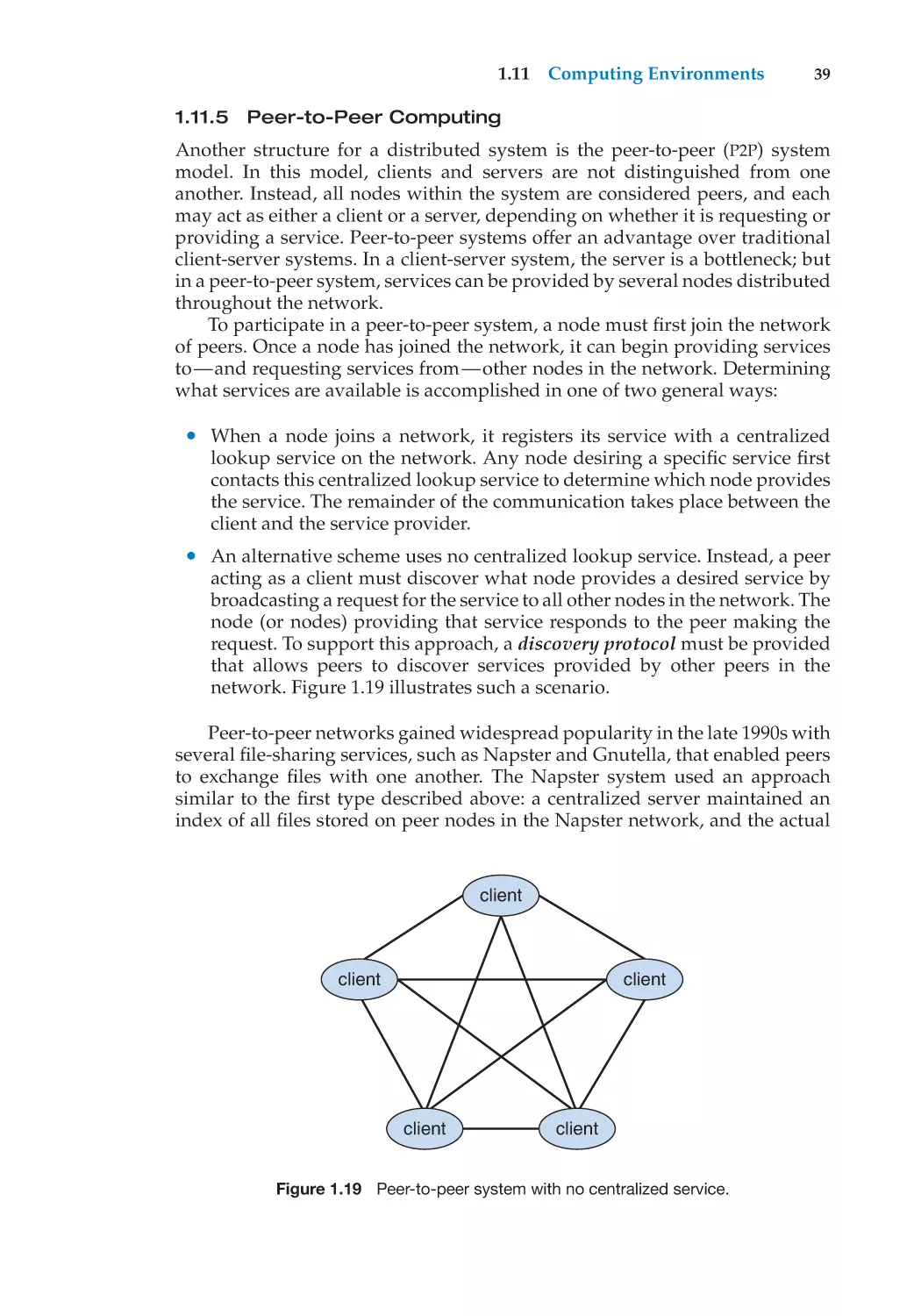


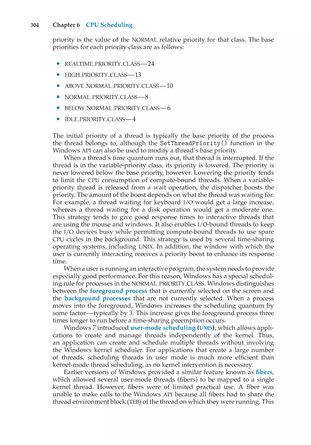


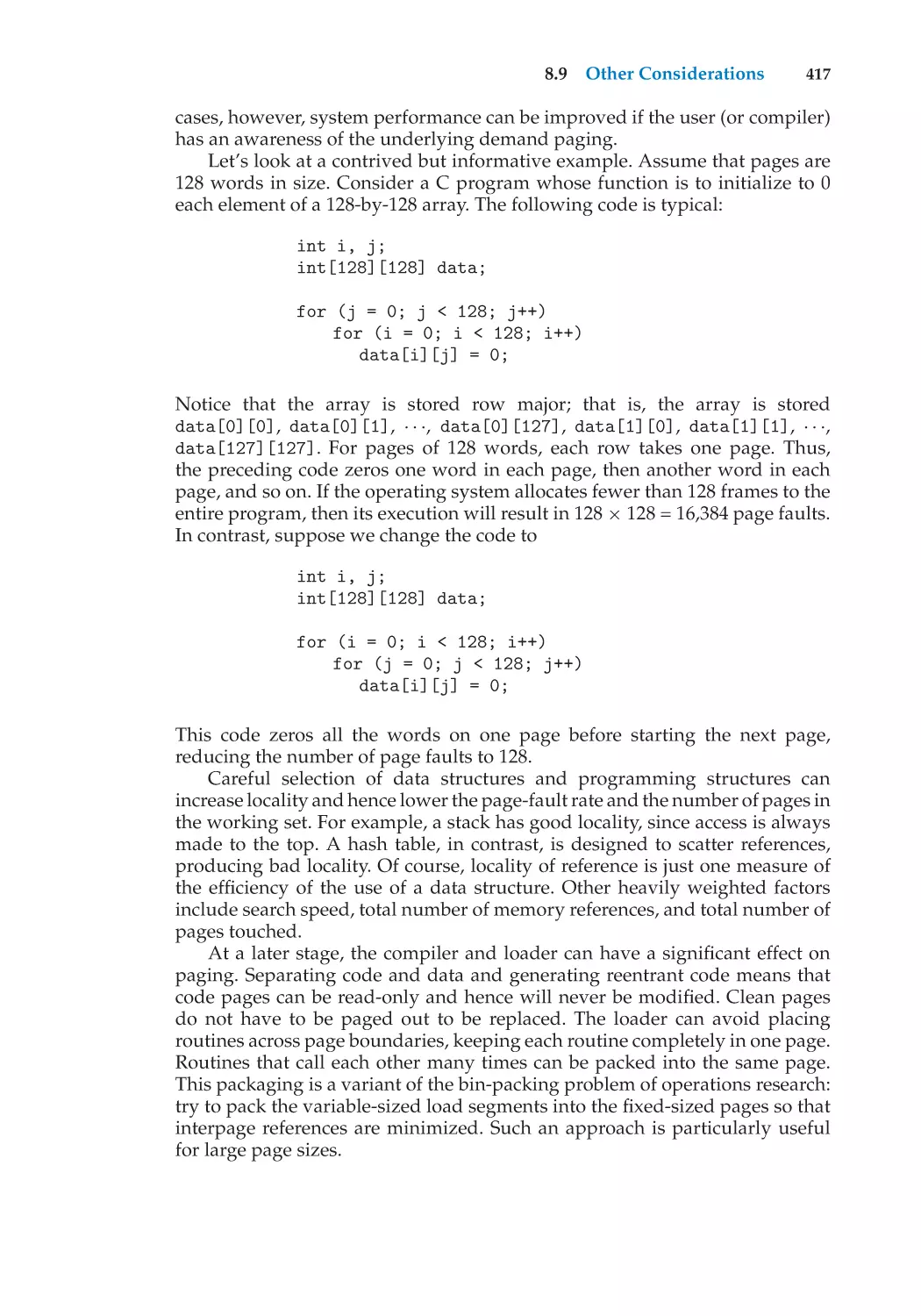


Текст
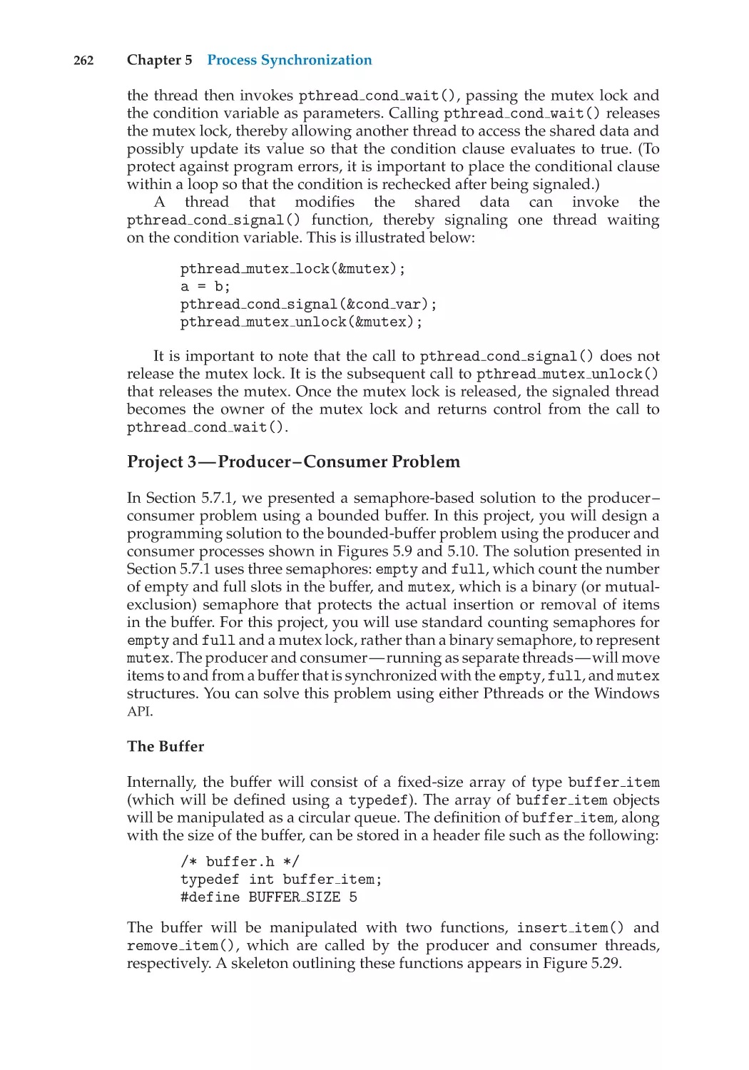
OPERATING
SYSTEM
CONCEPTS
ls
s
s
E
a
i
t
en
Second Edition
Abraham Silberschatz
Peter Baer Galvin
Greg Gagne
Operating
System Concepts
Essential s
Second Edition
This page is intentionally left blank
Operating
System Concepts
Essential s
Second Edition
ABRAHAM SILBERSCHATZ
Yale University
PETER BAER GALVIN
Corporate Technologies, Inc.
GREG GAGNE
Westminster College
Vice President & Executive Publisher
Executive Editor
Executive Marketing Manager
Associate Production Manager
Cover designer
Don Fowley
Beth Lang Golub
Christopher Ruel
Joyce Poh
Madelyn Lesure
This book was set in Palatino by the author using LaTeX and printed and bound by Courier Kendallville.
The cover was printed by Courier Kendallville. This book is printed on acid free paper.
Founded in 1807, John Wiley & Sons, Inc. has been a valued source of knowledge and understanding for more
than 200 years, helping people around the world meet their needs and fulfill their aspirations. Our company is
built on a foundation of principles that include responsibility to the communities we serve and where we live and
work. In 2008, we launched a Corporate Citizenship Initiative, a global effort to address the environmental, social,
economic, and ethical challenges we face in our business. Among the issues we are addressing are carbon impact,
paper specifications and procurement, ethical conduct within our business and among our vendors, and community
and charitable support. For more information, please visit our website: www.wiley.com/go/citizenship.
Copyright © 2014, 2011 John Wiley & Sons, Inc. All rights reserved. No part of this publication may be
reproduced, stored in a retrieval system or transmitted in any form or by any means, electronic, mechanical,
photocopying, recording, scanning or otherwise, except as permitted under Sections 107 or 108 of the 1976
United States Copyright Act, without either the prior written permission of the Publisher, or authorization
through payment of the appropriate per-copy fee to the Copyright Clearance Center, Inc. 222 Rosewood Drive,
Danvers, MA 01923, website www.copyright.com. Requests to the Publisher for permission should be addressed
to the Permissions Department, John Wiley & Sons, Inc., 111 River Street, Hoboken, NJ 07030-5774, (201)748-6011,
fax (201)748-6008, website http://www.wiley.com/go/permissions.
Evaluation copies are provided to qualified academics and professionals for review purposes only, for use in their
courses during the next academic year. These copies are licensed and may not be sold or transferred to a third
party. Upon completion of the review period, please return the evaluation copy to Wiley. Return instructions
and a free of charge return mailing label are available at www.wiley.com/go/returnlabel. If you have chosen to
adopt this textbook for use in your course, please accept this book as your complimentary desk copy. Outside of
the United States, please contact your local sales representative.
Printed in the United States of America
10 9 8 7 6 5 4 3 2 1
To my children, Lemor, Sivan, and Aaron
and my Nicolette
Avi Silberschatz
To my wife, Carla,
and my children, Gwen, Owen, and Maddie
Peter Baer Galvin
To my wife, Pat,
and our sons, Tom and Jay
Greg Gagne
This page is intentionally left blank
Preface
Operating systems are an essential part of any computer system. Similarly,
a course on operating systems is an essential part of any computer science
education. This field is undergoing rapid change, as computers are now
prevalent in virtually every arena of day-to-day life —from embedded devices
in automobiles through the most sophisticated planning tools for governments
and multinational firms. Yet the fundamental concepts remain fairly clear, and
it is on these that we base this book.
We wrote this book as a text for an introductory course in operating systems
at the junior or senior undergraduate level or at the first-year graduate level. We
hope that practitioners will also find it useful. It provides a clear description of
the concepts that underlie operating systems. As prerequisites, we assume that
the reader is familiar with basic data structures, computer organization, and
a high-level language, such as C or Java. The hardware topics required for an
understanding of operating systems are covered in Chapter 1. In that chapter,
we also include an overview of the fundamental data structures that are
prevalent in most operating systems. For code examples, we use predominantly
C, with some Java, but the reader can still understand the algorithms without
a thorough knowledge of these languages.
Concepts are presented using intuitive descriptions. Important theoretical
results are covered, but formal proofs are largely omitted. The bibliographical
notes at the end of each chapter contain pointers to research papers in which
results were first presented and proved, as well as references to recent material
for further reading. In place of proofs, figures and examples are used to suggest
why we should expect the result in question to be true.
The fundamental concepts and algorithms covered in the book are often
based on those used in both commercial and open-source operating systems.
Our aim is to present these concepts and algorithms in a general setting that
is not tied to one particular operating system. However, we present a large
number of examples that pertain to the most popular and the most innovative
operating systems, including Linux, Microsoft Windows, Apple Mac OS X, and
Solaris. We also include examples of both Android and iOS, currently the two
dominant mobile operating systems.
The organization of the text reflects our many years of teaching courses on
operating systems, as well as curriculum guidelines published by the IEEE
vii
viii
Preface
Computing Society and the Association for Computing Machinery (ACM).
Consideration was also given to the feedback provided by the reviewers of
the text, along with the many comments and suggestions we received from
readers of our previous editions and from our current and former students.
Content of This Book
The text is organized in six major parts:
• Overview. Chapters 1 and 2 explain what operating systems are, what
they do, and how they are designed and constructed. These chapters
discuss what the common features of an operating system are and what an
operating system does for the user. We include coverage of both traditional
PC and server operating systems, as well as operating systems for mobile
devices. The presentation is motivational and explanatory in nature. We
have avoided a discussion of how things are done internally in these
chapters. Therefore, they are suitable for individual readers or for students
in lower-level classes who want to learn what an operating system is
without getting into the details of the internal algorithms.
• Process management. Chapters 3 through 6 describe the process concept
and concurrency as the heart of modern operating systems. A process
is the unit of work in a system. Such a system consists of a collection
of concurrently executing processes, some of which are operating-system
processes (those that execute system code) and the rest of which are user
processes (those that execute user code). These chapters cover methods for
process scheduling, interprocess communication, process synchronization,
and deadlock handling. Also included is a discussion of threads, as well
as an examination of issues related to multicore systems and parallel
programming.
• Memory management. Chapters 7 and 8 deal with the management of
main memory during the execution of a process. To improve both the
utilization of the CPU and the speed of its response to its users, the
computer must keep several processes in memory. There are many different
memory-management schemes, reflecting various approaches to memory
management, and the effectiveness of a particular algorithm depends on
the situation.
• Storage management. Chapters 9 through 12 describe how mass storage,
the file system, and I/O are handled in a modern computer system. The
file system provides the mechanism for on-line storage of and access
to both data and programs. We describe the classic internal algorithms
and structures of storage management and provide a firm practical
understanding of the algorithms used —their properties, advantages, and
disadvantages. Since the I/O devices that attach to a computer vary widely,
the operating system needs to provide a wide range of functionality to
applications to allow them to control all aspects of these devices. We
discuss system I/O in depth, including I/O system design, interfaces, and
Preface
ix
internal system structures and functions. In many ways, I/O devices are
the slowest major components of the computer. Because they represent a
performance bottleneck, we also examine performance issues associated
with I/O devices.
• Protection and security. Chapters 13 and 14 discuss the mechanisms
necessary for the protection and security of computer systems. The
processes in an operating system must be protected from one another’s
activities, and to provide such protection, we must ensure that only
processes that have gained proper authorization from the operating system
can operate on the files, memory, CPU, and other resources of the system.
Protection is a mechanism for controlling the access of programs, processes,
or users to computer-system resources. This mechanism must provide a
means of specifying the controls to be imposed, as well as a means of
enforcement. Security protects the integrity of the information stored in
the system (both data and code), as well as the physical resources of the
system, from unauthorized access, malicious destruction or alteration, and
accidental introduction of inconsistency.
• Case studies. Chapter 15 in the text, along with Appendices A and B
(which are available on http://www.os-book.com), present detailed case
studies of real operating systems, including Linux, FreeBSD, and Mach.
Coverage of Linux is presented throughout this text; however, the case
studies provide much more detail.
Operating System Essentials
We have based Operating System Essentials on the Ninth Edition of Operating
System Concepts, published in 2012. Our intention behind developing this
Essentials edition is to provide readers with a textbook that focuses on the
core concepts that underlie contemporary operating systems. By focusing on
core concepts, we believe students are able to grasp the essential features of a
modern operating system more easily and more quickly.
To achieve this, Operating System Essentials omits the following coverage
from the Ninth Edition of Operating System Concepts:
1. We removed Chapter 7—Deadlocks—and instead offer a detailed
overview of deadlocks in Chapter 6.
2. We removed Chapter 16—Virtual Machines.
3. We removed Chapter 17—Distributed Systems.
4. We removed Chapter 19—Windows 7.
5. We removed Chapter 20—Influential Operating Systems.
For those that wish to pursue a more comprehensive study of operating
systems, we refer you to the Ninth Edition of Operating System Concepts, and
in the following we describe the changes relevant to that edition.
x
Preface
The Second Edition
As we wrote this Second Edition of Operating System Concepts Essentials, we
were guided by the recent growth in the following fundamental areas that
affect operating systems:
1. Multicore systems
2. Mobile computing
We have integrated relevant coverage throughout this new edition To emphasize these topics. Additionally, we have rewritten material in almost every
chapter by bringing older material up to date and removing material that is no
longer interesting or relevant.
We have also made substantial organizational changes. For example, we
have eliminated the chapter on real-time systems and instead have integrated
appropriate coverage of these systems throughout the text. We have reordered
the chapters on storage management and have moved up the presentation
of process synchronization so that it appears before process scheduling. Most
of these organizational changes are based on our experiences while teaching
courses on operating systems.
Below, we provide a brief outline of the major changes to the various
chapters:
• Chapter 1, Introduction, includes updated coverage of multiprocessor
and multicore systems, as well as a new section on kernel data structures.
Additionally, the coverage of computing environments now includes
mobile systems and cloud computing. We also have incorporated an
overview of real-time systems.
• Chapter 2, Operating-System Structures, provides new coverage of user
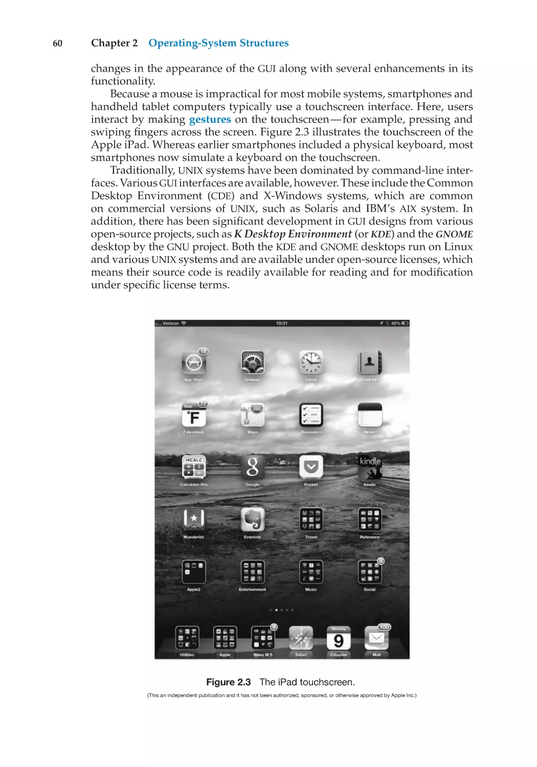
interfaces for mobile devices, including discussions of iOS and Android,
and expanded coverage of Mac OS X as a type of hybrid system.
• Chapter 3, Processes, now includes coverage of multitasking in mobile
operating systems, support for the multiprocess model in Google’s Chrome
web browser, and zombie and orphan processes in UNIX.
• Chapter 4, Threads, supplies expanded coverage of parallelism and
Amdahl’s law. It also provides a new section on implicit threading,
including OpenMP and Apple’s Grand Central Dispatch.
• Chapter 5, Process Synchronization (previously Chapter 6), adds a new
section on mutex locks as well as coverage of synchronization using
OpenMP, as well as functional languages.
• Chapter 6, CPU Scheduling (previously Chapter 5), contains new coverage
of the Linux CFS scheduler and Windows user-mode scheduling. Coverage
of real-time scheduling algorithms has also been integrated into this
chapter.
• Chapter 7, Main Memory, includes new coverage of swapping on mobile
systems and Intel 32- and 64-bit architectures. A new section discusses
ARM architecture.
Preface
xi
• Chapter 8, Virtual Memory, updates kernel memory management to
include the Linux SLUB and SLOB memory allocators.
• Chapter 9, Mass-Storage Structure (previously Chapter 11), adds coverage
of solid-state disks.
• Chapter 10, File-System Interface (previously Chapter 9), is updated with
information about current technologies.
• Chapter 11, File-System Implementation (previously Chapter 10), is
updated with coverage of current technologies.
• Chapter 12, I/O, updates technologies and performance numbers, expands
coverage of synchronous/asynchronous and blocking/nonblocking I/O,
and adds a section on vectored I/O.
• Chapter 13, Protection, has no major changes.
• Chapter 14, Security, has a revised cryptography section with modern
notation and an improved explanation of various encryption methods and
their uses. The chapter also includes new coverage of Windows 7 security.
• Chapter 15, The Linux System, has been updated to cover the Linux 3.2
kernel.
Programming Environments
This book uses examples of many real-world operating systems to illustrate
fundamental operating-system concepts. Particular attention is paid to Linux
and Microsoft Windows, but we also refer to various versions of UNIX
(including Solaris, BSD, and Mac OS X).
The text also provides several example programs written in C and
Java. These programs are intended to run in the following programming
environments:
•
POSIX. POSIX (which stands for Portable Operating System Interface) represents a set of standards implemented primarily for UNIX-based operating
systems. Although Windows systems can also run certain POSIX programs,
our coverage of POSIX focuses on UNIX and Linux systems. POSIX-compliant
systems must implement the POSIX core standard (POSIX.1); Linux, Solaris,
and Mac OS X are examples of POSIX-compliant systems. POSIX also
defines several extensions to the standards, including real-time extensions
(POSIX1.b) and an extension for a threads library (POSIX1.c, better known
as Pthreads). We provide several programming examples written in C
illustrating the POSIX base API, as well as Pthreads and the extensions for
real-time programming. These example programs were tested on Linux 2.6
and 3.2 systems, Mac OS X 10.7, and Solaris 10 using the gcc 4.0 compiler.
• Java. Java is a widely used programming language with a rich
API and
built-in language support for thread creation and management. Java
programs run on any operating system supporting a Java virtual machine
(or JVM). We illustrate various operating-system and networking concepts
with Java programs tested using the Java 1.6 JVM.
xii
Preface
• Windows systems. The primary programming environment for Windows
systems is the Windows API, which provides a comprehensive set of functions for managing processes, threads, memory, and peripheral devices.
We supply several C programs illustrating the use of this API. Programs
were tested on systems running Windows XP and Windows 7.
We have chosen these three programming environments because we
believe that they best represent the two most popular operating-system models
—Windows and UNIX/Linux—along with the widely used Java environment.
Most programming examples are written in C, and we expect readers to be
comfortable with this language. Readers familiar with both the C and Java
languages should easily understand most programs provided in this text.
In some instances—such as thread creation—we illustrate a specific
concept using all three programming environments, allowing the reader
to contrast the three different libraries as they address the same task. In
other situations, we may use just one of the APIs to demonstrate a concept.
For example, we illustrate shared memory using just the POSIX API; socket
programming in TCP/IP is highlighted using the Java API.
Linux Virtual Machine
To help students gain a better understanding of the Linux system, we provide
a Linux virtual machine, including the Linux source code, that is available for
download from the website supporting this text (http://www.os-book.com).
This virtual machine also includes a gcc development environment with
compilers and editors. Most of the programming assignments in the book
can be completed on this virtual machine, with the exception of assignments
that require Java or the Windows API.
We also provide three programming assignments that modify the Linux
kernel through kernel modules:
1. Adding a basic kernel module to the Linux kernel.
2. Adding a kernel module that uses various kernel data structures.
3. Adding a kernel module that iterates over tasks in a running Linux
system.
Over time it is our intention to add additional kernel module assignments on
the supporting website.
Supporting Website
When you visit the website supporting this text at http://www.os-book.com,
you can download the following resources:
• Linux virtual machine
• C and Java source code
Preface
•
•
•
•
•
•
•
•
xiii
Sample syllabi
Set of Powerpoint slides
Set of figures and illustrations
FreeBSD and Mach case studies
Set of review questions indexed by section
Solutions to practice exercises
Study guide for students
Errata
Notes to Instructors
On the website for this text, we provide several sample syllabi that suggest
various approaches for using the text in both introductory and advanced
courses. As a general rule, we encourage instructors to progress sequentially
through the chapters, as this strategy provides the most thorough study of
operating systems. However, by using the sample syllabi, an instructor can
select a different ordering of chapters (or subsections of chapters).
In this edition, we have added over sixty new written exercises and over
twenty new programming problems and projects. Most of the new programming assignments involve processes, threads, process synchronization, and
memory management. Some involve adding kernel modules to the Linux
system which requires using either the Linux virtual machine that accompanies
this text or another suitable Linux distribution.
Solutions to review questions, written exercises and programming assignments are available to instructors who have adopted this text for their
operating-system class. To obtain these restricted supplements, contact your
local John Wiley & Sons sales representative. You can find your Wiley representative by going to http://www.wiley.com/college and clicking “Who’s my
rep?”
Notes to Students
We encourage you to take advantage of the review questions (available
online) and practice exercises that appear at the end of each chapter. The
review questions as well as solutions to the practice exercises are available
for download from the supporting website http://www.os-book.com. We also
encourage you to read through the study guide, which was prepared by one of
our students. Finally, for students who are unfamiliar with UNIX and Linux
systems, we recommend that you download and install the Linux virtual
machine that we include on the supporting website. Not only will this provide
you with a new computing experience, but the open-source nature of Linux
will allow you to easily examine the inner details of this popular operating
system.
We wish you the very best of luck in your study of operating systems.
xiv
Preface
Contacting Us
We have endeavored to eliminate typos, bugs, and the like from the text. But,
as in new releases of software, bugs almost surely remain. An up-to-date errata
list is accessible from the book’s website. We would be grateful if you would
notify us of any errors or omissions in the book that are not on the current list
of errata.
We would be glad to receive suggestions on improvements to the book.
We also welcome any contributions to the book website that could be of
use to other readers, such as programming exercises, project suggestions,
on-line labs and tutorials, and teaching tips. E-mail should be addressed to
os-book-authors@cs.yale.edu.
Acknowledgments
This book is derived from the previous editions, the first three of which
were coauthored by James Peterson. Others who helped us with previous
editions include Hamid Arabnia, Rida Bazzi, Randy Bentson, David Black,
Joseph Boykin, Jeff Brumfield, Gael Buckley, Roy Campbell, P. C. Capon, John
Carpenter, Gil Carrick, Thomas Casavant, Bart Childs, Ajoy Kumar Datta,
Joe Deck, Sudarshan K. Dhall, Thomas Doeppner, Caleb Drake, M. Racsit
Eskicioğlu, Hans Flack, Robert Fowler, G. Scott Graham, Richard Guy, Max
Hailperin, Rebecca Hartman, Wayne Hathaway, Christopher Haynes, Don
Heller, Bruce Hillyer, Mark Holliday, Dean Hougen, Michael Huang, Ahmed
Kamel, Morty Kewstel, Richard Kieburtz, Carol Kroll, Morty Kwestel, Thomas
LeBlanc, John Leggett, Jerrold Leichter, Ted Leung, Gary Lippman, Carolyn
Miller, Michael Molloy, Euripides Montagne, Yoichi Muraoka, Jim M. Ng,
Banu Özden, Ed Posnak, Boris Putanec, Charles Qualline, John Quarterman,
Mike Reiter, Gustavo Rodriguez-Rivera, Carolyn J. C. Schauble, Thomas P.
Skinner, Yannis Smaragdakis, Jesse St. Laurent, John Stankovic, Adam Stauffer,
Steven Stepanek, John Sterling, Hal Stern, Louis Stevens, Pete Thomas, David
Umbaugh, Steve Vinoski, Tommy Wagner, Larry L. Wear, John Werth, James
M. Westall, J. S. Weston, and Yang Xiang
Robert Love updated both Chapter 15 and the Linux coverage throughout
the text, as well as answering many of our Android-related questions. Jonathan
Katz contributed to Chapter 14. Salahuddin Khan updated Section 14.9 to
provide new coverage of Windows 7 security.
Chapter 15 was derived from an unpublished manuscript by Stephen
Tweedie. Cliff Martin helped with updating the UNIX appendix to cover
FreeBSD. Some of the exercises and accompanying solutions were supplied by
Arvind Krishnamurthy. Andrew DeNicola prepared the student study guide
that is available on our website. Some of the slides were prepeared by Marilyn
Turnamian.
Mike Shapiro, Bryan Cantrill, and Jim Mauro answered several Solarisrelated questions, and Bryan Cantrill from Sun Microsystems helped with the
ZFS coverage. Josh Dees and Rob Reynolds contributed coverage of Microsoft’s
NET. The project for POSIX message queues was contributed by John Trono of
Saint Michael’s College in Colchester, Vermont.
Preface
xv
Judi Paige helped with generating figures and presentation of slides.
Thomas Gagne prepared new artwork for this edition. Mark Wogahn has made
sure that the software to produce this book (LATEX and fonts) works properly.
Ranjan Kumar Meher rewrote some of the LATEX software used in the production
of this new text.
Our Executive Editor, Beth Lang Golub, provided expert guidance as we
prepared this edition. She was assisted by Katherine Willis, who managed
many details of the project smoothly. The Senior Production Editor, Joyce Poh,
was instrumental in handling all the production details.
The cover illustrator was Susan Cyr, and the cover designer was Madelyn
Lesure. Beverly Peavler copy-edited the manuscript. The freelance proofreader
was Katrina Avery; the freelance indexer was WordCo, Inc.
Abraham Silberschatz, New Haven, CT, 2013
Peter Baer Galvin, Boston, MA, 2013
Greg Gagne, Salt Lake City, UT, 2013
This page is intentionally left blank
Contents
PART ONE
Chapter 1
1.1
1.2
1.3
1.4
1.5
1.6
1.7
1.8
OVERVIEW
Introduction
What Operating Systems Do 4
Computer-System Organization 7
Computer-System Architecture 12
Operating-System Structure 19
Operating-System Operations 21
Process Management 24
Memory Management 25
Storage Management 26
Chapter 2
PART TWO
3.1
3.2
3.3
3.4
3.5
Protection and Security 30
Kernel Data Structures 31
Computing Environments 35
Open-Source Operating Systems
Summary 47
Exercises 49
Bibliographical Notes 52
43
Operating-System Structures
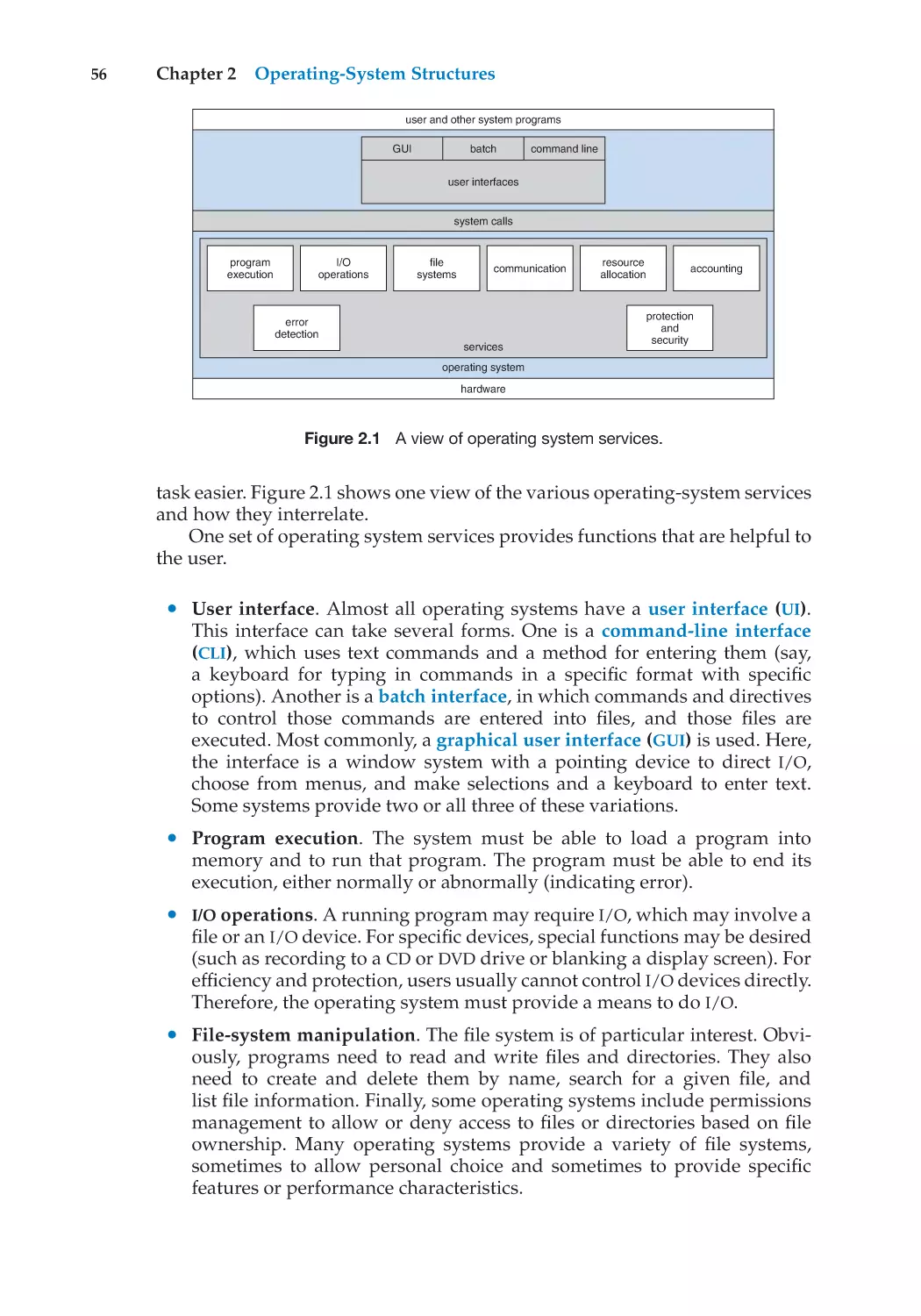
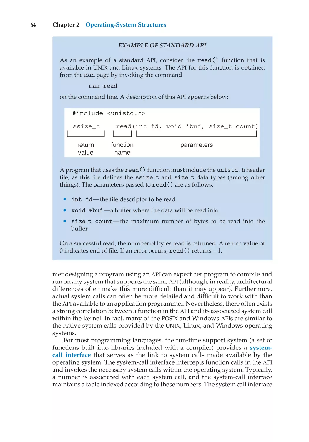
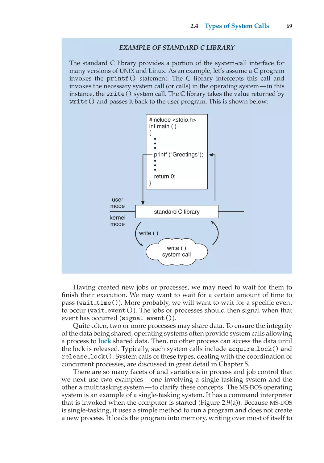
2.1 Operating-System Services 55
2.2 User and Operating-System
Interface 58
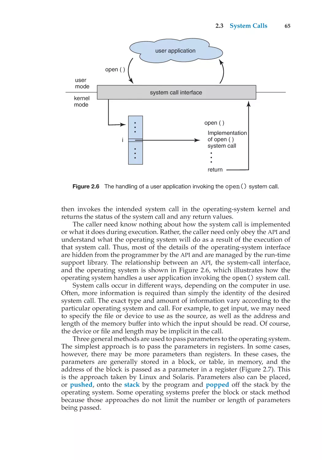
2.3 System Calls 62
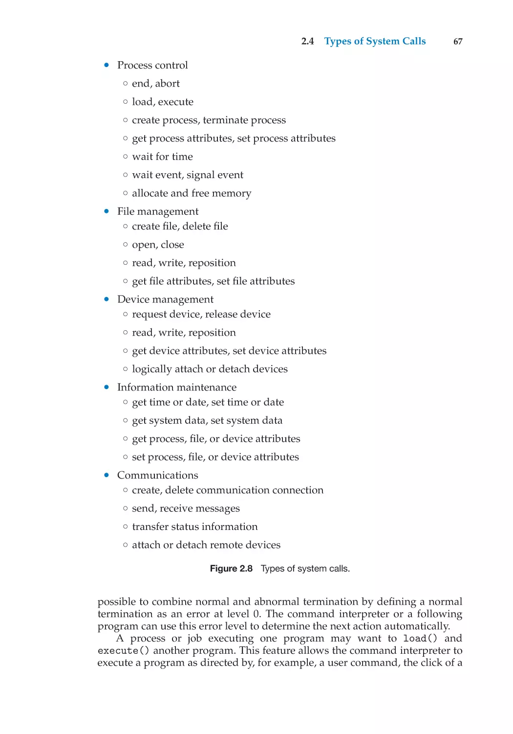
2.4 Types of System Calls 66
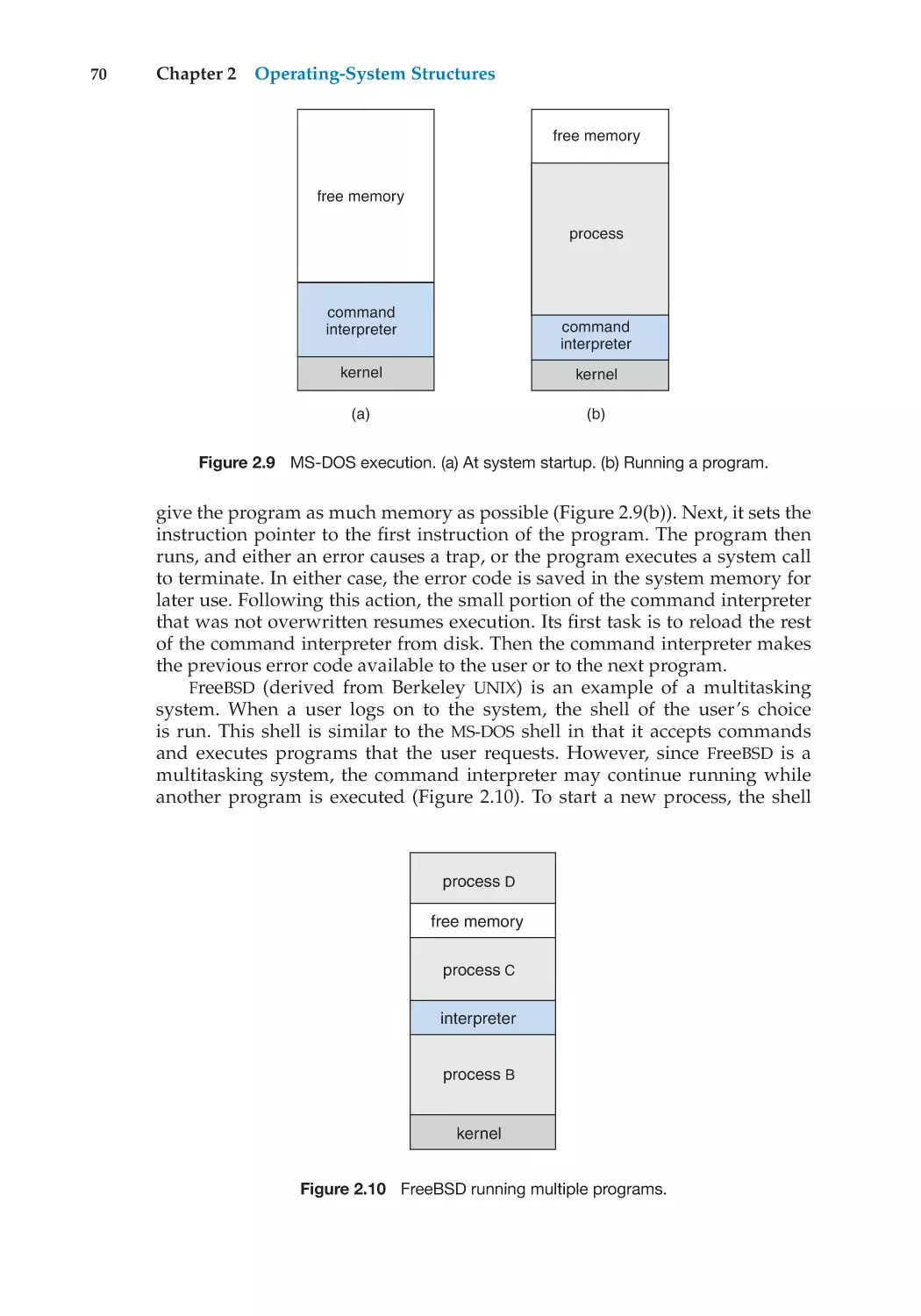
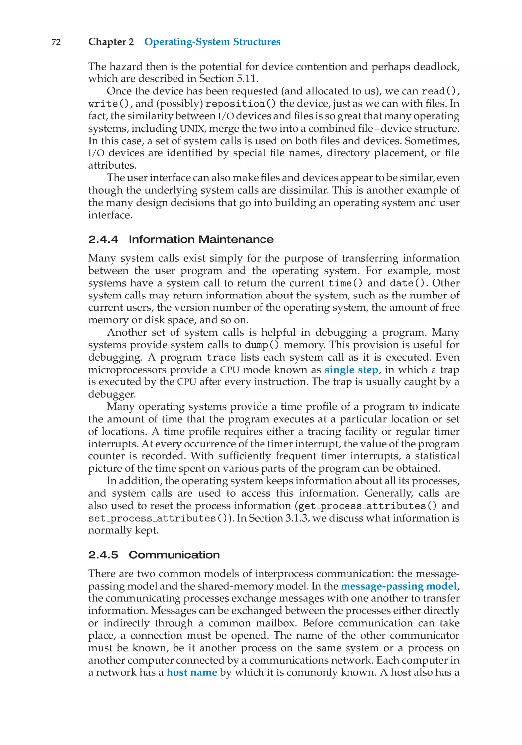
2.5 System Programs 74
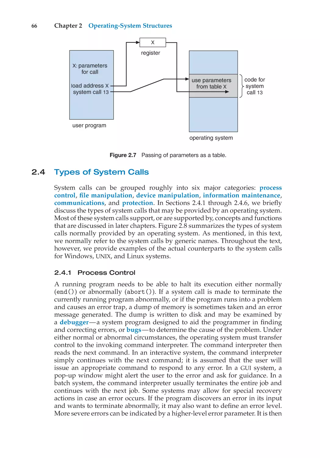
2.6 Operating-System Design and
Implementation 75
Chapter 3
1.9
1.10
1.11
1.12
1.13
2.7
2.8
2.9
2.10
2.11
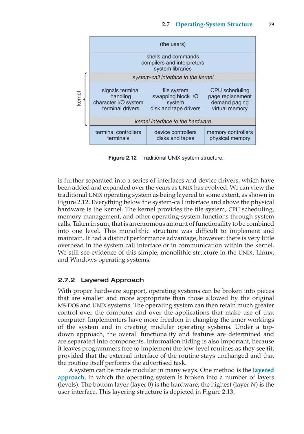
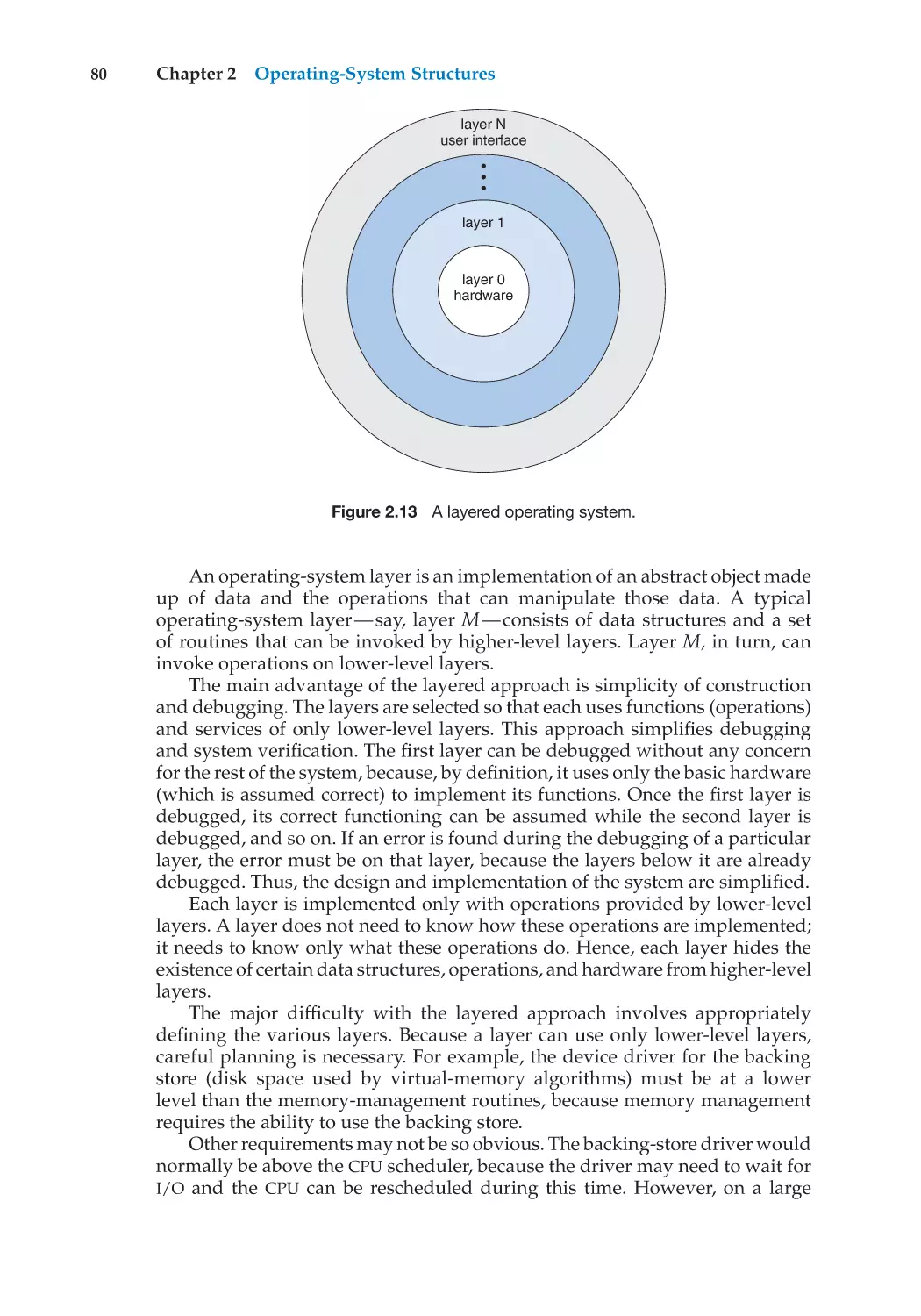
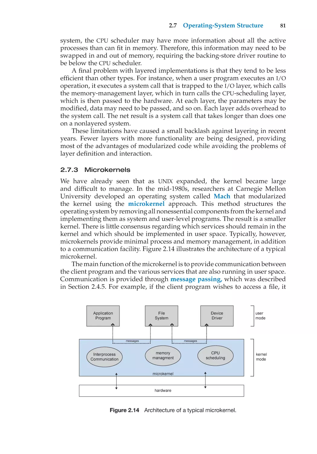
Operating-System Structure 78
Operating-System Debugging 86
Operating-System Generation 91
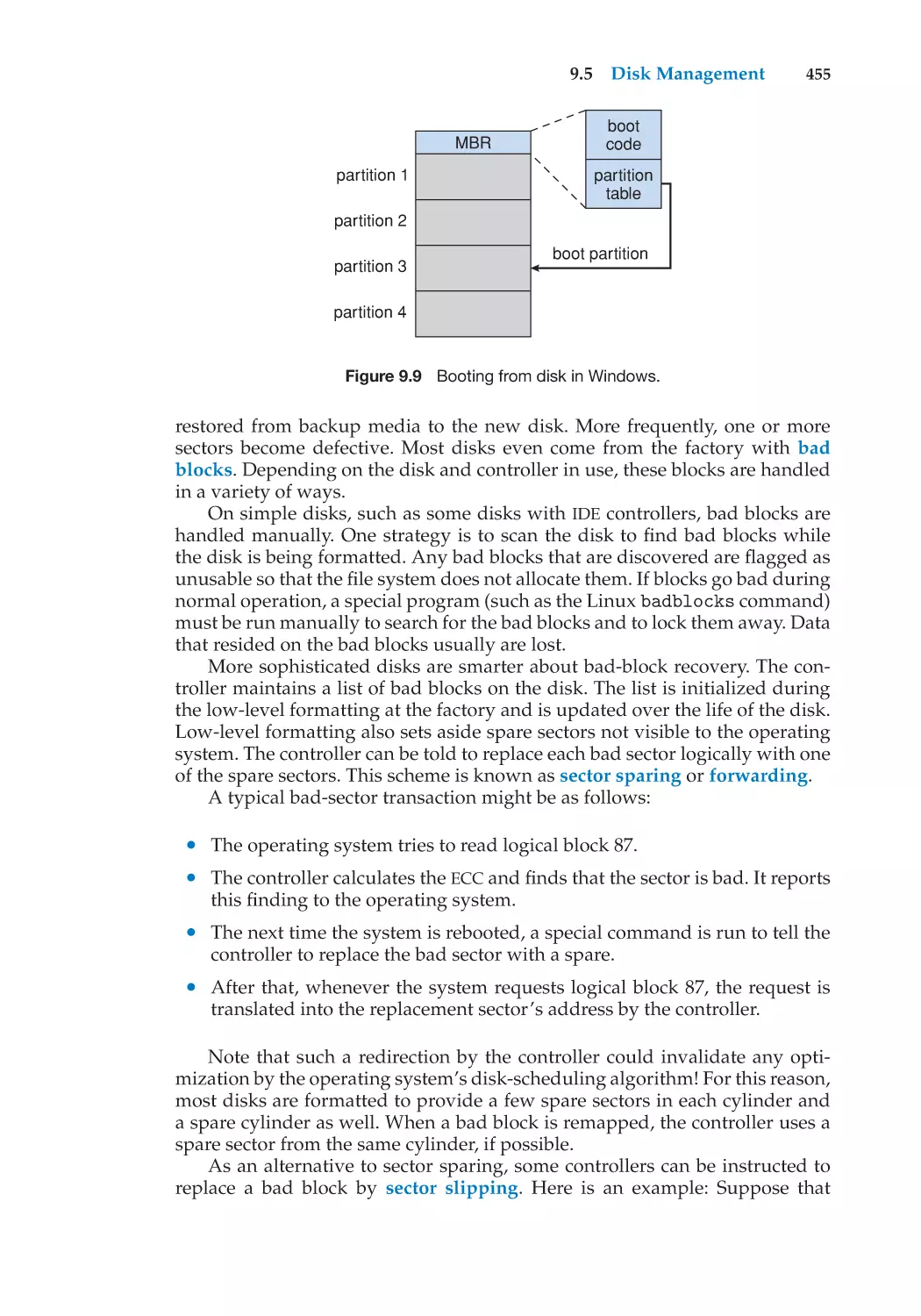
System Boot 92
Summary 93
Exercises 94
Bibliographical Notes 101
PROCESS MANAGEMENT
Processes
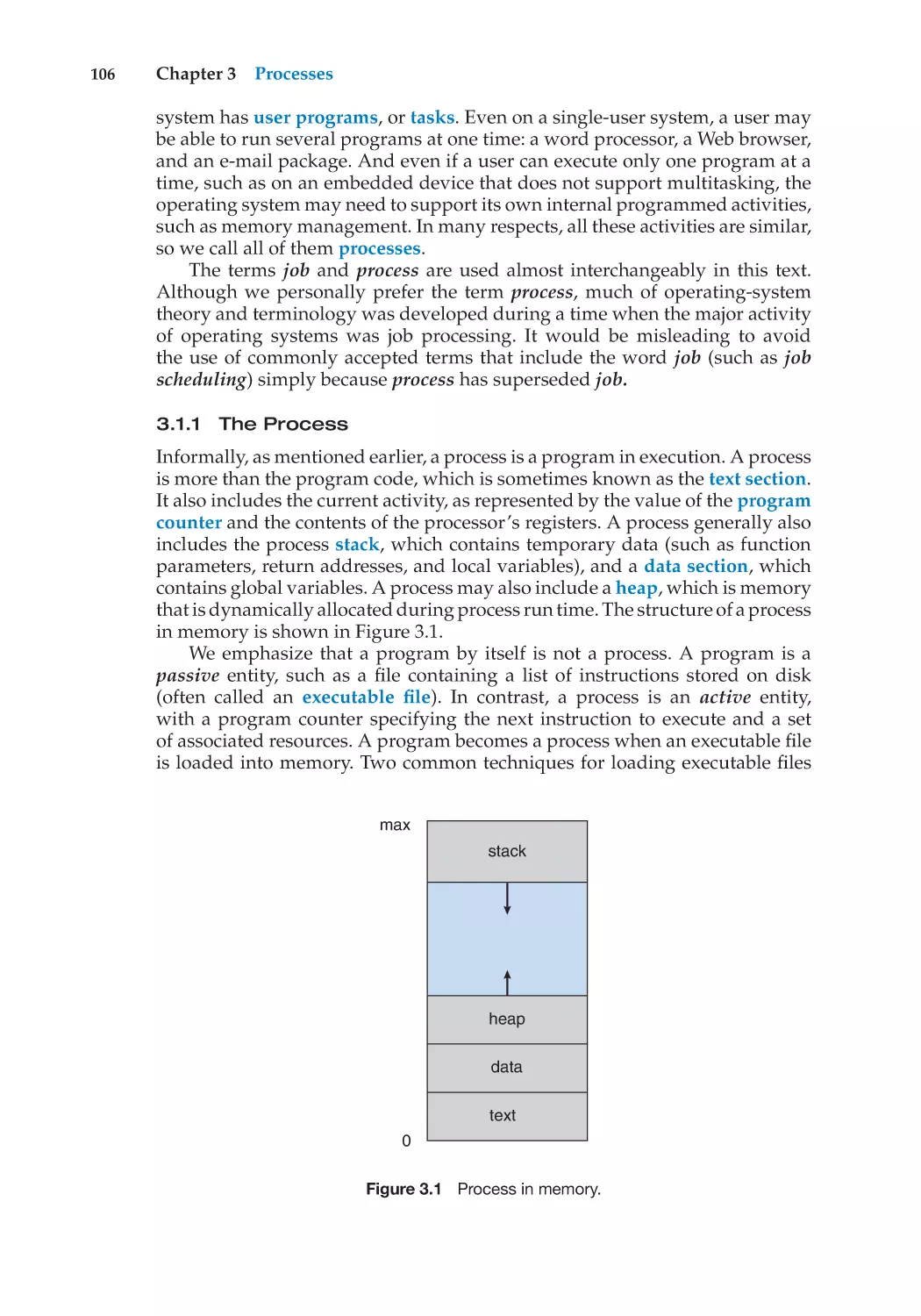
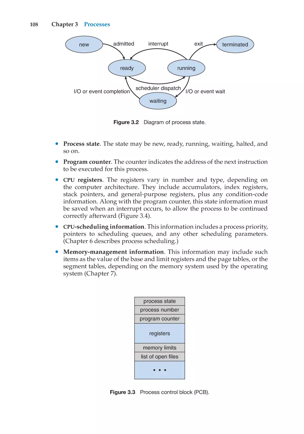
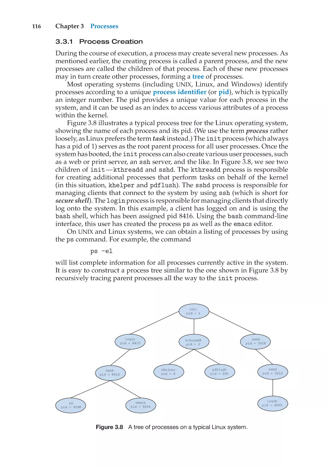
Process Concept 105
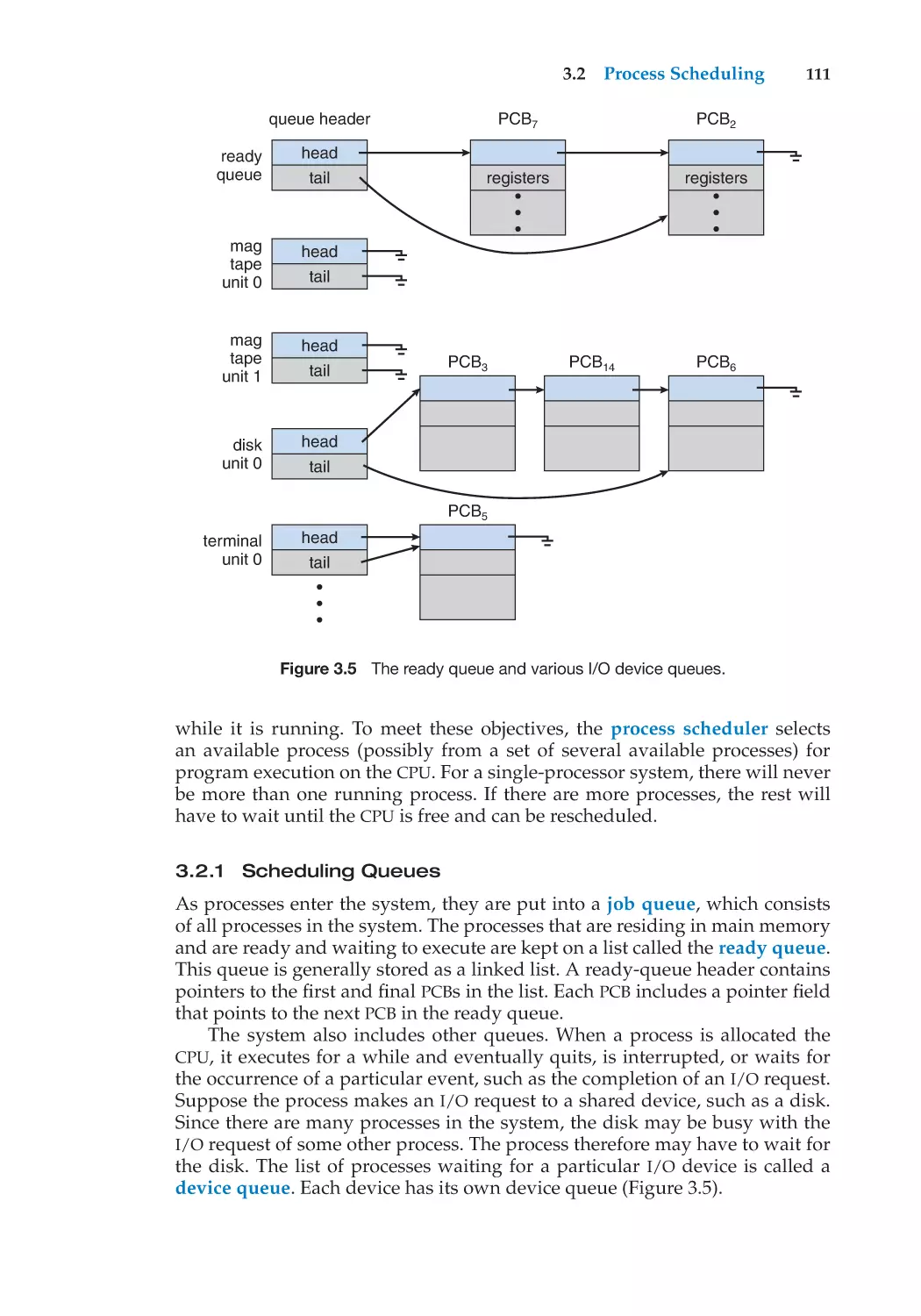
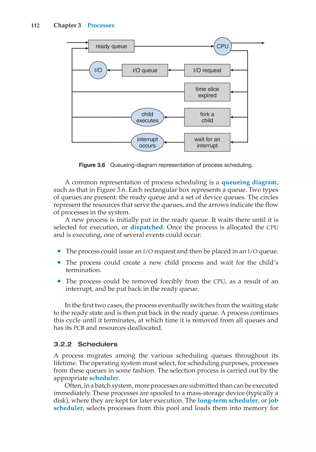
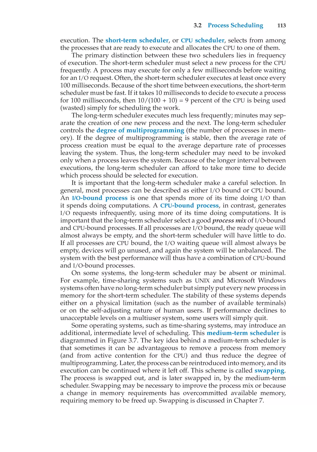
Process Scheduling 110
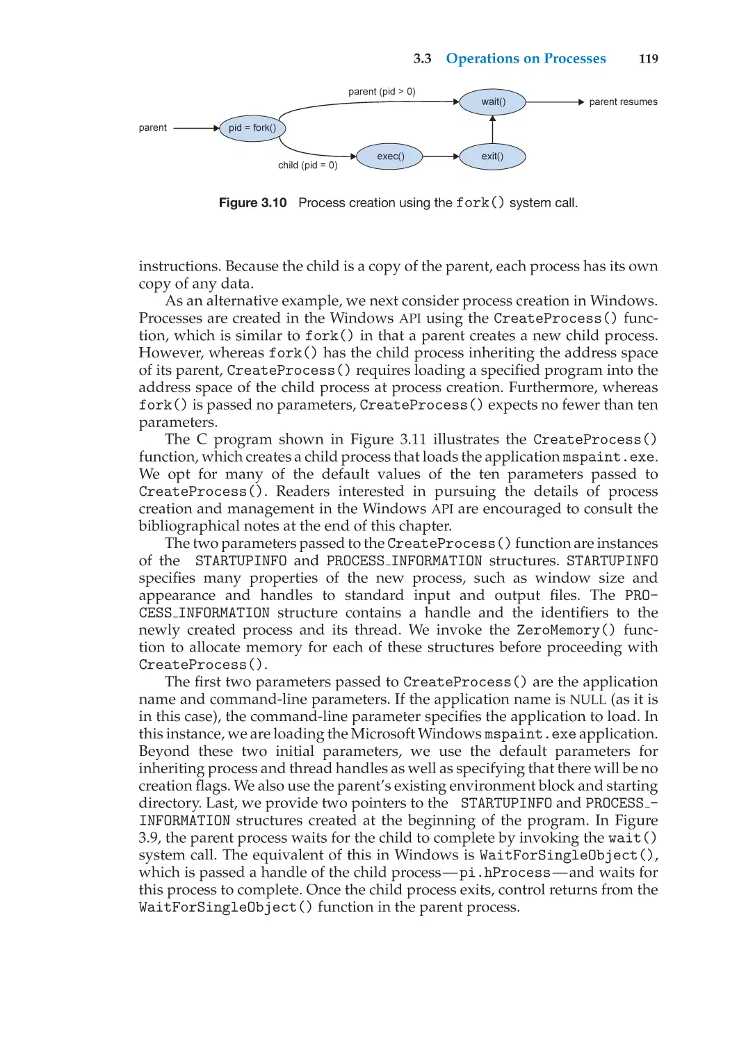
Operations on Processes 115
Interprocess Communication 122
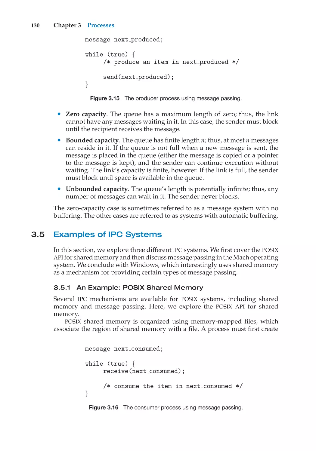
Examples of IPC Systems 130
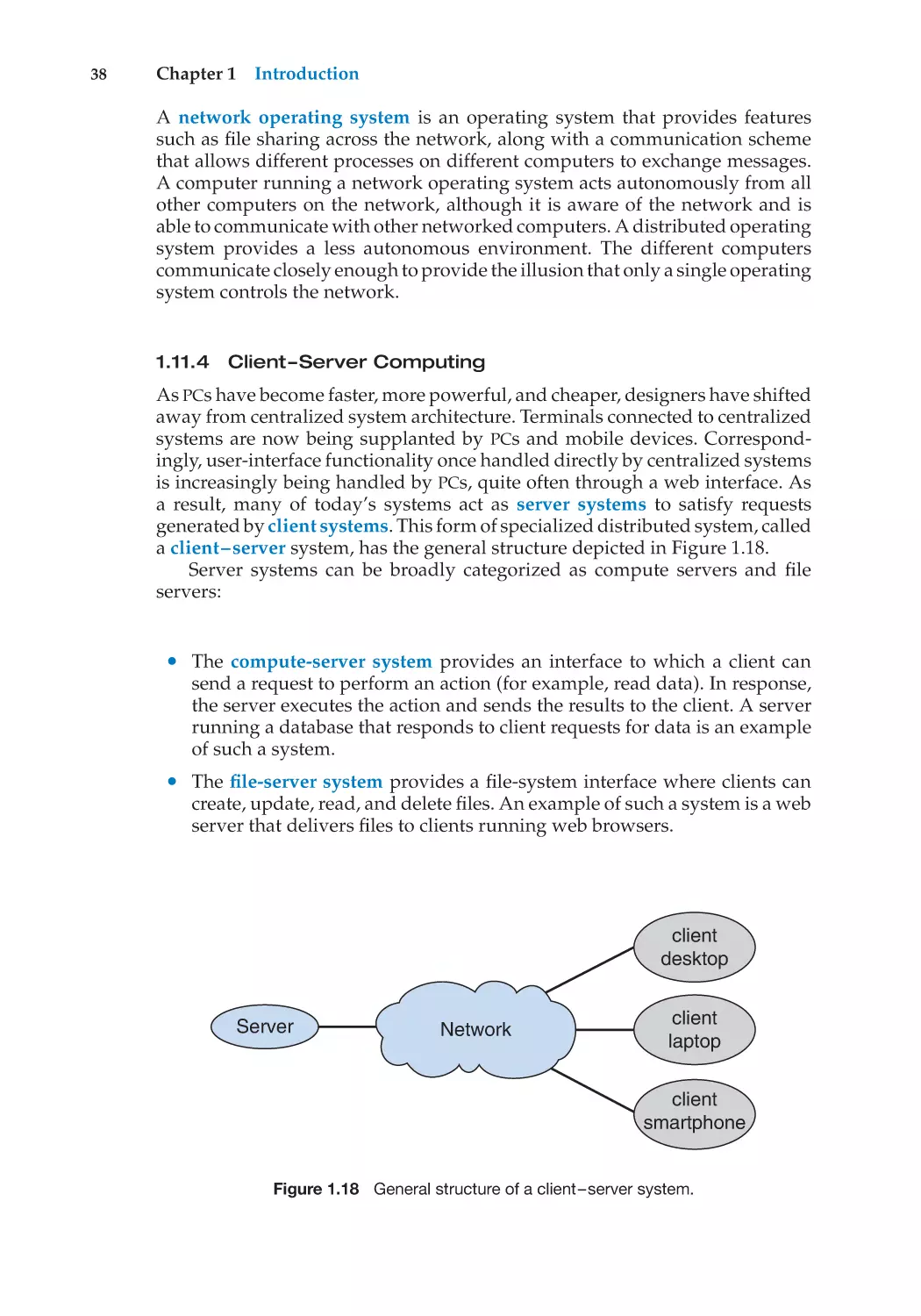
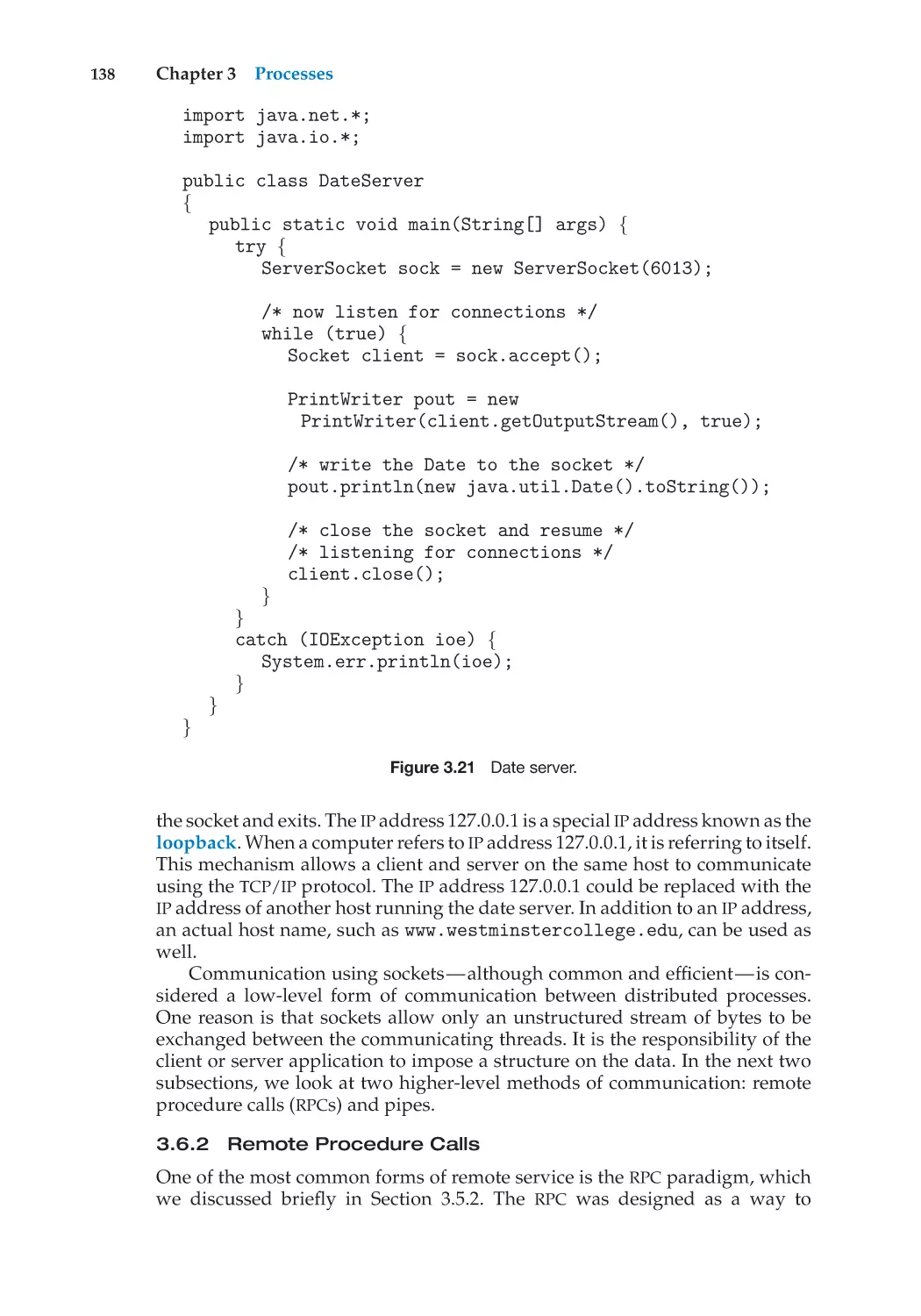
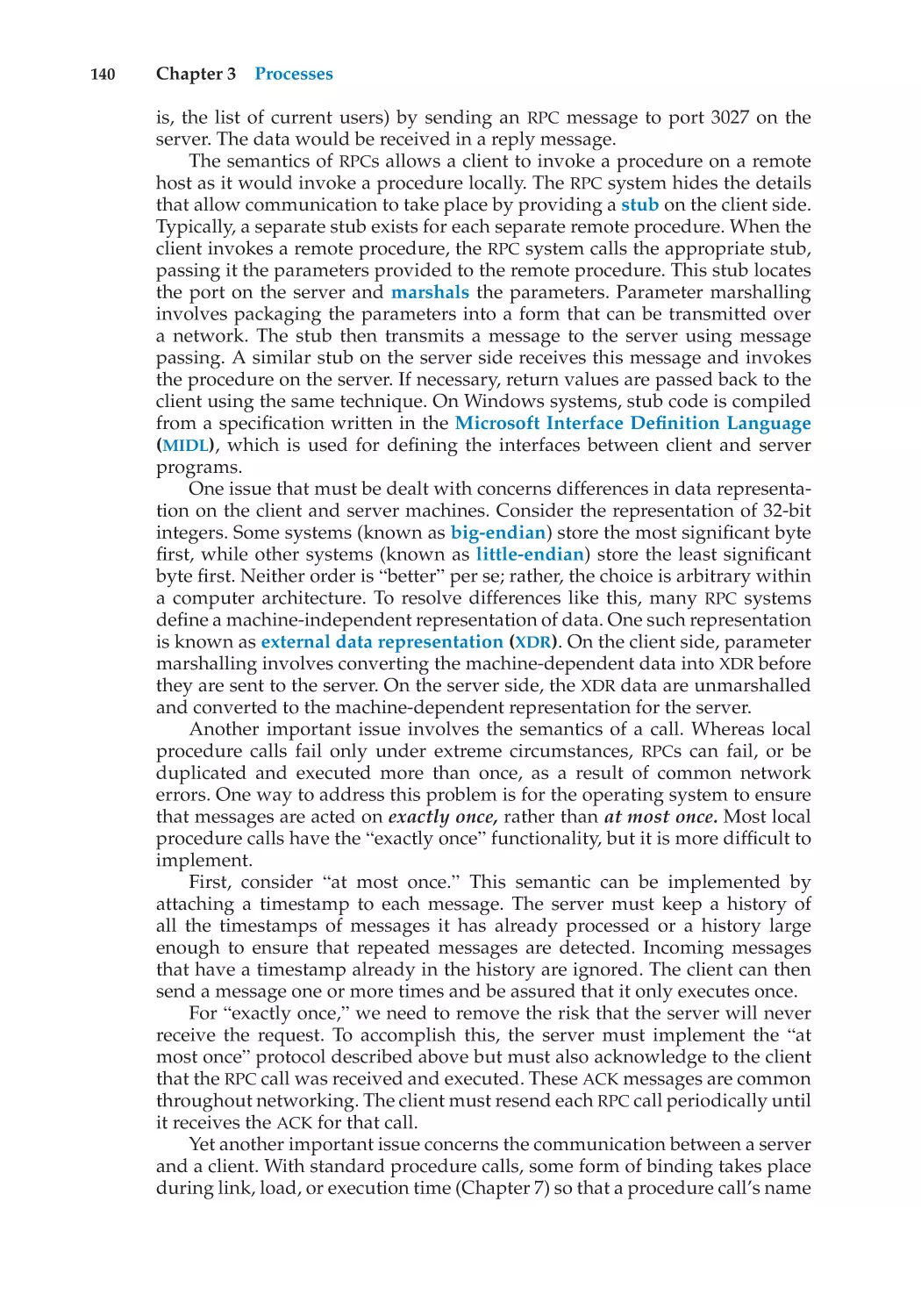
3.6 Communication in Client –
Server Systems 136
3.7 Summary 147
Exercises 149
Bibliographical Notes 162
xvii
xviii
Contents
Chapter 4
4.1
4.2
4.3
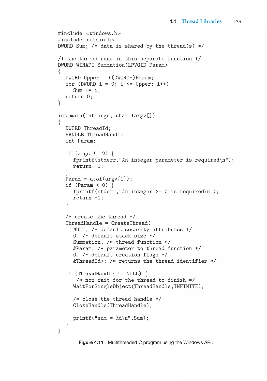
4.4
4.5
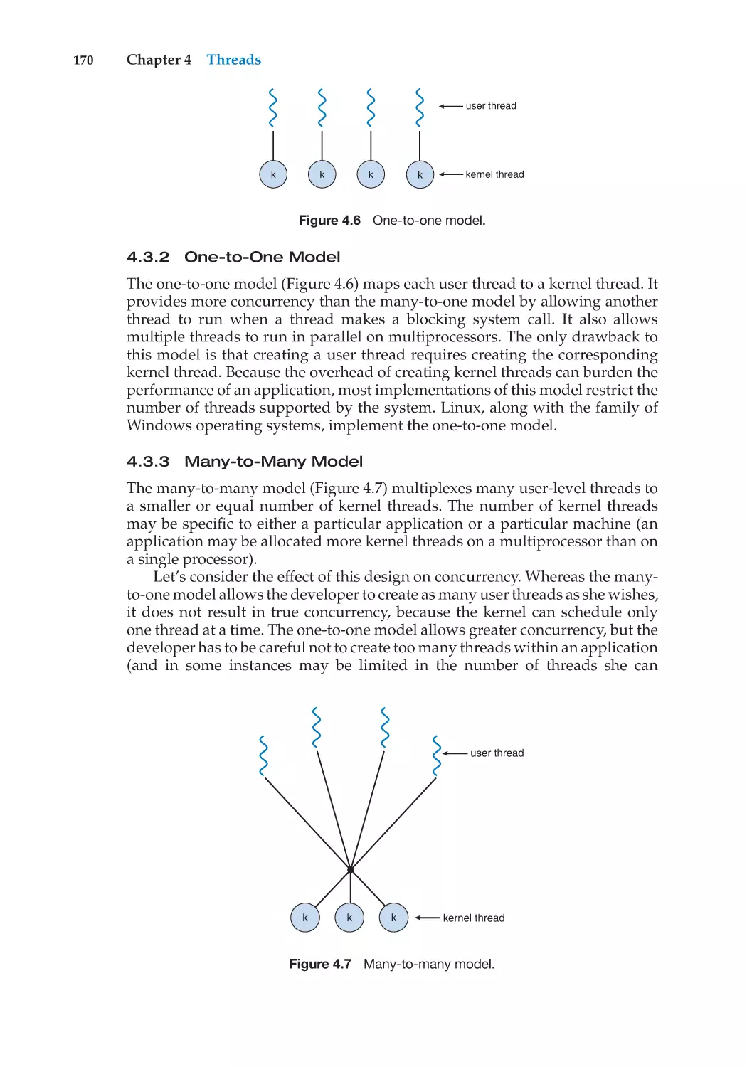
Overview 163
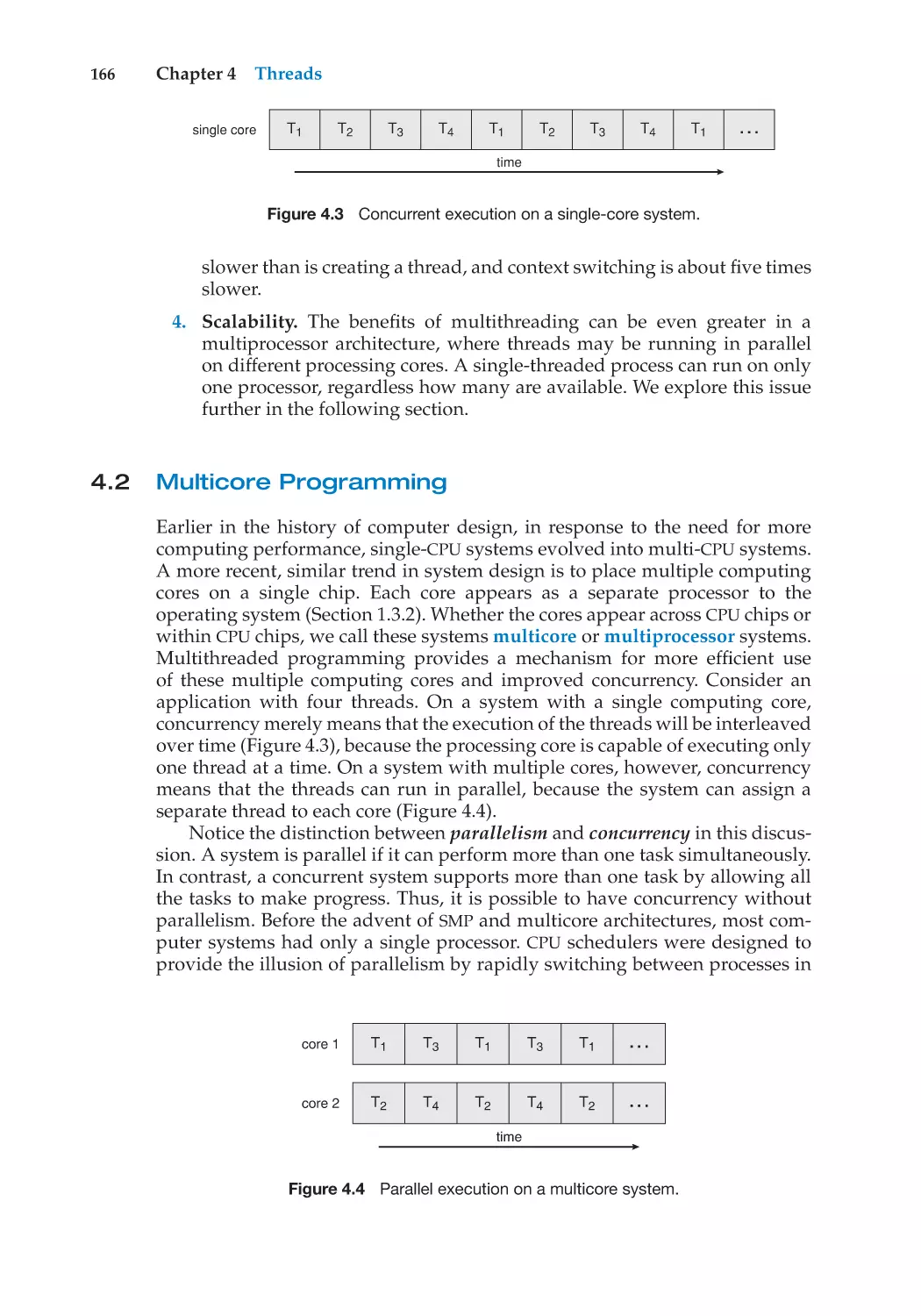
Multicore Programming 166
Multithreading Models 169
Thread Libraries 171
Implicit Threading 177
Chapter 5
5.1
5.2
5.3
5.4
5.5
5.6
5.7
PART THREE
7.1
7.2
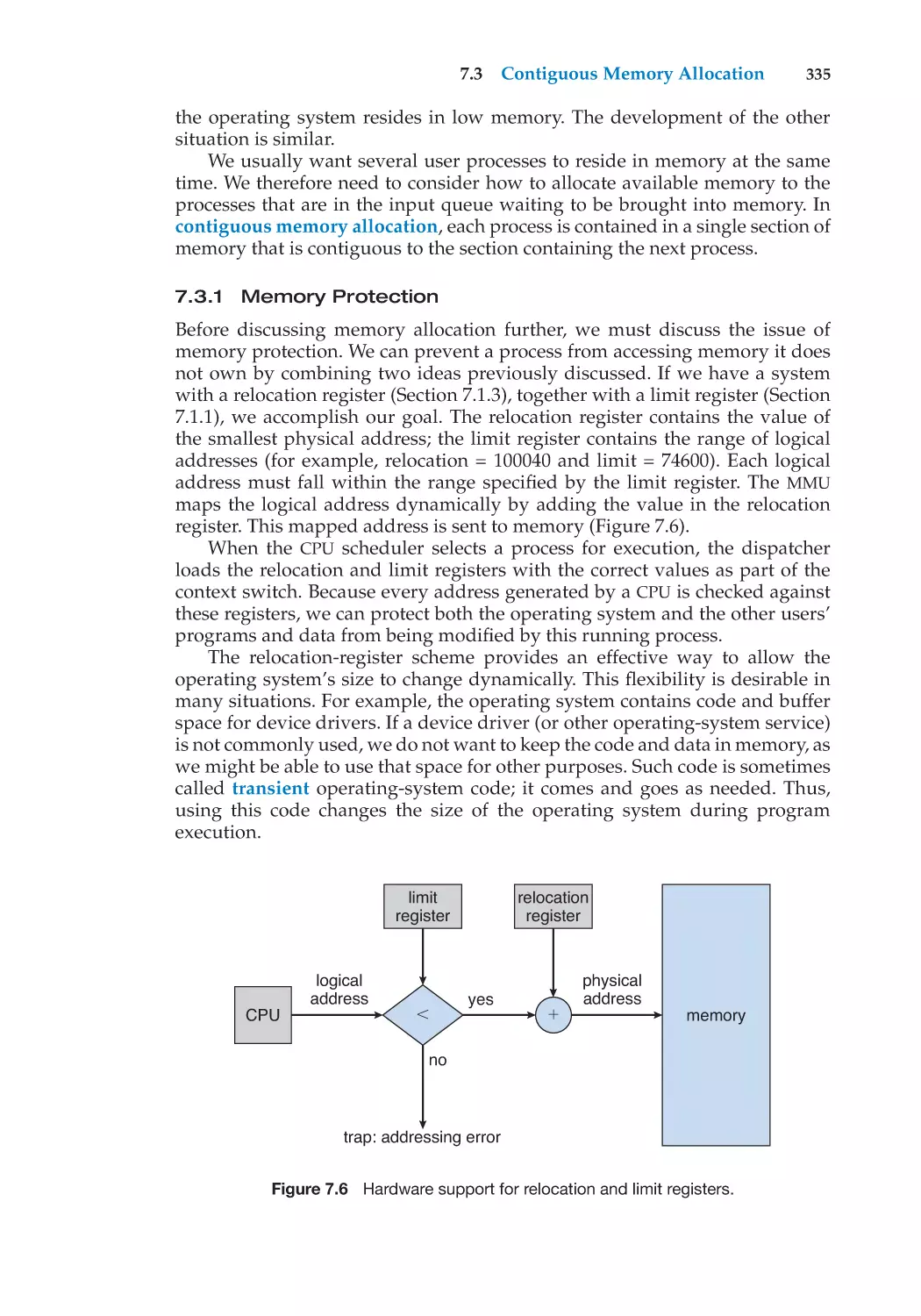
7.3
7.4
7.5
7.6
8.1
8.2
8.3
8.4
8.5
8.6
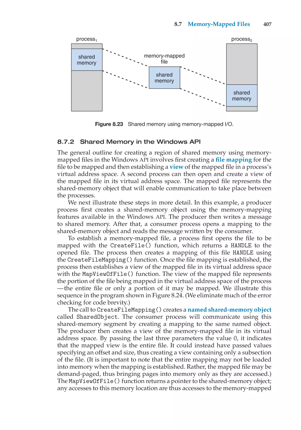
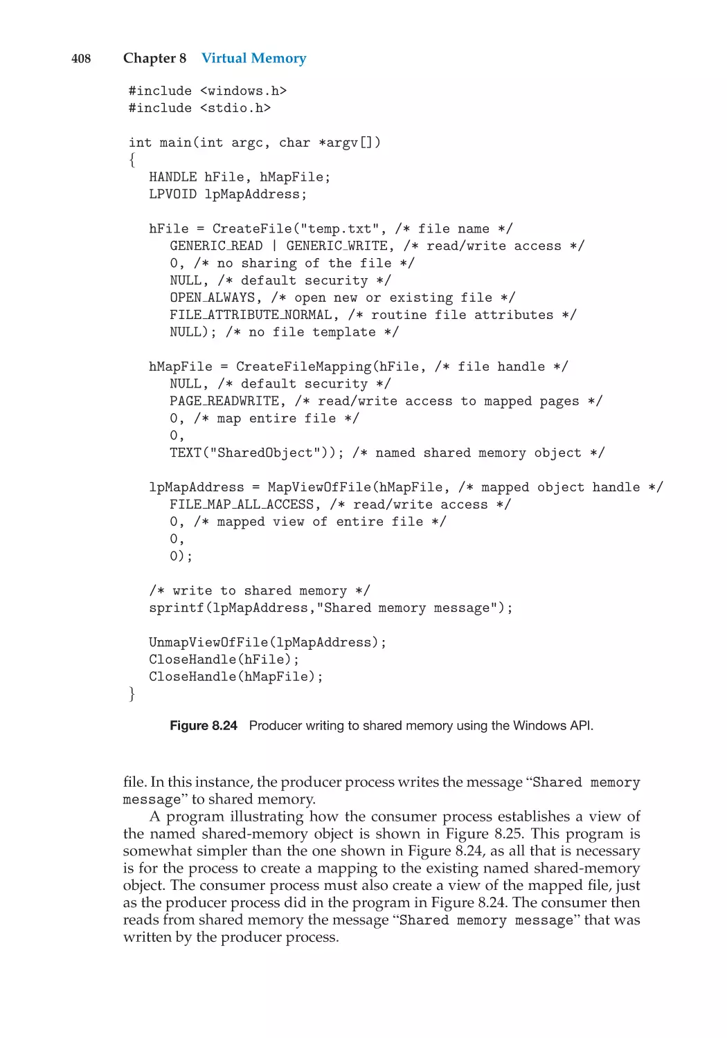
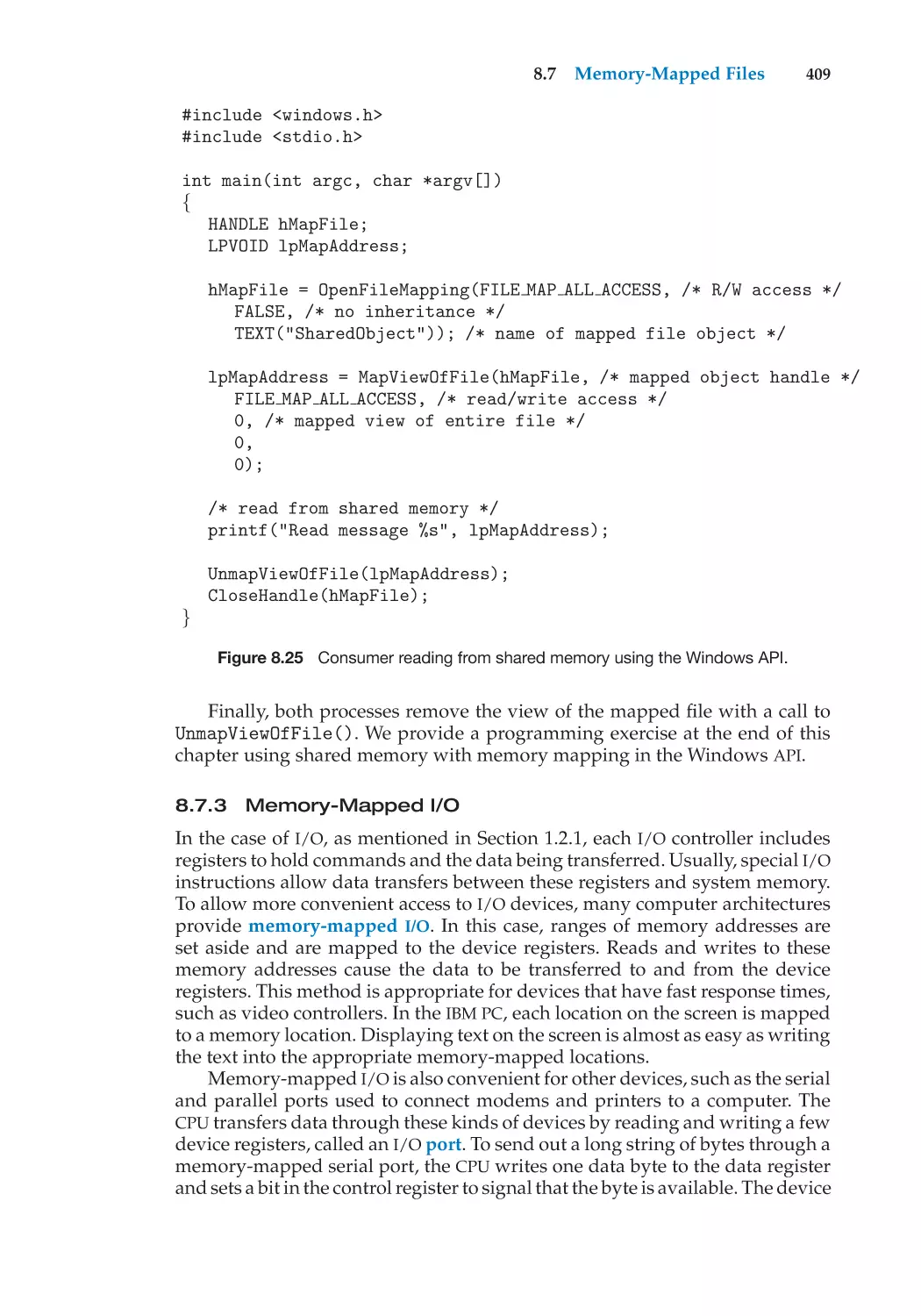
8.7
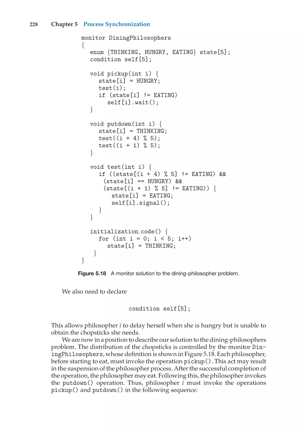
5.8
5.9
5.10
5.11
5.12
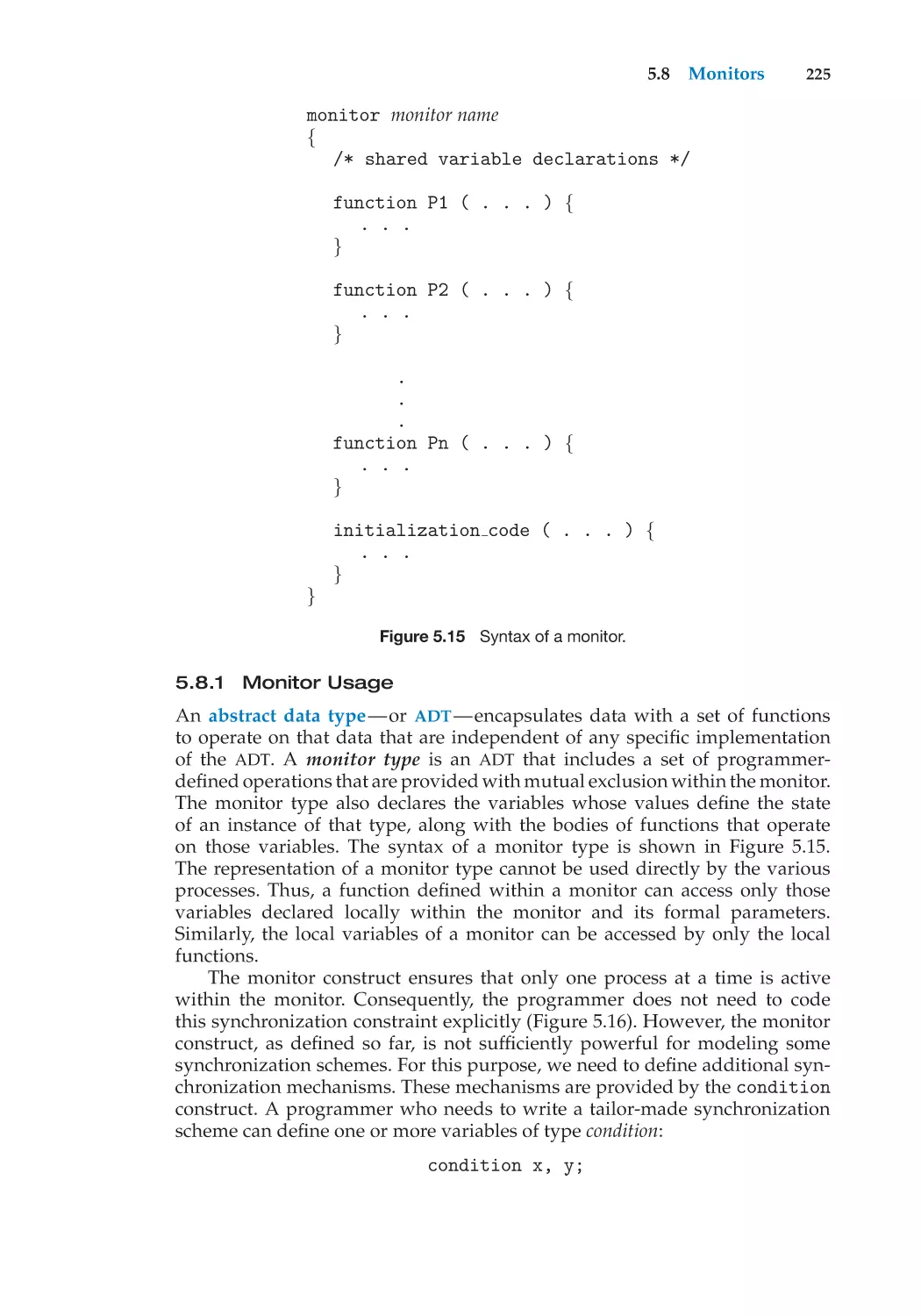
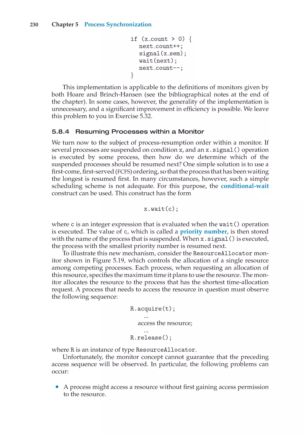
Monitors 223
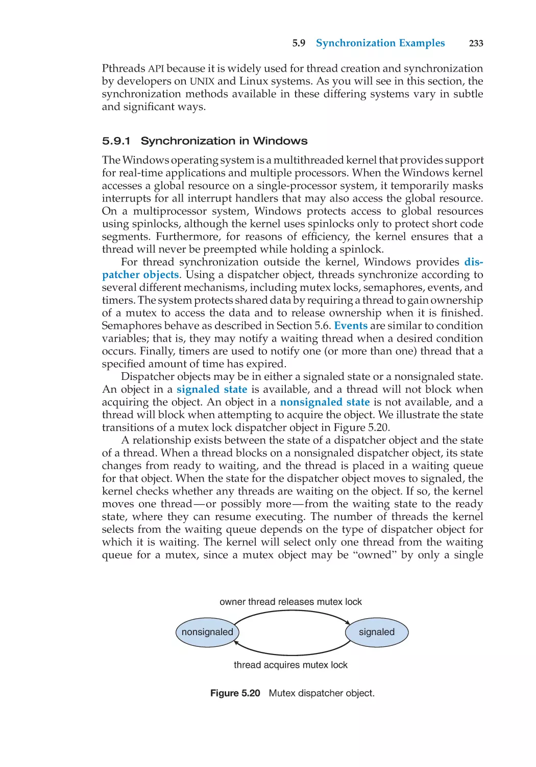
Synchronization Examples 232
Alternative Approaches 238
Deadlocks 242
Summary 249
Exercises 250
Bibliographical Notes 266
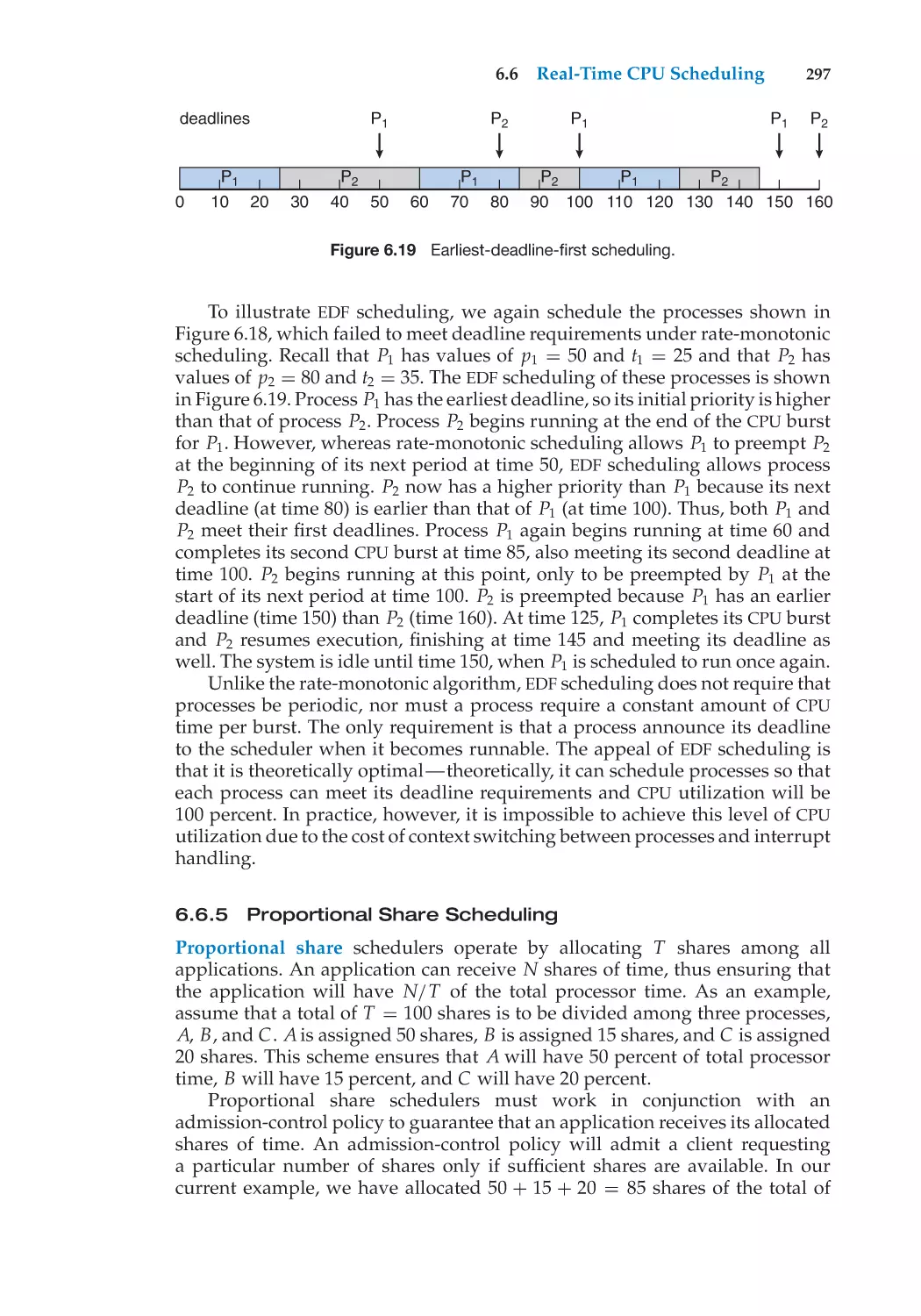
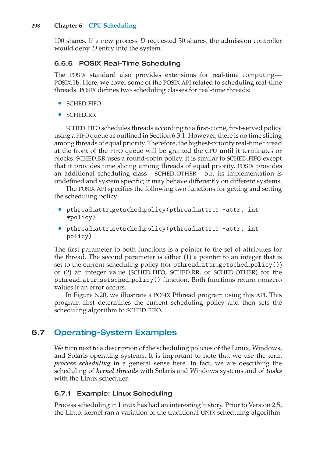
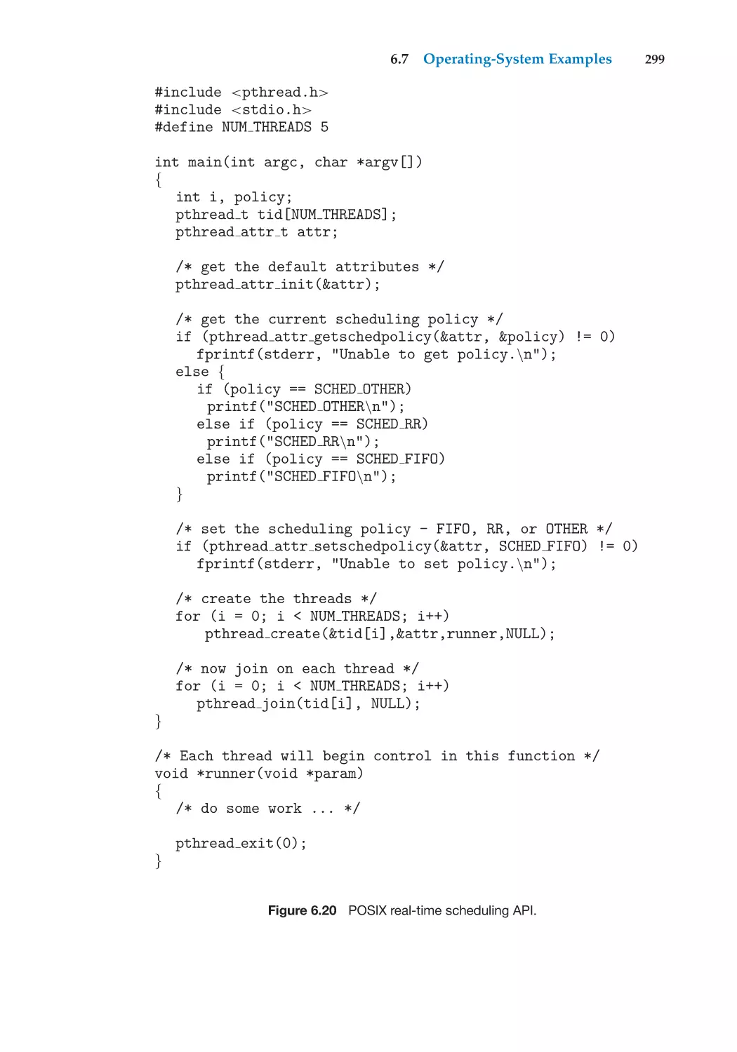
6.7 Operating-System Examples
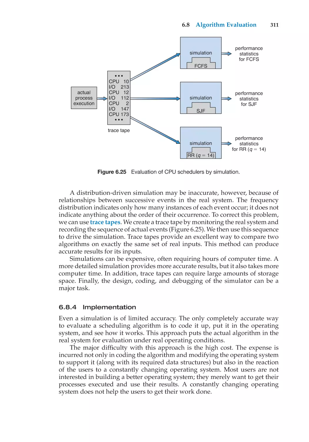
6.8 Algorithm Evaluation 308
6.9 Summary 312
Exercises 314
Bibliographical Notes 319
298
MEMORY MANAGEMENT
Main Memory
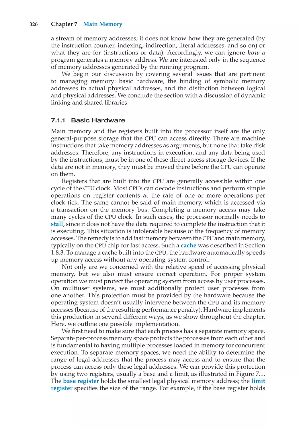
Background 325
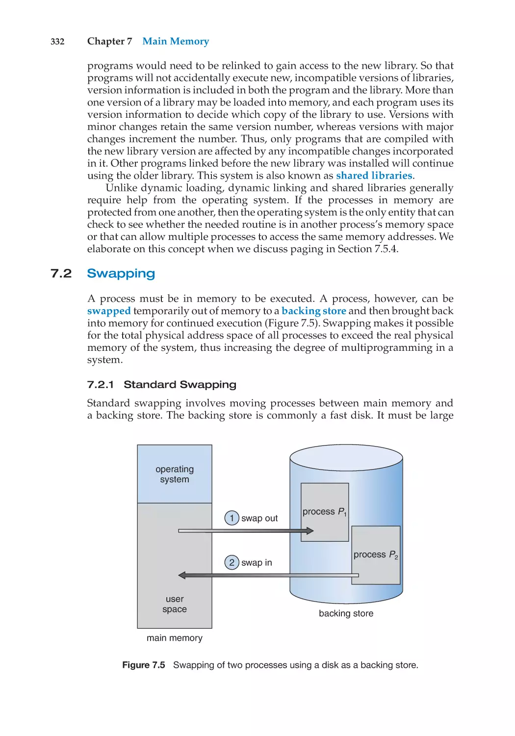
Swapping 332
Contiguous Memory Allocation 334
Segmentation 338
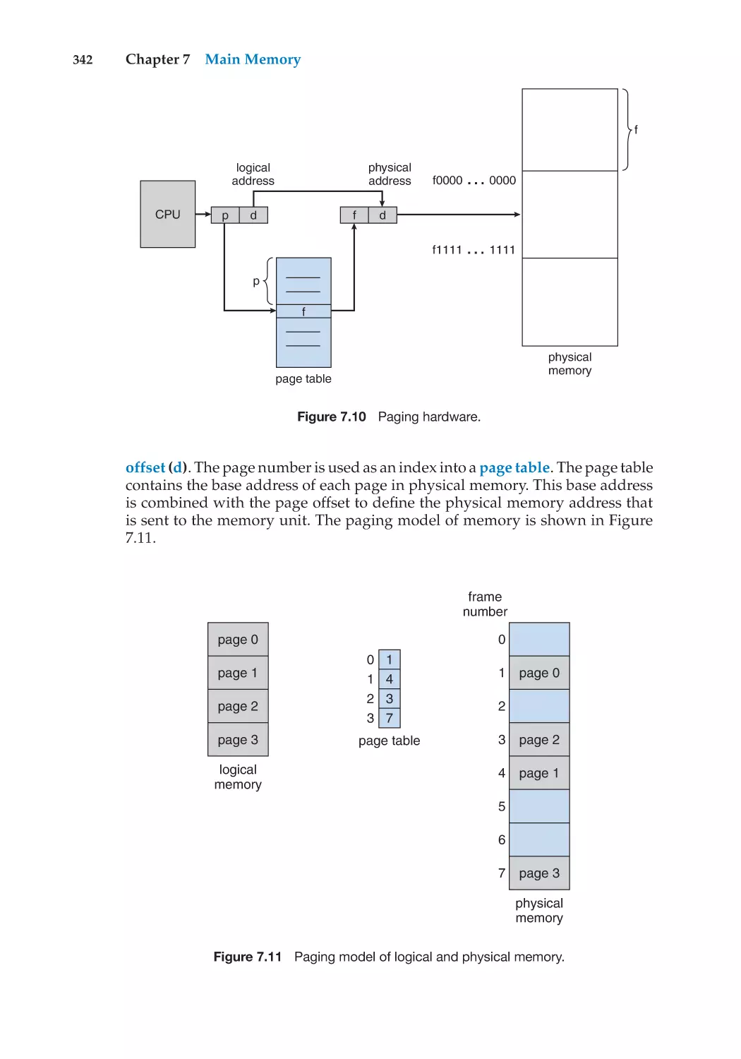
Paging 340
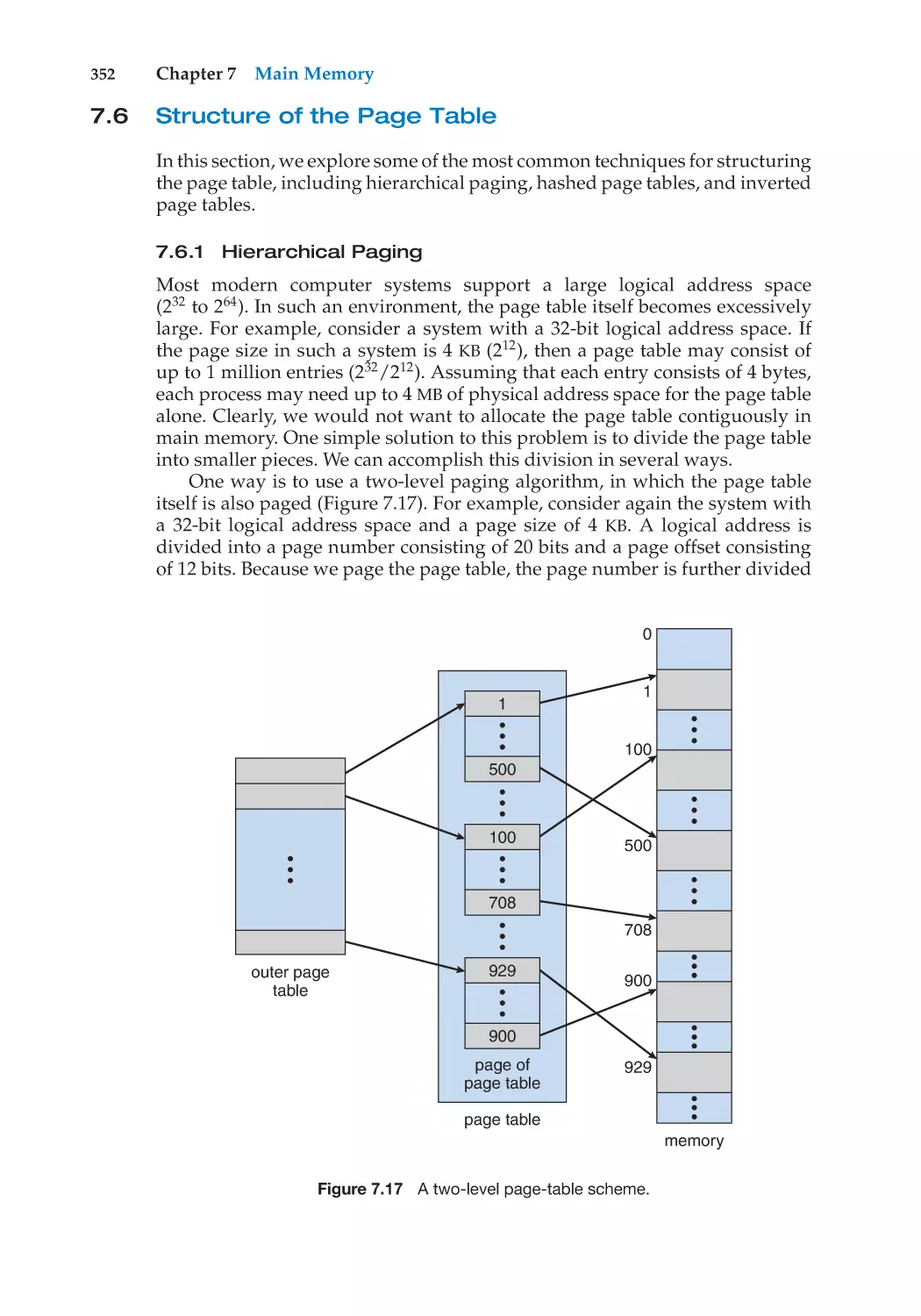
Structure of the Page Table 352
Chapter 8
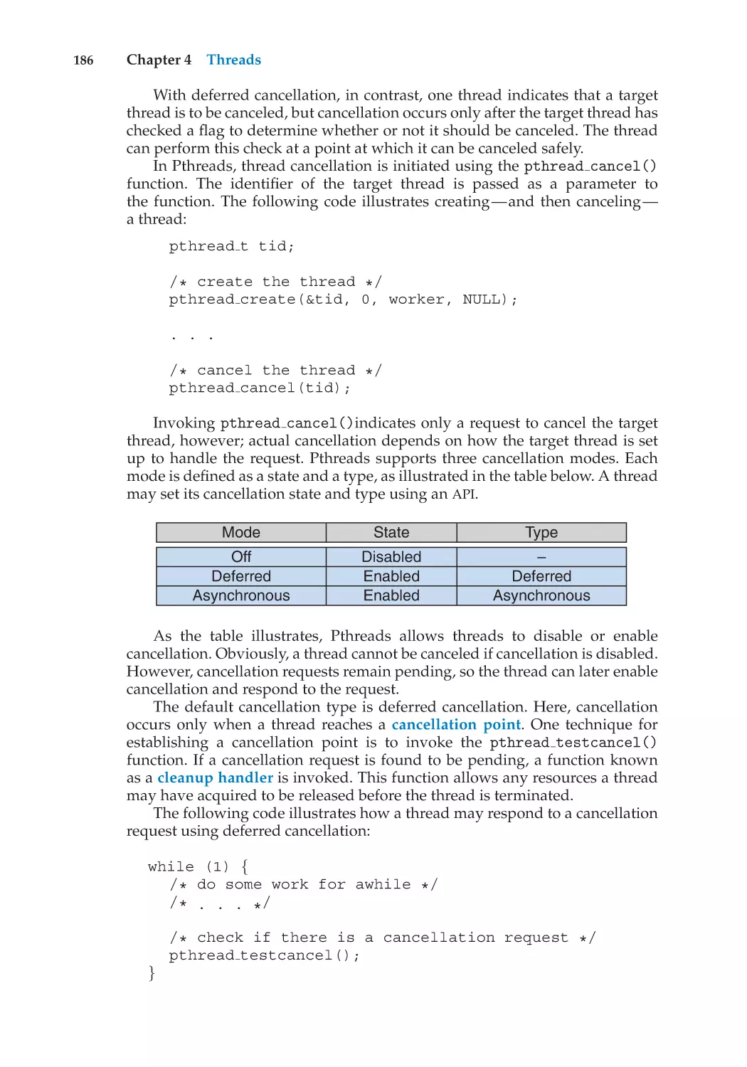
188
CPU Scheduling
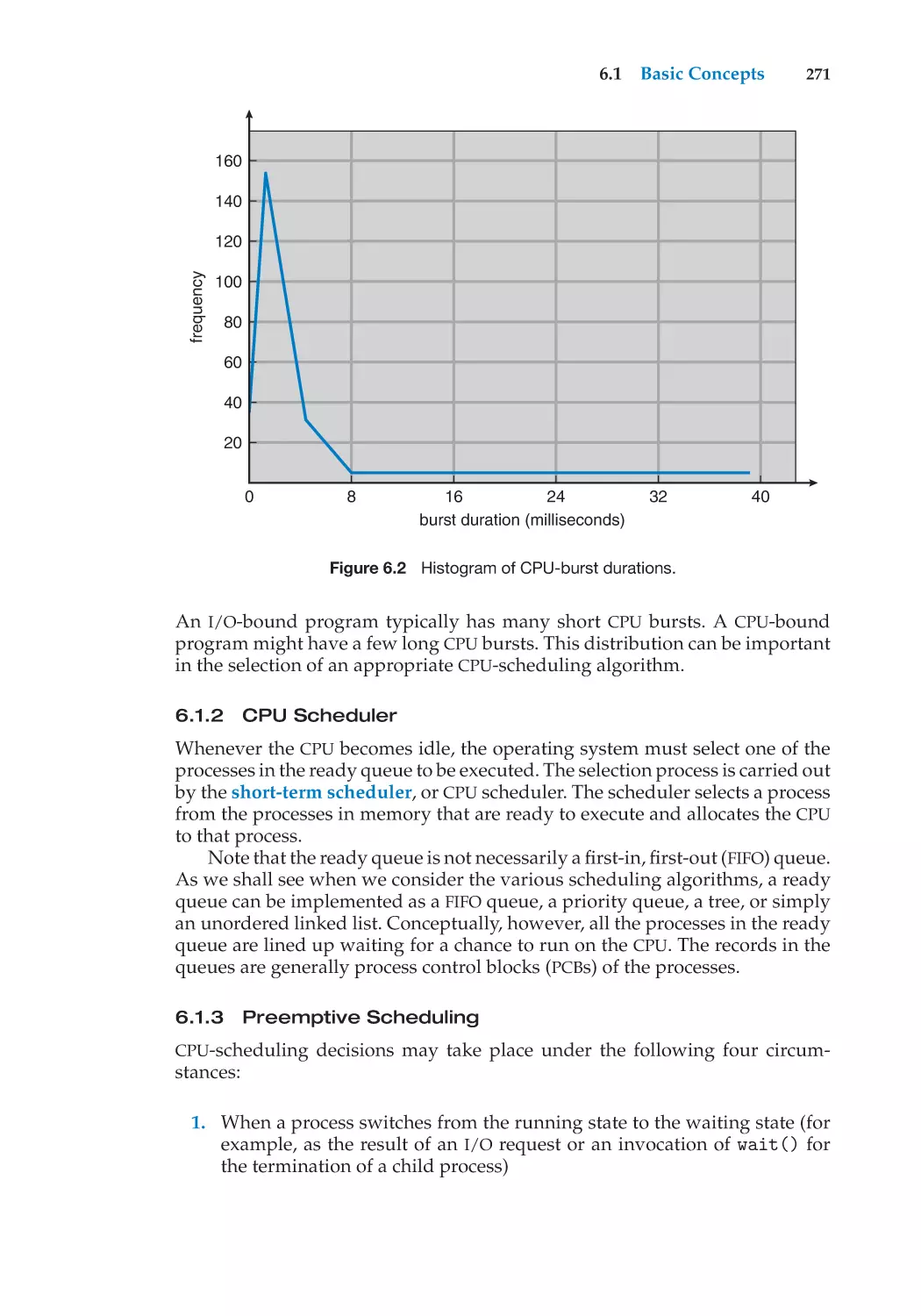
Basic Concepts 269
Scheduling Criteria 273
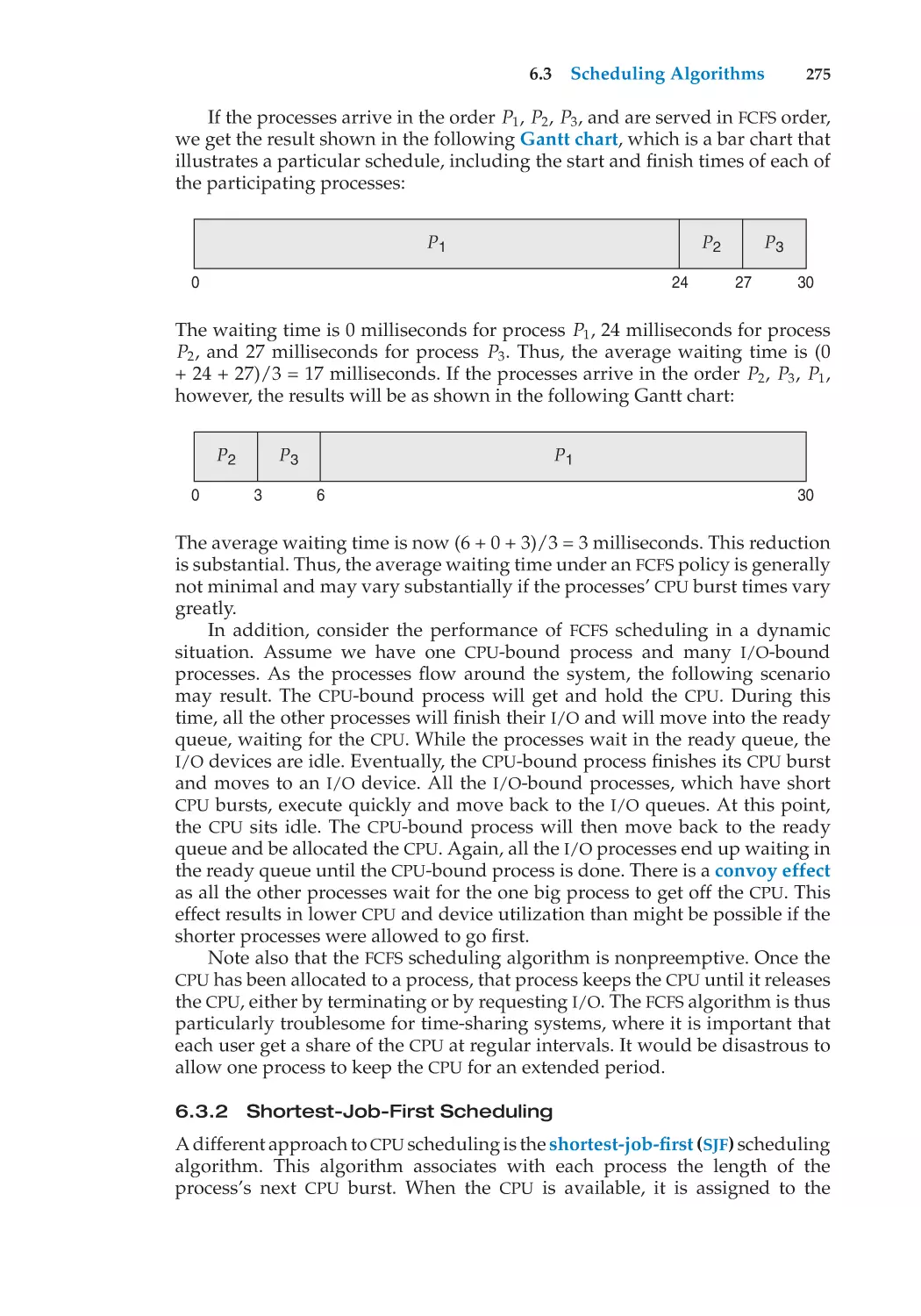
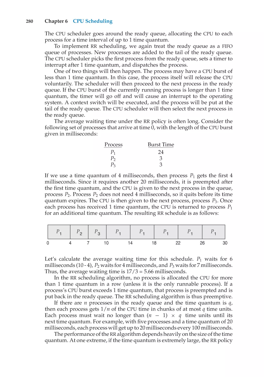
Scheduling Algorithms 274
Thread Scheduling 285
Multiple-Processor Scheduling 286
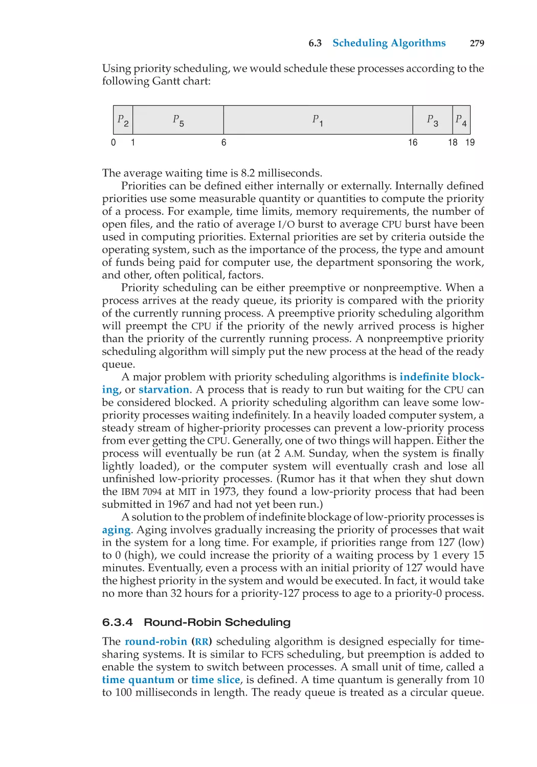
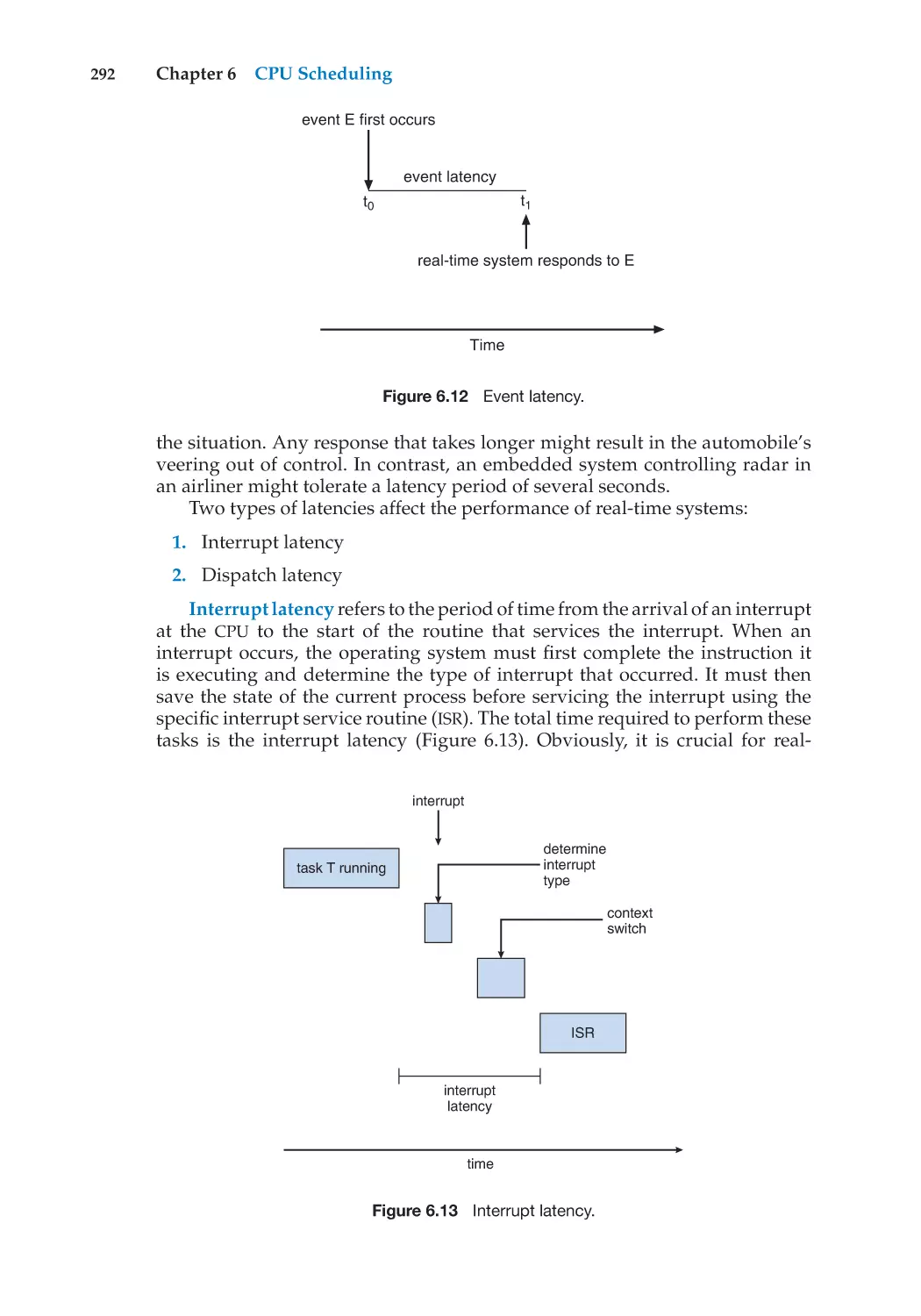
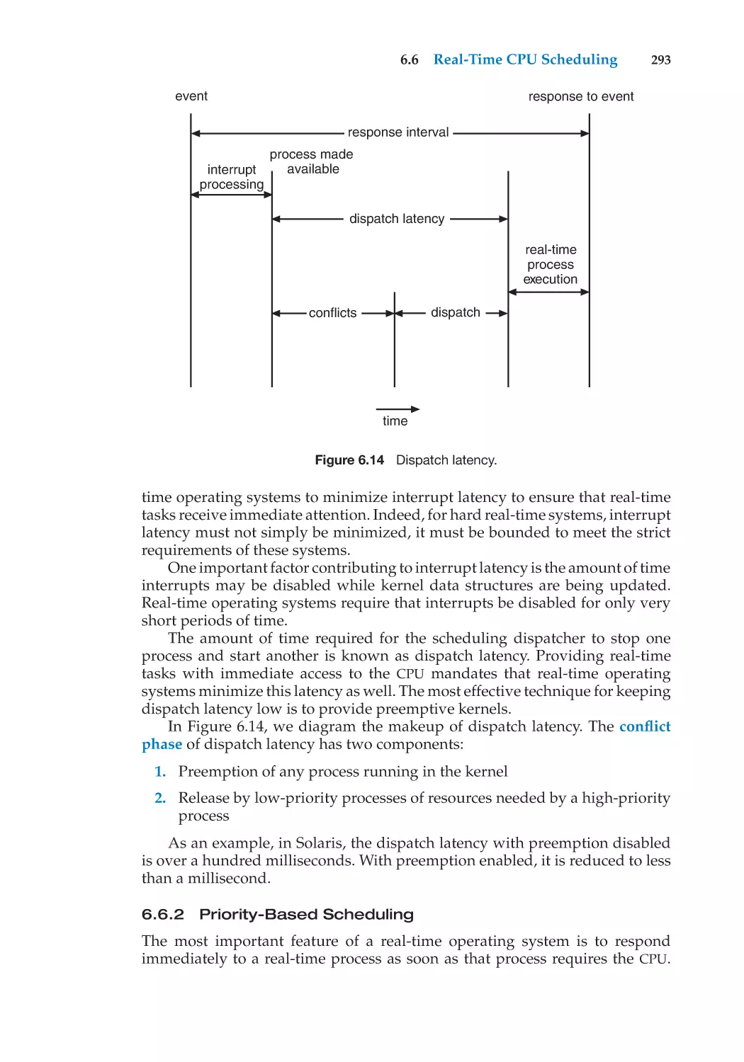
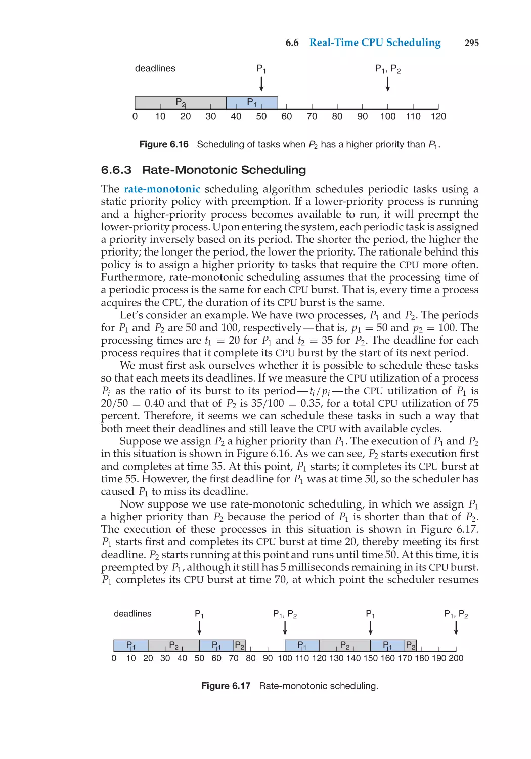
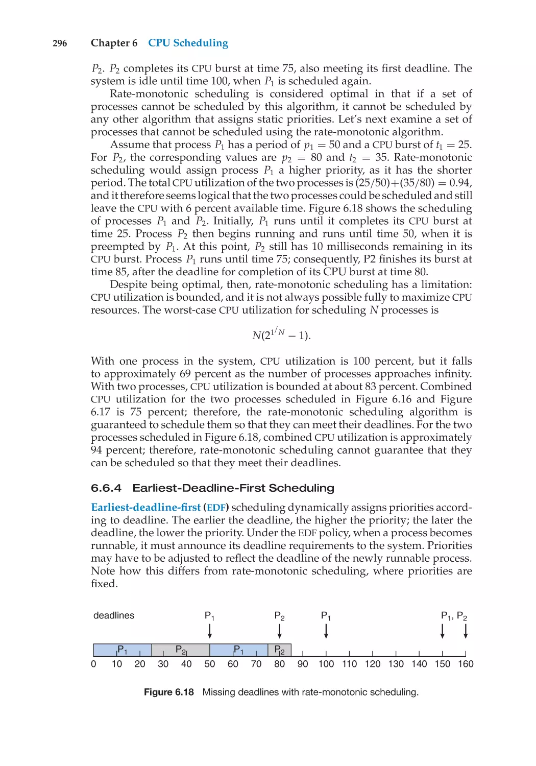
Real-Time CPU Scheduling 291
Chapter 7
4.6 Threading Issues 183
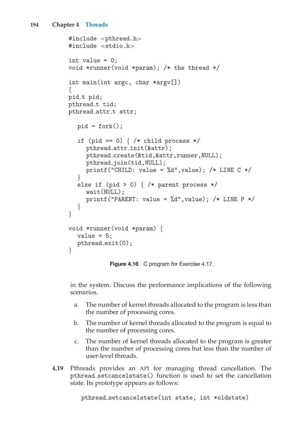
4.7 Operating-System Examples
4.8 Summary 191
Exercises 191
Bibliographical Notes 200
Process Synchronization
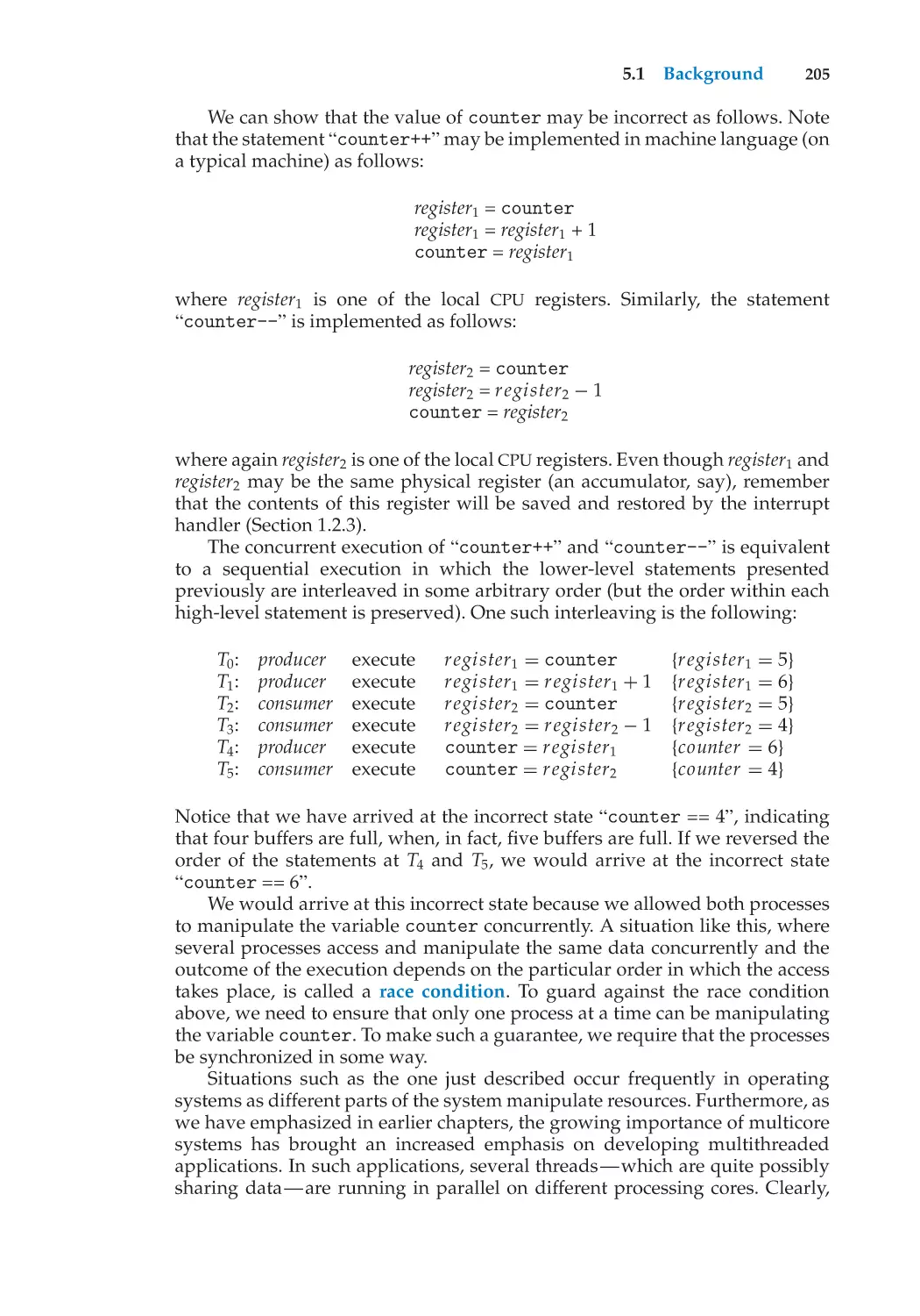
Background 203
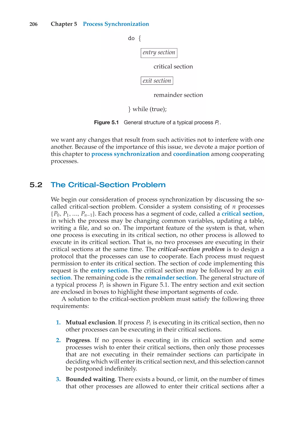
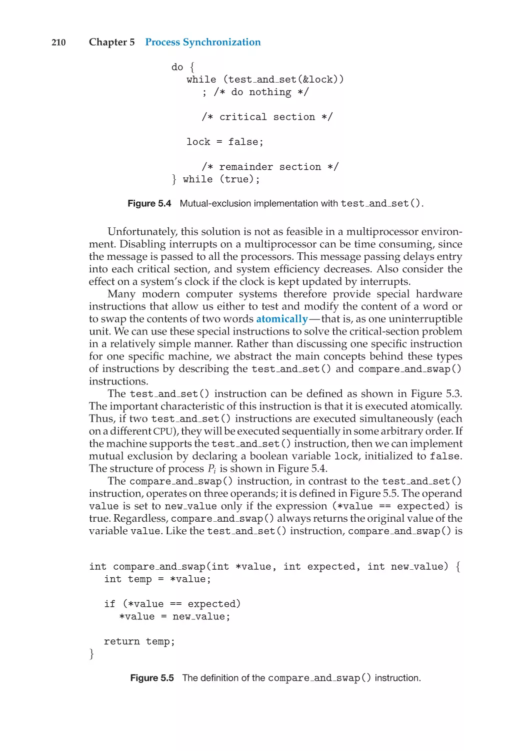
The Critical-Section Problem 206
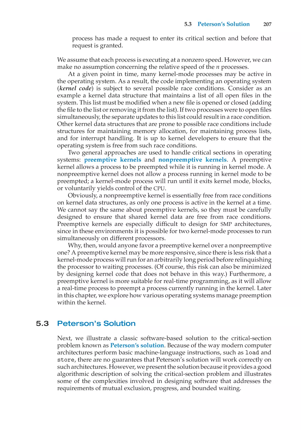
Peterson’s Solution 207
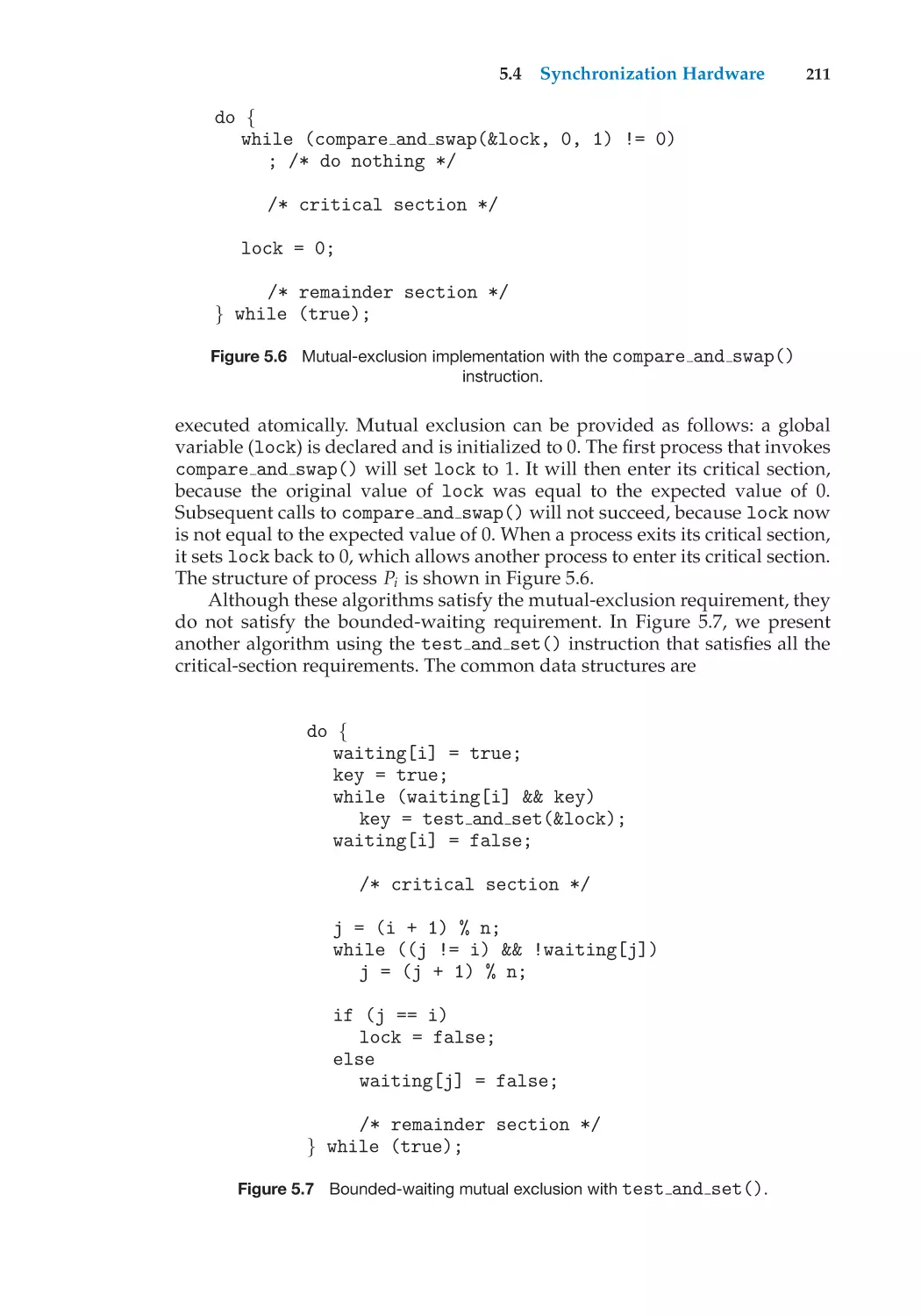
Synchronization Hardware 209
Mutex Locks 212
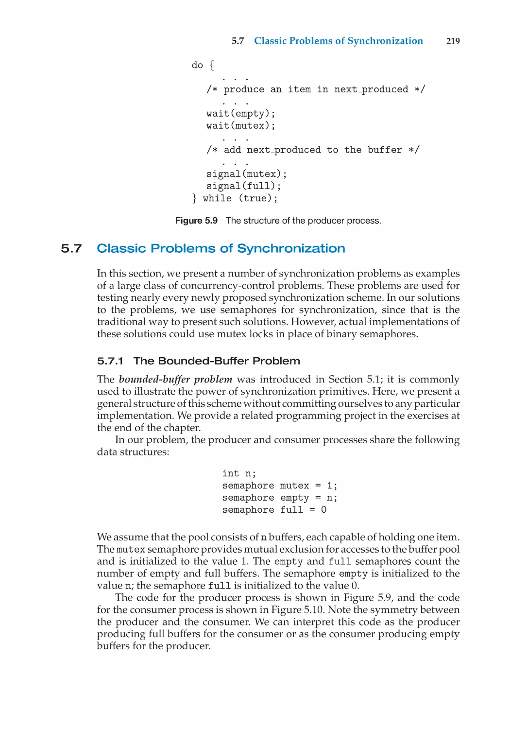
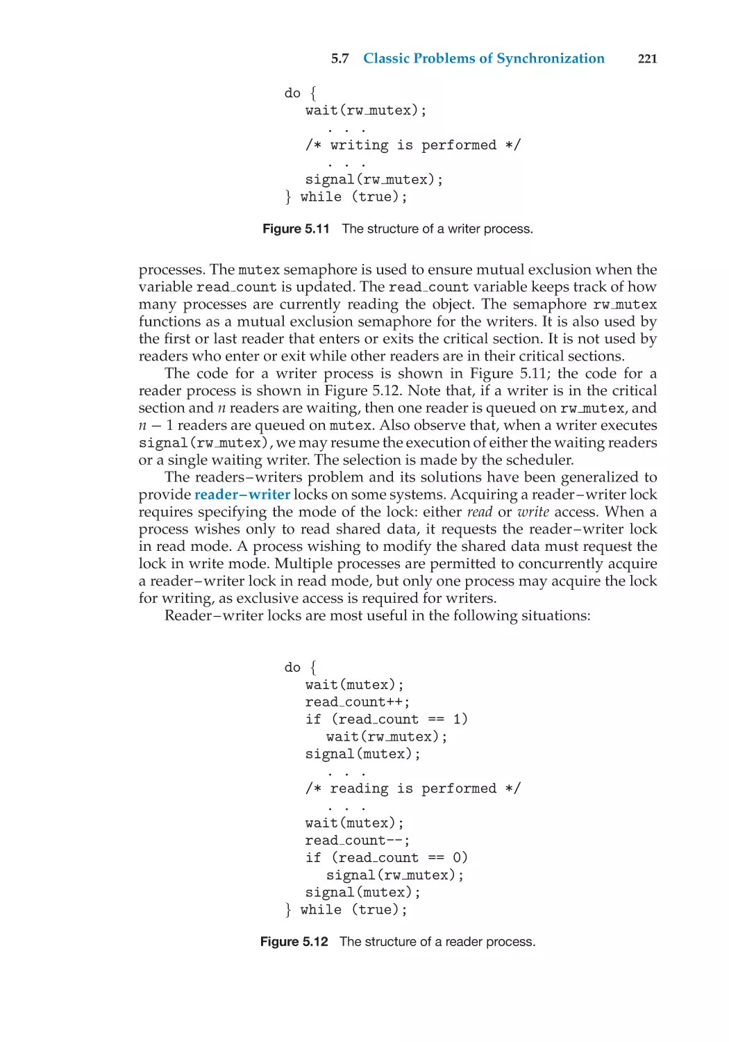
Semaphores 213
Classic Problems of
Synchronization 219
Chapter 6
6.1
6.2
6.3
6.4
6.5
6.6
Threads
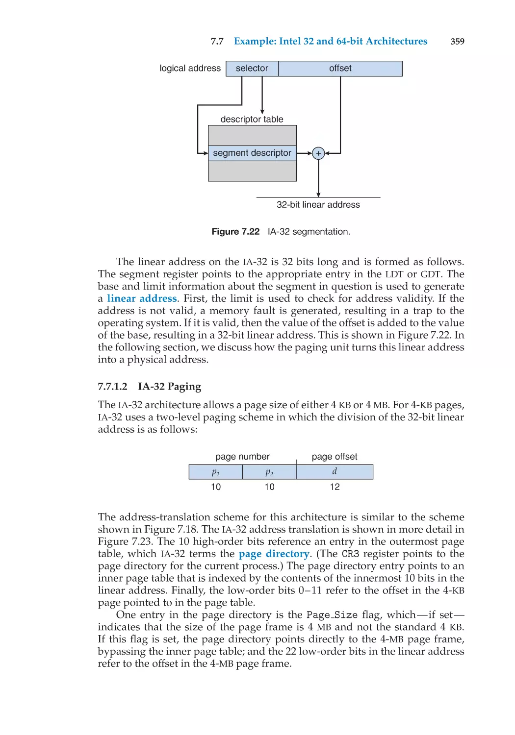
7.7 Example: Intel 32 and 64-bit
Architectures 357
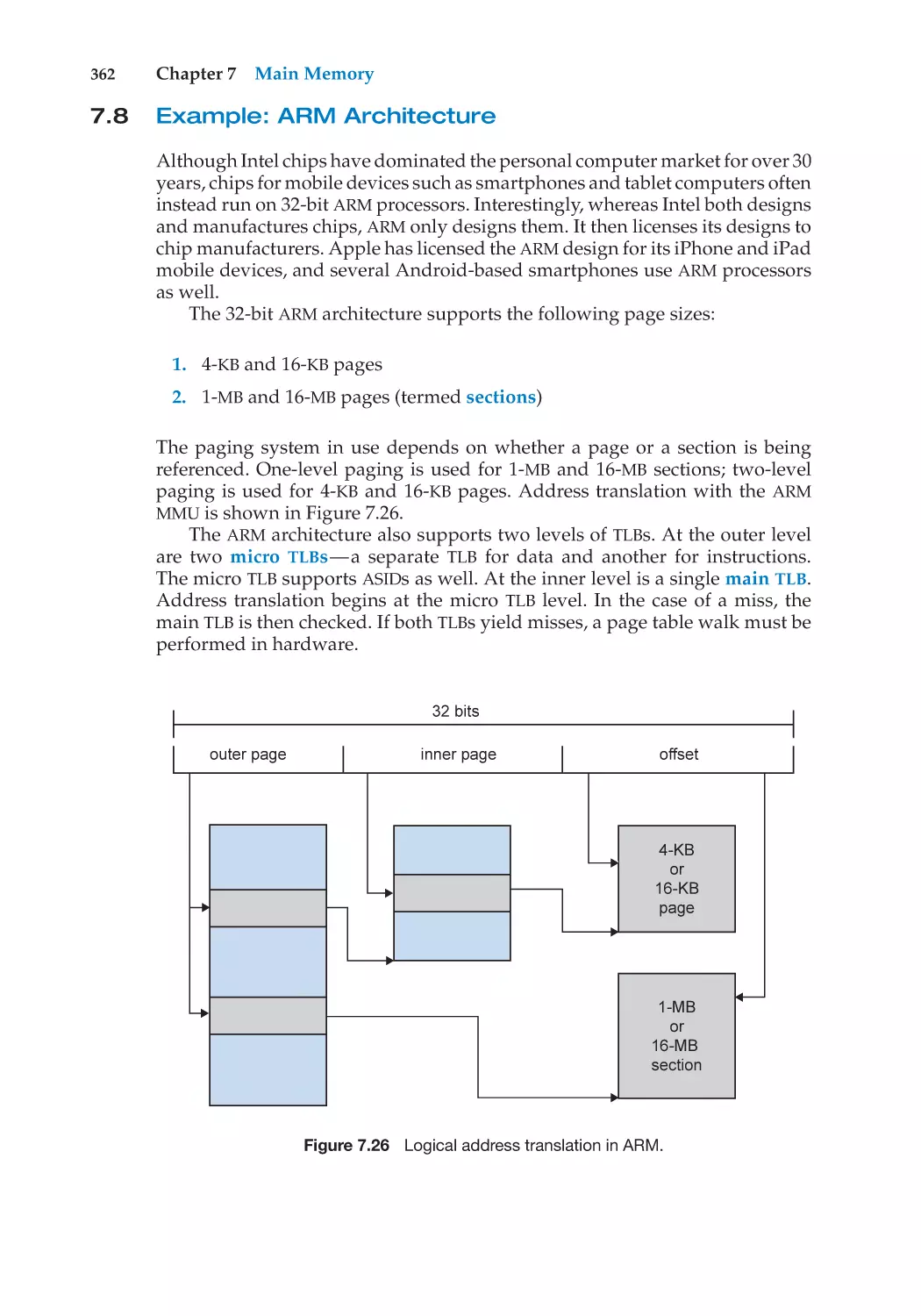
7.8 Example: ARM Architecture
7.9 Summary 363
Exercises 364
Bibliographical Notes 368
362
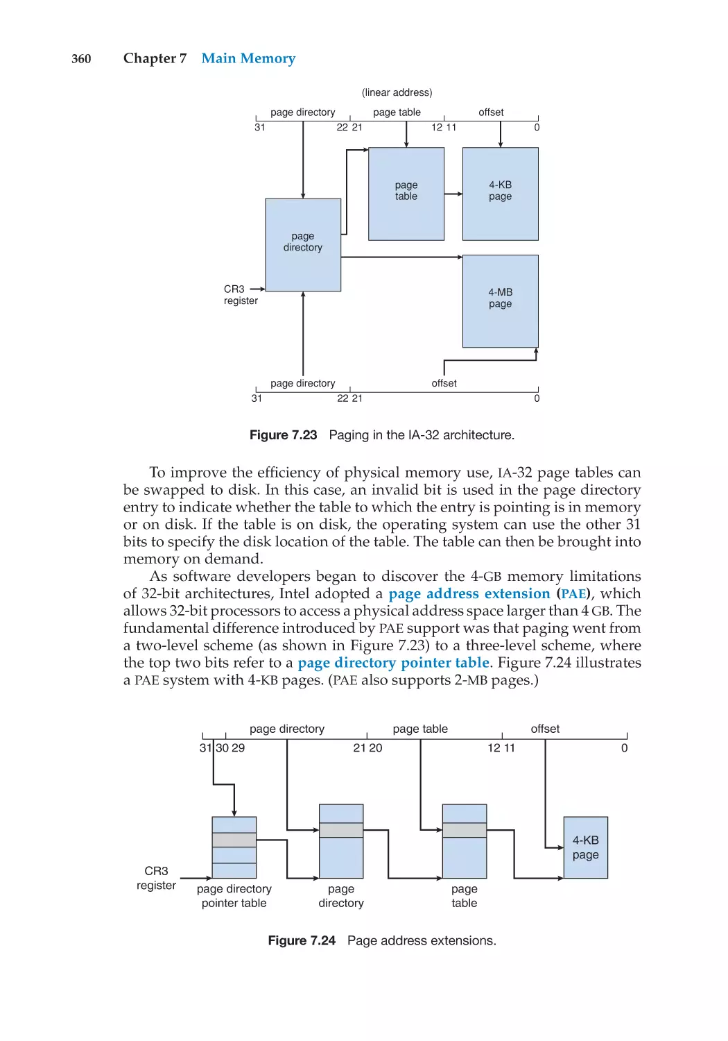
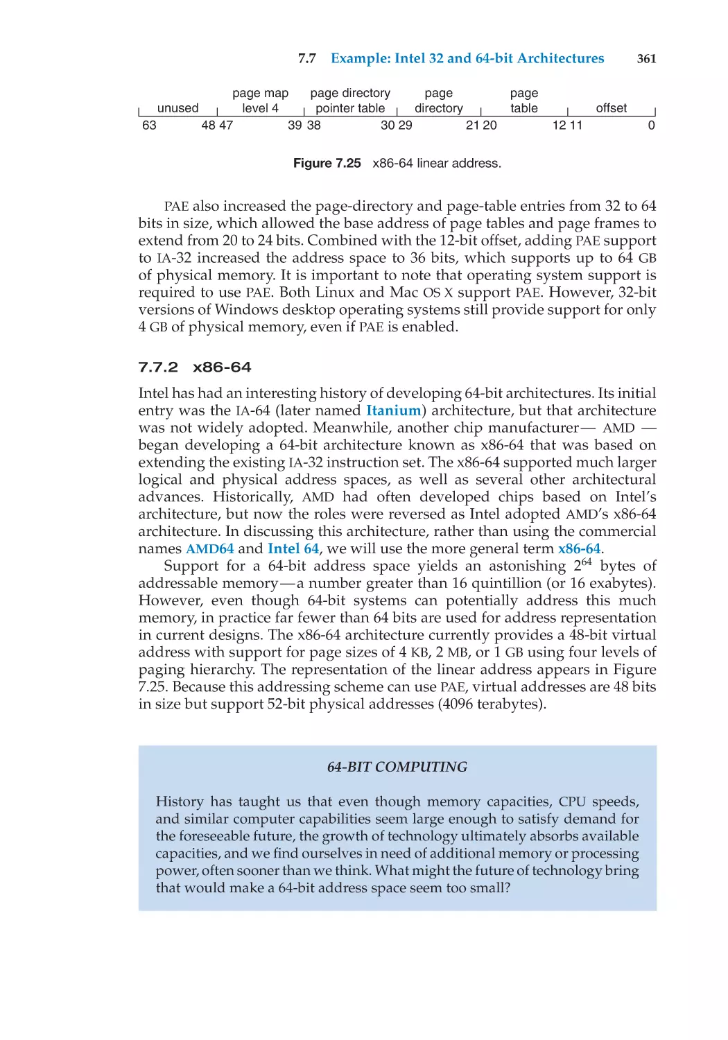
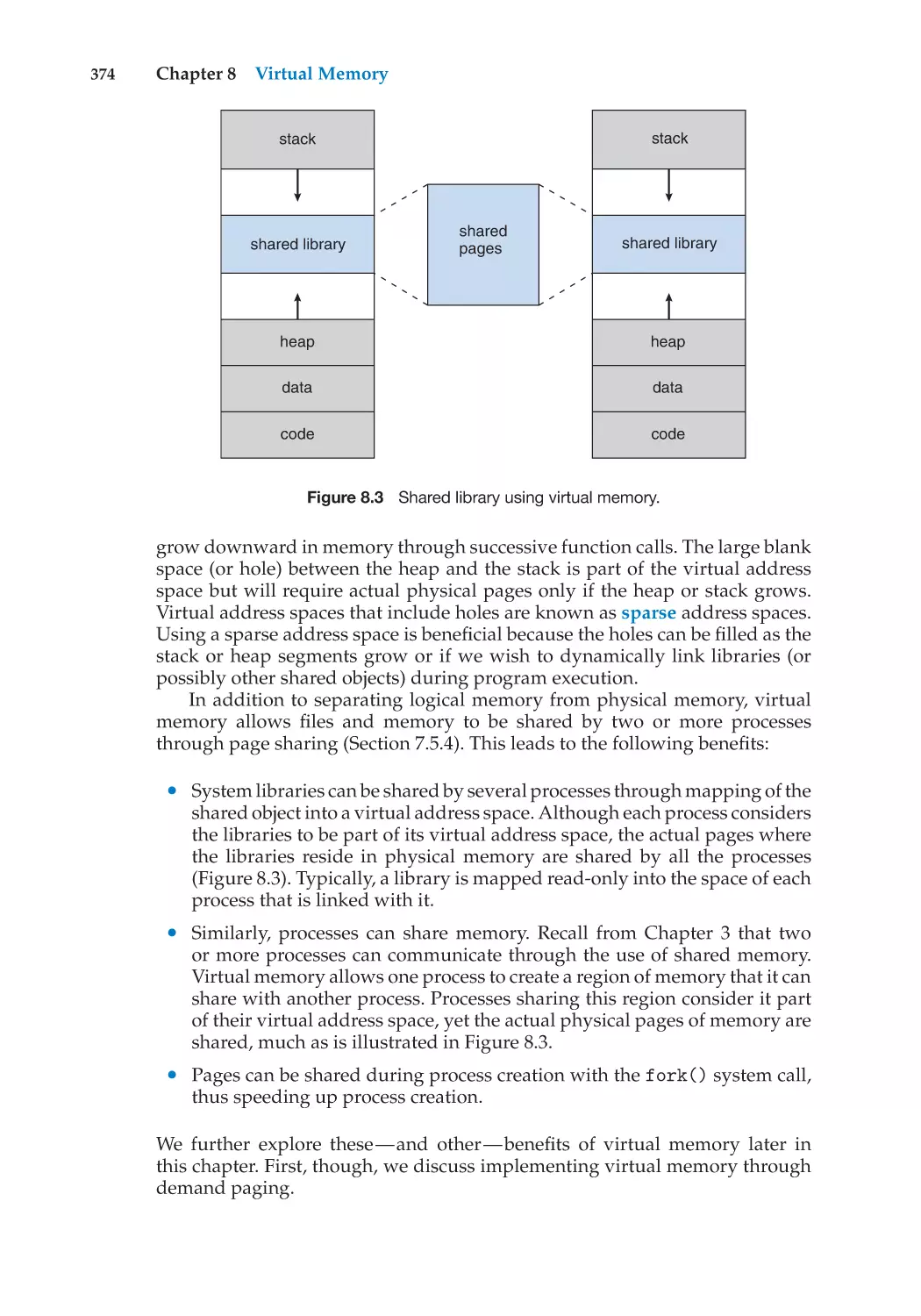
Virtual Memory
Background 371
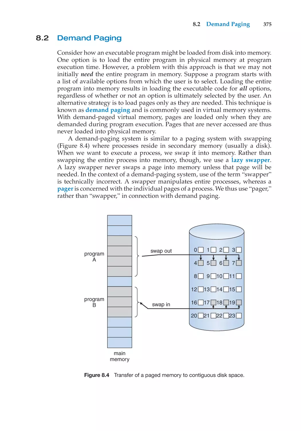
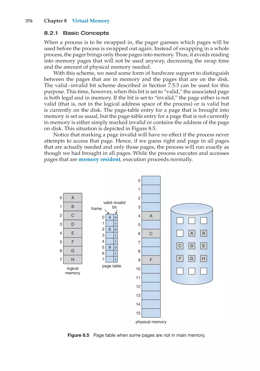
Demand Paging 375
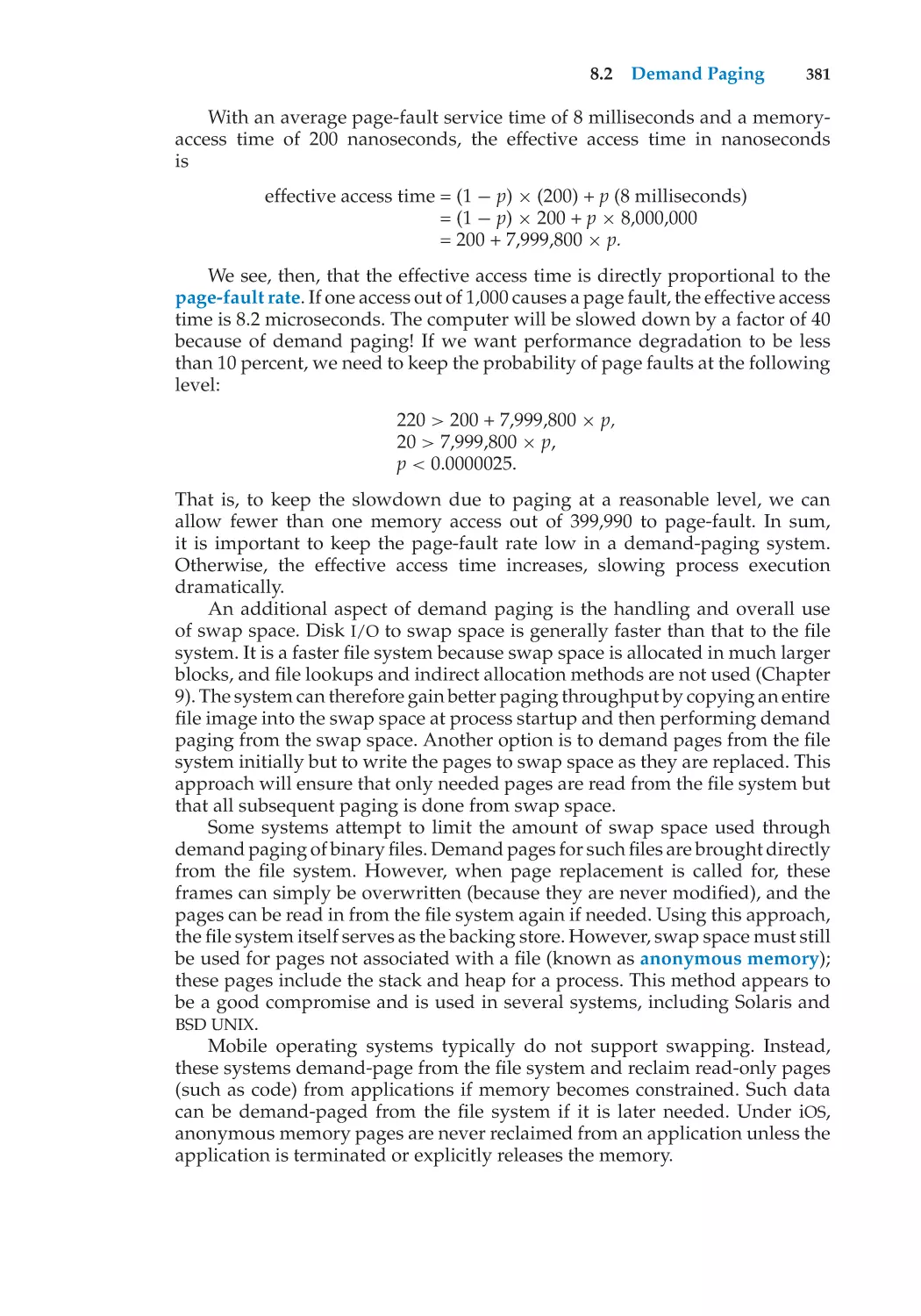
Copy-on-Write 382
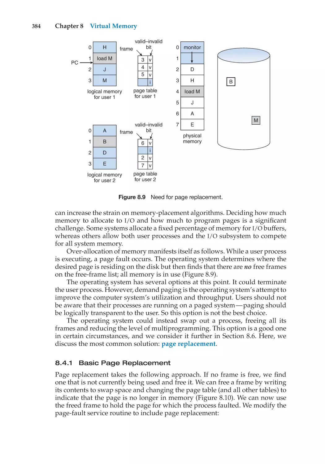
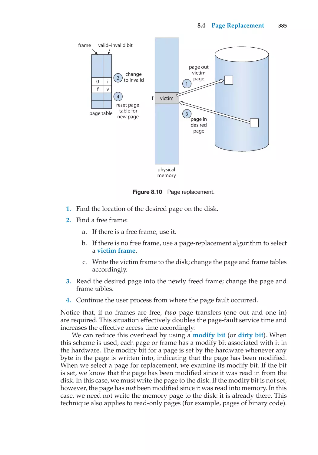
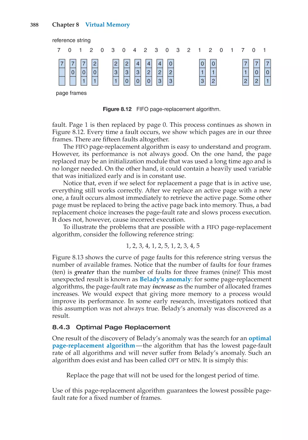
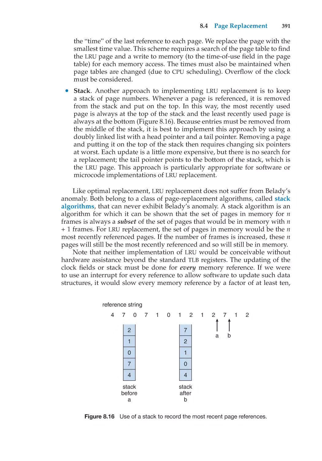
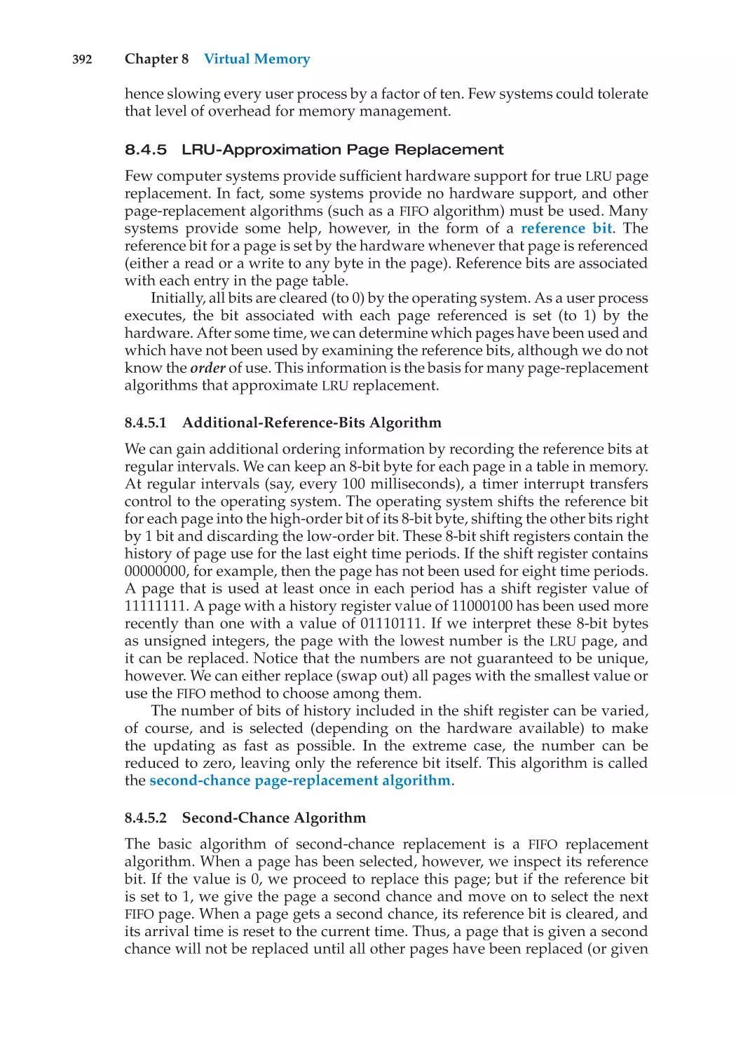
Page Replacement 383
Allocation of Frames 395
Thrashing 399
Memory-Mapped Files 404
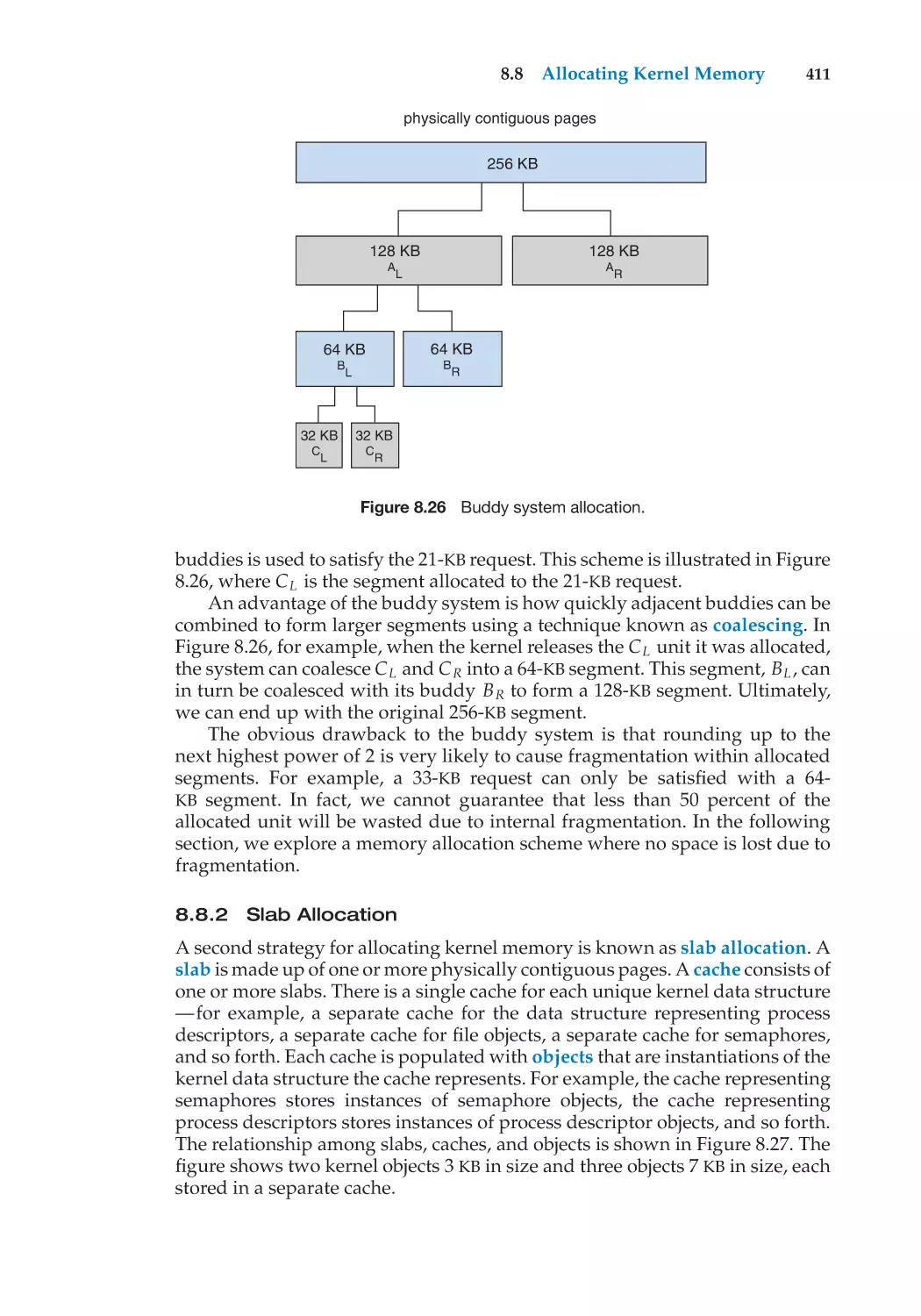
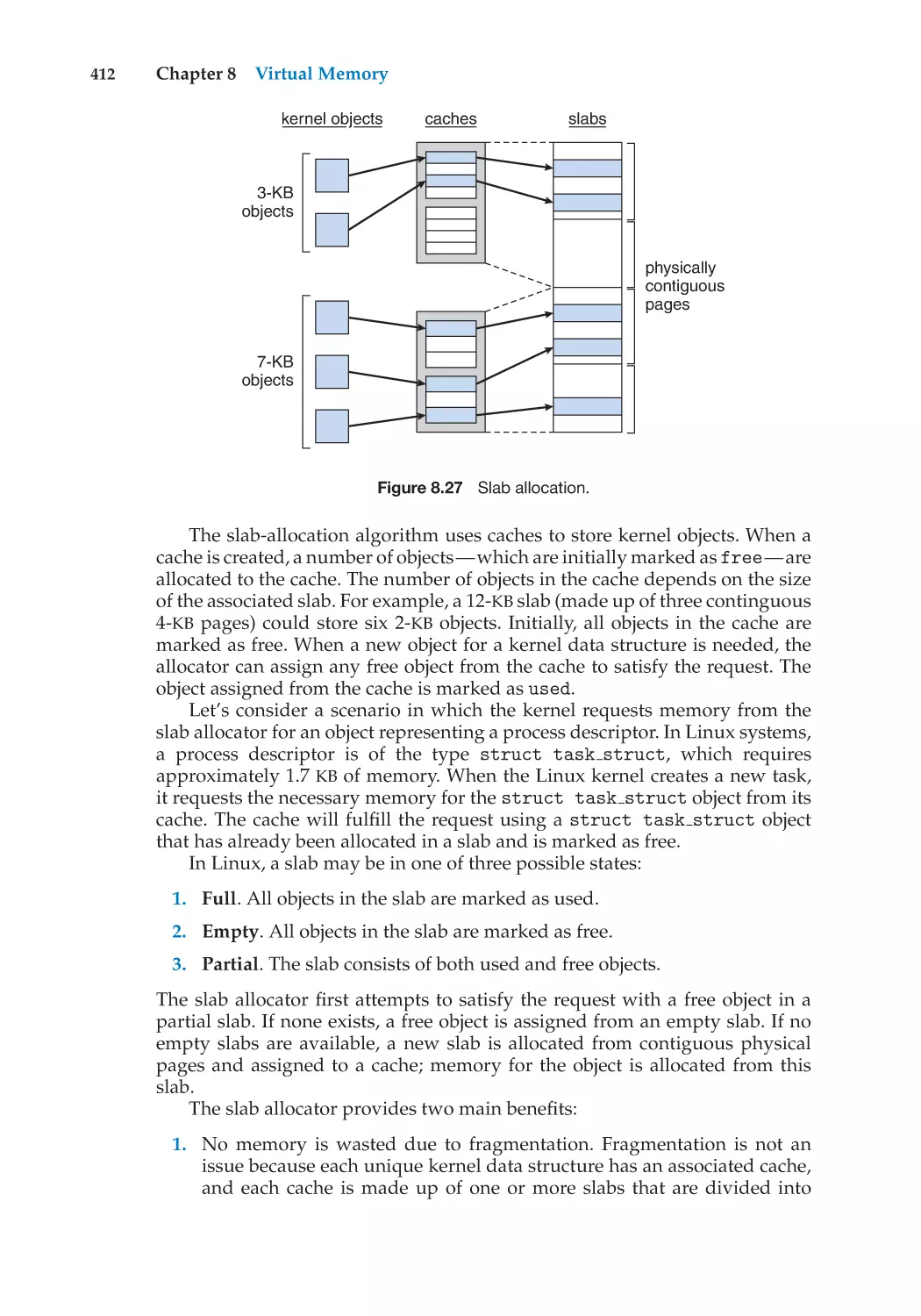
8.8
8.9
8.10
8.11
Allocating Kernel Memory 410
Other Considerations 413
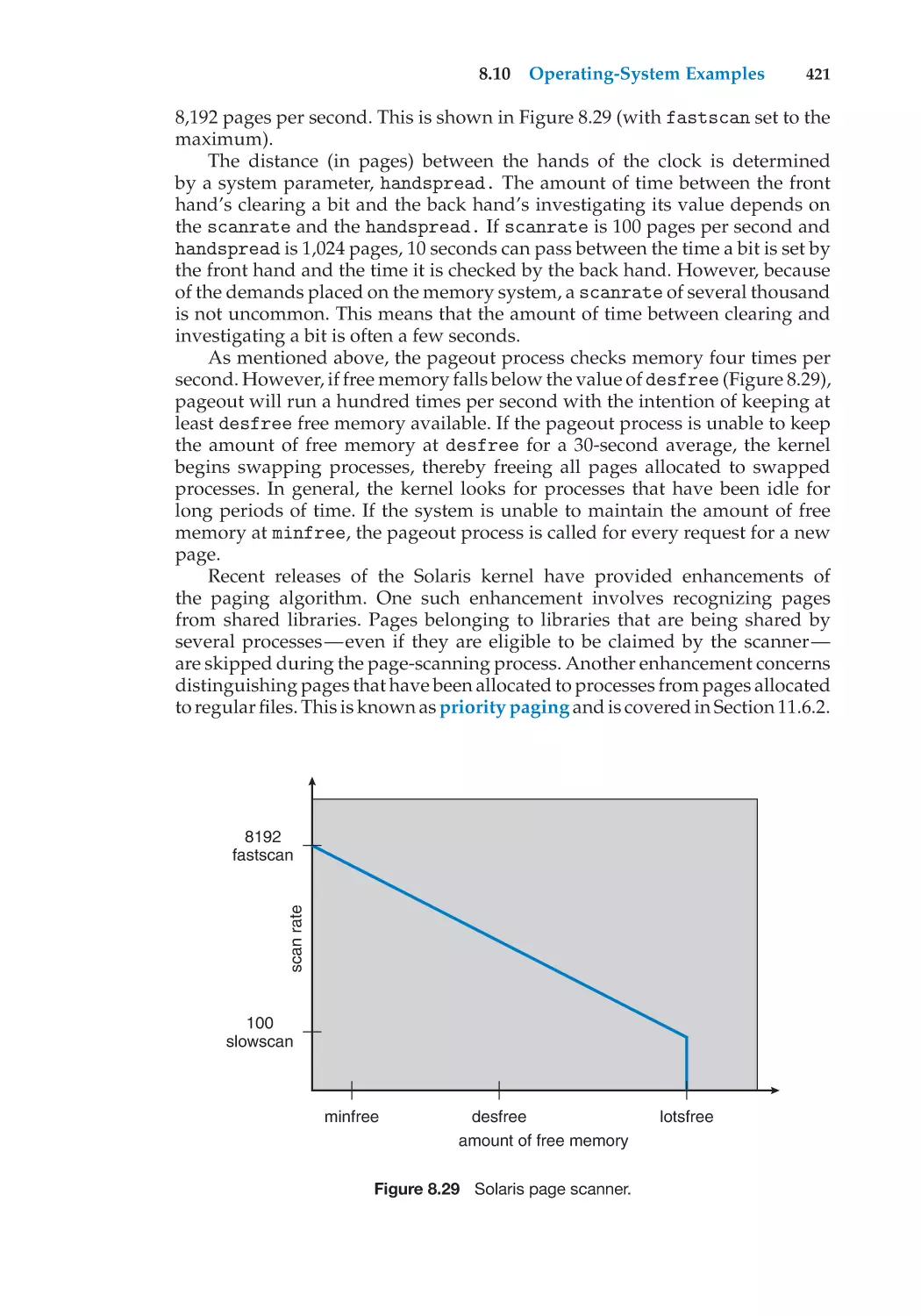
Operating-System Examples 419
Summary 422
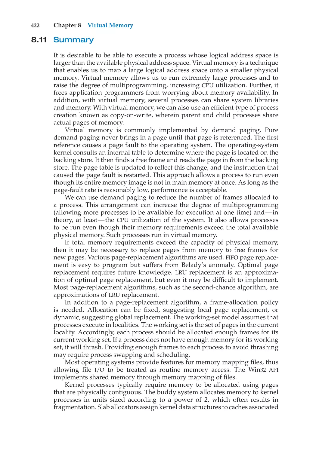
Exercises 423
Bibliographical Notes 435
Contents
PART FOUR
Chapter 9
xix
STORAGE MANAGEMENT
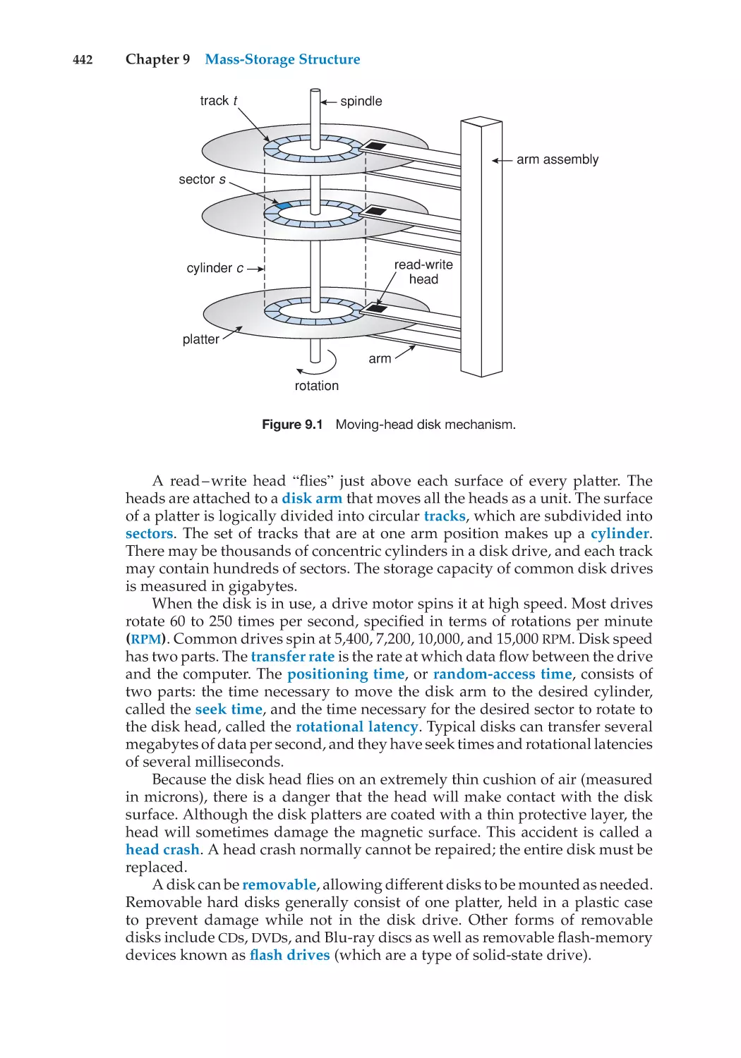
Mass-Storage Structure
9.1 Overview of Mass-Storage
Structure 441
9.2 Disk Structure 444
9.3 Disk Attachment 445
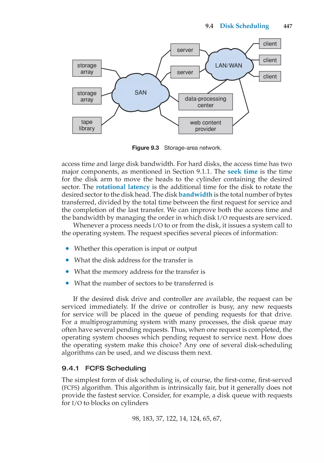
9.4 Disk Scheduling 446
9.5 Disk Management 452
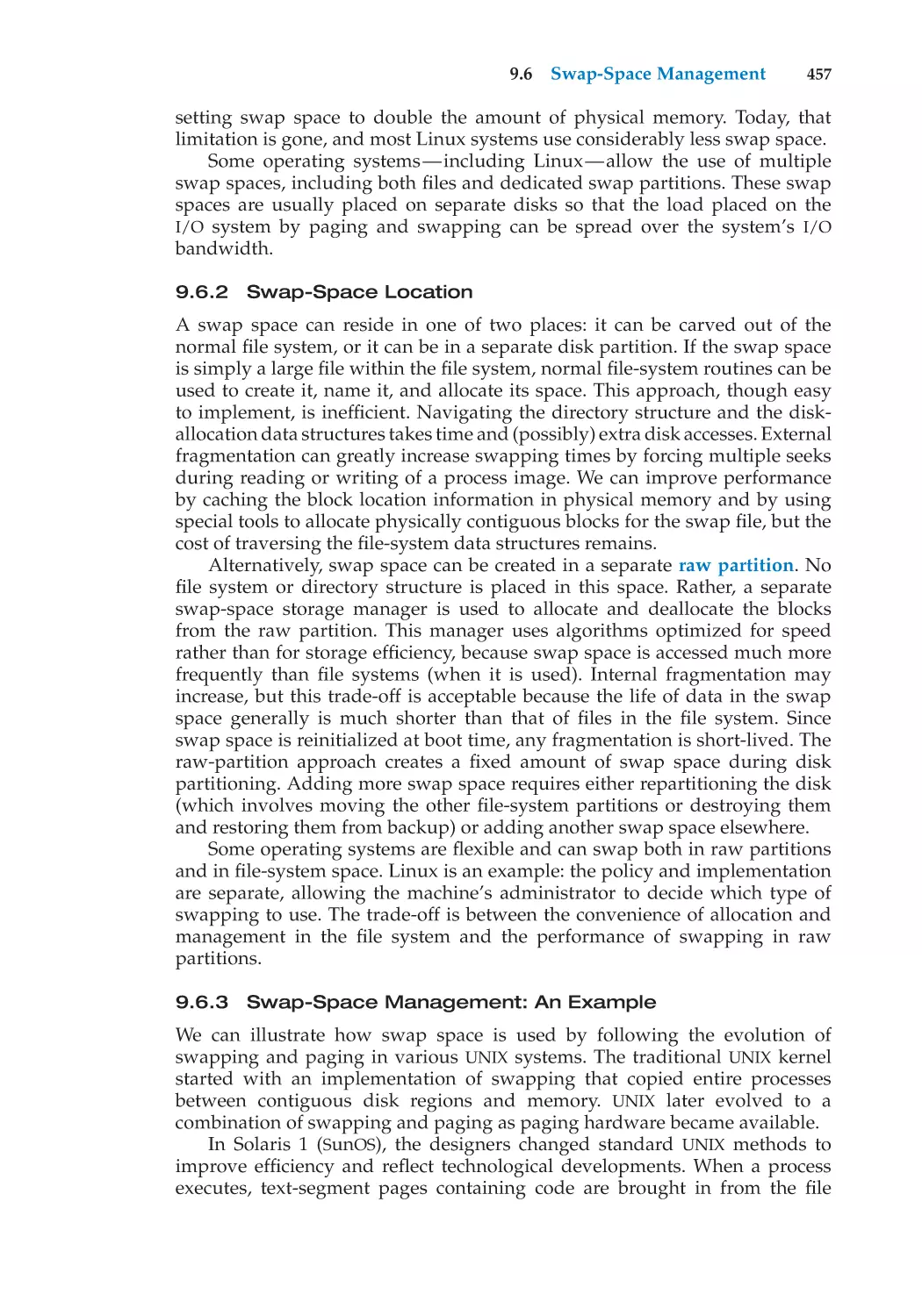
9.6
9.7
9.8
9.9
Swap-Space Management 456
RAID Structure 458
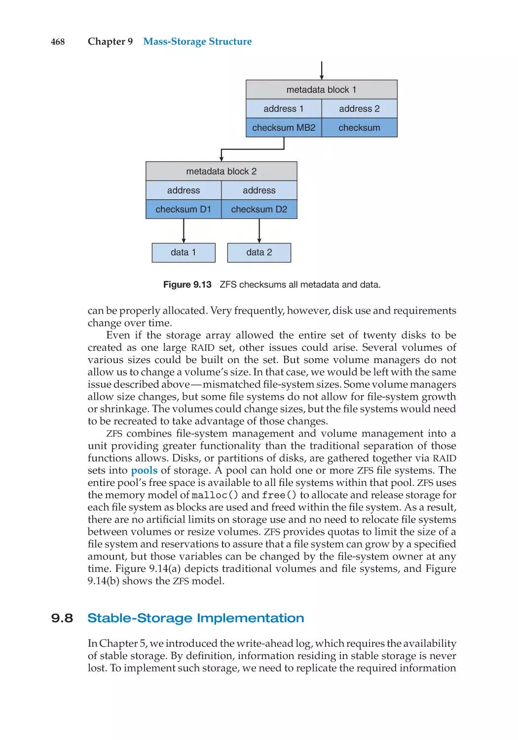
Stable-Storage Implementation 468
Summary 470
Exercises 471
Bibliographical Notes 475
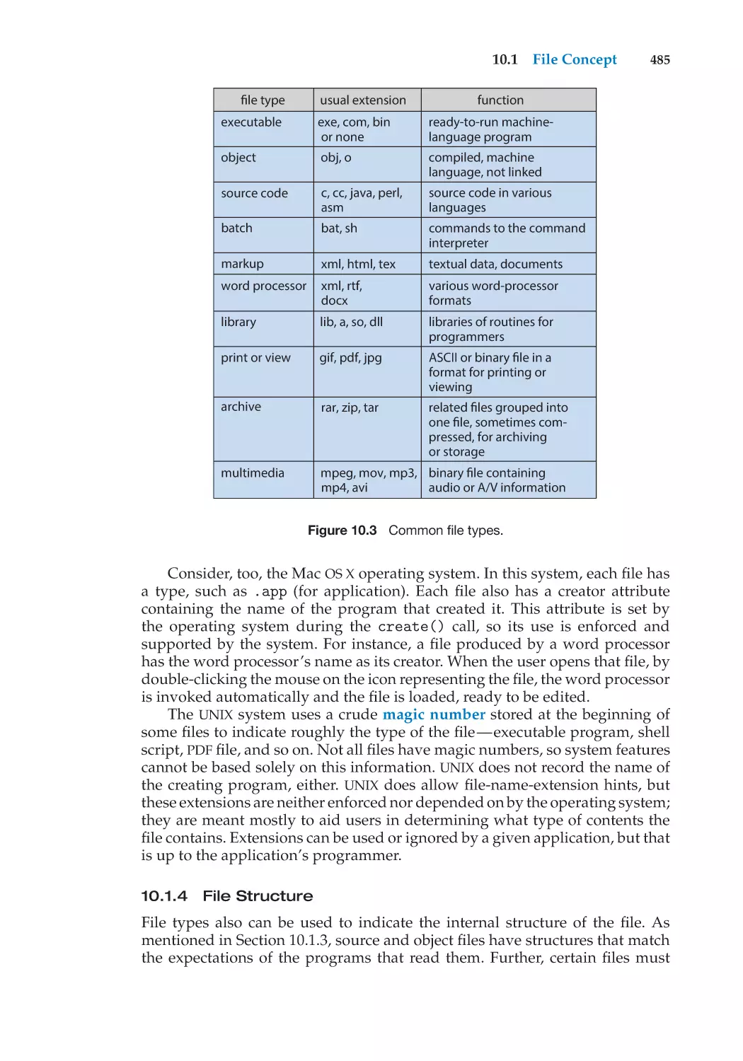
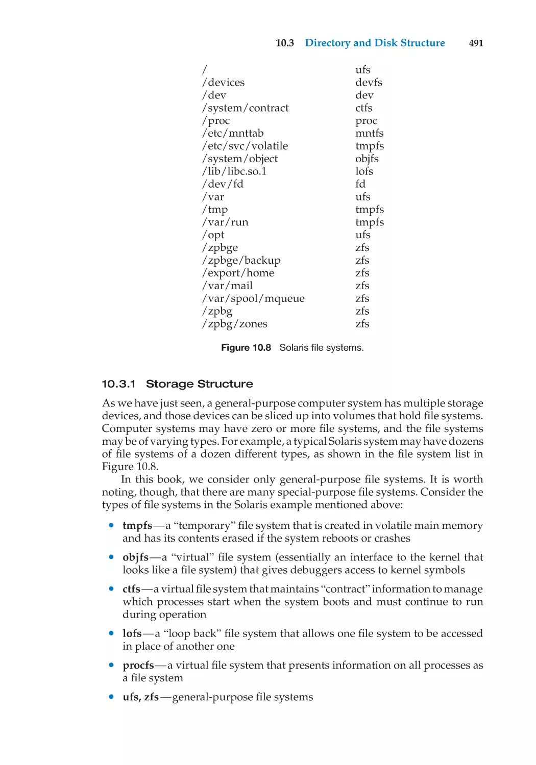
Chapter 10 File-System Interface
10.1
10.2
10.3
10.4
10.5
File Concept 477
Access Methods 487
Directory and Disk Structure
File-System Mounting 500
File Sharing 502
489
10.6 Protection 507
10.7 Summary 512
Exercises 513
Bibliographical Notes 515
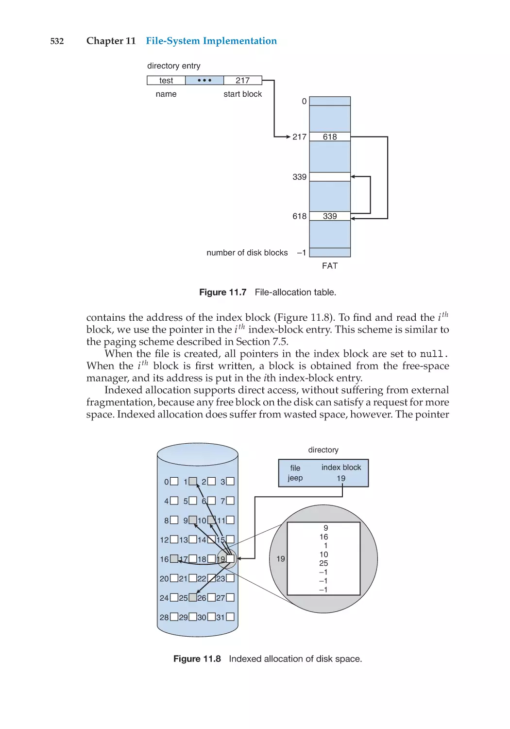
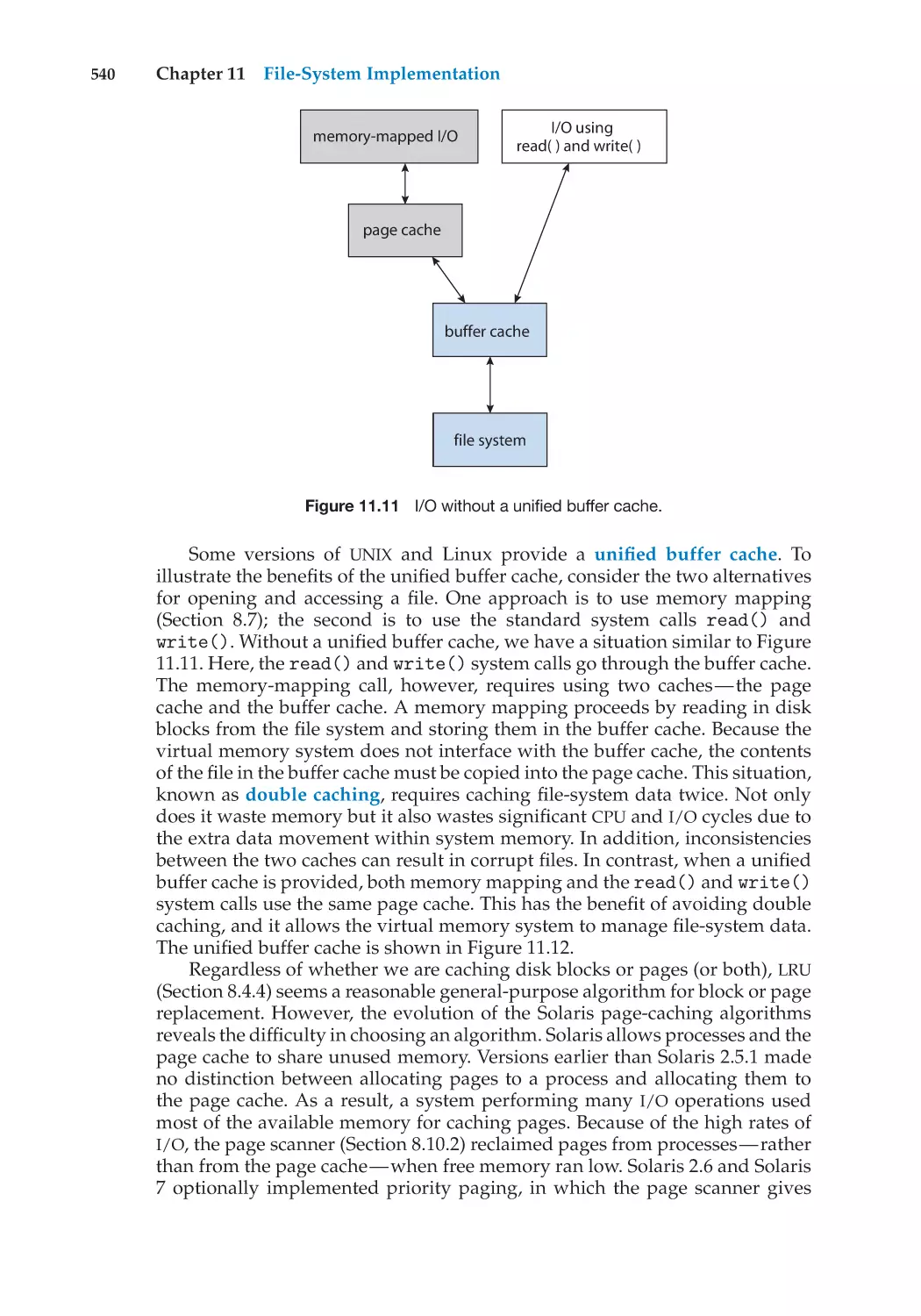
Chapter 11 File-System Implementation
11.1
11.2
11.3
11.4
11.5
11.6
File-System Structure 517
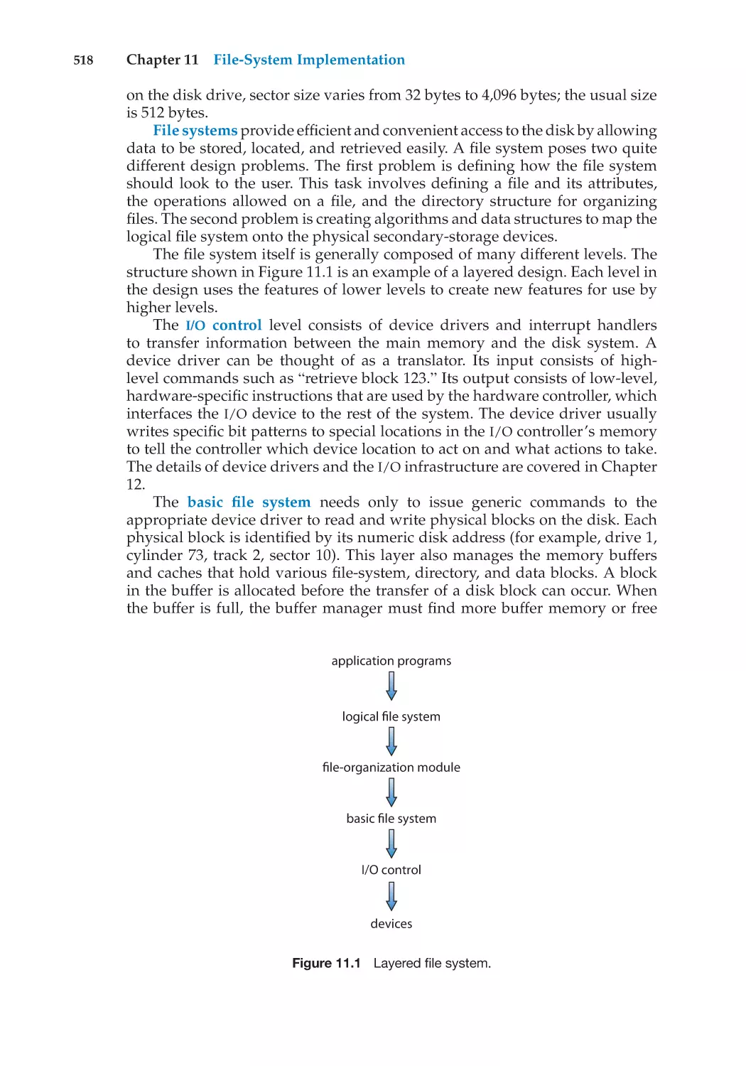
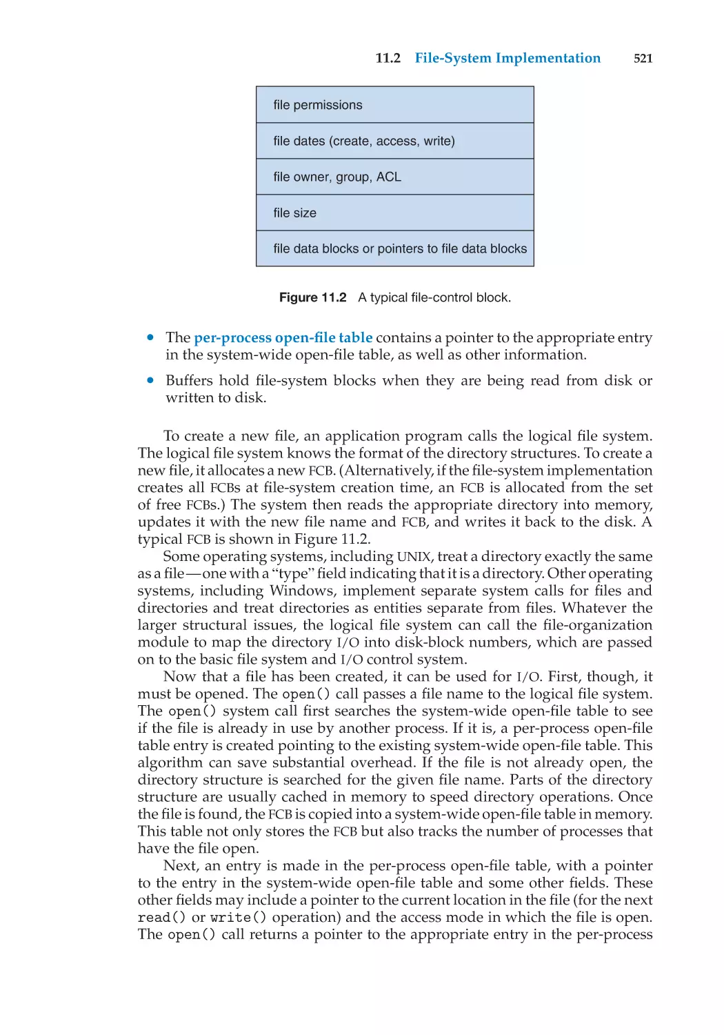
File-System Implementation 520
Directory Implementation 526
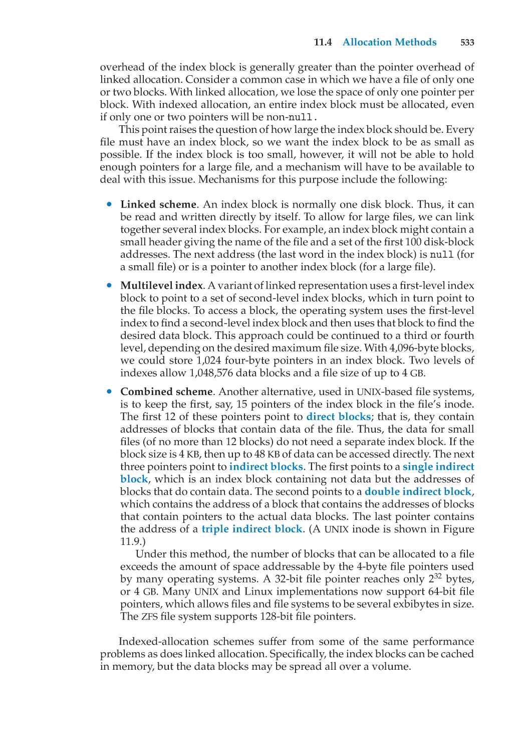
Allocation Methods 527
Free-Space Management 535
Efficiency and Performance 538
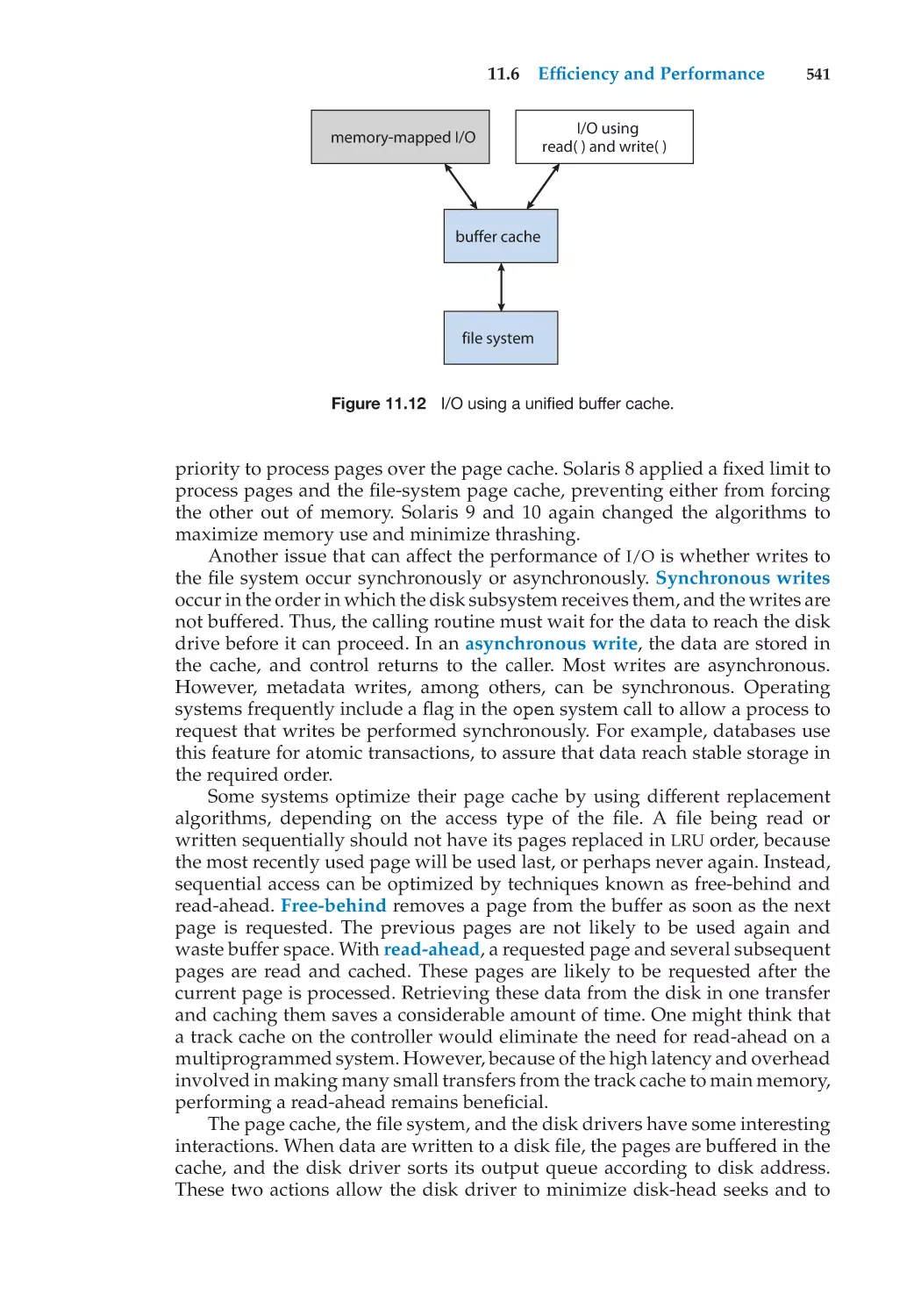
11.7
11.8
11.9
11.10
Recovery 542
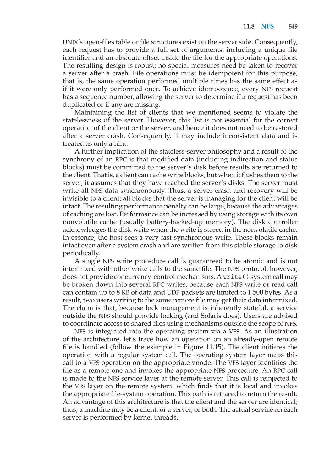
NFS 545
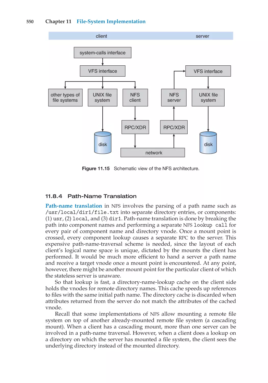
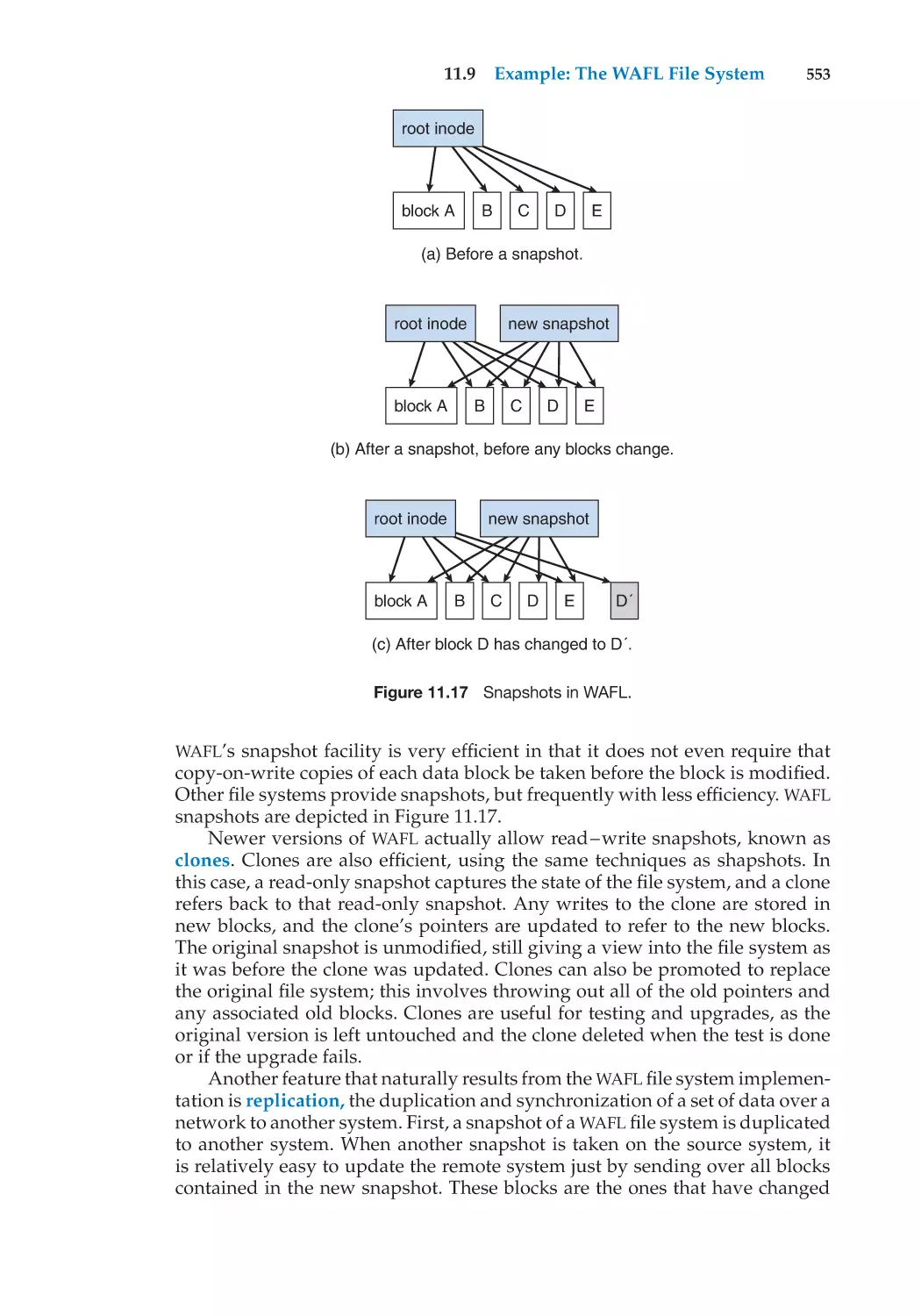
Example: The WAFL File System
Summary 554
Exercises 555
Bibliographical Notes 559
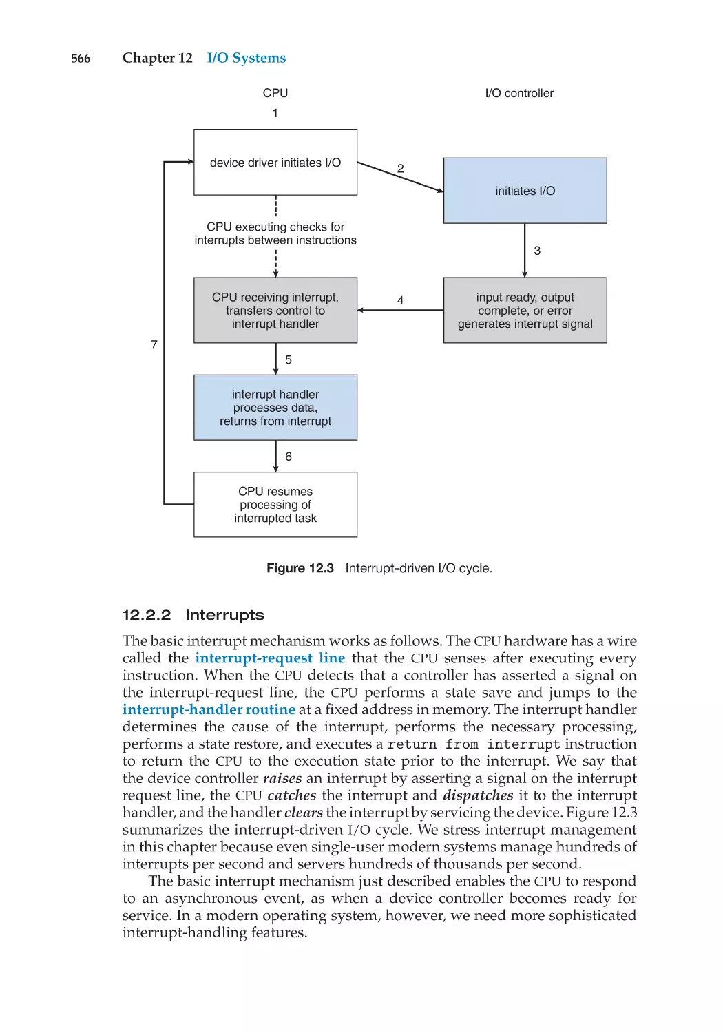
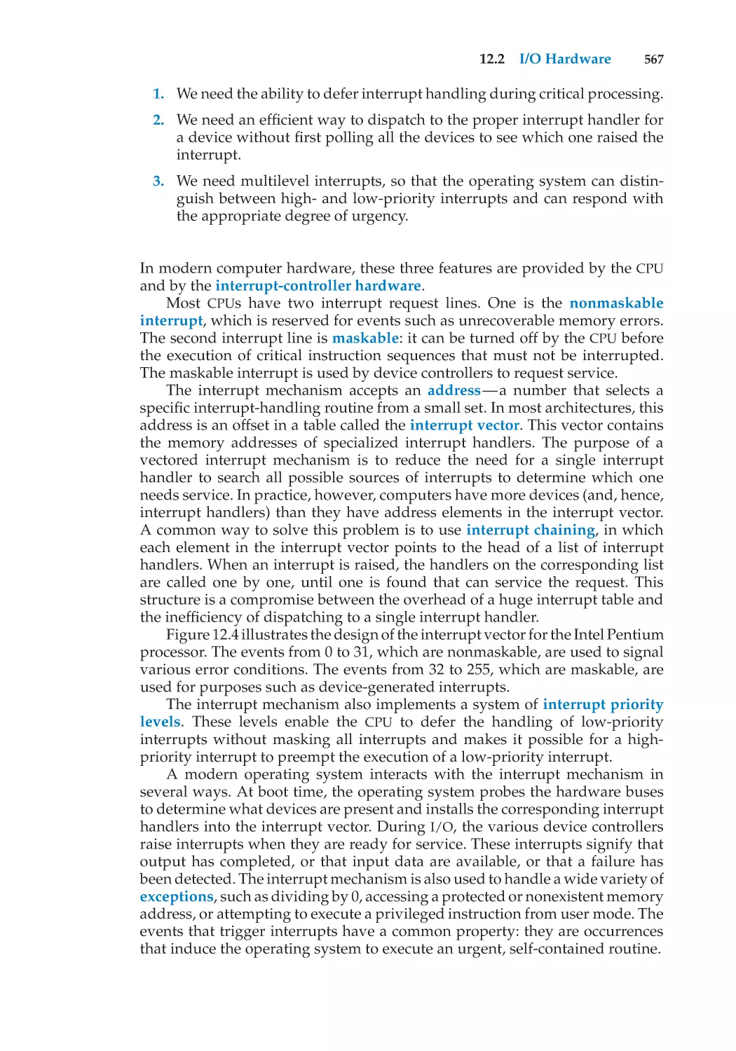
Chapter 12 I/O Systems
12.1
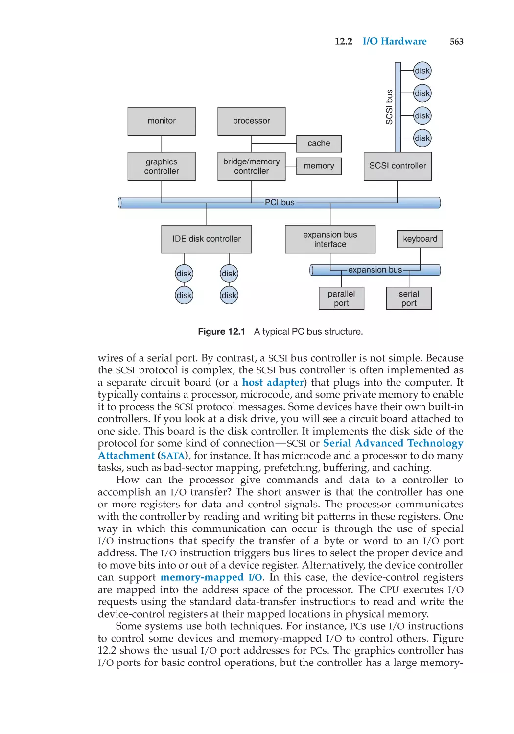
12.2
12.3
12.4
12.5
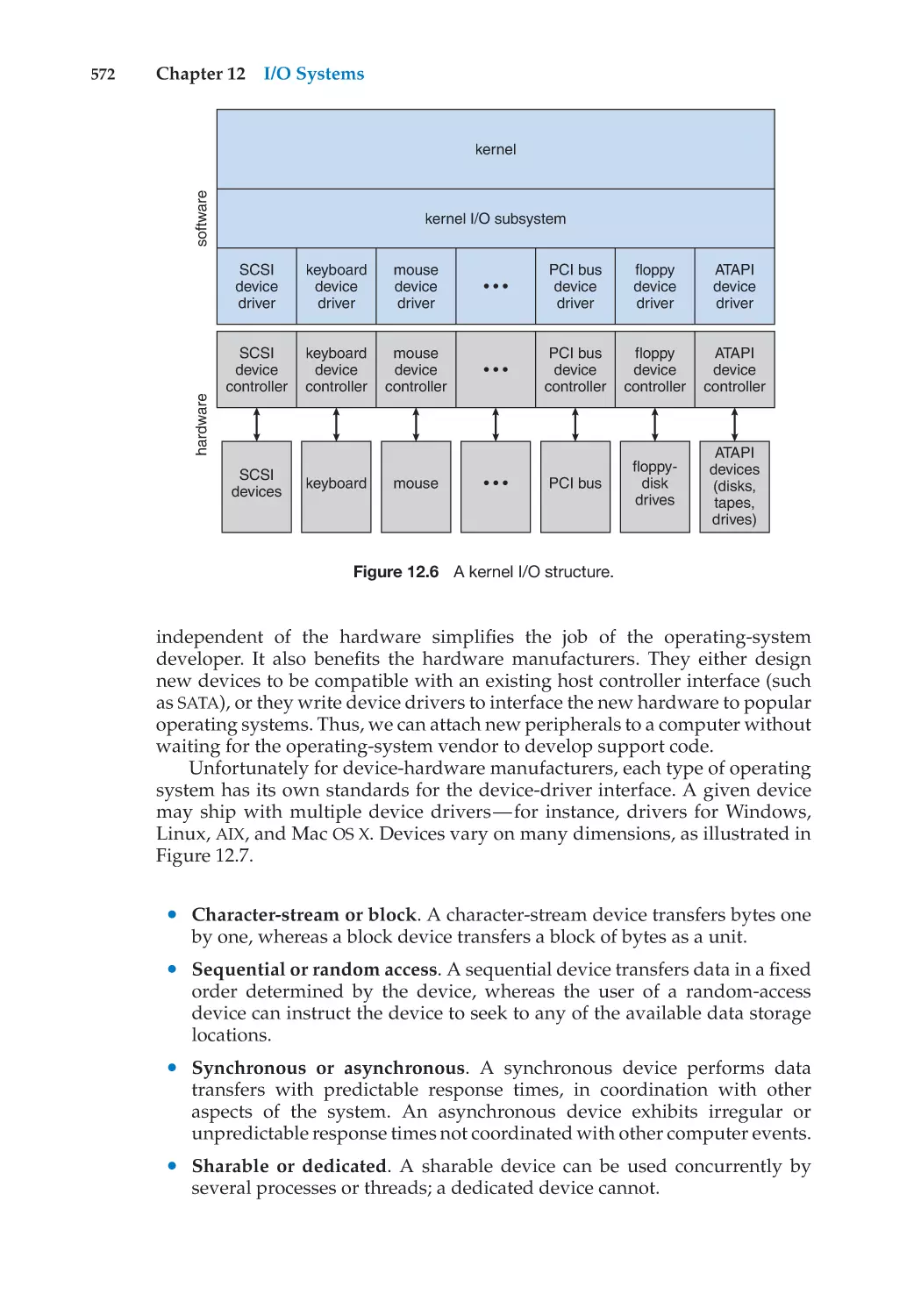
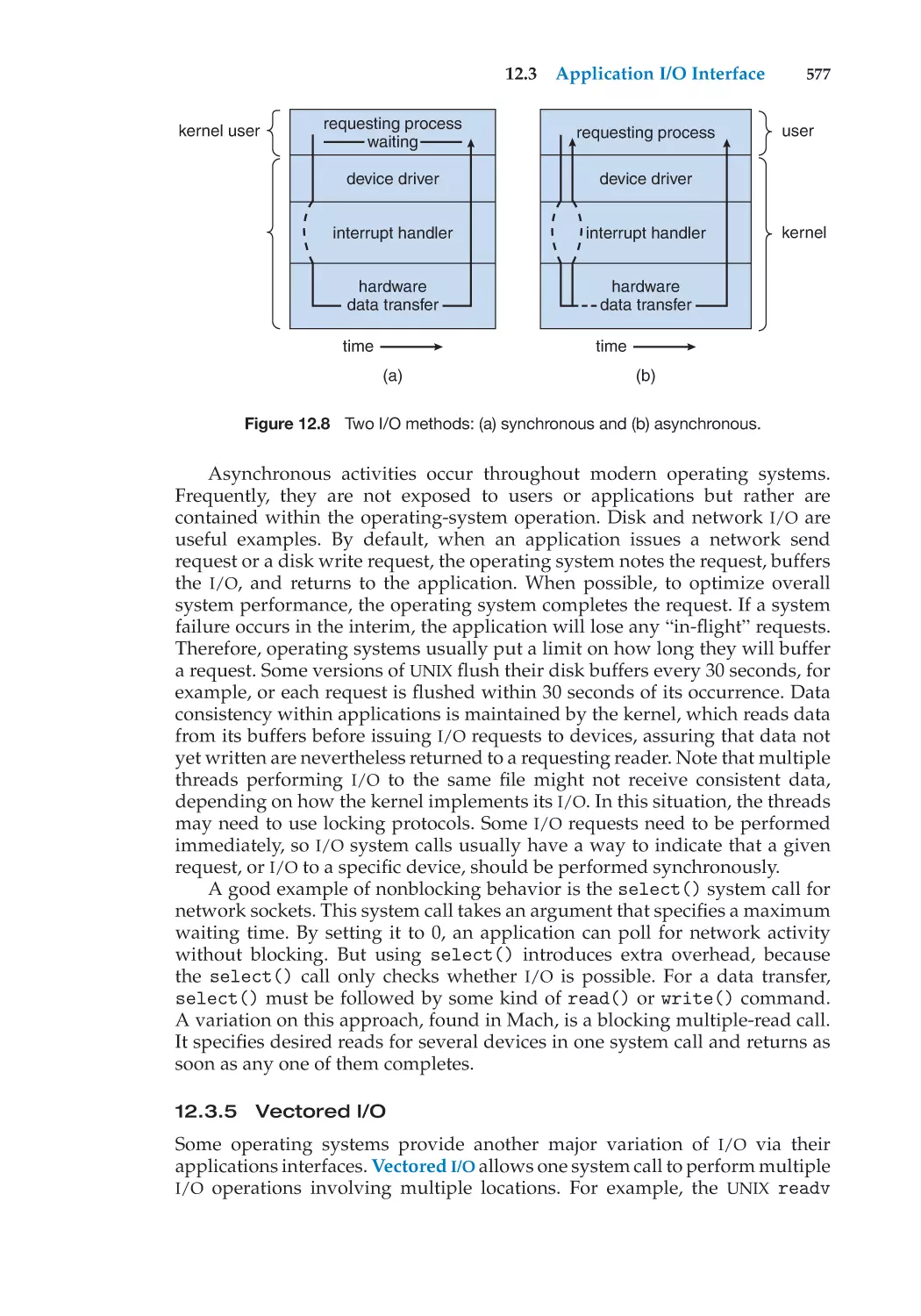
Overview 561
I/O Hardware 562
Application I/O Interface 571
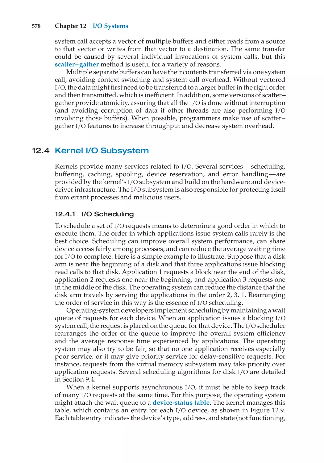
Kernel I/O Subsystem 578
Transforming I/O Requests to
Hardware Operations 586
PART FIVE
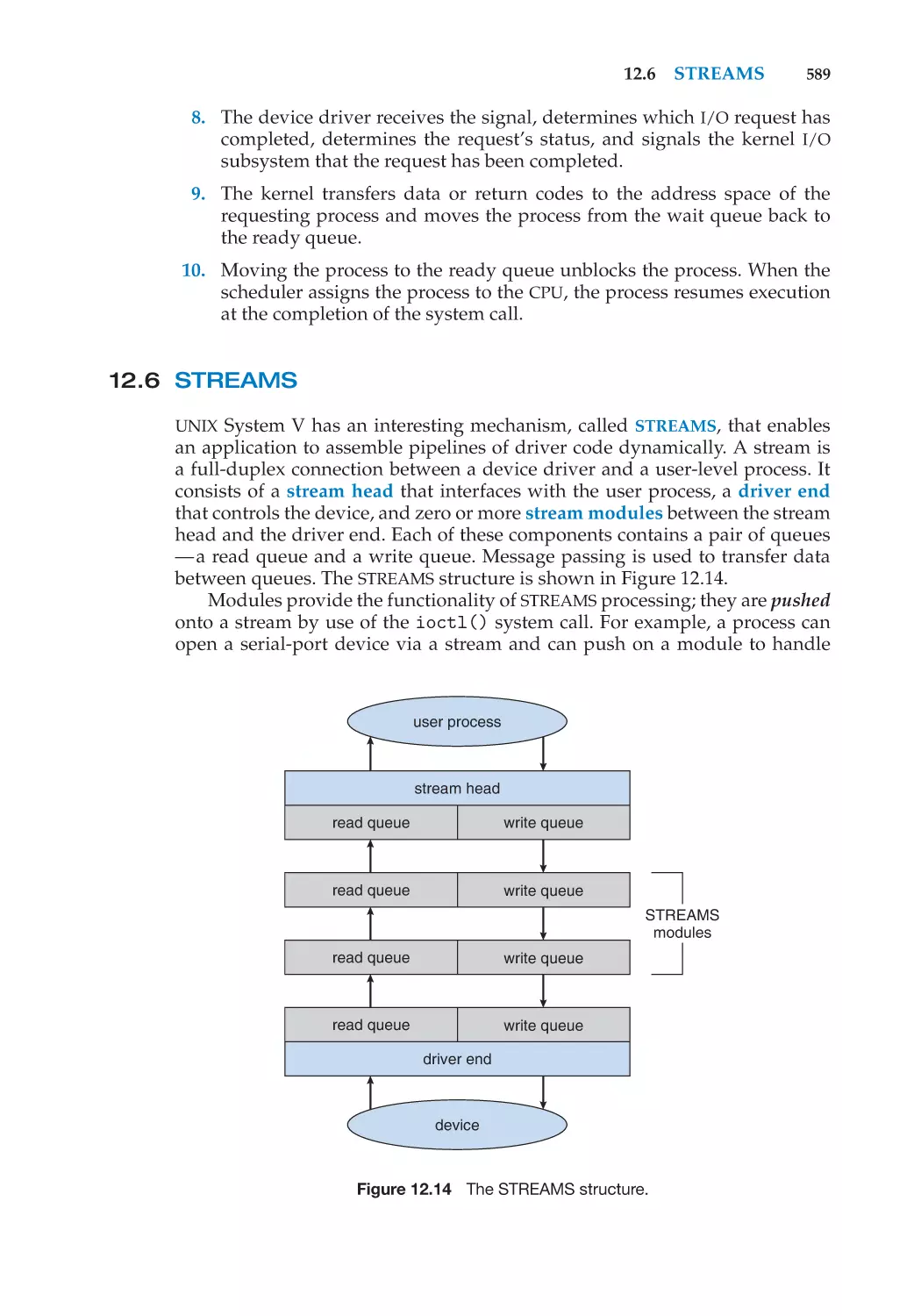
12.6 STREAMS 589
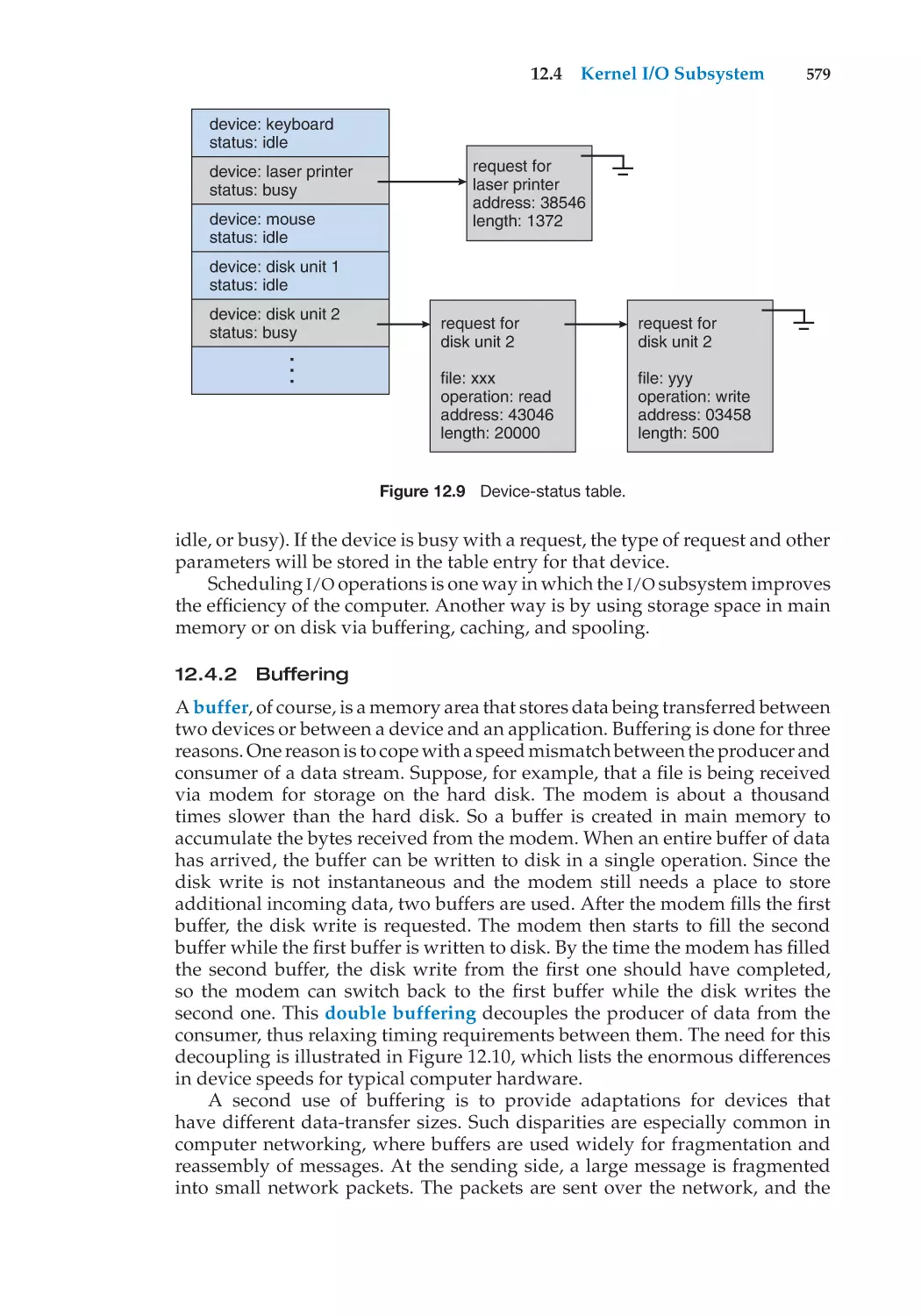
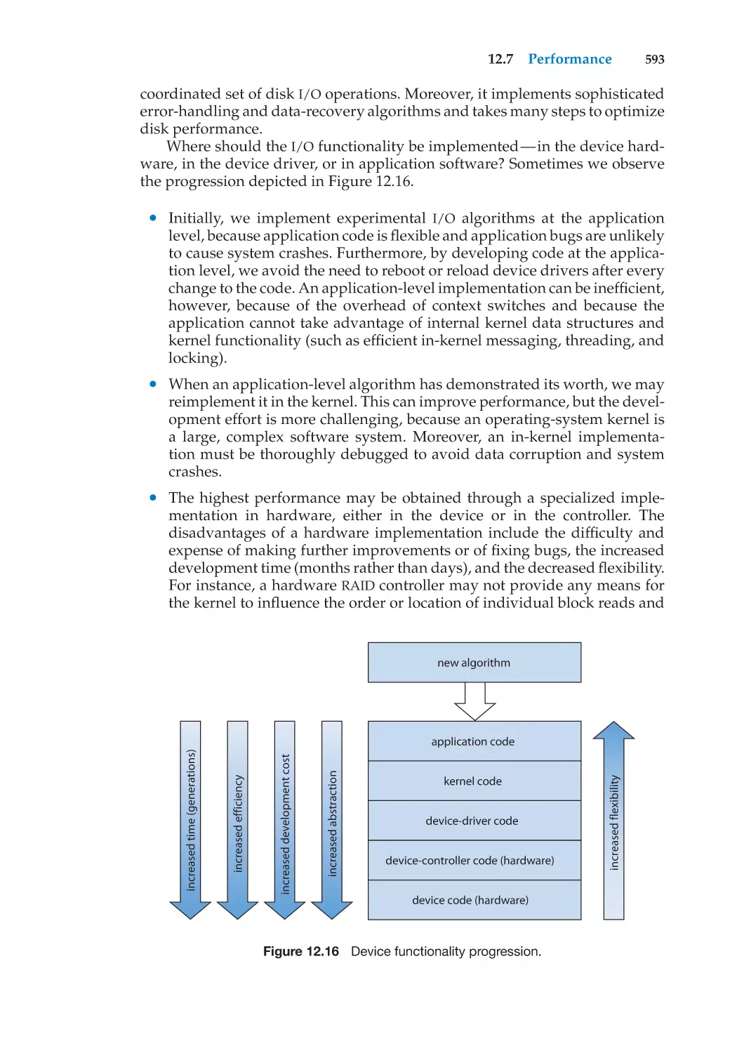
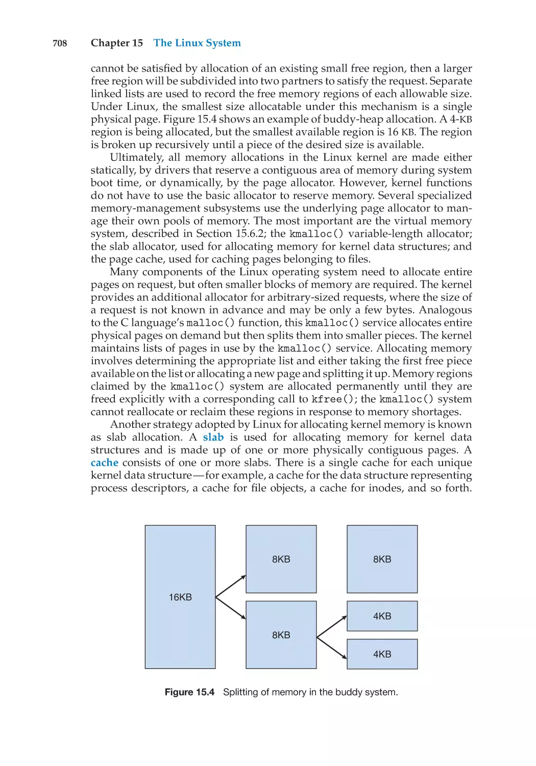
12.7 Performance 590
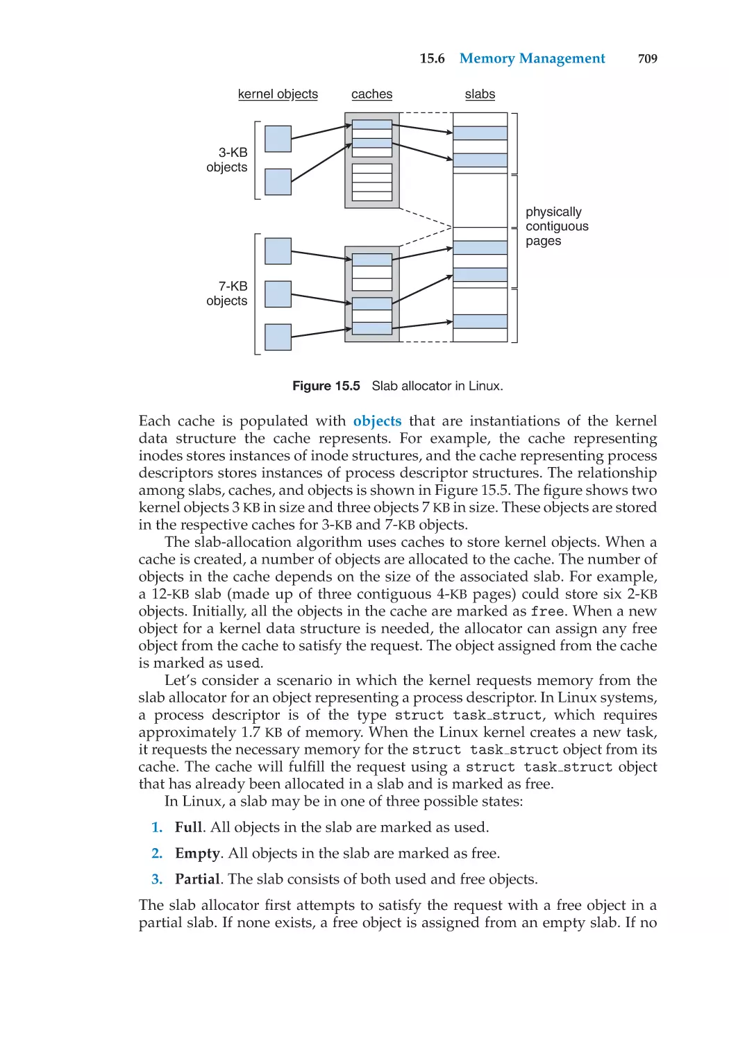
12.8 Summary 594
Exercises 594
Bibliographical Notes 596
PROTECTION AND SECURITY
Chapter 13 Protection
13.1
13.2
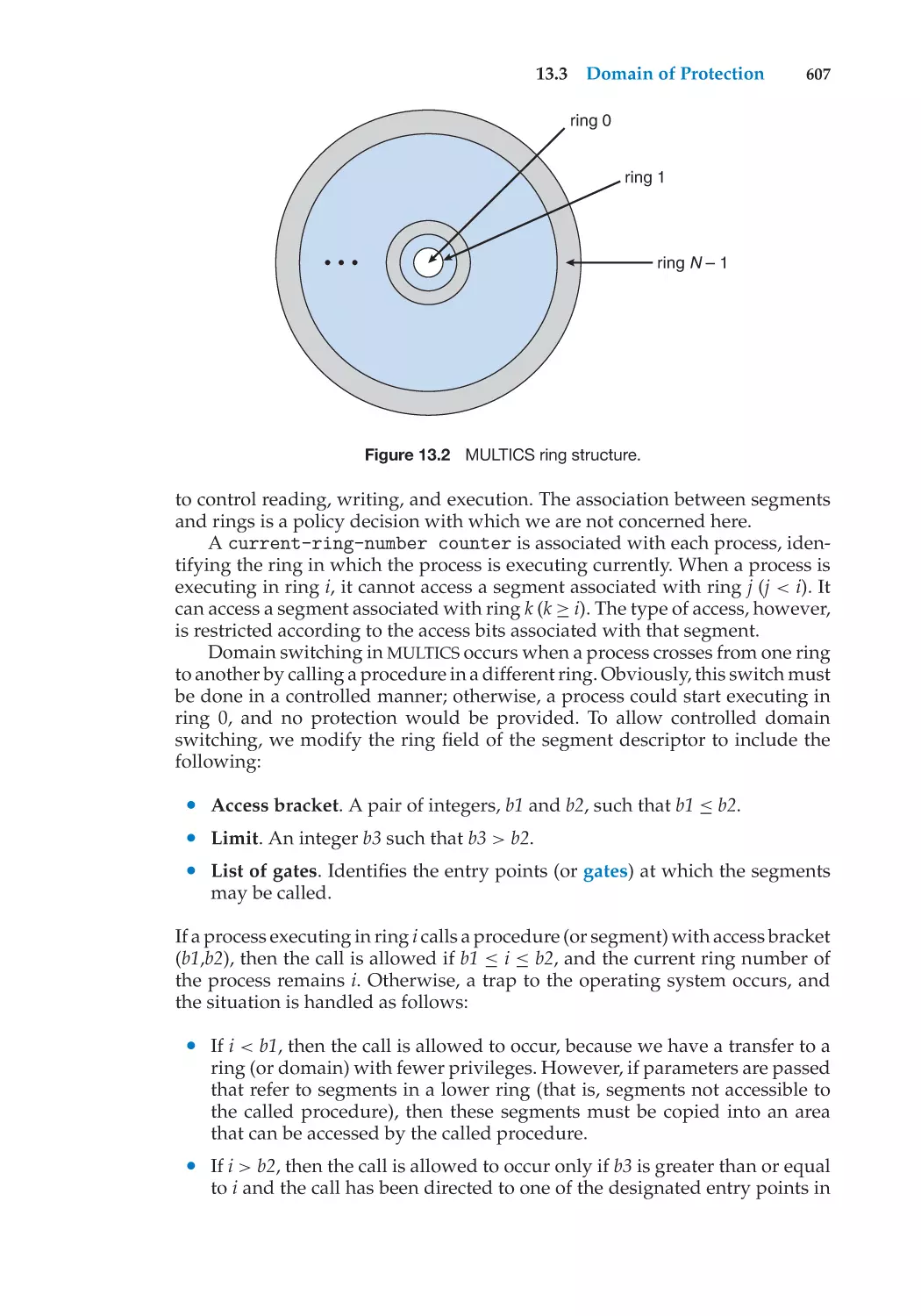
13.3
13.4
13.5
Goals of Protection 601
Principles of Protection 602
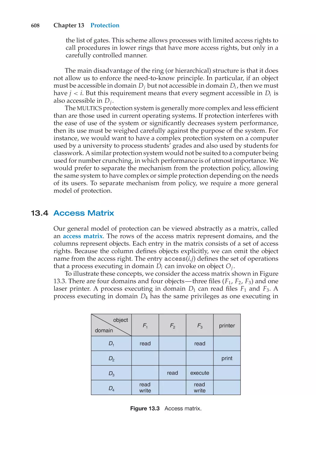
Domain of Protection 603
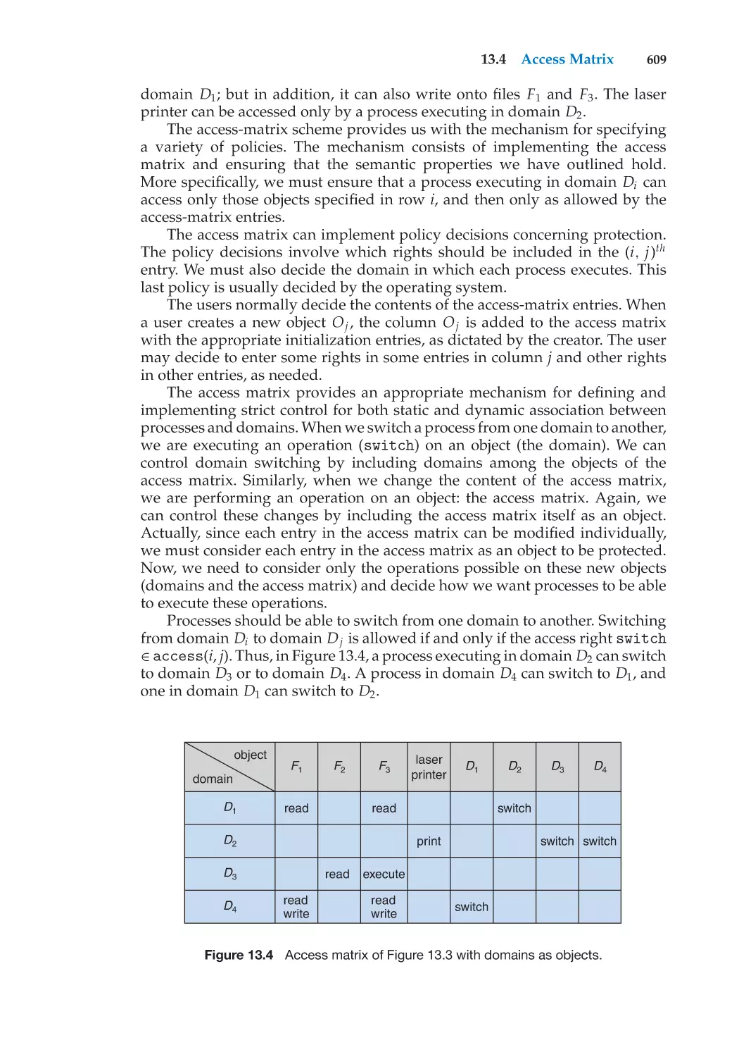
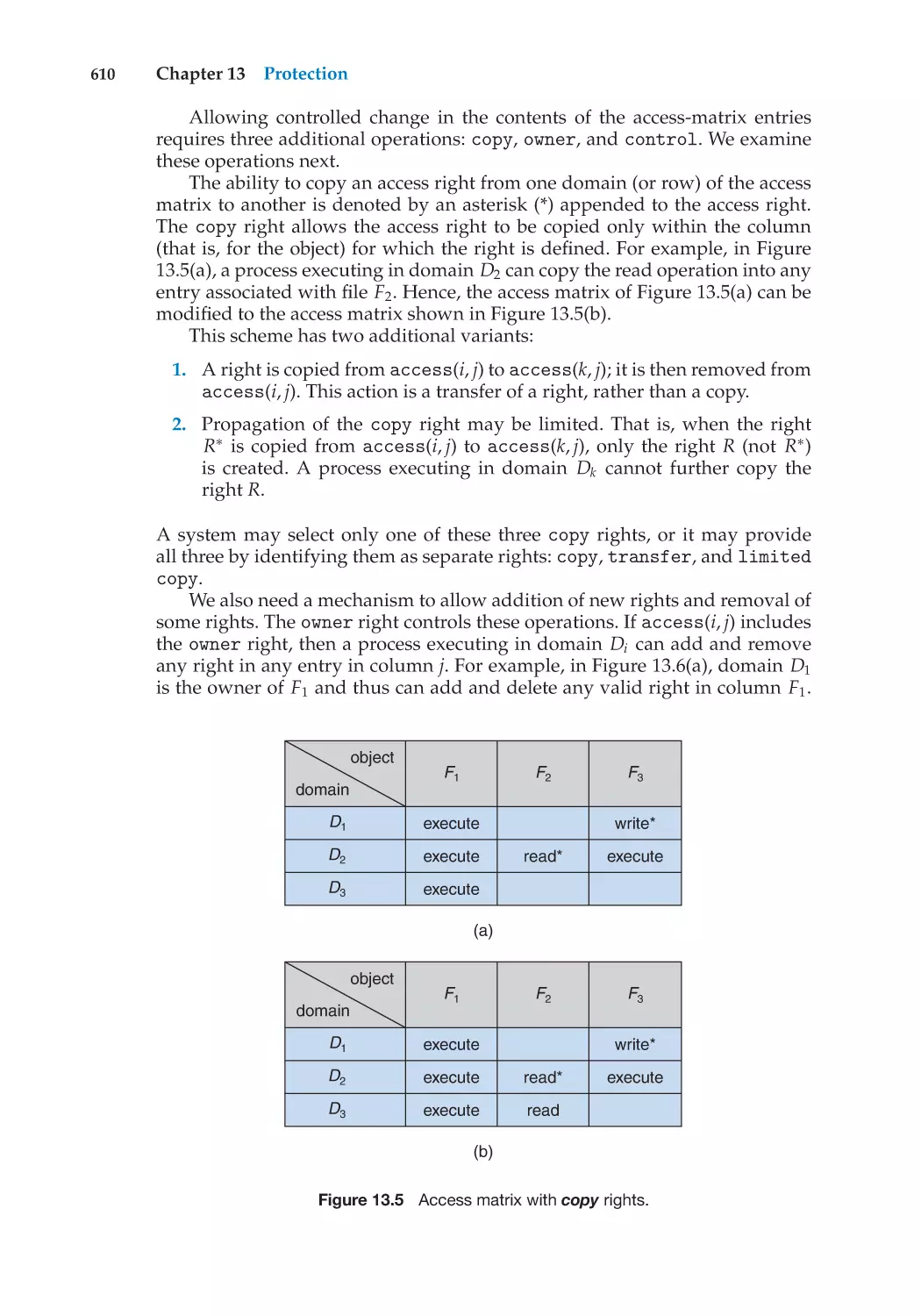
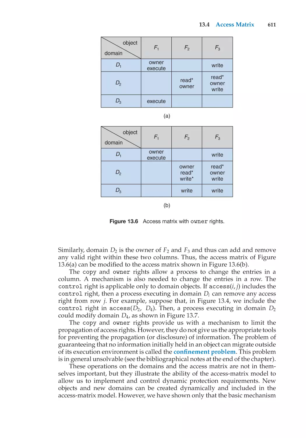
Access Matrix 608
Implementation of the Access
Matrix 612
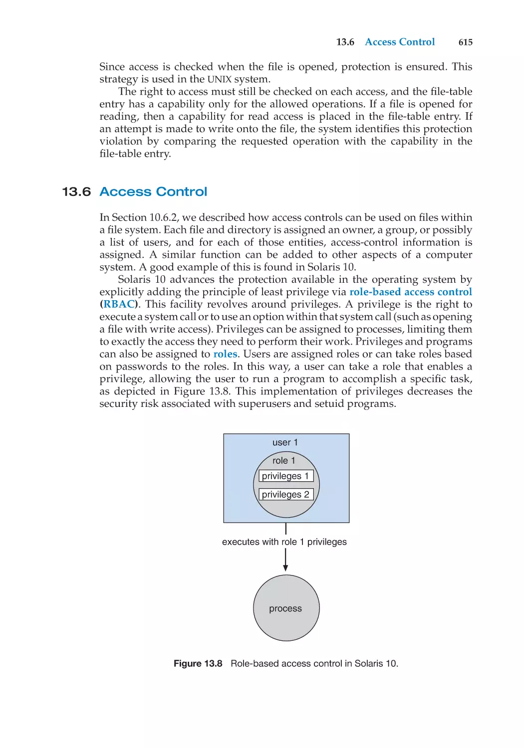
13.6 Access Control 615
13.7
13.8
13.9
13.10
Revocation of Access Rights 616
Capability-Based Systems 617
Language-Based Protection 620
Summary 625
Exercises 626
Bibliographical Notes 628
551
xx
Contents
Chapter 14
14.1
14.2
14.3
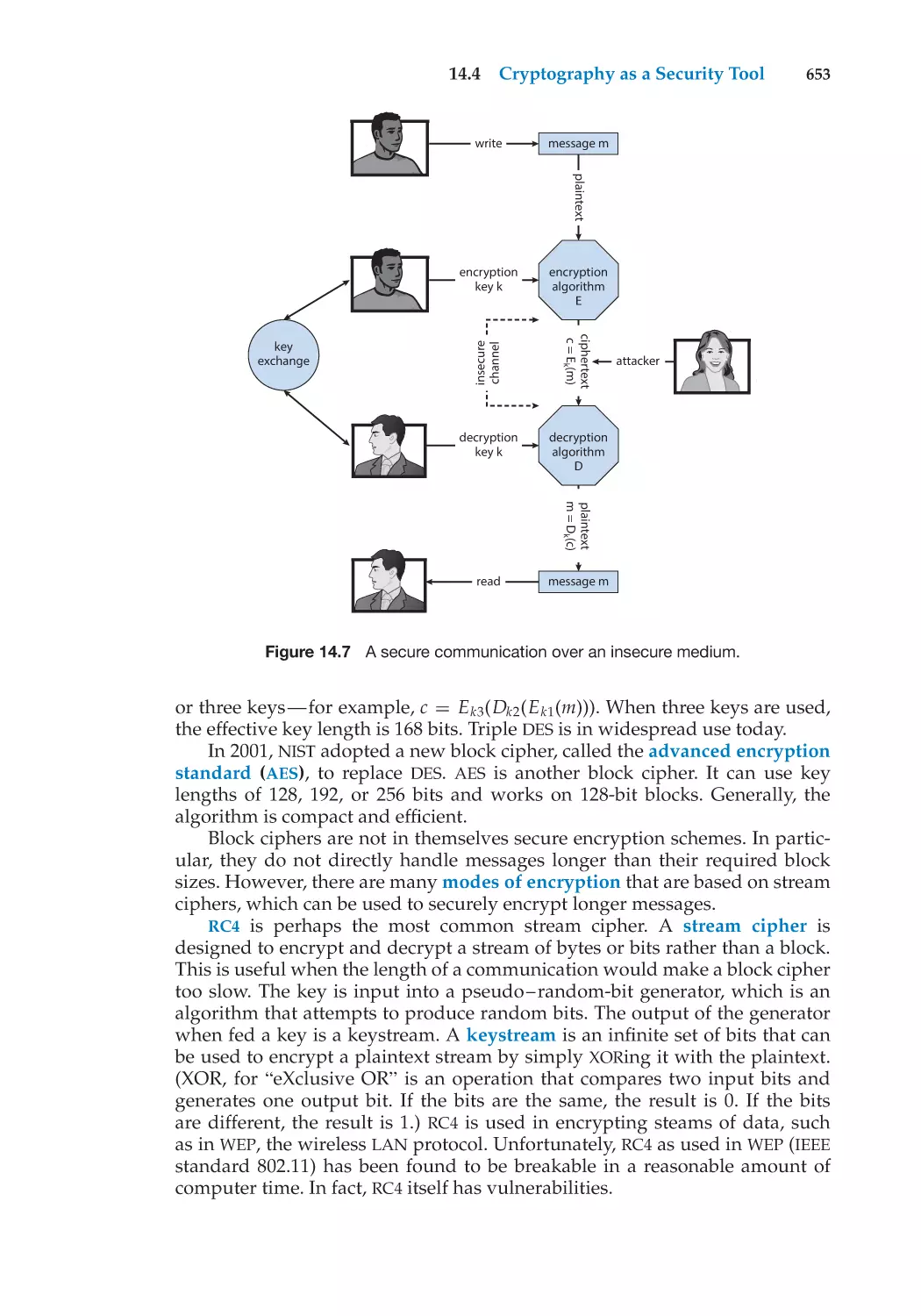
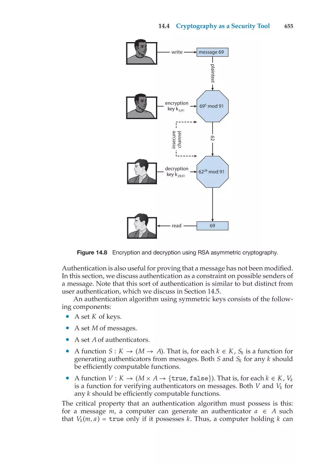
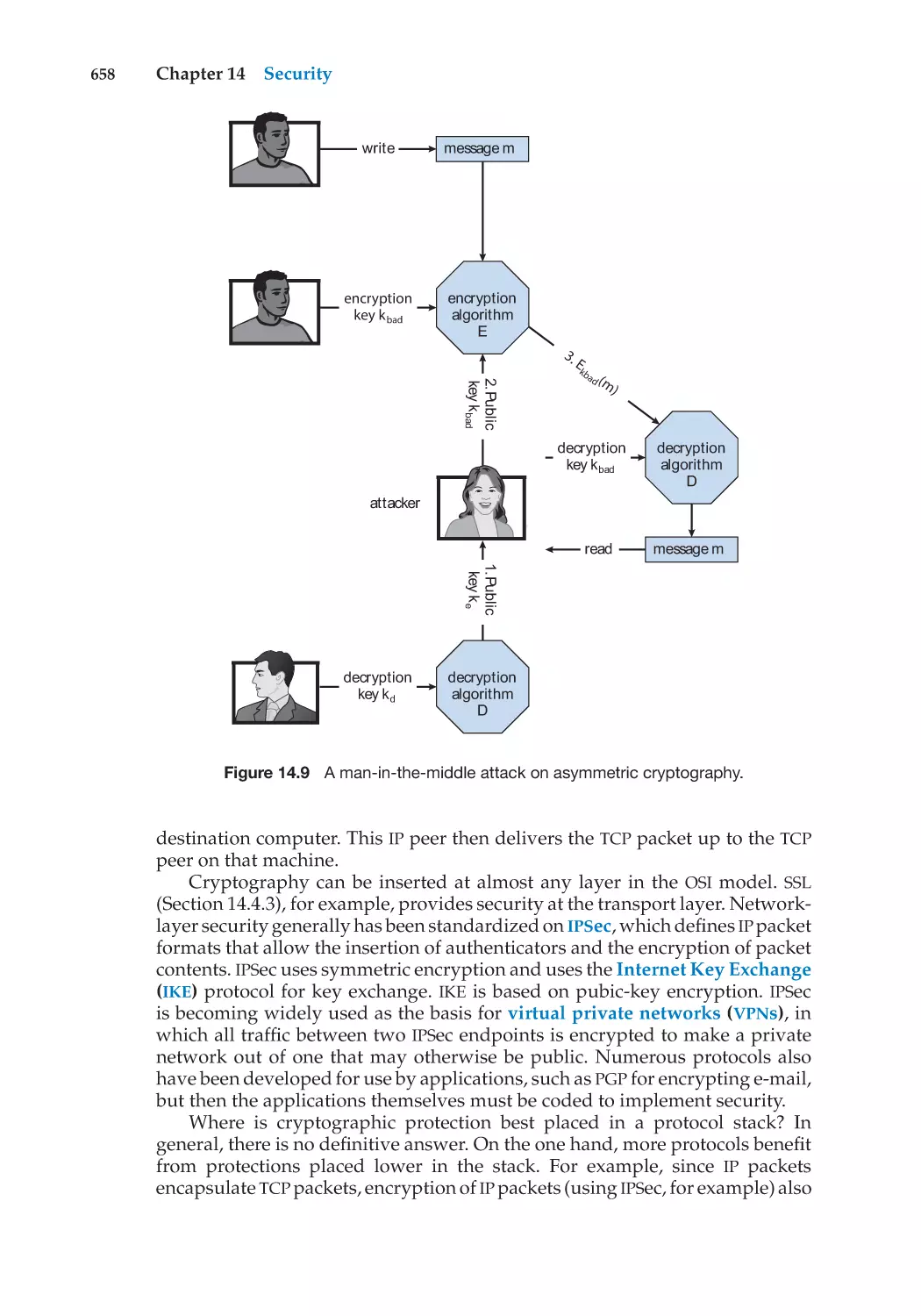
14.4
14.5
14.6
14.7
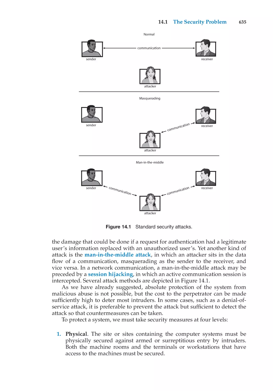
The Security Problem 633
14.8 Computer-Security
Program Threats 637
Classifications 674
System and Network Threats 645
14.9 An Example: Windows 7 675
Cryptography as a Security Tool 650 14.10 Summary 677
User Authentication 661
Exercises 678
Implementing Security Defenses 665
Bibliographical Notes 680
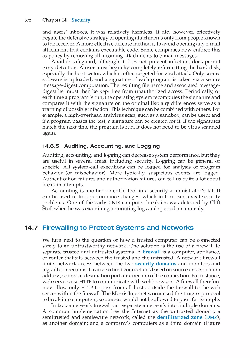
Firewalling to Protect Systems and
Networks 672
PART SIX
Chapter 15
15.1
15.2
15.3
15.4
15.5
15.6
15.7
CASE STUDIES
The Linux System
Linux History 687
Design Principles 692
Kernel Modules 695
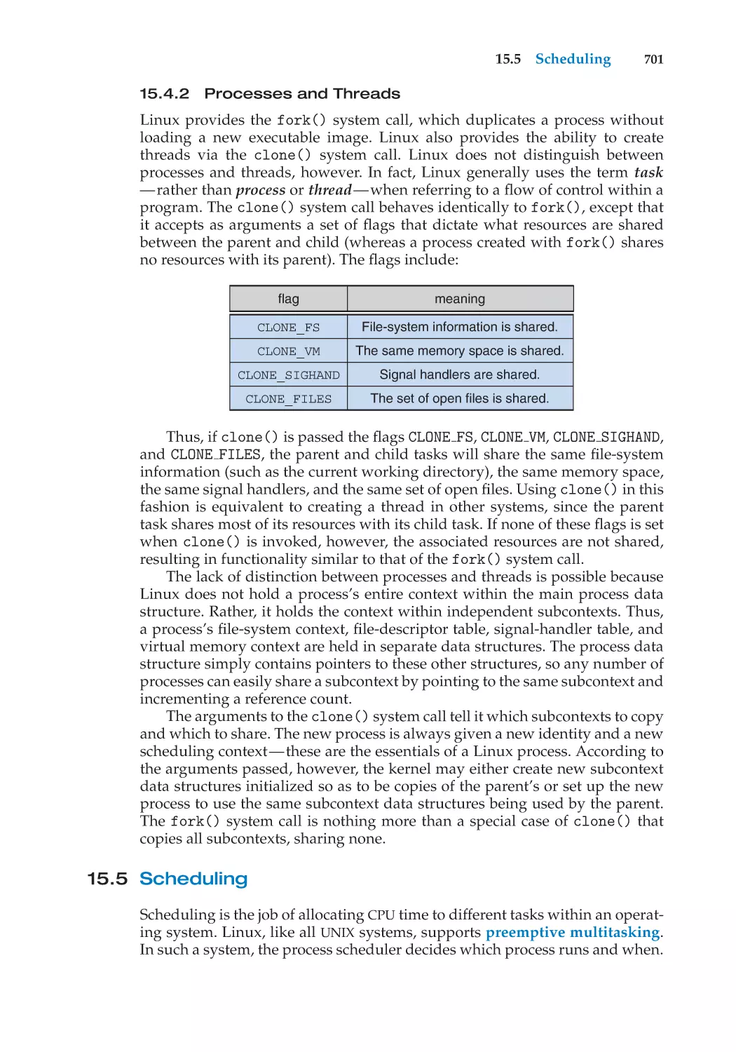
Process Management 698
Scheduling 701
Memory Management 706
File Systems 715
Appendix A
A.1
A.2
A.3
A.4
A.5
A.6
Security
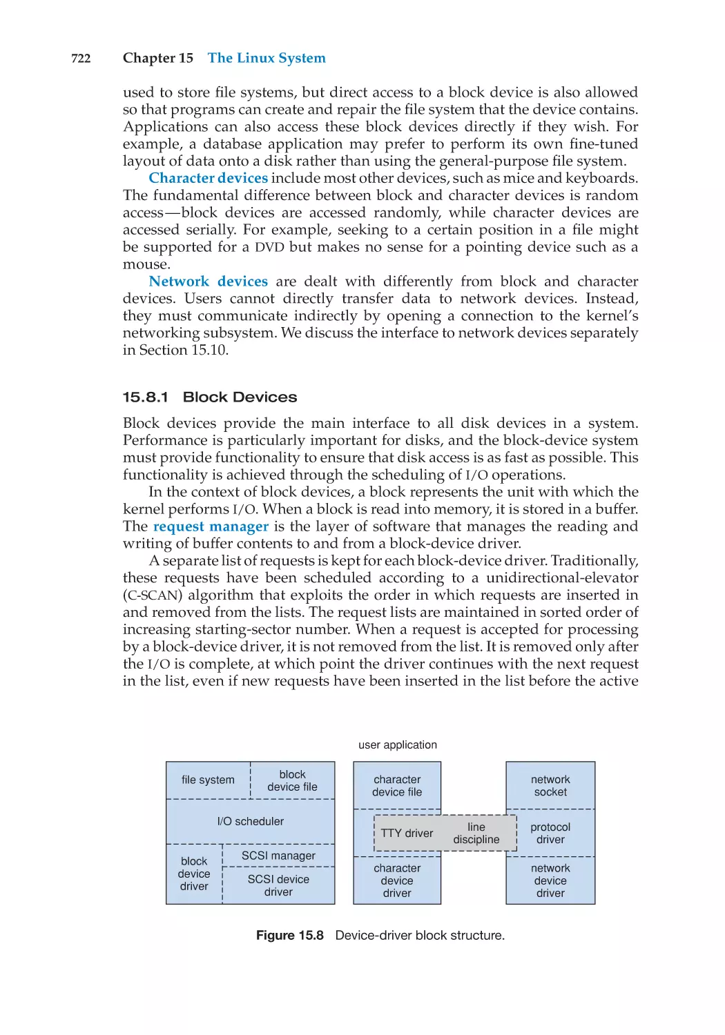
15.8
15.9
15.10
15.11
15.12
Input and Output 721
Interprocess Communication
Network Structure 725
Security 727
Summary 730
Exercises 731
Bibliographical Notes 733
BSD UNIX (contents online)
UNIX History A1
Design Principles A6
Programmer Interface A8
User Interface A15
Process Management A18
Memory Management A22
A.7
A.8
A.9
A.10
File System A25
I/O System A32
Interprocess Communication A36
Summary A41
Exercises A42
Bibliographical Notes A42
Appendix B The Mach System (contents online)
B.1
B.2
B.3
B.4
B.5
B.6
History of the Mach System B1
Design Principles B3
System Components B4
Process Management B7
Interprocess Communication B13
Memory Management B18
Index 735
724
B.7 Programmer Interface B
section.17.7
B.8 Summary B24
Exercises B25
Bibliographical Notes B26
Part One
Overview
An operating system acts as an intermediary between the user of a
computer and the computer hardware. The purpose of an operating
system is to provide an environment in which a user can execute
programs in a convenient and efficient manner.
An operating system is software that manages the computer hardware. The hardware must provide appropriate mechanisms to ensure the
correct operation of the computer system and to prevent user programs
from interfering with the proper operation of the system.
Internally, operating systems vary greatly in their makeup, since they
are organized along many different lines. The design of a new operating
system is a major task. It is important that the goals of the system be well
defined before the design begins. These goals form the basis for choices
among various algorithms and strategies.
Because an operating system is large and complex, it must be created
piece by piece. Each of these pieces should be a well-delineated portion
of the system, with carefully defined inputs, outputs, and functions.
This page is intentionally left blank
1
CHAPTER
Introduction
An operating system is a program that manages a computer’s hardware. It
also provides a basis for application programs and acts as an intermediary
between the computer user and the computer hardware. An amazing aspect of
operating systems is how they vary in accomplishing these tasks. Mainframe
operating systems are designed primarily to optimize utilization of hardware.
Personal computer (PC) operating systems support complex games, business
applications, and everything in between. Operating systems for mobile computers provide an environment in which a user can easily interface with the
computer to execute programs. Thus, some operating systems are designed to
be convenient, others to be efficient, and others to be some combination of the
two.
Before we can explore the details of computer system operation, we need to
know something about system structure. We thus discuss the basic functions
of system startup, I/O, and storage early in this chapter. We also describe
the basic computer architecture that makes it possible to write a functional
operating system.
Because an operating system is large and complex, it must be created
piece by piece. Each of these pieces should be a well-delineated portion of the
system, with carefully defined inputs, outputs, and functions. In this chapter,
we provide a general overview of the major components of a contemporary
computer system as well as the functions provided by the operating system.
Additionally, we cover several other topics to help set the stage for the
remainder of this text: data structures used in operating systems, computing
environments, and open-source operating systems.
CHAPTER OBJECTIVES
• To describe the basic organization of computer systems.
• To provide a grand tour of the major components of operating systems.
• To give an overview of the many types of computing environments.
• To explore several open-source operating systems.
3
4
Chapter 1 Introduction
user
1
user
2
user
3
…
user
n
compiler
assembler
text editor
…
database
system
system and application programs
operating system
computer hardware
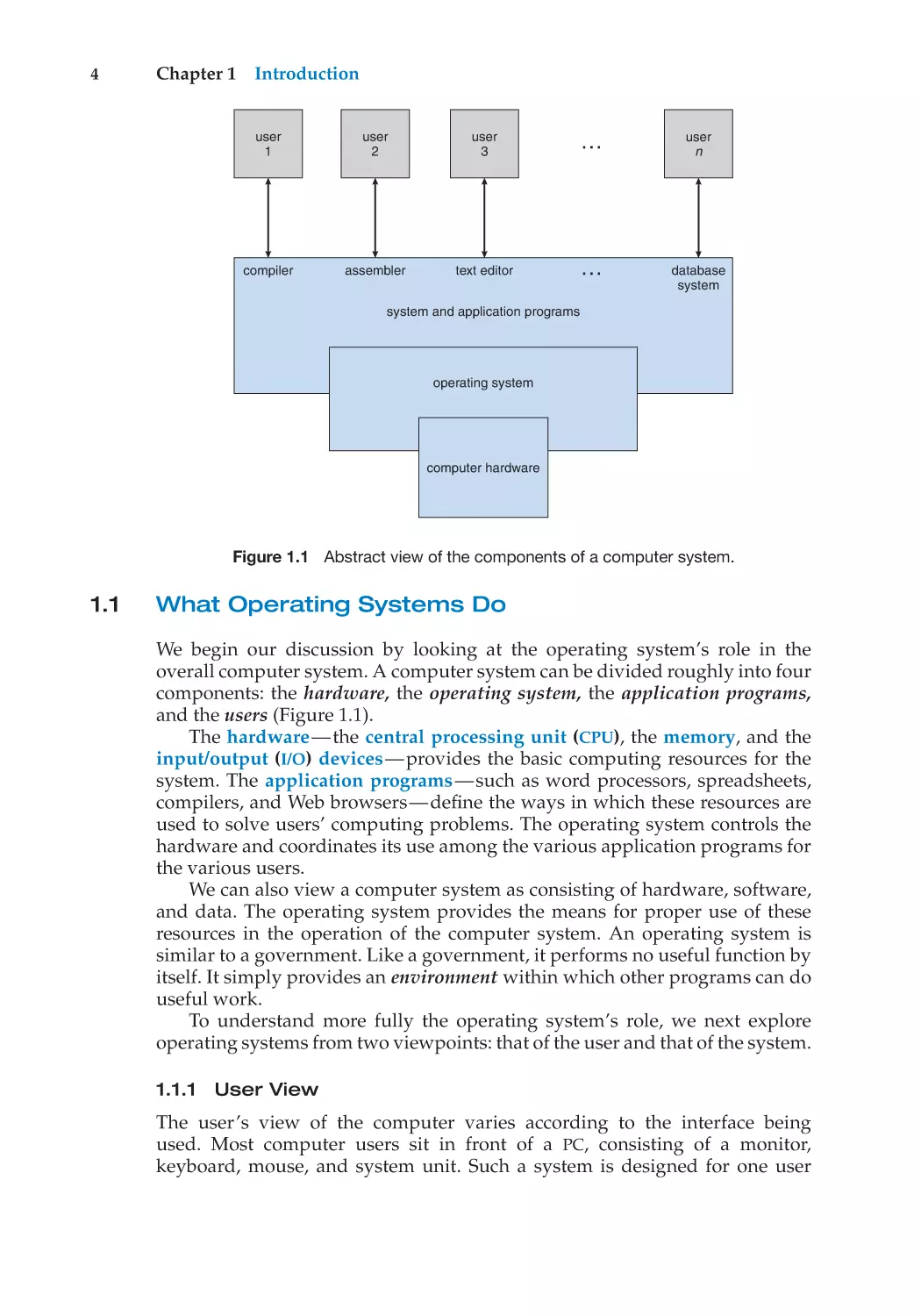
Figure 1.1 Abstract view of the components of a computer system.
1.1
What Operating Systems Do
We begin our discussion by looking at the operating system’s role in the
overall computer system. A computer system can be divided roughly into four
components: the hardware, the operating system, the application programs,
and the users (Figure 1.1).
The hardware—the central processing unit (CPU), the memory, and the
input/output (I/O) devices—provides the basic computing resources for the
system. The application programs—such as word processors, spreadsheets,
compilers, and Web browsers—define the ways in which these resources are
used to solve users’ computing problems. The operating system controls the
hardware and coordinates its use among the various application programs for
the various users.
We can also view a computer system as consisting of hardware, software,
and data. The operating system provides the means for proper use of these
resources in the operation of the computer system. An operating system is
similar to a government. Like a government, it performs no useful function by
itself. It simply provides an environment within which other programs can do
useful work.
To understand more fully the operating system’s role, we next explore
operating systems from two viewpoints: that of the user and that of the system.
1.1.1
User View
The user’s view of the computer varies according to the interface being
used. Most computer users sit in front of a PC, consisting of a monitor,
keyboard, mouse, and system unit. Such a system is designed for one user
1.1 What Operating Systems Do
5
to monopolize its resources. The goal is to maximize the work (or play) that
the user is performing. In this case, the operating system is designed mostly
for ease of use, with some attention paid to performance and none paid
to resource utilization —how various hardware and software resources are
shared. Performance is, of course, important to the user; but such systems
are optimized for the single-user experience rather than the requirements of
multiple users.
In other cases, a user sits at a terminal connected to a mainframe or a
minicomputer. Other users are accessing the same computer through other
terminals. These users share resources and may exchange information. The
operating system in such cases is designed to maximize resource utilization—
to assure that all available CPU time, memory, and I/O are used efficiently and
that no individual user takes more than her fair share.
In still other cases, users sit at workstations connected to networks of
other workstations and servers. These users have dedicated resources at
their disposal, but they also share resources such as networking and servers,
including file, compute, and print servers. Therefore, their operating system is
designed to compromise between individual usability and resource utilization.
Recently, many varieties of mobile computers, such as smartphones and
tablets, have come into fashion. Most mobile computers are standalone units for
individual users. Quite often, they are connected to networks through cellular
or other wireless technologies. Increasingly, these mobile devices are replacing
desktop and laptop computers for people who are primarily interested in
using computers for e-mail and web browsing. The user interface for mobile
computers generally features a touch screen, where the user interacts with the
system by pressing and swiping fingers across the screen rather than using a
physical keyboard and mouse.
Some computers have little or no user view. For example, embedded
computers in home devices and automobiles may have numeric keypads and
may turn indicator lights on or off to show status, but they and their operating
systems are designed primarily to run without user intervention.
1.1.2
System View
From the computer’s point of view, the operating system is the program
most intimately involved with the hardware. In this context, we can view
an operating system as a resource allocator. A computer system has many
resources that may be required to solve a problem: CPU time, memory space,
file-storage space, I/O devices, and so on. The operating system acts as the
manager of these resources. Facing numerous and possibly conflicting requests
for resources, the operating system must decide how to allocate them to specific
programs and users so that it can operate the computer system efficiently and
fairly. As we have seen, resource allocation is especially important where many
users access the same mainframe or minicomputer.
A slightly different view of an operating system emphasizes the need to
control the various I/O devices and user programs. An operating system is a
control program. A control program manages the execution of user programs
to prevent errors and improper use of the computer. It is especially concerned
with the operation and control of I/O devices.
6
Chapter 1 Introduction
1.1.3
Defining Operating Systems
By now, you can probably see that the term operating system covers many roles
and functions. That is the case, at least in part, because of the myriad designs
and uses of computers. Computers are present within toasters, cars, ships,
spacecraft, homes, and businesses. They are the basis for game machines, music
players, cable TV tuners, and industrial control systems. Although computers
have a relatively short history, they have evolved rapidly. Computing started
as an experiment to determine what could be done and quickly moved to
fixed-purpose systems for military uses, such as code breaking and trajectory
plotting, and governmental uses, such as census calculation. Those early
computers evolved into general-purpose, multifunction mainframes, and
that’s when operating systems were born. In the 1960s, Moore’s Law predicted
that the number of transistors on an integrated circuit would double every
eighteen months, and that prediction has held true. Computers gained in
functionality and shrunk in size, leading to a vast number of uses and a vast
number and variety of operating systems.
How, then, can we define what an operating system is? In general, we have
no completely adequate definition of an operating system. Operating systems
exist because they offer a reasonable way to solve the problem of creating a
usable computing system. The fundamental goal of computer systems is to
execute user programs and to make solving user problems easier. Computer
hardware is constructed toward this goal. Since bare hardware alone is not
particularly easy to use, application programs are developed. These programs
require certain common operations, such as those controlling the I/O devices.
The common functions of controlling and allocating resources are then brought
together into one piece of software: the operating system.
In addition, we have no universally accepted definition of what is part of the
operating system. A simple viewpoint is that it includes everything a vendor
ships when you order “the operating system.” The features included, however,
vary greatly across systems. Some systems take up less than a megabyte of
space and lack even a full-screen editor, whereas others require gigabytes of
space and are based entirely on graphical windowing systems. A more common
definition, and the one that we usually follow, is that the operating system
is the one program running at all times on the computer—usually called
the kernel. (Along with the kernel, there are two other types of programs:
system programs, which are associated with the operating system but are not
necessarily part of the kernel, and application programs, which include all
programs not associated with the operation of the system.)
The matter of what constitutes an operating system became increasingly
important as personal computers became more widespread and operating
systems grew increasingly sophisticated. In 1998, the United States Department
of Justice filed suit against Microsoft, in essence claiming that Microsoft
included too much functionality in its operating systems and thus prevented
application vendors from competing. (For example, a Web browser was an
integral part of the operating systems.) As a result, Microsoft was found guilty
of using its operating-system monopoly to limit competition.
Today, however, if we look at operating systems for mobile devices, we
see that once again the number of features constituting the operating system
is increasing. Mobile operating systems often include not only a core kernel
1.2 Computer-System Organization
7
but also middleware—a set of software frameworks that provide additional
services to application developers. For example, each of the two most prominent mobile operating systems—Apple’s iOS and Google’s Android —features
a core kernel along with middleware that supports databases, multimedia, and
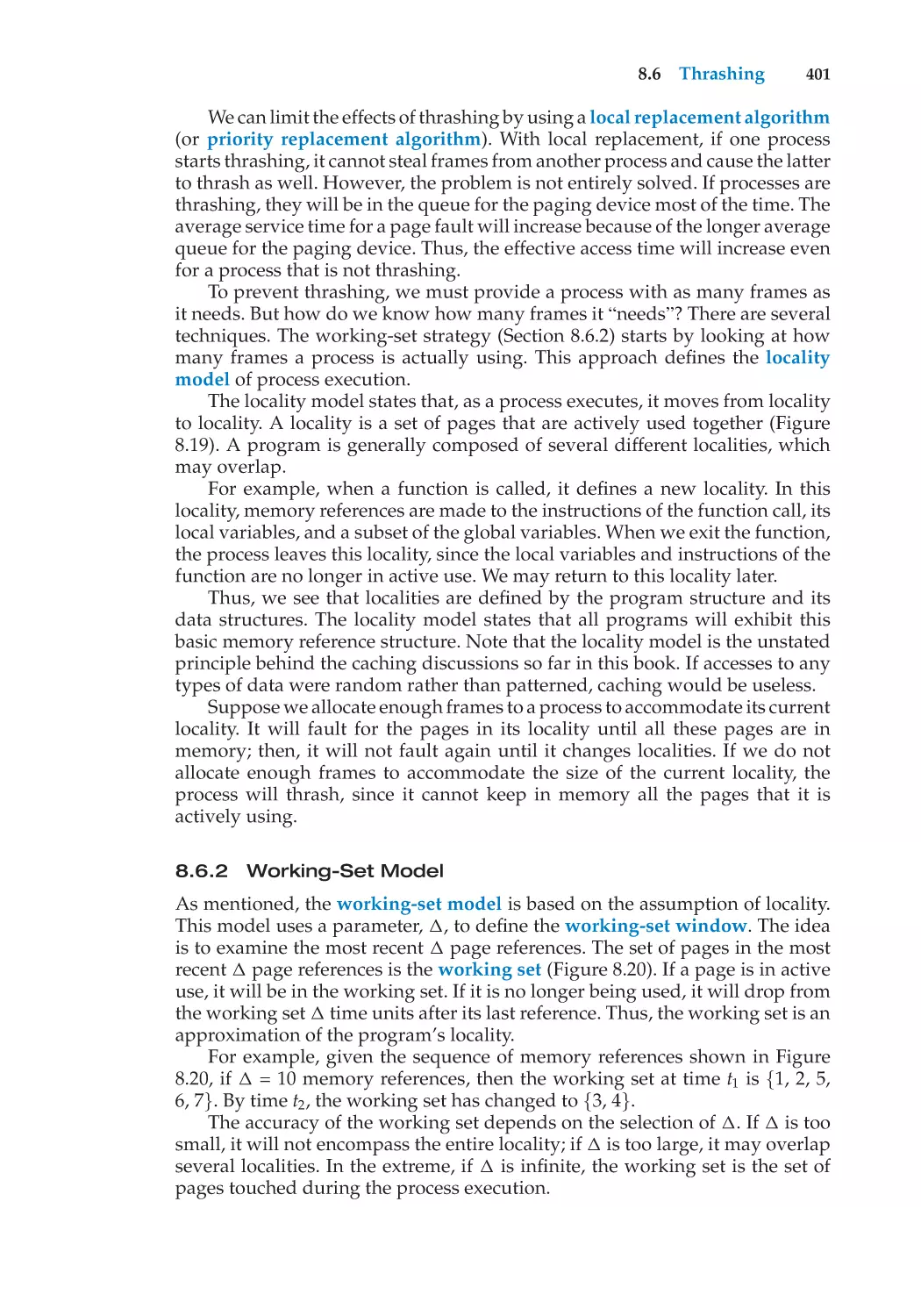
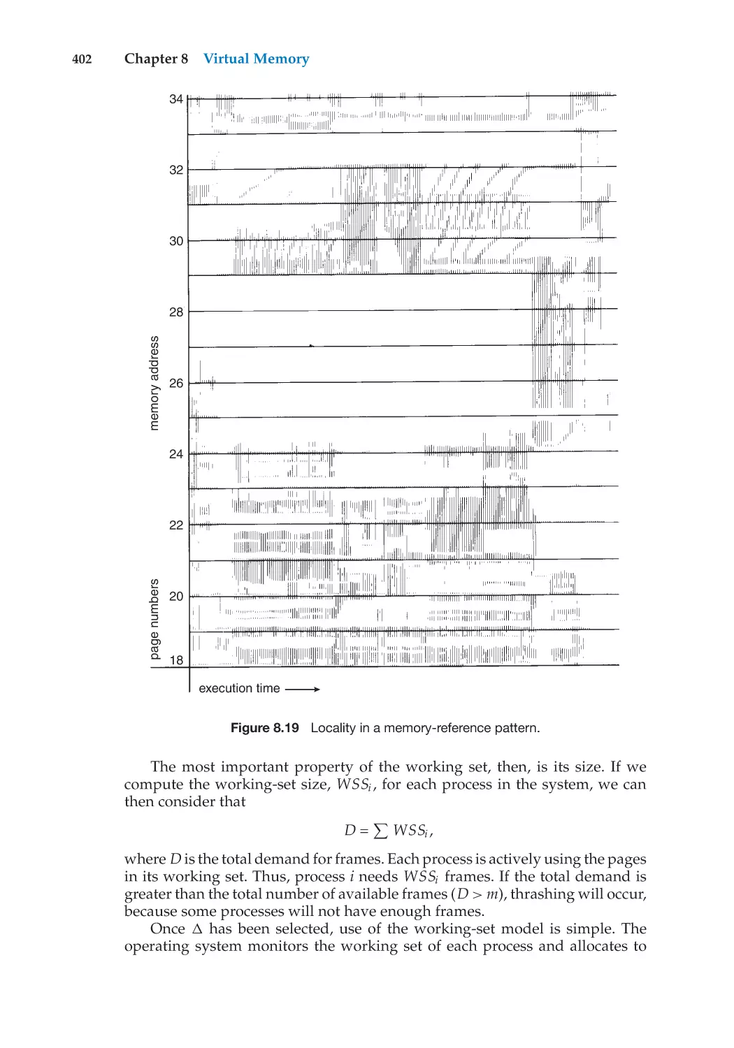
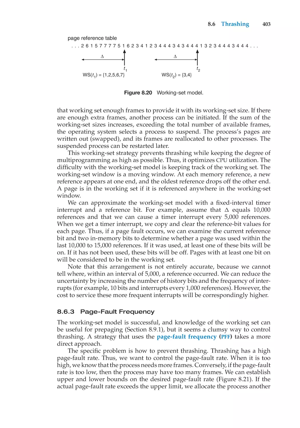
graphics (to name only a few).
1.2
Computer-System Organization
Before we can explore the details of how computer systems operate, we need
general knowledge of the structure of a computer system. In this section,
we look at several parts of this structure. The section is mostly concerned
with computer-system organization, so you can skim or skip it if you already
understand the concepts.
1.2.1
Computer-System Operation
A modern general-purpose computer system consists of one or more CPUs
and a number of device controllers connected through a common bus that
provides access to shared memory (Figure 1.2). Each device controller is in
charge of a specific type of device (for example, disk drives, audio devices,
or video displays). The CPU and the device controllers can execute in parallel,
competing for memory cycles. To ensure orderly access to the shared memory,
a memory controller synchronizes access to the memory.
For a computer to start running—for instance, when it is powered up or
rebooted —it needs to have an initial program to run. This initial program,
or bootstrap program, tends to be simple. Typically, it is stored within
the computer hardware in read-only memory (ROM) or electrically erasable
programmable read-only memory (EEPROM), known by the general term
firmware. It initializes all aspects of the system, from CPU registers to device
controllers to memory contents. The bootstrap program must know how to load
the operating system and how to start executing that system. To accomplish
mouse
keyboard
disks
CPU
printer
monitor
on-line
disk
controller
USB controller
memory
Figure 1.2 A modern computer system.
graphics
adapter
8
Chapter 1 Introduction
CPU
user
process
executing
I/O interrupt
processing
I/O
idle
device
transferring
I/O
request
transfer
done
I/O
transfer
request done
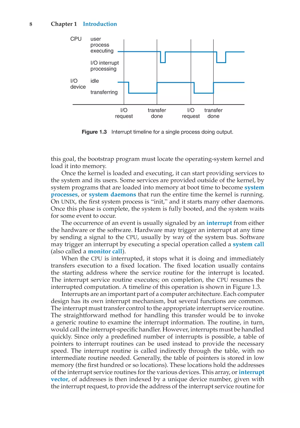
Figure 1.3 Interrupt timeline for a single process doing output.
this goal, the bootstrap program must locate the operating-system kernel and
load it into memory.
Once the kernel is loaded and executing, it can start providing services to
the system and its users. Some services are provided outside of the kernel, by
system programs that are loaded into memory at boot time to become system
processes, or system daemons that run the entire time the kernel is running.
On UNIX, the first system process is “init,” and it starts many other daemons.
Once this phase is complete, the system is fully booted, and the system waits
for some event to occur.
The occurrence of an event is usually signaled by an interrupt from either
the hardware or the software. Hardware may trigger an interrupt at any time
by sending a signal to the CPU, usually by way of the system bus. Software
may trigger an interrupt by executing a special operation called a system call
(also called a monitor call).
When the CPU is interrupted, it stops what it is doing and immediately
transfers execution to a fixed location. The fixed location usually contains
the starting address where the service routine for the interrupt is located.
The interrupt service routine executes; on completion, the CPU resumes the
interrupted computation. A timeline of this operation is shown in Figure 1.3.
Interrupts are an important part of a computer architecture. Each computer
design has its own interrupt mechanism, but several functions are common.
The interrupt must transfer control to the appropriate interrupt service routine.
The straightforward method for handling this transfer would be to invoke
a generic routine to examine the interrupt information. The routine, in turn,
would call the interrupt-specific handler. However, interrupts must be handled
quickly. Since only a predefined number of interrupts is possible, a table of
pointers to interrupt routines can be used instead to provide the necessary
speed. The interrupt routine is called indirectly through the table, with no
intermediate routine needed. Generally, the table of pointers is stored in low
memory (the first hundred or so locations). These locations hold the addresses
of the interrupt service routines for the various devices. This array, or interrupt
vector, of addresses is then indexed by a unique device number, given with
the interrupt request, to provide the address of the interrupt service routine for
1.2 Computer-System Organization
9
STORAGE DEFINITIONS AND NOTATION
The basic unit of computer storage is the bit. A bit can contain one of two
values, 0 and 1. All other storage in a computer is based on collections of bits.
Given enough bits, it is amazing how many things a computer can represent:
numbers, letters, images, movies, sounds, documents, and programs, to name
a few. A byte is 8 bits, and on most computers it is the smallest convenient
chunk of storage. For example, most computers don’t have an instruction to
move a bit but do have one to move a byte. A less common term is word,
which is a given computer architecture’s native unit of data. A word is made
up of one or more bytes. For example, a computer that has 64-bit registers and
64-bit memory addressing typically has 64-bit (8-byte) words. A computer
executes many operations in its native word size rather than a byte at a time.
Computer storage, along with most computer throughput, is generally
measured and manipulated in bytes and collections of bytes. A kilobyte, or
KB, is 1,024 bytes; a megabyte, or MB, is 1,0242 bytes; a gigabyte, or GB, is
1,0243 bytes; a terabyte, or TB, is 1,0244 bytes; and a petabyte, or PB, is 1,0245
bytes. Computer manufacturers often round off these numbers and say that
a megabyte is 1 million bytes and a gigabyte is 1 billion bytes. Networking
measurements are an exception to this general rule; they are given in bits
(because networks move data a bit at a time).
the interrupting device. Operating systems as different as Windows and UNIX
dispatch interrupts in this manner.
The interrupt architecture must also save the address of the interrupted
instruction. Many old designs simply stored the interrupt address in a
fixed location or in a location indexed by the device number. More recent
architectures store the return address on the system stack. If the interrupt
routine needs to modify the processor state —for instance, by modifying
register values—it must explicitly save the current state and then restore that
state before returning. After the interrupt is serviced, the saved return address
is loaded into the program counter, and the interrupted computation resumes
as though the interrupt had not occurred.
1.2.2
Storage Structure
The CPU can load instructions only from memory, so any programs to run must
be stored there. General-purpose computers run most of their programs from
rewritable memory, called main memory (also called random-access memory,
or RAM). Main memory commonly is implemented in a semiconductor
technology called dynamic random-access memory (DRAM).
Computers use other forms of memory as well. We have already mentioned
read-only memory, ROM) and electrically erasable programmable read-only
memory, EEPROM). Because ROM cannot be changed, only static programs, such
as the bootstrap program described earlier, are stored there. The immutability
of ROM is of use in game cartridges. EEPROM can be changed but cannot
be changed frequently and so contains mostly static programs. For example,
smartphones have EEPROM to store their factory-installed programs.
10
Chapter 1 Introduction
All forms of memory provide an array of bytes. Each byte has its
own address. Interaction is achieved through a sequence of load or store
instructions to specific memory addresses. The load instruction moves a byte
or word from main memory to an internal register within the CPU, whereas the
store instruction moves the content of a register to main memory. Aside from
explicit loads and stores, the CPU automatically loads instructions from main
memory for execution.
A typical instruction–execution cycle, as executed on a system with a von
Neumann architecture, first fetches an instruction from memory and stores
that instruction in the instruction register. The instruction is then decoded
and may cause operands to be fetched from memory and stored in some
internal register. After the instruction on the operands has been executed, the
result may be stored back in memory. Notice that the memory unit sees only
a stream of memory addresses. It does not know how they are generated (by
the instruction counter, indexing, indirection, literal addresses, or some other
means) or what they are for (instructions or data). Accordingly, we can ignore
how a memory address is generated by a program. We are interested only in
the sequence of memory addresses generated by the running program.
Ideally, we want the programs and data to reside in main memory
permanently. This arrangement usually is not possible for the following two
reasons:
1. Main memory is usually too small to store all needed programs and data
permanently.
2. Main memory is a volatile storage device that loses its contents when
power is turned off or otherwise lost.
Thus, most computer systems provide secondary storage as an extension of
main memory. The main requirement for secondary storage is that it be able to
hold large quantities of data permanently.
The most common secondary-storage device is a hard disk drive (HDD),
which provides storage for both programs and data. Most programs (system
and application) are stored on a disk until they are loaded into memory.
Many programs then use the disk as both the source and the destination of
their processing. Hence, the proper management of disk storage is of central
importance to a computer system, as we discuss in Chapter 9.
In a larger sense, however, the storage structure that we have described
—consisting of registers, main memory, and hard disks—is only one of many
possible storage systems. Others include cache memory, CD-ROM, magnetic
tapes, and so on. Each storage system provides the basic functions of storing
a datum and holding that datum until it is retrieved at a later time. The main
differences among the various storage systems lie in speed, cost, size, and
volatility.
The wide variety of storage systems can be organized in a hierarchy (Figure
1.4) according to speed and cost. The higher levels are expensive, but they are
fast. As we move down the hierarchy, the cost per bit generally decreases,
whereas the access time generally increases. This trade-off is reasonable; if a
given storage system were both faster and less expensive than another—other
properties being the same —then there would be no reason to use the slower,
more expensive memory. In fact, many early storage devices, including paper
1.2 Computer-System Organization
11
registers
cache
main memory
solid-state disk
hard disk
optical disk
magnetic tapes
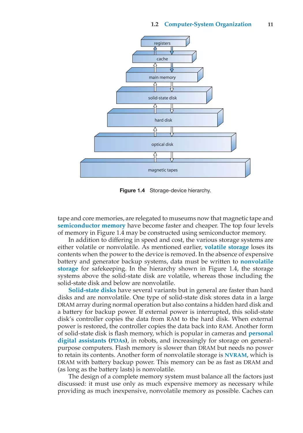
Figure 1.4 Storage-device hierarchy.
tape and core memories, are relegated to museums now that magnetic tape and
semiconductor memory have become faster and cheaper. The top four levels
of memory in Figure 1.4 may be constructed using semiconductor memory.
In addition to differing in speed and cost, the various storage systems are
either volatile or nonvolatile. As mentioned earlier, volatile storage loses its
contents when the power to the device is removed. In the absence of expensive
battery and generator backup systems, data must be written to nonvolatile
storage for safekeeping. In the hierarchy shown in Figure 1.4, the storage
systems above the solid-state disk are volatile, whereas those including the
solid-state disk and below are nonvolatile.
Solid-state disks have several variants but in general are faster than hard
disks and are nonvolatile. One type of solid-state disk stores data in a large
DRAM array during normal operation but also contains a hidden hard disk and
a battery for backup power. If external power is interrupted, this solid-state
disk’s controller copies the data from RAM to the hard disk. When external
power is restored, the controller copies the data back into RAM. Another form
of solid-state disk is flash memory, which is popular in cameras and personal
digital assistants (PDAs), in robots, and increasingly for storage on generalpurpose computers. Flash memory is slower than DRAM but needs no power
to retain its contents. Another form of nonvolatile storage is NVRAM, which is
DRAM with battery backup power. This memory can be as fast as DRAM and
(as long as the battery lasts) is nonvolatile.
The design of a complete memory system must balance all the factors just
discussed: it must use only as much expensive memory as necessary while
providing as much inexpensive, nonvolatile memory as possible. Caches can
12
Chapter 1 Introduction
be installed to improve performance where a large disparity in access time or
transfer rate exists between two components.
1.2.3
I/O Structure
Storage is only one of many types of I/O devices within a computer. A large
portion of operating system code is dedicated to managing I/O, both because
of its importance to the reliability and performance of a system and because of
the varying nature of the devices. Next, we provide an overview of I/O.
A general-purpose computer system consists of CPUs and multiple device
controllers that are connected through a common bus. Each device controller
is in charge of a specific type of device. Depending on the controller, more
than one device may be attached. For instance, seven or more devices can be
attached to the small computer-systems interface (SCSI) controller. A device
controller maintains some local buffer storage and a set of special-purpose
registers. The device controller is responsible for moving the data between
the peripheral devices that it controls and its local buffer storage. Typically,
operating systems have a device driver for each device controller. This device
driver understands the device controller and provides the rest of the operating
system with a uniform interface to the device.
To start an I/O operation, the device driver loads the appropriate registers
within the device controller. The device controller, in turn, examines the
contents of these registers to determine what action to take (such as “read
a character from the keyboard”). The controller starts the transfer of data from
the device to its local buffer. Once the transfer of data is complete, the device
controller informs the device driver via an interrupt that it has finished its
operation. The device driver then returns control to the operating system,
possibly returning the data or a pointer to the data if the operation was a read.
For other operations, the device driver returns status information.
This form of interrupt-driven I/O is fine for moving small amounts of data
but can produce high overhead when used for bulk data movement such as disk
I/O. To solve this problem, direct memory access (DMA) is used. After setting
up buffers, pointers, and counters for the I/O device, the device controller
transfers an entire block of data directly to or from its own buffer storage to
memory, with no intervention by the CPU. Only one interrupt is generated per
block, to tell the device driver that the operation has completed, rather than
the one interrupt per byte generated for low-speed devices. While the device
controller is performing these operations, the CPU is available to accomplish
other work.
Some high-end systems use switch rather than bus architecture. On these
systems, multiple components can talk to other components concurrently,
rather than competing for cycles on a shared bus. In this case, DMA is even
more effective. Figure 1.5 shows the interplay of all components of a computer
system.
1.3
Computer-System Architecture
In Section 1.2, we introduced the general structure of a typical computer system.
A computer system can be organized in a number of different ways, which we
1.3 Computer-System Architecture
cache
thread of execution
instruction execution
cycle
data movement
13
instructions
and
data
CPU (*N)
interrupt
data
I/O request
DMA
memory
device
(*M)
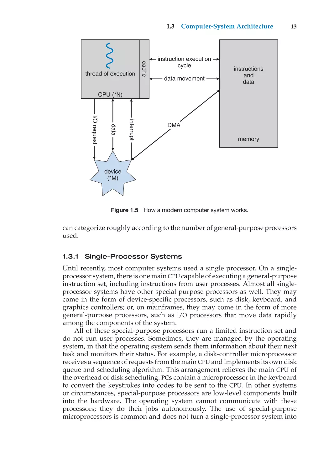
Figure 1.5 How a modern computer system works.
can categorize roughly according to the number of general-purpose processors
used.
1.3.1
Single-Processor Systems
Until recently, most computer systems used a single processor. On a singleprocessor system, there is one main CPU capable of executing a general-purpose
instruction set, including instructions from user processes. Almost all singleprocessor systems have other special-purpose processors as well. They may
come in the form of device-specific processors, such as disk, keyboard, and
graphics controllers; or, on mainframes, they may come in the form of more
general-purpose processors, such as I/O processors that move data rapidly
among the components of the system.
All of these special-purpose processors run a limited instruction set and
do not run user processes. Sometimes, they are managed by the operating
system, in that the operating system sends them information about their next
task and monitors their status. For example, a disk-controller microprocessor
receives a sequence of requests from the main CPU and implements its own disk
queue and scheduling algorithm. This arrangement relieves the main CPU of
the overhead of disk scheduling. PCs contain a microprocessor in the keyboard
to convert the keystrokes into codes to be sent to the CPU. In other systems
or circumstances, special-purpose processors are low-level components built
into the hardware. The operating system cannot communicate with these
processors; they do their jobs autonomously. The use of special-purpose
microprocessors is common and does not turn a single-processor system into
14
Chapter 1 Introduction
a multiprocessor. If there is only one general-purpose CPU, then the system is
a single-processor system.
1.3.2
Multiprocessor Systems
Within the past several years, multiprocessor systems (also known as parallel
systems or multicore systems) have begun to dominate the landscape of computing. Such systems have two or more processors in close communication,
sharing the computer bus and sometimes the clock, memory, and peripheral
devices. Multiprocessor systems first appeared prominently in servers and
have since migrated to desktop and laptop systems. Recently, multiple processors have appeared on mobile devices such as smartphones and tablet
computers.
Multiprocessor systems have three main advantages:
1. Increased throughput. By increasing the number of processors, we expect
to get more work done in less time. The speed-up ratio with N processors
is not N, however; rather, it is less than N. When multiple processors
cooperate on a task, a certain amount of overhead is incurred in keeping
all the parts working correctly. This overhead, plus contention for shared
resources, lowers the expected gain from additional processors. Similarly,
N programmers working closely together do not produce N times the
amount of work a single programmer would produce.
2. Economy of scale. Multiprocessor systems can cost less than equivalent
multiple single-processor systems, because they can share peripherals,
mass storage, and power supplies. If several programs operate on the
same set of data, it is cheaper to store those data on one disk and to have
all the processors share them than to have many computers with local
disks and many copies of the data.
3. Increased reliability. If functions can be distributed properly among
several processors, then the failure of one processor will not halt the
system, only slow it down. If we have ten processors and one fails, then
each of the remaining nine processors can pick up a share of the work of
the failed processor. Thus, the entire system runs only 10 percent slower,
rather than failing altogether.
Increased reliability of a computer system is crucial in many applications.
The ability to continue providing service proportional to the level of surviving
hardware is called graceful degradation. Some systems go beyond graceful
degradation and are called fault tolerant, because they can suffer a failure of
any single component and still continue operation. Fault tolerance requires
a mechanism to allow the failure to be detected, diagnosed, and, if possible,
corrected. The HP NonStop (formerly Tandem) system uses both hardware and
software duplication to ensure continued operation despite faults. The system
consists of multiple pairs of CPUs, working in lockstep. Both processors in the
pair execute each instruction and compare the results. If the results differ, then
one CPU of the pair is at fault, and both are halted. The process that was being
executed is then moved to another pair of CPUs, and the instruction that failed
1.3 Computer-System Architecture
15
is restarted. This solution is expensive, since it involves special hardware and
considerable hardware duplication.
The multiple-processor systems in use today are of two types. Some
systems use asymmetric multiprocessing, in which each processor is assigned
a specific task. A boss processor controls the system; the other processors either
look to the boss for instruction or have predefined tasks. This scheme defines
a boss–worker relationship. The boss processor schedules and allocates work
to the worker processors.
The most common systems use symmetric multiprocessing (SMP), in
which each processor performs all tasks, including operating system functions
and user processes. SMP means that all processors are peers; no boss–worker
relationship exists between processors. Figure 1.6 illustrates a typical SMP
architecture. Notice that each processor has its own set of registers, as well as a
private—or local—cache. However, all processors share physical memory. An
example of an SMP system is AIX, a commercial version of UNIX designed by IBM.
An AIX system can be configured to employ dozens of processors. The benefit
of this model is that many processes can run simultaneously— N processes
can run if there are N CPUs—without causing performance to deteriorate
significantly. However, we must carefully control I/O to ensure that the data
reach the appropriate processor. Also, since the CPUs are separate, one may
be sitting idle while another is overloaded, resulting in inefficiencies. These
inefficiencies can be avoided if the processors share certain data structures. A
multiprocessor system of this form will allow processes and resources—such
as memory—to be shared dynamically among the various processors and
can lower the variance among the processors. Such a system must be written
carefully, as we shall see in Chapter 5. Virtually all modern operating systems
—including Windows, Mac OS X, and Linux—now provide support for SMP.
The difference between symmetric and asymmetric multiprocessing may
result from either hardware or software. Special hardware can differentiate the
multiple processors, or the software can be written to allow only one boss and
multiple workers. For instance, Sun Microsystems’ operating system SunOS
Version 4 provided asymmetric multiprocessing, whereas Version 5 (Solaris) is
symmetric on the same hardware.
Multiprocessing adds CPUs to increase computing power. If the CPU has an
integrated memory controller, then adding CPUs can also increase the amount
CPU0
CPU1
CPU2
registers
registers
registers
cache
cache
cache
memory
Figure 1.6 Symmetric multiprocessing architecture.
16
Chapter 1 Introduction
of memory addressable in the system. Either way, multiprocessing can cause
a system to change its memory access model from uniform memory access
(UMA) to non-uniform memory access (NUMA). UMA is defined as the situation
in which access to any RAM from any CPU takes the same amount of time. With
NUMA, some parts of memory may take longer to access than other parts,
creating a performance penalty. Operating systems can minimize the NUMA
penalty through resource management, as discussed in Section 8.5.4.
A recent trend in CPU design is to include multiple computing cores
on a single chip. Such multiprocessor systems are termed multicore. They
can be more efficient than multiple chips with single cores because on-chip
communication is faster than between-chip communication. In addition, one
chip with multiple cores uses significantly less power than multiple single-core
chips.
It is important to note that while multicore systems are multiprocessor
systems, not all multiprocessor systems are multicore, as we shall see in Section
1.3.3. In our coverage of multiprocessor systems throughout this text, unless
we state otherwise, we generally use the more contemporary term multicore,
which excludes some multiprocessor systems.
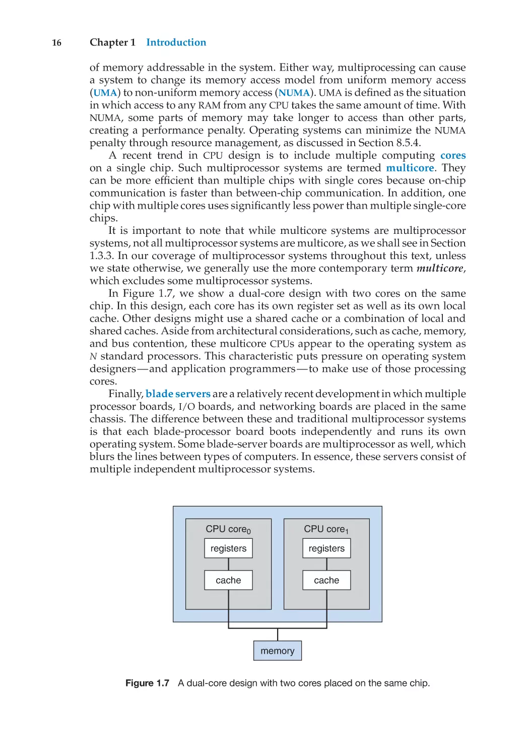
In Figure 1.7, we show a dual-core design with two cores on the same
chip. In this design, each core has its own register set as well as its own local
cache. Other designs might use a shared cache or a combination of local and
shared caches. Aside from architectural considerations, such as cache, memory,
and bus contention, these multicore CPUs appear to the operating system as
N standard processors. This characteristic puts pressure on operating system
designers—and application programmers—to make use of those processing
cores.
Finally, blade servers are a relatively recent development in which multiple
processor boards, I/O boards, and networking boards are placed in the same
chassis. The difference between these and traditional multiprocessor systems
is that each blade-processor board boots independently and runs its own
operating system. Some blade-server boards are multiprocessor as well, which
blurs the lines between types of computers. In essence, these servers consist of
multiple independent multiprocessor systems.
CPU core0
CPU core1
registers
registers
cache
cache
memory
Figure 1.7 A dual-core design with two cores placed on the same chip.
1.3 Computer-System Architecture
1.3.3
17
Clustered Systems
Another type of multiprocessor system is a clustered system, which gathers
together multiple CPUs. Clustered systems differ from the multiprocessor
systems described in Section 1.3.2 in that they are composed of two or more
individual systems—or nodes—joined together. Such systems are considered
loosely coupled. Each node may be a single processor system or a multicore
system. We should note that the definition of clustered is not concrete; many
commercial packages wrestle to define a clustered system and why one form
is better than another. The generally accepted definition is that clustered
computers share storage and are closely linked via a local-area network LAN
or a faster interconnect, such as InfiniBand.
Clustering is usually used to provide high-availability service —that is,
service will continue even if one or more systems in the cluster fail. Generally,
we obtain high availability by adding a level of redundancy in the system.
A layer of cluster software runs on the cluster nodes. Each node can monitor
one or more of the others (over the LAN). If the monitored machine fails,
the monitoring machine can take ownership of its storage and restart the
applications that were running on the failed machine. The users and clients of
the applications see only a brief interruption of service.
Clustering can be structured asymmetrically or symmetrically. In asymmetric clustering, one machine is in hot-standby mode while the other is
running the applications. The hot-standby host machine does nothing but
monitor the active server. If that server fails, the hot-standby host becomes
the active server. In symmetric clustering, two or more hosts are running
applications and are monitoring each other. This structure is obviously more
efficient, as it uses all of the available hardware. However it does require that
more than one application be available to run.
Since a cluster consists of several computer systems connected via a
network, clusters can also be used to provide high-performance computing
environments. Such systems can supply significantly greater computational
power than single-processor or even SMP systems because they can run an
application concurrently on all computers in the cluster. The application must
have been written specifically to take advantage of the cluster, however. This
involves a technique known as parallelization, which divides a program into
separate components that run in parallel on individual cores in a computer or
computers in a cluster. Typically, these applications are designed so that once
each computing node in the cluster has solved its portion of the problem, the
results from all the nodes are combined into a final solution.
Other forms of clusters include parallel clusters and clustering over a
wide-area network (WAN). Parallel clusters allow multiple hosts to access the
same data on shared storage. Because most operating systems lack support for
simultaneous data access by multiple hosts, parallel clusters usually require
the use of special versions of software and special releases of applications. For
example, Oracle Real Application Cluster is a version of Oracle’s database that
has been designed to run on a parallel cluster. Each machine runs Oracle, and a
layer of software tracks access to the shared disk. Each machine has full access
to all data in the database. To provide this shared access, the system must
also supply access control and locking to ensure that no conflicting operations
18
Chapter 1 Introduction
BEOWULF CLUSTERS
Beowulf clusters are designed to solve high-performance computing tasks.
A Beowulf cluster consists of commodity hardware — such as personal
computers — connected via a simple local-area network. No single specific
software package is required to construct a cluster. Rather, the nodes use a
set of open-source software libraries to communicate with one another. Thus,
there are a variety of approaches to constructing a Beowulf cluster. Typically,
though, Beowulf computing nodes run the Linux operating system. Since
Beowulf clusters require no special hardware and operate using open-source
software that is available free, they offer a low-cost strategy for building
a high-performance computing cluster. In fact, some Beowulf clusters built
from discarded personal computers are using hundreds of nodes to solve
computationally expensive scientific computing problems.
occur. This function, commonly known as a distributed lock manager (DLM),
is included in some cluster technology.
Cluster technology is changing rapidly. Some cluster products support
dozens of systems in a cluster, as well as clustered nodes that are separated
by miles. Many of these improvements are made possible by storage-area
networks (SANs), as described in Section 9.3.3, which allow many systems to
attach to a pool of storage. If the applications and their data are stored on the
SAN, then the cluster software can assign the application to run on any host
that is attached to the SAN. If the host fails, then any other host can take over.
In a database cluster, dozens of hosts can share the same database, greatly
increasing performance and reliability. Figure 1.8 depicts the general structure
of a clustered system.
computer
interconnect
computer
interconnect
computer
storage area
network
Figure 1.8 General structure of a clustered system.
1.4 Operating-System Structure
19
0
operating system
job 1
job 2
job 3
job 4
Max
Figure 1.9 Memory layout for a multiprogramming system.
1.4
Operating-System Structure
Now that we have discussed basic computer-system organization and architecture, we are ready to talk about operating systems. An operating system
provides the environment within which programs are executed. Internally,
operating systems vary greatly in their makeup, since they are organized
along many different lines. There are, however, many commonalities, which
we consider in this section.
One of the most important aspects of operating systems is the ability
to multiprogram. A single program cannot, in general, keep either the CPU
or the I/O devices busy at all times. Single users frequently have multiple
programs running. Multiprogramming increases CPU utilization by organizing
jobs (code and data) so that the CPU always has one to execute.
The idea is as follows: The operating system keeps several jobs in memory
simultaneously (Figure 1.9). Since, in general, main memory is too small to
accommodate all jobs, the jobs are kept initially on the disk in the job pool.
This pool consists of all processes residing on disk awaiting allocation of main
memory.
The set of jobs in memory can be a subset of the jobs kept in the job
pool. The operating system picks and begins to execute one of the jobs in
memory. Eventually, the job may have to wait for some task, such as an I/O
operation, to complete. In a non-multiprogrammed system, the CPU would sit
idle. In a multiprogrammed system, the operating system simply switches to,
and executes, another job. When that job needs to wait, the CPU switches to
another job, and so on. Eventually, the first job finishes waiting and gets the
CPU back. As long as at least one job needs to execute, the CPU is never idle.
This idea is common in other life situations. A lawyer does not work for
only one client at a time, for example. While one case is waiting to go to trial
or have papers typed, the lawyer can work on another case. If he has enough
clients, the lawyer will never be idle for lack of work. (Idle lawyers tend to
become politicians, so there is a certain social value in keeping lawyers busy.)
20
Chapter 1 Introduction
Multiprogrammed systems provide an environment in which the various
system resources (for example, CPU, memory, and peripheral devices) are
utilized effectively, but they do not provide for user interaction with the
computer system. Time sharing (or multitasking) is a logical extension of
multiprogramming. In time-sharing systems, the CPU executes multiple jobs
by switching among them, but the switches occur so frequently that the users
can interact with each program while it is running.
Time sharing requires an interactive computer system, which provides
direct communication between the user and the system. The user gives
instructions to the operating system or to a program directly, using a input
device such as a keyboard, mouse, touch pad, or touch screen, and waits for
immediate results on an output device. Accordingly, the response time should
be short—typically less than one second.
A time-shared operating system allows many users to share the computer
simultaneously. Since each action or command in a time-shared system tends
to be short, only a little CPU time is needed for each user. As the system switches
rapidly from one user to the next, each user is given the impression that the
entire computer system is dedicated to his use, even though it is being shared
among many users.
A time-shared operating system uses CPU scheduling and multiprogramming to provide each user with a small portion of a time-shared computer.
Each user has at least one separate program in memory. A program loaded
into memory is called a process. When a process executes, it typically executes
for only a short time before it either finishes or needs to perform I/O. I/O may be
interactive; that is, output goes to a display for the user, and input comes from
a user keyboard, mouse, or other device. Since interactive I/O typically runs at
“people speeds,” it may take a long time to complete. Input, for example, may
be bounded by the user’s typing speed; seven characters per second is fast for
people but incredibly slow for computers. Rather than let the CPU sit idle as
this interactive input takes place, the operating system will rapidly switch the
CPU to the program of some other user.
Time sharing and multiprogramming require that several jobs be kept
simultaneously in memory. If several jobs are ready to be brought into memory,
and if there is not enough room for all of them, then the system must choose
among them. Making this decision involves job scheduling, which we discuss
in Chapter 6. When the operating system selects a job from the job pool, it loads
that job into memory for execution. Having several programs in memory at
the same time requires some form of memory management, which we cover in
Chapters 7 and 8. In addition, if several jobs are ready to run at the same time,
the system must choose which job will run first. Making this decision is CPU
scheduling, which is also discussed in Chapter 6. Finally, running multiple
jobs concurrently requires that their ability to affect one another be limited in
all phases of the operating system, including process scheduling, disk storage,
and memory management. We discuss these considerations throughout the
text.
In a time-sharing system, the operating system must ensure reasonable
response time. This goal is sometimes accomplished through swapping,
whereby processes are swapped in and out of main memory to the disk. A more
common method for ensuring reasonable response time is virtual memory, a
technique that allows the execution of a process that is not completely in
1.5 Operating-System Operations
21
memory (Chapter 8). The main advantage of the virtual-memory scheme is that
it enables users to run programs that are larger than actual physical memory.
Further, it abstracts main memory into a large, uniform array of storage,
separating logical memory as viewed by the user from physical memory.
This arrangement frees programmers from concern over memory-storage
limitations.
A time-sharing system must also provide a file system (Chapters 10 and
11). The file system resides on a collection of disks; hence, disk management
must be provided (Chapter 9). In addition, a time-sharing system provides
a mechanism for protecting resources from inappropriate use (Chapter 13).
To ensure orderly execution, the system must provide mechanisms for job
synchronization and communication (Chapter 5), and it may ensure that jobs
do not get stuck in a deadlock, forever waiting for one another.
1.5
Operating-System Operations
As mentioned earlier, modern operating systems are interrupt driven. If there
are no processes to execute, no I/O devices to service, and no users to whom
to respond, an operating system will sit quietly, waiting for something to
happen. Events are almost always signaled by the occurrence of an interrupt
or a trap. A trap (or an exception) is a software-generated interrupt caused
either by an error (for example, division by zero or invalid memory access)
or by a specific request from a user program that an operating-system service
be performed. The interrupt-driven nature of an operating system defines
that system’s general structure. For each type of interrupt, separate segments
of code in the operating system determine what action should be taken. An
interrupt service routine is provided to deal with the interrupt.
Since the operating system and the users share the hardware and software
resources of the computer system, we need to make sure that an error in a
user program could cause problems only for the one program running. With
sharing, many processes could be adversely affected by a bug in one program.
For example, if a process gets stuck in an infinite loop, this loop could prevent
the correct operation of many other processes. More subtle errors can occur
in a multiprogramming system, where one erroneous program might modify
another program, the data of another program, or even the operating system
itself.
Without protection against these sorts of errors, either the computer must
execute only one process at a time or all output must be suspect. A properly
designed operating system must ensure that an incorrect (or malicious)
program cannot cause other programs to execute incorrectly.
1.5.1
Dual-Mode and Multimode Operation
In order to ensure the proper execution of the operating system, we must be
able to distinguish between the execution of operating-system code and userdefined code. The approach taken by most computer systems is to provide
hardware support that allows us to differentiate among various modes of
execution.
22
Chapter 1 Introduction
user process
user process executing
kernel
calls system call
trap
mode bit = 0
return from system call
return
mode bit = 1
execute system call
user mode
(mode bit = 1)
kernel mode
(mode bit = 0)
Figure 1.10 Transition from user to kernel mode.
At the very least, we need two separate modes of operation: user mode
and kernel mode (also called supervisor mode, system mode, or privileged
mode). A bit, called the mode bit, is added to the hardware of the computer
to indicate the current mode: kernel (0) or user (1). With the mode bit, we can
distinguish between a task that is executed on behalf of the operating system
and one that is executed on behalf of the user. When the computer system is
executing on behalf of a user application, the system is in user mode. However,
when a user application requests a service from the operating system (via a
system call), the system must transition from user to kernel mode to fulfill
the request. This is shown in Figure 1.10. As we shall see, this architectural
enhancement is useful for many other aspects of system operation as well.
At system boot time, the hardware starts in kernel mode. The operating
system is then loaded and starts user applications in user mode. Whenever a
trap or interrupt occurs, the hardware switches from user mode to kernel mode
(that is, changes the state of the mode bit to 0). Thus, whenever the operating
system gains control of the computer, it is in kernel mode. The system always
switches to user mode (by setting the mode bit to 1) before passing control to
a user program.
The dual mode of operation provides us with the means for protecting the
operating system from errant users—and errant users from one another. We
accomplish this protection by designating some of the machine instructions that
may cause harm as privileged instructions. The hardware allows privileged
instructions to be executed only in kernel mode. If an attempt is made to
execute a privileged instruction in user mode, the hardware does not execute
the instruction but rather treats it as illegal and traps it to the operating system.
The instruction to switch to kernel mode is an example of a privileged
instruction. Some other examples include I/O control, timer management, and
interrupt management. As we shall see throughout the text, there are many
additional privileged instructions.
The concept of modes can be extended beyond two modes (in which case
the CPU uses more than one bit to set and test the mode). CPUs that support
virtualization frequently have a separate mode to indicate when the virtual
machine manager (VMM)—and the virtualization management software —
is in control of the system. In this mode, the VMM has more privileges than
user processes but fewer than the kernel. It needs that level of privilege so
it can create and manage virtual machines, changing the CPU state to do so.
Sometimes, too, different modes are used by various kernel components. We
1.5 Operating-System Operations
23
should note that, as an alternative to modes, the CPU designer may use other
methods to differentiate operational privileges. The Intel 64 family of CPUs
supports four privilege levels, for example, and supports virtualization but
does not have a separate mode for virtualization.
We can now see the life cycle of instruction execution in a computer system.
Initial control resides in the operating system, where instructions are executed
in kernel mode. When control is given to a user application, the mode is set to
user mode. Eventually, control is switched back to the operating system via an
interrupt, a trap, or a system call.
System calls provide the means for a user program to ask the operating
system to perform tasks reserved for the operating system on the user
program’s behalf. A system call is invoked in a variety of ways, depending
on the functionality provided by the underlying processor. In all forms, it is the
method used by a process to request action by the operating system. A system
call usually takes the form of a trap to a specific location in the interrupt vector.
This trap can be executed by a generic trap instruction, although some systems
(such as MIPS) have a specific syscall instruction to invoke a system call.
When a system call is executed, it is typically treated by the hardware
as a software interrupt. Control passes through the interrupt vector to a
service routine in the operating system, and the mode bit is set to kernel
mode. The system-call service routine is a part of the operating system. The
kernel examines the interrupting instruction to determine what system call
has occurred; a parameter indicates what type of service the user program is
requesting. Additional information needed for the request may be passed in
registers, on the stack, or in memory (with pointers to the memory locations
passed in registers). The kernel verifies that the parameters are correct and
legal, executes the request, and returns control to the instruction following the
system call. We describe system calls more fully in Section 2.3.
The lack of a hardware-supported dual mode can cause serious shortcomings in an operating system. For instance, MS-DOS was written for the Intel
8088 architecture, which has no mode bit and therefore no dual mode. A user
program running awry can wipe out the operating system by writing over it
with data; and multiple programs are able to write to a device at the same
time, with potentially disastrous results. Modern versions of the Intel CPU
do provide dual-mode operation. Accordingly, most contemporary operating
systems—such as Microsoft Windows 7, as well as Unix and Linux—take
advantage of this dual-mode feature and provide greater protection for the
operating system.
Once hardware protection is in place, it detects errors that violate modes.
These errors are normally handled by the operating system. If a user program
fails in some way—such as by making an attempt either to execute an illegal
instruction or to access memory that is not in the user’s address space —then
the hardware traps to the operating system. The trap transfers control through
the interrupt vector to the operating system, just as an interrupt does. When
a program error occurs, the operating system must terminate the program
abnormally. This situation is handled by the same code as a user-requested
abnormal termination. An appropriate error message is given, and the memory
of the program may be dumped. The memory dump is usually written to a
file so that the user or programmer can examine it and perhaps correct it and
restart the program.
24
Chapter 1 Introduction
1.5.2
Timer
We must ensure that the operating system maintains control over the CPU.
We cannot allow a user program to get stuck in an infinite loop or to fail
to call system services and never return control to the operating system. To
accomplish this goal, we can use a timer. A timer can be set to interrupt
the computer after a specified period. The period may be fixed (for example,
1/60 second) or variable (for example, from 1 millisecond to 1 second). A
variable timer is generally implemented by a fixed-rate clock and a counter.
The operating system sets the counter. Every time the clock ticks, the counter
is decremented. When the counter reaches 0, an interrupt occurs. For instance,
a 10-bit counter with a 1-millisecond clock allows interrupts at intervals from
1 millisecond to 1,024 milliseconds, in steps of 1 millisecond.
Before turning over control to the user, the operating system ensures
that the timer is set to interrupt. If the timer interrupts, control transfers
automatically to the operating system, which may treat the interrupt as a fatal
error or may give the program more time. Clearly, instructions that modify the
content of the timer are privileged.
We can use the timer to prevent a user program from running too long.
A simple technique is to initialize a counter with the amount of time that a
program is allowed to run. A program with a 7-minute time limit, for example,
would have its counter initialized to 420. Every second, the timer interrupts,
and the counter is decremented by 1. As long as the counter is positive, control
is returned to the user program. When the counter becomes negative, the
operating system terminates the program for exceeding the assigned time
limit.
1.6
Process Management
A program does nothing unless its instructions are executed by a CPU. A
program in execution, as mentioned, is a process. A time-shared user program
such as a compiler is a process. A word-processing program being run by an
individual user on a PC is a process. A system task, such as sending output
to a printer, can also be a process (or at least part of one). For now, you can
consider a process to be a job or a time-shared program, but later you will learn
that the concept is more general. As we shall see in Chapter 3, it is possible
to provide system calls that allow processes to create subprocesses to execute
concurrently.
A process needs certain resources—including CPU time, memory, files,
and I/O devices—to accomplish its task. These resources are either given to
the process when it is created or allocated to it while it is running. In addition
to the various physical and logical resources that a process obtains when it is
created, various initialization data (input) may be passed along. For example,
consider a process whose function is to display the status of a file on the screen
of a terminal. The process will be given the name of the file as an input and will
execute the appropriate instructions and system calls to obtain and display
the desired information on the terminal. When the process terminates, the
operating system will reclaim any reusable resources.
We emphasize that a program by itself is not a process. A program is a
passive entity, like the contents of a file stored on disk, whereas a process
1.7 Memory Management
25
is an active entity. A single-threaded process has one program counter
specifying the next instruction to execute. (Threads are covered in Chapter
4.) The execution of such a process must be sequential. The CPU executes one
instruction of the process after another, until the process completes. Further,
at any time, one instruction at most is executed on behalf of the process. Thus,
although two processes may be associated with the same program, they are
nevertheless considered two separate execution sequences. A multithreaded
process has multiple program counters, each pointing to the next instruction
to execute for a given thread.
A process is the unit of work in a system. A system consists of a collection
of processes, some of which are operating-system processes (those that execute
system code) and the rest of which are user processes (those that execute
user code). All these processes can potentially execute concurrently—by
multiplexing on a single CPU, for example.
The operating system is responsible for the following activities in connection with process management:
•
•
•
•
•
Scheduling processes and threads on the CPUs
Creating and deleting both user and system processes
Suspending and resuming processes
Providing mechanisms for process synchronization
Providing mechanisms for process communication
We discuss process-management techniques in Chapters 3 through 5.
1.7
Memory Management
As we discussed in Section 1.2.2, the main memory is central to the operation
of a modern computer system. Main memory is a large array of bytes, ranging
in size from hundreds of thousands to billions. Each byte has its own address.
Main memory is a repository of quickly accessible data shared by the CPU and
I/O devices. The central processor reads instructions from main memory during
the instruction-fetch cycle and both reads and writes data from main memory
during the data-fetch cycle (on a von Neumann architecture). As noted earlier,
the main memory is generally the only large storage device that the CPU is able
to address and access directly. For example, for the CPU to process data from
disk, those data must first be transferred to main memory by CPU-generated
I/O calls. In the same way, instructions must be in memory for the CPU to
execute them.
For a program to be executed, it must be mapped to absolute addresses and
loaded into memory. As the program executes, it accesses program instructions
and data from memory by generating these absolute addresses. Eventually,
the program terminates, its memory space is declared available, and the next
program can be loaded and executed.
To improve both the utilization of the CPU and the speed of the computer’s
response to its users, general-purpose computers must keep several programs
in memory, creating a need for memory management. Many different memory-
26
Chapter 1 Introduction
management schemes are used. These schemes reflect various approaches, and
the effectiveness of any given algorithm depends on the situation. In selecting a
memory-management scheme for a specific system, we must take into account
many factors—especially the hardware design of the system. Each algorithm
requires its own hardware support.
The operating system is responsible for the following activities in connection with memory management:
• Keeping track of which parts of memory are currently being used and who
is using them
• Deciding which processes (or parts of processes) and data to move into
and out of memory
• Allocating and deallocating memory space as needed
Memory-management techniques are discussed in Chapters 7 and 8.
1.8
Storage Management
To make the computer system convenient for users, the operating system
provides a uniform, logical view of information storage. The operating system
abstracts from the physical properties of its storage devices to define a logical
storage unit, the file. The operating system maps files onto physical media and
accesses these files via the storage devices.
1.8.1
File-System Management
File management is one of the most visible components of an operating system.
Computers can store information on several different types of physical media.
Hard disk, optical disk, and magnetic tape are the most common. Each of these
media has its own characteristics and physical organization. Each medium is
controlled by a device, such as a disk drive or tape drive, that also has its
own unique characteristics. These properties include access speed, capacity,
data-transfer rate, and access method (sequential or random).
A file is a collection of related information defined by its creator. Commonly,
files represent programs (both source and object forms) and data. Data files may
be numeric, alphabetic, alphanumeric, or binary. Files may be free-form (for
example, text files), or they may be formatted rigidly (for example, fixed fields).
Clearly, the concept of a file is an extremely general one.
The operating system implements the abstract concept of a file by managing
mass-storage media, such as tapes and disks, and the devices that control them.
In addition, files are normally organized into directories to make them easier
to use. Finally, when multiple users have access to files, it may be desirable
to control which user may access a file and how that user may access it (for
example, read, write, append).
The operating system is responsible for the following activities in connection with file management:
• Creating and deleting files
1.8 Storage Management
•
•
•
•
27
Creating and deleting directories to organize files
Supporting primitives for manipulating files and directories
Mapping files onto secondary storage
Backing up files on stable (nonvolatile) storage media
File-management techniques are discussed in Chapters 10 and 11.
1.8.2
Mass-Storage Management
As we have already seen, because main memory is too small to accommodate
all data and programs, and because the data that it holds are lost when power
is lost, the computer system must provide secondary storage to back up main
memory. Most modern computer systems use disks as the principal on-line
storage medium for both programs and data. Most programs—including
compilers, assemblers, word processors, editors, and formatters—are stored
on a disk until loaded into memory. They then use the disk as both the source
and destination of their processing. Hence, the proper management of disk
storage is of central importance to a computer system. The operating system is
responsible for the following activities in connection with disk management:
• Free-space management
• Storage allocation
• Disk scheduling
Because secondary storage is used frequently, it must be used efficiently. The
entire speed of operation of a computer may hinge on the speeds of the disk
subsystem and the algorithms that manipulate that subsystem.
There are, however, many uses for storage that is slower and lower in
cost (and sometimes of higher capacity) than secondary storage. Backups of
disk data, storage of seldom-used data, and long-term archival storage are
some examples. Magnetic tape drives and their tapes and CD and DVD drives
and platters are typical tertiary storage devices. The media (tapes and optical
platters) vary between WORM (write-once, read-many-times) and RW (read –
write) formats.
Tertiary storage is not crucial to system performance, but it still must
be managed. Some operating systems take on this task, while others leave
tertiary-storage management to application programs. Some of the functions
that operating systems can provide include mounting and unmounting media
in devices, allocating and freeing the devices for exclusive use by processes,
and migrating data from secondary to tertiary storage.
Techniques for secondary and tertiary storage management are discussed
in Chapter 9.
1.8.3
Caching
Caching is an important principle of computer systems. Here’s how it works.
Information is normally kept in some storage system (such as main memory).
As it is used, it is copied into a faster storage system—the cache —on a
28
Chapter 1 Introduction
temporary basis. When we need a particular piece of information, we first
check whether it is in the cache. If it is, we use the information directly from
the cache. If it is not, we use the information from the source, putting a copy
in the cache under the assumption that we will need it again soon.
In addition, internal programmable registers, such as index registers,
provide a high-speed cache for main memory. The programmer (or compiler)
implements the register-allocation and register-replacement algorithms to
decide which information to keep in registers and which to keep in main
memory.
Other caches are implemented totally in hardware. For instance, most
systems have an instruction cache to hold the instructions expected to be
executed next. Without this cache, the CPU would have to wait several cycles
while an instruction was fetched from main memory. For similar reasons, most
systems have one or more high-speed data caches in the memory hierarchy.
We are not concerned with these hardware-only caches in this text, since they
are outside the control of the operating system.
Because caches have limited size, cache management is an important
design problem. Careful selection of the cache size and of a replacement policy
can result in greatly increased performance. Figure 1.11 compares storage
performance in large workstations and small servers. Various replacement
algorithms for software-controlled caches are discussed in Chapter 8.
Main memory can be viewed as a fast cache for secondary storage, since
data in secondary storage must be copied into main memory for use and
data must be in main memory before being moved to secondary storage for
safekeeping. The file-system data, which resides permanently on secondary
storage, may appear on several levels in the storage hierarchy. At the highest
level, the operating system may maintain a cache of file-system data in main
memory. In addition, solid-state disks may be used for high-speed storage that
is accessed through the file-system interface. The bulk of secondary storage
is on hard disks. The hard-disk storage, in turn, is often backed up onto
magnetic tapes or removable disks to protect against data loss in case of a harddisk failure. Some systems automatically archive old file data from secondary
storage to tertiary storage, such as tape jukeboxes, to lower the storage cost
(see Chapter 9).
Level
1
2
3
4
5
Name
registers
cache
main memory
solid state disk
hard disk
Typical size
< 1 KB
< 16MB
< 64GB
< 1 TB
< 10 TB
Implementation
technology
custom memory on-chip or
off-chip
with multiple
CMOS SRAM
ports CMOS
CMOS SRAM
flash memory
hard disk
Access time (ns)
0.25 - 0.5
80 - 250
25,000 - 50,000
5,000,000
Bandwidth (MB/sec)
20,000 - 100,000 5,000 - 10,000
1,000 - 5,000
500
20 - 150
Managed by
compiler
hardware
Backed by
cache
main memory disk
0.5 - 25
operating system operating system operating system
disk
Figure 1.11 Performance of various levels of storage.
disk or tape
1.8 Storage Management
hard
disk
A
main
memory
A
cache
A
29
hardware
register
Figure 1.12 Migration of integer A from disk to register.
The movement of information between levels of a storage hierarchy may
be either explicit or implicit, depending on the hardware design and the
controlling operating-system software. For instance, data transfer from cache
to CPU and registers is usually a hardware function, with no operating-system
intervention. In contrast, transfer of data from disk to memory is usually
controlled by the operating system.
In a hierarchical storage structure, the same data may appear in different
levels of the storage system. For example, suppose that an integer A that is
to be incremented by 1 is located in file B, and file B resides on hard disk.
The increment operation proceeds by first issuing an I/O operation to copy the
disk block on which A resides to main memory. This operation is followed by
copying A to the cache and to an internal register. Thus, the copy of A appears
in several places: on the hard disk, in main memory, in the cache, and in an
internal register (see Figure 1.12). Once the increment takes place in the internal
register, the value of A differs in the various storage systems. The value of A
becomes the same only after the new value of A is written from the internal
register back to the hard disk.
In a computing environment where only one process executes at a time,
this arrangement poses no difficulties, since an access to integer A will always
be to the copy at the highest level of the hierarchy. However, in a multitasking
environment, where the CPU is switched back and forth among various
processes, extreme care must be taken to ensure that, if several processes wish
to access A, then each of these processes will obtain the most recently updated
value of A.
The situation becomes more complicated in a multiprocessor environment
where, in addition to maintaining internal registers, each of the CPUs also
contains a local cache (Figure 1.6). In such an environment, a copy of A may
exist simultaneously in several caches. Since the various CPUs can all execute
in parallel, we must make sure that an update to the value of A in one cache
is immediately reflected in all other caches where A resides. This situation is
called cache coherency, and it is usually a hardware issue (handled below the
operating-system level).
In a distributed environment, the situation becomes even more complex.
In this environment, several copies (or replicas) of the same file can be kept on
different computers. Since the various replicas may be accessed and updated
concurrently, some distributed systems ensure that, when a replica is updated
in one place, all other replicas are brought up to date as soon as possible. There
are various ways to achieve this guarantee.
1.8.4
I/O Systems
One of the purposes of an operating system is to hide the peculiarities of specific
hardware devices from the user. For example, in UNIX, the peculiarities of I/O
30
Chapter 1 Introduction
devices are hidden from the bulk of the operating system itself by the I/O
subsystem. The I/O subsystem consists of several components:
• A memory-management component that includes buffering, caching, and
spooling
• A general device-driver interface
• Drivers for specific hardware devices
Only the device driver knows the peculiarities of the specific device to which
it is assigned.
We discussed in Section 1.2.3 how interrupt handlers and device drivers are
used in the construction of efficient I/O subsystems. In Chapter 12, we discuss
how the I/O subsystem interfaces to the other system components, manages
devices, transfers data, and detects I/O completion.
1.9
Protection and Security
If a computer system has multiple users and allows the concurrent execution
of multiple processes, then access to data must be regulated. For that purpose,
mechanisms ensure that files, memory segments, CPU, and other resources can
be operated on by only those processes that have gained proper authorization from the operating system. For example, memory-addressing hardware
ensures that a process can execute only within its own address space. The
timer ensures that no process can gain control of the CPU without eventually
relinquishing control. Device-control registers are not accessible to users, so
the integrity of the various peripheral devices is protected.
Protection, then, is any mechanism for controlling the access of processes
or users to the resources defined by a computer system. This mechanism must
provide means to specify the controls to be imposed and to enforce the controls.
Protection can improve reliability by detecting latent errors at the interfaces
between component subsystems. Early detection of interface errors can often
prevent contamination of a healthy subsystem by another subsystem that is
malfunctioning. Furthermore, an unprotected resource cannot defend against
use (or misuse) by an unauthorized or incompetent user. A protection-oriented
system provides a means to distinguish between authorized and unauthorized
usage, as we discuss in Chapter 13.
A system can have adequate protection but still be prone to failure and
allow inappropriate access. Consider a user whose authentication information
(her means of identifying herself to the system) is stolen. Her data could be
copied or deleted, even though file and memory protection are working. It is
the job of security to defend a system from external and internal attacks. Such
attacks spread across a huge range and include viruses and worms, denial-ofservice attacks (which use all of a system’s resources and so keep legitimate
users out of the system), identity theft, and theft of service (unauthorized
use of a system). Prevention of some of these attacks is considered an
operating-system function on some systems, while other systems leave it to
policy or additional software. Due to the alarming rise in security incidents,
1.10 Kernel Data Structures
31
operating-system security features represent a fast-growing area of research
and implementation. We discuss security in Chapter 14.
Protection and security require the system to be able to distinguish among
all its users. Most operating systems maintain a list of user names and
associated user identifiers (user IDs). In Windows parlance, this is a security
ID (SID). These numerical IDs are unique, one per user. When a user logs in
to the system, the authentication stage determines the appropriate user ID for
the user. That user ID is associated with all of the user’s processes and threads.
When an ID needs to be readable by a user, it is translated back to the user
name via the user name list.
In some circumstances, we wish to distinguish among sets of users rather
than individual users. For example, the owner of a file on a UNIX system may be
allowed to issue all operations on that file, whereas a selected set of users may
be allowed only to read the file. To accomplish this, we need to define a group
name and the set of users belonging to that group. Group functionality can
be implemented as a system-wide list of group names and group identifiers.
A user can be in one or more groups, depending on operating-system design
decisions. The user’s group IDs are also included in every associated process
and thread.
In the course of normal system use, the user ID and group ID for a user
are sufficient. However, a user sometimes needs to escalate privileges to gain
extra permissions for an activity. The user may need access to a device that is
restricted, for example. Operating systems provide various methods to allow
privilege escalation. On UNIX, for instance, the setuid attribute on a program
causes that program to run with the user ID of the owner of the file, rather than
the current user’s ID. The process runs with this effective UID until it turns off
the extra privileges or terminates.
1.10 Kernel Data Structures
We turn next to a topic central to operating-system implementation: the way
data are structured in the system. In this section, we briefly describe several
fundamental data structures used extensively in operating systems. Readers
who require further details on these structures, as well as others, should consult
the bibliography at the end of the chapter.
1.10.1
Lists, Stacks, and Queues
An array is a simple data structure in which each element can be accessed
directly. For example, main memory is constructed as an array. If the data item
being stored is larger than one byte, then multiple bytes can be allocated to the
item, and the item is addressed as item number × item size. But what about
storing an item whose size may vary? And what about removing an item if the
relative positions of the remaining items must be preserved? In such situations,
arrays give way to other data structures.
After arrays, lists are perhaps the most fundamental data structures in
computer science. Whereas each item in an array can be accessed directly, the
items in a list must be accessed in a particular order. That is, a list represents
a collection of data values as a sequence. The most common method for
32
Chapter 1 Introduction
data
data
data
null
•
•
•
Figure 1.13 Singly linked list.
implementing this structure is a linked list, in which items are linked to one
another. Linked lists are of several types:
• In a singly linked list, each item points to its successor, as illustrated in
Figure 1.13.
• In a doubly linked list, a given item can refer either to its predecessor or
to its successor, as illustrated in Figure 1.14.
• In a circularly linked list, the last element in the list refers to the first
element, rather than to null, as illustrated in Figure 1.15.
Linked lists accommodate items of varying sizes and allow easy insertion
and deletion of items. One potential disadvantage of using a list is that
performance for retrieving a specified item in a list of size n is linear — O(n),
as it requires potentially traversing all n elements in the worst case. Lists
are sometimes used directly by kernel algorithms. Frequently, though, they
are used for constructing more powerful data structures, such as stacks and
queues.
A stack is a sequentially ordered data structure that uses the last in, first
out (LIFO) principle for adding and removing items, meaning that the last item
placed onto a stack is the first item removed. The operations for inserting and
removing items from a stack are known as push and pop, respectively. An
operating system often uses a stack when invoking function calls. Parameters,
local variables, and the return address are pushed onto the stack when a
function is called; returning from the function call pops those items off the
stack.
A queue, in contrast, is a sequentially ordered data structure that uses the
first in, first out (FIFO) principle: items are removed from a queue in the order
in which they were inserted. There are many everyday examples of queues,
including shoppers waiting in a checkout line at a store and cars waiting in line
at a traffic signal. Queues are also quite common in operating systems—jobs
that are sent to a printer are typically printed in the order in which they were
submitted, for example. As we shall see in Chapter 6, tasks that are waiting to
be run on an available CPU are often organized in queues.
data null
data
data
data
•
Figure 1.14 Doubly linked list.
•
•
null
1.10 Kernel Data Structures
data
data
data
33
data
•
•
•
Figure 1.15 Circularly linked list.
1.10.2
Trees
A tree is a data structure that can be used to represent data hierarchically. Data
values in a tree structure are linked through parent–child relationships. In a
general tree, a parent may have an unlimited number of children. In a binary
tree, a parent may have at most two children, which we term the left child
and the right child. A binary search tree additionally requires an ordering
between the parent’s two children in which le f t child <= right child. Figure
1.16 provides an example of a binary search tree. When we search for an item in
a binary search tree, the worst-case performance is O(n) (consider how this can
occur). To remedy this situation, we can use an algorithm to create a balanced
binary search tree. Here, a tree containing n items has at most lg n levels, thus
ensuring worst-case performance of O(lg n). We shall see in Section 6.7.1 that
Linux uses a balanced binary search tree as part its CPU-scheduling algorithm.
1.10.3
Hash Functions and Maps
A hash function takes data as its input, performs a numeric operation on this
data, and returns a numeric value. This numeric value can then be used as an
index into a table (typically an array) to quickly retrieve the data. Whereas
searching for a data item through a list of size n can require up to O(n)
comparisons in the worst case, using a hash function for retrieving data from
table can be as good as O(1) in the worst case, depending on implementation
details. Because of this performance, hash functions are used extensively in
operating systems.
One potential difficulty with hash functions is that two inputs can result
in the same output value —that is, they can link to the same table location.
We can accommodate this hash collision by having a linked list at that table
17
12
6
35
14
32
40
Figure 1.16 Binary search tree.
34
Chapter 1 Introduction
hash_function(key)
hash map
0
1
.
.
n
value
Figure 1.17 Hash map.
location that contains all of the items with the same hash value. Of course, the
more collisions there are, the less efficient the hash function is.
One use of a hash function is to implement a hash map, which associates
(or maps) [key:value] pairs using a hash function. For example, we can map
the key operating to the value system. Once the mapping is established, we can
apply the hash function to the key to obtain the value from the hash map
(Figure 1.17). For example, suppose that a user name is mapped to a password.
Password authentication then proceeds as follows: a user enters his user name
and password. The hash function is applied to the user name, which is then
used to retrieve the password. The retrieved password is then compared with
the password entered by the user for authentication.
1.10.4
Bitmaps
A bitmap is a string of n binary digits that can be used to represent the status of
n items. For example, suppose we have several resources, and the availability
of each resource is indicated by the value of a binary digit: 0 means that the
resource is available, while 1 indicates that it is unavailable (or vice-versa). The
value of the i th position in the bitmap is associated with the i th resource. As an
example, consider the bitmap shown below:
001011101
Resources 2, 4, 5, 6, and 8 are unavailable; resources 0, 1, 3, and 7 are available.
The power of bitmaps becomes apparent when we consider their space
efficiency. If we were to use an eight-bit Boolean value instead of a single bit,
the resulting data structure would be eight times larger. Thus, bitmaps are
commonly used when there is a need to represent the availability of a large
number of resources. Disk drives provide a nice illustration. A medium-sized
disk drive might be divided into several thousand individual units, called disk
blocks. A bitmap can be used to indicate the availability of each disk block.
Data structures are pervasive in operating system implementations. Thus,
we will see the structures discussed here, along with others, throughout this
text as we explore kernel algorithms and their implementations.
1.11 Computing Environments
35
LINUX KERNEL DATA STRUCTURES
The data structures used in the Linux kernel are available in the kernel source
code. The include file <linux/list.h> provides details of the linked-list
data structure used throughout the kernel. A queue in Linux is known as
a kfifo, and its implementation can be found in the kfifo.c file in the
kernel directory of the source code. Linux also provides a balanced binary
search tree implementation using red-black trees. Details can be found in the
include file <linux/rbtree.h>.
1.11
Computing Environments
So far, we have briefly described several aspects of computer systems and the
operating systems that manage them. We turn now to a discussion of how
operating systems are used in a variety of computing environments.
1.11.1
Traditional Computing
As computing has matured, the lines separating many of the traditional computing environments have blurred. Consider the “typical office environment.”
Just a few years ago, this environment consisted of PCs connected to a network,
with servers providing file and print services. Remote access was awkward,
and portability was achieved by use of laptop computers. Terminals attached
to mainframes were prevalent at many companies as well, with even fewer
remote access and portability options.
The current trend is toward providing more ways to access these computing
environments. Web technologies and increasing WAN bandwidth are stretching
the boundaries of traditional computing. Companies establish portals, which
provide Web accessibility to their internal servers. Network computers (or
thin clients)—which are essentially terminals that understand web-based
computing—are used in place of traditional workstations where more security
or easier maintenance is desired. Mobile computers can synchronize with PCs
to allow very portable use of company information. Mobile computers can also
connect to wireless networks and cellular data networks to use the company’s
Web portal (as well as the myriad other Web resources).
At home, most users once had a single computer with a slow modem
connection to the office, the Internet, or both. Today, network-connection
speeds once available only at great cost are relatively inexpensive in many
places, giving home users more access to more data. These fast data connections
are allowing home computers to serve up Web pages and to run networks that
include printers, client PCs, and servers. Many homes use firewalls to protect
their networks from security breaches.
In the latter half of the 20th century, computing resources were relatively
scarce. (Before that, they were nonexistent!) For a period of time, systems
were either batch or interactive. Batch systems processed jobs in bulk, with
predetermined input from files or other data sources. Interactive systems
waited for input from users. To optimize the use of the computing resources,
multiple users shared time on these systems. Time-sharing systems used a
36
Chapter 1 Introduction
timer and scheduling algorithms to cycle processes rapidly through the CPU,
giving each user a share of the resources.
Today, traditional time-sharing systems are uncommon. The same scheduling technique is still in use on desktop computers, laptops, servers, and even
mobile computers, but frequently all the processes are owned by the same
user (or a single user and the operating system). User processes, and system
processes that provide services to the user, are managed so that each frequently
gets a slice of computer time. Consider the windows created while a user
is working on a PC, for example, and the fact that they may be performing
different tasks at the same time. Even a web browser can be composed of
multiple processes, one for each website currently being visited, with time
sharing applied to each web browser process.
1.11.2
Mobile Computing
Mobile computing refers to computing on handheld smartphones and tablet
computers. These devices share the distinguishing physical features of being
portable and lightweight. Historically, compared with desktop and laptop
computers, mobile systems gave up screen size, memory capacity, and overall
functionality in return for handheld mobile access to services such as e-mail
and web browsing. Over the past few years, however, features on mobile
devices have become so rich that the distinction in functionality between, say,
a consumer laptop and a tablet computer may be difficult to discern. In fact,
we might argue that the features of a contemporary mobile device allow it to
provide functionality that is either unavailable or impractical on a desktop or
laptop computer.
Today, mobile systems are used not only for e-mail and web browsing but
also for playing music and video, reading digital books, taking photos, and
recording high-definition video. Accordingly, tremendous growth continues
in the wide range of applications that run on such devices. Many developers
are now designing applications that take advantage of the unique features of
mobile devices, such as global positioning system (GPS) chips, accelerometers,
and gyroscopes. An embedded GPS chip allows a mobile device to use satellites
to determine its precise location on earth. That functionality is especially useful
in designing applications that provide navigation—for example, telling users
which way to walk or drive or perhaps directing them to nearby services, such
as restaurants. An accelerometer allows a mobile device to detect its orientation
with respect to the ground and to detect certain other forces, such as tilting
and shaking. In several computer games that employ accelerometers, players
interface with the system not by using a mouse or a keyboard but rather by
tilting, rotating, and shaking the mobile device! Perhaps more a practical use
of these features is found in augmented-reality applications, which overlay
information on a display of the current environment. It is difficult to imagine
how equivalent applications could be developed on traditional laptop or
desktop computer systems.
To provide access to on-line services, mobile devices typically use either
IEEE standard 802.11 wireless or cellular data networks. The memory capacity
and processing speed of mobile devices, however, are more limited than those
of PCs. Whereas a smartphone or tablet may have 64 GB in storage, it is not
uncommon to find 1 TB in storage on a desktop computer. Similarly, because
1.11 Computing Environments
37
power consumption is such a concern, mobile devices often use processors that
are smaller, are slower, and offer fewer processing cores than processors found
on traditional desktop and laptop computers.
Two operating systems currently dominate mobile computing: Apple iOS
and Google Android. iOS was designed to run on Apple iPhone and iPad
mobile devices. Android powers smartphones and tablet computers available
from many manufacturers. We examine these two mobile operating systems in
further detail in Chapter 2.
1.11.3
Distributed Systems
A distributed system is a collection of physically separate, possibly heterogeneous, computer systems that are networked to provide users with access to
the various resources that the system maintains. Access to a shared resource
increases computation speed, functionality, data availability, and reliability.
Some operating systems generalize network access as a form of file access, with
the details of networking contained in the network interface’s device driver.
Others make users specifically invoke network functions. Generally, systems
contain a mix of the two modes—for example FTP and NFS. The protocols
that create a distributed system can greatly affect that system’s utility and
popularity.
A network, in the simplest terms, is a communication path between
two or more systems. Distributed systems depend on networking for their
functionality. Networks vary by the protocols used, the distances between
nodes, and the transport media. TCP/IP is the most common network protocol,
and it provides the fundamental architecture of the Internet. Most operating
systems support TCP/IP, including all general-purpose ones. Some systems
support proprietary protocols to suit their needs. To an operating system, a
network protocol simply needs an interface device —a network adapter, for
example —with a device driver to manage it, as well as software to handle
data. These concepts are discussed throughout this book.
Networks are characterized based on the distances between their nodes.
A local-area network (LAN) connects computers within a room, a building,
or a campus. A wide-area network (WAN) usually links buildings, cities, or
countries. A global company may have a WAN to connect its offices worldwide,
for example. These networks may run one protocol or several protocols. The
continuing advent of new technologies brings about new forms of networks.
For example, a metropolitan-area network (MAN) could link buildings within
a city. BlueTooth and 802.11 devices use wireless technology to communicate
over a distance of several feet, in essence creating a personal-area network
(PAN) between a phone and a headset or a smartphone and a desktop computer.
The media to carry networks are equally varied. They include copper wires,
fiber strands, and wireless transmissions between satellites, microwave dishes,
and radios. When computing devices are connected to cellular phones, they
create a network. Even very short-range infrared communication can be used
for networking. At a rudimentary level, whenever computers communicate,
they use or create a network. These networks also vary in their performance
and reliability.
Some operating systems have taken the concept of networks and distributed systems further than the notion of providing network connectivity.
38
Chapter 1 Introduction
A network operating system is an operating system that provides features
such as file sharing across the network, along with a communication scheme
that allows different processes on different computers to exchange messages.
A computer running a network operating system acts autonomously from all
other computers on the network, although it is aware of the network and is
able to communicate with other networked computers. A distributed operating
system provides a less autonomous environment. The different computers
communicate closely enough to provide the illusion that only a single operating
system controls the network.
1.11.4
Client – Server Computing
As PCs have become faster, more powerful, and cheaper, designers have shifted
away from centralized system architecture. Terminals connected to centralized
systems are now being supplanted by PCs and mobile devices. Correspondingly, user-interface functionality once handled directly by centralized systems
is increasingly being handled by PCs, quite often through a web interface. As
a result, many of today’s systems act as server systems to satisfy requests
generated by client systems. This form of specialized distributed system, called
a client–server system, has the general structure depicted in Figure 1.18.
Server systems can be broadly categorized as compute servers and file
servers:
• The compute-server system provides an interface to which a client can
send a request to perform an action (for example, read data). In response,
the server executes the action and sends the results to the client. A server
running a database that responds to client requests for data is an example
of such a system.
• The file-server system provides a file-system interface where clients can
create, update, read, and delete files. An example of such a system is a web
server that delivers files to clients running web browsers.
client
desktop
Server
Network
client
laptop
client
smartphone
Figure 1.18 General structure of a client– server system.
1.11 Computing Environments
1.11.5
39
Peer-to-Peer Computing
Another structure for a distributed system is the peer-to-peer (P2P) system
model. In this model, clients and servers are not distinguished from one
another. Instead, all nodes within the system are considered peers, and each
may act as either a client or a server, depending on whether it is requesting or
providing a service. Peer-to-peer systems offer an advantage over traditional
client-server systems. In a client-server system, the server is a bottleneck; but
in a peer-to-peer system, services can be provided by several nodes distributed
throughout the network.
To participate in a peer-to-peer system, a node must first join the network
of peers. Once a node has joined the network, it can begin providing services
to—and requesting services from—other nodes in the network. Determining
what services are available is accomplished in one of two general ways:
• When a node joins a network, it registers its service with a centralized
lookup service on the network. Any node desiring a specific service first
contacts this centralized lookup service to determine which node provides
the service. The remainder of the communication takes place between the
client and the service provider.
• An alternative scheme uses no centralized lookup service. Instead, a peer
acting as a client must discover what node provides a desired service by
broadcasting a request for the service to all other nodes in the network. The
node (or nodes) providing that service responds to the peer making the
request. To support this approach, a discovery protocol must be provided
that allows peers to discover services provided by other peers in the
network. Figure 1.19 illustrates such a scenario.
Peer-to-peer networks gained widespread popularity in the late 1990s with
several file-sharing services, such as Napster and Gnutella, that enabled peers
to exchange files with one another. The Napster system used an approach
similar to the first type described above: a centralized server maintained an
index of all files stored on peer nodes in the Napster network, and the actual
client
client
client
client
client
Figure 1.19 Peer-to-peer system with no centralized service.
40
Chapter 1 Introduction
exchange of files took place between the peer nodes. The Gnutella system used
a technique similar to the second type: a client broadcasted file requests to
other nodes in the system, and nodes that could service the request responded
directly to the client. The future of exchanging files remains uncertain because
peer-to-peer networks can be used to exchange copyrighted materials (music,
for example) anonymously, and there are laws governing the distribution of
copyrighted material. Notably, Napster ran into legal trouble for copyright
infringement and its services were shut down in 2001.
Skype is another example of peer-to-peer computing. It allows clients to
make voice calls and video calls and to send text messages over the Internet
using a technology known as voice over IP (VoIP). Skype uses a hybrid peerto-peer approach. It includes a centralized login server, but it also incorporates
decentralized peers and allows two peers to communicate.
1.11.6
Virtualization
Virtualization is a technology that allows operating systems to run as applications within other operating systems. At first blush, there seems to be
little reason for such functionality. But the virtualization industry is vast and
growing, which is a testament to its utility and importance.
Broadly speaking, virtualization is one member of a class of software
that also includes emulation. Emulation is used when the source CPU type
is different from the target CPU type. For example, when Apple switched from
the IBM Power CPU to the Intel x86 CPU for its desktop and laptop computers,
it included an emulation facility called “Rosetta,” which allowed applications
compiled for the IBM CPU to run on the Intel CPU. That same concept can be
extended to allow an entire operating system written for one platform to run
on another. Emulation comes at a heavy price, however. Every machine-level
instruction that runs natively on the source system must be translated to the
equivalent function on the target system, frequently resulting in several target
instructions. If the source and target CPUs have similar performance levels, the
emulated code can run much slower than the native code.
A common example of emulation occurs when a computer language is
not compiled to native code but instead is either executed in its high-level
form or translated to an intermediate form. This is known as interpretation.
Some languages, such as BASIC, can be either compiled or interpreted. Java, in
contrast, is always interpreted. Interpretation is a form of emulation in that the
high-level language code is translated to native CPU instructions, emulating
not another CPU but a theoretical virtual machine on which that language could
run natively. Thus, we can run Java programs on “Java virtual machines,” but
technically those virtual machines are Java emulators.
With virtualization, in contrast, an operating system that is natively compiled for a particular CPU architecture runs within another operating system
also native to that CPU. Virtualization first came about on IBM mainframes
as a method for multiple users to run tasks concurrently. Running multiple
virtual machines allowed (and still allows) many users to run tasks on a system
designed for a single user. Later, in response to problems with running multiple
Microsoft Windows XP applications on the Intel x86 CPU, VMware created a
new virtualization technology in the form of an application that ran on XP.
That application ran one or more guest copies of Windows or other native
1.11 Computing Environments
41
processes
processes
processes
processes
programming
interface
kernel
VM1
kernel
kernel
kernel
VM2
VM3
virtual machine
manager
hardware
hardware
(a)
(b)
Figure 1.20 VMware.
x86 operating systems, each running its own applications. (See Figure 1.20.)
Windows was the host operating system, and the VMware application was the
VMM. The VMM runs the guest operating systems, manages their resource use,
and protects each guest from the others.
Even though modern operating systems are fully capable of running
multiple applications reliably, the use of virtualization continues to grow. On
laptops and desktops, a VMM allows the user to install multiple operating
systems for exploration or to run applications written for operating systems
other than the native host. For example, an Apple laptop running Mac OS
X on the x86 CPU can run a Windows guest to allow execution of Windows
applications. Companies writing software for multiple operating systems
can use virtualization to run all of those operating systems on a single
physical server for development, testing, and debugging. Within data centers,
virtualization has become a common method of executing and managing
computing environments. VMMs like VMware ESX, and Citrix XenServer no
longer run on host operating systems but rather are the hosts.
1.11.7
Cloud Computing
Cloud computing is a type of computing that delivers computing, storage,
and even applications as a service across a network. In some ways, it’s a
logical extension of virtualization, because it uses virtualization as a base for
its functionality. For example, the Amazon Elastic Compute Cloud (EC2) facility
has thousands of servers, millions of virtual machines, and petabytes of storage
available for use by anyone on the Internet. Users pay per month based on how
much of those resources they use.
There are actually many types of cloud computing, including the following:
• Public cloud —a cloud available via the Internet to anyone willing to pay
for the services
• Private cloud—a cloud run by a company for that company’s own use
42
Chapter 1 Introduction
• Hybrid cloud —a cloud that includes both public and private cloud
components
• Software as a service (SaaS)—one or more applications (such as word
processors or spreadsheets) available via the Internet
• Platform as a service (PaaS)—a software stack ready for application use
via the Internet (for example, a database server)
• Infrastructure as a service (IaaS)—servers or storage available over the
Internet (for example, storage available for making backup copies of
production data)
These cloud-computing types are not discrete, as a cloud computing environment may provide a combination of several types. For example, an organization
may provide both SaaS and IaaS as a publicly available service.
Certainly, there are traditional operating systems within many of the
types of cloud infrastructure. Beyond those are the VMMs that manage the
virtual machines in which the user processes run. At a higher level, the VMMs
themselves are managed by cloud management tools, such as Vware vCloud
Director and the open-source Eucalyptus toolset. These tools manage the
resources within a given cloud and provide interfaces to the cloud components,
making a good argument for considering them a new type of operating system.
Figure 1.21 illustrates a public cloud providing IaaS. Notice that both the
cloud services and the cloud user interface are protected by a firewall.
Internet
customer
requests
cloud
customer
interface
firewall
load balancer
virtual
machines
virtual
machines
servers
servers
storage
Figure 1.21 Cloud computing.
cloud
management
commands
cloud
managment
services
1.12 Open-Source Operating Systems
1.11.8
43
Real-Time Embedded Systems
Embedded computers are the most prevalent form of computers in existence.
These devices are found everywhere, from car engines and manufacturing
robots to DVDs and microwave ovens. They tend to have very specific tasks.
The systems they run on are usually primitive, and so the operating systems
provide limited features. Usually, they have little or no user interface, preferring
to spend their time monitoring and managing hardware devices, such as
automobile engines and robotic arms.
These embedded systems vary considerably. Some are general-purpose
computers, running standard operating systems—such as Linux—with
special-purpose applications to implement the functionality. Others are hardware devices with a special-purpose embedded operating system providing
just the functionality desired. Yet others are hardware devices with applicationspecific integrated circuits (ASICs) that perform their tasks without an operating system.
The use of embedded systems continues to expand. The power of these
devices, both as standalone units and as elements of networks and the web,
is sure to increase as well. Even now, entire houses can be computerized, so
that a central computer—either a general-purpose computer or an embedded
system—can control heating and lighting, alarm systems, and even coffee
makers. Web access can enable a home owner to tell the house to heat up
before she arrives home. Someday, the refrigerator can notify the grocery store
when it notices the milk is gone.
Embedded systems almost always run real-time operating systems. A
real-time system is used when rigid time requirements have been placed on
the operation of a processor or the flow of data; thus, it is often used as a
control device in a dedicated application. Sensors bring data to the computer.
The computer must analyze the data and possibly adjust controls to modify
the sensor inputs. Systems that control scientific experiments, medical imaging
systems, industrial control systems, and certain display systems are realtime systems. Some automobile-engine fuel-injection systems, home-appliance
controllers, and weapon systems are also real-time systems.
A real-time system has well-defined, fixed time constraints. Processing
must be done within the defined constraints, or the system will fail. For
instance, it would not do for a robot arm to be instructed to halt after it had
smashed into the car it was building. A real-time system functions correctly
only if it returns the correct result within its time constraints. Contrast this
system with a time-sharing system, where it is desirable (but not mandatory)
to respond quickly, or a batch system, which may have no time constraints at
all.
In Chapter 6, we consider the scheduling facility needed to implement
real-time functionality in an operating system. In Chapter 8, we describe the
design of memory management for real-time computing. Finally, in Chapters
15, we describe the real-time components of the Linux operating system.
1.12 Open-Source Operating Systems
We noted at the beginning of this chapter that the study of operating systems
has been made easier by the availability of a vast number of open-source
44
Chapter 1 Introduction
releases. Open-source operating systems are those available in source-code
format rather than as compiled binary code. Linux is the most famous opensource operating system, while Microsoft Windows is a well-known example
of the opposite closed-source approach. Apple’s Mac OS X and iOS operating
systems comprise a hybrid approach. They contain an open-source kernel
named Darwin yet include proprietary, closed-source components as well.
Starting with the source code allows the programmer to produce binary
code that can be executed on a system. Doing the opposite —reverse engineering the source code from the binaries—is quite a lot of work, and useful
items such as comments are never recovered. Learning operating systems by
examining the source code has other benefits as well. With the source code
in hand, a student can modify the operating system and then compile and
run the code to try out those changes, which is an excellent learning tool.
This text includes projects that involve modifying operating-system source
code, while also describing algorithms at a high level to be sure all important
operating-system topics are covered. Throughout the text, we provide pointers
to examples of open-source code for deeper study.
There are many benefits to open-source operating systems, including a
community of interested (and usually unpaid) programmers who contribute
to the code by helping to debug it, analyze it, provide support, and suggest
changes. Arguably, open-source code is more secure than closed-source code
because many more eyes are viewing the code. Certainly, open-source code has
bugs, but open-source advocates argue that bugs tend to be found and fixed
faster owing to the number of people using and viewing the code. Companies
that earn revenue from selling their programs often hesitate to open-source
their code, but Red Hat and a myriad of other companies are doing just that
and showing that commercial companies benefit, rather than suffer, when they
open-source their code. Revenue can be generated through support contracts
and the sale of hardware on which the software runs, for example.
1.12.1
History
In the early days of modern computing (that is, the 1950s), a great deal of
software was available in open-source format. The original hackers (computer
enthusiasts) at MIT’s Tech Model Railroad Club left their programs in drawers
for others to work on. “Homebrew” user groups exchanged code during their
meetings. Later, company-specific user groups, such as Digital Equipment
Corporation’s DEC, accepted contributions of source-code programs, collected
them onto tapes, and distributed the tapes to interested members.
Computer and software companies eventually sought to limit the use of
their software to authorized computers and paying customers. Releasing only
the binary files compiled from the source code, rather than the source code
itself, helped them to achieve this goal, as well as protecting their code and their
ideas from their competitors. Another issue involved copyrighted material.
Operating systems and other programs can limit the ability to play back movies
and music or display electronic books to authorized computers. Such copy
protection or digital rights management (DRM) would not be effective if the
source code that implemented these limits were published. Laws in many
countries, including the U.S. Digital Millennium Copyright Act (DMCA), make
it illegal to reverse-engineer DRM code or otherwise try to circumvent copy
protection.
1.12 Open-Source Operating Systems
45
To counter the move to limit software use and redistribution, Richard
Stallman in 1983 started the GNU project to create a free, open-source, UNIXcompatible operating system. In 1985, he published the GNU Manifesto, which
argues that all software should be free and open-sourced. He also formed
the Free Software Foundation (FSF) with the goal of encouraging the free
exchange of software source code and the free use of that software. Rather than
copyright its software, the FSF “copylefts” the software to encourage sharing
and improvement. The GNU General Public License (GPL) codifies copylefting
and is a common license under which free software is released. Fundamentally,
GPL requires that the source code be distributed with any binaries and that any
changes made to the source code be released under the same GPL license.
1.12.2
Linux
As an example of an open-source operating system, consider GNU/Linux.
The GNU project produced many UNIX-compatible tools, including compilers,
editors, and utilities, but never released a kernel. In 1991, a student in
Finland, Linus Torvalds, released a rudimentary UNIX-like kernel using the
GNU compilers and tools and invited contributions worldwide. The advent of
the Internet meant that anyone interested could download the source code,
modify it, and submit changes to Torvalds. Releasing updates once a week
allowed this so-called Linux operating system to grow rapidly, enhanced by
several thousand programmers.
The resulting GNU/Linux operating system has spawned hundreds of
unique distributions, or custom builds, of the system. Major distributions
include Red Hat, SUSE, Fedora, Debian, Slackware, and Ubuntu. Distributions
vary in function, utility, installed applications, hardware support, user interface, and purpose. For example, Red Hat Enterprise Linux is geared to large
commercial use. PCLinuxOS is a LiveCD—an operating system that can be
booted and run from a CD-ROM without being installed on a system’s boot
disk(s). One variant of PCLinuxOS —called “PCLinuxOS Supergamer DVD”—is
a LiveDVD that includes graphics drivers and games. A gamer can run it on
any compatible system simply by booting from the DVD. When the gamer is
finished, a reboot of the system resets it to its installed operating system.
You can run Linux on a Windows system using the following simple, free
approach:
1. Download the free “VMware Player” tool from
http://www.vmware.com/download/player/
and install it on your system.
2. Choose a Linux version from among the hundreds of “appliances,” or
virtual machine images, available from VMware at
http://www.vmware.com/appliances/
These images are preinstalled with operating systems and applications
and include many flavors of Linux.
46
Chapter 1 Introduction
3. Boot the virtual machine within VMware Player.
With this text, we provide a virtual machine image of Linux running the Debian
release. This image contains the Linux source code as well as tools for software
development. We cover examples involving that Linux image throughout this
text, as well as in a detailed case study in Chapter 15.
1.12.3
BSD UNIX
BSD UNIX has a longer and more complicated history than Linux. It started in
1978 as a derivative of AT&T’s UNIX. Releases from the University of California
at Berkeley (UCB) came in source and binary form, but they were not opensource because a license from AT&T was required. BSD UNIX’s development was
slowed by a lawsuit by AT&T, but eventually a fully functional, open-source
version, 4.4BSD-lite, was released in 1994.
Just as with Linux, there are many distributions of BSD UNIX, including
FreeBSD, NetBSD, OpenBSD, and DragonflyBSD. To explore the source code
of FreeBSD, simply download the virtual machine image of the version of
interest and boot it within VMware, as described above for Linux. The source
code comes with the distribution and is stored in /usr/src/. The kernel
source code is in /usr/src/sys. For example, to examine the virtual memory
implementation code in the FreeBSD kernel, see the files in /usr/src/sys/vm.
Darwin, the core kernel component of Mac OS X, is based on BSD
UNIX and is open-sourced as well. That source code is available from
http://www.opensource.apple.com/. Every Mac OS X release has its opensource components posted at that site. The name of the package that contains
the kernel begins with “xnu.” Apple also provides extensive developer tools,
documentation, and support at http://connect.apple.com. For more information, see Appendix A.
1.12.4
Solaris
Solaris is the commercial UNIX-based operating system of Sun Microsystems.
Originally, Sun’s SunOS operating system was based on BSD UNIX. Sun moved
to AT&T’s System V UNIX as its base in 1991. In 2005, Sun open-sourced most
of the Solaris code as the OpenSolaris project. The purchase of Sun by Oracle
in 2009, however, left the state of this project unclear. The source code as it
was in 2005 is still available via a source code browser and for download at
http://src.opensolaris.org/source.
Several groups interested in using OpenSolaris have started from that base
and expanded its features. Their working set is Project Illumos, which has
expanded from the OpenSolaris base to include more features and to be the
basis for several products. Illumos is available at http://wiki.illumos.org.
1.12.5
Open-Source Systems as Learning Tools
The free software movement is driving legions of programmers to create
thousands of open-source projects, including operating systems. Sites like
http://freshmeat.net/ and http://distrowatch.com/ provide portals to many
of these projects. As we stated earlier, open-source projects enable students to
use source code as a learning tool. They can modify programs and test them,
1.13 Summary
47
help find and fix bugs, and otherwise explore mature, full-featured operating
systems, compilers, tools, user interfaces, and other types of programs. The
availability of source code for historic projects, such as Multics, can help
students to understand those projects and to build knowledge that will help in
the implementation of new projects.
GNU/Linux and BSD UNIX are all open-source operating systems, but each
has its own goals, utility, licensing, and purpose. Sometimes, licenses are not
mutually exclusive and cross-pollination occurs, allowing rapid improvements
in operating-system projects. For example, several major components of
OpenSolaris have been ported to BSD UNIX. The advantages of free software
and open sourcing are likely to increase the number and quality of open-source
projects, leading to an increase in the number of individuals and companies
that use these projects.
1.13 Summary
An operating system is software that manages the computer hardware, as well
as providing an environment for application programs to run. Perhaps the
most visible aspect of an operating system is the interface to the computer
system it provides to the human user.
For a computer to do its job of executing programs, the programs must
be in main memory. Main memory is the only large storage area that the
processor can access directly. It is an array of bytes, ranging in size from
millions to billions. Each byte in memory has its own address. The main
memory is usually a volatile storage device that loses its contents when power
is turned off or lost. Most computer systems provide secondary storage as an
extension of main memory. Secondary storage provides a form of nonvolatile
storage that is capable of holding large quantities of data permanently. The most
common secondary-storage device is a hard disk, which provides storage of
both programs and data.
The wide variety of storage systems in a computer system can be organized
in a hierarchy according to speed and cost. The higher levels are expensive,
but they are fast. As we move down the hierarchy, the cost per bit generally
decreases, whereas the access time generally increases.
There are several different strategies for designing a computer system.
Single-processor systems have only one processor, while multiprocessor
systems contain two or more processors that share physical memory and
peripheral devices. The most common multiprocessor design is symmetric
multiprocessing (or SMP), where all processors are considered peers and run
independently of one another. Clustered systems are a specialized form of
multiprocessor systems and consist of multiple computer systems connected
by a local-area network.
To best utilize the CPU, modern operating systems employ multiprogramming, which allows several jobs to be in memory at the same time, thus ensuring
that the CPU always has a job to execute. Time-sharing systems are an extension of multiprogramming wherein CPU scheduling algorithms rapidly switch
between jobs, thus providing the illusion that each job is running concurrently.
The operating system must ensure correct operation of the computer
system. To prevent user programs from interfering with the proper operation of
48
Chapter 1 Introduction
THE STUDY OF OPERATING SYSTEMS
There has never been a more interesting time to study operating systems, and
it has never been easier. The open-source movement has overtaken operating
systems, causing many of them to be made available in both source and binary
(executable) format. The list of operating systems available in both formats
includes Linux, BSD UNIX, Solaris, and part of Mac OS X. The availability
of source code allows us to study operating systems from the inside out.
Questions that we could once answer only by looking at documentation or
the behavior of an operating system we can now answer by examining the
code itself.
Operating systems that are no longer commercially viable have been
open-sourced as well, enabling us to study how systems operated in a
time of fewer CPU, memory, and storage resources. An extensive but
incomplete list of open-source operating-system projects is available from
http://dmoz.org/Computers/Software/Operating Systems/Open Source/.
In addition, the rise of virtualization as a mainstream (and frequently free)
computer function makes it possible to run many operating systems on top of
one core system. For example, VMware (http://www.vmware.com) provides
a free “player” for Windows on which hundreds of free “virtual appliances”
can run. Virtualbox (http://www.virtualbox.com) provides a free, opensource virtual machine manager on many operating systems. Using such
tools, students can try out hundreds of operating systems without dedicated
hardware.
In some cases, simulators of specific hardware are also available, allowing
the operating system to run on “native” hardware, all within the confines
of a modern computer and modern operating system. For example, a
DECSYSTEM-20 simulator running on Mac OS X can boot TOPS-20, load the
source tapes, and modify and compile a new TOPS-20 kernel. An interested
student can search the Internet to find the original papers that describe the
operating system, as well as the original manuals.
The advent of open-source operating systems has also made it easier to
make the move from student to operating-system developer. With some
knowledge, some effort, and an Internet connection, a student can even create
a new operating-system distribution. Just a few years ago, it was difficult or
impossible to get access to source code. Now, such access is limited only by
how much interest, time, and disk space a student has.
the system, the hardware has two modes: user mode and kernel mode. Various
instructions (such as I/O instructions and halt instructions) are privileged and
can be executed only in kernel mode. The memory in which the operating
system resides must also be protected from modification by the user. A timer
prevents infinite loops. These facilities (dual mode, privileged instructions,
memory protection, and timer interrupt) are basic building blocks used by
operating systems to achieve correct operation.
A process (or job) is the fundamental unit of work in an operating system.
Process management includes creating and deleting processes and providing
mechanisms for processes to communicate and synchronize with each other.
Practice Exercises
49
An operating system manages memory by keeping track of what parts of
memory are being used and by whom. The operating system is also responsible
for dynamically allocating and freeing memory space. Storage space is also
managed by the operating system; this includes providing file systems for
representing files and directories and managing space on mass-storage devices.
Operating systems must also be concerned with protecting and securing the
operating system and users. Protection measures control the access of processes
or users to the resources made available by the computer system. Security
measures are responsible for defending a computer system from external or
internal attacks.
Several data structures that are fundamental to computer science are widely
used in operating systems, including lists, stacks, queues, trees, hash functions,
maps, and bitmaps.
Computing takes place in a variety of environments. Traditional computing
involves desktop and laptop PCs, usually connected to a computer network.
Mobile computing refers to computing on handheld smartphones and tablet
computers, which offer several unique features. Distributed systems allow
users to share resources on geographically dispersed hosts connected via
a computer network. Services may be provided through either the client–
server model or the peer-to-peer model. Virtualization involves abstracting
a computer’s hardware into several different execution environments. Cloud
computing uses a distributed system to abstract services into a “cloud,” where
users may access the services from remote locations. Real-time operating
systems are designed for embedded environments, such as consumer devices,
automobiles, and robotics.
The free software movement has created thousands of open-source projects,
including operating systems. Because of these projects, students are able to use
source code as a learning tool. They can modify programs and test them,
help find and fix bugs, and otherwise explore mature, full-featured operating
systems, compilers, tools, user interfaces, and other types of programs.
GNU/Linux and BSD UNIX are open-source operating systems. The advantages of free software and open sourcing are likely to increase the number
and quality of open-source projects, leading to an increase in the number of
individuals and companies that use these projects.
Review Questions
Review questions for this chapter can be accessed by visiting our website.
Practice Exercises
Answers for the Practice Exercises can be accceed by visiting our website.
1.1
What are the three main purposes of an operating system?
1.2
We have stressed the need for an operating system to make efficient use
of the computing hardware. When is it appropriate for the operating
system to forsake this principle and to “waste” resources? Why is such
a system not really wasteful?
50
Chapter 1 Introduction
1.3
What is the main difficulty that a programmer must overcome in writing
an operating system for a real-time environment?
1.4
Keeping in mind the various definitions of operating system, consider
whether the operating system should include applications such as web
browsers and mail programs. Argue both that it should and that it should
not, and support your answers.
1.5
How does the distinction between kernel mode and user mode function
as a rudimentary form of protection (security) system?
1.6
Which of the following instructions should be privileged?
a.
Set value of timer.
b.
Read the clock.
c.
Clear memory.
d.
Issue a trap instruction.
e.
Turn off interrupts.
f.
Modify entries in device-status table.
g.
Switch from user to kernel mode.
h.
Access I/O device.
1.7
Some early computers protected the operating system by placing it in
a memory partition that could not be modified by either the user job
or the operating system itself. Describe two difficulties that you think
could arise with such a scheme.
1.8
Some CPUs provide for more than two modes of operation. What are
two possible uses of these multiple modes?
1.9
Timers could be used to compute the current time. Provide a short
description of how this could be accomplished.
1.10
Give two reasons why caches are useful. What problems do they solve?
What problems do they cause? If a cache can be made as large as the
device for which it is caching (for instance, a cache as large as a disk),
why not make it that large and eliminate the device?
1.11
Distinguish between the client–server and peer-to-peer models of
distributed systems.
Exercises
1.12
In a multiprogramming and time-sharing environment, several users
share the system simultaneously. This situation can result in various
security problems.
a.
What are two such problems?
b.
Can we ensure the same degree of security in a time-shared
machine as in a dedicated machine? Explain your answer.
Exercises
1.13
51
The issue of resource utilization shows up in different forms in different
types of operating systems. List what resources must be managed
carefully in the following settings:
a.
Mainframe or minicomputer systems
b.
Workstations connected to servers
c.
Mobile computers
1.14
Under what circumstances would a user be better off using a timesharing system than a PC or a single-user workstation?
1.15
Describe the differences between symmetric and asymmetric multiprocessing. What are three advantages and one disadvantage of multiprocessor systems?
1.16
How do clustered systems differ from multiprocessor systems? What is
required for two machines belonging to a cluster to cooperate to provide
a highly available service?
1.17
Consider a computing cluster consisting of two nodes running a
database. Describe two ways in which the cluster software can manage
access to the data on the disk. Discuss the benefits and disadvantages of
each.
1.18
How are network computers different from traditional personal computers? Describe some usage scenarios in which it is advantageous to
use network computers.
1.19
What is the purpose of interrupts? How does an interrupt differ from a
trap? Can traps be generated intentionally by a user program? If so, for
what purpose?
1.20
Direct memory access is used for high-speed I/O devices in order to
avoid increasing the CPU’s execution load.
a.
How does the CPU interface with the device to coordinate the
transfer?
b.
How does the CPU know when the memory operations are complete?
c.
The CPU is allowed to execute other programs while the DMA
controller is transferring data. Does this process interfere with
the execution of the user programs? If so, describe what forms
of interference are caused.
1.21
Some computer systems do not provide a privileged mode of operation
in hardware. Is it possible to construct a secure operating system for
these computer systems? Give arguments both that it is and that it is not
possible.
1.22
Many SMP systems have different levels of caches; one level is local to
each processing core, and another level is shared among all processing
cores. Why are caching systems designed this way?
52
Chapter 1 Introduction
1.23
Consider an SMP system similar to the one shown in Figure 1.6. Illustrate
with an example how data residing in memory could in fact have a
different value in each of the local caches.
1.24
Discuss, with examples, how the problem of maintaining coherence of
cached data manifests itself in the following processing environments:
a.
Single-processor systems
b.
Multiprocessor systems
c.
Distributed systems
1.25
Describe a mechanism for enforcing memory protection in order to
prevent a program from modifying the memory associated with other
programs.
1.26
Which network configuration— LAN or WAN —would best suit the
following environments?
a.
A campus student union
b.
Several campus locations across a statewide university system
c.
A neighborhood
1.27
Describe some of the challenges of designing operating systems for
mobile devices compared with designing operating systems for traditional PCs.
1.28
What are some advantages of peer-to-peer systems over client-server
systems?
1.29
Describe some distributed applications that would be appropriate for a
peer-to-peer system.
1.30
Identify several advantages and several disadvantages of open-source
operating systems. Include the types of people who would find each
aspect to be an advantage or a disadvantage.
Bibliographical Notes
[Brookshear (2012)] provides an overview of computer science in general.
Thorough coverage of data structures can be found in [Cormen et al. (2009)].
[Russinovich and Solomon (2009)] give an overview of Microsoft Windows
and covers considerable technical detail about the system internals and
components. [McDougall and Mauro (2007)] cover the internals of the Solaris
operating system. Mac OS X internals are discussed in [Singh (2007)]. [Love
(2010)] provides an overview of the Linux operating system and great detail
about data structures used in the Linux kernel.
Many general textbooks cover operating systems, including [Stallings
(2011)], [Deitel et al. (2004)], and [Tanenbaum (2007)]. [Kurose and Ross (2013)]
provides a general overview of computer networks, including a discussion
of client-server and peer-to-peer systems. [Tarkoma and Lagerspetz (2011)]
Bibliography
53
examines several different mobile operating systems, including Android and
iOS.
[Hennessy and Patterson (2012)] provide coverage of I/O systems and buses
and of system architecture in general. [Bryant and O’Hallaron (2010)] provide
a thorough overview of a computer system from the perspective of a computer
programmer. Details of the Intel 64 instruction set and privilege modes can be
found in [Intel (2011)].
The history of open sourcing and its benefits and challenges appears in
[Raymond (1999)]. The Free Software Foundation has published its philosophy
in http://www.gnu.org/philosophy/free-software-for-freedom.html. The open
source of Mac OS X are available from http://www.apple.com/opensource/.
Wikipedia has an informative entry about the contributions of Richard
Stallman at http://en.wikipedia.org/wiki/Richard Stallman.
The source code of Multics is available at http://web.mit.edu/multics-history
/source/Multics Internet Server/Multics sources.html.
Bibliography
[Brookshear (2012)] J. G. Brookshear, Computer Science: An Overview, Eleventh
Edition, Addison-Wesley (2012).
[Bryant and O’Hallaron (2010)] R. Bryant and D. O’Hallaron, Computer Systems:
A Programmers Perspective, Second Edition, Addison-Wesley (2010).
[Cormen et al. (2009)] T. H. Cormen, C. E. Leiserson, R. L. Rivest, and C. Stein,
Introduction to Algorithms, Third Edition, MIT Press (2009).
[Deitel et al. (2004)] H. Deitel, P. Deitel, and D. Choffnes, Operating Systems,
Third Edition, Prentice Hall (2004).
[Hennessy and Patterson (2012)] J. Hennessy and D. Patterson, Computer Architecture: A Quantitative Approach, Fifth Edition, Morgan Kaufmann (2012).
[Intel (2011)] Intel 64 and IA-32 Architectures Software Developer’s Manual, Combined Volumes: 1, 2A, 2B, 3A and 3B. Intel Corporation (2011).
[Kurose and Ross (2013)] J. Kurose and K. Ross, Computer Networking — A Top–
Down Approach, Sixth Edition, Addison-Wesley (2013).
[Love (2010)] R. Love, Linux Kernel Development, Third Edition, Developer’s
Library (2010).
[McDougall and Mauro (2007)] R. McDougall and J. Mauro, Solaris Internals,
Second Edition, Prentice Hall (2007).
[Raymond (1999)] E. S. Raymond, The Cathedral and the Bazaar, O’Reilly &
Associates (1999).
[Russinovich and Solomon (2009)] M. E. Russinovich and D. A. Solomon, Windows Internals: Including Windows Server 2008 and Windows Vista, Fifth Edition,
Microsoft Press (2009).
[Singh (2007)] A. Singh, Mac OS X Internals: A Systems Approach, AddisonWesley (2007).
54
Chapter 1 Introduction
[Stallings (2011)]
(2011).
W. Stallings, Operating Systems, Seventh Edition, Prentice Hall
[Tanenbaum (2007)] A. S. Tanenbaum, Modern Operating Systems, Third Edition,
Prentice Hall (2007).
[Tarkoma and Lagerspetz (2011)] S. Tarkoma and E. Lagerspetz, “Arching over
the Mobile Computing Chasm: Platforms and Runtimes”, IEEE Computer,
Volume 44, (2011), pages 22–28.
Operating System
Structures
2
CHAPTER
An operating system provides the environment within which programs are
executed. Internally, operating systems vary greatly in their makeup, since
they are organized along many different lines. The design of a new operating
system is a major task. It is important that the goals of the system be well
defined before the design begins. These goals form the basis for choices among
various algorithms and strategies.
We can view an operating system from several vantage points. One view
focuses on the services that the system provides; another, on the interface that
it makes available to users and programmers; a third, on its components and
their interconnections. In this chapter, we explore all three aspects of operating
systems, showing the viewpoints of users, programmers, and operating system
designers. We consider what services an operating system provides, how they
are provided, how they are debugged, and what the various methodologies
are for designing such systems. Finally, we describe how operating systems
are created and how a computer starts its operating system.
CHAPTER OBJECTIVES
• To describe the services an operating system provides to users, processes,
and other systems.
• To discuss the various ways of structuring an operating system.
• To explain how operating systems are installed and customized and how
they boot.
2.1
Operating-System Services
An operating system provides an environment for the execution of programs.
It provides certain services to programs and to the users of those programs.
The specific services provided, of course, differ from one operating system to
another, but we can identify common classes. These operating system services
are provided for the convenience of the programmer, to make the programming
55
56
Chapter 2 Operating-System Structures
user and other system programs
GUI
batch
command line
user interfaces
system calls
program
execution
I/O
operations
file
systems
communication
error
detection
services
resource
allocation
accounting
protection
and
security
operating system
hardware
Figure 2.1 A view of operating system services.
task easier. Figure 2.1 shows one view of the various operating-system services
and how they interrelate.
One set of operating system services provides functions that are helpful to
the user.
• User interface. Almost all operating systems have a user interface (UI).
This interface can take several forms. One is a command-line interface
(CLI), which uses text commands and a method for entering them (say,
a keyboard for typing in commands in a specific format with specific
options). Another is a batch interface, in which commands and directives
to control those commands are entered into files, and those files are
executed. Most commonly, a graphical user interface (GUI) is used. Here,
the interface is a window system with a pointing device to direct I/O,
choose from menus, and make selections and a keyboard to enter text.
Some systems provide two or all three of these variations.
• Program execution. The system must be able to load a program into
memory and to run that program. The program must be able to end its
execution, either normally or abnormally (indicating error).
•
I/O operations. A running program may require I/O, which may involve a
file or an I/O device. For specific devices, special functions may be desired
(such as recording to a CD or DVD drive or blanking a display screen). For
efficiency and protection, users usually cannot control I/O devices directly.
Therefore, the operating system must provide a means to do I/O.
• File-system manipulation. The file system is of particular interest. Obviously, programs need to read and write files and directories. They also
need to create and delete them by name, search for a given file, and
list file information. Finally, some operating systems include permissions
management to allow or deny access to files or directories based on file
ownership. Many operating systems provide a variety of file systems,
sometimes to allow personal choice and sometimes to provide specific
features or performance characteristics.
2.1 Operating-System Services
57
• Communications. There are many circumstances in which one process
needs to exchange information with another process. Such communication
may occur between processes that are executing on the same computer or
between processes that are executing on different computer systems tied
together by a computer network. Communications may be implemented
via shared memory, in which two or more processes read and write to
a shared section of memory, or message passing, in which packets of
information in predefined formats are moved between processes by the
operating system.
• Error detection. The operating system needs to be detecting and correcting
errors constantly. Errors may occur in the CPU and memory hardware (such
as a memory error or a power failure), in I/O devices (such as a parity error
on disk, a connection failure on a network, or lack of paper in the printer),
and in the user program (such as an arithmetic overflow, an attempt to
access an illegal memory location, or a too-great use of CPU time). For
each type of error, the operating system should take the appropriate action
to ensure correct and consistent computing. Sometimes, it has no choice
but to halt the system. At other times, it might terminate an error-causing
process or return an error code to a process for the process to detect and
possibly correct.
Another set of operating system functions exists not for helping the user
but rather for ensuring the efficient operation of the system itself. Systems with
multiple users can gain efficiency by sharing the computer resources among
the users.
• Resource allocation. When there are multiple users or multiple jobs
running at the same time, resources must be allocated to each of them. The
operating system manages many different types of resources. Some (such
as CPU cycles, main memory, and file storage) may have special allocation
code, whereas others (such as I/O devices) may have much more general
request and release code. For instance, in determining how best to use
the CPU, operating systems have CPU-scheduling routines that take into
account the speed of the CPU, the jobs that must be executed, the number of
registers available, and other factors. There may also be routines to allocate
printers, USB storage drives, and other peripheral devices.
• Accounting. We want to keep track of which users use how much and
what kinds of computer resources. This record keeping may be used for
accounting (so that users can be billed) or simply for accumulating usage
statistics. Usage statistics may be a valuable tool for researchers who wish
to reconfigure the system to improve computing services.
• Protection and security. The owners of information stored in a multiuser or
networked computer system may want to control use of that information.
When several separate processes execute concurrently, it should not be
possible for one process to interfere with the others or with the operating
system itself. Protection involves ensuring that all access to system
resources is controlled. Security of the system from outsiders is also
important. Such security starts with requiring each user to authenticate
58
Chapter 2 Operating-System Structures
himself or herself to the system, usually by means of a password, to gain
access to system resources. It extends to defending external I/O devices,
including network adapters, from invalid access attempts and to recording
all such connections for detection of break-ins. If a system is to be protected
and secure, precautions must be instituted throughout it. A chain is only
as strong as its weakest link.
2.2
User and Operating-System Interface
We mentioned earlier that there are several ways for users to interface with
the operating system. Here, we discuss two fundamental approaches. One
provides a command-line interface, or command interpreter, that allows users
to directly enter commands to be performed by the operating system. The
other allows users to interface with the operating system via a graphical user
interface, or GUI.
2.2.1
Command Interpreters
Some operating systems include the command interpreter in the kernel. Others,
such as Windows and UNIX, treat the command interpreter as a special program
that is running when a job is initiated or when a user first logs on (on interactive
systems). On systems with multiple command interpreters to choose from, the
interpreters are known as shells. For example, on UNIX and Linux systems, a
user may choose among several different shells, including the Bourne shell, C
shell, Bourne-Again shell, Korn shell, and others. Third-party shells and free
user-written shells are also available. Most shells provide similar functionality,
and a user’s choice of which shell to use is generally based on personal
preference. Figure 2.2 shows the Bourne shell command interpreter being used
on Solaris 10.
The main function of the command interpreter is to get and execute the next
user-specified command. Many of the commands given at this level manipulate
files: create, delete, list, print, copy, execute, and so on. The MS-DOS and UNIX
shells operate in this way. These commands can be implemented in two general
ways.
In one approach, the command interpreter itself contains the code to
execute the command. For example, a command to delete a file may cause
the command interpreter to jump to a section of its code that sets up the
parameters and makes the appropriate system call. In this case, the number of
commands that can be given determines the size of the command interpreter,
since each command requires its own implementing code.
An alternative approach—used by UNIX, among other operating systems
—implements most commands through system programs. In this case, the
command interpreter does not understand the command in any way; it merely
uses the command to identify a file to be loaded into memory and executed.
Thus, the UNIX command to delete a file
rm file.txt
would search for a file called rm, load the file into memory, and execute it with
the parameter file.txt. The function associated with the rm command would
2.2 User and Operating-System Interface
59
Figure 2.2 The Bourne shell command interpreter in Solaris 10.
be defined completely by the code in the file rm. In this way, programmers can
add new commands to the system easily by creating new files with the proper
names. The command-interpreter program, which can be small, does not have
to be changed for new commands to be added.
2.2.2
Graphical User Interfaces
A second strategy for interfacing with the operating system is through a userfriendly graphical user interface, or GUI. Here, rather than entering commands
directly via a command-line interface, users employ a mouse-based windowand-menu system characterized by a desktop metaphor. The user moves the
mouse to position its pointer on images, or icons, on the screen (the desktop)
that represent programs, files, directories, and system functions. Depending
on the mouse pointer’s location, clicking a button on the mouse can invoke a
program, select a file or directory—known as a folder—or pull down a menu
that contains commands.
Graphical user interfaces first appeared due in part to research taking place
in the early 1970s at Xerox PARC research facility. The first GUI appeared on
the Xerox Alto computer in 1973. However, graphical interfaces became more
widespread with the advent of Apple Macintosh computers in the 1980s. The
user interface for the Macintosh operating system (Mac OS) has undergone
various changes over the years, the most significant being the adoption of
the Aqua interface that appeared with Mac OS X. Microsoft’s first version of
Windows—Version 1.0—was based on the addition of a GUI interface to the
MS-DOS operating system. Later versions of Windows have made cosmetic
60
Chapter 2 Operating-System Structures
changes in the appearance of the GUI along with several enhancements in its
functionality.
Because a mouse is impractical for most mobile systems, smartphones and
handheld tablet computers typically use a touchscreen interface. Here, users
interact by making gestures on the touchscreen—for example, pressing and
swiping fingers across the screen. Figure 2.3 illustrates the touchscreen of the
Apple iPad. Whereas earlier smartphones included a physical keyboard, most
smartphones now simulate a keyboard on the touchscreen.
Traditionally, UNIX systems have been dominated by command-line interfaces. Various GUI interfaces are available, however. These include the Common
Desktop Environment (CDE) and X-Windows systems, which are common
on commercial versions of UNIX, such as Solaris and IBM’s AIX system. In
addition, there has been significant development in GUI designs from various
open-source projects, such as K Desktop Environment (or KDE) and the GNOME
desktop by the GNU project. Both the KDE and GNOME desktops run on Linux
and various UNIX systems and are available under open-source licenses, which
means their source code is readily available for reading and for modification
under specific license terms.
Figure 2.3 The iPad touchscreen.
(This an independent publication and it has not been authorized, sponsored, or otherwise approved by Apple Inc.)
2.2 User and Operating-System Interface
2.2.3
61
Choice of Interface
The choice of whether to use a command-line or GUI interface is mostly
one of personal preference. System administrators who manage computers
and power users who have deep knowledge of a system frequently use the
command-line interface. For them, it is more efficient, giving them faster
access to the activities they need to perform. Indeed, on some systems, only a
subset of system functions is available via the GUI, leaving the less common
tasks to those who are command-line knowledgeable. Further, commandline interfaces usually make repetitive tasks easier, in part because they have
their own programmability. For example, if a frequent task requires a set of
command-line steps, those steps can be recorded into a file, and that file can
be run just like a program. The program is not compiled into executable code
but rather is interpreted by the command-line interface. These shell scripts are
very common on systems that are command-line oriented, such as UNIX and
Linux.
In contrast, most Windows users are happy to use the Windows GUI
environment and almost never use the MS-DOS shell interface. The various
changes undergone by the Macintosh operating systems provide a nice study
in contrast. Historically, Mac OS has not provided a command-line interface,
always requiring its users to interface with the operating system using its GUI.
However, with the release of Mac OS X (which is in part implemented using a
UNIX kernel), the operating system now provides both a Aqua interface and a
command-line interface. Figure 2.4 is a screenshot of the Mac OS X GUI.
Figure 2.4 The Mac OS X GUI.
(This an independent publication and it has not been authorized, sponsored, or otherwise approved by Apple Inc.)
62
Chapter 2 Operating-System Structures
The user interface can vary from system to system and even from user
to user within a system. It typically is substantially removed from the actual
system structure. The design of a useful and friendly user interface is therefore
not a direct function of the operating system. In this book, we concentrate on
the fundamental problems of providing adequate service to user programs.
From the point of view of the operating system, we do not distinguish between
user programs and system programs.
2.3
System Calls
System calls provide an interface to the services made available by an operating
system. These calls are generally available as routines written in C and
C++, although certain low-level tasks (for example, tasks where hardware
must be accessed directly) may have to be written using assembly-language
instructions.
Before we discuss how an operating system makes system calls available,
let’s first use an example to illustrate how system calls are used: writing a
simple program to read data from one file and copy them to another file. The
first input that the program will need is the names of the two files: the input file
and the output file. These names can be specified in many ways, depending on
the operating-system design. One approach is for the program to ask the user
for the names. In an interactive system, this approach will require a sequence of
system calls, first to write a prompting message on the screen and then to read
from the keyboard the characters that define the two files. On mouse-based and
icon-based systems, a menu of file names is usually displayed in a window.
The user can then use the mouse to select the source name, and a window
can be opened for the destination name to be specified. This sequence requires
many I/O system calls.
Once the two file names have been obtained, the program must open the
input file and create the output file. Each of these operations requires another
system call. Possible error conditions for each operation can require additional
system calls. When the program tries to open the input file, for example, it may
find that there is no file of that name or that the file is protected against access.
In these cases, the program should print a message on the console (another
sequence of system calls) and then terminate abnormally (another system call).
If the input file exists, then we must create a new output file. We may find that
there is already an output file with the same name. This situation may cause
the program to abort (a system call), or we may delete the existing file (another
system call) and create a new one (yet another system call). Another option,
in an interactive system, is to ask the user (via a sequence of system calls to
output the prompting message and to read the response from the terminal)
whether to replace the existing file or to abort the program.
When both files are set up, we enter a loop that reads from the input file
(a system call) and writes to the output file (another system call). Each read
and write must return status information regarding various possible error
conditions. On input, the program may find that the end of the file has been
reached or that there was a hardware failure in the read (such as a parity error).
The write operation may encounter various errors, depending on the output
device (for example, no more disk space).
2.3 System Calls
63
Finally, after the entire file is copied, the program may close both files
(another system call), write a message to the console or window (more system
calls), and finally terminate normally (the final system call). This system-call
sequence is shown in Figure 2.5.
As you can see, even simple programs may make heavy use of the
operating system. Frequently, systems execute thousands of system calls
per second. Most programmers never see this level of detail, however.
Typically, application developers design programs according to an application
programming interface (API). The API specifies a set of functions that are
available to an application programmer, including the parameters that are
passed to each function and the return values the programmer can expect.
Three of the most common APIs available to application programmers are
the Windows API for Windows systems, the POSIX API for POSIX-based systems
(which include virtually all versions of UNIX, Linux, and Mac OS X), and the Java
API for programs that run on the Java virtual machine. A programmer accesses
an API via a library of code provided by the operating system. In the case of
UNIX and Linux for programs written in the C language, the library is called
libc. Note that—unless specified —the system-call names used throughout
this text are generic examples. Each operating system has its own name for
each system call.
Behind the scenes, the functions that make up an API typically invoke the
actual system calls on behalf of the application programmer. For example, the
Windows function CreateProcess() (which unsurprisingly is used to create
a new process) actually invokes the NTCreateProcess() system call in the
Windows kernel.
Why would an application programmer prefer programming according to
an API rather than invoking actual system calls? There are several reasons for
doing so. One benefit concerns program portability. An application program-
source file
destination file
Example System Call Sequence
Acquire input file name
Write prompt to screen
Accept input
Acquire output file name
Write prompt to screen
Accept input
Open the input file
if file doesn't exist, abort
Create output file
if file exists, abort
Loop
Read from input file
Write to output file
Until read fails
Close output file
Write completion message to screen
Terminate normally
Figure 2.5 Example of how system calls are used.
64
Chapter 2 Operating-System Structures
EXAMPLE OF STANDARD API
As an example of a standard API, consider the read() function that is
available in UNIX and Linux systems. The API for this function is obtained
from the man page by invoking the command
man read
on the command line. A description of this API appears below:
#include <unistd.h>
ssize_t
return
value
read(int fd, void *buf, size_t count)
function
name
parameters
A program that uses the read() function must include the unistd.h header
file, as this file defines the ssize t and size t data types (among other
things). The parameters passed to read() are as follows:
• int fd — the file descriptor to be read
• void *buf — a buffer where the data will be read into
• size t count — the maximum number of bytes to be
read into the
buffer
On a successful read, the number of bytes read is returned. A return value of
0 indicates end of file. If an error occurs, read() returns −1.
mer designing a program using an API can expect her program to compile and
run on any system that supports the same API (although, in reality, architectural
differences often make this more difficult than it may appear). Furthermore,
actual system calls can often be more detailed and difficult to work with than
the API available to an application programmer. Nevertheless, there often exists
a strong correlation between a function in the API and its associated system call
within the kernel. In fact, many of the POSIX and Windows APIs are similar to
the native system calls provided by the UNIX, Linux, and Windows operating
systems.
For most programming languages, the run-time support system (a set of
functions built into libraries included with a compiler) provides a systemcall interface that serves as the link to system calls made available by the
operating system. The system-call interface intercepts function calls in the API
and invokes the necessary system calls within the operating system. Typically,
a number is associated with each system call, and the system-call interface
maintains a table indexed according to these numbers. The system call interface
2.3 System Calls
65
user application
open ( )
user
mode
system call interface
kernel
mode
open ( )
i
Implementation
of open ( )
system call
return
Figure 2.6 The handling of a user application invoking the open() system call.
then invokes the intended system call in the operating-system kernel and
returns the status of the system call and any return values.
The caller need know nothing about how the system call is implemented
or what it does during execution. Rather, the caller need only obey the API and
understand what the operating system will do as a result of the execution of
that system call. Thus, most of the details of the operating-system interface
are hidden from the programmer by the API and are managed by the run-time
support library. The relationship between an API, the system-call interface,
and the operating system is shown in Figure 2.6, which illustrates how the
operating system handles a user application invoking the open() system call.
System calls occur in different ways, depending on the computer in use.
Often, more information is required than simply the identity of the desired
system call. The exact type and amount of information vary according to the
particular operating system and call. For example, to get input, we may need
to specify the file or device to use as the source, as well as the address and
length of the memory buffer into which the input should be read. Of course,
the device or file and length may be implicit in the call.
Three general methods are used to pass parameters to the operating system.
The simplest approach is to pass the parameters in registers. In some cases,
however, there may be more parameters than registers. In these cases, the
parameters are generally stored in a block, or table, in memory, and the
address of the block is passed as a parameter in a register (Figure 2.7). This
is the approach taken by Linux and Solaris. Parameters also can be placed,
or pushed, onto the stack by the program and popped off the stack by the
operating system. Some operating systems prefer the block or stack method
because those approaches do not limit the number or length of parameters
being passed.
66
Chapter 2 Operating-System Structures
X
register
X: parameters
for call
use parameters
from table X
load address X
system call 13
code for
system
call 13
user program
operating system
Figure 2.7 Passing of parameters as a table.
2.4
Types of System Calls
System calls can be grouped roughly into six major categories: process
control, file manipulation, device manipulation, information maintenance,
communications, and protection. In Sections 2.4.1 through 2.4.6, we briefly
discuss the types of system calls that may be provided by an operating system.
Most of these system calls support, or are supported by, concepts and functions
that are discussed in later chapters. Figure 2.8 summarizes the types of system
calls normally provided by an operating system. As mentioned, in this text,
we normally refer to the system calls by generic names. Throughout the text,
however, we provide examples of the actual counterparts to the system calls
for Windows, UNIX, and Linux systems.
2.4.1
Process Control
A running program needs to be able to halt its execution either normally
(end()) or abnormally (abort()). If a system call is made to terminate the
currently running program abnormally, or if the program runs into a problem
and causes an error trap, a dump of memory is sometimes taken and an error
message generated. The dump is written to disk and may be examined by
a debugger—a system program designed to aid the programmer in finding
and correcting errors, or bugs—to determine the cause of the problem. Under
either normal or abnormal circumstances, the operating system must transfer
control to the invoking command interpreter. The command interpreter then
reads the next command. In an interactive system, the command interpreter
simply continues with the next command; it is assumed that the user will
issue an appropriate command to respond to any error. In a GUI system, a
pop-up window might alert the user to the error and ask for guidance. In a
batch system, the command interpreter usually terminates the entire job and
continues with the next job. Some systems may allow for special recovery
actions in case an error occurs. If the program discovers an error in its input
and wants to terminate abnormally, it may also want to define an error level.
More severe errors can be indicated by a higher-level error parameter. It is then
2.4 Types of System Calls
67
• Process control
◦ end, abort
◦ load, execute
◦ create process, terminate process
◦ get process attributes, set process attributes
◦ wait for time
◦ wait event, signal event
◦ allocate and free memory
• File management
◦ create file, delete file
◦ open, close
◦ read, write, reposition
◦ get file attributes, set file attributes
• Device management
◦ request device, release device
◦ read, write, reposition
◦ get device attributes, set device attributes
◦ logically attach or detach devices
• Information maintenance
◦ get time or date, set time or date
◦ get system data, set system data
◦ get process, file, or device attributes
◦ set process, file, or device attributes
• Communications
◦ create, delete communication connection
◦ send, receive messages
◦ transfer status information
◦ attach or detach remote devices
Figure 2.8 Types of system calls.
possible to combine normal and abnormal termination by defining a normal
termination as an error at level 0. The command interpreter or a following
program can use this error level to determine the next action automatically.
A process or job executing one program may want to load() and
execute() another program. This feature allows the command interpreter to
execute a program as directed by, for example, a user command, the click of a
68
Chapter 2 Operating-System Structures
EXAMPLES OF WINDOWS AND UNIX SYSTEM CALLS
Windows
Unix
Process
Control
CreateProcess()
ExitProcess()
WaitForSingleObject()
fork()
exit()
wait()
File
Manipulation
CreateFile()
ReadFile()
WriteFile()
CloseHandle()
open()
read()
write()
close()
Device
Manipulation
SetConsoleMode()
ReadConsole()
WriteConsole()
ioctl()
read()
write()
Information
Maintenance
GetCurrentProcessID()
SetTimer()
Sleep()
getpid()
alarm()
sleep()
Communication
CreatePipe()
CreateFileMapping()
MapViewOfFile()
pipe()
shm open()
mmap()
Protection
SetFileSecurity()
InitlializeSecurityDescriptor()
SetSecurityDescriptorGroup()
chmod()
umask()
chown()
mouse, or a batch command. An interesting question is where to return control
when the loaded program terminates. This question is related to whether the
existing program is lost, saved, or allowed to continue execution concurrently
with the new program.
If control returns to the existing program when the new program terminates, we must save the memory image of the existing program; thus, we have
effectively created a mechanism for one program to call another program. If
both programs continue concurrently, we have created a new job or process to
be multiprogrammed. Often, there is a system call specifically for this purpose
(create process() or submit job()).
If we create a new job or process, or perhaps even a set of jobs or
processes, we should be able to control its execution. This control requires
the ability to determine and reset the attributes of a job or process, including the job’s priority, its maximum allowable execution time, and so on
(get process attributes() and set process attributes()). We may also
want to terminate a job or process that we created (terminate process()) if
we find that it is incorrect or is no longer needed.
2.4 Types of System Calls
69
EXAMPLE OF STANDARD C LIBRARY
The standard C library provides a portion of the system-call interface for
many versions of UNIX and Linux. As an example, let’s assume a C program
invokes the printf() statement. The C library intercepts this call and
invokes the necessary system call (or calls) in the operating system — in this
instance, the write() system call. The C library takes the value returned by
write() and passes it back to the user program. This is shown below:
#include <stdio.h>
int main ( )
{
•
•
•
printf ("Greetings");
•
•
•
return 0;
}
user
mode
standard C library
kernel
mode
write ( )
write ( )
system call
Having created new jobs or processes, we may need to wait for them to
finish their execution. We may want to wait for a certain amount of time to
pass (wait time()). More probably, we will want to wait for a specific event
to occur (wait event()). The jobs or processes should then signal when that
event has occurred (signal event()).
Quite often, two or more processes may share data. To ensure the integrity
of the data being shared, operating systems often provide system calls allowing
a process to lock shared data. Then, no other process can access the data until
the lock is released. Typically, such system calls include acquire lock() and
release lock(). System calls of these types, dealing with the coordination of
concurrent processes, are discussed in great detail in Chapter 5.
There are so many facets of and variations in process and job control that
we next use two examples—one involving a single-tasking system and the
other a multitasking system—to clarify these concepts. The MS-DOS operating
system is an example of a single-tasking system. It has a command interpreter
that is invoked when the computer is started (Figure 2.9(a)). Because MS-DOS
is single-tasking, it uses a simple method to run a program and does not create
a new process. It loads the program into memory, writing over most of itself to
70
Chapter 2 Operating-System Structures
free memory
free memory
process
command
interpreter
command
interpreter
kernel
kernel
(a)
(b)
Figure 2.9 MS-DOS execution. (a) At system startup. (b) Running a program.
give the program as much memory as possible (Figure 2.9(b)). Next, it sets the
instruction pointer to the first instruction of the program. The program then
runs, and either an error causes a trap, or the program executes a system call
to terminate. In either case, the error code is saved in the system memory for
later use. Following this action, the small portion of the command interpreter
that was not overwritten resumes execution. Its first task is to reload the rest
of the command interpreter from disk. Then the command interpreter makes
the previous error code available to the user or to the next program.
FreeBSD (derived from Berkeley UNIX) is an example of a multitasking
system. When a user logs on to the system, the shell of the user’s choice
is run. This shell is similar to the MS-DOS shell in that it accepts commands
and executes programs that the user requests. However, since FreeBSD is a
multitasking system, the command interpreter may continue running while
another program is executed (Figure 2.10). To start a new process, the shell
process D
free memory
process C
interpreter
process B
kernel
Figure 2.10 FreeBSD running multiple programs.
2.4 Types of System Calls
71
executes a fork() system call. Then, the selected program is loaded into
memory via an exec() system call, and the program is executed. Depending
on the way the command was issued, the shell then either waits for the process
to finish or runs the process “in the background.” In the latter case, the shell
immediately requests another command. When a process is running in the
background, it cannot receive input directly from the keyboard, because the
shell is using this resource. I/O is therefore done through files or through a GUI
interface. Meanwhile, the user is free to ask the shell to run other programs, to
monitor the progress of the running process, to change that program’s priority,
and so on. When the process is done, it executes an exit() system call to
terminate, returning to the invoking process a status code of 0 or a nonzero
error code. This status or error code is then available to the shell or other
programs. Processes are discussed in Chapter 3 with a program example using
the fork() and exec() system calls.
2.4.2
File Management
The file system is discussed in more detail in Chapter 10 and in Chapter 11. We
can, however, identify several common system calls dealing with files.
We first need to be able to create() and delete() files. Either system call
requires the name of the file and perhaps some of the file’s attributes. Once
the file is created, we need to open() it and to use it. We may also read(),
write(), or reposition() (rewind or skip to the end of the file, for example).
Finally, we need to close() the file, indicating that we are no longer using it.
We may need these same sets of operations for directories if we have a
directory structure for organizing files in the file system. In addition, for either
files or directories, we need to be able to determine the values of various
attributes and perhaps to reset them if necessary. File attributes include the file
name, file type, protection codes, accounting information, and so on. At least
two system calls, get file attributes() and set file attributes(), are
required for this function. Some operating systems provide many more calls,
such as calls for file move() and copy(). Others might provide an API that
performs those operations using code and other system calls, and others might
provide system programs to perform those tasks. If the system programs are
callable by other programs, then each can be considered an API by other system
programs.
2.4.3
Device Management
A process may need several resources to execute—main memory, disk drives,
access to files, and so on. If the resources are available, they can be granted,
and control can be returned to the user process. Otherwise, the process will
have to wait until sufficient resources are available.
The various resources controlled by the operating system can be thought
of as devices. Some of these devices are physical devices (for example, disk
drives), while others can be thought of as abstract or virtual devices (for
example, files). A system with multiple users may require us to first request()
a device, to ensure exclusive use of it. After we are finished with the device, we
release() it. These functions are similar to the open() and close() system
calls for files. Other operating systems allow unmanaged access to devices.
72
Chapter 2 Operating-System Structures
The hazard then is the potential for device contention and perhaps deadlock,
which are described in Section 5.11.
Once the device has been requested (and allocated to us), we can read(),
write(), and (possibly) reposition() the device, just as we can with files. In
fact, the similarity between I/O devices and files is so great that many operating
systems, including UNIX, merge the two into a combined file –device structure.
In this case, a set of system calls is used on both files and devices. Sometimes,
I/O devices are identified by special file names, directory placement, or file
attributes.
The user interface can also make files and devices appear to be similar, even
though the underlying system calls are dissimilar. This is another example of
the many design decisions that go into building an operating system and user
interface.
2.4.4
Information Maintenance
Many system calls exist simply for the purpose of transferring information
between the user program and the operating system. For example, most
systems have a system call to return the current time() and date(). Other
system calls may return information about the system, such as the number of
current users, the version number of the operating system, the amount of free
memory or disk space, and so on.
Another set of system calls is helpful in debugging a program. Many
systems provide system calls to dump() memory. This provision is useful for
debugging. A program trace lists each system call as it is executed. Even
microprocessors provide a CPU mode known as single step, in which a trap
is executed by the CPU after every instruction. The trap is usually caught by a
debugger.
Many operating systems provide a time profile of a program to indicate
the amount of time that the program executes at a particular location or set
of locations. A time profile requires either a tracing facility or regular timer
interrupts. At every occurrence of the timer interrupt, the value of the program
counter is recorded. With sufficiently frequent timer interrupts, a statistical
picture of the time spent on various parts of the program can be obtained.
In addition, the operating system keeps information about all its processes,
and system calls are used to access this information. Generally, calls are
also used to reset the process information (get process attributes() and
set process attributes()). In Section 3.1.3, we discuss what information is
normally kept.
2.4.5
Communication
There are two common models of interprocess communication: the messagepassing model and the shared-memory model. In the message-passing model,
the communicating processes exchange messages with one another to transfer
information. Messages can be exchanged between the processes either directly
or indirectly through a common mailbox. Before communication can take
place, a connection must be opened. The name of the other communicator
must be known, be it another process on the same system or a process on
another computer connected by a communications network. Each computer in
a network has a host name by which it is commonly known. A host also has a
2.4 Types of System Calls
73
network identifier, such as an IP address. Similarly, each process has a process
name, and this name is translated into an identifier by which the operating
system can refer to the process. The get hostid() and get processid()
system calls do this translation. The identifiers are then passed to the generalpurpose open() and close() calls provided by the file system or to specific
open connection() and close connection() system calls, depending on the
system’s model of communication. The recipient process usually must give its
permission for communication to take place with an accept connection()
call. Most processes that will be receiving connections are special-purpose
daemons, which are system programs provided for that purpose. They execute
a wait for connection() call and are awakened when a connection is made.
The source of the communication, known as the client, and the receiving
daemon, known as a server, then exchange messages by using read message()
and write message() system calls. The close connection() call terminates
the communication.
In the shared-memory model, processes use shared memory create()
and shared memory attach() system calls to create and gain access to regions
of memory owned by other processes. Recall that, normally, the operating
system tries to prevent one process from accessing another process’s memory.
Shared memory requires that two or more processes agree to remove this
restriction. They can then exchange information by reading and writing data
in the shared areas. The form of the data is determined by the processes and is
not under the operating system’s control. The processes are also responsible for
ensuring that they are not writing to the same location simultaneously. Such
mechanisms are discussed in Chapter 5. In Chapter 4, we look at a variation of
the process scheme —threads—in which memory is shared by default.
Both of the models just discussed are common in operating systems,
and most systems implement both. Message passing is useful for exchanging
smaller amounts of data, because no conflicts need be avoided. It is also easier to
implement than is shared memory for intercomputer communication. Shared
memory allows maximum speed and convenience of communication, since it
can be done at memory transfer speeds when it takes place within a computer.
Problems exist, however, in the areas of protection and synchronization
between the processes sharing memory.
2.4.6
Protection
Protection provides a mechanism for controlling access to the resources
provided by a computer system. Historically, protection was a concern only on
multiprogrammed computer systems with several users. However, with the
advent of networking and the Internet, all computer systems, from servers to
mobile handheld devices, must be concerned with protection.
Typically, system calls providing protection include set permission()
and get permission(), which manipulate the permission settings of
resources such as files and disks. The allow user() and deny user() system
calls specify whether particular users can—or cannot—be allowed access to
certain resources.
We cover protection in Chapter 13 and the much larger issue of security in
Chapter 14.
74
Chapter 2 Operating-System Structures
2.5
System Programs
Another aspect of a modern system is its collection of system programs. Recall
Figure 1.1, which depicted the logical computer hierarchy. At the lowest level is
hardware. Next is the operating system, then the system programs, and finally
the application programs. System programs, also known as system utilities,
provide a convenient environment for program development and execution.
Some of them are simply user interfaces to system calls. Others are considerably
more complex. They can be divided into these categories:
• File management. These programs create, delete, copy, rename, print,
dump, list, and generally manipulate files and directories.
• Status information. Some programs simply ask the system for the date,
time, amount of available memory or disk space, number of users, or
similar status information. Others are more complex, providing detailed
performance, logging, and debugging information. Typically, these programs format and print the output to the terminal or other output devices
or files or display it in a window of the GUI. Some systems also support a
registry, which is used to store and retrieve configuration information.
• File modification. Several text editors may be available to create and
modify the content of files stored on disk or other storage devices. There
may also be special commands to search contents of files or perform
transformations of the text.
• Programming-language support. Compilers, assemblers, debuggers, and
interpreters for common programming languages (such as C, C++, Java,
and PERL) are often provided with the operating system or available as a
separate download.
• Program loading and execution. Once a program is assembled or compiled, it must be loaded into memory to be executed. The system may
provide absolute loaders, relocatable loaders, linkage editors, and overlay
loaders. Debugging systems for either higher-level languages or machine
language are needed as well.
• Communications. These programs provide the mechanism for creating
virtual connections among processes, users, and computer systems. They
allow users to send messages to one another’s screens, to browse Web
pages, to send e-mail messages, to log in remotely, or to transfer files from
one machine to another.
• Background services. All general-purpose systems have methods for
launching certain system-program processes at boot time. Some of these
processes terminate after completing their tasks, while others continue
to run until the system is halted. Constantly running system-program
processes are known as services, subsystems, or daemons. One example is
the network daemon discussed in Section 2.4.5. In that example, a system
needed a service to listen for network connections in order to connect
those requests to the correct processes. Other examples include process
schedulers that start processes according to a specified schedule, system
error monitoring services, and print servers. Typical systems have dozens
2.6 Operating-System Design and Implementation
75
of daemons. In addition, operating systems that run important activities
in user context rather than in kernel context may use daemons to run these
activities.
Along with system programs, most operating systems are supplied with
programs that are useful in solving common problems or performing common
operations. Such application programs include Web browsers, word processors and text formatters, spreadsheets, database systems, compilers, plotting
and statistical-analysis packages, and games.
The view of the operating system seen by most users is defined by the
application and system programs, rather than by the actual system calls.
Consider a user’s PC. When a user’s computer is running the Mac OS X
operating system, the user might see the GUI, featuring a mouse-and-windows
interface. Alternatively, or even in one of the windows, the user might have a
command-line UNIX shell. Both use the same set of system calls, but the system
calls look different and act in different ways. Further confusing the user view,
consider the user dual-booting from Mac OS X into Windows. Now the same
user on the same hardware has two entirely different interfaces and two sets of
applications using the same physical resources. On the same hardware, then,
a user can be exposed to multiple user interfaces sequentially or concurrently.
2.6
Operating-System Design and Implementation
In this section, we discuss problems we face in designing and implementing an
operating system. There are, of course, no complete solutions to such problems,
but there are approaches that have proved successful.
2.6.1
Design Goals
The first problem in designing a system is to define goals and specifications.
At the highest level, the design of the system will be affected by the choice of
hardware and the type of system: batch, time sharing, single user, multiuser,
distributed, real time, or general purpose.
Beyond this highest design level, the requirements may be much harder
to specify. The requirements can, however, be divided into two basic groups:
user goals and system goals.
Users want certain obvious properties in a system. The system should be
convenient to use, easy to learn and to use, reliable, safe, and fast. Of course,
these specifications are not particularly useful in the system design, since there
is no general agreement on how to achieve them.
A similar set of requirements can be defined by those people who must
design, create, maintain, and operate the system. The system should be easy to
design, implement, and maintain; and it should be flexible, reliable, error free,
and efficient. Again, these requirements are vague and may be interpreted in
various ways.
There is, in short, no unique solution to the problem of defining the
requirements for an operating system. The wide range of systems in existence
shows that different requirements can result in a large variety of solutions for
different environments. For example, the requirements for VxWorks, a real-
76
Chapter 2 Operating-System Structures
time operating system for embedded systems, must have been substantially
different from those for MVS, a large multiuser, multiaccess operating system
for IBM mainframes.
Specifying and designing an operating system is a highly creative task.
Although no textbook can tell you how to do it, general principles have
been developed in the field of software engineering, and we turn now to
a discussion of some of these principles.
2.6.2
Mechanisms and Policies
One important principle is the separation of policy from mechanism. Mechanisms determine how to do something; policies determine what will be done.
For example, the timer construct (see Section 1.5.2) is a mechanism for ensuring
CPU protection, but deciding how long the timer is to be set for a particular
user is a policy decision.
The separation of policy and mechanism is important for flexibility. Policies
are likely to change across places or over time. In the worst case, each change
in policy would require a change in the underlying mechanism. A general
mechanism insensitive to changes in policy would be more desirable. A change
in policy would then require redefinition of only certain parameters of the
system. For instance, consider a mechanism for giving priority to certain types
of programs over others. If the mechanism is properly separated from policy,
it can be used either to support a policy decision that I/O-intensive programs
should have priority over CPU-intensive ones or to support the opposite policy.
Microkernel-based operating systems (Section 2.7.3) take the separation of
mechanism and policy to one extreme by implementing a basic set of primitive
building blocks. These blocks are almost policy free, allowing more advanced
mechanisms and policies to be added via user-created kernel modules or user
programs themselves. As an example, consider the history of UNIX. At first,
it had a time-sharing scheduler. In the latest version of Solaris, scheduling
is controlled by loadable tables. Depending on the table currently loaded,
the system can be time sharing, batch processing, real time, fair share, or
any combination. Making the scheduling mechanism general purpose allows
vast policy changes to be made with a single load-new-table command. At
the other extreme is a system such as Windows, in which both mechanism
and policy are encoded in the system to enforce a global look and feel. All
applications have similar interfaces, because the interface itself is built into
the kernel and system libraries. The Mac OS X operating system has similar
functionality.
Policy decisions are important for all resource allocation. Whenever it is
necessary to decide whether or not to allocate a resource, a policy decision must
be made. Whenever the question is how rather than what, it is a mechanism
that must be determined.
2.6.3
Implementation
Once an operating system is designed, it must be implemented. Because
operating systems are collections of many programs, written by many people
over a long period of time, it is difficult to make general statements about how
they are implemented.
2.6 Operating-System Design and Implementation
77
Early operating systems were written in assembly language. Now, although
some operating systems are still written in assembly language, most are written
in a higher-level language such as C or an even higher-level language such as
C++. Actually, an operating system can be written in more than one language.
The lowest levels of the kernel might be assembly language. Higher-level
routines might be in C, and system programs might be in C or C++, in
interpreted scripting languages like PERL or Python, or in shell scripts. In
fact, a given Linux distribution probably includes programs written in all of
those languages.
The first system that was not written in assembly language was probably
the Master Control Program (MCP) for Burroughs computers. MCP was written
in a variant of ALGOL. MULTICS, developed at MIT, was written mainly in
the system programming language PL/1. The Linux and Windows operating
system kernels are written mostly in C, although there are some small sections
of assembly code for device drivers and for saving and restoring the state of
registers.
The advantages of using a higher-level language, or at least a systemsimplementation language, for implementing operating systems are the same
as those gained when the language is used for application programs: the code
can be written faster, is more compact, and is easier to understand and debug.
In addition, improvements in compiler technology will improve the generated
code for the entire operating system by simple recompilation. Finally, an
operating system is far easier to port—to move to some other hardware —
if it is written in a higher-level language. For example, MS-DOS was written in
Intel 8088 assembly language. Consequently, it runs natively only on the Intel
x86 family of CPUs. (Note that although MS-DOS runs natively only on Intel
x86, emulators of the x86 instruction set allow the operating system to run on
other CPUs—but more slowly, and with higher resource use. As we mentioned
in Chapter 1, emulators are programs that duplicate the functionality of one
system on another system.) The Linux operating system, in contrast, is written
mostly in C and is available natively on a number of different CPUs, including
Intel x86, Oracle SPARC, and IBM PowerPC.
The only possible disadvantages of implementing an operating system in a
higher-level language are reduced speed and increased storage requirements.
This, however, is no longer a major issue in today’s systems. Although an
expert assembly-language programmer can produce efficient small routines,
for large programs a modern compiler can perform complex analysis and apply
sophisticated optimizations that produce excellent code. Modern processors
have deep pipelining and multiple functional units that can handle the details
of complex dependencies much more easily than can the human mind.
As is true in other systems, major performance improvements in operating systems are more likely to be the result of better data structures and
algorithms than of excellent assembly-language code. In addition, although
operating systems are large, only a small amount of the code is critical to high
performance; the interrupt handler, I/O manager, memory manager, and CPU
scheduler are probably the most critical routines. After the system is written
and is working correctly, bottleneck routines can be identified and can be
replaced with assembly-language equivalents.
78
Chapter 2 Operating-System Structures
2.7
Operating-System Structure
A system as large and complex as a modern operating system must be
engineered carefully if it is to function properly and be modified easily. A
common approach is to partition the task into small components, or modules,
rather than have one monolithic system. Each of these modules should be
a well-defined portion of the system, with carefully defined inputs, outputs,
and functions. We have already discussed briefly in Chapter 1 the common
components of operating systems. In this section, we discuss how these
components are interconnected and melded into a kernel.
2.7.1
Simple Structure
Many operating systems do not have well-defined structures. Frequently, such
systems started as small, simple, and limited systems and then grew beyond
their original scope. MS-DOS is an example of such a system. It was originally
designed and implemented by a few people who had no idea that it would
become so popular. It was written to provide the most functionality in the
least space, so it was not carefully divided into modules. Figure 2.11 shows its
structure.
In MS-DOS, the interfaces and levels of functionality are not well separated.
For instance, application programs are able to access the basic I/O routines
to write directly to the display and disk drives. Such freedom leaves MS-DOS
vulnerable to errant (or malicious) programs, causing entire system crashes
when user programs fail. Of course, MS-DOS was also limited by the hardware
of its era. Because the Intel 8088 for which it was written provides no dual
mode and no hardware protection, the designers of MS-DOS had no choice but
to leave the base hardware accessible.
Another example of limited structuring is the original UNIX operating
system. Like MS-DOS, UNIX initially was limited by hardware functionality. It
consists of two separable parts: the kernel and the system programs. The kernel
application program
resident system program
MS-DOS device drivers
ROM BIOS device drivers
Figure 2.11 MS-DOS layer structure.
2.7 Operating-System Structure
79
(the users)
shells and commands
compilers and interpreters
system libraries
kernel
system-call interface to the kernel
signals terminal
handling
character I/O system
terminal drivers
file system
swapping block I/O
system
disk and tape drivers
CPU scheduling
page replacement
demand paging
virtual memory
kernel interface to the hardware
terminal controllers
terminals
device controllers
disks and tapes
memory controllers
physical memory
Figure 2.12 Traditional UNIX system structure.
is further separated into a series of interfaces and device drivers, which have
been added and expanded over the years as UNIX has evolved. We can view the
traditional UNIX operating system as being layered to some extent, as shown in
Figure 2.12. Everything below the system-call interface and above the physical
hardware is the kernel. The kernel provides the file system, CPU scheduling,
memory management, and other operating-system functions through system
calls. Taken in sum, that is an enormous amount of functionality to be combined
into one level. This monolithic structure was difficult to implement and
maintain. It had a distinct performance advantage, however: there is very little
overhead in the system call interface or in communication within the kernel.
We still see evidence of this simple, monolithic structure in the UNIX, Linux,
and Windows operating systems.
2.7.2
Layered Approach
With proper hardware support, operating systems can be broken into pieces
that are smaller and more appropriate than those allowed by the original
MS-DOS and UNIX systems. The operating system can then retain much greater
control over the computer and over the applications that make use of that
computer. Implementers have more freedom in changing the inner workings
of the system and in creating modular operating systems. Under a topdown approach, the overall functionality and features are determined and
are separated into components. Information hiding is also important, because
it leaves programmers free to implement the low-level routines as they see fit,
provided that the external interface of the routine stays unchanged and that
the routine itself performs the advertised task.
A system can be made modular in many ways. One method is the layered
approach, in which the operating system is broken into a number of layers
(levels). The bottom layer (layer 0) is the hardware; the highest (layer N) is the
user interface. This layering structure is depicted in Figure 2.13.
80
Chapter 2 Operating-System Structures
layer N
user interface
•
•
•
layer 1
layer 0
hardware
Figure 2.13 A layered operating system.
An operating-system layer is an implementation of an abstract object made
up of data and the operations that can manipulate those data. A typical
operating-system layer—say, layer M —consists of data structures and a set
of routines that can be invoked by higher-level layers. Layer M, in turn, can
invoke operations on lower-level layers.
The main advantage of the layered approach is simplicity of construction
and debugging. The layers are selected so that each uses functions (operations)
and services of only lower-level layers. This approach simplifies debugging
and system verification. The first layer can be debugged without any concern
for the rest of the system, because, by definition, it uses only the basic hardware
(which is assumed correct) to implement its functions. Once the first layer is
debugged, its correct functioning can be assumed while the second layer is
debugged, and so on. If an error is found during the debugging of a particular
layer, the error must be on that layer, because the layers below it are already
debugged. Thus, the design and implementation of the system are simplified.
Each layer is implemented only with operations provided by lower-level
layers. A layer does not need to know how these operations are implemented;
it needs to know only what these operations do. Hence, each layer hides the
existence of certain data structures, operations, and hardware from higher-level
layers.
The major difficulty with the layered approach involves appropriately
defining the various layers. Because a layer can use only lower-level layers,
careful planning is necessary. For example, the device driver for the backing
store (disk space used by virtual-memory algorithms) must be at a lower
level than the memory-management routines, because memory management
requires the ability to use the backing store.
Other requirements may not be so obvious. The backing-store driver would
normally be above the CPU scheduler, because the driver may need to wait for
I/O and the CPU can be rescheduled during this time. However, on a large
2.7 Operating-System Structure
81
system, the CPU scheduler may have more information about all the active
processes than can fit in memory. Therefore, this information may need to be
swapped in and out of memory, requiring the backing-store driver routine to
be below the CPU scheduler.
A final problem with layered implementations is that they tend to be less
efficient than other types. For instance, when a user program executes an I/O
operation, it executes a system call that is trapped to the I/O layer, which calls
the memory-management layer, which in turn calls the CPU-scheduling layer,
which is then passed to the hardware. At each layer, the parameters may be
modified, data may need to be passed, and so on. Each layer adds overhead to
the system call. The net result is a system call that takes longer than does one
on a nonlayered system.
These limitations have caused a small backlash against layering in recent
years. Fewer layers with more functionality are being designed, providing
most of the advantages of modularized code while avoiding the problems of
layer definition and interaction.
2.7.3
Microkernels
We have already seen that as UNIX expanded, the kernel became large
and difficult to manage. In the mid-1980s, researchers at Carnegie Mellon
University developed an operating system called Mach that modularized
the kernel using the microkernel approach. This method structures the
operating system by removing all nonessential components from the kernel and
implementing them as system and user-level programs. The result is a smaller
kernel. There is little consensus regarding which services should remain in the
kernel and which should be implemented in user space. Typically, however,
microkernels provide minimal process and memory management, in addition
to a communication facility. Figure 2.14 illustrates the architecture of a typical
microkernel.
The main function of the microkernel is to provide communication between
the client program and the various services that are also running in user space.
Communication is provided through message passing, which was described
in Section 2.4.5. For example, if the client program wishes to access a file, it
Application
Program
File
System
messages
Interprocess
Communication
Device
Driver
user
mode
messages
memory
managment
CPU
scheduling
microkernel
hardware
Figure 2.14 Architecture of a typical microkernel.
kernel
mode
82
Chapter 2 Operating-System Structures
must interact with the file server. The client program and service never interact
directly. Rather, they communicate indirectly by exchanging messages with the
microkernel.
One benefit of the microkernel approach is that it makes extending
the operating system easier. All new services are added to user space and
consequently do not require modification of the kernel. When the kernel does
have to be modified, the changes tend to be fewer, because the microkernel is
a smaller kernel. The resulting operating system is easier to port from one
hardware design to another. The microkernel also provides more security
and reliability, since most services are running as user—rather than kernel—
processes. If a service fails, the rest of the operating system remains untouched.
Some contemporary operating systems have used the microkernel
approach. Tru64 UNIX (formerly Digital UNIX) provides a UNIX interface to the
user, but it is implemented with a Mach kernel. The Mach kernel maps UNIX
system calls into messages to the appropriate user-level services. The Mac OS X
kernel (also known as Darwin) is also partly based on the Mach microkernel.
Another example is QNX, a real-time operating system for embedded
systems. The QNX Neutrino microkernel provides services for message passing
and process scheduling. It also handles low-level network communication
and hardware interrupts. All other services in QNX are provided by standard
processes that run outside the kernel in user mode.
Unfortunately, the performance of microkernels can suffer due to increased
system-function overhead. Consider the history of Windows NT. The first
release had a layered microkernel organization. This version’s performance
was low compared with that of Windows 95. Windows NT 4.0 partially
corrected the performance problem by moving layers from user space to
kernel space and integrating them more closely. By the time Windows XP
was designed, Windows architecture had become more monolithic than
microkernel.
2.7.4
Modules
Perhaps the best current methodology for operating-system design involves
using loadable kernel modules. Here, the kernel has a set of core components
and links in additional services via modules, either at boot time or during run
time. This type of design is common in modern implementations of UNIX, such
as Solaris, Linux, and Mac OS X, as well as Windows.
The idea of the design is for the kernel to provide core services while
other services are implemented dynamically, as the kernel is running. Linking
services dynamically is preferable to adding new features directly to the kernel,
which would require recompiling the kernel every time a change was made.
Thus, for example, we might build CPU scheduling and memory management
algorithms directly into the kernel and then add support for different file
systems by way of loadable modules.
The overall result resembles a layered system in that each kernel section
has defined, protected interfaces; but it is more flexible than a layered system,
because any module can call any other module. The approach is also similar to
the microkernel approach in that the primary module has only core functions
and knowledge of how to load and communicate with other modules; but it
2.7 Operating-System Structure
83
scheduling
classes
device and
bus drivers
file systems
core Solaris
kernel
miscellaneous
modules
STREAMS
modules
loadable
system calls
executable
formats
Figure 2.15 Solaris loadable modules.
is more efficient, because modules do not need to invoke message passing in
order to communicate.
The Solaris operating system structure, shown in Figure 2.15, is organized
around a core kernel with seven types of loadable kernel modules:
1. Scheduling classes
2. File systems
3. Loadable system calls
4. Executable formats
5. STREAMS modules
6. Miscellaneous
7. Device and bus drivers
Linux also uses loadable kernel modules, primarily for supporting device
drivers and file systems. We cover creating loadable kernel modules in Linux
as a programming exercise at the end of this chapter.
2.7.5
Hybrid Systems
In practice, very few operating systems adopt a single, strictly defined
structure. Instead, they combine different structures, resulting in hybrid
systems that address performance, security, and usability issues. For example,
both Linux and Solaris are monolithic, because having the operating system
in a single address space provides very efficient performance. However,
they are also modular, so that new functionality can be dynamically added
to the kernel. Windows is largely monolithic as well (again primarily for
performance reasons), but it retains some behavior typical of microkernel
systems, including providing support for separate subsystems (known as
operating-system personalities) that run as user-mode processes. Windows
systems also provide support for dynamically loadable kernel modules. We
provide a case study of Linux in Chapter 15. In the remainder of this section,
we explore the structure of three hybrid systems: the Apple Mac OS X operating
84
Chapter 2 Operating-System Structures
system and the two most prominent mobile operating systems—iOS and
Android.
2.7.5.1 Mac OS X
The Apple Mac OS X operating system uses a hybrid structure. As shown in
Figure 2.16, it is a layered system. The top layers include the Aqua user interface
(Figure 2.4) and a set of application environments and services. Notably,
the Cocoa environment specifies an API for the Objective-C programming
language, which is used for writing Mac OS X applications. Below these
layers is the kernel environment, which consists primarily of the Mach
microkernel and the BSD UNIX kernel. Mach provides memory management;
support for remote procedure calls (RPCs) and interprocess communication
(IPC) facilities, including message passing; and thread scheduling. The BSD
component provides a BSD command-line interface, support for networking
and file systems, and an implementation of POSIX APIs, including Pthreads.
In addition to Mach and BSD, the kernel environment provides an I/O kit
for development of device drivers and dynamically loadable modules (which
Mac OS X refers to as kernel extensions). As shown in Figure 2.16, the BSD
application environment can make use of BSD facilities directly.
2.7.5.2 iOS
iOS is a mobile operating system designed by Apple to run its smartphone, the
iPhone, as well as its tablet computer, the iPad. iOS is structured on the Mac
OS X operating system, with added functionality pertinent to mobile devices,
but does not directly run Mac OS X applications. The structure of iOS appears
in Figure 2.17.
Cocoa Touch is an API for Objective-C that provides several frameworks for
developing applications that run on iOS devices. The fundamental difference
between Cocoa, mentioned earlier, and Cocoa Touch is that the latter provides
support for hardware features unique to mobile devices, such as touch screens.
The media services layer provides services for graphics, audio, and video.
graphical user interface
Aqua
application environments and services
Java
Cocoa
Quicktime
BSD
kernel environment
BSD
Mach
I/O kit
kernel extensions
Figure 2.16 The Mac OS X structure.
2.7 Operating-System Structure
85
Cocoa Touch
Media Services
Core Services
Core OS
Figure 2.17 Architecture of Apple’s iOS.
The core services layer provides a variety of features, including support for
cloud computing and databases. The bottom layer represents the core operating
system, which is based on the kernel environment shown in Figure 2.16.
2.7.5.3 Android
The Android operating system was designed by the Open Handset Alliance
(led primarily by Google) and was developed for Android smartphones and
tablet computers. Whereas iOS is designed to run on Apple mobile devices
and is close-sourced, Android runs on a variety of mobile platforms and is
open-sourced, partly explaining its rapid rise in popularity. The structure of
Android appears in Figure 2.18.
Android is similar to iOS in that it is a layered stack of software that
provides a rich set of frameworks for developing mobile applications. At the
bottom of this software stack is the Linux kernel, although it has been modified
by Google and is currently outside the normal distribution of Linux releases.
Applications
Application Framework
Libraries
Android runtime
SQLite
openGL
surface
manager
media
framework
webkit
Core Libraries
Dalvik
virtual machine
libc
Linux kernel
Figure 2.18 Architecture of Google’s Android.
86
Chapter 2 Operating-System Structures
Linux is used primarily for process, memory, and device-driver support for
hardware and has been expanded to include power management. The Android
runtime environment includes a core set of libraries as well as the Dalvik virtual
machine. Software designers for Android devices develop applications in the
Java language. However, rather than using the standard Java API, Google has
designed a separate Android API for Java development. The Java class files are
first compiled to Java bytecode and then translated into an executable file that
runs on the Dalvik virtual machine. The Dalvik virtual machine was designed
for Android and is optimized for mobile devices with limited memory and
CPU processing capabilities.
The set of libraries available for Android applications includes frameworks
for developing web browsers (webkit), database support (SQLite), and multimedia. The libc library is similar to the standard C library but is much smaller
and has been designed for the slower CPUs that characterize mobile devices.
2.8
Operating-System Debugging
We have mentioned debugging frequently in this chapter. Here, we take a closer
look. Broadly, debugging is the activity of finding and fixing errors in a system,
both in hardware and in software. Performance problems are considered bugs,
so debugging can also include performance tuning, which seeks to improve
performance by removing processing bottlenecks. In this section, we explore
debugging process and kernel errors and performance problems. Hardware
debugging is outside the scope of this text.
2.8.1
Failure Analysis
If a process fails, most operating systems write the error information to a log
file to alert system operators or users that the problem occurred. The operating
system can also take a core dump—a capture of the memory of the process—
and store it in a file for later analysis. (Memory was referred to as the “core”
in the early days of computing.) Running programs and core dumps can be
probed by a debugger, which allows a programmer to explore the code and
memory of a process.
Debugging user-level process code is a challenge. Operating-system kernel
debugging is even more complex because of the size and complexity of the
kernel, its control of the hardware, and the lack of user-level debugging tools.
A failure in the kernel is called a crash. When a crash occurs, error information
is saved to a log file, and the memory state is saved to a crash dump.
Operating-system debugging and process debugging frequently use different tools and techniques due to the very different nature of these two tasks.
Consider that a kernel failure in the file-system code would make it risky for
the kernel to try to save its state to a file on the file system before rebooting.
A common technique is to save the kernel’s memory state to a section of disk
set aside for this purpose that contains no file system. If the kernel detects
an unrecoverable error, it writes the entire contents of memory, or at least the
kernel-owned parts of the system memory, to the disk area. When the system
reboots, a process runs to gather the data from that area and write it to a crash
2.8 Operating-System Debugging
87
Kernighan’s Law
“Debugging is twice as hard as writing the code in the first place. Therefore,
if you write the code as cleverly as possible, you are, by definition, not smart
enough to debug it.”
dump file within a file system for analysis. Obviously, such strategies would
be unnecessary for debugging ordinary user-level processes.
2.8.2
Performance Tuning
We mentioned earlier that performance tuning seeks to improve performance
by removing processing bottlenecks. To identify bottlenecks, we must be able
to monitor system performance. Thus, the operating system must have some
means of computing and displaying measures of system behavior. In a number
of systems, the operating system does this by producing trace listings of system
behavior. All interesting events are logged with their time and important
parameters and are written to a file. Later, an analysis program can process
the log file to determine system performance and to identify bottlenecks and
inefficiencies. These same traces can be run as input for a simulation of a
suggested improved system. Traces also can help people to find errors in
operating-system behavior.
Another approach to performance tuning uses single-purpose, interactive
tools that allow users and administrators to question the state of various system
components to look for bottlenecks. One such tool employs the UNIX command
top to display the resources used on the system, as well as a sorted list of
the “top” resource-using processes. Other tools display the state of disk I/O,
memory allocation, and network traffic.
The Windows Task Manager is a similar tool for Windows systems. The
task manager includes information for current applications as well as processes,
CPU and memory usage, and networking statistics. A screen shot of the task
manager appears in Figure 2.19.
Making operating systems easier to understand, debug, and tune as they
run is an active area of research and implementation. A new generation of
kernel-enabled performance analysis tools has made significant improvements
in how this goal can be achieved. Next, we discuss a leading example of such
a tool: the Solaris 10 DTrace dynamic tracing facility.
2.8.3
DTrace
DTrace is a facility that dynamically adds probes to a running system, both
in user processes and in the kernel. These probes can be queried via the D
programming language to determine an astonishing amount about the kernel,
the system state, and process activities. For example, Figure 2.20 follows an
application as it executes a system call (ioctl()) and shows the functional
calls within the kernel as they execute to perform the system call. Lines ending
with “U” are executed in user mode, and lines ending in “K” in kernel mode.
88
Chapter 2 Operating-System Structures
Figure 2.19 The Windows task manager.
Debugging the interactions between user-level and kernel code is nearly
impossible without a toolset that understands both sets of code and can
instrument the interactions. For that toolset to be truly useful, it must be able
to debug any area of a system, including areas that were not written with
debugging in mind, and do so without affecting system reliability. This tool
must also have a minimum performance impact—ideally it should have no
impact when not in use and a proportional impact during use. The DTrace tool
meets these requirements and provides a dynamic, safe, low-impact debugging
environment.
Until the DTrace framework and tools became available with Solaris 10,
kernel debugging was usually shrouded in mystery and accomplished via
happenstance and archaic code and tools. For example, CPUs have a breakpoint
feature that will halt execution and allow a debugger to examine the state of the
system. Then execution can continue until the next breakpoint or termination.
This method cannot be used in a multiuser operating-system kernel without
negatively affecting all of the users on the system. Profiling, which periodically
samples the instruction pointer to determine which code is being executed, can
show statistical trends but not individual activities. Code can be included in
the kernel to emit specific data under specific circumstances, but that code
slows down the kernel and tends not to be included in the part of the kernel
where the specific problem being debugged is occurring.
2.8 Operating-System Debugging
89
# ./all.d ‘pgrep xclock‘ XEventsQueued
dtrace: script ’./all.d’ matched 52377 probes
CPU FUNCTION
0 –> XEventsQueued
U
0
–> _XEventsQueued
U
0
–> _X11TransBytesReadable
U
0
<– _X11TransBytesReadable
U
0
–> _X11TransSocketBytesReadable U
0
<– _X11TransSocketBytesreadable U
0
–> ioctl
U
0
–> ioctl
K
0
–> getf
K
0
–> set_active_fd
K
0
<– set_active_fd
K
0
<– getf
K
0
–> get_udatamodel
K
0
<– get_udatamodel
K
...
0
–> releasef
K
0
–> clear_active_fd
K
0
<– clear_active_fd
K
0
–> cv_broadcast
K
0
<– cv_broadcast
K
0
<– releasef
K
0
<– ioctl
K
0
<– ioctl
U
0
<– _XEventsQueued
U
0 <– XEventsQueued
U
Figure 2.20 Solaris 10 dtrace follows a system call within the kernel.
In contrast, DTrace runs on production systems—systems that are running
important or critical applications—and causes no harm to the system. It
slows activities while enabled, but after execution it resets the system to its
pre-debugging state. It is also a broad and deep tool. It can broadly debug
everything happening in the system (both at the user and kernel levels and
between the user and kernel layers). It can also delve deep into code, showing
individual CPU instructions or kernel subroutine activities.
DTrace is composed of a compiler, a framework, providers of probes
written within that framework, and consumers of those probes. DTrace
providers create probes. Kernel structures exist to keep track of all probes that
the providers have created. The probes are stored in a hash-table data structure
that is hashed by name and indexed according to unique probe identifiers.
When a probe is enabled, a bit of code in the area to be probed is rewritten
to call dtrace probe(probe identifier) and then continue with the code’s
original operation. Different providers create different kinds of probes. For
example, a kernel system-call probe works differently from a user-process
probe, and that is different from an I/O probe.
DTrace features a compiler that generates a byte code that is run in the
kernel. This code is assured to be “safe” by the compiler. For example, no loops
are allowed, and only specific kernel state modifications are allowed when
specifically requested. Only users with DTrace “privileges” (or “root” users)
90
Chapter 2 Operating-System Structures
are allowed to use DTrace, as it can retrieve private kernel data (and modify
data if requested). The generated code runs in the kernel and enables probes.
It also enables consumers in user mode and enables communications between
the two.
A DTrace consumer is code that is interested in a probe and its results.
A consumer requests that the provider create one or more probes. When a
probe fires, it emits data that are managed by the kernel. Within the kernel,
actions called enabling control blocks, or ECBs, are performed when probes
fire. One probe can cause multiple ECBs to execute if more than one consumer
is interested in that probe. Each ECB contains a predicate (“if statement”) that
can filter out that ECB. Otherwise, the list of actions in the ECB is executed. The
most common action is to capture some bit of data, such as a variable’s value at
that point of the probe execution. By gathering such data, a complete picture of
a user or kernel action can be built. Further, probes firing from both user space
and the kernel can show how a user-level action caused kernel-level reactions.
Such data are invaluable for performance monitoring and code optimization.
Once the probe consumer terminates, its ECBs are removed. If there are no
ECBs consuming a probe, the probe is removed. That involves rewriting the
code to remove the dtrace probe() call and put back the original code. Thus,
before a probe is created and after it is destroyed, the system is exactly the
same, as if no probing occurred.
DTrace takes care to assure that probes do not use too much memory or
CPU capacity, which could harm the running system. The buffers used to hold
the probe results are monitored for exceeding default and maximum limits.
CPU time for probe execution is monitored as well. If limits are exceeded, the
consumer is terminated, along with the offending probes. Buffers are allocated
per CPU to avoid contention and data loss.
An example of D code and its output shows some of its utility. The following
program shows the DTrace code to enable scheduler probes and record the
amount of CPU time of each process running with user ID 101 while those
probes are enabled (that is, while the program runs):
sched:::on-cpu
uid == 101
{
self->ts = timestamp;
}
sched:::off-cpu
self->ts
{
@time[execname] = sum(timestamp - self->ts);
self->ts = 0;
}
The output of the program, showing the processes and how much time (in
nanoseconds) they spend running on the CPUs, is shown in Figure 2.21.
Because DTrace is part of the open-source OpenSolaris version of the Solaris
10 operating system, it has been added to other operating systems when those
2.9 Operating-System Generation
91
# dtrace -s sched.d
dtrace: script ’sched.d’ matched 6 probes
ˆC
gnome-settings-d
142354
gnome-vfs-daemon
158243
dsdm
189804
wnck-applet
200030
gnome-panel
277864
clock-applet
374916
mapping-daemon
385475
xscreensaver
514177
metacity
539281
Xorg
2579646
gnome-terminal
5007269
mixer applet2
7388447
java
10769137
Figure 2.21 Output of the D code.
systems do not have conflicting license agreements. For example, DTrace has
been added to Mac OS X and FreeBSD and will likely spread further due to its
unique capabilities. Other operating systems, especially the Linux derivatives,
are adding kernel-tracing functionality as well. Still other operating systems
are beginning to include performance and tracing tools fostered by research at
various institutions, including the Paradyn project.
2.9
Operating-System Generation
It is possible to design, code, and implement an operating system specifically
for one machine at one site. More commonly, however, operating systems
are designed to run on any of a class of machines at a variety of sites with
a variety of peripheral configurations. The system must then be configured
or generated for each specific computer site, a process sometimes known as
system generation (SYSGEN).
The operating system is normally distributed on disk, on CD-ROM or
DVD-ROM, or as an “ISO” image, which is a file in the format of a CD-ROM
or DVD-ROM. To generate a system, we use a special program. This SYSGEN
program reads from a given file, or asks the operator of the system for
information concerning the specific configuration of the hardware system, or
probes the hardware directly to determine what components are there. The
following kinds of information must be determined.
• What CPU is to be used? What options (extended instruction sets, floatingpoint arithmetic, and so on) are installed? For multiple CPU systems, each
CPU may be described.
• How will the boot disk be formatted? How many sections, or “partitions,”
will it be separated into, and what will go into each partition?
92
Chapter 2 Operating-System Structures
• How much memory is available? Some systems will determine this value
themselves by referencing memory location after memory location until an
“illegal address” fault is generated. This procedure defines the final legal
address and hence the amount of available memory.
• What devices are available? The system will need to know how to address
each device (the device number), the device interrupt number, the device’s
type and model, and any special device characteristics.
• What operating-system options are desired, or what parameter values are
to be used? These options or values might include how many buffers of
which sizes should be used, what type of CPU-scheduling algorithm is
desired, what the maximum number of processes to be supported is, and
so on.
Once this information is determined, it can be used in several ways. At one
extreme, a system administrator can use it to modify a copy of the source code of
the operating system. The operating system then is completely compiled. Data
declarations, initializations, and constants, along with conditional compilation,
produce an output-object version of the operating system that is tailored to the
system described.
At a slightly less tailored level, the system description can lead to the
creation of tables and the selection of modules from a precompiled library.
These modules are linked together to form the generated operating system.
Selection allows the library to contain the device drivers for all supported I/O
devices, but only those needed are linked into the operating system. Because
the system is not recompiled, system generation is faster, but the resulting
system may be overly general.
At the other extreme, it is possible to construct a system that is completely
table driven. All the code is always part of the system, and selection occurs at
execution time, rather than at compile or link time. System generation involves
simply creating the appropriate tables to describe the system.
The major differences among these approaches are the size and generality
of the generated system and the ease of modifying it as the hardware
configuration changes. Consider the cost of modifying the system to support a
newly acquired graphics terminal or another disk drive. Balanced against that
cost, of course, is the frequency (or infrequency) of such changes.
2.10 System Boot
After an operating system is generated, it must be made available for use by
the hardware. But how does the hardware know where the kernel is or how to
load that kernel? The procedure of starting a computer by loading the kernel
is known as booting the system. On most computer systems, a small piece of
code known as the bootstrap program or bootstrap loader locates the kernel,
loads it into main memory, and starts its execution. Some computer systems,
such as PCs, use a two-step process in which a simple bootstrap loader fetches
a more complex boot program from disk, which in turn loads the kernel.
When a CPU receives a reset event—for instance, when it is powered up
or rebooted —the instruction register is loaded with a predefined memory
location, and execution starts there. At that location is the initial bootstrap
program. This program is in the form of read-only memory (ROM), because
2.11 Summary
93
the RAM is in an unknown state at system startup. ROM is convenient because
it needs no initialization and cannot easily be infected by a computer virus.
The bootstrap program can perform a variety of tasks. Usually, one task
is to run diagnostics to determine the state of the machine. If the diagnostics
pass, the program can continue with the booting steps. It can also initialize all
aspects of the system, from CPU registers to device controllers and the contents
of main memory. Sooner or later, it starts the operating system.
Some systems—such as cellular phones, tablets, and game consoles—store
the entire operating system in ROM. Storing the operating system in ROM is
suitable for small operating systems, simple supporting hardware, and rugged
operation. A problem with this approach is that changing the bootstrap code
requires changing the ROM hardware chips. Some systems resolve this problem
by using erasable programmable read-only memory (EPROM), which is readonly except when explicitly given a command to become writable. All forms
of ROM are also known as firmware, since their characteristics fall somewhere
between those of hardware and those of software. A problem with firmware
in general is that executing code there is slower than executing code in RAM.
Some systems store the operating system in firmware and copy it to RAM for
fast execution. A final issue with firmware is that it is relatively expensive, so
usually only small amounts are available.
For large operating systems (including most general-purpose operating
systems like Windows, Mac OS X, and UNIX) or for systems that change
frequently, the bootstrap loader is stored in firmware, and the operating system
is on disk. In this case, the bootstrap runs diagnostics and has a bit of code
that can read a single block at a fixed location (say block zero) from disk into
memory and execute the code from that boot block. The program stored in the
boot block may be sophisticated enough to load the entire operating system
into memory and begin its execution. More typically, it is simple code (as it fits
in a single disk block) and knows only the address on disk and length of the
remainder of the bootstrap program. GRUB is an example of an open-source
bootstrap program for Linux systems. All of the disk-bound bootstrap, and the
operating system itself, can be easily changed by writing new versions to disk.
A disk that has a boot partition (more on that in Section 9.5.1) is called a boot
disk or system disk.
Now that the full bootstrap program has been loaded, it can traverse the
file system to find the operating system kernel, load it into memory, and start
its execution. It is only at this point that the system is said to be running.
2.11 Summary
Operating systems provide a number of services. At the lowest level, system
calls allow a running program to make requests from the operating system
directly. At a higher level, the command interpreter or shell provides a
mechanism for a user to issue a request without writing a program. Commands
may come from files during batch-mode execution or directly from a terminal
or desktop GUI when in an interactive or time-shared mode. System programs
are provided to satisfy many common user requests.
The types of requests vary according to level. The system-call level must
provide the basic functions, such as process control and file and device
94
Chapter 2 Operating-System Structures
manipulation. Higher-level requests, satisfied by the command interpreter or
system programs, are translated into a sequence of system calls. System services
can be classified into several categories: program control, status requests, and
I/O requests. Program errors can be considered implicit requests for service.
The design of a new operating system is a major task. It is important that
the goals of the system be well defined before the design begins. The type of
system desired is the foundation for choices among various algorithms and
strategies that will be needed.
Throughout the entire design cycle, we must be careful to separate policy
decisions from implementation details (mechanisms). This separation allows
maximum flexibility if policy decisions are to be changed later.
Once an operating system is designed, it must be implemented. Operating systems today are almost always written in a systems-implementation
language or in a higher-level language. This feature improves their implementation, maintenance, and portability.
A system as large and complex as a modern operating system must
be engineered carefully. Modularity is important. Designing a system as a
sequence of layers or using a microkernel is considered a good technique. Many
operating systems now support dynamically loaded modules, which allow
adding functionality to an operating system while it is executing. Generally,
operating systems adopt a hybrid approach that combines several different
types of structures.
Debugging process and kernel failures can be accomplished through the
use of debuggers and other tools that analyze core dumps. Tools such as DTrace
analyze production systems to find bottlenecks and understand other system
behavior.
To create an operating system for a particular machine configuration, we
must perform system generation. For the computer system to begin running,
the CPU must initialize and start executing the bootstrap program in firmware.
The bootstrap can execute the operating system directly if the operating system
is also in the firmware, or it can complete a sequence in which it loads
progressively smarter programs from firmware and disk until the operating
system itself is loaded into memory and executed.
Review Questions
Review questions for this chapter can be accessed by visiting our website.
Practice Exercises
Answers for the Practice Exercises can be accceed by visiting our website.
2.1
What is the purpose of system calls?
2.2
What are the five major activities of an operating system with regard to
process management?
2.3
What are the three major activities of an operating system with regard
to memory management?
Exercises
95
2.4
What are the three major activities of an operating system with regard
to secondary-storage management?
2.5
What is the purpose of the command interpreter? Why is it usually
separate from the kernel?
2.6
What system calls have to be executed by a command interpreter or shell
in order to start a new process?
2.7
What is the purpose of system programs?
2.8
What is the main advantage of the layered approach to system design?
What are the disadvantages of the layered approach?
2.9
List five services provided by an operating system, and explain how each
creates convenience for users. In which cases would it be impossible for
user-level programs to provide these services? Explain your answer.
2.10
Why do some systems store the operating system in firmware, while
others store it on disk?
2.11
How could a system be designed to allow a choice of operating systems
from which to boot? What would the bootstrap program need to do?
Exercises
2.12
The services and functions provided by an operating system can be
divided into two main categories. Briefly describe the two categories,
and discuss how they differ.
2.13
Describe three general methods for passing parameters to the operating
system.
2.14
Describe how you could obtain a statistical profile of the amount of time
spent by a program executing different sections of its code. Discuss the
importance of obtaining such a statistical profile.
2.15
What are the five major activities of an operating system with regard to
file management?
2.16
What are the advantages and disadvantages of using the same systemcall interface for manipulating both files and devices?
2.17
Would it be possible for the user to develop a new command interpreter
using the system-call interface provided by the operating system?
2.18
What are the two models of interprocess communication? What are the
strengths and weaknesses of the two approaches?
2.19
Why is the separation of mechanism and policy desirable?
2.20
It is sometimes difficult to achieve a layered approach if two components
of the operating system are dependent on each other. Identify a scenario
in which it is unclear how to layer two system components that require
tight coupling of their functionalities.
96
Chapter 2 Operating-System Structures
2.21
What is the main advantage of the microkernel approach to system
design? How do user programs and system services interact in a
microkernel architecture? What are the disadvantages of using the
microkernel approach?
2.22
What are the advantages of using loadable kernel modules?
2.23
How are iOS and Android similar? How are they different?
2.24
Explain why Java programs running on Android systems do not use the
standard Java API and virtual machine.
2.25
The experimental Synthesis operating system has an assembler incorporated in the kernel. To optimize system-call performance, the kernel
assembles routines within kernel space to minimize the path that the
system call must take through the kernel. This approach is the antithesis
of the layered approach, in which the path through the kernel is extended
to make building the operating system easier. Discuss the pros and cons
of the Synthesis approach to kernel design and system-performance
optimization.
Programming Problems
2.26
In Section 2.3, we described a program that copies the contents of one file
to a destination file. This program works by first prompting the user for
the name of the source and destination files. Write this program using
either the Windows or POSIX API. Be sure to include all necessary error
checking, including ensuring that the source file exists.
Once you have correctly designed and tested the program, if you
used a system that supports it, run the program using a utility that traces
system calls. Linux systems provide the strace utility, and Solaris and
Mac OS X systems use the dtrace command. As Windows systems do
not provide such features, you will have to trace through the Windows
version of this program using a debugger.
Programming Projects
Linux Kernel Modules
In this project, you will learn how to create a kernel module and load it into the
Linux kernel. The project can be completed using the Linux virtual machine
that is available with this text. Although you may use an editor to write these
C programs, you will have to use the terminal application to compile the
programs, and you will have to enter commands on the command line to
manage the modules in the kernel.
As you’ll discover, the advantage of developing kernel modules is that it
is a relatively easy method of interacting with the kernel, thus allowing you to
write programs that directly invoke kernel functions. It is important for you
to keep in mind that you are indeed writing kernel code that directly interacts
with the kernel. That normally means that any errors in the code could crash
Programming Projects
97
the system! However, since you will be using a virtual machine, any failures
will at worst only require rebooting the system.
Part I—Creating Kernel Modules
The first part of this project involves following a series of steps for creating and
inserting a module into the Linux kernel.
You can list all kernel modules that are currently loaded by entering the
command
lsmod
This command will list the current kernel modules in three columns: name,
size, and where the module is being used.
The following program (named simple.c and available with the source
code for this text) illustrates a very basic kernel module that prints appropriate
messages when the kernel module is loaded and unloaded.
#include <linux/init.h>
#include <linux/kernel.h>
#include <linux/module.h>
/* This function is called when the module is loaded. */
int simple init(void)
{
printk(KERN INFO "Loading Module\n");
}
return 0;
/* This function is called when the module is removed. */
void simple exit(void)
{
printk(KERN INFO "Removing Module\n");
}
/* Macros for registering module entry and exit points. */
module init(simple init);
module exit(simple exit);
MODULE LICENSE("GPL");
MODULE DESCRIPTION("Simple Module");
MODULE AUTHOR("SGG");
The function simple init() is the module entry point, which represents
the function that is invoked when the module is loaded into the kernel.
Similarly, the simple exit() function is the module exit point—the function
that is called when the module is removed from the kernel.
The module entry point function must return an integer value, with 0
representing success and any other value representing failure. The module exit
98
Chapter 2 Operating-System Structures
point function returns void. Neither the module entry point nor the module
exit point is passed any parameters. The two following macros are used for
registering the module entry and exit points with the kernel:
module init()
module exit()
Notice how both the module entry and exit point functions make calls
to the printk() function. printk() is the kernel equivalent of printf(),
yet its output is sent to a kernel log buffer whose contents can be read by
the dmesg command. One difference between printf() and printk() is that
printk() allows us to specify a priority flag whose values are given in the
<linux/printk.h> include file. In this instance, the priority is KERN INFO,
which is defined as an informational message.
The final lines— MODULE LICENSE(), MODULE DESCRIPTION(), and MODULE AUTHOR() —represent details regarding the software license, description
of the module, and author. For our purposes, we do not depend on this
information, but we include it because it is standard practice in developing
kernel modules.
This kernel module simple.c is compiled using the Makefile accompanying the source code with this project. To compile the module, enter the
following on the command line:
make
The compilation produces several files. The file simple.ko represents the
compiled kernel module. The following step illustrates inserting this module
into the Linux kernel.
Loading and Removing Kernel Modules
Kernel modules are loaded using the insmod command, which is run as follows:
sudo insmod simple.ko
To check whether the module has loaded, enter the lsmod command and search
for the module simple. Recall that the module entry point is invoked when
the module is inserted into the kernel. To check the contents of this message in
the kernel log buffer, enter the command
dmesg
You should see the message "Loading Module."
Removing the kernel module involves invoking the rmmod command
(notice that the .ko suffix is unnecessary):
sudo rmmod simple
Be sure to check with the dmesg command to ensure the module has been
removed.
Programming Projects
99
Because the kernel log buffer can fill up quickly, it often makes sense to
clear the buffer periodically. This can be accomplished as follows:
sudo dmesg -c
Part I Assignment
Proceed through the steps described above to create the kernel module and to
load and unload the module. Be sure to check the contents of the kernel log
buffer using dmesg to ensure you have properly followed the steps.
Part II—Kernel Data Structures
The second part of this project involves modifying the kernel module so that
it uses the kernel linked-list data structure.
In Section 1.10, we covered various data structures that are common in
operating systems. The Linux kernel provides several of these structures. Here,
we explore using the circular, doubly linked list that is available to kernel
developers. Much of what we discuss is available in the Linux source code —
in this instance, the include file <linux/list.h> —and we recommend that
you examine this file as you proceed through the following steps.
Initially, you must define a struct containing the elements that are to be
inserted in the linked list. The following C struct defines birthdays:
struct birthday {
int day;
int month;
int year;
struct list head list;
}
Notice the member struct list head list. The list head structure is
defined in the include file <linux/types.h>. Its intention is to embed the
linked list within the nodes that comprise the list. This list head structure is
quite simple —it merely holds two members, next and prev, that point to the
next and previous entries in the list. By embedding the linked list within the
structure, Linux makes it possible to manage the data structure with a series of
macro functions.
Inserting Elements into the Linked List
We can declare a list head object, which we use as a reference to the head of
the list by using the LIST HEAD() macro
static LIST HEAD(birthday list);
This macro defines and initializes the variable birthday list, which is of type
struct list head.
100
Chapter 2 Operating-System Structures
We create and initialize instances of struct birthday as follows:
struct birthday *person;
person = kmalloc(sizeof(*person), GFP KERNEL);
person->day = 2;
person->month= 8;
person->year = 1995;
INIT LIST HEAD(&person->list);
The kmalloc() function is the kernel equivalent of the user-level malloc()
function for allocating memory, except that kernel memory is being allocated.
(The GFP KERNEL flag indicates routine kernel memory allocation.) The macro
INIT LIST HEAD() initializes the list member in struct birthday. We can
then add this instance to the end of the linked list using the list add tail()
macro:
list add tail(&person->list, &birthday list);
Traversing the Linked List
Traversing the list involves using the list for each entry() Macro, which
accepts three parameters:
• A pointer to the structure being iterated over
• A pointer to the head of the list being iterated over
• The name of the variable containing the list head structure
The following code illustrates this macro:
struct birthday *ptr;
list for each entry(ptr, &birthday list, list) {
/* on each iteration ptr points */
/* to the next birthday struct */
}
Removing Elements from the Linked List
Removing elements from the list involves using the list del() macro, which
is passed a pointer to struct list head
list del(struct list head *element)
This removes element from the list while maintaining the structure of the
remainder of the list.
Perhaps the simplest approach for removing all elements from a
linked list is to remove each element as you traverse the list. The macro
list for each entry safe() behaves much like list for each entry()
Bibliographical Notes
101
except that it is passed an additional argument that maintains the value of the
next pointer of the item being deleted. (This is necessary for preserving the
structure of the list.) The following code example illustrates this macro:
struct birthday *ptr, *next
list for each entry safe(ptr,next,&birthday list,list) {
/* on each iteration ptr points */
/* to the next birthday struct */
list del(&ptr->list);
kfree(ptr);
}
Notice that after deleting each element, we return memory that was previously
allocated with kmalloc() back to the kernel with the call to kfree(). Careful
memory management—which includes releasing memory to prevent memory
leaks—is crucial when developing kernel-level code.
Part II Assignment
In the module entry point, create a linked list containing five struct birthday
elements. Traverse the linked list and output its contents to the kernel log buffer.
Invoke the dmesg command to ensure the list is properly constructed once the
kernel module has been loaded.
In the module exit point, delete the elements from the linked list and return
the free memory back to the kernel. Again, invoke the dmesg command to check
that the list has been removed once the kernel module has been unloaded.
Bibliographical Notes
[Dijkstra (1968)] advocated the layered approach to operating-system design.
[Brinch-Hansen (1970)] was an early proponent of constructing an operating
system as a kernel (or nucleus) on which more complete systems could be
built. [Tarkoma and Lagerspetz (2011)] provide an overview of various mobile
operating systems, including Android and iOS.
MS-DOS, Version 3.1, is described in [Microsoft (1986)]. Windows NT
and Windows 2000 are described by [Solomon (1998)] and [Solomon and
Russinovich (2000)]. Windows XP internals are described in [Russinovich
and Solomon (2009)]. [Hart (2005)] covers Windows systems programming
in detail. BSD UNIX is described in [McKusick et al. (1996)]. [Love (2010)] and
[Mauerer (2008)] thoroughly discuss the Linux kernel. In particular, [Love
(2010)] covers Linux kernel modules as well as kernel data structures. Several
UNIX systems—including Mach—are treated in detail in [Vahalia (1996)]. Mac
OS X is presented at http://www.apple.com/macosx and in [Singh (2007)].
Solaris is fully described in [McDougall and Mauro (2007)].
DTrace is discussed in [Gregg and Mauro (2011)]. The DTrace source code
is available at http://src.opensolaris.org/source/.
102
Chapter 2 Operating-System Structures
Bibliography
[Brinch-Hansen (1970)] P. Brinch-Hansen, “The Nucleus of a Multiprogramming System”, Communications of the ACM, Volume 13, Number 4 (1970), pages
238–241 and 250.
[Dijkstra (1968)] E. W. Dijkstra, “The Structure of the THE Multiprogramming
System”, Communications of the ACM, Volume 11, Number 5 (1968), pages
341–346.
[Gregg and Mauro (2011)] B. Gregg and J. Mauro, DTrace — Dynamic Tracing in
Oracle Solaris, Mac OS X, and FreeBSD, Prentice Hall (2011).
[Hart (2005)] J. M. Hart, Windows System Programming, Third Edition, AddisonWesley (2005).
[Love (2010)] R. Love, Linux Kernel Development, Third Edition, Developer’s
Library (2010).
[Mauerer (2008)] W. Mauerer, Professional Linux Kernel Architecture, John Wiley
and Sons (2008).
[McDougall and Mauro (2007)] R. McDougall and J. Mauro, Solaris Internals,
Second Edition, Prentice Hall (2007).
[McKusick et al. (1996)] M. K. McKusick, K. Bostic, and M. J. Karels, The Design
and Implementation of the 4.4 BSD UNIX Operating System, John Wiley and Sons
(1996).
[Microsoft (1986)] Microsoft MS-DOS User’s Reference and Microsoft MS-DOS
Programmer’s Reference. Microsoft Press (1986).
[Russinovich and Solomon (2009)] M. E. Russinovich and D. A. Solomon, Windows Internals: Including Windows Server 2008 and Windows Vista, Fifth Edition,
Microsoft Press (2009).
[Singh (2007)] A. Singh, Mac OS X Internals: A Systems Approach, AddisonWesley (2007).
[Solomon (1998)]
Press (1998).
D. A. Solomon, Inside Windows NT, Second Edition, Microsoft
[Solomon and Russinovich (2000)] D. A. Solomon and M. E. Russinovich, Inside
Microsoft Windows 2000, Third Edition, Microsoft Press (2000).
[Tarkoma and Lagerspetz (2011)] S. Tarkoma and E. Lagerspetz, “Arching over
the Mobile Computing Chasm: Platforms and Runtimes”, IEEE Computer,
Volume 44, (2011), pages 22–28.
[Vahalia (1996)]
(1996).
U. Vahalia, Unix Internals: The New Frontiers, Prentice Hall
Part Two
Process
Management
A process can be thought of as a program in execution. A process will
need certain resources — such as CPU time, memory, files, and I/O devices
— to accomplish its task. These resources are allocated to the process
either when it is created or while it is executing.
A process is the unit of work in most systems. Systems consist of
a collection of processes: operating-system processes execute system
code, and user processes execute user code. All these processes may
execute concurrently.
Although traditionally a process contained only a single thread of
control as it ran, most modern operating systems now support processes
that have multiple threads.
The operating system is responsible for several important aspects of
process and thread management: the creation and deletion of both user
and system processes; the scheduling of processes; and the provision of
mechanisms for synchronization, communication, and deadlock handling
for processes.
This page is intentionally left blank
3
CHAPTER
Processes
Early computers allowed only one program to be executed at a time. This
program had complete control of the system and had access to all the system’s
resources. In contrast, contemporary computer systems allow multiple programs to be loaded into memory and executed concurrently. This evolution
required firmer control and more compartmentalization of the various programs; and these needs resulted in the notion of a process, which is a program
in execution. A process is the unit of work in a modern time-sharing system.
The more complex the operating system is, the more it is expected to do on
behalf of its users. Although its main concern is the execution of user programs,
it also needs to take care of various system tasks that are better left outside the
kernel itself. A system therefore consists of a collection of processes: operatingsystem processes executing system code and user processes executing user
code. Potentially, all these processes can execute concurrently, with the CPU (or
CPUs) multiplexed among them. By switching the CPU between processes, the
operating system can make the computer more productive. In this chapter, you
will read about what processes are and how they work.
CHAPTER OBJECTIVES
• To introduce the notion of a process — a program in execution, which forms
the basis of all computation.
• To describe the various features of processes, including scheduling,
creation, and termination.
• To explore interprocess communication using shared memory and message passing.
• To describe communication in client – server systems.
3.1
Process Concept
A question that arises in discussing operating systems involves what to call
all the CPU activities. A batch system executes jobs, whereas a time-shared
105
106
Chapter 3 Processes
system has user programs, or tasks. Even on a single-user system, a user may
be able to run several programs at one time: a word processor, a Web browser,
and an e-mail package. And even if a user can execute only one program at a
time, such as on an embedded device that does not support multitasking, the
operating system may need to support its own internal programmed activities,
such as memory management. In many respects, all these activities are similar,
so we call all of them processes.
The terms job and process are used almost interchangeably in this text.
Although we personally prefer the term process, much of operating-system
theory and terminology was developed during a time when the major activity
of operating systems was job processing. It would be misleading to avoid
the use of commonly accepted terms that include the word job (such as job
scheduling) simply because process has superseded job.
3.1.1
The Process
Informally, as mentioned earlier, a process is a program in execution. A process
is more than the program code, which is sometimes known as the text section.
It also includes the current activity, as represented by the value of the program
counter and the contents of the processor’s registers. A process generally also
includes the process stack, which contains temporary data (such as function
parameters, return addresses, and local variables), and a data section, which
contains global variables. A process may also include a heap, which is memory
that is dynamically allocated during process run time. The structure of a process
in memory is shown in Figure 3.1.
We emphasize that a program by itself is not a process. A program is a
passive entity, such as a file containing a list of instructions stored on disk
(often called an executable file). In contrast, a process is an active entity,
with a program counter specifying the next instruction to execute and a set
of associated resources. A program becomes a process when an executable file
is loaded into memory. Two common techniques for loading executable files
max
stack
heap
data
text
0
Figure 3.1 Process in memory.
3.1 Process Concept
107
are double-clicking an icon representing the executable file and entering the
name of the executable file on the command line (as in prog.exe or a.out).
Although two processes may be associated with the same program, they
are nevertheless considered two separate execution sequences. For instance,
several users may be running different copies of the mail program, or the same
user may invoke many copies of the web browser program. Each of these is a
separate process; and although the text sections are equivalent, the data, heap,
and stack sections vary. It is also common to have a process that spawns many
processes as it runs. We discuss such matters in Section 3.4.
Note that a process itself can be an execution environment for other
code. The Java programming environment provides a good example. In most
circumstances, an executable Java program is executed within the Java virtual
machine (JVM). The JVM executes as a process that interprets the loaded Java
code and takes actions (via native machine instructions) on behalf of that code.
For example, to run the compiled Java program Program.class, we would
enter
java Program
The command java runs the JVM as an ordinary process, which in turns
executes the Java program Program in the virtual machine. The concept is the
same as simulation, except that the code, instead of being written for a different
instruction set, is written in the Java language.
3.1.2
Process State
As a process executes, it changes state. The state of a process is defined in part
by the current activity of that process. A process may be in one of the following
states:
• New. The process is being created.
• Running. Instructions are being executed.
• Waiting. The process is waiting for some event to occur (such as an I/O
completion or reception of a signal).
• Ready. The process is waiting to be assigned to a processor.
• Terminated. The process has finished execution.
These names are arbitrary, and they vary across operating systems. The states
that they represent are found on all systems, however. Certain operating
systems also more finely delineate process states. It is important to realize
that only one process can be running on any processor at any instant. Many
processes may be ready and waiting, however. The state diagram corresponding
to these states is presented in Figure 3.2.
3.1.3
Process Control Block
Each process is represented in the operating system by a process control block
(PCB)—also called a task control block. A PCB is shown in Figure 3.3. It contains
many pieces of information associated with a specific process, including these:
Chapter 3 Processes
new
admitted
interrupt
ready
I/O or event completion
exit
terminated
running
scheduler dispatch
I/O or event wait
waiting
Figure 3.2 Diagram of process state.
• Process state. The state may be new, ready, running, waiting, halted, and
so on.
• Program counter. The counter indicates the address of the next instruction
to be executed for this process.
•
CPU registers. The registers vary in number and type, depending on
the computer architecture. They include accumulators, index registers,
stack pointers, and general-purpose registers, plus any condition-code
information. Along with the program counter, this state information must
be saved when an interrupt occurs, to allow the process to be continued
correctly afterward (Figure 3.4).
•
CPU-scheduling information. This information includes a process priority,
pointers to scheduling queues, and any other scheduling parameters.
(Chapter 6 describes process scheduling.)
• Memory-management information. This information may include such
items as the value of the base and limit registers and the page tables, or the
segment tables, depending on the memory system used by the operating
system (Chapter 7).
process state
process number
program counter
registers
memory limits
list of open files
•
•
•
108
Figure 3.3 Process control block (PCB).
3.1 Process Concept
process P0
operating system
109
process P1
interrupt or system call
executing
save state into PCB0
•
•
•
reload state from PCB1
idle
interrupt or system call
idle
executing
save state into PCB1
•
•
•
reload state from PCB0
idle
executing
Figure 3.4 Diagram showing CPU switch from process to process.
• Accounting information. This information includes the amount of
CPU
and real time used, time limits, account numbers, job or process numbers,
and so on.
•
I/O status information. This information includes the list of I/O devices
allocated to the process, a list of open files, and so on.
In brief, the PCB simply serves as the repository for any information that may
vary from process to process.
3.1.4
Threads
The process model discussed so far has implied that a process is a program that
performs a single thread of execution. For example, when a process is running
a word-processor program, a single thread of instructions is being executed.
This single thread of control allows the process to perform only one task at
a time. The user cannot simultaneously type in characters and run the spell
checker within the same process, for example. Most modern operating systems
have extended the process concept to allow a process to have multiple threads
of execution and thus to perform more than one task at a time. This feature
is especially beneficial on multicore systems, where multiple threads can run
in parallel. On a system that supports threads, the PCB is expanded to include
information for each thread. Other changes throughout the system are also
needed to support threads. Chapter 4 explores threads in detail.
110
Chapter 3 Processes
PROCESS REPRESENTATION IN LINUX
The process control block in the Linux operating system is represented by
the C structure task struct, which is found in the <linux/sched.h>
include file in the kernel source-code directory. This structure contains all the
necessary information for representing a process, including the state of the
process, scheduling and memory-management information, list of open files,
and pointers to the process’s parent and a list of its children and siblings. (A
process’s parent is the process that created it; its children are any processes
that it creates. Its siblings are children with the same parent process.) Some
of these fields include:
long state; /* state of the process */
struct sched entity se; /* scheduling information */
struct task struct *parent; /* this process’s parent */
struct list head children; /* this process’s children */
struct files struct *files; /* list of open files */
struct mm struct *mm; /* address space of this process */
For example, the state of a process is represented by the field long state
in this structure. Within the Linux kernel, all active processes are represented
using a doubly linked list of task struct. The kernel maintains a pointer —
current — to the process currently executing on the system, as shown below:
struct task_struct
process information
•
•
•
struct task_struct
process information
•
•
•
• • •
struct task_struct
process information
•
•
•
current
(currently executing proccess)
As an illustration of how the kernel might manipulate one of the fields in
the task struct for a specified process, let’s assume the system would like
to change the state of the process currently running to the value new state.
If current is a pointer to the process currently executing, its state is changed
with the following:
current->state = new state;
3.2
Process Scheduling
The objective of multiprogramming is to have some process running at all
times, to maximize CPU utilization. The objective of time sharing is to switch the
CPU among processes so frequently that users can interact with each program
3.2 Process Scheduling
queue header
ready
queue
head
mag
tape
unit 0
head
mag
tape
unit 1
head
disk
unit 0
head
tail
PCB7
PCB2
registers
•
•
•
registers
•
•
•
111
tail
tail
PCB3
PCB14
PCB6
tail
PCB5
terminal
unit 0
head
tail
•
•
•
Figure 3.5 The ready queue and various I/O device queues.
while it is running. To meet these objectives, the process scheduler selects
an available process (possibly from a set of several available processes) for
program execution on the CPU. For a single-processor system, there will never
be more than one running process. If there are more processes, the rest will
have to wait until the CPU is free and can be rescheduled.
3.2.1
Scheduling Queues
As processes enter the system, they are put into a job queue, which consists
of all processes in the system. The processes that are residing in main memory
and are ready and waiting to execute are kept on a list called the ready queue.
This queue is generally stored as a linked list. A ready-queue header contains
pointers to the first and final PCBs in the list. Each PCB includes a pointer field
that points to the next PCB in the ready queue.
The system also includes other queues. When a process is allocated the
CPU, it executes for a while and eventually quits, is interrupted, or waits for
the occurrence of a particular event, such as the completion of an I/O request.
Suppose the process makes an I/O request to a shared device, such as a disk.
Since there are many processes in the system, the disk may be busy with the
I/O request of some other process. The process therefore may have to wait for
the disk. The list of processes waiting for a particular I/O device is called a
device queue. Each device has its own device queue (Figure 3.5).
112
Chapter 3 Processes
ready queue
I/O
CPU
I/O queue
I/O request
time slice
expired
child
executes
fork a
child
interrupt
occurs
wait for an
interrupt
Figure 3.6 Queueing-diagram representation of process scheduling.
A common representation of process scheduling is a queueing diagram,
such as that in Figure 3.6. Each rectangular box represents a queue. Two types
of queues are present: the ready queue and a set of device queues. The circles
represent the resources that serve the queues, and the arrows indicate the flow
of processes in the system.
A new process is initially put in the ready queue. It waits there until it is
selected for execution, or dispatched. Once the process is allocated the CPU
and is executing, one of several events could occur:
• The process could issue an I/O request and then be placed in an I/O queue.
• The process could create a new child process and wait for the child’s
termination.
• The process could be removed forcibly from the
CPU, as a result of an
interrupt, and be put back in the ready queue.
In the first two cases, the process eventually switches from the waiting state
to the ready state and is then put back in the ready queue. A process continues
this cycle until it terminates, at which time it is removed from all queues and
has its PCB and resources deallocated.
3.2.2
Schedulers
A process migrates among the various scheduling queues throughout its
lifetime. The operating system must select, for scheduling purposes, processes
from these queues in some fashion. The selection process is carried out by the
appropriate scheduler.
Often, in a batch system, more processes are submitted than can be executed
immediately. These processes are spooled to a mass-storage device (typically a
disk), where they are kept for later execution. The long-term scheduler, or job
scheduler, selects processes from this pool and loads them into memory for
3.2 Process Scheduling
113
execution. The short-term scheduler, or CPU scheduler, selects from among
the processes that are ready to execute and allocates the CPU to one of them.
The primary distinction between these two schedulers lies in frequency
of execution. The short-term scheduler must select a new process for the CPU
frequently. A process may execute for only a few milliseconds before waiting
for an I/O request. Often, the short-term scheduler executes at least once every
100 milliseconds. Because of the short time between executions, the short-term
scheduler must be fast. If it takes 10 milliseconds to decide to execute a process
for 100 milliseconds, then 10/(100 + 10) = 9 percent of the CPU is being used
(wasted) simply for scheduling the work.
The long-term scheduler executes much less frequently; minutes may separate the creation of one new process and the next. The long-term scheduler
controls the degree of multiprogramming (the number of processes in memory). If the degree of multiprogramming is stable, then the average rate of
process creation must be equal to the average departure rate of processes
leaving the system. Thus, the long-term scheduler may need to be invoked
only when a process leaves the system. Because of the longer interval between
executions, the long-term scheduler can afford to take more time to decide
which process should be selected for execution.
It is important that the long-term scheduler make a careful selection. In
general, most processes can be described as either I/O bound or CPU bound.
An I/O-bound process is one that spends more of its time doing I/O than
it spends doing computations. A CPU-bound process, in contrast, generates
I/O requests infrequently, using more of its time doing computations. It is
important that the long-term scheduler select a good process mix of I/O-bound
and CPU-bound processes. If all processes are I/O bound, the ready queue will
almost always be empty, and the short-term scheduler will have little to do.
If all processes are CPU bound, the I/O waiting queue will almost always be
empty, devices will go unused, and again the system will be unbalanced. The
system with the best performance will thus have a combination of CPU-bound
and I/O-bound processes.
On some systems, the long-term scheduler may be absent or minimal.
For example, time-sharing systems such as UNIX and Microsoft Windows
systems often have no long-term scheduler but simply put every new process in
memory for the short-term scheduler. The stability of these systems depends
either on a physical limitation (such as the number of available terminals)
or on the self-adjusting nature of human users. If performance declines to
unacceptable levels on a multiuser system, some users will simply quit.
Some operating systems, such as time-sharing systems, may introduce an
additional, intermediate level of scheduling. This medium-term scheduler is
diagrammed in Figure 3.7. The key idea behind a medium-term scheduler is
that sometimes it can be advantageous to remove a process from memory
(and from active contention for the CPU) and thus reduce the degree of
multiprogramming. Later, the process can be reintroduced into memory, and its
execution can be continued where it left off. This scheme is called swapping.
The process is swapped out, and is later swapped in, by the medium-term
scheduler. Swapping may be necessary to improve the process mix or because
a change in memory requirements has overcommitted available memory,
requiring memory to be freed up. Swapping is discussed in Chapter 7.
114
Chapter 3 Processes
swap in
swap out
partially executed
swapped-out processes
ready queue
I/O
CPU
end
I/O waiting
queues
Figure 3.7 Addition of medium-term scheduling to the queueing diagram.
3.2.3
Context Switch
As mentioned in Section 1.2.1, interrupts cause the operating system to change
a CPU from its current task and to run a kernel routine. Such operations happen
frequently on general-purpose systems. When an interrupt occurs, the system
needs to save the current context of the process running on the CPU so that
it can restore that context when its processing is done, essentially suspending
the process and then resuming it. The context is represented in the PCB of the
process. It includes the value of the CPU registers, the process state (see Figure
3.2), and memory-management information. Generically, we perform a state
save of the current state of the CPU, be it in kernel or user mode, and then a
state restore to resume operations.
Switching the CPU to another process requires performing a state save of
the current process and a state restore of a different process. This task is known
as a context switch. When a context switch occurs, the kernel saves the context
of the old process in its PCB and loads the saved context of the new process
scheduled to run. Context-switch time is pure overhead, because the system
does no useful work while switching. Switching speed varies from machine to
machine, depending on the memory speed, the number of registers that must
be copied, and the existence of special instructions (such as a single instruction
to load or store all registers). A typical speed is a few milliseconds.
Context-switch times are highly dependent on hardware support. For
instance, some processors (such as the Sun UltraSPARC) provide multiple sets
of registers. A context switch here simply requires changing the pointer to the
current register set. Of course, if there are more active processes than there are
register sets, the system resorts to copying register data to and from memory,
as before. Also, the more complex the operating system, the greater the amount
of work that must be done during a context switch. As we will see in Chapter
7, advanced memory-management techniques may require that extra data be
switched with each context. For instance, the address space of the current
process must be preserved as the space of the next task is prepared for use.
How the address space is preserved, and what amount of work is needed
to preserve it, depend on the memory-management method of the operating
system.
3.3 Operations on Processes
115
MULTITASKING IN MOBILE SYSTEMS
Because of the constraints imposed on mobile devices, early versions of iOS
did not provide user-application multitasking; only one application runs in
the foreground and all other user applications are suspended. Operatingsystem tasks were multitasked because they were written by Apple and well
behaved. However, beginning with iOS 4, Apple now provides a limited
form of multitasking for user applications, thus allowing a single foreground
application to run concurrently with multiple background applications. (On
a mobile device, the foreground application is the application currently
open and appearing on the display. The background application remains
in memory, but does not occupy the display screen.) The iOS 4 programming
API provides support for multitasking, thus allowing a process to run in
the background without being suspended. However, it is limited and only
available for a limited number of application types, including applications
•
running a single, finite-length task (such as completing a download of
content from a network);
•
receiving notifications of an event occurring (such as a new email
message);
•
with long-running background tasks (such as an audio player.)
Apple probably limits multitasking due to battery life and memory use
concerns. The CPU certainly has the features to support multitasking, but
Apple chooses to not take advantage of some of them in order to better
manage resource use.
Android does not place such constraints on the types of applications that
can run in the background. If an application requires processing while in
the background, the application must use a service, a separate application
component that runs on behalf of the background process. Consider a
streaming audio application: if the application moves to the background, the
service continues to send audio files to the audio device driver on behalf of
the background application. In fact, the service will continue to run even if the
background application is suspended. Services do not have a user interface
and have a small memory footprint, thus providing an efficient technique for
multitasking in a mobile environment.
3.3
Operations on Processes
The processes in most systems can execute concurrently, and they may
be created and deleted dynamically. Thus, these systems must provide a
mechanism for process creation and termination. In this section, we explore
the mechanisms involved in creating processes and illustrate process creation
on UNIX and Windows systems.
116
Chapter 3 Processes
3.3.1
Process Creation
During the course of execution, a process may create several new processes. As
mentioned earlier, the creating process is called a parent process, and the new
processes are called the children of that process. Each of these new processes
may in turn create other processes, forming a tree of processes.
Most operating systems (including UNIX, Linux, and Windows) identify
processes according to a unique process identifier (or pid), which is typically
an integer number. The pid provides a unique value for each process in the
system, and it can be used as an index to access various attributes of a process
within the kernel.
Figure 3.8 illustrates a typical process tree for the Linux operating system,
showing the name of each process and its pid. (We use the term process rather
loosely, as Linux prefers the term task instead.) The init process (which always
has a pid of 1) serves as the root parent process for all user processes. Once the
system has booted, the init process can also create various user processes, such
as a web or print server, an ssh server, and the like. In Figure 3.8, we see two
children of init — kthreadd and sshd. The kthreadd process is responsible
for creating additional processes that perform tasks on behalf of the kernel
(in this situation, khelper and pdflush). The sshd process is responsible for
managing clients that connect to the system by using ssh (which is short for
secure shell). The login process is responsible for managing clients that directly
log onto the system. In this example, a client has logged on and is using the
bash shell, which has been assigned pid 8416. Using the bash command-line
interface, this user has created the process ps as well as the emacs editor.
On UNIX and Linux systems, we can obtain a listing of processes by using
the ps command. For example, the command
ps -el
will list complete information for all processes currently active in the system.
It is easy to construct a process tree similar to the one shown in Figure 3.8 by
recursively tracing parent processes all the way to the init process.
init
pid = 1
login
pid = 8415
khelper
pid = 6
bash
pid = 8416
ps
pid = 9298
sshd
pid = 3028
kthreadd
pid = 2
pdflush
pid = 200
emacs
pid = 9204
Figure 3.8 A tree of processes on a typical Linux system.
sshd
pid = 3610
tcsch
pid = 4005
3.3 Operations on Processes
117
In general, when a process creates a child process, that child process will
need certain resources (CPU time, memory, files, I/O devices) to accomplish
its task. A child process may be able to obtain its resources directly from
the operating system, or it may be constrained to a subset of the resources
of the parent process. The parent may have to partition its resources among
its children, or it may be able to share some resources (such as memory or
files) among several of its children. Restricting a child process to a subset of
the parent’s resources prevents any process from overloading the system by
creating too many child processes.
In addition to supplying various physical and logical resources, the parent
process may pass along initialization data (input) to the child process. For
example, consider a process whose function is to display the contents of a file
—say, image.jpg —on the screen of a terminal. When the process is created,
it will get, as an input from its parent process, the name of the file image.jpg.
Using that file name, it will open the file and write the contents out. It may
also get the name of the output device. Alternatively, some operating systems
pass resources to child processes. On such a system, the new process may get
two open files, image.jpg and the terminal device, and may simply transfer
the datum between the two.
When a process creates a new process, two possibilities for execution exist:
1. The parent continues to execute concurrently with its children.
2. The parent waits until some or all of its children have terminated.
There are also two address-space possibilities for the new process:
1. The child process is a duplicate of the parent process (it has the same
program and data as the parent).
2. The child process has a new program loaded into it.
To illustrate these differences, let’s first consider the UNIX operating system.
In UNIX, as we’ve seen, each process is identified by its process identifier,
which is a unique integer. A new process is created by the fork() system
call. The new process consists of a copy of the address space of the original
process. This mechanism allows the parent process to communicate easily with
its child process. Both processes (the parent and the child) continue execution
at the instruction after the fork(), with one difference: the return code for
the fork() is zero for the new (child) process, whereas the (nonzero) process
identifier of the child is returned to the parent.
After a fork() system call, one of the two processes typically uses the
exec() system call to replace the process’s memory space with a new program.
The exec() system call loads a binary file into memory (destroying the
memory image of the program containing the exec() system call) and starts
its execution. In this manner, the two processes are able to communicate and
then go their separate ways. The parent can then create more children; or, if it
has nothing else to do while the child runs, it can issue a wait() system call to
move itself off the ready queue until the termination of the child. Because the
118
Chapter 3 Processes
#include <sys/types.h>
#include <stdio.h>
#include <unistd.h>
int main()
{
pid t pid;
/* fork a child process */
pid = fork();
if (pid < 0) { /* error occurred */
fprintf(stderr, "Fork Failed");
return 1;
}
else if (pid == 0) { /* child process */
execlp("/bin/ls","ls",NULL);
}
else { /* parent process */
/* parent will wait for the child to complete */
wait(NULL);
printf("Child Complete");
}
}
return 0;
Figure 3.9 Creating a separate process using the UNIX fork() system call.
call to exec() overlays the process’s address space with a new program, the
call to exec() does not return control unless an error occurs.
The C program shown in Figure 3.9 illustrates the UNIX system calls
previously described. We now have two different processes running copies
of the same program. The only difference is that the value of pid (the process
identifier) for the child process is zero, while that for the parent is an integer
value greater than zero (in fact, it is the actual pid of the child process). The
child process inherits privileges and scheduling attributes from the parent,
as well certain resources, such as open files. The child process then overlays
its address space with the UNIX command /bin/ls (used to get a directory
listing) using the execlp() system call (execlp() is a version of the exec()
system call). The parent waits for the child process to complete with the wait()
system call. When the child process completes (by either implicitly or explicitly
invoking exit()), the parent process resumes from the call to wait(), where it
completes using the exit() system call. This is also illustrated in Figure 3.10.
Of course, there is nothing to prevent the child from not invoking exec()
and instead continuing to execute as a copy of the parent process. In this
scenario, the parent and child are concurrent processes running the same code
3.3 Operations on Processes
parent (pid > 0)
parent
wait()
119
parent resumes
pid = fork()
child (pid = 0)
exec()
exit()
Figure 3.10 Process creation using the fork() system call.
instructions. Because the child is a copy of the parent, each process has its own
copy of any data.
As an alternative example, we next consider process creation in Windows.
Processes are created in the Windows API using the CreateProcess() function, which is similar to fork() in that a parent creates a new child process.
However, whereas fork() has the child process inheriting the address space
of its parent, CreateProcess() requires loading a specified program into the
address space of the child process at process creation. Furthermore, whereas
fork() is passed no parameters, CreateProcess() expects no fewer than ten
parameters.
The C program shown in Figure 3.11 illustrates the CreateProcess()
function, which creates a child process that loads the application mspaint.exe.
We opt for many of the default values of the ten parameters passed to
CreateProcess(). Readers interested in pursuing the details of process
creation and management in the Windows API are encouraged to consult the
bibliographical notes at the end of this chapter.
The two parameters passed to the CreateProcess() function are instances
of the STARTUPINFO and PROCESS INFORMATION structures. STARTUPINFO
specifies many properties of the new process, such as window size and
appearance and handles to standard input and output files. The PROCESS INFORMATION structure contains a handle and the identifiers to the
newly created process and its thread. We invoke the ZeroMemory() function to allocate memory for each of these structures before proceeding with
CreateProcess().
The first two parameters passed to CreateProcess() are the application
name and command-line parameters. If the application name is NULL (as it is
in this case), the command-line parameter specifies the application to load. In
this instance, we are loading the Microsoft Windows mspaint.exe application.
Beyond these two initial parameters, we use the default parameters for
inheriting process and thread handles as well as specifying that there will be no
creation flags. We also use the parent’s existing environment block and starting
directory. Last, we provide two pointers to the STARTUPINFO and PROCESS INFORMATION structures created at the beginning of the program. In Figure
3.9, the parent process waits for the child to complete by invoking the wait()
system call. The equivalent of this in Windows is WaitForSingleObject(),
which is passed a handle of the child process— pi.hProcess —and waits for
this process to complete. Once the child process exits, control returns from the
WaitForSingleObject() function in the parent process.
120
Chapter 3 Processes
#include <stdio.h>
#include <windows.h>
int main(VOID)
{
STARTUPINFO si;
PROCESS INFORMATION pi;
/* allocate memory */
ZeroMemory(&si, sizeof(si));
si.cb = sizeof(si);
ZeroMemory(&pi, sizeof(pi));
/* create child process */
if (!CreateProcess(NULL, /* use command line */
"C:\\WINDOWS\\system32\\mspaint.exe", /* command */
NULL, /* don’t inherit process handle */
NULL, /* don’t inherit thread handle */
FALSE, /* disable handle inheritance */
0, /* no creation flags */
NULL, /* use parent’s environment block */
NULL, /* use parent’s existing directory */
&si,
&pi))
{
fprintf(stderr, "Create Process Failed");
return -1;
}
/* parent will wait for the child to complete */
WaitForSingleObject(pi.hProcess, INFINITE);
printf("Child Complete");
}
/* close handles */
CloseHandle(pi.hProcess);
CloseHandle(pi.hThread);
Figure 3.11 Creating a separate process using the Windows API.
3.3.2
Process Termination
A process terminates when it finishes executing its final statement and asks the
operating system to delete it by using the exit() system call. At that point, the
process may return a status value (typically an integer) to its parent process
(via the wait() system call). All the resources of the process—including
physical and virtual memory, open files, and I/O buffers—are deallocated
by the operating system.
Termination can occur in other circumstances as well. A process can cause
the termination of another process via an appropriate system call (for example,
TerminateProcess() in Windows). Usually, such a system call can be invoked
3.3 Operations on Processes
121
only by the parent of the process that is to be terminated. Otherwise, users could
arbitrarily kill each other’s jobs. Note that a parent needs to know the identities
of its children if it is to terminate them. Thus, when one process creates a new
process, the identity of the newly created process is passed to the parent.
A parent may terminate the execution of one of its children for a variety of
reasons, such as these:
• The child has exceeded its usage of some of the resources that it has been
allocated. (To determine whether this has occurred, the parent must have
a mechanism to inspect the state of its children.)
• The task assigned to the child is no longer required.
• The parent is exiting, and the operating system does not allow a child to
continue if its parent terminates.
Some systems do not allow a child to exist if its parent has terminated. In
such systems, if a process terminates (either normally or abnormally), then
all its children must also be terminated. This phenomenon, referred to as
cascading termination, is normally initiated by the operating system.
To illustrate process execution and termination, consider that, in Linux
and UNIX systems, we can terminate a process by using the exit() system
call, providing an exit status as a parameter:
/* exit with status 1 */
exit(1);
In fact, under normal termination, exit() may be called either directly (as
shown above) or indirectly (by a return statement in main()).
A parent process may wait for the termination of a child process by using
the wait() system call. The wait() system call is passed a parameter that
allows the parent to obtain the exit status of the child. This system call also
returns the process identifier of the terminated child so that the parent can tell
which of its children has terminated:
pid t pid;
int status;
pid = wait(&status);
When a process terminates, its resources are deallocated by the operating
system. However, its entry in the process table must remain there until the
parent calls wait(), because the process table contains the process’s exit status.
A process that has terminated, but whose parent has not yet called wait(), is
known as a zombie process. All processes transition to this state when they
terminate, but generally they exist as zombies only briefly. Once the parent
calls wait(), the process identifier of the zombie process and its entry in the
process table are released.
Now consider what would happen if a parent did not invoke wait() and
instead terminated, thereby leaving its child processes as orphans. Linux and
UNIX address this scenario by assigning the init process as the new parent to
122
Chapter 3 Processes
orphan processes. (Recall from Figure 3.8 that the init process is the root of the
process hierarchy in UNIX and Linux systems.) The init process periodically
invokes wait(), thereby allowing the exit status of any orphaned process to be
collected and releasing the orphan’s process identifier and process-table entry.
3.4
Interprocess Communication
Processes executing concurrently in the operating system may be either
independent processes or cooperating processes. A process is independent
if it cannot affect or be affected by the other processes executing in the system.
Any process that does not share data with any other process is independent. A
process is cooperating if it can affect or be affected by the other processes
executing in the system. Clearly, any process that shares data with other
processes is a cooperating process.
There are several reasons for providing an environment that allows process
cooperation:
• Information sharing. Since several users may be interested in the same
piece of information (for instance, a shared file), we must provide an
environment to allow concurrent access to such information.
• Computation speedup. If we want a particular task to run faster, we must
break it into subtasks, each of which will be executing in parallel with the
others. Notice that such a speedup can be achieved only if the computer
has multiple processing cores.
• Modularity. We may want to construct the system in a modular fashion,
dividing the system functions into separate processes or threads, as we
discussed in Chapter 2.
• Convenience. Even an individual user may work on many tasks at the
same time. For instance, a user may be editing, listening to music, and
compiling in parallel.
Cooperating processes require an interprocess communication (IPC) mechanism that will allow them to exchange data and information. There are two
fundamental models of interprocess communication: shared memory and message passing. In the shared-memory model, a region of memory that is shared
by cooperating processes is established. Processes can then exchange information by reading and writing data to the shared region. In the message-passing
model, communication takes place by means of messages exchanged between
the cooperating processes. The two communications models are contrasted in
Figure 3.12.
Both of the models just mentioned are common in operating systems,
and many systems implement both. Message passing is useful for exchanging
smaller amounts of data, because no conflicts need be avoided. Message
passing is also easier to implement in a distributed system than shared memory.
(Although there are systems that provide distributed shared memory, we do not
consider them in this text.) Shared memory can be faster than message passing,
since message-passing systems are typically implemented using system calls
3.4 Interprocess Communication
123
MULTIPROCESS ARCHITECTURE— CHROME BROWSER
Many websites contain active content such as JavaScript, Flash, and HTML5 to
provide a rich and dynamic web-browsing experience. Unfortunately, these
web applications may also contain bugs, which can result in sluggish response
times and can even cause the web browser to crash. This isn’t a big problem
in a web browser that displays content from only one website. But most
contemporary web browsers provide tabbed browsing, which allows a single
instance of a web browser application to open several websites at the same
time, with each site in a separate tab. To switch between the different sites, a
user need only click on the appropriate tab. This arrangement is illustrated
below:
(Chrome is a registered trademark of Google, Inc. used with permission)
A problem with this approach is that if a web application in any tab crashes,
the entire process— including all other tabs displaying additional websites
— crashes as well.
Google’s Chrome web browser was designed to address this issue by
using a multiprocess architecture. Chrome identifies three different types of
processes: browser, renderers, and plug-ins.
•
The browser process is responsible for managing the user interface as
well as disk and network I/O. A new browser process is created when
Chrome is started. Only one browser process is created.
•
Renderer processes contain logic for rendering web pages. Thus, they
contain the logic for handling HTML, Javascript, images, and so forth. As
a general rule, a new renderer process is created for each website opened
in a new tab, and so several renderer processes may be active at the same
time.
•
A plug-in process is created for each type of plug-in (such as Flash or
QuickTime) in use. Plug-in processes contain the code for the plug-in as
well as additional code that enables the plug-in to communicate with
associated renderer processes and the browser process.
The advantage of the multiprocess approach is that websites run in
isolation from one another. If one website crashes, only its renderer process
is affected; all other processes remain unharmed. Furthermore, renderer
processes run in a sandbox, which means that access to disk and network
I/O is restricted, minimizing the effects of any security exploits.
and thus require the more time-consuming task of kernel intervention. In
shared-memory systems, system calls are required only to establish shared-
124
Chapter 3 Processes
process A
process A
process B
shared memory
process B
message queue
m0 m1 m2 m3 ... mn
kernel
(a)
kernel
(b)
Figure 3.12 Communications models. (a) Message passing. (b) Shared memory.
memory regions. Once shared memory is established, all accesses are treated
as routine memory accesses, and no assistance from the kernel is required.
Recent research on systems with several processing cores indicates that
message passing provides better performance than shared memory on such
systems. Shared memory suffers from cache coherency issues, which arise
because shared data migrate among the several caches. As the number of
processing cores on systems increases, it is possible that we will see message
passing as the preferred mechanism for IPC.
In the remainder of this section, we explore shared-memory and messagepassing systems in more detail.
3.4.1
Shared-Memory Systems
Interprocess communication using shared memory requires communicating
processes to establish a region of shared memory. Typically, a shared-memory
region resides in the address space of the process creating the shared-memory
segment. Other processes that wish to communicate using this shared-memory
segment must attach it to their address space. Recall that, normally, the
operating system tries to prevent one process from accessing another process’s
memory. Shared memory requires that two or more processes agree to remove
this restriction. They can then exchange information by reading and writing
data in the shared areas. The form of the data and the location are determined by
these processes and are not under the operating system’s control. The processes
are also responsible for ensuring that they are not writing to the same location
simultaneously.
To illustrate the concept of cooperating processes, let’s consider the
producer–consumer problem, which is a common paradigm for cooperating
processes. A producer process produces information that is consumed by a
consumer process. For example, a compiler may produce assembly code that
is consumed by an assembler. The assembler, in turn, may produce object
modules that are consumed by the loader. The producer–consumer problem
3.4 Interprocess Communication
125
item next produced;
while (true) {
/* produce an item in next produced */
while (((in + 1) % BUFFER SIZE) == out)
; /* do nothing */
}
buffer[in] = next produced;
in = (in + 1) % BUFFER SIZE;
Figure 3.13 The producer process using shared memory.
also provides a useful metaphor for the client–server paradigm. We generally
think of a server as a producer and a client as a consumer. For example, a web
server produces (that is, provides) HTML files and images, which are consumed
(that is, read) by the client web browser requesting the resource.
One solution to the producer–consumer problem uses shared memory. To
allow producer and consumer processes to run concurrently, we must have
available a buffer of items that can be filled by the producer and emptied by
the consumer. This buffer will reside in a region of memory that is shared by
the producer and consumer processes. A producer can produce one item while
the consumer is consuming another item. The producer and consumer must
be synchronized, so that the consumer does not try to consume an item that
has not yet been produced.
Two types of buffers can be used. The unbounded buffer places no practical
limit on the size of the buffer. The consumer may have to wait for new items,
but the producer can always produce new items. The bounded buffer assumes
a fixed buffer size. In this case, the consumer must wait if the buffer is empty,
and the producer must wait if the buffer is full.
Let’s look more closely at how the bounded buffer illustrates interprocess
communication using shared memory. The following variables reside in a
region of memory shared by the producer and consumer processes:
#define BUFFER SIZE 10
typedef struct {
. . .
}item;
item buffer[BUFFER SIZE];
int in = 0;
int out = 0;
The shared buffer is implemented as a circular array with two logical pointers:
in and out. The variable in points to the next free position in the buffer; out
points to the first full position in the buffer. The buffer is empty when in ==
out; the buffer is full when ((in + 1) % BUFFER SIZE) == out.
The code for the producer process is shown in Figure 3.13, and the code
for the consumer process is shown in Figure 3.14. The producer process has a
126
Chapter 3 Processes
item next consumed;
while (true) {
while (in == out)
; /* do nothing */
next consumed = buffer[out];
out = (out + 1) % BUFFER SIZE;
}
/* consume the item in next consumed */
Figure 3.14 The consumer process using shared memory.
local variable next produced in which the new item to be produced is stored.
The consumer process has a local variable next consumed in which the item
to be consumed is stored.
This scheme allows at most BUFFER SIZE − 1 items in the buffer at the
same time. We leave it as an exercise for you to provide a solution in which
BUFFER SIZE items can be in the buffer at the same time. In Section 3.5.1, we
illustrate the POSIX API for shared memory.
One issue this illustration does not address concerns the situation in which
both the producer process and the consumer process attempt to access the
shared buffer concurrently. In Chapter 5, we discuss how synchronization
among cooperating processes can be implemented effectively in a sharedmemory environment.
3.4.2
Message-Passing Systems
In Section 3.4.1, we showed how cooperating processes can communicate in a
shared-memory environment. The scheme requires that these processes share a
region of memory and that the code for accessing and manipulating the shared
memory be written explicitly by the application programmer. Another way to
achieve the same effect is for the operating system to provide the means for
cooperating processes to communicate with each other via a message-passing
facility.
Message passing provides a mechanism to allow processes to communicate
and to synchronize their actions without sharing the same address space. It is
particularly useful in a distributed environment, where the communicating
processes may reside on different computers connected by a network. For
example, an Internet chat program could be designed so that chat participants
communicate with one another by exchanging messages.
A message-passing facility provides at least two operations:
send(message)
receive(message)
Messages sent by a process can be either fixed or variable in size. If only
fixed-sized messages can be sent, the system-level implementation is straightforward. This restriction, however, makes the task of programming more
difficult. Conversely, variable-sized messages require a more complex system-
3.4 Interprocess Communication
127
level implementation, but the programming task becomes simpler. This is a
common kind of tradeoff seen throughout operating-system design.
If processes P and Q want to communicate, they must send messages to and
receive messages from each other: a communication link must exist between
them. This link can be implemented in a variety of ways. We are concerned
here not with the link’s physical implementation (such as shared memory,
hardware bus, or network), but rather with its logical implementation. Here are
several methods for logically implementing a link and the send()/receive()
operations:
• Direct or indirect communication
• Synchronous or asynchronous communication
• Automatic or explicit buffering
We look at issues related to each of these features next.
3.4.2.1 Naming
Processes that want to communicate must have a way to refer to each other.
They can use either direct or indirect communication.
Under direct communication, each process that wants to communicate
must explicitly name the recipient or sender of the communication. In this
scheme, the send() and receive() primitives are defined as:
• send(P, message) —Send a message to process P.
• receive(Q, message) —Receive a message from process Q.
A communication link in this scheme has the following properties:
• A link is established automatically between every pair of processes that
want to communicate. The processes need to know only each other’s
identity to communicate.
• A link is associated with exactly two processes.
• Between each pair of processes, there exists exactly one link.
This scheme exhibits symmetry in addressing; that is, both the sender
process and the receiver process must name the other to communicate. A
variant of this scheme employs asymmetry in addressing. Here, only the sender
names the recipient; the recipient is not required to name the sender. In this
scheme, the send() and receive() primitives are defined as follows:
• send(P, message) —Send a message to process P.
• receive(id, message) —Receive a message from any process. The
variable id is set to the name of the process with which communication
has taken place.
128
Chapter 3 Processes
The disadvantage in both of these schemes (symmetric and asymmetric)
is the limited modularity of the resulting process definitions. Changing the
identifier of a process may necessitate examining all other process definitions.
All references to the old identifier must be found, so that they can be modified
to the new identifier. In general, any such hard-coding techniques, where
identifiers must be explicitly stated, are less desirable than techniques involving
indirection, as described next.
With indirect communication, the messages are sent to and received from
mailboxes, or ports. A mailbox can be viewed abstractly as an object into which
messages can be placed by processes and from which messages can be removed.
Each mailbox has a unique identification. For example, POSIX message queues
use an integer value to identify a mailbox. A process can communicate with
another process via a number of different mailboxes, but two processes can
communicate only if they have a shared mailbox. The send() and receive()
primitives are defined as follows:
• send(A, message) —Send a message to mailbox A.
• receive(A, message) —Receive a message from mailbox A.
In this scheme, a communication link has the following properties:
• A link is established between a pair of processes only if both members of
the pair have a shared mailbox.
• A link may be associated with more than two processes.
• Between each pair of communicating processes, a number of different links
may exist, with each link corresponding to one mailbox.
Now suppose that processes P1 , P2 , and P3 all share mailbox A. Process
P1 sends a message to A, while both P2 and P3 execute a receive() from A.
Which process will receive the message sent by P1 ? The answer depends on
which of the following methods we choose:
• Allow a link to be associated with two processes at most.
• Allow at most one process at a time to execute a receive() operation.
• Allow the system to select arbitrarily which process will receive the
message (that is, either P2 or P3 , but not both, will receive the message). The
system may define an algorithm for selecting which process will receive the
message (for example, round robin, where processes take turns receiving
messages). The system may identify the receiver to the sender.
A mailbox may be owned either by a process or by the operating system.
If the mailbox is owned by a process (that is, the mailbox is part of the address
space of the process), then we distinguish between the owner (which can
only receive messages through this mailbox) and the user (which can only
send messages to the mailbox). Since each mailbox has a unique owner, there
can be no confusion about which process should receive a message sent to
this mailbox. When a process that owns a mailbox terminates, the mailbox
3.4 Interprocess Communication
129
disappears. Any process that subsequently sends a message to this mailbox
must be notified that the mailbox no longer exists.
In contrast, a mailbox that is owned by the operating system has an
existence of its own. It is independent and is not attached to any particular
process. The operating system then must provide a mechanism that allows a
process to do the following:
• Create a new mailbox.
• Send and receive messages through the mailbox.
• Delete a mailbox.
The process that creates a new mailbox is that mailbox’s owner by default.
Initially, the owner is the only process that can receive messages through this
mailbox. However, the ownership and receiving privilege may be passed to
other processes through appropriate system calls. Of course, this provision
could result in multiple receivers for each mailbox.
3.4.2.2 Synchronization
Communication between processes takes place through calls to send() and
receive() primitives. There are different design options for implementing
each primitive. Message passing may be either blocking or nonblocking—
also known as synchronous and asynchronous. (Throughout this text, you
will encounter the concepts of synchronous and asynchronous behavior in
relation to various operating-system algorithms.)
• Blocking send. The sending process is blocked until the message is
received by the receiving process or by the mailbox.
• Nonblocking send. The sending process sends the message and resumes
operation.
• Blocking receive. The receiver blocks until a message is available.
• Nonblocking receive. The receiver retrieves either a valid message or a
null.
Different combinations of send() and receive() are possible. When both
send() and receive() are blocking, we have a rendezvous between the
sender and the receiver. The solution to the producer–consumer problem
becomes trivial when we use blocking send() and receive() statements.
The producer merely invokes the blocking send() call and waits until the
message is delivered to either the receiver or the mailbox. Likewise, when the
consumer invokes receive(), it blocks until a message is available. This is
illustrated in Figures 3.15 and 3.16.
3.4.2.3 Buffering
Whether communication is direct or indirect, messages exchanged by communicating processes reside in a temporary queue. Basically, such queues can be
implemented in three ways:
130
Chapter 3 Processes
message next produced;
while (true) {
/* produce an item in next produced */
}
send(next produced);
Figure 3.15 The producer process using message passing.
• Zero capacity. The queue has a maximum length of zero; thus, the link
cannot have any messages waiting in it. In this case, the sender must block
until the recipient receives the message.
• Bounded capacity. The queue has finite length n; thus, at most n messages
can reside in it. If the queue is not full when a new message is sent, the
message is placed in the queue (either the message is copied or a pointer
to the message is kept), and the sender can continue execution without
waiting. The link’s capacity is finite, however. If the link is full, the sender
must block until space is available in the queue.
• Unbounded capacity. The queue’s length is potentially infinite; thus, any
number of messages can wait in it. The sender never blocks.
The zero-capacity case is sometimes referred to as a message system with no
buffering. The other cases are referred to as systems with automatic buffering.
3.5
Examples of IPC Systems
In this section, we explore three different IPC systems. We first cover the POSIX
API for shared memory and then discuss message passing in the Mach operating
system. We conclude with Windows, which interestingly uses shared memory
as a mechanism for providing certain types of message passing.
3.5.1
An Example: POSIX Shared Memory
Several IPC mechanisms are available for POSIX systems, including shared
memory and message passing. Here, we explore the POSIX API for shared
memory.
POSIX shared memory is organized using memory-mapped files, which
associate the region of shared memory with a file. A process must first create
message next consumed;
while (true) {
receive(next consumed);
}
/* consume the item in next consumed */
Figure 3.16 The consumer process using message passing.
3.5 Examples of IPC Systems
131
a shared-memory object using the shm open() system call, as follows:
shm fd = shm open(name, O CREAT | O RDWR, 0666);
The first parameter specifies the name of the shared-memory object. Processes
that wish to access this shared memory must refer to the object by this name.
The subsequent parameters specify that the shared-memory object is to be
created if it does not yet exist (O CREAT) and that the object is open for reading
and writing (O RDWR). The last parameter establishes the directory permissions
of the shared-memory object. A successful call to shm open() returns an integer
file descriptor for the shared-memory object.
Once the object is established, the ftruncate() function is used to
configure the size of the object in bytes. The call
ftruncate(shm fd, 4096);
sets the size of the object to 4,096 bytes.
Finally, the mmap() function establishes a memory-mapped file containing
the shared-memory object. It also returns a pointer to the memory-mapped file
that is used for accessing the shared-memory object.
The programs shown in Figures 3.17 and 3.18 use the producer–consumer
model in implementing shared memory. The producer establishes a sharedmemory object and writes to shared memory, and the consumer reads from
shared memory.
The producer, shown in Figure 3.17, creates a shared-memory object named
OS and writes the infamous string "Hello World!" to shared memory. The
program memory-maps a shared-memory object of the specified size and
allows writing to the object. (Obviously, only writing is necessary for the
producer.) The flag MAP SHARED specifies that changes to the shared-memory
object will be visible to all processes sharing the object. Notice that we write to
the shared-memory object by calling the sprintf() function and writing the
formatted string to the pointer ptr. After each write, we must increment the
pointer by the number of bytes written.
The consumer process, shown in Figure 3.18, reads and outputs the contents
of the shared memory. The consumer also invokes the shm unlink() function,
which removes the shared-memory segment after the consumer has accessed
it. We provide further exercises using the POSIX shared-memory API in the
programming exercises at the end of this chapter. Additionally, we provide
more detailed coverage of memory mapping in Section 8.7.
3.5.2
An Example: Mach
As an example of message passing, we next consider the Mach operating
system. You may recall that we introduced Mach in Chapter 2 as part of the Mac
OS X operating system. The Mach kernel supports the creation and destruction
of multiple tasks, which are similar to processes but have multiple threads
of control and fewer associated resources. Most communication in Mach—
including all intertask information—is carried out by messages. Messages are
sent to and received from mailboxes, called ports in Mach.
132
Chapter 3 Processes
#include
#include
#include
#include
#include
#include
<stdio.h>
<stdlib.h>
<string.h>
<fcntl.h>
<sys/shm.h>
<sys/stat.h>
int main()
{
/* the size (in bytes) of shared memory object */
const int SIZE = 4096;
/* name of the shared memory object */
const char *name = "OS";
/* strings written to shared memory */
const char *message 0 = "Hello";
const char *message 1 = "World!";
/* shared memory file descriptor */
int shm fd;
/* pointer to shared memory obect */
void *ptr;
/* create the shared memory object */
shm fd = shm open(name, O CREAT | O RDWR, 0666);
/* configure the size of the shared memory object */
ftruncate(shm fd, SIZE);
/* memory map the shared memory object */
ptr = mmap(0, SIZE, PROT WRITE, MAP SHARED, shm fd, 0);
/* write to the shared memory object */
sprintf(ptr,"%s",message 0);
ptr += strlen(message 0);
sprintf(ptr,"%s",message 1);
ptr += strlen(message 1);
}
return 0;
Figure 3.17 Producer process illustrating POSIX shared-memory API.
Even system calls are made by messages. When a task is created, two
special mailboxes—the Kernel mailbox and the Notify mailbox—are also
created. The kernel uses the Kernel mailbox to communicate with the task and
sends notification of event occurrences to the Notify port. Only three system
calls are needed for message transfer. The msg send() call sends a message
to a mailbox. A message is received via msg receive(). Remote procedure
calls (RPCs) are executed via msg rpc(), which sends a message and waits for
exactly one return message from the sender. In this way, the RPC models a
3.5 Examples of IPC Systems
#include
#include
#include
#include
#include
133
<stdio.h>
<stdlib.h>
<fcntl.h>
<sys/shm.h>
<sys/stat.h>
int main()
{
/* the size (in bytes) of shared memory object */
const int SIZE = 4096;
/* name of the shared memory object */
const char *name = "OS";
/* shared memory file descriptor */
int shm fd;
/* pointer to shared memory obect */
void *ptr;
/* open the shared memory object */
shm fd = shm open(name, O RDONLY, 0666);
/* memory map the shared memory object */
ptr = mmap(0, SIZE, PROT READ, MAP SHARED, shm fd, 0);
/* read from the shared memory object */
printf("%s",(char *)ptr);
/* remove the shared memory object */
shm unlink(name);
}
return 0;
Figure 3.18 Consumer process illustrating POSIX shared-memory API.
typical subroutine procedure call but can work between systems—hence the
term remote. Remote procedure calls are covered in detail in Section 3.6.2.
The port allocate() system call creates a new mailbox and allocates
space for its queue of messages. The maximum size of the message queue
defaults to eight messages. The task that creates the mailbox is that mailbox’s
owner. The owner is also allowed to receive from the mailbox. Only one task
at a time can either own or receive from a mailbox, but these rights can be sent
to other tasks.
The mailbox’s message queue is initially empty. As messages are sent to
the mailbox, the messages are copied into the mailbox. All messages have the
same priority. Mach guarantees that multiple messages from the same sender
are queued in first-in, first-out (FIFO) order but does not guarantee an absolute
ordering. For instance, messages from two senders may be queued in any order.
The messages themselves consist of a fixed-length header followed by a
variable-length data portion. The header indicates the length of the message
and includes two mailbox names. One mailbox name specifies the mailbox
134
Chapter 3 Processes
to which the message is being sent. Commonly, the sending thread expects a
reply, so the mailbox name of the sender is passed on to the receiving task,
which can use it as a “return address.”
The variable part of a message is a list of typed data items. Each entry
in the list has a type, size, and value. The type of the objects specified in the
message is important, since objects defined by the operating system—such as
ownership or receive access rights, task states, and memory segments—may
be sent in messages.
The send and receive operations themselves are flexible. For instance, when
a message is sent to a mailbox, the mailbox may be full. If the mailbox is not
full, the message is copied to the mailbox, and the sending thread continues. If
the mailbox is full, the sending thread has four options:
1. Wait indefinitely until there is room in the mailbox.
2. Wait at most n milliseconds.
3. Do not wait at all but rather return immediately.
4. Temporarily cache a message. Here, a message is given to the operating
system to keep, even though the mailbox to which that message is being
sent is full. When the message can be put in the mailbox, a message is sent
back to the sender. Only one message to a full mailbox can be pending at
any time for a given sending thread.
The final option is meant for server tasks, such as a line-printer driver. After
finishing a request, such tasks may need to send a one-time reply to the task
that requested service, but they must also continue with other service requests,
even if the reply mailbox for a client is full.
The receive operation must specify the mailbox or mailbox set from which a
message is to be received. A mailbox set is a collection of mailboxes, as declared
by the task, which can be grouped together and treated as one mailbox for the
purposes of the task. Threads in a task can receive only from a mailbox or
mailbox set for which the task has receive access. A port status() system
call returns the number of messages in a given mailbox. The receive operation
attempts to receive from (1) any mailbox in a mailbox set or (2) a specific
(named) mailbox. If no message is waiting to be received, the receiving thread
can either wait at most n milliseconds or not wait at all.
The Mach system was especially designed for distributed systems, but
Mach was shown to be suitable for systems with fewer processing cores,
as evidenced by its inclusion in the Mac OS X system. The major problem
with message systems has generally been poor performance caused by double
copying of messages: the message is copied first from the sender to the
mailbox and then from the mailbox to the receiver. The Mach message
system attempts to avoid double-copy operations by using virtual-memorymanagement techniques (Chapter 8). Essentially, Mach maps the address space
containing the sender’s message into the receiver’s address space. The message
itself is never actually copied. This message-management technique provides
a large performance boost but works for only intrasystem messages. The Mach
operating system is discussed in more detail in the online Appendix B.
3.5 Examples of IPC Systems
3.5.3
135
An Example: Windows
The Windows operating system is an example of modern design that employs
modularity to increase functionality and decrease the time needed to implement new features. Windows provides support for multiple operating environments, or subsystems. Application programs communicate with these
subsystems via a message-passing mechanism. Thus, application programs
can be considered clients of a subsystem server.
The message-passing facility in Windows is called the advanced local
procedure call (ALPC) facility. It is used for communication between two
processes on the same machine. It is similar to the standard remote procedure
call (RPC) mechanism that is widely used, but it is optimized for and specific
to Windows. (Remote procedure calls are covered in detail in Section 3.6.2.)
Like Mach, Windows uses a port object to establish and maintain a connection
between two processes. Windows uses two types of ports: connection ports
and communication ports.
Server processes publish connection-port objects that are visible to all
processes. When a client wants services from a subsystem, it opens a handle to
the server’s connection-port object and sends a connection request to that port.
The server then creates a channel and returns a handle to the client. The channel
consists of a pair of private communication ports: one for client—server
messages, the other for server—client messages. Additionally, communication
channels support a callback mechanism that allows the client and server to
accept requests when they would normally be expecting a reply.
When an ALPC channel is created, one of three message-passing techniques
is chosen:
1. For small messages (up to 256 bytes), the port’s message queue is used
as intermediate storage, and the messages are copied from one process to
the other.
2. Larger messages must be passed through a section object, which is a
region of shared memory associated with the channel.
3. When the amount of data is too large to fit into a section object, an API is
available that allows server processes to read and write directly into the
address space of a client.
The client has to decide when it sets up the channel whether it will need
to send a large message. If the client determines that it does want to send
large messages, it asks for a section object to be created. Similarly, if the server
decides that replies will be large, it creates a section object. So that the section
object can be used, a small message is sent that contains a pointer and size
information about the section object. This method is more complicated than
the first method listed above, but it avoids data copying. The structure of
advanced local procedure calls in Windows is shown in Figure 3.19.
It is important to note that the ALPC facility in Windows is not part of the
Windows API and hence is not visible to the application programmer. Rather,
applications using the Windows API invoke standard remote procedure calls.
When the RPC is being invoked on a process on the same system, the RPC is
handled indirectly through an ALPC. procedure call. Additionally, many kernel
services use ALPC to communicate with client processes.
136
Chapter 3 Processes
Client
Server
Connection
request
Handle
Connection
Port
Handle
Client
Communication Port
Server
Communication Port
Handle
Shared
Section Object
(> 256 bytes)
Figure 3.19 Advanced local procedure calls in Windows.
3.6
Communication in Client– Server Systems
In Section 3.4, we described how processes can communicate using shared
memory and message passing. These techniques can be used for communication in client–server systems (Section 1.11.4) as well. In this section, we explore
three other strategies for communication in client–server systems: sockets,
remote procedure calls (RPCs), and pipes.
3.6.1
Sockets
A socket is defined as an endpoint for communication. A pair of processes
communicating over a network employs a pair of sockets—one for each
process. A socket is identified by an IP address concatenated with a port
number. In general, sockets use a client–server architecture. The server waits
for incoming client requests by listening to a specified port. Once a request
is received, the server accepts a connection from the client socket to complete
the connection. Servers implementing specific services (such as telnet, FTP, and
HTTP) listen to well-known ports (a telnet server listens to port 23; an FTP
server listens to port 21; and a web, or HTTP, server listens to port 80). All
ports below 1024 are considered well known; we can use them to implement
standard services.
When a client process initiates a request for a connection, it is assigned a
port by its host computer. This port has some arbitrary number greater than
1024. For example, if a client on host X with IP address 146.86.5.20 wishes to
establish a connection with a web server (which is listening on port 80) at
address 161.25.19.8, host X may be assigned port 1625. The connection will
consist of a pair of sockets: (146.86.5.20:1625) on host X and (161.25.19.8:80)
on the web server. This situation is illustrated in Figure 3.20. The packets
traveling between the hosts are delivered to the appropriate process based on
the destination port number.
All connections must be unique. Therefore, if another process also on host
X wished to establish another connection with the same web server, it would be
assigned a port number greater than 1024 and not equal to 1625. This ensures
that all connections consist of a unique pair of sockets.
3.6 Communication in Client – Server Systems
137
host X
(146.86.5.20)
socket
(146.86.5.20:1625)
web server
(161.25.19.8)
socket
(161.25.19.8:80)
Figure 3.20 Communication using sockets.
Although most program examples in this text use C, we will illustrate
sockets using Java, as it provides a much easier interface to sockets and has a
rich library for networking utilities. Those interested in socket programming
in C or C++ should consult the bibliographical notes at the end of the chapter.
Java provides three different types of sockets. Connection-oriented (TCP)
sockets are implemented with the Socket class. Connectionless (UDP) sockets
use the DatagramSocket class. Finally, the MulticastSocket class is a subclass
of the DatagramSocket class. A multicast socket allows data to be sent to
multiple recipients.
Our example describes a date server that uses connection-oriented TCP
sockets. The operation allows clients to request the current date and time from
the server. The server listens to port 6013, although the port could have any
arbitrary number greater than 1024. When a connection is received, the server
returns the date and time to the client.
The date server is shown in Figure 3.21. The server creates a ServerSocket
that specifies that it will listen to port 6013. The server then begins listening
to the port with the accept() method. The server blocks on the accept()
method waiting for a client to request a connection. When a connection request
is received, accept() returns a socket that the server can use to communicate
with the client.
The details of how the server communicates with the socket are as follows.
The server first establishes a PrintWriter object that it will use to communicate
with the client. A PrintWriter object allows the server to write to the socket
using the routine print() and println() methods for output. The server
process sends the date to the client, calling the method println(). Once it
has written the date to the socket, the server closes the socket to the client and
resumes listening for more requests.
A client communicates with the server by creating a socket and connecting
to the port on which the server is listening. We implement such a client in the
Java program shown in Figure 3.22. The client creates a Socket and requests
a connection with the server at IP address 127.0.0.1 on port 6013. Once the
connection is made, the client can read from the socket using normal stream
I/O statements. After it has received the date from the server, the client closes
138
Chapter 3 Processes
import java.net.*;
import java.io.*;
public class DateServer
{
public static void main(String[] args) {
try {
ServerSocket sock = new ServerSocket(6013);
/* now listen for connections */
while (true) {
Socket client = sock.accept();
PrintWriter pout = new
PrintWriter(client.getOutputStream(), true);
/* write the Date to the socket */
pout.println(new java.util.Date().toString());
/* close the socket and resume */
/* listening for connections */
client.close();
}
}
}
}
catch (IOException ioe) {
System.err.println(ioe);
}
Figure 3.21 Date server.
the socket and exits. The IP address 127.0.0.1 is a special IP address known as the
loopback. When a computer refers to IP address 127.0.0.1, it is referring to itself.
This mechanism allows a client and server on the same host to communicate
using the TCP/IP protocol. The IP address 127.0.0.1 could be replaced with the
IP address of another host running the date server. In addition to an IP address,
an actual host name, such as www.westminstercollege.edu, can be used as
well.
Communication using sockets—although common and efficient—is considered a low-level form of communication between distributed processes.
One reason is that sockets allow only an unstructured stream of bytes to be
exchanged between the communicating threads. It is the responsibility of the
client or server application to impose a structure on the data. In the next two
subsections, we look at two higher-level methods of communication: remote
procedure calls (RPCs) and pipes.
3.6.2
Remote Procedure Calls
One of the most common forms of remote service is the RPC paradigm, which
we discussed briefly in Section 3.5.2. The RPC was designed as a way to
3.6 Communication in Client – Server Systems
139
import java.net.*;
import java.io.*;
public class DateClient
{
public static void main(String[] args) {
try {
/* make connection to server socket */
Socket sock = new Socket("127.0.0.1",6013);
InputStream in = sock.getInputStream();
BufferedReader bin = new
BufferedReader(new InputStreamReader(in));
/* read the date from the socket */
String line;
while ( (line = bin.readLine()) != null)
System.out.println(line);
/* close the socket connection*/
sock.close();
}
}
}
catch (IOException ioe) {
System.err.println(ioe);
}
Figure 3.22 Date client.
abstract the procedure-call mechanism for use between systems with network
connections. It is similar in many respects to the IPC mechanism described in
Section 3.4, and it is usually built on top of such a system. Here, however,
because we are dealing with an environment in which the processes are
executing on separate systems, we must use a message-based communication
scheme to provide remote service.
In contrast to IPC messages, the messages exchanged in RPC communication
are well structured and are thus no longer just packets of data. Each message is
addressed to an RPC daemon listening to a port on the remote system, and each
contains an identifier specifying the function to execute and the parameters
to pass to that function. The function is then executed as requested, and any
output is sent back to the requester in a separate message.
A port is simply a number included at the start of a message packet.
Whereas a system normally has one network address, it can have many ports
within that address to differentiate the many network services it supports. If a
remote process needs a service, it addresses a message to the proper port. For
instance, if a system wished to allow other systems to be able to list its current
users, it would have a daemon supporting such an RPC attached to a port—
say, port 3027. Any remote system could obtain the needed information (that
140
Chapter 3 Processes
is, the list of current users) by sending an RPC message to port 3027 on the
server. The data would be received in a reply message.
The semantics of RPCs allows a client to invoke a procedure on a remote
host as it would invoke a procedure locally. The RPC system hides the details
that allow communication to take place by providing a stub on the client side.
Typically, a separate stub exists for each separate remote procedure. When the
client invokes a remote procedure, the RPC system calls the appropriate stub,
passing it the parameters provided to the remote procedure. This stub locates
the port on the server and marshals the parameters. Parameter marshalling
involves packaging the parameters into a form that can be transmitted over
a network. The stub then transmits a message to the server using message
passing. A similar stub on the server side receives this message and invokes
the procedure on the server. If necessary, return values are passed back to the
client using the same technique. On Windows systems, stub code is compiled
from a specification written in the Microsoft Interface Definition Language
(MIDL), which is used for defining the interfaces between client and server
programs.
One issue that must be dealt with concerns differences in data representation on the client and server machines. Consider the representation of 32-bit
integers. Some systems (known as big-endian) store the most significant byte
first, while other systems (known as little-endian) store the least significant
byte first. Neither order is “better” per se; rather, the choice is arbitrary within
a computer architecture. To resolve differences like this, many RPC systems
define a machine-independent representation of data. One such representation
is known as external data representation (XDR). On the client side, parameter
marshalling involves converting the machine-dependent data into XDR before
they are sent to the server. On the server side, the XDR data are unmarshalled
and converted to the machine-dependent representation for the server.
Another important issue involves the semantics of a call. Whereas local
procedure calls fail only under extreme circumstances, RPCs can fail, or be
duplicated and executed more than once, as a result of common network
errors. One way to address this problem is for the operating system to ensure
that messages are acted on exactly once, rather than at most once. Most local
procedure calls have the “exactly once” functionality, but it is more difficult to
implement.
First, consider “at most once.” This semantic can be implemented by
attaching a timestamp to each message. The server must keep a history of
all the timestamps of messages it has already processed or a history large
enough to ensure that repeated messages are detected. Incoming messages
that have a timestamp already in the history are ignored. The client can then
send a message one or more times and be assured that it only executes once.
For “exactly once,” we need to remove the risk that the server will never
receive the request. To accomplish this, the server must implement the “at
most once” protocol described above but must also acknowledge to the client
that the RPC call was received and executed. These ACK messages are common
throughout networking. The client must resend each RPC call periodically until
it receives the ACK for that call.
Yet another important issue concerns the communication between a server
and a client. With standard procedure calls, some form of binding takes place
during link, load, or execution time (Chapter 7) so that a procedure call’s name
3.6 Communication in Client – Server Systems
messages
server
From: client
To: server
Port: matchmaker
Re: address
for RPC X
matchmaker
receives
message, looks
up answer
kernel places
port P in user
RPC message
From: server
To: client
Port: kernel
Re: RPC X
Port: P
matchmaker
replies to client
with port P
kernel sends
RPC
From: client
To: server
Port: port P
<contents>
daemon
listening to
port P receives
message
kernel receives
reply, passes
it to user
From: RPC
Port: P
To: client
Port: kernel
<output >
daemon
processes
request and
processes send
output
client
141
user calls kernel
to send RPC
message to
procedure X
kernel sends
message to
matchmaker to
find port number
Figure 3.23 Execution of a remote procedure call (RPC).
is replaced by the memory address of the procedure call. The RPC scheme
requires a similar binding of the client and the server port, but how does a client
know the port numbers on the server? Neither system has full information
about the other, because they do not share memory.
Two approaches are common. First, the binding information may be
predetermined, in the form of fixed port addresses. At compile time, an RPC
call has a fixed port number associated with it. Once a program is compiled,
the server cannot change the port number of the requested service. Second,
binding can be done dynamically by a rendezvous mechanism. Typically, an
operating system provides a rendezvous (also called a matchmaker) daemon
on a fixed RPC port. A client then sends a message containing the name of
the RPC to the rendezvous daemon requesting the port address of the RPC it
needs to execute. The port number is returned, and the RPC calls can be sent
to that port until the process terminates (or the server crashes). This method
requires the extra overhead of the initial request but is more flexible than the
first approach. Figure 3.23 shows a sample interaction.
The RPC scheme is useful in implementing a distributed file system. Such a
system can be implemented as a set of RPC daemons and clients. The messages
142
Chapter 3 Processes
are addressed to the distributed file system port on a server on which a
file operation is to take place. The message contains the disk operation to
be performed. The disk operation might be read, write, rename, delete,
or status, corresponding to the usual file-related system calls. The return
message contains any data resulting from that call, which is executed by the
DFS daemon on behalf of the client. For instance, a message might contain
a request to transfer a whole file to a client or be limited to a simple block
request. In the latter case, several requests may be needed if a whole file is to
be transferred.
3.6.3
Pipes
A pipe acts as a conduit allowing two processes to communicate. Pipes were
one of the first IPC mechanisms in early UNIX systems. They typically provide
one of the simpler ways for processes to communicate with one another,
although they also have some limitations. In implementing a pipe, four issues
must be considered:
1. Does the pipe allow bidirectional communication, or is communication
unidirectional?
2. If two-way communication is allowed, is it half duplex (data can travel
only one way at a time) or full duplex (data can travel in both directions
at the same time)?
3. Must a relationship (such as parent–child) exist between the communicating processes?
4. Can the pipes communicate over a network, or must the communicating
processes reside on the same machine?
In the following sections, we explore two common types of pipes used on both
UNIX and Windows systems: ordinary pipes and named pipes.
3.6.3.1 Ordinary Pipes
Ordinary pipes allow two processes to communicate in standard producer–
consumer fashion: the producer writes to one end of the pipe (the write-end)
and the consumer reads from the other end (the read-end). As a result, ordinary
pipes are unidirectional, allowing only one-way communication. If two-way
communication is required, two pipes must be used, with each pipe sending
data in a different direction. We next illustrate constructing ordinary pipes
on both UNIX and Windows systems. In both program examples, one process
writes the message Greetings to the pipe, while the other process reads this
message from the pipe.
On UNIX systems, ordinary pipes are constructed using the function
pipe(int fd[])
This function creates a pipe that is accessed through the int fd[] file
descriptors: fd[0] is the read-end of the pipe, and fd[1] is the write-end.
3.6 Communication in Client – Server Systems
parent
fd[0]
143
child
fd[1]
fd[0]
fd[1]
pipe
Figure 3.24 File descriptors for an ordinary pipe.
UNIX treats a pipe as a special type of file. Thus, pipes can be accessed using
ordinary read() and write() system calls.
An ordinary pipe cannot be accessed from outside the process that created
it. Typically, a parent process creates a pipe and uses it to communicate with
a child process that it creates via fork(). Recall from Section 3.3.1 that a child
process inherits open files from its parent. Since a pipe is a special type of file,
the child inherits the pipe from its parent process. Figure 3.24 illustrates the
relationship of the file descriptor fd to the parent and child processes.
In the UNIX program shown in Figure 3.25, the parent process creates a
pipe and then sends a fork() call creating the child process. What occurs after
the fork() call depends on how the data are to flow through the pipe. In
this instance, the parent writes to the pipe, and the child reads from it. It is
important to notice that both the parent process and the child process initially
close their unused ends of the pipe. Although the program shown in Figure
3.25 does not require this action, it is an important step to ensure that a process
reading from the pipe can detect end-of-file (read() returns 0) when the writer
has closed its end of the pipe.
Ordinary pipes on Windows systems are termed anonymous pipes, and
they behave similarly to their UNIX counterparts: they are unidirectional and
#include
#include
#include
#include
<sys/types.h>
<stdio.h>
<string.h>
<unistd.h>
#define BUFFER SIZE 25
#define READ END 0
#define WRITE END 1
int main(void)
{
char write msg[BUFFER SIZE] = "Greetings";
char read msg[BUFFER SIZE];
int fd[2];
pid t pid;
/* Program continues in Figure 3.26 */
Figure 3.25 Ordinary pipe in UNIX.
144
Chapter 3 Processes
/* create the pipe */
if (pipe(fd) == -1) {
fprintf(stderr,"Pipe failed");
return 1;
}
/* fork a child process */
pid = fork();
if (pid < 0) { /* error occurred */
fprintf(stderr, "Fork Failed");
return 1;
}
if (pid > 0) { /* parent process */
/* close the unused end of the pipe */
close(fd[READ END]);
/* write to the pipe */
write(fd[WRITE END], write msg, strlen(write msg)+1);
/* close the write end of the pipe */
close(fd[WRITE END]);
}
else { /* child process */
/* close the unused end of the pipe */
close(fd[WRITE END]);
/* read from the pipe */
read(fd[READ END], read msg, BUFFER SIZE);
printf("read %s",read msg);
}
}
/* close the read end of the pipe */
close(fd[READ END]);
return 0;
Figure 3.26 Figure 3.25, continued.
employ parent–child relationships between the communicating processes.
In addition, reading and writing to the pipe can be accomplished with the
ordinary ReadFile() and WriteFile() functions. The Windows API for
creating pipes is the CreatePipe() function, which is passed four parameters.
The parameters provide separate handles for (1) reading and (2) writing to the
pipe, as well as (3) an instance of the STARTUPINFO structure, which is used to
specify that the child process is to inherit the handles of the pipe. Furthermore,
(4) the size of the pipe (in bytes) may be specified.
Figure 3.27 illustrates a parent process creating an anonymous pipe for
communicating with its child. Unlike UNIX systems, in which a child process
3.6 Communication in Client – Server Systems
145
#include <stdio.h>
#include <stdlib.h>
#include <windows.h>
#define BUFFER SIZE 25
int main(VOID)
{
HANDLE ReadHandle, WriteHandle;
STARTUPINFO si;
PROCESS INFORMATION pi;
char message[BUFFER SIZE] = "Greetings";
DWORD written;
/* Program continues in Figure 3.28 */
Figure 3.27 Windows anonymous pipe—parent process.
automatically inherits a pipe created by its parent, Windows requires the
programmer to specify which attributes the child process will inherit. This is
accomplished by first initializing the SECURITY ATTRIBUTES structure to allow
handles to be inherited and then redirecting the child process’s handles for
standard input or standard output to the read or write handle of the pipe.
Since the child will be reading from the pipe, the parent must redirect the
child’s standard input to the read handle of the pipe. Furthermore, as the
pipes are half duplex, it is necessary to prohibit the child from inheriting the
write-end of the pipe. The program to create the child process is similar to the
program in Figure 3.11, except that the fifth parameter is set to TRUE, indicating
that the child process is to inherit designated handles from its parent. Before
writing to the pipe, the parent first closes its unused read end of the pipe. The
child process that reads from the pipe is shown in Figure 3.29. Before reading
from the pipe, this program obtains the read handle to the pipe by invoking
GetStdHandle().
Note that ordinary pipes require a parent–child relationship between the
communicating processes on both UNIX and Windows systems. This means
that these pipes can be used only for communication between processes on the
same machine.
3.6.3.2 Named Pipes
Ordinary pipes provide a simple mechanism for allowing a pair of processes
to communicate. However, ordinary pipes exist only while the processes are
communicating with one another. On both UNIX and Windows systems, once
the processes have finished communicating and have terminated, the ordinary
pipe ceases to exist.
Named pipes provide a much more powerful communication tool. Communication can be bidirectional, and no parent–child relationship is required.
Once a named pipe is established, several processes can use it for communication. In fact, in a typical scenario, a named pipe has several writers. Additionally, named pipes continue to exist after communicating processes have
146
Chapter 3 Processes
/* set up security attributes allowing pipes to be inherited */
SECURITY ATTRIBUTES sa = {sizeof(SECURITY ATTRIBUTES),NULL,TRUE};
/* allocate memory */
ZeroMemory(&pi, sizeof(pi));
/* create the pipe */
if (!CreatePipe(&ReadHandle, &WriteHandle, &sa, 0)) {
fprintf(stderr, "Create Pipe Failed");
return 1;
}
/* establish the START INFO structure for the child process */
GetStartupInfo(&si);
si.hStdOutput = GetStdHandle(STD OUTPUT HANDLE);
/* redirect standard input to the read end of the pipe */
si.hStdInput = ReadHandle;
si.dwFlags = STARTF USESTDHANDLES;
/* don’t allow the child to inherit the write end of pipe */
SetHandleInformation(WriteHandle, HANDLE FLAG INHERIT, 0);
/* create the child process */
CreateProcess(NULL, "child.exe", NULL, NULL,
TRUE, /* inherit handles */
0, NULL, NULL, &si, &pi);
/* close the unused end of the pipe */
CloseHandle(ReadHandle);
/* the parent writes to the pipe */
if (!WriteFile(WriteHandle, message,BUFFER SIZE,&written,NULL))
fprintf(stderr, "Error writing to pipe.");
/* close the write end of the pipe */
CloseHandle(WriteHandle);
/* wait for the child to exit */
WaitForSingleObject(pi.hProcess, INFINITE);
CloseHandle(pi.hProcess);
CloseHandle(pi.hThread);
return 0;
}
Figure 3.28 Figure 3.27, continued.
finished. Both UNIX and Windows systems support named pipes, although the
details of implementation differ greatly. Next, we explore named pipes in each
of these systems.
3.7 Summary
147
#include <stdio.h>
#include <windows.h>
#define BUFFER SIZE 25
int main(VOID)
{
HANDLE Readhandle;
CHAR buffer[BUFFER SIZE];
DWORD read;
/* get the read handle of the pipe */
ReadHandle = GetStdHandle(STD INPUT HANDLE);
/* the child reads from the pipe */
if (ReadFile(ReadHandle, buffer, BUFFER SIZE, &read, NULL))
printf("child read %s",buffer);
else
fprintf(stderr, "Error reading from pipe");
}
return 0;
Figure 3.29 Windows anonymous pipes —child process.
Named pipes are referred to as FIFOs in UNIX systems. Once created, they
appear as typical files in the file system. A FIFO is created with the mkfifo()
system call and manipulated with the ordinary open(), read(), write(),
and close() system calls. It will continue to exist until it is explicitly deleted
from the file system. Although FIFOs allow bidirectional communication, only
half-duplex transmission is permitted. If data must travel in both directions,
two FIFOs are typically used. Additionally, the communicating processes must
reside on the same machine. If intermachine communication is required,
sockets (Section 3.6.1) must be used.
Named pipes on Windows systems provide a richer communication mechanism than their UNIX counterparts. Full-duplex communication is allowed,
and the communicating processes may reside on either the same or different
machines. Additionally, only byte-oriented data may be transmitted across a
UNIX FIFO, whereas Windows systems allow either byte- or message-oriented
data. Named pipes are created with the CreateNamedPipe() function, and a
client can connect to a named pipe using ConnectNamedPipe(). Communication over the named pipe can be accomplished using the ReadFile() and
WriteFile() functions.
3.7
Summary
A process is a program in execution. As a process executes, it changes state. The
state of a process is defined by that process’s current activity. Each process may
be in one of the following states: new, ready, running, waiting, or terminated.
148
Chapter 3 Processes
PIPES IN PRACTICE
Pipes are used quite often in the UNIX command-line environment for
situations in which the output of one command serves as input to another. For
example, the UNIX ls command produces a directory listing. For especially
long directory listings, the output may scroll through several screens. The
command more manages output by displaying only one screen of output at
a time; the user must press the space bar to move from one screen to the next.
Setting up a pipe between the ls and more commands (which are running as
individual processes) allows the output of ls to be delivered as the input to
more, enabling the user to display a large directory listing a screen at a time.
A pipe can be constructed on the command line using the | character. The
complete command is
ls | more
In this scenario, the ls command serves as the producer, and its output is
consumed by the more command.
Windows systems provide a more command for the DOS shell with
functionality similar to that of its UNIX counterpart. The DOS shell also uses
the | character for establishing a pipe. The only difference is that to get
a directory listing, DOS uses the dir command rather than ls, as shown
below:
dir | more
Each process is represented in the operating system by its own process control
block (PCB).
A process, when it is not executing, is placed in some waiting queue. There
are two major classes of queues in an operating system: I/O request queues
and the ready queue. The ready queue contains all the processes that are ready
to execute and are waiting for the CPU. Each process is represented by a PCB.
The operating system must select processes from various scheduling
queues. Long-term (job) scheduling is the selection of processes that will be
allowed to contend for the CPU. Normally, long-term scheduling is heavily
influenced by resource-allocation considerations, especially memory management. Short-term (CPU) scheduling is the selection of one process from the
ready queue.
Operating systems must provide a mechanism for parent processes to
create new child processes. The parent may wait for its children to terminate
before proceeding, or the parent and children may execute concurrently. There
are several reasons for allowing concurrent execution: information sharing,
computation speedup, modularity, and convenience.
The processes executing in the operating system may be either independent
processes or cooperating processes. Cooperating processes require an interprocess communication mechanism to communicate with each other. Principally,
communication is achieved through two schemes: shared memory and message passing. The shared-memory method requires communicating processes
Practice Exercises
149
to share some variables. The processes are expected to exchange information
through the use of these shared variables. In a shared-memory system, the
responsibility for providing communication rests with the application programmers; the operating system needs to provide only the shared memory.
The message-passing method allows the processes to exchange messages.
The responsibility for providing communication may rest with the operating
system itself. These two schemes are not mutually exclusive and can be used
simultaneously within a single operating system.
Communication in client–server systems may use (1) sockets, (2) remote
procedure calls (RPCs), or (3) pipes. A socket is defined as an endpoint for
communication. A connection between a pair of applications consists of a pair
of sockets, one at each end of the communication channel. RPCs are another
form of distributed communication. An RPC occurs when a process (or thread)
calls a procedure on a remote application. Pipes provide a relatively simple
ways for processes to communicate with one another. Ordinary pipes allow
communication between parent and child processes, while named pipes permit
unrelated processes to communicate.
Review Questions
Review questions for this chapter can be accessed by visiting our website.
Practice Exercises
Answers for the Practice Exercises can be accceed by visiting our website.
3.1
Using the program shown in Figure 3.30, explain what the output will
be at LINE A.
3.2
Including the initial parent process, how many processes are created by
the program shown in Figure 3.31?
3.3
Original versions of Apple’s mobile iOS operating system provided no
means of concurrent processing. Discuss three major complications that
concurrent processing adds to an operating system.
3.4
The Sun UltraSPARC processor has multiple register sets. Describe what
happens when a context switch occurs if the new context is already
loaded into one of the register sets. What happens if the new context is
in memory rather than in a register set and all the register sets are in
use?
3.5
When a process creates a new process using the fork() operation, which
of the following states is shared between the parent process and the child
process?
a.
Stack
b.
Heap
c.
Shared memory segments
150
Chapter 3 Processes
#include <sys/types.h>
#include <stdio.h>
#include <unistd.h>
int value = 5;
int main()
{
pid t pid;
pid = fork();
}
if (pid == 0) { /* child process */
value += 15;
return 0;
}
else if (pid > 0) { /* parent process */
wait(NULL);
printf("PARENT: value = %d",value); /* LINE A */
return 0;
}
Figure 3.30 What output will be at Line A?
3.6
Consider the “exactly once”semantic with respect to the RPC mechanism.
Does the algorithm for implementing this semantic execute correctly
even if the ACK message sent back to the client is lost due to a network
problem? Describe the sequence of messages, and discuss whether
“exactly once” is still preserved.
#include <stdio.h>
#include <unistd.h>
int main()
{
/* fork a child process */
fork();
/* fork another child process */
fork();
/* and fork another */
fork();
}
return 0;
Figure 3.31 How many processes are created?
Exercises
151
#include <stdio.h>
#include <unistd.h>
int main()
{
int i;
for (i = 0; i < 4; i++)
fork();
}
return 0;
Figure 3.32 How many processes are created?
3.7
Assume that a distributed system is susceptible to server failure. What
mechanisms would be required to guarantee the “exactly once” semantic
for execution of RPCs?
Exercises
3.8
Describe the differences among short-term, medium-term, and longterm scheduling.
3.9
Describe the actions taken by a kernel to context-switch between
processes.
3.10
Construct a process tree similar to Figure 3.8. To obtain process information for the UNIX or Linux system, use the command ps -ael.
Use the command man ps to get more information about the ps command. The task manager on Windows systems does not provide the
parent process ID, but the process monitor tool, available from technet.microsoft.com, provides a process-tree tool.
3.11
Explain the role of the init process on UNIX and Linux systems in regard
to process termination.
3.12
Including the initial parent process, how many processes are created by
the program shown in Figure 3.32?
3.13
Explain the circumstances under which the line of code marked
printf("LINE J") in Figure 3.33 will be reached.
3.14
Using the program in Figure 3.34, identify the values of pid at lines A, B,
C, and D. (Assume that the actual pids of the parent and child are 2600
and 2603, respectively.)
3.15
Give an example of a situation in which ordinary pipes are more suitable
than named pipes and an example of a situation in which named pipes
are more suitable than ordinary pipes.
3.16
Consider the RPC mechanism. Describe the undesirable consequences
that could arise from not enforcing either the “at most once” or “exactly
152
Chapter 3 Processes
#include <sys/types.h>
#include <stdio.h>
#include <unistd.h>
int main()
{
pid t pid;
/* fork a child process */
pid = fork();
if (pid < 0) { /* error occurred */
fprintf(stderr, "Fork Failed");
return 1;
}
else if (pid == 0) { /* child process */
execlp("/bin/ls","ls",NULL);
printf("LINE J");
}
else { /* parent process */
/* parent will wait for the child to complete */
wait(NULL);
printf("Child Complete");
}
}
return 0;
Figure 3.33 When will LINE
J be reached?
once” semantic. Describe possible uses for a mechanism that has neither
of these guarantees.
3.17
Using the program shown in Figure 3.35, explain what the output will
be at lines X and Y.
3.18
What are the benefits and the disadvantages of each of the following?
Consider both the system level and the programmer level.
a.
Synchronous and asynchronous communication
b.
Automatic and explicit buffering
c.
Send by copy and send by reference
d.
Fixed-sized and variable-sized messages
Programming Problems
3.19
Using either a UNIX or a Linux system, write a C program that forks
a child process that ultimately becomes a zombie process. This zombie
Programming Problems
153
#include <sys/types.h>
#include <stdio.h>
#include <unistd.h>
int main()
{
pid t pid, pid1;
/* fork a child process */
pid = fork();
if (pid < 0) { /* error occurred */
fprintf(stderr, "Fork Failed");
return 1;
}
else if (pid == 0) { /* child process */
pid1 = getpid();
printf("child: pid = %d",pid); /* A */
printf("child: pid1 = %d",pid1); /* B */
}
else { /* parent process */
pid1 = getpid();
printf("parent: pid = %d",pid); /* C */
printf("parent: pid1 = %d",pid1); /* D */
wait(NULL);
}
}
return 0;
Figure 3.34 What are the pid values?
process must remain in the system for at least 10 seconds. Process states
can be obtained from the command
ps -l
The process states are shown below the S column; processes with a state
of Z are zombies. The process identifier (pid) of the child process is listed
in the PID column, and that of the parent is listed in the PPID column.
Perhaps the easiest way to determine that the child process is indeed
a zombie is to run the program that you have written in the background
(using the &) and then run the command ps -l to determine whether
the child is a zombie process. Because you do not want too many zombie
processes existing in the system, you will need to remove the one that
you have created. The easiest way to do that is to terminate the parent
process using the kill command. For example, if the process id of the
parent is 4884, you would enter
kill -9 4884
154
Chapter 3 Processes
#include <sys/types.h>
#include <stdio.h>
#include <unistd.h>
#define SIZE 5
int nums[SIZE] = {0,1,2,3,4};
int main()
{
int i;
pid t pid;
pid = fork();
if (pid == 0) {
for (i = 0; i < SIZE; i++) {
nums[i] *= -i;
printf("CHILD: %d ",nums[i]); /* LINE X */
}
}
else if (pid > 0) {
wait(NULL);
for (i = 0; i < SIZE; i++)
printf("PARENT: %d ",nums[i]); /* LINE Y */
}
}
return 0;
Figure 3.35 What output will be at Line X and Line Y?
3.20
An operating system’s pid manager is responsible for managing process
identifiers. When a process is first created, it is assigned a unique pid
by the pid manager. The pid is returned to the pid manager when the
process completes execution, and the manager may later reassign this
pid. Process identifiers are discussed more fully in Section 3.3.1. What
is most important here is to recognize that process identifiers must be
unique; no two active processes can have the same pid.
Use the following constants to identify the range of possible pid values:
#define MIN PID 300
#define MAX PID 5000
You may use any data structure of your choice to represent the availability of process identifiers. One strategy is to adopt what Linux has
done and use a bitmap in which a value of 0 at position i indicates that
a process id of value i is available and a value of 1 indicates that the
process id is currently in use.
Programming Problems
155
Implement the following API for obtaining and releasing a pid:
• int allocate map(void) —Creates and initializes a data structure
for representing pids; returns—1 if unsuccessful, 1 if successful
• int allocate pid(void) —Allocates and returns a pid; returns—
1 if unable to allocate a pid (all pids are in use)
• void release pid(int pid) —Releases a pid
This programming problem will be modified later on in Chapter 4 and
in Chapter 5.
3.21
The Collatz conjecture concerns what happens when we take any
positive integer n and apply the following algorithm:
n=
n/2,
if n is even
3 × n + 1, if n is odd
The conjecture states that when this algorithm is continually applied,
all positive integers will eventually reach 1. For example, if n = 35, the
sequence is
35, 106, 53, 160, 80, 40, 20, 10, 5, 16, 8, 4, 2, 1
Write a C program using the fork() system call that generates this
sequence in the child process. The starting number will be provided
from the command line. For example, if 8 is passed as a parameter on
the command line, the child process will output 8, 4, 2, 1. Because the
parent and child processes have their own copies of the data, it will be
necessary for the child to output the sequence. Have the parent invoke
the wait() call to wait for the child process to complete before exiting
the program. Perform necessary error checking to ensure that a positive
integer is passed on the command line.
3.22
In Exercise 3.21, the child process must output the sequence of numbers
generated from the algorithm specified by the Collatz conjecture because
the parent and child have their own copies of the data. Another
approach to designing this program is to establish a shared-memory
object between the parent and child processes. This technique allows the
child to write the contents of the sequence to the shared-memory object.
The parent can then output the sequence when the child completes.
Because the memory is shared, any changes the child makes will be
reflected in the parent process as well.
This program will be structured using POSIX shared memory as
described in Section 3.5.1. The parent process will progress through the
following steps:
a.
Establish the shared-memory object (shm open(), ftruncate(),
and mmap()).
b.
Create the child process and wait for it to terminate.
156
Chapter 3 Processes
c.
Output the contents of shared memory.
d.
Remove the shared-memory object.
One area of concern with cooperating processes involves synchronization issues. In this exercise, the parent and child processes must be
coordinated so that the parent does not output the sequence until the
child finishes execution. These two processes will be synchronized using
the wait() system call: the parent process will invoke wait(), which
will suspend it until the child process exits.
3.23
Section 3.6.1 describes port numbers below 1024 as being well known—
that is, they provide standard services. Port 17 is known as the quote-ofthe-day service. When a client connects to port 17 on a server, the server
responds with a quote for that day.
Modify the date server shown in Figure 3.21 so that it delivers a quote
of the day rather than the current date. The quotes should be printable
ASCII characters and should contain fewer than 512 characters, although
multiple lines are allowed. Since port 17 is well known and therefore
unavailable, have your server listen to port 6017. The date client shown
in Figure 3.22 can be used to read the quotes returned by your server.
3.24
A haiku is a three-line poem in which the first line contains five syllables,
the second line contains seven syllables, and the third line contains five
syllables. Write a haiku server that listens to port 5575. When a client
connects to this port, the server responds with a haiku. The date client
shown in Figure 3.22 can be used to read the quotes returned by your
haiku server.
3.25
An echo server echoes back whatever it receives from a client. For
example, if a client sends the server the string Hello there!, the server
will respond with Hello there!
Write an echo server using the Java networking API described in
Section 3.6.1. This server will wait for a client connection using the
accept() method. When a client connection is received, the server will
loop, performing the following steps:
• Read data from the socket into a buffer.
• Write the contents of the buffer back to the client.
The server will break out of the loop only when it has determined that
the client has closed the connection.
Consider again the date server shown in Figure 3.21, which
uses the java.io.BufferedReader class. BufferedReader extends
the java.io.Reader class, which is used for reading character
streams. However, the echo server cannot guarantee that it will
read characters from clients; it may receive binary data as well. The
class java.io.InputStream deals with data at the byte level rather
than the character level. Thus, your echo server must use an object
that extends java.io.InputStream. The read() method in the
java.io.InputStream class returns −1 when the client has closed its
end of the socket connection.
Programming Projects
157
3.26
Design a program using ordinary pipes in which one process sends a
string message to a second process, and the second process reverses
the case of each character in the message and sends it back to the first
process. For example, if the first process sends the message Hi There, the
second process will return hI tHERE. This will require using two pipes,
one for sending the original message from the first to the second process
and the other for sending the modified message from the second to the
first process. You can write this program using either UNIX or Windows
pipes.
3.27
Design a file-copying program named filecopy using ordinary pipes.
This program will be passed two parameters: the name of the file to be
copied and the name of the copied file. The program will then create
an ordinary pipe and write the contents of the file to be copied to the
pipe. The child process will read this file from the pipe and write it to
the destination file. For example, if we invoke the program as follows:
filecopy input.txt copy.txt
the file input.txt will be written to the pipe. The child process will
read the contents of this file and write it to the destination file copy.txt.
You may write this program using either UNIX or Windows pipes.
Programming Projects
Project 1 —UNIX Shell and History Feature
This project consists of designing a C program to serve as a shell interface
that accepts user commands and then executes each command in a separate
process. This project can be completed on any Linux, UNIX, or Mac OS X system.
A shell interface gives the user a prompt, after which the next command
is entered. The example below illustrates the prompt osh> and the user’s
next command: cat prog.c. (This command displays the file prog.c on the
terminal using the UNIX cat command.)
osh> cat prog.c
One technique for implementing a shell interface is to have the parent process
first read what the user enters on the command line (in this case, cat
prog.c), and then create a separate child process that performs the command.
Unless otherwise specified, the parent process waits for the child to exit
before continuing. This is similar in functionality to the new process creation
illustrated in Figure 3.10. However, UNIX shells typically also allow the child
process to run in the background, or concurrently. To accomplish this, we add
an ampersand (&) at the end of the command. Thus, if we rewrite the above
command as
osh> cat prog.c &
the parent and child processes will run concurrently.
158
Chapter 3 Processes
#include <stdio.h>
#include <unistd.h>
#define MAX LINE 80 /* The maximum length command */
int main(void)
{
char *args[MAX LINE/2 + 1]; /* command line arguments */
int should run = 1; /* flag to determine when to exit program */
while (should run) {
printf("osh>");
fflush(stdout);
}
}
/**
* After reading user input, the steps are:
* (1) fork a child process using fork()
* (2) the child process will invoke execvp()
* (3) if command included &, parent will invoke wait()
*/
return 0;
Figure 3.36 Outline of simple shell.
The separate child process is created using the fork() system call, and the
user’s command is executed using one of the system calls in the exec() family
(as described in Section 3.3.1).
A C program that provides the general operations of a command-line shell
is supplied in Figure 3.36. The main() function presents the prompt osh->
and outlines the steps to be taken after input from the user has been read. The
main() function continually loops as long as should run equals 1; when the
user enters exit at the prompt, your program will set should run to 0 and
terminate.
This project is organized into two parts: (1) creating the child process and
executing the command in the child, and (2) modifying the shell to allow a
history feature.
Part I— Creating a Child Process
The first task is to modify the main() function in Figure 3.36 so that a child
process is forked and executes the command specified by the user. This will
require parsing what the user has entered into separate tokens and storing the
tokens in an array of character strings (args in Figure 3.36). For example, if the
user enters the command ps -ael at the osh> prompt, the values stored in the
args array are:
Programming Projects
159
args[0] = "ps"
args[1] = "-ael"
args[2] = NULL
This args array will be passed to the execvp() function, which has the
following prototype:
execvp(char *command, char *params[]);
Here, command represents the command to be performed and params stores the
parameters to this command. For this project, the execvp() function should
be invoked as execvp(args[0], args). Be sure to check whether the user
included an & to determine whether or not the parent process is to wait for the
child to exit.
Part II—Creating a History Feature
The next task is to modify the shell interface program so that it provides
a history feature that allows the user to access the most recently entered
commands. The user will be able to access up to 10 commands by using the
feature. The commands will be consecutively numbered starting at 1, and
the numbering will continue past 10. For example, if the user has entered 35
commands, the 10 most recent commands will be numbered 26 to 35.
The user will be able to list the command history by entering the command
history
at the osh> prompt. As an example, assume that the history consists of the
commands (from most to least recent):
ps, ls -l, top, cal, who, date
The command history will output:
6
5
4
3
2
1
ps
ls -l
top
cal
who
date
Your program should support two techniques for retrieving commands
from the command history:
1. When the user enters !!, the most recent command in the history is
executed.
2. When the user enters a single ! followed by an integer N, the Nth
command in the history is executed.
Continuing our example from above, if the user enters !!, the ps command
will be performed; if the user enters !3, the command cal will be executed.
Any command executed in this fashion should be echoed on the user’s screen.
The command should also be placed in the history buffer as the next command.
160
Chapter 3 Processes
The program should also manage basic error handling. If there are
no commands in the history, entering !! should result in a message “No
commands in history.” If there is no command corresponding to the number
entered with the single !, the program should output "No such command in
history."
Project 2 —Linux Kernel Module for Listing Tasks
In this project, you will write a kernel module that lists all current tasks in a
Linux system. Be sure to review the programming project in Chapter 2, which
deals with creating Linux kernel modules, before you begin this project. The
project can be completed using the Linux virtual machine provided with this
text.
Part I—Iterating over Tasks Linearly
As illustrated in Section 3.1, the PCB in Linux is represented by the structure
task struct, which is found in the <linux/sched.h> include file. In Linux,
the for each process() macro easily allows iteration over all current tasks
in the system:
#include <linux/sched.h>
struct task struct *task;
for each process(task) {
/* on each iteration task points to the next task */
}
The various fields in task struct can then be displayed as the program loops
through the for each process() macro.
Part I Assignment
Design a kernel module that iterates through all tasks in the system using the
for each process() macro. In particular, output the task name (known as
executable name), state, and process id of each task. (You will probably have
to read through the task struct structure in <linux/sched.h> to obtain the
names of these fields.) Write this code in the module entry point so that its
contents will appear in the kernel log buffer, which can be viewed using the
dmesg command. To verify that your code is working correctly, compare the
contents of the kernel log buffer with the output of the following command,
which lists all tasks in the system:
ps -el
The two values should be very similar. Because tasks are dynamic, however, it
is possible that a few tasks may appear in one listing but not the other.
Programming Projects
161
Part II—Iterating over Tasks with a Depth-First Search Tree
The second portion of this project involves iterating over all tasks in the system
using a depth-first search (DFS) tree. (As an example: the DFS iteration of the
processes in Figure 3.8 is 1, 8415, 8416, 9298, 9204, 2, 6, 200, 3028, 3610, 4005.)
Linux maintains its process tree as a series of lists. Examining the
task struct in <linux/sched.h>, we see two struct list head objects:
children
and
sibling
These objects are pointers to a list of the task’s children, as well as its siblings. Linux also maintains references to the init task (struct task struct
init task). Using this information as well as macro operations on lists, we
can iterate over the children of init as follows:
struct task struct *task;
struct list head *list;
list for each(list, &init task->children) {
task = list entry(list, struct task struct, sibling);
/* task points to the next child in the list */
}
The list for each() macro is passed two parameters, both of type struct
list head:
• A pointer to the head of the list to be traversed
• A pointer to the head node of the list to be traversed
At each iteration of list for each(), the first parameter is set to the list
structure of the next child. We then use this value to obtain each structure in
the list using the list entry() macro.
Part II Assignment
Beginning from the init task, design a kernel module that iterates over all tasks
in the system using a DFS tree. Just as in the first part of this project, output
the name, state, and pid of each task. Perform this iteration in the kernel entry
module so that its output appears in the kernel log buffer.
If you output all tasks in the system, you may see many more tasks than
appear with the ps -ael command. This is because some threads appear as
children but do not show up as ordinary processes. Therefore, to check the
output of the DFS tree, use the command
ps -eLf
162
Chapter 3 Processes
Bibliographical Notes
Process creation, management, and IPC in UNIX and Windows systems,
respectively, are discussed in [Robbins and Robbins (2003)] and [Russinovich
and Solomon (2009)]. [Love (2010)] covers support for processes in the Linux
kernel, and [Hart (2005)] covers Windows systems programming in detail.
Coverage of the multiprocess model used in Google’s Chrome can be found at
http://blog.chromium.org/2008/09/multi-process-architecture.html.
Message passing for multicore systems is discussed in [Holland and
Seltzer (2011)]. [Baumann et al. (2009)] describe performance issues in sharedmemory and message-passing systems. [Vahalia (1996)] describes interprocess
communication in the Mach system.
The implementation of RPCs is discussed by [Birrell and Nelson (1984)].
[Staunstrup (1982)] discusses procedure calls versus message-passing communication. [Harold (2005)] provides coverage of socket programming.
[Hart (2005)] and [Robbins and Robbins (2003)] cover pipes in Windows
and UNIX systems, respectively.
Bibliography
[Baumann et al. (2009)] A. Baumann, P. Barham, P.-E. Dagand, T. Harris,
R. Isaacs, P. Simon, T. Roscoe, A. Schüpbach, and A. Singhania, “The multikernel:
a new OS architecture for scalable multicore systems” (2009), pages 29–44.
[Birrell and Nelson (1984)] A. D. Birrell and B. J. Nelson, “Implementing
Remote Procedure Calls”, ACM Transactions on Computer Systems, Volume 2,
Number 1 (1984), pages 39–59.
[Harold (2005)] E. R. Harold, Java Network Programming, Third Edition, O’Reilly
& Associates (2005).
[Hart (2005)] J. M. Hart, Windows System Programming, Third Edition, AddisonWesley (2005).
[Holland and Seltzer (2011)] D. Holland and M. Seltzer, “Multicore OSes: looking forward from 1991, er, 2011”, Proceedings of the 13th USENIX conference on
Hot topics in operating systems (2011), pages 33–33.
[Love (2010)] R. Love, Linux Kernel Development, Third Edition, Developer’s
Library (2010).
[Robbins and Robbins (2003)] K. Robbins and S. Robbins, Unix Systems Programming: Communication, Concurrency and Threads, Second Edition, Prentice
Hall (2003).
[Russinovich and Solomon (2009)] M. E. Russinovich and D. A. Solomon, Windows Internals: Including Windows Server 2008 and Windows Vista, Fifth Edition,
Microsoft Press (2009).
[Staunstrup (1982)] J. Staunstrup, “Message Passing Communication Versus
Procedure Call Communication”, Software — Practice and Experience, Volume 12,
Number 3 (1982), pages 223–234.
[Vahalia (1996)]
(1996).
U. Vahalia, Unix Internals: The New Frontiers, Prentice Hall
4
CHAPTER
Threads
The process model introduced in Chapter 3 assumed that a process was
an executing program with a single thread of control. Virtually all modern
operating systems, however, provide features enabling a process to contain
multiple threads of control. In this chapter, we introduce many concepts
associated with multithreaded computer systems, including a discussion of
the APIs for the Pthreads, Windows, and Java thread libraries. We look at a
number of issues related to multithreaded programming and its effect on the
design of operating systems. Finally, we explore how the Windows and Linux
operating systems support threads at the kernel level.
CHAPTER OBJECTIVES
• To introduce the notion of a thread— a fundamental unit of CPU utilization
that forms the basis of multithreaded computer systems.
• To discuss the APIs for the Pthreads, Windows, and Java thread libraries.
• To explore several strategies that provide implicit threading.
• To examine issues related to multithreaded programming.
• To cover operating system support for threads in Windows and Linux.
4.1
Overview
A thread is a basic unit of CPU utilization; it comprises a thread ID, a program
counter, a register set, and a stack. It shares with other threads belonging
to the same process its code section, data section, and other operating-system
resources, such as open files and signals. A traditional (or heavyweight) process
has a single thread of control. If a process has multiple threads of control, it
can perform more than one task at a time. Figure 4.1 illustrates the difference
between a traditional single-threaded process and a multithreaded process.
4.1.1
Motivation
Most software applications that run on modern computers are multithreaded.
An application typically is implemented as a separate process with several
163
164
Chapter 4 Threads
code
registers
data
files
code
data
files
stack
registers
registers
registers
stack
stack
stack
thread
thread
single-threaded process
multithreaded process
Figure 4.1 Single-threaded and multithreaded processes.
threads of control. A web browser might have one thread display images or
text while another thread retrieves data from the network, for example. A
word processor may have a thread for displaying graphics, another thread for
responding to keystrokes from the user, and a third thread for performing
spelling and grammar checking in the background. Applications can also
be designed to leverage processing capabilities on multicore systems. Such
applications can perform several CPU-intensive tasks in parallel across the
multiple computing cores.
In certain situations, a single application may be required to perform
several similar tasks. For example, a web server accepts client requests for
web pages, images, sound, and so forth. A busy web server may have several
(perhaps thousands of) clients concurrently accessing it. If the web server ran
as a traditional single-threaded process, it would be able to service only one
client at a time, and a client might have to wait a very long time for its request
to be serviced.
One solution is to have the server run as a single process that accepts
requests. When the server receives a request, it creates a separate process
to service that request. In fact, this process-creation method was in common
use before threads became popular. Process creation is time consuming and
resource intensive, however. If the new process will perform the same tasks as
the existing process, why incur all that overhead? It is generally more efficient
to use one process that contains multiple threads. If the web-server process is
multithreaded, the server will create a separate thread that listens for client
requests. When a request is made, rather than creating another process, the
server creates a new thread to service the request and resume listening for
additional requests. This is illustrated in Figure 4.2.
Threads also play a vital role in remote procedure call (RPC) systems. Recall
from Chapter 3 that RPCs allow interprocess communication by providing a
communication mechanism similar to ordinary function or procedure calls.
Typically, RPC servers are multithreaded. When a server receives a message, it
4.1 Overview
(2) create new
thread to service
the request
(1) request
client
165
server
thread
(3) resume listening
for additional
client requests
Figure 4.2 Multithreaded server architecture.
services the message using a separate thread. This allows the server to service
several concurrent requests.
Finally, most operating-system kernels are now multithreaded. Several
threads operate in the kernel, and each thread performs a specific task, such
as managing devices, managing memory, or interrupt handling. For example,
Solaris has a set of threads in the kernel specifically for interrupt handling;
Linux uses a kernel thread for managing the amount of free memory in the
system.
4.1.2
Benefits
The benefits of multithreaded programming can be broken down into four
major categories:
1. Responsiveness. Multithreading an interactive application may allow
a program to continue running even if part of it is blocked or is
performing a lengthy operation, thereby increasing responsiveness to
the user. This quality is especially useful in designing user interfaces. For
instance, consider what happens when a user clicks a button that results
in the performance of a time-consuming operation. A single-threaded
application would be unresponsive to the user until the operation had
completed. In contrast, if the time-consuming operation is performed in
a separate thread, the application remains responsive to the user.
2. Resource sharing. Processes can only share resources through techniques
such as shared memory and message passing. Such techniques must
be explicitly arranged by the programmer. However, threads share the
memory and the resources of the process to which they belong by default.
The benefit of sharing code and data is that it allows an application to
have several different threads of activity within the same address space.
3. Economy. Allocating memory and resources for process creation is costly.
Because threads share the resources of the process to which they belong,
it is more economical to create and context-switch threads. Empirically
gauging the difference in overhead can be difficult, but in general it is
significantly more time consuming to create and manage processes than
threads. In Solaris, for example, creating a process is about thirty times
166
Chapter 4 Threads
single core
T1
T2
T3
T4
T1
T2
T3
T4
T1
…
time
Figure 4.3 Concurrent execution on a single-core system.
slower than is creating a thread, and context switching is about five times
slower.
4. Scalability. The benefits of multithreading can be even greater in a
multiprocessor architecture, where threads may be running in parallel
on different processing cores. A single-threaded process can run on only
one processor, regardless how many are available. We explore this issue
further in the following section.
4.2
Multicore Programming
Earlier in the history of computer design, in response to the need for more
computing performance, single-CPU systems evolved into multi-CPU systems.
A more recent, similar trend in system design is to place multiple computing
cores on a single chip. Each core appears as a separate processor to the
operating system (Section 1.3.2). Whether the cores appear across CPU chips or
within CPU chips, we call these systems multicore or multiprocessor systems.
Multithreaded programming provides a mechanism for more efficient use
of these multiple computing cores and improved concurrency. Consider an
application with four threads. On a system with a single computing core,
concurrency merely means that the execution of the threads will be interleaved
over time (Figure 4.3), because the processing core is capable of executing only
one thread at a time. On a system with multiple cores, however, concurrency
means that the threads can run in parallel, because the system can assign a
separate thread to each core (Figure 4.4).
Notice the distinction between parallelism and concurrency in this discussion. A system is parallel if it can perform more than one task simultaneously.
In contrast, a concurrent system supports more than one task by allowing all
the tasks to make progress. Thus, it is possible to have concurrency without
parallelism. Before the advent of SMP and multicore architectures, most computer systems had only a single processor. CPU schedulers were designed to
provide the illusion of parallelism by rapidly switching between processes in
core 1
T1
T3
T1
T3
T1
…
core 2
T2
T4
T2
T4
T2
…
time
Figure 4.4 Parallel execution on a multicore system.
4.2 Multicore Programming
167
AMDAHL’S LAW
Amdahl’s Law is a formula that identifies potential performance gains from
adding additional computing cores to an application that has both serial
(nonparallel) and parallel components. If S is the portion of the application
that must be performed serially on a system with N processing cores, the
formula appears as follows:
speedup ≤
1
S+
(1−S)
N
As an example, assume we have an application that is 75 percent parallel and
25 percent serial. If we run this application on a system with two processing
cores, we can get a speedup of 1.6 times. If we add two additional cores (for
a total of four), the speedup is 2.28 times.
One interesting fact about Amdahl’s Law is that as N approaches infinity,
the speedup converges to 1/S. For example, if 40 percent of an application
is performed serially, the maximum speedup is 2.5 times, regardless of
the number of processing cores we add. This is the fundamental principle
behind Amdahl’s Law: the serial portion of an application can have a
disproportionate effect on the performance we gain by adding additional
computing cores.
Some argue that Amdahl’s Law does not take into account the hardware
performance enhancements used in the design of contemporary multicore
systems. Such arguments suggest Amdahl’s Law may cease to be applicable
as the number of processing cores continues to increase on modern computer
systems.
the system, thereby allowing each process to make progress. Such processes
were running concurrently, but not in parallel.
As systems have grown from tens of threads to thousands of threads, CPU
designers have improved system performance by adding hardware to improve
thread performance. Modern Intel CPUs frequently support two threads per
core, while the Oracle T4 CPU supports eight threads per core. This support
means that multiple threads can be loaded into the core for fast switching.
Multicore computers will no doubt continue to increase in core counts and
hardware thread support.
4.2.1
Programming Challenges
The trend towards multicore systems continues to place pressure on system
designers and application programmers to make better use of the multiple
computing cores. Designers of operating systems must write scheduling
algorithms that use multiple processing cores to allow the parallel execution
shown in Figure 4.4. For application programmers, the challenge is to modify
existing programs as well as design new programs that are multithreaded.
In general, five areas present challenges in programming for multicore
systems:
168
Chapter 4 Threads
1. Identifying tasks. This involves examining applications to find areas
that can be divided into separate, concurrent tasks. Ideally, tasks are
independent of one another and thus can run in parallel on individual
cores.
2. Balance. While identifying tasks that can run in parallel, programmers
must also ensure that the tasks perform equal work of equal value. In
some instances, a certain task may not contribute as much value to the
overall process as other tasks. Using a separate execution core to run that
task may not be worth the cost.
3. Data splitting. Just as applications are divided into separate tasks, the
data accessed and manipulated by the tasks must be divided to run on
separate cores.
4. Data dependency. The data accessed by the tasks must be examined for
dependencies between two or more tasks. When one task depends on
data from another, programmers must ensure that the execution of the
tasks is synchronized to accommodate the data dependency. We examine
such strategies in Chapter 5.
5. Testing and debugging. When a program is running in parallel on
multiple cores, many different execution paths are possible. Testing and
debugging such concurrent programs is inherently more difficult than
testing and debugging single-threaded applications.
Because of these challenges, many software developers argue that the advent of
multicore systems will require an entirely new approach to designing software
systems in the future. (Similarly, many computer science educators believe that
software development must be taught with increased emphasis on parallel
programming.)
4.2.2
Types of Parallelism
In general, there are two types of parallelism: data parallelism and task
parallelism. Data parallelism focuses on distributing subsets of the same data
across multiple computing cores and performing the same operation on each
core. Consider, for example, summing the contents of an array of size N. On a
single-core system, one thread would simply sum the elements [0] . . . [N − 1].
On a dual-core system, however, thread A, running on core 0, could sum the
elements [0] . . . [N/2 − 1] while thread B, running on core 1, could sum the
elements [N/2] . . . [N − 1]. The two threads would be running in parallel on
separate computing cores.
Task parallelism involves distributing not data but tasks (threads) across
multiple computing cores. Each thread is performing a unique operation.
Different threads may be operating on the same data, or they may be operating
on different data. Consider again our example above. In contrast to that
situation, an example of task parallelism might involve two threads, each
performing a unique statistical operation on the array of elements. The threads
again are operating in parallel on separate computing cores, but each is
performing a unique operation.
4.3 Multithreading Models
169
Fundamentally, then, data parallelism involves the distribution of data
across multiple cores and task parallelism on the distribution of tasks across
multiple cores. In practice, however, few applications strictly follow either data
or task parallelism. In most instances, applications use a hybrid of these two
strategies.
4.3
Multithreading Models
Our discussion so far has treated threads in a generic sense. However, support
for threads may be provided either at the user level, for user threads, or by the
kernel, for kernel threads. User threads are supported above the kernel and
are managed without kernel support, whereas kernel threads are supported
and managed directly by the operating system. Virtually all contemporary
operating systems—including Windows, Linux, Mac OS X, and Solaris—
support kernel threads.
Ultimately, a relationship must exist between user threads and kernel
threads. In this section, we look at three common ways of establishing such a
relationship: the many-to-one model, the one-to-one model, and the many-tomany model.
4.3.1
Many-to-One Model
The many-to-one model (Figure 4.5) maps many user-level threads to one
kernel thread. Thread management is done by the thread library in user space,
so it is efficient (we discuss thread libraries in Section 4.4). However, the entire
process will block if a thread makes a blocking system call. Also, because only
one thread can access the kernel at a time, multiple threads are unable to run in
parallel on multicore systems. Green threads—a thread library available for
Solaris systems and adopted in early versions of Java—used the many-to-one
model. However, very few systems continue to use the model because of its
inability to take advantage of multiple processing cores.
user thread
k
kernel thread
Figure 4.5 Many-to-one model.
170
Chapter 4 Threads
user thread
k
k
k
k
kernel thread
Figure 4.6 One-to-one model.
4.3.2
One-to-One Model
The one-to-one model (Figure 4.6) maps each user thread to a kernel thread. It
provides more concurrency than the many-to-one model by allowing another
thread to run when a thread makes a blocking system call. It also allows
multiple threads to run in parallel on multiprocessors. The only drawback to
this model is that creating a user thread requires creating the corresponding
kernel thread. Because the overhead of creating kernel threads can burden the
performance of an application, most implementations of this model restrict the
number of threads supported by the system. Linux, along with the family of
Windows operating systems, implement the one-to-one model.
4.3.3
Many-to-Many Model
The many-to-many model (Figure 4.7) multiplexes many user-level threads to
a smaller or equal number of kernel threads. The number of kernel threads
may be specific to either a particular application or a particular machine (an
application may be allocated more kernel threads on a multiprocessor than on
a single processor).
Let’s consider the effect of this design on concurrency. Whereas the manyto-one model allows the developer to create as many user threads as she wishes,
it does not result in true concurrency, because the kernel can schedule only
one thread at a time. The one-to-one model allows greater concurrency, but the
developer has to be careful not to create too many threads within an application
(and in some instances may be limited in the number of threads she can
user thread
k
k
k
kernel thread
Figure 4.7 Many-to-many model.
4.4 Thread Libraries
171
user thread
k
k
k
k
kernel thread
Figure 4.8 Two-level model.
create). The many-to-many model suffers from neither of these shortcomings:
developers can create as many user threads as necessary, and the corresponding
kernel threads can run in parallel on a multiprocessor. Also, when a thread
performs a blocking system call, the kernel can schedule another thread for
execution.
One variation on the many-to-many model still multiplexes many userlevel threads to a smaller or equal number of kernel threads but also allows a
user-level thread to be bound to a kernel thread. This variation is sometimes
referred to as the two-level model (Figure 4.8). The Solaris operating system
supported the two-level model in versions older than Solaris 9. However,
beginning with Solaris 9, this system uses the one-to-one model.
4.4
Thread Libraries
A thread library provides the programmer with an API for creating and
managing threads. There are two primary ways of implementing a thread
library. The first approach is to provide a library entirely in user space with no
kernel support. All code and data structures for the library exist in user space.
This means that invoking a function in the library results in a local function
call in user space and not a system call.
The second approach is to implement a kernel-level library supported
directly by the operating system. In this case, code and data structures for
the library exist in kernel space. Invoking a function in the API for the library
typically results in a system call to the kernel.
Three main thread libraries are in use today: POSIX Pthreads, Windows, and
Java. Pthreads, the threads extension of the POSIX standard, may be provided
as either a user-level or a kernel-level library. The Windows thread library
is a kernel-level library available on Windows systems. The Java thread API
allows threads to be created and managed directly in Java programs. However,
because in most instances the JVM is running on top of a host operating system,
the Java thread API is generally implemented using a thread library available
on the host system. This means that on Windows systems, Java threads are
typically implemented using the Windows API; UNIX and Linux systems often
use Pthreads.
172
Chapter 4 Threads
For POSIX and Windows threading, any data declared globally—that is,
declared outside of any function—are shared among all threads belonging to
the same process. Because Java has no notion of global data, access to shared
data must be explicitly arranged between threads. Data declared local to a
function are typically stored on the stack. Since each thread has its own stack,
each thread has its own copy of local data.
In the remainder of this section, we describe basic thread creation using
these three thread libraries. As an illustrative example, we design a multithreaded program that performs the summation of a non-negative integer in a
separate thread using the well-known summation function:
sum =
N
i
i=0
For example, if N were 5, this function would represent the summation of
integers from 0 to 5, which is 15. Each of the three programs will be run with
the upper bounds of the summation entered on the command line. Thus, if the
user enters 8, the summation of the integer values from 0 to 8 will be output.
Before we proceed with our examples of thread creation, we introduce
two general strategies for creating multiple threads: asynchronous threading
and synchronous threading. With asynchronous threading, once the parent
creates a child thread, the parent resumes its execution, so that the parent
and child execute concurrently. Each thread runs independently of every other
thread, and the parent thread need not know when its child terminates. Because
the threads are independent, there is typically little data sharing between
threads. Asynchronous threading is the strategy used in the multithreaded
server illustrated in Figure 4.2.
Synchronous threading occurs when the parent thread creates one or more
children and then must wait for all of its children to terminate before it resumes
—the so-called fork-join strategy. Here, the threads created by the parent
perform work concurrently, but the parent cannot continue until this work
has been completed. Once each thread has finished its work, it terminates
and joins with its parent. Only after all of the children have joined can the
parent resume execution. Typically, synchronous threading involves significant
data sharing among threads. For example, the parent thread may combine the
results calculated by its various children. All of the following examples use
synchronous threading.
4.4.1
Pthreads
Pthreads refers to the POSIX standard (IEEE 1003.1c) defining an API for thread
creation and synchronization. This is a specification for thread behavior,
not an implementation. Operating-system designers may implement the
specification in any way they wish. Numerous systems implement the Pthreads
specification; most are UNIX-type systems, including Linux, Mac OS X, and
Solaris. Although Windows doesn’t support Pthreads natively, some thirdparty implementations for Windows are available.
The C program shown in Figure 4.9 demonstrates the basic Pthreads API for
constructing a multithreaded program that calculates the summation of a nonnegative integer in a separate thread. In a Pthreads program, separate threads
4.4 Thread Libraries
173
#include <pthread.h>
#include <stdio.h>
int sum; /* this data is shared by the thread(s) */
void *runner(void *param); /* threads call this function */
int main(int argc, char *argv[])
{
pthread t tid; /* the thread identifier */
pthread attr t attr; /* set of thread attributes */
if (argc != 2) {
fprintf(stderr,"usage: a.out <integer value>\n");
return -1;
}
if (atoi(argv[1]) < 0) {
fprintf(stderr,"%d must be >= 0\n",atoi(argv[1]));
return -1;
}
/* get the default attributes */
pthread attr init(&attr);
/* create the thread */
pthread create(&tid,&attr,runner,argv[1]);
/* wait for the thread to exit */
pthread join(tid,NULL);
}
printf("sum = %d\n",sum);
/* The thread will begin control in this function */
void *runner(void *param)
{
int i, upper = atoi(param);
sum = 0;
for (i = 1; i <= upper; i++)
sum += i;
}
pthread exit(0);
Figure 4.9 Multithreaded C program using the Pthreads API.
begin execution in a specified function. In Figure 4.9, this is the runner()
function. When this program begins, a single thread of control begins in
main(). After some initialization, main() creates a second thread that begins
control in the runner() function. Both threads share the global data sum.
Let’s look more closely at this program. All Pthreads programs must
include the pthread.h header file. The statement pthread t tid declares
174
Chapter 4 Threads
#define NUM THREADS 10
/* an array of threads to be joined upon */
pthread t workers[NUM THREADS];
for (int i = 0; i < NUM THREADS; i++)
pthread join(workers[i], NULL);
Figure 4.10 Pthread code for joining ten threads.
the identifier for the thread we will create. Each thread has a set of attributes,
including stack size and scheduling information. The pthread attr t attr
declaration represents the attributes for the thread. We set the attributes in the
function call pthread attr init(&attr). Because we did not explicitly set
any attributes, we use the default attributes provided. (In Chapter 6, we discuss
some of the scheduling attributes provided by the Pthreads API.) A separate
thread is created with the pthread create() function call. In addition to
passing the thread identifier and the attributes for the thread, we also pass the
name of the function where the new thread will begin execution—in this case,
the runner() function. Last, we pass the integer parameter that was provided
on the command line, argv[1].
At this point, the program has two threads: the initial (or parent) thread
in main() and the summation (or child) thread performing the summation
operation in the runner() function. This program follows the fork-join strategy
described earlier: after creating the summation thread, the parent thread
will wait for it to terminate by calling the pthread join() function. The
summation thread will terminate when it calls the function pthread exit().
Once the summation thread has returned, the parent thread will output the
value of the shared data sum.
This example program creates only a single thread. With the growing
dominance of multicore systems, writing programs containing several threads
has become increasingly common. A simple method for waiting on several
threads using the pthread join() function is to enclose the operation within
a simple for loop. For example, you can join on ten threads using the Pthread
code shown in Figure 4.10.
4.4.2
Windows Threads
The technique for creating threads using the Windows thread library is similar
to the Pthreads technique in several ways. We illustrate the Windows thread
API in the C program shown in Figure 4.11. Notice that we must include the
windows.h header file when using the Windows API.
Just as in the Pthreads version shown in Figure 4.9, data shared by the
separate threads—in this case, Sum —are declared globally (the DWORD data
type is an unsigned 32-bit integer). We also define the Summation() function
that is to be performed in a separate thread. This function is passed a pointer
to a void, which Windows defines as LPVOID. The thread performing this
function sets the global data Sum to the value of the summation from 0 to the
parameter passed to Summation().
4.4 Thread Libraries
175
#include <windows.h>
#include <stdio.h>
DWORD Sum; /* data is shared by the thread(s) */
/* the thread runs in this separate function */
DWORD WINAPI Summation(LPVOID Param)
{
DWORD Upper = *(DWORD*)Param;
for (DWORD i = 0; i <= Upper; i++)
Sum += i;
return 0;
}
int main(int argc, char *argv[])
{
DWORD ThreadId;
HANDLE ThreadHandle;
int Param;
if (argc != 2) {
fprintf(stderr,"An integer parameter is required\n");
return -1;
}
Param = atoi(argv[1]);
if (Param < 0) {
fprintf(stderr,"An integer >= 0 is required\n");
return -1;
}
/* create the thread */
ThreadHandle = CreateThread(
NULL, /* default security attributes */
0, /* default stack size */
Summation, /* thread function */
&Param, /* parameter to thread function */
0, /* default creation flags */
&ThreadId); /* returns the thread identifier */
if (ThreadHandle != NULL) {
/* now wait for the thread to finish */
WaitForSingleObject(ThreadHandle,INFINITE);
/* close the thread handle */
CloseHandle(ThreadHandle);
}
}
printf("sum = %d\n",Sum);
Figure 4.11 Multithreaded C program using the Windows API.
176
Chapter 4 Threads
Threads are created in the Windows API using the CreateThread()
function, and—just as in Pthreads—a set of attributes for the thread is passed
to this function. These attributes include security information, the size of the
stack, and a flag that can be set to indicate if the thread is to start in a suspended
state. In this program, we use the default values for these attributes. (The
default values do not initially set the thread to a suspended state and instead
make it eligible to be run by the CPU scheduler.) Once the summation thread
is created, the parent must wait for it to complete before outputting the value
of Sum, as the value is set by the summation thread. Recall that the Pthread
program (Figure 4.9) had the parent thread wait for the summation thread
using the pthread join() statement. We perform the equivalent of this in the
Windows API using the WaitForSingleObject() function, which causes the
creating thread to block until the summation thread has exited.
In situations that require waiting for multiple threads to complete, the
WaitForMultipleObjects() function is used. This function is passed four
parameters:
1. The number of objects to wait for
2. A pointer to the array of objects
3. A flag indicating whether all objects have been signaled
4. A timeout duration (or INFINITE)
For example, if THandles is an array of thread HANDLE objects of size N, the
parent thread can wait for all its child threads to complete with this statement:
WaitForMultipleObjects(N, THandles, TRUE, INFINITE);
4.4.3
Java Threads
Threads are the fundamental model of program execution in a Java program,
and the Java language and its API provide a rich set of features for the creation
and management of threads. All Java programs comprise at least a single thread
of control—even a simple Java program consisting of only a main() method
runs as a single thread in the JVM. Java threads are available on any system that
provides a JVM including Windows, Linux, and Mac OS X. The Java thread API
is available for Android applications as well.
There are two techniques for creating threads in a Java program. One
approach is to create a new class that is derived from the Thread class and
to override its run() method. An alternative —and more commonly used —
technique is to define a class that implements the Runnable interface. The
Runnable interface is defined as follows:
public interface Runnable
{
public abstract void run();
}
When a class implements Runnable, it must define a run() method. The code
implementing the run() method is what runs as a separate thread.
4.5 Implicit Threading
177
Figure 4.12 shows the Java version of a multithreaded program that
determines the summation of a non-negative integer. The Summation class
implements the Runnable interface. Thread creation is performed by creating
an object instance of the Thread class and passing the constructor a Runnable
object.
Creating a Thread object does not specifically create the new thread; rather,
the start() method creates the new thread. Calling the start() method for
the new object does two things:
1. It allocates memory and initializes a new thread in the JVM.
2. It calls the run() method, making the thread eligible to be run by the JVM.
(Note again that we never call the run() method directly. Rather, we call
the start() method, and it calls the run() method on our behalf.)
When the summation program runs, the JVM creates two threads. The first
is the parent thread, which starts execution in the main() method. The second
thread is created when the start() method on the Thread object is invoked.
This child thread begins execution in the run() method of the Summation class.
After outputting the value of the summation, this thread terminates when it
exits from its run() method.
Data sharing between threads occurs easily in Windows and Pthreads, since
shared data are simply declared globally. As a pure object-oriented language,
Java has no such notion of global data. If two or more threads are to share
data in a Java program, the sharing occurs by passing references to the shared
object to the appropriate threads. In the Java program shown in Figure 4.12,
the main thread and the summation thread share the object instance of the Sum
class. This shared object is referenced through the appropriate getSum() and
setSum() methods. (You might wonder why we don’t use an Integer object
rather than designing a new sum class. The reason is that the Integer class is
immutable—that is, once its value is set, it cannot change.)
Recall that the parent threads in the Pthreads and Windows libraries
use pthread join() and WaitForSingleObject() (respectively) to wait
for the summation threads to finish before proceeding. The join() method
in Java provides similar functionality. (Notice that join() can throw an
InterruptedException, which we choose to ignore.) If the parent must wait
for several threads to finish, the join() method can be enclosed in a for loop
similar to that shown for Pthreads in Figure 4.10.
4.5
Implicit Threading
With the continued growth of multicore processing, applications containing
hundreds—or even thousands—of threads are looming on the horizon.
Designing such applications is not a trivial undertaking: programmers must
address not only the challenges outlined in Section 4.2 but additional difficulties
as well. These difficulties, which relate to program correctness, are covered in
Chapter 5.
One way to address these difficulties and better support the design of
multithreaded applications is to transfer the creation and management of
178
Chapter 4 Threads
class Sum
{
private int sum;
public int getSum() {
return sum;
}
}
public void setSum(int sum) {
this.sum = sum;
}
class Summation implements Runnable
{
private int upper;
private Sum sumValue;
public Summation(int upper, Sum sumValue) {
this.upper = upper;
this.sumValue = sumValue;
}
}
public void run() {
int sum = 0;
for (int i = 0; i <= upper; i++)
sum += i;
sumValue.setSum(sum);
}
public class Driver
{
public static void main(String[] args) {
if (args.length > 0) {
if (Integer.parseInt(args[0]) < 0)
System.err.println(args[0] + " must be >= 0.");
else {
Sum sumObject = new Sum();
int upper = Integer.parseInt(args[0]);
Thread thrd = new Thread(new Summation(upper, sumObject));
thrd.start();
try {
thrd.join();
System.out.println
("The sum of "+upper+" is "+sumObject.getSum());
} catch (InterruptedException ie) { }
}
}
else
System.err.println("Usage: Summation <integer value>"); }
}
Figure 4.12 Java program for the summation of a non-negative integers.
4.5 Implicit Threading
179
THE JVM AND THE HOST OPERATING SYSTEM
The JVM is typically implemented on top of a host operating system. This
setup allows the JVM to hide the implementation details of the underlying
operating system and to provide a consistent, abstract environment that
allows Java programs to operate on any platform that supports a JVM.
The specification for the JVM does not indicate how Java threads are to be
mapped to the underlying operating system, instead leaving that decision
to the particular implementation of the JVM. For example, the Windows XP
operating system uses the one-to-one model; therefore, each Java thread for a
JVM running on such a system maps to a kernel thread. On operating systems
that use the many-to-many model (such as Tru64 UNIX), a Java thread is
mapped according to the many-to-many model. Solaris initially implemented
the JVM using the many-to-one model (the green threads library, mentioned
earlier). Later releases of the JVM were implemented using the many-to-many
model. Beginning with Solaris 9, Java threads were mapped using the one-toone model. In addition, there may be a relationship between the Java thread
library and the thread library on the host operating system. For example,
implementations of a JVM for the Windows family of operating systems might
use the Windows API when creating Java threads; Linux, Solaris, and Mac OS
X systems might use the Pthreads API.
threading from application developers to compilers and run-time libraries.
This strategy, termed implicit threading, is a popular trend today. In this
section, we explore three alternative approaches for designing multithreaded
programs that can take advantage of multicore processors through implicit
threading.
4.5.1
Thread Pools
In Section 4.1, we described a multithreaded web server. In this situation,
whenever the server receives a request, it creates a separate thread to service
the request. Whereas creating a separate thread is certainly superior to creating
a separate process, a multithreaded server nonetheless has potential problems.
The first issue concerns the amount of time required to create the thread,
together with the fact that the thread will be discarded once it has completed
its work. The second issue is more troublesome. If we allow all concurrent
requests to be serviced in a new thread, we have not placed a bound on the
number of threads concurrently active in the system. Unlimited threads could
exhaust system resources, such as CPU time or memory. One solution to this
problem is to use a thread pool.
The general idea behind a thread pool is to create a number of threads at
process startup and place them into a pool, where they sit and wait for work.
When a server receives a request, it awakens a thread from this pool—if one
is available—and passes it the request for service. Once the thread completes
its service, it returns to the pool and awaits more work. If the pool contains no
available thread, the server waits until one becomes free.
180
Chapter 4 Threads
Thread pools offer these benefits:
1. Servicing a request with an existing thread is faster than waiting to create
a thread.
2. A thread pool limits the number of threads that exist at any one point.
This is particularly important on systems that cannot support a large
number of concurrent threads.
3. Separating the task to be performed from the mechanics of creating the
task allows us to use different strategies for running the task. For example,
the task could be scheduled to execute after a time delay or to execute
periodically.
The number of threads in the pool can be set heuristically based on factors
such as the number of CPUs in the system, the amount of physical memory,
and the expected number of concurrent client requests. More sophisticated
thread-pool architectures can dynamically adjust the number of threads in the
pool according to usage patterns. Such architectures provide the further benefit
of having a smaller pool—thereby consuming less memory—when the load
on the system is low. We discuss one such architecture, Apple’s Grand Central
Dispatch, later in this section.
The Windows API provides several functions related to thread pools. Using
the thread pool API is similar to creating a thread with the Thread Create()
function, as described in Section 4.4.2. Here, a function that is to run as a
separate thread is defined. Such a function may appear as follows:
DWORD WINAPI PoolFunction(AVOID Param) {
/*
* this function runs as a separate thread.
*/
}
A pointer to PoolFunction() is passed to one of the functions in the thread
pool API, and a thread from the pool executes this function. One such member
in the thread pool API is the QueueUserWorkItem() function, which is passed
three parameters:
• LPTHREAD START ROUTINE Function —a pointer to the function that is to
run as a separate thread
• PVOID Param —the parameter passed to Function
• ULONG Flags —flags indicating how the thread pool is to create and
manage execution of the thread
An example of invoking a function is the following:
QueueUserWorkItem(&PoolFunction, NULL, 0);
This causes a thread from the thread pool to invoke PoolFunction() on behalf
of the programmer. In this instance, we pass no parameters to PoolFunc-
4.5 Implicit Threading
181
tion(). Because we specify 0 as a flag, we provide the thread pool with no
special instructions for thread creation.
Other members in the Windows thread pool API include utilities that invoke
functions at periodic intervals or when an asynchronous I/O request completes.
The java.util.concurrent package in the Java API provides a thread-pool
utility as well.
4.5.2
OpenMP
OpenMP is a set of compiler directives as well as an API for programs written
in C, C++, or FORTRAN that provides support for parallel programming in
shared-memory environments. OpenMP identifies parallel regions as blocks
of code that may run in parallel. Application developers insert compiler
directives into their code at parallel regions, and these directives instruct the
OpenMP run-time library to execute the region in parallel. The following C
program illustrates a compiler directive above the parallel region containing
the printf() statement:
#include <omp.h>
#include <stdio.h>
int main(int argc, char *argv[])
{
/* sequential code */
#pragma omp parallel
{
printf("I am a parallel region.");
}
/* sequential code */
}
return 0;
When OpenMP encounters the directive
#pragma omp parallel
it creates as many threads as there are processing cores in the system. Thus, for
a dual-core system, two threads are created, for a quad-core system, four are
created; and so forth. All the threads then simultaneously execute the parallel
region. As each thread exits the parallel region, it is terminated.
OpenMP provides several additional directives for running code regions
in parallel, including parallelizing loops. For example, assume we have two
arrays a and b of size N. We wish to sum their contents and place the results
in array c. We can have this task run in parallel by using the following code
segment, which contains the compiler directive for parallelizing for loops:
182
Chapter 4 Threads
#pragma omp parallel for
for (i = 0; i < N; i++) {
c[i] = a[i] + b[i];
}
OpenMP divides the work contained in the for loop among the threads it has
created in response to the directive
#pragma omp parallel for
In addition to providing directives for parallelization, OpenMP allows developers to choose among several levels of parallelism. For example, they can set
the number of threads manually. It also allows developers to identify whether
data are shared between threads or are private to a thread. OpenMP is available
on several open-source and commercial compilers for Linux, Windows, and
Mac OS X systems. We encourage readers interested in learning more about
OpenMP to consult the bibliography at the end of the chapter.
4.5.3
Grand Central Dispatch
Grand Central Dispatch (GCD)—a technology for Apple’s Mac OS X and iOS
operating systems—is a combination of extensions to the C language, an API,
and a run-time library that allows application developers to identify sections
of code to run in parallel. Like OpenMP, GCD manages most of the details of
threading.
GCD identifies extensions to the C and C++ languages known as blocks. A
block is simply a self-contained unit of work. It is specified by a caret ˆ inserted
in front of a pair of braces { }. A simple example of a block is shown below:
ˆ{ printf("I am a block"); }
GCD schedules blocks for run-time execution by placing them on a dispatch
queue. When it removes a block from a queue, it assigns the block to an
available thread from the thread pool it manages. GCD identifies two types of
dispatch queues: serial and concurrent.
Blocks placed on a serial queue are removed in FIFO order. Once a block has
been removed from the queue, it must complete execution before another block
is removed. Each process has its own serial queue (known as its main queue).
Developers can create additional serial queues that are local to particular
processes. Serial queues are useful for ensuring the sequential execution of
several tasks.
Blocks placed on a concurrent queue are also removed in FIFO order, but
several blocks may be removed at a time, thus allowing multiple blocks to
execute in parallel. There are three system-wide concurrent dispatch queues,
and they are distinguished according to priority: low, default, and high.
Priorities represent an approximation of the relative importance of blocks.
Quite simply, blocks with a higher priority should be placed on the highpriority dispatch queue.
The following code segment illustrates obtaining the default-priority
concurrent queue and submitting a block to the queue using the
dispatch async() function:
4.6 Threading Issues
183
dispatch queue t queue = dispatch get global queue
(DISPATCH QUEUE PRIORITY DEFAULT, 0);
dispatch async(queue, ˆ{ printf("I am a block."); });
Internally, GCD’s thread pool is composed of POSIX threads. GCD actively
manages the pool, allowing the number of threads to grow and shrink
according to application demand and system capacity.
4.5.4
Other Approaches
Thread pools, OpenMP, and Grand Central Dispatch are just a few of many
emerging technologies for managing multithreaded applications. Other commercial approaches include parallel and concurrent libraries, such as Intel’s
Threading Building Blocks (TBB) and several products from Microsoft. The Java
language and API have seen significant movement toward supporting concurrent programming as well. A notable example is the java.util.concurrent
package, which supports implicit thread creation and management.
4.6
Threading Issues
In this section, we discuss some of the issues to consider in designing
multithreaded programs.
4.6.1
The fork() and exec() System Calls
In Chapter 3, we described how the fork() system call is used to create a
separate, duplicate process. The semantics of the fork() and exec() system
calls change in a multithreaded program.
If one thread in a program calls fork(), does the new process duplicate
all threads, or is the new process single-threaded? Some UNIX systems have
chosen to have two versions of fork(), one that duplicates all threads and
another that duplicates only the thread that invoked the fork() system call.
The exec() system call typically works in the same way as described
in Chapter 3. That is, if a thread invokes the exec() system call, the program
specified in the parameter to exec() will replace the entire process—including
all threads.
Which of the two versions of fork() to use depends on the application.
If exec() is called immediately after forking, then duplicating all threads is
unnecessary, as the program specified in the parameters to exec() will replace
the process. In this instance, duplicating only the calling thread is appropriate.
If, however, the separate process does not call exec() after forking, the separate
process should duplicate all threads.
4.6.2
Signal Handling
A signal is used in UNIX systems to notify a process that a particular event has
occurred. A signal may be received either synchronously or asynchronously,
184
Chapter 4 Threads
depending on the source of and the reason for the event being signaled. All
signals, whether synchronous or asynchronous, follow the same pattern:
1. A signal is generated by the occurrence of a particular event.
2. The signal is delivered to a process.
3. Once delivered, the signal must be handled.
Examples of synchronous signal include illegal memory access and division by 0. If a running program performs either of these actions, a signal
is generated. Synchronous signals are delivered to the same process that
performed the operation that caused the signal (that is the reason they are
considered synchronous).
When a signal is generated by an event external to a running process, that
process receives the signal asynchronously. Examples of such signals include
terminating a process with specific keystrokes (such as <control><C>) and
having a timer expire. Typically, an asynchronous signal is sent to another
process.
A signal may be handled by one of two possible handlers:
1. A default signal handler
2. A user-defined signal handler
Every signal has a default signal handler that the kernel runs when
handling that signal. This default action can be overridden by a user-defined
signal handler that is called to handle the signal. Signals are handled in
different ways. Some signals (such as changing the size of a window) are
simply ignored; others (such as an illegal memory access) are handled by
terminating the program.
Handling signals in single-threaded programs is straightforward: signals
are always delivered to a process. However, delivering signals is more
complicated in multithreaded programs, where a process may have several
threads. Where, then, should a signal be delivered?
In general, the following options exist:
1. Deliver the signal to the thread to which the signal applies.
2. Deliver the signal to every thread in the process.
3. Deliver the signal to certain threads in the process.
4. Assign a specific thread to receive all signals for the process.
The method for delivering a signal depends on the type of signal generated.
For example, synchronous signals need to be delivered to the thread causing
the signal and not to other threads in the process. However, the situation with
asynchronous signals is not as clear. Some asynchronous signals—such as a
signal that terminates a process (<control><C>, for example)—should be
sent to all threads.
4.6 Threading Issues
185
The standard UNIX function for delivering a signal is
kill(pid t pid, int signal)
This function specifies the process (pid) to which a particular signal (signal) is
to be delivered. Most multithreaded versions of UNIX allow a thread to specify
which signals it will accept and which it will block. Therefore, in some cases,
an asynchronous signal may be delivered only to those threads that are not
blocking it. However, because signals need to be handled only once, a signal is
typically delivered only to the first thread found that is not blocking it. POSIX
Pthreads provides the following function, which allows a signal to be delivered
to a specified thread (tid):
pthread kill(pthread t tid, int signal)
Although Windows does not explicitly provide support for signals, it
allows us to emulate them using asynchronous procedure calls (APCs). The
APC facility enables a user thread to specify a function that is to be called
when the user thread receives notification of a particular event. As indicated
by its name, an APC is roughly equivalent to an asynchronous signal in UNIX.
However, whereas UNIX must contend with how to deal with signals in a
multithreaded environment, the APC facility is more straightforward, since an
APC is delivered to a particular thread rather than a process.
4.6.3
Thread Cancellation
Thread cancellation involves terminating a thread before it has completed. For
example, if multiple threads are concurrently searching through a database and
one thread returns the result, the remaining threads might be canceled. Another
situation might occur when a user presses a button on a web browser that stops
a web page from loading any further. Often, a web page loads using several
threads—each image is loaded in a separate thread. When a user presses the
stop button on the browser, all threads loading the page are canceled.
A thread that is to be canceled is often referred to as the target thread.
Cancellation of a target thread may occur in two different scenarios:
1. Asynchronous cancellation. One thread immediately terminates the
target thread.
2. Deferred cancellation. The target thread periodically checks whether it
should terminate, allowing it an opportunity to terminate itself in an
orderly fashion.
The difficulty with cancellation occurs in situations where resources have
been allocated to a canceled thread or where a thread is canceled while in
the midst of updating data it is sharing with other threads. This becomes
especially troublesome with asynchronous cancellation. Often, the operating
system will reclaim system resources from a canceled thread but will not
reclaim all resources. Therefore, canceling a thread asynchronously may not
free a necessary system-wide resource.
186
Chapter 4 Threads
With deferred cancellation, in contrast, one thread indicates that a target
thread is to be canceled, but cancellation occurs only after the target thread has
checked a flag to determine whether or not it should be canceled. The thread
can perform this check at a point at which it can be canceled safely.
In Pthreads, thread cancellation is initiated using the pthread cancel()
function. The identifier of the target thread is passed as a parameter to
the function. The following code illustrates creating—and then canceling—
a thread:
pthread t tid;
/* create the thread */
pthread create(&tid, 0, worker, NULL);
. . .
/* cancel the thread */
pthread cancel(tid);
Invoking pthread cancel()indicates only a request to cancel the target
thread, however; actual cancellation depends on how the target thread is set
up to handle the request. Pthreads supports three cancellation modes. Each
mode is defined as a state and a type, as illustrated in the table below. A thread
may set its cancellation state and type using an API.
Mode
State
Type
Off
Deferred
Asynchronous
Disabled
Enabled
Enabled
–
Deferred
Asynchronous
As the table illustrates, Pthreads allows threads to disable or enable
cancellation. Obviously, a thread cannot be canceled if cancellation is disabled.
However, cancellation requests remain pending, so the thread can later enable
cancellation and respond to the request.
The default cancellation type is deferred cancellation. Here, cancellation
occurs only when a thread reaches a cancellation point. One technique for
establishing a cancellation point is to invoke the pthread testcancel()
function. If a cancellation request is found to be pending, a function known
as a cleanup handler is invoked. This function allows any resources a thread
may have acquired to be released before the thread is terminated.
The following code illustrates how a thread may respond to a cancellation
request using deferred cancellation:
while (1) {
/* do some work for awhile */
/* . . . */
/* check if there is a cancellation request */
pthread testcancel();
}
4.6 Threading Issues
187
Because of the issues described earlier, asynchronous cancellation is not
recommended in Pthreads documentation. Thus, we do not cover it here. An
interesting note is that on Linux systems, thread cancellation using the Pthreads
API is handled through signals (Section 4.6.2).
4.6.4
Thread-Local Storage
Threads belonging to a process share the data of the process. Indeed, this
data sharing provides one of the benefits of multithreaded programming.
However, in some circumstances, each thread might need its own copy of
certain data. We will call such data thread-local storage (or TLS.) For example,
in a transaction-processing system, we might service each transaction in a
separate thread. Furthermore, each transaction might be assigned a unique
identifier. To associate each thread with its unique identifier, we could use
thread-local storage.
It is easy to confuse TLS with local variables. However, local variables
are visible only during a single function invocation, whereas TLS data are
visible across function invocations. In some ways, TLS is similar to static
data. The difference is that TLS data are unique to each thread. Most thread
libraries—including Windows and Pthreads—provide some form of support
for thread-local storage; Java provides support as well.
4.6.5
Scheduler Activations
A final issue to be considered with multithreaded programs concerns communication between the kernel and the thread library, which may be required
by the many-to-many and two-level models discussed in Section 4.3.3. Such
coordination allows the number of kernel threads to be dynamically adjusted
to help ensure the best performance.
Many systems implementing either the many-to-many or the two-level
model place an intermediate data structure between the user and kernel
threads. This data structure —typically known as a lightweight process, or
LWP —is shown in Figure 4.13. To the user-thread library, the LWP appears to
be a virtual processor on which the application can schedule a user thread to
run. Each LWP is attached to a kernel thread, and it is kernel threads that the
user thread
LWP
k
lightweight process
kernel thread
Figure 4.13 Lightweight process (LWP).
188
Chapter 4 Threads
operating system schedules to run on physical processors. If a kernel thread
blocks (such as while waiting for an I/O operation to complete), the LWP blocks
as well. Up the chain, the user-level thread attached to the LWP also blocks.
An application may require any number of LWPs to run efficiently. Consider
a CPU-bound application running on a single processor. In this scenario, only
one thread can run at a time, so one LWP is sufficient. An application that is
I/O-intensive may require multiple LWPs to execute, however. Typically, an LWP
is required for each concurrent blocking system call. Suppose, for example, that
five different file-read requests occur simultaneously. Five LWPs are needed,
because all could be waiting for I/O completion in the kernel. If a process has
only four LWPs, then the fifth request must wait for one of the LWPs to return
from the kernel.
One scheme for communication between the user-thread library and the
kernel is known as scheduler activation. It works as follows: The kernel
provides an application with a set of virtual processors (LWPs), and the
application can schedule user threads onto an available virtual processor.
Furthermore, the kernel must inform an application about certain events. This
procedure is known as an upcall. Upcalls are handled by the thread library
with an upcall handler, and upcall handlers must run on a virtual processor.
One event that triggers an upcall occurs when an application thread is about to
block. In this scenario, the kernel makes an upcall to the application informing
it that a thread is about to block and identifying the specific thread. The kernel
then allocates a new virtual processor to the application. The application runs
an upcall handler on this new virtual processor, which saves the state of the
blocking thread and relinquishes the virtual processor on which the blocking
thread is running. The upcall handler then schedules another thread that is
eligible to run on the new virtual processor. When the event that the blocking
thread was waiting for occurs, the kernel makes another upcall to the thread
library informing it that the previously blocked thread is now eligible to run.
The upcall handler for this event also requires a virtual processor, and the kernel
may allocate a new virtual processor or preempt one of the user threads and
run the upcall handler on its virtual processor. After marking the unblocked
thread as eligible to run, the application schedules an eligible thread to run on
an available virtual processor.
4.7
Operating-System Examples
At this point, we have examined a number of concepts and issues related to
threads. We conclude the chapter by exploring how threads are implemented
in Windows and Linux systems.
4.7.1 Windows Threads
Windows implements the Windows API, which is the primary API for the
family of Microsoft operating systems (Windows 98, NT, 2000, and XP, as well
as Windows 7). Indeed, much of what is mentioned in this section applies to
this entire family of operating systems.
A Windows application runs as a separate process, and each process may
contain one or more threads. The Windows API for creating threads is covered in
4.7 Operating-System Examples
189
Section 4.4.2. Additionally, Windows uses the one-to-one mapping described
in Section 4.3.2, where each user-level thread maps to an associated kernel
thread.
The general components of a thread include:
• A thread ID uniquely identifying the thread
• A register set representing the status of the processor
• A user stack, employed when the thread is running in user mode, and a
kernel stack, employed when the thread is running in kernel mode
• A private storage area used by various run-time libraries and dynamic link
libraries (DLLs)
The register set, stacks, and private storage area are known as the context of
the thread.
The primary data structures of a thread include:
•
•
•
ETHREAD —executive thread block
KTHREAD —kernel thread block
TEB —thread environment block
The key components of the ETHREAD include a pointer to the process
to which the thread belongs and the address of the routine in which the
thread starts control. The ETHREAD also contains a pointer to the corresponding
KTHREAD.
The KTHREAD includes scheduling and synchronization information for
the thread. In addition, the KTHREAD includes the kernel stack (used when the
thread is running in kernel mode) and a pointer to the TEB.
The ETHREAD and the KTHREAD exist entirely in kernel space; this means
that only the kernel can access them. The TEB is a user-space data structure
that is accessed when the thread is running in user mode. Among other fields,
the TEB contains the thread identifier, a user-mode stack, and an array for
thread-local storage. The structure of a Windows thread is illustrated in Figure
4.14.
4.7.2
Linux Threads
Linux provides the fork() system call with the traditional functionality of
duplicating a process, as described in Chapter 3. Linux also provides the ability
to create threads using the clone() system call. However, Linux does not
distinguish between processes and threads. In fact, Linux uses the term task
—rather than process or thread— when referring to a flow of control within a
program.
When clone() is invoked, it is passed a set of flags that determine how
much sharing is to take place between the parent and child tasks. Some of these
flags are listed in Figure 4.15. For example, suppose that clone() is passed
the flags CLONE FS, CLONE VM, CLONE SIGHAND, and CLONE FILES. The parent
and child tasks will then share the same file-system information (such as the
current working directory), the same memory space, the same signal handlers,
190
Chapter 4 Threads
ETHREAD
thread start
address
pointer to
parent process
KTHREAD
scheduling
and
synchronization
information
•
•
•
kernel
stack
TEB
thread identifier
user
stack
•
•
•
thread-local
storage
•
•
•
kernel space
user space
Figure 4.14 Data structures of a Windows thread.
and the same set of open files. Using clone() in this fashion is equivalent to
creating a thread as described in this chapter, since the parent task shares most
of its resources with its child task. However, if none of these flags is set when
clone() is invoked, no sharing takes place, resulting in functionality similar
to that provided by the fork() system call.
The varying level of sharing is possible because of the way a task is
represented in the Linux kernel. A unique kernel data structure (specifically,
struct task struct) exists for each task in the system. This data structure,
instead of storing data for the task, contains pointers to other data structures
where these data are stored —for example, data structures that represent the list
of open files, signal-handling information, and virtual memory. When fork()
is invoked, a new task is created, along with a copy of all the associated data
flag
meaning
CLONE_FS
File-system information is shared.
CLONE_VM
The same memory space is shared.
CLONE_SIGHAND
Signal handlers are shared.
CLONE_FILES
The set of open files is shared.
Figure 4.15 Some of the flags passed when clone() is invoked.
Practice Exercises
191
structures of the parent process. A new task is also created when the clone()
system call is made. However, rather than copying all data structures, the new
task points to the data structures of the parent task, depending on the set of
flags passed to clone().
4.8
Summary
A thread is a flow of control within a process. A multithreaded process contains
several different flows of control within the same address space. The benefits of
multithreading include increased responsiveness to the user, resource sharing
within the process, economy, and scalability factors, such as more efficient use
of multiple processing cores.
User-level threads are threads that are visible to the programmer and are
unknown to the kernel. The operating-system kernel supports and manages
kernel-level threads. In general, user-level threads are faster to create and
manage than are kernel threads, because no intervention from the kernel is
required.
Three different types of models relate user and kernel threads. The manyto-one model maps many user threads to a single kernel thread. The one-to-one
model maps each user thread to a corresponding kernel thread. The many-tomany model multiplexes many user threads to a smaller or equal number of
kernel threads.
Most modern operating systems provide kernel support for threads. These
include Windows, Mac OS X, Linux, and Solaris.
Thread libraries provide the application programmer with an API for
creating and managing threads. Three primary thread libraries are in common
use: POSIX Pthreads, Windows threads, and Java threads.
In addition to explicitly creating threads using the API provided by a
library, we can use implicit threading, in which the creation and management
of threading is transferred to compilers and run-time libraries. Strategies for
implicit threading include thread pools, OpenMP, and Grand Central Dispatch.
Multithreaded programs introduce many challenges for programmers,
including the semantics of the fork() and exec() system calls. Other
issues include signal handling, thread cancellation, thread-local storage, and
scheduler activations.
Review Questions
Review questions for this chapter can be accessed by visiting our website.
Practice Exercises
Answers for the Practice Exercises can be accceed by visiting our website.
4.1
Provide two programming examples in which multithreading provides
better performance than a single-threaded solution.
192
Chapter 4 Threads
4.2
What are two differences between user-level threads and kernel-level
threads? Under what circumstances is one type better than the other?
4.3
Describe the actions taken by a kernel to context-switch between kernellevel threads.
4.4
What resources are used when a thread is created? How do they differ
from those used when a process is created?
4.5
Assume that an operating system maps user-level threads to the kernel
using the many-to-many model and that the mapping is done through
LWPs. Furthermore, the system allows developers to create real-time
threads for use in real-time systems. Is it necessary to bind a real-time
thread to an LWP? Explain.
Exercises
4.6
Provide two programming examples in which multithreading does not
provide better performance than a single-threaded solution.
4.7
Under what circumstances does a multithreaded solution using multiple kernel threads provide better performance than a single-threaded
solution on a single-processor system?
4.8
Which of the following components of program state are shared across
threads in a multithreaded process?
a.
Register values
b.
Heap memory
c.
Global variables
d.
Stack memory
4.9
Can a multithreaded solution using multiple user-level threads achieve
better performance on a multiprocessor system than on a singleprocessor system? Explain.
4.10
In Chapter 3, we discussed Google’s Chrome browser and its practice
of opening each new website in a separate process. Would the same
benefits have been achieved if instead Chrome had been designed to
open each new website in a separate thread? Explain.
4.11
Is it possible to have concurrency but not parallelism? Explain.
4.12
Using Amdahl’s Law, calculate the speedup gain of an application that
has a 60 percent parallel component for (a) two processing cores and (b)
four processing cores.
4.13
Determine if the following problems exhibit task or data parallelism:
• The multithreaded statistical program described in Exercise 4.21
• The multithreaded Sudoku validator described in Project 1 in this
chapter
Exercises
193
• The multithreaded sorting program described in Project 2 in this
chapter
• The multithreaded web server described in Section 4.1
4.14
A system with two dual-core processors has four processors available
for scheduling. A CPU-intensive application is running on this system.
All input is performed at program start-up, when a single file must
be opened. Similarly, all output is performed just before the program
terminates, when the program results must be written to a single
file. Between startup and termination, the program is entirely CPUbound. Your task is to improve the performance of this application
by multithreading it. The application runs on a system that uses the
one-to-one threading model (each user thread maps to a kernel thread).
• How many threads will you create to perform the input and output?
Explain.
• How many threads will you create for the CPU-intensive portion of
the application? Explain.
4.15
Consider the following code segment:
pid t pid;
pid = fork();
if (pid == 0) { /* child process */
fork();
thread create( . . .);
}
fork();
a.
How many unique processes are created?
b.
How many unique threads are created?
4.16
As described in Section 4.7.2, Linux does not distinguish between
processes and threads. Instead, Linux treats both in the same way,
allowing a task to be more akin to a process or a thread depending on the
set of flags passed to the clone() system call. However, other operating
systems, such as Windows, treat processes and threads differently.
Typically, such systems use a notation in which the data structure for
a process contains pointers to the separate threads belonging to the
process. Contrast these two approaches for modeling processes and
threads within the kernel.
4.17
The program shown in Figure 4.16 uses the Pthreads API. What would
be the output from the program at LINE C and LINE P?
4.18
Consider a multicore system and a multithreaded program written
using the many-to-many threading model. Let the number of user-level
threads in the program be greater than the number of processing cores
194
Chapter 4 Threads
#include <pthread.h>
#include <stdio.h>
int value = 0;
void *runner(void *param); /* the thread */
int main(int argc, char *argv[])
{
pid t pid;
pthread t tid;
pthread attr t attr;
pid = fork();
}
if (pid == 0) { /* child process */
pthread attr init(&attr);
pthread create(&tid,&attr,runner,NULL);
pthread join(tid,NULL);
printf("CHILD: value = %d",value); /* LINE C */
}
else if (pid > 0) { /* parent process */
wait(NULL);
printf("PARENT: value = %d",value); /* LINE P */
}
void *runner(void *param) {
value = 5;
pthread exit(0);
}
Figure 4.16 C program for Exercise 4.17.
in the system. Discuss the performance implications of the following
scenarios.
4.19
a.
The number of kernel threads allocated to the program is less than
the number of processing cores.
b.
The number of kernel threads allocated to the program is equal to
the number of processing cores.
c.
The number of kernel threads allocated to the program is greater
than the number of processing cores but less than the number of
user-level threads.
Pthreads provides an API for managing thread cancellation. The
pthread setcancelstate() function is used to set the cancellation
state. Its prototype appears as follows:
pthread setcancelstate(int state, int *oldstate)
Programming Problems
195
int oldstate;
pthread setcancelstate(PTHREAD CANCEL DISABLE, &oldstate);
/* What operations would be performed here? */
pthread setcancelstate(PTHREAD CANCEL ENABLE, &oldstate);
Figure 4.17 C program for Exercise 4.19.
The two possible values for the state are PTHREAD CANCEL ENABLE and
PTHREAD CANCEL DISABLE.
Using the code segment shown in Figure 4.17, provide examples of
two operations that would be suitable to perform between the calls to
disable and enable thread cancellation.
Programming Problems
4.20
Modify programming problem Exercise 3.20 from Chapter 3, which asks
you to design a pid manager. This modification will consist of writing
a multithreaded program that tests your solution to Exercise 3.20. You
will create a number of threads—for example, 100—and each thread will
request a pid, sleep for a random period of time, and then release the pid.
(Sleeping for a random period of time approximates the typical pid usage
in which a pid is assigned to a new process, the process executes and
then terminates, and the pid is released on the process’s termination.) On
UNIX and Linux systems, sleeping is accomplished through the sleep()
function, which is passed an integer value representing the number of
seconds to sleep. This problem will be modified in Chapter 5.
4.21
Write a multithreaded program that calculates various statistical values
for a list of numbers. This program will be passed a series of numbers on
the command line and will then create three separate worker threads.
One thread will determine the average of the numbers, the second
will determine the maximum value, and the third will determine the
minimum value. For example, suppose your program is passed the
integers
90 81 78 95 79 72 85
The program will report
The average value is 82
The minimum value is 72
The maximum value is 95
The variables representing the average, minimum, and maximum values
will be stored globally. The worker threads will set these values, and the
parent thread will output the values once the workers have exited. (We
196
Chapter 4 Threads
(−1, 1)
(1, 1)
(0, 0)
(−1, −1)
(1, −1)
Figure 4.18 Monte Carlo technique for calculating pi.
could obviously expand this program by creating additional threads
that determine other statistical values, such as median and standard
deviation.)
4.22
An interesting way of calculating is to use a technique known as Monte
Carlo, which involves randomization. This technique works as follows:
Suppose you have a circle inscribed within a square, as shown in Figure
4.18. (Assume that the radius of this circle is 1.) First, generate a series of
random points as simple (x, y) coordinates. These points must fall within
the Cartesian coordinates that bound the square. Of the total number of
random points that are generated, some will occur within the circle.
Next, estimate by performing the following calculation:
= 4× (number of points in circle) / (total number of points)
Write a multithreaded version of this algorithm that creates a separate
thread to generate a number of random points. The thread will count
the number of points that occur within the circle and store that result
in a global variable. When this thread has exited, the parent thread will
calculate and output the estimated value of . It is worth experimenting
with the number of random points generated. As a general rule, the
greater the number of points, the closer the approximation to .
In the source-code download for this text, we provide a sample program
that provides a technique for generating random numbers, as well as
determining if the random (x, y) point occurs within the circle.
Readers interested in the details of the Monte Carlo method for estimating should consult the bibliography at the end of this chapter. In
Chapter 5, we modify this exercise using relevant material from that
chapter.
4.23
Repeat Exercise 4.22, but instead of using a separate thread to generate
random points, use OpenMP to parallelize the generation of points. Be
careful not to place the calculcation of in the parallel region, since you
want to calculcate only once.
4.24
Write a multithreaded program that outputs prime numbers. This
program should work as follows: The user will run the program and
Programming Projects
197
will enter a number on the command line. The program will then create
a separate thread that outputs all the prime numbers less than or equal
to the number entered by the user.
4.25
Modify the socket-based date server (Figure 3.21) in Chapter 3 so that
the server services each client request in a separate thread.
4.26
The Fibonacci sequence is the series of numbers 0, 1, 1, 2, 3, 5, 8, ....
Formally, it can be expressed as:
f ib 0 = 0
f ib 1 = 1
f ib n = f ib n−1 + f ib n−2
Write a multithreaded program that generates the Fibonacci sequence.
This program should work as follows: On the command line, the user
will enter the number of Fibonacci numbers that the program is to
generate. The program will then create a separate thread that will
generate the Fibonacci numbers, placing the sequence in data that can
be shared by the threads (an array is probably the most convenient
data structure). When the thread finishes execution, the parent thread
will output the sequence generated by the child thread. Because the
parent thread cannot begin outputting the Fibonacci sequence until the
child thread finishes, the parent thread will have to wait for the child
thread to finish. Use the techniques described in Section 4.4 to meet this
requirement.
4.27
Exercise 3.25 in Chapter 3 involves designing an echo server using the
Java threading API. This server is single-threaded, meaning that the
server cannot respond to concurrent echo clients until the current client
exits. Modify the solution to Exercise 3.25 so that the echo server services
each client in a separate request.
Programming Projects
Project 1 —Sudoku Solution Validator
A Sudoku puzzle uses a 9 × 9 grid in which each column and row, as well as
each of the nine 3 × 3 subgrids, must contain all of the digits 1 · · · 9. Figure
4.19 presents an example of a valid Sudoku puzzle. This project consists of
designing a multithreaded application that determines whether the solution to
a Sudoku puzzle is valid.
There are several different ways of multithreading this application. One
suggested strategy is to create threads that check the following criteria:
• A thread to check that each column contains the digits 1 through 9
• A thread to check that each row contains the digits 1 through 9
198
Chapter 4 Threads
6
2
4
5
3
9
1
8
7
5
1
9
7
2
8
6
3
4
8
3
7
6
1
4
2
9
5
1
4
3
8
6
5
7
2
9
9
5
8
2
4
7
3
6
1
7
6
2
3
9
1
4
5
8
3
7
1
9
5
6
8
4
2
4
9
6
1
8
2
5
7
3
2
8
5
4
7
3
9
1
6
Figure 4.19 Solution to a 9 × 9 Sudoku puzzle.
• Nine threads to check that each of the 3 × 3 subgrids contains the digits 1
through 9
This would result in a total of eleven separate threads for validating a
Sudoku puzzle. However, you are welcome to create even more threads for
this project. For example, rather than creating one thread that checks all nine
columns, you could create nine separate threads and have each of them check
one column.
Passing Parameters to Each Thread
The parent thread will create the worker threads, passing each worker the
location that it must check in the Sudoku grid. This step will require passing
several parameters to each thread. The easiest approach is to create a data
structure using a struct. For example, a structure to pass the row and column
where a thread must begin validating would appear as follows:
/* structure for passing data to threads */
typedef struct
{
int row;
int column;
} parameters;
Both Pthreads and Windows programs will create worker threads using a
strategy similar to that shown below:
parameters *data = (parameters *) malloc(sizeof(parameters));
data->row = 1;
data->column = 1;
/* Now create the thread passing it data as a parameter */
Programming Projects
199
Original List
7, 12, 19, 3, 18, 4, 2, 6, 15, 8
Sorting
Thread0
Sorting
Thread1
4, 2, 6, 15, 8
7, 12, 19, 3, 18
Merge Thread
2, 3, 4, 6, 7, 8, 12, 15, 18, 19
Sorted List
Figure 4.20 Multithreaded sorting.
The data pointer will be passed to either the pthread create() (Pthreads)
function or the CreateThread() (Windows) function, which in turn will pass
it as a parameter to the function that is to run as a separate thread.
Returning Results to the Parent Thread
Each worker thread is assigned the task of determining the validity of a
particular region of the Sudoku puzzle. Once a worker has performed this
check, it must pass its results back to the parent. One good way to handle this
is to create an array of integer values that is visible to each thread. The i th
index in this array corresponds to the i th worker thread. If a worker sets its
corresponding value to 1, it is indicating that its region of the Sudoku puzzle
is valid. A value of 0 would indicate otherwise. When all worker threads have
completed, the parent thread checks each entry in the result array to determine
if the Sudoku puzzle is valid.
Project 2 —Multithreaded Sorting Application
Write a multithreaded sorting program that works as follows: A list of integers
is divided into two smaller lists of equal size. Two separate threads (which we
will term sorting threads) sort each sublist using a sorting algorithm of your
choice. The two sublists are then merged by a third thread—a merging thread
—which merges the two sublists into a single sorted list.
Because global data are shared across all threads, perhaps the easiest way
to set up the data is to create a global array. Each sorting thread will work on
one half of this array. A second global array of the same size as the unsorted
integer array will also be established. The merging thread will then merge
the two sublists into this second array. Graphically, this program is structured
according to Figure 4.20.
This programming project will require passing parameters to each of the
sorting threads. In particular, it will be necessary to identify the starting index
from which each thread is to begin sorting. Refer to the instructions in Project
1 for details on passing parameters to a thread.
200
Chapter 4 Threads
The parent thread will output the sorted array once all sorting threads have
exited.
Bibliographical Notes
Threads have had a long evolution, starting as “cheap concurrency” in
programming languages and moving to “lightweight processes,” with early
examples that included the Thoth system ([Cheriton et al. (1979)]) and the Pilot
system ([Redell et al. (1980)]). [Binding (1985)] described moving threads into
the UNIX kernel. Mach ([Accetta et al. (1986)], [Tevanian et al. (1987)]), and V
([Cheriton (1988)]) made extensive use of threads, and eventually almost all
major operating systems implemented them in some form or another.
[Vahalia (1996)] covers threading in several versions of UNIX. [McDougall
and Mauro (2007)] describes developments in threading the Solaris kernel.
[Russinovich and Solomon (2009)] discuss threading in the Windows operating
system family. [Mauerer (2008)] and [Love (2010)] explain how Linux handles
threading, and [Singh (2007)] covers threads in Mac OS X.
Information on Pthreads programming is given in [Lewis and Berg
(1998)] and [Butenhof (1997)]. [Oaks and Wong (1999)] and [Lewis and
Berg (2000)] discuss multithreading in Java. [Goetz et al. (2006)] present a
detailed discussion of concurrent programming in Java. [Hart (2005)] describes
multithreading using Windows. Details on using OpenMP can be found at
http://openmp.org.
An analysis of an optimal thread-pool size can be found in [Ling et al.
(2000)]. Scheduler activations were first presented in [Anderson et al. (1991)],
and [Williams (2002)] discusses scheduler activations in the NetBSD system.
[Breshears (2009)] and [Pacheco (2011)] cover parallel programming in
detail. [Hill and Marty (2008)] examine Amdahl’s Law with respect to multicore
systems. The Monte Carlo technique for estimating is further discussed in
http://math.fullerton.edu/mathews/n2003/montecarlopimod.html.
Bibliography
[Accetta et al. (1986)] M. Accetta, R. Baron, W. Bolosky, D. B. Golub, R. Rashid,
A. Tevanian, and M. Young, “Mach: A New Kernel Foundation for UNIX
Development”, Proceedings of the Summer USENIX Conference (1986), pages
93–112.
[Anderson et al. (1991)] T. E. Anderson, B. N. Bershad, E. D. Lazowska, and
H. M. Levy, “Scheduler Activations: Effective Kernel Support for the User-Level
Management of Parallelism”, Proceedings of the ACM Symposium on Operating
Systems Principles (1991), pages 95–109.
[Binding (1985)] C. Binding, “Cheap Concurrency in C”, SIGPLAN Notices,
Volume 20, Number 9 (1985), pages 21–27.
[Breshears (2009)]
(2009).
C. Breshears, The Art of Concurrency, O’Reilly & Associates
Bibliography
[Butenhof (1997)]
Wesley (1997).
201
D. Butenhof, Programming with POSIX Threads, Addison-
[Cheriton (1988)] D. Cheriton, “The V Distributed System”, Communications of
the ACM, Volume 31, Number 3 (1988), pages 314–333.
[Cheriton et al. (1979)] D. R. Cheriton, M. A. Malcolm, L. S. Melen, and G. R.
Sager, “Thoth, a Portable Real-Time Operating System”, Communications of the
ACM, Volume 22, Number 2 (1979), pages 105–115.
[Goetz et al. (2006)] B. Goetz, T. Peirls, J. Bloch, J. Bowbeer, D. Holmes, and
D. Lea, Java Concurrency in Practice, Addison-Wesley (2006).
[Hart (2005)] J. M. Hart, Windows System Programming, Third Edition, AddisonWesley (2005).
[Hill and Marty (2008)] M. Hill and M. Marty, “Amdahl’s Law in the Multicore
Era”, IEEE Computer, Volume 41, Number 7 (2008), pages 33–38.
[Lewis and Berg (1998)] B. Lewis and D. Berg, Multithreaded Programming with
Pthreads, Sun Microsystems Press (1998).
[Lewis and Berg (2000)] B. Lewis and D. Berg, Multithreaded Programming with
Java Technology, Sun Microsystems Press (2000).
[Ling et al. (2000)] Y. Ling, T. Mullen, and X. Lin, “Analysis of Optimal Thread
Pool Size”, Operating System Review, Volume 34, Number 2 (2000), pages 42–55.
[Love (2010)] R. Love, Linux Kernel Development, Third Edition, Developer’s
Library (2010).
[Mauerer (2008)] W. Mauerer, Professional Linux Kernel Architecture, John Wiley
and Sons (2008).
[McDougall and Mauro (2007)] R. McDougall and J. Mauro, Solaris Internals,
Second Edition, Prentice Hall (2007).
[Oaks and Wong (1999)] S. Oaks and H. Wong, Java Threads, Second Edition,
O’Reilly & Associates (1999).
[Pacheco (2011)] P. S. Pacheco, An Introduction to Parallel Programming, Morgan
Kaufmann (2011).
[Redell et al. (1980)] D. D. Redell, Y. K. Dalal, T. R. Horsley, H. C. Lauer, W. C.
Lynch, P. R. McJones, H. G. Murray, and S. P. Purcell, “Pilot: An Operating System
for a Personal Computer”, Communications of the ACM, Volume 23, Number 2
(1980), pages 81–92.
[Russinovich and Solomon (2009)] M. E. Russinovich and D. A. Solomon, Windows Internals: Including Windows Server 2008 and Windows Vista, Fifth Edition,
Microsoft Press (2009).
[Singh (2007)] A. Singh, Mac OS X Internals: A Systems Approach, AddisonWesley (2007).
[Tevanian et al. (1987)] A. Tevanian, Jr., R. F. Rashid, D. B. Golub, D. L. Black,
E. Cooper, and M. W. Young, “Mach Threads and the Unix Kernel: The Battle
for Control”, Proceedings of the Summer USENIX Conference (1987).
202
Chapter 4 Threads
[Vahalia (1996)]
(1996).
U. Vahalia, Unix Internals: The New Frontiers, Prentice Hall
[Williams (2002)] N. Williams, “An Implementation of Scheduler Activations
on the NetBSD Operating System”, 2002 USENIX Annual Technical Conference,
FREENIX Track (2002).
5
CHAPTER
Process
Synchronization
A cooperating process is one that can affect or be affected by other processes
executing in the system. Cooperating processes can either directly share a
logical address space (that is, both code and data) or be allowed to share data
only through files or messages. The former case is achieved through the use of
threads, discussed in Chapter 4. Concurrent access to shared data may result in
data inconsistency, however. In this chapter, we discuss various mechanisms
to ensure the orderly execution of cooperating processes that share a logical
address space, so that data consistency is maintained.
CHAPTER OBJECTIVES
• To introduce the critical-section problem, whose solutions can be used to
ensure the consistency of shared data.
• To present both software and hardware solutions of the critical-section
problem.
• To examine several classical process-synchronization problems.
• To explore several tools that are used to solve process synchronization
problems.
5.1
Background
We’ve already seen that processes can execute concurrently or in parallel.
Section 3.2.2 introduced the role of process scheduling and described how
the CPU scheduler switches rapidly between processes to provide concurrent
execution. This means that one process may only partially complete execution
before another process is scheduled. In fact, a process may be interrupted at
any point in its instruction stream, and the processing core may be assigned
to execute instructions of another process. Additionally, Section 4.2 introduced
parallel execution, in which two instruction streams (representing different
processes) execute simultaneously on separate processing cores. In this chapter,
203
204
Chapter 5 Process Synchronization
we explain how concurrent or parallel execution can contribute to issues
involving the integrity of data shared by several processes.
Let’s consider an example of how this can happen. In Chapter 3, we developed a model of a system consisting of cooperating sequential processes or
threads, all running asynchronously and possibly sharing data. We illustrated
this model with the producer–consumer problem, which is representative of
operating systems. Specifically, in Section 3.4.1, we described how a bounded
buffer could be used to enable processes to share memory.
We now return to our consideration of the bounded buffer. As we pointed
out, our original solution allowed at most BUFFER SIZE − 1 items in the buffer
at the same time. Suppose we want to modify the algorithm to remedy this
deficiency. One possibility is to add an integer variable counter, initialized to
0. counter is incremented every time we add a new item to the buffer and is
decremented every time we remove one item from the buffer. The code for the
producer process can be modified as follows:
while (true) {
/* produce an item in next produced */
while (counter == BUFFER SIZE)
; /* do nothing */
}
buffer[in] = next produced;
in = (in + 1) % BUFFER SIZE;
counter++;
The code for the consumer process can be modified as follows:
while (true) {
while (counter == 0)
; /* do nothing */
next consumed = buffer[out];
out = (out + 1) % BUFFER SIZE;
counter--;
}
/* consume the item in next consumed */
Although the producer and consumer routines shown above are correct
separately, they may not function correctly when executed concurrently. As
an illustration, suppose that the value of the variable counter is currently
5 and that the producer and consumer processes concurrently execute the
statements “counter++” and “counter--”. Following the execution of these
two statements, the value of the variable counter may be 4, 5, or 6! The only
correct result, though, is counter == 5, which is generated correctly if the
producer and consumer execute separately.
5.1 Background
205
We can show that the value of counter may be incorrect as follows. Note
that the statement “counter++” may be implemented in machine language (on
a typical machine) as follows:
register1 = counter
register1 = register1 + 1
counter = register1
where register1 is one of the local CPU registers. Similarly, the statement
“counter--” is implemented as follows:
register2 = counter
register2 = r egister2 − 1
counter = register2
where again register2 is one of the local CPU registers. Even though register1 and
register2 may be the same physical register (an accumulator, say), remember
that the contents of this register will be saved and restored by the interrupt
handler (Section 1.2.3).
The concurrent execution of “counter++” and “counter--” is equivalent
to a sequential execution in which the lower-level statements presented
previously are interleaved in some arbitrary order (but the order within each
high-level statement is preserved). One such interleaving is the following:
T0 :
T1 :
T2 :
T3 :
T4 :
T5 :
producer
producer
consumer
consumer
producer
consumer
execute
execute
execute
execute
execute
execute
r egister1 = counter
r egister1 = r egister1 + 1
r egister2 = counter
r egister2 = r egister2 − 1
counter = r egister1
counter = r egister2
{r egister1 = 5}
{r egister1 = 6}
{r egister2 = 5}
{r egister2 = 4}
{counter = 6}
{counter = 4}
Notice that we have arrived at the incorrect state “counter == 4”, indicating
that four buffers are full, when, in fact, five buffers are full. If we reversed the
order of the statements at T4 and T5 , we would arrive at the incorrect state
“counter == 6”.
We would arrive at this incorrect state because we allowed both processes
to manipulate the variable counter concurrently. A situation like this, where
several processes access and manipulate the same data concurrently and the
outcome of the execution depends on the particular order in which the access
takes place, is called a race condition. To guard against the race condition
above, we need to ensure that only one process at a time can be manipulating
the variable counter. To make such a guarantee, we require that the processes
be synchronized in some way.
Situations such as the one just described occur frequently in operating
systems as different parts of the system manipulate resources. Furthermore, as
we have emphasized in earlier chapters, the growing importance of multicore
systems has brought an increased emphasis on developing multithreaded
applications. In such applications, several threads—which are quite possibly
sharing data—are running in parallel on different processing cores. Clearly,
206
Chapter 5 Process Synchronization
do {
entry section
critical section
exit section
remainder section
} while (true);
Figure 5.1 General structure of a typical process Pi .
we want any changes that result from such activities not to interfere with one
another. Because of the importance of this issue, we devote a major portion of
this chapter to process synchronization and coordination among cooperating
processes.
5.2
The Critical-Section Problem
We begin our consideration of process synchronization by discussing the socalled critical-section problem. Consider a system consisting of n processes
{P0 , P1 , ..., Pn−1 }. Each process has a segment of code, called a critical section,
in which the process may be changing common variables, updating a table,
writing a file, and so on. The important feature of the system is that, when
one process is executing in its critical section, no other process is allowed to
execute in its critical section. That is, no two processes are executing in their
critical sections at the same time. The critical-section problem is to design a
protocol that the processes can use to cooperate. Each process must request
permission to enter its critical section. The section of code implementing this
request is the entry section. The critical section may be followed by an exit
section. The remaining code is the remainder section. The general structure of
a typical process Pi is shown in Figure 5.1. The entry section and exit section
are enclosed in boxes to highlight these important segments of code.
A solution to the critical-section problem must satisfy the following three
requirements:
1. Mutual exclusion. If process Pi is executing in its critical section, then no
other processes can be executing in their critical sections.
2. Progress. If no process is executing in its critical section and some
processes wish to enter their critical sections, then only those processes
that are not executing in their remainder sections can participate in
deciding which will enter its critical section next, and this selection cannot
be postponed indefinitely.
3. Bounded waiting. There exists a bound, or limit, on the number of times
that other processes are allowed to enter their critical sections after a
5.3 Peterson’s Solution
207
process has made a request to enter its critical section and before that
request is granted.
We assume that each process is executing at a nonzero speed. However, we can
make no assumption concerning the relative speed of the n processes.
At a given point in time, many kernel-mode processes may be active in
the operating system. As a result, the code implementing an operating system
(kernel code) is subject to several possible race conditions. Consider as an
example a kernel data structure that maintains a list of all open files in the
system. This list must be modified when a new file is opened or closed (adding
the file to the list or removing it from the list). If two processes were to open files
simultaneously, the separate updates to this list could result in a race condition.
Other kernel data structures that are prone to possible race conditions include
structures for maintaining memory allocation, for maintaining process lists,
and for interrupt handling. It is up to kernel developers to ensure that the
operating system is free from such race conditions.
Two general approaches are used to handle critical sections in operating
systems: preemptive kernels and nonpreemptive kernels. A preemptive
kernel allows a process to be preempted while it is running in kernel mode. A
nonpreemptive kernel does not allow a process running in kernel mode to be
preempted; a kernel-mode process will run until it exits kernel mode, blocks,
or voluntarily yields control of the CPU.
Obviously, a nonpreemptive kernel is essentially free from race conditions
on kernel data structures, as only one process is active in the kernel at a time.
We cannot say the same about preemptive kernels, so they must be carefully
designed to ensure that shared kernel data are free from race conditions.
Preemptive kernels are especially difficult to design for SMP architectures,
since in these environments it is possible for two kernel-mode processes to run
simultaneously on different processors.
Why, then, would anyone favor a preemptive kernel over a nonpreemptive
one? A preemptive kernel may be more responsive, since there is less risk that a
kernel-mode process will run for an arbitrarily long period before relinquishing
the processor to waiting processes. (Of course, this risk can also be minimized
by designing kernel code that does not behave in this way.) Furthermore, a
preemptive kernel is more suitable for real-time programming, as it will allow
a real-time process to preempt a process currently running in the kernel. Later
in this chapter, we explore how various operating systems manage preemption
within the kernel.
5.3
Peterson’s Solution
Next, we illustrate a classic software-based solution to the critical-section
problem known as Peterson’s solution. Because of the way modern computer
architectures perform basic machine-language instructions, such as load and
store, there are no guarantees that Peterson’s solution will work correctly on
such architectures. However, we present the solution because it provides a good
algorithmic description of solving the critical-section problem and illustrates
some of the complexities involved in designing software that addresses the
requirements of mutual exclusion, progress, and bounded waiting.
208
Chapter 5 Process Synchronization
do {
flag[i] = true;
turn = j;
while (flag[j] && turn == j);
critical section
flag[i] = false;
remainder section
} while (true);
Figure 5.2 The structure of process Pi in Peterson’s solution.
Peterson’s solution is restricted to two processes that alternate execution
between their critical sections and remainder sections. The processes are
numbered P0 and P1 . For convenience, when presenting Pi , we use P j to
denote the other process; that is, j equals 1 − i.
Peterson’s solution requires the two processes to share two data items:
int turn;
boolean flag[2];
The variable turn indicates whose turn it is to enter its critical section. That is,
if turn == i, then process Pi is allowed to execute in its critical section. The
flag array is used to indicate if a process is ready to enter its critical section.
For example, if flag[i] is true, this value indicates that Pi is ready to enter
its critical section. With an explanation of these data structures complete, we
are now ready to describe the algorithm shown in Figure 5.2.
To enter the critical section, process Pi first sets flag[i] to be true and
then sets turn to the value j, thereby asserting that if the other process wishes
to enter the critical section, it can do so. If both processes try to enter at the same
time, turn will be set to both i and j at roughly the same time. Only one of these
assignments will last; the other will occur but will be overwritten immediately.
The eventual value of turn determines which of the two processes is allowed
to enter its critical section first.
We now prove that this solution is correct. We need to show that:
1. Mutual exclusion is preserved.
2. The progress requirement is satisfied.
3. The bounded-waiting requirement is met.
To prove property 1, we note that each Pi enters its critical section only
if either flag[j] == false or turn == i. Also note that, if both processes
can be executing in their critical sections at the same time, then flag[0] ==
flag[1] == true. These two observations imply that P0 and P1 could not have
successfully executed their while statements at about the same time, since the
5.4 Synchronization Hardware
209
value of turn can be either 0 or 1 but cannot be both. Hence, one of the processes
—say, P j —must have successfully executed the while statement, whereas Pi
had to execute at least one additional statement (“turn == j”). However, at
that time, flag[j] == true and turn == j, and this condition will persist as
long as P j is in its critical section; as a result, mutual exclusion is preserved.
To prove properties 2 and 3, we note that a process Pi can be prevented from
entering the critical section only if it is stuck in the while loop with the condition
flag[j] == true and turn == j; this loop is the only one possible. If P j is not
ready to enter the critical section, then flag[j] == false, and Pi can enter its
critical section. If P j has set flag[j] to true and is also executing in its while
statement, then either turn == i or turn == j. If turn == i, then Pi will enter
the critical section. If turn == j, then P j will enter the critical section. However,
once P j exits its critical section, it will reset flag[j] to false, allowing Pi to
enter its critical section. If P j resets flag[j] to true, it must also set turn to i.
Thus, since Pi does not change the value of the variable turn while executing
the while statement, Pi will enter the critical section (progress) after at most
one entry by P j (bounded waiting).
5.4
Synchronization Hardware
We have just described one software-based solution to the critical-section
problem. However, as mentioned, software-based solutions such as Peterson’s
are not guaranteed to work on modern computer architectures. In the following
discussions, we explore several more solutions to the critical-section problem
using techniques ranging from hardware to software-based APIs available to
both kernel developers and application programmers. All these solutions are
based on the premise of locking —that is, protecting critical regions through
the use of locks. As we shall see, the designs of such locks can be quite
sophisticated.
We start by presenting some simple hardware instructions that are available
on many systems and showing how they can be used effectively in solving the
critical-section problem. Hardware features can make any programming task
easier and improve system efficiency.
The critical-section problem could be solved simply in a single-processor
environment if we could prevent interrupts from occurring while a shared
variable was being modified. In this way, we could be sure that the current
sequence of instructions would be allowed to execute in order without preemption. No other instructions would be run, so no unexpected modifications
could be made to the shared variable. This is often the approach taken by
nonpreemptive kernels.
boolean test and set(boolean *target) {
boolean rv = *target;
*target = true;
}
return rv;
Figure 5.3 The definition of the test
and set() instruction.
210
Chapter 5 Process Synchronization
do {
while (test and set(&lock))
; /* do nothing */
/* critical section */
lock = false;
/* remainder section */
} while (true);
Figure 5.4 Mutual-exclusion implementation with test
and set().
Unfortunately, this solution is not as feasible in a multiprocessor environment. Disabling interrupts on a multiprocessor can be time consuming, since
the message is passed to all the processors. This message passing delays entry
into each critical section, and system efficiency decreases. Also consider the
effect on a system’s clock if the clock is kept updated by interrupts.
Many modern computer systems therefore provide special hardware
instructions that allow us either to test and modify the content of a word or
to swap the contents of two words atomically—that is, as one uninterruptible
unit. We can use these special instructions to solve the critical-section problem
in a relatively simple manner. Rather than discussing one specific instruction
for one specific machine, we abstract the main concepts behind these types
of instructions by describing the test and set() and compare and swap()
instructions.
The test and set() instruction can be defined as shown in Figure 5.3.
The important characteristic of this instruction is that it is executed atomically.
Thus, if two test and set() instructions are executed simultaneously (each
on a different CPU), they will be executed sequentially in some arbitrary order. If
the machine supports the test and set() instruction, then we can implement
mutual exclusion by declaring a boolean variable lock, initialized to false.
The structure of process Pi is shown in Figure 5.4.
The compare and swap() instruction, in contrast to the test and set()
instruction, operates on three operands; it is defined in Figure 5.5. The operand
value is set to new value only if the expression (*value == expected) is
true. Regardless, compare and swap() always returns the original value of the
variable value. Like the test and set() instruction, compare and swap() is
int compare and swap(int *value, int expected, int new value) {
int temp = *value;
if (*value == expected)
*value = new value;
}
return temp;
Figure 5.5 The definition of the compare
and swap() instruction.
5.4 Synchronization Hardware
211
do {
while (compare and swap(&lock, 0, 1) != 0)
; /* do nothing */
/* critical section */
lock = 0;
/* remainder section */
} while (true);
Figure 5.6 Mutual-exclusion implementation with the compare
instruction.
and swap()
executed atomically. Mutual exclusion can be provided as follows: a global
variable (lock) is declared and is initialized to 0. The first process that invokes
compare and swap() will set lock to 1. It will then enter its critical section,
because the original value of lock was equal to the expected value of 0.
Subsequent calls to compare and swap() will not succeed, because lock now
is not equal to the expected value of 0. When a process exits its critical section,
it sets lock back to 0, which allows another process to enter its critical section.
The structure of process Pi is shown in Figure 5.6.
Although these algorithms satisfy the mutual-exclusion requirement, they
do not satisfy the bounded-waiting requirement. In Figure 5.7, we present
another algorithm using the test and set() instruction that satisfies all the
critical-section requirements. The common data structures are
do {
waiting[i] = true;
key = true;
while (waiting[i] && key)
key = test and set(&lock);
waiting[i] = false;
/* critical section */
j = (i + 1) % n;
while ((j != i) && !waiting[j])
j = (j + 1) % n;
if (j == i)
lock = false;
else
waiting[j] = false;
/* remainder section */
} while (true);
Figure 5.7 Bounded-waiting mutual exclusion with test
and set().
212
Chapter 5 Process Synchronization
boolean waiting[n];
boolean lock;
These data structures are initialized to false. To prove that the mutualexclusion requirement is met, we note that process Pi can enter its critical
section only if either waiting[i] == false or key == false. The value
of key can become false only if the test and set() is executed. The first
process to execute the test and set() will find key == false; all others must
wait. The variable waiting[i] can become false only if another process
leaves its critical section; only one waiting[i] is set to false, maintaining the
mutual-exclusion requirement.
To prove that the progress requirement is met, we note that the arguments
presented for mutual exclusion also apply here, since a process exiting the
critical section either sets lock to false or sets waiting[j] to false. Both
allow a process that is waiting to enter its critical section to proceed.
To prove that the bounded-waiting requirement is met, we note that, when
a process leaves its critical section, it scans the array waiting in the cyclic
ordering (i + 1, i + 2, ..., n − 1, 0, ..., i − 1). It designates the first process in this
ordering that is in the entry section (waiting[j] == true) as the next one to
enter the critical section. Any process waiting to enter its critical section will
thus do so within n − 1 turns.
Details describing the implementation of the atomic test and set()
and compare and swap() instructions are discussed more fully in books on
computer architecture.
5.5
Mutex Locks
The hardware-based solutions to the critical-section problem presented in
Section 5.4 are complicated as well as generally inaccessible to application
programmers. Instead, operating-systems designers build software tools to
solve the critical-section problem. The simplest of these tools is the mutex
lock. (In fact, the term mutex is short for mutual exclusion.) We use the mutex
lock to protect critical regions and thus prevent race conditions. That is, a
process must acquire the lock before entering a critical section; it releases the
lock when it exits the critical section. The acquire()function acquires the lock,
and the release() function releases the lock, as illustrated in Figure 5.8.
A mutex lock has a boolean variable available whose value indicates if
the lock is available or not. If the lock is available, a call to acquire() succeeds,
and the lock is then considered unavailable. A process that attempts to acquire
an unavailable lock is blocked until the lock is released.
The definition of acquire() is as follows:
acquire() {
while (!available)
; /* busy wait */
available = false;
}
5.6 Semaphores
213
do {
acquire lock
critical section
release lock
remainder section
} while (true);
Figure 5.8 Solution to the critical-section problem using mutex locks.
The definition of release() is as follows:
release() {
available = true;
}
Calls to either acquire() or release() must be performed atomically.
Thus, mutex locks are often implemented using one of the hardware mechanisms described in Section 5.4, and we leave the description of this technique
as an exercise.
The main disadvantage of the implementation given here is that it requires
busy waiting. While a process is in its critical section, any other process that
tries to enter its critical section must loop continuously in the call to acquire().
In fact, this type of mutex lock is also called a spinlock because the process
“spins” while waiting for the lock to become available. (We see the same issue
with the code examples illustrating the test and set() instruction and the
compare and swap() instruction.) This continual looping is clearly a problem
in a real multiprogramming system, where a single CPU is shared among many
processes. Busy waiting wastes CPU cycles that some other process might be
able to use productively.
Spinlocks do have an advantage, however, in that no context switch is
required when a process must wait on a lock, and a context switch may
take considerable time. Thus, when locks are expected to be held for short
times, spinlocks are useful. They are often employed on multiprocessor systems
where one thread can “spin” on one processor while another thread performs
its critical section on another processor.
Later in this chapter (Section 5.7), we examine how mutex locks can be
used to solve classical synchronization problems. We also discuss how these
locks are used in several operating systems, as well as in Pthreads.
5.6
Semaphores
Mutex locks, as we mentioned earlier, are generally considered the simplest of
synchronization tools. In this section, we examine a more robust tool that can
214
Chapter 5 Process Synchronization
behave similarly to a mutex lock but can also provide more sophisticated ways
for processes to synchronize their activities.
A semaphore S is an integer variable that, apart from initialization, is
accessed only through two standard atomic operations: wait() and signal().
The wait() operation was originally termed P (from the Dutch proberen, “to
test”); signal() was originally called V (from verhogen, “to increment”). The
definition of wait() is as follows:
wait(S) {
while (S <= 0)
; // busy wait
S--;
}
The definition of signal() is as follows:
signal(S) {
S++;
}
All modifications to the integer value of the semaphore in the wait() and
signal() operations must be executed indivisibly. That is, when one process
modifies the semaphore value, no other process can simultaneously modify
that same semaphore value. In addition, in the case of wait(S), the testing of
the integer value of S (S ≤ 0), as well as its possible modification (S--), must
be executed without interruption. We shall see how these operations can be
implemented in Section 5.6.2. First, let’s see how semaphores can be used.
5.6.1
Semaphore Usage
Operating systems often distinguish between counting and binary semaphores.
The value of a counting semaphore can range over an unrestricted domain.
The value of a binary semaphore can range only between 0 and 1. Thus, binary
semaphores behave similarly to mutex locks. In fact, on systems that do not
provide mutex locks, binary semaphores can be used instead for providing
mutual exclusion.
Counting semaphores can be used to control access to a given resource
consisting of a finite number of instances. The semaphore is initialized to the
number of resources available. Each process that wishes to use a resource
performs a wait() operation on the semaphore (thereby decrementing the
count). When a process releases a resource, it performs a signal() operation
(incrementing the count). When the count for the semaphore goes to 0, all
resources are being used. After that, processes that wish to use a resource will
block until the count becomes greater than 0.
We can also use semaphores to solve various synchronization problems.
For example, consider two concurrently running processes: P1 with a statement
S1 and P2 with a statement S2 . Suppose we require that S2 be executed only
after S1 has completed. We can implement this scheme readily by letting P1
and P2 share a common semaphore synch, initialized to 0. In process P1 , we
insert the statements
5.6 Semaphores
215
S1 ;
signal(synch);
In process P2 , we insert the statements
wait(synch);
S2 ;
Because synch is initialized to 0, P2 will execute S2 only after P1 has invoked
signal(synch), which is after statement S1 has been executed.
5.6.2
Semaphore Implementation
Recall that the implementation of mutex locks discussed in Section 5.5 suffers
from busy waiting. The definitions of the wait() and signal() semaphore
operations just described present the same problem. To overcome the need
for busy waiting, we can modify the definition of the wait() and signal()
operations as follows: When a process executes the wait() operation and finds
that the semaphore value is not positive, it must wait. However, rather than
engaging in busy waiting, the process can block itself. The block operation
places a process into a waiting queue associated with the semaphore, and the
state of the process is switched to the waiting state. Then control is transferred
to the CPU scheduler, which selects another process to execute.
A process that is blocked, waiting on a semaphore S, should be restarted
when some other process executes a signal() operation. The process is
restarted by a wakeup() operation, which changes the process from the waiting
state to the ready state. The process is then placed in the ready queue. (The
CPU may or may not be switched from the running process to the newly ready
process, depending on the CPU-scheduling algorithm.)
To implement semaphores under this definition, we define a semaphore as
follows:
typedef struct {
int value;
struct process *list;
} semaphore;
Each semaphore has an integer value and a list of processes list. When
a process must wait on a semaphore, it is added to the list of processes. A
signal() operation removes one process from the list of waiting processes
and awakens that process.
Now, the wait() semaphore operation can be defined as
wait(semaphore *S) {
S->value--;
if (S->value < 0) {
add this process to S->list;
block();
}
}
216
Chapter 5 Process Synchronization
and the signal() semaphore operation can be defined as
signal(semaphore *S) {
S->value++;
if (S->value <= 0) {
remove a process P from S->list;
wakeup(P);
}
}
The block() operation suspends the process that invokes it. The wakeup(P)
operation resumes the execution of a blocked process P. These two operations
are provided by the operating system as basic system calls.
Note that in this implementation, semaphore values may be negative,
whereas semaphore values are never negative under the classical definition of
semaphores with busy waiting. If a semaphore value is negative, its magnitude
is the number of processes waiting on that semaphore. This fact results from
switching the order of the decrement and the test in the implementation of the
wait() operation.
The list of waiting processes can be easily implemented by a link field in
each process control block (PCB). Each semaphore contains an integer value and
a pointer to a list of PCBs. One way to add and remove processes from the list
so as to ensure bounded waiting is to use a FIFO queue, where the semaphore
contains both head and tail pointers to the queue. In general, however, the list
can use any queueing strategy. Correct usage of semaphores does not depend
on a particular queueing strategy for the semaphore lists.
It is critical that semaphore operations be executed atomically. We must
guarantee that no two processes can execute wait() and signal() operations
on the same semaphore at the same time. This is a critical-section problem;
and in a single-processor environment, we can solve it by simply inhibiting
interrupts during the time the wait() and signal() operations are executing.
This scheme works in a single-processor environment because, once interrupts
are inhibited, instructions from different processes cannot be interleaved. Only
the currently running process executes until interrupts are reenabled and the
scheduler can regain control.
In a multiprocessor environment, interrupts must be disabled on every processor. Otherwise, instructions from different processes (running on different
processors) may be interleaved in some arbitrary way. Disabling interrupts on
every processor can be a difficult task and furthermore can seriously diminish
performance. Therefore, SMP systems must provide alternative locking techniques—such as compare and swap() or spinlocks—to ensure that wait()
and signal() are performed atomically.
It is important to admit that we have not completely eliminated busy
waiting with this definition of the wait() and signal() operations. Rather,
we have moved busy waiting from the entry section to the critical sections
of application programs. Furthermore, we have limited busy waiting to the
critical sections of the wait() and signal() operations, and these sections are
short (if properly coded, they should be no more than about ten instructions).
Thus, the critical section is almost never occupied, and busy waiting occurs
5.6 Semaphores
217
rarely, and then for only a short time. An entirely different situation exists
with application programs whose critical sections may be long (minutes or
even hours) or may almost always be occupied. In such cases, busy waiting is
extremely inefficient.
5.6.3
Deadlocks and Starvation
The implementation of a semaphore with a waiting queue may result in a
situation where two or more processes are waiting indefinitely for an event
that can be caused only by one of the waiting processes. The event in question
is the execution of a signal() operation. When such a state is reached, these
processes are said to be deadlocked.
To illustrate this, consider a system consisting of two processes, P0 and P1 ,
each accessing two semaphores, S and Q, set to the value 1:
P0
P1
wait(S);
wait(Q);
.
.
.
signal(S);
signal(Q);
wait(Q);
wait(S);
.
.
.
signal(Q);
signal(S);
Suppose that P0 executes wait(S) and then P1 executes wait(Q). When P0
executes wait(Q), it must wait until P1 executes signal(Q). Similarly, when
P1 executes wait(S), it must wait until P0 executes signal(S). Since these
signal() operations cannot be executed, P0 and P1 are deadlocked.
We say that a set of processes is in a deadlocked state when every process
in the set is waiting for an event that can be caused only by another process
in the set. The events with which we are mainly concerned here are resource
acquisition and release. However, other types of events may result in deadlocks,
which we discuss in Section 5.11.
Another problem related to deadlocks is indefinite blocking or starvation,
a situation in which processes wait indefinitely within the semaphore. Indefinite blocking may occur if we remove processes from the list associated with a
semaphore in LIFO (last-in, first-out) order.
5.6.4
Priority Inversion
A scheduling challenge arises when a higher-priority process needs to read
or modify kernel data that are currently being accessed by a lower-priority
process—or a chain of lower-priority processes. Since kernel data are typically
protected with a lock, the higher-priority process will have to wait for a
lower-priority one to finish with the resource. The situation becomes more
complicated if the lower-priority process is preempted in favor of another
process with a higher priority.
As an example, assume we have three processes— L, M, and H —whose
priorities follow the order L < M < H. Assume that process H requires
resource R, which is currently being accessed by process L. Ordinarily, process
218
Chapter 5 Process Synchronization
PRIORITY INVERSION AND THE MARS PATHFINDER
Priority inversion can be more than a scheduling inconvenience. On systems
with tight time constraints — such as real-time systems — priority inversion
can cause a process to take longer than it should to accomplish a task. When
that happens, other failures can cascade, resulting in system failure.
Consider the Mars Pathfinder, a NASA space probe that landed a robot, the
Sojourner rover, on Mars in 1997 to conduct experiments. Shortly after the
Sojourner began operating, it started to experience frequent computer resets.
Each reset reinitialized all hardware and software, including communications. If the problem had not been solved, the Sojourner would have failed in
its mission.
The problem was caused by the fact that one high-priority task, “bc dist,”
was taking longer than expected to complete its work. This task was being
forced to wait for a shared resource that was held by the lower-priority
“ASI/MET” task, which in turn was preempted by multiple medium-priority
tasks. The “bc dist” task would stall waiting for the shared resource, and
ultimately the “bc sched” task would discover the problem and perform the
reset. The Sojourner was suffering from a typical case of priority inversion.
The operating system on the Sojourner was the VxWorks real-time operating system, which had a global variable to enable priority inheritance on all
semaphores. After testing, the variable was set on the Sojourner (on Mars!),
and the problem was solved.
A full description of the problem, its detection, and its solution was written by the software team lead and is available at
http://research.microsoft.com/en-us/um/people/mbj/mars pathfinder/
authoritative account.html.
H would wait for L to finish using resource R. However, now suppose that
process M becomes runnable, thereby preempting process L. Indirectly, a
process with a lower priority—process M—has affected how long process
H must wait for L to relinquish resource R.
This problem is known as priority inversion. It occurs only in systems with
more than two priorities, so one solution is to have only two priorities. That is
insufficient for most general-purpose operating systems, however. Typically
these systems solve the problem by implementing a priority-inheritance
protocol. According to this protocol, all processes that are accessing resources
needed by a higher-priority process inherit the higher priority until they are
finished with the resources in question. When they are finished, their priorities
revert to their original values. In the example above, a priority-inheritance
protocol would allow process L to temporarily inherit the priority of process
H, thereby preventing process M from preempting its execution. When process
L had finished using resource R, it would relinquish its inherited priority from
H and assume its original priority. Because resource R would now be available,
process H —not M—would run next.
5.7 Classic Problems of Synchronization
219
do {
. . .
/* produce an item in next produced */
. . .
wait(empty);
wait(mutex);
. . .
/* add next produced to the buffer */
. . .
signal(mutex);
signal(full);
} while (true);
Figure 5.9 The structure of the producer process.
5.7
Classic Problems of Synchronization
In this section, we present a number of synchronization problems as examples
of a large class of concurrency-control problems. These problems are used for
testing nearly every newly proposed synchronization scheme. In our solutions
to the problems, we use semaphores for synchronization, since that is the
traditional way to present such solutions. However, actual implementations of
these solutions could use mutex locks in place of binary semaphores.
5.7.1
The Bounded-Buffer Problem
The bounded-buffer problem was introduced in Section 5.1; it is commonly
used to illustrate the power of synchronization primitives. Here, we present a
general structure of this scheme without committing ourselves to any particular
implementation. We provide a related programming project in the exercises at
the end of the chapter.
In our problem, the producer and consumer processes share the following
data structures:
int n;
semaphore mutex = 1;
semaphore empty = n;
semaphore full = 0
We assume that the pool consists of n buffers, each capable of holding one item.
The mutex semaphore provides mutual exclusion for accesses to the buffer pool
and is initialized to the value 1. The empty and full semaphores count the
number of empty and full buffers. The semaphore empty is initialized to the
value n; the semaphore full is initialized to the value 0.
The code for the producer process is shown in Figure 5.9, and the code
for the consumer process is shown in Figure 5.10. Note the symmetry between
the producer and the consumer. We can interpret this code as the producer
producing full buffers for the consumer or as the consumer producing empty
buffers for the producer.
220
Chapter 5 Process Synchronization
do {
wait(full);
wait(mutex);
. . .
/* remove an item from buffer to next consumed */
. . .
signal(mutex);
signal(empty);
. . .
/* consume the item in next consumed */
. . .
} while (true);
Figure 5.10 The structure of the consumer process.
5.7.2
The Readers – Writers Problem
Suppose that a database is to be shared among several concurrent processes.
Some of these processes may want only to read the database, whereas others
may want to update (that is, to read and write) the database. We distinguish
between these two types of processes by referring to the former as readers
and to the latter as writers. Obviously, if two readers access the shared data
simultaneously, no adverse effects will result. However, if a writer and some
other process (either a reader or a writer) access the database simultaneously,
chaos may ensue.
To ensure that these difficulties do not arise, we require that the writers
have exclusive access to the shared database while writing to the database. This
synchronization problem is referred to as the readers–writers problem. Since it
was originally stated, it has been used to test nearly every new synchronization
primitive. The readers–writers problem has several variations, all involving
priorities. The simplest one, referred to as the first readers–writers problem,
requires that no reader be kept waiting unless a writer has already obtained
permission to use the shared object. In other words, no reader should wait for
other readers to finish simply because a writer is waiting. The second readers
–writers problem requires that, once a writer is ready, that writer perform its
write as soon as possible. In other words, if a writer is waiting to access the
object, no new readers may start reading.
A solution to either problem may result in starvation. In the first case,
writers may starve; in the second case, readers may starve. For this reason,
other variants of the problem have been proposed. Next, we present a solution
to the first readers–writers problem. See the bibliographical notes at the end
of the chapter for references describing starvation-free solutions to the second
readers–writers problem.
In the solution to the first readers–writers problem, the reader processes
share the following data structures:
semaphore rw mutex = 1;
semaphore mutex = 1;
int read count = 0;
The semaphores mutex and rw mutex are initialized to 1; read count is
initialized to 0. The semaphore rw mutex is common to both reader and writer
5.7 Classic Problems of Synchronization
221
do {
wait(rw mutex);
. . .
/* writing is performed */
. . .
signal(rw mutex);
} while (true);
Figure 5.11 The structure of a writer process.
processes. The mutex semaphore is used to ensure mutual exclusion when the
variable read count is updated. The read count variable keeps track of how
many processes are currently reading the object. The semaphore rw mutex
functions as a mutual exclusion semaphore for the writers. It is also used by
the first or last reader that enters or exits the critical section. It is not used by
readers who enter or exit while other readers are in their critical sections.
The code for a writer process is shown in Figure 5.11; the code for a
reader process is shown in Figure 5.12. Note that, if a writer is in the critical
section and n readers are waiting, then one reader is queued on rw mutex, and
n − 1 readers are queued on mutex. Also observe that, when a writer executes
signal(rw mutex), we may resume the execution of either the waiting readers
or a single waiting writer. The selection is made by the scheduler.
The readers–writers problem and its solutions have been generalized to
provide reader–writer locks on some systems. Acquiring a reader–writer lock
requires specifying the mode of the lock: either read or write access. When a
process wishes only to read shared data, it requests the reader–writer lock
in read mode. A process wishing to modify the shared data must request the
lock in write mode. Multiple processes are permitted to concurrently acquire
a reader–writer lock in read mode, but only one process may acquire the lock
for writing, as exclusive access is required for writers.
Reader–writer locks are most useful in the following situations:
do {
wait(mutex);
read count++;
if (read count == 1)
wait(rw mutex);
signal(mutex);
. . .
/* reading is performed */
. . .
wait(mutex);
read count--;
if (read count == 0)
signal(rw mutex);
signal(mutex);
} while (true);
Figure 5.12 The structure of a reader process.
222
Chapter 5 Process Synchronization
RICE
Figure 5.13 The situation of the dining philosophers.
• In applications where it is easy to identify which processes only read shared
data and which processes only write shared data.
• In applications that have more readers than writers. This is because reader–
writer locks generally require more overhead to establish than semaphores
or mutual-exclusion locks. The increased concurrency of allowing multiple
readers compensates for the overhead involved in setting up the reader–
writer lock.
5.7.3
The Dining-Philosophers Problem
Consider five philosophers who spend their lives thinking and eating. The
philosophers share a circular table surrounded by five chairs, each belonging
to one philosopher. In the center of the table is a bowl of rice, and the table is laid
with five single chopsticks (Figure 5.13). When a philosopher thinks, she does
not interact with her colleagues. From time to time, a philosopher gets hungry
and tries to pick up the two chopsticks that are closest to her (the chopsticks
that are between her and her left and right neighbors). A philosopher may pick
up only one chopstick at a time. Obviously, she cannot pick up a chopstick that
is already in the hand of a neighbor. When a hungry philosopher has both her
chopsticks at the same time, she eats without releasing the chopsticks. When
she is finished eating, she puts down both chopsticks and starts thinking again.
The dining-philosophers problem is considered a classic synchronization
problem neither because of its practical importance nor because computer
scientists dislike philosophers but because it is an example of a large class
of concurrency-control problems. It is a simple representation of the need
to allocate several resources among several processes in a deadlock-free and
starvation-free manner.
One simple solution is to represent each chopstick with a semaphore. A
philosopher tries to grab a chopstick by executing a wait() operation on that
semaphore. She releases her chopsticks by executing the signal() operation
on the appropriate semaphores. Thus, the shared data are
semaphore chopstick[5];
5.8 Monitors
223
do {
wait(chopstick[i]);
wait(chopstick[(i+1) % 5]);
. . .
/* eat for awhile */
. . .
signal(chopstick[i]);
signal(chopstick[(i+1) % 5]);
. . .
/* think for awhile */
. . .
} while (true);
Figure 5.14 The structure of philosopher i.
where all the elements of chopstick are initialized to 1. The structure of
philosopher i is shown in Figure 5.14.
Although this solution guarantees that no two neighbors are eating
simultaneously, it nevertheless must be rejected because it could create a
deadlock. Suppose that all five philosophers become hungry at the same time
and each grabs her left chopstick. All the elements of chopstick will now be
equal to 0. When each philosopher tries to grab her right chopstick, she will be
delayed forever.
Several possible remedies to the deadlock problem are replaced by:
• Allow at most four philosophers to be sitting simultaneously at the table.
• Allow a philosopher to pick up her chopsticks only if both chopsticks are
available (to do this, she must pick them up in a critical section).
• Use an asymmetric solution—that is, an odd-numbered philosopher picks
up first her left chopstick and then her right chopstick, whereas an evennumbered philosopher picks up her right chopstick and then her left
chopstick.
In Section 5.8, we present a solution to the dining-philosophers problem
that ensures freedom from deadlocks. Note, however, that any satisfactory
solution to the dining-philosophers problem must guard against the possibility
that one of the philosophers will starve to death. A deadlock-free solution does
not necessarily eliminate the possibility of starvation.
5.8
Monitors
Although semaphores provide a convenient and effective mechanism for
process synchronization, using them incorrectly can result in timing errors
that are difficult to detect, since these errors happen only if particular execution
sequences take place and these sequences do not always occur.
We have seen an example of such errors in the use of counters in our
solution to the producer–consumer problem (Section 5.1). In that example,
the timing problem happened only rarely, and even then the counter value
224
Chapter 5 Process Synchronization
appeared to be reasonable —off by only 1. Nevertheless, the solution is
obviously not an acceptable one. It is for this reason that semaphores were
introduced in the first place.
Unfortunately, such timing errors can still occur when semaphores are
used. To illustrate how, we review the semaphore solution to the critical-section
problem. All processes share a semaphore variable mutex, which is initialized
to 1. Each process must execute wait(mutex) before entering the critical section
and signal(mutex) afterward. If this sequence is not observed, two processes
may be in their critical sections simultaneously. Next, we examine the various
difficulties that may result. Note that these difficulties will arise even if a
single process is not well behaved. This situation may be caused by an honest
programming error or an uncooperative programmer.
• Suppose that a process interchanges the order in which the wait() and
signal() operations on the semaphore mutex are executed, resulting in
the following execution:
signal(mutex);
...
critical section
...
wait(mutex);
In this situation, several processes may be executing in their critical sections
simultaneously, violating the mutual-exclusion requirement. This error
may be discovered only if several processes are simultaneously active
in their critical sections. Note that this situation may not always be
reproducible.
• Suppose that a process replaces signal(mutex) with wait(mutex). That
is, it executes
wait(mutex);
...
critical section
...
wait(mutex);
In this case, a deadlock will occur.
• Suppose that a process omits the wait(mutex), or the signal(mutex), or
both. In this case, either mutual exclusion is violated or a deadlock will
occur.
These examples illustrate that various types of errors can be generated easily
when programmers use semaphores incorrectly to solve the critical-section
problem. Similar problems may arise in the other synchronization models
discussed in Section 5.7.
To deal with such errors, researchers have developed high-level language
constructs. In this section, we describe one fundamental high-level synchronization construct—the monitor type.
5.8 Monitors
225
monitor monitor name
{
/* shared variable declarations */
function P1 ( . . . ) {
. . .
}
function P2 ( . . . ) {
. . .
}
.
.
.
function Pn ( . . . ) {
. . .
}
}
initialization code ( . . . ) {
. . .
}
Figure 5.15 Syntax of a monitor.
5.8.1
Monitor Usage
An abstract data type—or ADT —encapsulates data with a set of functions
to operate on that data that are independent of any specific implementation
of the ADT. A monitor type is an ADT that includes a set of programmerdefined operations that are provided with mutual exclusion within the monitor.
The monitor type also declares the variables whose values define the state
of an instance of that type, along with the bodies of functions that operate
on those variables. The syntax of a monitor type is shown in Figure 5.15.
The representation of a monitor type cannot be used directly by the various
processes. Thus, a function defined within a monitor can access only those
variables declared locally within the monitor and its formal parameters.
Similarly, the local variables of a monitor can be accessed by only the local
functions.
The monitor construct ensures that only one process at a time is active
within the monitor. Consequently, the programmer does not need to code
this synchronization constraint explicitly (Figure 5.16). However, the monitor
construct, as defined so far, is not sufficiently powerful for modeling some
synchronization schemes. For this purpose, we need to define additional synchronization mechanisms. These mechanisms are provided by the condition
construct. A programmer who needs to write a tailor-made synchronization
scheme can define one or more variables of type condition:
condition x, y;
226
Chapter 5 Process Synchronization
entry queue
shared data
...
operations
initialization
code
Figure 5.16 Schematic view of a monitor.
The only operations that can be invoked on a condition variable are wait()
and signal(). The operation
x.wait();
means that the process invoking this operation is suspended until another
process invokes
x.signal();
The x.signal() operation resumes exactly one suspended process. If no
process is suspended, then the signal() operation has no effect; that is, the
state of x is the same as if the operation had never been executed (Figure
5.17). Contrast this operation with the signal() operation associated with
semaphores, which always affects the state of the semaphore.
Now suppose that, when the x.signal() operation is invoked by a process
P, there exists a suspended process Q associated with condition x. Clearly, if the
suspended process Q is allowed to resume its execution, the signaling process
P must wait. Otherwise, both P and Q would be active simultaneously within
the monitor. Note, however, that conceptually both processes can continue
with their execution. Two possibilities exist:
1. Signal and wait. P either waits until Q leaves the monitor or waits for
another condition.
2. Signal and continue. Q either waits until P leaves the monitor or waits
for another condition.
5.8 Monitors
227
entry queue
shared data
queues associated with
x, y conditions
x
y
•••
operations
initialization
code
Figure 5.17 Monitor with condition variables.
There are reasonable arguments in favor of adopting either option. On
the one hand, since P was already executing in the monitor, the signal-andcontinue method seems more reasonable. On the other, if we allow thread P
to continue, then by the time Q is resumed, the logical condition for which Q
was waiting may no longer hold. A compromise between these two choices
was adopted in the language Concurrent Pascal. When thread P executes the
signal operation, it immediately leaves the monitor. Hence, Q is immediately
resumed.
Many programming languages have incorporated the idea of the monitor
as described in this section, including Java and C# (pronounced “C-sharp”).
Other languages—such as Erlang—provide some type of concurrency support
using a similar mechanism.
5.8.2
Dining-Philosophers Solution Using Monitors
Next, we illustrate monitor concepts by presenting a deadlock-free solution to
the dining-philosophers problem. This solution imposes the restriction that a
philosopher may pick up her chopsticks only if both of them are available. To
code this solution, we need to distinguish among three states in which we may
find a philosopher. For this purpose, we introduce the following data structure:
enum {THINKING, HUNGRY, EATING} state[5];
Philosopher i can set the variable state[i] = EATING only if her two
neighbors are not eating: (state[(i+4) % 5] != EATING) and (state[(i+1)
% 5] != EATING).
228
Chapter 5 Process Synchronization
monitor DiningPhilosophers
{
enum {THINKING, HUNGRY, EATING} state[5];
condition self[5];
void pickup(int i) {
state[i] = HUNGRY;
test(i);
if (state[i] != EATING)
self[i].wait();
}
void putdown(int i) {
state[i] = THINKING;
test((i + 4) % 5);
test((i + 1) % 5);
}
void test(int i) {
if ((state[(i + 4) % 5] != EATING) &&
(state[i] == HUNGRY) &&
(state[(i + 1) % 5] != EATING)) {
state[i] = EATING;
self[i].signal();
}
}
}
initialization code() {
for (int i = 0; i < 5; i++)
state[i] = THINKING;
}
Figure 5.18 A monitor solution to the dining-philosopher problem.
We also need to declare
condition self[5];
This allows philosopher i to delay herself when she is hungry but is unable to
obtain the chopsticks she needs.
We are now in a position to describe our solution to the dining-philosophers
problem. The distribution of the chopsticks is controlled by the monitor DiningPhilosophers, whose definition is shown in Figure 5.18. Each philosopher,
before starting to eat, must invoke the operation pickup(). This act may result
in the suspension of the philosopher process. After the successful completion of
the operation, the philosopher may eat. Following this, the philosopher invokes
the putdown() operation. Thus, philosopher i must invoke the operations
pickup() and putdown() in the following sequence:
5.8 Monitors
229
DiningPhilosophers.pickup(i);
...
eat
...
DiningPhilosophers.putdown(i);
It is easy to show that this solution ensures that no two neighbors are eating
simultaneously and that no deadlocks will occur. We note, however, that it is
possible for a philosopher to starve to death. We do not present a solution to
this problem but rather leave it as an exercise for you.
5.8.3
Implementing a Monitor Using Semaphores
We now consider a possible implementation of the monitor mechanism using
semaphores. For each monitor, a semaphore mutex (initialized to 1) is provided.
A process must execute wait(mutex) before entering the monitor and must
execute signal(mutex) after leaving the monitor.
Since a signaling process must wait until the resumed process either leaves
or waits, an additional semaphore, next, is introduced, initialized to 0. The
signaling processes can use next to suspend themselves. An integer variable
next count is also provided to count the number of processes suspended on
next. Thus, each external function F is replaced by
wait(mutex);
...
body of F
...
if (next count > 0)
signal(next);
else
signal(mutex);
Mutual exclusion within a monitor is ensured.
We can now describe how condition variables are implemented as well.
For each condition x, we introduce a semaphore x sem and an integer
variable x count, both initialized to 0. The operation x.wait() can now be
implemented as
x count++;
if (next count > 0)
signal(next);
else
signal(mutex);
wait(x sem);
x count--;
The operation x.signal() can be implemented as
230
Chapter 5 Process Synchronization
if (x count > 0) {
next count++;
signal(x sem);
wait(next);
next count--;
}
This implementation is applicable to the definitions of monitors given by
both Hoare and Brinch-Hansen (see the bibliographical notes at the end of
the chapter). In some cases, however, the generality of the implementation is
unnecessary, and a significant improvement in efficiency is possible. We leave
this problem to you in Exercise 5.32.
5.8.4
Resuming Processes within a Monitor
We turn now to the subject of process-resumption order within a monitor. If
several processes are suspended on condition x, and an x.signal() operation
is executed by some process, then how do we determine which of the
suspended processes should be resumed next? One simple solution is to use a
first-come, first-served (FCFS) ordering, so that the process that has been waiting
the longest is resumed first. In many circumstances, however, such a simple
scheduling scheme is not adequate. For this purpose, the conditional-wait
construct can be used. This construct has the form
x.wait(c);
where c is an integer expression that is evaluated when the wait() operation
is executed. The value of c, which is called a priority number, is then stored
with the name of the process that is suspended. When x.signal() is executed,
the process with the smallest priority number is resumed next.
To illustrate this new mechanism, consider the ResourceAllocator monitor shown in Figure 5.19, which controls the allocation of a single resource
among competing processes. Each process, when requesting an allocation of
this resource, specifies the maximum time it plans to use the resource. The monitor allocates the resource to the process that has the shortest time-allocation
request. A process that needs to access the resource in question must observe
the following sequence:
R.acquire(t);
...
access the resource;
...
R.release();
where R is an instance of type ResourceAllocator.
Unfortunately, the monitor concept cannot guarantee that the preceding
access sequence will be observed. In particular, the following problems can
occur:
• A process might access a resource without first gaining access permission
to the resource.
5.8 Monitors
231
monitor ResourceAllocator
{
boolean busy;
condition x;
void acquire(int time) {
if (busy)
x.wait(time);
busy = true;
}
void release() {
busy = false;
x.signal();
}
}
initialization code() {
busy = false;
}
Figure 5.19 A monitor to allocate a single resource.
• A process might never release a resource once it has been granted access
to the resource.
• A process might attempt to release a resource that it never requested.
• A process might request the same resource twice (without first releasing
the resource).
The same difficulties are encountered with the use of semaphores, and
these difficulties are similar in nature to those that encouraged us to develop
the monitor constructs in the first place. Previously, we had to worry about
the correct use of semaphores. Now, we have to worry about the correct use of
higher-level programmer-defined operations, with which the compiler can no
longer assist us.
One possible solution to the current problem is to include the resourceaccess operations within the ResourceAllocator monitor. However, using
this solution will mean that scheduling is done according to the built-in
monitor-scheduling algorithm rather than the one we have coded.
To ensure that the processes observe the appropriate sequences, we must
inspect all the programs that make use of the ResourceAllocator monitor
and its managed resource. We must check two conditions to establish the
correctness of this system. First, user processes must always make their calls
on the monitor in a correct sequence. Second, we must be sure that an
uncooperative process does not simply ignore the mutual-exclusion gateway
provided by the monitor and try to access the shared resource directly, without
using the access protocols. Only if these two conditions can be ensured can we
guarantee that no time-dependent errors will occur and that the scheduling
algorithm will not be defeated.
232
Chapter 5 Process Synchronization
JAVA MONITORS
Java provides a monitor-like concurrency mechanism for thread synchronization. Every object in Java has associated with it a single lock. When a
method is declared to be synchronized, calling the method requires owning
the lock for the object. We declare a synchronized method by placing the
synchronized keyword in the method definition. The following defines
safeMethod() as synchronized, for example:
public class SimpleClass {
. . .
public synchronized void safeMethod() {
. . .
/* Implementation of safeMethod() */
. . .
}
}
Next, we create an object instance of SimpleClass, such as the following:
SimpleClass sc = new SimpleClass();
Invoking sc.safeMethod() method requires owning the lock on the object
instance sc. If the lock is already owned by another thread, the thread calling
the synchronized method blocks and is placed in the entry set for the object’s
lock. The entry set represents the set of threads waiting for the lock to become
available. If the lock is available when a synchronized method is called,
the calling thread becomes the owner of the object’s lock and can enter the
method. The lock is released when the thread exits the method. A thread from
the entry set is then selected as the new owner of the lock.
Java also provides wait() and notify() methods, which are similar in
function to the wait() and signal() statements for a monitor. The Java
API provides support for semaphores, condition variables, and mutex locks
(among other concurrency mechanisms) in the java.util.concurrent
package.
Although this inspection may be possible for a small, static system, it is
not reasonable for a large system or a dynamic system. This access-control
problem can be solved only through the use of the additional mechanisms that
are described in Chapter 13.
5.9
Synchronization Examples
We next describe the synchronization mechanisms provided by the Windows,
Linux, and Solaris operating systems, as well as the Pthreads API. We have
chosen these three operating systems because they provide good examples of
different approaches to synchronizing the kernel, and we have included the
5.9 Synchronization Examples
233
Pthreads API because it is widely used for thread creation and synchronization
by developers on UNIX and Linux systems. As you will see in this section, the
synchronization methods available in these differing systems vary in subtle
and significant ways.
5.9.1
Synchronization in Windows
The Windows operating system is a multithreaded kernel that provides support
for real-time applications and multiple processors. When the Windows kernel
accesses a global resource on a single-processor system, it temporarily masks
interrupts for all interrupt handlers that may also access the global resource.
On a multiprocessor system, Windows protects access to global resources
using spinlocks, although the kernel uses spinlocks only to protect short code
segments. Furthermore, for reasons of efficiency, the kernel ensures that a
thread will never be preempted while holding a spinlock.
For thread synchronization outside the kernel, Windows provides dispatcher objects. Using a dispatcher object, threads synchronize according to
several different mechanisms, including mutex locks, semaphores, events, and
timers. The system protects shared data by requiring a thread to gain ownership
of a mutex to access the data and to release ownership when it is finished.
Semaphores behave as described in Section 5.6. Events are similar to condition
variables; that is, they may notify a waiting thread when a desired condition
occurs. Finally, timers are used to notify one (or more than one) thread that a
specified amount of time has expired.
Dispatcher objects may be in either a signaled state or a nonsignaled state.
An object in a signaled state is available, and a thread will not block when
acquiring the object. An object in a nonsignaled state is not available, and a
thread will block when attempting to acquire the object. We illustrate the state
transitions of a mutex lock dispatcher object in Figure 5.20.
A relationship exists between the state of a dispatcher object and the state
of a thread. When a thread blocks on a nonsignaled dispatcher object, its state
changes from ready to waiting, and the thread is placed in a waiting queue
for that object. When the state for the dispatcher object moves to signaled, the
kernel checks whether any threads are waiting on the object. If so, the kernel
moves one thread—or possibly more —from the waiting state to the ready
state, where they can resume executing. The number of threads the kernel
selects from the waiting queue depends on the type of dispatcher object for
which it is waiting. The kernel will select only one thread from the waiting
queue for a mutex, since a mutex object may be “owned” by only a single
owner thread releases mutex lock
nonsignaled
signaled
thread acquires mutex lock
Figure 5.20 Mutex dispatcher object.
234
Chapter 5 Process Synchronization
thread. For an event object, the kernel will select all threads that are waiting
for the event.
We can use a mutex lock as an illustration of dispatcher objects and
thread states. If a thread tries to acquire a mutex dispatcher object that is in a
nonsignaled state, that thread will be suspended and placed in a waiting queue
for the mutex object. When the mutex moves to the signaled state (because
another thread has released the lock on the mutex), the thread waiting at the
front of the queue will be moved from the waiting state to the ready state and
will acquire the mutex lock.
A critical-section object is a user-mode mutex that can often be acquired
and released without kernel intervention. On a multiprocessor system, a
critical-section object first uses a spinlock while waiting for the other thread to
release the object. If it spins too long, the acquiring thread will then allocate a
kernel mutex and yield its CPU. Critical-section objects are particularly efficient
because the kernel mutex is allocated only when there is contention for the
object. In practice, there is very little contention, so the savings are significant.
We provide a programming project at the end of this chapter that uses
mutex locks and semaphores in the Windows API.
5.9.2
Synchronization in Linux
Prior to Version 2.6, Linux was a nonpreemptive kernel, meaning that a process
running in kernel mode could not be preempted —even if a higher-priority
process became available to run. Now, however, the Linux kernel is fully
preemptive, so a task can be preempted when it is running in the kernel.
Linux provides several different mechanisms for synchronization in the
kernel. As most computer architectures provide instructions for atomic versions of simple math operations, the simplest synchronization technique within
the Linux kernel is an atomic integer, which is represented using the opaque
data type atomic t. As the name implies, all math operations using atomic
integers are performed without interruption. The following code illustrates
declaring an atomic integer counter and then performing various atomic
operations:
atomic t counter;
int value;
atomic set(&counter,5); /* counter = 5 */
atomic add(10, &counter); /* counter = counter + 10 */
atomic sub(4, &counter); /* counter = counter - 4 */
atomic inc(&counter); /* counter = counter + 1 */
value = atomic read(&counter); /* value = 12 */
Atomic integers are particularly efficient in situations where an integer variable
—such as a counter—needs to be updated, since atomic operations do not
require the overhead of locking mechanisms. However, their usage is limited
to these sorts of scenarios. In situations where there are several variables
contributing to a possible race condition, more sophisticated locking tools
must be used.
Mutex locks are available in Linux for protecting critical sections within the
kernel. Here, a task must invoke the mutex lock() function prior to entering
5.9 Synchronization Examples
235
a critical section and the mutex unlock() function after exiting the critical
section. If the mutex lock is unavailable, a task calling mutex lock() is put into
a sleep state and is awakened when the lock’s owner invokes mutex unlock().
Linux also provides spinlocks and semaphores (as well as reader–writer
versions of these two locks) for locking in the kernel. On SMP machines, the
fundamental locking mechanism is a spinlock, and the kernel is designed
so that the spinlock is held only for short durations. On single-processor
machines, such as embedded systems with only a single processing core,
spinlocks are inappropriate for use and are replaced by enabling and disabling
kernel preemption. That is, on single-processor systems, rather than holding a
spinlock, the kernel disables kernel preemption; and rather than releasing the
spinlock, it enables kernel preemption. This is summarized below:
single processor
multiple processors
Disable kernel preemption.
Acquire spin lock.
Enable kernel preemption.
Release spin lock.
Linux uses an interesting approach to disable and enable kernel preemption. It provides two simple system calls— preempt disable() and preempt enable() —for disabling and enabling kernel preemption. The kernel
is not preemptible, however, if a task running in the kernel is holding a lock.
To enforce this rule, each task in the system has a thread-info structure
containing a counter, preempt count, to indicate the number of locks being
held by the task. When a lock is acquired, preempt count is incremented. It
is decremented when a lock is released. If the value of preempt count for
the task currently running in the kernel is greater than 0, it is not safe to
preempt the kernel, as this task currently holds a lock. If the count is 0, the
kernel can safely be interrupted (assuming there are no outstanding calls to
preempt disable()).
Spinlocks—along with enabling and disabling kernel preemption—are
used in the kernel only when a lock (or disabling kernel preemption) is held
for a short duration. When a lock must be held for a longer period, semaphores
or mutex locks are appropriate for use.
5.9.3
Synchronization in Solaris
To control access to critical sections, Solaris provides adaptive mutex locks,
condition variables, semaphores, reader–writer locks, and turnstiles. Solaris
implements semaphores and condition variables essentially as they are presented in Sections 5.6 and 5.7 In this section, we describe adaptive mutex locks,
reader–writer locks, and turnstiles.
An adaptive mutex protects access to every critical data item. On a
multiprocessor system, an adaptive mutex starts as a standard semaphore
implemented as a spinlock. If the data are locked and therefore already in use,
the adaptive mutex does one of two things. If the lock is held by a thread that
is currently running on another CPU, the thread spins while waiting for the
lock to become available, because the thread holding the lock is likely to finish
soon. If the thread holding the lock is not currently in run state, the thread
236
Chapter 5 Process Synchronization
blocks, going to sleep until it is awakened by the release of the lock. It is put
to sleep so that it will not spin while waiting, since the lock will not be freed
very soon. A lock held by a sleeping thread is likely to be in this category. On
a single-processor system, the thread holding the lock is never running if the
lock is being tested by another thread, because only one thread can run at a
time. Therefore, on this type of system, threads always sleep rather than spin
if they encounter a lock.
Solaris uses the adaptive-mutex method to protect only data that are
accessed by short code segments. That is, a mutex is used if a lock will be
held for less than a few hundred instructions. If the code segment is longer
than that, the spin-waiting method is exceedingly inefficient. For these longer
code segments, condition variables and semaphores are used. If the desired
lock is already held, the thread issues a wait and sleeps. When a thread frees
the lock, it issues a signal to the next sleeping thread in the queue. The extra
cost of putting a thread to sleep and waking it, and of the associated context
switches, is less than the cost of wasting several hundred instructions waiting
in a spinlock.
Reader–writer locks are used to protect data that are accessed frequently
but are usually accessed in a read-only manner. In these circumstances,
reader–writer locks are more efficient than semaphores, because multiple
threads can read data concurrently, whereas semaphores always serialize access
to the data. Reader–writer locks are relatively expensive to implement, so again
they are used only on long sections of code.
Solaris uses turnstiles to order the list of threads waiting to acquire either
an adaptive mutex or a reader–writer lock. A turnstile is a queue structure
containing threads blocked on a lock. For example, if one thread currently
owns the lock for a synchronized object, all other threads trying to acquire the
lock will block and enter the turnstile for that lock. When the lock is released,
the kernel selects a thread from the turnstile as the next owner of the lock.
Each synchronized object with at least one thread blocked on the object’s lock
requires a separate turnstile. However, rather than associating a turnstile with
each synchronized object, Solaris gives each kernel thread its own turnstile.
Because a thread can be blocked only on one object at a time, this is more
efficient than having a turnstile for each object.
The turnstile for the first thread to block on a synchronized object becomes
the turnstile for the object itself. Threads subsequently blocking on the lock will
be added to this turnstile. When the initial thread ultimately releases the lock,
it gains a new turnstile from a list of free turnstiles maintained by the kernel. To
prevent a priority inversion, turnstiles are organized according to a priorityinheritance protocol. This means that if a lower-priority thread currently holds
a lock on which a higher-priority thread is blocked, the thread with the lower
priority will temporarily inherit the priority of the higher-priority thread. Upon
releasing the lock, the thread will revert to its original priority.
Note that the locking mechanisms used by the kernel are implemented
for user-level threads as well, so the same types of locks are available inside
and outside the kernel. A crucial implementation difference is the priorityinheritance protocol. Kernel-locking routines adhere to the kernel priorityinheritance methods used by the scheduler, as described in Section 5.6.4.
User-level thread-locking mechanisms do not provide this functionality.
5.9 Synchronization Examples
237
To optimize Solaris performance, developers have refined and fine-tuned
the locking methods. Because locks are used frequently and typically are used
for crucial kernel functions, tuning their implementation and use can produce
great performance gains.
5.9.4
Pthreads Synchronization
Although the locking mechanisms used in Solaris are available to user-level
threads as well as kernel threads, basically the synchronization methods
discussed thus far pertain to synchronization within the kernel. In contrast,
the Pthreads API is available for programmers at the user level and is not part
of any particular kernel. This API provides mutex locks, condition variables,
and read –write locks for thread synchronization.
Mutex locks represent the fundamental synchronization technique used
with Pthreads. A mutex lock is used to protect critical sections of code —that
is, a thread acquires the lock before entering a critical section and releases it
upon exiting the critical section. Pthreads uses the pthread mutex t data type
for mutex locks. A mutex is created with the pthread mutex init() function.
The first parameter is a pointer to the mutex. By passing NULL as a second
parameter, we initialize the mutex to its default attributes. This is illustrated
below:
#include <pthread.h>
pthread mutex t mutex;
/* create the mutex lock */
pthread mutex init(&mutex,NULL);
The mutex is acquired and released with the pthread mutex lock()
and pthread mutex unlock() functions. If the mutex lock is unavailable
when pthread mutex lock() is invoked, the calling thread is blocked until
the owner invokes pthread mutex unlock(). The following code illustrates
protecting a critical section with mutex locks:
/* acquire the mutex lock */
pthread mutex lock(&mutex);
/* critical section */
/* release the mutex lock */
pthread mutex unlock(&mutex);
All mutex functions return a value of 0 with correct operation; if an error
occurs, these functions return a nonzero error code. Condition variables and
read –write locks behave similarly to the way they are described in Section 5.8
and Section 5.7.2, respectively.
Many systems that implement Pthreads also provide semaphores, although
semaphores are not part of the Pthreads standard and instead belong to the
POSIX SEM extension. POSIX specifies two types of semaphores—named and
238
Chapter 5 Process Synchronization
unnamed. The fundamental distinction between the two is that a named
semaphore has an actual name in the file system and can be shared by
multiple unrelated processes. Unnamed semaphores can be used only by
threads belonging to the same process. In this section, we describe unnamed
semaphores.
The code below illustrates the sem init() function for creating and
initializing an unnamed semaphore:
#include <semaphore.h>
sem t sem;
/* Create the semaphore and initialize it to 1 */
sem init(&sem, 0, 1);
The sem init() function is passed three parameters:
1. A pointer to the semaphore
2. A flag indicating the level of sharing
3. The semaphore’s initial value
In this example, by passing the flag 0, we are indicating that this semaphore can
be shared only by threads belonging to the process that created the semaphore.
A nonzero value would allow other processes to access the semaphore as well.
In addition, we initialize the semaphore to the value 1.
In Section 5.6, we described the classical wait() and signal() semaphore
operations. Pthreads names these operations sem wait() and sem post(),
respectively. The following code sample illustrates protecting a critical section
using the semaphore created above:
/* acquire the semaphore */
sem wait(&sem);
/* critical section */
/* release the semaphore */
sem post(&sem);
Just like mutex locks, all semaphore functions return 0 when successful, and
nonzero when an error condition occurs.
There are other extensions to the Pthreads API — including spinlocks —
but it is important to note that not all extensions are considered portable from
one implementation to another. We provide several programming problems
and projects at the end of this chapter that use Pthreads mutex locks and
condition variables as well as POSIX semaphores.
5.10 Alternative Approaches
With the emergence of multicore systems has come increased pressure to
develop multithreaded applications that take advantage of multiple processing
5.10 Alternative Approaches
239
cores. However, multithreaded applications present an increased risk of race
conditions and deadlocks. Traditionally, techniques such as mutex locks,
semaphores, and monitors have been used to address these issues, but as the
number of processing cores increases, it becomes increasingly difficult to design
multithreaded applications that are free from race conditions and deadlocks.
In this section, we explore various features provided in both programming languages and hardware that support designing thread-safe concurrent
applications.
5.10.1
Transactional Memory
Quite often in computer science, ideas from one area of study can be used
to solve problems in other areas. The concept of transactional memory
originated in database theory, for example, yet it provides a strategy for process
synchronization. A memory transaction is a sequence of memory read –write
operations that are atomic. If all operations in a transaction are completed, the
memory transaction is committed. Otherwise, the operations must be aborted
and rolled back. The benefits of transactional memory can be obtained through
features added to a programming language.
Consider an example. Suppose we have a function update() that modifies
shared data. Traditionally, this function would be written using mutex locks
(or semaphores) such as the following:
void update ()
{
acquire();
/* modify shared data */
}
release();
However, using synchronization mechanisms such as mutex locks and
semaphores involves many potential problems, including deadlock. Additionally, as the number of threads increases, traditional locking scales less well,
because the level of contention among threads for lock ownership becomes
very high.
As an alternative to traditional locking methods, new features that take
advantage of transactional memory can be added to a programming language.
In our example, suppose we add the construct atomic{S}, which ensures
that the operations in S execute as a transaction. This allows us to rewrite the
update() function as follows:
void update ()
{
atomic {
/* modify shared data */
}
}
The advantage of using such a mechanism rather than locks is that
the transactional memory system—not the developer—is responsible for
240
Chapter 5 Process Synchronization
guaranteeing atomicity. Additionally, because no locks are involved, deadlock
is not possible. Furthermore, a transactional memory system can identify which
statements in atomic blocks can be executed concurrently, such as concurrent
read access to a shared variable. It is, of course, possible for a programmer
to identify these situations and use reader–writer locks, but the task becomes
increasingly difficult as the number of threads within an application grows.
Transactional memory can be implemented in either software or hardware.
Software transactional memory (STM), as the name suggests, implements
transactional memory exclusively in software—no special hardware is needed.
STM works by inserting instrumentation code inside transaction blocks. The
code is inserted by a compiler and manages each transaction by examining
where statements may run concurrently and where specific low-level locking
is required. Hardware transactional memory (HTM) uses hardware cache
hierarchies and cache coherency protocols to manage and resolve conflicts
involving shared data residing in separate processors’ caches. HTM requires no
special code instrumentation and thus has less overhead than STM. However,
HTM does require that existing cache hierarchies and cache coherency protocols
be modified to support transactional memory.
Transactional memory has existed for several years without widespread
implementation. However, the growth of multicore systems and the associated emphasis on concurrent and parallel programming have prompted a
significant amount of research in this area on the part of both academics and
commercial software and hardware vendors.
5.10.2
OpenMP
In Section 4.5.2, we provided an overview of OpenMP and its support of parallel
programming in a shared-memory environment. Recall that OpenMP includes
a set of compiler directives and an API. Any code following the compiler
directive #pragma omp parallel is identified as a parallel region and is
performed by a number of threads equal to the number of processing cores
in the system. The advantage of OpenMP (and similar tools) is that thread
creation and management are handled by the OpenMP library and are not the
responsibility of application developers.
Along with its #pragma omp parallel compiler directive, OpenMP provides the compiler directive #pragma omp critical, which specifies the code
region following the directive as a critical section in which only one thread may
be active at a time. In this way, OpenMP provides support for ensuring that
threads do not generate race conditions.
As an example of the use of the critical-section compiler directive, first
assume that the shared variable counter can be modified in the update()
function as follows:
void update(int value)
{
counter += value;
}
If the update() function can be part of—or invoked from—a parallel region,
a race condition is possible on the variable counter.
5.10 Alternative Approaches
241
The critical-section compiler directive can be used to remedy this race
condition and is coded as follows:
void update(int value)
{
#pragma omp critical
{
counter += value;
}
}
The critical-section compiler directive behaves much like a binary semaphore
or mutex lock, ensuring that only one thread at a time is active in the critical
section. If a thread attempts to enter a critical section when another thread is
currently active in that section (that is, owns the section), the calling thread is
blocked until the owner thread exits. If multiple critical sections must be used,
each critical section can be assigned a separate name, and a rule can specify
that no more than one thread may be active in a critical section of the same
name simultaneously.
An advantage of using the critical-section compiler directive in OpenMP
is that it is generally considered easier to use than standard mutex locks.
However, a disadvantage is that application developers must still identify
possible race conditions and adequately protect shared data using the compiler
directive. Additionally, because the critical-section compiler directive behaves
much like a mutex lock, deadlock is still possible when two or more critical
sections are identified.
5.10.3
Functional Programming Languages
Most well-known programming languages—such as C, C++, Java, and C#—
are known as imperative (or procedural) languages. Imperative languages are
used for implementing algorithms that are state-based. In these languages, the
flow of the algorithm is crucial to its correct operation, and state is represented
with variables and other data structures. Of course, program state is mutable,
as variables may be assigned different values over time.
With the current emphasis on concurrent and parallel programming for
multicore systems, there has been greater focus on functional programming
languages, which follow a programming paradigm much different from
that offered by imperative languages. The fundamental difference between
imperative and functional languages is that functional languages do not
maintain state. That is, once a variable has been defined and assigned a value, its
value is immutable —it cannot change. Because functional languages disallow
mutable state, they need not be concerned with issues such as race conditions
and deadlocks. Essentially, most of the problems addressed in this chapter are
nonexistent in functional languages.
Several functional languages are presently in use, and we briefly mention
two of them here: Erlang and Scala. The Erlang language has gained significant
attention because of its support for concurrency and the ease with which it
can be used to develop applications that run on parallel systems. Scala is a
functional language that is also object-oriented. In fact, much of the syntax of
Scala is similar to the popular object-oriented languages Java and C#. Readers
242
Chapter 5 Process Synchronization
interested in Erlang and Scala, and in further details about functional languages
in general, are encouraged to consult the bibliography at the end of this chapter
for additional references.
5.11 Deadlocks
In a multiprogramming environment, several processes may compete for a
finite number of resources. A process requests resources; if the resources are
not available at that time, the process enters a waiting state. Sometimes, a
waiting process is never again able to change state, because the resources it
has requested are held by other waiting processes. This situation is called a
deadlock. We discussed this issue briefly in Section 5.6.3 in connection with
semaphores, although we will see that deadlocks can occur with many other
types of resources available in a computer system.
Perhaps the best illustration of a deadlock can be drawn from a law passed
by the Kansas legislature early in the 20th century. It said, in part: “When two
trains approach each other at a crossing, both shall come to a full stop and
neither shall start up again until the other has gone.”
5.11.1
System Model
A system consists of a finite number of resources to be distributed among
a number of competing processes. The resources are partitioned into several
types, each consisting of some number of identical instances. Memory space,
CPU cycles, files, and I/O devices (such as printers and DVD drives) are examples
of resource types. If a system has two CPUs, then the resource type CPU has
two instances. Similarly, the resource type printer may have five instances.
If a process requests an instance of a resource type, the allocation of any
instance of the type will satisfy the request. If it will not, then the instances are
not identical, and the resource type classes have not been defined properly. For
example, a system may have two printers. These two printers may be defined to
be in the same resource class if no one cares which printer prints which output.
However, if one printer is on the ninth floor and the other is in the basement,
then people on the ninth floor may not see both printers as equivalent, and
separate resource classes may need to be defined for each printer.
A process must request a resource before using it and must release the
resource after using it. A process may request as many resources as it requires
to carry out its designated task. Obviously, the number of resources requested
may not exceed the total number of resources available in the system. In other
words, a process cannot request three printers if the system has only two.
Under the normal mode of operation, a process may utilize a resource in
only the following sequence:
1. Request. The process requests the resource. If the request cannot be
granted immediately (for example, if the resource is being used by another
process), then the requesting process must wait until it can acquire the
resource.
2. Use. The process can operate on the resource (for example, if the resource
is a printer, the process can print on the printer).
5.11 Deadlocks
243
3. Release. The process releases the resource.
The request and release of resources are system calls, as explained in
Chapter 2. Examples are the request() and release() device, open() and
close() file, and allocate() and free() memory system calls. Request and
release of resources that are not managed by the operating system can be
accomplished through the wait() and signal() operations on semaphores
or through acquisition and release of a mutex lock. For each use of a kernelmanaged resource by a process or thread, the operating system checks to
make sure that the process has requested and has been allocated the resource.
A system table records whether each resource is free or allocated; for each
resource that is allocated, the table also records the process to which it is
allocated. If a process requests a resource that is currently allocated to another
process, it can be added to a queue of processes waiting for this resource.
A set of processes is in a deadlocked state when every process in the set is
waiting for an event that can be caused only by another process in the set. The
events with which we are mainly concerned here are resource acquisition and
release. The resources may be either physical resources (for example, printers,
tape drives, memory space, and CPU cycles) or logical resources (for example,
files, semaphores, and monitors). However, other types of events may result in
deadlocks (for example, the IPC facilities discussed in Chapter 3).
To illustrate a deadlocked state, consider a system with three CD RW drives.
Suppose each of three processes holds one of these drives. If each process now
requests another drive, the three processes will be in a deadlocked state. Each
is waiting for the event “CD RW is released,” which can be caused only by one
of the other waiting processes. This example illustrates a deadlock involving
the same resource type.
Deadlocks may also involve different resource types. For example, consider
a system with one printer and one DVD drive. Suppose that process Pi is holding
the DVD and process P j is holding the printer. If Pi requests the printer and P j
requests the DVD drive, a deadlock occurs.
A programmer who is developing multithreaded applications must pay
particular attention to this problem. Multithreaded programs are good candidates for deadlock because multiple threads can compete for shared resources.
5.11.2
Deadlock Characterization
In a deadlock, processes never finish executing, and system resources are tied
up, preventing other jobs from starting. Before we discuss the various methods
for dealing with the deadlock problem, we look more closely at features that
characterize deadlocks.
5.11.2.1 Necessary Conditions
A deadlock situation can arise if the following four conditions hold simultaneously in a system:
1. Mutual exclusion. At least one resource must be held in a nonsharable
mode; that is, only one process at a time can use the resource. If another
process requests that resource, the requesting process must be delayed
until the resource has been released.
244
Chapter 5 Process Synchronization
2. Hold and wait. A process must be holding at least one resource and
waiting to acquire additional resources that are currently being held by
other processes.
3. No preemption. Resources cannot be preempted; that is, a resource can
be released only voluntarily by the process holding it, after that process
has completed its task.
4. Circular wait. A set {P0 , P1 , ..., Pn } of waiting processes must exist such
that P0 is waiting for a resource held by P1 , P1 is waiting for a resource
held by P2 , ..., Pn−1 is waiting for a resource held by Pn , and Pn is waiting
for a resource held by P0 .
We emphasize that all four conditions must hold for a deadlock to occur.
The circular-wait condition implies the hold-and-wait condition, so the four
conditions are not completely independent.
5.11.2.2 Resource-Allocation Graph
Deadlocks can be described more precisely in terms of a directed graph called
a system resource-allocation graph. This graph consists of a set of vertices V
and a set of edges E. The set of vertices V is partitioned into two different types
of nodes: P = {P1 , P2 , ..., Pn }, the set consisting of all the active processes in the
system, and R = {R1 , R2 , ..., Rm }, the set consisting of all resource types in the
system.
DEADLOCK WITH MUTEX LOCKS
Let’s see how deadlock can occur in a multithreaded Pthread program
using mutex locks. The pthread mutex init() function initializes
an unlocked mutex. Mutex locks are acquired and released using
pthread mutex lock() and pthread mutex unlock(), respectively. If a thread attempts to acquire a locked mutex, the call to
pthread mutex lock() blocks the thread until the owner of the mutex
lock invokes pthread mutex unlock().
Two mutex locks are created in the following code example:
/* Create and initialize the mutex locks */
pthread mutex t first mutex;
pthread mutex t second mutex;
pthread mutex init(&first mutex,NULL);
pthread mutex init(&second mutex,NULL);
Next, two threads— thread one and thread two — are created, and both
these threads have access to both mutex locks. thread one and thread two
run in the functions do work one() and do work two(), respectively, as
shown in Figure 5.21.
(continued on following page.)
5.11 Deadlocks
245
DEADLOCK WITH MUTEX LOCKS (continued)
/* thread one runs in this function */
void *do work one(void *param)
{
}
pthread mutex lock(&first mutex);
pthread mutex lock(&second mutex);
/**
* Do some work
*/
pthread mutex unlock(&second mutex);
pthread mutex unlock(&first mutex);
pthread exit(0);
/* thread two runs in this function */
void *do work two(void *param)
{
pthread mutex lock(&second mutex);
pthread mutex lock(&first mutex);
/**
* Do some work
*/
pthread mutex unlock(&first mutex);
pthread mutex unlock(&second mutex);
pthread exit(0);
}
Figure 5.21 Deadlock example.
In this example, thread one attempts to acquire the mutex locks in the
order (1) first mutex, (2) second mutex, while thread two attempts to
acquire the mutex locks in the order (1) second mutex, (2) first mutex.
Deadlock is possible if thread one acquires first mutex while thread two
aacquites second mutex.
Note that, even though deadlock is possible, it will not occur if thread one
is able to acquire and release the mutex locks for first mutex and second mutex before thread two attempts to acquire the locks. This example
illustrates a problem with handling deadlocks: it is difficult to identify and
test for deadlocks that may occur only under certain circumstances.
A directed edge from process Pi to resource type R j is denoted by Pi → R j ;
it signifies that process Pi has requested an instance of resource type R j and
is currently waiting for that resource. A directed edge from resource type R j
to process Pi is denoted by R j → Pi ; it signifies that an instance of resource
type R j has been allocated to process Pi . A directed edge Pi → R j is called a
request edge; a directed edge R j → Pi is called an assignment edge.
246
Chapter 5 Process Synchronization
R1
P1
R3
P2
P3
R2
R4
Figure 5.22 Resource-allocation graph.
Pictorially, we represent each process Pi as a circle and each resource type
R j as a rectangle. Since resource type R j may have more than one instance, we
represent each such instance as a dot within the rectangle. Note that a request
edge points to only the rectangle R j , whereas an assignment edge must also
designate one of the dots in the rectangle.
When process Pi requests an instance of resource type R j , a request edge
is inserted in the resource-allocation graph. When this request can be fulfilled,
the request edge is instantaneously transformed to an assignment edge. When
the process no longer needs access to the resource, it releases the resource; as a
result, the assignment edge is deleted.
The resource-allocation graph shown in Figure 5.22 depicts the following
situation.
• The sets P, R, and E:
◦ P = {P1 , P2 , P3 }
◦ R = {R1 , R2 , R3 , R4 }
◦ E = {P1 → R1 , P2 → R3 , R1 → P2 , R2 → P2 , R2 → P1 , R3 → P3 }
• Resource instances:
◦ One instance of resource type R1
◦ Two instances of resource type R2
◦ One instance of resource type R3
◦ Three instances of resource type R4
• Process states:
◦ Process P1 is holding an instance of resource type R2 and is waiting for
an instance of resource type R1 .
◦ Process P2 is holding an instance of R1 and an instance of R2 and is
waiting for an instance of R3 .
5.11 Deadlocks
R1
P1
247
R3
P2
P3
R2
R4
Figure 5.23 Resource-allocation graph with a deadlock.
◦ Process P3 is holding an instance of R3 .
Given the definition of a resource-allocation graph, it can be shown that, if
the graph contains no cycles, then no process in the system is deadlocked. If
the graph does contain a cycle, then a deadlock may exist.
If each resource type has exactly one instance, then a cycle implies that a
deadlock has occurred. If the cycle involves only a set of resource types, each
of which has only a single instance, then a deadlock has occurred. Each process
involved in the cycle is deadlocked. In this case, a cycle in the graph is both a
necessary and a sufficient condition for the existence of deadlock.
If each resource type has several instances, then a cycle does not necessarily
imply that a deadlock has occurred. In this case, a cycle in the graph is a
necessary but not a sufficient condition for the existence of deadlock.
To illustrate this concept, we return to the resource-allocation graph
depicted in Figure 5.22. Suppose that process P3 requests an instance of resource
type R2 . Since no resource instance is currently available, a request edge P3 →
R2 is added to the graph (Figure 5.23). At this point, two minimal cycles exist
in the system:
P1 → R1 → P2 → R3 → P3 → R2 → P1
P2 → R3 → P3 → R2 → P2
Processes P1 , P2 , and P3 are deadlocked. Process P2 is waiting for the resource
R3 , which is held by process P3 . Process P3 is waiting for either process P1 or
process P2 to release resource R2 . In addition, process P1 is waiting for process
P2 to release resource R1 .
Now consider the resource-allocation graph in Figure 5.24. In this example,
we also have a cycle:
P1 → R1 → P3 → R2 → P1
However, there is no deadlock. Observe that process P4 may release its instance
of resource type R2 . That resource can then be allocated to P3 , breaking the cycle.
248
Chapter 5 Process Synchronization
R1
P2
P3
P1
R2
P4
Figure 5.24 Resource-allocation graph with a cycle but no deadlock.
In summary, if a resource-allocation graph does not have a cycle, then the
system is not in a deadlocked state. If there is a cycle, then the system may or
may not be in a deadlocked state. This observation is important when we deal
with the deadlock problem.
5.11.3
Methods for Handling Deadlocks
Generally speaking, we can deal with the deadlock problem in one of three
ways:
• We can use a protocol to prevent or avoid deadlocks, ensuring that the
system will never enter a deadlocked state.
• We can allow the system to enter a deadlocked state, detect it, and recover.
• We can ignore the problem altogether and pretend that deadlocks never
occur in the system.
The third solution is the one used by most operating systems, including UNIX
and Windows; it is then up to the application developer to write programs that
handle deadlocks.
Next, we elaborate briefly on each of the three methods for handling
deadlocks. Before proceeding, we should mention that some researchers have
argued that none of the basic approaches alone is appropriate for the entire
spectrum of resource-allocation problems in operating systems. The basic
approaches can be combined, however, allowing us to select an optimal
approach for each class of resources in a system.
To ensure that deadlocks never occur, the system can use either a deadlockprevention or a deadlock-avoidance scheme. Deadlock prevention provides a
set of methods for ensuring that at least one of the necessary conditions (Section
5.11.2.1) cannot hold. These methods prevent deadlocks by constraining how
requests for resources can be made.
Deadlock avoidance requires that the operating system be given in
advance additional information concerning which resources a process will
request and use during its lifetime. With this additional knowledge, it can
5.12 Summary
249
decide for each request whether or not the process should wait. To decide
whether the current request can be satisfied or must be delayed, the system must consider the resources currently available, the resources currently
allocated to each process, and the future requests and releases of each process.
If a system does not employ either a deadlock-prevention or a deadlockavoidance algorithm, then a deadlock situation may arise. In this environment,
the system can provide an algorithm that examines the state of the system to
determine whether a deadlock has occurred and an algorithm to recover from
the deadlock (if a deadlock has indeed occurred).
In the absence of algorithms to detect and recover from deadlocks, we may
arrive at a situation in which the system is in a deadlock state yet has no way
of recognizing what has happened. In this case, the undetected deadlock will
result in deterioration of the system’s performance, because resources are being
held by processes that cannot run and because more and more processes, as
they make requests for resources, will enter a deadlocked state. Eventually, the
system will stop functioning and will need to be restarted manually.
Although this method may not seem to be a viable approach to the deadlock
problem, it is nevertheless used in most operating systems, as mentioned
earlier. In many systems, deadlocks occur infrequently (say, once per year);
thus, this method is cheaper than the prevention, avoidance, or detection and
recovery methods, which must be used constantly. Also, in some circumstances,
a system is in a frozen state but not in a deadlocked state. We see this situation,
for example, with a real-time process running at the highest priority (or any
process running on a nonpreemptive scheduler) and never returning control
to the operating system. The system must have manual recovery methods for
such conditions and may simply use those techniques for deadlock recovery.
5.12 Summary
Given a collection of cooperating sequential processes that share data, mutual
exclusion must be provided to ensure that a critical section of code is used by
only one process or thread at a time. Typically, computer hardware provides
several operations that ensure mutual exclusion. However, such hardwarebased solutions are too complicated for most developers to use. Mutex locks
and semaphores overcome this obstacle. Both tools can be used to solve various
synchronization problems and can be implemented efficiently, especially if
hardware support for atomic operations is available.
Various synchronization problems (such as the bounded-buffer problem,
the readers–writers problem, and the dining-philosophers problem) are important mainly because they are examples of a large class of concurrency-control
problems. These problems are used to test nearly every newly proposed
synchronization scheme.
The operating system must provide the means to guard against timing
errors, and several language constructs have been proposed to deal with
these problems. Monitors provide a synchronization mechanism for sharing
abstract data types. A condition variable provides a method by which a monitor
function can block its execution until it is signaled to continue.
250
Chapter 5 Process Synchronization
Operating systems also provide support for synchronization. For example,
Windows, Linux, and Solaris provide mechanisms such as semaphores, mutex
locks, spinlocks, and condition variables to control access to shared data. The
Pthreads API provides support for mutex locks and semaphores, as well as
condition variables.
Several alternative approaches focus on synchronization for multicore
systems. One approach uses transactional memory, which may address synchronization issues using either software or hardware techniques. Another
approach uses the compiler extensions offered by OpenMP. Finally, functional programming languages address synchronization issues by disallowing
mutability.
A deadlocked state occurs when two or more processes are waiting
indefinitely for an event that can be caused only by one of the waiting processes.
There are three principal methods for dealing with deadlocks:
• Use some protocol to prevent or avoid deadlocks, ensuring that the system
will never enter a deadlocked state.
• Allow the system to enter a deadlocked state, detect it, and then recover.
• Ignore the problem altogether and pretend that deadlocks never occur in
the system.
The third solution is the one used by most operating systems, including UNIX
and Windows.
A deadlock can occur only if four necessary conditions hold simultaneously
in the system: mutual exclusion, hold and wait, no preemption, and circular
wait. To prevent deadlocks, we can ensure that at least one of the necessary
conditions never holds.
Review Questions
Review questions for this chapter can be accessed by visiting our website.
Practice Exercises
Answers for the Practice Exercises can be accceed by visiting our website.
5.1
In Section 5.4, we mentioned that disabling interrupts frequently can
affect the system’s clock. Explain why this can occur and how such
effects can be minimized.
5.2
Explain why Windows, Linux, and Solaris implement multiple locking
mechanisms. Describe the circumstances under which they use spinlocks, mutex locks, semaphores, adaptive mutex locks, and condition
variables. In each case, explain why the mechanism is needed.
5.3
What is the meaning of the term busy waiting? What other kinds of
waiting are there in an operating system? Can busy waiting be avoided
altogether? Explain your answer.
Exercises
251
5.4
Explain why spinlocks are not appropriate for single-processor systems
yet are often used in multiprocessor systems.
5.5
Show that, if the wait() and signal() semaphore operations are not
executed atomically, then mutual exclusion may be violated.
5.6
Illustrate how a binary semaphore can be used to implement mutual
exclusion among n processes.
5.7
List three examples of deadlocks that are not related to a computersystem environment.
5.8
Is it possible to have a deadlock involving only a single process? Explain
your answer.
Exercises
5.9
Race conditions are possible in many computer systems. Consider a
banking system that maintains an account balance with two functions:
deposit(amount) and withdraw(amount). These two functions are
passed the amount that is to be deposited or withdrawn from the bank
account balance. Assume that a husband and wife share a bank account.
Concurrently, the husband calls the withdraw() function and the wife
calls deposit(). Describe how a race condition is possible and what
might be done to prevent the race condition from occurring.
5.10
The first known correct software solution to the critical-section problem
for two processes was developed by Dekker. The two processes, P0 and
P1 , share the following variables:
boolean flag[2]; /* initially false */
int turn;
The structure of process Pi (i == 0 or 1) is shown in Figure 5.25. The
other process is P j (j == 1 or 0). Prove that the algorithm satisfies all
three requirements for the critical-section problem.
5.11
The first known correct software solution to the critical-section problem
for n processes with a lower bound on waiting of n − 1 turns was
presented by Eisenberg and McGuire. The processes share the following
variables:
enum pstate {idle, want in, in cs};
pstate flag[n];
int turn;
All the elements of flag are initially idle. The initial value of turn is
immaterial (between 0 and n-1). The structure of process Pi is shown in
Figure 5.26. Prove that the algorithm satisfies all three requirements for
the critical-section problem.
252
Chapter 5 Process Synchronization
do {
flag[i] = true;
while (flag[j]) {
if (turn == j) {
flag[i] = false;
while (turn == j)
; /* do nothing */
flag[i] = true;
}
}
/* critical section */
turn = j;
flag[i] = false;
/* remainder section */
} while (true);
Figure 5.25 The structure of process Pi in Dekker’s algorithm.
5.12
Explain why implementing synchronization primitives by disabling
interrupts is not appropriate in a single-processor system if the synchronization primitives are to be used in user-level programs.
5.13
Explain why interrupts are not appropriate for implementing synchronization primitives in multiprocessor systems.
5.14
The Linux kernel has a policy that a process cannot hold a spinlock while
attempting to acquire a semaphore. Explain why this policy is in place.
5.15
Describe two kernel data structures in which race conditions are possible.
Be sure to include a description of how a race condition can occur.
5.16
Describe how the compare and swap() instruction can be used to provide mutual exclusion that satisfies the bounded-waiting requirement.
5.17
Consider how to implement a mutex lock using an atomic hardware
instruction. Assume that the following structure defining the mutex
lock is available:
typedef struct {
int available;
} lock;
(available == 0) indicates that the lock is available, and a value of 1
indicates that the lock is unavailable. Using this struct, illustrate how
the following functions can be implemented using the test and set()
and compare and swap() instructions:
• void acquire(lock *mutex)
• void release(lock *mutex)
Exercises
253
do {
while (true) {
flag[i] = want in;
j = turn;
while (j != i) {
if (flag[j] != idle) {
j = turn;
else
j = (j + 1) % n;
}
flag[i] = in cs;
j = 0;
while ( (j < n) && (j == i || flag[j] != in cs))
j++;
}
if ( (j >= n) && (turn == i || flag[turn] == idle))
break;
/* critical section */
j = (turn + 1) % n;
while (flag[j] == idle)
j = (j + 1) % n;
turn = j;
flag[i] = idle;
/* remainder section */
} while (true);
Figure 5.26 The structure of process Pi in Eisenberg and McGuire’s algorithm.
Be sure to include any initialization that may be necessary.
5.18
The implementation of mutex locks provided in Section 5.5 suffers from
busy waiting. Describe what changes would be necessary so that a
process waiting to acquire a mutex lock would be blocked and placed
into a waiting queue until the lock became available.
5.19
Assume that a system has multiple processing cores. For each of the
following scenarios, describe which is a better locking mechanism—a
spinlock or a mutex lock where waiting processes sleep while waiting
for the lock to become available:
• The lock is to be held for a short duration.
• The lock is to be held for a long duration.
254
Chapter 5 Process Synchronization
• A thread may be put to sleep while holding the lock.
5.20
Assume that a context switch takes T time. Suggest an upper bound
(in terms of T) for holding a spinlock. If the spinlock is held for any
longer, a mutex lock (where waiting threads are put to sleep) is a better
alternative.
5.21
A multithreaded web server wishes to keep track of the number
of requests it services (known as hits). Consider the two following
strategies to prevent a race condition on the variable hits. The first
strategy is to use a basic mutex lock when updating hits:
int hits;
mutex lock hit lock;
hit lock.acquire();
hits++;
hit lock.release();
A second strategy is to use an atomic integer:
atomic t hits;
atomic inc(&hits);
Explain which of these two strategies is more efficient.
5.22
Consider the code example for allocating and releasing processes shown
in Figure 5.27.
a.
Identify the race condition(s).
b.
Assume you have a mutex lock named mutex with the operations
acquire() and release(). Indicate where the locking needs to
be placed to prevent the race condition(s).
c.
Could we replace the integer variable
int number of processes = 0
with the atomic integer
atomic t number of processes = 0
to prevent the race condition(s)?
5.23
Servers can be designed to limit the number of open connections. For
example, a server may wish to have only N socket connections at any
point in time. As soon as N connections are made, the server will
not accept another incoming connection until an existing connection
is released. Explain how semaphores can be used by a server to limit the
number of concurrent connections.
5.24
Windows Vista provides a lightweight synchronization tool called slim
reader–writer locks. Whereas most implementations of reader–writer
locks favor either readers or writers, or perhaps order waiting threads
using a FIFO policy, slim reader–writer locks favor neither readers nor
Exercises
255
#define MAX PROCESSES 255
int number of processes = 0;
/* the implementation of fork() calls this function */
int allocate process() {
int new pid;
if (number of processes == MAX PROCESSES)
return -1;
else {
/* allocate necessary process resources */
++number of processes;
}
}
return new pid;
/* the implementation of exit() calls this function */
void release process() {
/* release process resources */
--number of processes;
}
Figure 5.27 Allocating and releasing processes.
writers, nor are waiting threads ordered in a FIFO queue. Explain the
benefits of providing such a synchronization tool.
5.25
Show how to implement the wait() and signal() semaphore operations in multiprocessor environments using the test and set()
instruction. The solution should exhibit minimal busy waiting.
5.26
Exercise 4.26 requires the parent thread to wait for the child thread to
finish its execution before printing out the computed values. If we let the
parent thread access the Fibonacci numbers as soon as they have been
computed by the child thread —rather than waiting for the child thread
to terminate—what changes would be necessary to the solution for this
exercise? Implement your modified solution.
5.27
Demonstrate that monitors and semaphores are equivalent insofar
as they can be used to implement solutions to the same types of
synchronization problems.
5.28
Design an algorithm for a bounded-buffer monitor in which the buffers
(portions) are embedded within the monitor itself.
5.29
The strict mutual exclusion within a monitor makes the bounded-buffer
monitor of Exercise 5.28 mainly suitable for small portions.
a.
Explain why this is true.
b.
Design a new scheme that is suitable for larger portions.
256
Chapter 5 Process Synchronization
5.30
Discuss the tradeoff between fairness and throughput of operations
in the readers–writers problem. Propose a method for solving the
readers–writers problem without causing starvation.
5.31
How does the signal() operation associated with monitors differ from
the corresponding operation defined for semaphores?
5.32
Suppose the signal() statement can appear only as the last statement
in a monitor function. Suggest how the implementation described in
Section 5.8 can be simplified in this situation.
5.33
Consider a system consisting of processes P1 , P2 , ..., Pn , each of which has
a unique priority number. Write a monitor that allocates three identical
printers to these processes, using the priority numbers for deciding the
order of allocation.
5.34
A file is to be shared among different processes, each of which has
a unique number. The file can be accessed simultaneously by several
processes, subject to the following constraint: the sum of all unique
numbers associated with all the processes currently accessing the file
must be less than n. Write a monitor to coordinate access to the file.
5.35
When a signal is performed on a condition inside a monitor, the signaling
process can either continue its execution or transfer control to the process
that is signaled. How would the solution to the preceding exercise differ
with these two different ways in which signaling can be performed?
5.36
Suppose we replace the wait() and signal() operations of monitors with a single construct await(B), where B is a general Boolean
expression that causes the process executing it to wait until B becomes
true.
a.
Write a monitor using this scheme to implement the readers–
writers problem.
b.
Explain why, in general, this construct cannot be implemented
efficiently.
c.
What restrictions need to be put on the await statement so that it
can be implemented efficiently? (Hint: Restrict the generality of B;
see [Kessels (1977)].)
5.37
Design an algorithm for a monitor that implements an alarm clock that
enables a calling program to delay itself for a specified number of time
units (ticks). You may assume the existence of a real hardware clock that
invokes a function tick() in your monitor at regular intervals.
5.38
Consider the traffic deadlock depicted in Figure 5.28.
5.39
a.
Show that the four necessary conditions for deadlock hold in this
example.
b.
State a simple rule for avoiding deadlocks in this system.
Consider the deadlock situation that can occur in the diningphilosophers problem when the philosophers obtain the chopsticks one
at a time. Discuss how the four necessary conditions for deadlock hold
Programming Problems
257
•
•
•
•
•
•
•
•
•
•
•
•
Figure 5.28 Traffic deadlock for Exercise 5.38.
in this setting. Discuss how deadlocks could be avoided by eliminating
any one of the four necessary conditions.
Programming Problems
5.40
Programming Exercise 3.20 required you to design a PID manager that
allocated a unique process identifier to each process. Exercise 4.20
required you to modify your solution to Exercise 3.20 by writing a
program that created a number of threads that requested and released
process identifiers. Now modify your solution to Exercise 4.20 by
ensuring that the data structure used to represent the availability of
process identifiers is safe from race conditions. Use Pthreads mutex
locks, described in Section 5.9.4.
5.41
Assume that a finite number of resources of a single resource type must
be managed. Processes may ask for a number of these resources and will
return them once finished. As an example, many commercial software
packages provide a given number of licenses, indicating the number of
applications that may run concurrently. When the application is started,
the license count is decremented. When the application is terminated, the
license count is incremented. If all licenses are in use, requests to start
the application are denied. Such requests will only be granted when
an existing license holder terminates the application and a license is
returned.
The following program segment is used to manage a finite number of
instances of an available resource. The maximum number of resources
and the number of available resources are declared as follows:
258
Chapter 5 Process Synchronization
#define MAX RESOURCES 5
int available resources = MAX RESOURCES;
When a process wishes to obtain a number of resources, it invokes the
decrease count() function:
/* decrease available resources by count resources */
/* return 0 if sufficient resources available, */
/* otherwise return -1 */
int decrease count(int count) {
if (available resources < count)
return -1;
else {
available resources -= count;
}
return 0;
}
When a process wants to return a number of resources, it calls the
increase count() function:
/* increase available resources by count */
int increase count(int count) {
available resources += count;
}
return 0;
The preceding program segment produces a race condition. Do the
following:
5.42
a.
Identify the data involved in the race condition.
b.
Identify the location (or locations) in the code where the race
condition occurs.
c.
Using a semaphore or mutex lock, fix the race condition. It is
permissible to modify the decrease count() function so that the
calling process is blocked until sufficient resources are available.
The decrease count() function in the previous exercise currently
returns 0 if sufficient resources are available and −1 otherwise. This
leads to awkward programming for a process that wishes to obtain a
number of resources:
while (decrease count(count) == -1)
;
Rewrite the resource-manager code segment using a monitor and
condition variables so that the decrease count() function suspends
Programming Problems
259
the process until sufficient resources are available. This will allow a
process to invoke decrease count() by simply calling
decrease count(count);
The process will return from this function call only when sufficient
resources are available.
5.43
Exercise 4.22 asked you to design a multithreaded program that estimated using the Monte Carlo technique. In that exercise, you were
asked to create a single thread that generated random points, storing
the result in a global variable. Once that thread exited, the parent thread
performed the calcuation that estimated the value of . Modify that
program so that you create several threads, each of which generates
random points and determines if the points fall within the circle. Each
thread will have to update the global count of all points that fall within
the circle. Protect against race conditions on updates to the shared global
variable by using mutex locks.
5.44
Exercise 4.23 asked you to design a program using OpenMP that
estimated using the Monte Carlo technique. Examine your solution to
that program looking for any possible race conditions. If you identify a
race condition, protect against it using the strategy outlined in Section
5.10.2.
5.45
A barrier is a tool for synchronizing the activity of a number of threads.
When a thread reaches a barrier point, it cannot proceed until all other
threads have reached this point as well. When the last thread reaches
the barrier point, all threads are released and can resume concurrent
execution.
Assume that the barrier is initialized to N —the number of threads that
must wait at the barrier point:
init(N);
Each thread then performs some work until it reaches the barrier point:
/* do some work for awhile */
barrier point();
/* do some work for awhile */
Using synchronization tools described in this chapter, construct a barrier
that implements the following API:
• int init(int n) —Initializes the barrier to the specified size.
• int barrier point(void) —Identifies the barrier point. All
threads are released from the barrier when the last thread reaches
this point.
260
Chapter 5 Process Synchronization
The return value of each function is used to identify error conditions.
Each function will return 0 under normal operation and will return
−1 if an error occurs. A testing harness is provided in the source code
download to test your implementation of the barrier.
Programming Projects
Project 1 —The Sleeping Teaching Assistant
A university computer science department has a teaching assistant (TA) who
helps undergraduate students with their programming assignments during
regular office hours. The TA’s office is rather small and has room for only one
desk with a chair and computer. There are three chairs in the hallway outside
the office where students can sit and wait if the TA is currently helping another
student. When there are no students who need help during office hours, the
TA sits at the desk and takes a nap. If a student arrives during office hours
and finds the TA sleeping, the student must awaken the TA to ask for help. If a
student arrives and finds the TA currently helping another student, the student
sits on one of the chairs in the hallway and waits. If no chairs are available, the
student will come back at a later time.
Using POSIX threads, mutex locks, and semaphores, implement a solution
that coordinates the activities of the TA and the students. Details for this
assignment are provided below.
The Students and the TA
Using Pthreads (Section 4.4.1), begin by creating n students. Each will run as a
separate thread. The TA will run as a separate thread as well. Student threads
will alternate between programming for a period of time and seeking help
from the TA. If the TA is available, they will obtain help. Otherwise, they will
either sit in a chair in the hallway or, if no chairs are available, will resume
programming and will seek help at a later time. If a student arrives and notices
that the TA is sleeping, the student must notify the TA using a semaphore. When
the TA finishes helping a student, the TA must check to see if there are students
waiting for help in the hallway. If so, the TA must help each of these students
in turn. If no students are present, the TA may return to napping.
Perhaps the best option for simulating students programming—as well as
the TA providing help to a student—is to have the appropriate threads sleep
for a random period of time.
POSIX Synchronization
Coverage of POSIX mutex locks and semaphores is provided in Section 5.9.4.
Consult that section for details.
Project 2 —The Dining Philosophers Problem
In Section 5.7.3, we provide an outline of a solution to the dining-philosophers
problem using monitors. This problem will require implementing a solution
using Pthreads mutex locks and condition variables.
Programming Projects
261
The Philosophers
Begin by creating five philosophers, each identified by a number 0 . . 4. Each
philosopher will run as a separate thread. Thread creation using Pthreads is
covered in Section 4.4.1. Philosophers alternate between thinking and eating.
To simulate both activities, have the thread sleep for a random period between
one and three seconds. When a philosopher wishes to eat, she invokes the
function
pickup forks(int philosopher number)
where philosopher number identifies the number of the philosopher wishing
to eat. When a philosopher finishes eating, she invokes
return forks(int philosopher number)
Pthreads Condition Variables
Condition variables in Pthreads behave similarly to those described in Section
5.8. However, in that section, condition variables are used within the context
of a monitor, which provides a locking mechanism to ensure data integrity.
Since Pthreads is typically used in C programs—and since C does not have
a monitor— we accomplish locking by associating a condition variable with
a mutex lock. Pthreads mutex locks are covered in Section 5.9.4. We cover
Pthreads condition variables here.
Condition variables in Pthreads use the pthread cond t data type and
are initialized using the pthread cond init() function. The following code
creates and initializes a condition variable as well as its associated mutex lock:
pthread mutex t mutex;
pthread cond t cond var;
pthread mutex init(&mutex,NULL);
pthread cond init(&cond var,NULL);
The pthread cond wait() function is used for waiting on a condition
variable. The following code illustrates how a thread can wait for the condition
a == b to become true using a Pthread condition variable:
pthread mutex lock(&mutex);
while (a != b)
pthread cond wait(&mutex, &cond var);
pthread mutex unlock(&mutex);
The mutex lock associated with the condition variable must be locked
before the pthread cond wait() function is called, since it is used to protect
the data in the conditional clause from a possible race condition. Once this
lock is acquired, the thread can check the condition. If the condition is not true,
262
Chapter 5 Process Synchronization
the thread then invokes pthread cond wait(), passing the mutex lock and
the condition variable as parameters. Calling pthread cond wait() releases
the mutex lock, thereby allowing another thread to access the shared data and
possibly update its value so that the condition clause evaluates to true. (To
protect against program errors, it is important to place the conditional clause
within a loop so that the condition is rechecked after being signaled.)
A thread that modifies the shared data can invoke the
pthread cond signal() function, thereby signaling one thread waiting
on the condition variable. This is illustrated below:
pthread mutex lock(&mutex);
a = b;
pthread cond signal(&cond var);
pthread mutex unlock(&mutex);
It is important to note that the call to pthread cond signal() does not
release the mutex lock. It is the subsequent call to pthread mutex unlock()
that releases the mutex. Once the mutex lock is released, the signaled thread
becomes the owner of the mutex lock and returns control from the call to
pthread cond wait().
Project 3 —Producer – Consumer Problem
In Section 5.7.1, we presented a semaphore-based solution to the producer–
consumer problem using a bounded buffer. In this project, you will design a
programming solution to the bounded-buffer problem using the producer and
consumer processes shown in Figures 5.9 and 5.10. The solution presented in
Section 5.7.1 uses three semaphores: empty and full, which count the number
of empty and full slots in the buffer, and mutex, which is a binary (or mutualexclusion) semaphore that protects the actual insertion or removal of items
in the buffer. For this project, you will use standard counting semaphores for
empty and full and a mutex lock, rather than a binary semaphore, to represent
mutex. The producer and consumer—running as separate threads—will move
items to and from a buffer that is synchronized with the empty, full, and mutex
structures. You can solve this problem using either Pthreads or the Windows
API.
The Buffer
Internally, the buffer will consist of a fixed-size array of type buffer item
(which will be defined using a typedef). The array of buffer item objects
will be manipulated as a circular queue. The definition of buffer item, along
with the size of the buffer, can be stored in a header file such as the following:
/* buffer.h */
typedef int buffer item;
#define BUFFER SIZE 5
The buffer will be manipulated with two functions, insert item() and
remove item(), which are called by the producer and consumer threads,
respectively. A skeleton outlining these functions appears in Figure 5.29.
Programming Projects
263
#include "buffer.h"
/* the buffer */
buffer item buffer[BUFFER SIZE];
int insert item(buffer item item) {
/* insert item into buffer
return 0 if successful, otherwise
return -1 indicating an error condition */
}
int remove item(buffer item
/* remove an object from
placing it in item
return 0 if successful,
return -1 indicating an
}
*item) {
buffer
otherwise
error condition */
Figure 5.29 Outline of buffer operations.
The insert item() and remove item() functions will synchronize the
producer and consumer using the algorithms outlined in Figures 5.9 and
5.10. The buffer will also require an initialization function that initializes the
mutual-exclusion object mutex along with the empty and full semaphores.
The main() function will initialize the buffer and create the separate
producer and consumer threads. Once it has created the producer and
consumer threads, the main() function will sleep for a period of time and,
upon awakening, will terminate the application. The main() function will be
passed three parameters on the command line:
1. How long to sleep before terminating
2. The number of producer threads
3. The number of consumer threads
A skeleton for this function appears in Figure 5.30.
#include "buffer.h"
int
/*
/*
/*
/*
/*
/*
}
main(int argc, char *argv[]) {
1. Get command line arguments argv[1],argv[2],argv[3] */
2. Initialize buffer */
3. Create producer thread(s) */
4. Create consumer thread(s) */
5. Sleep */
6. Exit */
Figure 5.30 Outline of skeleton program.
264
Chapter 5 Process Synchronization
#include <stdlib.h> /* required for rand() */
#include "buffer.h"
void *producer(void *param) {
buffer item item;
}
while (true) {
/* sleep for a random period of time */
sleep(...);
/* generate a random number */
item = rand();
if (insert item(item))
fprintf("report error condition");
else
printf("producer produced %d\n",item);
void *consumer(void *param) {
buffer item item;
}
while (true) {
/* sleep for a random period of time */
sleep(...);
if (remove item(&item))
fprintf("report error condition");
else
printf("consumer consumed %d\n",item);
Figure 5.31 An outline of the producer and consumer threads.
The Producer and Consumer Threads
The producer thread will alternate between sleeping for a random period of
time and inserting a random integer into the buffer. Random numbers will
be produced using the rand() function, which produces random integers
between 0 and RAND MAX. The consumer will also sleep for a random period
of time and, upon awakening, will attempt to remove an item from the buffer.
An outline of the producer and consumer threads appears in Figure 5.31.
As noted earlier, you can solve this problem using either Pthreads or the
Windows API. In the following sections, we supply more information on each
of these choices.
Pthreads Thread Creation and Synchronization
Creating threads using the Pthreads API is discussed in Section 4.4.1. Coverage
of mutex locks and semaphores using Pthreads is provided in Section 5.9.4.
Refer to those sections for specific instructions on Pthreads thread creation and
synchronization.
Programming Projects
265
Windows
Section 4.4.2 discusses thread creation using the Windows API. Refer to that
section for specific instructions on creating threads.
Windows Mutex Locks
Mutex locks are a type of dispatcher object, as described in Section 5.9.1. The
following illustrates how to create a mutex lock using the CreateMutex()
function:
#include <windows.h>
HANDLE Mutex;
Mutex = CreateMutex(NULL, FALSE, NULL);
The first parameter refers to a security attribute for the mutex lock. By setting
this attribute to NULL, we disallow any children of the process creating this
mutex lock to inherit the handle of the lock. The second parameter indicates
whether the creator of the mutex lock is the lock’s initial owner. Passing a value
of FALSE indicates that the thread creating the mutex is not the initial owner.
(We shall soon see how mutex locks are acquired.) The third parameter allows
us to name the mutex. However, because we provide a value of NULL, we do
not name the mutex. If successful, CreateMutex() returns a HANDLE to the
mutex lock; otherwise, it returns NULL.
In Section 5.9.1, we identified dispatcher objects as being either signaled or
nonsignaled. A signaled dispatcher object (such as a mutex lock) is available
for ownership. Once it is acquired, it moves to the nonsignaled state. When it
is released, it returns to signaled.
Mutex locks are acquired by invoking the WaitForSingleObject() function. The function is passed the HANDLE to the lock along with a flag indicating
how long to wait. The following code demonstrates how the mutex lock created
above can be acquired:
WaitForSingleObject(Mutex, INFINITE);
The parameter value INFINITE indicates that we will wait an infinite amount
of time for the lock to become available. Other values could be used that would
allow the calling thread to time out if the lock did not become available within
a specified time. If the lock is in a signaled state, WaitForSingleObject()
returns immediately, and the lock becomes nonsignaled. A lock is released
(moves to the signaled state) by invoking ReleaseMutex() —for example, as
follows:
ReleaseMutex(Mutex);
Windows Semaphores
Semaphores in the Windows API are dispatcher objects and thus use the same
signaling mechanism as mutex locks. Semaphores are created as follows:
266
Chapter 5 Process Synchronization
#include <windows.h>
HANDLE Sem;
Sem = CreateSemaphore(NULL, 1, 5, NULL);
The first and last parameters identify a security attribute and a name for the
semaphore, similar to what we described for mutex locks. The second and third
parameters indicate the initial value and maximum value of the semaphore. In
this instance, the initial value of the semaphore is 1, and its maximum value
is 5. If successful, CreateSemaphore() returns a HANDLE to the mutex lock;
otherwise, it returns NULL.
Semaphores are acquired with the same WaitForSingleObject() function as mutex locks. We acquire the semaphore Sem created in this example by
using the following statement:
WaitForSingleObject(Sem, INFINITE);
If the value of the semaphore is > 0, the semaphore is in the signaled state
and thus is acquired by the calling thread. Otherwise, the calling thread blocks
indefinitely—as we are specifying INFINITE —until the semaphore returns to
the signaled state.
The equivalent of the signal() operation for Windows semaphores is the
ReleaseSemaphore() function. This function is passed three parameters:
1. The HANDLE of the semaphore
2. How much to increase the value of the semaphore
3. A pointer to the previous value of the semaphore
We can use the following statement to increase Sem by 1:
ReleaseSemaphore(Sem, 1, NULL);
Both ReleaseSemaphore() and ReleaseMutex() return a nonzero value if
successful and 0 otherwise.
Bibliographical Notes
The mutual-exclusion problem was first discussed in a classic paper by
[Dijkstra (1965)]. Dekker’s algorithm (Exercise 5.10)—the first correct software
solution to the two-process mutual-exclusion problem—was developed by the
Dutch mathematician T. Dekker. This algorithm also was discussed by [Dijkstra
(1965)]. A simpler solution to the two-process mutual-exclusion problem has
since been presented by [Peterson (1981)] (Figure 5.2). The semaphore concept
was suggested by [Dijkstra (1965)].
The classic process-coordination problems that we have described are
paradigms for a large class of concurrency-control problems. The boundedbuffer problem and the dining-philosophers problem were suggested in
Bibliography
267
[Dijkstra (1965)] and [Dijkstra (1971)]. The readers–writers problem was
suggested by [Courtois et al. (1971)].
The critical-region concept was suggested by [Hoare (1972)] and
by [Brinch-Hansen (1972)]. The monitor concept was developed by
[Brinch-Hansen (1973)]. [Hoare (1974)] gave a complete description of
the monitor.
Some details of the locking mechanisms used in Solaris were presented
in [Mauro and McDougall (2007)]. As noted earlier, the locking mechanisms
used by the kernel are implemented for user-level threads as well, so the same
types of locks are available inside and outside the kernel. Details of Windows
2000 synchronization can be found in [Solomon and Russinovich (2000)]. [Love
(2010)] describes synchronization in the Linux kernel.
Information on Pthreads programming can be found in [Lewis and Berg
(1998)] and [Butenhof (1997)]. [Hart (2005)] describes thread synchronization
using Windows. [Goetz et al. (2006)] present a detailed discussion of concurrent programming in Java as well as the java.util.concurrent package.
[Breshears (2009)] and [Pacheco (2011)] provide detailed coverage of synchronization issues in relation to parallel programming. [Lu et al. (2008)] provide a
study of concurrency bugs in real-world applications.
[Adl-Tabatabai et al. (2007)] discuss transactional memory. Details on using
OpenMP can be found at http://openmp.org. Functional programming using
Erlang and Scala is covered in [Armstrong (2007)] and [Odersky et al. (2006)]
respectively.
[Dijkstra (1965)] was one of the first and most influential contributors in
the deadlock area. A study of deadlock handling is provided in [Levine (2003)].
Bibliography
[Adl-Tabatabai et al. (2007)] A.-R. Adl-Tabatabai, C. Kozyrakis, and B. Saha,
“Unlocking Concurrency”, Queue, Volume 4, Number 10 (2007), pages 24–33.
[Armstrong (2007)] J. Armstrong, Programming Erlang Software for a Concurrent
World, The Pragmatic Bookshelf (2007).
[Breshears (2009)]
(2009).
C. Breshears, The Art of Concurrency, O’Reilly & Associates
[Brinch-Hansen (1972)] P. Brinch-Hansen, “Structured Multiprogramming”,
Communications of the ACM, Volume 15, Number 7 (1972), pages 574–578.
[Brinch-Hansen (1973)]
Hall (1973).
[Butenhof (1997)]
Wesley (1997).
P. Brinch-Hansen, Operating System Principles, Prentice
D. Butenhof, Programming with POSIX Threads, Addison-
[Courtois et al. (1971)] P. J. Courtois, F. Heymans, and D. L. Parnas, “Concurrent
Control with ‘Readers’ and ‘Writers’”, Communications of the ACM, Volume 14,
Number 10 (1971), pages 667–668.
[Dijkstra (1965)] E. W. Dijkstra, “Cooperating Sequential Processes”, Technical
report, Technological University, Eindhoven, the Netherlands (1965).
268
Chapter 5 Process Synchronization
[Dijkstra (1971)] E. W. Dijkstra, “Hierarchical Ordering of Sequential Processes”,
Acta Informatica, Volume 1, Number 2 (1971), pages 115–138.
[Goetz et al. (2006)] B. Goetz, T. Peirls, J. Bloch, J. Bowbeer, D. Holmes, and
D. Lea, Java Concurrency in Practice, Addison-Wesley (2006).
[Hart (2005)] J. M. Hart, Windows System Programming, Third Edition, AddisonWesley (2005).
[Hoare (1972)] C. A. R. Hoare, “Towards a Theory of Parallel Programming”, in
[Hoare and Perrott 1972] (1972), pages 61–71.
[Hoare (1974)] C. A. R. Hoare, “Monitors: An Operating System Structuring
Concept”, Communications of the ACM, Volume 17, Number 10 (1974), pages
549–557.
[Kessels (1977)] J. L. W. Kessels, “An Alternative to Event Queues for Synchronization in Monitors”, Communications of the ACM, Volume 20, Number 7 (1977),
pages 500–503.
[Levine (2003)] G. Levine, “Defining Deadlock”, Operating Systems Review, Volume 37, Number 1 (2003).
[Lewis and Berg (1998)] B. Lewis and D. Berg, Multithreaded Programming with
Pthreads, Sun Microsystems Press (1998).
[Love (2010)] R. Love, Linux Kernel Development, Third Edition, Developer’s
Library (2010).
[Lu et al. (2008)] S. Lu, S. Park, E. Seo, and Y. Zhou, “Learning from mistakes: a
comprehensive study on real world concurrency bug characteristics”, SIGPLAN
Notices, Volume 43, Number 3 (2008), pages 329–339.
[Mauro and McDougall (2007)] J. Mauro and R. McDougall, Solaris Internals:
Core Kernel Architecture, Prentice Hall (2007).
[Odersky et al. (2006)] M. Odersky, V. Cremet, I. Dragos, G. Dubochet, B. Emir,
S. Mcdirmid, S. Micheloud, N. Mihaylov, M. Schinz, E. Stenman, L. Spoon, and
M. Zenger, “An overview of the Scala programming language”, EPFL (2006).
[Pacheco (2011)] P. S. Pacheco, An Introduction to Parallel Programming, Morgan
Kaufmann (2011).
[Peterson (1981)] G. L. Peterson, “Myths About the Mutual Exclusion Problem”,
Information Processing Letters, Volume 12, Number 3 (1981).
[Solomon and Russinovich (2000)] D. A. Solomon and M. E. Russinovich, Inside
Microsoft Windows 2000, Third Edition, Microsoft Press (2000).
6
CHAPTER
CPU
Scheduling
CPU scheduling is the basis of multiprogrammed operating systems. By
switching the CPU among processes, the operating system can make the
computer more productive. In this chapter, we introduce basic CPU-scheduling
concepts and present several CPU-scheduling algorithms. We also consider the
problem of selecting an algorithm for a particular system.
In Chapter 4, we introduced threads to the process model. On operating
systems that support them, it is kernel-level threads—not processes—that
are in fact being scheduled by the operating system. However, the terms
"process scheduling" and "thread scheduling" are often used interchangeably.
In this chapter, we use process scheduling when discussing general scheduling
concepts and thread scheduling to refer to thread-specific ideas.
CHAPTER OBJECTIVES
• To introduce CPU scheduling, which is the basis for multiprogrammed
operating systems.
• To describe various CPU-scheduling algorithms.
• To discuss evaluation criteria for selecting a CPU-scheduling algorithm for
a particular system.
• To examine the scheduling algorithms of several operating systems.
6.1
Basic Concepts
In a single-processor system, only one process can run at a time. Others
must wait until the CPU is free and can be rescheduled. The objective of
multiprogramming is to have some process running at all times, to maximize
CPU utilization. The idea is relatively simple. A process is executed until
it must wait, typically for the completion of some I/O request. In a simple
computer system, the CPU then just sits idle. All this waiting time is wasted;
no useful work is accomplished. With multiprogramming, we try to use this
time productively. Several processes are kept in memory at one time. When
269
270
Chapter 6 CPU Scheduling
•
•
•
load store
add store
read from file
wait for I/O
store increment
index
write to file
wait for I/O
load store
add store
read from file
wait for I/O
CPU burst
I/O burst
CPU burst
I/O burst
CPU burst
I/O burst
•
•
•
Figure 6.1 Alternating sequence of CPU and I/O bursts.
one process has to wait, the operating system takes the CPU away from that
process and gives the CPU to another process. This pattern continues. Every
time one process has to wait, another process can take over use of the CPU.
Scheduling of this kind is a fundamental operating-system function.
Almost all computer resources are scheduled before use. The CPU is, of course,
one of the primary computer resources. Thus, its scheduling is central to
operating-system design.
6.1.1
CPU – I/O Burst Cycle
The success of CPU scheduling depends on an observed property of processes:
process execution consists of a cycle of CPU execution and I/O wait. Processes
alternate between these two states. Process execution begins with a CPU burst.
That is followed by an I/O burst, which is followed by another CPU burst, then
another I/O burst, and so on. Eventually, the final CPU burst ends with a system
request to terminate execution (Figure 6.1).
The durations of CPU bursts have been measured extensively. Although
they vary greatly from process to process and from computer to computer,
they tend to have a frequency curve similar to that shown in Figure 6.2. The
curve is generally characterized as exponential or hyperexponential, with a
large number of short CPU bursts and a small number of long CPU bursts.
6.1 Basic Concepts
271
160
140
frequency
120
100
80
60
40
20
0
8
16
24
burst duration (milliseconds)
32
40
Figure 6.2 Histogram of CPU-burst durations.
An I/O-bound program typically has many short CPU bursts. A CPU-bound
program might have a few long CPU bursts. This distribution can be important
in the selection of an appropriate CPU-scheduling algorithm.
6.1.2
CPU Scheduler
Whenever the CPU becomes idle, the operating system must select one of the
processes in the ready queue to be executed. The selection process is carried out
by the short-term scheduler, or CPU scheduler. The scheduler selects a process
from the processes in memory that are ready to execute and allocates the CPU
to that process.
Note that the ready queue is not necessarily a first-in, first-out (FIFO) queue.
As we shall see when we consider the various scheduling algorithms, a ready
queue can be implemented as a FIFO queue, a priority queue, a tree, or simply
an unordered linked list. Conceptually, however, all the processes in the ready
queue are lined up waiting for a chance to run on the CPU. The records in the
queues are generally process control blocks (PCBs) of the processes.
6.1.3
Preemptive Scheduling
CPU-scheduling decisions may take place under the following four circumstances:
1. When a process switches from the running state to the waiting state (for
example, as the result of an I/O request or an invocation of wait() for
the termination of a child process)
272
Chapter 6 CPU Scheduling
2. When a process switches from the running state to the ready state (for
example, when an interrupt occurs)
3. When a process switches from the waiting state to the ready state (for
example, at completion of I/O)
4. When a process terminates
For situations 1 and 4, there is no choice in terms of scheduling. A new process
(if one exists in the ready queue) must be selected for execution. There is a
choice, however, for situations 2 and 3.
When scheduling takes place only under circumstances 1 and 4, we say
that the scheduling scheme is nonpreemptive or cooperative. Otherwise,
it is preemptive. Under nonpreemptive scheduling, once the CPU has been
allocated to a process, the process keeps the CPU until it releases the CPU either
by terminating or by switching to the waiting state. This scheduling method
was used by Microsoft Windows 3.x. Windows 95 introduced preemptive
scheduling, and all subsequent versions of Windows operating systems have
used preemptive scheduling. The Mac OS X operating system for the Macintosh
also uses preemptive scheduling; previous versions of the Macintosh operating
system relied on cooperative scheduling. Cooperative scheduling is the only
method that can be used on certain hardware platforms, because it does not
require the special hardware (for example, a timer) needed for preemptive
scheduling.
Unfortunately, preemptive scheduling can result in race conditions when
data are shared among several processes. Consider the case of two processes
that share data. While one process is updating the data, it is preempted so that
the second process can run. The second process then tries to read the data,
which are in an inconsistent state. This issue was explored in detail in Chapter
5.
Preemption also affects the design of the operating-system kernel. During
the processing of a system call, the kernel may be busy with an activity on behalf
of a process. Such activities may involve changing important kernel data (for
instance, I/O queues). What happens if the process is preempted in the middle
of these changes and the kernel (or the device driver) needs to read or modify
the same structure? Chaos ensues. Certain operating systems, including most
versions of UNIX, deal with this problem by waiting either for a system call
to complete or for an I/O block to take place before doing a context switch.
This scheme ensures that the kernel structure is simple, since the kernel will
not preempt a process while the kernel data structures are in an inconsistent
state. Unfortunately, this kernel-execution model is a poor one for supporting
real-time computing where tasks must complete execution within a given time
frame. In Section 6.6, we explore scheduling demands of real-time systems.
Because interrupts can, by definition, occur at any time, and because
they cannot always be ignored by the kernel, the sections of code affected
by interrupts must be guarded from simultaneous use. The operating system
needs to accept interrupts at almost all times. Otherwise, input might be lost or
output overwritten. So that these sections of code are not accessed concurrently
by several processes, they disable interrupts at entry and reenable interrupts
at exit. It is important to note that sections of code that disable interrupts do
not occur very often and typically contain few instructions.
6.2 Scheduling Criteria
6.1.4
273
Dispatcher
Another component involved in the CPU-scheduling function is the dispatcher.
The dispatcher is the module that gives control of the CPU to the process selected
by the short-term scheduler. This function involves the following:
• Switching context
• Switching to user mode
• Jumping to the proper location in the user program to restart that program
The dispatcher should be as fast as possible, since it is invoked during every
process switch. The time it takes for the dispatcher to stop one process and
start another running is known as the dispatch latency.
6.2
Scheduling Criteria
Different CPU-scheduling algorithms have different properties, and the choice
of a particular algorithm may favor one class of processes over another. In
choosing which algorithm to use in a particular situation, we must consider
the properties of the various algorithms.
Many criteria have been suggested for comparing CPU-scheduling algorithms. Which characteristics are used for comparison can make a substantial
difference in which algorithm is judged to be best. The criteria include the
following:
• CPU utilization. We want to keep the CPU as busy as possible. Conceptually, CPU utilization can range from 0 to 100 percent. In a real system, it
should range from 40 percent (for a lightly loaded system) to 90 percent
(for a heavily loaded system).
• Throughput. If the CPU is busy executing processes, then work is being
done. One measure of work is the number of processes that are completed
per time unit, called throughput. For long processes, this rate may be one
process per hour; for short transactions, it may be ten processes per second.
• Turnaround time. From the point of view of a particular process, the
important criterion is how long it takes to execute that process. The interval
from the time of submission of a process to the time of completion is the
turnaround time. Turnaround time is the sum of the periods spent waiting
to get into memory, waiting in the ready queue, executing on the CPU, and
doing I/O.
• Waiting time. The CPU-scheduling algorithm does not affect the amount
of time during which a process executes or does I/O. It affects only the
amount of time that a process spends waiting in the ready queue. Waiting
time is the sum of the periods spent waiting in the ready queue.
• Response time. In an interactive system, turnaround time may not be
the best criterion. Often, a process can produce some output fairly early
and can continue computing new results while previous results are being
274
Chapter 6 CPU Scheduling
output to the user. Thus, another measure is the time from the submission
of a request until the first response is produced. This measure, called
response time, is the time it takes to start responding, not the time it takes
to output the response. The turnaround time is generally limited by the
speed of the output device.
It is desirable to maximize CPU utilization and throughput and to minimize
turnaround time, waiting time, and response time. In most cases, we optimize
the average measure. However, under some circumstances, we prefer to
optimize the minimum or maximum values rather than the average. For
example, to guarantee that all users get good service, we may want to minimize
the maximum response time.
Investigators have suggested that, for interactive systems (such as desktop
systems), it is more important to minimize the variance in the response time
than to minimize the average response time. A system with reasonable and
predictable response time may be considered more desirable than a system
that is faster on the average but is highly variable. However, little work has
been done on CPU-scheduling algorithms that minimize variance.
As we discuss various CPU-scheduling algorithms in the following section,
we illustrate their operation. An accurate illustration should involve many
processes, each a sequence of several hundred CPU bursts and I/O bursts.
For simplicity, though, we consider only one CPU burst (in milliseconds) per
process in our examples. Our measure of comparison is the average waiting
time. More elaborate evaluation mechanisms are discussed in Section 6.8.
6.3
Scheduling Algorithms
CPU scheduling deals with the problem of deciding which of the processes in the
ready queue is to be allocated the CPU. There are many different CPU-scheduling
algorithms. In this section, we describe several of them.
6.3.1
First-Come, First-Served Scheduling
By far the simplest CPU-scheduling algorithm is the first-come, first-served
(FCFS) scheduling algorithm. With this scheme, the process that requests the
CPU first is allocated the CPU first. The implementation of the FCFS policy is
easily managed with a FIFO queue. When a process enters the ready queue, its
PCB is linked onto the tail of the queue. When the CPU is free, it is allocated to
the process at the head of the queue. The running process is then removed from
the queue. The code for FCFS scheduling is simple to write and understand.
On the negative side, the average waiting time under the FCFS policy is
often quite long. Consider the following set of processes that arrive at time 0,
with the length of the CPU burst given in milliseconds:
Process
P1
P2
P3
Burst Time
24
3
3
6.3 Scheduling Algorithms
275
If the processes arrive in the order P1 , P2 , P3 , and are served in FCFS order,
we get the result shown in the following Gantt chart, which is a bar chart that
illustrates a particular schedule, including the start and finish times of each of
the participating processes:
P1
P2
0
24
P3
27
30
The waiting time is 0 milliseconds for process P1 , 24 milliseconds for process
P2 , and 27 milliseconds for process P3 . Thus, the average waiting time is (0
+ 24 + 27)/3 = 17 milliseconds. If the processes arrive in the order P2 , P3 , P1 ,
however, the results will be as shown in the following Gantt chart:
P2
0
P3
3
P1
6
30
The average waiting time is now (6 + 0 + 3)/3 = 3 milliseconds. This reduction
is substantial. Thus, the average waiting time under an FCFS policy is generally
not minimal and may vary substantially if the processes’ CPU burst times vary
greatly.
In addition, consider the performance of FCFS scheduling in a dynamic
situation. Assume we have one CPU-bound process and many I/O-bound
processes. As the processes flow around the system, the following scenario
may result. The CPU-bound process will get and hold the CPU. During this
time, all the other processes will finish their I/O and will move into the ready
queue, waiting for the CPU. While the processes wait in the ready queue, the
I/O devices are idle. Eventually, the CPU-bound process finishes its CPU burst
and moves to an I/O device. All the I/O-bound processes, which have short
CPU bursts, execute quickly and move back to the I/O queues. At this point,
the CPU sits idle. The CPU-bound process will then move back to the ready
queue and be allocated the CPU. Again, all the I/O processes end up waiting in
the ready queue until the CPU-bound process is done. There is a convoy effect
as all the other processes wait for the one big process to get off the CPU. This
effect results in lower CPU and device utilization than might be possible if the
shorter processes were allowed to go first.
Note also that the FCFS scheduling algorithm is nonpreemptive. Once the
CPU has been allocated to a process, that process keeps the CPU until it releases
the CPU, either by terminating or by requesting I/O. The FCFS algorithm is thus
particularly troublesome for time-sharing systems, where it is important that
each user get a share of the CPU at regular intervals. It would be disastrous to
allow one process to keep the CPU for an extended period.
6.3.2
Shortest-Job-First Scheduling
A different approach to CPU scheduling is the shortest-job-first (SJF) scheduling
algorithm. This algorithm associates with each process the length of the
process’s next CPU burst. When the CPU is available, it is assigned to the
276
Chapter 6 CPU Scheduling
process that has the smallest next CPU burst. If the next CPU bursts of two
processes are the same, FCFS scheduling is used to break the tie. Note that a
more appropriate term for this scheduling method would be the shortest-nextCPU-burst algorithm, because scheduling depends on the length of the next
CPU burst of a process, rather than its total length. We use the term SJF because
most people and textbooks use this term to refer to this type of scheduling.
As an example of SJF scheduling, consider the following set of processes,
with the length of the CPU burst given in milliseconds:
Process
P1
P2
P3
P4
Burst Time
6
8
7
3
Using SJF scheduling, we would schedule these processes according to the
following Gantt chart:
P4
0
P1
3
P3
9
P2
16
24
The waiting time is 3 milliseconds for process P1 , 16 milliseconds for process
P2 , 9 milliseconds for process P3 , and 0 milliseconds for process P4 . Thus, the
average waiting time is (3 + 16 + 9 + 0)/4 = 7 milliseconds. By comparison, if
we were using the FCFS scheduling scheme, the average waiting time would
be 10.25 milliseconds.
The SJF scheduling algorithm is provably optimal, in that it gives the
minimum average waiting time for a given set of processes. Moving a short
process before a long one decreases the waiting time of the short process more
than it increases the waiting time of the long process. Consequently, the average
waiting time decreases.
The real difficulty with the SJF algorithm is knowing the length of the next
CPU request. For long-term (job) scheduling in a batch system, we can use
the process time limit that a user specifies when he submits the job. In this
situation, users are motivated to estimate the process time limit accurately,
since a lower value may mean faster response but too low a value will cause
a time-limit-exceeded error and require resubmission. SJF scheduling is used
frequently in long-term scheduling.
Although the SJF algorithm is optimal, it cannot be implemented at the
level of short-term CPU scheduling. With short-term scheduling, there is no
way to know the length of the next CPU burst. One approach to this problem
is to try to approximate SJF scheduling. We may not know the length of the
next CPU burst, but we may be able to predict its value. We expect that the
next CPU burst will be similar in length to the previous ones. By computing
an approximation of the length of the next CPU burst, we can pick the process
with the shortest predicted CPU burst.
The next CPU burst is generally predicted as an exponential average of
the measured lengths of previous CPU bursts. We can define the exponential
6.3 Scheduling Algorithms
277
12
τi 10
8
ti
6
4
2
time
CPU burst (ti)
"guess" (τi)
10
6
4
6
4
13
13
13
8
6
6
5
9
11
12
…
…
Figure 6.3 Prediction of the length of the next CPU burst.
average with the following formula. Let tn be the length of the nth CPU burst,
and let n+1 be our predicted value for the next CPU burst. Then, for ␣, 0 ≤ ␣ ≤
1, define
n+1 = ␣ tn + (1 − ␣)n .
The value of tn contains our most recent information, while n stores the past
history. The parameter ␣ controls the relative weight of recent and past history
in our prediction. If ␣ = 0, then n+1 = n , and recent history has no effect (current
conditions are assumed to be transient). If ␣ = 1, then n+1 = tn , and only the most
recent CPU burst matters (history is assumed to be old and irrelevant). More
commonly, ␣ = 1/2, so recent history and past history are equally weighted.
The initial 0 can be defined as a constant or as an overall system average.
Figure 6.3 shows an exponential average with ␣ = 1/2 and 0 = 10.
To understand the behavior of the exponential average, we can expand the
formula for n+1 by substituting for n to find
n+1 = ␣tn + (1 − ␣)␣tn−1 + · · · + (1 − ␣) j ␣tn− j + · · · + (1 − ␣)n+1 0 .
Typically, ␣ is less than 1. As a result, (1 − ␣) is also less than 1, and each
successive term has less weight than its predecessor.
The SJF algorithm can be either preemptive or nonpreemptive. The choice
arises when a new process arrives at the ready queue while a previous process is
still executing. The next CPU burst of the newly arrived process may be shorter
than what is left of the currently executing process. A preemptive SJF algorithm
will preempt the currently executing process, whereas a nonpreemptive SJF
algorithm will allow the currently running process to finish its CPU burst.
Preemptive SJF scheduling is sometimes called shortest-remaining-time-first
scheduling.
278
Chapter 6 CPU Scheduling
As an example, consider the following four processes, with the length of
the CPU burst given in milliseconds:
Process
P1
P2
P3
P4
Arrival Time
0
1
2
3
Burst Time
8
4
9
5
If the processes arrive at the ready queue at the times shown and need the
indicated burst times, then the resulting preemptive SJF schedule is as depicted
in the following Gantt chart:
P1
0
P2
1
P4
5
P1
10
P3
17
26
Process P1 is started at time 0, since it is the only process in the queue. Process
P2 arrives at time 1. The remaining time for process P1 (7 milliseconds) is
larger than the time required by process P2 (4 milliseconds), so process P1 is
preempted, and process P2 is scheduled. The average waiting time for this
example is [(10 − 1) + (1 − 1) + (17 − 2) + (5 − 3)]/4 = 26/4 = 6.5 milliseconds.
Nonpreemptive SJF scheduling would result in an average waiting time of 7.75
milliseconds.
6.3.3
Priority Scheduling
The SJF algorithm is a special case of the general priority-scheduling algorithm.
A priority is associated with each process, and the CPU is allocated to the process
with the highest priority. Equal-priority processes are scheduled in FCFS order.
An SJF algorithm is simply a priority algorithm where the priority (p) is the
inverse of the (predicted) next CPU burst. The larger the CPU burst, the lower
the priority, and vice versa.
Note that we discuss scheduling in terms of high priority and low priority.
Priorities are generally indicated by some fixed range of numbers, such as 0
to 7 or 0 to 4,095. However, there is no general agreement on whether 0 is the
highest or lowest priority. Some systems use low numbers to represent low
priority; others use low numbers for high priority. This difference can lead to
confusion. In this text, we assume that low numbers represent high priority.
As an example, consider the following set of processes, assumed to have
arrived at time 0 in the order P1 , P2 , · · ·, P5 , with the length of the CPU burst
given in milliseconds:
Process
P1
P2
P3
P4
P5
Burst Time
10
1
2
1
5
Priority
3
1
4
5
2
6.3 Scheduling Algorithms
279
Using priority scheduling, we would schedule these processes according to the
following Gantt chart:
P2
0
P5
1
P1
6
P3
16
P4
18 19
The average waiting time is 8.2 milliseconds.
Priorities can be defined either internally or externally. Internally defined
priorities use some measurable quantity or quantities to compute the priority
of a process. For example, time limits, memory requirements, the number of
open files, and the ratio of average I/O burst to average CPU burst have been
used in computing priorities. External priorities are set by criteria outside the
operating system, such as the importance of the process, the type and amount
of funds being paid for computer use, the department sponsoring the work,
and other, often political, factors.
Priority scheduling can be either preemptive or nonpreemptive. When a
process arrives at the ready queue, its priority is compared with the priority
of the currently running process. A preemptive priority scheduling algorithm
will preempt the CPU if the priority of the newly arrived process is higher
than the priority of the currently running process. A nonpreemptive priority
scheduling algorithm will simply put the new process at the head of the ready
queue.
A major problem with priority scheduling algorithms is indefinite blocking, or starvation. A process that is ready to run but waiting for the CPU can
be considered blocked. A priority scheduling algorithm can leave some lowpriority processes waiting indefinitely. In a heavily loaded computer system, a
steady stream of higher-priority processes can prevent a low-priority process
from ever getting the CPU. Generally, one of two things will happen. Either the
process will eventually be run (at 2 A.M. Sunday, when the system is finally
lightly loaded), or the computer system will eventually crash and lose all
unfinished low-priority processes. (Rumor has it that when they shut down
the IBM 7094 at MIT in 1973, they found a low-priority process that had been
submitted in 1967 and had not yet been run.)
A solution to the problem of indefinite blockage of low-priority processes is
aging. Aging involves gradually increasing the priority of processes that wait
in the system for a long time. For example, if priorities range from 127 (low)
to 0 (high), we could increase the priority of a waiting process by 1 every 15
minutes. Eventually, even a process with an initial priority of 127 would have
the highest priority in the system and would be executed. In fact, it would take
no more than 32 hours for a priority-127 process to age to a priority-0 process.
6.3.4
Round-Robin Scheduling
The round-robin (RR) scheduling algorithm is designed especially for timesharing systems. It is similar to FCFS scheduling, but preemption is added to
enable the system to switch between processes. A small unit of time, called a
time quantum or time slice, is defined. A time quantum is generally from 10
to 100 milliseconds in length. The ready queue is treated as a circular queue.
280
Chapter 6 CPU Scheduling
The CPU scheduler goes around the ready queue, allocating the CPU to each
process for a time interval of up to 1 time quantum.
To implement RR scheduling, we again treat the ready queue as a FIFO
queue of processes. New processes are added to the tail of the ready queue.
The CPU scheduler picks the first process from the ready queue, sets a timer to
interrupt after 1 time quantum, and dispatches the process.
One of two things will then happen. The process may have a CPU burst of
less than 1 time quantum. In this case, the process itself will release the CPU
voluntarily. The scheduler will then proceed to the next process in the ready
queue. If the CPU burst of the currently running process is longer than 1 time
quantum, the timer will go off and will cause an interrupt to the operating
system. A context switch will be executed, and the process will be put at the
tail of the ready queue. The CPU scheduler will then select the next process in
the ready queue.
The average waiting time under the RR policy is often long. Consider the
following set of processes that arrive at time 0, with the length of the CPU burst
given in milliseconds:
Process
P1
P2
P3
Burst Time
24
3
3
If we use a time quantum of 4 milliseconds, then process P1 gets the first 4
milliseconds. Since it requires another 20 milliseconds, it is preempted after
the first time quantum, and the CPU is given to the next process in the queue,
process P2 . Process P2 does not need 4 milliseconds, so it quits before its time
quantum expires. The CPU is then given to the next process, process P3 . Once
each process has received 1 time quantum, the CPU is returned to process P1
for an additional time quantum. The resulting RR schedule is as follows:
P1
0
P2
4
P3
7
P1
10
P1
14
P1
18
P1
22
P1
26
30
Let’s calculate the average waiting time for this schedule. P1 waits for 6
milliseconds (10 - 4), P2 waits for 4 milliseconds, and P3 waits for 7 milliseconds.
Thus, the average waiting time is 17/3 = 5.66 milliseconds.
In the RR scheduling algorithm, no process is allocated the CPU for more
than 1 time quantum in a row (unless it is the only runnable process). If a
process’s CPU burst exceeds 1 time quantum, that process is preempted and is
put back in the ready queue. The RR scheduling algorithm is thus preemptive.
If there are n processes in the ready queue and the time quantum is q,
then each process gets 1/n of the CPU time in chunks of at most q time units.
Each process must wait no longer than (n − 1) × q time units until its
next time quantum. For example, with five processes and a time quantum of 20
milliseconds, each process will get up to 20 milliseconds every 100 milliseconds.
The performance of the RR algorithm depends heavily on the size of the time
quantum. At one extreme, if the time quantum is extremely large, the RR policy
6.3 Scheduling Algorithms
process time ⫽ 10
quantum
0
6
1
1
9
10
0
0
12
context
switches
0
281
10
6
1
2
3
4
5
6
7
8
9
10
Figure 6.4 How a smaller time quantum increases context switches.
is the same as the FCFS policy. In contrast, if the time quantum is extremely
small (say, 1 millisecond), the RR approach can result in a large number of
context switches. Assume, for example, that we have only one process of 10
time units. If the quantum is 12 time units, the process finishes in less than 1
time quantum, with no overhead. If the quantum is 6 time units, however, the
process requires 2 quanta, resulting in a context switch. If the time quantum is
1 time unit, then nine context switches will occur, slowing the execution of the
process accordingly (Figure 6.4).
Thus, we want the time quantum to be large with respect to the contextswitch time. If the context-switch time is approximately 10 percent of the
time quantum, then about 10 percent of the CPU time will be spent in context
switching. In practice, most modern systems have time quanta ranging from
10 to 100 milliseconds. The time required for a context switch is typically less
than 10 microseconds; thus, the context-switch time is a small fraction of the
time quantum.
Turnaround time also depends on the size of the time quantum. As we
can see from Figure 6.5, the average turnaround time of a set of processes
does not necessarily improve as the time-quantum size increases. In general,
the average turnaround time can be improved if most processes finish their
next CPU burst in a single time quantum. For example, given three processes
of 10 time units each and a quantum of 1 time unit, the average turnaround
time is 29. If the time quantum is 10, however, the average turnaround time
drops to 20. If context-switch time is added in, the average turnaround time
increases even more for a smaller time quantum, since more context switches
are required.
Although the time quantum should be large compared with the contextswitch time, it should not be too large. As we pointed out earlier, if the time
quantum is too large, RR scheduling degenerates to an FCFS policy. A rule of
thumb is that 80 percent of the CPU bursts should be shorter than the time
quantum.
6.3.5
Multilevel Queue Scheduling
Another class of scheduling algorithms has been created for situations in
which processes are easily classified into different groups. For example, a
Chapter 6 CPU Scheduling
12.5
12.0
average turnaround time
282
11.5
process
time
P1
P2
P3
P4
6
3
1
7
11.0
10.5
10.0
9.5
9.0
1
2
3
4
5
6
time quantum
7
Figure 6.5 How turnaround time varies with the time quantum.
common division is made between foreground (interactive) processes and
background (batch) processes. These two types of processes have different
response-time requirements and so may have different scheduling needs. In
addition, foreground processes may have priority (externally defined) over
background processes.
A multilevel queue scheduling algorithm partitions the ready queue into
several separate queues (Figure 6.6). The processes are permanently assigned to
one queue, generally based on some property of the process, such as memory
size, process priority, or process type. Each queue has its own scheduling
algorithm. For example, separate queues might be used for foreground and
background processes. The foreground queue might be scheduled by an RR
algorithm, while the background queue is scheduled by an FCFS algorithm.
In addition, there must be scheduling among the queues, which is commonly implemented as fixed-priority preemptive scheduling. For example, the
foreground queue may have absolute priority over the background queue.
Let’s look at an example of a multilevel queue scheduling algorithm with
five queues, listed below in order of priority:
1. System processes
2. Interactive processes
3. Interactive editing processes
4. Batch processes
5. Student processes
6.3 Scheduling Algorithms
283
highest priority
system processes
interactive processes
interactive editing processes
batch processes
student processes
lowest priority
Figure 6.6 Multilevel queue scheduling.
Each queue has absolute priority over lower-priority queues. No process in the
batch queue, for example, could run unless the queues for system processes,
interactive processes, and interactive editing processes were all empty. If an
interactive editing process entered the ready queue while a batch process was
running, the batch process would be preempted.
Another possibility is to time-slice among the queues. Here, each queue gets
a certain portion of the CPU time, which it can then schedule among its various
processes. For instance, in the foreground–background queue example, the
foreground queue can be given 80 percent of the CPU time for RR scheduling
among its processes, while the background queue receives 20 percent of the
CPU to give to its processes on an FCFS basis.
6.3.6
Multilevel Feedback Queue Scheduling
Normally, when the multilevel queue scheduling algorithm is used, processes
are permanently assigned to a queue when they enter the system. If there
are separate queues for foreground and background processes, for example,
processes do not move from one queue to the other, since processes do not
change their foreground or background nature. This setup has the advantage
of low scheduling overhead, but it is inflexible.
The multilevel feedback queue scheduling algorithm, in contrast, allows
a process to move between queues. The idea is to separate processes according
to the characteristics of their CPU bursts. If a process uses too much CPU time,
it will be moved to a lower-priority queue. This scheme leaves I/O-bound and
interactive processes in the higher-priority queues. In addition, a process that
waits too long in a lower-priority queue may be moved to a higher-priority
queue. This form of aging prevents starvation.
For example, consider a multilevel feedback queue scheduler with three
queues, numbered from 0 to 2 (Figure 6.7). The scheduler first executes all
284
Chapter 6 CPU Scheduling
quantum ⫽ 8
quantum ⫽ 16
FCFS
Figure 6.7 Multilevel feedback queues.
processes in queue 0. Only when queue 0 is empty will it execute processes
in queue 1. Similarly, processes in queue 2 will be executed only if queues 0
and 1 are empty. A process that arrives for queue 1 will preempt a process in
queue 2. A process in queue 1 will in turn be preempted by a process arriving
for queue 0.
A process entering the ready queue is put in queue 0. A process in queue 0
is given a time quantum of 8 milliseconds. If it does not finish within this time,
it is moved to the tail of queue 1. If queue 0 is empty, the process at the head
of queue 1 is given a quantum of 16 milliseconds. If it does not complete, it is
preempted and is put into queue 2. Processes in queue 2 are run on an FCFS
basis but are run only when queues 0 and 1 are empty.
This scheduling algorithm gives highest priority to any process with a CPU
burst of 8 milliseconds or less. Such a process will quickly get the CPU, finish
its CPU burst, and go off to its next I/O burst. Processes that need more than
8 but less than 24 milliseconds are also served quickly, although with lower
priority than shorter processes. Long processes automatically sink to queue
2 and are served in FCFS order with any CPU cycles left over from queues 0
and 1.
In general, a multilevel feedback queue scheduler is defined by the
following parameters:
• The number of queues
• The scheduling algorithm for each queue
• The method used to determine when to upgrade a process to a higherpriority queue
• The method used to determine when to demote a process to a lowerpriority queue
• The method used to determine which queue a process will enter when that
process needs service
The definition of a multilevel feedback queue scheduler makes it the most
general CPU-scheduling algorithm. It can be configured to match a specific
system under design. Unfortunately, it is also the most complex algorithm,
6.4 Thread Scheduling
285
since defining the best scheduler requires some means by which to select
values for all the parameters.
6.4
Thread Scheduling
In Chapter 4, we introduced threads to the process model, distinguishing
between user-level and kernel-level threads. On operating systems that support
them, it is kernel-level threads—not processes—that are being scheduled by
the operating system. User-level threads are managed by a thread library,
and the kernel is unaware of them. To run on a CPU, user-level threads
must ultimately be mapped to an associated kernel-level thread, although
this mapping may be indirect and may use a lightweight process (LWP). In this
section, we explore scheduling issues involving user-level and kernel-level
threads and offer specific examples of scheduling for Pthreads.
6.4.1
Contention Scope
One distinction between user-level and kernel-level threads lies in how they
are scheduled. On systems implementing the many-to-one (Section 4.3.1) and
many-to-many (Section 4.3.3) models, the thread library schedules user-level
threads to run on an available LWP. This scheme is known as processcontention scope (PCS), since competition for the CPU takes place among
threads belonging to the same process. (When we say the thread library
schedules user threads onto available LWPs, we do not mean that the threads
are actually running on a CPU. That would require the operating system to
schedule the kernel thread onto a physical CPU.) To decide which kernel-level
thread to schedule onto a CPU, the kernel uses system-contention scope (SCS).
Competition for the CPU with SCS scheduling takes place among all threads
in the system. Systems using the one-to-one model (Section 4.3.2), such as
Windows, Linux, and Solaris, schedule threads using only SCS.
Typically, PCS is done according to priority—the scheduler selects the
runnable thread with the highest priority to run. User-level thread priorities
are set by the programmer and are not adjusted by the thread library, although
some thread libraries may allow the programmer to change the priority of
a thread. It is important to note that PCS will typically preempt the thread
currently running in favor of a higher-priority thread; however, there is no
guarantee of time slicing (Section 6.3.4) among threads of equal priority.
6.4.2
Pthread Scheduling
We provided a sample POSIX Pthread program in Section 4.4.1, along with an
introduction to thread creation with Pthreads. Now, we highlight the POSIX
Pthread API that allows specifying PCS or SCS during thread creation. Pthreads
identifies the following contention scope values:
•
•
PTHREAD SCOPE PROCESS schedules threads using PCS scheduling.
PTHREAD SCOPE SYSTEM schedules threads using SCS scheduling.
286
Chapter 6 CPU Scheduling
On
systems
implementing
the
many-to-many
model,
the
PTHREAD SCOPE PROCESS policy schedules user-level threads onto available
LWPs. The number of LWPs is maintained by the thread library, perhaps using
scheduler activations (Section 4.6.5). The PTHREAD SCOPE SYSTEM scheduling
policy will create and bind an LWP for each user-level thread on many-to-many
systems, effectively mapping threads using the one-to-one policy.
The Pthread IPC (Interprocess Communication) provides two functions for
getting—and setting—the contention scope policy:
• pthread attr setscope(pthread attr t *attr, int scope)
• pthread attr getscope(pthread attr t *attr, int *scope)
The first parameter for both functions contains a pointer to the attribute set for
the thread. The second parameter for the pthread attr setscope() function
is passed either the PTHREAD SCOPE SYSTEM or the PTHREAD SCOPE PROCESS
value, indicating how the contention scope is to be set. In the case of
pthread attr getscope(), this second parameter contains a pointer to an
int value that is set to the current value of the contention scope. If an error
occurs, each of these functions returns a nonzero value.
In Figure 6.8, we illustrate a Pthread scheduling API. The program first determines the existing contention scope and sets it to
PTHREAD SCOPE SYSTEM. It then creates five separate threads that will
run using the SCS scheduling policy. Note that on some systems, only certain
contention scope values are allowed. For example, Linux and Mac OS X
systems allow only PTHREAD SCOPE SYSTEM.
6.5
Multiple-Processor Scheduling
Our discussion thus far has focused on the problems of scheduling the CPU in
a system with a single processor. If multiple CPUs are available, load sharing
becomes possible —but scheduling problems become correspondingly more
complex. Many possibilities have been tried; and as we saw with singleprocessor CPU scheduling, there is no one best solution.
Here, we discuss several concerns in multiprocessor scheduling. We
concentrate on systems in which the processors are identical—homogeneous
—in terms of their functionality. We can then use any available processor to
run any process in the queue. Note, however, that even with homogeneous
multiprocessors, there are sometimes limitations on scheduling. Consider a
system with an I/O device attached to a private bus of one processor. Processes
that wish to use that device must be scheduled to run on that processor.
6.5.1
Approaches to Multiple-Processor Scheduling
One approach to CPU scheduling in a multiprocessor system has all scheduling
decisions, I/O processing, and other system activities handled by a single
processor—the master server. The other processors execute only user code.
This asymmetric multiprocessing is simple because only one processor
accesses the system data structures, reducing the need for data sharing.
6.5 Multiple-Processor Scheduling
287
#include <pthread.h>
#include <stdio.h>
#define NUM THREADS 5
int main(int argc, char *argv[])
{
int i, scope;
pthread t tid[NUM THREADS];
pthread attr t attr;
/* get the default attributes */
pthread attr init(&attr);
/* first inquire on the current scope */
if (pthread attr getscope(&attr, &scope) != 0)
fprintf(stderr, "Unable to get scheduling scope\n");
else {
if (scope == PTHREAD SCOPE PROCESS)
printf("PTHREAD SCOPE PROCESS");
else if (scope == PTHREAD SCOPE SYSTEM)
printf("PTHREAD SCOPE SYSTEM");
else
fprintf(stderr, "Illegal scope value.\n");
}
/* set the scheduling algorithm to PCS or SCS */
pthread attr setscope(&attr, PTHREAD SCOPE SYSTEM);
/* create the threads */
for (i = 0; i < NUM THREADS; i++)
pthread create(&tid[i],&attr,runner,NULL);
}
/* now join on each thread */
for (i = 0; i < NUM THREADS; i++)
pthread join(tid[i], NULL);
/* Each thread will begin control in this function */
void *runner(void *param)
{
/* do some work ... */
}
pthread exit(0);
Figure 6.8 Pthread scheduling API.
A second approach uses symmetric multiprocessing (SMP), where each
processor is self-scheduling. All processes may be in a common ready queue, or
each processor may have its own private queue of ready processes. Regardless,
288
Chapter 6 CPU Scheduling
scheduling proceeds by having the scheduler for each processor examine the
ready queue and select a process to execute. As we saw in Chapter 5, if we have
multiple processors trying to access and update a common data structure, the
scheduler must be programmed carefully. We must ensure that two separate
processors do not choose to schedule the same process and that processes are
not lost from the queue. Virtually all modern operating systems support SMP,
including Windows, Linux, and Mac OS X. In the remainder of this section, we
discuss issues concerning SMP systems.
6.5.2
Processor Affinity
Consider what happens to cache memory when a process has been running on
a specific processor. The data most recently accessed by the process populate
the cache for the processor. As a result, successive memory accesses by the
process are often satisfied in cache memory. Now consider what happens
if the process migrates to another processor. The contents of cache memory
must be invalidated for the first processor, and the cache for the second
processor must be repopulated. Because of the high cost of invalidating and
repopulating caches, most SMP systems try to avoid migration of processes
from one processor to another and instead attempt to keep a process running
on the same processor. This is known as processor affinity—that is, a process
has an affinity for the processor on which it is currently running.
Processor affinity takes several forms. When an operating system has a
policy of attempting to keep a process running on the same processor—but
not guaranteeing that it will do so—we have a situation known as soft affinity.
Here, the operating system will attempt to keep a process on a single processor,
but it is possible for a process to migrate between processors. In contrast, some
systems provide system calls that support hard affinity, thereby allowing a
process to specify a subset of processors on which it may run. Many systems
provide both soft and hard affinity. For example, Linux implements soft affinity,
but it also provides the sched setaffinity() system call, which supports
hard affinity.
The main-memory architecture of a system can affect processor affinity
issues. Figure 6.9 illustrates an architecture featuring non-uniform memory
access (NUMA), in which a CPU has faster access to some parts of main memory
than to other parts. Typically, this occurs in systems containing combined CPU
and memory boards. The CPUs on a board can access the memory on that
board faster than they can access memory on other boards in the system.
If the operating system’s CPU scheduler and memory-placement algorithms
work together, then a process that is assigned affinity to a particular CPU
can be allocated memory on the board where that CPU resides. This example
also shows that operating systems are frequently not as cleanly defined and
implemented as described in operating-system textbooks. Rather, the “solid
lines” between sections of an operating system are frequently only “dotted
lines,” with algorithms creating connections in ways aimed at optimizing
performance and reliability.
6.5.3
Load Balancing
On SMP systems, it is important to keep the workload balanced among all
processors to fully utilize the benefits of having more than one processor.
6.5 Multiple-Processor Scheduling
CPU
fast access
289
CPU
slo
w
acc
ess
fast access
memory
memory
computer
Figure 6.9 NUMA and CPU scheduling.
Otherwise, one or more processors may sit idle while other processors have
high workloads, along with lists of processes awaiting the CPU. Load balancing
attempts to keep the workload evenly distributed across all processors in an
SMP system. It is important to note that load balancing is typically necessary
only on systems where each processor has its own private queue of eligible
processes to execute. On systems with a common run queue, load balancing
is often unnecessary, because once a processor becomes idle, it immediately
extracts a runnable process from the common run queue. It is also important to
note, however, that in most contemporary operating systems supporting SMP,
each processor does have a private queue of eligible processes.
There are two general approaches to load balancing: push migration and
pull migration. With push migration, a specific task periodically checks the
load on each processor and—if it finds an imbalance —evenly distributes the
load by moving (or pushing) processes from overloaded to idle or less-busy
processors. Pull migration occurs when an idle processor pulls a waiting task
from a busy processor. Push and pull migration need not be mutually exclusive
and are in fact often implemented in parallel on load-balancing systems. For
example, the Linux scheduler (described in Section 6.7.1) and the ULE scheduler
available for FreeBSD systems implement both techniques.
Interestingly, load balancing often counteracts the benefits of processor
affinity, discussed in Section 6.5.2. That is, the benefit of keeping a process
running on the same processor is that the process can take advantage of its data
being in that processor’s cache memory. Either pulling or pushing a process
from one processor to another removes this benefit. As is often the case in
systems engineering, there is no absolute rule concerning what policy is best.
Thus, in some systems, an idle processor always pulls a process from a non-idle
processor. In other systems, processes are moved only if the imbalance exceeds
a certain threshold.
6.5.4
Multicore Processors
Traditionally, SMP systems have allowed several threads to run concurrently by
providing multiple physical processors. However, a recent practice in computer
290
Chapter 6 CPU Scheduling
C
thread
C
M
compute cycle
M
C
M
C
memory stall cycle
M
C
M
time
Figure 6.10 Memory stall.
hardware has been to place multiple processor cores on the same physical chip,
resulting in a multicore processor. Each core maintains its architectural state
and thus appears to the operating system to be a separate physical processor.
SMP systems that use multicore processors are faster and consume less power
than systems in which each processor has its own physical chip.
Multicore processors may complicate scheduling issues. Let’s consider how
this can happen. Researchers have discovered that when a processor accesses
memory, it spends a significant amount of time waiting for the data to become
available. This situation, known as a memory stall, may occur for various
reasons, such as a cache miss (accessing data that are not in cache memory).
Figure 6.10 illustrates a memory stall. In this scenario, the processor can spend
up to 50 percent of its time waiting for data to become available from memory.
To remedy this situation, many recent hardware designs have implemented
multithreaded processor cores in which two (or more) hardware threads are
assigned to each core. That way, if one thread stalls while waiting for memory,
the core can switch to another thread. Figure 6.11 illustrates a dual-threaded
processor core on which the execution of thread 0 and the execution of thread 1
are interleaved. From an operating-system perspective, each hardware thread
appears as a logical processor that is available to run a software thread. Thus,
on a dual-threaded, dual-core system, four logical processors are presented to
the operating system. The UltraSPARC T3 CPU has sixteen cores per chip and
eight hardware threads per core. From the perspective of the operating system,
there appear to be 128 logical processors.
In general, there are two ways to multithread a processing core: coarsegrained and fine-grained multithreading. With coarse-grained multithreading,
a thread executes on a processor until a long-latency event such as a memory
stall occurs. Because of the delay caused by the long-latency event, the
processor must switch to another thread to begin execution. However, the
cost of switching between threads is high, since the instruction pipeline must
thread1
thread0
C
C
M
C
M
C
M
M
C
M
C
M
C
time
Figure 6.11 Multithreaded multicore system.
C
6.6 Real-Time CPU Scheduling
291
be flushed before the other thread can begin execution on the processor core.
Once this new thread begins execution, it begins filling the pipeline with its
instructions. Fine-grained (or interleaved) multithreading switches between
threads at a much finer level of granularity—typically at the boundary of an
instruction cycle. However, the architectural design of fine-grained systems
includes logic for thread switching. As a result, the cost of switching between
threads is small.
Notice that a multithreaded multicore processor actually requires two
different levels of scheduling. On one level are the scheduling decisions that
must be made by the operating system as it chooses which software thread to
run on each hardware thread (logical processor). For this level of scheduling,
the operating system may choose any scheduling algorithm, such as those
described in Section 6.3. A second level of scheduling specifies how each core
decides which hardware thread to run. There are several strategies to adopt
in this situation. The UltraSPARC T3, mentioned earlier, uses a simple roundrobin algorithm to schedule the eight hardware threads to each core. Another
example, the Intel Itanium, is a dual-core processor with two hardwaremanaged threads per core. Assigned to each hardware thread is a dynamic
urgency value ranging from 0 to 7, with 0 representing the lowest urgency
and 7 the highest. The Itanium identifies five different events that may trigger
a thread switch. When one of these events occurs, the thread-switching logic
compares the urgency of the two threads and selects the thread with the highest
urgency value to execute on the processor core.
6.6
Real-Time CPU Scheduling
CPU scheduling for real-time operating systems involves special issues. In
general, we can distinguish between soft real-time systems and hard real-time
systems. Soft real-time systems provide no guarantee as to when a critical
real-time process will be scheduled. They guarantee only that the process will
be given preference over noncritical processes. Hard real-time systems have
stricter requirements. A task must be serviced by its deadline; service after the
deadline has expired is the same as no service at all. In this section, we explore
several issues related to process scheduling in both soft and hard real-time
operating systems.
6.6.1
Minimizing Latency
Consider the event-driven nature of a real-time system. The system is typically
waiting for an event in real time to occur. Events may arise either in software
—as when a timer expires—or in hardware —as when a remote-controlled
vehicle detects that it is approaching an obstruction. When an event occurs, the
system must respond to and service it as quickly as possible. We refer to event
latency as the amount of time that elapses from when an event occurs to when
it is serviced (Figure 6.12).
Usually, different events have different latency requirements. For example,
the latency requirement for an antilock brake system might be 3 to 5 milliseconds. That is, from the time a wheel first detects that it is sliding, the system
controlling the antilock brakes has 3 to 5 milliseconds to respond to and control
292
Chapter 6 CPU Scheduling
event E first occurs
event latency
t1
t0
real-time system responds to E
Time
Figure 6.12 Event latency.
the situation. Any response that takes longer might result in the automobile’s
veering out of control. In contrast, an embedded system controlling radar in
an airliner might tolerate a latency period of several seconds.
Two types of latencies affect the performance of real-time systems:
1. Interrupt latency
2. Dispatch latency
Interrupt latency refers to the period of time from the arrival of an interrupt
at the CPU to the start of the routine that services the interrupt. When an
interrupt occurs, the operating system must first complete the instruction it
is executing and determine the type of interrupt that occurred. It must then
save the state of the current process before servicing the interrupt using the
specific interrupt service routine (ISR). The total time required to perform these
tasks is the interrupt latency (Figure 6.13). Obviously, it is crucial for realinterrupt
determine
interrupt
type
task T running
context
switch
ISR
interrupt
latency
time
Figure 6.13 Interrupt latency.
6.6 Real-Time CPU Scheduling
event
293
response to event
response interval
interrupt
processing
process made
available
dispatch latency
real-time
process
execution
dispatch
conflicts
time
Figure 6.14 Dispatch latency.
time operating systems to minimize interrupt latency to ensure that real-time
tasks receive immediate attention. Indeed, for hard real-time systems, interrupt
latency must not simply be minimized, it must be bounded to meet the strict
requirements of these systems.
One important factor contributing to interrupt latency is the amount of time
interrupts may be disabled while kernel data structures are being updated.
Real-time operating systems require that interrupts be disabled for only very
short periods of time.
The amount of time required for the scheduling dispatcher to stop one
process and start another is known as dispatch latency. Providing real-time
tasks with immediate access to the CPU mandates that real-time operating
systems minimize this latency as well. The most effective technique for keeping
dispatch latency low is to provide preemptive kernels.
In Figure 6.14, we diagram the makeup of dispatch latency. The conflict
phase of dispatch latency has two components:
1. Preemption of any process running in the kernel
2. Release by low-priority processes of resources needed by a high-priority
process
As an example, in Solaris, the dispatch latency with preemption disabled
is over a hundred milliseconds. With preemption enabled, it is reduced to less
than a millisecond.
6.6.2
Priority-Based Scheduling
The most important feature of a real-time operating system is to respond
immediately to a real-time process as soon as that process requires the CPU.
294
Chapter 6 CPU Scheduling
As a result, the scheduler for a real-time operating system must support a
priority-based algorithm with preemption. Recall that priority-based scheduling algorithms assign each process a priority based on its importance; more
important tasks are assigned higher priorities than those deemed less important. If the scheduler also supports preemption, a process currently running
on the CPU will be preempted if a higher-priority process becomes available to
run.
Preemptive, priority-based scheduling algorithms are discussed in detail in
Section 6.3.3, and Section 6.7 presents examples of the soft real-time scheduling
features of the Linux, Windows, and Solaris operating systems. Each of
these systems assigns real-time processes the highest scheduling priority. For
example, Windows has 32 different priority levels. The highest levels—priority
values 16 to 31—are reserved for real-time processes. Solaris and Linux have
similar prioritization schemes.
Note that providing a preemptive, priority-based scheduler only guarantees soft real-time functionality. Hard real-time systems must further guarantee
that real-time tasks will be serviced in accord with their deadline requirements,
and making such guarantees requires additional scheduling features. In the
remainder of this section, we cover scheduling algorithms appropriate for
hard real-time systems.
Before we proceed with the details of the individual schedulers, however,
we must define certain characteristics of the processes that are to be scheduled.
First, the processes are considered periodic. That is, they require the CPU at
constant intervals (periods). Once a periodic process has acquired the CPU, it
has a fixed processing time t, a deadline d by which it must be serviced by the
CPU, and a period p. The relationship of the processing time, the deadline, and
the period can be expressed as 0 ≤ t ≤ d ≤ p. The rate of a periodic task is 1/ p.
Figure 6.15 illustrates the execution of a periodic process over time. Schedulers
can take advantage of these characteristics and assign priorities according to a
process’s deadline or rate requirements.
What is unusual about this form of scheduling is that a process may have to
announce its deadline requirements to the scheduler. Then, using a technique
known as an admission-control algorithm, the scheduler does one of two
things. It either admits the process, guaranteeing that the process will complete
on time, or rejects the request as impossible if it cannot guarantee that the task
will be serviced by its deadline.
p
p
d
p
d
t
d
t
t
Time
period1
period2
Figure 6.15 Periodic task.
period3
6.6 Real-Time CPU Scheduling
deadlines
0
10
P1, P2
P1
P2
295
P1
20
30
40
50
60
70
80
90
100
110
120
Figure 6.16 Scheduling of tasks when P2 has a higher priority than P1 .
6.6.3
Rate-Monotonic Scheduling
The rate-monotonic scheduling algorithm schedules periodic tasks using a
static priority policy with preemption. If a lower-priority process is running
and a higher-priority process becomes available to run, it will preempt the
lower-priority process. Upon entering the system, each periodic task is assigned
a priority inversely based on its period. The shorter the period, the higher the
priority; the longer the period, the lower the priority. The rationale behind this
policy is to assign a higher priority to tasks that require the CPU more often.
Furthermore, rate-monotonic scheduling assumes that the processing time of
a periodic process is the same for each CPU burst. That is, every time a process
acquires the CPU, the duration of its CPU burst is the same.
Let’s consider an example. We have two processes, P1 and P2 . The periods
for P1 and P2 are 50 and 100, respectively—that is, p1 = 50 and p2 = 100. The
processing times are t1 = 20 for P1 and t2 = 35 for P2 . The deadline for each
process requires that it complete its CPU burst by the start of its next period.
We must first ask ourselves whether it is possible to schedule these tasks
so that each meets its deadlines. If we measure the CPU utilization of a process
Pi as the ratio of its burst to its period —ti / pi —the CPU utilization of P1 is
20/50 = 0.40 and that of P2 is 35/100 = 0.35, for a total CPU utilization of 75
percent. Therefore, it seems we can schedule these tasks in such a way that
both meet their deadlines and still leave the CPU with available cycles.
Suppose we assign P2 a higher priority than P1 . The execution of P1 and P2
in this situation is shown in Figure 6.16. As we can see, P2 starts execution first
and completes at time 35. At this point, P1 starts; it completes its CPU burst at
time 55. However, the first deadline for P1 was at time 50, so the scheduler has
caused P1 to miss its deadline.
Now suppose we use rate-monotonic scheduling, in which we assign P1
a higher priority than P2 because the period of P1 is shorter than that of P2 .
The execution of these processes in this situation is shown in Figure 6.17.
P1 starts first and completes its CPU burst at time 20, thereby meeting its first
deadline. P2 starts running at this point and runs until time 50. At this time, it is
preempted by P1 , although it still has 5 milliseconds remaining in its CPU burst.
P1 completes its CPU burst at time 70, at which point the scheduler resumes
deadlines
P1
0
P1, P2
P1
P2
P1
P2
P1
P1
P2
P1, P2
P1
P2
10 20 30 40 50 60 70 80 90 100 110 120 130 140 150 160 170 180 190 200
Figure 6.17 Rate-monotonic scheduling.
296
Chapter 6 CPU Scheduling
P2 . P2 completes its CPU burst at time 75, also meeting its first deadline. The
system is idle until time 100, when P1 is scheduled again.
Rate-monotonic scheduling is considered optimal in that if a set of
processes cannot be scheduled by this algorithm, it cannot be scheduled by
any other algorithm that assigns static priorities. Let’s next examine a set of
processes that cannot be scheduled using the rate-monotonic algorithm.
Assume that process P1 has a period of p1 = 50 and a CPU burst of t1 = 25.
For P2 , the corresponding values are p2 = 80 and t2 = 35. Rate-monotonic
scheduling would assign process P1 a higher priority, as it has the shorter
period. The total CPU utilization of the two processes is (25/50)+(35/80) = 0.94,
and it therefore seems logical that the two processes could be scheduled and still
leave the CPU with 6 percent available time. Figure 6.18 shows the scheduling
of processes P1 and P2 . Initially, P1 runs until it completes its CPU burst at
time 25. Process P2 then begins running and runs until time 50, when it is
preempted by P1 . At this point, P2 still has 10 milliseconds remaining in its
CPU burst. Process P1 runs until time 75; consequently, P2 finishes its burst at
time 85, after the deadline for completion of its CPU burst at time 80.
Despite being optimal, then, rate-monotonic scheduling has a limitation:
CPU utilization is bounded, and it is not always possible fully to maximize CPU
resources. The worst-case CPU utilization for scheduling N processes is
N(21/N − 1).
With one process in the system, CPU utilization is 100 percent, but it falls
to approximately 69 percent as the number of processes approaches infinity.
With two processes, CPU utilization is bounded at about 83 percent. Combined
CPU utilization for the two processes scheduled in Figure 6.16 and Figure
6.17 is 75 percent; therefore, the rate-monotonic scheduling algorithm is
guaranteed to schedule them so that they can meet their deadlines. For the two
processes scheduled in Figure 6.18, combined CPU utilization is approximately
94 percent; therefore, rate-monotonic scheduling cannot guarantee that they
can be scheduled so that they meet their deadlines.
6.6.4
Earliest-Deadline-First Scheduling
Earliest-deadline-first (EDF) scheduling dynamically assigns priorities according to deadline. The earlier the deadline, the higher the priority; the later the
deadline, the lower the priority. Under the EDF policy, when a process becomes
runnable, it must announce its deadline requirements to the system. Priorities
may have to be adjusted to reflect the deadline of the newly runnable process.
Note how this differs from rate-monotonic scheduling, where priorities are
fixed.
deadlines
P1
0
10
P2
P1
P2
20
30
40
P1
50
60
P1
P1, P2
P2
70
80
90
100 110 120 130 140 150 160
Figure 6.18 Missing deadlines with rate-monotonic scheduling.
6.6 Real-Time CPU Scheduling
deadlines
P1
0
10
P2
P1
P2
20
30
40
P1
50
60
70
P1
P2
80
90
297
P1
P1
P2
P2
100 110 120 130 140 150 160
Figure 6.19 Earliest-deadline-first scheduling.
To illustrate EDF scheduling, we again schedule the processes shown in
Figure 6.18, which failed to meet deadline requirements under rate-monotonic
scheduling. Recall that P1 has values of p1 = 50 and t1 = 25 and that P2 has
values of p2 = 80 and t2 = 35. The EDF scheduling of these processes is shown
in Figure 6.19. Process P1 has the earliest deadline, so its initial priority is higher
than that of process P2 . Process P2 begins running at the end of the CPU burst
for P1 . However, whereas rate-monotonic scheduling allows P1 to preempt P2
at the beginning of its next period at time 50, EDF scheduling allows process
P2 to continue running. P2 now has a higher priority than P1 because its next
deadline (at time 80) is earlier than that of P1 (at time 100). Thus, both P1 and
P2 meet their first deadlines. Process P1 again begins running at time 60 and
completes its second CPU burst at time 85, also meeting its second deadline at
time 100. P2 begins running at this point, only to be preempted by P1 at the
start of its next period at time 100. P2 is preempted because P1 has an earlier
deadline (time 150) than P2 (time 160). At time 125, P1 completes its CPU burst
and P2 resumes execution, finishing at time 145 and meeting its deadline as
well. The system is idle until time 150, when P1 is scheduled to run once again.
Unlike the rate-monotonic algorithm, EDF scheduling does not require that
processes be periodic, nor must a process require a constant amount of CPU
time per burst. The only requirement is that a process announce its deadline
to the scheduler when it becomes runnable. The appeal of EDF scheduling is
that it is theoretically optimal—theoretically, it can schedule processes so that
each process can meet its deadline requirements and CPU utilization will be
100 percent. In practice, however, it is impossible to achieve this level of CPU
utilization due to the cost of context switching between processes and interrupt
handling.
6.6.5
Proportional Share Scheduling
Proportional share schedulers operate by allocating T shares among all
applications. An application can receive N shares of time, thus ensuring that
the application will have N/T of the total processor time. As an example,
assume that a total of T = 100 shares is to be divided among three processes,
A, B, and C. A is assigned 50 shares, B is assigned 15 shares, and C is assigned
20 shares. This scheme ensures that A will have 50 percent of total processor
time, B will have 15 percent, and C will have 20 percent.
Proportional share schedulers must work in conjunction with an
admission-control policy to guarantee that an application receives its allocated
shares of time. An admission-control policy will admit a client requesting
a particular number of shares only if sufficient shares are available. In our
current example, we have allocated 50 + 15 + 20 = 85 shares of the total of
298
Chapter 6 CPU Scheduling
100 shares. If a new process D requested 30 shares, the admission controller
would deny D entry into the system.
6.6.6
POSIX Real-Time Scheduling
The POSIX standard also provides extensions for real-time computing—
POSIX.1b. Here, we cover some of the POSIX API related to scheduling real-time
threads. POSIX defines two scheduling classes for real-time threads:
•
•
SCHED FIFO
SCHED RR
SCHED FIFO schedules threads according to a first-come, first-served policy
using a FIFO queue as outlined in Section 6.3.1. However, there is no time slicing
among threads of equal priority. Therefore, the highest-priority real-time thread
at the front of the FIFO queue will be granted the CPU until it terminates or
blocks. SCHED RR uses a round-robin policy. It is similar to SCHED FIFO except
that it provides time slicing among threads of equal priority. POSIX provides
an additional scheduling class— SCHED OTHER —but its implementation is
undefined and system specific; it may behave differently on different systems.
The POSIX API specifies the following two functions for getting and setting
the scheduling policy:
• pthread attr getsched policy(pthread attr t *attr, int
*policy)
• pthread attr setsched policy(pthread attr t *attr, int
policy)
The first parameter to both functions is a pointer to the set of attributes for
the thread. The second parameter is either (1) a pointer to an integer that is
set to the current scheduling policy (for pthread attr getsched policy())
or (2) an integer value (SCHED FIFO, SCHED RR, or SCHED OTHER) for the
pthread attr setsched policy() function. Both functions return nonzero
values if an error occurs.
In Figure 6.20, we illustrate a POSIX Pthread program using this API. This
program first determines the current scheduling policy and then sets the
scheduling algorithm to SCHED FIFO.
6.7
Operating-System Examples
We turn next to a description of the scheduling policies of the Linux, Windows,
and Solaris operating systems. It is important to note that we use the term
process scheduling in a general sense here. In fact, we are describing the
scheduling of kernel threads with Solaris and Windows systems and of tasks
with the Linux scheduler.
6.7.1 Example: Linux Scheduling
Process scheduling in Linux has had an interesting history. Prior to Version 2.5,
the Linux kernel ran a variation of the traditional UNIX scheduling algorithm.
6.7 Operating-System Examples
#include <pthread.h>
#include <stdio.h>
#define NUM THREADS 5
int main(int argc, char *argv[])
{
int i, policy;
pthread t tid[NUM THREADS];
pthread attr t attr;
/* get the default attributes */
pthread attr init(&attr);
/* get the current scheduling policy */
if (pthread attr getschedpolicy(&attr, &policy) != 0)
fprintf(stderr, "Unable to get policy.\n");
else {
if (policy == SCHED OTHER)
printf("SCHED OTHER\n");
else if (policy == SCHED RR)
printf("SCHED RR\n");
else if (policy == SCHED FIFO)
printf("SCHED FIFO\n");
}
/* set the scheduling policy - FIFO, RR, or OTHER */
if (pthread attr setschedpolicy(&attr, SCHED FIFO) != 0)
fprintf(stderr, "Unable to set policy.\n");
/* create the threads */
for (i = 0; i < NUM THREADS; i++)
pthread create(&tid[i],&attr,runner,NULL);
}
/* now join on each thread */
for (i = 0; i < NUM THREADS; i++)
pthread join(tid[i], NULL);
/* Each thread will begin control in this function */
void *runner(void *param)
{
/* do some work ... */
}
pthread exit(0);
Figure 6.20 POSIX real-time scheduling API.
299
300
Chapter 6 CPU Scheduling
However, as this algorithm was not designed with SMP systems in mind, it
did not adequately support systems with multiple processors. In addition, it
resulted in poor performance for systems with a large number of runnable
processes. With Version 2.5 of the kernel, the scheduler was overhauled to
include a scheduling algorithm—known as O(1)—that ran in constant time
regardless of the number of tasks in the system. The O(1) scheduler also
provided increased support for SMP systems, including processor affinity and
load balancing between processors. However, in practice, although the O(1)
scheduler delivered excellent performance on SMP systems, it led to poor
response times for the interactive processes that are common on many desktop
computer systems. During development of the 2.6 kernel, the scheduler was
again revised; and in release 2.6.23 of the kernel, the Completely Fair Scheduler
(CFS) became the default Linux scheduling algorithm.
Scheduling in the Linux system is based on scheduling classes. Each class is
assigned a specific priority. By using different scheduling classes, the kernel can
accommodate different scheduling algorithms based on the needs of the system
and its processes. The scheduling criteria for a Linux server, for example, may
be different from those for a mobile device running Linux. To decide which
task to run next, the scheduler selects the highest-priority task belonging to
the highest-priority scheduling class. Standard Linux kernels implement two
scheduling classes: (1) a default scheduling class using the CFS scheduling
algorithm and (2) a real-time scheduling class. We discuss each of these classes
here. New scheduling classes can, of course, be added.
Rather than using strict rules that associate a relative priority value with
the length of a time quantum, the CFS scheduler assigns a proportion of CPU
processing time to each task. This proportion is calculated based on the nice
value assigned to each task. Nice values range from −20 to +19, where a
numerically lower nice value indicates a higher relative priority. Tasks with
lower nice values receive a higher proportion of CPU processing time than
tasks with higher nice values. The default nice value is 0. (The term nice comes
from the idea that if a task increases its nice value from, say, 0 to +10, it is being
nice to other tasks in the system by lowering its relative priority.) CFS doesn’t
use discrete values of time slices and instead identifies a targeted latency,
which is an interval of time during which every runnable task should run at
least once. Proportions of CPU time are allocated from the value of targeted
latency. In addition to having default and minimum values, targeted latency
can increase if the number of active tasks in the system grows beyond a certain
threshold.
The CFS scheduler doesn’t directly assign priorities. Rather, it records how
long each task has run by maintaining the virtual run time of each task using
the per-task variable vruntime. The virtual run time is associated with a decay
factor based on the priority of a task: lower-priority tasks have higher rates
of decay than higher-priority tasks. For tasks at normal priority (nice values
of 0), virtual run time is identical to actual physical run time. Thus, if a task
with default priority runs for 200 milliseconds, its vruntime will also be 200
milliseconds. However, if a lower-priority task runs for 200 milliseconds, its
vruntime will be higher than 200 milliseconds. Similarly, if a higher-priority
task runs for 200 milliseconds, its vruntime will be less than 200 milliseconds.
To decide which task to run next, the scheduler simply selects the task that has
the smallest vruntime value. In addition, a higher-priority task that becomes
available to run can preempt a lower-priority task.
6.7 Operating-System Examples
301
CFS PERFORMANCE
The Linux CFS scheduler provides an efficient algorithm for selecting which
task to run next. Each runnable task is placed in a red-black tree — a balanced
binary search tree whose key is based on the value of vruntime. This tree is
shown below:
T0
Task with the smallest
value of vruntime
T3
T7
smaller
T1
T2
T5
T4
T8
Value of vruntime
T6
T9
larger
When a task becomes runnable, it is added to the tree. If a task on the
tree is not runnable (for example, if it is blocked while waiting for I/O), it is
removed. Generally speaking, tasks that have been given less processing time
(smaller values of vruntime) are toward the left side of the tree, and tasks
that have been given more processing time are on the right side. According
to the properties of a binary search tree, the leftmost node has the smallest
key value, which for the sake of the CFS scheduler means that it is the task
with the highest priority. Because the red-black tree is balanced, navigating
it to discover the leftmost node will require O(lg N) operations (where N
is the number of nodes in the tree). However, for efficiency reasons, the
Linux scheduler caches this value in the variable rb leftmost, and thus
determining which task to run next requires only retrieving the cached value.
Let’s examine the CFS scheduler in action: Assume that two tasks have the
same nice values. One task is I/O-bound and the other is CPU-bound. Typically,
the I/O-bound task will run only for short periods before blocking for additional
I/O, and the CPU-bound task will exhaust its time period whenever it has
an opportunity to run on a processor. Therefore, the value of vruntime will
eventually be lower for the I/O-bound task than for the CPU-bound task, giving
the I/O-bound task higher priority than the CPU-bound task. At that point, if
the CPU-bound task is executing when the I/O-bound task becomes eligible
to run (for example, when I/O the task is waiting for becomes available), the
I/O-bound task will preempt the CPU-bound task.
Linux also implements real-time scheduling using the POSIX standard as
described in Section 6.6.6. Any task scheduled using either the SCHED FIFO or
the SCHED RR real-time policy runs at a higher priority than normal (non-real-
302
Chapter 6 CPU Scheduling
Real-Time
Normal
0
99 100
Higher
139
Lower
Priority
Figure 6.21 Scheduling priorities on a Linux system.
time) tasks. Linux uses two separate priority ranges, one for real-time tasks
and a second for normal tasks. Real-time tasks are assigned static priorities
within the range of 0 to 99, and normal (i.e. non real-time) tasks are assigned
priorities from 100 to 139. These two ranges map into a global priority scheme
wherein numerically lower values indicate higher relative priorities. Normal
tasks are assigned a priority based on their nice values, where a value of –20
maps to priority 100 and a nice value of +19 maps to 139. This scheme is shown
in Figure 6.21.
6.7.2
Example: Windows Scheduling
Windows schedules threads using a priority-based, preemptive scheduling
algorithm. The Windows scheduler ensures that the highest-priority thread
will always run. The portion of the Windows kernel that handles scheduling
is called the dispatcher. A thread selected to run by the dispatcher will run
until it is preempted by a higher-priority thread, until it terminates, until its
time quantum ends, or until it calls a blocking system call, such as for I/O. If a
higher-priority real-time thread becomes ready while a lower-priority thread
is running, the lower-priority thread will be preempted. This preemption gives
a real-time thread preferential access to the CPU when the thread needs such
access.
The dispatcher uses a 32-level priority scheme to determine the order of
thread execution. Priorities are divided into two classes. The variable class
contains threads having priorities from 1 to 15, and the real-time class contains
threads with priorities ranging from 16 to 31. (There is also a thread running at
priority 0 that is used for memory management.) The dispatcher uses a queue
for each scheduling priority and traverses the set of queues from highest to
lowest until it finds a thread that is ready to run. If no ready thread is found,
the dispatcher will execute a special thread called the idle thread.
There is a relationship between the numeric priorities of the Windows
kernel and the Windows API. The Windows API identifies the following six
priority classes to which a process can belong:
•
•
•
•
IDLE PRIORITY CLASS
BELOW NORMAL PRIORITY CLASS
NORMAL PRIORITY CLASS
ABOVE NORMAL PRIORITY CLASS
6.7 Operating-System Examples
•
•
303
HIGH PRIORITY CLASS
REALTIME PRIORITY CLASS
Processes are typically members of the NORMAL PRIORITY CLASS. A process
belongs to this class unless the parent of the process was a member of the
IDLE PRIORITY CLASS or unless another class was specified when the process
was created. Additionally, the priority class of a process can be altered with
the SetPriorityClass() function in the Windows API. Priorities in all classes
except the REALTIME PRIORITY CLASS are variable, meaning that the priority of
a thread belonging to one of these classes can change.
A thread within a given priority class also has a relative priority. The values
for relative priorities include:
•
•
•
•
•
•
•
IDLE
LOWEST
BELOW NORMAL
NORMAL
ABOVE NORMAL
HIGHEST
TIME CRITICAL
The priority of each thread is based on both the priority class it belongs to
and its relative priority within that class. This relationship is shown in Figure
6.22. The values of the priority classes appear in the top row. The left column
contains the values for the relative priorities. For example, if the relative priority
of a thread in the ABOVE NORMAL PRIORITY CLASS is NORMAL, the numeric
priority of that thread is 10.
Furthermore, each thread has a base priority representing a value in the
priority range for the class to which the thread belongs. By default, the base
realtime
high
above
normal
normal
below
normal
idle
priority
time-critical
31
15
15
15
15
15
highest
26
15
12
10
8
6
above normal
25
14
11
9
7
5
normal
24
13
10
8
6
4
below normal
23
12
9
7
5
3
lowest
22
11
8
6
4
2
idle
16
1
1
1
1
1
Figure 6.22 Windows thread priorities.
304
Chapter 6 CPU Scheduling
priority is the value of the NORMAL relative priority for that class. The base
priorities for each priority class are as follows:
•
•
•
•
•
•
REALTIME PRIORITY CLASS —24
HIGH PRIORITY CLASS —13
ABOVE NORMAL PRIORITY CLASS —10
NORMAL PRIORITY CLASS —8
BELOW NORMAL PRIORITY CLASS —6
IDLE PRIORITY CLASS —4
The initial priority of a thread is typically the base priority of the process
the thread belongs to, although the SetThreadPriority() function in the
Windows API can also be used to modify a thread’s base priority.
When a thread’s time quantum runs out, that thread is interrupted. If the
thread is in the variable-priority class, its priority is lowered. The priority is
never lowered below the base priority, however. Lowering the priority tends
to limit the CPU consumption of compute-bound threads. When a variablepriority thread is released from a wait operation, the dispatcher boosts the
priority. The amount of the boost depends on what the thread was waiting for.
For example, a thread waiting for keyboard I/O would get a large increase,
whereas a thread waiting for a disk operation would get a moderate one.
This strategy tends to give good response times to interactive threads that
are using the mouse and windows. It also enables I/O-bound threads to keep
the I/O devices busy while permitting compute-bound threads to use spare
CPU cycles in the background. This strategy is used by several time-sharing
operating systems, including UNIX. In addition, the window with which the
user is currently interacting receives a priority boost to enhance its response
time.
When a user is running an interactive program, the system needs to provide
especially good performance. For this reason, Windows has a special scheduling rule for processes in the NORMAL PRIORITY CLASS. Windows distinguishes
between the foreground process that is currently selected on the screen and
the background processes that are not currently selected. When a process
moves into the foreground, Windows increases the scheduling quantum by
some factor—typically by 3. This increase gives the foreground process three
times longer to run before a time-sharing preemption occurs.
Windows 7 introduced user-mode scheduling (UMS), which allows applications to create and manage threads independently of the kernel. Thus,
an application can create and schedule multiple threads without involving
the Windows kernel scheduler. For applications that create a large number
of threads, scheduling threads in user mode is much more efficient than
kernel-mode thread scheduling, as no kernel intervention is necessary.
Earlier versions of Windows provided a similar feature known as fibers,
which allowed several user-mode threads (fibers) to be mapped to a single
kernel thread. However, fibers were of limited practical use. A fiber was
unable to make calls to the Windows API because all fibers had to share the
thread environment block (TEB) of the thread on which they were running. This
6.7 Operating-System Examples
305
presented a problem if a Windows API function placed state information into
the TEB for one fiber, only to have the information overwritten by a different
fiber. UMS overcomes this obstacle by providing each user-mode thread with
its own thread context.
In addition, unlike fibers, UMS is not intended to be used directly by
the programmer. The details of writing user-mode schedulers can be very
challenging, and UMS does not include such a scheduler. Rather, the schedulers
come from programming language libraries that build on top of UMS. For
example, Microsoft provides Concurrency Runtime (ConcRT), a concurrent
programming framework for C++ that is designed for task-based parallelism
(Section 4.2) on multicore processors. ConcRT provides a user-mode scheduler
together with facilities for decomposing programs into tasks, which can then
be scheduled on the available processing cores.
6.7.3
Example: Solaris Scheduling
Solaris uses priority-based thread scheduling. Each thread belongs to one of
six classes:
1. Time sharing (TS)
2. Interactive (IA)
3. Real time (RT)
4. System (SYS)
5. Fair share (FSS)
6. Fixed priority (FP)
Within each class there are different priorities and different scheduling algorithms.
The default scheduling class for a process is time sharing. The scheduling
policy for the time-sharing class dynamically alters priorities and assigns time
slices of different lengths using a multilevel feedback queue. By default, there
is an inverse relationship between priorities and time slices. The higher the
priority, the smaller the time slice; and the lower the priority, the larger the
time slice. Interactive processes typically have a higher priority; CPU-bound
processes, a lower priority. This scheduling policy gives good response time
for interactive processes and good throughput for CPU-bound processes. The
interactive class uses the same scheduling policy as the time-sharing class, but
it gives windowing applications—such as those created by the KDE or GNOME
window managers—a higher priority for better performance.
Figure 6.23 shows the dispatch table for scheduling time-sharing and
interactive threads. These two scheduling classes include 60 priority levels,
but for brevity, we display only a handful. The dispatch table shown in Figure
6.23 contains the following fields:
• Priority. The class-dependent priority for the time-sharing and interactive
classes. A higher number indicates a higher priority.
306
Chapter 6 CPU Scheduling
priority
time
quantum
time
quantum
expired
return
from
sleep
0
200
0
50
5
200
0
50
10
160
0
51
15
160
5
51
20
120
10
52
25
120
15
52
30
80
20
53
35
80
25
54
40
40
30
55
45
40
35
56
50
40
40
58
55
40
45
58
59
20
49
59
Figure 6.23 Solaris dispatch table for time-sharing and interactive threads.
• Time quantum. The time quantum for the associated priority. This illustrates the inverse relationship between priorities and time quanta: the
lowest priority (priority 0) has the highest time quantum (200 milliseconds), and the highest priority (priority 59) has the lowest time quantum
(20 milliseconds).
• Time quantum expired. The new priority of a thread that has used
its entire time quantum without blocking. Such threads are considered
CPU-intensive. As shown in the table, these threads have their priorities
lowered.
• Return from sleep. The priority of a thread that is returning from sleeping
(such as from waiting for I/O). As the table illustrates, when I/O is available
for a waiting thread, its priority is boosted to between 50 and 59, supporting
the scheduling policy of providing good response time for interactive
processes.
Threads in the real-time class are given the highest priority. A real-time
process will run before a process in any other class. This assignment allows
a real-time process to have a guaranteed response from the system within
a bounded period of time. In general, however, few processes belong to the
real-time class.
Solaris uses the system class to run kernel threads, such as the scheduler
and paging daemon. Once the priority of a system thread is established, it does
not change. The system class is reserved for kernel use (user processes running
in kernel mode are not in the system class).
6.7 Operating-System Examples
307
The fixed-priority and fair-share classes were introduced with Solaris 9.
Threads in the fixed-priority class have the same priority range as those in
the time-sharing class; however, their priorities are not dynamically adjusted.
The fair-share scheduling class uses CPU shares instead of priorities to
make scheduling decisions. CPU shares indicate entitlement to available CPU
resources and are allocated to a set of processes (known as a project).
Each scheduling class includes a set of priorities. However, the scheduler
converts the class-specific priorities into global priorities and selects the thread
with the highest global priority to run. The selected thread runs on the CPU
until it (1) blocks, (2) uses its time slice, or (3) is preempted by a higher-priority
thread. If there are multiple threads with the same priority, the scheduler uses
a round-robin queue. Figure 6.24 illustrates how the six scheduling classes
relate to one another and how they map to global priorities. Notice that the
kernel maintains ten threads for servicing interrupts. These threads do not
belong to any scheduling class and execute at the highest priority (160–169).
As mentioned, Solaris has traditionally used the many-to-many model (Section
4.3.3) but switched to the one-to-one model (Section 4.3.2) beginning with
Solaris 9.
global
priority
highest
scheduling
order
169
interrupt threads
first
160
159
realtime (RT) threads
100
99
system (SYS) threads
60
59
fair share (FSS) threads
fixed priority (FX) threads
timeshare (TS) threads
lowest
0
interactive (IA) threads
Figure 6.24 Solaris scheduling.
last
308
Chapter 6 CPU Scheduling
6.8
Algorithm Evaluation
How do we select a CPU-scheduling algorithm for a particular system? As we
saw in Section 6.3, there are many scheduling algorithms, each with its own
parameters. As a result, selecting an algorithm can be difficult.
The first problem is defining the criteria to be used in selecting an algorithm.
As we saw in Section 6.2, criteria are often defined in terms of CPU utilization,
response time, or throughput. To select an algorithm, we must first define
the relative importance of these elements. Our criteria may include several
measures, such as these:
• Maximizing
CPU utilization under the constraint that the maximum
response time is 1 second
• Maximizing throughput such that turnaround time is (on average) linearly
proportional to total execution time
Once the selection criteria have been defined, we want to evaluate the
algorithms under consideration. We next describe the various evaluation
methods we can use.
6.8.1
Deterministic Modeling
One major class of evaluation methods is analytic evaluation. Analytic
evaluation uses the given algorithm and the system workload to produce
a formula or number to evaluate the performance of the algorithm for that
workload.
Deterministic modeling is one type of analytic evaluation. This method
takes a particular predetermined workload and defines the performance of each
algorithm for that workload. For example, assume that we have the workload
shown below. All five processes arrive at time 0, in the order given, with the
length of the CPU burst given in milliseconds:
Process
P1
P2
P3
P4
P5
Burst Time
10
29
3
7
12
Consider the FCFS, SJF, and RR (quantum = 10 milliseconds) scheduling
algorithms for this set of processes. Which algorithm would give the minimum
average waiting time?
For the FCFS algorithm, we would execute the processes as
P1
0
P2
10
P3
39
42
P4
P5
49
61
6.8 Algorithm Evaluation
309
The waiting time is 0 milliseconds for process P1 , 10 milliseconds for process
P2 , 39 milliseconds for process P3 , 42 milliseconds for process P4 , and 49
milliseconds for process P5 . Thus, the average waiting time is (0 + 10 + 39
+ 42 + 49)/5 = 28 milliseconds.
With nonpreemptive SJF scheduling, we execute the processes as
P3
0
P4
3
P1
10
P5
P2
20
32
61
The waiting time is 10 milliseconds for process P1 , 32 milliseconds for process
P2 , 0 milliseconds for process P3 , 3 milliseconds for process P4 , and 20
milliseconds for process P5 . Thus, the average waiting time is (10 + 32 + 0
+ 3 + 20)/5 = 13 milliseconds.
With the RR algorithm, we execute the processes as
P1
0
P2
10
P3
20 23
P4
P5
30
P2
40
P5
50 52
P2
61
The waiting time is 0 milliseconds for process P1 , 32 milliseconds for process
P2 , 20 milliseconds for process P3 , 23 milliseconds for process P4 , and 40
milliseconds for process P5 . Thus, the average waiting time is (0 + 32 + 20
+ 23 + 40)/5 = 23 milliseconds.
We can see that, in this case, the average waiting time obtained with the SJF
policy is less than half that obtained with FCFS scheduling; the RR algorithm
gives us an intermediate value.
Deterministic modeling is simple and fast. It gives us exact numbers,
allowing us to compare the algorithms. However, it requires exact numbers for
input, and its answers apply only to those cases. The main uses of deterministic
modeling are in describing scheduling algorithms and providing examples. In
cases where we are running the same program over and over again and can
measure the program’s processing requirements exactly, we may be able to use
deterministic modeling to select a scheduling algorithm. Furthermore, over a
set of examples, deterministic modeling may indicate trends that can then be
analyzed and proved separately. For example, it can be shown that, for the
environment described (all processes and their times available at time 0), the
SJF policy will always result in the minimum waiting time.
6.8.2
Queueing Models
On many systems, the processes that are run vary from day to day, so there
is no static set of processes (or times) to use for deterministic modeling. What
can be determined, however, is the distribution of CPU and I/O bursts. These
distributions can be measured and then approximated or simply estimated. The
result is a mathematical formula describing the probability of a particular CPU
burst. Commonly, this distribution is exponential and is described by its mean.
Similarly, we can describe the distribution of times when processes arrive in
the system (the arrival-time distribution). From these two distributions, it is
310
Chapter 6 CPU Scheduling
possible to compute the average throughput, utilization, waiting time, and so
on for most algorithms.
The computer system is described as a network of servers. Each server has
a queue of waiting processes. The CPU is a server with its ready queue, as is
the I/O system with its device queues. Knowing arrival rates and service rates,
we can compute utilization, average queue length, average wait time, and so
on. This area of study is called queueing-network analysis.
As an example, let n be the average queue length (excluding the process
being serviced), let W be the average waiting time in the queue, and let be
the average arrival rate for new processes in the queue (such as three processes
per second). We expect that during the time W that a process waits, × W
new processes will arrive in the queue. If the system is in a steady state, then
the number of processes leaving the queue must be equal to the number of
processes that arrive. Thus,
n = × W.
This equation, known as Little’s formula, is particularly useful because it is
valid for any scheduling algorithm and arrival distribution.
We can use Little’s formula to compute one of the three variables if we
know the other two. For example, if we know that 7 processes arrive every
second (on average) and that there are normally 14 processes in the queue,
then we can compute the average waiting time per process as 2 seconds.
Queueing analysis can be useful in comparing scheduling algorithms,
but it also has limitations. At the moment, the classes of algorithms and
distributions that can be handled are fairly limited. The mathematics of
complicated algorithms and distributions can be difficult to work with. Thus,
arrival and service distributions are often defined in mathematically tractable
—but unrealistic—ways. It is also generally necessary to make a number of
independent assumptions, which may not be accurate. As a result of these
difficulties, queueing models are often only approximations of real systems,
and the accuracy of the computed results may be questionable.
6.8.3
Simulations
To get a more accurate evaluation of scheduling algorithms, we can use
simulations. Running simulations involves programming a model of the
computer system. Software data structures represent the major components
of the system. The simulator has a variable representing a clock. As this
variable’s value is increased, the simulator modifies the system state to reflect
the activities of the devices, the processes, and the scheduler. As the simulation
executes, statistics that indicate algorithm performance are gathered and
printed.
The data to drive the simulation can be generated in several ways. The
most common method uses a random-number generator that is programmed to
generate processes, CPU burst times, arrivals, departures, and so on, according
to probability distributions. The distributions can be defined mathematically
(uniform, exponential, Poisson) or empirically. If a distribution is to be defined
empirically, measurements of the actual system under study are taken. The
results define the distribution of events in the real system; this distribution can
then be used to drive the simulation.
6.8 Algorithm Evaluation
simulation
311
performance
statistics
for FCFS
FCFS
actual
process
execution
•••
CPU 10
I/O 213
CPU 12
I/O 112
CPU 2
I/O 147
CPU 173
•••
simulation
performance
statistics
for SJF
SJF
trace tape
simulation
RR (q ⫽ 14)
performance
statistics
for RR (q ⫽ 14)
Figure 6.25 Evaluation of CPU schedulers by simulation.
A distribution-driven simulation may be inaccurate, however, because of
relationships between successive events in the real system. The frequency
distribution indicates only how many instances of each event occur; it does not
indicate anything about the order of their occurrence. To correct this problem,
we can use trace tapes. We create a trace tape by monitoring the real system and
recording the sequence of actual events (Figure 6.25). We then use this sequence
to drive the simulation. Trace tapes provide an excellent way to compare two
algorithms on exactly the same set of real inputs. This method can produce
accurate results for its inputs.
Simulations can be expensive, often requiring hours of computer time. A
more detailed simulation provides more accurate results, but it also takes more
computer time. In addition, trace tapes can require large amounts of storage
space. Finally, the design, coding, and debugging of the simulator can be a
major task.
6.8.4
Implementation
Even a simulation is of limited accuracy. The only completely accurate way
to evaluate a scheduling algorithm is to code it up, put it in the operating
system, and see how it works. This approach puts the actual algorithm in the
real system for evaluation under real operating conditions.
The major difficulty with this approach is the high cost. The expense is
incurred not only in coding the algorithm and modifying the operating system
to support it (along with its required data structures) but also in the reaction
of the users to a constantly changing operating system. Most users are not
interested in building a better operating system; they merely want to get their
processes executed and use their results. A constantly changing operating
system does not help the users to get their work done.
312
Chapter 6 CPU Scheduling
Another difficulty is that the environment in which the algorithm is used
will change. The environment will change not only in the usual way, as new
programs are written and the types of problems change, but also as a result
of the performance of the scheduler. If short processes are given priority, then
users may break larger processes into sets of smaller processes. If interactive
processes are given priority over noninteractive processes, then users may
switch to interactive use.
For example, researchers designed one system that classified interactive
and noninteractive processes automatically by looking at the amount of
terminal I/O. If a process did not input or output to the terminal in a 1-second
interval, the process was classified as noninteractive and was moved to a
lower-priority queue. In response to this policy, one programmer modified his
programs to write an arbitrary character to the terminal at regular intervals of
less than 1 second. The system gave his programs a high priority, even though
the terminal output was completely meaningless.
The most flexible scheduling algorithms are those that can be altered
by the system managers or by the users so that they can be tuned for
a specific application or set of applications. A workstation that performs
high-end graphical applications, for instance, may have scheduling needs
different from those of a Web server or file server. Some operating systems—
particularly several versions of UNIX —allow the system manager to fine-tune
the scheduling parameters for a particular system configuration. For example,
Solaris provides the dispadmin command to allow the system administrator
to modify the parameters of the scheduling classes described in Section 6.7.3.
Another approach is to use APIs that can modify the priority of a process
or thread. The Java, POSIX, and Windows API provide such functions. The
downfall of this approach is that performance-tuning a system or application
most often does not result in improved performance in more general situations.
6.9
Summary
CPU scheduling is the task of selecting a waiting process from the ready queue
and allocating the CPU to it. The CPU is allocated to the selected process by the
dispatcher.
First-come, first-served (FCFS) scheduling is the simplest scheduling algorithm, but it can cause short processes to wait for very long processes. Shortestjob-first (SJF) scheduling is provably optimal, providing the shortest average
waiting time. Implementing SJF scheduling is difficult, however, because predicting the length of the next CPU burst is difficult. The SJF algorithm is a special
case of the general priority scheduling algorithm, which simply allocates the
CPU to the highest-priority process. Both priority and SJF scheduling may suffer
from starvation. Aging is a technique to prevent starvation.
Round-robin (RR) scheduling is more appropriate for a time-shared (interactive) system. RR scheduling allocates the CPU to the first process in the ready
queue for q time units, where q is the time quantum. After q time units, if
the process has not relinquished the CPU, it is preempted, and the process is
put at the tail of the ready queue. The major problem is the selection of the
time quantum. If the quantum is too large, RR scheduling degenerates to FCFS
6.9 Summary
313
scheduling. If the quantum is too small, scheduling overhead in the form of
context-switch time becomes excessive.
The FCFS algorithm is nonpreemptive; the RR algorithm is preemptive. The
SJF and priority algorithms may be either preemptive or nonpreemptive.
Multilevel queue algorithms allow different algorithms to be used for
different classes of processes. The most common model includes a foreground
interactive queue that uses RR scheduling and a background batch queue that
uses FCFS scheduling. Multilevel feedback queues allow processes to move
from one queue to another.
Many contemporary computer systems support multiple processors and
allow each processor to schedule itself independently. Typically, each processor
maintains its own private queue of processes (or threads), all of which are
available to run. Additional issues related to multiprocessor scheduling include
processor affinity, load balancing, and multicore processing.
A real-time computer system requires that results arrive within a deadline
period; results arriving after the deadline has passed are useless. Hard real-time
systems must guarantee that real-time tasks are serviced within their deadline
periods. Soft real-time systems are less restrictive, assigning real-time tasks
higher scheduling priority than other tasks.
Real-time scheduling algorithms include rate-monotonic and earliestdeadline-first scheduling. Rate-monotonic scheduling assigns tasks that
require the CPU more often a higher priority than tasks that require the
CPU less often. Earliest-deadline-first scheduling assigns priority according
to upcoming deadlines—the earlier the deadline, the higher the priority.
Proportional share scheduling divides up processor time into shares and
assigning each process a number of shares, thus guaranteeing each process
a proportional share of CPU time. The POSIX Pthread API provides various
features for scheduling real-time threads as well.
Operating systems supporting threads at the kernel level must schedule
threads—not processes—for execution. This is the case with Solaris and
Windows. Both of these systems schedule threads using preemptive, prioritybased scheduling algorithms, including support for real-time threads. The
Linux process scheduler uses a priority-based algorithm with real-time support
as well. The scheduling algorithms for these three operating systems typically
favor interactive over CPU-bound processes.
The wide variety of scheduling algorithms demands that we have methods
to select among algorithms. Analytic methods use mathematical analysis to
determine the performance of an algorithm. Simulation methods determine
performance by imitating the scheduling algorithm on a “representative”
sample of processes and computing the resulting performance. However,
simulation can at best provide an approximation of actual system performance.
The only reliable technique for evaluating a scheduling algorithm is to
implement the algorithm on an actual system and monitor its performance
in a “real-world” environment.
Review Questions
Review questions for this chapter can be accessed by visiting our website.
314
Chapter 6 CPU Scheduling
Practice Exercises
Answers for the Practice Exercises can be accceed by visiting our website.
6.1
A CPU-scheduling algorithm determines an order for the execution
of its scheduled processes. Given n processes to be scheduled on one
processor, how many different schedules are possible? Give a formula
in terms of n.
6.2
Explain the difference between preemptive and nonpreemptive scheduling.
6.3
Suppose that the following processes arrive for execution at the times
indicated. Each process will run for the amount of time listed. In
answering the questions, use nonpreemptive scheduling, and base all
decisions on the information you have at the time the decision must be
made.
Process
P1
P2
P3
a.
Arrival Time
0.0
0.4
1.0
Burst Time
8
4
1
What is the average turnaround time for these processes with the
FCFS scheduling algorithm?
b.
What is the average turnaround time for these processes with the
SJF scheduling algorithm?
c.
The SJF algorithm is supposed to improve performance, but notice
that we chose to run process P1 at time 0 because we did not know
that two shorter processes would arrive soon. Compute what the
average turnaround time will be if the CPU is left idle for the first
1 unit and then SJF scheduling is used. Remember that processes
P1 and P2 are waiting during this idle time, so their waiting time
may increase. This algorithm could be called future-knowledge
scheduling.
6.4
What advantage is there in having different time-quantum sizes at
different levels of a multilevel queueing system?
6.5
Many CPU-scheduling algorithms are parameterized. For example, the
RR algorithm requires a parameter to indicate the time slice. Multilevel
feedback queues require parameters to define the number of queues, the
scheduling algorithm for each queue, the criteria used to move processes
between queues, and so on.
These algorithms are thus really sets of algorithms (for example, the
set of RR algorithms for all time slices, and so on). One set of algorithms
may include another (for example, the FCFS algorithm is the RR algorithm
with an infinite time quantum). What (if any) relation holds between the
following pairs of algorithm sets?
Exercises
a.
Priority and SJF
b.
Multilevel feedback queues and FCFS
c.
Priority and FCFS
d.
RR and SJF
315
6.6
Suppose that a scheduling algorithm (at the level of short-term CPU
scheduling) favors those processes that have used the least processor
time in the recent past. Why will this algorithm favor I/O-bound
programs and yet not permanently starve CPU-bound programs?
6.7
Distinguish between PCS and SCS scheduling.
6.8
Assume that an operating system maps user-level threads to the kernel
using the many-to-many model and that the mapping is done through
the use of LWPs. Furthermore, the system allows program developers to
create real-time threads. Is it necessary to bind a real-time thread to an
LWP?
6.9
The traditional UNIX scheduler enforces an inverse relationship between
priority numbers and priorities: the higher the number, the lower the
priority. The scheduler recalculates process priorities once per second
using the following function:
Priority = (recent CPU usage / 2) + base
where base = 60 and recent CPU usage refers to a value indicating how
often a process has used the CPU since priorities were last recalculated.
Assume that recent CPU usage is 40 for process P1 , 18 for process P2 ,
and 10 for process P3 . What will be the new priorities for these three
processes when priorities are recalculated? Based on this information,
does the traditional UNIX scheduler raise or lower the relative priority
of a CPU-bound process?
Exercises
6.10
Why is it important for the scheduler to distinguish I/O-bound programs
from CPU-bound programs?
6.11
Discuss how the following pairs of scheduling criteria conflict in certain
settings.
6.12
a.
CPU utilization and response time
b.
Average turnaround time and maximum waiting time
c.
I/O device utilization and CPU utilization
One technique for implementing lottery scheduling works by assigning
processes lottery tickets, which are used for allocating CPU time. Whenever a scheduling decision has to be made, a lottery ticket is chosen
at random, and the process holding that ticket gets the CPU. The BTV
operating system implements lottery scheduling by holding a lottery
50 times each second, with each lottery winner getting 20 milliseconds
of CPU time (20 milliseconds × 50 = 1 second). Describe how the BTV
316
Chapter 6 CPU Scheduling
scheduler can ensure that higher-priority threads receive more attention
from the CPU than lower-priority threads.
6.13
In Chapter 5, we discussed possible race conditions on various kernel
data structures. Most scheduling algorithms maintain a run queue,
which lists processes eligible to run on a processor. On multicore systems,
there are two general options: (1) each processing core has its own run
queue, or (2) a single run queue is shared by all processing cores. What
are the advantages and disadvantages of each of these approaches?
6.14
Consider the exponential average formula used to predict the length of
the next CPU burst. What are the implications of assigning the following
values to the parameters used by the algorithm?
a.
␣ = 0 and 0 = 100 milliseconds
b.
␣ = 0.99 and 0 = 10 milliseconds
6.15
A variation of the round-robin scheduler is the regressive round-robin
scheduler. This scheduler assigns each process a time quantum and a
priority. The initial value of a time quantum is 50 milliseconds. However,
every time a process has been allocated the CPU and uses its entire time
quantum (does not block for I/O), 10 milliseconds is added to its time
quantum, and its priority level is boosted. (The time quantum for a
process can be increased to a maximum of 100 milliseconds.) When a
process blocks before using its entire time quantum, its time quantum is
reduced by 5 milliseconds, but its priority remains the same. What type
of process (CPU-bound or I/O-bound) does the regressive round-robin
scheduler favor? Explain.
6.16
Consider the following set of processes, with the length of the CPU burst
given in milliseconds:
Process
P1
P2
P3
P4
P5
Burst Time
2
1
8
4
5
Priority
2
1
4
2
3
The processes are assumed to have arrived in the order P1 , P2 , P3 , P4 , P5 ,
all at time 0.
a.
Draw four Gantt charts that illustrate the execution of these
processes using the following scheduling algorithms: FCFS, SJF,
nonpreemptive priority (a larger priority number implies a higher
priority), and RR (quantum = 2).
b.
What is the turnaround time of each process for each of the
scheduling algorithms in part a?
c.
What is the waiting time of each process for each of these scheduling algorithms?
Exercises
d.
6.17
317
Which of the algorithms results in the minimum average waiting
time (over all processes)?
The following processes are being scheduled using a preemptive, roundrobin scheduling algorithm. Each process is assigned a numerical
priority, with a higher number indicating a higher relative priority.
In addition to the processes listed below, the system also has an idle
task (which consumes no CPU resources and is identified as Pidle ). This
task has priority 0 and is scheduled whenever the system has no other
available processes to run. The length of a time quantum is 10 units.
If a process is preempted by a higher-priority process, the preempted
process is placed at the end of the queue.
Thread
P1
P2
P3
P4
P5
P6
Priority
40
30
30
35
5
10
Burst
20
25
25
15
10
10
Arrival
0
25
30
60
100
105
a.
Show the scheduling order of the processes using a Gantt chart.
b.
What is the turnaround time for each process?
c.
What is the waiting time for each process?
d.
What is the CPU utilization rate?
6.18
The nice command is used to set the nice value of a process on Linux,
as well as on other UNIX systems. Explain why some systems may allow
any user to assign a process a nice value >= 0 yet allow only the root
user to assign nice values < 0.
6.19
Which of the following scheduling algorithms could result in starvation?
6.20
a.
First-come, first-served
b.
Shortest job first
c.
Round robin
d.
Priority
Consider a variant of the RR scheduling algorithm in which the entries
in the ready queue are pointers to the PCBs.
a.
What would be the effect of putting two pointers to the same
process in the ready queue?
b.
What would be two major advantages and two disadvantages of
this scheme?
c.
How would you modify the basic RR algorithm to achieve the same
effect without the duplicate pointers?
318
Chapter 6 CPU Scheduling
6.21
Consider a system running ten I/O-bound tasks and one CPU-bound
task. Assume that the I/O-bound tasks issue an I/O operation once for
every millisecond of CPU computing and that each I/O operation takes
10 milliseconds to complete. Also assume that the context-switching
overhead is 0.1 millisecond and that all processes are long-running tasks.
Describe the CPU utilization for a round-robin scheduler when:
a.
The time quantum is 1 millisecond
b.
The time quantum is 10 milliseconds
6.22
Consider a system implementing multilevel queue scheduling. What
strategy can a computer user employ to maximize the amount of CPU
time allocated to the user’s process?
6.23
Consider a preemptive priority scheduling algorithm based on dynamically changing priorities. Larger priority numbers imply higher priority.
When a process is waiting for the CPU (in the ready queue, but not
running), its priority changes at a rate ␣. When it is running, its priority
changes at a rate . All processes are given a priority of 0 when they
enter the ready queue. The parameters ␣ and  can be set to give many
different scheduling algorithms.
6.24
6.25
a.
What is the algorithm that results from  > ␣ > 0?
b.
What is the algorithm that results from ␣ <  < 0?
Explain the differences in how much the following scheduling algorithms discriminate in favor of short processes:
a.
FCFS
b.
RR
c.
Multilevel feedback queues
Using the Windows scheduling algorithm, determine the numeric
priority of each of the following threads.
a.
A thread in the REALTIME PRIORITY CLASS with a relative priority
of NORMAL
b.
A thread in the ABOVE NORMAL PRIORITY CLASS with a relative
priority of HIGHEST
c.
A thread in the BELOW NORMAL PRIORITY CLASS with a relative
priority of ABOVE NORMAL
6.26
Assuming that no threads belong to the REALTIME PRIORITY CLASS and
that none may be assigned a TIME CRITICAL priority, what combination
of priority class and priority corresponds to the highest possible relative
priority in Windows scheduling?
6.27
Consider the scheduling algorithm in the Solaris operating system for
time-sharing threads.
a.
What is the time quantum (in milliseconds) for a thread with
priority 15? With priority 40?
Bibliographical Notes
6.28
319
b.
Assume that a thread with priority 50 has used its entire time
quantum without blocking. What new priority will the scheduler
assign this thread?
c.
Assume that a thread with priority 20 blocks for I/O before its time
quantum has expired. What new priority will the scheduler assign
this thread?
Assume that two tasks A and B are running on a Linux system. The nice
values of Aand B are −5 and +5, respectively. Using the CFS scheduler as
a guide, describe how the respective values of vruntime vary between
the two processes given each of the following scenarios:
• Both A and B are CPU-bound.
• A is I/O-bound, and B is CPU-bound.
• A is CPU-bound, and B is I/O-bound.
6.29
Discuss ways in which the priority inversion problem could be
addressed in a real-time system. Also discuss whether the solutions
could be implemented within the context of a proportional share scheduler.
6.30
Under what circumstances is rate-monotonic scheduling inferior to
earliest-deadline-first scheduling in meeting the deadlines associated
with processes?
6.31
Consider two processes, P1 and P2 , where p1 = 50, t1 = 25, p2 = 75, and
t2 = 30.
6.32
a.
Can these two processes be scheduled using rate-monotonic
scheduling? Illustrate your answer using a Gantt chart such as
the ones in Figure 6.16–Figure 6.19.
b.
Illustrate the scheduling of these two processes using earliestdeadline-first (EDF) scheduling.
Explain why interrupt and dispatch latency times must be bounded in
a hard real-time system.
Bibliographical Notes
Feedback queues were originally implemented on the CTSS system described in
[Corbato et al. (1962)]. This feedback queue scheduling system was analyzed by
[Schrage (1967)]. The preemptive priority scheduling algorithm of Exercise 6.23
was suggested by [Kleinrock (1975)]. The scheduling algorithms for hard realtime systems, such as rate monotonic scheduling and earliest-deadline-first
scheduling, are presented in [Liu and Layland (1973)].
[Anderson et al. (1989)], [Lewis and Berg (1998)], and [Philbin et al. (1996)]
discuss thread scheduling. Multicore scheduling is examined in [McNairy and
Bhatia (2005)] and [Kongetira et al. (2005)].
[Fisher (1981)], [Hall et al. (1996)], and [Lowney et al. (1993)] describe
scheduling techniques that take into account information regarding process
execution times from previous runs.
320
Chapter 6 CPU Scheduling
Fair-share schedulers are covered by [Henry (1984)], [Woodside (1986)],
and [Kay and Lauder (1988)].
Scheduling policies used in the UNIX V operating system are described
by [Bach (1987)]; those for UNIX FreeBSD 5.2 are presented by [McKusick and
Neville-Neil (2005)]; and those for the Mach operating system are discussed
by [Black (1990)]. [Love (2010)] and [Mauerer (2008)] cover scheduling in
Linux. [Faggioli et al. (2009)] discuss adding an EDF scheduler to the Linux
kernel. Details of the ULE scheduler can be found in [Roberson (2003)]. Solaris
scheduling is described by [Mauro and McDougall (2007)]. [Russinovich and
Solomon (2009)] discusses scheduling in Windows internals. [Butenhof (1997)]
and [Lewis and Berg (1998)] describe scheduling in Pthreads systems. [Siddha
et al. (2007)] discuss scheduling challenges on multicore systems.
Bibliography
[Anderson et al. (1989)] T. E. Anderson, E. D. Lazowska, and H. M. Levy,
“The Performance Implications of Thread Management Alternatives for
Shared-Memory Multiprocessors”, IEEE Transactions on Computers, Volume 38,
Number 12 (1989), pages 1631–1644.
[Bach (1987)]
(1987).
M. J. Bach, The Design of the UNIX Operating System, Prentice Hall
[Black (1990)] D. L. Black, “Scheduling Support for Concurrency and Parallelism
in the Mach Operating System”, IEEE Computer, Volume 23, Number 5 (1990),
pages 35–43.
[Butenhof (1997)]
Wesley (1997).
D. Butenhof, Programming with POSIX Threads, Addison-
[Corbato et al. (1962)] F. J. Corbato, M. Merwin-Daggett, and R. C. Daley, “An
Experimental Time-Sharing System”, Proceedings of the AFIPS Fall Joint Computer
Conference (1962), pages 335–344.
[Faggioli et al. (2009)] D. Faggioli, F. Checconi, M. Trimarchi, and C. Scordino,
“An EDF scheduling class for the Linux kernel”, Proceedings of the 11th Real-Time
Linux Workshop (2009).
[Fisher (1981)] J. A. Fisher, “Trace Scheduling: A Technique for Global Microcode
Compaction”, IEEE Transactions on Computers, Volume 30, Number 7 (1981),
pages 478–490.
[Hall et al. (1996)] L. Hall, D. Shmoys, and J. Wein, “Scheduling To Minimize
Average Completion Time: Off-line and On-line Algorithms”, SODA: ACMSIAM Symposium on Discrete Algorithms (1996).
[Henry (1984)] G. Henry, “The Fair Share Scheduler”, AT&T Bell Laboratories
Technical Journal (1984).
[Kay and Lauder (1988)] J. Kay and P. Lauder, “A Fair Share Scheduler”, Communications of the ACM, Volume 31, Number 1 (1988), pages 44–55.
Bibliography
321
[Kleinrock (1975)] L. Kleinrock, Queueing Systems, Volume II: Computer Applications, Wiley-Interscience (1975).
[Kongetira et al. (2005)] P. Kongetira, K. Aingaran, and K. Olukotun, “Niagara:
A 32-Way Multithreaded SPARC Processor”, IEEE Micro Magazine, Volume 25,
Number 2 (2005), pages 21–29.
[Lewis and Berg (1998)] B. Lewis and D. Berg, Multithreaded Programming with
Pthreads, Sun Microsystems Press (1998).
[Liu and Layland (1973)] C. L. Liu and J. W. Layland, “Scheduling Algorithms
for Multiprogramming in a Hard Real-Time Environment”, Communications of
the ACM, Volume 20, Number 1 (1973), pages 46–61.
[Love (2010)] R. Love, Linux Kernel Development, Third Edition, Developer’s
Library (2010).
[Lowney et al. (1993)] P. G. Lowney, S. M. Freudenberger, T. J. Karzes, W. D.
Lichtenstein, R. P. Nix, J. S. O’Donnell, and J. C. Ruttenberg, “The Multiflow
Trace Scheduling Compiler”, Journal of Supercomputing, Volume 7, Number 1-2
(1993), pages 51–142.
[Mauerer (2008)] W. Mauerer, Professional Linux Kernel Architecture, John Wiley
and Sons (2008).
[Mauro and McDougall (2007)] J. Mauro and R. McDougall, Solaris Internals:
Core Kernel Architecture, Prentice Hall (2007).
[McKusick and Neville-Neil (2005)] M. K. McKusick and G. V. Neville-Neil,
The Design and Implementation of the FreeBSD UNIX Operating System, Addison
Wesley (2005).
[McNairy and Bhatia (2005)] C. McNairy and R. Bhatia, “Montecito: A Dual–
Core, Dual-Threaded Itanium Processor”, IEEE Micro Magazine, Volume 25,
Number 2 (2005), pages 10–20.
[Philbin et al. (1996)] J. Philbin, J. Edler, O. J. Anshus, C. C. Douglas, and K. Li,
“Thread Scheduling for Cache Locality”, Architectural Support for Programming
Languages and Operating Systems (1996), pages 60–71.
[Roberson (2003)] J. Roberson, “ULE: A Modern Scheduler For FreeBSD”,
Proceedings of the USENIX BSDCon Conference (2003), pages 17–28.
[Russinovich and Solomon (2009)] M. E. Russinovich and D. A. Solomon, Windows Internals: Including Windows Server 2008 and Windows Vista, Fifth Edition,
Microsoft Press (2009).
[Schrage (1967)] L. E. Schrage, “The Queue M/G/I with Feedback to Lower
Priority Queues”, Management Science, Volume 13, (1967), pages 466–474.
[Siddha et al. (2007)] S. Siddha, V. Pallipadi, and A. Mallick, “Process Scheduling Challenges in the Era of Multi-Core Processors”, Intel Technology Journal,
Volume 11, Number 4 (2007).
[Woodside (1986)] C. Woodside, “Controllability of Computer Performance
Tradeoffs Obtained Using Controlled-Share Queue Schedulers”, IEEE Transactions on Software Engineering, Volume SE-12, Number 10 (1986), pages 1041–1048.
This page is intentionally left blank
Part Three
Memory
Management
The main purpose of a computer system is to execute programs. These
programs, together with the data they access, must be at least partially
in main memory during execution.
To improve both the utilization of the CPU and the speed of its
response to users, a general-purpose computer must keep several processes in memory. Many memory-management schemes exist, reflecting various approaches, and the effectiveness of each algorithm depends
on the situation. Selection of a memory-management scheme for a system depends on many factors, especially on the hardware design of the
system. Most algorithms require hardware support.
This page is intentionally left blank
7
CHAPTER
Main Memory
In Chapter 6, we showed how the CPU can be shared by a set of processes. As
a result of CPU scheduling, we can improve both the utilization of the CPU and
the speed of the computer’s response to its users. To realize this increase in
performance, however, we must keep several processes in memory—that is,
we must share memory.
In this chapter, we discuss various ways to manage memory. The memorymanagement algorithms vary from a primitive bare-machine approach to
paging and segmentation strategies. Each approach has its own advantages
and disadvantages. Selection of a memory-management method for a specific
system depends on many factors, especially on the hardware design of the
system. As we shall see, many algorithms require hardware support, leading
many systems to have closely integrated hardware and operating-system
memory management.
CHAPTER OBJECTIVES
• To provide a detailed description of various ways of organizing memory
hardware.
• To explore various techniques of allocating memory to processes.
• To discuss in detail how paging works in contemporary computer systems.
7.1
Background
As we saw in Chapter 1, memory is central to the operation of a modern
computer system. Memory consists of a large array of bytes, each with its own
address. The CPU fetches instructions from memory according to the value of
the program counter. These instructions may cause additional loading from
and storing to specific memory addresses.
A typical instruction-execution cycle, for example, first fetches an instruction from memory. The instruction is then decoded and may cause operands
to be fetched from memory. After the instruction has been executed on the
operands, results may be stored back in memory. The memory unit sees only
325
326
Chapter 7 Main Memory
a stream of memory addresses; it does not know how they are generated (by
the instruction counter, indexing, indirection, literal addresses, and so on) or
what they are for (instructions or data). Accordingly, we can ignore how a
program generates a memory address. We are interested only in the sequence
of memory addresses generated by the running program.
We begin our discussion by covering several issues that are pertinent
to managing memory: basic hardware, the binding of symbolic memory
addresses to actual physical addresses, and the distinction between logical
and physical addresses. We conclude the section with a discussion of dynamic
linking and shared libraries.
7.1.1
Basic Hardware
Main memory and the registers built into the processor itself are the only
general-purpose storage that the CPU can access directly. There are machine
instructions that take memory addresses as arguments, but none that take disk
addresses. Therefore, any instructions in execution, and any data being used
by the instructions, must be in one of these direct-access storage devices. If the
data are not in memory, they must be moved there before the CPU can operate
on them.
Registers that are built into the CPU are generally accessible within one
cycle of the CPU clock. Most CPUs can decode instructions and perform simple
operations on register contents at the rate of one or more operations per
clock tick. The same cannot be said of main memory, which is accessed via
a transaction on the memory bus. Completing a memory access may take
many cycles of the CPU clock. In such cases, the processor normally needs to
stall, since it does not have the data required to complete the instruction that it
is executing. This situation is intolerable because of the frequency of memory
accesses. The remedy is to add fast memory between the CPU and main memory,
typically on the CPU chip for fast access. Such a cache was described in Section
1.8.3. To manage a cache built into the CPU, the hardware automatically speeds
up memory access without any operating-system control.
Not only are we concerned with the relative speed of accessing physical
memory, but we also must ensure correct operation. For proper system
operation we must protect the operating system from access by user processes.
On multiuser systems, we must additionally protect user processes from
one another. This protection must be provided by the hardware because the
operating system doesn’t usually intervene between the CPU and its memory
accesses (because of the resulting performance penalty). Hardware implements
this production in several different ways, as we show throughout the chapter.
Here, we outline one possible implementation.
We first need to make sure that each process has a separate memory space.
Separate per-process memory space protects the processes from each other and
is fundamental to having multiple processes loaded in memory for concurrent
execution. To separate memory spaces, we need the ability to determine the
range of legal addresses that the process may access and to ensure that the
process can access only these legal addresses. We can provide this protection
by using two registers, usually a base and a limit, as illustrated in Figure 7.1.
The base register holds the smallest legal physical memory address; the limit
register specifies the size of the range. For example, if the base register holds
7.1 Background
327
0
operating
system
256000
process
300040
300040
base
process
120900
420940
limit
process
880000
1024000
Figure 7.1 A base and a limit register define a logical address space.
300040 and the limit register is 120900, then the program can legally access all
addresses from 300040 through 420939 (inclusive).
Protection of memory space is accomplished by having the CPU hardware
compare every address generated in user mode with the registers. Any attempt
by a program executing in user mode to access operating-system memory or
other users’ memory results in a trap to the operating system, which treats the
attempt as a fatal error (Figure 7.2). This scheme prevents a user program from
(accidentally or deliberately) modifying the code or data structures of either
the operating system or other users.
The base and limit registers can be loaded only by the operating system,
which uses a special privileged instruction. Since privileged instructions can
be executed only in kernel mode, and since only the operating system executes
in kernel mode, only the operating system can load the base and limit registers.
base ⫹ limit
base
CPU
address
yes
≥
yes
<
no
trap to operating system
monitor—addressing error
no
memory
Figure 7.2 Hardware address protection with base and limit registers.
328
Chapter 7 Main Memory
This scheme allows the operating system to change the value of the registers
but prevents user programs from changing the registers’ contents.
The operating system, executing in kernel mode, is given unrestricted
access to both operating-system memory and users’ memory. This provision
allows the operating system to load users’ programs into users’ memory, to
dump out those programs in case of errors, to access and modify parameters
of system calls, to perform I/O to and from user memory, and to provide
many other services. Consider, for example, that an operating system for a
multiprocessing system must execute context switches, storing the state of one
process from the registers into main memory before loading the next process’s
context from main memory into the registers.
7.1.2
Address Binding
Usually, a program resides on a disk as a binary executable file. To be executed,
the program must be brought into memory and placed within a process.
Depending on the memory management in use, the process may be moved
between disk and memory during its execution. The processes on the disk that
are waiting to be brought into memory for execution form the input queue.
The normal single-tasking procedure is to select one of the processes
in the input queue and to load that process into memory. As the process
is executed, it accesses instructions and data from memory. Eventually, the
process terminates, and its memory space is declared available.
Most systems allow a user process to reside in any part of the physical
memory. Thus, although the address space of the computer may start at 00000,
the first address of the user process need not be 00000. You will see later how
a user program actually places a process in physical memory.
In most cases, a user program goes through several steps—some of which
may be optional—before being executed (Figure 7.3). Addresses may be
represented in different ways during these steps. Addresses in the source
program are generally symbolic (such as the variable count). A compiler
typically binds these symbolic addresses to relocatable addresses (such as
“14 bytes from the beginning of this module”). The linkage editor or loader
in turn binds the relocatable addresses to absolute addresses (such as 74014).
Each binding is a mapping from one address space to another.
Classically, the binding of instructions and data to memory addresses can
be done at any step along the way:
• Compile time. If you know at compile time where the process will reside
in memory, then absolute code can be generated. For example, if you know
that a user process will reside starting at location R, then the generated
compiler code will start at that location and extend up from there. If, at
some later time, the starting location changes, then it will be necessary
to recompile this code. The MS-DOS .COM-format programs are bound at
compile time.
• Load time. If it is not known at compile time where the process will reside
in memory, then the compiler must generate relocatable code. In this case,
final binding is delayed until load time. If the starting address changes, we
need only reload the user code to incorporate this changed value.
7.1 Background
329
source
program
compiler or
assembler
other
object
modules
compile
time
object
module
linkage
editor
load
module
load
time
system
library
loader
dynamically
loaded
system
library
dynamic
linking
in-memory
binary
memory
image
execution
time (run
time)
Figure 7.3 Multistep processing of a user program.
• Execution time. If the process can be moved during its execution from
one memory segment to another, then binding must be delayed until run
time. Special hardware must be available for this scheme to work, as will
be discussed in Section 7.1.3. Most general-purpose operating systems use
this method.
A major portion of this chapter is devoted to showing how these various bindings can be implemented effectively in a computer system and to discussing
appropriate hardware support.
7.1.3
Logical Versus Physical Address Space
An address generated by the CPU is commonly referred to as a logical address,
whereas an address seen by the memory unit—that is, the one loaded into
the memory-address register of the memory—is commonly referred to as a
physical address.
The compile-time and load-time address-binding methods generate identical logical and physical addresses. However, the execution-time address-
330
Chapter 7 Main Memory
relocation
register
14000
logical
address
CPU
346
⫹
physical
address
memory
14346
MMU
Figure 7.4 Dynamic relocation using a relocation register.
binding scheme results in differing logical and physical addresses. In this
case, we usually refer to the logical address as a virtual address. We use
logical address and virtual address interchangeably in this text. The set of all
logical addresses generated by a program is a logical address space. The set
of all physical addresses corresponding to these logical addresses is a physical
address space. Thus, in the execution-time address-binding scheme, the logical
and physical address spaces differ.
The run-time mapping from virtual to physical addresses is done by a
hardware device called the memory-management unit (MMU). We can choose
from many different methods to accomplish such mapping, as we discuss in
Section 7.3 through Section 7.5. For the time being, we illustrate this mapping
with a simple MMU scheme that is a generalization of the base-register scheme
described in Section 7.1.1. The base register is now called a relocation register.
The value in the relocation register is added to every address generated by a
user process at the time the address is sent to memory (see Figure 7.4). For
example, if the base is at 14000, then an attempt by the user to address location
0 is dynamically relocated to location 14000; an access to location 346 is mapped
to location 14346.
The user program never sees the real physical addresses. The program can
create a pointer to location 346, store it in memory, manipulate it, and compare it
with other addresses—all as the number 346. Only when it is used as a memory
address (in an indirect load or store, perhaps) is it relocated relative to the base
register. The user program deals with logical addresses. The memory-mapping
hardware converts logical addresses into physical addresses. This form of
execution-time binding was discussed in Section 7.1.2. The final location of
a referenced memory address is not determined until the reference is made.
We now have two different types of addresses: logical addresses (in the
range 0 to max) and physical addresses (in the range R + 0 to R + max for a base
value R). The user program generates only logical addresses and thinks that
the process runs in locations 0 to max. However, these logical addresses must
be mapped to physical addresses before they are used. The concept of a logical
7.1 Background
331
address space that is bound to a separate physical address space is central to
proper memory management.
7.1.4
Dynamic Loading
In our discussion so far, it has been necessary for the entire program and all
data of a process to be in physical memory for the process to execute. The size
of a process has thus been limited to the size of physical memory. To obtain
better memory-space utilization, we can use dynamic loading. With dynamic
loading, a routine is not loaded until it is called. All routines are kept on disk
in a relocatable load format. The main program is loaded into memory and
is executed. When a routine needs to call another routine, the calling routine
first checks to see whether the other routine has been loaded. If it has not, the
relocatable linking loader is called to load the desired routine into memory and
to update the program’s address tables to reflect this change. Then control is
passed to the newly loaded routine.
The advantage of dynamic loading is that a routine is loaded only when it
is needed. This method is particularly useful when large amounts of code are
needed to handle infrequently occurring cases, such as error routines. In this
case, although the total program size may be large, the portion that is used
(and hence loaded) may be much smaller.
Dynamic loading does not require special support from the operating
system. It is the responsibility of the users to design their programs to take
advantage of such a method. Operating systems may help the programmer,
however, by providing library routines to implement dynamic loading.
7.1.5
Dynamic Linking and Shared Libraries
Dynamically linked libraries are system libraries that are linked to user
programs when the programs are run (refer back to Figure 7.3). Some operating
systems support only static linking, in which system libraries are treated
like any other object module and are combined by the loader into the binary
program image. Dynamic linking, in contrast, is similar to dynamic loading.
Here, though, linking, rather than loading, is postponed until execution time.
This feature is usually used with system libraries, such as language subroutine
libraries. Without this facility, each program on a system must include a copy
of its language library (or at least the routines referenced by the program) in the
executable image. This requirement wastes both disk space and main memory.
With dynamic linking, a stub is included in the image for each libraryroutine reference. The stub is a small piece of code that indicates how to locate
the appropriate memory-resident library routine or how to load the library if
the routine is not already present. When the stub is executed, it checks to see
whether the needed routine is already in memory. If it is not, the program loads
the routine into memory. Either way, the stub replaces itself with the address
of the routine and executes the routine. Thus, the next time that particular
code segment is reached, the library routine is executed directly, incurring no
cost for dynamic linking. Under this scheme, all processes that use a language
library execute only one copy of the library code.
This feature can be extended to library updates (such as bug fixes). A library
may be replaced by a new version, and all programs that reference the library
will automatically use the new version. Without dynamic linking, all such
332
Chapter 7 Main Memory
programs would need to be relinked to gain access to the new library. So that
programs will not accidentally execute new, incompatible versions of libraries,
version information is included in both the program and the library. More than
one version of a library may be loaded into memory, and each program uses its
version information to decide which copy of the library to use. Versions with
minor changes retain the same version number, whereas versions with major
changes increment the number. Thus, only programs that are compiled with
the new library version are affected by any incompatible changes incorporated
in it. Other programs linked before the new library was installed will continue
using the older library. This system is also known as shared libraries.
Unlike dynamic loading, dynamic linking and shared libraries generally
require help from the operating system. If the processes in memory are
protected from one another, then the operating system is the only entity that can
check to see whether the needed routine is in another process’s memory space
or that can allow multiple processes to access the same memory addresses. We
elaborate on this concept when we discuss paging in Section 7.5.4.
7.2
Swapping
A process must be in memory to be executed. A process, however, can be
swapped temporarily out of memory to a backing store and then brought back
into memory for continued execution (Figure 7.5). Swapping makes it possible
for the total physical address space of all processes to exceed the real physical
memory of the system, thus increasing the degree of multiprogramming in a
system.
7.2.1 Standard Swapping
Standard swapping involves moving processes between main memory and
a backing store. The backing store is commonly a fast disk. It must be large
operating
system
1 swap out
2 swap in
user
space
process P1
process P2
backing store
main memory
Figure 7.5 Swapping of two processes using a disk as a backing store.
7.2 Swapping
333
enough to accommodate copies of all memory images for all users, and it must
provide direct access to these memory images. The system maintains a ready
queue consisting of all processes whose memory images are on the backing
store or in memory and are ready to run. Whenever the CPU scheduler decides
to execute a process, it calls the dispatcher. The dispatcher checks to see whether
the next process in the queue is in memory. If it is not, and if there is no free
memory region, the dispatcher swaps out a process currently in memory and
swaps in the desired process. It then reloads registers and transfers control to
the selected process.
The context-switch time in such a swapping system is fairly high. To get an
idea of the context-switch time, let’s assume that the user process is 100 MB in
size and the backing store is a standard hard disk with a transfer rate of 50 MB
per second. The actual transfer of the 100-MB process to or from main memory
takes
100 MB/50 MB per second = 2 seconds
The swap time is 2000 milliseconds. Since we must swap both out and in, the
total swap time is about 4,000 milliseconds. (Here, we are ignoring other disk
performance aspects, which we cover in Chapter 9.)
Notice that the major part of the swap time is transfer time. The total
transfer time is directly proportional to the amount of memory swapped.
If we have a computer system with 4 GB of main memory and a resident
operating system taking 1 GB, the maximum size of the user process is 3
GB. However, many user processes may be much smaller than this—say, 100
MB. A 100-MB process could be swapped out in 2 seconds, compared with
the 60 seconds required for swapping 3 GB. Clearly, it would be useful to
know exactly how much memory a user process is using, not simply how
much it might be using. Then we would need to swap only what is actually
used, reducing swap time. For this method to be effective, the user must
keep the system informed of any changes in memory requirements. Thus,
a process with dynamic memory requirements will need to issue system calls
(request memory() and release memory()) to inform the operating system
of its changing memory needs.
Swapping is constrained by other factors as well. If we want to swap
a process, we must be sure that it is completely idle. Of particular concern
is any pending I/O. A process may be waiting for an I/O operation when
we want to swap that process to free up memory. However, if the I/O is
asynchronously accessing the user memory for I/O buffers, then the process
cannot be swapped. Assume that the I/O operation is queued because the
device is busy. If we were to swap out process P1 and swap in process P2 , the
I/O operation might then attempt to use memory that now belongs to process
P2 . There are two main solutions to this problem: never swap a process with
pending I/O, or execute I/O operations only into operating-system buffers.
Transfers between operating-system buffers and process memory then occur
only when the process is swapped in. Note that this double buffering itself
adds overhead. We now need to copy the data again, from kernel memory to
user memory, before the user process can access it.
Standard swapping is not used in modern operating systems. It requires too
much swapping time and provides too little execution time to be a reasonable
334
Chapter 7 Main Memory
memory-management solution. Modified versions of swapping, however, are
found on many systems, including UNIX, Linux, and Windows. In one common
variation, swapping is normally disabled but will start if the amount of free
memory (unused memory available for the operating system or processes to
use) falls below a threshold amount. Swapping is halted when the amount
of free memory increases. Another variation involves swapping portions of
processes—rather than entire processes—to decrease swap time. Typically,
these modified forms of swapping work in conjunction with virtual memory,
which we cover in Chapter 8.
7.2.2
Swapping on Mobile Systems
Although most operating systems for PCs and servers support some modified
version of swapping, mobile systems typically do not support swapping in any
form. Mobile devices generally use flash memory rather than more spacious
hard disks as their persistent storage. The resulting space constraint is one
reason why mobile operating-system designers avoid swapping. Other reasons
include the limited number of writes that flash memory can tolerate before it
becomes unreliable and the poor throughput between main memory and flash
memory in these devices.
Instead of using swapping, when free memory falls below a certain
threshold, Apple’s iOS asks applications to voluntarily relinquish allocated
memory. Read-only data (such as code) are removed from the system and later
reloaded from flash memory if necessary. Data that have been modified (such
as the stack) are never removed. However, any applications that fail to free up
sufficient memory may be terminated by the operating system.
Android does not support swapping and adopts a strategy similar to that
used by iOS. It may terminate a process if insufficient free memory is available.
However, before terminating a process, Android writes its application state to
flash memory so that it can be quickly restarted.
Because of these restrictions, developers for mobile systems must carefully
allocate and release memory to ensure that their applications do not use too
much memory or suffer from memory leaks. Note that both iOS and Android
support paging, so they do have memory-management abilities. We discuss
paging later in this chapter.
7.3
Contiguous Memory Allocation
The main memory must accommodate both the operating system and the
various user processes. We therefore need to allocate main memory in the most
efficient way possible. This section explains one early method, contiguous
memory allocation.
The memory is usually divided into two partitions: one for the resident
operating system and one for the user processes. We can place the operating
system in either low memory or high memory. The major factor affecting this
decision is the location of the interrupt vector. Since the interrupt vector is
often in low memory, programmers usually place the operating system in low
memory as well. Thus, in this text, we discuss only the situation in which
7.3 Contiguous Memory Allocation
335
the operating system resides in low memory. The development of the other
situation is similar.
We usually want several user processes to reside in memory at the same
time. We therefore need to consider how to allocate available memory to the
processes that are in the input queue waiting to be brought into memory. In
contiguous memory allocation, each process is contained in a single section of
memory that is contiguous to the section containing the next process.
7.3.1
Memory Protection
Before discussing memory allocation further, we must discuss the issue of
memory protection. We can prevent a process from accessing memory it does
not own by combining two ideas previously discussed. If we have a system
with a relocation register (Section 7.1.3), together with a limit register (Section
7.1.1), we accomplish our goal. The relocation register contains the value of
the smallest physical address; the limit register contains the range of logical
addresses (for example, relocation = 100040 and limit = 74600). Each logical
address must fall within the range specified by the limit register. The MMU
maps the logical address dynamically by adding the value in the relocation
register. This mapped address is sent to memory (Figure 7.6).
When the CPU scheduler selects a process for execution, the dispatcher
loads the relocation and limit registers with the correct values as part of the
context switch. Because every address generated by a CPU is checked against
these registers, we can protect both the operating system and the other users’
programs and data from being modified by this running process.
The relocation-register scheme provides an effective way to allow the
operating system’s size to change dynamically. This flexibility is desirable in
many situations. For example, the operating system contains code and buffer
space for device drivers. If a device driver (or other operating-system service)
is not commonly used, we do not want to keep the code and data in memory, as
we might be able to use that space for other purposes. Such code is sometimes
called transient operating-system code; it comes and goes as needed. Thus,
using this code changes the size of the operating system during program
execution.
relocation
register
limit
register
logical
address
CPU
⬍
yes
⫹
physical
address
memory
no
trap: addressing error
Figure 7.6 Hardware support for relocation and limit registers.
336
Chapter 7 Main Memory
7.3.2
Memory Allocation
Now we are ready to turn to memory allocation. One of the simplest
methods for allocating memory is to divide memory into several fixed-sized
partitions. Each partition may contain exactly one process. Thus, the degree
of multiprogramming is bound by the number of partitions. In this multiplepartition method, when a partition is free, a process is selected from the input
queue and is loaded into the free partition. When the process terminates, the
partition becomes available for another process. This method was originally
used by the IBM OS/360 operating system (called MFT) but is no longer in use.
The method described next is a generalization of the fixed-partition scheme
(called MVT); it is used primarily in batch environments. Many of the ideas
presented here are also applicable to a time-sharing environment in which
pure segmentation is used for memory management (Section 7.4).
In the variable-partition scheme, the operating system keeps a table
indicating which parts of memory are available and which are occupied.
Initially, all memory is available for user processes and is considered one
large block of available memory, a hole. Eventually, as you will see, memory
contains a set of holes of various sizes.
As processes enter the system, they are put into an input queue. The
operating system takes into account the memory requirements of each process
and the amount of available memory space in determining which processes are
allocated memory. When a process is allocated space, it is loaded into memory,
and it can then compete for CPU time. When a process terminates, it releases its
memory, which the operating system may then fill with another process from
the input queue.
At any given time, then, we have a list of available block sizes and an
input queue. The operating system can order the input queue according to
a scheduling algorithm. Memory is allocated to processes until, finally, the
memory requirements of the next process cannot be satisfied—that is, no
available block of memory (or hole) is large enough to hold that process. The
operating system can then wait until a large enough block is available, or it can
skip down the input queue to see whether the smaller memory requirements
of some other process can be met.
In general, as mentioned, the memory blocks available comprise a set of
holes of various sizes scattered throughout memory. When a process arrives
and needs memory, the system searches the set for a hole that is large enough
for this process. If the hole is too large, it is split into two parts. One part is
allocated to the arriving process; the other is returned to the set of holes. When
a process terminates, it releases its block of memory, which is then placed back
in the set of holes. If the new hole is adjacent to other holes, these adjacent holes
are merged to form one larger hole. At this point, the system may need to check
whether there are processes waiting for memory and whether this newly freed
and recombined memory could satisfy the demands of any of these waiting
processes.
This procedure is a particular instance of the general dynamic storageallocation problem, which concerns how to satisfy a request of size n from a
list of free holes. There are many solutions to this problem. The first-fit, best-fit,
and worst-fit strategies are the ones most commonly used to select a free hole
from the set of available holes.
7.3 Contiguous Memory Allocation
337
• First fit. Allocate the first hole that is big enough. Searching can start either
at the beginning of the set of holes or at the location where the previous
first-fit search ended. We can stop searching as soon as we find a free hole
that is large enough.
• Best fit. Allocate the smallest hole that is big enough. We must search the
entire list, unless the list is ordered by size. This strategy produces the
smallest leftover hole.
• Worst fit. Allocate the largest hole. Again, we must search the entire list,
unless it is sorted by size. This strategy produces the largest leftover hole,
which may be more useful than the smaller leftover hole from a best-fit
approach.
Simulations have shown that both first fit and best fit are better than worst
fit in terms of decreasing time and storage utilization. Neither first fit nor best
fit is clearly better than the other in terms of storage utilization, but first fit is
generally faster.
7.3.3
Fragmentation
Both the first-fit and best-fit strategies for memory allocation suffer from
external fragmentation. As processes are loaded and removed from memory,
the free memory space is broken into little pieces. External fragmentation exists
when there is enough total memory space to satisfy a request but the available
spaces are not contiguous: storage is fragmented into a large number of small
holes. This fragmentation problem can be severe. In the worst case, we could
have a block of free (or wasted) memory between every two processes. If all
these small pieces of memory were in one big free block instead, we might be
able to run several more processes.
Whether we are using the first-fit or best-fit strategy can affect the amount
of fragmentation. (First fit is better for some systems, whereas best fit is better
for others.) Another factor is which end of a free block is allocated. (Which is
the leftover piece —the one on the top or the one on the bottom?) No matter
which algorithm is used, however, external fragmentation will be a problem.
Depending on the total amount of memory storage and the average process
size, external fragmentation may be a minor or a major problem. Statistical
analysis of first fit, for instance, reveals that, even with some optimization,
given N allocated blocks, another 0.5 N blocks will be lost to fragmentation.
That is, one-third of memory may be unusable! This property is known as the
50-percent rule.
Memory fragmentation can be internal as well as external. Consider a
multiple-partition allocation scheme with a hole of 18,464 bytes. Suppose that
the next process requests 18,462 bytes. If we allocate exactly the requested block,
we are left with a hole of 2 bytes. The overhead to keep track of this hole will be
substantially larger than the hole itself. The general approach to avoiding this
problem is to break the physical memory into fixed-sized blocks and allocate
memory in units based on block size. With this approach, the memory allocated
to a process may be slightly larger than the requested memory. The difference
between these two numbers is internal fragmentation —unused memory that
is internal to a partition.
338
Chapter 7 Main Memory
One solution to the problem of external fragmentation is compaction. The
goal is to shuffle the memory contents so as to place all free memory together
in one large block. Compaction is not always possible, however. If relocation
is static and is done at assembly or load time, compaction cannot be done. It is
possible only if relocation is dynamic and is done at execution time. If addresses
are relocated dynamically, relocation requires only moving the program and
data and then changing the base register to reflect the new base address. When
compaction is possible, we must determine its cost. The simplest compaction
algorithm is to move all processes toward one end of memory; all holes move in
the other direction, producing one large hole of available memory. This scheme
can be expensive.
Another possible solution to the external-fragmentation problem is to
permit the logical address space of the processes to be noncontiguous, thus
allowing a process to be allocated physical memory wherever such memory is
available. Two complementary techniques achieve this solution: segmentation
(Section 7.4) and paging (Section 7.5). These techniques can also be combined.
Fragmentation is a general problem in computing that can occur wherever
we must manage blocks of data. We discuss the topic further in the storage
management chapters (Chapter 9 through Chapter 11.)
7.4
Segmentation
As we’ve already seen, the user’s view of memory is not the same as the actual
physical memory. This is equally true of the programmer’s view of memory.
Indeed, dealing with memory in terms of its physical properties is inconvenient
to both the operating system and the programmer. What if the hardware could
provide a memory mechanism that mapped the programmer’s view to the
actual physical memory? The system would have more freedom to manage
memory, while the programmer would have a more natural programming
environment. Segmentation provides such a mechanism.
7.4.1 Basic Method
Do programmers think of memory as a linear array of bytes, some containing
instructions and others containing data? Most programmers would say “no.”
Rather, they prefer to view memory as a collection of variable-sized segments,
with no necessary ordering among the segments (Figure 7.7).
When writing a program, a programmer thinks of it as a main program
with a set of methods, procedures, or functions. It may also include various data
structures: objects, arrays, stacks, variables, and so on. Each of these modules or
data elements is referred to by name. The programmer talks about “the stack,”
“the math library,” and “the main program” without caring what addresses
in memory these elements occupy. She is not concerned with whether the
stack is stored before or after the Sqrt() function. Segments vary in length,
and the length of each is intrinsically defined by its purpose in the program.
Elements within a segment are identified by their offset from the beginning of
the segment: the first statement of the program, the seventh stack frame entry
in the stack, the fifth instruction of the Sqrt(), and so on.
Segmentation is a memory-management scheme that supports this programmer view of memory. A logical address space is a collection of segments.
7.4 Segmentation
subroutine
339
stack
symbol
table
Sqrt
main
program
logical address
Figure 7.7 Programmer’s view of a program.
Each segment has a name and a length. The addresses specify both the segment
name and the offset within the segment. The programmer therefore specifies
each address by two quantities: a segment name and an offset.
For simplicity of implementation, segments are numbered and are referred
to by a segment number, rather than by a segment name. Thus, a logical address
consists of a two tuple:
<segment-number, offset>.
Normally, when a program is compiled, the compiler automatically constructs
segments reflecting the input program.
A C compiler might create separate segments for the following:
1. The code
2. Global variables
3. The heap, from which memory is allocated
4. The stacks used by each thread
5. The standard C library
Libraries that are linked in during compile time might be assigned separate
segments. The loader would take all these segments and assign them segment
numbers.
7.4.2
Segmentation Hardware
Although the programmer can now refer to objects in the program by a
two-dimensional address, the actual physical memory is still, of course, a onedimensional sequence of bytes. Thus, we must define an implementation to
map two-dimensional programmer-defined addresses into one-dimensional
340
Chapter 7 Main Memory
s
limit base
CPU
s
segment
table
d
yes
<
+
no
trap: addressing error
physical memory
Figure 7.8 Segmentation hardware.
physical addresses. This mapping is effected by a segment table. Each entry in
the segment table has a segment base and a segment limit. The segment base
contains the starting physical address where the segment resides in memory,
and the segment limit specifies the length of the segment.
The use of a segment table is illustrated in Figure 7.8. A logical address
consists of two parts: a segment number, s, and an offset into that segment, d.
The segment number is used as an index to the segment table. The offset d of
the logical address must be between 0 and the segment limit. If it is not, we trap
to the operating system (logical addressing attempt beyond end of segment).
When an offset is legal, it is added to the segment base to produce the address
in physical memory of the desired byte. The segment table is thus essentially
an array of base –limit register pairs.
As an example, consider the situation shown in Figure 7.9. We have five
segments numbered from 0 through 4. The segments are stored in physical
memory as shown. The segment table has a separate entry for each segment,
giving the beginning address of the segment in physical memory (or base) and
the length of that segment (or limit). For example, segment 2 is 400 bytes long
and begins at location 4300. Thus, a reference to byte 53 of segment 2 is mapped
onto location 4300 + 53 = 4353. A reference to segment 3, byte 852, is mapped to
3200 (the base of segment 3) + 852 = 4052. A reference to byte 1222 of segment
0 would result in a trap to the operating system, as this segment is only 1000
bytes long.
7.5
Paging
Segmentation permits the physical address space of a process to be noncontiguous. Paging is another memory-management scheme that offers this
advantage. However, paging avoids external fragmentation and the need for
7.5 Paging
subroutine
341
stack
1400
segment 0
segment 3
segment 0
symbol
table
segment 4
Sqrt
main
program
segment 1
2400
segment 2
limit
base
0 1000
1 400
2 400
3 1100
4 1000
1400
6300
4300
3200
4700
segment table
3200
segment 3
4300
4700
segment 2
segment 4
logical address space
5700
6300
segment 1
6700
physical memory
Figure 7.9 Example of segmentation.
compaction, whereas segmentation does not. It also solves the considerable
problem of fitting memory chunks of varying sizes onto the backing store.
Most memory-management schemes used before the introduction of paging
suffered from this problem. The problem arises because, when code fragments
or data residing in main memory need to be swapped out, space must be found
on the backing store. The backing store has the same fragmentation problems
discussed in connection with main memory, but access is much slower, so
compaction is impossible. Because of its advantages over earlier methods,
paging in its various forms is used in most operating systems, from those for
mainframes through those for smartphones. Paging is implemented through
cooperation between the operating system and the computer hardware.
7.5.1
Basic Method
The basic method for implementing paging involves breaking physical memory into fixed-sized blocks called frames and breaking logical memory into
blocks of the same size called pages. When a process is to be executed, its
pages are loaded into any available memory frames from their source (a file
system or the backing store). The backing store is divided into fixed-sized
blocks that are the same size as the memory frames or clusters of multiple
frames. This rather simple idea has great functionality and wide ramifications.
For example, the logical address space is now totally separate from the physical
address space, so a process can have a logical 64-bit address space even though
the system has less than 264 bytes of physical memory.
The hardware support for paging is illustrated in Figure 7.10. Every address
generated by the CPU is divided into two parts: a page number (p) and a page
342
Chapter 7 Main Memory
f
physical
address
logical
address
CPU
p
f
d
f0000
… 0000
f1111
… 1111
d
p
f
physical
memory
page table
Figure 7.10 Paging hardware.
offset (d). The page number is used as an index into a page table. The page table
contains the base address of each page in physical memory. This base address
is combined with the page offset to define the physical memory address that
is sent to the memory unit. The paging model of memory is shown in Figure
7.11.
frame
number
0
page 0
page 1
page 2
page 3
logical
memory
0
1
2
3
1
4
3
7
page table
1
page 0
2
3
page 2
4
page 1
5
6
7
page 3
physical
memory
Figure 7.11 Paging model of logical and physical memory.
7.5 Paging
343
The page size (like the frame size) is defined by the hardware. The size of a
page is a power of 2, varying between 512 bytes and 1 GB per page, depending
on the computer architecture. The selection of a power of 2 as a page size
makes the translation of a logical address into a page number and page offset
particularly easy. If the size of the logical address space is 2m , and a page size is
2n bytes, then the high-order m − n bits of a logical address designate the page
number, and the n low-order bits designate the page offset. Thus, the logical
address is as follows:
page number
page offset
p
d
m–n
n
where p is an index into the page table and d is the displacement within the
page.
As a concrete (although minuscule) example, consider the memory in
Figure 7.12. Here, in the logical address, n= 2 and m = 4. Using a page size
of 4 bytes and a physical memory of 32 bytes (8 pages), we show how the
programmer’s view of memory can be mapped into physical memory. Logical
address 0 is page 0, offset 0. Indexing into the page table, we find that page 0
0 a
1 b
2 c
3 d
4 e
5
f
6 g
7 h
8
i
9
j
10 k
11 l
12 m
13 n
14 o
15 p
logical memory
0
4
0
1
2
3
5
6
1
2
8
page table
i
j
k
l
m
n
o
p
12
16
20
24
a
b
c
d
e
f
g
h
28
physical memory
Figure 7.12 Paging example for a 32-byte memory with 4-byte pages.
344
Chapter 7 Main Memory
OBTAINING THE PAGE SIZE ON LINUX SYSTEMS
On a Linux system, the page size varies according to architecture, and
there are several ways of obtaining the page size. One approach is to use
the getpagesize() system call. Another strategy is to enter the following
command on the command line:
getconf PAGESIZE
Each of these techniques returns the page size as a number of bytes.
is in frame 5. Thus, logical address 0 maps to physical address 20 [= (5 × 4) +
0]. Logical address 3 (page 0, offset 3) maps to physical address 23 [= (5 × 4) +
3]. Logical address 4 is page 1, offset 0; according to the page table, page 1 is
mapped to frame 6. Thus, logical address 4 maps to physical address 24 [= (6
× 4) + 0]. Logical address 13 maps to physical address 9.
You may have noticed that paging itself is a form of dynamic relocation.
Every logical address is bound by the paging hardware to some physical
address. Using paging is similar to using a table of base (or relocation) registers,
one for each frame of memory.
When we use a paging scheme, we have no external fragmentation: any free
frame can be allocated to a process that needs it. However, we may have some
internal fragmentation. Notice that frames are allocated as units. If the memory
requirements of a process do not happen to coincide with page boundaries,
the last frame allocated may not be completely full. For example, if page size
is 2,048 bytes, a process of 72,766 bytes will need 35 pages plus 1,086 bytes. It
will be allocated 36 frames, resulting in internal fragmentation of 2,048 − 1,086
= 962 bytes. In the worst case, a process would need n pages plus 1 byte. It
would be allocated n + 1 frames, resulting in internal fragmentation of almost
an entire frame.
If process size is independent of page size, we expect internal fragmentation
to average one-half page per process. This consideration suggests that small
page sizes are desirable. However, overhead is involved in each page-table
entry, and this overhead is reduced as the size of the pages increases. Also,
disk I/O is more efficient when the amount of data being transferred is larger
(Chapter 9). Generally, page sizes have grown over time as processes, data sets,
and main memory have become larger. Today, pages typically are between 4 KB
and 8 KB in size, and some systems support even larger page sizes. Some CPUs
and kernels even support multiple page sizes. For instance, Solaris uses page
sizes of 8 KB and 4 MB, depending on the data stored by the pages. Researchers
are now developing support for variable on-the-fly page size.
Frequently, on a 32-bit CPU, each page-table entry is 4 bytes long, but that
size can vary as well. A 32-bit entry can point to one of 232 physical page frames.
If frame size is 4 KB (212 ), then a system with 4-byte entries can address 244 bytes
(or 16 TB) of physical memory. We should note here that the size of physical
memory in a paged memory system is different from the maximum logical size
of a process. As we further explore paging, we introduce other information that
must be kept in the page-table entries. That information reduces the number
7.5 Paging
free-frame list
14
13
18
20
15
13
page 0
page 1
page 2
page 3
new process
13 page 1
14
14 page 0
15
15
16
17
18
19
20
21
(a)
free-frame list
15
345
page 0
page 1
page 2
page 3
new process
16
0 14
1 13
2 18
3 20
new-process page table
19
17
18 page 2
20 page 3
21
(b)
Figure 7.13 Free frames (a) before allocation and (b) after allocation.
of bits available to address page frames. Thus, a system with 32-bit page-table
entries may address less physical memory than the possible maximum. A 32-bit
CPU uses 32-bit addresses, meaning that a given process space can only be 232
bytes (4 GB). Therefore, paging lets us use physical memory that is larger than
what can be addressed by the CPU’s address pointer length.
When a process arrives in the system to be executed, its size, expressed
in pages, is examined. Each page of the process needs one frame. Thus, if the
process requires n pages, at least n frames must be available in memory. If n
frames are available, they are allocated to this arriving process. The first page
of the process is loaded into one of the allocated frames, and the frame number
is put in the page table for this process. The next page is loaded into another
frame, its frame number is put into the page table, and so on (Figure 7.13).
An important aspect of paging is the clear separation between the programmer’s view of memory and the actual physical memory. The programmer views
memory as one single space, containing only this one program. In fact, the user
program is scattered throughout physical memory, which also holds other
programs. The difference between the programmer’s view of memory and
the actual physical memory is reconciled by the address-translation hardware.
The logical addresses are translated into physical addresses. This mapping is
hidden from the programmer and is controlled by the operating system. Notice
that the user process by definition is unable to access memory it does not own.
It has no way of addressing memory outside of its page table, and the table
includes only those pages that the process owns.
Since the operating system is managing physical memory, it must be aware
of the allocation details of physical memory—which frames are allocated,
which frames are available, how many total frames there are, and so on. This
information is generally kept in a data structure called a frame table. The frame
table has one entry for each physical page frame, indicating whether the latter
346
Chapter 7 Main Memory
is free or allocated and, if it is allocated, to which page of which process or
processes.
In addition, the operating system must be aware that user processes operate
in user space, and all logical addresses must be mapped to produce physical
addresses. If a user makes a system call (to do I/O, for example) and provides
an address as a parameter (a buffer, for instance), that address must be mapped
to produce the correct physical address. The operating system maintains a copy
of the page table for each process, just as it maintains a copy of the instruction
counter and register contents. This copy is used to translate logical addresses to
physical addresses whenever the operating system must map a logical address
to a physical address manually. It is also used by the CPU dispatcher to define
the hardware page table when a process is to be allocated the CPU. Paging
therefore increases the context-switch time.
7.5.2
Hardware Support
Each operating system has its own methods for storing page tables. Some
allocate a page table for each process. A pointer to the page table is stored with
the other register values (like the instruction counter) in the process control
block. When the dispatcher is told to start a process, it must reload the user
registers and define the correct hardware page-table values from the stored user
page table. Other operating systems provide one or at most a few page tables,
which decreases the overhead involved when processes are context-switched.
The hardware implementation of the page table can be done in several
ways. In the simplest case, the page table is implemented as a set of dedicated
registers. These registers should be built with very high-speed logic to make the
paging-address translation efficient. Every access to memory must go through
the paging map, so efficiency is a major consideration. The CPU dispatcher
reloads these registers, just as it reloads the other registers. Instructions to load
or modify the page-table registers are, of course, privileged, so that only the
operating system can change the memory map. The DEC PDP-11 is an example
of such an architecture. The address consists of 16 bits, and the page size is 8
KB. The page table thus consists of eight entries that are kept in fast registers.
The use of registers for the page table is satisfactory if the page table is
reasonably small (for example, 256 entries). Most contemporary computers,
however, allow the page table to be very large (for example, 1 million entries).
For these machines, the use of fast registers to implement the page table is
not feasible. Rather, the page table is kept in main memory, and a page-table
base register (PTBR) points to the page table. Changing page tables requires
changing only this one register, substantially reducing context-switch time.
The problem with this approach is the time required to access a user
memory location. If we want to access location i, we must first index into
the page table, using the value in the PTBR offset by the page number for i. This
task requires a memory access. It provides us with the frame number, which
is combined with the page offset to produce the actual address. We can then
access the desired place in memory. With this scheme, two memory accesses
are needed to access a byte (one for the page-table entry, one for the byte). Thus,
memory access is slowed by a factor of 2. This delay would be intolerable under
most circumstances. We might as well resort to swapping!
7.5 Paging
347
The standard solution to this problem is to use a special, small, fastlookup hardware cache called a translation look-aside buffer (TLB). The TLB
is associative, high-speed memory. Each entry in the TLB consists of two parts:
a key (or tag) and a value. When the associative memory is presented with an
item, the item is compared with all keys simultaneously. If the item is found,
the corresponding value field is returned. The search is fast; a TLB lookup in
modern hardware is part of the instruction pipeline, essentially adding no
performance penalty. To be able to execute the search within a pipeline step,
however, the TLB must be kept small. It is typically between 32 and 1,024 entries
in size. Some CPUs implement separate instruction and data address TLBs. That
can double the number of TLB entries available, because those lookups occur
in different pipeline steps. We can see in this development an example of the
evolution of CPU technology: systems have evolved from having no TLBs to
having multiple levels of TLBs, just as they have multiple levels of caches.
The TLB is used with page tables in the following way. The TLB contains
only a few of the page-table entries. When a logical address is generated by the
CPU, its page number is presented to the TLB. If the page number is found, its
frame number is immediately available and is used to access memory. As just
mentioned, these steps are executed as part of the instruction pipeline within
the CPU, adding no performance penalty compared with a system that does
not implement paging.
If the page number is not in the TLB (known as a TLB miss), a memory
reference to the page table must be made. Depending on the CPU, this may be
done automatically in hardware or via an interrupt to the operating system.
When the frame number is obtained, we can use it to access memory (Figure
7.14). In addition, we add the page number and frame number to the TLB, so
logical
address
CPU
p
d
page
frame
number number
TLB hit
physical
address
f
d
TLB
p
TLB miss
f
physical
memory
page table
Figure 7.14 Paging hardware with TLB.
348
Chapter 7 Main Memory
that they will be found quickly on the next reference. If the TLB is already full
of entries, an existing entry must be selected for replacement. Replacement
policies range from least recently used (LRU) through round-robin to random.
Some CPUs allow the operating system to participate in LRU entry replacement,
while others handle the matter themselves. Furthermore, some TLBs allow
certain entries to be wired down, meaning that they cannot be removed from
the TLB. Typically, TLB entries for key kernel code are wired down.
Some TLBs store address-space identifiers (ASIDs) in each TLB entry. An
ASID uniquely identifies each process and is used to provide address-space
protection for that process. When the TLB attempts to resolve virtual page
numbers, it ensures that the ASID for the currently running process matches the
ASID associated with the virtual page. If the ASIDs do not match, the attempt is
treated as a TLB miss. In addition to providing address-space protection, an ASID
allows the TLB to contain entries for several different processes simultaneously.
If the TLB does not support separate ASIDs, then every time a new page table
is selected (for instance, with each context switch), the TLB must be flushed
(or erased) to ensure that the next executing process does not use the wrong
translation information. Otherwise, the TLB could include old entries that
contain valid virtual addresses but have incorrect or invalid physical addresses
left over from the previous process.
The percentage of times that the page number of interest is found in the
TLB is called the hit ratio. An 80-percent hit ratio, for example, means that
we find the desired page number in the TLB 80 percent of the time. If it takes
100 nanoseconds to access memory, then a mapped-memory access takes 100
nanoseconds when the page number is in the TLB. If we fail to find the page
number in the TLB then we must first access memory for the page table and
frame number (100 nanoseconds) and then access the desired byte in memory
(100 nanoseconds), for a total of 200 nanoseconds. (We are assuming that a
page-table lookup takes only one memory access, but it can take more, as we
shall see.) To find the effective memory-access time, we weight the case by its
probability:
effective access time = 0.80 × 100 + 0.20 × 200
= 120 nanoseconds
In this example, we suffer a 20-percent slowdown in average memory-access
time (from 100 to 120 nanoseconds).
For a 99-percent hit ratio, which is much more realistic, we have
effective access time = 0.99 × 100 + 0.01 × 200
= 101 nanoseconds
This increased hit rate produces only a 1 percent slowdown in access time.
As we noted earlier, CPUs today may provide multiple levels of TLBs.
Calculating memory access times in modern CPUs is therefore much more
complicated than shown in the example above. For instance, the Intel Core
i7 CPU has a 128-entry L1 instruction TLB and a 64-entry L1 data TLB. In the
case of a miss at L1, it takes the CPU six cycles to check for the entry in the L2
512-entry TLB. A miss in L2 means that the CPU must either walk through the
7.5 Paging
349
page-table entries in memory to find the associated frame address, which can
take hundreds of cycles, or interrupt to the operating system to have it do the
work.
A complete performance analysis of paging overhead in such a system
would require miss-rate information about each TLB tier. We can see from the
general information above, however, that hardware features can have a significant effect on memory performance and that operating-system improvements
(such as paging) can result in and, in turn, be affected by hardware changes
(such as TLBs). We will further explore the impact of the hit ratio on the TLB in
Chapter 8.
TLBs are a hardware feature and therefore would seem to be of little concern
to operating systems and their designers. But the designer needs to understand
the function and features of TLBs, which vary by hardware platform. For
optimal operation, an operating-system design for a given platform must
implement paging according to the platform’s TLB design. Likewise, a change in
the TLB design (for example, between generations of Intel CPUs) may necessitate
a change in the paging implementation of the operating systems that use it.
7.5.3
Protection
Memory protection in a paged environment is accomplished by protection bits
associated with each frame. Normally, these bits are kept in the page table.
One bit can define a page to be read –write or read-only. Every reference
to memory goes through the page table to find the correct frame number. At
the same time that the physical address is being computed, the protection bits
can be checked to verify that no writes are being made to a read-only page. An
attempt to write to a read-only page causes a hardware trap to the operating
system (or memory-protection violation).
We can easily expand this approach to provide a finer level of protection.
We can create hardware to provide read-only, read –write, or execute-only
protection; or, by providing separate protection bits for each kind of access, we
can allow any combination of these accesses. Illegal attempts will be trapped
to the operating system.
One additional bit is generally attached to each entry in the page table: a
valid –invalid bit. When this bit is set to valid, the associated page is in the
process’s logical address space and is thus a legal (or valid) page. When the
bit is set to invalid, the page is not in the process’s logical address space. Illegal
addresses are trapped by use of the valid –invalid bit. The operating system
sets this bit for each page to allow or disallow access to the page.
Suppose, for example, that in a system with a 14-bit address space (0 to
16383), we have a program that should use only addresses 0 to 10468. Given
a page size of 2 KB, we have the situation shown in Figure 7.15. Addresses in
pages 0, 1, 2, 3, 4, and 5 are mapped normally through the page table. Any
attempt to generate an address in pages 6 or 7, however, will find that the
valid –invalid bit is set to invalid, and the computer will trap to the operating
system (invalid page reference).
Notice that this scheme has created a problem. Because the program
extends only to address 10468, any reference beyond that address is illegal.
However, references to page 5 are classified as valid, so accesses to addresses
up to 12287 are valid. Only the addresses from 12288 to 16383 are invalid. This
350
Chapter 7 Main Memory
0
1
frame number
00000
page 0
page 1
page 2
page 3
page 4
10,468
page 5
0
1
2
3
4
5
6
7
2
page 0
3
page 1
4
page 2
valid–invalid bit
2
3
4
7
8
9
0
0
v
v
v
v
v
v
i
i
5
6
7
page 3
8
page 4
9
page 5
page table
12,287
•
•
•
page n
Figure 7.15 Valid (v) or invalid (i) bit in a page table.
problem is a result of the 2-KB page size and reflects the internal fragmentation
of paging.
Rarely does a process use all its address range. In fact, many processes
use only a small fraction of the address space available to them. It would be
wasteful in these cases to create a page table with entries for every page in the
address range. Most of this table would be unused but would take up valuable
memory space. Some systems provide hardware, in the form of a page-table
length register (PTLR), to indicate the size of the page table. This value is
checked against every logical address to verify that the address is in the valid
range for the process. Failure of this test causes an error trap to the operating
system.
7.5.4
Shared Pages
An advantage of paging is the possibility of sharing common code. This consideration is particularly important in a time-sharing environment. Consider a
system that supports 40 users, each of whom executes a text editor. If the text
editor consists of 150 KB of code and 50 KB of data space, we need 8,000 KB to
support the 40 users. If the code is reentrant code (or pure code), however, it
can be shared, as shown in Figure 7.16. Here, we see three processes sharing
a three-page editor—each page 50 KB in size (the large page size is used to
simplify the figure). Each process has its own data page.
Reentrant code is non-self-modifying code: it never changes during execution. Thus, two or more processes can execute the same code at the same time.
7.5 Paging
ed 1
351
0
3
ed 2
ed 3
4
6
1
data 1
2
data 3
3
ed 1
4
ed 2
1
data 1
process P1
page table
for P1
ed 1
3
ed 2
ed 3
data 2
ed 1
3
ed 2
ed 3
process P3
5
6
7
6
ed 3
page table
for P2
7
data 2
8
4
6
2
data 3
process P2
4
page table
for P3
9
10
11
Figure 7.16 Sharing of code in a paging environment.
Each process has its own copy of registers and data storage to hold the data for
the process’s execution. The data for two different processes will, of course, be
different.
Only one copy of the editor need be kept in physical memory. Each user’s
page table maps onto the same physical copy of the editor, but data pages are
mapped onto different frames. Thus, to support 40 users, we need only one
copy of the editor (150 KB), plus 40 copies of the 50 KB of data space per user.
The total space required is now 2,150 KB instead of 8,000 KB —a significant
savings.
Other heavily used programs can also be shared —compilers, window
systems, run-time libraries, database systems, and so on. To be sharable, the
code must be reentrant. The read-only nature of shared code should not be
left to the correctness of the code; the operating system should enforce this
property.
The sharing of memory among processes on a system is similar to the
sharing of the address space of a task by threads, described in Chapter 4.
Furthermore, recall that in Chapter 3 we described shared memory as a method
of interprocess communication. Some operating systems implement shared
memory using shared pages.
Organizing memory according to pages provides numerous benefits in
addition to allowing several processes to share the same physical pages. We
cover several other benefits in Chapter 8.
352
Chapter 7 Main Memory
7.6
Structure of the Page Table
In this section, we explore some of the most common techniques for structuring
the page table, including hierarchical paging, hashed page tables, and inverted
page tables.
7.6.1 Hierarchical Paging
Most modern computer systems support a large logical address space
(232 to 264 ). In such an environment, the page table itself becomes excessively
large. For example, consider a system with a 32-bit logical address space. If
the page size in such a system is 4 KB (212 ), then a page table may consist of
up to 1 million entries (232 /212 ). Assuming that each entry consists of 4 bytes,
each process may need up to 4 MB of physical address space for the page table
alone. Clearly, we would not want to allocate the page table contiguously in
main memory. One simple solution to this problem is to divide the page table
into smaller pieces. We can accomplish this division in several ways.
One way is to use a two-level paging algorithm, in which the page table
itself is also paged (Figure 7.17). For example, consider again the system with
a 32-bit logical address space and a page size of 4 KB. A logical address is
divided into a page number consisting of 20 bits and a page offset consisting
of 12 bits. Because we page the page table, the page number is further divided
0
•
•
•
outer page
table
1
•
•
•
500
•
•
•
100
•
•
•
708
•
•
•
929
•
•
•
900
page of
page table
1
100
•
•
•
•
•
•
500
•
•
•
708
900
•
•
•
•
•
•
929
page table
Figure 7.17 A two-level page-table scheme.
•
•
•
memory
7.6 Structure of the Page Table
353
logical address
p 1 p2
d
p1
p2
outer page
table
d
page of
page table
Figure 7.18 Address translation for a two-level 32-bit paging architecture.
into a 10-bit page number and a 10-bit page offset. Thus, a logical address is as
follows:
page number
page offset
p1
p2
d
10
10
12
where p1 is an index into the outer page table and p2 is the displacement
within the page of the inner page table. The address-translation method for this
architecture is shown in Figure 7.18. Because address translation works from
the outer page table inward, this scheme is also known as a forward-mapped
page table.
Consider the memory management of one of the classic systems, the VAX
minicomputer from Digital Equipment Corporation (DEC). The VAX was the
most popular minicomputer of its time and was sold from 1977 through 2000.
The VAX architecture supported a variation of two-level paging. The VAX is a 32bit machine with a page size of 512 bytes. The logical address space of a process
is divided into four equal sections, each of which consists of 230 bytes. Each
section represents a different part of the logical address space of a process. The
first 2 high-order bits of the logical address designate the appropriate section.
The next 21 bits represent the logical page number of that section, and the final
9 bits represent an offset in the desired page. By partitioning the page table in
this manner, the operating system can leave partitions unused until a process
needs them. Entire sections of virtual address space are frequently unused, and
multilevel page tables have no entries for these spaces, greatly decreasing the
amount of memory needed to store virtual memory data structures.
An address on the VAX architecture is as follows:
section
page
offset
s
p
d
2
21
9
where s designates the section number, p is an index into the page table, and d
is the displacement within the page. Even when this scheme is used, the size
of a one-level page table for a VAX process using one section is 221 bits ∗ 4
354
Chapter 7 Main Memory
bytes per entry = 8 MB. To further reduce main-memory use, the VAX pages the
user-process page tables.
For a system with a 64-bit logical address space, a two-level paging scheme
is no longer appropriate. To illustrate this point, let’s suppose that the page
size in such a system is 4 KB (212 ). In this case, the page table consists of up
to 252 entries. If we use a two-level paging scheme, then the inner page tables
can conveniently be one page long, or contain 210 4-byte entries. The addresses
look like this:
outer page
inner page
offset
p1
p2
d
42
10
12
The outer page table consists of 242 entries, or 244 bytes. The obvious way to
avoid such a large table is to divide the outer page table into smaller pieces.
(This approach is also used on some 32-bit processors for added flexibility and
efficiency.)
We can divide the outer page table in various ways. For example, we can
page the outer page table, giving us a three-level paging scheme. Suppose that
the outer page table is made up of standard-size pages (210 entries, or 212 bytes).
In this case, a 64-bit address space is still daunting:
2nd outer page
outer page
inner page
offset
p1
p2
p3
d
32
10
10
12
The outer page table is still 234 bytes (16 GB) in size.
The next step would be a four-level paging scheme, where the second-level
outer page table itself is also paged, and so forth. The 64-bit UltraSPARC would
require seven levels of paging—a prohibitive number of memory accesses—
to translate each logical address. You can see from this example why, for 64-bit
architectures, hierarchical page tables are generally considered inappropriate.
7.6.2
Hashed Page Tables
A common approach for handling address spaces larger than 32 bits is to use
a hashed page table, with the hash value being the virtual page number. Each
entry in the hash table contains a linked list of elements that hash to the same
location (to handle collisions). Each element consists of three fields: (1) the
virtual page number, (2) the value of the mapped page frame, and (3) a pointer
to the next element in the linked list.
The algorithm works as follows: The virtual page number in the virtual
address is hashed into the hash table. The virtual page number is compared
with field 1 in the first element in the linked list. If there is a match, the
corresponding page frame (field 2) is used to form the desired physical address.
If there is no match, subsequent entries in the linked list are searched for a
matching virtual page number. This scheme is shown in Figure 7.19.
A variation of this scheme that is useful for 64-bit address spaces has
been proposed. This variation uses clustered page tables, which are similar to
7.6 Structure of the Page Table
physical
address
logical address
p
355
d
r
hash
function
q
s
p
d
r
•••
physical
memory
hash table
Figure 7.19 Hashed page table.
hashed page tables except that each entry in the hash table refers to several
pages (such as 16) rather than a single page. Therefore, a single page-table
entry can store the mappings for multiple physical-page frames. Clustered
page tables are particularly useful for sparse address spaces, where memory
references are noncontiguous and scattered throughout the address space.
7.6.3
Inverted Page Tables
Usually, each process has an associated page table. The page table has one
entry for each page that the process is using (or one slot for each virtual
address, regardless of the latter’s validity). This table representation is a natural
one, since processes reference pages through the pages’ virtual addresses. The
operating system must then translate this reference into a physical memory
address. Since the table is sorted by virtual address, the operating system is
able to calculate where in the table the associated physical address entry is
located and to use that value directly. One of the drawbacks of this method
is that each page table may consist of millions of entries. These tables may
consume large amounts of physical memory just to keep track of how other
physical memory is being used.
To solve this problem, we can use an inverted page table. An inverted
page table has one entry for each real page (or frame) of memory. Each entry
consists of the virtual address of the page stored in that real memory location,
with information about the process that owns the page. Thus, only one page
table is in the system, and it has only one entry for each page of physical
memory. Figure 7.20 shows the operation of an inverted page table. Compare
it with Figure 7.10, which depicts a standard page table in operation. Inverted
page tables often require that an address-space identifier (Section 7.5.2) be
stored in each entry of the page table, since the table usually contains several
different address spaces mapping physical memory. Storing the address-space
identifier ensures that a logical page for a particular process is mapped to the
corresponding physical page frame. Examples of systems using inverted page
tables include the 64-bit UltraSPARC and PowerPC.
356
Chapter 7 Main Memory
logical
address
CPU
pid
p
physical
address
d
i
d
physical
memory
i
search
pid
p
page table
Figure 7.20 Inverted page table.
To illustrate this method, we describe a simplified version of the inverted
page table used in the IBM RT . IBM was the first major company to use inverted
page tables, starting with the IBM System 38 and continuing through the
RS/6000 and the current IBM Power CPUs. For the IBM RT, each virtual address
in the system consists of a triple:
<process-id, page-number, offset>.
Each inverted page-table entry is a pair <process-id, page-number> where the
process-id assumes the role of the address-space identifier. When a memory
reference occurs, part of the virtual address, consisting of <process-id, pagenumber>, is presented to the memory subsystem. The inverted page table
is then searched for a match. If a match is found—say, at entry i—then the
physical address <i, offset> is generated. If no match is found, then an illegal
address access has been attempted.
Although this scheme decreases the amount of memory needed to store
each page table, it increases the amount of time needed to search the table when
a page reference occurs. Because the inverted page table is sorted by physical
address, but lookups occur on virtual addresses, the whole table might need
to be searched before a match is found. This search would take far too long.
To alleviate this problem, we use a hash table, as described in Section 7.6.2,
to limit the search to one —or at most a few—page-table entries. Of course,
each access to the hash table adds a memory reference to the procedure, so one
virtual memory reference requires at least two real memory reads—one for the
hash-table entry and one for the page table. (Recall that the TLB is searched first,
before the hash table is consulted, offering some performance improvement.)
Systems that use inverted page tables have difficulty implementing shared
memory. Shared memory is usually implemented as multiple virtual addresses
(one for each process sharing the memory) that are mapped to one physical
address. This standard method cannot be used with inverted page tables;
because there is only one virtual page entry for every physical page, one
7.7 Example: Intel 32 and 64-bit Architectures
357
physical page cannot have two (or more) shared virtual addresses. A simple
technique for addressing this issue is to allow the page table to contain only
one mapping of a virtual address to the shared physical address. This means
that references to virtual addresses that are not mapped result in page faults.
7.6.4
Oracle SPARC Solaris
Consider as a final example a modern 64-bit CPU and operating system that are
tightly integrated to provide low-overhead virtual memory. Solaris running
on the SPARC CPU is a fully 64-bit operating system and as such has to solve
the problem of virtual memory without using up all of its physical memory
by keeping multiple levels of page tables. Its approach is a bit complex but
solves the problem efficiently using hashed page tables. There are two hash
tables—one for the kernel and one for all user processes. Each maps memory
addresses from virtual to physical memory. Each hash-table entry represents a
contiguous area of mapped virtual memory, which is more efficient than having
a separate hash-table entry for each page. Each entry has a base address and a
span indicating the number of pages the entry represents.
Virtual-to-physical translation would take too long if each address required
searching through a hash table, so the CPU implements a TLB that holds
translation table entries (TTEs) for fast hardware lookups. A cache of these TTEs
reside in a translation storage buffer (TSB), which includes an entry per recently
accessed page. When a virtual address reference occurs, the hardware searches
the TLB for a translation. If none is found, the hardware walks through the
in-memory TSB looking for the TTE that corresponds to the virtual address that
caused the lookup. This TLB walk functionality is found on many modern CPUs.
If a match is found in the TSB, the CPU copies the TSB entry into the TLB, and
the memory translation completes. If no match is found in the TSB, the kernel
is interrupted to search the hash table. The kernel then creates a TTE from the
appropriate hash table and stores it in the TSB for automatic loading into the TLB
by the CPU memory-management unit. Finally, the interrupt handler returns
control to the MMU, which completes the address translation and retrieves the
requested byte or word from main memory.
7.7
Example: Intel 32 and 64-bit Architectures
The architecture of Intel chips has dominated the personal computer landscape
for several years. The 16-bit Intel 8086 appeared in the late 1970s and was soon
followed by another 16-bit chip—the Intel 8088—which was notable for being
the chip used in the original IBM PC. Both the 8086 chip and the 8088 chip were
based on a segmented architecture. Intel later produced a series of 32-bit chips
—the IA-32—which included the family of 32-bit Pentium processors. The
IA-32 architecture supported both paging and segmentation. More recently,
Intel has produced a series of 64-bit chips based on the x86-64 architecture.
Currently, all the most popular PC operating systems run on Intel chips,
including Windows, Mac OS X, and Linux (although Linux, of course, runs
on several other architectures as well). Notably, however, Intel’s dominance
has not spread to mobile systems, where the ARM architecture currently enjoys
considerable success (see Section 7.8).
358
Chapter 7 Main Memory
CPU
logical
address
segmentation
unit
linear
address
paging
unit
physical
address
physical
memory
Figure 7.21 Logical to physical address translation in IA-32.
In this section, we examine address translation for both IA-32 and x86-64
architectures. Before we proceed, however, it is important to note that because
Intel has released several versions—as well as variations—of its architectures
over the years, we cannot provide a complete description of the memorymanagement structure of all its chips. Nor can we provide all of the CPU details,
as that information is best left to books on computer architecture. Rather, we
present the major memory-management concepts of these Intel CPUs.
7.7.1 IA-32 Architecture
Memory management in IA-32 systems is divided into two components—
segmentation and paging—and works as follows: The CPU generates logical
addresses, which are given to the segmentation unit. The segmentation unit
produces a linear address for each logical address. The linear address is then
given to the paging unit, which in turn generates the physical address in main
memory. Thus, the segmentation and paging units form the equivalent of the
memory-management unit (MMU). This scheme is shown in Figure 7.21.
7.7.1.1 IA-32 Segmentation
The IA-32 architecture allows a segment to be as large as 4 GB, and the maximum
number of segments per process is 16 K. The logical address space of a process is
divided into two partitions. The first partition consists of up to 8 K segments that
are private to that process. The second partition consists of up to 8 K segments
that are shared among all the processes. Information about the first partition is
kept in the local descriptor table (LDT); information about the second partition
is kept in the global descriptor table (GDT). Each entry in the LDT and GDT
consists of an 8-byte segment descriptor with detailed information about a
particular segment, including the base location and limit of that segment.
The logical address is a pair (selector, offset), where the selector is a 16-bit
number:
s
g
p
13
1
2
in which s designates the segment number, g indicates whether the segment is
in the GDT or LDT, and p deals with protection. The offset is a 32-bit number
specifying the location of the byte within the segment in question.
The machine has six segment registers, allowing six segments to be
addressed at any one time by a process. It also has six 8-byte microprogram
registers to hold the corresponding descriptors from either the LDT or GDT.
This cache lets the Pentium avoid having to read the descriptor from memory
for every memory reference.
7.7 Example: Intel 32 and 64-bit Architectures
logical address
selector
359
offset
descriptor table
segment descriptor
+
32-bit linear address
Figure 7.22 IA-32 segmentation.
The linear address on the IA-32 is 32 bits long and is formed as follows.
The segment register points to the appropriate entry in the LDT or GDT. The
base and limit information about the segment in question is used to generate
a linear address. First, the limit is used to check for address validity. If the
address is not valid, a memory fault is generated, resulting in a trap to the
operating system. If it is valid, then the value of the offset is added to the value
of the base, resulting in a 32-bit linear address. This is shown in Figure 7.22. In
the following section, we discuss how the paging unit turns this linear address
into a physical address.
7.7.1.2 IA-32 Paging
The IA-32 architecture allows a page size of either 4 KB or 4 MB. For 4-KB pages,
IA-32 uses a two-level paging scheme in which the division of the 32-bit linear
address is as follows:
page number
page offset
p1
p2
d
10
10
12
The address-translation scheme for this architecture is similar to the scheme
shown in Figure 7.18. The IA-32 address translation is shown in more detail in
Figure 7.23. The 10 high-order bits reference an entry in the outermost page
table, which IA-32 terms the page directory. (The CR3 register points to the
page directory for the current process.) The page directory entry points to an
inner page table that is indexed by the contents of the innermost 10 bits in the
linear address. Finally, the low-order bits 0–11 refer to the offset in the 4-KB
page pointed to in the page table.
One entry in the page directory is the Page Size flag, which—if set—
indicates that the size of the page frame is 4 MB and not the standard 4 KB.
If this flag is set, the page directory points directly to the 4-MB page frame,
bypassing the inner page table; and the 22 low-order bits in the linear address
refer to the offset in the 4-MB page frame.
360
Chapter 7 Main Memory
(linear address)
page table
page directory
31
22 21
offset
12 11
page
table
0
4-KB
page
page
directory
CR3
register
4-MB
page
offset
page directory
31
22 21
0
Figure 7.23 Paging in the IA-32 architecture.
To improve the efficiency of physical memory use, IA-32 page tables can
be swapped to disk. In this case, an invalid bit is used in the page directory
entry to indicate whether the table to which the entry is pointing is in memory
or on disk. If the table is on disk, the operating system can use the other 31
bits to specify the disk location of the table. The table can then be brought into
memory on demand.
As software developers began to discover the 4-GB memory limitations
of 32-bit architectures, Intel adopted a page address extension (PAE), which
allows 32-bit processors to access a physical address space larger than 4 GB. The
fundamental difference introduced by PAE support was that paging went from
a two-level scheme (as shown in Figure 7.23) to a three-level scheme, where
the top two bits refer to a page directory pointer table. Figure 7.24 illustrates
a PAE system with 4-KB pages. (PAE also supports 2-MB pages.)
page directory
31 30 29
page table
offset
21 20
12 11
0
4-KB
page
CR3
register
page directory
pointer table
page
directory
page
table
Figure 7.24 Page address extensions.
7.7 Example: Intel 32 and 64-bit Architectures
unused
63
page map
page directory
page
level 4
pointer table
directory
48 47
39 38
30 29
21 20
page
table
361
offset
12 11
0
Figure 7.25 x86-64 linear address.
PAE also increased the page-directory and page-table entries from 32 to 64
bits in size, which allowed the base address of page tables and page frames to
extend from 20 to 24 bits. Combined with the 12-bit offset, adding PAE support
to IA-32 increased the address space to 36 bits, which supports up to 64 GB
of physical memory. It is important to note that operating system support is
required to use PAE. Both Linux and Mac OS X support PAE. However, 32-bit
versions of Windows desktop operating systems still provide support for only
4 GB of physical memory, even if PAE is enabled.
7.7.2
x86-64
Intel has had an interesting history of developing 64-bit architectures. Its initial
entry was the IA-64 (later named Itanium) architecture, but that architecture
was not widely adopted. Meanwhile, another chip manufacturer— AMD —
began developing a 64-bit architecture known as x86-64 that was based on
extending the existing IA-32 instruction set. The x86-64 supported much larger
logical and physical address spaces, as well as several other architectural
advances. Historically, AMD had often developed chips based on Intel’s
architecture, but now the roles were reversed as Intel adopted AMD’s x86-64
architecture. In discussing this architecture, rather than using the commercial
names AMD64 and Intel 64, we will use the more general term x86-64.
Support for a 64-bit address space yields an astonishing 264 bytes of
addressable memory—a number greater than 16 quintillion (or 16 exabytes).
However, even though 64-bit systems can potentially address this much
memory, in practice far fewer than 64 bits are used for address representation
in current designs. The x86-64 architecture currently provides a 48-bit virtual
address with support for page sizes of 4 KB, 2 MB, or 1 GB using four levels of
paging hierarchy. The representation of the linear address appears in Figure
7.25. Because this addressing scheme can use PAE, virtual addresses are 48 bits
in size but support 52-bit physical addresses (4096 terabytes).
64-BIT COMPUTING
History has taught us that even though memory capacities, CPU speeds,
and similar computer capabilities seem large enough to satisfy demand for
the foreseeable future, the growth of technology ultimately absorbs available
capacities, and we find ourselves in need of additional memory or processing
power, often sooner than we think. What might the future of technology bring
that would make a 64-bit address space seem too small?
362
Chapter 7 Main Memory
7.8
Example: ARM Architecture
Although Intel chips have dominated the personal computer market for over 30
years, chips for mobile devices such as smartphones and tablet computers often
instead run on 32-bit ARM processors. Interestingly, whereas Intel both designs
and manufactures chips, ARM only designs them. It then licenses its designs to
chip manufacturers. Apple has licensed the ARM design for its iPhone and iPad
mobile devices, and several Android-based smartphones use ARM processors
as well.
The 32-bit ARM architecture supports the following page sizes:
1. 4-KB and 16-KB pages
2. 1-MB and 16-MB pages (termed sections)
The paging system in use depends on whether a page or a section is being
referenced. One-level paging is used for 1-MB and 16-MB sections; two-level
paging is used for 4-KB and 16-KB pages. Address translation with the ARM
MMU is shown in Figure 7.26.
The ARM architecture also supports two levels of TLBs. At the outer level
are two micro TLBs—a separate TLB for data and another for instructions.
The micro TLB supports ASIDs as well. At the inner level is a single main TLB.
Address translation begins at the micro TLB level. In the case of a miss, the
main TLB is then checked. If both TLBs yield misses, a page table walk must be
performed in hardware.
32 bits
outer page
inner page
offset
4-KB
or
16-KB
page
1-MB
or
16-MB
section
Figure 7.26 Logical address translation in ARM.
7.9 Summary
7.9
363
Summary
Memory-management algorithms for multiprogrammed operating systems
range from the simple single-user system approach to segmentation and
paging. The most important determinant of the method used in a particular
system is the hardware provided. Every memory address generated by the
CPU must be checked for legality and possibly mapped to a physical address.
The checking cannot be implemented (efficiently) in software. Hence, we are
constrained by the hardware available.
The various memory-management algorithms (contiguous allocation, paging, segmentation, and combinations of paging and segmentation) differ in
many aspects. In comparing different memory-management strategies, we use
the following considerations:
• Hardware support. A simple base register or a base–limit register pair is
sufficient for the single- and multiple-partition schemes, whereas paging
and segmentation need mapping tables to define the address map.
• Performance. As the memory-management algorithm becomes more
complex, the time required to map a logical address to a physical address
increases. For the simple systems, we need only compare or add to the
logical address—operations that are fast. Paging and segmentation can be
as fast if the mapping table is implemented in fast registers. If the table is
in memory, however, user memory accesses can be degraded substantially.
A TLB can reduce the performance degradation to an acceptable level.
• Fragmentation. A multiprogrammed system will generally perform more
efficiently if it has a higher level of multiprogramming. For a given
set of processes, we can increase the multiprogramming level only by
packing more processes into memory. To accomplish this task, we must
reduce memory waste, or fragmentation. Systems with fixed-sized allocation units, such as the single-partition scheme and paging, suffer from
internal fragmentation. Systems with variable-sized allocation units, such
as the multiple-partition scheme and segmentation, suffer from external
fragmentation.
• Relocation. One solution to the external-fragmentation problem is compaction. Compaction involves shifting a program in memory in such a
way that the program does not notice the change. This consideration
requires that logical addresses be relocated dynamically, at execution time.
If addresses are relocated only at load time, we cannot compact storage.
• Swapping. Swapping can be added to any algorithm. At intervals determined by the operating system, usually dictated by CPU-scheduling policies, processes are copied from main memory to a backing store and later
are copied back to main memory. This scheme allows more processes to
be run than can be fit into memory at one time. In general, PC operating
systems support paging, and operating systems for mobile devices do not.
• Sharing. Another means of increasing the multiprogramming level is to
share code and data among different processes. Sharing generally requires
that either paging or segmentation be used to provide small packets of
364
Chapter 7 Main Memory
information (pages or segments) that can be shared. Sharing is a means
of running many processes with a limited amount of memory, but shared
programs and data must be designed carefully.
• Protection. If paging or segmentation is provided, different sections of a
user program can be declared execute-only, read-only, or read–write. This
restriction is necessary with shared code or data and is generally useful
in any case to provide simple run-time checks for common programming
errors.
Review Questions
Review questions for this chapter can be accessed by visiting our website.
Practice Exercises
Answers for the Practice Exercises can be accceed by visiting our website.
7.1
Name two differences between logical and physical addresses.
7.2
Consider a system in which a program can be separated into two
parts: code and data. The CPU knows whether it wants an instruction
(instruction fetch) or data (data fetch or store). Therefore, two base –
limit register pairs are provided: one for instructions and one for data.
The instruction base –limit register pair is automatically read-only, so
programs can be shared among different users. Discuss the advantages
and disadvantages of this scheme.
7.3
Why are page sizes always powers of 2?
7.4
Consider a logical address space of 64 pages of 1,024 words each, mapped
onto a physical memory of 32 frames.
a.
How many bits are there in the logical address?
b.
How many bits are there in the physical address?
7.5
What is the effect of allowing two entries in a page table to point to the
same page frame in memory? Explain how this effect could be used to
decrease the amount of time needed to copy a large amount of memory
from one place to another. What effect would updating some byte on the
one page have on the other page?
7.6
Describe a mechanism by which one segment could belong to the address
space of two different processes.
7.7
Sharing segments among processes without requiring that they have the
same segment number is possible in a dynamically linked segmentation
system.
a.
Define a system that allows static linking and sharing of segments
without requiring that the segment numbers be the same.
b.
Describe a paging scheme that allows pages to be shared without
requiring that the page numbers be the same.
Exercises
7.8
365
In the IBM/370, memory protection is provided through the use of keys.
A key is a 4-bit quantity. Each 2-K block of memory has a key (the
storage key) associated with it. The CPU also has a key (the protection
key) associated with it. A store operation is allowed only if both keys
are equal or if either is 0. Which of the following memory-management
schemes could be used successfully with this hardware?
a.
Bare machine
b.
Single-user system
c.
Multiprogramming with a fixed number of processes
d.
Multiprogramming with a variable number of processes
e.
Paging
f.
Segmentation
Exercises
7.9
Explain the difference between internal and external fragmentation.
7.10
Consider the following process for generating binaries. A compiler is
used to generate the object code for individual modules, and a linkage
editor is used to combine multiple object modules into a single program
binary. How does the linkage editor change the binding of instructions
and data to memory addresses? What information needs to be passed
from the compiler to the linkage editor to facilitate the memory-binding
tasks of the linkage editor?
7.11
Given six memory partitions of 300 KB, 600 KB, 350 KB, 200 KB, 750 KB,
and 125 KB (in order), how would the first-fit, best-fit, and worst-fit
algorithms place processes of size 115 KB, 500 KB, 358 KB, 200 KB, and
375 KB (in order)? Rank the algorithms in terms of how efficiently they
use memory.
7.12
Most systems allow a program to allocate more memory to its address
space during execution. Allocation of data in the heap segments of
programs is an example of such allocated memory. What is required
to support dynamic memory allocation in the following schemes?
7.13
a.
Contiguous memory allocation
b.
Pure segmentation
c.
Pure paging
Compare the memory organization schemes of contiguous memory
allocation, pure segmentation, and pure paging with respect to the
following issues:
a.
External fragmentation
b.
Internal fragmentation
c.
Ability to share code across processes
366
Chapter 7 Main Memory
7.14
On a system with paging, a process cannot access memory that it does
not own. Why? How could the operating system allow access to other
memory? Why should it or should it not?
7.15
Explain why mobile operating systems such as iOS and Android do not
support swapping.
7.16
Although Android does not support swapping on its boot disk, it is
possible to set up a swap space using a separate SD nonvolatile memory
card. Why would Android disallow swapping on its boot disk yet allow
it on a secondary disk?
7.17
Compare paging with segmentation with respect to how much memory
the address translation structures require to convert virtual addresses to
physical addresses.
7.18
Explain why address space identifiers (ASIDs) are used.
7.19
Program binaries in many systems are typically structured as follows.
Code is stored starting with a small, fixed virtual address, such as 0. The
code segment is followed by the data segment that is used for storing
the program variables. When the program starts executing, the stack is
allocated at the other end of the virtual address space and is allowed
to grow toward lower virtual addresses. What is the significance of this
structure for the following schemes?
7.20
7.21
a.
Contiguous memory allocation
b.
Pure segmentation
c.
Pure paging
Assuming a 1-KB page size, what are the page numbers and offsets for
the following address references (provided as decimal numbers):
a.
3085
b.
42095
c.
215201
d.
650000
e.
2000001
The BTV operating system has a 21-bit virtual address, yet on certain
embedded devices, it has only a 16-bit physical address. It also has a
2-KB page size. How many entries are there in each of the following?
a.
A conventional, single-level page table
b.
An inverted page table
7.22
What is the maximum amount of physical memory?
7.23
Consider a logical address space of 256 pages with a 4-KB page size,
mapped onto a physical memory of 64 frames.
Exercises
7.24
7.25
a.
How many bits are required in the logical address?
b.
How many bits are required in the physical address?
367
Consider a computer system with a 32-bit logical address and 4-KB page
size. The system supports up to 512 MB of physical memory. How many
entries are there in each of the following?
a.
A conventional single-level page table
b.
An inverted page table
Consider a paging system with the page table stored in memory.
a.
If a memory reference takes 50 nanoseconds, how long does a
paged memory reference take?
b.
If we add TLBs, and 75 percent of all page-table references are found
in the TLBs, what is the effective memory reference time? (Assume
that finding a page-table entry in the TLBs takes 2 nanoseconds, if
the entry is present.)
7.26
Why are segmentation and paging sometimes combined into one
scheme?
7.27
Explain why sharing a reentrant module is easier when segmentation is
used than when pure paging is used.
Consider the following segment table:
7.28
Segment
Base
Length
0
1
2
3
4
219
2300
90
1327
1952
600
14
100
580
96
What are the physical addresses for the following logical addresses?
a.
0,430
b.
1,10
c.
2,500
d.
3,400
e.
4,112
7.29
What is the purpose of paging the page tables?
7.30
Consider the hierarchical paging scheme used by the VAX architecture.
How many memory operations are performed when a user program
executes a memory-load operation?
7.31
Compare the segmented paging scheme with the hashed page table
scheme for handling large address spaces. Under what circumstances is
one scheme preferable to the other?
7.32
Consider the Intel address-translation scheme shown in Figure 7.22.
368
Chapter 7 Main Memory
a.
Describe all the steps taken by the Intel Pentium in translating a
logical address into a physical address.
b.
What are the advantages to the operating system of hardware that
provides such complicated memory translation?
c.
Are there any disadvantages to this address-translation system? If
so, what are they? If not, why is this scheme not used by every
manufacturer?
Programming Problems
7.33
Assume that a system has a 32-bit virtual address with a 4-KB page size.
Write a C program that is passed a virtual address (in decimal) on the
command line and have it output the page number and offset for the
given address. As an example, your program would run as follows:
./a.out 19986
Your program would output:
The address 19986 contains:
page number = 4
offset = 3602
Writing this program will require using the appropriate data type to
store 32 bits. We encourage you to use unsigned data types as well.
Bibliographical Notes
Dynamic storage allocation was discussed by [Knuth (1973)] (Section 2.5), who
found through simulation that first fit is generally superior to best fit. [Knuth
(1973)] also discussed the 50-percent rule.
The concept of paging can be credited to the designers of the Atlas system,
which has been described by [Kilburn et al. (1961)] and by [Howarth et al.
(1961)]. The concept of segmentation was first discussed by [Dennis (1965)].
Paged segmentation was first supported in the GE 645, on which MULTICS was
originally implemented ([Organick (1972)] and [Daley and Dennis (1967)]).
Inverted page tables are discussed in an article about the IBM RT storage
manager by [Chang and Mergen (1988)].
[Hennessy and Patterson (2012)] explains the hardware aspects of TLBs,
caches, and MMUs. [Talluri et al. (1995)] discusses page tables for 64-bit address
spaces. [Jacob and Mudge (2001)] describes techniques for managing the TLB.
[Fang et al. (2001)] evaluates support for large pages.
http://msdn.microsoft.com/en-us/library/windows/hardware/gg487512.
aspx discusses PAE support for Windows systems.
http://www.intel.com/content/www/us/en/processors/architectures-software-developer-manuals.html provides various manuals for Intel 64 and
IA-32 architectures.
http://www.arm.com/products/processors/cortex-a/cortex-a9.php provides an overview of the ARM architecture.
Bibliography
369
Bibliography
[Chang and Mergen (1988)] A. Chang and M. F. Mergen, “801 Storage: Architecture and Programming”, ACM Transactions on Computer Systems, Volume 6,
Number 1 (1988), pages 28–50.
[Daley and Dennis (1967)] R. C. Daley and J. B. Dennis, “Virtual Memory,
Processes, and Sharing in Multics”, Proceedings of the ACM Symposium on
Operating Systems Principles (1967), pages 121–128.
[Dennis (1965)] J. B. Dennis, “Segmentation and the Design of Multiprogrammed Computer Systems”, Communications of the ACM, Volume 8, Number
4 (1965), pages 589–602.
[Fang et al. (2001)] Z. Fang, L. Zhang, J. B. Carter, W. C. Hsieh, and S. A. McKee,
“Reevaluating Online Superpage Promotion with Hardware Support”, Proceedings of the International Symposium on High-Performance Computer Architecture,
Volume 50, Number 5 (2001).
[Hennessy and Patterson (2012)] J. Hennessy and D. Patterson, Computer Architecture: A Quantitative Approach, Fifth Edition, Morgan Kaufmann (2012).
[Howarth et al. (1961)] D. J. Howarth, R. B. Payne, and F. H. Sumner, “The
Manchester University Atlas Operating System, Part II: User’s Description”,
Computer Journal, Volume 4, Number 3 (1961), pages 226–229.
[Jacob and Mudge (2001)] B. Jacob and T. Mudge, “Uniprocessor Virtual Memory Without TLBs”, IEEE Transactions on Computers, Volume 50, Number 5
(2001).
[Kilburn et al. (1961)] T. Kilburn, D. J. Howarth, R. B. Payne, and F. H. Sumner,
“The Manchester University Atlas Operating System, Part I: Internal Organization”, Computer Journal, Volume 4, Number 3 (1961), pages 222–225.
[Knuth (1973)] D. E. Knuth, The Art of Computer Programming, Volume 1: Fundamental Algorithms, Second Edition, Addison-Wesley (1973).
[Organick (1972)] E. I. Organick, The Multics System: An Examination of Its
Structure, MIT Press (1972).
[Talluri et al. (1995)] M. Talluri, M. D. Hill, and Y. A. Khalidi, “A New Page
Table for 64-bit Address Spaces”, Proceedings of the ACM Symposium on Operating
Systems Principles (1995), pages 184–200.
This page is intentionally left blank
8
CHAPTER
Virtual
Memory
In Chapter 7, we discussed various memory-management strategies used in
computer systems. All these strategies have the same goal: to keep many
processes in memory simultaneously to allow multiprogramming. However,
they tend to require that an entire process be in memory before it can execute.
Virtual memory is a technique that allows the execution of processes
that are not completely in memory. One major advantage of this scheme is
that programs can be larger than physical memory. Further, virtual memory
abstracts main memory into an extremely large, uniform array of storage,
separating logical memory as viewed by the user from physical memory.
This technique frees programmers from the concerns of memory-storage
limitations. Virtual memory also allows processes to share files easily and
to implement shared memory. In addition, it provides an efficient mechanism
for process creation. Virtual memory is not easy to implement, however, and
may substantially decrease performance if it is used carelessly. In this chapter,
we discuss virtual memory in the form of demand paging and examine its
complexity and cost.
CHAPTER OBJECTIVES
• To describe the benefits of a virtual memory system.
• To explain the concepts of demand paging, page-replacement algorithms,
and allocation of page frames.
• To discuss the principles of the working-set model.
• To examine the relationship between shared memory and memory-mapped
files.
• To explore how kernel memory is managed.
8.1
Background
The memory-management algorithms outlined in Chapter 7 are necessary
because of one basic requirement: The instructions being executed must be
371
372
Chapter 8 Virtual Memory
in physical memory. The first approach to meeting this requirement is to place
the entire logical address space in physical memory. Dynamic loading can help
to ease this restriction, but it generally requires special precautions and extra
work by the programmer.
The requirement that instructions must be in physical memory to be
executed seems both necessary and reasonable; but it is also unfortunate, since
it limits the size of a program to the size of physical memory. In fact, an
examination of real programs shows us that, in many cases, the entire program
is not needed. For instance, consider the following:
• Programs often have code to handle unusual error conditions. Since these
errors seldom, if ever, occur in practice, this code is almost never executed.
• Arrays, lists, and tables are often allocated more memory than they actually
need. An array may be declared 100 by 100 elements, even though it is
seldom larger than 10 by 10 elements. An assembler symbol table may
have room for 3,000 symbols, although the average program has less than
200 symbols.
• Certain options and features of a program may be used rarely. For instance,
the routines on U.S. government computers that balance the budget have
not been used in many years.
Even in those cases where the entire program is needed, it may not all be
needed at the same time.
The ability to execute a program that is only partially in memory would
confer many benefits:
• A program would no longer be constrained by the amount of physical
memory that is available. Users would be able to write programs for an
extremely large virtual address space, simplifying the programming task.
• Because each user program could take less physical memory, more
programs could be run at the same time, with a corresponding increase in
CPU utilization and throughput but with no increase in response time or
turnaround time.
• Less I/O would be needed to load or swap user programs into memory, so
each user program would run faster.
Thus, running a program that is not entirely in memory would benefit both
the system and the user.
Virtual memory involves the separation of logical memory as perceived
by users from physical memory. This separation allows an extremely large
virtual memory to be provided for programmers when only a smaller physical
memory is available (Figure 8.1). Virtual memory makes the task of programming much easier, because the programmer no longer needs to worry about
the amount of physical memory available; she can concentrate instead on the
problem to be programmed.
The virtual address space of a process refers to the logical (or virtual) view
of how a process is stored in memory. Typically, this view is that a process
begins at a certain logical address—say, address 0—and exists in contiguous
memory, as shown in Figure 8.2. Recall from Chapter 7, though, that in fact
8.1 Background
373
page 0
page 1
page 2
•
•
•
memory
map
page v
physical
memory
virtual
memory
Figure 8.1 Diagram showing virtual memory that is larger than physical memory.
physical memory may be organized in page frames and that the physical page
frames assigned to a process may not be contiguous. It is up to the memorymanagement unit (MMU) to map logical pages to physical page frames in
memory.
Note in Figure 8.2 that we allow the heap to grow upward in memory as
it is used for dynamic memory allocation. Similarly, we allow for the stack to
Max
stack
heap
data
code
0
Figure 8.2 Virtual address space.
374
Chapter 8 Virtual Memory
stack
stack
shared library
shared
pages
shared library
heap
heap
data
data
code
code
Figure 8.3 Shared library using virtual memory.
grow downward in memory through successive function calls. The large blank
space (or hole) between the heap and the stack is part of the virtual address
space but will require actual physical pages only if the heap or stack grows.
Virtual address spaces that include holes are known as sparse address spaces.
Using a sparse address space is beneficial because the holes can be filled as the
stack or heap segments grow or if we wish to dynamically link libraries (or
possibly other shared objects) during program execution.
In addition to separating logical memory from physical memory, virtual
memory allows files and memory to be shared by two or more processes
through page sharing (Section 7.5.4). This leads to the following benefits:
• System libraries can be shared by several processes through mapping of the
shared object into a virtual address space. Although each process considers
the libraries to be part of its virtual address space, the actual pages where
the libraries reside in physical memory are shared by all the processes
(Figure 8.3). Typically, a library is mapped read-only into the space of each
process that is linked with it.
• Similarly, processes can share memory. Recall from Chapter 3 that two
or more processes can communicate through the use of shared memory.
Virtual memory allows one process to create a region of memory that it can
share with another process. Processes sharing this region consider it part
of their virtual address space, yet the actual physical pages of memory are
shared, much as is illustrated in Figure 8.3.
• Pages can be shared during process creation with the fork() system call,
thus speeding up process creation.
We further explore these—and other—benefits of virtual memory later in
this chapter. First, though, we discuss implementing virtual memory through
demand paging.
8.2 Demand Paging
8.2
375
Demand Paging
Consider how an executable program might be loaded from disk into memory.
One option is to load the entire program in physical memory at program
execution time. However, a problem with this approach is that we may not
initially need the entire program in memory. Suppose a program starts with
a list of available options from which the user is to select. Loading the entire
program into memory results in loading the executable code for all options,
regardless of whether or not an option is ultimately selected by the user. An
alternative strategy is to load pages only as they are needed. This technique is
known as demand paging and is commonly used in virtual memory systems.
With demand-paged virtual memory, pages are loaded only when they are
demanded during program execution. Pages that are never accessed are thus
never loaded into physical memory.
A demand-paging system is similar to a paging system with swapping
(Figure 8.4) where processes reside in secondary memory (usually a disk).
When we want to execute a process, we swap it into memory. Rather than
swapping the entire process into memory, though, we use a lazy swapper.
A lazy swapper never swaps a page into memory unless that page will be
needed. In the context of a demand-paging system, use of the term “swapper”
is technically incorrect. A swapper manipulates entire processes, whereas a
pager is concerned with the individual pages of a process. We thus use “pager,”
rather than “swapper,” in connection with demand paging.
swap out
program
A
program
B
swap in
0
1
2
3
4
5
6
7
8
9
10
11
12
13
14
15
16
17
18
19
20
21
22
23
main
memory
Figure 8.4 Transfer of a paged memory to contiguous disk space.
376
Chapter 8 Virtual Memory
8.2.1
Basic Concepts
When a process is to be swapped in, the pager guesses which pages will be
used before the process is swapped out again. Instead of swapping in a whole
process, the pager brings only those pages into memory. Thus, it avoids reading
into memory pages that will not be used anyway, decreasing the swap time
and the amount of physical memory needed.
With this scheme, we need some form of hardware support to distinguish
between the pages that are in memory and the pages that are on the disk.
The valid –invalid bit scheme described in Section 7.5.3 can be used for this
purpose. This time, however, when this bit is set to “valid,” the associated page
is both legal and in memory. If the bit is set to “invalid,” the page either is not
valid (that is, not in the logical address space of the process) or is valid but
is currently on the disk. The page-table entry for a page that is brought into
memory is set as usual, but the page-table entry for a page that is not currently
in memory is either simply marked invalid or contains the address of the page
on disk. This situation is depicted in Figure 8.5.
Notice that marking a page invalid will have no effect if the process never
attempts to access that page. Hence, if we guess right and page in all pages
that are actually needed and only those pages, the process will run exactly as
though we had brought in all pages. While the process executes and accesses
pages that are memory resident, execution proceeds normally.
0
1
0
A
1
B
2
C
3
D
4
E
5
F
6
G
7
H
logical
memory
2
valid–invalid
bit
frame
0
1
2
3
4
5
6
7
4 v
i
6 v
i
i
9 v
i
i
page table
3
4
A
5
6
A
B
C
D
E
F
G
H
C
7
8
9
F
10
11
12
13
14
15
physical memory
Figure 8.5 Page table when some pages are not in main memory.
8.2 Demand Paging
377
page is on
3 backing store
operating
system
2
reference
trap
1
i
load M
6
restart
instruction
page table
free frame
5
4
reset page
table
bring in
missing page
physical
memory
Figure 8.6 Steps in handling a page fault.
But what happens if the process tries to access a page that was not brought
into memory? Access to a page marked invalid causes a page fault. The paging
hardware, in translating the address through the page table, will notice that
the invalid bit is set, causing a trap to the operating system. This trap is the
result of the operating system’s failure to bring the desired page into memory.
The procedure for handling this page fault is straightforward (Figure 8.6):
1. We check an internal table (usually kept with the process control block)
for this process to determine whether the reference was a valid or an
invalid memory access.
2. If the reference was invalid, we terminate the process. If it was valid but
we have not yet brought in that page, we now page it in.
3. We find a free frame (by taking one from the free-frame list, for example).
4. We schedule a disk operation to read the desired page into the newly
allocated frame.
5. When the disk read is complete, we modify the internal table kept with
the process and the page table to indicate that the page is now in memory.
6. We restart the instruction that was interrupted by the trap. The process
can now access the page as though it had always been in memory.
In the extreme case, we can start executing a process with no pages in
memory. When the operating system sets the instruction pointer to the first
378
Chapter 8 Virtual Memory
instruction of the process, which is on a non-memory-resident page, the process
immediately faults for the page. After this page is brought into memory, the
process continues to execute, faulting as necessary until every page that it
needs is in memory. At that point, it can execute with no more faults. This
scheme is pure demand paging: never bring a page into memory until it is
required.
Theoretically, some programs could access several new pages of memory
with each instruction execution (one page for the instruction and many for
data), possibly causing multiple page faults per instruction. This situation
would result in unacceptable system performance. Fortunately, analysis of
running processes shows that this behavior is exceedingly unlikely. Programs
tend to have locality of reference, described in Section 8.6.1, which results in
reasonable performance from demand paging.
The hardware to support demand paging is the same as the hardware for
paging and swapping:
• Page table. This table has the ability to mark an entry invalid through a
valid –invalid bit or a special value of protection bits.
• Secondary memory. This memory holds those pages that are not present
in main memory. The secondary memory is usually a high-speed disk. It
is known as the swap device, and the section of disk used for this purpose
is known as swap space. Swap-space allocation is discussed in Chapter 9.
A crucial requirement for demand paging is the ability to restart any
instruction after a page fault. Because we save the state (registers, condition
code, instruction counter) of the interrupted process when the page fault
occurs, we must be able to restart the process in exactly the same place and
state, except that the desired page is now in memory and is accessible. In most
cases, this requirement is easy to meet. A page fault may occur at any memory
reference. If the page fault occurs on the instruction fetch, we can restart by
fetching the instruction again. If a page fault occurs while we are fetching an
operand, we must fetch and decode the instruction again and then fetch the
operand.
As a worst-case example, consider a three-address instruction such as ADD
the content of A to B, placing the result in C. These are the steps to execute this
instruction:
1. Fetch and decode the instruction (ADD).
2. Fetch A.
3. Fetch B.
4. Add A and B.
5. Store the sum in C.
If we fault when we try to store in C (because C is in a page not currently
in memory), we will have to get the desired page, bring it in, correct the
page table, and restart the instruction. The restart will require fetching the
instruction again, decoding it again, fetching the two operands again, and
then adding again. However, there is not much repeated work (less than one
8.2 Demand Paging
379
complete instruction), and the repetition is necessary only when a page fault
occurs.
The major difficulty arises when one instruction may modify several
different locations. For example, consider the IBM System 360/370 MVC (move
character) instruction, which can move up to 256 bytes from one location to
another (possibly overlapping) location. If either block (source or destination)
straddles a page boundary, a page fault might occur after the move is partially
done. In addition, if the source and destination blocks overlap, the source
block may have been modified, in which case we cannot simply restart the
instruction.
This problem can be solved in two different ways. In one solution, the
microcode computes and attempts to access both ends of both blocks. If a page
fault is going to occur, it will happen at this step, before anything is modified.
The move can then take place; we know that no page fault can occur, since all
the relevant pages are in memory. The other solution uses temporary registers
to hold the values of overwritten locations. If there is a page fault, all the old
values are written back into memory before the trap occurs. This action restores
memory to its state before the instruction was started, so that the instruction
can be repeated.
This is by no means the only architectural problem resulting from adding
paging to an existing architecture to allow demand paging, but it illustrates
some of the difficulties involved. Paging is added between the CPU and the
memory in a computer system. It should be entirely transparent to the user
process. Thus, people often assume that paging can be added to any system.
Although this assumption is true for a non-demand-paging environment,
where a page fault represents a fatal error, it is not true where a page fault
means only that an additional page must be brought into memory and the
process restarted.
8.2.2
Performance of Demand Paging
Demand paging can significantly affect the performance of a computer system.
To see why, let’s compute the effective access time for a demand-paged
memory. For most computer systems, the memory-access time, denoted ma,
ranges from 10 to 200 nanoseconds. As long as we have no page faults, the
effective access time is equal to the memory access time. If, however, a page
fault occurs, we must first read the relevant page from disk and then access the
desired word.
Let p be the probability of a page fault (0 ≤ p ≤ 1). We would expect p to
be close to zero—that is, we would expect to have only a few page faults. The
effective access time is then
effective access time = (1 − p) × ma + p × page fault time.
To compute the effective access time, we must know how much time is
needed to service a page fault. A page fault causes the following sequence to
occur:
1. Trap to the operating system.
2. Save the user registers and process state.
380
Chapter 8 Virtual Memory
3. Determine that the interrupt was a page fault.
4. Check that the page reference was legal and determine the location of the
page on the disk.
5. Issue a read from the disk to a free frame:
a. Wait in a queue for this device until the read request is serviced.
b. Wait for the device seek and/or latency time.
c. Begin the transfer of the page to a free frame.
6. While waiting, allocate the CPU to some other user (CPU scheduling,
optional).
7. Receive an interrupt from the disk I/O subsystem (I/O completed).
8. Save the registers and process state for the other user (if step 6 is executed).
9. Determine that the interrupt was from the disk.
10. Correct the page table and other tables to show that the desired page is
now in memory.
11. Wait for the CPU to be allocated to this process again.
12. Restore the user registers, process state, and new page table, and then
resume the interrupted instruction.
Not all of these steps are necessary in every case. For example, we are assuming
that, in step 6, the CPU is allocated to another process while the I/O occurs.
This arrangement allows multiprogramming to maintain CPU utilization but
requires additional time to resume the page-fault service routine when the I/O
transfer is complete.
In any case, we are faced with three major components of the page-fault
service time:
1. Service the page-fault interrupt.
2. Read in the page.
3. Restart the process.
The first and third tasks can be reduced, with careful coding, to several
hundred instructions. These tasks may take from 1 to 100 microseconds each.
The page-switch time, however, will probably be close to 8 milliseconds.
(A typical hard disk has an average latency of 3 milliseconds, a seek of
5 milliseconds, and a transfer time of 0.05 milliseconds. Thus, the total
paging time is about 8 milliseconds, including hardware and software time.)
Remember also that we are looking at only the device-service time. If a queue
of processes is waiting for the device, we have to add device-queueing time as
we wait for the paging device to be free to service our request, increasing even
more the time to swap.
8.2 Demand Paging
381
With an average page-fault service time of 8 milliseconds and a memoryaccess time of 200 nanoseconds, the effective access time in nanoseconds
is
effective access time = (1 − p) × (200) + p (8 milliseconds)
= (1 − p) × 200 + p × 8,000,000
= 200 + 7,999,800 × p.
We see, then, that the effective access time is directly proportional to the
page-fault rate. If one access out of 1,000 causes a page fault, the effective access
time is 8.2 microseconds. The computer will be slowed down by a factor of 40
because of demand paging! If we want performance degradation to be less
than 10 percent, we need to keep the probability of page faults at the following
level:
220 > 200 + 7,999,800 × p,
20 > 7,999,800 × p,
p < 0.0000025.
That is, to keep the slowdown due to paging at a reasonable level, we can
allow fewer than one memory access out of 399,990 to page-fault. In sum,
it is important to keep the page-fault rate low in a demand-paging system.
Otherwise, the effective access time increases, slowing process execution
dramatically.
An additional aspect of demand paging is the handling and overall use
of swap space. Disk I/O to swap space is generally faster than that to the file
system. It is a faster file system because swap space is allocated in much larger
blocks, and file lookups and indirect allocation methods are not used (Chapter
9). The system can therefore gain better paging throughput by copying an entire
file image into the swap space at process startup and then performing demand
paging from the swap space. Another option is to demand pages from the file
system initially but to write the pages to swap space as they are replaced. This
approach will ensure that only needed pages are read from the file system but
that all subsequent paging is done from swap space.
Some systems attempt to limit the amount of swap space used through
demand paging of binary files. Demand pages for such files are brought directly
from the file system. However, when page replacement is called for, these
frames can simply be overwritten (because they are never modified), and the
pages can be read in from the file system again if needed. Using this approach,
the file system itself serves as the backing store. However, swap space must still
be used for pages not associated with a file (known as anonymous memory);
these pages include the stack and heap for a process. This method appears to
be a good compromise and is used in several systems, including Solaris and
BSD UNIX.
Mobile operating systems typically do not support swapping. Instead,
these systems demand-page from the file system and reclaim read-only pages
(such as code) from applications if memory becomes constrained. Such data
can be demand-paged from the file system if it is later needed. Under iOS,
anonymous memory pages are never reclaimed from an application unless the
application is terminated or explicitly releases the memory.
382
Chapter 8 Virtual Memory
8.3
Copy-on-Write
In Section 8.2, we illustrated how a process can start quickly by demand-paging
in the page containing the first instruction. However, process creation using the
fork() system call may initially bypass the need for demand paging by using
a technique similar to page sharing (covered in Section 7.5.4). This technique
provides rapid process creation and minimizes the number of new pages that
must be allocated to the newly created process.
Recall that the fork() system call creates a child process that is a duplicate
of its parent. Traditionally, fork() worked by creating a copy of the parent’s
address space for the child, duplicating the pages belonging to the parent.
However, considering that many child processes invoke the exec() system
call immediately after creation, the copying of the parent’s address space may
be unnecessary. Instead, we can use a technique known as copy-on-write,
which works by allowing the parent and child processes initially to share the
same pages. These shared pages are marked as copy-on-write pages, meaning
that if either process writes to a shared page, a copy of the shared page is
created. Copy-on-write is illustrated in Figures 8.7 and 8.8, which show the
contents of the physical memory before and after process 1 modifies page C.
For example, assume that the child process attempts to modify a page
containing portions of the stack, with the pages set to be copy-on-write. The
operating system will create a copy of this page, mapping it to the address space
of the child process. The child process will then modify its copied page and not
the page belonging to the parent process. Obviously, when the copy-on-write
technique is used, only the pages that are modified by either process are copied;
all unmodified pages can be shared by the parent and child processes. Note, too,
that only pages that can be modified need be marked as copy-on-write. Pages
that cannot be modified (pages containing executable code) can be shared by
the parent and child. Copy-on-write is a common technique used by several
operating systems, including Windows XP, Linux, and Solaris.
When it is determined that a page is going to be duplicated using copyon-write, it is important to note the location from which the free page will
be allocated. Many operating systems provide a pool of free pages for such
requests. These free pages are typically allocated when the stack or heap for a
process must expand or when there are copy-on-write pages to be managed.
process1
physical
memory
page A
page B
page C
Figure 8.7 Before process 1 modifies page C.
process2
8.4 Page Replacement
physical
memory
process1
383
process2
page A
page B
page C
Copy of page C
Figure 8.8 After process 1 modifies page C.
Operating systems typically allocate these pages using a technique known as
zero-fill-on-demand. Zero-fill-on-demand pages have been zeroed-out before
being allocated, thus erasing the previous contents.
Several versions of UNIX (including Solaris and Linux) provide a variation
of the fork() system call— vfork() (for virtual memory fork)—that operates
differently from fork() with copy-on-write. With vfork(), the parent process
is suspended, and the child process uses the address space of the parent.
Because vfork() does not use copy-on-write, if the child process changes
any pages of the parent’s address space, the altered pages will be visible to the
parent once it resumes. Therefore, vfork() must be used with caution to ensure
that the child process does not modify the address space of the parent. vfork()
is intended to be used when the child process calls exec() immediately after
creation. Because no copying of pages takes place, vfork() is an extremely
efficient method of process creation and is sometimes used to implement UNIX
command-line shell interfaces.
8.4
Page Replacement
In our earlier discussion of the page-fault rate, we assumed that each page
faults at most once, when it is first referenced. This representation is not strictly
accurate, however. If a process of ten pages actually uses only half of them, then
demand paging saves the I/O necessary to load the five pages that are never
used. We could also increase our degree of multiprogramming by running
twice as many processes. Thus, if we had forty frames, we could run eight
processes, rather than the four that could run if each required ten frames (five
of which were never used).
If we increase our degree of multiprogramming, we are over-allocating
memory. If we run six processes, each of which is ten pages in size but actually
uses only five pages, we have higher CPU utilization and throughput, with
ten frames to spare. It is possible, however, that each of these processes, for a
particular data set, may suddenly try to use all ten of its pages, resulting in a
need for sixty frames when only forty are available.
Further, consider that system memory is not used only for holding program
pages. Buffers for I/O also consume a considerable amount of memory. This use
384
Chapter 8 Virtual Memory
PC
0
H
1
load M
2
J
3
frame
valid–invalid
bit
0 monitor
1
M
3 v
4 v
5 v
i
logical memory
for user 1
page table
for user 1
valid–invalid
bit
frame
0
A
1
B
2
D
3
E
6 v
i
2 v
7 v
logical memory
for user 2
page table
for user 2
2
D
3
H
4
load M
5
J
6
A
7
E
B
M
physical
memory
Figure 8.9 Need for page replacement.
can increase the strain on memory-placement algorithms. Deciding how much
memory to allocate to I/O and how much to program pages is a significant
challenge. Some systems allocate a fixed percentage of memory for I/O buffers,
whereas others allow both user processes and the I/O subsystem to compete
for all system memory.
Over-allocation of memory manifests itself as follows. While a user process
is executing, a page fault occurs. The operating system determines where the
desired page is residing on the disk but then finds that there are no free frames
on the free-frame list; all memory is in use (Figure 8.9).
The operating system has several options at this point. It could terminate
the user process. However, demand paging is the operating system’s attempt to
improve the computer system’s utilization and throughput. Users should not
be aware that their processes are running on a paged system—paging should
be logically transparent to the user. So this option is not the best choice.
The operating system could instead swap out a process, freeing all its
frames and reducing the level of multiprogramming. This option is a good one
in certain circumstances, and we consider it further in Section 8.6. Here, we
discuss the most common solution: page replacement.
8.4.1
Basic Page Replacement
Page replacement takes the following approach. If no frame is free, we find
one that is not currently being used and free it. We can free a frame by writing
its contents to swap space and changing the page table (and all other tables) to
indicate that the page is no longer in memory (Figure 8.10). We can now use
the freed frame to hold the page for which the process faulted. We modify the
page-fault service routine to include page replacement:
8.4 Page Replacement
frame
385
valid–invalid bit
0
f
i
v
page out
victim
page
change
2 to invalid
4
1
f
victim
reset page
page table table for
new page
3
page in
desired
page
physical
memory
Figure 8.10 Page replacement.
1. Find the location of the desired page on the disk.
2. Find a free frame:
a. If there is a free frame, use it.
b. If there is no free frame, use a page-replacement algorithm to select
a victim frame.
c. Write the victim frame to the disk; change the page and frame tables
accordingly.
3. Read the desired page into the newly freed frame; change the page and
frame tables.
4. Continue the user process from where the page fault occurred.
Notice that, if no frames are free, two page transfers (one out and one in)
are required. This situation effectively doubles the page-fault service time and
increases the effective access time accordingly.
We can reduce this overhead by using a modify bit (or dirty bit). When
this scheme is used, each page or frame has a modify bit associated with it in
the hardware. The modify bit for a page is set by the hardware whenever any
byte in the page is written into, indicating that the page has been modified.
When we select a page for replacement, we examine its modify bit. If the bit
is set, we know that the page has been modified since it was read in from the
disk. In this case, we must write the page to the disk. If the modify bit is not set,
however, the page has not been modified since it was read into memory. In this
case, we need not write the memory page to the disk: it is already there. This
technique also applies to read-only pages (for example, pages of binary code).
386
Chapter 8 Virtual Memory
Such pages cannot be modified; thus, they may be discarded when desired.
This scheme can significantly reduce the time required to service a page fault,
since it reduces I/O time by one-half if the page has not been modified.
Page replacement is basic to demand paging. It completes the separation
between logical memory and physical memory. With this mechanism, an
enormous virtual memory can be provided for programmers on a smaller
physical memory. With no demand paging, user addresses are mapped into
physical addresses, and the two sets of addresses can be different. All the
pages of a process still must be in physical memory, however. With demand
paging, the size of the logical address space is no longer constrained by physical
memory. If we have a user process of twenty pages, we can execute it in ten
frames simply by using demand paging and using a replacement algorithm to
find a free frame whenever necessary. If a page that has been modified is to be
replaced, its contents are copied to the disk. A later reference to that page will
cause a page fault. At that time, the page will be brought back into memory,
perhaps replacing some other page in the process.
We must solve two major problems to implement demand paging: we must
develop a frame-allocation algorithm and a page-replacement algorithm.
That is, if we have multiple processes in memory, we must decide how many
frames to allocate to each process; and when page replacement is required,
we must select the frames that are to be replaced. Designing appropriate
algorithms to solve these problems is an important task, because disk I/O
is so expensive. Even slight improvements in demand-paging methods yield
large gains in system performance.
There are many different page-replacement algorithms. Every operating
system probably has its own replacement scheme. How do we select a
particular replacement algorithm? In general, we want the one with the lowest
page-fault rate.
We evaluate an algorithm by running it on a particular string of memory
references and computing the number of page faults. The string of memory
references is called a reference string. We can generate reference strings
artificially (by using a random-number generator, for example), or we can trace
a given system and record the address of each memory reference. The latter
choice produces a large number of data (on the order of 1 million addresses
per second). To reduce the number of data, we use two facts.
First, for a given page size (and the page size is generally fixed by the
hardware or system), we need to consider only the page number, rather than
the entire address. Second, if we have a reference to a page p, then any references
to page p that immediately follow will never cause a page fault. Page p will
be in memory after the first reference, so the immediately following references
will not fault.
For example, if we trace a particular process, we might record the following
address sequence:
0100, 0432, 0101, 0612, 0102, 0103, 0104, 0101, 0611, 0102, 0103,
0104, 0101, 0610, 0102, 0103, 0104, 0101, 0609, 0102, 0105
At 100 bytes per page, this sequence is reduced to the following reference
string:
1, 4, 1, 6, 1, 6, 1, 6, 1, 6, 1
8.4 Page Replacement
387
number of page faults
16
14
12
10
8
6
4
2
1
2
3
4
number of frames
5
6
Figure 8.11 Graph of page faults versus number of frames.
To determine the number of page faults for a particular reference string and
page-replacement algorithm, we also need to know the number of page frames
available. Obviously, as the number of frames available increases, the number
of page faults decreases. For the reference string considered previously, for
example, if we had three or more frames, we would have only three faults—
one fault for the first reference to each page. In contrast, with only one frame
available, we would have a replacement with every reference, resulting in
eleven faults. In general, we expect a curve such as that in Figure 8.11. As the
number of frames increases, the number of page faults drops to some minimal
level. Of course, adding physical memory increases the number of frames.
We next illustrate several page-replacement algorithms. In doing so, we
use the reference string
7, 0, 1, 2, 0, 3, 0, 4, 2, 3, 0, 3, 2, 1, 2, 0, 1, 7, 0, 1
for a memory with three frames.
8.4.2
FIFO Page Replacement
The simplest page-replacement algorithm is a first-in, first-out (FIFO) algorithm.
A FIFO replacement algorithm associates with each page the time when that
page was brought into memory. When a page must be replaced, the oldest
page is chosen. Notice that it is not strictly necessary to record the time when
a page is brought in. We can create a FIFO queue to hold all pages in memory.
We replace the page at the head of the queue. When a page is brought into
memory, we insert it at the tail of the queue.
For our example reference string, our three frames are initially empty. The
first three references (7, 0, 1) cause page faults and are brought into these empty
frames. The next reference (2) replaces page 7, because page 7 was brought in
first. Since 0 is the next reference and 0 is already in memory, we have no fault
for this reference. The first reference to 3 results in replacement of page 0, since
it is now first in line. Because of this replacement, the next reference, to 0, will
388
Chapter 8 Virtual Memory
reference string
7
0
7
1
2
0
3
0
4
2
3
0
3
2
1
2
0
1
7
0
1
7
7
2
2
2
4
4
4
0
0
0
7
7
7
0
0
0
3
3
3
2
2
2
1
1
1
0
0
1
1
1
0
0
0
3
3
3
2
2
2
1
page frames
Figure 8.12 FIFO page-replacement algorithm.
fault. Page 1 is then replaced by page 0. This process continues as shown in
Figure 8.12. Every time a fault occurs, we show which pages are in our three
frames. There are fifteen faults altogether.
The FIFO page-replacement algorithm is easy to understand and program.
However, its performance is not always good. On the one hand, the page
replaced may be an initialization module that was used a long time ago and is
no longer needed. On the other hand, it could contain a heavily used variable
that was initialized early and is in constant use.
Notice that, even if we select for replacement a page that is in active use,
everything still works correctly. After we replace an active page with a new
one, a fault occurs almost immediately to retrieve the active page. Some other
page must be replaced to bring the active page back into memory. Thus, a bad
replacement choice increases the page-fault rate and slows process execution.
It does not, however, cause incorrect execution.
To illustrate the problems that are possible with a FIFO page-replacement
algorithm, consider the following reference string:
1, 2, 3, 4, 1, 2, 5, 1, 2, 3, 4, 5
Figure 8.13 shows the curve of page faults for this reference string versus the
number of available frames. Notice that the number of faults for four frames
(ten) is greater than the number of faults for three frames (nine)! This most
unexpected result is known as Belady’s anomaly: for some page-replacement
algorithms, the page-fault rate may increase as the number of allocated frames
increases. We would expect that giving more memory to a process would
improve its performance. In some early research, investigators noticed that
this assumption was not always true. Belady’s anomaly was discovered as a
result.
8.4.3
Optimal Page Replacement
One result of the discovery of Belady’s anomaly was the search for an optimal
page-replacement algorithm—the algorithm that has the lowest page-fault
rate of all algorithms and will never suffer from Belady’s anomaly. Such an
algorithm does exist and has been called OPT or MIN. It is simply this:
Replace the page that will not be used for the longest period of time.
Use of this page-replacement algorithm guarantees the lowest possible pagefault rate for a fixed number of frames.
8.4 Page Replacement
389
number of page faults
16
14
12
10
8
6
4
2
1
2
3
4
number of frames
5
6
7
Figure 8.13 Page-fault curve for FIFO replacement on a reference string.
For example, on our sample reference string, the optimal page-replacement
algorithm would yield nine page faults, as shown in Figure 8.14. The first three
references cause faults that fill the three empty frames. The reference to page
2 replaces page 7, because page 7 will not be used until reference 18, whereas
page 0 will be used at 5, and page 1 at 14. The reference to page 3 replaces
page 1, as page 1 will be the last of the three pages in memory to be referenced
again. With only nine page faults, optimal replacement is much better than
a FIFO algorithm, which results in fifteen faults. (If we ignore the first three,
which all algorithms must suffer, then optimal replacement is twice as good as
FIFO replacement.) In fact, no replacement algorithm can process this reference
string in three frames with fewer than nine faults.
Unfortunately, the optimal page-replacement algorithm is difficult to
implement, because it requires future knowledge of the reference string. (We
encountered a similar situation with the SJF CPU-scheduling algorithm in
Section 6.3.2.) As a result, the optimal algorithm is used mainly for comparison
studies. For instance, it may be useful to know that, although a new algorithm
is not optimal, it is within 12.3 percent of optimal at worst and within 4.7
percent on average.
reference string
7
0
7
1
2
0
3
0
4
2
3
0
3
2
1
2
0
1
7
0
7
7
2
2
2
2
2
7
0
0
0
0
4
0
0
0
1
1
3
3
3
1
1
page frames
Figure 8.14 Optimal page-replacement algorithm.
1
390
Chapter 8 Virtual Memory
8.4.4
LRU Page Replacement
If the optimal algorithm is not feasible, perhaps an approximation of the
optimal algorithm is possible. The key distinction between the FIFO and OPT
algorithms (other than looking backward versus forward in time) is that the
FIFO algorithm uses the time when a page was brought into memory, whereas
the OPT algorithm uses the time when a page is to be used. If we use the recent
past as an approximation of the near future, then we can replace the page that
has not been used for the longest period of time. This approach is the least
recently used (LRU) algorithm.
LRU replacement associates with each page the time of that page’s last use.
When a page must be replaced, LRU chooses the page that has not been used
for the longest period of time. We can think of this strategy as the optimal
page-replacement algorithm looking backward in time, rather than forward.
(Strangely, if we let S R be the reverse of a reference string S, then the page-fault
rate for the OPT algorithm on S is the same as the page-fault rate for the OPT
algorithm on S R . Similarly, the page-fault rate for the LRU algorithm on S is the
same as the page-fault rate for the LRU algorithm on S R .)
The result of applying LRU replacement to our example reference string is
shown in Figure 8.15. The LRU algorithm produces twelve faults. Notice that
the first five faults are the same as those for optimal replacement. When the
reference to page 4 occurs, however, LRU replacement sees that, of the three
frames in memory, page 2 was used least recently. Thus, the LRU algorithm
replaces page 2, not knowing that page 2 is about to be used. When it then faults
for page 2, the LRU algorithm replaces page 3, since it is now the least recently
used of the three pages in memory. Despite these problems, LRU replacement
with twelve faults is much better than FIFO replacement with fifteen.
The LRU policy is often used as a page-replacement algorithm and
is considered to be good. The major problem is how to implement LRU
replacement. An LRU page-replacement algorithm may require substantial
hardware assistance. The problem is to determine an order for the frames
defined by the time of last use. Two implementations are feasible:
• Counters. In the simplest case, we associate with each page-table entry a
time-of-use field and add to the CPU a logical clock or counter. The clock is
incremented for every memory reference. Whenever a reference to a page
is made, the contents of the clock register are copied to the time-of-use
field in the page-table entry for that page. In this way, we always have
reference string
7
0
7
1
2
0
3
0
4
2
3
0
3
2
1
2
0
1
7
0
7
7
2
2
4
4
4
0
1
1
1
0
0
0
0
0
0
3
3
3
0
0
1
1
3
3
2
2
2
2
2
7
page frames
Figure 8.15 LRU page-replacement algorithm.
1
8.4 Page Replacement
391
the “time” of the last reference to each page. We replace the page with the
smallest time value. This scheme requires a search of the page table to find
the LRU page and a write to memory (to the time-of-use field in the page
table) for each memory access. The times must also be maintained when
page tables are changed (due to CPU scheduling). Overflow of the clock
must be considered.
• Stack. Another approach to implementing
LRU replacement is to keep
a stack of page numbers. Whenever a page is referenced, it is removed
from the stack and put on the top. In this way, the most recently used
page is always at the top of the stack and the least recently used page is
always at the bottom (Figure 8.16). Because entries must be removed from
the middle of the stack, it is best to implement this approach by using a
doubly linked list with a head pointer and a tail pointer. Removing a page
and putting it on the top of the stack then requires changing six pointers
at worst. Each update is a little more expensive, but there is no search for
a replacement; the tail pointer points to the bottom of the stack, which is
the LRU page. This approach is particularly appropriate for software or
microcode implementations of LRU replacement.
Like optimal replacement, LRU replacement does not suffer from Belady’s
anomaly. Both belong to a class of page-replacement algorithms, called stack
algorithms, that can never exhibit Belady’s anomaly. A stack algorithm is an
algorithm for which it can be shown that the set of pages in memory for n
frames is always a subset of the set of pages that would be in memory with n
+ 1 frames. For LRU replacement, the set of pages in memory would be the n
most recently referenced pages. If the number of frames is increased, these n
pages will still be the most recently referenced and so will still be in memory.
Note that neither implementation of LRU would be conceivable without
hardware assistance beyond the standard TLB registers. The updating of the
clock fields or stack must be done for every memory reference. If we were
to use an interrupt for every reference to allow software to update such data
structures, it would slow every memory reference by a factor of at least ten,
reference string
4
7
0
7
1
0
1
2
2
7
1
2
0
1
7
0
4
4
stack
before
a
stack
after
b
1
2
7
a
1
2
b
Figure 8.16 Use of a stack to record the most recent page references.
392
Chapter 8 Virtual Memory
hence slowing every user process by a factor of ten. Few systems could tolerate
that level of overhead for memory management.
8.4.5
LRU-Approximation Page Replacement
Few computer systems provide sufficient hardware support for true LRU page
replacement. In fact, some systems provide no hardware support, and other
page-replacement algorithms (such as a FIFO algorithm) must be used. Many
systems provide some help, however, in the form of a reference bit. The
reference bit for a page is set by the hardware whenever that page is referenced
(either a read or a write to any byte in the page). Reference bits are associated
with each entry in the page table.
Initially, all bits are cleared (to 0) by the operating system. As a user process
executes, the bit associated with each page referenced is set (to 1) by the
hardware. After some time, we can determine which pages have been used and
which have not been used by examining the reference bits, although we do not
know the order of use. This information is the basis for many page-replacement
algorithms that approximate LRU replacement.
8.4.5.1 Additional-Reference-Bits Algorithm
We can gain additional ordering information by recording the reference bits at
regular intervals. We can keep an 8-bit byte for each page in a table in memory.
At regular intervals (say, every 100 milliseconds), a timer interrupt transfers
control to the operating system. The operating system shifts the reference bit
for each page into the high-order bit of its 8-bit byte, shifting the other bits right
by 1 bit and discarding the low-order bit. These 8-bit shift registers contain the
history of page use for the last eight time periods. If the shift register contains
00000000, for example, then the page has not been used for eight time periods.
A page that is used at least once in each period has a shift register value of
11111111. A page with a history register value of 11000100 has been used more
recently than one with a value of 01110111. If we interpret these 8-bit bytes
as unsigned integers, the page with the lowest number is the LRU page, and
it can be replaced. Notice that the numbers are not guaranteed to be unique,
however. We can either replace (swap out) all pages with the smallest value or
use the FIFO method to choose among them.
The number of bits of history included in the shift register can be varied,
of course, and is selected (depending on the hardware available) to make
the updating as fast as possible. In the extreme case, the number can be
reduced to zero, leaving only the reference bit itself. This algorithm is called
the second-chance page-replacement algorithm.
8.4.5.2 Second-Chance Algorithm
The basic algorithm of second-chance replacement is a FIFO replacement
algorithm. When a page has been selected, however, we inspect its reference
bit. If the value is 0, we proceed to replace this page; but if the reference bit
is set to 1, we give the page a second chance and move on to select the next
FIFO page. When a page gets a second chance, its reference bit is cleared, and
its arrival time is reset to the current time. Thus, a page that is given a second
chance will not be replaced until all other pages have been replaced (or given
8.4 Page Replacement
reference
bits
0
0
1
0
1
0
0
0
…
0
…
0
…
next
victim
pages
1
1
1
1
pages
…
reference
bits
393
circular queue of pages
circular queue of pages
(a)
(b)
Figure 8.17 Second-chance (clock) page-replacement algorithm.
second chances). In addition, if a page is used often enough to keep its reference
bit set, it will never be replaced.
One way to implement the second-chance algorithm (sometimes referred
to as the clock algorithm) is as a circular queue. A pointer (that is, a hand on
the clock) indicates which page is to be replaced next. When a frame is needed,
the pointer advances until it finds a page with a 0 reference bit. As it advances,
it clears the reference bits (Figure 8.17). Once a victim page is found, the page
is replaced, and the new page is inserted in the circular queue in that position.
Notice that, in the worst case, when all bits are set, the pointer cycles through
the whole queue, giving each page a second chance. It clears all the reference
bits before selecting the next page for replacement. Second-chance replacement
degenerates to FIFO replacement if all bits are set.
8.4.5.3 Enhanced Second-Chance Algorithm
We can enhance the second-chance algorithm by considering the reference bit
and the modify bit (described in Section 8.4.1) as an ordered pair. With these
two bits, we have the following four possible classes:
1. (0, 0) neither recently used nor modified—best page to replace
2. (0, 1) not recently used but modified —not quite as good, because the
page will need to be written out before replacement
394
Chapter 8 Virtual Memory
3. (1, 0) recently used but clean—probably will be used again soon
4. (1, 1) recently used and modified—probably will be used again soon, and
the page will be need to be written out to disk before it can be replaced
Each page is in one of these four classes. When page replacement is called for,
we use the same scheme as in the clock algorithm; but instead of examining
whether the page to which we are pointing has the reference bit set to 1,
we examine the class to which that page belongs. We replace the first page
encountered in the lowest nonempty class. Notice that we may have to scan
the circular queue several times before we find a page to be replaced.
The major difference between this algorithm and the simpler clock algorithm is that here we give preference to those pages that have been modified
in order to reduce the number of I/Os required.
8.4.6
Counting-Based Page Replacement
There are many other algorithms that can be used for page replacement. For
example, we can keep a counter of the number of references that have been
made to each page and develop the following two schemes.
• The least frequently used (LFU) page-replacement algorithm requires that
the page with the smallest count be replaced. The reason for this selection is
that an actively used page should have a large reference count. A problem
arises, however, when a page is used heavily during the initial phase of
a process but then is never used again. Since it was used heavily, it has a
large count and remains in memory even though it is no longer needed.
One solution is to shift the counts right by 1 bit at regular intervals, forming
an exponentially decaying average usage count.
• The most frequently used (MFU) page-replacement algorithm is based
on the argument that the page with the smallest count was probably just
brought in and has yet to be used.
As you might expect, neither MFU nor LFU replacement is common. The
implementation of these algorithms is expensive, and they do not approximate
OPT replacement well.
8.4.7
Page-Buffering Algorithms
Other procedures are often used in addition to a specific page-replacement
algorithm. For example, systems commonly keep a pool of free frames. When
a page fault occurs, a victim frame is chosen as before. However, the desired
page is read into a free frame from the pool before the victim is written out. This
procedure allows the process to restart as soon as possible, without waiting
for the victim page to be written out. When the victim is later written out, its
frame is added to the free-frame pool.
An expansion of this idea is to maintain a list of modified pages. Whenever
the paging device is idle, a modified page is selected and is written to the disk.
Its modify bit is then reset. This scheme increases the probability that a page
will be clean when it is selected for replacement and will not need to be written
out.
8.5 Allocation of Frames
395
Another modification is to keep a pool of free frames but to remember
which page was in each frame. Since the frame contents are not modified when
a frame is written to the disk, the old page can be reused directly from the
free-frame pool if it is needed before that frame is reused. No I/O is needed in
this case. When a page fault occurs, we first check whether the desired page is
in the free-frame pool. If it is not, we must select a free frame and read into it.
This technique is used in the VAX/VMS system along with a FIFO replacement algorithm. When the FIFO replacement algorithm mistakenly replaces a
page that is still in active use, that page is quickly retrieved from the free-frame
pool, and no I/O is necessary. The free-frame buffer provides protection against
the relatively poor, but simple, FIFO replacement algorithm. This method is
necessary because the early versions of VAX did not implement the reference
bit correctly.
Some versions of the UNIX system use this method in conjunction with
the second-chance algorithm. It can be a useful augmentation to any pagereplacement algorithm, to reduce the penalty incurred if the wrong victim
page is selected.
8.4.8
Applications and Page Replacement
In certain cases, applications accessing data through the operating system’s
virtual memory perform worse than if the operating system provided no
buffering at all. A typical example is a database, which provides its own
memory management and I/O buffering. Applications like this understand
their memory use and disk use better than does an operating system that is
implementing algorithms for general-purpose use. If the operating system is
buffering I/O and the application is doing so as well, however, then twice the
memory is being used for a set of I/O.
In another example, data warehouses frequently perform massive sequential disk reads, followed by computations and writes. The LRU algorithm would
be removing old pages and preserving new ones, while the application would
more likely be reading older pages than newer ones (as it starts its sequential
reads again). Here, MFU would actually be more efficient than LRU.
Because of such problems, some operating systems give special programs
the ability to use a disk partition as a large sequential array of logical blocks,
without any file-system data structures. This array is sometimes called the raw
disk, and I/O to this array is termed raw I/O. Raw I/O bypasses all the filesystem services, such as file I/O demand paging, file locking, prefetching, space
allocation, file names, and directories. Note that although certain applications
are more efficient when implementing their own special-purpose storage
services on a raw partition, most applications perform better when they use
the regular file-system services.
8.5
Allocation of Frames
We turn next to the issue of allocation. How do we allocate the fixed amount
of free memory among the various processes? If we have 93 free frames and
two processes, how many frames does each process get?
The simplest case is the single-user system. Consider a single-user system
with 128 KB of memory composed of pages 1 KB in size. This system has 128
396
Chapter 8 Virtual Memory
frames. The operating system may take 35 KB, leaving 93 frames for the user
process. Under pure demand paging, all 93 frames would initially be put on
the free-frame list. When a user process started execution, it would generate a
sequence of page faults. The first 93 page faults would all get free frames from
the free-frame list. When the free-frame list was exhausted, a page-replacement
algorithm would be used to select one of the 93 in-memory pages to be replaced
with the 94th, and so on. When the process terminated, the 93 frames would
once again be placed on the free-frame list.
There are many variations on this simple strategy. We can require that the
operating system allocate all its buffer and table space from the free-frame list.
When this space is not in use by the operating system, it can be used to support
user paging. We can try to keep three free frames reserved on the free-frame list
at all times. Thus, when a page fault occurs, there is a free frame available to
page into. While the page swap is taking place, a replacement can be selected,
which is then written to the disk as the user process continues to execute.
Other variants are also possible, but the basic strategy is clear: the user process
is allocated any free frame.
8.5.1
Minimum Number of Frames
Our strategies for the allocation of frames are constrained in various ways. We
cannot, for example, allocate more than the total number of available frames
(unless there is page sharing). We must also allocate at least a minimum number
of frames. Here, we look more closely at the latter requirement.
One reason for allocating at least a minimum number of frames involves
performance. Obviously, as the number of frames allocated to each process
decreases, the page-fault rate increases, slowing process execution. In addition,
remember that, when a page fault occurs before an executing instruction
is complete, the instruction must be restarted. Consequently, we must have
enough frames to hold all the different pages that any single instruction can
reference.
For example, consider a machine in which all memory-reference instructions may reference only one memory address. In this case, we need at least one
frame for the instruction and one frame for the memory reference. In addition,
if one-level indirect addressing is allowed (for example, a load instruction on
page 16 can refer to an address on page 0, which is an indirect reference to page
23), then paging requires at least three frames per process. Think about what
might happen if a process had only two frames.
The minimum number of frames is defined by the computer architecture.
For example, the move instruction for the PDP-11 includes more than one word
for some addressing modes, and thus the instruction itself may straddle two
pages. In addition, each of its two operands may be indirect references, for a
total of six frames. Another example is the IBM 370 MVC instruction. Since the
instruction is from storage location to storage location, it takes 6 bytes and can
straddle two pages. The block of characters to move and the area to which it
is to be moved can each also straddle two pages. This situation would require
six frames. The worst case occurs when the MVC instruction is the operand of
an EXECUTE instruction that straddles a page boundary; in this case, we need
eight frames.
8.5 Allocation of Frames
397
The worst-case scenario occurs in computer architectures that allow
multiple levels of indirection (for example, each 16-bit word could contain
a 15-bit address plus a 1-bit indirect indicator). Theoretically, a simple load
instruction could reference an indirect address that could reference an indirect
address (on another page) that could also reference an indirect address (on yet
another page), and so on, until every page in virtual memory had been touched.
Thus, in the worst case, the entire virtual memory must be in physical memory.
To overcome this difficulty, we must place a limit on the levels of indirection (for
example, limit an instruction to at most 16 levels of indirection). When the first
indirection occurs, a counter is set to 16; the counter is then decremented for
each successive indirection for this instruction. If the counter is decremented to
0, a trap occurs (excessive indirection). This limitation reduces the maximum
number of memory references per instruction to 17, requiring the same number
of frames.
Whereas the minimum number of frames per process is defined by the
architecture, the maximum number is defined by the amount of available
physical memory. In between, we are still left with significant choice in frame
allocation.
8.5.2
Allocation Algorithms
The easiest way to split m frames among n processes is to give everyone an
equal share, m/n frames (ignoring frames needed by the operating system
for the moment). For instance, if there are 93 frames and five processes, each
process will get 18 frames. The three leftover frames can be used as a free-frame
buffer pool. This scheme is called equal allocation.
An alternative is to recognize that various processes will need differing
amounts of memory. Consider a system with a 1-KB frame size. If a small
student process of 10 KB and an interactive database of 127 KB are the only
two processes running in a system with 62 free frames, it does not make much
sense to give each process 31 frames. The student process does not need more
than 10 frames, so the other 21 are, strictly speaking, wasted.
To solve this problem, we can use proportional allocation, in which we
allocate available memory to each process according to its size. Let the size of
the virtual memory for process pi be si , and define
S=
si .
Then, if the total number of available frames is m, we allocate a i frames to
process pi , where a i is approximately
a i = si /S × m.
Of course, we must adjust each a i to be an integer that is greater than the
minimum number of frames required by the instruction set, with a sum not
exceeding m.
With proportional allocation, we would split 62 frames between two
processes, one of 10 pages and one of 127 pages, by allocating 4 frames and 57
frames, respectively, since
10/137 × 62 ≈ 4, and
127/137 × 62 ≈ 57.
398
Chapter 8 Virtual Memory
In this way, both processes share the available frames according to their
“needs,” rather than equally.
In both equal and proportional allocation, of course, the allocation may
vary according to the multiprogramming level. If the multiprogramming level
is increased, each process will lose some frames to provide the memory needed
for the new process. Conversely, if the multiprogramming level decreases, the
frames that were allocated to the departed process can be spread over the
remaining processes.
Notice that, with either equal or proportional allocation, a high-priority
process is treated the same as a low-priority process. By its definition, however,
we may want to give the high-priority process more memory to speed its
execution, to the detriment of low-priority processes. One solution is to use
a proportional allocation scheme wherein the ratio of frames depends not on
the relative sizes of processes but rather on the priorities of processes or on a
combination of size and priority.
8.5.3
Global versus Local Allocation
Another important factor in the way frames are allocated to the various
processes is page replacement. With multiple processes competing for frames,
we can classify page-replacement algorithms into two broad categories: global
replacement and local replacement. Global replacement allows a process to
select a replacement frame from the set of all frames, even if that frame is
currently allocated to some other process; that is, one process can take a frame
from another. Local replacement requires that each process select from only its
own set of allocated frames.
For example, consider an allocation scheme wherein we allow high-priority
processes to select frames from low-priority processes for replacement. A
process can select a replacement from among its own frames or the frames
of any lower-priority process. This approach allows a high-priority process to
increase its frame allocation at the expense of a low-priority process. With a
local replacement strategy, the number of frames allocated to a process does not
change. With global replacement, a process may happen to select only frames
allocated to other processes, thus increasing the number of frames allocated to
it (assuming that other processes do not choose its frames for replacement).
One problem with a global replacement algorithm is that a process cannot
control its own page-fault rate. The set of pages in memory for a process
depends not only on the paging behavior of that process but also on the paging
behavior of other processes. Therefore, the same process may perform quite
differently (for example, taking 0.5 seconds for one execution and 10.3 seconds
for the next execution) because of totally external circumstances. Such is not
the case with a local replacement algorithm. Under local replacement, the
set of pages in memory for a process is affected by the paging behavior of
only that process. Local replacement might hinder a process, however, by
not making available to it other, less used pages of memory. Thus, global
replacement generally results in greater system throughput and is therefore
the more commonly used method.
8.5.4
Non-Uniform Memory Access
Thus far in our coverage of virtual memory, we have assumed that all main
memory is created equal—or at least that it is accessed equally. On many
8.6 Thrashing
399
computer systems, that is not the case. Often, in systems with multiple CPUs
(Section 1.3.2), a given CPU can access some sections of main memory faster
than it can access others. These performance differences are caused by how
CPUs and memory are interconnected in the system. Frequently, such a system
is made up of several system boards, each containing multiple CPUs and some
memory. The system boards are interconnected in various ways, ranging from
system buses to high-speed network connections like InfiniBand. As you might
expect, the CPUs on a particular board can access the memory on that board with
less delay than they can access memory on other boards in the system. Systems
in which memory access times vary significantly are known collectively as
non-uniform memory access (NUMA) systems, and without exception, they
are slower than systems in which memory and CPUs are located on the same
motherboard.
Managing which page frames are stored at which locations can significantly
affect performance in NUMA systems. If we treat memory as uniform in such
a system, CPUs may wait significantly longer for memory access than if we
modify memory allocation algorithms to take NUMA into account. Similar
changes must be made to the scheduling system. The goal of these changes is
to have memory frames allocated “as close as possible” to the CPU on which
the process is running. The definition of “close” is “with minimum latency,”
which typically means on the same system board as the CPU.
The algorithmic changes consist of having the scheduler track the last CPU
on which each process ran. If the scheduler tries to schedule each process onto
its previous CPU, and the memory-management system tries to allocate frames
for the process close to the CPU on which it is being scheduled, then improved
cache hits and decreased memory access times will result.
The picture is more complicated once threads are added. For example, a
process with many running threads may end up with those threads scheduled
on many different system boards. How is the memory to be allocated in this
case? Solaris solves the problem by creating lgroups (for “latency groups”) in
the kernel. Each lgroup gathers together close CPUs and memory. In fact, there
is a hierarchy of lgroups based on the amount of latency between the groups.
Solaris tries to schedule all threads of a process and allocate all memory of a
process within an lgroup. If that is not possible, it picks nearby lgroups for the
rest of the resources needed. This practice minimizes overall memory latency
and maximizes CPU cache hit rates.
8.6
Thrashing
If the number of frames allocated to a low-priority process falls below the
minimum number required by the computer architecture, we must suspend
that process’s execution. We should then page out its remaining pages, freeing
all its allocated frames. This provision introduces a swap-in, swap-out level of
intermediate CPU scheduling.
In fact, look at any process that does not have “enough” frames. If the
process does not have the number of frames it needs to support pages in
active use, it will quickly page-fault. At this point, it must replace some page.
However, since all its pages are in active use, it must replace a page that will
be needed again right away. Consequently, it quickly faults again, and again,
and again, replacing pages that it must bring back in immediately.
Chapter 8 Virtual Memory
This high paging activity is called thrashing. A process is thrashing if it is
spending more time paging than executing.
8.6.1
Cause of Thrashing
Thrashing results in severe performance problems. Consider the following
scenario, which is based on the actual behavior of early paging systems.
The operating system monitors CPU utilization. If CPU utilization is too low,
we increase the degree of multiprogramming by introducing a new process
to the system. A global page-replacement algorithm is used; it replaces pages
without regard to the process to which they belong. Now suppose that a process
enters a new phase in its execution and needs more frames. It starts faulting and
taking frames away from other processes. These processes need those pages,
however, and so they also fault, taking frames from other processes. These
faulting processes must use the paging device to swap pages in and out. As
they queue up for the paging device, the ready queue empties. As processes
wait for the paging device, CPU utilization decreases.
The CPU scheduler sees the decreasing CPU utilization and increases the
degree of multiprogramming as a result. The new process tries to get started by
taking frames from running processes, causing more page faults and a longer
queue for the paging device. As a result, CPU utilization drops even further,
and the CPU scheduler tries to increase the degree of multiprogramming even
more. Thrashing has occurred, and system throughput plunges. The pagefault rate increases tremendously. As a result, the effective memory-access
time increases. No work is getting done, because the processes are spending
all their time paging.
This phenomenon is illustrated in Figure 8.18, in which CPU utilization
is plotted against the degree of multiprogramming. As the degree of multiprogramming increases, CPU utilization also increases, although more slowly,
until a maximum is reached. If the degree of multiprogramming is increased
even further, thrashing sets in, and CPU utilization drops sharply. At this point,
to increase CPU utilization and stop thrashing, we must decrease the degree of
multiprogramming.
thrashing
CPU utilization
400
degree of multiprogramming
Figure 8.18 Thrashing.
8.6 Thrashing
401
We can limit the effects of thrashing by using a local replacement algorithm
(or priority replacement algorithm). With local replacement, if one process
starts thrashing, it cannot steal frames from another process and cause the latter
to thrash as well. However, the problem is not entirely solved. If processes are
thrashing, they will be in the queue for the paging device most of the time. The
average service time for a page fault will increase because of the longer average
queue for the paging device. Thus, the effective access time will increase even
for a process that is not thrashing.
To prevent thrashing, we must provide a process with as many frames as
it needs. But how do we know how many frames it “needs”? There are several
techniques. The working-set strategy (Section 8.6.2) starts by looking at how
many frames a process is actually using. This approach defines the locality
model of process execution.
The locality model states that, as a process executes, it moves from locality
to locality. A locality is a set of pages that are actively used together (Figure
8.19). A program is generally composed of several different localities, which
may overlap.
For example, when a function is called, it defines a new locality. In this
locality, memory references are made to the instructions of the function call, its
local variables, and a subset of the global variables. When we exit the function,
the process leaves this locality, since the local variables and instructions of the
function are no longer in active use. We may return to this locality later.
Thus, we see that localities are defined by the program structure and its
data structures. The locality model states that all programs will exhibit this
basic memory reference structure. Note that the locality model is the unstated
principle behind the caching discussions so far in this book. If accesses to any
types of data were random rather than patterned, caching would be useless.
Suppose we allocate enough frames to a process to accommodate its current
locality. It will fault for the pages in its locality until all these pages are in
memory; then, it will not fault again until it changes localities. If we do not
allocate enough frames to accommodate the size of the current locality, the
process will thrash, since it cannot keep in memory all the pages that it is
actively using.
8.6.2
Working-Set Model
As mentioned, the working-set model is based on the assumption of locality.
This model uses a parameter, , to define the working-set window. The idea
is to examine the most recent page references. The set of pages in the most
recent page references is the working set (Figure 8.20). If a page is in active
use, it will be in the working set. If it is no longer being used, it will drop from
the working set time units after its last reference. Thus, the working set is an
approximation of the program’s locality.
For example, given the sequence of memory references shown in Figure
8.20, if = 10 memory references, then the working set at time t1 is {1, 2, 5,
6, 7}. By time t2 , the working set has changed to {3, 4}.
The accuracy of the working set depends on the selection of . If is too
small, it will not encompass the entire locality; if is too large, it may overlap
several localities. In the extreme, if is infinite, the working set is the set of
pages touched during the process execution.
Chapter 8 Virtual Memory
34
32
30
memory address
28
26
24
22
page numbers
402
20
18
execution time
Figure 8.19 Locality in a memory-reference pattern.
The most important property of the working set, then, is its size. If we
compute the working-set size, WSSi , for each process in the system, we can
then consider that
D=
WSSi ,
where D is the total demand for frames. Each process is actively using the pages
in its working set. Thus, process i needs WSSi frames. If the total demand is
greater than the total number of available frames (D > m), thrashing will occur,
because some processes will not have enough frames.
Once has been selected, use of the working-set model is simple. The
operating system monitors the working set of each process and allocates to
8.6 Thrashing
403
page reference table
. . . 2 6 1 5 7 7 7 7 5 1 6 2 3 4 1 2 3 4 4 4 3 4 3 4 4 4 1 3 2 3 4 4 4 3 4 4 4 . . .
Δ
Δ
t1
WS(t 1) = {1,2,5,6,7}
t2
WS(t 2 ) = {3,4}
Figure 8.20 Working-set model.
that working set enough frames to provide it with its working-set size. If there
are enough extra frames, another process can be initiated. If the sum of the
working-set sizes increases, exceeding the total number of available frames,
the operating system selects a process to suspend. The process’s pages are
written out (swapped), and its frames are reallocated to other processes. The
suspended process can be restarted later.
This working-set strategy prevents thrashing while keeping the degree of
multiprogramming as high as possible. Thus, it optimizes CPU utilization. The
difficulty with the working-set model is keeping track of the working set. The
working-set window is a moving window. At each memory reference, a new
reference appears at one end, and the oldest reference drops off the other end.
A page is in the working set if it is referenced anywhere in the working-set
window.
We can approximate the working-set model with a fixed-interval timer
interrupt and a reference bit. For example, assume that equals 10,000
references and that we can cause a timer interrupt every 5,000 references.
When we get a timer interrupt, we copy and clear the reference-bit values for
each page. Thus, if a page fault occurs, we can examine the current reference
bit and two in-memory bits to determine whether a page was used within the
last 10,000 to 15,000 references. If it was used, at least one of these bits will be
on. If it has not been used, these bits will be off. Pages with at least one bit on
will be considered to be in the working set.
Note that this arrangement is not entirely accurate, because we cannot
tell where, within an interval of 5,000, a reference occurred. We can reduce the
uncertainty by increasing the number of history bits and the frequency of interrupts (for example, 10 bits and interrupts every 1,000 references). However, the
cost to service these more frequent interrupts will be correspondingly higher.
8.6.3
Page-Fault Frequency
The working-set model is successful, and knowledge of the working set can
be useful for prepaging (Section 8.9.1), but it seems a clumsy way to control
thrashing. A strategy that uses the page-fault frequency (PFF) takes a more
direct approach.
The specific problem is how to prevent thrashing. Thrashing has a high
page-fault rate. Thus, we want to control the page-fault rate. When it is too
high, we know that the process needs more frames. Conversely, if the page-fault
rate is too low, then the process may have too many frames. We can establish
upper and lower bounds on the desired page-fault rate (Figure 8.21). If the
actual page-fault rate exceeds the upper limit, we allocate the process another
Chapter 8 Virtual Memory
page-fault rate
404
increase number
of frames
upper bound
lower bound
decrease number
of frames
number of frames
Figure 8.21 Page-fault frequency.
frame. If the page-fault rate falls below the lower limit, we remove a frame
from the process. Thus, we can directly measure and control the page-fault
rate to prevent thrashing.
As with the working-set strategy, we may have to swap out a process. If the
page-fault rate increases and no free frames are available, we must select some
process and swap it out to backing store. The freed frames are then distributed
to processes with high page-fault rates.
8.6.4
Concluding Remarks
Practically speaking, thrashing and the resulting swapping have a disagreeably
large impact on performance. The current best practice in implementing a
computer facility is to include enough physical memory, whenever possible,
to avoid thrashing and swapping. From smartphones through mainframes,
providing enough memory to keep all working sets in memory concurrently,
except under extreme conditions, gives the best user experience.
8.7
Memory-Mapped Files
Consider a sequential read of a file on disk using the standard system calls
open(), read(), and write(). Each file access requires a system call and disk
access. Alternatively, we can use the virtual memory techniques discussed
so far to treat file I/O as routine memory accesses. This approach, known as
memory mapping a file, allows a part of the virtual address space to be logically
associated with the file. As we shall see, this can lead to significant performance
increases.
8.7.1 Basic Mechanism
Memory mapping a file is accomplished by mapping a disk block to a page (or
pages) in memory. Initial access to the file proceeds through ordinary demand
paging, resulting in a page fault. However, a page-sized portion of the file is
read from the file system into a physical page (some systems may opt to read
8.7 Memory-Mapped Files
405
WORKING SETS AND PAGE-FAULT RATES
There is a direct relationship between the working set of a process and its
page-fault rate. Typically, as shown in Figure 8.20, the working set of a process
changes over time as references to data and code sections move from one
locality to another. Assuming there is sufficient memory to store the working
set of a process (that is, the process is not thrashing), the page-fault rate of
the process will transition between peaks and valleys over time. This general
behavior is shown below:
working set
1
page
fault
rate
0
time
A peak in the page-fault rate occurs when we begin demand-paging a new
locality. However, once the working set of this new locality is in memory,
the page-fault rate falls. When the process moves to a new working set, the
page-fault rate rises toward a peak once again, returning to a lower rate once
the new working set is loaded into memory. The span of time between the
start of one peak and the start of the next peak represents the transition from
one working set to another.
in more than a page-sized chunk of memory at a time). Subsequent reads and
writes to the file are handled as routine memory accesses. Manipulating files
through memory rather than incurring the overhead of using the read() and
write() system calls simplifies and speeds up file access and usage.
Note that writes to the file mapped in memory are not necessarily
immediate (synchronous) writes to the file on disk. Some systems may choose
to update the physical file when the operating system periodically checks
whether the page in memory has been modified. When the file is closed, all the
memory-mapped data are written back to disk and removed from the virtual
memory of the process.
Some operating systems provide memory mapping only through a specific
system call and use the standard system calls to perform all other file I/O.
However, some systems choose to memory-map a file regardless of whether
the file was specified as memory-mapped. Let’s take Solaris as an example. If
a file is specified as memory-mapped (using the mmap() system call), Solaris
maps the file into the address space of the process. If a file is opened and
accessed using ordinary system calls, such as open(), read(), and write(),
406
Chapter 8 Virtual Memory
1
2
3
4
5
6
1
2
3
4
5
6
3
6
1
5
process A
virtual memory
process B
virtual memory
4
2
physical memory
1
2
3
4
5
6
disk file
Figure 8.22 Memory-mapped files.
Solaris still memory-maps the file; however, the file is mapped to the kernel
address space. Regardless of how the file is opened, then, Solaris treats all
file I/O as memory-mapped, allowing file access to take place via the efficient
memory subsystem.
Multiple processes may be allowed to map the same file concurrently,
to allow sharing of data. Writes by any of the processes modify the data in
virtual memory and can be seen by all others that map the same section of
the file. Given our earlier discussions of virtual memory, it should be clear
how the sharing of memory-mapped sections of memory is implemented:
the virtual memory map of each sharing process points to the same page of
physical memory—the page that holds a copy of the disk block. This memory
sharing is illustrated in Figure 8.22. The memory-mapping system calls can
also support copy-on-write functionality, allowing processes to share a file in
read-only mode but to have their own copies of any data they modify. So that
access to the shared data is coordinated, the processes involved might use one
of the mechanisms for achieving mutual exclusion described in Chapter 5.
Quite often, shared memory is in fact implemented by memory mapping
files. Under this scenario, processes can communicate using shared memory
by having the communicating processes memory-map the same file into their
virtual address spaces. The memory-mapped file serves as the region of shared
memory between the communicating processes (Figure 8.23). We have already
seen this in Section 3.4.1, where a POSIX shared memory object is created and
each communicating process memory-maps the object into its address space.
In the following section, we illustrate support in the Windows API for shared
memory using memory-mapped files.
8.7 Memory-Mapped Files
process1
shared
memory
407
process2
memory-mapped
file
shared
memory
shared
memory
Figure 8.23 Shared memory using memory-mapped I/O.
8.7.2
Shared Memory in the Windows API
The general outline for creating a region of shared memory using memorymapped files in the Windows API involves first creating a file mapping for the
file to be mapped and then establishing a view of the mapped file in a process’s
virtual address space. A second process can then open and create a view of
the mapped file in its virtual address space. The mapped file represents the
shared-memory object that will enable communication to take place between
the processes.
We next illustrate these steps in more detail. In this example, a producer
process first creates a shared-memory object using the memory-mapping
features available in the Windows API. The producer then writes a message
to shared memory. After that, a consumer process opens a mapping to the
shared-memory object and reads the message written by the consumer.
To establish a memory-mapped file, a process first opens the file to be
mapped with the CreateFile() function, which returns a HANDLE to the
opened file. The process then creates a mapping of this file HANDLE using
the CreateFileMapping() function. Once the file mapping is established, the
process then establishes a view of the mapped file in its virtual address space
with the MapViewOfFile() function. The view of the mapped file represents
the portion of the file being mapped in the virtual address space of the process
—the entire file or only a portion of it may be mapped. We illustrate this
sequence in the program shown in Figure 8.24. (We eliminate much of the error
checking for code brevity.)
The call to CreateFileMapping() creates a named shared-memory object
called SharedObject. The consumer process will communicate using this
shared-memory segment by creating a mapping to the same named object.
The producer then creates a view of the memory-mapped file in its virtual
address space. By passing the last three parameters the value 0, it indicates
that the mapped view is the entire file. It could instead have passed values
specifying an offset and size, thus creating a view containing only a subsection
of the file. (It is important to note that the entire mapping may not be loaded
into memory when the mapping is established. Rather, the mapped file may be
demand-paged, thus bringing pages into memory only as they are accessed.)
The MapViewOfFile() function returns a pointer to the shared-memory object;
any accesses to this memory location are thus accesses to the memory-mapped
408
Chapter 8 Virtual Memory
#include <windows.h>
#include <stdio.h>
int main(int argc, char *argv[])
{
HANDLE hFile, hMapFile;
LPVOID lpMapAddress;
hFile = CreateFile("temp.txt", /* file name */
GENERIC READ | GENERIC WRITE, /* read/write access */
0, /* no sharing of the file */
NULL, /* default security */
OPEN ALWAYS, /* open new or existing file */
FILE ATTRIBUTE NORMAL, /* routine file attributes */
NULL); /* no file template */
hMapFile = CreateFileMapping(hFile, /* file handle */
NULL, /* default security */
PAGE READWRITE, /* read/write access to mapped pages */
0, /* map entire file */
0,
TEXT("SharedObject")); /* named shared memory object */
lpMapAddress = MapViewOfFile(hMapFile, /* mapped object handle */
FILE MAP ALL ACCESS, /* read/write access */
0, /* mapped view of entire file */
0,
0);
/* write to shared memory */
sprintf(lpMapAddress,"Shared memory message");
}
UnmapViewOfFile(lpMapAddress);
CloseHandle(hFile);
CloseHandle(hMapFile);
Figure 8.24 Producer writing to shared memory using the Windows API.
file. In this instance, the producer process writes the message “Shared memory
message” to shared memory.
A program illustrating how the consumer process establishes a view of
the named shared-memory object is shown in Figure 8.25. This program is
somewhat simpler than the one shown in Figure 8.24, as all that is necessary
is for the process to create a mapping to the existing named shared-memory
object. The consumer process must also create a view of the mapped file, just
as the producer process did in the program in Figure 8.24. The consumer then
reads from shared memory the message “Shared memory message” that was
written by the producer process.
8.7 Memory-Mapped Files
409
#include <windows.h>
#include <stdio.h>
int main(int argc, char *argv[])
{
HANDLE hMapFile;
LPVOID lpMapAddress;
hMapFile = OpenFileMapping(FILE MAP ALL ACCESS, /* R/W access */
FALSE, /* no inheritance */
TEXT("SharedObject")); /* name of mapped file object */
lpMapAddress = MapViewOfFile(hMapFile, /* mapped object handle */
FILE MAP ALL ACCESS, /* read/write access */
0, /* mapped view of entire file */
0,
0);
/* read from shared memory */
printf("Read message %s", lpMapAddress);
}
UnmapViewOfFile(lpMapAddress);
CloseHandle(hMapFile);
Figure 8.25 Consumer reading from shared memory using the Windows API.
Finally, both processes remove the view of the mapped file with a call to
UnmapViewOfFile(). We provide a programming exercise at the end of this
chapter using shared memory with memory mapping in the Windows API.
8.7.3
Memory-Mapped I/O
In the case of I/O, as mentioned in Section 1.2.1, each I/O controller includes
registers to hold commands and the data being transferred. Usually, special I/O
instructions allow data transfers between these registers and system memory.
To allow more convenient access to I/O devices, many computer architectures
provide memory-mapped I/O. In this case, ranges of memory addresses are
set aside and are mapped to the device registers. Reads and writes to these
memory addresses cause the data to be transferred to and from the device
registers. This method is appropriate for devices that have fast response times,
such as video controllers. In the IBM PC, each location on the screen is mapped
to a memory location. Displaying text on the screen is almost as easy as writing
the text into the appropriate memory-mapped locations.
Memory-mapped I/O is also convenient for other devices, such as the serial
and parallel ports used to connect modems and printers to a computer. The
CPU transfers data through these kinds of devices by reading and writing a few
device registers, called an I/O port. To send out a long string of bytes through a
memory-mapped serial port, the CPU writes one data byte to the data register
and sets a bit in the control register to signal that the byte is available. The device
410
Chapter 8 Virtual Memory
takes the data byte and then clears the bit in the control register to signal that
it is ready for the next byte. Then the CPU can transfer the next byte. If the
CPU uses polling to watch the control bit, constantly looping to see whether
the device is ready, this method of operation is called programmed I/O (PIO).
If the CPU does not poll the control bit, but instead receives an interrupt when
the device is ready for the next byte, the data transfer is said to be interrupt
driven.
8.8
Allocating Kernel Memory
When a process running in user mode requests additional memory, pages
are allocated from the list of free page frames maintained by the kernel.
This list is typically populated using a page-replacement algorithm such as
those discussed in Section 8.4 and most likely contains free pages scattered
throughout physical memory, as explained earlier. Remember, too, that if a
user process requests a single byte of memory, internal fragmentation will
result, as the process will be granted an entire page frame.
Kernel memory is often allocated from a free-memory pool different from
the list used to satisfy ordinary user-mode processes. There are two primary
reasons for this:
1. The kernel requests memory for data structures of varying sizes, some of
which are less than a page in size. As a result, the kernel must use memory
conservatively and attempt to minimize waste due to fragmentation. This
is especially important because many operating systems do not subject
kernel code or data to the paging system.
2. Pages allocated to user-mode processes do not necessarily have to be in
contiguous physical memory. However, certain hardware devices interact
directly with physical memory—without the benefit of a virtual memory
interface—and consequently may require memory residing in physically
contiguous pages.
In the following sections, we examine two strategies for managing free memory
that is assigned to kernel processes: the “buddy system” and slab allocation.
8.8.1
Buddy System
The buddy system allocates memory from a fixed-size segment consisting of
physically contiguous pages. Memory is allocated from this segment using a
power-of-2 allocator, which satisfies requests in units sized as a power of 2
(4 KB, 8 KB, 16 KB, and so forth). A request in units not appropriately sized is
rounded up to the next highest power of 2. For example, a request for 11 KB is
satisfied with a 16-KB segment.
Let’s consider a simple example. Assume the size of a memory segment
is initially 256 KB and the kernel requests 21 KB of memory. The segment is
initially divided into two buddies—which we will call AL and AR —each 128
KB in size. One of these buddies is further divided into two 64-KB buddies—
B L and B R . However, the next-highest power of 2 from 21 KB is 32 KB so either
B L or B R is again divided into two 32-KB buddies, C L and C R . One of these
8.8 Allocating Kernel Memory
411
physically contiguous pages
256 KB
128 KB
128 KB
A
A
L
64 KB
64 KB
B
B
R
L
32 KB
C
L
R
32 KB
C
R
Figure 8.26 Buddy system allocation.
buddies is used to satisfy the 21-KB request. This scheme is illustrated in Figure
8.26, where C L is the segment allocated to the 21-KB request.
An advantage of the buddy system is how quickly adjacent buddies can be
combined to form larger segments using a technique known as coalescing. In
Figure 8.26, for example, when the kernel releases the C L unit it was allocated,
the system can coalesce C L and C R into a 64-KB segment. This segment, B L , can
in turn be coalesced with its buddy B R to form a 128-KB segment. Ultimately,
we can end up with the original 256-KB segment.
The obvious drawback to the buddy system is that rounding up to the
next highest power of 2 is very likely to cause fragmentation within allocated
segments. For example, a 33-KB request can only be satisfied with a 64KB segment. In fact, we cannot guarantee that less than 50 percent of the
allocated unit will be wasted due to internal fragmentation. In the following
section, we explore a memory allocation scheme where no space is lost due to
fragmentation.
8.8.2
Slab Allocation
A second strategy for allocating kernel memory is known as slab allocation. A
slab is made up of one or more physically contiguous pages. A cache consists of
one or more slabs. There is a single cache for each unique kernel data structure
—for example, a separate cache for the data structure representing process
descriptors, a separate cache for file objects, a separate cache for semaphores,
and so forth. Each cache is populated with objects that are instantiations of the
kernel data structure the cache represents. For example, the cache representing
semaphores stores instances of semaphore objects, the cache representing
process descriptors stores instances of process descriptor objects, and so forth.
The relationship among slabs, caches, and objects is shown in Figure 8.27. The
figure shows two kernel objects 3 KB in size and three objects 7 KB in size, each
stored in a separate cache.
412
Chapter 8 Virtual Memory
kernel objects
caches
slabs
3-KB
objects
physically
contiguous
pages
7-KB
objects
Figure 8.27 Slab allocation.
The slab-allocation algorithm uses caches to store kernel objects. When a
cache is created, a number of objects—which are initially marked as free —are
allocated to the cache. The number of objects in the cache depends on the size
of the associated slab. For example, a 12-KB slab (made up of three continguous
4-KB pages) could store six 2-KB objects. Initially, all objects in the cache are
marked as free. When a new object for a kernel data structure is needed, the
allocator can assign any free object from the cache to satisfy the request. The
object assigned from the cache is marked as used.
Let’s consider a scenario in which the kernel requests memory from the
slab allocator for an object representing a process descriptor. In Linux systems,
a process descriptor is of the type struct task struct, which requires
approximately 1.7 KB of memory. When the Linux kernel creates a new task,
it requests the necessary memory for the struct task struct object from its
cache. The cache will fulfill the request using a struct task struct object
that has already been allocated in a slab and is marked as free.
In Linux, a slab may be in one of three possible states:
1. Full. All objects in the slab are marked as used.
2. Empty. All objects in the slab are marked as free.
3. Partial. The slab consists of both used and free objects.
The slab allocator first attempts to satisfy the request with a free object in a
partial slab. If none exists, a free object is assigned from an empty slab. If no
empty slabs are available, a new slab is allocated from contiguous physical
pages and assigned to a cache; memory for the object is allocated from this
slab.
The slab allocator provides two main benefits:
1. No memory is wasted due to fragmentation. Fragmentation is not an
issue because each unique kernel data structure has an associated cache,
and each cache is made up of one or more slabs that are divided into
8.9 Other Considerations
413
chunks the size of the objects being represented. Thus, when the kernel
requests memory for an object, the slab allocator returns the exact amount
of memory required to represent the object.
2. Memory requests can be satisfied quickly. The slab allocation scheme
is thus particularly effective for managing memory when objects are
frequently allocated and deallocated, as is often the case with requests
from the kernel. The act of allocating—and releasing—memory can be
a time-consuming process. However, objects are created in advance and
thus can be quickly allocated from the cache. Furthermore, when the
kernel has finished with an object and releases it, it is marked as free and
returned to its cache, thus making it immediately available for subsequent
requests from the kernel.
The slab allocator first appeared in the Solaris 2.4 kernel. Because of its
general-purpose nature, this allocator is now also used for certain user-mode
memory requests in Solaris. Linux originally used the buddy system; however,
beginning with Version 2.2, the Linux kernel adopted the slab allocator.
Recent distributions of Linux now include two other kernel memory allocators—the SLOB and SLUB allocators. (Linux refers to its slab implementation
as SLAB.)
The SLOB allocator is designed for systems with a limited amount of
memory, such as embedded systems. SLOB (which stands for Simple List of
Blocks) works by maintaining three lists of objects: small (for objects less than
256 bytes), medium (for objects less than 1,024 bytes), and large (for objects
less than 1,024 bytes). Memory requests are allocated from an object on an
appropriately sized list using a first-fit policy.
Beginning with Version 2.6.24, the SLUB allocator replaced SLAB as the
default allocator for the Linux kernel. SLUB addresses performance issues
with slab allocation by reducing much of the overhead required by the
SLAB allocator. One change is to move the metadata that is stored with
each slab under SLAB allocation to the page structure the Linux kernel
uses for each page. Additionally, SLUB removes the per-CPU queues that the
SLAB allocator maintains for objects in each cache. For systems with a large
number of processors, the amount of memory allocated to these queues was
not insignificant. Thus, SLUB provides better performance as the number of
processors on a system increases.
8.9
Other Considerations
The major decisions that we make for a paging system are the selections of
a replacement algorithm and an allocation policy, which we discussed earlier
in this chapter. There are many other considerations as well, and we discuss
several of them here.
8.9.1
Prepaging
An obvious property of pure demand paging is the large number of page faults
that occur when a process is started. This situation results from trying to get the
initial locality into memory. The same situation may arise at other times. For
414
Chapter 8 Virtual Memory
instance, when a swapped-out process is restarted, all its pages are on the disk,
and each must be brought in by its own page fault. Prepaging is an attempt to
prevent this high level of initial paging. The strategy is to bring into memory at
one time all the pages that will be needed. Some operating systems—notably
Solaris—prepage the page frames for small files.
In a system using the working-set model, for example, we could keep with
each process a list of the pages in its working set. If we must suspend a process
(due to an I/O wait or a lack of free frames), we remember the working set for
that process. When the process is to be resumed (because I/O has finished or
enough free frames have become available), we automatically bring back into
memory its entire working set before restarting the process.
Prepaging may offer an advantage in some cases. The question is simply
whether the cost of using prepaging is less than the cost of servicing the
corresponding page faults. It may well be the case that many of the pages
brought back into memory by prepaging will not be used.
Assume that s pages are prepaged and a fraction ␣ of these s pages is
actually used (0 ≤ ␣ ≤ 1). The question is whether the cost of the s * ␣ saved
page faults is greater or less than the cost of prepaging s * (1 − ␣) unnecessary
pages. If ␣ is close to 0, prepaging loses; if ␣ is close to 1, prepaging wins.
8.9.2
Page Size
The designers of an operating system for an existing machine seldom have
a choice concerning the page size. However, when new machines are being
designed, a decision regarding the best page size must be made. As you might
expect, there is no single best page size. Rather, there is a set of factors that
support various sizes. Page sizes are invariably powers of 2, generally ranging
from 4,096 (212 ) to 4,194,304 (222 ) bytes.
How do we select a page size? One concern is the size of the page table. For
a given virtual memory space, decreasing the page size increases the number
of pages and hence the size of the page table. For a virtual memory of 4 MB
(222 ), for example, there would be 4,096 pages of 1,024 bytes but only 512 pages
of 8,192 bytes. Because each active process must have its own copy of the page
table, a large page size is desirable.
Memory is better utilized with smaller pages, however. If a process is
allocated memory starting at location 00000 and continuing until it has as much
as it needs, it probably will not end exactly on a page boundary. Thus, a part
of the final page must be allocated (because pages are the units of allocation)
but will be unused (creating internal fragmentation). Assuming independence
of process size and page size, we can expect that, on the average, half of the
final page of each process will be wasted. This loss is only 256 bytes for a page
of 512 bytes but is 4,096 bytes for a page of 8,192 bytes. To minimize internal
fragmentation, then, we need a small page size.
Another problem is the time required to read or write a page. I/O time is
composed of seek, latency, and transfer times. Transfer time is proportional to
the amount transferred (that is, the page size)—a fact that would seem to argue
for a small page size. However, as we shall see in Section 9.1.1, latency and
seek time normally dwarf transfer time. At a transfer rate of 2 MB per second,
it takes only 0.2 milliseconds to transfer 512 bytes. Latency time, though, is
perhaps 8 milliseconds, and seek time 20 milliseconds. Of the total I/O time
8.9 Other Considerations
415
(28.2 milliseconds), therefore, only 1 percent is attributable to the actual transfer.
Doubling the page size increases I/O time to only 28.4 milliseconds. It takes 28.4
milliseconds to read a single page of 1,024 bytes but 56.4 milliseconds to read
the same amount as two pages of 512 bytes each. Thus, a desire to minimize
I/O time argues for a larger page size.
With a smaller page size, though, total I/O should be reduced, since locality
will be improved. A smaller page size allows each page to match program
locality more accurately. For example, consider a process 200 KB in size, of
which only half (100 KB) is actually used in an execution. If we have only one
large page, we must bring in the entire page, a total of 200 KB transferred and
allocated. If instead we had pages of only 1 byte, then we could bring in only
the 100 KB that are actually used, resulting in only 100 KB transferred and
allocated. With a smaller page size, then, we have better resolution, allowing
us to isolate only the memory that is actually needed. With a larger page size,
we must allocate and transfer not only what is needed but also anything else
that happens to be in the page, whether it is needed or not. Thus, a smaller
page size should result in less I/O and less total allocated memory.
But did you notice that with a page size of 1 byte, we would have a page
fault for each byte? A process of 200 KB that used only half of that memory
would generate only one page fault with a page size of 200 KB but 102,400 page
faults with a page size of 1 byte. Each page fault generates the large amount
of overhead needed for processing the interrupt, saving registers, replacing a
page, queueing for the paging device, and updating tables. To minimize the
number of page faults, we need to have a large page size.
Other factors must be considered as well (such as the relationship between
page size and sector size on the paging device). The problem has no best
answer. As we have seen, some factors (internal fragmentation, locality) argue
for a small page size, whereas others (table size, I/O time) argue for a large
page size. Nevertheless, the historical trend is toward larger page sizes, even
for mobile systems. Indeed, the first edition of Operating System Concepts (1983)
used 4,096 bytes as the upper bound on page sizes, and this value was the most
common page size in 1990. Modern systems may now use much larger page
sizes, as we will see in the following section.
8.9.3
TLB Reach
In Chapter 7, we introduced the hit ratio of the TLB. Recall that the hit ratio
for the TLB refers to the percentage of virtual address translations that are
resolved in the TLB rather than the page table. Clearly, the hit ratio is related
to the number of entries in the TLB, and the way to increase the hit ratio is
by increasing the number of entries in the TLB. This, however, does not come
cheaply, as the associative memory used to construct the TLB is both expensive
and power hungry.
Related to the hit ratio is a similar metric: the TLB reach. The TLB reach refers
to the amount of memory accessible from the TLB and is simply the number
of entries multiplied by the page size. Ideally, the working set for a process is
stored in the TLB. If it is not, the process will spend a considerable amount of
time resolving memory references in the page table rather than the TLB. If we
double the number of entries in the TLB, we double the TLB reach. However,
416
Chapter 8 Virtual Memory
for some memory-intensive applications, this may still prove insufficient for
storing the working set.
Another approach for increasing the TLB reach is to either increase the
size of the page or provide multiple page sizes. If we increase the page size
—say, from 8 KB to 32 KB —we quadruple the TLB reach. However, this may
lead to an increase in fragmentation for some applications that do not require
such a large page size. Alternatively, an operating system may provide several
different page sizes. For example, the UltraSPARC supports page sizes of 8 KB,
64 KB, 512 KB, and 4 MB. Of these available pages sizes, Solaris uses both 8-KB
and 4-MB page sizes. And with a 64-entry TLB, the TLB reach for Solaris ranges
from 512 KB with 8-KB pages to 256 MB with 4-MB pages. For the majority of
applications, the 8-KB page size is sufficient, although Solaris maps the first 4 MB
of kernel code and data with two 4-MB pages. Solaris also allows applications
—such as databases—to take advantage of the large 4-MB page size.
Providing support for multiple page sizes requires the operating system
—not hardware —to manage the TLB. For example, one of the fields in a TLB
entry must indicate the size of the page frame corresponding to the TLB entry.
Managing the TLB in software and not hardware comes at a cost in performance.
However, the increased hit ratio and TLB reach offset the performance costs.
Indeed, recent trends indicate a move toward software-managed TLBs and
operating-system support for multiple page sizes.
8.9.4
Inverted Page Tables
Section 7.6.3 introduced the concept of the inverted page table. The purpose
of this form of page management is to reduce the amount of physical memory
needed to track virtual-to-physical address translations. We accomplish this
savings by creating a table that has one entry per page of physical memory,
indexed by the pair <process-id, page-number>.
Because they keep information about which virtual memory page is stored
in each physical frame, inverted page tables reduce the amount of physical
memory needed to store this information. However, the inverted page table
no longer contains complete information about the logical address space of a
process, and that information is required if a referenced page is not currently
in memory. Demand paging requires this information to process page faults.
For the information to be available, an external page table (one per process)
must be kept. Each such table looks like the traditional per-process page table
and contains information on where each virtual page is located.
But do external page tables negate the utility of inverted page tables? Since
these tables are referenced only when a page fault occurs, they do not need to
be available quickly. Instead, they are themselves paged in and out of memory
as necessary. Unfortunately, a page fault may now cause the virtual memory
manager to generate another page fault as it pages in the external page table it
needs to locate the virtual page on the backing store. This special case requires
careful handling in the kernel and a delay in the page-lookup processing.
8.9.5
Program Structure
Demand paging is designed to be transparent to the user program. In many
cases, the user is completely unaware of the paged nature of memory. In other
8.9 Other Considerations
417
cases, however, system performance can be improved if the user (or compiler)
has an awareness of the underlying demand paging.
Let’s look at a contrived but informative example. Assume that pages are
128 words in size. Consider a C program whose function is to initialize to 0
each element of a 128-by-128 array. The following code is typical:
int i, j;
int[128][128] data;
for (j = 0; j < 128; j++)
for (i = 0; i < 128; i++)
data[i][j] = 0;
Notice that the array is stored row major; that is, the array is stored
data[0][0], data[0][1], · · ·, data[0][127], data[1][0], data[1][1], · · ·,
data[127][127]. For pages of 128 words, each row takes one page. Thus,
the preceding code zeros one word in each page, then another word in each
page, and so on. If the operating system allocates fewer than 128 frames to the
entire program, then its execution will result in 128 × 128 = 16,384 page faults.
In contrast, suppose we change the code to
int i, j;
int[128][128] data;
for (i = 0; i < 128; i++)
for (j = 0; j < 128; j++)
data[i][j] = 0;
This code zeros all the words on one page before starting the next page,
reducing the number of page faults to 128.
Careful selection of data structures and programming structures can
increase locality and hence lower the page-fault rate and the number of pages in
the working set. For example, a stack has good locality, since access is always
made to the top. A hash table, in contrast, is designed to scatter references,
producing bad locality. Of course, locality of reference is just one measure of
the efficiency of the use of a data structure. Other heavily weighted factors
include search speed, total number of memory references, and total number of
pages touched.
At a later stage, the compiler and loader can have a significant effect on
paging. Separating code and data and generating reentrant code means that
code pages can be read-only and hence will never be modified. Clean pages
do not have to be paged out to be replaced. The loader can avoid placing
routines across page boundaries, keeping each routine completely in one page.
Routines that call each other many times can be packed into the same page.
This packaging is a variant of the bin-packing problem of operations research:
try to pack the variable-sized load segments into the fixed-sized pages so that
interpage references are minimized. Such an approach is particularly useful
for large page sizes.
418
Chapter 8 Virtual Memory
8.9.6
I/O Interlock and Page Locking
When demand paging is used, we sometimes need to allow some of the pages
to be locked in memory. One such situation occurs when I/O is done to or from
user (virtual) memory. I/O is often implemented by a separate I/O processor.
For example, a controller for a USB storage device is generally given the number
of bytes to transfer and a memory address for the buffer (Figure 8.28). When
the transfer is complete, the CPU is interrupted.
We must be sure the following sequence of events does not occur: A process
issues an I/O request and is put in a queue for that I/O device. Meanwhile, the
CPU is given to other processes. These processes cause page faults, and one of
them, using a global replacement algorithm, replaces the page containing the
memory buffer for the waiting process. The pages are paged out. Some time
later, when the I/O request advances to the head of the device queue, the I/O
occurs to the specified address. However, this frame is now being used for a
different page belonging to another process.
There are two common solutions to this problem. One solution is never to
execute I/O to user memory. Instead, data are always copied between system
memory and user memory. I/O takes place only between system memory
and the I/O device. To write a block on tape, we first copy the block to system
memory and then write it to tape. This extra copying may result in unacceptably
high overhead.
Another solution is to allow pages to be locked into memory. Here, a lock
bit is associated with every frame. If the frame is locked, it cannot be selected
for replacement. Under this approach, to write a block on tape, we lock into
memory the pages containing the block. The system can then continue as
usual. Locked pages cannot be replaced. When the I/O is complete, the pages
are unlocked.
buffer
disk drive
Figure 8.28 The reason why frames used for I/O must be in memory.
8.10 Operating-System Examples
419
Lock bits are used in various situations. Frequently, some or all of the
operating-system kernel is locked into memory. Many operating systems
cannot tolerate a page fault caused by the kernel or by a specific kernel module,
including the one performing memory management. User processes may also
need to lock pages into memory. A database process may want to manage
a chunk of memory, for example, moving blocks between disk and memory
itself because it has the best knowledge of how it is going to use its data. Such
pinning of pages in memory is fairly common, and most operating systems
have a system call allowing an application to request that a region of its logical
address space be pinned. Note that this feature could be abused and could
cause stress on the memory-management algorithms. Therefore, an application
frequently requires special privileges to make such a request.
Another use for a lock bit involves normal page replacement. Consider
the following sequence of events: A low-priority process faults. Selecting a
replacement frame, the paging system reads the necessary page into memory.
Ready to continue, the low-priority process enters the ready queue and waits
for the CPU. Since it is a low-priority process, it may not be selected by the
CPU scheduler for a time. While the low-priority process waits, a high-priority
process faults. Looking for a replacement, the paging system sees a page that
is in memory but has not been referenced or modified: it is the page that the
low-priority process just brought in. This page looks like a perfect replacement:
it is clean and will not need to be written out, and it apparently has not been
used for a long time.
Whether the high-priority process should be able to replace the low-priority
process is a policy decision. After all, we are simply delaying the low-priority
process for the benefit of the high-priority process. However, we are wasting
the effort spent to bring in the page for the low-priority process. If we decide
to prevent replacement of a newly brought-in page until it can be used at least
once, then we can use the lock bit to implement this mechanism. When a page
is selected for replacement, its lock bit is turned on. It remains on until the
faulting process is again dispatched.
Using a lock bit can be dangerous: the lock bit may get turned on but
never turned off. Should this situation occur (because of a bug in the operating
system, for example), the locked frame becomes unusable. On a single-user
system, the overuse of locking would hurt only the user doing the locking.
Multiuser systems must be less trusting of users. For instance, Solaris allows
locking “hints,” but it is free to disregard these hints if the free-frame pool
becomes too small or if an individual process requests that too many pages be
locked in memory.
8.10 Operating-System Examples
In this section, we describe how Windows and Solaris implement virtual
memory.
8.10.1
Windows
Windows implements virtual memory using demand paging with clustering.
Clustering handles page faults by bringing in not only the faulting page but also
420
Chapter 8 Virtual Memory
several pages following the faulting page. When a process is first created, it is
assigned a working-set minimum and maximum. The working-set minimum
is the minimum number of pages the process is guaranteed to have in memory.
If sufficient memory is available, a process may be assigned as many pages as
its working-set maximum. (In some circumstances, a process may be allowed
to exceed its working-set maximum.) The virtual memory manager maintains a
list of free page frames. Associated with this list is a threshold value that is used
to indicate whether sufficient free memory is available. If a page fault occurs for
a process that is below its working-set maximum, the virtual memory manager
allocates a page from this list of free pages. If a process that is at its working-set
maximum incurs a page fault, it must select a page for replacement using a
local LRU page-replacement policy.
When the amount of free memory falls below the threshold, the virtual
memory manager uses a tactic known as automatic working-set trimming to
restore the value above the threshold. Automatic working-set trimming works
by evaluating the number of pages allocated to processes. If a process has
been allocated more pages than its working-set minimum, the virtual memory
manager removes pages until the process reaches its working-set minimum.
A process that is at its working-set minimum may be allocated pages from
the free-page-frame list once sufficient free memory is available. Windows
performs working-set trimming on both user mode and system processes.
8.10.2
Solaris
In Solaris, when a thread incurs a page fault, the kernel assigns a page to the
faulting thread from the list of free pages it maintains. Therefore, it is imperative
that the kernel keep a sufficient amount of free memory available. Associated
with this list of free pages is a parameter— lotsfree —that represents a
threshold to begin paging. The lotsfree parameter is typically set to 1/64
the size of the physical memory. Four times per second, the kernel checks
whether the amount of free memory is less than lotsfree. If the number of
free pages falls below lotsfree, a process known as a pageout starts up. The
pageout process is similar to the second-chance algorithm described in Section
8.4.5.2, except that it uses two hands while scanning pages, rather than one.
The pageout process works as follows: The front hand of the clock scans
all pages in memory, setting the reference bit to 0. Later, the back hand of the
clock examines the reference bit for the pages in memory, appending each page
whose reference bit is still set to 0 to the free list and writing to disk its contents
if modified. Solaris maintains a cache list of pages that have been “freed” but
have not yet been overwritten. The free list contains frames that have invalid
contents. Pages can be reclaimed from the cache list if they are accessed before
being moved to the free list.
The pageout algorithm uses several parameters to control the rate at which
pages are scanned (known as the scanrate). The scanrate is expressed in
pages per second and ranges from slowscan to fastscan. When free memory
falls below lotsfree, scanning occurs at slowscan pages per second and
progresses to fastscan, depending on the amount of free memory available.
The default value of slowscan is 100 pages per second. Fastscan is typically
set to the value (total physical pages)/2 pages per second, with a maximum of
8.10 Operating-System Examples
421
8,192 pages per second. This is shown in Figure 8.29 (with fastscan set to the
maximum).
The distance (in pages) between the hands of the clock is determined
by a system parameter, handspread. The amount of time between the front
hand’s clearing a bit and the back hand’s investigating its value depends on
the scanrate and the handspread. If scanrate is 100 pages per second and
handspread is 1,024 pages, 10 seconds can pass between the time a bit is set by
the front hand and the time it is checked by the back hand. However, because
of the demands placed on the memory system, a scanrate of several thousand
is not uncommon. This means that the amount of time between clearing and
investigating a bit is often a few seconds.
As mentioned above, the pageout process checks memory four times per
second. However, if free memory falls below the value of desfree (Figure 8.29),
pageout will run a hundred times per second with the intention of keeping at
least desfree free memory available. If the pageout process is unable to keep
the amount of free memory at desfree for a 30-second average, the kernel
begins swapping processes, thereby freeing all pages allocated to swapped
processes. In general, the kernel looks for processes that have been idle for
long periods of time. If the system is unable to maintain the amount of free
memory at minfree, the pageout process is called for every request for a new
page.
Recent releases of the Solaris kernel have provided enhancements of
the paging algorithm. One such enhancement involves recognizing pages
from shared libraries. Pages belonging to libraries that are being shared by
several processes—even if they are eligible to be claimed by the scanner—
are skipped during the page-scanning process. Another enhancement concerns
distinguishing pages that have been allocated to processes from pages allocated
to regular files. This is known as priority paging and is covered in Section 11.6.2.
scan rate
8192
fastscan
100
slowscan
minfree
desfree
amount of free memory
Figure 8.29 Solaris page scanner.
lotsfree
422
Chapter 8 Virtual Memory
8.11 Summary
It is desirable to be able to execute a process whose logical address space is
larger than the available physical address space. Virtual memory is a technique
that enables us to map a large logical address space onto a smaller physical
memory. Virtual memory allows us to run extremely large processes and to
raise the degree of multiprogramming, increasing CPU utilization. Further, it
frees application programmers from worrying about memory availability. In
addition, with virtual memory, several processes can share system libraries
and memory. With virtual memory, we can also use an efficient type of process
creation known as copy-on-write, wherein parent and child processes share
actual pages of memory.
Virtual memory is commonly implemented by demand paging. Pure
demand paging never brings in a page until that page is referenced. The first
reference causes a page fault to the operating system. The operating-system
kernel consults an internal table to determine where the page is located on the
backing store. It then finds a free frame and reads the page in from the backing
store. The page table is updated to reflect this change, and the instruction that
caused the page fault is restarted. This approach allows a process to run even
though its entire memory image is not in main memory at once. As long as the
page-fault rate is reasonably low, performance is acceptable.
We can use demand paging to reduce the number of frames allocated to
a process. This arrangement can increase the degree of multiprogramming
(allowing more processes to be available for execution at one time) and —in
theory, at least—the CPU utilization of the system. It also allows processes
to be run even though their memory requirements exceed the total available
physical memory. Such processes run in virtual memory.
If total memory requirements exceed the capacity of physical memory,
then it may be necessary to replace pages from memory to free frames for
new pages. Various page-replacement algorithms are used. FIFO page replacement is easy to program but suffers from Belady’s anomaly. Optimal page
replacement requires future knowledge. LRU replacement is an approximation of optimal page replacement, but even it may be difficult to implement.
Most page-replacement algorithms, such as the second-chance algorithm, are
approximations of LRU replacement.
In addition to a page-replacement algorithm, a frame-allocation policy
is needed. Allocation can be fixed, suggesting local page replacement, or
dynamic, suggesting global replacement. The working-set model assumes that
processes execute in localities. The working set is the set of pages in the current
locality. Accordingly, each process should be allocated enough frames for its
current working set. If a process does not have enough memory for its working
set, it will thrash. Providing enough frames to each process to avoid thrashing
may require process swapping and scheduling.
Most operating systems provide features for memory mapping files, thus
allowing file I/O to be treated as routine memory access. The Win32 API
implements shared memory through memory mapping of files.
Kernel processes typically require memory to be allocated using pages
that are physically contiguous. The buddy system allocates memory to kernel
processes in units sized according to a power of 2, which often results in
fragmentation. Slab allocators assign kernel data structures to caches associated
Practice Exercises
423
with slabs, which are made up of one or more physically contiguous pages.
With slab allocation, no memory is wasted due to fragmentation, and memory
requests can be satisfied quickly.
In addition to requiring us to solve the major problems of page replacement
and frame allocation, the proper design of a paging system requires that
we consider prepaging, page size, TLB reach, inverted page tables, program
structure, I/O interlock and page locking, and other issues.
Review Questions
Review questions for this chapter can be accessed by visiting our website.
Practice Exercises
Answers for the Practice Exercises can be accceed by visiting our website.
8.1
Under what circumstances do page faults occur? Describe the actions
taken by the operating system when a page fault occurs.
8.2
Assume that you have a page-reference string for a process with m
frames (initially all empty). The page-reference string has length p, and
n distinct page numbers occur in it. Answer these questions for any
page-replacement algorithms:
8.3
a.
What is a lower bound on the number of page faults?
b.
What is an upper bound on the number of page faults?
Consider the page table shown in Figure 8.30 for a system with 12-bit
virtual and physical addresses and with 256-byte pages. The list of free
Page
Page Frame
0
–
1
2
2
C
3
A
4
–
5
4
6
3
7
–
8
B
9
0
Figure 8.30 Page table for Exercise 8.3.
424
Chapter 8 Virtual Memory
page frames is D, E, F (that is, D is at the head of the list, E is second,
and F is last).
Convert the following virtual addresses to their equivalent physical
addresses in hexadecimal. All numbers are given in hexadecimal. (A
dash for a page frame indicates that the page is not in memory.)
•
•
•
•
8.4
9EF
111
700
0FF
Consider the following page-replacement algorithms. Rank these algorithms on a five-point scale from “bad” to “perfect” according to their
page-fault rate. Separate those algorithms that suffer from Belady’s
anomaly from those that do not.
a.
LRU replacement
b.
FIFO replacement
c.
Optimal replacement
d.
Second-chance replacement
8.5
Discuss the hardware support required to support demand paging.
8.6
An operating system supports a paged virtual memory. The central
processor has a cycle time of 1 microsecond. It costs an additional 1
microsecond to access a page other than the current one. Pages have 1,000
words, and the paging device is a drum that rotates at 3,000 revolutions
per minute and transfers 1 million words per second. The following
statistical measurements were obtained from the system:
• One percent of all instructions executed accessed a page other than
the current page.
• Of the instructions that accessed another page, 80 percent accessed
a page already in memory.
• When a new page was required, the replaced page was modified 50
percent of the time.
Calculate the effective instruction time on this system, assuming that the
system is running one process only and that the processor is idle during
drum transfers.
8.7
Consider the two-dimensional array A:
int A[][] = new int[100][100];
where A[0][0] is at location 200 in a paged memory system with pages
of size 200. A small process that manipulates the matrix resides in page
0 (locations 0 to 199). Thus, every instruction fetch will be from page 0.
Practice Exercises
425
For three page frames, how many page faults are generated by the
following array-initialization loops? Use LRU replacement, and assume
that page frame 1 contains the process and the other two are initially
empty.
8.8
a.
for (int j = 0; j < 100; j++)
for (int i = 0; i < 100; i++)
A[i][j] = 0;
b.
for (int i = 0; i < 100; i++)
for (int j = 0; j < 100; j++)
A[i][j] = 0;
Consider the following page reference string:
1, 2, 3, 4, 2, 1, 5, 6, 2, 1, 2, 3, 7, 6, 3, 2, 1, 2, 3, 6.
How many page faults would occur for the following replacement
algorithms, assuming one, two, three, four, five, six, and seven frames?
Remember that all frames are initially empty, so your first unique pages
will cost one fault each.
• LRU replacement
• FIFO replacement
• Optimal replacement
8.9
Suppose that you want to use a paging algorithm that requires a reference
bit (such as second-chance replacement or working-set model), but
the hardware does not provide one. Sketch how you could simulate a
reference bit even if one were not provided by the hardware, or explain
why it is not possible to do so. If it is possible, calculate what the cost
would be.
8.10
You have devised a new page-replacement algorithm that you think may
be optimal. In some contorted test cases, Belady’s anomaly occurs. Is the
new algorithm optimal? Explain your answer.
8.11
Segmentation is similar to paging but uses variable-sized “pages.” Define
two segment-replacement algorithms, one based on the FIFO pagereplacement scheme and the other on the LRU page-replacement scheme.
Remember that since segments are not the same size, the segment that
is chosen for replacement may be too small to leave enough consecutive
locations for the needed segment. Consider strategies for systems where
segments cannot be relocated and strategies for systems where they can.
8.12
Consider a demand-paged computer system where the degree of multiprogramming is currently fixed at four. The system was recently
measured to determine utilization of the CPU and the paging disk. Three
alternative results are shown below. For each case, what is happening?
Can the degree of multiprogramming be increased to increase the CPU
utilization? Is the paging helping?
a.
CPU utilization 13 percent; disk utilization 97 percent
426
Chapter 8 Virtual Memory
8.13
b.
CPU utilization 87 percent; disk utilization 3 percent
c.
CPU utilization 13 percent; disk utilization 3 percent
We have an operating system for a machine that uses base and limit
registers, but we have modified the machine to provide a page table.
Can the page tables be set up to simulate base and limit registers? How
can they be, or why can they not be?
Exercises
8.14
Assume that a program has just referenced an address in virtual memory.
Describe a scenario in which each of the following can occur. (If no such
scenario can occur, explain why.)
•
•
•
•
8.15
8.16
TLB miss with no page fault
TLB miss and page fault
TLB hit and no page fault
TLB hit and page fault
A simplified view of thread states is Ready, Running, and Blocked, where
a thread is either ready and waiting to be scheduled, is running on the
processor, or is blocked (for example, waiting for I/O). This is illustrated
in Figure 8.31. Assuming a thread is in the Running state, answer the
following questions, and explain your answer:
a.
Will the thread change state if it incurs a page fault? If so, to what
state will it change?
b.
Will the thread change state if it generates a TLB miss that is resolved
in the page table? If so, to what state will it change?
c.
Will the thread change state if an address reference is resolved in
the page table? If so, to what state will it change?
Consider a system that uses pure demand paging.
a.
When a process first starts execution, how would you characterize
the page-fault rate?
Ready
Blocked
Running
Figure 8.31 Thread state diagram for Exercise 8.15.
Exercises
427
b.
Once the working set for a process is loaded into memory, how
would you characterize the page-fault rate?
c.
Assume that a process changes its locality and the size of the new
working set is too large to be stored in available free memory.
Identify some options system designers could choose from to
handle this situation.
8.17
What is the copy-on-write feature, and under what circumstances is its
use beneficial? What hardware support is required to implement this
feature?
8.18
A certain computer provides its users with a virtual memory space of
232 bytes. The computer has 222 bytes of physical memory. The virtual
memory is implemented by paging, and the page size is 4,096 bytes.
A user process generates the virtual address 11123456. Explain how
the system establishes the corresponding physical location. Distinguish
between software and hardware operations.
8.19
Assume that we have a demand-paged memory. The page table is held in
registers. It takes 8 milliseconds to service a page fault if an empty frame
is available or if the replaced page is not modified and 20 milliseconds if
the replaced page is modified. Memory-access time is 100 nanoseconds.
Assume that the page to be replaced is modified 70 percent of the
time. What is the maximum acceptable page-fault rate for an effective
access time of no more than 200 nanoseconds?
8.20
When a page fault occurs, the process requesting the page must block
while waiting for the page to be brought from disk into physical memory.
Assume that there exists a process with five user-level threads and that
the mapping of user threads to kernel threads is one to one. If one user
thread incurs a page fault while accessing its stack, would the other
user threads belonging to the same process also be affected by the page
fault—that is, would they also have to wait for the faulting page to be
brought into memory? Explain.
8.21
Consider the following page reference string:
7, 2, 3, 1, 2, 5, 3, 4, 6, 7, 7, 1, 0, 5, 4, 6, 2, 3, 0 , 1.
Assuming demand paging with three frames, how many page faults
would occur for the following replacement algorithms?
• LRU replacement
• FIFO replacement
• Optimal replacement
8.22
The page table shown in Figure 8.32 is for a system with 16-bit virtual
and physical addresses and with 4,096-byte pages. The reference bit is
set to 1 when the page has been referenced. Periodically, a thread zeroes
out all values of the reference bit. A dash for a page frame indicates
the page is not in memory. The page-replacement algorithm is localized
LRU, and all numbers are provided in decimal.
428
Chapter 8 Virtual Memory
Page
Page Frame
Reference Bit
0
1
2
3
4
5
6
7
8
9
10
11
12
13
14
15
9
1
14
10
–
13
8
15
–
0
5
4
–
–
3
2
0
0
0
0
0
0
0
0
0
0
0
0
0
0
0
0
Figure 8.32 Page table for Exercise 8.22.
a.
Convert the following virtual addresses (in hexadecimal) to the
equivalent physical addresses. You may provide answers in either
hexadecimal or decimal. Also set the reference bit for the appropriate entry in the page table.
•
•
•
•
•
8.23
0xE12C
0x3A9D
0xA9D9
0x7001
0xACA1
b.
Using the above addresses as a guide, provide an example of a
logical address (in hexadecimal) that results in a page fault.
c.
From what set of page frames will the LRU page-replacement
algorithm choose in resolving a page fault?
Assume that you are monitoring the rate at which the pointer in the
clock algorithm moves. (The pointer indicates the candidate page for
replacement.) What can you say about the system if you notice the
following behavior:
a.
Pointer is moving fast.
b.
Pointer is moving slow.
8.24
Discuss situations in which the least frequently used (LFU) pagereplacement algorithm generates fewer page faults than the least recently
used (LRU) page-replacement algorithm. Also discuss under what circumstances the opposite holds.
8.25
Discuss situations in which the most frequently used (MFU) pagereplacement algorithm generates fewer page faults than the least recently
Exercises
429
used (LRU) page-replacement algorithm. Also discuss under what circumstances the opposite holds.
8.26
8.27
The VAX/VMS system uses a FIFO replacement algorithm for resident
pages and a free-frame pool of recently used pages. Assume that the
free-frame pool is managed using the LRU replacement policy. Answer
the following questions:
a.
If a page fault occurs and the page does not exist in the free-frame
pool, how is free space generated for the newly requested page?
b.
If a page fault occurs and the page exists in the free-frame pool,
how is the resident page set and the free-frame pool managed to
make space for the requested page?
c.
What does the system degenerate to if the number of resident pages
is set to one?
d.
What does the system degenerate to if the number of pages in the
free-frame pool is zero?
Consider a demand-paging system with the following time-measured
utilizations:
CPU utilization
Paging disk
Other I/O devices
20%
97.7%
5%
For each of the following, indicate whether it will (or is likely to) improve
CPU utilization. Explain your answers.
a.
Install a faster CPU.
b.
Install a bigger paging disk.
c.
Increase the degree of multiprogramming.
d.
Decrease the degree of multiprogramming.
e.
Install more main memory.
f.
Install a faster hard disk or multiple controllers with multiple hard
disks.
g.
Add prepaging to the page-fetch algorithms.
h.
Increase the page size.
8.28
Suppose that a machine provides instructions that can access memory
locations using the one-level indirect addressing scheme. What sequence
of page faults is incurred when all of the pages of a program are
currently nonresident and the first instruction of the program is an
indirect memory-load operation? What happens when the operating
system is using a per-process frame allocation technique and only two
pages are allocated to this process?
8.29
Suppose that your replacement policy (in a paged system) is to examine
each page regularly and to discard that page if it has not been used since
430
Chapter 8 Virtual Memory
the last examination. What would you gain and what would you lose
by using this policy rather than LRU or second-chance replacement?
8.30
A page-replacement algorithm should minimize the number of page
faults. We can achieve this minimization by distributing heavily used
pages evenly over all of memory, rather than having them compete for
a small number of page frames. We can associate with each page frame
a counter of the number of pages associated with that frame. Then,
to replace a page, we can search for the page frame with the smallest
counter.
a.
b.
Define a page-replacement algorithm using this basic idea. Specifically address these problems:
i.
What is the initial value of the counters?
ii.
When are counters increased?
iii.
When are counters decreased?
iv.
How is the page to be replaced selected?
How many page faults occur for your algorithm for the following
reference string with four page frames?
1, 2, 3, 4, 5, 3, 4, 1, 6, 7, 8, 7, 8, 9, 7, 8, 9, 5, 4, 5, 4, 2.
c.
What is the minimum number of page faults for an optimal pagereplacement strategy for the reference string in part b with four
page frames?
8.31
Consider a demand-paging system with a paging disk that has an
average access and transfer time of 20 milliseconds. Addresses are
translated through a page table in main memory, with an access time of 1
microsecond per memory access. Thus, each memory reference through
the page table takes two accesses. To improve this time, we have added
an associative memory that reduces access time to one memory reference
if the page-table entry is in the associative memory.
Assume that 80 percent of the accesses are in the associative memory
and that, of those remaining, 10 percent (or 2 percent of the total) cause
page faults. What is the effective memory access time?
8.32
What is the cause of thrashing? How does the system detect thrashing?
Once it detects thrashing, what can the system do to eliminate this
problem?
8.33
Is it possible for a process to have two working sets, one representing
data and another representing code? Explain.
8.34
Consider the parameter used to define the working-set window in the
working-set model. When is set to a small value, what is the effect
on the page-fault frequency and the number of active (nonsuspended)
processes currently executing in the system? What is the effect when
is set to a very high value?
Programming Problems
8.35
431
In a 1,024-KB segment, memory is allocated using the buddy system.
Using Figure 8.26 as a guide, draw a tree illustrating how the following
memory requests are allocated:
•
•
•
•
•
Request 6-KB
Request 250 bytes
Request 900 bytes
Request 1,500 bytes
Request 7-KB
Next, modify the tree for the following releases of memory. Perform
coalescing whenever possible:
• Release 250 bytes
• Release 900 bytes
• Release 1,500 bytes
8.36
A system provides support for user-level and kernel-level threads. The
mapping in this system is one to one (there is a corresponding kernel
thread for each user thread). Does a multithreaded process consist of (a)
a working set for the entire process or (b) a working set for each thread?
Explain
8.37
The slab-allocation algorithm uses a separate cache for each different
object type. Assuming there is one cache per object type, explain why
this scheme doesn’t scale well with multiple CPUs. What could be done
to address this scalability issue?
8.38
Consider a system that allocates pages of different sizes to its processes.
What are the advantages of such a paging scheme? What modifications
to the virtual memory system provide this functionality?
Programming Problems
8.39
Write a program that implements the FIFO, LRU, and optimal pagereplacement algorithms presented in this chapter. First, generate a
random page-reference string where page numbers range from 0 to 9.
Apply the random page-reference string to each algorithm, and record
the number of page faults incurred by each algorithm. Implement the
replacement algorithms so that the number of page frames can vary from
1 to 7. Assume that demand paging is used.
8.40
Repeat Exercise 3.22, this time using Windows shared memory. In particular, using the producer—consumer strategy, design two programs that
communicate with shared memory using the Windows API as outlined
in Section 8.7.2. The producer will generate the numbers specified in
the Collatz conjecture and write them to a shared memory object. The
432
Chapter 8 Virtual Memory
consumer will then read and output the sequence of numbers from
shared memory.
In this instance, the producer will be passed an integer parameter
on the command line specifying how many numbers to produce (for
example, providing 5 on the command line means the producer process
will generate the first five numbers).
Programming Projects
Designing a Virtual Memory Manager
This project consists of writing a program that translates logical to physical
addresses for a virtual address space of size 216 = 65,536 bytes. Your program
will read from a file containing logical addresses and, using a TLB as well as
a page table, will translate each logical address to its corresponding physical
address and output the value of the byte stored at the translated physical
address. The goal behind this project is to simulate the steps involved in
translating logical to physical addresses.
Specifics
Your program will read a file containing several 32-bit integer numbers that
represent logical addresses. However, you need only be concerned with 16-bit
addresses, so you must mask the rightmost 16 bits of each logical address.
These 16 bits are divided into (1) an 8-bit page number and (2) 8-bit page offset.
Hence, the addresses are structured as shown in Figure 8.33.
Other specifics include the following:
•
•
•
•
•
•
28 entries in the page table
Page size of 28 bytes
16 entries in the TLB
Frame size of 28 bytes
256 frames
Physical memory of 65,536 bytes (256 frames × 256-byte frame size)
Additionally, your program need only be concerned with reading logical
addresses and translating them to their corresponding physical addresses. You
do not need to support writing to the logical address space.
page
number
31
16 15
offset
8 7
Figure 8.33 Address structure.
0
Programming Projects
433
Address Translation
Your program will translate logical to physical addresses using a TLB and page
table as outlined in Section 7.5. First, the page number is extracted from the
logical address, and the TLB is consulted. In the case of a TLB-hit, the frame
number is obtained from the TLB. In the case of a TLB-miss, the page table
must be consulted. In the latter case, either the frame number is obtained
from the page table or a page fault occurs. A visual representation of the
address-translation process appears in Figure 8.34.
Handling Page Faults
Your program will implement demand paging as described in Section 8.2. The
backing store is represented by the file BACKING STORE.bin, a binary file of size
65,536 bytes. When a page fault occurs, you will read in a 256-byte page from the
file BACKING STORE and store it in an available page frame in physical memory.
For example, if a logical address with page number 15 resulted in a page fault,
your program would read in page 15 from BACKING STORE (remember that
pages begin at 0 and are 256 bytes in size) and store it in a page frame in
physical memory. Once this frame is stored (and the page table and TLB are
updated), subsequent accesses to page 15 will be resolved by either the TLB or
the page table.
You will need to treat BACKING STORE.bin as a random-access file so that
you can randomly seek to certain positions of the file for reading. We suggest
page
number
offset
frame
page
number number
0
1
2
.
.
.
.
15
TLB
0
1
2
TLB miss
0
1
2
TLB hit
page 0
page 1
page 2
frame
number
offset
frame 0
frame 1
frame 2
.
.
.
.
255
.
.
.
.
255 page 255
page
table
Figure 8.34 A representation of the address-translation process.
frame 255
physical
memory
434
Chapter 8 Virtual Memory
using the standard C library functions for performing I/O, including fopen(),
fread(), fseek(), and fclose().
The size of physical memory is the same as the size of the virtual
address space—65,536 bytes—so you do not need to be concerned about
page replacements during a page fault. Later, we describe a modification
to this project using a smaller amount of physical memory; at that point, a
page-replacement strategy will be required.
Test File
We provide the file addresses.txt, which contains integer values representing logical addresses ranging from 0 − 65535 (the size of the virtual address
space). Your program will open this file, read each logical address and translate
it to its corresponding physical address, and output the value of the signed byte
at the physical address.
How to Begin
First, write a simple program that extracts the page number and offset (based
on Figure 8.33) from the following integer numbers:
1, 256, 32768, 32769, 128, 65534, 33153
Perhaps the easiest way to do this is by using the operators for bit-masking
and bit-shifting. Once you can correctly establish the page number and offset
from an integer number, you are ready to begin.
Initially, we suggest that you bypass the TLB and use only a page table. You
can integrate the TLB once your page table is working properly. Remember,
address translation can work without a TLB; the TLB just makes it faster. When
you are ready to implement the TLB, recall that it has only 16 entries, so you
will need to use a replacement strategy when you update a full TLB. You may
use either a FIFO or an LRU policy for updating your TLB.
How to Run Your Program
Your program should run as follows:
./a.out addresses.txt
Your program will read in the file addresses.txt, which contains 1,000 logical
addresses ranging from 0 to 65535. Your program is to translate each logical
address to a physical address and determine the contents of the signed byte
stored at the correct physical address. (Recall that in the C language, the char
data type occupies a byte of storage, so we suggest using char values.)
Your program is to output the following values:
1. The logical address being translated (the integer value being read from
addresses.txt).
2. The corresponding physical address (what your program translates the
logical address to).
3. The signed byte value stored at the translated physical address.
Bibliographical Notes
435
We also provide the file correct.txt, which contains the correct output
values for the file addresses.txt. You should use this file to determine if your
program is correctly translating logical to physical addresses.
Statistics
After completion, your program is to report the following statistics:
1. Page-fault rate —The percentage of address references that resulted in
page faults.
2. TLB hit rate —The percentage of address references that were resolved in
the TLB.
Since the logical addresses in addresses.txt were generated randomly
and do not reflect any memory access locality, do not expect to have a high TLB
hit rate.
Modifications
This project assumes that physical memory is the same size as the virtual
address space. In practice, physical memory is typically much smaller than a
virtual address space. A suggested modification is to use a smaller physical
address space. We recommend using 128 page frames rather than 256. This
change will require modifying your program so that it keeps track of free page
frames as well as implementing a page-replacement policy using either FIFO
or LRU (Section 8.4).
Bibliographical Notes
Demand paging was first used in the Atlas system, implemented on the
Manchester University MUSE computer around 1960 ([Kilburn et al. (1961)]).
Another early demand-paging system was MULTICS, implemented on the GE
645 system ([Organick (1972)]). Virtual memory was added to Unix in 1979
[Babaoglu and Joy (1981)]
[Belady et al. (1969)] were the first researchers to observe that the FIFO
replacement strategy may produce the anomaly that bears Belady’s name.
[Mattson et al. (1970)] demonstrated that stack algorithms are not subject to
Belady’s anomaly.
The optimal replacement algorithm was presented by [Belady (1966)]
and was proved to be optimal by [Mattson et al. (1970)]. Belady’s optimal
algorithm is for a fixed allocation; [Prieve and Fabry (1976)] presented an
optimal algorithm for situations in which the allocation can vary.
The enhanced clock algorithm was discussed by [Carr and Hennessy
(1981)].
The working-set model was developed by [Denning (1968)]. Discussions
concerning the working-set model were presented by [Denning (1980)].
The scheme for monitoring the page-fault rate was developed by [Wulf
(1969)], who successfully applied this technique to the Burroughs B5500
computer system.
436
Chapter 8 Virtual Memory
Buddy system memory allocators were described in [Knowlton (1965)],
[Peterson and Norman (1977)], and [Purdom, Jr. and Stigler (1970)]. [Bonwick
(1994)] discussed the slab allocator, and [Bonwick and Adams (2001)] extended
the discussion to multiple processors. Other memory-fitting algorithms can be
found in [Stephenson (1983)], [Bays (1977)], and [Brent (1989)]. A survey of
memory-allocation strategies can be found in [Wilson et al. (1995)].
[Solomon and Russinovich (2000)] and [Russinovich and Solomon (2005)]
described how Windows implements virtual memory. [McDougall and Mauro
(2007)] discussed virtual memory in Solaris. Virtual memory techniques in
Linux and FreeBSD were described by [Love (2010)] and [McKusick and
Neville-Neil (2005)], respectively. [Ganapathy and Schimmel (1998)] and
[Navarro et al. (2002)] discussed operating system support for multiple page
sizes.
Bibliography
[Babaoglu and Joy (1981)] O. Babaoglu and W. Joy, “Converting a Swap-Based
System to Do Paging in an Architecture Lacking Page-Reference Bits”, Proceedings of the ACM Symposium on Operating Systems Principles (1981), pages
78–86.
[Bays (1977)] C. Bays, “A Comparison of Next-Fit, First-Fit and Best-Fit”, Communications of the ACM, Volume 20, Number 3 (1977), pages 191–192.
[Belady (1966)] L. A. Belady, “A Study of Replacement Algorithms for a Virtual-Storage Computer”, IBM Systems Journal, Volume 5, Number 2 (1966), pages
78–101.
[Belady et al. (1969)] L. A. Belady, R. A. Nelson, and G. S. Shedler, “An Anomaly
in Space-Time Characteristics of Certain Programs Running in a Paging
Machine”, Communications of the ACM, Volume 12, Number 6 (1969), pages
349–353.
[Bonwick (1994)] J. Bonwick, “The Slab Allocator: An Object-Caching Kernel
Memory Allocator”, USENIX Summer (1994), pages 87–98.
[Bonwick and Adams (2001)] J. Bonwick and J. Adams, “Magazines and Vmem:
Extending the Slab Allocator to Many CPUs and Arbitrary Resources”, Proceedings of the 2001 USENIX Annual Technical Conference (2001).
[Brent (1989)] R. Brent, “Efficient Implementation of the First-Fit Strategy for
Dynamic Storage Allocation”, ACM Transactions on Programming Languages and
Systems, Volume 11, Number 3 (1989), pages 388–403.
[Carr and Hennessy (1981)] W. R. Carr and J. L. Hennessy, “WSClock — A
Simple and Effective Algorithm for Virtual Memory Management”, Proceedings
of the ACM Symposium on Operating Systems Principles (1981), pages 87–95.
[Denning (1968)] P. J. Denning, “The Working Set Model for Program Behavior”,
Communications of the ACM, Volume 11, Number 5 (1968), pages 323–333.
[Denning (1980)] P. J. Denning, “Working Sets Past and Present”, IEEE Transactions on Software Engineering, Volume SE-6, Number 1 (1980), pages 64–84.
Bibliography
437
[Ganapathy and Schimmel (1998)] N. Ganapathy and C. Schimmel, “General
Purpose Operating System Support for Multiple Page Sizes”, Proceedings of the
USENIX Technical Conference (1998).
[Kilburn et al. (1961)] T. Kilburn, D. J. Howarth, R. B. Payne, and F. H. Sumner,
“The Manchester University Atlas Operating System, Part I: Internal Organization”, Computer Journal, Volume 4, Number 3 (1961), pages 222–225.
[Knowlton (1965)] K. C. Knowlton, “A Fast Storage Allocator”, Communications
of the ACM, Volume 8, Number 10 (1965), pages 623–624.
[Love (2010)] R. Love, Linux Kernel Development, Third Edition, Developer’s
Library (2010).
[Mattson et al. (1970)] R. L. Mattson, J. Gecsei, D. R. Slutz, and I. L. Traiger,
“Evaluation Techniques for Storage Hierarchies”, IBM Systems Journal, Volume
9, Number 2 (1970), pages 78–117.
[McDougall and Mauro (2007)] R. McDougall and J. Mauro, Solaris Internals,
Second Edition, Prentice Hall (2007).
[McKusick and Neville-Neil (2005)] M. K. McKusick and G. V. Neville-Neil,
The Design and Implementation of the FreeBSD UNIX Operating System, Addison
Wesley (2005).
[Navarro et al. (2002)] J. Navarro, S. Lyer, P. Druschel, and A. Cox, “Practical,
Transparent Operating System Support for Superpages”, Proceedings of the
USENIX Symposium on Operating Systems Design and Implementation (2002).
[Organick (1972)] E. I. Organick, The Multics System: An Examination of Its
Structure, MIT Press (1972).
[Peterson and Norman (1977)] J. L. Peterson and T. A. Norman, “Buddy Systems”, Communications of the ACM, Volume 20, Number 6 (1977), pages 421–431.
[Prieve and Fabry (1976)] B. G. Prieve and R. S. Fabry, “VMIN — An Optimal
Variable Space Page-Replacement Algorithm”, Communications of the ACM,
Volume 19, Number 5 (1976), pages 295–297.
[Purdom, Jr. and Stigler (1970)] P. W. Purdom, Jr. and S. M. Stigler, “Statistical
Properties of the Buddy System”, J. ACM, Volume 17, Number 4 (1970), pages
683–697.
[Russinovich and Solomon (2005)] M. E. Russinovich and D. A. Solomon,
Microsoft Windows Internals, Fourth Edition, Microsoft Press (2005).
[Solomon and Russinovich (2000)] D. A. Solomon and M. E. Russinovich, Inside
Microsoft Windows 2000, Third Edition, Microsoft Press (2000).
[Stephenson (1983)] C. J. Stephenson, “Fast Fits: A New Method for Dynamic
Storage Allocation”, Proceedings of the Ninth Symposium on Operating Systems
Principles (1983), pages 30–32.
[Wilson et al. (1995)] P. R. Wilson, M. S. Johnstone, M. Neely, and D. Boles,
“Dynamic Storage Allocation: A Survey and Critical Review”, Proceedings of the
International Workshop on Memory Management (1995), pages 1–116.
438
Chapter 8 Virtual Memory
[Wulf (1969)] W. A. Wulf, “Performance Monitors for Multiprogramming Systems”, Proceedings of the ACM Symposium on Operating Systems Principles (1969),
pages 175–181.
Part Four
Storage
Management
Since main memory is usually too small to accommodate all the data and
programs permanently, the computer system must provide secondary
storage to back up main memory. Modern computer systems use disks
as the primary on-line storage medium for information (both programs
and data). The file system provides the mechanism for on-line storage
of and access to both data and programs residing on the disks. A file
is a collection of related information defined by its creator. The files are
mapped by the operating system onto physical devices. Files are normally
organized into directories for ease of use.
The devices that attach to a computer vary in many aspects. Some
devices transfer a character or a block of characters at a time. Some
can be accessed only sequentially, others randomly. Some transfer
data synchronously, others asynchronously. Some are dedicated, some
shared. They can be read-only or read – write. They vary greatly in speed.
In many ways, they are also the slowest major component of the
computer.
Because of all this device variation, the operating system needs to
provide a wide range of functionality to applications, to allow them to
control all aspects of the devices. One key goal of an operating system’s
I/O subsystem is to provide the simplest interface possible to the rest of
the system. Because devices are a performance bottleneck, another key
is to optimize I/O for maximum concurrency.
This page is intentionally left blank
9
CHAPTER
Mass -Storage
Structure
The file system can be viewed logically as consisting of three parts. In Chapter
10, we examine the user and programmer interface to the file system. In
Chapter 11, we describe the internal data structures and algorithms used by
the operating system to implement this interface. In this chapter, we begin
a discussion of file systems at the lowest level: the structure of secondary
storage. We first describe the physical structure of hard disks and magnetic
tapes. We then describe disk-scheduling algorithms, which schedule the order
of disk I/Os to maximize performance. Next, we discuss disk formatting and
management of boot blocks, damaged blocks, and swap space. We conclude
with an examination of the structure of RAID systems.
CHAPTER OBJECTIVES
• To describe the physical structure of secondary storage devices and its
effects on the uses of the devices.
• To explain the performance characteristics of mass-storage devices.
• To evaluate disk scheduling algorithms.
• To discuss operating-system services provided for mass storage, including
RAID.
9.1
Overview of Mass-Storage Structure
In this section, we present a general overview of the physical structure of
secondary and tertiary storage devices.
9.1.1
Hard Disks
Hard disks provide the bulk of secondary storage for modern computer
systems. Conceptually, disks are relatively simple (Figure 9.1). Each disk platter
has a flat circular shape, like a CD. Common platter diameters range from 1.8 to
3.5 inches. The two surfaces of a platter are covered with a magnetic material.
We store information by recording it magnetically on the platters.
441
442
Chapter 9 Mass-Storage Structure
track t
spindle
arm assembly
sector s
read-write
head
cylinder c
platter
arm
rotation
Figure 9.1 Moving-head disk mechanism.
A read –write head “flies” just above each surface of every platter. The
heads are attached to a disk arm that moves all the heads as a unit. The surface
of a platter is logically divided into circular tracks, which are subdivided into
sectors. The set of tracks that are at one arm position makes up a cylinder.
There may be thousands of concentric cylinders in a disk drive, and each track
may contain hundreds of sectors. The storage capacity of common disk drives
is measured in gigabytes.
When the disk is in use, a drive motor spins it at high speed. Most drives
rotate 60 to 250 times per second, specified in terms of rotations per minute
(RPM). Common drives spin at 5,400, 7,200, 10,000, and 15,000 RPM. Disk speed
has two parts. The transfer rate is the rate at which data flow between the drive
and the computer. The positioning time, or random-access time, consists of
two parts: the time necessary to move the disk arm to the desired cylinder,
called the seek time, and the time necessary for the desired sector to rotate to
the disk head, called the rotational latency. Typical disks can transfer several
megabytes of data per second, and they have seek times and rotational latencies
of several milliseconds.
Because the disk head flies on an extremely thin cushion of air (measured
in microns), there is a danger that the head will make contact with the disk
surface. Although the disk platters are coated with a thin protective layer, the
head will sometimes damage the magnetic surface. This accident is called a
head crash. A head crash normally cannot be repaired; the entire disk must be
replaced.
A disk can be removable, allowing different disks to be mounted as needed.
Removable hard disks generally consist of one platter, held in a plastic case
to prevent damage while not in the disk drive. Other forms of removable
disks include CDs, DVDs, and Blu-ray discs as well as removable flash-memory
devices known as flash drives (which are a type of solid-state drive).
9.1 Overview of Mass-Storage Structure
443
A disk drive is attached to a computer by a set of wires called an I/O
bus. Several kinds of buses are available, including advanced technology
attachment (ATA), serial ATA (SATA), eSATA, universal serial bus (USB), and
fibre channel (FC). The data transfers on a bus are carried out by special
electronic processors called controllers. The host controller is the controller at
the computer end of the bus. A disk controller is built into each disk drive. To
perform a disk I/O operation, the computer places a command into the host
controller, typically using memory-mapped I/O ports, as described in Section
8.7.3. The host controller then sends the command via messages to the disk
controller, and the disk controller operates the disk-drive hardware to carry
out the command. Disk controllers usually have a built-in cache. Data transfer
at the disk drive happens between the cache and the disk surface, and data
transfer to the host, at fast electronic speeds, occurs between the cache and the
host controller.
9.1.2
Solid-State Disks
Sometimes old technologies are used in new ways as economics change or
the technologies evolve. An example is the growing importance of solid-state
disks, or SSDs. Simply described, an SSD is nonvolatile memory that is used like
a hard drive. There are many variations of this technology, from DRAM with a
battery to allow it to maintain its state in a power failure through flash-memory
technologies like single-level cell (SLC) and multilevel cell (MLC) chips.
SSDs have the same characteristics as traditional hard disks but can be more
reliable because they have no moving parts and faster because they have no
seek time or latency. In addition, they consume less power. However, they are
more expensive per megabyte than traditional hard disks, have less capacity
than the larger hard disks, and may have shorter life spans than hard disks,
so their uses are somewhat limited. One use for SSDs is in storage arrays,
where they hold file-system metadata that require high performance. SSDs are
also used in some laptop computers to make them smaller, faster, and more
energy-efficient.
Because SSDs can be much faster than hard disk drives, standard bus
interfaces can cause a major limit on throughput. Some SSDs are designed to
connect directly to the system bus (PCI, for example). SSDs are changing other
traditional aspects of computer design as well. Some systems use them as a
direct replacement for disk drives, while others use them as a new cache tier,
moving data between hard disks, SSDs, and memory to optimize performance.
In the remainder of this chapter, some sections pertain to SSDs, while
others do not. For example, because SSDs have no disk head, disk-scheduling
algorithms largely do not apply. Throughput and formatting, however, do
apply.
9.1.3
Magnetic Tapes
Magnetic tape was used as an early secondary-storage medium. Although it
is relatively permanent and can hold large quantities of data, its access time is
slow compared with that of main memory and hard disk. In addition, random
access to magnetic tape is about a thousand times slower than random access
to hard disk, so tapes are not very useful for secondary storage. Tapes are
444
Chapter 9 Mass-Storage Structure
DISK TRANSFER RATES
As with many aspects of computing, published performance numbers for
disks are not the same as real-world performance numbers. Stated transfer
rates are always lower than effective transfer rates, for example. The transfer
rate may be the rate at which bits can be read from the magnetic media by
the disk head, but that is different from the rate at which blocks are delivered
to the operating system.
used mainly for backup, for storage of infrequently used information, and as
a medium for transferring information from one system to another.
A tape is kept in a spool and is wound or rewound past a read –write head.
Moving to the correct spot on a tape can take minutes, but once positioned, tape
drives can write data at speeds comparable to disk drives. Tape capacities vary
greatly, depending on the particular kind of tape drive, with current capacities
exceeding several terabytes. Some tapes have built-in compression that can
more than double the effective storage. Tapes and their drivers are usually
categorized by width, including 4, 8, and 19 millimeters and 1/4 and 1/2 inch.
Some are named according to technology, such as LTO-5 and SDLT.
9.2
Disk Structure
Modern hard disk drives are addressed as large one-dimensional arrays of
logical blocks, where the logical block is the smallest unit of transfer. The size
of a logical block is usually 512 bytes, although some disks can be low-level
formatted to have a different logical block size, such as 1,024 bytes. This option
is described in Section 9.5.1. The one-dimensional array of logical blocks is
mapped onto the sectors of the disk sequentially. Sector 0 is the first sector
of the first track on the outermost cylinder. The mapping proceeds in order
through that track, then through the rest of the tracks in that cylinder, and then
through the rest of the cylinders from outermost to innermost.
By using this mapping, we can—at least in theory—convert a logical block
number into an old-style disk address that consists of a cylinder number, a track
number within that cylinder, and a sector number within that track. In practice,
it is difficult to perform this translation, for two reasons. First, most disks have
some defective sectors, but the mapping hides this by substituting spare sectors
from elsewhere on the disk. Second, the number of sectors per track is not a
constant on some drives.
Let’s look more closely at the second reason. On media that use constant
linear velocity (CLV), the density of bits per track is uniform. The farther a
track is from the center of the disk, the greater its length, so the more sectors it
can hold. As we move from outer zones to inner zones, the number of sectors
per track decreases. Tracks in the outermost zone typically hold 40 percent
more sectors than do tracks in the innermost zone. The drive increases its
rotation speed as the head moves from the outer to the inner tracks to keep
the same rate of data moving under the head. This method is used in CD-ROM
9.3 Disk Attachment
445
and DVD-ROM drives. Alternatively, the disk rotation speed can stay constant;
in this case, the density of bits decreases from inner tracks to outer tracks to
keep the data rate constant. This method is used in hard disks and is known as
constant angular velocity (CAV).
The number of sectors per track has been increasing as disk technology
improves, and the outer zone of a disk usually has several hundred sectors per
track. Similarly, the number of cylinders per disk has been increasing; large
disks have tens of thousands of cylinders.
9.3
Disk Attachment
Computers access disk storage in two ways. One way is via I/O ports (or
host-attached storage); this is common on small systems. The other way is via
a remote host in a distributed file system; this is referred to as network-attached
storage.
9.3.1
Host-Attached Storage
Host-attached storage is storage accessed through local I/O ports. These ports
use several technologies. The typical desktop PC uses an I/O bus architecture
called IDE or ATA. This architecture supports a maximum of two drives per I/O
bus. A newer, similar protocol that has simplified cabling is SATA.
High-end workstations and servers generally use more sophisticated I/O
architectures such as fibre channel (FC), a high-speed serial architecture that
can operate over optical fiber or over a four-conductor copper cable. It has
two variants. One is a large switched fabric having a 24-bit address space. This
variant is expected to dominate in the future and is the basis of storage-area
networks (SANs), discussed in Section 9.3.3. Because of the large address space
and the switched nature of the communication, multiple hosts and storage
devices can attach to the fabric, allowing great flexibility in I/O communication.
The other FC variant is an arbitrated loop (FC-AL) that can address 126 devices
(drives and controllers).
A wide variety of storage devices are suitable for use as host-attached
storage. Among these are hard disk drives, RAID arrays, and CD, DVD, and
tape drives. The I/O commands that initiate data transfers to a host-attached
storage device are reads and writes of logical data blocks directed to specifically
identified storage units (such as bus ID or target logical unit).
9.3.2
Network-Attached Storage
A network-attached storage (NAS) device is a special-purpose storage system
that is accessed remotely over a data network (Figure 9.2). Clients access
network-attached storage via a remote-procedure-call interface such as NFS
for UNIX systems or CIFS for Windows machines. The remote procedure calls
(RPCs) are carried via TCP or UDP over an IP network—usually the same localarea network (LAN) that carries all data traffic to the clients. Thus, it may be
easiest to think of NAS as simply another storage-access protocol. The networkattached storage unit is usually implemented as a RAID array with software
that implements the RPC interface.
446
Chapter 9 Mass-Storage Structure
client
NAS
LAN/WAN
client
NAS
client
Figure 9.2 Network-attached storage.
Network-attached storage provides a convenient way for all the computers
on a LAN to share a pool of storage with the same ease of naming and access
enjoyed with local host-attached storage. However, it tends to be less efficient
and have lower performance than some direct-attached storage options.
iSCSI is the latest network-attached storage protocol. In essence, it uses the
IP network protocol to carry the SCSI protocol. Thus, networks—rather than
SCSI cables—can be used as the interconnects between hosts and their storage.
As a result, hosts can treat their storage as if it were directly attached, even if
the storage is distant from the host.
9.3.3
Storage-Area Network
One drawback of network-attached storage systems is that the storage I/O
operations consume bandwidth on the data network, thereby increasing the
latency of network communication. This problem can be particularly acute
in large client–server installations—the communication between servers and
clients competes for bandwidth with the communication among servers and
storage devices.
A storage-area network (SAN) is a private network (using storage protocols
rather than networking protocols) connecting servers and storage units, as
shown in Figure 9.3. The power of a SAN lies in its flexibility. Multiple hosts
and multiple storage arrays can attach to the same SAN, and storage can
be dynamically allocated to hosts. A SAN switch allows or prohibits access
between the hosts and the storage. As one example, if a host is running low
on disk space, the SAN can be configured to allocate more storage to that host.
SANs make it possible for clusters of servers to share the same storage and for
storage arrays to include multiple direct host connections. SANs typically have
more ports—as well as more expensive ports—than storage arrays.
FC is the most common SAN interconnect, although the simplicity of iSCSI is
increasing its use. Another SAN interconnect is InfiniBand — a special-purpose
bus architecture that provides hardware and software support for high-speed
interconnection networks for servers and storage units.
9.4
Disk Scheduling
One of the responsibilities of the operating system is to use the hardware
efficiently. For the disk drives, meeting this responsibility entails having fast
9.4 Disk Scheduling
447
client
server
client
storage
array
storage
array
LAN/WAN
server
client
SAN
data-processing
center
tape
library
web content
provider
Figure 9.3 Storage-area network.
access time and large disk bandwidth. For hard disks, the access time has two
major components, as mentioned in Section 9.1.1. The seek time is the time
for the disk arm to move the heads to the cylinder containing the desired
sector. The rotational latency is the additional time for the disk to rotate the
desired sector to the disk head. The disk bandwidth is the total number of bytes
transferred, divided by the total time between the first request for service and
the completion of the last transfer. We can improve both the access time and
the bandwidth by managing the order in which disk I/O requests are serviced.
Whenever a process needs I/O to or from the disk, it issues a system call to
the operating system. The request specifies several pieces of information:
•
•
•
•
Whether this operation is input or output
What the disk address for the transfer is
What the memory address for the transfer is
What the number of sectors to be transferred is
If the desired disk drive and controller are available, the request can be
serviced immediately. If the drive or controller is busy, any new requests
for service will be placed in the queue of pending requests for that drive.
For a multiprogramming system with many processes, the disk queue may
often have several pending requests. Thus, when one request is completed, the
operating system chooses which pending request to service next. How does
the operating system make this choice? Any one of several disk-scheduling
algorithms can be used, and we discuss them next.
9.4.1
FCFS Scheduling
The simplest form of disk scheduling is, of course, the first-come, first-served
(FCFS) algorithm. This algorithm is intrinsically fair, but it generally does not
provide the fastest service. Consider, for example, a disk queue with requests
for I/O to blocks on cylinders
98, 183, 37, 122, 14, 124, 65, 67,
448
Chapter 9 Mass-Storage Structure
queue ⫽ 98, 183, 37, 122, 14, 124, 65, 67
head starts at 53
0 14
37 5365 67
98 122124
183 199
Figure 9.4 FCFS disk scheduling.
in that order. If the disk head is initially at cylinder 53, it will first move from
53 to 98, then to 183, 37, 122, 14, 124, 65, and finally to 67, for a total head
movement of 640 cylinders. This schedule is diagrammed in Figure 9.4.
The wild swing from 122 to 14 and then back to 124 illustrates the problem
with this schedule. If the requests for cylinders 37 and 14 could be serviced
together, before or after the requests for 122 and 124, the total head movement
could be decreased substantially, and performance could be thereby improved.
9.4.2
SSTF Scheduling
It seems reasonable to service all the requests close to the current head position
before moving the head far away to service other requests. This assumption is
the basis for the shortest-seek-time-first (SSTF) algorithm. The SSTF algorithm
selects the request with the least seek time from the current head position.
In other words, SSTF chooses the pending request closest to the current head
position.
For our example request queue, the closest request to the initial head
position (53) is at cylinder 65. Once we are at cylinder 65, the next closest
request is at cylinder 67. From there, the request at cylinder 37 is closer than
the one at 98, so 37 is served next. Continuing, we service the request at cylinder
14, then 98, 122, 124, and finally 183 (Figure 9.5). This scheduling method results
in a total head movement of only 236 cylinders—little more than one-third of
the distance needed for FCFS scheduling of this request queue. Clearly, this
algorithm gives a substantial improvement in performance.
SSTF scheduling is essentially a form of shortest-job-first (SJF) scheduling;
and like SJF scheduling, it may cause starvation of some requests. Remember
that requests may arrive at any time. Suppose that we have two requests in
the queue, for cylinders 14 and 186, and while the request from 14 is being
serviced, a new request near 14 arrives. This new request will be serviced
next, making the request at 186 wait. While this request is being serviced,
another request close to 14 could arrive. In theory, a continual stream of requests
near one another could cause the request for cylinder 186 to wait indefinitely.
9.4 Disk Scheduling
449
queue ⫽ 98, 183, 37, 122, 14, 124, 65, 67
head starts at 53
0 14
37 53 6567
98 122124
183199
Figure 9.5 SSTF disk scheduling.
This scenario becomes increasingly likely as the pending-request queue grows
longer.
Although the SSTF algorithm is a substantial improvement over the FCFS
algorithm, it is not optimal. In the example, we can do better by moving the
head from 53 to 37, even though the latter is not closest, and then to 14, before
turning around to service 65, 67, 98, 122, 124, and 183. This strategy reduces
the total head movement to 208 cylinders.
9.4.3
SCAN Scheduling
In the SCAN algorithm, the disk arm starts at one end of the disk and moves
toward the other end, servicing requests as it reaches each cylinder, until it gets
to the other end of the disk. At the other end, the direction of head movement
is reversed, and servicing continues. The head continuously scans back and
forth across the disk. The SCAN algorithm is sometimes called the elevator
algorithm, since the disk arm behaves just like an elevator in a building, first
servicing all the requests going up and then reversing to service requests the
other way.
Let’s return to our example to illustrate. Before applying SCAN to schedule
the requests on cylinders 98, 183, 37, 122, 14, 124, 65, and 67, we need to know
the direction of head movement in addition to the head’s current position.
Assuming that the disk arm is moving toward 0 and that the initial head
position is again 53, the head will next service 37 and then 14. At cylinder 0,
the arm will reverse and will move toward the other end of the disk, servicing
the requests at 65, 67, 98, 122, 124, and 183 (Figure 9.6). If a request arrives in
the queue just in front of the head, it will be serviced almost immediately; a
request arriving just behind the head will have to wait until the arm moves to
the end of the disk, reverses direction, and comes back.
Assuming a uniform distribution of requests for cylinders, consider the
density of requests when the head reaches one end and reverses direction. At
this point, relatively few requests are immediately in front of the head, since
these cylinders have recently been serviced. The heaviest density of requests
450
Chapter 9 Mass-Storage Structure
queue ⫽ 98, 183, 37, 122, 14, 124, 65, 67
head starts at 53
0 14
37 53 65 67
98 122124
183199
Figure 9.6 SCAN disk scheduling.
is at the other end of the disk. These requests have also waited the longest, so
why not go there first? That is the idea of the next algorithm.
9.4.4
C-SCAN Scheduling
Circular SCAN (C-SCAN) scheduling is a variant of SCAN designed to provide
a more uniform wait time. Like SCAN, C-SCAN moves the head from one end
of the disk to the other, servicing requests along the way. When the head
reaches the other end, however, it immediately returns to the beginning of the
disk without servicing any requests on the return trip (Figure 9.7). The C-SCAN
scheduling algorithm essentially treats the cylinders as a circular list that wraps
around from the final cylinder to the first one.
queue = 98, 183, 37, 122, 14, 124, 65, 67
head starts at 53
0 14
37 53 65 67
98 122124
183199
Figure 9.7 C-SCAN disk scheduling.
9.4 Disk Scheduling
9.4.5
451
LOOK Scheduling
As we described them, both SCAN and C-SCAN move the disk arm across the
full width of the disk. In practice, neither algorithm is often implemented this
way. More commonly, the arm goes only as far as the final request in each
direction. Then, it reverses direction immediately, without going all the way to
the end of the disk. Versions of SCAN and C-SCAN that follow this pattern are
called LOOK and C-LOOK scheduling, because they look for a request before
continuing to move in a given direction (Figure 9.8).
9.4.6
Selection of a Disk-Scheduling Algorithm
Given so many disk-scheduling algorithms, how do we choose the best one?
SSTF is common and has a natural appeal because it increases performance over
FCFS. SCAN and C-SCAN perform better for systems that place a heavy load on
the disk, because they are less likely to cause a starvation problem. For any
particular list of requests, we can define an optimal order of retrieval, but the
computation needed to find an optimal schedule may not justify the savings
over SSTF or SCAN. With any scheduling algorithm, however, performance
depends heavily on the number and types of requests. For instance, suppose
that the queue usually has just one outstanding request. Then, all scheduling
algorithms behave the same, because they have only one choice of where to
move the disk head: they all behave like FCFS scheduling.
Requests for disk service can be greatly influenced by the file-allocation
method. A program reading a contiguously allocated file will generate several
requests that are close together on the disk, resulting in limited head movement.
A linked or indexed file, in contrast, may include blocks that are widely
scattered on the disk, resulting in greater head movement.
The location of directories and index blocks is also important. Since every
file must be opened to be used, and opening a file requires searching the
directory structure, the directories will be accessed frequently. Suppose that a
directory entry is on the first cylinder and a file’s data are on the final cylinder. In
this case, the disk head has to move the entire width of the disk. If the directory
queue = 98, 183, 37, 122, 14, 124, 65, 67
head starts at 53
0 14
37 53 65 67
98 122124
183199
Figure 9.8 C-LOOK disk scheduling.
452
Chapter 9 Mass-Storage Structure
DISK SCHEDULING and SSDs
The disk-scheduling algorithms discussed in this section focus primarily
on minimizing the amount of disk head movement in hard disk drives.
SSDs — which do not contain moving disk heads — commonly use a simple
FCFS policy. For example, the Linux Noop scheduler uses an FCFS policy
but modifies it to merge adjacent requests. The observed behavior of SSDs
indicates that the time required to service reads is uniform but that, because
of the properties of flash memory, write service time is not uniform. Some
SSD schedulers have exploited this property and merge only adjacent write
requests, servicing all read requests in FCFS order.
entry were on the middle cylinder, the head would have to move only one-half
the width. Caching the directories and index blocks in main memory can also
help to reduce disk-arm movement, particularly for read requests.
Because of these complexities, the disk-scheduling algorithm should be
written as a separate module of the operating system, so that it can be replaced
with a different algorithm if necessary. Either SSTF or LOOK is a reasonable
choice for the default algorithm.
The scheduling algorithms described here consider only the seek distances.
For modern disks, the rotational latency can be nearly as large as the
average seek time. It is difficult for the operating system to schedule for
improved rotational latency, though, because modern disks do not disclose the
physical location of logical blocks. Disk manufacturers have been alleviating
this problem by implementing disk-scheduling algorithms in the controller
hardware built into the disk drive. If the operating system sends a batch of
requests to the controller, the controller can queue them and then schedule
them to improve both the seek time and the rotational latency.
If I/O performance were the only consideration, the operating system
would gladly turn over the responsibility of disk scheduling to the disk hardware. In practice, however, the operating system may have other constraints on
the service order for requests. For instance, demand paging may take priority
over application I/O, and writes are more urgent than reads if the cache is
running out of free pages. Also, it may be desirable to guarantee the order
of a set of disk writes to make the file system robust in the face of system
crashes. Consider what could happen if the operating system allocated a
disk page to a file and the application wrote data into that page before the
operating system had a chance to flush the file system metadata back to disk.
To accommodate such requirements, an operating system may choose to do its
own disk scheduling and to spoon-feed the requests to the disk controller, one
by one, for some types of I/O.
9.5
Disk Management
The operating system is responsible for several other aspects of disk management, too. Here we discuss disk initialization, booting from disk, and bad-block
recovery.
9.5 Disk Management
9.5.1
453
Disk Formatting
A new hard disk is a blank slate: it is just a platter of a magnetic recording
material. Before a disk can store data, it must be divided into sectors that the
disk controller can read and write. This process is called low-level formatting,
or physical formatting. Low-level formatting fills the disk with a special data
structure for each sector. The data structure for a sector typically consists of a
header, a data area (usually 512 bytes in size), and a trailer. The header and
trailer contain information used by the disk controller, such as a sector number
and an error-correcting code (ECC). When the controller writes a sector of data
during normal I/O, the ECC is updated with a value calculated from all the bytes
in the data area. When the sector is read, the ECC is recalculated and compared
with the stored value. If the stored and calculated numbers are different, this
mismatch indicates that the data area of the sector has become corrupted and
that the disk sector may be bad (Section 9.5.3). The ECC is an error-correcting
code because it contains enough information, if only a few bits of data have
been corrupted, to enable the controller to identify which bits have changed
and calculate what their correct values should be. It then reports a recoverable
soft error. The controller automatically does the ECC processing whenever a
sector is read or written.
Most hard disks are low-level-formatted at the factory as a part of the
manufacturing process. This formatting enables the manufacturer to test the
disk and to initialize the mapping from logical block numbers to defect-free
sectors on the disk. For many hard disks, when the disk controller is instructed
to low-level-format the disk, it can also be told how many bytes of data space
to leave between the header and trailer of all sectors. It is usually possible to
choose among a few sizes, such as 256, 512, and 1,024 bytes. Formatting a disk
with a larger sector size means that fewer sectors can fit on each track; but it
also means that fewer headers and trailers are written on each track and more
space is available for user data. Some operating systems can handle only a
sector size of 512 bytes.
Before it can use a disk to hold files, the operating system still needs to
record its own data structures on the disk. It does so in two steps. The first step
is to partition the disk into one or more groups of cylinders. The operating
system can treat each partition as though it were a separate disk. For instance,
one partition can hold a copy of the operating system’s executable code, while
another holds user files. The second step is logical formatting, or creation of a
file system. In this step, the operating system stores the initial file-system data
structures onto the disk. These data structures may include maps of free and
allocated space and an initial empty directory.
To increase efficiency, most file systems group blocks together into larger
chunks, frequently called clusters. Disk I/O is done via blocks, but file system
I/O is done via clusters, effectively assuring that I/O has more sequential-access
and fewer random-access characteristics.
Some operating systems give special programs the ability to use a disk
partition as a large sequential array of logical blocks, without any file-system
data structures. This array is sometimes called the raw disk, and I/O to this
array is termed raw I/O. For example, some database systems prefer raw
I/O because it enables them to control the exact disk location where each
database record is stored. Raw I/O bypasses all the file-system services, such
454
Chapter 9 Mass-Storage Structure
as the buffer cache, file locking, prefetching, space allocation, file names, and
directories. We can make certain applications more efficient by allowing them
to implement their own special-purpose storage services on a raw partition,
but most applications perform better when they use the regular file-system
services.
9.5.2
Boot Block
For a computer to start running—for instance, when it is powered up or
rebooted —it must have an initial program to run. This initial bootstrap
program tends to be simple. It initializes all aspects of the system, from CPU
registers to device controllers and the contents of main memory, and then
starts the operating system. To do its job, the bootstrap program finds the
operating-system kernel on disk, loads that kernel into memory, and jumps to
an initial address to begin the operating-system execution.
For most computers, the bootstrap is stored in read-only memory (ROM).
This location is convenient, because ROM needs no initialization and is at a fixed
location that the processor can start executing when powered up or reset. And,
since ROM is read only, it cannot be infected by a computer virus. The problem is
that changing this bootstrap code requires changing the ROM hardware chips.
For this reason, most systems store a tiny bootstrap loader program in the boot
ROM whose only job is to bring in a full bootstrap program from disk. The full
bootstrap program can be changed easily: a new version is simply written onto
the disk. The full bootstrap program is stored in the “boot blocks” at a fixed
location on the disk. A disk that has a boot partition is called a boot disk or
system disk.
The code in the boot ROM instructs the disk controller to read the boot
blocks into memory (no device drivers are loaded at this point) and then starts
executing that code. The full bootstrap program is more sophisticated than the
bootstrap loader in the boot ROM. It is able to load the entire operating system
from a non-fixed location on disk and to start the operating system running.
Even so, the full bootstrap code may be small.
Let’s consider as an example the boot process in Windows. First, note that
Windows allows a hard disk to be divided into partitions, and one partition
—identified as the boot partition—contains the operating system and device
drivers. The Windows system places its boot code in the first sector on the
hard disk, which it terms the master boot record, or MBR. Booting begins by
running code that is resident in the system’s ROM memory. This code directs
the system to read the boot code from the MBR. In addition to containing boot
code, the MBR contains a table listing the partitions for the hard disk and a flag
indicating which partition the system is to be booted from, as illustrated in
Figure 9.9. Once the system identifies the boot partition, it reads the first sector
from that partition (which is called the boot sector) and continues with the
remainder of the boot process, which includes loading the various subsystems
and system services.
9.5.3
Bad Blocks
Because disks have moving parts and small tolerances (recall that the disk
head flies just above the disk surface), they are prone to failure. Sometimes the
failure is complete; in this case, the disk needs to be replaced and its contents
9.5 Disk Management
MBR
partition 1
455
boot
code
partition
table
partition 2
partition 3
boot partition
partition 4
Figure 9.9 Booting from disk in Windows.
restored from backup media to the new disk. More frequently, one or more
sectors become defective. Most disks even come from the factory with bad
blocks. Depending on the disk and controller in use, these blocks are handled
in a variety of ways.
On simple disks, such as some disks with IDE controllers, bad blocks are
handled manually. One strategy is to scan the disk to find bad blocks while
the disk is being formatted. Any bad blocks that are discovered are flagged as
unusable so that the file system does not allocate them. If blocks go bad during
normal operation, a special program (such as the Linux badblocks command)
must be run manually to search for the bad blocks and to lock them away. Data
that resided on the bad blocks usually are lost.
More sophisticated disks are smarter about bad-block recovery. The controller maintains a list of bad blocks on the disk. The list is initialized during
the low-level formatting at the factory and is updated over the life of the disk.
Low-level formatting also sets aside spare sectors not visible to the operating
system. The controller can be told to replace each bad sector logically with one
of the spare sectors. This scheme is known as sector sparing or forwarding.
A typical bad-sector transaction might be as follows:
• The operating system tries to read logical block 87.
• The controller calculates the ECC and finds that the sector is bad. It reports
this finding to the operating system.
• The next time the system is rebooted, a special command is run to tell the
controller to replace the bad sector with a spare.
• After that, whenever the system requests logical block 87, the request is
translated into the replacement sector’s address by the controller.
Note that such a redirection by the controller could invalidate any optimization by the operating system’s disk-scheduling algorithm! For this reason,
most disks are formatted to provide a few spare sectors in each cylinder and
a spare cylinder as well. When a bad block is remapped, the controller uses a
spare sector from the same cylinder, if possible.
As an alternative to sector sparing, some controllers can be instructed to
replace a bad block by sector slipping. Here is an example: Suppose that
456
Chapter 9 Mass-Storage Structure
logical block 17 becomes defective and the first available spare follows sector
202. Sector slipping then remaps all the sectors from 17 to 202, moving them
all down one spot. That is, sector 202 is copied into the spare, then sector 201
into 202, then 200 into 201, and so on, until sector 18 is copied into sector 19.
Slipping the sectors in this way frees up the space of sector 18 so that sector 17
can be mapped to it.
The replacement of a bad block generally is not totally automatic, because
the data in the bad block are usually lost. Soft errors may trigger a process in
which a copy of the block data is made and the block is spared or slipped.
An unrecoverable hard error, however, results in lost data. Whatever file was
using that block must be repaired (for instance, by restoration from a backup
tape), and that requires manual intervention.
9.6
Swap-Space Management
Swapping was first presented in Section 7.2, where we discussed moving
entire processes between disk and main memory. Swapping in that setting
occurs when the amount of physical memory reaches a critically low point and
processes are moved from memory to swap space to free available memory.
In practice, very few modern operating systems implement swapping in
this fashion. Rather, systems now combine swapping with virtual memory
techniques (Chapter 8) and swap pages, not necessarily entire processes. In fact,
some systems now use the terms “swapping” and “paging” interchangeably,
reflecting the merging of these two concepts.
Swap-space management is another low-level task of the operating
system. Virtual memory uses disk space as an extension of main memory.
Since disk access is much slower than memory access, using swap space
significantly decreases system performance. The main goal for the design and
implementation of swap space is to provide the best throughput for the virtual
memory system. In this section, we discuss how swap space is used, where
swap space is located on disk, and how swap space is managed.
9.6.1
Swap-Space Use
Swap space is used in various ways by different operating systems, depending
on the memory-management algorithms in use. For instance, systems that
implement swapping may use swap space to hold an entire process image,
including the code and data segments. Paging systems may simply store pages
that have been pushed out of main memory. The amount of swap space needed
on a system can therefore vary from a few megabytes of disk space to gigabytes,
depending on the amount of physical memory, the amount of virtual memory
it is backing, and the way in which the virtual memory is used.
Note that it may be safer to overestimate than to underestimate the amount
of swap space required, because if a system runs out of swap space it may be
forced to abort processes or may crash entirely. Overestimation wastes disk
space that could otherwise be used for files, but it does no other harm. Some
systems recommend the amount to be set aside for swap space. Solaris, for
example, suggests setting swap space equal to the amount by which virtual
memory exceeds pageable physical memory. In the past, Linux has suggested
9.6 Swap-Space Management
457
setting swap space to double the amount of physical memory. Today, that
limitation is gone, and most Linux systems use considerably less swap space.
Some operating systems—including Linux—allow the use of multiple
swap spaces, including both files and dedicated swap partitions. These swap
spaces are usually placed on separate disks so that the load placed on the
I/O system by paging and swapping can be spread over the system’s I/O
bandwidth.
9.6.2
Swap-Space Location
A swap space can reside in one of two places: it can be carved out of the
normal file system, or it can be in a separate disk partition. If the swap space
is simply a large file within the file system, normal file-system routines can be
used to create it, name it, and allocate its space. This approach, though easy
to implement, is inefficient. Navigating the directory structure and the diskallocation data structures takes time and (possibly) extra disk accesses. External
fragmentation can greatly increase swapping times by forcing multiple seeks
during reading or writing of a process image. We can improve performance
by caching the block location information in physical memory and by using
special tools to allocate physically contiguous blocks for the swap file, but the
cost of traversing the file-system data structures remains.
Alternatively, swap space can be created in a separate raw partition. No
file system or directory structure is placed in this space. Rather, a separate
swap-space storage manager is used to allocate and deallocate the blocks
from the raw partition. This manager uses algorithms optimized for speed
rather than for storage efficiency, because swap space is accessed much more
frequently than file systems (when it is used). Internal fragmentation may
increase, but this trade-off is acceptable because the life of data in the swap
space generally is much shorter than that of files in the file system. Since
swap space is reinitialized at boot time, any fragmentation is short-lived. The
raw-partition approach creates a fixed amount of swap space during disk
partitioning. Adding more swap space requires either repartitioning the disk
(which involves moving the other file-system partitions or destroying them
and restoring them from backup) or adding another swap space elsewhere.
Some operating systems are flexible and can swap both in raw partitions
and in file-system space. Linux is an example: the policy and implementation
are separate, allowing the machine’s administrator to decide which type of
swapping to use. The trade-off is between the convenience of allocation and
management in the file system and the performance of swapping in raw
partitions.
9.6.3
Swap-Space Management: An Example
We can illustrate how swap space is used by following the evolution of
swapping and paging in various UNIX systems. The traditional UNIX kernel
started with an implementation of swapping that copied entire processes
between contiguous disk regions and memory. UNIX later evolved to a
combination of swapping and paging as paging hardware became available.
In Solaris 1 (SunOS), the designers changed standard UNIX methods to
improve efficiency and reflect technological developments. When a process
executes, text-segment pages containing code are brought in from the file
458
Chapter 9 Mass-Storage Structure
swap area
page
slot
swap partition
or swap file
swap map
1
0
3
0
1
Figure 9.10 The data structures for swapping on Linux systems.
system, accessed in main memory, and thrown away if selected for pageout. It
is more efficient to reread a page from the file system than to write it to swap
space and then reread it from there. Swap space is only used as a backing store
for pages of anonymous memory, which includes memory allocated for the
stack, heap, and uninitialized data of a process.
More changes were made in later versions of Solaris. The biggest change
is that Solaris now allocates swap space only when a page is forced out of
physical memory, rather than when the virtual memory page is first created.
This scheme gives better performance on modern computers, which have more
physical memory than older systems and tend to page less.
Linux is similar to Solaris in that swap space is used only for anonymous
memory—that is, memory not backed by any file. Linux allows one or more
swap areas to be established. A swap area may be in either a swap file on a
regular file system or a dedicated swap partition. Each swap area consists of a
series of 4-KB page slots, which are used to hold swapped pages. Associated
with each swap area is a swap map—an array of integer counters, each
corresponding to a page slot in the swap area. If the value of a counter is 0,
the corresponding page slot is available. Values greater than 0 indicate that the
page slot is occupied by a swapped page. The value of the counter indicates the
number of mappings to the swapped page. For example, a value of 3 indicates
that the swapped page is mapped to three different processes (which can occur
if the swapped page is storing a region of memory shared by three processes).
The data structures for swapping on Linux systems are shown in Figure 9.10.
9.7
RAID Structure
Disk drives have continued to get smaller and cheaper, so it is now economically feasible to attach many disks to a computer system. Having a large
number of disks in a system presents opportunities for improving the rate
at which data can be read or written, if the disks are operated in parallel.
Furthermore, this setup offers the potential for improving the reliability of data
storage, because redundant information can be stored on multiple disks. Thus,
failure of one disk does not lead to loss of data. A variety of disk-organization
techniques, collectively called redundant arrays of independent disks (RAID),
are commonly used to address the performance and reliability issues.
In the past, RAIDs composed of small, cheap disks were viewed as a
cost-effective alternative to large, expensive disks. Today, RAIDs are used for
9.7 RAID Structure
459
STRUCTURING RAID
RAID storage can be structured in a variety of ways. For example, a system
can have disks directly attached to its buses. In this case, the operating
system or system software can implement RAID functionality. Alternatively,
an intelligent host controller can control multiple attached disks and can
implement RAID on those disks in hardware. Finally, a storage array, or RAID
array, can be used. A RAID array is a standalone unit with its own controller,
cache (usually), and disks. It is attached to the host via one or more standard
controllers (for example, FC). This common setup allows an operating system
or software without RAID functionality to have RAID-protected disks. It is
even used on systems that do have RAID software layers because of its
simplicity and flexibility.
their higher reliability and higher data-transfer rate, rather than for economic
reasons. Hence, the I in RAID, which once stood for “inexpensive,” now stands
for “independent.”
9.7.1
Improvement of Reliability via Redundancy
Let’s first consider the reliability of RAIDs. The chance that some disk out of
a set of N disks will fail is much higher than the chance that a specific single
disk will fail. Suppose that the mean time to failure of a single disk is 100,000
hours. Then the mean time to failure of some disk in an array of 100 disks
will be 100,000/100 = 1,000 hours, or 41.66 days, which is not long at all! If we
store only one copy of the data, then each disk failure will result in loss of a
significant amount of data—and such a high rate of data loss is unacceptable.
The solution to the problem of reliability is to introduce redundancy; we
store extra information that is not normally needed but that can be used in the
event of failure of a disk to rebuild the lost information. Thus, even if a disk
fails, data are not lost.
The simplest (but most expensive) approach to introducing redundancy is
to duplicate every disk. This technique is called mirroring. With mirroring, a
logical disk consists of two physical disks, and every write is carried out on
both disks. The result is called a mirrored volume. If one of the disks in the
volume fails, the data can be read from the other. Data will be lost only if the
second disk fails before the first failed disk is replaced.
The mean time to failure of a mirrored volume —where failure is the loss of
data—depends on two factors. One is the mean time to failure of the individual
disks. The other is the mean time to repair, which is the time it takes (on
average) to replace a failed disk and to restore the data on it. Suppose that the
failures of the two disks are independent; that is, the failure of one disk is not
connected to the failure of the other. Then, if the mean time to failure of a single
disk is 100,000 hours and the mean time to repair is 10 hours, the mean time
to data loss of a mirrored disk system is 100, 0002 /(2 ∗ 10) = 500 ∗ 106 hours,
or 57,000 years!
460
Chapter 9 Mass-Storage Structure
You should be aware that we cannot really assume that disk failures will
be independent. Power failures and natural disasters, such as earthquakes,
fires, and floods, may result in damage to both disks at the same time.
Also, manufacturing defects in a batch of disks can cause correlated failures.
As disks age, the probability of failure grows, increasing the chance that a
second disk will fail while the first is being repaired. In spite of all these
considerations, however, mirrored-disk systems offer much higher reliability
than do single-disk systems.
Power failures are a particular source of concern, since they occur far more
frequently than do natural disasters. Even with mirroring of disks, if writes are
in progress to the same block in both disks, and power fails before both blocks
are fully written, the two blocks can be in an inconsistent state. One solution
to this problem is to write one copy first, then the next. Another is to add a
solid-state nonvolatile RAM (NVRAM) cache to the RAID array. This write-back
cache is protected from data loss during power failures, so the write can be
considered complete at that point, assuming the NVRAM has some kind of error
protection and correction, such as ECC or mirroring.
9.7.2
Improvement in Performance via Parallelism
Now let’s consider how parallel access to multiple disks improves performance. With disk mirroring, the rate at which read requests can be handled is
doubled, since read requests can be sent to either disk (as long as both disks
in a pair are functional, as is almost always the case). The transfer rate of each
read is the same as in a single-disk system, but the number of reads per unit
time has doubled.
With multiple disks, we can improve the transfer rate as well (or instead)
by striping data across the disks. In its simplest form, data striping consists
of splitting the bits of each byte across multiple disks; such striping is called
bit-level striping. For example, if we have an array of eight disks, we write
bit i of each byte to disk i. The array of eight disks can be treated as a single
disk with sectors that are eight times the normal size and, more important, that
have eight times the access rate. Every disk participates in every access (read
or write); so the number of accesses that can be processed per second is about
the same as on a single disk, but each access can read eight times as many data
in the same time as on a single disk.
Bit-level striping can be generalized to include a number of disks that either
is a multiple of 8 or divides 8. For example, if we use an array of four disks,
bits i and 4 + i of each byte go to disk i. Further, striping need not occur at
the bit level. In block-level striping, for instance, blocks of a file are striped
across multiple disks; with n disks, block i of a file goes to disk (i mod n) + 1.
Other levels of striping, such as bytes of a sector or sectors of a block, also are
possible. Block-level striping is the most common.
Parallelism in a disk system, as achieved through striping, has two main
goals:
1. Increase the throughput of multiple small accesses (that is, page accesses)
by load balancing.
2. Reduce the response time of large accesses.
9.7 RAID Structure
9.7.3
461
RAID Levels
Mirroring provides high reliability, but it is expensive. Striping provides high
data-transfer rates, but it does not improve reliability. Numerous schemes
to provide redundancy at lower cost by using disk striping combined with
“parity” bits (which we describe shortly) have been proposed. These schemes
have different cost–performance trade-offs and are classified according to
levels called RAID levels. We describe the various levels here; Figure 9.11
shows them pictorially (in the figure, P indicates error-correcting bits and C
indicates a second copy of the data). In all cases depicted in the figure, four
disks’ worth of data are stored, and the extra disks are used to store redundant
information for failure recovery.
(a) RAID 0: non-redundant striping.
C
C
C
C
(b) RAID 1: mirrored disks.
P
P
P
(c) RAID 2: memory-style error-correcting codes.
P
(d) RAID 3: bit-interleaved parity.
P
(e) RAID 4: block-interleaved parity.
P
P
P
P
P
(f) RAID 5: block-interleaved distributed parity.
P
P
P
P
P
P
P
P
(g) RAID 6: P ⫹ Q redundancy.
Figure 9.11 RAID levels.
P
P
462
Chapter 9 Mass-Storage Structure
•
RAID level 0. RAID level 0 refers to disk arrays with striping at the level of
blocks but without any redundancy (such as mirroring or parity bits), as
shown in Figure 9.11(a).
•
RAID level 1. RAID level 1 refers to disk mirroring. Figure 9.11(b) shows a
mirrored organization.
•
RAID level 2. RAID level 2 is also known as memory-style error-correctingcode (ECC) organization. Memory systems have long detected certain
errors by using parity bits. Each byte in a memory system may have a
parity bit associated with it that records whether the number of bits in the
byte set to 1 is even (parity = 0) or odd (parity = 1). If one of the bits in the
byte is damaged (either a 1 becomes a 0, or a 0 becomes a 1), the parity of
the byte changes and thus does not match the stored parity. Similarly, if the
stored parity bit is damaged, it does not match the computed parity. Thus,
all single-bit errors are detected by the memory system. Error-correcting
schemes store two or more extra bits and can reconstruct the data if a single
bit is damaged.
The idea of ECC can be used directly in disk arrays via striping of bytes
across disks. For example, the first bit of each byte can be stored in disk 1,
the second bit in disk 2, and so on until the eighth bit is stored in disk 8; the
error-correction bits are stored in further disks. This scheme is shown in
Figure 9.11(c), where the disks labeled P store the error-correction bits. If
one of the disks fails, the remaining bits of the byte and the associated errorcorrection bits can be read from other disks and used to reconstruct the
damaged data. Note that RAID level 2 requires only three disks’ overhead
for four disks of data, unlike RAID level 1, which requires four disks’
overhead.
•
RAID level 3. RAID level 3, or bit-interleaved parity organization, improves
on level 2 by taking into account the fact that, unlike memory systems, disk
controllers can detect whether a sector has been read correctly, so a single
parity bit can be used for error correction as well as for detection. The idea
is as follows: If one of the sectors is damaged, we know exactly which
sector it is, and we can figure out whether any bit in the sector is a 1 or
a 0 by computing the parity of the corresponding bits from sectors in the
other disks. If the parity of the remaining bits is equal to the stored parity,
the missing bit is 0; otherwise, it is 1. RAID level 3 is as good as level 2 but is
less expensive in the number of extra disks required (it has only a one-disk
overhead), so level 2 is not used in practice. Level 3 is shown pictorially in
Figure 9.11(d).
RAID level 3 has two advantages over level 1. First, the storage overhead is reduced because only one parity disk is needed for several regular
disks, whereas one mirror disk is needed for every disk in level 1. Second,
since reads and writes of a byte are spread out over multiple disks with
N-way striping of data, the transfer rate for reading or writing a single
block is N times as fast as with RAID level 1. On the negative side, RAID
level 3 supports fewer I/Os per second, since every disk has to participate
in every I/O request.
A further performance problem with RAID 3—and with all paritybased RAID levels—is the expense of computing and writing the parity.
9.7 RAID Structure
463
This overhead results in significantly slower writes than with non-parity
RAID arrays. To moderate this performance penalty, many RAID storage
arrays include a hardware controller with dedicated parity hardware. This
controller offloads the parity computation from the CPU to the array. The
array has an NVRAM cache as well, to store the blocks while the parity is
computed and to buffer the writes from the controller to the spindles. This
combination can make parity RAID almost as fast as non-parity. In fact, a
caching array doing parity RAID can outperform a non-caching non-parity
RAID.
•
RAID level 4. RAID level 4, or block-interleaved parity organization, uses
block-level striping, as in RAID 0, and in addition keeps a parity block on
a separate disk for corresponding blocks from N other disks. This scheme
is diagrammed in Figure 9.11(e). If one of the disks fails, the parity block
can be used with the corresponding blocks from the other disks to restore
the blocks of the failed disk.
A block read accesses only one disk, allowing other requests to be
processed by the other disks. Thus, the data-transfer rate for each access
is slower, but multiple read accesses can proceed in parallel, leading to a
higher overall I/O rate. The transfer rates for large reads are high, since all
the disks can be read in parallel. Large writes also have high transfer rates,
since the data and parity can be written in parallel.
Small independent writes cannot be performed in parallel. An operatingsystem write of data smaller than a block requires that the block be read,
modified with the new data, and written back. The parity block has to be
updated as well. This is known as the read-modify-write cycle. Thus, a
single write requires four disk accesses: two to read the two old blocks and
two to write the two new blocks.
WAFL (which we cover in Chapter 11) uses RAID level 4 because this RAID
level allows disks to be added to a RAID set seamlessly. If the added disks
are initialized with blocks containing only zeros, then the parity value does
not change, and the RAID set is still correct.
•
RAID level 5. RAID level 5, or block-interleaved distributed parity, differs
from level 4 in that it spreads data and parity among all N + 1 disks, rather
than storing data in N disks and parity in one disk. For each block, one of
the disks stores the parity and the others store data. For example, with an
array of five disks, the parity for the nth block is stored in disk (n mod 5)+1.
The nth blocks of the other four disks store actual data for that block. This
setup is shown in Figure 9.11(f), where the Ps are distributed across all
the disks. A parity block cannot store parity for blocks in the same disk,
because a disk failure would result in loss of data as well as of parity, and
hence the loss would not be recoverable. By spreading the parity across
all the disks in the set, RAID 5 avoids potential overuse of a single parity
disk, which can occur with RAID 4. RAID 5 is the most common parity RAID
system.
•
RAID level 6. RAID level 6, also called the P + Q redundancy scheme, is
much like RAID level 5 but stores extra redundant information to guard
against multiple disk failures. Instead of parity, error-correcting codes such
as the Reed–Solomon codes are used. In the scheme shown in Figure
464
Chapter 9 Mass-Storage Structure
9.11(g), 2 bits of redundant data are stored for every 4 bits of data—
compared with 1 parity bit in level 5—and the system can tolerate two
disk failures.
•
RAID levels 0 + 1 and 1 + 0. RAID level 0 + 1 refers to a combination of RAID
levels 0 and 1. RAID 0 provides the performance, while RAID 1 provides
the reliability. Generally, this level provides better performance than RAID
5. It is common in environments where both performance and reliability
are important. Unfortunately, like RAID 1, it doubles the number of disks
needed for storage, so it is also relatively expensive. In RAID 0 + 1, a set
of disks are striped, and then the stripe is mirrored to another, equivalent
stripe.
Another RAID option that is becoming available commercially is RAID
level 1 + 0, in which disks are mirrored in pairs and then the resulting
mirrored pairs are striped. This scheme has some theoretical advantages
over RAID 0 + 1. For example, if a single disk fails in RAID 0 + 1, an entire
stripe is inaccessible, leaving only the other stripe. With a failure in RAID 1
+ 0, a single disk is unavailable, but the disk that mirrors it is still available,
as are all the rest of the disks (Figure 9.12).
Numerous variations have been proposed to the basic RAID schemes described
here. As a result, some confusion may exist about the exact definitions of the
different RAID levels.
stripe
x
mirror
stripe
a) RAID 0 ⫹ 1 with a single disk failure.
x
stripe
mirror
mirror
mirror
b) RAID 1 ⫹ 0 with a single disk failure.
Figure 9.12 RAID 0 + 1 and 1 + 0.
mirror
9.7 RAID Structure
465
The implementation of RAID is another area of variation. Consider the
following layers at which RAID can be implemented.
• Volume-management software can implement RAID within the kernel or
at the system software layer. In this case, the storage hardware can provide
minimal features and still be part of a full RAID solution. Parity RAID is
fairly slow when implemented in software, so typically RAID 0, 1, or 0 + 1
is used.
•
RAID can be implemented in the host bus-adapter (HBA) hardware. Only
the disks directly connected to the HBA can be part of a given RAID set.
This solution is low in cost but not very flexible.
•
RAID can be implemented in the hardware of the storage array. The storage
array can create RAID sets of various levels and can even slice these sets
into smaller volumes, which are then presented to the operating system.
The operating system need only implement the file system on each of the
volumes. Arrays can have multiple connections available or can be part of
a SAN, allowing multiple hosts to take advantage of the array’s features.
•
RAID can be implemented in the SAN interconnect layer by disk virtualization devices. In this case, a device sits between the hosts and the storage.
It accepts commands from the servers and manages access to the storage.
It could provide mirroring, for example, by writing each block to two
separate storage devices.
Other features, such as snapshots and replication, can be implemented
at each of these levels as well. A snapshot is a view of the file system
before the last update took place. (Snapshots are covered more fully in
Chapter 11.) Replication involves the automatic duplication of writes between
separate sites for redundancy and disaster recovery. Replication can be
synchronous or asynchronous. In synchronous replication, each block must be
written locally and remotely before the write is considered complete, whereas
in asynchronous replication, the writes are grouped together and written
periodically. Asynchronous replication can result in data loss if the primary
site fails, but it is faster and has no distance limitations.
The implementation of these features differs depending on the layer at
which RAID is implemented. For example, if RAID is implemented in software,
then each host may need to carry out and manage its own replication. If
replication is implemented in the storage array or in the SAN interconnect,
however, then whatever the host operating system or its features, the host’s
data can be replicated.
One other aspect of most RAID implementations is a hot spare disk or disks.
A hot spare is not used for data but is configured to be used as a replacement in
case of disk failure. For instance, a hot spare can be used to rebuild a mirrored
pair should one of the disks in the pair fail. In this way, the RAID level can be
reestablished automatically, without waiting for the failed disk to be replaced.
Allocating more than one hot spare allows more than one failure to be repaired
without human intervention.
466
Chapter 9 Mass-Storage Structure
9.7.4
Selecting a RAID Level
Given the many choices they have, how do system designers choose a RAID
level? One consideration is rebuild performance. If a disk fails, the time needed
to rebuild its data can be significant. This may be an important factor if a
continuous supply of data is required, as it is in high-performance or interactive
database systems. Furthermore, rebuild performance influences the mean time
to failure.
Rebuild performance varies with the RAID level used. Rebuilding is easiest
for RAID level 1, since data can be copied from another disk. For the other
levels, we need to access all the other disks in the array to rebuild data in a
failed disk. Rebuild times can be hours for RAID 5 rebuilds of large disk sets.
RAID level 0 is used in high-performance applications where data loss is
not critical. RAID level 1 is popular for applications that require high reliability
with fast recovery. RAID 0 + 1 and 1 + 0 are used where both performance and
reliability are important—for example, for small databases. Due to RAID 1’s
high space overhead, RAID 5 is often preferred for storing large volumes of
data. Level 6 is not supported currently by many RAID implementations, but it
should offer better reliability than level 5.
RAID system designers and administrators of storage have to make several
other decisions as well. For example, how many disks should be in a given
RAID set? How many bits should be protected by each parity bit? If more disks
are in an array, data-transfer rates are higher, but the system is more expensive.
If more bits are protected by a parity bit, the space overhead due to parity bits
is lower, but the chance that a second disk will fail before the first failed disk is
repaired is greater, and that will result in data loss.
9.7.5
Extensions
The concepts of RAID have been generalized to other storage devices, including
arrays of tapes, and even to the broadcast of data over wireless systems. When
applied to arrays of tapes, RAID structures are able to recover data even if one
of the tapes in an array is damaged. When applied to broadcast of data, a block
of data is split into short units and is broadcast along with a parity unit. If one
of the units is not received for any reason, it can be reconstructed from the
other units. Commonly, tape-drive robots containing multiple tape drives will
stripe data across all the drives to increase throughput and decrease backup
time.
9.7.6
Problems with RAID
Unfortunately, RAID does not always assure that data are available for the
operating system and its users. A pointer to a file could be wrong, for example,
or pointers within the file structure could be wrong. Incomplete writes, if not
properly recovered, could result in corrupt data. Some other process could
accidentally write over a file system’s structures, too. RAID protects against
physical media errors, but not other hardware and software errors. As large as
is the landscape of software and hardware bugs, that is how numerous are the
potential perils for data on a system.
The Solaris ZFS file system takes an innovative approach to solving these
problems through the use of checksums—a technique used to verify the
9.7 RAID Structure
467
THE InServ STORAGE ARRAY
Innovation, in an effort to provide better, faster, and less expensive solutions,
frequently blurs the lines that separated previous technologies. Consider the
InServ storage array from 3Par. Unlike most other storage arrays, InServ
does not require that a set of disks be configured at a specific RAID level.
Rather, each disk is broken into 256-MB “chunklets.” RAID is then applied at
the chunklet level. A disk can thus participate in multiple and various RAID
levels as its chunklets are used for multiple volumes.
InServ also provides snapshots similar to those created by the WAFL file
system. The format of InServ snapshots can be read– write as well as readonly, allowing multiple hosts to mount copies of a given file system without
needing their own copies of the entire file system. Any changes a host makes
in its own copy are copy-on-write and so are not reflected in the other copies.
A further innovation is utility storage. Some file systems do not expand
or shrink. On these systems, the original size is the only size, and any change
requires copying data. An administrator can configure InServ to provide a
host with a large amount of logical storage that initially occupies only a small
amount of physical storage. As the host starts using the storage, unused disks
are allocated to the host, up to the original logical level. The host thus can
believe that it has a large fixed storage space, create its file systems there, and
so on. Disks can be added or removed from the file system by InServ without
the file system’s noticing the change. This feature can reduce the number of
drives needed by hosts, or at least delay the purchase of disks until they are
really needed.
integrity of data. ZFS maintains internal checksums of all blocks, including
data and metadata. These checksums are not kept with the block that is being
checksummed. Rather, they are stored with the pointer to that block. (See Figure
9.13.) Consider an inode — a data structure for storing file system metadata —
with pointers to its data. Within the inode is the checksum of each block of data.
If there is a problem with the data, the checksum will be incorrect, and the file
system will know about it. If the data are mirrored, and there is a block with a
correct checksum and one with an incorrect checksum, ZFS will automatically
update the bad block with the good one. Similarly, the directory entry that
points to the inode has a checksum for the inode. Any problem in the inode
is detected when the directory is accessed. This checksumming takes places
throughout all ZFS structures, providing a much higher level of consistency,
error detection, and error correction than is found in RAID disk sets or standard
file systems. The extra overhead that is created by the checksum calculation
and extra block read-modify-write cycles is not noticeable because the overall
performance of ZFS is very fast.
Another issue with most RAID implementations is lack of flexibility.
Consider a storage array with twenty disks divided into four sets of five disks.
Each set of five disks is a RAID level 5 set. As a result, there are four separate
volumes, each holding a file system. But what if one file system is too large to fit
on a five-disk RAID level 5 set? And what if another file system needs very little
space? If such factors are known ahead of time, then the disks and volumes
468
Chapter 9 Mass-Storage Structure
metadata block 1
address 1
address 2
checksum MB2
checksum
metadata block 2
address
address
checksum D1
checksum D2
data 1
data 2
Figure 9.13 ZFS checksums all metadata and data.
can be properly allocated. Very frequently, however, disk use and requirements
change over time.
Even if the storage array allowed the entire set of twenty disks to be
created as one large RAID set, other issues could arise. Several volumes of
various sizes could be built on the set. But some volume managers do not
allow us to change a volume’s size. In that case, we would be left with the same
issue described above —mismatched file-system sizes. Some volume managers
allow size changes, but some file systems do not allow for file-system growth
or shrinkage. The volumes could change sizes, but the file systems would need
to be recreated to take advantage of those changes.
ZFS combines file-system management and volume management into a
unit providing greater functionality than the traditional separation of those
functions allows. Disks, or partitions of disks, are gathered together via RAID
sets into pools of storage. A pool can hold one or more ZFS file systems. The
entire pool’s free space is available to all file systems within that pool. ZFS uses
the memory model of malloc() and free() to allocate and release storage for
each file system as blocks are used and freed within the file system. As a result,
there are no artificial limits on storage use and no need to relocate file systems
between volumes or resize volumes. ZFS provides quotas to limit the size of a
file system and reservations to assure that a file system can grow by a specified
amount, but those variables can be changed by the file-system owner at any
time. Figure 9.14(a) depicts traditional volumes and file systems, and Figure
9.14(b) shows the ZFS model.
9.8
Stable-Storage Implementation
In Chapter 5, we introduced the write-ahead log, which requires the availability
of stable storage. By definition, information residing in stable storage is never
lost. To implement such storage, we need to replicate the required information
9.8 Stable-Storage Implementation
FS
FS
FS
volume
volume
volume
469
(a) Traditional volumes and file systems.
ZFS
ZFS
ZFS
storage pool
(b) ZFS and pooled storage.
Figure 9.14 (a) Traditional volumes and file systems. (b) A ZFS pool and file systems.
on multiple storage devices (usually disks) with independent failure modes.
We also need to coordinate the writing of updates in a way that guarantees
that a failure during an update will not leave all the copies in a damaged state
and that, when we are recovering from a failure, we can force all copies to a
consistent and correct value, even if another failure occurs during the recovery.
In this section, we discuss how to meet these needs.
A disk write results in one of three outcomes:
1. Successful completion. The data were written correctly on disk.
2. Partial failure. A failure occurred in the midst of transfer, so only some of
the sectors were written with the new data, and the sector being written
during the failure may have been corrupted.
3. Total failure. The failure occurred before the disk write started, so the
previous data values on the disk remain intact.
Whenever a failure occurs during writing of a block, the system needs to
detect it and invoke a recovery procedure to restore the block to a consistent
state. To do that, the system must maintain two physical blocks for each logical
block. An output operation is executed as follows:
1. Write the information onto the first physical block.
2. When the first write completes successfully, write the same information
onto the second physical block.
3. Declare the operation complete only after the second write completes
successfully.
470
Chapter 9 Mass-Storage Structure
During recovery from a failure, each pair of physical blocks is examined.
If both are the same and no detectable error exists, then no further action is
necessary. If one block contains a detectable error then we replace its contents
with the value of the other block. If neither block contains a detectable error,
but the blocks differ in content, then we replace the content of the first block
with that of the second. This recovery procedure ensures that a write to stable
storage either succeeds completely or results in no change.
We can extend this procedure easily to allow the use of an arbitrarily large
number of copies of each block of stable storage. Although having a large
number of copies further reduces the probability of a failure, it is usually
reasonable to simulate stable storage with only two copies. The data in stable
storage are guaranteed to be safe unless a failure destroys all the copies.
Because waiting for disk writes to complete (synchronous I/O) is time
consuming, many storage arrays add NVRAM as a cache. Since the memory is
nonvolatile (it usually has battery power to back up the unit’s power), it can
be trusted to store the data en route to the disks. It is thus considered part of
the stable storage. Writes to it are much faster than to disk, so performance is
greatly improved.
9.9
Summary
Disk drives are the major secondary storage I/O devices on most computers.
Most secondary storage devices are either hard disks or magnetic tapes,
although solid-state disks are growing in importance. Modern disk drives are
structured as large one-dimensional arrays of logical disk blocks. Generally,
these logical blocks are 512 bytes in size. Disks may be attached to a computer
system in one of two ways: (1) through the local I/O ports on the host computer
or (2) through a network connection.
Requests for disk I/O are generated by the file system and by the virtual
memory system. Each request specifies the address on the disk to be referenced,
in the form of a logical block number. Disk-scheduling algorithms can improve
the effective bandwidth, the average response time, and the variance in
response time. Algorithms such as SSTF, SCAN, C-SCAN, LOOK, and C-LOOK
are designed to make such improvements through strategies for disk-queue
ordering. Performance of disk-scheduling algorithms can vary greatly on hard
disks. In contrast, because solid-state disks have no moving parts, performance
varies little among algorithms, and quite often a simple FCFS strategy is used.
Performance can be harmed by external fragmentation. Some systems
have utilities that scan the file system to identify fragmented files; they then
move blocks around to decrease the fragmentation. Defragmenting a badly
fragmented file system can significantly improve performance, but the system
may have reduced performance while the defragmentation is in progress.
Sophisticated file systems, such as the UNIX Fast File System, incorporate
many strategies to control fragmentation during space allocation so that disk
reorganization is not needed.
The operating system manages the disk blocks. First, a disk must be lowlevel-formatted to create the sectors on the raw hardware —new disks usually
come preformatted. Then, the disk is partitioned, file systems are created, and
Practice Exercises
471
boot blocks are allocated to store the system’s bootstrap program. Finally, when
a block is corrupted, the system must have a way to lock out that block or to
replace it logically with a spare.
Because an efficient swap space is a key to good performance, systems
usually bypass the file system and use raw-disk access for paging I/O. Some
systems dedicate a raw-disk partition to swap space, and others use a file
within the file system instead. Still other systems allow the user or system
administrator to make the decision by providing both options.
Because of the amount of storage required on large systems, disks are
frequently made redundant via RAID algorithms. These algorithms allow more
than one disk to be used for a given operation and allow continued operation
and even automatic recovery in the face of a disk failure. RAID algorithms
are organized into different levels; each level provides some combination of
reliability and high transfer rates.
Review Questions
Review questions for this chapter can be accessed by visiting our website.
Practice Exercises
Answers for the Practice Exercises can be accceed by visiting our website.
9.1
Is disk scheduling, other than FCFS scheduling, useful in a single-user
environment? Explain your answer.
9.2
Explain why SSTF scheduling tends to favor middle cylinders over the
innermost and outermost cylinders.
9.3
Why is rotational latency usually not considered in disk scheduling?
How would you modify SSTF, SCAN, and C-SCAN to include latency
optimization?
9.4
Why is it important to balance file-system I/O among the disks and
controllers on a system in a multitasking environment?
9.5
What are the tradeoffs involved in rereading code pages from the file
system versus using swap space to store them?
9.6
Is there any way to implement truly stable storage? Explain your answer.
9.7
It is sometimes said that tape is a sequential-access medium, whereas
a hard disk is a random-access medium. In fact, the suitability of a
storage device for random access depends on the transfer size. The
term “streaming transfer rate” denotes the rate for a data transfer that
is underway, excluding the effect of access latency. In contrast, the
“effective transfer rate” is the ratio of total bytes per total seconds,
including overhead time such as access latency.
Suppose we have a computer with the following characteristics: the
level-2 cache has an access latency of 8 nanoseconds and a streaming
transfer rate of 800 megabytes per second, the main memory has an
472
Chapter 9 Mass-Storage Structure
access latency of 60 nanoseconds and a streaming transfer rate of
80 megabytes per second, the hard disk has an access latency of 15
milliseconds and a streaming transfer rate of 5 megabytes per second,
and a tape drive has an access latency of 60 seconds and a streaming
transfer rate of 2 megabytes per second.
9.8
a.
Random access causes the effective transfer rate of a device to
decrease, because no data are transferred during the access time.
For the disk described, what is the effective transfer rate if an
average access is followed by a streaming transfer of (1) 512 bytes,
(2) 8 kilobytes, (3) 1 megabyte, and (4) 16 megabytes?
b.
The utilization of a device is the ratio of effective transfer rate to
streaming transfer rate. Calculate the utilization of the disk drive
for each of the four transfer sizes given in part a.
c.
Suppose that a utilization of 25 percent (or higher) is considered
acceptable. Using the performance figures given, compute the
smallest transfer size for disk that gives acceptable utilization.
d.
Complete the following sentence: A disk is a random-access device
for transfers larger than
bytes and is a sequential-access
device for smaller transfers.
e.
Compute the minimum transfer sizes that give acceptable utilization for cache, memory, and tape.
f.
When is a tape a random-access device, and when is it a sequentialaccess device?
Could a RAID level 1 organization achieve better performance for read
requests than a RAID level 0 organization (with nonredundant striping
of data)? If so, how?
Exercises
9.9
None of the disk-scheduling disciplines, except FCFS, is truly fair
(starvation may occur).
a.
Explain why this assertion is true.
b.
Describe a way to modify algorithms such as SCAN to ensure
fairness.
c.
Explain why fairness is an important goal in a time-sharing system.
d.
Give three or more examples of circumstances in which it is
important that the operating system be unfair in serving I/O
requests.
9.10
Explain why SSDs often use an FCFS disk-scheduling algorithm.
9.11
Suppose that a disk drive has 5,000 cylinders, numbered 0 to 4,999. The
drive is currently serving a request at cylinder 2,150, and the previous
Exercises
473
request was at cylinder 1,805. The queue of pending requests, in FIFO
order, is:
2,069, 1,212, 2,296, 2,800, 544, 1,618, 356, 1,523, 4,965, 3681
Starting from the current head position, what is the total distance (in
cylinders) that the disk arm moves to satisfy all the pending requests for
each of the following disk-scheduling algorithms?
9.12
9.13
9.14
a.
FCFS
b.
SSTF
c.
SCAN
d.
LOOK
e.
C-SCAN
f.
C-LOOK
Elementary physics states that when an object is subjected to a constant
acceleration a, the relationship between distance d and time t is given
by d = 12 a t 2 . Suppose that, during a seek, the disk in Exercise 9.11
accelerates the disk arm at a constant rate for the first half of the seek,
then decelerates the disk arm at the same rate for the second half of the
seek. Assume that the disk can perform a seek to an adjacent cylinder
in 1 millisecond and a full-stroke seek over all 5,000 cylinders in 18
milliseconds.
a.
The distance of a seek is the number of cylinders over which the
head moves. Explain why the seek time is proportional to the
square root of the seek distance.
b.
Write an equation for the seek time as a function of
√ the seek
distance. This equation should be of the form t = x + y L, where
t is the time in milliseconds and L is the seek distance in cylinders.
c.
Calculate the total seek time for each of the schedules in Exercise
9.11. Determine which schedule is the fastest (has the smallest total
seek time).
d.
The percentage speedup is the time saved divided by the original
time. What is the percentage speedup of the fastest schedule over
FCFS?
Suppose that the disk in Exercise 9.12 rotates at 7,200 RPM.
a.
What is the average rotational latency of this disk drive?
b.
What seek distance can be covered in the time that you found for
part a?
Describe some advantages and disadvantages of using SSDs as a caching
tier and as a disk-drive replacement compared with using only hard
disks.
474
Chapter 9 Mass-Storage Structure
9.15
Compare the performance of C-SCAN and SCAN scheduling, assuming
a uniform distribution of requests. Consider the average response time
(the time between the arrival of a request and the completion of that
request’s service), the variation in response time, and the effective
bandwidth. How does performance depend on the relative sizes of seek
time and rotational latency?
9.16
Requests are not usually uniformly distributed. For example, we can
expect a cylinder containing the file-system metadata to be accessed
more frequently than a cylinder containing only files. Suppose you know
that 50 percent of the requests are for a small, fixed number of cylinders.
9.17
9.18
a.
Would any of the scheduling algorithms discussed in this chapter
be particularly good for this case? Explain your answer.
b.
Propose a disk-scheduling algorithm that gives even better performance by taking advantage of this “hot spot” on the disk.
Consider a RAID level 5 organization comprising five disks, with the
parity for sets of four blocks on four disks stored on the fifth disk. How
many blocks are accessed in order to perform the following?
a.
A write of one block of data
b.
A write of seven continuous blocks of data
Compare the throughput achieved by a RAID level 5 organization with
that achieved by a RAID level 1 organization for the following:
a.
Read operations on single blocks
b.
Read operations on multiple contiguous blocks
9.19
Compare the performance of write operations achieved by a RAID level
5 organization with that achieved by a RAID level 1 organization.
9.20
Assume that you have a mixed configuration comprising disks organized as RAID level 1 and RAID level 5 disks. Assume that the system
has flexibility in deciding which disk organization to use for storing a
particular file. Which files should be stored in the RAID level 1 disks and
which in the RAID level 5 disks in order to optimize performance?
9.21
The reliability of a hard-disk drive is typically described in terms of
a quantity called mean time between failures (MTBF). Although this
quantity is called a “time,” the MTBF actually is measured in drive-hours
per failure.
a.
If a system contains 1,000 disk drives, each of which has a 750,000hour MTBF, which of the following best describes how often a drive
failure will occur in that disk farm: once per thousand years, once
per century, once per decade, once per year, once per month, once
per week, once per day, once per hour, once per minute, or once
per second?
b.
Mortality statistics indicate that, on the average, a U.S. resident has
about 1 chance in 1,000 of dying between the ages of 20 and 21.
Deduce the MTBF hours for 20-year-olds. Convert this figure from
Bibliographical Notes
475
hours to years. What does this MTBF tell you about the expected
lifetime of a 20-year-old?
c.
The manufacturer guarantees a 1-million-hour MTBF for a certain
model of disk drive. What can you conclude about the number of
years for which one of these drives is under warranty?
9.22
Discuss the relative advantages and disadvantages of sector sparing and
sector slipping.
9.23
Discuss the reasons why the operating system might require accurate
information on how blocks are stored on a disk. How could the operating
system improve file-system performance with this knowledge?
Programming Problems
9.24
Write a program that implements the following disk-scheduling algorithms:
a.
FCFS
b.
SSTF
c.
SCAN
d.
C-SCAN
e.
LOOK
f.
C-LOOK
Your program will service a disk with 5,000 cylinders numbered 0 to
4,999. The program will generate a random series of 1,000 cylinder
requests and service them according to each of the algorithms listed
above. The program will be passed the initial position of the disk head
(as a parameter on the command line) and report the total amount of
head movement required by each algorithm.
Bibliographical Notes
[Services (2012)] provides an overview of data storage in a variety of modern
computing environments. [Teorey and Pinkerton (1972)] present an early
comparative analysis of disk-scheduling algorithms using simulations that
model a disk for which seek time is linear in the number of cylinders crossed.
Scheduling optimizations that exploit disk idle times are discussed in [Lumb
et al. (2000)]. [Kim et al. (2009)] discusses disk-scheduling algorithms for SSDs.
Discussions of redundant arrays of independent disks (RAIDs) are presented by [Patterson et al. (1988)].
[Russinovich and Solomon (2009)], [McDougall and Mauro (2007)], and
[Love (2010)] discuss file system details in Windows, Solaris, and Linux,
respectively.
The I/O size and randomness of the workload influence disk performance
considerably. [Ousterhout et al. (1985)] and [Ruemmler and Wilkes (1993)]
476
Chapter 9 Mass-Storage Structure
report numerous interesting workload characteristics—for example, most files
are small, most newly created files are deleted soon thereafter, most files that
are opened for reading are read sequentially in their entirety, and most seeks
are short.
The concept of a storage hierarchy has been studied for more than forty
years. For instance, a 1970 paper by [Mattson et al. (1970)] describes a
mathematical approach to predicting the performance of a storage hierarchy.
Bibliography
[Kim et al. (2009)] J. Kim, Y. Oh, E. Kim, J. C. D. Lee, and S. Noh, “Disk
Schedulers for Solid State Drivers” (2009), pages 295–304.
[Love (2010)] R. Love, Linux Kernel Development, Third Edition, Developer’s
Library (2010).
[Lumb et al. (2000)] C. Lumb, J. Schindler, G. R. Ganger, D. F. Nagle, and
E. Riedel, “Towards Higher Disk Head Utilization: Extracting Free Bandwidth
From Busy Disk Drives”, Symposium on Operating Systems Design and Implementation (2000), pages 87–102.
[Mattson et al. (1970)] R. L. Mattson, J. Gecsei, D. R. Slutz, and I. L. Traiger,
“Evaluation Techniques for Storage Hierarchies”, IBM Systems Journal, Volume
9, Number 2 (1970), pages 78–117.
[McDougall and Mauro (2007)] R. McDougall and J. Mauro, Solaris Internals,
Second Edition, Prentice Hall (2007).
[Ousterhout et al. (1985)] J. K. Ousterhout, H. D. Costa, D. Harrison, J. A. Kunze,
M. Kupfer, and J. G. Thompson, “A Trace-Driven Analysis of the UNIX 4.2 BSD
File System”, Proceedings of the ACM Symposium on Operating Systems Principles
(1985), pages 15–24.
[Patterson et al. (1988)] D. A. Patterson, G. Gibson, and R. H. Katz, “A Case
for Redundant Arrays of Inexpensive Disks (RAID)”, Proceedings of the ACM
SIGMOD International Conference on the Management of Data (1988), pages 109–
116.
[Ruemmler and Wilkes (1993)] C. Ruemmler and J. Wilkes, “Unix Disk Access
Patterns”, Proceedings of the Winter USENIX Conference (1993), pages 405–420.
[Russinovich and Solomon (2009)] M. E. Russinovich and D. A. Solomon, Windows Internals: Including Windows Server 2008 and Windows Vista, Fifth Edition,
Microsoft Press (2009).
[Services (2012)] E. E. Services, Information Storage and Management: Storing,
Managing, and Protecting Digital Information in Classic, Virtualized, and Cloud
Environments, Wiley (2012).
[Teorey and Pinkerton (1972)] T. J. Teorey and T. B. Pinkerton, “A Comparative
Analysis of Disk Scheduling Policies”, Communications of the ACM, Volume 15,
Number 3 (1972), pages 177–184.
10
CHAPTER
File -System
Interface
For most users, the file system is the most visible aspect of an operating
system. It provides the mechanism for on-line storage of and access to both
data and programs of the operating system and all the users of the computer
system. The file system consists of two distinct parts: a collection of files, each
storing related data, and a directory structure, which organizes and provides
information about all the files in the system. File systems live on devices,
which we described in the preceding chapter and will continue to discuss in
the following one. In this chapter, we consider the various aspects of files and
the major directory structures. We also discuss the semantics of sharing files
among multiple processes, users, and computers. Finally, we discuss ways to
handle file protection, necessary when we have multiple users and we want to
control who may access files and how files may be accessed.
CHAPTER OBJECTIVES
• To explain the function of file systems.
• To describe the interfaces to file systems.
• To discuss file-system design tradeoffs, including access methods, file
sharing, file locking, and directory structures.
• To explore file-system protection.
10.1 File Concept
Computers can store information on various storage media, such as hard
disks, magnetic tapes, and optical disks. So that the computer system will
be convenient to use, the operating system provides a uniform logical view
of stored information. The operating system abstracts from the physical
properties of its storage devices to define a logical storage unit, the file. Files are
mapped by the operating system onto physical devices. These storage devices
are usually nonvolatile, so the contents are persistent between system reboots.
477
478
Chapter 10 File-System Interface
A file is a named collection of related information that is recorded on
secondary storage. From a user’s perspective, a file is the smallest allotment
of logical secondary storage; that is, data cannot be written to secondary
storage unless they are within a file. Commonly, files represent programs (both
source and object forms) and data. Data files may be numeric, alphabetic,
alphanumeric, or binary. Files may be free form, such as text files, or may be
formatted rigidly. In general, a file is a sequence of bits, bytes, lines, or records,
the meaning of which is defined by the file’s creator and user. The concept of
a file is thus extremely general.
The information in a file is defined by its creator. Many different types of
information may be stored in a file —source or executable programs, numeric or
text data, photos, music, video, and so on. A file has a certain defined structure,
which depends on its type. A text file is a sequence of characters organized
into lines (and possibly pages). A source file is a sequence of functions, each of
which is further organized as declarations followed by executable statements.
An executable file is a series of code sections that the loader can bring into
memory and execute.
10.1.1
File Attributes
A file is named, for the convenience of its human users, and is referred to by
its name. A name is usually a string of characters, such as example.c. Some
systems differentiate between uppercase and lowercase characters in names,
whereas other systems do not. When a file is named, it becomes independent
of the process, the user, and even the system that created it. For instance, one
user might create the file example.c, and another user might edit that file by
specifying its name. The file’s owner might write the file to a USB disk, send it
as an e-mail attachment, or copy it across a network, and it could still be called
example.c on the destination system.
A file’s attributes vary from one operating system to another but typically
consist of these:
• Name. The symbolic file name is the only information kept in humanreadable form.
• Identifier. This unique tag, usually a number, identifies the file within the
file system; it is the non-human-readable name for the file.
• Type. This information is needed for systems that support different types
of files.
• Location. This information is a pointer to a device and to the location of
the file on that device.
• Size. The current size of the file (in bytes, words, or blocks) and possibly
the maximum allowed size are included in this attribute.
• Protection. Access-control information determines who can do reading,
writing, executing, and so on.
• Time, date, and user identification. This information may be kept for
creation, last modification, and last use. These data can be useful for
protection, security, and usage monitoring.
10.1 File Concept
479
Some newer file systems also support extended file attributes, including
character encoding of the file and security features such as a file checksum.
Figure 10.1 illustrates a file info window on Mac OS X, which displays a file’s
attributes.
The information about all files is kept in the directory structure, which
also resides on secondary storage. Typically, a directory entry consists of the
file’s name and its unique identifier. The identifier in turn locates the other
Figure 10.1 A file info window on Mac OS X.
(This an independent publication and it has not been authorized, sponsored, or otherwise approved by Apple Inc.)
480
Chapter 10 File-System Interface
file attributes. It may take more than a kilobyte to record this information for
each file. In a system with many files, the size of the directory itself may be
megabytes. Because directories, like files, must be nonvolatile, they must be
stored on the device and brought into memory piecemeal, as needed.
10.1.2
File Operations
A file is an abstract data type. To define a file properly, we need to consider the
operations that can be performed on files. The operating system can provide
system calls to create, write, read, reposition, delete, and truncate files. Let’s
examine what the operating system must do to perform each of these six basic
file operations. It should then be easy to see how other similar operations, such
as renaming a file, can be implemented.
• Creating a file. Two steps are necessary to create a file. First, space in the
file system must be found for the file. We discuss how to allocate space for
the file in Chapter 11. Second, an entry for the new file must be made in
the directory.
• Writing a file. To write a file, we make a system call specifying both the
name of the file and the information to be written to the file. Given the
name of the file, the system searches the directory to find the file’s location.
The system must keep a write pointer to the location in the file where the
next write is to take place. The write pointer must be updated whenever a
write occurs.
• Reading a file. To read from a file, we use a system call that specifies the
name of the file and where (in memory) the next block of the file should
be put. Again, the directory is searched for the associated entry, and the
system needs to keep a read pointer to the location in the file where the
next read is to take place. Once the read has taken place, the read pointer
is updated. Because a process is usually either reading from or writing to
a file, the current operation location can be kept as a per-process currentfile-position pointer. Both the read and write operations use this same
pointer, saving space and reducing system complexity.
• Repositioning within a file. The directory is searched for the appropriate
entry, and the current-file-position pointer is repositioned to a given value.
Repositioning within a file need not involve any actual I/O. This file
operation is also known as a file seek.
• Deleting a file. To delete a file, we search the directory for the named file.
Having found the associated directory entry, we release all file space, so
that it can be reused by other files, and erase the directory entry.
• Truncating a file. The user may want to erase the contents of a file but
keep its attributes. Rather than forcing the user to delete the file and then
recreate it, this function allows all attributes to remain unchanged —except
for file length—but lets the file be reset to length zero and its file space
released.
These six basic operations comprise the minimal set of required file
operations. Other common operations include appending new information
10.1 File Concept
481
to the end of an existing file and renaming an existing file. These primitive
operations can then be combined to perform other file operations. For instance,
we can create a copy of a file —or copy the file to another I/O device, such as
a printer or a display—by creating a new file and then reading from the old
and writing to the new. We also want to have operations that allow a user to
get and set the various attributes of a file. For example, we may want to have
operations that allow a user to determine the status of a file, such as the file’s
length, and to set file attributes, such as the file’s owner.
Most of the file operations mentioned involve searching the directory for
the entry associated with the named file. To avoid this constant searching,
many systems require that an open() system call be made before a file is first
used. The operating system keeps a table, called the open-file table, containing
information about all open files. When a file operation is requested, the file is
specified via an index into this table, so no searching is required. When the file
is no longer being actively used, it is closed by the process, and the operating
system removes its entry from the open-file table. create() and delete() are
system calls that work with closed rather than open files.
Some systems implicitly open a file when the first reference to it is made.
The file is automatically closed when the job or program that opened the
file terminates. Most systems, however, require that the programmer open a
file explicitly with the open() system call before that file can be used. The
open() operation takes a file name and searches the directory, copying the
directory entry into the open-file table. The open() call can also accept accessmode information—create, read-only, read –write, append-only, and so on.
This mode is checked against the file’s permissions. If the request mode is
allowed, the file is opened for the process. The open() system call typically
returns a pointer to the entry in the open-file table. This pointer, not the actual
file name, is used in all I/O operations, avoiding any further searching and
simplifying the system-call interface.
The implementation of the open() and close() operations is more
complicated in an environment where several processes may open the file
simultaneously. This may occur in a system where several different applications
open the same file at the same time. Typically, the operating system uses two
levels of internal tables: a per-process table and a system-wide table. The perprocess table tracks all files that a process has open. Stored in this table is
information regarding the process’s use of the file. For instance, the current
file pointer for each file is found here. Access rights to the file and accounting
information can also be included.
Each entry in the per-process table in turn points to a system-wide open-file
table. The system-wide table contains process-independent information, such
as the location of the file on disk, access dates, and file size. Once a file has
been opened by one process, the system-wide table includes an entry for the
file. When another process executes an open() call, a new entry is simply
added to the process’s open-file table pointing to the appropriate entry in
the system-wide table. Typically, the open-file table also has an open count
associated with each file to indicate how many processes have the file open.
Each close() decreases this open count, and when the open count reaches
zero, the file is no longer in use, and the file’s entry is removed from the
open-file table.
482
Chapter 10 File-System Interface
In summary, several pieces of information are associated with an open file.
• File pointer. On systems that do not include a file offset as part of the
read() and write() system calls, the system must track the last read –
write location as a current-file-position pointer. This pointer is unique to
each process operating on the file and therefore must be kept separate from
the on-disk file attributes.
• File-open count. As files are closed, the operating system must reuse its
open-file table entries, or it could run out of space in the table. Multiple
processes may have opened a file, and the system must wait for the last
file to close before removing the open-file table entry. The file-open count
tracks the number of opens and closes and reaches zero on the last close.
The system can then remove the entry.
• Disk location of the file. Most file operations require the system to modify
data within the file. The information needed to locate the file on disk is
kept in memory so that the system does not have to read it from disk for
each operation.
• Access rights. Each process opens a file in an access mode. This information
is stored on the per-process table so the operating system can allow or deny
subsequent I/O requests.
Some operating systems provide facilities for locking an open file (or
sections of a file). File locks allow one process to lock a file and prevent other
processes from gaining access to it. File locks are useful for files that are shared
by several processes—for example, a system log file that can be accessed and
modified by a number of processes in the system.
File locks provide functionality similar to reader–writer locks, covered in
Section 5.7.2. A shared lock is akin to a reader lock in that several processes
can acquire the lock concurrently. An exclusive lock behaves like a writer lock;
only one process at a time can acquire such a lock. It is important to note
that not all operating systems provide both types of locks: some systems only
provide exclusive file locking.
FILE LOCKING IN JAVA
In the Java API, acquiring a lock requires first obtaining the FileChannel
for the file to be locked. The lock() method of the FileChannel is used to
acquire the lock. The API of the lock() method is
FileLock lock(long begin, long end, boolean shared)
where begin and end are the beginning and ending positions of the region
being locked. Setting shared to true is for shared locks; setting shared
to false acquires the lock exclusively. The lock is released by invoking the
release() of the FileLock returned by the lock() operation.
The program in Figure 10.2 illustrates file locking in Java. This program
acquires two locks on the file file.txt. The first half of the file is acquired
as an exclusive lock; the lock for the second half is a shared lock.
10.1 File Concept
483
FILE LOCKING IN JAVA (Continued)
import java.io.*;
import java.nio.channels.*;
public class LockingExample {
public static final boolean EXCLUSIVE = false;
public static final boolean SHARED = true;
public static void main(String args[]) throws IOException {
FileLock sharedLock = null;
FileLock exclusiveLock = null;
try {
RandomAccessFile raf = new RandomAccessFile("file.txt","rw");
// get the channel for the file
FileChannel ch = raf.getChannel();
// this locks the first half of the file - exclusive
exclusiveLock = ch.lock(0, raf.length()/2, EXCLUSIVE);
/** Now modify the data . . . */
// release the lock
exclusiveLock.release();
// this locks the second half of the file - shared
sharedLock = ch.lock(raf.length()/2+1,raf.length(),SHARED);
/** Now read the data . . . */
}
}
// release the lock
sharedLock.release();
} catch (java.io.IOException ioe) {
System.err.println(ioe);
}
finally {
if (exclusiveLock != null)
exclusiveLock.release();
if (sharedLock != null)
sharedLock.release();
}
Figure 10.2 File-locking example in Java.
Furthermore, operating systems may provide either mandatory or advisory file-locking mechanisms. If a lock is mandatory, then once a process
acquires an exclusive lock, the operating system will prevent any other process
484
Chapter 10 File-System Interface
from accessing the locked file. For example, assume a process acquires an
exclusive lock on the file system.log. If we attempt to open system.log
from another process—for example, a text editor—the operating system will
prevent access until the exclusive lock is released. This occurs even if the text
editor is not written explicitly to acquire the lock. Alternatively, if the lock
is advisory, then the operating system will not prevent the text editor from
acquiring access to system.log. Rather, the text editor must be written so that
it manually acquires the lock before accessing the file. In other words, if the
locking scheme is mandatory, the operating system ensures locking integrity.
For advisory locking, it is up to software developers to ensure that locks are
appropriately acquired and released. As a general rule, Windows operating
systems adopt mandatory locking, and UNIX systems employ advisory locks.
The use of file locks requires the same precautions as ordinary process
synchronization. For example, programmers developing on systems with
mandatory locking must be careful to hold exclusive file locks only while
they are accessing the file. Otherwise, they will prevent other processes from
accessing the file as well. Furthermore, some measures must be taken to ensure
that two or more processes do not become involved in a deadlock while trying
to acquire file locks.
10.1.3
File Types
When we design a file system—indeed, an entire operating system—we
always consider whether the operating system should recognize and support
file types. If an operating system recognizes the type of a file, it can then operate
on the file in reasonable ways. For example, a common mistake occurs when a
user tries to output the binary-object form of a program. This attempt normally
produces garbage; however, the attempt can succeed if the operating system
has been told that the file is a binary-object program.
A common technique for implementing file types is to include the type
as part of the file name. The name is split into two parts—a name and an
extension, usually separated by a period (Figure 10.3). In this way, the user
and the operating system can tell from the name alone what the type of a file
is. Most operating systems allow users to specify a file name as a sequence
of characters followed by a period and terminated by an extension made
up of additional characters. Examples include resume.docx, server.c, and
ReaderThread.cpp.
The system uses the extension to indicate the type of the file and the type
of operations that can be done on that file. Only a file with a .com, .exe, or .sh
extension can be executed, for instance. The .com and .exe files are two forms
of binary executable files, whereas the .sh file is a shell script containing, in
ASCII format, commands to the operating system. Application programs also
use extensions to indicate file types in which they are interested. For example,
Java compilers expect source files to have a .java extension, and the Microsoft
Word word processor expects its files to end with a .doc or .docx extension.
These extensions are not always required, so a user may specify a file without
the extension (to save typing), and the application will look for a file with
the given name and the extension it expects. Because these extensions are
not supported by the operating system, they can be considered “hints” to the
applications that operate on them.
10.1 File Concept
file type
usual extension
485
function
executable
exe, com, bin
or none
ready-to-run machinelanguage program
object
obj, o
compiled, machine
language, not linked
source code
c, cc, java, perl,
asm
source code in various
languages
batch
bat, sh
commands to the command
interpreter
markup
xml, html, tex
textual data, documents
word processor
xml, rtf,
docx
various word-processor
formats
library
lib, a, so, dll
libraries of routines for
programmers
print or view
gif, pdf, jpg
ASCII or binary file in a
format for printing or
viewing
archive
rar, zip, tar
related files grouped into
one file, sometimes compressed, for archiving
or storage
multimedia
mpeg, mov, mp3, binary file containing
mp4, avi
audio or A/V information
Figure 10.3 Common file types.
Consider, too, the Mac OS X operating system. In this system, each file has
a type, such as .app (for application). Each file also has a creator attribute
containing the name of the program that created it. This attribute is set by
the operating system during the create() call, so its use is enforced and
supported by the system. For instance, a file produced by a word processor
has the word processor’s name as its creator. When the user opens that file, by
double-clicking the mouse on the icon representing the file, the word processor
is invoked automatically and the file is loaded, ready to be edited.
The UNIX system uses a crude magic number stored at the beginning of
some files to indicate roughly the type of the file —executable program, shell
script, PDF file, and so on. Not all files have magic numbers, so system features
cannot be based solely on this information. UNIX does not record the name of
the creating program, either. UNIX does allow file-name-extension hints, but
these extensions are neither enforced nor depended on by the operating system;
they are meant mostly to aid users in determining what type of contents the
file contains. Extensions can be used or ignored by a given application, but that
is up to the application’s programmer.
10.1.4
File Structure
File types also can be used to indicate the internal structure of the file. As
mentioned in Section 10.1.3, source and object files have structures that match
the expectations of the programs that read them. Further, certain files must
486
Chapter 10 File-System Interface
conform to a required structure that is understood by the operating system. For
example, the operating system requires that an executable file have a specific
structure so that it can determine where in memory to load the file and what
the location of the first instruction is. Some operating systems extend this idea
into a set of system-supported file structures, with sets of special operations
for manipulating files with those structures.
This point brings us to one of the disadvantages of having the operating
system support multiple file structures: the resulting size of the operating
system is cumbersome. If the operating system defines five different file
structures, it needs to contain the code to support these file structures.
In addition, it may be necessary to define every file as one of the file
types supported by the operating system. When new applications require
information structured in ways not supported by the operating system, severe
problems may result.
For example, assume that a system supports two types of files: text files
(composed of ASCII characters separated by a carriage return and line feed)
and executable binary files. Now, if we (as users) want to define an encrypted
file to protect the contents from being read by unauthorized people, we may
find neither file type to be appropriate. The encrypted file is not ASCII text lines
but rather is (apparently) random bits. Although it may appear to be a binary
file, it is not executable. As a result, we may have to circumvent or misuse the
operating system’s file-type mechanism or abandon our encryption scheme.
Some operating systems impose (and support) a minimal number of file
structures. This approach has been adopted in UNIX, Windows, and others.
UNIX considers each file to be a sequence of 8-bit bytes; no interpretation of
these bits is made by the operating system. This scheme provides maximum
flexibility but little support. Each application program must include its own
code to interpret an input file as to the appropriate structure. However, all
operating systems must support at least one structure —that of an executable
file—so that the system is able to load and run programs.
10.1.5
Internal File Structure
Internally, locating an offset within a file can be complicated for the operating
system. Disk systems typically have a well-defined block size determined by
the size of a sector. All disk I/O is performed in units of one block (physical
record), and all blocks are the same size. It is unlikely that the physical record
size will exactly match the length of the desired logical record. Logical records
may even vary in length. Packing a number of logical records into physical
blocks is a common solution to this problem.
For example, the UNIX operating system defines all files to be simply
streams of bytes. Each byte is individually addressable by its offset from the
beginning (or end) of the file. In this case, the logical record size is 1 byte. The
file system automatically packs and unpacks bytes into physical disk blocks—
say, 512 bytes per block—as necessary.
The logical record size, physical block size, and packing technique determine how many logical records are in each physical block. The packing can be
done either by the user’s application program or by the operating system. In
either case, the file may be considered a sequence of blocks. All the basic I/O
10.2 Access Methods
current position
beginning
rewind
487
end
read or write
Figure 10.4 Sequential-access file.
functions operate in terms of blocks. The conversion from logical records to
physical blocks is a relatively simple software problem.
Because disk space is always allocated in blocks, some portion of the last
block of each file is generally wasted. If each block were 512 bytes, for example,
then a file of 1,949 bytes would be allocated four blocks (2,048 bytes); the last
99 bytes would be wasted. The waste incurred to keep everything in units
of blocks (instead of bytes) is internal fragmentation. All file systems suffer
from internal fragmentation; the larger the block size, the greater the internal
fragmentation.
10.2 Access Methods
Files store information. When it is used, this information must be accessed
and read into computer memory. The information in the file can be accessed
in several ways. Some systems provide only one access method for files.
while others support many access methods, and choosing the right one for
a particular application is a major design problem.
10.2.1
Sequential Access
The simplest access method is sequential access. Information in the file is
processed in order, one record after the other. This mode of access is by far the
most common; for example, editors and compilers usually access files in this
fashion.
Reads and writes make up the bulk of the operations on a file. A read
operation— read next() —reads the next portion of the file and automatically
advances a file pointer, which tracks the I/O location. Similarly, the write
operation— write next() —appends to the end of the file and advances to the
end of the newly written material (the new end of file). Such a file can be reset
to the beginning, and on some systems, a program may be able to skip forward
or backward n records for some integer n—perhaps only for n = 1. Sequential
access, which is depicted in Figure 10.4, is based on a tape model of a file and
works as well on sequential-access devices as it does on random-access ones.
10.2.2
Direct Access
Another method is direct access (or relative access). Here, a file is made up
of fixed-length logical records that allow programs to read and write records
rapidly in no particular order. The direct-access method is based on a disk
model of a file, since disks allow random access to any file block. For direct
488
Chapter 10 File-System Interface
access, the file is viewed as a numbered sequence of blocks or records. Thus,
we may read block 14, then read block 53, and then write block 7. There are no
restrictions on the order of reading or writing for a direct-access file.
Direct-access files are of great use for immediate access to large amounts
of information. Databases are often of this type. When a query concerning a
particular subject arrives, we compute which block contains the answer and
then read that block directly to provide the desired information.
As a simple example, on an airline-reservation system, we might store all
the information about a particular flight (for example, flight 713) in the block
identified by the flight number. Thus, the number of available seats for flight
713 is stored in block 713 of the reservation file. To store information about a
larger set, such as people, we might compute a hash function on the people’s
names or search a small in-memory index to determine a block to read and
search.
For the direct-access method, the file operations must be modified to
include the block number as a parameter. Thus, we have read(n), where
n is the block number, rather than read next(), and write(n) rather
than write next(). An alternative approach is to retain read next() and
write next(), as with sequential access, and to add an operation position file(n) where n is the block number. Then, to effect a read(n), we
would position file(n) and then read next().
The block number provided by the user to the operating system is normally
a relative block number. A relative block number is an index relative to the
beginning of the file. Thus, the first relative block of the file is 0, the next is
1, and so on, even though the absolute disk address may be 14703 for the
first block and 3192 for the second. The use of relative block numbers allows
the operating system to decide where the file should be placed (called the
allocation problem, as we discuss in Chapter 11) and helps to prevent the user
from accessing portions of the file system that may not be part of her file. Some
systems start their relative block numbers at 0; others start at 1.
How, then, does the system satisfy a request for record N in a file? Assuming
we have a logical record length L, the request for record N is turned into an
I/O request for L bytes starting at location L ∗ (N) within the file (assuming the
first record is N = 0). Since logical records are of a fixed size, it is also easy to
read, write, or delete a record.
Not all operating systems support both sequential and direct access for
files. Some systems allow only sequential file access; others allow only direct
access. Some systems require that a file be defined as sequential or direct when
it is created. Such a file can be accessed only in a manner consistent with its
declaration. We can easily simulate sequential access on a direct-access file by
simply keeping a variable cp that defines our current position, as shown in
Figure 10.5. Simulating a direct-access file on a sequential-access file, however,
is extremely inefficient and clumsy.
10.2.3
Other Access Methods
Other access methods can be built on top of a direct-access method. These
methods generally involve the construction of an index for the file. The index,
like an index in the back of a book, contains pointers to the various blocks. To
10.3 Directory and Disk Structure
sequential access
489
implementation for direct access
reset
cp
read_next
read cp ;
cp cp
1;
write cp;
cp cp
1;
write_next
0;
Figure 10.5 Simulation of sequential access on a direct-access file.
find a record in the file, we first search the index and then use the pointer to
access the file directly and to find the desired record.
For example, a retail-price file might list the universal product codes (UPCs)
for items, with the associated prices. Each record consists of a 10-digit UPC and
a 6-digit price, for a 16-byte record. If our disk has 1,024 bytes per block, we
can store 64 records per block. A file of 120,000 records would occupy about
2,000 blocks (2 million bytes). By keeping the file sorted by UPC, we can define
an index consisting of the first UPC in each block. This index would have 2,000
entries of 10 digits each, or 20,000 bytes, and thus could be kept in memory. To
find the price of a particular item, we can make a binary search of the index.
From this search, we learn exactly which block contains the desired record and
access that block. This structure allows us to search a large file doing little I/O.
With large files, the index file itself may become too large to be kept in
memory. One solution is to create an index for the index file. The primary
index file contains pointers to secondary index files, which point to the actual
data items.
For example, IBM’s indexed sequential-access method (ISAM) uses a small
master index that points to disk blocks of a secondary index. The secondary
index blocks point to the actual file blocks. The file is kept sorted on a defined
key. To find a particular item, we first make a binary search of the master index,
which provides the block number of the secondary index. This block is read
in, and again a binary search is used to find the block containing the desired
record. Finally, this block is searched sequentially. In this way, any record can
be located from its key by at most two direct-access reads. Figure 10.6 shows a
similar situation as implemented by VMS index and relative files.
10.3 Directory and Disk Structure
Next, we consider how to store files. Certainly, no general-purpose computer
stores just one file. There are typically thousands, millions, even billions of
files within a computer. Files are stored on random-access storage devices,
including hard disks, optical disks, and solid-state (memory-based) disks.
A storage device can be used in its entirety for a file system. It can also be
subdivided for finer-grained control. For example, a disk can be partitioned
into quarters, and each quarter can hold a separate file system. Storage devices
can also be collected together into RAID sets that provide protection from the
failure of a single disk (as described in Section 9.7). Sometimes, disks are
subdivided and also collected into RAID sets.
490
Chapter 10 File-System Interface
last name
logical record
number
Adams
Arthur
Asher
smith, john social-security age
•
•
•
Smith
index file
relative file
Figure 10.6 Example of index and relative files.
Partitioning is useful for limiting the sizes of individual file systems,
putting multiple file-system types on the same device, or leaving part of the
device available for other uses, such as swap space or unformatted (raw) disk
space. A file system can be created on each of these parts of the disk. Any entity
containing a file system is generally known as a volume. The volume may be
a subset of a device, a whole device, or multiple devices linked together into
a RAID set. Each volume can be thought of as a virtual disk. Volumes can also
store multiple operating systems, allowing a system to boot and run more than
one operating system.
Each volume that contains a file system must also contain information
about the files in the system. This information is kept in entries in a device
directory or volume table of contents. The device directory (more commonly
known simply as the directory) records information—such as name, location,
size, and type—for all files on that volume. Figure 10.7 shows a typical
file-system organization.
directory
directory
partition A
disk 2
files
disk 1
directory
partition B
partition C
files
files
disk 3
Figure 10.7 A typical file-system organization.
10.3 Directory and Disk Structure
/
/devices
/dev
/system/contract
/proc
/etc/mnttab
/etc/svc/volatile
/system/object
/lib/libc.so.1
/dev/fd
/var
/tmp
/var/run
/opt
/zpbge
/zpbge/backup
/export/home
/var/mail
/var/spool/mqueue
/zpbg
/zpbg/zones
491
ufs
devfs
dev
ctfs
proc
mntfs
tmpfs
objfs
lofs
fd
ufs
tmpfs
tmpfs
ufs
zfs
zfs
zfs
zfs
zfs
zfs
zfs
Figure 10.8 Solaris file systems.
10.3.1
Storage Structure
As we have just seen, a general-purpose computer system has multiple storage
devices, and those devices can be sliced up into volumes that hold file systems.
Computer systems may have zero or more file systems, and the file systems
may be of varying types. For example, a typical Solaris system may have dozens
of file systems of a dozen different types, as shown in the file system list in
Figure 10.8.
In this book, we consider only general-purpose file systems. It is worth
noting, though, that there are many special-purpose file systems. Consider the
types of file systems in the Solaris example mentioned above:
• tmpfs—a “temporary” file system that is created in volatile main memory
and has its contents erased if the system reboots or crashes
• objfs—a “virtual” file system (essentially an interface to the kernel that
looks like a file system) that gives debuggers access to kernel symbols
• ctfs—a virtual file system that maintains “contract” information to manage
which processes start when the system boots and must continue to run
during operation
• lofs—a “loop back” file system that allows one file system to be accessed
in place of another one
• procfs—a virtual file system that presents information on all processes as
a file system
• ufs, zfs—general-purpose file systems
492
Chapter 10 File-System Interface
The file systems of computers, then, can be extensive. Even within a file
system, it is useful to segregate files into groups and manage and act on those
groups. This organization involves the use of directories. In the remainder of
this section, we explore the topic of directory structure.
10.3.2
Directory Overview
The directory can be viewed as a symbol table that translates file names into
their directory entries. If we take such a view, we see that the directory itself can
be organized in many ways. The organization must allow us to insert entries,
to delete entries, to search for a named entry, and to list all the entries in the
directory. In this section, we examine several schemes for defining the logical
structure of the directory system.
When considering a particular directory structure, we need to keep in mind
the operations that are to be performed on a directory:
• Search for a file. We need to be able to search a directory structure to find
the entry for a particular file. Since files have symbolic names, and similar
names may indicate a relationship among files, we may want to be able to
find all files whose names match a particular pattern.
• Create a file. New files need to be created and added to the directory.
• Delete a file. When a file is no longer needed, we want to be able to remove
it from the directory.
• List a directory. We need to be able to list the files in a directory and the
contents of the directory entry for each file in the list.
• Rename a file. Because the name of a file represents its contents to its users,
we must be able to change the name when the contents or use of the file
changes. Renaming a file may also allow its position within the directory
structure to be changed.
• Traverse the file system. We may wish to access every directory and every
file within a directory structure. For reliability, it is a good idea to save the
contents and structure of the entire file system at regular intervals. Often,
we do this by copying all files to magnetic tape. This technique provides a
backup copy in case of system failure. In addition, if a file is no longer in
use, the file can be copied to tape and the disk space of that file released
for reuse by another file.
In the following sections, we describe the most common schemes for defining
the logical structure of a directory.
10.3.3
Single-Level Directory
The simplest directory structure is the single-level directory. All files are
contained in the same directory, which is easy to support and understand
(Figure 10.9).
A single-level directory has significant limitations, however, when the
number of files increases or when the system has more than one user. Since all
files are in the same directory, they must have unique names. If two users call
10.3 Directory and Disk Structure
cat
directory
bo
a
test
data
mail
cont
hex
493
records
files
Figure 10.9 Single-level directory.
their data file test.txt, then the unique-name rule is violated. For example,
in one programming class, 23 students called the program for their second
assignment prog2.c; another 11 called it assign2.c. Fortunately, most file
systems support file names of up to 255 characters, so it is relatively easy to
select unique file names.
Even a single user on a single-level directory may find it difficult to
remember the names of all the files as the number of files increases. It is not
uncommon for a user to have hundreds of files on one computer system and an
equal number of additional files on another system. Keeping track of so many
files is a daunting task.
10.3.4
Two-Level Directory
As we have seen, a single-level directory often leads to confusion of file names
among different users. The standard solution is to create a separate directory
for each user.
In the two-level directory structure, each user has his own user file
directory (UFD). The UFDs have similar structures, but each lists only the
files of a single user. When a user job starts or a user logs in, the system’s
master file directory (MFD) is searched. The MFD is indexed by user name or
account number, and each entry points to the UFD for that user (Figure 10.10).
When a user refers to a particular file, only his own UFD is searched. Thus,
different users may have files with the same name, as long as all the file names
within each UFD are unique. To create a file for a user, the operating system
searches only that user’s UFD to ascertain whether another file of that name
exists. To delete a file, the operating system confines its search to the local UFD;
thus, it cannot accidentally delete another user’s file that has the same name.
master file
directory
user file
directory
cat
bo
a
user 1 user 2 user 3 user 4
test
a
data
a
test
Figure 10.10 Two-level directory structure.
x
data
a
494
Chapter 10 File-System Interface
The user directories themselves must be created and deleted as necessary.
A special system program is run with the appropriate user name and account
information. The program creates a new UFD and adds an entry for it to the MFD.
The execution of this program might be restricted to system administrators. The
allocation of disk space for user directories can be handled with the techniques
discussed in Chapter 11 for files themselves.
Although the two-level directory structure solves the name-collision problem, it still has disadvantages. This structure effectively isolates one user from
another. Isolation is an advantage when the users are completely independent
but is a disadvantage when the users want to cooperate on some task and to
access one another’s files. Some systems simply do not allow local user files to
be accessed by other users.
If access is to be permitted, one user must have the ability to name a file
in another user’s directory. To name a particular file uniquely in a two-level
directory, we must give both the user name and the file name. A two-level
directory can be thought of as a tree, or an inverted tree, of height 2. The root
of the tree is the MFD. Its direct descendants are the UFDs. The descendants of
the UFDs are the files themselves. The files are the leaves of the tree. Specifying
a user name and a file name defines a path in the tree from the root (the MFD)
to a leaf (the specified file). Thus, a user name and a file name define a path
name. Every file in the system has a path name. To name a file uniquely, a user
must know the path name of the file desired.
For example, if user A wishes to access her own test file named test.txt,
she can simply refer to test.txt. To access the file named test.txt of
user B (with directory-entry name userb), however, she might have to refer
to /userb/test.txt. Every system has its own syntax for naming files in
directories other than the user’s own.
Additional syntax is needed to specify the volume of a file. For instance,
in Windows a volume is specified by a letter followed by a colon. Thus,
a file specification might be C:\userb\test. Some systems go even further and separate the volume, directory name, and file name parts of the
specification. In VMS, for instance, the file login.com might be specified as:
u:[sst.jdeck]login.com;1, where u is the name of the volume, sst is the
name of the directory, jdeck is the name of the subdirectory, and 1 is the
version number. Other systems—such as UNIX and Linux—simply treat the
volume name as part of the directory name. The first name given is that of the
volume, and the rest is the directory and file. For instance, /u/pbg/test might
specify volume u, directory pbg, and file test.
A special instance of this situation occurs with the system files. Programs
provided as part of the system—loaders, assemblers, compilers, utility routines, libraries, and so on—are generally defined as files. When the appropriate
commands are given to the operating system, these files are read by the loader
and executed. Many command interpreters simply treat such a command as
the name of a file to load and execute. In the directory system as we defined it
above, this file name would be searched for in the current UFD. One solution
would be to copy the system files into each UFD. However, copying all the
system files would waste an enormous amount of space. (If the system files
require 5 MB, then supporting 12 users would require 5 × 12 = 60 MB just for
copies of the system files.)
10.3 Directory and Disk Structure
495
The standard solution is to complicate the search procedure slightly. A
special user directory is defined to contain the system files (for example, user
0). Whenever a file name is given to be loaded, the operating system first
searches the local UFD. If the file is found, it is used. If it is not found, the system
automatically searches the special user directory that contains the system files.
The sequence of directories searched when a file is named is called the search
path. The search path can be extended to contain an unlimited list of directories
to search when a command name is given. This method is the one most used
in UNIX and Windows. Systems can also be designed so that each user has his
own search path.
10.3.5
Tree-Structured Directories
Once we have seen how to view a two-level directory as a two-level tree,
the natural generalization is to extend the directory structure to a tree of
arbitrary height (Figure 10.11). This generalization allows users to create their
own subdirectories and to organize their files accordingly. A tree is the most
common directory structure. The tree has a root directory, and every file in the
system has a unique path name.
A directory (or subdirectory) contains a set of files or subdirectories. A
directory is simply another file, but it is treated in a special way. All directories
have the same internal format. One bit in each directory entry defines the entry
as a file (0) or as a subdirectory (1). Special system calls are used to create and
delete directories.
In normal use, each process has a current directory. The current directory
should contain most of the files that are of current interest to the process.
When reference is made to a file, the current directory is searched. If a file
is needed that is not in the current directory, then the user usually must
root
stat
mail
dist
prog
copy
prt
list
obj
spell
bin
spell
find
count
exp
all
last
programs
hex
reorder
reorder
list
p
find
first
Figure 10.11 Tree-structured directory structure.
e
mail
hex
count
496
Chapter 10 File-System Interface
either specify a path name or change the current directory to be the directory
holding that file. To change directories, a system call is provided that takes a
directory name as a parameter and uses it to redefine the current directory.
Thus, the user can change her current directory whenever she wants. From one
change directory() system call to the next, all open() system calls search
the current directory for the specified file. Note that the search path may or
may not contain a special entry that stands for “the current directory.”
The initial current directory of a user’s login shell is designated when
the user job starts or the user logs in. The operating system searches the
accounting file (or some other predefined location) to find an entry for this
user (for accounting purposes). In the accounting file is a pointer to (or the
name of) the user’s initial directory. This pointer is copied to a local variable
for this user that specifies the user’s initial current directory. From that shell,
other processes can be spawned. The current directory of any subprocess is
usually the current directory of the parent when it was spawned.
Path names can be of two types: absolute and relative. An absolute path
name begins at the root and follows a path down to the specified file, giving
the directory names on the path. A relative path name defines a path from the
current directory. For example, in the tree-structured file system of Figure
10.11, if the current directory is root/spell/mail, then the relative path
name prt/first refers to the same file as does the absolute path name
root/spell/mail/prt/first.
Allowing a user to define her own subdirectories permits her to impose
a structure on her files. This structure might result in separate directories for
files associated with different topics (for example, a subdirectory was created
to hold the text of this book) or different forms of information (for example,
the directory programs may contain source programs; the directory bin may
store all the binaries).
An interesting policy decision in a tree-structured directory concerns how
to handle the deletion of a directory. If a directory is empty, its entry in the
directory that contains it can simply be deleted. However, suppose the directory
to be deleted is not empty but contains several files or subdirectories. One of
two approaches can be taken. Some systems will not delete a directory unless
it is empty. Thus, to delete a directory, the user must first delete all the files
in that directory. If any subdirectories exist, this procedure must be applied
recursively to them, so that they can be deleted also. This approach can result
in a substantial amount of work. An alternative approach, such as that taken
by the UNIX rm command, is to provide an option: when a request is made
to delete a directory, all that directory’s files and subdirectories are also to be
deleted. Either approach is fairly easy to implement; the choice is one of policy.
The latter policy is more convenient, but it is also more dangerous, because an
entire directory structure can be removed with one command. If that command
is issued in error, a large number of files and directories will need to be restored
(assuming a backup exists).
With a tree-structured directory system, users can be allowed to access, in
addition to their files, the files of other users. For example, user B can access a
file of user A by specifying its path names. User B can specify either an absolute
or a relative path name. Alternatively, user B can change her current directory
to be user A’s directory and access the file by its file names.
10.3 Directory and Disk Structure
10.3.6
497
Acyclic-Graph Directories
Consider two programmers who are working on a joint project. The files associated with that project can be stored in a subdirectory, separating them from
other projects and files of the two programmers. But since both programmers
are equally responsible for the project, both want the subdirectory to be in their
own directories. In this situation, the common subdirectory should be shared.
A shared directory or file exists in the file system in two (or more) places at
once.
A tree structure prohibits the sharing of files or directories. An acyclic graph
—that is, a graph with no cycles—allows directories to share subdirectories
and files (Figure 10.12). The same file or subdirectory may be in two different
directories. The acyclic graph is a natural generalization of the tree-structured
directory scheme.
It is important to note that a shared file (or directory) is not the same as two
copies of the file. With two copies, each programmer can view the copy rather
than the original, but if one programmer changes the file, the changes will not
appear in the other’s copy. With a shared file, only one actual file exists, so any
changes made by one person are immediately visible to the other. Sharing is
particularly important for subdirectories; a new file created by one person will
automatically appear in all the shared subdirectories.
When people are working as a team, all the files they want to share can be
put into one directory. The UFD of each team member will contain this directory
of shared files as a subdirectory. Even in the case of a single user, the user’s file
organization may require that some file be placed in different subdirectories.
For example, a program written for a particular project should be both in the
directory of all programs and in the directory for that project.
Shared files and subdirectories can be implemented in several ways. A
common way, exemplified by many of the UNIX systems, is to create a new
directory entry called a link. A link is effectively a pointer to another file
root
list
all
w
dict
spell
count
list
count words
rade
w7
Figure 10.12 Acyclic-graph directory structure.
list
498
Chapter 10 File-System Interface
or subdirectory. For example, a link may be implemented as an absolute or a
relative path name. When a reference to a file is made, we search the directory. If
the directory entry is marked as a link, then the name of the real file is included
in the link information. We resolve the link by using that path name to locate
the real file. Links are easily identified by their format in the directory entry
(or by having a special type on systems that support types) and are effectively
indirect pointers. The operating system ignores these links when traversing
directory trees to preserve the acyclic structure of the system.
Another common approach to implementing shared files is simply to
duplicate all information about them in both sharing directories. Thus, both
entries are identical and equal. Consider the difference between this approach
and the creation of a link. The link is clearly different from the original directory
entry; thus, the two are not equal. Duplicate directory entries, however, make
the original and the copy indistinguishable. A major problem with duplicate
directory entries is maintaining consistency when a file is modified.
An acyclic-graph directory structure is more flexible than a simple tree
structure, but it is also more complex. Several problems must be considered
carefully. A file may now have multiple absolute path names. Consequently,
distinct file names may refer to the same file. This situation is similar to the
aliasing problem for programming languages. If we are trying to traverse the
entire file system—to find a file, to accumulate statistics on all files, or to copy
all files to backup storage —this problem becomes significant, since we do not
want to traverse shared structures more than once.
Another problem involves deletion. When can the space allocated to a
shared file be deallocated and reused? One possibility is to remove the file
whenever anyone deletes it, but this action may leave dangling pointers to the
now-nonexistent file. Worse, if the remaining file pointers contain actual disk
addresses, and the space is subsequently reused for other files, these dangling
pointers may point into the middle of other files.
In a system where sharing is implemented by symbolic links, this situation
is somewhat easier to handle. The deletion of a link need not affect the original
file; only the link is removed. If the file entry itself is deleted, the space for
the file is deallocated, leaving the links dangling. We can search for these links
and remove them as well, but unless a list of the associated links is kept with
each file, this search can be expensive. Alternatively, we can leave the links
until an attempt is made to use them. At that time, we can determine that the
file of the name given by the link does not exist and can fail to resolve the
link name; the access is treated just as with any other illegal file name. (In this
case, the system designer should consider carefully what to do when a file is
deleted and another file of the same name is created, before a symbolic link to
the original file is used.) In the case of UNIX, symbolic links are left when a file
is deleted, and it is up to the user to realize that the original file is gone or has
been replaced. Microsoft Windows uses the same approach.
Another approach to deletion is to preserve the file until all references to
it are deleted. To implement this approach, we must have some mechanism
for determining that the last reference to the file has been deleted. We could
keep a list of all references to a file (directory entries or symbolic links). When
a link or a copy of the directory entry is established, a new entry is added to
the file-reference list. When a link or directory entry is deleted, we remove its
entry on the list. The file is deleted when its file-reference list is empty.
10.3 Directory and Disk Structure
499
The trouble with this approach is the variable and potentially large size
of the file-reference list. However, we really do not need to keep the entire
list—we need to keep only a count of the number of references. Adding a
new link or directory entry increments the reference count. Deleting a link
or entry decrements the count. When the count is 0, the file can be deleted;
there are no remaining references to it. The UNIX operating system uses this
approach for nonsymbolic links (or hard links), keeping a reference count in the
file information block (or inode; see Section A.7.2). By effectively prohibiting
multiple references to directories, we maintain an acyclic-graph structure.
To avoid problems such as the ones just discussed, some systems simply
do not allow shared directories or links.
10.3.7
General Graph Directory
A serious problem with using an acyclic-graph structure is ensuring that there
are no cycles. If we start with a two-level directory and allow users to create
subdirectories, a tree-structured directory results. It should be fairly easy to see
that simply adding new files and subdirectories to an existing tree-structured
directory preserves the tree-structured nature. However, when we add links,
the tree structure is destroyed, resulting in a simple graph structure (Figure
10.13).
The primary advantage of an acyclic graph is the relative simplicity of the
algorithms to traverse the graph and to determine when there are no more
references to a file. We want to avoid traversing shared sections of an acyclic
graph twice, mainly for performance reasons. If we have just searched a major
shared subdirectory for a particular file without finding it, we want to avoid
searching that subdirectory again; the second search would be a waste of time.
If cycles are allowed to exist in the directory, we likewise want to
avoid searching any component twice, for reasons of correctness as well as
performance. A poorly designed algorithm might result in an infinite loop
continually searching through the cycle and never terminating. One solution
root
text
avi
tc
jim
mail count book
book mail unhex hyp
avi
count
Figure 10.13 General graph directory.
unhex hex
500
Chapter 10 File-System Interface
is to limit arbitrarily the number of directories that will be accessed during a
search.
A similar problem exists when we are trying to determine when a file
can be deleted. With acyclic-graph directory structures, a value of 0 in the
reference count means that there are no more references to the file or directory,
and the file can be deleted. However, when cycles exist, the reference count
may not be 0 even when it is no longer possible to refer to a directory or file.
This anomaly results from the possibility of self-referencing (or a cycle) in the
directory structure. In this case, we generally need to use a garbage collection
scheme to determine when the last reference has been deleted and the disk
space can be reallocated. Garbage collection involves traversing the entire file
system, marking everything that can be accessed. Then, a second pass collects
everything that is not marked onto a list of free space. (A similar marking
procedure can be used to ensure that a traversal or search will cover everything
in the file system once and only once.) Garbage collection for a disk-based file
system, however, is extremely time consuming and is thus seldom attempted.
Garbage collection is necessary only because of possible cycles in the graph.
Thus, an acyclic-graph structure is much easier to work with. The difficulty
is to avoid cycles as new links are added to the structure. How do we know
when a new link will complete a cycle? There are algorithms to detect cycles
in graphs; however, they are computationally expensive, especially when the
graph is on disk storage. A simpler algorithm in the special case of directories
and links is to bypass links during directory traversal. Cycles are avoided, and
no extra overhead is incurred.
10.4 File-System Mounting
Just as a file must be opened before it is used, a file system must be mounted
before it can be available to processes on the system. More specifically, the
directory structure may be built out of multiple volumes, which must be
mounted to make them available within the file-system name space.
The mount procedure is straightforward. The operating system is given the
name of the device and the mount point—the location within the file structure
where the file system is to be attached. Some operating systems require that a
file system type be provided, while others inspect the structures of the device
and determine the type of file system. Typically, a mount point is an empty
directory. For instance, on a UNIX system, a file system containing a user’s home
directories might be mounted as /home; then, to access the directory structure
within that file system, we could precede the directory names with /home, as
in /home/jane. Mounting that file system under /users would result in the
path name /users/jane, which we could use to reach the same directory.
Next, the operating system verifies that the device contains a valid file
system. It does so by asking the device driver to read the device directory
and verifying that the directory has the expected format. Finally, the operating
system notes in its directory structure that a file system is mounted at the
specified mount point. This scheme enables the operating system to traverse
its directory structure, switching among file systems, and even file systems of
varying types, as appropriate.
10.4 File-System Mounting
501
/
users
fred
bill
jane
sue
help
prog
(a)
doc
(b)
Figure 10.14 File system. (a) Existing system. (b) Unmounted volume.
To illustrate file mounting, consider the file system depicted in Figure
10.14, where the triangles represent subtrees of directories that are of interest.
Figure 10.14(a) shows an existing file system, while Figure 10.14(b) shows an
unmounted volume residing on /device/dsk. At this point, only the files
on the existing file system can be accessed. Figure 10.15 shows the effects of
mounting the volume residing on /device/dsk over /users. If the volume is
unmounted, the file system is restored to the situation depicted in Figure 10.14.
Systems impose semantics to clarify functionality. For example, a system
may disallow a mount over a directory that contains files; or it may make the
mounted file system available at that directory and obscure the directory’s
existing files until the file system is unmounted, terminating the use of the file
system and allowing access to the original files in that directory. As another
example, a system may allow the same file system to be mounted repeatedly,
at different mount points; or it may only allow one mount per file system.
/
users
jane
sue
prog
doc
Figure 10.15 Mount point.
502
Chapter 10 File-System Interface
Consider the actions of the Mac OS X operating system. Whenever the
system encounters a disk for the first time (either at boot time or while the
system is running), the Mac OS X operating system searches for a file system
on the device. If it finds one, it automatically mounts the file system under
the /Volumes directory, adding a folder icon labeled with the name of the file
system (as stored in the device directory). The user is then able to click on the
icon and thus display the newly mounted file system.
The Microsoft Windows family of operating systems maintains an extended
two-level directory structure, with devices and volumes assigned drive letters.
Volumes have a general graph directory structure associated with the drive letter. The path to a specific file takes the form of drive-letter:\path\to\file.
The more recent versions of Windows allow a file system to be mounted
anywhere in the directory tree, just as UNIX does. Windows operating systems
automatically discover all devices and mount all located file systems at boot
time. In some systems, like UNIX, the mount commands are explicit. A system
configuration file contains a list of devices and mount points for automatic
mounting at boot time, but other mounts may be executed manually.
Issues concerning file system mounting are further discussed in Section
11.2.2 and in Section A.7.5.
10.5 File Sharing
In the previous sections, we explored the motivation for file sharing and some of
the difficulties involved in allowing users to share files. Such file sharing is very
desirable for users who want to collaborate and to reduce the effort required
to achieve a computing goal. Therefore, user-oriented operating systems must
accommodate the need to share files in spite of the inherent difficulties.
In this section, we examine more aspects of file sharing. We begin by
discussing general issues that arise when multiple users share files. Once
multiple users are allowed to share files, the challenge is to extend sharing to
multiple file systems, including remote file systems; we discuss that challenge
as well. Finally, we consider what to do about conflicting actions occurring on
shared files. For instance, if multiple users are writing to a file, should all the
writes be allowed to occur, or should the operating system protect the users’
actions from one another?
10.5.1
Multiple Users
When an operating system accommodates multiple users, the issues of file
sharing, file naming, and file protection become preeminent. Given a directory
structure that allows files to be shared by users, the system must mediate the
file sharing. The system can either allow a user to access the files of other users
by default or require that a user specifically grant access to the files. These are
the issues of access control and protection, which are covered in Section 10.6.
To implement sharing and protection, the system must maintain more
file and directory attributes than are needed on a single-user system. Although
many approaches have been taken to meet this requirement, most systems have
evolved to use the concepts of file (or directory) owner (or user) and group.
The owner is the user who can change attributes and grant access and who has
10.5 File Sharing
503
the most control over the file. The group attribute defines a subset of users who
can share access to the file. For example, the owner of a file on a UNIX system
can issue all operations on a file, while members of the file’s group can execute
one subset of those operations, and all other users can execute another subset
of operations. Exactly which operations can be executed by group members
and other users is definable by the file’s owner. More details on permission
attributes are included in the next section.
The owner and group IDs of a given file (or directory) are stored with the
other file attributes. When a user requests an operation on a file, the user ID can
be compared with the owner attribute to determine if the requesting user is the
owner of the file. Likewise, the group IDs can be compared. The result indicates
which permissions are applicable. The system then applies those permissions
to the requested operation and allows or denies it.
Many systems have multiple local file systems, including volumes of a
single disk or multiple volumes on multiple attached disks. In these cases,
the ID checking and permission matching are straightforward, once the file
systems are mounted.
10.5.2
Remote File Systems
With the advent of networks, communication among remote computers
became possible. Networking allows the sharing of resources spread across
a campus or even around the world. One obvious resource to share is data in
the form of files.
Through the evolution of network and file technology, remote file-sharing
methods have changed. The first implemented method involves manually
transferring files between machines via programs like ftp. The second major
method uses a distributed file system (DFS) in which remote directories are
visible from a local machine. In some ways, the third method, the World Wide
Web, is a reversion to the first. A browser is needed to gain access to the
remote files, and separate operations (essentially a wrapper for ftp) are used
to transfer files. Increasingly, cloud computing (Section 1.11.7) is being used
for file sharing as well.
ftp is used for both anonymous and authenticated access. Anonymous
access allows a user to transfer files without having an account on the remote
system. The World Wide Web uses anonymous file exchange almost exclusively.
DFS involves a much tighter integration between the machine that is accessing
the remote files and the machine providing the files. This integration adds
complexity, as we describe in this section.
10.5.2.1 The Client–Server Model
Remote file systems allow a computer to mount one or more file systems from
one or more remote machines. In this case, the machine containing the files
is the server, and the machine seeking access to the files is the client. The
client–server relationship is common with networked machines. Generally,
the server declares that a resource is available to clients and specifies exactly
which resource (in this case, which files) and exactly which clients. A server
can serve multiple clients, and a client can use multiple servers, depending on
the implementation details of a given client–server facility.
504
Chapter 10 File-System Interface
The server usually specifies the available files on a volume or directory
level. Client identification is more difficult. A client can be specified by
a network name or other identifier, such as an IP address, but these can
be spoofed, or imitated. As a result of spoofing, an unauthorized client
could be allowed access to the server. More secure solutions include secure
authentication of the client via encrypted keys. Unfortunately, with security
come many challenges, including ensuring compatibility of the client and
server (they must use the same encryption algorithms) and security of key
exchanges (intercepted keys could again allow unauthorized access). Because
of the difficulty of solving these problems, unsecure authentication methods
are most commonly used.
In the case of UNIX and its network file system (NFS), authentication takes
place via the client networking information, by default. In this scheme, the
user’s IDs on the client and server must match. If they do not, the server will
be unable to determine access rights to files. Consider the example of a user
who has an ID of 1000 on the client and 2000 on the server. A request from
the client to the server for a specific file will not be handled appropriately, as
the server will determine if user 1000 has access to the file rather than basing
the determination on the real user ID of 2000. Access is thus granted or denied
based on incorrect authentication information. The server must trust the client
to present the correct user ID. Note that the NFS protocols allow many-to-many
relationships. That is, many servers can provide files to many clients. In fact,
a given machine can be both a server to some NFS clients and a client of other
NFS servers.
Once the remote file system is mounted, file operation requests are sent
on behalf of the user across the network to the server via the DFS protocol.
Typically, a file-open request is sent along with the ID of the requesting user.
The server then applies the standard access checks to determine if the user has
credentials to access the file in the mode requested. The request is either allowed
or denied. If it is allowed, a file handle is returned to the client application,
and the application then can perform read, write, and other operations on the
file. The client closes the file when access is completed. The operating system
may apply semantics similar to those for a local file-system mount or may use
different semantics.
10.5.2.2 Distributed Information Systems
To make client–server systems easier to manage, distributed information
systems, also known as distributed naming services, provide unified access
to the information needed for remote computing. The domain name system
(DNS) provides host-name-to-network-address translations for the entire Internet. Before DNS became widespread, files containing the same information
were sent via e-mail or ftp between all networked hosts. Obviously, this
methodology was not scalable!
Other distributed information systems provide user name/password/user
ID/group ID space for a distributed facility. UNIX systems have employed a
wide variety of distributed information methods. Sun Microsystems (now
part of Oracle Corporation) introduced yellow pages (since renamed network
information service, or NIS), and most of the industry adopted its use. It
centralizes storage of user names, host names, printer information, and the like.
10.5 File Sharing
505
Unfortunately, it uses unsecure authentication methods, including sending
user passwords unencrypted (in clear text) and identifying hosts by IP address.
Sun’s NIS+ was a much more secure replacement for NIS but was much more
complicated and was not widely adopted.
In the case of Microsoft’s common Internet file system (CIFS), network
information is used in conjunction with user authentication (user name and
password) to create a network login that the server uses to decide whether
to allow or deny access to a requested file system. For this authentication to
be valid, the user names must match from machine to machine (as with NFS).
Microsoft uses active directory as a distributed naming structure to provide a
single name space for users. Once established, the distributed naming facility
is used by all clients and servers to authenticate users.
The industry is moving toward use of the lightweight directory-access
protocol (LDAP) as a secure distributed naming mechanism. In fact, active
directory is based on LDAP. Oracle Solaris and most other major operating
systems include LDAP and allow it to be employed for user authentication as
well as system-wide retrieval of information, such as availability of printers.
Conceivably, one distributed LDAP directory could be used by an organization
to store all user and resource information for all the organization’s computers.
The result would be secure single sign-on for users, who would enter
their authentication information once for access to all computers within the
organization. It would also ease system-administration efforts by combining,
in one location, information that is currently scattered in various files on each
system or in different distributed information services.
10.5.2.3 Failure Modes
Local file systems can fail for a variety of reasons, including failure of the
disk containing the file system, corruption of the directory structure or other
disk-management information (collectively called metadata), disk-controller
failure, cable failure, and host-adapter failure. User or system-administrator
failure can also cause files to be lost or entire directories or volumes to be
deleted. Many of these failures will cause a host to crash and an error condition
to be displayed, and human intervention will be required to repair the damage.
Remote file systems have even more failure modes. Because of the
complexity of network systems and the required interactions between remote
machines, many more problems can interfere with the proper operation of
remote file systems. In the case of networks, the network can be interrupted
between two hosts. Such interruptions can result from hardware failure, poor
hardware configuration, or networking implementation issues. Although some
networks have built-in resiliency, including multiple paths between hosts,
many do not. Any single failure can thus interrupt the flow of DFS commands.
Consider a client in the midst of using a remote file system. It has files open
from the remote host; among other activities, it may be performing directory
lookups to open files, reading or writing data to files, and closing files. Now
consider a partitioning of the network, a crash of the server, or even a scheduled
shutdown of the server. Suddenly, the remote file system is no longer reachable.
This scenario is rather common, so it would not be appropriate for the client
system to act as it would if a local file system were lost. Rather, the system can
either terminate all operations to the lost server or delay operations until the
506
Chapter 10 File-System Interface
server is again reachable. These failure semantics are defined and implemented
as part of the remote-file-system protocol. Termination of all operations can
result in users’ losing data—and patience. Thus, most DFS protocols either
enforce or allow delaying of file-system operations to remote hosts, with the
hope that the remote host will become available again.
To implement this kind of recovery from failure, some kind of state
information may be maintained on both the client and the server. If both server
and client maintain knowledge of their current activities and open files, then
they can seamlessly recover from a failure. In the situation where the server
crashes but must recognize that it has remotely mounted exported file systems
and opened files, NFS takes a simple approach, implementing a stateless DFS.
In essence, it assumes that a client request for a file read or write would not
have occurred unless the file system had been remotely mounted and the file
had been previously open. The NFS protocol carries all the information needed
to locate the appropriate file and perform the requested operation. Similarly,
it does not track which clients have the exported volumes mounted, again
assuming that if a request comes in, it must be legitimate. While this stateless
approach makes NFS resilient and rather easy to implement, it also makes it
unsecure. For example, forged read or write requests could be allowed by an
NFS server. These issues are addressed in the industry standard NFS Version
4, in which NFS is made stateful to improve its security, performance, and
functionality.
10.5.3
Consistency Semantics
Consistency semantics represent an important criterion for evaluating any
file system that supports file sharing. These semantics specify how multiple
users of a system are to access a shared file simultaneously. In particular, they
specify when modifications of data by one user will be observable by other
users. These semantics are typically implemented as code with the file system.
Consistency semantics are directly related to the process synchronization
algorithms of Chapter 5. However, the complex algorithms of that chapter tend
not to be implemented in the case of file I/O because of the great latencies and
slow transfer rates of disks and networks. For example, performing an atomic
transaction to a remote disk could involve several network communications,
several disk reads and writes, or both. Systems that attempt such a full set of
functionalities tend to perform poorly. A successful implementation of complex
sharing semantics can be found in the Andrew file system.
For the following discussion, we assume that a series of file accesses (that
is, reads and writes) attempted by a user to the same file is always enclosed
between the open() and close() operations. The series of accesses between
the open() and close() operations makes up a file session. To illustrate the
concept, we sketch several prominent examples of consistency semantics.
10.5.3.1 UNIX Semantics
The UNIX file system uses the following consistency semantics:
• Writes to an open file by a user are visible immediately to other users who
have this file open.
10.6 Protection
507
• One mode of sharing allows users to share the pointer of current location
into the file. Thus, the advancing of the pointer by one user affects all
sharing users. Here, a file has a single image that interleaves all accesses,
regardless of their origin.
In the UNIX semantics, a file is associated with a single physical image that
is accessed as an exclusive resource. Contention for this single image causes
delays in user processes.
10.5.3.2 Session Semantics
The Andrew file system (OpenAFS) uses the following consistency semantics:
• Writes to an open file by a user are not visible immediately to other users
that have the same file open.
• Once a file is closed, the changes made to it are visible only in sessions
starting later. Already open instances of the file do not reflect these changes.
According to these semantics, a file may be associated temporarily with several
(possibly different) images at the same time. Consequently, multiple users are
allowed to perform both read and write accesses concurrently on their images
of the file, without delay. Almost no constraints are enforced on scheduling
accesses.
10.5.3.3 Immutable-Shared-Files Semantics
A unique approach is that of immutable shared files. Once a file is declared
as shared by its creator, it cannot be modified. An immutable file has two key
properties: its name may not be reused, and its contents may not be altered.
Thus, the name of an immutable file signifies that the contents of the file are
fixed. The implementation of these semantics in a distributed system is simple,
because the sharing is disciplined (read-only).
10.6 Protection
When information is stored in a computer system, we want to keep it safe
from physical damage (the issue of reliability) and improper access (the issue
of protection).
Reliability is generally provided by duplicate copies of files. Many computers have systems programs that automatically (or through computer-operator
intervention) copy disk files to tape at regular intervals (once per day or week
or month) to maintain a copy should a file system be accidentally destroyed.
File systems can be damaged by hardware problems (such as errors in reading
or writing), power surges or failures, head crashes, dirt, temperature extremes,
and vandalism. Files may be deleted accidentally. Bugs in the file-system software can also cause file contents to be lost. Reliability is covered in more detail
in Chapter 9.
508
Chapter 10 File-System Interface
Protection can be provided in many ways. For a single-user laptop system,
we might provide protection by locking the computer in a desk drawer or file
cabinet. In a larger multiuser system, however, other mechanisms are needed.
10.6.1
Types of Access
The need to protect files is a direct result of the ability to access files. Systems
that do not permit access to the files of other users do not need protection. Thus,
we could provide complete protection by prohibiting access. Alternatively, we
could provide free access with no protection. Both approaches are too extreme
for general use. What is needed is controlled access.
Protection mechanisms provide controlled access by limiting the types of
file access that can be made. Access is permitted or denied depending on
several factors, one of which is the type of access requested. Several different
types of operations may be controlled:
•
•
•
•
•
•
Read. Read from the file.
Write. Write or rewrite the file.
Execute. Load the file into memory and execute it.
Append. Write new information at the end of the file.
Delete. Delete the file and free its space for possible reuse.
List. List the name and attributes of the file.
Other operations, such as renaming, copying, and editing the file, may also
be controlled. For many systems, however, these higher-level functions may
be implemented by a system program that makes lower-level system calls.
Protection is provided at only the lower level. For instance, copying a file may
be implemented simply by a sequence of read requests. In this case, a user with
read access can also cause the file to be copied, printed, and so on.
Many protection mechanisms have been proposed. Each has advantages
and disadvantages and must be appropriate for its intended application. A
small computer system that is used by only a few members of a research group,
for example, may not need the same types of protection as a large corporate
computer that is used for research, finance, and personnel operations. We
discuss some approaches to protection in the following sections and present a
more complete treatment in Chapter 13.
10.6.2
Access Control
The most common approach to the protection problem is to make access
dependent on the identity of the user. Different users may need different types
of access to a file or directory. The most general scheme to implement identitydependent access is to associate with each file and directory an access-control
list (ACL) specifying user names and the types of access allowed for each user.
When a user requests access to a particular file, the operating system checks
the access list associated with that file. If that user is listed for the requested
access, the access is allowed. Otherwise, a protection violation occurs, and the
user job is denied access to the file.
10.6 Protection
509
This approach has the advantage of enabling complex access methodologies. The main problem with access lists is their length. If we want to allow
everyone to read a file, we must list all users with read access. This technique
has two undesirable consequences:
• Constructing such a list may be a tedious and unrewarding task, especially
if we do not know in advance the list of users in the system.
• The directory entry, previously of fixed size, now must be of variable size,
resulting in more complicated space management.
These problems can be resolved by use of a condensed version of the access
list.
To condense the length of the access-control list, many systems recognize
three classifications of users in connection with each file:
• Owner. The user who created the file is the owner.
• Group. A set of users who are sharing the file and need similar access is a
group, or work group.
• Universe. All other users in the system constitute the universe.
The most common recent approach is to combine access-control lists with
the more general (and easier to implement) owner, group, and universe accesscontrol scheme just described. For example, Solaris uses the three categories
of access by default but allows access-control lists to be added to specific files
and directories when more fine-grained access control is desired.
To illustrate, consider a person, Sara, who is writing a new book. She has
hired three graduate students (Jim, Dawn, and Jill) to help with the project. The
text of the book is kept in a file named book.tex. The protection associated
with this file is as follows:
• Sara should be able to invoke all operations on the file.
• Jim, Dawn, and Jill should be able only to read and write the file; they
should not be allowed to delete the file.
• All other users should be able to read, but not write, the file. (Sara is
interested in letting as many people as possible read the text so that she
can obtain feedback.)
To achieve such protection, we must create a new group—say, text —
with members Jim, Dawn, and Jill. The name of the group, text, must then
be associated with the file book.tex, and the access rights must be set in
accordance with the policy we have outlined.
Now consider a visitor to whom Sara would like to grant temporary access
to Chapter 1. The visitor cannot be added to the text group because that would
give him access to all chapters. Because a file can be in only one group, Sara
cannot add another group to Chapter 1. With the addition of access-control-list
functionality, though, the visitor can be added to the access control list of
Chapter 1.
510
Chapter 10 File-System Interface
PERMISSIONS IN A UNIX SYSTEM
In the UNIX system, directory protection and file protection are handled
similarly. Associated with each subdirectory are three fields — owner, group,
and universe — each consisting of the three bits rwx. Thus, a user can list
the content of a subdirectory only if the r bit is set in the appropriate field.
Similarly, a user can change his current directory to another current directory
(say, foo) only if the x bit associated with the foo subdirectory is set in the
appropriate field.
A sample directory listing from a UNIX environment is shown in below:
-rw-rw-r-drwx-----drwxrwxr-x
drwxrwx---rw-r--r--rwxr-xr-x
drwx--x--x
drwx-----drwxrwxrwx
1 pbg
5 pbg
2 pbg
2 jwg
1 pbg
1 pbg
4 tag
3 pbg
3 pbg
31200 Sep 3 08:30
staff
512 Jul 8 09.33
staff
512 Jul 8 09:35
staff
512 Aug 3 14:13
student
9423 Feb 24 2012
staff
20471 Feb 24 2012
staff
512 Jul 31 10:31
faculty
1024 Aug 29 06:52
staff
512 Jul 8 09:35
staff
intro.ps
private/
doc/
student-proj/
program.c
program
lib/
mail/
test/
The first field describes the protection of the file or directory. A d as the first
character indicates a subdirectory. Also shown are the number of links to the
file, the owner’s name, the group’s name, the size of the file in bytes, the date
of last modification, and finally the file’s name (with optional extension).
For this scheme to work properly, permissions and access lists must be
controlled tightly. This control can be accomplished in several ways. For
example, in the UNIX system, groups can be created and modified only by
the manager of the facility (or by any superuser). Thus, control is achieved
through human interaction. Access lists are discussed further in Section 13.5.2.
With the more limited protection classification, only three fields are needed
to define protection. Often, each field is a collection of bits, and each bit either
allows or prevents the access associated with it. For example, the UNIX system
defines three fields of 3 bits each— rwx, where r controls read access, w controls
write access, and x controls execution. A separate field is kept for the file owner,
for the file’s group, and for all other users. In this scheme, 9 bits per file are
needed to record protection information. Thus, for our example, the protection
fields for the file book.tex are as follows: for the owner Sara, all bits are set;
for the group text, the r and w bits are set; and for the universe, only the r bit
is set.
One difficulty in combining approaches comes in the user interface. Users
must be able to tell when the optional ACL permissions are set on a file. In the
Solaris example, a “+” is appended to the regular permissions, as in:
19 -rw-r--r--+ 1 jim staff 130 May 25 22:13 file1
A separate set of commands, setfacl and getfacl, is used to manage the
ACLs.
10.6 Protection
511
R access-control list management.
Figure 10.16 Windows 7
Windows users typically manage access-control lists via the GUI. Figure
10.16 shows a file-permission window on Windows 7 NTFS file system. In this
example, user “guest” is specifically denied access to the file ListPanel.java.
Another difficulty is assigning precedence when permission and ACLs
conflict. For example, if Joe is in a file’s group, which has read permission,
but the file has an ACL granting Joe read and write permission, should a write
by Joe be granted or denied? Solaris gives ACLs precedence (as they are more
fine-grained and are not assigned by default). This follows the general rule that
specificity should have priority.
10.6.3
Other Protection Approaches
Another approach to the protection problem is to associate a password with
each file. Just as access to the computer system is often controlled by a
512
Chapter 10 File-System Interface
password, access to each file can be controlled in the same way. If the passwords
are chosen randomly and changed often, this scheme may be effective in
limiting access to a file. The use of passwords has a few disadvantages,
however. First, the number of passwords that a user needs to remember may
become large, making the scheme impractical. Second, if only one password is
used for all the files, then once it is discovered, all files are accessible; protection
is on an all-or-none basis. Some systems allow a user to associate a password
with a subdirectory, rather than with an individual file, to address this problem.
In a multilevel directory structure, we need to protect not only individual
files but also collections of files in subdirectories; that is, we need to provide
a mechanism for directory protection. The directory operations that must be
protected are somewhat different from the file operations. We want to control
the creation and deletion of files in a directory. In addition, we probably want
to control whether a user can determine the existence of a file in a directory.
Sometimes, knowledge of the existence and name of a file is significant in itself.
Thus, listing the contents of a directory must be a protected operation. Similarly,
if a path name refers to a file in a directory, the user must be allowed access to
both the directory and the file. In systems where files may have numerous path
names (such as acyclic and general graphs), a given user may have different
access rights to a particular file, depending on the path name used.
10.7 Summary
A file is an abstract data type defined and implemented by the operating
system. It is a sequence of logical records. A logical record may be a byte, a line
(of fixed or variable length), or a more complex data item. The operating system
may specifically support various record types or may leave that support to the
application program.
The major task for the operating system is to map the logical file concept
onto physical storage devices such as hard disk or tape. Since the physical
record size of the device may not be the same as the logical record size, it may
be necessary to order logical records into physical records. Again, this task may
be supported by the operating system or left for the application program.
Each device in a file system keeps a volume table of contents or a device
directory listing the location of the files on the device. In addition, it is useful
to create directories to allow files to be organized. A single-level directory
in a multiuser system causes naming problems, since each file must have a
unique name. A two-level directory solves this problem by creating a separate
directory for each user’s files. The directory lists the files by name and includes
the file’s location on the disk, length, type, owner, time of creation, time of last
use, and so on.
The natural generalization of a two-level directory is a tree-structured
directory. A tree-structured directory allows a user to create subdirectories
to organize files. Acyclic-graph directory structures enable users to share
subdirectories and files but complicate searching and deletion. A general graph
structure allows complete flexibility in the sharing of files and directories but
sometimes requires garbage collection to recover unused disk space.
Disks are segmented into one or more volumes, each containing a file
system or left “raw.” File systems may be mounted into the system’s naming
Practice Exercises
513
structures to make them available. The naming scheme varies by operating
system. Once mounted, the files within the volume are available for use. File
systems may be unmounted to disable access or for maintenance.
File sharing depends on the semantics provided by the system. Files may
have multiple readers, multiple writers, or limits on sharing. Distributed file
systems allow client hosts to mount volumes or directories from servers, as long
as they can access each other across a network. Remote file systems present
challenges in reliability, performance, and security. Distributed information
systems maintain user, host, and access information so that clients and servers
can share state information to manage use and access.
Since files are the main information-storage mechanism in most computer
systems, file protection is needed. Access to files can be controlled separately
for each type of access—read, write, execute, append, delete, list directory,
and so on. File protection can be provided by access lists, passwords, or other
techniques.
Review Questions
Review questions for this chapter can be accessed by visiting our website.
Practice Exercises
Answers for the Practice Exercises can be accceed by visiting our website.
10.1
Some systems automatically delete all user files when a user logs off or
a job terminates, unless the user explicitly requests that they be kept.
Other systems keep all files unless the user explicitly deletes them.
Discuss the relative merits of each approach.
10.2
Why do some systems keep track of the type of a file, while others leave
it to the user and others simply do not implement multiple file types?
Which system is “better”?
10.3
Similarly, some systems support many types of structures for a file’s
data, while others simply support a stream of bytes. What are the
advantages and disadvantages of each approach?
10.4
Could you simulate a multilevel directory structure with a single-level
directory structure in which arbitrarily long names can be used? If your
answer is yes, explain how you can do so, and contrast this scheme with
the multilevel directory scheme. If your answer is no, explain what
prevents your simulation’s success. How would your answer change
if file names were limited to seven characters?
10.5
Explain the purpose of the open() and close() operations.
10.6
In some systems, a subdirectory can be read and written by an
authorized user, just as ordinary files can be.
a.
Describe the protection problems that could arise.
514
Chapter 10 File-System Interface
b.
10.7
10.8
Suggest a scheme for dealing with each of these protection
problems.
Consider a system that supports 5,000 users. Suppose that you want to
allow 4,990 of these users to be able to access one file.
a.
How would you specify this protection scheme in UNIX?
b.
Can you suggest another protection scheme that can be used more
effectively for this purpose than the scheme provided by UNIX?
Researchers have suggested that, instead of having an access list
associated with each file (specifying which users can access the file,
and how), we should have a user control list associated with each user
(specifying which files a user can access, and how). Discuss the relative
merits of these two schemes.
Exercises
10.9
Consider a file system in which a file can be deleted and its disk space
reclaimed while links to that file still exist. What problems may occur if
a new file is created in the same storage area or with the same absolute
path name? How can these problems be avoided?
10.10
The open-file table is used to maintain information about files that are
currently open. Should the operating system maintain a separate table
for each user or maintain just one table that contains references to files
that are currently being accessed by all users? If the same file is being
accessed by two different programs or users, should there be separate
entries in the open-file table? Explain.
10.11
What are the advantages and disadvantages of providing mandatory
locks instead of advisory locks whose use is left to users’ discretion?
10.12
Provide examples of applications that typically access files according
to the following methods:
• Sequential
• Random
10.13
Some systems automatically open a file when it is referenced for the first
time and close the file when the job terminates. Discuss the advantages
and disadvantages of this scheme compared with the more traditional
one, where the user has to open and close the file explicitly.
10.14
If the operating system knew that a certain application was going
to access file data in a sequential manner, how could it exploit this
information to improve performance?
10.15
Give an example of an application that could benefit from operatingsystem support for random access to indexed files.
Bibliography
515
10.16
Discuss the advantages and disadvantages of supporting links to files
that cross mount points (that is, the file link refers to a file that is stored
in a different volume).
10.17
Some systems provide file sharing by maintaining a single copy of a
file. Other systems maintain several copies, one for each of the users
sharing the file. Discuss the relative merits of each approach.
10.18
Discuss the advantages and disadvantages of associating with remote
file systems (stored on file servers) a set of failure semantics different
from that associated with local file systems.
10.19
What are the implications of supporting UNIX consistency semantics
for shared access to files stored on remote file systems?
Bibliographical Notes
Database systems and their file structures are described in full in [Silberschatz
et al. (2010)].
A multilevel directory structure was first implemented on the MULTICS
system ([Organick (1972)]). Most operating systems now implement multilevel
directory structures. These include Linux ([Love (2010)]), Mac OS X ([Singh
(2007)]), Solaris ([McDougall and Mauro (2007)]), and all versions of Windows
([Russinovich and Solomon (2005)]).
The network file system (NFS), designed by Sun Microsystems, allows
directory structures to be spread across networked computer systems. NFS
Version 4 is described in RFC3505 (http://www.ietf.org/rfc/rfc3530.txt). A general discussion of Solaris file systems is found in the Sun System Administration
Guide: Devices and File Systems (http://docs.sun.com/app/docs/doc/817-5093).
DNS was first proposed by [Su (1982)] and has gone through several
revisions since. LDAP, also known as X.509, is a derivative subset of the X.500
distributed directory protocol. It was defined by [Yeong et al. (1995)] and has
been implemented on many operating systems.
Bibliography
[Love (2010)] R. Love, Linux Kernel Development, Third Edition, Developer’s
Library (2010).
[McDougall and Mauro (2007)] R. McDougall and J. Mauro, Solaris Internals,
Second Edition, Prentice Hall (2007).
[Organick (1972)] E. I. Organick, The Multics System: An Examination of Its
Structure, MIT Press (1972).
[Russinovich and Solomon (2005)] M. E. Russinovich and D. A. Solomon,
Microsoft Windows Internals, Fourth Edition, Microsoft Press (2005).
[Silberschatz et al. (2010)] A. Silberschatz, H. F. Korth, and S. Sudarshan,
Database System Concepts, Sixth Edition, McGraw-Hill (2010).
516
Chapter 10 File-System Interface
[Singh (2007)] A. Singh, Mac OS X Internals: A Systems Approach, AddisonWesley (2007).
[Su (1982)] Z. Su, “A Distributed System for Internet Name Service”, Network
Working Group, Request for Comments: 830 (1982).
[Yeong et al. (1995)] W. Yeong, T. Howes, and S. Kille, “Lightweight Directory
Access Protocol”, Network Working Group, Request for Comments: 1777 (1995).
11
CHAPTER
File -System
Implementation
As we saw in Chapter 10, the file system provides the mechanism for on-line
storage and access to file contents, including data and programs. The file system
resides permanently on secondary storage, which is designed to hold a large
amount of data permanently. This chapter is primarily concerned with issues
surrounding file storage and access on the most common secondary-storage
medium, the disk. We explore ways to structure file use, to allocate disk space,
to recover freed space, to track the locations of data, and to interface other
parts of the operating system to secondary storage. Performance issues are
considered throughout the chapter.
CHAPTER OBJECTIVES
• To describe the details of implementing local file systems and directory
structures.
• To describe the implementation of remote file systems.
• To discuss block allocation and free-block algorithms and trade-offs.
11.1
File-System Structure
Disks provide most of the secondary storage on which file systems are
maintained. Two characteristics make them convenient for this purpose:
1. A disk can be rewritten in place; it is possible to read a block from the
disk, modify the block, and write it back into the same place.
2. A disk can access directly any block of information it contains. Thus, it is
simple to access any file either sequentially or randomly, and switching
from one file to another requires only moving the read –write heads and
waiting for the disk to rotate.
We discuss disk structure in great detail in Chapter 9.
To improve I/O efficiency, I/O transfers between memory and disk are
performed in units of blocks. Each block has one or more sectors. Depending
517
518
Chapter 11 File-System Implementation
on the disk drive, sector size varies from 32 bytes to 4,096 bytes; the usual size
is 512 bytes.
File systems provide efficient and convenient access to the disk by allowing
data to be stored, located, and retrieved easily. A file system poses two quite
different design problems. The first problem is defining how the file system
should look to the user. This task involves defining a file and its attributes,
the operations allowed on a file, and the directory structure for organizing
files. The second problem is creating algorithms and data structures to map the
logical file system onto the physical secondary-storage devices.
The file system itself is generally composed of many different levels. The
structure shown in Figure 11.1 is an example of a layered design. Each level in
the design uses the features of lower levels to create new features for use by
higher levels.
The I/O control level consists of device drivers and interrupt handlers
to transfer information between the main memory and the disk system. A
device driver can be thought of as a translator. Its input consists of highlevel commands such as “retrieve block 123.” Its output consists of low-level,
hardware-specific instructions that are used by the hardware controller, which
interfaces the I/O device to the rest of the system. The device driver usually
writes specific bit patterns to special locations in the I/O controller’s memory
to tell the controller which device location to act on and what actions to take.
The details of device drivers and the I/O infrastructure are covered in Chapter
12.
The basic file system needs only to issue generic commands to the
appropriate device driver to read and write physical blocks on the disk. Each
physical block is identified by its numeric disk address (for example, drive 1,
cylinder 73, track 2, sector 10). This layer also manages the memory buffers
and caches that hold various file-system, directory, and data blocks. A block
in the buffer is allocated before the transfer of a disk block can occur. When
the buffer is full, the buffer manager must find more buffer memory or free
application programs
logical file system
file-organization module
basic file system
I/O control
devices
Figure 11.1 Layered file system.
11.1 File-System Structure
519
up buffer space to allow a requested I/O to complete. Caches are used to hold
frequently used file-system metadata to improve performance, so managing
their contents is critical for optimum system performance.
The file-organization module knows about files and their logical blocks,
as well as physical blocks. By knowing the type of file allocation used and
the location of the file, the file-organization module can translate logical block
addresses to physical block addresses for the basic file system to transfer.
Each file’s logical blocks are numbered from 0 (or 1) through N. Since the
physical blocks containing the data usually do not match the logical numbers,
a translation is needed to locate each block. The file-organization module also
includes the free-space manager, which tracks unallocated blocks and provides
these blocks to the file-organization module when requested.
Finally, the logical file system manages metadata information. Metadata
includes all of the file-system structure except the actual data (or contents of
the files). The logical file system manages the directory structure to provide
the file-organization module with the information the latter needs, given a
symbolic file name. It maintains file structure via file-control blocks. A filecontrol block (FCB) (an inode in UNIX file systems) contains information about
the file, including ownership, permissions, and location of the file contents. The
logical file system is also responsible for protection, as discussed in Chapters
10 and 13.
When a layered structure is used for file-system implementation, duplication of code is minimized. The I/O control and sometimes the basic file-system
code can be used by multiple file systems. Each file system can then have its
own logical file-system and file-organization modules. Unfortunately, layering
can introduce more operating-system overhead, which may result in decreased
performance. The use of layering, including the decision about how many
layers to use and what each layer should do, is a major challenge in designing
new systems.
Many file systems are in use today, and most operating systems support
more than one. For example, most CD-ROMs are written in the ISO 9660
format, a standard format agreed on by CD-ROM manufacturers. In addition
to removable-media file systems, each operating system has one or more diskbased file systems. UNIX uses the UNIX file system (UFS), which is based on the
Berkeley Fast File System (FFS). Windows supports disk file-system formats of
FAT, FAT32, and NTFS (or Windows NT File System), as well as CD-ROM and DVD
file-system formats. Although Linux supports over forty different file systems,
the standard Linux file system is known as the extended file system, with
the most common versions being ext3 and ext4. There are also distributed file
systems in which a file system on a server is mounted by one or more client
computers across a network.
File-system research continues to be an active area of operating-system
design and implementation. Google created its own file system to meet
the company’s specific storage and retrieval needs, which include highperformance access from many clients across a very large number of disks.
Another interesting project is the FUSE file system, which provides flexibility in
file-system development and use by implementing and executing file systems
as user-level rather than kernel-level code. Using FUSE, a user can add a new
file system to a variety of operating systems and can use that file system to
manage her files.
520
Chapter 11 File-System Implementation
11.2 File-System Implementation
As was described in Section 10.1.2, operating systems implement open()
and close() systems calls for processes to request access to file contents.
In this section, we delve into the structures and operations used to implement
file-system operations.
11.2.1
Overview
Several on-disk and in-memory structures are used to implement a file system.
These structures vary depending on the operating system and the file system,
but some general principles apply.
On disk, the file system may contain information about how to boot an
operating system stored there, the total number of blocks, the number and
location of free blocks, the directory structure, and individual files. Many of
these structures are detailed throughout the remainder of this chapter. Here,
we describe them briefly:
• A boot control block (per volume) can contain information needed by the
system to boot an operating system from that volume. If the disk does not
contain an operating system, this block can be empty. It is typically the
first block of a volume. In UFS, it is called the boot block. In NTFS, it is the
partition boot sector.
• A volume control block (per volume) contains volume (or partition)
details, such as the number of blocks in the partition, the size of the blocks,
a free-block count and free-block pointers, and a free-FCB count and FCB
pointers. In UFS, this is called a superblock. In NTFS, it is stored in the
master file table.
• A directory structure (per file system) is used to organize the files. In UFS,
this includes file names and associated inode numbers. In NTFS, it is stored
in the master file table.
• A per-file
FCB contains many details about the file. It has a unique
identifier number to allow association with a directory entry. In NTFS,
this information is actually stored within the master file table, which uses
a relational database structure, with a row per file.
The in-memory information is used for both file-system management and
performance improvement via caching. The data are loaded at mount time,
updated during file-system operations, and discarded at dismount. Several
types of structures may be included.
• An in-memory mount table contains information about each mounted
volume.
• An in-memory directory-structure cache holds the directory information
of recently accessed directories. (For directories at which volumes are
mounted, it can contain a pointer to the volume table.)
• The system-wide open-file table contains a copy of the FCB of each open
file, as well as other information.
11.2 File-System Implementation
521
file permissions
file dates (create, access, write)
file owner, group, ACL
file size
file data blocks or pointers to file data blocks
Figure 11.2 A typical file-control block.
• The per-process open-file table contains a pointer to the appropriate entry
in the system-wide open-file table, as well as other information.
• Buffers hold file-system blocks when they are being read from disk or
written to disk.
To create a new file, an application program calls the logical file system.
The logical file system knows the format of the directory structures. To create a
new file, it allocates a new FCB. (Alternatively, if the file-system implementation
creates all FCBs at file-system creation time, an FCB is allocated from the set
of free FCBs.) The system then reads the appropriate directory into memory,
updates it with the new file name and FCB, and writes it back to the disk. A
typical FCB is shown in Figure 11.2.
Some operating systems, including UNIX, treat a directory exactly the same
as a file —one with a “type” field indicating that it is a directory. Other operating
systems, including Windows, implement separate system calls for files and
directories and treat directories as entities separate from files. Whatever the
larger structural issues, the logical file system can call the file-organization
module to map the directory I/O into disk-block numbers, which are passed
on to the basic file system and I/O control system.
Now that a file has been created, it can be used for I/O. First, though, it
must be opened. The open() call passes a file name to the logical file system.
The open() system call first searches the system-wide open-file table to see
if the file is already in use by another process. If it is, a per-process open-file
table entry is created pointing to the existing system-wide open-file table. This
algorithm can save substantial overhead. If the file is not already open, the
directory structure is searched for the given file name. Parts of the directory
structure are usually cached in memory to speed directory operations. Once
the file is found, the FCB is copied into a system-wide open-file table in memory.
This table not only stores the FCB but also tracks the number of processes that
have the file open.
Next, an entry is made in the per-process open-file table, with a pointer
to the entry in the system-wide open-file table and some other fields. These
other fields may include a pointer to the current location in the file (for the next
read() or write() operation) and the access mode in which the file is open.
The open() call returns a pointer to the appropriate entry in the per-process
522
Chapter 11 File-System Implementation
directory structure
open (file name)
directory structure
user space
kernel memory
(a)
file-control block
secondary storage
index
data blocks
read (index)
per-process
open-file table
user space
system-wide
open-file table
kernel memory
(b)
file-control block
secondary storage
Figure 11.3 In-memory file-system structures. (a) File open. (b) File read.
file-system table. All file operations are then performed via this pointer. The
file name may not be part of the open-file table, as the system has no use for
it once the appropriate FCB is located on disk. It could be cached, though, to
save time on subsequent opens of the same file. The name given to the entry
varies. UNIX systems refer to it as a file descriptor; Windows refers to it as a
file handle.
When a process closes the file, the per-process table entry is removed, and
the system-wide entry’s open count is decremented. When all users that have
opened the file close it, any updated metadata is copied back to the disk-based
directory structure, and the system-wide open-file table entry is removed.
Some systems complicate this scheme further by using the file system as an
interface to other system aspects, such as networking. For example, in UFS, the
system-wide open-file table holds the inodes and other information for files
and directories. It also holds similar information for network connections and
devices. In this way, one mechanism can be used for multiple purposes.
The caching aspects of file-system structures should not be overlooked.
Most systems keep all information about an open file, except for its actual data
blocks, in memory. The BSD UNIX system is typical in its use of caches wherever
disk I/O can be saved. Its average cache hit rate of 85 percent shows that these
techniques are well worth implementing. The BSD UNIX system is described
fully in Appendix A.
The operating structures of a file-system implementation are summarized
in Figure 11.3.
11.2 File-System Implementation
11.2.2
523
Partitions and Mounting
The layout of a disk can have many variations, depending on the operating
system. A disk can be sliced into multiple partitions, or a volume can span
multiple partitions on multiple disks. The former layout is discussed here,
while the latter, which is more appropriately considered a form of RAID, is
covered in Section 9.7.
Each partition can be either “raw,” containing no file system, or “cooked,”
containing a file system. Raw disk is used where no file system is appropriate.
UNIX swap space can use a raw partition, for example, since it uses its own
format on disk and does not use a file system. Likewise, some databases use raw
disk and format the data to suit their needs. Raw disk can also hold information
needed by disk RAID systems, such as bit maps indicating which blocks are
mirrored and which have changed and need to be mirrored. Similarly, raw
disk can contain a miniature database holding RAID configuration information,
such as which disks are members of each RAID set. Raw disk use is discussed
in Section 9.5.1.
Boot information can be stored in a separate partition, as described in
Section 9.5.2. Again, it has its own format, because at boot time the system
does not have the file-system code loaded and therefore cannot interpret the
file-system format. Rather, boot information is usually a sequential series of
blocks, loaded as an image into memory. Execution of the image starts at a
predefined location, such as the first byte. This boot loader in turn knows
enough about the file-system structure to be able to find and load the kernel
and start it executing. It can contain more than the instructions for how to boot
a specific operating system. For instance, many systems can be dual-booted,
allowing us to install multiple operating systems on a single system. How does
the system know which one to boot? A boot loader that understands multiple
file systems and multiple operating systems can occupy the boot space. Once
loaded, it can boot one of the operating systems available on the disk. The disk
can have multiple partitions, each containing a different type of file system and
a different operating system.
The root partition, which contains the operating-system kernel and sometimes other system files, is mounted at boot time. Other volumes can be
automatically mounted at boot or manually mounted later, depending on
the operating system. As part of a successful mount operation, the operating
system verifies that the device contains a valid file system. It does so by asking
the device driver to read the device directory and verifying that the directory
has the expected format. If the format is invalid, the partition must have
its consistency checked and possibly corrected, either with or without user
intervention. Finally, the operating system notes in its in-memory mount table
that a file system is mounted, along with the type of the file system. The details
of this function depend on the operating system.
Microsoft Windows–based systems mount each volume in a separate name
space, denoted by a letter and a colon. To record that a file system is mounted
at F:, for example, the operating system places a pointer to the file system in
a field of the device structure corresponding to F:. When a process specifies
the driver letter, the operating system finds the appropriate file-system pointer
and traverses the directory structures on that device to find the specified file
524
Chapter 11 File-System Implementation
or directory. Later versions of Windows can mount a file system at any point
within the existing directory structure.
On UNIX, file systems can be mounted at any directory. Mounting is
implemented by setting a flag in the in-memory copy of the inode for that
directory. The flag indicates that the directory is a mount point. A field then
points to an entry in the mount table, indicating which device is mounted there.
The mount table entry contains a pointer to the superblock of the file system on
that device. This scheme enables the operating system to traverse its directory
structure, switching seamlessly among file systems of varying types.
11.2.3
Virtual File Systems
The previous section makes it clear that modern operating systems must
concurrently support multiple types of file systems. But how does an operating
system allow multiple types of file systems to be integrated into a directory
structure? And how can users seamlessly move between file-system types
as they navigate the file-system space? We now discuss some of these
implementation details.
An obvious but suboptimal method of implementing multiple types of file
systems is to write directory and file routines for each type. Instead, however,
most operating systems, including UNIX, use object-oriented techniques to
simplify, organize, and modularize the implementation. The use of these
methods allows very dissimilar file-system types to be implemented within
the same structure, including network file systems, such as NFS. Users can
access files contained within multiple file systems on the local disk or even on
file systems available across the network.
Data structures and procedures are used to isolate the basic systemcall functionality from the implementation details. Thus, the file-system
implementation consists of three major layers, as depicted schematically in
Figure 11.4. The first layer is the file-system interface, based on the open(),
read(), write(), and close() calls and on file descriptors.
The second layer is called the virtual file system (VFS) layer. The VFS layer
serves two important functions:
1. It separates file-system-generic operations from their implementation
by defining a clean VFS interface. Several implementations for the VFS
interface may coexist on the same machine, allowing transparent access
to different types of file systems mounted locally.
2. It provides a mechanism for uniquely representing a file throughout a
network. The VFS is based on a file-representation structure, called a
vnode, that contains a numerical designator for a network-wide unique
file. (UNIX inodes are unique within only a single file system.) This
network-wide uniqueness is required for support of network file systems.
The kernel maintains one vnode structure for each active node (file or
directory).
Thus, the VFS distinguishes local files from remote ones, and local files are
further distinguished according to their file-system types.
The VFS activates file-system-specific operations to handle local requests
according to their file-system types and calls the NFS protocol procedures for
11.2 File-System Implementation
525
file-system interface
VFS interface
local file system
type 1
local file system
type 2
disk
disk
remote file system
type 1
network
Figure 11.4 Schematic view of a virtual file system.
remote requests. File handles are constructed from the relevant vnodes and
are passed as arguments to these procedures. The layer implementing the
file-system type or the remote-file-system protocol is the third layer of the
architecture.
Let’s briefly examine the VFS architecture in Linux. The four main object
types defined by the Linux VFS are:
•
•
•
•
The inode object, which represents an individual file
The file object, which represents an open file
The superblock object, which represents an entire file system
The dentry object, which represents an individual directory entry
For each of these four object types, the VFS defines a set of operations that
may be implemented. Every object of one of these types contains a pointer to
a function table. The function table lists the addresses of the actual functions
that implement the defined operations for that particular object. For example,
an abbreviated API for some of the operations for the file object includes:
•
•
•
•
•
int open(. . .) —Open a file.
int close(. . .) —Close an already-open file.
ssize t read(. . .) —Read from a file.
ssize t write(. . .) —Write to a file.
int mmap(. . .) —Memory-map a file.
526
Chapter 11 File-System Implementation
An implementation of the file object for a specific file type is required to implement each function specified in the definition of the file object. (The complete
definition of the file object is specified in the struct file operations, which
is located in the file /usr/include/linux/fs.h.)
Thus, the VFS software layer can perform an operation on one of these
objects by calling the appropriate function from the object’s function table,
without having to know in advance exactly what kind of object it is dealing
with. The VFS does not know, or care, whether an inode represents a disk file,
a directory file, or a remote file. The appropriate function for that file’s read()
operation will always be at the same place in its function table, and the VFS
software layer will call that function without caring how the data are actually
read.
11.3 Directory Implementation
The selection of directory-allocation and directory-management algorithms
significantly affects the efficiency, performance, and reliability of the file
system. In this section, we discuss the trade-offs involved in choosing one
of these algorithms.
11.3.1
Linear List
The simplest method of implementing a directory is to use a linear list of file
names with pointers to the data blocks. This method is simple to program
but time-consuming to execute. To create a new file, we must first search the
directory to be sure that no existing file has the same name. Then, we add a
new entry at the end of the directory. To delete a file, we search the directory for
the named file and then release the space allocated to it. To reuse the directory
entry, we can do one of several things. We can mark the entry as unused (by
assigning it a special name, such as an all-blank name, or by including a used–
unused bit in each entry), or we can attach it to a list of free directory entries. A
third alternative is to copy the last entry in the directory into the freed location
and to decrease the length of the directory. A linked list can also be used to
decrease the time required to delete a file.
The real disadvantage of a linear list of directory entries is that finding a
file requires a linear search. Directory information is used frequently, and users
will notice if access to it is slow. In fact, many operating systems implement a
software cache to store the most recently used directory information. A cache
hit avoids the need to constantly reread the information from disk. A sorted
list allows a binary search and decreases the average search time. However, the
requirement that the list be kept sorted may complicate creating and deleting
files, since we may have to move substantial amounts of directory information
to maintain a sorted directory. A more sophisticated tree data structure, such
as a balanced tree, might help here. An advantage of the sorted list is that a
sorted directory listing can be produced without a separate sort step.
11.3.2
Hash Table
Another data structure used for a file directory is a hash table. Here, a linear
list stores the directory entries, but a hash data structure is also used. The hash
table takes a value computed from the file name and returns a pointer to the file
11.4 Allocation Methods
527
name in the linear list. Therefore, it can greatly decrease the directory search
time. Insertion and deletion are also fairly straightforward, although some
provision must be made for collisions—situations in which two file names
hash to the same location.
The major difficulties with a hash table are its generally fixed size and the
dependence of the hash function on that size. For example, assume that we
make a linear-probing hash table that holds 64 entries. The hash function
converts file names into integers from 0 to 63 (for instance, by using the
remainder of a division by 64). If we later try to create a 65th file, we must
enlarge the directory hash table —say, to 128 entries. As a result, we need
a new hash function that must map file names to the range 0 to 127, and we
must reorganize the existing directory entries to reflect their new hash-function
values.
Alternatively, we can use a chained-overflow hash table. Each hash entry
can be a linked list instead of an individual value, and we can resolve collisions
by adding the new entry to the linked list. Lookups may be somewhat slowed,
because searching for a name might require stepping through a linked list of
colliding table entries. Still, this method is likely to be much faster than a linear
search through the entire directory.
11.4 Allocation Methods
The direct-access nature of disks gives us flexibility in the implementation of
files. In almost every case, many files are stored on the same disk. The main
problem is how to allocate space to these files so that disk space is utilized
effectively and files can be accessed quickly. Three major methods of allocating
disk space are in wide use: contiguous, linked, and indexed. Each method has
advantages and disadvantages. Although some systems support all three, it is
more common for a system to use one method for all files within a file-system
type.
11.4.1
Contiguous Allocation
Contiguous allocation requires that each file occupy a set of contiguous blocks
on the disk. Disk addresses define a linear ordering on the disk. With this
ordering, assuming that only one job is accessing the disk, accessing block b +
1 after block b normally requires no head movement. When head movement
is needed (from the last sector of one cylinder to the first sector of the next
cylinder), the head need only move from one track to the next. Thus, the
number of disk seeks required for accessing contiguously allocated files is
minimal, as is seek time when a seek is finally needed.
Contiguous allocation of a file is defined by the disk address of the first
block and length (in block units) of the file. If the file is n blocks long and starts
at location b, then it occupies blocks b, b + 1, b + 2, ..., b + n − 1. The directory
entry for each file indicates the address of the starting block and the length of
the area allocated for this file (Figure 11.5).
Accessing a file that has been allocated contiguously is easy. For sequential
access, the file system remembers the disk address of the last block referenced
and, when necessary, reads the next block. For direct access to block i of a
528
Chapter 11 File-System Implementation
directory
count
1
0
file
2
3
f
4
5
6
7
8
9
10
12
13
14
11
tr
15
16
17
20
18
mail
21 22
23
24
25
27
28
26
list
29 30
count
tr
mail
list
f
start length
0
14
19
28
6
2
3
6
4
2
19
31
Figure 11.5 Contiguous allocation of disk space.
file that starts at block b, we can immediately access block b + i. Thus, both
sequential and direct access can be supported by contiguous allocation.
Contiguous allocation has some problems, however. One difficulty is
finding space for a new file. The system chosen to manage free space determines
how this task is accomplished; these management systems are discussed in
Section 11.5. Any management system can be used, but some are slower than
others.
The contiguous-allocation problem can be seen as a particular application
of the general dynamic storage-allocation problem discussed in Section 7.3,
which involves how to satisfy a request of size n from a list of free holes. First
fit and best fit are the most common strategies used to select a free hole from
the set of available holes. Simulations have shown that both first fit and best fit
are more efficient than worst fit in terms of both time and storage utilization.
Neither first fit nor best fit is clearly best in terms of storage utilization, but
first fit is generally faster.
All these algorithms suffer from the problem of external fragmentation.
As files are allocated and deleted, the free disk space is broken into little pieces.
External fragmentation exists whenever free space is broken into chunks. It
becomes a problem when the largest contiguous chunk is insufficient for a
request; storage is fragmented into a number of holes, none of which is large
enough to store the data. Depending on the total amount of disk storage and the
average file size, external fragmentation may be a minor or a major problem.
One strategy for preventing loss of significant amounts of disk space to
external fragmentation is to copy an entire file system onto another disk. The
original disk is then freed completely, creating one large contiguous free space.
We then copy the files back onto the original disk by allocating contiguous
space from this one large hole. This scheme effectively compacts all free space
into one contiguous space, solving the fragmentation problem. The cost of this
11.4 Allocation Methods
529
compaction is time, however, and the cost can be particularly high for large
hard disks. Compacting these disks may take hours and may be necessary on
a weekly basis. Some systems require that this function be done off-line, with
the file system unmounted. During this down time, normal system operation
generally cannot be permitted, so such compaction is avoided at all costs on
production machines. Most modern systems that need defragmentation can
perform it on-line during normal system operations, but the performance
penalty can be substantial.
Another problem with contiguous allocation is determining how much
space is needed for a file. When the file is created, the total amount of space
it will need must be found and allocated. How does the creator (program or
person) know the size of the file to be created? In some cases, this determination
may be fairly simple (copying an existing file, for example). In general,
however, the size of an output file may be difficult to estimate.
If we allocate too little space to a file, we may find that the file cannot
be extended. Especially with a best-fit allocation strategy, the space on both
sides of the file may be in use. Hence, we cannot make the file larger in place.
Two possibilities then exist. First, the user program can be terminated, with
an appropriate error message. The user must then allocate more space and
run the program again. These repeated runs may be costly. To prevent them,
the user will normally overestimate the amount of space needed, resulting
in considerable wasted space. The other possibility is to find a larger hole,
copy the contents of the file to the new space, and release the previous space.
This series of actions can be repeated as long as space exists, although it can
be time consuming. The user need never be informed explicitly about what
is happening, however; the system continues despite the problem, although
more and more slowly.
Even if the total amount of space needed for a file is known in advance,
preallocation may be inefficient. A file that will grow slowly over a long period
(months or years) must be allocated enough space for its final size, even though
much of that space will be unused for a long time. The file therefore has a large
amount of internal fragmentation.
To minimize these drawbacks, some operating systems use a modified
contiguous-allocation scheme. Here, a contiguous chunk of space is allocated
initially. Then, if that amount proves not to be large enough, another chunk of
contiguous space, known as an extent, is added. The location of a file’s blocks
is then recorded as a location and a block count, plus a link to the first block
of the next extent. On some systems, the owner of the file can set the extent
size, but this setting results in inefficiencies if the owner is incorrect. Internal
fragmentation can still be a problem if the extents are too large, and external
fragmentation can become a problem as extents of varying sizes are allocated
and deallocated. The commercial Veritas file system uses extents to optimize
performance. Veritas is a high-performance replacement for the standard UNIX
UFS.
11.4.2
Linked Allocation
Linked allocation solves all problems of contiguous allocation. With linked
allocation, each file is a linked list of disk blocks; the disk blocks may be
scattered anywhere on the disk. The directory contains a pointer to the first
530
Chapter 11 File-System Implementation
directory
0
11 2
3
4
5
7
8
9 1 10 2 11
6
12
13
14
15
16
17
18
19
20
21
22
23
24
25 -1 26
27
28
29
31
30
file
jeep
start
9
end
25
Figure 11.6 Linked allocation of disk space.
and last blocks of the file. For example, a file of five blocks might start at block
9 and continue at block 16, then block 1, then block 10, and finally block 25
(Figure 11.6). Each block contains a pointer to the next block. These pointers
are not made available to the user. Thus, if each block is 512 bytes in size, and
a disk address (the pointer) requires 4 bytes, then the user sees blocks of 508
bytes.
To create a new file, we simply create a new entry in the directory. With
linked allocation, each directory entry has a pointer to the first disk block of
the file. This pointer is initialized to null (the end-of-list pointer value) to
signify an empty file. The size field is also set to 0. A write to the file causes
the free-space management system to find a free block, and this new block
is written to and is linked to the end of the file. To read a file, we simply
read blocks by following the pointers from block to block. There is no external
fragmentation with linked allocation, and any free block on the free-space list
can be used to satisfy a request. The size of a file need not be declared when the
file is created. A file can continue to grow as long as free blocks are available.
Consequently, it is never necessary to compact disk space.
Linked allocation does have disadvantages, however. The major problem
is that it can be used effectively only for sequential-access files. To find the
ith block of a file, we must start at the beginning of that file and follow the
pointers until we get to the ith block. Each access to a pointer requires a disk
read, and some require a disk seek. Consequently, it is inefficient to support a
direct-access capability for linked-allocation files.
Another disadvantage is the space required for the pointers. If a pointer
requires 4 bytes out of a 512-byte block, then 0.78 percent of the disk is being
used for pointers, rather than for information. Each file requires slightly more
space than it would otherwise.
The usual solution to this problem is to collect blocks into multiples, called
clusters, and to allocate clusters rather than blocks. For instance, the file system
11.4 Allocation Methods
531
may define a cluster as four blocks and operate on the disk only in cluster
units. Pointers then use a much smaller percentage of the file’s disk space.
This method allows the logical-to-physical block mapping to remain simple
but improves disk throughput (because fewer disk-head seeks are required)
and decreases the space needed for block allocation and free-list management.
The cost of this approach is an increase in internal fragmentation, because
more space is wasted when a cluster is partially full than when a block is
partially full. Clusters can be used to improve the disk-access time for many
other algorithms as well, so they are used in most file systems.
Yet another problem of linked allocation is reliability. Recall that the files
are linked together by pointers scattered all over the disk, and consider what
would happen if a pointer were lost or damaged. A bug in the operating-system
software or a disk hardware failure might result in picking up the wrong
pointer. This error could in turn result in linking into the free-space list or into
another file. One partial solution is to use doubly linked lists, and another is
to store the file name and relative block number in each block. However, these
schemes require even more overhead for each file.
An important variation on linked allocation is the use of a file-allocation
table (FAT). This simple but efficient method of disk-space allocation was used
by the MS-DOS operating system. A section of disk at the beginning of each
volume is set aside to contain the table. The table has one entry for each disk
block and is indexed by block number. The FAT is used in much the same
way as a linked list. The directory entry contains the block number of the
first block of the file. The table entry indexed by that block number contains
the block number of the next block in the file. This chain continues until it
reaches the last block, which has a special end-of-file value as the table entry.
An unused block is indicated by a table value of 0. Allocating a new block to
a file is a simple matter of finding the first 0-valued table entry and replacing
the previous end-of-file value with the address of the new block. The 0 is then
replaced with the end-of-file value. An illustrative example is the FAT structure
shown in Figure 11.7 for a file consisting of disk blocks 217, 618, and 339.
The FAT allocation scheme can result in a significant number of disk head
seeks, unless the FAT is cached. The disk head must move to the start of the
volume to read the FAT and find the location of the block in question, then
move to the location of the block itself. In the worst case, both moves occur for
each of the blocks. A benefit is that random-access time is improved, because
the disk head can find the location of any block by reading the information in
the FAT.
11.4.3
Indexed Allocation
Linked allocation solves the external-fragmentation and size-declaration problems of contiguous allocation. However, in the absence of a FAT, linked
allocation cannot support efficient direct access, since the pointers to the blocks
are scattered with the blocks themselves all over the disk and must be retrieved
in order. Indexed allocation solves this problem by bringing all the pointers
together into one location: the index block.
Each file has its own index block, which is an array of disk-block addresses.
The i th entry in the index block points to the i th block of the file. The directory
532
Chapter 11 File-System Implementation
directory entry
•••
test
name
217
start block
0
217
618
339
618
number of disk blocks
339
–1
FAT
Figure 11.7 File-allocation table.
contains the address of the index block (Figure 11.8). To find and read the i th
block, we use the pointer in the i th index-block entry. This scheme is similar to
the paging scheme described in Section 7.5.
When the file is created, all pointers in the index block are set to null.
When the i th block is first written, a block is obtained from the free-space
manager, and its address is put in the ith index-block entry.
Indexed allocation supports direct access, without suffering from external
fragmentation, because any free block on the disk can satisfy a request for more
space. Indexed allocation does suffer from wasted space, however. The pointer
directory
0
1
2
3
4
5
6
7
8
9
10
11
12
13
14
15
16
17
18
19
20
21
22
23
24
25
26
27
28
29
30
31
file
jeep
19
index block
19
9
16
1
10
25
–1
–1
–1
Figure 11.8 Indexed allocation of disk space.
11.4 Allocation Methods
533
overhead of the index block is generally greater than the pointer overhead of
linked allocation. Consider a common case in which we have a file of only one
or two blocks. With linked allocation, we lose the space of only one pointer per
block. With indexed allocation, an entire index block must be allocated, even
if only one or two pointers will be non-null.
This point raises the question of how large the index block should be. Every
file must have an index block, so we want the index block to be as small as
possible. If the index block is too small, however, it will not be able to hold
enough pointers for a large file, and a mechanism will have to be available to
deal with this issue. Mechanisms for this purpose include the following:
• Linked scheme. An index block is normally one disk block. Thus, it can
be read and written directly by itself. To allow for large files, we can link
together several index blocks. For example, an index block might contain a
small header giving the name of the file and a set of the first 100 disk-block
addresses. The next address (the last word in the index block) is null (for
a small file) or is a pointer to another index block (for a large file).
• Multilevel index. A variant of linked representation uses a first-level index
block to point to a set of second-level index blocks, which in turn point to
the file blocks. To access a block, the operating system uses the first-level
index to find a second-level index block and then uses that block to find the
desired data block. This approach could be continued to a third or fourth
level, depending on the desired maximum file size. With 4,096-byte blocks,
we could store 1,024 four-byte pointers in an index block. Two levels of
indexes allow 1,048,576 data blocks and a file size of up to 4 GB.
• Combined scheme. Another alternative, used in UNIX-based file systems,
is to keep the first, say, 15 pointers of the index block in the file’s inode.
The first 12 of these pointers point to direct blocks; that is, they contain
addresses of blocks that contain data of the file. Thus, the data for small
files (of no more than 12 blocks) do not need a separate index block. If the
block size is 4 KB, then up to 48 KB of data can be accessed directly. The next
three pointers point to indirect blocks. The first points to a single indirect
block, which is an index block containing not data but the addresses of
blocks that do contain data. The second points to a double indirect block,
which contains the address of a block that contains the addresses of blocks
that contain pointers to the actual data blocks. The last pointer contains
the address of a triple indirect block. (A UNIX inode is shown in Figure
11.9.)
Under this method, the number of blocks that can be allocated to a file
exceeds the amount of space addressable by the 4-byte file pointers used
by many operating systems. A 32-bit file pointer reaches only 232 bytes,
or 4 GB. Many UNIX and Linux implementations now support 64-bit file
pointers, which allows files and file systems to be several exbibytes in size.
The ZFS file system supports 128-bit file pointers.
Indexed-allocation schemes suffer from some of the same performance
problems as does linked allocation. Specifically, the index blocks can be cached
in memory, but the data blocks may be spread all over a volume.
534
Chapter 11 File-System Implementation
mode
owners (2)
timestamps (3)
data
size block count
data
direct blocks
data
•
•
•
data
•
•
•
single indirect
double indirect
triple indirect
•
•
•
data
data
•
•
•
•
•
•
data
•
•
•
data
data
data
Figure 11.9 The UNIX inode.
11.4.4
Performance
The allocation methods that we have discussed vary in their storage efficiency
and data-block access times. Both are important criteria in selecting the proper
method or methods for an operating system to implement.
Before selecting an allocation method, we need to determine how the
systems will be used. A system with mostly sequential access should not use
the same method as a system with mostly random access.
For any type of access, contiguous allocation requires only one access to get
a disk block. Since we can easily keep the initial address of the file in memory,
we can calculate immediately the disk address of the i th block (or the next
block) and read it directly.
For linked allocation, we can also keep the address of the next block in
memory and read it directly. This method is fine for sequential access; for
direct access, however, an access to the i th block might require i disk reads. This
problem indicates why linked allocation should not be used for an application
requiring direct access.
As a result, some systems support direct-access files by using contiguous
allocation and sequential-access files by using linked allocation. For these
systems, the type of access to be made must be declared when the file is created.
A file created for sequential access will be linked and cannot be used for direct
access. A file created for direct access will be contiguous and can support both
direct access and sequential access, but its maximum length must be declared
when it is created. In this case, the operating system must have appropriate
data structures and algorithms to support both allocation methods. Files can be
converted from one type to another by the creation of a new file of the desired
type, into which the contents of the old file are copied. The old file may then
be deleted and the new file renamed.
11.5 Free-Space Management
535
Indexed allocation is more complex. If the index block is already in memory,
then the access can be made directly. However, keeping the index block in
memory requires considerable space. If this memory space is not available,
then we may have to read first the index block and then the desired data
block. For a two-level index, two index-block reads might be necessary. For an
extremely large file, accessing a block near the end of the file would require
reading in all the index blocks before the needed data block finally could
be read. Thus, the performance of indexed allocation depends on the index
structure, on the size of the file, and on the position of the block desired.
Some systems combine contiguous allocation with indexed allocation by
using contiguous allocation for small files (up to three or four blocks) and
automatically switching to an indexed allocation if the file grows large. Since
most files are small, and contiguous allocation is efficient for small files, average
performance can be quite good.
Many other optimizations are in use. Given the disparity between CPU
speed and disk speed, it is not unreasonable to add thousands of extra
instructions to the operating system to save just a few disk-head movements.
Furthermore, this disparity is increasing over time, to the point where hundreds
of thousands of instructions could reasonably be used to optimize head
movements.
11.5 Free-Space Management
Since disk space is limited, we need to reuse the space from deleted files for
new files, if possible. (Write-once optical disks allow only one write to any
given sector, and thus reuse is not physically possible.) To keep track of free
disk space, the system maintains a free-space list. The free-space list records all
free disk blocks—those not allocated to some file or directory. To create a file,
we search the free-space list for the required amount of space and allocate that
space to the new file. This space is then removed from the free-space list. When
a file is deleted, its disk space is added to the free-space list. The free-space list,
despite its name, may not be implemented as a list, as we discuss next.
11.5.1
Bit Vector
Frequently, the free-space list is implemented as a bit map or bit vector. Each
block is represented by 1 bit. If the block is free, the bit is 1; if the block is
allocated, the bit is 0.
For example, consider a disk where blocks 2, 3, 4, 5, 8, 9, 10, 11, 12, 13, 17,
18, 25, 26, and 27 are free and the rest of the blocks are allocated. The free-space
bit map would be
001111001111110001100000011100000 ...
The main advantage of this approach is its relative simplicity and its
efficiency in finding the first free block or n consecutive free blocks on the
disk. Indeed, many computers supply bit-manipulation instructions that can
be used effectively for that purpose. One technique for finding the first free
block on a system that uses a bit-vector to allocate disk space is to sequentially
check each word in the bit map to see whether that value is not 0, since a
536
Chapter 11 File-System Implementation
0-valued word contains only 0 bits and represents a set of allocated blocks. The
first non-0 word is scanned for the first 1 bit, which is the location of the first
free block. The calculation of the block number is
(number of bits per word) × (number of 0-value words) + offset of first 1 bit.
Again, we see hardware features driving software functionality. Unfortunately, bit vectors are inefficient unless the entire vector is kept in main
memory (and is written to disk occasionally for recovery needs). Keeping it in
main memory is possible for smaller disks but not necessarily for larger ones.
A 1.3-GB disk with 512-byte blocks would need a bit map of over 332 KB to
track its free blocks, although clustering the blocks in groups of four reduces
this number to around 83 KB per disk. A 1-TB disk with 4-KB blocks requires 32
MB (240 / 212 = 228 bits = 225 bytes = 25 MB) to store its bit map. Given that disk
size constantly increases, the problem with bit vectors will continue to escalate
as well.
11.5.2
Linked List
Another approach to free-space management is to link together all the free
disk blocks, keeping a pointer to the first free block in a special location on the
disk and caching it in memory. This first block contains a pointer to the next
free disk block, and so on. Recall our earlier example (Section 11.5.1), in which
blocks 2, 3, 4, 5, 8, 9, 10, 11, 12, 13, 17, 18, 25, 26, and 27 were free and the
rest of the blocks were allocated. In this situation, we would keep a pointer to
block 2 as the first free block. Block 2 would contain a pointer to block 3, which
would point to block 4, which would point to block 5, which would point to
block 8, and so on (Figure 11.10). This scheme is not efficient; to traverse the
list, we must read each block, which requires substantial I/O time. Fortunately,
free-space list head
0
1
2
3
4
5
6
7
8
9
10
11
12
13
14
15
16
17
18
19
20
21
22
23
24
25
26
27
28
29
30
31
Figure 11.10 Linked free-space list on disk.
11.5 Free-Space Management
537
however, traversing the free list is not a frequent action. Usually, the operating
system simply needs a free block so that it can allocate that block to a file, so
the first block in the free list is used. The FAT method incorporates free-block
accounting into the allocation data structure. No separate method is needed.
11.5.3
Grouping
A modification of the free-list approach stores the addresses of n free blocks
in the first free block. The first n−1 of these blocks are actually free. The last
block contains the addresses of another n free blocks, and so on. The addresses
of a large number of free blocks can now be found quickly, unlike the situation
when the standard linked-list approach is used.
11.5.4
Counting
Another approach takes advantage of the fact that, generally, several contiguous blocks may be allocated or freed simultaneously, particularly when space
is allocated with the contiguous-allocation algorithm or through clustering.
Thus, rather than keeping a list of n free disk addresses, we can keep the
address of the first free block and the number (n) of free contiguous blocks that
follow the first block. Each entry in the free-space list then consists of a disk
address and a count. Although each entry requires more space than would a
simple disk address, the overall list is shorter, as long as the count is generally
greater than 1. Note that this method of tracking free space is similar to the
extent method of allocating blocks. These entries can be stored in a balanced
tree, rather than a linked list, for efficient lookup, insertion, and deletion.
11.5.5
Space Maps
Oracle’s ZFS file system (found in Solaris and other operating systems) was
designed to encompass huge numbers of files, directories, and even file systems
(in ZFS, we can create file-system hierarchies). On these scales, metadata I/O can
have a large performance impact. Consider, for example, that if the free-space
list is implemented as a bit map, bit maps must be modified both when blocks
are allocated and when they are freed. Freeing 1 GB of data on a 1-TB disk could
cause thousands of blocks of bit maps to be updated, because those data blocks
could be scattered over the entire disk. Clearly, the data structures for such a
system could be large and inefficient.
In its management of free space, ZFS uses a combination of techniques to
control the size of data structures and minimize the I/O needed to manage
those structures. First, ZFS creates metaslabs to divide the space on the device
into chunks of manageable size. A given volume may contain hundreds of
metaslabs. Each metaslab has an associated space map. ZFS uses the counting
algorithm to store information about free blocks. Rather than write counting
structures to disk, it uses log-structured file-system techniques to record them.
The space map is a log of all block activity (allocating and freeing), in time
order, in counting format. When ZFS decides to allocate or free space from a
metaslab, it loads the associated space map into memory in a balanced-tree
structure (for very efficient operation), indexed by offset, and replays the log
into that structure. The in-memory space map is then an accurate representation
of the allocated and free space in the metaslab. ZFS also condenses the map as
538
Chapter 11 File-System Implementation
much as possible by combining contiguous free blocks into a single entry.
Finally, the free-space list is updated on disk as part of the transaction-oriented
operations of ZFS. During the collection and sorting phase, block requests can
still occur, and ZFS satisfies these requests from the log. In essence, the log plus
the balanced tree is the free list.
11.6 Efficiency and Performance
Now that we have discussed various block-allocation and directorymanagement options, we can further consider their effect on performance
and efficient disk use. Disks tend to represent a major bottleneck in system
performance, since they are the slowest main computer component. In this
section, we discuss a variety of techniques used to improve the efficiency and
performance of secondary storage.
11.6.1
Efficiency
The efficient use of disk space depends heavily on the disk-allocation and
directory algorithms in use. For instance, UNIX inodes are preallocated on
a volume. Even an empty disk has a percentage of its space lost to inodes.
However, by preallocating the inodes and spreading them across the volume,
we improve the file system’s performance. This improved performance results
from the UNIX allocation and free-space algorithms, which try to keep a file’s
data blocks near that file’s inode block to reduce seek time.
As another example, let’s reconsider the clustering scheme discussed in
Section 11.4, which improves file-seek and file-transfer performance at the cost
of internal fragmentation. To reduce this fragmentation, BSD UNIX varies the
cluster size as a file grows. Large clusters are used where they can be filled, and
small clusters are used for small files and the last cluster of a file. This system
is described in Appendix A.
The types of data normally kept in a file’s directory (or inode) entry also
require consideration. Commonly, a “last write date” is recorded to supply
information to the user and to determine whether the file needs to be backed
up. Some systems also keep a “last access date,” so that a user can determine
when the file was last read. The result of keeping this information is that,
whenever the file is read, a field in the directory structure must be written
to. That means the block must be read into memory, a section changed, and
the block written back out to disk, because operations on disks occur only in
block (or cluster) chunks. So any time a file is opened for reading, its directory
entry must be read and written as well. This requirement can be inefficient for
frequently accessed files, so we must weigh its benefit against its performance
cost when designing a file system. Generally, every data item associated with
a file needs to be considered for its effect on efficiency and performance.
Consider, for instance, how efficiency is affected by the size of the pointers
used to access data. Most systems use either 32-bit or 64-bit pointers throughout
the operating system. Using 32-bit pointers limits the size of a file to 232 , or 4
GB. Using 64-bit pointers allows very large file sizes, but 64-bit pointers require
11.6 Efficiency and Performance
539
more space to store. As a result, the allocation and free-space-management
methods (linked lists, indexes, and so on) use more disk space.
One of the difficulties in choosing a pointer size —or, indeed, any fixed
allocation size within an operating system—is planning for the effects of
changing technology. Consider that the IBM PC XT had a 10-MB hard drive
and an MS-DOS file system that could support only 32 MB. (Each FAT entry
was 12 bits, pointing to an 8-KB cluster.) As disk capacities increased, larger
disks had to be split into 32-MB partitions, because the file system could not
track blocks beyond 32 MB. As hard disks with capacities of over 100 MB became
common, the disk data structures and algorithms in MS-DOS had to be modified
to allow larger file systems. (Each FAT entry was expanded to 16 bits and later
to 32 bits.) The initial file-system decisions were made for efficiency reasons;
however, with the advent of MS-DOS Version 4, millions of computer users were
inconvenienced when they had to switch to the new, larger file system. Solaris’
ZFS file system uses 128-bit pointers, which theoretically should never need
to be extended. (The minimum mass of a device capable of storing 2128 bytes
using atomic-level storage would be about 272 trillion kilograms.)
As another example, consider the evolution of the Solaris operating system.
Originally, many data structures were of fixed length, allocated at system
startup. These structures included the process table and the open-file table.
When the process table became full, no more processes could be created. When
the file table became full, no more files could be opened. The system would fail
to provide services to users. Table sizes could be increased only by recompiling
the kernel and rebooting the system. With later releases of Solaris, almost all
kernel structures were allocated dynamically, eliminating these artificial limits
on system performance. Of course, the algorithms that manipulate these tables
are more complicated, and the operating system is a little slower because it
must dynamically allocate and deallocate table entries; but that price is the
usual one for more general functionality.
11.6.2
Performance
Even after the basic file-system algorithms have been selected, we can still
improve performance in several ways. As will be discussed in Chapter 12,
most disk controllers include local memory to form an on-board cache that is
large enough to store entire tracks at a time. Once a seek is performed, the
track is read into the disk cache starting at the sector under the disk head
(reducing latency time). The disk controller then transfers any sector requests
to the operating system. Once blocks make it from the disk controller into main
memory, the operating system may cache the blocks there.
Some systems maintain a separate section of main memory for a buffer
cache, where blocks are kept under the assumption that they will be used
again shortly. Other systems cache file data using a page cache. The page
cache uses virtual memory techniques to cache file data as pages rather than
as file-system-oriented blocks. Caching file data using virtual addresses is far
more efficient than caching through physical disk blocks, as accesses interface
with virtual memory rather than the file system. Several systems—including
Solaris, Linux, and Windows —use page caching to cache both process pages
and file data. This is known as unified virtual memory.
540
Chapter 11 File-System Implementation
memory-mapped I/O
I/O using
read( ) and write( )
page cache
buffer cache
file system
Figure 11.11 I/O without a unified buffer cache.
Some versions of UNIX and Linux provide a unified buffer cache. To
illustrate the benefits of the unified buffer cache, consider the two alternatives
for opening and accessing a file. One approach is to use memory mapping
(Section 8.7); the second is to use the standard system calls read() and
write(). Without a unified buffer cache, we have a situation similar to Figure
11.11. Here, the read() and write() system calls go through the buffer cache.
The memory-mapping call, however, requires using two caches—the page
cache and the buffer cache. A memory mapping proceeds by reading in disk
blocks from the file system and storing them in the buffer cache. Because the
virtual memory system does not interface with the buffer cache, the contents
of the file in the buffer cache must be copied into the page cache. This situation,
known as double caching, requires caching file-system data twice. Not only
does it waste memory but it also wastes significant CPU and I/O cycles due to
the extra data movement within system memory. In addition, inconsistencies
between the two caches can result in corrupt files. In contrast, when a unified
buffer cache is provided, both memory mapping and the read() and write()
system calls use the same page cache. This has the benefit of avoiding double
caching, and it allows the virtual memory system to manage file-system data.
The unified buffer cache is shown in Figure 11.12.
Regardless of whether we are caching disk blocks or pages (or both), LRU
(Section 8.4.4) seems a reasonable general-purpose algorithm for block or page
replacement. However, the evolution of the Solaris page-caching algorithms
reveals the difficulty in choosing an algorithm. Solaris allows processes and the
page cache to share unused memory. Versions earlier than Solaris 2.5.1 made
no distinction between allocating pages to a process and allocating them to
the page cache. As a result, a system performing many I/O operations used
most of the available memory for caching pages. Because of the high rates of
I/O, the page scanner (Section 8.10.2) reclaimed pages from processes—rather
than from the page cache—when free memory ran low. Solaris 2.6 and Solaris
7 optionally implemented priority paging, in which the page scanner gives
11.6 Efficiency and Performance
memory-mapped I/O
541
I/O using
read( ) and write( )
buffer cache
file system
Figure 11.12 I/O using a unified buffer cache.
priority to process pages over the page cache. Solaris 8 applied a fixed limit to
process pages and the file-system page cache, preventing either from forcing
the other out of memory. Solaris 9 and 10 again changed the algorithms to
maximize memory use and minimize thrashing.
Another issue that can affect the performance of I/O is whether writes to
the file system occur synchronously or asynchronously. Synchronous writes
occur in the order in which the disk subsystem receives them, and the writes are
not buffered. Thus, the calling routine must wait for the data to reach the disk
drive before it can proceed. In an asynchronous write, the data are stored in
the cache, and control returns to the caller. Most writes are asynchronous.
However, metadata writes, among others, can be synchronous. Operating
systems frequently include a flag in the open system call to allow a process to
request that writes be performed synchronously. For example, databases use
this feature for atomic transactions, to assure that data reach stable storage in
the required order.
Some systems optimize their page cache by using different replacement
algorithms, depending on the access type of the file. A file being read or
written sequentially should not have its pages replaced in LRU order, because
the most recently used page will be used last, or perhaps never again. Instead,
sequential access can be optimized by techniques known as free-behind and
read-ahead. Free-behind removes a page from the buffer as soon as the next
page is requested. The previous pages are not likely to be used again and
waste buffer space. With read-ahead, a requested page and several subsequent
pages are read and cached. These pages are likely to be requested after the
current page is processed. Retrieving these data from the disk in one transfer
and caching them saves a considerable amount of time. One might think that
a track cache on the controller would eliminate the need for read-ahead on a
multiprogrammed system. However, because of the high latency and overhead
involved in making many small transfers from the track cache to main memory,
performing a read-ahead remains beneficial.
The page cache, the file system, and the disk drivers have some interesting
interactions. When data are written to a disk file, the pages are buffered in the
cache, and the disk driver sorts its output queue according to disk address.
These two actions allow the disk driver to minimize disk-head seeks and to
542
Chapter 11 File-System Implementation
write data at times optimized for disk rotation. Unless synchronous writes are
required, a process writing to disk simply writes into the cache, and the system
asynchronously writes the data to disk when convenient. The user process sees
very fast writes. When data are read from a disk file, the block I/O system does
some read-ahead; however, writes are much more nearly asynchronous than
are reads. Thus, output to the disk through the file system is often faster than
is input for large transfers, counter to intuition.
11.7 Recovery
Files and directories are kept both in main memory and on disk, and care must
be taken to ensure that a system failure does not result in loss of data or in data
inconsistency. We deal with these issues in this section. We also consider how
a system can recover from such a failure.
A system crash can cause inconsistencies among on-disk file-system data
structures, such as directory structures, free-block pointers, and free FCB
pointers. Many file systems apply changes to these structures in place. A
typical operation, such as creating a file, can involve many structural changes
within the file system on the disk. Directory structures are modified, FCBs are
allocated, data blocks are allocated, and the free counts for all of these blocks
are decreased. These changes can be interrupted by a crash, and inconsistencies
among the structures can result. For example, the free FCB count might indicate
that an FCB had been allocated, but the directory structure might not point to
the FCB. Compounding this problem is the caching that operating systems do
to optimize I/O performance. Some changes may go directly to disk, while
others may be cached. If the cached changes do not reach disk before a crash
occurs, more corruption is possible.
In addition to crashes, bugs in file-system implementation, disk controllers,
and even user applications can corrupt a file system. File systems have varying
methods to deal with corruption, depending on the file-system data structures
and algorithms. We deal with these issues next.
11.7.1
Consistency Checking
Whatever the cause of corruption, a file system must first detect the problems
and then correct them. For detection, a scan of all the metadata on each file
system can confirm or deny the consistency of the system. Unfortunately, this
scan can take minutes or hours and should occur every time the system boots.
Alternatively, a file system can record its state within the file-system metadata.
At the start of any metadata change, a status bit is set to indicate that the
metadata is in flux. If all updates to the metadata complete successfully, the file
system can clear that bit. If, however, the status bit remains set, a consistency
checker is run.
The consistency checker—a systems program such as fsck in UNIX —
compares the data in the directory structure with the data blocks on disk
and tries to fix any inconsistencies it finds. The allocation and free-spacemanagement algorithms dictate what types of problems the checker can find
and how successful it will be in fixing them. For instance, if linked allocation is
used and there is a link from any block to its next block, then the entire file can be
11.7 Recovery
543
reconstructed from the data blocks, and the directory structure can be recreated.
In contrast, the loss of a directory entry on an indexed allocation system can
be disastrous, because the data blocks have no knowledge of one another. For
this reason, UNIX caches directory entries for reads; but any write that results
in space allocation, or other metadata changes, is done synchronously, before
the corresponding data blocks are written. Of course, problems can still occur
if a synchronous write is interrupted by a crash.
11.7.2
Log-Structured File Systems
Computer scientists often find that algorithms and technologies originally
used in one area are equally useful in other areas. Such is the case with the
database log-based recovery algorithms. These logging algorithms have been
applied successfully to the problem of consistency checking. The resulting
implementations are known as log-based transaction-oriented (or journaling)
file systems.
Note that with the consistency-checking approach discussed in the preceding section, we essentially allow structures to break and repair them on
recovery. However, there are several problems with this approach. One is that
the inconsistency may be irreparable. The consistency check may not be able to
recover the structures, resulting in loss of files and even entire directories.
Consistency checking can require human intervention to resolve conflicts,
and that is inconvenient if no human is available. The system can remain
unavailable until the human tells it how to proceed. Consistency checking also
takes system and clock time. To check terabytes of data, hours of clock time
may be required.
The solution to this problem is to apply log-based recovery techniques to
file-system metadata updates. Both NTFS and the Veritas file system use this
method, and it is included in recent versions of UFS on Solaris. In fact, it is
becoming common on many operating systems.
Fundamentally, all metadata changes are written sequentially to a log.
Each set of operations for performing a specific task is a transaction. Once
the changes are written to this log, they are considered to be committed,
and the system call can return to the user process, allowing it to continue
execution. Meanwhile, these log entries are replayed across the actual filesystem structures. As the changes are made, a pointer is updated to indicate
which actions have completed and which are still incomplete. When an entire
committed transaction is completed, it is removed from the log file, which is
actually a circular buffer. A circular buffer writes to the end of its space and
then continues at the beginning, overwriting older values as it goes. We would
not want the buffer to write over data that had not yet been saved, so that
scenario is avoided. The log may be in a separate section of the file system or
even on a separate disk spindle. It is more efficient, but more complex, to have
it under separate read and write heads, thereby decreasing head contention
and seek times.
If the system crashes, the log file will contain zero or more transactions.
Any transactions it contains were not completed to the file system, even though
they were committed by the operating system, so they must now be completed.
The transactions can be executed from the pointer until the work is complete
544
Chapter 11 File-System Implementation
so that the file-system structures remain consistent. The only problem occurs
when a transaction was aborted—that is, was not committed before the system
crashed. Any changes from such a transaction that were applied to the file
system must be undone, again preserving the consistency of the file system.
This recovery is all that is needed after a crash, eliminating any problems with
consistency checking.
A side benefit of using logging on disk metadata updates is that those
updates proceed much faster than when they are applied directly to the ondisk data structures. The reason is found in the performance advantage of
sequential I/O over random I/O. The costly synchronous random metadata
writes are turned into much less costly synchronous sequential writes to the
log-structured file system’s logging area. Those changes, in turn, are replayed
asynchronously via random writes to the appropriate structures. The overall
result is a significant gain in performance of metadata-oriented operations,
such as file creation and deletion.
11.7.3
Other Solutions
Another alternative to consistency checking is employed by Network Appliance’s WAFL file system and the Solaris ZFS file system. These systems never
overwrite blocks with new data. Rather, a transaction writes all data and metadata changes to new blocks. When the transaction is complete, the metadata
structures that pointed to the old versions of these blocks are updated to point
to the new blocks. The file system can then remove the old pointers and the old
blocks and make them available for reuse. If the old pointers and blocks are
kept, a snapshot is created; the snapshot is a view of the file system before the
last update took place. This solution should require no consistency checking if
the pointer update is done atomically. WAFL does have a consistency checker,
however, so some failure scenarios can still cause metadata corruption. (See
Section 11.9 for details of the WAFL file system.)
ZFS takes an even more innovative approach to disk consistency. It never
overwrites blocks, just like WAFL. However, ZFS goes further and provides
checksumming of all metadata and data blocks. This solution (when combined
with RAID) assures that data are always correct. ZFS therefore has no consistency
checker. (More details on ZFS are found in Section 9.7.6.)
11.7.4
Backup and Restore
Magnetic disks sometimes fail, and care must be taken to ensure that the data
lost in such a failure are not lost forever. To this end, system programs can be
used to back up data from disk to another storage device, such as a magnetic
tape or other hard disk. Recovery from the loss of an individual file, or of an
entire disk, may then be a matter of restoring the data from backup.
To minimize the copying needed, we can use information from each file’s
directory entry. For instance, if the backup program knows when the last
backup of a file was done, and the file’s last write date in the directory indicates
that the file has not changed since that date, then the file does not need to be
copied again. A typical backup schedule may then be as follows:
• Day 1. Copy to a backup medium all files from the disk. This is called a
full backup.
11.8 NFS
545
• Day 2. Copy to another medium all files changed since day 1. This is an
incremental backup.
• Day 3. Copy to another medium all files changed since day 2.
.
.
.
• Day N. Copy to another medium all files changed since day N− 1. Then
go back to day 1.
The new cycle can have its backup written over the previous set or onto a
new set of backup media.
Using this method, we can restore an entire disk by starting restores with
the full backup and continuing through each of the incremental backups. Of
course, the larger the value of N, the greater the number of media that must be
read for a complete restore. An added advantage of this backup cycle is that
we can restore any file accidentally deleted during the cycle by retrieving the
deleted file from the backup of the previous day.
The length of the cycle is a compromise between the amount of backup
medium needed and the number of days covered by a restore. To decrease the
number of tapes that must be read to do a restore, an option is to perform a
full backup and then each day back up all files that have changed since the
full backup. In this way, a restore can be done via the most recent incremental
backup and the full backup, with no other incremental backups needed. The
trade-off is that more files will be modified each day, so each successive
incremental backup involves more files and more backup media.
A user may notice that a particular file is missing or corrupted long after
the damage was done. For this reason, we usually plan to take a full backup
from time to time that will be saved “forever.” It is a good idea to store these
permanent backups far away from the regular backups to protect against
hazard, such as a fire that destroys the computer and all the backups too.
And if the backup cycle reuses media, we must take care not to reuse the
media too many times—if the media wear out, it might not be possible to
restore any data from the backups.
11.8 NFS
Network file systems are commonplace. They are typically integrated with
the overall directory structure and interface of the client system. NFS is a good
example of a widely used, well implemented client–server network file system.
Here, we use it as an example to explore the implementation details of network
file systems.
NFS is both an implementation and a specification of a software system for
accessing remote files across LANs (or even WANs). NFS is part of ONC+, which
most UNIX vendors and some PC operating systems support. The implementation described here is part of the Solaris operating system, which is a modified
version of UNIX SVR4. It uses either the TCP or UDP/IP protocol (depending on
546
Chapter 11 File-System Implementation
U:
S1:
usr
S2:
usr
local
usr
shared
dir2
dir1
Figure 11.13 Three independent file systems.
the interconnecting network). The specification and the implementation are
intertwined in our description of NFS. Whenever detail is needed, we refer to
the Solaris implementation; whenever the description is general, it applies to
the specification also.
There are multiple versions of NFS, with the latest being Version 4. Here,
we describe Version 3, as that is the one most commonly deployed.
11.8.1
Overview
NFS views a set of interconnected workstations as a set of independent machines
with independent file systems. The goal is to allow some degree of sharing
among these file systems (on explicit request) in a transparent manner. Sharing
is based on a client–server relationship. A machine may be, and often is, both a
client and a server. Sharing is allowed between any pair of machines. To ensure
machine independence, sharing of a remote file system affects only the client
machine and no other machine.
So that a remote directory will be accessible in a transparent manner
from a particular machine —say, from M1—a client of that machine must
first carry out a mount operation. The semantics of the operation involve
mounting a remote directory over a directory of a local file system. Once the
mount operation is completed, the mounted directory looks like an integral
subtree of the local file system, replacing the subtree descending from the
local directory. The local directory becomes the name of the root of the newly
mounted directory. Specification of the remote directory as an argument for the
mount operation is not done transparently; the location (or host name) of the
remote directory has to be provided. However, from then on, users on machine
M1 can access files in the remote directory in a totally transparent manner.
To illustrate file mounting, consider the file system depicted in Figure 11.13,
where the triangles represent subtrees of directories that are of interest. The
figure shows three independent file systems of machines named U, S1, and
S2. At this point, on each machine, only the local files can be accessed. Figure
11.14(a) shows the effects of mounting S1:/usr/shared over U:/usr/local.
This figure depicts the view users on U have of their file system. After the
mount is complete, they can access any file within the dir1 directory using the
11.8 NFS
U:
547
U:
usr
usr
local
local
dir1
(a)
dir1
(b)
Figure 11.14 Mounting in NFS. (a) Mounts. (b) Cascading mounts.
prefix /usr/local/dir1. The original directory /usr/local on that machine
is no longer visible.
Subject to access-rights accreditation, any file system, or any directory
within a file system, can be mounted remotely on top of any local directory.
Diskless workstations can even mount their own roots from servers. Cascading
mounts are also permitted in some NFS implementations. That is, a file system
can be mounted over another file system that is remotely mounted, not local. A
machine is affected by only those mounts that it has itself invoked. Mounting a
remote file system does not give the client access to other file systems that were,
by chance, mounted over the former file system. Thus, the mount mechanism
does not exhibit a transitivity property.
In Figure 11.14(b), we illustrate cascading mounts. The figure shows the
result of mounting S2:/usr/dir2 over U:/usr/local/dir1, which is already
remotely mounted from S1. Users can access files within dir2 on U using the
prefix /usr/local/dir1. If a shared file system is mounted over a user’s home
directories on all machines in a network, the user can log into any workstation
and get their home environment. This property permits user mobility.
One of the design goals of NFS was to operate in a heterogeneous environment of different machines, operating systems, and network architectures.
The NFS specification is independent of these media. This independence is
achieved through the use of RPC primitives built on top of an external data
representation (XDR) protocol used between two implementation-independent
interfaces. Hence, if the system’s heterogeneous machines and file systems are
properly interfaced to NFS, file systems of different types can be mounted both
locally and remotely.
The NFS specification distinguishes between the services provided by a
mount mechanism and the actual remote-file-access services. Accordingly, two
separate protocols are specified for these services: a mount protocol and a
protocol for remote file accesses, the NFS protocol. The protocols are specified as
sets of RPCs. These RPCs are the building blocks used to implement transparent
remote file access.
548
Chapter 11 File-System Implementation
11.8.2
The Mount Protocol
The mount protocol establishes the initial logical connection between a server
and a client. In Solaris, each machine has a server process, outside the kernel,
performing the protocol functions.
A mount operation includes the name of the remote directory to be
mounted and the name of the server machine storing it. The mount request
is mapped to the corresponding RPC and is forwarded to the mount server
running on the specific server machine. The server maintains an export list
that specifies local file systems that it exports for mounting, along with names
of machines that are permitted to mount them. (In Solaris, this list is the
/etc/dfs/dfstab, which can be edited only by a superuser.) The specification
can also include access rights, such as read only. To simplify the maintenance
of export lists and mount tables, a distributed naming scheme can be used to
hold this information and make it available to appropriate clients.
Recall that any directory within an exported file system can be mounted
remotely by an accredited machine. A component unit is such a directory. When
the server receives a mount request that conforms to its export list, it returns to
the client a file handle that serves as the key for further accesses to files within
the mounted file system. The file handle contains all the information that the
server needs to distinguish an individual file it stores. In UNIX terms, the file
handle consists of a file-system identifier and an inode number to identify the
exact mounted directory within the exported file system.
The server also maintains a list of the client machines and the corresponding
currently mounted directories. This list is used mainly for administrative
purposes—for instance, for notifying all clients that the server is going down.
Only through addition and deletion of entries in this list can the server state
be affected by the mount protocol.
Usually, a system has a static mounting preconfiguration that is established
at boot time (/etc/vfstab in Solaris); however, this layout can be modified. In
addition to the actual mount procedure, the mount protocol includes several
other procedures, such as unmount and return export list.
11.8.3
The NFS Protocol
The NFS protocol provides a set of RPCs for remote file operations. The
procedures support the following operations:
•
•
•
•
•
Searching for a file within a directory
Reading a set of directory entries
Manipulating links and directories
Accessing file attributes
Reading and writing files
These procedures can be invoked only after a file handle for the remotely
mounted directory has been established.
The omission of open and close operations is intentional. A prominent
feature of NFS servers is that they are stateless. Servers do not maintain
information about their clients from one access to another. No parallels to
11.8 NFS
549
UNIX’s open-files table or file structures exist on the server side. Consequently,
each request has to provide a full set of arguments, including a unique file
identifier and an absolute offset inside the file for the appropriate operations.
The resulting design is robust; no special measures need be taken to recover
a server after a crash. File operations must be idempotent for this purpose,
that is, the same operation performed multiple times has the same effect as
if it were only performed once. To achieve idempotence, every NFS request
has a sequence number, allowing the server to determine if a request has been
duplicated or if any are missing.
Maintaining the list of clients that we mentioned seems to violate the
statelessness of the server. However, this list is not essential for the correct
operation of the client or the server, and hence it does not need to be restored
after a server crash. Consequently, it may include inconsistent data and is
treated as only a hint.
A further implication of the stateless-server philosophy and a result of the
synchrony of an RPC is that modified data (including indirection and status
blocks) must be committed to the server’s disk before results are returned to
the client. That is, a client can cache write blocks, but when it flushes them to the
server, it assumes that they have reached the server’s disks. The server must
write all NFS data synchronously. Thus, a server crash and recovery will be
invisible to a client; all blocks that the server is managing for the client will be
intact. The resulting performance penalty can be large, because the advantages
of caching are lost. Performance can be increased by using storage with its own
nonvolatile cache (usually battery-backed-up memory). The disk controller
acknowledges the disk write when the write is stored in the nonvolatile cache.
In essence, the host sees a very fast synchronous write. These blocks remain
intact even after a system crash and are written from this stable storage to disk
periodically.
A single NFS write procedure call is guaranteed to be atomic and is not
intermixed with other write calls to the same file. The NFS protocol, however,
does not provide concurrency-control mechanisms. A write() system call may
be broken down into several RPC writes, because each NFS write or read call
can contain up to 8 KB of data and UDP packets are limited to 1,500 bytes. As a
result, two users writing to the same remote file may get their data intermixed.
The claim is that, because lock management is inherently stateful, a service
outside the NFS should provide locking (and Solaris does). Users are advised
to coordinate access to shared files using mechanisms outside the scope of NFS.
NFS is integrated into the operating system via a VFS. As an illustration
of the architecture, let’s trace how an operation on an already-open remote
file is handled (follow the example in Figure 11.15). The client initiates the
operation with a regular system call. The operating-system layer maps this
call to a VFS operation on the appropriate vnode. The VFS layer identifies the
file as a remote one and invokes the appropriate NFS procedure. An RPC call
is made to the NFS service layer at the remote server. This call is reinjected to
the VFS layer on the remote system, which finds that it is local and invokes
the appropriate file-system operation. This path is retraced to return the result.
An advantage of this architecture is that the client and the server are identical;
thus, a machine may be a client, or a server, or both. The actual service on each
server is performed by kernel threads.
550
Chapter 11 File-System Implementation
client
server
system-calls interface
VFS interface
other types of
file systems
UNIX file
system
VFS interface
NFS
client
NFS
server
RPC/XDR
RPC/XDR
UNIX file
system
disk
disk
network
Figure 11.15 Schematic view of the NFS architecture.
11.8.4
Path-Name Translation
Path-name translation in NFS involves the parsing of a path name such as
/usr/local/dir1/file.txt into separate directory entries, or components:
(1) usr, (2) local, and (3) dir1. Path-name translation is done by breaking the
path into component names and performing a separate NFS lookup call for
every pair of component name and directory vnode. Once a mount point is
crossed, every component lookup causes a separate RPC to the server. This
expensive path-name-traversal scheme is needed, since the layout of each
client’s logical name space is unique, dictated by the mounts the client has
performed. It would be much more efficient to hand a server a path name
and receive a target vnode once a mount point is encountered. At any point,
however, there might be another mount point for the particular client of which
the stateless server is unaware.
So that lookup is fast, a directory-name-lookup cache on the client side
holds the vnodes for remote directory names. This cache speeds up references
to files with the same initial path name. The directory cache is discarded when
attributes returned from the server do not match the attributes of the cached
vnode.
Recall that some implementations of NFS allow mounting a remote file
system on top of another already-mounted remote file system (a cascading
mount). When a client has a cascading mount, more than one server can be
involved in a path-name traversal. However, when a client does a lookup on
a directory on which the server has mounted a file system, the client sees the
underlying directory instead of the mounted directory.
11.9 Example: The WAFL File System
11.8.5
551
Remote Operations
With the exception of opening and closing files, there is an almost one-to-one
correspondence between the regular UNIX system calls for file operations and
the NFS protocol RPCs. Thus, a remote file operation can be translated directly
to the corresponding RPC. Conceptually, NFS adheres to the remote-service
paradigm; but in practice, buffering and caching techniques are employed for
the sake of performance. No direct correspondence exists between a remote
operation and an RPC. Instead, file blocks and file attributes are fetched by the
RPCs and are cached locally. Future remote operations use the cached data,
subject to consistency constraints.
There are two caches: the file-attribute (inode-information) cache and the
file-blocks cache. When a file is opened, the kernel checks with the remote
server to determine whether to fetch or revalidate the cached attributes. The
cached file blocks are used only if the corresponding cached attributes are up
to date. The attribute cache is updated whenever new attributes arrive from
the server. Cached attributes are, by default, discarded after 60 seconds. Both
read-ahead and delayed-write techniques are used between the server and the
client. Clients do not free delayed-write blocks until the server confirms that
the data have been written to disk. Delayed-write is retained even when a file
is opened concurrently, in conflicting modes. Hence, UNIX semantics (Section
10.5.3.1) are not preserved.
Tuning the system for performance makes it difficult to characterize the
consistency semantics of NFS. New files created on a machine may not be
visible elsewhere for 30 seconds. Furthermore, writes to a file at one site may
or may not be visible at other sites that have this file open for reading. New
opens of a file observe only the changes that have already been flushed to the
server. Thus, NFS provides neither strict emulation of UNIX semantics nor the
session semantics of Andrew (Section 10.5.3.2). In spite of these drawbacks, the
utility and good performance of the mechanism make it the most widely used
multi-vendor-distributed system in operation.
11.9 Example: The WAFL File System
Because disk I/O has such a huge impact on system performance, file-system
design and implementation command quite a lot of attention from system
designers. Some file systems are general purpose, in that they can provide
reasonable performance and functionality for a wide variety of file sizes, file
types, and I/O loads. Others are optimized for specific tasks in an attempt to
provide better performance in those areas than general-purpose file systems.
The write-anywhere file layout (WAFL) from Network Appliance is an example
of this sort of optimization. WAFL is a powerful, elegant file system optimized
for random writes.
WAFL is used exclusively on network file servers produced by Network
Appliance and is meant for use as a distributed file system. It can provide files
to clients via the NFS, CIFS, ftp, and http protocols, although it was designed
just for NFS and CIFS. When many clients use these protocols to talk to a file
server, the server may see a very large demand for random reads and an even
larger demand for random writes. The NFS and CIFS protocols cache data from
read operations, so writes are of the greatest concern to file-server creators.
552
Chapter 11 File-System Implementation
WAFL is used on file servers that include an NVRAM cache for writes.
The WAFL designers took advantage of running on a specific architecture to
optimize the file system for random I/O, with a stable-storage cache in front.
Ease of use is one of the guiding principles of WAFL. Its creators also designed it
to include a new snapshot functionality that creates multiple read-only copies
of the file system at different points in time, as we shall see.
The file system is similar to the Berkeley Fast File System, with many
modifications. It is block-based and uses inodes to describe files. Each inode
contains 16 pointers to blocks (or indirect blocks) belonging to the file described
by the inode. Each file system has a root inode. All of the metadata lives in
files. All inodes are in one file, the free-block map in another, and the free-inode
map in a third, as shown in Figure 11.16. Because these are standard files, the
data blocks are not limited in location and can be placed anywhere. If a file
system is expanded by addition of disks, the lengths of the metadata files are
automatically expanded by the file system.
Thus, a WAFL file system is a tree of blocks with the root inode as its
base. To take a snapshot, WAFL creates a copy of the root inode. Any file or
metadata updates after that go to new blocks rather than overwriting their
existing blocks. The new root inode points to metadata and data changed as a
result of these writes. Meanwhile, the snapshot (the old root inode) still points
to the old blocks, which have not been updated. It therefore provides access to
the file system just as it was at the instant the snapshot was made —and takes
very little disk space to do so. In essence, the extra disk space occupied by a
snapshot consists of just the blocks that have been modified since the snapshot
was taken.
An important change from more standard file systems is that the free-block
map has more than one bit per block. It is a bitmap with a bit set for each
snapshot that is using the block. When all snapshots that have been using the
block are deleted, the bit map for that block is all zeros, and the block is free to
be reused. Used blocks are never overwritten, so writes are very fast, because
a write can occur at the free block nearest the current head location. There are
many other performance optimizations in WAFL as well.
Many snapshots can exist simultaneously, so one can be taken each hour
of the day and each day of the month. A user with access to these snapshots
can access files as they were at any of the times the snapshots were taken.
The snapshot facility is also useful for backups, testing, versioning, and so on.
root inode
inode file
free block map
free inode map
•••
•••
file in the file system...
Figure 11.16 The WAFL file layout.
•••
11.9 Example: The WAFL File System
553
root inode
block A
B
C
D
E
(a) Before a snapshot.
root inode
block A
new snapshot
B
C
D
E
(b) After a snapshot, before any blocks change.
root inode
block A
new snapshot
B
C
D
E
D´
(c) After block D has changed to D´.
Figure 11.17 Snapshots in WAFL.
WAFL’s snapshot facility is very efficient in that it does not even require that
copy-on-write copies of each data block be taken before the block is modified.
Other file systems provide snapshots, but frequently with less efficiency. WAFL
snapshots are depicted in Figure 11.17.
Newer versions of WAFL actually allow read–write snapshots, known as
clones. Clones are also efficient, using the same techniques as shapshots. In
this case, a read-only snapshot captures the state of the file system, and a clone
refers back to that read-only snapshot. Any writes to the clone are stored in
new blocks, and the clone’s pointers are updated to refer to the new blocks.
The original snapshot is unmodified, still giving a view into the file system as
it was before the clone was updated. Clones can also be promoted to replace
the original file system; this involves throwing out all of the old pointers and
any associated old blocks. Clones are useful for testing and upgrades, as the
original version is left untouched and the clone deleted when the test is done
or if the upgrade fails.
Another feature that naturally results from the WAFL file system implementation is replication, the duplication and synchronization of a set of data over a
network to another system. First, a snapshot of a WAFL file system is duplicated
to another system. When another snapshot is taken on the source system, it
is relatively easy to update the remote system just by sending over all blocks
contained in the new snapshot. These blocks are the ones that have changed
554
Chapter 11 File-System Implementation
between the times the two snapshots were taken. The remote system adds these
blocks to the file system and updates its pointers, and the new system then is a
duplicate of the source system as of the time of the second snapshot. Repeating
this process maintains the remote system as a nearly up-to-date copy of the first
system. Such replication is used for disaster recovery. Should the first system
be destroyed, most of its data are available for use on the remote system.
Finally, we should note that the ZFS file system supports similarly efficient
snapshots, clones, and replication.
11.10 Summary
The file system resides permanently on secondary storage, which is designed to
hold a large amount of data permanently. The most common secondary-storage
medium is the disk.
Physical disks may be segmented into partitions to control media use
and to allow multiple, possibly varying, file systems on a single spindle.
These file systems are mounted onto a logical file system architecture to make
them available for use. File systems are often implemented in a layered or
modular structure. The lower levels deal with the physical properties of storage
devices. Upper levels deal with symbolic file names and logical properties of
files. Intermediate levels map the logical file concepts into physical device
properties.
Any file-system type can have different structures and algorithms. A VFS
layer allows the upper layers to deal with each file-system type uniformly. Even
remote file systems can be integrated into the system’s directory structure and
acted on by standard system calls via the VFS interface.
The various files can be allocated space on the disk in three ways: through
contiguous, linked, or indexed allocation. Contiguous allocation can suffer
from external fragmentation. Direct access is very inefficient with linked
allocation. Indexed allocation may require substantial overhead for its index
block. These algorithms can be optimized in many ways. Contiguous space
can be enlarged through extents to increase flexibility and to decrease external
fragmentation. Indexed allocation can be done in clusters of multiple blocks
to increase throughput and to reduce the number of index entries needed.
Indexing in large clusters is similar to contiguous allocation with extents.
Free-space allocation methods also influence the efficiency of disk-space
use, the performance of the file system, and the reliability of secondary storage.
The methods used include bit vectors and linked lists. Optimizations include
grouping, counting, and the FAT, which places the linked list in one contiguous
area.
Directory-management routines must consider efficiency, performance,
and reliability. A hash table is a commonly used method, as it is fast and
efficient. Unfortunately, damage to the table or a system crash can result
in inconsistency between the directory information and the disk’s contents.
A consistency checker can be used to repair the damage. Operating-system
backup tools allow disk data to be copied to tape, enabling the user to recover
from data or even disk loss due to hardware failure, operating system bug, or
user error.
Practice Exercises
555
Network file systems, such as NFS, use client–server methodology to
allow users to access files and directories from remote machines as if they
were on local file systems. System calls on the client are translated into
network protocols and retranslated into file-system operations on the server.
Networking and multiple-client access create challenges in the areas of data
consistency and performance.
Due to the fundamental role that file systems play in system operation,
their performance and reliability are crucial. Techniques such as log structures
and caching help improve performance, while log structures and RAID improve
reliability. The WAFL file system is an example of optimization of performance
to match a specific I/O load.
Review Questions
Review questions for this chapter can be accessed by visiting our website.
Practice Exercises
Answers for the Practice Exercises can be accceed by visiting our website.
11.1
Consider a file currently consisting of 100 blocks. Assume that the filecontrol block (and the index block, in the case of indexed allocation)
is already in memory. Calculate how many disk I/O operations are
required for contiguous, linked, and indexed (single-level) allocation
strategies, if, for one block, the following conditions hold. In the
contiguous-allocation case, assume that there is no room to grow at
the beginning but there is room to grow at the end. Also assume that
the block information to be added is stored in memory.
a.
The block is added at the beginning.
b.
The block is added in the middle.
c.
The block is added at the end.
d.
The block is removed from the beginning.
e.
The block is removed from the middle.
f.
The block is removed from the end.
11.2
What problems could occur if a system allowed a file system to be
mounted simultaneously at more than one location?
11.3
Why must the bit map for file allocation be kept on mass storage, rather
than in main memory?
11.4
Consider a system that supports the strategies of contiguous, linked,
and indexed allocation. What criteria should be used in deciding which
strategy is best utilized for a particular file?
11.5
One problem with contiguous allocation is that the user must preallocate enough space for each file. If the file grows to be larger than the
556
Chapter 11 File-System Implementation
space allocated for it, special actions must be taken. One solution to this
problem is to define a file structure consisting of an initial contiguous
area (of a specified size). If this area is filled, the operating system
automatically defines an overflow area that is linked to the initial
contiguous area. If the overflow area is filled, another overflow area
is allocated. Compare this implementation of a file with the standard
contiguous and linked implementations.
11.6
How do caches help improve performance? Why do systems not use
more or larger caches if they are so useful?
11.7
Why is it advantageous to the user for an operating system to dynamically allocate its internal tables? What are the penalties to the operating
system for doing so?
11.8
Explain how the VFS layer allows an operating system to support
multiple types of file systems easily.
Exercises
11.9
Consider a file system that uses a modifed contiguous-allocation
scheme with support for extents. A file is a collection of extents, with
each extent corresponding to a contiguous set of blocks. A key issue in
such systems is the degree of variability in the size of the extents. What
are the advantages and disadvantages of the following schemes?
a.
All extents are of the same size, and the size is predetermined.
b.
Extents can be of any size and are allocated dynamically.
c.
Extents can be of a few fixed sizes, and these sizes are predetermined.
11.10
Contrast the performance of the three techniques for allocating disk
blocks (contiguous, linked, and indexed) for both sequential and
random file access.
11.11
What are the advantages of the variant of linked allocation that uses a
FAT to chain together the blocks of a file?
11.12
Consider a system where free space is kept in a free-space list.
11.13
a.
Suppose that the pointer to the free-space list is lost. Can the
system reconstruct the free-space list? Explain your answer.
b.
Consider a file system similar to the one used by UNIX with
indexed allocation. How many disk I/O operations might be
required to read the contents of a small local file at /a/b/c?
Assume that none of the disk blocks is currently being cached.
c.
Suggest a scheme to ensure that the pointer is never lost as a result
of memory failure.
Some file systems allow disk storage to be allocated at different levels
of granularity. For instance, a file system could allocate 4 KB of disk
space as a single 4-KB block or as eight 512-byte blocks. How could
Exercises
557
we take advantage of this flexibility to improve performance? What
modifications would have to be made to the free-space management
scheme in order to support this feature?
11.14
Discuss how performance optimizations for file systems might result
in difficulties in maintaining the consistency of the systems in the event
of computer crashes.
11.15
Consider a file system on a disk that has both logical and physical
block sizes of 512 bytes. Assume that the information about each
file is already in memory. For each of the three allocation strategies
(contiguous, linked, and indexed), answer these questions:
a.
How is the logical-to-physical address mapping accomplished
in this system? (For the indexed allocation, assume that a file is
always less than 512 blocks long.)
b.
If we are currently at logical block 10 (the last block accessed was
block 10) and want to access logical block 4, how many physical
blocks must be read from the disk?
11.16
Consider a file system that uses inodes to represent files. Disk blocks
are 8 KB in size, and a pointer to a disk block requires 4 bytes. This file
system has 12 direct disk blocks, as well as single, double, and triple
indirect disk blocks. What is the maximum size of a file that can be
stored in this file system?
11.17
Fragmentation on a storage device can be eliminated by recompaction
of the information. Typical disk devices do not have relocation or base
registers (such as those used when memory is to be compacted), so
how can we relocate files? Give three reasons why recompacting and
relocation of files are often avoided.
11.18
Assume that in a particular augmentation of a remote-file-access
protocol, each client maintains a name cache that caches translations
from file names to corresponding file handles. What issues should we
take into account in implementing the name cache?
11.19
Explain why logging metadata updates ensures recovery of a file
system after a file-system crash.
11.20
Consider the following backup scheme:
• Day 1. Copy to a backup medium all files from the disk.
• Day 2. Copy to another medium all files changed since day 1.
• Day 3. Copy to another medium all files changed since day 1.
This differs from the schedule given in Section 11.7.4 by having all
subsequent backups copy all files modified since the first full backup.
What are the benefits of this system over the one in Section 11.7.4?
What are the drawbacks? Are restore operations made easier or more
difficult? Explain your answer.
558
Chapter 11 File-System Implementation
Programming Problems
The following exercise examines the relationship between files and
inodes on a UNIX or Linux system. On these systems, files are represented with inodes. That is, an inode is a file (and vice versa). You can
complete this exercise on the Linux virtual machine that is provided
with this text. You can also complete the exercise on any Linux, UNIX, or
Mac OS X system, but it will require creating two simple text files named
file1.txt and file3.txt whose contents are unique sentences.
11.21
In the source code available with this text, open file1.txt and
examine its contents. Next, obtain the inode number of this file with
the command
ls -li file1.txt
This will produce output similar to the following:
16980 -rw-r--r-- 2 os os 22 Sep 14 16:13 file1.txt
where the inode number is boldfaced. (The inode number of file1.txt
is likely to be different on your system.)
The UNIX ln command creates a link between a source and target file.
This command works as follows:
ln [-s] <source file> <target file>
UNIX provides two types of links: (1) hard links and (2) soft links.
A hard link creates a separate target file that has the same inode as the
source file. Enter the following command to create a hard link between
file1.txt and file2.txt:
ln file1.txt file2.txt
What are the inode values of file1.txt and file2.txt? Are they
the same or different? Do the two files have the same —or different—
contents?
Next, edit file2.txt and change its contents. After you have done
so, examine the contents of file1.txt. Are the contents of file1.txt
and file2.txt the same or different?
Next, enter the following command which removes file1.txt:
rm file1.txt
Does file2.txt still exist as well?
Now examine the man pages for both the rm and unlink commands.
Afterwards, remove file2.txt by entering the command
strace rm file2.txt
The strace command traces the execution of system calls as the
command rm file2.txt is run. What system call is used for removing
file2.txt?
Bibliography
559
A soft link (or symbolic link) creates a new file that “points” to the
name of the file it is linking to. In the source code available with this text,
create a soft link to file3.txt by entering the following command:
ln -s file3.txt file4.txt
After you have done so, obtain the inode numbers of file3.txt and
file4.txt using the command
ls -li file*.txt
Are the inodes the same, or is each unique? Next, edit the contents
of file4.txt. Have the contents of file3.txt been altered as well?
Last, delete file3.txt. After you have done so, explain what happens
when you attempt to edit file4.txt.
Bibliographical Notes
The MS-DOS FAT system is explained in [Norton and Wilton (1988)]. The
internals of the BSD UNIX system are covered in full in [McKusick and
Neville-Neil (2005)]. Details concerning file systems for Linux can be found in
[Love (2010)]. The Google file system is described in [Ghemawat et al. (2003)].
FUSE can be found at http://fuse.sourceforge.net.
Log-structured file organizations for enhancing both performance and
consistency are discussed in [Rosenblum and Ousterhout (1991)], [Seltzer
et al. (1993)], and [Seltzer et al. (1995)]. Algorithms such as balanced
trees (and much more) are covered by [Knuth (1998)] and [Cormen et al.
(2009)]. [Silvers (2000)] discusses implementing the page cache in the
NetBSD operating system. The ZFS source code for space maps can be found at
http://src.opensolaris.org/source/xref/onnv/onnv-gate/usr/src/uts/common/
fs/zfs/space map.c.
The network file system (NFS) is discussed in [Callaghan (2000)]. NFS Version 4 is a standard described at http://www.ietf.org/rfc/rfc3530.txt. [Ouster-
hout (1991)] discusses the role of distributed state in networked file systems.
Log-structured designs for networked file systems are proposed in [Hartman
and Ousterhout (1995)] and [Thekkath et al. (1997)]. NFS and the UNIX file
system (UFS) are described in [Vahalia (1996)] and [Mauro and McDougall
(2007)]. The NTFS file system is explained in [Solomon (1998)]. The Ext3 file
system used in Linux is described in [Mauerer (2008)] and the WAFL file
system is covered in [Hitz et al. (1995)]. ZFS documentation can be found
at http://www.opensolaris.org/os/community/ZFS/docs.
Bibliography
[Callaghan (2000)]
B. Callaghan, NFS Illustrated, Addison-Wesley (2000).
[Cormen et al. (2009)] T. H. Cormen, C. E. Leiserson, R. L. Rivest, and C. Stein,
Introduction to Algorithms, Third Edition, MIT Press (2009).
[Ghemawat et al. (2003)] S. Ghemawat, H. Gobioff, and S.-T. Leung, “The
Google File System”, Proceedings of the ACM Symposium on Operating Systems
Principles (2003).
560
Chapter 11 File-System Implementation
[Hartman and Ousterhout (1995)] J. H. Hartman and J. K. Ousterhout, “The
Zebra Striped Network File System”, ACM Transactions on Computer Systems,
Volume 13, Number 3 (1995), pages 274–310.
[Hitz et al. (1995)] D. Hitz, J. Lau, and M. Malcolm, “File System Design for an
NFS File Server Appliance”, Technical report, NetApp (1995).
[Knuth (1998)] D. E. Knuth, The Art of Computer Programming, Volume 3: Sorting
and Searching, Second Edition, Addison-Wesley (1998).
[Love (2010)] R. Love, Linux Kernel Development, Third Edition, Developer’s
Library (2010).
[Mauerer (2008)] W. Mauerer, Professional Linux Kernel Architecture, John Wiley
and Sons (2008).
[Mauro and McDougall (2007)] J. Mauro and R. McDougall, Solaris Internals:
Core Kernel Architecture, Prentice Hall (2007).
[McKusick and Neville-Neil (2005)] M. K. McKusick and G. V. Neville-Neil,
The Design and Implementation of the FreeBSD UNIX Operating System, Addison
Wesley (2005).
[Norton and Wilton (1988)] P. Norton and R. Wilton, The New Peter Norton
Programmer’s Guide to the IBM PC & PS/2, Microsoft Press (1988).
[Ousterhout (1991)] J. Ousterhout. “The Role of Distributed State”. In CMU
Computer Science: a 25th Anniversary Commemorative, R. F. Rashid, Ed., AddisonWesley (1991).
[Rosenblum and Ousterhout (1991)] M. Rosenblum and J. K. Ousterhout, “The
Design and Implementation of a Log-Structured File System”, Proceedings of the
ACM Symposium on Operating Systems Principles (1991), pages 1–15.
[Seltzer et al. (1993)] M. I. Seltzer, K. Bostic, M. K. McKusick, and C. Staelin, “An
Implementation of a Log-Structured File System for UNIX”, USENIX Winter
(1993), pages 307–326.
[Seltzer et al. (1995)] M. I. Seltzer, K. A. Smith, H. Balakrishnan, J. Chang,
S. McMains, and V. N. Padmanabhan, “File System Logging Versus Clustering:
A Performance Comparison”, USENIX Winter (1995), pages 249–264.
[Silvers (2000)] C. Silvers, “UBC: An Efficient Unified I/O and Memory Caching
Subsystem for NetBSD”, USENIX Annual Technical Conference — FREENIX Track
(2000).
[Solomon (1998)]
Press (1998).
D. A. Solomon, Inside Windows NT, Second Edition, Microsoft
[Thekkath et al. (1997)] C. A. Thekkath, T. Mann, and E. K. Lee, “Frangipani:
A Scalable Distributed File System”, Symposium on Operating Systems Principles
(1997), pages 224–237.
[Vahalia (1996)]
(1996).
U. Vahalia, Unix Internals: The New Frontiers, Prentice Hall
12
CHAPTER
I/O Systems
The two main jobs of a computer are I/O and processing. In many cases, the
main job is I/O, and the processing is merely incidental. For instance, when
we browse a web page or edit a file, our immediate interest is to read or enter
some information, not to compute an answer.
The role of the operating system in computer I/O is to manage and
control I/O operations and I/O devices. Although related topics appear in
other chapters, here we bring together the pieces to paint a complete picture
of I/O. First, we describe the basics of I/O hardware, because the nature of the
hardware interface places constraints on the internal facilities of the operating
system. Next, we discuss the I/O services provided by the operating system
and the embodiment of these services in the application I/O interface. Then,
we explain how the operating system bridges the gap between the hardware
interface and the application interface. We also discuss the UNIX System V
STREAMS mechanism, which enables an application to assemble pipelines of
driver code dynamically. Finally, we discuss the performance aspects of I/O
and the principles of operating-system design that improve I/O performance.
CHAPTER OBJECTIVES
• To explore the structure of an operating system’s I/O subsystem.
• To discuss the principles and complexities of I/O hardware.
• To explain the performance aspects of I/O hardware and software.
12.1 Overview
The control of devices connected to the computer is a major concern of
operating-system designers. Because I/O devices vary so widely in their
function and speed (consider a mouse, a hard disk, and a tape robot), varied
methods are needed to control them. These methods form the I/O subsystem
of the kernel, which separates the rest of the kernel from the complexities of
managing I/O devices.
561
562
Chapter 12 I/O Systems
I/O-device technology exhibits two conflicting trends. On the one hand, we
see increasing standardization of software and hardware interfaces. This trend
helps us to incorporate improved device generations into existing computers
and operating systems. On the other hand, we see an increasingly broad variety
of I/O devices. Some new devices are so unlike previous devices that it is a
challenge to incorporate them into our computers and operating systems. This
challenge is met by a combination of hardware and software techniques. The
basic I/O hardware elements, such as ports, buses, and device controllers,
accommodate a wide variety of I/O devices. To encapsulate the details and
oddities of different devices, the kernel of an operating system is structured
to use device-driver modules. The device drivers present a uniform deviceaccess interface to the I/O subsystem, much as system calls provide a standard
interface between the application and the operating system.
12.2 I/O Hardware
Computers operate a great many kinds of devices. Most fit into the general
categories of storage devices (disks, tapes), transmission devices (network connections, Bluetooth), and human-interface devices (screen, keyboard, mouse,
audio in and out). Other devices are more specialized, such as those involved in
the steering of a jet. In these aircraft, a human gives input to the flight computer
via a joystick and foot pedals, and the computer sends output commands that
cause motors to move rudders and flaps and fuels to the engines. Despite
the incredible variety of I/O devices, though, we need only a few concepts to
understand how the devices are attached and how the software can control the
hardware.
A device communicates with a computer system by sending signals over
a cable or even through the air. The device communicates with the machine
via a connection point, or port—for example, a serial port. If devices share a
common set of wires, the connection is called a bus. A bus is a set of wires and
a rigidly defined protocol that specifies a set of messages that can be sent on
the wires. In terms of the electronics, the messages are conveyed by patterns
of electrical voltages applied to the wires with defined timings. When device
A has a cable that plugs into device B, and device B has a cable that plugs into
device C, and device C plugs into a port on the computer, this arrangement is
called a daisy chain. A daisy chain usually operates as a bus.
Buses are used widely in computer architecture and vary in their signaling
methods, speed, throughput, and connection methods. A typical PC bus
structure appears in Figure 12.1. In the figure, a PCI bus (the common PC
system bus) connects the processor–memory subsystem to fast devices, and
an expansion bus connects relatively slow devices, such as the keyboard and
serial and USB ports. In the upper-right portion of the figure, four disks are
connected together on a Small Computer System Interface (SCSI) bus plugged
into a SCSI controller. Other common buses used to interconnect main parts of
a computer include PCI Express (PCIe), with throughput of up to 16 GB per
second, and HyperTransport, with throughput of up to 25 GB per second.
A controller is a collection of electronics that can operate a port, a bus,
or a device. A serial-port controller is a simple device controller. It is a single
chip (or portion of a chip) in the computer that controls the signals on the
12.2 I/O Hardware
563
monitor
SCSI bus
disk
processor
disk
disk
disk
cache
graphics
controller
bridge/memory
controller
memory
SCSI controller
PCI bus
IDE disk controller
disk
disk
disk
disk
expansion bus
interface
keyboard
expansion bus
parallel
port
serial
port
Figure 12.1 A typical PC bus structure.
wires of a serial port. By contrast, a SCSI bus controller is not simple. Because
the SCSI protocol is complex, the SCSI bus controller is often implemented as
a separate circuit board (or a host adapter) that plugs into the computer. It
typically contains a processor, microcode, and some private memory to enable
it to process the SCSI protocol messages. Some devices have their own built-in
controllers. If you look at a disk drive, you will see a circuit board attached to
one side. This board is the disk controller. It implements the disk side of the
protocol for some kind of connection— SCSI or Serial Advanced Technology
Attachment (SATA), for instance. It has microcode and a processor to do many
tasks, such as bad-sector mapping, prefetching, buffering, and caching.
How can the processor give commands and data to a controller to
accomplish an I/O transfer? The short answer is that the controller has one
or more registers for data and control signals. The processor communicates
with the controller by reading and writing bit patterns in these registers. One
way in which this communication can occur is through the use of special
I/O instructions that specify the transfer of a byte or word to an I/O port
address. The I/O instruction triggers bus lines to select the proper device and
to move bits into or out of a device register. Alternatively, the device controller
can support memory-mapped I/O. In this case, the device-control registers
are mapped into the address space of the processor. The CPU executes I/O
requests using the standard data-transfer instructions to read and write the
device-control registers at their mapped locations in physical memory.
Some systems use both techniques. For instance, PCs use I/O instructions
to control some devices and memory-mapped I/O to control others. Figure
12.2 shows the usual I/O port addresses for PCs. The graphics controller has
I/O ports for basic control operations, but the controller has a large memory-
564
Chapter 12 I/O Systems
I/O address range (hexadecimal)
device
000–00F
DMA controller
020–021
interrupt controller
040–043
timer
200–20F
game controller
2F8–2FF
serial port (secondary)
320–32F
hard-disk controller
378–37F
parallel port
3D0–3DF
graphics controller
3F0–3F7
diskette-drive controller
3F8–3FF
serial port (primary)
Figure 12.2 Device I/O port locations on PCs (partial).
mapped region to hold screen contents. The process sends output to the screen
by writing data into the memory-mapped region. The controller generates
the screen image based on the contents of this memory. This technique is
simple to use. Moreover, writing millions of bytes to the graphics memory
is faster than issuing millions of I/O instructions. But the ease of writing
to a memory-mapped I/O controller is offset by a disadvantage. Because a
common type of software fault is a write through an incorrect pointer to an
unintended region of memory, a memory-mapped device register is vulnerable
to accidental modification. Of course, protected memory helps to reduce this
risk.
An I/O port typically consists of four registers, called the status, control,
data-in, and data-out registers.
• The data-in register is read by the host to get input.
• The data-out register is written by the host to send output.
• The status register contains bits that can be read by the host. These bits
indicate states, such as whether the current command has completed,
whether a byte is available to be read from the data-in register, and whether
a device error has occurred.
• The control register can be written by the host to start a command or to
change the mode of a device. For instance, a certain bit in the control
register of a serial port chooses between full-duplex and half-duplex
communication, another bit enables parity checking, a third bit sets the
word length to 7 or 8 bits, and other bits select one of the speeds supported
by the serial port.
The data registers are typically 1 to 4 bytes in size. Some controllers have
FIFO chips that can hold several bytes of input or output data to expand the
capacity of the controller beyond the size of the data register. A FIFO chip can
hold a small burst of data until the device or host is able to receive those data.
12.2 I/O Hardware
12.2.1
565
Polling
The complete protocol for interaction between the host and a controller
can be intricate, but the basic handshaking notion is simple. We explain
handshaking with an example. Assume that 2 bits are used to coordinate
the producer–consumer relationship between the controller and the host. The
controller indicates its state through the busy bit in the status register. (Recall
that to set a bit means to write a 1 into the bit and to clear a bit means to write
a 0 into it.) The controller sets the busy bit when it is busy working and clears
the busy bit when it is ready to accept the next command. The host signals its
wishes via the command-ready bit in the command register. The host sets the
command-ready bit when a command is available for the controller to execute.
For this example, the host writes output through a port, coordinating with the
controller by handshaking as follows.
1. The host repeatedly reads the busy bit until that bit becomes clear.
2. The host sets the write bit in the command register and writes a byte into
the data-out register.
3. The host sets the command-ready bit.
4. When the controller notices that the command-ready bit is set, it sets the
busy bit.
5. The controller reads the command register and sees the write command.
It reads the data-out register to get the byte and does the I/O to the
device.
6. The controller clears the command-ready bit, clears the error bit in the
status register to indicate that the device I/O succeeded, and clears the
busy bit to indicate that it is finished.
This loop is repeated for each byte.
In step 1, the host is busy-waiting or polling: it is in a loop, reading the
status register over and over until the busy bit becomes clear. If the controller
and device are fast, this method is a reasonable one. But if the wait may be
long, the host should probably switch to another task. How, then, does the
host know when the controller has become idle? For some devices, the host
must service the device quickly, or data will be lost. For instance, when data
are streaming in on a serial port or from a keyboard, the small buffer on the
controller will overflow and data will be lost if the host waits too long before
returning to read the bytes.
In many computer architectures, three CPU-instruction cycles are sufficient
to poll a device: read a device register, logical -- and to extract a status bit,
and branch if not zero. Clearly, the basic polling operation is efficient. But
polling becomes inefficient when it is attempted repeatedly yet rarely finds a
device ready for service, while other useful CPU processing remains undone. In
such instances, it may be more efficient to arrange for the hardware controller to
notify the CPU when the device becomes ready for service, rather than to require
the CPU to poll repeatedly for an I/O completion. The hardware mechanism
that enables a device to notify the CPU is called an interrupt.
566
Chapter 12 I/O Systems
CPU
I/O controller
1
device driver initiates I/O
2
initiates I/O
CPU executing checks for
interrupts between instructions
CPU receiving interrupt,
transfers control to
interrupt handler
3
4
input ready, output
complete, or error
generates interrupt signal
7
5
interrupt handler
processes data,
returns from interrupt
6
CPU resumes
processing of
interrupted task
Figure 12.3 Interrupt-driven I/O cycle.
12.2.2
Interrupts
The basic interrupt mechanism works as follows. The CPU hardware has a wire
called the interrupt-request line that the CPU senses after executing every
instruction. When the CPU detects that a controller has asserted a signal on
the interrupt-request line, the CPU performs a state save and jumps to the
interrupt-handler routine at a fixed address in memory. The interrupt handler
determines the cause of the interrupt, performs the necessary processing,
performs a state restore, and executes a return from interrupt instruction
to return the CPU to the execution state prior to the interrupt. We say that
the device controller raises an interrupt by asserting a signal on the interrupt
request line, the CPU catches the interrupt and dispatches it to the interrupt
handler, and the handler clears the interrupt by servicing the device. Figure 12.3
summarizes the interrupt-driven I/O cycle. We stress interrupt management
in this chapter because even single-user modern systems manage hundreds of
interrupts per second and servers hundreds of thousands per second.
The basic interrupt mechanism just described enables the CPU to respond
to an asynchronous event, as when a device controller becomes ready for
service. In a modern operating system, however, we need more sophisticated
interrupt-handling features.
12.2 I/O Hardware
567
1. We need the ability to defer interrupt handling during critical processing.
2. We need an efficient way to dispatch to the proper interrupt handler for
a device without first polling all the devices to see which one raised the
interrupt.
3. We need multilevel interrupts, so that the operating system can distinguish between high- and low-priority interrupts and can respond with
the appropriate degree of urgency.
In modern computer hardware, these three features are provided by the CPU
and by the interrupt-controller hardware.
Most CPUs have two interrupt request lines. One is the nonmaskable
interrupt, which is reserved for events such as unrecoverable memory errors.
The second interrupt line is maskable: it can be turned off by the CPU before
the execution of critical instruction sequences that must not be interrupted.
The maskable interrupt is used by device controllers to request service.
The interrupt mechanism accepts an address—a number that selects a
specific interrupt-handling routine from a small set. In most architectures, this
address is an offset in a table called the interrupt vector. This vector contains
the memory addresses of specialized interrupt handlers. The purpose of a
vectored interrupt mechanism is to reduce the need for a single interrupt
handler to search all possible sources of interrupts to determine which one
needs service. In practice, however, computers have more devices (and, hence,
interrupt handlers) than they have address elements in the interrupt vector.
A common way to solve this problem is to use interrupt chaining, in which
each element in the interrupt vector points to the head of a list of interrupt
handlers. When an interrupt is raised, the handlers on the corresponding list
are called one by one, until one is found that can service the request. This
structure is a compromise between the overhead of a huge interrupt table and
the inefficiency of dispatching to a single interrupt handler.
Figure 12.4 illustrates the design of the interrupt vector for the Intel Pentium
processor. The events from 0 to 31, which are nonmaskable, are used to signal
various error conditions. The events from 32 to 255, which are maskable, are
used for purposes such as device-generated interrupts.
The interrupt mechanism also implements a system of interrupt priority
levels. These levels enable the CPU to defer the handling of low-priority
interrupts without masking all interrupts and makes it possible for a highpriority interrupt to preempt the execution of a low-priority interrupt.
A modern operating system interacts with the interrupt mechanism in
several ways. At boot time, the operating system probes the hardware buses
to determine what devices are present and installs the corresponding interrupt
handlers into the interrupt vector. During I/O, the various device controllers
raise interrupts when they are ready for service. These interrupts signify that
output has completed, or that input data are available, or that a failure has
been detected. The interrupt mechanism is also used to handle a wide variety of
exceptions, such as dividing by 0, accessing a protected or nonexistent memory
address, or attempting to execute a privileged instruction from user mode. The
events that trigger interrupts have a common property: they are occurrences
that induce the operating system to execute an urgent, self-contained routine.
568
Chapter 12 I/O Systems
vector number
0
1
2
3
4
5
6
7
8
9
10
11
12
13
14
15
16
17
18
19–31
32–255
description
divide error
debug exception
null interrupt
breakpoint
INTO-detected overflow
bound range exception
invalid opcode
device not available
double fault
coprocessor segment overrun (reserved)
invalid task state segment
segment not present
stack fault
general protection
page fault
(Intel reserved, do not use)
floating-point error
alignment check
machine check
(Intel reserved, do not use)
maskable interrupts
Figure 12.4 Intel Pentium processor event-vector table.
An operating system has other good uses for an efficient hardware and
software mechanism that saves a small amount of processor state and then
calls a privileged routine in the kernel. For example, many operating systems
use the interrupt mechanism for virtual memory paging. A page fault is an
exception that raises an interrupt. The interrupt suspends the current process
and jumps to the page-fault handler in the kernel. This handler saves the state
of the process, moves the process to the wait queue, performs page-cache
management, schedules an I/O operation to fetch the page, schedules another
process to resume execution, and then returns from the interrupt.
Another example is found in the implementation of system calls. Usually,
a program uses library calls to issue system calls. The library routines check
the arguments given by the application, build a data structure to convey
the arguments to the kernel, and then execute a special instruction called a
software interrupt, or trap. This instruction has an operand that identifies
the desired kernel service. When a process executes the trap instruction, the
interrupt hardware saves the state of the user code, switches to kernel mode,
and dispatches to the kernel routine that implements the requested service. The
trap is given a relatively low interrupt priority compared with those assigned
to device interrupts—executing a system call on behalf of an application is less
urgent than servicing a device controller before its FIFO queue overflows and
loses data.
Interrupts can also be used to manage the flow of control within the kernel.
For example, consider one example of the processing required to complete
12.2 I/O Hardware
569
a disk read. One step is to copy data from kernel space to the user buffer.
This copying is time consuming but not urgent—it should not block other
high-priority interrupt handling. Another step is to start the next pending I/O
for that disk drive. This step has higher priority. If the disks are to be used
efficiently, we need to start the next I/O as soon as the previous one completes.
Consequently, a pair of interrupt handlers implements the kernel code that
completes a disk read. The high-priority handler records the I/O status, clears
the device interrupt, starts the next pending I/O, and raises a low-priority
interrupt to complete the work. Later, when the CPU is not occupied with highpriority work, the low-priority interrupt will be dispatched. The corresponding
handler completes the user-level I/O by copying data from kernel buffers to
the application space and then calling the scheduler to place the application
on the ready queue.
A threaded kernel architecture is well suited to implement multiple
interrupt priorities and to enforce the precedence of interrupt handling over
background processing in kernel and application routines. We illustrate this
point with the Solaris kernel. In Solaris, interrupt handlers are executed
as kernel threads. A range of high priorities is reserved for these threads.
These priorities give interrupt handlers precedence over application code and
kernel housekeeping and implement the priority relationships among interrupt
handlers. The priorities cause the Solaris thread scheduler to preempt lowpriority interrupt handlers in favor of higher-priority ones, and the threaded
implementation enables multiprocessor hardware to run several interrupt
handlers concurrently. We describe the interrupt architecture of UNIX in
Appendix A.
In summary, interrupts are used throughout modern operating systems to
handle asynchronous events and to trap to supervisor-mode routines in the
kernel. To enable the most urgent work to be done first, modern computers
use a system of interrupt priorities. Device controllers, hardware faults, and
system calls all raise interrupts to trigger kernel routines. Because interrupts
are used so heavily for time-sensitive processing, efficient interrupt handling
is required for good system performance.
12.2.3
Direct Memory Access
For a device that does large transfers, such as a disk drive, it seems wasteful
to use an expensive general-purpose processor to watch status bits and to
feed data into a controller register one byte at a time —a process termed
programmed I/O (PIO). Many computers avoid burdening the main CPU with
PIO by offloading some of this work to a special-purpose processor called a
direct-memory-access (DMA) controller. To initiate a DMA transfer, the host
writes a DMA command block into memory. This block contains a pointer to
the source of a transfer, a pointer to the destination of the transfer, and a count
of the number of bytes to be transferred. The CPU writes the address of this
command block to the DMA controller, then goes on with other work. The DMA
controller proceeds to operate the memory bus directly, placing addresses on
the bus to perform transfers without the help of the main CPU. A simple DMA
controller is a standard component in all modern computers, from smartphones
to mainframes.
570
Chapter 12 I/O Systems
Handshaking between the DMA controller and the device controller is
performed via a pair of wires called DMA-request and DMA-acknowledge.
The device controller places a signal on the DMA-request wire when a word
of data is available for transfer. This signal causes the DMA controller to seize
the memory bus, place the desired address on the memory-address wires,
and place a signal on the DMA-acknowledge wire. When the device controller
receives the DMA-acknowledge signal, it transfers the word of data to memory
and removes the DMA-request signal.
When the entire transfer is finished, the DMA controller interrupts the CPU.
This process is depicted in Figure 12.5. When the DMA controller seizes the
memory bus, the CPU is momentarily prevented from accessing main memory,
although it can still access data items in its primary and secondary caches.
Although this cycle stealing can slow down the CPU computation, offloading
the data-transfer work to a DMA controller generally improves the total system
performance. Some computer architectures use physical memory addresses for
DMA, but others perform direct virtual memory access (DVMA), using virtual
addresses that undergo translation to physical addresses. DVMA can perform
a transfer between two memory-mapped devices without the intervention of
the CPU or the use of main memory.
On protected-mode kernels, the operating system generally prevents
processes from issuing device commands directly. This discipline protects data
from access-control violations and also protects the system from erroneous use
of device controllers that could cause a system crash. Instead, the operating
system exports functions that a sufficiently privileged process can use to
access low-level operations on the underlying hardware. On kernels without
memory protection, processes can access device controllers directly. This direct
access can be used to achieve high performance, since it can avoid kernel
communication, context switches, and layers of kernel software. Unfortunately,
1. device driver is told
to transfer disk data
to buffer at address X
2. device driver tells
disk controller to
transfer C bytes
from disk to buffer
at address X
5. DMA controller
transfers bytes to
buffer X, increasing
memory address
and decreasing C
until C 0
6. when C 0, DMA
interrupts CPU to signal
transfer completion
DMA/bus/
interrupt
controller
CPU
cache
CPU memory bus
PCI bus
IDE disk
controller
disk disk
3. disk controller initiates
DMA transfer
4. disk controller sends
each byte to DMA
controller
disk disk
Figure 12.5 Steps in a DMA transfer.
memory
x
buffer
12.3 Application I/O Interface
571
it interferes with system security and stability. The trend in general-purpose
operating systems is to protect memory and devices so that the system can try
to guard against erroneous or malicious applications.
12.2.4
I/O Hardware Summary
Although the hardware aspects of I/O are complex when considered at the
level of detail of electronics-hardware design, the concepts that we have
just described are sufficient to enable us to understand many I/O features
of operating systems. Let’s review the main concepts:
•
•
•
•
•
•
A bus
A controller
An I/O port and its registers
The handshaking relationship between the host and a device controller
The execution of this handshaking in a polling loop or via interrupts
The offloading of this work to a DMA controller for large transfers
We gave a basic example of the handshaking that takes place between a
device controller and the host earlier in this section. In reality, the wide variety
of available devices poses a problem for operating-system implementers. Each
kind of device has its own set of capabilities, control-bit definitions, and
protocols for interacting with the host—and they are all different. How can
the operating system be designed so that we can attach new devices to the
computer without rewriting the operating system? And when the devices
vary so widely, how can the operating system give a convenient, uniform I/O
interface to applications? We address those questions next.
12.3 Application I/O Interface
In this section, we discuss structuring techniques and interfaces for the
operating system that enable I/O devices to be treated in a standard, uniform
way. We explain, for instance, how an application can open a file on a disk
without knowing what kind of disk it is and how new disks and other devices
can be added to a computer without disruption of the operating system.
Like other complex software-engineering problems, the approach here
involves abstraction, encapsulation, and software layering. Specifically, we
can abstract away the detailed differences in I/O devices by identifying a few
general kinds. Each general kind is accessed through a standardized set of
functions—an interface. The differences are encapsulated in kernel modules
called device drivers that internally are custom-tailored to specific devices
but that export one of the standard interfaces. Figure 12.6 illustrates how the
I/O-related portions of the kernel are structured in software layers.
The purpose of the device-driver layer is to hide the differences among
device controllers from the I/O subsystem of the kernel, much as the I/O
system calls encapsulate the behavior of devices in a few generic classes
that hide hardware differences from applications. Making the I/O subsystem
Chapter 12 I/O Systems
software
kernel
hardware
572
kernel I/O subsystem
SCSI
device
driver
keyboard
device
driver
mouse
device
driver
•••
PCI bus
device
driver
floppy
device
driver
ATAPI
device
driver
SCSI
device
controller
keyboard
device
controller
mouse
device
controller
•••
PCI bus
device
controller
floppy
device
controller
ATAPI
device
controller
PCI bus
floppydisk
drives
ATAPI
devices
(disks,
tapes,
drives)
SCSI
devices
keyboard
mouse
•••
Figure 12.6 A kernel I/O structure.
independent of the hardware simplifies the job of the operating-system
developer. It also benefits the hardware manufacturers. They either design
new devices to be compatible with an existing host controller interface (such
as SATA), or they write device drivers to interface the new hardware to popular
operating systems. Thus, we can attach new peripherals to a computer without
waiting for the operating-system vendor to develop support code.
Unfortunately for device-hardware manufacturers, each type of operating
system has its own standards for the device-driver interface. A given device
may ship with multiple device drivers—for instance, drivers for Windows,
Linux, AIX, and Mac OS X. Devices vary on many dimensions, as illustrated in
Figure 12.7.
• Character-stream or block. A character-stream device transfers bytes one
by one, whereas a block device transfers a block of bytes as a unit.
• Sequential or random access. A sequential device transfers data in a fixed
order determined by the device, whereas the user of a random-access
device can instruct the device to seek to any of the available data storage
locations.
• Synchronous or asynchronous. A synchronous device performs data
transfers with predictable response times, in coordination with other
aspects of the system. An asynchronous device exhibits irregular or
unpredictable response times not coordinated with other computer events.
• Sharable or dedicated. A sharable device can be used concurrently by
several processes or threads; a dedicated device cannot.
12.3 Application I/O Interface
aspect
variation
example
data-transfer mode
character
block
terminal
disk
access method
sequential
random
modem
CD-ROM
transfer schedule
synchronous
asynchronous
tape
keyboard
sharing
dedicated
sharable
tape
keyboard
device speed
I/O direction
573
latency
seek time
transfer rate
delay between operations
read only
write only
read–write
CD-ROM
graphics controller
disk
Figure 12.7 Characteristics of I/O devices.
• Speed of operation. Device speeds range from a few bytes per second to
a few gigabytes per second.
• Read–write, read only, or write only. Some devices perform both input
and output, but others support only one data transfer direction.
For the purpose of application access, many of these differences are hidden
by the operating system, and the devices are grouped into a few conventional
types. The resulting styles of device access have been found to be useful
and broadly applicable. Although the exact system calls may differ across
operating systems, the device categories are fairly standard. The major access
conventions include block I/O, character-stream I/O, memory-mapped file
access, and network sockets. Operating systems also provide special system
calls to access a few additional devices, such as a time-of-day clock and a timer.
Some operating systems provide a set of system calls for graphical display,
video, and audio devices.
Most operating systems also have an escape (or back door) that transparently passes arbitrary commands from an application to a device driver. In
UNIX, this system call is ioctl() (for “I/O control”). The ioctl() system call
enables an application to access any functionality that can be implemented by
any device driver, without the need to invent a new system call. The ioctl()
system call has three arguments. The first is a file descriptor that connects the
application to the driver by referring to a hardware device managed by that
driver. The second is an integer that selects one of the commands implemented
in the driver. The third is a pointer to an arbitrary data structure in memory
that enables the application and driver to communicate any necessary control
information or data.
574
Chapter 12 I/O Systems
12.3.1
Block and Character Devices
The block-device interface captures all the aspects necessary for accessing disk
drives and other block-oriented devices. The device is expected to understand
commands such as read() and write(). If it is a random-access device,
it is also expected to have a seek() command to specify which block to
transfer next. Applications normally access such a device through a file-system
interface. We can see that read(), write(), and seek() capture the essential
behaviors of block-storage devices, so that applications are insulated from the
low-level differences among those devices.
The operating system itself, as well as special applications such as databasemanagement systems, may prefer to access a block device as a simple linear
array of blocks. This mode of access is sometimes called raw I/O. If the
application performs its own buffering, then using a file system would cause
extra, unneeded buffering. Likewise, if an application provides its own locking
of file blocks or regions, then any operating-system locking services would be
redundant at the least and contradictory at the worst. To avoid these conflicts,
raw-device access passes control of the device directly to the application, letting
the operating system step out of the way. Unfortunately, no operating-system
services are then performed on this device. A compromise that is becoming
common is for the operating system to allow a mode of operation on a file that
disables buffering and locking. In the UNIX world, this is called direct I/O.
Memory-mapped file access can be layered on top of block-device drivers.
Rather than offering read and write operations, a memory-mapped interface
provides access to disk storage via an array of bytes in main memory. The
system call that maps a file into memory returns the virtual memory address
that contains a copy of the file. The actual data transfers are performed only
when needed to satisfy access to the memory image. Because the transfers
are handled by the same mechanism as that used for demand-paged virtual
memory access, memory-mapped I/O is efficient. Memory mapping is also
convenient for programmers—access to a memory-mapped file is as simple
as reading from and writing to memory. Operating systems that offer virtual
memory commonly use the mapping interface for kernel services. For instance,
to execute a program, the operating system maps the executable into memory
and then transfers control to the entry address of the executable. The mapping
interface is also commonly used for kernel access to swap space on disk.
A keyboard is an example of a device that is accessed through a characterstream interface. The basic system calls in this interface enable an application
to get() or put() one character. On top of this interface, libraries can be
built that offer line-at-a-time access, with buffering and editing services (for
example, when a user types a backspace, the preceding character is removed
from the input stream). This style of access is convenient for input devices such
as keyboards, mice, and modems that produce data for input “spontaneously”
—that is, at times that cannot necessarily be predicted by the application. This
access style is also good for output devices such as printers and audio boards,
which naturally fit the concept of a linear stream of bytes.
12.3.2
Network Devices
Because the performance and addressing characteristics of network I/O differ
significantly from those of disk I/O, most operating systems provide a network
12.3 Application I/O Interface
575
I/O interface that is different from the read() – write() – seek() interface used
for disks. One interface available in many operating systems, including UNIX
and Windows, is the network socket interface.
Think of a wall socket for electricity: any electrical appliance can be plugged
in. By analogy, the system calls in the socket interface enable an application
to create a socket, to connect a local socket to a remote address (which plugs
this application into a socket created by another application), to listen for
any remote application to plug into the local socket, and to send and receive
packets over the connection. To support the implementation of servers, the
socket interface also provides a function called select() that manages a set
of sockets. A call to select() returns information about which sockets have a
packet waiting to be received and which sockets have room to accept a packet
to be sent. The use of select() eliminates the polling and busy waiting that
would otherwise be necessary for network I/O. These functions encapsulate the
essential behaviors of networks, greatly facilitating the creation of distributed
applications that can use any underlying network hardware and protocol stack.
Many other approaches to interprocess communication and network
communication have been implemented. For instance, Windows provides one
interface to the network interface card and a second interface to the network
protocols. In UNIX, which has a long history as a proving ground for network
technology, we find half-duplex pipes, full-duplex FIFOs, full-duplex STREAMS,
message queues, and sockets. Information on UNIX networking is given in
Section A.9.
12.3.3
Clocks and Timers
Most computers have hardware clocks and timers that provide three basic
functions:
• Give the current time.
• Give the elapsed time.
• Set a timer to trigger operation X at time T.
These functions are used heavily by the operating system, as well as by timesensitive applications. Unfortunately, the system calls that implement these
functions are not standardized across operating systems.
The hardware to measure elapsed time and to trigger operations is called
a programmable interval timer. It can be set to wait a certain amount of time
and then generate an interrupt, and it can be set to do this once or to repeat the
process to generate periodic interrupts. The scheduler uses this mechanism to
generate an interrupt that will preempt a process at the end of its time slice.
The disk I/O subsystem uses it to invoke the periodic flushing of dirty cache
buffers to disk, and the network subsystem uses it to cancel operations that are
proceeding too slowly because of network congestion or failures. The operating
system may also provide an interface for user processes to use timers. The
operating system can support more timer requests than the number of timer
hardware channels by simulating virtual clocks. To do so, the kernel (or the
timer device driver) maintains a list of interrupts wanted by its own routines
and by user requests, sorted in earliest-time-first order. It sets the timer for the
576
Chapter 12 I/O Systems
earliest time. When the timer interrupts, the kernel signals the requester and
reloads the timer with the next earliest time.
On many computers, the interrupt rate generated by the hardware clock is
between 18 and 60 ticks per second. This resolution is coarse, since a modern
computer can execute hundreds of millions of instructions per second. The
precision of triggers is limited by the coarse resolution of the timer, together
with the overhead of maintaining virtual clocks. Furthermore, if the timer
ticks are used to maintain the system time-of-day clock, the system clock
can drift. In most computers, the hardware clock is constructed from a highfrequency counter. In some computers, the value of this counter can be read
from a device register, in which case the counter can be considered a highresolution clock. Although this clock does not generate interrupts, it offers
accurate measurements of time intervals.
12.3.4
Nonblocking and Asynchronous I/O
Another aspect of the system-call interface relates to the choice between
blocking I/O and nonblocking I/O. When an application issues a blocking
system call, the execution of the application is suspended. The application
is moved from the operating system’s run queue to a wait queue. After the
system call completes, the application is moved back to the run queue, where
it is eligible to resume execution. When it resumes execution, it will receive
the values returned by the system call. The physical actions performed by
I/O devices are generally asynchronous—they take a varying or unpredictable
amount of time. Nevertheless, most operating systems use blocking system
calls for the application interface, because blocking application code is easier
to understand than nonblocking application code.
Some user-level processes need nonblocking I/O. One example is a user
interface that receives keyboard and mouse input while processing and
displaying data on the screen. Another example is a video application that
reads frames from a file on disk while simultaneously decompressing and
displaying the output on the display.
One way an application writer can overlap execution with I/O is to write
a multithreaded application. Some threads can perform blocking system calls,
while others continue executing. Some operating systems provide nonblocking
I/O system calls. A nonblocking call does not halt the execution of the
application for an extended time. Instead, it returns quickly, with a return
value that indicates how many bytes were transferred.
An alternative to a nonblocking system call is an asynchronous system
call. An asynchronous call returns immediately, without waiting for the I/O to
complete. The application continues to execute its code. The completion of the
I/O at some future time is communicated to the application, either through the
setting of some variable in the address space of the application or through the
triggering of a signal or software interrupt or a call-back routine that is executed
outside the linear control flow of the application. The difference between
nonblocking and asynchronous system calls is that a nonblocking read()
returns immediately with whatever data are available—the full number of
bytes requested, fewer, or none at all. An asynchronous read() call requests a
transfer that will be performed in its entirety but will complete at some future
time. These two I/O methods are shown in Figure 12.8.
12.3 Application I/O Interface
kernel user
requesting process
waiting
requesting process
device driver
device driver
interrupt handler
interrupt handler
hardware
data transfer
hardware
data transfer
time
time
(a)
577
user
kernel
(b)
Figure 12.8 Two I/O methods: (a) synchronous and (b) asynchronous.
Asynchronous activities occur throughout modern operating systems.
Frequently, they are not exposed to users or applications but rather are
contained within the operating-system operation. Disk and network I/O are
useful examples. By default, when an application issues a network send
request or a disk write request, the operating system notes the request, buffers
the I/O, and returns to the application. When possible, to optimize overall
system performance, the operating system completes the request. If a system
failure occurs in the interim, the application will lose any “in-flight” requests.
Therefore, operating systems usually put a limit on how long they will buffer
a request. Some versions of UNIX flush their disk buffers every 30 seconds, for
example, or each request is flushed within 30 seconds of its occurrence. Data
consistency within applications is maintained by the kernel, which reads data
from its buffers before issuing I/O requests to devices, assuring that data not
yet written are nevertheless returned to a requesting reader. Note that multiple
threads performing I/O to the same file might not receive consistent data,
depending on how the kernel implements its I/O. In this situation, the threads
may need to use locking protocols. Some I/O requests need to be performed
immediately, so I/O system calls usually have a way to indicate that a given
request, or I/O to a specific device, should be performed synchronously.
A good example of nonblocking behavior is the select() system call for
network sockets. This system call takes an argument that specifies a maximum
waiting time. By setting it to 0, an application can poll for network activity
without blocking. But using select() introduces extra overhead, because
the select() call only checks whether I/O is possible. For a data transfer,
select() must be followed by some kind of read() or write() command.
A variation on this approach, found in Mach, is a blocking multiple-read call.
It specifies desired reads for several devices in one system call and returns as
soon as any one of them completes.
12.3.5
Vectored I/O
Some operating systems provide another major variation of I/O via their
applications interfaces. Vectored I/O allows one system call to perform multiple
I/O operations involving multiple locations. For example, the UNIX readv
578
Chapter 12 I/O Systems
system call accepts a vector of multiple buffers and either reads from a source
to that vector or writes from that vector to a destination. The same transfer
could be caused by several individual invocations of system calls, but this
scatter–gather method is useful for a variety of reasons.
Multiple separate buffers can have their contents transferred via one system
call, avoiding context-switching and system-call overhead. Without vectored
I/O, the data might first need to be transferred to a larger buffer in the right order
and then transmitted, which is inefficient. In addition, some versions of scatter–
gather provide atomicity, assuring that all the I/O is done without interruption
(and avoiding corruption of data if other threads are also performing I/O
involving those buffers). When possible, programmers make use of scatter–
gather I/O features to increase throughput and decrease system overhead.
12.4 Kernel I/O Subsystem
Kernels provide many services related to I/O. Several services—scheduling,
buffering, caching, spooling, device reservation, and error handling—are
provided by the kernel’s I/O subsystem and build on the hardware and devicedriver infrastructure. The I/O subsystem is also responsible for protecting itself
from errant processes and malicious users.
12.4.1
I/O Scheduling
To schedule a set of I/O requests means to determine a good order in which to
execute them. The order in which applications issue system calls rarely is the
best choice. Scheduling can improve overall system performance, can share
device access fairly among processes, and can reduce the average waiting time
for I/O to complete. Here is a simple example to illustrate. Suppose that a disk
arm is near the beginning of a disk and that three applications issue blocking
read calls to that disk. Application 1 requests a block near the end of the disk,
application 2 requests one near the beginning, and application 3 requests one
in the middle of the disk. The operating system can reduce the distance that the
disk arm travels by serving the applications in the order 2, 3, 1. Rearranging
the order of service in this way is the essence of I/O scheduling.
Operating-system developers implement scheduling by maintaining a wait
queue of requests for each device. When an application issues a blocking I/O
system call, the request is placed on the queue for that device. The I/O scheduler
rearranges the order of the queue to improve the overall system efficiency
and the average response time experienced by applications. The operating
system may also try to be fair, so that no one application receives especially
poor service, or it may give priority service for delay-sensitive requests. For
instance, requests from the virtual memory subsystem may take priority over
application requests. Several scheduling algorithms for disk I/O are detailed
in Section 9.4.
When a kernel supports asynchronous I/O, it must be able to keep track
of many I/O requests at the same time. For this purpose, the operating system
might attach the wait queue to a device-status table. The kernel manages this
table, which contains an entry for each I/O device, as shown in Figure 12.9.
Each table entry indicates the device’s type, address, and state (not functioning,
12.4 Kernel I/O Subsystem
579
device: keyboard
status: idle
device: laser printer
status: busy
device: mouse
status: idle
request for
laser printer
address: 38546
length: 1372
device: disk unit 1
status: idle
device: disk unit 2
status: busy
..
.
request for
disk unit 2
request for
disk unit 2
file: xxx
operation: read
address: 43046
length: 20000
file: yyy
operation: write
address: 03458
length: 500
Figure 12.9 Device-status table.
idle, or busy). If the device is busy with a request, the type of request and other
parameters will be stored in the table entry for that device.
Scheduling I/O operations is one way in which the I/O subsystem improves
the efficiency of the computer. Another way is by using storage space in main
memory or on disk via buffering, caching, and spooling.
12.4.2
Buffering
A buffer, of course, is a memory area that stores data being transferred between
two devices or between a device and an application. Buffering is done for three
reasons. One reason is to cope with a speed mismatch between the producer and
consumer of a data stream. Suppose, for example, that a file is being received
via modem for storage on the hard disk. The modem is about a thousand
times slower than the hard disk. So a buffer is created in main memory to
accumulate the bytes received from the modem. When an entire buffer of data
has arrived, the buffer can be written to disk in a single operation. Since the
disk write is not instantaneous and the modem still needs a place to store
additional incoming data, two buffers are used. After the modem fills the first
buffer, the disk write is requested. The modem then starts to fill the second
buffer while the first buffer is written to disk. By the time the modem has filled
the second buffer, the disk write from the first one should have completed,
so the modem can switch back to the first buffer while the disk writes the
second one. This double buffering decouples the producer of data from the
consumer, thus relaxing timing requirements between them. The need for this
decoupling is illustrated in Figure 12.10, which lists the enormous differences
in device speeds for typical computer hardware.
A second use of buffering is to provide adaptations for devices that
have different data-transfer sizes. Such disparities are especially common in
computer networking, where buffers are used widely for fragmentation and
reassembly of messages. At the sending side, a large message is fragmented
into small network packets. The packets are sent over the network, and the
580
Chapter 12 I/O Systems
system bus
HyperTransport (32-pair)
PCI Express 2.0 ( 32)
Infiniband (QDR 12X)
Serial ATA (SATA-300)
Gigabit Ethernet
SCSI bus
FireWire
hard disk
modem
mouse
keyboard
0. 00001
0.001
0.1
10
1000
100000
10E6
Figure 12.10 Sun Enterprise 6000 device-transfer rates (logarithmic).
receiving side places them in a reassembly buffer to form an image of the
source data.
A third use of buffering is to support copy semantics for application I/O.
An example will clarify the meaning of “copy semantics.” Suppose that an
application has a buffer of data that it wishes to write to disk. It calls the
write() system call, providing a pointer to the buffer and an integer specifying
the number of bytes to write. After the system call returns, what happens if
the application changes the contents of the buffer? With copy semantics, the
version of the data written to disk is guaranteed to be the version at the
time of the application system call, independent of any subsequent changes
in the application’s buffer. A simple way in which the operating system can
guarantee copy semantics is for the write() system call to copy the application
data into a kernel buffer before returning control to the application. The disk
write is performed from the kernel buffer, so that subsequent changes to the
application buffer have no effect. Copying of data between kernel buffers and
application data space is common in operating systems, despite the overhead
that this operation introduces, because of the clean semantics. The same effect
can be obtained more efficiently by clever use of virtual memory mapping and
copy-on-write page protection.
12.4.3
Caching
A cache is a region of fast memory that holds copies of data. Access to the cached
copy is more efficient than access to the original. For instance, the instructions
of the currently running process are stored on disk, cached in physical memory,
12.4 Kernel I/O Subsystem
581
and copied again in the CPU’s secondary and primary caches. The difference
between a buffer and a cache is that a buffer may hold the only existing copy
of a data item, whereas a cache, by definition, holds a copy on faster storage of
an item that resides elsewhere.
Caching and buffering are distinct functions, but sometimes a region
of memory can be used for both purposes. For instance, to preserve copy
semantics and to enable efficient scheduling of disk I/O, the operating system
uses buffers in main memory to hold disk data. These buffers are also used as
a cache, to improve the I/O efficiency for files that are shared by applications
or that are being written and reread rapidly. When the kernel receives a file
I/O request, the kernel first accesses the buffer cache to see whether that region
of the file is already available in main memory. If it is, a physical disk I/O can
be avoided or deferred. Also, disk writes are accumulated in the buffer cache
for several seconds, so that large transfers are gathered to allow efficient write
schedules.
12.4.4
Spooling and Device Reservation
A spool is a buffer that holds output for a device, such as a printer, that cannot
accept interleaved data streams. Although a printer can serve only one job
at a time, several applications may wish to print their output concurrently,
without having their output mixed together. The operating system solves this
problem by intercepting all output to the printer. Each application’s output
is spooled to a separate disk file. When an application finishes printing, the
spooling system queues the corresponding spool file for output to the printer.
The spooling system copies the queued spool files to the printer one at a time. In
some operating systems, spooling is managed by a system daemon process. In
others, it is handled by an in-kernel thread. In either case, the operating system
provides a control interface that enables users and system administrators to
display the queue, remove unwanted jobs before those jobs print, suspend
printing while the printer is serviced, and so on.
Some devices, such as tape drives and printers, cannot usefully multiplex
the I/O requests of multiple concurrent applications. Spooling is one way
operating systems can coordinate concurrent output. Another way to deal with
concurrent device access is to provide explicit facilities for coordination. Some
operating systems (including VMS) provide support for exclusive device access
by enabling a process to allocate an idle device and to deallocate that device
when it is no longer needed. Other operating systems enforce a limit of one
open file handle to such a device. Many operating systems provide functions
that enable processes to coordinate exclusive access among themselves. For
instance, Windows provides system calls to wait until a device object becomes
available. It also has a parameter to the OpenFile() system call that declares the
types of access to be permitted to other concurrent threads. On these systems,
it is up to the applications to avoid deadlock.
12.4.5
Error Handling
An operating system that uses protected memory can guard against many
kinds of hardware and application errors, so that a complete system failure is
not the usual result of each minor mechanical malfunction. Devices and I/O
transfers can fail in many ways, either for transient reasons, as when a network
582
Chapter 12 I/O Systems
becomes overloaded, or for “permanent” reasons, as when a disk controller
becomes defective. Operating systems can often compensate effectively for
transient failures. For instance, a disk read() failure results in a read() retry,
and a network send() error results in a resend(), if the protocol so specifies.
Unfortunately, if an important component experiences a permanent failure, the
operating system is unlikely to recover.
As a general rule, an I/O system call will return one bit of information
about the status of the call, signifying either success or failure. In the UNIX
operating system, an additional integer variable named errno is used to
return an error code—one of about a hundred values—indicating the general
nature of the failure (for example, argument out of range, bad pointer, or
file not open). By contrast, some hardware can provide highly detailed error
information, although many current operating systems are not designed to
convey this information to the application. For instance, a failure of a SCSI
device is reported by the SCSI protocol in three levels of detail: a sense key that
identifies the general nature of the failure, such as a hardware error or an illegal
request; an additional sense code that states the category of failure, such as a
bad command parameter or a self-test failure; and an additional sense-code
qualifier that gives even more detail, such as which command parameter was
in error or which hardware subsystem failed its self-test. Further, many SCSI
devices maintain internal pages of error-log information that can be requested
by the host—but seldom are.
12.4.6
I/O Protection
Errors are closely related to the issue of protection. A user process may
accidentally or purposely attempt to disrupt the normal operation of a system
by attempting to issue illegal I/O instructions. We can use various mechanisms
to ensure that such disruptions cannot take place in the system.
To prevent users from performing illegal I/O, we define all I/O instructions
to be privileged instructions. Thus, users cannot issue I/O instructions directly;
they must do it through the operating system. To do I/O, a user program
executes a system call to request that the operating system perform I/O on its
behalf (Figure 12.11). The operating system, executing in monitor mode, checks
that the request is valid and, if it is, does the I/O requested. The operating
system then returns to the user.
In addition, any memory-mapped and I/O port memory locations must
be protected from user access by the memory-protection system. Note that a
kernel cannot simply deny all user access. Most graphics games and video
editing and playback software need direct access to memory-mapped graphics
controller memory to speed the performance of the graphics, for example. The
kernel might in this case provide a locking mechanism to allow a section of
graphics memory (representing a window on screen) to be allocated to one
process at a time.
12.4.7
Kernel Data Structures
The kernel needs to keep state information about the use of I/O components.
It does so through a variety of in-kernel data structures, such as the open-file
table structure from Section 11.1. The kernel uses many similar structures to
12.4 Kernel I/O Subsystem
kernel
case n
1
trap to
monitor
•
•
•
read
583
2
perform I/O
•
•
•
3
•
•
•
system call n
return
to user
user
program
•
•
•
Figure 12.11 Use of a system call to perform I/O.
track network connections, character-device communications, and other I/O
activities.
UNIX provides file-system access to a variety of entities, such as user files,
raw devices, and the address spaces of processes. Although each of these
entities supports a read() operation, the semantics differ. For instance, to
read a user file, the kernel needs to probe the buffer cache before deciding
whether to perform a disk I/O. To read a raw disk, the kernel needs to ensure
that the request size is a multiple of the disk sector size and is aligned on a
sector boundary. To read a process image, it is merely necessary to copy data
from memory. UNIX encapsulates these differences within a uniform structure
by using an object-oriented technique. The open-file record, shown in Figure
12.12, contains a dispatch table that holds pointers to the appropriate routines,
depending on the type of file.
Some operating systems use object-oriented methods even more extensively. For instance, Windows uses a message-passing implementation for I/O.
An I/O request is converted into a message that is sent through the kernel to
the I/O manager and then to the device driver, each of which may change the
message contents. For output, the message contains the data to be written. For
input, the message contains a buffer to receive the data. The message-passing
approach can add overhead, by comparison with procedural techniques that
use shared data structures, but it simplifies the structure and design of the I/O
system and adds flexibility.
12.4.8
Power Management
Computers residing in data centers may seem far removed from the concerns
of power use, but as power costs increase and the world becomes increasingly
584
Chapter 12 I/O Systems
system-wide open-file table
file-system record
file descriptor
per-process
open-file table
user-process memory
inode pointer
pointer to read and write functions
pointer to select function
pointer to ioctl function
pointer to close function
•
•
•
networking (socket) record
active-inode
table
networkinformation
table
pointer to network info
pointer to read and write functions
pointer to select function
pointer to ioctl function
pointer to close function
•
•
•
kernel memory
Figure 12.12 UNIX I/O kernel structure.
concerned with the long term effects of greenhouse gas emissions, datacenters
have become a cause of concern and a target for increased efficiencies.
Electricity use generates heat, and computer components can fail due to high
temperatures, so cooling is part of the equation as well. Consider that the
cooling of a modern datacenter may use twice as much electricity as powering
the equipment does. Many approaches to datacenter power optimization are in
use, ranging from interchanging datacenter air without side air, chilling with
natural sources such as lake water, and solar panels.
Operating systems play a role in power use (and therefore heat generation
and cooling). In cloud computing environments, processing loads can be
adjusted by monitoring and management tools to evacuate all user processes
from systems, idling those systems and powering them off until the load
requires their power on and resource use. An operating system could analyze
its load, and if sufficiently low and hardware-enabled, power off components
such as CPUs and external I/O devices.
In mobile computing, power management becomes a first class operating
system aspect. Minimizing power use and therefore maximizing battery life
increases the usability of a device and helps a device compete with alternative
devices. Today’s mobile devices offer the functionality of yesterday’s high-end
desktop, yet are powered by batteries and are small enough to fit in your pocket.
In order to provide satisfactory battery life, modern mobile operating systems
are designed from the ground up with power management as a key feature.
Let’s examine in detail three major features that enable the popular Android
12.4 Kernel I/O Subsystem
585
mobile system to maximize battery life: power collapse, component-level
power management, and wake locks.
Power collapse is the ability to put a device into a very deep sleep state,
where it uses only marginally more power than if it were fully powered off, yet
is still able to respond to external stimuli such as the user pressing a button, at
which time it quickly powers back on. This is achieved by powering off many
of the individual components within a device–such as the screen, speakers,
and I/O subsystem–such that they consume no power. The operating system
then places the CPU in its lowest sleep state. A modern ARM CPU might
consume hundreds of milliwatts per core under typical load yet only a handful
of milliwatts in its lowest sleep state. In such a state, the CPU is idle, yet is able
to receive an interrupt, wake up, and resume its previous activity very quickly.
Thus an idle Android phone in your pocket uses very little power, yet is able
to spring to life when it receives a phone call.
How is Android able to turn off the individual components of a phone?
How does it know when it is safe to power off the flash storage and how does
it know to do that before powering down the overall I/O subsystem? The
answer is component-level power management, which is the infrastructure to
understand the relationship between components and whether each component is in use. To understand the relationship between components, Android
builds a device tree that represents the physical device topology of a phone. For
example, in such a topology flash and USB storage would be sub-nodes of the
I/O subsystem, which is a sub-node of the system bus, which in turn connects
to the CPU. To understand usage, each component is associated with its device
driver and the driver tracks whether the component is in use–for example, if
there is I/O pending to flash or if an application has an open reference to the
audio subsystem. With this information, Android can manage the power of the
individual components in a phone: If a component is unused, it is turned off.
If all of the components on, say, the system bus are unused, the system bus is
turned off. And if all of the components in the entire device tree are unused,
the system may enter power collapse.
With these technologies, Android can aggressively manage its power
consumption. But a final piece of the solution is missing: The ability for
applications to temporarily prevent the system from entering power collapse.
Consider a user playing a game, watching a video, or waiting for a webpage to
render. In all of these cases, the application desires a way, at least temporarily,
to keep the device awake. Wake locks enable this functionality. Applications
acquire and release wake locks as needed. While an application holds a wake
lock, the kernel will prevent the system from entering power collapse. For
example, while the Android Market is updating an application, it will hold
a wake lock to ensure that the system does not go to sleep until the update
is complete. Once complete, the Android Market will release the wake lock,
allowing the system to enter power collapse.
Modern mobile devices juggle the need to provide extensive features
and high performance with the limited power capacity of today’s batteries.
Aggressive powering down of components, called power collapse, coupled
with component-level power management and wake locks, allow the Android
system to optimize its power consumption.
586
Chapter 12 I/O Systems
12.4.9
Kernel I/O Subsystem Summary
In summary, the I/O subsystem coordinates an extensive collection of services
that are available to applications and to other parts of the kernel. The I/O
subsystem supervises these procedures:
•
•
•
•
•
•
•
•
•
•
Management of the name space for files and devices
Access control to files and devices
Operation control (for example, a modem cannot seek())
File-system space allocation
Device allocation
Buffering, caching, and spooling
I/O scheduling
Device-status monitoring, error handling, and failure recovery
Device-driver configuration and initialization
Power management if I/O devices
The upper levels of the I/O subsystem access devices via the uniform
interface provided by the device drivers.
12.5 Transforming I/O Requests to Hardware Operations
Earlier, we described the handshaking between a device driver and a device
controller, but we did not explain how the operating system connects an
application request to a set of network wires or to a specific disk sector.
Consider, for example, reading a file from disk. The application refers to the
data by a file name. Within a disk, the file system maps from the file name
through the file-system directories to obtain the space allocation of the file. For
instance, in MS-DOS, the name maps to a number that indicates an entry in the
file-access table, and that table entry tells which disk blocks are allocated to
the file. In UNIX, the name maps to an inode number, and the corresponding
inode contains the space-allocation information. But how is the connection
made from the file name to the disk controller (the hardware port address or
the memory-mapped controller registers)?
One method is that used by MS-DOS, a relatively simple operating system.
The first part of an MS-DOS file name, preceding the colon, is a string that
identifies a specific hardware device. For example, C: is the first part of every
file name on the primary hard disk. The fact that C: represents the primary hard
disk is built into the operating system; C: is mapped to a specific port address
through a device table. Because of the colon separator, the device name space
is separate from the file-system name space. This separation makes it easy
for the operating system to associate extra functionality with each device. For
instance, it is easy to invoke spooling on any files written to the printer.
12.5 Transforming I/O Requests to Hardware Operations
587
If, instead, the device name space is incorporated in the regular file-system
name space, as it is in UNIX, the normal file-system name services are provided
automatically. If the file system provides ownership and access control to all
file names, then devices have owners and access control. Since files are stored
on devices, such an interface provides access to the I/O system at two levels.
Names can be used to access the devices themselves or to access the files stored
on the devices.
UNIX represents device names in the regular file-system name space. Unlike
an MS-DOS file name, which has a colon separator, a UNIX path name has no
clear separation of the device portion. In fact, no part of the path name is the
name of a device. UNIX has a mount table that associates prefixes of path names
with specific device names. To resolve a path name, UNIX looks up the name in
the mount table to find the longest matching prefix; the corresponding entry
in the mount table gives the device name. This device name also has the form
of a name in the file-system name space. When UNIX looks up this name in the
file-system directory structures, it finds not an inode number but a <major,
minor> device number. The major device number identifies a device driver
that should be called to handle I/O to this device. The minor device number
is passed to the device driver to index into a device table. The corresponding
device-table entry gives the port address or the memory-mapped address of
the device controller.
Modern operating systems gain significant flexibility from the multiple
stages of lookup tables in the path between a request and a physical device
controller. The mechanisms that pass requests between applications and
drivers are general. Thus, we can introduce new devices and drivers into a
computer without recompiling the kernel. In fact, some operating systems
have the ability to load device drivers on demand. At boot time, the system
first probes the hardware buses to determine what devices are present. It then
loads in the necessary drivers, either immediately or when first required by an
I/O request.
We next describe the typical life cycle of a blocking read request, as depicted
in Figure 12.13. The figure suggests that an I/O operation requires a great many
steps that together consume a tremendous number of CPU cycles.
1. A process issues a blocking read() system call to a file descriptor of a file
that has been opened previously.
2. The system-call code in the kernel checks the parameters for correctness.
In the case of input, if the data are already available in the buffer cache,
the data are returned to the process, and the I/O request is completed.
3. Otherwise, a physical I/O must be performed. The process is removed
from the run queue and is placed on the wait queue for the device, and
the I/O request is scheduled. Eventually, the I/O subsystem sends the
request to the device driver. Depending on the operating system, the
request is sent via a subroutine call or an in-kernel message.
4. The device driver allocates kernel buffer space to receive the data and
schedules the I/O. Eventually, the driver sends commands to the device
controller by writing into the device-control registers.
588
Chapter 12 I/O Systems
user
process
request I/O
system call
can already
satisfy request?
I/O completed,
input data available, or
output completed
return from system call
kernel
I/O subsystem
yes
transfer data
(if appropriate) to process,
return completion
or error code
no
send request to device
driver, block process if
appropriate
kernel
I/O subsystem
process request, issue
commands to controller,
configure controller to
block until interrupted
device
driver
determine which I/O
completed, indicate state
change to I/O subsystem
device-controller commands
interrupt
handler
receive interrupt, store
data in device-driver buffer
if input, signal to unblock
device driver
interrupt
monitor device,
interrupt when I/O
completed
device
controller
I/O completed,
generate interrupt
time
Figure 12.13 The life cycle of an I/O request.
5. The device controller operates the device hardware to perform the data
transfer.
6. The driver may poll for status and data, or it may have set up a DMA
transfer into kernel memory. We assume that the transfer is managed
by a DMA controller, which generates an interrupt when the transfer
completes.
7. The correct interrupt handler receives the interrupt via the interruptvector table, stores any necessary data, signals the device driver, and
returns from the interrupt.
12.6 STREAMS
589
8. The device driver receives the signal, determines which I/O request has
completed, determines the request’s status, and signals the kernel I/O
subsystem that the request has been completed.
9. The kernel transfers data or return codes to the address space of the
requesting process and moves the process from the wait queue back to
the ready queue.
10. Moving the process to the ready queue unblocks the process. When the
scheduler assigns the process to the CPU, the process resumes execution
at the completion of the system call.
12.6 STREAMS
UNIX System V has an interesting mechanism, called STREAMS, that enables
an application to assemble pipelines of driver code dynamically. A stream is
a full-duplex connection between a device driver and a user-level process. It
consists of a stream head that interfaces with the user process, a driver end
that controls the device, and zero or more stream modules between the stream
head and the driver end. Each of these components contains a pair of queues
—a read queue and a write queue. Message passing is used to transfer data
between queues. The STREAMS structure is shown in Figure 12.14.
Modules provide the functionality of STREAMS processing; they are pushed
onto a stream by use of the ioctl() system call. For example, a process can
open a serial-port device via a stream and can push on a module to handle
user process
stream head
read queue
write queue
read queue
write queue
STREAMS
modules
read queue
write queue
read queue
write queue
driver end
device
Figure 12.14 The STREAMS structure.
590
Chapter 12 I/O Systems
input editing. Because messages are exchanged between queues in adjacent
modules, a queue in one module may overflow an adjacent queue. To prevent
this from occurring, a queue may support flow control. Without flow control,
a queue accepts all messages and immediately sends them on to the queue
in the adjacent module without buffering them. A queue that supports flow
control buffers messages and does not accept messages without sufficient
buffer space. This process involves exchanges of control messages between
queues in adjacent modules.
A user process writes data to a device using either the write() or putmsg()
system call. The write() system call writes raw data to the stream, whereas
putmsg() allows the user process to specify a message. Regardless of the
system call used by the user process, the stream head copies the data into a
message and delivers it to the queue for the next module in line. This copying of
messages continues until the message is copied to the driver end and hence the
device. Similarly, the user process reads data from the stream head using either
the read() or getmsg() system call. If read() is used, the stream head gets
a message from its adjacent queue and returns ordinary data (an unstructured
byte stream) to the process. If getmsg() is used, a message is returned to the
process.
STREAMS I/O is asynchronous (or nonblocking) except when the user
process communicates with the stream head. When writing to the stream,
the user process will block, assuming the next queue uses flow control, until
there is room to copy the message. Likewise, the user process will block when
reading from the stream until data are available.
As mentioned, the driver end —like the stream head and modules—has
a read and write queue. However, the driver end must respond to interrupts,
such as one triggered when a frame is ready to be read from a network. Unlike
the stream head, which may block if it is unable to copy a message to the
next queue in line, the driver end must handle all incoming data. Drivers
must support flow control as well. However, if a device’s buffer is full, the
device typically resorts to dropping incoming messages. Consider a network
card whose input buffer is full. The network card must simply drop further
messages until there is enough buffer space to store incoming messages.
The benefit of using STREAMS is that it provides a framework for a
modular and incremental approach to writing device drivers and network
protocols. Modules may be used by different streams and hence by different
devices. For example, a networking module may be used by both an Ethernet
network card and a 802.11 wireless network card. Furthermore, rather than
treating character-device I/O as an unstructured byte stream, STREAMS allows
support for message boundaries and control information when communicating
between modules. Most UNIX variants support STREAMS, and it is the preferred
method for writing protocols and device drivers. For example, System V UNIX
and Solaris implement the socket mechanism using STREAMS.
12.7 Performance
I/O is a major factor in system performance. It places heavy demands on the CPU
to execute device-driver code and to schedule processes fairly and efficiently
as they block and unblock. The resulting context switches stress the CPU and its
12.7 Performance
591
hardware caches. I/O also exposes any inefficiencies in the interrupt-handling
mechanisms in the kernel. In addition, I/O loads down the memory bus during
data copies between controllers and physical memory and again during copies
between kernel buffers and application data space. Coping gracefully with all
these demands is one of the major concerns of a computer architect.
Although modern computers can handle many thousands of interrupts per
second, interrupt handling is a relatively expensive task. Each interrupt causes
the system to perform a state change, to execute the interrupt handler, and then
to restore state. Programmed I/O can be more efficient than interrupt-driven
I/O, if the number of cycles spent in busy waiting is not excessive. An I/O
completion typically unblocks a process, leading to the full overhead of a
context switch.
Network traffic can also cause a high context-switch rate. Consider, for
instance, a remote login from one machine to another. Each character typed
on the local machine must be transported to the remote machine. On the local
machine, the character is typed; a keyboard interrupt is generated; and the
character is passed through the interrupt handler to the device driver, to the
kernel, and then to the user process. The user process issues a network I/O
system call to send the character to the remote machine. The character then
flows into the local kernel, through the network layers that construct a network
packet, and into the network device driver. The network device driver transfers
the packet to the network controller, which sends the character and generates
an interrupt. The interrupt is passed back up through the kernel to cause the
network I/O system call to complete.
Now, the remote system’s network hardware receives the packet, and an
interrupt is generated. The character is unpacked from the network protocols
and is given to the appropriate network daemon. The network daemon
identifies which remote login session is involved and passes the packet to
the appropriate subdaemon for that session. Throughout this flow, there are
context switches and state switches (Figure 12.15). Usually, the receiver echoes
the character back to the sender; that approach doubles the work.
To eliminate the context switches involved in moving each character
between daemons and the kernel, the Solaris developers reimplemented the
telnet daemon using in-kernel threads. Sun estimated that this improvement
increased the maximum number of network logins from a few hundred to a
few thousand on a large server.
Other systems use separate front-end processors for terminal I/O to reduce
the interrupt burden on the main CPU. For instance, a terminal concentrator
can multiplex the traffic from hundreds of remote terminals into one port on a
large computer. An I/O channel is a dedicated, special-purpose CPU found in
mainframes and in other high-end systems. The job of a channel is to offload
I/O work from the main CPU. The idea is that the channels keep the data flowing
smoothly, while the main CPU remains free to process the data. Like the device
controllers and DMA controllers found in smaller computers, a channel can
process more general and sophisticated programs, so channels can be tuned
for particular workloads.
We can employ several principles to improve the efficiency of I/O:
• Reduce the number of context switches.
• Reduce the number of times that data must be copied in memory while
passing between device and application.
Chapter 12 I/O Systems
network
adapter
save
interrupt
generated
kernel
device
driver
kernel
kernel
network
daemon
switch
user
process
context
switch
sending system
network
subdaemon
context
switch
device
driver
switch
network
adapter
context
device
driver
context
network
save
interrupt
generated
state
save
interrupt
handled
ware
hard-
switch
context
interrupt
handled
state
interrupt
generated
state
network
packet
received
system call
completes
ware
hard-
character
typed
context
592
kernel
switch
receiving system
Figure 12.15 Intercomputer communications.
• Reduce the frequency of interrupts by using large transfers, smart controllers, and polling (if busy waiting can be minimized).
• Increase concurrency by using DMA-knowledgeable controllers or channels to offload simple data copying from the CPU.
• Move processing primitives into hardware, to allow their operation in
device controllers to be concurrent with CPU and bus operation.
• Balance CPU, memory subsystem, bus, and I/O performance, because an
overload in any one area will cause idleness in others.
I/O devices vary greatly in complexity. For instance, a mouse is simple. The
mouse movements and button clicks are converted into numeric values that
are passed from hardware, through the mouse device driver, to the application.
By contrast, the functionality provided by the Windows disk device driver is
complex. It not only manages individual disks but also implements RAID arrays
(Section 9.7). To do so, it converts an application’s read or write request into a
12.7 Performance
593
coordinated set of disk I/O operations. Moreover, it implements sophisticated
error-handling and data-recovery algorithms and takes many steps to optimize
disk performance.
Where should the I/O functionality be implemented —in the device hardware, in the device driver, or in application software? Sometimes we observe
the progression depicted in Figure 12.16.
• Initially, we implement experimental
I/O algorithms at the application
level, because application code is flexible and application bugs are unlikely
to cause system crashes. Furthermore, by developing code at the application level, we avoid the need to reboot or reload device drivers after every
change to the code. An application-level implementation can be inefficient,
however, because of the overhead of context switches and because the
application cannot take advantage of internal kernel data structures and
kernel functionality (such as efficient in-kernel messaging, threading, and
locking).
• When an application-level algorithm has demonstrated its worth, we may
reimplement it in the kernel. This can improve performance, but the development effort is more challenging, because an operating-system kernel is
a large, complex software system. Moreover, an in-kernel implementation must be thoroughly debugged to avoid data corruption and system
crashes.
• The highest performance may be obtained through a specialized implementation in hardware, either in the device or in the controller. The
disadvantages of a hardware implementation include the difficulty and
expense of making further improvements or of fixing bugs, the increased
development time (months rather than days), and the decreased flexibility.
For instance, a hardware RAID controller may not provide any means for
the kernel to influence the order or location of individual block reads and
new algorithm
kernel code
device-driver code
device-controller code (hardware)
device code (hardware)
Figure 12.16 Device functionality progression.
increased flexibility
increased abstraction
increased development cost
increased efficiency
increased time (generations)
application code
594
Chapter 12 I/O Systems
writes, even if the kernel has special information about the workload that
would enable it to improve the I/O performance.
12.8 Summary
The basic hardware elements involved in I/O are buses, device controllers, and
the devices themselves. The work of moving data between devices and main
memory is performed by the CPU as programmed I/O or is offloaded to a DMA
controller. The kernel module that controls a device is a device driver. The
system-call interface provided to applications is designed to handle several
basic categories of hardware, including block devices, character devices,
memory-mapped files, network sockets, and programmed interval timers. The
system calls usually block the processes that issue them, but nonblocking and
asynchronous calls are used by the kernel itself and by applications that must
not sleep while waiting for an I/O operation to complete.
The kernel’s I/O subsystem provides numerous services. Among these
are I/O scheduling, buffering, caching, spooling, device reservation, error
handling. Another service, name translation, makes the error handling, and
power management. Another service, name translation, makes the error
handling, and power management. Another service, name translation, makes
the connections between hardware devices and the symbolic file names used by
applications. It involves several levels of mapping that translate from characterstring names, to specific device drivers and device addresses, and then to
physical addresses of I/O ports or bus controllers. This mapping may occur
within the file-system name space, as it does in UNIX, or in a separate device
name space, as it does in MS-DOS.
STREAMS is an implementation and methodology that provides a framework for a modular and incremental approach to writing device drivers and
network protocols. Through streams, drivers can be stacked, with data passing
through them sequentially and bidirectionally for processing.
I/O system calls are costly in terms of CPU consumption because of the
many layers of software between a physical device and an application. These
layers imply overhead from several sources: context switching to cross the
kernel’s protection boundary, signal and interrupt handling to service the I/O
devices, and the load on the CPU and memory system to copy data between
kernel buffers and application space.
Review Questions
Review questions for this chapter can be accessed by visiting our website.
Practice Exercises
Answers for the Practice Exercises can be accceed by visiting our website.
12.1
State three advantages of placing functionality in a device controller,
rather than in the kernel. State three disadvantages.
Exercises
595
12.2
The example of handshaking in Section 12.2 used two bits: a busy bit
and a command-ready bit. Is it possible to implement this handshaking
with only one bit? If it is, describe the protocol. If it is not, explain why
one bit is insufficient.
12.3
Why might a system use interrupt-driven I/O to manage a single serial
port and polling I/O to manage a front-end processor, such as a terminal
concentrator?
12.4
Polling for an I/O completion can waste a large number of CPU cycles
if the processor iterates a busy-waiting loop many times before the I/O
completes. But if the I/O device is ready for service, polling can be much
more efficient than is catching and dispatching an interrupt. Describe
a hybrid strategy that combines polling, sleeping, and interrupts for
I/O device service. For each of these three strategies (pure polling, pure
interrupts, hybrid), describe a computing environment in which that
strategy is more efficient than is either of the others.
12.5
How does DMA increase system concurrency? How does it complicate
hardware design?
12.6
Why is it important to scale up system-bus and device speeds as CPU
speed increases?
12.7
Distinguish between a STREAMS driver and a STREAMS module.
Exercises
12.8
When multiple interrupts from different devices appear at about the
same time, a priority scheme could be used to determine the order in
which the interrupts would be serviced. Discuss what issues need to
be considered in assigning priorities to different interrupts.
12.9
What are the advantages and disadvantages of supporting memorymapped I/O to device control registers?
12.10
Consider the following I/O scenarios on a single-user PC:
a.
A mouse used with a graphical user interface
b.
A tape drive on a multitasking operating system (with no device
preallocation available)
c.
A disk drive containing user files
d.
A graphics card with direct bus connection, accessible through
memory-mapped I/O
For each of these scenarios, would you design the operating system
to use buffering, spooling, caching, or a combination? Would you use
polled I/O or interrupt-driven I/O? Give reasons for your choices.
12.11
In most multiprogrammed systems, user programs access memory
through virtual addresses, while the operating system uses raw physical addresses to access memory. What are the implications of this
596
Chapter 12 I/O Systems
design for the initiation of I/O operations by the user program and
their execution by the operating system?
12.12
What are the various kinds of performance overhead associated with
servicing an interrupt?
12.13
Describe three circumstances under which blocking I/O should be used.
Describe three circumstances under which nonblocking I/O should be
used. Why not just implement nonblocking I/O and have processes
busy-wait until their devices are ready?
12.14
Typically, at the completion of a device I/O, a single interrupt is raised
and appropriately handled by the host processor. In certain settings,
however, the code that is to be executed at the completion of the
I/O can be broken into two separate pieces. The first piece executes
immediately after the I/O completes and schedules a second interrupt
for the remaining piece of code to be executed at a later time. What is
the purpose of using this strategy in the design of interrupt handlers?
12.15
Some DMA controllers support direct virtual memory access, where
the targets of I/O operations are specified as virtual addresses and
a translation from virtual to physical address is performed during
the DMA. How does this design complicate the design of the DMA
controller? What are the advantages of providing such functionality?
12.16
UNIX coordinates the activities of the kernel I/O components by
manipulating shared in-kernel data structures, whereas Windows
uses object-oriented message passing between kernel I/O components.
Discuss three pros and three cons of each approach.
12.17
Write (in pseudocode) an implementation of virtual clocks, including
the queueing and management of timer requests for the kernel and
applications. Assume that the hardware provides three timer channels.
12.18
Discuss the advantages and disadvantages of guaranteeing reliable
transfer of data between modules in the STREAMS abstraction.
Bibliographical Notes
[Vahalia (1996)] provides a good overview of I/O and networking in UNIX.
[McKusick and Neville-Neil (2005)] detail the I/O structures and methods
employed in FreeBSD. The use and programming of the various interprocesscommunication and network protocols in UNIX are explored in [Stevens (1992)].
[Hart (2005)] covers Windows programming.
[Intel (2011)] provides a good source for Intel processors. [Rago (1993)]
provides a good discussion of STREAMS. [Hennessy and Patterson (2012)]
describe multiprocessor systems and cache-consistency issues.
Bibliography
[Hart (2005)] J. M. Hart, Windows System Programming, Third Edition, AddisonWesley (2005).
Bibliography
597
[Hennessy and Patterson (2012)] J. Hennessy and D. Patterson, Computer Architecture: A Quantitative Approach, Fifth Edition, Morgan Kaufmann (2012).
[Intel (2011)] Intel 64 and IA-32 Architectures Software Developer’s Manual, Combined Volumes: 1, 2A, 2B, 3A and 3B. Intel Corporation (2011).
[McKusick and Neville-Neil (2005)] M. K. McKusick and G. V. Neville-Neil,
The Design and Implementation of the FreeBSD UNIX Operating System, Addison
Wesley (2005).
[Rago (1993)]
(1993).
S. Rago, UNIX System V Network Programming, Addison-Wesley
[Stevens (1992)] R. Stevens, Advanced Programming in the UNIX Environment,
Addison-Wesley (1992).
[Vahalia (1996)]
(1996).
U. Vahalia, Unix Internals: The New Frontiers, Prentice Hall
This page is intentionally left blank
Part Five
Protection and
Security
Protection mechanisms control access to a system by limiting the types
of file access permitted to users. In addition, protection must ensure
that only processes that have gained proper authorization from the
operating system can operate on memory segments, the CPU, and other
resources.
Protection is provided by a mechanism that controls the access of
programs, processes, or users to the resources defined by a computer
system. This mechanism must provide a means for specifying the controls
to be imposed, together with a means of enforcing them.
Security ensures the authentication of system users to protect the
integrity of the information stored in the system (both data and code),
as well as the physical resources of the computer system. The security
system prevents unauthorized access, malicious destruction or alteration
of data, and accidental introduction of inconsistency.
This page is intentionally left blank
13
CHAPTER
Protection
The processes in an operating system must be protected from one another’s
activities. To provide such protection, we can use various mechanisms to ensure
that only processes that have gained proper authorization from the operating
system can operate on the files, memory segments, CPU, and other resources
of a system.
Protection refers to a mechanism for controlling the access of programs,
processes, or users to the resources defined by a computer system. This
mechanism must provide a means for specifying the controls to be imposed,
together with a means of enforcement. We distinguish between protection and
security, which is a measure of confidence that the integrity of a system and
its data will be preserved. In this chapter, we focus on protection. Security
assurance is a much broader topic, and we address it in Chapter 14.
CHAPTER OBJECTIVES
• To discuss the goals and principles of protection in a modern computer
system.
• To explain how protection domains, combined with an access matrix, are
used to specify the resources a process may access.
• To examine capability- and language-based protection systems.
13.1 Goals of Protection
As computer systems have become more sophisticated and pervasive in their
applications, the need to protect their integrity has also grown. Protection was
originally conceived as an adjunct to multiprogramming operating systems,
so that untrustworthy users might safely share a common logical name space,
such as a directory of files, or share a common physical name space, such as
memory. Modern protection concepts have evolved to increase the reliability
of any complex system that makes use of shared resources.
We need to provide protection for several reasons. The most obvious is the
need to prevent the mischievous, intentional violation of an access restriction
601
602
Chapter 13 Protection
by a user. Of more general importance, however, is the need to ensure that
each program component active in a system uses system resources only in
ways consistent with stated policies. This requirement is an absolute one for a
reliable system.
Protection can improve reliability by detecting latent errors at the interfaces
between component subsystems. Early detection of interface errors can often
prevent contamination of a healthy subsystem by a malfunctioning subsystem.
Also, an unprotected resource cannot defend against use (or misuse) by an
unauthorized or incompetent user. A protection-oriented system provides
means to distinguish between authorized and unauthorized usage.
The role of protection in a computer system is to provide a mechanism for
the enforcement of the policies governing resource use. These policies can be
established in a variety of ways. Some are fixed in the design of the system,
while others are formulated by the management of a system. Still others are
defined by the individual users to protect their own files and programs. A
protection system must have the flexibility to enforce a variety of policies.
Policies for resource use may vary by application, and they may change
over time. For these reasons, protection is no longer the concern solely of
the designer of an operating system. The application programmer needs to
use protection mechanisms as well, to guard resources created and supported
by an application subsystem against misuse. In this chapter, we describe the
protection mechanisms the operating system should provide, but application
designers can use them as well in designing their own protection software.
Note that mechanisms are distinct from policies. Mechanisms determine
how something will be done; policies decide what will be done. The separation
of policy and mechanism is important for flexibility. Policies are likely to
change from place to place or time to time. In the worst case, every change
in policy would require a change in the underlying mechanism. Using general
mechanisms enables us to avoid such a situation.
13.2 Principles of Protection
Frequently, a guiding principle can be used throughout a project, such as
the design of an operating system. Following this principle simplifies design
decisions and keeps the system consistent and easy to understand. A key,
time-tested guiding principle for protection is the principle of least privilege. It
dictates that programs, users, and even systems be given just enough privileges
to perform their tasks.
Consider the analogy of a security guard with a passkey. If this key allows
the guard into just the public areas that she guards, then misuse of the key
will result in minimal damage. If, however, the passkey allows access to all
areas, then damage from its being lost, stolen, misused, copied, or otherwise
compromised will be much greater.
An operating system following the principle of least privilege implements
its features, programs, system calls, and data structures so that failure or
compromise of a component does the minimum damage and allows the
minimum damage to be done. The overflow of a buffer in a system daemon
might cause the daemon process to fail, for example, but should not allow the
execution of code from the daemon process’s stack that would enable a remote
13.3 Domain of Protection
603
user to gain maximum privileges and access to the entire system (as happens
too often today).
Such an operating system also provides system calls and services that
allow applications to be written with fine-grained access controls. It provides
mechanisms to enable privileges when they are needed and to disable them
when they are not needed. Also beneficial is the creation of audit trails for
all privileged function access. The audit trail allows the programmer, system
administrator, or law-enforcement officer to trace all protection and security
activities on the system.
Managing users with the principle of least privilege entails creating a
separate account for each user, with just the privileges that the user needs. An
operator who needs to mount tapes and back up files on the system has access
to just those commands and files needed to accomplish the job. Some systems
implement role-based access control (RBAC) to provide this functionality.
Computers implemented in a computing facility under the principle of least
privilege can be limited to running specific services, accessing specific remote
hosts via specific services, and doing so during specific times. Typically, these
restrictions are implemented through enabling or disabling each service and
through using access control lists, as described in Section 10.6.2 and in Section
13.6.
The principle of least privilege can help produce a more secure computing
environment. Unfortunately, it frequently does not. For example, Windows
2000 has a complex protection scheme at its core and yet has many security
holes. By comparison, Solaris is considered relatively secure, even though it
is a variant of UNIX, which historically was designed with little protection
in mind. One reason for the difference may be that Windows 2000 has more
lines of code and more services than Solaris and thus has more to secure and
protect. Another reason could be that the protection scheme in Windows 2000
is incomplete or protects the wrong aspects of the operating system, leaving
other areas vulnerable.
13.3 Domain of Protection
A computer system is a collection of processes and objects. By objects, we mean
both hardware objects (such as the CPU, memory segments, printers, disks, and
tape drives) and software objects (such as files, programs, and semaphores).
Each object has a unique name that differentiates it from all other objects in the
system, and each can be accessed only through well-defined and meaningful
operations. Objects are essentially abstract data types.
The operations that are possible may depend on the object. For example,
on a CPU, we can only execute. Memory segments can be read and written,
whereas a CD-ROM or DVD-ROM can only be read. Tape drives can be read,
written, and rewound. Data files can be created, opened, read, written, closed,
and deleted; program files can be read, written, executed, and deleted.
A process should be allowed to access only those resources for which it
has authorization. Furthermore, at any time, a process should be able to access
only those resources that it currently requires to complete its task. This second
requirement, commonly referred to as the need-to-know principle, is useful
in limiting the amount of damage a faulty process can cause in the system.
604
Chapter 13 Protection
For example, when process p invokes procedure A(), the procedure should be
allowed to access only its own variables and the formal parameters passed to it;
it should not be able to access all the variables of process p. Similarly, consider
the case in which process p invokes a compiler to compile a particular file. The
compiler should not be able to access files arbitrarily but should have access
only to a well-defined subset of files (such as the source file, listing file, and
so on) related to the file to be compiled. Conversely, the compiler may have
private files used for accounting or optimization purposes that process p should
not be able to access. The need-to-know principle is similar to the principle of
least privilege discussed in Section 13.2 in that the goals of protection are to
minimize the risks of possible security violations.
13.3.1
Domain Structure
To facilitate the scheme just described, a process operates within a protection
domain, which specifies the resources that the process may access. Each
domain defines a set of objects and the types of operations that may be invoked
on each object. The ability to execute an operation on an object is an access
right. A domain is a collection of access rights, each of which is an ordered
pair <object-name, rights-set>. For example, if domain D has the access
right <file F, {read,write}>, then a process executing in domain D can both
read and write file F. It cannot, however, perform any other operation on that
object.
Domains may share access rights. For example, in Figure 13.1, we have
three domains: D1 , D2 , and D3 . The access right <O4 , {print}> is shared by D2
and D3 , implying that a process executing in either of these two domains can
print object O4 . Note that a process must be executing in domain D1 to read
and write object O1 , while only processes in domain D3 may execute object O1 .
The association between a process and a domain may be either static, if
the set of resources available to the process is fixed throughout the process’s
lifetime, or dynamic. As might be expected, establishing dynamic protection
domains is more complicated than establishing static protection domains.
If the association between processes and domains is fixed, and we want to
adhere to the need-to-know principle, then a mechanism must be available to
change the content of a domain. The reason stems from the fact that a process
may execute in two different phases and may, for example, need read access
in one phase and write access in another. If a domain is static, we must define
the domain to include both read and write access. However, this arrangement
provides more rights than are needed in each of the two phases, since we have
read access in the phase where we need only write access, and vice versa.
D1
D2
⬍ O3, {read, write} ⬎
⬍ O1, {read, write} ⬎
⬍ O2, {execute} ⬎
⬍ O2, {write} ⬎ ⬍ O4, {print} ⬎
D3
⬍ O1, {execute} ⬎
⬍ O3, {read} ⬎
Figure 13.1 System with three protection domains.
13.3 Domain of Protection
605
Thus, the need-to-know principle is violated. We must allow the contents of
a domain to be modified so that the domain always reflects the minimum
necessary access rights.
If the association is dynamic, a mechanism is available to allow domain
switching, enabling the process to switch from one domain to another. We may
also want to allow the content of a domain to be changed. If we cannot change
the content of a domain, we can provide the same effect by creating a new
domain with the changed content and switching to that new domain when we
want to change the domain content.
A domain can be realized in a variety of ways:
• Each user may be a domain. In this case, the set of objects that can be
accessed depends on the identity of the user. Domain switching occurs
when the user is changed —generally when one user logs out and another
user logs in.
• Each process may be a domain. In this case, the set of objects that can be
accessed depends on the identity of the process. Domain switching occurs
when one process sends a message to another process and then waits for
a response.
• Each procedure may be a domain. In this case, the set of objects that can be
accessed corresponds to the local variables defined within the procedure.
Domain switching occurs when a procedure call is made.
We discuss domain switching in greater detail in Section 13.4.
Consider the standard dual-mode (monitor–user mode) model of
operating-system execution. When a process executes in monitor mode, it
can execute privileged instructions and thus gain complete control of the
computer system. In contrast, when a process executes in user mode, it can
invoke only nonprivileged instructions. Consequently, it can execute only
within its predefined memory space. These two modes protect the operating
system (executing in monitor domain) from the user processes (executing
in user domain). In a multiprogrammed operating system, two protection
domains are insufficient, since users also want to be protected from one
another. Therefore, a more elaborate scheme is needed. We illustrate such a
scheme by examining two influential operating systems— UNIX and MULTICS
—to see how they implement these concepts.
13.3.2
An Example: UNIX
In the UNIX operating system, a domain is associated with the user. Switching
the domain corresponds to changing the user identification temporarily.
This change is accomplished through the file system as follows. An owner
identification and a domain bit (known as the setuid bit) are associated with
each file. When the setuid bit is on, and a user executes that file, the userID is
set to that of the owner of the file. When the bit is off, however, the userID
does not change. For example, when a user A (that is, a user with userID =
A) starts executing a file owned by B, whose associated domain bit is off, the
userID of the process is set to A. When the setuid bit is on, the userID is set to
606
Chapter 13 Protection
that of the owner of the file: B. When the process exits, this temporary userID
change ends.
Other methods are used to change domains in operating systems in which
userIDs are used for domain definition, because almost all systems need
to provide such a mechanism. This mechanism is used when an otherwise
privileged facility needs to be made available to the general user population.
For instance, it might be desirable to allow users to access a network without
letting them write their own networking programs. In such a case, on a UNIX
system, the setuid bit on a networking program would be set, causing the
userID to change when the program was run. The userID would change to
that of a user with network access privilege (such as root, the most powerful
userID). One problem with this method is that if a user manages to create a file
with userID root and with its setuid bit on, that user can become root and
do anything and everything on the system. The setuid mechanism is discussed
further in Appendix A.
An alternative to this method used in some other operating systems is
to place privileged programs in a special directory. The operating system is
designed to change the userID of any program run from this directory, either
to the equivalent of root or to the userID of the owner of the directory. This
eliminates one security problem, which occurs when intruders create programs
to manipulate the setuid feature and hide the programs in the system for later
use (using obscure file or directory names). This method is less flexible than
that used in UNIX, however.
Even more restrictive, and thus more protective, are systems that simply
do not allow a change of userID. In these instances, special techniques must
be used to allow users access to privileged facilities. For instance, a daemon
process may be started at boot time and run as a special userID. Users then
run a separate program, which sends requests to this process whenever they
need to use the facility. This method is used by the TOPS-20 operating system.
In any of these systems, great care must be taken in writing privileged
programs. Any oversight can result in a total lack of protection on the system.
Generally, these programs are the first to be attacked by people trying to
break into a system. Unfortunately, the attackers are frequently successful.
For example, security has been breached on many UNIX systems because of the
setuid feature. We discuss security in Chapter 14.
13.3.3
An Example: MULTICS
In the MULTICS system, the protection domains are organized hierarchically
into a ring structure. Each ring corresponds to a single domain (Figure 13.2).
The rings are numbered from 0 to 7. Let Di and D j be any two domain rings.
If j < i, then Di is a subset of D j . That is, a process executing in domain D j
has more privileges than does a process executing in domain Di . A process
executing in domain D0 has the most privileges. If only two rings exist, this
scheme is equivalent to the monitor–user mode of execution, where monitor
mode corresponds to D0 and user mode corresponds to D1 .
MULTICS has a segmented address space; each segment is a file, and each
segment is associated with one of the rings. A segment description includes an
entry that identifies the ring number. In addition, it includes three access bits
13.3 Domain of Protection
607
ring 0
ring 1
ring N – 1
• • •
Figure 13.2 MULTICS ring structure.
to control reading, writing, and execution. The association between segments
and rings is a policy decision with which we are not concerned here.
A current-ring-number counter is associated with each process, identifying the ring in which the process is executing currently. When a process is
executing in ring i, it cannot access a segment associated with ring j (j < i). It
can access a segment associated with ring k (k ≥ i). The type of access, however,
is restricted according to the access bits associated with that segment.
Domain switching in MULTICS occurs when a process crosses from one ring
to another by calling a procedure in a different ring. Obviously, this switch must
be done in a controlled manner; otherwise, a process could start executing in
ring 0, and no protection would be provided. To allow controlled domain
switching, we modify the ring field of the segment descriptor to include the
following:
• Access bracket. A pair of integers, b1 and b2, such that b1 ≤ b2.
• Limit. An integer b3 such that b3 > b2.
• List of gates. Identifies the entry points (or gates) at which the segments
may be called.
If a process executing in ring i calls a procedure (or segment) with access bracket
(b1,b2), then the call is allowed if b1 ≤ i ≤ b2, and the current ring number of
the process remains i. Otherwise, a trap to the operating system occurs, and
the situation is handled as follows:
• If i < b1, then the call is allowed to occur, because we have a transfer to a
ring (or domain) with fewer privileges. However, if parameters are passed
that refer to segments in a lower ring (that is, segments not accessible to
the called procedure), then these segments must be copied into an area
that can be accessed by the called procedure.
• If i > b2, then the call is allowed to occur only if b3 is greater than or equal
to i and the call has been directed to one of the designated entry points in
608
Chapter 13 Protection
the list of gates. This scheme allows processes with limited access rights to
call procedures in lower rings that have more access rights, but only in a
carefully controlled manner.
The main disadvantage of the ring (or hierarchical) structure is that it does
not allow us to enforce the need-to-know principle. In particular, if an object
must be accessible in domain D j but not accessible in domain Di , then we must
have j < i. But this requirement means that every segment accessible in Di is
also accessible in D j .
The MULTICS protection system is generally more complex and less efficient
than are those used in current operating systems. If protection interferes with
the ease of use of the system or significantly decreases system performance,
then its use must be weighed carefully against the purpose of the system. For
instance, we would want to have a complex protection system on a computer
used by a university to process students’ grades and also used by students for
classwork. A similar protection system would not be suited to a computer being
used for number crunching, in which performance is of utmost importance. We
would prefer to separate the mechanism from the protection policy, allowing
the same system to have complex or simple protection depending on the needs
of its users. To separate mechanism from policy, we require a more general
model of protection.
13.4 Access Matrix
Our general model of protection can be viewed abstractly as a matrix, called
an access matrix. The rows of the access matrix represent domains, and the
columns represent objects. Each entry in the matrix consists of a set of access
rights. Because the column defines objects explicitly, we can omit the object
name from the access right. The entry access(i,j) defines the set of operations
that a process executing in domain Di can invoke on object O j .
To illustrate these concepts, we consider the access matrix shown in Figure
13.3. There are four domains and four objects—three files (F1 , F2 , F3 ) and one
laser printer. A process executing in domain D1 can read files F1 and F3 . A
process executing in domain D4 has the same privileges as one executing in
object
domain
D1
F1
F2
read
F3
read
print
D2
read
D3
D4
printer
read
write
execute
read
write
Figure 13.3 Access matrix.
13.4 Access Matrix
609
domain D1 ; but in addition, it can also write onto files F1 and F3 . The laser
printer can be accessed only by a process executing in domain D2 .
The access-matrix scheme provides us with the mechanism for specifying
a variety of policies. The mechanism consists of implementing the access
matrix and ensuring that the semantic properties we have outlined hold.
More specifically, we must ensure that a process executing in domain Di can
access only those objects specified in row i, and then only as allowed by the
access-matrix entries.
The access matrix can implement policy decisions concerning protection.
The policy decisions involve which rights should be included in the (i, j)th
entry. We must also decide the domain in which each process executes. This
last policy is usually decided by the operating system.
The users normally decide the contents of the access-matrix entries. When
a user creates a new object O j , the column O j is added to the access matrix
with the appropriate initialization entries, as dictated by the creator. The user
may decide to enter some rights in some entries in column j and other rights
in other entries, as needed.
The access matrix provides an appropriate mechanism for defining and
implementing strict control for both static and dynamic association between
processes and domains. When we switch a process from one domain to another,
we are executing an operation (switch) on an object (the domain). We can
control domain switching by including domains among the objects of the
access matrix. Similarly, when we change the content of the access matrix,
we are performing an operation on an object: the access matrix. Again, we
can control these changes by including the access matrix itself as an object.
Actually, since each entry in the access matrix can be modified individually,
we must consider each entry in the access matrix as an object to be protected.
Now, we need to consider only the operations possible on these new objects
(domains and the access matrix) and decide how we want processes to be able
to execute these operations.
Processes should be able to switch from one domain to another. Switching
from domain Di to domain D j is allowed if and only if the access right switch
∈ access(i, j). Thus, in Figure 13.4, a process executing in domain D2 can switch
to domain D3 or to domain D4 . A process in domain D4 can switch to D1 , and
one in domain D1 can switch to D2 .
object
domain
D1
F1
F2
F3
D1
read
read
D2
read
read
write
D2
D3
D4
switch
print
D3
D4
laser
printer
switch switch
execute
read
write
switch
Figure 13.4 Access matrix of Figure 13.3 with domains as objects.
610
Chapter 13 Protection
Allowing controlled change in the contents of the access-matrix entries
requires three additional operations: copy, owner, and control. We examine
these operations next.
The ability to copy an access right from one domain (or row) of the access
matrix to another is denoted by an asterisk (*) appended to the access right.
The copy right allows the access right to be copied only within the column
(that is, for the object) for which the right is defined. For example, in Figure
13.5(a), a process executing in domain D2 can copy the read operation into any
entry associated with file F2 . Hence, the access matrix of Figure 13.5(a) can be
modified to the access matrix shown in Figure 13.5(b).
This scheme has two additional variants:
1. A right is copied from access(i, j) to access(k, j); it is then removed from
access(i, j). This action is a transfer of a right, rather than a copy.
2. Propagation of the copy right may be limited. That is, when the right
R∗ is copied from access(i, j) to access(k, j), only the right R (not R∗ )
is created. A process executing in domain Dk cannot further copy the
right R.
A system may select only one of these three copy rights, or it may provide
all three by identifying them as separate rights: copy, transfer, and limited
copy.
We also need a mechanism to allow addition of new rights and removal of
some rights. The owner right controls these operations. If access(i, j) includes
the owner right, then a process executing in domain Di can add and remove
any right in any entry in column j. For example, in Figure 13.6(a), domain D1
is the owner of F1 and thus can add and delete any valid right in column F1 .
object
domain
F2
F1
D1
execute
D2
execute
D3
execute
F3
write*
read*
execute
F2
F3
(a)
object
domain
F1
D1
execute
D2
execute
read*
D3
execute
read
write*
execute
(b)
Figure 13.5 Access matrix with copy rights.
13.4 Access Matrix
object
domain
F1
F2
owner
execute
D1
D2
D3
611
F3
write
read*
owner
read*
owner
write
F2
F3
execute
(a)
object
domain
D1
F1
owner
execute
write
D2
owner
read*
write*
read*
owner
write
D3
write
write
(b)
Figure 13.6 Access matrix with owner rights.
Similarly, domain D2 is the owner of F2 and F3 and thus can add and remove
any valid right within these two columns. Thus, the access matrix of Figure
13.6(a) can be modified to the access matrix shown in Figure 13.6(b).
The copy and owner rights allow a process to change the entries in a
column. A mechanism is also needed to change the entries in a row. The
control right is applicable only to domain objects. If access(i, j) includes the
control right, then a process executing in domain Di can remove any access
right from row j. For example, suppose that, in Figure 13.4, we include the
control right in access(D2 , D4 ). Then, a process executing in domain D2
could modify domain D4 , as shown in Figure 13.7.
The copy and owner rights provide us with a mechanism to limit the
propagation of access rights. However, they do not give us the appropriate tools
for preventing the propagation (or disclosure) of information. The problem of
guaranteeing that no information initially held in an object can migrate outside
of its execution environment is called the confinement problem. This problem
is in general unsolvable (see the bibliographical notes at the end of the chapter).
These operations on the domains and the access matrix are not in themselves important, but they illustrate the ability of the access-matrix model to
allow us to implement and control dynamic protection requirements. New
objects and new domains can be created dynamically and included in the
access-matrix model. However, we have shown only that the basic mechanism
612
Chapter 13 Protection
object
domain
D1
F1
F2
read
F3
D1
read
D2
D2
read
write
D3
D4
switch
switch
control
switch
print
D3
D4
laser
printer
execute
write
switch
Figure 13.7 Modified access matrix of Figure 13.4.
exists. System designers and users must make the policy decisions concerning
which domains are to have access to which objects in which ways.
13.5 Implementation of the Access Matrix
How can the access matrix be implemented effectively? In general, the matrix
will be sparse; that is, most of the entries will be empty. Although datastructure techniques are available for representing sparse matrices, they are
not particularly useful for this application, because of the way in which
the protection facility is used. Here, we first describe several methods of
implementing the access matrix and then compare the methods.
13.5.1
Global Table
The simplest implementation of the access matrix is a global table consisting
of a set of ordered triples <domain, object, rights-set>. Whenever an
operation M is executed on an object O j within domain Di , the global table
is searched for a triple <Di , O j , Rk >, with M ∈ Rk . If this triple is found, the
operation is allowed to continue; otherwise, an exception (or error) condition
is raised.
This implementation suffers from several drawbacks. The table is usually
large and thus cannot be kept in main memory, so additional I/O is needed.
Virtual memory techniques are often used for managing this table. In addition,
it is difficult to take advantage of special groupings of objects or domains.
For example, if everyone can read a particular object, this object must have a
separate entry in every domain.
13.5.2
Access Lists for Objects
Each column in the access matrix can be implemented as an access list for
one object, as described in Section 10.6.2. Obviously, the empty entries can be
discarded. The resulting list for each object consists of ordered pairs <domain,
rights-set>, which define all domains with a nonempty set of access rights
for that object.
This approach can be extended easily to define a list plus a default set of
access rights. When an operation M on an object O j is attempted in domain
Di , we search the access list for object O j , looking for an entry <Di , Rk > with
13.5 Implementation of the Access Matrix
613
M ∈ Rk . If the entry is found, we allow the operation; if it is not, we check the
default set. If M is in the default set, we allow the access. Otherwise, access is
denied, and an exception condition occurs. For efficiency, we may check the
default set first and then search the access list.
13.5.3
Capability Lists for Domains
Rather than associating the columns of the access matrix with the objects as
access lists, we can associate each row with its domain. A capability list for
a domain is a list of objects together with the operations allowed on those
objects. An object is often represented by its physical name or address, called
a capability. To execute operation M on object O j , the process executes the
operation M, specifying the capability (or pointer) for object O j as a parameter.
Simple possession of the capability means that access is allowed.
The capability list is associated with a domain, but it is never directly
accessible to a process executing in that domain. Rather, the capability list
is itself a protected object, maintained by the operating system and accessed
by the user only indirectly. Capability-based protection relies on the fact that
the capabilities are never allowed to migrate into any address space directly
accessible by a user process (where they could be modified). If all capabilities
are secure, the object they protect is also secure against unauthorized access.
Capabilities were originally proposed as a kind of secure pointer, to
meet the need for resource protection that was foreseen as multiprogrammed
computer systems came of age. The idea of an inherently protected pointer
provides a foundation for protection that can be extended up to the application
level.
To provide inherent protection, we must distinguish capabilities from other
kinds of objects, and they must be interpreted by an abstract machine on which
higher-level programs run. Capabilities are usually distinguished from other
data in one of two ways:
• Each object has a tag to denote whether it is a capability or accessible
data. The tags themselves must not be directly accessible by an application
program. Hardware or firmware support may be used to enforce this
restriction. Although only one bit is necessary to distinguish between
capabilities and other objects, more bits are often used. This extension
allows all objects to be tagged with their types by the hardware. Thus,
the hardware can distinguish integers, floating-point numbers, pointers,
Booleans, characters, instructions, capabilities, and uninitialized values by
their tags.
• Alternatively, the address space associated with a program can be split into
two parts. One part is accessible to the program and contains the program’s
normal data and instructions. The other part, containing the capability list,
is accessible only by the operating system. A segmented memory space
(Section 7.4) is useful to support this approach.
Several capability-based protection systems have been developed; we describe
them briefly in Section 13.8. The Mach operating system also uses a version of
capability-based protection; it is described in Appendix B.
614
Chapter 13 Protection
13.5.4
A Lock – Key Mechanism
The lock –key scheme is a compromise between access lists and capability
lists. Each object has a list of unique bit patterns, called locks. Similarly, each
domain has a list of unique bit patterns, called keys. A process executing in a
domain can access an object only if that domain has a key that matches one of
the locks of the object.
As with capability lists, the list of keys for a domain must be managed
by the operating system on behalf of the domain. Users are not allowed to
examine or modify the list of keys (or locks) directly.
13.5.5
Comparison
As you might expect, choosing a technique for implementing an access matrix
involves various trade-offs. Using a global table is simple; however, the table
can be quite large and often cannot take advantage of special groupings of
objects or domains. Access lists correspond directly to the needs of users.
When a user creates an object, he can specify which domains can access the
object, as well as what operations are allowed. However, because access-right
information for a particular domain is not localized, determining the set of
access rights for each domain is difficult. In addition, every access to the object
must be checked, requiring a search of the access list. In a large system with
long access lists, this search can be time consuming.
Capability lists do not correspond directly to the needs of users, but they are
useful for localizing information for a given process. The process attempting
access must present a capability for that access. Then, the protection system
needs only to verify that the capability is valid. Revocation of capabilities,
however, may be inefficient (Section 13.7).
The lock–key mechanism, as mentioned, is a compromise between access
lists and capability lists. The mechanism can be both effective and flexible,
depending on the length of the keys. The keys can be passed freely from
domain to domain. In addition, access privileges can be effectively revoked by
the simple technique of changing some of the locks associated with the object
(Section 13.7).
Most systems use a combination of access lists and capabilities. When a
process first tries to access an object, the access list is searched. If access is
denied, an exception condition occurs. Otherwise, a capability is created and
attached to the process. Additional references use the capability to demonstrate
swiftly that access is allowed. After the last access, the capability is destroyed.
This strategy is used in the MULTICS system and in the CAL system.
As an example of how such a strategy works, consider a file system in
which each file has an associated access list. When a process opens a file, the
directory structure is searched to find the file, access permission is checked, and
buffers are allocated. All this information is recorded in a new entry in a file
table associated with the process. The operation returns an index into this table
for the newly opened file. All operations on the file are made by specification
of the index into the file table. The entry in the file table then points to the file
and its buffers. When the file is closed, the file-table entry is deleted. Since the
file table is maintained by the operating system, the user cannot accidentally
corrupt it. Thus, the user can access only those files that have been opened.
13.6 Access Control
615
Since access is checked when the file is opened, protection is ensured. This
strategy is used in the UNIX system.
The right to access must still be checked on each access, and the file-table
entry has a capability only for the allowed operations. If a file is opened for
reading, then a capability for read access is placed in the file-table entry. If
an attempt is made to write onto the file, the system identifies this protection
violation by comparing the requested operation with the capability in the
file-table entry.
13.6 Access Control
In Section 10.6.2, we described how access controls can be used on files within
a file system. Each file and directory is assigned an owner, a group, or possibly
a list of users, and for each of those entities, access-control information is
assigned. A similar function can be added to other aspects of a computer
system. A good example of this is found in Solaris 10.
Solaris 10 advances the protection available in the operating system by
explicitly adding the principle of least privilege via role-based access control
(RBAC). This facility revolves around privileges. A privilege is the right to
execute a system call or to use an option within that system call (such as opening
a file with write access). Privileges can be assigned to processes, limiting them
to exactly the access they need to perform their work. Privileges and programs
can also be assigned to roles. Users are assigned roles or can take roles based
on passwords to the roles. In this way, a user can take a role that enables a
privilege, allowing the user to run a program to accomplish a specific task,
as depicted in Figure 13.8. This implementation of privileges decreases the
security risk associated with superusers and setuid programs.
user 1
role 1
privileges 1
privileges 2
executes with role 1 privileges
process
Figure 13.8 Role-based access control in Solaris 10.
616
Chapter 13 Protection
Notice that this facility is similar to the access matrix described in Section
13.4. This relationship is further explored in the exercises at the end of the
chapter.
13.7 Revocation of Access Rights
In a dynamic protection system, we may sometimes need to revoke access
rights to objects shared by different users. Various questions about revocation
may arise:
• Immediate versus delayed. Does revocation occur immediately, or is it
delayed? If revocation is delayed, can we find out when it will take place?
• Selective versus general. When an access right to an object is revoked,
does it affect all the users who have an access right to that object, or can
we specify a select group of users whose access rights should be revoked?
• Partial versus total. Can a subset of the rights associated with an object be
revoked, or must we revoke all access rights for this object?
• Temporary versus permanent. Can access be revoked permanently (that
is, the revoked access right will never again be available), or can access be
revoked and later be obtained again?
With an access-list scheme, revocation is easy. The access list is searched for
any access rights to be revoked, and they are deleted from the list. Revocation
is immediate and can be general or selective, total or partial, and permanent
or temporary.
Capabilities, however, present a much more difficult revocation problem,
as mentioned earlier. Since the capabilities are distributed throughout the
system, we must find them before we can revoke them. Schemes that implement
revocation for capabilities include the following:
• Reacquisition. Periodically, capabilities are deleted from each domain. If
a process wants to use a capability, it may find that that capability has been
deleted. The process may then try to reacquire the capability. If access has
been revoked, the process will not be able to reacquire the capability.
• Back-pointers. A list of pointers is maintained with each object, pointing
to all capabilities associated with that object. When revocation is required,
we can follow these pointers, changing the capabilities as necessary. This
scheme was adopted in the MULTICS system. It is quite general, but its
implementation is costly.
• Indirection. The capabilities point indirectly, not directly, to the objects.
Each capability points to a unique entry in a global table, which in turn
points to the object. We implement revocation by searching the global table
for the desired entry and deleting it. Then, when an access is attempted,
the capability is found to point to an illegal table entry. Table entries can
be reused for other capabilities without difficulty, since both the capability
and the table entry contain the unique name of the object. The object for a
13.8 Capability-Based Systems
617
capability and its table entry must match. This scheme was adopted in the
CAL system. It does not allow selective revocation.
• Keys. A key is a unique bit pattern that can be associated with a capability.
This key is defined when the capability is created, and it can be neither
modified nor inspected by the process that owns the capability. A master
key is associated with each object; it can be defined or replaced with
the set-key operation. When a capability is created, the current value
of the master key is associated with the capability. When the capability
is exercised, its key is compared with the master key. If the keys match,
the operation is allowed to continue; otherwise, an exception condition
is raised. Revocation replaces the master key with a new value via the
set-key operation, invalidating all previous capabilities for this object.
This scheme does not allow selective revocation, since only one master
key is associated with each object. If we associate a list of keys with each
object, then selective revocation can be implemented. Finally, we can group
all keys into one global table of keys. A capability is valid only if its
key matches some key in the global table. We implement revocation by
removing the matching key from the table. With this scheme, a key can be
associated with several objects, and several keys can be associated with
each object, providing maximum flexibility.
In key-based schemes, the operations of defining keys, inserting them
into lists, and deleting them from lists should not be available to all users.
In particular, it would be reasonable to allow only the owner of an object
to set the keys for that object. This choice, however, is a policy decision
that the protection system can implement but should not define.
13.8 Capability-Based Systems
In this section, we survey two capability-based protection systems. These
systems differ in their complexity and in the types of policies that can be
implemented on them. Neither system is widely used, but both provide
interesting proving grounds for protection theories.
13.8.1
An Example: Hydra
Hydra is a capability-based protection system that provides considerable
flexibility. The system implements a fixed set of possible access rights, including
such basic forms of access as the right to read, write, or execute a memory
segment. In addition, a user (of the protection system) can declare other rights.
The interpretation of user-defined rights is performed solely by the user’s
program, but the system provides access protection for the use of these rights,
as well as for the use of system-defined rights. These facilities constitute a
significant development in protection technology.
Operations on objects are defined procedurally. The procedures that
implement such operations are themselves a form of object, and they are
accessed indirectly by capabilities. The names of user-defined procedures must
be identified to the protection system if it is to deal with objects of the userdefined type. When the definition of an object is made known to Hydra, the
names of operations on the type become auxiliary rights. Auxiliary rights
618
Chapter 13 Protection
can be described in a capability for an instance of the type. For a process to
perform an operation on a typed object, the capability it holds for that object
must contain the name of the operation being invoked among its auxiliary
rights. This restriction enables discrimination of access rights to be made on an
instance-by-instance and process-by-process basis.
Hydra also provides rights amplification. This scheme allows a procedure
to be certified as trustworthy to act on a formal parameter of a specified type
on behalf of any process that holds a right to execute the procedure. The rights
held by a trustworthy procedure are independent of, and may exceed, the
rights held by the calling process. However, such a procedure must not be
regarded as universally trustworthy (the procedure is not allowed to act on
other types, for instance), and the trustworthiness must not be extended to any
other procedures or program segments that might be executed by a process.
Amplification allows implementation procedures access to the representation variables of an abstract data type. If a process holds a capability to a typed
object A, for instance, this capability may include an auxiliary right to invoke
some operation P but does not include any of the so-called kernel rights, such
as read, write, or execute, on the segment that represents A. Such a capability
gives a process a means of indirect access (through the operation P) to the
representation of A, but only for specific purposes.
When a process invokes the operation P on an object A, however, the
capability for access to A may be amplified as control passes to the code body
of P. This amplification may be necessary to allow P the right to access the
storage segment representing A so as to implement the operation that P defines
on the abstract data type. The code body of P may be allowed to read or to
write to the segment of A directly, even though the calling process cannot.
On return from P, the capability for A is restored to its original, unamplified
state. This case is a typical one in which the rights held by a process for access
to a protected segment must change dynamically, depending on the task to
be performed. The dynamic adjustment of rights is performed to guarantee
consistency of a programmer-defined abstraction. Amplification of rights can
be stated explicitly in the declaration of an abstract type to the Hydra operating
system.
When a user passes an object as an argument to a procedure, we may need
to ensure that the procedure cannot modify the object. We can implement this
restriction readily by passing an access right that does not have the modification
(write) right. However, if amplification may occur, the right to modify may
be reinstated. Thus, the user-protection requirement can be circumvented.
In general, of course, a user may trust that a procedure performs its task
correctly. This assumption is not always correct, however, because of hardware
or software errors. Hydra solves this problem by restricting amplifications.
The procedure-call mechanism of Hydra was designed as a direct solution
to the problem of mutually suspicious subsystems. This problem is defined
as follows. Suppose that a program can be invoked as a service by a number
of different users (for example, a sort routine, a compiler, a game). When
users invoke this service program, they take the risk that the program will
malfunction and will either damage the given data or retain some access right to
the data to be used (without authority) later. Similarly, the service program may
have some private files (for accounting purposes, for example) that should not
13.8 Capability-Based Systems
619
be accessed directly by the calling user program. Hydra provides mechanisms
for directly dealing with this problem.
A Hydra subsystem is built on top of its protection kernel and may require
protection of its own components. A subsystem interacts with the kernel
through calls on a set of kernel-defined primitives that define access rights to
resources defined by the subsystem. The subsystem designer can define policies
for use of these resources by user processes, but the policies are enforced by
use of the standard access protection provided by the capability system.
Programmers can make direct use of the protection system after acquainting themselves with its features in the appropriate reference manual. Hydra
provides a large library of system-defined procedures that can be called by
user programs. Programmers can explicitly incorporate calls on these system
procedures into their program code or can use a program translator that has
been interfaced to Hydra.
13.8.2
An Example: Cambridge CAP System
A different approach to capability-based protection has been taken in the
design of the Cambridge CAP system. CAP’s capability system is simpler and
superficially less powerful than that of Hydra. However, closer examination
shows that it, too, can be used to provide secure protection of user-defined
objects. CAP has two kinds of capabilities. The ordinary kind is called a
data capability. It can be used to provide access to objects, but the only
rights provided are the standard read, write, and execute of the individual
storage segments associated with the object. Data capabilities are interpreted
by microcode in the CAP machine.
The second kind of capability is the so-called software capability, which
is protected, but not interpreted, by the CAP microcode. It is interpreted
by a protected (that is, privileged) procedure, which may be written by an
application programmer as part of a subsystem. A particular kind of rights
amplification is associated with a protected procedure. When executing the
code body of such a procedure, a process temporarily acquires the right to
read or write the contents of a software capability itself. This specific kind
of rights amplification corresponds to an implementation of the seal and
unseal primitives on capabilities. Of course, this privilege is still subject to
type verification to ensure that only software capabilities for a specified abstract
type are passed to any such procedure. Universal trust is not placed in any code
other than the CAP machine’s microcode. (See the bibliographical notes at the
end of the chapter for references.)
The interpretation of a software capability is left completely to the subsystem, through the protected procedures it contains. This scheme allows a
variety of protection policies to be implemented. Although programmers can
define their own protected procedures (any of which might be incorrect), the
security of the overall system cannot be compromised. The basic protection
system will not allow an unverified, user-defined, protected procedure access
to any storage segments (or capabilities) that do not belong to the protection
environment in which it resides. The most serious consequence of an insecure
protected procedure is a protection breakdown of the subsystem for which that
procedure has responsibility.
620
Chapter 13 Protection
The designers of the CAP system have noted that the use of software
capabilities allowed them to realize considerable economies in formulating
and implementing protection policies commensurate with the requirements of
abstract resources. However, subsystem designers who want to make use of
this facility cannot simply study a reference manual, as is the case with Hydra.
Instead, they must learn the principles and techniques of protection, since the
system provides them with no library of procedures.
13.9 Language-Based Protection
To the degree that protection is provided in existing computer systems, it is
usually achieved through an operating-system kernel, which acts as a security
agent to inspect and validate each attempt to access a protected resource. Since
comprehensive access validation may be a source of considerable overhead,
either we must give it hardware support to reduce the cost of each validation,
or we must allow the system designer to compromise the goals of protection.
Satisfying all these goals is difficult if the flexibility to implement protection
policies is restricted by the support mechanisms provided or if protection
environments are made larger than necessary to secure greater operational
efficiency.
As operating systems have become more complex, and particularly as they
have attempted to provide higher-level user interfaces, the goals of protection
have become much more refined. The designers of protection systems have
drawn heavily on ideas that originated in programming languages and
especially on the concepts of abstract data types and objects. Protection systems
are now concerned not only with the identity of a resource to which access is
attempted but also with the functional nature of that access. In the newest
protection systems, concern for the function to be invoked extends beyond
a set of system-defined functions, such as standard file-access methods, to
include functions that may be user-defined as well.
Policies for resource use may also vary, depending on the application, and
they may be subject to change over time. For these reasons, protection can no
longer be considered a matter of concern only to the designer of an operating
system. It should also be available as a tool for use by the application designer,
so that resources of an application subsystem can be guarded against tampering
or the influence of an error.
13.9.1
Compiler-Based Enforcement
At this point, programming languages enter the picture. Specifying the desired
control of access to a shared resource in a system is making a declarative
statement about the resource. This kind of statement can be integrated into a
language by an extension of its typing facility. When protection is declared
along with data typing, the designer of each subsystem can specify its
requirements for protection, as well as its need for use of other resources in a
system. Such a specification should be given directly as a program is composed,
and in the language in which the program itself is stated. This approach has
several significant advantages:
13.9 Language-Based Protection
621
1. Protection needs are simply declared, rather than programmed as a
sequence of calls on procedures of an operating system.
2. Protection requirements can be stated independently of the facilities
provided by a particular operating system.
3. The means for enforcement need not be provided by the designer of a
subsystem.
4. A declarative notation is natural because access privileges are closely
related to the linguistic concept of data type.
A variety of techniques can be provided by a programming-language
implementation to enforce protection, but any of these must depend on some
degree of support from an underlying machine and its operating system. For
example, suppose a language is used to generate code to run on the Cambridge
CAP system. On this system, every storage reference made on the underlying
hardware occurs indirectly through a capability. This restriction prevents any
process from accessing a resource outside of its protection environment at
any time. However, a program may impose arbitrary restrictions on how
a resource can be used during execution of a particular code segment.
We can implement such restrictions most readily by using the software
capabilities provided by CAP. A language implementation might provide
standard protected procedures to interpret software capabilities that would
realize the protection policies that could be specified in the language. This
scheme puts policy specification at the disposal of the programmers, while
freeing them from implementing its enforcement.
Even if a system does not provide a protection kernel as powerful as those
of Hydra or CAP, mechanisms are still available for implementing protection
specifications given in a programming language. The principal distinction is
that the security of this protection will not be as great as that supported by
a protection kernel, because the mechanism must rely on more assumptions
about the operational state of the system. A compiler can separate references
for which it can certify that no protection violation could occur from those
for which a violation might be possible, and it can treat them differently. The
security provided by this form of protection rests on the assumption that the
code generated by the compiler will not be modified prior to or during its
execution.
What, then, are the relative merits of enforcement based solely on a kernel,
as opposed to enforcement provided largely by a compiler?
• Security. Enforcement by a kernel provides a greater degree of security
of the protection system itself than does the generation of protectionchecking code by a compiler. In a compiler-supported scheme, security
rests on correctness of the translator, on some underlying mechanism of
storage management that protects the segments from which compiled
code is executed, and, ultimately, on the security of files from which a
program is loaded. Some of these considerations also apply to a softwaresupported protection kernel, but to a lesser degree, since the kernel may
reside in fixed physical storage segments and may be loaded only from
a designated file. With a tagged-capability system, in which all address
622
Chapter 13 Protection
computation is performed either by hardware or by a fixed microprogram,
even greater security is possible. Hardware-supported protection is also
relatively immune to protection violations that might occur as a result of
either hardware or system software malfunction.
• Flexibility. There are limits to the flexibility of a protection kernel in
implementing a user-defined policy, although it may supply adequate
facilities for the system to provide enforcement of its own policies.
With a programming language, protection policy can be declared and
enforcement provided as needed by an implementation. If a language
does not provide sufficient flexibility, it can be extended or replaced
with less disturbance than would be caused by the modification of an
operating-system kernel.
• Efficiency. The greatest efficiency is obtained when enforcement of protection is supported directly by hardware (or microcode). Insofar as software
support is required, language-based enforcement has the advantage that
static access enforcement can be verified off-line at compile time. Also,
since an intelligent compiler can tailor the enforcement mechanism to
meet the specified need, the fixed overhead of kernel calls can often be
avoided.
In summary, the specification of protection in a programming language
allows the high-level description of policies for the allocation and use of
resources. A language implementation can provide software for protection
enforcement when automatic hardware-supported checking is unavailable. In
addition, it can interpret protection specifications to generate calls on whatever
protection system is provided by the hardware and the operating system.
One way of making protection available to the application program is
through the use of a software capability that could be used as an object
of computation. Inherent in this concept is the idea that certain program
components might have the privilege of creating or examining these software
capabilities. A capability-creating program would be able to execute a primitive
operation that would seal a data structure, rendering the latter’s contents
inaccessible to any program components that did not hold either the seal or
the unseal privilege. Such components might copy the data structure or pass
its address to other program components, but they could not gain access to
its contents. The reason for introducing such software capabilities is to bring a
protection mechanism into the programming language. The only problem with
the concept as proposed is that the use of the seal and unseal operations takes
a procedural approach to specifying protection. A nonprocedural or declarative
notation seems a preferable way to make protection available to the application
programmer.
What is needed is a safe, dynamic access-control mechanism for distributing capabilities to system resources among user processes. To contribute to the
overall reliability of a system, the access-control mechanism should be safe
to use. To be useful in practice, it should also be reasonably efficient. This
requirement has led to the development of a number of language constructs
that allow the programmer to declare various restrictions on the use of a specific
managed resource. (See the bibliographical notes for appropriate references.)
These constructs provide mechanisms for three functions:
13.9 Language-Based Protection
623
1. Distributing capabilities safely and efficiently among customer processes.
In particular, mechanisms ensure that a user process will use the managed
resource only if it was granted a capability to that resource.
2. Specifying the type of operations that a particular process may invoke on
an allocated resource (for example, a reader of a file should be allowed
only to read the file, whereas a writer should be able both to read and
to write). It should not be necessary to grant the same set of rights to
every user process, and it should be impossible for a process to enlarge
its set of access rights, except with the authorization of the access-control
mechanism.
3. Specifying the order in which a particular process may invoke the various
operations of a resource (for example, a file must be opened before it can
be read). It should be possible to give two processes different restrictions
on the order in which they can invoke the operations of the allocated
resource.
The incorporation of protection concepts into programming languages, as
a practical tool for system design, is in its infancy. Protection will likely become
a matter of greater concern to the designers of new systems with distributed
architectures and increasingly stringent requirements on data security. Then
the importance of suitable language notations in which to express protection
requirements will be recognized more widely.
13.9.2
Protection in Java
Because Java was designed to run in a distributed environment, the Java
virtual machine—or JVM —has many built-in protection mechanisms. Java
programs are composed of classes, each of which is a collection of data fields
and functions (called methods) that operate on those fields. The JVM loads a
class in response to a request to create instances (or objects) of that class. One of
the most novel and useful features of Java is its support for dynamically loading
untrusted classes over a network and for executing mutually distrusting classes
within the same JVM.
Because of these capabilities, protection is a paramount concern. Classes
running in the same JVM may be from different sources and may not be equally
trusted. As a result, enforcing protection at the granularity of the JVM process
is insufficient. Intuitively, whether a request to open a file should be allowed
will generally depend on which class has requested the open. The operating
system lacks this knowledge.
Thus, such protection decisions are handled within the JVM. When the
JVM loads a class, it assigns the class to a protection domain that gives
the permissions of that class. The protection domain to which the class is
assigned depends on the URL from which the class was loaded and any digital
signatures on the class file. (Digital signatures are covered in Section 14.4.1.3.)
A configurable policy file determines the permissions granted to the domain
(and its classes). For example, classes loaded from a trusted server might be
placed in a protection domain that allows them to access files in the user’s
home directory, whereas classes loaded from an untrusted server might have
no file access permissions at all.
624
Chapter 13 Protection
It can be complicated for the JVM to determine what class is responsible for a
request to access a protected resource. Accesses are often performed indirectly,
through system libraries or other classes. For example, consider a class that
is not allowed to open network connections. It could call a system library to
request the load of the contents of a URL. The JVM must decide whether or not
to open a network connection for this request. But which class should be used
to determine if the connection should be allowed, the application or the system
library?
The philosophy adopted in Java is to require the library class to explicitly
permit a network connection. More generally, in order to access a protected
resource, some method in the calling sequence that resulted in the request must
explicitly assert the privilege to access the resource. By doing so, this method
takes responsibility for the request. Presumably, it will also perform whatever
checks are necessary to ensure the safety of the request. Of course, not every
method is allowed to assert a privilege; a method can assert a privilege only if
its class is in a protection domain that is itself allowed to exercise the privilege.
This implementation approach is called stack inspection. Every thread
in the JVM has an associated stack of its ongoing method invocations. When
a caller may not be trusted, a method executes an access request within a
doPrivileged block to perform the access to a protected resource directly or
indirectly. doPrivileged() is a static method in the AccessController class
that is passed a class with a run() method to invoke. When the doPrivileged
block is entered, the stack frame for this method is annotated to indicate this
fact. Then, the contents of the block are executed. When an access to a protected
resource is subsequently requested, either by this method or a method it
calls, a call to checkPermissions() is used to invoke stack inspection to
determine if the request should be allowed. The inspection examines stack
frames on the calling thread’s stack, starting from the most recently added
frame and working toward the oldest. If a stack frame is first found that has the
doPrivileged() annotation, then checkPermissions() returns immediately
and silently, allowing the access. If a stack frame is first found for which
access is disallowed based on the protection domain of the method’s class,
then checkPermissions() throws an AccessControlException. If the stack
inspection exhausts the stack without finding either type of frame, then
whether access is allowed depends on the implementation (for example, some
implementations of the JVM may allow access, while other implementations
may not).
Stack inspection is illustrated in Figure 13.9. Here, the gui() method of
a class in the untrusted applet protection domain performs two operations,
first a get() and then an open(). The former is an invocation of the
get() method of a class in the URL loader protection domain, which is
permitted to open() sessions to sites in the lucent.com domain, in particular
a proxy server proxy.lucent.com for retrieving URLs. For this reason, the
untrusted applet’s get() invocation will succeed: the checkPermissions()
call in the networking library encounters the stack frame of the get()
method, which performed its open() in a doPrivileged block. However,
the untrusted applet’s open() invocation will result in an exception, because
the checkPermissions() call finds no doPrivileged annotation before
encountering the stack frame of the gui() method.
13.10
Summary
protection
domain:
untrusted
applet
URL loader
networking
socket
permission:
none
*.lucent.com:80, connect
any
class:
gui:
get(URL u):
open(Addr a):
…
get(url);
open(addr);
…
…
doPrivileged {
open(‘proxy.lucent.com:80’);
}
⬍request u from proxy⬎
…
625
…
checkPermission
(a, connect);
connect (a);
…
Figure 13.9 Stack inspection.
Of course, for stack inspection to work, a program must be unable to
modify the annotations on its own stack frame or to otherwise manipulate
stack inspection. This is one of the most important differences between Java
and many other languages (including C++). A Java program cannot directly
access memory; it can manipulate only an object for which it has a reference.
References cannot be forged, and manipulations are made only through welldefined interfaces. Compliance is enforced through a sophisticated collection of
load-time and run-time checks. As a result, an object cannot manipulate its runtime stack, because it cannot get a reference to the stack or other components
of the protection system.
More generally, Java’s load-time and run-time checks enforce type safety of
Java classes. Type safety ensures that classes cannot treat integers as pointers,
write past the end of an array, or otherwise access memory in arbitrary ways.
Rather, a program can access an object only via the methods defined on that
object by its class. This is the foundation of Java protection, since it enables a
class to effectively encapsulate and protect its data and methods from other
classes loaded in the same JVM. For example, a variable can be defined as
private so that only the class that contains it can access it or protected so
that it can be accessed only by the class that contains it, subclasses of that class,
or classes in the same package. Type safety ensures that these restrictions can
be enforced.
13.10 Summary
Computer systems contain many objects, and they need to be protected from
misuse. Objects may be hardware (such as memory, CPU time, and I/O devices)
or software (such as files, programs, and semaphores). An access right is
permission to perform an operation on an object. A domain is a set of access
rights. Processes execute in domains and may use any of the access rights in
the domain to access and manipulate objects. During its lifetime, a process may
be either bound to a protection domain or allowed to switch from one domain
to another.
626
Chapter 13 Protection
The access matrix is a general model of protection that provides a
mechanism for protection without imposing a particular protection policy on
the system or its users. The separation of policy and mechanism is an important
design property.
The access matrix is sparse. It is normally implemented either as access lists
associated with each object or as capability lists associated with each domain.
We can include dynamic protection in the access-matrix model by considering
domains and the access matrix itself as objects. Revocation of access rights in a
dynamic protection model is typically easier to implement with an access-list
scheme than with a capability list.
Real systems are much more limited than the general model and tend to
provide protection only for files. UNIX is representative, providing read, write,
and execution protection separately for the owner, group, and general public
for each file. MULTICS uses a ring structure in addition to file access. Hydra, the
Cambridge CAP system, and Mach are capability systems that extend protection
to user-defined software objects. Solaris 10 implements the principle of least
privilege via role-based access control, a form of the access matrix.
Language-based protection provides finer-grained arbitration of requests
and privileges than the operating system is able to provide. For example, a
single Java JVM can run several threads, each in a different protection class. It
enforces the resource requests through sophisticated stack inspection and via
the type safety of the language.
Review Questions
Review questions for this chapter can be accessed by visiting our website.
Practice Exercises
Answers for the Practice Exercises can be accceed by visiting our website.
13.1
What are the main differences between capability lists and access lists?
13.2
A Burroughs B7000/B6000 MCP file can be tagged as sensitive data.
When such a file is deleted, its storage area is overwritten by some
random bits. For what purpose would such a scheme be useful?
13.3
In a ring-protection system, level 0 has the greatest access to objects,
and level n (where n > 0) has fewer access rights. The access rights of
a program at a particular level in the ring structure are considered a
set of capabilities. What is the relationship between the capabilities of
a domain at level j and a domain at level i to an object (for j > i)?
13.4
The RC 4000 system, among others, has defined a tree of processes
(called a process tree) such that all the descendants of a process can
be given resources (objects) and access rights by their ancestors only.
Thus, a descendant can never have the ability to do anything that its
ancestors cannot do. The root of the tree is the operating system, which
has the ability to do anything. Assume that the set of access rights is
represented by an access matrix, A. A(x,y) defines the access rights of
Exercises
627
process x to object y. If x is a descendant of z, what is the relationship
between A(x,y) and A(z,y) for an arbitrary object y?
13.5
What protection problems may arise if a shared stack is used for
parameter passing?
13.6
Consider a computing environment where a unique number is associated with each process and each object in the system. Suppose that we
allow a process with number n to access an object with number m only
if n > m. What type of protection structure do we have?
13.7
Consider a computing environment where a process is given the
privilege of accessing an object only n times. Suggest a scheme for
implementing this policy.
13.8
If all the access rights to an object are deleted, the object can no longer
be accessed. At this point, the object should also be deleted, and the
space it occupies should be returned to the system. Suggest an efficient
implementation of this scheme.
13.9
Why is it difficult to protect a system in which users are allowed to do
their own I/O?
13.10
Capability lists are usually kept within the address space of the user.
How does the system ensure that the user cannot modify the contents
of the list?
Exercises
13.11
Consider the ring-protection scheme in MULTICS. If we were to implement the system calls of a typical operating system and store them in a
segment associated with ring 0, what should be the values stored in the
ring field of the segment descriptor? What happens during a system
call when a process executing in a higher-numbered ring invokes a
procedure in ring 0?
13.12
The access-control matrix can be used to determine whether a process
can switch from, say, domain A to domain B and enjoy the access
privileges of domain B. Is this approach equivalent to including the
access privileges of domain B in those of domain A?
13.13
Consider a computer system in which computer games can be played
by students only between 10 P.M. and 6 A.M., by faculty members
between 5 P.M. and 8 A.M., and by the computer center staff at all
times. Suggest a scheme for implementing this policy efficiently.
13.14
What hardware features does a computer system need for efficient
capability manipulation? Can these features be used for memory
protection?
13.15
Discuss the strengths and weaknesses of implementing an access matrix
using access lists that are associated with objects.
628
Chapter 13 Protection
13.16
Discuss the strengths and weaknesses of implementing an access matrix
using capabilities that are associated with domains.
13.17
Explain why a capability-based system such as Hydra provides greater
flexibility than the ring-protection scheme in enforcing protection
policies.
13.18
Discuss the need for rights amplification in Hydra. How does this
practice compare with the cross-ring calls in a ring-protection scheme?
13.19
What is the need-to-know principle? Why is it important for a protection system to adhere to this principle?
13.20
Discuss which of the following systems allow module designers to
enforce the need-to-know principle.
a.
The MULTICS ring-protection scheme
b.
Hydra’s capabilities
c.
JVM’s stack-inspection scheme
13.21
Describe how the Java protection model would be compromised if a
Java program were allowed to directly alter the annotations of its stack
frame.
13.22
How are the access-matrix facility and the role-based access-control
facility similar? How do they differ?
13.23
How does the principle of least privilege aid in the creation of protection
systems?
13.24
How can systems that implement the principle of least privilege still
have protection failures that lead to security violations?
Bibliographical Notes
The access-matrix model of protection between domains and objects was
developed by [Lampson (1969)] and [Lampson (1971)]. [Popek (1974)] and
[Saltzer and Schroeder (1975)] provided excellent surveys on the subject
of protection. [Harrison et al. (1976)] used a formal version of the accessmatrix model to enable them to prove properties of a protection system
mathematically.
The concept of a capability evolved from Iliffe’s and Jodeit’s codewords,
which were implemented in the Rice University computer ([Iliffe and Jodeit
(1962)]). The term capability was introduced by [Dennis and Horn (1966)].
The Hydra system was described by [Wulf et al. (1981)]. The CAP system
was described by [Needham and Walker (1977)]. [Organick (1972)] discussed
the MULTICS ring-protection system.
Revocation was discussed by [Redell and Fabry (1974)], [Cohen and
Jefferson (1975)], and [Ekanadham and Bernstein (1979)]. The principle of
separation of policy and mechanism was advocated by the designer of
Hydra ([Levin et al. (1975)]). The confinement problem was first discussed
by [Lampson (1973)] and was further examined by [Lipner (1975)].
Bibliography
629
The use of higher-level languages for specifying access control was suggested first by [Morris (1973)], who proposed the use of the seal and
unseal operations discussed in Section 13.9. [Kieburtz and Silberschatz (1978)],
[Kieburtz and Silberschatz (1983)], and [McGraw and Andrews (1979)] proposed various language constructs for dealing with general dynamic-resourcemanagement schemes. [Jones and Liskov (1978)] considered how a static accesscontrol scheme can be incorporated in a programming language that supports
abstract data types. The use of minimal operating-system support to enforce
protection was advocated by the Exokernel Project ([Ganger et al. (2002)],
[Kaashoek et al. (1997)]). Extensibility of system code through language-based
protection mechanisms was discussed in [Bershad et al. (1995)]. Other techniques for enforcing protection include sandboxing ([Goldberg et al. (1996)])
and software fault isolation ([Wahbe et al. (1993)]). The issues of lowering the
overhead associated with protection costs and enabling user-level access to
networking devices were discussed in [McCanne and Jacobson (1993)] and
[Basu et al. (1995)].
More detailed analyses of stack inspection, including comparisons with
other approaches to Java security, can be found in [Wallach et al. (1997)] and
[Gong et al. (1997)].
Bibliography
[Basu et al. (1995)] A. Basu, V. Buch, W. Vogels, and T. von Eicken, “U-Net:
A User-Level Network Interface for Parallel and Distributed Computing”,
Proceedings of the ACM Symposium on Operating Systems Principles (1995), pages
40–53.
[Bershad et al. (1995)] B. N. Bershad, S. Savage, P. Pardyak, E. G. Sirer,
M. Fiuczynski, D. Becker, S. Eggers, and C. Chambers, “Extensibility, Safety and
Performance in the SPIN Operating System”, Proceedings of the ACM Symposium
on Operating Systems Principles (1995), pages 267–284.
[Cohen and Jefferson (1975)] E. S. Cohen and D. Jefferson, “Protection in the
Hydra Operating System”, Proceedings of the ACM Symposium on Operating
Systems Principles (1975), pages 141–160.
[Dennis and Horn (1966)] J. B. Dennis and E. C. V. Horn, “Programming Semantics for Multiprogrammed Computations”, Communications of the ACM, Volume
9, Number 3 (1966), pages 143–155.
[Ekanadham and Bernstein (1979)] K. Ekanadham and A. J. Bernstein, “Conditional Capabilities”, IEEE Transactions on Software Engineering, Volume SE-5,
Number 5 (1979), pages 458–464.
[Ganger et al. (2002)] G. R. Ganger, D. R. Engler, M. F. Kaashoek, H. M. Briceno,
R. Hunt, and T. Pinckney, “Fast and Flexible Application-Level Networking on
Exokernel Systems”, ACM Transactions on Computer Systems, Volume 20, Number
1 (2002), pages 49–83.
630
Chapter 13 Protection
[Goldberg et al. (1996)] I. Goldberg, D. Wagner, R. Thomas, and E. A. Brewer,
“A Secure Environment for Untrusted Helper Applications”, Proceedings of the
6th Usenix Security Symposium (1996).
[Gong et al. (1997)] L. Gong, M. Mueller, H. Prafullchandra, and R. Schemers,
“Going Beyond the Sandbox: An Overview of the New Security Architecture in
the Java Development Kit 1.2”, Proceedings of the USENIX Symposium on Internet
Technologies and Systems (1997).
[Harrison et al. (1976)] M. A. Harrison, W. L. Ruzzo, and J. D. Ullman, “Protection in Operating Systems”, Communications of the ACM, Volume 19, Number 8
(1976), pages 461–471.
[Iliffe and Jodeit (1962)] J. K. Iliffe and J. G. Jodeit, “A Dynamic Storage Allocation System”, Computer Journal, Volume 5, Number 3 (1962), pages 200–209.
[Jones and Liskov (1978)] A. K. Jones and B. H. Liskov, “A Language Extension
for Expressing Constraints on Data Access”, Communications of the ACM, Volume
21, Number 5 (1978), pages 358–367.
[Kaashoek et al. (1997)] M. F. Kaashoek, D. R. Engler, G. R. Ganger, H. M.
Briceno, R. Hunt, D. Mazieres, T. Pinckney, R. Grimm, J. Jannotti, and K. Mackenzie, “Application Performance and Flexibility on Exokernel Systems”, Proceedings of the ACM Symposium on Operating Systems Principles (1997), pages
52–65.
[Kieburtz and Silberschatz (1978)] R. B. Kieburtz and A. Silberschatz, “Capability Managers”, IEEE Transactions on Software Engineering, Volume SE-4, Number
6 (1978), pages 467–477.
[Kieburtz and Silberschatz (1983)] R. B. Kieburtz and A. Silberschatz, “Access
Right Expressions”, ACM Transactions on Programming Languages and Systems,
Volume 5, Number 1 (1983), pages 78–96.
[Lampson (1969)] B. W. Lampson, “Dynamic Protection Structures”, Proceedings
of the AFIPS Fall Joint Computer Conference (1969), pages 27–38.
[Lampson (1971)] B. W. Lampson, “Protection”, Proceedings of the Fifth Annual
Princeton Conference on Information Systems Science (1971), pages 437–443.
[Lampson (1973)] B. W. Lampson, “A Note on the Confinement Problem”,
Communications of the ACM, Volume 10, Number 16 (1973), pages 613–615.
[Levin et al. (1975)] R. Levin, E. S. Cohen, W. M. Corwin, F. J. Pollack, and
W. A. Wulf, “Policy/Mechanism Separation in Hydra”, Proceedings of the ACM
Symposium on Operating Systems Principles (1975), pages 132–140.
[Lipner (1975)] S. Lipner, “A Comment on the Confinement Problem”, Operating
System Review, Volume 9, Number 5 (1975), pages 192–196.
[McCanne and Jacobson (1993)] S. McCanne and V. Jacobson, “The BSD Packet
Filter: A New Architecture for User-level Packet Capture”, USENIX Winter
(1993), pages 259–270.
[McGraw and Andrews (1979)] J. R. McGraw and G. R. Andrews, “Access
Control in Parallel Programs”, IEEE Transactions on Software Engineering, Volume
SE-5, Number 1 (1979), pages 1–9.
Bibliography
631
[Morris (1973)] J. H. Morris, “Protection in Programming Languages”, Communications of the ACM, Volume 16, Number 1 (1973), pages 15–21.
[Needham and Walker (1977)] R. M. Needham and R. D. H. Walker, “The
Cambridge CAP Computer and Its Protection System”, Proceedings of the Sixth
Symposium on Operating System Principles (1977), pages 1–10.
[Organick (1972)] E. I. Organick, The Multics System: An Examination of Its
Structure, MIT Press (1972).
[Popek (1974)] G. J. Popek, “Protection Structures”, Computer, Volume 7, Number 6 (1974), pages 22–33.
[Redell and Fabry (1974)] D. D. Redell and R. S. Fabry, “Selective Revocation
of Capabilities”, Proceedings of the IRIA International Workshop on Protection in
Operating Systems (1974), pages 197–210.
[Saltzer and Schroeder (1975)] J. H. Saltzer and M. D. Schroeder, “The Protection of Information in Computer Systems”, Proceedings of the IEEE (1975), pages
1278–1308.
[Wahbe et al. (1993)] R. Wahbe, S. Lucco, T. E. Anderson, and S. L. Graham,
“Efficient Software-Based Fault Isolation”, ACM SIGOPS Operating Systems
Review, Volume 27, Number 5 (1993), pages 203–216.
[Wallach et al. (1997)] D. S. Wallach, D. Balfanz, D. Dean, and E. W. Felten,
“Extensible Security Architectures for Java”, Proceedings of the ACM Symposium
on Operating Systems Principles (1997), pages 116–128.
[Wulf et al. (1981)] W. A. Wulf, R. Levin, and S. P. Harbison, Hydra/C.mmp: An
Experimental Computer System, McGraw-Hill (1981).
This page is intentionally left blank
14
CHAPTER
Security
Protection, as we discussed in Chapter 13, is strictly an internal problem: How
do we provide controlled access to programs and data stored in a computer
system? Security, on the other hand, requires not only an adequate protection
system but also consideration of the external environment within which the
system operates. A protection system is ineffective if user authentication is
compromised or a program is run by an unauthorized user.
Computer resources must be guarded against unauthorized access, malicious destruction or alteration, and accidental introduction of inconsistency.
These resources include information stored in the system (both data and code),
as well as the CPU, memory, disks, tapes, and networking that are the computer. In this chapter, we start by examining ways in which resources may
be accidentally or purposely misused. We then explore a key security enabler
—cryptography. Finally, we look at mechanisms to guard against or detect
attacks.
CHAPTER OBJECTIVES
• To discuss security threats and attacks.
• To explain the fundamentals of encryption, authentication, and hashing.
• To examine the uses of cryptography in computing.
• To describe various countermeasures to security attacks.
14.1 The Security Problem
In many applications, ensuring the security of the computer system is worth
considerable effort. Large commercial systems containing payroll or other
financial data are inviting targets to thieves. Systems that contain data pertaining to corporate operations may be of interest to unscrupulous competitors.
Furthermore, loss of such data, whether by accident or fraud, can seriously
impair the ability of the corporation to function.
In Chapter 13, we discussed mechanisms that the operating system can
provide (with appropriate aid from the hardware) that allow users to protect
633
634
Chapter 14 Security
their resources, including programs and data. These mechanisms work well
only as long as the users conform to the intended use of and access to these
resources. We say that a system is secure if its resources are used and accessed
as intended under all circumstances. Unfortunately, total security cannot be
achieved. Nonetheless, we must have mechanisms to make security breaches
a rare occurrence, rather than the norm.
Security violations (or misuse) of the system can be categorized as intentional (malicious) or accidental. It is easier to protect against accidental misuse
than against malicious misuse. For the most part, protection mechanisms are
the core of protection from accidents. The following list includes several forms
of accidental and malicious security violations. We should note that in our discussion of security, we use the terms intruder and cracker for those attempting
to breach security. In addition, a threat is the potential for a security violation,
such as the discovery of a vulnerability, whereas an attack is the attempt to
break security.
• Breach of confidentiality. This type of violation involves unauthorized
reading of data (or theft of information). Typically, a breach of confidentiality is the goal of an intruder. Capturing secret data from a system or
a data stream, such as credit-card information or identity information for
identity theft, can result directly in money for the intruder.
• Breach of integrity. This violation involves unauthorized modification
of data. Such attacks can, for example, result in passing of liability to
an innocent party or modification of the source code of an important
commercial application.
• Breach of availability. This violation involves unauthorized destruction of
data. Some crackers would rather wreak havoc and gain status or bragging
rights than gain financially. Website defacement is a common example of
this type of security breach.
• Theft of service. This violation involves unauthorized use of resources.
For example, an intruder (or intrusion program) may install a daemon on
a system that acts as a file server.
• Denial of service. This violation involves preventing legitimate use of
the system. Denial-of-service (DOS) attacks are sometimes accidental. The
original Internet worm turned into a DOS attack when a bug failed to delay
its rapid spread. We discuss DOS attacks further in Section 14.3.3.
Attackers use several standard methods in their attempts to breach
security. The most common is masquerading, in which one participant in
a communication pretends to be someone else (another host or another
person). By masquerading, attackers breach authentication, the correctness
of identification; they can then gain access that they would not normally be
allowed or escalate their privileges—obtain privileges to which they would not
normally be entitled. Another common attack is to replay a captured exchange
of data. A replay attack consists of the malicious or fraudulent repeat of a
valid data transmission. Sometimes the replay comprises the entire attack—
for example, in a repeat of a request to transfer money. But frequently it is
done along with message modification, again to escalate privileges. Consider
14.1 The Security Problem
635
Normal
communication
sender
receiver
attacker
Masquerading
sender
n
icatio
mun
com
receiver
n
icatio
mun
com
receiver
attacker
Man-in-the-middle
sender
com
mun
icatio
n
attacker
Figure 14.1 Standard security attacks.
the damage that could be done if a request for authentication had a legitimate
user’s information replaced with an unauthorized user’s. Yet another kind of
attack is the man-in-the-middle attack, in which an attacker sits in the data
flow of a communication, masquerading as the sender to the receiver, and
vice versa. In a network communication, a man-in-the-middle attack may be
preceded by a session hijacking, in which an active communication session is
intercepted. Several attack methods are depicted in Figure 14.1.
As we have already suggested, absolute protection of the system from
malicious abuse is not possible, but the cost to the perpetrator can be made
sufficiently high to deter most intruders. In some cases, such as a denial-ofservice attack, it is preferable to prevent the attack but sufficient to detect the
attack so that countermeasures can be taken.
To protect a system, we must take security measures at four levels:
1. Physical. The site or sites containing the computer systems must be
physically secured against armed or surreptitious entry by intruders.
Both the machine rooms and the terminals or workstations that have
access to the machines must be secured.
636
Chapter 14 Security
2. Human. Authorization must be done carefully to assure that only
appropriate users have access to the system. Even authorized users,
however, may be “encouraged” to let others use their access (in exchange
for a bribe, for example). They may also be tricked into allowing
access via social engineering. One type of social-engineering attack
is phishing. Here, a legitimate-looking e-mail or web page misleads
a user into entering confidential information. Another technique is
dumpster diving, a general term for attempting to gather information in
order to gain unauthorized access to the computer (by looking through
trash, finding phone books, or finding notes containing passwords, for
example). These security problems are management and personnel issues,
not problems pertaining to operating systems.
3. Operating system. The system must protect itself from accidental or
purposeful security breaches. A runaway process could constitute an
accidental denial-of-service attack. A query to a service could reveal passwords. A stack overflow could allow the launching of an unauthorized
process. The list of possible breaches is almost endless.
4. Network. Much computer data in modern systems travels over private
leased lines, shared lines like the Internet, wireless connections, or dial-up
lines. Intercepting these data could be just as harmful as breaking into a
computer, and interruption of communications could constitute a remote
denial-of-service attack, diminishing users’ use of and trust in the system.
Security at the first two levels must be maintained if operating-system
security is to be ensured. A weakness at a high level of security (physical or
human) allows circumvention of strict low-level (operating-system) security
measures. Thus, the old adage that a chain is only as strong as its weakest link
is especially true of system security. All of these aspects must be addressed for
security to be maintained.
Furthermore, the system must provide protection (Chapter 13) to allow the
implementation of security features. Without the ability to authorize users
and processes, to control their access, and to log their activities, it would
be impossible for an operating system to implement security measures or
to run securely. Hardware protection features are needed to support an overall
protection scheme. For example, a system without memory protection cannot
be secure. New hardware features are allowing systems to be made more
secure, as we shall discuss.
Unfortunately, little in security is straightforward. As intruders exploit
security vulnerabilities, security countermeasures are created and deployed.
This causes intruders to become more sophisticated in their attacks. For
example, recent security incidents include the use of spyware to provide
a conduit for spam through innocent systems (we discuss this practice in
Section 14.2). This cat-and-mouse game is likely to continue, with more security
tools needed to block the escalating intruder techniques and activities.
In the remainder of this chapter, we address security at the network and
operating-system levels. Security at the physical and human levels, although
important, is for the most part beyond the scope of this text. Security within the
operating system and between operating systems is implemented in several
14.2 Program Threats
637
ways, ranging from passwords for authentication through guarding against
viruses to detecting intrusions. We start with an exploration of security threats.
14.2 Program Threats
Processes, along with the kernel, are the only means of accomplishing work
on a computer. Therefore, writing a program that creates a breach of security,
or causing a normal process to change its behavior and create a breach, is a
common goal of crackers. In fact, even most nonprogram security events have
as their goal causing a program threat. For example, while it is useful to log in
to a system without authorization, it is quite a lot more useful to leave behind
a back-door daemon that provides information or allows easy access even if
the original exploit is blocked. In this section, we describe common methods
by which programs cause security breaches. Note that there is considerable
variation in the naming conventions for security holes and that we use the
most common or descriptive terms.
14.2.1
Trojan Horse
Many systems have mechanisms for allowing programs written by users to
be executed by other users. If these programs are executed in a domain that
provides the access rights of the executing user, the other users may misuse
these rights. A text-editor program, for example, may include code to search
the file to be edited for certain keywords. If any are found, the entire file
may be copied to a special area accessible to the creator of the text editor.
A code segment that misuses its environment is called a Trojan horse. Long
search paths, such as are common on UNIX systems, exacerbate the Trojanhorse problem. The search path lists the set of directories to search when an
ambiguous program name is given. The path is searched for a file of that
name, and the file is executed. All the directories in such a search path must
be secure, or a Trojan horse could be slipped into the user’s path and executed
accidentally.
For instance, consider the use of the “.” character in a search path. The “.”
tells the shell to include the current directory in the search. Thus, if a user has
“.” in her search path, has set her current directory to a friend’s directory, and
enters the name of a normal system command, the command may be executed
from the friend’s directory. The program will run within the user’s domain,
allowing the program to do anything that the user is allowed to do, including
deleting the user’s files, for instance.
A variation of the Trojan horse is a program that emulates a login program.
An unsuspecting user starts to log in at a terminal and notices that he has
apparently mistyped his password. He tries again and is successful. What
has happened is that his authentication key and password have been stolen
by the login emulator, which was left running on the terminal by the thief.
The emulator stored away the password, printed out a login error message,
and exited; the user was then provided with a genuine login prompt. This
type of attack can be defeated by having the operating system print a usage
message at the end of an interactive session or by a nontrappable key sequence,
638
Chapter 14 Security
such as the control-alt-delete combination used by all modern Windows
operating systems.
Another variation on the Trojan horse is spyware. Spyware sometimes
accompanies a program that the user has chosen to install. Most frequently, it
comes along with freeware or shareware programs, but sometimes it is included
with commercial software. The goal of spyware is to download ads to display
on the user’s system, create pop-up browser windows when certain sites are
visited, or capture information from the user’s system and return it to a central
site. This latter practice is an example of a general category of attacks known as
covert channels, in which surreptitious communication occurs. For example,
the installation of an innocuous-seeming program on a Windows system could
result in the loading of a spyware daemon. The spyware could contact a central
site, be given a message and a list of recipient addresses, and deliver a spam
message to those users from the Windows machine. This process continues
until the user discovers the spyware. Frequently, the spyware is not discovered.
In 2010, it was estimated that 90 percent of spam was being delivered by this
method. This theft of service is not even considered a crime in most countries!
Spyware is a micro example of a macro problem: violation of the principle
of least privilege. Under most circumstances, a user of an operating system
does not need to install network daemons. Such daemons are installed via
two mistakes. First, a user may run with more privileges than necessary (for
example, as the administrator), allowing programs that she runs to have more
access to the system than is necessary. This is a case of human error—a common
security weakness. Second, an operating system may allow by default more
privileges than a normal user needs. This is a case of poor operating-system
design decisions. An operating system (and, indeed, software in general)
should allow fine-grained control of access and security, but it must also be easy
to manage and understand. Inconvenient or inadequate security measures are
bound to be circumvented, causing an overall weakening of the security they
were designed to implement.
14.2.2
Trap Door
The designer of a program or system might leave a hole in the software that only
she is capable of using. This type of security breach (or trap door) was shown in
the movie War Games. For instance, the code might check for a specific user ID or
password, and it might circumvent normal security procedures. Programmers
have been arrested for embezzling from banks by including rounding errors
in their code and having the occasional half-cent credited to their accounts.
This account crediting can add up to a large amount of money, considering the
number of transactions that a large bank executes.
A clever trap door could be included in a compiler. The compiler could
generate standard object code as well as a trap door, regardless of the source
code being compiled. This activity is particularly nefarious, since a search of
the source code of the program will not reveal any problems. Only the source
code of the compiler would contain the information.
Trap doors pose a difficult problem because, to detect them, we have to
analyze all the source code for all components of a system. Given that software
systems may consist of millions of lines of code, this analysis is not done
frequently, and frequently it is not done at all!
14.2 Program Threats
14.2.3
639
Logic Bomb
Consider a program that initiates a security incident only under certain
circumstances. It would be hard to detect because under normal operations,
there would be no security hole. However, when a predefined set of parameters
was met, the security hole would be created. This scenario is known as a logic
bomb. A programmer, for example, might write code to detect whether he
was still employed; if that check failed, a daemon could be spawned to allow
remote access, or code could be launched to cause damage to the site.
14.2.4
Stack and Buffer Overflow
The stack- or buffer-overflow attack is the most common way for an attacker
outside the system, on a network or dial-up connection, to gain unauthorized
access to the target system. An authorized user of the system may also use this
exploit for privilege escalation.
Essentially, the attack exploits a bug in a program. The bug can be a simple
case of poor programming, in which the programmer neglected to code bounds
checking on an input field. In this case, the attacker sends more data than the
program was expecting. By using trial and error, or by examining the source
code of the attacked program if it is available, the attacker determines the
vulnerability and writes a program to do the following:
1. Overflow an input field, command-line argument, or input buffer—for
example, on a network daemon—until it writes into the stack.
2. Overwrite the current return address on the stack with the address of the
exploit code loaded in step 3.
3. Write a simple set of code for the next space in the stack that includes
the commands that the attacker wishes to execute —for instance, spawn
a shell.
The result of this attack program’s execution will be a root shell or other
privileged command execution.
For instance, if a web-page form expects a user name to be entered into a
field, the attacker could send the user name, plus extra characters to overflow
the buffer and reach the stack, plus a new return address to load onto the stack,
plus the code the attacker wants to run. When the buffer-reading subroutine
returns from execution, the return address is the exploit code, and the code is
run.
Let’s look at a buffer-overflow exploit in more detail. Consider the simple
C program shown in Figure 14.2. This program creates a character array of
size BUFFER SIZE and copies the contents of the parameter provided on the
command line — argv[1]. As long as the size of this parameter is less than
BUFFER SIZE (we need one byte to store the null terminator), this program
works properly. But consider what happens if the parameter provided on the
command line is longer than BUFFER SIZE. In this scenario, the strcpy()
function will begin copying from argv[1] until it encounters a null terminator
(\0) or until the program crashes. Thus, this program suffers from a potential
buffer-overflow problem in which copied data overflow the buffer array.
640
Chapter 14 Security
#include <stdio.h>
#define BUFFER SIZE 256
int main(int argc, char *argv[])
{
char buffer[BUFFER SIZE];
}
if (argc < 2)
return -1;
else {
strcpy(buffer,argv[1]);
return 0;
}
Figure 14.2 C program with buffer-overflow condition.
Note that a careful programmer could have performed bounds checking
on the size of argv[1] by using the strncpy() function rather than strcpy(),
replacing the line “strcpy(buffer, argv[1]);” with “strncpy(buffer,
argv[1], sizeof(buffer)-1);”. Unfortunately, good bounds checking is
the exception rather than the norm.
Furthermore, lack of bounds checking is not the only possible cause of the
behavior of the program in Figure 14.2. The program could instead have been
carefully designed to compromise the integrity of the system. We now consider
the possible security vulnerabilities of a buffer overflow.
When a function is invoked in a typical computer architecture, the variables
defined locally to the function (sometimes known as automatic variables), the
parameters passed to the function, and the address to which control returns
once the function exits are stored in a stack frame. The layout for a typical stack
frame is shown in Figure 14.3. Examining the stack frame from top to bottom,
we first see the parameters passed to the function, followed by any automatic
variables declared in the function. We next see the frame pointer, which is
the address of the beginning of the stack frame. Finally, we have the return
bottom
frame pointer
return address
saved frame pointer
grows
automatic variables
parameter(s)
top
Figure 14.3 The layout for a typical stack frame.
14.2 Program Threats
641
address, which specifies where to return control once the function exits. The
frame pointer must be saved on the stack, as the value of the stack pointer can
vary during the function call. The saved frame pointer allows relative access
to parameters and automatic variables.
Given this standard memory layout, a cracker could execute a bufferoverflow attack. Her goal is to replace the return address in the stack frame so
that it now points to the code segment containing the attacking program.
The programmer first writes a short code segment such as the following:
#include <stdio.h>
int main(int argc, char *argv[])
{
execvp(‘‘\bin\sh’’,‘‘\bin \sh’’, NULL);
return 0;
}
Using the execvp() system call, this code segment creates a shell process. If
the program being attacked runs with system-wide permissions, this newly
created shell will gain complete access to the system. Of course, the code
segment could do anything allowed by the privileges of the attacked process.
This code segment is then compiled so that the assembly language instructions
can be modified. The primary modification is to remove unnecessary features
in the code, thereby reducing the code size so that it can fit into a stack frame.
This assembled code fragment is now a binary sequence that will be at the
heart of the attack.
Refer again to the program shown in Figure 14.2. Let’s assume that when
the main() function is called in that program, the stack frame appears as
shown in Figure 14.4(a). Using a debugger, the programmer then finds the
return address
address of modified
shell code
saved frame pointer
•
•
•
NO _OP
buffer(BUFFER_SIZE - 1)
copied
•
•
•
•
•
•
buffer(1)
modified shell code
buffer(0)
(a)
(b)
Figure 14.4 Hypothetical stack frame for Figure 14.2, (a) before and (b) after.
642
Chapter 14 Security
address of buffer[0] in the stack. That address is the location of the code the
attacker wants executed. The binary sequence is appended with the necessary
amount of NO-OP instructions (for NO-OPeration) to fill the stack frame up
to the location of the return address, and the location of buffer[0], the new
return address, is added. The attack is complete when the attacker gives this
constructed binary sequence as input to the process. The process then copies
the binary sequence from argv[1] to position buffer[0] in the stack frame.
Now, when control returns from main(), instead of returning to the location
specified by the old value of the return address, we return to the modified shell
code, which runs with the access rights of the attacked process! Figure 14.4(b)
contains the modified shell code.
There are many ways to exploit potential buffer-overflow problems. In
this example, we considered the possibility that the program being attacked —
the code shown in Figure 14.2—ran with system-wide permissions. However,
the code segment that runs once the value of the return address has been
modified might perform any type of malicious act, such as deleting files,
opening network ports for further exploitation, and so on.
This example buffer-overflow attack reveals that considerable knowledge
and programming skill are needed to recognize exploitable code and then
to exploit it. Unfortunately, it does not take great programmers to launch
security attacks. Rather, one cracker can determine the bug and then write an
exploit. Anyone with rudimentary computer skills and access to the exploit—
a so-called script kiddie—can then try to launch the attack at target systems.
The buffer-overflow attack is especially pernicious because it can be run
between systems and can travel over allowed communication channels. Such
attacks can occur within protocols that are expected to be used to communicate
with the target machine, and they can therefore be hard to detect and prevent.
They can even bypass the security added by firewalls (Section 14.7).
One solution to this problem is for the CPU to have a feature that disallows
execution of code in a stack section of memory. Recent versions of Sun’s SPARC
chip include this setting, and recent versions of Solaris enable it. The return
address of the overflowed routine can still be modified; but when the return
address is within the stack and the code there attempts to execute, an exception
is generated, and the program is halted with an error.
Recent versions of AMD and Intel x86 chips include the NX feature to prevent
this type of attack. The use of the feature is supported in several x86 operating
systems, including Linux and Windows XP SP2. The hardware implementation
involves the use of a new bit in the page tables of the CPUs. This bit marks the
associated page as nonexecutable, so that instructions cannot be read from it
and executed. As this feature becomes more prevalent, buffer-overflow attacks
should greatly diminish.
14.2.5
Viruses
Another form of program threat is a virus. A virus is a fragment of code embedded in a legitimate program. Viruses are self-replicating and are designed to
“infect” other programs. They can wreak havoc in a system by modifying or
destroying files and causing system crashes and program malfunctions. As
with most penetration attacks, viruses are very specific to architectures, operating systems, and applications. Viruses are a particular problem for users of
14.2 Program Threats
643
PCs. UNIX and other multiuser operating systems generally are not susceptible
to viruses because the executable programs are protected from writing by the
operating system. Even if a virus does infect such a program, its powers usually
are limited because other aspects of the system are protected.
Viruses are usually borne via e-mail, with spam the most common vector.
They can also spread when users download viral programs from Internet
file-sharing services or exchange infected disks.
Another common form of virus transmission uses Microsoft Office files,
such as Microsoft Word documents. These documents can contain macros (or
Visual Basic programs) that programs in the Office suite (Word, PowerPoint,
and Excel) will execute automatically. Because these programs run under the
user’s own account, the macros can run largely unconstrained (for example,
deleting user files at will). Commonly, the virus will also e-mail itself to others
in the user’s contact list. Here is a code sample that shows how simple it is to
write a Visual Basic macro that a virus could use to format the hard drive of a
Windows computer as soon as the file containing the macro was opened:
Sub AutoOpen()
Dim oFS
Set oFS = CreateObject(’’Scripting.FileSystemObject’’)
vs = Shell(’’c: command.com /k format c:’’,vbHide)
End Sub
How do viruses work? Once a virus reaches a target machine, a program
known as a virus dropper inserts the virus into the system. The virus dropper
is usually a Trojan horse, executed for other reasons but installing the virus
as its core activity. Once installed, the virus may do any one of a number of
things. There are literally thousands of viruses, but they fall into several main
categories. Note that many viruses belong to more than one category.
• File. A standard file virus infects a system by appending itself to a file.
It changes the start of the program so that execution jumps to its code.
After it executes, it returns control to the program so that its execution is
not noticed. File viruses are sometimes known as parasitic viruses, as they
leave no full files behind and leave the host program still functional.
• Boot. A boot virus infects the boot sector of the system, executing every
time the system is booted and before the operating system is loaded. It
watches for other bootable media and infects them. These viruses are also
known as memory viruses, because they do not appear in the file system.
Figure 14.5 shows how a boot virus works.
• Macro. Most viruses are written in a low-level language, such as assembly
or C. Macro viruses are written in a high-level language, such as Visual
Basic. These viruses are triggered when a program capable of executing
the macro is run. For example, a macro virus could be contained in a
spreadsheet file.
• Source code. A source code virus looks for source code and modifies it to
include the virus and to help spread the virus.
644
Chapter 14 Security
virus copies boot
sector to unused
location X
virus replaces
original boot block
with itself
at system boot, virus
decreases physical
memory, hides in memory
above new limit
virus attaches to disk readwrite interrupt, monitors all
disk activity
whenever new
removable R/W disk
is installed, it infects
that as well
it blocks any attempts of
other programs to write the
boot sector
it has a logic bomb to
wreak havoc at a
certain date
Figure 14.5 A boot-sector computer virus.
• Polymorphic. A polymorphic virus changes each time it is installed to
avoid detection by antivirus software. The changes do not affect the virus’s
functionality but rather change the virus’s signature. A virus signature is
a pattern that can be used to identify a virus, typically a series of bytes that
make up the virus code.
• Encrypted. An encrypted virus includes decryption code along with the
encrypted virus, again to avoid detection. The virus first decrypts and then
executes.
• Stealth. This tricky virus attempts to avoid detection by modifying parts
of the system that could be used to detect it. For example, it could modify
the read system call so that if the file it has modified is read, the original
form of the code is returned rather than the infected code.
• Tunneling. This virus attempts to bypass detection by an antivirus scanner
by installing itself in the interrupt-handler chain. Similar viruses install
themselves in device drivers.
14.3 System and Network Threats
645
• Multipartite. A virus of this type is able to infect multiple parts of a system,
including boot sectors, memory, and files. This makes it difficult to detect
and contain.
• Armored. An armored virus is coded to make it hard for antivirus
researchers to unravel and understand. It can also be compressed to avoid
detection and disinfection. In addition, virus droppers and other full files
that are part of a virus infestation are frequently hidden via file attributes
or unviewable file names.
This vast variety of viruses has continued to grow. For example, in 2004
a new and widespread virus was detected. It exploited three separate bugs
for its operation. This virus started by infecting hundreds of Windows servers
(including many trusted sites) running Microsoft Internet Information Server
(IIS). Any vulnerable Microsoft Explorer web browser visiting those sites
received a browser virus with any download. The browser virus installed
several back-door programs, including a keystroke logger, which records
everything entered on the keyboard (including passwords and credit-card
numbers). It also installed a daemon to allow unlimited remote access by
an intruder and another that allowed an intruder to route spam through the
infected desktop computer.
Generally, viruses are the most disruptive security attacks, and because
they are effective, they will continue to be written and to spread. An active
security-related debate within the computing community concerns the existence of a monoculture, in which many systems run the same hardware,
operating system, and application software. This monoculture supposedly
consists of Microsoft products. One question is whether such a monoculture
even exists today. Another question is whether, if it does, it increases the threat
of and damage caused by viruses and other security intrusions.
14.3 System and Network Threats
Program threats typically use a breakdown in the protection mechanisms of a
system to attack programs. In contrast, system and network threats involve the
abuse of services and network connections. System and network threats create
a situation in which operating-system resources and user files are misused.
Sometimes, a system and network attack is used to launch a program attack,
and vice versa.
The more open an operating system is—the more services it has enabled
and the more functions it allows—the more likely it is that a bug is available
to exploit. Increasingly, operating systems strive to be secure by default.
For example, Solaris 10 moved from a model in which many services (FTP,
telnet, and others) were enabled by default when the system was installed
to a model in which almost all services are disabled at installation time and
must specifically be enabled by system administrators. Such changes reduce
the system’s attack surface—the set of ways in which an attacker can try to
break into the system.
In the remainder of this section, we discuss some examples of system
and network threats, including worms, port scanning, and denial-of-service
646
Chapter 14 Security
attacks. It is important to note that masquerading and replay attacks are also
commonly launched over networks between systems. In fact, these attacks
are more effective and harder to counter when multiple systems are involved.
For example, within a computer, the operating system usually can determine
the sender and receiver of a message. Even if the sender changes to the ID of
someone else, there may be a record of that ID change. When multiple systems
are involved, especially systems controlled by attackers, then such tracing is
much more difficult.
In general, we can say that sharing secrets (to prove identity and as keys to
encryption) is required for authentication and encryption, and sharing secrets
is easier in environments (such as a single operating system) in which secure
sharing methods exist. These methods include shared memory and interprocess communications. Creating secure communication and authentication is
discussed in Section 14.4 and in Section 14.5.
14.3.1
Worms
A worm is a process that uses the spawn mechanism to duplicate itself. The
worm spawns copies of itself, using up system resources and perhaps locking
out all other processes. On computer networks, worms are particularly potent,
since they may reproduce themselves among systems and thus shut down an
entire network. Such an event occurred in 1988 to UNIX systems on the Internet,
causing the loss of system and system-administrator time worth millions of
dollars.
At the close of the workday on November 2, 1988, Robert Tappan Morris,
Jr., a first-year Cornell graduate student, unleashed a worm program on one
or more hosts connected to the Internet. Targeting Sun Microsystems’ Sun 3
workstations and VAX computers running variants of Version 4 BSD UNIX, the
worm quickly spread over great distances. Within a few hours of its release,
it had consumed system resources to the point of bringing down the infected
machines.
Although Morris designed the self-replicating program for rapid reproduction and distribution, some of the features of the UNIX networking environment
provided the means to propagate the worm throughout the system. It is likely
that Morris chose for initial infection an Internet host left open for and accessible
to outside users. From there, the worm program exploited flaws in the UNIX
operating system’s security routines and took advantage of UNIX utilities that
simplify resource sharing in local-area networks to gain unauthorized access
to thousands of other connected sites. Morris’s methods of attack are outlined
next.
The worm was made up of two programs, a grappling hook (also called
a bootstrap or vector) program and the main program. Named l1.c, the
grappling hook consisted of 99 lines of C code compiled and run on each
machine it accessed. Once established on the computer system under attack,
the grappling hook connected to the machine where it originated and uploaded
a copy of the main worm onto the hooked system (Figure 14.6). The main
program proceeded to search for other machines to which the newly infected
system could connect easily. In these actions, Morris exploited the UNIX
networking utility rsh for easy remote task execution. By setting up special files
that list host–login name pairs, users can omit entering a password each time
14.3 System and Network Threats
647
rsh attack
finger attack
grappling
hook
sendmail attack
request for worm
worm
worm sent
target system
worm
infected system
Figure 14.6 The Morris Internet worm.
they access a remote account on the paired list. The worm searched these special
files for site names that would allow remote execution without a password.
Where remote shells were established, the worm program was uploaded and
began executing anew.
The attack via remote access was one of three infection methods built into
the worm. The other two methods involved operating-system bugs in the UNIX
finger and sendmail programs.
The finger utility functions as an electronic telephone directory. The
command
finger user-name@hostname
returns a person’s real and login names along with other information that
the user may have provided, such as office and home address and telephone
number, research plan, or clever quotation. Finger runs as a background
process (or daemon) at each BSD site and responds to queries throughout the
Internet. The worm executed a buffer-overflow attack on finger. The program
queried finger with a 536-byte string crafted to exceed the buffer allocated
for input and to overwrite the stack frame. Instead of returning to the main
routine where it resided before Morris’s call, the finger daemon was routed
to a procedure within the invading 536-byte string now residing on the stack.
The new procedure executed /bin/sh, which, if successful, gave the worm a
remote shell on the machine under attack.
The bug exploited in sendmail also involved using a daemon process
for malicious entry. sendmail sends, receives, and routes electronic mail.
Debugging code in the utility permits testers to verify and display the state of
the mail system. The debugging option was useful to system administrators
and was often left on. Morris included in his attack arsenal a call to debug that
—instead of specifying a user address, as would be normal in testing—issued
a set of commands that mailed and executed a copy of the grappling-hook
program.
Once in place, the main worm systematically attempted to discover user
passwords. It began by trying simple cases of no password or passwords
constructed of account–user-name combinations, then used comparisons with
an internal dictionary of 432 favorite password choices, and then went to the
648
Chapter 14 Security
final stage of trying each word in the standard UNIX on-line dictionary as a
possible password. This elaborate and efficient three-stage password-cracking
algorithm enabled the worm to gain access to other user accounts on the
infected system. The worm then searched for rsh data files in these newly
broken accounts and used them as described previously to gain access to user
accounts on remote systems.
With each new access, the worm program searched for already active
copies of itself. If it found one, the new copy exited, except in every seventh
instance. Had the worm exited on all duplicate sightings, it might have
remained undetected. Allowing every seventh duplicate to proceed (possibly
to confound efforts to stop its spread by baiting with “fake” worms) created a
wholesale infestation of Sun and VAX systems on the Internet.
The very features of the UNIX network environment that assisted in the
worm’s propagation also helped to stop its advance. Ease of electronic communication, mechanisms to copy source and binary files to remote machines, and
access to both source code and human expertise allowed cooperative efforts to
develop solutions quickly. By the evening of the next day, November 3, methods
of halting the invading program were circulated to system administrators via
the Internet. Within days, specific software patches for the exploited security
flaws were available.
Why did Morris unleash the worm? The action has been characterized
as both a harmless prank gone awry and a serious criminal offense. Based
on the complexity of the attack, it is unlikely that the worm’s release or the
scope of its spread was unintentional. The worm program took elaborate steps
to cover its tracks and to repel efforts to stop its spread. Yet the program
contained no code aimed at damaging or destroying the systems on which it
ran. The author clearly had the expertise to include such commands; in fact,
data structures were present in the bootstrap code that could have been used to
transfer Trojan-horse or virus programs. The behavior of the program may lead
to interesting observations, but it does not provide a sound basis for inferring
motive. What is not open to speculation, however, is the legal outcome: a
federal court convicted Morris and handed down a sentence of three years’
probation, 400 hours of community service, and a $10,000 fine. Morris’s legal
costs probably exceeded $100,000.
Security experts continue to evaluate methods to decrease or eliminate
worms. A more recent event, though, shows that worms are still a fact of
life on the Internet. It also shows that as the Internet grows, the damage
that even “harmless” worms can do also grows and can be significant. This
example occurred during August 2003. The fifth version of the “Sobig” worm,
more properly known as “W32.Sobig.F@mm,” was released by persons at this
time unknown. It was the fastest-spreading worm released to date, at its peak
infecting hundreds of thousands of computers and one in seventeen e-mail
messages on the Internet. It clogged e-mail inboxes, slowed networks, and
took a huge number of hours to clean up.
Sobig.F was launched by being uploaded to a pornography newsgroup via
an account created with a stolen credit card. It was disguised as a photo. The
virus targeted Microsoft Windows systems and used its own SMTP engine to
e-mail itself to all the addresses found on an infected system. It used a variety
of subject lines to help avoid detection, including “Thank You!” “Your details,”
14.3 System and Network Threats
649
and “Re: Approved.” It also used a random address on the host as the “From:”
address, making it difficult to determine from the message which machine was
the infected source. Sobig.F included an attachment for the target e-mail reader
to click on, again with a variety of names. If this payload was executed, it stored
a program called WINPPR32.EXE in the default Windows directory, along with
a text file. It also modified the Windows registry.
The code included in the attachment was also programmed to periodically
attempt to connect to one of twenty servers and download and execute a
program from them. Fortunately, the servers were disabled before the code
could be downloaded. The content of the program from these servers has not
yet been determined. If the code was malevolent, untold damage to a vast
number of machines could have resulted.
14.3.2
Port Scanning
Port scanning is not an attack but rather a means for a cracker to detect
a system’s vulnerabilities to attack. Port scanning typically is automated,
involving a tool that attempts to create a TCP/IP connection to a specific port
or a range of ports. For example, suppose there is a known vulnerability (or
bug) in sendmail. A cracker could launch a port scanner to try to connect, say,
to port 25 of a particular system or to a range of systems. If the connection
was successful, the cracker (or tool) could attempt to communicate with the
answering service to determine if the service was indeed sendmail and, if so,
if it was the version with the bug.
Now imagine a tool in which each bug of every service of every operating
system was encoded. The tool could attempt to connect to every port of one
or more systems. For every service that answered, it could try to use each
known bug. Frequently, the bugs are buffer overflows, allowing the creation of
a privileged command shell on the system. From there, of course, the cracker
could install Trojan horses, back-door programs, and so on.
There is no such tool, but there are tools that perform subsets of that
functionality. For example, nmap (from http://www.insecure.org/nmap/) is
a very versatile open-source utility for network exploration and security
auditing. When pointed at a target, it will determine what services are running,
including application names and versions. It can identify the host operating
system. It can also provide information about defenses, such as what firewalls
are defending the target. It does not exploit any known bugs.
Because port scans are detectable (Section 14.6.3), they frequently are
launched from zombie systems. Such systems are previously compromised,
independent systems that are serving their owners while being used for nefarious purposes, including denial-of-service attacks and spam relay. Zombies
make crackers particularly difficult to prosecute because determining the
source of the attack and the person that launched it is challenging. This is
one of many reasons for securing “inconsequential” systems, not just systems
containing “valuable” information or services.
14.3.3
Denial of Service
As mentioned earlier, denial-of-service attacks are aimed not at gaining
information or stealing resources but rather at disrupting legitimate use of
a system or facility. Most such attacks involve systems that the attacker has
650
Chapter 14 Security
not penetrated. Launching an attack that prevents legitimate use is frequently
easier than breaking into a machine or facility.
Denial-of-service attacks are generally network based. They fall into two
categories. Attacks in the first category use so many facility resources that,
in essence, no useful work can be done. For example, a website click could
download a Java applet that proceeds to use all available CPU time or to pop
up windows infinitely. The second category involves disrupting the network
of the facility. There have been several successful denial-of-service attacks of
this kind against major websites. These attacks result from abuse of some of the
fundamental functionality of TCP/IP. For instance, if the attacker sends the part
of the protocol that says “I want to start a TCP connection,” but never follows
with the standard “The connection is now complete,” the result can be partially
started TCP sessions. If enough of these sessions are launched, they can eat up
all the network resources of the system, disabling any further legitimate TCP
connections. Such attacks, which can last hours or days, have caused partial or
full failure of attempts to use the target facility. The attacks are usually stopped
at the network level until the operating systems can be updated to reduce their
vulnerability.
Generally, it is impossible to prevent denial-of-service attacks. The attacks
use the same mechanisms as normal operation. Even more difficult to prevent
and resolve are distributed denial-of-service (DDOS) attacks. These attacks
are launched from multiple sites at once, toward a common target, typically
by zombies. DDOS attacks have become more common and are sometimes
associated with blackmail attempts. A site comes under attack, and the
attackers offer to halt the attack in exchange for money.
Sometimes a site does not even know it is under attack. It can be difficult
to determine whether a system slowdown is an attack or just a surge in system
use. Consider that a successful advertising campaign that greatly increases
traffic to a site could be considered a DDOS.
There are other interesting aspects of DOS attacks. For example, if an
authentication algorithm locks an account for a period of time after several
incorrect attempts to access the account, then an attacker could cause all
authentication to be blocked by purposely making incorrect attempts to access
all accounts. Similarly, a firewall that automatically blocks certain kinds of
traffic could be induced to block that traffic when it should not. These examples
suggest that programmers and systems managers need to fully understand the
algorithms and technologies they are deploying. Finally, computer science
classes are notorious sources of accidental system DOS attacks. Consider the
first programming exercises in which students learn to create subprocesses
or threads. A common bug involves spawning subprocesses infinitely. The
system’s free memory and CPU resources don’t stand a chance.
14.4 Cryptography as a Security Tool
There are many defenses against computer attacks, running the gamut from
methodology to technology. The broadest tool available to system designers
and users is cryptography. In this section, we discuss cryptography and its
use in computer security. Note that the cryptography discussed here has been
simplified for educational purposes; readers are cautioned against using any
14.4 Cryptography as a Security Tool
651
of the schemes described here in the real world. Good cryptography libraries
are widely available and would make a good basis for production applications.
In an isolated computer, the operating system can reliably determine the
sender and recipient of all interprocess communication, since it controls all
communication channels in the computer. In a network of computers, the
situation is quite different. A networked computer receives bits “from the
wire” with no immediate and reliable way of determining what machine or
application sent those bits. Similarly, the computer sends bits onto the network
with no way of knowing who might eventually receive them. Additionally,
when either sending or receiving, the system has no way of knowing if an
eavesdropper listened to the communication.
Commonly, network addresses are used to infer the potential senders
and receivers of network messages. Network packets arrive with a source
address, such as an IP address. And when a computer sends a message, it
names the intended receiver by specifying a destination address. However, for
applications where security matters, we are asking for trouble if we assume
that the source or destination address of a packet reliably determines who sent
or received that packet. A rogue computer can send a message with a falsified
source address, and numerous computers other than the one specified by the
destination address can (and typically do) receive a packet. For example, all of
the routers on the way to the destination will receive the packet, too. How, then,
is an operating system to decide whether to grant a request when it cannot trust
the named source of the request? And how is it supposed to provide protection
for a request or data when it cannot determine who will receive the response
or message contents it sends over the network?
It is generally considered infeasible to build a network of any scale in
which the source and destination addresses of packets can be trusted in this
sense. Therefore, the only alternative is somehow to eliminate the need to
trust the network. This is the job of cryptography. Abstractly, cryptography is
used to constrain the potential senders and/or receivers of a message. Modern
cryptography is based on secrets called keys that are selectively distributed to
computers in a network and used to process messages. Cryptography enables a
recipient of a message to verify that the message was created by some computer
possessing a certain key. Similarly, a sender can encode its message so that
only a computer with a certain key can decode the message. Unlike network
addresses, however, keys are designed so that it is not computationally feasible
to derive them from the messages they were used to generate or from any
other public information. Thus, they provide a much more trustworthy means
of constraining senders and receivers of messages. Note that cryptography is
a field of study unto itself, with large and small complexities and subtleties.
Here, we explore the most important aspects of the parts of cryptography that
pertain to operating systems.
14.4.1
Encryption
Because it solves a wide variety of communication security problems, encryption is used frequently in many aspects of modern computing. It is used to send
messages securely across across a network, as well as to protect database data,
files, and even entire disks from having their contents read by unauthorized
entities. An encryption algorithm enables the sender of a message to ensure that
652
Chapter 14 Security
only a computer possessing a certain key can read the message, or ensure that
the writer of data is the only reader of that data. Encryption of messages is an
ancient practice, of course, and there have been many encryption algorithms,
dating back to ancient times. In this section, we describe important modern
encryption principles and algorithms.
An encryption algorithm consists of the following components:
•
•
•
•
A set K of keys.
A set M of messages.
A set C of ciphertexts.
An encrypting function E : K → (M → C). That is, for each k ∈ K , E k is a
function for generating ciphertexts from messages. Both E and E k for any k
should be efficiently computable functions. Generally, E k is a randomized
mapping from messages to ciphertexts.
• A decrypting function D : K → (C → M). That is, for each k ∈ K , Dk is a
function for generating messages from ciphertexts. Both D and Dk for any
k should be efficiently computable functions.
An encryption algorithm must provide this essential property: given a
ciphertext c ∈ C, a computer can compute m such that E k (m) = c only if
it possesses k. Thus, a computer holding k can decrypt ciphertexts to the
plaintexts used to produce them, but a computer not holding k cannot decrypt
ciphertexts. Since ciphertexts are generally exposed (for example, sent on a
network), it is important that it be infeasible to derive k from the ciphertexts.
There are two main types of encryption algorithms: symmetric and
asymmetric. We discuss both types in the following sections.
14.4.1.1 Symmetric Encryption
In a symmetric encryption algorithm, the same key is used to encrypt and to
decrypt. Therefore, the secrecy of k must be protected. Figure 14.7 shows an
example of two users communicating securely via symmetric encryption over
an insecure channel. Note that the key exchange can take place directly between
the two parties or via a trusted third party (that is, a certificate authority), as
discussed in Section 14.4.1.4.
For the past several decades, the most commonly used symmetric encryption algorithm in the United States for civilian applications has been the
data-encryption standard (DES) cipher adopted by the National Institute of
Standards and Technology (NIST). DES works by taking a 64-bit value and
a 56-bit key and performing a series of transformations that are based on
substitution and permutation operations. Because DES works on a block of bits
at a time, is known as a block cipher, and its transformations are typical of
block ciphers. With block ciphers, if the same key is used for encrypting an
extended amount of data, it becomes vulnerable to attack.
DES is now considered insecure for many applications because its keys can
be exhaustively searched with moderate computing resources. (Note, though,
that it is still frequently used.) Rather than giving up on DES, NIST created a
modification called triple DES, in which the DES algorithm is repeated three
times (two encryptions and one decryption) on the same plaintext using two
14.4 Cryptography as a Security Tool
message m
encryption
key k
encryption
algorithm
E
ciphertext
c = Ek(m)
key
exchange
insecure
channel
plaintext
write
653
decryption
algorithm
D
read
message m
plaintext
m = Dk(c)
decryption
key k
attacker
Figure 14.7 A secure communication over an insecure medium.
or three keys—for example, c = E k3 (Dk2 (E k1 (m))). When three keys are used,
the effective key length is 168 bits. Triple DES is in widespread use today.
In 2001, NIST adopted a new block cipher, called the advanced encryption
standard (AES), to replace DES. AES is another block cipher. It can use key
lengths of 128, 192, or 256 bits and works on 128-bit blocks. Generally, the
algorithm is compact and efficient.
Block ciphers are not in themselves secure encryption schemes. In particular, they do not directly handle messages longer than their required block
sizes. However, there are many modes of encryption that are based on stream
ciphers, which can be used to securely encrypt longer messages.
RC4 is perhaps the most common stream cipher. A stream cipher is
designed to encrypt and decrypt a stream of bytes or bits rather than a block.
This is useful when the length of a communication would make a block cipher
too slow. The key is input into a pseudo–random-bit generator, which is an
algorithm that attempts to produce random bits. The output of the generator
when fed a key is a keystream. A keystream is an infinite set of bits that can
be used to encrypt a plaintext stream by simply XORing it with the plaintext.
(XOR, for “eXclusive OR” is an operation that compares two input bits and
generates one output bit. If the bits are the same, the result is 0. If the bits
are different, the result is 1.) RC4 is used in encrypting steams of data, such
as in WEP, the wireless LAN protocol. Unfortunately, RC4 as used in WEP (IEEE
standard 802.11) has been found to be breakable in a reasonable amount of
computer time. In fact, RC4 itself has vulnerabilities.
654
Chapter 14 Security
14.4.1.2 Asymmetric Encryption
In an asymmetric encryption algorithm, there are different encryption and
decryption keys. An entity preparing to receive encrypted communication
creates two keys and makes one of them (called the public key) available to
anyone who wants it. Any sender can use that key to encrypt a communication,
but only the key creator can decrypt the communication. This scheme, known
as public-key encryption, was a breakthrough in cryptography. No longer
must a key be kept secret and delivered securely. Instead, anyone can encrypt
a message to the receiving entity, and no matter who else is listening, only that
entity can decrypt the message.
As an example of how public-key encryption works, we describe an
algorithm known as RSA, after its inventors, Rivest, Shamir, and Adleman.
RSA is the most widely used asymmetric encryption algorithm. (Asymmetric
algorithms based on elliptic curves are gaining ground, however, because
the key length of such an algorithm can be shorter for the same amount of
cryptographic strength.)
In RSA, ke is the public key, and kd is the private key. N is the product of
two large, randomly chosen prime numbers p and q (for example, p and q are
512 bits each). It must be computationally infeasible to derive kd,N from ke,N , so
that ke need not be kept secret and can be widely disseminated. The encryption
algorithm is E ke,N (m) = mke mod N, where ke satisfies ke kd mod ( p −1)(q −1) =
1. The decryption algorithm is then Dkd ,N (c) = c kd mod N.
An example using small values is shown in Figure 14.8. In this example, we
make p = 7 and q = 13. We then calculate N = 7∗13 = 91 and ( p−1)(q −1) = 72.
We next select ke relatively prime to 72 and < 72, yielding 5. Finally, we calculate
kd such that ke kd mod 72 = 1, yielding 29. We now have our keys: the public
key, ke,N = 5, 91, and the private key, kd,N = 29, 91. Encrypting the message 69
with the public key results in the message 62, which is then decoded by the
receiver via the private key.
The use of asymmetric encryption begins with the publication of the public
key of the destination. For bidirectional communication, the source also must
publish its public key. “Publication” can be as simple as handing over an
electronic copy of the key, or it can be more complex. The private key (or “secret
key”) must be zealously guarded, as anyone holding that key can decrypt any
message created by the matching public key.
We should note that the seemingly small difference in key use between
asymmetric and symmetric cryptography is quite large in practice. Asymmetric
cryptography is much more computationally expensive to execute. It is much
faster for a computer to encode and decode ciphertext by using the usual
symmetric algorithms than by using asymmetric algorithms. Why, then, use
an asymmetric algorithm? In truth, these algorithms are not used for generalpurpose encryption of large amounts of data. However, they are used not
only for encryption of small amounts of data but also for authentication,
confidentiality, and key distribution, as we show in the following sections.
14.4.1.3 Authentication
We have seen that encryption offers a way of constraining the set of possible
receivers of a message. Constraining the set of potential senders of a message
is called authentication. Authentication is thus complementary to encryption.
14.4 Cryptography as a Security Tool
message 69
encryption
key k 5,91
695 mod 91
insecure
channel
plaintext
write
655
62
decryption
key k 29,91
6229 mod 91
read
69
Figure 14.8 Encryption and decryption using RSA asymmetric cryptography.
Authentication is also useful for proving that a message has not been modified.
In this section, we discuss authentication as a constraint on possible senders of
a message. Note that this sort of authentication is similar to but distinct from
user authentication, which we discuss in Section 14.5.
An authentication algorithm using symmetric keys consists of the following components:
• A set K of keys.
• A set M of messages.
• A set A of authenticators.
• A function S : K → (M → A). That is, for each k ∈ K , Sk is a function for
generating authenticators from messages. Both S and Sk for any k should
be efficiently computable functions.
• A function V : K → (M × A → {true, false}). That is, for each k ∈ K , Vk
is a function for verifying authenticators on messages. Both V and Vk for
any k should be efficiently computable functions.
The critical property that an authentication algorithm must possess is this:
for a message m, a computer can generate an authenticator a ∈ A such
that Vk (m, a ) = true only if it possesses k. Thus, a computer holding k can
656
Chapter 14 Security
generate authenticators on messages so that any computer possessing k can
verify them. However, a computer not holding k cannot generate authenticators
on messages that can be verified using Vk . Since authenticators are generally
exposed (for example, sent on a network with the messages themselves), it
must not be feasible to derive k from the authenticators. Practically, if Vk (m, a )
= true, then we know that m has not been modified, and that the sender of
the message has k. If we share k with only one entity, then we know that the
message originated from k.
Just as there are two types of encryption algorithms, there are two main
varieties of authentication algorithms. The first step in understanding these
algorithms is to explore hash functions. A hash function H(m) creates a small,
fixed-sized block of data, known as a message digest or hash value, from a
message m. Hash functions work by taking a message, splitting it into blocks,
and processing the blocks to produce an n-bit hash. H must be collision resistant
—that is, it must be infeasible to find an m = m such that H(m) = H(m ). Now,
if H(m) = H(m ), we know that m = m —that is, we know that the message
has not been modified. Common message-digest functions include MD5, now
considered insecure, which produces a 128-bit hash, and SHA-1, which outputs
a 160-bit hash. Message digests are useful for detecting changed messages but
are not useful as authenticators. For example, H(m) can be sent along with a
message; but if H is known, then someone could modify m to m and recompute
H(m ), and the message modification would not be detected. Therefore, we
must authenticate H(m).
The first main type of authentication algorithm uses symmetric encryption. In a message-authentication code (MAC), a cryptographic checksum is
generated from the message using a secret key. A MAC provides a way to
securely authenticate short values. If we use it to authenticate H(m) for an H
that is collision resistant, then we obtain a way to securely authenticate long
messages by hashing them first. Note that k is needed to compute both Sk and
Vk , so anyone able to compute one can compute the other.
The second main type of authentication algorithm is a digital-signature
algorithm, and the authenticators thus produced are called digital signatures.
Digital signatures are very useful in that they enable anyone to verify the
authenticity of the message. In a digital-signature algorithm, it is computationally infeasible to derive ks from kv . Thus, kv is the public key, and ks is the
private key.
Consider as an example the RSA digital-signature algorithm. It is similar
to the RSA encryption algorithm, but the key use is reversed. The digital
signature of a message is derived by computing Sks (m) = H(m)ks mod N.
The key ks again is a pair d, N, where N is the product of two large,
randomly chosen prime numbers p and q . The verification algorithm is then
?
Vkv (m, a )=a kv mod N = H(m)), where kv satisfies kv ks mod ( p − 1)(q − 1) = 1.
Note that encryption and authentication may be used together or separately. Sometimes, for instance, we want authentication but not confidentiality.
For example, a company could provide a software patch and could “sign” that
patch to prove that it came from the company and that it hasn’t been modified.
Authentication is a component of many aspects of security. For example,
digital signatures are the core of nonrepudiation, which supplies proof that
an entity performed an action. A typical example of nonrepudiation involves
14.4 Cryptography as a Security Tool
657
the filling out of electronic forms as an alternative to the signing of paper
contracts. Nonrepudiation assures that a person filling out an electronic form
cannot deny that he did so.
14.4.1.4 Key Distribution
Certainly, a good part of the battle between cryptographers (those inventing
ciphers) and cryptanalysts (those trying to break them) involves keys. With
symmetric algorithms, both parties need the key, and no one else should
have it. The delivery of the symmetric key is a huge challenge. Sometimes
it is performed out-of-band—say, via a paper document or a conversation.
These methods do not scale well, however. Also consider the key-management
challenge. Suppose a user wanted to communicate with N other users privately.
That user would need N keys and, for more security, would need to change
those keys frequently.
These are the very reasons for efforts to create asymmetric key algorithms.
Not only can the keys be exchanged in public, but a given user needs only
one private key, no matter how many other people she wants to communicate
with. There is still the matter of managing a public key for each recipient of the
communication, but since public keys need not be secured, simple storage can
be used for that key ring.
Unfortunately, even the distribution of public keys requires some care.
Consider the man-in-the-middle attack shown in Figure 14.9. Here, the person
who wants to receive an encrypted message sends out his public key, but an
attacker also sends her “bad” public key (which matches her private key). The
person who wants to send the encrypted message knows no better and so uses
the bad key to encrypt the message. The attacker then happily decrypts it.
The problem is one of authentication—what we need is proof of who (or
what) owns a public key. One way to solve that problem involves the use
of digital certificates. A digital certificate is a public key digitally signed by a
trusted party. The trusted party receives proof of identification from some entity
and certifies that the public key belongs to that entity. But how do we know
we can trust the certifier? These certificate authorities have their public keys
included within web browsers (and other consumers of certificates) before they
are distributed. The certificate authorities can then vouch for other authorities
(digitally signing the public keys of these other authorities), and so on, creating
a web of trust. The certificates can be distributed in a standard X.509 digital
certificate format that can be parsed by computer. This scheme is used for
secure web communication, as we discuss in Section 14.4.3.
14.4.2
Implementation of Cryptography
Network protocols are typically organized in layers, like an onion or a parfait,
with each layer acting as a client of the one below it. That is, when one protocol
generates a message to send to its protocol peer on another machine, it hands
its message to the protocol below it in the network-protocol stack for delivery
to its peer on that machine. For example, in an IP network, TCP (a transportlayer protocol) acts as a client of IP (a network-layer protocol): TCP packets are
passed down to IP for delivery to the IP peer at the other end of the connection.
IP encapsulates the TCP packet in an IP packet, which it similarly passes down
to the data-link layer to be transmitted across the network to its peer on the
658
Chapter 14 Security
write
message m
encryption
key k bad
encryption
algorithm
E
3.
Ek
2. Public
key k bad
ba
d (m
)
decryption
key k bad
decryption
algorithm
D
attacker
read
message m
1. Public
key k e
decryption
key k d
decryption
algorithm
D
Figure 14.9 A man-in-the-middle attack on asymmetric cryptography.
destination computer. This IP peer then delivers the TCP packet up to the TCP
peer on that machine.
Cryptography can be inserted at almost any layer in the OSI model. SSL
(Section 14.4.3), for example, provides security at the transport layer. Networklayer security generally has been standardized on IPSec, which defines IP packet
formats that allow the insertion of authenticators and the encryption of packet
contents. IPSec uses symmetric encryption and uses the Internet Key Exchange
(IKE) protocol for key exchange. IKE is based on pubic-key encryption. IPSec
is becoming widely used as the basis for virtual private networks (VPNs), in
which all traffic between two IPSec endpoints is encrypted to make a private
network out of one that may otherwise be public. Numerous protocols also
have been developed for use by applications, such as PGP for encrypting e-mail,
but then the applications themselves must be coded to implement security.
Where is cryptographic protection best placed in a protocol stack? In
general, there is no definitive answer. On the one hand, more protocols benefit
from protections placed lower in the stack. For example, since IP packets
encapsulate TCP packets, encryption of IP packets (using IPSec, for example) also
14.4 Cryptography as a Security Tool
659
hides the contents of the encapsulated TCP packets. Similarly, authenticators
on IP packets detect the modification of contained TCP header information.
On the other hand, protection at lower layers in the protocol stack
may give insufficient protection to higher-layer protocols. For example, an
application server that accepts connections encrypted with IPSec might be
able to authenticate the client computers from which requests are received.
However, to authenticate a user at a client computer, the server may need to use
an application-level protocol—the user may be required to type a password.
Also consider the problem of e-mail. E-mail delivered via the industry-standard
SMTP protocol is stored and forwarded, frequently multiple times, before it is
delivered. Each of these transmissions could go over a secure or an insecure
network. For e-mail to be secure, the e-mail message needs to be encrypted so
that its security is independent of the transports that carry it.
14.4.3
An Example: SSL
SSL 3.0 is a cryptographic protocol that enables two computers to communicate
securely—that is, so that each can limit the sender and receiver of messages
to the other. It is perhaps the most commonly used cryptographic protocol
on the Internet today, since it is the standard protocol by which web browsers
communicate securely with web servers. For completeness, we should note that
SSL was designed by Netscape and that it evolved into the industry- standard
TLS protocol. In this discussion, we use SSL to mean both SSL and TLS.
SSL is a complex protocol with many options. Here, we present only a single
variation of it. Even then, we describe it in a very simplified and abstract form,
so as to maintain focus on its use of cryptographic primitives. What we are
about to see is a complex dance in which asymmetric cryptography is used so
that a client and a server can establish a secure session key that can be used
for symmetric encryption of the session between the two—all of this while
avoiding man-in-the-middle and replay attacks. For added cryptographic
strength, the session keys are forgotten once a session is completed. Another
communication between the two will require generation of new session keys.
The SSL protocol is initiated by a client c to communicate securely with a
server. Prior to the protocol’s use, the server s is assumed to have obtained a
certificate, denoted certs , from certification authority CA. This certificate is a
structure containing the following:
• Various attributes (attrs) of the server, such as its unique distinguished
name and its common (DNS) name
• The identity of a asymmetric encryption algorithm E () for the server
• The public key ke of this server
• A validity interval (interval) during which the certificate should be considered valid
• A digital signature a on the above information made by the CA —that is,
a = SkC A( attrs, Eke , interval )
In addition, prior to the protocol’s use, the client is presumed to have
obtained the public verification algorithm VkC A for CA. In the case of the Web,
the user’s browser is shipped from its vendor containing the verification
660
Chapter 14 Security
algorithms and public keys of certain certification authorities. The user can
add or delete these as she chooses.
When c connects to s, it sends a 28-byte random value nc to the server, which
responds with a random value ns of its own, plus its certificate certs . The client
verifies that VkC A( attrs, E ke , interval, a) = true and that the current time is
in the validity interval interval. If both of these tests are satisfied, the server
has proved its identity. Then the client generates a random 46-byte premaster
secret pms and sends cpms = E ke (pms) to the server. The server recovers pms
= Dkd (cpms). Now both the client and the server are in possession of nc , ns ,
and pms, and each can compute a shared 48-byte master secret ms = H(nc , ns ,
pms). Only the server and client can compute ms, since only they know pms.
Moreover, the dependence of ms on nc and ns ensures that ms is a fresh value
—that is, a session key that has not been used in a previous communication.
At this point, the client and the server both compute the following keys from
the ms:
• A symmetric encryption key kcscrypt for encrypting messages from the client
to the server
• A symmetric encryption key ksccrypt for encrypting messages from the server
to the client
• A
mac
MAC generation key kcs
for generating authenticators on messages
from the client to the server
• A
mac
MAC generation key ksc
for generating authenticators on messages
from the server to the client
To send a message m to the server, the client sends
c = E kcscrypt (m, Skcsmac (m)).
Upon receiving c, the server recovers
m, a = Dkcscrypt (c)
and accepts m if Vkcsmac (m, a ) = true. Similarly, to send a message m to the client,
the server sends
c = E ksccrypt (m, Skscmac (m))
and the client recovers
m, a = Dksccrypt (c)
and accepts m if Vkscmac (m, a ) = true.
This protocol enables the server to limit the recipients of its messages to the
client that generated pms and to limit the senders of the messages it accepts
to that same client. Similarly, the client can limit the recipients of the messages
it sends and the senders of the messages it accepts to the party that knows kd
(that is, the party that can decrypt cpms). In many applications, such as web
transactions, the client needs to verify the identity of the party that knows kd .
This is one purpose of the certificate certs . In particular, the attrs field contains
information that the client can use to determine the identity—for example, the
14.5 User Authentication
661
domain name —of the server with which it is communicating. For applications
in which the server also needs information about the client, SSL supports an
option by which a client can send a certificate to the server.
In addition to its use on the Internet, SSL is being used for a wide variety
of tasks. For example, IPSec VPNs now have a competitor in SSL VPNs. IPSec
is good for point-to-point encryption of traffic—say, between two company
offices. SSL VPNs are more flexible but not as efficient, so they might be used
between an individual employee working remotely and the corporate office.
14.5 User Authentication
Our earlier discussion of authentication involves messages and sessions. But
what about users? If a system cannot authenticate a user, then authenticating
that a message came from that user is pointless. Thus, a major security problem
for operating systems is user authentication. The protection system depends
on the ability to identify the programs and processes currently executing,
which in turn depends on the ability to identify each user of the system.
Users normally identify themselves. How do we determine whether a user’s
identity is authentic? Generally, user authentication is based on one or more
of three things: the user’s possession of something (a key or card), the user’s
knowledge of something (a user identifier and password), or an attribute of
the user (fingerprint, retina pattern, or signature).
14.5.1
Passwords
The most common approach to authenticating a user identity is the use of
passwords. When the user identifies herself by user ID or account name, she
is asked for a password. If the user-supplied password matches the password
stored in the system, the system assumes that the account is being accessed by
the owner of that account.
Passwords are often used to protect objects in the computer system, in
the absence of more complete protection schemes. They can be considered a
special case of either keys or capabilities. For instance, a password may be
associated with each resource (such as a file). Whenever a request is made to
use the resource, the password must be given. If the password is correct, access
is granted. Different passwords may be associated with different access rights.
For example, different passwords may be used for reading files, appending
files, and updating files.
In practice, most systems require only one password for a user to gain
full rights. Although more passwords theoretically would be more secure,
such systems tend not to be implemented due to the classic trade-off between
security and convenience. If security makes something inconvenient, then the
security is frequently bypassed or otherwise circumvented.
14.5.2
Password Vulnerabilities
Passwords are extremely common because they are easy to understand and use.
Unfortunately, passwords can often be guessed, accidentally exposed, sniffed
(read by an eavesdropper), or illegally transferred from an authorized user to
an unauthorized one, as we show next.
662
Chapter 14 Security
There are two common ways to guess a password. One way is for the
intruder (either human or program) to know the user or to have information
about the user. All too frequently, people use obvious information (such as the
names of their cats or spouses) as their passwords. The other way is to use brute
force, trying enumeration—or all possible combinations of valid password
characters (letters, numbers, and punctuation on some systems)—until the
password is found. Short passwords are especially vulnerable to this method.
For example, a four-character password provides only 10,000 variations. On
average, guessing 5,000 times would produce a correct hit. A program that
could try a password every millisecond would take only about 5 seconds to
guess a four-character password. Enumeration is less successful where systems
allow longer passwords that include both uppercase and lowercase letters,
along with numbers and all punctuation characters. Of course, users must take
advantage of the large password space and must not, for example, use only
lowercase letters.
In addition to being guessed, passwords can be exposed as a result of
visual or electronic monitoring. An intruder can look over the shoulder of a
user (shoulder surfing) when the user is logging in and can learn the password
easily by watching the keyboard. Alternatively, anyone with access to the
network on which a computer resides can seamlessly add a network monitor,
allowing him to sniff, or watch, all data being transferred on the network,
including user IDs and passwords. Encrypting the data stream containing the
password solves this problem. Even such a system could have passwords
stolen, however. For example, if a file is used to contain the passwords, it
could be copied for off-system analysis. Or consider a Trojan-horse program
installed on the system that captures every keystroke before sending it on to
the application.
Exposure is a particularly severe problem if the password is written down
where it can be read or lost. Some systems force users to select hard-toremember or long passwords, or to change their password frequently, which
may cause a user to record the password or to reuse it. As a result, such
systems provide much less security than systems that allow users to select
easy passwords!
The final type of password compromise, illegal transfer, is the result of
human nature. Most computer installations have a rule that forbids users to
share accounts. This rule is sometimes implemented for accounting reasons but
is often aimed at improving security. For instance, suppose one user ID is shared
by several users, and a security breach occurs from that user ID. It is impossible
to know who was using the ID at the time the break occurred or even whether
the user was an authorized one. With one user per user ID, any user can be
questioned directly about use of the account; in addition, the user might notice
something different about the account and detect the break-in. Sometimes,
users break account-sharing rules to help friends or to circumvent accounting,
and this behavior can result in a system’s being accessed by unauthorized users
—possibly harmful ones.
Passwords can be either generated by the system or selected by a user.
System-generated passwords may be difficult to remember, and thus users may
write them down. As mentioned, however, user-selected passwords are often
easy to guess (the user’s name or favorite car, for example). Some systems will
check a proposed password for ease of guessing or cracking before accepting
14.5 User Authentication
663
it. Some systems also age passwords, forcing users to change their passwords
at regular intervals (every three months, for instance). This method is not
foolproof either, because users can easily toggle between two passwords. The
solution, as implemented on some systems, is to record a password history for
each user. For instance, the system could record the last N passwords and not
allow their reuse.
Several variants on these simple password schemes can be used. For
example, the password can be changed more frequently. At the extreme, the
password is changed from session to session. A new password is selected
(either by the system or by the user) at the end of each session, and that
password must be used for the next session. In such a case, even if a password
is used by an unauthorized person, that person can use it only once. When
the legitimate user tries to use a now-invalid password at the next session, he
discovers the security violation. Steps can then be taken to repair the breached
security.
14.5.3
Securing Passwords
One problem with all these approaches is the difficulty of keeping the password
secret within the computer. How can the system store a password securely yet
allow its use for authentication when the user presents her password? The UNIX
system uses secure hashing to avoid the necessity of keeping its password list
secret. Because the list is hashed rather than encrypted, it is impossible for the
system to decrypt the stored value and determine the original password.
Here’s how this system works. Each user has a password. The system
contains a function that is extremely difficult—the designers hope impossible
—to invert but is simple to compute. That is, given a value x, it is easy to
compute the hash function value f (x). Given a function value f (x), however,
it is impossible to compute x. This function is used to encode all passwords.
Only encoded passwords are stored. When a user presents a password, it is
hashed and compared against the stored encoded password. Even if the stored
encoded password is seen, it cannot be decoded, so the password cannot be
determined. Thus, the password file does not need to be kept secret.
The flaw in this method is that the system no longer has control over the
passwords. Although the passwords are hashed, anyone with a copy of the
password file can run fast hash routines against it—hashing each word in
a dictionary, for instance, and comparing the results against the passwords.
If the user has selected a password that is also a word in the dictionary, the
password is cracked. On sufficiently fast computers, or even on clusters of
slow computers, such a comparison may take only a few hours. Furthermore,
because UNIX systems use a well-known hashing algorithm, a cracker might
keep a cache of passwords that have been cracked previously. For these
reasons, systems include a “salt,” or recorded random number, in the hashing
algorithm. The salt value is added to the password to ensure that if two plaintext
passwords are the same, they result in different hash values. In addition, the
salt value makes hashing a dictionary ineffective, because each dictionary term
would need to be combined with each salt value for comparison to the stored
passwords. Newer versions of UNIX also store the hashed password entries in
a file readable only by the superuser. The programs that compare the hash to
664
Chapter 14 Security
the stored value are run setuid to root, so they can read this file, but other
users cannot.
Another weakness in the UNIX password methods is that many UNIX
systems treat only the first eight characters as significant. It is therefore
extremely important for users to take advantage of the available password
space. Complicating the issue further is the fact that some systems do not allow
the use of dictionary words as passwords. A good technique is to generate your
password by using the first letter of each word of an easily remembered phrase
using both upper and lower characters with a number or punctuation mark
thrown in for good measure. For example, the phrase “My mother’s name is
Katherine” might yield the password “Mmn.isK!”. The password is hard to
crack but easy for the user to remember. A more secure system would allow
more characters in its passwords. Indeed, a system might also allow passwords
to include the space character, so that a user could create a passphrase.
14.5.4
One-Time Passwords
To avoid the problems of password sniffing and shoulder surfing, a system can
use a set of paired passwords. When a session begins, the system randomly
selects and presents one part of a password pair; the user must supply the
other part. In this system, the user is challenged and must respond with the
correct answer to that challenge.
This approach can be generalized to the use of an algorithm as a password.
Such algorithmic passwords are not susceptible to reuse. That is, a user
can type in a password, and no entity intercepting that password will be
able to reuse it. In this scheme, the system and the user share a symmetric
password. The password pw is never transmitted over a medium that allows
exposure. Rather, the password is used as input to the function, along with a
challenge ch presented by the system. The user then computes the function
H( pw, ch). The result of this function is transmitted as the authenticator to
the computer. Because the computer also knows pw and ch, it can perform
the same computation. If the results match, the user is authenticated. The next
time the user needs to be authenticated, another ch is generated, and the same
steps ensue. This time, the authenticator is different. This one-time password
system is one of only a few ways to prevent improper authentication due to
password exposure.
One-time password systems are implemented in various ways. Commercial implementations use hardware calculators with a display or a display
and numeric keypad. These calculators generally take the shape of a credit
card, a key-chain dongle, or a USB device. Software running on computers
or smartphones provides the user with H( pw, ch); pw can be input by the
user or generated by the calculator in synchronization with the computer.
Sometimes, pw is just a personal identification number (PIN). The output
of any of these systems shows the one-time password. A one-time password
generator that requires input by the user involves two-factor authentication.
Two different types of components are needed in this case —for example, a
one-time password generator that generates the correct response only if the PIN
is valid. Two-factor authentication offers far better authentication protection
than single-factor authentication because it requires “something you have” as
well as “something you know.”
14.6 Implementing Security Defenses
665
Another variation on one-time passwords uses a code book, or one-time
pad, which is a list of single-use passwords. Each password on the list is used
once and then is crossed out or erased. The commonly used S/Key system
uses either a software calculator or a code book based on these calculations
as a source of one-time passwords. Of course, the user must protect his code
book, and it is helpful if the code book does not identify the system to which
the codes are authenticators.
14.5.5
Biometrics
Yet another variation on the use of passwords for authentication involves
the use of biometric measures. Palm- or hand-readers are commonly used to
secure physical access—for example, access to a data center. These readers
match stored parameters against what is being read from hand-reader pads.
The parameters can include a temperature map, as well as finger length, finger
width, and line patterns. These devices are currently too large and expensive
to be used for normal computer authentication.
Fingerprint readers have become accurate and cost-effective and should
become more common in the future. These devices read finger ridge patterns
and convert them into a sequence of numbers. Over time, they can store a set of
sequences to adjust for the location of the finger on the reading pad and other
factors. Software can then scan a finger on the pad and compare its features
with these stored sequences to determine if they match. Of course, multiple
users can have profiles stored, and the scanner can differentiate among them.
A very accurate two-factor authentication scheme can result from requiring
a password as well as a user name and fingerprint scan. If this information
is encrypted in transit, the system can be very resistant to spoofing or replay
attack.
Multifactor authentication is better still. Consider how strong authentication can be with a USB device that must be plugged into the system, a PIN, and
a fingerprint scan. Except for having to place ones finger on a pad and plug the
USB into the system, this authentication method is no less convenient than that
using normal passwords. Recall, though, that strong authentication by itself is
not sufficient to guarantee the ID of the user. An authenticated session can still
be hijacked if it is not encrypted.
14.6 Implementing Security Defenses
Just as there are myriad threats to system and network security, there are many
security solutions. The solutions range from improved user education, through
technology, to writing bug-free software. Most security professionals subscribe
to the theory of defense in depth, which states that more layers of defense are
better than fewer layers. Of course, this theory applies to any kind of security.
Consider the security of a house without a door lock, with a door lock, and
with a lock and an alarm. In this section, we look at the major methods, tools,
and techniques that can be used to improve resistance to threats.
14.6.1
Security Policy
The first step toward improving the security of any aspect of computing is to
have a security policy. Policies vary widely but generally include a statement
666
Chapter 14 Security
of what is being secured. For example, a policy might state that all outsideaccessible applications must have a code review before being deployed, or that
users should not share their passwords, or that all connection points between a
company and the outside must have port scans run every six months. Without
a policy in place, it is impossible for users and administrators to know what
is permissible, what is required, and what is not allowed. The policy is a road
map to security, and if a site is trying to move from less secure to more secure,
it needs a map to know how to get there.
Once the security policy is in place, the people it affects should know it
well. It should be their guide. The policy should also be a living document
that is reviewed and updated periodically to ensure that it is still pertinent and
still followed.
14.6.2
Vulnerability Assessment
How can we determine whether a security policy has been correctly implemented? The best way is to execute a vulnerability assessment. Such assessments can cover broad ground, from social engineering through risk assessment to port scans. Risk assessment, for example, attempts to value the assets
of the entity in question (a program, a management team, a system, or a
facility) and determine the odds that a security incident will affect the entity
and decrease its value. When the odds of suffering a loss and the amount of the
potential loss are known, a value can be placed on trying to secure the entity.
The core activity of most vulnerability assessments is a penetration test,
in which the entity is scanned for known vulnerabilities. Because this book
is concerned with operating systems and the software that runs on them, we
concentrate on those aspects of vulnerability assessment.
Vulnerability scans typically are done at times when computer use is
relatively low, to minimize their impact. When appropriate, they are done on
test systems rather than production systems, because they can induce unhappy
behavior from the target systems or network devices.
A scan within an individual system can check a variety of aspects of the
system:
•
•
•
•
•
•
Short or easy-to-guess passwords
Unauthorized privileged programs, such as setuid programs
Unauthorized programs in system directories
Unexpectedly long-running processes
Improper directory protections on user and system directories
Improper protections on system data files, such as the password file, device
drivers, or the operating-system kernel itself
• Dangerous entries in the program search path (for example, the Trojan
horse discussed in Section 14.2.1)
• Changes to system programs detected with checksum values
• Unexpected or hidden network daemons
Any problems found by a security scan can be either fixed automatically or
reported to the managers of the system.
14.6 Implementing Security Defenses
667
Networked computers are much more susceptible to security attacks than
are standalone systems. Rather than attacks from a known set of access
points, such as directly connected terminals, we face attacks from an unknown
and large set of access points—a potentially severe security problem. To a
lesser extent, systems connected to telephone lines via modems are also more
exposed.
In fact, the U.S. government considers a system to be only as secure as its
most far-reaching connection. For instance, a top-secret system may be accessed
only from within a building also considered top-secret. The system loses its topsecret rating if any form of communication can occur outside that environment.
Some government facilities take extreme security precautions. The connectors
that plug a terminal into the secure computer are locked in a safe in the office
when the terminal is not in use. A person must have proper ID to gain access to
the building and her office, must know a physical lock combination, and must
know authentication information for the computer itself to gain access to the
computer—an example of multifactor authentication.
Unfortunately for system administrators and computer-security professionals, it is frequently impossible to lock a machine in a room and disallow
all remote access. For instance, the Internet currently connects millions of
computers and has become a mission-critical, indispensable resource for many
companies and individuals. If you consider the Internet a club, then, as in any
club with millions of members, there are many good members and some bad
members. The bad members have many tools they can use to attempt to gain
access to the interconnected computers, just as Morris did with his worm.
Vulnerability scans can be applied to networks to address some of the
problems with network security. The scans search a network for ports that
respond to a request. If services are enabled that should not be, access to them
can be blocked, or they can be disabled. The scans then determine the details of
the application listening on that port and try to determine if it has any known
vulnerabilities. Testing those vulnerabilities can determine if the system is
misconfigured or lacks needed patches.
Finally, though, consider the use of port scanners in the hands of a cracker
rather than someone trying to improve security. These tools could help crackers
find vulnerabilities to attack. (Fortunately, it is possible to detect port scans
through anomaly detection, as we discuss next.) It is a general challenge to
security that the same tools can be used for good and for harm. In fact, some
people advocate security through obscurity, stating that no tools should be
written to test security, because such tools can be used to find (and exploit)
security holes. Others believe that this approach to security is not a valid one,
pointing out, for example, that crackers could write their own tools. It seems
reasonable that security through obscurity be considered one of the layers
of security only so long as it is not the only layer. For example, a company
could publish its entire network configuration, but keeping that information
secret makes it harder for intruders to know what to attack or to determine
what might be detected. Even here, though, a company assuming that such
information will remain a secret has a false sense of security.
14.6.3
Intrusion Detection
Securing systems and facilities is intimately linked to intrusion detection. Intrusion detection, as its name suggests, strives to detect attempted or successful
668
Chapter 14 Security
intrusions into computer systems and to initiate appropriate responses to the
intrusions. Intrusion detection encompasses a wide array of techniques that
vary on a number of axes, including the following:
• The time at which detection occurs. Detection can occur in real time (while
the intrusion is occurring) or after the fact.
• The types of inputs examined to detect intrusive activity. These may
include user-shell commands, process system calls, and network packet
headers or contents. Some forms of intrusion might be detected only by
correlating information from several such sources.
• The range of response capabilities. Simple forms of response include
alerting an administrator to the potential intrusion or somehow halting
the potentially intrusive activity—for example, killing a process engaged
in such activity. In a sophisticated form of response, a system might
transparently divert an intruder’s activity to a honeypot—a false resource
exposed to the attacker. The resource appears real to the attacker and
enables the system to monitor and gain information about the attack.
These degrees of freedom in the design space for detecting intrusions have
yielded a wide range of solutions, known as intrusion-detection systems
(IDSs) and intrusion-prevention systems (IDPs). IDS systems raise an alarm
when an intrusion is detected, while IDP systems act as routers, passing traffic
unless an intrusion is detected (at which point that traffic is blocked).
But just what constitutes an intrusion? Defining a suitable specification of
intrusion turns out to be quite difficult, and thus automatic IDSs and IDPs today
typically settle for one of two less ambitious approaches. In the first, called
signature-based detection, system input or network traffic is examined for
specific behavior patterns (or signatures) known to indicate attacks. A simple
example of signature-based detection is scanning network packets for the string
/etc/passwd/ targeted for a UNIX system. Another example is virus-detection
software, which scans binaries or network packets for known viruses.
The second approach, typically called anomaly detection, attempts
through various techniques to detect anomalous behavior within computer
systems. Of course, not all anomalous system activity indicates an intrusion,
but the presumption is that intrusions often induce anomalous behavior. An
example of anomaly detection is monitoring system calls of a daemon process
to detect whether the system-call behavior deviates from normal patterns,
possibly indicating that a buffer overflow has been exploited in the daemon
to corrupt its behavior. Another example is monitoring shell commands to
detect anomalous commands for a given user or detecting an anomalous login
time for a user, either of which may indicate that an attacker has succeeded in
gaining access to that user’s account.
Signature-based detection and anomaly detection can be viewed as two
sides of the same coin. Signature-based detection attempts to characterize
dangerous behaviors and to detect when one of these behaviors occurs,
whereas anomaly detection attempts to characterize normal (or nondangerous)
behaviors and to detect when something other than these behaviors occurs.
These different approaches yield IDSs and IDPs with very different properties, however. In particular, anomaly detection can find previously unknown
14.6 Implementing Security Defenses
669
methods of intrusion (so-called zero-day attacks). Signature-based detection,
in contrast, will identify only known attacks that can be codified in a recognizable pattern. Thus, new attacks that were not contemplated when the
signatures were generated will evade signature-based detection. This problem
is well known to vendors of virus-detection software, who must release new
signatures with great frequency as new viruses are detected manually.
Anomaly detection is not necessarily superior to signature-based detection,
however. Indeed, a significant challenge for systems that attempt anomaly
detection is to benchmark “normal” system behavior accurately. If the system
has already been penetrated when it is benchmarked, then the intrusive activity
may be included in the “normal” benchmark. Even if the system is benchmarked cleanly, without influence from intrusive behavior, the benchmark
must give a fairly complete picture of normal behavior. Otherwise, the number
of false positives (false alarms) or, worse, false negatives (missed intrusions)
will be excessive.
To illustrate the impact of even a marginally high rate of false alarms,
consider an installation consisting of a hundred UNIX workstations from which
security-relevant events are recorded for purposes of intrusion detection. A
small installation such as this could easily generate a million audit records per
day. Only one or two might be worthy of an administrator’s investigation. If we
suppose, optimistically, that each actual attack is reflected in ten audit records,
we can roughly compute the rate of occurrence of audit records reflecting truly
intrusive activity as follows:
records
2 intrusions · 10 intrusion
day
= 0.00002.
106 records
day
Interpreting this as a “probability of occurrence of intrusive records,” we
denote it as P(I ); that is, event I is the occurrence of a record reflecting truly
intrusive behavior. Since P(I ) = 0.00002, we also know that P(¬I ) = 1− P(I ) =
0.99998. Now we let A denote the raising of an alarm by an IDS. An accurate IDS
should maximize both P(I |A) and P(¬I |¬A)—that is, the probabilities that an
alarm indicates an intrusion and that no alarm indicates no intrusion. Focusing
on P(I |A) for the moment, we can compute it using Bayes’ theorem:
P(I |A) =
=
P(I ) · P(A|I )
P(I ) · P(A|I ) + P(¬I ) · P(A|¬I )
0.00002 · P(A|I )
0.00002 · P(A|I ) + 0.99998 · P(A|¬I )
Now consider the impact of the false-alarm rate P(A|¬I ) on P(I |A). Even
with a very good true-alarm rate of P(A|I ) = 0.8, a seemingly good falsealarm rate of P(A|¬I ) = 0.0001 yields P(I |A) ≈ 0.14. That is, fewer than one
in every seven alarms indicates a real intrusion! In systems where a security
administrator investigates each alarm, a high rate of false alarms—called a
“Christmas tree effect”—is exceedingly wasteful and will quickly teach the
administrator to ignore alarms.
670
Chapter 14 Security
This example illustrates a general principle for IDSs and IDPs: for usability,
they must offer an extremely low false-alarm rate. Achieving a sufficiently
low false-alarm rate is an especially serious challenge for anomaly-detection
systems, as mentioned, because of the difficulties of adequately benchmarking
normal system behavior. However, research continues to improve anomalydetection techniques. Intrusion detection software is evolving to implement
signatures, anomaly algorithms, and other algorithms and to combine the
results to arrive at a more accurate anomaly-detection rate.
14.6.4
Virus Protection
As we have seen, viruses can and do wreak havoc on systems. Protection from
viruses thus is an important security concern. Antivirus programs are often
used to provide this protection. Some of these programs are effective against
only particular known viruses. They work by searching all the programs on
a system for the specific pattern of instructions known to make up the virus.
When they find a known pattern, they remove the instructions, disinfecting
the program. Antivirus programs may have catalogs of thousands of viruses
for which they search.
Both viruses and antivirus software continue to become more sophisticated.
Some viruses modify themselves as they infect other software to avoid the basic
pattern-match approach of antivirus programs. Antivirus programs in turn
now look for families of patterns rather than a single pattern to identify a virus.
In fact, some antivirus programs implement a variety of detection algorithms.
They can decompress compressed viruses before checking for a signature.
Some also look for process anomalies. A process opening an executable file
for writing is suspicious, for example, unless it is a compiler. Another popular
technique is to run a program in a sandbox, which is a controlled or emulated
section of the system. The antivirus software analyzes the behavior of the code
in the sandbox before letting it run unmonitored. Some antivirus programs also
put up a complete shield rather than just scanning files within a file system.
They search boot sectors, memory, inbound and outbound e-mail, files as they
are downloaded, files on removable devices or media, and so on.
The best protection against computer viruses is prevention, or the practice
of safe computing. Purchasing unopened software from vendors and avoiding
free or pirated copies from public sources or disk exchange offer the safest
route to preventing infection. However, even new copies of legitimate software
applications are not immune to virus infection: in a few cases, disgruntled
employees of a software company have infected the master copies of software
programs to do economic harm to the company. For macro viruses, one defense
is to exchange Microsoft Word documents in an alternative file format called
rich text format (RTF). Unlike the native Word format, RTF does not include the
capability to attach macros.
Another defense is to avoid opening any e-mail attachments from unknown
users. Unfortunately, history has shown that e-mail vulnerabilities appear as
fast as they are fixed. For example, in 2000, the love bug virus became very
widespread by traveling in e-mail messages that pretended to be love notes
sent by friends of the receivers. Once a receiver opened the attached Visual
Basic script, the virus propagated by sending itself to the first addresses in the
receiver’s e-mail contact list. Fortunately, except for clogging e-mail systems
14.6 Implementing Security Defenses
671
THE TRIPWIRE FILE SYSTEM
An example of an anomaly-detection tool is the Tripwire file system integritychecking tool for UNIX, developed at Purdue University. Tripwire operates on
the premise that many intrusions result in modification of system directories
and files. For example, an attacker might modify the system programs,
perhaps inserting copies with Trojan horses, or might insert new programs
into directories commonly found in user-shell search paths. Or an intruder
might remove system log files to cover his tracks. Tripwire is a tool to
monitor file systems for added, deleted, or changed files and to alert system
administrators to these modifications.
The operation of Tripwire is controlled by a configuration file tw.config
that enumerates the directories and files to be monitored for changes,
deletions, or additions. Each entry in this configuration file includes a
selection mask to specify the file attributes (inode attributes) that will be
monitored for changes. For example, the selection mask might specify that a
file’s permissions be monitored but its access time be ignored. In addition, the
selection mask can instruct that the file be monitored for changes. Monitoring
the hash of a file for changes is as good as monitoring the file itself, and storing
hashes of files requires far less room than copying the files themselves.
When run initially, Tripwire takes as input the tw.config file and
computes a signature for each file or directory consisting of its monitored
attributes (inode attributes and hash values). These signatures are stored in a
database. When run subsequently, Tripwire inputs both tw.config and the
previously stored database, recomputes the signature for each file or directory
named in tw.config, and compares this signature with the signature (if any)
in the previously computed database. Events reported to an administrator
include any monitored file or directory whose signature differs from that in
the database (a changed file), any file or directory in a monitored directory
for which a signature does not exist in the database (an added file), and any
signature in the database for which the corresponding file or directory no
longer exists (a deleted file).
Although effective for a wide class of attacks, Tripwire does have limitations. Perhaps the most obvious is the need to protect the Tripwire program
and its associated files, especially the database file, from unauthorized modification. For this reason, Tripwire and its associated files should be stored
on some tamper-proof medium, such as a write-protected disk or a secure
server where logins can be tightly controlled. Unfortunately, this makes it
less convenient to update the database after authorized updates to monitored
directories and files. A second limitation is that some security-relevant files
— for example, system log files — are supposed to change over time, and
Tripwire does not provide a way to distinguish between an authorized and
an unauthorized change. So, for example, an attack that modifies (without
deleting) a system log that would normally change anyway would escape
Tripwire’s detection capabilities. The best Tripwire can do in this case is to
detect certain obvious inconsistencies (for example, a shrinking log file). Free
and commercial versions of Tripwire are available from http://tripwire.org
and http://tripwire.com.
672
Chapter 14 Security
and users’ inboxes, it was relatively harmless. It did, however, effectively
negate the defensive strategy of opening attachments only from people known
to the receiver. A more effective defense method is to avoid opening any e-mail
attachment that contains executable code. Some companies now enforce this
as policy by removing all incoming attachments to e-mail messages.
Another safeguard, although it does not prevent infection, does permit
early detection. A user must begin by completely reformatting the hard disk,
especially the boot sector, which is often targeted for viral attack. Only secure
software is uploaded, and a signature of each program is taken via a secure
message-digest computation. The resulting file name and associated messagedigest list must then be kept free from unauthorized access. Periodically, or
each time a program is run, the operating system recomputes the signature and
compares it with the signature on the original list; any differences serve as a
warning of possible infection. This technique can be combined with others. For
example, a high-overhead antivirus scan, such as a sandbox, can be used; and
if a program passes the test, a signature can be created for it. If the signatures
match the next time the program is run, it does not need to be virus-scanned
again.
14.6.5
Auditing, Accounting, and Logging
Auditing, accounting, and logging can decrease system performance, but they
are useful in several areas, including security. Logging can be general or
specific. All system-call executions can be logged for analysis of program
behavior (or misbehavior). More typically, suspicious events are logged.
Authentication failures and authorization failures can tell us quite a lot about
break-in attempts.
Accounting is another potential tool in a security administrator’s kit. It
can be used to find performance changes, which in turn can reveal security
problems. One of the early UNIX computer break-ins was detected by Cliff
Stoll when he was examining accounting logs and spotted an anomaly.
14.7 Firewalling to Protect Systems and Networks
We turn next to the question of how a trusted computer can be connected
safely to an untrustworthy network. One solution is the use of a firewall to
separate trusted and untrusted systems. A firewall is a computer, appliance,
or router that sits between the trusted and the untrusted. A network firewall
limits network access between the two security domains and monitors and
logs all connections. It can also limit connections based on source or destination
address, source or destination port, or direction of the connection. For instance,
web servers use HTTP to communicate with web browsers. A firewall therefore
may allow only HTTP to pass from all hosts outside the firewall to the web
server within the firewall. The Morris Internet worm used the finger protocol
to break into computers, so finger would not be allowed to pass, for example.
In fact, a network firewall can separate a network into multiple domains.
A common implementation has the Internet as the untrusted domain; a
semitrusted and semisecure network, called the demilitarized zone (DMZ),
as another domain; and a company’s computers as a third domain (Figure
14.7 Firewalling to Protect Systems and Networks
673
Internet access from company’s
computers
Internet
DMZ access from Internet
company computers
firewall
access between DMZ and
company’s computers
DMZ
Figure 14.10 Domain separation via firewall.
14.10). Connections are allowed from the Internet to the DMZ computers and
from the company computers to the Internet but are not allowed from the
Internet or DMZ computers to the company computers. Optionally, controlled
communications may be allowed between the DMZ and one company computer
or more. For instance, a web server on the DMZ may need to query a database
server on the corporate network. With a firewall, however, access is contained,
and any DMZ systems that are broken into still are unable to access the company
computers.
Of course, a firewall itself must be secure and attack-proof. Otherwise,
its ability to secure connections can be compromised. Furthermore, firewalls
do not prevent attacks that tunnel, or travel within protocols or connections
that the firewall allows. A buffer-overflow attack to a web server will not be
stopped by the firewall, for example, because the HTTP connection is allowed;
it is the contents of the HTTP connection that house the attack. Likewise, denialof-service attacks can affect firewalls as much as any other machines. Another
vulnerability of firewalls is spoofing, in which an unauthorized host pretends
to be an authorized host by meeting some authorization criterion. For example,
if a firewall rule allows a connection from a host and identifies that host by its
IP address, then another host could send packets using that same address and
be allowed through the firewall.
In addition to the most common network firewalls, there are other, newer
kinds of firewalls, each with its pros and cons. A personal firewall is a
software layer either included with the operating system or added as an
application. Rather than limiting communication between security domains, it
limits communication to (and possibly from) a given host. A user could add
a personal firewall to her PC so that a Trojan horse would be denied access to
the network to which the PC is connected, for example. An application proxy
firewall understands the protocols that applications speak across the network.
For example, SMTP is used for mail transfer. An application proxy accepts a
connection just as an SMTP server would and then initiates a connection to
the original destination SMTP server. It can monitor the traffic as it forwards
the message, watching for and disabling illegal commands, attempts to exploit
674
Chapter 14 Security
bugs, and so on. Some firewalls are designed for one specific protocol. An
XML firewall, for example, has the specific purpose of analyzing XML traffic
and blocking disallowed or malformed XML. System-call firewalls sit between
applications and the kernel, monitoring system-call execution. For example,
in Solaris 10, the “least privilege” feature implements a list of more than fifty
system calls that processes may or may not be allowed to make. A process that
does not need to spawn other processes can have that ability taken away, for
instance.
14.8 Computer-Security Classifications
The U.S. Department of Defense Trusted Computer System Evaluation Criteria
specify four security classifications in systems: A, B, C, and D. This specification
is widely used to determine the security of a facility and to model security
solutions, so we explore it here. The lowest-level classification is division D, or
minimal protection. Division D includes only one class and is used for systems
that have failed to meet the requirements of any of the other security classes.
For instance, MS-DOS and Windows 3.1 are in division D.
Division C, the next level of security, provides discretionary protection and
accountability of users and their actions through the use of audit capabilities.
Division C has two levels: C1 and C2. A C1-class system incorporates some
form of controls that allow users to protect private information and to
keep other users from accidentally reading or destroying their data. A C1
environment is one in which cooperating users access data at the same levels
of sensitivity. Most versions of UNIX are C1 class.
The total of all protection systems within a computer system (hardware,
software, firmware) that correctly enforce a security policy is known as a
trusted computer base (TCB). The TCB of a C1 system controls access between
users and files by allowing the user to specify and control sharing of objects
by named individuals or defined groups. In addition, the TCB requires that the
users identify themselves before they start any activities that the TCB is expected
to mediate. This identification is accomplished via a protected mechanism or
password. The TCB protects the authentication data so that they are inaccessible
to unauthorized users.
A C2-class system adds an individual-level access control to the requirements of a C1 system. For example, access rights of a file can be specified
to the level of a single individual. In addition, the system administrator can
selectively audit the actions of any one or more users based on individual
identity. The TCB also protects itself from modification of its code or data
structures. In addition, no information produced by a prior user is available
to another user who accesses a storage object that has been released back to
the system. Some special, secure versions of UNIX have been certified at the C2
level.
Division-B mandatory-protection systems have all the properties of a
class-C2 system. In addition, they attach a sensitivity label to each object
in the system. The B1-class TCB maintains these labels, which are used for
decisions pertaining to mandatory access control. For example, a user at the
confidential level could not access a file at the more sensitive secret level.
The TCB also denotes the sensitivity level at the top and bottom of each
14.9 An Example: Windows 7
675
page of any human-readable output. In addition to the normal user-name –
password authentication information, the TCB also maintains the clearance
and authorizations of individual users and will support at least two levels of
security. These levels are hierarchical, so that a user may access any objects
that carry sensitivity labels equal to or lower than his security clearance. For
example, a secret-level user could access a file at the confidential level in the
absence of other access controls. Processes are also isolated through the use of
distinct address spaces.
A B2-class system extends the sensitivity labels to each system resource,
such as storage objects. Physical devices are assigned minimum and maximum
security levels that the system uses to enforce constraints imposed by the
physical environments in which the devices are located. In addition, a B2
system supports covert channels and the auditing of events that could lead to
the exploitation of a covert channel.
A B3-class system allows the creation of access-control lists that denote
users or groups not granted access to a given named object. The TCB also
contains a mechanism to monitor events that may indicate a violation of
security policy. The mechanism notifies the security administrator and, if
necessary, terminates the event in the least disruptive manner.
The highest-level classification is division A. Architecturally, a class-A1
system is functionally equivalent to a B3 system, but it uses formal design
specifications and verification techniques, granting a high degree of assurance
that the TCB has been implemented correctly. A system beyond class A1 might
be designed and developed in a trusted facility by trusted personnel.
The use of a TCB merely ensures that the system can enforce aspects of a
security policy; the TCB does not specify what the policy should be. Typically,
a given computing environment develops a security policy for certification
and has the plan accredited by a security agency, such as the National
Computer Security Center. Certain computing environments may require other
certification, such as that supplied by TEMPEST, which guards against electronic
eavesdropping. For example, a TEMPEST-certified system has terminals that
are shielded to prevent electromagnetic fields from escaping. This shielding
ensures that equipment outside the room or building where the terminal is
housed cannot detect what information is being displayed by the terminal.
14.9 An Example: Windows 7
Microsoft Windows 7 is a general-purpose operating system designed to
support a variety of security features and methods. In this section, we examine
features that Windows 7 uses to perform security functions.
The Windows 7 security model is based on the notion of user accounts.
Windows 7 allows the creation of any number of user accounts, which can
be grouped in any manner. Access to system objects can then be permitted or
denied as desired. Users are identified to the system by a unique security ID.
When a user logs on, Windows 7 creates a security access token that includes
the security ID for the user, security IDs for any groups of which the user is
a member, and a list of any special privileges that the user has. Examples
of special privileges include backing up files and directories, shutting down
the computer, logging on interactively, and changing the system clock. Every
676
Chapter 14 Security
process that Windows 7 runs on behalf of a user will receive a copy of the
access token. The system uses the security IDs in the access token to permit or
deny access to system objects whenever the user, or a process on behalf of the
user, attempts to access the object. Authentication of a user account is typically
accomplished via a user name and password, although the modular design of
Windows 7 allows the development of custom authentication packages. For
example, a retinal (or eye) scanner might be used to verify that the user is who
she says she is.
Windows 7 uses the idea of a subject to ensure that programs run by a user
do not get greater access to the system than the user is authorized to have.
A subject is used to track and manage permissions for each program that a
user runs. It is composed of the user’s access token and the program acting
on behalf of the user. Since Windows 7 operates with a client–server model,
two classes of subjects are used to control access: simple subjects and server
subjects. An example of a simple subject is the typical application program
that a user executes after she logs on. The simple subject is assigned a security
context based on the security access token of the user. A server subject is a
process implemented as a protected server that uses the security context of the
client when acting on the client’s behalf.
As mentioned in Section 14.7, auditing is a useful security technique.
Windows 7 has built-in auditing that allows many common security threats to
be monitored. Examples include failure auditing for login and logoff events
to detect random password break-ins, success auditing for login and logoff
events to detect login activity at strange hours, success and failure write-access
auditing for executable files to track a virus outbreak, and success and failure
auditing for file access to detect access to sensitive files.
Windows added mandatory integrity control, which works by assigning an
integrity label to each securable object and subject. In order for a given subject
to have access to an object, it must have the access requested in the discretionary
access-control list, and its integrity label must be equal to or higher than that
of the secured object (for the given operation). The integrity labels in Windows
7 are (in ascending order): untrusted, low, medium, high, and system. In
addition, three access mask bits are permitted for integrity labels: NoReadUp,
NoWriteUp, and NoExecuteUp. NoWriteUp is automatically enforced, so a
lower-integrity subject cannot perform a write operation on a higher-integrity
object. However, unless explictly blocked by the security descriptor, it can
perform read or execute operations.
For securable objects without an explicit integrity label, a default label
of medium is assigned. The label for a given subject is assigned during
logon. For instance, a nonadministrative user will have an integrity label
of medium. In addition to integrity labels, Windows Vista also added User
Account Control (UAC), which represents an administrative account (not the
built-in Administrators account) with two separate tokens. One, for normal
usage, has the built-in Administrators group disabled and has an integrity
label of medium. The other, for elevated usage, has the built-in Administrators
group enabled and an integrity label of high.
Security attributes of an object in Windows 7 are described by a security
descriptor. The security descriptor contains the security ID of the owner of
the object (who can change the access permissions), a group security ID used
only by the POSIX subsystem, a discretionary access-control list that identifies
14.10
Summary
677
which users or groups are allowed (and which are explicitly denied) access, and
a system access-control list that controls which auditing messages the system
will generate. Optionally, the system access-control list can set the integrity of
the object and identify which operations to block from lower-integrity subjects:
read, write (always enforced), or execute. For example, the security descriptor
of the file foo.bar might have owner avi and this discretionary access-control
list:
• avi—all access
• group cs—read–write access
• user cliff—no access
In addition, it might have a system access-control list that tells the system to
audit writes by everyone, along with an integrity label of medium that denies
read, write, and execute to lower-integrity subjects.
An access-control list is composed of access-control entries that contain
the security ID of the individual and an access mask that defines all possible
actions on the object, with a value of AccessAllowed or AccessDenied for
each action. Files in Windows 7 may have the following access types: ReadData, WriteData, AppendData, Execute, ReadExtendedAttribute, WriteExtendedAttribute, ReadAttributes, and WriteAttributes. We can see
how this allows a fine degree of control over access to objects.
Windows 7 classifies objects as either container objects or noncontainer
objects. Container objects, such as directories, can logically contain other
objects. By default, when an object is created within a container object, the new
object inherits permissions from the parent object. Similarly, if the user copies a
file from one directory to a new directory, the file will inherit the permissions of
the destination directory. Noncontainer objects inherit no other permissions.
Furthermore, if a permission is changed on a directory, the new permissions
do not automatically apply to existing files and subdirectories; the user may
explicitly apply them if he so desires.
The system administrator can prohibit printing to a printer on the system
for all or part of a day and can use the Windows 7 Performance Monitor to
help her spot approaching problems. In general, Windows 7 does a good job of
providing features to help ensure a secure computing environment. Many of
these features are not enabled by default, however, which may be one reason
for the myriad security breaches on Windows 7 systems. Another reason is the
vast number of services Windows 7 starts at system boot time and the number
of applications that typically are installed on a Windows 7 system. For a real
multiuser environment, the system administrator should formulate a security
plan and implement it, using the features that Windows 7 provides and other
security tools.
14.10 Summary
Protection is an internal problem. Security, in contrast, must consider both
the computer system and the environment—people, buildings, businesses,
valuable objects, and threats—within which the system is used.
The data stored in the computer system must be protected from unauthorized access, malicious destruction or alteration, and accidental introduction of
678
Chapter 14 Security
inconsistency. It is easier to protect against accidental loss of data consistency
than to protect against malicious access to the data. Absolute protection of the
information stored in a computer system from malicious abuse is not possible;
but the cost to the perpetrator can be made sufficiently high to deter most, if
not all, attempts to access that information without proper authority.
Several types of attacks can be launched against programs and against
individual computers or the masses. Stack- and buffer-overflow techniques
allow successful attackers to change their level of system access. Viruses and
worms are self-perpetuating, sometimes infecting thousands of computers.
Denial-of-service attacks prevent legitimate use of target systems.
Encryption limits the domain of receivers of data, while authentication
limits the domain of senders. Encryption is used to provide confidentiality
of data being stored or transferred. Symmetric encryption requires a shared
key, while asymmetric encryption provides a public key and a private key.
Authentication, when combined with hashing, can prove that data have not
been changed.
User authentication methods are used to identify legitimate users of a
system. In addition to standard user-name and password protection, several
authentication methods are used. One-time passwords, for example, change
from session to session to avoid replay attacks. Two-factor authentication
requires two forms of authentication, such as a hardware calculator with an
activation PIN. Multifactor authentication uses three or more forms. These
methods greatly decrease the chance of authentication forgery.
Methods of preventing or detecting security incidents include intrusiondetection systems, antivirus software, auditing and logging of system events,
monitoring of system software changes, system-call monitoring, and firewalls.
Review Questions
Review questions for this chapter can be accessed by visiting our website.
Practice Exercises
Answers for the Practice Exercises can be accceed by visiting our website.
Exercises
14.1
Buffer-overflow attacks can be avoided by adopting a better programming methodology or by using special hardware support. Discuss these
solutions.
14.2
A password may become known to other users in a variety of ways. Is
there a simple method for detecting that such an event has occurred?
Explain your answer.
Exercises
679
14.3
What is the purpose of using a “salt” along with the user-provided
password? Where should the “salt” be stored, and how should it be
used?
14.4
The list of all passwords is kept within the operating system. Thus,
if a user manages to read this list, password protection is no longer
provided. Suggest a scheme that will avoid this problem. (Hint: Use
different internal and external representations.)
14.5
An experimental addition to UNIX allows a user to connect a watchdog
program to a file. The watchdog is invoked whenever a program
requests access to the file. The watchdog then either grants or denies
access to the file. Discuss two pros and two cons of using watchdogs
for security.
14.6
The UNIX program COPS scans a given system for possible security
holes and alerts the user to possible problems. What are two potential
hazards of using such a system for security? How can these problems
be limited or eliminated?
14.7
Discuss a means by which managers of systems connected to the
Internet could design their systems to limit or eliminate the damage
done by worms. What are the drawbacks of making the change that
you suggest?
14.8
Argue for or against the judicial sentence handed down against Robert
Morris, Jr., for his creation and execution of the Internet worm discussed
in Section 14.3.1.
14.9
Make a list of six security concerns for a bank’s computer system. For
each item on your list, state whether this concern relates to physical,
human, or operating-system security.
14.10
What are two advantages of encrypting data stored in the computer
system?
14.11
What commonly used computer programs are prone to man-in-themiddle attacks? Discuss solutions for preventing this form of attack.
14.12
Compare symmetric and asymmetric encryption schemes, and discuss
the circumstances under which a distributed system would use one or
the other.
14.13
Why doesn’t Dkd,N (E ke,N (m)) provide authentication of the sender? To
what uses can such an encryption be put?
14.14
Discuss how the asymmetric encryption algorithm can be used to
achieve the following goals.
a.
Authentication: the receiver knows that only the sender could
have generated the message.
b.
Secrecy: only the receiver can decrypt the message.
c.
Authentication and secrecy: only the receiver can decrypt the
message, and the receiver knows that only the sender could have
generated the message.
680
Chapter 14 Security
14.15
Consider a system that generates 10 million audit records per day.
Assume that, on average, there are 10 attacks per day on this system
and each attack is reflected in 20 records. If the intrusion-detection
system has a true-alarm rate of 0.6 and a false-alarm rate of 0.0005,
what percentage of alarms generated by the system correspond to real
intrusions?
Bibliographical Notes
General discussions concerning security are given by [Denning (1982)],
[Pfleeger and Pfleeger (2006)] and [Tanenbaum (2010)]. Computer networking
is discussed in [Kurose and Ross (2013)].
Issues concerning the design and verification of secure systems are discussed by [Rushby (1981)] and by [Silverman (1983)]. A security kernel for a
multiprocessor microcomputer is described by [Schell (1983)]. A distributed
secure system is described by [Rushby and Randell (1983)].
[Morris and Thompson (1979)] discuss password security. [Morshedian
(1986)] presents methods to fight password pirates. Password authentication
with insecure communications is considered by [Lamport (1981)]. The issue
of password cracking is examined by [Seely (1989)]. Computer break-ins are
discussed by [Lehmann (1987)] and by [Reid (1987)]. Issues related to trusting
computer programs are discussed in [Thompson (1984)].
Discussions concerning UNIX security are offered by [Grampp and Morris
(1984)], [Wood and Kochan (1985)], [Farrow (1986)], [Filipski and Hanko
(1986)], [Hecht et al. (1988)], [Kramer (1988)], and [Garfinkel et al. (2003)].
[Bershad and Pinkerton (1988)] present the watchdog extension to BSD UNIX.
[Spafford (1989)] presents a detailed technical discussion of the Internet
worm. The Spafford article appears with three others in a special section on
the Morris Internet worm in Communications of the ACM (Volume 32, Number
6, June 1989).
Security problems associated with the TCP/IP protocol suite are described in
[Bellovin (1989)]. The mechanisms commonly used to prevent such attacks are
discussed in [Cheswick et al. (2003)]. Another approach to protecting networks
from insider attacks is to secure topology or route discovery. [Kent et al.
(2000)], [Hu et al. (2002)], [Zapata and Asokan (2002)], and [Hu and Perrig
(2004)] present solutions for secure routing. [Savage et al. (2000)] examine
the distributed denial-of-service attack and propose IP trace-back solutions to
address the problem. [Perlman (1988)] proposes an approach to diagnose faults
when the network contains malicious routers.
Information about various viruses and worms can be found at
http://www.securelist.com, as well as in two books authored by [Ludwig
(1998)] and [Ludwig (2002)]. Another website containing up-to-date security
information is http://www.eeye.com/resources/security-center/research.
A paper on the dangers of a computer monoculture can be found at
http://cryptome.org/cyberinsecurity.htm.
[Diffie and Hellman (1976)] and [Diffie and Hellman (1979)] were the
first researchers to propose the use of the public-key encryption scheme. The
algorithm presented in Section 14.4.1 is based on the public-key encryption
scheme; it was developed by [Rivest et al. (1978)]. [C. Kaufman (2002)] and
Bibliography
681
[Stallings and Brown (2011)] explore the use of cryptography in computer
systems. Discussions concerning protection of digital signatures are offered by
[Akl (1983)], [Davies (1983)], [Denning (1983)], and [Denning (1984)]. Complete
cryptography information is presented in [Schneier (1996)] and [Katz and
Lindell (2008)].
The RSA algorithm is presented in [Rivest et al. (1978)]. Information about
NIST’s AES activities can be found at http://www.nist.gov/aes; information
about other cryptographic standards for the United States can also be found
at that site. In 1999, SSL 3.0 was modified slightly and presented in an IETF
Request for Comments (RFC) under the name TLS.
The example in Section 14.6.3 illustrating the impact of false-alarm rate
on the effectiveness of IDSs is based on [Axelsson (1999)]. The description of
Tripwire in Section 14.6.4 is based on [Kim and Spafford (1993)]. Research into
system-call-based anomaly detection is described in [Forrest et al. (1996)].
The U.S. government is, of course, concerned about security. The Department of Defense Trusted Computer System Evaluation Criteria ([DoD
(1985)]), known also as the Orange Book, describes a set of security levels and
the features that an operating system must have to qualify for each security
rating. Reading it is a good starting point for understanding security concerns.
The Microsoft Windows NT Workstation Resource Kit ([Microsoft (1996)])
describes the security model of NT and how to use that model.
Bibliography
[Akl (1983)] S. G. Akl, “Digital Signatures: A Tutorial Survey”, Computer, Volume
16, Number 2 (1983), pages 15–24.
[Axelsson (1999)] S. Axelsson, “The Base-Rate Fallacy and Its Implications
for Intrusion Detection”, Proceedings of the ACM Conference on Computer and
Communications Security (1999), pages 1–7.
[Bellovin (1989)] S. M. Bellovin, “Security Problems in the TCP/IP Protocol
Suite”, Computer Communications Review, Volume 19:2, (1989), pages 32–48.
[Bershad and Pinkerton (1988)] B. N. Bershad and C. B. Pinkerton, “Watchdogs:
Extending the Unix File System”, Proceedings of the Winter USENIX Conference,
Volume 1, Number 2 (1988), pages 169–188.
[C. Kaufman (2002)] M. S. C. Kaufman, R. Perlman, Network Security: Private
Communication in a Public World, Second Edition, Prentice Hall (2002).
[Cheswick et al. (2003)] W. Cheswick, S. Bellovin, and A. Rubin, Firewalls and
Internet Security: Repelling the Wily Hacker, Second Edition, Addison-Wesley
(2003).
[Davies (1983)] D. W. Davies, “Applying the RSA Digital Signature to Electronic
Mail”, Computer, Volume 16, Number 2 (1983), pages 55–62.
[Denning (1982)]
Wesley (1982).
D. E. Denning, Cryptography and Data Security, Addison-
682
Chapter 14 Security
[Denning (1983)] D. E. Denning, “Protecting Public Keys and Signature Keys”,
Computer, Volume 16, Number 2 (1983), pages 27–35.
[Denning (1984)] D. E. Denning, “Digital Signatures with RSA and Other
Public-Key Cryptosystems”, Communications of the ACM, Volume 27, Number 4
(1984), pages 388–392.
[Diffie and Hellman (1976)] W. Diffie and M. E. Hellman, “New Directions in
Cryptography”, IEEE Transactions on Information Theory, Volume 22, Number 6
(1976), pages 644–654.
[Diffie and Hellman (1979)] W. Diffie and M. E. Hellman, “Privacy and Authentication”, Proceedings of the IEEE (1979), pages 397–427.
[DoD (1985)] Trusted Computer System Evaluation Criteria.
Defense (1985).
Department of
[Farrow (1986)] R. Farrow, “Security Issues and Strategies for Users”, UNIX
World (April 1986), pages 65–71.
[Filipski and Hanko (1986)] A. Filipski and J. Hanko, “Making UNIX Secure”,
Byte (April 1986), pages 113–128.
[Forrest et al. (1996)] S. Forrest, S. A. Hofmeyr, and T. A. Longstaff, “A Sense
of Self for UNIX Processes”, Proceedings of the IEEE Symposium on Security and
Privacy (1996), pages 120–128.
[Garfinkel et al. (2003)] S. Garfinkel, G. Spafford, and A. Schwartz, Practical
UNIX & Internet Security, O’Reilly & Associates (2003).
[Grampp and Morris (1984)] F. T. Grampp and R. H. Morris, “UNIX Operating-System Security”, AT&T Bell Laboratories Technical Journal, Volume 63,
Number 8 (1984), pages 1649–1672.
[Hecht et al. (1988)] M. S. Hecht, A. Johri, R. Aditham, and T. J. Wei, “Experience
Adding C2 Security Features to UNIX”, Proceedings of the Summer USENIX
Conference (1988), pages 133–146.
[Hu and Perrig (2004)] Y.-C. Hu and A. Perrig, “SPV: A Secure Path Vector
Routing Scheme for Securing BGP”, Proceedings of ACM SIGCOMM Conference
on Data Communication (2004).
[Hu et al. (2002)] Y.-C. Hu, A. Perrig, and D. Johnson, “Ariadne: A Secure
On-Demand Routing Protocol for Ad Hoc Networks”, Proceedings of the Annual
International Conference on Mobile Computing and Networking (2002).
[Katz and Lindell (2008)] J. Katz and Y. Lindell, Introduction to Modern Cryptography, Chapman & Hall/CRC Press (2008).
[Kent et al. (2000)] S. Kent, C. Lynn, and K. Seo, “Secure Border Gateway
Protocol (Secure-BGP)”, IEEE Journal on Selected Areas in Communications, Volume
18, Number 4 (2000), pages 582–592.
[Kim and Spafford (1993)] G. H. Kim and E. H. Spafford, “The Design and
Implementation of Tripwire: A File System Integrity Checker”, Technical report,
Purdue University (1993).
Bibliography
683
[Kramer (1988)] S. M. Kramer, “Retaining SUID Programs in a Secure UNIX”,
Proceedings of the Summer USENIX Conference (1988), pages 107–118.
[Kurose and Ross (2013)] J. Kurose and K. Ross, Computer Networking — A Top–
Down Approach, Sixth Edition, Addison-Wesley (2013).
[Lamport (1981)] L. Lamport, “Password Authentication with Insecure Communications”, Communications of the ACM, Volume 24, Number 11 (1981), pages
770–772.
[Lehmann (1987)] F. Lehmann, “Computer Break-Ins”, Communications of the
ACM, Volume 30, Number 7 (1987), pages 584–585.
[Ludwig (1998)] M. Ludwig, The Giant Black Book of Computer Viruses, Second
Edition, American Eagle Publications (1998).
[Ludwig (2002)] M. Ludwig, The Little Black Book of Email Viruses, American
Eagle Publications (2002).
[Microsoft (1996)]
Press (1996).
Microsoft Windows NT Workstation Resource Kit. Microsoft
[Morris and Thompson (1979)] R. Morris and K. Thompson, “Password Security: A Case History”, Communications of the ACM, Volume 22, Number 11 (1979),
pages 594–597.
[Morshedian (1986)] D. Morshedian, “How to Fight Password Pirates”, Computer, Volume 19, Number 1 (1986).
[Perlman (1988)] R. Perlman, Network Layer Protocols with Byzantine Robustness.
PhD thesis, Massachusetts Institute of Technology (1988).
[Pfleeger and Pfleeger (2006)] C. Pfleeger and S. Pfleeger, Security in Computing,
Fourth Edition, Prentice Hall (2006).
[Reid (1987)] B. Reid, “Reflections on Some Recent Widespread Computer
Break-Ins”, Communications of the ACM, Volume 30, Number 2 (1987), pages
103–105.
[Rivest et al. (1978)] R. L. Rivest, A. Shamir, and L. Adleman, “On Digital
Signatures and Public Key Cryptosystems”, Communications of the ACM, Volume
21, Number 2 (1978), pages 120–126.
[Rushby (1981)] J. M. Rushby, “Design and Verification of Secure Systems”,
Proceedings of the ACM Symposium on Operating Systems Principles (1981), pages
12–21.
[Rushby and Randell (1983)] J. Rushby and B. Randell, “A Distributed Secure
System”, Computer, Volume 16, Number 7 (1983), pages 55–67.
[Savage et al. (2000)] S. Savage, D. Wetherall, A. R. Karlin, and T. Anderson,
“Practical Network Support for IP Traceback”, Proceedings of ACM SIGCOMM
Conference on Data Communication (2000), pages 295–306.
[Schell (1983)] R. R. Schell, “A Security Kernel for a Multiprocessor Microcomputer”, Computer (1983), pages 47–53.
684
Chapter 14 Security
[Schneier (1996)] B. Schneier, Applied Cryptography, Second Edition, John Wiley
and Sons (1996).
[Seely (1989)] D. Seely, “Password Cracking: A Game of Wits”, Communications
of the ACM, Volume 32, Number 6 (1989), pages 700–704.
[Silverman (1983)] J. M. Silverman, “Reflections on the Verification of the
Security of an Operating System Kernel”, Proceedings of the ACM Symposium
on Operating Systems Principles (1983), pages 143–154.
[Spafford (1989)] E. H. Spafford, “The Internet Worm: Crisis and Aftermath”,
Communications of the ACM, Volume 32, Number 6 (1989), pages 678–687.
[Stallings and Brown (2011)] W. Stallings and L. Brown, Computer Security:
Principles and Practice, Second Edition, Prentice Hall (2011).
[Tanenbaum (2010)]
tice Hall (2010).
A. S. Tanenbaum, Computer Networks, Fifth Edition, Pren-
[Thompson (1984)] K. Thompson, “Reflections on Trusting Trust”, Communications of ACM, Volume 27, Number 8 (1984), pages 761–763.
[Wood and Kochan (1985)]
Hayden (1985).
P. Wood and S. Kochan, UNIX System Security,
[Zapata and Asokan (2002)] M. Zapata and N. Asokan, “Securing Ad Hoc
Routing Protocols”, Proc. 2002 ACM Workshop on Wireless Security (2002), pages
1–10.
Part Six
Case Studies
In the final part of the book, we integrate the concepts described earlier by
examining real operating systems. We cover in detail — Linux, for several
reasons: it is popular, it is freely available, and it represents a full-featured
UNIX system. This gives a student of operating systems an opportunity to
read — and modify — real operating-system source code.
We also provide on-line coverage of two more systems: FreeBSD and
Mach. The FreeBSD system is another UNIX system. However, whereas
Linux combines features from several UNIX systems, FreeBSD is based
on the BSD model. FreeBSD source code, like Linux source code, is freely
available. Mach is a modern operating system that provides compatibility
with BSD UNIX.
This page is intentionally left blank
15
CHAPTER
The Linux
System
Updated by Robert Love
This chapter presents an in-depth examination of the Linux operating system.
By examining a complete, real system, we can see how the concepts we have
discussed relate both to one another and to practice.
Linux is a variant of UNIX that has gained popularity over the last several
decades, powering devices as small as mobile phones and as large as roomfilling supercomputers. In this chapter, we look at the history and development
of Linux and cover the user and programmer interfaces that Linux presents
—interfaces that owe a great deal to the UNIX tradition. We also discuss the
design and implementation of these interfaces. Linux is a rapidly evolving
operating system. This chapter describes developments through the Linux 3.2
kernel, which was released in 2012.
CHAPTER OBJECTIVES
• To explore the history of the UNIX operating system from which Linux is
derived and the principles upon which Linux’s design is based.
• To examine the Linux process model and illustrate how Linux schedules
processes and provides interprocess communication.
• To look at memory management in Linux.
• To explore how Linux implements file systems and manages I/O devices.
15.1 Linux History
Linux looks and feels much like any other UNIX system; indeed, UNIX
compatibility has been a major design goal of the Linux project. However,
Linux is much younger than most UNIX systems. Its development began in
1991, when a Finnish university student, Linus Torvalds, began developing
a small but self-contained kernel for the 80386 processor, the first true 32-bit
processor in Intel’s range of PC-compatible CPUs.
687
688
Chapter 15 The Linux System
Early in its development, the Linux source code was made available free—
both at no cost and with minimal distributional restrictions—on the Internet.
As a result, Linux’s history has been one of collaboration by many developers
from all around the world, corresponding almost exclusively over the Internet.
From an initial kernel that partially implemented a small subset of the UNIX
system services, the Linux system has grown to include all of the functionality
expected of a modern UNIX system.
In its early days, Linux development revolved largely around the central
operating-system kernel—the core, privileged executive that manages all
system resources and interacts directly with the computer hardware. We
need much more than this kernel, of course, to produce a full operating
system. We thus need to make a distinction between the Linux kernel and
a complete Linux system. The Linux kernel is an original piece of software
developed from scratch by the Linux community. The Linux system, as we
know it today, includes a multitude of components, some written from scratch,
others borrowed from other development projects, and still others created in
collaboration with other teams.
The basic Linux system is a standard environment for applications and
user programming, but it does not enforce any standard means of managing
the available functionality as a whole. As Linux has matured, a need has arisen
for another layer of functionality on top of the Linux system. This need has
been met by various Linux distributions. A Linux distribution includes all the
standard components of the Linux system, plus a set of administrative tools
to simplify the initial installation and subsequent upgrading of Linux and to
manage installation and removal of other packages on the system. A modern
distribution also typically includes tools for management of file systems,
creation and management of user accounts, administration of networks, Web
browsers, word processors, and so on.
15.1.1
The Linux Kernel
The first Linux kernel released to the public was version 0.01, dated May 14,
1991. It had no networking, ran only on 80386-compatible Intel processors
and PC hardware, and had extremely limited device-driver support. The
virtual memory subsystem was also fairly basic and included no support
for memory-mapped files; however, even this early incarnation supported
shared pages with copy-on-write and protected address spaces. The only file
system supported was the Minix file system, as the first Linux kernels were
cross-developed on a Minix platform.
The next milestone, Linux 1.0, was released on March 14, 1994. This release
culminated three years of rapid development of the Linux kernel. Perhaps the
single biggest new feature was networking: 1.0 included support for UNIX’s
standard TCP/IP networking protocols, as well as a BSD-compatible socket
interface for networking programming. Device-driver support was added for
running IP over Ethernet or (via the PPP or SLIP protocols) over serial lines or
modems.
The 1.0 kernel also included a new, much enhanced file system without the
limitations of the original Minix file system, and it supported a range of SCSI
controllers for high-performance disk access. The developers extended the virtual memory subsystem to support paging to swap files and memory mapping
15.1 Linux History
689
of arbitrary files (but only read-only memory mapping was implemented in
1.0).
A range of extra hardware support was included in this release. Although
still restricted to the Intel PC platform, hardware support had grown to include
floppy-disk and CD-ROM devices, as well as sound cards, a range of mice, and
international keyboards. Floating-point emulation was provided in the kernel
for 80386 users who had no 80387 math coprocessor. System V UNIX-style
interprocess communication (IPC), including shared memory, semaphores,
and message queues, was implemented.
At this point, development started on the 1.1 kernel stream, but numerous
bug-fix patches were released subsequently for 1.0. A pattern was adopted as
the standard numbering convention for Linux kernels. Kernels with an odd
minor-version number, such as 1.1 or 2.5, are development kernels; evennumbered minor-version numbers are stable production kernels. Updates
for the stable kernels are intended only as remedial versions, whereas the
development kernels may include newer and relatively untested functionality.
As we will see, this pattern remained in effect until version 3.
In March 1995, the 1.2 kernel was released. This release did not offer
nearly the same improvement in functionality as the 1.0 release, but it did
support a much wider variety of hardware, including the new PCI hardware
bus architecture. Developers added another PC-specific feature —support for
the 80386 CPU’s virtual 8086 mode—to allow emulation of the DOS operating
system for PC computers. They also updated the IP implementation with
support for accounting and firewalling. Simple support for dynamically
loadable and unloadable kernel modules was supplied as well.
The 1.2 kernel was the final PC-only Linux kernel. The source distribution
for Linux 1.2 included partially implemented support for SPARC, Alpha, and
MIPS CPUs, but full integration of these other architectures did not begin until
after the 1.2 stable kernel was released.
The Linux 1.2 release concentrated on wider hardware support and more
complete implementations of existing functionality. Much new functionality
was under development at the time, but integration of the new code into the
main kernel source code was deferred until after the stable 1.2 kernel was
released. As a result, the 1.3 development stream saw a great deal of new
functionality added to the kernel.
This work was released in June 1996 as Linux version 2.0. This release
was given a major version-number increment because of two major new
capabilities: support for multiple architectures, including a 64-bit native Alpha
port, and symmetric multiprocessing (SMP) support. Additionally, the memorymanagement code was substantially improved to provide a unified cache for
file-system data independent of the caching of block devices. As a result
of this change, the kernel offered greatly increased file-system and virtualmemory performance. For the first time, file-system caching was extended
to networked file systems, and writable memory-mapped regions were also
supported. Other major improvements included the addition of internal kernel
threads, a mechanism exposing dependencies between loadable modules,
support for the automatic loading of modules on demand, file-system quotas,
and POSIX-compatible real-time process-scheduling classes.
690
Chapter 15 The Linux System
Improvements continued with the release of Linux 2.2 in 1999. A port to
UltraSPARC systems was added. Networking was enhanced with more flexible
firewalling, improved routing and traffic management, and support for TCP
large window and selective acknowledgement. Acorn, Apple, and NT disks
could now be read, and NFS was enhanced with a new kernel-mode NFS
daemon. Signal handling, interrupts, and some I/O were locked at a finer
level than before to improve symmetric multiprocessor (SMP) performance.
Advances in the 2.4 and 2.6 releases of the kernel included increased
support for SMP systems, journaling file systems, and enhancements to the
memory-management and block I/O systems. The process scheduler was
modified in version 2.6, providing an efficient O(1) scheduling algorithm. In
addition, the 2.6 kernel was preemptive, allowing a process to be preempted
even while running in kernel mode.
Linux kernel version 3.0 was released in July 2011. The major version bump
from 2 to 3 occurred to commemorate the twentieth anniversary of Linux.
New features include improved virtualization support, a new page write-back
facility, improvements to the memory-management system, and yet another
new process scheduler—the Completely Fair Scheduler (CFS). We focus on this
newest kernel in the remainder of this chapter.
15.1.2
The Linux System
As we noted earlier, the Linux kernel forms the core of the Linux project, but
other components make up a complete Linux operating system. Whereas the
Linux kernel is composed entirely of code written from scratch specifically for
the Linux project, much of the supporting software that makes up the Linux
system is not exclusive to Linux but is common to a number of UNIX-like
operating systems. In particular, Linux uses many tools developed as part
of Berkeley’s BSD operating system, MIT’s X Window System, and the Free
Software Foundation’s GNU project.
This sharing of tools has worked in both directions. The main system
libraries of Linux were originated by the GNU project, but the Linux community
greatly improved the libraries by addressing omissions, inefficiencies, and
bugs. Other components, such as the GNU C compiler (gcc), were already of
sufficiently high quality to be used directly in Linux. The network administration tools under Linux were derived from code first developed for 4.3 BSD, but
more recent BSD derivatives, such as FreeBSD, have borrowed code from Linux
in return. Examples of this sharing include the Intel floating-point-emulation
math library and the PC sound-hardware device drivers.
The Linux system as a whole is maintained by a loose network of
developers collaborating over the Internet, with small groups or individuals
having responsibility for maintaining the integrity of specific components.
A small number of public Internet file-transfer-protocol (FTP) archive sites
act as de facto standard repositories for these components. The File System
Hierarchy Standard document is also maintained by the Linux community
as a means of ensuring compatibility across the various system components.
This standard specifies the overall layout of a standard Linux file system; it
determines under which directory names configuration files, libraries, system
binaries, and run-time data files should be stored.
15.1 Linux History
15.1.3
691
Linux Distributions
In theory, anybody can install a Linux system by fetching the latest revisions
of the necessary system components from the FTP sites and compiling them. In
Linux’s early days, this is precisely what a Linux user had to do. As Linux has
matured, however, various individuals and groups have attempted to make
this job less painful by providing standard, precompiled sets of packages for
easy installation.
These collections, or distributions, include much more than just the
basic Linux system. They typically include extra system-installation and
management utilities, as well as precompiled and ready-to-install packages
of many of the common UNIX tools, such as news servers, web browsers,
text-processing and editing tools, and even games.
The first distributions managed these packages by simply providing
a means of unpacking all the files into the appropriate places. One of
the important contributions of modern distributions, however, is advanced
package management. Today’s Linux distributions include a package-tracking
database that allows packages to be installed, upgraded, or removed painlessly.
The SLS distribution, dating back to the early days of Linux, was the first
collection of Linux packages that was recognizable as a complete distribution.
Although it could be installed as a single entity, SLS lacked the packagemanagement tools now expected of Linux distributions. The Slackware
distribution represented a great improvement in overall quality, even though
it also had poor package management. In fact, it is still one of the most widely
installed distributions in the Linux community.
Since Slackware’s release, many commercial and noncommercial Linux
distributions have become available. Red Hat and Debian are particularly popular distributions; the first comes from a commercial Linux support company
and the second from the free-software Linux community. Other commercially
supported versions of Linux include distributions from Canonical and SuSE,
and others too numerous to list here. There are too many Linux distributions in
circulation for us to list all of them here. The variety of distributions does not
prevent Linux distributions from being compatible, however. The RPM package
file format is used, or at least understood, by the majority of distributions, and
commercial applications distributed in this format can be installed and run on
any distribution that can accept RPM files.
15.1.4
Linux Licensing
The Linux kernel is distributed under version 2.0 of the GNU General Public
License (GPL), the terms of which are set out by the Free Software Foundation.
Linux is not public-domain software. Public domain implies that the authors
have waived copyright rights in the software, but copyright rights in Linux
code are still held by the code’s various authors. Linux is free software, however,
in the sense that people can copy it, modify it, use it in any manner they want,
and give away (or sell) their own copies.
The main implication of Linux’s licensing terms is that nobody using Linux,
or creating a derivative of Linux (a legitimate exercise), can distribute the
derivative without including the source code. Software released under the GPL
cannot be redistributed as a binary-only product. If you release software that
includes any components covered by the GPL, then, under the GPL, you must
692
Chapter 15 The Linux System
make source code available alongside any binary distributions. (This restriction
does not prohibit making—or even selling—binary software distributions, as
long as anybody who receives binaries is also given the opportunity to get the
originating source code for a reasonable distribution charge.)
15.2 Design Principles
In its overall design, Linux resembles other traditional, nonmicrokernel UNIX
implementations. It is a multiuser, preemptively multitasking system with a
full set of UNIX-compatible tools. Linux’s file system adheres to traditional UNIX
semantics, and the standard UNIX networking model is fully implemented. The
internal details of Linux’s design have been influenced heavily by the history
of this operating system’s development.
Although Linux runs on a wide variety of platforms, it was originally
developed exclusively on PC architecture. A great deal of that early development was carried out by individual enthusiasts rather than by well-funded
development or research facilities, so from the start Linux attempted to squeeze
as much functionality as possible from limited resources. Today, Linux can run
happily on a multiprocessor machine with many gigabytes of main memory
and many terabytes of disk space, but it is still capable of operating usefully in
under 16 MB of RAM.
As PCs became more powerful and as memory and hard disks became
cheaper, the original, minimalist Linux kernels grew to implement more
UNIX functionality. Speed and efficiency are still important design goals, but
much recent and current work on Linux has concentrated on a third major
design goal: standardization. One of the prices paid for the diversity of UNIX
implementations currently available is that source code written for one may not
necessarily compile or run correctly on another. Even when the same system
calls are present on two different UNIX systems, they do not necessarily behave
in exactly the same way. The POSIX standards comprise a set of specifications
for different aspects of operating-system behavior. There are POSIX documents
for common operating-system functionality and for extensions such as process
threads and real-time operations. Linux is designed to comply with the relevant
POSIX documents, and at least two Linux distributions have achieved official
POSIX certification.
Because it gives standard interfaces to both the programmer and the user,
Linux presents few surprises to anybody familiar with UNIX. We do not detail
these interfaces here. The sections on the programmer interface (Section A.3)
and user interface (Section A.4) of BSD apply equally well to Linux. By default,
however, the Linux programming interface adheres to SVR4 UNIX semantics,
rather than to BSD behavior. A separate set of libraries is available to implement
BSD semantics in places where the two behaviors differ significantly.
Many other standards exist in the UNIX world, but full certification of
Linux with respect to these standards is sometimes slowed because certification
is often available only for a fee, and the expense involved in certifying an
operating system’s compliance with most standards is substantial. However,
supporting a wide base of applications is important for any operating system,
so implementation of standards is a major goal for Linux development, even
if the implementation is not formally certified. In addition to the basic POSIX
15.2 Design Principles
693
standard, Linux currently supports the POSIX threading extensions—Pthreads
—and a subset of the POSIX extensions for real-time process control.
15.2.1
Components of a Linux System
The Linux system is composed of three main bodies of code, in line with most
traditional UNIX implementations:
1. Kernel. The kernel is responsible for maintaining all the important
abstractions of the operating system, including such things as virtual
memory and processes.
2. System libraries. The system libraries define a standard set of functions
through which applications can interact with the kernel. These functions
implement much of the operating-system functionality that does not need
the full privileges of kernel code. The most important system library is
the C library, known as libc. In addition to providing the standard C
library, libc implements the user mode side of the Linux system call
interface, as well as other critical system-level interfaces.
3. System utilities. The system utilities are programs that perform individual, specialized management tasks. Some system utilities are invoked
just once to initialize and configure some aspect of the system. Others
—known as daemons in UNIX terminology—run permanently, handling
such tasks as responding to incoming network connections, accepting
logon requests from terminals, and updating log files.
Figure 15.1 illustrates the various components that make up a full Linux
system. The most important distinction here is between the kernel and
everything else. All the kernel code executes in the processor’s privileged
mode with full access to all the physical resources of the computer. Linux
refers to this privileged mode as kernel mode. Under Linux, no user code is
built into the kernel. Any operating-system-support code that does not need to
run in kernel mode is placed into the system libraries and runs in user mode.
Unlike kernel mode, user mode has access only to a controlled subset of the
system’s resources.
systemmanagement
programs
user
processes
user
utility
programs
system shared libraries
Linux kernel
loadable kernel modules
Figure 15.1 Components of the Linux system.
compilers
694
Chapter 15 The Linux System
Although various modern operating systems have adopted a messagepassing architecture for their kernel internals, Linux retains UNIX’s historical
model: the kernel is created as a single, monolithic binary. The main reason
is performance. Because all kernel code and data structures are kept in a
single address space, no context switches are necessary when a process calls an
operating-system function or when a hardware interrupt is delivered. Moreover, the kernel can pass data and make requests between various subsystems
using relatively cheap C function invocation and not more complicated interprocess communication (IPC). This single address space contains not only the
core scheduling and virtual memory code but all kernel code, including all
device drivers, file systems, and networking code.
Even though all the kernel components share this same melting pot, there
is still room for modularity. In the same way that user applications can load
shared libraries at run time to pull in a needed piece of code, so the Linux
kernel can load (and unload) modules dynamically at run time. The kernel
does not need to know in advance which modules may be loaded—they are
truly independent loadable components.
The Linux kernel forms the core of the Linux operating system. It provides
all the functionality necessary to run processes, and it provides system services
to give arbitrated and protected access to hardware resources. The kernel
implements all the features required to qualify as an operating system. On
its own, however, the operating system provided by the Linux kernel is not
a complete UNIX system. It lacks much of the functionality and behavior of
UNIX, and the features that it does provide are not necessarily in the format
in which a UNIX application expects them to appear. The operating-system
interface visible to running applications is not maintained directly by the
kernel. Rather, applications make calls to the system libraries, which in turn
call the operating-system services as necessary.
The system libraries provide many types of functionality. At the simplest
level, they allow applications to make system calls to the Linux kernel. Making
a system call involves transferring control from unprivileged user mode to
privileged kernel mode; the details of this transfer vary from architecture to
architecture. The libraries take care of collecting the system-call arguments and,
if necessary, arranging those arguments in the special form necessary to make
the system call.
The libraries may also provide more complex versions of the basic system
calls. For example, the C language’s buffered file-handling functions are all
implemented in the system libraries, providing more advanced control of file
I/O than the basic kernel system calls. The libraries also provide routines that do
not correspond to system calls at all, such as sorting algorithms, mathematical
functions, and string-manipulation routines. All the functions necessary to
support the running of UNIX or POSIX applications are implemented in the
system libraries.
The Linux system includes a wide variety of user-mode programs—both
system utilities and user utilities. The system utilities include all the programs
necessary to initialize and then administer the system, such as those to set
up networking interfaces and to add and remove users from the system.
User utilities are also necessary to the basic operation of the system but do
not require elevated privileges to run. They include simple file-management
utilities such as those to copy files, create directories, and edit text files. One
15.3 Kernel Modules
695
of the most important user utilities is the shell, the standard command-line
interface on UNIX systems. Linux supports many shells; the most common is
the bourne-again shell (bash).
15.3 Kernel Modules
The Linux kernel has the ability to load and unload arbitrary sections of kernel
code on demand. These loadable kernel modules run in privileged kernel mode
and as a consequence have full access to all the hardware capabilities of the
machine on which they run. In theory, there is no restriction on what a kernel
module is allowed to do. Among other things, a kernel module can implement
a device driver, a file system, or a networking protocol.
Kernel modules are convenient for several reasons. Linux’s source code is
free, so anybody wanting to write kernel code is able to compile a modified
kernel and to reboot into that new functionality. However, recompiling,
relinking, and reloading the entire kernel is a cumbersome cycle to undertake
when you are developing a new driver. If you use kernel modules, you do not
have to make a new kernel to test a new driver—the driver can be compiled
on its own and loaded into the already running kernel. Of course, once a new
driver is written, it can be distributed as a module so that other users can
benefit from it without having to rebuild their kernels.
This latter point has another implication. Because it is covered by the
GPL license, the Linux kernel cannot be released with proprietary components
added to it unless those new components are also released under the GPL and
the source code for them is made available on demand. The kernel’s module
interface allows third parties to write and distribute, on their own terms, device
drivers or file systems that could not be distributed under the GPL.
Kernel modules allow a Linux system to be set up with a standard minimal
kernel, without any extra device drivers built in. Any device drivers that the
user needs can be either loaded explicitly by the system at startup or loaded
automatically by the system on demand and unloaded when not in use. For
example, a mouse driver can be loaded when a USB mouse is plugged into the
system and unloaded when the mouse is unplugged.
The module support under Linux has four components:
1. The module-management system allows modules to be loaded into
memory and to communicate with the rest of the kernel.
2. The module loader and unloader, which are user-mode utilities, work
with the module-management system to load a module into memory.
3. The driver-registration system allows modules to tell the rest of the
kernel that a new driver has become available.
4. A conflict-resolution mechanism allows different device drivers to
reserve hardware resources and to protect those resources from accidental
use by another driver.
15.3.1
Module Management
Loading a module requires more than just loading its binary contents into
kernel memory. The system must also make sure that any references the
696
Chapter 15 The Linux System
module makes to kernel symbols or entry points are updated to point to the
correct locations in the kernel’s address space. Linux deals with this reference
updating by splitting the job of module loading into two separate sections: the
management of sections of module code in kernel memory and the handling
of symbols that modules are allowed to reference.
Linux maintains an internal symbol table in the kernel. This symbol table
does not contain the full set of symbols defined in the kernel during the latter’s
compilation; rather, a symbol must be explicitly exported. The set of exported
symbols constitutes a well-defined interface by which a module can interact
with the kernel.
Although exporting symbols from a kernel function requires an explicit
request by the programmer, no special effort is needed to import those symbols
into a module. A module writer just uses the standard external linking of the
C language. Any external symbols referenced by the module but not declared
by it are simply marked as unresolved in the final module binary produced by
the compiler. When a module is to be loaded into the kernel, a system utility
first scans the module for these unresolved references. All symbols that still
need to be resolved are looked up in the kernel’s symbol table, and the correct
addresses of those symbols in the currently running kernel are substituted into
the module’s code. Only then is the module passed to the kernel for loading. If
the system utility cannot resolve all references in the module by looking them
up in the kernel’s symbol table, then the module is rejected.
The loading of the module is performed in two stages. First, the moduleloader utility asks the kernel to reserve a continuous area of virtual kernel
memory for the module. The kernel returns the address of the memory
allocated, and the loader utility can use this address to relocate the module’s
machine code to the correct loading address. A second system call then passes
the module, plus any symbol table that the new module wants to export, to the
kernel. The module itself is now copied verbatim into the previously allocated
space, and the kernel’s symbol table is updated with the new symbols for
possible use by other modules not yet loaded.
The final module-management component is the module requester. The
kernel defines a communication interface to which a module-management
program can connect. With this connection established, the kernel will inform
the management process whenever a process requests a device driver, file
system, or network service that is not currently loaded and will give the
manager the opportunity to load that service. The original service request will
complete once the module is loaded. The manager process regularly queries
the kernel to see whether a dynamically loaded module is still in use and
unloads that module when it is no longer actively needed.
15.3.2
Driver Registration
Once a module is loaded, it remains no more than an isolated region of memory
until it lets the rest of the kernel know what new functionality it provides.
The kernel maintains dynamic tables of all known drivers and provides a
set of routines to allow drivers to be added to or removed from these tables
at any time. The kernel makes sure that it calls a module’s startup routine
when that module is loaded and calls the module’s cleanup routine before
15.3 Kernel Modules
697
that module is unloaded. These routines are responsible for registering the
module’s functionality.
A module may register many types of functionality; it is not limited
to only one type. For example, a device driver might want to register two
separate mechanisms for accessing the device. Registration tables include,
among others, the following items:
• Device drivers. These drivers include character devices (such as printers,
terminals, and mice), block devices (including all disk drives), and network
interface devices.
• File systems. The file system may be anything that implements Linux’s
virtual file system calling routines. It might implement a format for storing
files on a disk, but it might equally well be a network file system, such as
NFS, or a virtual file system whose contents are generated on demand, such
as Linux’s /proc file system.
• Network protocols. A module may implement an entire networking
protocol, such as TCP or simply a new set of packet-filtering rules for
a network firewall.
• Binary format. This format specifies a way of recognizing, loading, and
executing a new type of executable file.
In addition, a module can register a new set of entries in the sysctl and /proc
tables, to allow that module to be configured dynamically (Section 15.7.4).
15.3.3
Conflict Resolution
Commercial UNIX implementations are usually sold to run on a vendor’s own
hardware. One advantage of a single-supplier solution is that the software
vendor has a good idea about what hardware configurations are possible.
PC hardware, however, comes in a vast number of configurations, with
large numbers of possible drivers for devices such as network cards and
video display adapters. The problem of managing the hardware configuration
becomes more severe when modular device drivers are supported, since the
currently active set of devices becomes dynamically variable.
Linux provides a central conflict-resolution mechanism to help arbitrate
access to certain hardware resources. Its aims are as follows:
• To prevent modules from clashing over access to hardware resources
• To prevent autoprobes—device-driver probes that auto-detect device
configuration—from interfering with existing device drivers
• To resolve conflicts among multiple drivers trying to access the same
hardware —as, for example, when both the parallel printer driver and
the parallel line IP (PLIP) network driver try to talk to the parallel port
To these ends, the kernel maintains lists of allocated hardware resources.
The PC has a limited number of possible I/O ports (addresses in its hardware
I/O address space), interrupt lines, and DMA channels. When any device driver
wants to access such a resource, it is expected to reserve the resource with
698
Chapter 15 The Linux System
the kernel database first. This requirement incidentally allows the system
administrator to determine exactly which resources have been allocated by
which driver at any given point.
A module is expected to use this mechanism to reserve in advance any
hardware resources that it expects to use. If the reservation is rejected because
the resource is not present or is already in use, then it is up to the module
to decide how to proceed. It may fail in its initialization attempt and request
that it be unloaded if it cannot continue, or it may carry on, using alternative
hardware resources.
15.4 Process Management
A process is the basic context in which all user-requested activity is serviced
within the operating system. To be compatible with other UNIX systems, Linux
must use a process model similar to those of other versions of UNIX. Linux
operates differently from UNIX in a few key places, however. In this section,
we review the traditional UNIX process model (Section A.3.2) and introduce
Linux’s threading model.
15.4.1
The fork() and exec() Process Model
The basic principle of UNIX process management is to separate into two steps
two operations that are usually combined into one: the creation of a new
process and the running of a new program. A new process is created by the
fork() system call, and a new program is run after a call to exec(). These are
two distinctly separate functions. We can create a new process with fork()
without running a new program—the new subprocess simply continues to
execute exactly the same program, at exactly the same point, that the first
(parent) process was running. In the same way, running a new program does
not require that a new process be created first. Any process may call exec() at
any time. A new binary object is loaded into the process’s address space and
the new executable starts executing in the context of the existing process.
This model has the advantage of great simplicity. It is not necessary to
specify every detail of the environment of a new program in the system call that
runs that program. The new program simply runs in its existing environment.
If a parent process wishes to modify the environment in which a new program
is to be run, it can fork and then, still running the original executable in a child
process, make any system calls it requires to modify that child process before
finally executing the new program.
Under UNIX, then, a process encompasses all the information that the
operating system must maintain to track the context of a single execution of a
single program. Under Linux, we can break down this context into a number of
specific sections. Broadly, process properties fall into three groups: the process
identity, environment, and context.
15.4.1.1 Process Identity
A process identity consists mainly of the following items:
• Process ID (PID). Each process has a unique identifier. The PID is used to
specify the process to the operating system when an application makes a
15.4 Process Management
699
system call to signal, modify, or wait for the process. Additional identifiers
associate the process with a process group (typically, a tree of processes
forked by a single user command) and login session.
• Credentials. Each process must have an associated user ID and one or more
group IDs (user groups are discussed in Section 10.6.2) that determine the
rights of a process to access system resources and files.
• Personality. Process personalities are not traditionally found on
UNIX
systems, but under Linux each process has an associated personality
identifier that can slightly modify the semantics of certain system calls.
Personalities are primarily used by emulation libraries to request that
system calls be compatible with certain varieties of UNIX.
• Namespace. Each process is associated with a specific view of the filesystem hierarchy, called its namespace. Most processes share a common
namespace and thus operate on a shared file-system hierarchy. Processes
and their children can, however, have different namespaces, each with a
unique file-system hierarchy—their own root directory and set of mounted
file systems.
Most of these identifiers are under the limited control of the process itself.
The process group and session identifiers can be changed if the process
wants to start a new group or session. Its credentials can be changed, subject
to appropriate security checks. However, the primary PID of a process is
unchangeable and uniquely identifies that process until termination.
15.4.1.2 Process Environment
A process’s environment is inherited from its parent and is composed of two
null-terminated vectors: the argument vector and the environment vector. The
argument vector simply lists the command-line arguments used to invoke the
running program; it conventionally starts with the name of the program itself.
The environment vector is a list of “NAME=VALUE” pairs that associates named
environment variables with arbitrary textual values. The environment is not
held in kernel memory but is stored in the process’s own user-mode address
space as the first datum at the top of the process’s stack.
The argument and environment vectors are not altered when a new process
is created. The new child process will inherit the environment of its parent.
However, a completely new environment is set up when a new program
is invoked. On calling exec(), a process must supply the environment for
the new program. The kernel passes these environment variables to the next
program, replacing the process’s current environment. The kernel otherwise
leaves the environment and command-line vectors alone—their interpretation
is left entirely to the user-mode libraries and applications.
The passing of environment variables from one process to the next and the
inheriting of these variables by the children of a process provide flexible ways
to pass information to components of the user-mode system software. Various
important environment variables have conventional meanings to related parts
of the system software. For example, the TERM variable is set up to name the
type of terminal connected to a user’s login session. Many programs use this
700
Chapter 15 The Linux System
variable to determine how to perform operations on the user’s display, such as
moving the cursor and scrolling a region of text. Programs with multilingual
support use the LANG variable to determine the language in which to display
system messages for programs that include multilingual support.
The environment-variable mechanism custom-tailors the operating system
on a per-process basis. Users can choose their own languages or select their
own editors independently of one another.
15.4.1.3 Process Context
The process identity and environment properties are usually set up when a
process is created and not changed until that process exits. A process may
choose to change some aspects of its identity if it needs to do so, or it may
alter its environment. In contrast, process context is the state of the running
program at any one time; it changes constantly. Process context includes the
following parts:
• Scheduling context. The most important part of the process context is its
scheduling context—the information that the scheduler needs to suspend
and restart the process. This information includes saved copies of all the
process’s registers. Floating-point registers are stored separately and are
restored only when needed. Thus, processes that do not use floating-point
arithmetic do not incur the overhead of saving that state. The scheduling
context also includes information about scheduling priority and about any
outstanding signals waiting to be delivered to the process. A key part of
the scheduling context is the process’s kernel stack, a separate area of
kernel memory reserved for use by kernel-mode code. Both system calls
and interrupts that occur while the process is executing will use this stack.
• Accounting. The kernel maintains accounting information about the
resources currently being consumed by each process and the total resources
consumed by the process in its entire lifetime so far.
• File table. The file table is an array of pointers to kernel file structures
representing open files. When making file-I/O system calls, processes refer
to files by an integer, known as a file descriptor (fd), that the kernel uses
to index into this table.
• File-system context. Whereas the file table lists the existing open files, the
file-system context applies to requests to open new files. The file-system
context includes the process’s root directory, current working directory,
and namespace.
• Signal-handler table. UNIX systems can deliver asynchronous signals to
a process in response to various external events. The signal-handler table
defines the action to take in response to a specific signal. Valid actions
include ignoring the signal, terminating the process, and invoking a routine
in the process’s address space.
• Virtual memory context. The virtual memory context describes the full
contents of a process’s private address space; we discuss it in Section 15.6.
15.5 Scheduling
15.4.2
701
Processes and Threads
Linux provides the fork() system call, which duplicates a process without
loading a new executable image. Linux also provides the ability to create
threads via the clone() system call. Linux does not distinguish between
processes and threads, however. In fact, Linux generally uses the term task
—rather than process or thread—when referring to a flow of control within a
program. The clone() system call behaves identically to fork(), except that
it accepts as arguments a set of flags that dictate what resources are shared
between the parent and child (whereas a process created with fork() shares
no resources with its parent). The flags include:
flag
meaning
CLONE_FS
File-system information is shared.
CLONE_VM
The same memory space is shared.
CLONE_SIGHAND
Signal handlers are shared.
CLONE_FILES
The set of open files is shared.
Thus, if clone() is passed the flags CLONE FS, CLONE VM, CLONE SIGHAND,
and CLONE FILES, the parent and child tasks will share the same file-system
information (such as the current working directory), the same memory space,
the same signal handlers, and the same set of open files. Using clone() in this
fashion is equivalent to creating a thread in other systems, since the parent
task shares most of its resources with its child task. If none of these flags is set
when clone() is invoked, however, the associated resources are not shared,
resulting in functionality similar to that of the fork() system call.
The lack of distinction between processes and threads is possible because
Linux does not hold a process’s entire context within the main process data
structure. Rather, it holds the context within independent subcontexts. Thus,
a process’s file-system context, file-descriptor table, signal-handler table, and
virtual memory context are held in separate data structures. The process data
structure simply contains pointers to these other structures, so any number of
processes can easily share a subcontext by pointing to the same subcontext and
incrementing a reference count.
The arguments to the clone() system call tell it which subcontexts to copy
and which to share. The new process is always given a new identity and a new
scheduling context—these are the essentials of a Linux process. According to
the arguments passed, however, the kernel may either create new subcontext
data structures initialized so as to be copies of the parent’s or set up the new
process to use the same subcontext data structures being used by the parent.
The fork() system call is nothing more than a special case of clone() that
copies all subcontexts, sharing none.
15.5 Scheduling
Scheduling is the job of allocating CPU time to different tasks within an operating system. Linux, like all UNIX systems, supports preemptive multitasking.
In such a system, the process scheduler decides which process runs and when.
702
Chapter 15 The Linux System
Making these decisions in a way that balances fairness and performance across
many different workloads is one of the more complicated challenges in modern
operating systems.
Normally, we think of scheduling as the running and interrupting of user
processes, but another aspect of scheduling is also important to Linux: the
running of the various kernel tasks. Kernel tasks encompass both tasks that are
requested by a running process and tasks that execute internally on behalf of
the kernel itself, such as tasks spawned by Linux’s I/O subsystem.
15.5.1
Process Scheduling
Linux has two separate process-scheduling algorithms. One is a time-sharing
algorithm for fair, preemptive scheduling among multiple processes. The other
is designed for real-time tasks, where absolute priorities are more important
than fairness.
The scheduling algorithm used for routine time-sharing tasks received
a major overhaul with version 2.6 of the kernel. Earlier versions ran a
variation of the traditional UNIX scheduling algorithm. This algorithm does
not provide adequate support for SMP systems, does not scale well as the
number of tasks on the system grows, and does not maintain fairness among
interactive tasks, particularly on systems such as desktops and mobile devices.
The process scheduler was first overhauled with version 2.5 of the kernel.
Version 2.5 implemented a scheduling algorithm that selects which task to
run in constant time —known as O(1)—regardless of the number of tasks
or processors in the system. The new scheduler also provided increased
support for SMP, including processor affinity and load balancing. These
changes, while improving scalability, did not improve interactive performance
or fairness—and, in fact, made these problems worse under certain workloads.
Consequently, the process scheduler was overhauled a second time, with Linux
kernel version 2.6. This version ushered in the Completely Fair Scheduler
(CFS).
The Linux scheduler is a preemptive, priority-based algorithm with two
separate priority ranges: a real-time range from 0 to 99 and a nice value
ranging from −20 to 19. Smaller nice values indicate higher priorities. Thus,
by increasing the nice value, you are decreasing your priority and being “nice”
to the rest of the system.
CFS is a significant departure from the traditional UNIX process scheduler.
In the latter, the core variables in the scheduling algorithm are priority and
time slice. The time slice is the length of time —the slice of the processor—
that a process is afforded. Traditional UNIX systems give processes a fixed
time slice, perhaps with a boost or penalty for high- or low-priority processes,
respectively. A process may run for the length of its time slice, and higherpriority processes run before lower-priority processes. It is a simple algorithm
that many non-UNIX systems employ. Such simplicity worked well for early
time-sharing systems but has proved incapable of delivering good interactive
performance and fairness on today’s modern desktops and mobile devices.
CFS introduced a new scheduling algorithm called fair scheduling that
eliminates time slices in the traditional sense. Instead of time slices, all processes
are allotted a proportion of the processor’s time. CFS calculates how long a
process should run as a function of the total number of runnable processes.
15.5 Scheduling
703
To start, CFS says that if there are N runnable processes, then each should
be afforded 1/N of the processor’s time. CFS then adjusts this allotment by
weighting each process’s allotment by its nice value. Processes with the default
nice value have a weight of 1—their priority is unchanged. Processes with a
smaller nice value (higher priority) receive a higher weight, while processes
with a larger nice value (lower priority) receive a lower weight. CFS then runs
each process for a “time slice” proportional to the process’s weight divided by
the total weight of all runnable processes.
To calculate the actual length of time a process runs, CFS relies on a
configurable variable called target latency, which is the interval of time during
which every runnable task should run at least once. For example, assume
that the target latency is 10 milliseconds. Further assume that we have two
runnable processes of the same priority. Each of these processes has the same
weight and therefore receives the same proportion of the processor’s time. In
this case, with a target latency of 10 milliseconds, the first process runs for
5 milliseconds, then the other process runs for 5 milliseconds, then the first
process runs for 5 milliseconds again, and so forth. If we have 10 runnable
processes, then CFS will run each for a millisecond before repeating.
But what if we had, say, 1,000 processes? Each process would run for 1
microsecond if we followed the procedure just described. Due to switching
costs, scheduling processes for such short lengths of time is inefficient.
CFS consequently relies on a second configurable variable, the minimum
granularity, which is a minimum length of time any process is allotted the
processor. All processes, regardless of the target latency, will run for at least the
minimum granularity. In this manner, CFS ensures that switching costs do not
grow unacceptably large when the number of runnable processes grows too
large. In doing so, it violates its attempts at fairness. In the usual case, however,
the number of runnable processes remains reasonable, and both fairness and
switching costs are maximized.
With the switch to fair scheduling, CFS behaves differently from traditional
UNIX process schedulers in several ways. Most notably, as we have seen, CFS
eliminates the concept of a static time slice. Instead, each process receives
a proportion of the processor’s time. How long that allotment is depends on
how many other processes are runnable. This approach solves several problems
in mapping priorities to time slices inherent in preemptive, priority-based
scheduling algorithms. It is possible, of course, to solve these problems in other
ways without abandoning the classic UNIX scheduler. CFS, however, solves the
problems with a simple algorithm that performs well on interactive workloads
such as mobile devices without compromising throughput performance on the
largest of servers.
15.5.2
Real-Time Scheduling
Linux’s real-time scheduling algorithm is significantly simpler than the fair
scheduling employed for standard time-sharing processes. Linux implements
the two real-time scheduling classes required by POSIX.1b: first-come, firstserved (FCFS) and round-robin (Section 6.3.1 and Section 6.3.4, respectively). In
both cases, each process has a priority in addition to its scheduling class. The
scheduler always runs the process with the highest priority. Among processes
of equal priority, it runs the process that has been waiting longest. The only
704
Chapter 15 The Linux System
difference between FCFS and round-robin scheduling is that FCFS processes
continue to run until they either exit or block, whereas a round-robin process
will be preempted after a while and will be moved to the end of the scheduling
queue, so round-robin processes of equal priority will automatically time-share
among themselves.
Linux’s real-time scheduling is soft—rather than hard—real time. The
scheduler offers strict guarantees about the relative priorities of real-time
processes, but the kernel does not offer any guarantees about how quickly
a real-time process will be scheduled once that process becomes runnable. In
contrast, a hard real-time system can guarantee a minimum latency between
when a process becomes runnable and when it actually runs.
15.5.3
Kernel Synchronization
The way the kernel schedules its own operations is fundamentally different
from the way it schedules processes. A request for kernel-mode execution
can occur in two ways. A running program may request an operating-system
service, either explicitly via a system call or implicitly—for example, when a
page fault occurs. Alternatively, a device controller may deliver a hardware
interrupt that causes the CPU to start executing a kernel-defined handler for
that interrupt.
The problem for the kernel is that all these tasks may try to access the same
internal data structures. If one kernel task is in the middle of accessing some
data structure when an interrupt service routine executes, then that service
routine cannot access or modify the same data without risking data corruption.
This fact relates to the idea of critical sections—portions of code that access
shared data and thus must not be allowed to execute concurrently. As a result,
kernel synchronization involves much more than just process scheduling. A
framework is required that allows kernel tasks to run without violating the
integrity of shared data.
Prior to version 2.6, Linux was a nonpreemptive kernel, meaning that a
process running in kernel mode could not be preempted —even if a higherpriority process became available to run. With version 2.6, the Linux kernel
became fully preemptive. Now, a task can be preempted when it is running in
the kernel.
The Linux kernel provides spinlocks and semaphores (as well as reader–
writer versions of these two locks) for locking in the kernel. On SMP machines,
the fundamental locking mechanism is a spinlock, and the kernel is designed
so that spinlocks are held for only short durations. On single-processor
machines, spinlocks are not appropriate for use and are replaced by enabling
and disabling kernel preemption. That is, rather than holding a spinlock, the
task disables kernel preemption. When the task would otherwise release the
spinlock, it enables kernel preemption. This pattern is summarized below:
single processor
multiple processors
Disable kernel preemption.
Acquire spin lock.
Enable kernel preemption.
Release spin lock.
15.5 Scheduling
705
Linux uses an interesting approach to disable and enable kernel preemption. It provides two simple kernel interfaces— preempt disable() and
preempt enable(). In addition, the kernel is not preemptible if a kernel-mode
task is holding a spinlock. To enforce this rule, each task in the system has
a thread-info structure that includes the field preempt count, which is a
counter indicating the number of locks being held by the task. The counter is
incremented when a lock is acquired and decremented when a lock is released.
If the value of preempt count for the task currently running is greater than
zero, it is not safe to preempt the kernel, as this task currently holds a lock. If
the count is zero, the kernel can safely be interrupted, assuming there are no
outstanding calls to preempt disable().
Spinlocks—along with the enabling and disabling of kernel preemption—
are used in the kernel only when the lock is held for short durations. When a
lock must be held for longer periods, semaphores are used.
The second protection technique used by Linux applies to critical sections
that occur in interrupt service routines. The basic tool is the processor’s
interrupt-control hardware. By disabling interrupts (or using spinlocks) during
a critical section, the kernel guarantees that it can proceed without the risk of
concurrent access to shared data structures.
However, there is a penalty for disabling interrupts. On most hardware
architectures, interrupt enable and disable instructions are not cheap. More
importantly, as long as interrupts remain disabled, all I/O is suspended, and
any device waiting for servicing will have to wait until interrupts are reenabled;
thus, performance degrades. To address this problem, the Linux kernel uses a
synchronization architecture that allows long critical sections to run for their
entire duration without having interrupts disabled. This ability is especially
useful in the networking code. An interrupt in a network device driver can
signal the arrival of an entire network packet, which may result in a great deal
of code being executed to disassemble, route, and forward that packet within
the interrupt service routine.
Linux implements this architecture by separating interrupt service routines
into two sections: the top half and the bottom half. The top half is the
standard interrupt service routine that runs with recursive interrupts disabled.
Interrupts of the same number (or line) are disabled, but other interrupts may
run. The bottom half of a service routine is run, with all interrupts enabled,
by a miniature scheduler that ensures that bottom halves never interrupt
themselves. The bottom-half scheduler is invoked automatically whenever
an interrupt service routine exits.
This separation means that the kernel can complete any complex processing
that has to be done in response to an interrupt without worrying about being
interrupted itself. If another interrupt occurs while a bottom half is executing,
then that interrupt can request that the same bottom half execute, but the
execution will be deferred until the one currently running completes. Each
execution of the bottom half can be interrupted by a top half but can never be
interrupted by a similar bottom half.
The top-half/bottom-half architecture is completed by a mechanism for
disabling selected bottom halves while executing normal, foreground kernel
code. The kernel can code critical sections easily using this system. Interrupt
handlers can code their critical sections as bottom halves; and when the
foreground kernel wants to enter a critical section, it can disable any relevant
706
Chapter 15 The Linux System
bottom-half interrupt handlers
kernel-system service routines (preemptible)
user-mode programs (preemptible)
increasing priority
top-half interrupt handlers
Figure 15.2 Interrupt protection levels.
bottom halves to prevent any other critical sections from interrupting it. At
the end of the critical section, the kernel can reenable the bottom halves and
run any bottom-half tasks that have been queued by top-half interrupt service
routines during the critical section.
Figure 15.2 summarizes the various levels of interrupt protection within
the kernel. Each level may be interrupted by code running at a higher level
but will never be interrupted by code running at the same or a lower level.
Except for user-mode code, user processes can always be preempted by another
process when a time-sharing scheduling interrupt occurs.
15.5.4
Symmetric Multiprocessing
The Linux 2.0 kernel was the first stable Linux kernel to support symmetric
multiprocessor (SMP) hardware, allowing separate processes to execute in
parallel on separate processors. The original implementation of SMP imposed
the restriction that only one processor at a time could be executing kernel code.
In version 2.2 of the kernel, a single kernel spinlock (sometimes termed
BKL for “big kernel lock”) was created to allow multiple processes (running on
different processors) to be active in the kernel concurrently. However, the BKL
provided a very coarse level of locking granularity, resulting in poor scalability
to machines with many processors and processes. Later releases of the kernel
made the SMP implementation more scalable by splitting this single kernel
spinlock into multiple locks, each of which protects only a small subset of the
kernel’s data structures. Such spinlocks are described in Section 15.5.3. The 3.0
kernel provides additional SMP enhancements, including ever-finer locking,
processor affinity, and load-balancing algorithms.
15.6 Memory Management
Memory management under Linux has two components. The first deals with
allocating and freeing physical memory—pages, groups of pages, and small
blocks of RAM. The second handles virtual memory, which is memory-mapped
into the address space of running processes. In this section, we describe these
two components and then examine the mechanisms by which the loadable
components of a new program are brought into a process’s virtual memory in
response to an exec() system call.
15.6 Memory Management
15.6.1
707
Management of Physical Memory
Due to specific hardware constraints, Linux separates physical memory into
four different zones, or regions:
•
•
•
•
ZONE DMA
ZONE DMA32
ZONE NORMAL
ZONE HIGHMEM
These zones are architecture specific. For example, on the Intel x86-32 architecture, certain ISA (industry standard architecture) devices can only access the
lower 16 MB of physical memory using DMA. On these systems, the first 16
MB of physical memory comprise ZONE DMA. On other systems, certain devices
can only access the first 4 GB of physical memory, despite supporting 64bit addresses. On such systems, the first 4 GB of physical memory comprise
ZONE DMA32. ZONE HIGHMEM (for “high memory”) refers to physical memory
that is not mapped into the kernel address space. For example, on the 32-bit Intel
architecture (where 232 provides a 4-GB address space), the kernel is mapped
into the first 896 MB of the address space; the remaining memory is referred
to as high memory and is allocated from ZONE HIGHMEM. Finally, ZONE NORMAL
comprises everything else —the normal, regularly mapped pages. Whether
an architecture has a given zone depends on its constraints. A modern, 64-bit
architecture such as Intel x86-64 has a small 16 MB ZONE DMA (for legacy devices)
and all the rest of its memory in ZONE NORMAL, with no “high memory”.
The relationship of zones and physical addresses on the Intel x86-32
architecture is shown in Figure 15.3. The kernel maintains a list of free pages
for each zone. When a request for physical memory arrives, the kernel satisfies
the request using the appropriate zone.
The primary physical-memory manager in the Linux kernel is the page
allocator. Each zone has its own allocator, which is responsible for allocating
and freeing all physical pages for the zone and is capable of allocating ranges
of physically contiguous pages on request. The allocator uses a buddy system
(Section 8.8.1) to keep track of available physical pages. In this scheme,
adjacent units of allocatable memory are paired together (hence its name). Each
allocatable memory region has an adjacent partner (or buddy). Whenever two
allocated partner regions are freed up, they are combined to form a larger
region—a buddy heap. That larger region also has a partner, with which it can
combine to form a still larger free region. Conversely, if a small memory request
zone
physical memory
ZONE_DMA
< 16 MB
ZONE_NORMAL
16 .. 896 MB
ZONE_HIGHMEM
> 896 MB
Figure 15.3 Relationship of zones and physical addresses in Intel x86-32.
708
Chapter 15 The Linux System
cannot be satisfied by allocation of an existing small free region, then a larger
free region will be subdivided into two partners to satisfy the request. Separate
linked lists are used to record the free memory regions of each allowable size.
Under Linux, the smallest size allocatable under this mechanism is a single
physical page. Figure 15.4 shows an example of buddy-heap allocation. A 4-KB
region is being allocated, but the smallest available region is 16 KB. The region
is broken up recursively until a piece of the desired size is available.
Ultimately, all memory allocations in the Linux kernel are made either
statically, by drivers that reserve a contiguous area of memory during system
boot time, or dynamically, by the page allocator. However, kernel functions
do not have to use the basic allocator to reserve memory. Several specialized
memory-management subsystems use the underlying page allocator to manage their own pools of memory. The most important are the virtual memory
system, described in Section 15.6.2; the kmalloc() variable-length allocator;
the slab allocator, used for allocating memory for kernel data structures; and
the page cache, used for caching pages belonging to files.
Many components of the Linux operating system need to allocate entire
pages on request, but often smaller blocks of memory are required. The kernel
provides an additional allocator for arbitrary-sized requests, where the size of
a request is not known in advance and may be only a few bytes. Analogous
to the C language’s malloc() function, this kmalloc() service allocates entire
physical pages on demand but then splits them into smaller pieces. The kernel
maintains lists of pages in use by the kmalloc() service. Allocating memory
involves determining the appropriate list and either taking the first free piece
available on the list or allocating a new page and splitting it up. Memory regions
claimed by the kmalloc() system are allocated permanently until they are
freed explicitly with a corresponding call to kfree(); the kmalloc() system
cannot reallocate or reclaim these regions in response to memory shortages.
Another strategy adopted by Linux for allocating kernel memory is known
as slab allocation. A slab is used for allocating memory for kernel data
structures and is made up of one or more physically contiguous pages. A
cache consists of one or more slabs. There is a single cache for each unique
kernel data structure—for example, a cache for the data structure representing
process descriptors, a cache for file objects, a cache for inodes, and so forth.
8KB
8KB
16KB
4KB
8KB
4KB
Figure 15.4 Splitting of memory in the buddy system.
15.6 Memory Management
kernel objects
caches
709
slabs
3-KB
objects
physically
contiguous
pages
7-KB
objects
Figure 15.5 Slab allocator in Linux.
Each cache is populated with objects that are instantiations of the kernel
data structure the cache represents. For example, the cache representing
inodes stores instances of inode structures, and the cache representing process
descriptors stores instances of process descriptor structures. The relationship
among slabs, caches, and objects is shown in Figure 15.5. The figure shows two
kernel objects 3 KB in size and three objects 7 KB in size. These objects are stored
in the respective caches for 3-KB and 7-KB objects.
The slab-allocation algorithm uses caches to store kernel objects. When a
cache is created, a number of objects are allocated to the cache. The number of
objects in the cache depends on the size of the associated slab. For example,
a 12-KB slab (made up of three contiguous 4-KB pages) could store six 2-KB
objects. Initially, all the objects in the cache are marked as free. When a new
object for a kernel data structure is needed, the allocator can assign any free
object from the cache to satisfy the request. The object assigned from the cache
is marked as used.
Let’s consider a scenario in which the kernel requests memory from the
slab allocator for an object representing a process descriptor. In Linux systems,
a process descriptor is of the type struct task struct, which requires
approximately 1.7 KB of memory. When the Linux kernel creates a new task,
it requests the necessary memory for the struct task struct object from its
cache. The cache will fulfill the request using a struct task struct object
that has already been allocated in a slab and is marked as free.
In Linux, a slab may be in one of three possible states:
1. Full. All objects in the slab are marked as used.
2. Empty. All objects in the slab are marked as free.
3. Partial. The slab consists of both used and free objects.
The slab allocator first attempts to satisfy the request with a free object in a
partial slab. If none exists, a free object is assigned from an empty slab. If no
710
Chapter 15 The Linux System
empty slabs are available, a new slab is allocated from contiguous physical
pages and assigned to a cache; memory for the object is allocated from this
slab.
Two other main subsystems in Linux do their own management of physical
pages: the page cache and the virtual memory system. These systems are closely
related to each other. The page cache is the kernel’s main cache for files and
is the main mechanism through which I/O to block devices (Section 15.8.1)
is performed. File systems of all types, including the native Linux disk-based
file systems and the NFS networked file system, perform their I/O through
the page cache. The page cache stores entire pages of file contents and is not
limited to block devices. It can also cache networked data. The virtual memory
system manages the contents of each process’s virtual address space. These
two systems interact closely with each other because reading a page of data
into the page cache requires mapping pages in the page cache using the virtual
memory system. In the following section, we look at the virtual memory system
in greater detail.
15.6.2
Virtual Memory
The Linux virtual memory system is responsible for maintaining the address
space accessible to each process. It creates pages of virtual memory on demand
and manages loading those pages from disk and swapping them back out to
disk as required. Under Linux, the virtual memory manager maintains two
separate views of a process’s address space: as a set of separate regions and as
a set of pages.
The first view of an address space is the logical view, describing instructions
that the virtual memory system has received concerning the layout of the
address space. In this view, the address space consists of a set of nonoverlapping
regions, each region representing a continuous, page-aligned subset of the
address space. Each region is described internally by a single vm area struct
structure that defines the properties of the region, including the process’s read,
write, and execute permissions in the region as well as information about any
files associated with the region. The regions for each address space are linked
into a balanced binary tree to allow fast lookup of the region corresponding to
any virtual address.
The kernel also maintains a second, physical view of each address space.
This view is stored in the hardware page tables for the process. The pagetable entries identify the exact current location of each page of virtual memory,
whether it is on disk or in physical memory. The physical view is managed by a
set of routines, which are invoked from the kernel’s software-interrupt handlers
whenever a process tries to access a page that is not currently present in the
page tables. Each vm area struct in the address-space description contains a
field pointing to a table of functions that implement the key page-management
functionality for any given virtual memory region. All requests to read or write
an unavailable page are eventually dispatched to the appropriate handler
in the function table for the vm area struct, so that the central memorymanagement routines do not have to know the details of managing each
possible type of memory region.
15.6 Memory Management
711
15.6.2.1 Virtual Memory Regions
Linux implements several types of virtual memory regions. One property
that characterizes virtual memory is the backing store for the region, which
describes where the pages for the region come from. Most memory regions
are backed either by a file or by nothing. A region backed by nothing is the
simplest type of virtual memory region. Such a region represents demand-zero
memory: when a process tries to read a page in such a region, it is simply given
back a page of memory filled with zeros.
A region backed by a file acts as a viewport onto a section of that file.
Whenever the process tries to access a page within that region, the page table
is filled with the address of a page within the kernel’s page cache corresponding
to the appropriate offset in the file. The same page of physical memory is used
by both the page cache and the process’s page tables, so any changes made to
the file by the file system are immediately visible to any processes that have
mapped that file into their address space. Any number of processes can map
the same region of the same file, and they will all end up using the same page
of physical memory for the purpose.
A virtual memory region is also defined by its reaction to writes. The
mapping of a region into the process’s address space can be either private or
shared. If a process writes to a privately mapped region, then the pager detects
that a copy-on-write is necessary to keep the changes local to the process. In
contrast, writes to a shared region result in updating of the object mapped into
that region, so that the change will be visible immediately to any other process
that is mapping that object.
15.6.2.2 Lifetime of a Virtual Address Space
The kernel creates a new virtual address space in two situations: when a process
runs a new program with the exec() system call and when a new process is
created by the fork() system call. The first case is easy. When a new program is
executed, the process is given a new, completely empty virtual address space.
It is up to the routines for loading the program to populate the address space
with virtual memory regions.
The second case, creating a new process with fork(), involves creating
a complete copy of the existing process’s virtual address space. The kernel
copies the parent process’s vm area struct descriptors, then creates a new set
of page tables for the child. The parent’s page tables are copied directly into
the child’s, and the reference count of each page covered is incremented. Thus,
after the fork, the parent and child share the same physical pages of memory
in their address spaces.
A special case occurs when the copying operation reaches a virtual memory
region that is mapped privately. Any pages to which the parent process has
written within such a region are private, and subsequent changes to these pages
by either the parent or the child must not update the page in the other process’s
address space. When the page-table entries for such regions are copied, they
are set to be read only and are marked for copy-on-write. As long as neither
process modifies these pages, the two processes share the same page of physical
memory. However, if either process tries to modify a copy-on-write page, the
reference count on the page is checked. If the page is still shared, then the
712
Chapter 15 The Linux System
process copies the page’s contents to a brand-new page of physical memory
and uses its copy instead. This mechanism ensures that private data pages are
shared between processes whenever possible and copies are made only when
absolutely necessary.
15.6.2.3 Swapping and Paging
An important task for a virtual memory system is to relocate pages of memory
from physical memory out to disk when that memory is needed. Early UNIX
systems performed this relocation by swapping out the contents of entire
processes at once, but modern versions of UNIX rely more on paging—the
movement of individual pages of virtual memory between physical memory
and disk. Linux does not implement whole-process swapping; it uses the newer
paging mechanism exclusively.
The paging system can be divided into two sections. First, the policy
algorithm decides which pages to write out to disk and when to write them.
Second, the paging mechanism carries out the transfer and pages data back
into physical memory when they are needed again.
Linux’s pageout policy uses a modified version of the standard clock (or
second-chance) algorithm described in Section 8.4.5.2. Under Linux, a multiplepass clock is used, and every page has an age that is adjusted on each pass of
the clock. The age is more precisely a measure of the page’s youthfulness, or
how much activity the page has seen recently. Frequently accessed pages will
attain a higher age value, but the age of infrequently accessed pages will drop
toward zero with each pass. This age valuing allows the pager to select pages
to page out based on a least frequently used (LFU) policy.
The paging mechanism supports paging both to dedicated swap devices
and partitions and to normal files, although swapping to a file is significantly
slower due to the extra overhead incurred by the file system. Blocks are
allocated from the swap devices according to a bitmap of used blocks, which
is maintained in physical memory at all times. The allocator uses a next-fit
algorithm to try to write out pages to continuous runs of disk blocks for
improved performance. The allocator records the fact that a page has been
paged out to disk by using a feature of the page tables on modern processors:
the page-table entry’s page-not-present bit is set, allowing the rest of the pagetable entry to be filled with an index identifying where the page has been
written.
15.6.2.4 Kernel Virtual Memory
Linux reserves for its own internal use a constant, architecture-dependent
region of the virtual address space of every process. The page-table entries
that map to these kernel pages are marked as protected, so that the pages are
not visible or modifiable when the processor is running in user mode. This
kernel virtual memory area contains two regions. The first is a static area that
contains page-table references to every available physical page of memory
in the system, so that a simple translation from physical to virtual addresses
occurs when kernel code is run. The core of the kernel, along with all pages
allocated by the normal page allocator, resides in this region.
15.6 Memory Management
713
The remainder of the kernel’s reserved section of address space is not
reserved for any specific purpose. Page-table entries in this address range
can be modified by the kernel to point to any other areas of memory. The
kernel provides a pair of facilities that allow kernel code to use this virtual
memory. The vmalloc() function allocates an arbitrary number of physical
pages of memory that may not be physically contiguous into a single region of
virtually contiguous kernel memory. The vremap() function maps a sequence
of virtual addresses to point to an area of memory used by a device driver for
memory-mapped I/O.
15.6.3
Execution and Loading of User Programs
The Linux kernel’s execution of user programs is triggered by a call to
the exec() system call. This exec() call commands the kernel to run a
new program within the current process, completely overwriting the current
execution context with the initial context of the new program. The first job of
this system service is to verify that the calling process has permission rights to
the file being executed. Once that matter has been checked, the kernel invokes
a loader routine to start running the program. The loader does not necessarily
load the contents of the program file into physical memory, but it does at least
set up the mapping of the program into virtual memory.
There is no single routine in Linux for loading a new program. Instead,
Linux maintains a table of possible loader functions, and it gives each such
function the opportunity to try loading the given file when an exec() system
call is made. The initial reason for this loader table was that, between the
releases of the 1.0 and 1.2 kernels, the standard format for Linux’s binary files
was changed. Older Linux kernels understood the a.out format for binary
files—a relatively simple format common on older UNIX systems. Newer
Linux systems use the more modern ELF format, now supported by most
current UNIX implementations. ELF has a number of advantages over a.out,
including flexibility and extendability. New sections can be added to an ELF
binary (for example, to add extra debugging information) without causing
the loader routines to become confused. By allowing registration of multiple
loader routines, Linux can easily support the ELF and a.out binary formats in
a single running system.
In Section 15.6.3.1 and Section 15.6.3.2, we concentrate exclusively on the
loading and running of ELF-format binaries. The procedure for loading a.out
binaries is simpler but similar in operation.
15.6.3.1 Mapping of Programs into Memory
Under Linux, the binary loader does not load a binary file into physical memory.
Rather, the pages of the binary file are mapped into regions of virtual memory.
Only when the program tries to access a given page will a page fault result in
the loading of that page into physical memory using demand paging.
It is the responsibility of the kernel’s binary loader to set up the initial
memory mapping. An ELF-format binary file consists of a header followed by
several page-aligned sections. The ELF loader works by reading the header and
mapping the sections of the file into separate regions of virtual memory.
Figure 15.6 shows the typical layout of memory regions set up by the ELF
loader. In a reserved region at one end of the address space sits the kernel, in
714
Chapter 15 The Linux System
kernel virtual memory
memory invisible to user-mode code
stack
memory-mapped region
memory-mapped region
memory-mapped region
the ‘brk’ pointer
run-time data
uninitialized data
initialized data
program text
forbidden region
Figure 15.6 Memory layout for ELF programs.
its own privileged region of virtual memory inaccessible to normal user-mode
programs. The rest of virtual memory is available to applications, which can use
the kernel’s memory-mapping functions to create regions that map a portion
of a file or that are available for application data.
The loader’s job is to set up the initial memory mapping to allow the
execution of the program to start. The regions that need to be initialized include
the stack and the program’s text and data regions.
The stack is created at the top of the user-mode virtual memory; it
grows downward toward lower-numbered addresses. It includes copies of the
arguments and environment variables given to the program in the exec()
system call. The other regions are created near the bottom end of virtual
memory. The sections of the binary file that contain program text or read-only
data are mapped into memory as a write-protected region. Writable initialized
data are mapped next; then any uninitialized data are mapped in as a private
demand-zero region.
Directly beyond these fixed-sized regions is a variable-sized region that
programs can expand as needed to hold data allocated at run time. Each
process has a pointer, brk, that points to the current extent of this data region,
and processes can extend or contract their brk region with a single system call
— sbrk().
Once these mappings have been set up, the loader initializes the process’s
program-counter register with the starting point recorded in the ELF header,
and the process can be scheduled.
15.6.3.2 Static and Dynamic Linking
Once the program has been loaded and has started running, all the necessary
contents of the binary file have been loaded into the process’s virtual address
15.7 File Systems
715
space. However, most programs also need to run functions from the system
libraries, and these library functions must also be loaded. In the simplest
case, the necessary library functions are embedded directly in the program’s
executable binary file. Such a program is statically linked to its libraries, and
statically linked executables can commence running as soon as they are loaded.
The main disadvantage of static linking is that every program generated
must contain copies of exactly the same common system library functions. It is
much more efficient, in terms of both physical memory and disk-space usage,
to load the system libraries into memory only once. Dynamic linking allows
that to happen.
Linux implements dynamic linking in user mode through a special linker
library. Every dynamically linked program contains a small, statically linked
function that is called when the program starts. This static function just maps
the link library into memory and runs the code that the function contains. The
link library determines the dynamic libraries required by the program and the
names of the variables and functions needed from those libraries by reading the
information contained in sections of the ELF binary. It then maps the libraries
into the middle of virtual memory and resolves the references to the symbols
contained in those libraries. It does not matter exactly where in memory these
shared libraries are mapped: they are compiled into position-independent
code (PIC), which can run at any address in memory.
15.7 File Systems
Linux retains UNIX’s standard file-system model. In UNIX, a file does not have
to be an object stored on disk or fetched over a network from a remote file
server. Rather, UNIX files can be anything capable of handling the input or
output of a stream of data. Device drivers can appear as files, and interprocesscommunication channels or network connections also look like files to the
user.
The Linux kernel handles all these types of files by hiding the implementation details of any single file type behind a layer of software, the virtual file
system (VFS). Here, we first cover the virtual file system and then discuss the
standard Linux file system—ext3.
15.7.1
The Virtual File System
The Linux VFS is designed around object-oriented principles. It has two
components: a set of definitions that specify what file-system objects are
allowed to look like and a layer of software to manipulate the objects. The
VFS defines four main object types:
•
•
•
•
An inode object represents an individual file.
A file object represents an open file.
A superblock object represents an entire file system.
A dentry object represents an individual directory entry.
716
Chapter 15 The Linux System
For each of these four object types, the VFS defines a set of operations.
Every object of one of these types contains a pointer to a function table. The
function table lists the addresses of the actual functions that implement the
defined operations for that object. For example, an abbreviated API for some of
the file object’s operations includes:
•
•
•
•
int open(. . .) — Open a file.
ssize t read(. . .) — Read from a file.
ssize t write(. . .) — Write to a file.
int mmap(. . .) — Memory-map a file.
The complete definition of the file object is specified in the struct
file operations, which is located in the file /usr/include/linux/fs.h.
An implementation of the file object (for a specific file type) is required to
implement each function specified in the definition of the file object.
The VFS software layer can perform an operation on one of the file-system
objects by calling the appropriate function from the object’s function table,
without having to know in advance exactly what kind of object it is dealing
with. The VFS does not know, or care, whether an inode represents a networked
file, a disk file, a network socket, or a directory file. The appropriate function
for that file’s read() operation will always be at the same place in its function
table, and the VFS software layer will call that function without caring how the
data are actually read.
The inode and file objects are the mechanisms used to access files. An inode
object is a data structure containing pointers to the disk blocks that contain the
actual file contents, and a file object represents a point of access to the data in an
open file. A process cannot access an inode’s contents without first obtaining a
file object pointing to the inode. The file object keeps track of where in the file
the process is currently reading or writing, to keep track of sequential file I/O.
It also remembers the permissions (for example, read or write) requested when
the file was opened and tracks the process’s activity if necessary to perform
adaptive read-ahead, fetching file data into memory before the process requests
the data, to improve performance.
File objects typically belong to a single process, but inode objects do not.
There is one file object for every instance of an open file, but always only a
single inode object. Even when a file is no longer in use by any process, its
inode object may still be cached by the VFS to improve performance if the file
is used again in the near future. All cached file data are linked onto a list in the
file’s inode object. The inode also maintains standard information about each
file, such as the owner, size, and time most recently modified.
Directory files are dealt with slightly differently from other files. The UNIX
programming interface defines a number of operations on directories, such as
creating, deleting, and renaming a file in a directory. The system calls for these
directory operations do not require that the user open the files concerned,
unlike the case for reading or writing data. The VFS therefore defines these
directory operations in the inode object, rather than in the file object.
The superblock object represents a connected set of files that form a
self-contained file system. The operating-system kernel maintains a single
15.7 File Systems
717
superblock object for each disk device mounted as a file system and for each
networked file system currently connected. The main responsibility of the
superblock object is to provide access to inodes. The VFS identifies every
inode by a unique file-system/inode number pair, and it finds the inode
corresponding to a particular inode number by asking the superblock object to
return the inode with that number.
Finally, a dentry object represents a directory entry, which may include the
name of a directory in the path name of a file (such as /usr) or the actual file
(such as stdio.h). For example, the file /usr/include/stdio.h contains the
directory entries (1) /, (2) usr, (3) include, and (4) stdio.h. Each of these
values is represented by a separate dentry object.
As an example of how dentry objects are used, consider the situation in which a process wishes to open the file with the pathname
/usr/include/stdio.h using an editor. Because Linux treats directory names
as files, translating this path requires first obtaining the inode for the root—
/. The operating system must then read through this file to obtain the inode
for the file include. It must continue this process until it obtains the inode for
the file stdio.h. Because path-name translation can be a time-consuming task,
Linux maintains a cache of dentry objects, which is consulted during path-name
translation. Obtaining the inode from the dentry cache is considerably faster
than having to read the on-disk file.
15.7.2
The Linux ext3 File System
The standard on-disk file system used by Linux is called ext3, for historical
reasons. Linux was originally programmed with a Minix-compatible file
system, to ease exchanging data with the Minix development system, but
that file system was severely restricted by 14-character file-name limits and a
maximum file-system size of 64 MB. The Minix file system was superseded by
a new file system, which was christened the extended file system (extfs). A
later redesign to improve performance and scalability and to add a few missing
features led to the second extended file system (ext2). Further development
added journaling capabilities, and the system was renamed the third extended
file system (ext3). Linux kernel developers are working on augmenting ext3
with modern file-system features such as extents. This new file system is called
the fourth extended file system (ext4). The rest of this section discusses ext3,
however, since it remains the most-deployed Linux file system. Most of the
discussion applies equally to ext4.
Linux’s ext3 has much in common with the BSD Fast File System (FFS)
(Section A.7.7). It uses a similar mechanism for locating the data blocks
belonging to a specific file, storing data-block pointers in indirect blocks
throughout the file system with up to three levels of indirection. As in FFS,
directory files are stored on disk just like normal files, although their contents
are interpreted differently. Each block in a directory file consists of a linked list
of entries. In turn, each entry contains the length of the entry, the name of a
file, and the inode number of the inode to which that entry refers.
The main differences between ext3 and FFS lie in their disk-allocation
policies. In FFS, the disk is allocated to files in blocks of 8 KB. These blocks
are subdivided into fragments of 1 KB for storage of small files or partially
filled blocks at the ends of files. In contrast, ext3 does not use fragments at all
718
Chapter 15 The Linux System
but performs all its allocations in smaller units. The default block size on ext3
varies as a function of the total size of the file system. Supported block sizes
are 1, 2, 4, and 8 KB.
To maintain high performance, the operating system must try to perform
I/O operations in large chunks whenever possible by clustering physically
adjacent I/O requests. Clustering reduces the per-request overhead incurred by
device drivers, disks, and disk-controller hardware. A block-sized I/O request
size is too small to maintain good performance, so ext3 uses allocation policies
designed to place logically adjacent blocks of a file into physically adjacent
blocks on disk, so that it can submit an I/O request for several disk blocks as a
single operation.
The ext3 allocation policy works as follows: As in FFS, an ext3 file system is
partitioned into multiple segments. In ext3, these are called block groups. FFS
uses the similar concept of cylinder groups, where each group corresponds to
a single cylinder of a physical disk. (Note that modern disk-drive technology
packs sectors onto the disk at different densities, and thus with different
cylinder sizes, depending on how far the disk head is from the center of the
disk. Therefore, fixed-sized cylinder groups do not necessarily correspond to
the disk’s geometry.)
When allocating a file, ext3 must first select the block group for that file.
For data blocks, it attempts to allocate the file to the block group to which the
file’s inode has been allocated. For inode allocations, it selects the block group
in which the file’s parent directory resides for nondirectory files. Directory
files are not kept together but rather are dispersed throughout the available
block groups. These policies are designed not only to keep related information
within the same block group but also to spread out the disk load among the
disk’s block groups to reduce the fragmentation of any one area of the disk.
Within a block group, ext3 tries to keep allocations physically contiguous
if possible, reducing fragmentation if it can. It maintains a bitmap of all free
blocks in a block group. When allocating the first blocks for a new file, it
starts searching for a free block from the beginning of the block group. When
extending a file, it continues the search from the block most recently allocated
to the file. The search is performed in two stages. First, ext3 searches for an
entire free byte in the bitmap; if it fails to find one, it looks for any free bit.
The search for free bytes aims to allocate disk space in chunks of at least eight
blocks where possible.
Once a free block has been identified, the search is extended backward until
an allocated block is encountered. When a free byte is found in the bitmap,
this backward extension prevents ext3 from leaving a hole between the most
recently allocated block in the previous nonzero byte and the zero byte found.
Once the next block to be allocated has been found by either bit or byte search,
ext3 extends the allocation forward for up to eight blocks and preallocates
these extra blocks to the file. This preallocation helps to reduce fragmentation
during interleaved writes to separate files and also reduces the CPU cost of
disk allocation by allocating multiple blocks simultaneously. The preallocated
blocks are returned to the free-space bitmap when the file is closed.
Figure 15.7 illustrates the allocation policies. Each row represents a
sequence of set and unset bits in an allocation bitmap, indicating used and
free blocks on disk. In the first case, if we can find any free blocks sufficiently
near the start of the search, then we allocate them no matter how fragmented
15.7 File Systems
719
allocating scattered free blocks
allocating continuous free blocks
block in use
block selected
by allocator
bit boundary
free block
bitmap search
byte boundary
Figure 15.7 ext3 block-allocation policies.
they may be. The fragmentation is partially compensated for by the fact that
the blocks are close together and can probably all be read without any disk
seeks. Furthermore, allocating them all to one file is better in the long run than
allocating isolated blocks to separate files once large free areas become scarce
on disk. In the second case, we have not immediately found a free block close
by, so we search forward for an entire free byte in the bitmap. If we allocated
that byte as a whole, we would end up creating a fragmented area of free space
between it and the allocation preceding it. Thus, before allocating, we back
up to make this allocation flush with the allocation preceding it, and then we
allocate forward to satisfy the default allocation of eight blocks.
15.7.3
Journaling
The ext3 file system supports a popular feature called journaling, whereby
modifications to the file system are written sequentially to a journal. A set of
operations that performs a specific task is a transaction. Once a transaction
is written to the journal, it is considered to be committed. Meanwhile, the
journal entries relating to the transaction are replayed across the actual filesystem structures. As the changes are made, a pointer is updated to indicate
which actions have completed and which are still incomplete. When an entire
committed transaction is completed, it is removed from the journal. The journal,
which is actually a circular buffer, may be in a separate section of the file
system, or it may even be on a separate disk spindle. It is more efficient, but
more complex, to have it under separate read –write heads, thereby decreasing
head contention and seek times.
If the system crashes, some transactions may remain in the journal. Those
transactions were never completed to the file system even though they were
committed by the operating system, so they must be completed once the system
720
Chapter 15 The Linux System
recovers. The transactions can be executed from the pointer until the work is
complete, and the file-system structures remain consistent. The only problem
occurs when a transaction has been aborted—that is, it was not committed
before the system crashed. Any changes from those transactions that were
applied to the file system must be undone, again preserving the consistency of
the file system. This recovery is all that is needed after a crash, eliminating all
problems with consistency checking.
Journaling file systems may perform some operations faster than nonjournaling systems, as updates proceed much faster when they are applied
to the in-memory journal rather than directly to the on-disk data structures.
The reason for this improvement is found in the performance advantage of
sequential I/O over random I/O. Costly synchronous random writes to the file
system are turned into much less costly synchronous sequential writes to the
file system’s journal. Those changes, in turn, are replayed asynchronously via
random writes to the appropriate structures. The overall result is a significant
gain in performance of file-system metadata-oriented operations, such as file
creation and deletion. Due to this performance improvement, ext3 can be
configured to journal only metadata and not file data.
15.7.4
The Linux Process File System
The flexibility of the Linux VFS enables us to implement a file system that does
not store data persistently at all but rather provides an interface to some other
functionality. The Linux process file system, known as the /proc file system,
is an example of a file system whose contents are not actually stored anywhere
but are computed on demand according to user file I/O requests.
A /proc file system is not unique to Linux. SVR4 UNIX introduced a /proc
file system as an efficient interface to the kernel’s process debugging support.
Each subdirectory of the file system corresponded not to a directory on any
disk but rather to an active process on the current system. A listing of the file
system reveals one directory per process, with the directory name being the
ASCII decimal representation of the process’s unique process identifier (PID).
Linux implements such a /proc file system but extends it greatly by
adding a number of extra directories and text files under the file system’s root
directory. These new entries correspond to various statistics about the kernel
and the associated loaded drivers. The /proc file system provides a way for
programs to access this information as plain text files; the standard UNIX user
environment provides powerful tools to process such files. For example, in
the past, the traditional UNIX ps command for listing the states of all running
processes has been implemented as a privileged process that reads the process
state directly from the kernel’s virtual memory. Under Linux, this command
is implemented as an entirely unprivileged program that simply parses and
formats the information from /proc.
The /proc file system must implement two things: a directory structure
and the file contents within. Because a UNIX file system is defined as a set of file
and directory inodes identified by their inode numbers, the /proc file system
must define a unique and persistent inode number for each directory and the
associated files. Once such a mapping exists, the file system can use this inode
number to identify just what operation is required when a user tries to read
from a particular file inode or to perform a lookup in a particular directory
15.8 Input and Output
721
inode. When data are read from one of these files, the /proc file system will
collect the appropriate information, format it into textual form, and place it
into the requesting process’s read buffer.
The mapping from inode number to information type splits the inode
number into two fields. In Linux, a PID is 16 bits in size, but an inode number
is 32 bits. The top 16 bits of the inode number are interpreted as a PID, and the
remaining bits define what type of information is being requested about that
process.
A PID of zero is not valid, so a zero PID field in the inode number is
taken to mean that this inode contains global—rather than process-specific—
information. Separate global files exist in /proc to report information such as
the kernel version, free memory, performance statistics, and drivers currently
running.
Not all the inode numbers in this range are reserved. The kernel can allocate
new /proc inode mappings dynamically, maintaining a bitmap of allocated
inode numbers. It also maintains a tree data structure of registered global /proc
file-system entries. Each entry contains the file’s inode number, file name, and
access permissions, along with the special functions used to generate the file’s
contents. Drivers can register and deregister entries in this tree at any time,
and a special section of the tree—appearing under the /proc/sys directory
—is reserved for kernel variables. Files under this tree are managed by a set
of common handlers that allow both reading and writing of these variables,
so a system administrator can tune the value of kernel parameters simply by
writing out the new desired values in ASCII decimal to the appropriate file.
To allow efficient access to these variables from within applications, the
/proc/sys subtree is made available through a special system call, sysctl(),
that reads and writes the same variables in binary, rather than in text, without
the overhead of the file system. sysctl() is not an extra facility; it simply reads
the /proc dynamic entry tree to identify the variables to which the application
is referring.
15.8 Input and Output
To the user, the I/O system in Linux looks much like that in any UNIX system.
That is, to the extent possible, all device drivers appear as normal files. Users
can open an access channel to a device in the same way they open any
other file —devices can appear as objects within the file system. The system
administrator can create special files within a file system that contain references
to a specific device driver, and a user opening such a file will be able to read
from and write to the device referenced. By using the normal file-protection
system, which determines who can access which file, the administrator can set
access permissions for each device.
Linux splits all devices into three classes: block devices, character devices,
and network devices. Figure 15.8 illustrates the overall structure of the devicedriver system.
Block devices include all devices that allow random access to completely
independent, fixed-sized blocks of data, including hard disks and floppy disks,
CD-ROMs and Blu-ray discs, and flash memory. Block devices are typically
722
Chapter 15 The Linux System
used to store file systems, but direct access to a block device is also allowed
so that programs can create and repair the file system that the device contains.
Applications can also access these block devices directly if they wish. For
example, a database application may prefer to perform its own fine-tuned
layout of data onto a disk rather than using the general-purpose file system.
Character devices include most other devices, such as mice and keyboards.
The fundamental difference between block and character devices is random
access—block devices are accessed randomly, while character devices are
accessed serially. For example, seeking to a certain position in a file might
be supported for a DVD but makes no sense for a pointing device such as a
mouse.
Network devices are dealt with differently from block and character
devices. Users cannot directly transfer data to network devices. Instead,
they must communicate indirectly by opening a connection to the kernel’s
networking subsystem. We discuss the interface to network devices separately
in Section 15.10.
15.8.1
Block Devices
Block devices provide the main interface to all disk devices in a system.
Performance is particularly important for disks, and the block-device system
must provide functionality to ensure that disk access is as fast as possible. This
functionality is achieved through the scheduling of I/O operations.
In the context of block devices, a block represents the unit with which the
kernel performs I/O. When a block is read into memory, it is stored in a buffer.
The request manager is the layer of software that manages the reading and
writing of buffer contents to and from a block-device driver.
A separate list of requests is kept for each block-device driver. Traditionally,
these requests have been scheduled according to a unidirectional-elevator
(C-SCAN) algorithm that exploits the order in which requests are inserted in
and removed from the lists. The request lists are maintained in sorted order of
increasing starting-sector number. When a request is accepted for processing
by a block-device driver, it is not removed from the list. It is removed only after
the I/O is complete, at which point the driver continues with the next request
in the list, even if new requests have been inserted in the list before the active
user application
file system
block
device file
I/O scheduler
TTY driver
block
device
driver
network
socket
character
device file
line
discipline
protocol
driver
SCSI manager
SCSI device
driver
character
device
driver
Figure 15.8 Device-driver block structure.
network
device
driver
15.8 Input and Output
723
request. As new I/O requests are made, the request manager attempts to merge
requests in the lists.
Linux kernel version 2.6 introduced a new I/O scheduling algorithm.
Although a simple elevator algorithm remains available, the default I/O
scheduler is now the Completely Fair Queueing (CFQ) scheduler. The CFQ I/O
scheduler is fundamentally different from elevator-based algorithms. Instead
of sorting requests into a list, CFQ maintains a set of lists—by default, one
for each process. Requests originating from a process go in that process’s list.
For example, if two processes are issuing I/O requests, CFQ will maintain
two separate lists of requests, one for each process. The lists are maintained
according to the C-SCAN algorithm.
CFQ services the lists differently as well. Where a traditional C-SCAN
algorithm is indifferent to a specific process, CFQ services each process’s list
round-robin. It pulls a configurable number of requests (by default, four)
from each list before moving on to the next. This method results in fairness
at the process level—each process receives an equal fraction of the disk’s
bandwidth. The result is beneficial with interactive workloads where I/O
latency is important. In practice, however, CFQ performs well with most
workloads.
15.8.2
Character Devices
A character-device driver can be almost any device driver that does not offer
random access to fixed blocks of data. Any character-device drivers registered
to the Linux kernel must also register a set of functions that implement the
file I/O operations that the driver can handle. The kernel performs almost no
preprocessing of a file read or write request to a character device. It simply
passes the request to the device in question and lets the device deal with the
request.
The main exception to this rule is the special subset of character-device
drivers that implement terminal devices. The kernel maintains a standard
interface to these drivers by means of a set of tty struct structures. Each of
these structures provides buffering and flow control on the data stream from
the terminal device and feeds those data to a line discipline.
A line discipline is an interpreter for the information from the terminal
device. The most common line discipline is the tty discipline, which glues the
terminal’s data stream onto the standard input and output streams of a user’s
running processes, allowing those processes to communicate directly with the
user’s terminal. This job is complicated by the fact that several such processes
may be running simultaneously, and the tty line discipline is responsible for
attaching and detaching the terminal’s input and output from the various
processes connected to it as those processes are suspended or awakened by the
user.
Other line disciplines also are implemented that have nothing to do with
I/O to a user process. The PPP and SLIP networking protocols are ways of
encoding a networking connection over a terminal device such as a serial
line. These protocols are implemented under Linux as drivers that at one end
appear to the terminal system as line disciplines and at the other end appear
to the networking system as network-device drivers. After one of these line
disciplines has been enabled on a terminal device, any data appearing on that
terminal will be routed directly to the appropriate network-device driver.
724
Chapter 15 The Linux System
15.9 Interprocess Communication
Linux provides a rich environment for processes to communicate with each
other. Communication may be just a matter of letting another process know
that some event has occurred, or it may involve transferring data from one
process to another.
15.9.1
Synchronization and Signals
The standard Linux mechanism for informing a process that an event has
occurred is the signal. Signals can be sent from any process to any other
process, with restrictions on signals sent to processes owned by another user.
However, a limited number of signals are available, and they cannot carry
information. Only the fact that a signal has occurred is available to a process.
Signals are not generated only by processes. The kernel also generates signals
internally. For example, it can send a signal to a server process when data
arrive on a network channel, to a parent process when a child terminates, or to
a waiting process when a timer expires.
Internally, the Linux kernel does not use signals to communicate with
processes running in kernel mode. If a kernel-mode process is expecting an
event to occur, it will not use signals to receive notification of that event.
Rather, communication about incoming asynchronous events within the kernel
takes place through the use of scheduling states and wait queue structures.
These mechanisms allow kernel-mode processes to inform one another about
relevant events, and they also allow events to be generated by device drivers or
by the networking system. Whenever a process wants to wait for some event
to complete, it places itself on a wait queue associated with that event and
tells the scheduler that it is no longer eligible for execution. Once the event has
completed, every process on the wait queue will be awoken. This procedure
allows multiple processes to wait for a single event. For example, if several
processes are trying to read a file from a disk, then they will all be awakened
once the data have been read into memory successfully.
Although signals have always been the main mechanism for communicating asynchronous events among processes, Linux also implements the
semaphore mechanism of System V UNIX. A process can wait on a semaphore
as easily as it can wait for a signal, but semaphores have two advantages:
large numbers of semaphores can be shared among multiple independent processes, and operations on multiple semaphores can be performed atomically.
Internally, the standard Linux wait queue mechanism synchronizes processes
that are communicating with semaphores.
15.9.2
Passing of Data among Processes
Linux offers several mechanisms for passing data among processes. The standard UNIX pipe mechanism allows a child process to inherit a communication
channel from its parent; data written to one end of the pipe can be read at the
other. Under Linux, pipes appear as just another type of inode to virtual file
system software, and each pipe has a pair of wait queues to synchronize the
reader and writer. UNIX also defines a set of networking facilities that can send
streams of data to both local and remote processes. Networking is covered in
Section 15.10.
15.10
Network Structure
725
Another process communications method, shared memory, offers an
extremely fast way to communicate large or small amounts of data. Any data
written by one process to a shared memory region can be read immediately by
any other process that has mapped that region into its address space. The main
disadvantage of shared memory is that, on its own, it offers no synchronization.
A process can neither ask the operating system whether a piece of shared
memory has been written to nor suspend execution until such a write occurs.
Shared memory becomes particularly powerful when used in conjunction with
another interprocess-communication mechanism that provides the missing
synchronization.
A shared-memory region in Linux is a persistent object that can be created
or deleted by processes. Such an object is treated as though it were a small,
independent address space. The Linux paging algorithms can elect to page
shared-memory pages out to disk, just as they can page out a process’s data
pages. The shared-memory object acts as a backing store for shared-memory
regions, just as a file can act as a backing store for a memory-mapped memory
region. When a file is mapped into a virtual address space region, then any
page faults that occur cause the appropriate page of the file to be mapped into
virtual memory. Similarly, shared-memory mappings direct page faults to map
in pages from a persistent shared-memory object. Also just as for files, sharedmemory objects remember their contents even if no processes are currently
mapping them into virtual memory.
15.10 Network Structure
Networking is a key area of functionality for Linux. Not only does Linux
support the standard Internet protocols used for most UNIX-to-UNIX communications, but it also implements a number of protocols native to other,
non-UNIX operating systems. In particular, since Linux was originally implemented primarily on PCs, rather than on large workstations or on server-class
systems, it supports many of the protocols typically used on PC networks, such
as AppleTalk and IPX.
Internally, networking in the Linux kernel is implemented by three layers
of software:
1. The socket interface
2. Protocol drivers
3. Network-device drivers
User applications perform all networking requests through the socket
interface. This interface is designed to look like the 4.3 BSD socket layer, so
that any programs designed to make use of Berkeley sockets will run on Linux
without any source-code changes. This interface is described in Section A.9.1.
The BSD socket interface is sufficiently general to represent network addresses
for a wide range of networking protocols. This single interface is used in Linux
to access not just those protocols implemented on standard BSD systems but all
the protocols supported by the system.
726
Chapter 15 The Linux System
The next layer of software is the protocol stack, which is similar in
organization to BSD’s own framework. Whenever any networking data arrive at
this layer, either from an application’s socket or from a network-device driver,
the data are expected to have been tagged with an identifier specifying which
network protocol they contain. Protocols can communicate with one another
if they desire; for example, within the Internet protocol set, separate protocols
manage routing, error reporting, and reliable retransmission of lost data.
The protocol layer may rewrite packets, create new packets, split or
reassemble packets into fragments, or simply discard incoming data. Ultimately, once the protocol layer has finished processing a set of packets, it
passes them on, either upward to the socket interface if the data are destined
for a local connection or downward to a device driver if the data need to be
transmitted remotely. The protocol layer decides to which socket or device it
will send the packet.
All communication between the layers of the networking stack is performed by passing single skbuff (socket buffer) structures. Each of these
structures contains a set of pointers into a single continuous area of memory,
representing a buffer inside which network packets can be constructed. The
valid data in a skbuff do not need to start at the beginning of the skbuff’s
buffer, and they do not need to run to the end. The networking code can
add data to or trim data from either end of the packet, as long as the result
still fits into the skbuff. This capacity is especially important on modern
microprocessors, where improvements in CPU speed have far outstripped the
performance of main memory. The skbuff architecture allows flexibility in
manipulating packet headers and checksums while avoiding any unnecessary
data copying.
The most important set of protocols in the Linux networking system is the
TCP/IP protocol suite. This suite comprises a number of separate protocols.
The IP protocol implements routing between different hosts anywhere on the
network. On top of the routing protocol are the UDP, TCP, and ICMP protocols.
The UDP protocol carries arbitrary individual datagrams between hosts. The
TCP protocol implements reliable connections between hosts with guaranteed
in-order delivery of packets and automatic retransmission of lost data. The
ICMP protocol carries various error and status messages between hosts.
Each packet (skbuff) arriving at the networking stack’s protocol software
is expected to be already tagged with an internal identifier indicating the
protocol to which the packet is relevant. Different networking-device drivers
encode the protocol type in different ways; thus, the protocol for incoming
data must be identified in the device driver. The device driver uses a hash table
of known networking-protocol identifiers to look up the appropriate protocol
and passes the packet to that protocol. New protocols can be added to the hash
table as kernel-loadable modules.
Incoming IP packets are delivered to the IP driver. The job of this layer
is to perform routing. After deciding where the packet is to be sent, the IP
driver forwards the packet to the appropriate internal protocol driver to be
delivered locally or injects it back into a selected network-device-driver queue
to be forwarded to another host. It performs the routing decision using two
tables: the persistent forwarding information base (FIB) and a cache of recent
routing decisions. The FIB holds routing-configuration information and can
specify routes based either on a specific destination address or on a wildcard
15.11
Security
727
representing multiple destinations. The FIB is organized as a set of hash tables
indexed by destination address; the tables representing the most specific routes
are always searched first. Successful lookups from this table are added to
the route-caching table, which caches routes only by specific destination. No
wildcards are stored in the cache, so lookups can be made quickly. An entry in
the route cache expires after a fixed period with no hits.
At various stages, the IP software passes packets to a separate section
of code for firewall management—selective filtering of packets according
to arbitrary criteria, usually for security purposes. The firewall manager
maintains a number of separate firewall chains and allows a skbuff to be
matched against any chain. Chains are reserved for separate purposes: one is
used for forwarded packets, one for packets being input to this host, and one
for data generated at this host. Each chain is held as an ordered list of rules,
where a rule specifies one of a number of possible firewall-decision functions
plus some arbitrary data for matching purposes.
Two other functions performed by the IP driver are disassembly and
reassembly of large packets. If an outgoing packet is too large to be queued to
a device, it is simply split up into smaller fragments, which are all queued to
the driver. At the receiving host, these fragments must be reassembled. The IP
driver maintains an ipfrag object for each fragment awaiting reassembly and
an ipq for each datagram being assembled. Incoming fragments are matched
against each known ipq. If a match is found, the fragment is added to it;
otherwise, a new ipq is created. Once the final fragment has arrived for a
ipq, a completely new skbuff is constructed to hold the new packet, and this
packet is passed back into the IP driver.
Packets identified by the IP as destined for this host are passed on to one
of the other protocol drivers. The UDP and TCP protocols share a means of
associating packets with source and destination sockets: each connected pair
of sockets is uniquely identified by its source and destination addresses and
by the source and destination port numbers. The socket lists are linked to
hash tables keyed on these four address and port values for socket lookup on
incoming packets. The TCP protocol has to deal with unreliable connections, so
it maintains ordered lists of unacknowledged outgoing packets to retransmit
after a timeout and of incoming out-of-order packets to be presented to the
socket when the missing data have arrived.
15.11 Security
Linux’s security model is closely related to typical UNIX security mechanisms.
The security concerns can be classified in two groups:
1. Authentication. Making sure that nobody can access the system without
first proving that she has entry rights
2. Access control. Providing a mechanism for checking whether a user has
the right to access a certain object and preventing access to objects as
required
728
Chapter 15 The Linux System
15.11.1
Authentication
Authentication in UNIX has typically been performed through the use of a
publicly readable password file. A user’s password is combined with a random
“salt” value, and the result is encoded with a one-way transformation function
and stored in the password file. The use of the one-way function means that
the original password cannot be deduced from the password file except by
trial and error. When a user presents a password to the system, the password is
recombined with the salt value stored in the password file and passed through
the same one-way transformation. If the result matches the contents of the
password file, then the password is accepted.
Historically, UNIX implementations of this mechanism have had several
drawbacks. Passwords were often limited to eight characters, and the number
of possible salt values was so low that an attacker could easily combine a
dictionary of commonly used passwords with every possible salt value and
have a good chance of matching one or more passwords in the password
file, gaining unauthorized access to any accounts compromised as a result.
Extensions to the password mechanism have been introduced that keep the
encrypted password secret in a file that is not publicly readable, that allow
longer passwords, or that use more secure methods of encoding the password.
Other authentication mechanisms have been introduced that limit the periods
during which a user is permitted to connect to the system. Also, mechanisms
exist to distribute authentication information to all the related systems in a
network.
A new security mechanism has been developed by UNIX vendors to
address authentication problems. The pluggable authentication modules
(PAM) system is based on a shared library that can be used by any system
component that needs to authenticate users. An implementation of this system
is available under Linux. PAM allows authentication modules to be loaded on
demand as specified in a system-wide configuration file. If a new authentication
mechanism is added at a later date, it can be added to the configuration file,
and all system components will immediately be able to take advantage of it.
PAM modules can specify authentication methods, account restrictions, sessionsetup functions, and password-changing functions (so that, when users change
their passwords, all the necessary authentication mechanisms can be updated
at once).
15.11.2
Access Control
Access control under UNIX systems, including Linux, is performed through the
use of unique numeric identifiers. A user identifier (UID) identifies a single user
or a single set of access rights. A group identifier (GID) is an extra identifier
that can be used to identify rights belonging to more than one user.
Access control is applied to various objects in the system. Every file
available in the system is protected by the standard access-control mechanism. In addition, other shared objects, such as shared-memory sections and
semaphores, employ the same access system.
Every object in a UNIX system under user and group access control has a
single UID and a single GID associated with it. User processes also have a single
15.11
Security
729
UID, but they may have more than one GID. If a process’s UID matches the UID
of an object, then the process has user rights or owner rights to that object.
If the UIDs do not match but any GID of the process matches the object’s GID,
then group rights are conferred; otherwise, the process has world rights to the
object.
Linux performs access control by assigning objects a protection mask that
specifies which access modes—read, write, or execute —are to be granted to
processes with owner, group, or world access. Thus, the owner of an object
might have full read, write, and execute access to a file; other users in a certain
group might be given read access but denied write access; and everybody else
might be given no access at all.
The only exception is the privileged root UID. A process with this special
UID is granted automatic access to any object in the system, bypassing
normal access checks. Such processes are also granted permission to perform
privileged operations, such as reading any physical memory or opening
reserved network sockets. This mechanism allows the kernel to prevent normal
users from accessing these resources: most of the kernel’s key internal resources
are implicitly owned by the root UID.
Linux implements the standard UNIX setuid mechanism described in
Section A.3.2. This mechanism allows a program to run with privileges different
from those of the user running the program. For example, the lpr program
(which submits a job to a print queue) has access to the system’s print queues
even if the user running that program does not. The UNIX implementation of
setuid distinguishes between a process’s real and effective UID. The real
UID is that of the user running the program; the effective UID is that of the file’s
owner.
Under Linux, this mechanism is augmented in two ways. First, Linux
implements the POSIX specification’s saved user-id mechanism, which
allows a process to drop and reacquire its effective UID repeatedly. For security
reasons, a program may want to perform most of its operations in a safe mode,
waiving the privileges granted by its setuid status; but it may wish to perform
selected operations with all its privileges. Standard UNIX implementations
achieve this capacity only by swapping the real and effective UIDs. When this
is done, the previous effective UID is remembered, but the program’s real UID
does not always correspond to the UID of the user running the program. Saved
UIDs allow a process to set its effective UID to its real UID and then return to
the previous value of its effective UID without having to modify the real UID at
any time.
The second enhancement provided by Linux is the addition of a process
characteristic that grants just a subset of the rights of the effective UID. The
fsuid and fsgid process properties are used when access rights are granted
to files. The appropriate property is set every time the effective UID or GID is
set. However, the fsuid and fsgid can be set independently of the effective ids,
allowing a process to access files on behalf of another user without taking on the
identity of that other user in any other way. Specifically, server processes can
use this mechanism to serve files to a certain user without becoming vulnerable
to being killed or suspended by that user.
730
Chapter 15 The Linux System
Finally, Linux provides a mechanism for flexible passing of rights from
one program to another—a mechanism that has become common in modern
versions of UNIX. When a local network socket has been set up between any
two processes on the system, either of those processes may send to the other
process a file descriptor for one of its open files; the other process receives a
duplicate file descriptor for the same file. This mechanism allows a client to
pass access to a single file selectively to some server process without granting
that process any other privileges. For example, it is no longer necessary for a
print server to be able to read all the files of a user who submits a new print
job. The print client can simply pass the server file descriptors for any files to
be printed, denying the server access to any of the user’s other files.
15.12 Summary
Linux is a modern, free operating system based on UNIX standards. It has been
designed to run efficiently and reliably on common PC hardware; it also runs on
a variety of other platforms, such as mobile phones. It provides a programming
interface and user interface compatible with standard UNIX systems and can
run a large number of UNIX applications, including an increasing number of
commercially supported applications.
Linux has not evolved in a vacuum. A complete Linux system includes
many components that were developed independently of Linux. The core
Linux operating-system kernel is entirely original, but it allows much existing
free UNIX software to run, resulting in an entire UNIX-compatible operating
system free from proprietary code.
The Linux kernel is implemented as a traditional monolithic kernel for
performance reasons, but it is modular enough in design to allow most drivers
to be dynamically loaded and unloaded at run time.
Linux is a multiuser system, providing protection between processes and
running multiple processes according to a time-sharing scheduler. Newly
created processes can share selective parts of their execution environment
with their parent processes, allowing multithreaded programming. Interprocess communication is supported by both System V mechanisms—message
queues, semaphores, and shared memory—and BSD’s socket interface. Multiple networking protocols can be accessed simultaneously through the socket
interface.
The memory-management system uses page sharing and copy-on-write
to minimize the duplication of data shared by different processes. Pages are
loaded on demand when they are first referenced and are paged back out to
backing store according to an LFU algorithm if physical memory needs to be
reclaimed.
To the user, the file system appears as a hierarchical directory tree that
obeys UNIX semantics. Internally, Linux uses an abstraction layer to manage
multiple file systems. Device-oriented, networked, and virtual file systems are
supported. Device-oriented file systems access disk storage through a page
cache that is unified with the virtual memory system.
Exercises
731
Review Questions
Review questions for this chapter can be accessed by visiting our website.
Practice Exercises
Answers for the Practice Exercises can be accceed by visiting our website.
15.1
Dynamically loadable kernel modules give flexibility when drivers are
added to a system, but do they have disadvantages too? Under what
circumstances would a kernel be compiled into a single binary file, and
when would it be better to keep it split into modules? Explain your
answer.
15.2
Multithreading is a commonly used programming technique. Describe
three different ways to implement threads, and compare these three
methods with the Linux clone() mechanism. When might using each
alternative mechanism be better or worse than using clones?
15.3
The Linux kernel does not allow paging out of kernel memory. What
effect does this restriction have on the kernel’s design? What are two
advantages and two disadvantages of this design decision?
15.4
Discuss three advantages of dynamic (shared) linkage of libraries
compared with static linkage. Describe two cases in which static linkage
is preferable.
15.5
Compare the use of networking sockets with the use of shared memory
as a mechanism for communicating data between processes on a single
computer. What are the advantages of each method? When might each
be preferred?
15.6
At one time, UNIX systems used disk-layout optimizations based
on the rotation position of disk data, but modern implementations,
including Linux, simply optimize for sequential data access. Why do
they do so? Of what hardware characteristics does sequential access
take advantage? Why is rotational optimization no longer so useful?
Exercises
15.7
What are the advantages and disadvantages of writing an operating
system in a high-level language, such as C?
15.8
In what circumstances is the system-call sequence fork() exec() most
appropriate? When is vfork() preferable?
15.9
What socket type should be used to implement an intercomputer
file-transfer program? What type should be used for a program that
periodically tests to see whether another computer is up on the
network? Explain your answer.
15.10
Linux runs on a variety of hardware platforms. What steps must
Linux developers take to ensure that the system is portable to different
732
Chapter 15 The Linux System
processors and memory-management architectures and to minimize
the amount of architecture-specific kernel code?
15.11
What are the advantages and disadvantages of making only some of the
symbols defined inside a kernel accessible to a loadable kernel module?
15.12
What are the primary goals of the conflict-resolution mechanism used
by the Linux kernel for loading kernel modules?
15.13
Discuss how the clone() operation supported by Linux is used to
support both processes and threads.
15.14
Would you classify Linux threads as user-level threads or as kernel-level
threads? Support your answer with the appropriate arguments.
15.15
What extra costs are incurred in the creation and scheduling of a
process, compared with the cost of a cloned thread?
15.16
How does Linux’s Completely Fair Scheduler (CFS) provide improved
fairness over a traditional UNIX process scheduler? When is the fairness
guaranteed?
15.17
What are the two configurable variables of the Completely Fair Scheduler (CFS)? What are the pros and cons of setting each of them to very
small and very large values?
15.18
The Linux scheduler implements “soft” real-time scheduling. What
features necessary for certain real-time programming tasks are missing?
How might they be added to the kernel? What are the costs (downsides)
of such features?
15.19
Under what circumstances would a user process request an operation
that results in the allocation of a demand-zero memory region?
15.20
What scenarios would cause a page of memory to be mapped into a user
program’s address space with the copy-on-write attribute enabled?
15.21
In Linux, shared libraries perform many operations central to the
operating system. What is the advantage of keeping this functionality
out of the kernel? Are there any drawbacks? Explain your answer.
15.22
What are the benefits of a journaling file system such as Linux’s ext3?
What are the costs? Why does ext3 provide the option to journal only
metadata?
15.23
The directory structure of a Linux operating system could include files
corresponding to several different file systems, including the Linux
/proc file system. How might the need to support different file-system
types affect the structure of the Linux kernel?
15.24
In what ways does the Linux setuid feature differ from the setuid
feature SVR4?
15.25
The Linux source code is freely and widely available over the Internet and from CD-ROM vendors. What are three implications of this
availability for the security of the Linux system?
Bibliography
733
Bibliographical Notes
The Linux system is a product of the Internet; as a result, much of the
available documentation on Linux is available in some form on the Internet.
The following key sites reference most of the useful information available:
• The Linux Cross-Reference Page (LXR) (http://lxr.linux.no) maintains current
listings of the Linux kernel, browsable via the Web and fully crossreferenced.
• The Kernel Hackers’ Guide provides a helpful overview of the Linux kernel
components and internals and is located at http://tldp.org/LDP/tlk/tlk.html.
• The Linux Weekly News (LWN) (http://lwn.net) provides weekly Linuxrelated news, including a very well researched subsection on Linux kernel
news.
Many mailing lists devoted to Linux are also available. The most important
are maintained by a mailing-list manager that can be reached at the e-mail
address majordomo@vger.rutgers.edu. Send e-mail to this address with the
single line “help” in the mail’s body for information on how to access the list
server and to subscribe to any lists.
Finally, the Linux system itself can be obtained over the Internet. Complete
Linux distributions are available from the home sites of the companies
concerned, and the Linux community also maintains archives of current
system components at several places on the Internet. The most important is
ftp://ftp.kernel.org/pub/linux.
In addition to investigating Internet resources, you can read about the
internals of the Linux kernel in [Mauerer (2008)] and [Love (2010)].
Bibliography
[Love (2010)] R. Love, Linux Kernel Development, Third Edition, Developer’s
Library (2010).
[Mauerer (2008)] W. Mauerer, Professional Linux Kernel Architecture, John Wiley
and Sons (2008).
This page is intentionally left blank
Index
50-percent rule, 337
64-bit computing, 361
A
absolute code, 328
absolute path names, 496
abstract data type, 480
access:
anonymous, 503
controlled, 508
file, see file access
access control, in Linux, 728-730
access-control list (ACL), 508
access matrix, 608-612
and access control, 615-616
defined, 608
implementation of, 612-615
and revocation of access rights, 616-617
access rights, 604, 616-617
accounting (operating system service), 57,
672
accreditation, 675
ACL (access-control list), 508
acyclic graph, 497
acyclic-graph directories, 497-499
adaptive mutex, 235
additional-reference-bits algorithm, 392
additional sense code, 582
additional sense-code qualifier, 582
address(es)
defined, 567
linear, 359
logical, 330
physical, 329
virtual, 330
address binding, 328-329
address space:
logical vs. physical, 329-331
virtual, 372-373, 711-712
address-space identifiers (ASIDs), 348
admission-control algorithm, 294
advanced encryption standard (AES), 653
advanced technology attachment (ATA)
buses, 443
advisory file-locking mechanisms, 483,
484
AES (advanced encryption standard), 653
affinity, processor, 288, 289
aging, 279
allocation:
buddy-system, 410-411
of disk space, 527-535
contiguous allocation, 527-529
indexed allocation, 531-533
linked allocation, 529-531
and performance, 534-535
equal, 397
as problem, 488
proportional, 397
slab, 411-413
Amdahl’s Law, 167
analytic evaluation, 308
Android, 37, 85-86, 115, 334
anomaly detection, 668-669, 671
anonymous access, 503
anonymous memory, 458
anonymous pipes, 143-144
APCs (asynchronous procedure calls), 185
API (application program interface), 63-64
Apple Computers, 59
Apple iOS, iOS
application interface (I/O systems),
571-577
735
736
Index
block and character devices, 574
blocking and nonblocking I/O, 576-577
clocks and timers, 575-576
network devices, 574-575
vectored I/O, 577-578
application programs, 4, 6, 75
multistep processing of, 328-329
processes vs., 24-25
system utilities, 75
application program interface (API), 63-64
application proxy firewalls, 673
application state, 334
arbitrated loop (FC-AL), 445
architecture(s), 12-18
clustered systems, 17-18
multiprocessor systems, 14-16
single-processor systems, 13-14
argument vector, 699
armored viruses, 645
ARM processors, 362
arrays, 372
ASIDs (address-space identifiers), 348
assignment edge, 245
asymmetric clustering, 17
asymmetric encryption, 654, 655
asymmetric multiprocessing, 15, 286
asynchronous devices, 572, 573
asynchronous (nonblocking) message
passing, 129
asynchronous procedure calls (APCs), 185
asynchronous thread cancellation, 185
asynchronous writes, 541
ATA buses, 443
atomic transactions, 210
attacks, 634-635. See also denial-of-service
attacks
man-in-the-middle, 635
replay, 634
auditing, 672
augmented reality, 36
authentication:
breaching of, 634
and encryption, 654-657
in Linux, 728
two-factor, 664
automatic variables, 640
automatic working-set trimming, 420
autoprobes, 697
auxiliary rights (Hydra), 617-618
B
back door, 573
background applications, 115
background processes, 74-75, 282
backing store, 332
backups, 544-545
bad blocks, 454-456
bandwidth, disk, 447
barriers, 259
barrier point, 259
base register, 326-327
basic file systems, 518
batch files, 484
batch interface, 56
Bayes’ theorem, 669
Belady’s anomaly, 388
Beowulf clusters, 18
best-fit strategy, 337
big kernel lock (BKL), 706
binary semaphore, 214
binding, 328
biometrics, 665
bit(s):
defined, 9
mode, 22
modify (dirty), 385
reference, 392
valid-invalid, 349, 350
bit-interleaved parity organization,
462-463
bit-level striping, 460
bitmaps, 34
bit vector (bit map), 535-536
BKL (big kernel lock), 706
black-box transformations, 652
blade servers, 16
block(s), 65, 336, 486-487
bad, 454-456
boot, 93, 454, 455
boot control, 520
defined, 722
direct, 533
file-control, 519
index, 531-532
index to, 488-489
indirect, 533
logical, 444
volume control, 520
block ciphers, 652-653
block devices, 572, 574, 721-723
block groups, 718
blocking, indefinite, 279
blocking I/O, 576-577
blocking (synchronous) message passing,
129
block-interleaved distributed parity, 463
block-interleaved parity organization, 463
Index
block-level striping, 460
block number, relative, 488
boot block, 93, 454, 455, 520
boot control block, 520
boot disk (system disk), 93, 454
booting, 92-93
boot partition, 454
boot sector, 454
bootstrap programs (bootstrap loaders),
7-8, 92-93, 454, 646
boot viruses, 643
bottlenecks, 86
bottom half interrupt service routines, 705
bounded-buffer problem, 219-220
bounded capacity (of queue), 130
bourne-again shell (bash), 695
Bourne shell command interpreter, 58, 59
breach of availability, 634
breach of confidentiality, 634
breach of integrity, 634
browser process, 123
BSD UNIX, 46
buddy heap (Linux), 707
buddy system (Linux), 707
buddy-system allocation, 410-411
buffer, 722
circular, 543
defined, 579
buffer cache, 539
buffering, 129-130, 579-580
buffer-overflow attacks, 639-642
bugs, 86
bus, 443
defined, 562
expansion, 562
PCI, 562
bus architecture, 12
bus-mastering I/O boards, 569
busy waiting, 213, 565
byte, 9
C
cache, 539
buffer, 539
defined, 580
in Linux, 708-710
as memory buffer, 326
in NFS, 551
nonvolatile RAM, 460
page, 539
and performance improvement, 539-53
slabs in, 411-412
unified buffer, 540, 541
737
cache coherency, 29
cache management, 27-28
caching, 27-29, 540, 580-581
Cambridge CAP system, 619-620
cancellation, thread, 185-187
cancellation points, 186
capability(-ies), 613, 619
capability-based protection systems,
617-620
Cambridge CAP system, 619-620
Hydra, 617-619
capability lists, 613
cascading termination, 121
CAV (constant angular velocity), 445
central processing unit, see under CPU
certificate authorities, 657
certification, 675
CFS, see Completely Fair Scheduler
challenging (passwords), 664
character devices (Linux), 723
character-stream devices, 572-574
checksums, 466-467
children, 116
Chrome browser, 123
CIFS (common Internet file system), 505
cipher-block chaining, 652
circular buffer, 543
circularly linked list, 32
circular SCAN (C-SCAN) scheduling
algorithm, 450
classes (Java programs), 623
cleanup handler, 186
CLI (DTrace command-line interface), 56
C library, 69
client(s), in SSL, 659-661
client-server systems:
file sharing, 503-504
interprocess communication in, 127-148
pipes, 142-147
remote procedure calls, 138-142
sockets, 136-139
client systems, 38
clocks, 575-576
clock algorithm, 392-393
C-LOOK scheduling algorithm, 451
closed-source operating systems, 44
close() operation, 481
cloud computing, 41-42, 584
clusters, 17, 453
clustered page tables, 354-355
clustered systems, 17-18
clustering:
asymmetric, 17
in Windows, 419-420
738
Index
CLV (constant linear velocity), 444
coarse-grained multithreading, 290-291
Cocoa, 84
Cocoa Touch, 84, 85
code:
absolute, 328
reentrant, 350
code books, 665
collisions (of file names), 526
combined scheme index block, 533
command interpreter, 58-59
common Internet file system (CIFS), 505
communication(s):
direct, 127
indirect, 128
interprocess, interprocess communication
systems programs for, 74-75
communications (operating system
service), 57
communication links, 127
communication system calls, 72-73
compaction, 338, 528-529
compiler-based protection enforcement,
620-623
compile time, 328
Completely Fair Scheduler (CFS), 300,
301, 702-703
computer environments, 35-40
client-server computing, 38
cloud computing, 41-42
mobile computing, 36-37
peer-to-peer computing, 39-40
traditional, 35-36
virtualization, 40-41
computer programs, see application
programs
computer system(s):
architecture of:
clustered systems, 17-18
multiprocessor systems, 14-16
single-processor systems, 13-14
distributed systems, 37-38
file-system management in, 26-27
I/O structure in, 12
kernel data structures in, 31-35
memory management in, 25-26
operating system viewed by, 5
operation of, 7-9
process management in, 24-25
protection in, 30-31
secure, 634
security in, 30-31
special-purpose systems:
real-time embedded systems, 43
storage in, 9-12
storage management in, 26-30
caching, 27-29
I/O systems, 29-30
mass-storage management, 27
threats to, 645-650
concurrency, parallelism vs., 166
Concurrency Runtime (ConcRT), 305
concurrent dispatch queues, 182
conditional-wait construct, 230
confidentiality, breach of, 634
confinement problem, 611
conflict resolution module (Linux), 695,
697-698
connectionless (UDP) sockets, 137
connection-oriented (TCP) sockets, 137
consistency checker, 542
consistency checking, 542-543
consistency semantics, 506-507
constant angular velocity (CAV), 445
constant linear velocity (CLV), 444
consumers (DTrace), 89
container objects (Windows 7), 677
contention scope, 285
context (of process), 114
context switches, 114, 591
contiguous disk space allocation, 527-529
contiguous memory allocation, 334-338
control cards, 66
controlled access, 508
controller(s), 443, 562-563
defined, 562
direct-memory-access, 569
disk, 443
host, 443
control programs, 5
control register, 564
convenience, 3
convoy effect, 275
cooperating process, 203
cooperating processes, 122
cooperative scheduling, 272
copylefting, 45
copy-on-write technique, 382-383
copy protection, 44
copy semantics, 580
core dump, 86
cores, 16
core services layer, iOS, 85
counting, 537
counting-based page replacement
algorithm, 394
counting semaphore, 214
covert channels, 638
Index
CPU (central processing unit), 4, 325-326
CPU-bound processes, 113
CPU burst, 270
CPU clock, 326
CPU-I/O burst cycle, 270-271
CPU scheduler, see short-term scheduler
CPU scheduling, 20
about, 269-270
algorithms for, 273-285
criteria, 273-274
evaluation of, 308-312
first-come, first-served scheduling of,
274-275
implementation of, 311-312
multilevel feedback-queue scheduling
of, 283-285
multilevel queue scheduling of,
281-283
priority scheduling of, 278-279
round-robin scheduling of, 279-282
shortest-job-first scheduling of,
275-278
dispatcher, role of, 273
and I/O-CPU burst cycle, 270-271
models for, 308-312
deterministic modeling, 308-309
and implementation, 311-312
queueing models, 309-310
simulations, 310-311
multiprocessor scheduling, 286-291
approaches to, 286-288
and load balancing, 288-289
and processor affinity, 288, 289
preemptive scheduling, 271-272
real-time, 291-298
short-term scheduler, role of, 271
crackers, 634
crashes, 86
crash dumps, 86
creation:
of files, 480
process, 116-119
critical sections, 206
critical-section problem, 206-207
and mutex locks, 212-213
Peterson’s solution to, 207-209
and semaphores, 213-218
deadlocks, 217
implementation, 215-217
priority inversion, 217-218
starvation, 217
usage, 214-215
and synchronization hardware, 209-212
cryptography, 650-661
and encryption, 651-658
implementation of, 657-659
SSL example of, 659-661
C-SCAN scheduling algorithm, 450
current directory, 495-496
current-file-position pointer, 480
cycles, CPU-I/O burst, 270-271
cycle stealing, 570
cylinder groups, 718
D
d (page offset), 341-342
daemon process, 606
daemons, 74-75
daisy chain, 562
data capability, 619
data-encryption standard (DES), 652
data files, 478
data-in register, 564
data loss, mean time to, 459
data-out register, 564
data parallelism, 168
data recovery, 542-545
data section (of process), 106
data striping, 460
DDOS attacks, 634
deadlock(s), 217, 242-249
deadlock avoidance, 248-249
deadlock prevention, 248
debuggers, 66, 86
debugging, 72, 86-91
defined, 86
failure analysis, 86-87
and performance tuning, 87
using DTrace for, 87-91
dedicated devices, 572, 573
default signal handlers, 184
defense in depth, 665
deferred thread cancellation, 184
degree of multiprogramming, 113
deletion, file, 480
demand paging, 375-381
basic mechanism, 376-378
defined, 375
with inverted page tables, 416
and I/O interlock, 418-419
and page size, 414-415
and performance, 379-381
and prepaging, 413-414
and program structure, 416-417
pure, 377
and restarting instructions, 378-379
and TLB reach, 415-416
739
740
Index
demand-zero memory, 711
demilitarized zones (DMZs), 672
denial-of-service (DOS) attacks, 634,
649-650
dentry objects, 525, 715
DES (data-encryption standard), 652
design of operating systems:
goals, 75-76
Linux, 692-695
mechanisms and policies, 76
desktop, 59
deterministic modeling, 308-309
development kernels (Linux), 689
device controllers, 7, 587, 588. See also I/O
system(s)
device directory, 490. See also directories
device drivers, 12, 518, 562, 587-589
device-management system calls, 71-72
device queues, 111
device reservation, 581
DFSs (distributed file systems), 503,
505-506
digital certificates, 657
Digital Rights Management (DRM), 44
digital signatures, 656
digital-signature algorithm, 656
dining-philosophers problem, 222-223,
227-229
direct access (files), 487-488
direct blocks, 533
direct communication, 127
direct I/O, 574
direct memory access (DMA), 12, 569-571
direct-memory-access (DMA) controller,
569
directories, 490-500
acyclic-graph, 497-499
general graph, 499-500
implementation of, 526-527
recovery of, 542-545
single-level, 492-493
tree-structured, 495-496
two-level, 493-495
direct virtual memory access (DVMA),
570
dirty bits (modify bits), 385
disinfection, 670
disk(s), 441-443. See also mass-storage
structure
allocation of space on, 527-535
contiguous allocation, 527-529
indexed allocation, 531-533
linked allocation, 529-531
and performance, 534-535
bad blocks, 454-456
boot, 93, 454
boot block, 454, 455
efficient use of, 538-539
electronic, 11
formatting, 453-454
free-space management for, 535-538
hard, 10
host-attached, 445
low-level formatted, 444
network-attached, 445-446
performance improvement for, 539-542
raw, 395, 490, 523
scheduling algorithms, 446-452
C-SCAN, 450
FCFS, 447-448
LOOK, 451
SCAN, 449-450
selecting, 451-452
SSDs, 452
SSTF, 447-448
solid-state, 28
storage-area network, 446
structure of, 444-445
system, 454
disk arm, 442
disk controller, 443
dispatched process, 112
dispatcher, 273, 302
dispatcher objects, 233
dispatch latency, 273, 293
distributed denial-of-service (DDOS)
attacks, 634
distributed file systems (DFSs), 503,
505-506
distributed information systems
(distributed naming services),
504-505
distributed lock manager (DLM), 18
distributed systems, 37-38
distributions (GNU/Linux), 45
DLLs (dynamic link libraries), 331-332
DLM (distributed lock manager), 18
DMA, direct memory access
DMCA (U.S. Digital Millennium
Copyright Act), 44
DMZs (demilitarized zones), 672
domains, 505
domain-name system (DNS), 504
domain switching, 605
DOS (denial-of-service) attacks, 634,
649-650
double buffering, 579
double caching, 540
Index
double indirect blocks, 533
doubly linked list, 32
down time, 529
DRAM (dynamic random-access
memory), 9
driver end (STREAM), 589-590
driver registration module (Linux),
696-697
DRM (Digital Rights Management), 44
DTrace, 87-91
DTrace command-line interface (CLI), 56
dual-booted systems, 523
dual-core design, 16
dumpster diving, 636
DVMA (direct virtual memory access),
570
dynamic linking, 714-715
dynamic link libraries (DLLs), 331-332
dynamic loading, 331
dynamic protection, 604
dynamic random-access memory
(DRAM), 9
dynamic storage-allocation problem,
336-337, 528
E
earliest-deadline-first (EDF) scheduling
algorithm, 296-297
ease of use, 4
ECBs (enabling control blocks), 90
ECC (error-correcting code), 451-452, 462
EDF (earliest-deadline-first) scheduling
algorithm, 296-297
effective access time, 379
effective memory-access time, 348
effective transfer rates, 444, 471
effective UID, 31
efficiency, 3, 538-539
elevator algorithm, 449-450
emulation, 40
emulators, 77
enabling control blocks (ECBs), 90
encapsulation (Java protection), 624
encrypted passwords, 663-664
encrypted viruses, 644
encryption, 651-658
asymmetric, 654, 655
authentication, 654-657
key distribution, 657, 658
symmetric, 652-653
entry section, 206
entry set, 232
environment vector, 699
741
EPROM (erasable programmable
read-only memory), 93
equal allocation, 397
erasable programmable read-only
memory (EPROM), 93
Erlang, 241
error(s), 581-582
hard, 456
soft, 453
error conditions, 372
error-correcting code (ECC), 451-452, 462
error detection, 57
eSATA buses, 443
escalate privileges, 31
escape (operating systems), 573
events, 233
exceptions (with interrupts), 567
exclusive locks, 482
exec() system call, 183
executable files, 106-107, 478
execution of user programs, 713
execution time, 329
exit section, 206
expansion bus, 562
exponential average, 276-277
ext2fs (second extended file system), 717
extended file attributes, 479
extended file system, 519, 717-719
extent (contiguous space), 529
external data representation (XDR), 140
external fragmentation, 337-338, 528
F
failure, mean time to, 459
failure analysis, 86-87
failure modes (directories), 505-506
false negatives, 669
false positives, 669
FAT (file-allocation table), 531, 532
fault tolerance, 14
FC (fiber channel), 445
FC-AL (arbitrated loop), 445
FCB (file-control block), 519
FC buses, 443
FCFS scheduling algorithm,first-come,
first-served scheduling algorithm
fiber channel (FC), 445
fiber channel (FC) buses, 443
FIFO page replacement algorithm,
387-389
FIFO queuing system, 32
50-percent rule, 337
file(s), 26-27, 477-478. See also directories
742
Index
accessing information on, 487-490
direct access, 487-488
sequential access, 487
attributes of, 478-480
batch, 484
defined, 478
executable, 106-107
internal structure of, 485-486
locking open, 482-483
operations on, 480-484
protecting, 507-512
via file access, 508-512
via passwords/permissions, 511-512
recovery of, 542-545
storage structure for, 491-492
file access, 482, 508-512
file-allocation table (FAT), 531, 532
file-attribute cache, 551
file-blocks cache, 551
file-control block (FCB), 519
file descriptor, 522
file extensions, 484-485
file handle, 522
file info window, 479
FileLock (Java), 482
file management, 74
file-management system calls, 71
file mapping, 407
file modification, 74
file objects, 525, 715
file-organization module, 519
file pointers, 482
file session, 506
file sharing, 502-507
and consistency semantics, 506-507
with multiple users, 502-503
with networks, 504-506
and client-server model, 503-504
and distributed information systems,
504-505
and failure modes, 505-506
file systems, 477, 517-519
basic, 518
creation of, 492
design problems with, 518
distributed, distributed file systems
extended, 518
implementation of, 520-526
mounting, 523-524
partitions, 523-524
virtual systems, 524-526
levels of, 518
Linux, 715-721
log-based transaction-oriented, 543-544
logical, 518
mounting of, 500-502
network file systems, 545-554
remote, 503-506
File System Hierarchy Standard
document, 690
file-system management, 26-27
file-system manipulation (operating
system service), 56
file transfer protocol (FTP), 503
file viruses, 643
fine-grained multithreading, 290, 291
firewalls, 35, 672-674
firewall chains, 727
firewall management, 727
firmware, 8, 93
first-come, first-served (FCFS) scheduling
algorithm, 274-275, 447-448
first-fit strategy, 337
first in, first out (FIFO), 32
fixed-partition scheme, 336
flow control, 590
flushing, 348
folders, 59
foreground applications, 115
foreground processes, 282
fork() and exec() process model (Linux),
698-700
fork-join strategy, 172
fork() system call, 183
formatting, 453-454
forwarding, 455
forward-mapped page tables, 353
fourth extended file system (ext4), 717
fragments, packet, 727
fragmentation, 337-338
external, 337-338, 528
internal, 337, 487
frame(s), 341
stack, 640-641
victim, 385
frame allocation, 395-399
equal allocation, 397
global vs. local, 398
proportional allocation, 397-398
frame-allocation algorithm, 386
frame pointers, 640-641
free-behind technique, 541
free objects, 412, 709
Free Software Foundation (FSF), 45
free-space list, 535
free-space management (disks), 535-538
bit vector, 535-536
counting, 537
Index
grouping, 537
linked list, 536-537
and space maps, 537-538
front-end processors, 591
FSF (Free Software Foundation), 45
FTP (file transfer protocol), 503
full backup, 544
functional programming languages,
241-242
FUSE file-system, 519
G
Gantt chart, 275
garbage collection, 500
GB (gigabyte), 9
gcc (GNU C compiler), 690
GCD (Grand Central Dispatch), 182-183
GDT (global descriptor table), 358
general graph directories, 499-500
gigabyte (GB), 9
global descriptor table (GDT), 358
global replacement, 398
GNU C compiler (gcc), 690
GNU General Public License (GPL), 45
GNU/Linux, 45
GNU Portable Threads, 169
Google Android, see Android
Google Chrome browser, 123
GPL (GNU General Public License), 45
graceful degradation, 14
Grand Central Dispatch (GCD), 182-183
granularity, minimum, 703
graphs, acyclic, 497
graphical user interfaces (GUIs), 59-62
grappling hook, 646
green threads, 169
group identifiers, 31
grouping, 537
group rights (Linux), 729
guests, 40-41
GUIs (graphical user interfaces), 59-62
H
handheld computers, 5
handshaking, 565, 586
hands-on (interactive) computer systems,
20
hard affinity, 288
hard-coding techniques, 128
hard disk(s), 10, 441-443. See also disk(s)
hard errors, 456
hard links, 499, 558
743
hard real-time systems, 291
hardware, 4
I/O systems, 562-571
direct memory access, 569-571
interrupts, 566-569
polling, 565
for storing page tables, 346-349
synchronization, 209-212
hardware objects, 603
hardware transactional memory (HTM),
240
hash collision, 33, 34
hashed page tables, 354-355
hash functions, 33-34, 656
hash maps, 34
hash tables, 526-527
hash value (message digest), 656
heaps, 106
heavyweight processes, 163
hierarchical paging, 352-354
high availability, 17
high memory (Linux), 707
high-performance computing, 17
hijacking, session, 635
hit ratio, 348, 415
holes, 336-337
homogeneity, 286
honeypot, 668
host(s), 41
host adapter, 563
host-attached storage, 445
host controller, 443
hot spare disks, 465
hot-standby mode, 17
HTM (hardware transactional memory),
240
human security, 636
hybrid cloud, 42
hybrid operating systems, 83-86
Hydra, 617-619
I
identifiers:
file, 478
group, 31
user, 31
idle threads, 302
IDSs (intrusion-detection systems), 668
IKE protocol, 658
immutable shared files, 507
imperative (procedural) languages, 241
implementation:
of CPU scheduling algorithms, 311-312
744
Index
of operating systems, 76-77
implicit threading, 177-183
Grand Central Dispatch, 182-183
OpenMP, 181-182
thread pools, 179-181
incremental backup, 545
indefinite blocking (starvation), 217, 279
independent disks, 459
independent processes, 122
index, 488-489
index block, 531-532
indexed disk space allocation, 531-533
indirect blocks, 533
indirect communication, 128
information-maintenance system calls, 72
infrastructure as a service (IaaS), 42
inode, 519
inode objects, 525, 715
input/output, see under I/O
input queue, 328
InServ storage array, 467
instruction-execution cycle, 10, 325-326
instruction register, 10
integrity, breach of, 634
integrity label (Windows 7), 676
Intel IA-32 processor, 357-361
Intel x86-64 architecture, 361
interface(s):
batch, 56
defined, 571
interlock, I/O, 418-419
internal fragmentation, 337, 487
Internet Protocol (IP), 657-659
interprocess communication (IPC),
122-130
in client-server systems, 127-148
pipes, 142-147
remote procedure calls, 138-142
sockets, 136-139
in Linux, 689, 724-725
Mach example of, 131-134
in message-passing systems, 126-130
POSIX shared-memory example of,
130-131
in shared-memory systems, 124-126
Windows example of, 135-136
interrupt(s), 8-9, 566-569
defined, 566
in Linux, 705-706
interrupt chaining, 567
interrupt-controller hardware, 567
interrupt-driven data transfer, 410
interrupt-driven operating systems, 21-24
interrupt-handler routine, 566
interrupt latency, 292-293
interrupt priority levels, 567
interrupt-request line, 566
interrupt vector, 8-9, 334, 567
intruders, 634
intrusion detection, 667-670
intrusion-detection systems (IDSs), 668
intrusion-prevention systems (IPSs), 668
inverted page tables, 355-357, 416
I/O (input/output), 4, 12
memory-mapped, 409-410
programmed, 410
I/O-bound processes, 113
I/O burst, 270
I/O channel, 591
I/O interlock, 418-419
I/O operations (operating system service),
56-57
I/O ports, 409
iOS, 37, 84, 85, 115, 334
I/O subsystem(s), 29-30
kernels in, 578-586
procedures supervised by, 586
I/O system(s), 561-562
application interface, 571-577
block and character devices, 574
blocking and nonblocking I/O,
576-577
clocks and timers, 575-576
network devices, 574-575
vectored I/O, 577-578
hardware, 562-571
direct memory access, 569-571
interrupts, 566-569
polling, 565
kernels, 578-586
buffering, 579-580
caching, 580-581
data structures, 582-584
error handling, 581-582
I/O scheduling, 578-579
and I/O subsystems, 586
power management, 583-585
protection, 582, 583
spooling and device reservation, 581
Linux, 721-723
block devices, 721-723
character devices, 723
STREAMS mechanism, 589-590
and system performance, 590-594
transformation of requests to hardware
operations, 586-589
IP (Internet Protocol), 657-659
IPC, interprocess communication
Index
IPSec, 658
IPSs (intrusion-prevention systems), 668
ISCSI, 446
ISO Reference Model, 658
Itanium, 361
J
Java:
file locking in, 482-483
file types, 484
monitors in, 232
protection systems in, 623-625
Java threads, 176-178
Java Virtual Machine (JVM), 179, 623-625
jobs, processes vs., 106
job pool, 20
job queues, 111
job scheduler, 112
job scheduling, 20
journaling, 719-720
journaling file systems, 543-544
JVM (Java Virtual Machine), 179, 623-625
K
KB (kilobyte), 9
kernel(s), 6, 578-586
buffering, 579-580
caching, 580-581
data structures, 31-35, 582-584
bitmaps, 34
hash functions/maps, 33-34
Linux, 35
lists, stacks, and queues, 31-33
tree(s), 33
error handling, 581-582
I/O scheduling, 578-579
and I/O subsystems, 586
Linux, 693-694
nonpreemptive, 207
power management, 583-585
preemptive, 207
protection, 582, 583, 621-622
spooling and device reservation, 581
task synchronization (in Linux), 704-706
kernel memory allocation, 410-413
kernel mode, 22, 693
kernel modules, 695-698
conflict resolution, 697-698
driver registration, 696-697
management of, 695-696
kernel threads, 169
Kernighan’s Law, 87
745
keys, 614, 617
private, 654
public, 654
key distribution, 657, 658
key ring, 657
keystreams, 653
keystroke logger, 645
kilobyte (KB), 9
L
language-based protection systems,
620-625
compiler-based enforcement, 620-623
Java, 623-625
LANs (local-area networks), 16, 37
last in, first out (LIFO), 32
latency, in real-time CPU scheduling,
291-293
layers (of network protocols), 657
layered approach (operating system
structure), 79-81
lazy swapper, 375
LDAP (lightweight directory-access
protocol), 505
LDT (local descriptor table), 358
least-frequently used (LFU)
page-replacement algorithm, 394
least privilege, principle of, 602-603
least-recently-used (LRU)
page-replacement algorithm,
388-389
LFU page-replacement algorithm, 394
lgroups, 399
libraries:
Linux system, 693, 694
shared, 332, 372
licenses, software, 257
LIFO queuing system, 32
lightweight directory-access protocol
(LDAP), 505
lightweight process (LWP), 187
limit register, 326-327
linear addresses, 359
linear lists (files), 526
line discipline, 723
link(s):
communication, 127
defined, 497-498
hard, 499, 558
resolving, 498
soft, 558
linked disk space allocation, 529-531
linked lists, 536-537
746
Index
linked scheme index block, 533
linking, dynamic vs. static, 331-332,
714-715
Linux, 45-46, 687-730
adding system call to Linux kernel
(project), 98-100
design principles for, 692-695
file systems, 715-721
ext3, 717-719
journaling, 719-720
process, 720-721
virtual, 715-717
history of, 687-692
distributions, 691
kernel, 688-690
licensing, 691-692
system description, 690
interprocess communication, 724-725
I/O system, 721-723
block devices, 721-723
character devices, 723
kernel data structures, 35
kernel memory allocation, 413
kernel modules, 695-698
memory management, 706-715
execution and loading of user
programs, 713
physical memory, 707-710
virtual memory, 710-713
network structure, 725-727
page size in, 344
process management, 698-701
fork() and exec() process model,
698-700
processes and threads, 701
and processor affinity, 288
process representation in, 110
scheduling, 702-706
kernel synchronization, 704-706
process, 702-703
real-time, 703-704
symmetric multiprocessing, 706
scheduling example, 298-302
security model, 727-730
access control, 728-730
authentication, 728
swap-space management in, 458
synchronization in, 234-235
system components, 688, 693-695
threads example, 189-191
Linux distributions, 688, 691
Linux kernel, 688-690
lists, 31-33, 372
Little’s formula, 310
LiveCD, 45
LiveDVD, 45
living document, 666
loadable kernel modules, 82
load balancing, 288-289
loading:
dynamic, 331
in Linux, 713
load sharing, 286
load time, 328
local-area networks (LANs), 16, 37
local descriptor table (LDT), 358
locality model, 401, 402
locality of reference, 378
local replacement, 398
local replacement algorithm (priority
replacement algorithm), 401
location, file, 478
lock(s), 209, 614
acquire, 69
advisory, 483, 484
exclusive, 482
in Java API, 482-483
mandatory, 483-484
mutex, 214
reader-writer, 220-222
release, 69
shared, 482
lock-key scheme, 614
lock() operation, 482
log-based transaction-oriented file
systems, 543-544
log files, 86
logging, 672
logical address, 330
logical address space, 329-331
logical blocks, 444
logical file system, 519
logical formatting, 453
logical memory, 21, 372. See also virtual
memory
logical records, 487
logical units, 445
login, network, 505
long-term scheduler (job scheduler), 112
LOOK scheduling algorithm, 451
loopback, 138
lottery scheduling, 315
low-level formatting (disks), 453
LRU-approximation page replacement
algorithm, 392-394
LWP (lightweight process), 187
Index
M
MAC (message-authentication code), 656
Mach operating system, 81-82, 84, 131-134
Mac OS X, 84
macro viruses, 643
magic number (files), 485
magnetic tapes, 443-444
mailboxes, 128-129
mailbox sets, 134
mainframes, 5
main memory, 9-10
and address binding, 328-329
contiguous allocation of, 334-338
and fragmentation, 337-338
mapping, 335
methods, 335-337
protection, 335
and dynamic linking, 331-332
and dynamic loading, 331
and hardware, 326-328
Intel IA-32 example:
paging, 359-361
segmentation, 358-359
Intel x86-64, 361
and logical vs. physical address space,
329-331
paging for management of, 340-357
ARM processors, 362
basic method, 341-346
hardware, 346-349
hashed page tables, 354-355
hierarchical paging, 352-354
Intel IA-32 example, 359-361
Intel x86-64 example, 361
inverted page tables, 355-357
Oracle SPARC Solaris, 357
protection, 349-350
and shared pages, 350-351
segmentation for management of,
355-357
basic method, 338-339
hardware, 339-341
Intel IA-32 example, 358-359
and swapping, 332-334
main TLB, 362
MANs (metropolitan-area networks), 37
mandatory file-locking mechanisms,
483-484
man-in-the-middle attack, 635
many-to-many multithreading model,
170-171
many-to-one multithreading model, 169
mapping, 34
747
Mars Pathfinder, 218
maskable interrupts, 567
masquerading, 634
mass-storage management, 27
mass-storage structure, 441-444
disk attachment:
host-attached, 445
network-attached, 445-446
storage-area network, 446
disk management:
bad blocks, 454-456
boot block, 454, 455
formatting of disks, 453-454
disk scheduling algorithms, 446-452
C-SCAN, 450
FCFS, 447-448
LOOK, 451
SCAN, 449-450
selecting, 451-452
SSTF, 448-449
disk structure, 444-445
magnetic tapes, 443-444
RAID structure, 458-468
performance improvement, 460
RAID levels, 461-465
reliability improvement, 459-460
solid-state disks, 443
stable-storage implementation, 468-470
swap-space management, 456-458
master book record (MBR), 454
master file directory (MFD), 493
master file table, 520
master key, 617
master secret (SSL), 660
matchmakers, 140
MB (megabyte), 9
MBR (master book record), 454
mean time between failures (MTBF), 474
mean time to data loss, 459
mean time to failure, 459
mean time to repair, 459
mechanisms, 76
media services layer, iOS, 84
medium-term scheduler, 113, 114
megabyte (MB), 9
memory:
anonymous, 458
direct memory access, 12
direct virtual memory access, 570
logical, 21, 372
main, see main memory
over-allocation of, 383-384
physical, 21
secondary, 378
748
Index
semiconductor, 11
shared, 122, 374
unified virtual memory, 539
virtual, see virtual memory
memory-address register, 329
memory allocation, 336-337
memory management, 25-26
in Linux, 706-715
execution and loading of user
programs, 713
physical memory, 707-710
virtual memory, 710-713
memory-management unit (MMU), 330
memory-mapped I/O, 409-410, 563
memory mapping, 335, 404-410
basic mechanism, 404-407
defined, 404
I/O, memory-mapped, 409-410
in Linux, 713-714
in Windows API, 407-409
memory protection, 335
memory-resident pages, 376
memory stall, 290
memory-style error-correcting
organization, 462
memory transaction, 239
message-authentication code (MAC), 656
message digest (hash value), 656
message modification, 634
message passing, 122
message-passing model, 72, 126-130
metadata, 505
metaslabs, 537
methods (in Java programs), 623
metropolitan-area networks (MANs), 37
MFD (master file directory), 493
MFU page-replacement algorithm, 394
microkernels, 81-82
Microsoft Interface Definition Language
(MIDL), 140
Microsoft Windows, see Windows
micro TLBs, 362
middleware, 7
MIDL (Microsoft Interface Definition
Language), 140
minicomputers, 5
minimum granularity, 703
mirroring, 459
MMU (memory-management unit), 330
mobile computing, 36-37
mobile systems:
multitasking in, 115
operating systems for, 6-7
power management, 584-585
swapping on, 334
mode bit, 22
modify bits (dirty bits), 385
modules, 82-83, 589-590
module loader (Linux), 695, 696
module management (Linux), 695-696
monitors, 223-232
dining-philosophers solution using,
227-229
implementation of, using semaphores,
229-230
resumption of processes within, 230-232
usage of, 225-227
monitor calls, see system calls
monoculture, 645
Moore’s Law, 6
Morris, Robert, 646-648
most-frequently used (MFU)
page-replacement algorithm, 394
mounting, 523-524
mount points, 500
mount protocol, 548
mount table, 523, 587
MTBF (mean time between failures), 474
multicore processors, 289-291
multicore programming, 166-169
programming challenges, 167-168
types of parallelism, 168-169
multicore systems, 166
MULTICS operating system, 606-608
multilevel feedback-queue scheduling
algorithm, 283-285
multilevel index, 533
multilevel queue scheduling algorithm,
281-283
multipartite viruses, 645
multiple-partition method, 336
multiprocessing:
asymmetric, 15, 286
in Google Chrome browser, 123
memory access model for, 15
symmetric, 15, 287, 706
multiprocessor scheduling, 286-291
approaches to, 286-288
examples of:
Linux, 298-302
Solaris, 305-307
Windows, 302-304
and load balancing, 288-289
and multicore processors, 289-291
and processor affinity, 288, 289
multiprocessor systems (parallel systems,
tightly coupled systems), 14-16, 166
multiprogramming, 19-21, 113
Index
multitasking (time sharing), 20
multithreading:
benefits of, 165-166
cancellation, thread, 185-187
coarse-grained, 290-291
and exec() system call, 183
fine-grained, 290, 291
and fork() system call, 183
models of, 169-171
pools, thread, 179-181
and scheduler activations, 187-188
and signal handling, 183-185
and thread-local storage, 187
mutex locks, 212-214, 234-235, 244-245
N
named pipes, 145-147
named semaphores, 237-238
named shared-memory object, 407
namespace, 699
naming, 127-129, 504-505
domain name system, 504
of files, 478
lightweight directory-access protocol,
505
network(s). See also local-area networks
(LANs); wide-area networks
(WANs)
defined, 37-38
in Linux, 725-727
metropolitan-area (MANs), 37
security in, 636
small-area, 37
threats to, 645-650
wireless, 35
network-attached storage (NAS), 445-446
network computers, 35
network devices, 574-575, 722
network file systems, 545-554
about, 545-547
mount protocol, 548
NFS protocol, 548-550
path-name translation, 550
remote operations, 551
network information service (NIS), 504
network-layer protocol, 657
network login, 505
network operating systems, 38
new state, 107
NFS protocol, 547-550
nice value (Linux), 300, 702
NIS (network information service), 504
nonblocking I/O, 576-577
749
nonblocking (asynchronous) message
passing, 129
noncontainer objects (Windows 7), 677
nonmaskable interrupt, 567
nonpreemptive kernels, 207
nonpreemptive scheduling, 272
nonrepudiation, 656-657
nonsignaled state, 233
non-uniform memory access (NUMA), 16,
398-399
nonvolatile RAM (NVRAM), 11
nonvolatile RAM (NVRAM) cache, 460
nonvolatile storage, 10-11
Noop scheduler, 452
NUMA (non-uniform memory access), 16,
398-399
NVRAM (nonvolatile RAM), 11
NVRAM (nonvolatile RAM) cache, 460,
470
O
objects:
access lists for, 612-613
in cache, 411-412
free, 412
hardware vs. software, 603
in Linux, 709
used, 412
object types, 525
obscurity, security through, 667
off-line compaction of space, 529
one-time pad, 665
one-time passwords, 664
one-to-one multithreading model, 170
on-line compaction of space, 529
open-file table, 481
OpenMP, 181-182, 240-241
open() operation, 481
open-source operating systems, 43-48
operating system(s):
choice of interface, 61-62
closed-source, 44
defined, 3, 6
design goals for, 75-76
features of, 3
functioning of, 4-6
implementation of, 76-77
interrupt-driven, 21-24
mechanisms for, 76
network, 38
open-source, 43-47
operations of:
modes, 21-23
750
Index
and timer, 24
policies for, 76
real-time, 43
as resource allocator, 5
security in, 636
services provided by, 55-58
structure of, 19-21, 78-86
hybrid systems, 83-86
layered approach, 79-81
microkernels, 81-82
modules, 82-83
simple structure, 78-79
study of, 48
system’s view of, 5
user interface with, 4-5, 58-62
optimal page replacement algorithm,
388-389
ordinary pipes, 142-145
ordinary (anonymous) pipes, 142-145
orphans (orphan processes), 121-122
out-of-band key delivery, 657
over allocation (of memory), 383-384
owner rights (Linux), 729
P
p (page number), 341
packets, 727
packing, 486
pages:
defined, 341
shared, 350-351
page address extension (PAE), 360
page allocator (Linux), 707
page-buffering algorithms, 394-395
page cache, 539, 710
page directory pointer table, 360
page fault, 377
page-fault-frequency (PFF), 403-405
page-fault rate, 381
page number (p), 341
page offset (d), 341-342
pageout (Solaris), 420
pageout policy (Linux), 712
pager (term), 375
page replacement, 383-395. See also frame
allocation
and application performance, 395
basic mechanism, 384-387
counting-based page replacement, 394
FIFO page replacement, 387-389
global vs. local, 398
LRU-approximation page replacement,
392-394
LRU page replacement, 390-392
optimal page replacement, 388-389
and page-buffering algorithms, 394-395
page replacement algorithm, 386
page size, 414-415
page slots, 458
page table(s), 341-346, 378
clustered, 354-355
forward-mapped, 353
hardware for storing, 346-349
hashed, 354-355
inverted, 355-357, 416
Oracle SPARC Solaris, 357
page-table base register (PTBR), 346
page-table length register (PTLR), 350
paging, 340-362
ARM processors, 362
basic method of, 341-346
hardware support for, 346-349
hashed page tables, 354-355
hierarchical, 352-354
Intel IA-32 example, 359-361
inverted, 355-357
in Linux, 712
and memory protection, 349-350
Oracle SPARC Solaris, 357
priority, 421
and shared pages, 350-351
swapping vs., 456
paging mechanism (Linux), 712
paired passwords, 664
PAM (pluggable authentication
modules), 728
parallelism:
concurrency vs., 166
types of, 168-169
parallelization, 17
parallel regions, 181
parallel systems, see multiprocessor
systems
parent process, 116
partition(s), 336, 489, 523-524
boot, 454
raw, 457
root, 523
partition boot sector, 520
partitioning, disk, 453
passwords, 661-665
encrypted, 663-664
one-time, 664-665
vulnerabilities of, 661-663
path name, 494
path names:
absolute, 496
Index
relative, 496
path-name translation, 550
PCBs (process control blocks, task control
blocks), 107-109
PCI bus, 562
PCS (process-contention scope), 285
PC systems, 3
PDAs (personal digital assistants), 11
peer-to-peer computing, 39-40
penetration test, 666
percentage speedup, 473
performance:
and allocation of disk space, 534-535
and I/O system, 590-594
performance improvement, 460, 539-542
performance tuning, 87
periodic processes, 294
permissions, 510
per-process open-file table, 521
personal computer (PC) systems, 3
personal digital assistants (PDAs), 11
personal firewalls, 673
personal identification number (PIN), 664
Peterson’s solution, 207-209
PFF (page-fault-frequency), 403-405
phishing, 636
physical address, 329
physical address space, 329-330
physical formatting, 453
physical memory, 21, 372, 707-710
physical security, 635
PIC (position-independent code), 715
pid (process identifier), 116
PIN (personal identification number), 664
pinning, 419
PIO (programmed I/O), 410, 569
pipe mechanism, 724
pipes, 142-147
named, 145-147
ordinary, 142-145
platform as a service (PaaS), 42
platter (disks), 441-442
pluggable authentication modules
(PAM), 728
plug-in processes, 123
policy(ies), 76
policy algorithm (Linux), 712
polling, 565
polymorphic viruses, 644
pools:
of free pages, 382
of storage, 468
thread, 179-181
pop-up browser windows, 638
751
ports, 409, 562
portals, 35
port scanning, 649
position-independent code (PIC), 715
positioning time (disks), 442
POSIX:
interprocess communication example,
130-131
real-time scheduling, 298, 299
possession (of capability), 613
power collapse, 585
power management, 583-585
power-of-2 allocator, 410
power users, 61
P + Q redundancy scheme, 463-464
preemptive kernels, 207
preemptive multitasking, 701-702
preemptive scheduling, 271-272
premaster secret (SSL), 660
prepaging, 413-414
principle of least privilege, 602-603
priority-based scheduling algorithm,
293-294
priority-inheritance protocol, 218, 236
priority inversion, 217-218, 236
priority number, 230
priority paging, 421
priority replacement algorithm, 401
priority scheduling algorithm, 278-279
private cloud, 41
private keys, 654
privileged instructions, 22
privileged mode, see kernel mode
probes (DTrace), 89
procedural (imperative) languages, 241
process(es), 20
background, 282
communication between, see
interprocess communication
components of, 106-107
context of, 114, 700
and context switches, 114
cooperating, 122
defined, 105
environment of, 699-700
foreground, 282
heavyweight, 163
independent, 122
I/O-bound vs. CPU-bound, 113
job vs., 106
in Linux, 701
multithreaded, see multithreading
operations on, 116-122
creation, 116-119
752
Index
termination, 120-121
programs vs., 24-25, 106-107
scheduling of, 110-114
single-threaded, 163
state of, 107, 108
as term, 105-106
threads performed by, 109
process-contention scope (PCS), 285
process control blocks (PCBs, task control
blocks), 107-109
process-control system calls, 66-71
process file systems (Linux), 720-721
process identifier (pid), 116
process identity (Linux), 698-699
process management, 24-25, 698-701
process mix, 113
processor affinity, 288, 289
processor sets, 288
process representation (Linux), 110
process scheduler, 111
process scheduling:
Linux, 702-703
thread scheduling vs., 269
process synchronization:
about, 203-206
bounded-buffer problem, 219-220
critical-section problem, 206-207
hardware solution to, 209-212
and mutex locks, 212-213
Peterson’s solution to, 207-209
dining-philosophers problem, 222-223,
227-229
examples of:
functional programming languages,
241-242
Java, 232
Linux, 234-235
OpenMP, 240-241
Pthreads, 237-238
Solaris, 235-237
transactional memory, 239-240
Windows, 233-234
monitors for, 223-232
dining-philosophers solution, 227-229
resumption of processes within,
230-232
semaphores, implementation using,
229-230
usage, 225-227
readers-writers problem, 220-222
semaphores for, 213-218
production kernels (Linux), 689
profiling (DTrace), 88
programs, processes vs., 106-107. See also
application programs
program counters, 25, 106
program execution (operating system
service), 56
program files, 478
program loading and execution, 74
programmable interval timer, 575
programmed I/O (PIO), 410, 569
programming languages, functional,
241-242
programming-language support, 74
program threats, 637-638
logic bombs, 639
stack- or buffer overflow attacks, 639-642
trap doors, 638
Trojan horses, 637-638
viruses, 642-645
projects, 307
proportional allocation, 397-398
proportional share scheduling, 297-298
protection, 73, 601-602
access control for, 508-512
access matrix as model of, 608-612
control, access, 615-616
implementation, 612-615
capability-based systems, 617-620
Cambridge CAP system, 619-620
Hydra, 617-619
in computer systems, 30-31
domain of, 603-608
MULTICS example, 606-608
structure, 604-605
UNIX example, 605-606
error handling, 581-582
file, 478
of file systems, 507-512
goals of, 601-602
I/O, 582, 583
language-based systems, 620-625
compiler-based enforcement, 620-623
Java, 623-625
as operating system service, 57-58
in paged environment, 349-350
permissions, 510
and principle of least privilege, 602-603
and revocation of access rights, 616-617
security vs., 633
static vs. dynamic, 604
protection domain, 604
protection mask (Linux), 729
providers (DTrace), 89
PTBR (page-table base register), 346
Pthreads, 172-174
Index
scheduling, 285-286
synchronization in, 237-238
thread cancellation in, 186-187
PTLR (page-table length register), 350
public cloud, 41
public domain, 691
public keys, 654
pull migration, 289
pure code, 350
pure demand paging, 378
push migration, 289
Q
queue(s), 32, 111-112
capacity of, 130
input, 328
ready, 111, 112, 333
queueing diagram, 112
queueing-network analysis, 310
R
race condition, 205
RAID (redundant arrays of inexpensive
disks), 458-468
extensions, 466
levels of, 461-465
performance improvement, 460
problems with, 466-468
reliability improvement, 459-460
selecting a level, 466
structuring, 459
RAID array, 459
RAID levels, 461-466
RAM (random-access memory), 9
random-access devices, 572, 573
random-access memory (RAM), 9
random-access time (disks), 442
rate, of periodic task, 294
rate-monotonic scheduling algorithm,
295-296
raw disk, 395, 490, 523
raw I/O, 453-454, 574
raw partitions, 457
RBAC (role-based access control), 615
read-ahead technique, 541
read-end, 142
readers, 220
reader-writer locks, 220-222
readers-writers problem, 220-222
reading files, 480
read only devices, 573
read-only memory (ROM), 92-93, 454
753
read-write devices, 573
ready queue, 111, 112, 333
ready state, 107
real-time class, 302
real-time CPU scheduling, 291-298
earliest-deadline-first scheduling,
296-297
Linux, 703-704
minimizing latency, 291-293
POSIX, 298, 299
priority-based scheduling, 293-294
proportional share scheduling, 297-298
rate-monotonic scheduling, 295-296
real-time operating systems, 43
real-time range (Linux schedulers), 702
real-time systems, 43
real-time value (Linux), 300
records:
logical, 487
master boot, 454
recovery:
backup and restore, 544-545
and consistency checking, 542-543
of files and directories, 542-545
red-black trees, 35
redundancy, 459. See also RAID
redundant arrays of inexpensive disks,
see RAID
Reed-Solomon codes, 463-464
reentrant code (pure code), 350
reference bits, 392
Reference Model, ISO, 658
reference string, 386
register(s), 65
base, 326-327
limit, 326-327
memory-address, 329
page-table base, 346
page-table length, 350
for page tables, 346
relocation, 330
registry, 74
regressive round-robin scheduler, 316
relative block number, 488
relative path names, 496
relative speed, 207
release() operation, 482
relocation register, 330
remainder section, 206
remote file systems, 503-506
remote operations, network file system,
551
removable storage media:
hard disks, 441-443
754
Index
magnetic tapes, 443-444
solid-state disks, 443
renderer processes, 123
rendezvous, 129
repair, mean time to, 459
replay attacks, 634
replication:
in RAID, 465
in WAFL, 553-554
repositioning (in files), 480
request edge, 245
request manager, 722
resolution, and page size, 415
resolving links, 498
resource allocation (operating system
service), 57
resource-allocation graph, 244-248
resource allocator,operating system as, 5
resource sharing, 165
resource utilization, 5
response time, 20, 273-274
restore:
data, 545
state, 114
reverse engineering, 44
revocation of access rights, 616-617
rich text format (RTF), 670
rights amplification (Hydra), 618
risk assessment, 666
roles, 615
role-based access control (RBAC), 615
ROM (read-only memory), 92-93, 454
root partitions, 523
root uid (Linux), 729
rotational latency (disks), 442, 447
round-robin (RR) scheduling algorithm,
279-282, 316
RTF (rich text format), 670
running state, 107
running system, 93
run queue, 316
RW (read-write) format, 27
S
safe computing, 670
sandboxes, 123, 670
SANs, see storage-area networks
SATA buses, 443
save, state, 114
Scala, 241-242
scalability, 166
SCAN (elevator) scheduling algorithm,
449-450
scatter-gather I/O method, 578
scheduler(s), 112-114
long-term, 112-113
medium-term, 113, 114
short-term, 113
scheduler activation, 187-188
scheduling:
cooperative, 272
CPU, see CPU scheduling
disk scheduling algorithms, 446-452
C-SCAN, 450
FCFS, 447-448
LOOK, 451
SCAN, 449-450
selecting, 451-452
SSTF, 448-449
I/O, 578-579
job, 20
in Linux, 702-706
kernel synchronization, 704-706
process, 702-703
real-time, 703-704
symmetric multiprocessing, 706
multiprocessor, see multiprocessor
scheduling
nonpreemptive, 272
preemptive, 271-272
thread, 285-286
scheduling classes, Linux, 300
script kiddies, 642
SCS (system-contention scope), 285
SCSI (small computer-systems interface),
12
SCSI buses, 443
SCSI initiator, 445
SCSI targets, 445
search path, 495
secondary memory, 378
secondary storage, 10, 517. See also disk(s)
second-chance page-replacement
algorithm (clock algorithm),
392-393
second extended file system (ext2fs), 717
section objects, 135
sectors, disk, 442
sector slipping, 455-456
sector sparing, 455
secure single sign-on, 505
secure systems, 634
security. See also file access; program
threats; protection; user
authentication
in computer systems, 30-31
firewalling, 672-674
Index
implementing defenses, 665-672
accounting, 672
auditing, 672
intrusion detection, 667-670
logging, 672
security policy, 665-666
virus protection, 670, 672
vulnerability assessment, 666-667
kernel-based vs. compiler-based, 621-622
levels of, 635-636
in Linux, 727-730
access control, 728-730
authentication, 728
as operating system service, 57-58
as problem, 633-637
protection vs., 633
and system/network threats, 645-650
denial of service, 649-650
port scanning, 649
worms, 646-649
use of cryptography for, 650-661
and encryption, 651-658
implementation, 657-659
SSL example, 659-661
via user authentication, 661-665
biometrics, 665
passwords, 661-665
in Windows 7, 675-677
security access tokens (Windows 7), 675
security context (Windows 7), 676
security descriptor (Windows 7), 676-677
security domains, 672
security policies, 665-666
security through obscurity, 667
seeds, 664
seek, file, 480
seek time (disks), 442, 447
segmentation, 338-339
basic method, 338-339
defined, 338-339
hardware, 339-341
Intel IA-32 example, 358-359
segment base, 340
segment limit, 340
segment tables, 340
semantics:
consistency, 506-507
copy, 580
immutable-shared-files, 507
session, 507
semaphore(s), 213-218
binary, 214
counting, 214
and deadlocks, 217
755
defined, 214
implementation, 215-217
implementation of monitors using,
229-230
and priority inversion, 217-218
and starvation, 217
usage of, 214-215
semiconductor memory, 11
sense key, 582
sequential access (files), 487
sequential devices, 572, 573
serial ATA (SATA) buses, 443
serial dispatch queues, 182
server(s), 5, 659-661
server subject (Windows 7), 676
services, Android, 115
services, operating system, 55-58, 74
session hijacking, 635
session semantics, 507
sharable devices, 572, 573
shares, 307
shared files, immutable, 507
shared libraries, 332, 374
shared lock, 482
shared memory, 122, 374
shared-memory model, 73, 124-126
sharing:
load, 286
and paging, 350-351
time, 20
shells, 58
shell scripts, 61, 484
shortest-job-first (SJF) scheduling
algorithm, 275-278
shortest-remaining-time-first scheduling,
277-278
shortest-seek-time (SSTF) scheduling
algorithm, 448-449
short-term scheduler (CPU scheduler),
113, 271
shoulder surfing, 662
signals:
Linux, 724
UNIX, 183-185
signaled state, 233
signal handlers, 183-185
signatures, 668
signature-based systems, 668
simple operating system structure, 78-79
simple subject (Windows 7), 676
simulation(s), 310-311
single indirect blocks, 533
single kernel spinlock, 706
single-level directories, 492-493
756
Index
single-processor systems, 13-14, 269
single-threaded processes, 163
singly linked list, 32
64-bit computing, 361
SJF scheduling algorithm, 275-278
slab (Linux), 708
slab allocation, 411-413, 708-710
slim reader-writer locks, 254
small-area networks, 37
small computer-systems interface, see
under SCSI
SMP, see symmetric multiprocessing
snapshots, 544
sniffing, 662
social engineering, 636
sockets, 136-139
socket interface, 574
soft affinity, 288
soft error, 453
soft links, 558
soft real-time systems, 291, 704
software as a service (SaaS), 42
software capability, 619
software interrupts (traps), 567
software objects, 603
software transactional memory (STM),
240
Solaris, 46
paging with SPARC CPU, 357
scheduling example, 305-307
swap-space management in, 457-458
synchronization in, 235-237
virtual memory in, 420-421
solid-state disks (SSDs), 11, 28, 443, 452
source-code viruses, 643
source files, 478
space maps, 537-538
SPARC, 357
sparseness, 355, 374
special-purpose computer systems, 43
speed:
of operations (I/O devices), 573
relative, 207
spinlock, 213
spoofed client identification, 504
spoofing, 673
spool, 581
spooling, 581
spyware, 638
SSDs, see solid-state disks
SSL 3.0, 659-661
SSTF (shortest-seek-time) scheduling
algorithm, 448-449
stack, 65, 106
stack(s), 32
stack algorithms, 391
stack frame, 640-641
stack inspection, 624-625
stack-overflow attacks, 639-642
stalling, 326
starvation, see indefinite blocking
state (of process), 107, 108
stateless DFS, 506
state restore, 114
state save, 114
static linking, 331-332, 714-715
static protection, 604
status information, 74
status register, 564
stealth viruses, 644
STM (software transactional memory),
240
Stoll, Clifford, 672
storage, 9-12. See also mass-storage
structure
definitions and notations, 9
nonvolatile, 10-11
secondary, 10, 517
tertiary, 27
volatile, 10-11
storage-area networks (SANs), 18, 445, 446
storage array, 459, 467
storage management, 26-30
caching, 27-29
I/O systems, 29-30
mass-storage management, 27
stream ciphers, 653
stream head, 589
streaming transfer rates, 471
stream modules, 589-590
STREAMS mechanism, 589-590
string, reference, 386
stubs, 331
subsystems, 74
SunOS, 46
superblock, 520
superblock objects, 525, 715
supervisor mode, see kernel mode
swap map, 458
swapper (term), 375
swapping, 113, 332-334
defined, 20
and demand paging, 375
in Linux, 712
on mobile systems, 334
paging vs., 456
standard, 332-334
swap space, 378
Index
swap-space management, 456-458
switch architecture, 12
switching, domain, 605
symmetric encryption, 652-653
symmetric mode, 17
symmetric multiprocessing (SMP), 15,
287, 706
synchronization, 129. See also process
synchronization
synchronous devices, 572, 573
synchronous message passing, 129
synchronous writes, 541
SYSGEN (system generation), 91-92
system administrators, 61
system boot, 92-93
system calls (monitor calls), 8, 62-73
and API, 63-64
for communication, 72-73
for device management, 71-72
for file management, 71
functioning of, 62-65
for information maintenance, 72
for process control, 66-71
system-call firewalls, 674
system-call interface, 64-65
system-contention scope (SCS), 285
system disk, see boot disk
system files, 495
system generation (SYSGEN), 91-92
system libraries (Linux), 693, 694
system mode, see kernel mode
system programs, 74-75
systems programs, 6
system resource-allocation graph, 244-248
system utilities, 74-75, 693-695
system-wide open-file table, 520
T
table(s), 372
file-allocation, 531, 532
hash, 526-527
master file, 520
mount, 523, 587
open-file, 481
page, 378
per-process open-file, 521
segment, 340
system-wide open-file, 520
tags, 613
tapes, magnetic, 443-444
target latency, 703
target thread, 185
tasks (Linux), 701
757
task control blocks (process control
blocks, PCBs), 107-109
task parallelism, 168
TCBs (trusted computer bases), 674-675
TCP sockets, 137
terminal concentrators, 591
terminated state, 107
termination:
cascading, 121
process, 120-121
tertiary storage devices, 27
text files, 478
text section (of process), 106
theft of service, 634
third extended file system (ext3), 717-719
thrashing, 400-401
cause of, 400-401
defined, 400
and page-fault-frequency strategy,
403-404
and working-set model, 401-403
threads. See also multithreading
cancellation, thread, 185-187
components of, 163
functions of, 163-168
idle, 302
implicit threading, 177-183
JVM and host operating system, 179
kernel, 169
libraries, 171-177
in Linux, 189-191, 701
and multicore programming, 166-169
pools, thread, 179-181
and process model, 109
scheduling of, 285-286
target, 185
user, 169
in Windows, 188-189
thread libraries, 171-177
about, 171-172
Java threads, 176-178
Pthreads, 172-174
Windows threads, 174-176
thread-local storage (TLS), 187
thread scheduling, 269
threats, 634. See also program threats
throughput, 273
tightly coupled systems,see
multiprocessor systems
time:
compile, 328
effective access, 379
effective memory-access, 348
execution, 329
758
Index
of file creation/use, 478
load, 328
response, 20, 273-274
turnaround, 273
waiting, 273
time profiles, 72
time quantum, 279
timers, 24, 575-576
time sharing (multitasking), 20
time slice, 702
TLB (translation look-aside buffer), 347,
362
TLB miss, 347
TLB reach, 415-416
TLB walk, 357
TLS (thread-local storage), 187
top half interrupt service routines, 705
Torvalds, Linus, 687
touchscreens, 60
trace listings, 87
trace tapes, 311
tracks, disk, 442
traditional computing, 35-36
transactions:
atomic, 210
defined, 719
in Linux, 719-720
in log-structured file systems, 543-544
transactional memory, 239-240
transfer rate (disks), 444
translation look-aside buffer (TLB), 347,
362
transport-layer protocol (TCP), 657
traps, 21, 377, 568
trap doors, 638
tree(s), 33
tree-structured directories, 495-496
triple DES, 652-653
triple indirect blocks, 533
Tripwire file system, 671
Trojan horses, 637-638
trusted computer bases (TCBs), 674-675
tunnels, 673
tunneling viruses, 644
turnaround time, 273
turnstiles, 236
two-factor authentication, 664
two-level directories, 493-495
two tuple, 339
type safety (Java protection), 624
U
UDP sockets, 137
UFD (user file directory), 493
UFS (UNIX file system), 519
UI, see user interface
UMA (uniform memory access), 16
UMS (user-mode scheduling), 304-305
unbounded capacity (of queue), 130
unified buffer cache, 540, 541
unified virtual memory, 539
uniform memory access (UMA), 16
universal serial buses (USBs), 443
UNIX file system (UFS), 519
UNIX operating system:
consistency semantics for, 506-507
domain switching in, 605-606
and Linux, 687
permissions in, 510
signals in, 183-185
swapping in, 334
unnamed semaphores, 238
upcalls, 188
upcall handler, 188
U.S. Digital Millennium Copyright Act
(DMCA), 44
USBs (universal serial buses), 443
used objects, 412, 709
users, 4-5, 502-503
user accounts, 675
user authentication, 661-665
with biometrics, 665
with passwords, 661-665
user control list, 514
user-defined signal handlers, 184
user file directory (UFD), 493
user identifiers (user IDs), 31
effective, 31
for files, 478
user interface (UI), 56, 58-52, 61-62
user mode, 22, 693
user-mode scheduling (UMS), 304-305
user programs (user tasks), 106, 713
user rights (Linux), 729
user threads, 169
utility storage, 467
V
valid-invalid bit, 349, 350
variable class, 302
variables, automatic, 640
variable timer, 24
vectored I/O, 577-578
vector programs, 646
vfork() (virtual memory fork), 383
VFS, see virtual file system
Index
victim frames, 385
virtual address, 330
virtual address space, 372-373, 711-712
virtual file system (VFS), 524-526, 715-717
virtualization, 40-41
virtual machine manager (VMM), 22
virtual memory, 21, 371-374
and copy-on-write technique, 382-383
demand paging for conserving, 375-381
basic mechanism, 376-378
with inverted page tables, 416
and I/O interlock, 418-419
and page size, 414-415
and performance, 379-381
and prepaging, 413-414
and program structure, 416-417
pure demand paging, 378
and restarting instructions, 378-379
and TLB reach, 415-416
direct virtual memory access, 570
and frame allocation, 395-399
equal allocation, 397
global vs. local allocation, 398
proportional allocation, 397-398
kernel, 712-713
and kernel memory allocation, 410-413
in Linux, 710-713
and memory mapping, 404-410
basic mechanism, 404-407
I/O, memory-mapped, 409-410
in Windows API, 407-409
page replacement for conserving,
383-395
and application performance, 395
basic mechanism, 384-387
counting-based page replacement, 394
FIFO page replacement, 387-389
LRU-approximation page
replacement, 392-394
LRU page replacement, 390-392
optimal page replacement, 388-389
and page-buffering algorithms,
394-395
separation of logical memory from
physical memory by, 372
size of, 372
in Solaris, 420-421
and thrashing, 400-401
cause, 400-401
page-fault-frequency strategy, 403-404
working-set model, 401-403
unified, 539
in Windows, 419-420
virtual memory fork, 383
759
virtual memory regions, 711
virtual private networks (VPNs), 658
virtual run time, Linux, 300
viruses, 642-645
virus dropper, 643
virus protection, 670, 672
VMM (virtual machine manager), 22
vnode, 524
voice over IP (VoIP), 40
volatile storage, 10-11
volumes, 490
volume control block, 520
volume table of contents, 490
von Neumann architecture, 10
VPNs (virtual private networks), 658
vulnerability assessments, 666-667
W
WAFL file system, 544, 551-554
waiting state, 107
waiting time, 273
wait queue, 724
watchdogs, 679
wide-area networks (WANs), 17, 37
WiFi networks, 34
Windows:
interprocess communication example,
135-136
scheduling example, 302-304
security in, 675-677
synchronization in, 233-234
threads example, 188-189
user-mode scheduling, 304-305
virtual memory in, 419-420
Windows API, 407-409
Windows Task Manager, 87, 88
Windows thread library, 174-176
wireless (WiFi) networks, 34
working sets, 401, 405
working-set maximum (Windows), 420
working-set minimum (Windows XP), 420
working-set model, 401-403
workstations, 5
world rights (Linux), 729
World Wide Web, 503
worms, 646-649
WORM (write-once, read-many) format,
27
worst-fit strategy, 337
write-anywhere file layout (WAFL), 551.
See also WAFL file system
write-end, 142
write only devices, 573
760
Index
writers, 220
writing files, 480
X
XDR (external data representation), 140
Xerox, 59
XML firewall, 674
Y
yellow pages (network information
service), 504
Z
zero capacity (of queue), 130
zero-day attacks, 669
zero-fill-on-demand technique, 383
ZFS file system, 466-467, 537-538, 544
zombie process, 121
zombie systems, 649
zones (Linux), 707