/


Текст
Nanoscale Energy Transport
and Conversion
Nanoscale Energy Transport
and Conversion
A Parallel Treatment of Electrons, Molecules, Phonons, and Photons
Gang Chen
Massachusetts Institute of Technology
OXFORD
UNIVERSITY PRESS
2005
OXFORD
UNIVERSITY PRESS
Oxford University Press, Inc., publishes works that further
Oxford University’s objective of excellence
in research, scholarship, and education.
Oxford New York
Auckland Cape Town Dar es Salaam Hong Kong Karachi
Kuala Lumpur Madrid Melbourne Mexico City Nairobi
New Delhi Shanghai Taipei Toronto
With offices in
Argentina Austria Brazil Chile Czech Republic France Greece
Guatemala Hungary Italy Japan Poland Portugal Singapore
South Korea Switzerland Thailand Turkey Ukraine Vietnam
Copyright © 2005 by Oxford University Press, Inc.
Published by Oxford University Press, Inc.
198 Madison Avenue, New York, New York 10016
www.oup.com
Oxford is a registered trademark of Oxford University Press
All rights reserved. No part of this publication may be reproduced,
stored in a retrieval system, or transmitted, in any form or by any means,
electronic, mechanical, photocopying, recording, or otherwise,
without the prior permission of Oxford University Press.
Library of Congress Cataloging-in-Publication Data
Chen, Gang PhD
Nanoscale energy transport and conversion; a parallel treatment of electrons,
molecules, phonons, and photons/Gang Chen.
p. cm.
Includes bibliographical references and index.
ISBN-13 978-0-19-515942-4
I. Thermodynamics. 2. Heat—Transmission. I. Title
TJ265.C497 2004
621.4021—dc22 2004052066
Printed in the United States of America
on acid-free paper
In Memory of
Chang-Lin Tien
A Pioneer
A Source of Inspiration
Foreword
As the size of devices and structures has become smaller and smaller and entered the
nanoscale, the physical principles governing their operation are changing dramatically.
We can thus expect the experts in heat transfer and energy conversion at the nanoscale
will be in large demand in the coming years, as the electronics, biotech, and aeronautics
industries develop smaller and smaller devices with increased heat dissipation density,
and increased flows through narrow channels, and the energy industry takes advantage
of nanotechnology to improve energy conversion efficiency. This new type of engineer
will require more knowledge of the fundamentals of heat transfer and energy exchange
between electrons, phonons, photons, and molecules.
These changes in the world around us are profoundly changing educational curricula
and programs as we prepare students to work in a future era that is difficult to envision
based on what we know today. Students now enrolled in degree programs will face many
new demands on their knowledge base - demands that are much broader in scope, more
rapidly changing in time, and less poorly defined in ultimate content than anything we
have yet experienced in educating students for their lifetime careers.
To address these concerns, mechanical engineering departments nationwide have
been developing new courses. It is in this context that this textbook Nanoscale Energy
Transport and Conversion by Professor Gang Chen, sponsored by the MIT-Pappalardo
Series in Mechanical Engineering, makes such a valuable contribution. Furthermore, the
American Society for Mechanical Engineers (ASME) recently formed the Nanotechno¬
logy Institute with a charge to provide an effective knowledge base in nanotechnology to
address future problem-solving needs of practicing mechanical engineers and mechani¬
cal engineering students who will become the next generation of practitioners. This book
viii FOREWORD
clearly contributes strongly to implementing the vision of the ASME Nanotechnology
Institute.
The book itself provides a parallel treatment of electrons, molecules, phonons, and
photons, providing many examples, references, and exercises for the student or practic¬
ing engineer to further advance their skills and follow up on their interests or needs. The
topics are selected to prepare students both to solve problems in heat transfer/energy
conversion at the nanoscale and to work with engineers and scientists from other fields
who are creating the problems that need solution. Nanoscience and nanotechnology char¬
acteristically couple many traditional disciplines, ranging from electrical engineering
aerospace engineering, physics, chemistry, biology, and neuroscience, and nanoscale¬
based problems generally require a strong interdisciplinary approach. Not only does
this book prepare students to solve problems arising from other disciplines, but also
the applications presented in the book help the student to acquire the multidisciplinary
perspective that will be needed to work effectively in the interdisciplinary environment
necessary to address the grand challenges of the 21st century and beyond. As it has
been used successfully at both UCLA and MIT for several years, I am confident that
this book can provide an effective mechanism to give the necessary knowledge base in
nanoscience and nanotechnology that will be needed by future mechanical engineers as
well as current practitioners now attempting to navigate these waters.
Mildred S. Dresselhaus
MIT
Preface
This book aims to provide microscopic pictures of thermal energy transport, and energy
conversion processes from nanoscale continuously to macroscale. Energy conversion
and transport are ubiquitous to natural processes, as well as to engineered devices and
systems. The macroscopic description of heat transfer is based on phenomenological
laws, such as the Fourier law for heat conduction, Newton’s law of shear stress and
Newton’s law of cooling for convection, and the Stefan-Boltzmann law for thermal
radiation. These laws, combined with the first and second laws of thermodynamics,
lead to equations for determining energy conversion efficiency, heat transfer rates,
and temperature fields in a system. The traditional engineering approach pays little
attention to the microscopic processes that govern macroscopic energy conversion and
heat transport phenomena. While this engineering approach was adequate for most
engineering applications in the past, it becomes increasingly insufficient for other evolv¬
ing and emerging technologies, particularly nanotechnology, direct energy conversion
technologies, biotechnology, microelectronics, and photonics.
The fundamentals of heat transfer and energy conversion are embedded in diverse
subjects in different disciplines, such as quantum mechanics, solid-state physics, statisti¬
cal mechanics, kinetics, and electrodynamics. The closest siblings of this book are those
covering kinetic theory, which mostly deal with gases. However, emerging technologies
call for the understanding of heat transferred by other energy carriers: electrons, phonons,
photons, and liquid molecules. The daunting tasks I face are to integrate diverse materials
into one book that can be understood by both students and researchers. I took an approach
to treat these energy carriers in a parallel fashion wherever appropriate.
The parallel treatment serves several purposes. First, pedagogically, some readers
may be more familiar with the energy transport of one type of carriers and can use
X
PREFACE
analogy to understand other types of energy carriers. For example, mechanical engineers
may be more familiar with radiation heat transfer by photons, heat conduction by gas
molecules, and acoustic wave propagation, while readers with physics or electrical
engineering backgrounds may be more familiar with electrons and electromagnetic
waves. 1 assume most readers have not been extensively exposed to modern physics
other than a course in undergraduate physics, as is the situation in a typical mechanical
engineering curriculum. Thus, readers who already have taken courses in quantum
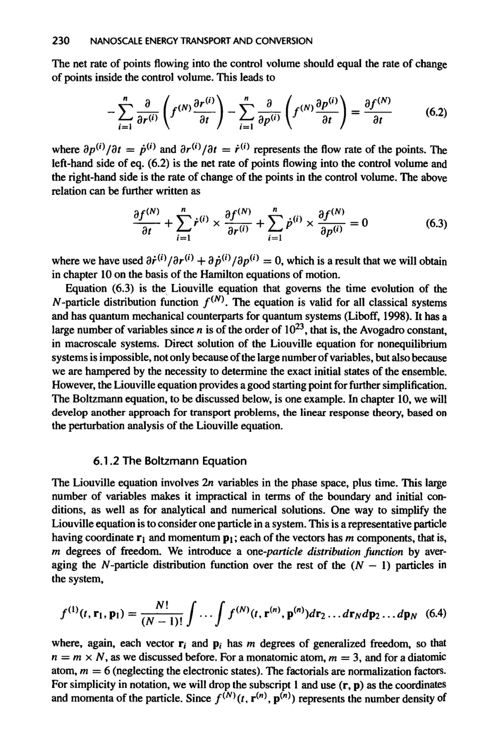
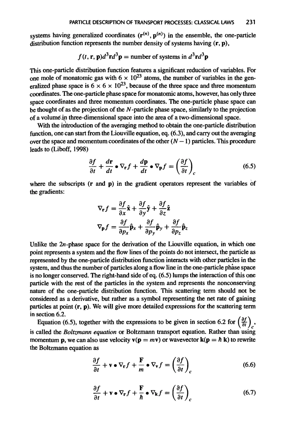
mechanics and solid-state physics will have an easier time going through the contents.
Second, the parallel treatment reflects my conviction that we should provide students
with interdisciplinary training for their future multidisciplinary working environment.
Through the parallel treatment, readers will see that the diverse energy carriers share
many common grounds and are often described by the same equations. It will be revealing
for some readers to see that the Fourier law of heat conduction, the Newton law of shear
stress, and the Ohm law for electrical current flow can all be derived from the Boltzmann
equation, and that heat conduction at nanoscale can be similar to thermal radiation at
macroscale. Through these examples and many others in the book, I hope that the readers
will see that the discipline boundaries are easy to cross. As the traditional disciplines
have been extensively plowed in the last century, it is in the boundary areas that more
room exists for future discoveries and innovations. Nanotechnology is just one example
that intersects many different disciplines. In fact, there is no single nanotechnology, but
there are many potential nano-based technologies that await the readers to invent and
to develop.
One purpose of the book is to serve as a senior or graduate level textbook in nanoscale
heat transfer and energy conversion; the other goal is to provide researchers, veterans
as well as starters, with a reference. The contents and mathematical details of this book
are a delicate balance between conflicting requirements on breadth versus depth, and
instruction versus research. I tried to set the book at such a level that a serious reader
with a mechanical engineering background can go through the derivations and use the
book as a starting point for his or her own research, but anticipate that researchers will
need to dig out original papers and other reference books for details. The references
cited emphasize original papers and are not intended to be inclusive of publications in
the area of nano- and micro-scale heat transfer, simply because of the wide range of
topics covered. The choice of contents of this book is strongly influenced by my own
learning and research experience.
Because of the wide range of topics covered in this book, one challenge for the readers
is to embrace different terminologies. This can indeed be sometimes daunting. I have
taught part of the contents of the book at both the University of California at Los Angeles
and Massachusetts Institute of Technology; the students included graduates, seniors,
and even several juniors, most of them having mechanical engineering backgrounds.
Feedback from students is overwhelmingly positive but it is also clear that the contents
can be “shocking” to some students. My attitude is: no pain, no gain. The gap that
needs to be filled is large but the reward is also large. As the reading progresses, I
advise students often to skim the most recent issues in journals such as Science, Nature,
Applied Physics Letters, and the many new journals in nanotechnology, in addition to
reading nanoscale heat transfer papers, and hope that they will enjoy the pleasure of
starting to understand what are being discussed in some of the papers. Of course, the
PREFACE XI
true pleasure will come from applying what they have learnt from the book to their
own work, and I will be happy to share with readers such joys, as well as criticism of
the book.
Gang Chen
Carlisle, Massachusetts
Acknowledgments
I used to think that the acknowledgments are just a routine duty of the author until
I got near to finishing this book. It is a personal feeling best expressed in a public form.
It actually became the section that I wanted to write most. Seldom can anyone write
a book without building on the work of others, and this book is no exception. Some
of the contributors are acknowledged in the form of references while contributions of
others may have been treated as common knowledge. At the personal level, I have many
friends to thank, starting from my college studies at Huazhong University of Science
and Technology in China, the University of California at Berkeley, and my colleagues at
Duke University, the University of California at Los Angeles, and now at Massachusetts
Institute of Technology. I will not list all of them because of the length of the list and the
possibility of missing some of them. But there are two persons who are even more special
that I must acknowledge. I would not have been able to make this contribution if it were
not for my Ph.D. thesis advisor, the late Professor Chang-Lin Tien, who hand-picked me
while traveling in China and continued to supervise me even during his tenure as the chan¬
cellor at UC Berkeley. His vision and pioneering work led to the rapid development of the
field of micro- and nanoscale heat transfer. Although he left us at an early age, his spirit
will continue to inspire many of us who had the fortune to associate with him personally
or through his work. I am also deeply grateful to Professor Mildred S. Dresselhaus,
who serves as my other role model with her dedication and energy. She also read and
commented on the first few chapters of the book. Students who have taken my course on
the subject at UCLA and MIT provided many inputs to the book and I thank them without
mentioning their names. Also to be thanked are students from RPI in Professor T. Borca-
Tasciuc’s class and from U. Kentucky in Professor M.P. Menguc’s class, who provided
written feedback on some chapters. Several students in my current group helped greatly
Xiv ACKNOWLEDGMENTS
in proofreading and figure drawing: D. Borca-Tasciuc, Z. Chen, J. Cybulski, C. Dames,
T. Harris, A. Henry, L. Hu, A. Narayanaswamy, A. Schmidt, A. Shah, and, particularly,
R.G. Yang, for summarizing students’ comments. Several former students and post-docs
are also acknowledged for stimulating me and contributing to my knowledge in the areas
covered, including Drs T. Borca-Tasciuc, W.L. Liu, D. Song, S.G. Volz, B. Yang, and
T.F. Zeng. Professors J.B. Freund (UIUC), P.M. Norris (U. Virginia), and M. Kaviany
(U. Michigan) have provided constructive feedback on chapters of the book. I, of course,
take responsibility for any mistakes. I would also acknowledge the K.C. Wong Education
Foundation in Hong Kong and the Simon-Guggenheim Foundation for supporting my
career at various stages. The inclusion of this book in the MIT-Papallardo Series in
Mechanical Engineering would not have been possible without the generous support
of Neil and Jane Papallardo and the series editors, Professors Rohan Abeyarantne and
Nam Suh.
I would like to thank several funding agencies, including DOE, DARPA, JPL,
NASA, NSF, and ONR, that provided support for my research in this area, among
them particularly the NSF Young Investigator Award that supported my early career
and the DOD/ONR Multidisciplinary University Research Initiative that provided me
an opportunity to work across disciplines. This book is in many ways an integration of
education and research. Several papers that I have written in the past few years were
stimulated from making analogies between different energy carriers.
My editor at Oxford University Press, Danielle Christensen, put gentle pressure on
me to finish the seemingly never-ending manuscript. Lisa Stallings and Barbara Brown
at OUP were of great help in the production phase of the book. Sue Nicholls and Ian
Guy at Keyword Publishing Services Ltd. carried out careful editing of the manuscript.
My thanks go to them for turning the manuscript into final print.
I would like to thank my parents and my wife’s parents for their moral support and
prayers. Most of all my thanks go to my dear wife Tracy and our son and daughter,
Andrew and Karen. I once read from the preface of a book in which the author (whom I
know) claimed that on average every printed page of his book took three hours. I did not
believe him until I came close to finishing this book. I started writing this book about
five years ago, when we were expecting our daughter Karen and I changed my working
habit to have a few hours in the early morning. I thought that the book could be finished
as a gift at the birth of my daughter. That goal turned out to be a gross underestimation
of the time needed to complete a book. Karen is now four and Andrew is ten. They have
often been checking which chapter I was writing while waiting patiently with Tracy.
A big portion of the roughly 1500 hours that I spent on the book was stolen from them.
I hope the delivery of this manuscript will mean that I will now find more time to spend
with them.
Figure Credits
Fig. 1.1(a) and (b): Courtesy of International Business Machines Corporation.
Unauthorized use not permitted.
Fig. 1.1(c): Reprinted with permission from Steven Pei
Fig. 1.1(d): Reprinted with permission from Steven Pei. Photo by Michael Weimer.
Fig. 1.2(c): Reprinted with permission from Venkatasubramanian, R. et al., 2001,
“Thin-Film Thermoelectric Devices with High Room-Temperature Figures of Merit,”
Nature, vol. 413, pp. 597-602. Copyright 2001 Nature.
Fig. 1.4(c): Reprinted with permission from Ren et al., 1998, Science, vol. 282,
pp. 1105-1107. Copyright 1998 AAAS.
Fig. 2.6(a): Reprinted from Amnon Yariv, 1989, Quantum Electronics, 3rd ed., Wiley,
New York, with permission from John Wiley and Sons, Inc.
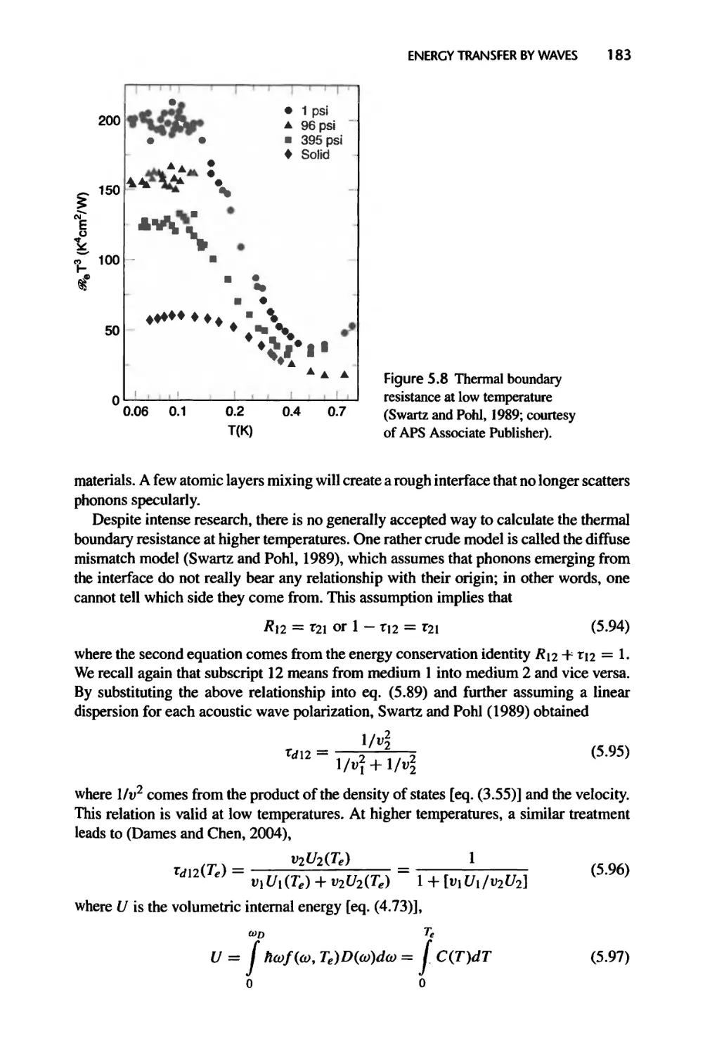
Fig. 5.8: Reprinted with permission from Swartz, E.T. and Pohl, R.O., 1989, “Thermal
Boundary Resistance,” Reviews of Modem Physics, vol. 61, pp. 605-668. Copyright
1989 by the American Physical Society.
Fig. 5.15(b): Reprinted with permission from Odom, T.W., Huang, J., Kim, P. and
Lieber, C.M., 1998, “Atomic Structure and Electronic Properties of Single-Walled
Carbon Nanotubes,” Nature, vol. 391, pp. 62-64. Copyright 1998 Nature.
Fig. 5.17(a): Reprinted from Domoto G.A., Boehm, R.F. and Tien, C.L., 1970,
“Experimental Investigation of Radiative Transfer between Metallic Surfaces at
Cryogenic Temperatures,” Journal of Heat Transfer, vol. 92, pp. 412-417, with
permission from ASME.
Fig. 5.17(b): Reprinted from Hargreaves, C.M., 1969, “Anomalous Radiative Trans¬
fer between Closely-Spaced Bodies,” Physics Letters, vol. 30A, pp. 491-492, with
permission from Elsevier.
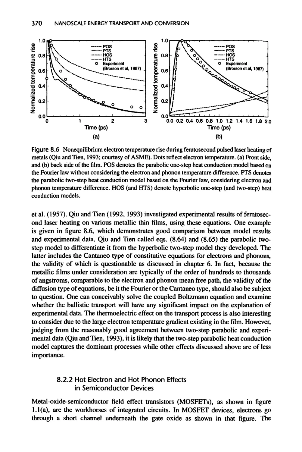
Fig. 8.6(a) and (b): Reprinted from Qiu, T.Q. and Tien, C.L., 1993, “Heat Transfer
Mechanisms during Short-Pulse Laser Heating of Metals,” Journal of Heat Transfer,
vol. 115, pp. 835-841, with permission from ASME.
xvi FIGURE CREDITS
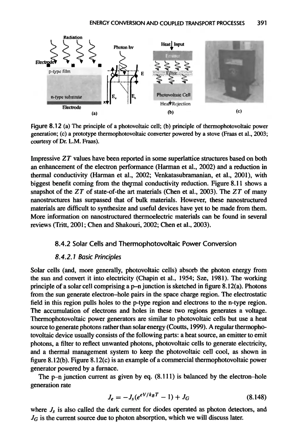
Fig. 8.12(c): From Fraas L.M., Avery J.E., Huang H.X. and Martinelli, R.U., 2003,
“Thermophotovoltaic System Configurations and Spectral Control,” Semiconductor
Science Technology, vol. 18, pp. S165-S173.
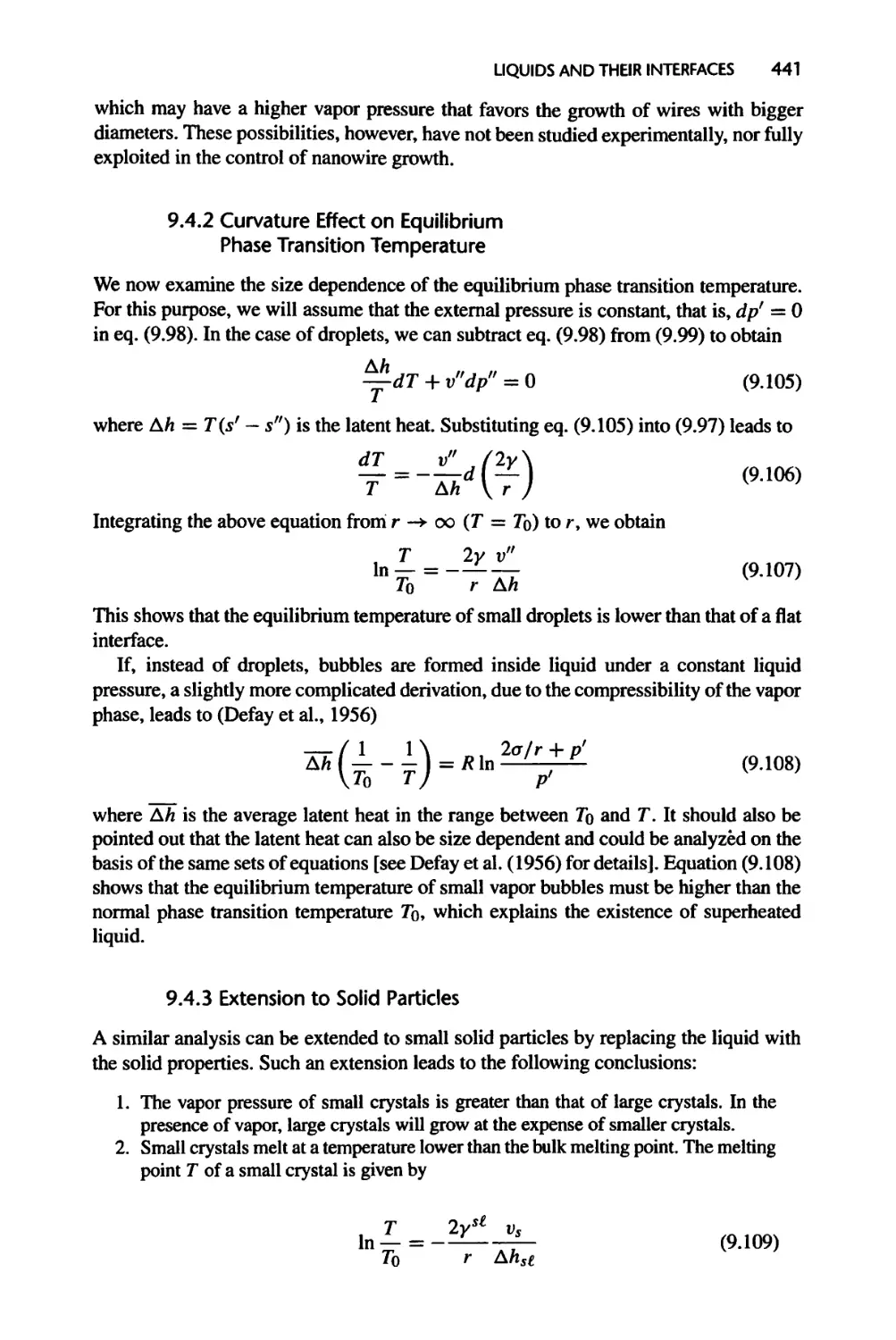
Fig. 9.18: Reprinted with permission from Buffat, Ph. and Borel, J.-P., 1976, “Size
Effect on the Melting Temperature of Gold Particles,” Physical Review A., vol. 13,
pp. 2287-2298. Copyright 1976 by the American Physical Society.
Contents
Foreword, vii
1 Introduction, 3
1.1 There Is Plenty of Room at the Bottom, 4
1.2 Classical Definition of Temperature and Heat, 9
1.3 Macroscopic Theory of Heat Transfer, 9
1.3.1 Conduction, 9
1.3.2 Convection, 11
1.3.3 Radiation, 13
1.3.4 Energy Balance, 16
1.3.5 Local Equilibrium, 17
1.3.6 Scaling Trends under Macroscopic Theories, 17
1.4 Microscopic Picture of Heat Carriers and Their Transport, 18
1.4.1 Heat Carriers, 18
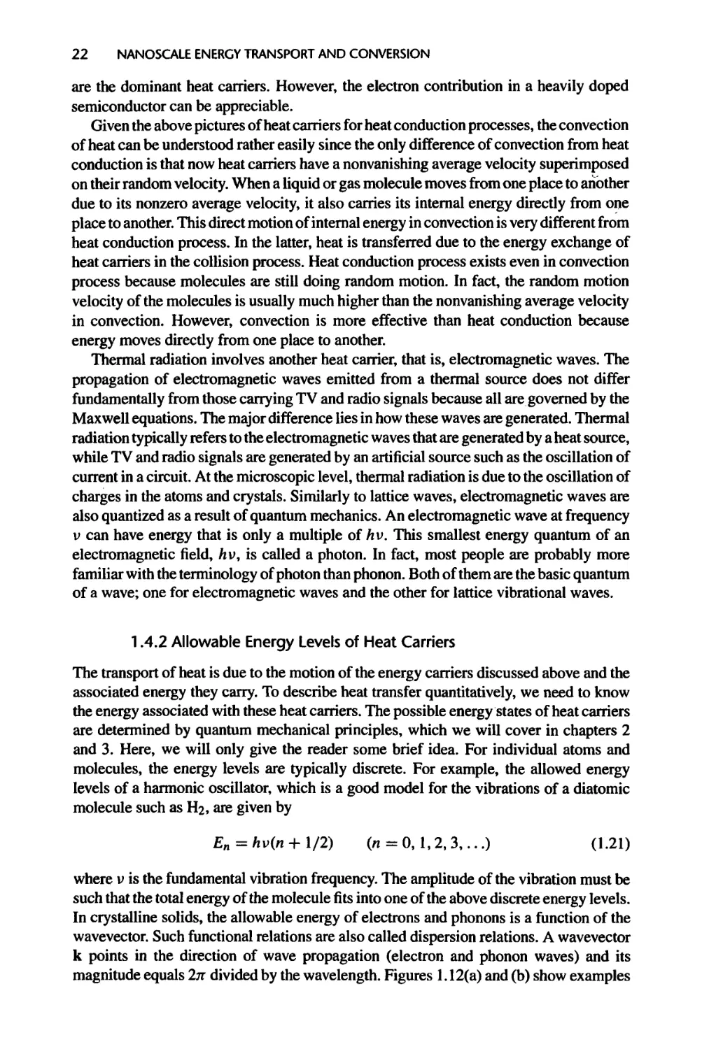
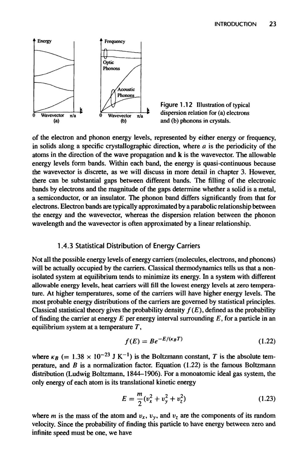
1.4.2 Allowable Energy Levels of Heat Carriers, 22
1.4.3 Statistical Distribution of Energy Carriers, 23
1.4.4 Simple Kinetic Theory, 25
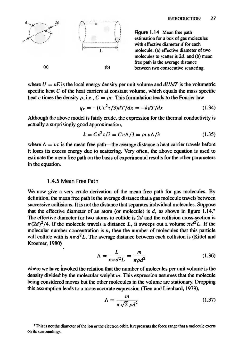
1.4.5 Mean Free Path, 27
1.5 Micro- and Nanoscale Transport Phenomena, 28
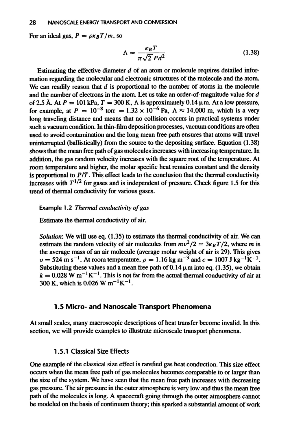
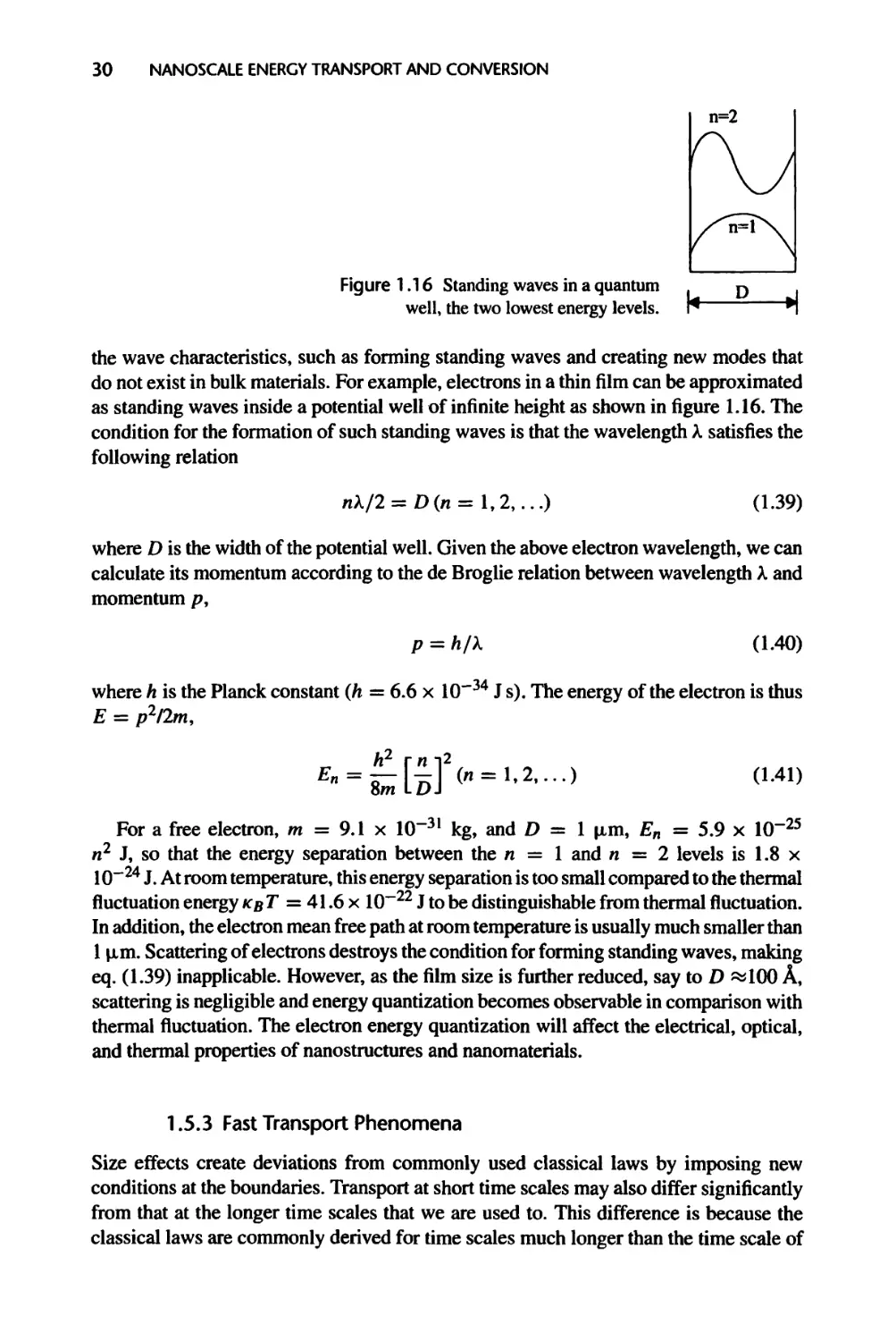
1.5.1 Classical Size Effects, 28
1.5.2 Quantum Size Effects, 29
1.5.3 Fast Transport Phenomena, 30
1.6 Philosophy of This Book, 32
1.7 Nomenclature for Chapter 1,34
1.8 References, 35
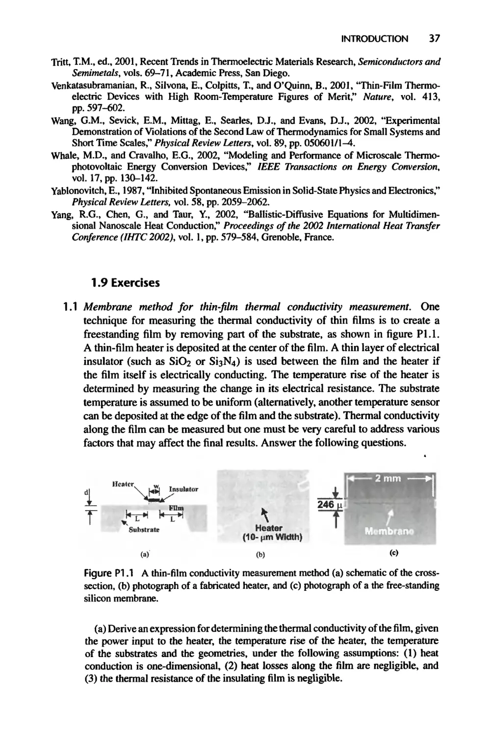
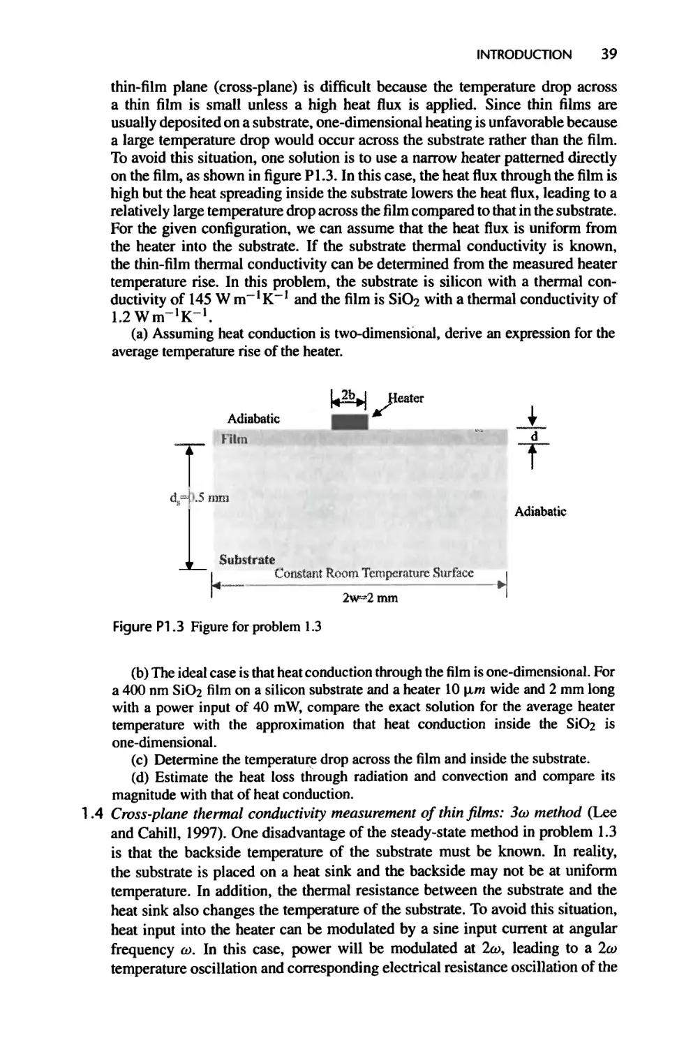
1.9 Exercises, 37
2 Material Waves and Energy Quantization, 43
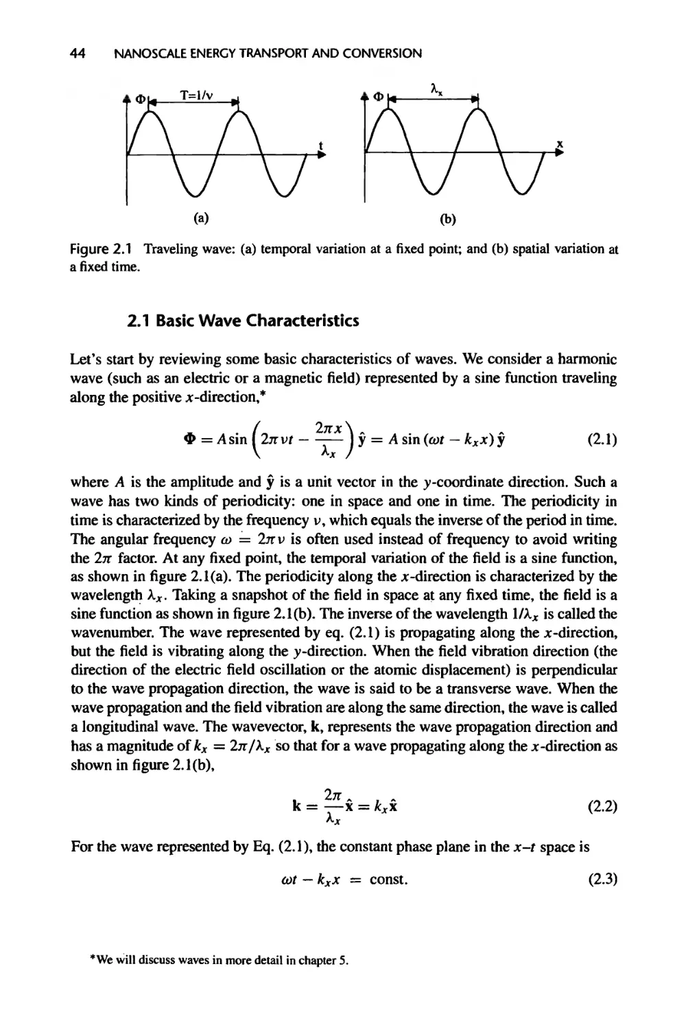
2.1 Basic Wave Characteristics, 44
2.2 Wave Nature of Matter, 46
xviii CONTENTS
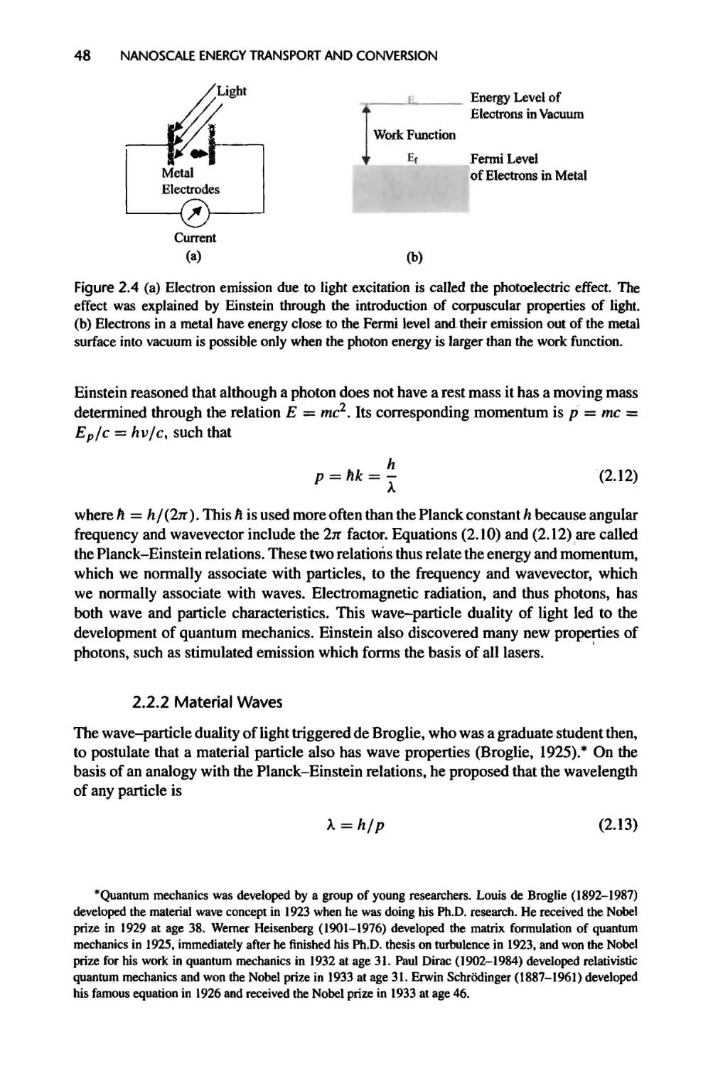
2.2.1 Wave-Particle Duality of Light, 46
2.2.2 Material Waves, 48
2.2.3 The Schrodinger Equation, 49
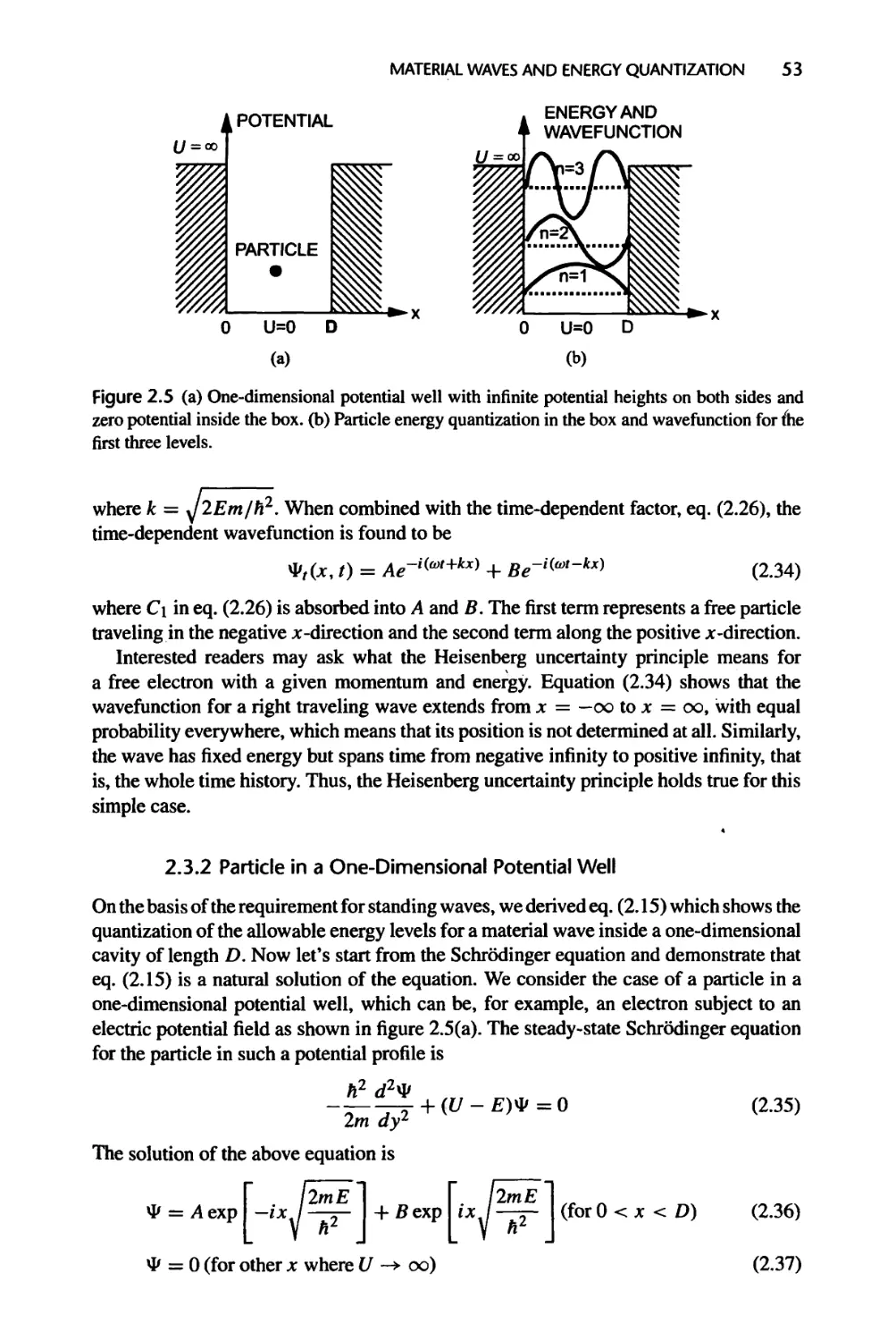
2.3 Example Solutions of the Schrodinger Equation, 52
2.3.1 Free Particles, 52
2.3.2 Particle in a One-Di men si on al Potential Well, 53
2.3.3 Electron Spin and the Pauli Exclusion Principle, 58
2.3.4 Harmonic Oscillator, 59
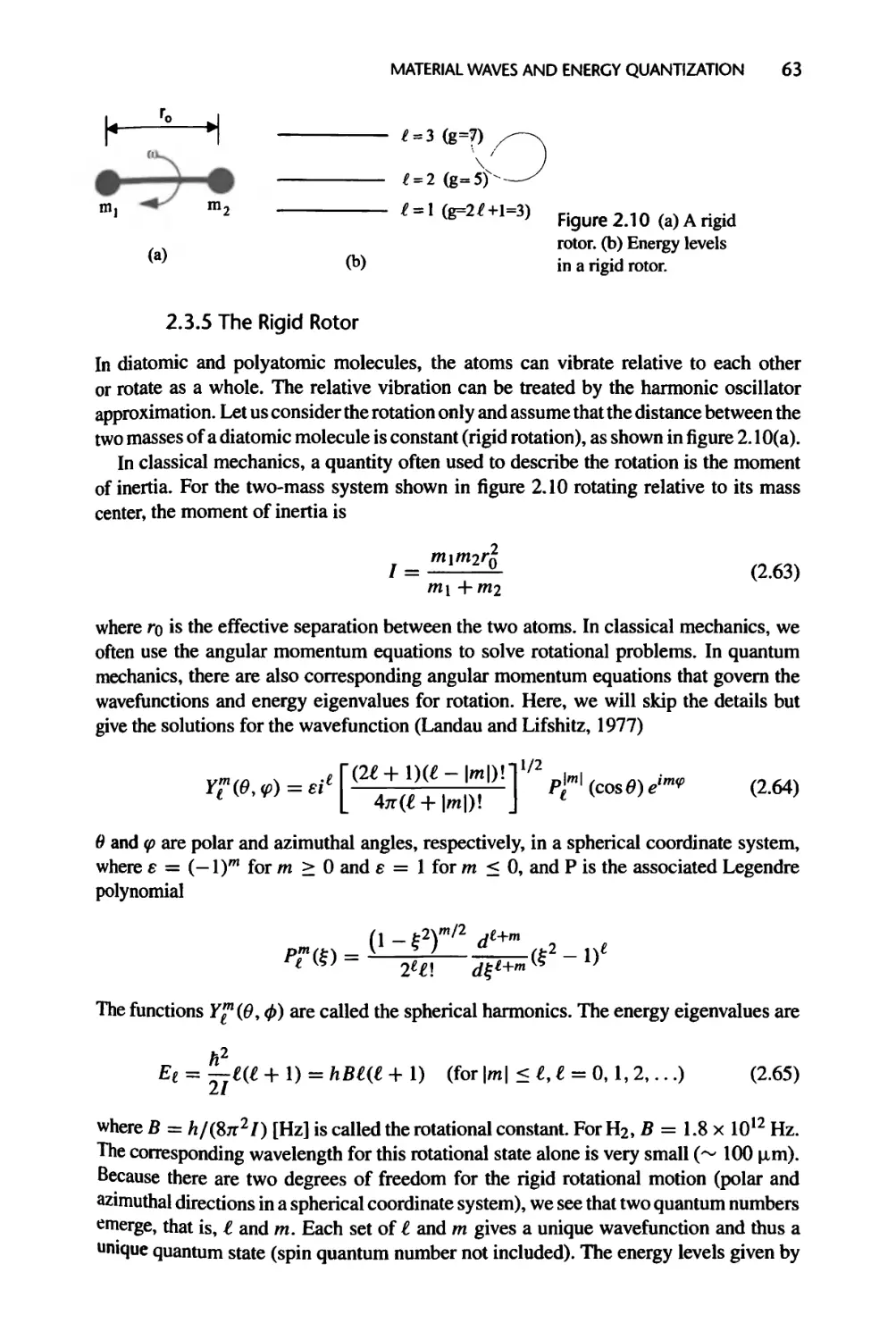
2.3.5 The Rigid Rotor, 63
2.3.6 Electronic Energy Levels of the Hydrogen Atom, 64
2.4 Summary of Chapter 2, 70
2.5 Nomenclature for Chapter 2,72
2.6 References, 72
2.7 Exercises, 73
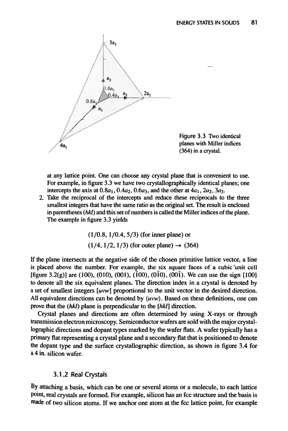
3 Energy States in Solids 77
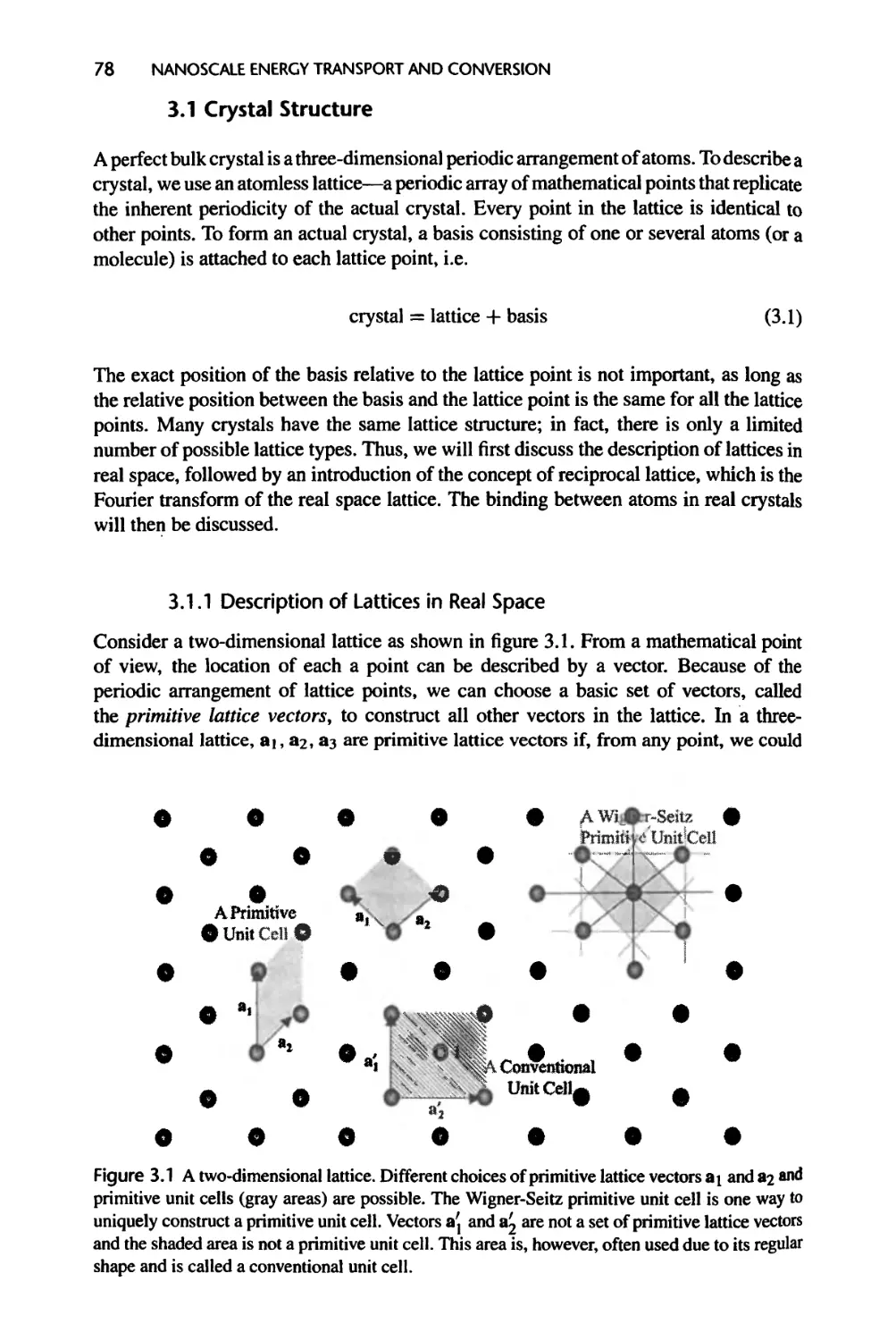
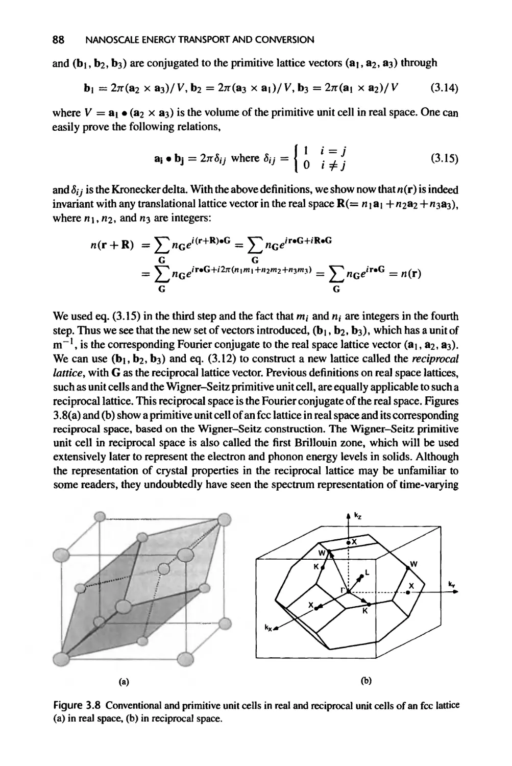
3.1 Crystal Structure, 78
3.1.1 Description of Lattices in Real Space, 78
3.1.2 Real Crystals, 81
3.1.3 Crystal Bonding Potential, 84
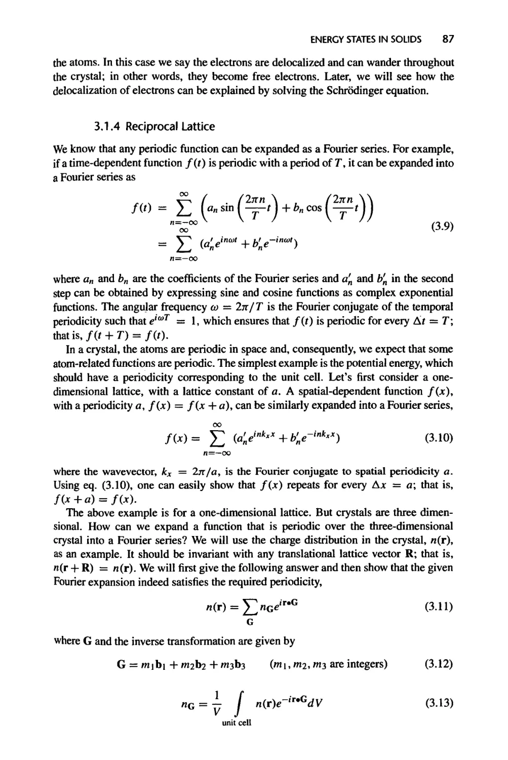
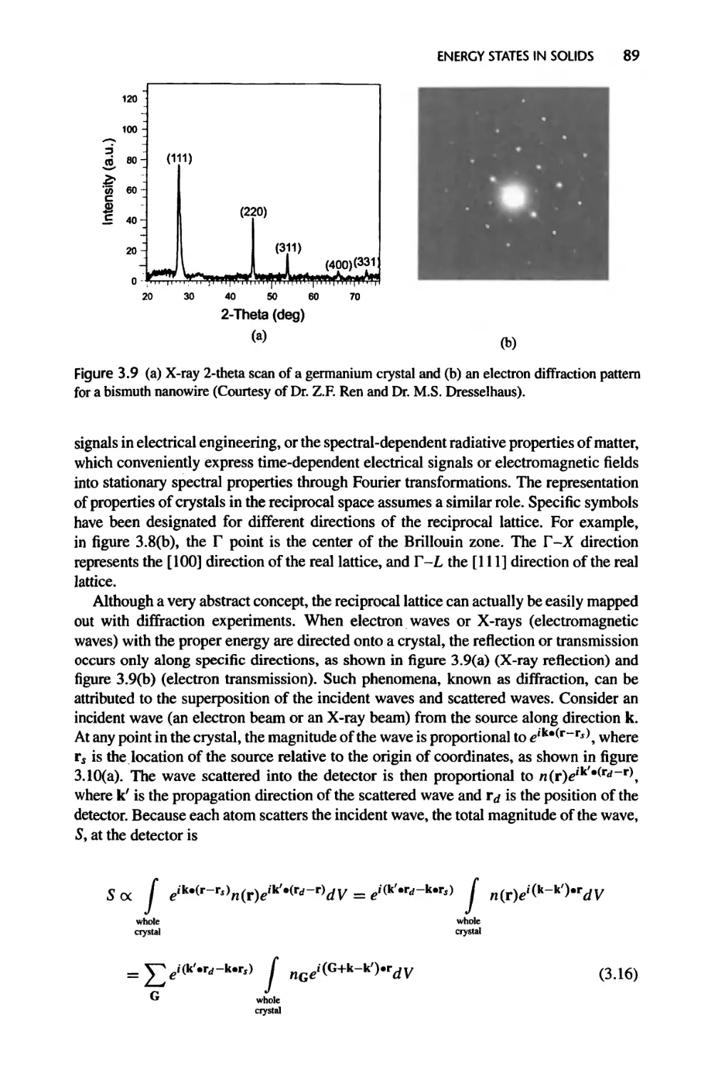
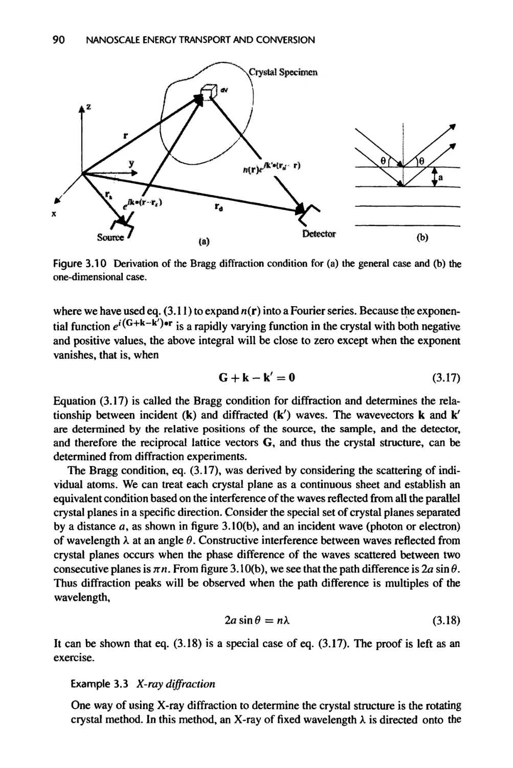
3.1.4 Reciprocal Lattice, 87
3.2 Electron Energy States in Crystals, 91
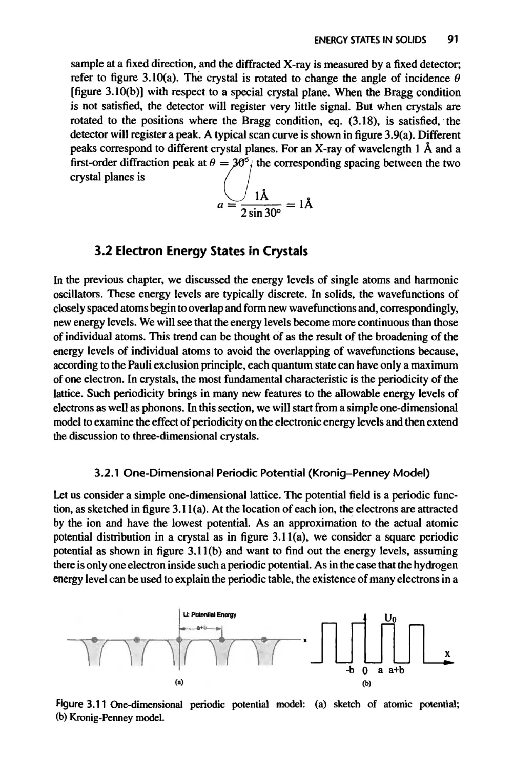
3.2.1 One-Dimensional Periodic Potential (Kronig-Penney Model), 91
3.2.2 Electron Energy Bands in Real Crystals, 98
3.3 Lattice Vibration and Phonons, 100
3.3.1 One-Dimensional Monatomic Lattice Chains, 100
3.3.2 Energy Quantization and Phonons, 103
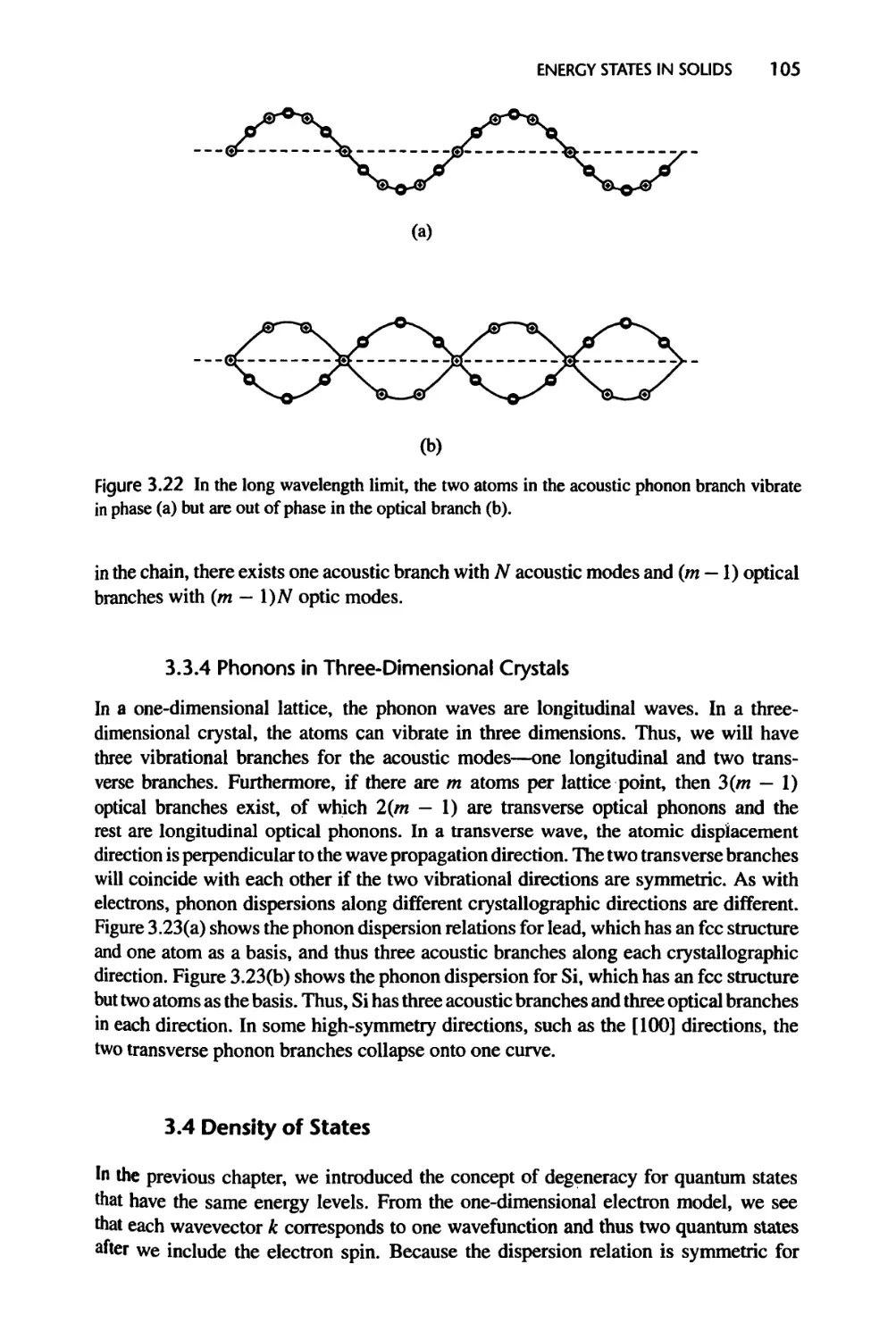
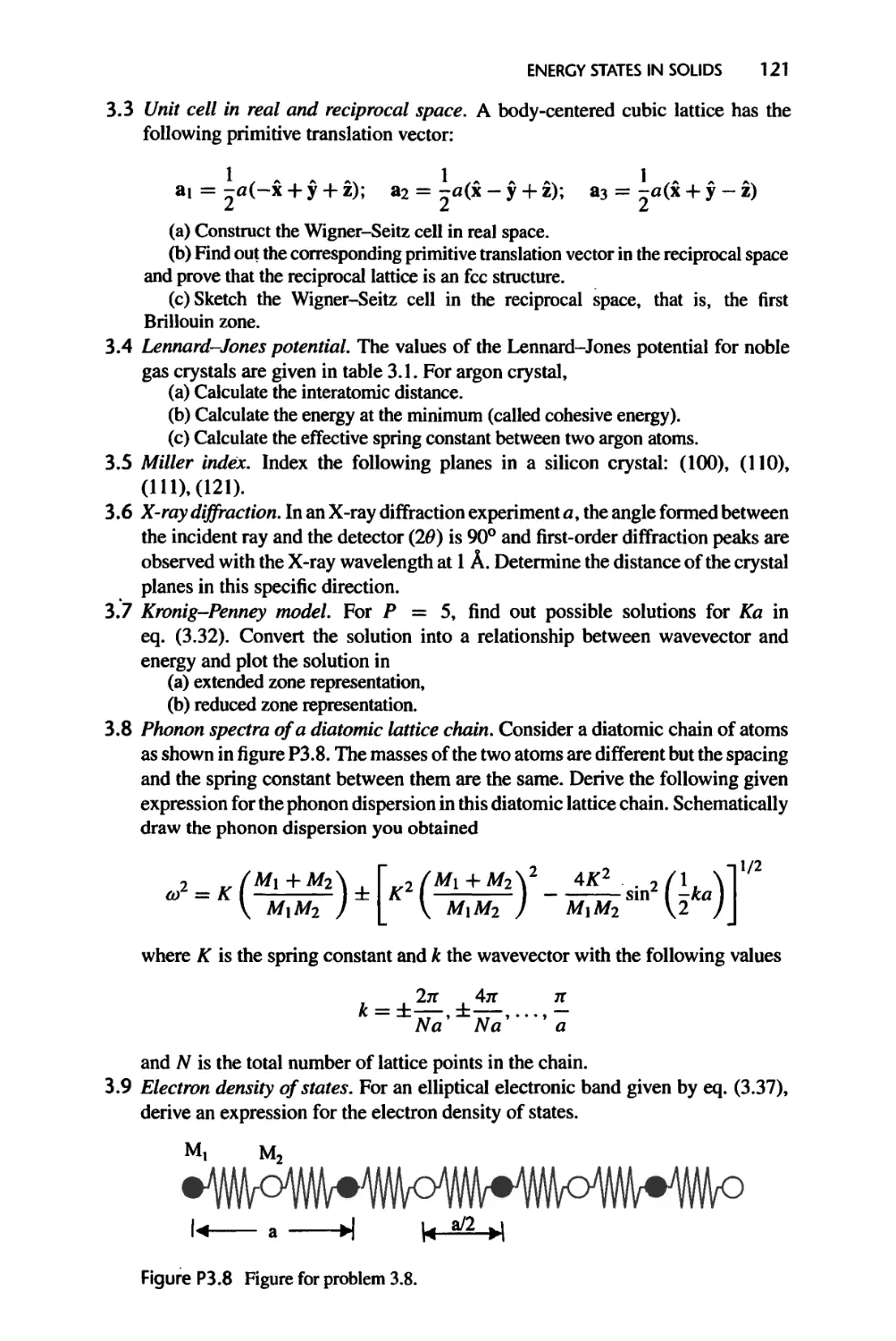
3.3.3 One-Dimensional Diatomic and Polyatomic Lattice Chains, 104
3.3.4 Phonons in Three-Dimensional Crystals, 105
3.4 Density of States, 105
3.4.1 Electron Density of States, 107
3.4.2 Phonon Density of States, 109
3.4.3 Photon Density of States, 110
3.4.4 Differential Density of States and Solid Angle, 111
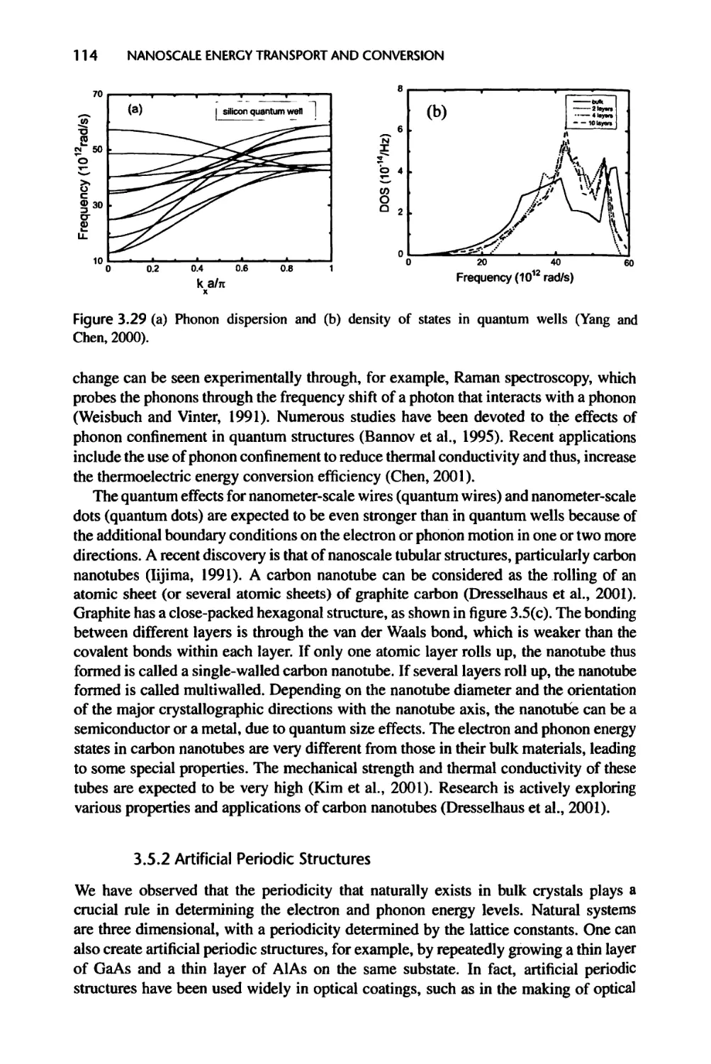
3.5 Energy Levels in Artificial Structures, 111
3.5.1 Quantum Wells, Wires, Dots, and Carbon Nanotubes, 111
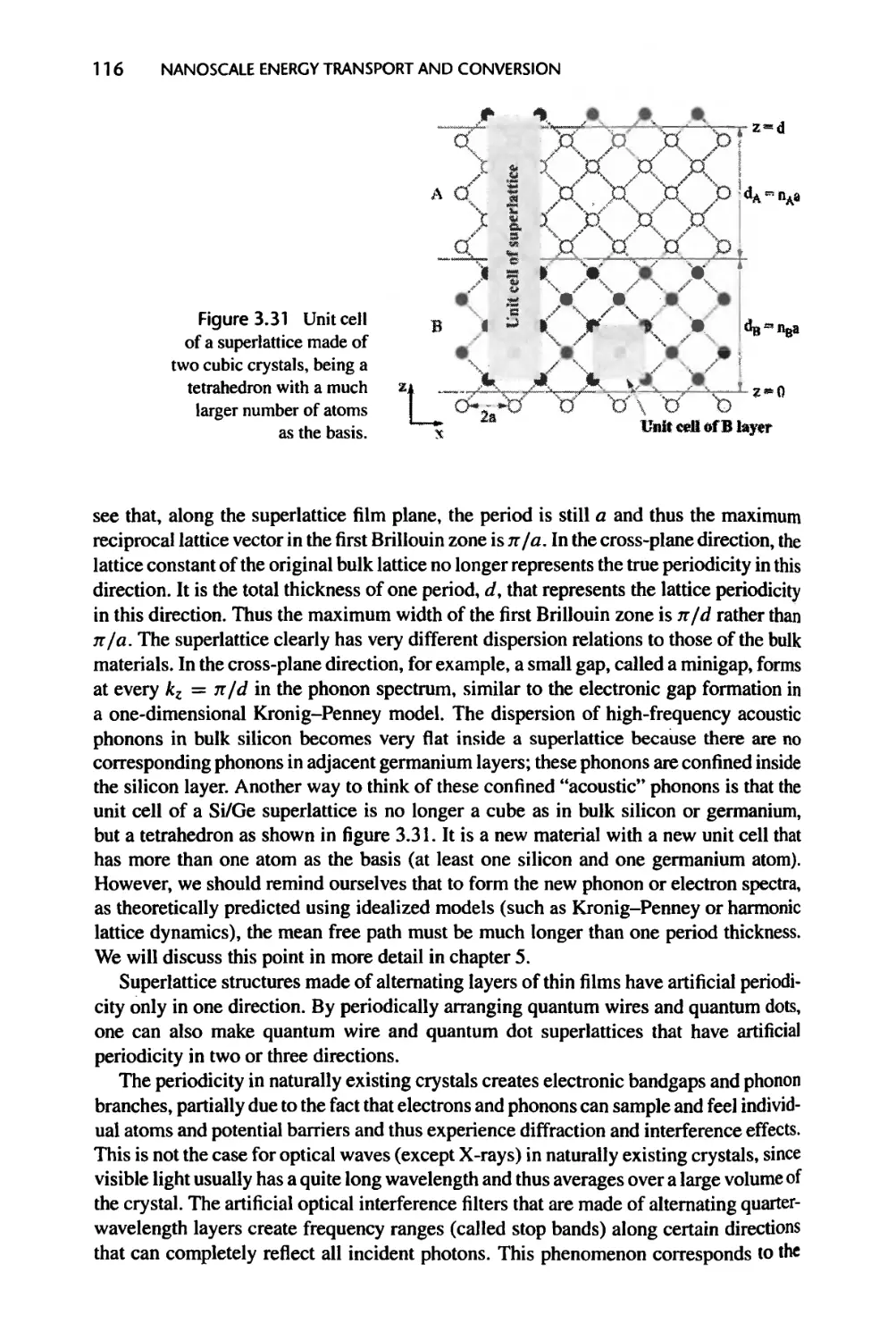
3.5.2 Artificial Periodic Structures, 114
CONTENTS xix
3.6 Summary of Chapter 3,117
3.7 Nomenclature for Chapter 3,118
3.8 References, 119
3.9 Exercises, 121
4 Statistical Thermodynamics and Thermal Energy Storage 123
4.1 Ensembles and Statistical Distribution Functions, 124
4.1.1 Microcanonical Ensemble and Entropy, 124
4.1.2 Canonical and Grand Canonical Ensembles, 127
4.1.3 Molecular Partition Functions, 130
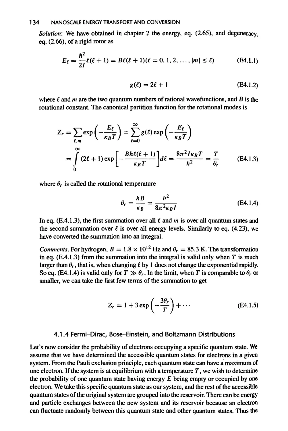
4.1.4 Fermi-Dirac, Bose-Einstein, and Boltzmann Distributions, 134
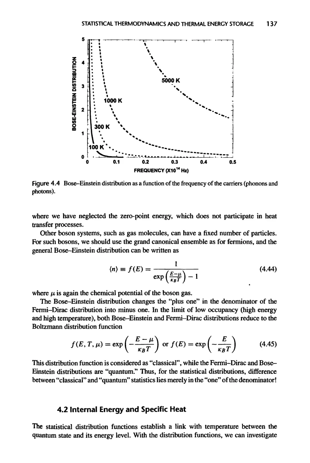
4.2 Internal Energy and Specific Heat, 137
4.2.1 Gases, 138
4.2.2 Electrons in Crystals, 141
4.2.3 Phonons, 144
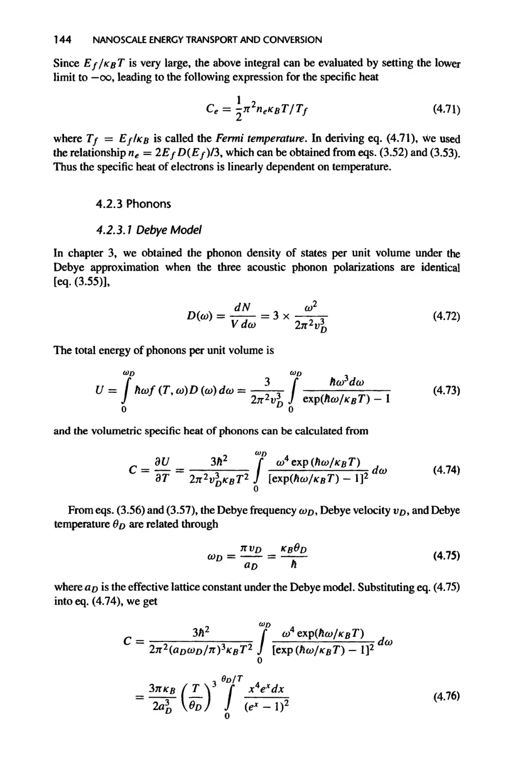
4.2.4 Photons, 146
4.3 Size Effects on Internal Energy and Specific Heat, 148
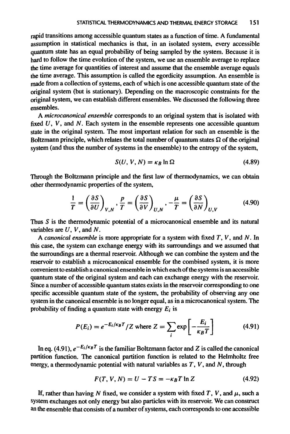
4.4 Summary of Chapter 4, 150
4.5 Nomenclature for Chapter 4, 153
4.6 References, 154
4.7 Exercises, 155
5 Energy Transfer by Waves, 159
5.1 Plane Waves, 160
5.1.1 Plane Electron Waves, 161
5.1.2 Plane Electromagnetic Waves, 161
5.1.3 Plane Acoustic Waves, 167
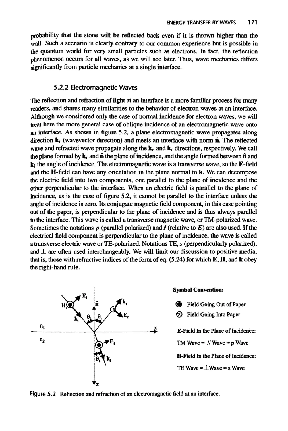
5.2 Interface Reflection and Refraction of a Plane Wave, 169
5.2.1 Electron Waves, 169
5.2.2 Electromagnetic Waves, 171
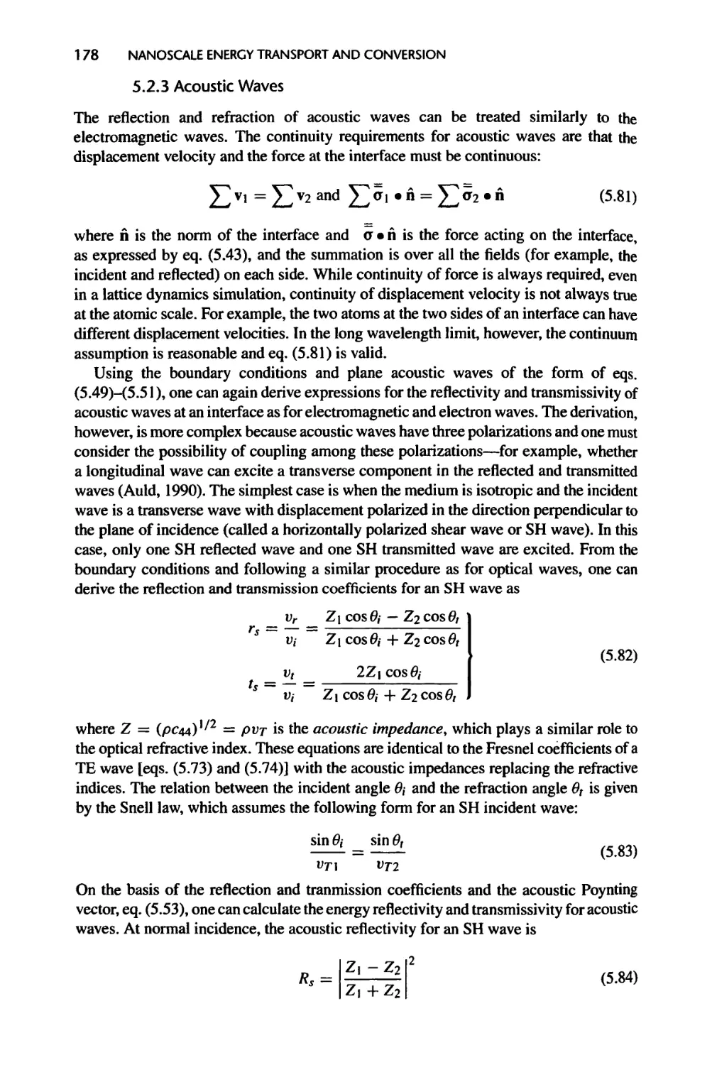
5.2.3 Acoustic Waves, 178
5.2.4 Thermal Boundary Resistance, 180
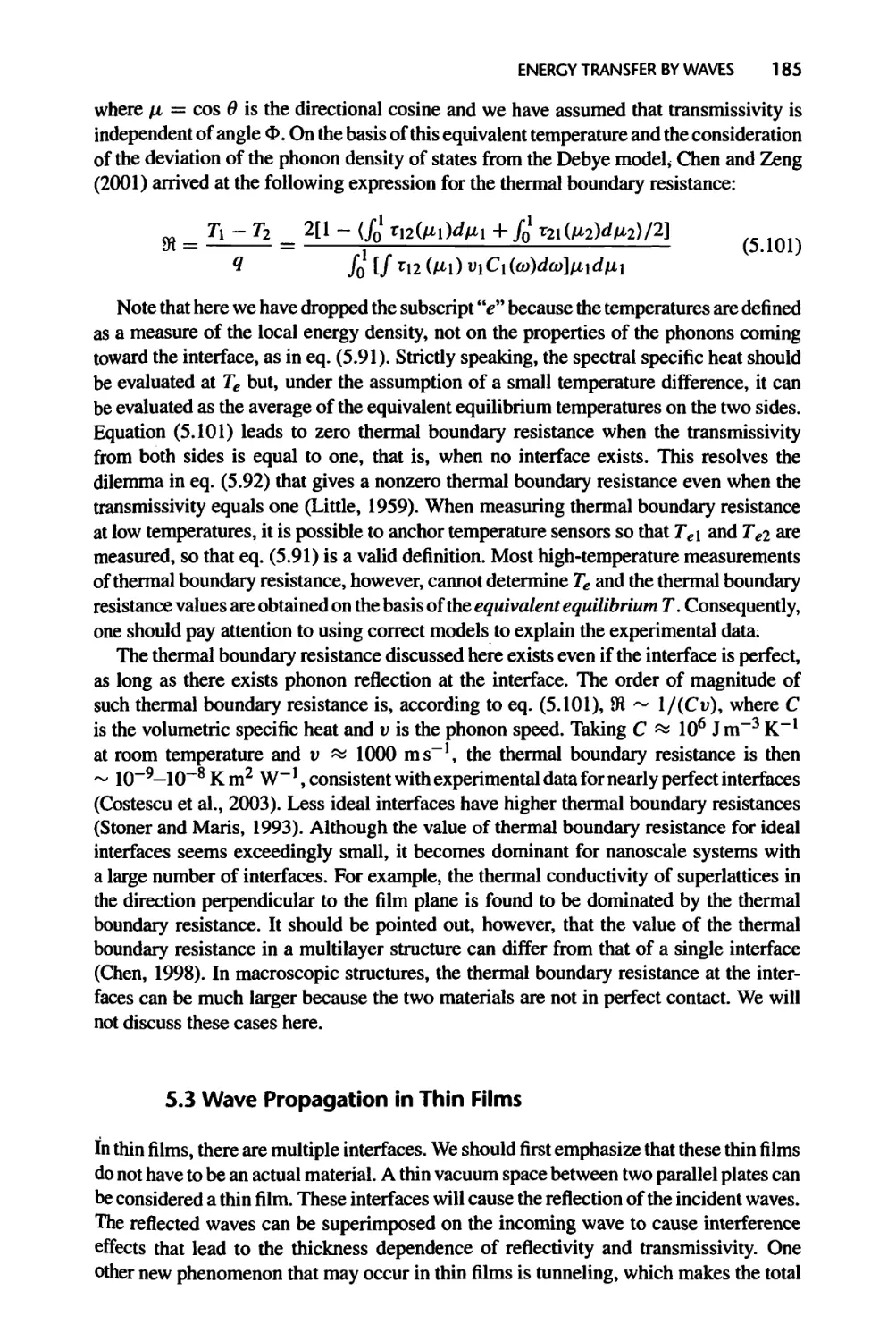
5.3 Wave Propagation in Thin Films, 185
5.3.1 Propagation of EM Waves, 186
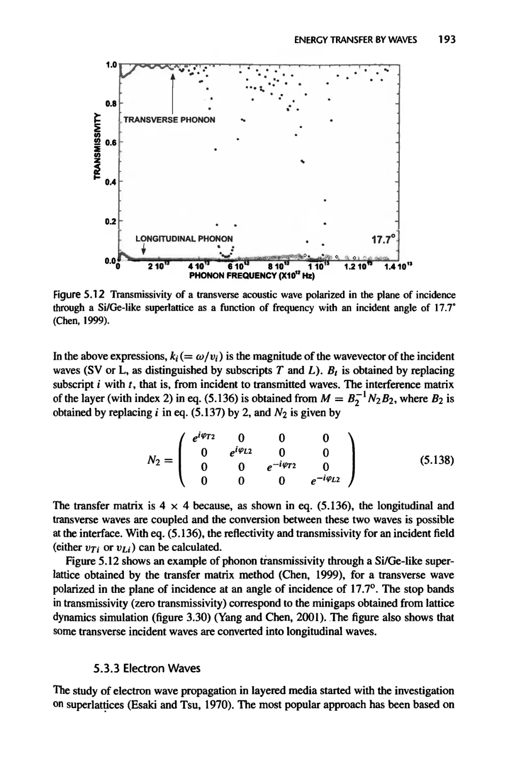
5.3.2 Phonons and Acoustic Waves, 191
5.3.3 Electron Waves, 193
XX
CONTENTS
5.4 Evanescent Waves and Tunneling, 194
5.4.1 Evanescent Waves 194
5.4.2 Tunneling 195
5.5 Energy Transfer in Nanostructures: Landauer Formalism, 198
5.6 Transition to Particle Description, 204
5.6.1 Wave Packets and Group Velocity, 204
5.6.2 Coherence and Transition to Particle Description, 207
5.7 Summary of Chapter 5, 216
5.8 Nomenclature for Chapter 5,218
5.9 References, 220
5.10 Exercises, 223
6 Particle Description of Transport Processes: Classical Laws, 227
6.1 The Liouville Equation and the Boltzmann Equation, 228
6.1.1 The Phase Space and Liouville’s Equation, 228
6.1.2 The Boltzmann Equation, 230
6.1.3 Intensity for Energy Flow, 233
6.2 Carrier Scattering, 233
6.2.1 Scattering Integral and Relaxation Time Approximation, 234
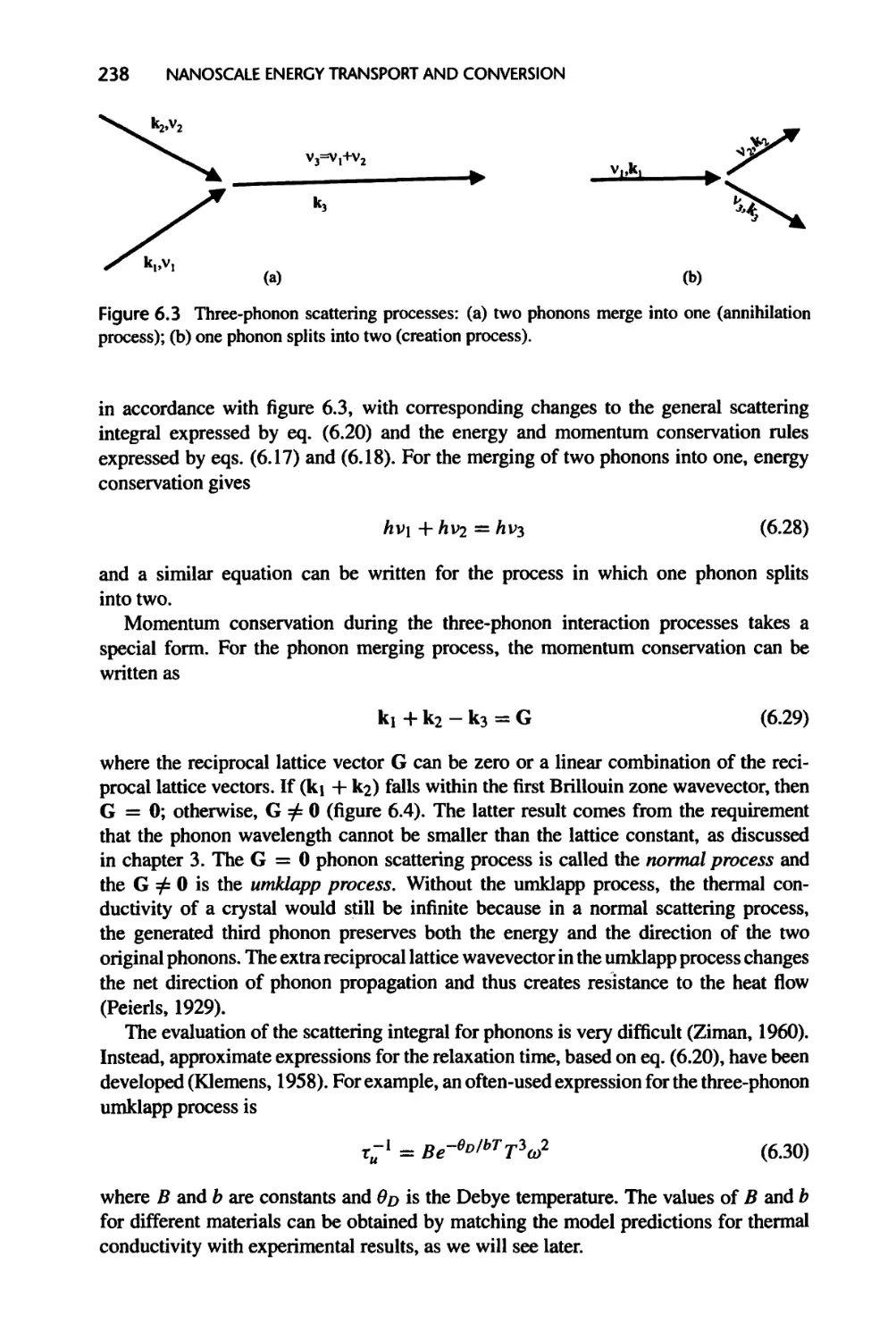
6.2.2 Scattering of Phonons, 237
6.2.3 Scattering of Electrons, 240
6.2.4 Scattering of Photons, 240
6.2.5 Scattering of Molecules, 242
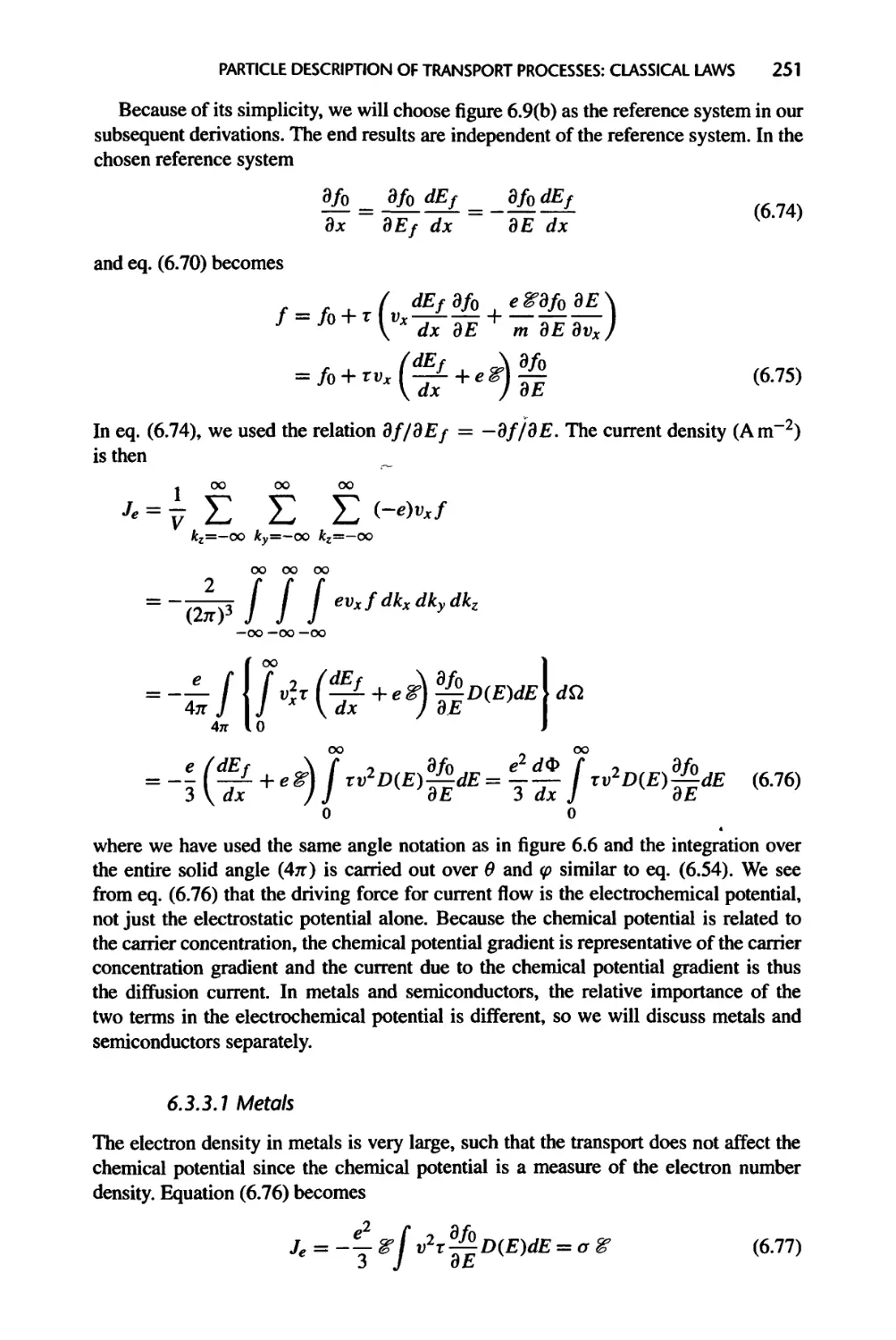
6.3 Classical Constitutive Laws, 242
6.3.1 Fourier Law and Phonon Thermal Conductivity, 243
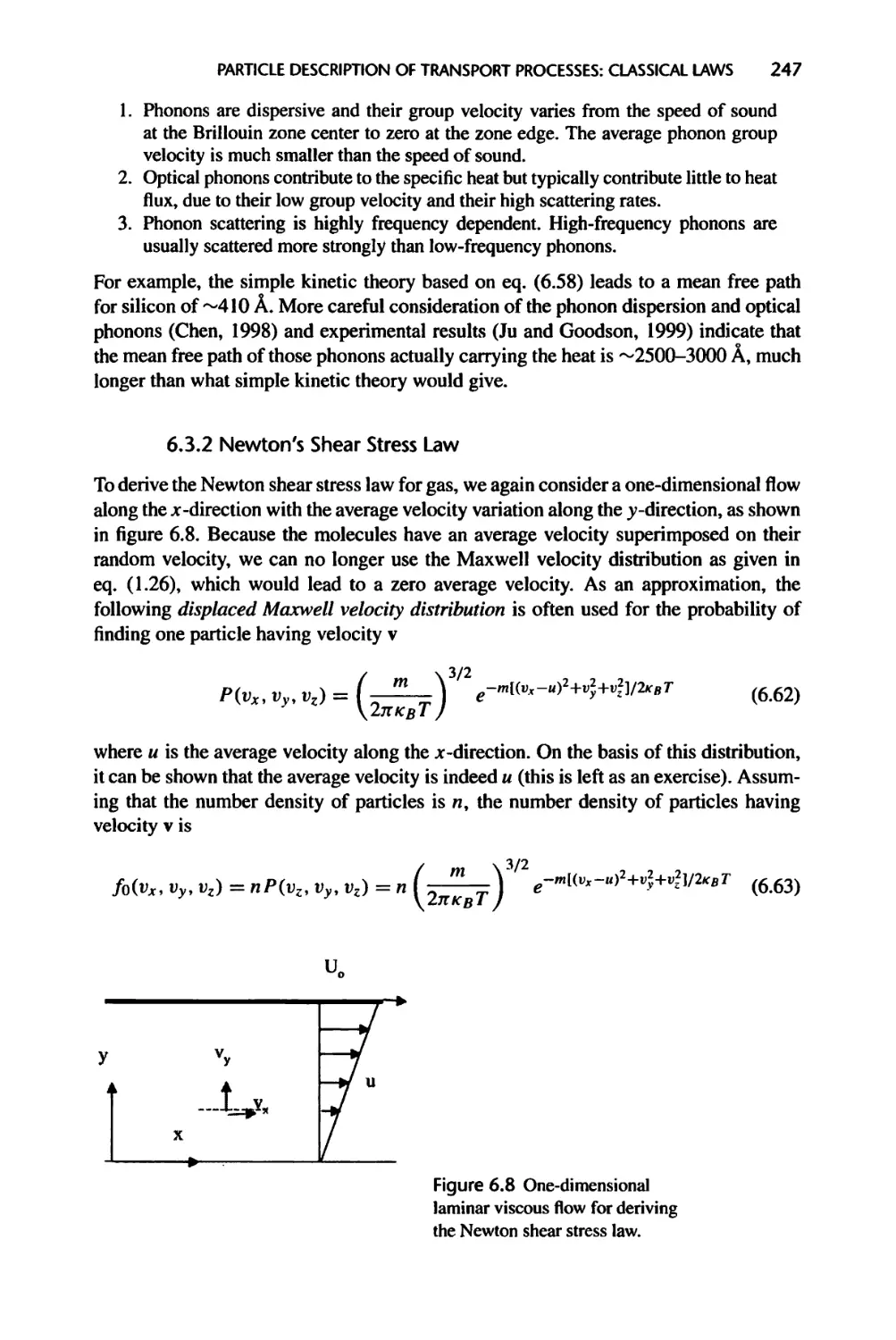
6.3.2 Newton’s Shear Stress Law, 247
6.3.3 Ohm’s Law and the Wiedemann-Franz Law, 249
6.3.4 Thermoelectric Effects and Onsager Relations, 254
6.3.5 Hyperpolic Heat Conduction Equation and Its Validity, 258
6.3.6 Meaning of Local Equilibrium and Validity of Diffusion Theories, 260
6.4 Conservative Equations, 262
6.4.1 Navier-Stokes Equations, 263
6.4.2 Electrohydrodynamic Equation, 266
6.4.3 Phonon Hydrodynamic Equations, 268
6.5 Summary of Chapter 6,273
6.7 Nomenclature for Chapter 6, 275
6.8 References, 277
6.9 Exercises, 279
CONTENTS xxi
7 Classical Size Effects, 282
7.1 Size Effects on Electron and Phonon Conduction Parallel
to Boundaries, 283
7.1.1 Electrical Conduction along Thin Films, 285
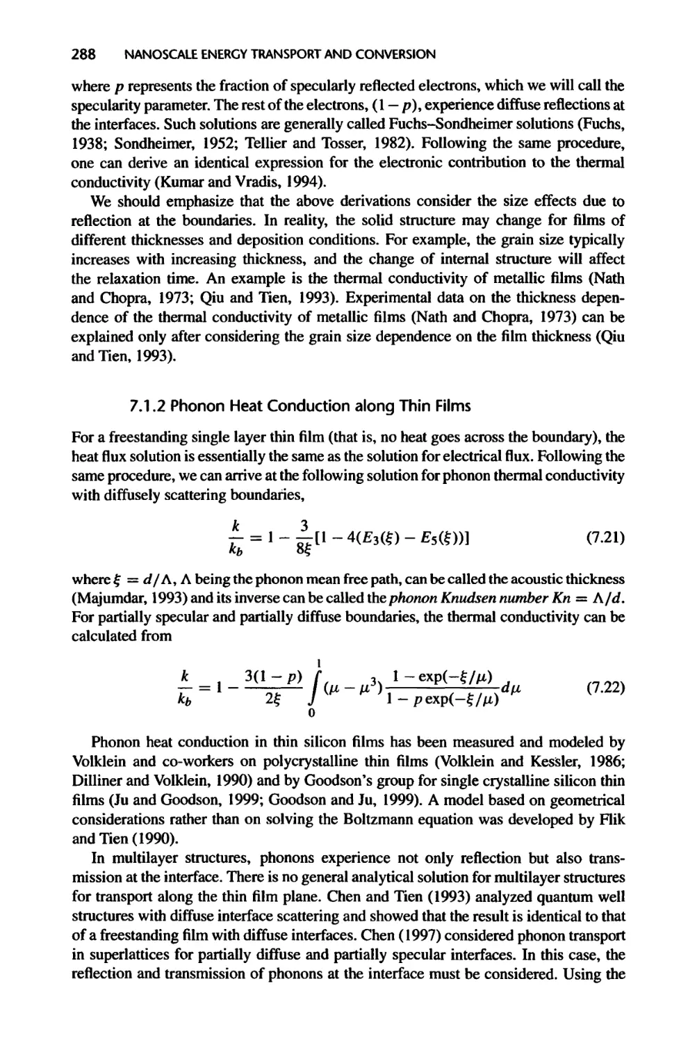
7.1.2 Phonon Heat Conduction along Thin Films, 288
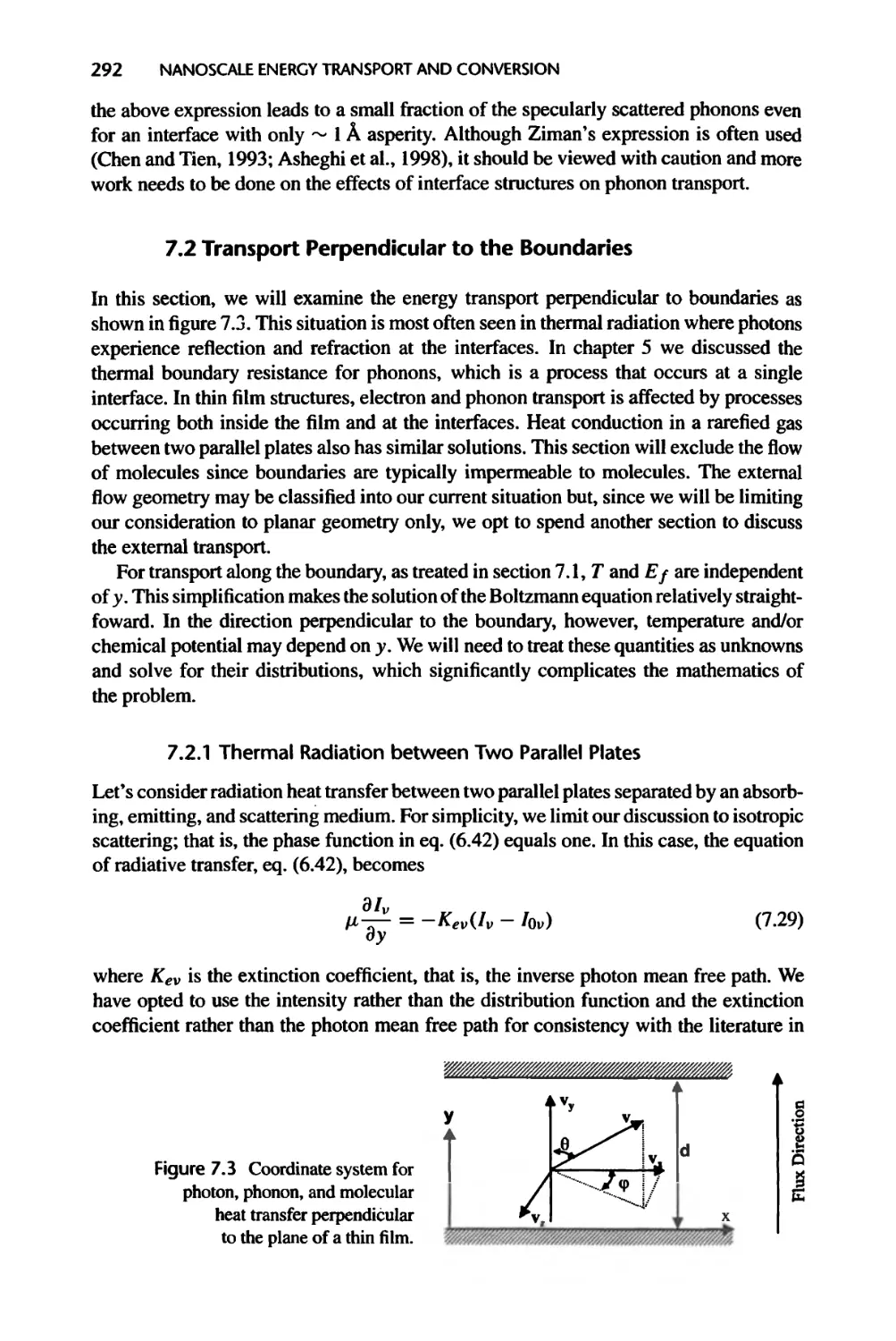
7.2 Transport Perpendicular to the Boundaries, 292
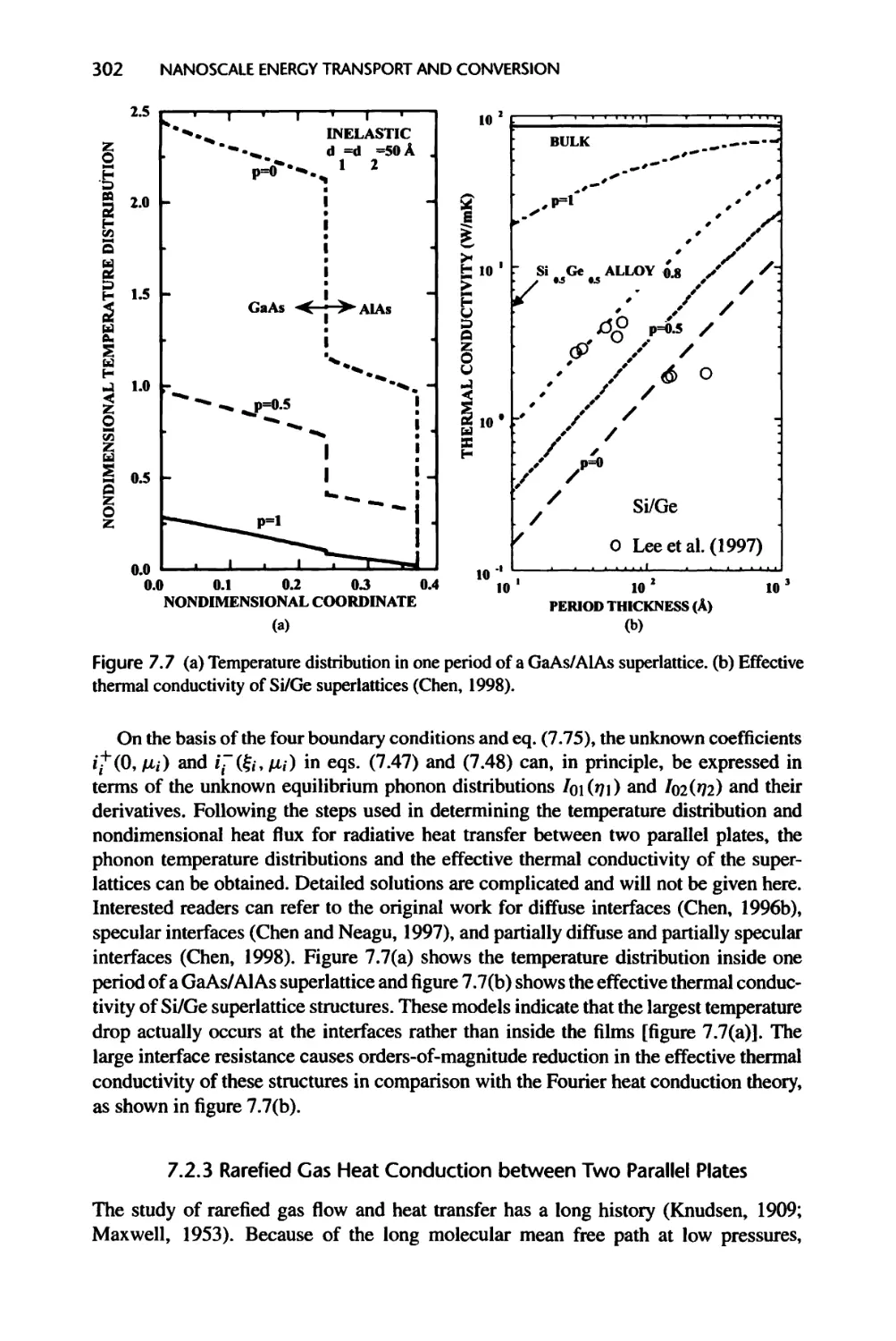
7.2.1 Thermal Radiation between Two Parallel Plates, 292
7.2.2 Heat Conduction across Thin Films and Superlattices, 299
7.2.3 Rarefied Gas Heat Conduction between Two Parallel Plates, 302
7.2.4 Current Flow across Heterojunctions, 307
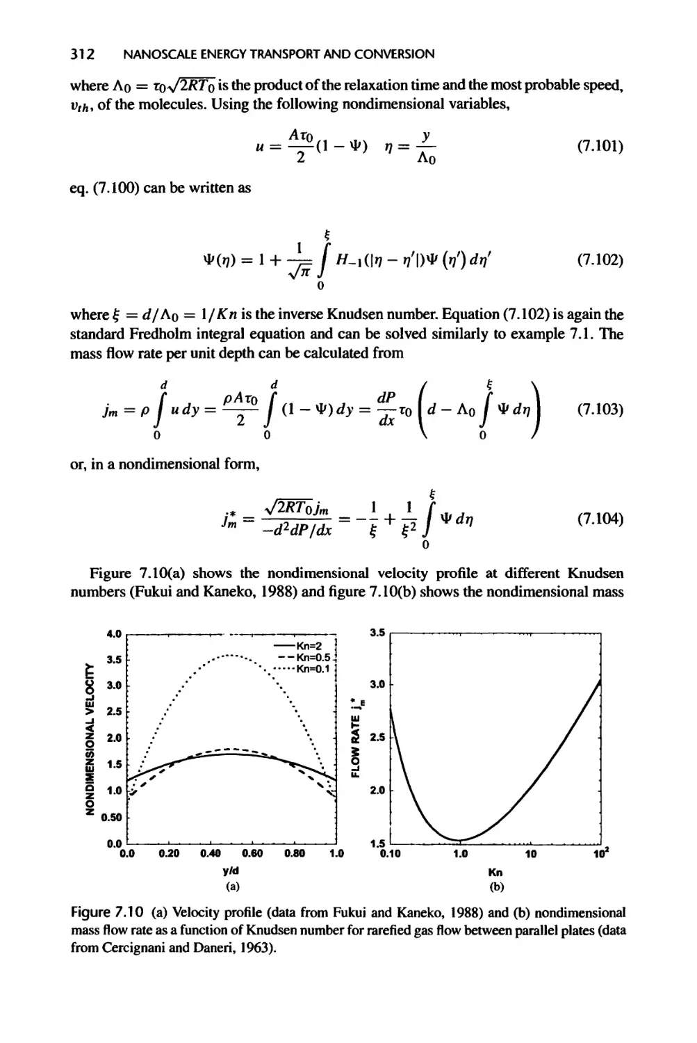
7.3 Rarefied Poiseuille Flow and Knudsen Minimum, 308
7.4 Transport in Nonplanar Structures, 313
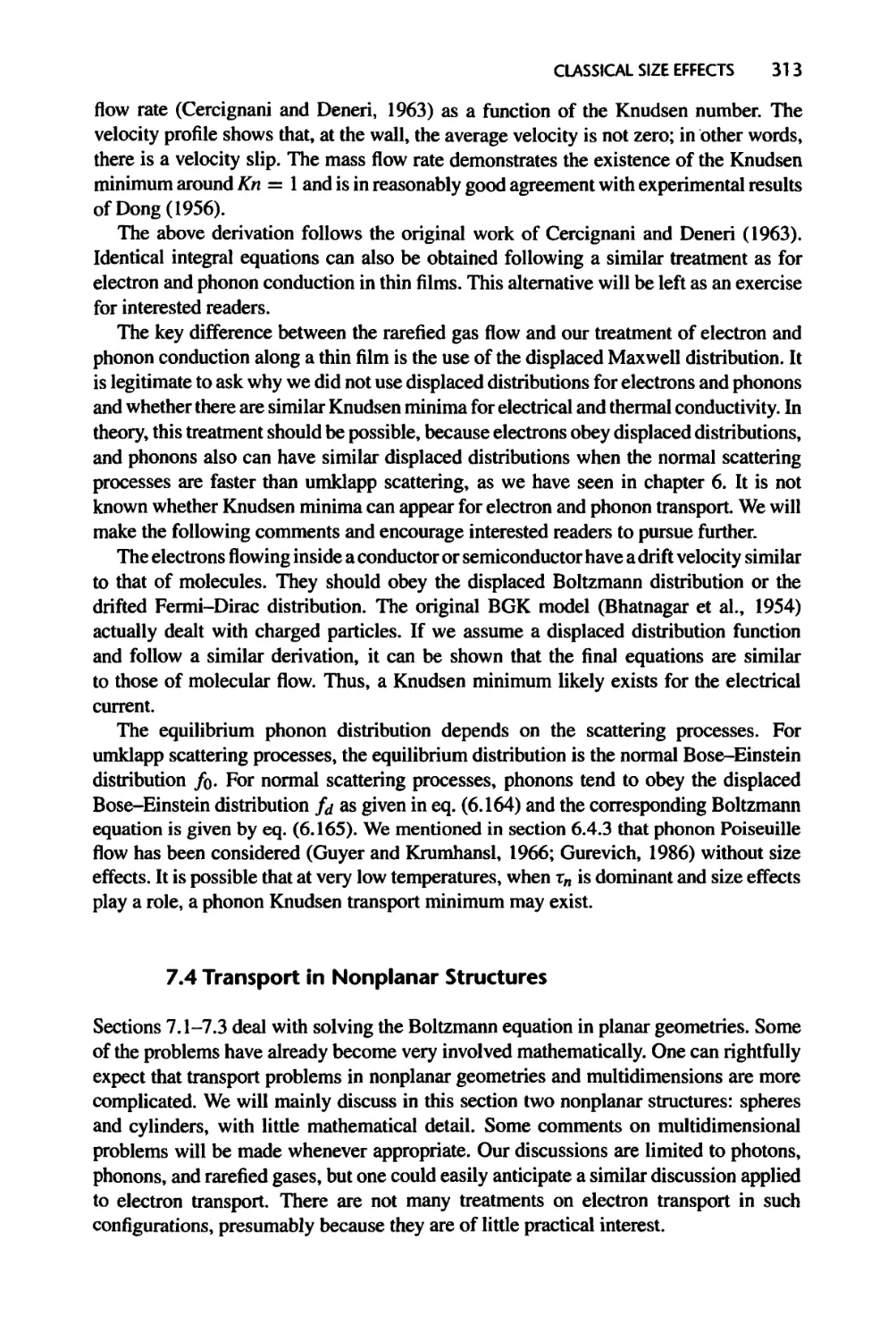
7.4.1 Thermal Radiation between Concentric Cylinders and Spheres, 314
7.4.2 Rarefied Gas Flow and Convection, 314
7.4.3 Phonon Heat Conduction, 315
7.4.4 Multidimensional Transport Problems, 316
7.5 Diffusion Approximation with Diffusion-Transmission Boundary
Conditions, 317
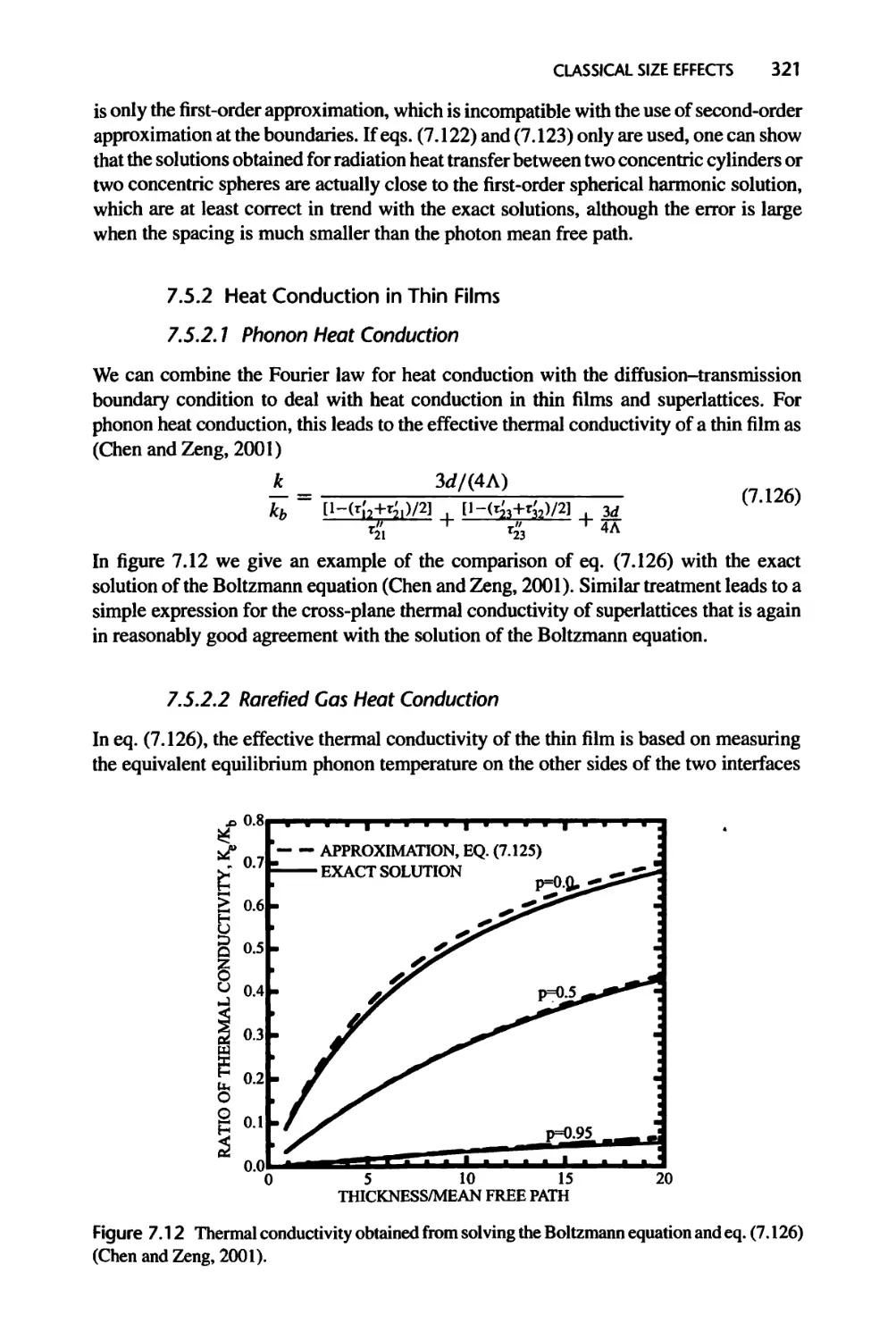
7.5.1 Thermal Radiation between Two Parallel Plates, 319
7.5.2 Heat Conduction in Thin Films, 321
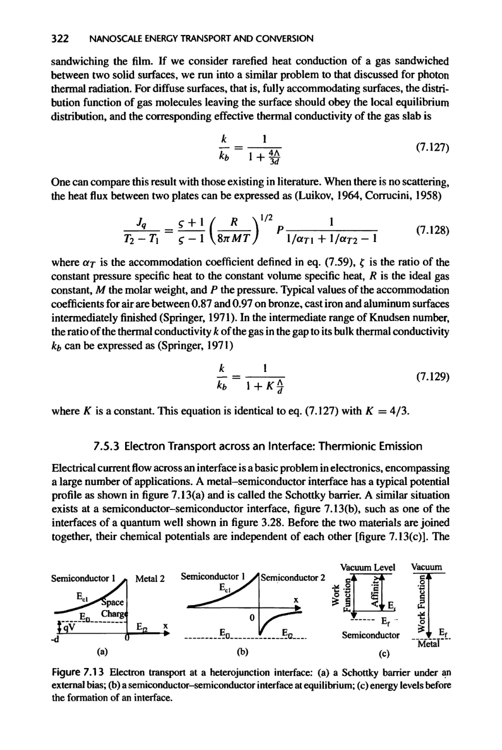
7.5.3 Electron Transport across an Interface: Thermionic Emission, 322
7.5.4 Velocity Slip for Rarefied Gas Flow, 327
7.6 Ballistic-Diffusive Treatments, 331
7.6.1 Modified Differential Approximation for Thermal Radiation, 331
7.6.2 Ballistic-Diffusive Equations for Phonon Transport, 333
7.7 Summary of Chapter 7, 336
7.8 Nomenclature for Chapter 7, 338
7.9 References, 340
7.10 Exercises, 344
8 Energy Conversion and Coupled Transport Processes, 348
8.1 Carrier Scattering, Generation, and Recombination, 349
8.1.1 Nonequilibrium Electron-Phonon Interactions, 349
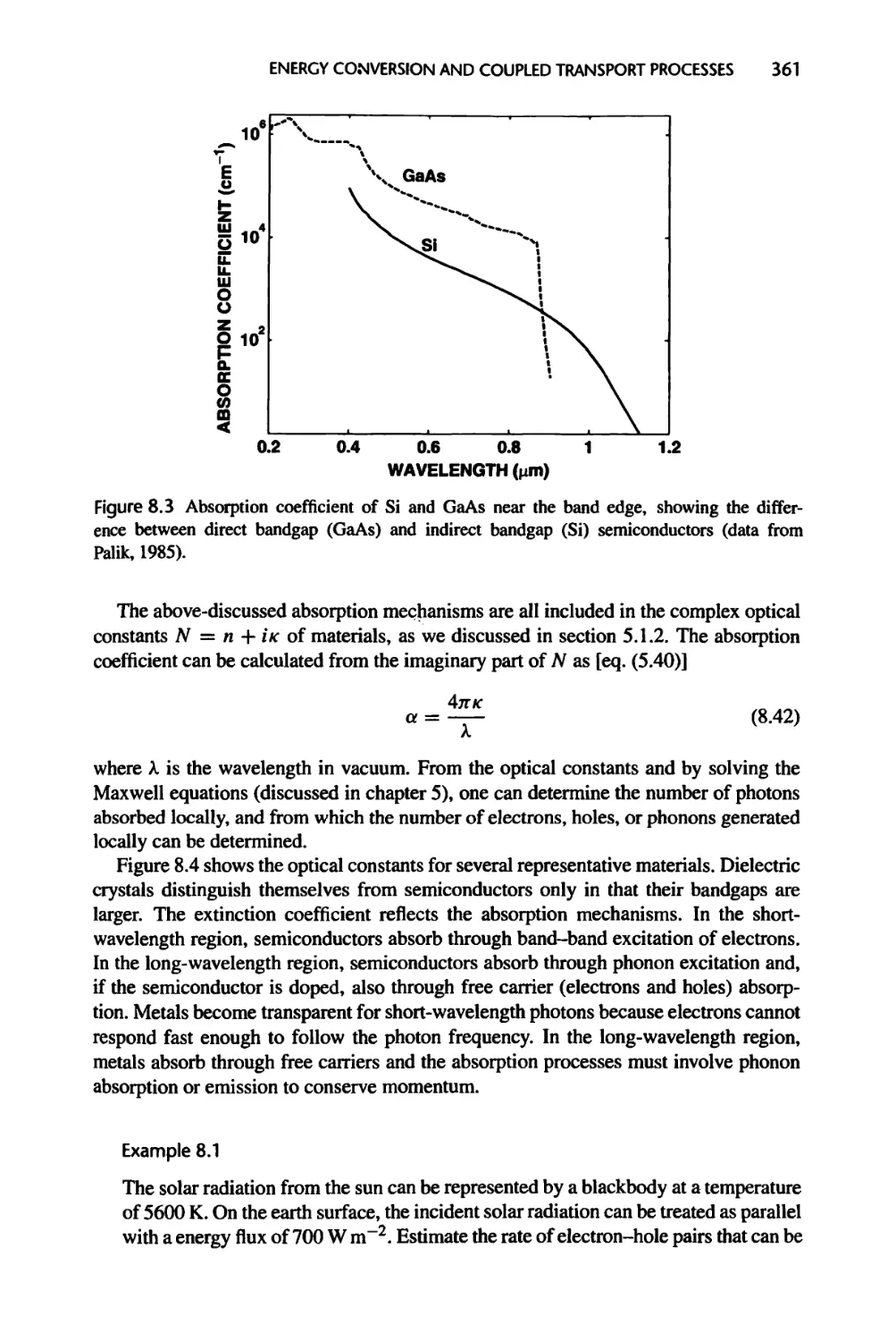
8.1.2 Photon Absorption and Carrier Excitation, 358
8.1.3 Relaxation and Recombination of Excited Carriers, 363
8.1.4 Boltzmann Equation Revisited, 366
xxii CONTENTS
8.2 Coupled Nonequilibrium Electron-Phonon Transport without
Recombination, 367
8.2.1 Hot Electron Effects in Short Pulse Laser Heating of Metals, 369
8.2.2 Hot Electron and Hot Phonon Effects in Semiconductor Devices, 370
8.2.3 Cold and Hot Phonons in Energy Conversion Devices, 373
8.3 Energy Exchange in Semiconductor Devices with Recombination, 373
8.3.1 Energy Source Formulation, 373
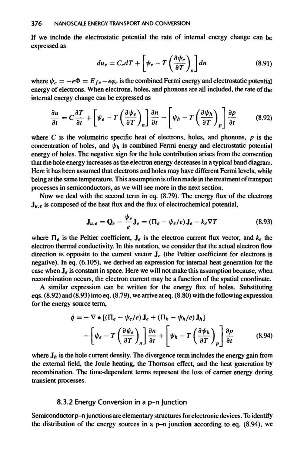
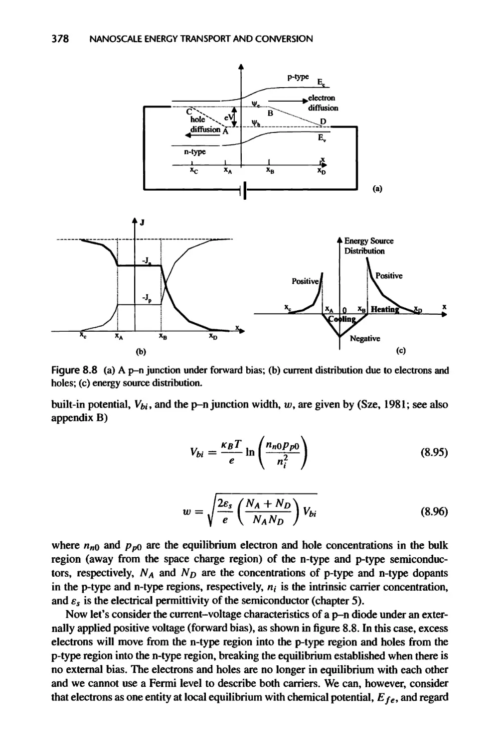
8.3.2 Energy Conversion in a p-n Junction, 376
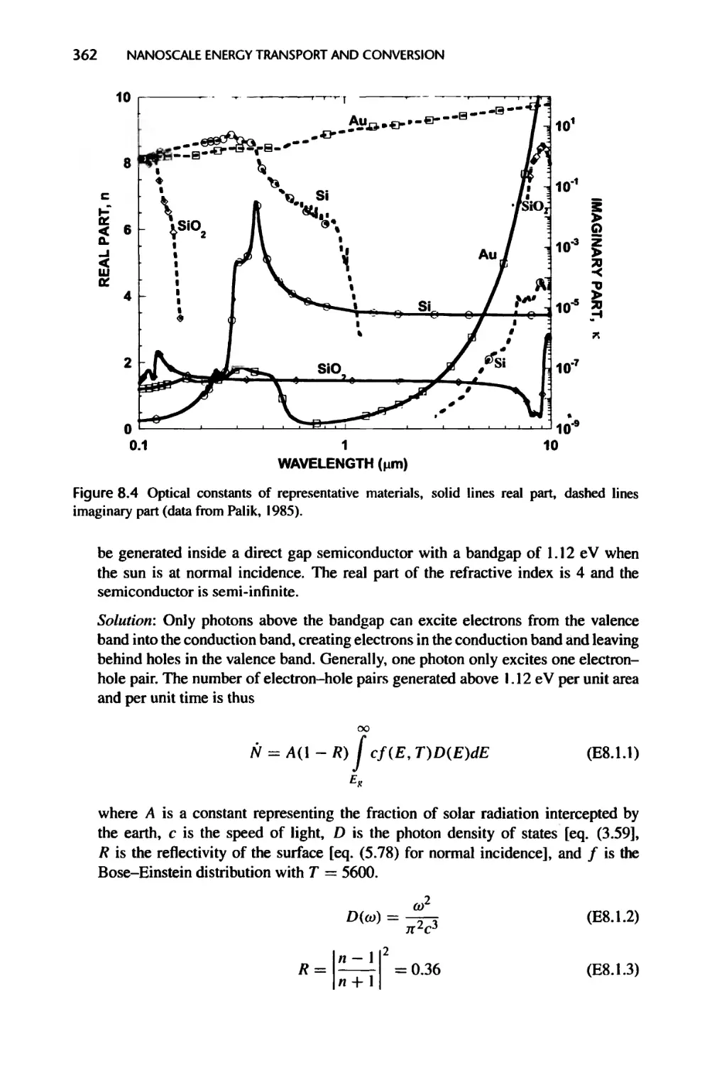
8.3.3 Radiation Heating of Semiconductors, 384
8.4 Nanostructures for Energy Conversion, 386
8.4.1 Thermoelectric Devices, 386
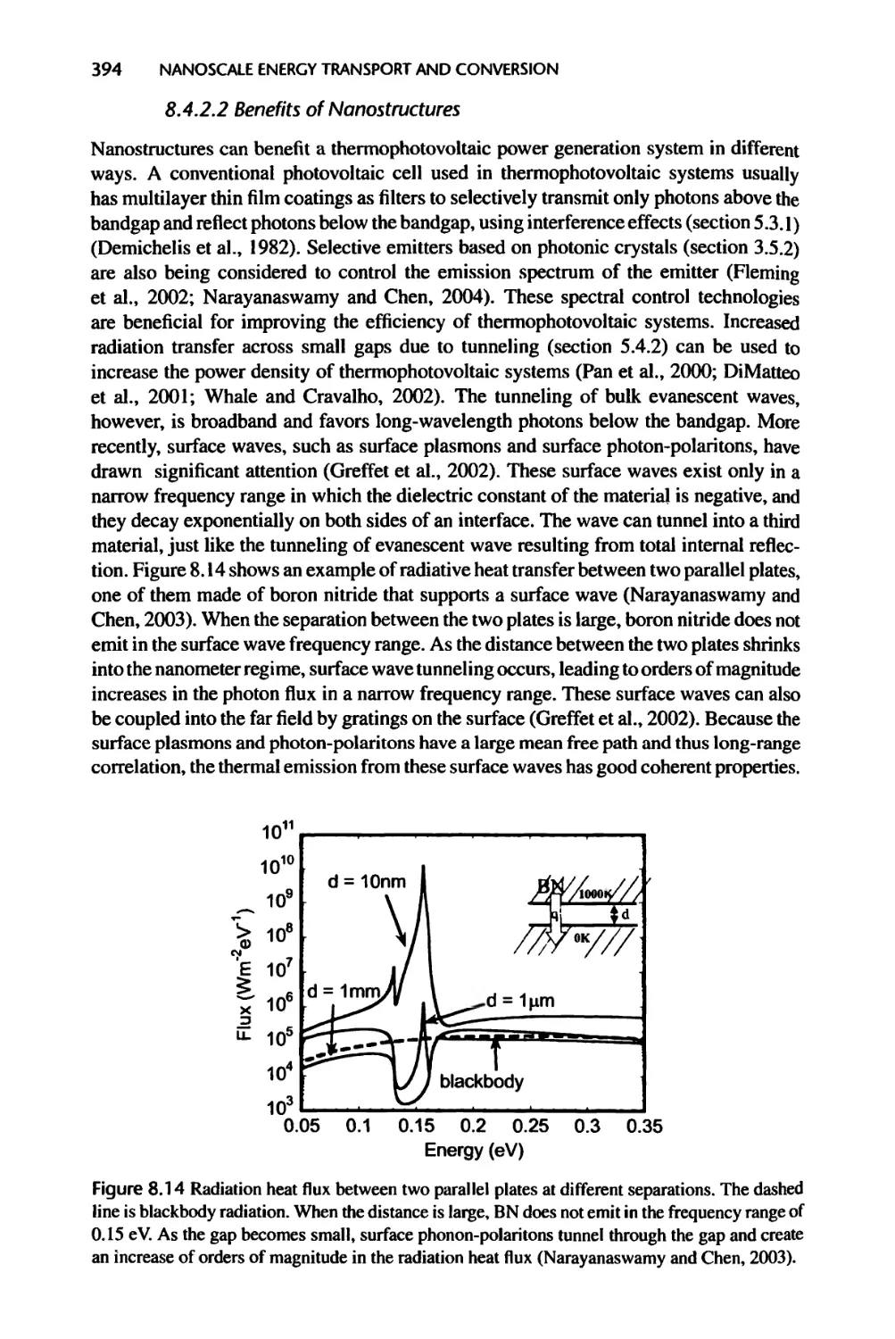
8.4.2 Solar Cells and Thermophotovoltaic Power Conversion, 391
8.5 Summary of Chapter 8, 395
8.6 Nomenclature for Chapter 8, 396
8.7 References, 398
8.8 Exercises, 401
9 Liquids and Their Interfaces, 404
9.1 Bulk Liquids and Their Transport Properties, 405
9.1.1 Radial Distribution Function and van der Waals Equation of State, 405
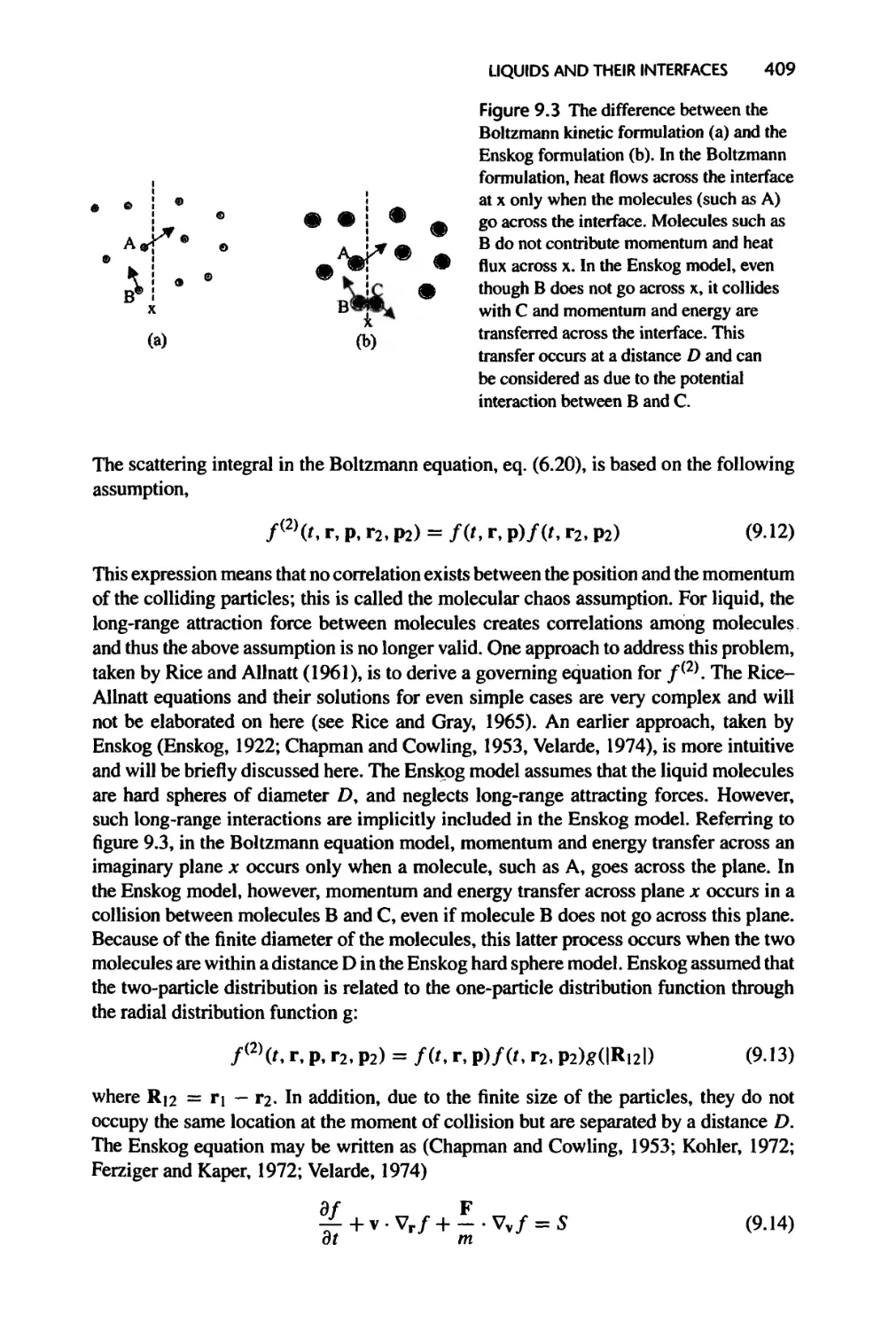
9.1.2 Kinetic Theories of Liquids, 408
9.1.3 Brownian Motion and the Langevin Equation, 411
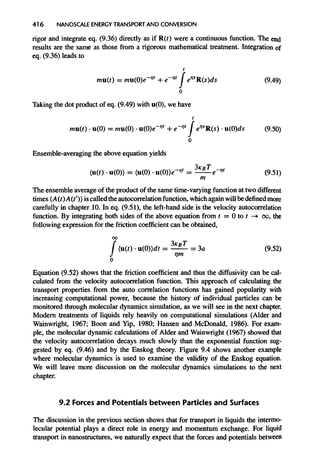
9.2 Forces and Potentials between Particles and Surfaces, 416
9.2.1 Intermolecular Potentials, 417
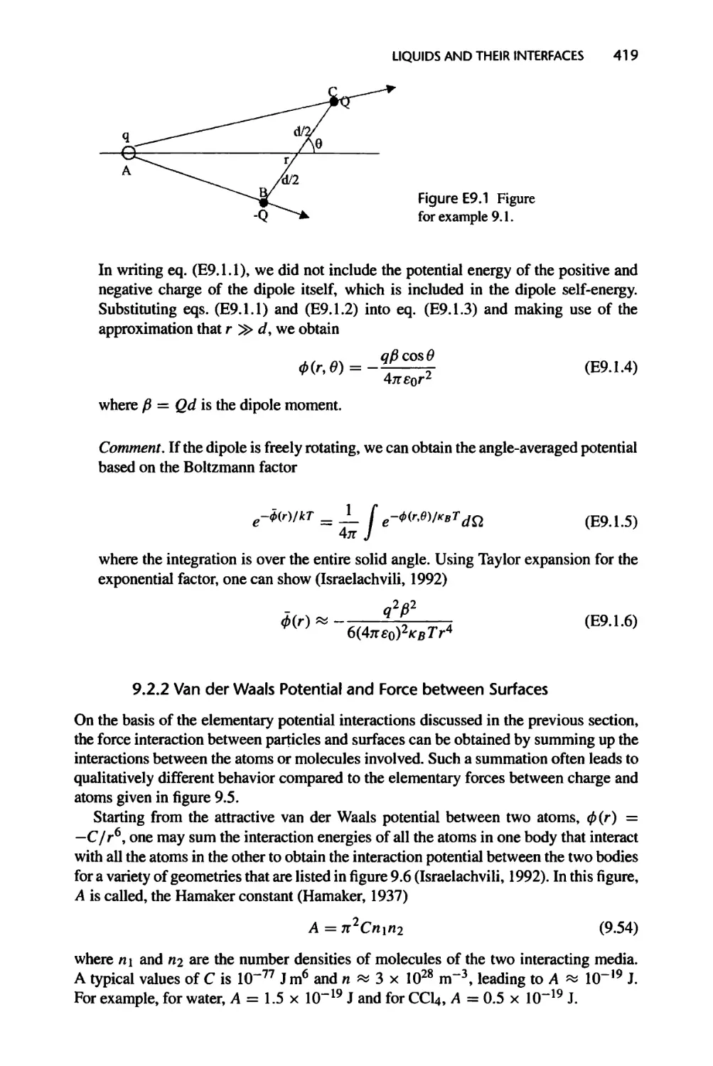
9.2.2 Van der Waals Potential and Force between Surfaces, 419
9.2.3 Electric Double Layer Potential and Force at Interfaces, 421
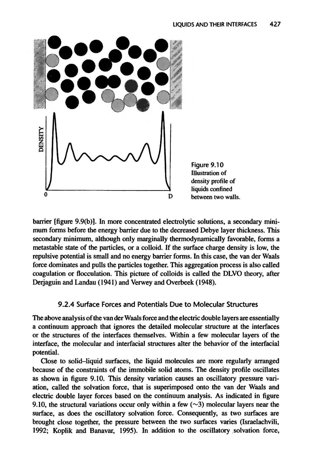
9.2.4 Surface Forces and Potentials Due to Molecular Structures, 427
9.2.5 Surface Tension, 428
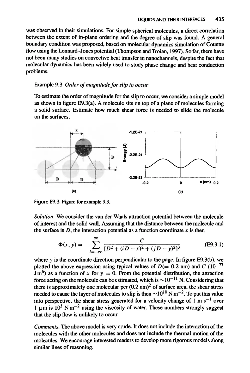
9.3 Size Effects on Single-Phase Flow and Convection, 433
9.3.1 Pressure-Driven Flow and Heat Transfer in Micro- and Nanochannels, 433
9.3.2 Electrokinetic Flows, 436
9.4 Size Effects on Phase Transition, 438
9.4.1 Curvature Effect on Vapor Pressure of Droplets, 439
9.4.2 Curvature Effect on Equilibrium Phase Transition Temperature, 441
9.4.3 Extension to Solid Particles, 441
9.4.4 Curvature Effect on Surface Tension, 442
9.5 Summary of Chapter 9,443
9.6 Nomenclature for Chaper 9,445
CONTENTS xxiii
9.7 References, 447
9.8 Exercises, 449
10 Molecular Dynamics Simulation 452
10.1 The Equations of Motion, 453
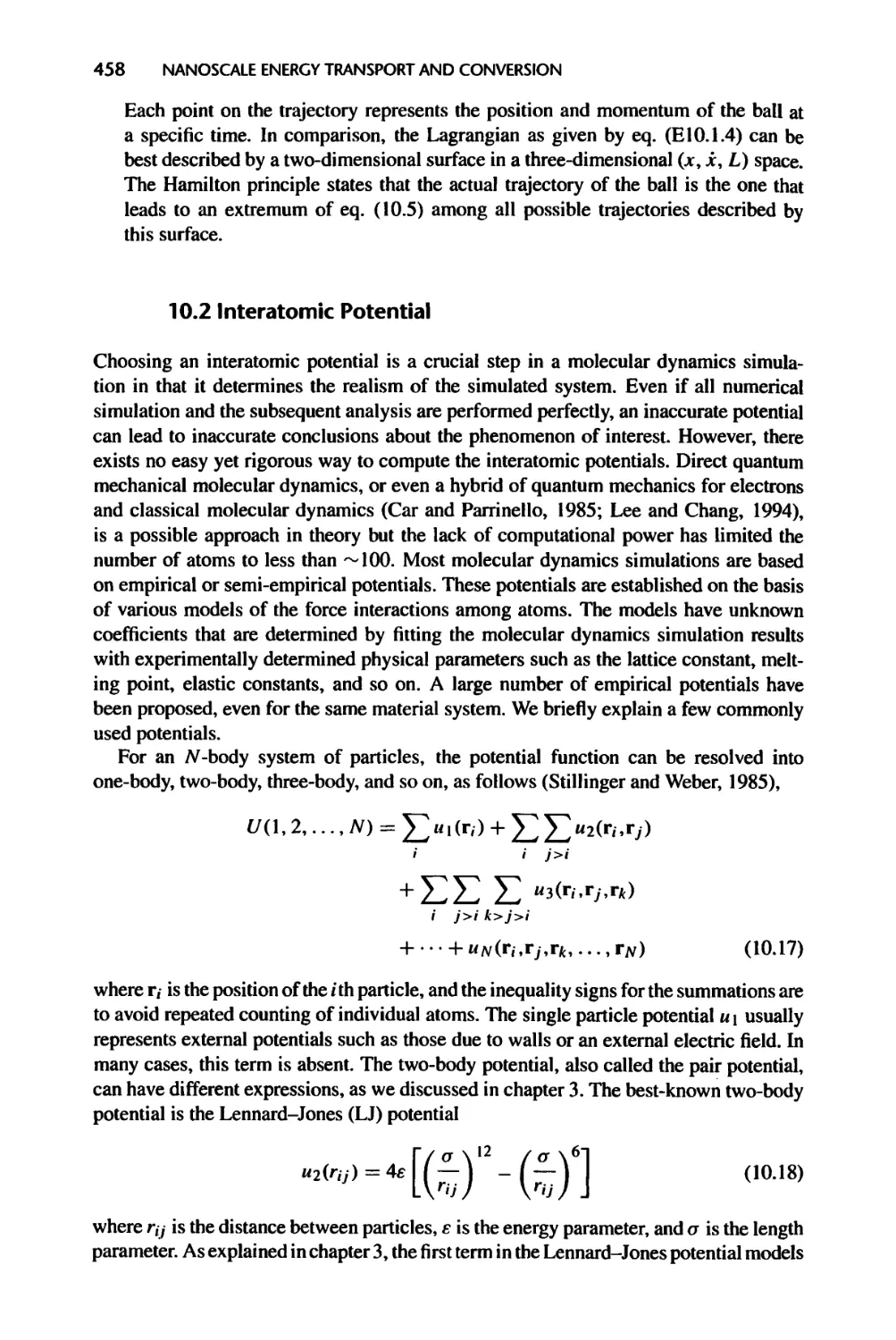
10.2 Interatomic Potential, 458
10.3 Statistical Foundation for Molecular Dynamic Simulations, 462
10.3.1 Time Average versus Ensemble Average, 462
10.3.2 Response Function and Kramers-Kronig Relations, 464
10.3.3 Linear Response Theory, 466
10.3.4 Linear Response to Internal Thermal Disturbance, 473
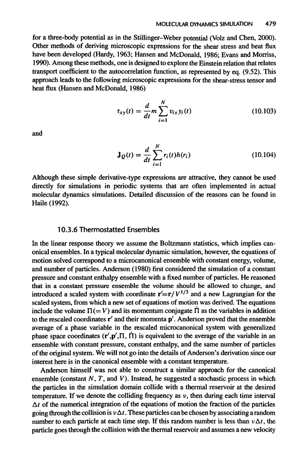
10.3.5 Microscopic Expressions of Thermodynamic and Transport
Properties, 476
10.3.6 Thermostatted Ensembles, 479
10.4 Solving the Equations of Motion, 483
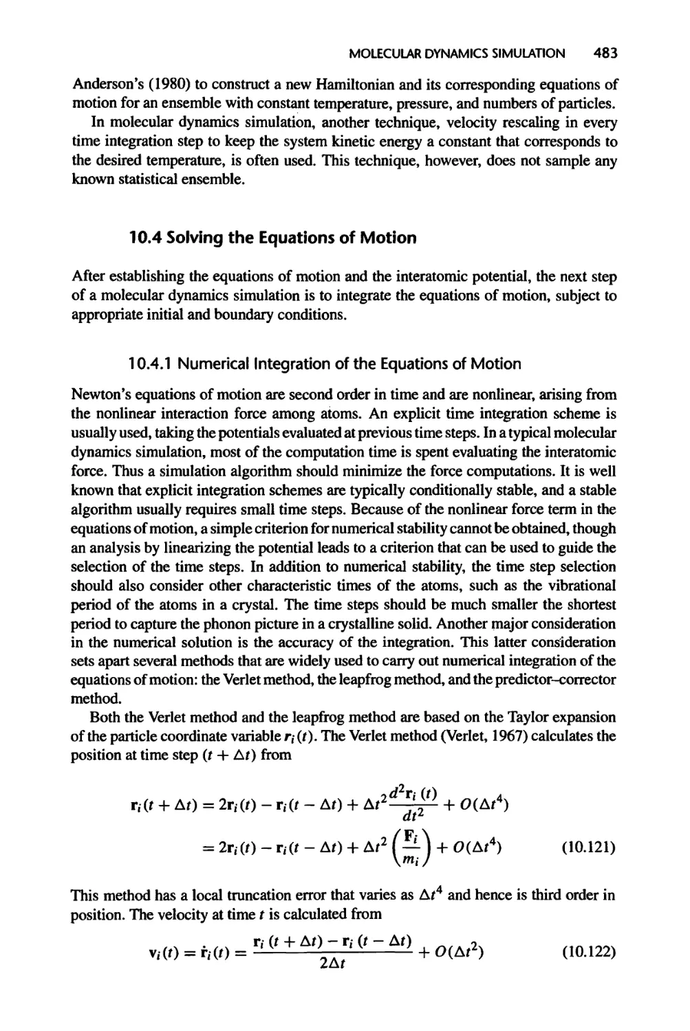
10.4.1 Numerical Integration of the Equations of Motion, 483
10.4.2 Initial Conditions, 485
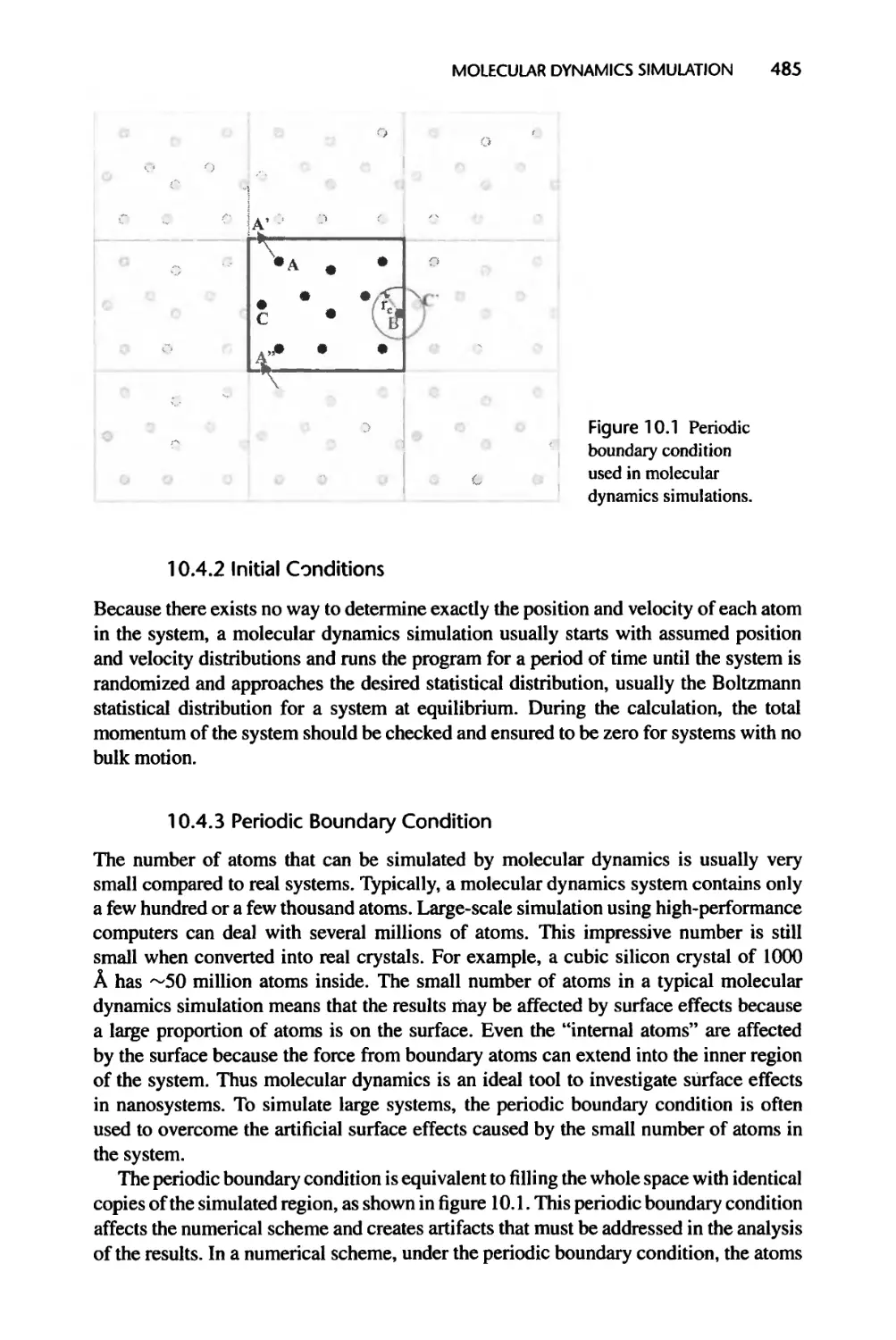
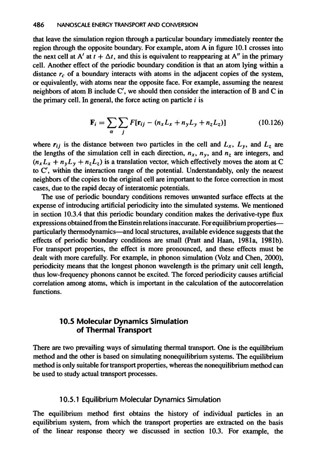
10.4.3 Periodic Boundary Condition, 485
10.5 Molecular Dynamics Simulation of Thermal Transport, 486
10.5.1 Equilibrium Molecular Dynamics Simulation, 486
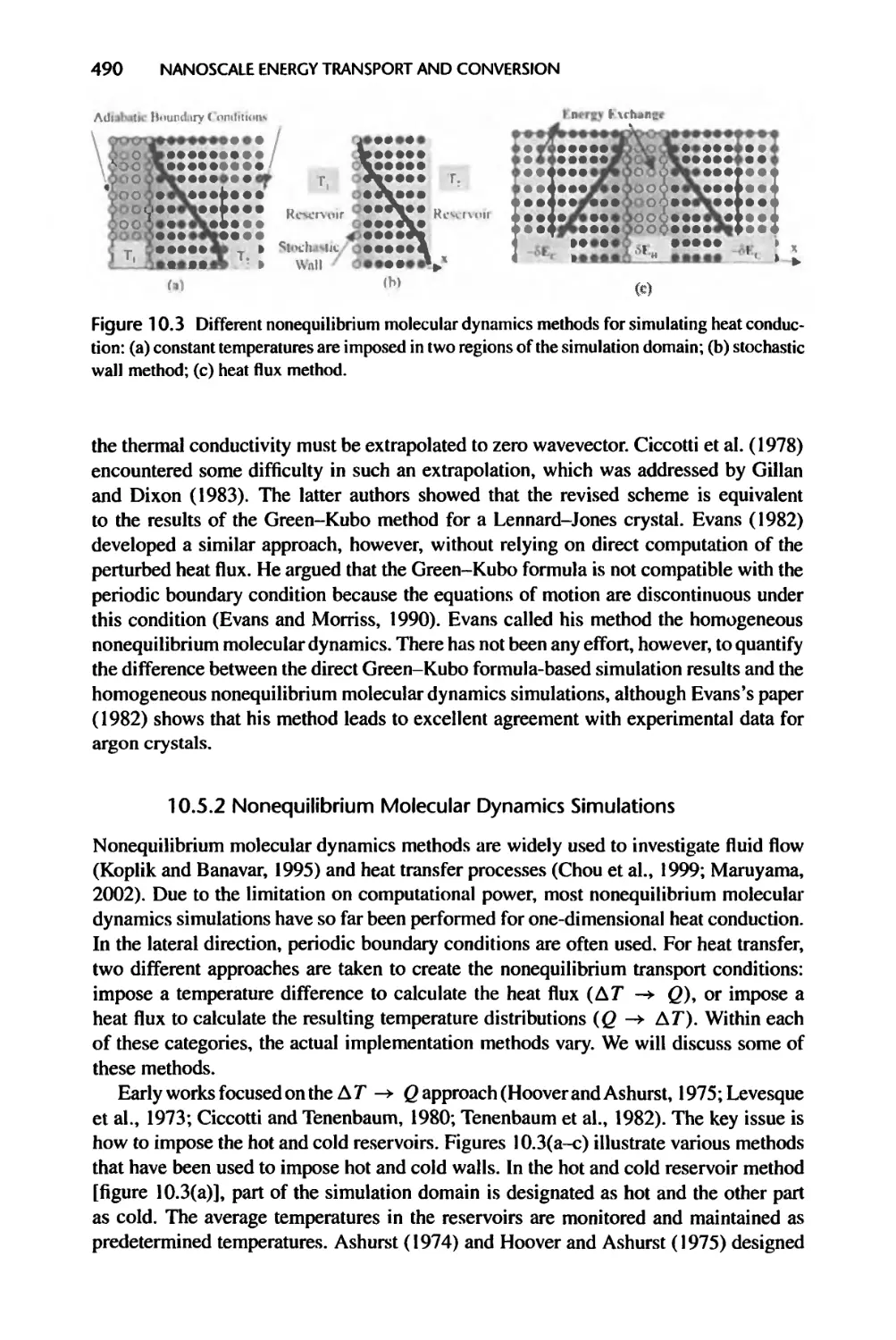
10.5.2 Nonequilibrium Molecular Dynamics Simulations, 490
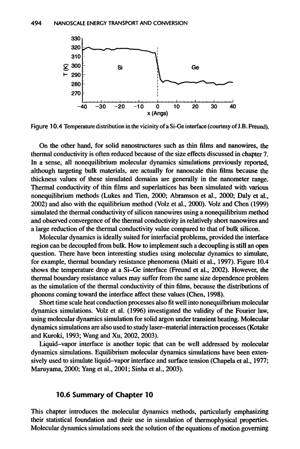
10.5.3 Molecular Dynamics Simulation of Nanoscale Heat Transfer, 493
10.6 Summary of Chapter 10,494
10.7 Nomenclature for Chapter 10,496
10.8 References, 498
10.9 Exercises, 502
Appendix A: Homogeneous Semiconductors, 505
Appendix B: Seconductor p-n Junctions, 509
Index, 513
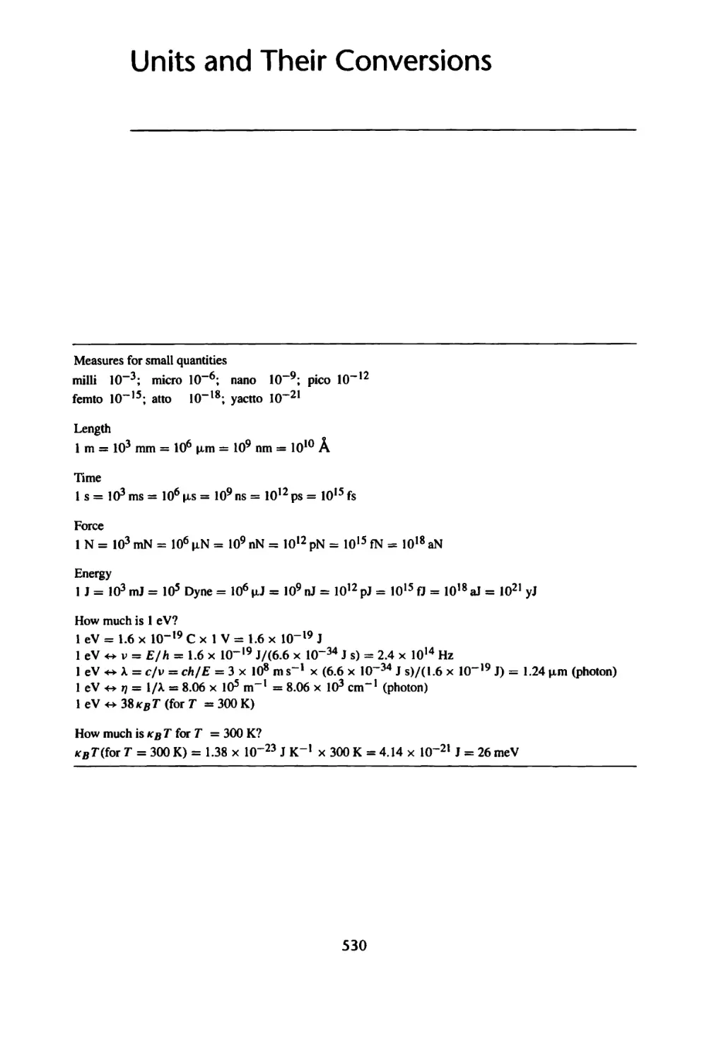
Units and Their Conversions, 530
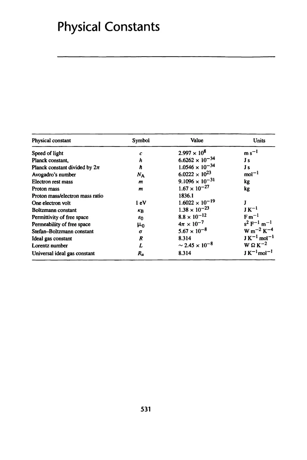
Physical Constants, 531
Nanoscale Energy Transport
and Conversion
1
Introduction
The major sources of inspiration for this book are the recent rapid advancements
in microtechnology and nanotechnology. Microtechnology deals with devices and
materials with characteristic lengths in the range of submicron to micron scales
(0.1 —100 |im), while nanotechnology generally covers the length scale from 1 to
100 nm. For example, integrated circuits are now built on transistors with characteristic
device length scales around 100 nm. The semiconductor industry roadmap predicts that,
in 2010, the characteristic length in integrated circuits will further shrink to 25 nm
(SEMATECH, 2002). In the late 1980s, microelectronics fabrication technology began-
to impact mechanical engineering, and the field of microelectromechanical systems,
or MEMS, blossomed (Trimmer, 1997). Meanwhile, nanoscience and nanotechnology,
explored by a few pioneers (Feynman, 1959, 1983), are currently generating much
excitement across all disciplines of science and engineering. The fields of micro- and
nanotechnologies are enormous in breadth and cannot be covered completely in any
single book. In this book, we focus on microscopic mechanisms behind energy transport,
particularly thermal energy transport. As the device or structure characteristic length
scales (such as the gate length in field-effect transistors, used to build computers, and the
film thickness in coatings) become comparable to the mean free path and the wavelength
of energy and information carriers (mainly electrons, photons, phonons, and molecules),
some of the classical laws are no longer applicable. By examining the microscopic
pictures underlying transport processes, we will develop a consistent framework for
treating thermal energy transport phenomena from the nanoscale to the macroscale.
In this chapter, we will first give a few examples of micro- and nanoscale transport
phenomena from contemporary technologies to provide motivation for the rest of this
book. We will then briefly summarize classical laws governing heat transfer processes
3
4 NANOSCALE ENERGY TRANSPORT AND CONVERSION
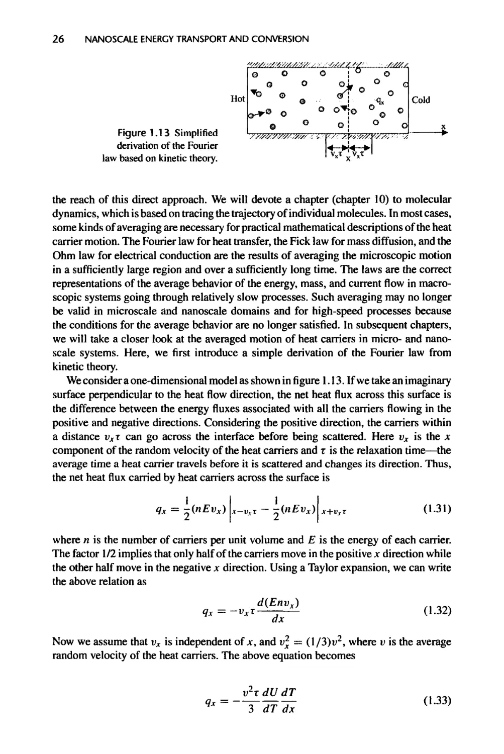
and discuss the microscopic pictures behind heat transfer phenomena, followed by a
simple derivation of the Fourier law, based on the kinetic theory, to demonstrate that
many classical laws we have learned are actually not as fundamental as their names may
suggest! The rest of the book will further expand on this chapter and answer in depth
some of the questions we raise.
1.1 There Is Plenty of Room at the Bottom
Richard Feynman, who won the 1963 Nobel Prize in physics for his work in quantum
electrodynamics, gave a visionary talk in 1959 entitled “There is plenty of room at
the bottom” (Feynman, 1959, 1983). In this talk, Feynman described the possibilities
of storing all the books in the world in a piece of dust, making micromachines that
can go into the human body, shrinking computers, rearranging atoms, and so on. To
put his ideas in a historic perspective, the possibility of integrated circuits was first
demonstrated in 1958 and, at the time of Feynman’s famous lecture, computers filled
entire rooms and lasers were shown only to be theoretically possible. Feynman not only
spoke of theoretical possibilities, but also provided potential approaches to realize his
dreams. Although his talk was considered bold at the time, his insights on what was
possible, or, better put, what was not impossible, were based on the laws of physics.
Most of the audience at that 1959 talk did not take Feynman’s visions seriously—rather,
they thought he was trying to be humorous. Subsequent developments in micro- and
nanotechnologies, however, have realized many of his dreams, and some have even
followed the technical approaches that he envisioned.
Great visionaries like Richard Feynman point to directions and provide inspiration.
Often, at the beginning of a revolutionary idea, only a small group appreciates the ideas
and begins to work on practical ways to demonstrate the concepts. Some of them make
breakthroughs along the way and prove that the idea works in principle; this attracts
more attention from wider communities and eventually the general public. This small
group is privileged because they have access to the ideas at an earlier stage, but, more
importantly, they have the training and judgments to appreciate the importance of these
ideas. Some of this small group have insights of their own, enabling them to realize
these ideas and generate their own ideas along the way. With the rapid development
of information technology, ideas propagate quickly nowadays. Academic training and
scientific knowledge become even more important for one to filter through the flood
of information for gold and to develop one’s own ideas and visions. One objective of
this book is to provide a knowledge base to its readers, assuming that most are not
familiar with modem physics, with a foundation to understand energy transport and
conversion processes, particularly thermal energy, from nanoscale up to macroscale,
with an emphasis on nanoscale processes. We will give a few examples here to illustrate
the importance of understanding nanoscale transport and energy conversion processes.
One major driver behind microtechnology and nanotechnology is information
processing, which includes microelectronics, data storage, and data transmission. The
information carriers are electrons in electrical circuits and photons in optical fibers. The
transport of electrons and photons often generate unwanted heat. As more and more
devices are compacted into a small area, heat generation density increases and thermal
management becomes a major challenge for the microelectronics industry. A Pentium4
INTRODUCTION 5
Major Haat Generation Region
Source Oam
Channel
Substrate (a)
(b)
(O
(0
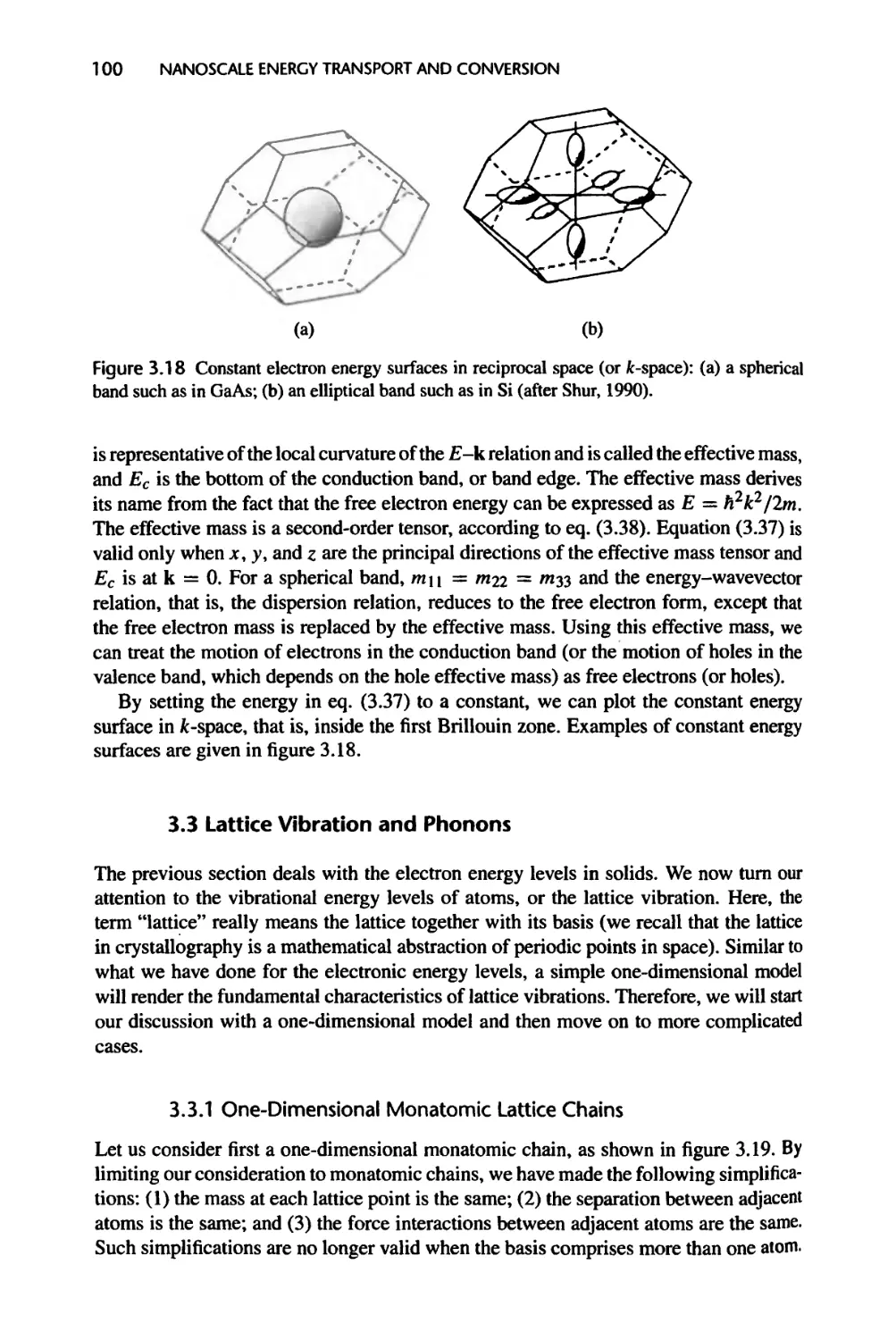
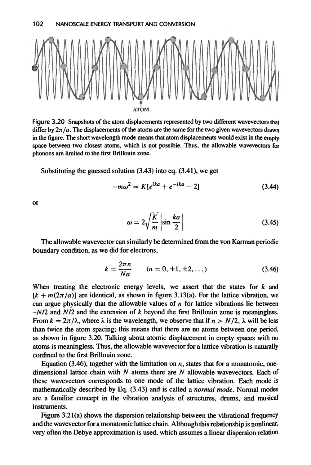
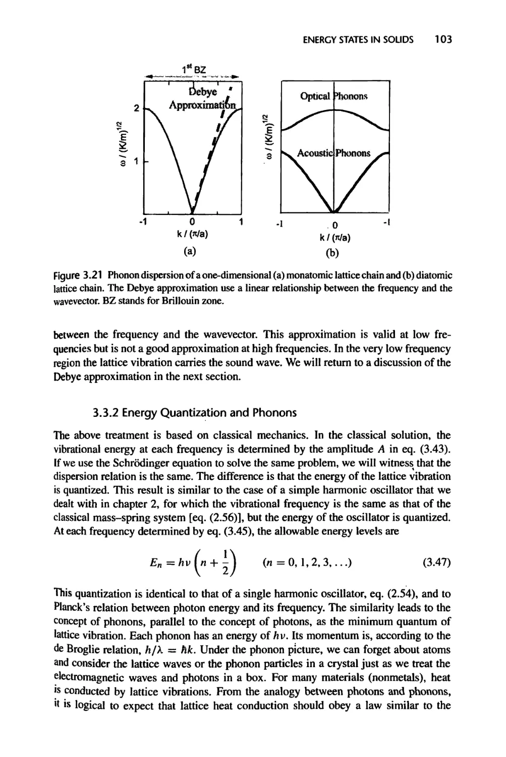
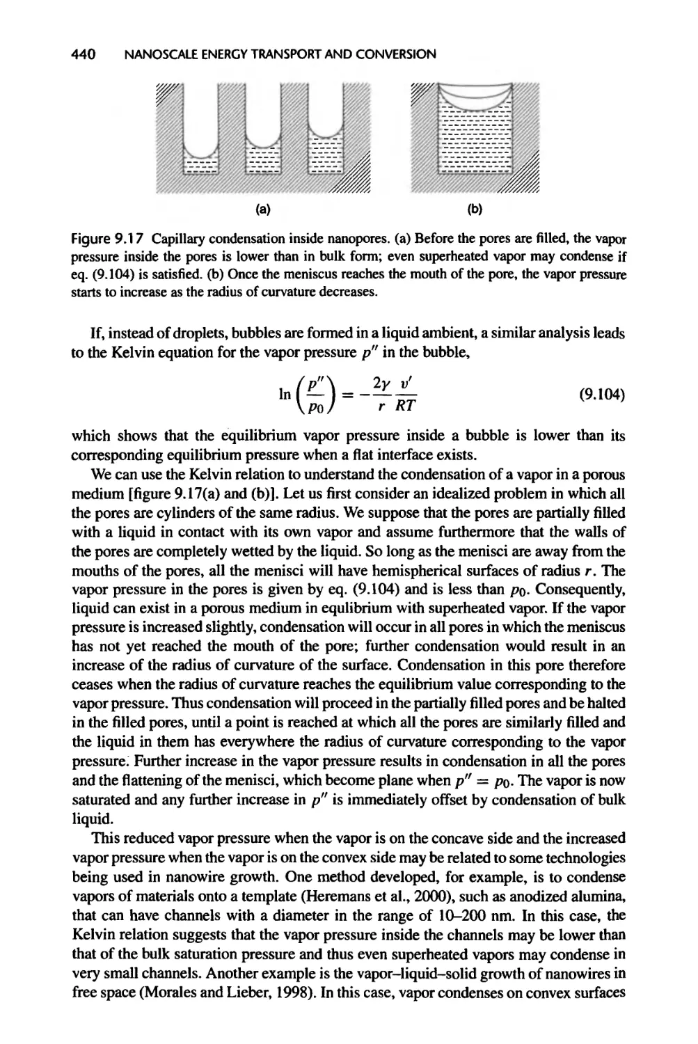
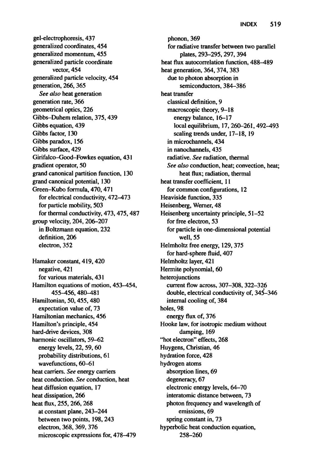
Figure 1.1 Nanoscale transport examples in information-oriented devices, (a) & (b): A MOSFET
device (courtesy of IBM) and electron energy dissipation in a MOSFET (courtesy of Dr. S.E. Laux
and Dr. M.V. Fischetti), indicating most heat is generated in nanometer region at the drain. Heat
conduction from such small source cannot be described by Fourier law; (c) & (d): A InAs/AlSb
based quantum cascade laser is made of many layers of thin films, each ranging from a few to
hundreds Angstrom thick (courtesy of Dr. S. Pei). These films have thermal conductivity values
significantly lower than those of their bulk materials; (e) & (f): A disk drive in magnetic data
storage with the slider head hovering about 10 nm on top of the disk rotating at 10,000 rpm. Fluid
flow through the gap between the slider and the disk is rarefied and cannot be described by the
Newton shear stress law.
chip from Intel Corporation, for example, has an area of ~ 1 cm2 and dissipates about
60 W of heat. The size of the fan used to maintain the chip temperature below its standard
(typically 80-120°C) is much larger than the chip itself. As engineers develop various
cooling solutions, it also becomes clearer that heat transfer characteristics must be con¬
sidered at the device level (Cahill et al., 2002). The most important device in a computer
chip is the metal-on-insulator field-effect transistor or MOSFET (Sze, 1981), as shown
in figures 1.1(a) and (b). The source, drain, and channel are made of doped silicon
(or other types of semiconductor). Electrons (or holes) flow from the source into the
drain through the channel under an externally applied voltage between the source and
the drain. The width of the channel is controlled by another voltage applied between
the back of the substrate and the gate electrode, which is insulated from the channel
by a very thin silicon dioxide layer. A MOSFET is thus like a variable resistor with its
resistance controlled by the gate voltage. To make faster devices, the channel length
(and thus the gate length) is shrinking by about 30% every 2 years, with the current
gate length at around 90 nm. Electrons convert most of their energy into heat in a small
region in the drain side [figure 1.1(b)]. Both modeling (Chen, 1996a) and experiments
(Svedrup et al., 2001) suggest that the temperature rise due to heat generation in the
small region is much higher than that predicted by the Fourier law, which can accelerate
the failure of the device. As another example, semiconductor lasers used in telecom¬
munication and data storage are often composed of multilayers of thin films, as shown
6 NANOSCALE ENERGY TRANSPORT AND CONVERSION
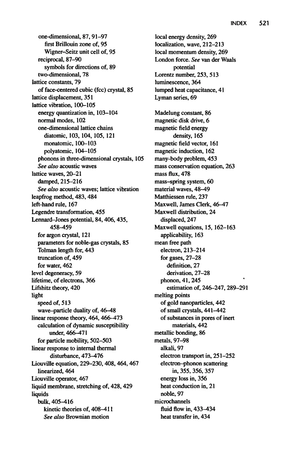
Figure 1.2 Illustration of thermoelectric devices, (a) a photograph of a thermoelectric cooler,
(b) illustration of charge flow inside one pair of legs, (c) microcoolers fabricated based on
superlattices (Venkatasubramanian et al., 2001; courtesy of Nature Publishing Groups), and (d) an
example of a Si/Ge superlattice structure (courtesy of Dr. K.L. Wang).
(c)
(d)
in figures 1.1(c) and (d). Past studies have shown that the thermal conductivity of these
structures is much lower than effective values calculated from their bulk materials on
the basis of the Fourier heat conduction theory (Chen, 1996b). These lasers have severe
heating problems that limit their performance. The reduced thermal conductivity calls
for careful design of the lasers to minimize the number of interfaces. In a different
example, figure 1.1(e) sketches the disk head in a magnetic disk drive. The separation
between the slider and the magnetic disk [figure 1.1(f)] determines the data storage
density. Currently, this separation distance is around 10-50 nm while the disk rotates
at ~ 10,000 rotations per minute (rpm). The relative motion between the slider and the
disk is analogous to flying a Boeing 747 a few millimeters above the ground. The airflow
between the slider and the disk is crucial in maintaining the slider-disk separation and
is very different from the prediction of continuum fluid mechanics at this small spacing
(Fukui and Kaneko, 1988). Some data storage processes are also based on heat transfer
(Chen et al., 2004). Examples are rewritable CDs based on the phase change of the
materials upon laser heating and thermomechanical data storage, where data bits are
written on polymer substrates by heated atomic force microscope (AFM) tips. For such
applications, it is desirable to limit the heating to a small domain. Nanoscale heat
transfer effects including reduced thermal conductivity of thin films and nonlocal heat
conduction surrounding nanoscale heating spots can be utilized to confine heat for writing
smaller spots.
While heat in information technology is, in most cases, undesirable and needs to be
“managed,” it becomes a dominant factor in energy conversion technology. Nanoscale
energy transport phenomena can be used for developing new strategies to improve the
energy conversion efficiency. For example, the reduced thermal conductivity observed
in semiconductor thin films can potentially be used to develop highly efficient thermo¬
electric materials for cooling and power generation (Tritt, 2001; Chen and Shakouri,
2002). Thermoelectric devices, as shown in figure 1.2(a-d), use electrons in solids
as the media to carry energy from one location to another. Low thermal conductivity
materials are required to reduce the thermal leakage between the hot and cold sides. At the
same time, the materials must have good electron energy-carrying properties (Goldsmid,
1964). The use of nanostructures to control the thermoelectric transport properties for
improving the electron energy carrying capability and reducing the thermal conductivity
emerged over the last ten years as a very promising approach for realizing highly
INTRODUCTION 7
Step 1
WAFER SLICE
AND POLISH
Step 2
WAFER
Step 3 Step 4 WAFER PROCESSING Step 5 Step 6
DIE ATTACH
Step 7 Step 8
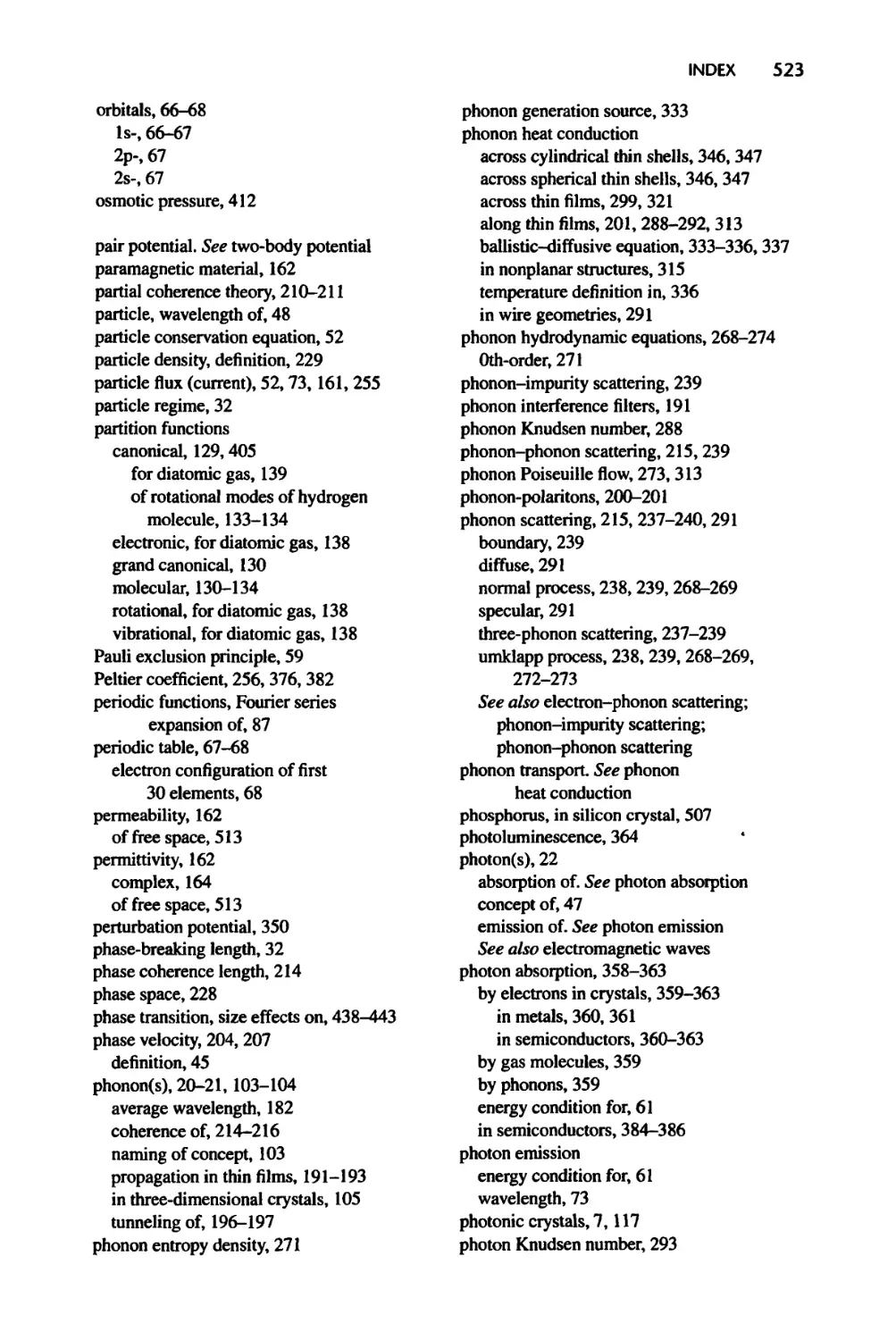
Figure 1.3 Illustration of major microelectronic device fabrication processes.
efficient thermoelectric devices (Dresselhaus et al., 1999; Tritt, 2001; Harman et al.,
2002; Chen et al., 2003).
Radiation transport in micro- and nanostructures is also different from that in
macrostructures because the wave properties of photons become dominant. For example,
radiation exchange between two closely spaced vacuum gaps is much higher than that
predicted on the basis of standard view-factor calculations because of tunneling and
interference effects (Domoto et al., 1970), which potentially can be used to develop
high power density thermophotovoltaic power generators (Whale and Cravalho, 2002).
Photonic crystals, a concept developed in 1987 (Yablonovitch, 1987), can be used to
design special thermal radiation surfaces with desirable properties (Fleming et al., 2002).
Using microstructures, coherent thermal radiation was recently demonstrated (Greffet
et al., 2002).
There are many outstanding nanoscale transport problems related to the fabrication
of nanodevices and synthesis of nanomaterials. As an example, consider a typical fabri¬
cation process, shown in figure 1.3, for an integrated circuit. Important transport issues
exist in almost every step and some of them are particularly relevant to the nanoscale
transport discussed in this book. With regard to the process illustrated in figure 1.3,
in step 1, heat transfer and fluid flow problems in crystal growth are in the continuum
range and have been addressed extensively in literature. Many of the material deposition
processes (step 3) occur at high temperatures and under low pressures. Atoms or gas
molecules have long mean free paths at low pressures, and this must be considered in
developing proper working conditions for filling trenches between devices. Lithogra¬
phy processes (step 4) should consider photon transport carefully. Optical interference
and scattering effects can be either detrimental or useful for the lithography techno¬
logy. Heat transfer issues arise in both the mask-making and lithography processes.
For example, some candidates for next-generation lithography, such as extreme
8
NANOSCALE ENERGY TRANSPORT AND CONVERSION
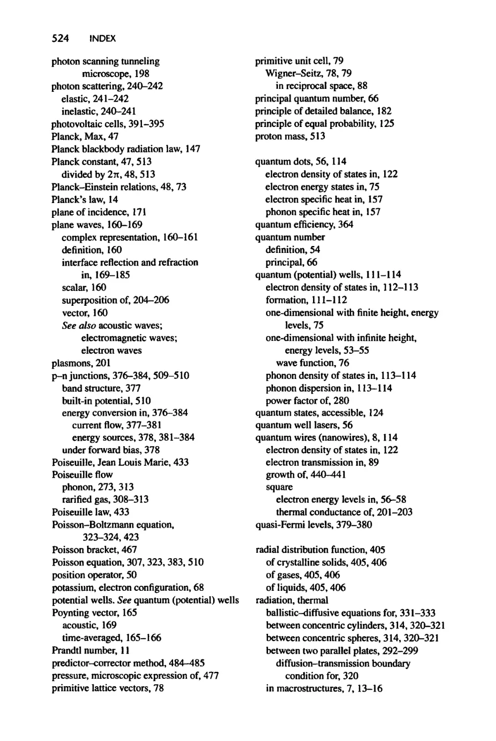
Figure 1.4 Examples of nanowires and nanotubes synthesized by various methods: (a) a pair
of bismuth nanowires obtained by pressure injection into a template (Dresselhaus et al., 2001;
courtesy of Dr. M.S. Dresselhaus), (b) TiO2 nanowires obtained by vapor condensation (courtesy
of Dr. Z.E Ren), (c) carbon nanotubes grown by plasma CVD (Ren et al., 1998; courtesy of
AAAS).
ultra-violet lithography (EUV) and X-ray lithography, rely on multilayer structures for
reflecting light (Hector and Mangat, 2001). The consequence of reduced thermal conduc¬
tivity on mask reliability has yet to be investigated. The synthesis of nanoscale materials
is a wide-open field and many nanomaterial and nanostructure synthesis methods being
developed raise intriguing nanoscale transport questions. For example, nanowires and
carbon nanotubes, shown in figure 1.4, have been synthesized with several different
methods such as chemical or physical vapor deposition, filling of templates, plasma
deposition, and laser ablation (Morales and Lieber, 1998; Ren et al., 1998; Dresselhaus
et al., 2001). Understanding the transport processes during nanomaterial formation will
allow better control of the final material quality.
The preceding examples emphasize the small length scales involved in nanodevices
and nanomaterials. Short time scales are also becoming increasingly important. Similar
questions can be raised for transport at short time scales as for the small length scales.
Lasers can deliver a pulse as short as a few femtoseconds (1 fs = 10”15s). Energy
transduction mechanisms at such short time scales can differ significantly from those at
macroscales (Qiu and Tien, 1993). Microelectronic devices are pushing to the tens of
gigahertz clock frequency with much shorter transient times. The temperature rise of the
device in such short time scales can be very different from that predicted by the Fourier
law (Yang et al., 2002).
The examples given above illustrate a few of the motivations behind the rapid devel¬
opment in micro- and nanoscale heat transfer research over the last decade (see Tien and
Chen, 1994; Tien et al., 1998). In the meantime, similar developments are occurring in
various fields, as evidenced in the strong interest in nanoscience and nanotechnology
from numerous fields of science and engineering, as well as from industry. Yet we are
only at the entrance, and the room at the bottom is big. The convergence of interests from
disparate fields into common subjects also creates confusion because different languages
are used in each field for similar phenomena. For newcomers, these differences are often
intimidating. One of the objectives of this book is to get the readers familiar with the
terminologies. In fact, once they get involved, the readers will find that drastically
different equations used in unrelated fields, such as the Fourier law for heat conduction
and the drift-diffusion equation for electrical current flow, actually originate from the
same principle. For this reason, the text will adopt a parallel treatment of different energy
carriers whenever possible.
INTRODUCTION 9
1.2 Classical Definition of Temperature and Heat
The classical definition of heat transfer from thermodynamics can be stated as follows:
“Heat transfer is the energy flow across the boundaries of a system under a temperature
difference.” We can emphasize several points in this definition: heat transfer is a form of
energy flow; heat transfer is associated with a temperature difference; and finally, heat
transfer is a boundary phenomenon.
Since heat transfer is driven by temperature differences, it is necessary that we
pay attention to the definition of temperature. In classical thermodynamics, temper¬
ature is defined on the basis of the concept of thermal equilibrium. If system A is
in thermal equilibrium with system B, then system A and system B have the same
temperature. In other words, temperature is a quantity that describes thermal equilibrium
phenomena.
These definitions of temperature and heat transfer are independent of the material and
serve well in establishing the universality of classical thermodynamics. Their strengths,
however, are also their weaknesses. These definitions are devoid of the physical micro¬
scopic pictures underlying heat transfer processes and the meaning of temperature. This
book aims to provide a more detailed picture of thermal energy transport processes. We
will study how heat is transferred at the microscopic level and how temperature should
be defined for transport processes that are intrinsically nonequilibrium.
13 Macroscopic Theory of Heat Transfer
There exist three basic modes of heat transfer: conduction, convection, and thermal
radiation. We briefly review the classical laws that are used to describe these modes. Later
in this book we will show how these laws can be derived and on what approximations
they are built.
13.1 Conduction
Heat conduction represents the energy transfer processes through a medium, caused by
a temperature difference due to the random motion of heat carriers in the substance.
The key is that a medium is needed for heat conduction, and heat is the part of the
energy that is carried around through random motion of heat carriers such as molecules.
An example is heat transfer through a solid wall separating the inside and the outside
of a room, which is due to the random vibrations of atoms within the wall materials.
Heat conduction processes are usually modeled on the basis of the Fourier law (Joseph
Fourier, 1768-1830) that relates the local heat flux to the local temperature gradient
q = -kVT
(1.1)
where k is the thermal conductivity, which is a temperature dependent material property
and has units of q has units of [Wm"2], and V is the gradient operator
such that
VT =
ar. ar A ar
a7x+ayJ’+fc
(1.2)
10 NANOSCALE ENERGY TRANSPORT AND CONVERSION
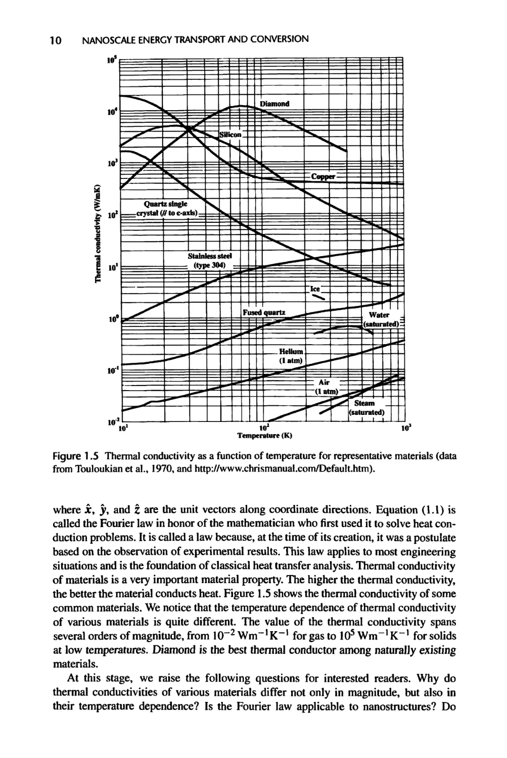
Figure 1.5 Thermal conductivity as a function of temperature for representative materials (data
from Touloukian et al., 1970, and http://www.chrismanual.com/Default.htm).
where x, y, and z are the unit vectors along coordinate directions. Equation (1.1) is
called the Fourier law in honor of the mathematician who first used it to solve heat con¬
duction problems. It is called a law because, at the time of its creation, it was a postulate
based on the observation of experimental results. This law applies to most engineering
situations and is the foundation of classical heat transfer analysis. Thermal conductivity
of materials is a very important material property. The higher the thermal conductivity,
the better the material conducts heat. Figure 1.5 shows the thermal conductivity of some
common materials. We notice that the temperature dependence of thermal conductivity
of various materials is quite different. The value of the thermal conductivity spans
several orders of magnitude, from 10~2 Wm“’ K“1 for gas to 105 Wm-1 K“’ for solids
at low temperatures. Diamond is the best thermal conductor among naturally existing
materials.
At this stage, we raise the following questions for interested readers. Why do
thermal conductivities of various materials differ not only in magnitude, but also in
their temperature dependence? Is the Fourier law applicable to nanostructures? Do
INTRODUCTION 11
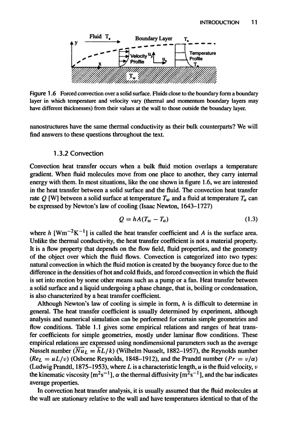
Figure 1.6 Forced convection over a solid surface. Fluids close to the boundary form a boundary
layer in which temperature and velocity vary (thermal and momentum boundaiy layers may
have different thicknesses) from their values at the wall to those outside the boundary layer.
nanostructures have the same thermal conductivity as their bulk counterparts? We will
find answers to these questions throughout the text.
1.3.2 Convection
Convection heat transfer occurs when a bulk fluid motion overlaps a temperature
gradient. When fluid molecules move from one place to another, they carry internal
energy with them. In most situations, like the one shown in figure 1.6, we are interested
in the heat transfer between a solid surface and the fluid. The convection heat transfer
rate Q [W] between a solid surface at temperature Tw and a fluid at temperature Ta can
be expressed by Newton’s law of cooling (Isaac Newton, 1643-1727)
Q=hA(Tw-Ta) (1.3)
where h [Wm“2K~l] is called the heat transfer coefficient and A is the surface area.
Unlike the thermal conductivity, the heat transfer coefficient is not a material property.
It is a flow property that depends on the flow field, fluid properties, and the geometry
of the object over which the fluid flows. Convection is categorized into two types:
natural convection in which the fluid motion is created by the buoyancy force due to the
difference in the densities of hot and cold fluids, and forced convection in which the fluid
is set into motion by some other means such as a pump or a fan. Heat transfer between
a solid surface and a liquid undergoing a phase change, that is, boiling or condensation,
is also characterized by a heat transfer coefficient.
Although Newton’s law of cooling is simple in form, h is difficult to determine in
general. The heat transfer coefficient is usually determined by experiment, although
analysis and numerical simulation can be performed for certain simple geometries and
flow conditions. Table 1.1 gives some empirical relations and ranges of heat trans¬
fer coefficients for simple geometries, mostly under laminar flow conditions. These
empirical relations are expressed using nondimensional parameters such as the average
Nusselt number {Nul = hL/k) (Wilhelm Nusselt, 1882-1957), the Reynolds number
{Ret = uL/v) (Osborne Reynolds, 1848-1912), and the Prandtl number (Pr = v/a)
(Ludwig Prandtl, 1875-1953), where L is a characteristic length, u is the fluid velocity, v
the kinematic viscosity [m2s-1 ], a the thermal diffusivity [m2s-1 ], and the bar indicates
average properties.
In convection heat transfer analysis, it is usually assumed that the fluid molecules at
the wall are stationary relative to the wall and have temperatures identical to that of the
12 NANOSCALE ENERGY TRANSPORT AND CONVERSION
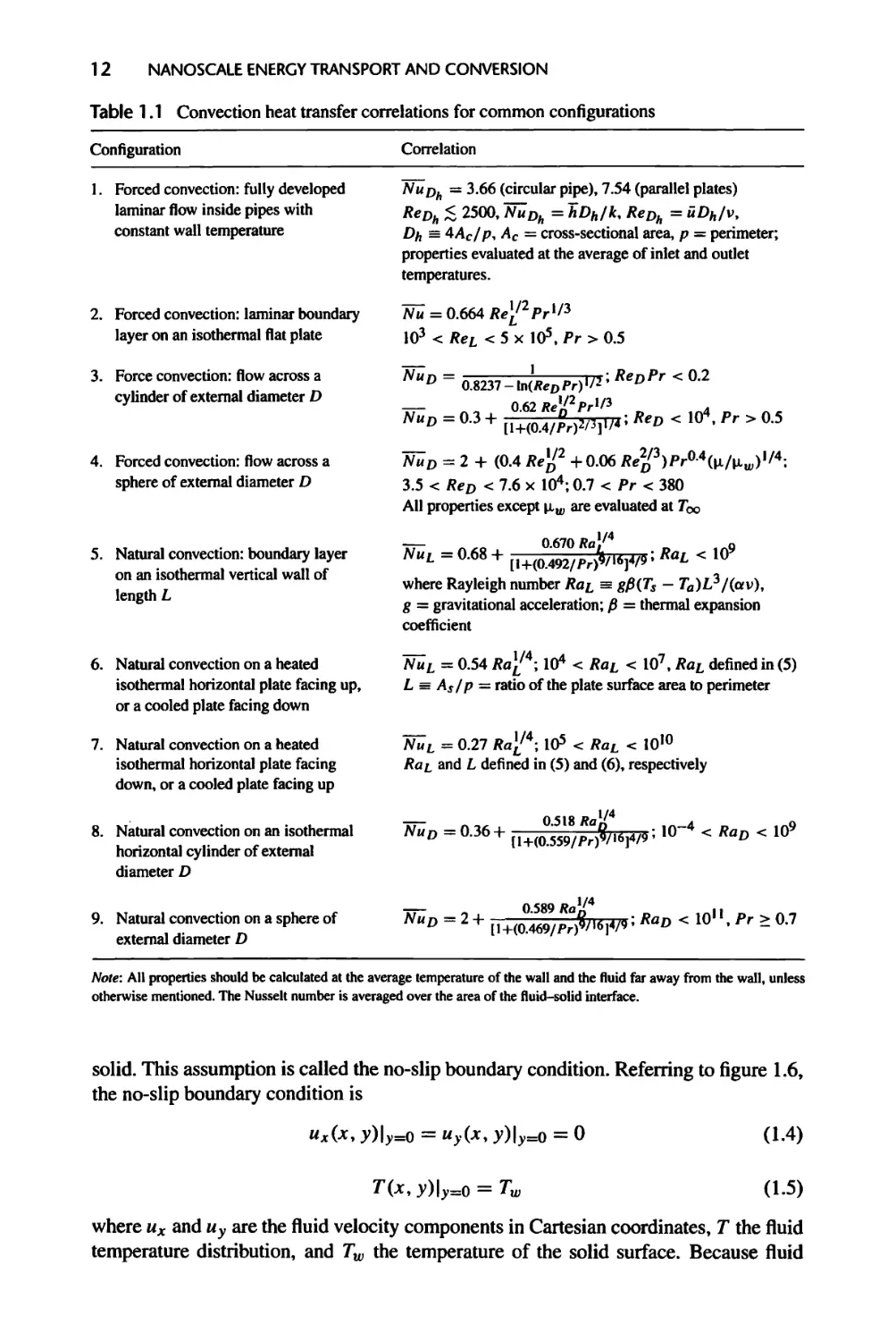
Table 1.1 Convection heat transfer correlations for common configurations
Configuration
Correlation
1. Forced convection: fully developed
laminar flow inside pipes with
constant wall temperature
Nur>h =3.66 (circular pipe), 7.54 (parallel plates)
R?Dh < 2500, Nuj)h = hDfJlc, R?Dh = uD^/vy
Dh = 4Ac/p, = cross-sectional area, p = perimeter;
properties evaluated at the average of inlet and outlet
temperatures.
2. Forced convection: laminar boundary
layer on an isothermal flat plate
Na = 0.664 Re[/2Pr^3
103 < Ret < 5 x 10⁵, Pr > 0.5
3. Force convection: flow across a
cylinder of external diameter D
NuD- 0.8237 -ln(ReDPr)W ReDPr < 0 2
—— „„ 0.62 Re1/2 Pr1/3 „ . „
Nud - 0.3 + (i+(0i4/^02/3Jr/4: ReD <10 , Pr > 0.5
4. Forced convection: flow across a
sphere of external diameter D
~Nud = 2 + (0.4 Re^2 +0.06 ^/3)Pr0-4(u/nw),/4:
3.5 < ReD < 7.6 x 10⁴; 0.7 < Pr < 380
All properties except piw are evaluated at Too
5. Natural convection: boundary layer
on an isothermal vertical wall of
length L
— 0.670 fa}/4 „
Nul -0.68+ < io
where Rayleigh number Rat = gp(Ts — Ta)L?/(av),
g = gravitational acceleration; p = thermal expansion
coefficient
6. Natural convection on a heated
isothermal horizontal plate facing up,
or a cooled plate facing down
~Nul = 0.54 Ra[/4; 104 < RaL < 107, RaL defined in (5)
L = As/p — ratio of the plate surface area to perimeter
7. Natural convection on a heated
isothermal horizontal plate facing
down, or a cooled plate facing up
1^L = 0.27 Ra^-, 105 < RaL < 1010
Ra^ and L defined in (5) and (6), respectively
8. Natural convection on an isothermal
horizontal cylinder of external
diameter D
Nu°=o-36+(i^X>>^: 10-4 <RaD < 109
9. Natural convection on a sphere of
external diameter D
NuD = 2 + [1 WwJlW ’ RaD < 10‘' • Pr- °-7
Note: All properties should be calculated at the average temperature of the wall and the fluid far away from the wall, unless
otherwise mentioned. The Nusselt number is averaged over the area of the fluid-solid interface.
solid. This assumption is called the no-slip boundary condition. Referring to figure 1.6,
the no-slip boundary condition is
Ux(x, y)|y=0 = Hy(x, y)|y=o = 0 (1.4)
T(x, y)|?=0 = Tw (1.5)
where ux and uy are the fluid velocity components in Cartesian coordinates, T the fluid
temperature distribution, and Tw the temperature of the solid surface. Because fluid
INTRODUCTION 13
particles are stationary on the surface, the heat transfer from the wall to the fluid in the
vicinity of the surface is actually through heat conduction. We can calculate this heat
transfer rate according to the Fourier law,
dT
Q = -kA—
dy y=0
(1.6)
Combining eqs. (1.3) and (1.6) leads to the expression for calculating the heat transfer
coefficient
h =
-k
arl
ay ly=0
(1.7)
The above equation furnishes a formula for determining the heat transfer coefficient,
provided the fluid temperature gradient at the wall can be determined. This task usually
requires solving the velocity and temperature distributions of the whole flow field on
the basis of the Navier-Stokes equations. In typical heat transfer or fluid mechanics
textbooks, the Navier-Stokes equations are derived on the basis of the conservation
principles for mass, momentum, and energy, together with constitutive relations such as
the Fourier law, which relates the heat flux to the temperature gradient, and the Newton
shear stress law, which relates the local velocity gradient to the local shear stress. We
will discuss the Navier-Stokes equations in greater detail further in chapter 6. In its
simplest form, assuming that the velocity component u in figure 1.6 depends on y only,
the Newton shear stress law can be written as
dwx
Txy=
(1.8)
where the first subscript on r denotes the direction of the shear stress and the second
subscript denotes the plane of action of the shear stress (y = constant plane), and
lx [N s m“2] is the dynamic viscosity (or absolute viscosity). A popular unit Tor /z is
P (poise), where 1 P = 0.1 Nsm”2. The ratio of the dynamic viscosity to the fluid
density, pip, gives the kinematic viscosity, v. Viscosity is generally regarded as an
intrinsic property of the fluid.
Going back to the theme of this book, microfluidics, which deals with fluid flow
at micro- and nanoscales, has attracted significant attention due to its applications in
chemical and biological analysis (Ho and Tai, 1998). Many questions can be asked about
fluid flow and heat transfer at such scales. Is the Newton shear stress law applicable to
fluid flow at these length scales? Is the no-slip boundary condition always correct? In
this book, we will answer these questions via the Boltzmann equation, surface force
analysis, and molecular dynamics simulations.
1.3.3 Radiation
Thermal radiation, the third basic heat transfer mode, is different from conduction
and convection. Heat transfer by thermal radiation does not require a medium and can
propagate in vacuum, and the energy is carried by electromagnetic waves. A blackbody,
14 NANOSCALE ENERGY TRANSPORT AND CONVERSION
Figure 1.7 Blackbody emissive power as a function of wavelength at different temperatures.
which is an idealized object that emits the maximum amount of thermal radiation,
radiates according to Planck’s law
C1
eb’X k5(ec2/^T _ i)
(1.9)
where Ci(= 37,413 Wjim4 cm”2) and C2<= 14,388 |xmK) are constants, k is the
wavelength of the radiation, and T is the absolute temperature. The spectral emis¬
sive power, is defined as the radiated power per unit emitting area and per unit
wavelength interval,
Power
eb X = A A AX
(1.10)
and has units of Wm“2jim-1. Examples of blackbody radiation spectra are shown in
figure 1.7. The wavelength at which the maximum emissive power occurs is given by
the Wien displacement law
^•maxT — 2898 |imK
(LU)
Solar radiation has an equivalent blackbody temperature of 5600 K and peaks around
0.52 p,m. Thus, the fact that the human visibility range is between 0.4 and 0.7 p,m is not
incidental.
Integrating Eq. (1.9) over all wavelengths, we obtain the total emissive power of
a blackbody
eb =
ebtKdk = aT4
(1.12)
0
INTRODUCTION 15
wherea(= 5.67 x 10“8 Wm“2 K“4) is the Stefan-Boltzmann constant. Equation (1.12)
is called the Stefan-Boltzmann Law.
Real objects typically radiate less than a blackbody. The emissivity characterizes the
thermal radiation characteristics of a surface. The spectral emissivity is defined as
(1-13)
where e\ is the spectral emissive power of the surface.
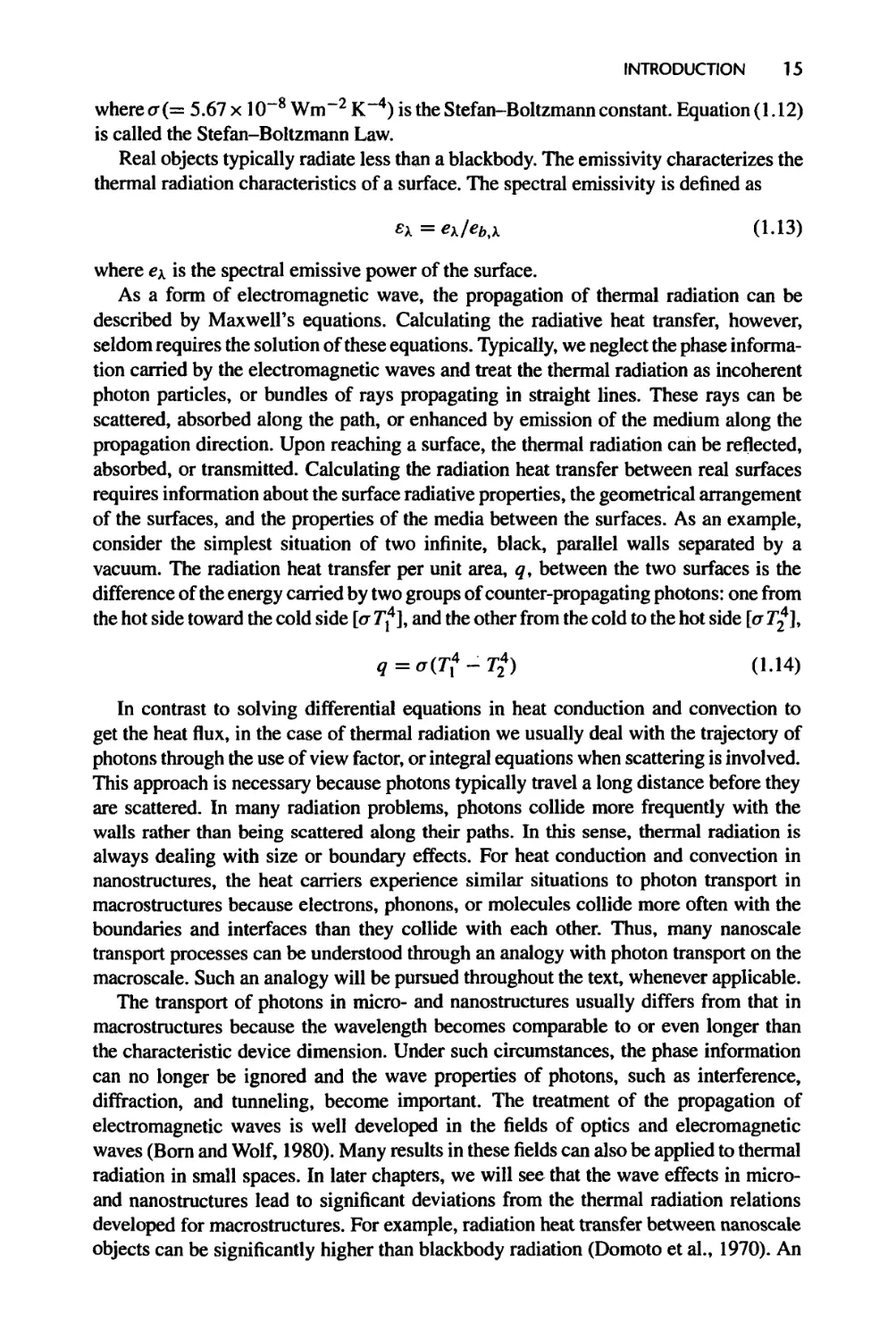
As a form of electromagnetic wave, the propagation of thermal radiation can be
described by Maxwell’s equations. Calculating the radiative heat transfer, however,
seldom requires the solution of these equations. Typically, we neglect the phase informa¬
tion carried by the electromagnetic waves and treat the thermal radiation as incoherent
photon particles, or bundles of rays propagating in straight lines. These rays can be
scattered, absorbed along the path, or enhanced by emission of the medium along the
propagation direction. Upon reaching a surface, the thermal radiation can be reflected,
absorbed, or transmitted. Calculating the radiation heat transfer between real surfaces
requires information about the surface radiative properties, the geometrical arrangement
of the surfaces, and the properties of the media between the surfaces. As an example,
consider the simplest situation of two infinite, black, parallel walls separated by a
vacuum. The radiation heat transfer per unit area, g, between the two surfaces is the
difference of the energy carried by two groups of counter-propagating photons: one from
the hot side toward the cold side [a T4], and the other from the cold to the hot side [a T4],
9=ct(T14-7’24) (1.14)
In contrast to solving differential equations in heat conduction and convection to
get the heat flux, in the case of thermal radiation we usually deal with the trajectory of
photons through the use of view factor, or integral equations when scattering is involved.
This approach is necessary because photons typically travel a long distance before they
are scattered. In many radiation problems, photons collide more frequently with the
walls rather than being scattered along their paths. In this sense, thermal radiation is
always dealing with size or boundary effects. For heat conduction and convection in
nanostructures, the heat carriers experience similar situations to photon transport in
macrostructures because electrons, phonons, or molecules collide more often with the
boundaries and interfaces than they collide with each other. Thus, many nanoscale
transport processes can be understood through an analogy with photon transport on the
macroscale. Such an analogy will be pursued throughout the text, whenever applicable.
The transport of photons in micro- and nanostructures usually differs from that in
macrostructures because the wavelength becomes comparable to or even longer than
the characteristic device dimension. Under such circumstances, the phase information
can no longer be ignored and the wave properties of photons, such as interference,
diffraction, and tunneling, become important. The treatment of the propagation of
electromagnetic waves is well developed in the fields of optics and elecromagnetic
waves (Bom and Wolf, 1980). Many results in these fields can also be applied to thermal
radiation in small spaces. In later chapters, we will see that the wave effects in micro-
and nanostructures lead to significant deviations from the thermal radiation relations
developed for macrostructures. For example, radiation heat transfer between nanoscale
objects can be significantly higher than blackbody radiation (Domoto et al., 1970). An
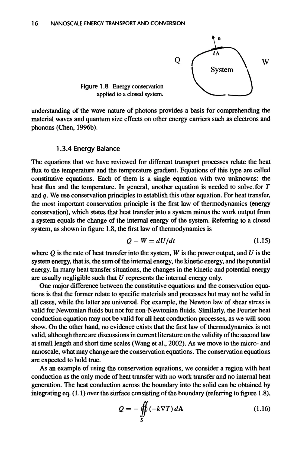
16 NANOSCALE ENERGY TRANSPORT AND CONVERSION
Figure 1.8 Energy conservation
applied to a closed system.
understanding of the wave nature of photons provides a basis for comprehending the
material waves and quantum size effects on other energy carriers such as electrons and
phonons (Chen, 1996b).
1.3.4 Energy Balance
The equations that we have reviewed for different transport processes relate the heat
flux to the temperature and the temperature gradient. Equations of this type are called
constitutive equations. Each of them is a single equation with two unknowns: the
heat flux and the temperature. In general, another equation is needed to solve for T
and q. We use conservation principles to establish this other equation. For heat transfer,
the most important conservation principle is the first law of thermodynamics (energy
conservation), which states that heat transfer into a system minus the work output from
a system equals the change of the internal eneigy of the system. Referring to a closed
system, as shown in figure 1.8, the first law of thermodynamics is
Q-W = dU/dt (1.15)
where Q is the rate of heat transfer into the system, W is the power output, and U is the
system energy, that is, the sum of the internal energy, the kinetic energy, and the potential
energy. In many heat transfer situations, the changes in the kinetic and potential energy
are usually negligible such that U represents the internal energy only.
One major difference between the constitutive equations and the conservation equa¬
tions is that the former relate to specific materials and processes but may not be valid in
all cases, while the latter are universal. For example, the Newton law of shear stress is
valid for Newtonian fluids but not for non-Newtonian fluids. Similarly, the Fourier heat
conduction equation may not be valid for all heat conduction processes, as we will soon
show. On the other hand, no evidence exists that the first law of thermodynamics is not
valid, although there are discussions in current literature on the validity of the second law
at small length and short time scales (Wang et al., 2002). As we move to the micro- and
nanoscale, what may change are the conservation equations. The conservation equations
are expected to hold true.
As an example of using the conservation equations, we consider a region with heat
conduction as the only mode of heat transfer with no work transfer and no internal heat
generation. The heat conduction across the boundary into the solid can be obtained by
integrating eq. (1.1) over the surface consisting of the boundary (referring to figure 1.8),
Q = -$(-kVT)dA. (1.16)
s
INTRODUCTION 17
where rfA is a differential area on the boundary with the norm pointing outward; thus a
minus sign is added to eq. (1.16) to indicate heat conduction into the region. Substituting
eq. (1.16) into eq. (1.15), we get
^(-fcVT).JA =
s
d
dt
udV
(1.17)
V
where u is the internal energy per unit volume and the integration on the right hand
side is over the volume. The left-hand side of eq. (1.17) can be converted into volume
integration using Gauss’s divergence theorem and the right-hand side can be further
related to temperature through the chain rule and the specific heat c,
V • (kVT)dV =
f dT
/ pc—dV
J dt
V
For this equation to be valid in any region, we must have
V(fcVT) = pc—
(1.18)
(1.19)
which is the familiar heat diffusion equation that is used to solve heat conduction
problems on the macroscale.
1.3.5 Local Equilibrium
In thermodynamics, we define equilibrium as a state of an isolated system in which no
macroscopic change can be observed as a function of time. Quantities such as temper¬
ature and pressure are defined only under equilibrium conditions. Transport processes
happen when the system is driven out of equilibrium. A system undergoing steady-state
heat conduction is not in an equilibrium state. Although no change occurs in such a
system, the steady state does not violate the definition of equilibrium, since the system
is not isolated. However, the nonequilibrium state of the system does pose a problem
because the temperature cannot be defined in accordance with thermodynamics. It would
seem the constitutive relations we have introduced are meaningless. This dilemma can
be resolved by employing the concept of local equilibrium. Although a system may be
out of equilibrium globally, the deviation from equilibrium at each point is usually small.
A small region surrounding each space point may be approximated as being in equili¬
brium, which allows us to define a local temperature, pressure, and chemical potential.
We have not, however, established rigorous criteria based on when we can assume local
equilibrium and we do not know yet how small this region should be. We can further
ask what happens if the system is smaller than this minimal size.
1.3.6 Scaling Trends under Macroscopic Theories
The characteristic length scales at which the classical theories discussed in this section
fail are typically on the order of submicrons, although the exact demarcation line
depends on the type of energy carriers, the media, and the temperature. A wide range
18 NANOSCALE ENERGY TRANSPORT AND CONVERSION
of microdevices exists with characteristic lengths larger than microns for which the
classical transport theories are still applicable. It is, however, interesting to consider
how the miniaturization will change the heat transfer characteristics. As the device size
shrinks, the ratio of surface area to volume increases, leading to significant changes
in thermal, electrical, ancj mechanical behavior. A well-known example in mechanics
is the diminishing effect of inertia and the increasing importance of surface tension,
as is evident in the fact that ants (with a characteristic dimension of millimeters) are
not injured by falling off a table but can be easily trapped in a drop of water, which
is contrary to what may happen to humans (with a characteristic length of meters)
in similar situations. In table 1.2, we show some examples of the scaling trend for
simple heat transfer configurations, assuming that macroscopic transport theories are
still applicable.
1.4 Microscopic Picture of Heat Carriers and Their Transport
This section briefly addresses the following questions: (1) What carries heat? (2) How
much energy do the carriers possess? (3) How fast do they travel? and (4) How far do
they travel? The explanation will be brief here since these questions will be discussed
in more detail in subsequent chapters.
1.4.1 Heat Carriers
People used to think that heat was carried by a special form of matter termed calories,
which were supposedly massless and colorless. When two objects at different temper¬
atures are in contact with each other, calories from the object at the high temperature
would flow into the object at the lower temperature. This view prevailed in the early 19th
century and contributed significantly to the development of classical thermodynamics.
Of course, we now know that this is an incorrect picture. In fact, the caloric theory,
despite its inception in the late 18th century, was completely abandoned by the middle
of the 19th century. Yet most of the results on classical thermodynamics derived from
such a wrong picture turned out to be correct and are still valid today because, as
we mentioned before, classical thermodynamics does not consider detailed pictures of
heat carriers.
Heat conduction actually results from the random motion of the material particles
in the system carrying thermal energy from one location to another. These material
particles are electrons, atoms, and molecules in gases, liquids, and solids. We use heat
conduction in a gas, as shown schematically in figure 1.9, to illustrate the microscopic
energy transport process. Gas molecules near the hot wall collide with the solid atoms
of the wall often and gain a higher kinetic energy, that is, a higher random velocity.
These molecules are in random motion and have the possibility of moving toward the
lower temperature end. During this process, they collide with molecules having smaller
random velocity (and thus cooler) and pass some of the excess energy to those molecules.
Such a process cascades for all adjacent molecules until it reaches the molecules in the
proximity of the cold wall. These molecules have a higher kinetic energy than the
atoms in the solid wall and will impart their excess energy to the wall through collisions.
Table 1.2 Scaling trend under classical transport theories for representative microgeometries
Mode and Example
Quantity
Scaling Trend
Heat conduction
(1) Along thin films
(2) Perpendicular to thin films
Heat transfer rate: Q = kAc&T/L
Heat fiux: q = kAT/L
Thermal diffusion time: t = L2 /a
L:heat conduction path length
L = film length (along film plane)
L = film thickness (perpendicular)
a: thermal diffusivity, m2 s“1
Case (1): Q small since Ac is small
q larger than bulk, depending on L
t shorter than bulk, depending on L
Case (2): Q depending on AcIL
q very large since L is small
t very short
Convection
(1) Inside a microchannel
(2) Across a microcylinder
Heat transfer rate: Q = hA(Tw - Ta)
Heat flux: q = h(Tw - Ta)
Nusselt No. for (1): Nu = hd/k — const.
h for case (1): h a 1/d
Nusselt No. for (2): Nu — 0.3 oc Re1/2
h for (2): h a 1/d1/2 to 1/d
For case (1): Q independent of d
q increases as \/d
h increases as 1 /d
For case (2): Q decreases with to d1 /2
q increases with 1/d1^2 to \/d
h increases with l/</1/2 to \/d
Radiation
Between two black parallel plates
Heat transfer rate: Q = a A(rf - T*}
Heat flux: g =ct(T4-T4)
Q decreases since A decreases
q remains constant
Coupled conduction and convection
(1) Heat conduction along fins
(2) Lumped capacitance
Case(l)
Temperature: = e~YX
Heat transfer rate: Q — kAcy(Tb -Ta)
fin parameter: y — [hp/{kAcy\x^2
Case (2)
Temperature:
Time Constant: r = pcV/(hA)
p = fin perimeter; 7} = initial temperature
Tb = fin base temperature
For case (1): y increases, temperature decreases rapidly along fins
Q decreases due to decreasing Ac
For case (2): r decreases due to decreasing V/A and increasing h
20 NANOSCALE ENERGY TRANSPORT AND CONVERSION
Figure 1.9 Microscopic heat
conduction process through a gas.
Hol
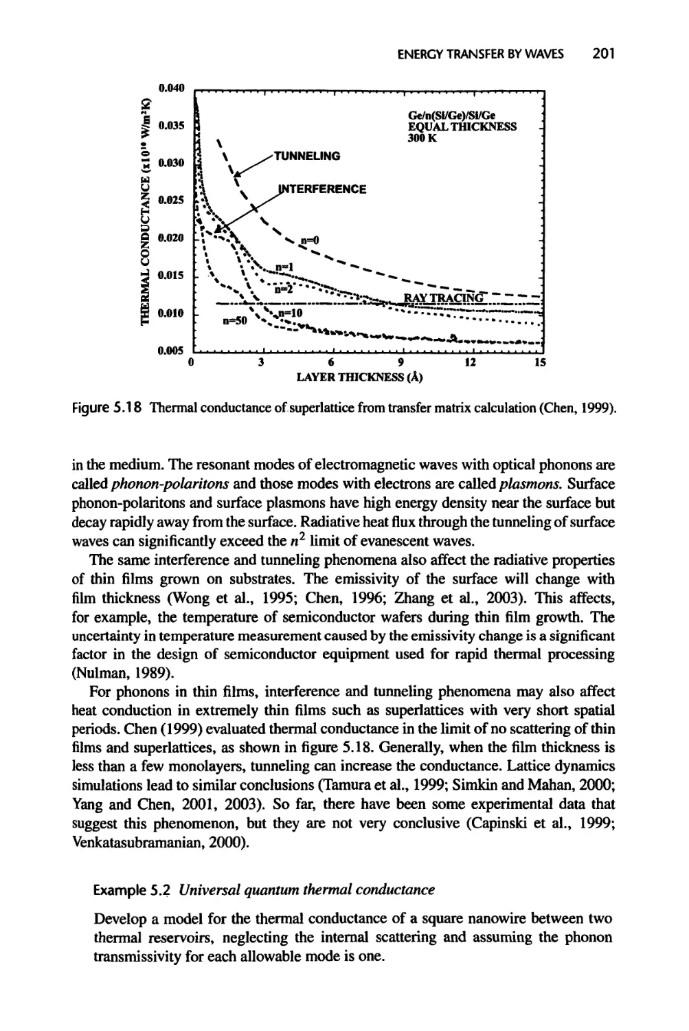
G O © ° Q
0 O O ® G
^> © © ® e
Q O O O ° o ®
0 e o 0 ©
Cold
The resultant effect is that a net energy flows from the hot wall to the cold wall due to
the temperature difference between the two walls. It should become clear that the net
energy flow is due to the random motion of the molecules and that the molecules do not
necessarily move from the hot to the cold side.
In dielectric solid materials (electrical insulators), heat is conducted through the
vibration of atoms. The atoms are bonded to each other in a dielectric material through
interatomic force interactions. Figure 1.10 shows a schematic of the interatomic poten¬
tial, 0, between two atoms as a function of their separation, x. The force interaction
between two atoms is the derivative of such an interatomic potential
—dd>
F = —- (1.20)
dx
If the two atoms are far apart, an attractive force exists between the atoms because
the electrons of one atom attract the nucleus of the other. When the atoms are close, the
interaction force becomes repulsive because the electron orbits, or the nuclei, of different
atoms begin to overlap. The minimum potential defines the equilibrium positions of the
atoms. Each atom in a solid vibrates around its equilibrium position. The motion of
each atom is constrained by its neighboring atoms through the interatomic potential. A
simplified picture of the interatomic interactions in crystals can be represented by a mass¬
spring system, as shown in figure 1.11 (a). In such a system, the vibration of any one atom
can cause the vibration of the whole system by creating lattice waves in the system. The
propagation of sound in a solid is due to long-wavelength lattice waves. If one side of the
solid is hotter, the atoms near the hot side will have larger vibrational amplitudes, which
will be felt by the atoms on the other side of the system through the propagation and
interaction of lattice waves. Quantum mechanical principles dictate that the energy of
each lattice wave is discrete and must be a multiple of h v (except for a small modification
called zero point energy that equals /w/2), where v is the frequency of the lattice wave
Potential Energy
♦-Repulsion
Interatomic
Distance
'Attraction
Figure 1.10 A typical interatomic
potential profile.
Equilibrium Position
INTRODUCTION 21
(a)
0 e © ’
© ® ®
® © ® ®
©
• ® ® ® • • •
• © • ft ® ®
• • •
® 6 ©
0 ©
(b)
Figure 1.11 (a) A mass-spring system representing interconnected atoms in a crystal, and
(b) phonon gas model replaces the solid atoms in a crystal.
and h the Planck constant (6.6 x 10“34 J s). This minimum energy hv of a quantized
lattice wave is called a phonon. A phonon at a specific frequency and wavelength is a
wave that extends through the entire crystal. The superposition of phonons of multiple
frequencies existing in the solid forms wave packets that have a narrow spatial extent.
These wave packets can be considered as particles as long as they are much smaller than
the crystal size. Using this phonon particle picture, the spring system in figure 1.11(a)
can be replaced by a box of phonon particles as in figure 1.11(b). Heat in a dielectric
crystal is conducted by such a phonon gas similar to that in a box of gas molecules as
shown in figure 1.9. The collision of phonon particles is due to the interaction of phonon
waves, which can be further attributed to the nonparabolicity (or anharmonic) potential
profile as shown in figure 1.10. A parabolic potential, according to eq. (1.20), would lead
to an ideal spring with force linearly proportional to displacement from the minimum
potential position. Phonons in such an ideal potential do not collide with each other.
In chapters 3 and 5 we will explain in more detail the phonon concept and when we can
treat phonons as particles rather than waves.
In metals, heat is conducted by free electrons as well as by phonons. When atoms
are bonded together to form a metal, some of the electrons in the outer orbits of the
nuclei become free from the bonding of the nuclei. These free electrons can travel a
distance much longer than the interatomic distance until they are scattered by either
atoms, electrons, or impurities. Under this picture, the free electrons inside a metal
can also be thought of as a gas—an electron gas. The heat conduction process for the
electron gas is again similar to that shown in figure 1.9 for molecules. Electrons in a metal
travel at a velocity typically three orders of magnitude larger than phonons do. Thus,
compared to the energy carried by lattice waves, the eneigy flux carried by electrons is
in general much larger. Therefore, in metals, electrons are usually the dominant heat
carriers.
One may guess that, in semiconductors, heat is probably conducted partially by
phonons and partially by electrons. That assumption is not completely correct. In fact,
heat is carried dominantly by phonons in most semiconductors, because the free electron
density in a normal semiconductor is much smaller than that in a metal. As an example,
the electron carrier density in a metal is MO23 cm”3 while in a semiconductor it is
typically less than 1018 cm-3. In lightly and moderately doped semiconductors, phonons
22 NANOSCALE ENERGY TRANSPORT AND CONVERSION
are the dominant heat carriers. However, the electron contribution in a heavily doped
semiconductor can be appreciable.
Given the above pictures of heat carriers for heat conduction processes, the convection
of heat can be understood rather easily since the only difference of convection from heat
conduction is that now heat carriers have a nonvanishing average velocity superimposed
on their random velocity. When a liquid or gas molecule moves from one place to another
due to its nonzero average velocity, it also carries its internal energy directly from one
place to another. This direct motion of internal energy in convection is very different from
heat conduction process. In the latter, heat is transferred due to the energy exchange of
heat carriers in the collision process. Heat conduction process exists even in convection
process because molecules are still doing random motion. In fact, the random motion
velocity of the molecules is usually much higher than the nonvanishing average velocity
in convection. However, convection is more effective than heat conduction because
energy moves directly from one place to another.
Thermal radiation involves another heat carrier, that is, electromagnetic waves. The
propagation of electromagnetic waves emitted from a thermal source does not differ
fundamentally from those carrying TV and radio signals because all are governed by the
Maxwell equations. The major difference lies in how these waves are generated. Thermal
radiation typically refers to the electromagnetic waves that are generated by a heat source,
while TV and radio signals are generated by an artificial source such as the oscillation of
current in a circuit. At the microscopic level, thermal radiation is due to the oscillation of
charges in the atoms and crystals. Similarly to lattice waves, electromagnetic waves are
also quantized as a result of quantum mechanics. An electromagnetic wave at frequency
v can have energy that is only a multiple of hv. This smallest energy quantum of an
electromagnetic field, hv, is called a photon. In fact, most people are probably more
familiar with the terminology of photon than phonon. Both of them are the basic quantum
of a wave; one for electromagnetic waves and the other for lattice vibrational waves.
1.4.2 Allowable Energy Levels of Heat Carriers
The transport of heat is due to the motion of the energy carriers discussed above and the
associated energy they carry. To describe heat transfer quantitatively, we need to know
the energy associated with these heat carriers. The possible energy states of heat carriers
are determined by quantum mechanical principles, which we will cover in chapters 2
and 3. Here, we will only give the reader some brief idea. For individual atoms and
molecules, the energy levels are typically discrete. For example, the allowed energy
levels of a harmonic oscillator, which is a good model for the vibrations of a diatomic
molecule such as H2, are given by
En = hv(n + 1/2) (n = 0, 1,2, 3,...) (1.21)
where v is the fundamental vibration frequency. The amplitude of the vibration must be
such that the total energy of the molecule fits into one of the above discrete energy levels.
In crystalline solids, the allowable energy of electrons and phonons is a function of the
wavevector. Such functional relations are also called dispersion relations. A wavevector
k points in the direction of wave propagation (electron and phonon waves) and its
magnitude equals divided by the wavelength. Figures 1.12(a) and (b) show examples
INTRODUCTION 23
Figure 1.12 Illustration of typical
dispersion relation for (a) electrons
and (b) phonons in crystals.
of the electron and phonon energy levels, represented by either energy or frequency,
in solids along a specific crystallographic direction, where a is the periodicity of the
atoms in the direction of the wave propagation and k is the wavevector. The allowable
energy levels form bands. Within each band, the energy is quasi-continuous because
the wavevector is discrete, as we will discuss in more detail in chapter 3. However,
there can be substantial gaps between different bands. The filling of the electronic
bands by electrons and the magnitude of the gaps determine whether a solid is a metal,
a semiconductor, or an insulator. The phonon band differs significantly from that for
electrons. Electron bands are typically approximated by a parabolic relationship between
the energy and the wavevector, whereas the dispersion relation between the phonon
wavelength and the wavevector is often approximated by a linear relationship.
1.4.3 Statistical Distribution of Energy Carriers
Not all the possible energy levels of energy carriers (molecules, electrons, and phonons)
will be actually occupied by the carriers. Classical thermodynamics tells us that a non¬
isolated system at equilibrium tends to minimize its energy. In a system with different
allowable energy levels, heat carriers will fill the lowest energy levels at zero tempera¬
ture. At higher temperatures, some of the carriers will have higher energy levels. The
most probable energy distributions of the carriers are governed by statistical principles.
Classical statistical theory gives the probability density /(E), defined as the probability
of finding the carrier at energy E per energy interval surrounding E, for a particle in an
equilibrium system at a temperature T,
f(E) = Be~E/(KB7"> (1.22)
where kb (= 1.38 x 10~23 J K_|) is the Boltzmann constant, T is the absolute tem-
perature, and B is a normalization factor. Equation (1.22) is the famous Boltzmann
distribution (Ludwig Boltzmann, 1844-1906). For a monoatomic ideal gas system, the
only energy of each atom is its translational kinetic energy
E = ^(v2x + v2y + v2z) (1.23)
where m is the mass of the atom and vx, vy, and vz are the components of its random
velocity. Since the probability of finding this particle to have energy between zero and
infinite speed must be one, we have
24 NANOSCALE ENERGY TRANSPORT AND CONVERSION
m{v} + V? + vj)
2^T
dvz = 1
(1.24)
Carrying out the above integration leads to
The probability density of a monatomic gas is thus
/(v) =
m \3/2 ’ m(v2 + v2 + v2)
IxkbT / eXP 2k bT
(1.25)
(1.26)
which is called the Maxwell distribution. With this probability density, we can calculate
other expectation values (or average values). For example, the average energy (internal
energy) of a monatomic gas molecule is
(1.27)
Transforming the Cartesian coordinates vXlvy, vz into spherical coordinates makes the
above integration much easier. The final result is
(£) = ^kbT (1.28)
The above expression means that temperature is a measure of the average kinetic
energy for a monoatomic gas. Equation (1.28) is a very useful result to remember and is
an example of the equipartition theorem in statistical thermodynamics. The equipartition
theorem for classical systems states that at sufficiently high temperatures (such that the
Boltzmann distribution is valid) each quadratic term of the molecular energy contributes
to the molecule an average energy kbT/2. For a monoatomic gas, each molecule has three
quadratic energy components, from its translational motion, as indicated by eq. (1.23),
so that the total average kinetic energy is 3kbT/2.
Example 1.1 Speed and specific heat of gas molecules
Estimate the average speed of helium atoms as an ideal gas at 300 K, and also estimate
its specific heat at constant volume.
Solution: The average speed of molecules obeying the Maxwell distribution is
m(v* + vj +
_ 2^T
INTRODUCTION 25
The mass of a helium atom is 4 x 1.67 x IO-27 kg, where 4 comes from the fact that a
helium atom has two protons and two neutrons, and 1.67 x 10”27 kg is the rest mass
of a proton (a neutron has approximately the same weight as a proton). We thus obtain
the average velocity of helium atoms as 1257 m s”1. To obtain the specific heat, we
know that a mole contains Na = 6.02 x 10²³ (Avogadro’s constant) molecules. The
total energy of a mole of helium atoms is thus u = 3NaKbT/2. The specific heat
at constant volume is cv = du/dT — 'SkrNa/'Z = ^Ru/2 = 12.5 JK"1 mol”1, where
Ru = kNa = 8.314 J K”1 mol”1 is the universal gas constant. The actual specific
heat of helium is in agreement with this number.
Comment: A quick order-of-magnitude estimation of the average speed can be
obtained by setting the average kinetic energy of each atom, 3k b T/2, equal to mv2/2,
which leads to v = (S/c^T/m)1/2 ~1364 m s”1, which is slightly higher than {v}.
When energy levels are not continuous, the normalization factor B in eq. (1.22) can
no longer be determined as is done in deriving the Maxwell distribution. We will give the
distribution functions for electrons and phonons here, leaving the details to chapter 4.
The electron probability density is governed by the Fermi-Dirac distribution and that of
phonons and photons by the Bose-Einstein distribution,
Fermi-Dirac distribution: /(E) = z * x (1.29)
»p(» + i
Bose-Einstein distribution: /(v) = z — . (1.30)
«p(£r)-'
where is the chemical potential. The Bose-Einstein distribution is expressed in terms
of the phonon energy E = hv rather than E directly.
From the above discussion, we see that temperature is only meaningful when we deal
with a large number of molecules. At equilibrium, the temperature alone determines the
statistical distribution of all the heat carriers in the system. It is meaningless to speak
of the temperature of one single particle. But it is meaningful to talk about the energy
of one particle and the average energy of a cluster of particles, even if the particles are
out of equilibrium such that they do not obey the Boltzmann distribution (or other kinds
of expected statistical distributions). Later, we will use the concept of temperature for
highly nonequilibrium systems. In these situations, temperature should be understood
as a measure of the local average energy density, but one cannot determine the statistical
distributions of the particles on the basis of temperature alone.
1.4.4 Simple Kinetic Theory
By definition, heat transfer involves the motion of heat carriers generated by temper¬
ature differences. Statistically, heat carriers generated by thermal sources are randomly
distributed in all directions. Given the position and velocity of all heat carriers, their
subsequent motion determines the energy transport. Although, in principle, the trajectory
of these eneigy carriers can be traced on an individual basis, such an analytical approach
is usually impractical due to the large number of carriers existing in the medium. With
the rapid advancement of computational power, however, some problems are within
26 NANOSCALE ENERGY TRANSPORT AND CONVERSION
Figure 1.13 Simplified
derivation of the Fourier
law based on kinetic theory.
0 O 0 • ° 0
the reach of this direct approach. We will devote a chapter (chapter 10) to molecular
dynamics, which is based on tracing the trajectory of individual molecules. In most cases,
some kinds of averaging are necessary for practical mathematical descriptions of the heat
carrier motion. The Fourier law for heat transfer, the Fick law for mass diffusion, and the
Ohm law for electrical conduction are the results of averaging the microscopic motion
in a sufficiently large region and over a sufficiently long time. The laws are the correct
representations of the average behavior of the energy, mass, and current flow in macro¬
scopic systems going through relatively slow processes. Such averaging may no longer
be valid in microscale and nanoscale domains and for high-speed processes because
the conditions for the average behavior are no longer satisfied. In subsequent chapters,
we will take a closer look at the averaged motion of heat carriers in micro- and nano¬
scale systems. Here, we first introduce a simple derivation of the Fourier law from
kinetic theory.
We consider a one-dimensional model as shown in figure 1.13. If we take an imaginary
surface perpendicular to the heat flow direction, the net heat flux across this surface is
the difference between the energy fluxes associated with all the carriers flowing in the
positive and negative directions. Considering the positive direction, the carriers within
a distance vxt can go across the interface before being scattered. Here vx is the x
component of the random velocity of the heat carriers and r is the relaxation time—the
average time a heat carrier travels before it is scattered and changes its direction. Thus,
the net heat flux carried by heat carriers across the surface is
qx = ^(n£vA)
1
VvT — Jf+VjrT
(131)
where n is the number of carriers per unit volume and E is the energy of each carrier.
The factor 1/2 implies that only half of the carriers move in the positive x direction while
the other half move in the negative x direction. Using a Taylor expansion, we can write
the above relation as
Qx =
d(Envx)
dx
(1.32)
Now we assume that vx is independent of x, and = (l/3)v2, where v is the average
random velocity of the heat carriers. The above equation becomes
v2t dU dT
q* ~ THr'fa
(1.33)
INTRODUCTION 27
(b)
(a)
Figure 1.14 Mean free path
estimation for a box of gas molecules
with effective diameter d for each
molecule: (a) effective diameter of two
molecules to scatter is 2d, and (b) mean
free path is the average distance
between two consecutive scattering.
where U = nE is the local energy density per unit volume and dUldT is the volumetric
specific heat C of the heat carriers at constant volume, which equals the mass specific
heat c times the density p, i.e., C = pc. This formulation leads to the Fourier law
qx = -(Cv2r/3)dT/dx = -kdT/dx (1.34)
Although the above model is fairly crude, the expression for the thermal conductivity is
actually a surprisingly good approximation,
k = Cv2r/3 = CvA/3 = pcvK/3 (1.35)
where A = vr is the mean free path—the average distance a heat carrier travels before
it loses its excess energy due to scattering. Very often, the above equation is used to
estimate the mean free path on the basis of experimental results for the other parameters
in the equation.
1.4.5 Mean Free Path
We now give a very crude derivation of the mean free path for gas molecules. By
definition, the mean free path is the average distance that a gas molecule travels between
successive collisions. It is not the distance that separates individual molecules. Suppose
that the effective diameter of an atom (or molecule) is d, as shown in figure 1.14.*
The effective diameter for two atoms to collide is 2d and the collision cross-section is
tt(2J)2/4. If the molecule travels a distance L, it sweeps out a volume jtd2L. If the
molecular number concentration is n, then the number of molecules that this particle
will collide with is nnd2L. The average distance between each collision is (Kittel and
Kroemer, 1980)
(136)
_ L _ m
nnd2L npd2
where we have invoked the relation that the number of molecules per unit volume is the
density divided by the molecular weight m. This expression assumes that the molecule
being considered moves but the other molecules in the volume are stationary. Dropping
this assumption leads to a more accurate expression (Tien and Lienhard, 1979),
m
a = —7= 7
pd2
(1.37)
*This is not the diameter of the ion or the electron orbit. It represents the force range that a molecule exerts
on its surroundings.
28 NANOSCALE ENERGY TRANSPORT AND CONVERSION
For an ideal gas, P = pkbT/m, so
kbT_
nJlPd1
(1.38)
Estimating the effective diameter d of an atom or molecule requires detailed infor¬
mation regarding the molecular and electronic structures of the molecule and the atom.
We can readily reason that d is proportional to the number of atoms in the molecule
and the number of electrons in the atom. Let us take an order-of-magnitude value for d
of 2.5 A. At P = 101 kPa, T = 300 K, A is approximately 0.14 pm. At a low pressure,
for example, at P = 10“8 torr = 1.32 x 10“6 Pa, A 14,000 m, which is a very
long traveling distance and means that no collision occurs in practical systems under
such a vacuum condition. In thin-film deposition processes, vacuum conditions are often
used to avoid contamination and the long mean free path ensures that atoms will travel
uninterrupted (ballistically) from the source to the depositing surface. Equation (1.38)
shows that the mean free path of gas molecules increases with increasing temperature. In
addition, the gas random velocity increases with the square root of the temperature. At
room temperature and higher, the molar specific heat remains constant and the density
is proportional to P/T. This effect leads to the conclusion that the thermal conductivity
increases with T1/2 for gases and is independent of pressure. Check figure 1.5 for this
trend of thermal conductivity for various gases.
Example 1.2 Thermal conductivity of gas
Estimate the thermal conductivity of air.
Solution: We will use eq. (1.35) to estimate the thermal conductivity of air. We can
estimate the random velocity of air molecules from mv2/2 = 3kbT/2, where m is
the average mass of an air molecule (average molar weight of air is 29). This gives
v = 524 m s-1. At room temperature, p = 1.16 kg m“3 and c = 1007 J kg-1K-1.
Substituting these values and a mean free path of 0.14 pm into eq. (1.35), we obtain
k — 0.028 W m-1K_1. This is not far from the actual thermal conductivity of air at
300 K, which is 0.026 W m^K”1.
1.5 Micro- and Nanoscale Transport Phenomena
At small scales, many macroscopic descriptions of heat transfer become invalid. In this
section, we will provide examples to illustrate microscale transport phenomena.
1.5.1 Classical Size Effects
One example of the classical size effect is rarefied gas heat conduction. This size effect
occurs when the mean free path of gas molecules becomes comparable to or larger than
the size of the system. We have seen that the mean free path increases with decreasing
gas pressure. The air pressure in the outer atmosphere is very low and thus the mean free
path of the molecules is long. A spacecraft going through the outer atmosphere cannot
be modeled on the basis of continuum theory; this sparked a substantial amount of work
INTRODUCTION 29
Silicon Layer Thickness, d* (m)
Figure 1.15 Thermal conductivity of silicon films as a function of the film thickness or wire
diameter. (Courtesy of M. Ashegli).
in the past on rarefied gas flow and heat transfer. Certain semiconductor manufacturing
processes are often performed in vacuum environments, for which heat transfer and fluid
flow may fall into the rarefied gas regime.
Past research interests in rarefied gas dynamics and heat transfer were stimulated
by the increasing mean free path encountered in low-pressure environments. Micro¬
fabrication and nanotechnology led to micrometer and nanometer structures with the
characteristic length comparable to the mean free path of gas molecules, even at normal
atmospheric pressures. The rarefaction effects must be considered for gas flow and
heat transfer in such structures. The small size also brings in additional factors. For
example, despite the fact that liquids molecules have a mean free path only on the order
of angstroms, the surface charges that build up may significantly affect the heat transfer
and fluid flow in submicron channels.
Size effects, which are well studied for gases, can also be expected for electrons
and phonons, since both electrons and phonons can be considered as gases existing
within solids (electron gas and phonon gas). When the mean free paths of electrons
and phonons become comparable to or larger than an object’s characteristic length,
heat conduction in solids can deviate significantly from the predictions of the Fourier
law. The thermal conductivity of thin films or nanowires is no longer solely a material
property, but also depends on the film thickness or the wire diameter. Figure 1.15 shows
the thermal conductivity of Si single crystal thin films and nanowires as a function of
the film thickness and wire diameter.
1.5.2 Quantum Size Effects
According to quantum mechanics heat carriers such as electrons and phonons are also
material waves. The finite size of the system can influence the energy transport by altering
30 NANOSCALE ENERGY TRANSPORT AND CONVERSION
Figure 1.16 Standing waves in a quantum
well, the two lowest energy levels.
the wave characteristics, such as forming standing waves and creating new modes that
do not exist in bulk materials. For example, electrons in a thin film can be approximated
as standing waves inside a potential well of infinite height as shown in figure 1.16. The
condition for the formation of such standing waves is that the wavelength k satisfies the
following relation
nA/2 = D(n = 1,2,...)
(139)
where D is the width of the potential well. Given the above electron wavelength, we can
calculate its momentum according to the de Broglie relation between wavelength k and
momentum p,
P = h/k
(1.40)
where h is the Planck constant (h = 6.6 x 10 34 J s). The energy of the electron is thus
E — p2l2m,
£”=£k]2<"=‘.2->
(1.41)
For a free electron, m = 9.1 x 10“31 kg, and D = 1 |im, En = 5.9 x 10“25
n2 J, so that the energy separation between the n = 1 and n = 2 levels is 1.8 x
1 O'24 J. At room temperature, this energy separation is too small compared to the thermal
fluctuation energy kb T = 41.6 x 10~22 J to be distinguishable from thermal fluctuation.
In addition, the electron mean free path at room temperature is usually much smaller than
1 |im. Scattering of electrons destroys the condition for forming standing waves, making
eq. (1.39) inapplicable. However, as the film size is further reduced, say to D %100 A,
scattering is negligible and energy quantization becomes observable in comparison with
thermal fluctuation. The electron energy quantization will affect the electrical, optical,
and thermal properties of nanostructures and nanomaterials.
1.5.3 Fast Transport Phenomena
Size effects create deviations from commonly used classical laws by imposing new
conditions at the boundaries. Transport at short time scales may also differ significantly
from that at the longer time scales that we are used to. This difference is because the
classical laws are commonly derived for time scales much longer than the time scale of
INTRODUCTION 31
Table 1.3 Basic characteristics of energy carriers
Free Electrons
Phonons
Photons
Molecules
Source
Freed from
Lattice
Electron and
Atoms
nucleic bonding
vibration
atom motion
Propagation
In vacuum
In media
In vacuum
In vacuum
media
or media
or media
or media
Statistics
Fermi-Dirac
Bose-Einstein
Bose-Einstein
Boltzmann
Frequency
0-infinite
Debye cutoff
0-infinite
0-infinite
or energy range
Velocity (ms-1)
-IO6
~103
~108
~102
microscopic processes. We can quickly estimate, for example, the average time interval
t between successive collisions of phonons as
r = A/v (1.42)
where A is the phonon mean free path and v the average phonon velocity. For many
materials, this relaxation time is of the order 10”12 to 10”10 s. Although this appears
to be an amazingly short time, a laser pulse can be as short as a few femtoseconds
(1 fs = 10”15 s). Clearly, if we deal with processes shorter than the relaxation time,
the classical Fourier diffusion law will no longer hold true, since the diffusion process
is established by considering the multiple collisions of the heat carriers such that their
motion is almost random. In addition to the relaxation time, there are also other time
scales that need to be considered, such as the time characterizing the energy exchange
between electrons and phonons. An example of the latter is the femtosecond laser heating
of metals (Qiu and Tien, 1993).
Table 1.3 summarizes the basic characteristics of energy carriers, including:
• Free electrons in solids, which are released from the bonding of the nuclei and can
propagate in solids as well in a vacuum;
• Phonons, which are due to atom vibration in crystals and cannot propagate in a
vacuum;
• Photons, which are generated from the electron and atom motion and can propagate
in a vacuum;
• Molecules, which form due to bonding of atoms.
Electrons obey the Fermi-Dirac statistics and are called fermions, while photons and
phonons obey the Bose-Einstein statistics and are called bosons. Molecules obey the
Boltzmann statistics (classical) under most temperatures except when approaching abso¬
lute zero, when Bose-Einstein statistics must be considered. The quantum mechanically
allowable energy (or frequency) of one carrier spans a wide range, from zero to infinite,
except for phonons for which the maximum is capped. The allowable energy only tells
what is possible, but not the average, which is determined by the temperature and the
statistics. The random average velocity of the heat carriers increases from molecules, to
phonons, to electrons, and to photons, approximately.
Table 1.4 illustrates the transport regimes of energy carriers. This regime table can
be best understood after reading through chapters 5-7. It divides the transport into
32 NANOSCALE ENERGY TRANSPORT AND CONVERSION
Table 1.4 Transport regimes of energy carriers; O represents order of magnitude
Important Length Scales
Regimes
Photon
Electron
Phonon
Fluids
Coherence length, £c g
£ D < O(tp)
Maxwell
Quantum
Quantum
Super
Phase-breaking length, tp
£c: for photon: pm—km
for phonon: 10 A c
g* d < 0(ec)
EM theory
mechanics
mechanics
fluidity
for electron: 100 A
e z>-o(£p)
Coherence
Quantum
Boltzmann
> Mean free path c
Mean free path, A g
g* d - o(ec)
D < O(A)
ballistic
A
theory
Ray
tracing
equation
Ballistic Ray
transport tracing
Free
molecular
flow
Photon: 100 A—1 km
Q D ~ O(A)
Radiative
Boltzmann
Boltzmann
Boltzmann
Electron: 100-1000 A o
quasi-
transfer
transport
transport
transport
Photon: 100-1000 A £
qj diffusive
A
Q £>>O(A)
diffusive
equation
Diffusion
approxi¬
mation
equation
Ohm’s
law
equation
Fourier’s
law
equation
Newton’s
shear stress
several regimes. The wave regime is where the phase information of the energy carriers
must be considered and the transport is coherent, and the particle regime is where the
phase information can be neglected and the transport is incoherent. In between is the
partially coherent transition regime from wave description to the particle description.
The phase-breaking length is the distance needed to completely destroy the phase of the
heat carriers through various collision processes such as phonon—phonon collision and
phonon-electron collision, and it is usually comparable to or slightly longer than the
mean free path. The coherence length measures the distance beyond which waves from
the same source can be superimposed without considering the phase information. The
overlapping length scales in table 1.4 hint at the complexity in judging when to treat
them as waves and when to treat them as particles, but this should become clearer after
we treat wave and particle size effects in chapters 5 and 7.
Most engineering courses teach only the classical transport theories; that is, the
bottom row of table 1.4. Some engineering disciplines may be more familiar with
electromagnetic waves and photon radiative transfer: in other words, the column for
photons. A wide range of transport problems fall into territories that are not familiar to
classical engineering disciplines but are becoming increasingly important in contempo¬
rary technology. This book covers these unfamiliar domains as well as the more familiar
regimes to help the reader solve problems on all scales.
1.6 Philosophy of This Book
The introductory discussion thus far suggests that, to deal with micro- and nanoscale
thermal energy transport processes, one needs to have a clear picture of the motion of
energy carriers and the thermal energy associated with their motion. This book aims
INTRODUCTION 33
Figure 1.17 Structure of this book.
to develop a unified microscopic picture on energy transport processes for elemen¬
tary heat carriers including electrons, phonons, photons, and molecules. Figure 1.17
shows the structure of this book. We will began with the energy states of energy
carriers, which are established on quantum mechanical principles, solid-state physics,
and electrodynamics (chapters 2 and 3). The association of these energy states with
heat transfer comes about through the statistical distribution of heat carriers at equi¬
librium, where temperature enters the picture. Statistical thermodynamics is discussed
in chapter 4. Heat carriers have both wave and particle characteristics, as is implied
by quantum-mechanical wave-particle duality. The transport of thermal energy can be
analyzed from either the wave or the particle picture. It is important to understand when
to treat the carriers as waves and when as particles. A key question is whether the
phase information of the carriers is maintained or not in the transport process. Energy
transport as waves is treated in chapter 5, together with a discussion on when the wave
characteristics can be ignored so that the particle description alone is sufficient. Energy
transfer by particles is treated in chapter 6 on the basis of the Boltzmann equation,
from which classical laws valid at macroscales are derived, accompanied by discussions
on the approximations used behind the derivations. Classical size effects are treated
in chapter 7. Energy conversion between different carriers is discussed in chapter 8.
Throughout the entire text, attempts are made to treat all the energy carriers—electrons,
phonons, photons, and molecules—in parallel so that readers can draw analogies from
their previous engineering and scientific backgrounds. Liquid molecules, however, defy
such a unified treatment and thus chapter 9 is devoted to a discussion on liquids.
Direct simulation tools based on molecular dynamics are becoming increasingly use¬
ful. Thus, chapter 10 introduces molecular dynamics techniques, with an emphasis
on the statistical foundation for analyzing the trajectory of the molecules obtained in
a typical molecular dynamics simulation. It should be noted that the linear response
theory introduced in this chapter has much broader applications than just to molecular
dynamics.
34 NANOSCALE ENERGY TRANSPORT AND CONVERSION
The text strives to develop connections and analogies among the energy carriers. The
transport of these carriers is often discussed in various disciplines and is often considered
to be governed by different laws. The underlying principles, however, are either very
similar or identical, as is indicated by table 1.4, which justifies the attempt to develop a
parallel treatment. In this table, we divide transport into generally the wave regime and
the particle regime because all matter has both wave and particle characteristics. In the
wave regime, the phase information of the energy carriers must be considered, whereas in
the particle regime, only the trajectory is important. The propagation of material waves or
electromagnetic waves shares many similarities despite the differences in the governing
equations. In the particle regime, the phase information of the energy carriers can be
ignored. Particle transport, under most conditions, can be described by the Boltzmann
equation. The bottom line of table 1.4 lists the diffusion theories that most readers with an
engineering background are familiar with. Some readers may also be familiar with prop¬
agation of electromagnetic waves or photon transport (or an acoustic wave equivalent).
Other regimes in the table are most likely less familiar for readers in engineering but
are often encountered in dealing with nanoscale transport. This book aims to cover the
transport in all of the aforementioned regimes, while developing a parallel treatment for
all carriers so that readers with different backgrounds can draw on their prior knowledge
in exploring the nano-territory. Because of the wide range of topics covered in this
book, however, readers should be prepared to embrace new terminologies. I believe
that familiarity with different terminologies is a necessity for interdisciplinary work,
which is becoming increasingly important in our exploration of the “ample room at the
bottom.”
1.7 Nomenclature for Chapter 1
a
thermal diffusivity, m2s-1
E
allowed energy level, J
A
cross-sectional
f
probability distribution function
area for conduction,
F
interatomic force, N
and surface area
g
gravitational acceleration, m s-2
for convection, m2
h
convection heat transfer coefficient,
B
normalization factor
W m"2 K-1; Planck constant, J s
c
specific heat, J kg_|K-1
k
thermal conductivity, W m_| K”1
C
volumetric specific heat, J m-3K-1
k
wavevector, m-1
d
effective diameter
L
characteristic length, m
of molecules, m
m
mass, kg
D
diameter of cylinders
n
integer; Particular number
or spheres; separation
density, m“3
of plates, m
Na
Avogadro constant, mol-1
Dh
hydraulic diameter, m
Nu
Nusselt number
e
emissive power per
P
perimeter, m;
unit area, W m“2
momentum, kg m s“J
ex
spectral emissive power per
Pr
Prandtl number
wavelength interval,
q
heat flux
Wm-2|xm-1
vector, W m“2
INTRODUCTION
35
Q
heat transfer rate, W
V
kinematic viscosity, m2s-1; frequency
Ra
Rayleigh number
of phonons and photons, s-1
Re
Reynolds number
P
density, kg m-3
t
time, s
u
Stefan-Boltzmann constant, W m-2K-4
T
temperature, K
r
relaxation time, s; time constant, s
u
internal energy
shear stress, N m-2
per unit volume, J m"3
0
interatomic potential, J
u
fluid velocity, ms’1
U
system or internal energy, J
Subscripts
V
molecular instantaneous
random velocity, m s-1
a
ambient
V
volume, m3
b
blackbody
W
power output, W
c
cross-section
P
thermal expansion coefficient, K-1
A
per unit wavelength
V
fin parameter, m"1
w
wall
kb
Boltzmann constant, J K-1
x, y, z
Cartesian components
A
wavelength, m
A
mean free path, m
dynamic viscosity, N s m-2;
Superscripts
chemical potential, J
—
average
1.8 References
Asheghi, A., Touzelbaev, M.N., Goodson, K.E., Leung, Y.K., and Wong, S.S., 1998,
“Temperature-Dependent Thermal Conductivity of Single-Crystal Silicon Layers in SOI
Substrates,” Journal of Heat Transfer, vol. 120, pp. 30-36.
Bom, M. and Wolf, E., 1980, Principles of Optics, 6th ed., Pergamon Press, Oxford.
Cahill, D.G., Goodson, K.E., and Majumdar, A., 2002, “Thermometry and Thermal Transport in
Micro/Nanoscale Solid-State Devices and Structures,” Journal of Heat Transfer, vol. 124,
pp. 223-241.
Chen, G., 1996a, “Nonlocal and Nonequilibrium Heat Conduction in the Vicinity of Nanoparti¬
cles,” Journal of Heat Transfer, vol. 118, pp. 539-545.
Chen, G., 1996b, “Heat Transfer in Micro- and Nanoscale Photonic Devices,” Annual Review of
Heat Transfer, vol. 7, pp. 1-57.
Chen, G., and Shakouri, A., 2002, “Nanoengineered Structures for Solid-State Energy
Conversion,” Journal of Heat Transfer, vol. 124, pp. 242-252.
Chen, G., Borca-Tasciuc, D., and Yang, R.G., 2004, “Nanoscale Heat Transfer,” in Encyclopedia
of Nanoscience and Nanotechnology, ed. Nalwa, H.S., TAP Press, La Jolla, CA.
Chen, G., Dresselhaus, M.S., Fleurial, J.-P., and Caillat, T., 2003, “Recent Developments in
Thermoelectric Materials,” International Materials Review, vol. 48, pp. 45-66.
Domoto, G.A., Boehm, R.E, and Tien, C.L., 1970, “Experimental Investigation of Radiative
Transfer between Metallic Surfaces at Cryogenic Temperatures,” Journal of Heat Transfer,
vol. 92, pp. 412-417.
Dresselhaus, M.S., Dresselhaus, G., Sun, X., Zhang, Z., Cronin, S.B., Koga, T., Ying, J.Y, and
Chen, G., 1999, “The Promise of Low-Dimensional Thermoelectric Materials,” Microscale
Thermophysical Engineering, vol. 3, pp. 89-100.
Dresselhaus, M.S., Lin, Y.M., Cronin, S.B., Rabin, O., Black, M.R., Dresselhaus, G., and Koga, T,
2001, “Quantum Wells and Quantum Wires for Potential Thermoelectric Applications,”
Semiconductors and Semimetals, vol. 71, pp. 1-121.
36 NANOSCALE ENERGY TRANSPORT AND CONVERSION
Feynman, R.P., 1959, “There’s Plenty of Room at the Bottom,” Talk at Annual Meeting of
American Physical Society, December 26; see Journal of Microelectromechanical Systems,
vol. 1, pp. 60-66 (1992) or Science, vol. 254, pp. 1300-1301 (1991).
Feynman, R.P., 1983, “Infinitesimal Machinery,” Talk at Jet Propulsion Laboratory, February 23;
see also Journal of Microelectromechanical Systems, vol. 2, pp. 4-14 (1993).
Fleming, J.G., Lin, S.Y., ELKady, 1., Biswas, R., and Ho, K.M., 2002, “All-Metallic Three-
Dimensional Photonic Crystals with a Large Infrared Bandgap,” Nature, vol. 417, pp. 52-55.
Fukui, S., and Kaneko, R., 1988, “Analysis of Ultra-Thin Gas Film Lubication Based on Linearized
Boltzmann Equation: First Report—Derivation of a Generalized Lubrication Equation
Including Thermal Creep Flow,” ASME Journal of Tribology, vol. 110, pp. 253-263.
Goldsmid, H.J., 1964, Thermoelectric Refrigeration, Plenum Press, New York.
Greffet, J.-J., Carminati, R., Joulain, K., Mulet, J.-P., Malnguy, S., and Chen, Y, 2002, “Coherent
Emission of Light by Thermal Sources,” Nature, vol. 416, pp. 61-64.
Harman, T.C., Taylor, P.J., Walsh, M.P., and LaForge, B.E., 2002, “Quantum Dot Superlattice
Thermoelectric Materials and Devices,” Science, vol. 297, pp. 2229-2232.
Hatta, I., 1990, “Thermal Diffusivity Measurement of Thin Films and Multilayered Composites,”
International Journal of Thermophysics, vol. 11, pp. 293-302.
Hector, S., and Mangat, P., 2001, “Review of Progress in Extreme Ultraviolet Lithography Masks,”
Journal of Vacuum Science and Technology B, vol. 19, pp. 2612-2616.
Ho, C.M., and Tai, Y.-C., 1998, “Micro-Electro-Mechanical Systems (MEMS) and Fluid Flow,”
Annual Review of Fluid Mechanics, vol. 30, pp. 579-612.
Ju, Y.S., and Goodson, K.E., 1999, “Phonon Scattering in Silicon Films with Thickness of Order
of 100 nm,” Applied Physics Letters, vol. 74, pp. 3005-3007.
Kittel, C., and Kroemer, H., 1980, Thermal Physics, Wiley, New York.
Lee, S.M., and Cahill, D.G., 1997, “Heat Transport in Thin Dielectric Films,” Journal of Applied
Physics, vol. 81, pp. 2590-2595.
Li, D., Wu, Y, Shi, L., Yang, P., and Majumdar, A., 2003 “Thermal Conductivity of Individual
Silicon Nanowires,” Applied Physics Letters, vol. 83, pp. 2934-2936.
Liu, W. and Asheghi, A., 2004 “Phonon-Boundary Scattering in Ultrathin Single-Crystal Silicon
Layers,” Applied Physics Letters, vol. 84, pp. 3819-3821.
Morales, A.M., and Lieber, C.M., 1998, “A Laser Ablation Method for the Synthesis of Ciystalline
Semiconductor Nanowires,” Science, vol. 279, pp. 208-211.
Qiu, T.Q., and Tien, C.L., 1993, “Heat Transfer Mechanisms during Short-Pulse Laser Heating
of Metals,” Journal of Heat Transfer, vol. 115, pp. 835-841.
Ren, Z.F., Huang, Z.P., Xu, J.W., Wang, J.H., Bush, P., Siegal, M.P., and Provencio, P.N., 1998,
“Synthesis of Large Arrays of Well-Aligned Carbon Nanotubes on Glass,” Science, vol. 282,
pp. 1105-1107.
SEMATECH, 2001, International Technology Roadmap for Semiconductors, http://www.
sematech.org
Sverdrup, P.G., Sinha, S., Asheghi, M., Uma, S., and Goodson, K.E., 2001, “Measurement
of Ballistic Phonon Heat Conduction near Hot Spots in Silicon,” Applied Physics Letters,
vol. 78, pp. 3331-3333.
Sze, S.M., 1981, Physics of Semiconductor Devices, John Wiley, New York.
Tien, C.L., and Chen, G., 1994, “Challenges in Microscale Conductive and Radiative Heat
Transfer,” Journal of Heat Transfer, vol. 116, pp. 799-807.
Tien, C.L., and Lienhard, J.H., 1979, Statistical Thermodynamics, pp. 344-346, Hemisphere,
Washington.
Tien, C.-L., Majumdar, A., and Gemer, F.M., 1998, Microscale Energy Transport, Taylor &
Francis, Washington.
Touloukian, Y.S., Powell, R.W., Ho, C.Y., and Klemens, P.G., 1970, “Thermal Physics Properties
of Matter,” TPRC Data Series, Ifi/Plenum Press, New York.
Trimmer, W., 1997, Micromechanics and MEMS: Classical and Seminal Papers to 1990, IEEE
Press, New York.
INTRODUCTION 37
Tritt, T.M., ed., 2001, Recent Trends in Thermoelectric Materials Research, Semiconductors and
Semimetals, vols. 69-71, Academic Press, San Diego.
Venkatasubramanian, R., Silvona, E., Colpitts, T., and O’Quinn, B., 2001, “Thin-Film Thermo¬
electric Devices with High Room-Temperature Figures of Merit,” Nature, vol. 413,
pp. 597-602.
Wang, G.M., Sevick, E.M., Mittag, E., Searles, D.J., and Evans, D.J., 2002, “Experimental
Demonstration of Violations of the Second Law of Thermodynamics for Small Systems and
Short Time Scales,” Physical Review Letters, vol. 89, pp. 050601/1-4.
Whale, M.D., and Cravalho, E.G., 2002, “Modeling and Performance of Microscale Thermo-
photovoltaic Energy Conversion Devices,” IEEE Transactions on Energy Conversion,
vol. 17, pp. 130-142.
Yablonovitch, E., 1987, “Inhibited Spontaneous Emission in Solid-State Physics and Electronics,”
Physical Review Letters, vol. 58, pp. 2059-2062.
Yang, R.G., Chen, G., and Taur, Y, 2002, “Ballistic-Diffusive Equations for Multidimen¬
sional Nanoscale Heat Conduction,” Proceedings of the 2002 International Heat Transfer
Conference (IHTC 2002), vol. 1, pp. 579-584, Grenoble, France.
1.9 Exercises
1.1 Membrane method for thin-film thermal conductivity measurement. One
technique for measuring the thermal conductivity of thin films is to create a
freestanding film by removing part of the substrate, as shown in figure Pl.l.
A thin-film heater is deposited at the center of the film. A thin layer of electrical
insulator (such as SiO2 or SisN^ is used between the film and the heater if
the film itself is electrically conducting. The temperature rise of the heater is
determined by measuring the change in its electrical resistance. The substrate
temperature is assumed to be uniform (alternatively, another temperature sensor
can be deposited at the edge of the film and the substrate). Thermal conductivity
along the film can be measured but one must be very careful to address various
factors that may affect the final results. Answer the following questions.
Substrate
1
T
Heater
(10-pm WitfthJ
(b)
Figure PI .1 A thin-film conductivity measurement method (a) schematic of the cross¬
section, (b) photograph of a fabricated heater, and (c) photograph of a the free-standing
silicon membrane.
(a) Derive an expression for determining the thermal conductivity of the film, given
the power input to the heater, the temperature rise of the heater, the temperature
of the substrates and the geometries, under the following assumptions: (1) heat
conduction is one-dimensional, (2) heat losses along the film are negligible, and
(3) the thermal resistance of the insulating film is negligible.
38 NANOSCALE ENERGY TRANSPORT AND CONVERSION
(b) For a 3pim thick silicon membrane, the thermal conductivity at room
temperature is 145 W m_| K-1. The measured temperature rise of the heater is 2°C.
Given the geometries in figure Pl. 1(b) and (c), estimate how much power input is
needed.
(c) For the silicon thermal conductivity measurement, an insulating layer must
be placed between the heater and the silicon film for electrical isolation. Assuming
a 200 nm thick SiOa film with a thermal conductivity of 1.2 W m-1K”1 is used,
estimate what thermal conductivity you will get if the thermal resistance of the SiO2
layer is not taken into account in analyzing the experimental data, based on the power
input condition given in (b).
(d) Now consider heat losses along the film. The combined heat transfer coeffi¬
cient due to convection and radiation is 10 W m-2K-1. For the silicon membrane
example given in (b), determine how much additional power input is needed as a
result of this heat loss.
(e) One concern in measuring low thermal conductivity membranes is the heat
loss along the heater, which has a relatively high thermal conductivity. Assuming
that the heater thickness is t = 200 nm and the material is gold with a thermal
conductivity of 315 W m”1 K“1, develop a model to estimate the heat loss along the
heater to the substrate.
1.2 AC calorimetry method for measuring thin-film thermal diffusivity (Hatta, 1990).
One thin-film thermal diffusivity measurement method is to use a modulated light
source to heat up a membrane, as shown in figure Pl.2. A small temperature
sensor, either a tiny thermocouple or a microfabricated sensor, is placed onto the
film. The distance between the film and the temperature sensor is controlled by a
mask that blocks part of the light source. Amplitude and phase of the temperature
response are measured as a function of the distance L between the temperature
sensor and the edge of the light source. This is equivalent to measuring the
distribution of the amplitude and phase as a function of x. Derive an expression
for determining the thermal diffusivity on the basis of (a) phase signal and
(b) amplitude signal. List all the assumptions made in establishing the model.
°l<. I >1
Figure PI .2 AC calorimetry method for determining thermal diffusivity of thin films.
1.3 Cross-plane thermal conductivity measurement of thin films: steady-state
method. The measurement of the thermal conductivity perpendicular to a
INTRODUCTION 39
thin-film plane (cross-plane) is difficult because the temperature drop across
a thin film is small unless a high heat flux is applied. Since thin films are
usually deposited on a substrate, one-dimensional heating is unfavorable because
a large temperature drop would occur across the substrate rather than the film.
To avoid this situation, one solution is to use a narrow heater patterned directly
on the film, as shown in figure Pl.3. In this case, the heat flux through the film is
high but the heat spreading inside the substrate lowers the heat flux, leading to a
relatively large temperature drop across the film compared to that in the substrate.
For the given configuration, we can assume that the heat flux is uniform from
the heater into the substrate. If the substrate thermal conductivity is known,
the thin-film thermal conductivity can be determined from the measured heater
temperature rise. In this problem, the substrate is silicon with a thermal con¬
ductivity of 145 W m^K-1 and the film is SiC>2 with a thermal conductivity of
1.2Wm-1K-1.
(a) Assuming heat conduction is two-dimensional, derive an expression for the
average temperature rise of the heater.
............... Film
Adiabatic
1.5 mm
Substrate
Constant Room Temperature Surface
»—
2w~2 mm
Figure Pl .3 Figure for problem 1.3
(b) The ideal case is that heat conduction through the film is one-dimensional. For
a 400 nm SiC>2 film on a silicon substrate and a heater 10 \un wide and 2 mm long
with a power input of 40 mW, compare the exact solution for the average heater
temperature with the approximation that heat conduction inside the SiC>2 is
one-dimensional.
(c) Determine the temperature drop across the film and inside the substrate.
(d) Estimate the heat loss through radiation and convection and compare its
magnitude with that of heat conduction.
1.4 Cross-plane thermal conductivity measurement of thin films: 3a) method (Lee
and Cahill, 1997). One disadvantage of the steady-state method in problem 1.3
is that the backside temperature of the substrate must be known. In reality,
the substrate is placed on a heat sink and the backside may not be at uniform
temperature. In addition, the thermal resistance between the substrate and the
heat sink also changes the temperature of the substrate. To avoid this situation,
heat input into the heater can be modulated by a sine input current at angular
frequency co. In this case, power will be modulated at 2to, leading to a 2a)
temperature oscillation and corresponding electrical resistance oscillation of the
40 NANOSCALE ENERGY TRANSPORT AND CONVERSION
heater, due to the temperature dependence of the resistance. This resistance
oscillation at 2&> leads to a third harmonic component in the heater voltage. By
measuring the phase and amplitude of this third harmonic, the temperature rise
of the heater due to the modulating power input can be determined and, from
this, the thermal conductivity of the film can be determined. This is called the
method.
(a) Assuming a power input of the form of A sin (2<z>r), derive an expression for
the in-phase (sine function) and out-of-phase (cosine function) components of the
heater temperature rise. Assume that all the thermal properties (thermal diffusivity,
thermal conductivity, and specific heat) of the film and the substrate are known.
(b) One additional advantage of the 3a> method is that the substrate thermal
conductivity can be determined from the frequency dependency of the temperature
response under appropriate conditions. Try to identify these conditions.
(c) Another advantage of the 3a> method is that the radiation loss can be mini¬
mized, which is particularly important for low thermal conductivity materials and
measurements at extreme temperatures (low and high). Explain why.
1.5 Thermal diffusivity determination of thin films: laser pulse method. One method
for determining the thermal diffusivity of a thin film is to use a short laser pulse
to heat up the front side of the film and to measure the decay of the front side
temperature by monitoring the change in reflectance of a probe laser beam (see
figure Pl.5). The short pulse concentrates temperature drop in the film rather
than across the substrate. In this case, it is not the absolute surface temperature
rise that is measured but the normalized profile of the surface temperature decay
as a function of time. For a heating pulse of the following profile,
0
0
Q =
t <0
0 < t < tp
t > tp
(a) Derive an expression for the temporal response of the front surface temperature,
assuming all thermal properties (thermal conductivity k, thermal diffusivity a, and
specific heat c) are known for both the film and the substrate.
Figure Pl .5 Figure for problem 1.5.
INTRODUCTION 41
(b) What are the requirements on the pulse width that will maximize the sensitivity
for measuring the thermal diffusivity of the film?
1.6 Lumped heat capacitance and time constant. Develop a lumped capacitance
model for a solid sphere at uniform temperature 7} that is suddenly immersed
inside a liquid at temperature To. In such a model, the temperature of the solid is
assumed to be uniform, and the heat transfer coefficient between the solid object
and the fluid is taken to be h. Other known parameters are the surface area A,
the volume V, the density p, and specific heat c of the solid.
(a) Derive the differential equation governing the temperature history of the solid,
(b) Solve the equation and find the time constant of the process.
(c) Investigate how the time constant varies with the diameter of the solid
sphere.
1.7 kbTenergy. One unit for energy is the electron-volt (eV). It is the energy differ¬
ence of one electron under a potential difference of 1 V. Convert 1 kb T at 300 K
into milli-eV (meV).
1.8 Thermal conductivity of gases. Estimate the thermal conductivity of air and argon
as a function of temperature between 300 K and 1000 K at 1 atm.
1.9 Mean free path in air. Estimate the mean free path of air molecules as a function
of temperature at atmospheric pressure on the basis of (a) kinetic theory and
(b) experimental data on the thermal conductivity and specific heat of air.
1.10 Speed of electrons. Estimate the average random speed of an electron gas in a
semiconductor at 300 K.
1.11 Thermal conductivity of liquid. Although the application of kinetic theory to
a dense liquid is questionable, estimate the thermal conductivity of water at
room temperature on the basis of a simple derivation for the mean free path
and the results from the kinetic theory. This estimation is typically smaller than
experimental values because, for liquid, potential energy exchange contributes
to heat conduction.
1.12 Phonon mean free path and relaxation time. Given the thermal conductivity of
Si at room temperature as 145 W m^K”1, the speed of sound as 6400 ms-1,
the volumetric specific heat as 1.66 x 10⁶ J m-3K-1 ,
(a) Estimate the phonon mean free path in Si at room temperature from the
kinetic theory. In reality, this estimation usually leads to a much shorter mean free
path (about a factor of 10 shorter) than with more sophisticated modeling.
(b) Estimate the relaxation time of phonons in silicon.
1.13 Fick’s law of diffusion. Using a simple kinetic argument that is similar to the
derivation of the Fourier law, derive the Fick law of diffusion, which gives the
mass flux for species i under a concentration gradient as
Ji = ~pd~t~
dx
where D is the mass diffusivity, p is the density of the mixture, and mi the local
mass fraction of species i.
1.14 Newton’s shear stress law. Using a simple kinetic argument that is similar to
the derivation of the Fourier law, derive the Newton law of shear stress (in
one-dimensional form). Hint: consider the momentum exchange across a plane
parallel to the flow.
42 NANOSCALE ENERGY TRANSPORT AND CONVERSION
1.15 Energy quantization.
(a) Assuming a person weighing 100 kg trapped deep inside a two-dimensional
ditch 1 m in width, estimate the energy difference between the first and second
quantized energy levels. Compare this energy difference with the thermal fluctuation
energy kqT for T = 300 K.
(b) Assuming an electron of mass 9.1 x 10“31 kg is trapped inside a two-
dimensional infinitely high potential well, plot the first and second energy levels
of the electron as a function of well width between 10 and 100 A. Also mark the
thermal energy kb T on the graph for T = 300 K.
2
Material Waves
and Energy Quantization
For macroscopic systems, we take the continuity of many variables for granted, including
the continuity in energy. For example, the heat flux along a rod through conduction,
according to the Fourier law, can be continuously varied to any desired value by con¬
trolling the temperature difference and the material properties. The microscopic picture
of energy, however, is entirely different. According to quantum mechanical principles,
the permissible energy levels of matter (electrons, crystals, molecules, and so on) are
often discontinuous. Differences in allowable energy levels among materials are major
factors that distinguish them from each other. For example, why is glass transparent in
the visible light range but not silicon, and why are some materials electrical insulators
but others are conductors?
In this chapter, we introduce the basic quantum mechanical concepts necessary to
appreciate various energy states found in different materials. It should be remembered
that these energy states represent the range of possibilities for the matter but do not tell
which state the matter will be in. The latter depends on the temperature, a topic we will
discuss in chapter 4. Important concepts that should be mastered through this chapter
include the wave-particle duality, the Schrodinger equation and the meaning of the
wavefunction, the Pauli exclusion principle, quantum states, and degeneracy. Solutions
of the Schrodinger equation for various simple yet very common potentials will be
given. Key concepts and results of this chapter are summarized in the last section of
the chapter.
43
44 NANOSCALE ENERGY TRANSPORT AND CONVERSION
■' fW
(a) (b)
Figure 2.1 Traveling wave: (a) temporal variation at a fixed point; and (b) spatial variation at
a fixed time.
2.1 Basic Wave Characteristics
Let’s start by reviewing some basic characteristics of waves. We consider a harmonic
wave (such as an electric or a magnetic field) represented by a sine function traveling
along the positive x-direction,*
\
2jrvr 1 y = A sin (cot — kxx)y
kr /
(2.1)
where A is the amplitude and y is a unit vector in the y-coordinate direction. Such a
wave has two kinds of periodicity: one in space and one in time. The periodicity in
time is characterized by the frequency v, which equals the inverse of the period in time.
The angular frequency co = 2/rv is often used instead of frequency to avoid writing
the factor. At any fixed point, the temporal variation of the field is a sine function,
as shown in figure 2.1(a). The periodicity along the x-direction is characterized by the
wavelength kx. Taking a snapshot of the field in space at any fixed time, the field is a
sine function as shown in figure 2.1(b). The inverse of the wavelength 1/Xx is called the
wavenumber. The wave represented by eq. (2.1) is propagating along the x-direction,
but the field is vibrating along the y-direction. When the field vibration direction (the
direction of the electric field oscillation or the atomic displacement) is perpendicular
to the wave propagation direction, the wave is said to be a transverse wave. When the
wave propagation and the field vibration are along the same direction, the wave is called
a longitudinal wave. The wavevector, k, represents the wave propagation direction and
has a magnitude of kx = 2n/kx so that for a wave propagating along the x-direction as
shown in figure 2.1(b),
k = ^x = kxi (2.2)
For the wave represented by Eq. (2.1), the constant phase plane in the x-t space is
a>t — kxx = const.
(2.3)
We will discuss waves in more detail in chapter 5.
MATERIAL WAVES AND ENERGY QUANTIZATION 45
Figure 2.2 Standing waves, with
vanishing amplitude at the boundaries.
This constant phase plane propagates along the positive x direction at the speed
dx (1)
vPtX = = T = vk* (2.4)
dr kx
which is called the phase velocity. Eq. (2.1) therefore represents a transverse traveling
wave along the positive x-direction. For such a simple wave, the constant phase plane
is also the constant amplitude plane, as is shown by substituting eq. (2.3) into (2.1). The
frequency and wavevector of a wave are not independent of each other. The relationship
between co and k, or cu(k), is called the dispersion relation and may be different along
different wavevector directions. For electromagnetic waves, we know that vp is the
speed of light, c, and eq. (2.4) gives a> = ck. The dispersion relations for electrons and
phonons are not this simple, as we indicated in table 1.3 and will discuss in more detail in
chapter 3.
Sometimes, it is convenient to use the complex representation of the sine and cosine
functions
<I>C = Ae~l^~kxX^y = A[cos(art — kxx) — i sin(a>t — fcxx)]y (2.5)
where i = V—7 is the unit imaginary number. This is because mathematical operations
with the exponential function are much easier to manipulate than those with sine and
cosine functions. In a typical mathematical operation using the complex representation,
it is implicitly assumed that either the real or the imaginary part of the final solution is
the true solution to the problem of interest. Which one of the two parts is the desired
solution depends on whether the input (such as the initial or the boundary conditions) is
in terms of a sine (imaginary part) or a cosine (real part).
A standing wave has fixed boundary points, as shown in figure 2.2. We can create such
a standing wave by superimposing two traveling waves along the positive and negative
x-directions (assuming that the problem is linear such that the superposition principle
applies),
♦ = A[sin(cut - kxx) + sin(tut 4- kxx)]y = -2A cos(cut) sin(fcxx)y (2.6)
Unlike a traveling wave, eq. (2.6) has fixed nodes in space such that $ = 0 at all
times. Also, we see that the magnitude of at different locations is a cosine function
in time. Equation (2.6) is a simple form of a standing wave. It is a good representation
46 NANOSCALE ENERGY TRANSPORT AND CONVERSION
of a wave inside a cavity of length D that requires the amplitude of the wave to vanish
at the cavity boundaries, that is, = 0) = 4>(x = D) = 0, which leads to
/ 2n \
sin I —Dj =0 (2.7)
X /
or
D = ^ (n = 1,2,3,...) (2.8)
Thus, for a stable wave to form inside a cavity that vanishes completely outside the
cavity, the cavity length D must be multiples of the half wavelength.
The energy contained in a wave is usually proportional to the square of the field,
U a |0|2 (2.9)
One can understand this point intuitively by imagining that eq. (2.1) represents the
instantaneous displacement of a particle. Its velocity is the derivative of this displacement
with respect to time and the kinetic energy is proportional to the square of this velocity.
Classically, the allowable energy of the wave can change continuously since there is
no limit on the amplitude of vibration. This picture, however, is no longer true under
quantum mechanical principles.
2.2 Wave Nature of Matter
From the previous section, we see that a wave is characterized by its frequency and
wavelength, and its energy is determined by the magnitude of the wave. We also know
that a particle is characterized by its energy and momentum. Waves and particles are
two completely different and unrelated phenomena in classical mechanics and electro¬
dynamics. In quantum mechanics, however, they are interrelated and are two aspects
of matter.
2.2.1 Wave-Particle Duality of Light
Quantum mechanics started with the explanation of blackbody radiation and the absorp¬
tion spectra of gases. By the end of the 19th century, classical Newtonian mechanics
and electromagnetism were well established as two separate entities: Newtonian
mechanics is based on the particle picture of materials, and electromagnetism is based
on the wave picture. Interestingly, Sir Isaac Newton believed that radiation was particle¬
like in nature rather than wave-like, as we are more familiar with today. It was
the discovery and explanation of interference and diffraction phenomena, from the
work of Christian Huygens (1629-1695), Thomas Young (1773-1829), Augustin Jean
Fresnel (1788-1827), and others, followed by Maxwell (1831-1879) and his celebrated
equations, that solidified the foundation of the wave nature of the electromagnetic
field.
The Maxwell equations, however, fail to explain the emission and absorption pro¬
cesses, such as the experimentally observed fine spectra of absorption in various gases,
and the blackbody radiation (figure 2.3). According to classical theory, the blackbody
MATERIAL WAVES AND ENERGY QUANTIZATION 47
Figure 23 (a) An example of the hydrogen emission spectrum for the final state of n = 2.
Classical mechanics fails to explain discrete lines in the emission spectrum, (b) Experimental
measurement on blackbody radiation contradicts the predictions of continuum theory.
emissive power should be proportional to (kT)~5, which approaches infinity at short
wavelengths, while the experimental blackbody spectrum is reduced to zero as the wave¬
length decreases, as shown in figure 1.7. The discrete absorption lines in the hydrogen
spectrum also cannot be explained by continuum mechanics. To explain blackbody
radiation, Max Planck (1858-1948) introduced a radical hypothesis that the allowable
energy of the electromagnetic field at a frequency vp is not continuous, but is a multiple
of the following basic energy unit*
Ep — hvp (2.10)
where h is called the Planck constant and has a value h = 6.6 x 10“34 J s. We will show
later how the idea of photon energy quantization leads to the Planck law. His success led
Albert Einstein (1879-1955) to consider that the electromagnetic field also has particle
(granular or corpuscular) characteristics such as momentum (Einstein, 1905, 1906).**
The basic energy unit as given by eq. (2.10) was later called a photon (Lewis, 1926).
Einstein used the corpuscular characteristics of electromagnetic radiation to explain
some puzzling results from the basic photoelectricity experiment shown in figure 2.4.
It was found that when light is incident on one of two metal electrodes separated by a
vacuum, a current can be generated in the loop. The current generation, however, occurs
only when the wavelength is shorter than a certain value. No current can be generated
for wavelengths longer than this value, even at high light intensities. This experimental
observation could not be explained from the classical wave point of view, according to
which the energy of an electromagnetic wave is proportional to its intensity, as implied
by eq. (2.8). On the basis of the photon particle concept, Einstein reasoned that one
photon can excite an electron out of the metal surface only when the photon energy is
higher than the electrode workfunction A(= Ev — Ef), which is the energy difference
between electrons at the vacuum level, Ev, and inside the metal, Ef,
hvp>Ev — Ef (2.11)
*We will neglect the zero point energy in the discussion here.
**Einstein developed theories on special relativity, particle characteristics of photons, and Brownian
motion before age 26, while he worked at a patent office.
48 NANOSCALE ENERGY TRANSPORT AND CONVERSION
Energy Level of
Electrons in Vacuum
Work Function
Er Fermi Level
of Electrons in Metal
(b)
Figure 2.4 (a) Electron emission due to light excitation is called the photoelectric effect. The
effect was explained by Einstein through the introduction of corpuscular properties of light,
(b) Electrons in a metal have energy close to the Fermi level and their emission out of the metal
surface into vacuum is possible only when the photon energy is larger than the work function.
Einstein reasoned that although a photon does not have a rest mass it has a moving mass
determined through the relation E = me2. Its corresponding momentum is p = me =
Ep/c =? hv/c, such that
p = hk =
A
(2.12)
where h = h/(2n). This h is used more often than the Planck constant h because angular
frequency and wavevector include the 2tt factor. Equations (2.10) and (2.12) are called
the Planck-Einstein relations. These two relations thus relate the energy and momentum,
which we normally associate with particles, to the frequency and wavevector, which
we normally associate with waves. Electromagnetic radiation, and thus photons, has
both wave and particle characteristics. This wave-particle duality of light led to the
development of quantum mechanics. Einstein also discovered many new properties of
photons, such as stimulated emission which forms the basis of all lasers.
2.2.2 Material Waves
The wave-particle duality of light triggered de Broglie, who was a graduate student then,
to postulate that a material particle also has wave properties (Broglie, 1925).* On the
basis of an analogy with the Planck-Einstein relations, he proposed that the wavelength
of any particle is
k = h/p
(2.13)
*Quantum mechanics was developed by a group of young researchers. Louis de Broglie (1892-1987)
developed the material wave concept in 1923 when he was doing his Ph.D. research. He received the Nobel
prize in 1929 at age 38. Werner Heisenberg (1901-1976) developed the matrix formulation of quantum
mechanics in 1925, immediately after he finished his Ph.D. thesis on turbulence in 1923, and won the Nobel
prize for his work in quantum mechanics in 1932 at age 31. Paul Dirac (1902-1984) developed relativistic
quantum mechanics and won the Nobel prize in 1933 at age 31. Erwin Schrodinger (1887-1961) developed
his famous equation in 1926 and received the Nobel prize in 1933 at age 46.
MATERIAL WAVES AND ENERGY QUANTIZATION 49
where p is the magnitude of the particle momentum. To see how large this wavelength
is for a macroscopic object, let’s assume p = mv & 1 kg ms"1, leading to X &
6.6 x 10⁻³⁴ m which is impossible to detect even with current technology. On the
other hand, an electron with a velocity of 1 ms-1 and a mass of 9.1 x 10“31 kg yields
X ~ 0.7 x 10“3 m; a quite long wavelength. The first proof of the wave properties
of particles came from the electron diffraction experiment performed by Davisson and
Germer (1927).
Now let’s consider a simple example to illustrate the consequence of material waves.
Consider an electron as a wave that is situated inside a one-dimensional cavity of length
D surrounded by an infinite potential. Outside this cavity, the wave amplitude must be
zero since an infinitely high potential means that no electrons can have an energy larger
than this potential height. This means that the electron wave inside the cavity must be a
standing wave and its wavelength must satisfy eq. (2.8),
2D
X =— (n = 1,2,3,...) (2.14)
n
The momentum and energy of the electron are
A, = Ji and E. = £ = — (^Y („ = 1.2.3....) (2.15)
F 2D 2m 2m \2DJ k k '
which are discontinuous, or quantized. Later, we will derive the same result from solving
the Schrodinger equation.
2.2.3 The Schrodinger Equation
Two basic methods have been developed to describe the material waves. The first was the
matrix method developed by Heisenberg (1925). Shortly after, Schrodinger developed
the famous equation that bears his name. These two descriptions are equivalent among
themselves, so we will focus on the Schrodinger equation (Schrodinger, 1926), which
states that the wavefunction of any matter obeys the following:
a2 o
v2^, + UWt = ih—1- (2.16)
2m at
where m is the mass, t is the time, U is the potential energy constraint that the matter is
subject to and (z, r) is called the wavefunction of the matter and is a function of time
and coordinate r. If U = 0, that is, a matter with no potential constraint, the Schrodinger
equation becomes
ft2„2T
v 2yt = ih-—
2m dt
(2.17)
One may think that the equation is a parabolic type of equation similar to the transient
heat conduction equation [eq. (1.19)], but the “magic” imaginary unit i really gives
rise to wave behavior. Schrodinger himself did not come up with an explanation for the
meaning of wavefunction. The right explanation was given by Bom, who suggested that
♦r itself is not an observable quantity, but that is the probability density function
50 NANOSCALE ENERGY TRANSPORT AND CONVERSION
to find the matter at location r, where means complex conjugate. The normalization
requirement for the probability function is then
00
I VtV?dx = 1
—oo
(2.18)
for the one-dimensional case. For three-dimensional problems, the integration should
be over the volume. The probabilistic interpretation is difficult to appreciate since we
are most used to deterministic events in mechanics. Einstein, and even Schrodinger
himself, rejected this interpretation. However, this interpretation has endured the test
of experiments and time. Since is a probability, the quantum world is full of
uncertainties. Any quantities, such as energy, momentum, and location, are no longer a
deterministic quantity but have an average, or expectation, value and uncertainties. The
expectation value (or most probable value) of any quantity can be calculated from
oo
I W*QWtdx
(2.19)
where (Q) is the expectation value and Q is the operator for this quantity. The operators
for position, momentum, and energy of matter are
position operator:
(2.20)
momentum operator:
Q = p = —ihV
( a . a . a A
= -tfi I r-x + z-y + 7-z I
\3x ay dz J
= Px* + Pyl + Pzi
(2.21)
and the energy operator:
Q = H =
2m
h2 9
= -—v2 + t/ =
2m
p2
+ u = ^- + u
2m
2m \ dx2
a2
(2.22)
Q = r
+ u
The first term in eq. (2.22) corresponds to the kinetic energy operator and the second
term to the potential energy. In classical mechanics, the kinetic energy plus the poten¬
tial energy of an energy-conserve system is called the Hamiltonian of the system. In
quantum mechanics, the Hamiltonian becomes an operator, according to eq. (2.22). In
a Cartesian coordinate system, the gradient operator V and the Laplace operator V2 are
given by
2 32 d2
dx2 dy2 dz2
„ A d A d A d
V = x by bz—, V
dx Jdy dz
(2.23)
MATERIAL WAVES AND ENERGY QUANTIZATION 51
The differentials in the operators are applied to the function immediately following the
operator. Thus the order cannot be exchanged, which is similar to the matrix operation.
Heisenberg’s matrix formulation of quantum mechanics naturally possesses such char¬
acteristics. In eq. (2.19), inside the integral means that the operator Q is first
applied to and the obtained function is multiplied by As another example,
.fc a / \ 2d2v,
PxPx^t = ( -tH-7— I = -ft 7T
ox \ ox / dxz
(2.24)
which explains the way of expressing H in terms of p in eq. (2.22).
The Schrodinger equation is time dependent. When the potential energy is inde¬
pendent of time, we can derive the steady-state Schrodinger equation using the
separation-of-variables method. Assuming ty(r, t) = 4/(r)T(r) and substituting into
the Schrodinger equation, we get
1
¥
A2 ,
2m
hidY r
= ih—— = E
Y dt
(2.25)
where E is a constant (eigenvalue) since 'I' depends on r only and Y depends on t only,
and its meaning will be explained later. Solving for Y leads to
Y = Ci exp
,E ‘
(2.26)
The governing equation for *P(r) is called the steady-state Schrodinger equation
A2 ,
__V2q> + (U - £) = 0
2m
(2.27)
This is an eigenvalue equation with the eigenvalue E and eigenfunction 4> determined
by the potential energy profile U and the boundary conditions. On the basis of eqs. (2.19)
and (2.22), we can prove that the expected energy of a system is
00
<">=/
—00
W*HWtdx = E
(2.28)
So the separation-of-variable constant E, or the eigenvalue, actually represents the
energy states of the system. Correspondingly, we could write the time-dependent part as
Y = with E — ha>. So the material waves obey the Planck-Einstein relation,
eq. (2.10).
Because 4^* is a probability and the physical observable quantities are only the
expectation values, there are also standard deviations for these expectations, such as the
standard deviations in location Ax, momentum Ap, energy AE, and time Al It can
be proven that, for any solution of the Schrodinger equation, the following relationship
holds
Apx • Ax > h/2 and AE • Ar > h/2
(2.29)
This is the famous Heisenberg uncertainty principle, which means that position and
momentum, or energy and time, cannot be accurately determined simultaneously in
52 NANOSCALE ENERGY TRANSPORT AND CONVERSION
the quantum world. Because h is a very small number, the uncertainty represented by
eq. (2.29) for a macroscopic object is very small. For example, if we decide that an object
with a momentum of 1 kg m s“* has an uncertainty of 1O“10 kg m s-1, the correspond¬
ing uncertainty in determining its position is ~ 10“24 m, a negligible quantity. This
uncertainty, however, becomes quite appreciable for small particles such as electrons.
For our further use, we need also to have an expression for the flux of the matter
being considered. This can be obtained by (1) first multiplying the Schrodinger equa¬
tion, (2.16), by %*, (2) taking the complex conjugate of the Schrodinger equation and
multiplying the obtained equation by , and (3) subtracting the two resulting equations,
which leads to
d I O', I2
_LL + V«J = 0 (2.30)
ot
where J is
J = - 4',*V4>,) (2.31)
Since the first term in eq. (2.30) is the rate of the change of the probability of finding the
matter at each location, the second term in eq. (2.30) must be the net rate of matter flowing
out of the point. Equation (2.30) is the particle conservation equation and J [m-2s~1 ] is
understood as the current density (or flux) of the material wave.
The wavefunction is a difficult concept to grasp at first sight and this is not strange,
since even Schrodinger himself was not able to explain the meaning of the wavefunction.
However, Schrodinger was successful in using the equation to show that the energy states
of electrons are quantized, as we will see later. Bom’s explanation of the wavefunction
products as a probability density of matter implies that material particles have
spatial extent with some ambiguity, as we will see from the example solutions of the
Schrodinger equation.
2.3 Example Solutions of the Schrodinger Equation
In this section, we will give solutions to the Schrodinger equation for several important
cases that we will use later.
2.3.1 Free Particles
A free particle is one that it is not subject to any potential constraints; that is, U = 0.
We can think of this free particle as a free electron. For the particle traveling along the
x -direction, eq. (2.27) becomes
h2 d2V
2m dx2
- EV =Q
The solution of the above equation is
4>(x) = Aexp(—ikx) 4- Bexp(zkx)
(2:32)
(2.33)
MATERIAL WAVES AND ENERGY QUANTIZATION 5 3
Figure 2.5 (a) One-dimensional potential well with infinite potential heights on both sides and
zero potential inside the box. (b) Particle energy quantization in the box and wavefunction for /he
first three levels.
where k = yj2Em/h2, When combined with the time-dependent factor, eq. (2.26), the
time-dependent wavefunction is found to be
4>,(x, t) = Ae~i(o>t+kx) 4- (2.34)
where Ci in eq. (2.26) is absorbed into A and B. The first term represents a free particle
traveling in the negative x-direction and the second term along the positive x-direction.
Interested readers may ask what the Heisenberg uncertainty principle means for
a free electron with a given momentum and energy. Equation (2.34) shows that the
wavefunction for a right traveling wave extends from x = —00 to x = 00, with equal
probability everywhere, which means that its position is not determined at all. Similarly,
the wave has fixed energy but spans time from negative infinity to positive infinity, that
is, the whole time history. Thus, the Heisenberg uncertainty principle holds true for this
simple case.
2.3.2 Particle in a One-Dimensional Potential Well
On the basis of the requirement for standing waves, we derived eq. (2.15) which shows the
quantization of the allowable energy levels for a material wave inside a one-dimensional
cavity of length D. Now let’s start from the Schrodinger equation and demonstrate that
eq. (2.15) is a natural solution of the equation. We consider the case of a particle in a
one-dimensional potential well, which can be, for example, an electron subject to an
electric potential field as shown in figure 2.5(a). The steady-state Schrodinger equation
for the particle in such a potential profile is
h2 d2W
- ——T + (t/-F)4>=0 (2.35)
2m ay*
The solution of the above equation is
4* = A exp —ix
2m E
+ Bexp
(for 0 < x < D)
(2.36)
4* = 0 (for other x where U -> 00)
(2.37)
54 NANOSCALE ENERGY TRANSPORT AND CONVERSION
The general boundary conditions are the continuity of the wavefunctions and their
first-order derivatives at the boundaries. The continuity of the wavefunction states that
the probability density of finding the matter cannot be double valued at the same loca¬
tion. The continuity of the first-order derivative of the wavefunction can be derived by
integrating eq. (2.16) over an infinitely thin control volume encompassing the boundary,
and this condition implies the continuity of the particle flux. For the current problem,
the continuity of the first derivatives is not required because the wavefunction at the
boundaries is already known to be zero. Applying the continuity of the wave function
for x = 0 and x = D, we have at x — 0
A + B = 0 (2.38)
at x = D
A exp
+ Bexp
(2.39)
Simultaneous solution of eqs. (2.38) and (2.39) yields
sin
= 0
(2.40)
so that multiple solutions for E exist at
l2mEn
(n = 1,2, 3...)
(2.41)
= M7T
Here we take only positive values of n since the negative values give the same electron
probability distribution functions and are thus identical to the positive solutions. The
value n = 0 is excluded since taking this value will lead to = 0, which means no
particle exists inside the region. The integer n is called the quantum number. Each n
corresponds to a wavefunction and an energy level. For multidimensional problems,
which we will encounter later, there will be more quantum numbers, including the spin
quantum number for electrons. From eq. (2.41), the allowable energy levels are
2m
7tHn\2 _ 1 /hn\2
D ) 2m \2D)
(2.42)
(n = 1,2,3,...)
which is the same result as eq. (2.15). The material wave function inside the potential
well is
% = —2i A sin (^) (2.43)
To find the coefficient A, we use the normalization condition
—oo
= 1
(2.44)
MATERIAL WAVES AND ENERGY QUANTIZATION 55
which gives A = and thus
(2.45)
These wavefunctions are standing waves, as shown in figure 2.5(b). The separation
between successive energy levels depends on the width D of the potential well, the
mass, and the order of the energy level. When D is large, the energy separation is very
small. The observation of such energy separation requires sensitive tools that can discern
small energy separation. When the energy separation is larger than the thermal energy
fluctuation, the quantization effect can be easily observed. For electrons with a small
mass, this requires in general that D is smaller than 100 A.
Let us now show that the Heisenberg principle is satisfied for n — 1. The most
probable position and the standard deviation in its position can be calculated
following eq. (2.19):
(2.46)
Ax — ((x — (x))2)1/2 =
-]1/2
4/*(x - (x))2^]dx
J 1_
12 2jt2
(2.47)
Similarly, the most probable momentum and the uncertainty standard deviation in its
momentum are
(p} = - ( = o
J dx
o
(2.48)
Ap = ((p-(p»2>,/2 =
^f(-h2)
J24>|
dx2
dx
1/2
7th
= ~D
(2.49)
From eqs. (2.47) and (2.49), we obtain Ax Ap = 0.57ft, thus satisfying the Heisenberg
uncertainty principle. This example shows although the electron at n = 1 energy level
is most probably positioned in the middle of the potential well (x = D/2) and has zero
average momentum, it can also be at other locations, as the wavefunction suggests.
Although the above solution for an electron in a potential well is one of the simplest
solutions of the Schrodinger equation, the experimental realization of such a system came
only in the 1970s, after the concept of superlattices was proposed (Esaki and Tsu, 1970)
and the molecular-beam-epitaxy (MBE) thin-film growth technique was invented. The
MBE technique allows the controlled growth of thin films to an accuracy of one atomic
layer or less. Since then, studies of man-made quantum structures have become one of
56 NANOSCALE ENERGY TRANSPORT AND CONVERSION
Figure 2.6 (a) Quantum well laser (Yariv, 1989; courtesy of Wiley), (b) A carbon nanotube
(courtesy of Dr. Z.F. Ren), (c) Ge quantum dots in silicon (Liu et al., 2001).
the most active areas of research. Figure 2.6(a) shows a practical quantum well made
of a very thin solid layer of gallium arsenide (GaAs) semiconductor. It is sandwiched
between other materials in which the potential energy for the electrons is higher than
that in the GaAs layer. The allowed electron energy states inside the GaAs layer become
discrete. This quantum size effect has been used to make better semiconductor lasers and
detectors. In addition to thin films, in which the quantum effect occurs in the direction
of film thickness, other quantum structures, such as quantum wires, carbon nanotubes,
and dots (quantum dots), are also being actively studied, as shown in figures 2.6(b) and
(c), respectively. The potentials in the surrounding for these cases may not be infinite
as in the preceding simple example. Thus, the energy levels may be more complicated
than given by eq. (2.42).
Example 2.1 Electron energy levels inside a square nanowire
Determine the allowable energy levels of an electron in a two-dimensional square
quantum wire, assuming the potential inside the quantum wire is U = 0 and outside
is U = oo.
Solution: We establish a coordinate system as shown in figure E2.1. Clearly, outside
the potential well, we have 4* = 0 because U = oo. We thus focus on the solution
inside the potential well. The Schrodinger equation inside the well (U = 0) is
A1 2
2m
=0
(E2.1.1)
a2» a2^
3x2 + 3y2 )
with the following boundary conditions
x = 0 or D, 4> = 0
y = 0 or D, 4> = 0
(E2.1.2)
We use the separation-of-variables technique. Assuming 4* (x, y) = X(x)Y(y) and
substituting into the above equation lead to
1 d2X 1 d2Y 2mE _
X Jx2 + Y dy2 + "ft2” " °
(E2.1.3)
MATERIAL WAVES AND ENERGY QUANTIZATION 57
y
Figure E2.1 A square potential well.
In this equation, the first term depends on x and the second term on y. The third
term is a constant. This leads to the requirement that both the first and the second
term must be a constant. Since E is positive, we can show that neither of the first
two terms can be positive (see what happens if you assume one of them is positive).
Thus, we write
1 d2X
X dx2 ~ 01
(E2.1.4)
1 d2Y
Y~d^~~^
The solution for X is
X(x) — A sin(ax) 4- B cos(ax) (E2.1.5)
To satisfy the boundary condition that 'P = 0 at x — 0 and x — D, we must have
X = 0 at x = 0 and x = D. Applying these boundary conditions, we see that
njr
(x = — (n = l,2,...) (E2.1.6)
Xn(x) = A„sin(^x) (E2.1.7)
Similarly, for Y, we have
0 = — (£ = 1,2,...) (E2.1.8)
Ye(y) = Bt sin
(E2.1.9)
58 NANOSCALE ENERGY TRANSPORT AND CONVERSION
On the basis of the allowable values of a and ft, we can determine the allowable
energy levels as
Etn = (€, n = 1,2,...) (E2.1.10)
Corresponding to each set of £ and n, there is a distinct wavefunction
(E2.1.11)
We can further determine that the constant C^n — fyD using normalization
condition (2.44)
Comment: For the above two-dimensional problem, we obtain two quantum numbers
£ and n. Typically, the number of the quantum numbers is identical to the dimen¬
sionality of the problem. For a three-dimensional problem, there are three quantum
numbers, as we will see later. Each set of quantum numbers determines a unique
wavefunction. The energy levels for different sets of £ and n, however, can be
identical. For example, the wavefunction corresponding to £ = 1 and n = 2 has
the same energy as that corresponding to £ = 2 and n — 1. These states that have
different wavefunctions but the same energy are said to be degenerate.
2.3.3 Electron Spin and the Pauli Exclusion Principle
Each wavefunction obtained from the Schrodinger equation, as exemplified in the
previous sections represents a possible quantum mechanical state at which a particle
can exist under the given potential. The solutions of the Schrodinger equation, however,
do not tell the entire story regarding the quantum state of a particle. For example, the
equation cannot predict the spin of a particle. The spin is a property that preserves the par¬
ticle’s rotational symmetry and can only be derived from relativistic quantum mechanics,
developed originally by Dirac. It is an intrinsic property of the particle and should not
be understood, simply for example, as the rotation of an electron around a nucleus. For
electrons, corresponding to each wavefunction obtained from the Schrodinger equation,
there are two quantum states (or two relativistic wavefunctions), which are usually
denoted by an additional quantum number s that can have the following values
s = \ or - 1 (2.50)
where s = 1/2 is called spin up and s = —1/2 is called spin down. The spin quan¬
tum numbers for other types of particle are different. Interested readers should consult
quantum mechanics textbooks (Feynman, 1965; Cohen-Tannoudji et al., 1977; Landau
and Liftshitz, 1977).
We can combine this spin quantum number with the wavefunctions obtained from
the Schrodinger equation to denote the complete set of wavefunctions that a particle can
have. For an electron in a one-dimensional box, the wavefunction can be denoted as
4^. Each set of quantum numbers n and 5 represents a quantum state. For each n, there
are two quantum states (s = 1 /2 or s = — 1 /2) with identical energy. The number of
MATERIAL WAVES AND ENERGY QUANTIZATION 59
wavefunctions, that is, the number of quantum states, at an identical energy level is called
the level degeneracy. Thus, the electron in a one-dimensional box at any energy level
n has a degeneracy of two. The Pauli exclusion principle says that each quantum state
can be occupied by at most one electron. This principle determines how the allowable
energy levels, such as those given by eqs. (2.42) and (E2.1.10), will actually be occupied
by electrons. Although eq. (2.42) [or (E2.1.10)] is derived under the assumption of one
electron in an infinite potential, the solution should be valid if there is more than one
electron inside the well, under the approximation that the interactions of these electrons
do not change the potential profile. From the principles of thermodynamics, we know
that electrons tend to occupy the lowest energy states. If there are five electrons in the
potential well and the temperature is at absolute zero (to avoid thermal fluctuations),
two electrons will take the lowest E\ energy level (^1,1/2 and 1 /2 quantum states),
and another two will occupy the next lowest level Ez (^2,1/2^2,-1/2 quantum states).
The fifth electron will occupy either the ^33/2 or the ^3,-172 state. The occupation of
a quantum state at non-zero temperatures will be discussed in chapter 4.
2.3.4 Harmonic Oscillator
Two main factors govern the Schrodinger equation and the consequent energy eigen¬
values and wavefunctions: the potential distribution and the boundary conditions. The
rectangular potential profile for the particle-in-a-box (problem discussed in section
2.3.2) gives energy eigenvalues that depend on the square of the quantum numbers,
as represented by eqs. (2.42) and (E2.1.10). In this section, we will study the energy
levels and eigenfunctions of a harmonic oscillator, which is a very useful model for
describing the atomic vibrations in simple molecules, such as H2 and CO, or the atomic
vibrations in solids. We can appreciate this by considering the general shape of the
interatomic potential, shown in figure 2.7(a). If the vibrational amplitude of the atom is
not large, we can expand the potential around the equilibrium position, xq, such that
, 1
"(<* = "(«>)+ 2^
(x'-xo)2 + 0[(x'-x0)3] (2.51)
=*o
Id
<4—Repulsion
Harmonic Potential
Approximation
(a)
i 1 Energy Eigenvalues
For A Harmonic Oscillator
Figure 2.7 (a) The harmonic oscillator model approximates the potential at equilibrium by
a parabola, (b) The energy levels of a harmonic oscillator.
60 NANOSCALE ENERGY TRANSPORT AND CONVERSION
where we have used the fact that dU/dx' = 0 at the equilibrium point xf = xq (the
minimum of a curve). Neglecting the higher order term O[(x' — xo)3], the force acting
on the atom thus becomes
F = -dUfdx = —K{x - x0) = -Kx
(2.52)
where x(= x' — Xq) represents the displacement from the equilibrium position rather
than the separation between atoms, and K = (d2l//dx/2)x=xois the spring constant
such that U = Ax2/2. This potential represents a classical mass-spring system, the
Schrodinger equation for the system is
Boundary conditions for the above equation are
4/(x —> oo) = (x -» —oo) = 0
(2.54)
because as x —> ±oo, the potential U -» oo, which requires vanishing wavefunction
values in these limits. Solving eq. (2.53) involves a coordinate transformation and a
series expansion, and will not be pursued here (see Landau and Lifshitz, 1977). Final
results for the energy levels and wavefunctions are
where
ma>x2 \ 5
A J
(2.57)
cd = 2ttv is the angular frequency, and Hn is a standard function called the Hermite
polynomial, given by
= (—1)" exp(|2)—— [exp(r2)]
(2.58)
We see that v is the fundamental vibration frequency that we get from classical
mechanics for a mass-spring system. In classical mechanics, however, the mass-spring
system energy, which equals the sum of the kinetic and the potential energy, can be a
continuous function of the amplitude of the oscillator. Equation (2.55) says, however, that
the energy of the harmonic oscillator is quantized and can only be a multiple number of
hv plus ^A v, which means that the separation between adjacent energy levels is constant
and equal to Av, as shown in figure 2.7(b). The |Av term in eq. (2.55a) is called the zero
point energy, which is unimportant for most heat transfer problems. It is a manifestation
of the Heisenberg uncertainty principle. In figure 2.8, we show the wavefunctions (4/)
MATERIAL WAVES AND ENERGY QUANTIZATION 61
Figure 2.8 (a) Normalized wavefunction and (b) normalized probability distribution for a
harmonic oscillator.
and the probability density distributions (|4/|2) of the harmonic oscillator states. The
latter shows the probability of finding the vibrating atom at position x. As the quantum
number n increases, |4^|2 spreads wider which means that the potential energy grows
with increasing n. The kinetic energy also increases with increasing n.
The harmonic oscillator model is important for understanding the absoiption char¬
acteristics of gases in the infrared spectrum. When a photon interacts with the gas,
absorption occurs only when the photon energy equals the energy difference between
the final state and the initial state of the molecule,
Ep = hvp = Ef - Ei
(2.59)
where the subscript p represents photons. For the vibrational modes of a molecule, eqs
(2.55) and (2.59) lead to vp = v An. Further quantum mechanical consideration limits
An = ±1 (the minus sign corresponds to emission), which is called the selection rule.
The absorption or emission of a photon occurs when the photon frequency equals the
molecular vibration frequency (also called an absorption line),
vp =
(2.60)
The relative vibration of atoms in a polyatomic molecule can be modeled as a har¬
monic oscillator. When applying the above expression to a diatomic molecule with two
atoms of mass m\ and m2, the reduced mass should be used,
m =
m\m2
mi + m2
(2.61)
62 NANOSCALE ENERGY TRANSPORT AND CONVERSION
Symmetric
Stretching
3586 cm’1
Asymmetric
Stretching
3725 cm-'
Bending
Motion
1595 cm'1
(a) Water Molecule
Symmetric
Stretching
1351 cm'1
Asymmetric
Stretching
2335 cm'1
J $
Bending
(two directions
double degeneracy)
663 cm-1
(b) CO2 Molecule
Figure 2.9 Vibrational normal modes of (a) H2O and (b) CO2 molecules. Arrows represent atom
vibration direction at one instant.
Consider, for example, an H2 molecule having K = 1113 Nm 1 and a reduced mass
of 1.67 x 10 27 kg. The corresponding vibrational frequency is 1.319 x 10¹⁴ Hz,
or, in terms of wavelengh, X = 2.3 Jim, and wavenumber, 17 = 1/X = 4401 cm-1
(wavenumber equals the inverse of wavelength). Experimentally, we can determine the
absorption frequency using spectroscopy techniques and thus use eq. (2.60) to estimate
the effective spring constant of the interatomic bonds in such molecules.
For polyatomic molecules (larger than two atoms), there exists more than one
vibrational frequency. In general, the complex vibrational patterns can be decomposed
into normal modes. Each normal mode can be thought of as one harmonic oscillator with
a corresponding fundamental frequency. Examples of the normal modes for water and
carbon dioxide (CO2) are shown in figures 2.9(a) and (b). These fundamental normal
modes can be superimposed to form new absorption lines. For example, the difference
between the asymmetric and symmetric stretching gives the familiar absorption line of
CO2 at ~ 10 pirn, which is a major factor in global warming because this absorption line
is near the peak of terrestrial thermal radiation.
The harmonic oscillator model also represents quantized electromagnetic fields and
atomic vibrations in solids. For an electromagnetic field at frequency v, the allowable
energy levels are
Ep = hvp (n + 0 (n = 0, 1,2,...) (2.62)
where n is the number of photons in the field having frequency vp. This expression is
consistent with our previous discussion on the quantized electromagnetic field eq. (2.10).
In the next chapter, we will show that atomic vibrations in a crystalline solid can also
be decomposed into normal modes and that the energy of each mode obeys eq. (2.62)
as well.
MATERIAL WAVES AND ENERGY QUANTIZATION 63
(a)
£ = 3
f. -1 (g-2 € +1-3) Fjgure 2 J 0 (a) A rig.d
rotor, (b) Energy levels
00 in a rigid rotor.
2.3.5 The Rigid Rotor
In diatomic and polyatomic molecules, the atoms can vibrate relative to each other
or rotate as a whole. The relative vibration can be treated by the harmonic oscillator
approximation. Let us consider the rotation only and assume that the distance between the
two masses of a diatomic molecule is constant (rigid rotation), as shown in figure 2.10(a).
In classical mechanics, a quantity often used to describe the rotation is the moment
of inertia. For the two-mass system shown in figure 2.10 rotating relative to its mass
center, the moment of inertia is
2
m\ +W2
(2.63)
where ro is the effective separation between the two atoms. In classical mechanics, we
often use the angular momentum equations to solve rotational problems. In quantum
mechanics, there are also corresponding angular momentum equations that govern the
wavefunctions and energy eigenvalues for rotation. Here, we will skip the details but
give the solutions for the wavefunction (Landau and Lifshitz, 1977)
y£m(6»,^) = £j€
■(2£+ 1)(€ — |m|)!l1/2
4tt(£ + |m|)!
)l"jl
€
(cos0)e/m^
(2.64)
6 and <p are polar and azimuthal angles, respectively, in a spherical coordinate system,
where £ = (— I)"1 for m > 0 and £ = 1 for m < 0, and P is the associated Legendre
polynomial
=
(1 - $2)m/2 dl+m
d$t+m
(f2 - 1/
The functions Y™(0, (f)) are called the spherical harmonics. The energy eigenvalues are
Ee = -T 0 = hBW + 1) (for \m\ < £, £ = 0,1, 2,...) (2.65)
where B = [Hz] is called the rotational constant. ForH2, B = 1.8 x 10¹² Hz.
The corresponding wavelength for this rotational state alone is very small (^ 100 |im).
Because there are two degrees of freedom for the rigid rotational motion (polar and
azimuthal directions in a spherical coordinate system), we see that two quantum numbers
emerge, that is, £ and m. Each set of € and m gives a unique wavefunction and thus a
unique quantum state (spin quantum number not included). The energy levels given by
64 NANOSCALE ENERGY TRANSPORT AND CONVERSION
eq. (2.65), however, do not depend on the magnitude of m. For each £, there are (2£ +1)
values of m, that is, (2£ 4- 1) wavefunctions having the same energy level. The energy
level Et is thus (2£ 4- l)-fold degenerate, similar to the degeneracy of a particle in a
two-dimensional box discussed in example 2.1, because there are (2€ 4- 1) rotational
orbits. We use g to denote the degeneracy so that, for the rotational level at energy Et
we have
g(£) = 2£ + 1 (2.66)
Similar to the case of harmonic oscillators, the photon absorption by rigid rotors
occurs only when the separation of the energy levels of the oscillators matches the
photon energy. The selection rule in quantum mechanics further limits the photon to two
adjacent energy levels (A^ = 1),
= (EM - Et)/h = 2B(£ 4- 1) (2.67)
where B in the unit of wavelength is of the order of 100 |im for hydrogen molecules;
thus pure rotational modes have long wavelengths and are typically unimportant in
thermal energy transfer, but they can be important in the microwave range. Since a
diatomic molecule can have both vibrational and rotational modes, we can approximate
their allowable energy states as the superposition of the rotational and vibrational energy
levels, forming vibrational-rotational states. Assuming, for simplicity, that the rotational
and vibrational motions are independent, we can then write
E(vib 4- rot) = E„(vib) 4- £f(rot) (2.68)
and, correspondingly, the absorption lines of the combined vibrational-rotational states
can be written as
vp = v ± 2B(£ 4- 1) (2.69)
where the positive sign means that accompanying the increase of the vibrational energy
level due to the photon absorption, the rotational energy also increases by one level,
while the negative sign means that the rotational energy decreases by one level. Thus,
surrounding each fundamental vibrational frequency v of polyatomic molecules, spectral
lines with fine structures due to molecular rotations are formed. These lines often overlap
due to various broadening and interaction mechanisms (such as thermal vibrations) so
that the absorption of gases effectively occurs over certain bandwidths (called bands),
rather than only at sharp discrete lines. Figure 2.11 illustrates the absorption bands of
CO2 molecules at 0.5 atm and 300 K.
2.3.6 Electronic Energy Levels of the Hydrogen Atom
The vibrational and rotational energy levels that we previously obtained are for the atomic
motion of polyatomic molecules. Now let’s consider the electronic energy levels of an
atom. We use hydrogen atom as an example since there is only one electron surrounding
the nucleus. The solution we will find, however, can be used as a basis for understanding
the energy levels of other atoms having multiple electrons. The nucleus of a hydrogen
MATERIAL WAVES AND ENERGY QUANTIZATION 65
Figure 2.11 Vibrational-rotational absorption bands of CO2 molecules (Siegel and Howell, 1992;
courtesy of J.R. Howell).
atom can be treated as stationary because its mass is relatively heavy compared to that of
the electron. The interaction between the nucleus and the orbiting electron is governed
by the Coulomb electrostatic force
1 e2 _ C]
4tt£o r2 r2
(2.70)
where c\ = e2/47r$o and the electron charge is e = 1.6 x 10-|9[C], while e0 = 1-124 x
10_,o/47r[C2 m~2 N-1] is the electrical permittivity of the vacuum. The potential is
(2.71)
Since the nucleus is stationary, we can take it as the origin of the coordinate system. The
Schrodinger equation then becomes
V24*+ (-—-£) 4' = 0 (2.72)
2m \ r /
In spherical coordinates, the Laplace operator is
. i a / , a \ i a /. n a \ i a2 „„„
V “ r2 dr V dr) + r2 sin 0 d0 V*" ° d0 ) + r2 sin2 0 dtp2 (Z73)
The solution of eq. (2.72) can then be separated into a radial wavefunction Rne(f) and
into spherical harmonics T” (Griffiths, 1994)
^ntm = Rndr)Y^(0,V)
(2.74)
66 NANOSCALE ENERGY TRANSPORT AND CONVERSION
Figure 2.12 (a) and (b) Amplitude square of spherical harmonic functions in polar coordinate 0,
The <p direction is axisymmetric around the 0 = 0 axis and (c) normalized radial wavefunction
of the hydrogen atom.
where Y™ is given by eq. (2.64). Because of the three degrees of freedom in space, there
are three quantum numbers n, £, and m in the wavefunction. We will skip the analytical
expressions for the radial wavefunction, but give a few graphical examples of Rn£ (r)
and | Y™ |2 in figure 2.12. The allowable energy levels of the electron-nucleus system are
me? 13.6 eV
En = “^Z2~2 = ~~2 - 11 " - + 11 and I"11
2/rn2 n2
<£,£ = 0, 1,2,...)
(2.75)
where n is an integer called principal quantum number. We note that the energy levels
depend on n but not on £ or m. The allowable values of £ and m are, however, restricted by
the value of n. Let us recall the concept of degeneracy; this means that the energy levels
are degenerate. The three quantum numbers are as follows: n is the principal quantum
number, £ is the quantum number of total angular momentum, and m is the magnetic
quantum number. Corresponding to each set of n, Z, m quantum numbers, there are two
wave functions where 5 = ±1/2 is for the electron spin, which determine
two quantum states. For n = 1, the allowable values for £ and m are 0. The wave
functions for this set of n, /, m values are 'Pj .o.o.s and are called the Is-orbital (s-shell),
MATERIAL WAVES AND ENERGY QUANTIZATION 67
Figure 2.13 Illustration of first three energy
levels of the hydrogen atom.
where “1” in front of s represents n = 1 and “s” following 1 represents £ = 0. Since
a maximum of one electron is allowable for each quantum state (Pauli exclusion
principle), the Is-orbital can have a maximum of two electrons as a result of the two pos¬
sible values of the spin ($ = 1 /2, — 1 /2). For n — 2, the following values of £ and m are
possible
n = 2 —>
Z=0
1= 1
m = 0 2s orbital
m = — 1,0, 1 2p orbital
Two electrons are allowed for the 2s-orbital and six electrons in total are allowable for
the three quantum states in the 2p-orbital (p-shell). A total of eight electrons is thus
allowed for the n = 2 states. In general, the degeneracy for a hydrogen atom of any
arbitrary n is
g = 2n2
(2.76)
Figure 2.13 shows the energy levels of a hydrogen atom. An alphabetical symbol is
assigned for each value of £, which is inherited from the historical studies of absorption
spectra of hydrogen before quantum mechanics was developed:
£ = 0 *+ 5; £ = 1 ++ p; £ = 2 «-> J; t = 3 £ = 4 o g
The allowable hydrogen energy levels provide a framework for understanding the
periodic table. Since the electron-ion interaction dominates the potential, the existence
of more electrons in other atoms does not alter very much the major picture of the
allowable energy levels and we can assume that the energy levels of a hydrogen atom
also apply to other atoms for qualitative understanding. As a start, let’s fill the electronic
energy states, as shown in figure 2.13, according to the thermodynamics principle that
the lowest level will be occupied first and each quantum state can have at most one
electron. The one electron in hydrogen will occupy one of the two Is orbitals. The two
electrons in a helium atom will fully occupy the two Is quantum states. Lithium has
three electrons and the first two will fill the Is-orbital and its third electron will fill one
2s-orbital, and so on.
Table 2.1 lists the electron orbital occupancy of elemental atoms. Up to the argon
atom, it is always the case that quantum states with smaller orbital quantum number
68 NANOSCALE ENERGY TRANSPORT AND CONVERSION
Table 2.1 Electron configuration of first 30 elements in the periodic table
Atomic
Number
Element
Electron Configuration
Is
2s
2p
3s
3P
3d
4s 4p 4d 4f
1
H hydrogen
1
2
He helium
2
3
Li lithium
1
4
Be beryllium
2
5
B boron
2
1
6
C carbon
Filled
2
2
7
N nitrogen
(2)
2
3
8
0 oxygen
2
4
9
F fluorine
2
5
10
Ne neon
2
6
11
Na sodium
1
12
Mg magnesium
2
13
Al aluminum
2
1
14
Si silicon
2
2
15
P phosphor
2
3
16
S sulfur
2
4
17
Cl chlorine
2
5
18
A argon
Filled
Filled
2
6
19
K potassium
(2)
(8)
2
6
1
20
Ca calcium
2
6
2
21
Sc scandium
2
6
1
2
22
Ti titanium
2
6
2
2
23
V vanadium
2
6
3
2
24
Cr chromium
2
6
5
1
25
Mn manganese
2
6
5
2
26
Fe iron
2
6
6
2
27
Co cobalt
2
6
7
2
28
Ni nickel
2
6
8
29
Cu copper
2
6
10
1
30
Zn zinc
2
6
10
I 2
are filled first. Starting with potassium, however, we begin to see deviations from this
trend. Rather than filling the 3d-orbital, one electron actually fills the 4s-orbital first.
This effect is due to electron-electron interaction such that the energy levels for the
same n (for example, 3s, 3p, and 3d have the same n = 3) are no longer the same. This
change is called the lifting of the degeneracy, and is because the 3d levels have a slightly
higher energy than the 4s level. Therefore, the extra electron in potassium will fill the
4s-orbital rather than occupy one of the 3d-orbitals.
The filling of the electronic states determines the chemical activity of each atom. If
all orbitals of the same principal quantum number n are filled, the atom is inert because
the energy difference to the next level of n is much larger than kbT (26 meV at room
temperature). Otherwise, the vacant quantum states within the same principal quantum
MATERIAL WAVES AND ENERGY QUANTIZATION 69
number can accept other electrons or lose electrons to form a more stable state. For
example, the H2 molecule has two electrons sharing the two Is quantum states in the
hydrogen atom, such that each atom “feels” that it has two electrons. In various acids,
the hydrogen atom is also happy to give up its electrons. We call the electrons in the
outermost principal orbitals the valence electrons.
Using eq. (2.75), we can calculate the absorption lines of hydrogen atoms as
ftvp (ni -> 122) = 13.6 (j eV
\n2 nV
(2.77)
Example 2.2
Determine the photon frequency and wavelength for series of allowable emission
from all other states to the n = 1 states from the hydrogen atom. This series is called
the Lyman series.
Solution: The emission occurs when the energy of the hydrogen atom drops from a
high energy state to a low one. From eq. (2.77), the emission spectrum is
13.6 eV / 1
VP = —T.— ( 1 “ “2
h \ nz
= 3.288 x 10¹⁵ ( 1 - X | Hz(n = 2,3,4,...)
\ n2 7
(E2.2.1)
The emitted photon frequency and wavelength are listed in the following table. These
numbers are in excellent agreement with experiments.
n
Vp(n —► 1) x IO'* Hz Ap(n —> l)(nm)
2
3
4
2.466 121.57
2.9227 102.57
3.8025 97.255
oo
3.288 91.177
Now we are in a position to discuss the total energy of an atom or molecule. The total
energy can be approximated as the summation of translational, vibrational, rotational,
and electronic energies:
£tot = £trans + £el £vib £rot
(2.78)
For a monatomic gas, there are no vibrational or rotational energy levels. Although we did
not discuss the translational energy levels much, the particle in a potential well model
describes the allowable translational energy levels of an atom or molecule. Parallel
70 NANOSCALE ENERGY TRANSPORT AND CONVERSION
to example 2.1, the translational energy level of an atom (or a molecule) in a three-
dimensional potential well can be expressed as
^2 2 \
+ + (nx,n„nz = 1,2,3,...) (2.79)
8m Dj D*
where Dx, Dy, Dz are the lengths of the potential well in the x, y, and z directions,
respectively. Since the mass of an atom is typically much larger than that of an electron,
the separations between translational energy levels are very small. Thus the translational
energy can be considered as a continuous variable and is often simply expressed as the
kinetic energy;
£trans = + + y2y
(2.80)
Comparing eqs. (2.80) and (2.79), we see that
and this is similar for y and z directions. The left-hand side of eq. (2.81) is momentum
px. The right-hand side, according eqs. (2.8) or (1.38), is h/Xx. Thus, eq. (2.81) is
a consequence of the Planck-Einstein relation, eq. (2.12), between momentum and
wavelength.
2.4 Summary of Chapter 2
In this chapter, we have introduced the wave-particle duality of electromagnetic radi¬
ation. It was through the work of Planck and Einstein that the particle characteristics
of electromagnetic radiation were revealed. Planck suggested that the energy of an
electromagnetic wave at frequency v must be an integral multiple of E = hv. Einstein
further showed that this basic energy unit has particle characteristics, and this basic
quantum of energy was eventually named photon. The momentum and energy relations
between waves and particles are called the Planck-Einstein relations
E = hv, p = -
A
On the basis of the wave-particle duality of light, de Broglie further suggested that
matter has wave characteristics that follow the same Planck-Einstein relations. This
suggestion led to the development of quantum mechanics. The Schrodinger equation
describes material waves,
where is the wavefunction. The meaning of the wavefunction is that gives the
probability that matter will be found at location r and time t. In the quantum mechanics
world, things are uncertain and the most probable value of any quantity is calculated
from the operator for that quantity, including its location, momentum, energy, and
MATERIAL WAVES AND ENERGY QUANTIZATION 71
so on. The uncertainties of the location and momentum, and of time and energy, obey
the Heisenberg uncertainty principle
ApAx > A/2 and AEAt > h/2
Solution of the Schrodinger equation leads to eigenvalues that are identified as the
(most probable) energies of the system. We have given solutions for the following
potential fields:
1. Free electrons. The free electron energy level is a continuous variable.
2. Particle in an infinite one-dimensional potential well. The particle energies are
quantized and their wavefunctions form standing waves. Research on artificial
quantum structures has become a mainstream research field and has led to many
exciting applications.
3. Harmonic oscillator. The energy levels of a harmonic oscillator are quantized
according to
£vlb = hv (n + ( where v = — (n = 0,1, 2,...)
\ 2 / 2n V m
The harmonic oscillator represents a wide range of phenomena such as the vibra¬
tional energy levels in polyatomic molecules, an electromagnetic field, and atom
vibrations in solids.
4. Rigid rotor. The energy levels of a rigid rotor are given by
h2
Et = —£(£ + 1) (for \m\ < £, £ = 0, 1, 2,...)
where € and m are integers. Because there are multiple £ and m values that give the
same energy, and each set of € and m represents one quantum state, the rotational
energy levels are degenerate. The degeneracy is g(£) = 2£ 4- 1. The energy sepa¬
ration between rotational energy levels is very small. They are typically observed
together with vibrational energy levels.
5. Hydrogen atom. The electron energy levels of a hydrogen atom are
= — ^'^eV (n > 1, n > £ 4- 1, and |m| < £, £ = 0, 1,2,...)
2h2n2 ' h2
where, again, each set of (n, zn, £), plus the spin quantum number s, determines
a quantum state. Because the energy level depends on n only, the energy levels
are degenerate, the degeneracy being g(n) = 2n2. The electron energy levels in
the hydrogen atom provide a basis for understanding the periodic table and the
chemical activity of atoms.
6. For an atom or molecule, the total energy is the sum of translational, electronic,
rotational, and vibrational energy levels (the latter two are for polyatomic molecules
only).
7. A photon interacts with matter (absorption or emission) only when the photon
energy and allowable energy levels of the matter satisfy the following relation
^photon = ^photon = Ef “ Ei
In addition, we should understand that each wavefunction determines one quantum
stale. Electrons also have spin, which cannot be obtained from solving the Schrodinger
equation. The two spin quantum numbers for an electron are 5 = 1 /2 and -1/2. The Pauli
exclusion principle dictates that each quantum state can have a maximum of one electron.
72 NANOSCALE ENERGY TRANSPORT AND CONVERSION
2.5 Nomenclature for Chapter 2
A
wave amplitude
a
separation of variable constant
B
rotational constant, Hz;
P
separation of variable constant
or undetermined coefficient in
Ax
standard deviation in x from the
the wavefunction
expected value
c
constant in eq. (2.70), N m2
V
gradient operator
D
width of potential well, m
V2
Laplace operator
e
charge per electron, C
£0
electrical permittivity of
F
force, N
vacuum, C2 N-1 m~2
g
degeneracy
kb
Boltzmann constant, J K-1
h
Planck constant, J s
A
wavelength, m
h
Planck constant divided by 2?r, J s
V
frequency, s-1
H
system Hamiltonian, J
vector waveform
I
moment of inertia, kg m2
complex waveform
J
particle flux, m“2 s”1
4*
wavefunction
k
magnitude of wavevector, m”1
0)
angular frequency, rad s-1
k
wavevector, m”1
Q
operator
K
spring constant, N m-1
0
expectation value
I
quantum number
m
mass, kg; quantum number
Subscripts
n
quantum number
P
magnitude of the momentum,
0
equilibrium position
kg ms-1
f
Fermi level
P
momentum operator, kg m s“1
e
quantum number
effective distance between
m
quantum number
two atoms
n
quantum number
r
radial distance from origin, m
P
photon
r
position vector
s
spin quantum number
s
spin quantum number
t
total
t
time, s
V
vacuum level
U
system energy or potential energy, J
X, y, z
Cartesian components
x, y, z
Cartesian coordinates
X
separation of variable component
Superscripts
y
unit vector in y direction
Y
separation of variable component;
*•
unit vector
spherical harmonics
*
complex conjugate
2.6 References
Broglie, L. de, 1925, “Recherches sur la Theorie des Quanta,” Annales de Physique, vol. 3, p. 22.
Cohen-Tannoudji, C., Diu, B., and Laloe, F., 1977, Quantum Mechanics, vol. 1, p. 502, Wiley,
New York.
Davisson, C., and Germer, L.H., 1927, “Diffraction of Electrons by a Crystal of Nickel,” Physical
Review, vol. 30, pp. 705-740.
Einstein, A., 1905, “On a Heuristic Point of View Concerning the Production and Transformation
of Light,” Annalen der Physik, vol. 17, pp. 132-148; see also Collected Papers of Albert
Einstein, vol. 2, Princeton University Press, Princeton, NJ, 1989.
MATERIAL WAVES AND ENERGY QUANTIZATION 73
Einstein, A., 1906, “On the theory of Light Production and Light Absorption,” Annalen der
Physik, vol. 20, pp. 199-206; see also Collected Papers of Albert Einstein, vol. 2, Princeton
University Press, Princeton, NJ, 1989.
Esaki, L., and Tsu, R., 1970, “Superlattice and Negative Differential Conductivity in Semi¬
conductors,” IBM Journal of Research and Development, vol. 14, pp. 61-65.
Feynman, R., 1965, Lectures on Physics, vol. 3, chapters 1-3, Addison-Wesley, Reading, MA.
Griffiths, D.J., 1994, Introduction to Quantum Mechanics, Prentice Hall, Englewood Cliffs, NJ.
Heisenberg, W, 1925, “Uber Quantentheoretische Umdeutung Kinematischer und Mechanischer
Beziehungen,” Zeitschrift fur Physik, vol. 33, pp. 879-893.
Landau, L.D., and Lifshitz, E.M., 1977, Quantum Mechanics, Pergamon, New York.
Lewis, G.N., 1926, Letters to Editor, Nature, vol. 118, pt. 2, pp. 874-875.
Liu, W.L., Borca-Tasciuc, T., Chen, G., Liu, J.L., and Wang, K.L., 2001, “Anisotropic Thermal
Conductivity of Ge-Quantum Dot and Symmetrically Strained Si/Ge Superlattice,” Journal
of Nanoscience and Nanotechnology, vol. 1, no. 1, pp. 39-42.
Schrodinger, E., 1926, “Quantisation as a Problem of Characteristic Values,” Annalen der Physik,
vol. 79, pp. 361-376,489-527.
Siegel, R., and Howell, J.R., 1992, Thermal Radiation Heat Transfer, Hemisphere,
Washington, DC.
Yariv, A., 1989, Quantum Electronics, Wiley, New York.
2.7 Exercises
2.1 Planck-Einstein relations, (a) An argon laser emits light at 514 nm and at a power
of 1 W. Calculate (1) the frequency of the photons in Hz, (2) their wavelength,
expressed as a wavenumber, (3) the energy of each photon, (4) the momentum
of each photon, and (5) the number of photons generated per second.
(b) If the photons are completely absorbed by a 1 mm2 surface, calculate (1) the
pressure exerted on the surface by the photons, and (2) the heat flux generated
by the photon absorption.
2.2 Transmission electron microscope. Electron beams are used to study the atomic
structure of crystals, as in the transmission electron microscope (TEM). The
resolution of the microscope depends on the energy of the electrons, which
determines the corresponding wavelength of the electrons. The minimum focal
point of the electron beam depends on its wavelength. Determine the electron
wavelength if they have an energy of (a) 100 keV and (b) 1 MeV.
2.3 Spring constant and interatomic distance between H atoms in H2. The funda¬
mental vibrational frequency of the H2 molecule is 4401 cm-1 and the rotational
constant is 59.32 cm-1. Estimate the effective spring constant and the interatomic
distance between the two hydrogen atoms. What are the photon wavelength and
frequency corresponding to the vibration transition?
2.4 Expectation value of Hamiltonian. Prove that E in the separation of variables of
the time-dependent Schrodinger equation represents the system energy; in other
words, prove eq. (2.28).
2.5 Particle Flux. Derive the material wave continuity equation (2.30) and the flux
expression (2.31).
2.6 Photon emission wavelength. Calculate the emitted photon wavelength if an
electron falls from the n = 2 state into n — 1 state inside an infinite potential
quantum well of width D = 20 A.
74 NANOSCALE ENERGY TRANSPORT AND CONVERSION
2.7 Heisenberg uncertainty principle. For then = 2 state of an electron inside an infi¬
nite potential well, prove that the Heisenberg uncertainty relation ApAx > h/2
is satisfied.
2.8 Spring constant of C—O bonds. The absorption by a CO molecule at 5.61 |im
is its fundamental vibrational mode. Determine the effective spring constant of
C—O bonds.
2.9 Vibrational-rotational energy levels. The fundamental vibrational frequency of
the H2 molecule is 4401 cm-1 and its rotational constant is 59.32 cm-1. Deter¬
mine the photon emission wavelengths due to combined vibrational-rotational
modes in H2 near the fundamental vibrational mode.
2.10 Electron reflection. As shown in figure P2.10, an electron of energy E moving
from left to right encounters a potential barrier of height 8. The electron wave
can be reflected or transmitted.
(a) Show that the proper forms of the incoming, reflected, and transmitted wave
functions are
= Ae~i{a)t~klX\ = Ce~^wt~k2X\
respectively, where
, l2mE t t 12m (E — 8)
Ar 1 = / —=— and ko == / z
y ft2 y ft2
and A, B, C are constants to be determined from the interface conditions at x = 0.
(b) At the interface x = 0, the wavefunction and its first derivative must be
continuous. Using these conditions, derive expressions for Bl A and CM.
Electron
Potential
Figure P2.10 Figure for problem 2.10.
(c) The reflectivity R is defined as the ratio of the reflected particle flux divided
by the incoming particle flux, and similarly for transmissivity T,
Jr Jt
R = and T = —
Ji
Derive expressions for R and T.
(d) For E = 1.2 eV and <5 = 1 eV, calculate the electron reflectivity and
transmissivity.
(e) For E = I eV and <5=1.2 eV, show that the transmissivity T is zero, and also
show that is not zero. This nonzero wavefunction that does not cany a material
flux is called an evanescent wave.
2.11 Electron tunneling through a potential barrier. An electron moving from left
in region I encounters a potential barrier of finite width D and barrier height
MATERIAL WAVES AND ENERGY QUANTIZATION 75
Figure P2.11 Figure for problem 2.11.
8 (region II), as shown in figure P2.ll. The electron has a certain probability
of traversing the potential barrier and entering region III. The objective of this
exercise is to derive expressions for the electron reflectivity and transmissvity.
To complete the derivation, go through the following steps:
(a) Solve the Schrodinger equation for each region. Identify which parts of the
solution represent the incoming, reflected, and transmitted waves.
(b) Use the continuity of the wavefuction and its first-order derivative at the two
interfaces to relate the solutions in the three regions.
(c) Use the definitions of reflectivity and transmissivity that are discussed in
problem 2.10 to derive expressions for the electron reflectivity and transmissivity
through the barrier region.
(d) Examine the solutions and show that even if the incoming electron energy
E is lower than the Barrier height 8, there is still a nonzero probability that the
transmissivity is not zero. The phenomenon that an electron with energy lower than
the barrier height can transverse the barrier is called tunneling.
2.12 Electron energy quantization in a potential well of finite barrier height.
(a) Derive expressions determining the electron energy levels in a potential well
surrounded by a barrier of finite height, as shown in figure P2.12.
Electron
U = V /
Figure P2.12 Figure for problem 2.12.
(b) For D = 50 A, determine the first three energy levels for V = 0.5 eV
and 1 eV.
2.13 Electron energy states in a quantum dot. Determine (a) the energy levels of an
electron in a cubic quantum dot of length D, assuming an infinitely high potential
barrier around the cube, (b) the allowable energy levels for D = 100 A, and
(c) the degeneracy of the first four energy levels.
2.14 Electron energy states in a potential wire. Determine (a) the energy levels of an
electron in a two-dimensional square box of length D, assuming an infinitely high
76 NANOSCALE ENERGY TRANSPORT AND CONVERSION
potential barrier around the box, (b) the allowable energy levels for D = 50 A,
and (c) the degeneracy of the first four energy levels.
2.15 Wave function in a one-dimensional potential well. Plot the most probable
electron distribution in a one-dimensional infinite potential well for n = 1,2,3.
2.16 Degeneracy of electron energy levels in a hydrogen atom. Prove that the electron
degeneracy in a hydrogen atom is 2n2.
2.17 Translational energy level. A 10 cm3 box contains a Hi molecule at 300 K.
(a) Estimate the average translational energy of the Hi molecule.
(b) How do the first few translational energy levels compare with krTI
(c) Can you think about a way to count the degeneracy of the translational energy
levels corresponding to this average energy?
3
Energy States in Solids
The previous chapter introduced the energy levels in simple potential fields, such as
quantum wells, harmonic oscillators, atoms, and molecules. In this chapter, we will
discuss energy levels in solids. We focus our discussion on single crystals, which are
the simplest form of solids because the atoms are regularly arranged. As we will see,
crystal periodicity plays a central role in determining the energy levels. So we will start
by discussing crystal structures, including lattices and the potentials binding the atoms
into a crystal. Since atoms in solids are packed closely, the electron wavefunctions
of individual atoms overlap and form new wavefunctions and, correspondingly, new
electron energy levels. The interatomic forces bond nuclei together so that the vibration
of the atoms inside the crystal is strongly coupled. The collective atomic vibration can be
decomposed into normal modes extending over the crystal and the basic energy quantum
of each normal mode is called a phonon, in the same way of that the basic energy quantum
of an electromagnetic mode is called a photon. Each electron and phonon wavefunction
is characterized by a frequency (or energy) and a wavevector. The relationship between
the energy and the wavevector is called the dispersion relation, which plays a central
role in determining the properties of the crystal. We limit mathematical derivations to
the dispersion relations of electrons and phonons in one-dimensional periodic structures
and explain the energy levels in real crystals without a more detailed mathematical
derivation, because the dispersion relation in a real crystal can be appreciated on the
basis of a sound understanding of the behavior of a one-dimensional periodic system.
The energy levels in crystals are highly degenerate. A very useful tool that takes into
account the degeneracy of the energy states is the density of states, which will be used
repeatedly throughout the book and should be mastered.
77
78 NANOSCALE ENERGY TRANSPORT AND CONVERSION
3.1 Crystal Structure
A perfect bulk crystal is a three-dimensional periodic arrangement of atoms. To describe a
crystal, we use an atomless lattice—a periodic array of mathematical points that replicate
the inherent periodicity of the actual crystal. Every point in the lattice is identical to
other points. To form an actual crystal, a basis consisting of one or several atoms (or a
molecule) is attached to each lattice point, i.e.
crystal = lattice + basis
(3.1)
The exact position of the basis relative to the lattice point is not important, as long as
the relative position between the basis and the lattice point is the same for all the lattice
points. Many crystals have the same lattice structure; in fact, there is only a limited
number of possible lattice types. Thus, we will first discuss the description of lattices in
real space, followed by an introduction of the concept of reciprocal lattice, which is the
Fourier transform of the real space lattice. The binding between atoms in real crystals
will then be discussed.
3.1.1 Description of Lattices in Real Space
Consider a two-dimensional lattice as shown in figure 3.1. From a mathematical point
of view, the location of each a point can be described by a vector. Because of the
periodic arrangement of lattice points, we can choose a basic set of vectors, called
the primitive lattice vectors, to construct all other vectors in the lattice. In a three-
dimensional lattice, ai, a2, aa are primitive lattice vectors if, from any point, we could
A Primitive
©Unit Cell©
Figure 3.1 A two-dimensional lattice. Different choices of primitive lattice vectors ai and 32 and
primitive unit cells (gray areas) are possible. The Wigner-Seitz primitive unit cell is one way to
uniquely construct a primitive unit cell. Vectors a j and are not a set of primitive lattice vectors
and the shaded area is not a primitive unit cell. This area is, however, often used due to its regular
shape and is called a conventional unit cell.
ENERGY STATES IN SOLIDS 79
reach all other lattice points by a proper choice of integers through the following
construction
R = njat + «232 + ^383 («i, nz, cover all integers) (3.2)
The magnitudes of aj, a2, and 33 are called the lattice constants. A lattice constructed
according to eq. (3.2) is often called a Bravais lattice. Primitive lattice vectors are not
unique. We have drawn two sets of primitive lattice vectors in figure 3.1 with primitive
unit vectors denoted by aj and 32. The other set of vectors, a'] and a2, are not primitive
lattice vectors because we cannot use them to construct all other lattice points by a
two-dimensional version of eq. (3.2). For example, we cannot reach point 1 through any
linear integer combination of a'j and a2.
A primitive unit cell is the parallelepiped defined by the primitive lattice vectors. There
is only one lattice point (equivalently speaking) per primitive unit cell. For example, each
of the four lattice points in the two parallelograms formed by the two sets of primitive
lattice vectors in figure 3.1 is shared by four unit cells and thus the number of equivalent
lattice points in each parallelogram is one. These are thus primitive unit cells. On the
other hand, the shaded rectangle formed by a, and a2 is not a primitive unit cell because
there are two lattice points in such a rectangle: the center point plus the four corners, each
of the latter being shared by four cells. Because the choice of primitive lattice vectors
is not unique, there can be different ways to draw a primitive unit cell, as shown by the
two examples in figure 3.1. One method to construct a unit cell uniquely is the Wigner-
Seitz cell (see figure 3.1), which is constructed by connecting all the neighboring points
surrounding an arbitrary lattice point (as shown by the solid lines in figure 3.1) and
drawing the bisecting plane (shown by dashed lines in the figure) perpendicular to each
connection line. The smallest space formed by all the bisecting planes is a Wigner-Seitz
cell, as indicated in the figure.
Sometimes, it is more convenient to describe a lattice by the conventional unit cell.
For example, in figure 3.1, the rectangle formed by a^ and a2 is more convenient than
the parallelogram formed by the primitive lattice vectors. This unit cell has two lattice
points and is called a conventional unit cell. The crystal can also be constructed by
repeating such a cell.
A general unit cell in the three-dimensional space is designated by three lattice
vectors and the three angles formed between them. In the most general case, these
three lattice vectors are of different lengths and the three angles are all oblique, as
shown in figure 3.2(a). This lattice is called a triclinic lattice and does not have much
symmetry. The symmetry of a lattice is often characterized by the symmetry operations,
which include rotation of the unit cell around a fixed lattice point, reflection of the unit
cell along a specific plane, and inversion with respect to a lattice point. A fundamental
requirement on the lattice is that one can fill the entire space by placing a primitive
unit cell at every lattice point. This requirement puts a limitation on the symmetric
operations of a lattice. For example, the allowable rotational symmetry operations are
2?r, tt, 2tt/3, 2tz74, and 2tf/6. No lattice, however, can have 2n77 or 2zr/5 rotational
symmetry.* Given these conditions, it turns out that there are 13 other types of lattice
that have special symmetry operations on top of the n and 2n rotational symmetry of
*Some quasicrystals can have five-fold symmetry patterns but they do not satisfy the definition of a crystal
discussed in this section (Kittel, 1996).
80 NANOSCALE ENERGY TRANSPORT AND CONVERSION
(a) Triclinic system
(c) Trigonal system
oj =fl2 -«3
a = p=y<\20°
(e) Tetrahedral system
ai~a2*a$
(d) Hexagonal system
a = ^ = 90° y = 120v
simple cubic (sc) body centered cubic(bcc)
face-centered cubic (fee)
(g) Cubic system = a3 a 9 /J = 7 - 90*'
Figure 3.2 Fourteen Bravais lattices and the associated seven systems.
a triclinic lattice, so that there are in total 14 types of Bravais lattice. These 14 lattices
can be further grouped into seven types of point symmetry operations (seven crystal
systems) or operations around a fixed lattice point (such as rotation and inversion), as
shown in figure 3.2. For example, in the cubic system, there are three types of Bravais
lattices, the simple cubic (sc), the body-centered cubic (bcc), or the face-centered cubic
(fee). The cube is a primitive unit cell only for the sc lattice and is a conventional unit
cell for the bcc and fee lattices.
Certain crystal planes inside a lattice are identical. These planes are parallel to each
other and equally spaced. A common convention for indexing the crystal planes and the
high symmetry directions is in terms of the Miller indices. The Miller indices of crystal
planes, represented by a set of integers in parentheses (hkl\ are obtained in accordance
with the following steps:
1. Find the intercepts of the crystal plane with the axes formed by the lattice vectors
ai, a2,83 in terms of the lattice constants. The origin of the lattice vectors can be
ENERGY STATES IN SOLIDS 81
Figure 3.3 Two identical
planes with Miller indices
(364) in a crystal.
at any lattice point. One can choose any crystal plane that is convenient to use.
For example, in figure 3.3 we have two crystallographically identical planes; one
intercepts the axis at 0.8«i, 0.4^2,0.6«3, and the other at 4ai, 2^2, 3^3-
2. Take the reciprocal of the intercepts and reduce these reciprocals to the three
smallest integers that have the same ratio as the original set. The result is enclosed
in parentheses (hkl) and this set of numbers is called the Miller indices of the plane.
The example in figure 3.3 yields
(1/0.8, 1/0.4,5/3) (for inner plane) or
(1/4,1/2,1/3) (for outer plane) (364)
If the plane intersects at the negative side of the chosen primitive lattice vector, a line
is placed above the number. For example, the six square faces of a cubic 'unit cell
[figure 3.2(g)] are (100), (010), (001), (100), (010), (001). We can use the sign {100}
to denote all the six equivalent planes. The direction index in a crystal is denoted by
a set of smallest integers [uvw] proportional to the unit vector in the desired direction.
All equivalent directions can be denoted by (uvw). Based on these definitions, one can
prove that the (hkl) plane is perpendicular to the [hkl] direction.
Ciystal planes and directions are often determined by using X-rays or through
transmission electron microscopy. Semiconductor wafers are sold with the major crystal¬
lographic directions and dopant types marked by the wafer flats. A wafer typically has a
primary flat representing a crystal plane and a secondary flat that is positioned to denote
the dopant type and the surface crystallographic direction, as shown in figure 3.4 for
a 4 in. silicon wafer.
3.1.2 Real Crystals
By attaching a basis, which can be one or several atoms or a molecule, to each lattice
point, real crystals are formed. For example, silicon has an fee structure and the basis is
made of two silicon atoms. If we anchor one atom at the fee lattice point, for example
82 NANOSCALE ENERGY TRANSPORT AND CONVERSION
n4ype(1ll)
p-type(llt)
n-lype(lOO)
p4jpe(IO0)
I
Secondary
flat
Figure 3.4 Semiconductor wafers are sold with major crystallographic indices and dopant type
denoted by primary and secondary flats. These are common notations for 4 in. wafers.
at (0,0,0), the other silicon atom is then at («/4, a/4, a/4) as shown in figure 3.5(a).
In a conventional fee unit cell, there are four lattice points and eight silicon atoms. In
a primitive unit cell, there are two silicon atoms. The silicon crystal structure is called
diamond structure, which is shared by several other crystals such as germanium and
diamond. The zinc blende structure [Figure 3.5(b)], such as that of gallium arsenide
(GaAs), is similar to the diamond structure but the basis is made of two different
atoms, one Ga and one As atom for GaAs. If we take the Ga atom at (0,0,0), then
the As atom is at (a/4, «/4, a/4). Since the Ga and the As atoms are different from
one another, the zinc blende crystal structure has fewer symmetry operations than
the diamond structure. Graphite has a close-packed hexagonal structure, as shown in
figure 3.5(c).
Example 3.1 Density of Si crystals
Silicon is an fee lattice with a lattice constant of 5.43 A and two atoms per lattice
site. Determine the density of Si crystals.
Solution: An fee lattice has four lattice points. Since there are two Si atoms at
each lattice point, there is a total of eight Si atoms per conventional fee cell. Each
atom weighs 28 x 1.67 x 10'27 kg, where 28 is the number of protons and neutrons,
(a) Diamond
C, Si, Ge,...
(b) Zinc blende
ZnS, GaAs, GaP, SiC,...
(c) Hexagonal Close-packed (hep)
Graphite, He, Mg, Zn, Co,...
Figure 3.5 Three-types of common crystal structure: (a) diamond, (b) zinc blende, (c) close-
packed hexagonal.
ENERGY STATES IN SOLIDS 83
and 1.67 x 10 27 kg is the weight of a proton or neutron. The density of Si crystal
is thus
P =
8 x 28 x 1.67 x 10-27kg
(5.43 x 10⁻¹⁰m)3
= 2.34 x 10³kgm-3
Real crystals also have defects, at which the periodicity of the crystal is disturbed. The
defects can be divided into the following three types: points, lines, and planes. Examples
of point defects art vacancies, where the atoms at the lattice points do not exist, and
impurities, where the original atoms are substituted by different atoms. Another form of
a point defect is an interstitial defect, where an additional atom is inserted in the space
that does not belong to any allowed atomic site in the original lattice. Examples of line
defects are dislocations. The two simplest types of dislocation are the edge dislocation
and screw dislocation, as shown in figures 3.6(a) and (b). The edge dislocation can
be constructed by inserting an extra plane of atoms in the upper half of the crystal.
The screw dislocation can be thought of as the result of cutting the crystal partway
through with a knife and shearing it parallel to the edge of the cut by one lattice vector.
Dislocations can only form loops or be terminated at the surfaces (or interfaces), as
is vortex in a fluid flow. The number of dislocations is measured by the dislocation
density (dislocations/cm2), which is the number of dislocation lines that intersect a unit
area in the crystal. Typical values for the dislocation density are 108 cm-2, and they
vary significantly depending on how the materials are made. Because the dislocated
regions are highly stressed, it takes a relatively small disturbance (shear stress) to move
the location of the dislocation to the next lattice plane along the directions drawn in
Figure 3.6. Thus crystals with dislocations have a lower plastic deformation limit. But
this is not the whole story. In highly dislocated crystals, because there are many defects
and dislocations along the path of the dislocation motion, the work needed to move these
dislocations over other defects is much higher. Thus, poorly prepared crystals that have
many dislocations can be harder than relatively good but yet not perfect (because the
existence of dislocations) crystals. Examples of planar defects are the grain boundaries
between two small crystalline regions inside a crystal, or polycrystals.
Figure 3.6 Illustrations of (a) edge and (b) screw dislocations. The arrows mark the direction
of motion of the dislocation.
84 NANOSCALE ENERGY TRANSPORT AND CONVERSION
3.1.3 Crystal Bonding Potential
What holds the atoms together in a crystal? Fundamentally, it is the electron-electron
and electron-nucleus interactions between atoms that hold them together. We touched
on the topic of interatomic potential in chapter 1 and will now give a more detailed
discussion, focusing on solids. More discussion on the interatomic potential will be
given in chapter 10, for molecular dynamic simulations.
The force interaction between atoms always consists of a long-range attractive force
and a short-range repulsive force. The short-range repulsive force is effective, due to the
Pauli exclusion principle, when the inner-shell electrons or the nuclei of the atoms begin
to overlap. Two often-used empirical expressions for the repulsive potential between the
atoms separated by a distance r are
B
Ur(t) = -pr (Lennard-Jones) (3.3)
rlz
and
UR(r) = Uoe~r/i (Born-Mayer) (3.4)
where B, f, and Uq are empirical constants determined from experimental data, such as
the interatomic spacing and the binding energy. The differences between various types
of crystals, however, are mainly due to the long-range attractive interaction, which will
be discussed below.
Molecular crystals are characterized by the dipole-dipole interaction between atoms.
An isolated atom is not polarized, but, when another atom is close by, the electrical field
of electrons from the neighboring atom distorts the positions of the electrons and the
nucleus of the current atom, creating an induced dipole. The attractive potential between
the induced dipole of two atoms is given by
Ua = -4 (3.5)
Combining this attractive potential (van der Waals potential) with the Lennard-Jones
potential for the repulsive force, we obtain the Lennard-Jones interaction potential
between a pair of atoms i and j in a crystal as
= ~J2 “ ZfT
ij ij
This potential is most appropriate for crystals of inert atoms (such as argon atoms which
form a crystal at low temperatures) that have a neutral, spherically symmetric charge.
Such a potential, however, can also be used to describe the interactions between similar
atoms or molecules in liquidus or gaseous phases. A crystal structure is stable when the
total potential energy of the system
ENERGY STATES IN SOLIDS 85
reaches a minimum, as required by the second law of thermodynamics for a stable
system. In eq. (3.7), a = (Z?/A)l/6and e = A2/(4B), and the factor of one-half is there
because the potential is shared between two atoms and the summation double-counts
the potential. Values of Lennard-Jones parameters for noble-gas crystals are given in
table 3.1.
Table 3.1 Lennard-Jones potential parameters for noble-gas crystals
Neon
Argon
Krypton
Xenon
Crystal structure
fee
fee
fee
fee
Lattice constant (A)
4.46
5.31
5.64
6.13
E (1O“20 J)
0.050
0.167
0.225
0.320
e(eV)
0.031
0.0104
0.014
0.0200
o (A)
2.74
3.40
3.65
3.98
Source-. Ashcroft and Mermin. 1976.
Example 3.2 Lattice constant
Determine the lattice constant of an fee crystal described by the Lennard-Jones
potential in terms of a in eq. (3.7).
Solution: We assume that the nearest neighbor distance is R. We first compute the
potential energy for any one atom i interacting with the rest of the atoms in the
crystal. The total energy of the crystal with N atoms is thus N!2 times this energy.
From eq. (3.7), we have
(4e)AT
L/fot — —X—
(E3.2.1)
where pij is the interatomic distance in terms of the neighbor distance R. For an fee
crystal, we can deduce that
£ P7y?2 = 12.13188 pj = 14.45392
j J
(E3.2.2)
The lattice constant is the point when l/tot is minimum. Thus,
dUy^'
dR . R=R0
= -2Ne
12 x 12.13^-6 x 14.45^=
pJ3 pi
K0 K0
(E3.2.3)
= 0
which leads to
Ro! a = 1.09
(E3.2.4)
The observed values for Ne, Ar, Kr, Xe are Rq/<j = 1.14,1.11,1.10, 1.09, very
close to the calculation.
86 NANOSCALE ENERGY TRANSPORT AND CONVERSION
In ionic crystals, such as NaCl, the single valence electron in the sodium atom
moves to the chlorine atom so that both Na+ and Cl~ have closed electron shells
but, meanwhile, become charged. The Coulomb potential among the ions becomes
the major attractive force. The potential energy of any ion i in the presence of other ions
j is then
—'.InEWij
where q is the charge per ion, eo the dielectric permittivity of free space, and ro the
nearest-neighbor separation. The parameter a is called the Madelung constant and is
related to the crystal structure. This attractive potential, combined with an appropriate
repulsive potential, constitutes the total potential energy in ionic crystals.
Covalent bonds are formed when electrons from neighboring atoms share common
orbitals, rather than being attached to individual ions as in ionic crystals. Biological
molecules are often formed through covalent bonding. Many inorganic systems are also
covalently bonded, such as the H2 molecule. The electron in each hydrogen atom of an H2
molecule shares a common orbital (one spin-up and the other spin down) with the other
electron in the other H atom. The covalent bond is strongly directional. In the case of the
H2 molecule, the bond is oriented along the line of the two nuclei. Diamond, silicon, and
germanium are all covalent crystals. Each atom has four electrons in the outer shell and
forms a tetrahedral system of covalent bonds with four neighboring atoms, as indicated
in figure 3.5(a). In certain crystals, such as GaAs, both covalent and ionic bonding are
important. Fundamentally, the covalent bonding force is also due to charge interaction.
However, unlike the van der Waals force in molecular crystals or the electrostatic force
in ionic crystals, it is more difficult to construct simple expressions for covalent crystals.
Empirical potentials have been developed, such as the Stillinger-Weber potential for
silicon (Stillinger and Weber, 1985). Expressions for various empirical potentials will
be presented in chapter 10.
In covalent bonds, electrons are preferentially concentrated in regions connecting the
nuclei, leaving some regions in the crystal with low charge concentration, as illustrated
in figure 3.7(a). Metals and their associated metallic bonds can be considered an extreme
case of covalent bonds, in which the bonds begin to overlap and all regions of the crystal
become filled up with charges [figure 3.7(b)]. In the case of total filling of the empty
space, it becomes impossible to tell which electron belongs to which atom. One can
imagine the entire crystal as one big molecule with the electrons shared amongst all
Figure 3.7 Distribution of electrons (gray area) in (a) a covalent bonding crystal and (b) a metallic
bonding crystal (after Ashcroft and Mermin, 1970).
ENERGY STATES IN SOLIDS 87
the atoms. In this case we say the electrons are delocalized and can wander throughout
the crystal; in other words, they become free electrons. Later, we will see how the
delocalization of electrons can be explained by solving the Schrodinger equation.
3.1.4 Reciprocal Lattice
We know that any periodic function can be expanded as a Fourier series. For example,
if a time-dependent function f(f) is periodic with a period of T, it can be expanded into
a Fourier series as
(3.9)
where an and bn are the coefficients of the Fourier series and a'n and b'n in the second
step can be obtained by expressing sine and cosine functions as complex exponential
functions. The angular frequency co = 2tt/T is the Fourier conjugate of the temporal
periodicity such that elCt>T = 1, which ensures that f(t) is periodic for eveiy Az = T;
thatis,/(r + D = /(r).
In a crystal, the atoms are periodic in space and, consequently, we expect that some
atom-related functions are periodic. The simplest example is the potential energy, which
should have a periodicity corresponding to the unit cell. Let’s first consider a one¬
dimensional lattice, with a lattice constant of a. A spatial-dependent function /(x),
with a periodicity a, f(x) = f(x + a), can be similarly expanded into a Fourier series,
00
/(x) = (fl'neinkxX + b'ne~inkxX) (3.10)
n=~ oo
where the wavevector, kx = 2n/a, is the Fourier conjugate to spatial periddicity a.
Using eq. (3.10), one can easily show that f(x) repeats for every Ax == a\ that is,
f(x+a) = f(x).
The above example is for a one-dimensional lattice. But crystals are three dimen¬
sional. How can we expand a function that is periodic over the three-dimensional
crystal into a Fourier series? We will use the charge distribution in the ciystal, n(r),
as an example. It should be invariant with any translational lattice vector R; that is,
n(r + R) = n(r). We will first give the following answer and then show that the given
Fourier expansion indeed satisfies the required periodicity,
/J(r) = ^nG?r*G (3.11)
G
where G and the inverse transformation are given by
G = m]bi 4- W2b2 + (mi, m2, m3 are integers) (3.12)
nG = l I n(r)e~l"GdV
unit cell
(3.13)
88 NANOSCALE ENERGY TRANSPORT AND CONVERSION
and (bi, b2, ba) are conjugated to the primitive lattice vectors (aj, 32, 33) through
bi = 2yr(a2 x 33)/ V, b2 = 2^(33 x aj)/V, ba = 2jr(ai x 32)/V (3.14)
where V = ai • (a2 x 33) is the volume of the primitive unit cell in real space. One can
easily prove the following relations,
3j • bj = 2n8ij where 8tj = { q j (3.15)
and 8ij is the Kronecker delta. With the above definitions, we show now that n (r) is indeed
invariant with any translational lattice vector in the real space R(= n 1 a 1 +112*2 + ^333),
where n\, M2, and ny are integers:
n(r + R) = "Ge'(r+R)*G = ^2 «Ge'r*G+'R’G
G G
= y^nGei^G+i2n(n]m\^n2m2^nym3) __ ^2nGe/reG = n(r)
G G
We used eq. (3.15) in the third step and the fact that mf- and nf are integers in the fourth
step. Thus we see that the new set of vectors introduced, (bi, b2, ba), which has a unit of
m”1, is the corresponding Fourier conjugate to the real space lattice vector (ai, 32,33).
We can use (bi, b2, ba) and eq. (3.12) to construct a new lattice called the reciprocal
lattice, with G as the reciprocal lattice vector. Previous definitions on real space lattices,
such as unit cells and the Wigner-Seitz primitive unit cell, are equally applicable to such a
reciprocal lattice. This reciprocal space is the Fourier conjugate of the real space. Figures
3.8(a) and (b) show a primitive unit cell of an fee lattice in real space and its corresponding
reciprocal space, based on the Wigner-Seitz construction. The Wigner-Seitz primitive
unit cell in reciprocal space is also called the first Brillouin zone, which will be used
extensively later to represent the electron and phonon energy levels in solids. Although
the representation of crystal properties in the reciprocal lattice may be unfamiliar to
some readers, they undoubtedly have seen the spectrum representation of time-varying
Figure 3.8 Conventional and primitive unit cells in real and reciprocal unit cells of an fee lattice
(a) in real space, (b) in reciprocal space.
ENERGY STATES IN SOLIDS 89
(a)
Figure 3.9 (a) X-ray 2-theta scan of a germanium crystal and (b) an electron diffraction pattern
for a bismuth nanowire (Courtesy of Dr. Z.F. Ren and Dr. M.S. Dresselhaus).
(b)
signals in electrical engineering, or the spectral-dependent radiative properties of matter,
which conveniently express time-dependent electrical signals or electromagnetic fields
into stationary spectral properties through Fourier transformations. The representation
of properties of crystals in the reciprocal space assumes a similar role. Specific symbols
have been designated for different directions of the reciprocal lattice. For example,
in figure 3.8(b), the T point is the center of the Brillouin zone. The T-X direction
represents the [100] direction of the real lattice, and T-L the [111] direction of the real
lattice.
Although a very abstract concept, the reciprocal lattice can actually be easily mapped
out with diffraction experiments. When electron waves or X-rays (electromagnetic
waves) with the proper energy are directed onto a crystal, the reflection or transmission
occurs only along specific directions, as shown in figure 3.9(a) (X-ray reflection) and
figure 3.9(b) (electron transmission). Such phenomena, known as diffraction, can be
attributed to the superposition of the incident waves and scattered waves. Consider an
incident wave (an electron beam or an X-ray beam) from the source along direction k.
At any point in the ciystal, the magnitude of the wave is proportional to elke(r“rj\ where
rs is the location of the source relative to the origin of coordinates, as shown in figure
3.10(a). The wave scattered into the detector is then proportional to n(r)elk
where k' is the propagation direction of the scattered wave and is the position of the
detector. Because each atom scatters the incident wave, the total magnitude of the wave,
S, at the detector is
SOC j e.k.(r-rJ)n(r)eik'.(r</-r)JV = j n(r)e<(k-k').rjy
whole whole
crystal crystal
= 52e,(k’r‘' k*ri> / «Ge'(G+k-k'),rdV (3.16)
G whole
crystal
90 NANOSCALE ENERGY TRANSPORT AND CONVERSION
Figure 3.10 Derivation of the Bragg diffraction condition for (a) the general case and (b) the
one-dimensional case.
where we have used eq. (3.11) to expand n(r) into a Fourier series. Because the exponen¬
tial function e«(G+k“k')*r is a rapidly varying function in the crystal with both negative
and positive values, the above integral will be close to zero except when the exponent
vanishes, that is, when
G + k- k' = 0 (3.17)
Equation (3.17) is called the Bragg condition for diffraction and determines the rela¬
tionship between incident (k) and diffracted (k') waves. The wavevectors k and k'
are determined by the relative positions of the source, the sample, and the detector,
and therefore the reciprocal lattice vectors G, and thus the crystal structure, can be
determined from diffraction experiments.
The Bragg condition, eq. (3.17), was derived by considering the scattering of indi¬
vidual atoms. We can treat each crystal plane as a continuous sheet and establish an
equivalent condition based on the interference of the waves reflected from all the parallel
ciystal planes in a specific direction. Consider the special set of crystal planes separated
by a distance a, as shown in figure 3.10(b), and an incident wave (photon or electron)
of wavelength k at an angle 0. Constructive interference between waves reflected from
crystal planes occurs when the phase difference of the waves scattered between two
consecutive planes is run. From figure 3.10(b), we see that the path difference is 2a sin 0.
Thus diffraction peaks will be observed when the path difference is multiples of the
wavelength,
2flsin0 = nA (3.18)
It can be shown that eq. (3.18) is a special case of eq. (3.17). The proof is left as an
exercise.
Example 3.3 X-ray diffraction
One way of using X-ray diffraction to determine the crystal structure is the rotating
crystal method. In this method, an X-ray of fixed wavelength k is directed onto the
ENERGY STATES IN SOLIDS 91
sample at a fixed direction, and the diffracted X-ray is measured by a fixed detector;
refer to figure 3.10(a). The crystal is rotated to change the angle of incidence 6
[figure 3.10(b)] with respect to a special crystal plane. When the Bragg condition
is not satisfied, the detector will register very little signal. But when crystals are
rotated to the positions where the Bragg condition, eq. (3.18), is satisfied, the
detector will register a peak. A typical scan curve is shown in figure 3.9(a). Different
peaks correspond to different crystal planes. For an X-ray of wavelength 1 A and a
first-order diffraction peak at 6 = 3G6! the corresponding spacing between the two
crystal planes is / /
2 sin 30°
3.2 Electron Energy States in Crystals
In the previous chapter, we discussed the energy levels of single atoms and harmonic
oscillators. These energy levels are typically discrete. In solids, the wavefunctions of
closely spaced atoms begin to overlap and form new wavefunctions and, correspondingly,
new energy levels. We will see that the energy levels become more continuous than those
of individual atoms. This trend can be thought of as the result of the broadening of the
energy levels of individual atoms to avoid the overlapping of wavefunctions because,
according to the Pauli exclusion principle, each quantum state can have only a maximum
of one electron. In crystals, the most fundamental characteristic is the periodicity of the
lattice. Such periodicity brings in many new features to the allowable energy levels of
electrons as well as phonons. In this section, we will start from a simple one-dimensional
model to examine the effect of periodicity on the electronic energy levels and then extend
the discussion to three-dimensional crystals.
3.2.1 One-Dimensional Periodic Potential (Kronig-Penney Model)
Let us consider a simple one-dimensional lattice. The potential field is a periodic func¬
tion, as sketched in figure 3.11(a). At the location of each ion, the electrons are attracted
by the ion and have the lowest potential. As an approximation to the actual atomic
potential distribution in a crystal as in figure 3.11(a), we consider a square periodic
potential as shown in figure 3.11(b) and want to find out the energy levels, assuming
there is only one electron inside such a periodic potential. As in the case that the hydrogen
energy level can be used to explain the periodic table, the existence of many electrons in a
(a)
(b)
Figure 3.11 One-dimensional periodic potential model: (a) sketch of atomic potential;
(b) Kronig-Penney model.
92 NANOSCALE ENERGY TRANSPORT AND CONVERSION
crystal does not change the main picture obtained from the one-electron assumption. This
one-electron, rectangular periodic potential model is called the Kronig-Penney model.
The Schrodinger equation is then
h2 d2V
- —+ (3.19)
2m ax*
The potential distribution U (x) is given by
rr, x |o 0 < X < a 2
C'W=1U —A < x < 0 (3'20>
subject to the following periodicity requirement
U(x+a + b) = U(x) (3.21)
Solutions for eq. (3.19) are
= AeiKx + Be~iKx (0 < x < a) (3.22)
= CeQx 4- De~Qx(-b < x < 0)
where
„ *2K2 ... „ *2Q2
E = —— and Uq — E = ——
2m 2m
(3.23)
(3.24)
and K and Q are to be determined, from which the eigen energy E of the electron inside
such a periodic potential is to be extracted.
Four boundary conditions are needed to determine the unknown coefficients A, B, C,
and D. We can use the continuity of the wavefunction and its derivative at x = 0,
which gives
A + B = C + D
(3.25)
IK(A — B) = Q(C - D)
(3.26)
Two more boundary conditions are necessary to determine the four unknown coefficients.
We can consider the continuity of the wavefunction and its derivative at x = a, but this
requires that we know the wavefunction in a < x < a + b. The wavefunction in this
region can be related to that in the region —b<x<a because the potential is periodic.
Due to the periodicity in the potential, the wavefunction at any two points separated by
a lattice vector is related through the Bloch theorem,
<P(r + R) = 4>(r) exp(ik • R)
(3.27)
where R is a lattice vector and k is the wavevector of the ciystal. The Bloch theorem
implies that the wavefunction values at two equivalent points (r and r 4- R) inside a
crystal differ by only a phase factor exp(ik • R) and that we need to know only the
ENERGY STATES IN SOLIDS 93
wavefunction inside one unit cell. For the one-dimensional problem being considered,
denoting k as the magnitude of k in the x-direction, eq. (3.27) is
*[x + (a 4- 6)] = *(*) exp[ifc(a 4- b)] (3.28)
We should distinguish the wavevector k from the propagation vector of the solution, K
in eq. (3.22). The latter contains the energy of the electrons that we want to find. We will
explain later, in more detail, the meaning of wavevector k. We want to find a relation
between k and E, which is equivalent to a relation between k and K.
From Bloch’s theorem, we know that if the wavefunction for — b < x < 0 is given
by eq. (3.23), the wavefunction for a < x < a 4- b is then given by eq. (3.23) multiplied
by exp[ik(a 4- b)]. The continuity requirements for the wavefunction and its derivative
at x = a are then
AeiKa + Be~iKa = (Ce~Qb + DeQb) exp[/*(a +b)J (3.29)
iK(AeiKa - Be~iKa) = Q(Ce~Qb - DeQb)e*p[ik(a +b)] (3.30)
Now we have four equations, eqs. (3.25), (3.26), (3.29), (3.30), and four unknowns,
A, B, C, D. Examining these equations indicates that this is a set of linear homogeneous
equations and is thus again an eigenvalue problem, and a solution exists only when the
determinant of the coefficients A, E, C, and D equals zero. From this condition, we
arrive at the following equation
Q2 - K2
sinh(e&) sin(A’a) + cosh(C/>) cos(tfa) = cos[£(a 4- />)] (3.31)
2/C Q
where “sinh(x)” and “cosh(x)” are hyperbolic sine and cosine functions. For a given
wavevector k9 the only unknown in the above equation is the electron energy E, which
is embedded in both K and Q. Thus the above equation can be used to determine a
relationship between E and k. To get a better idea of what the solution looks like, let’s
assume b -> 0 and Uq -> oo, but keep Qlbal'l(= P) equal to a constant. Under this
approximation, sinh(C^) ~ Qb, and cosh(C^) 1. Equation (3.31) reduces to
P
sin Ka + cos Ka = cos ka (3.32)
Ka
We can solve the above equation for (Ka) as a function of (ka) and use eq. (3.24)
to find out allowable energy E from K. One important observation is that the magni¬
tude of the left-hand side of eq. (3.32) can be larger than 1 whereas the right-hand
side cannot. Therefore, the equation has no solution for those values of K (and
thus energy) where the absolute values of the left-hand side are larger than one.
A graphical representation of the left-hand side is shown in figure 3.12, where the
right-hand side is bounded within [—1,1]. In the shaded region, there is no solution for
K, and thus no electrons with energies corresponding to such K values exist. We can
convert the solution for K into energy, and redraw the graph as a function of ka as shown
in figure 3.13(a). The figure shows that, for each wavevector k, there are multiple values
for the electron energy E.
94 NANOSCALE ENERGY TRANSPORT AND CONVERSION
Ka/n
Figure 3.12 Left-hand side of eq. (3.32) as a function of Kain. Because the right-hand side
is always less than or equal to one, there are regions (the shaded area) where no solution for
Ka)n exists, and thus no electrons exist with energy corresponding to the values of K in these
regions.
The electron energy forms quasi-continuous bands (because k itself is quasi-
continuous) separated from each other by a minimum gap that occurs at ka = sn
(s = 0, ±1, ±2,...), or k = sn/a, at which the right-hand side of eq. (3.32) is ±1.
Figure 3.13(a) implies that there are multiple values of k for each energy E. However,
the Bloch theorem, eq. (3.28), says that wavefunctions correspond to the wavevectors
k separated by m(27r/a) (since b = 0) are identical, they are the same quantum state
and should be counted only once. Thus, rather than plotting the energy eigenvalues for
all the wavevectors, we can plot them in one period, as shown in figure 3.13(b). This
Normalized Wavevector k / (n/a)
(a)
Figure 3.13 Electron energy as a function of its wavevector: (a) extended zone representation;
(b) reduced zone representation. Dashed lines are free electron energy levels. Solid lines from
Kronig-Penney model.
k/(n/a)
ENERGY STATES IN SOLIDS 95
Reciprocal Space O O ©
Real Space O O o
4
First Brillouin Zone
Wigner-Seitz Unit Cell
Figure 3.14 The Brillouin zone and Wigner-Seitz unit cell of a one-dimensional lattice.
way of representation is called the reduced-zone representation. Often, only half of the
band, [0,7r/a], needs to be drawn because the band is symmetric for both positive and
negative wavevector values. The relationship between the energy and the wavevector,
as examplified in figure 3.13(b), is the dispersion relation.
We see that the minimum separation between two energy bands occurs at
km(= sjr/a, s = 0, ± 1, ±2,...). What do these km stand for and why do the minimum
separations occur at km? For the one-dimensional lattice being considered with a lattice
constant equal to a, its reciprocal lattice is also one-dimensional with a lattice constant
equal to 'lit/a. The Wigner-Seitz cell in the reciprocal lattice, which is the first Brillouin
zone as we explained before, is shown in figure 3.14. The boundaries of this primitive
unit cell in the reciprocal space are at ±7r/n. Thus km represents the lattice vectors
constructed using the primitive lattice vector of the Wigner-Seitz cell in the reciprocal
space for the one-dimensional lattice. When we generalize to three-dimensional ciystals,
km will be replaced by the reciprocal lattice vector G. In most cases, the energy gap
occurs at the Brillouin zone boundaries, that is, when k = G. This is not a coincidence
since it results from the interference effects of electrons in periodic structures. This
mechanism is not veiy different from the observation of diffraction peaks by X-ray and
electron beams that we discussed in section 3.1.4. We also plotted the energy dispersion
of a free electron in the reduced-zone representation in figure 3.13, which does not show
an energy jump at km but is otherwise similar to that of an electron inside the periodic
potential. The main effect of the periodic potential is to modify the band structure
near km, as a result of the diffraction of the electron waves. More discussion on wave
interference will be given in chapter 5.
We now determine the value of the wavevector k in the Bloch theorem, using the
Bom-von Karman periodic boundary condition. This boundary condition deals with
the end points of a crystal. Ordinarily, we would think that the two end points are
different from the internal points. For many applications, however, it is not necessary
to distinguish the boundary points from the internal points, because a crystal usually
has a tremendous number of lattice points (this is not true for quantum wells, quantum
wires, and quantum dots). The Born-von Karman boundary condition requires that the
wave functions at the two end points be equal to each other; that is, the two end points
[points 1 and TV + 1 in figure 3.15(a)] are overlapped to form a lattice loop as shown in
figure 3.15(b),
4/[x + N(a + b)] = 4/(x)
(3.33)
96 NANOSCALE ENERGY TRANSPORT AND CONVERSION
N Cells
L=N (a+b)
(a)
Figure 3.15 The von Karman boundary condition joins the two boundary points in (a) into
a periodic loop in (b).
Using Bloch’s theorem, eq. (3.23) can be written as
Kp(x) = Kp(x) exp[ikN(a + b)]
(3.34)
The above equation imposes conditions on the allowable wavevectors of the Bloch wave
inside the periodic potential
, 2jrn 2nn
k = — = (n = 0, ±1, ±2,...)
N(a+b) L K
(3.35)
where L is the length of the crystal.
What is the meaning of the wavevector k in the Bloch theorem? The exponential
factor elkx in eq. (3.28) resembles that for a free electron, as we discussed in section
2.3.1 and eq. (2.34). In the latter case, hk represents the momentum of the free electron.
The momentum of an electron in the crystal, however, should be calculated from the
wavefunction using the momentum operator — ihW. Such a calculation would show
that hk is not the momentum of the electron in a crystal. Nevertheless, in many ways hk
for a periodic potential behaves as the momentum of a free electron and thus it is called
the crystal momentum. The momentum conservation rule during the collision of several
particles (now electrons, and later to be generalized to photons and phonons) is
(3.36)
i f
where the indices i and /mean the states before and after the collision, respectively. The
addition of the reciprocal lattice vector maintains both k; and k f into the first Brillouin
zone, and is a consequence of the identical wavefunctions and energy eigenvalues for
waves with wavevector k and k 4- G.
The simple model of one electron inside a periodic potential carries many important
messages which we will discuss below. This model shows that the electron does not
belong to an individual atom. Its wavefunction extends over the whole crystal; therefore,
it can be considered a free electron. In reality, the scattering due to the distortion of
potential from the perfect periodicity reduces the spatial extension of the wavefunction.
ENERGY STATES IN SOLIDS 97
Figure 3.16 Explanation of metals, insulators, and semiconductors based on the one-dimensional
band structure, (a) Electrons in metal partially fill a band. The top-most level (Ef) is called the
Fermi level, (b) Electrons fill to the top of the band. When the energy gap Eg is large, no electrons
can be excited to the next higher energy band and the material is an electrical insulator, (c) When
the energy gap Eg is relatively small, some electrons can be thermally excited to the next higher
energy band (called the conduction band), leaving the same number of empty states (holes) in the
valence band. The material is an intrinsic semiconductor, (d) Impurities (more commonly called
dopants) may have an energy level close to that of the conduction band. Electrons can be excited
from the impurities and fall into the conduction band, resulting in more electrons than holes. Such
a semiconductor is called an n-type semiconductor and the dopants are called donors, (e) When
the impurity energy levels are close to the valence band, electrons are excited from the valence
band into the impurity level, leaving more holes behind. Such semiconductors are called p-type
and the impurities are called acceptors.
Yet still the mean free path of an electron can be as long as thousands of angstroms, and
the number of atoms in a cube on the order of one mean free path is enormous, HO6
to MO8 atoms. It is amazing that an electron can zigzag through these atoms without
getting scattered. Because of this behavior, we often treat electrons as a gas and neglect
the ions completely, except when considering their occasional scattering effect.
Although the above solution is valid only for one electron, the existence of multiple
electrons does not affect the qualitative picture of the energy bands, as long as the
Coulomb potential between electrons is small compared to the potentials between elec¬
trons and ions. With such a simple picture of the energy bands, we can begin to understand
the difference between insulators, metals, and semiconductors. In the first Brillouin zone,
there are N allowable wavevectors for a lattice chain with N lattice points. Because each
wavevector represents a wavefunction and each wavefunction can have a maximum of
two electrons with different spins, each band can have a maximum of 2N electrons
for a one-dimensional lattice. At zero temperature, the filling rule for the electrons is
that they always fill the lowest energy level first, as required by thermodynamics. For
alkali metals and noble metals that have one valence (free) electron per primitive cell,
the band is only half filled since there are only N valence electrons in this case, as
shown in figure 3.16(a). The topmost energy level that is filled with electrons at zero
kelvin is called the Fermi level. The electron energy and momentum can be changed
(almost) continuously within the same band because the separation between successive
energy levels is small. Thus, the electrons in these metals can flow freely, making the
98 NANOSCALE ENERGY TRANSPORT AND CONVERSION
materials good electrical conductors. If the valence electrons exactly fill one or more
bands, leaving others empty [figure 3.16(b)], the crystal will be an insulator at zero
kelvin and can be an insulator or a semiconductor at other temperatures, depending
on the value of the minimum energy gap between the filled and the empty band. If a
filled band is separated by a large energy gap (>3 eV) from the next higher unfilled
band, one cannot change the energy and the momentum of an electron in the filled band
easily; that is, these electrons cannot move freely and the material is an insulator [figure
3.16(b)]. A semiconductor is essentially similar to an insulator in terms of bandgap. The
difference between them is that for a semiconductor, the gap between the filled and the
empty bands is not so large (<3 eV), such that some electrons have enough thermal
energy to jump across the gap to the empty band above (called the conduction band)
[figure 3.16(c)], and these electrons can conduct electricity (these materials are called
intrinsic semiconductors). The unoccupied states left behind also leave room for the
electrons in the original band (called the valence band) to move. It turns out that the
motion of these electrons in the valence band is equivalent to vacant states moving as
positive electrons, or holes. The energy of these holes is opposite to that of electrons;
it is a minimum at the peak in the valence band and increases as the electron energy
becomes smaller. Impurities are added to most semiconductors and these impurities have
energy levels somewhere within the bandgap; some are close to the bottom edge of the
conduction band or the top edge of the valence band (or band edge). The electrons in the
impurity levels can be thermally excited to the conduction band if their level is close to
the bottom of the conduction band, thus creating more electrons than holes in the semi¬
conductor. Such semiconductors are called n-type and the impurities are called donors
[figure 3.16(d)]. Similarly, if the impurity energy level is close to the valence band edge,
electrons in the valence band can be excited to the impurity levels, leaving more empty
states or holes behind. Such semiconductors are called p-type and the impurities are
called acceptors. Apparently, the number of electrons that are excited to the conduction
band depends on the thermal energy of these electrons. This is why semiconductors are
especially sensitive to temperature variation. Refer to Appendix B for more discussion on
semiconductors.
3.2.2 Electron Energy Bands in Real Crystals
The energy band structures for real materials are more complex but have similarities to
the one-dimensional potential model. In three-dimensional crystals, there are different
crystallographic directions. Each of the directions has a different periodicity and a corre¬
spondingly different potential profile. Taking a cubic conventional cell as an example, the
period is equal to the lattice parameters in the (100) direction, V2a in the (110) direction,
and Via in the (111) direction. In each direction, due to the difference in the potential
and periodicity, the energy bands will be different. The energy bands can be plotted along
each of these directions and, particularly, along the major crystallographic directions, as
in figure 3.17 for Cu, Si, and GaAs, the latter two being common semiconductors. The
special points on the first Brillouin zone surface, such as X and L, which are indicated in
figure 3.8(b), represent the major crystallographic directions. In copper, the Fermi level
at zero kelvin falls inside a band. Therefore, electrons close to the Fermi level are free
to move with minimum thermal energy disturbance. For Si and GaAs, the Fermi level is
ENERGY STATES IN SOLIDS 99
Figure 3.17 Electron band structures of (a) copper (after Mattheiss, 1964), (b) silicon, and
(c) GaAs (after Chelikowsky and Cohen, 1976). Copper is a metal because the Fermi level falls
inside the bands. The Fermi level for Si and GaAs at zero temperature is at the top of the valence
band (E =0). Silicon is an indirect gap semiconductor since the minimum of the conduction
band and that of the valence band are not at the same wavevector location. GaAs is a direct gap
semiconductor because the minima occur at the same wavevector (k = 0 for this case). All bandgap
values are those at 300 K.
at E = 0 so that all bands below this level are filled. Above the filled bands, an energy
gap exists in which no electrons are allowed at T = 0 K. The values and locations of
the energy gap are different for dissimilar crystallographic directions, and the absolute
minimum gap is called the bandgap. GaAs is a direct gap semiconductor because the
minima of the conduction and the valence bands occur at the same wavevector. Si is an
indirect gap semiconductor because the two minima do not occur at the same wavevector.
Direct and indirect gap semiconductors have major differences in their optical properties.
Direct bandgap semiconductors are more efficient photon emitters, semiconductor lasers
are made of direct gap semiconductors such as GaAs, whereas most electronic devices
are built on silicon technology.
For semiconductors, since most electrons are close to the minimum of the conduction
band and holes are close to the minimum of the valence band, it is convenient to express
the band structure near the minima in analytical form. Since the minima typically
mean that the first-order derivative, dE/dk, is zero (as long as the first-order derivative
exists), the second-order terms often are used. For the conduction band, the expansion
of the electron allowable energy level near the minimum is often written in the form
E-Ec =
h2
~2
(3.37)
where
fi2
mii (d2E/dkidkj)
(3.38)
100 NANOSCALE ENERGY TRANSPORT AND CONVERSION
Figure 3.18 Constant electron energy surfaces in reciprocal space (or fc-space): (a) a spherical
band such as in GaAs; (b) an elliptical band such as in Si (after Shur, 1990).
is representative of the local curvature of the E-k relation and is called the effective mass,
and Ec is the bottom of the conduction band, or band edge. The effective mass derives
its name from the fact that the free electron energy can be expressed as E = h2k2/2m.
The effective mass is a second-order tensor, according to eq. (3.38). Equation (3.37) is
valid only when x, y, and z are the principal directions of the effective mass tensor and
Ec is at k = 0. For a spherical band, m\\ = m22 = ^33 and the energy-wavevector
relation, that is, the dispersion relation, reduces to the free electron form, except that
the free electron mass is replaced by the effective mass. Using this effective mass, we
can treat the motion of electrons in the conduction band (or the motion of holes in the
valence band, which depends on the hole effective mass) as free electrons (or holes).
By setting the energy in eq. (3.37) to a constant, we can plot the constant energy
surface in fc-space, that is, inside the first Brillouin zone. Examples of constant energy
surfaces are given in figure 3.18.
3.3 Lattice Vibration and Phonons
The previous section deals with the electron energy levels in solids. We now turn our
attention to the vibrational energy levels of atoms, or the lattice vibration. Here, the
term “lattice” really means the lattice together with its basis (we recall that the lattice
in crystallography is a mathematical abstraction of periodic points in space). Similar to
what we have done for the electronic energy levels, a simple one-dimensional model
will render the fundamental characteristics of lattice vibrations. Therefore, we will start
our discussion with a one-dimensional model and then move on to more complicated
cases.
3.3.1 One-Dimensional Monatomic Lattice Chains
Let us consider first a one-dimensional monatomic chain, as shown in figure 3.19. By
limiting our consideration to monatomic chains, we have made the following simplifica¬
tions: (1) the mass at each lattice point is the same; (2) the separation between adjacent
atoms is the same; and (3) the force interactions between adjacent atoms are the same.
Such simplifications are no longer valid when the basis comprises more than one atom.
ENERGY STATES IN SOLIDS 101
Na
(j-1)a ja (j+1)a
Figure 3.19 One-dimensional monatomic lattice chain model.
We will make the following assumptions in the analysis. First, we consider the
force interaction between the nearest neighbors only. Second, the interaction force
between atoms is assumed to be a harmonic force (which obeys Hooke’s law) with
spring constant K. This assumption can be justified in a similar fashion to that done for
harmonic oscillators. Now consider a typical atom j. The displacement of atom j from
its equilibrium position is
Uj = Xj - x° (3.39)
The force acting on atom j comes from two components. One is due to the relative
displacement between atom (j — 1) and atom j, and the other is due to the relative
displacement between atom j and (j + 1). The net force is then
Fj = K(uj+i - uj) - K(uj - Uj_i) (3.40)
At this point, we have two choices for continuing this discussion. The first choice
includes writing out the potential and the Schrodinger equation, and then solving for
the allowable energy. But for our understanding here, a classical approach is easier to
grasp and the quantum effect can be added into the classical solution later. Let’s apply
Newton’s second law to atom j to obtain
d2u j
~ “ K(uj ~ uJ-i) (3.41)
The above equation is a special form of the differential wave equation
32u 9 32m
‘S -K° (M2>
which has a solution of the form u oc (**-**), Such a similarity suggests a wave type
of solution for Eq. (3.41),
Uj = A exp[—i(cot — kja)] (3.43)
where ja is the discrete equilibrium location of atom J, co is the frequency, and k is the
wavevector. The major difference between this “guessed” solution and the conventional
continuous wave, exp[—i(a>t — far)], lies in the use of “ja” as a discrete lattice coordi¬
nate rather than an infinitely divisible continuum coordinate “x” used in a continuous
medium, because talking about the vibration at locations other than the atomic sites is
meaningless.
102 NANOSCALE ENERGY TRANSPORT AND CONVERSION
ATOM
Figure 3.20 Snapshots of the atom displacements represented by two different wavevectors that
differ by 2nja. The displacements of the atoms are the same for the two given wavevectors drawn
in the figure. The short wavelength mode means that atom displacements would exist in the empty
space between two closest atoms, which is not possible. Thus, the allowable wavevectors for
phonons are limited to the first Brillouin zone.
Substituting the guessed solution (3.43) into eq. (3.41), we get
-ma>2 = K[eika + e~ika - 2]
(3.44)
or
. ka
sin —
2
(3.45)
The allowable wavevector can similarly be determined from the von Karman periodic
boundary condition, as we did for electrons,
k=^- (n = 0, ±1, ±2,...) (3.46)
Na
When treating the electronic energy levels, we assert that the states for k and
[k + m(2n/a)] are identical, as shown in figure 3.13(a). For the lattice vibration, we
can argue physically that the allowable values of n for lattice vibrations lie between
-N!2 and N/2 and the extension of k beyond the first Brillouin zone is meaningless.
From k = 2tt/A, where A is the wavelength, we observe that if n > N/2. k will be less
than twice the atom spacing; this means that there are no atoms between one period,
as shown in figure 3.20. Talking about atomic displacement in empty spaces with no
atoms is meaningless. Thus, the allowable wavevector for a lattice vibration is naturally
confined to the first Brillouin zone.
Equation (3.46), together with the limitation on n, states that for a monatomic, one¬
dimensional lattice chain with N atoms there are N allowable wavevectors. Each of
these wavevectors corresponds to one mode of the lattice vibration. Each mode is
mathematically described by Eq. (3.43) and is called a normal mode. Normal modes
are a familiar concept in the vibration analysis of structures, drums, and musical
instruments.
Figure 3.21(a) shows the dispersion relationship between the vibrational frequency
and the wavevector for a monatomic lattice chain. Although this relationship is nonlinear,
very often the Debye approximation is used, which assumes a linear dispersion relation
ENERGY STATES IN SOLIDS 103
k/(n/a)
(b)
Figure 3.21 Phonon dispersion of a one-dimensional (a) monatomic lattice chain and (b) diatomic
lattice chain. The Debye approximation use a linear relationship between the frequency and the
wavevector. BZ stands for Brillouin zone.
between the frequency and the wavevector. This approximation is valid at low fre¬
quencies but is not a good approximation at high frequencies. In the very low frequency
region the lattice vibration carries the sound wave. We will return to a discussion of the
Debye approximation in the next section.
3.3.2 Energy Quantization and Phonons
The above treatment is based on classical mechanics. In the classical solution, the
vibrational energy at each frequency is determined by the amplitude A in eq. (3.43).
If we use the Schrodinger equation to solve the same problem, we will witness that the
dispersion relation is the same. The difference is that the energy of the lattice vibration
is quantized. This result is similar to the case of a simple harmonic oscillator that we
dealt with in chapter 2, for which the vibrational frequency is the same as that of the
classical mass-spring system [eq. (2.56)], but the eneigy of the oscillator is quantized.
At each frequency determined by eq. (3.45), the allowable energy levels are
v u 1
En = Av I n 4- -
(n = 0, 1,2, 3,...)
(3.47)
This quantization is identical to that of a single harmonic oscillator, eq. (2.54), and to
Planck’s relation between photon energy and its frequency. The similarity leads to the
concept of phonons, parallel to the concept of photons, as the minimum quantum of
lattice vibration. Each phonon has an energy of Av. Its momentum is, according to the
de Broglie relation, h/k = hk. Under the phonon picture, we can forget about atoms
and consider the lattice waves or the phonon particles in a crystal just as we treat the
electromagnetic waves and photons in a box. For many materials (nonmetals), heat
is conducted by lattice vibrations. From the analogy between photons and phonons,
it is logical to expect that lattice heat conduction should obey a law similar to the
104 NANOSCALE ENERGY TRANSPORT AND CONVERSION
Stefan-Boltzmann law, which is proportional to the fourth power of the temperature.
This temperature dependence is not evident in most of (if not all) the heat conduction
calculations that we learned in an undergraduate heat transfer course. The reason is that
in most cases the phonon scattering is so strong that these waves cannot travel a long
distance. At very low temperatures, in fact, we can calculate heat conduction just as we
do with radiation (Casimir, 1938). A similar situation arises when dealing with very thin
films, for which internal scattering does not occur as often as in bulk materials.
Although eq. (3.47) is identical to the expression of a single spring-mass har¬
monic oscillator, there are indeed differences. For an isolated harmonic oscillator
only one vibrational frequency exists, while for a lattice chain N wavevectors (where
N is the total number of atoms in the chain) present, and thus TV frequencies are possible.
Each of these allowable frequencies supports an energy that must be a multiple of hv.
How many phonons actually occupy each state at a specific frequency is a point that we
will address in the next chapter.
We should emphasize that although photons and phonons can be thought of as particles
with an energy hv, these particles are fundamentally different from electrons. Some of
the differences are discussed here. Unlike electrons, phonons and photons at rest do not
have mass; and are fictitious particles since they are the quantization of the normal mode
of a field. Electrons obey the Pauli exclusion principle, which says that each quantum
state can have only one electron at most. Photons and phonons are not limited by the Pauli
exclusion principle. Each quantum state, which corresponds to one set of wavevectors,
can have many phonons and photons, as is indicated by eq. (3.47). The differences in
behavior between the various quantum species will later be reflected in their statistical
behavior, which we will discuss in more detail in chapter 4. Due to the differences in
their statistical behavior, electrons are called fermions, while phonons and photons are
called bosons.
3.3.3 One-Dimensional Diatomic and Polyatomic Lattice Chains
If there is more than one atom at each lattice point, several changes should be made to
the above monatomic model. First, the masses of two adjacent atoms may be different
(such as in a GaAs crystal) or the same (such as the two silicon atoms in the basis of
a silicon crystal). Second, the distances between two adjacent atoms may be different.
And third, the spring constants between adjacent atoms can also be different. Taking
these differences into consideration and following a similar analysis as for the one¬
dimensional lattice chain, one can derive the dispersion relation between the vibrational
frequency and the wavevector. For a diatomic lattice chain, a typical solution looks
like figure 3.21(b). The lower branch is similar to that of a monatomic lattice chain,
and the upper branch is similar to the folded representation of the electronic energy
levels. Note that a gap exists between the two branches. The upper branch is due to the
additional degrees of vibrational freedom caused by the additional atom in a unit cell.
In the long wavelength limit, the vibration of the two atoms at each lattice point can be
either in-phase or out-of phase, as illustrated in figure 3.22. Clearly, the out-of-phase
modes require more energy. The lower frequency branch is called the acoustic branch,
and the higher frequency one is called the optical branch, because the high-frequency
phonons in the optical branch can interact with electromagnetic waves more easily. In
general, for a one-dimensional lattice chain with m atoms in a basis and N lattice points
ENERGY STATES IN SOLIDS 105
(a)
Figure 3.22 In the long wavelength limit, the two atoms in the acoustic phonon branch vibrate
in phase (a) but are out of phase in the optical branch (b).
in the chain, there exists one acoustic branch with N acoustic modes and (m — 1) optical
branches with (m — 1)N optic modes.
3.3.4 Phonons in Three-Dimensional Crystals
In a one-dimensional lattice, the phonon waves are longitudinal waves. In a three-
dimensional crystal, the atoms can vibrate in three dimensions. Thus, we will have
three vibrational branches for the acoustic modes—one longitudinal and two trans¬
verse branches. Furthermore, if there are m atoms per lattice point, then 3(m — 1)
optical branches exist, of which 2(m — 1) are transverse optical phonons and the
rest are longitudinal optical phonons. In a transverse wave, the atomic displacement
direction is perpendicular to the wave propagation direction. The two transverse branches
will coincide with each other if the two vibrational directions are symmetric. As with
electrons, phonon dispersions along different crystallographic directions are different.
Figure 3.23(a) shows the phonon dispersion relations for lead, which has an fee structure
and one atom as a basis, and thus three acoustic branches along each crystallographic
direction. Figure 3.23(b) shows the phonon dispersion for Si, which has an fee structure
but two atoms as the basis. Thus, Si has three acoustic branches and three optical branches
in each direction. In some high-symmetry directions, such as the [100] directions, the
two transverse phonon branches collapse onto one curve.
3.4 Density of States
In the previous chapter, we introduced the concept of degeneracy for quantum states
that have the same energy levels. From the one-dimensional electron model, we see
that each wavevector k corresponds to one wavefunction and thus two quantum states
after we include the electron spin. Because the dispersion relation is symmetric for
106 NANOSCALE ENERGY TRANSPORT AND CONVERSION
(HO)
Figure 3.23 Phonon dispersion relations for lead and silicon; both have an fee lattice. Lead has
one atom as the basis, so only acoustic phonons are present. Silicon has two atoms as a basis,
and thus there are three acoustic phonons and three optical phonons (lead after Brockhouse et al..
1962, and silicon after Giannozzi et al., 1991).
both positive and negative k values, the degeneracy for electrons at each energy level
can be regarded as 4. In three-dimensional crystals, however, the dispersion picture is
totally different because each crystallographic direction has its own dispersion relation
between the energy and the wavevector. There exist potentially many combinations
of wavevectors that have the same energy. As shown in figure 3.24, for the constant
energy surface in the wavevector space for a spherical band, that is, equal effective mass
[eq. (3.37)] but in two dimensions. Clearly, there can be many wavevectors on each
constant energy surface. Because the energy levels in solids are quasi-continuous, we
use the concept of density of states to describe the energy degeneracy. We will discuss
next how the density of states is defined, and derive expressions for the density of
states for electrons, phonons, and photons, using simplified dispersion relations derived
earlier.
Figure 3.24 Constant energy surface in -space for a spherical band, and volume of one electron
state in the fc-space: (a) two-dimensional projection; (b) three-dimensional view.
ENERGY STATES IN SOLIDS 107
3.4.1 Electron Density of States
Consider a spherical parabolic band with the following relatiohsfii^between the energy
and the wavevector,
h2
E-Ec = —(k2x+k2y+k2z)
kx, ky, kz = 0, ±—, ±—,
/ y z Na Na
h2k2
2m*
where k is the magnitude of the wavevector,
k2 = k2 -I- k2 4- k2
(3.48)
(3.49)
For each constant E value, there can be potentially many combinations of kx,ky, kz
satisfying eq. (3.48). To find the density of states, we refer to figure 3.24. The allowable
wavevectors for kx, ky, and kz are integral multiples of IjifL, where L(= Na) is
the length of the crystal along the x, y, and z directions. The volume of each quantum
mechanical state in three-dimensional fc-space is (2jt/L)3. The number of states between
k and k + dk in three-dimensional space is then
47r£2d* Vk2dk
# states = 2 x y = =—
(2n/L)3 Jr2
(3.50)
where the factor of two accounts for the electron spin and V(= L3) is the crystal
volume. In the above treatment, we have implicitly assumed that k and E are continuous
functions. This should be valid as long as the number of atoms in the system is large
enough (N is large).
On the basis of eq. (3.50), we can define the density of states as the number of
quantum states per unit interval of the wavevector and per unit volume,
4
# states between k and k+dk k2
D(k) = 77^7 = — <3-51>
Vdk 7r2
We can also define the density of states as the number of states per unit volume and
per unit energy interval
ffsutes between E and E + dE 1 (2m‘\3'2 1/2
D<£,_ VdE ’
where we have used eq. (3.48) to replace k and dk in terms of E and dE. Sometimes,
we also define the density of states on the basis of a frequency interval (as we will do
for phonons). For electrons, eq. (3.52) is used most often. A schematic of eq. (3.52) is
shown in figure 3.25.
The density of states is a purely mathematical convenience, but nevertheless, it is
central for correctly counting the number of electrons and the energy (or charge and
momentum) that they carry. As a simple example of how the density of states is needed,
let’s evaluate the electron energy of the topmost level at T = 0 K, that is, the Fermi
level Ef. At 0 K, the filling of electron quantum states starts from the lowest energy
108 NANOSCALE ENERGY TRANSPORT AND CONVERSION
Figure 3.25 Density of states of electrons in a bulk crystal.
level and moves up from one energy level to the next until all electrons are placed into
distinct quantum states. The number of electrons per unit volume at T = 0 K is
Ef
n = J D(E)dE =
Ec
1
3^2
(Ef - Ec)3'2
(3.53)
2m* \3/2
Often, Ec is taken as a reference point and set to zero. From the above relation, we
can calculate easily the Fermi level from the given electron number density and the
effective mass.
Example 3.4 Fermi level
A gold crystal has an fee lattice with one gold atom per lattice point and a lattice
constant of 4.08 A. Every gold atom has one valence electron. Estimate the electron
Fermi level in a gold crystal.
Solution: We assume that the electron effective mass in gold is identical to that of
free electrons. For an fee lattice, there are four lattice points and thus four valence
electrons. Consequently, the electron number density is
n = 4/(4.08 x IO-10)3 = 5.89 x 1028 m~3 = 5.89 x 10²²crrT3
From eq. (3.53), the Fermi level at 0 K is
*2
Ef = — (3n-2n)2/3 = 8.66 x IO-’9 J = 5.4 eV
2m
Comment: We give the number density in terms of cm-3 because such a unit
is commonly used in semiconductors. Typical dopant levels for silicon-based
semiconductor devices are ~ 1017—1019 cm"3, which is much smaller than those in
metals.
ENERGY STATES IN SOLIDS 109
3.4.2 Phonon Density of States
The phonon dispersion relation differs considerably from the electron dispersion relation,
as is seen by comparing eq. (3.45) with eq. (3.37). Rather than having spins, phonons
have different polarizations (branches) in crystals. One common simplification to the
phonon dispersion is the Debye approximation, which assumes a linear relation between
the frequency and the wavevector,
a) — vp|k| — vpk
(3.54)
Following a similar procedure to our previous treatment of electrons, we calculate
the density of states of phonons. The volume of one phonon state in k-space is
(2n/L)3 = (2?r)3 / V. Under the Debye approximation, the density of states for phonons
per unit volume and per unit frequency interval is then
Vda)
2ti2v3d
(3.55)
where a factor of 3 has been added to account for the three polarizations of phonons.
The Debye approximation, as represented by eq. (3.54), implies that all phonon
branches have the same speed in all directions; in other words, the medium is isotropic. In
reality, even a cubic crystal does not have the same velocity in different crystallographic
directions. This isotropic medium will therefore have a different lattice constant ap
compared to real crystals. To calculate the equivalent lattice constant of a Debye crystal,
we require that the total number of states in this isotropic crystal equal that of a real
crystal. We assume that ka is the wavevector at the boundary of the Brillouin zone, that
is, = it I an in the Debye model. The number of states existing in a real crystal having
TV ions is equal to 37V.* A Debye crystal should contain the same number of states,
(3.56)
which gives
where ko is called the Debye cutoff wavevector. Correspondingly, the Debye frequency
is cod = voko.
It should be noted that the Debye approximation does not represent the reality at the
Brillouin zone boundary, where the dispersion is flat, as shown in figures 3.21 and 3.23,
as well as eq. (3.45). It is also not suitable for optical phonons. For the latter, a much
better approximation is to set all the frequencies to the same value, that is, co = o)e
(for each branch). If there are N' lattice points in the crystal, there should be a total of
N' modes for each branch, with the degeneracy equal to N'. This approximation was
first used by Einstein to explain the specific heat, and the resultant theory is called the
Einstein model. A more thorough discussion regarding the Einstein model will be given
in the next chapter.
*This includes both acoustic and optical modes. In a Debye model, however, all the modes are approximated
by the three identical acoustic branches.
110 NANOSCALE ENERGY TRANSPORT AND CONVERSION
Figure 3.26 Phonon density of states, (a) approximated by the Debye and Einstein models
and (b) in real crystals.
Optical
Phonon Frequency co
(b)
The densities of states for the Debye and Einstein models are illustrated in figure 3.26.
The Debye model gives D oc o>2, while the Einstein model gives a spike at cue. The
densities of states in real crystals can be quite different from the predictions of these
simple models, as illustrated in figure 3.26(b). At each frequency that the phonons
intersect the zone boundary, a singularity, called the van Hove singularity, appears in
the density of states because the dispersion curve is perpendicular to the zone boundary.
3.4.3 Photon Density of States
Photons also have a linear dispersion between frequency and its wavevector, co = ck,
which is identical to that of phonons under the Debye approximation. Consider an
electromagnetic wave in a cubic box of length L. The electromagnetic fields can be
decomposed into normal modes using Fourier series, as we did for phonons. The
allowable wavevectors are then
kXi ky, kz = 0, ±2tt/L, ±4jt/L, ...
(3.58)
Hence, as before, photons share much commonality with phonons. However, significant
differences exist: unlike phonon waves in a crystal, which have a minimum wavelength
as imposed by the interatomic distance, no such a limit presents on the wavevector for
photons. Following a derivation similar to phonons, we can obtain the density of states
for an electromagnetic wave as
D(a>) =
dN _ o>2
Vd(D 7T2C3
(3.59)
One difference in the above equation from eq. (3.55) is that a factor of two rather
than three is used to reflect the fact that electromagnetic waves (photons) have two
transverse polarizations, whereas phonons can be longitudinally polarized as well. The
other difference is that while the phonon density of states has a cut-off frequency given
by the Debye frequency, photons do not have such a cutoff frequency.
ENERGY STATES IN SOLIDS 111
Figure 3.27 Differential density of states and solid angle.
3.4.4 Differential Density of States and Solid Angle
Although the density of states is usually defined on the basis of the magnitude of
wavevector k or energy, we found that it is useful in the study of transport process
to define a differential density of states. We first define the solid angle Q in fc-space as
(figure 3.27)
dA<
dQ = —z- = sin 0 dG dip (3.60)
k1
where dAs is a differential area perpendicular to the k direction and 0 and </> are polar
and azimuthal angles, defined in figure 3.27. With this definition, it is easy to show that
the solid angle over the entire space is 4tt. The differential density of states, along a
specific wave vector direction k is defined as
No. of states within(E, E 4- dE) and dQ D (E)
dD(E, k> = (3*61)
VdEdQ 4tt
where the second equality applies to isotropic dispersions only.
3.5 Energy Levels in Artificial Structures
We touched upon quantum wells and quantum dots in the previous chapters. These
structures can be made by various synthesis routes such as molecular beam epitaxy and
self-assembly. The energy states of electrons, phonons, and photons in such structures
are often different from those in their bulk counterparts. Many of the novel properties
of these artificial structures originate from the different energy states and, consequently,
different densities of states. These artificial structures can be categorized into two groups.
One imposes new boundary conditions, as in quantum wells and quantum dots, and the
other creates new periodicity, as in superlattices. We will briefly illustrate some examples
in this section.
3.5.1 Quantum Wells, Wires, Dots, and Carbon Nanotubes
A quantum well can be formed by sandwiching a thin film between two other materials.
For example, a thin layer of GaAs (typically < 200 A can be sandwiched between
112 NANOSCALE ENERGY TRANSPORT AND CONVERSION
Figure 3.28 A quantum well can be
formed by sandwiching one material
(GaAs) between two materials
(AlxGai-xAs). The top figure shows the
band-edge alignment. The band-edge offset
provides the potential barrier to confine
electrons in the GaAs layer.
AlxGa|_xAs GaAs Al^Ga^As
two AlxGai-xAs layers, where the AlAs volume fraction x can be controlled to a
high precision between 0 and 1. Both GaAs and AlAs are semiconductors. AlAs
(bandgap 2.17 eV) and its alloy with GaAs, AlxGai-xAs, have larger bandgaps than
GaAs (bandgap 1.42 eV). When two materials form an interface, a general rule for the
alignment of the bands is that the vacuum level must be the same. The energy required
to bring an electron from the conduction band edge to the vacuum level, that is, the
energy needed to take an electron out of the conduction band to vacuum, is called
the electron affinity [figure 3.28], which is different for different materials. For the
AlxGai-xAs/GaAs/AlxGai-x As sandwich structure, the final band-edge alignment is
shown in figure 3.28. A potential difference exists at the interface in both the conduction
band and the valence band, called the band-edge offset. For electrons in the conduction
band, the conduction band-edge offset AEC provides the potential barrier to form a
quantum well. Similarly, the valence band-edge offset provides a potential well for
holes. In chapter 2, we solved the energy levels for a one-dimensional quantum well. In
a realistic quantum well constructed of a thin film, the electrons are not constrained in
the x-y plane (the film plane) and the potential barrier is not infinitely high. Hence, the
solution is more complicated and will not be pursued here (see exercise 2.12). Instead,
we assume for simplicity an infinite potential barrier height in the z-direction. We then
can obtain the following energy-wavevector relation from the Schrodinger equation,
h2
E(kx,ky,n) =-~—(k2+ky) + n2-——r (n = 1,2,... , N) (3.62)
2m* y 2m*dz
where d is the width of the quantum well and m* the electron effective mass. In the
above relation, the dispersion relations in the kx and ky directions are the same as in
the bulk material, but in the z-direction, the energy becomes discrete as given by the
one-dimensional particle-in-a-box model presented in chapter 2.
Example 3.5 Quantum well density of states
For the energy dispersion relation given by eq. (3.62), determine the corresponding
electron density of states.
ENERGY STATES IN SOLIDS 113
Solution: The allowable wavevectors for kx and ky are
kx,ky = ±——(n = 0,1,2,...)
s I\f rt
(E3.5.1)
where a is the lattice constant. Thus, the area per state in the kx, ky plane is (2/r/L)2.
We can rewrite eq. (3.62) as
E(kx,ky,n) =
. 2 ft2jr2
2m* 2m* d2
(E3.5.2)
where k2y = k2 + k2. Examining eq. (E3.5.2), we see that for energy E larger than
En = n2h27i2/(2m*d2) but smaller than E(n+i), there exist n series of kxy values
that can satisfy eq. (E3.5.2) because the value n in the last term can be any integer
between 1 and n. For each of these n series, the number of states between kxy and
kxy dkxy is
4jt kx-ydkx-y Akxydkxy
N = No. of states = —= (for each allowable series of kxy)
(2jt/L)2 7T y
where A = L2 is the area along the x-y plane. From eq. (E3.5.2) we get
dE =
' kXvdkXv
m* y y
(for each allowable series of kxy)
(E3.5.3)
So the electron density of states per energy interval and per unit area of film for each
allowable kxy series is
Di (E) =
N m*
AdE jth2
(E3.5.4)
For an energy state En < E < E(n+i)»the total number of states is D(E) = nD\ (E).
The electron density of states for such a dispersion relation is a staircase, as illustrated
in figure E3.5.
As with electrons, phonon energy states in quantum structures are also altered because
of new boundary conditions. Figure 3.29 compares the phonon dispersion and the phonon
density of states in a freestanding thin film (Yang and Chen, 2000). The phonon spectrum
Figure E3.5 Density of states of electrons in a quantum well.
114 NANOSCALE ENERGY TRANSPORT AND CONVERSION
Figure 3.29 (a) Phonon dispersion and (b) density of states in quantum wells (Yang and
Chen, 2000).
change can be seen experimentally through, for example, Raman spectroscopy, which
probes the phonons through the frequency shift of a photon that interacts with a phonon
(Weisbuch and Vinter, 1991). Numerous studies have been devoted to the effects of
phonon confinement in quantum structures (Bannov et al., 1995). Recent applications
include the use of phonon confinement to reduce thermal conductivity and thus, increase
the thermoelectric energy conversion efficiency (Chen, 2001).
The quantum effects for nanometer-scale wires (quantum wires) and nanometer-scale
dots (quantum dots) are expected to be even stronger than in quantum wells because of
the additional boundary conditions on the electron or phonon motion in one or two more
directions. A recent discovery is that of nanoscale tubular structures, particularly carbon
nanotubes (lijima, 1991). A carbon nanotube can be considered as the rolling of an
atomic sheet (or several atomic sheets) of graphite carbon (Dresselhaus et al., 2001).
Graphite has a close-packed hexagonal structure, as shown in figure 3.5(c). The bonding
between different layers is through the van der Waals bond, which is weaker than the
covalent bonds within each layer. If only one atomic layer rolls up, the nanotube thus
formed is called a single-walled carbon nanotube. If several layers roll up, the nanotube
formed is called multiwalled. Depending on the nanotube diameter and the orientation
of the major crystallographic directions with the nanotube axis, the nanotube can be a
semiconductor or a metal, due to quantum size effects. The electron and phonon energy
states in carbon nanotubes are very different from those in their bulk materials, leading
to some special properties. The mechanical strength and thermal conductivity of these
tubes are expected to be very high (Kim et al., 2001). Research is actively exploring
various properties and applications of carbon nanotubes (Dresselhaus et al., 2001).
3.5.2 Artificial Periodic Structures
We have observed that the periodicity that naturally exists in bulk crystals plays a
crucial rule in determining the electron and phonon energy levels. Natural systems
are three dimensional, with a periodicity determined by the lattice constants. One can
also create artificial periodic structures, for example, by repeatedly growing a thin layer
of GaAs and a thin layer of AlAs on the same substate. In fact, artificial periodic
structures have been used widely in optical coatings, such as in the making of optical
ENERGY STATES IN SOLIDS 115
Figure 3.30 (a) A Si/Ge superlattice (Borca-Tasciuc et al., 2000); (b) acoustic phonons in bulk
silicon; and phonon dispersion (c) along and (d) perpendicular to the superlattice plane (Yang and
Chen, 2004).
interference filters that consist of alternating layers of quarter-wavelength thin films
(Heavens, 1965). An optical wave can be totally reflected when the wavelength matches
the period thickness, as the Bragg condition in figure 3.10(b) and eq. (3.18) dictates.
We will discuss optical interference filters further in chapter 5. In an analogy to the
optical interference filters, Esaki and Tsu (1970) proposed superlattices, which are
periodic structures with the thickness of each layer less than the electron or phonon
mean free path. Since the electron and phonon mean free path and wavelength are very
short, such an analogy requires much thinner films than those used in optical interference
filters. Consequently, the concept was demonstrated only after the invention of advanced
thin film deposition techniques such as molecular beam epitaxy (Chang et al., 1973).
Electron wave propagation and energy states in superlattices can be modeled using the
Kronig-Penney model, leading to drastically different electrical and optical properties
from those of their constituent materials (Weisbuch and Vinter, 1991). Phonons can also
exhibit similar behavior, forming bandgaps and new energy states (Narayanamurti et al.,
1979). Figure 3.30 shows an example of a model Si/Ge superlattice and the calculated
phonon spectra for acoustic phonons in a model Si/Ge-like superlattice, together with
the acoustic phonon dispersion relations in bulk Si (Yang and Chen, 2001). We can
116 NANOSCALE ENERGY TRANSPORT AND CONVERSION
Figure 3.31 Unit cell
of a superlattice made of
two cubic crystals, being a
tetrahedron with a much
larger number of atoms
as the basis.
see that, along the superlattice film plane, the period is still a and thus the maximum
reciprocal lattice vector in the first Brillouin zone is n/a. In the cross-plane direction, the
lattice constant of the original bulk lattice no longer represents the true periodicity in this
direction. It is the total thickness of one period, J, that represents the lattice periodicity
in this direction. Thus the maximum width of the first Brillouin zone is n/d rather than
n/a. The superlattice clearly has very different dispersion relations to those of the bulk
materials. In the cross-plane direction, for example, a small gap, called a minigap, forms
at every kz = tt/J in the phonon spectrum, similar to the electronic gap formation in
a one-dimensional Kronig-Penney model. The dispersion of high-frequency acoustic
phonons in bulk silicon becomes very flat inside a superlattice because there are no
corresponding phonons in adjacent germanium layers; these phonons are confined inside
the silicon layer. Another way to think of these confined “acoustic” phonons is that the
unit cell of a Si/Ge superlattice is no longer a cube as in bulk silicon or germanium,
but a tetrahedron as shown in figure 3.31. It is a new material with a new unit cell that
has more than one atom as the basis (at least one silicon and one germanium atom).
However, we should remind ourselves that to form the new phonon or electron spectra,
as theoretically predicted using idealized models (such as Kronig-Penney or harmonic
lattice dynamics), the mean free path must be much longer than one period thickness.
We will discuss this point in more detail in chapter 5.
Superlattice structures made of alternating layers of thin films have artificial periodi¬
city only in one direction. By periodically arranging quantum wires and quantum dots,
one can also make quantum wire and quantum dot superlattices that have artificial
periodicity in two or three directions.
The periodicity in naturally existing crystals creates electronic bandgaps and phonon
branches, partially due to the fact that electrons and phonons can sample and feel individ¬
ual atoms and potential barriers and thus experience diffraction and interference effects.
This is not the case for optical waves (except X-rays) in naturally existing crystals, since
visible light usually has a quite long wavelength and thus averages over a large volume of
the crystal. The artificial optical interference filters that are made of alternating quarter¬
wavelength layers create frequency ranges (called stop bands) along certain directions
that can completely reflect all incident photons. This phenomenon corresponds to the
ENERGY STATES IN SOLIDS 11 7
photon bandgap, similar to that in the Kronig-Penney model for electrons. By extending
such a concept to three dimensions to make three-dimensional periodic structures with
periods comparable to optical wavelength, Yablonovitch (1986) proposed the concept of
three-dimensional photonic bandgap structures. These photonic crystals have become a
very active research field and have potential applications in lasers, telecommunication,
and optical coatings (Joannopoulos et al., 1995, 1997).
3.6 Summary of Chapter 3
The contents of this chapter are often covered, in a solid-state physics course, in at least
three individual chapters: crystal structure, electronic energy states, and phonon energy
states (Kittel, 1996; Ashcroft and Mermin, 1976). This condensed chapter introduces the
terminology and often-used methodologies for the analysis of energy states in crystalline
structures.
The most important characteristic of crystals is their periodicity, which is described
by a lattice. Real crystals are obtained by attaching a basis to each lattice point. The basis
can consist of one atom or a cluster of atoms. Lattices are described by the primitive
lattice vectors. A primitive unit cell contains one lattice point, but a conventional unit
cell can have more than one lattice point. One way to construct a primitive unit cell
unambiguously is to form the Wigner-Seitz cell. In three-dimensional space, a total of
14 lattice types exists. The Miller index method is commonly used to denote crystal
planes and directions.
A lattice is periodic in real space, and we often express a periodic function in
terms of its Fourier transformation. The Fourier conjugate of real space is called the
reciprocal space. The primitive lattice vectors in reciprocal space can be calculated from
the primitive lattice vectors in real space. Diffraction experiments provide an image of
reciprocal space. A Wigner-Seitz cell in reciprocal space is called the first Brillouin
zone. Later, we express the energy dispersion of electrons and phonons in the frist
Brillouin zone.
In a periodic structure, the electronic energy levels form energy bands. The band
formation is demonstrated by the solution of the Schrodinger equation based on the
Kronig-Penney model. In real crystals, each crystallographic direction has its own
dispersion relation. The electronic band structure determines whether a material is metal,
semiconductor, or insulator. In metals, an electronic band is only partially filled and
electrons can move to the empty quantum states within the same band. The topmost
electron energy level at 0 K is called the Fermi level. If a band is totally filled and the
next band has an energy gap from this band, electrons cannot move within the band.
Whether the electron can go to the next energy band depends on the magnitude of the
bandgap compared to the thermal energy which is 26 meV at 300 K. A material can be
a semiconductor if the bandgap is relatively small such that there exist some electrons
with high enough energy to jump to the conduction band, leaving some vacant quantum
states behind. If the bandgap is very large, no electrons can jump to the conduction band
and the material is an insulator.
In a semiconductor, the motion of electrons in the valence band can be described
by the motion of equivalent positive charges, called holes, that occupy the empty states
in the band. Semiconductors can be intrinsic or extrinsic. Extrinsic semiconductors
are obtained by adding impurities that have an energy level close to the conduction or
118 NANOSCALE ENERGY TRANSPORT AND CONVERSION
valence band such that they can contribute electrons to the conduction band or holes to
the valence band. Semiconductors can also be divided into direct gap or indirect gap,
depending on whether the minima of the conduction band and the valence band have
identical or different wavevectors, respectively. The motion of electrons or holes in a
semiconductor is similar to the motion of free electrons, except that their masses should
be replaced by their effective mases.
The vibration of atoms in a crystal was investigated using Newtonian mechanics,
assuming harmonic force interaction between nearest neighbors. The vibration can be
decomposed into normal modes, each having a specific wavevector and frequency. The
dispersion relation obtained between the wavevector and the frequency is identical to
the result from quantum mechanics. Quantum mechanics requires, however, that each
normal mode be quantized and that the minimum quantum has an energy of hv. This
minimum energy quantum is called a phonon, similar to a photon which is the quantized
normal mode of an electromagnetic wave. Phonons can exist only in the first Brillouin
zone since larger wavevectors are meaningless in terms of atomic displacement. In three-
dimensional crystals, one longitudinal acoustic mode and two transverse acoustic modes
exist along each crystallographic direction. If there are m atoms in a basis and N lattice
points, 3N acoustic modes and 3(m — 1)N optical modes exist.
An important counting method for the degeneracy of energy levels is the density of
states. The density of states can be defined on the basis of per unit magnitude of the
wavevector, per unit frequency interval, or per unit energy interval. The most often used
definition is based on the per unit energy interval. We have shown how to compute the
density of states for electrons, phonons, and photons, for three-dimensional structures
as well as structures of lower dimensions.
Artificial nanostructures, such as quantum wells, superlattices, carbon nanotubes,
and photonic crystals, can have artificial energy levels and densities of states. These
artificial structures break down the analysis for bulk materials by imposing new boundary
conditions and creating new periodicities that do not exist naturally in bulk materials.
The new energy states and densities of states lead to novel properties that are often
hard to find in bulk materials. To form the new energy spectra, the mean free path of
the carriers (electrons, phonons, or photons) usually should be much larger than the
characteristic length; thus the most interesting regime is often at nanoscale, when these
conditions are relatively easily satisfied, which speaks strongly for the current interest
in nanotechnology.
3.7 Nomenclature for Chapter 3
a lattice constant or length in B
figure 3.11, m d
a primitive or conventional lattice
vector, m D
A constant; area, m2 E
b length in figure 3.11, m Ec
b reciprocal space primitive lattice f
vector, m-1
constant
thickness of quantum well or period of
superlattice, m
density of states per unit volume, m“3
energy, J
conduction band edge, J
arbitrary function, periodic in time
or space
ENERGY STATES IN SOLIDS 119
F
interatomic force, N
G
reciprocal space lattice vector, m“’
h
Planck constant, J s
h
Planck constant divided by 2tt, J s
k
magnitude of wavevector, m-1
k
wavevector, m-1
K
spring constant between atoms,
N m“1; quantity defined by eq. (3.24)
L
L-point of the Brillouin zone of an
fee lattice, [111] direction; length
of crystal, m
m
mass, kg
mij
effective mass tensor, kg
m*
effective mass, kg
n
integer; local electron
density, m-3
N
total number of atoms in the crystal;
number of states
P
constant in eq. (3.32)
Q
charge per ion, C
Q
quantity defined by eq. (3.24)
r
separation between atoms
ro
nearest neighbor separation, m
r
atom position
R
translational vector
s
integer
S
electron or photon amplitude
at detector
t
time, s
T
period in time, s
u
atom displacement from
its equilibrium position
U
interatomic potential, J
V
velocity, m s"1
V
volume of primitive unit cell, m3;
volume of crystal
X
atom coordinate
X
X-point of fee reciprocal lattice,
[100] direction
a
Madelung constant for
ionic crystals
T center of the first Brillouin zone
for an fee lattice
8 delta function, eq. (3.15)
AE band edge offset, J
e parameter in Lennard-Jones
potential, J
£o electrical permittivity in vacuum,
C2 m~2 N-1
< parameter in Born-Meyer repulsive
potential, m, eq. (3.4)
0 polar angle
kb Boltzmann constant, J K“1
X wavelength, m
v frequency of phonons
and photons, Hz
p density, kg m“3
ct parameter in Lennard-Jones
potential, m
(f> azimuthal angle
wavefunction
a) angular frequency, rad.Hz
Q solid angle, srad
() Miller index of a crystal plane
{} Miller index for identical
crystal planes
[ ] vector along
a crystallographic direction
Subscripts
A attractive
c conduction band
D Debye
f Fermi level
G bandgap
ij between atom i and atom j
R repulsive
x, y, z Cartesian coordinate direction
v valence band
Superscript
complex conjugate
3.8 References
Ashcroft, N.W., and Mermin, N.D., 1976, Solid State Physics, Saunders College,
Philadelphia.
Bannov, N., Aristov, V., Mitin, V., and Stroscio, M.A., 1995, “Electron Relaxation Time due
to the Deformation-Potential. Interaction of Electron with Confined Acoustic Phonons in
a Free-Standing Quantum Well,” Physical Review B, vol. 51, pp. 9930-9942.
120 NANOSCALE ENERGY TRANSPORT AND CONVERSION
Borca-Tasciuc, T., Liu, W.L., Zeng, T., Song, D.W., Moore, C.D., Chen, G., Wang, K.L.,
Goorsky, M.S., Radetic, T., Gronsky, R., Koga, T., and Dresselhaus, M.S., 2000,
“Thermal Conductivity of Symmetrically Strained Si/Ge Superlattices,” Superlattices and
Microstructures, vol. 28, pp. 119-206.
Brockhouse, B.N., Arase, T., Caglioti, G., Rao, K.R., and Woods, D.B., 1962, “Crystal Dynamics
of Lead. I. Dispersion Curves at 100°K,” Physical Review, vol. 128, pp. 1099-1 111.
Casimir, H.B.G., 1938, “Note on the Conduction of Heat in Crystals” Physica, vol. 5, pp. 495-500.
Chang, L.L., Esaki, L., Howard, W.E., and Ludeke, R., 1973, “The Growth of GaAs-GaAlAs
Superlattice,” Journal of Vacuum Science and Technology, vol. 10, pp. 11-16.
Chelikowsky, J.R., and Cohen, M.L., 1976, “Nonlocal Pseudopotential Calculations for the
Electronic Structure of Eleven Zinc-Blende Structures,” Physical Review B, vol. 14,
pp. 556-582.
Chen, G., 2001, “Phonon Heat Conduction in Low-Dimensional Structures,” in Semicon¬
ductors and Semimetals, Recent Trends in Thermoelectric Materials Research III, vol. 71,
pp. 203-259, Academic Press, San Diego.
Dresselhaus, M.S., Dresselhaus, G., and Phaedon, A., 2001, Carbon Nanotubes: Synthesis,
Structure, Properties, and Applications, Springer, New York.
Esaki, L., and Tsu, R., 1970, “Superlattice and Negative Differential Conductivity in Semicon¬
ductors,” IBM Journal of Research and Development, vol. 14, pp. 61-65.
Giannozzi, P., de Cironocoli, S., Pavone, P., and Baroni, S., 1991, “Ab Initio Calculation of
Phonon Dispersions in Semiconductors,” Physical Review B, vol. 43, pp. 7231-7242.
Heavens, O.S., 1965, Optical Properties of Thin Solid Films, Dover Publications, New York,
lijima, S., 1991, “Helical Microtubules of Graphitic Carbon,” Nature, vol. 354, pp. 56-58.
Joannopoulos, J.D., Meade, R.D., and Winn, J., 1995, Photonic Crystals, Princeton University
Press, Princeton, NJ.
Joannopoulos, J.D., Villeneuve, P.R., and Fan, S., 1997, “Photonic Crystals: Putting a New Twist
on Light,” Nature, vol. 386, pp. 143-149.
Kim, P., Shi, L., Majumdar, A., and McEuen, P.L., 2001, “Thermal Transport Measurements of
Individual Multi walled Nanotubes,” Physical Review Letters, vol. 87, pp. 215502/1-4.
Kittel, C., 1996, Introduction to Solid State Physics, 7th ed., Wiley, New York.
Mattheiss, L.F., 1964, “Energy Bands for Iron Transition Series,” Physical Review, vol. 134,
pp. A970-A973.
Narayanamurti, V., Stormer, H.L., Chin, M.A., Gossard, A.C., and Wiegmann, W, 1979,
“Selective Transmission of High-Frequency Phonons by a Superlattice: The ‘Dielectric’
Phonon Filter,” Physical Review Letters, vol. 43, pp. 2012-2016.
Shur, M., 1990, Physics of Semiconductor Devices, Prentice Hall, Englewood Cliffs, NJ.
Stillinger, F.H., and Weber, T., 1985, “Computer Simulation of Local Order in Condensed Phases
of Silicon,” Physical Review B, vol. 31, pp. 5262-5271.
Weisbuch, C., and Vinter, B., 1991, Quantum Semiconductor Structures, Academic Press, Boston.
Yablonovitch, E., 1986, “Inhibited Spontaneous Emission in Solid-State Physics and Electronics,”
Physics Review Letters, vol. 58, pp. 2059-2062.
Yang, B., and Chen, G., 2000, “Lattice Dynamics Study of Phonon Heat Conduction in Quantum
Wells,” Physics of Low-Dimensional Structures Journal, vol. 5/6, pp. 37-48.
Yang, B., and Chen, G., 2001, “Anisotropy of Heat Conduction in Superlattices,” Microscale
Thermophysical Engineering, vol. 5, pp. 107-116.
3.9 Exercises
3.1 Number of atoms. How many silicon atoms are there in a cube of 100 A,
1000 A, and 1 pim?
3.2 Density of crystals. The lattice constants of germanium and GaAs are 5.66 A and
5.65 A, respectively. Ge has a diamond structure and GaAs has a zinc-blende
structure. Calculate their density.
ENERGY STATES IN SOLIDS 121
3.3 Unit cell in real and reciprocal space. A body-centered cubic lattice has the
following primitive translation vector:
ai = ^o(—x + y + z); a2 = |o(x - y + z); a3 = |a(x + y-z)
(a) Construct the Wigner-Seitz cell in real space.
(b) Find out the corresponding primitive translation vector in the reciprocal space
and prove that the reciprocal lattice is an fee structure.
(c) Sketch the Wigner-Seitz cell in the reciprocal space, that is, the first
Brillouin zone.
3.4 Lennard-Jones potential. The values of the Lennard-Jones potential for noble
gas crystals are given in table 3.1. For argon crystal,
(a) Calculate the interatomic distance.
(b) Calculate the energy at the minimum (called cohesive energy).
(c) Calculate the effective spring constant between two argon atoms.
3.5 Miller index. Index the following planes in a silicon crystal: (100), (110),
(Hl), (121).
3.6 X-ray diffraction. In an X-ray diffraction experiment a, the angle formed between
the incident ray and the detector (20) is 90° and first-order diffraction peaks are
observed with the X-ray wavelength at 1 A. Determine the distance of the crystal
planes in this specific direction.
3.7 Kronig-Penney model. For P = 5, find out possible solutions for Ka in
eq. (3.32). Convert the solution into a relationship between wavevector and
energy and plot the solution in
(a) extended zone representation,
(b) reduced zone representation.
3.8 Phonon spectra of a diatomic lattice chain. Consider a diatomic chain of atoms
as shown in figure P3.8. The masses of the two atoms are different but the spacing
and the spring constant between them are the same. Derive the following given
expression for the phonon dispersion in this diatomic lattice chain. Schematically
draw the phonon dispersion you obtained
2 r(Mi+M2\ , k2/A/i+A/2\2 4K2 ,2/l \11/2
cd — K I I ± K I J sin I -ka )
\ M\M2 / \ M\Mz / M\Mz \2 /
where K is the spring constant and k the wavevector with the following values
Na Na a
and N is the total number of lattice points in the chain.
3.9 Electron density of states. For an elliptical electronic band given by eq. (3.37),
derive an expression for the electron density of states.
Figure P3.8 Figure for problem 3.8.
122 NANOSCALE ENERGY TRANSPORT AND CONVERSION
3.10 Electron density of states inside quantum wires. The electron energy dispersion
in an infinite potential barrier quantum wire can be expressed as
h2k2 h2n2
E(kx,£,n) = —£ + -
v 2m* 2m*
where £, n can take integer values 1,2 Derive an expression for the electron
density of states and plot this expression for Ly = Lz = 50 A.
3.11 Electron density of states inside quantum dots. Determine the electron density
of states of a cubic quantum dot with side length d = 20 A, assuming that the
electron effective mass equals the free electron mass.
3.12 Phonon density of states. Assuming that phonons of a three-dimensional crystal
obey the following isotropic dispersion relation,
n Fk . ka
a> = 2J — sin —
V m 2
where a is the lattice constant, derive an expression for the phonon density of
states.
3.13 Debye approximation. Derive an expression for sound velocity from eq. (3.45).
Calculate the sound velocity for a monatomic fee crystal along (100) and (111)
directions, using this simplified expression. Assume that the mass of the atom is
9.32 x 10“23 kg, the lattice constant of the conventional fee unit cell is 5.54 x
10“10 m, and the spring constant is 7600 him-1.
3.14 Transverse and longitudinal phonons. Consider three separate acoustic phonons
in a three-dimensional isotropic medium with an effective lattice constant
of 2.5 A. The dispersion for each branch is cut = a>t = vtk (degenerate).
For vt = 8000 ms-1 and vt = 5000 ms-1, plot the density of states as a
function of frequency.
3.15 Size effects on density of states. The density of states expressions we derived are
valid when the separations between states are small and the number of states is
large, such that we can calculate the number of states by eq. (3.50). In small
geometries, the energy separations between different states can be large and the
number of states at each energy level can be small, so that eq. (3.50) is no longer
valid. As an example, consider a cubic cavity of (2 pm)3 size. Find out how
many states are allowed to exist inside the cavity for electromagnetic waves with
a wavelength in the range of 0.5-1 pm, using the following two methods:
(a) by finding out how many sets of (kx, ky, kz) are allowed in this cavity that fall
into the given wavelength range;
(b) by integrating eq. (3.59) over the given wavelength range.
4
Statistical Thermodynamics
and Thermal Energy Storage
The quantum mechanics principles covered in the previous two chapters give the
allowable energy states of matter. The number of allowable states in typical macroscopic
matter is usually very large, and at any instant, the matter can be at any one of these
states. Although our mathematical treatments in the previous two chapters were based
on solving the steady-state Schrodinger equation for the energy states and the wavefunc¬
tions, matter will not stay at one particular quantum state (a microscopic state) for long
because of the interactions among particles (atoms, molecules, electrons, and phonons)
in the matter. For example, we assumed a harmonic potential between atoms to obtain the
phonon dispersion relation. In reality, the interatomic potential is not harmonic, as one
can easily infer from examining the Lennard-Jones potential. When the anharmonicity
(the deviation from the harmonic potential) is small, the solutions of the Schrodinger
equation for the quantum states based on the harmonic potential are approximately
correct. Yet a small degree of anharmonicity can cause a rapid (~10“9—10~13 s) change
of the matter from one quantum state to another. Due to the large number of quantum
states available in matter, it is impractical to follow the real time evolution of matter
among its allowable quantum states. The bridge connecting the allowable quantum
states to the macroscopic behavior is provided by statistical thermodynamics, which
determines the probability that matter will be at a particular quantum state when it is at
equilibrium. Through statistical thermodynamics, temperature enters into the picture of
energy storage and transport.
In this chapter, we focus on the equilibrium state of a system and discuss different
probability functions for systems under different constraints, such as an isolated system
or a system at constant temperature. From the probability distribution functions, we
will show how to calculate the internal energy and specific heat of a system, including
123
124 NANOSCALE ENERGY TRANSPORT AND CONVERSION
nanostructures, using what we learned in previous chapters about the energy levels,
degeneracy, and the density of states.
4.1 Ensembles and Statistical Distribution Functions
In an actual experiment, we often follow the time history of a system and observe its
time-averaged behavior. In analysis, however, following the time history requires the
solution of master equations that govern the motion of a large number of particles,
such as the Newton equations of motion and the time-dependent Schrodinger equation.
Although, with increasing computational power, such computation is becoming feasible
for limited situations, as in the molecular dynamics simulations to be introduced in
chapter 10, for most applications direct computation of the time history is impractical.
Statistical thermodynamics avoids the time averaging by introducing ensembles, which
are large collections of systems, each representing a microscopic state that satisfies the
macroscopic constraints. Examples of the macroscopic constraints of a system are its
total energy, temperature, and volume. The quantities to be measured are averaged over
the ensemble at a fixed time, rather than, as in an experimental situation, over a time
period of a single system. A fundamental assumption made in statistical mechanics
is that the ensemble average of an observed quantity is equal to the time average
of the same quantity. This assumption is called the ergodic hypothesis. The study of
conditions necessary for this hypothesis to be valid is an ongoing research area (Kubo
et al., 1998). Our analysis will assume that all systems are ergodic. Depending on
the macroscopic constraints, various ensembles are developed, each has a probability
distribution for the microscopic states in the ensemble that differs from other ensembles.
In the following, we will discuss three ensembles: microcanonical, canonical, and grand
canonical ensembles.
4.1.1 Microcanonical Ensemble and Entropy
Unlike classical thermodynamics, which completely neglects the microscopic processes
in a system, statistical thermodynamics builds the system properties from its microscopic
states (Kittel and Kroemer, 1980; Callen, 1985). We consider an isolated macroscopic
system with a volume V, a total number of particles N, and a total energy of U (macro¬
scopic constraints). The quantum states of the system that satisfy these macroscopic
constraints are called the accessible quantum states (or simply accessible states). Given
these macroscopic constraints, together with detailed information about the interatomic
potentials between the particles in the system and the initial conditions, one could in
principle solve the Schrodinger equation to follow the temporal evolution of the system
among the accessible quantum states. The macroscopic properties of the system, such
as temperature and pressure, are a measure of the average corresponding microscopic
properties over a certain amount of time.
How can we calculate the average values of this system? If we performed an experi¬
ment, we would measure these values as a function of time and carry out a time average.
In statistical mechanics, instead of tracing the time evolution of the system, we focus on
the probability of a system being at a specific accessible quantum state. A fundamental
STATISTICAL THERMODYNAMICS AND THERMAL ENERGY STORAGE 125
Figure 4.1 A microcanonical ensemble is made of isolated systems with fixed U, V, and N.
Each system corresponds to one accessible quantum state of the original system.
postulate in statistical mechanics is that an isolated macroscopic system samples every
accessible quantum state with equal probability. This postulate is also called the principle
of equal probability. If Q is the total number of accessible quantum states, the probability
of each accessible quantum state, denoted by s, being sampled is
P(5) = l/Q (4.1)
Once the probability of each accessible quantum state is known, we can construct a
way to calculate a desired macroscopic quantity (X) of a macroscopic system. We
first evaluate the corresponding property X (such as temperature, pressure) for each
accessible quantum state, and then calculate the average according to
Q
(X) = £P(s)X(s) (4.2)
5=1
Note that the summation is over all accessible quantum states.
Because each accessible quantum state is a state of the system that satisfies the
macroscopic constraints and each one has equal probability to be sampled, we are
effectively dealing with a collection of Q stationary systems, as shown in figure 4.1.
These systems are identical from the macroscopic points of view; that is, they have the
same U, V, and N and are all isolated from their surroundings. This collection of Q
systems is called an ensemble. A fixed (/, V, N ensemble is called a microcanonical
ensemble. The principle of equal probability is valid only for each system in a micro-
canonical ensemble. Later, we will introduce canonical and grand canonical ensembles
and derive the probability of each system in such ensembles on the basis of results
we obtained from the microcanonical ensemble. Equation (4.2) means that each of
the stationary systems in the ensemble is sampled once in the computing of the aver¬
age. Such an average is called the ensemble average. For a microcanonical ensemble,
P(s) = 1/Q, thus
Q
(X) = £x(s)/Q (4.3)
5=1
The idea of equal probability for each accessible quantum state in an isolated system
may seem unreasonable for some readers. For example, for a system of 1023 particles,
one accessible quantum state might be that one particle has energy U and the rest have
zero energy. This distribution of energy among N particles seems to be a quite unlikely
126 NANOSCALE ENERGY TRANSPORT AND CONVERSION
event but the principle of equal probability states that such a state is just as probable
as any other quantum states, for example, a state in which each particle has an energy
U/N (assuming that such a state is also accessible). The latter is perceived to be more
likely. This concern can be resolved by noting that there is usually a large number of
accessible states close to the latter case (large degeneracy) so that an actual observation
would most likely sample one of these high-degeneracy states.
Suppose that we have determined the number of accessible states Q of an isolated
system with fixed (/, V, and N. How can we relate Q to macroscopic thermodynamic
quantities? For a microcanonical ensemble, we rarely use eq. (4.3) to calculate the
average quantities. Rather, we use a crucial link established by Ludwig Boltzmann
(1844-1906), who showed that Q is directly related to the entropy of the system through
S = kb In Q (4.4)
where kb is the Boltzmann constant (= 1.38 x 10⁻²³ J K“l). Equation (4.4) is called the
Boltzmann principle. This relation between entropy and accessible states is consistent
with the typical interpretation in classical thermodynamics that entropy is a measure
of the randomness of the system. The larger the number of accessible states, the more
freedom a macroscopic system has, and thus the more randomness it has. The Boltzmann
constant (and its units) is a conversion factor that makes the classical definition of entropy
consistent with its microscopic definition while the logarithm satisfies the additiveness
of the entropy used in classical thermodynamics. For example, if the system can be
divided into two subsystems, each having Qi and Q2 accessible states, the total number
of accessible states of the system is then Qi x Q2- Equation (4.4) leads to S' = Si + S2,
satisfying the additiveness of entropy.
Because Q is constrained by U, V, and N, we anticipate that it is a function of these
variables, and thus so is entropy,
S = S(U, V, N) (4.5)
If we know the above function, we can construct all other thermodynamic properties of
the system. For example, eq. (4.5) can be written as
/9S\ f9S\
dS=(—I ^ + (777) ^V + (^T7> dN
\9U/V,N \dV/U,N \dN/U,V
The above equation, when combined with the more familiar form of dU = T dS -
pdV 4- pdN from classical thermodynamics, immediately leads to
1 = £ = = (46)
T \dUjVN’T \dv)UN' T \dNjuv
where pt is the chemical potential. Equation (4.6) means that if we know the function
S(U,V,N) [or U(S,V,N)], we can determine all other thermodynamic state variables
such as temperature, pressure, and chemical potential. The function S(U,V,N) is called
a thermodynamic potential.
It is important to realize that a thermodynamic potential must be expressed in terms of
its corresponding variables U, V, and N. Not any arbitrary combination of macroscopic
STATISTICAL THERMODYNAMICS AND THERMAL ENERGY STORAGE 127
thermodynamic properties can be the variables of a thermodynamic potential. For
example, a known function of entropy S(T, p, N) with T, p, N as variables does not give
all the other thermodynamic properties of the system and is thus not a thermodynamic
potential. In the next section, we will examine two other types of ensemble, each leads
to the construction of a thermodynamic potential that gives a full description of the
macroscopic thermodynamic properties of the system.
4.1.2 Canonical and Grand Canonical Ensembles
In practice, we are often more interested in determining how system properties change
with temperature. The microcanonical ensemble is not convenient for this purpose since
one of its natural thermodynamic variables is internal energy rather than temperature.
Instead of considering an isolated system of fixed energy, let’s now consider a system
of given temperature T, fixed volume V, and fixed number of particles N. To maintain
the system at a fixed temperature, we assume that it is in contact with a thermal reser¬
voir at the same temperature. A thermal reservoir is a very large object, such that its
temperature does not change even if there is energy transfer between the system and the
reservoir. Because of this energy exchange, the system energy is not fixed. Our goal is to
obtain the probability of finding the system at a specific accessible quantum state with
energy Ez, satisfying the macroscopic constraints of constant T, V, and N. We will
see that, because of the change of constraint from fixed U to fixed T, the probability of
observing each accessible quantum state is no longer identical as in a microcanonical
ensemble.
We start from the microcanonical ensemble statistics established in the previous
section by considering that the system (and let’s call it the original system) and the
thermal reservoir form a large isolated system (we will call it the combined system)
with fixed Ut,Vt, and Nt. The combined system has a total number of Qz quantum
states. We can construct a microcanonical ensemble of the combined system as shown
in figure 4.2. In such an ensemble, because the reservoir is very large, the total number of
accessible quantum states of the combined system Qz is much larger than the number of
accessible quantum states of the original system. It is very likely that corresponding
to a specific accessible quantum state of the original system there are many accessible
quantum states in the reservoir. Rather than examining a microcanonical ensemble of
the combined system as shown in figure 4.2(a), we construct a new ensemble made of
systems. Each of the systems in the new ensemble is an accessible quantum state
of the original system with macroscopic constraints of constant T, V, and N, as shown
in figure 4.2(b), and is in thermal equilibrium with a common reservoir. Because each
system in the new ensemble may have a different number of accessible states in the
reservoir, the chance that we observe each system in the ensemble is no longer identical
to each other as in a microcanonical ensemble. Consequently, we call this ensemble
a canonical ensemble. We would like to determine the probability of finding a system
at a specific accessible quantum state with an energy Ez. Let’s assume that there are
Qr(L7z — Ei) accessible states in the reservoir corresponding to this specific system
state. The probability of observing the system is then
P(Ei) =
- Ei)
Qt(Et)
(4.7)
128 NANOSCALE ENERGY TRANSPORT AND CONVERSION
Original system
~* af q uantifm stale" V “
Combined System U..V„Nt
z<z4%,
6A .
Original system
“ at quantum'Wfe Z ~ ‘ ~
Combined .S-^tem lkV,,N.
Quantum
State !r
TA^NpU-E) . -
. Qu^nrum
State 1%
iTjVJS,^
Quantum
State 2, ..
State 2,
i;vm
Quantum .
£ Stere
H T,Vf,NrQ-E
Original System
Quantum
State & j ■:
Quantum
State q
TXNX
; y«ant«m
State 2,
J>VAK;.
Quantum State of
Combined System UcVt,N,
'-Z£V
Reservoir at
T,V^hqq~£? with a total
/ of ^Quantum Mate
Quantum.
State 1 B
J - T\V^E|
zz
^1, Reservoir at . J
J with a tetel
Z Quantum Stere
Quantum
State 2,
.. T,V,NXt[^
-•zZ/z-^z -ZzzW%Z%
t/T
Original system
z*
lb)
Figure 4.2 Constructing a canonical ensemble from a microcanonical ensemble, (a) A micro-
canonical ensemble for the combined system comprises the reservoir and the original system,
with a total of Qj systems, each with equal probability. Each column represents microcanonical
ensembles with the original system in one quantum state, while the reservoirs may have many
quantum states, (b) A canonical ensemble has Qv systems with fixed T, V, and N. Each system
has a number of quantum states in the reservoir and thus not every system has an equal probability
of being observed.
To find Qr in the above expression, we consider another combined system made of one
quantum state of the original system at energy Ei and Qr quantum states of the reservoir
with an energy (Ut — Ei). This “new” combined system occupies only one column in
figure 4.2(a) of the previously established “old” combined microcanonical ensemble
and is also a microcanonical ensemble because of its fixed energy. Assuming that the
entropy of this new combined system is Sr and the entropy of the old microcanonical
ensemble in figure 4.2(a) is St(Ut), we can use eq. (4.4) to rewrite eq. (4.7) as
= e*p[Sr(Ut - Ej)/KB]
exp[SdUt)/KB]
(4.8)
STATISTICAL THERMODYNAMICS AND THERMAL ENERGY STORAGE 129
If U is the average energy of the original system, then the total entropy of the old
combined system is
St(Ut) = Sr(Ut - U) + S(U) (4.9)
By a Taylor expansion, we can express Sr(Ut — Ei) as
Sr(Ut - Ei) = Sr[(Ut - U) + ((/ - Ef)]
dSr
= Sr(U'-U)+ (U — Ei)
ut-U
U - Ei
■= Sr(Ut — U) + (4.10)
where we have applied eq. (4.6) to the new combined microcanonical ensemble,
1
T
~dSr~
.dEr]ui-U
(4.11)
Substituting eq. (4.10) into eq. (4.8) leads to
P(Ei) = exp
~U — TS~
kbT
kbT
(4.12)
where we have used S(U) = St(Ut) — Sr(Ut — U), that is, eq. (4.9), to eliminate the
entropy of the thermal reservoir. We recognize that F = U — TS is the Helmholtz free
energy of the system—a thermodynamic potential with natural variables of T, V, and N.
Given F(7\ V, N), we can calculate all other thermodynamic properties of the system.
We use the probability normalization requirement to find F,
r p “I r E "I
52 = exp — exp = 1
i LkbTJ" L kbTJ
(4.13)
where the summation is over all the accessible quantum states of the system. Equation
(4.13) gives
F(T, V, N) = -kbT In Z
(4.14)
where Z is called the canonical partition function
L kbT]
(4.15)
Substituting eq. (4.14) into eq. (4.12) leads to the probability of a fixed V, N, T system
at a quantum state having energy £) as
P(Ei) = e-Ei/kBT/Z (4.16)
The factor exp(—E, / kB T) is called the Boltzmann factor. It is widely seen in different
disciplines of science. You may have encountered this exponential form somewhere else.
130 NANOSCALE ENERGY TRANSPORT AND CONVERSION
For example, the Arrhenius law governing chemical reactions is a manifestation of the
Boltzmann factor.
A similar analysis can be extended to consider a system of fixed volume that exchanges
both energy and particles with a larger reservoir. From classical thermodynamics,
we know that the driving force for particle flow is the chemical potential that is
defined by eq. (4.6). An ensemble of such a system in equilibrium with the reservoir
is called a grand canonical ensemble. The variables for such an ensemble are T, V,
and /i, and the corresponding thermodynamic potential is called the grand canonical
potential G(T, V, p). Following a similar analysis to that of a canonical ensemble,
the probability of a quantum state having energy E, and number of particles N; is
given by
exp[^7^]
P(Eh Ni) = L_?_1 (4.17)
The exponential factor is called the Gibbs factor and the denominator is the grand
canonical partition function, given by
S(T, V, n) = £ E exp [ ^"**1 = E yNi Zi > 8)
Ni Ei *- KB -I Ni
where y = exp(/i/KfiT) and the double summation is over all accessible energy stales
and number of the particles of the system. The grand canonical potential is
G(T, V,p) = U -TS-pN = Tin3 (4.19)
where U and N are the average energy and number of particles of the system,
respectively.
4.1.3 Molecular Partition Functions
The above discussion shows that if the partition function is known, the thermody¬
namic potential of a system can be determined, and consequently all other thermo¬
dynamic quantities are also known. We discuss below the partition function of gas
molecules.
Let’s start with the partition function of a single molecule. To find the accessible
quantum states, we can extend the solution for the energy levels of a particle-in-a-
potential-well model to the three-dimensional case and arrive at the following form of
the quantized energy levels for the translational motion of a gas molecule in a cubic box
of length L [see eq. (E2.1.6)1,
E =
n2b2
2mL2
(n2K + ny where
nx*nz
1,2,3,...
(4.20)
and the density of states per unit volume is
D(E) = -L(2m/ri2)3/2E'1/2
4tt2
(4.2!)
STATISTICAL THERMODYNAMICS AND THERMAL ENERGY STORAGE 131
Substituting eq. (4.20) into eq. (4.15) leads to the canonical partition function for the
translational motion of one gas molecule,
Jt2h2(n2 4- n2 4- n2)
2mL2KsT
OO OO OO r
z = 22 22 22 exp -
Wjf = 1 Ily — X rt£ = l —
(4.22)
To evaluate the above triple summation, we first notice that \_7t2h2/(2mL2 kqT)\ in
the exponent is a very small number such that the exponential function is slowly vaiying.
Second, nX9 ny9 andnz are integers spaced by Anx (or Any, Lnz) = 1. Due to the above
two reasons, the summation can be well approximated by integration,
7r2^2(«2 4- n2 4- n2)
2mL2KBT
dnxdnydnz
00 00 00
Z = ///«xp
0 0 0
V
I3
(4.23)
where V = L3 and
^27rmKgT
(4.24)
is called the thermal de Broglie wavelength.
Another way to arrive at the same answer as eq. (4.23) is to realize that the triple
summation in eq. (4.22) is essentially sampling all the quantum states. With a slowly
varying exponential, we can convert this summation over the quantum states into an
integration over allowable energy levels, using the density-of-states,
(4.25)
which is identical to eq. (4.23).
For a dilute gaseous system with N molecules, the energy eigenvalues from a single
particle-in-a-box model apply to every particle because the potential interactions among
the particles are weak. The total energy of the system equals the summation of the energy
of all particles Et = E14- E2 4 F E/v, where Ei represents the possible energy values
of particle i and is given by eq. (4.20) without any additional constraints for the indices
Wjci, nyi, nzi, because the total energy of a canonical system is not a prior constraint of
the system and thus can take any value. From eq. (4.15), we can write the canonical
particle function for this TV-molecule system as
7 ( ^1 + ^2 4
zn= 22 22 •• 22 exp( ) (4-26)
nx2^ny2tnz2 nxNinyN^nzN
132 NANOSCALE ENERGY TRANSPORT AND CONVERSION
where each summation is over all possible states of molecule i as determined by indices
(fijn, nyi, nZi) with specified values as in eq. (4.22). If the molecules were distinguish¬
able, that is, if every quantum state of particle i were different from that of particle
j, eq. (4.22) could be factorized into ZN. Real molecules, however, are identical to
each other and are thus indistinguishable. This indinstinguishability affects how we
perform the summations in eq. (4.26) because one accessible quantum state should
be counted only once in the summation. The indistinguishability of molecules means
that if two molecules i and j are at an identical quantum state, for example, with
nxi = nxj = 10, nyi = nyj = 10, and nZi — nzj = 10, they should be counted
in the summation of eq. (4.26) once only rather than twice because no way exists to
distinguish the two molecules in the system. In general, counting such indistinguishable
cases is difficult, but can be done when the accessible quantum states of one molecule
as given by eq. (4.20) are much larger than the total number of molecules such that
no two molecules occupy the same energy states at the same time. Under this dilute¬
gas limit, we overcount the indistinguishable molecules by Nl when treating them as
distinguishable, where Nl = N(N — 1)(7V — 2)... 1 is the factorial of N. Thus in the
dilute gas limit, the canonical partition function, eq. (4.26), can be simplified to
From the canonical partition function Zyy, we can calculate the Helmholtz energy of
the gas system:
F(T, V, N) = - kbT In ZN = -NkbT
+ kbT(N InN-N)
(4.28)
where we have used the Stirling approximation: In Nl % N In N — N. This approxi¬
mation is valid when N is large, which is typically the case. With F(T, V, N) known,
all other thermodynamic quantities of the system can be obtained. For example, from
dF — —S dT — p dV + p, dN, we can calculate the pressure as
Z3F\ _ kbTN
\9v)t,n ~
(4.29)
and the internal energy can be calculated from
U = Y,EiP(Ei) = Yl
E,eKp(-Ej/KBT)
Zn
zdlnZfi/ 3NkbT
(4.30)
The last two equations should be familiar. Equation (4.29) is the ideal gas law that
applies to dilute gas. Equation (4.30) is equivalent to eq. (1.28) and is a special case of
the equipartition theorem, which says that, at high temperature, every degree of freedom
with a quadratic energy term contributes kbT/2\.q the average energy of the system.
STATISTICAL THERMODYNAMICS AND THERMAL ENERGY STORAGE 133
A monatomic molecule has three degrees of translational freedom only and the energy
is in quadratic form, as eq. (4.20) shows. Each quadratic term in energy contributes
kbT 12, and thus, we have an average energy of 3kbT/2 for each molecule.
For a polyatomic gas, the energy level of each molecule can be separated into
translational, vibrational, rotational, and electronic components:
E = Et + Ev + Er + Ee
(4.31)
and the corresponding partition function is
= ^e-Et/KBT ^e-Ev/KBT ^e'Er/KBT Y^e~Ee/KBT
— Z^ZpZ^Z^
(4.32)
where Zr, Zv, Zr, and Ze are the canonical partition functions for each energy compo¬
nent of the molecule as represented by the corresponding subscripts. Once the partition
function for one molecule is known, the canonical partition function for a dilute system
of N molecules can be calculated from eq. (4.27).
Before concluding this section, we present a criterion that determines when the dilute
gas limit, which leads to the factorial Nl in eq. (4.27), is valid. The requirement for
this limit is that the number of quantum states for one molecule is much larger than
the number of molecules in the box. Thus if the number of quantum states between
zero energy and the average molecular energy is much larger than the number of
molecules per unit volume, then the dilute gas assumption should be valid; in other
words,
3kbT/2
(4.33)
0
where the left-hand side is the number of quantum states with an energy between zero
and 3kbT!2. Substituting eq. (4.21) into eq. (4.33) and carrying out the integration, we
obtain a criterion for the dilute gas assumption to be valid as
6N
nV
h> \3/2
l2mKeT /
, N zn-\i/2 . ,
«'“V(6) A<<‘
(4.34)
Because the intermolecular distance is of the order of (V/AT)1/3, eq. (4.34) also means
that the thermal de Broglie wavelength must be much smaller than the intermolecular
distance.
Example 4.1 Canonical partition function
Derive an expression for the canonical partition function of the rotational modes of
a Hi molecule in a box of Hi gas.
134 NANOSCALE ENERGY TRANSPORT AND CONVERSION
Solution: We have obtained in chapter 2 the energy, eq. (2.65), and degeneracy,
eq. (2.66), of a rigid rotor as
h2
Et = —£(£ + 1) = BW + 1)(£ = 0, 1,2,..., |m| < £) (E4.1.1)
g(£) = 2£ + 1
(E4.1.2)
where £ and m are the two quantum numbers of rational wavefunctions, and B is the
rotational constant. The canonical partition function for the rotational modes is
00
y* (2£ + l)exp
o
Bht(£ + 1)1 _ Sir21 kbT _ T
kbT \ h2 ~ er
where 0r is called the rotational temperature
hB _ h2
kb %ji2kbI
(E4.1.3)
(E4.1.4)
In eq. (E.4.1.3), the first summation over all £ and m is over all quantum states and
the second summation over £ is over all energy levels. Similarly to eq. (4.23), we
have converted the summation into an integral.
Comments. For hydrogen, B = 1.8 x 10¹² Hz and Gr = 85.3 K. The transformation
in eq. (E.4.1.3) from the summation into the integral is valid only when T is much
larger than 6r, that is, when changing £ by 1 does not change the exponential rapidly.
So eq. (E4.1.4) is valid only for T 0r. In the limit, when T is comparable to 0r or
smaller, we can take the first few terms of the summation to get
Zr = 1 +3expf—— I + •••
(E4.1.5)
4.1.4 Fermi-Dirac, Bose-Einstein, and Boltzmann Distributions
Let’s now consider the probability of electrons occupying a specific quantum state. We
assume that we have determined the accessible quantum states for electrons in a given
system. From the Pauli exclusion principle, each quantum state can have a maximum of
one electron. If the system is at equilibrium with a temperature T, we wish to determine
the probability of one quantum state having energy E being empty or occupied by one
electron. We take this specific quantum state as our system, and the rest of the accessible
quantum states of the original system are grouped into the reservoir. There can be energy
and particle exchanges between the new system and its reservoir because an electron
can fluctuate randomly between this quantum state and other quantum states. Thus the
STATISTICAL THERMODYNAMICS AND THERMAL ENERGY STORAGE 135
appropriate ensemble for the new system is the grand canonical ensemble. The grand
canonical partition function for the new system can be evaluated from eq. (4.18),
I
S (T, V,n)=Y, yNi Zi = 1+ exp
Nj=Q
/ p, — E\
\ kbT )
(4.35)
where M = 0 means that the quantum state is unoccupied, with system energy at zero,
and Nt = 1 means that the state is occupied, with system energy at E. According to
eq. (4.17), the probability that this quantum state is empty or occupied is, respectively,
P(Ei = 0, Ni = 0) = P0 = r—T (empty) (4.36)
and
exP (ttt)
P(Ej = E, Ni = 1) = Pi = x . 7 . (occupied) (4.37)
The average number of occupancy of this quantum state is thus
(n) = /(E) = 0 x P(Ei = 0, Nt = 0) + 1 x P(EZ = E, M = 1)
1 (4.38)
and the average energy of this quantum state is
(E) = 0 x P(Ei = 0, Ni = 0) + E x P(EZ = E, M = 1)
(n), or in a more popular symbol /, is called the Fermi-Dirac distribution function.
Electrons and other particles that obey the Fermi-Dirac distributions are fermions.
Figure 4.3 illustrates this distribution function. Recall that m is the chemical potential.
When the energy is a few times of kbTsmaller than the chemical potential, the dis¬
tribution is close to one, indicating that most of the energy states below the chemical
potential are occupied. When the energy is a few times of kbT larger than the chemical
potential, the distribution function is close to zero, indicating that most states above the
chemical potential are empty. Because the motion of electrons means that there must
be unoccupied states for the electrons to fill, only the electrons close to the chemical
potential are active in carrying the charge. At zero temperature, the chemical potential
equals the Fermi level. In some fields, however, particularly electrical engineering, the
chemical potential and the Fermi level are used interchangeably.
Next, let’s consider the probability of phonons or photons occupying an accessible
quantum state of the system. Unlike electrons, the number of phonons or photons in
a system is not conserved. Thus N is not a thermodynamic variable for the system,
136 NANOSCALE ENERGY TRANSPORT AND CONVERSION
Figure 4.3 Fermi-Dirac distribution as a function of the electron energy relative to the
chemical potential.
and, correspondingly, neither is the chemical potential. We know that for an accessible
quantum state of the system, with frequency v, there can be an arbitrary number n of
photons or phonons such that the total energy of this state is E = (n + 1 /2)h v (n =
0,1,2,...). Following a similar argument as for electrons, we take this quantum state
to be our new system and the remaining quantum states to be the reservoir. Since neither
the chemical potential nor the particle number is a thermodynamic variable, the new
system is best described by a canonical ensemble with the canonical partition function
oo
z(v) = 52 exp
n=0
(n + l/2)Av\
k’bT' /
exp( 2^r)
1 -exp(-^r)
(4.40)
The probability that the quantum state (the new system) has n particles (photons or
phonons) is thus
exo (- (■n+imhv\ z . x r / , x,
„z „ exp i— KbT i / M/jV\ / hv \ tA
P(v, n) = - = exp I - I 1 - exp ( ) (4.41)
Z \ kbT/ \ kbT/
and the average number of the particles, or the occupancy of the quantum state, is
<"> = /(v) = P(v, n) = — (4.42)
«?(&)-’
This equation is the Bose-Einstein distribution function, and the particles obeying
this distribution are called bosons. Figure 4.4 shows the Bose-Einstein distribution.
Because each particle has energy hv, the average energy of the quantum state is
(E)=/zv/(v)
(4.43)
STATISTICAL THERMODYNAMICS AND THERMAL ENERGY STORAGE 137
FREQUENCY (X1014 Hz)
Figure 4.4 Bose-Einstein distribution as a function of the frequency of the carriers (phonons and
photons).
where we have neglected the zero-point energy, which does not participate in heat
transfer processes.
Other boson systems, such as gas molecules, can have a fixed number of particles.
For such bosons, we should use the grand canonical ensemble as for fermions, and the
general Bose-Einstein distribution can be written as
W ee /(E) =
1
(4.44)
where is again the chemical potential of the boson gas.
The Bose-Einstein distribution changes the “plus one” in the denominator of the
Fermi-Dirac distribution into minus one. In the limit of low occupancy (high energy
and high temperature), both Bose-Einstein and Fermi-Dirac distributions reduce to the
Boltzmann distribution function
/(E, T, /i) = exp
E — / E
— I or /(E) = exp ( —
kbT J \ kbT
(4.45)
This distribution function is considered as “classical”, while the Fermi-Dirac and Bose-
Einstein distributions are “quantum.” Thus, for the statistical distributions, difference
between “classical” and “quantum” statistics lies merely in the “one” of the denominator!
4.2 Internal Energy and Specific Heat
The statistical distribution functions establish a link with temperature between the
quantum state and its energy level. With the distribution functions, we can investigate
138 NANOSCALE ENERGY TRANSPORT AND CONVERSION
the properties of matter at finite temperatures. In this section we consider the internal
energy and specific heat. Recall that the constant volume specific heat per unit volume,
Cy [J m“3 K“l], is defined as
(4.46)
where U is the average internal energy of the system. We will consider the internal
energy and specific heat of various energy carriers in this section.
4.2.1 Gases
For a dilute monatomic gas, the total internal energy is given by eq. (4.30). Consequently,
the volumetric specific heat is
1 3
Cy = — -KbN
(4.47)
Since the number of molecules per mole equals Avogadro’s constant Na = 6.02 x
1023 mol-1, the specific heat per mole for a monatomic gas is
3 3
cy = 2Kb^a = 2^
(4.48)
where /?(= «bNa = 8.314 J K”1 mol-1) is the universal gas constant.
For a diatomic gas, we should consider the contributions from the rotational and
vibrational states. We already have from eq. (E.4.1.3) the rotational partition function
of one diatomic molecule,
00
zr = ^(2£ + l)exp
/=o
(4.49)
We will consider next the vibrational partition function. The vibrational energy of a
harmonic oscillator was derived in chapter 2 as
E = hv
(n =0, 1,2,...)
(4.50)
The vibrational partition function is thus
oo
z« = 12 exp
n=0
hy(n + 1/2)
kb T
exp(
exp(^)-1
(4.51)
<W+ 1)‘
T
where 6V = hv/KB is called the vibrational temperature.
In addition, the molecule also has electronic energy states. From the solution of the
electronic energy levels in chapter 2 for a hydrogen atom, we know that the electronic
STATISTICAL THERMODYNAMICS AND THERMAL ENERGY STORAGE 139
energy levels are high and that their separations are large. So we can take the first term
only of the electronic partition function
= gel exp
r
kbT j
+ &>?exp
Eel
kbT _
+ • • • gel exp
Eel "I
kbT J
(4.52)
where Eei is the ith electronic energy level and gej is the degeneracy for that
energy level. From eqs. (4.27) and (4.32), the canonical partition function for N
molecules is
_ (Z,ZrZvZe)N
z" = —w—
(4.53)
and the average internal energy of the molecule, according to eq. (4.30), is thus
2 d J /(ztzrzvze)N\l
ar | \ n\ yj
9 f 8 8 8
= *bT2N —(In Z,) 4- —(In Zr) 4- — (In Z„)
( Ol 01 01
a 1
+—(lnZJ-(ln2V-l)|
(4.54)
The volumetric specific heat can be obtained by taking the derivative of U with
respect to T at constant V. The translational energy contribution to the specific
heat is given by eq. (4.47). The electronic energy level contribution to the specific
heat is
Cy e =
V.e y dT
n a r 9.
kbT2 —— InZ,
01
(4.55)
This result is because the electrons are only sitting in the first energy states and their con¬
tribution to the total system energy does not change with temperature. The contribution
of rotational energy states to specific heat is
r
V.r y dT
, 9 r 0M +1)1\
kbT2— In I 52(2/ 4-1) exp )
dT LT J/
(4.56)
We know, from eq. (E4.1.3), that the summation in the above equation is proportional
to TI6r at high temperatures. In this limit, the contribution of the rotational energy level
to the specific heat is
Cy>r = Nkb/V(&i high temperature)
(4.57)
This result is again a manifestation of the equipartition theorem. A diatomic molecule
has two degrees of rotational freedom. So at high temperatures, when the rotational
levels are fully excited, each molecule contributes 2 x kbT/2 = kbT to the average
= 0
140 NANOSCALE ENERGY TRANSPORT AND CONVERSION
energy. At low temperatures, the rotational specific heat must be calculated from the
full rotational partition function in the summation format, eq. (4.56). Similarly, the
contribution of the vibrational energy state to the specific heat is
_ kbN el ee'>!T
Cv.v- v T2(eev/T_l)2
(4.58)
At high temperatures, the above formula leads to
(4.59)
which is again a manifestation of the equipartition theorem. After obtaining the con¬
tributions from all the energy modes, we calculate the total specific heat of a diatomic
molecule by summing each of the contributing terms: Cy = Cy + Cv,r + Cy,v + Cy>c.
The following example shows more numerical details.
Example 4.2 Specific heat of H2
The rotational temperature of a hydrogen molecule is 85.3 K and its vibrational
temperature is 6332 K. Plot the specific heat of hydrogen gas as a function of
temperature.
Solution: From eqs. (4.48), (4.56), and (4.58), we can write the total specific heat
per mole of a diatomic gas as
CV = 3 (0V\2 ee^T
R 2*\t) (eev/T_j)2
T2
9 i fVn/xn F ^W+l)‘|
1)exp “
(E4.2.1)
T
The last term in the above equation can be written as
cv,r (0r\2
—— = 1 — I x
/? V 7
Zr ^(2£ + 1)£2(£ + I)2 exp [-^±12] - |££(2€ + 1)£(£ + l)exp
zi
(E4.2.2)
A computer program is used to carry out the above summation. Figure E4.2 plots
the variation of cy/R with temperature. At low temperatures, only the translational
energy levels are fully excited and the specific heat is 3R/2. As the temperature
increases, the rotational energy levels become excited and contribute to the specific
heat up to a maximum of R so that the total specific heat reaches 5R/2. At even
higher temperatures, the vibrational energy levels start contributing to the specific
heat, which approaches a final value of 7R/2.
STATISTICAL THERMODYNAMICS AND THERMAL ENERGY STORAGE 141
Figure E4.2 Specific heat of H2
gas as a function of temperature.
4.2.2 Electrons in Crystals
Now we investigate the specific heat of electrons in a crystal. We assume that the electrons
have a parabolic band with an isotropic effective mass
h2
E-Ec = —(k2x+k2 + kj) (4.60)
We obtained the density of states in chapter 3, eq. (3.52),
D(E) = 2^2 (ir) (£ " £c)i/2 (4'61)
The total number of electrons per unit volume is thus
00
n = y f(E, T, fi)D(E)dE (4.62)
0
From eq. (4.62), the chemical potential as a function of temperature can be determined
for a given n. For T = 0, the above relation leads to
f 1 /2/n*\3/2
n = / D(E) JE = — — (p. - Ec)3/2 (4.63)
J 37T2 \ hz J
Ec
We have already obtained this relation, eq. (3.53), in chapter 3. The chemical potential
M at T = 0 is called the Fermi level, Ef* At other temperatures, eq. (4.62) cannot be
explicitly integrated. However, when (E—fiy/ksT 1, which is the classical limit, we
can use the Boltzmann distribution as an approximation of the Fermi-Dirac distribution.
Equation (4.62) can be integrated explicitly,
f /-E + /z\ 1 72m*\3/2 ./2jr, ( Ec-ii\
n = / exP I 7— ) y-j I -TT I (£ “ Ec> 2 dE = Nc exp I — )
J \ kbT ) 2tt2 \hz J \ kbT /
Ec
(4.64)
In electronics, however, Ef is often used to represent the chemical potential at all temperatures.
142 NANOSCALE ENERGY TRANSPORT AND CONVERSION
with
(2nm*KBT\i/2
\ & )
(4.65)
Equation (4.64) is often used to determine the chemical potential level in doped
semiconductors, as will be seen from the following example.
Example 4.3 Chemical potential level in doped semiconductors
Silicon is a widely used semiconductor material, and it is often doped with phos¬
phorus to form an n-type semiconductor. Determine the chemical potential of an
n-type semiconductor doped with phosphorus with a concentration of 1017 cm'3
at 300 K, assuming that every phosphorus atom contributes one free electron to the
conduction band and neglecting thermally excited electrons from the valence band.
Although the silicon conduction bands are not spherical [figure 3.18(b)], they can
be approximated by an isotropic band with an effective mass equal to 0.33m, where
m is the free electron mass.
Solution: Silicon has six identical conduction bands [figure 3.18(b)]. When counting
all six bands, eq. (4.64) should be written as
(E4.3.1)
Taking n = 1017 cm 3, we can find the chemical potential as
l*-Ec
kbT
= In
n (2nm*KBT\~3/2
12 \ h2 J
1023 /2tt x 0.33 x 9.1 x IO-31 x 1.38 x 10-23 x 300\ 3/2
“12~ ( 6.62 x 10-68 )
= -5.65
(E4.3.2)
Thus
M - Ec = -5.65 x 26 meV = -147 meV (E4.3.3)
Comments. 1. The negative sign means that the chemical potential is below
the conduction band edge. The silicon bandgap at room temperature is 1.12 eV.
Thus the chemical potential level is within the bandgap. In fact, only in this
case, the Boltzmann approximation we used in eq. (4.64) is applicable because
the electron energy inside the conduction band, minus the chemical potential,
is much larger than KbT. If the chemical potential is close to the band edge or falls
STATISTICAL THERMODYNAMICS AND THERMAL ENERGY STORAGE 143
inside the conduction band, which is the case when the semiconductors are heavily
doped, we need to carry out numerical integration with the Fermi-Dirac statistical
distribution.
2. The value of the chemical potential needs a reference point. Equation (4.64)
suggests that it is the relative difference between and Ec that determines the electron
number density, and thus this difference is the value of the chemical potential. In
chapter 6 (figure 6.9), we will give a more detailed discussion on the reference
point issue.
To calculate the specific heat of electrons, we first formulate the internal energy of
electrons as
oo
U(T) = I EF(E, T, p,)D(E)dE (4.66)
Ec
For convenience, we limit our discussion to metals so that the number of electrons per
unit volume ne is fixed. We further take Ec = 0 as reference, eq. (4.62) becomes
oo
ne = y f(E, T, n)D(E)dE = constant
0
We can use eq. (4.67) to rewrite eq. (4.66) as
oo
U(T) = I (E-Ef)f(E, T, ii)D(E)dE+Efne
o
(4.67)
(4.68)
where Ef is the Fermi level (/z at T =0 K). In eq. (4.68), since only f is temperature
dependent, we obtain the heat capacity of the electron system as
oo
Ce = I (E-Ef) D(E)dE (4.69)
0
Typically, dfldT is nonzero only in the region close to the chemical potential. If the
density of states does not vary rapidly around /z, we can use its value at E = /z and pull
£)(/z) out of the integration. In addition, the change of /z with temperature in metal is
very small because Ef is very large. We can thus neglect the temperature dependence
of /z and set jz % Ef. Under these approximations, eq. (4.69) becomes
7 dftE.T.Li)
Ce « D(M) j (E - Ef)
o
= D(ul)
oo / E-n\
/• (e-ez)(e-m) exPy^d dE
! kbT2 HfsO+i]2
OO
K2BTD(Ef) I
-Ef/KBT
x^ex
(ex +1)2***
(4.70)
144 NANOSCALE ENERGY TRANSPORT AND CONVERSION
Since Ef/KBT is very large, the above integral can be evaluated by setting the lower
limit to —oo, leading to the following expression for the specific heat
1 7
Ce = -7t2neKBTITf (4.71)
where Tf — EflKB is called the Fermi temperature. In deriving eq. (4.71), we used
the relationship ne = 2EfD(Ef)/3, which can be obtained from eqs. (3.52) and (3.53).
Thus the specific heat of electrons is linearly dependent on temperature.
4.2.3 Phonons
4.2.3.1 Debye Model
In chapter 3, we obtained the phonon density of states per unit volume under the
Debye approximation when the three acoustic phonon polarizations are identical
[eq. (3.55)],
z x dN » 0)2
D(a>) = —— = 3 x ———
V da) 2n2v3D
(4.72)
The total energy of phonons per unit volume is
J 2n2v3D
o
3 f harda)
~ I J exp(fia>/KBT) - 1
u o
(4.73)
and the volumetric specific heat of phonons can be calculated from
du __ 3ft2 f ^expCftto/KfiT)
dT 2n2v^KBT2 J [exp(ft<v//CB7’) — I]2
(4.74)
From eqs. (3.56) and (3.57), the Debye frequency top, Debye velocity vd, and Debye
temperature Op are related through
vD kb0d
(Od = — -
Qd *
(4.75)
where a& is the effective lattice constant under the Debye model. Substituting eq. (4.75)
into eq. (4.74), we get
3A2 f a>4 e\p(ha>/KBT)
—z z z / z do)
2jt2(aDa)D/7t)3KBT2 J [exp (h<D/KBT) - I]2
o
3tikb
(4.76)
STATISTICAL THERMODYNAMICS AND THERMAL ENERGY STORAGE 145
Using eq. (3.57), the specific heat can be further written as
Qd!t
x*exdx
(e* -1)2
(4.77)
where N/V is the number of atoms per unit volume. At low temperatures, the integration
limit can be set to infinity, leading to the familiar T3 law,
C(T) =
36tt4kb
15
(4.78)
Generally, the Debye temperature is unknown and the above expression is used to
calculate the Debye temperature from experimentally measured values of specific heat.
If the Debye model is accurate, a single value of the Debye temperature should be able
to fit all of the temperature-dependent specific heat data. Such a situation happens rarely,
however, and the Debye temperature is sometimes given as a function of temperature.
This temperature-dependent Debye temperature is because the Debye model assumes
a linear dispersion, which is not valid for phonons close to the boundary of the first
Brillouin zone. In particular, it is completely wrong for optical phonons, for which the
Einstein model is more appropriate, as we discuss below.
4.23.2 Einstein Model
Einstein’s model assumes that all phonons have the same frequency o>e and is thus more
appropriate for optical phonons. We assume that there are N' states; that is, N' is the
number of lattice points or primitive cells for each optical phonon polarization.* The
total energy of the crystal per unit volume due to the contribution of the optical phonons
with a frequency o>e is then
P v V[exp(fia>E/KBT) - 1]
where the factor Np accounts for the number of polarizations of optical phonons at this
frequency. The specific heat per unit volume is then
3U N' (ha)E/KBT)2exp(ti<l>E/KB'r)
c = ^ = N'K‘v (.xp(to£AjW-iF (480)
The contributions of other optical phonons at a different frequency can be similarly
calculated. At high temperature, both the Debye model and the Einstein model lead to
the same result, as required by the equipartition theorem because the oscillator has three
directions and each direction has two degrees of freedom (kinetic energy plus potential
energy).
Clearly, the Debye model will be more appropriate for acoustic phonons and the
Einstein model for optical phonons. At low temperatures, acoustic phonons are normally
*Notice that this N' is different from N in the Debye model, in which all phonon modes (including the
optical modes) are lumped as three identical acoustic modes.
146 NANOSCALE ENERGY TRANSPORT AND CONVERSION
Figure 4.5 Estimated contribution of different phonon branches to the specific heat of GaAs
(Chen, 1997).
excited, so the Debye approximation is more appropriate. At room and higher tempera¬
tures, both acoustic and optical phonons are excited and a combination of the two models
is more appropriate. Figure 4.5 shows the estimated contributions of different phonon
polarizations to the specific heat of GaAs (Chen, 1997). In this figure, a sine-function
was assumed for the acoustic phonon dispersion.
4.2.4 Photons
Photons are bosons and obey the Bose-Einstein distribution. We have obtained the
photon density of states in a three-dimensional cavity in eq. (3.59),
D(w) =
dN _ a?
V da> tt2c3
(4.81)
From eq. (4.81), the photon energy density per unit volume per unit angular frequency
interval is
Ua> = f(a>, T)ha>D(a>) = „ (4.82)
7r2cJ [exp(fia>/KBT) — 1]
Since a photon propagates in al] directions at the speed of light c, the intensity is then*
= rf'~ * - (4.83)
4?r 4tt3c2 [exp(ha>/KBT) — 1]
See section 6.1.3 for a more detailed explanation of intensity.
STATISTICAL THERMODYNAMICS AND THERMAL ENERGY STORAGE 147
Equation (4.83) is the Planck blackbody radiation law, expressed in terms of per angular
frequency interval. In terms of wavelength, we have
Z " dk " A5[exp(C2/XT) - 1] (4-*4)
where C\ = lithe2 and C2 = hc/Kg. The blackbody emissivity power that is given
in eq. (1.9) can be obtained easily from the above expression for intensity through
= 7iIIntegration of eq. (4.82) for frequencies ranging from 0 to oo leads to the
total photon energy density
4
U = -ffT4 (4.85)
c
where a(= 5.67 x 10"8 Wm"2K"4) is the Stefan-Boltzmann constant. The total
intensity is
oT4
I = (4.86)
71
and the blackbody emissive power is thus
eb = 7tl =aT4 (4.87)
Although the concept of specific heat is seldom used in radiation, we can follow the
previous treatment for electrons and phonons and calculate the photon specific heat,
C =
16aT3
(4.88)
which has the same temperature dependence as the specific heat of phonons at low
temperatures [eq. (4.78)].
Example 4.4 Electron and phonon contributions to specific heat
The Debye temperature of gold is 170 K and its Fermi level is 5.53 eV. Compute the
specific heat of phonons and electrons in the temperature range of 0-1000 K.
Solution: The phonon and electron contributions to specific heat are given by
Phonon: C = 9kb
sn\ (—Y
WU/
eD/T
x4exdx
(e* - I)2
o
1 9
Electron: Ce = -nlneKBT/Tf
Gold has an fee structure with a lattice constant of 4.08 A, and the number of
atoms per unit cell is 4. Each atom contributes one valence electron. We have
ne = N /V = 4/(4.08)3 x 10-30 m“3. The Fermi temperature Tf = Ef/kg = 64,
115 K. Substituting these numbers into the above expressions, we obtain the phonon
148 NANOSCALE ENERGY TRANSPORT AND CONVERSION
Figure E4.4 Phonon and
electron contributions to the
specific heat of gold.
TEMPERATURE (K)
and electron specific heats. The volumetric specific heats are converted into mass
specific heat (c = C/p) and plotted in figure E4.4. We observe that the electron
specific heat is typically much smaller than the phonon specific heat, except at very
low temperatures.
43 Size Effects on Internal Energy and Specific Heat
In nanostructures, we expect that the internal energy and specific heat will be different
from what we have given in the preceding sections. The differences come from two
sources: one is physical and the other is mathematical. On the physics side, the energy
levels, and their associated densities of states, will differ from those in bulk materials, as
we have seen in chapter 3. On the mathematical side, for bulk materials we have replaced
the summation over all energy states by integration in calculating the total energy. For
nanostructures, this approximation may no longer be accurate.
A few experimental and theoretical studies exist about the size effects on the
phonon specific heat of nanostructures. For systems of dimensionality J of 1 or higher
(d = 1 for nanowires, d = 2 for films, and d = 3 for bulk structures), the Debye
model predicts that at low temperatures the lattice specific heat should be proportional
to Td. The most common criterion for dimensional crossover is to compare the aver¬
age phonon wavelength A to the length scale of the structure. The average phonon
wavelength can be estimated from the spectral-dependent phonon internal energy [the
integrand of eq. (4.73)], similar to that obtaining the Wien’s displacement law, eq. (1.11),
from the Planck law. Well below the Debye temperature, this wavelength is given by
X T 50 nm Kfor sound velocity vs (5000 m s-1). For example, a 3 nm Si thin film
would be expected to exhibit C ~ T3 behavior at 50 K (X 1 nm), but C T2
behavior at 5 K (X 10 nm). Some questions exist about whether the resulting low¬
dimensional specific heat should be larger or smaller than the corresponding bulk value.
A simple model (Dames et al., 2004) summing over all of the normal modes of an
elastic continuum with free boundaries predicts that the low-temperature specific heat of
STATISTICAL THERMODYNAMICS AND THERMAL ENERGY STORAGE 149
Figure 4.6 Experimental specific heat of anatase TiO2 nanotubes (four kinds of tubes synthesized
under different conditions) and that of bulk TiO2 (Dames et al., 2004). Insert shows transmission
electron micrographs of the nanotubes.
1- or 2-dimensional systems should exceed the bulk value, but several other calculations
predict the low-temperature, low-dimensional specific heat should be reduced compared
to bulk (Prasher and Phelan, 1998; Yang and Chen, 2000), slightly larger than the bulk
value (Grille et al., 1996), or varying from both below and above bulk (Hotz and Siems,
1987; Tosic et al., 1992).
Limited experimental data are available to test these theories. The first studies were
on zero-dimensional (0D) metallic nanoparticles of ~2-10 nm diameter, where experi¬
ments (Novotny and Meincke, 1973; Chen et al., 1995) show a specific heat enhanced
by 50-100% at temperatures where the average phonon wavelength is comparable to
the diameter of the nanoparticles, an exponential decay at lower temperatures, and an
asymptotic return to bulk values at higher temperatures. These results have been success¬
fully explained by theories that sum over all of the normal modes of an elastic sphere
with free boundaries (Baltes and Hilf, 1973; Lautenschlager, 1975; Nonnenmacher,
1975). For anatase nanoparticles, Wu et al. (2001) reported enhancement by 20% for
particles of about 15 nm diameter between 78 K and 370 K. In figure 4.6, we compare the
experimental data on the specific heat of compacted titanium dioxide (TiCh) nanotubes
with that of bulk TiCh, and show that the nanotubes have higher specific heat at low
temperatures (Dames et al., 2004).
Considerable effort has been devoted to studying the specific heat of carbon nanotubes
(CNT). Yi et al. (1999) observed a linear temperature dependence down to 10 K in multi-
walled (MW) CNT, in close agreement with isolated sheets of graphene. In contrast,
another MWCNT experiment by Mizel et al. (1999) showed a much steeper decay,
with temperatures of about T25 down to K, a better match to graphite. Bundles of
150 NANOSCALE ENERGY TRANSPORT AND CONVERSION
single-walled (SW) CNT were studied by both Hone et al. (2000) and Mizel et al. (1999),
and exhibited a linear or slightly superlinear temperature dependence from MOO K
down to ~2-4 K. At lower temperatures, Lasjaunias et al. (2003) reported a transition
to T3 attributed to the filling up of inter-tube modes, plus a surprising additional term
proportional to T034 or T0'62 below M K that was qualitatively attributed to localized
excitations of atomic rearrangement as in glasses and amorphous materials. In all of
these CNT, the specific heat is bounded between that of graphite and graphene. Various
theoretical efforts have had mixed success at explaining these MWCNT and SWCNT
measurements by extending isolated tube models to include the effects of interlayer
coupling (in MWCNT) and intertube coupling (Mizel et al., 1999; Hone et al., 2000;
Zhang et al., 2003). Overall, more work is needed to reconcile the diverse experimental
results with theory (Dresselhaus and Eklund, 2000).
In comparison with phonons, we anticipate that the specific heat of electrons will have
a stronger size dependence, due to the following factors: (1) the energy quantization of
electrons is more dramatic than that of phonons; (2) the specific heat also depends on
the Fermi level, particularly the rate of change of the density of states at the Fermi level.
In our derivation of the electron specific heat in metals, we assumed that the density of
states does not change much near the Fermi level. For nanostructures, the sharp features
in the electronic density of states suggest that this assumption may not be valid. Indeed,
existing studies show that the specific heat is a strong function of the size (Ghatak and
Biswas, 1994; Lin and Shung, 1996).
For photons, we are not interested in the specific heat but rather in the energy density
or emission spectrum from small objects. Since thermal radiation can have relatively
long wavelengths, the issue of size effects on the energy density of the emission spectrum
from a small object has been studied for various geometries (Rytov, 1959; Rytov et al.,
1989). One interesting question is whether the thermal emission from any structure at
any specific wavelength can exceed the blackbody radiation given by the Planck law.
For example, the density of states in photonic crystals can be very different from that in
free space. It can be inferred that in the frequency region where the photon density of
states of the photonic crystal is larger than that in its parent crystal, the energy density
of the thermal radiation inside the photonic crystal can exceed that in its parent crystal.
However, not all of the energy can be emitted into free space since the density of states in
free space is limited by eq. (4.81), and thus the maximum emissive power in an open free
space is the blackbody radiation. There are, however, some recent experimental reports
of the far-field thermal emission from photonic crystals being larger than that of the
blackbody, although the physics is not clear (Lin et al., 2003). At small scales, however,
radiative heat exchange can exceed that between two blackbodies due to the tunneling
of evanescent and surface waves (Polder and Van Hove, 1971; Tien and Cunnington,
1973; Pendry, 1999; Mulet et al.; 2002; Narayanaswamy and Chen, 2003), which we
will discuss in more detail in the next chapter. Another example is that the emissivity
of particles with a diameter comparable to the wavelength can exceed 1 because of the
diffraction effect (Bohren and Huffman, 1983).
4.4 Summary of Chapter 4
Through statistical mechanics, this chapter establishes the link between the energy
states and temperature for a system in equilibrium. A system in equilibrium makes
STATISTICAL THERMODYNAMICS AND THERMAL ENERGY STORAGE 151
rapid transitions among accessible quantum states as a function of time. A fundamental
assumption in statistical mechanics is that, in an isolated system, every accessible
quantum state has an equal probability of being sampled by the system. Because it is
hard to follow the time evolution of the system, we use an ensemble average to replace
the time average for quantities of interest and assume that the ensemble average equals
the time average. This assumption is called the egordicity assumption. An ensemble is
made from a collection of systems, each of which is one accessible quantum state of the
original system (but is stationary). Depending on the macroscopic constraints for the
original system, we can establish different ensembles. We discussed the following three
ensembles.
A microcanonical ensemble corresponds to an original system that is isolated with
fixed L/, V, and N. Each system in the ensemble represents one accessible quantum
state in the original system. The most important relation for such an ensemble is the
Boltzmann principle, which relates the total number of quantum states Q of the original
system (and thus the number of systems in the ensemble) to the entropy of the system,
S(U, V, N) = kb In Q
(4.89)
Through the Boltzmann principle and the first law of thermodynamics, we can obtain
other thermodynamic properties of the system,
T ~ \du)y,N ’ T ’ \dv)UiN ’ ~T “ V
(4.90)
Thus S is the thermodynamic potential of a microcanonical ensemble and its natural
variables are U, V, and N.
A canonical ensemble is more appropriate for a system with fixed T, V, and N. In
this case, the system can exchange energy with its surroundings and we assumed that
the surroundings are a thermal reservoir. Although we can combine the system and the
reservoir to establish a microcanonical ensemble for the combined system, it is more
convenient to establish a canonical ensemble in which each of the systems is an accessible
quantum state of the original system and each can exchange energy with the reservoir.
Since a number of accessible quantum states exists in the reservoir corresponding to one
specific accessible quantum state of the system, the probability of observing any one
system in the canonical ensemble is no longer equal, as in a microcanonical system. The
probability of finding a quantum state with energy Ei is
P(Ei) = e EifKBT/Z where Z = y^exp
(4.91)
In eq. (4.91), e~Ei^KBT is the familiar Boltzmann factor and Z is called the canonical
partition function. The canonical partition function is related to the Helmholtz free
energy, a thermodynamic potential with natural variables as T, V, and N, through
F(T, V, TV) = U - TS = -kbT In Z
(4.92)
If, rather than having N fixed, we consider a system with fixed T, V, and /z, such a
system exchanges not only energy but also particles with its reservoir. We can construct
an the ensemble that consists of a number of systems, each corresponds to one accessible
152 NANOSCALE ENERGY TRANSPORT AND CONVERSION
quantum states in the original system and can exchange energy and particles with the
reservoir. This ensemble is called the grand canonical ensemble, and the probability of
finding a particular system with energy Ei and number of particles Ni is given by
(4.93)
where the exponential is called the Gibbs factor and
Nt Ei L B J Ni
(4.94)
is the grand canonical partition function.
After establishing the probabilities and partition functions for different ensembles,
we applied them to different particles. The partition function for a dilute gas made of N
indistinguishable molecules is given by
(Z,ZrZvZe)N
z" =—w—
(4.95)
where Zt,Zr,Zv, and Ze are the partition functions for the translational, the rotational,
the vibrational, and the electronic states, respectively.
For electrons and other fermions, the average number of particles in a specific
accessible quantum state with an energy E is given by the Fermi-Dirac distribution
function,
f(E,T,M) =
1
(4.96)
On the basis of f, we can calculate the amount of energy this quantum state contributes
to the total energy as (E) = E x f.
For phonons, photons, and other bosons, the average number of particles in a specific
quantum state with frequency v is given by the Bose-Einstein distribution
/(v, n = —
exp
1
(4.97)
Given this average number of particles, each having an energy hv, we can calculate
the contribution of this specific accessible quantum state to the total system energy as
{E)=hvf.
In the classical limit, when the exponential in these distributions is much larger
than one, both Bose-Einstein and Fermi-Dirac distributions reduces to the classical
Boltzmann distribution
(E — u\
(4.98)
With the distribution functions, we are in a position to count the energy of the system,
from which other properties related to the energy, such as the specific heat for electrons
STATISTICAL THERMODYNAMICS AND THERMAL ENERGY STORAGE 153
and phonons and the emissive power forblackbody radiation, can be determined. Since,
at each allowable energy level, the system can be degenerate as measured by the density
of states D(E), the total energy at this level is U(E) = E x f x D(E). If we want
the total energy of the system, we should sum U(E) over all energy levels. In a three-
dimensional space (bulk materials), the summation is often replaced by integration since
the separation between energy levels is usually very small. This procedure leads to the
following results for electrons, phonons, and photons:
Electron specific heat:
Phonon specific heat:
Photon emissive power:
Cv oc T
Cy oc T3 (at low temperature)
Cy = constant (at high temperatures)
h a?
= T 7T~/———(Planck’s law) (4.102)
[exp (Juo/kbT) — 1]
(4.99)
(4.100)
(4.101)
For nanostructures, the statistical distributions are still valid as long as the systems
are in thermal equilibrium. However, there are several reasons that could invalidate the
derivations of the specific heat and emissive power for bulk materials. One is that the
energy levels are different in nanostructures from these in macrostructures, which will
change the density of states. Second is that the energy separation is usually large and
the replacement of the summation by integration over energy is no longer valid as it was
for bulk materials.
With the contents of this chapter and the previous two chapters, the readers are
encouraged to read through current literature. With persistency and patience, readers
may find that they begin to understand (or partially understand) some of the nanoscience
and nanotechnology research topics.
4.5 Nomenclature for Chapter 4
a
lattice constant, m
h
Planck constant, J s
c
speed of light
h
Planck constant divided by
cv
specific heat per mole,
2tt, J s
J K"1 mol-1
I
intensity, W m-2 srad”1
C
volumetric specific heat,
k
magnitude of wave
J m~3K~*
vector, m-1
D
density of states per unit
L
length of box, m
volume, m“3
m
mass, kg
eb
blackbody radiation emissive
m*
effective mass, kg
power, W m-2
n
quantum number; electron
E
energy, J
number density, m-3
Ec
conduction band edge, J
N
total number of particles in
Ef
Fermi level, J
the system
f
distribution function
Na
Avogadro constant, mol-1
F
Helmholz free energy, J
Np
number of polarization of
G
grand canonical potential, J
optical phonons
154 NANOSCALE ENERGY TRANSPORT AND CONVERSION
R
universal gas constant,
O)
angular frequency,
J K-1 mor1
rad.Hz
s
accessible quantum state
Q
number of accessible states
S
entropy, J K-1
in a microcanonical system
T
temperature, K
3
grand canonical partition
U
system energy, J
function
V
V
speed, m s-1
system volume, m3
0
ensemble average
X
Z
integration variable
canonical partition function
Subscripts
0
temperature, K
D
Debye
kb
Boltzmann constant, J K-1
e
electronic
k
thermal de Broglie
f
at Fermi level
wavelength, m
i
i th energy level
chemical potential, J
r
reservoir; rotational
V
frequency of phonons or
t
total
photons, Hz
V
vibrational
P
density, kg m“3
V
constant volume
a
Stefan-Boltzmann constant,
W m-2 K“4
x,y,z
Cartesian coordinate
direction
4.6 References
Adachi, S., ed., 1993, Properties of Aluminum Gallium Arsenide, INSPEC, London.
Baltes, H.P., and Hilf, E.R., 1973, “Specific Heat of Lead Grains,” Solid State Communications,
vol. 12, pp. 369-373.
Bohren, C.E, and Huffman, D.R., 1983, Absorption and Scattering of Light by Small Particles,
Wiley, New York.
Callen, H.B., 1985, Thermodynamics and an Introduction to Thermostatistics, Wiley,
New York.
Chen, Y.Y., Yao, Y.D., Hsiao, S.S., Jen, S.U., Lin, B.T., Lin, H.M., and Tung, C.Y, 1995, “Specific
Heat Study of Nanocrystalline Palladium,” Physical Review B, vol. 52, pp. 9364-9369.
Chen, G., 1997, “Size and Interface Effects on Thermal Conductivity of Superlattices and Periodic
Thin-Film Structures,” Journal of Heat Transfer, vol. 119, pp. 220-229.
Dames, C., Poudel, B., Wang, W.Z., Huang, J.Y, Ren, Z.F., Sun, Y, Oh, J.I., Opeil, C., Naughton,
S.J., Naughton, M.J., and Chen, G., “Low-dimensional phonon specific heat of titanium
dioxide nanotubes,” submitted for publication.
Dresselhaus, M.S., and Eklund, P.C., 2000, “Phonons in Carbon Nanotubes,” Advances in Physics,
vol. 49, pp. 705-814.
Ghatak, K., and Biswas, S., 1994, “Influence of Quantum Confinement on the Heat Capacity of
Graphite,” Fizika A, vol. 3, pp. 7-24.
Grille, H., Karch, K., and Bechstedt, F., 1996, “Thermal Properties of (GaAs)/y(Ga]_x
AlxAs)/v(001) Superlattices,” Physica B, vol. 119-120, pp. 690-692.
Hone, J., Batlogg, B., Benes, Z., Johnson, A.T., and Fischer, J.E., 2000, “Quantized Phonon
Spectrum of Single-Wall Carbon Nanotubes,” Science, vol. 289, pp. 1730-1733.
Hotz, R., and Siems, R., 1987, “Density of States and Specific Heat of Elastic Vibrations in Layer
Structures,” Superlattices and Microstructures, vol. 3, pp. 445-454.
Kittel, C., and Kroemer, H., 1980, Thermal Physics, 2nd ed., Freeman, New York.
Kubo, R., Toda, M., and Hashitsume, N., 1998, Statistical Physics ll, 2nd ed., Springer, Berlin.
STATISTICAL THERMODYNAMICS AND THERMAL ENERGY STORAGE 155
Lasjaunias, J.C., Biljakovic, K., Monceau, P., and Sauvajol, J.L., 2003, “Low-Energy Vibrational
Excitations in Carbon Nanotubes Studied by Heat Capacity,” Nanotechnology, vol. 14,
pp. 998-1003.
Lautenschlager, R., 1975, “Improved Theory of the Vibrational Specific Heat of Lead Grains,”
Solid State Communications, vol. 16, pp. 1331-1334.
Lin, M.E, and Shung, W.W.K., 1996, “Electronic Specific Heat of Single-Walled Carbon
Nanotubes,” Physical Review B, vol. 54, pp. 2896-2900.
Lin, S.Y., Moreno, J., and Fleming, J.G., 2003, “Three-Dimensional Photonic-Crystal Emitters
for Thermal Photovoltaic Power Generation,” Applied Physics Letters, vol. 83, pp. 380-381.
Mizel, A., Benedict, L.X., Cohen, M.L., Louie, S.G., et al., 1999, “Analysis of the Low-
Temperature Specific Heat of Multi walled Carbon Nanotubes and Carbon Nanotube Ropes,”
Physical Review B, vol. 60, pp. 3264-3270.
Mulet, J.-P., Joulain, K.L., Carminati, R., and Greffet, J.-J., 2002, “Enhanced Radiative
Heat Transfer at Nanometric Distances,” Microscale Thermophysical Engineering, vol. 6,
pp. 209-222.
Narayanaswamy, A., and Chen, G., 2003, “Surface Modes for Near-Field Thermophotovoltaics,”
Applied Physics Letters, vol. 82, pp. 3544-3546.
Nonnenmacher, Th.F., 1975 “Quantum Size Effect on the Specific Heat of Small Particles,” Physics
Letters A, vol. 51, pp. 213-214.
Novotny, V, and Meincke, P.P.M., 1973, “Thermodynamic Lattice and Electronic Properties of
Small Particles,” Physical Review B, vol. 8, pp. 4186-4199.
Pendiy, J.B., 1999, “Radiative Exchange of Heat between Nanostructures,” Journal of Physics,
Condensed Matter, vol. 11, pp. 6621-6633.
Polder, D., and Van Hove, M., 1971, “Theory of Radiative Heat Transfer between Closely Spaced
Bodies,” Physical Review B, vol. 4, pp. 3303-3314.
Prasher, R.S., and Phelan, P.E., 1998, “Size Effects on the Thermodynamic Properties of Thin
Solid Films,” Journal of Heat Transfer, vol. 120, pp. 1078-1086.
Rytov, S.M., 1959, Theory of Electric Fluctuations and Thermal Radiation, Air Force Cambridge
Research Center, Bedford, MA, Report AFCRC-TR-59-162.
Rytov, S.M., Kravtsov, Y.A., and Tatarskii, V.L, 1989, Principles of Statistical Radiophysics,
vol. 3, Springer-Verlag, Berlin.
Tien, C.L., and Cunnington, G.R., 1973, “Cryogenic Insulation Heat Transfer,” Advances in Heat
Transfer, vol. 9, pp. 349-417.
Tosic, B.S., Setrajcic, J.P., Mirjanic, D.L., and Bundalo, Z.V., 1992, “Low-Temperature Properties
of Thin Films,” Physica A, vol. 184, pp. 354-366.
Wu, X.M., Wang, L„ Tan, Z.C., Li, G.H., and Qu, S.S., 2001, “Preparation, Characterization,
and Low-Temperature Heat Capacities of Nanocrystalline Ti€>2 Ultrafine Powder,” Journal
of Solid State Chemistry, vol. 156, pp. 220-223.
Yang, B., and Chen, G., 2000, “Lattice Dynamics Study of Phonon Heat Conduction in Quantum
Wells,” Physics of Low-Dimensional Structures, vol. 5/6, pp. 37-48.
Yi, W., Lu, L., Zhang, D.-L., Pan, Z.W., and Xie, S.S., 1999, “Linear Specific Heat of Carbon
Nanotubes,” Physical Review B, vol. 59, pp. R9015-R9018.
Zhang, S., Xia, M., Zhao, S., Xu, T., and Zhang, E., 2003, “Specific Heat of Single-Walled Carbon
Nanotubes,” Physical Review B, vol. 68, 075415/1-7.
4.7 Exercises
4.1 Grand canonical ensemble. Establish a grand canonical ensemble and derive the
probability distribution for the ensemble, that is, eq. (4.17).
4.2 Thermal de Broglie wavelength. Calculate the thermal de Broglie wavelength of
a He molecule at 300 K and show that the dilute gas condition, eq. (4.34), is
satisfied at 1 atm and 300 K.
156 NANOSCALE ENERGY TRANSPORT AND CONVERSION
43 Specific heat of monatomic gas. Derive an expression for the specific heat of a
box of He gas and plot it as a function of temperature.
4.4 Entropy of mixing. There are two tanks of gas. Both tanks have N molecules and
a volume V, and are at the same temperature and pressure. The two tanks are
connected by a pipe with a valve. After the valve is opened, the gases in both
tanks eventually mix into a homogeneous mixture. Show the following:
(a) If the two gases are identical, there is no change in entropy due to the
mixing.
(b) If the two gases are different, the mixing causes an entropy production of
2/V In 2.
The difference in the results is called the Gibbs paradox and comes from the
distinguishability of the molecules.
4.5 Bose-Einstein distribution. Plot the Bose-Einstein distribution as a function of
frequency for T = 100 K, 300 K, and 1000 K. Compare with the Boltzmann
distribution at the same temperatures.
4.6 Electrons in semiconductors. A semiconductor has a parabolic band
structure
The Fermi level in the semiconductor could be above or below the conduction
band edge. Take the electron effective mass as the free electron mass. For p -
Ec = 0.05 eV and T = 300 K, do the following in the range 0.0 eV < E—Ec <
0.1 eV:
(a) Plot the Fermi-Dirac distribution as a function of E,
(b) Plot the density of states as a function of E,
(c) Calculate the product of f(E,T)D(E), which means the average number of
electrons at each E, and plot the product as a function of E,
(d) Calculate the product of E/(E,T)D(E), which means the actual energy at each
allowable energy level, and plot the product as a function of E.
Repeat the questions for p — Ec — —0.05 eV.
4.7 Chemical potential. The number of electrons in the conduction band can be
assumed to be equal to the dopant concentration. Calculate the chemical potential
levels relative to the band edge for the dopant concentrations of 1018 cm"3 and
1019 cm-3, assuming free electron mass and T = 300 K.
4.8 Debye crystal. A crystal has a Debye velocity of 5000 ms"1, and a Debye
temperature of 500 K. For T = 300 K,
(a) Plot the Bose-Einstein distribution as a function of co,
(b) Plot the density of states as a function co using the Debye model.
(c) Plot fD as a function of frequency co.
(d) Plot haifD as a function of co.
(e) Compute the specific heat of the crystal as a function of temperature for
1 < T < 1000 K
4.9 Blackbody radiation. Consider the blackbody radiation at T = 300 K.
(a) Plot the Bose-Einstein distribution as a function of angular frequency co.
(b) Plot the density of states as a function of co, using the Debye model.
(c) Plot fD as a function of co.
(d) Plot haifD as a function of co.
STATISTICAL THERMODYNAMICS AND THERMAL ENERGY STORAGE 157
(e) Compute the emissive power as a function of temperature and the
corresponding specific heat.
(f) Also compare (a)-(e) with corresponding questions for phonons in
problem 4.8.
4.10 Specific heat of diatomic molecules. A diatomic molecule has one rotational
energy state at 100 meV and one vibrational energy state at 1 eV. Plot the
contribution of this molecule to the specific heat of a box of such molecules
as a function of temperature.
4.11 Electron specific heat of a quantum well. Derive and plot the electron internal
energy and specific heat for an infinite-barrier-height quantum well, Lz = 20
A and 100 A, as a function of temperature. Take the electron effective mass equal
to the free electron mass and an electron density ne = 2 x 1028 m-3.
4.12 Electron specific heat of quantum dots. Derive and plot the electron internal
energy and specific heat for a cubic quantum dot with infinite potential barrier
height with L = 20 A or 100 A as a function of temperature. Take the electron
effective mass equal to the free electron mass and an electron density ne —
2 x 1028 m-3.
4.13 Phonon specific heat. Assuming that phonons obey the following dispersion
relation (three-dimensional isotropic medium)
0 [K . |k|a
co = 2J — sin —-
V m 2
where a is the lattice constant, K the spring constant, and k the wavevector.
Derive an expression for the phonon internal energy and specific heat.
4.14 Fermi level and specific heat in Au. The valence electron concentration in gold
is 5.9 xlO22 cm-3.
(a) Calculate the Fermi level in gold at zero temperature.
(b) What is the corresponding Fermi temperature?
(c) Estimate the electronic contribution to the specific heat of gold at 300 K.
(d) Calculate the Fermi level at 300 K. ♦
4.15 Phonon specific heat in Ge. Germanium has an fee structure with two Ge atoms
per basis and a lattice constant of 5.66 A. On the basis of the equipartition
theorem, estimate the phonon specific heat per unit mass in germanium at high
temperatures and compare it with the experimental specific heat value at 300 K.
4.16 Phonon high temperature specific heat—Debye model. Prove that at high
temperatures the Debye model leads to a specific heat of 3&b7V, where N is
the number of atoms in the crystal.
4.17 Diamond specific heat. The Debye temperature of diamond is 1320 K. Calculate
the specific heat of diamond at 300 K and compare it with the literature value
(the lattice constant of diamond is 3.567 A).
4.18 Phonon specific heat in a quantum dot. A bulk crystal has a Debye velocity of
5000 ms-1 and a Debye temperature of 300 K. Assuming that phonons in a
quantum dot obey the same dispersion relation as those in the bulk material, but
considering the discrete nature of the wavevectors, compute the specific heat of
a cubic quantum dot with the following lengths: 10 A, 20 A, and compare it with
the specific heat of the bulk crystal.
158 NANOSCALE ENERGY TRANSPORT AND CONVERSION
4.19 Blackbody radiation in a small cavity. Consider thermal radiation in equilibrium
inside such a cubic cavity. Compute the radiation energy density in a cubic cavity
of length L = 1 |im at T = 400 K and compare it with the Planck distribution
obtained by assuming that the cavity is very large compared to the wavelength.
4.20 Entropy of one phonon state. From eqs. (4.14) and (4.40), show that the entropy,
s, of one phonon state having a frequency co obeys the following relationship:
ha) . Z1 ( _. kbt ds
+ jo) = 7—
T n dco
Where /o is the Bose-Einstein distribution.
5
Energy Transfer by Waves
The wave-particle duality of matter from quantum mechanics implies that energy carriers
have both wave and particle characteristics. One way to think about this duality is that
material waves are granular rather than continuous. For example, a phonon wave at
frequency v contains a discrete number of identical waves, each having an energy Av.
A fundamental property of waves is their phase information. A coherent wave has a
fixed relationship between two points in space or at two different times. Due to the fixed
phase relationship, the superposition of waves from the same source creates interference
and diffraction phenomena that are familiar in optics.
The wave characteristics of matter (electrons, phonons, and photons) are important
for transport processes at interfaces and in nanostructures. We have seen in previous
chapters that the size effects on energy quantization can be considered as a result of
the formation of standing waves. In this chapter, we will discuss the reflection of
waves at a single interface, and interference and tunneling phenomena in thin films
and multilayers. We will make parallel presentations for three major energy carriers:
electrons, photons, and phonons. We have discussed rather extensively in chapters 2
and 3 the electron waves based on the Schrodinger equation. Optical wave effects are
readily observable and can be understood from classical electrodynamics based on the
Maxwell equations, which will be reviewed in this chapter. For phonons, we will adapt
a continuum approach based on the acoustic waves, rather than on the discrete lattice
dynamics method we used in chapter 3. The acoustic-wave-based approach allows us to
treat phonons in parallel with electrons and photons. We will see that wave reflection,
interference, and tunneling phenomena can occur for all three types of carriers and the
descriptions of these phenomena are also similar (table 1.4), despite the differences in
their statistical behavior, dispersion, and origin (table 1.3), as we discussed in previous
159
160 NANOSCALE ENERGY TRANSPORT AND CONVERSION
chapters. Readers familiar with any of these waves can use the analogy for understanding
the other waves.
For macroscale transport processes, however, we seldom consider the phase of
material waves. Rather, we treat the entities as particles. Why and when can we do
so? Section 5.6 answers these questions and briefly discusses transport in the partially
coherent regime.
5.1 Plane Waves
When throwing a stone into water, one can observe a concentric wave propagating
outward. Television antennas emit electromagnetic waves that are approximately
spherical. Rather than considering these nonplanar waves, we will carry out most of
our discussion in this chapter on the basis of plane waves, although the phenomena to
be discussed also exist for other forms of waves such as the cylindrical or spherical
waves. A plane wave is one that has a constant amplitude at any plane perpendicular to
the direction of propagation at any fixed time. These waves must satisfy the equation
governing their motion. Later, we will discuss these governing equations, such as the
Maxwell equations for electromagnetic waves. Before getting into these details, let’s first
examine some common forms of plane waves. For example, in chapter 2, we showed
that the wavefunction of a free electron is [eq. (2.34)]
*P(x, z) = A1 -I- A2e-'(",+*x> (5.1)
where the first term represents a plane wave traveling in the positive x-direction and
the second term in the negative x -direction. These are scalar plane waves because the
wavefunction is a scalar. Other waves, such as the electromagnetic field, are vector
waves because the electric/magnetic fields have directions. We can express a harmonic,
vector plane wave propagating in three-dimensional space as
F(Z, r) = A sin(^ - k • r) (5.2)
where A represents the amplitude and direction of the field (e.g., electric, magnetic, or
atomic displacement), a> is the angular frequency, k [with components (kx, ky, £z)] is
the wavevector representing the direction of wave propagation and its spatial periodicity
(|k| = 2tt/A), and r is the spatial coordinate. Equation (5.2) is a plane wave because all
the points r satisfying k • r = constant form a plane perpendicular to the wavevector
k, and the field F is a constant on this plane at any given time.
Very often, it is much more convenient to use the complex representation rather than
the sine and cosine representation for the waves. For example, instead of eq. (5.2), we
can write F as
F(r, r) = Aexp[—i(a>t — k • r)] (5.3)
When using such a complex representation, we resort to either the real part or the
imaginary part of the final solution as the solution of the problem, in accordance with
whether the initial or boundary conditions are represented in terms of cosine (real part)
or sine (imaginary part) functions. For example, the imaginary part of F in eq. (5.3) is
ENERGY TRANSFER BY WAVES 161
identical to eq. (5.2) and we thus expect that the solution to a physical problem will be
the imaginary part of the complex variables used in solving the governing equations.
In the following sections, we will examine three types of waves: the electron wave
as a material waves, the electromagnetic wave governing the radiation transfer, and the
acoustic wave representing lattice vibration.
5.1.1 Plane Electron Waves
In chapter 2, we dealt extensively with electron waves in planar geometries, such as free
electrons and electrons in a potential well. The wavefunction of a plane electron wave
propagating along the positive x-direction is
^(x, t) = A exp[—i(a>t — kx)] (5.4)
From the Schrodinger equation, we obtained in chapter 2 the following dispersion
relation between the electron energy E and wavevector k
where U is the electrostatic potential. The particle current (or flux) can be calculated
from [eq. (2.31)]:
J = = Re
2m \ m
(5.6)
As we will see later, this flux expression is similar to the Poynting vector that represents
the energy flux of electromagnetic and acoustic waves.
5.1.2 Plane Electromagnetic Waves
In this section, we will introduce the Maxwell equations that govern the propagation
of electromagnetic waves. We will show that a plane wave of the form of eq. (5.3)
satisfies the Maxwell equations and discuss how to calculate the energy flux of the
electromagnetic waves.
An electromagnetic wave in vacuum is characterized by an electric field vector
E [N C-1 = V m-1], and a magnetic field vector H [C m-1 s"1 = Am-1]. When the
electromagnetic field interacts with a medium, under the force of the electric and mag¬
netic fields the electrons and ions of the atoms in the medium are set into motion. These
electrons and ions generate their own electric and magnetic fields that influence each
other and are superimposed onto the external fields. For example, the positive ions and
negative electrons of an atom under an external field will be deformed from the original
equilibrium condition, forming an electrical dipole.* A measure of the capability of
the material to respond to the incoming electric field is the electric polarization per unit
*A dipole is a pair of positive charge Q and negative charge -Q, separated by a small distance a. The
dipole moment of the pair of charges equals p = Qa.
162 NANOSCALE ENERGY TRANSPORT AND CONVERSION
volume, or the dipole moment per unit volume P [C m“2], which is related to the electric
field through the electric susceptibility
P = soxE (5.7)
where Eo is the vacuum permittivity, £o = 8.85 x 10“12 [C2 N“1 m“2 = F m“1 ], and the
electric susceptibility is nondimensional. The total field inside the medium is measured
by the electric displacement D [C m“2], which is a superposition of the contributions
from the external electric field and the electric polarization,
D = e0E + P = e0(1 + x)E = eE (5.8)
where e is called the electrical permittivity of the medium.
The electron and ion motion in a medium also induces a magnetic field, which is
superimposed onto the external magnetic field. A measure of the total magnetic field
inside the medium is called the magnetic induction B [N s m-1 C-1 = N A-1 m""1],
B = pH (5.9)
where p is the magnetic permeability. In vacuum and in most materials, p = po = 4?r x
10“7 N s2 C“2 = H m-1. If a material has p larger than po, it is called paramagnetic,
and if p < po it is diamagnetic. Many materials are nonmagnetic, with p = po.
The electric dipoles and electric polarization are most appropriate when describing
the distortions of electrons bound to ions. The free electrons that are not bound to any
atoms will also be set into motion by the external electric field. The motion of free
electrons forms a current, which is related to the electric field through Ohm’s law,
Je=<T€E (5.10)
where ae [C2 N“ 1 m 1 s 1 = £2 1 m !] is the electrical conductivity.
The propagation of an electromagnetic wave is governed by the following Maxwell
equations:
dB
VxE = (5.11)
dr
VxH=^+Je (5.12)
ot
V.D = pc (5.13)
V«B = 0 (5.14)
where pe is the net charge density [C m“3]. Equation (5.11) is the Faraday law, which
states that a changing magnetic field induces an electric field. Without the first term on
the right-hand side, eq. (5.12) is the Ampere law, which says an electric current induces
a magnetic field. Maxwell’s (1831-1879) ingenuity lies in the first term of the right¬
hand side of eq. (5.12), which represents the current due to electron oscillation around
the ion even though the electrons are not free to move. This additional term, however,
places the electric and the magnetic fields at similar positions with respect to time and
space, and endows the electromagnetic field with a wave type of behavior, as we will
ENERGY TRANSFER BY WAVES 163
see later. The Maxwell equations govern the propagation of all electromagnetic waves,
including, for example, the signals of cellular phones, radios and televisions, lasers,
light, thermal radiation, and X-rays, despite the fact that these waves are generated by
different sources. The differences between these waves, in terms of propagation, are
mainly the wavelength.
We will next demonstrate how to derive a wave type of equation for the electric field.
By taking the curl of eq. (5.11), we get
d
V x V x E = (V x B) (5.15)
The left-hand side can be manipulated using the vector identity
V x V xE = V(V.E)-V2E (5.16)
For a region free of electrical charge, eq. (5.13) leads to
V • D = 0 and thus V • E = 0 (5.17)
We should mention that the second of the above equations is based on the assumption that
the dielectric constant 8 is independent of space, which is not the case for the photonic
crystal that we discussed in chapter 3. Substituting eqs. (5.16) and (5.17) into eq. (5.15)
and using B = /zH [eq. (5.9)] yields
9 9
-V2E = -H—(V X H) (5.18)
To eliminate H, we substitute eq. (5.12) into the above equation and utilize eqs. (5.8)
and (5.10),
, a2E as
V2E = fie + iwe — (5.19)
If ae = 0, eq. (5.19) is clearly a wave type of equation. The first-order derivative in
eq. (5.19) introduces damping to the wave, because of the absorption by free electrons.
A similar equation for the magnetic field can be derived. We seek a solution to eq. (5.19)
in the form of a plane wave, eq. (5.3),
E(r, 0 = Eo exp[—i (cot — k • r)] (5.20)
where Eo represents both the amplitude and direction of the electric field. Substituting
cq. (5.20) into eq. (5.19), we obtain
k • k = [L8(D2 + = M^2[co(l + X) + icre/a>] = ijlsco2 (5.21)
or
Na)
Ikl = —
co
(5.22)
with
co = . 8 = Co (1 + x) + N = J = n + iK (5.23)
VeoMo V ^°e°
164 NANOSCALE ENERGY TRANSPORT AND CONVERSION
where co is the speed of light in vacuum, e is called the complex permittivity, and N is
called the complex refractive index or complex optical constant* The real part of N, n, is
the usual refractive index of materials. The imaginary part of N, k, is called the extinction
coefficient and measures the damping of the electromagnetic field, which arises not only
from the absorption of free electrons [the conductivity part in eq. (5.21)], but also from
the dipole oscillation of bound electrons and other mechanisms [the susceptibility part
of eq. (5.21)]. For nonmagnetic materials (p = /zo),
(5.24)
and Er — e/eq is called the dielectric constant or dielectric function. Neither N nor
sr is really a constant, as their names suggest, because they are dependent on wave¬
length. Studies on the wavelength dependence of the dielectric function can lead to
insights into the material constituents and energy states. For example, some electron
and phonon states can be identified from measuring the dielectric function or complex
refractive indices. There exists a large library of complex refractive indices of materials
(Palik, 1985).
Substituting eq. (5.22) into eq. (5.20), we see that the electric field of a harmonic
electromagnetic wave can be expressed as
r /
E(r, t) — Eo exp — ico 11 k • r
L \ cq
(5.25)
where k is the unit vector along the wavevector direction. With the electric field deter¬
mined, the magnetic field can be computed according to eq. (5.11). One can further prove
that the electromagnetic wave is a transverse wave, and that the electric and magnetic
fields are perpendicular to each other:
E±H±k
(5.26)
In the special case that a plane wave is traveling along the x-direction with the electric
and magnetic fields pointing in the y- and z-directions, respectively, the electric and
magnetic fields can be expressed as
Ey = Eya exp — ico 11
L \ Q)
Hz = Hza exp — ia) (t —
L \ co
(5.27)
(5.28)
where the minus and plus signs represent waves propagating in the positive and negative
x-direction, respectively. Substituting eqs. (5.27) and (5.28) back into the Maxwell
equation (5.11), we can see that the electric and the magnetic fields are related:
— i Eya
(5.29)
where the plus and minus signs correspond to those in the exponential factor.
*N is sometimes expressed as N = n — i#c, coupled with a plane wave of the form E(r, t) = Eo
exp[i(cor — k • r)] rather than eq. (5.20). As long as they are consistent, the end results will be the same.
ENERGY TRANSFER BY WAVES 165
Now let us see how we can calculate the energy flow associated with electromagnetic
gelds. We start by manipulating the Maxwell equations. Taking the dot product of H
with eq. (5.11) and the dot product of E with eq. (5.12), then, subtracting the resulting
two equations, we get
-V • (E x H) =
d_
dt
• H + ieE • E
2 2
4- E • Je
(5.30)
where we have used the vector identity, V • (E x H) = H • (V x E) — E • (V x H) We
identify the meaning of each term on the right-hand side of eq. (5.30) as
Magnetic field energy density [J m 3]:
^mH.h
(5.31)
Electric field energy density [J m-3]:
X fiE.E
2
(5.32)
Joule heating [W m“3]:
E.Je
(5.33)
To see what E x H means in eq. (5.30), we integrate the equation over a volume,
-fff
V • (E x H)JV
<0-4-)
+ E*Je dV
(5.34)
and rewrite the left-hand side into a surface integral, using Gauss’s theorem,
^(E x H).n<fA
gHeH + ^eE.E
-|-E.Je dV
(5.35)
where the surface integration is carried out over the surface enclosing the volume and
n is the local normal of the surface, pointing outward. The right-hand side of eq. (5.35)
represents the rate of change of the stored electromagnetic energy inside the volume plus
the heat generated. The first law of thermodynamics requires that this must be supplied
by the energy flow into the volume across the boundaries, hence the left-hand side must
be this energy flow. Because of the negative sign and the fact that n points outward, the
cross product E x H must mean the rate of energy flow into the volume. We call this
product the Poynting vector S [W m“2]
S = ExH
(5.36)
The Poynting vector represents the instantaneous energy flux. It oscillates at twice the
frequency of the electromagnetic field. Currently, no electronic devices can measure
such a fast signal. What can be measured is the time-averaged Poynting vector
(S) =
(5.37)
166 NANOSCALE ENERGY TRANSPORT AND CONVERSION
If the complex representation of E and H is used, as is the case most of the time, it can
be shown that the time-averaged Poynting vector can be calculated from
(S) = |Re(Ec x H*
(5.38)
where the subscript c is used, only in this equation, to emphasize the complex repre¬
sentation of E and H, and the superscript * means the complex conjugate. Because
we use the complex representation most of the time, we will drop the subscript c
whenever it is clear, as we have been doing so far. The time-averaged Poynting
vector expression, eq. (5.38), is similar to the particle flux expression, eq. (5.6), for
quantum mechanical waves. As we move on, we will see more similarities between
these waves.
As an example, we consider a plane wave propagating in the positive x-direction as
given by eqs. (5.27) and (5.28). The corresponding Poynting vector is
<S) = ^Re(Ec X Hc*)
4jtkx
1 n
= ~ exP
2 (jlcq
1 n _ar „
= o e Eya*
2 /zco y
E2 x
Xo J yo
(5.39)
where Aq is the wavelength in vacuum and we have used eq. (5.29) to replace Hza
by Eya, and
a =
[m ']
AO
(5.40)
is called the absorption coefficient. Its inverse, 8 = 1/a, is called the skin depth.
Equation (5.39) shows that as the electromagnetic field propagates, the energy decays
exponentially. The skin depth is where the energy flux has dropped by e~x. With a
k ~ 0.1, the skin depth is of the order of one wavelength Ao. For optical fibers,
a low absorption coefficient is essential. For a 8 ~ 1000 m and Ao = 1.55 Jim,
which is the wavelength used in long-distance optical communication, k, must be less
than 10“10. For metals, k is usually large in the range from visible to far infrared, and
thus electromagnetic fields usually do not penetrate far into metal.
In closing this section, we comment further on the relationship between E, H, and k.
Equation (5.26) says that they form an orthogonal set. Usually, it is further understood
that this set follows the so-called right-hand rule: with the right hand fully extended and
the thumb perpendicular to the four other fingers, close the hand by turning the four
ENERGY TRANSFER BY WAVES 167
fingers, which originally pointed in the E-field direction, toward the H-field direction;
the thumb then points in the k-direction. In artificial materials with both negative s and
negative /i, however, the Maxwell equations actually require that E, H, and k follow
the left-hand rule (Veselago, 1968). Such left-handed materials may have interesting
properties such as negative refractive index arising from taking the negative root of
eq. (5.21), and could focus light to a spot much smaller than the wavelength (Pendry,
2000; Shelby et al., 2001).
5.1.3 Plane Acoustic Waves
Having explored quantum mechanical material waves and electromagnetic waves in the
form of plane waves, we examine in this section the appropriate form of plane lattice
waves. We discussed in chapter 3 lattice waves based on a simple one-dimensional lattice
chain model, treating atoms as discrete points. In the long wavelength range, we can
neglect the atomic structure and treat the medium as a continuum. The lattice wave in
this range can be described by acoustic wave equations. Our discussion of lattice waves
in this section will be based on acoustic wave equations, which resemble strongly the
electromagnetic waves dealt with in the previous section.
In the continuum representation, the acoustic wave propagation can be described in
terms of the local medium displacement, u, from its equilibrium position, or, more often,
the velocity v of this displacement,
Ju
~dt
(5.41)
The displacement can be related to the strain tensor S, where the “=” above the symbol
means that it is a second-rank tensor, which can be represented by a (3 x 3) matrix with
9 components, Sy (i, j = 1,2, 3), calculated from
^(r,0 = 5
(5.42)
The strain can be further related to the stress tensor a, which is again a second-rank
tensor, through the generalized Hooke law. The force acting on any surface with a norm
n is F = a • ii, where the product of a tensor with a vector is carried out using the
following matrix product rule:
(5.43)
Using eqs. (5.41)-(5.43) and Newton’s second law of motion, a relationship between
the stress tensor and displacement can be obtained and finally expressed in terms of the
displacement velocity. The acoustic wave equations thus obtained in their general form
are very complicated in an anisotropic medium with damping (Auld, 1990), because the
constitutive relationship between the stress and the strain involves the elastic stiffness
tensor and the viscosity tensor (representing damping), both are fourth-rank tensors with
168 NANOSCALE ENERGY TRANSPORT AND CONVERSION
81 components, although symmetry requirements render many of the matrix components
to be zero. We will not list the acoustic wave equations but focus only on the special
case when the medium is isotropic with no damping, for which only two constants are
needed for the stiffness tensor. These two constants, denoted here as Al and ml, are
called the Lame constants. In this case, the acoustic wave equations are significantly
simplified. In particular, if we assume a plane wave of the form v exp[—i (art — Ak • r)J,
where k is the magnitude of the wavevector and k is the unit wavevector, the acoustic
wave equations lead to the following eigenvalue equation (Auld, 1990)
(Al +
c\\k2 + p.L{\-k2)
(A-t + HL)kzky
(kL + P^kxkz
(A-l + VL)kykz
cuk2 +aq,(1 ~k2)_
vx
Vy
A.
= pa>2
~vx
vy
(5.44)
Lrd
where cn = Al + 2ml- The above eigenvalue equation determines the dispersion
relation between a> and k, and is called the Christoffel equation.
Consider a plane transverse wave propagating along the ^-direction and vibrating in
the x -direction,
yT =
Substituting eq. (5.45) into (5.44) leads to the following solution
HLk^ = pa>2 or a> = vrkr
(5.45)
(5.46)
where v? = (hl/p)^2 is the velocity of the wave. There is an identical transverse wave
vibrating in the y-direction since the medium is isotropic, as is the case when we consider
phonons in three-dimensional crystals on the basis of lattice-dynamics calculations.
A longitudinal wave that vibrates along the z-direction,
VL = ALe~i{a>t-kLZ)i (5.47)
also satisfies eq. (5.44). Substituting eq. (5.47) into (5.44) yields the following dispersion
relation
&lci 1 = or w = vl^l (5.48)
where the longitudinal wave velocity vl = (c\\/p){^2 = [(Al + 2/zl)/p]1^2. Thus,
unlike electromagnetic waves, which are transverse and always have the electric field
E and the magnetic field H perpendicular to the wave propagation direction k, acoustic
waves can exist in both transverse and longitudinal forms. Sound propagation in gases is
a longitudinal wave. For a plane wave propagating along an arbitrary direction k, we
can express the transverse and longitudinal plane waves in the general form
vyi = a/4 Ti , (a • k = 0) (5.49)
VT2 = a x kA7-2e_'(“'_*rfe,r) (5.50)
vL = kALe~i{a,,-kLiw} (5.51)
ENERGY TRANSFER BY WAVES 169
where eq. (5.49) defines a transverse acoustic wave with displacement direction a
perpendicular to k, and eq. (5.50) denotes another transverse acoustic wave with dis¬
placement normal to both a and k. Based on the displacement velocity, components of
the stress tensor can be calculated from
&XX
Al
C12
Q2
0
0
0 '
Oyy
A2
Al
C12
0
0
0
a
dt
°ZZ
ayz
c12
0
C12
0
Cll
0
0
C44
0
0
.0
0
dvy/dz + 3vz/3y
(5.52)
&xz
0
0
0
0
C44
0
dvx/dz + dvz/dx
_pxy_
0
0
0
0
0
C44_
9vx/9y + dvy/dx
where c\2 = Al and C44 = /zl- Equation (5.52) is a form of the Hooke law for an
isotropic medium without damping. The symmetry relations axy = ayx, ayz = ozy,
and axz = ctzx can be used to obtain all nine components of the second-order stress
tensor.
The time-averaged power carried by the acoustic wave can be calculated from the
acoustic Poynting vector [W m“2]
Ja = -^Re(v*.a) (5.53)
which is again similar to that of an electromagnetic wave [eq. (5.38)] and of quantum
mechanical material waves [eq. (5.6)].
The above discussion on acoustic waves and electromagnetic waves is clearly very
sketchy and also mathematically involved. The main purpose is to get the reader familiar
with the plane waves propagating along an arbitrary wavevector k direction, as repre¬
sented by eq. (5.3) and the flux carried by the plane waves. In the next section, we will
examine how these plane waves behave at an interface.
5.2 Interface Reflection and Refraction of a Plane Wave
When a wave, be it an electron, photon, or phonon wave, meets a boundary, it will be
reflected and refracted. In this section, we will determine how much of the incoming
wave is reflected and how much is refracted, by imposing boundary conditions for these
waves. The reader will find that although the electron, photon, and phonon waves are
quite different in nature, the expressions for their respective interface reflectivity and
transmissivity, which we will define soon, are similar.
5.2.1 Electron Waves
At an interface between two materials, an electrical potential generally exists as shown
in figure 3.28. We examine the transport of a plane electron wave across an interface
represented by a step potential as shown in figure 5.1. Although the more general
case of a wave with any arbitrary angle of incidence can be treated, we focus only
on the normal incidence case, that is, when the wave is traveling along the z-direction.
1 70 NANOSCALE ENERGY TRANSPORT AND CONVERSION
POTENTIAL
1
Uo *
—- ►
Figure 5.1 Reflection and transmission
of an electron wave at an interface, r
caused by the potential barrier _______
Z
at the interface. (
) *■
The wavefunctions of the incident, ty, the reflected, and the transmitted waves
can be expressed as
V, = Aie-i(w,~k'z\ Vr = Are-i(a,l+k'z), = Aie-‘^'-k^ (5.54)
where A: । and kz are the electron wavevectors in the two media, respectively, and
E , /2mE , /2m (E - l/0)
“=»• ‘l = V"^ 2 = v——
(5.S5I
These wavefunctions have been obtained in sections 2.3.1 and 3.2.1. Using the boundary
conditions on the continuity of the wavefunction and its first-order derivative, similar to
eqs. (3.25) and (3.26), we obtain the reflection and transmission coefficients
k\-k2 . 2k\
— _ anc| f — — —
Aj k] + ki Ai k\ + k2
The corresponding reflectivity and transmissivity of the particle flux are
R
± = Re A*] = 4 Re^fc*) =
J/ - Re [^4, At] |A|+A2I2 "
(5.56)
(5.57)
where the incident, reflected, and transmitted particle fluxes (J/, Jr, and Jz) are calculated
from eq. (5.6).
When E < Uq, it can be shown that R = 1 and r = 0, which means that all electrons
are reflected (total reflection). In this case, however, the wavefunction is not zero,
as one can easily show by substituting k2 from eq. (5.55), which gives an imaginary k2
when E < Uq, into eq. (5.54). The wavefunction thus obtained decays exponentially
from the interface but is nonetheless not zero. This transmitted wave, however, does not
carry a net particle flux across the boundary (Jt = 0), and it is called an evanescent
wave, which will be discussed in section 5.4.
When E > Uq, electrons will be partially reflected and partially transmitted, whereas
classical mechanics would lead to 100% transmission without reflection. Making a
mundane daily analogy, this means that if one throws a stone at a wall, there is some
ENERGY TRANSFER BY WAVES 171
probability that the stone will be reflected back even if it is thrown higher than the
wall. Such a scenario is clearly contrary to our common experience but is possible in
the quantum world for very small particles such as electrons. In fact, the reflection
phenomenon occurs for all waves, as we will see later. Thus, wave mechanics differs
significantly from particle mechanics at a single interface.
5.2.2 Electromagnetic Waves
The reflection and refraction of light at an interface is a more familiar process for many
readers, and shares many similarities to the behavior of electron waves at an interface.
Although we considered only the case of normal incidence for electron waves, we will
treat here the more general case of oblique incidence of an electromagnetic wave onto
an interface. As shown in figure 5.2, a plane electromagnetic wave propagates along
direction kf- (wavevector direction) and meets an interface with norm ii. The reflected
wave and refracted wave propagate along the kr and kf directions, respectively. We call
the plane formed by kz and n the plane of incidence, and the angle formed between n and
ki the angle of incidence. The electromagnetic wave is a transverse wave, so the E-field
and the H-field can have any orientation in the plane normal to k. We can decompose
the electric field into two components, one parallel to the plane of incidence and the
other perpendicular to the interface. When an electric field is parallel to the plane of
incidence, as is the case of figure 5.2, it cannot be parallel to the interface unless the
angle of incidence is zero. Its conjugate magnetic field component, in this case pointing
out of the paper, is perpendicular to the plane of incidence and is thus always parallel
to the interface. This wave is called a transverse magnetic wave, or TM-polarized wave.
Sometimes the notations p (parallel polarized) and / (relative to E) are also used. If the
electrical field component is perpendicular to the plane of incidence, the wave is called
a transverse electric wave or TE-polarized. Notations TE, s (perpendicularly polarized),
and ± are often used interchangeably. We will limit our discussion to positive media,
that is, those with refractive indices of the form of eq. (5.24) for which E, H, and k obey
the right-hand rule.
Hi
*2
Symbol Convention:
® Field Going Out of Paper
® Field Going Into Paper
E-Field In the Plane of Incidence:
TMWave= If Wave = p Wave
H-Field In the Plane of Incidence:
TE Wave = JLWave = s Wave
Figure 5.2 Reflection and refraction of an electromagnetic field at an interface.
172 NANOSCALE ENERGY TRANSPORT AND CONVERSION
We need to establish boundary conditions for the electric and magnetic fields to
determine the reflection and transmission at the interface. By applying the Maxwell
equations to a very thin control volume surrounding an interface, the following boundary
conditions can be obtained (Bom and Wolf, 1980)
n • (D2 - Di) = ps
n x (E2 — Ej) =0
n • (B2 — B]) = 0
nx(H2-H|) = Js
(5.58)
(5.59)
(5.60)
(5.61)
where ps [Cm-2] and [Am-1] are the net surface charge density and the surface
current density, respectively, Ej and E2 are the total electric fields on the two sides
of the interface, and similarly Hj and H2 are the total magnetic fields on the two sides
of the interface. To obtain the “total” E and H for side 1 of figure 5.2, we need to sum up
the incident and the reflected fields. Equation (5.58) means that the difference between
the normal components of the electric displacements across the interface must be equal
to interface charge density, while eq. (5.59) means that the tangential components of the
electric field must be continuous. Equation (5.60) says that the normal components of
the magnetic induction must be continuous, while eq. (5.61) means that the difference
of the tangential components of the magnetic field across a surface equals the surface
current density.
With the above boundary conditions, we can determine the amount of reflection
and transmission of an incident electromagnetic wave onto a surface. We consider
a plane TM wave incident onto a surface at an incident angle ft. The wavevector
directions of the incident, reflected, and transmitted waves are (sin ft, 0, cos ft),
(sinft, 0, —cosft), and (sinft, 0, cosft), respectively. Using a plane wave of the
form of eq. (5.25), the incident, reflected, and transmitted electric fields can be
expressed as
[/ n\x sin ft + n\z cos ft
—IO) 1t
\
[/ nix sinft — nizcosft
— IO) (t
\ co
(5.62)
(5.63)
E//z exp —io) 11 —
n2X sin ft — n2z cos ft
co
(5.64)
respectively. Here, we temporarily assume that the refractive indices are real. The
subscript “//” means that the electric field is polarized parallel to the plane of incidence
(TM wave as shown in figure 5.2).
Some readers may ask how to determine the direction of Er and Hr in figure 5.2.
The answer is that a correct assumption of the direction is not important as long as both
Er and Hr follow the right-hand rule. The signs in the final results will take care of
the directions. Notice the sign change in eq. (5.63) before z in the exponent due to the
ENERGY TRANSFER BY WAVES 173
change in the wave propagation direction for the reflected wave. Based on a similar
derivation of eq. (5.29), the magnitude of the magnetic field, which is pointing out of
the plane of the paper, is related to the electric field by
Hy — ~^~E// (forward), Hy = ——E//(backward) (5.65)
where the “forward” denotes waves propagating along the positive ^-direction (incident
and refracted waves) and “backward” applies to the reflected wave propagating along
the negative z-direction, the subscript “y” of H denotes that H points perpendicular
to the plane of incidence, in the y-direction, and E// is the magnitude of vector E//.
In figure 5.2 we show the reflected magnetic fields pointing into the paper because
of the negative sign in eq. (5.65) for the reflected wave. In reality, the actual sign
change may be in the reflected electric field rather than the magnetic field. As long
as one is consistent with the mathematical operations, the end result will give the
correct sign.
We consider a surface free of net charge and current, and take this surface as z = 0.
To determine the magnitudes of the reflected and refracted fields, we need consider only
the continuity of the tangential components. The boundary conditions on the normal
components will be automatically satisfied. Applying the continuity of the electric field,
and noting that the electric field of a TM wave is not perpendicular to the surface, we
use the component along the x-direction,
CGsOiEf/i exp
nixsinfli
ia>
co
+ cos0rE//r exp
nixsin0r
io)
co
[. n2xsin0r"
= cos0tE//t exp to)
L co
(5.66)
where we have dropped the factor of since it is contained in all the terms and
cancels out. Since x can take any value, the above equation is valid only when the
exponents are equal. This gives
n \ sin0j = sin0r = n2sin0f
(5.67)
which leads to the Snell law for reflection and refraction
0i = 6r and n\ sin 0, = n2 sin 0t (5.68)
Substituting eqs. (5.67) and (5.68) back into eq. (5.66) leads to
cosO-iE/ji +cos0iE//r =
(5.69)
which gives one equation relating £*///, E//r, and E//t. Another relation can be
obtained on the basis of the continuity of the tangential components of the magnetic
field at the interface, since there is no surface current. On the basis of eq. (5.65),
we can write the continuity of the tangential component of the magnetic field,
eq. (5.61), as
n\Eni - n\Enr = n2E//r
(5.70)’
174 NANOSCALE ENERGY TRANSPORT AND CONVERSION
Solving eqs. (5.69) and (5.70), we obtain the reflection coefficient r// and transmission
coefficient tn for a TM wave as
E Hr —ti2 cos r + n 1 cos Gt
E//i «2 cos 0i + n 1 cos Gt
(5.71)
E//t 2n\ cos 0i
*ZZ Em n2 cos + n 1 cos Gt
(5.72)
Similarly, for a TE wave,
_ n\cosGi — n2cos0t
Hl COS0f + H2COS0J
(5.73)
2«i COS 0;
t_L =
n\ cosGi 4- H2cos0f
(5.74)
Equations (5.71)-(5.74) are called the Fresnel coefficients of reflection and
transmission.
The above discussion assumes real refractive indices for both media. If any of the
media is absorbing, one can prove that the expressions for the Snell law and the Fresnel
coefficients remain the same except that we should replace n by the complex refractive
index N. This statement can raise questions. For example, the Snell law becomes
n\ sin 0i = A^sin Gt. If N2 is complex, the angle of refraction Gt is also complex.
What does a complex angle mean? To answer this question, one can substitute the
complex angle into the transmitted wave expression, eq. (5.64), and see that in this case
the constant amplitude surface does not coincide with the constant phase surface. Such a
wave with different constant amplitude and phase surfaces is called an inhomogeneous
wave. The proof is left as an exercise.
The Fresnel coefficients give the magnitudes of reflected and transmitted fields. To
calculate the energy flux going across the interface, we need to examine the Poynting
vector. For a TM wave, we have
<S) = |Re(E X H*) = -lRe(EzWpx + ^Re(ExHj)i
n A n n
= Ey/Sint? x4 Ef/CosO z
2/zco zz 2/zc0 zz
=
Since only the component in the z-direction goes across the interface, we define the
reflectivity and transmissivity, based on the power arriving per unit area normal to the
interface, $tZ, as
Reflectivity: /?// = = |r/z|2 |
Rj. = Ir±|2 I
(5.75)
ENERGY TRANSFER BY WAVES 175
Transmissivity: t// =
S/h _ . .2
Sf/i ~ Re(7V*cos#,) 't//'
Recces#,)
Re (TV] cos#,)
kxi2
(5.76)
S//i.z
Equations (5.75) and (5.76) apply to the cases when either or both of the two media
are absorbing. When medium 1 is non-absorbing, it can be shown that
/? + r = 1
(5.77)
for both TM and TE waves. However, when medium 1 is also absorbing, it can be shown
that the above intuitive expression is no longer valid. This is because of the interference
of the incident and reflected waves (Knittl, 1976).
At normal incidence, the reflectivity can be simplified to
/? = /?// = /?! =
*1 ~*2 2
kl + kz
2 _ (w2-ni)2 + (/C2-yi)2
A^+^l («2 + «1)2 + (*2 +K|)2
(5.78)
which is identical to eq. (5.57) for the reflectivity of an electron wave. For an air/glass
interface, where n = 1 for air and n ~ 1.45 for glass between X = 0.5 and 0.6 Jim,
the reflectivity at normal incidence is ~3.4%. For an air/silicon interface (n for Si 4
between A — 0.5 and 0.6 |im), the reflectivity is ~ 36% at normal incidence.
In figure 5.3, we show the reflectivity for typical dielectric and metallic materials as
a function of the angle of incidence. The figure shows that the reflectivity depends on
the polarization of the incident radiation. The reflectivity for a TM wave can be zero for
dielectric materials. From eq. (5.71), this happens when the numerator equals zero, that
figure 5.3 Reflectivity as a functionof the angle of incidence for a dielectric material with n = 4
and for gold with N — 10.8 + i51.6.
176 NANOSCALE ENERGY TRANSPORT AND CONVERSION
is, when sin (20,) = sin(20f) or 0f = tt/2 - 0,. Substituting this condition into the Snell
law, eq. (5.67), leads to the following incidence angle, 0b, at which the reflectivity of
the TM mode is zero,
tan 0b = n2/ni (5.79)
This angle is called the Brewster angle. At this angle, only TE waves are reflected. This
phenomenon can be exploited to control the polarization of white light and is also the
cause of shiny dark (seemingly wet) surfaces on the freeway on a sunny day.
Another interesting situation is when the refractive index of medium 1 (inci¬
dent side) is larger than that of medium 2. Because the maximum angle of the
refracted wave is 0t = 90°, there exists an angle of incidence above which no
real solution for 0t exists. This critical angle happens when, according to the
Snell law,
n i sin 0C = n2 sin 90° or 0C = arcsin(n2/n i) (5.80)
Above this angle, the reflectivity equals one; that is, all the incident energy is reflected.
This is called total internal reflection and is the basis of waveguides that confine the
photon waves laterally, as in an optical fiber and a semiconductor laser. An optical
fiber has a core region and a cladding layer [figure 5.4(a)]. The refractive index in the
core region is higher than in the cladding layer. If light is launched into the fiber at an
angle of incidence (relative to the core/cladding interface) larger than the critical angle,
the light will be bounced inside the core only without leakage, thus traveling a long
distance along the fiber if the absorption coefficient of the core is small. However, if
the angle of incidence is smaller than the critical angle, the light can escape the fiber
core. In a semiconductor laser, light is emitted through electron-hole recombination
inside the active region. The emitted light spreads over the core region and is confined
by cladding layers that have a lower refractive index than the core [figure 5.4(b)]. We
mention here, however, that even though the reflectivity is one and transmissivity is
zero for a wave incident above the critical angle, there is still a nonzero electromagnetic
BI cel rode
^Quantum
Wells
Cladding Layer
Electrode
(b)
Figure 5.4 Examples of waveguides based on total internal reflection, (a) An optical fiber is
made of a core (a few microns wide) and a cladding layer in concentric cylindrical configuration,
(b) An edge-emitting semiconductor layer has a planar geometry. Light is emitted inside the
quantum wells (a few tens of angstroms) through electron-hole recombination. The emitted light
is confined inside the core microns in total thickness) by total internal reflection effects. Some
of the emitted light comes out from the edges because the side surfaces (mirrors or facets) has a
nonzero transmissivity.
ENERGY TRANSFER BY WAVES 177
wave in medium 2. This is called the evanescent wave, similar to the evanescent electron
wave we mentioned in the previous section. We will discuss the evanescent wave in more
detail in section 5.4.
Example 5.1
A 0.5 W laser with a beam diameter of 1 mm and wavelength 0.5 |im is directed at
normal incidence to a piece of aluminum. The complex refractive index of aluminum
at 0.5 |im is 0.769 + i 6.08. Determine the distribution of heat generation inside the
aluminum.
Solution: From eq. (5.39), we know that the Poynting vector, thus the intensity of
the laser beam, decreases exponentially inside the film. The distribution of the laser
intensity can be expressed as
I = (1 - R)Iie~ax [Wm-2]
(E5.1.1)
where x is the coordinate perpendicular to the surface, R is the reflectivity, and ot
the absorption coefficient. The decrease in intensity is converted into heat. So, the
heat generation distribution is
di
q = = (1 - R)alie~ax [Wm-3]
dx
(E5.1.2)
We can calculate R and a as
1 —N
1 + 7V
0.231 - 6.08i
1.769 + 6.08<
2
= 0.923
(E5.1.3)
2
4tfk 4ir x 6.08 . M o
a = — = — —-z— = 1.53 x 10s m
X 0.5 x IO"6 m
«(E5.1.4)
Substituting these values and = 0.5 W/(tt x 0.0012/4) = 6.34 x 10⁵
Wm ”2 into the heat generation distribution expression leads to the final
answer as
q = 7.5 x 10¹² e~ax [Wm~3] (E5.1.5)
Comment. Because a is very large, heat absorption occurs only in the region near
the surface.
With the expression for the surface reflectivity and transmissivity, the emissivity
of the surface at the same wavelength can be readily calculated. If medium 2 is
semi-infinite, the energy transmitted into the medium will eventually be absorbed
and thus the absorptivity equals the transmissivity at the interface. From Kirchoff’s
law, the emissivity equals the absorptivity at the same incident direction and the same
wavelength.
178 NANOSCALE ENERGY TRANSPORT AND CONVERSION
5.2.3 Acoustic Waves
The reflection and refraction of acoustic waves can be treated similarly to the
electromagnetic waves. The continuity requirements for acoustic waves are that the
displacement velocity and the force at the interface must be continuous:
52 vi = £v2 and ^ai *n = «n (5.81)
where n is the norm of the interface and a • n is the force acting on the interface,
as expressed by eq. (5.43), and the summation is over all the fields (for example, the
incident and reflected) on each side. While continuity of force is always required, even
in a lattice dynamics simulation, continuity of displacement velocity is not always true
at the atomic scale. For example, the two atoms at the two sides of an interface can have
different displacement velocities. In the long wavelength limit, however, the continuum
assumption is reasonable and eq. (5.81) is valid.
Using the boundary conditions and plane acoustic waves of the form of eqs.
(5.49)-(5.51), one can again derive expressions for the reflectivity and transmissivity of
acoustic waves at an interface as for electromagnetic and electron waves. The derivation,
however, is more complex because acoustic waves have three polarizations and one must
consider the possibility of coupling among these polarizations—for example, whether
a longitudinal wave can excite a transverse component in the reflected and transmitted
waves (Auld, 1990). The simplest case is when the medium is isotropic and the incident
wave is a transverse wave with displacement polarized in the direction perpendicular to
the plane of incidence (called a horizontally polarized shear wave or SH wave). In this
case, only one SH reflected wave and one SH transmitted wave are excited. From the
boundary conditions and following a similar procedure as for optical waves, one can
derive the reflection and transmission coefficients for an SH wave as
vr Z\ cos 0i — Z2 cos 6t
Vi Z1 COS 0i + Z2 cos 0t
vt __ 2Zjcos0,
Vj Z1 COS 0j + Z2 cos 0t
(5.82)
where Z = (pc44>,/2 = Pvt is the acoustic impedance, which plays a similar role to
the optical refractive index. These equations are identical to the Fresnel coefficients of a
TE wave [eqs. (5.73) and (5.74)] with the acoustic impedances replacing the refractive
indices. The relation between the incident angle fy and the refraction angle 0t is given
by the Snell law, which assumes the following form for an SH incident wave:
sin 0i sin 0t
- = - (5.83)
VT} VT2
On the basis of the reflection and tranmission coefficients and the acoustic Poynting
vector, eq. (5.53), one can calculate the energy reflectivity and transmissivity for acoustic
waves. At normal incidence, the acoustic reflectivity for an SH wave is
Rs
Zi -Z2
Z| + Z2
(5.84)
ENERGY TRANSFER BY WAVES 179
MEDIUM 1
INCIDENT
PHONON
WAVE
RANSVERSE
RANSVERSE
P*h
MEDIUM 2 ।
LONGITUDINAL
TRANSVERSE
(a)
TRANSVERSE
I /'^^’LONGITUDINAL
Figure 5.5 Reflection and refraction of acoustic waves in (a) anisotropic and (b) isotropic media,
for longitudinally polarized waves (L waves) or transversely polarized waves with the displacement
vector in the plane of incidence (vertically polarized shearwave or SV waves).
For a transverse wave polarized in the plane of incidence (vertically polarized shear
wave or SV wave) and for a longitudinally polarized incident wave (L wave), coupling of
different polarizations can occur. In general, an incident wave can excite three reflected
waves and three transmitted waves, as shown in figure 5.5(a). For isotropic media, the
two transverse waves are degenerate, so the picture reduces to 5.5(b). Correspondingly,
the Snell law looks slightly different,
sin ft sin ft £ _ sinftr sinftt _ sinftr
Vi VL\ Vt\ VL2 VT2
(5.85)
where subscripts r and t represent the reflected and transmitted components, and L and
T represent longitudinal (L) and transverse modes (SH and SV).
For isotropic media, the reflection and transmission coefficients can be found by
solving a 4 x 4 matrix equation (Auld, 1990). An example of phonon reflectivity
and transmissivity at an interface between two isotropic media with acoustic prop¬
erties similar to those of Si and Ge is shown in figure 5.6 (Chen, 1999). It shows
INCIDENT ANGLE (DEGREE)
Figure 5.6 Phonon transmissivity and reflectivity at an interface similar to Si and Ge for an
acoustic wave (incident from the Ge side) with the displacement vector polarized in the plane of
incidence (Chen, 1999), that is, an SV incident wave. Note that L waves are also excited.
180 NANOSCALE ENERGY TRANSPORT AND CONVERSION
that part of the transverse incident wave is converted into a longitudinal wave. This
is called mode conversion. Total reflection of acoustic waves can also occur and
several critical angles can exist, as one can infer from eq. (5.85), for refracted waves
of different polarizations. In figure 5.6, the total reflection of an SV wave from a
germanium-like medium into a silicon-like medium occurs at 33°. Above this angle,
an evanescent wave exists in the silicon side, similar to the evanescent electron and
photon waves.
5.2.4 Thermal Boundary Resistance
The reflection of waves reduces the number of forward-going carriers (electrons,
phonons, and photons) and is thus a source of resistance to the carrier flow. For the
current flow, electron interface reflection creates an additional electrical resistance. For
photons, highly reflective materials are used as radiation shields for thermal insulation,
as exemplified in multilayer thermal insulation materials (lien and Cunnington, 1973).
The reflection of acoustic waves results in a resistance to heat flow, called the ther¬
mal boundary resistance. This is well known in cryogenics, where thermal boundary
resistance was first discovered to exist between liquid helium and solid walls and
is called the Kapitza resistance (Kapitza, 1941; Swartz and Pohl, 1989). The same
phenomenon also occurs for two solid interfaces and was first treated theoretically by
Little (1959).
We take figure 5.7(a) as a model system, where a heat current flows across the
interface from medium 1 into medium 2, the media being maintained at two dif¬
ferent temperatures. We neglect the temperature drop inside each material due to
phonon scattering, but will come back to this issue in chapter 7. We first count the
phonon heat flux going from medium 1 into medium 2, qi_>2 [W m“2], which can be
written as
3/W । &max &max ^max
<71->2 = 22 22 22 52 ^l^wr12/(<0, Tel)
p=l ~ £x=~fcmax ^y=~^max — 0
(5.86)
where Te\ represents the temperature of the phonons coming toward the interface and
/(co, Te\) is the Bose-Einstein distribution for phonons at T^i, and 112 is the phonon
transmissivity from medium 1 into medium 2. The summations are over all the wave¬
vectors of kx, ky, and positive wavevector of kz, so that only phonons coming toward
the interface are counted. The maximum wavevector is jr/a; that is, the boundaries of
the first Brillouin zone. Equation (5.86) is a mixture of the phonon concept we learnt in
chapter 3 and the acoustic wave propagation discussed in this chapter. The transmissivity
can, for example, be calculated on the basis of the discussion in the previous section. The
term Aa>/(co, Te\) inside eq. (5.86) represents the average energy per quantum state and
the summation over the wavevectors denotes the allowable quantum states of medium 1
within a volume The division by the volume is to obtain the energy density per unit
volume. These phonons are propagating toward the interface at a speed vzi—the phonon
velocity along the z-direction. The summation over p denotes the phonon polarizations,
that is, 3m if there are m atoms per basis. To carry out the summation over wavevectors
ENERGY TRANSFER BY WAVES 181
i TEMPERATURE
T.t EMITTED PHONI N
T. EQUILIBRIUM ^U|L|BR|UM
Tej EMITTED PHONON
' ► Z
(C)
Figure 5.7 (a) Transmission and reflection of phonons at an interface, (b) Coordinate system for
thermal boundaiy resistance evaluation, (c) Difference between the emitted phonon temperature
and the local equivalent equilibrium temperature.
in eq. (5.86), we will convert it into an integration using the differential density-of-states
concept outlined in section 3.4.4. For an isotropic medium, we have
(71—>2
Qj >2n L 0
Tei)
01M.
—- da> dU]
4jt
2n jt/2
<*>D\
y V] cos 01,0i)Aa>/(cu, Te\)D\(a))du)
_o
(5.87)
where o>d\ is the Debye frequency of medium 1 and the angles are denoted in
figure 5.7(b). We use the notation Q] > 2tt to represent the half-space solid angle
toward the interface from medium 1. We should point out, however, that the Debye
assumption is not really necessary for the derivation. Similarly, there exists a phonon
heat flux from medium 2 to medium 1. The net heat flux from material 1 into material 2
is the difference of the two,
■III!
Qi>2tt
vi cos0\ha)f(a), Te\)T[2(co, (f)\, 6])Dx(a>)/4jrda}
d£2\
V2COS02^/(<W» ^€2)T21 (<W,02» 02)^2(6>)/4jtda)
d^2
(5.88)
where we have suppressed the integration limits and used JQ = sin 0 dO dcj) for
simplicity in notation; details can be worked out by following eq. (5.87). At thermal
equilibrium, that is, when Tei = 7^2, the net heat flux is zero, so that
Pi>2tt
Vl -^1)T12(^» 01»01)^1 (a))da>/4nj dQ]
V2 cos 02 A (to, Tei)t2i(a>, 02» 02)D2(tu)Jto/4jr I d&2 (5.89)
Q2<2tt
182 NANOSCALE ENERGY TRANSPORT AND CONVERSION
Equation (5.89) is an example of the principle of detailed balance, which requires that
no net flux of any kind (heat, particle, or charge) crosses an interface if the system is at
equilibrium. Using eq. (5.89), we can write eq. (5.88) as
vi cos0\ha)[f(a>, Tei)
Q]>2tT
- f(a>, Te2)]T\2(a>,^\,0\)D\((D)/4nda) d&i
(5.90)
Thus, with the help of the principle of detailed balance, we can express the flux
with properties in one of the two media plus, of course, the transmissivity. This greatly
simplifies the calculations. When the difference between Te\ and Te2 is small, eq. (5.90)
can be further written as
1 ~ Te2
Q =
(5.91)
where is the specific thermal boundary resistance [K m2 W 1],
2?r n/2
1 i f r r T)
— = — / d(j>\ I d0\ I vj cos 0i sin0iba>———ti2(w, 01,0i)L>i ((o)du)
471 J J J dl
0 0 0
V]Ci(co)ti2(tt>, p,\)da>
(5.92)
where p = cos 0 is the directional cosine and Ci (o>)[= ha)D(a>)df /3T] is the spectral
(mode) specific heat. The second equation in (5.92) used the fact that for an isotropic
medium T12 is independent of d>. When the temperature is low and r is independent of
frequency, it can be shown from the above equation that
a T~3 (5.93)
because of the T3 dependence of the specific heat. The agreement of eq. (5.93) with
experimental results depends on how the transmissivity r is calculated. Modeling results
based on acoustic wave relations such as eq. (5.82) generally agree well with experi¬
mental results at very low temperatures, as shown in figure 5.8, and such a model is
called the acoustic mismatch model (Little, 1959). At higher temperatures, however,
the experimental results deviate from the acoustic mismatch model. This is because
the thermal boundary resistance, calculated on the basis of the phonon transmissivity
discussed in section 5.2.3, requires that phonon scattering at the interface be specular and
elastic; that is, the phonon frequency does not change and the Snell law is obeyed. These
conditions are satisfied at very low temperatures when the phonon wavelengths are long,
but are more difficult to satisfy at higher temperatures when the phonon wavelengths
contributing dominantly to heat transfer are comparable or shorter than the surface
roughness. At room temperature, the average phonon wavelength is ~ 10-20 A in most
ENERGY TRANSFER BY WAVES 183
Figure 5.8 Thermal boundary
resistance at low temperature
(Swartz and Pohl, 1989; courtesy
of APS Associate Publisher).
materials. A few atomic layers mixing will create a rough interface that no longer scatters
phonons specularly.
Despite intense research, there is no generally accepted way to calculate the thermal
boundary resistance at higher temperatures. One rather crude model is called the diffuse
mismatch model (Swartz and Pohl, 1989), which assumes that phonons emerging from
the interface do not really bear any relationship with their origin; in other words, one
cannot tell which side they come from. This assumption implies that
= *21 OF 1 - t|2 = *21
(5.94)
where the second equation comes from the energy conservation identity /?i2 + *12 = 1.
We recall again that subscript 12 means from medium 1 into medium 2 and vice versa.
By substituting the above relationship into eq. (5.89) and further assuming a linear
dispersion for each acoustic wave polarization, Swartz and Pohl (1989) obtained
1/vj
d12 l/Vi + l/v|
(5.95)
where 1/v2 comes from the product of the density of states [eq. (3.55)] and the velocity.
This relation is valid at low temperatures. At higher temperatures, a similar treatment
leads to (Dames and Chen, 2004),
1
rjl2( vxU{(Te) + v2U2(Te) 1 + [v\U\/v2U2]
(5.96)
where U is the volumetric internal energy [eq. (4.73)],
a>D Tt
U = y Te)D(a>)da> = I C(T)dT
o o
(5.97)
184 NANOSCALE ENERGY TRANSPORT AND CONVERSION
Chen (1998) assumed that the specific heat is independent of temperature and further
expressed eq. (5.96) in terms of the specific heat. Equation (5.96), however, is more
accurate and includes all other simplified cases, including eq. (5.95). Using the Debye
approximation, the ratio in the denominator of eq. (5.96) can be expressed as
V|t/| l/a? /t?0' a>3/(a», Te)da>
V2U2 \/v]
We should caution, however, that the diffuse mismatch model discussed above is a very
crude approximation and is clearly not valid when the two materials are very similar. In
this case, the transmissivity should approach one but eq. (5.96) predicts a transmissivity
approaching 0.5.
The case when the two materials are similar, and in the limit of an identical material
with an imaginary interface, poses another dilemma for the usual thermal boundary
resistance expression defined on the basis of eq. (5.91). In this limit, the thermal
boundary resistance should clearly be zero but eq. (5.92) gives a finite value, even
if one sets rj2 = 1. This dilemma (Little, 1959) arises from the temperature defini¬
tion used in eq. (5.91). So far, we have been careful in saying that Te represents the
temperature of the phonons coming toward the interface, and avoided discussing what
are the real temperatures of medium 1 and medium 2 at the interface. This is because
phonon interface transport is a highly nonequilibrium process and it is hard to define a
temperature. Referring to figure 5.7(a), we see that on each side of the interface there
are three groups of phonons. For example, on the side of medium 1, one group is the
incoming phonons with a temperature Te\, the other group is the reflected phonons
leaving the interface, which has an energy distribution determined by the convolution of
the incoming phonon at Te\ and the interface reflectivity. The third group comes from
the transmission of side 2, with an energy distribution determined by the convolution of
phonons at temperature Te2 and the interface transmissivity. The local phonon energy
spectra at the interface are thus very different from that of the incoming phonons and
cannot be represented by an equilibrium, or close to equilibrium, distribution with a
single equilibrium temperature (Katerberg et al., 1977). However, if these phonons were
to adiabatically approach an equilibrium, we could obtain the final equilibrium temper¬
ature of this adiabatic system and will call this temperature the equivalent equilibrium
temperature. This equivalent equilibrium temperature is really just a measure of the
local energy density rather than one that represents the spectral characteristics of the
energy distribution, but it is consistent with the local equilibrium approximation used in
heat transfer calculations such as the Fourier law. Figure 5.7(c) illustrates the difference
between the incoming phonon temperature and the equivalent equilibrium temperature.
It can be shown that the equivalent temperature can be related to the incoming phonon
temperature by
1
Ty = Te\ - {T€\ - Te2) y*
0
(5.99)
1
T1 = Te2 + (Te\ — Te2) / r2i(/Z2)^M2/2
0
(5.100)
ENERGY TRANSFER BY WAVES 185
where /x = cos 0 is the directional cosine and we have assumed that transmissivity is
independent of angle d>. On the basis of this equivalent temperature and the consideration
of the deviation of the phonon density of states from the Debye model, Chen and Zeng
(2001) arrived at the following expression for the thermal boundary resistance:
_ 71 - T2 _ 2[1 - (/0‘ T|2(mi)^Mi +fo *21(M2)</M2)/2]
9 Jo [/*12 (Ml) viCi(ai)da>]nidni
Note that here we have dropped the subscript “e” because the temperatures are defined
as a measure of the local energy density, not on the properties of the phonons coming
toward the interface, as in eq. (5.91). Strictly speaking, the spectral specific heat should
be evaluated at Te but, under the assumption of a small temperature difference, it can
be evaluated as the average of the equivalent equilibrium temperatures on the two sides.
Equation (5.101) leads to zero thermal boundary resistance when the transmissivity
from both sides is equal to one, that is, when no interface exists. This resolves the
dilemma in eq. (5.92) that gives a nonzero thermal boundary resistance even when the
transmissivity equals one (Little, 1959). When measuring thermal boundary resistance
at low temperatures, it is possible to anchor temperature sensors so that Te\ and Tez are
measured, so that eq. (5.91) is a valid definition. Most high-temperature measurements
of thermal boundary resistance, however, cannot determine Te and the thermal boundary
resistance values are obtained on the basis of the equivalent equilibrium T. Consequently,
one should pay attention to using correct models to explain the experimental data.
The thermal boundary resistance discussed here exists even if the interface is perfect,
as long as there exists phonon reflection at the interface. The order of magnitude of
such thermal boundary resistance is, according to eq. (5.101), JR ~ l/(Cv), where C
is the volumetric specific heat and v is the phonon speed. Taking C 106 J m-3 K-1
at room temperature and v « 1000 ms-1, the thermal boundary resistance is then
~ 10”9—10~8 K m2 W"1, consistent with experimental data for nearly perfect interfaces
(Costescu et al., 2003). Less ideal interfaces have higher thermal boundary resistances
(Stoner and Maris, 1993). Although the value of thermal boundary resistance for ideal
interfaces seems exceedingly small, it becomes dominant for nanoscale systems with
a large number of interfaces. For example, the thermal conductivity of superlattices in
the direction perpendicular to the film plane is found to be dominated by the thermal
boundary resistance. It should be pointed out, however, that the value of the thermal
boundary resistance in a multilayer structure can differ from that of a single interface
(Chen, 1998). In macroscopic structures, the thermal boundary resistance at the inter¬
faces can be much larger because the two materials are not in perfect contact. We will
not discuss these cases here.
5.3 Wave Propagation In Thin Films
In thin films, there are multiple interfaces. We should first emphasize that these thin films
do not have to be an actual material. A thin vacuum space between two parallel plates can
be considered a thin film. These interfaces will cause the reflection of the incident waves.
The reflected waves can be superimposed on the incoming wave to cause interference
effects that lead to the thickness dependence of reflectivity and transmissivity. One
other new phenomenon that may occur in thin films is tunneling, which makes the total
186 NANOSCALE ENERGY TRANSPORT AND CONVERSION
reflection phenomenon that occurs at one interface disappear. These interference and
tunneling processes can occur for photons, phonons, and electrons. In this section, we
will first examine the interference phenomenon. The formulation established can also
be applied to tunneling processes, which will be discussed in section 5.4.
5.3.1 Propagation of EM Waves
There are three ways to derive an expression for the radiative properties (reflectivity
and transmissivity) of thin films: the field-tracing method, the resultant wave method,
and the transfer matrix method, as explained in figure 5.9. The field-tracing method,
figure 5.9(a), follows the trajectory of the wave and counts each reflection and transmis¬
sion when the wave meets an interface (Bom and Wolf, 1980), using the Fresnel reflection
and transmission coefficients. This method is intuitive but cumbersome. Because all the
forwarding waves in the same medium have the same exponential factor, we can sum
them up into one wave with a undetermined amplitude and call this wave the resultant
wave [figure 5.9(b)]. Similarly, all the backward propagating waves in the same medium
can be summed into a resultant wave. There are then four resultant waves in the single
layer thin film situation, one reflected, two inside the film (forward and backward),
and one transmitted, as shown in figure 5.9(b). The amplitude of each resultant wave
will be determined by applying the boundary conditions at the two interfaces. The
transfer matrix method combines all the waves (both forward and backward) in each
medium into one wave, and uses a matrix to relate the electric and magnetic fields
between two different points inside a medium, as shown in figure 5.9(c). Because the
tangential components of the electric and magnetic fields are continuous across the
interface when no interface charge or interface current exists, the transfer matrix method
can be easily extended to multilayers. We will therefore focus on the transfer matrix
method.
Consider a TM wave, for example, the .r-component of the electric field and the
y-component of the magnetic field inside the film, as a function of location z:
Ex(z) = cos02E+*,'W) + cos02E~e~if,(z) (5.102)
Hy(z) = -^-[E+eiv(z) - E~e‘v(z)] (5.103)
MQ)
Figure 5.9 Three methods of treating reflection and transmission of electromagnetic fields
through a thin film: (a) the field tracing method; (b) the resultant wave method; (c) the transfer
matrix method.
ENERGY TRANSFER BY WAVES 187
where and E are the amplitudes of the resultant forward and backward propagating
waves inside the film and
where 62 is the angle formed between wavevector direction and z- Again, if «2 is complex,
this angle is also complex, and can be calculated according to the Snell law. In the above
equations, we have dropped the terms exp(—ia>t) and exp(—kxx) because all terms have
these factors and eventually cancel.
We want to relate the electric and magnetic fields at any location z inside the film to
these fields at the interface z = 0. This can be realized by first taking z = 0 in eq. (5.102)
and (5.103) and then eliminating E+ and E~ in these equations,
Ex(z) = Fx(0) cos^(z) + ip2H(0) sin^(z) (5.105)
Hy(z) = —Fx(0)sin^(z) + Hy(0)cos^(z) (5.106)
where P2 = [cos02/(«2/aico)] is the surface impedance for a TM wave. The above
equations can be written in matrix form
/£x(z)\ = (
\Hy(z)) ~ ^sin^(z)
ip2sm<p(z)\ /Ex(0)\
cos <p (z) )\Hy(ty)
(5.107)
Taking z = d and inverting the above matrix, we get
/ Ex(0)\ / cos <p2 -ipi sin M / Ex(d)\ _ /Ex(d)\
\HX(O)J “ sin^2 cos?2 ) \Hy(d)J “ M\Hy(d)J
where <p2 = <p{d) and M is the second-order matrix in the above equation. We call M
the interference matrix. It is easy to show that |A/| = 1.
Equation (5.108) relates the electric and magnetic fields inside the film at z = d to
their values at the boundary z = 0. To find the reflectivity or transmissivity, we need to
further relate them to the fields outside the film through the boundary conditions. For a
boundary free of charge and current, eqs. (5.58) and (5.61) dictate that the electric and
magnetic fields are continuous, which means that at z = 0,
Ex(0) = Ei cos#/ 4- Er cos0r = EiX + Erx (5.109)
Hy(0) = — (Ei — Er) = — (Eix - Erx) (5.110)
MCo Pl
and at z = d, only the transmitted wave exists,
Ex(d) — Et cos ft = Etx
(5.111)
Hy(d) = —Et = —(5.112)
P'Cq P3
188 NANOSCALE ENERGY TRANSPORT AND CONVERSION
where pi = cos0z/(ni//zco) and p3 = cos0t/(n3/pcG), and we have assumed that
p is the same for all layers because most materials are diamagnetic in the infrared to
visible frequency range. We can again write the above equations in matrix form,
= 1 YM
(5.113)
(5.114)
We now combine eqs. (5.113), (5.114), and (5.108), using the continuity of Ex and Hy
at the interfaces, to get
/• 1 - /"’ll mn\ ( 1 F
\?7 “£AW V”21 "’22/\]£/
(5.115)
where my are the elements of the interference matrix M. Inverting the matrix of the
left-hand side and multiplying out the three matrices, we obtain
fEir\ 1 /("’ll + mOT12) + ("»21 + ^"»22)P1\
(f J = nl i ? )£« (5.116)
\ErxJ 2 \(W|1 + ^Wl|2) - (W21 + ^»122)P1 /
From the above matrix, we get the reflection and transmission coefficients through the
film as
r = E, = Erx_ = ("»H + ^"» 12) ~ 0"2l + j^22)pi j
Ei Eix (mu 4- + (m2i 4- ^m22)pi
and
__ Ei _ £/*/ cosflr 2ctm
f r _* _ —— -lO/
Ei Eix/CGStii (mu + ^12) 4- (^21 + ^m22)pi
where ctm = cos0t7cos0r. For a TE wave, the above expressions are still valid if p
and ctm are replaced by
n cos0
p = and cfe = 1 (5.119)
MQ)
With the reflection and transmission coefficients known, we can calculate the reflectivity
and transmissivity according to eqs. (5.75) and (5.76). For absorbing films, the above
formulation is still valid by if n is replaced with the complex refractive index N.
The power of the matrix method can be best appreciated when dealing with multilayers
of thin films. In this case, we can relate the electric and magnetic field inside the ith
layer at both interfaces by the interference matrix M] for that layer. Since the transverse
components of the electric and magnetic fields are continuous at each interface that
is free of net charge and current, the total interference matrix of the whole multilayer
structure is
M = M\M2M3...Mn
(5.120)
ENERGY TRANSFER BY WAVES 189
Thus, with such a simple substitution, all previous expressions for the single-layer film
are still valid.
For a single layer of film, eqs. (5.117) and (5.118) can be written as
_ ri2 +
1 + '■12''23«2i<^
(5.121)
and
1 + ri2''23«2'*’2
(5.122)
where rn, ri3 and Zi2, >23 are the Fresnel reflection and transmission coefficients from
medium 1 into medium 2 or from medium 2 to medium 3. The above formula is valid
for both TM and TE waves.
On the basis of these expressions, we can calculate the reflectivity and transmissivity
of the film. For a nonabsorbing film,
R = |r|2 = r?2+^+2r12r23COS2y2
1 + 2ri2r23 cos 2<pz + rf2r%3
(5.123)
j, _ n3cos0; 2 _ (1 - ri2)(l ~ ^23)
ni cos1 1 1+ 2ri2f23 cos2<p2 + rf2r23
(5.124)
If the optical constants of any media are complex, we should use eq. (5.76) to calculate
the transmissivity, and carry out complex number operation, R = rr* and r = tt*.
The cosine function in eqs. (5.123) and (5.124) suggests that the reflectivity and
transmissivity vary as a function of thickness, and when there is no absorption the
variation is periodic, as shown in figure 5.10. This periodic variation in reflectivity and
FILM THICKNESS (pm)
Figure 5.10 Reflectivity,
transmissivity, and
absorptivity of a thin film
as a function of the film
thickness, assuming
vacuum on both sides.
190 NANOSCALE ENERGY TRANSPORT AND CONVERSION
transmissivity is the interference phenomenon, caused by the constructive or destruct
superposition of the reflected and the incident waves. The maximum or minimum in i
reflectivity can be found by setting dRtdrpi = 0, which leads to
sin 2<pi = 0
(5.E
or
47rn2^cos02
= mn
A-o
mko
a = —
4«2 COS 02
(5.i:
(5.i:
Under the above condition, eq. (5.123) becomes
R =
ri2 ~ r23 V
1 — ri2f23 /
2
— «2
n\ni + n%
2
(foroddm = 21+1)
(5.1:
/ x 2 / \ 2
D ( ri2 + T23 \ (ni-n3\
R = I I = I ) (for even m = 21)
\l+r12f*23/ \W1+W3/
(5.1:
where the first equality in the above two equations is valid for an arbitrary angle
incidence while the second is for normal incidence only. When the film thickness
(2£ + 1) Xo/(4zi2 cos #2), the reflectivity R can be a maximum («2 < «3) or a minim
(«2 < ^3). Zero reflection occurs when the film has a refractive index ^/ni/13 and
thickness satisfies eq. (5.127) for odd m. Such interference phenomena are the be
for antireflection coatings. When the film thickness is £Aq/(2h2 cos 02), the reflectiv
does not depend on the second layer.
The reflectivity and transmissivity of multilayer thin films can be calculated us
the transfer matrix method. In practice, the reflectivity and transmissivity of multilay
can be controlled quite accurately with various thin-film deposition techniques '<
the possibility of controlling spectral and directional properties is large. One spec
example is the Bragg reflector, which is made from two alternating layers of t
films, figure 5.11(a). Each layer has a thickness equal to one-quarter of the li
wavelength inside the film. Although, at one interface, the reflectivity between
two materials may be small, the coherent superposition of the reflected fields can ere
a reflectivity that is close to 100%. Such Bragg reflectors are used as coatings
mirrors that are highly reflective at a specific required wavelength, such as for las
and X-rays. Figure 5.11(b) gives an example of the reflectivity of a quarter-wavelen
mirror, similar to those used in special semiconductor laser structures called vertk
cavity surface-emitting lasers (Koyama et al., 1989; Walker, 1993). The reflects
in certain spectral regions can reach 100%, meaning that no electromagnetic fields
that wavelength regime exist inside the reflector. These spectral regions, called s
bands, occur when the round-trip phase difference through one period (two layc
equals that is, when the forward and backward propagating fields inside the fil
cancel each other,
4ttzi 1 d\ cos 0i 4?r«2^2 cos 02
—— + —s—=
(5.1
ENERGY TRANSFER BY WAVES 191
Figure 5.11 (a) A Bragg reflector is a periodic thin-film structure, (b) Calculated reflectivity of
a Bragg reflector as a function of the incident photon wavelength for a reflector with refractive
indices of 3 and 3.5 and a corresponding thickness of 417 A and 352 A for each layer.
where the subscripts 1 and 2 denote layer 1 and layer 2 respectively. Denoting a =
cos 0} + cos 02 as the optical thickness of one period, the above equation can
be written as (Knittl, 1976)
ka = en (5.131)
where k(= 2tz7Xo) is the wavevector in vacuum. Equation (5.131) is identical to the
condition of the electron bandgap formation discussed in chapter 3, which was obtained
by solving the Schrodinger equation. We have said before that the formation of the
electron bandgap is due to the cancellation of the electron waves inside the crystal. The
discussion on the photon stop bands reinforces this picture. The similarities of these
different waves, including electrons, photons, and phonons, have, in the past, been
explored extensively to develop new concepts. For example, the phonon interference
filters (Narayanamurti et al., 1979) and the electron minigaps (Esaki and Tsu, 1970),
based on superlattices, benefited from the analogy of photon stop bands in interference
filters. In return, it was exactly on the basis of the analogy of three-dimensional band
structure in naturally existing crystals for electrons and phonons that the concept of
three-dimensional photonic crystals was proposed (Yablonovitch, 1986), although one
can also argue that this concept is an extension of the thin-film Bragg reflectors to
three dimensions. Not only are these concepts very similar to each other; the mathe¬
matical techniques are also often interchangeable. For example, one popular approach
for calculating the band structures of three-dimensional photonic crystals is based on a
generalized transfer matrix method (Pendry, 1996).
5.3.2 Phonons and Acoustic Waves
In chapter 3, we considered phonon waves in a periodic lattice chain and discussed
phonons in superlattices. The periodicity in naturally existing crystal lattices leads to
192 NANOSCALE ENERGY TRANSPORT AND CONVERSION
the representation of phonons in the first Brillouin zone. The periodicity of superlattices
adds an additional restriction to the phonon wavevector and leads to the folded zone
representation and the formation of phonon minibands [figure 3.30]. Similar to the
photon stop bands, the phonon minigaps formed in the dispersion of superlattices can be
thought of as stop bands generated by multiple reflections and coherent superposition of
the lattice waves, as for photons in periodic structures. For long-wavelength phonons,
that is, acoustic waves, one can also use the transfer matrix method as for optical waves to
calculate the transmission of lattice waves through single-layer and multilayer structures
(Nayfeh, 1995). The reflectivity r and transmissivity t of an SH wave through a film with
thickness d can be calculated from the following matrix
= A~lMA,
(5.132)
where the interference matrix is similar to that of an electromagnetic wave
COS (pT2
i sin (pri
i sin (pri/Yi
COS (pT2
(5.133)
/ 1
y—Zti COS @Ti
1
ZTi cos 0Ti
(5.134)
where (pri = o)dcos 02/vt2, ^2 = ~Zt2 cos 02, and At is obtained by replacing the
subscript i in eq. (5.134) by t. The subscript T is used to represent properties of the
transverse waves and, in this case, a transverse wave polarized perpendicular to the plane
of incidence. The reflection and transmission coefficients are defined as
r = vr(0)/vf(0) t = vt(d)/Vi(0)
(5.135)
The matrix formulation for SH acoustic waves is clearly similar to that for optical
waves. Multilayers can again be treated by simply replacing the interference matrix M
with the product Mi M2 •.. Af2n+1 • The order of the matrices is the same as the sequence
of the layers. For longitudinal waves (L) and vertically polarized transverse waves (SV)
with the displacement polarized in the plane of incidence, the relationship between the
incident, reflected, and transmitted wave velocity components of isotropic media is
/ vn(0)
vl,(0)
«Tr(0)
\ VLr(O)
( vTt(d)\
VLt(d) I
0
\ 0 )
(5.136)
= B~'MBt
where vn and vjj are the amplitudes of the displacement velocities of the incident
transverse and longitudinal waves, respectively, and subscripts r and t represent the
reflected and transmitted waves, as usual. Matrix Bi is a 4 x 4 matrix given by
Bi =
- sin Bn
cos Bn
sin 20n
H\kn cos2077
cos 0^/
sin Bu
(A । +2/z( cos20z., )A£f
p,\ku sin20t,
sin Bn
cos Bn
—/jLikfi sin 2Bn
—mkn cos 20n
— cos Bu
sin0t/
(A| +2/Z| cos2 BLi)kLi
-iuku sin 2Bu
(5.137)
ENERGY TRANSFER BY WAVES 193
Figure 5.12 Transmissivity of a transverse acoustic wave polarized in the plane of incidence
through a Si/Ge-like superlattice as a function of frequency with an incident angle of 17.7°
(Chen, 1999).
In the above expressions, ki (= <w/vf ) is the magnitude of the wavevector of the incident
waves (SV or L, as distinguished by subscripts T and L). Bt is obtained by replacing
subscript i with t, that is, from incident to transmitted waves. The interference matrix
of the layer (with index 2) in eq. (5.136) is obtained from M = where Bi is
obtained by replacing i in eq. (5.137) by 2, and N2 is given by
/
e‘VT2
0
0
0
0
0
0
N2 =
0
0
e~‘V>T2
0
0
0
0
e-i<PL2
(5.138)
The transfer matrix is 4 x 4 because, as shown in eq. (5.136), the longitudinal and
transverse waves are coupled and the conversion between these two waves is possible
at the interface. With eq. (5.136), the reflectivity and transmissivity for an incident field
(either vn or vu) can be calculated.
Figure 5.12 shows an example of phonon transmissivity through a Si/Ge-like super-
lattice obtained by the transfer matrix method (Chen, 1999), for a transverse wave
polarized in the plane of incidence at an angle of incidence of 17.7°. The stop bands
in transmissivity (zero transmissivity) correspond to the minigaps obtained from lattice
dynamics simulation (figure 3.30) (Yang and Chen, 2001). The figure also shows that
some transverse incident waves are converted into longitudinal waves.
5.3.3 Electron Waves
The study of electron wave propagation in layered media started with the investigation
on superlattices (Esaki and Tsu, 1970). The most popular approach has been based on
194 NANOSCALE ENERGY TRANSPORT AND CONVERSION
solving the Schrodinger equation using the Kronig-Penney model. There are, however,
also a few approaches based on the transfer matrix method for electron transport in
superlattices (Tsu and Esaki, 1973; Huang and Wu, 1992). Because we have dealt
extensively with the Kronig-Penney model in chapter 3 and described the transfer matrix
method above, we will not present any details on the applications of the transfer matrix
method to electron waves here.
5,4 Evanescent Waves and Tunneling
In section 5.2, we saw that when total internal reflection occurs for each of the three
types of waves, an evanescent wave exists on the other side of the interface. The fields or
wavefunctions of the evanescent wave decay exponentially from the interface. The time
averaged net energy or particle flux carried by the evanescent wave is zero. However, if
a third medium is brought close to the interface before the evanescent wave dies down
completely, the evanescent wave can refract into this third medium. If this refracted wave
is a propagating mode in the third medium, the evanescent wave becomes “revitalized”
and a net energy or particle flux “tunnels” through the small region between the incident
medium and the third medium. The reflection will no longer be total. In fact, one can
even reach 100% transmission under appropriate conditions. The descriptions of these
evanescent waves and the tunneling phenomena are based on the same mathematical
expressions as we have obtained in the previous section.
5.4.1 Evanescent Waves
For electron reflection at a step potential, as shown, in figure 5.1, total reflection
occurs when the electron energy E is smaller than the potential height Uq. In this case,
eqs. (5.54)-(5.56) lead to
2f|^|e-|*2|z
=
(5.139)
where
. 2m(U0-E)
ik2' = r &
(5.140)
Thus the penetration depth of the evanescent wave, which we define as the depth at
which the wavefunction decays to of its boundary value, is
l*2|
(5.141)
Taking Uq — E = 1 eV, we get 8 2 A, which is a very short distance.
For an electromagnetic wave incident above the critical angle, the Snell law gives
sinfy =
n । sin 0j
ni
(5.142)
> 1
ENERGY TRANSFER BY WAVES 195
and thus
cos0, = Jl — sin20, = ij( -1 Sm 1 ] — 1 = i|cos0f| (5.143)
V \ «2 /
Substituting the above expression into eq. (5.72) and then into eq. (5.64) gives the
evanescent electric field for a TM wave as
2«i cos 0/(x cos 0Z — zsin0r) T . / M2*sin0f\"| / nia) \
- —— |Ef-// exp —io) 11 I exp I —z 1 cos0,| I
«2cos0/ +nj|cos0f|i /z L \ co /J \ co /
(5.144)
where x and z are is the unit vectors along the x and z coordinate directions. The above
equation demonstrates that the evanescent field decays exponentially with a penetration
depth
27rn2|cos0r|
which is roughly of the same order as the wavelength inside the medium. Using
eq. (5.144) and the corresponding expression for the magnetic field, it is also easy to show
that the z-component time-averaged Poynting vector of the evanescent electromagnetic
field is zero,
(Sz) = ^Re(E x H*)z = ~Re(ExHy)z = 0 (5.146)
that is, no net energy flows across the interface. However, if the instantaneous Poynting
vector is examined, it can be seen that there is instantaneous energy flow into and out
of the second medium carried by the evanescent field. The net energy flow in and out
averaged over time, however, is zero.
The above discussion shows the similarities between evanescent electron waves and
electromagnetic waves. Evanescent acoustic waves can be similarly analyzed. We will
not go into the details.
5.4.2 Tunneling
Tunneling of the evanescent waves may occur if a third medium is brought close to the
first interface such that the exponentially decaying evanescent wave has finite magnitude
at the interface between the second medium and the third medium. If the wave refracted
into the third medium is propagating, a net flow of particles or energy from the first to
the third medium occurs. In figure 5.13, we illustrate the tunneling of electromagnetic
and electron waves. The analysis of the tunneling process can be based on the same
methods that are used for treating interference phenomena. For electromagnetic waves
passing through one layer of a thin film, for example, the transmissivity is given by
eq. (5.122). Substituting relations, eqs. (5.104) and (5.143), into eq. (5.122), we get
112(23 exp
,= 1 + ri2r23exp[-^«l] (5’147)
196 NANOSCALE ENERGY TRANSPORT AND CONVERSION
(b)
Figure 5.13 Tunneling of totally reflected waves, (a) for an electromagnetic wave and (b) for
an electron wave.
where we have used 02 rather than 0t to denote that the angle is for the wave inside the
second medium, not medium 3. The transmissivity due to tunneling for a TM wave is
r = a kl2 (5.148)
n \ cos 0i
If the refractive index is larger than nz, there are certain incident angles of 0f- that
allow a real solution for 0f, while 02 is an imaginary angle. From the Snell law, this
occurs when the incident angle falls in the range
sin-1 (—< 0/ < sin”1 (—(5.149)
\«i/ \«i/
When tunneling happens, it goes without saying that the reflectivity is no longer 100%
as for the case of total reflection. If the medium through which the wave tunnels is
nonabsorbing, energy or particle conservation gives R = 1 — r.
For electrons, we can solve the Schrodinger equation for a barrier structure as shown
in figure 5.13. The solution follows closely the method we used in section 3.2.1, which
also resembles the derivation of the transfer matrix method for electromagnetic waves.
The tunneling transmissivity through a potential barrier of height Uq and width d is
(Cohen-Tannoudji et al., 1997)
4E(U0 - E) + t/o sinh2[72m(l/0 - E)d/h]
When the argument of the hyperbolic sine function is large, the above expression can
be approximated as
r « 16£(CZ°~ £) exp[_2v/2m (l/0 - E)d/h] = — (t/°~£)e-2feM (5.151)
^0 ^0
The same tunneling phenomenon can also occur for phonons. Figure 5.14 shows the
transmissivity of an acoustic wave through a superlattice, calculated on the basis of the
transfer matrix method as a function of frequency and angle of incidence (Chen, 1999).
At a low angle of incidence, the transmission behaves as normal and has several stop
ENERGY TRANSFER BY WAVES 197
Figure 5.14 Phonon transmissivity through a Si/Ge-like superlattice, each layer 5 A thick,
showing the stop bands, the total reflection region, and the tunneling region (Chen, 1999).
bands. At a large angle of incidence, for which total reflection occurs, the transmissivity
across the superlattice is not zero but decreases exponentially as the frequency increases,
due to tunneling of acoustic waves.
Tunneling phenomena are the basis of several inventions that led to Nobel prizes,
including the tunneling diode by Esaki (1958) and the scanning tunneling electron
microscope (STM) (Binnig and Rhorer, 1982). The principle of an STM is shown in
figure 5.15(a). A sharp tip is brought into close proximity with a conducting surface
but without contacting the surface. Under an applied voltage, electrons tunnel through
the vacuum gap and create a current in the loop. The current is extremely sensitive
to the separation (sub-angstrom) between the tip and the surface, as one can easily
TIP
(a)
Figure 5.15 (a) The scanning tunneling microscope is based on the sub-angstrom level sensitivity
of the tunneling current between a conducting tip to a conducting sample as a feedback to control
the piezoelectric translation stage, which is also capable of sub-angstrom motion precision, to
fly the tip over the sample and to obtain information on the topographical and electron structure
of the sample surface, (b) STM image of two single-walled carbon nanotubes (Odom et al., 1998;
courtesy of Nature Publishing Group).
(b)
198 NANOSCALE ENERGY TRANSPORT AND CONVERSION
see from eq. (5.151) since k2 is of the order of ~1 A-1. As the tip is scanned over
the sample, different regions have different potential barriers of different heights. By
using the current as a feedback signal to control the tip-sample separation, one can map
the electronic wavefunction surrounding individual atoms or the surface roughness.
Figure 5.15(b) shows the STM images of two single-walled carbon nanotubes (Odom
etal., 1998).
Since the invention of the STM, a host of other types of microscope have been
invented, including the atomic force microscope (Binnig et al., 1986), photon scanning
tunneling microscope (Reddick et al., 1989), scanning thermal microscope (Majumdar
et al., 1995), and others. The photon scanning tunneling microscope is also based
on the evanescent electromagnetic wave hovering above a surface. The atomic force
microscope, however, is based on an even simpler principle: the effective spring constant
between atoms can be quite large—much larger, for example, than that of a Si cantilever
3 |im (thickness) x 100 |im (length) x 10 p,m (width). When such a cantilever is in
contact with a sample via a sharp tip, the atoms of the sample will not be scratched
off. Rather, the cantilever will be displaced. Angstrom-level displacement can be easily
measured with either the STM (Binnig et al., 1986) or through laser deflection, making
it possible to use such a device to measure the angstrom-level topography of surfaces,
particularly for dielectric surfaces that cannot be characterized with an STM because
the sample is nonconducting.
5.5 Energy Transfer in Nanostructures: Landauer Formalism
Knowing the transmissivity from one point to another in a system, one can easily estimate
various fluxes associated with the carriers (charge, momentum, energy, etc.). Consider
for example, the heat transfer between two reservoirs at temperatures 7\ and ?2, as
shown in figure 5.16. The heat flux from reservoir 1 to 2 is
1 ^max ^max ^max
= F E E E v*i£r,2/(£>r>)
P _ ^jcl=“^niax ^jl=—^max fczl=0
(5.152)
where E is the energy of one carrier and T12 is the transmissivity from point 1 to point
2 for the carrier with energy E, vz\ is the velocity of the carrier, the index p represents
summation over all the polarizations of the carriers, and the wavevector summation
indices are over all values of kx and ky and positive values of kz. Equation (5.152) is a
recasting of eq. (5.86) and is valid for electrons and photons as well as phonons. We can
similarly write the reverse heat flux from point 2 to point 1. The difference between these
heat fluxes gives the net heat flux between point 1 and point 2, similar to eq. (5.88). The
Figure 5.16 The Landauer
formulation of the net (energy, charge,
particle) flux between two points is
based on the carrier transmissivity
between the two points.
ENERGY TRANSFER BY WAVES 199
principle of detailed balance can once again be applied to obtain a relationship between
the transmissivity from point 1 to point 2 and the reverse direction, as expressed in
eq. (5.89). With such an approach, and when the difference between T\ and T2 is not
large, the heat flux between point 1 and point 2 can be expressed as
q = (71 ~ T2)
df(E, T) 1
ricos6>E^-^Ti2(E,</>,6>)Di(£;)JE/47r dQ
oT
= K\T
(5.153)
where K is the thermal conductance with units ofWm'1 K"1, Q is the solid angle
defined in figure 3.27, and T is the average temperature. One can write down similar
expressions for the current density and particle flux. These types of expressions for flux
are called the Landauer formalism, which views the transport as a transmission process
(Imry and Landauer, 1999).
The key for applying the Landauer formalism is the calculation of the transmissivity.
When scattering exists, the calculation of the transmissivity is more difficult and the
Landauer formalism is less useful. When no internal scattering exists, which is also
called ballistic transport, the transmissivity can be calculated relatively easily, as we
have done for a single interface and multilayers, and the Landauer formalism is very
convenient to use.
The effects of interference and tunneling in thin films, and more generally in nano¬
structures, on the transport processes can be studied from the Landauer formalism, using
appropriately calculated transmissivity between two points. As an example, we consider
radiative heat transfer between two parallel plates, paying special attention to the case
when the spacing between the plates is small. Quite a few studies have been devoted
to radiative heat transfer across small gaps. In a series of studies, Tien and co-workers
(Cravolho et al., 1967; Domoto et al., 1970) investigated the effects of tunneling and
interference on radiative heat transfer between small vacuum gaps, which are used in low-
temperature thermal insulation materials (Tien and Cunnington, 1973). More extensive
experiments were performed by Hargreaves (1969). The approach championed by Tien
and co-workers was equivalent to the Landauer formalism. Polder and van Hove (1971)
established a direct approach that considered the emission processes based on Rytov's
electromagnetic field fluctuation theory (Rytov et al., 1987; Narayanaswamy and Chen,
2004). Pendry (1999) provided a slightly different point of view on radiative heat transfer
in small gaps, based on the Landauer formalism. Figures 5.17(a) and (b) show the
modeling and experimental data for radiative heat transfer between small gaps. Due to
tunneling, the radiation flux increases as the vacuum gap decreases and a radiative heat
flux much higher than that between two blackbodies can be realized, as shown in figure
5.17(c). Some recent applications of the tunneling phenomena include the scanning
tunneling microscope (Xu et al., 1994) and thermophotovoltaics (DiMatteo et al., 2001;
Whale and Cravalho, 2002). When the two objects are identical, the maximum radiation
heat transfer can be increased by n2 times the blackbody radiation heat transfer between
two surfaces through tunneling of the internally reflected wave. The n2 limit is the
blackbody emissive power inside an object, which can be derived following similar
steps as we arrived at eq. (4.83). In addition to the tunneling of evanescent waves,
the tunneling of surface waves that decay exponentially on both sides of the interface
200 NANOSCALE ENERGY TRANSPORT AND CONVERSION
6
-2
Copper-vacuum-copper '
Theroretical result
14.6’K/4.6°K ‘
Experimental data
a 15.1°K/4.5°K
v 13.8°K/4.5’K .
lAAAA
-Interference
contribution
Tunneling „
contribution
Thick
i film
x solution _
-3 -2 -1
Log d, d in cm
25 -8
Q (mbl)
♦ 16 August
« 19 August
+ 19 August
• 20 August
a 21 August
o 22 August
o 23 August
v 26 August
0 2 3 4 5
Distance between plates (pm)
-J
5.8
Figure 5.17 Size effects on radiation heat transfer between two parallel plates (a) at low tem¬
perature (Domoto et al., 1970; courtesy of ASME), (b) at room temperature (Hargreaves, 1969;
courtesy of Elsevier), (c) Radiative heat flux as a function of frequency for radiation heat transfer
between a plate at 300 K and another at 0 K, demonstrating that the heat flux can exceed the
exchange between two blackbodies.
4 -
2
0
0
can also occur (Mulet et al., 2002; Narayanaswamy and Chen, 2003). The surface
waves exist when the dielectric constants of the two sides of the interface are equal
in magnitude but are of opposite signs (Raether, 1987). If one side of the interface is
vacuum, the other side should have a negative dielectric constant close to unit, which
can occur when the electrons or phonons are in resonance with electromagnetic waves
ENERGY TRANSFER BY WAVES 201
LAYER THICKNESS (A)
Figure 5.18 Thermal conductance of superlattice from transfer matrix calculation (Chen, 1999).
in the medium. The resonant modes of electromagnetic waves with optical phonons are
called phonon-polaritons and those modes with electrons are called plasmons. Surface
phonon-polaritons and surface plasmons have high energy density near the surface but
decay rapidly away from the surface. Radiative heat flux through the tunneling of surface
waves can significantly exceed the n2 limit of evanescent waves.
The same interference and tunneling phenomena also affect the radiative properties
of thin films grown on substrates. The emissivity of the surface will change with
film thickness (Wong et al., 1995; Chen, 1996; Zhang et al., 2003). This affects,
for example, the temperature of semiconductor wafers during thin film growth. The
uncertainty in temperature measurement caused by the emissivity change is a significant
factor in the design of semiconductor equipment used for rapid thermal processing
(Nulman, 1989).
For phonons in thin films, interference and tunneling phenomena may also affect
heat conduction in extremely thin films such as superlattices with very short spatial
periods. Chen (1999) evaluated thermal conductance in the limit of no scattering of thin
films and superlattices, as shown in figure 5.18. Generally, when the film thickness is
less than a few monolayers, tunneling can increase the conductance. Lattice dynamics
simulations lead to similar conclusions (Tamura et al., 1999; Simkin and Mahan, 2000;
Yang and Chen, 2001, 2003). So far, there have been some experimental data that
suggest this phenomenon, but they are not very conclusive (Capinski et al., 1999;
Venkatasubramanian, 2000).
Example 5.2 Universal quantum thermal conductance
Develop a model for the thermal conductance of a square nanowire between two
thermal reservoirs, neglecting the internal scattering and assuming the phonon
transmissivity for each allowable mode is one.
202 NANOSCALE ENERGY TRANSPORT AND CONVERSION
Figure E.5.2 Nanowire
connecting two thermal
reservoirs.
Solution: Consider a square nanowire as shown in figure E.5.2. In the cross-sectional
direction, standing waves must be formed so that the allowable wavevectors in the
x and y directions are
, ~ m nm t nit , , , ~
kx = 2?r— = , ky — —(m, n — ±1, ±2,...)
2a a a
We assume that the linear dispersion relation as used in the Debye model is still
valid. The allowable modes inside the nanowire are
I/mirx2/nn\l T
co = ck = J + —J + (E5.2.1)
for each polarization. With a phonon transmissivity of one (which requires that
the materials of the reservoirs and the nanowire are the same, and also a tapered
joint between the wire and the reservoir, similar to that drawn in figure 5.16),
we can use the Landauer formalism to express the heat transfer through the
nanowire as
(712 = 2i->2 - 22->i = 7j) - T2)]dkz (E5.2.2)
where the factor (1/2tt) arises from the conversion of the summation over the
quantum state determined by kz in eq. (5.152) into an integration over kz, because
the separation between two consecutive kz is 2?r/L, where L is the length of
the wire. We also used direct summation for the modes in the x and y direc¬
tions because the separations between two consecutive wavevectors in these
directions are large when a is small. We will see in the next section that the
phonon velocity vz used for energy transport calculations should be the group
velocity
vz = do)/dkz (E5.2.3)
Thus, eq. (E5.2.2) can be converted into integration over frequency,
<712 = 2^ 22 f ha> T| > - ™ da) <E5-2-4)
m,n J
ENERGY TRANSFER BY WAVES 203
If we further assume that T\ — T2 is small, the thermal conductance of the nanowire,
eq. (E5.2.2), can be expressed as
912
T1-T2
<^max
3 v- f . df
= — > / hu)——da>
2?r J dT
m.n ;
(E5.2.5)
where the factor of 3 represents the three phonon polarizations, a>max is the maximum
phonon frequency, and
//mjix'2- /njr\2
) +(v)
(ES.2.6)
For the first few quantized modes (m, n are small, so that a>mn is small) and at low
temperature, eq. (E5.2.5) can be simplified to
f X2e*
K = —-— > I ~dx
h m^n «*-D2
*mn
(E5.2.7)
where xmn = hcomn/KBT. When m and n are small, such that the lower limit can be
extended to zero, the integral value is tt2/3. In this limit, the thermal conductance
of each mode is
Kl = —rf-
(E5.2.8)
Comment. This thermal conductance expression does not depend on the material
properties and thus is the same for all materials. Such universal conductance behavior
also happens for electrons. Quantum size effects on thermal conductance have been
observed experimentally (Angelescu et al., 1998; Schwab et al., 2000).
In closing this section, we would like to point out that the Landauer formalism,
as expressed in eqs. (5.152) and (5.153), is based on the assumption that the carrier
distributions going from point 1 to point 2 are determined by the equilibrium reservoir
temperatures (and chemical potentials). In reality, the local carriers at point 1 are not
at equilibrium because there are also carriers coming from point 2 with a characteristic
temperature of T2. So T\ and 7i actually do not represent the local temperatures at points
1 and 2. We have discussed this point carefully in connection with the treatment of the
thermal boundary resistance as represented by figures 5.7(a)-(c). Whether one should
use eq. (5.153) or the local equivalent equilibrium temperature (or chemical potential)
depends on how experiments are conducted or how models are laid out. So far, most
experiments are done in electron systems with the electrochemical potentials of the
reservoirs measured, and thus the Landauer formulation is directly applicable. If one
treats the transport inside the reservoirs concurrently with the ballistic transport between
point 1 and point 2, the consistency of the definitions in each region must be considered
carefully (Chen, 2003).
204 NANOSCALE ENERGY TRANSPORT AND CONVERSION
5.6 Transition to Particle Description
Our discussion in this chapter so far has centered on the wave nature of the energy carriers
by considering their phase. From quantum mechanics, we know that energy carriers have
both wave and particle characteristics. When the energy carriers are treated as waves,
their particle characteristics are included, for example, by considering the energy of one
phonon as hv. In macroscale, we often ignore the phase and treat the energy carriers as
particles, either quantum particles such as photons or phonons, or simply as classical
particles with no energy quantization. The question is then: when must we consider the
energy carriers as waves, and when can we ignore the phase information and treat them
simply as pure particles, either quantized particles or classical particles? We will attempt
to answer these questions in this section.
5.6.1 Wave Packets and Group Velocity
In our previous discussion on energy propagation, such as eq. (5.152), we did not
give much consideration to the meaning of the velocity. This velocity should repre¬
sent the speed and direction of energy propagation and is usually the group velocity.
To understand the group velocity, we first consider a plane wave traveling along the
x-direction
Ae-i(a>t-kx) (5.154)
Its phase velocity is [eq. (2.4)]
Is this velocity the speed of signal or energy propagation? Generally, the answer is no.
We see that the plane wave represented by eq. (5.154) extends from minus infinity to
plus infinity in both time and space. It has no start or finish, and does not represent any
meaningful signal. In practice, a signal has a starting point and an ending point in time.
Let’s suppose that a harmonic signal at frequency a>$ is generated during a time period
[0, foL as shown in figure 5.19(a). Such a finite-time harmonic signal can be decomposed
through a Fourier series into the summation of true plane waves with time extending
from minus infinity to plus infinity, as shown in figure 5.19(b). The frequencies of these
plane waves are centered around too and their amplitudes decay as the frequency moves
away from too, as illustrated in figure 5.19(c). One can better understand these pictures
by actually carrying out the Fourier expansion. Because each of the plane waves in such
a series expansion is at a frequency slightly different from the central frequency too,
it also has a corresponding wavevector that is different from ko, as determined by the
dispersion relation between to and k. The subsequent propagation of the signal can be
obtained from tracing the spatial evolution of all these Fourier components as a function
of time.
For simplicity, let’s consider that the signal is an electromagnetic wave with the
electric field points to y-direction. We pick only two Fourier components of equal
amplitude and consider their superposition, one at frequency coq — A<w/2 and another at
ENERGY TRANSFER BY WAVES 205
t —> —00 t -> 00
Figure 5.19 (a) A finite-time period signal generated between time period (0,to) contains a
spectrum of plane waves extending infinitely in time (b), with a power spectrum shown in (c). The
propagation of these plane waves evolves into a wave packet.
frequency coo + Acu/2, propagating along the positive x-direction [Figure 5.20(a)]. The
superposition of these two waves gives the electric field as
Ey (x, t) = a cos
+ a cos
= 2a — Akx) cos(&)Qt — k$x)
(5.156)
The above electric field is shown schematically in figure 5.20(b). There appear to be
two waves: one is the carrier wave at central frequency c^o, another is the modulation of
the carrier wave by a wave at frequency Aa>. If the frequency Aco is much smaller than
coo, we can calculate the Poynting vector time-averaged over a period much shorter than
(a) (c)
Figure 5.20 Example of the superposition of two plane waves (a) into wave packets (b). If there
are many different frequency components, the superposition leads to a narrow wave packet (c).
206 NANOSCALE ENERGY TRANSPORT AND CONVERSION
1 / Aco but much longer than 1/cuo according to eq. (5.37), to obtain the average energy
flux as
4a2n o
S(x, t) = cos (t Ato — x&k) (5.157)
co/*
which is another wave propagating at the speed
Act>
M (5158>
This means that the energy is propagating at the speed of vgtX rather than the phase
velocity. This vg is called the group velocity. In the more general case of the existence
of a spectrum of frequencies, the superposition of waves leads to a narrow wave packet
as sketched in figure 5.20(c). The group velocity can be calculated from
3ct> * * 3*
Vg = Vkft> = —kx + —kx + — kz (5.159)
dkx dky dkz
The above derivation is by no means rigorous, but the concept of wave packets and
group velocity is generally applicable to all waves. In the following, we will discuss
two points related to the group velocity. One is whether the group velocity is always the
velocity of energy flow. The other is the difference between the momentum of a wave
packet and the crystal momentum.
The group velocity is usually considered to be the velocity of energy propagation of
all carriers. We have shown this point in the above example for electromagnetic waves.
The recognition of the significance of the group velocity actually started with the study
of sound by Rayleigh (1945). It should also be pointed out, however, that the group
velocity does not always represent the energy velocity. We can appreciate this from the
step between eqs. (5.156) and (5.157), where we assumed that Ao> is much smaller than
two- In the case of a veiy large variation in the dispersion relation, the group velocity no
longer represents the energy velocity. In figure 5.21, we show the real and the imaginary
parts of the refractive index of silver. There is a region, called anomalous dispersion,
in which the refractive index changes rapidly with wavelength. In this region, the real
part of the refractive index is less than 1 and the phase velocity is larger than the speed
of light. The group velocity is also larger than the speed of light. This does not mean
a violation of the principle of relativity, however, which says that the maximum speed
cannot be larger than the speed of light in free space. In this region, if we have a signal
starting at t = 0 as shown in figure 5.19(a), one cannot superimpose all spectra of the
light and still obtain a nice wave packet as sketched in figure 5.20(c). For such situations,
the superimposed wave is more extended in space and the velocity of the majority of
the energy propagation, called the signal velocity (Brillouin, 1960), is still less than the
speed of light. A detailed discussion of this anomalous region is given by Bohren and
Huffman (1983).
The group velocity of electrons is the velocity at which the electron wave packet
moves in free space and inside a crystal. The energy dispersion of a free electron is
E = —— (5.1w)
2m
ENERGY TRANSFER BY WAVES 207
Figure 5.21 Refractive index of silver as a function of wavelength, showing the anomalous
dispersion region in which both the phase velocity and the group velocity are larger than the speed
of light. The signal velocity, however, is still smaller than the speed of light.
and thus the phase and group velocity are, respectively,
E/h hk , 9(E/ft) Ak
—-— = — and Vn = ——— = —
k 2m * 3k m
(5.161)
Clearly, the group velocity is consistent with the de Broglie relation p = hk and our
classical relation p = mvg, but not the phase velocity. When we deal with electron
motion in crystals, however, mvg does not normally equal hk, where k are the electron
wavevectors determined from the von Karman boundary condition. We call hk the crystal
momentum and use it to satisfy the momentum conservation rules and to calculate the
external force field, Fext
Fext —
d(hk)
dt
(5.162)
The reason for doing so is that the periodic potential also exerts another force on the
electrons. When the crystal momentum is used, one can carry out the calculations as if
electrons are not subject to the internal field of the crystal (Aschroft and Mermin, 1976;
Slater, 1967). For such calculations, however, one still should use the group velocity as
defined by eq. (5.159) as the actual speed of motion of the electrons, while using the
crystal momentum for the external force and the momentum conservation rules. Similar
arguments hold for phonons inside crystals.
5.6.2 Coherence and Transition to Partide Description
When should we consider the phase of the waves and when not? The answer to this
question is fundamental for the transport of all these carriers and has been studied in
208 NANOSCALE ENERGY TRANSPORT AND CONVERSION
different disciplines. If the phase of the carriers must be considered, transport is coherent
and the wave approaches illustrated in this chapter should be followed. In the other limit,
the transport is incoherent. Transport in the incoherent regime will be treated in the
following two chapters. In between the two limits is the partially coherent regime. Most
engineering approaches for transport, built on diffusion equations, ignore the phase and
treat carriers as incoherent particles. What are the conditions for these approaches to
be valid?
Answers to these questions are by no means straightforward and vary with the types
of carrier. For photons, the scattering is less frequent and mostly elastic; consequently,
the discussion of coherence has been based more or less on the spectral purity (Bom
and Wolf, 1980). For electrons, inelastic scattering is strong and thus the discussion of
coherence is closely related to scattering. There is less research on phonon coherence.
Consequently, we will first discuss photon coherence and then electron coherence,
followed by some discussion on phonons.
5.6.2.1 Coherence of Electromagnetic Waves
From eq. (5.156), we infer that the spatial spread of the wave packets in figure 5.20 is
Ax Afc ~ 2/r, or, denoting Ax as €c,
lc * (5.163)
Av
For electromagnetic wave propagation, this length is called the coherence length (Bom
and Wolf, 1980), which is inversely proportional to the effective bandwidth of the waves
in the system. A ray of electromagnetic waves contains a series of wave packets fired
by individual emitters in the source, as shown in figure 5.22(a). Each wave packet has
a coherence length given by eq. (5.163). However, no phase relations exist between the
wave packets.
(a)
Figure 5.22 Traveling and interference of wave packets, (a) In a big domain, individual wave
packets are uncorrelated and can be thought of as point particles, (b) At an interface, the tail of
the wave packet and the reflected wave packet have a fixed relationship and thus can interfere
with each other, (c) Inside a thick film, two wave packets can have transient interference but,
since they do not have a fixed phase relationship, such transient interference can be anywhere
inside the film. The end results are that no interference beats can be observed and thus geometrical
optics should be used rather than wave optics, (d) In a periodic structure, however, the same
wave packets are split many times at each interface and it is possible that the wave packets in
a layer that are returned from other interfaces can overlap with the other wave packets inside
the layer.
ENERGY TRANSFER BY WAVES 209
For blackbody thermal radiation, the energy uncertainty of the individual radiation
emitters (atoms, electrons, or molecules) is of the order of kr7\ due to the collision of
the emitters with the reservoir, which also means that the effective bandwidth for thermal
emission is KBT/h. Using this effective bandwidth and eq. (5.163), one can estimate
that the coherence length is of the order of hc/(KBT). A more detailed calculation of
the coherence length leads to (Mehta, 1963)
he
£c = 0.15— (5.164)
kbT
This equation can be rewritten as
£CT = 2167.8 |imK (5.165)
For reasons to be explained later, eq. (5.164) will also be called thermal length, reflecting
the origin of this coherence length. Compared with Wien’s displacement law, the coher¬
ence length of a blackbody radiation field is very close to the wavelength corresponding
to the peak radiation intensity.
The coherence length, taken as a measure of the wave packet size, gives an indication
of whether the phase information needs to be considered for transport processes or
not. If the size of the transport domain is much larger than the wave packets or the
coherence length, then the wave packets can be treated as point-wise particles traveling
through the domain, as shown in figure 5.22(a). When a wave packet meets a perfect
interface, however, it will be reflected and refracted. The reflected wave packet has a
fixed phase relationship with the incoming one and can thus interfere with the incoming
wave packet [figure 5.22(b)]. This is why we always use the Fresnel formula—the wave
solution of the Maxwell equations—to calculate the reflectivity and transmissivity of a
perfect interface. If multiple interfaces exist, as in a film, the reflected wave packet in the
domain can encounter another incoming wave packet [figure 5.22(c)]. Although these
two wave packets can create a transient interference when they overlap, their overlapping
locations are not fixed because no fixed phase relationship exists between the'two wave
packets coming from a random thermal source. Because the number of random wave
packets inside a ray is large, on average, we can ignore the phase relationship inside
the domain and treat the wave packets as particles. Transport in this regime is called
incoherent.
Consider now a thin film with two interfaces. If the size of a wave packet is small
compared to the film thickness, transport is incoherent. In this regime, we can neglect
the interference phenomenon discussed in section 5.3 and use energy superposition to
calculate the reflectivity and transmissivity of the film. The energy superposition, also
called ray tracing, is based on tracing the trajectory of photons and their intensity, rather
than the electromagnetic fields, thus completely neglecting the phase information of the
electromagnetic fields. The next two chapters will discuss such particle transport in more
detail. The horizontal line in figure 5.23 gives the transmissivity of a non-absorbing thin
film calculated on the basis of the energy superposition method, which is independent of
the film thickness. In the other limit, when the wave packet is large compared to the film
thickness, the same wave packet can overlap after experiencing multiple reflections; that
is, the tail of one wave packet is still entering the film while the head has gone through
multiple reflections. In such a case, consideration of the phase of the waves becomes
210 NANOSCALE ENERGY TRANSPORT AND CONVERSION
Figure 5.23 Transmissivity of a film subjected to polychromatic incident light as a function of
the film thickness parameter calculated from different methods: wave approach, particle approach,
and partial coherence theory. In the thin film limit, results from the partial coherence theory agree
with wave approach. In the thick film limit, the theory agrees with the particle picture (Chen and
Tien, 1992).
necessary and one can observe the interference phenomenon discussed in section 5.3
and shown in figure 5.23. If the number of overlapping reflections inside the film for the
same wave packet is large enough, the solution obtained in section 5.3, which includes
an infinite number of reflections for a single frequency (also called monochromatic), can
be a good approximation, as shown in figure 5.23. In the intermediate case, when the
wave packet is comparable to the film thickness, the same wave packet may overlap only
partially inside the film or only within a few reflection cycles, and the transport falls into
the partially coherent regime. In this regime, one can use the partial coherence theory
for electromagnetic waves (Born and Wolf, 1980; Chen and Tien, 1992) to calculate the
reflectivity and transmissivity. On the other hand, since a wave packet can be decomposed
into the superposition of monochromatic waves, it is also permissible to calculate the
reflectivity and transmissivity first for each frequency, using the wave formulation, and
then to superimpose the results for all the frequencies to obtain the final results,
- Jt R(<o)Ji(a))d(D
r = — = r and R = — = —— (5.166)
Jo w fo* Ji(a))d(t)
where is the incident photon Poynting vector and Atu is the spectral width of the
incident photon. Figure 5.23 shows results obtained from the above spectral averaging
(marked as exact) and from a partial coherence formulation (marked as approximate)
(Chen and Tien, 1992). The two approaches lead to the same results, which shows that
when the film is thin, the single frequency formulation is approximately correct, and
ENERGY TRANSFER BY WAVES 211
Figure 5.24 Directional and spectral averaged transmissivity of a Bragg reflector for a thermal
radiation source at 1000 K. (a) Comparison between wave optics results and ray tracing results for
perfect Bragg refectors at different period thickness, showing that for a thick period (thicker than
the thermal length) the transmissivity does not depend on the period thickness, but the results from
the two methods never agree with each other, (b) If the period varies randomly, the transmissivity
decreases similarly to ray tracing but numerical values still do not always agree with those of the
ray tracing method. Thus, random thickness variations do not justify the use of the particle picture.
a is standard deviation in thickness, and £c is the thermal wavelength given by eq. (5.165) (Hu
etal., 2005).
when the film is thick, the particle picture should be used. For film thickness in between,
in the partially coherent regime, either the spectral averaging method or a treatment
based on partial coherence theory should be adopted.
The situation is more complicated if there are more interfaces. Consider a periodic
structure such as a Bragg reflector, as shown in figure 5.22(d). A wave packet can
experience multiple reflections in multiple layers and the coherence property of the
wave packet can be altered. In a single-layer-thick film, for example, the multiple
reflection of a narrow wave packet does not overlap with itself. In a multilayer structure,
however, wave packets split at different interfaces have a chance of overlapping each
other, as sketched in figure 5.22(d). Thus, in the case of Bragg reflectors, the spectral
averaging of reflectivity and transmissivity based on wave optics and based on ray tracing
lead to different results for a blackbody radiation source even with a period thickness
much larger than the coherence length given by eq. (5.164). Figure 5.24(a) shows an
example of transmissivity of a Bragg reflector for incident blackbody radiation at 1000 K,
averaged over all frequencies and incident angles. The transmissivity, calculated from
the wave method using the transfer matrix method, approaches a constant as the number
of layers increases but is independent of the period thickness (for films with periods
much larger than the blackbody coherence length). However, the results based on ray
tracing continuously decrease with increasing number of periods. One can understand
this phenomenon from the Kronig-Penney model for electron waves inside a periodic
potential. In a periodic structure, the electron waves can extend over the whole structure,
except in the bandgap region where no electrons exist at all. For these extended waves,
the transmissivity is one even if the number of layers approaches infinity. On the other
hand, if the phase of the waves is ignored, as in ray tracing, photons experience sequential
reflection at every interface. As a result, the number of transmitted photons decrease
212 NANOSCALE ENERGY TRANSPORT AND CONVERSION
with increasing number of periods, as shown in figure 5.24(a). In another demonstration,
it has been shown that the blackbody radiation passing through two pinholes is partially
coherent even for a pinhole separation as large as a few centimeters, much longer than
the coherence length of the blackbody radiation source (Mandel and Wolf, 1995; James
and Wolf, 1991; Santarsiero and Gori, 1992).
The above discussion throws us into trouble. The coherence length is not a proper
measure for neglecting the phase information of waves, as shown in the case of
Bragg reflectors. In practice, however, the modeling of radiation transport through
thick multilayers, such as windows, is often done with the ray tracing method. How
we can justify the use of the particle picture? There are three possible justifications:
(1) surface roughness; (2) nonparallel surfaces; and (3) thickness variations. All
these factors create a certain randomness in the phase of the reflected and refracted
waves. However, randomness in a structure does not necessarily lead to the particle
picture.
As an example, we consider that the thickness of a Bragg reflector has a certain
randomness. For this case, the transfer matrix method is still applicable. Lu et al. (2005)
computed the transmissivity of Bragg reflectors with different level of randomness in
the film thickness, as shown in figure 5.24(b). With randomness in the period thickness,
the transmissivity does decrease with increasing number of periods as with ray tracing.
However, the wave approach still does not agree with the ray tracing method. Depending
on the degree of randomness, the transmissivity from wave optics can be either larger
or smaller than the ray tracing results.
It turns out that the decreasing transmissivity in the case of random thickness
variations is due to another phenomenon—the wave localization. When the phases
have enough randomness, the superposition of waves can create complete cancellation
of waves at certain frequencies for the one-dimensional superlattice considered here
(Sheng, 1990). Figure 5.25 shows the transmissivity as a function of wavelength. It can
be seen that the transmissivity of high-frequency waves is nearly zero. These waves do
not propagate through the structure because of destructive interference among the waves.
This phenomenon is called localization. In a three-dimensional structure, localization
implies that waves are localized in some region and do not propagate. If a wave is
localized, the transmissivity decreases exponentially with thickness of the structure.
Thermal radiation, however, contains waves of many frequencies, not all of which can
be localized. Thus the transmissivity does not exactly follow an exponential behavior.
The phenomenon of localization was first studied for electron waves by Anderson (1958),
and similar phenomena have been found for all kinds of waves, including photon and
phonon waves (Sheng, 1990). The investigation of localization phenomena is still a
very active area of research. It has been found that localization can easily occur in one¬
dimensional and two-dimensional structures, and when the number of modes is small.
However, it is much more difficult to create localization in three-dimensional structures,
particularly for electromagnetic waves (Garcia-Martin et al., 2000). The example of
Bragg reflectors with random thickness variations is a simple one-dimensional case
and thus it is relatively easy to observe the localization phenomenon, as the computed
transmissivity in figures 5.24(b) and 5.25 shows. Surface roughness, however, makes
the wave three-dimensional. In these situations, it is likely that the phase of the waves
can be ignored and the particle picture can be used, provided the coherence length is
smaller than the characteristic length of the surface randomness.
ENERGY TRANSFER BY WAVES 213
Figure 5.25 Photon transmissivity through a random Bragg reflection, showing that high-
frequency photons are readily localized (Hu et al., 2005). The four curves have increasing thickness
variations, a, measured in terms of coherence length, as indicated by the dashed arrow.
5.6.2.2 Coherence of Electron Waves
The coherence of electron waves is an important issue for electron transport. One
major difference between electrons and photons is the scattering mechanisms. Photon
scattering is mostly elastic; that is, the wavelength and energy of the scattered photons
are the same as that of the incoming photons and a fixed phase relationship between
the incoming and scattered waves exists. The scattering of electrons can be elastic, in
which the electrons merely change direction but have the same energy before and after
the scattering, or inelastic, in which both the direction and the energy of the electrons
are changed. The scattering of electrons by impurities and at the boundaries is elastic.
The elastic scattering itself does not destroy the phase but the random locations of the
impurities and the surface roughness may create enough randomness in the phase such
that the particle approach is approximately valid. In other cases, the randomness can also
create localization of the electron waves. On the other hand, inelastic scattering, such as
electron-phonon scattering, randomizes the phases because the location and the phase of
the electron-phonon scattering change all the time. These scattering events completely
destroy the phase. If one uses the wave approach without proper consideration of the
phase-destroying inelastic scattering processes, the results will be wrong.
Thus, electron transport has used a different set of definitions from those of photon
transport (Ferry and Goodnick, 1997). Three major length scales that are often used in
describing electron transport are the mean free path, the phase coherence length, and
the thermal length. The mean free path is a measure of the average distance between
successive scattering events and is A « vpr, where vf is the electron velocity at the
Fermi level, or the Fermi velocity, and r is the relaxation time, that is, the average
214 NANOSCALE ENERGY TRANSPORT AND CONVERSION
time between successive collisions. The approximation sign is used because the Fermi
velocity is only an approximation to the average electron velocity; this approximation
works best in metals and in heavily doped semiconductors.* Not all the scattering events
governing the mean free path are phase destroying. The inelastic scattering mean free
path is Ajn = where t<? is the inelastic relaxation time or phase-breaking time. The
phase coherence length, also called the Thouless length, is defined as = (ar^)1/2,
where a is the electron diffusivity, which we will discuss more in the next chapter, and
a v2ft. Because the relaxation time is used in the diffusivity, A^ is slightly different
from Ajn. The use of diffusivity in the definition of phase coherence length implies
that electrons may experience multiple elastic scattering, that is, diffusion, during the
phase-breaking time. Typically, we have A < A^ < Ajn.
In addition to these length scales, there is also another length scale that is related to the
thermal broadening of the energy levels of electrons. As in the discussion of the coherence
length of blackbody radiation, the thermal broadening in energy is of the order of KbT.
Thus, according to the Heisenburg uncertainty principle, the corresponding uncertainty
in time is h/ftcsT). The thermal length is defined as Ar = (ah/KRT)^2. Comparing
this thermal length with the photon coherence length, eq. (5.164), the thermal length here
is defined based on the diffusion transport, with the diffusion length given as (a^)1/2,
where rc is the characteristic time. The photon coherence length given by eq. (5.164) is
based on the ballistic transport of photons of different energy spreading over «bT, with
the transport length given by vrc. Both lengths are a measure of the thermal spreading
in the energy (wavelength) of the energy carriers, and thus are fundamentally similar
concepts. This is the reason that we also call the coherence length given by eq. (5.164)
the thermal length.
The phase coherence length A^and the thermal length A r are usually used in judging
whether transport is in the wave regime or the particle regime. If Ap > A^, the inelastic
scattering is considered as the dominant phase-destroying process. Under this condition,
if the structure characteristic length, such as the diameter of a nanowire or the width
of a quantum well, is larger than A^, quantum states, as predicted by simple quantum
well and quantum wire models in chapter 2, cannot be created because of the loss of
phase correlation of the electron waves. The transport should be treated with the particle
approach for such situations. If A^ > Ap, thermal excitation is often considered as
the dominant dephasing mechanism. Under this condition, if the structure characteristic
length is much larger than Ap, it is often thought that the particle treatment leads to the
same results as that of the wave approach. However, as pointed out before for photons,
the wave and the particle approaches lead to the same results for simple geometries
only. For periodic multilayer structures such as superlattices, the particle and the wave
treatments do not lead to the same results, as explained in figures 5.22(c) and 5.24.
5.6.23 Coherence of Phonons
Phonon coherence from a transport point of view is the least considered one among
electrons, photons, and phonons. The discussions on photons and electrons, however,
*For non-degenerate semiconductors, that is, semiconductors with the chemical potential lying inside
the bandgap, vp should be replaced by the thermal velocity v/ = (3/c^T/m*)1/2, where m* is the electron
effective mass.
ENERGY TRANSFER BY WAVES 215
shed some light on the coherence issues of phonons. Scattering of phonons by
boundaries and impurities is elastic and thus not phase destroying. Consequently,
these scattering centers can either lead to localization or make the particle picture a
good approximation. Because the dominant phonon wavelength is typically very short,
~ 10-20 A at room temperature (Chen, 1997), interface roughness of the same order or
much larger exists at most material interfaces or boundaries, and thus the particle-based
treatment is likely to be valid for most practical situations. Phonon-phonon scattering,
which is dominant in most materials at room temperature—a topic we will discuss in the
next chapter—is inelastic. The mean free path of such scattering processes can be long,
however. For example, in silicon, the estimated mean free path is 2500-3000 A (Chen,
1998; Ju and Goodson, 1999). For structures much larger than the phonon-phonon
scattering mean free path, the phase of phonons must be ignored. For structures smaller
than the mean free path, rough interface scattering most likely can justify the particle
treatment because of the short phonon wavelength, as mentioned before. The particle
approach is particularly useful when the detailed interface structures are not clear and
thus exclude a full-scale wave treatment.
One can also estimate the thermal coherence length on a basis similar to that for
photons and electrons (Chen, 1997). Using an energy spread of kbT, we obtain the
phonon thermal wavelength, defined as v/Av, as ~ vh/ (kbT). At room temperature,
taking a typical value of v ~ 5000 ms-1, we get a thermal length of 10 A. Such a
thermal length, although useful as an indicator of width of the wave packet due to thermal
spreading, cannot be applied to periodic structures such as superlattices (Chen, 1999)
in deciding whether wave effect can be neglected, as in the case of the application of
eq. (5.165) to Bragg reflectors.
The thermal conductivity of superlattices is a good example to illustrate the coherence
issues related to phonon transport. It has been experimentally observed that the ther¬
mal conductivities of superlattices are significantly reduced in comparison with values
obtained from the Fourier heat conduction law using the bulk properties of each layer
(Yao, 1987; Chen et al., 1994; Lee et al., 1997; Capinski et al., 1999). The mechanisms
of the thermal conductivity reduction, however, have been under debate (Chen, 2001;
Yang and Chen, 2003). One approach is based on treating phonons as particles, with the
phonons in each individual layer having their bulk properties but experiencing incoherent
interface scattering. The other approach is based on treating superlattices as a new crystal
structure with a unit cell spanning over one period of the superlattice, that is, treating
phonons as coherent waves extending over the whole structure. The particle approach
assumes that interface scattering destroys the phase. Particle-based model can fit experi¬
mental data based on the assumption of hbw many phonons are diffusely scattered at
the interfaces. The coherent phonon wave approach, based on a pure harmonic lattice
dynamics model, assumes that the reduction in thermal conductivity is caused by the
phonon spectrum change and the associated reduction in group velocity, as shown in
figure 3.30. The ideal lattice dynamics model, however, cannot predict the same order
of thermal conductivity reduction as is experimentally observed. Recently, it has been
shown that a lattice dynamics model based on damped lattice waves, that is, lattice waves
that do not extend over the whole superlattice but can exist in one layer or over a few
periods, can capture the same trends as experimental data, as shown in figure 5.26 (Yang
and Chen, 2003). Such damped waves are created by introducing a complex wavevector
into eq. (3.43) (Simkin and Mahan, 2000). The imaginary part of the wavevector, for
example, can be due to the loss of coherence resulting from diffuse interface scattering
216 NANOSCALE ENERGY TRANSPORT AND CONVERSION
Figure 5.26 Thermal conductivity of
superlattices obtained from a lattice
dynamics model with damped lattice
waves (Yang and Chen, 2003). The
damping is determined by the interface
specularity parameter p, representing
the fraction of specularly scattered
phonons. In the thin period limit, the
results represent coherent transport
whereas, in the thick period limit,
the coherence is lost and the results
represent the particle transport regime.
U00
E
£
(Yang and Chen, 2003). In figure 5.26, the interface specularity parameter p repre¬
sents the fraction of specularly scattered phonons, which are assumed to be coherent.
The other phonons are diffusely scattered and are assumed to be incoherent. We first
examine the case p = 1, that is, all phonons are specularly reflected and waves extend
through the whole superlattice. In this case, the thermal conductivity is independent
of the period thickness until the period is only 1-5 monolayers, in which regime the
cross-plane thermal conductivity actually increases with decreasing film thickness. This
recovery in thermal conductivity is due to phonon tunneling, as shown in figure 5.14.
The fact that above about 10 A the thermal conductivity does not change with thickness
is related to thermal broadening. As we indicated earlier, the thermal length is also
about 10 A. However, in this case, the particle approach would lead to different results
(Chen, 1999) and thus the wave and the particle approaches do not agree with each
other. When p is less than one, the phonon waves are damped in the superlattice due
to diffuse scattering. When the period thickness is large, the phonon waves are not
coherent over many periods and thus the spectra calculated from lattice dynamics with
imaginary wavevectors are close to those of bulk phonons. In this case, the thermal
boundary resistances at interfaces dominate the thermal conductivity until the period
becomes much larger than the mean free path in the bulk material, for which the thermal
conductivity eventually approaches the predictions of the Fourier law (Chen, 1998).
In the thin period limit, the superposition of coherent phonons extending over many
periods leads to new phonon band structures and, correspondingly, wave phenomena
such as stop bands, interference, and tunneling all contribute to the thermal conductivity
behavior.
5.7 Summary of Chapter 5
This chapter discussed the wave picture of energy transport and the transition from
the wave to the particle description. The purpose of section 5.1 was to familiarize the
readers with various forms of waves including electromagnetic waves, acoustic waves,
and material waves. The electromagnetic waves are governed by the Maxwell equations.
ENERGY TRANSFER BY WAVES 217
Acoustic waves, which are long-wavelength phonons, are described by the acoustic field
equations or the Christoffel equation. Material waves are described by the Schrodinger
equation. Solutions of the wave equations lead to the fields at each point as a function of
time. The energy flux associated with each wave is usually a product of various fields,
as given by the Poynting vector for electromagnetic and acoustic waves, and the particle
flux expression for material waves. Although these waves are described by different
governing equations, the key point is that all forms of waves share similar behavior, as is
clearly demonstrated in the following four sections. Although the material presented in
this chapter is diverse, some readers may be familiar with one or several forms of these
waves and can understand other forms of waves by analogy.
At an interface, all waves experience the phenomena of reflection and refraction.
A Snell-law type of relation governs the angles of incidence and transmission. The
reflection and transmission coefficients, which are called Fresnel coefficients for elec¬
tromagnetic waves, can be obtained by applying the appropriate boundary conditions
for each type of wave. The expressions for these coefficients are quite similar among
different types of waves. From the reflection and transmission coefficients, one can
calculate the reflectivity and transmissivity of energy or particle flux. Several special
cases for reflection and transmission of waves at one interface are of great importance.
One example is total reflection, which occurs when the refractive index or the acoustic
impedance of the medium at the incident side is larger than that at the transmission side
for optical and acoustic waves, respectively, or the potential barrier is higher than the
energy of the incident material waves. When total reflection occurs, an evanescent wave
exists that extends into the second medium. The time-averaged energy or particle flux
into the second medium carried by the evanescent wave is zero but the instantaneous
field and energy are not zero. Thermal boundary resistance between two perfect solids
is due to the reflection of phonons at the interface.
When multiple interfaces exist, superposition of waves due to reflection at multiple
interfaces creates the familiar interference and tunneling phenomena in thin films. For
multidimensional problems, which we did not discuss in this chapter here, the super¬
position of scattered waves leads to diffraction phenomena. We introduced the transfer
matrix method for calculating the reflection and transmission coefficients of multilayers,
which is valid for both interference and tunneling regimes. Interference gives the familiar
oscillation of reflectivity and transmissivity of optical coatings as a function of the film
thickness, and affects the thermal radiative properties of thin films and multilayers. In
multilayer structures, particularly periodic structures, interference leads to the formation
of stop-bands, which corresponds to the formation of gaps in the energy spectrum of
electrons, phonons, and photons as discussed in chapter 3. Tunneling of evanescent
waves that exist near the interface under appropriate conditions can occur when a third
medium is brought close to the interface, before the evanescent wave significantly decays
in the second medium, and when the third medium allows the propagation of the wave.
The tunneling phenomenon is the basis of several recent inventions such as scanning
tunneling microscopy for electrons and photons. It also occurs for acoustic waves and
may affect heat conduction.
Given the transmissivity of heat carriers through two points of a system, we can
calculate the net heat transfer (or other fluxes of interest) between the two points, using the
Landauer formalism as manifested by eqs. (5.88) and (5.153). The Landauer formalism
views transport as a transmission process. The net flux (energy or particle) between any
218 NANOSCALE ENERGY TRANSPORT AND CONVERSION
two points A and B is the difference between the corresponding flux transmitted from
A to B and that from B to A. The principle of detailed balance can be used to write the
final flux in terms of the properties of one side (or one point) only, together with the
transmissivity.
Calculation of energy or particle transport under the wave picture is often tedious and
requires mathematical manipulation of the field quantities. In section 5.6, we discussed
under what conditions we can neglect the phase information and treat energy carriers as
particles. First, we demonstrated that the superposition of monochromatic waves leads
to wave packets that propagate at the group velocity rather than the phase velocity. This
group velocity is normally the velocity at which energy is propagating, but in a highly
dispersive medium the group velocity is not necessarily the energy propagation velocity.
The width of these wave packets is the coherence length, which is inversely proportional
to the inverse effective spectrum width (or energy spread) of the carriers. If the coherence
length is long compared to the structural characteristic length, the wave picture should
be used. In the opposite limit, however, we should be more careful. We can treat the
transport as particles as long as the wave packets split from the same original one, for
example, through reflection at an interface, do not overlap at the same place and the same
time. This often happens when the structural size is large compared to that of the wave
packets. However, in periodic structures, such as Bragg reflectors and superlattices, the
wave packets reflected at different layers can merge and still overlap. Consequently, the
particle approach and wave approach do not agree with each other. Elastic scattering,
caused by inhomogeneities such as impurities and interface roughness, does not destroy
the coherence of the waves. The random elastic scattering can potentially lead to two
effects. One is localization, for which the waves are localized and do not propagate.
Localization is generally easier to observe in low-dimensional structures than in three-
dimensional structures. The other effect is that random scattering and the subsequent
superposition of scattered waves usually leads to results that are close to those obtained
from the particle treatment. When the exact locations of the scattering centers and surface
topology are not known, which is usually the case, the particle treatment leads to better
agreement with experimental results. Inelastic scattering completely destroys the phase.
When the structure characteristic length is much larger than the inelastic scattering
mean free path, or, for electrons, the phase coherence length, the particle, treatment is
mandatory.
5.8 Nomenclature for Chapter 5
a electron diffusivity, m s-2
A amplitude and direction of field
B magnetic induction, N s
m-1 C-1
<?o speed of light in vacuum,
ms’1
d film thickness, m
D electric displacement, C m“2
E allowed energy level, J
E electric field, NC'1 = Vm'1
f probability distribution
function
F vector wave field; force, N
h Planck constant, J s
h Planck constant divided by
2tt, J s
ENERGY TRANSFER BY WAVES 219
H magnetic field,
C m-1 s-1 = A m-1
i imaginary number unit, V—I
J flux of particles, s-1 m“2
Ja acoustic wave power flux,
W m“2
Je current density, C s-1 m“2
Jj surface current density,
A m-1
k magnitude of wavevector,
m*1
k wavevector, m-1
k unit vector along wavevector
direction
/ integer
£c coherence length, m
m mass, kg; integer
n real part of complex
refractive index N
N complex refractive index or
complex optical constant
p surface impedance,
P polarization per unit volume,
Cm-2
q magnitude of heat flux,
Wm”2
q heat flux vector, W m“2
Q charge, C
r reflection coefficient
r position vector
R reflectivity
S Poynting vector, W m“2
S strain tensor
t time, s; or transmission
coefficient
T temperature, K
Te temperature of phonons
coming toward interface, i.e.,
temperature of emitted
phonons, K
u displacement, m
Uq potential barrier height, J
vp Fermi velocity, m s-1
v velocity, ms-1
group velocity, m s-1
Z
acoustic impedance,
kg m“2 s-1
a
absorption coefficient, m“!
6
skin depth, m
Av
spectral width, s-1
e
electric permittivity,
s
complex electric permittivity,
C2N-!m-2
£o
electric permittivity of
vacuum, C2 N”1 m“2
dielectric constant
e
angle, rad
K
imaginary part of complex
refractive index
Kb
Boltzmann constant, J K”1
k
wavelength, m
Lamb constant, N m“2
A
mean free path, m
Ajn
inelastic scattering mean free
path, m
Ap
thermal wavelength, m
A(p
phase coherence length, m
M
magnetic permeability, N s2
C”2
ML
Lamb constant, N m“2
V
frequency of phonons and
photons, s-1
electric polarizibility
P
net charge density,
Cm"3
Ps
surface charge density,
Cm“2
ae
electrical conductivity,
O'1!!!-1
T
transmissivity
0
azimuthal angle, rad
<P
phase factor
X
electric susceptibility
4/
wavefunction
CD
angular frequency,
rad.Hz
91"
specific thermal boundary
resistance, K m2 W-1
220 NANOSCALE ENERGY TRANSPORT AND CONVERSION
Subscripts
r
reflected wave
0
vacuum
s
surface
1,2
medium 1 or medium 2
t
transmitted wave
12
from medium 1 into
T
transverse wave
medium 2
x,y,z
Cartesian
21
from medium 2 into
medium 1
components
a
amplitude
Superscripts
c
e
complex
based on emitted phonon
temperature
*
complex
conjugate
second-order
i
incident wave
tensor
L
longitudinal, or Lamb
constant
-
average
5.9 References
Anderson, P.W., 1958, “The Absence of Diffusion in Certain Random Lattices,” Physical Review,
vol. 109, pp. 1492-1505.
Angelescu, D.E., Cross, M.C., and Roukes, M.L., 1998, “Heat Transport in Mesoscopic Systems,”
Superlattices and Microstructures, vol. 23, pp. 673-689.
Ashcroft, N.W., and Mermin, N.D., 1976, Solid State Physics, Saunders College Publishing, Fort
Worth, TX.
Auld, B.A., 1990, Acoustic Fields and Waves in Solids, I, II, 2nd ed., Krieger, FL.
Binnig, G., and Rohrer, H., 1982, “Scanning Tunneling Microscopy,” Helvetica Physica Acta,
vol. 55, pp. 726-735.
Binnig, G., Quate, C.F., and Gerber, C., 1986, “Atomic Force Microscope,” Physical Review
Letters, vol. 56, pp. 930-933.
Bohren, C.F., and Huffman, D.R., 1983, Absorption and Scattering of Light by Small Particles,
Wiley, New York, pp. 235-239.
Bom, M., and Wolf, E., 1980, Principles of Optics, 6th ed., Pergamon Press, Oxford, chapters
1 and 10.
Brillouin, L., 1960, Wave Propagation and Group Velocity, Academic Press, New York.
Capinski, W.S., Maris, H.J., Ruf, T., Cardona, M., Ploog, K., and Katzer, D.S., 1999, “Thermal-
Conductivity Measurements of GaAs/AlAs Superlattices Using a Picosecond Optical
Pump-and-Probe Technique,” Physical Review B, vol. 59, pp. 8105-8113.
Chen, G., 1996, “Wave Effects on Radiative Transfer in Absorbing and Emitting Thin-Film
Media,” Microscale Thermophysical Engineering, vol. 1, pp. 215-224.
Chen, G., 1997, “Size and Interface Effects on Thermal Conductivity of Superlattices and Periodic
Thin-Film Structures,” Journal of Heat Transfer, vol. 119, pp. 220-229.
Chen, G., 1998, “Thermal Conductivity and Ballistic Phonon Transport in Cross-Plane Direction
of Superlattices,” Physical Review B, vol. 57, pp. 14958-14973.
Chen, G., 1999, “Phonon Wave Effects on Heat Conduction in Thin Films and Superlattices,”
Journal of Heat Transfer, vol. 121, pp. 945-953.
Chen, G., 2001, “Phonon Transport in Low-Dimensional Structures,” Semiconductors and
Semimetals, vol. 71, pp. 203-259.
Chen, G., 2003, “Diffusion-Transmission Interface Conditions,” Applied Physics Letters, vol. 82,
pp. 991-993.
ENERGY TRANSFER BY WAVES 221
Chen, G., and Tien, C.L., 1992, “Partial Coherence Theory of Thin Film Radiative Properties,”
Journal of Heat Transfer, vol. 114, pp. 636-643.
Chen, G., and Zeng, T, 2001, “Nonequilibrium Phonon and Electron Transport in Heterostructures
and Superlattices,” Microscale Thermophysical Engineering, vol. 5, pp. 71-88.
Chen, G., Tien, C.L., Wu, X., and Smith, J.S., 1994, “Measurement of Thermal Dif¬
fusivity of GaAs/AlGaAs Thin-Film Structures,” Journal of Heat Transfer, vol. 116,
pp. 325-331.
Cohen-Tannoudji, C., Diu, B., and Laloe, F., 1977, Quantum Mechanics, vol. I, Wiley, New York.
Costescu, R.M., Wall, M.A., and Cahill, D.G., 2003, “Thermal Conductance of Epitaxial
Interfaces,” Physical Review B, vol. 67, pp. 054302/1-5.
Cravalho, E.G., Tien, C.L., and Caren, R.P., 1967, “Effect of Small Spacing on Radiation Transfer
between Two Dielectrics,” Journal of Heat Transfer, vol. 89, pp. 351-358.
Dames, C., and Chen, G., 2004, “Theoretical Phonon Thermal Conductivity of Si/Ge Superlattice
Nanowires,” Journal of Applied Physics, vol. 95, pp. 682-693.
DiMatteo, R.S., Greiff, R, Finberg, S.L., Young-Waithe, K.A., Choy, H.K.H., and Masaki, M.M.,
2001, “Enhanced Photogeneration of Carriers in a Semiconductor Via Coupling Across a
Nonisothermal Nanoscale Vacuum Gap,” Applied Physics Letters, vol. 79, pp. 1894-1896.
Domoto, G.A., Boehm, R.F., and Tien, C.L., 1970, “Experimental Investigation of Radiative
Transfer between Metallic Surfaces at Cryogenic Temperatures,” Journal of Heat Transfer,
vol. 92, pp. 412-417.
Esaki, L., 1958, “New Phenomenon in Narrow Germanium p-n Junctions,” Physical Review,
vol.. 109, pp. 603-604.
Esaki, L., and Tsu, R., 1970, “Superlattice and Negative Differential Conductivity in Semicon¬
ductors,” IBM Journal of Research and Development, vol. 14, pp. 61-65.
Ferry, D.K., and Goodnick, S.M., 1997, Transport in Nanostructures, Cambridge University
Press, Cambridge, UK.
Garcia-Martin, A., and Niero-Vesperinas, M., Saenz, J.J., 2000, “Spatial Field Distributions in
the Transition from Ballistic to Diffusive Transport in Randomly Corrugated Waveguides,”
Physical Review Letters, vol. 84, pp. 3578-3581.
Hargreaves, C.M., 1969, “Anomalous Radiative Transfer between Closely-Spaced Bodies,”
Physics Letters, vol. 30A, pp. 491-492.
Hu, L., Schmidt, A., Narayanaswamy, A., and Chen, G., 2005, “Effects of Periodic Structure on
Coherence Properties of Blackbody Radiation,” Journal of Heat Transfer, in press.
Huang, K.-M., and Wu, G.Y., 1992, “Transfer-Matrix Theory of the Energy Levels and Electron
Tunneling in Heterostructures under an In-Plane Magnetic Field,” Physical Review B,
vol. 45, pp. 3461-3464.
Imry, Y, and Landauer, R., 1999, “Conductance Viewed as Transmission,” Review of Modern
Physics, vol. 71, pp. S306-S312.
James, D.F.V., and Wolf, E., 1991, “Spectral Changes Produced in Young’s Interference
Experiment,” Optics Communications, vol. 81, pp. 150-154.
Ju, Y.S., and Goodson, K.E., 1999, “Phonon Scattering in Silicon Films of Thickness Below
100 nm,” Applied Physics Letters, vol. 74, pp. 3005-3007.
Kapitza, P.L., 1941, “The Study of Heat Transfer in Helium II,” J. Phys. (USSR) vol. 4,
pp. 181-210; in Collected Papers of P.L. Kapitza, vol. 2, p. 581, ed. der Haar, D., 1965,
Pergamon, Oxford.
Katerberg, J.A., Reynolds, C.L., Jr., and Anderson, A.C., 1977, “Calculations of the Thermal
Boundary Resistance,” Physical Review B, vol. 16, pp. 672-679.
Knittl, Z., 1976, Optics of Thin Films, Wiley, New York, chapter 4.
Koyama, F., Kinoshita, S., and Iga, K., 1989, “Room-Temperature Continuous Wave Lasing
Characteristics of a GaAs Vertical-Cavity Surface-Emitting Laser,” Applied Physics Letters,
vol. 55, pp. 221-222.
Lee, S.M., Cahill, D.G., and Venkatasubramanian, R., 1997, “Thermal Conductivity of Si-Ge
Superlattices,” Applied Physics Letters, vol. 70, pp. 2957-2959.
222 NANOSCALE ENERGY TRANSPORT AND CONVERSION
Little, W.A., 1959, “The Transport of Heat between Dissimilar Solids at Low Temperatures,”
Canadian Journal of Physics, vol. 37, pp. 334-349.
Majumdar, A., Lai, J., Chandrachood, M., Nakabeppu, O., and others, 1995, “Thermal Imaging
by Atomic Force Microscopy Using Thermocouple Cantilever Probes,” Review of Scientific
Instruments, vol. 66, pp. 3584-3592.
Mandel, L., and Wolf, E., 1995, Optical Coherence and Quantum Optics, Cambridge University
Press, Cambridge, UK, pp. 307-318.
Mehta, C.L., 1963, “Coherence-Time and Effective Bandwidth of Blackbody Radiation,” Nuovo
Cimento, vol. 21, pp. 401-408.
Mulet, J.-P, Joulain, K.L., Carminati, R., and Greffet, J.-J., 2002, “Enhanced Radiative
Heat Transfer at Nanometric Distances,” Microscale Thermophysical Engineering, vol. 6,
p. 209-222.
Narayanamurti, V., Stormer, J.L., Chin, M.A., Gossard, A.C., and Wiegmann, W., 1979, “Selective
Transmission of High-Frequency Phonons by a Superlattice: the ‘Dielectric’ Phonon Filter,”
Physical Review Letters, vol. 43, pp. 2012-2016.
Narayanaswamy, A., and Chen, G., 2003, “Surface Modes for Near-Field Thermophotovoltaics,”
Applied Physics Letters, vol. 82, pp. 3544-3546.
Narayanaswamy, A., and Chen, G., 2004, “Direct Computation of Thermal Emission from
Nanostructures,” Annual Review of Heat Transfer, vol. 14, in press.
Nayfeh, A.H., 1995, Wave Propagation in Layered Anisotropic Media, Elsevier, Amsterdam.
Nulman, J., 1989, “Emissivity Issues in Pyrometric Temperature Monitoring for RTP Systems,”
SPIE, vol. 1189, Rapid Thermal Processing, pp. 72-82.
Odom, T.W., Huang, J., Kim, P., and Lieber, C.M., 1998, “Atomic Structure and Electronic
Properties of Single-Walled Carbon Nanotubes,” Nature, vol. 391, pp. 62-64.
Palik, E., 1985, Handbook of Optical Constants of Solids, Academic Press, San Diego, CA.
Pendry, J.B., 1996, “Calculating Photonic Band Structure,” Journal of Physics-Condensed Matter,
vol. 8, pp. 1085-1108.
Pendry, J.B., 1999, “Radiative Exchange of Heat between Nanostructures,” Journal of Physics-
Condensed Matter, vol. 11, pp. 6621-6633.
Pendry, J.B., 2000, “Negative Refraction Makes a Perfect Lens,” Physical Review Letters, vol. 85,
pp. 3966-3969.
Polder, D., and Van Hove, M., 1971, “Theory of Radiative Heat Transfer between Closely Spaced
Bodies,” Physical Review B, vol. 4, pp. 3303-3314.
Raether, H., 1987, Surface Plasmons on Smooth and Rough Surfaces and on Gratings, Springer-
Verlag, Berlin.
Rayleigh, J.W.S., 1945, The Theory of Sound, Dover, New York.
Reddick, R.C., Warmack, R.J., and Ferrell, T.L., 1989, “New Form of Scanning Optical
Microscopy,” Physical Review B, vol. 39, pp. 767-770.
Rytov, S.M., Kravtsov, Y. A., and Tatarski, V.I., 1987, Principles of Statistical Radiophysics,
vol. 3, Springer-Verlag, Berlin.
Santarsiero, M., and Gori, F., 1992, “Spectral Change in Young Interference Pattern,” Physics
Letters A, vol. 167, p. 123.
Schwab, K., Henriksen, E.A., Worlock, J.M., and Roukes, M.L., 2000, “Measurement of the
Quantum of Thermal Conductance,” Nature, vol. 404, pp. 974-977.
Shelby, R.A., Smith, D.R., and Schultz, S., 2001, “Experimental Verification of a Negative Index
of Refraction,” Science, vol. 292, pp. 77-79.
Sheng, P., ed., 1990, Scattering and Localization of Classical Waves in Random Media, World
Scientific, Singapore.
Siegel, R., and Howell, J., 1972, Thermal Radiation Heat Transfer, 3rd ed., Hemisphere,
Washington, DC, p. 928.
Simkin, M.V., and Mahan, G.D., 2000, “Minimum of Thermal Conductivity of Superlattices,”
Physical Review Letters, vol. 84, pp. 927-930.
ENERGY TRANSFER BY WAVES 223
Slater, J.C., 1967, Quantum Theory of Molecules and Solids, vol. 3, McGraw-Hill, New York,
chapter 2 and appendix 1.
Stoner, R.J., and Maris, H.J., 1993, “Kapitza Conductance and Heat Flow between Solids at
Temperatures from 50 to 300 K,” Physical Review B, vol. 48, p. 16373.
Swartz, E.T., and Pohl, R.O., 1989, “Thermal Boundary Resistance,” Reviews of Modem Physics,
vol. 61, pp. 605-668.
Tamura, S., Tanaka, Y., and Maris, H.J., 1999, “Phonon Group Velocity and Thermal Conduction
in Superlattices,” Physical Review B, vol. 60, pp. 2627-2630.
Tien, C.L., and Cunnington, G.R., 1973, “Cryogenic Insulation Heat Transfer,” Advances in Heat
Transfer, vol. 9, pp. 349-417.
Tsu, R., and Esaki, L., 1973, “Tunneling in a Finite Superlattice,” Applied Physics Letters,
vol. 22, pp. 562-564.
Valanju, P.M., Walser, R.M., and Valanju, A.P., 2002, “Wave Refraction in Negative-Index Media:
Always Positive and Very Inhomogeneous,” Physical Review Letters, vol. 88, pp. 187401-1
to 187401 (1-4).
Venkatasubramanian, R., 2000, “Lattice Thermal Conductivity Reduction and Phonon Localiza¬
tion Phenomena in Superlattices,” Physical Review B, vol. 61, pp. 3091-3097.
Veselago, V.G., 1968, “Electrodynamics of Substances with Simultaneously Negative Electrical
and Magnetic Permeabilities,” Soviet Physics Usp., vol. 10, p. 509.
Walker, J.D., 1993, Vertical-Cavity Laser Diodes Fabricated by Phase-Locked Epitaxy, Ph.D.
thesis, Berkeley, CA.
Whale, M.D., and Cravalho, E.G., 2000, “Modeling and Performance of Microscale Thermopho-
tovoltaic Energy Conversion Devices,” IEEE Transactions on Energy Conversion, vol. 17,
pp. 130-142.
Wong, P.Y., Hess, C.K., and Miaoulis, I.N., 1995, “Coherence Thermal Radiation Effects on
Temperature Dependent Emissivity of Thin-Film Structures on Optically Thick Substrates,”
Optical Engineering, vol. 34, pp. 1776-1781.
Xu, J.B., Lauger, K., Moller, R., Dransfeld, K., and Wilson, I.H., 1994, “Heat Transfer
between Two Metallic Surfaces at Small Distances,” Journal of Applied Physics, vol. 76,
pp. 7209-7216.
Yablonovitch, E., 1986, “Inihibited Spontaneous Emission in Solid-State Physics and Electronics,”
Physical Review Letters, vol. 58, pp. 2059-2062.
Y ang, B., and Chen, G., 2001, “Anisotropy of Heat Conduction in Superlattices,” Microscale
Thermophysical Engineering, vol. 5, pp. 107-116.
Y ang, B., and Chen, G., 2003, “Partially Coherent Heat Conduction in Superlattices,” Physical
Review B, vol. 67, pp. 195311 (1^1).
Y ao, T., 1987, “Thermal Properties of AlAs/GaAs Superlattices,” Applied Physics Letters, vol. 51,
pp. 1798-1780.
Z hang, Z.M., Fu, C.J., and Zhu, Q.Z., 2003, “Optical and Thermal Radiative Properties of
Semiconductors Related to Micro/Nanotechnology.” Advances in Heat Transfer, vol. 37,
pp. 179-296.
5.10 Exercises
5.1 Surface emissivity. The refractive index of silicon at 0.63 |im is (3.882,0.019).
Calculate the surface reflectivity, transmissivity, and emissivity of a semi-infinite
silicon wafer (a) at normal incidence, (b) at 30° angle of inidence, and (c) at 60°
angle of incidence, for both TE and TM waves. Also, estimate the penetration
depth for normal incidence.
224 NANOSCALE ENERGY TRANSPORT AND CONVERSION
5.2 Inhomogeneous wave in an absorbing medium. A plane wave in vacuum is
reflected by a medium with a complex refractive index N = n 4- iic at an angle
of incidence 3. Derive an expression for the electric and magnetic fields inside
the medium. Show that the constant amplitude and constant phase surfaces of
the wave do not coincide with each other. Such waves are called inhomogeneous
waves. Derive an expression for the Poynting vector inside the medium.
5.3 Heat generation distribution due to absorption. A plane wave with an intensity
of 104 W m“2 at 0.517 |im meets a gold surface at 30° of incidence. Determine
the heat generation distribution inside the gold specimen. The refractive index
of gold at 0.517 |im is N = 0.608 4- 2.12/.
5.4 Fresnel formula for TE wave. Derive the Fresnel formula for a transverse electric
wave incident onto a plane surface, that is, eqs. (5.73) and (5.74).
5.5 Transmissivity into an absorbing medium. If the medium is absorbing, one must
be careful in writing down the Poynting vector. Examining eq. (5.76) and assum¬
ing that only «2 is complex, «2 + * *2, derive an expression for the transmissivity,
using nt and K2 explicitly.
5.6 Interference effects in thin films—Color of thin film. Experienced workers in thin-
film deposition can tell the film thickness from its color. At 0.5 jxm, the refractive
index ofSiCh is N = (1.46,0) and that of silicon is N = (4.14,0.045). Calculate
the reflectivity of a thin film of SiO2 deposited on the silicon wafer for a film
thickness between 500 A and 2000 A at normal incidence. Mark down a few
colors you expect to see at normal incidence for a few film thickness values in
the given range.
5.7 Optical interference effects in thin films—Angle effects. A substrate coated with
a film may have different colors when looked at from different directions. At
0.5 |Jim, the refractive index of SiC>2 is TV = (1.46,0) and that of silicon is
N = (4.14,0.045). Calculate the reflectivity of a 500 A SiC>2 film deposited on
silicon wafer for the angles of incidence 0°, 30°, and 45°.
5.8 Critical angle of incidence for optical waves. For radiation going from a high
refractive index medium into air, calculate the critical angle if the refractive index
of the medium is (a) 1.4 and (b) 3.5.
5.9 Acoustic wave reflection and transmission—SH wave. For a transverse acoustic
wave polarized in the direction perpendicular to the plane of incidence (an SH
wave), calculate the reflectivity and transmissivity of the wave at an interface
between two isotropic materials at the following angles of incidence: (a) normal,
(b) 15°, and (c) 60°. The materials* properties are: material 1: pi = 5.33 x 10³
kgm“3, vri = 3900 ms-1; material 2: P2 = 2.33 x 10³ kgm~3, vti — 6400
ms-1.
5.10 Reflection of electron wave. Calculate the reflectivity of a free electron with an
energy of 1 eV propagating toward a potential barrier with the following barrier
heights: (a) 0.2 eV, (b) 0.8 eV, (c) 1.5 eV.
5.11 Thermal boundary resistance. Estimate the thermal boundaiy resistance between
two materials with the following properties on the basis of the diffuse inter¬
face scattering model: material 1: vj = 3900 ms-1, Ci = 1.67 x 10⁶
Jm“3 K”1; material 2: t?2 = 6400 ms-1, C2 = 1.66 x 10⁶ Jm“3 K-1.
For a heat flux of 108 W m-2, estimate the temperature drop occurring at the
interface?
ENERGY TRANSFER BY WAVES 225
5.12 Reflection of longitudinal acoustic wave. A longitudinal acoustic wave is incident
from medium 1 into medium 2. Derive an expression for the reflection and
transmission coefficients of the excited longitudinal and transverse waves as a
function of the angle of incidence. Both media are assumed to be isotropic and
their properties are: vt\ — 6400 ms”1, via = 8000 ms-1, pi = 2.3 x 10³
kgm“3; vti = 3900 ms"1, vlz = 5000 ms-1, pz = 5.3 x 10³ kgm“3. Use
Auld’s book (1990) as a reference for solving this problem.
5.13 Thermal boundary resistance at low temperature. Thermal boundary resistance
is a phenomenon that is important at low temperatures even for bulk materials
and becomes important even at room temperature in nanostructures. Treating
the transmissivity in eq. (5.92) as independent of angle and frequency, derive an
expression for the proportionality coefficient in eq. (5.93) at low temperatures.
5.14 Analogy of thermal boundary resistance for photons. Reflection of carriers can be
regarded as an additional resistance, as in the case of thermal boundary resistance.
Photons can be reflected at an interface too, as we discussed in this chapter.
Now we want to develop an analogy of thermal boundary resistance for photons
by considering a partially reflecting and partially transmitting interface located
between two parallel black walls maintained at temperatures T\ and Tz. The
transmissivity of the interface is t\z- Derive an expression for the net radiation
heat transfer exchange between the two walls, and a corresponding expression
for the photon thermal boundary resistance at the interface. In radiation, however,
we do not call such a phenomenon thermal boundary resistance.
5.15 Interference in multilayer structures. Two layers of thin films are grown on
a silicon substrate. At the optical wavelength of 1 jxm, the refractive index of
silicon is (3.6,0). The refractive index of the layer grown directly on silicon is
(2.4,0) and its thickness is 2000 A. The refractive index of the subsequent layer is
(1.3,0) and its thickness varies in the range of 0.1-1 |im. Calculate the reflectivity
of the structure at the given wavelength, using the transfer matrix method, for
normal incidence.
5.16 Tunneling of electrons. For a potential barrier of height 1.0 eV, plot the transmis¬
sivity of a free electron with an energy of 0.5 eV through the barrier for a barrier
width ranging from 1 A to 50 A.
5.17 Tunneling of photons. A vacuum gap of 0.2 jxm is formed between two glass
substrates. Plot the transmissivity of light from one glass substrate into another
as a function of angle of incidence for an incident TM wave with a wavelength
at 0.5 jxm. The refractive index of the glass is taken as 1.46. Compare the results
with the situation if a thin film of glass, of 0.2 Jim thick, is sandwiched within a
vacuum.
5.18 Landauer formula for phonon heat conduction. A freestanding thin film of
thickness d is suspended between two thermal reservoirs at temperatures T\
and Tz- The dispersion can be approximated as
Assuming that the phonon transmissivity is one and neglecting scattering, derive
an expression for the thermal conductance for heat conduction along the thin
film plane (x-direction).
226 NANOSCALE ENERGY TRANSPORT AND CONVERSION
O)
5.19 Landauer formulation for electron thermal conduction. A metallic square
nanowire is placed between two thermal reservoirs at temperatures 7\ and T2.
Assume that electron transmissivity is equal to one. Derive an expression for the
thermal conductivity of the nanowire contributed by the electrons.
5.20 Coherence length of blackbody radiation. Estimate the coherence length of a
blackbody radiation source at 10 K and 300 K.
5.21 Coherence length of laser radiation. Estimate the coherence of a laser radiation
with a central wavelength of 1.06 pm and a spectral width of 10 A.
5.22 Coherence properties of electrons. At low temperatures, the Fermi velocity in
a material is 2.76 x 10⁵ ms-1, the electron relaxation time is 3.8 ps (1 ps =
10“12 s), and the phase-breaking time is 18 ps. Calculate the mean free path and
the phase coherence length of an electron.
5.23 Phonon group velocity. The phonon dispersion for a monatomic lattice chain is
. ka
sin —
2
Derive an expression of its group velocity. Prove that the group velocity at the
zone boundary is zero.
5.24 Difference between wave and particle approaches (project type). In section 5.6
we stated that wave optics and geometrical optics do not lead to the same
results for the radiative properties of periodic multilayer structures for blackbody
radiation. Consider a periodic structure made of two alternating layers with
refractive indices of (4,0) and (2,0), that is, nonabsorbing films. Blackbody
radiation at 1000 K comes toward the periodic multilayer structure at normal
incidence. Assuming both sides of the multilayer structure are vacuum, calculate
the reflectivity and transmissivity averaged over the blackbody spectrum for the
following cases, using wave optics and ray tracing:
(a) For each layer thickness of 1 pm, 10 pm, and 100 pm calculate the variation
of reflectivity and transmissivity as a function of the number of periods in the
structure. Compare the results for wave and ray tracing.
(b) For 10,100,1000 periods, calculate the average reflectivity and transmissivity
as a function of the thickness of each layer, assuming all layers are of equal thickness,
for the layer thickness range of 1 pm to 100 pm.
Geometrical optics can be obtained using the following recursive formula for the
addition of every interface (Siegel and Howell, 1992, p. 928)
n n t _ TmTn
— Am T" Tm+n —
1 Kn 1 Km Kn
where the subscript m refers to the total reflectivity and transmissivity of the
first m interfaces (counted from the incident side) and n represents those of the
subsequent n additional interfaces. For example, for one layer with two interfaces
(the reflectivity and transmissivity at the first interface are and tj and those
at the second interface are R2 and t2), the above formula becomes
D n . fo*!2 r!r2
1+1 *+l-/?1/?2 T|+1 1- R1R2
Hint: one numerical problem with the transfer matrix method for thick film
is that the exponential function may blow up. One must find ways to solve this
problem for calculating thick films using the transfer matrix method.
6
Particle Description
of Transport Processes: Classical Laws
We discussed in the previous chapter when we can ignore the coherence effects and
treat heat carriers as individual particles without considering their phase information.
In the next few chapters, we will describe how to deal with energy transfer under the
particle picture. Most constitutive equations for macroscale transport processes, such
as the Fourier law and the Newton shear stress laws, are obtained under such particle
pictures. These equations are often formulated as laws summarized from experiments.
In this chapter, we will see that most of the classical laws governing transport processes
can be derived from a few fundamental principles.
In chapter 4, we studied systems at equilibrium and developed the equilibrium
distribution functions (Fermi-Dirac, Bose-Einstein, and Boltzmann distributions). The
distribution function for a quantum state at equilibrium is a function of the energy of the
quantum state, the system temperature, and the chemical potential. When the system
is not at equilibrium, these distribution functions are no longer applicable. Ideally, we
would like to trace the trajectory of all the particles in the system, as in the molecular
dynamics approach that we will discuss in chapter 10. This approach, however, is not
realistic for most systems, because they have a large number of atoms or molecules.
Thus, we resort to a statistical description of the particle trajectory.
In the statistical description we use nonequilibrium distribution functions, which
depend not only on the energy and temperature of the system but also on positions
and other variables. We will develop in this chapter the governing equations for the
nonequilibrium distribution functions. In particular, we will rely on the Boltzmann
equation, also called the Boltzmann transport equation. From the Boltzmann equation
we will derive familiar constitutive equations such as the Fourier law, the Newton shear
stress law, and the Ohm law. We will also demonstrate that conservation equations,
227
228 NANOSCALE ENERGY TRANSPORT AND CONVERSION
such as the Navier-Stokes equations for fluids and electrohydrodynamic equations for
charged particles, can be obtained from the Boltzmann equation. Special attention will
be paid to the approximations made in these derivations, which will be relaxed in the next
chapter when we consider various classical size effects. A discussion is also presented
in this chapter on thermal waves and their appropriate descriptions.
6.1 The Liouville Equation and the Boltzmann Equation
We discussed, in chapter 4, the probability distribution of an equilibrium system
occupying a specific accessible quantum state. Because the system is at equilibrium,
the probability distribution take a simple form. For example, the Boltzmann distribution
depends only on the energy of the quantum state and on the system temperature. Transport
occurs, however, only when the system is in a nonequilibrium state and consequently
the equilibrium distribution can no longer describe the state of the system. Conceivably,
to describe the state of such a nonequilibrium system, more information is needed. In
this section, we will introduce nonequilibrium distribution functions that describe the
states of systems and the governing equations for the evolution of the nonequilibrium
distribution functions. We will start from the general Liouville equation, which is
valid for all classical systems but is difficult to solve, and move on to the simpler
Boltzmann equation that serves as the basis for our future analysis. We will also discuss
the assumptions made in the Boltzmann equation and see, consequently, its limitations.
6.1.1 The Phase Space and Liouville's Equation
Consider a system with N particles, where each particle can be described by the
generalized coordinate r and momentum p. For example, the generalized coordinates
of a diatomic molecule, 14, include the position (*i, yi, zi), the vibrational coordinate
(the separation between the two atoms, Axi), the rotational coordinates (polar and
azimuthal angles, 0i and <p\)\ likewise, the generalized momentum, pi, includes the
translational momenta (mvxi, mvy\, mvz\), the vibrational momentum proportional to
the relative velocity of the two atoms (mdkx\/dt), and the rotational momenta (angular
momenta of rotation corresponding to 6 and <p directions). We assume here that there are
m degrees of freedom in space, that is, m generalized spatial coordinates, and m degrees
of freedom in momentum for each particle. The number of the degree of freedom of the
whole system is 2n = 2m x N. These 2n variables form a 2n-dimensional space that is
called a phase space. The system at any instant can be described as one point in such
a space. The time evolution of the system, that is, the time history of all the particles
in the system, traces one line in such a 2n-dimensional phase space, which we will call
the flow line as in fluid mechanics.
Now we consider an ensemble of systems—a collection of many systems satisfying
the same macroscopic constraints—as we did in chapter 4. At time t = 0, each system
in the ensemble is represented by a different point in the phase space, as shown in
figure 6.1. From classical mechanics, we know that with a given initial condition the
trajectory of the system is uniquely determined. Since the initial condition for each
system differs from that of other systems in the ensemble, the traces of systems in
PARTICLE DESCRIPTION OF TRANSPORT PROCESSES: CLASSICAL LAWS 229
Figure 6.1 Phase space, and an ensemble
in the phase space.
such an ensemble never intersect, so that the flow lines in phase space do not intersect
each other.
The number of systems in an ensemble is usually very large, much larger than the
number of the particles in one system. Because of the large number of systems in one
ensemble, we can treat the points of the ensemble, each representing one microstate of
the original macroscopic system, as forming a continuum in the phase space, just as
we treat atoms or molecules in a macroscopic system as a continuous medium in real
space. We define a particle density fW such that, surrounding any point (r(n\ p(n^)
in the phase space, where = (n, ri,..., iw) = (r(1\ r^2\ ..., includes
all the space coordinates of N particles and similarly represents all the momentum
coordinates, the number of systems is
No. of systems = r(n), p(n))Ar(n) Ap(n) (6.1)
in a small volume of the phase space, Ar^Ap^, where Ar(n) = Ari Ar2... Ar# =
Ar^Ar^2)... Ar(n) and Ap(n) = Api Ap2 ... Apjv = Ap(1) Ap(2)... A//n\ We
use superscript (n) to denote the generalized space and momentum coordinates, and
superscript (N) to represent the N particles. The particles density in the phase space
fW(t9 p<"), p(")) is called the N-particle distribution function, which represents
the probability density of finding a particular system at a specific state defined by
and p(n\ If we assume that the ensemble is ergodic for all time, this distribution function
also represents the probability of observing one system at a particular state and p(n)
over a period of time (such a time period should be smaller than the characteristic time
we use in tracing the trajectory, or the relaxation time that we will discuss later).
The time evolution of f^N\t, r(w), p(n)) in the phase space is governed by the
Liouville equation, which can be derived on the basis that the flow lines of systems in
the ensemble do not intersect. Consider a tube formed by the traces of a set of points (a
subset of systems in the ensemble) as shown in figure 6.1. Since the flow lines do not
intersect, the points in the phase space are conserved. We want to derive an equation
for the distribution function based on this conservation requirement. Recall that
in fluid mechanics or heat transfer, we often use the control volume method rather than
tracing the trajectoiy of individual fluid particles. We could do the same for the points in
phase space and examine a small control volume in phase space, as shown in figure 6.1.
230 NANOSCALE ENERGY TRANSPORT AND CONVERSION
The net rate of points flowing into the control volume should equal the rate of change
of points inside the control volume. This leads to
4tap(/)\ dt I
1=1 \ /
= ar
(6.2)
where dp^/fit = p(,) and /dt = r(,) represents the flow rate of the points. The
left-hand side of eq. (6.2) is the net rate of points flowing into the control volume and
the right-hand side is the rate of change of the points in the control volume. The above
relation can be further written as
A
a/(W) "
9r(i) + L
1=1
aP(«)
(6.3)
where we have used dr^/dr^ + dp^/dp^ = 0, which is a result that we will obtain
in chapter 10 on the basis of the Hamilton equations of motion.
Equation (6.3) is the Liouville equation that governs the time evolution of the
AT-particle distribution function f^N\ The equation is valid for all classical systems
and has quantum mechanical counterparts for quantum systems (Liboff, 1998). It has a
large number of variables since n is of the order of 1023, that is, the Avogadro constant,
in macroscale systems. Direct solution of the Liouville equation for nonequilibrium
systems is impossible, not only because of the large number of variables, but also because
we are hampered by the necessity to determine the exact initial states of the ensemble.
However, the Liouville equation provides a good starting point for further simplification.
The Boltzmann equation, to be discussed below, is one example. In chapter 10, we will
develop another approach for transport problems, the linear response theory, based on
the perturbation analysis of the Liouville equation.
6.1.2 The Boltzmann Equation
The Liouville equation involves 2n variables in the phase space, plus time. This large
number of variables makes it impractical in terms of the boundary and initial con¬
ditions, as well as for analytical and numerical solutions. One way to simplify the
Liouville equation is to consider one particle in a system. This is a representative particle
having coordinate 14 and momentum pi; each of the vectors has m components, that is,
m degrees of freedom. We introduce a one-particle distribution function by aver¬
aging the AT-particle distribution function over the rest of the (N — 1) particles in
the system,
/(l)(r, n, Pl) = - f... f r(n), p(n))Jr2.. .drNdp2 ■ --dpN (6.4)
where, again, each vector 17 and pf- has m degrees of generalized freedom, so that
n = m x N, as we discussed before. For a monatomic atom, m = 3, and for a diatomic
atom, m = 6 (neglecting the electronic states). The factorials are normalization factors.
For simplicity in notation, we will drop the subscript 1 and use (r, p) as the coordinates
and momenta of the particle. Since /(Af)(r, p(n)) represents the number density of
PARTICLE DESCRIPTION OF TRANSPORT PROCESSES: CLASSICAL LAWS 231
systems having generalized coordinates (r("\p(n^) in the ensemble, the one-particle
distribution function represents the number density of systems having (r, p),
/(/, r, p)d3rd3p = number of systems in J3rd3p
This one-particle distribution function features a significant reduction of variables. For
one mole of monatomic gas with 6 x 10²³ atoms, the number of variables in the gen¬
eralized phase space is 6 x 6 x 1023, because of the three space and three momentum
coordinates. The one-particle phase space for monatomic atoms, however, has only three
space coordinates and three momentum coordinates. The one-particle phase space can
be thought of as the projection of the N-particle phase space, similarly to the projection
of a volumekin three-dimensional space into the area of a two-dimensional space.
With the introduction of the averaging method to obtain the one-particle distribution
function, one can start from the Lionville equation, eq. (6.3), and carry out the averaging
over the space and momentum coordinates of the other (N — 1) particles. This procedure
leads to (Liboff, 1998)
3/ dr r dp
ot dt dt \ ot / c
where the subscripts (r and p) in the gradient operators represent the variables of
the gradients:
„ . V. V. Va
Vr/ = y-x + ^-y + -^-z
ox ay oz
„ df df . df .
Vp/ = ^-Px + ^-Py + ^-Pz
°Px OPy opz
Unlike the 2n -phase space for the derivation of the Liouville equation, in which one
point represents a system and the flow lines of the points do not intersect, the particle as
represented by the one-particle distribution function interacts with other particles in the
system, and thus the number of particles along a flow line in the one-particle phase space
is no longer conserved. The right-hand side of eq. (6.5) lumps the interaction of this one
particle with the rest of the particles in the system and represents the nonconserving
nature of the one-particle distribution function. This scattering term should not be
considered as a derivative, but rather as a symbol representing the net rate of gaining
particles at point (r, p). We will give more detailed expressions for the scattering term
in section 6.2.
Equation (6.5), together with the expressions to be given in section 6.2 for ,
is called the Boltzmann equation or Boltzmann transport equation. Rather than using
momentum p, we can also use velocity v(p — my) or wavevector k(p = h k) to rewrite
the Boltzmann equation as
^+v.Vr/+-.V¥/ =
(df\
(6.6)
K + v.vr/ + J.vk/ =
(6.7)
232 NANOSCALE ENERGY TRANSPORT AND CONVERSION
where F = dp/dt is the external force acting on the particle. The use of h in eq. (6.7)
implies that the Boltzmann equation can also be applied to quantum particles as long as
we do not consider the phase coherence of the particles. In connection with the discussion
in the previous chapter on the group velocity and the crystal momentum, it should be
understood that v in these forms of the Boltzmann equation is the group velocity, while
h k in eq. (6.7) is the crystal momentum. In the following treatment, we will use p, v,
and k as momentum variables interchangeably. Variables v or p are often used as
continuum variables when treating gases, and variables k are often used for treating
electron and phonon transport in crystals. Please be reminded that v = is the group
velocity.
The Boltzmann equation gives the distribution function at r and p (or k or v) in the
phase space. Typically, we are interested in the quantities averaged over p, for example,
the average velocity and energy. If the solution of the Boltzmann equation is known for
a problem, we can calculate the volume-average of any microscopic property X of the
particle from
(X(r)) = 122 X(r, k)f = -Lj [ X(r, k)/J3k (6.8)
where 5 is the polarization, if appropriate. When going from the summation over discrete
wave vector k to the integration, the factor (2jt)3 comes from the fact that the volume
of one quantum state in fc-space is V/(2jt)3.
There are two directions in exploring the solution of the Boltzmann equation. One is
to solve for f and to calculate the average quantities of interest according to eq. (6.8).
This approach will be used in section 6.3 to derive constitutive equations such as the
Fourier law and the Ohm law, and the Newton shear stress law. It will also be used in
the next chapter when considering the classical size effects. The other approach is to
take the moments of the Boltzmann equation, from which conservation equations such
as the Navier-Stokes equations can be derived.
The above arguments leading to the Boltzmann equation are by no means a rigorous
derivation. The derivation of the Boltzmann equation from the Liouville equation is a
fundamental topic in statistical physics (Kubo et al., 1991; Liboff, 1998). Here it is
appropriate to comment on the range of validity of the Boltzmann equation. We use
the one-particle distribution instead of the TV-particle distribution function and assume
that this one-particle distribution function is an appropriate representation of all the
particles in the system. This will only be true if the N-particle distribution function can
be factorized as the product of the distribution function for each particle, that is,
f(N\t, r(n), p(n)) = ri, P1)/(1)O, r2, P2)... fa\t, rN, pN) (6.9)
Such a factorization means that the particles in the system are quite independent of each
other, even though collisions between particles can affect the one-particle distribution
function. Consider the collision of two particles. Before and after the collision, the
distribution functions of one particle are independent of the coordinates and momentum
of the other particle. This is the so-called molecular chaos assumption. Such factorization
is only valid when the interactions of the particles are infrequent. Thus, the Boltzmann
equation is appropriate only for dilute systems such as molecular gases, electron gases,
phonon gases, and photon gases. It is not valid for dense fluids such as liquids. The
PARTICLE DESCRIPTION OF TRANSPORT PROCESSES: CLASSICAL LAWS 233
Boltzmann equation does not include explicitly wave effects such as interference and
tunneling. Extension of the classical particle picture to the quantum wave picture involves
the so-called Wigner function (Liboff, 1998), which we will not discuss here. Despite
these restrictions, the Boltzmann equation is powerful and can be applied to a wide range
of problems from nanoscale to macroscale.
6.1.3 Intensity for Energy Flow
The single-particle distribution function f is a scalar in the one-particle phase space.
Sometimes we try to map this and related quantities into the real space r. At each point
in real space, the possible wavevectors lie in all directions. Along each wavevector
direction, the particle moves at the group velocity vg(k) and the energy flows at the rate
of E x Vg(k) x f for the specific quantum state. In section 3.4.4, we introduced the
differential density-of-states dD(E, k) as
.x No. of States within (E, E 4- dE) andd□ £>(E)
k) vdEja “
where the last equality is valid only for isotropic media. The rate of energy propagating
along this direction per unit solid angle is then
(6.10)
/(t, E, k) = E x vg(k)/(t, r, k)dD(E, k)
= lExv,(k)/(t,r,k)D(E)
(6.11)
In thermal radiation, E = hv for photons, and I is called the intensity. Majumdar
(1993) extended the intensity concept to phonons. Equation (6.11) shows that intensity
is a simple transformation of the distribution function. It is usually defined, without
referring to the phase space, as the power flowing along direction Q per unit solid angle,
per unit frequency interval, and per unit area normal to the direction of propagation:
Power
dAy_ dQ dv
(6.12)
where dA± is a differential area peipendicular to the direction of propagation.
Comparing eq. (6.12) with (6.11), we see that the solid angle, which is usually
considered as an angle in real space, is actually sustained by the wavevectors in the
phase space. In phase space, intensity is a scalar. Without considering the phase space,
it is difficult to tell whether intensity is a scalar or a vector. Although the concept of
intensity is widely used in thermal radiation, it is not very common in the treatment
of charge transport since the major concern is not energy but the flux of charges. In
the following treatment, we will use both f and the intensity, in accordance with the
customs in each field, while attempting to present different carriers in a parallel fashion.
6.2 Carrier Scattering
The key to the Boltzmann equation lies in the description of the scattering term. This
term, in its most general form, is a complex multi-variable integral that contains the
234 NANOSCALE ENERGY TRANSPORT AND CONVERSION
Figure 6.2 Collision of two particles with
initial wavevector and energy (k, E) and
(ki, Ei). After the collision, the two
particles are at states (k', E') and (k'j, Ej).
distribution function, making the Boltzmann equation an integro-differential equation
that is extremely difficult to solve. The relaxation time approximation is often made to
simplify the scattering term. In this section, we will first give the general expression for
the scattering integral and then introduce the relaxation time approximation, followed
by a more detailed discussion of the scattering mechanisms of various carriers.
6.2.1 Scattering Integral and Relaxation Time Approximation
We consider the collision process between two particles as shown in figure 6.2. After the
collision, the energy and the velocity of each particle may change. Clearly, the collision
is a time-dependent process. The rigorous way of dealing with the collision process
is to solve the corresponding time-dependent Schrodinger equation for the combined
system of both particles. This approach is, however, usually very complicated and not
practical. A simpler way to treat the collision is to use the perturbation method (Landau
and Lifshitz, 1977). This method considers the time-dependent interaction between the
two particles as a small perturbation in energy, H'(r, t), from the original steady-state,
non-interacting energy Hq of the two particles, such that the total system energy is
H = //0(r) + H'(r,z)
For example, when we use the harmonic oscillator approximation for the actual inter¬
atomic potentials, the higher order term O[(x' — xq)3] in eq. (2.51) can be considered as
the perturbation from the harmonic potential. In quantum mechanics, we must treat H as
an operator and solve the Schrodinger equation for the two-particle system with the new
H, the Hamiltonian of the system, as in eq. (2.22). By treating H' as a small perturbation
to the unperturbed Hamiltonian Hq, the solution of the Schrodinger equation for the new
H can be obtained through the perturbation method and expressed in terms of the wave
functions of the unperturbed two-particle system with Hamiltonian Hq. Using the
perturbation solution, one can calculate the probability for the system jumping from one
quantum state to another quantum state /, both being accessible quantum states of
the original two-particle system. The rate of this transition probability is the transition
rate and is given by
WjH'WnPr
2
S(Ef - Ei)
= - E.)
= - Ei)
(6.13)
PARTICLE DESCRIPTION OF TRANSPORT PROCESSES: CLASSICAL LAWS 235
where d3r = dx dy dz means integration over the whole volume of the system and
Mif = ■ / V*fH'Vid3r
(6.14)
is called the scattering matrix. The delta function, 8(Ef — Ei), defined as
E, = Ef
Ei * Ef
and f^°oo8Mdx -1
(6.15)
is a manifestation of the requirements of the conservation of energy. According to
eq. (6.15), 8(Ef — Ei) has a unit of J-*1. Equation (6.13) is often-referred to the Fermi
golden rule. It should be kept in mind that Ei and Ef are the initial and final total
energies of the two-particle system.
The Fermi golden rule gives the transition rate from one set of quantum states of the
two particles into another set due to the scattering. The scattering term in the Boltzmann
equation is the net gain of particles in one quantum state. This net gain consists of two
components: one is the increase in the number of particles due to scattering from other
quantum states into the quantum state under consideration (“in-scattering”); the other
is the decrease of the number of particles due to scattering from the current quantum
state to other quantum states (“out-scattering”): We again take the two-particle scattering
process as an example. The initial wavevector of one particle is k and it collides with
another particle with a wavevector kj. The corresponding distribution functions for the
two particles are f (t, r, k) and f (r, rj, ki). After scattering, the momenta of the two
particles are k' and kj and their distribution functions are f(t, r', k') and /(r, rj, kj),
respectively. The scattering term for the particle at state k can be expressed as
(10 =- E Z(r,r.k)/a,r,ki)IV(k,ki-^k',k/1)
\ / C f
kltk',kt
+ £ /(z1r,k,)fa,r.k'1)W(kz,k,1->k.ki)
k],k',k']
= —K J f(t, r, k)/(r, r, kj) VK(k, ki -> k', k'j^kiJ’k'J3^
4- K j f(t, r, k’)f(t, r, k',) W(k', k'i -> k, ki)J3kid3k'd3k\ (6.16)
where K = V3/(2tt)9 is a factor that converts the summation over wavector into
integration over the phase space. The first term represents the rate of particles being
scattered out of quantum states determined by k and kj, and the second term represents
the rate of particles scattered into the quantum state. We have used the same r, assuming
that at the point of scattering all the particles are at the same location. This means
that the particles do not have a finite volume. The integration must be done over all
other possible particles in the initial states k] and counts all possibilities of the final
states k' and kj. For a particle with only translational motion, as we will assume from
here on, d3k = dkxdkydkz. Equation (6.16) thus contains a nesting of nine integrals.
236 NANOSCALE ENERGY TRANSPORT AND CONVERSION
However, the conservation of energy and momentum, which is included in the transition
probability, eq. (6.13), and the scattering matrix
£(k) + E(ki) = E(k!) + E(k']) (6.17)
k + ki =k' + k'i
(6.18)
lead to a reduction in the number of integrals. Also, the following reciprocity relation
W(k, kj -> k', kj) = W(k', k', -> k, ki) (6.19)
arising from the principle of detailed balance, is valid and can be used to write
eq. (6.16) as
/9f \ f
77 = - * Wx [f(t9 r, k)/(z, r, k0
- f(t, r, k')/(r, r, k'^d3 k, d3 k'd3 k/ (6.20)
Combining eqs. (6.20) and. (6.7), we see that the Boltzmann equation
df F
7T+v.Vr/ + -.Vk/
dt n
= -K I Wxf/a.r.kVa.r.k,)
- f (t, r, k')f(t, r, k'pjd’kid’k'd’k; (6.21)
is a complicated integral-differential equation with seven variables (z, r, k), due to our
assumption of translational motion only.
The integral-differential Boltzman equation, eq. (6.21), is very difficult to solve in
general. Most solutions rely on a drastic simplification of the scattering integral by the
relaxation time approximation
PA
/-/q(T,£,M)
r(r, k)
(6.22)
where r(r, k) is the relaxation time, and /o represents the equilibrium distribution of the
carriers, such as the Boltzmann, the Fermi-Dirac, and the Bose-Einstein distributions
given in chapter 4. The relaxation time approxi-mation is also called the BGK approxi¬
mation in gas dynamics in honor of the joint work of Bhatnagar, Gross, and Krook
(1954). In chapter 8, we will go through the scattering integrals more carefully for the
case of electron-phonon scattering and show that the approximation is valid only for
elastic scattering. Despite this limitation, the relaxation time approximation is actually
used widely, even for processes including inelastic scattering, with correct end results
for most situations.
We can understand the meaning of r easily by neglecting the spatial nonuniformity
of the distribution function. Equation (6.7) becomes
/-/o
dt T
(6.23)
PARTICLE DESCRIPTION OF TRANSPORT PROCESSES: CLASSICAL LAWS 237
and thus
f - fo = Ce~,/T (6.24)
So the relaxation time is a measure of how long it takes for a nonequilibrium system
to relax back to an equilibrium distribution. Often, the relaxation time is expressed
in terms of the energy rather than the velocity, t = t(E), which implies isotropic
scattering.
The scattering may be caused by the coexistence of different processes and a relax¬
ation time can be defined for each process. The total relaxation time, Tt, can be calculated
from individual relaxation times, rj, according to the Matthiessen rule,
- = 22- (6.25)
-y Tj
The Matthiessen rule assumes that the scattering mechanisms are independent of each
other (Ashcroft and Mermin, 1976).
Under the relaxation time approximation, the Boltzmann equation becomes
^+v.Vr/ + -.Vv/ = -^^ (6.26)
dt m r
where we have used v rather than k as the variable. The corresponding equation
using k as the variable is, from eq. (6.7),
^ + v.Vr/ + |.Vk/ = -^^ (6.27)
dt n T
Equations (6.26) and (6.27) are also called the Krook equation in gas dynamics
(Chapman and Cowling, 1970). In the rest of this section, we will discuss in greater
detail the scattering mechanisms and the relaxation time of various energy carriers.
6.2.2 Scattering of Phonons
The derivation of the phonon modes in chapter 3 is based on the assumption of harmonic
interatomic potential. Under this assumption, the lattice waves are decomposed into
normal modes which do not interact with each other. For such an ideal case, there is no
resistance to heat flow and the thermal conductivity is infinite. In contrast, real crystals
clearly have a finite thermal conductivity, which is caused by the scattering of phonons.
In a pure dielectric crystal, the phonon scattering is primarily due to the scattering
of phonons among themselves. Anharmonic force interaction is the source of scattering
among phonons. The second-order term in the Taylor expansion of the interatomic
potential around the equilibrium point, as in eq. (2.51), gives the harmonic oscillator
model that we used to represent phonons. By considering the third-order term in the
potential as a perturbation to the original Hamiltonian, Hf ~ x3, and through the use of
the Fermi golden rule, it is found that this anharmonic force term acts as a mechanism for
two phonons to merge into a third phonon or for one phonon to split into two phonons,
as shown in figure 6.3 (Ziman, 1960). Such scattering processes are called three-phonon
scattering. The two-particle collision picture shown in figure 6.2 must now be modified
238 NANOSCALE ENERGY TRANSPORT AND CONVERSION
(b)
Figure 6.3 Three-phonon scattering processes: (a) two phonons merge into one (annihilation
process); (b) one phonon splits into two (creation process).
in accordance with figure 6.3, with corresponding changes to the general scattering
integral expressed by eq. (6.20) and the energy and momentum conservation rules
expressed by eqs. (6.17) and (6.18). For the merging of two phonons into one, energy
conservation gives
hv\ + hv2 = hvi (6.28)
and a similar equation can be written for the process in which one phonon splits
into two.
Momentum conservation during the three-phonon interaction processes takes a
special form. For the phonon merging process, the momentum conservation can be
written as
ki+k2- k3 = G (6.29)
where the reciprocal lattice vector G can be zero or a linear combination of the reci¬
procal lattice vectors. If (kj + k2) falls within the first Brillouin zone wavevector, then
G = 0; otherwise, G 0 (figure 6.4). The latter result comes from the requirement
that the phonon wavelength cannot be smaller than the lattice constant, as discussed
in chapter 3. The G = 0 phonon scattering process is called the normal process and
the G 0 is the umklapp process. Without the umklapp process, the thermal con¬
ductivity of a crystal would still be infinite because in a normal scattering process,
the generated third phonon preserves both the energy and the direction of the two
original phonons. The extra reciprocal lattice wavevector in the umklapp process changes
the net direction of phonon propagation and thus creates resistance to the heat flow
(Peierls, 1929).
The evaluation of the scattering integral for phonons is very difficult (Ziman, 1960).
Instead, approximate expressions for the relaxation time, based on eq. (6.20), have been
developed (Klemens, 1958). For example, an often-used expression for the three-phonon
umklapp process is
t~1 = Be-eDlbTT3a)2 (6.30)
where B and b are constants and @d is the Debye temperature. The values of B and b
for different materials can be obtained by matching the model predictions for thermal
conductivity with experimental results, as we will see later.
PARTICLE DESCRIPTION OF TRANSPORT PROCESSES: CLASSICAL LAWS 239
Figure 6.4 Three-phonon
(a) normal and (b) umklapp
scattering processes, using the
merging of two phonons into one
as an example. The gray region
represents the first Brillouin
zone. In the umklapp process,
kj, which is the sum of k] and
k2, is outside the first Brillouin
zone. It is brought back into the
first Brillouin zone by the
reciprocal lattice wavevector G.
Energy must be conserved
during both scattering processes.
The normal processes in (a) do
not create thermal resistance
because the merged phonon
carries the same amount of
energy and momentum as the
original two phonons. Umklapp
scattering causes thermal
resistance because the momenta
of the two original phonons are
changed after scattering.
In real crystals, there are defects such as impurities, dislocations, and grain bound¬
aries. These can all scatter phonons; details can be found in the given references (Ziman,
1960; Klemens, 1958). For impurities, the scattering obeys the familiar Rayleigh law
rf1 = Aid4 (6.31)
Boundary scattering is also sometimes included in the total relaxation time; using the
Matthiessen rule. The relaxation time due to boundary scattering is of the order of
T"1 = bsv/L (6.32)
where L is a characteristic length, such as the diameter of a circular rod for heat
conduction along the axial direction, and bs is a shape factor that can be modeled
similarly to the radiation shape factor (Berman et al., 1955).
The total relaxation time is obtained by combining the expressions for individual
relaxation processes according to the Matthiessen rule. We should point out, however,
that incorporating the boundary scattering with the Matthiessen rule is questionable
because the boundary scattering is a surface process whereas the phonon-phonon and
phonon-impurity scattering occur inside the volume. In chapter 7, we will consider
many size effects by imposing interfaces and boundaries as boundary conditions of the
Boltzmann equation rather than being based on the Matthiessen rule. Although Tt can
include several potential mechanisms, typically, in a certain temperature range, there
is a dominant scattering mechanism. We will come back to this point when discussing
thermal conductivity.
240 NANOSCALE ENERGY TRANSPORT AND CONVERSION
Phonons cannot be acted upon by external force. Under the relaxation time
approximation, the force term in eq. (6.27) drops out in the phonon Boltzmann equation.
6.2.3 Scattering of Electrons
Electrons are predominantly scattered by phonons. Electron-electron scattering is typi¬
cally much weaker. An electron can create or annihilate a phonon in the scattering
process, and must obey the energy conservation and momentum conservation during the
process. For a phonon creation process, the energy and momentum conservation rules are
Ei = Ef+hvp (6.33)
ki =k/ + kp + G (6.34)
where hvp and kp are the energy and wavevector of the created phonon, respectively.
Again, the process can be a normal or an umklapp one, depending on whether G = 0
or not. In most cases, the dominant scattering process has G = 0.
In metals, at temperatures higher than the Debye temperature, the number of
phonons is proportional to temperature T, as the temperature independent specific heat
suggests. The more phonons, the more chance that the electron will experience scat¬
tering by phonons; consequently, the electron-phonon relaxation time is (Ashcroft and
Mermin, 1976)
- oc T (6.35)
T
Scattering in semiconductors is more complicated and one must determine whether
the scattering is caused by acoustic or optical phonons. The optical phonons can be
further divided into nonpolar, such as in silicon and germanium, or polar, such as in
gallium arsenide (GaAs). In chapter 8, we will discuss in more detail the electron¬
phonon scattering in relation to energy exchange mechanisms. Impurity scattering in
semiconductors is also a very important mechanism. Refer to Lundstrom (2000) and
Hess (2000) for a more detailed discussion of various electron scattering mechanisms.
6.2.4 Scattering of Photons
Photon scattering is often divided into two parts: the inelastic and the elastic processes.
In the inelastic process, photons are absorbed or emitted. The absorption coefficient is
often used to represent the process. Under the relaxation time approximation, inelastic
scattering that includes absorption and emission of photons can be expressed as
/-/o
\^ / c, inelastic r
and the steady-state Boltzmann equation becomes
(6.36)
f-fo
ds T
(6.37)
PARTICLE DESCRIPTION OF TRANSPORT PROCESSES: CLASSICAL LAWS 241
where we have used
Wr/ = v/
ds
s is the distance along the direction of propagation and u is the speed of light in the
medium. The term Vr f in the Boltzmann equation for photons drops out because photons
do not interact with external force. The elastic scattering term can be obtained from
solving the Maxwell equations. A familiar example is the Mie scattering theory, which
represents the full solution of the Maxwell equations for a plane wave interacting with
a spherical particle with given optical constants (Bohren and Huffman, 1983).
As mentioned before, for thermal radiation it is customary to use intensity rather than
the distribution function. Using the intensity notation, eq. (6.37) can be written as
dlv Iv — Zvo 1 / 3/v\
ds A V \ dt / ^elastic
(6.38)
where A = vr is the photon inelastic scattering mean free path, and Iq is the blackbody
radiation intensity, as we have proven in chapter 4. Here we have added the subscript v
to denote that the quantities are frequency dependent. Using the terminology that is more
frequently used in thermal radiation, the absorption coefficient is the inverse of inelastic
scattering mean free path,
1 1 _ 4ttk
A vt Ao
(6.39)
where the last equality is the expression we introduced in eq. (5.40) and is valid only
for a homogeneous medium with k as the imaginary part of the complex refractive
index. For other systems such as a system with particulates, the absorption coefficient
can be obtained from solving the Maxwell equations (Bohren and Huffman, 1983;
Siegel and Howell, 1992). The elastic scattering term is also divided into two parts: the
outgoing scattering, which is proportional to the scattering coefficient, and the incoming
scattering,
v
— —&svl\> 4“
(6.40)
where asv is the scattering coefficient. The incoming scattering is often expressed as
i m
v \ dt
c,elastic,in
— / /'(Q')</>(Q' -> Q)dQ'
4tt J
(6.41)
where 0 is called the scattering phase function, representing the fraction of photons
scattered from direction Q' to Q per unit solid angle of the incident direction. The
integration in eq. (6.41) is thus the total radiation scattered into the Q direction. The
final equation, which is called the equation of radiative transfer, becomes (Siegel and
Howell, 1992)
= —KevIv + avZv0 + f -►
ds J
(6.42)
242 NANOSCALE ENERGY TRANSPORT AND CONVERSION
where the extinction coefficient, Kev = av + avv, combines absorption and outgoing
scattering into an extinction term.
Although the equation of radiative heat transfer, eq. (6.42), looks quite different
from the Boltzmann equation, eq. (6.21), the above explanation illustrates that it does
come from the Boltzmann equation. This point was exploited by Majumdar (1993),
who transformed the phonon Boltzmann equation into a form that is similar to the
equation of radiative heat transfer by introducing phonon intensity. We see that the
analogy is natural because all of these equations originate from the Boltzmann equa¬
tion. For electron transport, the intensity concept is not customarily used, although
it can be similarly introduced, not in terms of the energy flux but in terms of the
particle flux.
6.2.5 Scattering of Molecules
<
In eq. (1.37), we gave the mean free path between successive collisions of two
molecules as
a m
A = ~F ?
pd1
(6.43)
where d is the molecule diameter, m is the molecular weight, and p is the density. From
the mean free path, the relaxation time can be obtained,
1 v y/2npvd2
r A m
(6.44)
where v is the average speed of the molecules,
oo oo oo
i = f f / vfo(v)dVxdvydvz = \J~~~' (6.45)
0 0 0
and fo is the Maxwell velocity distribution given by eq. (1.26).
6.3 Classical Constitutive Laws
Using the Boltzmann equation under the relaxation time approximation, we can inves¬
tigate the transport of energy carriers. We will show in this section that classical laws,
such as the Fourier law, the Newton shear stress law, the Ohm law, and so on, are special
solutions of the Boltzmann equation under the assumption of local thermal equilibrium.
The limitations of this assumption can be appreciated through the derivations.
Consider the Boltzmann equation under the relaxation time approximation, that is,
eqs. (6.26) and (6.27). Let us introduce a deviation function g,
g = f - fo
(6.46)
and write eq. (6.26) as
PARTICLE DESCRIPTION OF TRANSPORT PROCESSES: CLASSICAL LAWS 243
All the diffusion laws can be obtained under the following assumptions: (1) the transient
terms are negligible; (2) the gradient of g is much smaller than the gradient of fo‘, and
similarly, (3) g is much smaller than /o- Under these assumptions, eq. (6.47) becomes
or
(6.48)
f = /o - r v • Vr/0 +
Vv/o
(6.49)
F
— •
m
This solution for the distribution function can also be obtained by treating g as the first-
order expansion of f (/o is the Oth-order expansion) and neglecting higher order terms.
The Boltzmann equation thus obtained is said to be the linearized Boltzmann equation.
From the distribution function, we can calculate the flux of various quantities of interest
(charge, momentum, energy). We will narrow our focus next to examine some of the
fluxes associated with various carriers.
6.3.1 Fourier Law and Phonon Thermal Conductivity
We first consider the heat conduction by phonons. In this case, there is no external force.
Since the Bose-Einstein distribution
1
exp(ha>/kBT)-1
(6.50)
depends only on temperature, we can write eq. (6.49) as
/(r,k) = /o-r^v.VT
dT
(6.51)
where T is a function of coordinate r, i.e., T(t, r). We have dropped the subscript r in
the gradient operator. The nonequilibrium carrier distribution depends on both r and v.
For simplicity, we consider a temperature gradient along the x -direction without loss
of generality. We can calculate the heat flux from
OO OO 00
.. ou ou cu
= E 7 E £ £ VxhMf
*xi=-oo ^]=-oo fczl=-oo
(6.52)
s
where 5 represents the summation over all polarizations. It is interesting to compare
this expression with eq. (5.152) which we used in deriving the Landauer formalism. In
eq. (5.152), we are considering only the heat flux going from point 1 to point 2 but
there also exists a reverse heat flux from point 2 to point 1. In eq. (6.52), we are
considering the net heat flux at any constant x-plane inside the domain. There are carriers
going across the plane in both directions, as determined by eq. (6.51) and sketched in
figure 6.5. Following a similar procedure to that used before, we can transform eq. (6.52)
first into an integration over all wavevectors and then into an integration over energy
and solid angle, using a spherical coordinate system for the wavevectors as shown in
figure 6.6.
244 NANOSCALE ENERGY TRANSPORT AND CONVERSION
Figure 6.5 In the calculation of heat flux at a
constant x plane, carriers moving in all directions
may contribute to the net heat flux in the x-direction,
depending on the velocity component ux of the
carriers. Note that we align kx parallel to x, but the
k-space origin is located at r.
OO OO OO
f
-00 —00 -00
Jqxk*)
vxha>f dkx dky dkz/{2n/L)3
^max
V2n
Lo
7F
/£)(&>)
vcosOhaif —— sin0d0 dtp
0
(6.53)
0
where <wmax represents the highest phonon frequency, such as the Debye frequency in
the Debye model. Substituting eq. (6.51) into the above equation, we obtain
Jqx (*)
UCOS0fad
2~dx
o lo
’ dfodT
/o-T ——VCOS0
dT dx
D(cd)
—7—sin0d0
47T
rv2sin0cos20 x hci)D{(jS)^^d0
dip
(6.54)
We see that the first term /o in eq. (6.51) naturally drops out of the integration. This is
because /o represents the equilibrium distribution and it contributes an equal amount of
energy going from left to right as in the reverse direction. Equation (6.54) can be written
as the Fourier law
r --k^
qx~ kdx
Figure 6.6 Polar coordinates for the momentum
components. Note that we align the momentum and
space Cartesian components in the same direction.
(6.55)
PARTICLE DESCRIPTION OF TRANSPORT PROCESSES: CLASSICAL LAWS 245
with the following expression for thermal conductivity
rv2Cwsin0 x cos2 QdO
da)
(6.56)
where = ha)D(co) dfy/dT is the specific heat per unit frequency at frequency a) and
temperature T. When v and r are isotropic, eq. (6.56) can be integrated to
1 / ry
k — - I TV Caydo)
(6.57)
In the case that both r and v are independent of frequency, the above expression reverts
to the kinetic relation, eq. (1.35), that we obtained in chapter 1,
k = -CvA
3
(6.58)
where A = tv is the phonon mean free path.
Our previous discussion suggests that the relaxation time is highly frequency
dependent. On the basis of the Mathiessen rule, and considering the following phonon
scattering mechanisms: (1) phonon-phonon umklapp scattering, (2) phonon-impurity
scattering, and (3) phonon-boundary scattering, we have
L = ^ + A^+Be-eD/bTT3a)2
T L
(6.59)
We cautioned before that our treatment of boundary scattering is very crude and
should be taken as a rough approximation. Substituting eq. (6.59) into (6.57), we obtain
an expression to calculate the thermal conductivity. There are three unknown parameters,
particularly A, B and b, since bs can be modeled (Berman et al., 1955). These parameters
can be determined from fitting eq. (6.57) with experimental temperature-dependent
thermal conductivity data. In figure 6.7, we show a fit of the thermal conductivity of
GaAs (Chen and Tien, 1993). The thermal conductivity of a crystalline solid typi¬
cally shows a dome shape with a peak around 20 K, depending on the size of the
crystals. At high temperature, the dominant scattering mechanism is due to phonon¬
phonon scattering and thermal conductivity is approximately inversely proportional to
temperature,
k oc y (6.60)
In practice, the high temperature dependence is often T~n with n = 1 — 1.5. At low tem¬
perature, phonon-boundary scattering dominates heat conduction. Thermal conductivity
is proportional to specific heat and also to the size of the crystal (Casimir, 1938),
k ex T3 (6.61)
246 NANOSCALE ENERGY TRANSPORT AND CONVERSION
Figure 6.7 Thermal conductivity of GaAs, based on a model that considers phonon disper¬
sion and contributions from different phonon branches, kto from low-frequency transverse
phonons and ktu from high-frequency ones, and kt from longitudinal phonons (Chen and
Tien, 1993).
The reader should be reminded that the fitting of the thermal conductivity model based
on eq. (6.57) and (6.59) with experimental data has some arbitrariness since the model
also depends on the treatment of the density of states, the phonon group velocity v, and
the dispersion of phonons. Often, the Debye model is used with a constant phonon group
velocity. In addition, expressions for phonon-phonon scattering such as eq. (6.30) are
obtained with a number of assumptions that also involve phonon dispersion. The fitting
of the GaAs thermal conductivity data in figure 6.7 was based on Holland’s model
(Holland, 1963; Chen and Tien, 1993), which considered, approximately, the changing
group velocity of phonons as a function of frequency, and used different relaxation time
expressions for different branches of phonons. It was found that, depending on how the
dispersion is approximated, the experimental data can be fitted equally well with different
sets of parameters. Thus, extracting the exact relaxation time is, to a large extent, a still
unsolved question even for bulk materials. Another point that should be mentioned is
that although the normal three-phonon scattering process does not create resistance,
it can redistribute phonons and thus indirectly affect the umklapp scattering process.
A phenomenological model, based on displaced equilibrium distribution for the normal
process, was established by Callaway (1959) to take the normal scattering process
into consideration and this model has become a standard in thermal conductivity
modeling.
Rather than being a convenient way of calculating thermal conductivity, eq. (6.58)
is often used to estimate the mean free path on the basis of the experimental values of
thermal conductivity, the specific heat, and the speed of sound in a material. This way
of estimating the phonon mean free path, however, usually leads to an underestimation
of the mean free path for those phonons that are actually carrying the heat because of
the following reasons (Chen, 2001a):
PARTICLE DESCRIPTION OF TRANSPORT PROCESSES: CLASSICAL LAWS 247
1. Phonons are dispersive and their group velocity varies from the speed of sound
at the Brillouin zone center to zero at the zone edge. The average phonon group
velocity is much smaller than the speed of sound.
2. Optical phonons contribute to the specific heat but typically contribute little to heat
flux, due to their low group velocity and their high scattering rates.
3. Phonon scattering is highly frequency dependent. High-frequency phonons are
usually scattered more strongly than low-frequency phonons.
For example, the simple kinetic theory based on eq. (6.58) leads to a mean free path
for silicon of ^410 A. More careful consideration of the phonon dispersion and optical
phonons (Chen, 1998) and experimental results (Ju and Goodson, 1999) indicate that
the mean free path of those phonons actually carrying the heat is ^2500-3000 A, much
longer than what simple kinetic theory would give.
63.2 Newton's Shear Stress Law
To derive the Newton shear stress law for gas, we again consider a one-dimensional flow
along the x-direction with the average velocity variation along the y-direction, as shown
in figure 6.8. Because the molecules have an average velocity superimposed on their
random velocity, we can no longer use the Maxwell velocity distribution as given in
eq. (1.26), which would lead to a zero average velocity. As an approximation, the
following displaced Maxwell velocity distribution is often used for the probability of
finding one particle having velocity v
P(vx, vy, vz) =
(\ 3/2
m ] e-m[(vx-u)2-^vj-^vl]/2KBT
2jtkbT J
(6.62)
where u is the average velocity along the x-direction. On the basis of this distribution,
it can be shown that the average velocity is indeed u (this is left as an exercise). Assum¬
ing that the number density of particles is n, the number density of particles having
velocity v is
/ m \ 777
fo(vx, Vy, vz) = nP(yz, vy, vz) = n +vy+vz]/2xBT
Figure 6.8 One-dimensional
laminar viscous flow for deriving
the Newton shear stress law.
248 NANOSCALE ENERGY TRANSPORT AND CONVERSION
From eq. (6.49), the distribution function is
t r dfo dfo du
f = fo- Wy— = fo- ^Vy — —
dy du dy
(6.64)
The shear stress along the x-direction on a plane perpendicular to the y-axis can be
calculated by considering the momentum exchange across the plane,
OO OO OO
VytmVjJ/ dvx dvy dvz
OO OO OO
du f [ f 2 dfo, , , du
— I I I ivxmvx—dvxdvydvz=p.—
dy J J J du dy
—oo —oo —oo
(6.65)
where mvx is the momentum of one particle along the x-direction and the vy(mvx) f
represents the rate of momentum change along the x-direction due to the flow of
molecules across the constant y-plane. Such a rate of change of momentum equals
the shear force acting on the constant y-plane, according to Newton’s second law. The
dynamic viscosity is
At = ~y y y rvj(mvx)^dvxdvydvz
= m2rn
e-^j{2KBT)dv^
vx_ c-mvr2/(2KBT)dvf
kbT x
(6.66)
In the last equation, we assume that the relaxation time is a constant and use v' = vx — u.
Carrying out the above integration, we obtain the following expression for the dynamic
viscosity:
jj, = nxKBT =
1 mKBT
4d2V 7T
(6.67)
In writing the last step, we have used the mean free path expression [eq. (1.36)] and
r — A/(v), where the average speed of molecules is <v> = [8k£as given
in example 1.1.
Following a similar procedure, we can also calculate the energy flux due to molecular
heat conduction and obtain the thermal conductivity for a gas as
I nTKBT —
m /
5 skb\
2 \m /
(6.68)
Thus the thermal conductivity and viscosity are related to each other, because all these
quantities arise from the same microscopic carrier motion. The difference is that for
PARTICLE DESCRIPTION OF TRANSPORT PROCESSES: CLASSICAL LAWS 249
the shear stress we examine the momentum of the carriers, whereas for heat conduction
we examine the energy of the carriers. Relationships as such are often found between
kinetic coefficients. We will see similar relations in the next few sections between the
electrical conductivity and mobility, the electrical and thermal conductivity of electrons,
and the Seebeck and Peltier coefficients.
Equations (6.67) and (6.68) for viscosity and thermal conductivity are obtained on
the basis of the relaxation time approximation. Enskog and Chapman, independently,
solved the Boltzmann equation in its integral form (Chapman and Cowling, 1970) by
series expansion of the distribution function. The final results for the viscosity and
thermal conductivity for gas molecules, approximated as elastic spheres, are (Vincenti
and Kruger, 1986)
M =
5 IfnicsT
16J2 V Tt
15 (KB\
and k = — I — ) /z
4 \ m /
(6.68a)
6.3.3 Ohm's Law and the Wiedemann-Franz Law
Having considered phonon and molecule transport, let us turn our attention now to
electron transport. We first limit our consideration to electron flow in an isothermal
conductor driven by an external electric field. The force acting on the electron from the
external field is
F = — e%= e^(pe
(6.69)
where e is the unit charge, the charge of an electron is (—e), £4s the electric field, and
<pe is the electrostatic potential that is related to the field by —V(pe- Consider the
one-dimensional case with charge flow in the x-direction due to a field of magnitude
Substituting eq. (6.69) into (6.49), we have
f= f _rL
f fo TI Vx dx m
(6.70)
where /o obeys the Fermi-Dirac distribution
fQ(E, Ef, T) =
1
exp(^) + 1
(6.71)
Here we are using Ef to represent the chemical potential. In chapter 4, we used E f
for the Fermi level and /z for the chemical potential, but in this chapter m is used for the
dynamic viscosity. Sometimes the distinction between the Fermi level and the chemical
potential is not rigorously made. In electrical engineering, chemical potential is usually
called the Fermi level. To calculate 3/o/^x in eq. (6.70), we should be careful where
we place the reference for E and Ef. In a semiconductor, the conduction band energy
is [Eq. (4.60)]
h2
£ = £c + w(*2+*2+*2)
where Ec is the location of the band edge. If we choose a common flat reference point
for Ec, Ef, and E, such as shown in figure 6.9(a), it is clear that all three quantities
250 NANOSCALE ENERGY TRANSPORT AND CONVERSION
Figure 6.9 Choice of reference level for
Ef and E. In (a), Ef, Ec, and E are
relative to an absolute reference level.
In this case all three quantities are
x-dependent. In (b), E f and E are
relative to Ec and Ec is relative to an
absolute reference level. The arrows
in the dashed lines mark the reference
point of the quantities.
are dependent on x. It is easier, however, to measure Ef relative to Ec. For a given
carrier concentration, for example, the chemical potential should be measured relative
to the bottom of the conduction band for electrons, as is clearly seen from eq. (4.64).
In this reference system, Ef is actually the sum of the chemical potential (Ef — Ec)
and Ec, that is, Ef = (Ef — Ec) + Ec The bottom of the conduction band Ec is
related to the electrostatic potential <pe from the relation between force and potential (for
electrons with a negative charge)
dE dEc d<pe
— — — e
dx dx dx
(6.72)
Thus, -Ec/e is parallel to the electrostatic potential. We can usually take <p€ = —Ecfe.
Note the difference of the “potential” used in electricity from what we normally call
the potential energy. The sum of the electrostatic potential <pe and chemical potential
(divided by charge) (Ef — Ec)/(—e) is often called the electrochemical potential, 4>,
0 = <pe - (Ef - Ec)/e = -Ef/e (6.73)
Thus, in a reference system as shown in figure 6.9(a), E / itself includes both electrostatic
and chemical potential contributions.
A different reference system, as shown in figure 6.9(b), is to have Ef and E always
relative to Ec while Ec refers to an absolute potential level. This reference system has
the advantage that Ef always represents the chemical potential and E is independent
of x. This can also be seen from eq. (6.71), if we write (E — Ef) in the Fermi-Dirac
distribution as
h2
E — Ef = (E — Ec) — (Ef - Ec) = —(k2 + k2 + kj) - (Ef - Ec)
zm
Under this reference, the electrochemical potential is then
0 - —(Ec + Ef)/e -<pe~ Ef/e
(6.73a)
where we have taken <pe = —Ec/e.
PARTICLE DESCRIPTION OF TRANSPORT PROCESSES: CLASSICAL LAWS 251
Because of its simplicity, we will choose figure 6.9(b) as the reference system in our
subsequent derivations. The end results are independent of the reference system. In the
chosen reference system
3/o dfo dEf dfodEf
T- — TV;—t~ = ~TT~T~ (o-'4)
dx oEf dx dE dx
and eq. (6.70) becomes
\ dx dE m dE dvx /
= fo + TVX (6.75)
\dx J dE
In eq. (6.74), we used the relation df/dEf = —df jdE. The current density (Am-2)
is then
- oo oo oo
j*=v £ £ s (~e^f
kz=-oo ky=~oo kz=—oo
oo oo oo
(S? f 11
—oo — oo —oo
T(dEf ■ dfo^FyJF
dx + 7 dED{E}dE
dQ
= TV2 D(E)^dE TV2 D(E)^dE (6.76)
3 \ dx ) J dE 3 dx J dE
0 o
where we have used the same angle notation as in figure 6.6 and the integration over
the entire solid angle (4?r) is carried out over 0 and (p similar to eq. (6.54). We see
from eq. (6.76) that the driving force for current flow is the electrochemical potential,
not just the electrostatic potential alone. Because the chemical potential is related to
the carrier concentration, the chemical potential gradient is representative of the carrier
concentration gradient and the current due to the chemical potential gradient is thus
the diffusion current. In metals and semiconductors, the relative importance of the
two terms in the electrochemical potential is different, so we will discuss metals and
semiconductors separately.
633.1 Metals
The electron density in metals is very large, such that the transport does not affect the
chemical potential since the chemical potential is a measure of the electron number
density. Equation (6.76) becomes
je = _?Lgf v2r^D(E)dE = a % (6.77)
3 J dE
252 NANOSCALE ENERGY TRANSPORT AND CONVERSION
where a is the electrical conductivity. Equation (6.77) is the Ohm law. The electrical
conductivity is
a = -y y v2r^D(E)dE= Lu (6.78)
where L11 is a notation to be used later. Because dfo/dE is zero everywhere except close
to the chemical potential or Fermi level, we can use a delta function to approximate it,
dfo/dE = — &(E — Ef). Equation (6.78) becomes
where subscript F represents the values at the Fermi level. Equation (6.79) means
that not all the electrons in a metal actually participate in carrying the current. Only
those close to the Fermi level are actively contributing to current flow. From eq. (3.53),
we have
2 1 9
n = -EfDf = -mvFDF
so that
ne2
a = tf (6.80)
m
In the above derivation, we have used the relation Ef = mv^/2.
633.2 Semiconductors
For transport in semiconductors, the carrier concentration changes with position and
thus the chemical potential is not constant. We can start from eq. (6.70) to rewrite
eq. (6.76) as
e
D(E)dE+-
f v2t^ D(E)dE
J dx
(6.81)
The first term represents current flow caused by the electrostatic field and the second
term arises from the concentration gradient. Equation (6.81) is often written as
_ d(an) _ dn
Je = en/ie e—— enjie ea—
dx dx
(6.82)
where /xe is called the mobility [m2 V”1 s-1] and a is the diffusivity [m2s“1]. The
approximation is valid only when the diffusivity is independent of location (Hess, 2000).
The latter expression in eq. (6.82) is called the drift-diffusion equation. The electrostatic
field causes the drifting of electrons while the concentration gradient drives the diffusion
of electrons. The product of the mobility and the electric field
Vd = Me
(6.83)
PARTICLE DESCRIPTION OF TRANSPORT PROCESSES: CLASSICAL LAWS 253
defines a velocity which is called the drift velocity. It is the average velocity that the
electrons gain under the external field. Equation (6.83) is often used as the definition of
mobility (Sze, 1981). Because the drift current density is equal to enuj, the electrical
conductivity is related to mobility through
a = eniLe (6.84)
For semiconductors, because the carrier concentration is not fixed, the mobility is a
measure of the mobile properties of individual electrons and thus is more useful. From
eqs. (6.81) and (6.82), we can write the following expressions for the mobility and the
diffusivity
f /0°° v2tO/o/3E)D(E)JE _ erm
f™fQD(E)dE ~ m
_ |/0oov2r/0D(E)JE ~ kbT
f™f0D(E)dE * e
(6.85)
(6.86)
where rw is called the momentum relaxation time and the approximate relationship
between the diffusivity and the mobility, eq. (6.86), which is valid only when the
distribution function obeys the Boltzmann distribution, is called the Einstein relation.
6.33.3 Wiedemann-Franz Law
The thermal conductivity of electrons can be derived in a similar manner to the derivation
for phonons. Assuming no current flow, the thermal conductivity due to electrons can
be expressed as
ke = ^Cev2FTE (6.87)
where te is the energy relaxation time of electrons and is an average of r weighed
against the energy of the electrons, and Ce is the volumetric specific heat of electrons.
te represents the average time for an electron to lose its excess energy. In general, the
energy relaxation time can be different from the momentum relaxation time. Typically,
however, the two relaxation times are very close. From eqs. (6.80) and (6.87), and
neglecting the difference between the relaxation times, we get
L = 4 = = "4 (^)2 = 2.45 x W-(WBK-’) (6.88)
aT 3nTe* 3 \ e J
where we have used the specific heat of metal obtained in chapter 4, eq. (4.71). This is
called the Wiedemann-Franz law and L is called the Lorentz number. Many metals obey
this law, with slight changes in the value of the Lorentz number. For semiconductors,
the Lorentz number should be calculated since the relation between n and the Fermi
level depends on doping, but the magnitude of the Lorentz number remains close to the
value. The Wiedemann-Franz law is often used to estimate the electron contribution
to the thermal conductivity. For metals, it is sometimes used to calculate the thermal
conductivity directly from the electrical conductivity because electrons are the dominant
heat carriers in most metals.
254 NANOSCALE ENERGY TRANSPORT AND CONVERSION
6.3.4 Thermoelectric Effects and Onsager Relations
We have considered electron transport under the condition of either uniform temperature
or no current flow (heat conduction by electrons). Now, let’s examine the coupling of
the temperature gradient with the electric field. In this case, both the Fermi level and
temperature are functions of location, and 3/b/d* can he expressed as
d/o Vo dEf E — Ef dfodT
lx = ” 11 ’ ~dx T Hix
(6.89)
Substituting the above equation into eq. (6.70) and further into eq. (6.76), we obtain
J. = 4 f A (S + 4=4^ +«?) (6.90)
3 J \ dx T dx J dE
or
/ ldEf\ / dT\
/e = L1i(r+-^) + Li2 )
\ e dx / \ dx /
/ d<D\ / dT\
= — ) 4- Z,12 (6.91)
\ dx J \ dx J
where Ln is the electrical conductivity as given by eq. (6.78), and L\2 is the coupling
coefficient between current and the temperature gradient
Ln = f v2T(E - Ef$±D(E)dE (6.92)
JI J ol
The first term in eq. (6.91) is the normal electrical conduction due to the electrochemical
potential gradient. The second term arises from the thermal diffusion of electrons under
a temperature gradient. Under an open circuit, equation (6.91) leads to
L\2dT dT
~r = = ~szr (6.93)
dx L\\ dx dx
where S [V K-1] is called the Seebeck coefficient, defined as
-d<b/dx _ Ln
dT/dx ~ Ln
= 1 fv2T(E-Ef)d^D(E)dE
eT fv2T$D(E)dE
where the negative sign arises because we are dealing with electrons. Similar treatment
for holes would lead to a positive sign. This expression shows that the Seebeck coefficient
is a measure of the average energy of an electron above the Fermi level under the open
circuit condition, weighted against the differential electrical conductivity at each energy
level. As we will show later, (E — Ef) is related to the heat carried by an electron and
(E — E f)IT is related to the entropy. Thus the Seebeck coefficient is a measure of the
average heat current carried per electron.
PARTICLE DESCRIPTION OF TRANSPORT PROCESSES: CLASSICAL LAWS 255
Equation (6.93) can also be written as
-(<D2 - OO = S(T2 - TO = -V (6.95)
where V is the voltage drop measured from point 2 (hot point) to point 1 (cold point).
Thus, in a conductor or semiconductor, a temperature difference generates a voltage
difference. Physically, when one side of the conductor (or semiconductor) is hot, elec¬
trons have higher thermal energy and will diffuse to the cold side. The higher charge
concentration in the cold side builds an internal electric field that resists the diffusion.
The Seebeck voltage is the steady-state voltage accumulated under the open-circuit
condition. If the conductor is a uniform material such that 5 is constant, the voltage
difference does not depend on the temperature profile. This is the principle behind the
thermocouple for temperature measurement. A thermocouple employs two conductors
for ease of measuring the voltage difference. The same effect can also be used for power
generation. We will present more discussion in chapter 8 on thermoelectric effects for
energy conversion applications (Goldsmid, 1986).
We can also examine the heat flow when temperature and voltage gradients coexist in
the conductor. When calculating the heat flow, we must carefully distinguish the energy
flux from the heat flux because we are treating an open system with particles flowing
across the boundaries. Consider a small control volume of fixed volume. The first law
of thermodynamics should be written as
dU = dQ + EfdN (6.96)
In terms of energy flux, the above equation can be expressed as
dJq=dJE-EfdJn (6.97)
where Jq is the heat flux, Je the energy flux, and Jn the particle flux. Considering again
one-dimensional flow along the x-direction, these fluxes can be expressed as
JE = y* Evxfdvxdvydvz and Jn = j vxfdvxdvydvz (6.98)
so that the heat flux along the x-direction can be calculated from
Jq = y (E - Ef) vxfdvxdvydvz (6.99)
Substituting eqs. (6.70) and (6.89) into the above expression and following the same
procedure as we used for the electrical current, we obtain the following expression for
the heat flux
/ ldEf\ / dT\
Jq — L2\ ( 3— ) + L22 ( — —- ) (6.100)
\ e dx / \ dx /
The first term is the energy carried due to the convection of electrons under an electro¬
chemical potential gradient, and the second term is due to the diffusion of electrons
under a temperature gradient. The expressions for the coefficients are
L2\ = l f (E- Ef)v2T^D(E)dE= TLl2 (6.101)
3 J dt.
256 NANOSCALE ENERGY TRANSPORT AND CONVERSION
and
Figure 6.10 Cooling or
heating at the junction of two
materials occurs because of
the difference between the
Peltier coefficients of
the two materials.
q—je(n2-rij)
L22 = ~ j (E - Ef)2v2r^D(E)dE
(6.102)
Eliminating the electrochemical potential in eqs. (6.91) and (6.100) leads to
^22 -
^>12^21
^11
(6.103)
where
1-r ™ . T £12^21
fl = = TS and k — L22
£11 £11
(6.104)
n [J K”1] is called the Peltier coefficient and k is the electronic thermal conductivity.
The relationship between the Peltier coefficient and the Seebeck coefficient is one of the
Kelvin relations.
Equation (6.103) shows that in addition to the normal heat conduction by electrons,
the charge flow also carries another heat that is proportional to the current. When two
materials are joined together and a current passes through the junction, heat must
be supplied or rejected at the interface because of the difference between the Peltier
coefficients of the two materials, as shown in figure 6.10. The energy absorbed (q > 0)
or rejected (q < 0) is
q = (fl2 - nojg
depending on the sign of q. The rejection or absorption of heat depends on the current
direction and therefore, unlike heat conduction, the Peltier heat is reversible. This effect
has been used to make thermoelectric refrigerators and heat pumps (Goldsmid, 1986).
A third thermoelectric effect, the Thomson effect, refers to reversible heating or
cooling along a conductor when both a current and a temperature gradient are applied
to the conductor. The energy deposited inside a differential volume along the con¬
ductor includes contributions from the heat flux variation and the electrochemical
potential drop,
PARTICLE DESCRIPTION OF TRANSPORT PROCESSES: CLASSICAL LAWS 257
dYldT d (dT\ (dT\ d<t>
dT dx dx \ dx) \dx / dx
(dS\dT d (dT\ J?
= “ r 77 —I" ) “I
\ dT / dx dx \ dx J a
(6.105)
In the above derivation we have used eqs. (6.91), (6.103), and (6.104). In the last
equation, the second term is due to heat conduction and the third term is due to Joule
heating. These two terms are quite familiar in a heat conduction equation. The first term,
however, is not familiar. It shows that heat can be absorbed or released, depending on
the current direction. This reversible heat absorption or rejection is called the Thomson
effect. The Thomson coefficient [V K”1] is defined as the rate of cooling
(6.106)
where the negative sign in the first term of eq. (6.105) does not appear because a positive
Thomson effect is based on cooling whereas q is the heat generation. Equations (6.104)
and (6.106), relating the three thermoelectric coefficients, 5, n, and are called the
Kelvin relations.
Throughout this section, we have seen that the transport coefficients are often related,
as for example in the Kelvin relations between the thermoelectric coefficients and the
Einstein relation for the electrical diffusivity and the mobility. The fact that many of
these coefficients are related has a more profound origin than a result from the Boltzmann
equation. It is a requirement of the “time reversal invariance” of the mechanical equations
of motion, that is, the particles retrace their former paths if all velocities are reversed.
On the basis of this principle, Onsager (1931) derived the famous Onsager reciprocity
relations. Here we will give a brief explanation of the reciprocity relations without
proof (Callen, 1985). The flux of any extensive variable of a system (such as energy
flux, particle flux) or at a local point of a system can be expressed as a linear combination
of all the generalized driving forces Fj,
Jk — } L jk Fj
J
(6.107)
where Ljk are called the kinetic coefficients. The generalized forces are the driving
forces for entropy production. The Onsager reciprocal relations are
Ljk — Lkj
(6.108)
For local thermoelectric transport, the generalized forces are V (1 / T) for heat flow and
(—V<J>)/T for electrical current, which leads to a relation between the two coefficients
L12 and L21 as given by eq. (6.101).
Example 6.1
The relaxation time usually depends on the electron energy as t ~ Ey, where
r differs among scattering mechanisms for electron transport (y = — 1 /2 for acoustic
phonon scattering, y = 1 /2 for optical phonon scattering, and y = 3/2 for impurity
scattering). Derive an expression for the Seebeck coefficient of a nondegenerate
semiconductor.
258 NANOSCALE ENERGY TRANSPORT AND CONVERSION
Solution: A nondegenerate semiconductor is one with the Fermi level inside the
bandgap. In this case, the Fermi-Dirac distribution function can be approximated by
the Boltzmann distribution
E~Ef\
kbT /
(E6.1.1)
The Seebeck coefficient can be calculated from eq. (6.94). Assuming a parabolic
band, the density of states is
D(E) =
1 (2m*\3/2
(E6.1.2)
Substituting (E6.1.2) and the relaxation time into eq. (6.94), we obtain the Seebeck
coefficient as
1 /»”(£-£/>£,">3,2exp(-^)<iE
‘T f^Er^»f(-^)dE
where Ef is the chemical potential, which can be controlled by doping. Using
eq. (4.64) (Ec = 0 for the reference system here), we can write the above
equation as
(E6.1.4)
Comment. The value of kb te is 86 |i V K 1, which gives an idea of the order of the
magnitude of the Seebeck coefficient in many materials.
63.5 Hyperbolic Heat Conduction Equation and Its Validity
One assumption we made in the derivation of the classical constitutive equations, such
as the Fourier law, is that the transient effect on the distribution function is negligible,
3/
' <<rveV/ (6.109)
ot
This will be valid if the variation of the distribution function in the time scale is much
smaller than the variation of the distribution function in the length scale. Now, let’s relax
this approximation but still make the assumption that deviation from spatial equilibrium
is small. Equation (6.49) becomes
9/ / F \
+ / = /o - t v • vr/0 + - • Vvf0 (6.110)
dt \ m )
PARTICLE DESCRIPTION OF TRANSPORT PROCESSES: CLASSICAL LAWS 259
Let’s consider one-dimensional phonon transport as the case for study and neglect
the force term. We can transform the above expression by considering the energy flux
of the left- and right-hand sides:
4?r
——da) dtl
4tt
4tt
/ dfo\D(a))
|/o-Tv^-—I—-—da) dQ
\ dx /
(6.111)
where we have used 4tt under the integral to denote that the solid angle integration is
over all directions. Eq. (6.111) can be written as
TlF + J" = -k^
(6.112)
where t is a weighted average of the relaxation time relative to the heat flux expression.
Equation (6.112) is the Cattaneo equation (Cattaneo, 1958; Joseph and Preziosi, 1989;
Tamma and Zhou, 1997). Combining this equation with the energy conservation equation
(no heat generation considered)
dJq
dx
dT
— pc—
dt
(6.113)
and eliminating Jq, we arrive at the following governing equation for the temperature
distribution
.a2r dr k <Pt
T dt2 + dt pc dx2
(6.114)
This is a hyperbolic type of equation, or telegraph equation. It differs from the parabolic
heat conduction equation obtained under the Fourier law, eq. (1.19), by adding the first
term on the left-hand side. The parabolic heat conduction equation implies that if a
temperature perturbation is applied at the boundary, it will be immediately felt through
the whole region (the temperature rise at infinity may be infinitely small but it is still
not absolutely zero). The hyperbolic heat conduction equation overcomes this dilemma
since the heat propagation is in the form of a wave and the temperature rise is zero on
the other side of the wave front. The solution is typically a damped wave due to the
existence of the second term on the left-hand side. In addition to the Cattaneo equation,
there are also other accepted modifications such as the Jeffreys type of equation (Joseph
and Preziosi, 1989),
_dq far a /ar
t— +q = -k- I —
dt dx dt \ dx
(6.115)
where k] is another physical property similar to thermal conductivity.
We comment here that although these equations can overcome the dilemma of infinite
speed of Fourier’s heat conduction equation, neither should be taken as generally appli¬
cable. There are many mathematical studies on the solution of the hyperbolic type of heat
260 NANOSCALE ENERGY TRANSPORT AND CONVERSION
Figure 6.11 Local distribution f under the local-equilibrium
distribution deviates slightly from the equilibrium distribution /o-
The difference between f and /o, that is, the arrowed area, is the
driving force for the heat and current flux.
conduction equation with various boundary conditions, but few experimental reports on
the observation of hyperbolic heat conduction. Most of the theoretical studies are for
conditions that are difficult to realize in practice. This is because heat conduction in a fast
heat transfer process is typically confined in a very small region such that the assumption
of small deviation from equilibrium in space is no longer valid. For such cases, one should
resort to the Boltzmann equation (Majumdar, 1993) or to other approximations such as
the ballistic-diffusive equations that take the spatial deviation from local equilibrium
into consideration (Chen, 2001b). Although there is also experimental evidence on the
wave type of response in different media, these are mostly caused by energy exchange
between two fluids such as electrons and phonons (Qiu and Tien, 1993) or between
solids and liquids in porous media.
Thermal waves in dielectrics have been observed experimentally (Landau, 1941;
Ackerman et al., 1966; Narayanamurti and Dynes, 1972) and are often used as support
for the hyperbolic heat conduction equations. These thermal waves can only be observed
under special conditions when the mean free path of the umklapp scattering is long
compared to the specimen size and that of the normal scattering process is relatively
short (Guyer and Krumhansl, 1966). In this case, heat waves will propagate at a speed
of v/\/3; this speed is called the second sound. In section 6.4.3, we will discuss in more
detail the origin of the second sound. It will be seen there that the second sound cannot
be attributed to the approximation made in eq. (6.110). Rather, it is due to the fact that
in a transport process dominated by normal scattering, the equilibrium distribution must
be replaced by the displaced function, as in the displaced Maxwell distribution we used
in section 6.3.2. Thus it is justifiable to say that the hyperbolic heat conduction equation,
as derived in this section, cannot be used in most situations.
6.3.6 Meaning of Local Equilibrium
and Validity of Diffusion Theories
From the derivation of the classical constitutive laws, the meaning of local equilibrium
that underlies all these relations becomes clear. From eq. (6.47) to eq. (6.49) we assumed
that the deviation of the distribution function from equilibrium is small, such that the local
distribution function can be represented by its equilibrium value modified by a small devi¬
ation term that is proportional to the local gradient, as implied by eq. (6.49). In this sense,
the local equilibrium is not equilibrium at all. In figure 6.11, we illustrate the equilibrium
distribution function /o and the actual distribution function represented by eq. (6.49).
The distortion of f from /o is small under the local equilibrium assumption. Because
/o is isotropically distributed, it does not contribute to any net flux. Only the difference
between f and /o, that is, the arrowed area, contributes to the next current or heat fluxes.
PARTICLE DESCRIPTION OF TRANSPORT PROCESSES: CLASSICAL LAWS 261
Thus, for the (drift) diffusion theories to be valid, the deviation from the equilibrium
must be small:
/ F
/o » r I v • Vr/0 4- — • Vv/0
\ m
(6.116)
Taking phonon heat conduction as an example, multiplying the above inequality by hco
and summing over all the phonon states, we have
r wo»• Vr^°
k k
(6.117)
The left-hand side is the phonon internal energy and the right-hand side is of the order
of q/v, where v is the average phonon velocity; thus,
kdT dT
CA —
v dx dx
(6.118)
where we used k = CvA/3.
If we make the approximation that the specific heat is independent of temperature
such that U = CT, the above condition becomes
AdT
T~dx
(6.119)
Equation (6.119) means that the temperature variation within one mean free path must
be small compared to the absolute temperature for the diffusion theory to be valid.
Another assumption that we made in our derivations, in going from eq. (6.47)
to (6.48), is that the deviation term g is much larger than the gradient of g:
| » v • Vg (6.120)
If we approximate Vg ~ g/L, where L is a characteristic length that can be associated
with, for example, the film thickness, the above inequality becomes
rv A
= tfn <£ 1
Li L
(6.121)
where Kn is called the Knudsen number. The above relation means the characteristic
length must be much larger than the mean free path for the diffusion theory to be valid.
Temporal wise, for the term df/dt to be negligible, we must have
(6.122)
For a transient phenomenon occurring with a characteristic time scale rc (such as a laser
pulse width), the above inequality requires
which means that the transient process must be slow compared to the relaxation time.
« i
T
Tc » r
(6.123)
262 NANOSCALE ENERGY TRANSPORT AND CONVERSION
If any of the conditions (6.119), (6.121), or (6.123) are not satisfied, one must be
careful about whether the drift-diffusion relations discussed in this section are still valid.
Sometimes, eq. (6.121) can be violated but (6.119) is still valid, as in the case of heat
conduction along a thin film. In this case, the Fourier law, for example, is still valid
for heat conduction along the film, but the thermal conductivity must be modified. In
chapter 7, we will discuss various size effects for which one or several of these conditions
are no longer valid.
6.4 Conservation Equations
In the previous section we saw how constitutive equations, for example, relations
between heat flux and temperature gradient, or between electric current density and the
electrochemical potential gradient, can be derived from the Boltzmann equation. In this
section we will derive conservation equations, such as the particle continuity equation,
Navier-Stokes equations, and so on, from the Boltzmann equation. For simplicity in
notation, we will change the Cartesian coordinate notation from (x, y, z) to (xi, X2, X3)
and from (vx, vy, vz) to (vi, V2, V3). This will permit us to write long summations using
the so-called Einstein summation convention, for example
dvx dvy dvz dV] dv2 dV3 dvj
dx dy + dz 0X1 dx2 0X3 dxj
(6.124)
where i is a dummy index and the repeating of i means summation over i. As another
example, VjVt = vj + + vj.
From the probability distribution function f we can calculate the average quantities
of every microscopic variable X,
fXfd\ _ [Xfd\
ffd3v n
= - f Xfd3v
P J
(6.125)
where we have used the short notation d3v = dv\dv2dv3, p is the density, m is the
mass per particle, and the integration, which is a triple integration, is over all the
possible values of ui,V2, f3» that is, (—00,00). In the previous section we solved
the distribution function first and then proceeded to find the average quantities such
as the heat and current fluxes, or the shear stress as a function of the generalized
driven force. Here, we do not seek a solution for the distribution function. Rather, we
will seek equations governing the average value of X. We multiply both sides of the
Boltzmann equation by X and integrate over the momentum space (Reif, 1965; Vincenti
and Kruger, 1986)
/x(a7 + v<Vr/ + ~*Vv/)</3v= d3v
J ydt m J J ydt/c
(6.126)
From the above equation, one can derive the Navier-Stokes equations for gas flow,
and similar “convective” type of equation for electron and phonon transport, as will be
demonstrated below.
PARTICLE DESCRIPTION OF TRANSPORT PROCESSES: CLASSICAL LAWS 263
6.4.1 Navier-Stokes Equations
If we take the quantity X as meaning conserved quantities (such as mass, momentum,
and energy), the net scattering term, that is, the right-hand side of eq. (6.126), should
vanish. In these cases, the averaged Boltzmann equation can be significantly simplified.
The microscopic expressions for these conserved quantities per particle of a dilute
gas are
Mass X = m (6.127)
Momentum X = mv (6.128)
Energy X — mv2/2 + (6.129)
Where V'mt is the potential energy per unit mass of a particle.
Substituting eq. (6.127) into (6.126), the three terms on the left-hand side of
eq. (6.126) become, respectively,
oo oo oo
f f f V. , , W ip
J J J = — = a7
—oo —oo —oo
oooooo
f y J mv»Vrf dv idV2dv3
—00 —OO —00
00 00 oo
= / / / I —z + —x + —« Idvidv2dv3
J J J \ 3x1 3x2 3x3 /
-oo —oo —oo
d(mnui) d(puf)
dxi 8xi
(6.130)
(6.131)
oo oo oo
y y y w—•vv/du1ju2^f3
—oo —oo —oo
= 111 =0
—oo —oo —oo
(6.132)
where u is the average velocity. Equation (6.132) ends in zero because f approaches
zero as v approaches infinity. We also used the fact that t, r, v are independent variables.
Although the average quantity, such as u, depends on r, this dependence is due to the
dependence of f on r. Using eqs. (6.126,6.130-6.132), the mass conservation equation
can be written as
|= °
ot OX/
(6.133)
264 NANOSCALE ENERGY TRANSPORT AND CONVERSION
Next, we examine the momentum equation. In this case, mv is a vector and as an
example, we choose one component, X = mvj. The three terms on the left-hand side
of eq. (6.126) become
OO OO OO oo oo oo
f / I 1 f I f '^^d,:3d,:,dn
—OQ —OO —OO
—oo —oo —oo
d(m x nuj) d(puj)
dt = dt
(6.134)
OO OO OO
mv/v • Vr/ dvidv2dv$
—oo —OO —00
J77(^>~
-oo —oo -oo
(6.135)
oo oo oo
—oo —oo —oo
• Vv/dv{dv2dv^
oo oo oo
= 111
—oo —oo —oo
OO OO OO
= - y y* y Fjfdvidv2dv3 = -nFj = —^j
—oo —oo —oo
(6.136)
where 'V is the force per unit volume or the body force. To further simplify eq. (6.135),
we now decompose the velocity into a random component and an average component,
v = u 4- v'
(6.137)
such that
u“ ffd3
= U(t, r)
(6.138)
_ / (v - u) fd3v
ffd3? ~U
(6.139)
PARTICLE DESCRIPTION OF TRANSPORT PROCESSES: CLASSICAL LAWS 265
Equation (6.135) can be written as
d(fvivj) ,3 , 9(mfv’iv'Jfd3v)
m—-——dv = —-—— H —
OXj OXj oXj
_ d(pUiUj) Wv'jV'j))
dXi dxt
(6.140)
With eqs. (6.134), (6.136), and (6.140), the averaged Boltzmann equation, (6.126),
becomes
+ 3(pW + Wfr})) _ „f (6 M1)
dt dxj dx.
We can write the cross term as
p(v'iv'j) = P-rij (6.142)
where P is the pressure, which comprises the normal components of the random
thermal velocity
p = + (v'2) + (v'3)) = (6.143)
and Tij is the shear stress
Tij = -Wvjv;.) - PSij] (6.144)
where Sy is again the Kronecker delta function, which equals 1 when i = j and zero
when i £ j. Equation (6.141) then becomes
d(puj) d(pUjUj) = 8P drtj
dt & dx, dxj dx, 3
This is the momentum conservation equation for the component in the j-direction.
Similarly, we can derive the energy conservation equation by setting X = mv2/2 +
mfrrnt (Vincenti and Kruger, 1986).
(6.145)
9 r
rf
a / , i
T- I P$ + -pUiUi
dt \ z
Q
= T—(TikUk - Jqi) + p{FiVi)
dx.
H +
(6.146)
where
* = + (6.147)
is the total internal energy (translational plus other forms of internal energy) and H is
the enthalpy per unit mass [J kg-1]
H = + - (6.148)
P
266 NANOSCALE ENERGY TRANSPORT AND CONVERSION
The heat flux is defined as
Jqt = ^P(Vi'v'2) + p(UiVint) (6.149)
Equations (6.133), (6.145), and (6.146) are the conservation equations for mass,
momentum, and energy. To further simply the equation, we need the relation between
the shear stress and the average velocity, and between heat flux and temperature.
The previous section has shown how to derive these constitutive equations. Following
eqs. (6.63-6.65) and maintaining a more general three-dimensional velocity profile, one
can show that the shear stress can be expressed as
T,; = nKBTx
du; _ 2du^
dx: dxi 3 dxk
~dui
= M
dxj ' dx; 3 dxk
(6.150)
Substituting the above-generalized Newton shear stress law into eq. (6.145), we obtain
the familiar Navier-Stokes equations.
6.4.2 Electrohydrodynamic Equation
When electrons flow in an electric field, they acquire a nonzero average velocity. We
can perform similar operations for electron transport as we did above for gas molecules
to derive the governing equations for electron transport. There is, however, one compli¬
cation. In a semiconductor, the numbers of electrons and holes can vary. An electron in
the conduction band can fall back into the valence band, a process called recombination
which we will discuss in more detail in chapter 8. Due to electron and hole recombination,
the number of electrons in the conduction band and the number of holes in the valence
band are reduced. During this process, the excess energy of the electron is lost, either
by emitting a photon or by generating phonons. The latter becomes heat dissipation.
The reverse process, that an electron is excited from the valence band to the conduction
band by absorbing photons and phonons, or kicked by other electrons, thus creating an
electron in the conduction band and a hole in the valence band, is called generation. The
existence of the generation and recombination processes means that the scattering term
is no longer zero. Other than this major difference, the derivation of the electron mass,
momentum, and energy conservation equation is very similar to the derivation of the
Navier-Stokes equations given in the previous section (Blotekjaer, 1970; Lundstrom,
2000). Without the detailed derivation, we write down the continuity equation as
9m 9(mh,)
— 1 = Cf — K
dt dxi
(6.151)
where n is the number density of electrons or holes, u is the average velocity of the
electrons defined according to eq. (6.138) and is called the drift velocity, G is the rate of
generation of electrons, and R is the rate of recombination. We can also write the above
equation in terms of the current density for electrons
1 dJei „
dF + (^)~d^~
(6.152)
PARTICLE DESCRIPTION OF TRANSPORT PROCESSES: CLASSICAL LAWS 267
The momentum equation can be written as (Lundstrom, 2000)
d(nuj) d(nuiUj) ne<§j
dt dxi m
1 d(nKB Tjj) _ pPj
m dxi _ dt
(6.153)
where the temperature tensor is defined as
KB Tij = -nt I (Vi - Ui)(vj -Uj)fd3v
(6.154)
Equation (6.154) actually corresponds to eq. (6.142). In fluid mechanics, this term is
split into the normal stress (pressure) and shear stress. In electrohydrodynamics, this
term is often directly related to the electron temperature T by treating the tensor as
diagonal and isotropic so that
d Tjj _ dT
dxi dXj
(6.155)
The right-hand side of eq. (6.153) is the rate of momentum scattering, which is often
expressed using the relaxation time approximation
dpj 1 nuj
dt _ c
(6.156)
Using eqs. (6.155) and (6.156), we can write the momentum conservation equation as
S(nuj) । dfnujUj) , ne^j t 1 dlnKgr) _ nuj
dt dxi m m dxi rm
The second term on the left-hand side represents the inertia effects of the electrons.
When these effects are negligible, the steady-state solution for the electron velocity is
nuj
*mne _ rm d(nKBT)
m m dxj
(6.158)
The current is Je = — enu, and thus
*7ej —
rmne2 , erm d(nkBT)
m m dxj
dn
o 4- ea-—
J dxj
(6.159)
where we have neglected the variation of T with x. If this variation is included, we
obtain an additional term corresponding to the thermoelectric effect. Equation (6.159)
is identical to eq. (6.82), the drift-diffusion equation.
Taking the moment from the Boltzmann equation for the kinetic energy of electrons
leads to the following energy conservation equation
We WWe)
dt dXj
(6.160)
dxi
268 NANOSCALE ENERGY TRANSPORT AND CONVERSION
where the energy comprises the thermal energy plus the average kinetic energy:
tye = ^nKBT + ~^nuiui “ + ynt|2 (6.161)
The heat flux is expressed by the Fourier law
(6.162)
and the energy scattering rate must be determined for different scattering processes
(Blotekjaer, 1970). One example, which considers the electron and phonon at non¬
equilibrium temperatures, is
where ie is the energy relaxation time, Tp is the phonon temperature, and tm is the
momentum relaxation time. This equation is valid only for electrons in the same
conduction band. Similar equations can be written for holes and for electrons in
different bands. The equation can be coupled to the phonon heat conduction equa¬
tion to form a closed set of equations. Further consideration of different phonon
groups, such as optical and acoustic phonons, has also been undertaken (Fushinobu
et al., 1995; Lai and Majumdar, 1996).
Equations (6.152), (6.157), and (6.160) form a set of closed equations, called
electrohydrodynamic equations, that can be used to solve for the electron density, drift
velocity, and temperature distributions. These equations were studied quite intensively
in investigations of “hot electron” effects, that is, when the electron temperature is
significantly higher than the phonon temperature. Such hot electrons can be generated
under a high electric field. Small electronic devices, such as the field-effect transistors
used in integrated circuits, are often operated with a high electric field and often have
an electron temperature much higher than that of phonons. The electrohydrodynamic
equations are sometimes used to study submicron devices. The applicability of the
electrohydrodynamic equations to very small devices, however, is highly questionable
because these equations are derived under the assumption of local equilibrium, which
may not be valid when the electron mean free path is much larger than the characteristic
length of the device.
The above summary shows although the electrohydrodynamic equations share many
similarities with the Navier-Stokes equation, there are clearly places where different
concepts are used, such as the temperature tensor rather than the stress tensors. The
consequences of these subtle differences have not been examined in detail.
6.4.3 Phonon Hydrodynamic Equations
In analogy to the hydrodynamic equations for molecules and electrons, theories have
been developed for the hydrodynamics of phonons (Gurevich, 1986). The motivation
behind phonon hydrodynamics is the relative importance of the normal scattering process
(TV-process) that conserves crystal momentum versus the umklapp scattering that does
not conserve the momentum. Denoting the relaxation times for these two processes
PARTICLE DESCRIPTION OF TRANSPORT PROCESSES: CLASSICAL LAWS 269
as T/v and rU9 the phonon hydrodynamic equations are established for the regime when
and the time constant of heat transfer ic is comparable with or smaller than tu .
When tc tu, that is, there exist no momentum-destroying scattering processes, the
phonon energy is redistributed in the normal scattering processes but the total momentum
along the direction of heat flow does not change. In this case, phonons have a nonzero
average velocity, u, as do molecules or electrons. The equilibrium distribution function
for the normal process is the drifted Bose-Einstein distribution
(6.164)
where u is the average phonon drift velocity and k is the phonon wavevector. The phonon
Boltzmann equation can be written as
dz r tu tn
(6.165)
We define the local energy and momentum density variables as
(6.166)
P = f hkfd3k
(2?r)3 J
(6.167)
Here, for simplicity in notation, we have assumed that the three phonon polarizations
are identical. Because phonons can be created and annihilated, the number density is
not conserved and no continuity equation is needed. Multiplying eq. (6.165) by hki and
integrating over all wavevectors leads to the following momentum equation,
dPj dEjj
dt + dxj
f J—^hkicPk
(2rr)3 J tu
' (6.168)
where the term related to tn is
Af-process, and
zero because momentum is conserved for the
3
(2rr)3
(6.169)
is similar to the inertia terms in the Navier-Stokes equations.
Multiplying eq. (6.165) by ha> and integrating over all wavevectors, we obtain the
energy equation as
9U dJq,
dt + dx.
(6.170)
where
= 0
(6.171)
270 NANOSCALE ENERGY TRANSPORT AND CONVERSION
The above derivations have not made any assumption and are thus generally
applicable. Now we will follow strategies similar to those used in deriving the thermal
conductivity in order to further evaluate various terms in the momentum and energy
equations. From eq. (6.165), we see that the distribution function approaches
/o/rM + fd/*l±
\/ru 4- \/tn
(6.172)
When r/v rM, the dominant term is fd- As a Oth-order approximation, we first
examine how a nonzero drift velocity affects the momentum and energy transport. In
this case, we can approximate
r r _ r Vo. r , r/1 .
f fd /0 — • « = /0 + /od + /o) ~
dCD KgT
(6.173)
Using this distribution function, eq. (6.167) becomes
3 f a
Ao = ——3 / Mifdd *
(2tt)3 J
~ 7A3 Ihki + ^o(1 + ^3k
(2?r)3 J \ kbT 7
3
(2ir)3
[ f/o(l
J \ kbT /
H.K * \
/o(l + /o)—7 I rf3k = TjijUj
3
= Uj y
(2tt)3
(6.174)
where raj is a second-order tensor.
3
- (2»>3
J \ kbT )
(6.175)
and has units of kg m-3, which makes the P term in eq. (6.168) similar to the pu term in
the Navier-Stokes equations. Substituting eq. (6.173) into (6.169) and maintaining only
the leading terms, we obtain the following expression for the second derivative term in
eq. (6.168):
d^ij'O
(2?r)3 J
3 PfddT t dfdduk
r / hkjVj 1
(2?r)3 J 1
3 f
(2nr)3 J
■*W
d3k
3T dxj duk dxj
(ha) dT hkk duk\
rod+/o)-^ —+/od+ro)-~^) <
KBTzdXj KBTdXjJ
da) / 1 3s dT \ * dT 3 f 9 3s
ri—r~ I —tt-7—|Jk = — r I ki d k
dkj \ h da> dxj / dxj (2tt)3 J dkj
5 d k ( - I — Sp -
\0Xi 7 OXj
(6.176)
PARTICLE DESCRIPTION OF TRANSPORT PROCESSES: CLASSICAL LAWS 2 71
In the above derivation, 5 is the entropy of one phonon quantum state and Sp is the phonon
entropy density. We have used integration by parts in carrying out the second-to-last step,
and the following relationship for the entropy of one phonon state,’
f n , f v kbT ds
"7“ fo(i + jo) = —
T n da)
(6.177)
Substituting eq. (6.173) into (6.171), we obtain a Oth-order expression for the second
term in eq. (6.170):
dJqi _ 3
dxi ~ (2?r)3
dxt‘
3
(W
3
(2ir)3
' z< , x hw dT , Z1 . „ hkk duk
/od + /o)—77 a + /o)—t a”
KftT OX/ KrT OXj
, z, । 9uk j3u
/o(l + /o) = d3k
k q T dXf
d3k
Buk 3
dx? (2?r)3
d3k
d3k
du.
pdxt
(6.178)
_ duk 3 .
“ dx, (2tt)3 J
_ j,duk 3
dxi (2jt)3
Substituting eqs. (6.174), (6.176), and (6.178) into (6.168) and (6.170), we obtain
where we have used
.o dT _ a
dt +SpdXi~
(6.179)
dT „ du,
c-^+tsp-^=0
(6.180)
dU_ _ cdT_
dt ” dt
(6.181)
Equations (6.179) and (6.180) constitute the Oth-order phonon hydrodynamic
equation, that is, the inviscid phonon flow since we have completely neglected the
umklapp scattering. Elminating w/ from eqs. (6.179) and (6.180), we obtain
32t _ re2 a2r
dt2 Cr)ij dxjdxj
(6.182)
Equation (6.177) can be proven based on eqs. (4.14) and (4.40). See exercise 4.20.
272 NANOSCALE ENERGY TRANSPORT AND CONVERSION
This equation is a hyperbolic one that implies that the temperature field propagates
as a wave. In an isotropic medium, rjij degenerates into a scalar rj and the corresponding
speed of wave propagation is called the second sound (Ward and Wilks, 1952):
Vs =
(6.183)
In helium-II (Gurevich, 1986),
_ 27r2^T4
45ft3v5 ’
27r2v4T3
C = f-;- and C = 3SP
\5h3v3 P
(6.184)
where v is the speed of sound. Substituting the above expressions into eq. (6.183) leads
to vs = v/y/3. This thermal wave has a very different origin to that of the hyperbolic heat
conduction equation discussed in section 6.3.5. The latter is derived under the relaxation
time approximation while keeping the time derivative of the distribution function. The
former is derived on the basis of the displaced Bose-Einstein distribution for processes
dominated by normal scattering. Although the hyperbolic heat conduction equation
can be applied to umklapp-dominated processes, its derivation implies that the spatial
deviation from equilibrium is small. This condition is unlikely to be realized in fast
transport processes, which are usually accompanied by a steep temperature gradient or
masked by other carrier transport, as in fast laser experiments (Qiu and Tien, 1993).
The derivation of the phonon hydrodynamic equation does not consider the steep tem¬
perature gradient either. However, its premise is built on the assumption that the normal
scattering is much faster than the umklapp scattering, such that phonons have a large
drift velocity. This condition can be satisfied only at low temperatures. Thus, at room
temperature, the wave types of equation, either the hyperbolic heat conduction equation
discussed in section 6.3.5 or the hydrodynamic equation discussed here, are unlikely to
be applicable.
If the umklapp scattering is included, the phonon hydrodynamic equations can be
expressed as (Gurevich, 1986)
dPi „dT d2Uj TS2
a< + 'ax, fv""ax„ax, +
(6.185)
c? + ^ = o
dt dxt
(6.186)
ST
Jqi = TSpUj - Xij
(6.187)
Pi = IlijUj
(6.188)
where Zijmn is analogous to viscosity for normal scattering processes, and Xij is
thermal conductivity tensor due to normal scattering processes, whereas K/yis the ther¬
mal conductivity tensor due to non-momentum-conserving scattering processes such as
PARTICLE DESCRIPTION OF TRANSPORT PROCESSES: CLASSICAL LAWS 273
Umklapp scattering. These coefficients can be derived similarly to what we have done
in section 6.3 for other transport coefficients, that is, by substituting eq. (6.164) in the
left-hand side of the Boltzmann equation and solving for from eq. (6.165), followed by
substituting f into eqs. (6.169) and (6.171). Details can be found in Gurevich (1986).*
Here we will give only the final results:
&mnp —
“VtAi f Wo(/o + l)
kbT (2ny J
c \ / c \
-£ ) \knVp -SnpO)-^-) J3k
(6.189)
ft2 3 f / TS \ / TS \
Xij = =2 7773 / + 0 I “W ~k”> I (wvj ~km I(6.190)
KBTZ (2tt)j J \ f)im/\ r)jm /
k''=^^lzfM+')k‘klA <6191)
where Vi is the component of the group velocity. Their orders of magnitude are
t t(T\3 4 2 (T\3
\hv/ \hv/
K4„T4 4 ( T \3 ,
T) ~ -|-r, k ~ k4b I — ) v2ru (6.192)
/Pi>5 \^«7
Equations (6.185) and (6.186) are very similar to the Navier-Stokes equations. Similar
flow regimes can also be expected. For example, the phonon Poiseuille flow has been
observed and discussed in literature (Guyer and Krumhansl, 1966; Gurevich, 1986).
6.5 Summary of Chapter 6
This chapter has two major aims: one is to introduce the Boltzmann equation, and the
other is to illustrate that classical laws can be derived from the Boltzmann equation
under appropriate approximations.
The Boltzmann equation, or the Boltzmann transport equation, can be derived from
the general Liouville equation. These equations are all established in phase space, which
is multidimensional. The state of a system, described by the generalized coordinates
and momentum p(n) of all the particles in the system, is one point in the phase space at any
specific time. The Liouville equation of motion describes the evolution of the distribution
function for an ensemble of systems in phase space. The Boltzmann equation is simplified
from the Liouville equation through the use of the one-particle distribution function. The
interaction of this particle with the rest of the particles in the system is represented by the
* Gurevich’s book does not carry kq in the Boltzmann factor. Expressions given here included kb for
consistency.
274 NANOSCALE ENERGY TRANSPORT AND CONVERSION
scattering term. The Boltzmann equation is valid only for a dilute system of particles,
such as gases, electrons, photons, and phonons in the particle regime. Because the
Boltzmann equation is based on the one-particle distribution function, the phase-space
coordinates comprise six coordinates: position r and translational momentum p (we did
not consider other modes of motion, such as rotation).
The key to the Boltzmann equation is the scattering term. Quantum mechanical prin¬
ciples are often used to deal with scattering. The time-dependent perturbation treatment
in quantum mechanics leads to the Fermi golden rule for calculating the scattering
probability from one quantum state to another. A general expression of the scattering
integral can be formally written down on the basis of the scattering probability and
the distribution function. This leads to an integral-differential form of the Boltzmann
equation, which is difficult to solve but has often been treated in thermal radiation
transport in the form of the equation of radiative transfer. For phonon and electron
transport, as well as gas transport, we often use the relaxation time approximation.
In chapter 8, we will further examine the cases in which the relaxation time approx¬
imation is invalid. The relaxation times for different carriers, including electrons,
phonons, photons, and molecules, are discussed. These typically involve unknown
constants that are determined by fitting experimental data on transport properties.
When multiple scattering coexists, the Matthiessen rule is often used to obtain the total
relaxation time.
Starting from the Boltzmann equation under the relaxation time approximation, we
proceed to derive the classical constitutive equations including the Fourier law, the
Newton shear stress law, the Ohm law, the drift-diffusion equations, and the thermo¬
electric relations. The common assumptions made in all these relations are that
(1) the transport process occurs in a time scale much longer than the relaxation time,
and (2) deviation from equilibrium at every point is small—that is, the local equilibrium
assumption. We showed that the kinetic coefficients of a particular type of carrier are
often related, because of their common origin, such as the relationship between viscosity
and thermal conductivity, the Einstein relation between diffusivity and mobility, and the
Wiedmann-Franz law linking electrical and thermal conductivity. The relationship of
kinetic coefficients culminates in the Onsager reciprocal relations. We also commented
on the appropriateness of the hyperbolic heat conduction equation. The key message is
that all the constitutive relations are derived under certain approximations, which may
no longer be valid for transport at micro- and nanoscales, as we will discuss in more
detail in the next chapter.
From the Boltzmann equation, we can also derive the familiar conservation equations.
We explained the derivation of the Navier-Stokes equations. Along a similar line of
derivation, one can obtain the electrohydrodynamic equations for charged carriers and
the phonon hydrodynamic equations. For phonons, we showed the phonon hydrody¬
namic equations that originate from the difference between the normal scattering and
momentum-destroying scattering processes. The phonon hydrodynamic equations lead
to second sound and temperature waves, which occur only when the time scale of the
transport is longer than the relaxation time of normal scattering but much shorter than
the umklapp or other momentum-destroying processes. From our discussion, it should
become clear that the hyperbolic heat conduction equation, which often invokes the
existence of the second sound at low temperatures as a proof of its validity, has a limited
validity range that is difficult to realize through experiments, at least for single-carrier
PARTICLE DESCRIPTION OF TRANSPORT PROCESSES: CLASSICAL LAWS 275
systems. In multiple-carrier systems, such as electron-phonon interactions, a subject
we will discuss in more detail in chapter 8, the coupling of electrons and phonons, with
their different heat capacities, can lead to hyperbolic types of heat conduction equation,
even though the governing equation for each carrier is still of the diffusion type. Such
wave-like equations should not be confused with the wave behavior of single carrier
systems.
We again followed the tradition of parallel development for electrons, photons,
phonons, and molecules. Through this effort, we hope that the reader can see that
divisions between different disciplines are quite arbitrary. Although the languages are
very different, due to the historical developments within each field, common grounds
exist among them.
6.7 Nomenclature for Chapter 6
a
diffusivity, m2 s-1
H
enthalpy, J kg~3
A
coefficient in eq. (6.31), s3
1
intensity, W m”2 srad-1
b
coefficient in eq. (6.30)
J
flux of heat transfer rate,
B
coefficient in eq. (6.30), K"3s
W m“2; energy transfer rate,
c
specific heat, J kg--1 K”1
W m"2; current, A m“2, and
• « —1 —9
C
volumetric specific heat,
particles, s 1 m z
J m-3 K'1
k
thermal conductivity,
d
molecule diameter, m
W m-1 K-1
D
density of states per unit
volume, m-3
kij
thermal conductivity tensor
due to umklapp process,
e
unit charge, C
W tn-1 K"‘
E
energy of one particle, J
k
k
wavevector, m-1
Ec
conduction band edge, J
unit vector along the
Ef
chemical potential, J
wavevector direction
&
magnitude of electric field,
Ke
extinction coefficient, m-1
Vm~'
L
characteristic length or
Z
electric field vector, V m-1
crystal length, m; Lorentz
f
one-particle distribution
function
number, W Q K-2;
coefficients
fo
equilibrium distribution
function
m
space or momentum degrees
of freedom of one particle;
N -particle distribution
mass, kg
function
Mif
scattering matrix element, J
F
external force on the
particle, N
n
total degree of freedom in
space or momentum for N
g
deviation from equilibrium
distribution
particles; particle number
density, m-3
G
rate of generation per unit
volume, s-1 m"3
N
number of particles in the
system
h
Planck constant, J s
p"
ith component of the
h
Planck constant divided by
2tt, J s
momentum in phase space,
kg ms-1
276 NANOSCALE ENERGY TRANSPORT AND CONVERSION
p
momentum coordinate vector of
one particle, kgms-1
0
Od
polar angle
Debye temperature, K
Pl
momentum coordinate vector of
A
mean free path, m
particle z, kgms-1
M
dynamic viscosity, N s m“2
p
pressure, N m“2
Me
electron mobility,
p
average momentum per unit
m2 V"1 s-1
volume, kg m"2 s"1
viscosity defined by
q
heat absorbed or rejected,
eq. (6.189), kg m“J s-1
Wm~2
n
Peltier coefficient, V
q
heat generation,
p
density, kg m“3
r(i)
WnT3
a
electrical conductivity,
ith component of the space
Q-1 m-1
coordinates, m
&sv
frequency-dependent
r
space coordinate vector of one
scattering coefficient, m“l
particle, m
^ij
defined by eq. (6.169), J m“4
rj
space coordinate vector of
T
relaxation time, s
particle z, m
Tc
characteristic time of a
R
rate of recombination,
process, s
s-1 m-3
</>
scattering phase function
s
polarization index; entropy
V
azimuthal angle
JK”1
Ve
electrostatic potential, V
S
Seebeck coefficient, V K-1
<t>
electrochemical
sp
entropy density, J K"1 m“3
potential, V
t
time, s
Xij
thermal conductivity tensor
?
temperature, K
due to normal process,
T
temperature tensor, K
W m-1 K-1
u
average velocity, m s-1
internal energy of molecules,
U
total energy density, J
J kg“3
V
velocity, m s-1
♦e
electron energy density,
Vd
drift velocity, m s-1
J m“3
VF
Fermi velocity, m s-1
♦tat
potential energy,
group velocity, m s-1
J kg-3
Vs
second sound, m s-1
4*
body force, N m“3
V
volume, m3
0)
angular frequency, Hz
W
transition rate from initial state z
Q
solid angle, srad
x, y, z
to final state /, s-1
Cartesian coordinates
0
ensemble average
X
a
microscopic quantity
absorption coefficient, m"1
Subscripts
fl
Thomson coefficient, V K-1
0
zeroth order
Y
parameter in the energy
dependence of electron
scattering
1,2,3
components of Cartesian
coordinates, corresponding to
x,y,z
8
delta function
b
boundary
KJ
second-order tensor defined by
d
drift
eq. (6.175), kg m“3
e
electron
PARTICLE DESCRIPTION OF TRANSPORT PROCESSES: CLASSICAL LAWS 277
E
energy
t
total
f
final state
u
umklapp scattering
F
Fermi level
*,y,z
Cartesian component
g
group velocity
V
frequency dependent,
i
initial state; coordinate
spectral quantity
index
I
impurity
Superscripts
m
momentum
(n)
n component in the phase
n
total degree
space
N
normal process
W
Af-particle
P
phonon
•
time derivative
<1
heat
-
average
6.8 References
Ackerman, C.C., Bertman, B., Fairbank, H.A., and Guyer, R.A., 1966, “Second Sound in Solid
Helium,” Physical Review Letters, vol. 16, pp. 789-791.
Amith, A., Kudman, L, and Steigmeier, E.F., 1965, “Electron and Phonon Scattering in GaAs at
High Temperatures,” Physical Review, vol. 138, pp. A1270-Al276.
Ashcroft, N.W., and Mermin, N.D., 1976, Solid State Physics, Saunders College Publishing, Fort
Worth, TX, p. 525.
Berman, R., Foster, E.L., and Ziman, J.M., 1955, “Thermal Conduction in Artificial Sapphire
Crystals at Low Temperatures,” Proceedings of the Royal Society A (London), vol. 231,
pp. 130-144.
Bhatnagar, P.L., Gross, E.P., and Krook, M., 1954, “A Model for Collision Process in Gases,
I. Small Amplitude Processes in Charged and Neutral One-Component Systems,” Physical
Review, vol. 94, pp. 511-525.
Blotekjaer, K., 1970, Transport Equations for Electrons in Two-Valley Semiconductors, IEEE
Transactions on Electron Devices^ vol. ED-17, pp. 38-47.
Bohren, C.F., and Huffman, D.R., 1983, Absorption and Scattering of Light by Small Particles,
Wiley, New York.
Callaway, J., 1959, “Model for Lattice Thermal Conductivity at Low Temperatures,” Physical
Review, vol. 113, pp. 1046-1051.
Callen, H.B., 1985, Thermodynamics and an Introduction to Thermostatistics, 2nded., chapter 14,
Wiley, New York.
Casimir, H.B.G., 1938, “Note on the Conduction of Heat in Crystals,” Physica, vol. 5,
pp. 495-500.
Cattaneo, C., 1958, “A Form of Heat Conduction Equation which Eliminates the Paradox
of Instantaneous Propagation,” Comptes Rendus, Paris Academy of Sciences, vol. 247,
pp. 431-433.
Chapman, S., and T.G. Cowling, 1970, The Mathematical Theory of Non-Uniform Gases,
3rd ed., Cambridge University Press, Cambridge, UK.
Chen, G., 1996, “Heat Transfer in Micro- and Nanoscale Photonic Devices,” Annual Review of
Heat Transfer, vol. 7, pp. 1-58.
Chen, G., 1998, “Thermal Conductivity and Ballistic Phonon Transport in Cross-Plane Direction
of Superlattices,” Physical Review B, vol. 57, pp. 14958-14973.
Chen, G., 2001a, “Phonon Heat Conduction in Low-Dimensional Structures,” Semiconductors
and Semimetals, vol. 71, pp. 203-259.
Chen, G., 2001b, “Ballistic-Diffusive Heat-Conduction Equations,” Physical Review Letters,
vol. 86, pp. 2297-2300.
278 NANOSCALE ENERGY TRANSPORT AND CONVERSION
Chen, G., and Tien, C.L., 1993, “Thermal Conductivity of Quantum Well Structures,” Journal of
Thermophysics and Heat Transfer, vol. 7, pp. 311-318.
Fushinobu, K., Majumdar, A., and Hijikata, K., 1995, “Heat Generation and Transport in
Submicron Semiconductor Devices,” Journal of Heat Transfer, vol. 117, pp. 25-31.
Goldsmid, H.J., 1986, Electronic Refrigeration, Pidn Limited, London.
Gurevich, V.L., 1986, Transport in Phonon Systems, chapter 2, North-Holland, Amsterdam.
Guyer, R.A., and Krumhansl, J.A., 1966, “Thermal Conductivity, Second Sound, and
Phonon Hydrodynamic Phenomena in Nonmetallic Crystals,” Physical Review, vol. 148,
pp. 778-788.
Hess, K., 2000, Advanced Theory of Semiconductor Devices, chapters 7 and 11, IEEE Press,
Piscataway.
Holland, M.G., 1963, “Analysis of Lattice Thermal Conductivity,” Physical Review, vol. 132,
pp. 2461-2471.
Holland, M.G., 1964, “Phonon Scattering in Semiconductors from Thermal Conductivity Studies,”
Physical Review, vol. 134, pp. A471-A480.
Joseph, D.D., and Preziosi, L., 1989, “Heat Waves,” Review of Modern Physics, vol. 61,
pp. 41-73.
Ju, Y.S., and Goodson, K.E., 1999, “Phonon Scattering in Silicon Films with Thickness of Order
100 nm,” Applied Physics Letters, vol. 74, pp. 3005-3007.
Klemens, P.G., 1958, “Thermal Conductivity of Lattice Vibrational Modes,” Solid State Physics,
vol. 7, pp. 1-98.
Kubo, R., Toda, M., and Hashitsume, N., 1991, Statistical Physics II, Nonequilibrium Statistical
Mechanics, 2nd ed., Springer, Berlin.
Lai, J., and Majumdar, A., 1996, “Concurrent Thermal and Electrical Modeling of Sub-
Micrometer Silicon Devices,” Journal of Applied Physics, vol. 79, pp. 7353-7361.
Landau, L.D., 1941, “The Theory of Superfluidity of Helium II,” Journal of Physics (Moscow),
vol. 5, pp. 71-90.
Landau, L.D., and Lifshitz, E.M., 1977, Quantum Mechanics, chapter 6, Pergamon, Oxford.
Liboff, R.L., 1998, Kinetic Theory, 2nd ed., chapter 3, pp. 338-341, Wiley, New York.
Lundstrom, M., 2000, Fundamentals of Carrier Transport, 2nd ed., chapters 2 and 7, Cambridge
University Press, Cambridge, UK.
Majumdar, A., 1993, “Microscale Heat Conduction in Dielectric Thin Films,” Journal of Heat
Transfer, vol. 115, pp. 7-16.
Narayanamurti, V., and Dynes, R.C., 1972, “Observation of Second Sound in Bismuth,” Physical
Review Letters, vol. 28, pp. 1461-1465.
Onsager, L., 1931, “Reciprocal Relations in Irreversible Processes I,” Physical Review, vol. 37,
pp. 405-426.
Peierls, R.E., 1929, “Zur Kinetischen Theorie der Warmeleitung in Kristallen,” Annalen der
Physik, vol. 3, pp. 1055-1101.
Qiu, T.Q., and Tien, C.L., 1993, “Heat Transfer Mechanism during Short-Pulse Laser Heating of
Metals,” Journal of Heat Transfer, vol. 115, pp. 835-841.
Reif, F., 1965, Fundamentals of Statistical and Thermal Physics, p. 527, McGraw-Hill,
New York.
Siegel, R., and Howell, J.R., 1992, Thermal Radiation Heat Transfer, Hemisphere,
Washington, DC.
Sze, S.M., 1981, Physics of Semiconductor Devices, Wiley, New York.
Tamma, K.K., and Zhou, X., 1997, “Macroscale and Microscale Thermal Transport and Thermo¬
Mechanical Interactions: Some Noteworthy Perspectives,” Journal of Thermal Stress,
vol. 21, pp. 405-449.
Vincenti, W.G., and Kruger, C.H., 1986, Introduction to Physical Gas Dynamics, pp. 325-348,
Krieger, Malabar.
Ward, J.C., and Wilks, J., 1952, “Second Sound and the Thermo-Mechanical Effect at Very Low
Temperature,” Philosophical Magazine, vol. 43, pp. 48-50.
Ziman, J.M., 1960, Electrons and Phonons, chapter 3, Clarendon Press, Oxford.
PARTICLE DESCRIPTION OF TRANSPORT PROCESSES: CLASSICAL LAWS 279
6.9 Exercises
6.1 Phonon thermal conductivity at intermediate temperature. The phonon-phonon
scattering relaxation time in the intermediate range of temperature (when
T < 0q) can be approximated as
- = A exp
0 '
aT
T3w2
On the basis of the Debye model (linear dispersion), derive an expression for the
thermal conductivity and discuss its dependence on temperature.
6.2 High-temperature thermal conductivity. At high temperature, the phonon
relaxation time in a crystal is
1 _ kbT
t mva
where a is of the order of distance between atoms and m is the atomic weight.
(a) Prove that the high-temperature thermal conductivity is proportional
to 1/T.
(b) The thermal conductivity of silicon at 300 K is 145 W m-1 K-1. Estimate its
thermal conductivity at 400 K.
6.3 Rosseland diffusion approximation for phonon transport. Consider an absorbing
and emitting medium for thermal radiation transport. When the photon mean free
path is much smaller than the characteristic length in the transport direction, the
local equilibrium approximation is valid. Prove that under this condition (called
optically thick) the radiative heat flux can be expressed as
4tt dlb
3a dx
where a is the absorption coefficient. This is called the Rosseland diffusion
approximation.
6.4 Wiedemann-Franz law. The electrical resistivity of gold at 300 K is 3.107 x
10“8 Q m. Estimate its thermal conductivity.
6.5 Wiedemann-Franz law. The thermal conductivity of copper is 40 IWm-1 KT1 at
300 K. Estimate its electrical conductivity at the same temperature.
6.6 Energy and momentum relaxation time. The electrical resistivity and thermal
conductivity of gold at 300 K are 3.107 x 10“8Q m and 315 Wm-1 K^1.
Estimate the momentum and energy relaxation time, and the momentum and
energy relaxation length, of electrons in gold.
6.7 Thermal conductivity and viscosity. The thermal conductivity of air is
0.025 W m-1 K"1. Estimate its dynamic viscosity.
6.8 Electrons in semiconductors. An n-type semiconductor has a carrier concen¬
tration of 1018 cm-3 and a mobility of 200 cm2 V-1 s-1 at 300 K. Estimate
the following: (a) electrical conductivity; (b) electron diffusivity; (c) momentum
relaxation time; and (d) electron mean free path. Take the electron effective mass
as that of a free electron.
280 NANOSCALE ENERGY TRANSPORT AND CONVERSION
6.9 Thermal conductivity of gases. Prove that the thermal conductivity of a dilute
monatomic gas is
k = - ( — ]nxKBT
2 \m /
6.10 Thermoelectric cooler. A thermoelectric device is typically made of p-n junc¬
tions as shown in figure P6.10. When a current flows through the p-n junction,
both electrons and holes carry energy from the cold side to the hot side. The
Peltier coefficients of both p and n materials are equal in magnitude, IT, but of
opposite sign. The cooling rate due to current flow is 211 x /. In addition to
this cooling, there is also Joule heating and reverse heat conduction. Assuming
that the electrical and thermal conductivities of both legs are the same, derive an
expression for the net cooling power at the cold side in terms of the temperatures
at the cold and the hot side, the current, and the cross-sectional area and length
of the leg. Show that the cooling power reaches a maximum at a certain optimum
current value.
Figure P6.10 Figure for problem 6.10.
COLD SIDE
6.11 Seebeck coefficients of a quantum well. Derive an expression for the Seebeck
coefficient of a quantum well of well-width d and with an infinite potential
barrier height, as a function of the doping concentration.
6.12 Power factor of a quantum well. Because of Joule heating and reverse heat
conduction, the efficiency of a thermoelectric device is determined by the figure
of merit, defined as Z = S2a/k^ where S is the Seebeck coefficient, a the
electrical conductivity, and k the thermal conductivity. The numerator S2a is
also called the power factor.
(a) Derive an expression for the power factor S2a for a quantum well of width
d and with an infinite barrier height, in terms of electron effective mass, relaxation
time, chemical potential, and quantum well width.
(b) Assuming constant relaxation time and Boltzmann distribution, simplify the
results obtained.
6.1 3 Seebeck coefficient of nondegenerate silicon. For silicon with doping concen¬
tration between 1016 and 1018 cm-3, the Boltzmann distribution can be used
instead of the Fermi-Dirac distribution. Silicon has six identical conduction
bands with an effective mass of 0.33 me for each conduction band, where
me is the mass of a free electron. Assume a constant relaxation time.
PARTICLE DESCRIPTION OF TRANSPORT PROCESSES: CLASSICAL LAWS 281
(a) Calculate the Fermi level as a function of the carrier concentration from both
the Fermi-Dirac and the Boltzmann distribution, and show that the levels do not
differ much in the given doping range.
(b) Calculate the Seebeck coefficient as a function of the dopant concentration.
6.14 Seebeck coefficient of a metal.
(a) Assuming a constant relaxation time, prove that the Seebeck coefficient
of a metal is given by
(b) Prove that ZT for a metal satisfies the following inequality
3n2K^T2
ZT < —
4E}
(c) Estimate the Seebeck coefficient of copper.
6.15 Einstein relation. When the Boltzmann approximation is valid, prove the Einstein
relation between mobility and diffusivity for electrons
kBT
a = m
e
7
Classical Size Effects
In section 6.3.6, we discussed the premises of the diffusion laws. Generally, for the
diffusion laws to be applicable, the length scale of the structures in which the trans¬
port occurs must be much larger than the mean free path and the time scale of the
process must be much longer than the relaxation time. When one or both of these
conditions is violated, the transport can no longer be described by diffusion theory.
Chapter 5 examined interface and size effects from the wave propagation point of
view. In this chapter, we will study size effects on transport processes by treating
energy carriers as particles to which the Boltzmann equation is applicable. In this
sense, we are dealing with classical size effects. However, even under the particle
picture, quantum effects can be included to a certain extent, based on consideration
of factors such as the density of states and statistical distributions. For example,
when we take the energy of one phonon as /iu, we are implicitly using the quantum
concept.
Classical size effects on transport processes and transport properties of all the
energy carriers have been studied in the past. Classical size effects on electron trans¬
port were summarized in the book of Tellier and Tosser (1982). The transport of
photons is inherently related to the conditions at the boundaries, due to the long
photon mean free path in weakly absorbing and scattering media, and thus the vast
literature on photon transport is always a good source to consult for solutions and
solution methods of the Boltzmann equation. Another useful source of reference
is the past literature on neutron transport (Davison, 1957), built on the neutron
Boltzmann equation. Flow and heat transfer of rarefied gas has also been studied
extensively in the past (Cercignani, 2000). Studies of size effects on phonon transport
began in the 1930s through Casimir’s pioneering work (Casimir, 1938). The last two
282
CLASSICAL SIZE EFFECTS 283
decades have seen a surge of investigations on phonon size effects in thin films (Tien
et al., 1998).
Although these topics are diverse and often studied in different fields under different
names, the starting point in most cases is the Boltzmann equation and thus treatments are
often similar. One of our objectives in this chapter is to bring these seemingly diverse
subjects under one roof, as we have been doing in previous chapters for electrons,
phonons, photons, and gas molecules. Size effect problems typically involve integral
equations because field quantities such as temperature and chemical potential in the
domain of interest are affected directly by other points in the domain or points at the
boundaries. Problems of this type are also called nonlocal. An example is thermal
radiation in an evacuated enclosure. Photon density inside the enclosure at every point
depends on emissions from the boundaries, rather than the local temperature gradient
of the photons as in the Fourier law. We will see further that, for nonlocal transport,
the local equilibrium conditions are no longer satisfied and thus the meanings of field
quantities, usually thermodynamic variables definable only under equilibrium condi¬
tions, are different from our conventional understanding and their appropriateness can
be rightfully questioned.
We divide this chapter along the following lines. Section 7.1 treats electron and
phonon transport parallel to thin film planes. Section 7.2 deals with transport perpen¬
dicular to boundaries and interfaces in layered media. Rarefied gas flow in planar
geometries is discussed in section 7.3. These first three sections can be categorized
as transport in planar geometries. Ideally, sections 7.1 and 7.3 should be treated together
as transport parallel to interfaces and boundaries. The mathematical solution of rarefied
gas flow, however, is more complicated and is actually closer to the solution method
used for transport perpendicular to the interfaces and boundaries. Thus, rarefied gas
flow is treated in a separate section. Transport in nonplanar geometries is introduced
in section 7.4. Except for simple cases such as heat and electrical conduction along a
thin-film plane, these transport problems typically involve integral equations with no
analytical solutions. Integral equations are usually more difficult to solve numerically
than differential equations, because while the derivative of a quantity in a differential
equation depends only on the immediate neighboring points, the integral of a quan¬
tity in the integral equation depends on the distribution of the same quantity over the
whole domain. We will introduce two approximations that convert integral equations
into differential equations. One is the diffusion approximation (section 7.5), coupled
with discontinuous boundary conditions. The other is a ballistic-diffusive treatment
(section 7.6).
7.1 Size Effects on Electron and Phonon
Conduction Parallel to Boundaries
When the electron and/or phonon mean free paths are comparable to or larger than the
thickness of a thin film, the carriers will collide more with the boundaries. The random
motion of the carriers, and thus their possible collision with the boundaries, means that
we need to consider multidimensional transport. In this section, we consider transport
parallel to boundaries, such as thermal and electrical conduction along a thin film plane
284 NANOSCALE ENERGY TRANSPORT AND CONVERSION
* Temperature Gradient
Or Electrical Field
(a)
Figure 7.1 (a) One-dimensional electrical or thermal conduction along a thin film; and
(b) momentum (velocity) coordinates.
or a wire axis. We start from the steady-state Boltzmann equation under the relaxation
time approximation
F
V • vrf + — • Vvf = -
m
f-fo
(7.1)
where /o is the equilibrium distribution that depends on the spatial coordinates
through the spatial variations of temperature T and/or chemical potential p, for elec¬
trons and phonons, and on the average velocity for fluid flow. To simplify the
analysis, we further limit the consideration to two-dimensional geometries, as shown
in figure 7.1, such as thin films for electrical and thermal conduction. We also
assume that along the x-direction the length is long, so that the end effects can
be neglected. The Boltzmann equation for such a two-dimensional problem can be
written as
V^ V . a/
X dx y dy m dvx i
We introduce a deviation function g such that
g = f ~ /o
(7.2)
(7.3)
Equation (7.2) can be written as
Vo , 9g dfQ dg Fx dfo Fx dg g
dx dx y dy ' dy m dvx m dvx r
(7.4)
In the above equation, dfo/dy = 0 because /o is a function of x only for transport
along the film. We can also set dg/dvx = 0 on the basis that the spatial size effect
does not affect f in the moment space. Along the x-direction, we will use the same
approximation as we did in df/dx term deriving the diffusion equations and keep only
the dfo/dx term while neglecting dg/dx term, which is justified since we assumed that
the length in this direction is long. This approximation leads to
Vo , 9g , Fx dfp g
x dx Vy dy m dvx r
(7.5)
CLASSICAL SIZE EFFECTS 285
or
dg rFxdf0 df0
TV cos e—+g = rvx— = —So
oy m dvx dx
(7.6)
in the coordinate system shown in figure 7.1. Note that we have chosen the polar angle
0 oriented from the vy direction instead of the x-direction as we did in chapter 6. We
call So the source function. The major difference of eq. (7.6) from the derivation of
the diffusion equation is that, due to the existence of boundaries in the y-direction, the
distribution function f or g becomes dependent on y.
Equation (7.6) is a first-order differential equation and only one boundary condition
is needed. If this is the case, how will the two surfaces, such as the two surfaces of a
film in figure 7.1, affect the transport? The answer lies in that we need one boundary
condition for all the velocity components, that is, for all directions 0 in eq. (7.6). Taking
a boundary point at y = 0, we need the boundary condition for carriers both coming
toward the boundary and leaving the boundary. Because the carriers coming toward the
boundary at y = 0 can originate from the other boundary at y = J, the distribution of
these carriers is again unknown. Thus, it is usually difficult to specify the carriers coming
toward the boundary as a known boundary condition. Instead, the boundary conditions
are often specified for only the carriers leaving the boundary and at both y = 0 and
y = J, each covering half the space, and this is equivalent to specifying a boundary
condition at one boundary for the entire space. This point will become clearer in the
subsequent sections.
7.1.1 Electrical Conduction along Thin Films
For electron flow along the x-direction of an isothermal conductor, the chemical potential
Ef is a function of x only, such that d/o/ay is zero and the source function Sb depends
only on x. Using the results in chapter 6, such as eq. (6.75), we can write the source
function as
So
a/o
= — eivx-—
dE
(7.7)
\ e dx )
which does not depend on y. Introducing a nondimensional coordinate r\ — y/(r v), the
general solution of eq. (7.6) is
g+(’l, M) = g(»7. M) = gt exp ( - So
\ M /
(0 < n < 1)
(7.8)
g 01. M) =? M) = g2 exp
-So
(-1 < M < 0)
(7.9)
where /z(= cos 0) is the directional cosine, £ = d/(vr) is the nondimensional thickness,
and 7) = y/(vr) is the nondimensional y-coordinate. We split the solution into two
parts because, as discussed before, at the two boundaries y = 0 and y = d, it is
easier to specify the boundary conditions for the particles leaving the surfaces. To
286 NANOSCALE ENERGY TRANSPORT AND CONVERSION
evaluate the electrical current, we must specify these boundary conditions such that
gi and g2 can be determined. Carrier reflection at an interface or surface was dealt
with in chapter 5. If the interface is very smooth in comparison with the wavelength,
the carrier reflection is specular and the reflectivity and transmissivity can be calcu¬
lated using relations such as the Fresnel coefficients. Specular interfaces, however,
are usually difficult to realize because of material imperfections. In many cases, the
interfaces can be considered as diffuse^ meaning that an incident carrier has equal
probability to be reflected in all directions, or somewhere between specular and dif¬
fuse. We will consider two special cases: in the first limit, the boundaries scatter
electrons diffusely; in the other limit, the boundaries scatter electrons specularly.
The solution for partially specular and partially diffuse surfaces will be given without
mathematical details.
When the boundary scatters electrons diffusely, and when there is no current flowing
out of the boundary, electrons leaving the boundaries are distributed isotropically and
follow the local Fermi-Dirac distribution; that is, f = fy. We have
g+(y = 0) = 0andg-(y = d) = 0 (7.10)
Substituting the above equations into eqs. (7.8) and (7.9), we obtain
£1 = g2 = So
(7.11)
and
g+(jj, m) =g(^.M) = So
exp
(0 < /z < 1)
(7.12)
g fa p) = gfa p) = So exp
(7.13)
The total electrical current (per unit depth perpendicular to the xy-plane)
x -direction is
in the
d
je = I U\JdE]dy
0
d
2k
0
d
1 f
4tt J
0
j dv\j ^xg(^^9^)sin0 d0/4n
0 \o
2k / I
dE dy
j d<p\j vx[g+(y, m) + g (y, -&)]dp,
o \o
dE dy
(7.14)
where we have again used the fact that /o is isotropic and cancels after carrying
out the angular integrations, and have used the variable transformation p = cos0.
CLASSICAL SIZE EFFECTS 287
Substituting eqs. (7.12) and (7.13) (with vx = v sin 0 cos (p) into eq. (7.14) and carrying
out the integration over <p, we obtain the following expression
1
x y (1 - Ai2)[e_,?/'x + _ 2]dp, JE j
0
dy
(7.15)
The left-hand side is the current density divided by the electrochemical potential gradient,
which gives the effective electrical conductivity of the film [eq. (6.76)]. Carrying out
the integration over y in eq. (7.15) yields the following expression for the electrical
conductivity
O = -e2 f rv2|^D(E)dE|| - ~ 1 -4E3 (^\ 4-4E5 !
J dE [3 8d |_ \A/ \A/JJ
(7.16)
where the electron mean free path A = tv and the integral exponential function of nth
order is defined as
1
o
(7.17)
The first term, |, inside the curly bracket of eq. (7.16) is the bulk electrical conductivity
and the rest represents the size effects. Generally, A = tv depends on frequency
(energy), so that we cannot pull the exponential functions out of the integration over
energy. Under a simplified picture, we can use the average mean free path to approximate
tv. In this case, the ratio of the electrical conductivity of the film to the bulk value is
a 3
— = 1 - - 4<£3«) - ^5d)>] (7.18)
' °b
where the nondimensional film thickness § = d/A will be called the electronic
thickness. Its inverse Kn = A/d can be called the electron Knudsen number, in
accordance with the convention of rarefied gas dynamics (Kennard, 1938).
For specular interfaces, the boundary conditions are
/+(y = 0, /z) = f~(y = 0, -M) and f+(y =d,/i) = f~(y = d, -ft) (7.19)
For this case, one can prove that the electrical conductivity of the film equals the bulk
value because the electrons change direction only in the y-direction upon reflection at
the boundary. The flux along the x-direction remains the same.
For interfaces that are partially diffuse and partially specular, solutions have been
given for the electrical conductivity,
— = 1 -
<?b
3(1-p)
1—exp(—|//z) j
dp
1 - pexp(-t//z)
(7.20)
o
288 NANOSCALE ENERGY TRANSPORT AND CONVERSION
where p represents the fraction of specularly reflected electrons, which we will call the
specularity parameter. The rest of the electrons, (1 — p), experience diffuse reflections at
the interfaces. Such solutions are generally called Fuchs-Sondheimer solutions (Fuchs,
1938; Sondheimer, 1952; Tellier and Tosser, 1982). Following the same procedure,
one can derive an identical expression for the electronic contribution to the thermal
conductivity (Kumar and Vradis, 1994).
We should emphasize that the above derivations consider the size effects due to
reflection at the boundaries. In reality, the solid structure may change for films of
different thicknesses and deposition conditions. For example, the grain size typically
increases with increasing thickness, and the change of internal structure will affect
the relaxation time. An example is the thermal conductivity of metallic films (Nath
and Chopra, 1973; Qiu and Tien, 1993). Experimental data on the thickness depen¬
dence of the thermal conductivity of metallic films (Nath and Chopra, 1973) can be
explained only after considering the grain size dependence on the film thickness (Qiu
and Tien, 1993).
7.1.2 Phonon Heat Conduction along Thin Films
For a freestanding single layer thin film (that is, no heat goes across the boundary), the
heat flux solution is essentially the same as the solution for electrical flux. Following the
same procedure, we can arrive at the following solution for phonon thermal conductivity
with diffusely scattering boundaries,
r =1 ~ - £5(l))] (7.2i)
kb of
where $ = d/ A, A being the phonon mean free path, can be called the acoustic thickness
(Majumdar, 1993) and its inverse can be called the phonon Knudsen number Kn = A /d.
For partially specular and partially diffuse boundaries, the thermal conductivity can be
calculated from
2< J l-pexp(-$/p)
0
Phonon heat conduction in thin silicon films has been measured and modeled by
Volklein and co-workers on polycrystalline thin films (Volklein and Kessler, 1986;
Dilliner and Volklein, 1990) and by Goodson’s group for single crystalline silicon thin
films (Ju and Goodson, 1999; Goodson and Ju, 1999). A model based on geometrical
considerations rather than on solving the Boltzmann equation was developed by Flik
and Tien (1990).
In multilayer structures, phonons experience not only reflection but also trans¬
mission at the interface. There is no general analytical solution for multilayer structures
for transport along the thin film plane. Chen and Tien (1993) analyzed quantum well
structures with diffuse interface scattering and showed that the result is identical to that
of a freestanding film with diffuse interfaces. Chen (1997) considered phonon transport
in superlattices for partially diffuse and partially specular interfaces. In this case, the
reflection and transmission of phonons at the interface must be considered. Using the
CLASSICAL SIZE EFFECTS 289
phonon mean free path and the gray medium approximation, that is, the mean free path
is independent of frequency, the effective thermal conductivity of a superlattice can be
expressed in terms of the bulk properties of each layer as (Chen, 1997)
2
k = 52 Xiki [1 - 1 -5p( 1 - aj/ai)Asi/^ - 1.5(1 - />)Arff/fe] (7.23)
i=l
where fc, and a, are the thermal conductivity and diffusivity of the ith layer (i = 1, 2) of
one period of a superlattice, respectively, Xi is the fractional thickness of the t th layer,
Xi = di /(d\ +dz). The nondimensional integral functions and Aji are given below:
1
Al = J[T12/I1 (1 - rf)(l - - pe-^)/N]dm (7.24)
0
1
Adi= f (Mid - Mi)d -
0
x [1 - p(/?2i - Ti2a2/aik-fc/g2]/AWMi(ri2 #= 0) (7.25)
1
An = I (Mid - M?)(l - e~^')
0
X [1 4- pe-W^Ml - p2e^'^']}dlii(T12 = 0) (7.26)
N = 1 - p(Ri2e~^/fl} + 7?2ie-fe/,i2)
4- P2 (*12*21 - r12T2i) (7.27)
where ?i2 and R\2 represent the phonon transmissivity and reflectivity at the interface
for phonons going from medium 1 to 2 and vice versa. Models for these coefficients have
been discussed in chapter 5. Similar expressions can be written for layer 2 by replacing
and permuting the subscript index.
In the above expressions, we have used the phonon mean free path to express the
results. For phonons, the estimation of the mean free path must be done very carefully.
Often, an estimation of the mean free path is obtained from the simple kinetic theory
derived in chapter 1,
k =
using the measured volumetric specific heat, C, and the speed of sound. This method of
estimating the phonon mean free path, however, usually leads to an underestimation of
the mean free path for those phonons that are actually carrying the heat, for the following
reasons (Hyldgaard and Mahan, 1996; Chen, 1997):
1. Phonons are dispersive and their group velocities vary from the speed of sound
at the Brillouin zone center to zero at the zone edge. The average phonon group
velocity is much smaller than the speed of sound.
290 NANOSCALE ENERGY TRANSPORT AND CONVERSION
Figure 7.2 Calculated thermal conductivity of GaAs/AlAs superlattices based on different ways
of estimating the phonon mean free path in bulk materials: (a) kinetic theory, (b) averaging
the phonon mean free path over the acoustic branches and neglecting contributions from optical
phonons, and (c) based on frequency-dependent phonon relaxation time. Points are experimental
data (Chen, 1997).
2. Optical phonons contribute to the specific heat but typically contribute little to heat
flux, due to their small group velocity and their high scattering rates.
3. Phonon scattering is highly frequency dependent. High-frequency phonons are
usually scattered more strongly than low-frequency phonons.
We use figures 7.2(a)-(c) to strengthen these points (Chen, 1997). These figures
compare the modeling results with experimental data of the in-plane thermal conduc¬
tivity for GaAs/AlAs superlattices, based on different ways of estimating the phonon
mean free path. In figure 7.2(a), the mean free path is estimated on the basis of simple
kinetic theory, the bulk specific heat, and the speed of sound, which leads to a phonon
mean free path of about 209 A in GaAs and 369 A in AlAs. The underestimation
of phonon mean free path is clear since results for even the worst scenario, totally
diffuse interfaces, lead to theoretical values much larger than the experimental results.
In figure 7.2(b), we estimate the average phonon group velocity and the mean free path
on the basis of a sine-function approximation to the acoustic phonon dispersion relation,
totally neglecting optical phonon contributions to thermal transport. The phonon mean
free paths thus obtained are 1058 A for GaAs and 2248 A for AlAs. The agreement
with experimental data is much better. In figure 7.2(c), we show the calculated thermal
CLASSICAL SIZE EFFECTS 291
conductivity on the basis of the frequency-dependent phonon relaxation time, and again
good agreement with experimental data is obtained, albeit with a veiy different interface
specularity parameter from figure 7.2 (b). For silicon, simple kinetic theory will give a
phonon mean free path of ~400 A, but more careful estimation leads to a value between
2500 and 3000 A (Chen, 1998; Ju and Goodson, 1999).
Naturally, one would think that the frequency-dependent treatment is more accurate.
It should be noted, however, that the frequency-dependent relaxation time is obtained
from fitting the bulk thermal conductivity data of those materials. These bulk thermal
conductivity models are subject to uncertainty (as we explained in the previous chapter)
that will propagate into the thin-film models.
The solutions given above are for planar geometries. Phonon heat conduction in
wire geometries, based on the Boltzmann equation, has also been discussed in literature
(Ziman, 1960; Volz and Chen, 1999; Walkauskas et al., 1999). All these solutions are
based on the assumption that the length of the wire is much longer than the mean free
path. In very low temperatures, the phonon mean free path is long and the finite-length
of the sample should also be considered (Berman et al., 1955).
An unsolved issue is that of the specularity parameter p. This is the case not only for
phonon interface transport but also for all types of carriers. Most of the chapter 5 treat¬
ments on interface reflection and transmission processes deal with specular interfaces that
obey the Snell law. In section 5.2.3, for thermal boundary resistance, we pointed out that
there exists no rigorous model for interface reflectivity and transmissivity when interface
scattering is not specular. The phonon diffuse scattering model (Swartz and Pohl, 1989)
was introduced as a limit for diffuse scattering, but we also cautioned that the model
is crude and not generally applicable. It is accepted that if the boundary roughness is
much larger than the dominant carrier wavelength, the scattering can be approximated as
diffuse and, in the opposite limit, specular. It should be realized, however, that interface
roughness is not the only reason for diffuse scattering and different carriers have different
interface scattering mechanisms. For example, it is the contrast of the refractive index that
scatters photons but it is the electrostatic potential that scatters electrons. An interface
may be very flat structurally but has “bumpy” electrostatic potentials. The scattering of
gas molecules at an interface will depend strongly on the interaction potential of the
molecules with the solid wall. For phonons, while the acoustic mismatch can be a major
interface scattering mechanism, and thus the interface roughness reflects the fluctuations
of the acoustic mismatch, it is also possible that inelastic force interaction provides
another channel for diffuse interface scattering (Stoner and Maris, 1993). There has been
some modeling in the past for interface roughness scattering of electrons (Weisbuch and
Vinter, 1991) and phonons (Majumdar, 1991). A relatively large amount of literature
exists for the effects of roughness on radiative properties (Modest, 2003; Siegel and
Howell, 1992). However, as is often the case for complex problems, there are no general
answers. An approximate formula was derived by Ziman (1960) for the fraction of
specularly scattered phonons,
/ 16tt3A2\
p(A) = exp I —J (7.28)
where A is the root mean square deviation of the height of the surface from the reference
plane, also called the asperity parameter, and A. is the phonon wavelength. Because the
dominant phonon wavelength is very short at room temperature, typically ~ 10-20 A,
292 NANOSCALE ENERGY TRANSPORT AND CONVERSION
the above expression leads to a small fraction of the specularly scattered phonons even
for an interface with only ~ 1 A asperity. Although Ziman’s expression is often used
(Chen and Tien, 1993; Asheghi et al., 1998), it should be viewed with caution and more
work needs to be done on the effects of interface structures on phonon transport.
7.2 Transport Perpendicular to the Boundaries
In this section, we will examine the energy transport perpendicular to boundaries as
shown in figure 7.3. This situation is most often seen in thermal radiation where photons
experience reflection and refraction at the interfaces. In chapter 5 we discussed the
thermal boundary resistance for phonons, which is a process that occurs at a single
interface. In thin film structures, electron and phonon transport is affected by processes
occurring both inside the film and at the interfaces. Heat conduction in a rarefied gas
between two parallel plates also has similar solutions. This section will exclude the flow
of molecules since boundaries are typically impermeable to molecules. The external
flow geometry may be classified into our current situation but, since we will be limiting
our consideration to planar geometry only, we opt to spend another section to discuss
the external transport.
For transport along the boundary, as treated in section 7.1, T and Ef are independent
of y. This simplification makes the solution of the Boltzmann equation relatively straight-
foward. In the direction perpendicular to the boundary, however, temperature and/or
chemical potential may depend on y. We will need to treat these quantities as unknowns
and solve for their distributions, which significantly complicates the mathematics of
the problem.
7.2.1 Thermal Radiation between Two Parallel Plates
Let’s consider radiation heat transfer between two parallel plates separated by an absorb¬
ing, emitting, and scattering medium. For simplicity, we limit our discussion to isotropic
scattering; that is, the phase function in eq. (6.42) equals one. In this case, the equation
of radiative transfer, eq. (6.42), becomes
3/y _ j, a ix
M rj Aev(/p /Ov)
(7.29)
where Kev is the extinction coefficient, that is, the inverse photon mean free path. We
have opted to use the intensity rather than the distribution function and the extinction
coefficient rather than the photon mean free path for consistency with the literature in
Figure 7.3 Coordinate system for
photon, phonon, and molecular
heat transfer perpendicular
to the plane of a thin film.
B
I
CLASSICAL SIZE EFFECTS 293
radiation heat transfer (Modest, 2003, Siegel and Howell, 1992). Intensity is related to
the distribution function through a simple transformation, as discussed in section 6.1.3.
Correspondingly, Iqv is the blackbody radiation intensity. We further assume that the
boundaries are diffuse and that the medium is gray, which means that the extinction
coefficient is independent of wavelength, and thus we will drop the spectral symbol in
the subscript and treat the intensity as spectrally integrated. The solution of eq. (7.29) is
l+(r), m) = — exp
7T
, f r ( r]-ry dr]
4- / /o(^)exp —
J L M J M
0
(m > 0)
/ O?,At) = —exp -—-1 - [ ~ — (m < 0)
yr L m J J LmJm
(7.30)
(7.31)
-
where r] = Key and f = Ked (also called the optical thickness), , and J~2 are the heat
fluxes leaving surface 1 and surface 2 respectively. The inverse of f is the photon Knudsen
number Kn = 1 /{Ked). In thermal radiation, J t and J~2 are called the radiosity of the
surfaces (Siegel and Howell, 1992; Modest, 1993). The first term on the right-hand side
represents the contribution to the intensity at location t] in the direction /z(= cos 0) from
the wall. The second term represents the contribution from the emission along the ray
propagation path, or the optical path for photons. The heat flux at any point is given by
2jt it
I sin0 CGsOdOdtp
0 0
4jt
tt/2
= (?;, g) sin0 cos
0
J I (q,/x)sin0 cos0d0
ir/2
1 1
y* i+(ri, fjL)]jLdfji,—2n y*
0 0
= #00- Jgtf)
where
1 1
j+(t]) = 2tz I iil+(r], n)d]jL and J~(r]) = 2tt / iil~(r],—i£)dp, (7.33)
I T f
0 0
represent the photon heat flux propagating in the positive and negative y-directions,
respectively. Substituting the intensity solutions, eqs. (7.30) and (7.31), into eqs. (7.33)
and carrying out the integration, we get
j;=2l
0
exp
*7
, f z m L r]-r]\dr]
+ / e0(r]) exp —
J L J M
0
lidu
(7.34)
294 NANOSCALE ENERGY TRANSPORT AND CONVERSION
and
Lidin, (7.35)
where eo is the blackbody emissive power, eo = ttZo = The net heat flux in the
y direction at location t] is
'<1 ~ J q J q
q
^£30?) + J eo(t]')E2(T]-T)')dT]'
0
£
~JnE3<$ - J?) - y eo(r)')E2(j]' - T^di]
q
(7.36)
When no other forms of heat transfer are present, that is, no conduction or con¬
vection, and no other forms of internal heat generation, the radiation heat flux must be
constant, or
dJq/dq = 0
(7.37)
Substituting eq. (7.36) into (7.37) leads to
q
J+E2(rf) +1eotfyEitr] - i/)drf - 2e0(rj) + J~E2^ - if)
0
+ j M = 0 (7.38)
q
The above equation determines the distribution of eo or temperature. We can write the
equation in a more amenable form by introducing
efa) = —— and Jq = (7.39)
•' j-r j— q t+ j— x '
Jq\ Jqi Jq\ Jqz
Equation (7.38) becomes
£
2^(zo=E200+y - vw
0
(7.40)
This is a linear, nonhomogeneous, Fredholm integral equation of the second kind. The
function inside the integral beside the unknown ej, that is, Eid?; — ?f I), is called the
kernel. Such a Fredholm integral equation does not have an analytical solution, although
CLASSICAL SIZE EFFECTS 295
NONDIMENSIONAL COORDINATE rj
(a)
OPTICAL THICKNESS ^(M/Kn)
(b)
Figure 7.4 (a) Nondimensional emissive power; (b) heat flux for radiation transfer between two
parallel plates. Approximate solution will be discussed in section 7.5.1.
approximate solution methods have been developed. In example 7.1, we introduce a
direct numerical solution method for such integral equations. With known, the heat
flux can be calculated from eq. (7.36) as
£
-J* = 1 -2^ e^)E2(T]W
o
(7.41)
Figure 7.4(a) shows the distribution of nondimensional blackbody emissive power
for different optical thicknesses £, and figure 7.4(b) shows the nondimensional heat
flux distribution as a function of the optical thickness f. The approximate solution will
be explained in section 7.5.1.
We notice from figure 7.4(a) that, for a small optical thickness, there exist disconti¬
nuities in the temperature distribution at the two boundaries. Let’s take an extreme case
where both walls are black and are at temperatures Ti and T2, respectively. In this case,
= £01 (T’l) and J“ = eo2(7i)- We then have
£q(?/) - £02(71)
£01 (T^i) -eo2(T2)
(7.42)
At r] = 0, is not equal to 1. This means that eo(y = 0) =/= eoi (T^i); in other words, the
photon gas temperature at y = 0 is not equal to the wall temperature. A similar situation
exists at the other wall. This phenomenon is called temperature slip. Such discontinuous
phenomena are common in the interface regions. It is very important that we understand
why the discontinuity occurs, as will be discussed below.
In chapter 5, we carefully explained the origins of the temperature discontinuity at
an interface in the thermal boundary resistance phenomenon, which include (1) the
interface reflection of phonons and (2) the use of equilibrium quantities to represent the
highly nonequilibrium process at the boundaries. We also emphasized the importance
296 NANOSCALE ENERGY TRANSPORT AND CONVERSION
Figure 7.5 Meaning of temperature for thermal radiation when no scattering exists. In (a),
Teq is a measure of the photon energy denisty in between the two objects. The photon distribution
deviates significantly from the Planck law and the photons are at highly nonequilibrium states as
illustrated in (b).
of using a consistent temperature in calculating the thermal boundary resistance. The
photon temperature slips observed in figure 7.4 are of similar origins, but with a subtle
difference regarding which temperature should be used. We consider the limit § =
Ked —> 0, when there is no scattering in the medium between the plates. In this case,
photons propagating from one wall to the other do not interact with photons emitted
from the other wall, nor do they interact with the medium, as shown in figure 7.5(a).
There exists no equilibrium among photons inside the medium. The local energy density
distribution at any point between the space is the summation of the two groups of
photons originating from each wall, which gives ej = 0.5, agreeing with the results
shown in figure 7.4(a). However, the local photon spectral distribution, as sketched in
figure 7.5(b), deviates far from the Planck distribution. The photon temperature, which
can be shown to be Tave = (T* + T4)ly/4, cannot be understood as a near-equilibrium
quantity but can be regarded as a measure of the average local photon energy. Such a
photon temperature can be understood as the equivalent equilibrium photon temperature,
similar to what we defined for phonons in chapter 5. It is also clear that T\ and T2 are
the temperatures of photons emitted into the medium from the two boundaries and
are not the local photon temperatures at the other sides of the two interfaces; that is,
they correspond to the emitted photon temperature, as we discussed for phonons in
section 5.2.3. Clearly, we are using two inconsistent temperature definitions. In the case
of black walls, the reflectivity is zero and thus photons incident toward an interface
are all transmitted into the wall. If we could measure the local equivalent equilibrium
photon temperature immediately inside the wall, this temperature should equal Tave with
no temperature jump, as shown in figure 7.5(a), similarly to our discussion on thermal
boundary resistance in the limit that no interface exists. For thermal radiation, however,
we cannot measure the photon temperature immediately inside the wall. The emitted
photon temperatures T\ and T2 actually represent temperatures of the solids. When
the temperature of the solid is uniform due to heat conduction, the photons coming
toward the interfaces are at temperatures Tj and T2, although these are not the equivalent
CLASSICAL SIZE EFFECTS 297
equilibrium photon temperatures at y = 0 and y = d, respectively. In this case, the
inconsistent use of temperature is actually warranted.
For nonblack but diffuse-gray walls, we can use additional energy conservation
relations at the walls. For example, at surface 1 we have
= <1 ~ J~q\ “d + (1 “ (743)
where is the radiative flux coming toward the wall (irradiation) and is the
emissivity. Similar relations can be written for the other surface. Eliminating J"j and
similarly J~2 and using eq. (7.39), we arrive at
IpO?) - gQ2 _ gpW +
epi - ep2 14- q*(± 4- ± - 2)
(7.44)
7^(^pi - ep2)
1 + +
(7.45)
In the general case, the temperature discontinuities are a combination of the reflection
effect and the inconsistent use of temperature definitions. A physical discontinuity
always exists unless the reflectivity is zero. The inconsistent use of temperature definition
leads to an artificial discontinuity. However, in the case of thermal radiation, as discussed
above, the inconsistent use of temperature is necessary since T\ and T2, which are the
temperatures of the solids and also represent the temperatures of the photons away from
the interface, are the temperatures that can actually be measured. Similar situations exist
for other cases such as the electrochemical potential for electron transport. Readers must
develop their own judgments on when to use which definition, depending on the problem
they are dealing with.
If the properties are spectrally dependent, eq. (7.36) is then the spectral heat flux. The
total heat flux is obtained by integrating eq. (7.36) over all frequencies. Equation (7.37)
applies only to the integrated total heat flux. Strategies for the solution of spectral-
dependent problems are similar but the mathematics is much more complicated.
Example 7.1 Develop a numerical method to solve integral equation (7.40)
Solution: The key steps to solve an integral equation such as (7.40) are: (1) choosing
a numerical integration scheme; (2) dealing with the singularity point at rf =
(3) formulating the matrix equation; and (4) inverting the matrix, as explained below.
1. Choosing a numerical integration scheme. There are many ways to carry out
the numerical integration of a function, with different levels of simplicity
and efficiency. Consider the integration of a function f(x) from jq to xn\
the trapezoidal method is to approximate the function f (x) as small, equally
spaced trapezoids with spacing Ax, and to approximate the integral as
Xn n—1
/Ay " ' Ay.
f(x)dx = f(xi)— 4- Ax ^2/(•*«) + fM— (E7.L1)
XI '=2
298 NANOSCALE ENERGY TRANSPORT AND CONVERSION
The trapezoidal integration method, however, is not very efficient. A more
efficient integration method is the Gauss-Legendre method,
n
I f(x)dx = '^f(xi)wi (E7.1.2)
4 *='
where x; are the roots of the Gauss quadrature and wi are the weights,
both depending on the choice of the number of integration points n. There
are standard numerical routines to find these roots and weights (Press
et al., 1992).
2. Dealing with singularities. If we apply Gauss-Legendre points directly to
eq. (7.40), we have
n
= E2(ii) + ^e^E^r) - rj^Wi (E7.1.3)
/ = !
The above equation is valid for every point rj. To solve for the n
unknowns of ej(qf), we should set r] equal to every point rjj and thus
obtain n algebraic equations. There exists, however, one glitch. The kernel
Ei(|q — ifcl) approaches infinity, E\(0) -> oo, at rj = rjj. Such sin¬
gularities are often encountered in integral equations. To deal with this
singularity point inside the kernel, one common method is to rewrite
eq. (7.40) as
£
2^) = E2(») + f IM) - e^E^n -
0
$
+ e^T))l E^-nW (E7.1.4)
0
The advantage of this treatment is that [ej(?f) — e^fa)] will be zero at the
singularity point, and the third term on the right-hand side can be integrated
directly,
I E^M
0
$ 1
[ dtf f — e-^-v V^dii
J J M
o o
i
= y*(2-e-^
o
= 2 — E2(ji) — E2($ — tj) = c(rf)
(E7.1.5)
CLASSICAL SIZE EFFECTS 299
3. On the basis of the above discussion, we can now discretize eq. (E7.1.4) as
n
2eQ<Jlj) = + +
i=l
(E7.1.6)
The above equation can be written in a matrix form
Aijefoj) = Bi (E7.1.7)
and solved by any standard matrix inversion method for the unknown distri¬
bution function. Figure 7.4(a) shows such distribution functions for different
$ values.
Comments,
1. When using the finite difference method to solve differential equations, most
of the matrix elements are zero and the matrix is typically tridiagonal; that
is, nonzero elements exist only in the diagonal and its immediately adjacent
elements. In contrast, the matrix elements Aij for integral equations are not
zero in most cases, and the matrix is no longer a sparse matrix.
2. Because the Gauss-Legendre integration points xi and the weights change with
the integration limits, it is often more convenient to transform the integration
limits to fixed values, for example, [0,1] rather than [0, $].
7.2.2 Heat Conduction across Thin Films and Superlattices
Heat conduction perpendicular to a thin film was dealt with in several papers (Majumdar,
1993; Chen and Tien; 1993; Jen and Chieng, 1998; Chen and Zeng, 2001; Zeng and
Chen, 2001). Majumdar (1993) solved the phonon Boltzmann equation by assuming that
the two surfaces of the film are black phonon emitters. Chen and Tien (1993) employed
solutions from radiative heat transfer to express the thermal conductivity of a thin film
sandwiched between two thermal reservoirs. The boundary conditions used in these two
initial studies (Majumdar, 1993; Chen and Tien, 1993) were analogous to those used in
thermal radiation, which also implies the use of inconsistent temperature definitions as
discussed in the previous section. For radiation, this inconsistency is not only tolerable
but justified. For heat conduction, however, this treatment is prone to errors because
the temperature that one can measure is usually the equivalent equilibrium temperature,
not the emitted phonon temperature. In thermal boundary resistance measurements at
very low temperatures, measurements of emitted phonon temperature are possible with
care in placing the thermometer (Swartz and Pohl, 1989) because the phonon mean free
path is very long at low temperatures. At room temperature, the short phonon mean
free path makes the direct measurement of the emitted phonon temperatures difficult.
Also, all the simulations based on either the Fourier law or the Boltzmann equation
are made on the basis of equivalent equilibrium temperature. Chen (1998) employed a
consistent temperature definition when solving the Boltzmann equation for superlattice
structures with multiple interfaces. Heat conduction perpendicular to a thin film plane,
using a consistent temperature definition based on equivalent equilibrium temperature,
was reconsidered by Zeng and Chen (2001).
300 NANOSCALE ENERGY TRANSPORT AND CONVERSION
Heat conduction in superlattices is an interesting example of solving the phonon
Boltzmann equation. We discussed the superlattice phonon spectrum in chapter 5. The
superlattice modes are formed if the phases of phonon waves are preserved over several
periods. If the interface scattering is strongly phase destroying, which is likely to be
the case if diffuse scattering is predominant, the superlattice modes are not formed
(Yang et al., 2003). In this case, we can use the bulk phonon properties for each layer
and consider the impacts of interfaces on the phonon transport based on the Boltzmann
equation. For each layer, we write down the Boltzmann equation, again in intensity
form, as
COS ft 1 = — COS ft ——
dy, Ai dyi
(7.46)
where if-(y/,ft) = ktyhfy) — Ioi(Ti) is the deviation of intensity for the Zth layer
(i = 1,2), corresponding to the deviation function g we used in section 7.1. The
solutions of eq. (7.46) are similar to eqs. (7.30) and (7.31),
Vi) = *t(0, (for 0 < < D (7.47)
v '/ i
0
Hi
+ f di]': (for —1 < m < 0)
J dt]i
r)i
(7.48)
where Mi (= cos ft) is the directional cosine, 7?f(= yJAi) the nondimensional
y-coordinate, and £,(= di/Ai) the nondimensional layer thickness of the ith layer.
The local heat flux in the y-direction can be obtained, according to eq. (7.32), from
I
J9l= 2n j I'A (4i> Mi) - 7 (m, -Hifliadm
o
(7.49)
To establish boundary conditions, we use the energy balance at the interface between
two adjacent layers. We consider the case of diffuse interfaces only. For the interface
between layer 2p and layer 1, as shown in figure 7.6, the energy balance gives
y /]+(0, y 11 (0,
2tt 2tt
+ r</2i
M2)M2d^2
(7.50)
where the integration with respect to the solid angle is over the half-space, and R^j and
Tdij(i, j = 1,2) are the energy reflectivity and transmissivity, respectively, at an interface
for phonons incident from the ith layer toward the jth layer, which are independent of
CLASSICAL SIZE EFFECTS 301
Figure 7.6 Model for phonon heat
conduction in periodic thin film structures
such as superlattices.
direction for diffuse interface scattering. The symbol / J (£2, M2) in eq. (7.50) represents
the phonon intensity at point 2p, which corresponds to 172 = I2 in the layer preceding
layer 1. Because phonons are scattered diffusely at the interfaces, phonons leaving an
interface are isotropically distributed. Thus, the left-hand side of eq. (7.50) can be
integrated analytically, leading to
/1+(O,M1) = 27?di2 j Ii (0,+ 2t</21 J (7.51)
2k 2k
We can establish similar equations for the other three quantities by applying the energy
balance to each side of the two interfaces in one period:
I\ (£1, “Ml) = 27?<H2 j 7i+(|1.M1)M1^M1 +2t</21 j I2 (°» ~M2)M2^M2 (7.52)
2k 2k
I2 (fi, m) = 2Rdii j I2 (0. — M2)M2^M2 + 2tdi2 J /+(£!, (7.53)
2k 2k
72 (I2,-M2) = 2/?rf2i j + j /ln(0, -(ii)fiidfn (7.54)
2k 2k
where /j” (0, —Ml) represents the phonon intensity corresponding to t)\ =0 in the layer
next to layer 2. The above set of interface conditions is applicable to multilayer structures
and is not subject to the periodicity requirement of superlattices. For a periodic structure
with heat flow in the y-direction, temperatures at the corresponding locations of two
identical layers and thus the equilibrium intensities, 7o2Pfe)and 7^(11), are not equal
to each other. Chen (1998) reasoned that the following conditions must be satisfied
«2p(^?2, M2) = *20/2, M2) and qn0n, Ml) = hOn, Ml) (7.55)
due to the periodicity of the superlattice.
302 NANOSCALE ENERGY TRANSPORT AND CONVERSION
(a) (b)
Figure 7.7 (a) Temperature distribution in one period of a GaAs/AlAs superlattice, (b) Effective
thermal conductivity of Si/Ge superlattices (Chen, 1998).
On the basis of the four boundary conditions and eq. (7.75), the unknown coefficients
if (0, Mi) and if fa) in eqs. (7.47) and (7.48) can, in principle, be expressed in
terms of the unknown equilibrium phonon distributions /oiO/j) and A>2(^72) and their
derivatives. Following the steps used in determining the temperature distribution and
nondimensional heat flux for radiative heat transfer between two parallel plates, the
phonon temperature distributions and the effective thermal conductivity of the super-
lattices can be obtained. Detailed solutions are complicated and will not be given here.
Interested readers can refer to the original work for diffuse interfaces (Chen, 1996b),
specular interfaces (Chen and Neagu, 1997), and partially diffuse and partially specular
interfaces (Chen, 1998). Figure 7.7(a) shows the temperature distribution inside one
period of a GaAs/Al As superlattice and figure 7.7(b) shows the effective thermal conduc¬
tivity of Si/Ge superlattice structures. These models indicate that the largest temperature
drop actually occurs at the interfaces rather than inside the films [figure 7.7(a)]. The
large interface resistance causes orders-of-magnitude reduction in the effective thermal
conductivity of these structures in comparison with the Fourier heat conduction theory,
as shown in figure 7.7(b).
7.2.3 Rarefied Gas Heat Conduction between Two Parallel Plates
The study of rarefied gas flow and heat transfer has a long history (Knudsen, 1909;
Maxwell, 1953). Because of the long molecular mean free path at low pressures,
CLASSICAL SIZE EFFECTS 303
(7.56)
(7.57)
the subject gained significant attention with its applications in vacuum and space
technologies. The Boltzmann-equation-based solution for rarefied gas heat conduction
between two parallel plates was formulated by Willis (1962). Here, we will recast it into
our current formulation, based on the description of Patterson (1971).
We consider heat conduction in the y-direction as shown in figure 7.3. The Boltzmann
equation under the relaxation time approximation can be written as
ydy r
The equilibrium distribution fo is given by the Maxwell distribution,
/ m \3/2 r v2x + v2 + v2'
A = ,,U^) e,lp[~ 2,,T/m
n / v2 \
“ (27r/?T)3/2eXP\ 2RT)
where v2 = v2 + v2 + v2, R = kbNa/^Na) = Ru/Ma [J K"1 kg"1] is the ideal gas
constant, Ma being the molar weight and Ru the universal gas constant. For the heat
conduction problem, both T(y) and the local particle density n(y) are functions of y.
The dependences of both T and n on y significantly complicate the mathematics, as we
will see. In addition, the relaxation time may also depend on the local particle number
density. In chapter 1, we derived the mean free path as A = \/(nTCd2), where da is the
molecular diameter, which means that the relaxation time r = N/vth is also dependent
on y through its dependency on n and T.
Similarly to electrons and phonons, the reflection of molecules can also be approxi¬
mated as specular or diffuse. In a specular reflection, the momentum and energy of
the reflected molecules equal that of the incident ones. In a diffuse reflection, it is
normally assumed that the reflected molecules obey the local Boltzmann distribution
as determined by the local temperature and velocity of the wall. Thus, for a partially
specular and partially diffuse interface, the distribution function of the molecules leaving
a wall (vy > 0) is (Maxwell, 1953)
f(y = 0, vy > 0) =pf(y = 0, vy < 0) 4- (1 - p)fo(Tw, vw, nw) (7.58)
where /o is the Boltzmann distribution as determined by the wall temperature, velocity
and gas molecule density. From this relation, one can also derive relationships between
the momentum (M) and energy (or temperature) of the reflected molecules and those of
the incoming ones,
Ti - Tr = aT(Ti - Tw), Mi - Mr = av(Mi - Mw) (7.59)
where i, r, and w represent corresponding quantities for incident, reflected, and wall,
respectively. The prefactor ar is called the energy (temperature) accommodation coef¬
ficient and otv the momentum accommodation coefficient. Their relationship with p can
be derived by taking the moments of eq. (7.58) with respect to energy and tangential
momentum, respectively, as we will show in section 7.5.4.
304 NANOSCALE ENERGY TRANSPORT AND CONVERSION
Next, we will assume here that when a molecule collides with the surface, it is
completely thermalized with the surface and bounces back diffusely with the equilibrium
distnbution as determined by the wall temperature. The boundary conditions are then
r 2
_ n\ I v
y ~ (2tt/?Ti)3/2 eXP [-27?Ti
(for vy > 0)
(7.60)
«2 r v2 i
y = dt f2 = exp - (foi Vy<0) (7.61)
' (2jtRT2)3/2 L 2/?T2J
The solutions of eq. (7.56) for f are
n
f+(y) = fi exp ( ) 4- [ — exp ( -y(y)~—- ) dif (for cy > 0) (7.62)
\ cy / J Cy \ Cy j
0
/“(j) = /?. exp (y2-—-) - [ — exp (-y(y)-——) dr)' (for cy < 0)
X -y / J cy \ cy /
(7.63)
where we have defined the following nondimensional variables
- f dy - v>' ( > - ( A1/2 n
J t(2RTi)W Cy (27?T1)1/2 7 wJ ( ’ }
0
and | = T)(y = J), y2 = (T’l/Ti)1/2. The governing equations determining the density
and temperature distributions can be obtained from
oo oo oo
n(y) =
//M
dvydvz
(7.65)
—oo -oo -oo
(7.66)
—oo -oo -oo
For heat conduction, the average velocity of the gas molecules is zero, u — 0.
Equation (7.66) needs more explanation. In previous sections, we have used the
requirement that heat flux Jq is a constant to determine the temperature distribution.
These two methods are equivalent as long as the relaxation time does not depend on
random velocity. We can show this by multiplying both sides of equation (7.56) by
mv2/2 and integrating over all velocities, which leads to
dvxdvydvz
(7.67)
CLASSICAL SIZE EFFECTS 305
The left-hand side of eq. (7.67) is dJqldy. According to eq. (7.66), if r is independent
of v, the right-hand side equals zero, and thus Jq is constant. On the other hand, if
r depends on the random velocity, it cannot be pulled out of the integral and the right¬
hand side of eq. (7.67) is not zero. In that case, we must redefine the instantaneous local
temperature on the basis of
oo oo oo
I /
—oo —oo —oo
OO OO OO
= f f f 7(^r)dv’‘,v^
(7.68)
—oo —oo —oo
to reflect the different rate of the relaxation at different velocities. Such a definition
should lead to a consistent result with the requirement that the heat flux is continuous.
Equation (7.66) defines temperature directly from the solution for f.
Substituting eqs. (7.62) and (7.63) into (7.65), and performing integration over v*
and vz, we obtain the following equation
'nn (j?) = n\Ho(r})+ n2Ho[y2(.^ - »?)] + f n(i})H-dy(y)\ri ~ tl'Wrf (7.69)
0
where the integral function Hn(x) is defined as
oo
Hn(x) = y* trtexp t2 — y) dt
o
(7.70)
Similarly, substituting eqs. (7.62) and (7.63) into (7.66) and performing the integration
over vx and vz yields
3 -^n(^) _ K +niHo(. y + ^2 _ ^)]
2 y(t})2 y2
+ f (7.71)
J ytf)
o
where
K = + -HMl- ->?)] + f ^«i[y(»/)l»? - (7.72)
y,2 J rW
0
Although K seems to be dependent on tj, it actually should be constant since this term
is proportional to fff v2fdv. We can prove this by multiplying eq. (7.56) by vy and
integrating over all velocities,
(7.73)
306 NANOSCALE ENERGY TRANSPORT AND CONVERSION
The right-hand side of eq. (7.73) gives the average velocity in the y-direction, which
should be zero since there is no convection. Substituting f into the left-hand side of
eq. (7.73) leads to
$
-»?)]+ [ sign(q - - ij'ndij' = 0
Y2 J
0
(7.74)
where sign(x) takes a positive sign when x > 0 and a negative sign when x < 0.
One can further show, by differentiating eq. (7.72), that if K is constant eq. (7.74) is
automatically satisfied.
Now we have three equations, eqs. (7.69), (7.71), and (7.72), that can be used to
determine the distributions n(rf) and y (rj). In addition, we also need to determine n i and
«2, the densities of gas molecules on the wall. Two concerns arise. One is whether we
have too many equations. The other is whether we have enough to determine n i and «2-
These questions can be answered by noticing that eq. (7.74) provides only one additional
condition for the two unknowns n\ and n2 which can be taken by setting t] equal to any
allowable value. This reduction can be seen by integrating eq. (7.56) over all velocities to
show that if eq. (7.69) is satisfied, duldy must be zero and thus u must be constant. Since
there is no convection, u must be zero. Thus, when solving the distributions of n and y,
eqs. (7.69) and (7.71) should be used. Equation (7.74) provides only one condition for
the two unknown densities n\ and «2- The other condition can be found by specifying
the average density n in the region,
(7.75)
Substituting eq. (7.69) into (7.75) leads to the additional required condition. With
a given n, the values of $ can also be evaluated,
dy d
r(2/?TI)1/2 A
(7.76)
where A = \/(njrd^). We used an approximation sign in eq. (7.76) because we assumed
that r does not depend on temperature, and vth = y/2RTi .* In conjunction with this
assumption, it is interesting to note that in the previous discussions for photons, phonons,
and electrons, we assumed that the mean free path is independent of the random velocity,
which is reasonable in view of the derivation of mean free path in chapter 1. Based on the
relation A = vr, the relaxation time is inversely proportional to the random velocity. In
rarefied gas literature, however, it is typically assumed that r, a 1 /(nA), is independent
of the random velocity, where A is a constant. Whether one assumes A or r independent
*vlh = s/lRT is the most probable speed of molecules. The average speed of molecules is v = JSRT/n.
Rigorously, the Knudsen number should be defined on the basis of average speed. However, vth is more
convenient to use because of its natural appearance in the Maxwell distribution, and is thus frequently used.
CLASSICAL SIZE EFFECTS 307
NONDIMENSIONAL COORDINATE y/d
Figure 7.8 Nondimensional
temperature distribution at different
values of the Knudsen number for
heat conduction of rarefied gas
between two parallel plates (data
from Patterson, 1971).
of random velocity has significant consequences on the form of exponential integrals.
When A is assumed to be independent of random velocity, we encounter exponential
integral functions En(x). When r is assumed to be independent of random velocity,
the integral function takes the form of Hn(x). It is suspected that the two approaches
lead to similar results because of the averaging of both types of integral functions.
Interested readers may reformulate the problem and check whether this is indeed the case
or not.
Figure 7.8 gives an example of the temperature distribution obtained by Willis
(Patterson, 1971) for a given set of Knudsen number Kn(= 1/|) values at T2/T1 =
¥2 = 4. The figure shows the familiar temperature discontinuities at the two surfaces,
due to similar reasons to those we discussed for photons and phonons.
7.2.4 Current Flow across Heterojunctions
The equivalent electron transport problem to the above-discussed photon, phonon, and
molecule energy transfer perpendicular to a thin film is electrical current flow through
double heterojunction structures (Hess, 2000), which are used frequently in electronics
and photonics. Examples of transport perpendicular to interfaces are applications in
semiconductor lasers, photodiodes, and heterojunction bipolar transistors. Surprisingly,
no treatment based on the Boltzmann equation for such structures can be found. Most
treatments are based on the drift-diffusion equation coupled to thermionic emission
interface conditions, which we will discuss in more detail later when introducing
approximations.
Treatment of electron transport is complicated by the fact that the Boltzmann distri¬
bution contains the force term, as shown in eqs (7.1) and (7.2). For electron transport,
the local force is proportional to the local electrical potential, which is described by
the Poisson equation, which can be obtained by substituting eqs. (5.8) and (6.69) into
eq. (5.13). Thus the Boltzmann equation is coupled to the Poisson equation and is highly
nonlinear. The closest study we have identified is the solution of the Boltzmann equation
for a heterojunction structure with one interface (Stettler and Lundstrom, 1994). At the
308 NANOSCALE ENERGY TRANSPORT AND CONVERSION
interface region, because of the reflection of electrons, a discontinuity in the Fermi level
and electron temperature appears. The behavior is similar in its physical origins to what
we have shown consistently for photons, phonons, and molecules in this section, all
reflecting the highly nonequilibrium nature of transport near the interfaces.
7.3 Rarefied Poiseuille Flow and Knudsen Minimum
We originally planned to include rarefied gas flow between two parallel plates (Poiseuille
flow) in section 7.1, analogously to the treatment of electron and phonon heat conduction
inside a thin film. It soon became clear thar such a reconciliation is not feasible on the
basis of existing solutions for these problems. The key difference is that the molecules
have a nonzero average velocity and thus they obey the displaced Maxwellian velocity
distribution. For fully developed Poiseuille flow between two parallel plates along the
x-direction, as in figure 7.9, and with a constant temperature throughout the channel,
the displaced Maxwell distribution given by eq. (6.63) is repeated here,
fd(vx, vv, vz) = n(x) ( —(7.77)
\2tikbT /
where u(y) is the average velocity to be determined and n(x) is the local density along
the x -direction. Because of this y dependency of w, the solution for the Poiseuille flow
of rarefield gas will bear a stronger resemblance to transport perpendicular to a thin film
plane, although the transport is along the film plane.
A peculiar phenomenon associated with rarefied gas flow inside a duct is the Knudsen
minimum in the flow rate through the duct, which occurs when the Knudsen number is
around Kn = 1. This minimum was experimentally observed by Knudsen in the early
1900s (Knudsen, 1909; 1950). The existence of the minimum was a topic of debate
for a long time until Cercignani and Deneri (1963) solved the Boltzmann equation for
Poiseuille flow between two parallel plates and indeed found such a minimum in the
solution. Rarefied gas flow and heat conduction become important for some micro- and
nanodevices, even at atmospheric pressure (Karniadakis and Beskok, 2002). An example
is the air-bearing problem in hard-drive data storage devices (Fukui and Kaneko, 1988).
To increase the data storage density, the distance between the magnetic head and the
magnetic disk is pushed down to tens of nanometers, much smaller than the molecular
mean free path. Describing the fluid flow under such stringent conditions is a topic of
Figure 7.9 Poiseuille flow between two parallel plates.
CLASSICAL SIZE EFFECTS 309
current interest. We will recap here the solution of Cercignani and Deneri (1963) for
Poiseuille flow between two parallel plates (see also Patterson, 1971).
The Boltzmann equation under the relaxation time approximation is
V f-fd
=
ox oy t
(7.78)
where the z-direction has been eliminated since f does not depend on z. Cercignani and
Deneri’s approach is based on a Taylor expansion of the displaced Maxwell distribution
as used by Bhatnagar et al. (1954)—the BGK model. Considering the general case that
temperature is not uniform at each cross-section and assuming that the deviations of
n and T from reference values at each constant x cross-section, «o(x) and 7b(x), are
small, that is,
n = n0 + n, T = Tq + T'
(7.79)
the Taylor expansion of is
/ m \3/2 9
fd(.vx, vy, vz) = (n0 + «') ( z ) e m(v u) '^bWo+t )
\2nKB(T0 + T')J
fo 11 + — +
I n0
v2
_2RTo
3] r Uy* j
2 J 7b RT0 j
(7.80)
where we have kept only the first-order terms from the expansion, (v — u)2 =
(vx - u)2 + v2 + v2, and
/ | \3/2 / v2 + v2 _|_ v2 \
foM = no(x) ( I exp I )
\2nRTo{x) J \ 2/cTo(x) J
(7.81)
is the local Maxwell distribution that depends on the local values of no(x) and Tq(x).
We further expand the distribution function f as
/ = /0(l+4>)
(7.82)
Then, from eqs. (7.65) and (7.66),
=///
(7.83)
3/?(7bn' + n0T')
(v — u)2/o<w3v
v2fo<t>d3v
(7.84)
V
which gives
Rn0T'
(7.85)
fo<t>d\
310 NANOSCALE ENERGY TRANSPORT AND CONVERSION
Because the relaxation time also depends on density, we can write it as
(7.86)
Substituting eqs. (7.80) and (7.86) into Eq. (7.78) and retaining only the first-order term,
we have
d(/o + /o<t>) , 3(/o + /o<I>)
Vjc a + a
ox ay
=+h f—+ry2 _ 21 t' ।Vxu i
tq To [no L2/?7b 2_ Tq RTq J
(7.87)
which is one form of BGK approximation of the Boltzmann equation.
For the Poiseuille flow under consideration, we assume a linear pressure gradient.
For a channel of length L,
P(X) = Pi- X = Pl(1 + nx) (7.88)
where Pi and Pi are the inlet and exit pressure, respectively, and n = — (Pi — Pi)/(P\L)
is a constant. For ideal gas, P = mnRl\ we also have
n0=m(l + IU) (7.89)
In reality, the local number density also depends on y in addition to x, as represented
by the deviation n'. The left-hand side of eq. (7.87) becomes
n 34) 34>
Vat—=^/o(l + <!>) + Vx/o— + vy/0—
1 + fix ox dy
Retaining only the first-order term in the above expression and substituting back into
eq. (7.87), we have
„ d<I> O 1 In' T v2 31 T' m|
nvx + i>y—= 1 | F —- — + -r=- } (7.90)
dy to tq I no [_2P7o 2 J To RTq J
where we have dropped the term 34>/3x as we did for thermal and electrical conduction
along x direction. The diffuse boundary condition at y = 0 for f is
/+(y = 0) = n1(l + nx) —— exp M(vv>0) (7.91)
yZTrn/o/ I ZaIq J
The boundary condition at y = d is identical with fv < 0. The corresponding conditions
for 4> are
4>(y = 0 or y = d) = 0 (for vy > 0 or vy < 0)
(7.92)
CLASSICAL SIZE EFFECTS 311
Now our task is to solve eq. (7.90) with the boundary condition (7.92) for d>. Note that
nf and T' can be expressed in terms of d> as given by eqs. (7.83) and (7.85). Similarly,
the average velocity u can be expressed in terms of 4>,
« = (7-93)
Rather than solving C* directly, which is the strategy we used in treating phonon and
photon transport problems, we will introduce a new function Z(y, vy),
oo 00 / *
1 f f / v* + v*\
—00 —00 ' '
(7.94)
and transform eq. (7.90) into an equation for Z by multiplying both sides of the equation
by vx exp[—(v* 4- vI)/(2RTq)]/(2tiRTo) and integrating over allowable values of vx
and vz, which leads to
1 dZ u-Z
-A + vv—- =
2 y dy to
(7.95)
where A = 2/?ToIl. Note that in such an operation the terms associated with n' and T'
drop out because the integrands are odd functions of vx. The corresponding boundary
conditions can be derived from eq. (7.92) as
Z(y = 0, vy > 0 or y — d, vy < 0) = 0 (7.96)
The solutions for eq. (7.95) with boundary conditions (7.96) are
y 7 /X
■7/ f (u~ Aro/2) / y - y \ , ,
Z(y, vv > 0) = / exp I ]dy (7.97)
J vyro \ vyro /
0
Z(J, „<»)=/ (" - exp (7.98)
J VyTQ \ VyTQ /
The average velocity u can be calculated from Z according to the definition
00 / 2 \
1 f I vy \ >
= > - I z exP I —I
y/2nRTo J \ 2RT0/ y
—00 x '
Substituting eqs. (7.97) and (7.98) into the above equation yields
1 r (\y- y'|\
U = / (u - Atq/2)H-\ dy' (7.100)
AoVtf J \ Ao /
0 x f
312 NANOSCALE ENERGY TRANSPORT AND CONVERSION
where Ao = to^2RTq is the product of the relaxation time and the most probable speed,
vth, of the molecules. Using the following nondimensional variables,
« = ^(1 - ♦) fl = (7.101)
2 Ao
eq. (7.100) can be written as
I
W) = 1 + I - i/D* (rfidrf
0
(7.102)
where $ = d/Ao = 1 /Kn is the inverse Knudsen number. Equation (7.102) is again the
standard Fredholm integral equation and can be solved similarly to example 7.1. The
mass flow rate per unit depth can be calculated from
(7.103)
or, in a nondimensional form,
Jm ~ —d2dP/dx
$
= -| +f^dt}
0
(7.104)
Figure 7.10(a) shows the nondimensional velocity profile at different Knudsen
numbers (Fukui and Kaneko, 1988) and figure 7.10(b) shows the nondimensional mass
Figure 7.10 (a) Velocity profile (data from Fukui and Kaneko, 1988) and (b) nondimensional
mass flow rate as a function of Knudsen number for rarefied gas flow between parallel plates (data
from Cercignani and Daneri, 1963).
CLASSICAL SIZE EFFECTS 313
flow rate (Cercignani and Deneri, 1963) as a function of the Knudsen number. The
velocity profile shows that, at the wall, the average velocity is not zero; in other words,
there is a velocity slip. The mass flow rate demonstrates the existence of the Knudsen
minimum around Kn = 1 and is in reasonably good agreement with experimental results
of Dong (1956).
The above derivation follows the original work of Cercignani and Deneri (1963).
Identical integral equations can also be obtained following a similar treatment as for
electron and phonon conduction in thin films. This alternative will be left as an exercise
for interested readers.
The key difference between the rarefied gas flow and our treatment of electron and
phonon conduction along a thin film is the use of the displaced Maxwell distribution. It
is legitimate to ask why we did not use displaced distributions for electrons and phonons
and whether there are similar Knudsen minima for electrical and thermal conductivity. In
theory, this treatment should be possible, because electrons obey displaced distributions,
and phonons also can have similar displaced distributions when the normal scattering
processes are faster than umklapp scattering, as we have seen in chapter 6. It is not
known whether Knudsen minima can appear for electron and phonon transport. We will
make the following comments and encourage interested readers to pursue further.
The electrons flowing inside a conductor or semiconductor have a drift velocity similar
to that of molecules. They should obey the displaced Boltzmann distribution or the
drifted Fermi-Dirac distribution. The original BGK model (Bhatnagar et al., 1954)
actually dealt with charged particles. If we assume a displaced distribution function
and follow a similar derivation, it can be shown that the final equations are similar
to those of molecular flow. Thus, a Knudsen minimum likely exists for the electrical
current.
The equilibrium phonon distribution depends on the scattering processes. For
umklapp scattering processes, the equilibrium distribution is the normal Bose-Einstein
distribution /o- For normal scattering processes, phonons tend to obey the displaced
Bose-Einstein distribution fa as given in eq. (6.164) and the corresponding Boltzmann
equation is given by eq. (6.165). We mentioned in section 6.4.3 that phonon Poiseuille
flow has been considered (Guyer and Krumhansl, 1966; Gurevich, 1986) without size
effects. It is possible that at very low temperatures, when rn is dominant and size effects
play a role, a phonon Knudsen transport minimum may exist.
7.4 Transport in Nonplanar Structures
Sections 7.1-7.3 deal with solving the Boltzmann equation in planar geometries. Some
of the problems have already become very involved mathematically. One can rightfully
expect that transport problems in nonplanar geometries and multidimensions are more
complicated. We will mainly discuss in this section two nonplanar structures: spheres
and cylinders, with little mathematical detail. Some comments on multidimensional
problems will be made whenever appropriate. Our discussions are limited to photons,
phonons, and rarefied gases, but one could easily anticipate a similar discussion applied
to electron transport. There are not many treatments on electron transport in such
configurations, presumably because they are of little practical interest.
314 NANOSCALE ENERGY TRANSPORT AND CONVERSION
Figure 7.11 (a) Spherical and (b) cylindrical coordinates for the Boltzmann equation.
7.4.1 Thermal Radiation between Concentric
Cylinders and Spheres
Photon thermal radiation in nonplanar structures has been extensively studied (Siegel
and Howell, 1992; Modest, 1993). These solutions and the solution methods can often
be consulted for studying the transport of other types of carriers.
In a spherical coordinate system, the photon Boltzmann equation or the equation of
photon radiative transfer is (Modest, 1993)
= s<r*’ ~1 (7-105)
dr* r* o/z
where S is the source term, r* = r/A = Ker is the nondimensional radial coordinate,
and /z(= cos0) is the directional cosine formed between the direction of intensity and
the radial vector as shown in figure 7.11(a). For an isotropically scattering medium
without an internal heat source, S = /^(T) is given by the blackbody intensity and is
ultimately related to the local temperature. The numerical solution for radiation heat
transfer between concentric spheres was considered by Sparrow et al. (1961), Ryhming
(1966), Viskanta and Crosbie (1967), and well summarized by Modest (1993).
Radiative transfer in cylindrical coordinates has also been studied extensively. In
these coordinates, the equation of radiative transfer can be expressed as
sin#
3/
COSUT
3r*
(JAM)
sin^ 9Z
r* 3^
= 5- I
with the angular notations shown in figure 7.11(b) (Modest, 1993). Solution of radiative
transfer in cylindrical coordinates is considerably more difficult than in spherical coor¬
dinates. The Monte Carlo simulation results obtained by Perlmutter and Howell (1964)
are considered as exact and often used as a standard.
7.4.2 Rarefied Gas Flow and Convection
Rarefied gas flow and heat transfer have drawn considerable attention in the past (Eckert
and Drake, 1972; Cercignani, 2000). For nonplanar geometries, exact solutions based
CLASSICAL SIZE EFFECTS 315
on the Boltzmann equation are again difficult to find because of the mathematical
difficulties. Rarefied gas flow is characterized by the Knudsen number, defined as the
ratio of the gas molecule mean free path A to a characteristic length L,
Kn = y (7.107)
Lt
In eq. (7.100), we defined Ao as the relaxation time multiplied by the most probable
speed of the gas molecules. But more often, the average gas molecule velocity is used
in the definition of the mean free path,
A = VT
where the average velocity
-_f-Q0f-0o f-00 vfodvxdvydvz _ I8kbT /8
V fZfZfZf^Vydv, V m K
(7.108)
(7.109)
Depending on the magnitude of the Knudsen number, the flow is often divided into
the following regimes (Schaaf and Chambre, 1961)
Continuum regime:
Slip flow regime:
Transition flow regime:
Free molecular flow regime:
Kn < 10“2
10-2<A7j<0.1
0.1 < Kn < 10
Kn> 10
In the slip flow regime, slip boundary condition, which we will discuss in more
detail later, is often used in combination with the Navier-Stokes equations. In the
free-molecule flow regime, scattering among molecules is totally neglected and only
the gas molecule-surface interaction is counted for. In the transition regime, the full
Boltzmann equation should be used but its solutions are difficult to obtain for complicated
geometries.
7.4.3 Phonon Heat Conduction
Chen (1996a) considered the issue of rarefied phonon gas heat conduction surrounding a
nanoscale heat generation region by approximating the region as a spherical nanoparticle.
The solution follows the formulation for radiative heat transfer between two concentric
spheres (Viskanta and Crosbie, 1967) and showed the following characteristics: (1) a
temperature discontinuity at the interface between the nanoparticle and its surrounding
media; and (2) a reduced effective thermal conductivity that the nanoparticle “feels”
about its surrounding. Although these conclusions are in general valid, it was also pointed
out that one must be careful about the temperature definition since the emitted phonon
temperature was assumed to be the temperature at the boundary whereas the equivalent
equilibrium temperature is used inside the surrounding (Yang et al., 2005). Later, we
will show that, with consistent use of the temperature definition, the temperature of
a nanoscale heat generation region is still higher than predicted by the Fourier law.
Goodson’s group recently provided some experimental evidence on the existence of
such a nonlocal, rarefied heat conduction phenomenon (Sverdrup et al., 2001b), and
simulated the effect on the basis of a numerical solution of the Boltzmann equation
(Sverdrup et al., 2001a).
316 NANOSCALE ENERGY TRANSPORT AND CONVERSION
7.4.4 Multidimensional Transport Problems
Multidimensional problems are much harder to deal with. Typical solution methods
involve starting directly from the Boltzmann equation, rather than solving the integral
equations as we did in sections 7.2 and 7.3. Here we will briefly introduce the ideas
behind three numerical methods: (1) discrete ordinates method; (2) spherical harmonics
method; and (3) Monte Carlo simulations. Detailed descriptions of these methods can
be found in thermal radiation textbooks (Modest, 1993).
The discrete ordinates method (Chandrasekhar, 1960) solves the Boltzmann equation
for specific wavevector directions, that is, for specific directional cosine values /i/ as
in eq. (7.29). The values of these discrete wavevector directions are determined by the
Gauss quadrature integration scheme. If f(ji) is the function to be integrated over the
interval — 1 < /z < 1, such as the integrand in eq. (7.47), the Gaussian quadrature
formula is
f N
/= (7.110)
-1 '='
where wf- are the weight factors and w are the zeroes of the Legendre polynomial of
order N, and thus are different for different choices of N. There are standard programs
to calculate the values of w, and /zf- (Press et al., 1992). The numerical accuracy usually
increases with increasing N. The spatial gradients in the Boltzmann equation for each
discrete ordinate direction can be solved by finite difference or other numerical schemes
for differential equations. For lower values of N (such as N = 2), approximate analytical
solutions are also possible.
Similar to the discrete ordinates method, the strategy behind the spherical harmonics
method (Jeans, 1917) is to decouple the spatial coordinate from the wavevector coordi¬
nates. The spherical harmonics method arrives at such a decoupling by expanding the
distribution function /(r,v) or intensity /(r, s) (where s is a unit vector in the direction
of propagation) into a series with the spherical harmonic functions //”(§) as the basis,
similar to the sine or cosine functions used in Fourier expansion. We have encountered the
spherical harmonics function in chapter 2. Using intensity as an example, the spherical
harmonics expansion is
oo
/(r,s) = 22 22 VW® (7.111)
£=0 m=-£
Substituting such an expansion into the Boltzmann equation and exploiting the orthogo¬
nality of the spherical harmonics functions, one can obtain a set of differential equations
for If. The expansion can be of arbitrary accuracy, depending on the order to which
£ is truncated. In reality, either one (called P\ approximation) or three (called P3
approximation) terms in £ are retained.
Monte Carlo simulations are a stochastic approach that is totally different from
the previous deterministic approaches. In a typical Monte Carlo scheme, the particles
(electrons, photons, phonons, or molecules) are divided into bundles. The trajectories
of these bundles are traced. Their interactions with each other or with boundaries are
described with probabilities that are determined by the relaxation time (or more detailed
CLASSICAL SIZE EFFECTS 317
scattering rules) and the boundary conditions. The Monte Carlo method is most suited
for complex geometries for which it is difficult to solve the Boltzmann equation. Monte
Carlo methods have been widely used for transport of many different carriers, such as
photons (Siegel and Howell, 1992), electrons (Hess, 2000), molecules (Bird, 1994),
and phonons (Klitsner et al., 1988; Peterson, 1994; Mazumder and Majumdar, 2001;
Song and Chen, 2003). Because Monte Carlo simulations are stochastic methods, a large
number of samples is needed to reduce the statistical variation of the computation, which
means long computational time.
7.5 Diffusion Approximation with Diffusion-Transmission
Boundary Conditions
Because the Boltzmann equation is difficult to solve, various approximate treatments
have been developed. Many of these techniques are discussed in detail in radiation
heat transfer textbooks (Modest, 1993; Siegel and Howell, 1992). This section and the
one that follows will introduce two levels of approximations that are believed to be
particularly convenient (Chen, 2001, 2002, 2003).
The approximation discussed in this section attributes all the nonlocal transport effects
to the interfacial and boundary regions by modifying the boundary condition. Away
from the boundary, normal diffusion laws are used. Similar boundary conditions have
been introduced in different fields for the transport of photons, molecules, phonons,
and electrons. We will first give a generalized treatment and introduce the transmission¬
diffusion boundary condition (Chen, 2003) and then discuss different carriers and, along
the way, show that previously established boundary conditions are included in such a
generalized boundary condition, and how the boundary condition can be used to simplify
transport problems.
We have shown in the previous chapter that we can derive all the diffusion laws,
including the drift-diffusion equation for electrons, from the Boltzmann equation under
the local equilibrium assumption, eq. (6.49), reproduced here:
f = fo - T (v • Vr/o + - • Vv/o) (7.112)
\ m J
The first term on the right-hand side cancels in all the transport fluxes (heat flux,
current, shear stress, etc.) because the equilibrium distribution function /o is isotropic
and does not contribute to the net flux. At the boundaries or interfaces, however, the
equilibrium distribution functions at the two sides are no longer the same. Examples
are the thermal boundary resistance that we considered in chapter 5. The boundary
conditions for phonons at an interface, eqs. (7.51-7.54), and for molecules, (7.60) and
(7.61), are other examples. In general, we do not expect that /o will cancel at the
interfaces or boundaries, and this leads to the discontinuities in temperature, velocity,
and Fermi level that we are now familiar with.
The classical way to deal with interfacial transport is to consider the transmission
of particles across the interface, as shown in figure 5.7. On each side of the interface,
incoming carriers are assumed to be at an equilibrium state as determined by the local
temperature, the local Fermi level, and so on. The net flux for the microscopic quantity
318 NANOSCALE ENERGY TRANSPORT AND CONVERSION
of interest, X (X can be the charge, energy, momentum, etc. of a particle), can be
obtained from
kx>Q
jx (2tt)3
T\iXfe(Ey Te\, E€f\)vxid3k\
T2\Xfe(E, T€2, Eef2)vx2d3k2
(7.113)
fcx<0
where we use fe to denote that it presents the equilibrium distribution function for carriers
coming toward the interface with characteristic temperature and chemical potentials at
Te and m and t2i are the transmissivities of carriers from one side to the other
as denoted by the order of the subscript. Using the principle of detailed balance we
introduced following eq. (5.89), eq. (7.113) can be written as
= £ [ Ti2X[fe(E,Tei,Eefi)-fe(E,Te2,Eef2)]vxid3ki/(2n)3 (7.114)
P kx>0
which is the familiar Landauer formalism discussed in section 5.5. Equation (7.114)
implies that a nonzero flux must be sustained by a difference in either the temperature
or the Fermi level. However, eq. (7.114) presents a dilemma in the limit of no interface
because it leads to an artificial drop in the Fermi level or temperature at such a fictitious
interface. We discussed this dilemma in section 5.2.3 when using this method to treat
thermal boundary resistance. The discussion in section 7.2.1 on temperature jump at the
interface is also related to this issue.
From eqs. (5.99) to (5.101) we introduced a way to remedy this deficiency by distin¬
guishing the local equivalent equilibrium temperature from the temperature of incoming
phonons for a consistent formulation of the thermal boundary resistance. The equivalent
equilibrium distributions at the two sides of the carriers, /o, are typically different from
fe. There is another delicate difference between the treatments of interfacial transport
in eq. (7.114) and the diffusion laws derived from eq. (7.112) that we did not consider
in eq. (5.103). In eq. (5.103), the carriers coming toward the interface are assumed
to have an isotropic distribution. The diffusion approximation, eq. (7.112), however,
clearly has an anisotropic distribution. To combine the diffusion approximation with
the interface treatment, it becomes apparent that we should use eq. (7.112) to replace
fe in eq. (7.113). We call the boundary conditions thus established the diffusion-
transmission conditions (Chen, 2003). For simplicity, we consider one-dimensional
transport along the x-direction. Replacing fe in eq. (7.113) with f in eq. (7.112),
we obtain
7X=(2^j3S f r'2X[/oi(£’7’’’£/l)-/oi(£’r2,£/2)]Vxl</3kl
P *X>0
+ + (7.115)
CLASSICAL SIZE EFFECTS 319
where Jxi and Jx2 are diffusion fluxes of quantity X in regions 1 and 2, respectively.
The average transmissivity r12" is defined as
<2 = -(2^)-3 22 f mriXv^dfoy/dx + Fxdfoi/dE)d3ki/(JXi/2) (7.116)
p kx>0
with a similar definition for 121"- With the assumption of flux continuity (no source or
sink at the interface), that is, Jx = Jxi = Jxi> efl- (7.115) becomes
[1 - (r" + r£)/2]Jx
= ^3 12 / X[/oi(£,7’i,E/1)-/oi(E,T2,E/2)K^3ki (7.117)
P kx>0
where
*12 = 12 / TnXvxlf0(E,Ti,Efl)d3kl/'£( I Xvxlf0(E, T, Efi)d3ki
p kx>Q p kx>Q
(7.118)
Equation (7.117) resolves the previously mentioned dilemmas inherent in eq. (7.114).
One can appreciate this statement by examining the case where no interface is in
existence. In this case,
T12 = *21 = r{2 = T21 = *12 = *21 = 1 (7.119)
and we have the following solutions
Ti =T2,E/i = E/2 (7.120)
for any arbitrary flux Jx- If one uses eq. (7.114), however, an artificial temperature
or chemical potential drop develops over such a completely transmitting—that is, non¬
existing—interface. In addition, equilibrium properties T and Ef are consistent with
those used by the diffusion approximation, and thus eq. (7.117) can be used as the
boundary condition in combination with the diffusion laws inside the medium away
from the boundaries. We should point out that eq. (7.117) is not the only way to express
the diffusion-transmission boundary conditions, as the following applications will show.
7.5.1 Thermal Radiation between Two Parallel Plates
Now let’s consider radiation between two parallel plates, which we treated in section
7.2.1. We can apply the diffusion approximation for radiative transfer and obtain the
following expression for heat flux (exercise 6.3)
4 deG
q~ 3KeHy
(7.121)
This equation is essentially the Fourier law for thermal radiation, but in radiative parlance
it is called the Rosseland diffusion approximation. Like the Fourier law, this approxima¬
tion should be valid between two parallel plates if the spacing is large compared to the
320 NANOSCALE ENERGY TRANSPORT AND CONVERSION
optical thickness. Within a distance of a few photon mean free paths from the boundary,
however, this approximation is clearly not applicable.
The application of the diffusion-transmission boundary condition to thermal radiation
between two parallel plates is complicated by the question of what happens within the
plates. As discussed in section 7.2.1, the temperatures of the plates are not the same as
the temperatures of the photons inside the plates due to heat conduction. Since photons
coming toward the surface within the plates are emitted by the solid, their distribution
follows the Bose-Einstein distribution as determined by the solid temperature, which will
be assumed to be uniform, although the photon temperature, as sketched in figure 7.5,
varies inside the plate. We can address this situation by removing the second term in
the right-hand side of eq. (7.115), because this term represents the diffusion photon
transport inside the plate. The corresponding boundary condition is, by setting X = hv
and assuming diffuse gray surfaces,
Vi
0Z/=eoi(7’i)-eo[7’()- = O)]
(7.122)
1
£2
Jq = «0 [T (y = <01 — £02 (72)
(7.123)
1
2
where £| and £2 are the emissivities and are equivalent to the transmissivities of photons
through surface 1 and surface 2, respectively, and eoi and eo2 are the emissive powers
of the emitted photons while eo(j) represents the local emissive power at point y in
between the plates. We have assumed that the two averaged transmissivities r^i and t'12
are the same and equal to e. In thermal radiation literature (Siegel and Howell, 1992;
Modest, 1993), eqs. (7.122) and (7.123) are called the Deissler boundary conditions
(Probstein, 1963; Deissler, 1964). If we solve eq. (7.121) for a constant radiation
heat flux, assuming heat conduction is negligible in the medium of interest, subject to
eqs. (7.122) and (7.123) as the boundary conditions, we obtain the following solutions
for the nondimensional temperature distributions and the nondimensional heat flux:
eS(t),?) =
£o(q) — gQ2
£01 - £02
1
l+4/(3$)
2__ rf
31 I.
(7.124)
Jq _ 1
£01 - £02 -1- J. _|_ ± _ 1
4 £| ’ E2
(7.125)
This result compares very well with the exact solution from eqs. (7.40) and (7.41), as
shown in figure 7.4(b).
In passing, we point out that sometimes second-order terms, that is, d2/o/d2*, are
used in deriving the Deissler boundary condition, as exemplified in the treatment of
radiation heat transfer between two concentric cylinders and two concentric spheres
(Siegel and Howell, 1992; Modest, 1993). For these geometries, however, the inclusion
of higher order terms actually leads to results worse than including the first-order term
only because the diffusion approximation itself used for regions away from the interfaces
CLASSICAL SIZE EFFECTS 321
is only the first-order approximation, which is incompatible with the use of second-order
approximation at the boundaries. If eqs. (7.122) and (7.123) only are used, one can show
that the solutions obtained for radiation heat transfer between two concentric cylinders or
two concentric spheres are actually close to the first-order spherical harmonic solution,
which are at least correct in trend with the exact solutions, although the error is large
when the spacing is much smaller than the photon mean free path.
7.5.2 Heat Conduction in Thin Films
7.5.2.1 Phonon Heat Conduction
We can combine the Fourier law for heat conduction with the diffusion-transmission
boundary condition to deal with heat conduction in thin films and superlattices. For
phonon heat conduction, this leads to the effective thermal conductivity of a thin film as
(Chen and Zeng, 2001)
k 3rf/(4A)
kb ~ U-(r;2+T^)/2] [l-(r;3+^)/2] 3d
Tf/ ’ t" ' 4A
r21 r23
(7.126)
In figure 7.12 we give an example of the comparison of eq. (7.126) with the exact
solution of the Boltzmann equation (Chen and Zeng, 2001). Similar treatment leads to a
simple expression for the cross-plane thermal conductivity of superlattices that is again
in reasonably good agreement with the solution of the Boltzmann equation.
7.5.2.2 Rarefied Ga$ Heat Conduction
In eq. (7.126), the effective thermal conductivity of the thin film is based on measuring
the equivalent equilibrium phonon temperature on the other sides of the two interfaces
Figure 7.12 Thermal conductivity obtained from solving the Boltzmann equation and eq. (7.126)
(Chen and Zeng, 2001).
322 NANOSCALE ENERGY TRANSPORT AND CONVERSION
sandwiching the film. If we consider rarefied heat conduction of a gas sandwiched
between two solid surfaces, we run into a similar problem to that discussed for photon
thermal radiation. For diffuse surfaces, that is, fully accommodating surfaces, the distri¬
bution function of gas molecules leaving the surface should obey the local equilibrium
distribution, and the corresponding effective thermal conductivity of the gas slab is
k 1
(7.127)
One can compare this result with those existing in literature. When there is no scattering,
the heat flux between two plates can be expressed as (Luikov, 1964, Comicini, 1958)
Jg = g+1 / R \'/2 p 1
T2 — T\ g — 1 \8jtA/T / 1/«ti + l/ofri — 1
(7.128)
where ar is the accommodation coefficient defined in eq. (7.59), < is the ratio of the
constant pressure specific heat to the constant volume specific heat, R is the ideal gas
constant, M the molar weight, and P the pressure. Typical values of the accommodation
coefficients for air are between 0.87 and 0.97 on bronze, cast iron and aluminum surfaces
intermediately finished (Springer, 1971). In the intermediate range of Knudsen number,
the ratio of the thermal conductivity k of the gas in the gap to its bulk thermal conductivity
kb can be expressed as (Springer, 1971)
A - 1
kb ~ i + K$
(7.129)
where A’ is a constant. This equation is identical to eq. (7.127) with K = 4/3.
7.5.3 Electron Transport across an Interface: Thermionic Emission
Electrical current flow across an interface is a basic problem in electronics, encompassing
a large number of applications. A metal-semiconductor interface has a typical potential
profile as shown in figure 7.13(a) and is called the Schottky barrier. A similar situation
exists at a semiconductor-semiconductor interface, figure 7.13(b), such as one of the
interfaces of a quantum well shown in figure 3.28. Before the two materials are joined
together, their chemical potentials are independent of each other [figure 7.13(c)]. The
Vacuum Level
Figure 7.13 Electron transport at a heterojunction interface: (a) a Schottky barrier under an
external bias; (b) a semiconductor-semiconductor interface at equilibrium; (c) energy levels before
the formation of an interface.
Vacuum
Metal
CLASSICAL SIZE EFFECTS 323
energy difference between the chemical potential and the vacuum, that is, the amount
of energy needed to eject one electron inside the metal into vacuum, is called the work
function, W. The electron affinity x is the energy needed to eject one electron from the
conduction band edge of a semiconductor to vacuum. When the two materials are joined
together and form an interface, the chemical potentials in both materials must be equal
at equilibrium [figure 7.13(b)], Electrons in the conduction band of the semiconductor
have a higher energy than the chemical potential inside the metal and thus tend to migrate
into the metal when the interface is formed (a similar argument can be made for one of
the two semiconductors in the case of a semiconductor-semiconductor interface). Thus
there are fewer electrons in the semiconductor sides near the interface, which translates
into a larger separation between E f and £c, creating a bent conduction band as shown
in figure 7.13(a) [or figure 7.13(b) for a semiconductor-semiconductor interface]. This
bent band creates an electrostatic potential which balances the migration of the electrons
from the semiconductor into the metal.
The equation that determines the profile of Ec is one of the Maxwell equations,
eq. (5.13). The right-hand side of eq. (5.13) is the net charge density. Let us consider
an n-type semiconductor with dopant concentration A/j, each dopant contributing one
free electron. The dopant ions are then positively charged and the net charge density
is then e(Nd — n), where n is the electron density. Using eqs. (5.8) and (6.72) for the
electrostatic potential, eq. (5.13) becomes
d / 1 dEc
~T~ I &e
dx \ e dx
= e(Nd - n)
(7.130)
where Ee is the electrical permittivity of the semiconductor. The electron density n is
given by eq. (4.64), that is,
n
00
I fD(E)dE
0
( Ec — E f
Nc exp ' -
kbT
(7.131)
Here Boltzmann statistics have been used to approximate the Fermi-Dirac distribution.
This approximation is valid when the doping concentration is relatively low so that
Ec — Ef » krT. This approximation will be used throughout this section, even though
some of the situations to be discussed should really use the Fermi-Dirac distribution.
Substituting eq. (7.131) into (7.130), we obtain
d2Ec e2 / / Ec-Ef\\
—c- = - ( Nd - 7Vcexp ( c-—± (7.132)
dx2 ee \ \ kbT 7/
with the following boundary conditions:
x = 0, Ec - Ef = e(W - x) = e</> (7.133)
X —► 00, Eq E J Eqqq Ef qq
(7.134)
where </> is the electrostatic potential discontinuity at the interface, called the barrier
height, and (Ec00 ~ £foo) are undisturbed values determined by setting n equal to Nd
in eq. (7.131). Equation (7.132) is also called the Poisson-Boltzmann equation and is
324 NANOSCALE ENERGY TRANSPORT AND CONVERSION
applicable to many electrostatic phenomena at interfaces such as the semiconductor¬
semiconductor interface and even the solid-liquid interface, as we will see in chapter 9.
The equation does not, however, have an explicit solution. Often, it is assumed that the
nonuniform distribution of Ec occurs only in a small region [—J, 0] in the sketch of
figure 7.13(a). In this region, called the space charge region, n is much smaller than
Nd and can be neglected; in other words, very few mobile electrons exist in this region.
With this approximation, eq. (7.132) can be easily solved to obtain the profile of Ec as
a function of x. For the following presentation, however, an explicit solution for Ec is
not necessary.
There are three standard theories to describe the current flow through a Schottky
barrier as described in textbooks (for example, Sze, 1981). The Bethe theory assumes
no scattering across the space charge region and thus transport is completely ballistic.
In this case, the external voltage drop occurs only at the interface. The Schottky theory
assumes that diffusion inside the space charge region dominates and thus no voltage drop
occurs at the interface. The Crowell-Sze theory combines these two limits by dividing
the space charge region into two parts. One region is approximately one mean free path
within the interface where thermionic emission dominates, and the other is the rest of
the space charge region where diffusion dominates. An effective recombination velocity
is introduced to treat the thermionic region. All these theories assume that the barrier
height <f> is much larger than kbT. We will use the transmission-diffusion boundary
condition in combination with the drift-diffusion equation to derive an expression for
the themionic emission current that includes both thermionic emission at the interface
and diffusion in the space charge region, and is therefore similar to the Crowell-Sze
theory, but without requiring that the barrier height be much larger than kb T.
Assuming a uniform electron temperature on both sides of the interface, the
corresponding interface condition, eq. (7.117), becomes
[1 - (r^ -F r^)/2]ye
—2er' f
==_(2^L J l/oi(£’7’-£n(°))-/oi(£-7'>£/2(O))X,d3kl (7.135)
*x>0
Our choice of coordinate in figure 7.13(a) leads to Tj2 = r[2 = 1. We now need
to evaluate the transmission coefficient t2v defined similarly to eq. (7.116). We
assume a constant relaxation time and that only carriers with velocity component
> (2e^/m)lyZ2 can go across the barrier, that is,
[1 for vx2 > (2e<t>/m)x/2
21 I 0 for Vx2 < (2e<t>/m)^2
(7.136)
Such a transmissivity expression neglects quantum reflection and also the possibility of
tunneling. Equation (7.116) becomes
„ _ 4,2<q r2ir2ev^2 (dfin/dx + FxdfQ2/dE)d3k
T2‘ ~ Ax2<o r2<^2 (Sfm/dx + Fxdfa/dE)d3k
tz d»s jz
fZ>d"> f-co dot ^Ufa/aEdv,
CLASSICAL SIZE EFFECTS 325
where
oo
*0
__ 2
= erfc(xo) + (2/5/jr)xo^-x°
(7.137)
00
2 C
x0 = (etp/KsT)1^2 and erfc(xo) = —7= / e~*2dx
J it J
*o
(7.138)
and erfc(x) is the complementary error function. In deriving eq. (7.137), the Boltzmann
distribution was used instead of the Fermi-Dirac distribution. Equation (7.135) can be
easily integrated to give
[l-Cr^ + r")/^
A t2[ ( Sci(0)-E/i(0)\ / Eci(O) - E/2(0)\“|
=—ArT exp I I-expI ) (7.139)
L X kbT J \ kbT /J
where
4nemKl
(7.140)
is called the Richardson constant (Sze, 1981), Ec and Ef are the conduction band edge
and the Fermi level, respectively, with the subscripts denoting which side of the interface
is considered.
As a result of the application of the general diffusion-transmission interface condition,
the interface condition, eq. (7.139), is applicable to both metal-semiconductor and
semiconductor-semiconductor interfaces, with the requirement that Ef \ — Eci(0)^>
KB T for the Boltzmann distribution to be valid. Because we used the principle of detailed
balance to express the right-hand side of eq. (7.135) in terms of the properties of side one
only, the Boltzmann statistics are only imposed on this side. However, the transmissivity
expression, eq. (7.137), also used the Boltzmann statistics and thus it is subject to the
same requirement. More general cases can be treated with the Fermi-Dirac distribution
correspondingly.
If we apply expression (7.139) to a metal-semiconductor Schottky barrier and assume
that there is no additional voltage drop in the space charge region, eq. (7.139) becomes
[1 - (<2 + t£)/2]4 =
\ kb * ,
• /EZi(0)-E/2(0)\ '
exP I zH— I -1
v \ kbT )
= A/fT2exp
(7.141)
where
Vi = [E/i(0) - Ef2(0)]/e
326 NANOSCALE ENERGY TRANSPORT AND CONVERSION
is the voltage drop at the interface. The right-hand side of the eq. (7.141) identical
to the Richardson formula for thermionic emission current over a potential barrier.
The prefactor in front of Je on the left-hand side, however, is new. This prefactor should
affect the magnitude of the Richardson constant Ar, which has a standard value of
120 A cm"2 K“2. The initial experiments on electron emission were done on metals,
for which one cannot easily measure the equivalent chemical potential at the interface.
Instead, the measured voltage can be associated directly with the emitted electrons.
Under such experimental conditions the prefactor should be one, analogously to our
discussion on photon radiation between two plates in section 7.5.1. For semiconductor-
metal junctions, the Richardson constant and the barrier heights are often used as
adjustable parameters to fit the experiments such that one cannot check the validity
of the extra factor.
The advantage of the interface condition, eq. (7.141), lies in that it can be used in
conjunction with diffusion theory for transport in the space charge region so that the
voltage drop in the space charge region is consistently included. On the semiconductor
side, we apply the drift-diffusion equation and the Einstein relation to write eq. (6.82) as
Je =
kbT dx
(7.142)
Substituting eq. (7.131) into eq. (7.142), rearranging the resultant equation, and carrying
out integration, we get
// Ec\ \
exp I —— \dx — —eaNc exp
■* J
ZEpMX expf£ziO\l
\ kbT / \ kbT /J
(7.143)
In the above expressions, F\ is an integral function as defined by the first equality in
eq. (7.143). F\ is known once the electric potential distribution is obtained from the
solution of the Poisson-Boltzmann equation, (7.132). On the metal side, the Fermi level
is approximately constant, E/2(0) = Ef2- Combining eqs. (7.139) and (7.143), we get
(Chen, 2003)
1-Q-12" + T21") _Fj_1 _ _ (Ef2\ r /eV_\ _
ArT2exp(—Eci (0)/kbT) eaNc e L V\kbTJ
(7.144)
where V = [E f2(—d) — Ef\ (0)]/e is the external voltage drop and the negative sign
arises from the negative charge of electrons. The above expression is very similar to the
Crowell-Sze theory, as rederived by Hess (2000), except that the first term on the left¬
hand side includes the transmissivity, which makes the formula applicable to any barrier
height. It should be cautioned, however, that we have used the Boltzmann distribution
whereas the Fermi-Dirac distribution should be used in a more vigorous treatment.
The issue of interface conditions for electron transport has been discussed in various
literatures related to electron transport in conventional semiconductor-semiconductor
interfaces (Schroeder, 1992; Ferry and Goodnick, 1997). Our discussion on electrons,
phonons, photons, and molecules in this section again shows the similarities among
these carriers.
CLASSICAL SIZE EFFECTS 327
7.5.4 Velocity Slip for Rarefied Gas Flow
The above application of the diffusion-transmission interface condition suggests that
a similar strategy should be applicable to fluid flow. This, however, is only partially
true, because the flow is parallel to the surfaces rather than perpendicular to them. In
this section, we will start from the classical slip boundary condition and move on to
discuss the problems with the diffusion-transmission treatments. From such discussion,
we hope to show consistencies between all existing treatments, starting with the work
of Maxwell (Kennard, 1938).
In the slip-flow region, a velocity and a temperature jump are often used in com¬
bination with the continuum description for flow and heat transfer inside the fluids
(Kennard, 1938),
2 — av ttkbT (du\
uo-uw = t J — I — I
av V 2m ydy /
2 — ar k rTw / m / 3T\
= I k— |
te + lRvF \
(7.145)
(7.146)
where g is the ratio of constant pressure to constant volume specific heat, ar and av
are the energy and momentum accommodation coefficients, and the subscript o repre¬
sents the values of the fluid adjacent to the wall while w is for the corresponding values
on the wall.
The slip boundary conditions given by eqs. (7.145) and (7.146) are similar to the
discontinuities on the temperatures and Fermi levels that we discussed above for trans¬
port perpendicular to interfaces. We can indeed derive these slip conditions from the
distribution function, under certain approximations. Our derivation here will neglect the
effects of heat transfer, which can be dealt with following a similar line. We can start
from two distribution functions. One is eq. (7.82), with 4> obtained from eq. (7.90) by
dropping the 3<I>/3y term. The other approach is to directly approximate V/ in the
Boltzmann eq. (7.78) by V/^, as we did before for phonon and photon transport. Both
approaches lead to similar results and conclusions. We choose the latter approach for
its consistency with our treatments of other carriers and also for its consistency with
historical development (Kennard, 1938).
The distribution function coming toward the wall can be approximated as
f = fd + nv, Tfd + vy t (7.147)
dy
where r is the relaxation time. The shear stress across any surface y — constant can be
calculated from Newton’s second law [eq. (6.65)]
Tjry = - j fmvxvyd3v- j fmvxvyd3v
Vy<0 Vy>0
(7.148)
At an internal point inside the channel, substituting eq. (7.147) into (7.148) leads to the
Newton shear stress law. At the boundary, eq. (7.147) represents only those molecules
328 NANOSCALE ENERGY TRANSPORT AND CONVERSION
coming toward the boundary (vy < 0 at y = 0). The scattered carriers leaving the
boundary are assumed to consist of a specular part and a diffuse part,
/o(O, vy > 0) = (1 - p)(l + nx)n0
m \3/2
m \
2kkbT )
x exp
v* + vj + v%'
2KBT/m
-I- p/(0, Vy < 0)
(7.149)
where p is again the specularity parameter we used before for electrons and phonons.
Substituting eq. (7.147) for vy < 0 and eq. (7.149) for vy > 0 into eq. (7.148) and
performing the integration, we obtain
t dP"\ 1 Z3m\ 1
nom I I w (y = 0) — + -p I — I >
\2nmJ |_ mno ar J 2 \dy/y-o|
(7.150)
where p = hqtkbT is the dynamic viscosity as given by eq. (6.67). Again, our strategy
is to extend the diffusion approximation (the Newton shear stress law) inside the medium
at the wall such that rxy (y = 0) = p(du/dy)y=o. This leads to the following boundary
condition
, 1+p l2nKBT fdu\ T dP
w(y=0) = — -rd I — I + — (7.151)
2(1 - p) y m \dy/y=o mnodx
Without the second term, the above expression reduces to the standard slip boundary
condition
= (7.152)
(1-p) V 2m \dyJy=Q
By setting 1 — p = av, we see that eq. (7.152) is exactly eq. (7.145) (here uw = 0
since the wall is stationary). Thus the commonly used slip condition (Maxwell, 1952;
Millikan, 1923) can be derived by neglecting the pressure term in eq. (7.151) and the
relationship between p and av becomes very clear. The velocity slip boundary condition,
eq. (7.145), introduced by Maxwell is widely used to treat the flow in the slip regime. One
cannot, however, predict the Knudsen minimum on the basis of this expression for the
velocity slip. Can the extra term in eq. (7.151), obtained from the diffusion-transmission
interface condition, explain the Knudsen minimum? We have solved the Navier-Stokes
equations for Poiseuille flow subject to the boundary condition given by eq. (7.151) on
both surfaces for flow between two parallel plates. Unfortunately, the additional term
does not lead to the prediction of the Knudsen minimum. A Knudsen minimum would
be predicted only if the sign in front of the pressure gradient changed to negative. In
fact, without such a sign change, the velocity slip can become negative because dPIdx is
negative.
The reason for such a dilemma is that in this case the flow is parallel to the interface.
The diffusion-transmission interface condition we introduced earlier assumes that the
distribution within approximately one mean free path of the interface obeys a profile
determined by the diffusion approximation. When the flow is parallel to the interface
CLASSICAL SIZE EFFECTS 329
Figure 7.14 Pressure gradient effects on
the slip boundary condition near a solid
surface.
there is an additional pressure force acting in this region, as shown in figure 7.14.
Dufresne (1996) and Wu and Bogy (2001) realized this point and derived a modified
boundary condition by considering that the thickness of this layer is one mean free path
(called the Knudsen layer). Their derivations, however, did not include the distortion of
the distribution due to pressure, that is, the second term in eq. (7.151). If we include the
pressure force within the Knudsen layer, eq. (7.150) should be written as
rxy(y = 0) = (1 - p)
M(y = 0) -
r dP
mno dx
(JA53)
where A is the mean free path
A = vi
(7.154)
and v being the average velocity of the molecules. With eq. (7.153), we can show that
w(y = 0) =
1 + p ttkbT f9u\
(1-p) V 2m \3y)y=0
/ 4
\1 ~P
t dP
mnQ dx
(7.155)
- 1
The above expression is similar to the results of Dufresne (1996) and Wu and Bogy
(2001), albeit different in the coefficient for the pressure term. With the above equation
as the boundary condition, one can demonstrate the existence of the Knudsen minimum.
The proof for the diffuse interface case will be given in example (7.2). From such a
derivation, we see that the recovery of the flow rate in figure 7.10(b) is due to the
pressure gradient.
We should point out that there are also efforts to expand the velocity slip at the
boundaries to second order directly. These models, however, do not start with the basic
distribution profiles (Hsia and Domoto, 1983; Mitsuya, 1993). Although these higher
order models can also lead to a prediction of the Knudsen minimum phenomenon, the
physical origin of the Knudsen minimum becomes less obvious.
Example 7.2
Using the slip boundary condition, eq. (7.155), derive an analytical solution for the
Poiseuille flow of gas between two parallel plates for a diffuse interface (p = 0).
Solution: For Poiseuille flow, we can neglect the acceleration, that is, the left-hand
side of eq. (6.145), of the fluids and consider only the balance of the pressure against
330 NANOSCALE ENERGY TRANSPORT AND CONVERSION
Figure E7.2 Figure
for example 7.2.
the viscous force. In the coordinates given as shown in figure E7.2 and based on the
Newton shear stress law [eq. (6.65)], eq. (6.145) becomes
dp d2u
dx dy1
with the following boundary conditions
3r dP
mno dx
(E7.2.1)
(E7.2.2)
(E7.2.3)
The solution of eq. (E 7.2.1) under the above boundary conditions is
1 dP
u(y) = -T~~r
dx
dx itkbT dP 3r dP
2p V 2m dx mno dx
(E7.2.4)
where the first term on the right-hand side is the continuum solution for Poiseuille
flow and the other two terms are due to slip at the boundaries. The mass flow rate
per unit depth is
J/2
m = y pudy (E7.2.5)
-d/2
Following eq. (7.104), we can write the mass flow rate in a nondimensional form as
j2RTm _ d y/jr 3xyf2RT
-d2dP/dx ~ + 2 + d
= T^- + ^+3A:n (E7.2.6)
oa n Z
This flow rate has a minimum when
x\/2RT
Kn = —-— = 0.23 (E7.2.7)
Comment. To compare the Kn number obtained from this simple treatment with that
obtained by solving the Boltzmann equation, figure 7.10(b), we can relate | and Kn
through
£ = -J- = 4.3 (E7.2.8)
Kn
Although the boundary condition can predict the phenomenon of the Knudsen
minimum, the location of this minimum is quite far from the solution of the
Boltzmann equation that we discussed in section 7.3 (Cercignani and Daneri, 1963).
CLASSICAL SIZE EFFECTS 331
7.6 Ballistic-Diffusive Treatments
Although the diffusion approximation in conjunction with the diffusion-transmission
boundary conditions leads to excellent results for planar geometries, as discussed above,
they are not as accurate for nonplanar geometries and multidimensional problems. When
the mean free path is much larger than the characteristic length, energy carriers at any
points come mostly from the boundaries and their distributions are highly nonuniform
and unsymmetric, deviating far from the diffusion picture as shown in figure 6.11.
One solution method is to treat the carriers from the boundaries separately from those
emitted or scattered inside the medium. For radiation heat transfer, this approach is
called modified differential approximation and was originally proposed by Olfe (1967a,
1967b, 1970) and further developed by several other groups (Wu et al., 1987; Modest,
1989, 1993). Chen (2001, 2002) used a similar treatment for phonons and named the
derived heat conduction equations the ballistic-diffusive equations. Although such a
strategy has not been applied to rarefied gas, nor to electron transport, it is reasonable
to expect that extension to these carriers is feasible and useful. Interested readers are
encouraged to explore such possibilities.
7.6.1 Modified Differential Approximation for Thermal Radiation
For thermal radiation, we again use the intensity notation. Assuming isotropic scattering
and a gray medium, the equation of radiative transfer can be written as
Sl.VI = -Ke(I - Iq) (7.156)
where S2 is the unit vector in the direction of carrier propagation. Treatment for more
generally anisotropic scattering and non-gray medium has been given in other references
(Modest, 1993).
In Olfe’s approach (1967a, 1967b), named the modified differential approximation,
the intensity at any point is written as the sum of two components:
Z(r, «) = Iw(r, S2) + /w(r, S2) (7.157)
where Im is due to the emission and scattering within the medium and Iw originates
from the wall, which can be the emission from the wall or the reflection of the incoming
radiation toward the wall. Iw includes outgoing scattering and absorption along the
photon path from the boundary to the point of interest,
Q.VIw = -KeIw (7.158)
A general solution for eq. (7.158) is
Iw(r, fi) = Im (rw) (7.159)
where 7wo(rw) is intensity at the boundary point that intersects with the S2 direction
at r, as shown in figure 7.15. The heat flux carried by Iw is
Jgw = [ Iw(r,Q)&dQ (7.160)
332 NANOSCALE ENERGY TRANSPORT AND CONVERSION
Figure 7.15 In the ballistic-diffusive
approximation, local carrier distribution
is divided into two parts. One originates
from the boundary (or internal sources)
and experiences outscattering only.
The rest is classified as the diffusive
part and is treated with the diffusion
approximation (Chen, 2001).
The other part of eq. (7.157), Im, represents those photons originating from inside
the medium due to emission or scattering,
£2eV7m = -^(7m-70) (7.161)
For this part of the radiation, we can use the diffusion approximation that is familiar
in thermal radiation. This can be derived from the spherical harmonic expansion of the
intensity (Modest, 1993),
Zm(ft) = Im0 (r) + Imi (r) • ft (7.162)
Substituting eq. (7.162) into (7.161) yields
ft • VIm0 + ft • V(Imi • ft) = KeUo - Imo) - Kelmi • ft (7.163)
Integrating the above equation over the solid angle of entire space leads to
• Imi = —Ke (Im0 - /o) (7.164)
Multiplying eq. (7.163) by unit vector S2 and integrating the obtained equation over
the solid angle of entire space gives
ImQ —
The heat flux carried due to Im is
/*. 4tt 4tt
/m(r, ft)ft JQ = — ImI = V/m0 (7.166)
This equation is nothing but the Rosseland diffusion approximation. However, in the
current treatment, the diffusion heat flux $qm is only part of the total heat flux. The other
part comprises contributions direct from the boundaries, given by eq. (7.160).
Appropriate boundary conditions for the modified diffusion approximation have been
the subject of few studies (Wu et al., 1987; Modest, 1989). Olfe considered only
CLASSICAL SIZE EFFECTS 333
blackbody radiation from the wall. Modest (1989) considered a diffuse gray wall and
argued that the diffusive part of the intensity, upon reflection at the interface, should
remain as the diffusive part. This reasoning leads to the diffusive heat flux at the wall
• n = e I Im(r, S2)S2 •ndQ
(7.167)
Substituting the expression for Im into the above equation yields
(7.168)
which is the Deissler boundary condition [eq. (7.122)] for the diffusive photons. The
boundary condition for the ballistic part includes the radiation emitted by the wall and
reflection of the incident radiation that originates from other boundaries:
/, COS 6 COS O' jr
I(rw) z e KeSdA (7.169)
ns1
A
or in finite difference form, for a point on surface i,
N
Iw (rwi) — & lbw (rwi) + (1 £) y e Fij
7=1
(7.170)
where lbw is the blackbody radiation at the wall, Fij is the radiation view factor
(Modest, 1993), and sy is the distance between surfaces i and j.
The above treatment of the boundary conditions implies that ballistic and diffusive
parts remain ballistic and diffusive upon reflection at the boundaries. The appropriateness
of this treatment can be questioned. If the wall is diffuse, it will be impossible to
distinguish which part of the radiation leaving the wall is from the ballistic photons that
originate from other parts of the wall and which is from the diffusive photons inside the
medium that reach the wall.
7.6.2 Ballistic-Diffusive Equations for Phonon Transport
Since the strategy of separating radiation intensity into two parts works well for photon
transport, it should be applicable to phonon transport. One major difference is that, for
phonon transport, we may encounter transient problems. Chen (2001,2002) started from
the transient Boltzmann equation under the relaxation time approximation and followed
a similar procedure to treat transient phonon heat conduction. An extension to include a
nanoscale internal heat generation region was given by Yang et al. (2002).
The transient Boltzmann equation under the relaxation time approximation is
f-fo
+fg
(7.171)
where fg is the phonon generation source, which we will discuss in more detail in the
next chapter. We assume here that the distribution of fg is known. As in the previous
334 NANOSCALE ENERGY TRANSPORT AND CONVERSION
section, we divide the carrier distribution function at any internal point along a specific
direction into two parts
f(t, r, ft) = /w(r, r, ft) + fm(t, r, ft) (7.172)
and, consequently, the heat flux and local internal energy density can be expressed as
the sum of two parts,
Jq(t, r) = Jqw(t, r) 4- Jqm(t, r) (7.173)
U(t, r) = Uw(t, r) + l/m(r, r) (7.174)
where the ballistic terms are
J9u) (f, r) = 3
ft&>/u,vd3k
(h \3 f 1
z- I / ha>fwd\ = —
2tT / J 47T
(7.175)
(7.176)
and similarly for iqm and Um. The governing equations for the ballistic and diffusive
parts are
|v| 3r
(7.177)
|v| 3r
+ ft • Vr/m
fm fo
|v|r
(7.178)
Note here that we have grouped fg as a source contributing to the ballistic component.
A general solution for the ballistic part, eq. (7.177), is (Pomraning, 1973)
(|r-rwl \
f ds' ।
J jvjr) * ~ “ r“’l)
o /
H (r|v| - s) dV
H(s-|v|t)dV (7.179)
where fw is the distribution of the phonons entering the system through the boundary
surface, fg is the distribution of the source inside the domain (denoted by D), ft
represents the initial carrier distribution, and s is the distance between the source (r')
and the point of interest r. The integral equation simply follows the fact that phonons
CLASSICAL SIZE EFFECTS 335
of direction Q which are at point r at time t must have originated at some point r —
at time t — s|v| due to the finite speed of the phonon, that is, the time retardation. The
exponential in the equation accounts for the out-scattering. The Heaviside or unit step
function /7(x)is defined as
H(x)= 0
x > 0
x < 0
indicating that fi should be taken as zero for negative time and fw should be taken as
zero for points outside the system.
Following a similar derivation to that in the previous section, we obtain the constitutive
relation for the diffusive and ballistic components (Chen, 2002; Yang et al., 2002):
9, +J«ra- c^um
(JAW)
r-TT:+V.J9w=-C7U)+^ (7.181)
01
where k is the thermal conductivity, C is the specific heat capacity, and qg is the internal
heat generation responsible for fg. The final governing equation for the diffusive carriers
can be written as
rS1 + ^r = v(Fvt/m)“v*J^+^ (7J82)
Equation (7.182) is similar in appearance to the hyperbolic heat conduction equation
we discussed in chapter 6, but it is different in nature. First, Um is only the inter¬
nal energy of the diffusive carriers. Second, the diffusive carriers are coupled to the
ballistic carriers through an additional ballistic term V • J^w. This additional term,
together with the appropriate boundary conditions, makes a large difference in the final
results in comparison with the hyperbolic heat conduction equation, as will be seen
later. We will call eq. (7.182), together with the expressions for the ballistic compo¬
nent, the ballistic-diffusive heat conduction equations, or simply the ballistic-diffusive
equations.
In the previous section, we mentioned that whether to treat the reflected carriers as
diffusive or ballistic is a point of contention. Chen (2001, 2002) favors considering all
the carriers leaving the boundary as ballistic in origin; that is, the boundary does not
contribute to the diffusive component. Under this picture, the diffusive heat flux at the
boundary is
f Im(OQ.nda (7.183)
Q«n<0
which leads to
J9ro.n = -|v|^/2
(7.184)
336 NANOSCALE ENERGY TRANSPORT AND CONVERSION
We can further eliminate Jqnt in eq. (7.184) on the basis of the constitutive relation,
eq. (7.180), to obtain the following boundary conditions for the diffusion components,
r^ + Um = ^Vt/m.n (7.185)
01 J
where A is the average mean free path of the heat carriers.
We have emphasized in this chapter the consistent use of the temperature definition.
When applying the ballistic-diffusive equations or the Boltzmann equations, it is always
convenient to specify the distribution of the carriers leaving the boundaries by their
temperature. We pointed out before that the temperature of this part of the carriers is
not the local temperature that we are familiar with, and thus one must be very careful
when using the ballistic-diffusive equations or the Boltzmann equation for phonon
transport. The requirement in a consistent temperature definition typically means that
the emitted phonon temperature is not known. We take a fixed temperature boundary
condition as an example. This boundary temperature is the average local energy density
at the boundary. We do not know the distribution function in eq. (7.179) from the given
boundary temperature, because this distribution represents only the equivalent phonon
temperature leaving the boundaries. The correct way is to use an iterative procedure
such that the specific local boundary temperature is satisfied (Yang et al., 2002).
So far, the ballistic-diffusive equations have been tested for heat conduction in thin
films by Chen (2001, 2002), and for two-dimensional heat conduction problems with a
nanoscale heat source at the boundary or inside the medium (Yang et al., 2002, 2005).
Figure 7.16 shows an example of the temperature distribution around a nanoscale heat
source at the boundary. Because the heat input region is much smaller than the phonon
mean free path in the surrounding, the peak temperature rise is much higher than given
by the predictions of the Fourier law, as expected [figure 7.16(b)]. Comparison between
the solution of the Boltzmann equation and the ballistic-diffusive equation is favorable,
but error increases for the case of an internal nanoscale heat source (Yang et al., 2005).
The higher device temperature rise was also predicted by Sverdrup et al. (2001a) on the
basis of a solution to the Boltzmann equation. Some experimental results suggest the
existence of the predicted effect (Sverdrup et al., 2001b).
7.7 Summary of Chapter 7
Classical size effects can be treated on the basis of the Boltzmann equation. Interfaces and
boundaries impose boundary conditions for this equation. We used the relaxation time
approximation in this chapter and treated photons, phonons, electrons, and molecules in
parallel. Classical size effects have been treated extensively in various different fields,
including electronics, photon transport, rarefied gas dynamics, and phonon heat con¬
duction. This chapter is probably the first attempt to bring all the phenomena together to
demonstrate the similarities among these vastly different subjects, and also some subtle
differences among them.
Sections 7.1 to 7.4 are more or less exact solutions of the Boltzmann equation under
various simplifying conditions. For transport along the film plane, it is assumed that
the gradient of the distribution function along the transport direction can be approxi¬
mated by the gradient of the equilibrium distribution function. This leads to analytical
expressions for the transport properties. For transport perpendicular to the film plane,
CLASSICAL SIZE EFFECTS 337
Figure 7.16 (a) Transient heat transfer near a nanoscale heat source at the boundary. Com¬
parison of transient temperature and heat flux distribution at the centerline using the Fourier
theory, the Boltzmann equation (BTE), and the ballistic-diffusive equations (BDE) based on
thermalized temperature boundary conditions; (b) temperature distribution; (c) and (d) heat flux q*
distribution (Yang et al., 2004). All for Knudsen number Kn = A/d = 10. Nondimensional time
t* = r/t.
we can no longer make the same assumption and the obtained equations determining
the temperature, or the Fermi level, are of integral type that typically requires numerical
solution. Rarefied gas flow represents a mixture of these two situations.
The Boltzmann equation is difficult to solve. Sections 7.5 and 7.6 introduce two
approximations that can greatly simplify the solution of the Boltzmann equation. The
diffusion-transmission boundary condition attributes all the size effects to the interface
region only. It is easy to use and is a good starting point for estimating the order of
magnitude of size effects for transport perpendicular to interfaces. Its accuracy, however,
is limited and it is best suited for transport perpendicular to planar interfaces. The
ballistic-diffusive treatment should be more accurate but it needs further validation by
comparing its predictions with those from the Boltzmann equation. There is room to
extend this approach to gas and electron transport.
One important point to keep in mind is that, when size effects are important, the
systems are typically highly nonequilibrium. The classical thermodynamic quantities
338 NANOSCALE ENERGY TRANSPORT AND CONVERSION
such as temperature and Fermi level no longer have their usual meaning. Nevertheless,
we can still feel comfortable in using these equilibrium quantities if we think of them
as a representation of local energy density or particle density. It is fair to say that, close
to all interfaces and boundaries, all transport processes are highly nonequilibrium. It is
important to understand the meaning of conventional thermodynamic variables and to use
a definition that is consistent with actual applications. For example, in thermal radiation,
the photons coming out of the wall are determined by the local solid temperature, which
is not the temperature of the photons inside the solid near the wall. For phonons, a
consistent use of the same temperature definition, inside the region as well as at the
boundaries, is crucial.
7.8 Nomenclature for Chapter 7
a
thermal or electron
diffusivity, m2 s-1
/o
equilibrium distribution
function
A
= 2/?7on, following
eq. (7.95)
Fl
function defined by
eq. (7.143), m
Arf, Aj
functions given by eqs. (7.24)
and (7.25)
PiJ
radiation view factor from
surface i to point j
Ar
Richardson constant,
Am'2K-2
F
external force on the
particle, N
c
normalized velocity, defined
by eq. (7.64)
8
deviation from equilibrium
distribution
C
volumetric specific heat,
h
Planck constant, J s
Jm-’K'1
h
Planck constant divided
d
film thickness, m
by 2jt, J s
da
atomic or molecular
H
Heaviside step function
diameter, m
Hn
integral function defined by
D
density of states per unit
eq. (7.70)
volume, m-3
i
deviation in intensity,
e
unit charge, C
Wm'2
eo
blackbody emissive power,
I
intensity, W tn-2 srad-1
WnT2
Im
diffusive component
E
energy of one particle, J
of intensity,
Ec
conduction band edge, J
Wm-2srad-1
Ef
chemical potential, J
ImO
first term in the spherical
En
integral function of order n,
defined by eq. (7.17)
harmonics expansion,
eq. (7.162),
f
one-particle distribution
Wm-2srad-1
function
Iml
vector in the spherical
fd
displaced Maxwell
distribution
harmonics expansion,
eq. (7.162),
fe
distribution of carriers
W m-2 srad-2
coming toward the interface,
i.e., emitted carriers
Je
electrical current per unit
depth, A m-1
CLASSICAL SIZE EFFECTS 339
jm
mass flow rate, kg s~l m”1
ar
Jq
heat flux, W m“2
J
flux of heat, W m~2; energy,
W m-2; current, A m“2, and
particles, s-1 m~2
Y
k
thermal conductivity,
W m'1 K“]
A
K
defined by eq. (7.72)
k
wavevector, m"1
£
Ke
extinction coefficient, m-1
Kne
electron Knudsen number
L
channel length or
characteristic length, m
Q
m
mass, kg
V
M
momentum, kg ms-1
Ma
molar weight, kg mol~l
0
n
particle number density, m“3
kb
n
surface norm unit vector
A
Nd
dopant concentration, m-3
A
P
interface specularity
M
parameter
Me
P
pressure, N m"2
$
$8
heat generation, W m“3
r
space coordinate vector
te
R
ideal gas constant,
J K“' kg'1
n
Ru
universal gas constant,
JK-’mor*
p
R12
reflectivity for incident flux
from layer 1 toward layer 2
G
So
source function
T
t
time, s
T12
T
temperature, K
u
average velocity, m s-1
H2'
U
internal energy per unit
volume, J m-3
V
velocity, ms-1
T12"
V
external voltage, V
Wi
weight factor in
Gauss-Legendre integration
0
VV
work function, J
x,y,z
Cartesian coordinates
<P
X
microscopic quantity
0
Y”
spherical harmonics function
Z
function introduced by
eq. (7.94)
X
temperature accommodation
coefficient
momentum accommodation
coefficient
nondimensional temperature,
defined by eq. (7.64)
interface asperity
parameter, m
emissivity
electrical permittivity,
C2N_| m-2
ratio of constant pressure to
constant volume specific heat
nondimensional coordinate
= y/(rv)
polar angle
Boltzmann constant, J K-1
wavelength, m
mean free path, m
directional cosine = cos 0
electron mobility, m2 V-1 s”1
nondimensional film
thickness
nondimensional film
thickness
normalized pressure
gradient, m-1
density, kg m~3
electrical conductivity,
Q-1 m-1
relaxation time, s
transmissivity from layer
1 into layer 2
transmissivity from layer
1 into layer 2, averaged
according to eq. (7.118)
transmissivity from layer
1 into layer 2, averaged
according to eq. (7.116)
electrostatic potential
barrier, V
azimuthal angle, rad
nondimensional deviation
function, defined
by eq. (7.82)
electron affinity, J
340 NANOSCALE ENERGY TRANSPORT AND CONVERSION
Xi
fractional thickness of
layer i
m
mass; or originating from
inside the medium
angle in cylindrical system,
n
next period
figure 7.11(b)
o
inside the medium but
♦
nondimensional average
adjacent to the wall
velocity, defined
P
previous period
in eq. (7.101)
th
thermal average
co
angular frequency, Hz
w
originating from wall or
Q
solid angle, srad
boundary
SI
unit vector along
x,y,z
Cartesian component
propagation direction
Superscripts
Subscripts
f
deviation from
0
equilibrium
equilibrium
12
from layer 1 to layer 2
+
propagating toward positive
1,2
layer one or layer 2
y direction, i.e., /z > 0
b
bulk
—
propagating toward
d
diffuse interface
negative y direction, i.e.,
e
electron; emitted carriers
fi < 0
i
i th layer; initial condition
*
normalized quantity
7.9 References
Asheghi, M., Touzelbaev, M.N., Goodson, K.E., Leung, Y.K., and Wong, S.S., 1998,
“Temperature-Dependent Thermal Conductivity of Single-Crystal Silicon Layers in SOI
Substrates,” Journal of Heat Transfer, vol. 120, pp. 31-36.
Berman, R., Foster, E.L., and Ziman, J.M., 1955, “Thermal Conductivity in Artificial
Sapphire Crystals at Low Temperatures,” Proceedings of Royal Society A (London), vol.
231, pp. 130-144.
Bhatnagar, P.L., Gross, E.P., and Krook, M., 1954, “A Model for Collision Processes in Gases.
I. Small Amplitude Processes in Charged and Neutral One-Component Systems,” Physical
Review, vol. 94, pp. 511-525.
Bird, G.A., 1994, Molecular Gas Dynamics and the Direct Simulation of Gas Flow, 2nd ed.,
Oxford University Press, Oxford.
Casimir, H.B.G., 1938, “Note on the Conduction of Heat in Crystals,” Physica, vol. 5, pp. 495-500.
Cercignani, C., 2000, Rarefied Gas Dynamics: from Basic Concepts to Actual Calculations,
Cambridge, New York.
Cercignani, C., and Daneri, A., 1963, “Flow of a Rarefied Gas between two Parallel Plates,”
Journal of Applied Physics, vol. 34, pp. 3509-3513.
Chandrasekhar, S., 1960, Radiative Transfer, Dover, New York.
Chen, G., 1996a, “Nonlocal and Nonequilibrium Heat Conduction in the Vicinity of Nanoparti¬
cles,” Journal of Heat Transfer, vol. 118, pp. 539-545.
Chen, G., 1996b, “Heat Transport in the Perpendicular Direction of Superlattices and Peri¬
odic Thin-Film Structures,” Proceedings of the 1996 International Mechanical Engineering
Congress, DSC-vol. 59, pp. 13-24.
Chen, G., 1997, “Size and Interface Effects on Thermal Conductivity of Superlattices and Periodic
Thin-Film Structures,” Journal of Heat Transfer, vol. 119, pp. 220-229.
CLASSICAL SIZE EFFECTS 341
Chen, G., 1998, “Thermal Conductivity and Ballistic Phonon Transport in the Cross-Plane
Direction of Superlattices,” Physical Review B, vol. 57, pp. 14958-14973.
Chen, G., 2001, “Ballistic-Diffusive Heat Conduction Equations,” Physical Review Letters,
vol. 85, pp. 2297-2300.
Chen, G., 2002, “Ballistic-Diffusive Equations for Transient Heat Conduction from Nano- to
Macroscales,” Journal of Heat Transfer, vol. 124, pp. 320-328.
Chen, G., 2003, “Diffusion-Transmission Interface Condition for Electron and Phonon Transport,”
Applied Physics Letters, vol. 82, pp. 991-993.
Chen, G., and Neagu, M., 1997, “Thermal Conductivity and Heat Transfer in Superlattices,”
Applied Physics Letters, vol. 71, pp. 2761-2763.
Chen, G., and Tien, C.L., 1993, “Thermal Conductivity of Quantum Well Structures,” A1AA
Journal of Thermophysics and Heat Transfer, vol. 7, pp. 311-318.
Chen, G., and Zeng, T., 2001, “Nonequilibrium Phonon and Electron Transport in Heterostructures
and Superlattices,” Microscale Thermophysical Engineering, vol. 5, pp. 71-88.
Corrucini, R.J., 1958, “Calculation of Gaseous Heat Conduction in Dewars,” Advances in
Cryogenic Engineering, vol. 3, pp. 353-362.
Davison, B., 1957, Neutron Transport Theory, Clarendon Press, Oxford.
Deissler, R.G., 1964, “Diffusion Approximation for Thermal Radiation in Gases with Jump
Boundary Conditions,” Journal of Heat Transfer, vol. 86, pp. 240-246.
Dilliner, U., and Volklein, E, 1990, “Transport Properties of Flash-Evaporated (Bii_JCSbJC)2Te3
Films. 2. Theoretical Analysis,” Thin Solid Films, vol. 187, pp. 263-273.
Dong, W., 1956, “Vacuum Flow of Gases through Channels with Circular, Annular and
Rectangular Cross Sections,” University of California Radiation Laboratory, Report No.
UCRL-3353.
Dufresne, M.A., 1996, “On the Development of a Reynolds Equation for Air Bearings with
Contact,” Ph.D. thesis, Mechanical Engineering Dept., Carnegie Mellon University.
Eckert, E.R.G., and Drake, R.M., Jr, 1972, Analysis of Heat and Mass Transfer, McGraw-Hill,
New York, pp. 467-542.
Ferry, D.K., and Goodnick, S.M., 1997, Transport in Nanostructures, Cambridge University
Press, Cambridge, pp. 127-128.
Flik, M.L, and Tien, C.L., 1990, “Size Effect on Thermal Conductivity of High-Tc Thin-Film
Superconductors,” Journal of Heat Transfer, vol. 112, pp. 872-881.
Fuchs, F., 1938, “The Conductivity of Thin Metallic Films According to the Electron Theory of
Metals,” Proceedings of Cambridge Philosophy Society, vol. 34, pp. 100-108. ,
Fukui, S., and Kaneko, R. 1998, “Analysis of Ultra-Thin Gas Film Lubrication Based on
Linearized Boltzmann Equation: First Report—Derivation of a Generalized Lubrication
Equation Including Thermal Creep Flow,” Journal of Tribology, vol. 110, pp. 253-263.
Goodson, K.E., and Ju, Y.S., 1999, “Heat Conduction in Novel Electronic Films,” Annual Review
of Material Science, vol. 29, pp. 261-293.
Gurevich, V.L., 1986, Transport in Phonon Systems, North-Holland, Amsterdam, chapter 2.
Guyer, R.A., and Krumhansl, J.A., 1966, “Thermal Conductivity, Second Sound, and
Phonon Hydrodynamic Phenomena in Nonmetallic Crystals,” Physical Review, vol. 148,
pp. 778-788.
Hess, K., 2000, Advanced Theory of Semiconductor Devices, IEEE Press, New York.
Hsia, Y.T., and Domoto, G.A., 1983, “An Experimental Investigation of Molecular Rarefac¬
tion Effects in Gas Lubricated Bearings at Ultra-Low Clearances,” Journal of Lubrication
Technology, vol. 105, pp. 120-130.
Hyldgaard, P., and Mahan, G.D., 1996, “Phonon Knudsen Flow in GaAs/AlAs Superlat¬
tices,” in Thermal Conductivity 23, ed. Wilkes, K.E., Dinwiddie, R.B., and Graves, R.S.,
pp. 172-182, Technomic, Lancaster, PA.
Jeans, J.H., 1917, “The Equation of Radiative Transfer of Energy,” Monthly Notices Royal
Astronomical Society, vol. 78, pp. 28-36.
342 NANOSCALE ENERGY TRANSPORT AND CONVERSION
Jen, C. P., and Chieng, C.-C., 1998, “Microscale Thermal Characterization for Two Adjacent
Dielectric Thin Films,” Journal of Thermophysics and Heat Transfer, vol. 12, pp. 146-152.
Ju, Y.S., and Goodson, K.E., 1999, “Phonon Scattering in Silicon Films with Thickness of
Order of 100 nm,” Applied Physics Letters, vol. 74, pp. 3005-3007.
Kamiadakis, G.E., and Beskok, A., 2002, Micro Flows, Fundamentals and Simulation, Springer-
Verlag, New York.
Kennard, E.H., 1938, Kinetic Theory of Gases, McGraw-Hill, New York.
Klitsner, T., VanCleve, J.E., Henry, E.F., and Pohl, R.O., 1988, “Phonon Radiative Heat Transfer
and Surface Scattering,” Physical Review B, vol. 38, pp. 7576-7594.
Knudsen, M., 1909, “Die Gesetze der Molekular Stromung und der Inneren Reibungstromung
der Gas durch Rohren,” Annalen der Physik, vol. 28, pp. 30-75.
Knudsen, M., 1950, Kinetic Theory of Gases, Methuen, London.
Kumar, S., and Vradis, G.C., 1994, “Thermal Conductivity of Thin Metallic Films,” Journal of
Heat Transfer, vol. 116, pp. 28-34.
Lee, S.M., Cahill, D.G., and Venkatasubramanian, R., 1997, “Thermal Conductivity of Si-Ge
Superlattices,” Applied Physics Letters, vol. 70, pp. 2957-2959.
Luikov, A.V., 1964, Heat and Mass Transfer in Capillary-Porous Bodies, Pergamon, Oxford.
Majumdar, A., 1991 “Effect of Interfacial Roughness on Phonon Radiative Heat Conduction,”
Journal of Heat Transfer, vol. 113, pp. 787-805.
Majumdar, A., 1993, “Microscale Heat Conduction in Dielectric Thin Films,” Journal of Heat
Transfer, vol. 115, pp. 7-16.
Maxwell, J.C., 1952, Scientific Papers, vol. 2, Dover, New York.
Maxwell, J.C., 1953, Collected Works, Dover Publications, New York.
Mazumder, S., and Majumdar, A., 2001, “Monte Carlo Study of Phonon Transport in Solid
Thin Films Including Dispersion and Polarization,” Journal of Heat Transfer, vol. 123,
pp. 749-759.
Millikan, R.A., 1923, “Coefficients of Slip in Gases and the Law of the Reflection of Molecules
from the Surfaces of Solids and Liquids,” Physical Review, vol. 21, pp. 217-238.
Mitsuya, Y., 1993, “Modified Reynolds Equation for Ultra-Thin Film Gas Lubrication Using
1.5-Order Slip-Flow Model and Considering Surface Accommodation Coefficient,” Journal
of Tribology, vol. 115, pp. 289-294.
Modest, M.F., 1989, “The Modified Differential Approximation for Radiative Transfer in
General Three-Dimensional Media,” Journal of Thermophysics and Heat Transfer, vol. 3,
pp. 283—288.
Modest, M.F., 1993, Radiative Heat Transfer, McGraw-Hill, New York.
Nath, P., and Chopra, K.L., 1973, “Experimental Determination of the Thermal Conductivity of
Thin Films,” Thin Solid Films, vol. 18, pp. 29-37.
Olfe, D.B., 1967a, “A Modification of the Differential Approximation for Radiative Transfer,”
AIAA Journal, vol. 5, pp. 638-643.
Olfe, D.B., 1967b, “Application of a Modified Differential Approximation to Radiative Transfer
in a Gray Medium between Concentric Spheres and Cylinders,” Journal of Quantitative
Spectroscopy and Radiative Transfer, vol. 8, pp. 899-907.
Olfe, D.B., 1970, “Radiative Equilibrium of a Gray Medium Bounded by Nonisothermal Walls,”
Progress in Astronautics and Aeronautics, vol. 23, pp. 29-317.
Patterson, G.N., 1971, Introduction to the Kinetic Theory of Gas Flow, University of Toronto
Press, Toronto, pp. 221-227.
Perlmutter, M., and Howell, J.R., 1964, “Radiant Transfer through a Gray Gas between Concentric
Cylinders using Monte Carlo,” Journal of Heat Transfer, vol. 86, pp. 169-179.
Peterson, R.B., 1994, “Direct Simulation of Phonon-Mediated Heat Transfer in a Debye Crystal,”
Journal of Heat Transfer, vol. 116, pp. 815-822.
Pomraning, G.C., 1973, The Equation of Radiation Hydrodynamics, Pergamon Press, Oxford.
Press, W.H., Teukolsky, S.A., Vetterling, W.T., and Flannery, B.P., 1992, Numerical Recipes in
Fortran, Cambridge University Press, New York.
CLASSICAL SIZE EFFECTS 343
Probstein, R.F., 1963, “Radiation Slip,” AZAA Journal, vol. 1, pp. 1022-1024.
Qiu, T.Q., and Tien, C.L., 1993, “Size Effects on Nonequilibrium Laser Heating of Metal Films,”
Journal of Heat Transfer, vol. 115, pp. 842-847.
Ryhming, I.L., 1966, “Radiative Transfer between Two Concentric Spheres Separated by an
Absorbing and Emitting Gas,” International Journal of Heat and Mass Transfer, vol. 9,
pp. 315-324.
Schaaf, S.A., and Chambre, P.L., 1961, Flow of Rarefied Gases, Princeton University Press,
Princeton, NJ.
Schroeder, D., 1992, “The Inflow Moments Method for the Description of Electron Transport at
Material Interfaces,” Journal of Applied Physics, vol. 72, pp. 964-970.
Siegel, R., and Howell, J.R., 1992, Thermal Radiation Heat Transfer, 3rd ed., Hemisphere,
Washington, DC.
Sondheimer, E.H., 1952, “The Mean Free Path of Electrons in Metals,” Advances in Physics,
vol. 1, pp. 1-42.
Song, D., and Chen, G., 2003, “Monte Carlo Simulation of In-Plane Phonon Transport in Porous
Silicon Membranes,” Proceedings of 2003 ASME Heat Transfer Conference, July 21-23,
Las Vegas, Nevada, Paper HT2003-40592.
Sparrow, E.M., Usiskin, C.M., and Hubbard, H.A., 1961, “Radiation Heat Transfer in a Spherical
Enclosure Containing a Participating, Heat-Generating Gas,” Journal of Heat Transfer,
vol. 83, pp. 199-206.
Springer, G.S., 1971, “Heat Transfer in Rarefied Gases,” Advances in Heat Transfer, vol. 7,
pp. 163-218.
Stettler, M.A., and Lundstrom, M.S., 1994, “A Detailed Investigation of Heterojunction Transport
Using a Rigorous Solution to the Boltzmann Equation,” IEEE Transactions on Electron
Devices, vol. 41, pp. 592-600.
Stoner, R.J., and Maris, H.J., 1993, “Kipitza Conductance and Heat Flow between Solids at
Temperatures from 50 to 300 K,” Physical Review B, vol. 48, pp. 16373-16387.
Sverdrup, P.G., Ju, Y.S., and Goodson, K.E., 2001a, “Sub-Continuum Simulations of
Heat Conduction in Silicon-on-Insulator Transistors,” Journal of Heat Transfer, vol. 123,
pp. 130-137.
Sverdrup, P.G., Sinha, S., Asheghi, M., Uma, S., and Goodson, K.E., 2001b, “Measurement of
Ballistic Phonon Conduction near Hotspots in Silicon,” Applied Physics Letters, vol. 78,
pp. 3331-3333.
Swartz, E.T., and Pohl, R.O., 1989, “Thermal Boundary Resistance,” Reviews of Modern Physics,
vol. 61, pp. 605-668.
Sze, S.M., 1981, Physics of Semiconductor Devices, 2nd ed., Wiley, New York.
Tellier, C.R., and Tosser, A.J., 1982, Size Effects in Thin Films, Elsevier, Amsterdam.
Tien, C.L., Majumdar, A., and Gemer, F., 1998, Microscale Energy Transport, Taylor and Francis,
Washington, DC.
Viskanta, R., and Crosbie, A.L., 1967, “Radiative Transfer through a Spherical Shell of an
Absorbing Emitting Gray Medium,” Journal of Quantitative Spectroscopy and Radiative
Transfer, vol. 7, pp. 871-889.
Volklein, F., and Kessler, E., 1986, “Analysis of the Lattice Thermal Conductivity of Thin Films
by Means of a Modified Mayadas-Shatzkes Model: the Case of Bismuth Films,” Thin Solid
Films, vol. 142, pp. 169-181.
Volz, S.G., and Chen, G., 1999, “Molecular Dynamics Simulation of Thermal Conductivity of Si
Nanowires,” Applied Physics Letters, vol. 75, pp. 2056-2058.
Walkauskas, S.G., Broido, D.A., Kempa, K., and Reinecke, T.L., 1999, “Lattice Thermal
Conductivity of Wires,” Journal of Applied Physics, vol. 85, pp. 2579-2582.
Weisbuch, C., and Vinter, B., 1991, Quantum Semiconductor Structures: Fundamentals and
Applications, Academic Press, Boston.
Willis, D.R., 1962, “Heat Transfer in a Rarefied Gas between Parallel Plates at Large Temperature
Ratios,” Princeton University James Forrestal Research Center, Gas Dynamics Lab., Report
No. 615.
344 NANOSCALE ENERGY TRANSPORT AND CONVERSION
Wu, L., and Bogy, D.B., 2001, “A Generalized Compressible Reynolds Lubrication Equation with
Bounded Contact Pressure,” Physics of Fluids, vol. 13, pp. 2237-2244.
Wu, C.-Y, Sutton, W.H., and Love, T.J., 1987, “Successive Improvement of the Modified
Differential Approximation in Radiative Heat Transfer,” Journal of Thermophysics and
Heat Transfer, vol. 1, pp. 296-300.
Yang, R.G., Chen, G., and Taur, Y, 2002, “Ballistic-Diffusive Equations for Multidimen¬
sional Nanoscale Heat Conduction,” Proceedings of the 2002 International Heat Transfer
Conference (IHTC 2002), vol. 1, pp. 579-584, Grenoble, France.
Yang, R.G., Laroche, M., Chen, G., and Taur, Y, 2005, “Simulation of Nanoscale Multidi¬
mensional Transient Heat Conduction Problems Using Ballistic-Diffusive Equations and
Boltzmann Equation,” Journal of Heat Transfer, in press.
Zeng, T., and Chen, G., 2001, “Phonon Heat Conduction in Thin Films: Impacts of Thermal
Boundary Resistance and Internal Heat Generation,” Journal of Heat Transfer, vol. 123,
pp. 340-347.
Ziman, J.M., 1960, Electrons and Phonons, Clarendon Press, Oxford, chapter 11.
7.10 Exercises
7.1 Size effects on the in-plane phonon thermal conductivity of thin films with
specular surfaces. For heat conduction along a freestanding thin film, starting
from the Boltzmann equation, prove that if the boundary is specularly reflecting
the thin-film thermal conductivity equals the bulk thermal conductivity of the
same material.
7.2 Size effects on the in-plane phonon thermal conductivity of thin films with diffuse
surfaces. The phonon mean free path in silicon is —2500 A. Estimate the thermal
conductivity of a 1000 A thick free-standing silicon membrane at room tem¬
perature, assuming interfaces scatter phonons diffusely. The room temperature
thermal conductivity of silicon is 145 W m-1 K”1.
7.3 Size effects of partially specular and partially diffuse surfaces on the electrical
conductivity of thin films. Derive an expression for the electrical conductivity
along a thin film, assuming that the interfaces scatter electrons partially diffusely
and partially specularly, with p representing the fraction of specularly scattered
electrons. Neglect quantum size effects.
7.4 Size effects of partially specular and partially diffuse surfaces on the electronic
contribution to the thermal conductivity of thin films. Derive an expression
for the electronic contribution to the thermal conductivity along a thin film,
assuming that the interfaces scatter electrons partially diffusely and partially
specularly, with p representing the fraction of specularly scattered electrons.
Neglect quantum size effects.
7.5 Effects of diffuse interface scattering on the Seebeck coefficient along a thin film.
Derive an expression for the Seebeck coefficient along a thin film, assuming
that the interfaces scatter electrons diffusely. Is the Seebeck coefficient higher or
lower, due to boundary scattering, compared to that of the bulk material for the
same doping concentration?
7.6 Effects of partially specular and partially diffuse surfaces on the Seebeck coeffi¬
cient along a thin film. Derive an expression for the Seebeck coefficient along a
CLASSICAL SIZE EFFECTS 345
thin film, assuming that the interfaces scatter electrons partially diffusely and
partially specularly, with p representing the fraction of specularly scattered
electrons. Neglect quantum size effects.
7.7 Size effect on the phonon thermal conductivity along a circular nanowire.
Derive an expression for the effective phonon thermal conductivity of a circular
nanowire.
7.8 Size effect on the phonon thermal conductivity of a square nanowire. Derive an
expression for the effective phonon thermal conductivity of a square nanowire.
7.9 Phonon transport perpendicular to interfaces of thin films. A thin film is sand¬
wiched between two identical cladding materials. The parent material of the
film has a thermal conductivity of k\ = 145 Wm-1 K-1, = 6400ms-1,
and Ci = 1.66 x 10⁶ J m-3 K-1. The cladding materials have the following
properties: v = 3900ms"1, C = 1.67 x 10⁶ J m-3 K-1. Estimate the effective
thermal conductivity in the direction perpendicular to the film as a function of
the film thickness for the film thickness in the range of 10-1000 A, taking the
phonon reflection at the two interfaces into consideration.
7.10 Rarefied gas heat conduction. Extend the diffusion approximation, together with
appropriate boundary conditions for partially accommodating surfaces, for heat
conduction through a gas sandwiched between two parallel plates. Derive an
expression for the effective thermal conductivity of the gas as a function of the
accommodation coefficients on the two surfaces and the Knudsen number.
7.11 Rarefied Couette flow. Derive an expression for the velocity distribution using
the slip boundary condition, eq. (7.145) for Couette flow, as shown in figure
P7.ll. The bottom plate is stationary and the top plate is moving at constant
speed Uq.
1 y
Stationary
Figure P7.11 Figure for
problem 7.11, Couette flow.
7.12 Electrical conductivity of a double heterojunction structure. A semiconductor
thin film sandwiched between two semiconductor materials has two interfaces
and is called a double heterojunction (see figure p7.12). Extend the drift-diffusion
approximation, with the diffusion-transmission boundary condition, for electri¬
cal conductivity perpendicular to a thin film with a barrier height (p at both
interfaces. Neglect quantum size effects on the electron energy levels, and the
electrostatic potential change due to the depletion or accumulation of electrons
in the barrier region.
346 NANOSCALE ENERGY TRANSPORT AND CONVERSION
Figure P7.12 Figure
for problem 7.12,
thermionic emission.
7.13 Radiative heat transfer between two concentric spheres. Apply the modified
differential approximation to solve the problem of radiative heat transfer between
two concentric spheres maintained at two different temperatures T\ and
Assume each wall is black and the gas between the shells is absorbing, emitting,
and isotropically scattering.
7.14 Radiative heat transfer between two concentric cylinders. Apply the modified
differential approximation to solve the problem of radiative heat transfer between
two concentric cylinders maintained at two different temperatures T\ and T2.
Assume each wall is black and the gas between the cylinders is absorbing,
emitting, and isotropically scattering.
7.15 Size effects of heat conduction across a cylindrical thin shell. Apply the ballistic-
diffusive equations to solve the problem of steady-state phonon heat conduction
between a cylindrical thin shell of thickness d. Derive an expression for the tem¬
perature distribution in the thin shell. The equivalent equilibrium temperatures
at the inner and the outer surfaces are 7} and To, respectively. Phonon mean free
path in the parent bulk material of the shell is A.
7.16 Size effects on phonon heat conduction across a spherical thin shell. Apply the
ballistic-diffusive equations to solve the problem of steady-state phonon heat
conduction between a spherical thin shell of thickness d. The inner and the outer
surfaces are maintained at 7} and To, respectively. Phonon mean free path in the
parent bulk material of the shell is A.
7.17 Size effects on heat conduction with an internal heat source: ballistic-diffusive
treatment. Heat is uniformly generated inside a nanoscale spherical region of
diameter d9 embedded inside an infinite medium. The heat generation region
and the surrounding are of the same material with no boundary; that is the
transmissivity is equal to one. Use the ballistic-diffusive approximation to solve
for the temperature profile inside the surrounding medium. Phonon mean free
path in the surrounding medium is A.
7.18 Size effects on heat conduction with internal heat source: diffusion-transmission
interface condition. Heat is uniformly generated inside a nanoscale spheri¬
cal region of diameter J, embedded inside an infinite medium. Use the
diffusion-transmission boundary condition to derive a simple expression for the
CLASSICAL SIZE EFFECTS 347
temperature distribution inside the sphere as well as in the surrounding medium,
assuming that the transmissivity at the interface is equal to one. Bulk phonon
mean free path in both media is A.
7.19 Size effects on phonon heat conduction across a spherical thin shell. Use the
diffusion approximation together with the diffusion-transmission boundary
condition to solve for phonon heat conduction across a spherical thin shell of
thickness d. Derive an expression for the effective thermal conductivity of the
shell. Bulk phonon mean free path in the thin shell material is A. The inner and
outer surfaces of the shell are maintained at 7} and To, respectively.
7.20 Size effects on phonon heat conduction across a cylindrical thin shell. Use
the diffusion approximation together with the diffusion-transmission boundary
condition to solve the problem of phonon heat conduction across a cylindrical thin
shell of thickness d. Derive an expression for the effective thermal conductivity
of the thin shell. Bulk phonon mean free path in the thin shell material is A. The
inner and the outer surfaces are maintained at 7} and To, respectively.
8
Energy Conversion and Coupled
Transport Processes
The collision of carriers may cause both energy and momentum transfer among them.
Energy conversion processes must involve energy exchange between at least two
different carriers. For example, Joule heating is due to the relaxation of energy from
electrons to phonons, and thermal radiation from a solid results from the conversion of
the energy of phonons or electrons in the solid into photons. The exchange of energy
among electrons, phonons, and photons can in principle be determined by evaluating the
collision integral in the Boltzmann equation. Discussions in the previous two chapters
are based on the relaxation time approximation, which is strictly valid only for elastic
scattering processes that do not involve energy exchange among carriers. The relaxation
time approximation, however, is often used even for inelastic collision without rigorous
justification.
Traditionally, the constitutive equations obtained from the relaxation time approxi¬
mation are used in combination with the energy conservation law to describe energy
exchange processes. For example, in heat conduction processes involving Joule heating,
one combines the Fourier law with the first law of thermodynamics to derive the heat
conduction equation that determines the temperature distribution. Joule heating is
included in the conservation law without consideration of how electrons deliver their
energy to the lattice systems. This approach is adequate in most macroscale processes and
in systems in which electrons and phonons are close to equilibrium and heat generation
occurs over a region much larger than the carrier mean free path, but can fail when these
conditions are not satisfied.
In this chapter, we will examine in more detail energy conversion associated with
collision processes, starting from the collision integral in the Boltzmann equation.
348
ENERGY CONVERSION AND COUPLED TRANSPORT PROCESSES 349
Carrier scattering, generation, and recombination are discussed in section 8.1, with
a detailed treatment of electron-phonon scattering processes and simplified treatments
of generation and recombination processes. Terms approximating these processes are
added to the Boltzmann equation in addition to the relaxation time term. Such a treatment
of carrier collision can be readily combined with the transport processes as represented
by the left-hand side of the Boltzmann equation, eq. (6.21). The Boltzmann equation thus
obtained can serve as a starting point for analyzing energy conversion and the accompa¬
nying transport processes. In section 8.2, we will discuss coupled transport and energy
exchange processes, emphasizing the nonequilibrium between electrons and phonons
during the transport processes. Section 8.3 examines the effects of recombination on
the distribution of heat generation. Section 8.4 introduces two direct energy conver¬
sion devices, thermoelectric devices and thermophotovoltaic devices, and discusses the
benefits of applying nanostructures to these devices. Many topics discussed in this
chapter have not been treated systematically. Interested readers are encouraged to
explore these topics further and answer some questions raised either in the text or by
themselves.
8.1 Carrier Scattering, Generation, and Recombination
In a scattering process, if the energy of each particle involved is not changed after scat¬
tering even though its direction may have changed, the scattering is called elastic. On the
other hand, if the energy does change, the scattering is called inelastic. In section 6.2.1
we gave an integral expression for the scattering term in the Boltzmann equation for
two-particle scattering. Other scattering processes can be similarly expressed, although
the details are slightly different. In chapters 6 and 7 we used the relaxation time
approximation for the scattering term, without much justification. We will see later
that the relaxation time approximation is strictly applicable only to elastic scattering
processes. Many energy exchange processes, such as energy exchange between electrons
and phonons, or between photons and electrons, are intrinsically inelastic. Although, in
principle, the integral-differential Boltzmann equation can be solved consistently for the
distribution functions, this approach is rarely feasible in practice due to its mathematical
complexity. We will see next how we can modify the relaxation time approximation
to deal with inelastic scattering processes. The treatment is based on evaluating the
scattering matrix in the Fermi golden rule [eqs. (6.13) and (6.14)] and then evaluating
the scattering integral [such as eq. (6.16)] in the Boltzmann equation, using approximate
expressions for the distribution function. We will illustrate this approach in more detail
only for electron scattering by acoustic phonons, and give results for other scattering
processes.
8.1.1 Nonequilibrium Electron-Phonon Interactions
Consider the scattering of an electron initially in a state (k', £') by phonons. The electron
can be scattered to another state at wavevector (k,E) by creating a phonon at (q,Act>),
350 NANOSCALE ENERGY TRANSPORT AND CONVERSION
or by annihilating (absorbing) a phonon at (q,Aw). The conservation of energy and
momentum requires
E'±ha) = E k'±q = k + G
(8.1)
where the plus and minus signs mean annihilation and creation of a phonon, respectively,
and G is any reciprocal lattice vector. Umklapp scattering processes (G £ 0) are
usually unimportant for electron-phonon scattering. Thus the rest of our discussion
will assume G = 0. This discussion implies that the number of electrons at state
(k,E) can be increased by the scattering of electrons from states (k',E') by two
processes: one is the creation of a phonon (for E < E') and the other is the
annihilation of a phonon (for E > E'). We will next determine the rate for each
process.
The scattering rate can be calculated from the Fermi golden rule [eq. (6.13)]. The
scattering matrix element for an electron from state (k',E') to (k,E) is
Mk'k = f = I e~ik*T H'eik*TdV
(8.2)
where we have assumed a plane-wave form for the electron wavefunctions, and V is
the volume of the crystal. Further evaluation of the above scattering matrix requires an
explicit form of the perturbation potential for the electron scattering, //'.
We first consider the perturbation potential of long-wavelength acoustic phonons
on the electron scattering. Because the long-wavelength phonons cover many unit
cells, the effect of the atomic displacement effectively changes the lattice constant.
From the Kronig-Penney model, we know that a lattice constant change creates varia¬
tion in the bandgap and thus the location of the bottom of the conduction band, Ec,
will change. This change corresponds to the perturbation potential of phonons on^
the electrons. For a one-dimensional lattice with lattice constant a, the perturbation
potential is
Hf = Ec
du \
a + ~T~a
dx /
- Ec(a) =
dEc du
da dx
where u is the atomic displacement. For a three-dimensional crystal, the above expression
can be generalized into
H = V-^V.u = ZAV.u
d V
(8.3)
where Za = VdEc/dV is called deformation potential. For semiconductors, Za can be
estimated on the basis of the temperature dependence of the bandgap and the thermal
expansion coefficient (Bardeen and Shockley, 1950). A typical deformation potential
value is 8 eV for the conduction bands of semiconductors (Hess, 2000; Lundstrom,
2000). The atomic displacement vector is a superposition of phonon waves of various
frequencies,
u = 22uqe-'(a,'-'1*r)
4
(8.4)
ENERGY CONVERSION AND COUPLED TRANSPORT PROCESSES 351
where the summation is over all allowable phonon wavevectors q. Substituting eq. (8.3)
and the time-independent part of eq. (8.4) (the time-dependent part has been included
in Fermi’s golden rule) into eq. (8.2), we obtain
Mk-k = V / €~'k‘rV * (?Uqe q"r) e'k ’rdV
= V^/q*Uq/ e/(k'+<»-k)*rJV
— i' ZaQ • (8.5)
where $k'+q,k denotes the Kronecker delta function
^k'+q,k —
1 k' + q = k
0 k' + q k
(8.6)
This Kronecker delta appears because the integrand in the second equation of (8.5) is
rapidly varying between (— 1, 1) and its integration is zero except when the exponential
equals zero. Equation (8.5) shows that transverse phonons have zero probability of
scattering electrons, because uq «q = 0. Only longitudinal phonons create instantaneous
variations in the lattice constant and scatter electrons.
We can relate the displacement uq to the phonon number density from energy con¬
servation considerations. Because eq. (8.4) is a complex representation, the true lattice
displacement at mode q is given by
Uq = Uqe-‘(<t"-k,r) + U;e'(<u'-k,r) (8.7)
The maximum kinetic energy of the mode over the whole crystal is thus
/fEmax = InM (1 W<u2|2uq|2 = 2p V<u2|uq|2 (8.8)
2 \ at / 2 4
where N is the number of atoms in the crystal, M is the mass per atom, and p the density.
Because the maximum kinetic energy occurs when the potential energy is minimum,
it should equal the total energy of the phonons at mode q,
2pVw2|uq|2 = A<onq (8.9)
where nq is the average number of phonons at mode q at equilibrium, and is given
by the Bose-Einstein distribution. Combining eqs. (8.8) and (8.5), we find that the
scattering matrix for an electron scattered from state k' to k by annihilating a phonon
with wavevector q is
( * V/2
Afk-k = iZk |q| I ■ —- ) 3k,k'+q (8.10)
where q is the wavevector of the longitudinal acoustic phonons. Substituting eq. (8.10)
into eq. (6.13), the transition rate from k' to k by absorbing a phonon is obtained. The
total rate of increase in the carrier numbers at state k due to the phonon annihilation
352 NANOSCALE ENERGY TRANSPORT AND CONVERSION
process can be obtained by summing up all the wavevectors q and k', and can be
expressed as
9/
dt
= t2>|2
q
2pVa>)
nqfk' (1 /k)^k,k'+q^(£ E
q
(tco)Z2a
pVv*
Hq/k' (1 “ /k)S(Ek - Ek-q -
(8.11)
where Ek and Ek-q are the energies of the electrons with wavevector k and k—q,
respectively, represents the average number of electrons at the starting state k', (1—/k)
gives the number of empty states at k to receive the electrons, and vs is the speed of
sound. We have assumed a linear phonon dispersion relation, a) = v5|q|, to derive the
second line of eq. (8.11). We combined the two delta functions into one by imposing
the wavevector relationship into the energy relationship. We can further write
E'k — Ek-q — ha) = E(k) — E(k — q) — ha)
dE _1( dE
dk * q “ 2 ( dk
y
|q|2 - ha>
= hve |q|cos0
n1 Iql2
na>
2m
(8.12)
where ve is the magnitude of the electron group velocity, 0 is the angle formed between
k and q, and m is the electron effective mass. Equation (8.12) shows the impact of the
momentum conservation rule on the scattering processes. If only energy conservation
is imposed, there are many phonons that can satisfy the first of eq. (8.1). However, due
to the simultaneous requirement of momentum conservation, the last delta function in
eq. (8.11) requires, according to eq. (8.12), that
A2 |q|2
Avc|q|cos0 - = hco
2m
(8.13)
or
= 2m v€
A |q| = 2mve
cos 0
< ve
2mve cos0
(8.14)
where the last approximation is based on the fact that the electron group velocity is
usually much larger than the speed of sound vs. This also means that the phonon energy
in eq. (8.12) is negligible compared to the electron energy and thus the electron energy
change is small during a scattering with a phonon. Equation (8.14) also sets the limit of
fiq from zero to 2mve and cos 0 to positive values only.
ENERGY CONVERSION AND COUPLED TRANSPORT PROCESSES 35 3
Equation (8.11) only gives the rate of scattering from state k' to k due to the phonon
annihilation process. The rate for the process that increases the population of electrons
at k through the creation of one phonon can be evaluated by replacing nq in eq. (8.11)
by (nq + 1) and 8(E — E' — hay) by 8{E — Ef + hay), because the phonon population
increases by one. In addition to the in-scattering mentioned above, the electrons at
quantum state k can also out-scatter to k' by the creation or annihilation of a phonon.
The net balance of the four processes leads to the scattering term in the Boltzmann
equation:
{fk'(1 “ /k)[(«q + l)3(Ek ~ Ek+q + Ha))
+ nq3(£k - Ek—q - Aw)] - /k(l - /k')[(Hq + l)5(Ek - Ek—q - ha>)
I + Hq3(£k - Ek+q + (8.15)
It should be remembered that k' in fa is related to k and q through the momentum
conservation rule and is thus different for each of the four terms containing the delta
function, even though we have written it in the form of a common multiplier. To evaluate
the scattering integral, we need to know the distribution functions fa, fa, and nq. As we
explained before, the rigorous evaluation of the distribution function requires concurrent
solution of eq. (8.15) with the left-hand side of the Boltzmann equation (6.7). This is
in general very complicated and not practical for most applications. Our next step is to
develop simplified expressions for the scattering in a form similar to the relaxation time.
For this purpose, we can decompose the distribution function /(k) into the sum of an
even function (/o) and an odd function (/i) (Lundstrom, 2000; Hess, 2000),
/(k) = /0(k) + /i(k)
(8.16)
Although such a decomposition is always possible for arbitrary f, fa and f\ are in
general unknown. Under the relaxation time approximation as expressed in. eq. (6.22),
fa is the equilibrium distribution and f\ is the deviation from equilibrium. We again
assume here that f\ is much smaller than fa, an assumption that is well justified for
diffusion-dominated transport processes and may be justified even when size effects
are important. For the electron system, we further assume that the phonon system is at
equilibrium. Substituting eq. (8.16) into eq. (8.15) and neglecting the higher order terms
in f\ leads to the following expressions,
(az 7
az
)c,e
(8.17)
( — y* (—
\ dt)c : \ pVv]
x / c,i q \ s .
{/k'.oU ~ /k,o)[(Hq + 1)^(Ek — Ek+q + Aw)
+ nq3(£k - Ek—q - Aw)]
- A,o(l - /k',o)[(«q + l)^(Ek - Ek-q - Aw)
+ nqS(Ek - Ek+q + Aw)]}
(8.18)
354 NANOSCALE ENERGY TRANSPORT AND CONVERSION
JlZ^O.
pVvj
{(1 - /k',0)[("q + W(Ek - Ek-q - ha.)
+ Hq3(Ek - Ek+q + Aw)]}
(8.19)
We will see later that (df/dt)Ci and (df/dt)ce represent inelastic and elastic scattering
respectively. In deriving eq. (8.19), we used the fact that the summation over q is
equivalent to summation over k' and that fa, ] is an odd function of k'. Equation (8.19)
shows that under the approximations we used, this term has the typical relaxation time
form, with the relaxation time defined as
1 / 7T Z^a 0) i
- = V -7^2 K1 - A',o)[(nq + 1 )«(*k - Ek_q - hay)
T \ PVVs f
+ nq5(Ek - Ek+q + Aw)]}
(8.20)
To further evaluate eqs. (8.18) and (8.20), we need to assume detailed expressions for
/k.o and rtq. We assume that both obey the equilibrium distributions but that the phonons
and electrons are at different temperatures, Tp and Te, respectively,
= /o(E),
1
(8.21)
We first evaluate eq. (8.20) by converting the summation into integration,
/ h^q^
x (nQ + 1)5 I hveq cos0 ha.
\ 2m
+ nq5
A2#2
—hveq cos 0 -— -4- Aw
2m
(8.22)
where q = |q| and we have used eq. (8.12). We consider high-temperature situations
such that nq is large and
«bTp
ha.
(8.23)
To evaluate the integrals of the delta function in eq. (8.22), we will use the following
property of the delta function,
nq + 1 ~ nq
b
f 8 (x — xq) dx =
a
a < xq < b
xq < a or *o > b
(8.24)
1
0
On the basis of the discussion following eq. (8.14), we see that the cos 0 in the first delta
function of eq. (8.22) is limited to positive values, that is, for 0 within [0, tt/2), and to
ENERGY CONVERSION AND COUPLED TRANSPORT PROCESSES 355
negative values, that is, for 0 within (n/2, jt], in the second delta function. Both these
delta functions set the minimum of q9 q^n* to zero and the maximum of q, qma\, to
2mve/h. Equation (8.22) can thus be written as
'Lmvejh . .
1 ( 1 A f 2j (kbTp\ „ , . . i
~ — I 7~2 ) / dq x I 2~ I I -Z I x (2 — /k+q,0 — /k-q,o)T
r \4ttzJ J \ pv; J \ hd) / nv€q
0 x 7
(8.25)
For semiconductors that are not heavily doped, the Fermi level is typically inside the
bandgap, so that /k+q,o and /k-q,o is much smaller than one and can be neglected. In
this case, eq. (8.25) can be explicitly integrated, leading to
^"»3/2^7’p£|/2
Tipvjh4
(8.26)
This expression is valid for electron scattering with longitudinal acoustic phonons in a
semiconductor at high temperature, that is, when the lattice temperature is higher than
the Debye temperature. For metals, the relaxation time due to longitudinal acoustic
phonons is different from the above expression because (1) /k+q,0 and /k-q,0 are no
longer negligible and (2) the upper limit for q is no longer 2m ve/h since the latter is much
laiger than the maximum allowable wavevector of the first Brillouin zone. A detailed
treatment of relaxation time due to electron and acoustic phonon scattering in metals
was given by Wilson (1953), and it is found that
1 = 3(6tt5)'/3 kbZ^Tp e_3/2
t 16^2 y/mpvja4
(8.27)
where a is the length of the unit cell.
We now turn our attention to inelastic scattering term, eq. (8.18). We follow a
similar derivation as for the relaxation time t and again limit the derivations to the
longitudinal acoustic phonon scattering of electrons in semiconductors. Equation (8.18)
can be expressed as
1
r nqf0(E) exp I —- )
nqVg \ KgTe J
fo(E + hoS) - fo(E - hw) exp
ha>
KgTe
r (hw \ /Mil
exp I —— I - exp I —— I | (8.28)
L \xbTp/ \KBTe/J)
Assuming that KgTe and kbTp are much larger than ha>, and also assuming
(E — Ef) KgTe, we can approximate the above equation to
356 NANOSCALE ENERGY TRANSPORT AND CONVERSION
2mve/h . .
1 f I irZjW \ / h(D hw
°4tT2 J 4 \ hvepvj / \KfiTp
0 ' '
2mve/h , \
1 f KbTp I TCZ\(D \ / hd) hit) \ hit)
°4tt2 J q q h(D \hvepv* I \kbTp kbT€) KBTe
0 x '
2-k/? m5/2Z2 E3/2
= -7—- tp) = g(Te - tp)
7T pn*KBT~
where the factor g can also be related to the relaxation time in eq. (8.26),
_ 2V2m5/2Z2E3/2 _ 2mv2E/0
8 JT ph4KBT2 ° K^T2TpT
dt
—— I 1 - exp
kBTJ [
ha>
«BTe
(8.29)
(8.30)
This expression shows that i represents the inelastic scattering that drives the
electrons and phonons to equilibrium. For metals, Qiu and Tien (1993) derived the
following expression,
an 3tt2 ( 3 \1/3 V^Z2^-1/2 X
a7 ) = ( T~ ) 4—-
dt)c i 2V2 \4tt / KBpa*
Te-Tp
T2
(8.31)
Equation (8.31) describes the energy loss trends in metals. If the electron energy is higher
than the Fermi level (/o < |), the term is negative, indicating that electrons are losing
high-energy carriers because of their collision with the lattice. If the electron energy is
lower than the Fermi level (/o > |) the scattering tends to supply carriers to these states.
In contrast, eq. (8.27) represents an elastic scattering process. One can understand this
statement by multiplying both sides of the Boltzmann equation by energy and integrating
over all allowable energy states. The two scattering terms are
(8.32)
(8.33)
where G is called the electron-phonon coupling factor. From eq. (8.29), the
electron-phonon coupling factor due to acoustic phonon scattering in nondegenerate
semiconductors (such that the Boltzmann statistics is valid) is
oo
G=Z£(^) .= I EgD{E)dE =
k c-‘ 0
nf^°EgD(E)dE
f” f0D(E)dE
241 nm5/2Z2A fo £3 exP ( kb T, )
~ E^2 exp (^) dE
\ly/2nm5l2Z2A
n^2 ph*Te
(8.34)
ENERGY CONVERSION AND COUPLED TRANSPORT PROCESSES 357
where n is the electron number density and we have used the density of states of a
parabolic band for electrons as derived in chapter 3. Substituting typical numbers for
electrons, we see that G M0~12n W m”3 K”1. From eq. (8.34), the rate of energy loss
per electron is thus
de
di
12^2 m5/2Z2
tt3/2 ph4Te
(«BTe)3/2(Te-Tp)
(8.35)
The above result differs from that given by Shockley (1951) (see also Conwell, 1967)
by a factor of 2/3.
The electron-phonon coupling factor for metals has been evaluated by various
researchers (Kaganov et al., 1957; Allen, 1987; Qiu and Tien, 1993). Kaganov et al.
(1957) gave the following expression for the electron-phonon coupling factor at high
temperatures in metals,
7T2 mv*n
r(Tp)fp
(8.36)
where the electron relaxation time is evaluated at the lattice temperature Tp.
We should remind ourselves that in addition to eq. (8.32) and (8.33), the following
relation also holds true,
(8.37)
This can be proven from eq. (8.18), but not from expressions (8.29) and (8.31) due to the
approximations invoked in the latter two. Equation (8.37) is important in the derivation
of the carrier conservation equation.
The above derivations are based on the expression for the scattering of electrons. We
can also carry out similar derivations for the scattering term of phonons. The phonon
scattering term due to electron-phonon interaction in the Boltzmann equation is (Ziman,
1960; Srivastava, 1990)
4zr a □ / h Z a \
TT-77- A(1 - AW - Ek+q + Ha>)
n ylpVco]
- (nq + l)6(Ek - £k-q - fto)]
(8.38)
One should be able to follow a similar strategy to that used above for electrons to
express the above expression into a relaxation time term for phonons plus an electron¬
phonon coupling term. Energy conservation also requires that the energy exchange from
electrons to phonons equals the energy received by the phonon system.
Equation (8.20) sums up all possible directions of the electron wavevector k' that
satisfy k — k' = q. The relaxation time thus obtained, r, is also called the single¬
mode relaxation time. The summation of all q, and thus over all k', means that r
is an average. Solving the Boltzmann equation using the single-mode relaxation time
implies that scattering is isotropic. There exist occasions where such an average is
not very good. For example, when the scattering deflects k' by only a small angle
358 NANOSCALE ENERGY TRANSPORT AND CONVERSION
from k, the momentum loss along the original k direction is small. The single-mode
relaxation time, however, does not distinguish a small angle scatter event because it
assumes that carriers are scattered isotropically in all directions. A rigorous way to
treat small angle scattering is to solve for f (k) directly from the integral-differential
Boltzmann equation with eq. (8.15) on the right-hand side. However, this is difficult
to do, as already stated. An alternative is to multiply the term inside the summation of
eq. (8.20) by (1 — k • k'/|k||k' |), which represents the fraction of actual momentum
lost for each collision. The relaxation time thus obtained is called the momentum
relaxation time (Lundstrom, 2000). Similarly, the energy relaxation time is often
obtained by multiplying eq. (8.20) by the fraction of energy lost during each collision.
The above derivations show that the energy relaxation, however, cannot be expressed
in the relaxation form, although the latter is often used in practice and also works
reasonably well.
8.1.2 Photon Absorption and Carrier Excitation
As with the electron-phonon scattering discussed in the previous section, one may
express the interaction between light and matter by evaluating the scattering integrals in
the Boltzmann equation. If the focus is on the photon number balance, as in the photon
equation of radiative transfer, we should investigate the scattering integral for photons
that includes the absorption, scattering, and emission of photons. We will npt discuss
these processes here but rather focus on how the photon energy is converted into that
of other carriers. For this purpose, we will first consider how photons are absorbed
by a material. Such absorption can be through electrons and phonons in crystals, and
can also occur for individual atoms and molecules in gases. In the next section, we
will turn our attention to the relaxation processes in which the excited material states
relax back to equilibrium, during which heat may be generated and/or light can be
re-emitted. Rather than using the rigorous approach to evaluate the collision integral, as
for electron-phonon scattering presented at the previous section, our discussion will be
mostly qualitative in this section. Quantitative treatments can be performed that follow
the strategies developed in the previous section (Harrison, 1979).
The absorption coefficient of a material for a given photon at frequency v is propor¬
tional to the transition probability from the initial states of the matter to the final states
of the matter after absorption of the photon,
a(v) = YtW(i^ f)mPf (8.39)
where W(i -> /) is the transition probability from an initial quantum state i to a final
quantum state f that can be evaluated on the basis of Fermi’s golden rule as given in
eq. (6.15), is the occupation number of the initial quantum state, Pf is the probability
that the final state of the transition is open, thus allowing such a transition to occur, and
the summation is over all allowable initial and final states. For example, if the photon
absorption is due to electrons, nf- is given by the Fermi-Dirac distribution corresponding
to the initial state ft and Pf is given by (1—//), representing the empty states of the
matter that can accept the excited electron. If the photon interacts with phonons, n/
is the Bose-Einstein distribution corresponding to the initial state while Pf = 1
ENERGY CONVERSION AND COUPLED TRANSPORT PROCESSES 359
because there is no limit to how many phonons an allowable state can take. During the
interaction, energy and momentum should be conserved,
Ei^ha) = Ef (8.40)
ki+kp = kf (8.41)
Umklapp scattering is generally not important because the photon wavevector kp is very
small, due to the long wavelength of photons compared to the wavevectors of electrons
and phonons (except X-rays), which means that the initial and final state of the matter
must have approximately the same wavevector, k, = ky.
8.1.2.1 Absorption by Cos Molecules
In chapter 2, we discussed the absorption of light by harmonic oscillators, rigid rotors,
and atoms according to the energy conservation requirement and selection rules. These
absorption processes excite electrons or molecules from a lower energy state into a higher
energy state. If the energy of the photons is high enough, it can excite electrons from
bound to free, releasing the electron from a state that is confined to an atomic orbital
into a free electron. High-energy photons can also break the bonds between molecules.
It should be emphasized that absorption does not mean that the absorbed photon energy
is converted into heat. Heat conversion occurs when some of these excited states relax
back into the lower energy states and release their energy into the random motion of the
atoms, molecules, or electrons, as we will discuss in the next section.
8.1.2.2 Absorption by Phonons
A photon can interact with one or several phonons in a crystal. This typically happens in
the infrared range when the photon energy becomes comparable to the phonon energy
(0.01-0.2 eV). The photon-phonon interaction is caused by the electric dipoles in polar
crystals such as GaAs or induced electric dipoles in nonpolar crystals such as silicon
(Srivastava, 1990; Pankove, 1971). It is thus anticipated that the absorption coefficients of
polar crystals are generally larger than those of nonpolar ones. As the photon represents
a transverse electromagnetic wave, it interacts more strongly with transverse optical
phonons than with longitudinal ones. Due to the small wavevector of photons, one-
phonon absorption processes should occur close to the center of the first Brillouin zone
and typically only in polar crystals. In nonpolar crystals such as silicon, the absorption
generally involves two or more phonons. The excited phonons usually relax their energy
to other phonons through phonon-phonon scattering processes, converting the excess
energy into heat during this relaxation process.
8.1.2.3 Absorption by Electrons in Crystals
The absorption of photons by free electrons (or holes) in metals and in semiconductors
must be accompanied by emission or absorption of phonons because of momentum
conservation. As shown in figure 8.1, the absorption of a photon by a free carrier inside
360 NANOSCALE ENERGY TRANSPORT AND CONVERSION
Figure 8.1 Free carrier absorpition
involves phonons to help satisfy
momentum conservation since
the photon wavevector
is too small
one band must be accompanied by a large change in the wavevector, which is provided
by the emission or absorption of phonons.
Interband absorption can happen in both metals and semiconductors. An electron
absorbs a photon and is pumped to a different band as shown in figure 8.2(a). Because of
the small photon wavevector, the transition must be nearly vertical at the wavevector k
such that Ef — Ei = h v. If the photon energy is smaller than the bandgap, no absorption
occurs. Subtle differences occur near the band gap, depending on whether the bandgap
is a direct or an indirect gap. Figure 8.2(a) represents a direct gap semiconductor with
its valence band maximum aligned to the conduction band minimum. In this case,
both energy and momentum conservation rules can be satisfied for photon absorption
exactly at the bandgap as long as the photon energy equals that of the bandgap. For
an indirect semiconductor, as shown in figure 8.2(b), the absorption of a photon cannot
happen at the band edge without the absorption or emission of phonons because photon¬
electron interaction alone does not satisfy the wavevector (momentum) conservation
requirements. Figure 8.3 shows the absorption coefficients of GaAs and silicon near the
band edge. GaAs is a direct gap semiconductor and has a very sharp absorption edge,
whereas silicon is an indirect one and its absorption edge is not as sharp as that of GaAs.
Figure 8.2 Interband absorption of photons near a bandgap in (a) direct and (b) indirect
semiconductors. Indirect semiconductors must involve the absorption or emission of phonons
to satisfy the momentum conservation rule.
ENERGY CONVERSION AND COUPLED TRANSPORT PROCESSES 361
WAVELENGTH (Mm)
Figure 8.3 Absorption coefficient of Si and GaAs near the band edge, showing the differ¬
ence between direct bandgap (GaAs) and indirect bandgap (Si) semiconductors (data from
Palik, 1985).
The above-discussed absorption mechanisms are all included in the complex optical
constants N = n 4- iK of materials, as we discussed in section 5.1.2. The absorption
coefficient can be calculated from the imaginary part of N as [eq. (5.40)]
47TK*
a =
(8.42)
where A is the wavelength in vacuum. From the optical constants and by solving the
Maxwell equations (discussed in chapter 5), one can determine the number of photons
absorbed locally, and from which the number of electrons, holes, or phonons generated
locally can be determined.
Figure 8.4 shows the optical constants for several representative materials. Dielectric
crystals distinguish themselves from semiconductors only in that their bandgaps are
larger. The extinction coefficient reflects the absorption mechanisms. In the short¬
wavelength region, semiconductors absorb through band-band excitation of electrons.
In the long-wavelength region, semiconductors absorb through phonon excitation and,
if the semiconductor is doped, also through free carrier (electrons and holes) absorp¬
tion. Metals become transparent for short-wavelength photons because electrons cannot
respond fast enough to follow the photon frequency. In the long-wavelength region,
metals absorb through free carriers and the absorption processes must involve phonon
absorption or emission to conserve momentum.
Example 8.1
The solar radiation from the sun can be represented by a blackbody at a temperature
of 5600 K. On the earth surface, the incident solar radiation can be treated as parallel
with a energy flux of 700 W m-2. Estimate the rate of electron-hole pairs that can be
362 NANOSCALE ENERGY TRANSPORT AND CONVERSION
Figure 8.4 Optical constants of representative materials, solid lines real part, dashed lines
imaginary part (data from Palik, 1985).
be generated inside a direct gap semiconductor with a bandgap of 1.12 eV when
the sun is at normal incidence. The real part of the refractive index is 4 and the
semiconductor is semi-infinite.
Solution: Only photons above the bandgap can excite electrons from the valence
band into the conduction band, creating electrons in the conduction band and leaving
behind holes in the valence band. Generally, one photon only excites one electron¬
hole pair. The number of electron-hole pairs generated above 1.12 eV per unit area
and per unit time is thus
oo
N = A(1 - fl) y cf(E, T)D(E)dE
(E8.1.1)
where A is a constant representing the fraction of solar radiation intercepted by
the earth, c is the speed of light, D is the photon density of states [eq. (3.59],
fl is the reflectivity of the surface [eq. (5.78) for normal incidence], and f is the
Bose-Einstein distribution with T = 5600.
fl =
(W2
D(co) =
2
= 0.36
(E8.1.2)
(E8.1.3)
n - 1
n + 1
ENERGY CONVERSION AND COUPLED TRANSPORT PROCESSES 363
where we have assumed that the imaginary part of the refractive index, k, is small
compared to one and is therefore negligible, which is usually the case near the
bandgap. Substituting (E8.1.2) into (E8.1.1), we get
N
00 n
f CO2
1 / ^2
/ 71 c exp
r d(D
— I - 1
-T J 1
= A(1
~ 3
f * .
I dx
(E8.1.4)
where xg = Egl^KgT) = 1.12 eV/0.485 eV = 2.58. A can be evaluated by the
ratio of the solar intensity on the surface of the sun to that on the surface of the earth,
„ Io 3.14 x 700 Wm-2 _ .
A = — = = 3 94 x 10 3
5.67 x 10~8(5600)4 Wm-2 x 1U
Numerical integration of the last integral in eq. (E8.1.4) leads to 3.91. The electron¬
hole pair generation rate is thus
»♦, (1.38 x 10⁻²³ x JK-1)3 x (5600 K)3 „
N = 3.94 x 10 5(1 - 0.36)- ix 3.91
(1.1 x IO"34 Js)3ir2(3 x 10⁸ ms'1)2
= 3.8 x 10²² m“2 s-1 (E8.1.5)
Note. Because the electromagnetic field decreases exponentially inside the medium,
the distribution of these electron-hole pairs inside the solar cell is also exponential
(see example 5.1).
8.1.3 Relaxation and Recombination of Excited Carriers
The electrons, phonons, and molecules excited by photon absorption are at nonequi¬
librium states and tend to relax back to equilibrium by giving off their excess energy.
Some of the excess energy will become random internal energy, a process that can be
considered as heat generation. The excess energy can also be converted into other forms
of energy such as light and electricity. In section 8.1.1, the electron-phonon coupling
term as represented by eq. (8.35) expresses the energy exchange rate between electrons
and phonons, which can lead to either heat generation or cooling as we will discuss
later. The molecules that have become excited due to light absorption can use the excess
energy to promote a chemical reaction as, for example, photosynthesis in biological
systems. In laser systems, such as the He-Ne laser, argon laser, and so on, the excited
states of the molecules emit light. Clearly, not all excitations are converted into heat. We
will discuss next, in more detail, the relaxation processes of electrons and holes excited
through band-to-band absorption.
The absorption of a photon through band-to-band transition generates an electron and
hole pair as shown in figure 8.2. There are different possibilities for this electron-hole
pair to relax their excess energy, as shown in figure 8.5. First, the electrons and holes
364 NANOSCALE ENERGY TRANSPORT AND CONVERSION
Figure 8.5 Relaxation of an excited state due to photon absorption in a semiconductor. In
(a), the electrons and holes first relax back to the bottom of the conduction band and the valence
bands by phonon emission, followed by band-to-band recombination, which can be radiative,
emitting photons, or nonradiative, emitting phonons. Another form of nonradiative band-to-band
recombination, shown in (b), is Auger recombination, in which the electrons and holes release
their energy to another electron (or hole), pushing them back to higher energy states in the band,
which subsequently releases its excess energy by phonon emission.
can relax to the bottom of the conduction and top of the valence band by emission of
phonons, which can be considered as heat generation because these phonons are likely
to interact with other phonons and eventually dissipate as random lattice vibration. The
electron and hole can also recombine, either directly without relaxing to the bottom of
the conduction band and top of the valence band, or after relaxing to these states. The
latter is usually the case because electron-phonon interaction (MO-12 s) is much faster
than band-to-band recombination. There are several band-to-band transition processes:
through light emission or phonon emission [figure 8.5(a)], or releasing the excess energy
to other electrons or holes (Auger recombination) [figure 8.5(b)]. If light is emitted, the
process is called luminescence. Depending on how the excited carriers are excited,
for example, by other photons or by an electrical field, the luminescence, phenomena
are correspondingly called photoluminescence and electroluminescence, respectively.
Band-to-band transition can also generate phonons that are eventually dissipated in other
phonons as heat. The light-emission recombination processes are called radiative and the
heat generation recombination processes are called nonradiative. Quantum efficiency is
defined as the ratio of the number of photons emitted for a given number of recombined
electron-hole pairs,
^/quantum —
^photon
We—h pair
(8.43)
which can be measured experimentally and used to estimate the fraction of electrons and
holes that are recombined nonradiatively into heat. In addition to recombination, it is
also possible to separate the electrons and the holes so that they flow into an external load
to do work, as in solar cells or photodiode detectors. In these devices, light absorption
ENERGY CONVERSION AND COUPLED TRANSPORT PROCESSES 365
generates electrons and holes in the p-n junction region. The built-in electrical field of
the p-n junction drives the electrons to the n-region and the holes to the p-region and
thus separates the two to prevent radiative or nonradiative recombination. The excess
electrons and holes in the n- and p-type regions convert their potential energy difference
in an external circuit to do useful work.
Which of the above processes dominates depend on the rate of each process. The
relaxation of electrons from excited states to the bottom of the conduction band is
generally quick, as determined by electron-electron and electron-phonon relaxation
times (10“12-10”13 s). The “radiative” or “nonradiative” recombination of electrons and
holes through the bandgap depends on whether the bandgap is direct or indirect. In direct
bandgap semiconductors such as GaAs, the radiative recombination rate is of the order of
10“7-10“9 s. In indirect bandgap semiconductors such as silicon, the recombination is
dominated by nonradiative recombination in which phonons are involved. Nonradiative
recombination is much slower and ranges from second to microseconds, depending on
impurity levels. Because both radiative and nonradiative recombination processes are
much slower than electron-electron and electron-phonon scattering processes, excited
electrons and holes typically first relax to the bottom of the conduction band and the
top of the valence band, releasing the excess energy to phonons as heat. These electrons
and holes further recombine through the bandgap by either radiative or nonradiative
processes. Semiconductor lasers are always built on direct gap semiconductors such as
GaAs because radiative recombination can be made dominant. In detectors, the relevant
time scales are the diffusion time of electrons and holes through the space charge region
versus the recombination rate. If electrons and holes recombine before they are diverted
to the n- and p-type regions, no useful electricity can be generated.
The recombination rate can be evaluated from the collision integral written specifi¬
cally for the carriers involved in the collision processes (Hess, 2000). For band-to-band
recombination, the recombination rate can be expressed as
Rr = B x n x p (8.44)
where n and p are the electron and hole concentrations, respectively, and B is a propor¬
tionality constant. When a system is at equilbrium, the recombination will balance the
generation of electron-hole pairs due to thermal excitation so that the generation rate
can be expressed as
Rg = B x no x Po (8.45)
where no and po are the equilibrium concentrations of electrons and holes. When a
system is driven out of equilibrium by, for example, photon excitation or injection
of current, the net recombination rate is the difference between recombination and
excitation,
Rn = Rr - Rg (8.46)
For electrons, this rate can be expressed approximately,
Rn * —- (8.47)
Tn
366 NANOSCALE ENERGY TRANSPORT AND CONVERSION
where Tn is called the lifetime of the electrons. Understandably, the lifetime depends
on the type of semiconductor, the impurity concentration, and the carrier density. For
detailed discussion on recombination and generation processes, a book on semiconductor
physics should be consulted (e.g., Wang, 1989; Hess, 2000).
Because surfaces often have more impurities and these impurities have energy states
different from those in the bulk, they are usually particularly active as nonradiative
recombination centers. The surface recombination rate Rs is often described as a surface
recombination velocity Vs [m s~l],
Rs = Vs(n - no)
(8.48)
Here the units of Rs are m 2 s 1
8.1.4 Boltzmann Equation Revisited
In principle, all of the processes discussed above, including scattering, generation,
and recombination, can be derived from the collision integral so that we can write the
scattering term into the following generic form,
W<
/ scattering
/ generation
/ recombination
(8.49)
For electron-phonon scattering, we have shown that the scattering term can be written
as the sum of elastic and inelastic processes,
MA
V'A
= g(Te - Tp) -
/-/o
v
(8.50)
The carrier generation rate term in eq. (8.49) depends on the form of the excitation.
For example, in photon-generated band-to-band transition processes, the absorption of
one photon generates one electron-hole pair. If a laser beam of intensity Iq and frequency
v is incident onto the surface of a semiconductor with surface reflectivity R and
absorption coefficient a, the intensity distribution inside the semiconductor is given by
eq. (E5.1.1)
IM = (1 - R)I0e~ax
and the local electron-hole generation rate is
/a/\ dl/dx (1-7?) _ax
I T- I = —7 = —T hcte
/ generation
(8.51)
(8.52)
The generated electrons and holes have energy as determined by the photon energy and
the electron band structure.
Conceivably, one may also start from the scattering integral and express electron-hole
recombination and generation processes into a relaxation time of the form -(/ —
Although such an expression has not been seen in other literature, eq. (8.47) is quite
similar to this expression.
ENERGY CONVERSION AND COUPLED TRANSPORT PROCESSES 367
In chapters 6 and 7, we solved the Boltzmann equation under the relaxation time
approximation
• vvy =
(8.53)
Such a simple treatment leads to constitutive equations without involving detailed
pictures of the energy exchange processes, and should be valid when different carriers are
not too far from equilibrium with each other. In the derivation of conservation equations
from the Boltzmann equation, as in section 6.4.2, we did take the moments of the collision
term and obtained expressions similar to what we discussed above for electron-phonon
scattering, generation, and recombination terms. These moment equations, however,
are normally coupled with constitutive equations, derived for bulk materials, that may
not be valid for nanoscale transport. Since eq. (8.49) and the subsequent expressions
for various collision processes also underlie the energy exchange among various carri¬
ers, it may be instructive to incorporate these expressions directly into the Boltzmann
equation
(8.54)
to examine the energy conversion and transport processes. One can infer that this
approach may become particularly necessary when different carriers are at highly
nonequilibrium states and when the transport involves nanoscale source terms. The
study of nonequilibrium electron-phonon transport during femtosecond laser heating
of metals (Qiu and Tien, 1993), the effects of nonlocal heat conduction in MOSFET
structures (Sverdrup et al., 2001 a), and the nonequilibrium between electron and phonon
transport in heterojunction structures (Zeng and Chen, 2002) are a few examples that
follow this approach.
8.2 Coupled Nonequilibrium Electron-Phonon
Transport without Recombination
In the treatments of chapters 6 and 7, the energy exchange processes between different
carriers were ignored in modeling the transport processes, or, at best, added into the
energy conservation equations rather than starting with the Boltzmann equation. In
this section, we will consider coupled electron and phonon transport, starting with the
Boltzmann equation.
We consider transport processes involving only one electron band so that there is no
recombination process. The scattering between electrons and phonons can be expressed
as eq. (8.50). The Boltzmann equations for electrons and for phonons can be respectively
written as
+ V • Vr/e + - • Vv/C = ge(Te - Tp) - fe~—e (8.55)
dt m Te
368 NANOSCALE ENERGY TRANSPORT AND CONVERSION
+ v . Vrfp = -Sp(Te - Tp) - f-p- f°p (8.56)
ot Tp
where the subscripts e and p denote electrons and phonons, respectively. Multiplying
eq. (8.55) by the electron kinetic energy E, and integrating over all wavevectors k,
we obtain
—e- + Vr • v Eyfe . V EVv/€ = —G(Te - Tp) (8.57)
dt m
k k
where % is the electric field, and
ue=yEfe (8-58)
k
Here, we have used the convention of figure 6.9(b), with Ec as the reference level for
E and Ef such that E and Ef represent the kinetic energy and chemical potential,
respectively. The last term in eq. (8.55) drops out because it is odd with respect to k, as
one can see from eq. (8.32). The third term on the left-hand side of eq. (8.57) is
op
- T L[Vk W - f‘Vk£] = e /eV = - r. Je (8.59)
k k
where Je(= —*52k *s current density of electrons. In the second step of
eq. (8.59), we have used the fact that the distribution of fe at large wavevectors is zero.
Thus the third term on the left-hand side of eq. (8.57) represents the gain in electron
energy under an electric field. The second term on the left-hand side of eq. (8.57) can
be written as
Vr. ^(E-E^v/e +Vr.|E/£vd
Ik \ k /
= V.Qe + Je.^VE/) (8.60)
where Qe is the heat flux carried by electrons, including both heat conduction flux and
the Peltier heat flux as dealt with in chapter 6 [eq. (6.100)]. We have assumed Je is
continuous in eq. (8.60). Substituting eqs. (8.58-8.60) back into eq. (8.57), we obtain
the energy conservation equation for electrons as
+ V • Qc - G(Te - Tp) = (r+ VEf/e) • Je (8.61)
dt
where
r+ VEf/e = -V<pe 4- VEf/e = -V(^c - Ef/e) = -Vd> (8.62)
and is the electrochemical potential [eq. (6.73a)]. Normally, the right-hand side is
considered as Joule heating and thus a heat source term. Equation (8.61) indicates that
it actually represents the gain of electron energy under an electrochemical potential
ENERGY CONVERSION AND COUPLED TRANSPORT PROCESSES 369
gradient. This gain is balanced by the energy storage as internal energy, the energy
loss from electrons to phonons, and the energy loss due to the gradient in the heat
current carried by electrons. Similarly, we can derive the energy conservation equation
for phonons as
dun
^ + V.Qp + G(Te-7»=0 (8.63)
where up is the phonon internal energy and Qp is the phonon heat flux.
The next question we ask is: what are the appropriate constitutive equations for
the electron and phonon heat fluxes? Under the relaxation time approximation and the
assumption of small deviation from spatial equlibrium, we derived the classical laws
for the heat flux of electrons [eq. (6.100)] and for phonons. The phonon heat flux is the
normal Fourier law but the electron heat flux includes both the heat conduction part and
the coupling with the electric field [eq. (6.100)],
Qe = L2i (- V<D) + L22 (-VT) (8.64)
If we start from eq. (8.55) and again make the same assumption that the spatial deviation
from equilibrium is small (local equilibrium assumption) as we did in chapter 6, we can
show that the same expression for the electron heat flux holds true, except that we should
use the electron temperature Te in all the calculations. The extra term -ge(Te — Tp) does
not enter into the constitutive equation for heat flux because this term is an even function
of the wavevector, meaning that there is an equal amount in the forward and backward
directions, thus not contributing to the heat flux.
In chapter 7, we dealt with classical size effects and showed that in this case the
constitutive equations for bulk materials are no longer applicable. All the considerations
in chapter 7 are based on the simple relaxation time approximation. The existence of
nonequilibrium among carriers in small scales may mandate a re-examination of the
topics considered in chapter 7. There are only very few studies addressing this issue,
which will be discussed here.
8.2.1 Hot Electron Effects in Short Pulse Laser Heating of Metals
In short pulse laser heating of metals, electrons absorb the photon energy and transfer it
to phonons. If the laser pulse is very short, the electrons will be driven to a temperature
much higher than that of the phonons. Using the Fourier law expression for the electron
and phonon heat flux, eqs. (8.61) and (8.63) can be written as
37;
Ce-^ = V(^V7;) - G(Te - Tp) (8.65)
ot
dTD
Cp—^ = V(kpVTp) + G(Te - Tp) (8.66)
ot
In the above equations, we have neglected the thermoelectric effects, particularly
the Thomson effect for the open-circuit condition. Also neglected is the potential
existence of a transient electrical current. Typically, the phonon thermal conductivity
is small and can be neglected. These equations were originally derived by Kaganov
370 NANOSCALE ENERGY TRANSPORT AND CONVERSION
Figure 8.6 Nonequilibrium electron temperature rise during femtosecond pulsed laser heating of
metals (Qiu and Tien, 1993; courtesy of ASME). Dots reflect electron temperature, (a) Front side,
and (b) back side of the film. POS denotes the parabolic one-step heat conduction model based on
the Fourier law without considering the electron and phonon temperature difference. PTS denotes
the parabolic two-step heat conduction model based on the Fourier law, considering electron and
phonon temperature difference. HOS (and HTS) denote hyperbolic one-step (and two-step) heat
conduction models.
et al. (1957). Qiu and Tien (1992,1993) investigated experimental results of femtosec¬
ond laser heating on various metallic thin films, using these equations. One example
is given in figure 8.6, which demonstrates good comparison between model results
and experimental data. Qiu and Tien called eqs. (8.64) and (8.65) the parabolic two-
step model to differentiate it from the hyperbolic two-step model they developed. The
latter includes the Cantaneo type of constitutive equations for electrons and phonons,
the validity of which is questionable as discussed in chapter 6. In fact, because the
metallic films under consideration are typically of the order of hundreds to thousands
of angstroms, comparable to the electron and phonon mean free path, the validity of the
diffusion type of equations, be it the Fourier or the Cantaneo type, should also be subject
to question. One can conceivably solve the coupled Boltzmann equation and examine
whether the ballistic transport will have any significant impact on the explanation of
experimental data. The thermoelectric effect on the transport process is also interesting
to consider due to the large electron temperature gradient existing in the film. However,
judging from the reasonably good agreement between two-step parabolic and experi¬
mental data (Qiu and Tien, 1993), it is likely that the two-step parabolic heat conduction
model captures the dominant processes while other effects discussed above are of less
importance.
8.2.2 Hot Electron and Hot Phonon Effects
in Semiconductor Devices
Metal-oxide-semiconductor field effect transistors (MOSFETs), as shown in figure
1.1(a), are the workhorses of integrated circuits. In MOSFET devices, electrons go
through a short channel underneath the gate oxide as shown in that figure. The
ENERGY CONVERSION AND COUPLED TRANSPORT PROCESSES 371
electron transport can be nonlocal or ballistic. In this case, the external electrical field
accelerates the electrons to the drain side, where the energy gained by the electrons is
dumped to phonons as seen from the Monte Carlo simulation shown in figure 1.1(b).
Because most phonons are heated in a small region that is much shorter than the
phonon mean free path in the bulk substrate, phonon transport is also nonlocal, as
figure 7.15 shows. In fact, phonon heating can also be a cascade process. Electrons
may first release their energy to optical phonons, which subsequently pass their energy
to acoustic phonons that conduct heat through the substrate to the ambient. Lai and
Majumdar (1996) considered the nonequilibrium between optical and acoustic phonons
on the basis of diffusion theories. Ju and Goodson (1999) further suggested splitting
the acoustic phonons into two groups of different velocities due to the large disper¬
sion of the phonons, and introduced a two-fluid model to distinguish fast and slow
propagating acoustic phonons, similar to that between electrons and phonons. Sverdrup
et al. (2001b) reported some initial data suggesting that both nonlocal and nonequili¬
brium effects are important with acoustic phonons. More experimental validations are
needed.
We can quickly evaluate the difference between electron and phonon temperatures
under an electric field using a simple one-dimensional model. Considering electrons
driven by an external field along a conductor and neglecting thermoelectric effects, the
energy balance equation for electrons and phonons can be written as
d2Te
ke-^-G(Te-Tp) =
(8.67)
d2T
kp-j-f + ~TP) = G
dx1
(8.68)
From eqs. (8.67) and (8.68) we obtain
dx2
1 \ 1 /
-W-Tp) = -jJ-—
.p / kg y dx
(8.69)
A general solution of the above equation is
'e
Te(x)-Tp(x) =
G(l+ke/kp)
d<$>
dx
(8.70)
where
g £
ke + kp
(8.71)
Let us consider the following boundary conditions
x = 0, Te — Tp = 0
(8.72)
x —> oo, Te — Tp is finite
(8.73)
372 NANOSCALE ENERGY TRANSPORT AND CONVERSION
With these two boundary conditions, we can determine the temperature distribution as
Te(x) - Tp(x) = (1 - e~Px)
G(l+ke/kp)\ dx /
(8.74)
and the corresponding heat generation distribution is
Je
(y+ke/kp)
qW =
(8.75)
The first term in eq. (8.70) is a measure of the temperature difference between electrons
and phonons in a bulk medium and the last two terms are determined by the boundary
conditions. The temperature difference between electrons and phonons in a bulk medium
is of the order of
a yr
G(l+ke/kp)
(8.76)
\ d* /
In metals, the thermal conductivity is controlled by the electronic thermal con¬
ductivity. G is typically ~1016 Wm"3 K“l (Qiu and Tien, 1993), kelkp is typically
~ 10-100, and the electrical resistivity is M0~8Qm. Consider a conductor 1 mm in
diameter carrying 1 A current, leading to a current density of ~ 106 A m“2; the estimated
temperature difference between electrons and phonons is ~ 10“13 K. This temperature
difference is clearly negligible, so electrons and phonons are essentially at equilibrium
with each other.
In modern semiconductor devices, the situation is different. The electric field in
some devices such as the MOSFET easily reaches 106 V m-1. The current density can
be estimated from eq. (6.82) as
Je ~ en/j,e &
(8.77)
where /ie is the electron mobility. We have estimated that G 10“l2n [Wm“3 K-1]
for semiconductors following eq. (8.34). So we can eliminate the carrier density, n,
and estimate the temperature difference between electrons and phonons from eq. (8.76).
The electronic thermal conductivity will be much smaller than the phonon thermal
conductivity, so ke!kp in the denominator of eq. (8.74) can be neglected. For a typical
carrier concentration n MO17 cm“3, and a field of 106-107 Vm-1, the temperature
difference between electrons and phonons would be ~ 102-103 K. In this case, the
electrons are much hotter than the lattice. Simulations of hot-electron effects in MOSFET
devices often show electron temperatures in the range of 104 K (Lundstrom, 2000).
Equation (8.75) also reveals that electric heating in a conductor is not necessarily
uniform but determined by the boundary conditions. If the temperatures of electrons
and phonons are equal at x = 0, the heat generation close to x = 0 is not uniform but
increases exponentially as shown in eq. (8.75). The distance it takes for the temperature
difference between electrons and phonons to reach 63% of the saturated value is
(8.78)
ENERGY CONVERSION AND COUPLED TRANSPORT PROCESSES 373
and this distance is called the energy coupling length. Using a typical value for metal,
this length scale is M0“7 m. For semiconductors, this value could be as large as several
microns. This means that Joule heating can be made nonuniform, an effect that can be
exploited to make potentially better thermoelectric devices (Zakordonets and Logvinov,
1997; Shakouri and coauthors, 1997, 1998; Zeng and Chen, 2000).
8.2.3 Cold and Hot Phonons in Energy Conversion Devices
The electron temperature can also fall below the phonon temperature. This must be the
case if cooling of the lattice occurs, as in the Peltier effect at the junction of two dissimilar
materials when the current flows in the correct direction. Surprisingly, the detailed picture
for the electron and phonon energy conversion processes at the junction between two
materials is not very clear. There have been a few studies in the past, starting on the
basis of the drift-diffusion equation (Stratton, 1962) or nonequilibrium electron-phonon
transport models as represented by eqs. (8.60) and (8.62) (Zakordonets and Logvinov,
1997; AnatychukandBalut, 1998; Mahan, 2001). There are several questions that remain
to be further clarified. One is the ballistic electron and phonon transport effect near the
boundary, which may render the diffusion type of equations nonapplicable. Studies of
electron transport near interfaces, based on the Boltzmann equation, can be found in the
literature (Stettler and Lundstrom, 1994), but their implications for energy conversion
are not clear. The other key question is on the boundary conditions. The diffusion¬
transmission boundary condition discussed in chapter 7 (Chen, 2003), for example, may
be applied in conjunction with the nonequilibrium electron-phonon transport equations.
Zeng and Chen (2002) considered concurrent ballistic electron and phonon transport
inside a thin film. They used the diffusion approximation coupled with the discontinuity
type of boundary conditions in the film side but not on the electrodes side. Their sim¬
ulations show that close to the cold region the electron temperature is higher, whereas
near the hot region the electron temperature is lower than that of the phonons.
83 Energy Exchange in
Semiconductor Devices with Recombination
The discussion in the previous section is limited to a single type of charged carriers.
In semiconductor devices, both electrons and holes can be present. When transport
processes involve both electrons and holes, the electrons and holes can recombine and
release their energy as either heat or light. Determining where this recombination occurs
and whether the energy is released as heat or light, is important for device thermal
modeling. In this section, we will first discuss the formulation of the energy source
term, then follow with two examples. One is energy conversion in a p-n junction and
the other is the heat generated when a semiconductor is subjected to laser heating.
8.3.1 Energy Source Formulation
The eneigy source term in semiconductor devices was discussed in several papers
by Wachutka (1990) and Lindefelt (1994). Wachutka (1990) started from the energy
374 NANOSCALE ENERGY TRANSPORT AND CONVERSION
conservation equations whereas Lindefelt (1994) started from the Boltzmann equation.
Since we have seen how the constitutive equations can be derived from the Boltzmann
equation in chapter 6, we will follow Wachutka’s approach. We should first point out
that these treatments assume that electrons, holes, and phonons are at equilibrium
with each other and neglect the nonlocal transport effects. We have seen in previ¬
ous chapters that such an assumption is usually not valid in nanodevices. Thus, the
content of this section should be viewed with caution when applied to nanostruc¬
tures. This section can serve as a starting point for further development on related
topics.
The general philosophy behind both Wachutka’s and Lindefelt’s treatments is the
energy conservation equation
du
—+ VJtt=0 (8.79)
ut
where u is the total system energy per unit volume, and JM is the flux of the total system
energy. In this expression, it is implicitly assumed that there is no local external energy
input such as a radiation source. The external electrical field will be included in the
energy flux term. The total internal energy and the energy flux include contributions
from electrons, holes, and phonons. Our goal is to cast eq. (8.79) into the typical heat
conduction equation form,
dT
C— = Ve(fcVT)+$ (8.80)
dt
so that the q term can be identified as a source term. Here C is the volumetric specific
heat. This source term was referred to as heat generation by Wachutka (1990) and
Lindefelt (1994). Calling it heat generation, however, is misleading since this term
can include reversible thermoelectric effects, discussed in chapter 6, and the energy
gain from an external field, as the right-hand side of eq. (8.60) represents. In addition,
this term can include radiative recombination that releases the energy as light. Thus
we will call it the energy source term. Again, since we have discussed extensively in
previous chapters, particularly in chapter 7, circumstances where the above equation is
no longer valid in nanostructures, we emphasize that neither Wachutka’s nor Lindefelt’s
formulation of the heat source includes nonlocal transport effects and thus their applica¬
bility to nanoscale devices should be questioned. The extension to include nonlocal
transport and nonequilibrium between carriers, however, should not be particularly
difficult.
In chapter 6, we obtained expressions for the energy flux carried by electrons. We
need an expression for the rate of internal energy change in eq. (8.79). Taking electrons
as an example, the first law of thermodynamics can be expressed as
dUe = TdS-PdV + EfedN (8.81)
where Ue, S, V, and N are respectively the internal energy, the entropy, the volume,
and the number of electrons. These variables depend on the size of the system and are
called extensive variables. The other three variables, T, P, Efey are the temperature,
pressure, and chemical potential of the electrons, and are intensive variables because
they are independent of system size.
ENERGY CONVERSION AND COUPLED TRANSPORT PROCESSES 375
We will now show that the three intensive variables are not independent of each other.
From thermodynamics, we can also express the energy as
Ue = TS-PV+ EfeN
(8.82)
which is one form of the Euler equation (Callen, 1985). Combining eqs. (8.81) and
(8.82) leads to
SdT — VdP + NdEfe = 0
(8.83)
This relation, called the Gibbs-Duhem relation, shows that the three intensive variables
are not independent of each other and thus we can choose two of them in formulating a
problem. When dealing with steam engines, for example, we often use temperature and
pressure. For electrons, since the total volume occupied by the electrons is constant, we
will choose temperature and chemical potential. If we normalize all extensive variables
by the volume of the electrons, we can obtain from eqs. (8.81) and (8.82)
due — T ds + Efedn
(8.84)
where ue = Ue/V, s = S/V, and n = N/V, Taking the entropy s as a function of
(T, n), we have
, ($s\ f ds\ .
ds = | — I dT + I — I dn
\dT/n \dn/ T
(8.85)
where the variable in the subscript is held fixed during the partial differentiation. The
partial derivatives in eq. (8.84) can be further expressed as
/ 8s \ / ds \ / du \ Ce
)„= (ar = T
(8.86)
/9s\ _ /
)T \ dT )n
(8.87)
where Ce is the volumetric specific heat of electrons. The last equation can be derived
from the Helmholtz free energy F(T, V, N) = U — TS (section 4.1.2) and
dF = -SdT - PdV + EfedN
(8.88)
Substituting eqs. (8.85-8.87) into eq. (8.84) leads to
due = CedT + - T ] dn
(8.89)
In the above derivations, we have not considered the existence of an external electric
field. In such a situation, the internal energy of electrons, eq. (8.82), should be modified
to include the electrostatic potential <pe,
Ue = TS — PV + E feN — e<peN
(8.90)
376 NANOSCALE ENERGY TRANSPORT AND CONVERSION
If we include the electrostatic potential the rate of internal energy change can be
expressed as
due — CedT 4-
^e~T
(8.91)
where = —e<b = Efe — e<pe is the combined Fermi energy and electrostatic potential
energy of electrons. When electrons, holes, and phonons are all included, the rate of the
internal energy change can be expressed as
du
~dt
dT r
= C— + fo-T
01
dfte
dT
1 dn
dt
nJ
^h~T
dp
dt
(8.92)
where C is the volumetric specific heat of electrons, holes, and phonons, p is the
concentration of holes, and is combined Fermi energy and electrostatic potential
energy of holes. The negative sign for the hole contribution arises from the convention
that the hole energy increases as the electron energy decreases in a typical band diagram.
Here it has been assumed that electrons and holes may have different Fermi levels, while
being at the same temperature. This assumption is often made in the treatment of transport
processes in semiconductors, as we will see more in the next section.
Now we deal with the second term in eq. (8.79). The energy flux of the electrons
JMie is composed of the heat flux and the flux of electrochemical potential,
Ju.e = Qe- —Je = (FIe - ^e/e) Je - ke VT (8.93)
e
where flc is the Peltier coefficient, Je is the electron current flux vector, and ke the
electron thermal conductivity. In this notation, we consider that the actual electron flow
direction is opposite to the current vector Je (the Peltier coefficient for electrons is
negative). In eq. (6.105), we derived an expression for internal heat generation for the
case when Je is constant in space. Here we will not make this assumption because, when
recombination occurs, the electron current may be a function of the spatial coordinate.
A similar expression can be written for the energy flux of holes. Substituting
eqs. (8.92) and (8.93) into eq. (8.79), we arrive at eq. (8.80) with the following expression
for the energy source term,
q = - V • [(ne - tye/e) Je + (n* - fa/e) Jft]
^e-T
\dT )
dn
dp
J*
(8.94)
\ V*
where Jh is the hole current density. The divergence term includes the energy gain from
the external field, the Joule heating, the Thomson effect, and the heat generation by
recombination. The time-dependent terms represent the loss of carrier energy during
transient processes.
8.3.2 Energy Conversion in a p-n Junction
Semiconductor p-n junctions are elementary structures for electronic devices. To identify
the distribution of the energy sources in a p-n junction according to eq. (8.94), we
ENERGY CONVERSION AND COUPLED TRANSPORT PROCESSES 377
Electron Enetgy Increasing
Built-In Potential
Ev Ev |«
Space Charge
n-TYPE p-Type V Rcgion
Hole Energy Increasing
(a) (b)
Built-in Potential
HM
Space Charge Region
n-Type p-Type
(C)
Figure 8.7 Formation of a p-n junction: (a) conduction and valence band edges and Fermi levels
before the n-type and p-type materials are joined; (b) when the p-n junction forms, the Fermi
level is continuous at equilibrium, forcing the band edge to bend, and a built-in potential is created
across the space charge region; (c) this can also be understood as meaning that the electrons in the
n-type region diffuse into the p-type region, leaving immobile positive charges (donors) behind,
and holes from the p-type region diffuse into the n-type region, leaving immobile negative charges
behind. The positive and negative charge regions near the interface form an electrostatic potential
to resist further diffusion, and thus establish an equilibrium state as in (b).
need to determine how the electron and the hole currents, Je and J*, vary in the p-n
junction. We will thus first discuss the principle of a p-n junction and the mathemati¬
cal formulation for the electron and hole current densities, and then the heat source
distribution.
8.3.2.1 Current Flow in a p-n junction
When two semiconductors (see appendix B) with different doping are joined together,
they form a p-n junction. The band structure of a p-n junction is as shown in figure 8.7(b).
Before the two semiconductors are joined together, the electrochemical potential levels
in each material are not related [figure 8.7(a)]. When they are connected together, the
electrochemical potential levels must be equal in both sides because of the requirement
of thermodynamic equilibrium, just as the temperatures must be equal [figure 8.7(b)].
This happens because electrons from the n-type material diffuse into the p-type material,
leaving positively charged immobile ions behind [figure 8.7(c)]. Conversely, holes from
the p-type material diffuse into the n-type material, leaving negatively charged ions
behind. At the interface, the positively charged ions in the n-side and the negatively
charged ions in the p-side form an electrostatic potential barrier that resists further
diffusion to establish an equilibrium state for the whole structure. This is reflected in
the band diagram [figure 8.7(b)]. The drawing of the built-in potential may seem a
little strange in figure 8.7 since it points from the lower edge of the conduction band
to the higher edge, but keep in mind that the larger the electron energy, the more
negative is its electrostatic potential. The region near the interface where negatively
and positively charged ions are not neutralized by electrons and holes is called the space
charge region. The concentrations of free electrons or holes in this space charge region
are very low compared to the number of electrons and holes in the bulk material. The
378 NANOSCALE ENERGY TRANSPORT AND CONVERSION
Figure 8.8 (a) A p-n junction under forward bias; (b) current distribution due to electrons and
holes; (c) energy source distribution.
built-in potential, Vm, and the p-n junction width, w, are given by (Sze, 1981; see also
appendix B)
(8.95)
kbT x ( nnQPpQ
n — m I 5
e \ ni
(8.96)
where n„o and ppo are the equilibrium electron and hole concentrations in the bulk
region (away from the space charge region) of the n-type and p-type semiconduc¬
tors, respectively, Na and Nd are the concentrations of p-type and n-type dopants
in the p-type and n-type regions, respectively, n,- is the intrinsic carrier concentration,
and es is the electrical permittivity of the semiconductor (chapter 5).
Now let’s consider the current-voltage characteristics of a p-n diode under an exter¬
nally applied positive voltage (forward bias), as shown in figure 8.8. In this case, excess
electrons will move from the n-type region into the p-type region and holes from the
p-type region into the n-type region, breaking the equilibrium established when there is
no external bias. The electrons and holes are no longer in equilibrium with each other
and we cannot use a Fermi level to describe both carriers. We can, however, consider
that electrons as one entity at local equilibrium with chemical potential, Efe, and regard
ENERGY CONVERSION AND COUPLED TRANSPORT PROCESSES 379
holes as another entity with a chemical potential Efh- Both of these chemical potentials
are functions of location and even time for transient cases. Assuming that the Boltz¬
mann statistics are still valid, we can express the local electron and hole concentrations
as [eq. (4.64)]
n = Nc exp
ec ~
kbT )
(8.97)
Ev
*bT
(8.98)
where Nv and Nc are the effective densities-of-states in the conduction and the valence
bands, respectively (appendix A). Here we have written the conduction and valence
band edges Ec and Ev explicitly, rather than taking Ec as the reference level. This
corresponds to the reference system in figure 6.9(a).* Consequently, 4^ and Wh include
both chemical potential and electrostatic potential, and are called quasi-Fermi levels.
To describe the motion of electrons or holes, we can use the drift-diffusion equation
introduced in eq. (6.82). For electrons
dn /
Je = epen + ea€— = I n ^+
dx \
kbT dn
e dx
(8.99)
where we dropped the vector sign for one-dimensional problems and used the Einstein
relation between the diffusivity and the mobility [eq. (6.86)]. The electrical field can be
related to the conduction band edge as
ld^
e dx
(8.100)
Substituting eqs. (8.97) and (8.100) into eq. (8.99), we have
dfa d<&e
Je = = -ePen-j—
dx dx
< (8.101)
and similarly
dtyh d<bh
Jh = P'hP-j— = ephP-j~
dx dx
(8.102)
which means that the electrochemical potentials, and 4>e(= —4'e/e) and
0^(= tyj/e), or quasi-Fermi levels, for electrons and holes, are the driving forces
for charge flow. The changes of and in the p-n junction as a function of space are
schematically illustrated in figure 8.8(a). In the bulk regions (beyond points C and D),
the changes in the quasi-Fermi levels can be neglected because the resistances of the bulk
regions are small compared to those of the junction region. It can be further proven that
in the space charge region the variation of the quasi-Fermi level is also small (Shockley,
1949; Sze, 1981). Thus most of the quasi-Fermi level drops occur in transition regions
* Because both Ec and Ev vary as a function of spatial coordinate, the reference system as shown in
figure 6.9(a) is more convenient here.
P =
380 NANOSCALE ENERGY TRANSPORT AND CONVERSION
starting from the edges of the space charge region and linking with the bulk regions, that
is, B-D for electrons in the p-type region and A-C for holes in the n-type region. We
will see that heat is also generated in these transition regions. To find the heat generation,
we need first to determine the current distribution due to electron transport in B-D and
hole transport in A-C. Since the external electric field in the transition regions is weak,
the drift term in eq. (8.99) can be neglected. We can write down the charge conservation
equation for electrons in region B-D as [eq. (6.152)]
d2n n—nrjQ
ae—, = 0 (8.103)
dxz Tn
where the second term represents the loss of electrons due to recombination and np$ is
the equilibrium electron concentration in the bulk region of the p-type semiconductor,
given by (see appendix A)
nj n2
"Po = — ^~- (8.104)
PpO NA
where Na is the acceptor concentration in the p-region. The appropriate boundary
conditions for eq. (8.103) are
/ eV \
x = xb : n = Hnoexp I —— ] (8.105)
\kbT J
and
x oo : n = nPQ
(8.106)
where V is the externally applied voltage. In eq. (8.105), we have used eq. (8.97) and
the fact that typ is approximately constant between A and D. Equation (8.103) can be
solved with the above boundary conditions, giving the n-type carrier distribution in the
p-type region as (B-D)
n-npo = npo
/ eV
exPl —7
\kbT
— 1 exp
X — Xfi\
Le )
(8.107)
where
ClgTg
e
(8.108)
is the electron diffusion length before it is recombined with a hole. The diffusion current
of the n-type carrier at x = xb is
Je = eae^- =-eW^[e‘VlkBT (8.109)
dx x=xB L‘
where the negative sign means that the current flows into the negative x-direction because
the electron diffuses along the positive x-direction. This current must be supplied by the
diffusion of holes from the bulk p-type region into region B-D. Similarly, at x = A, the
hole diffusion current into the n-type region is
_ J]
Lh
(8.110)
ENERGY CONVERSION AND COUPLED TRANSPORT PROCESSES 381
which must be supplied by electron diffusion from the bulk of the n-region. The total
current flowing through the p-n junction is thus
J = Jh + Je = —Js{eeV^kl,T _ i) (8,ni)
The negative sign is not normally explicitly written and is only specific to the coordinate
system we chose in figure 8.8(a). Js is called the saturation current, which can be
expressed as
Equation (8.111) is the celebrated Shockley equation (Shockley, 1949), which is a
description of ideal p-n junctions at low current densities. The factors that make real
devices deviate from this equation are (1) the finite lengths of the bulk regions of the
semiconductor such that the boundary condition, eq. (8.106), is no longer valid, and
(2) the recombination that occurs inside the depletion region. We will not discuss these
nonideal factors any further. Figure 8.8(b) shows the current distributions carried by
electrons and holes in the junction region. From A to C, the hole (minority carrier)
current diminishes to zero as the holes diffuse and recombine with electrons. The electron
current at xa, Jn (*/0, supplies the electron diffusion current between B and D. Another
component of the electron current in A-C is drawn from the bulk n-type region through
recombination with holes. The hole current in B-D consists similarly of two parts, one
to supply the diffusion current in A-C and the other drawn by recombination with
electrons in B-D.
83.2.2 Energy Sources in a p-n Junction
From the above discussion, we can see that in a p-n junction it is the diffusion of
minority carriers (holes in the n-type region or electrons in the p-type region) and their
recombination with the majority carrier (electrons in the n-type region or holes in the
p-type region) that control the current flow. Because of these characteristics, p-n diodes
are also called minority carrier devices. During recombination, heat is released. We now
evaluate the energy source distribution. Starting from eq. (8.94), since we are dealing
with a steady-state problem, the time derivative terms drop out and only the first two
terms contribute to the energy source:
q = -T"[(ne - ^e/e)Je + (nA - (8.113)
ax
Now we apply eq. (8.113) to three separate sections in figure 8.8(a), C-A,
A-B, and B-D. Consider the region between B and D first. In this region, it is
the diffusion of electrons that drives the current flow. For nondegenerate semi¬
conductors, that is, semiconductors with electron and hole distributions that can
382 NANOSCALE ENERGY TRANSPORT AND CONVERSION
be approximated by the Boltzmann distribution, we derived in example 6.1 an
expression for the Seebeck coefficient, from which the Peltier coefficient can be
expressed as
(8.114)
where ye is the parameter in the energy dependance of the electron scattering EYe).
In region B-D, Ec is a constant. If we further consider an isothermal condi¬
tion, consistent with Shockley’s derivation, the first term in eq. (8.113) can be
expressed as
. , x [^c^(ye + 5/2)/CffT]dJe
qn(xB <xD) = -T-
e ax
n-npp
re
npo
[eV 1 1 / x —xb\
— -1 exp
kbT J J \ Le )
(8.115)
To evaluate the second term in eq. (8.113), we start from the fact that the total electron
and hole current at each location must be a constant, and thus
V Je(x) = -VJp(x)
(8.116)
Thus the second term in eq. (8.113) is
4p(xb < x < xD) = - (fl* - &h/e)
/ 5\
-Ev+ I yh 4- - \kbT
dJe
dx
(8.117)
where FI^ is the Peltier coefficient for holes and yh is the parameter in the energy
dependence of the hole scattering. The total energy source term in the region
xb < x < xo is therefore
ENERGY CONVERSION AND COUPLED TRANSPORT PROCESSES 383
This is the energy released by the electron-hole recombination. The term EC~EV
inside the square brackets of the last equation is the energy across the bandgap
Eg, while the rest of the terms are the thermal energy of the electron and hole
currents. This energy release is often treated as heat generation, but it should be
remembered that some of the energy can be converted into light, as in luminescence,
particularly in direct gap semiconductors. For indirect semiconductors such as silicon-
based devices, most of the recombination is nonradiative and thus can be treated
as heat.
We can integrate eq. (8.118) from xB to infinity to obtain the total energy released in
this section,
e
Te
(eV\ i
exp I — I - 1
\kbT
77 » I I ~ 1 'T’iI I ~ 1 <T> Je&B)
= “ Eg + I Vh + - I KBT -I- I ye + “ I KbT
Qbd = I Eg + ( yh + 2 ) kbE + (ye + 2 ) kbT
F„ . ( 5\ „ ( 5\
- ■ I- ■ 2/
(8.119)
e
where the negative sign is because Je in eq. (8.109) is negative. Similarly, the total
energy released in region xc to xa is
• r / 5\ / 5\ 1 Jh(XA)
Qca = - Eg^\yh^-\KBT + [ye + ^}KBT
(8.120)
e
The total energy released, due to the recombination of electrons and holes, in regions
C-A and B-D is then
Qca-bd = - Eg +
(XA + i) kbT + (Xe +1) KbT
(8.121)
This energy released in regions AC and BD, however, is larger than the total energy
supplied by the external source, which should be—V x J (J < 0 here). Where does
the extra energy come from? We find the answer in region A-B, the space charge
region. In this region, the recombination current can be neglected and thus Je and
Jp are constant. However, Ec and Ev vary. Applying eq. (8.113) to this region,
we have
Je d r / 5\
q(*A < x < xB} = — — Ee 4- I ye + ~ I *bT
e dx I \ 2/
(8.122)
The profile of Ec and Ev can be obtained from solving the Poisson equation (Sze, 1981,
appendix B). The solutions are not listed here since we are interested in finding whether
the energy source term in this region can help the eneigy balance of the whole device.
Integrating eq. (8.122) leads to
QaB = [/e(*B)Ec(*B) “ Je(xB)Ec(xA}
+ Jh(xB}Ev(xB) - Jh(xB}Ev(xA)]/e
(8.123)
384 NANOSCALE ENERGY TRANSPORT AND CONVERSION
Adding eqs. (8.121) and (8.123), we can write the total energy dissipated in the
p—n junction as
QcD — [£# — (Ec tye)xB (&h Ev)XB]Je(XB)!e
~ [Eg — (Ec — tye)XA Wh Ev)XA]Jh(xA)/e
[Je(xA) + Jh(xA)] [ ( 5\
+ We - Ec) - I ye + - IA
e L \
[^(xB) +A(xb)] F .
(^ - Ev) + I yh +
(8.124)
e
Referring to figure 8.8(a), we see that [Eg - (Ec — tye)xB “ Wh — Ev)Xb] is equal to
the difference between and and thus the externally applied voltage. The first two
terms in the above equation give -JV, which is what we would like to see. The third term
can be written as
J We - Ec) -
jne(xc)
(8.125)
because the electrochemical and the electrostatic potential do not vary between C and A.
Equation (8.125) represents the energy carried into the region by electrons (both J and
ne are negative). Similarly, the last term in eq. (8.124) represents the energy carried by
holes into this region. The thermoelectric energy represented by these two terms, which
is small for typical p-n junctions, is not treated in Shockley’s model. We should also
point out that the above derivation of the energy source distribution did not include the
resistance of the majority carriers, that is, electrons in the n-type region and holes in
the p-type region, as is the case in the Shockley model. For real devices, these factors
should be taken into account.
On the basis of the above discussion and from eq. (8.123), we see that QAb is negative
because electrons driven by an external voltage extract energy from the built-in field
and release the energy in other regions of the (device. The energy source distribution
for the p-n junction under forward bias is sketched in Figure 8.8(c). The negative
energy source means that energy is extracted out of the region. Local cooling of the
p-n junction is thus possible. This issue was discussed by Stratton (1962), who indeed
showed possible cooling at a p-n junction. Surprisingly, there does not exist much
discussion on the energy source distribution in a p-n junction. Recently, there has been
discussion in the literature on using the internal cooling of heterojunctions for semicon¬
ductor devices, particularly semiconductor lasers, based on a simplified treatment of the
energy source distributions (Pipe et al., 2002). This section provides an example of how
one can treat such problems more rigorously. Treatments of heterojunctions, and the
inclusion of nonequilibrium electron-phonon interactions and ballistic electron trans¬
port, are potentially fruitful directions to explore for the benefit of electronic devices
and photonic devices, or energy conversion devices.
8.3.3 Radiation Heating of Semiconductors
Another example of heat generation due to recombination is photon absorption in semi¬
conductors. Although all the light (photons) may be absorbed very close to the surface,
ENERGY CONVERSION AND COUPLED TRANSPORT PROCESSES 385
Figure 8.9 Heat source distribution due to optical absorption. Although all the photons may be
absorbed very near the surface, the heat generation distribution still spreads out due to electron-hole
diffusion.
heat generation is not necessarily limited to this region. We consider the one-dimensional
steady-state laser heating of a piece of semiconductor material as shown in figure 8.9.
Under the assumption that absorption occurs at the surface only, the carrier density
distribution n is determined by the diffusion equation
(8.126)
dxz t
where the diffusivity and the recombination time are the average values for electrons
and holes. Equation (8.126) is subject to the following boundary conditions:
x = 0, —a—- + Vs(n - no) = —— (8.127)
dx hv
x oo, n no
(8.128)
where h is the Planck constant, I the radiation intensity, R the surface reflectance, the
surface recombination velocity, and v the photon frequency. The boundary condition at
x = 0 implies that the carriers generated at the surface due to absorption either recombine
at the surface or diffuse away from the surface. The solution of eq. (8.126) is
n(x) - no =
e-^/L
hv(Vs+a/L)
(8.129)
where L = (ar)*/2 is the recombination length, the average distance the electrons and
holes diffuse before they recombine. On the further assumption that the recombination
is all nonradiative, the heat generation distribution due to electron-hole recombination
can be calculated as
d
4W = ~~r Kn« “ Je + (Hft - ^h/e) J*]
dx
Ye +
+ I Yh + x
/ 5\ / 5\
Eg + ( Ye + 2 ) KbE + ( Yh + 2 ] KbT
'(!-*) -X/L
hvr(Vs + a/L)
(8.130)
386 NANOSCALE ENERGY TRANSPORT AND CONVERSION
where we have have calculated Je from the concentration distribution and used
Jh = — Je. The contribution of thermoelectric energy is often neglected in simulation,
which can be justified if the band gap is larger than the average thermal energy. The
surface heat flux is made of the following two parts,
q
1(1-R)
hv
1(1 -R)
/ 5\ / 5\
+ vy Eg+yf + - KB?’+ m + ~ )kbT
. \ 2/ \ 2/ Jhv(Vs+a/L)
(8.131)
The first term on the right-hand side of eq. (8.131) is the photon energy above the
bandgap. The relaxation of the excess carrier energy above the bandgap is a fast electron¬
phonon scattering process similar to that in metals. The carrier diffusion during this
period is negligible except in extremely thin films. Heat generated due to the conversion
of this excess part of the carrier energy can be treated as surface heating. We should
point out, however, that the use of (ye + 5/2) kbT and (yh + 5/2)kbT in this term
is somewhat arbitrary since the thermal energy is 3/2 kbT. This choice is justified on
the basis of energy balance considerations. The second term in eq. (8.131) is due to
nonradiative surface recombination. Equation (8.130) shows that, even for the steady¬
state surface-absorption process the heat source spreads to a distance on the order of
L. Using typical values of a = 12.3 cm2s-1 and r = 50 x 10-6 s in silicon yields
L — 248 |im. This heat-spreading length is much larger than the typical film thickness
used in electronic and photonic devices. It demonstrates that a surface absorption can
generate a volumetric heat source distribution.
8.4 Nanostructures for Energy Conversion
Most, if not all, energy conversion devices rely on some transport processes to move
energy from one place to another. Transport processes often incur large entropy gen¬
eration and degrade the efficiency of energy conversion. Some of the size effects in
nanostructures, both quantum and classical, can be utilized for improving the efficiency
of energy conversion devices. In this section, we will examine two examples based
on solid-state energy conversion. One is thermoelectric refrigeration and power gen¬
eration, and the other is the thermophotovoltaic power generation. Because the basic
transport phenomena have already been discussed in chapters 5-7, our discussion in this
section will emphasize energy conversion devices and how nanoscale size effects can
be exploited for improving the device efficiency or the power density.
8.4.1 Thermoelectric Devices
In section 6.3.4, we discussed three thermoelectric effects: the Seebeck effect, the
Peltier effect, and the Thomson effect. The Peltier effect is exploited for thermoelectric
refrigerators and the Seebeck effect is the basis of thermoelectric power generators
(Ioffe, 1957; Goldsmid, 1964). Thermoelectric devices are typically made of multiple
p-type and n-type semiconductor elements and connected such that the current flow
ENERGY CONVERSION AND COUPLED TRANSPORT PROCESSES 387
(c)
Figure 8.10 Thermoelectric devices: (a) cooling mode; (b) power generation mode; (c) an actual
device made of many pairs of p-n legs electrically in series and thermally in parallel.
is in series while the heat flow is in parallel, as shown in figure 8.10. The reason
for the use of both p- and n-type elements (legs) is because the Seebeck and Peltier
coefficients in these two types of materials are usually of opposite sign, so that both
types of element contribute to the desired thermoelectric effect. The reason that the legs
are electrically in series is due to the small electrical resistance of each element. Putting
many legs in series increases the total resistance, which simplifies the power source
[figure 8.10(c)].
8.4.1.1 Thermoelectric Refrigeration
We consider a pair of thermoelectric legs used for cooling, as shown in figure 8.10(a).
Current is passed from the n-type leg to the p-type leg so that both electrons in the n-type
leg and holes in the p-type leg move away from the cold junction, thus carrying thermal
energy out of the cold junction. The Peltier cooling is proportional to (112 — rh)Ze,
where Ie is the current. In addition to the heat taken out by the current flow, there is also
reverse heat flow from the hot side to the cold side due to heat conduction by the solid.
Some of the Joule heat generated inside the thermoelectric element is also conducted
back to the cold junction. The net cooling power of the couple is thus
Qc = (Sh - Sn)leTc - K(TH - TC) - ^Re (8.132)
where S is the Seebeck coefficient [eq. (6.93)], TS equals the Peltier coefficient
[eq. (6.104)], and
„ khAh keAe Hh He
K = + ~7T~ and R‘ = —7" + —V
Hh He (JhAh &eAe
(8.133)
are the thermal conductance and electrical resistance of the two branches, respectively.
Here H and A are the height and cross-sectional area of the thermoelectric elements,
and p the electrical resistivity. The one-half factor in eq. (8.132) appears because half
of the Joule heat conducts back to the cold side. The electrical power We consumed by
the pair of legs is
We = (Sh - Se)Ie(TH - Tc) 4- l}Re (8.134)
388 NANOSCALE ENERGY TRANSPORT AND CONVERSION
where the first term on the right-hand side accounts for the additional reverse voltage
developed over the device due to the Seebeck effect and the second term is power
dissipation due to Joule heating. The coefficient of performance used to describe the
efficiency of refrigeration is
Oc (Sh - Se)IeTc - K(Th - K) - pe2/?e
0 We (Sh - Se)Ie(TH - Tc) + I^Re
(8.135)
At a given temperature difference, the coefficient of performance is dependent on the
current Ie. For the refrigeration application, two special cases are of interest. One is
the maximum cooling power. The other is the maximum coefficient of performance at
a given temperature difference. For the first case, the current Ieq can be determined by
solving dQc!dIe = 0, which gives
(5ft - Se)Tc
leg ~ Re
(8.136)
0.5ZT2 - (Th - Tc)
09 ZThTc
(8.137)
where Z = (S* — Se)2/(KRe) is called the figure of merit of the device. The product
KRe is a minimum when (HeAh)/(HhAe) = [(PA^e)/(Pe^)]1^2, which gives the
maximum Z as
(Sh - Se)2
[(khPh)'/2 + (kepe)1'2]2
(8.138)
The device figure of merit thus depends on the properties of both legs. The figure of
merit of individual materials
Z = S2a/k
(8.139)
is nevertheless a useful measure of the material’s potential for making a useful device.
Because Z has units of inverse Kelvin, the nondimensional figure of merit ZT is often
used. To increase the coefficient of performance, one needs to identify materials with a
large Z or ZT.
The second case is to maximize the coefficient of performance by setting d(f>/d Ie = 0,
which leads to
z (Sh - SeXTH - Tc)
* Re(Jl+ZTM-l)
(8.140)
Tc(V) + ZTm - Th/Tc)
0max — m x z zq
(Th ~ Tc)(>/\ 4- ZTm + 1)
(8.141)
where Ty = (Th + Tc)/2 is the average temperature of the hot and cold junctions.
It is clear that as Z goes to infinity, 0max approaches the coefficient of performance of
a Carnot cycle.
ENERGY CONVERSION AND COUPLED TRANSPORT PROCESSES 389
Another parameter that is useful for refrigeration performance is the maximum
temperature difference that a given system can ideally reach. The maximum tem¬
perature difference is reached when there is no net cooling power taken from the
source. Therefore, the coefficient of performance is zero at the maximum temperature
difference. The corresponding maximum temperature difference can be obtained from
eq. (8.132) as
(Th ~ Tc)tnax = ^ZT$
(8.142)
8.4.1.2 Thermoelectric Power Generation
The thermoelectric power generation mode can be analyzed similarly. In a power
generation mode, as shown in figure 8.10(b), the heat supplied to the hot side should be
Qh = (Sh - Se)IeTH + K(Th - Tc) - ^Re (8.143)
and the power output is
We = I^Rl (8.144)
where Rl is the external load resistance of the output circuit. The output current is
given by
(Sh - Se)(TH - TC)
Re 4" Rl
Therefore, the thermal efficiency is
»7 =
I^Rl
Qh (Sh-Se)IeTH + K(TH-Tc)-^Re
(8.145)
(8.146)
It can be shown that the maximum power is obtained with a matched load Rl = Re. The
maximum efficiency, which does not have to occur at the maximum power, is determined
by setting dq/dRL = 0,
= (7H-Tc)(7i + zrM + i)
',max 7h(V1 + 4- Tc/Th)
(8.147)
Equations (8.141) and (8.147) show that one could make thermoelectric refrigerators
and power generators close to the Carnot efficiency if materials with large ZT could be
identified. The search for high ZT materials, however, has proven to be a very difficult
path. The best ZT materials are found in heavily doped semiconductors. Insulators
have poor electrical conductivities. Metals have relatively low Seebeck coefficients. In
addition, the thermal conductivity of a metal, which is dominated by electrons, is propor¬
tional to the electrical conductivity, as dictated by the Wiedmann-Franz law [eq. (6.88)].
It is thus hard to realize high ZT in metals. In semiconductors, the thermal conductivity
consists of contributions from electrons (ke) and phonons (kp), with the majority coming
from phonons. The phonon thermal conductivity can be reduced without causing too
390 NANOSCALE ENERGY TRANSPORT AND CONVERSION
Figure 8.11 State of the art of thermoelectric materials. Lines are for bulk materials and dots
are for nanostructured materials. A room-temperature ZT of 1.3 has recently been reported on
PbTe-based superlattices by Harman et al. (2002) (from Chen et al., 2003).
much reduction in the electrical conductivity. A proven approach to reduce the phonon
thermal conductivity is through alloying (Ioffe, 1957). The mass difference scattering in
an alloy reduces the lattice thermal conductivity significantly without much degradation
of the electrical conductivity. The traditional cooling materials are alloys of Bi2Te3 with
Sb2Te3 (such as Bio.5Sb1.5Te3, p-type) and Bi2Te3 with Bi2Se3 (such as Bi2Te2.7Seo,3>
n-type), with a ZT at room temperature approximately equal to one (Goldsmid, 1964).
A typical power generation material is an alloy of silicon and germanium, with a ZT
of -0.6 at 700 °C.
8.4.13 Benefits of Nanostructures
Before the 1990s, the search for high ZT materials was mostly limited to bulk materials.
The possibilities of using nanostructures for improving ZT started to attract attention
in the 1990s (Hicks and Dresselhaus, 1993). Compared to the research in bulk materials
that emphasizes reduction in thermal conductivity, nanostructures offer a chance of
improving both the electron and phonon transport through the use of quantum and
classical size and interface effects. Several directions have been explored, such as quan¬
tum size effects for electrons (Hicks and Dresselhaus, 1993; Dresselhaus et al., 2001)
(see exercises 6.11 and 6.12) and interface scattering of phonons (Chen et al., 2003;
Venkatasubramanian, et al. 2001) (see chapter 7). Interface scattering and filtering of
electrons and nonequilibrium between electrons and phonons have both been explored
(Shakouri and Bowers, 1997; Moyzhes and Nemchinsky, 1998; Zeng and Chen 2002).
ENERGY CONVERSION AND COUPLED TRANSPORT PROCESSES 391
Radiation
p-typsj film
tvtyp® substme
Electrode
Photovoltaic Cell
Heatt'Rejecfion
(b)
(c)
Figure 8.12 (a) The principle of a photovoltaic cell; (b) principle of thermophotovoltaic power
generation; (c) a prototype thermophotovoltaic converter powered by a stove (Fraas et al., 2003;
courtesy of Dr. L.M. Fraas).
Impressive ZT values have been reported in some superlattice structures based on both
an enhancement of the electron performance (Harman et al., 2002) and a reduction in
thermal conductivity (Harman et al., 2002; Venkatasubramanian, et al., 2001), with
biggest benefit coming from the thermal conductivity reduction. Figure 8.11 shows a
snapshot of the ZT of state-of-the art materials (Chen et al., 2003). The ZT of many
nanostructures has surpassed that of bulk materials. However, these nanostructured
materials are difficult to synthesize and useful devices have yet to be made from them.
More information on nanostructured thermoelectric materials can be found in several
reviews (Tritt, 2001; Chen and Shakouri, 2002; Chen et al., 2003).
8.4.2 Solar Cells and Thermophotovoltaic Power Conversion
8.4.2.1 Basic Principles
Solar cells (and, more generally, photovoltaic cells) absorb the photon energy from
the sun and convert it into electricity (Chapin et al., 1954; Sze, 1981). The working
principle of a solar cell comprising a p-n junction is sketched in figure 8.12(a). Photons
from the sun generate electron-hole pairs in the space charge region. The electrostatic
field in this region pulls holes to the p-type region and electrons to the n-type region.
The accumulation of electrons and holes in these two regions generates a voltage.
Thermophotovoltaic power generators are similar to photovoltaic cells but use a heat
source to generate photons rather than solar energy (Coutts, 1999). A regular thermopho¬
tovoltaic device usually consists of the following parts: a heat source, an emitter to emit
photons, a filter to reflect unwanted photons, photovoltaic cells to generate electricity,
and a thermal management system to keep the photovoltaic cell cool, as shown in
figure 8.12(b). Figure 8.12(c) is an example of a commercial thermophotovoltaic power
generator powered by a furnace.
The p-n junction current as given by eq. (8.111) is balanced by the electron-hole
generation rate
Je = -Js(eeV/kBT -1) + JG (8.148)
where Js is also called the dark current for diodes operated as photon detectors, and
Jg is the current source due to photon absorption, which we will discuss later.
392 NANOSCALE ENERGY TRANSPORT AND CONVERSION
Under an open-circuit condition, eq. (8.148) gives the open-circuit voltage of the
photovoltaic cell as
(8.149)
As eq. (8.112) shows, the dark current is dependent on the bandgap,
/ Eg
Js = A exp I -
\ kbT
(8.150)
where the coefficient A can be derived from eq. (8.112) for the Shockley ideal diode
model. In Shockley’s model, the dark current is due to nonradiative recombination
outside the space charge region. A more fundamental limit is the radiative recombi¬
nation (Shockley and Queisser, 1961; Henry, 1980) that must exist on the basis of
the Kirchoff law in radiation; that is, the absorption must balance the emission for a
system in equilibrium. This fundamental limit leads to the following expression for A
(Henry, 1980),
~ e(n2+\)E2gKBT
4n2h3c2
(8.151)
where n is the refractive index of the photovoltaic cell and c is the speed of light in
vacuum. This A is typically much smaller than that due to nonradiative recombination
as given by eq. (8.112). The dark current caused by radiative recombination is often
used to estimate the maximum efficiency of a solar cell.
Substituting eq. (8.150) into (8.149), the open-circuit voltage (Je = 0) can be
expressed as
Eg kbT , ( A\
,nH“
e e \jg /
(8.152)
which implies that the output voltage depends on the bandgap. The power output per
unit area from a solar cell is
= Je V = -Js V(eeV/keT - 1) + JG v
(8.153)
and the maximum power output can be obtained from dWJdV = 0. This mathematical
operation leads to the following expression for the optimum current and voltage,
«^opt
- £^opt
exp
* Vopt
kbT
*Jg 1
e Vopt
kbT
(8.154)
_ kbT / Jg/Js +1 \
opt" e a\\+eVapi/(KBT))
e K>pt \
kbT )
(8.155)
Vo - In (1 +
e \
We now determine Jg, the current source due to photon excitation of electrons and
holes. The radiation source is at temperature Ts. The quantity of photons entering the
photovoltaic cell depends on the emissivity of the emitter £*>, the transmissivity of
the medium between the emitter and the photovoltaic cell r^, the reflectivity of the
ENERGY CONVERSION AND COUPLED TRANSPORT PROCESSES 393
Figure 8.13 Maximum efficiency of a solar cell as a function of the bandgap at 1 and 1000 times
(as represented by C) solar radiation intensity (Henry, 1980; courtesy of the American Institute of
Physics).
photovoltaic cell itself and the radiation view factor. We further assume that each
photon entering the photovoltaic cell generates one electron-hole pair and neglect the
multiple reflection effect. The photon-generated electron-hole current density is then
Jg = 2e
Ec/h
E> j
e\aj) wCW
neo
(8.156)
where is the photon flux. The efficiency of a solar cell is defined as the amount
of electrical power generated, divided by the incident solar power,
JeV
r,~ /,
(8.157)
The maximum efficiency of a solar cell as a function of the bandgap is shown in
figure 8.13 (Henry, 1980). For solar radiation, an optimum bandgap exists. If the bandgap
is too large, there are few photons that can be used for electron-hole pair generation. If
the bandgap is too small, the voltage output of the photovoltaic cell is too small.
For a thermophotovoltaic power generator, the efficiency is defined on the basis of
the net power leaving the radiator,
*AoptK)pt
Jq
(8.158)
To maximize the efficiency, the ideal emissivity of the emitter should be unity above the
bandgap and zero below the bandgap. The maximum efficiency of thermophotovoltatic
systems is also addressed in the literature (Baldasaro et al., 2001).
394 NANOSCALE ENERGY TRANSPORT AND CONVERSION
8.4.2.2 Benefits of Nanostructures
Nanostructures can benefit a thermophotovoltaic power generation system in different
ways. A conventional photovoltaic cell used in thermophotovoltaic systems usually
has multilayer thin film coatings as filters to selectively transmit only photons above the
bandgap and reflect photons below the bandgap, using interference effects (section 5.3.1)
(Demichelis et al., 1982). Selective emitters based on photonic crystals (section 3.5.2)
are also being considered to control the emission spectrum of the emitter (Fleming
et al., 2002; Narayanaswamy and Chen, 2004). These spectral control technologies
are beneficial for improving the efficiency of thermophotovoltaic systems. Increased
radiation transfer across small gaps due to tunneling (section 5.4.2) can be used to
increase the power density of thermophotovoltaic systems (Pan et al., 2000; DiMatteo
et al., 2001; Whale and Cravalho, 2002). The tunneling of bulk evanescent waves,
however, is broadband and favors long-wavelength photons below the bandgap. More
recently, surface waves, such as surface plasmons and surface photon-polaritons, have
drawn significant attention (Greffet et al., 2002). These surface waves exist only in a
narrow frequency range in which the dielectric constant of the material is negative, and
they decay exponentially on both sides of an interface. The wave can tunnel into a third
material, just like the tunneling of evanescent wave resulting from total internal reflec¬
tion. Figure 8.14 shows an example of radiative heat transfer between two parallel plates,
one of them made of boron nitride that supports a surface wave (Narayanaswamy and
Chen, 2003). When the separation between the two plates is large, boron nitride does not
emit in the surface wave frequency range. As the distance between the two plates shrinks
into the nanometer regime, surface wave tunneling occurs, leading to orders of magnitude
increases in the photon flux in a narrow frequency range. These surface waves can also
be coupled into the far field by gratings on the surface (Greffet et al., 2002). Because the
surface plasmons and photon-polaritons have a large mean free path and thus long-range
correlation, the thermal emission from these surface waves has good coherent properties.
Energy (eV)
Figure 8.14 Radiation heat flux between two parallel plates at different separations. The dashed
line is blackbody radiation. When the distance is large, BN does not emit in the frequency range of
0.15 eV. As the gap becomes small, surface phonon-polaritons tunnel through the gap and create
an increase of orders of magnitude in the radiation heat flux (Narayanaswamy and Chen, 2003).
ENERGY CONVERSION AND COUPLED TRANSPORT PROCESSES 395
For solar cells, we have no control on the radiation source. Thus any improvement of
solar cells mainly comes from the photovoltaic cell itself. Various quantum structures
can be used to improve the photon collection and thus the cell efficiency. A key .driver
for solar cell research, however, is the cost. Thin-film-based quantum structures are not
cost competitive. Electrolytic solar cells based on photosensitive dyes in conjunction
with nanostructures have recently made impressive progress (O’Regan and Gratzel,
1991; Huynh et al., 2002). In such solar cells, photosensitive dyes are used to convert
photons into electrons while inorganic nanostructures are used to collect the electrons.
Efficiency higher than 10% has been reached with such photovoltaic cells (O’Regan and
Gratzel, 1991).
8.5 Summary of Chapter 8
The attention of this chapter is focused on how energy is exchanged from one type of
carrier to another. This chapter also serves to illustrate that energy conversion is closely
coupled to energy transport.
Energy exchange between different carriers results from their collisions. The collision
rates depend on the scattering matrix elements and are usually calculated on the basis of
the Fermi golden rule. During collision, momentum and energy conservation rules are
obeyed. In section 8.1.1, we treat electron-phonon scattering in detail and show that the
collision integral in the Boltzmann equation cannot in general be simply approximated by
the relaxation time approximation, which represents only the elastic scattering process.
The energy exchange between electrons and phonons is proportional to the temperature
difference between them. The proportionality constant is called the electron-phonon
coupling factor. The temperature differences between electrons and phonons are usually
small. However, there are also many cases in which electrons and phonons are at highly
nonequilibrium states, such as during short pulse laser heating of metals and semicon¬
ductors (section 8.2.1) and electron transport under a high field (section 8.2.2). Photon
absorption and the subsequent relaxation of excited carriers are treated in sections 8.1.2
and 8.1.3. These processes can also be evaluated in principle on the basis of the scattering
matrix, details of which are not given here. Emphasis has been placed on pointing out
that not necessarily all radiation absorption is heat. Heat generation occurs only if the
excited carriers relax their excess energy into the random lattice vibration. Electron¬
hole recombination can lead to light emission instead of heat generation. In thermal
modeling, it is thus important to distinguish where and how much heat is generated.
From the treatment of the scattering proceses, it becomes clear that the collision
integral usually includes more than just the relaxation time term. The previous two
chapters (6 and 7) are based exclusively on the relaxation time approximation of the
Boltzmann equation. The new additional source terms in the Boltzmann equation and
their impacts on heat transfer and energy conversion in nanostructures await further
exploration.
Section 8.2 emphasizes the coupling of energy conversion with the transport
processes. With the appropriate form of the collision integral, the coupled energy con¬
version and transport processes can in principle be treated on the basis of the Boltzmann
equation. This section focuses on a single type of charged carrier so that recombination
can be neglected, and emphasizes the nonequilbrium between electrons and phonons.
396 NANOSCALE ENERGY TRANSPORT AND CONVERSION
The equations derived, however, do not include ballistic transport and their validities for
nanostructures should be further examined. Several application examples are given in
this chapter, including short pulse laser interaction with metals, hot electron effects in
MOSFET devices, and hot/cold electrons and phonons in thermoelectric devices.
In semiconductors, with both electrons and holes used as energy carriers, recombina¬
tion processes must be dealt with carefully. In section 8.3, a general formulation of the
energy source term is given, again based on the diffusion approximation that signals room
for improvement with regard to applications to nanostructures. The general formulation
is applied to energy conversion inside a semiconductor p-n junction, and shows that
heat generation does not occur inside the space charge region where the electrostatic
field changes significantly. Heat is actually extracted out of the space charge region and
deposited in its near surroundings through electron-hole recombination. In a different
example, it is shown that the absorption of photons from a laser beam at the surface
actually creates a heat source, distributed beneath the surface, due to electron-hole
diffusion and their recombination.
The last section of this chapter explains several solid-state energy conversion devices,
thermoelectric devices, solar cells, and thermophotovoltatic devices, with a brief dis¬
cussion on how nanostructures can potentially improve the efficiency and power density
of these devices. Although the contents of this section do not necessarily integrate well
with the previous three sections, it is presented here in hope that interested readers will
explore the connection between the microscopic pictures and the actual device operation
processes. The benefits of nanostructures for these devices have been mentioned in
various places in the preceding chapters. The discussion on devices brings them together.
Through this chapter, we have been constantly reminding the readers that many of
the derivations are based on assumptions that may not be valid for nanostructures. It is
hoped that these reminders will arouse the interest of some readers to pursue some of
the topics further.
8.6 Nomenclature for Chapter 8
a
lattice constant, m
r
magnitude of electrostatic
A
cross-sectional
field, V m-1
2
area, m
f
distribution function
B
constant in eq. (8.44),
m3 s-1
fo
equilibrium distribution
function
C
volumetric specific heat,
F
external force, N
Jm-3K-1
g
defined by eq. (8.29), K-1 s-1
D
density of states per unit
volume, m”3 J”1
G
electron-phonon coupling
factor, W m"3 K-1
e
unit charge, C
G
reciprocal lattice vector, m”1
E
energy of one particle, J
h
Planck constant, J s
Ec
conduction band edge, J
h
Planck constant divided
Ef
chemical potential, J
by 2tt, J s
Eg
bandgap, J
H
height of thermoelectric
Ev
valence band edge, J
element, m
ENERGY CONVERSION AND COUPLED TRANSPORT PROCESSES 397
H’
perturbation Hamiltonian
operator, J
Rs
surface recombination rate,
m”2 s"1
I
intensity, W m“2 srad-1
S
entropy per unit volume,
le
current, A
J K-1 m-3
Jg
current density due to
electron-hole pair generation,
S
entropy, J K1; Seebeck
coefficient, V K”1
A m“2
t
time, s
Js
saturation current density,
T
temperature, K
also called dark current in
Te
electron temperature, K
photodiode, Am“2
TP
phonon temperature, K
J
current flux, A m“2
u
atom displacement, m
k
thermal conductivity,
Wm”1 K”1
u
internal energy per unit
volume, J m~3
k
wavevector, m-1
U
Internal energy, J
K
thermal conductance, W K~!
Ve
magnitude of the electron
L
recombination length, m
group velocity, m s-1
k'e
electron-phonon energy
coupling length, defined in
Vs
speed of sound for
longitudinal phonons, m s-1
eq. (8.78), m
V
crystal volume, m3; voltage
m
electron effective mass, kg
drop, V
M
scattering matrix, J
Vbi
built-in potential, V
n
electron number density, m~3
Vs
surface recombination
Na
p-type dopant (acceptor)
velocity, m s”1
concentration, m“3
w
width of p-n junction, m
Nd
n-type dopant (donor)
We
electrical power input, W
concentration, m“3
Wij
transition rate from quantum
P
hole concentration, m“3
state i to quantum state j, s“
P
pressure, N m~2
X
Cartesian coordinate
Pf
probability that the final
quantum state can accept
ZA
deformation potential
introduced in eq. (8.3), eV
carrier
a
absorption coefficient,
<1
magnitude of phonon
m-1
wavevector, m-1
P
quantity defined by
q
energy source term, W m“3
eq. (8.71), m"1
q
phonon wavevector, m-1
Y
parameter in the energy
Qe
electron heat flux, W m~2
dependence of the
Qp
phonon heat flux, W m“2
relaxation time
R
reflectivity
S
delta function
Re
electrical resistance, Q
Se
electrical permittivity,
Pg
generation rate, m“3 s-1
C2 N-1 m-2
Rl
external load
resistance, Q
£(1)
spectral-dependent
emissivity
Rn
net recombination rate,
m-3 s-1
quantum efficiency;
power generation
Rr
recombination rate,
efficiency
m“3s-1
e
polar angle
398 NANOSCALE ENERGY TRANSPORT AND CONVERSION
k imaginary part of complex
refractive index
kb Boltzmann
constant, J K-1
A. wavelength in vacuum, m
jite electron mobility,
m2 V-1 s-1
v frequency, Hz
n Peltier coefficient, V
p density, kg m“3
cr electrical conductivity,
Q"1 m-1
r relaxation time, s
rn lifetime, s
(j> coefficient of performance
<p azimuthal angle
(pe electrostatic potential, V
electrochemical
potential, V
x/s quasi-Fermi level, J
wave function
Subscripts
0 equilibrium
a) angular frequency, Hz.rad
Q solid angle, srad
C cold side
e electron
f final state
h hole
H hot side
i initial state
opt optimal
p phonon
f at state /
Superscripts
k particle with
wavevector k
q particles with
wavevector q
* complex conjugate
8.7 References
Allen, P.B., 1987, “Theory of Thermal Relaxation of Electrons in Metals,” Physical Review
Letters* vol. 59, pp. 1460-1463.
Anatychuk, L.I., and Bulat, L.P., 1998, “New Nonlinear Thermoelectric, Heat-Conducting
and Thermomagnetic Effects and their Classification,” Journal of Thermoelectricity* vol. 7,
pp. 41-55.
Baldasaro, P.F., Raynolds, J.E., Charache, G.W., DePoy, D.M., Ballinger, C.T., Donovan, T.,
and Borrego, J.M., 2001, “Thermodynamic Analysis of Thermophotovoltaic Efficiency
and Power Density Tradeoffs,” Journal of Applied Physics* vol. 89, pp. 3319-3327.
Bardeen, J., and Shockley, W., 1950, “Deformation Potentials and Mobilities in Nonpolar
Crystals,” Physical Review* vol. 80, pp. 72-80.
Brorson, S.D., Fujimoto, J.G., and Ippen, E.P., 1987, “Femtosecond Electronic Heat-Transport
Dynamics in Thin Gold-Films,” Physical Review Letters* vol. 59, pp. 1962-1965.
Callen, H.B., 1985, Thermodynamics and an Introduction to Thermostatistics* 2nd ed., Wiley,
New York.
Chapin, D.M., Fuller, C.S., and Pearson, G.L., 1954, “A New Silicon p-n Junction Photocell
for Converting Solar Radiation into Electrical Power,” Journal of Applied Physics* vol. 25,
pp. 676-677.
Chen, G., 2003, “Diffusion-Transmission Condition for Transport at Interfaces and Boundaries,”
Applied Physics Letters* vol. 82, pp. 991-993.
Chen, G., and Shakouri, A., 2002, “Heat Transfer in Nanostructures for Solid-State Energy
Conversion,” Journal of Heat Transfer* vol. 124, pp. 242-252.
Chen, G., Dresselhaus, M.S., Dresselhaus, G., Fleurial, J.P., and Caillat, T., 2003, “Recent
Developments in Thermoelectric Materials,” International Materials Review* vol. 48,
pp. 45-66.
ENERGY CONVERSION AND COUPLED TRANSPORT PROCESSES 399
Conwell, E.M., 1967, “High Field Transport in Semiconductors,” in Solid-State Physics, ed.
F. Seitz, D. Turnbull, and H. Ehrenreich, Supplement 9, Academic Press, New York,
pp. 119-127.
Coutts, T.J., 1999, “A Review of Progress in Thermophotovoltaic Generation of Electricity,”
Renewable and Sustainable Energy Reviews, vol. 3, pp. 77-184.
Demichelis, F., Minetti-Mezzetti, E., Agnello, M., and Perotto, V., 1982, “Bandpass Filters for
Thermophotovoltaic Conversion Systems,” Solar Cells, vol. 5, pp. 135-141.
DiMatteo, R.S., Greiff, P., Finberg, S.L., Young-Waithe, K., Choy, H.K.H., Masaki, M.M.,
and Fonstad, C.G., 2001, “Enhanced Photogeneration of Carriers in a Semiconductor
via Coupling across a Nonisothermal Nanoscale Vacuum Gap,” Applied Physics Letters,
vol. 79, pp. 1894-1896.
Dresselhaus, M.S., Lin, Y.M., Cronin, S.B., Rabin, O., Black, M.R., Dresselhaus, G.,
and Koga, T., 2001, “Quantum Wells and Quantum Wires for Potential Thermoelectric
Applications,” Semiconductors and Semimetals, vol. 71, pp. 1-121.
Fleming, J.G., Lin, S.Y., ELKady, I., Biswas, R., and Ho, K.M., 2002, “All-Metallic
Three-Dimensional Photonic Crystals with a Large Infrared Gap,” Nature, vol. 417,
pp. 52-55.
Fraas, L.M., Avery, J.E., Huang, H.X., and Martinelli, R.U., 2003, “Thermophotovoltaic System
Configurations and Spectral Control,” Semiconductor Science and Technology, vol. 18, pp.
S165-S173.
Goldsmid, H.J., 1964, Thermoelectric Refrigeration, Plenum Press, New York.
Greffet, J.J., Carminati, R., Joulain, K., Mulet, J.P., Mainguy, S., and Chen, Y, 2002, “Coherent
Emission of Light by Thermal Sources,” Nature, vol. 416, pp. 61-64.
Harman, T.C., Taylor, P.J., Walsh, M.P., and LaForge, B.E., 2002, “Quantum Dot Superlattice
Thermoelectric Materials and Devices,” Science, vol. 297, pp. 2229-2232.
Harrison, W.A., 1979, Solid State Theory, Dover, New York.
Henry, C.H., 1980, “Limiting Efficiencies of Ideal Single and Multiple Energy Gap Terrestrial
Solar Cells,” Journal of Applied Physics, vol. 51, pp. 4494-4450.
Hess, C., 2000, Advanced Theory of Semiconductor Devices, IEEE Press, New York, chapter 8.
Hicks, L.D., and Dresselhaus, M.S., 1993, “Effect of Quantum-Well Structures on the
Thermoelectric Figure of Merit,” Physical Review B, vol. 47, pp. 12727-12731.
Huynh, W.U., Dittmer, J.J., and Alivisatos, A.P., 2002, “Hybrid Nanorod-Polymer Solar Cells,”
Science, vol. 295, pp. 2425-2427.
Ioffe, A.F., 1957, Semiconductor Thermoelements and Thermoelectric Cooling, Infosearch,
London.
Ju, Y.S., and Goodson, K.E., 1999, “Phonon Scattering in Silicon Films of Thickness below
100 nm,” Applied Physics Letters, vol. 74, pp. 3005-3007.
Kaganov, M.I., Lifshitz, I.M., and Tanatarov, L.V., 1957, “Relaxation between Electrons and
Crystalline Lattices,” Soviet Physics JETP, vol. 4, pp. 173-178.
Lai, J., and Majumdar, A., 1996, “Concurrent Thermal and Electrical Modeling of Sub¬
Micrometer Silicon Devices,” Journal of Applied Physics, vol. 79, pp. 7353-7361.
Lindefelt, U., 1994, “Heat Generation in Semiconductor Devices,” Journal of Applied Physics,
vol. 75, pp. 942-957.
Lundstrom, M., 2000, Fundamentals of Carrier Transport, 2nd ed., Cambridge University Press,
Cambridge, UK, chapter 3.
Mahan, G.D., 2001, “Thermionic Refrigeration,” in Semiconductors and Semimetals, vol. 71,
pp. 157-174.
Moyzhes, B.Y., and Nemchinsky, V., 1998, “Thermoelectric Figure of Merit of Metal-
Semiconductor Barrier Structure based on Energy Relaxation Length,” Applied Physics
Letters, vol. 73, pp. 1895-1897.
Narayanaswamy, A., and Chen, G., 2003, “Surface Modes for Near-Field Thermophotovoltaics,”
Applied Physics Letters, vol. 82, pp. 3544-3546.
Narayanaswamy, A., and Chen, G., 2004, “Thermal Radiation Control with ID Metallo-Dielectric
Photonic Crystals,” Physical Review B, vol. 70, pp. 125101/1-4.
400 NANOSCALE ENERGY TRANSPORT AND CONVERSION
O’Regan, B., and Gratzel, M.A., 1991, “A Low-Cost, High-Efficiency Solar Cell Based on
Dye-Sensitized T1O2 Films,” Nature, vol. 335, pp. 737-739.
Palik, E.D., 1985, 1991, Handbook of Optical Constants of Solids, Academic Press, Orlando,
vol. 1(1985), vol. 2 (1991).
Pan, J.L., Choy, H.K.H., and Fonstad, C.G., 2000, “Very Large Radiative Transfer over Small
Distances from a Black Body for Thermophotovoltaic Applications,” IEEE Transactions on
Electron Devices, vol. 47, pp. 241-249.
Pankove, J.L, 1971, Optical Processes in Semiconductors, Dover, New York, pp. 76-80.
Pipe, K.P., Ram, R.J., and Shakouri, A., 2002, “Bias-Dependent Peltier Coefficient and Internal
Cooling in Bipolar Devices,” Physical Review B, vol. 66, pp. 1-11.
Qiu, T.Q., and Tien, C.L., 1992, “Short Pulse Laser Heating on Metals,” International Journal of
Heat and Mass Transfer, vol. 35, pp. 719-726.
Qiu, T.Q., and Tien, C.L., 1993, “Heat Transfer Mechanisms during Short-Pulse Laser Heating
of Metals,” Journal of Heat Transfer, vol. 115, pp. 835-841.
Shakouri, A., and Bowers, J.E., 1997, “Heterostructure Integrated Thermionic Coolers,” Applied
Physics Letters, vol. 71, pp. 1234-1236.
Shakouri, A., Lee, E.Y., Smith, D.L., Narayanamurti, V., and Bowers, J.E., 1998, “Thermoelectric
Effects in Submicron Heterostructure Barriers,” Microscale Thermophysical Engineering,
vol. 2, pp. 37-42.
Shockley, W., 1949, “The Theory of p-n Junctions in Semiconductors and p-n Junction
Transistors,” Bell System Technical Journal, vol. 28, pp. 435-489.
Shockley, W., 1951, “Hot Electrons in Germanium and Ohm’s Law,” Bell System Technical
Journal, vol. 30, pp. 990-1034.
Shockley, W., and Queisser, H.J., 1961, “Detailed Balance Limit of Efficiency of p-n Junction
Solar Cells,” Journal of Applied Physics, vol. 32, pp. 510-519.
Srivastava, G.P., 1990, The Physics of Phonons, Adam Hilger, Bristol, pp. 200-226.
Stettler, M.A., and Lundstrom, M.S., 1994, “A Detailed Investigation of Heterojunction Transport
Using a Rigorous Solution to the Boltzmann Equation,” IEEE Transactions on Electron
Devices, vol. 41, pp. 592-600.
Stratton, R., 1962, “Diffusion of Hot and Cold Electrons in Semiconductor Barriers,” Physical
Review, vol. 126, pp. 2002-2014.
Sverdrup, P.G., Ju, Y.S., and Goodson, K.E., 2001a, “Sub-Continuum Simulations of Heat
Conduction in Silicon-on-Insulator Transistors,” Journal of Heat Transfer, vol. 123,
pp. 130-137.
Sverdrup, P. G., Sinha, S., Uma, S., Asheghi, M., and Goodson, K. E., 2001b, “Measurement
of Ballistic Phonon Conduction Near Hotspots in Silicon,” Applied Physics Letters, vol. 78,
pp. 3331-3333.
Sze, S.M., 1981, Physics of Semiconductor Devices, 2nd ed., Wiley, New York.
Tritt, T.M., ed., 2001, Recent Trends in Thermoelectric Materials Research, Semiconductors and
Semimetals, vols. 69-71, Academic Press, San Diego.
Venkatasubramanian, R., 2001, “Thin-film Thermoelectric Devices with High Room-Temperature
Figures of Merit,” Nature, vol. 413, pp. 597-602.
Wachutka, G.K., 1990, “Rigorous Thermodynamic Treatment of Heat Generation and Conduc¬
tion in Semiconductor Device Modeling,” IEEE Transactions on Computer-Aided Design,
vol. 9, pp. 1141-1149.
Wang, S., 1989, Fundamentals of Semiconductor Theory and Device Physics, Prentice Hall,
Englewood Cliffs, NJ, p. 467.
Whale, M.D., andCravalho, E.G., 2002, “Modeling and Performance of Microscale Thermophoto¬
voltaic Energy Conversion Devices,” IEEE Transactions on Energy Conversion, vol. 17,
pp. 130-142.
Wilson, A.H., 1953, Theory of Metals, Cambridge University Press, Cambridge, UK.
Zakordonets, V.S., and Logvinov, G.N., 1997, “Thermoelectric Figure of Merit of Monopolar
Semiconductors with Finite Dimensions,” Semiconductors, vol. 31, pp. 265-267.
ENERGY CONVERSION AND COUPLED TRANSPORT PROCESSES 401
Zeng, T., and Chen, G., 2000, “Energy Conversion in Heterostructures for Thermionic Cooling,”
Microscale Thermophysical Engineering, vol. 4, pp. 39-50.
Zeng, T., and Chen, G., 2002, “Interplay between Thermoelectric and Thermionic Effects in
Heterostructures” Journal of Applied Physics, vol. 92, pp. 3152-3161.
Ziman, J.M., 1960, Electrons and Phonons, Clarendon Press, Oxford, chapter 5.
8.8 Exercises
8.1 Electron mobility in semiconductors (Bardeen and Shockley, 1950). On the basis
of eqs. (8.26) and (6.85),
(a) derive an expression for the electron mobility of a nondegenerate semi¬
conductor due to acoustic phonon scattering;
(b) show that the mobility depends on temperature through T-3/2;
(c) estimate the average momentum relaxation time in silicon due to acoustic
phonon scattering.
8.2 Electron-phonon coupling factor of semiconductors. Estimate the value of the
electron-phonon coupling factor in silicon (due to acoustic phonon scattering) as
a function of the electron temperature for a carrier concentration of 1017 cm-3.
Take a deformation potential value of 5 eV.
8.3 Relationship between mobility and electron-phonon coupling factor. Derive a
relationship between the electron mobility and the electron-phonon coupling
factor for semiconductors due to acoustic phonon scattering.
8.4 Classical collision model (Shockley, 1951; Wang, 1989). In an intuitive model
of electron-phonon interaction, we treat the phonon as a particle having mass M.
The phonon mass can be approximately modeled as the mass of a single atom.
Consider collinear collision of an electron having mass m and momentum pej
with a phonon of mass M initially at rest. Since the phonon mass is much larger
than the electron mass, the electron will bounce back with a momentum pej
while the phonon gains a momentum of Pp,f-
(a) On the basis of energy and momentum conservation, show that the amount
of energy transport per collision from electron to phonon is
(5E)e_p = = 2mv2 = KBTe
where ve is the electron random velocity and we have used the relation
mv2/2 = K^Te/2 (since we are dealing with one degree of freedom in a collinear
system).
(b) Similarly, consider a phonon with an initial momentum colliding with
an electron initially at rest, and show that the energy exchange per collision is
(8E)p^e = 2Mu2 =kbTp
(c) On the basis of the above results, show that the energy exchange rate between
electron and phonon can be expressed as
fdE\
— *G(Te-Tp)
\dt Jc
with G = kb/t, where r is the time interval between each collision, or the
relaxation time.
402 NANOSCALE ENERGY TRANSPORT AND CONVERSION
8.5 Electron-phonon coupling factor of metals. Estimate the electron-phonon
coupling factor in gold.
8.6 Electron-hole pair generation due to light absorption. Gallium antimonide
(GaSb) is used as a photovoltaic cell material in thermophotovoltaic energy
conversion. It is a direct gap semiconductor with a gap of 0.72 eV. The real
part of the refractive index is 3.8. The absorption coefficient above the bandgap
is MO4 cm-1. Determine the distribution of the electron-hole pairs for thermal
radiation at normal incidence from a blackbody source of 1500 K.
8.7 Hot electrons under a high field. A voltage V is applied to an n-type semicon¬
ductor of length L between two electrodes, as shown in figure P8.7. The electron
conductivity is cr and the electron-phonon coupling factor is G. We further
assume that at the cathode, x = 0, the electrons and phonons are at the same
room temperature. At the anode, the phonons are maintained at room temperature
but the electrons’ boundary condition is close to adiabatic (this is equivalent to
assuming that the thermal conductivity and the Peltier coefficient of electrons in
the anode are close to zero). The electron and phonon thermal conductivities of
the semiconductor are ke and kp, respectively. Neglect thermoelectric effects.
L
Figure P8.7 Figure for
Problem 8.7.
Cathodei
I Anode
iHype Semiconductor
Determine
(a) the temperature distributions of electrons and phonons;
(b) the heat source distribution in the semiconductor.
8.8 Heat generation in a p-n junction. Consider a silicon p-n junction. The dopant
concentrations for both the p and the n sides are 1018 cm-3. The mobilities of elec¬
trons and holes are 170 cm2 V“1 s“1 and 60 cm2 V1 s“1, respectively. The life¬
times of both electrons and holes are—10“10 s. The intrinsic carrier concentration
is 1.1 x 1010 cm-3. The bandgap of silicon is 1.12 eV.
(a) Estimate the electron and the hole diffusion lengths.
(b) Estimate the saturation current density.
(c) Plot the heat source distribution due to electron-hole recombination in the
n-type region.
8.9 Heat source distribution under laser irradiation. A laser beam with a wavelength
of 1.55 |im and with an intensity of 10,000 W m-2 is incident on a semiconductor
with a bandgap of 0.66 eV and a complex refractive index of (4, 0.01). The
electron-hole mobility is 1000cm2 V-1 s-1 and the electron-hole recombination
lifetime is 1 ms. Assuming that all recombination is nonradiative, determine the
heat source distribution at steady state.
8.10 Thermoelectric cooler. Bismuth telluride (Bi2Tea) is a common thermo¬
electric material. State-of-the-art bulk n-type Bi2Te3 has the following properties:
Seebeck coefficient, -240 mVK-1; electrical resistivity, 10 |1Q m; thermal
conductivity, 2.2 Wm"1 K-1.
ENERGY CONVERSION AND COUPLED TRANSPORT PROCESSES 403
(a) Calculate the figure of merit of this material.
(b) On the basis of the Wiedmann-Franz law and the Lorentz number, separate
the thermal conductivity contributions due to electrons and to phonons.
(c) If, through the use of nanostructures, the phonon thermal conductivity can
be reduced to 0.25 W m~l K^1 without degrading the Seebeck coefficient or the
electrical conductivity, what figure of merit can one get?
(d) If a p-type material with identical properties can also be obtained, calculate the
maximum temperature difference that can be generated with a thermoelectric device
made of the state-of-the-art material and the nanostructured material. Assume that
all properties are temperature independent.
8.11 Thermophotovoltaic generator. Assuming that the photovoltaic cell of a thermo-
photovoltaic converter has a refractive index of 4 and that the filter is ideal,
such that all photons above the bandgap are absorbed and all below the bandgap
are reflected back to the heat source, determine the optimum bandgap and the
maximum efficiency of the generator as a function of the emitter temperature.
8.12 Dielectric-coupled thermophotovoltaic generator. One idea to increase the
power output of a thermophotovoltaic generator is to place a dielectric material
between the emitter and the photovoltaic cell, as shown in figure P8.12. For
simplicity, we assume that the refractive indices of all three media are matched
above the bandgap of the photovoltaic cell and are equal to 4. We further assume
that the photovoltaic cell has a built-in filter that reflects all radiation below the
bandgap back to the emitter.
Emitter Tb Dielectric Coupler Photovoltaic Cell Tc
L
«
Refractive Index n
Thermal Conductivity k
Figure P8.12 Figure
for Problem 8.12.
(a) Show that the blackbody radiation heat flux is n2 higher in the dielectric
coupler than in vacuum, where n is the refractive index.
(b) Assuming that the dielectric coupler has zero thermal conductivity, determine
the optimum bandgap as a function of the emitter temperature and evaluate the
maximum efficiency of the thermophotovoltaic system.
(c) If the dielectric coupler has a thermal conductivity k = 1 Wm-1 K-1 but
no absorption, evaluate the maximum efficiency for a heat source at 1000°C as a
function of the thickness of the coupler.
Elaborate how absorption inside the dielectric coupler will affect the result
for (c). Assume that the absorption coefficient above the bandgap is a and
there is no absorption below the bandgap; also neglect the re-emission of the
dielectric coupler.
9
Liquids and Their Interfaces
So far we have considered photons, electrons, phonons, and gas molecules. The transport
processes of these energy carriers have many common characteristics and thus we have
treated them in parallel. Transport in liquid is considerably more difficult to deal with.
Compared to gases, liquids have molecules are closely packed and have short-range
interactions, while compared to crystalline solids, liquids lack the periodicity of crystal
structures. For these reasons, we cannot develop a parallel treatment for transport in
liquids as we have done in previous chapters for other energy carriers. This chapter
provides a brief description of transport processes in liquids and near the interfaces
between liquids and their surrounding media, such as liquid-solid, liquid-liquid, and
liquid-vapor interfaces.
We will start with a brief introduction to the methods used to deal with transport
in bulk liquids. Historically, some of the earliest approaches were attempts to modify
kinetic theory, particularly the Boltzmann equation, to include, for example, the finite
size of liquid molecules and the potential interaction among molecules. The success of
modified kinetic theories, however, is rather limited. Another line of development was
pioneered by Einstein (1905) in his studies of the Brownian motion of particles in a
liquid. Brownian motion was generalized by Langevin, and further developed by others
in the linear response theory (Kubo et al., 1998). With the development of computational
tools, the study of liquids has gradually shifted to computer simulations based on the
linear response theory. In section 9.1, we will discuss the modification of the Boltzmann
equation by Enskog, Einstein’s Brownian motion theory, and the Langevin equation.
The linear response theory will be discussed in chapter 10.
From the discussion on transport in bulk liquids, we will see that the trans¬
port processes involve not only kinetic energy exchange but also potential energy
404
LIQUIDS AND THEIR INTERFACES 405
exchange. For nanoscale liquid transport, the interfacial force and the interfacial
potential may be very different from those in bulk liquids, and this can impact
the transport processes. We thus spend a large fraction of this chapter discussing
the interfacial forces and interface potential between liquids and their surroundings.
Regretfully, since most studies of transport between liquids and their interfaces are
based on computer simulations of small domains, general information on how interfa¬
cial forces and potentials impact the liquid transport processes remains scarce in the
literature.
At the end of this chapter, we will discuss some size effects on the thermodynamic
properties at liquid-vapor interfaces. These effects are obtained from thermodynamics
and are, in general, well understood. With the increasing attention to nanotechnology,
these effects have new applications. Computational simulations also provide some new
insights into these phenomena.
9.1 Bulk Liquids and Their Transport Properties
9.1.1 Radial Distribution Function and
van der Waals Equation of State
We often regard liquids as structureless. This is not exactly true! Surrounding every
liquid molecule are other molecules and their positions cannot be completely random
because (1) the finite size of the liquid molecule determines that there are only a few
other molecules in its immediate surrounding, and (2) these few molecules are more or
less stabilized by the interatomic potential. One measure of the structure of a liquid is
the radial distribution function, g(r), which is defined as
2 x . the number of molecules with centers between
7rr n^r' r ~ r and r + dr measured relative to a specific molecule ' * '
where n(= N/ V) is the average particle number density. Typical distributions of g(r) for
liquids, crystalline solids, and gases are shown in figure 9.1. The first peak in g(r) for a
liquid represents the coordination shell of nearest neighbors, the second peak represents
the next nearest neighbors, and so on. The radial distribution function is a measure of
the correlation of the atom under consideration with the surrounding atoms. Figure 9.1
indicates that after a few intermoleculaf distances the correlation between liquid atoms
totally disappears. For example, in liquid argon, this occurs at around 20 A (Boon and
Yip, 1980). In contrast, the radial distribution function g(r) is periodic for crystalline
solids and is equal to one for ideal gases.
One use of the radial distribution function g(r) is in the construction of the equation of
states (Carey, 1999). From chapter 4, eqs. (4.14) and (4.15), we see that the equation of
states can be constructed from the canonical partition function Z, which depends on the
energy states of the system. For a liquid system, we can divide its energy into the sum of
its kinetic and potential energy. It is easy to write down the kinetic energy expression for
every molecule in the liquid system. The radial distribution can be used to construct an
expression of the potential energy. For example, if the average potential energy between
406 NANOSCALE ENERGY TRANSPORT AND CONVERSION
Figure 9.1 Typical behavior of the radial distribution function of liquids, crystalline solids
(one-dimensional), and gases.
two molecules as a function of their separation r is 0(r), the total potential energy of an
N-particle system is then
oo
N f ,
<&N = — I *rtr 4>(r)ng(r)dr
o
(9.2)
The integral represents the potential interaction of one particle with the rest of the
particles. N/2 includes all the particles in the system, where the factor | accounts for
the sharing of 0 between two particles. One example of the potential distribution function
is the Lennard-Jones potential between two molecules [see eq. (3.7)],
F/o'X12 zcr\6l
0(r)=4s|(-) -(-) I
(9.3)
where £ and a are the Lennard-Jones potential parameters (table 3.1). We make a further
assumption on the radial distribution function,
S(r) =
0 r < D
1 r>D
(9.4)
which means that there is no other molecule within a distance D surrounding the
molecule, and outside D the other molecules are not correlated to the molecule. This
is essentially a hard-sphere model for a molecule of diameter D. Under this model,
eq. (9.2) can be expressed as
aN2
(9.5)
where
a — — 2n
oo
y r20(r)dr
D
(9.6)
V
LIQUIDS AND THEIR INTERFACES 407
Figure 9.2 Isotherms
predicted by the van der
Waals equation. In region
D-E, the pressure increases
with increasing volume,
which is unlikely to occur.
Real systems avoid this
region by a phase transition
directly from A to B.
the negative sign ensuring that a is positive since the attractive part of the Lennard-Jones
potential is negative. With eq. (9.5) for the potential energy, the canonical partition
function can be derived for such a system (see, for example, Carey, 1999; Kittel and
Kroemer, 1980). We will skip the details of the derivation and give the final canonical
distribution function (the Helmholtz free energy) as
F(T, V, N) = -NkbT
ln(V — BN) — |In
h2 V
2twikbT )
+ KBT{N\nN -N)- —
(9.7)
The above expression is an extension of eq. (4.28) for an ideal gas to a hard-sphere fluid.
The extension includes two parts. One is the addition of the potential energy term we
have just obtained. The other is to replace the volume in eq. (4.28) by (V — BN), where
B is the volume of an individual molecule. This correction accounts for the finite size
of the molecules. From the Helmholtz free energy, the equation of states can be derived
from p = —(dF/dV)TtN as
NkbT aN2
V^BN ~ ~V2"
(9.8)
The above equation is the celebrated van der Waals equation of states. Compared to the
ideal gas equation of states, we see that BN accounts for the volume of the molecules
and that the last term on the right-hand side represents the potential energy contribution
to pressure.
The van der Waals equation of states is an idealized model that can describe both
the vapor and the liquid phases (Goodstein, 1985). Figure 9.2 shows the isotherms of
the equation of states on a p-V diagram. There exists a critical temperature below
which the p- V curves have a local minimum (point D) and a local maximum (point E).
Between the two extrema (DE), the pressure increases as the volume expands. This is
an unphysical result. Real systems overcome this by a sudden change in volume to go
408 NANOSCALE ENERGY TRANSPORT AND CONVERSION
from point A to point B of the curve, which corresponds to the evaporation of liquid
into vapor. Other familiar curves, such as the saturated liquid and saturated vapor lines,
as well as the critical point, are also marked in the figure.
9.1.2 Kinetic Theories of Liquids
Given the great success of the Boltzmann kinetic theory for gases and, as we have seen,
for electrons and phonons, it was natural to modify the Boltzmann equation for liquid
transport (Enskog, 1922; Chapman and Cowling, 1953; Rice and Gray, 1965; Kohler,
1972). The Boltzmann equation applies only to dilute systems of particles, assuming that
these particles occupy no volume and that their interactions are limited to the instant
of their collision, which is much shorter than the time spent by the particles moving
freely before and after the collision. Liquid molecules clearly violate these assumptions.
The molecules in a liquid are closely packed. While the repulsion force between the
molecules is strong and similar to that between gas molecules, the long-range attraction
force can no longer be neglected because such a force is the very reason that holds the
molecules together in the liquid.
In chapter 6, we explained that the Boltzmann equation is a one-particle distribution
function approximation to the general Liouville equation. In this section, we continue
to use f to denote this one-particle distribution function and to denote the two-
particle distribution function. The one-particle distribution function is an average of the
N-particle distribution function r/, pf) in the Liouville equation over the rest of
the (TV — 1) particles, eq. (6.4), which is repeated here,
f(t. ri,Pl) = (jV2~Yj~! / ‘ ‘ r<’ P')Jr2 • • -rfrNrfP2 • • <*PN (9.9)
We will drop the subscript 1 from here on. One can also define a two-particle distribution
function
/(2)(r, r, p, r2, p2) = [ • • • f fw(t, r;, p,)dr3.. .drNrfp3.. ,rfpN
(/V L)I J J
(9.10)
This two-particle distribution function describes the joint probability distribution of
finding particles 1 at (r, p) and particle 2 at (r2, pa). Similarly, higher order distribution
functions can also be defined. From the Liouville equation, a hierarchy of equations
for each of the distribution functions can be derived (Liboff, 1998). The equation of
the lower order will involve also the distribution of higher orders. For example, the
governing equation for the first order distribution function in its general form, is
+ V . Vrf + - . Vv/ = S(f, fO) (9.11)
dt m
The left-hand side comprises the familiar terms in the Boltzmann equation and the right¬
hand side is a generalized scattering term, which is a function of f and /(2\ To close
this equation, must be related to f. Similarly, governing equations for higher order
terms must be truncated by introducing closure relations, as in turbulence modeling.
LIQUIDS AND THEIR INTERFACES 409
(a)
(b)
Figure 9.3 The difference between the
Boltzmann kinetic formulation (a) and the
Enskog formulation (b). In the Boltzmann
formulation, heat flows across the interface
at x only when the molecules (such as A)
go across the interface. Molecules such as
B do not contribute momentum and heat
flux across x. In the Enskog model, even
though B does not go across x, it collides
with C and momentum and energy are
transferred across the interface. This
transfer occurs at a distance D and can
be considered as due to the potential
interaction between B and C.
The scattering integral in the Boltzmann equation, eq. (6.20), is based on the following
assumption,
/(2)(r, r, p, r2, p2) = f(t, r, p)/(t r2, p2) (9.12)
This expression means that no correlation exists between the position and the momentum
of the colliding particles; this is called the molecular chaos assumption. For liquid, the
long-range attraction force between molecules creates correlations among molecules
and thus the above assumption is no longer valid. One approach to address this problem,
taken by Rice and Allnatt (1961), is to derive a governing equation for /(2). The Rice-
Allnatt equations and their solutions for even simple cases are very complex and will
not be elaborated on here (see Rice and Gray, 1965). An earlier approach, taken by
Enskog (Enskog, 1922; Chapman and Cowling, 1953, Velarde, 1974), is more intuitive
and will be briefly discussed here. The Enskog model assumes that the liquid molecules
are hard spheres of diameter D, and neglects long-range attracting forces. However,
such long-range interactions are implicitly included in the Enskog model. Referring to
figure 9.3, in the Boltzmann equation model, momentum and energy transfer across an
imaginary plane x occurs only when a molecule, such as A, goes across the plane. In
the Enskog model, however, momentum and energy transfer across plane x occurs in a
collision between molecules B and C, even if molecule B does not go across this plane.
Because of the finite diameter of the molecules, this latter process occurs when the two
molecules are within a distance D in the Enskog hard sphere model. Enskog assumed that
the two-particle distribution is related to the one-particle distribution function through
the radial distribution function g:
/(2)a, r, p, r2, P2) = f(t, r, p)/(z, r2, p2)g(|R(2|) (9.13)
where R12 = rj — r2. In addition, due to the finite size of the particles, they do not
occupy the same location at the moment of collision but are separated by a distance D.
The Enskog equation may be written as (Chapman and Cowling, 1953; Kohler, 1972;
Ferziger and Kaper, 1972; Velarde, 1974)
df F
■77-+ v • Vr/+ — • Vv/= S' (9.14)
dt m
410 NANOSCALE ENERGY TRANSPORT AND CONVERSION
with the following expression for the scattering term,
x g
r,p')/(r,r + Dfl, p'2)
r — Dft, P2)
(9.15)
where the superscript ' represents properties after collision, SI is the unit vector con¬
necting the centers of the two colliding spherical molecules and the integration of dSl
means over the entire solid angle formed between the two molecules. The first term
inside the square brackets represents the in coming scattering into (r, p) and the second
term is the out going scattering. From momentum conservation, p' and p'2 are related to
p and p2 by
p' = p + ft[(p2 - p) • ft] P2 = P2 - ft[(P2 - p) • ft] (9.16)
Solution of the Enskog equation leads to the following expressions for the visco¬
sity and thermal conductivity of liquids (Kohler, 1972; Ferziger and Kaper, 1972;
Velarde, 1974):
Me =
iS) [' + B™0’*'0’] + |n
(9.17)
g(D)l +^n
2m
(9.18)
5 y/nmKgT
= 16 D^r
(9.19)
_ 25 JnmKBT 3kb
0 = 32 D2?r 2^
fl — ^•JntnKBT n2D4g(D)
_ (1 - 1 lw£>/9)
8 ~ 1 - 2nb
(9.20)
(9.21)
(9.22)
b = -nD3
3
(9.23)
&£ =
^[i+I”id3
LIQUIDS AND THEIR INTERFACES 411
where the subscript E represents Enskog results, and ko and /to are the kinetic theory
results for dilute gases [eq. (6.68a)]. These expressions can be written in normalized
form as
— = bn ( - + 0.8 + 0.76v
Mo V
(9.24)
kE (\ \
+ = bn I - + 1.2 + 0.76y ) (9.25)
ko \y J
where y = nbg(D). In using the above expressions to calculate the transport coefficient,
the key is to calculate an effective diameter D for the gas molecules. This can be done,
for example, on the basis of experimental data on dilute gases and from eq. (9.19) or
(9.20). Once the diameter is obtained, /Z£ and kE can be calculated as a function of the
mass density (or the molecular number density n) (Sengers, 1965).
Both the viscosity and the thermal conductivity expressions can be interpreted as
the result of a kinetic contribution, a collisional contribution, which is equivalent to
potential contribution, and a cross-coupling term between the kinetic and collisional
processes. Taking the thermal conductivity as an example, these two contributions can be
expressed as
kE 1
-—- = - + 1.2 + 0.76y = kinetic + cross + collisional (9.26)
k$nb y
which shows that the importance of the kinetic contribution decreases as the density
increases, whereas the collisional contribution increases with density. Figure 9.4 com¬
pares the results of molecular dynamics simulation with the results from the Enskog
equation for each of the three terms (Alder et al., 1970), showing good agreement for
V > 5Vo or n < 0.2no, where Vo and no are the volume and number density when
the molecules are close packed. At higher densities, significant deviations occur. Near
solidification, for example, the Enskog theory underestimates the shear viscosity by a
factor of two.
Despite the work of Enskog and many others, the success of the kinetic theory for
liquids, is limited. With the advance of computational power, direct simulation of liquid
molecules, that is, molecular dynamics, and the analysis of the simulation using linear
response theory, have largely replaced the kinetic theory approach for the study of
liquid transport properties. In chapter 10, we will discuss in more detail some molecular
dynamics simulation techniques and the linear response theory. In the following, we will
discuss Brownian motion. Einstein (1905) pioneered an entirely different approach from
that of the Boltzmann equation to study Brownian motion in liquids, and this eventually
led to the development of the linear response theory.
9.1.3 Brownian Motion and the Langevin Equation
Einstein is best known for his relativity theory. Few people are familiar with his work
on Brownian motion, which was a key step in the development of the atomic theory of
matter. Research on Brownian motion was carried out by Einstein (1905,1906a, 1906b,
1956) for his doctoral dissertation when he was an engineer in a patent office in Bern,
412 NANOSCALE ENERGY TRANSPORT AND CONVERSION
Figure 9.4 Shear viscosity of a
hard-sphere fluid, calculated
from molecular dynamics,
relative to its Enskog values for
contributions from the kinetic,
the potential, and cross terms,
where Vq = is the
volume at close packing
(after Alder et al., 1970).
Switzerland. In fact, when he wrote his first paper on the Brownian motion in 1905, he
was unaware that Brownian motion had been observed by botanist Brown in 1827. His
motivation was to determine the size of molecules. Prior to his work, the well-established
Boltzmann kinetic theory was applicable only to gases. He intended to develop a kinetic
theory for liquids and, from the theory, to determine the size of the molecules.
Einstein considered the mass transfer of dilute solutes in a solvent. He first proved,
from statistical thermodynamics, that the solute generates an additional pressure, called
the osmotic pressure, that can be expressed as
p = = nfCffT
(9.27)
where N is the number of solute particles in the total solution volume V and n = N/ V is
the solute concentration per unit volume. This expression is similar to the ideal gas law
and is valid only when the solute is dilute, similar to the condition of an ideal gas. This
osmotic pressure can be measured by an osmometer, which employs a semi-permeable
membrane that permits the crossing of only the solvent, not the solute (Hiemenz, 1986).
Einstein considered next the mass diffusion of solute particles under a concentration
gradient of the particles (Einstein, 1908). The osmotic pressure drives the diffusion of
the solute particles. When the solute particles traverse the solvent, they experience a drag
that can be modeled by the well-established Stokes law in continuum fluid mechanics,
Fp = 37rpDu
(9.28)
LIQUIDS AND THEIR INTERFACES 41 3
where p is the dynamic viscosity, D the particle diameter, and u the particle velocity.
At steady state, the osmotic pressure force is balanced by the frictional force on the
particles, leading to a steady drift velocity that is determined by the following balance
equation,
Ac[p(*) — p(x + dx)} — dN(^JtDp)ux = 0
(9.29)
for particles drifting in the x-direction, where dN is the number of solute particles in
the volume dV = Acdx. Substituting eqs. (9.27) into (9.29) leads to
The left-hand side is the volume flux of the solute particles. Thus the above equation is
just Fick’s law of diffusion,
(9.31)
where the diffusivity a[m2 s 1 ] is related to the viscosity by
Equation (9.32) is the celebrated Einstein relation. If both a and p are known, the
diameter of the Brownian particle can be estimated, as was Einstein’s original intent. This
expression is similar to eq. (6.86), which is also called the Einstein relation. Equation
(6.86) is an electron analogy to what Einstein actually derived for Brownian particles,
except that in eq. (6.86) the electron mobility is a measure of how mobile the charge is;
that is, the higher the mobility, the larger the diffusivity and conductivity of electrons.
By contrast, the viscosity in eq. (9.32) is a measure of the resistance to the particle flow
and thus is in the denominator rather than the numerator.* The Einstein relation shows an
intrinsic relationship between transport properties (diffusivity) and the internal friction
(viscosity), and is one example of the general fluctuation-dissipation theorem that we
will discuss in the next chapter.
Equation (9.32) reflects Einstein’s motivation of determining the diameter of the
solute molecules, which are assumed to be much larger than those of the solvent, from
the diffusivity of the solute in the solvent. Another question is how to determine the
solute diffusivity. Einstein further showed, by solving the mass balance equation, that
the mean displacement of the solute particles, for transport along the x-direction only, is
(Ax) = ((x(r) — x(0))2),/2 =
(9.33)
while for motion in a three-dimensional space the mean displacement is given by
(Ar) = ((|r(r) - r(0)|)2)1/2 =
(9.34)
*We have used g to present both the mobility of electrons in eq. (6.86) and the viscosity of a fluid, as is
customary in electronics and fluid mechanics, despite the opposite meaning of these two quantities.
414 NANOSCALE ENERGY TRANSPORT AND CONVERSION
where x(f) and r(t) are the instantaneous position of the particle. Thus, from measuring
the mean displacement of the solute, the diffusivity can be determined.
In addition to the above approach, Einstein established another method to determine
the diameter of solute particles. He proposed to measure the viscosity of the solvent
and of the solution, no, and fi, respectively, and derived, again assuming dilute solute
particles, the following relationship between the two viscosities,
u 1 i
— = 1 + 2.5^ = 1 + 2.5n-jrD3 (9.35)
Mo 6
where <p is the volumetric concentration of the solute particles. We will not repeat
Einstein’s derivation but instead refer the reader to his original work (1906a; 1956).
This result again applies only to dilute solutes. Many studies have been done to extend
his results to higher volumetric concentrations (Hiemenz, 1986). These works should be
a good starting point to examine recent claims on the novel properties of nanoparticle-
seeded fluids, also referred to as nanofluids (Choi et al., 2001).
The Einstein relation can also be derived from the stochastic approach developed by
Langevin to treat Brownian motion of particles much larger than those of the surrounding
medium. The key idea of the Langevin equation is to assume that the motion of a
Brownian particle is subject to a frictional force that is linearly proportional to its velocity,
as in the Stokes law [eq. (9.28)], and a random driving force, R(r), imparted by the
random motion of the molecules in the bath. The requirement that the Brownian particle
is much larger in size than the molecules in the bath implies that the collision time of
the bath molecules with the Brownian particle is much shorter than the relaxation time
of the Brownian particle from its initial velocity, and hence there is no time correlation
between the Brownian particle velocity and the molecular velocity. In the absence of
an external force, the Langevin equation that governs the instantaneous velocity of the
Brownian particle can be written as
Ju
m — = -mrju + R(r) (9.36)
where rj is the friction coefficient for Brownian particles in a fluid. The Stokes law gives
r] = D^/m. The random driving force R(f) has the following characteristics:
(R(0> = 0 (9.37)
(R(r)-u(r))=0 (9.38)
(R(f 4- 5) • R(s)> = 2jt/?o5(O (9.39)
where the bracket () represents the ensemble average, a concept we discussed in
chapter 4. Equation (9.37) indicates that the random driving force averages to zero
because it acts in all directions. Equation (9.38) states that the random driving force
is not correlated to the velocity of the Brownian particle. This can be justified if the
Brownian particle size is large and its velocity relaxation time is much longer than the
characteristic fluctuation time of the random driving force. Equation (9.39) implies that
the autocorrelation of the random driving force is infinitely short.
LIQUIDS AND THEIR INTERFACES 415
Now, we show how to derive the Einstein relation from the Langevin equation. Taking
the inner product of both sides of eq. (9.36) with r(r), the instantaneous position of the
Brownian particle, and utilizing the relation
du d2r 1 J2|r2| 9
~dt ~ r' d? = 2~di2~ “ |u|
(9.40)
we obtain
1 J2|r2| 1 J|r2| , 9
= ™|u 1 + r(r) ‘ R(f) (9.41)
2 dtz 2 dt
By ensemble averaging, the last term on the right-hand side of the above equation drops
out because there is no correlation between the particle instantaneous position and the
random driving force. Applying the equipartition theorem,
<|u(r)l2) = — (9.42)
m
we obtain from eq. (9.41)
1 rf2<|r2|> 1 JCIr2!)
—j— + ->»>?■—■ = 3kbT (9.43)
2 dt£ 2 dt
The initial conditions for the above differential equation are
<|r(0)|2> = 0 (9.44)
d ■,
— (|r(0)|2) = 2(r(0) • u(0)) = 0
(9.45)
Equation (9.43) can be readily solved with the above initial conditions, leading to
<|r(0l2) =
_ 1 +
rjm / \ r] i]
At large times such that r]t 1, eq. (9.46) becomes
= (^)r
Combining eq. (9.47) with eq. (9.34) leads to the Einstein relation
kbT
a =
rjm
(9.46)
(9.47)
(9.48)
This is identical to eq. (9.32), if we substitute ij =
From the Langevin equation, one can also derive another way to calculate the friction
coefficient. We start by integrating eq. (9.36) directly for a solution of the velocity.
Strictly speaking, because the driving force is random, direct integration of eq. (9.36)
is problematic from a mathematical point of view. This difficulty can be overcome by
spectral analysis of the equation. Here, however, we will put aside the mathematical
416 NANOSCALE ENERGY TRANSPORT AND CONVERSION
rigor and integrate eq. (9.36) directly as if R(r) were a continuous function. The end
results are the same as those from a rigorous mathematical treatment. Integration of
eq. (9.36) leads to
t
mu(t) = mu(0)e_,7f + j er]5R(s)ds (9.49)
o
Taking the dot product of eq. (9.49) with u(0), we have
t
• u(0) = /nu(0) • u(0)e-r?f + f e^R(s) • u(0)ds (9.50)
o
Ensemble-averaging the above equation yields
3krT
(u(t) • u(0)) = (u(0) • u(0))e = e m (9.51)
m
The ensemble average of the product of the same time-varying function at two different
times (A(f)A(r')) is called the autocorrelation function, which again will be defined more
carefully in chapter 10. In eq. (9.51), the left-hand side is the velocity autocorrelation
function. By integrating both sides of the above equation from t = 0 to t -> oo, the
following expression for the friction coefficient can be obtained,
00
(u(r) • u(0))dr = = 3a (9.52)
rjm
o
Equation (9.52) shows that the friction coefficient and thus the diffusivity can be cal¬
culated from the velocity autocorrelation function. This approach of calculating the
transport properties from the auto correlation functions has gained popularity with
increasing computational power, because the history of individual particles can be
monitored through molecular dynamics simulation, as we will see in the next chapter.
Modem treatments of liquids rely heavily on computational simulations (Alder and
Wainwright, 1967; Boon and Yip, 1980; Hansen and McDonald, 1986). For exam¬
ple, the molecular dynamic calculations of Alder and Wainwright (1967) showed that
the velocity autocorrelation decays much slowly than the exponential function sug¬
gested by eq. (9.46) and by the Enskog theory. Figure 9.4 shows another example
where molecular dynamics is used to examine the validity of the Enskog equation.
We will leave more discussion on the molecular dynamics simulations to the next
chapter.
9.2 Forces and Potentials between Particles and Surfaces
The discussion in the previous section shows that for transport in liquids the intermo-
lecular potential plays a direct role in energy and momentum exchange. For liquid
transport in nanostructures, we naturally expect that the forces and potentials between
LIQUIDS AND THEIR INTERFACES 417
the liquid molecules and their surroundings may become important. In our previous
consideration of boundary effects on the transport of dilute particles, based on the
Boltzmann equation or on wave propagation, the boundary impacts the transport only at
the point of particle trajectory or wavefunction overlapping with the boundary because
potential energy does not directly enter into the transport picture. On the other hand,
because dilute particles have relatively long mean free paths, a collision that occurs at
the boundary can affect the distribution quite far from the interface. Liquid molecules,
however, have short mean free paths, suggesting that boundary effects will most likely
be limited to the region where the interfacial potential changes significantly from that
in the bulk fluid. Despite this relatively straightforward argument, however, few studies
exist on how the interface potential impacts the transport properties. Most investigations
have so far been based on nonequilibrium molecular dynamics methods (Koplik and
Banavar, 1995; Thompson and Troian, 1997). On the other hand, there exists quite a large
literature on the forces and potentials between liquids and their interfaces, arising from
studies on surface tension, colloids, and complex fluids. Understanding such potentials
and forces is an important step in appreciating the interfacial transport processes and
incorporating them into either modeling or direct molecular dynamic simulations. In this
section, we will briefly summarize the interfacial interactions. We will start from the
intermolecular potentials to build expressions for interactions among surfaces, expressed
in terms of forces or interaction potentials. These surface interactions include van der
Waals interactions, which are typically attractive, and electrostatic interactions that
are typically repulsive, and other forces arising from the structure of the molecules
and the interfaces. We will talk about forces and potentials interchangeably, with the
understanding that force is related to the potential through
F = -V0 (9.53)
9.2.1 Intermolecular Potentials
Fundamentally, all the interatomic and intermolecular potentials are due to electrostatic
interactions. In chapter 3, we discussed bonding forces in crystals, such as van der
Waals bonding, ionic bonding, covalent bonding, and metallic bonding. In solids, the
force interactions are mainly due to electrostatic interactions among atoms. In liquids,
a greater variety of force interactions exists because liquids are made of molecules
and have more degrees of freedom. Figure 9.5 summarizes common types of interac¬
tions between atoms, ions and molecules in vacuum and the corresponding interaction
potential <!> (relative to the energy of the system in vacuum when the two parts are
far apart) (Israelachvili, 1992). The basic building block for all these potentials is the
Coulomb potential between two single charged particles, from which one can derive
other types of interaction potential based on the charge configurations in atoms and
molecules.
Example 9.1 Charge-dipole interaction
A dipole consists of two oppositely charged particles separated by a distance d.
Derive an expression for the potential between a charge and a fixed dipole in vacuum,
that is, the third line in figure 9.5.
418 NANOSCALE ENERGY TRANSPORT AND CONVERSION
Type of Interactions
Interaction Potential <|>
Covalent
strong, complicated, short range
Charge-Charge
r ♦ (NaCl)
Charge-Dipole
Dipole Moment p
471472
Coulomb Potential
47teor
pgcosB
7 (Fixed Dipole)
4neor
Dipole-Dipole
Dipole Moments pt and P2
6(4nEJA^(FreeRotating)
(P1P2? <t; D . A
3(4TOJABr(FreeRotet,ng)
Charge-Nonpolar
Polarizability a
?2<x
2(4nso^r4
Polar-Nonpolar
otating
Two Non-Polar
Molecules
P2a
(4neofr6
3 Ava2
4(4neo)2r6
Debye Energy
London
Dispersion
Energy
/ % <H>°>
a a
a
Hydrogen Bond
H H
complicated, short range,
roughly ~ -1/r2
Figure 9.5 Common types of interaction between atoms, ions, and molecules in vacuum (after
Israelachvili, 1992).
Solution: Consider a charge q placed in the field of the dipole, as shown in
figure E9.1. The potential energy between the charge and the dipole can be thought
of as the superposition of the potential energy of charge q interacting with Q
and -Q, respectively,
Qq [ 1
4tieq AB AC
(E9.1.1)
where
AB =
— COS0
2
(E9.1.2)
AC =
(E9.1.3)
LIQUIDS AND THEIR INTERFACES 419
Figure E9.1 Figure
for example 9.1.
In writing eq. (E9.1.1), we did not include the potential energy of the positive and
negative charge of the dipole itself, which is included in the dipole self-energy.
Substituting eqs. (E9.1.1) and (E9.1.2) into eq. (E9.1.3) and making use of the
approximation that r » rf, we obtain
0(r,0) = -
qfi cos 0
47T£o^2
(E9.1.4)
where fl = Qd is the dipole moment.
Comment, If the dipole is freely rotating, we can obtain the angle-averaged potential
based on the Boltzmann factor
e-0(r)AT = J_ f e-4>(r,e)/KBTdQ
4tt J
(E9.1.5)
where the integration is over the entire solid angle. Using Taylor expansion for the
exponential factor, one can show (Israelachvili, 1992)
o2^2
(E’-L6)
9.2.2 Van der Waals Potential and Force between Surfaces
On the basis of the elementary potential interactions discussed in the previous section,
the force interaction between particles and surfaces can be obtained by summing up the
interactions between the atoms or molecules involved. Such a summation often leads to
qualitatively different behavior compared to the elementary forces between charge and
atoms given in figure 9.5.
Starting from the attractive van der Waals potential between two atoms, <p(r) =
—C/r\ one may sum the interaction energies of all the atoms in one body that interact
with all the atoms in the other to obtain the interaction potential between the two bodies
for a variety of geometries that are listed in figure 9.6 (Israelachvili, 1992). In this figure,
A is called, the Hamaker constant (Hamaker, 1937)
A = 7t2Cn\n2 (9.54)
where n\ and «2 are the number densities of molecules of the two interacting media.
A typical values of C is 10“77 J m6 and n « 3 x 1028 m“3, leading to A IO-19 J.
For example, for water, A = 1.5 x 10”19 J and for CCI4, A = 0.5 x 10“19 J.
420 NANOSCALE ENERGY TRANSPORT AND CONVERSION
Figure E9.2 Figure for
example 9.2.
Example 9.2 Derive an expression for the van der Waals potential between one atom
and a surface.
Solution: We take a coordinate system as shown in figure E9.2. The atom is at equal
distance from all parts of a differential ring inside the surface and thus all the atoms
on the ring experience the same potential. The van der Waals attracting potential
between the atom and this differential volume of 27tr2drdx is
C
d<& = -
-znlTtr dr dx
o
(E9.2.1)
(E9.2.2)
Integrating the above expression for x from D to oo and for r from 0 to oo, we obtain
_ 7tCn
<D =
6D3
which is identical to the formula in figure 9.6(b).
In example 9.2, and similarly for all cases in figure 9.6, we neglected the influence of
the atoms inside the same solid and assumed that the medium between the two surfaces is
vacuum. This treatment always leads to a positive Hamaker constant and thus an attractive
potential between the two bodies. An alternative approach is the Lifshitz (1956) theory,
which neglects the atomic structure and treats the objects as continuous media. The final
expressions are similar to those listed in figure 9.6 but the Hamaker constant between
surfaces 1 and 2, separated by a medium 3, can be expressed in terms of the dielectric
constants of the media. If all three media are dielectrics and the electronic excitation
frequencies are the same (vc), the Hamaker constant from the Lifshitz theory can be
approximated as
4~3 T
A « -KBT
£r\ £r3
£rl + «r3
3hve
g>-2 ~ M \
«r2 + ®r3/
(wrl-nr3>(wr2-wr3)
:Mrl+«r3)(”r2 + nr3
rl+”r3
(9.55)
$3
LIQUIDS AND THEIR INTERFACES 421
•4 »
C
(a) Two Atoms
IftiCL
8cf2D5
U
A
l2mD2
A R\Ri
~6DR)+R2
(e) Two Spheres
nCn
6D3
(b) Atom-Surface
(c) Two Parallel
Chains of Molecules
(d) Two Surfaces
• A^RjRft
(f) Sphere—Surface (g) Two Parallel Cylinders (h) Two Crossed Cylinders
Figure 9.6 Van der Waals interaction free energies between two bodies. The Hamaker constant
A = 7r2Cnin2, where n\ and n2 are the atom number densities in the two media and C is the
coefficient in the atom-atom pair potential (after Israelachvili, 1992).
where er is the static dielectric constant (at zero frequency), nr is the refractive index
in the visible frequency range, and the number in the subscript represents the medium.
The purpose for showing the above formula is to demonstrate the possibility of negative
Hamaker constant values and thus a repulsive van der Waals force between two macro¬
scopic objects, separated by a third medium, depending on the relative magnitudes of
the dielectric constants of the media involved. Such negative Hamaker constant values
have indeed been observed, for example, between fused quartz and air, separated by a
water layer, and between CaF2 and helium vapor, separated by liquid helium.
The van der Waals force between surfaces is also called the London force or dispersion
force. This potential is universal among all surfaces because it arises from the induced
dipoles among atoms.
9.23 Electric Double Layer Potential and Force at Interfaces
Surfaces immersed in liquids are usually charged because of the ionization or dissociation
of surface groups or the adsorption of ions from the solution onto a previously uncharged
surface [figure 9.7(a)]. The charges accumulated at the surface are balanced by an equal
but oppositely charged region of counterions. Some of these counterions are also bounded
to the surface, forming a so-called Stem or Helmholtz layer, which is usually very thin
(a few angstroms). The remaining counterions distribute near the surfaces but are free to
move, forming a diffuse electric double layer. This electric double layer is of fundamental
importance for a wide range of technologies such as batteries, fuel cells, colloids, and
in biochemistry and biotechnology.
We first determine the magnitude of the potential developed on the solid-liquid
interface. This potential can be easily measured, using the solid as an electrode. Under the
422 NANOSCALE ENERGY TRANSPORT AND CONVERSION
Figure 9.7 (a) Electrical double layer near the interfacial region. The charge on the surface can
be due to dissociation or ionization of the surface materials or adsorption from the liquid. The
charges in the liquid can be of multiple species, (b) A repulsive potential develops between two
closely spaced surfaces when the charges in the liquids are of only one type, due, for example, to
ionization or dissociation from the surface.
(b)
condition of local equilibrium, the ion density on the solid surface obeys the Boltzmann
distribution
C — r e-Ze^s/KBT
CS — cZp&
(9.56)
where Z is the number of charges per ions and e is the unit charge (-e for an electron),
is the electrostatic potential of the solid surface, and czp is the ion density at zero
surface electrostatic potential. Equation (9.55) can be written as
/ _ KbT i (c*\
' 1 In I " I
e X czp /
kbT ( n
= In I -—
e \nzp
(9.57)
where n and nzp are the counterion densities in the solution corresponding to cs and czp
which are much easier to measure than the charge densities on the solid side. Equation
(9.57) is called the Nemst equation. This is very similar to the Seebeck coefficient
expression we derived in example 6.1.
As an example, consider a saturated solution of Agl in pure water with a solid
Agl electrode. The saturated solution has equal amounts of 8.7 x 10“9 moles per liter
(mol L-1) of Ag+ and 1“ ions at 25°C. It is found experimentally that the Agl electrode
is negatively charged in this situation, meaning that more 1“ ions are adsorbed on the
surface. At zero potential, the Ag+ concentration is 3 x 10⁻⁶ mol L-1. Using eq. (9.57),
the Nemst potential is = —150 mV.
To find the ion distribution near the surface, we need to solve the following equation
governing the distribution of electrostatic potential that can be derived from eq. (5.13),
-£0erV2^ = pn (9.58)
LIQUIDS AND THEIR INTERFACES 423
where er is the dielectric constant and pn is the net charge number density. The charge
distribution in the solution is also given by the Boltzmann distribution, leading to the
Poisson-Boltzmann equation
—EQErV2^ = ZienQt exp
kbT )
(9.59)
where no/ is the ion concentration far from the surface and the summation is over all
the ions in the solution. No simple analytical solution exists for the Poisson-Boltzmann
equation. The Debye-Hiickel theory of the electric double layer considers the limit when
<& kbT such that the Poisson-Boltzmann equation can be linearized as
-£0Er V2^ = Z‘en0> (1 “
\ KBT )
(9.60)
Far away from the surface, the liquid has no net charge. This requires £f. Z, eno/ = 0.
We further consider a planar geometry as shown in figure 9.7(a) such that eq. (9.60) can
be written as
d1^ _ Z?e2np/
dx1 bqBtKbT
with the boundary conditions
x = 0, = V's and x —> oo, 0
The solution for the potential distribution is then
to = -4rse~x/d
where 8 is called the Debye length,
1
8
(9.61)
(9.62)
(9.63)
(9.64)
Z2e^noi
SQ£rKBT
which is very similar to the p-n junction width given by eq. (8.96). In fact, the develop¬
ment of p-n junction theory also relies on solving the Poisson-Boltzmann equation and
exploited extensively the Debye-Hiickel theory for the electric double layer (Shockley,
1949). The Debye length is of the order of a few nanometers for typical electrolytes, but
can extend to hundreds of nanometers, depending on the dielectric constant and the ion
concentration.
Now we consider the force balance inside the liquid. Because the liquid is sta¬
tionary, the electrostatic force on the liquid must balance the pressure force. For the
one-dimensional geometry in figure 9.7(a), this leads to
dp / d^\
dx \ dx J
= 0
(9.65)
424 NANOSCALE ENERGY TRANSPORT AND CONVERSION
where (—dty/dx) gives the electric field and pn{—d^f/dx) gives the electrostatic force.
Again, substituting in the Boltzmann distribution for charge, we can write the above
equation as
dp = -dty > Z.enoi exp I --^y
(9.66)
The above equation can be integrated, from infinity where p = poo and = 0,
leading to
p(x) - Poo = > nOiKBT exp I — 1-1
“ L \ kbT ) J
= 52 Kb T ~ ”0' 1 (9.67)
i
The right-hand side of eq. (9.67) is always positive and thus the pressure inside the
electric double layer is higher than that inside the bulk liquid at the equilibrium state.
When the surface potential is negative, the anion concentration in the liquid near the
surface is in excess of its equilibrium distribution far away from the surface and
the cation concentration is smaller than its equilibrium distribution. The net effect is
that the electric double layer creates an attraction force between the ions on the solid
surface and the counterions in the liquid. This attractive electrostatic force is balanced
by the positive pressure in the liquid.
Hence, when two solid surfaces are brought close to each other as shown in figure
9.7(b), a repulsive force develops between the two surfaces because the electrostatic
force between the liquid and the solid surfaces no longer balances the positive pressure
inside the liquid. A detailed exact solution for the symmetric surface case with only
one type of counterions in the liquid has been obtained without invoking the Debye-
Hiickel approximation (Israelachvili, 1992). In this case, the potential distribution and
the repulsive pressure between the two surfaces are given by
1
cos2 Kx
(9.68)
p(D) = kb Tng (D) = 2Eo£r
(9.69)
where no is the counterion number density at the middle plane when the two surfaces
are separated by a distance D, and \/K is of the same order as the Debye length. K and
no are determined by the surface charge density cs,
2kbTK (KD\ cs
—-— tan I —- I =
Ze \ 2 / 8QEr
(9.70)
(9.71)
k2 = (Ze)2 np
2eoerxBT
LIQUIDS AND THEIR INTERFACES 425
Figure 9.8 A repulsive disjoining pressure in a liquid film can raise the liquid film much higher
than can surface tension.
As an example, consider two charged surfaces with cs = 0.2 C m“2 (which is one charge
per 0.6 nm2) separated by D = 2 nm of water. Assuming monovalent counterions, that
is, Z = 1, eq. (9.70) gives K = 1.34 x 10⁹ m-1 and eq. (9.69) gives p(D) = 1.7 x 10⁶
N m-2 or 17 atm. On the other hand, the van der Waals attraction force between the
two surfaces, based on figure 8.5, is only A/(12ttD3) « 3 x 10⁴ N m“2 for a typical
Hamaker constant of 1O“20 J, which is much smaller than the repulsive force of the
electrical double layer.
The repulsive force inside the liquid, due to the electric double layer for the case
discussed here and also due to a van der Waals force (when the Hamaker constant is
negative), leads to the concept of disjoining pressure (Derjaguin et al., 1987). The repul¬
sive force means that medium 3, in between media 1 and 2, experiences an expansion,
or a negative pressure, which is superimposed onto normal compressive pressure. This
disjoining pressure can result in a variety of consequences that may affect thin-film
spreading and phase-change processes (Israelachvili, 1992; Wayner, 1998).
Figure 9.8 shows an example where the disjoining pressure plays an important role.
The vapor-liquid interface can be thought of as the plane of symmetry in figure 9.7(b)
if the additional liquid-vapor interface charge adsorption is neglected. The correspond¬
ing repulsive pressure (disjoining pressure) inside the liquid layer due to the electric
double layer between the liquid-solid interface can be calculated from eq. (9.69) by
taking D — 2d, where d is the liquid film thickness. In the limit of high surface charge
density cs, eq. (9.70) leads to the solution K -> Jt/D and thus
Pd(d) = 2so£<
7tfcBT\2
2Zed )
(9.72)
426 NANOSCALE ENERGY TRANSPORT AND CONVERSION
Figure 9.9 (a) Superposition of the double layer potential and van der Waals potential (DLVO
theory), (b) Combined potential under varying salt concentration and surface potential.
This is known as the Langmuir equation. This repulsive pressure sucks the liquid film
to a height H. At steady state, this liquid film is balanced by the gravitational force,
PdgH, which leads to
(kkbT\2
Pdg \2Zed )
(9.73)
where pd is the density of the liquid.
Combining the discussion in this section with that in the previous one, we see that the
interaction potential between two close surfaces separated by a liquid layer experiences
both electrostatic and van der Waals force,
= ^(van der Waals) + ^(electric double layer)
(9.74)
The van der Waals force is usually attractive, although repulsive force can occur for some
combinations of surfaces. The electric double layer generates a repulsive force. One
possible combined potential profile between two surfaces is illustrated in figure 9.9(a).
Whether the maximum or minimum in the figure appears or not apparently depends on
the strength of each potential component. Unlike the interatomic potential, which has
a short-range electrostatic repulsive force and a long-range van der Waals force, the
electrostatic repulsive force due to a double layer is fairly long range. If the van der
Waals potential between surfaces is attractive, it tends to pull the surfaces toward each
other, whereas the repulsive electric double layer force prefers the separation of the solid
surfaces.
To make the discussion more concrete, we consider a particulate solution. The
balance between these two forces determines whether the particles form a stable solution
(a colloid) or aggregate. For highly charged particles in a dilute electrolyte, there is a
strong long-range repulsion that peaks at some distance (1-4 nm), creating an energy
LIQUIDS AND THEIR INTERFACES 427
Figure 9.10
Illustration of
density profile of
liquids confined
between two walls.
barrier [figure 9.9(b)]. In more concentrated electrolytic solutions, a secondary mini¬
mum forms before the energy barrier due to the decreased Debye layer thickness. This
secondary minimum, although only marginally thermodynamically favorable, forms a
metastable state of the particles, or a colloid. If the surface charge density is low, the
repulsive potential is small and no energy barrier forms. In this case, the van der Waals
force dominates and pulls the particles together. This aggregation process is also called
coagulation or flocculation. This picture of colloids is called the DLVO theory, after
Derjaguin and Landau (1941) and Verwey and Overbeek (1948).
9.2.4 Surface Forces and Potentials Due to Molecular Structures
The above analysis of the van der Waals force and the electric double layers are essentially
a continuum approach that ignores the detailed molecular structure at the interfaces
or the structures of the interfaces themselves. Within a few molecular layers of the
interface, the molecular and interfacial structures alter the behavior of the interfacial
potential.
Close to solid-liquid surfaces, the liquid molecules are more regularly arranged
because of the constraints of the immobile solid atoms. The density profile oscillates
as shown in figure 9.10. This density variation causes an oscillatory pressure vari¬
ation, called the solvation force, that is superimposed onto the van der Waals and
electric double layer forces based on the continuum analysis. As indicated in figure
9.10, the structural variations occur only within a few (^3) molecular layers near the
surface, as does the oscillatory solvation force. Consequently, as two surfaces are
brought close together, the pressure between the two surfaces varies (Israelachvili,
1992; Koplik and Banavar, 1995). In addition to the oscillatory solvation force,
428 NANOSCALE ENERGY TRANSPORT AND CONVERSION
a repulsive force exists between two hydrophilic surfaces and is called the hydration
force. The force decays exponentially from the surface at a much faster rate than that
of the electric double layer and is active within a range of 1-5 nm. The origins of
this hydration force are either the repulsive nature of the similarly charged hydrogen¬
bonding surface groups that modify the structure of the water near the surface (their
effective range is about 3-5 nm), or the repulsion of the thermally excited molecular
chains protruding from one medium into the other (their range is 1-2 nm). Similarly,
between hydrophobic surfaces, an attractive hydrophobic force exists and this force has
a range of MO nm and can be much stronger than that predicted for the van der Waals
attraction force.
It is assumed in the above discussions that the interacting surfaces are well defined,
rigid, and smooth. At liquid-liquid, and liquid-vapor interfaces, thermal fluctuation
changes the interface constantly, and this can be considered as a roughness of the
interface. Similarly, liquid-polymer and polymer-polymer interfaces are also “rough” to
the size of the polymers. As two such surfaces come together, a repulsive force develops,
due to either the confinement of the motion of each interface (fluctuation force) or the
interaction of the molecules (steric force). These repulsive forces are often understood
from the configurational entropy perspective. For a more detailed discussion on these
forces, refer to the excellent textbook by Israelachvili (1992).
9.2.5 Surface Tension
At a liquid-vapor interface, the atoms experience a different potential from those atoms
deep inside the liquid, and a similar argument can also be made for solid-vapor and
solid-liquid interfaces. The liquid molecules at the interface have the tendency to escape
to the vapor side and the intermolecular spacing at the interfaces is larger than deep inside
the liquid. This causes an effective density variation, as illustrated in figure 9.11. The
larger intermolecular distance also means that the molecules at the interfacial region
have a higher potential energy than those inside. The excess energy needed to bring
the liquid molecules from inside the liquid to the interfacial region, per unit area of
the interface, is the surface tension y, or the energy “cost” of creating the surface. The
surface tension units are [J m~2], or [N m“l] in the more familiar force unit. This force
unit is also related to the conventional understanding of surface tension as the tangential
force along the interface per unit length. Under this force picture, the work required to
stretch a liquid membrane as shown in figure 9.12 is
W = f Fdx = f 2yLdx = 2yL Ax = yAAS (9.75)
where AA5 is the total surface area increase and the factor of two arises from the
existence of two interfaces of the membrane. During this stretching, the liquid molecules
inside the membrane are pushed toward the interfaces. In thermodynamics, work is a
path dependent variable. However, the surface tension is a thermodynamic variable,
analogous to the pressure in bulk fluids (Defay et al., 1966; Hiemenz, 1986). Equation
(9.75) is similar to the pAV work in bulk fluids due to volume expansion. In fact,
the analogy between surface layer and bulk fluid extends far beyond surface tension
and pressure. Surface states are important topics in colloidal and surface chemistry.
LIQUIDS AND THEIR INTERFACES 429
SURFACE
Figure 9.11 Density variation
near a liquid-vapor interface.
The surface of tension is an
idealized plane that divides the
interfacial region into the vapor
side and the liquid side. On each
side, bulk properties of liquid
and vapor apply up to
the surface of tension.
The bulk equations of states and fluid flow all have analogies for two-dimensional
surfaces, which will not be discussed further (Hiemenz, 1986).
The surface tension concept approximates the interface as a mathematical plane
(figure 9.11)—the surface where the tension acts, which sharply divides the liquid and
the vapor. On each side of the surface of tension, the properties are assumed to be
uniform and equal to that of the bulk values on the same side. The physical interface
between liquid and vapor phases, however, is not sharp, as figure 9.11 indicates, with
the density varying from that of the liquid to that of the vapor over a narrow range. The
exact location of the surface of tension, however, depends on definition. Young (1972)
defines the surface of tension on the basis of the mechanical force balance, whereas the
Gibbs (1928) treatment, based on thermodynamics, defines the surface (Gibbs surface)
as the location where the liquid and the vapor are of equal molar concentration. Here,
Figure 9.12
Stretching of a
liquid membrane.
430 NANOSCALE ENERGY TRANSPORT AND CONVERSION
Unit Area
(a)
Unit Area
W12^
► Vacuum
(b)
Figure 9.13 (a) Work of cohesion Wjj is the energy needed to create two surfaces of unit area
from the same matter, (b) Work of adhesion W12 *s the energy needed per unit area to separate
two different surfaces in contact.
we will not get into details of these discussions but refer interested readers to references
on this topic (Defay et al., 1966; Hiemenz, 1986).
Theoretically, the surface tension can be determined from the interfacial potential
discussed earlier. We consider first the separation of a solid into two parts, separated
by a vacuum, as shown in figure 9.13(a). The energy needed per unit area, or the work
done to separate the solid, is called the work of cohesion Wi 1. After separation, two
surfaces are formed. The energy input during the separation of the solid is stored at the
two surfaces, and thus the surface tension is
1
yi =
(9.76)
For liquids, we cannot directly use this process to create two surfaces physically.
However, we can increase the area of an existing surface easily. The energy needed per
unit increase in the surface area is the surface tension, which can be similarly calculated
from eq. (9.76) if we imagine that liquid can be similarly separated. To evaluate Wn,
we can refer to figure 9.6 for the van der Waals force interaction between atoms in the
medium. The work done in separating two parallel plates from a separation of D to
infinity is
= 12^
(9.77)
where we have used the superscript d to denote that this is due to van der Waals, or the
London dispersion potential. When the two media are in contact, the effective separation
D & ct/2.5. For a typical value of a = 0.4 nm, D 0.16 nm. Substituting this value
into eqs. (9.77) and (9.76), we obtain
N zr-(0.16nm) 2
Z47T
(9.78)
This simple estimation based on D = 0.16 nm actually gives very good values of surface
energy for a wide variety of solid and liquid surfaces, as shown in Table 9.1.
Now consider the separation of two immiscible liquids in contact into two stand-alone
parts at the interface [figure 9.13(b)]. After separation, the interfacial energy on each
LIQUIDS AND THEIR INTERFACES 431
Table 9.1 Hamaker constant and surface tension of typical fluids
Material
Theoretical Hamaker
Constant (1O“20 J)
Surface Tension (mN m 1)
Eq. (9.78)
Experimental
Liquid helium
0.057
0.28
0.12-0.35
n-pentane
3.75
18.3
16.1
n-octane
4.5
21.9
21.6
CC14
5.5
26.8
29.7
Acetone
4.1
20
23.7
Ethanol
4.2
20.5
22.8
Methanol
3.6
18
23
Glycol
5.6
28
48
Glycerol
6.7
33
63
Water
3.7
18
73
Source: Israelachvili, 1992.
surface is yi and 72- The energy difference between the surface energy after separation
and the interfacial tension y\2 before separation is called the work of adhesion,
W12 = yi + yi - /12 (9.79)
The above is the Dupre equation, which leads to a way of calculating the surface tension
yi2. The work of adhesion can be approximately estimated from the work of cohesion,
W12 = (9.80)
Equations (9.79) and (9.80) lead to
/12 = Y\ + Y2 - ^/Y\dYld (9.81)
Equation (9.81) is often called the Girifalco-Good-Fowkes equation. The square root
term is due to the London dispersion force (van der Waals force), while (yi +72) includes
all mechanisms contributing to the interfacial potential, on the basis of the argument that
only the van der Waals potential operates across the interface.
Consider now a curved interface, figure 9.14. Because the surface tension is tangential
to the surface, it has a component pointing toward the concave side of the interface,
which must be balanced by a pressure difference across the surface. The normal force
component due to the pressure difference is
(/' - p')AxAy
where Ax and Ay are along two orthogonal directions. The surface tension force along
the two lines perpendicular to length Ax is y Ax, and its normal force component is
Ay
2yAx sin(A0y) = 2yAx x A0y = 2yAx-— (9.82)
Z/Vy
where ry is the radius of curvature for the curve Ay. A similar expression exists for
the force component along the two lines perpendicular to Ay. Equating the normal
432 NANOSCALE ENERGY TRANSPORT AND CONVERSION
Figure 9.14 Derivation
of Laplace equation for
pressure difference created
due to surface tension
on a curved surface.
pressure force to the projection of the surface tension force, we obtain the Laplace
equation
/I 1 \
I ' I
Vx ryJ
p” ~ P — V
(9.83)
where rx and ry are the two local radii of curvature in two orthogonal directions,
usually taken along the principal directions of the surface such that rx and ry are the
principal radii of curvature. For a spherical surface, rx = ry = r, the Laplace equation
becomes
p" - p' =
2y
(9.84)
When a liquid condenses on a solid surface, there are three phases and potentially
three interfaces, the liquid-vapor, the liquid-solid, and the solid-vapor. Knowing the
interfacial tension for each interface, we can use a simple force balance to derive the
static contact angle between a droplet and a surface as shown in figure 9.15,
X13 = y23COS0 + /|2
(9.85)
Figure 9.15 Derivation of the
Young equation.
LIQUIDS AND THEIR INTERFACES 433
which is known as the Young equation. Depending on the values of surface tension at
the three interfaces, a solution for 0 may exist. In this case, the liquid forms droplets
on the surface. When there exists no solution for 0, the liquid film spreads out to wet
the surface.
9.3 Size Effects on Single-Phase Flow and Convection
The above discussion suggests that in the range of a few to tens of nanometers, and
maybe even hundreds of nanometers in the case of the electric double layer (depending
on the Debye length), the intermolecular potential between liquid molecules and liquid¬
solid surfaces may be modified. These modifications can potentially impact the fluid
flow and heat transfer characteristics in micro- and nanostructures. Up to now, however,
there exists no simple way to estimate how the interfacial potential affects fluid flow
and heat transfer characteristics. The experimental data on pressure-driven fluid flow
in microchannels scatter widely and lead to different interpretations, and not much
data are available for nanochannels. In this section, we will first comment on pressure-
driven flow in micro- and nanoscale channels, then follow with a brief introduction to
electrokinetic and electrophoretic flows. The latter is much better understood and widely
used in biotechnology.
9.3.1 Pressure-Driven Flow and Heat Transfer
in Micro- and Nanochannels
Developments in micro-electro-mechanical systems (MEMS) have attracted strong inter¬
est in fluid flow and heat transfer in microchannels (Ho and Tai, 1998). Quite a large
amount of experimental work has been performed on fluid flow in microchannels, par¬
ticularly in relation to applications in biotechnology. Theoretically, one question that
has been debated is whether fluid flow in microchannels deviates from the laws used for
macrochannels. Unfortunately, experimental work so far has not been conclusive. The
earliest experiments on liquid flow in microchannels were carried out by Poiseuille [see
Sutera and Skalak, (1993) for an interesting historical review]. Poiseuille was interested
in blood flow in the arterioles and venules but realized that controlled experiments using
simple liquids would give him clearer formulations of the laws governing blood flow. His
experiments employed glass tubes with diameters in the range of 15-600 p>m and lengths
of 6.77-100.5 mm. Many fluids were tested, including water, aqueous salt solutions,
teas, wines and spirits, extracts of plants and roots, ethers, alcohols, and solutions of
ammonia. On the basis of these experiments, he derived the following expression for
the volumetric flow rate,
7tD4AP
Qv = (9.86)
128 /zL
which we now call the Poiseuille law. In eq. (9.86), D is the tube diameter, L is the
length of the tube, and AP is the total pressure drop.
At the time of Poiseuille’s experiments, the concept of viscosity was just being
developed and was not used in his work. Yet the viscosity values deduced from his
434 NANOSCALE ENERGY TRANSPORT AND CONVERSION
experimental data are within 0.1% of the accepted values! These facts strongly suggest
that liquid flow in microchannels of comparable diameter should not deviate signi¬
ficantly from predictions of the classical laws. However, some recent experiments
in microchannels of comparable or even larger diameters indicate deviations from
Poiseuille’s results. What are the possible reasons for the deviation observed in recent
experiments? Examining these experiments, we can infer the following causes:
1. Entrance and exit region effects. In Poiseuille’s experiments, the entrance region
was carefully shaped and the exit was situated in water to eliminate the effects of
surface tension at the exit. Long tubes were used such that the entrance region was
much shorter than the fully developed flow. More recent experiments using silicon
or stainless steel microchannels usually do not allow similar precautions to be taken
for the entrance and exit effects.
2. Surface roughness effects. Stainless steel tubes and micromachined channels typi¬
cally have a surface roughness larger than that of blown glass tubes. There exist
observations of early transition to turbulence and deviation from the Moody friction
factor chart in microchannels. Although the simple scaling law based on relative
surface roughness to the diameter seems to be sufficient for the modification of
the friction factor in macrochannels, one may argue that this may not be the most
appropriate parameter in a microchannel. For example, with decreasing diameter
the volume-to-surface ratio of the liquid in contact with the wall decreases. How
does such a ratio influence the friction factor for microchannel flow is an open
question.
3. Effects of surface forces. Because the surfaces of silicon and stainless steel are
different from that of glass, the surface forces discussed in section 9.2 may play
a role in determining the friction factor or heat transfer characteristics. However,
there is no modeling or simulation to quantify the effects of surface forces on
single-phase flow.
4. Experimental error. Because fluid flow in microchannels typically requires high
pressure and the flow rate is very small, it takes a long time to reach steady state.
Ari accurate characterization of the channel diameter is critical because the flow
rate is proportional to ~D4.
Given the existing large variations that exist in reported fluid flow characteristics in
microchannels, it is not strange to see a similarly large variation in the experimental data
on heat transfer characteristics in such channels (Obot, 2000; Sobhan and Garimella,
2000). Despite these large variations, consensus is gradually emerging that these vari¬
ations are more likely to be due to causes similar to those listed above rather than the
breakdown of the continuum approximation.
Moving further down in scale, fluid flow in nanoscale becomes of interest to the
understanding of a wide range of phenomena, such as self-assembly, DNA dynamics in
liquids, and nanofabrication. The extreme of very narrow channels is amenable to mole¬
cular dynamics simulation, as reviewed by Koplik and Banavar (1995). One question
on which molecular dynamics can provide considerable insight is that of boundary
conditions. Koplik et al. (1989) concluded that, in a simple liquid undergoing Poiseuille
or Couette flow, for all practical purposes the average velocity vanishes at the wall
and thus the non-slip boundary conditions are valid. Thompson and Robbins (1990)
showed that in-plane ordering is a key factor in being able to transmit shear stress across
the fluid-solid interface. By varying the temperature, the wall-fluid commensurability,
and the wall-fluid couplings, the range of behaviors from complete slip to non-slip
LIQUIDS AND THEIR INTERFACES 435
was observed in their simulations. For simple spherical molecules, a direct correlation
between the extent of in-plane ordering and the degree of slip was found. A general
boundary condition was proposed, based on molecular dynamics simulation of Couette
flow using the Lennard-Jones potential (Thompson and Troian, 1997). So far, there have
not been many studies on convective heat transfer in nanochannels, despite the fact that
molecular dynamics has been widely used to study phase change and heat conduction
problems.
Example 9.3 Order of magnitude for slip to occur
To estimate the order of magnitude for the slip to occur, we consider a simple model
as shown in figure E9.3(a). A molecule sits on top of a plane of molecules forming
a solid surface. Estimate how much shear force is needed to slide the molecule
on the surfaces.
Figure E9.3 Figure for example 9.3.
Solution: We consider the van der Waals attraction potential between the molecule
of interest and the solid wall. Assuming that the distance between the molecule and
the surface is D, the interaction potential as a function coordinate x is then
*<*• Vi = - ,£ ^ + 0D-^+(jO-^13 <E’’»
where y is the coordinate direction perpendicular to the page. In figure E9.3(b), we
plotted the above expression using typical values of D(= 0.2 nm) and C (10—77
J m6) as a function of x for y = 0. From the potential distribution, the attraction
force acting on the molecule can be estimated, which is ~ 10“11 N. Considering that
there is approximately one molecular per (0.2 nm)2 of surface area, the shear stress
needed to cause the layer of molecules to slip is then MO10 N m“2. To put this value
into perspective, the shear stress generated for a velocity change of 1 ms-1 over
1 pm is 103 N m“2 using the viscosity of water. These numbers strongly suggest
that the slip flow is unlikely to occur.
Comments. The above model is very crude. It does not include the interaction of the
molecules with the other molecules and does not include the thermal motion of the
molecules. We encourage interested readers to develop more rigorous models along
similar lines of reasoning.
436 NANOSCALE ENERGY TRANSPORT AND CONVERSION
Figure 9.16 Electrokinetic phenomena: (a) electrophoresis; (b) electro-osmosis.
9.3.2 Electrokinetic Flows
The electrical double layer discussed in section 9.2.3 can be exploited to create various
kinds of flows that have become increasingly important for micro- and nanofluidic
devices. Under an external electrical field, positively and negatively charged particles
experience forces in opposite directions, which may set either the liquid or the solid into
motion, depending on their relative mobility. For example, if a field is applied along a
stationary dielectric solid wall with an electric double layer, the ions in the liquid side
experience an electrostatic force and are set into motion. These ions will drag the bulk
liquid into motion through viscous force (Rice and Whitehead, 1965). Such fluid flow
phenomena are known as electro-osmosis [figure 9.16(b)]. In other situations, such as
when particles are suspended inside an electrolyte, an external electric field can set the
charged particles into motion, a phenomenon called electrophoresis [figure 9.16(a)].
9.3.2.1 Electrophoretic Motion
As an example of electrophoresis, we consider the motion of a charged sphere inside an
electrolytic solution under an external electric field as shown in figure 9.16(a). The
particle experiences a force and will be set into motion. A layer of liquid molecules in
the immediate vicinity of the particle will also move at the same velocity as the particle
due to the strong molecular bonding between the solid and the liquid molecules. This
layer is typically only a few atomic layers thick but it affects the net charge and thus
the electrostatic force on the particle [similar to the Stem layer in figure 9.7(a)]. The
boundary between this immobile liquid layer and the mobile liquid molecules is called
the surface of shear and its location is generally difficult to determine exactly. The
balance of the electrostatic force with the viscous force leads to
qg
3npDu = q 8br u = (9.87)
where u is the drift velocity of the particle relative to the solution. The charge on a
particle q should be considered as the net charge within the surface of shear. It can be
related to the electrostatic potential at the surface of shear, which is also called the zeta
LIQUIDS AND THEIR INTERFACES 437
potential «), by solving the Poisson-Boltzmann equation for a spherical coordinate.
When the Debye layer thickness 8 is much larger than the particle diameter, the zeta
potential is (Hiemenz, 1986)
< = - - (9.88)
27T£o^rD 8 4- D/2 27reQerD
Substituting eq (9.88) into (9.87) leads to an expression of the particle velocity in terms
of the zeta potential,
u = ^ (9.89)
3m
The above analysis can be applied to biomolecules. Different biomolecules (DNAs
and proteins) usually have different charge and effective diameters and thus will have
different terminal velocities. Under the same electric field, they have different drift
velocities and thus travel different distances, which means that different biomolecules
can be separated. This is the basis of gel-electrophoresis, which is widely used in biology
to separate biomolecules (Manchenko, 2003).
93.2.2 Electro-Osmotic Flow
We consider now the electrostatically driven osmotic fluid flow in microchannels
formed between two parallel plates as shown in figure 9.16(b). Taking a differential
control volume of the fluids, the balance of the viscous force and the electrostatic
force gives
(9.90)
where is the x component of the electric field. This equation should be coupled
to the Poisson-Boltzmann equation to obtain the potential profile. Here we assume
that the thickness of the electric double layer 8 is small compared to the plate spac¬
ing; that is, 8 D. Outside the electric double layer, = 0 and thus eq. (9.90)
becomes
d2u (D \ (D c
M-r-j- = 0for-(y-S)<y<( — - 5
<zy2 X2 / X2
(9.91)
The above equation can be integrated once to give
(9.92)
The symmetry requirement at y = 0 leads to Ci =0. Thus the velocity distribution
must be a constant outside the electric double layer,
«(y) = «o for
(9.93)
438 NANOSCALE ENERGY TRANSPORT AND CONVERSION
Now consider transport inside the electric double layer. Integrating eq. (9.90) once
leads to
du (dxlf\
fl-T- = -«0«r %x I 3- I + Cj (9.94)
ay \dy /
At the edge of the electric double layer, du/dy = 0 and dty/dy = 0, thus C2 = 0.
Integrating eq. (9.94) again, from the wall to the edge of the electric double layer,
we have
Mtwo - u(y = -D/2)] = -E0Er %W(y = -D/2 + 8) - <] (9.95)
where < is the zeta potential on the surface of the shear (we have neglected the thickness
of the surface of the shear). At the edge of the electric double layer, y = —D/2 4- 3,
the potential 1// is zero. On the surface of the shear, the velocity is zero. Thus, eq. (9.95)
gives the velocity of the fluid in the center region of the channel as
The velocity profile of an electro-osmotic flow is sketched in figure 16(b). Because
the electric double layer thickness is much smaller than the plate separation, the flow
is essentially a plug flow with uniform velocity. Within the electric double layer, the
velocity decreases continuously to zero at the surface of the shear.
The above derivation of electro-osmotic flow does not consider the fluid structure
near the surfaces such as that sketched in figure 9.10. A recent molecular dynamics
study (Freund, 2002) found that ions are more attracted to the wall than the Poisson-
Boltzmann equation predicts for electro-osmotic flow in nanochannels, suggesting that
discrete nature of ions can be important for flow in nanostructures.
9.4 Size Effects on Phase Transition
Size has profound effects on phase change processes. One can easily appreciate this from
the Laplace equation, eq. (9.84), that shows pressure dependence on curvature. Since
pressure is related to other thermodynamic properties, it is reasonable to anticipate
that certain thermodynamic properties will be influenced by size. Examples are surface
tension, phase transition pressure and temperature, and so on. In-depth discussion of
the thermodynamics of small systems can be found in the work of Hill (1963, 1964).
Here we focus on the effects of curvature. We further limit our discussion to the phase
transition of a pure substance; in other words, only one material exists in the system so
that only two phases are present.
The starting point in analyzing curvature effects on thermodynamic properties is
based on the Laplace equation and thermodynamic relations. We consider a spherical
geometry (droplet or bubble). The inner pressure is p" and the surrounding fluid pres¬
sure is p'. When the system goes from one equilibrium state to another, the Laplace
equation (9.84) leads to
dp" -dp' = d( — ) (9.97)
\ r }
LIQUIDS AND THEIR INTERFACES 439
Next, we eliminate some variables so that we can solve the above equation. Becaiuse
each phase is in thermal equilibrium, we can use the Gibbs-Duhem equation [eq. (8.83)]
for each of the bulk phases
s'dT — v'dp' + dpf — 0
(9.98)
s"dT- v"dp" + dp" = 0
(9.99)
where 5 and v are the entropy and volume per mole, respectively, and p is the
chemical potential. A similar equation, called the Gibbs equation, exists for the
interface,
dy = —SidT — Vdpi
(9.100)
where r is the number density of molecules per unit area at the surface of tension,
Si is the entropy per unit area, and pi is the chemical potential at the interface.
Equations (9.97)-(9.100) form the basis for analysing the effects of curvature on
thermodynamic properties. Which of the variables we choose to eliminate depends
on whether the liquid or the vapor is inside the sphere, and what are the system
constraints, that is, constant pressure or constant temperature. We discuss a few
cases below.
9.4.1 Curvature Effect on Vapor Pressure of Droplets
First we consider a droplet system at constant temperature so that p" is the pressure
inside the liquid droplet. At equilibrium, since pr = p" = Pi = p, eqs. (9.98) and
(9.99) lead to
vdpr = v"dp"
(9.101)
Substituting eq. (9.101) into (9.97) and eliminating p" yields
(9.102)
If we further assume v' v", the ideal gas law for the vapor phase, and that v" (liquid)
is independent of pressure, the above equation can be integrated, leading to the Kelvin
equation
In
2a v"
r RT
(9.103)
where R is the universal gas constant and po is the normal vapor pressure when the
interface is flat (r 00). This equation shows that the equilibrium vapor pressure
increases as the liquid droplet radius decreases. For a given vapor pressure, smaller
droplets tend to evaporate. Thus, in a mist of droplets of pure substance, the large
droplets will grow at the expense of the small droplets since they have a lower vapor
pressure.
440 NANOSCALE ENERGY TRANSPORT AND CONVERSION
(a)
(b)
Figure 9.17 Capillary condensation inside nanopores, (a) Before the pores are filled, the vapor
pressure inside the pores is lower than in bulk form; even superheated vapor may condense if
eq. (9.104) is satisfied, (b) Once the meniscus reaches the mouth of the pore, the vapor pressure
starts to increase as the radius of curvature decreases.
If, instead of droplets, bubbles are formed in a liquid ambient, a similar analysis leads
to the Kelvin equation for the vapor pressure p" in the bubble,
\ Po J r RT
(9.104)
which shows that the equilibrium vapor pressure inside a bubble is lower than its
corresponding equilibrium pressure when a flat interface exists.
We can use the Kelvin relation to understand the condensation of a vapor in a porous
medium [figure 9.17(a) and (b)]. Let us first consider an idealized problem in which all
the pores are cylinders of the same radius. We suppose that the pores are partially filled
with a liquid in contact with its own vapor and assume furthermore that the walls of
the pores are completely wetted by the liquid. So long as the menisci are away from the
mouths of the pores, all the menisci will have hemispherical surfaces of radius r. The
vapor pressure in the pores is given by eq. (9.104) and is less than po. Consequently,
liquid can exist in a porous medium in equlibrium with superheated vapor. If the vapor
pressure is increased slightly, condensation will occur in all pores in which the meniscus
has not yet reached the mouth of the pore; further condensation would result in an
increase of the radius of curvature of the surface. Condensation in this pore therefore
ceases when the radius of curvature reaches the equilibrium value corresponding to the
vapor pressure. Thus condensation will proceed in the partially filled pores and be halted
in the filled pores, until a point is reached at which all the pores are similarly filled and
the liquid in them has everywhere the radius of curvature corresponding to the vapor
pressure. Further increase in the vapor pressure results in condensation in all the pores
and the flattening of the menisci, which become plane when p" = po. The vapor is now
saturated and any further increase in p" is immediately offset by condensation of bulk
liquid.
This reduced vapor pressure when the vapor is on the concave side and the increased
vapor pressure when the vapor is on the convex side may be related to some technologies
being used in nanowire growth. One method developed, for example, is to condense
vapors of materials onto a template (Heremans et al., 2000), such as anodized alumina,
that can have channels with a diameter in the range of 10-200 nm. In this case, the
Kelvin relation suggests that the vapor pressure inside the channels may be lower than
that of the bulk saturation pressure and thus even superheated vapors may condense in
very small channels. Another example is the vapor-liquid-solid growth of nanowires in
free space (Morales and Lieber, 1998). In this case, vapor condenses on convex surfaces
LIQUIDS AND THEIR INTERFACES 441
which may have a higher vapor pressure that favors the growth of wires with bigger
diameters. These possibilities, however, have not been studied experimentally, nor fully
exploited in the control of nanowire growth.
9.4.2 Curvature Effect on Equilibrium
Phase Transition Temperature
We now examine the size dependence of the equilibrium phase transition temperature.
For this purpose, we will assume that the external pressure is constant, that is, dp' = 0
in eq. (9.98). In the case of droplets, we can subtract eq. (9.98) from (9.99) to obtain
A
—dT + v"dp" = 0 (9.105)
(9.106)
(9.107)
where tsh = T (s' — s") is the latent heat. Substituting eq. (9.105) into (9.97) leads to
dT v"/2y\
T ~ Ah\ r J
Integrating the above equation from r -> oo (T = 7b) to r, we obtain
, T 2y v”
7b r Ah
This shows that the equilibrium temperature of small droplets is lower than that of a flat
interface.
If, instead of droplets, bubbles are formed inside liquid under a constant liquid
pressure, a slightly more complicated derivation, due to the compressibility of the vapor
phase, leads to (Defay et al., 1956)
aT/ 1 1 A Pl 2<T/r + p>
I —— — I = R In
\7b T) p’
(9.108)
where A/z is the average latent heat in the range between To and T. It should also be
pointed out that the latent heat can also be size dependent and could be analyzed on the
basis of the same sets of equations [see Defay et al. (1956) for details]. Equation (9.108)
shows that the equilibrium temperature of small vapor bubbles must be higher than the
normal phase transition temperature To, which explains the existence of superheated
liquid.
9.4.3 Extension to Solid Particles
A similar analysis can be extended to small solid particles by replacing the liquid with
the solid properties. Such an extension leads to the following conclusions:
1. The vapor pressure of small crystals is greater than that of large crystals. In the
presence of vapor, large crystals will grow at the expense of smaller crystals.
2. Small crystals melt at a temperature lower than the bulk melting point. The melting
point T of a small crystal is given by
, T 2yst vs
In — = —
7b r £shsi
(9.109)
442 NANOSCALE ENERGY TRANSPORT AND CONVERSION
Figure 9.18
Experimental results
on the melting point of
gold nanoparticles as a
function of the particle
diameter (Buffat and
Borel, 1976; courtesy
of APS Associate
Publisher).
where To is the normal melting point at the same external pressure, yst is the
interfacial tension at the solid-liquid interface, vs is the molar volume of the solid,
and &hS£ is the heat of fusion. A well-established example is the lowering of the
melting point of gold nanoparticles, as shown in figure 9.18 (Buffat and Borel,
1976).
3. The melting point of a substance solidified in the pores of an inert material will
depend on the size of the pores. For a more detailed discussion, see Defay et al.
(1966).
4. Small crystals may have a heat of fusion and a heat of sublimation smaller than the
value for bulk solid.
9.4.4 Curvature Effect on Surface Tension
The size dependence of surface tension has been under investigation since Gibbs (1928)
but still remains a topic of debate. Tolman’s (1949) work is a classic in this field.
The Tolman theory treats a single-component system with two phases and uses the
same set of equations (9.97)-(9.100). Considering a droplet at constant temperature,
we have
d(—} = Y-ZT-dP" (9.110)
\ r / v
or
2 /1 \ v' -v"
-dy+2yd(-) = —^dp" (9.111)
To eliminate dp", we use eq. (9.100),
dy = -rdin = -Ft/'dp" (9.112)
From eqs. (9.111) and (9.112), we obtain
where pd and p'd are the densities of the two phases.
LIQUIDS AND THEIR INTERFACES 443
For a liquid droplet, pd (the vapor side) is negligible and eq. (9.113) can be integrated
to give
/(r) 1
yo l + (2r/p")/r
(9.114)
where yo is the surface tension for a flat surface. Equation (9.114) shows that the surface
tension of a droplet decreases with decreasing droplet diameter. For a vapor bubble
inside a liquid, pd (the vapor side) is negligible and eq. (9.113) leads to
yfr) 1
yo 1 - (2r/p^)/r
(9.115)
and thus the surface tension increases with decreasing bubble diameter. The above
expression can also be generalized as
y(r) % 1
yo 1 + 26r/r
(9.116)
where % F/(Pj — pd) is called the Tolman length. It is interpreted as the distance
between equimolar surface, where the densities of the liquid phase and the vapor phase
are equal, and the surface of the tension. A more accurate expression was given by
Tolman (1949).
Typically, the Tolman length is short. Molecular dynamics simulation by Haye and
Bruin (1994) found that for the Lennard-Jones potential, 5r/a = 0.2 ± 0.05. Since in
the Lennard-Jones potential a is only a few angstroms (3.542 A for argon), &t is very
small, so that the effect of radius on surface tension is negligible in most situations.
The size dependence of surface tension is of great interest to nucleation theory and has
received most attention in this field (Laaksonen et al., 1995). Typically, it is found that
the Tolman length is a function of radius and temperature and thus the original theory
by Tolman is often modified and revisited (Kalikmanov, 1997; Granasy, 1998).
9.5 Summary of Chapter 9
Because the liquid molecules are closely packed and lack long-range correlations as
in crystalline solids, conventional kinetic theory, which is based on the assumption of
dilute particles and infrequent interaction among the particles, is not applicable to liquid
systems. This difficulty has prevented us from pursuing a treatment of the transport
processes in liquid parallel to what we have done for gaseous molecules, electrons,
phonons, and photons in previous chapters. This chapter attempts to provide an overview
of theoretical tools for studying transport in liquids and key aspects of the interfaces
between liquids and their surroundings.
We started with a review of theoretical tools that treat transport in bulk liquids. The
radial distribution function provides a useful description of the structure of a liquid and
we used it to derive the van der Waals equation of state, which captures the vapor, the
liquid, and the liquid-vapor coexisting regions, at least qualitatively. For transport in
liquid, one effort is the extension of Boltzmann’s kinetic theory for gases to higher
444 NANOSCALE ENERGY TRANSPORT AND CONVERSION
densities. The Enskog equation is an example. This equation includes the effects of the
finite size of the molecules and, implicitly, the potential energy exchange. The solutions
of the Enskog equation for dense gas, however, are not valid at liquid densities. Einstein
started a different line of investigation—Brownian motion in liquids. The major result of
his investigation was to relate viscosity to the diffusivity of Brownian particles, which
provides a means of estimating the size of Brownian particles (and big molecules).
Einstein’s work laid the foundation for the later development of linear response theory,
which has a much broader impact than just liquid transport. The linear response theory
applies equally well to all other transport processes we have discussed in this book so far.
We have reserved the linear response theory for the next chapter and, instead, discussed
only the Langevin equation. This equation generalizes Brownian motion by splitting
the forces acting on a Brownian particle into a resistive term that is proportional to the
particle velocity and a random force term that arises from the particle interacting with the
surrounding. Although Brownian motion is discussed in the context of particle transport
in a liquid, it is a very general phenomenon and has found applications in many different
fields. We noted that many studies on transport in fluids are based on linear response
theory, which also rely heavily on direct computer simulation; hence the reason that we
delay further discussion to the next chapter.
Because potential interaction, with its associated momentum and energy exchange, is
an important part of transport in liquid, we next turned our attention to the potentials at
the interfaces of the liquid and its surroundings: liquid-solid, liquid-vapor, and liquid¬
liquid interfaces. These interfacial potentials play a central role in surface chemistry
and colloids, and have been extensively studied. However, their impacts on momentum
and energy transport processes have yet to be fully explored. The interfacial potentials
between surfaces can be constructed from the individual atomic and molecular potentials.
These interfacial potentials were discussed under three categories:
1. The van der Waals potential (also called London potential or dispersion potential),
which usually leads to an attractive force between surfaces separated by a vacuum.
The van der Waals potential can also be repulsive, depending on the medium
between the two surfaces, and is characterized by the Hamaker constant.
2. The electric double layer potential, formed as a result of the existence of surface
charges and leading to a repulsive force between two surfaces separated by the
liquid.
3. The potentials and forces arising from molecular structures near the interface,
such as the oscillatory solvation force due to the regular molecular arrangement
near a solid surface, the hydration force between hydrophilic surfaces (repulsive)
and hydrophobic surfaces (attractive), the steric force due to the overlapping of
long molecules (important in polymer systems), and the fluctuation force due to
molecular protrusion at mobile surfaces and random thermal fluctuation.
The van der Waals force usually decays as (table 9.1), where D is the separation
between surfaces. The electric double layer decays exponentially and its characteristic
length is the Debye length, which also depends on ion concentration and thus can
be controlled, while the molecular structure forces are typically active within a few
molecular diameters of the interface (a few nanometers). From the interfacial potential,
one can easily appreciate the concept of surface tension, a key phenomenon for micro-
and nanosystems, where the inertial force is normally unimportant and the surface force
LIQUIDS AND THEIR INTERFACES 445
dominates as the surface-to-volume ratio increases with decreasing size. The Laplace
equation determines the shape of an interface and the Young equation determines the
contact angle between a liquid droplet and a solid surface.
In section 9.3, we discussed the effects of size on single-phase liquid transport. There
have been many studies on fluid flow and heat transfer in microchannels, but the results
have been controversial. Size-dependent viscosity has been reported. Similarly, there
exist reports on the deviation of heat transfer in microchannels from the continuum
theorem. We caution that these data must be viewed critically. The monumental experi¬
mental work of Poiseuille, on fluid flow, which is almost 180 years old, was performed
in glass tubes with inner diameter 15 |im and above. Yet his data can be explained by
the continuum theory. This fact strongly indicates that discrepancies from more recent
experiments in microchannels of comparable diameter, when compared with continuum
theory, may not be due to the breakdown of the continuum theory but to the differences of
experimental conditions and models used. We also note that, at the other extreme, there
have been some studies on liquid transport in nanostructures, mostly based on molecular
dynamics simulations. Because the interfacial forces discussed in section 4.2 have an
active range from a few nanometers to tens or even hundreds of nanometers, these forces
may impact the heat transfer and fluid flow processes in nanostructures. This is a direction
that calls for more exploration, perhaps with a combination of simulation and modeling
tools. In comparison with pressure-driven flow, however, electrokinetic flow, which is
due to the existence of the electric double layer, has been well studied. Two basic motion
configurations were discussed: electrophoretic flow due to the motion of the particles,
and electro-osmotic flow due to the motion of the ionic solution. Such electrokinetic
driven flows are widely used in biotechnology and have also found increasing use in a
variety of microfluidic devices.
In the last section, we discussed the size dependence of thermodynamic properties
of small particles, such as the phase transition pressure, temperature, and surface
tension. The results have been well established but are finding new applications in
nanotechnology.
9.6 Nomenclature for Chapter 9
a
constant, eq. (9.6), J m3
e
unit charge, C
A
Hamaker constant, J
S’
electric field, Vm”1
As
surface area, m2
f
one-particle distribution
b
volume defined by
function for molecules, m“3
eq. (9.23), m3
two-particle distribution
B
volume per molecule, m3
function, m“6
c
charge concentration on surface,
Cm”2
f(N)
AT-particle distribution
function
C
coefficient in the atom-atom
pair potential, J m6
F
Helmholtz free energy, J;
force, N
D
effective diameter of
Fd
drag force, N
molecule or spacing between
surfaces, m
g
radial distribution
function, eq. (9.1)
446 NANOSCALE ENERGY TRANSPORT AND CONVERSION
h
Planck constant, J s
6
Lennard-Jones potential
H
height, m
parameter, J
J
particle number flux, m“2 s“l
e0
dielectric permittivity of
k
thermal conductivity,
vacuum, C2 N'1 m-2
W m-1 K-1
Er
dielectric constant
m
mass, kg
C
zeta potential, V
n
particle or atom number
V
friction coefficient, s-1
density, m-3
KB
Boltzmann constant, J K"1
nr
refractive index
P
dynamic viscosity,
N
total number of particles
N s m'2
P
pressure, N m-2
n
quantity defined by eq. (9.21),
P
particle momentum, kg m s-1
kg m“3 s-1
<1
charge, C
Pd
mass density, kg m”3
Q
charge, C
Pn
net charge density, C m-3
Qv
volumetric flow rate, m3 s-1
a
Lennard-Jones potential
r
radius, radial coordinate, or
parameter, m
radial separation between
<p
volumetric fraction of
particles, m
Brownian particles in a
r
position vector, m
solution
R
random driving force in
0
potential energy between
Brownian motion, N
particles, J
5
entropy per mole, J K"1 mol'1
o
total potential energy, J
t
time, s
4*
electrostatic
T
temperature, K
potential, J C'1
u
Brownian particle velocity or
Q
R
solid angle, srad
drift velocity, m s“1
unit vector connecting two
V
volume per mole, m3 mol-1
colliding molecules
W
work, J
Wn
cohesion energy between two
Subscripts
identical surfaces, J m"2
0
flat surface, far away
w12
adhesion energy between two
different surfaces, J m~2
d
dispersion force
z
canonical partition function, or
number of net elementary
E
s
Enskog model
surface
ot
charge per ion
electric polarizability,
^mN’1
X
zp
x -component
when surface potential is zero
0
electric dipole moment, C m
Superscripts
y
surface tension, J m“2 or
t
outside the spherical surface,
Nm-1
convex side
r
number density of molecules at
If
inside the spherical surface,
the Gibbs surface, m-2
concave side
8
Debye length, m
St
Tolmann length, m
A/i
enthalpy or latent
jyiTiuoi
heat, J mol'1
0
ensemble or time averaging
LIQUIDS AND THEIR INTERFACES 447
9.7 References
Alder, B.J., and Wainwright, T.E., 1967, “Velocity Autocorrelations for Hard Spheres,” Physical
Review Letters, vol. 18, pp. 988-990.
Alder, B.J., Gass, D.M., and Wainwright, T.E., 1970, “Studies in Molecular Dynamics. VIII.
The Transport Coefficients for a Hard-Sphere Fluid,” Journal of Chemical Physics, vol. 53,
pp. 3813-3826.
Boon, J.P., and Yip, S., 1980, Molecular Hydrodynamics, Dover, New York, p. 26.
Buffat, Ph., and Borel, J.-P., 1976, “Size Effect on the Melting Temperature of Gold Particles,”
Physical Review A, vol. 13, pp. 2287-2298.
Carey, V.P., 1999, Statistical Thermodynamics and Microscale Thermophysics, Cambridge
University Press, Cambridge, UK, chapter 6.
Chapman, S., and Cowling, T.G., 1953, The Mathematical Theory of Non-Uniform Gases,
Cambridge University Press, Cambridge, UK.
Choi, S.U.S., Zhang, Z.G., Yu, W., Lockwood, F.E., and Grulke, E.A., 2001, “Anomalous Thermal
Conductivity Enhancement in Nanotube Suspensions,” Applied Physics Letters, vol. 79,
pp. 2252-2254.
Defay, R., Prigogine, L, Bellemans, A., and Everett, D.H., 1966, Surface Tension and Adsorption,
Longmans, London.
Derjaguin, B.V., Churaev, N.V., and Muller, V.M., 1987, Surface Forces (translated from the
Russian by Kisin, V.L), New York, Consultants Bureau.
Deijaguin, B.V., and Landau, L., 1941, Acta Physicochim, USSR, vol. 14, pp. 633-662.
Einstein, A., 1905, “On the Movement of Small Particles Suspended in a Stationary Liquid
Demanded by the Molecular Kinetic Theory of Heat,” Annalen der Physik, vol. 17, p. 549.
Einstein, A., 1906a, “A New Determination of the Molecular Dimensions,” Annalen der Physik,
vol. 19, pp. 289-306; correction, ibid., vol. 34, pp. 591-592 (1911).
Einstein, A., 1906b, “On the Theory of the Brownian Movement,” Annalen der Physik, vol. 19,
pp. 371-381.
Einstein, A., 1908, “The Elementary Theory of the Brownian Motion,” Zeitschrift fur Elektro-
chemie, vol. 14, pp. 235-239.
Einstein, A., 1956, Investigations on the Theory of the Brownian Movement, ed. R. Furth, Dover,
New York.
Enskog, D., 1922, “Kungliga Svenska Vatenskapsakademiens Handlingar,” Ny Fold, vol. 63,
no. 4 (1922). For English translation, see Brush, S.G., 1972, Kinetic Theory, vol. 3, Pergamon
Press, Oxford.
Ferziger, J.H., and Kaper, H.G., 1972, Mathematical Theory of Transport Processes in Gases,
North-Holland, Amsterdam, chapter 12.
Freund, J.B., 2002, “Electro-Osmosis in a Nanometer Scale Channel Studied by Molecular
Dynamics,” Journal of Chemical Physics, vol. 116, pp. 2194-2200.
Gibbs, J.W., 1928, Collected Works, vol. I, Longmans Green, New York, p. 219.
Goodstein, D.L., 1985, States of Matter, Dover, New York, chapter 4.
Granasy, L., 1998, “Semiempirical van der Waals/Cahn-Hillar Theory: Size Dependence of the
Tolman Length,” Journal of Chemical Physics, vol. 109, pp. 9660-9663.
Hamaker, H.C., 1937, “The London-van der Waals Attraction between Spherical Particles,”
Physica, vol. 4, pp. 1058-1072.
Hansen, J.P., and McDonald, I.R., 1986, Theory of Simple Liquids, Academic Press, London,
chapter 7.
Haye, M.J., and Bruin, C., 1994, “Molecular Dynamics Study of the Curvature Correction to the
Surface Tension,” Journal of Chemical Physics, vol. 100, pp. 556-559.
Hemmans, J., Thrush, C.M., Lin, Y.-M., Cronin, S., Zhang, Z., Dresselhaus, M.S., and Mans¬
field, J.F., 2000, “Bismuth Nanowire Arrays: Synthesis and Galvanomagnetic Properties,”
Physical Review B, vol. 61, pp. 2921-2130.
Hiemenz, P.C., 1986, Principles of Colloid and Surface Chemistry, 2nd ed., Marcel Dekker,
New York.
448 NANOSCALE ENERGY TRANSPORT AND CONVERSION
Hill, T.L., 1963, Thermodynamics of Small Systems, Part 7, Benjamin, New York.
Hill, T.L., 1964, Thermodynamics of Small Systems, Part II, Benjamin, New York.
Ho, C.-M., and Tai, Y-C., 1998, “Micro-Electro-Mechanical Systems (MEMS) and Fluid Flow,**
Annual Review of Fluid Mechanics, vol. 30, pp. 579-612.
Israelachvili, J.N., 1992, Intermolecular and Surface Forces, 2nd ed., Academic Press, London.
Kalikmanov, V.I., 1997, “Semiphenomenological Theory of the Tolman Length,” Physical
Review E, vol. 55, pp. 3068-3071.
Kittel, C., and Kroemer, H., 1980, Thermal Physics, 2nd ed., Freeman and Company, New York.
Kohler, F., 1972, Liquid State, Verlag Chemie, Weinheim, chapters 8 and 9.
Koplik, J., and Banavar, J.R., 1995, “Continuum Deductions from Molecular Dynamics,” Annual
Review of Fluid Mechanics, vol. 27, pp. 257-292.
Koplik, J., Banavar, J.R., and Willemsen, J.F., 1989, “Molecular Dynamics of Poiseuille Flow at
Solid Surface,” Physics of Fluids A, vol. 1, pp. 781-794.
Kubo, R., Toda, M., and Hashitsume, N., 1998, Statistical Physics II, 2nd ed., Springer, Berlin.
Laaksonen, A., Talanquer, V., and Oxtoby, D.W., 1995, “Nucleation—Measurements, Theory,
and Atmospheric Applications,” Annual Review of Physical Chemistry, vol. 46, pp. 489-524.
Liboff, R.L., 1998, Kinetic Theory, Wiley, New York.
Lifshitz, E.M., 1956, “The Theory of Molecular Attractive Force between Solids,” Soviet Physics,
JETP (English Translation), vol. 2, pp. 72-83.
Manchenko, G.P., 2003, Handbook of Detection of Enzymes on Electrophoretic Gels, CRC Press,
Boca Raton, FL.
Morales, A.M., and Lieber, C.M., 1998, “A Laser Ablation Method for the Synthesis of Crystalline
Semiconductor Nanowires,” Science, vol. 279, pp. 208-211.
Obot, N.T., 2000, “Toward a Better Understanding of Friction and Heat/Mass Transfer in
Microchannels—A Literature Review,” in Proceedings of the International Conference on
Heat Transfer and Transport Phenomena in Microscale, ed. G.P. Celata, Begell House,
New York, pp. 72-79.
Rice, C.L., and Whitehead, R., 1965, “Electrokinetic Flow in a Narrow Cylindrical Capillary,”
Journal of Physical Chemistry, vol. 69, pp. 4017-4023.
Rice, S.A., and Allnatt, A.R., 1961, “On Kinetic Theory of Dense Fluids. VI. Singlet Distribution
Function for Rigid Spheres with an Attractive Potential,” Journal of Chemical Physics,
vol. 34, p. 2144.
Rice, S.A., and Gray, P., 1965, The Statistical Mechanics of Simple Liquids, Wiley, New York.
Sengers, J.V., 1965, “Thermal Conductivity and Viscosity of a Moderately Dense Gas,”
International Journal of Heat and Mass Transfer, vol. 8, pp. 1103-1116.
Shockley, W., 1949, “The Theory of p-n Junctions in Semiconductors and p-n Junction
Transistors,” Bell System Technical Journal, vol. 28, pp. 435-489.
Sobhan, C.B., and Garimella, S.V., 2000, “A Comparative Analysis of Studies on Heat Transfer
and Fluid Flow in Microchannels” in Proceedings of the International Conference on Heat
Transfer and Transport Phenomena in Microscale, ed. G.P. Celata, Begell House, New York,
pp. 80-92.
Sutera, S.P., and Skalak, R., 1993, “The History of Poiseuille’s Law,” Annual Review of Fluid
Mechanics, vol. 25, pp. 1-19.
Thompson, P.A., and Robbins, M.O., 1990, “Shear Flow Near Solids: Epitaxial Order and Flow
Boundary Conditions,” Physical Review A, vol. 41, pp. 6830-6837.
Thompson, P.A., and Troian, S.M., 1997, “A General Boundary Condition for Liquid Flow at
Solid Surfaces,” Nature, vol. 389, pp. 360-362.
Tolman, R.C., 1949, “The Effect of Droplet Size on Surface Tension,” Journal of Chemical
Physics, vol. 17, pp. 333-337.
Velarde, M.G., 1974, “On the Enskog Hard-Sphere Kinetic Equation and the Transport Phenomena
of Dense Simple Gases,” in Transport Phenomena, ed. G. Kirczenow and J. Marro, Springer-
Verlag, Berlin, pp. 289-336.
LIQUIDS AND THEIR INTERFACES 449
Verwey, E.J.W., and Overbeek, J. Th. G., 1948, Theory of Stability of Lyophobic Colloids,
Elsevier, Amsterdam.
Wayner, P.C., Jr, 1998, “Interfacial Forces and Phase Change in Thin Liquid Films,” in Microscale
Energy Transport, ed. C.L. Tien, A. Majumdar, and EM. Gemer, Taylor & Francis,
Washington, DC.
9.8 Exercises
9.1 van der Waals equation of states—critical point and the corresponding states.
The critical point of a liquid is where the D and E points in figure 9.2 coincide
with each other. This is an inflection point (point where both the first-order and
the second-order derivatives are zero) on the constant T curve in a p-V diagram.
(a) Start from the van der Waals equation, and demonstrate the critical temperature
Tc and pressure pc
„ 8a , a
Tc = and Pc = x-
27 Bkb 27B2
(b) Show that the van der Waals equation can be written as
87> 3
?r 3vr — 1
where pr = p/pc, Tr = T/Tc^ and vr = V/Vc. Thus, in this normalized form,
the equation of states is independent of the actual fluids. This is called the law of
corresponding states.
9.2 Saturation pressure. The saturation pressure, line A and B in figure 9.2 can
be found by requiring that the chemical potentials of the liquid and the vapor
phases are equal to each other. Derive a relation between the saturation pressure
and temperature for a van der Waals liquid.
9.3 Enskog equation. Argon gas at low density and 300 K has a thermal conductivity
of 0.018 W rrT1 K”1. Estimate its thermal conductivity as a function of density
at higher density. In what range do you expect this estimation to be valid?
9.4 Einstein relation. The viscosity of water at 300 K is 4 x 10⁻⁴ Nsm-2 and the
diffusivity of monodisperse Brownian particles in water is 1.1 x 10"11 m2 s”1.
Estimate the diameter of the particle.
9.5 Viscosity of nanofluids.
(a) The viscosity of water is 4 x 10“4 N s m“2. Nanoparticles are seeded into
water with a volume concentration of 5%. What is the viscosity of the nanoparticle-
loaded fluid according to the Einstein theory?
(b) The Einstein theory is based on the assumption of dilute particles such that
interparticle interactions can be neglected. Estimate the interparticle distance for
a 5% volume loading as a function of the nanoparticle diameter, assuming that
nanoparticles are monodisperse.
9.6 Van der Waals potential between two nanowires. Carbon nanotubes and
nanowires can be grown into aligned and closely spaced dense arrays
[see figure 1.4(c)]. Estimate the van der Waals potential and the attractive force
per unit length between two parallel silicon nanowires of equal diameter (10 nm)
with a center-to-center spacing of 20 nm. Assume C = 5 x 10”78 Jm6. The
silicon lattice constant is 5.2 A.
450 NANOSCALE ENERGY TRANSPORT AND CONVERSION
9.7 Debye length. Estimate the Debye length in water containing 0.01 mole of NaCl.
The dielectric constant of water is 78.54.
9.8 Liquid helium and disjoining pressure. It is known that if liquid helium is placed
in a beaker, it rapidly climbs up the walls and down the other side, and eventually
leaves the container. This is caused by a negative Hamaker constant between the
helium vapor and the container wall.
(a) Show that the liquid helium film varies as a function of its thickness,
(b) The Hamaker constant between helium vapor and the container, made of
CaF2, is —0.59 x 1O“20 J. Estimate the liquid helium film height at a thickness of
D = 2 nm. The density of liquid helium is 125 kg m“3.
9.9 Capillary rise of liquid in a tube. In a small tube inserted into a liquid bath, the
liquid rises above the height of the bath surface due to the surface tension if the
contact angle is less than 90° (figure P9.9). Show that the height of the liquid
column is
2crcos0
H =
(pi - Pv)gn
where pi and pv are the density of the liquid and its vapor and r, is the inner
radius of the capillary tube. For glass tubes with n = 10 |im, 100 |im, and
1 mm, estimate the heights of water inside the tube (y = 72.8 mN m-1)
Figure P9.9 Figure for
exercise 9.9.
9.10 Electrokineticflow. Consider fully developed electro-osmotic flow between two
parallel plates, assuming that the Debye thickness is much smaller than the
separation of the two plates. Use the Hiickel-Debye approximation to find the
electric double layer potential distribution,
(a) Develop an expression for the velocity distribution within the electric
double layer.
(b) Assuming that a constant heat flux is applied to the fluid on both surfaces and
the thermal profile is fully developed, derive an expression for the Nusselt number.
9.11 Effects of radius on water droplet surface tension and saturation vapor pressure.
For water, taking 9.6 A2 as the surface area occupied by a water molecule on
the surface of tension, half of the monolayer concentration is T = 0.9 x 10⁻⁹
mol cm”2. The liquid phase density is p" = 5.55 x 10”2 mol cm”3. Calculate the
surface tension and the saturation vapor pressure of water droplets as a function
of the diameter in the range of r = 10”9-10“6 m.
LIQUIDS AND THEIR INTERFACES 451
9.12 Effects of radius on water vapor bubble surface tension and saturation vapor
pressure. Using the same data as in exercise 9.11, calculate the surface tension
and the saturation vapor pressure of a water bubble inside water as a function of
its diameter in the range of r = 10“9-10"'6 m.
9.13 Melting temperature of Au nanoparticles. The surface tension between liquid
and solid gold is 0.27 N m-1, and its latent heat is 6.27 x 10⁴ J kg-1. Estimate
the melting temperature of gold nanoparticles as a function of their radius. The
melting point of bulk gold is 1064.43°C.
9.14 Bismuth condensation into anodized alumina template. Consider the conden¬
sation of bismuth vapor onto an anodized alumina template with cylindrical
channels. The channel diameter is between 5 and 20 nm. Comment on the filling
process of superheated bismuth vapor into the channel. The surface tension of
bismuth is 378 x 10“3 N m"1 at melting point 271°C.
10
Molecular Dynamics Simulation
So far most of our discussion of energy storage and energy transport has been built
on the reciprocal space: the dispersion relations between wavevectors and frequencies.
We discarded the history of the motion of individual particles (electrons and atoms)
and focused on their collective modal behavior. However, the approximate trajectory
of individual particles can be traced if the computational power is sufficient, and from
the calculated trajectory of all the particles we can evaluate the desired macroscopic
properties or examine the microscopic processes in real space. When the particles are
individual molecules or atoms, the approach is typically called molecular dynamics
simulation. In classical molecular dynamics, the equations of motion for each individual
atom in the system are established on the basis of an empirical interatomic force (or
potential) and Newton’s second law. These equations for all the atoms in the system are
coupled through the interatomic potential and solved numerically. A quantum molecular
dynamics simulation solves the coupled time-dependent Schrodinger equations for all
the particles in the system. Exact direct numerical solution of the Schrodinger equations
for a system comprising a large number of particles is impractical, and so various
approximations have been used. For example, Car and Parrinello (1985) combined
the classical atomistic simulation for atomic ions with the density function theory for
electrons. Both classical and quantum molecular dynamic simulations require extensive
computation but are becoming increasingly useful as computers become faster. The
simulation results are usually analyzed on the basis of statistical mechanics principles.
In this chapter, we focus on classical molecular dynamic simulations, since quantum
molecular dynamics is still limited to a small number of atoms. Molecular dynamic
simulation methods have been used as a basic tool in a wide range of fields. A single
chapter will not be able to cover even a small number of potential applications. There are
452
MOLECULAR DYNAMICS SIMULATION 453
many textbooks and research monographs published on molecular dynamic simulation
(Cicotti et al., 1987; Allen and Tildesley, 1987; Haile, 1992; Rapaport, 1995; Frenkel
and Smit, 1996). Interested readers should consult these books for numerical details.
Review articles on molecular dynamic simulations of thermal transport are also a good
source on past work (Chou et al., 1999; Maruyama, 2000).
Our discussion will focus on the basic principles underlying molecular dynamic
simulations and the computation of thermodynamic and transport properties. We start
with the equations of motion that determine the time evolution of the simulated system,
including the Newtonian, the Lagrangian, and the Hamiltonian descriptions. The inter¬
atomic potentials that enter into the equations of motion have been discussed in chapters 3
and 9 but will be further elaborated in section 10.2 to include potentials commonly used in
molecular dynamic simulations. While solving the equations of motion is conceptually
simple, analyzing the trajectories of atoms to obtain the desired physical properties
or to gain insight on the detailed transport processes is more challenging. Statistical
mechanics, and particularly the linear response theory, is the cornerstone for analyzing
molecular dynamics simulation results. It will be introduced in section 10.3. We should
emphasize, however, that linear response theory itself has much wider applications than
just in molecular dynamics simulations. In section 10.4, numerical integration methods
for the equations of motion will be introduced. The simulation of thermal transport
properties and processes will be discussed in section 10.5.
10.1 The Equations of Motion
Classical molecular dynamics is based on solving Newton’s equations of motion for all
the molecules in the system. For the ith particle with a mass mt-, its trajectory rf-(t) is
governed by
d2 N
=12 F-> 2 W (10.1)
where N is the number of particles in the system and Fy denotes the force exerted on
particle i by particle J. The summation is carried out over all other particles in the system.
Equation (10.1) represents a total of 3N equations due to the three Cartesian components
of Ti (if only translational motion is considered). The major tasks of a molecular dynamic
simulation are to solve these 3N equations, also known as the many-body problem, and
then to analyze the simulation results to obtain the information of interest.
The Newtonian equations of motion, though always correct in classical mechanics,
have limitations, however, when describing different kinds of motion. For example,
they are based on Cartesian coordinates and thus angular rotation and their associated
coordinates cannot be easily incorporated. To describe the rotation of an object by
Newton’s equation of motion, one needs to use the angular momentum equations rather
than eq. (10.1) directly. Such drawbacks can be overcome by using other equations of
motion, particularly (1) Lagrange’s equations of motion or (2) Hamilton’s equations
454 NANOSCALE ENERGY TRANSPORT AND CONVERSION
of motion. We will briefly introduce these equations for later use when dealing with the
molecular dynamics simulation of systems at constant temperature. Both the Lagrange
and the Hamilton equations of motion are based on a set of generalized coordinates that
describe all degrees of freedom in a system. For example, if a system has N diatomic
molecules, each molecule has three degrees of freedom in translation for its center
of mass, two degrees of freedom in rotation, and one other degree of freedom in the
relative vibration of the molecule; the total coordinates required to specify the state of the
system are then n = 6N. We can, conceivably, treat the problem as if there were 2N
individual atoms in the system and use Newton’s equation of motion for each atom,
which also leads to 67V equations. Such a treatment, however, separates the diatomic
molecule into two independent atoms and thus adds unnecessary complications to the
problem. In the Lagrangian or Hamiltonian approach, we use generalized coordinates
H, r2,..., rn that include position, angle, and so on, and define the generalized particle
coordinate vector
r = (n,r2, ...,rw)
(10.2)
and the generalized particle velocity
r = (n,r2,
(10.3)
In a conservative force field, the potential energy of the system is a function of its position
only, L/(r), and its kinetic energy K may depend on both r and r; thus we have A\r,r).
The Lagrangian of the system is defined as
L(t,r,r) = (r,r) - L/(r)
(10.4)
The Lagrangian depends on time because both r and r are functions of time. The
Lagrangian itself does not give the equations of motion. The Lagrange equation of
motion is derived from Hamilton’s principle, which states that the motion of a system
between two fixed points in space, which corresponds to two states of the system, renders
the action integral
2
S = f L(r,r)Jr
(10.5)
an extremum. Using variational calculus, one can prove from this principle that S will
be an extremum when
(10.6)
This constitutes the Lagrange equations of motion which describe the evolution of the
system. The advantage of the Lagrange equations over the Newtonian equations lies in
the generalized coordinates of the former compared to the simple Cartesian coordinates
used in the latter. Thus, rotational and vibrational motion can be described consistently,
using one set of equations. Later, when dealing with molecular dynamics simulation
in a constant-temperature ensemble, we will introduce new additional coordinates that
MOLECULAR DYNAMICS SIMULATION 455
mimic the functions of the surroundings. If r,- denotes a component of the Cartesian
coordinates for one of the atoms in a monatomic system (assuming identical mass), the
Lagrangian of the system is then
(10.7)
(10.8)
1 n
L(t,r,r) = ~ U(ri,r2, ...,rn)
i=i
Substituting eq. (10.7) into (10.6), we obtain
dn dU F
dt dn
which in Cartesian coordinates is nothing but Newton’s equations of motion.
Although Lagrange’s equations of motion extend the Cartesian coordinates of
Newton’s equations to generalized coordinates, the equations are not symmetric with
interchange of particle coordinates and velocities, as is clear in eq. (10.6). The Hamilton
equations of motion to be derived are equivalent to the Lagrange equations of motion
but are in a form that is symmetric with their variables. The Hamilton equations of
motion are obtained by replacing the generalized velocities r in the Lagrangian, with a
generalized momentum defined as
dL
Pi^
Using this variable, Lagrange’s equations, eq. (10.6) become
dpi 3L 3L
~T~ - 7- = 0 or Pi = T"
dt ar; dr^
(10.9)
(10.10)
The equivalence to the Lagrangian in the new variables system (r,p), is obtained through
the so-called Legendre transformation
H(t,r,p) = V —rt - L = V PM - L (10.11)
dr;
and the obtained function H (t ,r,p) is called the Hamiltonian. To derive the corresponding
equations of motion, we first recognize the identity
dH — E (d/dri + ^dpi] + ^dt (10.12)
“ \ dpi / dt
From eq. (10.11), we have,
<W,r,p) = ^2 tfidPi + Pidri) ~ dL
J dL X dL ,
dri + ~^dri) ~ '77dt
dri / dt
dL X 3L ,
■ -^—dr, I ——dt
dn ) dt
5-^ 3L
= > , (ndpi - Pidn) - —dt
(10.13)
456 NANOSCALE ENERGY TRANSPORT AND CONVERSION
where in the third step we have used eq. (10.9) and in the fourth step we used eqs. (10.10)
and (10.11). Comparing eq. (10.13) with (10.12), we obtain the Hamilton equations
of motion
dH dH
n = G' = l,2,...,n) (10.14)
dr/ dp/
These are first-order differential equations. Their beauty lies in the fact that the coor¬
dinates and momenta are symmetric and are of equal status in the Hamilton equations
of motion. Because of their similar status, (r,p) can be considered as a new set of
coordinates and they form an (r,p) phase space, which we discussed in chapters 4 and 6.
The solution of Hamilton’s equations gives the time history of a system in phase space,
called a trajectory.
As an example, we again consider the simple case of Cartesian coordinates with the
Lagrangian given by eq. (10.7). From eq. (10.9), the generalized momentum is then
Pi = mrt> that is, the linear momentum of the particles. According to eq. (10.11), the
Hamiltonian is
1 n
H(r,p) = —Yp? + U(r) = K + U (10.15)
2m
i=i
which is the total energy of the system and is constant for an isolated system,
= 0 (10.16)
dt
Substituting eq. (10.15) into the first of eq. (10.14) leads to the Newton equations
of motion.
The three ways of describing the motion, called the Newtonian mechanics, the
Lagrangian mechanics, and the Hamiltonian mechanics, are all equivalent. The dif¬
ference mainly lies in the mathematical convenience. For some situations, it is easier to
start with, for example, the Hamiltonian of a system to derive the equations of motion. We
will see such examples when dealing with molecular dynamics simulations of systems
at constant temperatures.
Example 10.1 Equivalence of Newtonian, Lagrangian, and Hamiltonian equations
of motion
A ball of mass m is thrown vertically into the air with an initial velocity vq. Derive
the equations of motion for the ball using Newtonian, Lagrangian, and Hamiltonian
mechanics. Neglect air friction.
Solution: The time-dependent height of the ball is x(t). Under the Newtonian
mechanics, the equation of motion is
d2x
m—^ = -mg (E10.1.1)
where g is the gravitational acceleration and the x -coordinate points up, opposite to
gravity. The above equation is subject to initial conditions
t = 0: x = 0 and dx/dt = vq (E10.1.2)
MOLECULAR DYNAMICS SIMULATION 457
Figure E10.1 (a) Time history of the ball height, (b) Trajectory of the ball in phase
space.
and its solution is
x(0 = -|t2 + vot
The potential energy of the ball is U = mgx. The Lagrangian of the ball is,
according to eq. (10.4),
(E10.1.3)
1 i
L(x, x) = ~ m8x
From eq. (10.6), the Lagrange equation of motion is
(E10.1.4)
or
= 0
(E10.1.5)
(E10.1.6)
(E10.1.7)
d
— (mx) + mg — Q
dt
which is the same as eq. (E10.1.1) since x = dx/dt.
The generalized momentum, according to eq. (10.9), is
which is also the momentum that we are familiar with. The Hamiltonian of the
system, according to eq. (10.11), is
p 1 / P\2 p2
H(x,p) = p —zn ( — 1 = —+zngx
m 2 \mJ 2m
From eq. (10.14), the Hamilton equations of motion are
dp dH , dx dH p
— = —— = -mg and — = —- = —
dt dx dt dp m
The first of the Hamiltonian equations is identical to the Newton equation of motion.
The second is consistent with eq. (E10.1.5).
(E10.1.8)
(E10.1.9)
Comment. Figure E10.1(a) shows the time history of the height of the ball. The phase
space is formed by (x, p), and the Hamiltonian in the phase space is a parabolic line,
determined by
p2 mvl
£-+mgX = —°
2m 2
(E10.1.10)
458 NANOSCALE ENERGY TRANSPORT AND CONVERSION
Each point on the trajectory represents the position and momentum of the ball at
a specific time. In comparison, the Lagrangian as given by eq. (El0.1.4) can be
best described by a two-dimensional surface in a three-dimensional (x, x, L) space.
The Hamilton principle states that the actual trajectory of the ball is the one that
leads to an extremum of eq. (10.5) among all possible trajectories described by
this surface.
10.2 Interatomic Potential
Choosing an interatomic potential is a crucial step in a molecular dynamics simula¬
tion in that it determines the realism of the simulated system. Even if all numerical
simulation and the subsequent analysis are performed perfectly, an inaccurate potential
can lead to inaccurate conclusions about the phenomenon of interest. However, there
exists no easy yet rigorous way to compute the interatomic potentials. Direct quantum
mechanical molecular dynamics, or even a hybrid of quantum mechanics for electrons
and classical molecular dynamics (Car and Parrinello, 1985; Lee and Chang, 1994),
is a possible approach in theory but the lack of computational power has limited the
number of atoms to less than ~100. Most molecular dynamics simulations are based
on empirical or semi-empirical potentials. These potentials are established on the basis
of various models of the force interactions among atoms. The models have unknown
coefficients that are determined by fitting the molecular dynamics simulation results
with experimentally determined physical parameters such as the lattice constant, melt¬
ing point, elastic constants, and so on. A large number of empirical potentials have
been proposed, even for the same material system. We briefly explain a few commonly
used potentials.
For an Af-body system of particles, the potential function can be resolved into
one-body, two-body, three-body, and so on, as follows (Stillinger and Weber, 1985),
<7(1. 2, . . ., N) = u 1 (Fr) + XL “2(F< ’r>)
' i j>i
+ IL IL IL M3(F.-.F/,r*)
i j>ik>j>i
+ • • • + w/v(n,ry,r^,..., rN) (10.17)
where 17 is the position of the i th particle, and the inequality signs for the summations are
to avoid repeated counting of individual atoms. The single particle potential u\ usually
represents external potentials such as those due to walls or an external electric field. In
many cases, this term is absent. The two-body potential, also called the pair potential,
can have different expressions, as we discussed in chapter 3. The best-known two-body
potential is the Lennard-Jones (LJ) potential
W2(n;) =
(10.18)
where is the distance between particles, e is the energy parameter, and a is the length
parameter. As explained in chapter 3, the first term in the Lennard-Jones potential models
MOLECULAR DYNAMICS SIMULATION 459
the strong repulsive force resulting from the overlapping the inner-shell electrons or ions,
and the second term is the attractive electrostatic force between the instantaneous dipole
of one atom and the induced instantaneous dipole of the other. The Lennard-Jones
potential has a tail at large interatomic separations that requires a large simulation time
if all such long-range interactions are included. In practice, the tail is truncated at an
arbitrarily chosen cut-off radius a that depends on the density of the material. A typical
value is a = 2.5 a. However, the truncation of the potential leaves a discontinuity in the
potential and its derivative at r = a. One remedy is to modify the truncated potential,
for example, into (Rapaport, 1995)
U2(Tij) - u2(a) - (du2/dr)r=a(rtj - a)
0
if rij < a
otherwise
(10.19)
which ensures the continuity of the energy and its first derivative (force) at r = a. Such
a modification of the original interatomic potential, however, changes the total energy
of the original system and thus it should be used carefully.
The Lennard-Jones potential is a realistic representation of molecular crystals such as
argon and has been widely used for liquids and various solids as a qualitative model. Real
material systems are more complicated and typically cannot be adequately described by
the Lennard-Jones potential or other forms of the pair potential. The two-body potential,
for example, cannot stabilize tetrahedral semiconductors such as silicon. An empirical
potential for silicon is the Stillinger-Weber (1985) potential, which has a pair potential
«2(nj) and a three-body potential 1/3,
«2(nj) =
[fi-(^)4-i]exp[(V)
rij < a
rij > a
(10.20)
0
and
«3(n, rjt rk) = e\h(rij, rik, Ojik) + h(rji, rjk, 0ijk)
+ h(rki,rkj.0ikj)]
(10.21)
with
h(.riji riki Ojik)
= X exp y
(rij—a\ 1 /njt — / z. ,1V
(10.22)
where 0jik is the angle between r/j and 17*. The three-body potential stabilizes the
tetrahedral bond angle of the silicon crystals. Table 10.1 shows the recommended
parameters for silicon crystals. Values for the energy s and distance a are deduced
from the observed atomic energy and lattice spacing at 0 K in silicon. Other parameters
are obtained by fitting the simulation with experimental data for the melting point and
liquid structure.
Although the Stillinger-Weber potential is widely used, it has limitations. For
example, Biswas and Hamann (1985) noted that the potential does not describe qualita¬
tively the behavior of nontetrahedral polytypes of silicon, and proposed a separate form
460 NANOSCALE ENERGY TRANSPORT AND CONVERSION
Table 10 .1 Recommended parameters in the Stillinger-Weber potential for silicon
e = 3.4723 x IO"19 J a = 0.209 51 nm = 7.049 556 277
Bsw = 0.602 224 5584 a = 1.80 a A = 21.0 y = 1.20
of the three-body potential. Among the various other potentials proposed for silicon, the
Tersoff potential (Tersoff, 1988a) is also often used. The Tersoff potential expresses the
total energy of the system as
. N N j N N
U = = fc^ijfRirij) - bijMnj)] (10.23)
i=l >1 i=l J-l
where
fR(r) = Atexp(-Mr)
fA(r) = Bzexp(-A2r)
and fc is a cutoff function
1,
| | sin
0
r < Rt — Dt
[f^], R,-Dt < r <Rt + D,
r > Rt + Dt
(10.24)
(10.25)
(10.26)
Although Uij looks like a two-body potential and /a and in eq. (10.23) resemble
the attractive and repulsive terms, the key departure from the normal two-body potential
lies in aij and particularly, bij. The latter is a measure of the bond order and is assumed
to be a monotonically decreasing function of the coordination of atoms i and j. Tersoff
(1988a) proposed the following form for bij,
by = (l +
where is given by
N
tij = /c(Hfc)g(0y*) exp[A^(r;> - r,*)3]
*=1
^2 <2
g(0) = 1 + " 42 + (/,icos0)2
He also suggested the following form for
a0 = (l+a,n'7J"')-,/2n'
where rjij is given by
N
riij = fc{rik) exPlxl(nj - n*)3J
*=i
but argued that at is generally small, such that a,j = 1.
(10.27)
(10.28)
(10.29)
(10.30)
(10.31)
MOLECULAR DYNAMICS SIMULATION 461
Table 10 .2 Suggested values for silicon for Tersoff potential (Tersoff, 1988)
At = 3264.7 eV
aT = 0
ct = 4.8381
X2 = X3 = 1.3258 A"1
Bt = 95.373 eV
bt = 0.336 75
dt = 2.0417
Rt = 3.0 A
A.j =3.2394 A"1
nt = 22.956
It = 0.0000
Dt = 0.2 A
The parameters recommended by Tersoff for silicon are given in table 10.2. Com¬
parisons of the various silicon potentials have been made by Balamane et al. (1992),
Cook and Clancy (1993), and Halicioglu et al. (1988). The same potentials have also
been widely applied to other material systems such as germanium (Ding and Andersen,
1986; Tersoff, 1989) and carbon (Tersoff, 1988b).
The Stillinger-Weber potential and the Tersoff potential have been mainly used for
covalent bonding systems. For metals, a more common approach to constructing the
potential function is the embedded-atom method developed by Daw and Baskes (1983,
1984). The starting point of this method is the observation that the total electron density
in a metal is reasonably approximated by the linear superposition of contributions from
the individual atoms. The electron density in the vicinity of each atom can then be
expressed as a sum of the electron density contributed by the atom in question plus
that contributed by all the surrounding atoms. This latter contribution to the electron
density is a slowly varying function of position and can be approximated as constant.
The potential energy of this atom is then the energy associated with the electrons of
the atom plus a contribution due to the constant background electron density. This sum
defines an embedding energy of an atom as a function of the background electron density
and the atomic species. In addition, there is a repulsive electrostatic energy component
due to core-core overlap. Under this picture, the embedded-atom method gives the total
energy in the form
N . N
u = £>i[p(r,)] + -£ £>o(ro) (10.32)
1=1 1=1
-jti
where p is the host electron density at atom i due to the remaining atoms of the system,
Ui is the energy needed to embed atom i into the background electron density p, and
uy is the core-core pair repulsion between atoms i and j separated by the distance ry.
The electron density at an atomic site is a superposition of the electrons of all other
atoms in the host
p(ri) = YtPa(rij) (10.33)
Daw and Baskes (1983,1984) discussed how to obtain empirically embedding energies
Ui and pairwise potential uq. Please refer to their work for details.
For water, the hydrogen bond (figure 9.5) between molecules due to the imbalance
of the charge distribution within an H2O molecule should be included. Many empirical
potentials for water have been developed (Guillot, 2002). The individual H2O molecule
is usually treated as rigid, with fixed interatomic distances and angles. Commonly used
462 NANOSCALE ENERGY TRANSPORT AND CONVERSION
Table 10.3 Parameters for water potentials (Jorgensen et al.,
1983; Maruyama, 2000)
Parameter
Unit
ST2
SPC/E
TIP4P
rOH
nm
0.100
0.100
0.09572
HOH angle
0
109.47
109.47
104.52
<?OO
nm
0.310
0.3166
0.3154
aoo x IO"21
J
0.52605
1.0797
1.0772
r0M
nm
0.08
0
0.015
Qh
e
0.2357
0.4238
0.52
Qm
e
-0.2357
-0.8476
-1.04
strategies are to treat the intermolecular potential between two water molecules as a sum
of one pair of Lennard-Jones potentials between the two oxygen atoms and electrostatic
potentials between charges of the two molecules (Jorgensen et al., 1983)
M2(nj) = 4soo
/ OQO\6
\ Hj )
QiQj
AnsRy
(10.34)
where rij is the distance of oxygen atoms, and eqo and oqo are the Lennard-Jones
potential parameters for the oxygen atoms; Qi and Qj are the effective charge of each
atom in the H2O molecule and Ry their distance, and e is the electric permittivity of
water. In some empirical potentials for H2O, charges are located at each atomic site, such
as the SPC model (Jorgensen et al., 1983), while in others, charges are also attached to
some fictitious sites where no atoms exist, such as the TIP4P (Jorgensen et al., 1983) and
ST2 (Stillinger and Rahman 1974) models. The summation of the Coulomb potentials
is over all the pairs of point charges between two H2O molecules. Table 10.3 gives the
parameters used in these potentials (Jorgensen et al., 1983; Maruyama, 2000). In this
table, M represents a fictitous charge site lying along the bisect of the HOH angle.
10.3 Statistical Foundation for Molecular
Dynamic Simulations
Before moving further into solving the equations of motion, we will first discuss the
statistical tools needed to analyze the molecular dynamics simulation results. This
approach is taken because the equations of motion can be modified so that molecular
dynamics simulation results correspond to different ensembles. From chapter 4, we have
seen that the equilibrium distributions differ among different ensembles. Thus, how the
molecular dynamics simulation data is going to be analyzed determines in turn what
equations of motion should be solved.
103.1 Time Average versus Ensemble Average
A molecular dynamic simulation gives the time history of the coordinates and momenta
of all particles in the system, r(r) and p(r). If a quantity A is an explicit function of the
MOLECULAR DYNAMICS SIMULATION 463
coordinates and momenta of the system, A(r(t),p(t)), that is, a phase space variable,
such as the system kinetic energy, the time average of A is
ro+Ar
A= lim -J- [ A(r(t),p(t))dt (10.35)
Ar->oo Ar J
fa
In this chapter, we use an overbar to denote time average and “()” for ensemble
average. For an_ equilibrium system, the time interval Ar can be taken as large as
possible since A is time independent. For a transient process, Ar is usually taken
much smaller than the characteristic time of the transient but large enough for there
to be enough statistical variations of system in this interval, although this is not always
possible.
While the time average is usually most convenient for a molecular dynamic simula¬
tion, the kinetic theories we have introduced earlier were based on the ensemble average.
As explained in chapter 4, an ensemble consists of all microscopic systems that satisfy
the same macroscopic constraints. Each system in the ensemble can be represented by a
point in phase space, and the whole ensemble forms a cluster of points in the phase space.
The distribution function f^(r,r,p) measures the number of these systems at (r,p) per
unit volume of the phase space at time t. In chapter 4, we discussed the distribution
function for equilibrium systems and, in chapter 6, the time evolution of the distribution
function was given, as represented by the Liouville and Boltzmann equations. The
ensemble average of a phase variable A(r,p), that is, a function that depends on (r,p) only,
is then
=// A (r’P)/W(^r-PWP (10.36)
where A(r,p) is the value of A at time t, dr = dr\dr2 ...drn, and dp = dp\dp2... dpn.
If a system is ergodic, as in most cases, its time average equals the ensemble
average.
There are, however, different ensembles. In chapter 4, we introduced the microcan-
onical ensemble with fixed V), the canonical ensemble with fixed (7V,T, V), and the
grand canonical ensemble with fixed (/z,T, V), where N is the number of particles in the
system, E the system energy, V the system volume, and p the chemical potential. A valid
question is then: which ensemble average does the time average correspond to? Most
molecular dynamic simulations maintain the system energy constant, for fixed particles
and fixed volume, hence the time average of quantities obtained from such a simulation
corresponds to the microcanonical ensemble average. There are situations where it is
desirable to impose a constant temperature on the system rather than a constant energy.
This is very common in practice and in thermodynamic analysis, but turns out to be
more difficult to realize in molecular dynamics simulations. Strategies have been devel¬
oped to realize such systems (Anderson, 1980; Nose, 1984; Hoover, 1985), as will be
discussed later.
In analyzing molecular dynamics simulation results we often deal with the time
correlation between two phase variables A[r(t 4- At),p(t + At)] = A(t 4- At)
464 NANOSCALE ENERGY TRANSPORT AND CONVERSION
and B[r(r),p(r)] = B(t) of an equilibrium system at two different times, t 4- Ar
and r,
1
A(r + Ar)B(r) = lim -
T
j A (r + Ar) B(t)dt
o
(10.37)
Note that the above integration is not over the time delay Ar, but over time origin r. The
integration means that the correlation function samples all possible different time origins.
When B = A, the correction function A (t 4- Ar) A(r) is called the autocorrelation
function. If the system is ergodic, this time average is equal to the ensemble average,
(A(r 4-Ar)B(r))
= HA[r(r + Ar),p(r + Ar)]B[r(r),p(r)]/0(N)(r,r,p)drJp (10.38)
(N}
where /J 7 is the equilibrium distribution function of the system.
10.3.2 Response Function and Kramers-Kronig Relations
Our previous treatment of transport has been mostly based on the kinetic theory of dilute
particles that predicts the transport from the distribution functions of reduced order, such
as the one-particle distribution function in the Boltzmann equation, which is an average
of the nth-order distribution function in the Liouville equation, discussed in section 6.1,
over the (n — 1) momentum and spatial coordinates. We have already pointed out some
limitations of this kinetic theory approach, particularly when applied to a dense medium
such as liquid. A different approach is the linear response theory, developed in the
1950s by Kubo (Kubo, 1957; Kubo et al., 1957, 1998) and others, which starts from
the Liouville equation and investigates the response of the system to small external
disturbances from equilibrium. This approach leads to general results for the system
response functions and transport coefficients, such as viscosity, thermal conductivity,
and electrical conductivity, under the approximation of the linearized Liouville equation.
Linear response theory is widely used to analyze molecular dynamics simulation results.
Here, we provide a brief introduction to the basic ideas underlying it. Although this
introduction is embedded in a chapter dealing with molecular dynamics, the theory
itself has much wider implications, as will become apparent.
Consider a system that is initially at equilibrium with a Hamiltonian Hq. The system
is then subjected to a small spatially homogeneous external force F(r), which causes a
perturbation to the system Hamiltonian, The assumption of a spatially homoge¬
neous external force is not essential and can be relaxed to include spatial inhomogeneity
(Kohler, 1972; Hansen and McDonald, 1986). The perturbation Hamiltonian H'(t) can
be related to the external force F(r) by
H'(t) = -AVF(r) (10.39)
where A(r,p) is a phase variable (per unit volume), that is, a function of the positions
and momenta of particles in the system, and V is the volume of the system. We will
discuss the form of A and F(f) in more detail later. We are interested in the response of
MOLECULAR DYNAMICS SIMULATION 465
another phase variable, B(r,p), to this .external force disturbance. In the linear response
theory, this response will be linear to the force through an “after-effect function”^ba (0»
<»(*)> = I
—oo
00
M - t')F(t')dt' = I Mr)F(t - T)dT
0
(10.40)
where we also assume that for the unperturbed case {Bq) = 0. The case when {Bq) 0
(such as for internal energy and pressure) is only a simple extension. Equation (10.40)
simply says that the response at time t is related to the previously applied force, as is
required for all natural processes. This requirement is sometimes called causality. Since
F(t) and the response {B) are both real functions, the after-effect function </>ba(i) must
also be real. Our task is to derive expressions for 0Bx(r) that relate the response to the
disturbance. This task will be accomplished in the next section. Here we will examine
the properties of 4>ba(0 itself.
First, we introduce the temporal Fourier transformation of a function F(t) and its
inverse transformation,
oo
F(ai)eia>lda>, F{<o) = / F(t)e~ia,dt
J
—00
(10.41)
Expressing the integrand of eq. (10.40) as the inverse of its Fourier transform, we
can write
i<Dt"
dt"
00
/■ oo
Mt) f F(a>WMe~i(OTda>
oo
0
oo 00
= y y Mt)e~ia>tdr
—oo 0
oo
y M&)F(o>)e,aad(i>
—OO
(10.42)
The function xba(oj) is called the dynamic susceptibility or the response function,
00
Xba(w) = y d>BA(^e~la>x dr
o
(10.43)
and is generally a complex valued function,
X«a(«o) = Xba(") + 'X*i(")
(10.44)
<Mt)dt
466 NANOSCALE ENERGY TRANSPORT AND CONVERSION
The real and imaginary parts of the dynamic susceptibility are related to each other.
One can see this from eq. (10.43) since the real and imaginary parts are the cosine and
(—sine) Fourier transformation of Qba (0, respectively. If one of these is known over the
whole spectrum, </>ra(Z) can be obtained from the inverse transformation and thus the
other part can also be calculated. The relationship between /' and x", without going
into detail, is called the Kramers-Kronig relation,
= ~p
— act)
a> — a)
CD- OO
lim [ — B/^- da> 4- lim f da>'
J Cl)' — CD 6t/—>Ct)+ J (v — CD
. —oo
(10.45)
where P represents the Cauchy principal value since the denominator goes to zero
at cd' = cm. The calculation of the principal value is given by the second equation in
which cm— and cm+ mean that the limit is taken for cm' to approach cm from cm' < cm and
cm' > cm, respectively. Similarly, if the imaginary part is known, the real part can be
calculated from
Xba(^) = p
a>— a>
(10.46)
Despite the mathematical simplicity, the major difficulty in the application of the
Kramers-Kronig relation lies in the fact that either the real or the imaginary part over
the whole spectrum must be known.
As a consequence of the causality, the Kramers-Kronig relations are general and apply
to various susceptibilities. The real and imaginary parts of the electric susceptibility
defined in eq. (5.7) obey the Kramers-Kronig relations, from which the corresponding
forms of the Kramer-Kronig relations for the real and imaginary parts of the dielectric
constant can be obtained. The Fresnel coefficient for reflection at an interface is the
response function for an incident electromagnetic field, and its real and imaginary part
also obeys the Kramers-Kronig relation.
It can also be shown that the imaginary part of the dynamic susceptibility xaa(<^)
(B = A) is related to the rate at which energy is dissipated in the system due to the
external disturbance F(cm) (Kohler, 1972)
dU ldH'(t)\ cd „ n
-7- = (—7T2) = "xVxLM |F(«)|2 (10.47)
Ul 1 UI f
The real part, x^A’ *s a measure °f the magnitude of the response. We will use
eq. (10.47) in the next section to explain the fluctuation-dissipation theorem.
103.3 Linear Response Theory
After the above general discussion on dynamic susceptibility, we move on to show
how it can be calculated under the linear response theory. As mentioned before,
MOLECULAR DYNAMICS SIMULATION 467
the linear response theory starts from the Liouville equation, eq. (6.3), which is
recastas
A aw a/w A aw ayw
+ “ dp, X dr, L 8r, X dp.
(10.48)
where f(N) is the Af-particle distribution function and we have used eq. (10.14) to
replace n and p,. In chapter 6, we used and to distinguish the coordinates of
N particles in phase space and reserved r and p for the coordinates of one particle. Here,
since we are always dealing with N particles, it is more convenient to use (r,p) for the
generalized coordinates of N particles and (rf-, pi) as the components of the generalized
coordinates. We will also use the following two notations for the Liouville equation to
simplify the mathematical operations,
8fm
8t
= {W, fw}
(10.49)
and
8t J
(10.50)
The {A, B] denotes the Poisson bracket that obeys the following operational rules,
n
i=i
dA dB
drt dpi
9A_dB_
Spi drt
(10.51)
and r is the Liouville operator, defined as
r = i [H,]
(10.52)
Using the definitions in eqs. (10.51) and (10.52), it is easy to show that eqs. (10.49) and
(10.50) are identical eq. (10.48). Any quantity that follows T will be placed into the
Poisson bracket, following H. Using the Liouville operator notation, a formal solution
of eq. (10.50) is obtained by treating T as an ordinary function and using the method of
separation of variables,
/w(t,r,p) = exp(—it f) /w(0,r,p) (10.53)
where we have assumed that T does not depend explicitly on time. The exponential
of the operator, exp(—it T), should be understood as another operator that acts on the
function following it, which is /(N)(0,r,p) in this case. The exponential of an operator
can be expressed as a power series of the operator, using its Taylor expansion (Evans
and Morriss, 1990),
~ ~ tn dn
exp(-,>r) = £ LL(-<r>” = £ (W.M)
n=0 zi=0
468 NANOSCALE ENERGY TRANSPORT AND CONVERSION
It also follows that if A is a phase function A(r,p), then
A- — -Vf— — —
dt dt dpi dt /
_A/0A3W dA dH\
^\dri dp, dp, dr, )
= {A,H}=iVA (10.55)
To investigate how a disturbance to the Hamiltonian, eq. (10.39), affects the
distribution function, we assume that the small external disturbance causes a small
deviation to the general distribution function /(7V)(r,p), which was originally at
(TV)
an equilibrium state /J ,
y(W) = f(N) + f(N) (10.56)
The Liouville equation under the disturbance is
nz-(TV) -AN)
+ = {Wo + W,,/o(W) + /|W) <10.57)
Ol dt
Following the definition of the Poisson bracket, eq. (10.57) can be written as
a AN)
= {Ho, f<Ny} + {Ho, f{N)} + {H', f<N'} + {H', ftw) (10.58)
dt dt
The first terms on the left- and right-hand sides in eq. (10.58) are equal to each other,
from the Liouville equation for an undisturbed system. The approximation made in the
linear response theory is to neglect the last term on the right-hand side of eq. (10.58),
because both Hf and are asumed to be small, so that the equation becomes
nf(TV)
-i- = {Ho, f{Ny] + {Hr, f<Ny] (10.59)
Since the undisturbed system is at equilibrium, its distribution function is given by the
Boltzmann distribution
fW = const • e~Ho,KBT (10.60)
where we assume that the system is conservative such that its Hamiltonian is also its
total energy. The use of the above distribution function implies dealing with a canonical
ensemble. Using eqs. (10.39), (10.50), and (10.60), eq. (10.59) becomes
-A- = -iVof[N} - {A, y0(Ar)}VF(t)
ot
f(N)
= -ilo/W + (A, H0] VF(f)
kbT
f(N)
= -iToft(N) + \;AVF(t) (10.61)
kbT
MOLECULAR DYNAMICS SIMULATION 469
where To is the Liouville operator for undisturbed potential Ho, and A is the time
derivative of the phase variable in the original equilibrium system. In the above
derivation, we have also used eq. (10.55). A formal solution for eq. (10.61) is
t
= ~^= f (10.62)
Kgl J
-oo
where we have written the time dependence of A through (r,p) to assist our future dis¬
cussion. With determined, we can calculate the ensemble average of any dynamic
variable B that responds to the disturbance,
(B(r)> = H fl[r(t),p(t)]/(N)(t,r,p)drdp
= // BlrW.P(0]/i(W) (f,r,p)drdp
t
= ~>^f I dt F(t ) /f /oWfilr«,P(O]e‘i(,_?)roA[r(f ),p(f)]drdp
-oo
t
= f ~ (10.63)
—OO
Again, we have assumed that the ensemble average of B at equilibrium is zero.
Comparing eq. (10.63) with eq. (10.40), we see that the after-effect function can be
expressed as
= yy’/owA[r(t,),p(r,)]e'(,-t')r‘’B[r(r).p(r)]drdp
= Hf^A[r(t'),P(t’)]B[r(t - t'),p(r - r')]drdp
V
= -(B(t-t')A(t’)) (10.64)
kbT
In the second step of the above derivation, we have used a special property of the Liouville
operator on phase variables (Evans and Morriss, 1990),
yjBe-‘(,_t')r°Adrdp = fjAe*-^0 Bdrdp (10.65)
In the third step of eq. (10.64), we used the solution of eq. (10.55) to express ^r°B
at time t in terms of value of B at time (t — t'). Because the correlation function of an
470 NANOSCALE ENERGY TRANSPORT AND CONVERSION
equilibrium system does not depend on the origin of time, we can set t' = 0 in eq. (10.64)
to write the after-effect function as
V V .
0^(0 = — (B(r)A(O)) = 7(B(OA(0)>
kbT kbT
V —
= —B(r' + t)A(t') (10.66)
kbT
In writing the above expressions, we have taken advantage of the fact that the correlation
function for an equilibrium system does not depend on the origin of time. The last expres¬
sion in eq. (10.66) relates the ensemble average to the time average, again for ergodic
systems, and thus connects the molecular dynamic simulation to the ensemble statistics.
The above derivation is based on the existence of external disturbance. In the limit
F(t) is very small (approaching zero), the phase space trajectory [r(z), p(z)] is not
affected by F(t), and A(r,p) and B(r,p) are just the phase functions of the system in
equilibrium. Although the time averages of phase functions are zero for an equilibrium
system, their correlations can have nonzero values. From eqs. (10.43) and (10.66), the
susceptibility can be written as
oo
VC
Xba(<0) = — / (B(t)A(0))e~ia>ldt (10.67)
kbT J
o
Equation (10.67) relates the susceptibility to the correlation functions of an equilibrium
system. Thus, by monitoring the time history of A and B and their correlation in an equi¬
librium system, their response under nonequilibrium conditions can be obtained. This
expression leads to various forms of the Green-Kubo formula for transport properties,
as we will see later (Green, 1952; Kubo, 1957).
We use now the above expression for the susceptibility to derive the fluctuation¬
dissipation theorem. Equation (10.47) shows that the dissipation in a system is related
to the imaginary part of xaa (ct>), which can be computed from
Xaa(“>) = ±Ixaa(«>) - (10-68)
where the complex conjugate x£a (&) can be calculated from
oo 0
VC . v f
Xaa^) = / {A(t)A(0)}ela>Tdr = / e~ta>t {A(t)A(O))dt (10.69)
kbT J kbT J
0 -oo
where we have used the identity
d d
(A(O)A(-r)) = -(A(f))A(-t)) = -_(A(0)X(0) = -(A(0)A(0) (10.70)
dt dt
From eqs. (10.68) and (10.69), we obtain
OO 00
V f . V/n r
Xaa^) = ^-^= / e~,a>t {A{t)A(fi))dt = —- / e~“* (A(f)A(0»dt (10.71)
2ikbT J 2kbT J
—OO —oo
MOLECULAR DYNAMICS SIMULATION 471
Because the imaginary part is also related to the dissipation of energy, as eq. (10.47)
suggests, the above relation is also called the fluctuation-dissipation theorem, which
was first derived by Callen and Welton (1951). The fluctuation theory relates the time
correlation of a dynamic variable A to the dissipation caused by the same variable through
the imaginary part of the susceptibility. The Einstein relation, eq. (9.52), is a special case
of this fluctuation-dissipation theorem. If quantum correction is considered, eq. (10.71)
should be modified to
oo
I e~M wyAmy<"
—OO
(10.72)
where coth is the hyperbolic cotangent function
(10.73)
Although this expression resembles the Bose-Einstein distribution, its physical origin is
not due to Bose-Einstein statistics but arises from the special characteristics of quantum¬
mechanical operators. Hence, eq. (10.72) also applies to the fluctuation of electron
systems. This form of fluctuation-dissipation theorem is often used in dealing with
thermal emission (Rytov et al., 1987; Polder and van Hove, 1971; Greffet et al., 2002).
In the above treatment, the disturbance F(t) is assumed to be spatially homogeneous.
If the disturbance is also space dependent, a spatially dependent response function can
be introduced such that the response of the dynamical variable can be expressed as
(Kohler, 1972, Hansen and McDonald, 1986; Kubo et al., 1998)
t
{B(r, 0) = I j ^(r - r', t - t')F(r', t')dr'dt (10.74)
—oo V
Through both time and space Fourier transforms, a frequency and wavevector-dependent
susceptibility can be defined
oo
XBA(k,a>) = j I ^(r^ye^-^drdt (10.75)
0 V
and the fluctuation-dissipation theorem is generalized to
oo
x^(k, w) = f e~io>t (A(k, r)A(-k, O))dt (10.76)
2VkbT J
—00
where A(k, t) is the spatial Fourier component of A(r, z),
A(k, r) = j A(r, 0?kwdr (10.77)
V
Based on the linear response theory, expressions for the transport coefficient can be
derived. These expressions are often called the Green-Kubo formula. Let’s consider
a simple example first.
472 NANOSCALE ENERGY TRANSPORT AND CONVERSION
Example 10.2 Green-Kubo formula for electrical conductivity
Consider a system of charged particles. Suppose that a spatially uniform, time¬
dependent electric field E(t) is applied to the particles. This field creates a
disturbance to the system Hamiltonian
N
H'(t) = 12 (-z«er<) • E (E10.2.1)
i=l
so that
1 N
X(r) = -y E(Zieri) (E10.2.2)
i=\
where Zi is the number of charges per particle and e is the positive unit charge,
so that the negative sign gives the electron charge. We can see that A depends on
r and is thus a phase function. The term in the bracket is the dipole moment. The
corresponding current can be expressed in terms of instantaneous velocity of all the
charged particles,
1 n , d k
= (E10.2.3)
V \ at J
i=l
Comparing eq. (E10.2.2) with (E10.2.3), we see that
A(t) = J(r) (E10.2.4)
The ensemble average of the current, in the form of eq. (10.40), is
t
{J(0> = y 0(r - t')E(t')dt' (E10.2.5)
-oo
and the response function is given, according to eq. (10.66), by
V V
<M) = — (J(r, r)A(0, r)) = — (J(r, r) J(0, r)) (E10.2.6)
kb* kbT
where the two-vector product J(r, r)J(0, r) should be understood as the product of
a (3 x 1) matrix, (A, Jyt Jz)> with a (1 x 3) matrix, that is, the transpose of J,
leading to a (3 x 3) matrix. The Fourier transform of eq. (E10.2.5) is
(J(w)) = a (a>)E(a>) (E10.2.7)
which is Ohm’s law with a (3 x 3) electrical conductivity tensor. For an isotropic
electrical conductor, the conductivity is given by
oo
V f
= z—y / (A(OA(0) + Jy(t)Jy(Q) + Jdt)Jz(Q))e~,a,'dt (E10.2.8)
5KB * J
0
MOLECULAR DYNAMICS SIMULATION 473
where the factor of 3 arises from our averaging the autocorrelation functions in three
directions. In a molecular dynamics simulation, eq. (El 0.2.3) can be used to evaluate
the instantaneous current flux in the system.
Comment. The above expression for electrical conductivity is one form of the
Green-Kubo formula, which relates the transport coefficient to the atomic level
fluctuation, originally derived by Kubo (1957). The usual static electrical conduc¬
tivity is given by
a = lim a (to) (E10.2.9)
The lengthy derivations in sections 10.3.1-10.3.3 lead to three major results:
(1) the Kramer-Kronig relations, eqs. (10.45) and (10.46), that are a require¬
ment of causality, in other words, the event cannot happen before the cause;
(2) the susceptibility relation, eq. (10.66), that relates the susceptibility to the
correlation function and eventually to the familiar Green-Kubo formula for trans¬
port properties; and (3) the fluctuation-dissipation theorem, eqs. (10.71), (10.72),
and (10.76).
10.3.4 Linear Response to Internal Thermal Disturbance
The above description of the linear response theory is based on the perturbation of
an external force to the system Hamiltonian, that is, eq. (10.39). Given an external
disturbance F(t), the phase function A(r,p) that couples F(t) to the system Hamiltonian
can be determined. Example 10.1 shows a clear case of how an external electric field
perturbs the system Hamiltonian. For thermal transport and viscous momentum transport
in fluids, however, the driving forces are the temperature and pressure gradients, which
are themselves of statistical nature and are internal to the system. The treatment of such
internal thermal disturbance is not as clear-cut as the linear response theory developed
in the previous section and is particularly difficult for heat conduction. In fact, many
different approaches toward deriving a Green-Kubo formula for thermal conductivity
have been developed. Kubo et al. (1957) used the generalized thermodynamic forces
that drive the entropy flux. Green’s (1954) original derivation was based on the Fokker-
Planck equation for random processes. Luttinger (1964) used the equivalence between
energy and mass under a gravitational field, and employed the latter as the external
potential to derive the Green-Kubo formula. A mathematically elegant wavevector¬
based analysis is often used (Hansen and McDonald, 1986; Evans and Morriss, 1990).
Zwanzig (1965) gave a critical review of various derivations of the Green-Kubo formula
for heat conduction. Here we will adapt an approach first developed by Mori (1958) and
recast by Allen and Feldman (1993). This derivation is not the most rigorous but it is
more intuitive.
Consider a canonical system at equilibrium temperature T which is subject to a small
temperature disturbance, ST. We assume that ST is stationary and its gradient, V (ST),
is a constant. Since the final expression for the thermal conductivity is expressed in
terms of the fluctuations in the original equilibrium system, the end result is not subject
474 NANOSCALE ENERGY TRANSPORT AND CONVERSION
to this assumption. We further assume that the system is at local equilibrium after the
disturbance. The local probability distribution in a canonical system is
f = C exp
/iAV
kb (T + ST)
1 - — Y
kbT v t/_
„ r h&v
C exp
(10.78)
where h is the local energy density and A V is the local volume. The above expression
shows that the local temperature disturbance is equal to a local energy disturbance
of ~ — h A V8T/T, and thus the total disturbed Hamiltonian of the system is
H\t) « - / h(r(t»-^-dV
(10.79)
where h(r(t)) should be understood as the local internal energy density when the system
is at equilibrium and the integration is over the system volume. Using this perturbed
Hamiltonian, we can write eq. (10.59) as
= (Ho, + {H', f<N)}
AN)
= -iVof(iN) + ^=H'
kbT
_ ,r An /o'” f
A") r
= -iVof^ - ^=2 / (-v • ioW^v
k B * J
fm f
= -iroft(N) - ^2 J t~v • <ic8T> +Jc •
= -iTo/,(W) - ^-2 VST . / jodV
%B < J
yf(N)
= -iiof™ - -^2 V8T • Je (io.8O)
where ,]q is the instantaneous local heat flux and Jg the instantaneous total heat flux
of the system per unit volume. From the third to the fourth step in eq. (10.80), we have
used the energy conservation principle
—+ V.jG=0 (10.81)
ot
and from the fifth to the sixth step in eq. (10.80) we assumed that jgSTon the system
boundary is zero. The formal solution of eq. (10.80) is
t
fjN)(t,r,p) = -JLvsr. I e-^-'^ojQdt'
(10.82)
—OO
MOLECULAR DYNAMICS SIMULATION 475
We now calculate the ensemble average of the system total heat flux Jg(O per unit
volume. We examine the x-component, Jqx, as an example,
(JQx(t)) = II JQx[r(t),p(t)]^N\t,r,p)drdp
-00
X {VST • Je[r(z'),p(r')]}drdp
t
V f
= ~^2 J (10.83)
—OO
This expression is similar to eq. (10.63). In addition, the equation is identical in form
to Fourier’s heat conduction law. Following steps similar to those between eqs. (10.63)
and (10.67), we can write the thermal conductivity tensor (2nd order) as
oo
V f
= J (10-84)
o
where i, j(= x,y,z) represent coordinate components. Equation (10.84) again expresses
the thermal transport coefficient in terms of the equilibrium heat flux autocorrelation
function, similar to the expression of the electrical conductivity in terms of the equili¬
brium autocorrelation function of the current fluctuation, and is called the Green-Kubo
formula for thermal conductivity. For an isotropic medium, the thermal conductivity can
be expressed as
oo
k(a>) = f [(70x(r)/0x(0)) + (JQy(T)JQy(O)}
0
+ (JQz(r) JQz(0)}]e~ia,TdT (10.85)
where the factor of three appears because the average of heat flux autocorrelation
function in three directions is taken. The above expression is a general one, showing
that the thermal conductivity is a function of the frequency of the disturbance. At high
frequency, that is, for fast transport processes, the effective thermal conductivity can
deviate significantly from the steady-state thermal conductivity (Volz, 2001). However,
we should note that the above derivation still assumes local equilibrium, and thus the
discussion in chapter 6 on the validity of the Cattaneo equation in fast processes should
be kept in mind. The static thermal conductivity is often quoted as the Green-Kubo
formula and used in molecular dynamics simulation,
00
k = fKJQ^)JQx(0)} + {JQy(.T)JQy(0)) + Wt)Jqz(9Wt (10.86)
I z J
0
476 NANOSCALE ENERGY TRANSPORT AND CONVERSION
Similarly, the Green-Kubo expression for the shear viscosity can be expressed as
OO
V f
M = —- / {Txz(i)Txz(0))dT (10.87)
kbT J
o
where txz is the off-diagonal component of the stress tensor on the constant z-plane
along the x-direction.
103.5 Microscopic Expressions of Thermodynamic
and Transport Properties
We have yet to express the heat flux, shear stress, and other macroscopic quantities in
terms of the trajectories of individual particles. The easiest example is the kinetic energy
of the system,
n 2
1=1
Similarly, the total system energy is the sum of the kinetic energy and the potential
energy,
n n / 2 \
w = Z> = E(tl+M (1o-89)
i=l 1=1 7
Even this simple expression, however, encounters some ambiguity because the potentials
are generally between particles and it is hard to define the potential of an individual
particle. This can be resolved if we simply sum up all the interaction potentials. For
example, if the interaction potential can be expressed as pair potential Uij, the total
energy can be written as
n 2 , n n
h = + “nW (io.9O)
i = l m r = l
with
? 1 ”
(10.91)
J=i
where | in the potential energy expression accounts for counting each particle twice
in the double summation. The thermodynamic properties are often obtained from basic
thermodynamic relations. For example, the temperature can be related to the kinetic
energy of the system,
3 lt
(K) = -NkbT = 7$- (10.92)
2 — 2m
MOLECULAR DYNAMICS SIMULATION 477
where, again, the bar means time average. This expression only counts for the
translational kinetic energy. If other degrees of freedom such as rotation and vibration
are involved, they should also be included.
A microscopic expression for pressure can be obtained from the virial theorem in
thermodynamics (Toda et al., 1995)
(10.93)
The first term on the right-hand side represents the kinetic energy contribution and equals
3NkbT, and the second is the potential energy contribution. If the potential interacts as
a two-body potential as in eq. (10.90), eq. (10.93) becomes
i N N i Q .
(10.94)
It goes without saying that the ensemble average can be replaced by the time average,
as long as the system is ergodic.
While the thermodynamic quantities are relatively easy to obtain, it is much more
difficult to derive the microscopic expressions for the fluxes needed in the Green-Kubo
formulae. Different approaches have been developed (Irving and Kirkwood, 1967; Evans
and Morriss, 1990). Irving and Kirkwood (1967) developed an approach in 1950 by com¬
paring the ensemble average of microscopic quantities with macroscopic conservation
equations. We will use a simple case, the mass conservation, to illustrate their approach.
Consider the time-averaged density at a spatial point R in one system of an ensemble.
The ensemble-averaged density at this point is
P(GR) =
(10.95)
where rz- is the particle position. The delta function with a vector argument is similar to
the normal delta function. It is zero if a particle is outside some microscopic volume dV
surrounding R and is normalized to the whole volume of the system,
8(R - r^dV = 1
(10.96)
The time derivative of the density is
- = y ^m8(R - r,) dndpt
1=1
3 r N
dridpif(N\t,ri,pi)— £
L=i
m8(R — 17(f))
478 NANOSCALE ENERGY TRANSPORT AND CONVERSION
r/.Pi)
[■" ^R-r.attaril
L?," ar, 17 J
M(R - r,(r))'
9 r r *
— / 4ridp,/(A,)(r,r/tpi) £ mv,-j(R - r,(t))
dK J b=l
9(p(t,R)v(t,R))
dR
(10.97)
where
p(t, R)v(t, R) = £ mvi^R - r<<0) (10.98)
defines the velocity field v. Equation (10.97) is simply the equation of continuity,
~ + V • (pv) = 0 (10.99)
ot
and pv is the macroscopic mass flux. From eq. (10.98), we see that the macroscopic
expression for the mass flux is
N
Jm(t) = ^mVi
i=l
(10.100)
which is an apparent result. We can follow similar procedures for the time derivative
of the momentum flux, pv, and compare the obtained expression with the macroscopic
momentum conservation equation. This procedure leads to a microscopic expression for
the shear stress tensor,
__ 1
r*y ~ y
Z — \z _ , 1 9M(rij)
2^m(vxi - vx)(vyi -Vy) + ~2^ > . xiJ-Q^~
i i=\
(10.101)
where Xij and yij are the projections of tq along the x- and y-directions, respectively.
The above expression is valid only when the interatomic potential can be expressed as a
pairwise sum, as in eq. (10.90). For a system in equilibrium, the average velocity is zero,
that is, v = 0 (which will be assumed in all following expressions). Similar procedures
also lead to a microscopic expression for the heat flux
JC(0 = V
N I J N
ZLlv,/!' + 2 52 r0(F,7*Vi)
,'=1 \
(10.102)
where Fij is the force interaction between the pair of particles i and j. Again, the
above expression is valid for pairwise potential only and modification should be made
N
MOLECULAR DYNAMICS SIMULATION 479
for a three-body potential as in the Stillinger-Weber potential (Volz and Chen, 2000).
Other methods of deriving microscopic expressions for the shear stress and heat flux
have been developed (Hardy, 1963; Hansen and McDonald, 1986; Evans and Morriss,
1990). Among these methods, one is designed to explore the Einstein relation that relates
transport coefficient to the autocorrelation function, as represented by eq. (9.52). This
approach leads to the following microscopic expressions for the shear-stress tensor and
heat flux (Hansen and McDonald, 1986)
d A
TryW = -7-rn 22 ViXyi(t) (10.103)
i=l
and
d A
Je(0 = ^2>.(0A(n) (10.104)
Although these simple derivative-type expressions are attractive, they cannot be used
directly for simulations in periodic systems that are often implemented in actual
molecular dynamics simulations. Detailed discussion of the reasons can be found in
Haile (1992).
10.3.6 Thermostatted Ensembles
In the linear response theory we assume the Boltzmann statistics, which implies can¬
onical ensembles. In a typical molecular dynamic simulation, however, the equations of
motion solved correspond to a microcanonical ensemble with constant energy, volume,
and number of particles. Anderson (1980) first considered the simulation of a constant
pressure and constant enthalpy ensemble with a fixed number of particles. He reasoned
that in a constant pressure ensemble the volume should be allowed to change, and
introduced a scaled system with coordinate r'=r/V1/3 and a new Lagrangian for the
scaled system, from which a new set of equations of motion was derived. The equations
include the volume 11 (= V) and its momentum conjugate fl as the variables in addition
to the rescaled coordinates r' and their momenta p'. Anderson proved that the ensemble
average of a phase variable in the rescaled microcanonical system with generalized
phase space coordinates (r',p',n, fl) is equivalent to the average of the variable in an
ensemble with constant pressure, constant enthalpy, and the same number of particles
of the original system. We will not go into the details of Anderson’s derivation since our
interest here is in the canonical ensemble with a constant temperature.
Anderson himself was not able to construct a similar approach for the canonical
ensemble (constant N, T, and V). Instead, he suggested a stochastic process in which
the particles in the simulation domain collide with a thermal reservoir at the desired
temperature. If we denote the colliding frequency as v, then during each time interval
At of the numerical integration of the equations of motion the fraction of the particles
going through the collision is v At. These particles can be chosen by associating a random
number to each particle at each time step. If this random number is less than v At, the
particle goes through the collision with the thermal reservoir and assumes a new velocity
480 NANOSCALE ENERGY TRANSPORT AND CONVERSION
based on the Boltzmann distribution. Anderson also recommended that the best rate of
collision with the thermal bath is of the order of
2afcV*/3
v = SP555 <10.105)
where a is a constant of the order of one, and k is the thermal conductivity. Anderson
proved that the ensemble thus simulated was identical to a canonical ensemble. This
method of imposing a constant temperature on the simulated system is called the
Anderson thermostat.
Anderson’s success in treating systems of constant pressure, constant enthalpy, and
constant number of particles on the basis of a new Lagrangian inspired others to develop
a similar method for the canonical ensemble. Nose (1984) succeeded in doing so by
constructing a new system with rescaled velocity and time,
v- = v, and dt' = sdt (10.106)
and treating 5 as a new dimensional coordinate. For the scaled system, Nose introduced
a new Hamiltonian of the form
HN(r, s, p', ps) = £ + «(r) + + (Nf + 1)kbT Ins (10.107)
where p< = mv- is the scaled momentum of particle i, ps is the momentum conjugating
to 5, T is the system temperature, and Nf is the number of the degree of freedom in
the momentum of the original physical system. Nose showed that this Hamiltonian is a
conserved quantity. The Hamilton equations of motion for the newly constructed system
are then
3P;. _ SHn = 3u(r) r
df 3rf dti 1
(10.108)
Bvj _ BHn __ p-
3rz 3pJ ms2
(10.109)
N i /
Bps BHn v-y p- • p.- 1
■£7 = = E - Wf +
Bt' Bs ms^ 5
1=1
(10.110)
Bs _ BH^ __ ps
Btf Bps Mn
(10.111)
Eliminating p' and ps, the equations of motion can be written as
d2ti 1 Bu 2 Bs Bti
dt'2 ms2 Bti s Bt' Bt'
(10.112)
d2s drt dti (Nf + V)KBT
dt'2 dt' dt' s
«=1
(10.113)
MOLECULAR DYNAMICS SIMULATION 481
The above procedure shows the advantage of Hamilton’s approach in constructing the
equations of motion over Newton’s approach. Although eqs. (10.112) and (10.113) are
in the form of Newton’s equations of motion, the “forces” are generalized. Generalized
forces are difficult to construct if one starts from Newton’s equations of motion.
Nose (1984) showed that the microcanonical ensemble average of a phase variable in
the scaled new system A'(r,p') corresponds to the canonical ensemble average of A(r,p)
in the original physical system. To do so, he first evaluated the partition function of the
scaled new system, Q, which is a microcanonical ensemble and thus with its partition
function equal to the number of states,
Q = C
dpsS (E - Hn)
+ (Nf + l)/CBTlns
where C is a normalization factor and H(r,p) is the Hamiltonian of the originarsystem.
In going from the second to the third equality, we have used the following property of
a delta function,
5[g(s)] = - 50)/g'(5)
(10.115)
The last double integral in eq. (10.114) is the core of the canonical distribution.
Following a similar procedure, it can be readily shown that the microcanonical ensemble
average of a phase function A'(r,p') is equal to the canonical ensemble average of A (r,p)
[= A'(r,p')] in the original physical system,
(A'(r, p'))w£
dpsA'(r,p')8(E —
— (A(t,p))nvt
(10.116)
482 NANOSCALE ENERGY TRANSPORT AND CONVERSION
which proves that a numerical simulation of the new equations of motion is equivalent to
one in which the original system is maintained at a constant temperature. The proof also
shows that the final results are independent of the choice of In an actual molecular
dynamics simulation, represents the strength of the coupling between the system
and a thermal reservoir. A small corresponds to a low inertia of the thermal reservoir
and a rapid temperature fluctuation when the system temperature changes, while a large
Mn leads to a slow, ringing type of response to a sudden temperature change (Frenkel
and Smit, 1996).
Although we have proved the equivalence of the microcanonical ensemble average
of the scaled new system and the canonical average of the physical system, the time
rescaling by 5, as in eq. (10.106), makes the time averaging in the physical system a
little trickier. Equation (10.116) implies that we must use the rescaled time to calculate
the physical system time correlation functions. Because 5 is a function of r', and this
function can be random as eq. (10.111) dictates, the real time t also fluctuates in the
Nose thermostat. If we use the real time to calculate the time average, we find
A = lim - [ A[r(0,p(0)df
r->oo r J
0
= lim — f
r->oo I Tf J S
0
= (Af/s)/(l/s) = M7^)we/(1 /s)nve
(10.117)
which clearly shows that the time averages in these two different time scales are not
equal. This problem was solved by Hoover (1985). He showed that, by reverting to the
physical time scale dt = sdt\ s can be eliminated from eqs. (10.112) and (10.113) and
thus time rescaling is not necessary. The corresponding equations of motion are
dp,
9rf- p,
dt mi
(10.118)
(10.119)
(10.120)
_ 1 Pi • Pi
Bt Mn , fn
— N ficsT
where < is effectively a friction factor. Under Hoover’s treatment, the phase variables
are (r,p,<). Note that there is one fewer variable than in Nose’s set of phase variables
(r,p,s,p5). The Nose and Hoover approaches to establish a canonical ensemble
equivalent to microcanonical simulation are together called the Nose-Hoover thermo¬
stat. Both Nose (1984) and Hoover (1985) had combined their approaches with that of
MOLECULAR DYNAMICS SIMULATION 483
Anderson’s (1980) to construct a new Hamiltonian and its corresponding equations of
motion for an ensemble with constant temperature, pressure, and numbers of particles.
In molecular dynamics simulation, another technique, velocity rescaling in every
time integration step to keep the system kinetic energy a constant that corresponds to
the desired temperature, is often used. This technique, however, does not sample any
known statistical ensemble.
10.4 Solving the Equations of Motion
After establishing the equations of motion and the interatomic potential, the next step
of a molecular dynamics simulation is to integrate the equations of motion, subject to
appropriate initial and boundary conditions.
10.4.1 Numerical Integration of the Equations of Motion
Newton’s equations of motion are second order in time and are nonlinear, arising from
the nonlinear interaction force among atoms. An explicit time integration scheme is
usually used, taking the potentials evaluated at previous time steps. In a typical molecular
dynamics simulation, most of the computation time is spent evaluating the interatomic
force. Thus a simulation algorithm should minimize the force computations. It is well
known that explicit integration schemes are typically conditionally stable, and a stable
algorithm usually requires small time steps. Because of the nonlinear force term in the
equations of motion, a simple criterion for numerical stability cannot be obtained, though
an analysis by linearizing the potential leads to a criterion that can be used to guide the
selection of the time steps. In addition to numerical stability, the time step selection
should also consider other characteristic times of the atoms, such as the vibrational
period of the atoms in a crystal. The time steps should be much smaller the shortest
period to capture the phonon picture in a crystalline solid. Another major consideration
in the numerical solution is the accuracy of the integration. This latter consideration
sets apart several methods that are widely used to carry out numerical integration of the
equations of motion: the Verlet method, the leapfrog method, and the predictor-corrector
method.
Both the Verlet method and the leapfrog method are based on the Taylor expansion
of the particle coordinate variable r, (t). The Verlet method (Verlet, 1967) calculates the
position at time step (t 4- At) from
rf* (t + At) = 2rf(t) - 17 (t - At) 4- At2** 4- O(At4)
atz
(F- \
— ) 4- O(At4) (10.121)
m;/
This method has a local truncation error that varies as At4 and hence is third order in
position. The velocity at time t is calculated from
„(,) = = r,(. + A0-r,(,-A,) * 0(a,2) (1O122)
484 NANOSCALE ENERGY TRANSPORT AND CONVERSION
and is accurate to the first order. The lower accuracy in velocity does not affect the
solution of the equations of motion since the position integration does not involve
velocity directly. The velocity computation accuracy, however, does impact the calcula¬
tion of other statistical properties, such as total energy and transport properties, which
can in turn affect the time steps required in the numerical simulation. The velocity Verlet
algorithm is algebraically equivalent to eq. (10.121), but it calculates the velocity from
(Swope et al., 1982)
v,(r + Ar) = v,(0 4- ^'(f +^f)±F,(f) + o(At4) (10.122a)
2m
which has the same order of accuracy as the Verlet algorithm.
Both the Verlet and the velocity Verlet schemes are excellent in preserving the energy
of the simulated systems, which makes them particularly attractive. This energy pre¬
serving characteristic is in a sense more important than formal order of accuracy, since
there is no way to accurately treat the phase-space trajectory of a complicated N-body
system.
The leapfrog method is based on the following Taylor expansion,
. ( Az\ rf2r/(r) q
= r h - y 1 + Ar . + O(Af3)
/F,(0\ 1
+ Af • ( ) + O(At3)
\ mi /
(10.123)
r,-(r + Ar) = r, (r) + Ar • r(r 4- Ar/2) 4- O(Ar3) (10.124)
and thus both position and velocity are of the same 2nd order in accuracy. However, in
the leapfrog scheme, the velocity and position are not evaluated at the same time. This
can be ratified by also computing the velocity at time z, from
Az d?Ti(t) o
r,(r) = r(r T Ar/2) ± — —+ O(At2) (10.125)
2 dt*-
This velocity, at the same time as the position, however, only possesses first-order
accuracy.
The predictor-corrector algorithms, as their name implies, are composed of predic¬
tions and corrections to the predictions. From the position r/(z) and velocity vf-(Z) at
current and previous time steps, the position r, (r 4- Az) and velocity v,(z 4- Ar) at the
end of the next step are first predicted by some form of Taylor expansion. Using this
new position, the potential is reevaluated, and similarly with other quantities involved
in the prediction step. Finally, the values at time step (z 4- Az) are corrected using
combinations of the predicted and previous values of the position and velocity. There
are different ways to combine the predicted and previous values, leading to different
orders of accuracy. Textbooks on molecular dynamics should be consulted for more
detailed descriptions (Haile, 1992; Rapaport, 1995). Compared to the Verlet and velocity
methods, the predictor-corrector method does not have comparable energy conservation
characteristics and is less popular.
MOLECULAR DYNAMICS SIMULATION 485
Figure 10.1 Periodic
boundaiy condition
used in molecular
dynamics simulations.
10.4.2 Initial Conditions
Because there exists no way to determine exactly the position and velocity of each atom
in the system, a molecular dynamics simulation usually starts with assumed position
and velocity distributions and runs the program for a period of time until the system is
randomized and approaches the desired statistical distribution, usually the Boltzmann
statistical distribution for a system at equilibrium. During the calculation, the total
momentum of the system should be checked and ensured to be zero for systems with no
bulk motion.
10.4.3 Periodic Boundary Condition
The number of atoms that can be simulated by molecular dynamics is usually very
small compared to real systems. Typically, a molecular dynamics system contains only
a few hundred or a few thousand atoms. Large-scale simulation using high-performance
computers can deal with several millions of atoms. This impressive number is still
small when converted into real crystals. For example, a cubic silicon crystal of 1000
A has ~50 million atoms inside. The small number of atoms in a typical molecular
dynamics simulation means that the results may be affected by surface effects because
a large proportion of atoms is on the surface. Even the “internal atoms” are affected
by the surface because the force from boundary atoms can extend into the inner region
of the system. Thus molecular dynamics is an ideal tool to investigate surface effects
in nanosystems. To simulate large systems, the periodic boundary condition is often
used to overcome the artificial surface effects caused by the small number of atoms in
the system.
The periodic boundary condition is equivalent to filling the whole space with identical
copies of the simulated region, as shown in figure 10.1. This periodic boundary condition
affects the numerical scheme and creates artifacts that must be addressed in the analysis
of the results. In a numerical scheme, under the periodic boundary condition, the atoms
486 NANOSCALE ENERGY TRANSPORT AND CONVERSION
that leave the simulation region through a particular boundary immediately reenter the
region through the opposite boundary. For example, atom A in figure 10.1 crosses into
the next cell at A' at t + At, and this is equivalent to reappearing at A" in the primary
cell. Another effect of the periodic boundary condition is that an atom lying within a
distance rc of a boundary interacts with atoms in the adjacent copies of the system,
or equivalently, with atoms near the opposite face. For example, assuming the nearest
neighbors of atom B include C', we should then consider the interaction of B and C in
the primary cell. In general, the force acting on particle i is
f. = 22 E F[ro “+ nyLy + (10.126)
« J
where r,; is the distance between two particles in the cell and Lx, Ly, and Lz are
the lengths of the simulation cell in each direction, nx, ny, and nz are integers, and
(nxLx + nyLy + nzLz) is a translation vector, which effectively moves the atom at C
to C', within the interaction range of the potential. Understandably, only the nearest
neighbors of the copies to the original cell are important to the force correction in most
cases, due to the rapid decay of interatomic potentials.
The use of periodic boundary conditions removes unwanted surface effects at the
expense of introducing artificial periodicity into the simulated systems. We mentioned
in section 10.3.4 that this periodic boundary condition makes the derivative-type flux
expressions obtained from the Einstein relations inaccurate. For equilibrium properties—
particularly thermodynamics—and local structures, available evidence suggests that the
effects of periodic boundary conditions are small (Pratt and Haan, 1981a, 1981b).
For transport properties, the effect is more pronounced, and these effects must be
dealt with more carefully. For example, in phonon simulation (Volz and Chen, 2000),
periodicity means that the longest phonon wavelength is the primary unit cell length,
thus low-frequency phonons cannot be excited. The forced periodicity causes artificial
correlation among atoms, which is important in the calculation of the autocorrelation
functions.
10.5 Molecular Dynamics Simulation
of Thermal Transport
There are two prevailing ways of simulating thermal transport. One is the equilibrium
method and the other is based on simulating nonequilibrium systems. The equilibrium
method is only suitable for transport properties, whereas the nonequilibrium method can
be used to study actual transport processes.
10.5.1 Equilibrium Molecular Dynamics Simulation
The equilibrium method first obtains the history of individual particles in an
equilibrium system, from which the transport properties are extracted on the basis
of the linear response theory we discussed in section 10.3. For example, the
MOLECULAR DYNAMICS SIMULATION 487
Green-Kubo formula for the thermal conductivity of an isotropic solid, according to
eq. (10.86), is
V
V
- 3kbT2
OO
I <je(0»Je(0))^
0
oo
I Je(0*Je(0)d/
0
(10.127)
where the instantaneous heat flux of the system per unit volume can be calculated from
eq. (10.102). To evaluate the second integral in eq. (10.127), the autocorrelation function
must first be computed as a function of the time delay. The autocorrelation function is
often evaluated after solving the equations of motion, during which the basic information
needed to calculate the desired properties, such as the position, velocity, and force, is
stored at a predetermined time interval Ats. Such a time interval is typically longer than
the time step At used in integrating the equations of motion, because storing the data
at every At would require a large amount of storage space. In addition, we also need
to decide when to start storing the data and when the stored data are useful, by judging
whether the system is already in a truly equilibrium state. As explained before, it takes
time for the system to randomize the initial conditions to reach a true equilibrium state.
Only data after such a state is achieved are useful. To compute the time average of a
correlation function, we resort to its definition in eq. (10.37). We assume that the time
step of the stored molecular dynamics simulation results is constant, Atv. The time span
of the useful data (after the system reaches equilibrium) is MtAts, where Mt is the total
number of useful time steps in the stored results. According to eq. (10.37), the time
correlation calculation should sample all possible time origins in the data set. If there
are M sets of time origins for a given time delay r, the latter must be a multiple of Afs,
that is, t = j Atand the autocorrelation function can then be calculated from
! m
Jq (0 • J0(0) = ^7 L Je <'*> • J<? +'> (10.128)
k=A
Taking t\ = 0 as the first useful time origin, that is, when the system is truly at an
equilibrium state, the available time origin M is dependent on the length of the time
delay t,
M = Mt- — = Mt-j (10.129)
where j is an integer less than Mt.
Numerical simulations of transport properties were first performed on liquids (Alder
and Wainwright, 1958, 1967; Levesque et al., 1973). Alder et al. (1970) simulated the
thermal conductivity and viscosity of hard-sphere fluids and found, for example, that
the thermal conductivity results are in close agreement with the Enskog theory (section
9.1.2) at all densities, but that the shear viscosity differs at higher densities (figure 9.4).
488 NANOSCALE ENERGY TRANSPORT AND CONVERSION
The larger shear stresses from molecular dynamics simulations than those of the Enskog
results were attributed to the presence of a slowly decaying, positive tail in the shear
stress autocorrelation function, ~ t-3/2 for time in the range from 10 to 30 mean collision
time (Erpenbeck and Wood, 1981).
Molecular dynamics simulation has been used to investigate the thermal conductivity
of various solids. Crystal solids with van der Waals potentials were first studied by
Levesque et al. (1973). Ladd et al. (1986) computed the thermal conductivity of fee
crystals with an interatomic potential proportional to the 12th power of the interatomic
separation. They also compared the results from the direct Green-Kubo formula with
those obtained from the phonon transport picture, and found good agreement between the
two sets. The equilibrium method was also applied to simulate the thermal conductivity
of amorphous materials (Lee et al., 1991; Michalski, 1992; Feldman et al., 1993) and
complex crystals such as clathrate (Dong et al., 2001). The simulation of low thermal con¬
ductivity materials, such as amorphous materials and inert crystals that can be described
by the van der Waals potential, is relatively easy because the interatomic potentials
are simple. More recently, molecular dynamics simulations of the thermal conductivity
of highly conductive crystalline materials were reported, including Si (Volz and Chen,
2000), 0-SiC (Li et al., 1998), and diamond (Che et al., 2000). For the simulation of high
thermal conductivity materials, it is found that direct integration of the static Green-Kubo
formula from numerical simulation usually does not lead to good results. Both Li et al.
(1998) and Che et al. (2000) used exponential fitting of the autocorrelation function. The
latter group considered two exponential decays, one representing the optical phonons
and the other the acoustic phonons, and found that optical phonons contribute less than
0.1% to the diamond thermal conductivity. Volz and Chen (2000) argued that the long¬
wave and low frequency modes are excluded due to the periodic boundary condition
in a molecular dynamics simulation, and thus opted to obtain the thermal conductivity
from the spectral analysis of the autocorrelation function. Their method is equivalent to
the assumption of an exponentially decaying autocorrelation function, and leads to the
following expression for the frequency-dependent thermal conductivity,
oo
V f
0
oo
= 3^2 /
0
v(IJe(Q)l2)
3KBT2(ia)+ 1/r)
(10.130)
(10.131)
l*(*>)l =
*(0)
x/l 4- (<z>r)2
where r is the heat flux autocorrelation function decay time and a> is the frequency
of excitation. Thus, by fitting the frequency-dependent thermal conductivity obtained
from direct Fourier transformation of the heat flux autocorrelation function with
eq. (10.131), the thermal conductivity at the zero frequency limit can be obtained.
Figure 10.2(a) shows an example of the such a fit, and figure 10.2(b) the simulated
MOLECULAR DYNAMICS SIMULATION 489
Temperature (K)
(b)
Figure 10.2 (a) Fit
of the modulus of the
spectral thermal
conductivity by
eq. (10.131). (b) Static
thermal conductivity
of silicon crystals
obtained as a function
of temperature; dots
are molecular
dynamics simulation
results, lines are
experimental results
for natural and •
isotope-enriched
silicon (Volz and
Chen, 2000).
temperature-dependent thermal conductivity of bulk silicon crystals. Also marked in
figure 10.2(a) is the minimum frequency allowed in the simulation domain, below which
the frequency-dependent data cannot be trusted because of the artificial autocorrelation
introduced by the periodic boundary conditions.
We also note that, in addition to the above-described simulation based on purely the
autocorrelation function of the equilibrium system, there have also been efforts to solve
the perturbed equations of motion (Ciccotti et al., 1978; Evans, 1982; Gillan and Dixon,
1983). Ciccotti et al. (1978) developed a method to simulate two equations; one is the
original equations of motion for an equilibrium system, and the other is the equations of
motion for a perturbed system. The autocorrelation of the heat flux vector arising from
the perturbation is computed and used to derive the thermal conductivity of the simulated
system. The perturbed heat flux depends on the wavevector of the perturbation and thus
490 NANOSCALE ENERGY TRANSPORT AND CONVERSION
Figure 10.3 Different nonequilibrium molecular dynamics methods for simulating heat conduc¬
tion: (a) constant temperatures are imposed in two regions of the simulation domain; (b) stochastic
wall method; (c) heat flux method.
I n> rt»
(C)
the thermal conductivity must be extrapolated to zero wavevector. Ciccotti et al. (1978)
encountered some difficulty in such an extrapolation, which was addressed by Gillan
and Dixon (1983). The latter authors showed that the revised scheme is equivalent
to the results of the Green-Kubo method for a Lennard-Jones crystal. Evans (1982)
developed a similar approach, however, without relying on direct computation of the
perturbed heat flux. He argued that the Green-Kubo formula is not compatible with the
periodic boundary condition because the equations of motion are discontinuous under
this condition (Evans and Morriss, 1990). Evans called his method the homogeneous
nonequilibrium molecular dynamics. There has not been any effort, however, to quantify
the difference between the direct Green-Kubo formula-based simulation results and the
homogeneous nonequilibrium molecular dynamics simulations, although Evans’s paper
(1982) shows that his method leads to excellent agreement with experimental data for
argon crystals.
10.5.2 Nonequilibrium Molecular Dynamics Simulations
Nonequilibrium molecular dynamics methods are widely used to investigate fluid flow
(Koplik and Banavar, 1995) and heat transfer processes (Chou et al., 1999; Maruyama,
2002). Due to the limitation on computational power, most nonequilibrium molecular
dynamics simulations have so far been performed for one-dimensional heat conduction.
In the lateral direction, periodic boundary conditions are often used. For heat transfer,
two different approaches are taken to create the nonequilibrium transport conditions:
impose a temperature difference to calculate the heat flux (AT g), or impose a
heat flux to calculate the resulting temperature distributions (Q -> AT). Within each
of these categories, the actual implementation methods vary. We will discuss some of
these methods.
Early works focused on the AT -> Q approach (Hoover and Ashurst, 1975;Levesque
et al., 1973; Ciccotti and Tenenbaum, 1980; Tenenbaum et al., 1982). The key issue is
how to impose the hot and cold reservoirs. Figures 10.3(a-c) illustrate various methods
that have been used to impose hot and cold walls. In the hot and cold reservoir method
[figure 10.3(a)], part of the simulation domain is designated as hot and the other part
as cold. The average temperatures in the reservoirs are monitored and maintained as
predetermined temperatures. Ashurst (1974) and Hoover and Ashurst (1975) designed
MOLECULAR DYNAMICS SIMULATION 491
methods to maintain the hot and cold reservoir temperatures. In the stochastic wall
method [Figure 10.3(b)] (Lebowitz and Spohn, 1978; Ciccotti and Tenenbaum, 1980;
Tenenbaum et al., 1982), no atoms are included in the hot and cold reservoirs. Instead,
the temperature difference is established between the two ends of the simulation domain
by the following method. Once an atom moves across the simulation domain during a
simulation step and enters the virtual reservoir, its velocity components are reassigned
by sampling the following Boltzmann statistics,
(similarly for vz)
(10.132)
f(vx) = —yvxexp (vx pointing to simulation domain)
(10.133)
and its position is reassigned to R + v(0 At, where R is the computed position in the
virtual reservoir. If this position falls back into the simulation domain, the subsequent
motion of the atom follows the same normal equations of motion as other particles. If
this newly assigned position is still outside the simulation domain, it is moved onto the
stochastic wall by translating along the x-direction from the newly calculated position.
One concern with specifying the temperatures of hot and cold sides is that a large
temperature difference is needed to establish a converging temperature profile. To over¬
come the problem, a constant heat flux method was developed (Kotake and Wakuri,
1994; Ikeshoji and Hafskjold, 1994). The heat flux is added into (or extracted from) the
hot (or cold) regions by rescaling the velocity in the region,
v,- = (H-a)v. + 0
(10.134)
(10.135)
where v< and v, are the velocities before and after the energy addition, respectively; a is
a scaling factor and 0 maintains the momentum before and after the eneigy addition at
zero so that the reservoirs remain stationary, and the summation is over all the particles
in each region. Energy conservation requires that the added energy At/ (or extracted
energy, by setting At/ negative) is
152 w'(v>? " vr
(10.136)
Equations (10.134-10.136) uniquely determine a and 0 for a given At/. Infigure 10.3(c),
two symmetric regions are simulated, a treatment that would also allow a periodic bound¬
ary condition to be applied for the large nonequilibrium unit cell. The corresponding
heat flux along the x-direction is
At/
'2>&tLyljZ
(10.137)
492 NANOSCALE ENERGY TRANSPORT AND CONVERSION
where Ly and Lz are the lengths in the y- and ^-direction, respectively. In addition to the
method of imposing a heat flux described above, another method is to swap the atoms
in the cold and hot sides randomly (Osman and Srivastava, 2001).
After the proper methods of imposing the hot and cold walls have been chosen, the
trajectories of the atoms in the whole simulation domain are obtained from solving the
equations of motion. The local thermodynamic and transport properties such as temper¬
ature, pressure, heat flux, and so on are calculated on the basis of similar microscopic
expressions as given in section 10.3.4. However, these properties are no longer averaged
over the whole simulation region, but only over all atoms in a small segment, such as
between x and x + Ax for heat conduction along the z-direction. The choice of Ax
depends on the statistical fluctuation. Often, for heat conduction problems, it was found
that Ax 1 atomic plane is reasonable (Tenenbaum et al., 1982; Hafskjold and Ratkje,
1995). To reduce statistical fluctuations, such properties are often averaged over some
time interval of the steady-state results.
The nonequilibrium molecular dynamics methods are relatively easy to implement
and are usually faster than the equilibrium method because the latter requires the cal¬
culation of the autocorrelation function, which can take a long time to decay. However,
nonequilibrium molecular dynamics simulations suffer from more drawbacks, as we
discuss below.
First, the statistical foundation of nonequilibrium molecular dynamics is not as
soundly established as that of equilibrium molecular dynamics simulations. For the
constant reservoir temperature method shown in figure 10.3(a), there have been efforts
to simulate the reservoirs using the Nose-Hoover thermostat (Poetzsch and Bottger,
1994), but most simulations often use a simple velocity rescaling scheme to maintain
the reservoirs obeying a Boltzmann statistical distribution. Moreland (2004) compared
the velocity rescaling scheme and the Anderson thermostat in the simulation of the
thermal conductivity of carbon nanotubes diamond nanowires and observed differences
in the results obtained for the two schemes. For the segment in between the reservoirs
Newton’s equations of motion are used, but it is not clear what kind of canonical ensemble
such a simulation corresponds to, nor it is clear that the system is at local equilibrium.
Hafskjold and Ratkje (1995) considered the criteria of local thermal equilibrium for heat
and mass transport in a binary mixture and studied the Onsager reciprocity relations by
molecular dynamics simulations (Onsager, 1931a, 1931b). They concluded that local
equilibrium can be reached within a few atomic layers away from the hot/cold walls.
Their conclusion should not be extended to solids, however, in which phonons may have
long mean free paths.
On the practical side, non-homogeneous boundary conditions impose limits on the
particle mean free path and the maximum wavelength. The simulation domain must be
longer than the mean free path to reduce the effects of the reservoirs. The technique
is thus best suitable for systems where the mean free path is small, such as liquids
and amorphous materials. In addition, the temperature difference and gradient must be
artificially large to reduce the computational error. It is thus difficult to determine the
reference temperature of the system.
Most nonequilibrium molecular dynamics simulations show some rapid, and some¬
times even discontinuous, change of temperature distributions near the hot and cold
walls. The major reason for this phenomenon is because the velocity distributions of the
particles near the walls are not similar to those in the internal region of the simulation
MOLECULAR DYNAMICS SIMULATION 493
domain. This is similar to photon (or phonon) transport between two parallel plates
as shown in figures 7.4 and 7.5. We assume that the particle distribution coming into
the simulation domain obeys the Boltzmann statistics. Inside the simulation domain,
if the transport is by diffusion, the particle distribution is described by eq. (6.51). The
transition from the Boltzmann distribution at the boundary to this diffusion distribution
leads to the rapid change in the temperature distribution. If the simulation domain is not
long enough, the internal region may never reach equilibrium as required for eq. (6.51)
to be valid. However, the temperature distribution can still be quite linear in the central
region. This is also the case of figure 7.4, which shows that the temperature distribution
(or internal energy for photons) can be quite linear even when the mean free path is much
longer than the separation of the two plates. In many molecular dynamics simulations,
it is often taken that local equilibrium is reached when the central section shows a linear
temperature profile. The slope of this temperature profile is used to calculate the thermal
conductivity of the “bulk” material. This treatment is dangerous since we know that the
solution of the Boltzmann equation for phonon transport in thin films does not lead to
the same thermal conductivity as for bulk. So far, however, most nonequilibrium mole¬
cular dynamics simulations in thin films target low thermal conductivity crystals, such
as argon crystals, for which this issue is less severe.
10.5.3 Molecular Dynamics Simulation of Nanoscale Heat Transfer
Nanostructures fall into the interesting regime that is reachable by direct molecu¬
lar dynamics simulation. Both equilibrium and nonequilibrium molecular dynamics
simulations have been used to study nanoscale heat transfer phenomena.
One interesting and challenging example is the thermal conductivity of carbon nano¬
tubes. Various molecular dynamics simulation methods have been attempted on this
problem because of the difficulties involved in measuring the thermal conductivity of a
single carbon nanotube (Kim et al., 2001). Equilibrium molecular dynamics simulations
have been used to simulate the thermal conductivity of carbon nanotubes and reported
a thermal conductivity of 2980 W m-1 K-1 for a (10,10) carbon nanotube (Che et al.,
2000), based on a cross-sectional area of 2.1 x 10“19 m2 (assuming a hollow cylinder
with a 1 A thick wall). Berber et al. (2000) employed Evans’s homogeneous nonequili¬
brium molecular dynamics simulation for carbon nanotubes and reported a high thermal
conductivity of6600 W m“1 K“1 for a (10,10) single-walled carbon nanotube, based on
a cross-sectional area of ~ 8 x 10“19 m2 (assuming a hollow cylinder with a 3.4 A thick
wall). Osman and Srivastava (2001) carried out a nonequilibrium molecular dynamics
simulation of (5,5), (10,10), and (15,5) carbon nanotubes and reported a thermal con¬
ductivity of ~2800 Wm"1 K“l for the (10,10) nanotube based on a cross-sectional
area of 8 x 10“19 m2 (using the same area as in Berber et al.’s simulation). Maruyama
(2002) performed a nonequilibrium molecular dynamics simulation and found that the
thermal conductivity increases linearly with length for tubes up to 0.5 |im and that
the value obtained for (10,10) nanotubes is less than 500 W m-1 K”1, based again on
Ac = 8 x 10”19 m2. Moreland et al. (2004) simulated longer (10,10) nanotubes and
observed convergence of thermal conductivity as a function of length, but the converging
value is ~830 Wm-1 K-1 for a cross-sectional area of 14.5 x 10“19 m2. The large
variations in the reported values based on various methods suggest the difficulties in
simulating materials of high thermal conductivity.
494 NANOSCALE ENERGY TRANSPORT AND CONVERSION
x (Angs)
Figure 10.4 Temperature distribution in the vicinity of a Si-Ge interface (courtesy of J.B. Freund).
On the other hand, for solid nanostructures such as thin films and nanowires, the
thermal conductivity is often reduced because of the size effects discussed in chapter 7.
In a sense, all nonequilibrium molecular dynamics simulations previously reported,
although targeting bulk materials, are actually for nanoscale thin films because the
thickness values of these simulated domains are generally in the nanometer range.
Thermal conductivity of thin films and superlattices has been simulated with various
nonequilibrium methods (Lukes and lien, 2000; Abramson et al., 2000; Daly et al.,
2002) and also with the equilibrium method (Volz et al., 2000). Volz and Chen (1999)
simulated the thermal conductivity of silicon nanowires using a nonequilibrium method
and observed convergence of the thermal conductivity in relatively short nanowires and
a large reduction of the thermal conductivity value compared to that of bulk silicon.
Molecular dynamics is ideally suited for interfacial problems, provided the interface
region can be decoupled from bulk. How to implement such a decoupling is still an open
question. There have been interesting studies using molecular dynamics to simulate,
for example, thermal boundary resistance phenomena (Maiti et al., 1997). Figure 10.4
shows the temperature drop at a Si-Ge interface (Freund et al., 2002). However, the
thermal boundary resistance values may suffer from the same size dependence problem
as the simulation of the thermal conductivity of thin films, because the distributions of
phonons coming toward the interface affect these values (Chen, 1998).
Short time scale heat conduction processes also fit well into nonequilbrium molecular
dynamics simulations. Volz et al. (1996) investigated the validity of the Fourier law,
using molecular dynamics simulation for solid argon under transient heating. Molecular
dynamics simulations are also used to study laser-material interaction processes (Kotake
and Kuroki, 1993; Wang and Xu, 2002, 2003).
Liquid-vapor interface is another topic that can be well addressed by molecular
dynamics simulations. Equilibrium molecular dynamics simulations have been exten¬
sively used to simulate liquid-vapor interface and surface tension (Chapela et al., 1977;
Maruyama, 2000; Yang et al., 2001; Sinha et al., 2003).
10.6 Summary of Chapter 10
This chapter introduces the molecular dynamics methods, particularly emphasizing
their statistical foundation and their use in simulation of thermophysical properties.
Molecular dynamics simulations seek the solution of the equations of motion governing
MOLECULAR DYNAMICS SIMULATION 495
the trajectory of all the molecules in the system and analyze the trajectories on the basis
of statistical principles to extract desired information.
There are different ways of establishing the equations of motion. Newton’s equations
of motion are the most familiar but they have limitations. Two alternative methods to
establish the equations of motion are introduced: the Lagrange equations of motion
and the Hamilton equations of motion. After discussing the equations of motion in
section 10.1, we furtherdiscuss the interatomic potential, which determines the fidelity of
the simulation to true systems. The simplest potential is the van der Waals potential. Other
potentials for covalently bonded crystals, for metals, and for water are also introduced.
Since most of the computational time in a molecular dynamics simulation is spent on
evaluating the interatomic potential, the complexity and computational efficiency of the
potential affects a molecular dynamics simulation significantly.
The statistical foundations needed to analyze a molecular dynamics simulation are
discussed in section 10.3, particularly for equilibrium systems. A molecular dynamics
simulation traces the time history of a system, while statistical analysis as introduced
in chapter 4 is based on ensemble averaging. The ergodicity of most practical systems
ensures that the ensemble average is equivalent to the time average. Linear response
theory is a fundamental tool for extracting transport properties from simulation of
equilibrium systems. The Green-Kubo formula relates the autocorrelation of the flux
(heat flux, charge flux, momentum flux) fluctuation of an equilibrium system to trans¬
port properties. The linear response theory is applicable to a wide range of problems
and is not just limited to the analysis of molecular dynamics simulation results. For
example, the Kramers-Kronig relation and the fluctuation-dissipation theorem are often
encountered in different disciplines. The microscopic expressions for thermodynamic
and transport properties, needed in the Green-Kubo formula and for other analyses
are introduced. Finally, the equations of motion in different ensembles are discussed.
Although a molecular dynamics simulation usually mimics a microcanonical ensemble,
other types of ensemble can be simulated. The Nose-Hoover scheme for simulating
canonical ensembles is given as an example.
In section 10.4, numerical integration schemes of the equations of motion are
introduced. One important technique used is the periodic boundary condition, which
effectively increases the size of the simulation domain. The periodic boundary con¬
dition, however, also introduces new complications that need to be addressed in a
simulation (such as potential calculation), and creates artifacts that can affect the
simulation results.
In section 10.5, we discuss the simulation of thermophysical properties and thermal
transport processes. Equilibrium molecular dynamics is often used to extract the thermal
conductivity of bulk materials, but artifacts due to periodic boundary conditions need to
be properly addressed. In addition, various nonequilibrium molecular dynamics simu¬
lation methods have been employed to simulate thermal transport. Most efforts using
nonequilibrium molecular dynamics simulations have been geared toward extracting the
thermal conductivity of bulk materials. For this purpose, the nonequilibrium molecular
dynamics simulations are trickier than the equilibrium methods because the boundaries
have much stronger effects on the simulation results.
Molecular dynamics simulations are ideal for nanostructures. Both equilibrium and
nonequilibrium molecular dynamics approaches are being used, although the nonequi¬
librium method does find a natural fit. A number of recent studies of heat transfer in
nanostructures are reviewed.
496 NANOSCALE ENERGY TRANSPORT AND CONVERSION
10.7 Nomenclature for Chapter 10
a
potential truncation
H
Hamiltonian, J
radius, m
Je
local heat flux, W m“2
aij
function in Tersoff potential,
J
flux of current, A m”2
eq. (10.30)
Jq
heat flux, W m-2
A
variables of the phase
k
thermal conductivity,
space (r,p)
W m-1 KT1
Asw
parameter in
k
wavevector, m-1
Stillinger-Weber potential
K
kinetic energy, J
At
parameter in Tersoff
L
Lagrangian, J
potential, eV
m
mass of each particle, kg
bij
function in Tersoff potential,
M
total number of available
eq. (10.27)
time origins for calculating
bt
parameter in Tersoff potential
autocorrelation function
B
phase variables of the phase
n
number of the degree of
space (r,p)
freedom in coordinates
Bsw
parameter in
parameter in Tersoff potential
Stillinger-Weber potential
N
number of particles
Bt
parameter in Tersoff
Nf
degree of freedom in the
potential, eV
momentum space in
Ct
parameter in Tersoff
original system
potential, A
P
momentum of the system
C
normalization factor
Pi
generalized momentum
dt
parameter in Tersoff potential
component
Dt
parameter in Tersoff
Pi
generalized momentum
potential, A
of particle i
e
electron charge, C
Ps
momentum conjugate to j
E
total energy, J
in Nose rescaled system
E
electric field, V m-1
p
pressure, N m-2
fA
function in Tersoff potential,
Q
effective charge, C
eq. (10.24)
r
generalized particle
fc
cut-off radius function,
coordinate
eq. (10.26)
r
generalized velocity
fR
function in Tersoff potential,
G
component of the coordinate
eq. (10.25)
or particles in the system
f(N)
N-particle distribution
Ff
vector coordinates
function
of one particle
Fi
force acting on particle i
riJ
distance between particles
force on particle i by
i and j, m
particle j
riJ
vector connecting particles
F(t)
external disturbance
i and j
g
function in Tersoff potential,
R
spatial coordinate
eq. (10.29)
parameter in Tersoff
h
local energy density, J m“3
potential, A
ht
parameter in Tersoff
s
new variable in rescaled
potential
system of Nose thermostat
MOLECULAR DYNAMICS SIMULATION 497
s
motion integral defined by
eq. (10.5)
t
time, s
T
temperature, K
Ui
potential on particle i
«2
two-body potential, J
u
potential energy, J
V
particle velocity, m s-1
V
volume, m3
z
number of charges
per particle
a
scaling factor in heat flux
method
parameter in Tersoff
potential
0
defined by eq. (10.135)
r
Liouville operator
8T
local temperature
disturbance, K
Ar
time interval, s
Atj
time interval used for
computing autocorrelation
function
£
parameter in Lennard-Jones
potential
friction factor in Hoover
thermostat
Kj
function in Tersoff potential,
eq. (10.31)
M, A.2, A.3
parameters in Tersoff
potential, J
M
chemical potential, J;
dynamic viscosity,
Nsm“2
V
rate of collision in Anderson
thermostat, s-1
n
volume in Anderson
rescaled system for
constant pressure
simulation .
p
background charge density,
C m~3; local mass density,
kg m“3
a length parameter in
Lennard-Jones potential, m;
electrical conductivity,
Q"1 m-1
r time interval or heat flux
autocorrelation function
decay time, s
Txy shear stress tensor, N m“2
<j>BA after-effect function
Xba susceptibility
co angular frequency, rad.Hz
Q partition function
Subscripts
0 equilibrium
AA autocorrelation of
variable A
AB correlation between
A and B
m mass
N Nose thermostat
OO between oxygen atoms
in water potential
Q heat
5 w Stillinger-Weber potential
t Tersoff potential
Superscripts
' real part, perturbation, or
rescaled phase-space
coordinates, or before
energy addition in
heat flux boundary
conditions
" imaginary part
• time derivative
- time average
~ Fourier transform
* complex conjugate
= second-order tensor
Symbol
() ensemble average
498 NANOSCALE ENERGY TRANSPORT AND CONVERSION
10.8 References
Abramson, A.R., Tien, C.-L., and Majumdar, A., 2002, “Interface and Strain Effects on Thermal
Conductivity of Heterostructures: A Molecular Dynamics Study,” Journal of Heat Transfer,
vol. 124, pp. 963-970.
Alder, B.J., and Wainwright, T.E., 1958, “Molecular Dynamics by Electronic Computers,” in
Proceedings of the International Symposium on Statistical Mechanical Theory of Transport
Processes, ed. Progigine, I., Interscience, Wiley, New York, pp. 97-131.
Alder, B.J., and Wainwright, T.E., 1967, “Velocity Autocorrelations for Hard Spheres,” Physical
Review Letters, vol. 18, pp. 988-990.
Alder, B.J., Gass, D.M., and Wainwright, T.E., 1970, “Studies in Molecular Dynamics. VIII.
The Transport Coefficients for a Hard-Sphere Fluid,” Journal of Chemical Physics, vol. 56,
pp. 3813-3826.
Allen, P.B., and Feldman, J.L., 1993, “Thermal Conductivity of Disordered Harmonic Solids,”
Physical Review B, vol. 48, pp. 12581-12588.
Allen, M.P., and Tildesley, D.J., 1987, Computer Simulation of Liquids, Oxford University Press,
Oxford.
Anderson, H.C., 1980, “Molecular Dynamic Simulations at Constant Pressure and/or Tempera¬
ture,” Journal of Chemical Physics, vol. 72, pp. 2384-2393.
Ashurst, W.T., 1974, “Determination of Thermal Conductivity Coefficient via Non-Equilibrium
Molecular Dynamics,” in Advances in Thermal Conductivity, ed. Reisberg, R.L., and
Sauer, H.J., Jr, University of Missouri-Rolla, MO, pp. 89-98.
Balamane, H., Halicioglu, H., and Tiller, W.A., 1992, “Comparative Study of Silicon Empirical
Interatomic Potentials,” Physical Review B, vol. 46, pp. 2250-2279.
Berber, S., Kwon, Y.-K., and Tomanek, D., 2000, “Unusually High Thermal Conductivity of
Carbon Nanotubes,” Physical Review Letters, vol. 84, pp. 4613-4616.
Biswas, R., and Hamann, D.R., 1985, “Interatomic Potentials for Silicon Structural Energies,”
Physical Review Letters, vol. 55, pp. 2001-2004.
Callen, H.B., and Welton, T.A., 1951, “Irreversibility and Generalized Noise,” Physical Review,
vol. 83, pp. 34-40.
Car, R., and Parrinello, M., 1985, “Unified Approach for Molecular Dynamics and Density-
Function Theory,” Physical Review Letters, vol. 55, pp. 2471-2474.
Chapela, G.A., Saville, G., Thompson, S.M., and Rowlinson, J.S., 1977, “Computer Simulation
of a Gas-Liquid Interface. I, ” Journal of the Chemical Society Faraday Transactions II,
vol. 73, pp. 1133-1144.
Che, J., Cagin, T., Deng, W., and Goddard, W.A., III, 2000, “Thermal Conductivity of Diamond
and Related Materials for Molecular Dynamics Simulations,” Journal of Chemical Physics,
vol. 113, pp. 6888-6900.
Chen, G., 1998, “Thermal Conductivity and Ballistic Phonon Transport in the Cross-Plane
Direction of Superlattices,” Physical Review B., vol. 57, pp. 14958-14973.
Chou, F.-C., Lukes, J.R., Liang, X.-G., Takahashi, K., and Tien, C.L., 1999, “Molecular Dynamics
in Microscale Thermophysical Engineering,” Annual Review of Heat Transfer, vol. 10,
pp. 141-176.
Ciccotti, G., and Tenenbaum, A., 1980, “Canonical Ensemble and Nonequilibrium States by
Molecular Dynamics,” Journal of Statistical Physics, vol. 23, pp. 767-772.
Ciccotti, G., Jacucci, G., and McDonald, K.R., 1978, “Thermal Response to a Weak External
Field,” Journal of Physics C: Solid State Physics, vol. 11, pp. L509-L513.
Ciccotti, G., Frenkel, D., and McDonald, K.R., 1987, Simulation of Liquids and Solids:
Molecular Dynamics and Monte Carlo Methods in Statistical Mechanics, North-Holland,
Amsterdam.
Cook, S.J., and Clancy, P., 1993, “Comparison of Semi-Empirical Potential Functions for Silicon
and Germanium,” Physical Review B, vol. 47, pp. 7686-7699.
Daly, B.C., Maris, H.J., Imamura, K., and Tamura, S., 2002, “Molecular Dynamics
Calculation of the Thermal Conductivity of Superlattices,” Physical Review B, vol. 66,
pp. 024301/1-7.
MOLECULAR DYNAMICS SIMULATION 499
Daw, M.S., and Baskes, M.I., 1983, “Semiempirical, Quantum Mechanical Calculation of
Hydrogen Embrittlement in Metals,” Physical Review Letters, vol. 50, pp. 1285-1288.
Daw, M.S., and Baskes, M.L, 1984, “Embedded-Atom Method: Derivation and Applica¬
tion to Impurities, Surfaces, and Other Defects in Metals,” Physical Review B, vol. 29,
pp. 6443-6453.
Ding, K., and Andersen, H.C., 1986, “Molecular Dynamics Simulation of Amorphous
Germanium,” Physical Review B, vol. 34, pp. 6987-6991.
Dong, J., Sankey, O.E, and Myles, C.W., 2001, “Theoretical Study of the Lattice
Thermal Conductivity in Ge Framework Semiconductors,” Physical Review Letters,
vol. 86, pp. 2361-2364.
Erpenbeck, J.J., and Wood, W.W., 1981, “Molecular Dynamics Calculations of Shear Visco¬
sity Time-Correlation Functions for Hard Spheres,” Journal of Statistical Physics, vol. 24,
pp. 455-468.
Evans, D.J., 1982, “Homogeneous NEMD Algorithm for Thermal Conductivity—Application of
Non-Canonical Linear Response Theory,” Physics Letters, vol. 91 A, pp. 457-460.
Evans, D.J., and Morriss, G.P., 1990, Statistical Mechanics of Nonequilibrium Liquids, Academic
Press, London.
Feldman, J.L., Kluge, M.D., Allen, P.B., and Wooten, E, 1993, “Thermal Conductivity and
Localization in Glasses: Numerical Study of a Model of Amorphous Silicon”, Physical
Review B, vol. 48, pp. 12589-12602.
Frenkel, D., and Smit, B., 1996, Understanding Molecular Simulation, Academic Press, London.
Freund, J.B. et al., 2002, private discussion.
Gillan, M.J., and Dixon, M., 1983, "The Calculation of Thermal Conductivities by Perturbed
Molecular Dynamics Simulation," Journal of Physics C, vol. 16, p. 869ff.
Green, M.S., 1952, 1954, “Markoff Random Processes and the Statistical Mechanics of Time-
Dependent Phenomena,” Journal of Chemical Physics, vol. 20, pp. 1281-1295; vol. 22,
pp. 398-413.
Grefett, J.-J., Carminati, R., Joulain, K., Mulet, J.-P., Malnguy S., and Chen, Y, 2002, “Coherent
Emission of Light by Thermal Sources,” Nature, vol. 416, pp. 61-64.
Guillot, B., 2002, “A Reappraisal of what we have Learnt during Three Decades of Computer
Simulations on Water,” Journal of Molecular Liquids, vol. 101, pp. 219-260.
Hafskjold, B., and Ratkje, S.K., 1995, “Criteria for Local Equilibrium in a System with Transport
of Heat and Mass,” Journal of Statistical Mechanics, vol. 78, pp. 463-494.
Haile, J.M., 1992, Molecular Dynamics Simulation, Wiley, New York.
Halicioglu, T., Pamuk, H.O., and Erkoc, S., 1998, “Interatomic Potential with Multi-Body
Interaction,” Physica Status Solidi B, vol. 149, pp. 81-92.
Hansen, J.P., and McDonald, I.R., 1986, Theory of Simple Liquids, Academic Press, London,
chapter 7.
Hardy, R.J., 1963, “Energy-Flux Operator for a Lattice,” Physical Review, vol. 132, pp. 168-177.
Hoover, W.G., 1985, “Canonical Dynamics: Equilibrium Phase-Space Distribution,” Physical
Review A, vol. 31, pp. 1695-1697.
Hoover, W.G., and Ashurst, W.T., 1975, “Nonequilibrium Molecular Dynamics,” in Theoretical
Chemistry: Advances and Perspectives, ed. Eyring H., and Henderson, D., Academic Press,
New York, vol. 1, pp. 1-51.
Ikeshoji, T., and Hafskjold, B., 1994, “Non-equilibrium Molecular Dynamics Calculation of
Heat Conduction in Liquid and Through Liquid-Gas Interface,” Molecular Physics, vol. 81,
pp. 251-261.
Irving, J.H., and Kirkwood, J.G., 1967, “The Statistical Mechanical Theory of Transport Pro¬
cesses. IV. The Equations of Hydrodynamics,” in John Gamble Kirkwood Collected Works,
Selected Topics in Statistical Mechanics, ed. Zwanzig, R.W., Gordon and Breach, New York,
pp. 51-75.
Jorgensen, W.L., Chandrasekhar, J., Madura, J.D., Impey, R.W., and Klein, M.L., 1983, “Com¬
parison of Simple Potential Functions for Simulating Liquid Water,” Journal of Chemical
Physics, vol. 79, pp. 926-935.
500 NANOSCALE ENERGY TRANSPORT AND CONVERSION
Kim, P., Shi, L., Majumdar, A., and McEuen, P.L., 2001, “Thermal Transport Measurements of
Individual Multi walled Nanotubes,” Physical Review Letters, vol. 87, pp. 215502/1-4.
Kohler, F., 1972, Liquid State. Verlag Chemie, Weinheim, chapters 8 and 9.
Koplik, J., and Banavar, J.R., 1995, “Continuum Deductions from Molecular Hydrodynamics,”
Annual Review of Fluid Mechanics, vol. 27, pp. 257-292.
Kotake, S., and Kuroki, M., 1993, “Molecular Dynamics Study of Solid Melting and Vaporiza¬
tion by Laser Irradiation,” International Journal of Heat and Mass Transfer, vol. 36,
pp. 2061-2067.
Kotake, S., and Wakuri, S., 1994, “Molecular Dynamics Study of Heat Conduction in Solid
Materials,” JSME International Journal B, vol. 37, pp. 103-108.
Kubo, R., 1957, “Satistical-Mechanical Theory of Irreversible Processes,” Journal of the Physical
Society of Japan, vol. 12, pp. 570-586.
Kubo, R., Yokota, M., and Nakajima, S., 1957, “Statistical-Mechanical Theory of Irreversible
Processes, IL Response to Thermal Disturbance,” Journal of the Physical Society of Japan,
vol. 12, pp. 1203-1211.
Kubo, R., Toda, M., and Hashitsume, N., 1998, Statistical Physics II, 2nd ed., Springer,
Berlin.
Ladd, A.J.C, Morgan, B., and Hoover, W.G., 1986, “Lattice Thermal Conductivity: A Comparison
of Molecular Dynamics and Anharmonic Lattice Dynamics,” Physical Review B, vol. 34,
pp. 5058-5064.
Lebowitz, J.L., and Spohn, H., 1978, “Transport Properties of the Lorentz Gas: Fourier’s Law,”
Journal of Statistical Physics, vol. 19, pp. 633-654.
Lee, I.-H., and Chang, K.J., 1994, “Atomic and Electronic Structure of Amorphous Si
from First-Principle Molecular-Dynamics Simulations,” Physical Review B, vol. 50,
pp. 18083-18089.
Lee, Y.H., Biswas, R., Soukoulis, C.M., Wang, C.Z., Chan, C.T., and Ho, K.M., 1991, “Molecular-
Dynamics Simulation of Thermal Conductivity in Amorphous Silicon,” Physical Review B,
vol. 43, pp. 6573-6580.
Levesque, D., Verlet, L., and Kiirkijarvi, J., 1973, “Computer ‘Experiments’ on Classical Fluids.
IV. Transport Properties and Time-Correlation Functions of the Lennard-Jones Liquid Near
Triple Point, Physics Review A, vol. 7, pp. 1690-1700.
Li, J., Porter, L., and Yip, S., 1998, “Atomistic Modeling of Finite-Temperature Properties of
Crystalline /J-SiC. II. Thermal Conductivity and Effects of Point Defects,” Journal of Nuclear
Material, vol. 255, pp. 139-152.
Lukes, J.R., and Tien, C.L., 2000, “Molecular Dynamics Study of Solid Thin Film Thermal
Conductivity” Journal of Heat Transfer, vol. 122, pp. 536-543.
Luttinger, J.M., 1964, “Thermal of Thermal Transport Coefficient,” Physical Review, vol. 135,
A1505-A1514.
Maiti, A., Mahan, G.D., and Pantelides, S.T., 1997, “Dynamical Simulations of Nonequilibrium
Processes-Heat Flow and the Kapitza Resistance across Grain Boundaries,” Solid-State
Communications, vol. 102, pp. 517-521.
Maruyama, S., 2000, “Molecular Dynamics Method for Microscale Heat Transfer,” Advances
in Numerical Heat Transfer, ed. Minkowycz, W.J., and Sparrow, E.M., Taylor & Francis,
New York, vol. 2, pp. 189-226.
Maruyama, S., 2002, “A Molecular Dynamics Simulation of Heat Conduction in Finite Length
SWNTs,” Physical, vol. 323, pp. 193-195.
Michalski, J., 1992, “Thermal Conductivity of Amorphous Solids above the Plateau: Molecular-
Dynamics Study,” Physical Review B, vol. 45, pp. 7054-7065.
Moreland, J.F., Freund, J.B., and Chen, G., 2004, “The Disparate Thermal Conductivity of
Carbon Nanotubes and Diamond Nanowires Studied by Atomistic Simulations,” Microscale
Thermophysical Engineering, vol. 8, pp. 61-69.
Mori, H., 1958, “Statistical-Mechanical Theory of Transport in Fluids,” Physical Review, vol. 112,
pp. 1829-1842.
MOLECULAR DYNAMICS SIMULATION 501
Nose, S., 1984, “A Molecular Dynamics Method for Simulations in the Canonical Ensemble,”
Molecular Physics, vol. 52, pp. 255-268.
Onsager, L., 1931a, “Reciprocal Relations in Irreversible Processes I,” Physical Review, vol. 37,
pp. 405-426.
Onsager, L., 1931b, “Reciprocal Relations in Irreversible Processes II,” Physical Review, vol. 38,
pp. 2265-2279.
Osman, M.A., and Srivastava, D., 2001, “Temperature Dependence of Thermal Conductivity of
Single-Wall Carbon Nanotubes,” Nanotechnology, vol. 12, pp. 21-24.
Poetzsch, R.H., and Bottger, H., 1994, “Interplay of Disorder and Anharmonicity in Heat
Conduction: Molecular-Dynamics Study,” Physical Review B, vol. 50, pp. 15757-15763.
Polder, D., and Van Hove, M., 1971, “Theory of Radiative Heat Transfer between Closely Spaced
Bodies,” Phys, Rev. B, vol. 4, pp. 3303-3314.
Pratt, L.R., and Haan, S.W., 1981a, “Effects of Periodic Boundary Conditions on Equilibrium
Properties of Computer Simulated Fluids, Theory,” Journal of Chemical Physics, vol. 74,
pp. 1864-1872.
Pratt, L.R., and Haan, S.W., 1981b, “Effects of Periodic Boundaiy Conditions on Equilibrium
Properties of Computer Simulated Fluids. II. Application to Simple Liquids,” Journal of
Chemical Physics, vol. 74, pp. 1873-1876.
Rapaport, D.C., 1995, The Art of Molecular Dynamics Simulation, Cambridge University Press,
Cambridge, UK.
Rytov, S.M., Kravtsov, Y. A., and Tatarski. V.I., 1987, Principles of Statistical Radiophysics,
vol. 3, Springer-Verlag, Berlin.
Sinha, S., Dhir, V.K., Shi, B., Freund, J., and Darve, E., 2003, “Surface Tension Evaluation
in Lennard-Jones Fluid System with Untruncated Potentials,” Proceedings of2003 ASME
Summer Heat Transfer Conference, HT2003-47164, Las Vegas, NV, July 21-28.
Stillinger, F.H., and Rahman, A.', 1974, “Improved Simulation of Liquid Water by Molecular
Dynamics,” Journal of Chemical Physics, vol. 60, pp. 1545-1557.
Stillinger, F.H., and Weber, T., 1985, “Computer Simulation of Local Order in Condensed Phases
of Silicon,” Physical Review B, vol. 31, pp. 5262-5271.
Swope, W.C., Andersen, H.C., Berens, P.H., and Wilson, K.R., 1982, “A Computer Simulation
Method for the Calculation of Equilibrium Constants for the Formation of Physical Clusters
of Molecules: Application to Small Water Clusters,” Journal of Chemical Physics, vol. 76,
pp. 637-649.
Tenenbaum, A., Ciccotti, G., and Gallico, R., 1982, “Stationary Nonequilibrium States by
Molecular Dynamics. Fourier’s Law,” Physical Review A, vol. 25, pp. 2778-2787.
Tersoff, J., 1988a, “New Empirical Approach for the Structure and Energy of Covalent Systems,”
Physical Review B, vol. 37, pp. 6991-7000.
Tersoff, J., 1988b, “Empirical Interatomic Potential for Carbon, with Application to Amorphous
Carbon,” Physical Review Letters, vol. 61, pp. 2879-2882.
Tersoff, J., 1989, “Modeling Solid-State Chemistry: Interatomic Potential for Multicomponent
Systems,” Physical Review B, vol. 39, pp. 5566-5568.
Toda, M., Kubo, R., and Saito, N., 1995, Statistical Physics 1,2nd ed., Springer, Berlin.
V erlet, L., 1967, “Computer ‘Experiments’ on Classical Fluids. I. Thermodynamical Properties
of Lennard-Jones Molecules,” Physical Review, vol. 159, pp. 98-103.
V olz, S.G., 2001, “Thermal Insulating Behavior in Crystals at High Frequencies,” Physical Review
Letters, vol. 87, pp. 074301/1-4.
V olz, S.G., and Chen, G., 1999, “Molecular Dynamics Simulation of Thermal Conductivity of
Silicon Nanowires,” Applied Physics Letters, vol. 75, pp. 2056-2058.
V olz, S.G., and Chen, G., 2000, “Molecular Dynamics Simulation of Thermal Conductivity of
Silicon Ciystals,” Physical Review B, vol. 61, pp. 2651-2656.
Volz, S., Saulnier, J.B., Lallemand, M., Perrin, B., Depondt, P., and Mareschal, M., 1996,
“Transient Fourier Law Deviation by Molecular Dynamics in Solid Argon,” Physical
Review B, vol. 54, pp. 340-347.
502 NANOSCALE ENERGY TRANSPORT AND CONVERSION
Volz, S.G., Saulnier, J.B., Chen, G., and Beauchamp, R, 2000, “Computation of Thermal
Conductivity of Si/Ge Superlattices by Molecular Dynamics Techniques,” Microelectronics
Journal, vol. 31, pp. 815-819.
Wang, X., and Xu, X., 2002, “Molecular Dynamics Simulation of Heat Transfer and Phase Change
during Laser Material Interaction,” Journal of Heat Transfer, vol. 124, pp. 264-274.
Wang, X., and Xu, X., 2003, “Molecular Dynamics Simulation of Thermal and Thermomechanical
Phenomena in Picosecond Laser Material Interaction,” International Journal of Heat and
Mass Transfer, vol. 46, pp. 45-53.
Yang, C., Chen, M., and Guo, Z.Y., 2001, “Molecular Dynamics Simulation of the Specific
Heat of Undercooled Fe-Ni Melts,” International Journal of Thermophysics, vol. 22,
pp. 1303-1309.
Zwanzig, R., 1965, “Time-Correlation Functions and Transport Coefficients in Statistical
Mechanics,” Annual Review of Physical Chemistry, vol. 16, pp. 67-102.
10.9 Exercises
10.1 Equations of motion for a constant pressure system. To simulate a constant
pressure system, Anderson (1980) designed a scaled system with a Lagrangian
of the form
1 N
L(r', r', n, fl) = -mn3/2 £f, • f,
i
1 N N ,
-2EE«(nr;?+2Mft2-an
i=l y=l
where a is the system pressure, and r'(r), r'(z) and H(t) are related to the
original system particle position r(r), momentum p(r), and volume V (r) (volume
fluctuates in a constant pressure ensemble) as follows,
n(r) = V(r).r,'(O = = V(r)-1/3p(r)
Answer the following questions:
(a) What is the generalized momentum conjugate to n?
(b) What is the Hamiltonian of the scaled system?
(c) Derive the Hamiltonian equations of motion for the scaled system.
(d) Derive the Lagrange equations of motion for the scaled system.
10.2 Linear response theory for particle mobility. If particles in a system are acted
upon by an external force F(t), the Hamiltonian of the system is then
//= //o + E>.F
i
where Hq is the Hamiltonian of the unperturbed system. The particle mobility
p is defined in relation to the average velocity by
(v) = mF
MOLECULAR DYNAMICS SIMULATION 503
Derive the following Green-Kubo formula for the particle mobility,
oo
M T f MO • v(0))dz
3kbT J
o
where v is the average instantaneous velocity of all the particles in the system.
10.3 Kramer—Kronig relation for thermal conductivity. Given a frequency dependent
thermal conductivity of the form
,, '
fc(w) = —r-rr
ia> + 1/t
show that the real and the imaginary parts of k(a>) obeys the Kramer-Kronig
relations.
10.4 Microscopic expression for temperature. We can derive the microscopic expres¬
sion for temperature from the thermodynamic definition of temperature in a
microcanonical system,
1 -
T
where E is the system energy, comprising a kinetic and a potential part,
E = K + U. The entropy of a microcanonical system is, according to the
Boltzmann principle,
S = kb In Q
where Q is the number of microcanonical states, which can be expressed as
(Haile, 1992)
Q = U? [ drdpG(E - H)
(27th)3 N N1J
= (—Z J f dr (E- U)3/26(E - H)
\h ) 2V!r(32V/2 4-1) J
where h is the Planck constant divided by 2tt, H is the system Hamiltonian, 0
is a step function and its derivative is a delta function, and F(N) is the gamma
function. From here, show that temperature can be expressed as an average of
the system kinetic energy
1kbT = N(K)
10.5 Effects of Boundary Conditions on Nonequilibrium Molecular Dynamics Simu¬
lation. To appreciate the potential effects of hot and cold walls on the molecular
dynamics simulation result, we consider phonon heat conduction across a thin
film as shown in figure P10.5. Solve the phonon Boltzmann equation numerically
for the following two boundary conditions, using the gray body approximation
and varying the phonon Knudsen number from 0.01 to 100.
504 NANOSCALE ENERGY TRANSPORT AND CONVERSION
Ihx
Rmrwir
Figure PI 0.5
Figure for
problem 10.5
(a) The incident phonons from the two reservoirs are isotropic.
(b) The arithmetic average of the intensities of incident phonon from the reservoir
and phonons coming toward the boundary from the opposite direction inside the him
is isotropic. Iteration is needed for this latter case.
(c) Examine the temperature distribution and temperature gradient as a function
of location for each case. Show that the effective thermal conductivity obtained from
case (a) is lower than from case (b) when the phonon Knudsen number is large.
(d) Consider various ways of imposing hot and cold walls in nonequilibrium
molecular dynamics simulation and elaborate on what might be the distributions of
the phonons entering into the transport region from the reservoirs.
10.6 Equilibrium Molecular Dynamics Simulation of Thermal Conductivity of
Nanowires. Develop an equilibrium molecular dynamics simulation algorithm
for the thermal conductivity of silicon nanowires.
10.7 Nonequilibrium Molecular Dynamics Simulation of Thermal Conductivity of
Nanowires. Develop a nonequilibrium molecular dynamics simulation algorithm
for the thermal conductivity of silicon nanowires.
Appendix A
Homogeneous Semiconductors
Semiconductors have a moderate band gap. For example, silicon has a band gap of
1.1 eV and GaAs has a band gap of 1.42 eV at room temperature. Silicon is widely
used in electronic devices while GaAs in semiconductor lasers (Sze, 1981). Silicon is an
indirect gap semiconductor with six conduction bands along the [100] direction, as shown
in figures 3.17(b) and 3.18(b). The conduction band can be described by the following
elliptical dispersion relation,
*2
2
E-£c =
/(k-fcxO)2
I Ml*
\ mL
m? rrif
(Al)
where kxQ is the location of the conduction band minimum along the [100] direction,
m*L(= 0.98 m) is the effective mass along the long-axis direction of the ellipsoid and
is called the longitudinal effective mass, m*(= 0.19 m) is the effective mass in the
other two directions, and m is the free electron mass. The valence bands of silicon are
approximately spherical, centered at k = 0, with the dispersion given by
h2
E — Ev = —(k2x + k2y + k2) (A2)
Figure 3.17(b) shows that there are actually two valence bands. The broader one has
a larger effective mass (mJ = 0.49 m) and is called the heavy-hole band. The narrower
one is called the light-hole band with an effective mass m* = 0.16 m.
505
506 NANOSCALE ENERGY TRANSPORT AND CONVERSION
The number densities of electrons and holes can be calculated following the strategies
laid out in section 4.2.2, and are given by eq. (4.64),
wq = Nc exp
(A3)
kt ( Ef
pQ = 7Vv exp-
\
(A4)
where we have used the Boltzmann distribution as an approximation to the Fermi-Dirac
distribution and have replaced the chemical potential p by Ef, We will call Ef the Fermi
level, as is customarily done in electrical engineering. The condition for the Boltzmann
distribution approximation to be valid is that (Ec—Ef) > 3kbT and(E^~ Ev) > 3kbT.
This condition is usually satisfied if the band gap is reasonably large (compared to KbT)
and doping levels (impurities) are not high. Under such conditions, Ef falls into the
band gap and the semiconductor is called nondegenerate. Nc and Nv in eqs. (A3) and
(A4) are given by
= 2KC
27tmcKBT\3/2
~h2 J
(A5)
Np
= 2KV
/27tmvKBT^^2
\ A2 J
(A6)
Nc
where Kc and Kv are the numbers of identical bands along different crystallographic
directions for the conduction and the valence bands, respectively; and mc and mv are the
effective masses of the conduction and valence bands. For the conduction band of silicon,
as shown in figures 3.17(b) and 3.18(b), Kc = 6 because of the six identical ellipsoids
of the conduction bands, and mc and mv are the effective masses of the conduction and
valence bands if these bands are spherical. The conduction band of Si is elliptical and its
equivalent effective mass mc = (/?^m*2)^3 (see problem 3.9). For holes, Kv equals 1,
with an average effective mass of the two hole bands mv = (m^2 4- m^2)2/3.
From eqs. (A3) and (A4), we have
(Ec — Ev \ ( Eg \ a
7— I = NcNv exp ( ) = n?
kbT / \ kbT)
(A7)
where n, as defined by the last equation is called the intrinsic carrier concentration. If
the semiconductor is very pure (intrinsic), the numbers of electrons and holes are equal.
Equation (A7) leads to
«o = Po = «i = INCNV exp
Eg
kbT ).
nl/2
(A8)
and the Fermi level
~ Eg . kbT 1
Ef = — + -—In
J 2 2
(A9)
APPENDIX A: HOMOGENEOUS SEMICONDUCTORS 507
Figure Al Typical
conduction and valence
bands of a direct gap
semiconductor.
When impurities are added into semiconductors, the energy levels of the impurities
may fall into the band gap, depending on the electronic configurations of the impurity
atoms. Phosphorus, for example, has five electrons. As an impurity inside a silicon
crystal, its energy level is close to the conduction band [figures Al, A2(b)]. An electron
from phosphorus can easily be excited from the phosphorus atomic orbital into the
conduction band orbital of the silicon crystal. The remaining four electrons form stable
bonds with the rest of the electrons in the neighboring silicon atoms [figure A2(a)]. Such
impurities that donate electrons to the conduction bands are called donors [figure A2(b)].
Similarly, some impurities have energy levels close to the valence band, such as boron
atoms in a silicon crystal. These impurities accept electrons from the valence band,
leaving mobile holes in the valence band. Such impurities are called acceptors. There
are also impurities having energy levels deep inside the bandgap, such as gold inside
silicon. They do not donate or accept electrons but can scatter electrons and holes and
serve as recombination centers for electron and hole recombination. These deep level
impurities are usually not desirable. Semiconductors with more donors are called n-type
and those with more acceptors are called p-type. For doped semiconductors, eqs. (A3)
and (A4) are still applicable. However, the electrons and holes are no longer equal in
number as in an intrinsic semiconductor. For an n-type semiconductor, if the donor
energy level is close to the conduction band edge (within one can assume that
all the donors are ionized. If it is further assumed that the intrinsic carrier concentration
ni is much smaller than the dopant (impurity) concentration, as is usually the case in
intentionally doped semiconductors with a moderate band gap (Si, GaAs, etc.), the
electron concentration no in eq. (A3) can be set to the donor dopant concentration,
no = Nd, which leads to
Ef = Ec + KBT\n
(Np\
\NC)
(A10)
The hole concentration in such an n-type doped semiconductor can be calculated from
eq. (A7), whose validity for doped semiconductors is ensured by eqs. (A3) and (A4).
Similar operations can be carried out for p-type semiconductors. If not all the donors
and/or acceptors are ionized, or if the n-type and p-type dopant concentrations are close
508 NANOSCALE ENERGY TRANSPORT AND CONVERSION
e • • e
e o • •
• • • •
> e o •
(a)
Conduction Band, Er
DonofE^eTgrPIfospKor)
_ Deep level
Acceptor EA (e.g._Boron)
Valence Band, Ev
(b)
Figure A2 (a) Phosphorus inside a silicon crystal serves as a donor. An electron is released from
a phosphorus atom into the conduction band, (b) Acceptors (such as boron in silicon) have energy
levels close to the valence band and receive electrons from the valence band, becoming negatively
charged and leaving a mobile hole in the valence band. Some impurities (such as gold in silicon)
have energy levels deep inside the band gap (deep levels) and usually do not contribute electrons
or holes, but they can scatter electrons and holes and serve as recombination centers.
to each other in the semiconductor, the Fermi level, and thus the electron and hole
concentrations, can be calculated from
n + NA =p + N%
(All)
where is the number of acceptors that are occupied by electrons and N& is the
number of donors that have already donated their electrons. Equation (All) states that
there are equal numbers of positive and negative charges in the crystal; this is called the
charge neutrality condition. The negative charges are free electrons in the conduction
band, n, and the acceptors that have already accepted an electron (thus creating a hole in
the valence band), N& . The distributions of the ionized acceptors and donors are given by
/v+ = atd 1-
1 + 7~exp( '£f
go r\ kbT
(A12)
Na
l+gA exp (^r1)
(A13)
where Ea and Ed are the energy levels of the acceptor and the donor, respectively, and
g is a factor that accounts for the degeneracy of the ground state of the impurity level,
with gp = 2 and gA = 4.
Reference
Sze, S.M., 1981, Physics of Semiconductor Devicesy John Wiley, New York.
Appendix B
Semiconductor p-n Junctions
As shown in figure 8.7, when an n-type semiconductor and a p-type semiconductor
are brought into physical contact, electrons in the n-type region diffuse into the p-type
region, leaving positively charged ions (donors) behind. Similarly, holes diffuse into
the n-type region, leaving negatively charged ions (acceptors) behind. At the interface,
the positively charged ions in the n-side and the negatively charged ions in the p-side
establish an electrostatic potential barrier that resists further diffusion to establish an
equilibrium state for the whole structure. This is reflected in the band diagram shown in
figure 8.7(b). The region around the interface where negatively and positively charged
ions are no longer neutral is called the space-charge region. The concentration of free
electrons or holes in this space-charge region is very low compared to the number of
electrons and holes in the bulk material. The built-in potential over the space-charge
region can be found from the requirements that the Fermi levels are equal at equilibrium
and that, far away from the space-charge region, the free carrier concentrations must
be the same as in homogeneous semiconductors. If we assume that both the donors in
the n-type region and the acceptors in the p-type region are fully ionized, the electron
concentration in the bulk n-type region, nnQ, that is, away from the space-charge region,
is given by eq. (A3),
= Nd = Ncexp( -
kbT
(Bl)
where Eci is the level of the conduction band in the bulk n-type. The electron
concentration in the bulk p-type region, npo» according to eqs. (A4) and (A7), is
np0 = —— = Ncexp
PpO
\ kbT
(B2)
509
510 NANOSCALE ENERGY TRANSPORT AND CONVERSION
Figure Bl (a) Space
charge distribution around
an abrupt p-n junction,
(b) Profile of conduction
and valence bands.
CHARGE DENSITY
(a)
(b)
where ppo is the hole concentration in the bulk p-type region and Ec2 is the level of the
conduction band in the bulk p-type region. Eliminating Ef in eqs. (Bl) and (B2), we
obtain the built-in potential
Ec2-Ec\ kbT (nnQ
Vbi = = In I
e e \npo
e
nnQ
nf/PpO
kbT
= In
e
ni
(B3)
where e is the positive unit charge.
Next, we would like to determine the potential profile in figure 8.7, which is redrawn
in figure Bl. The governing equation is the Poisson equation, that is, eq. (5.13) in the
Maxwell equations. For the one-dimensional coordinate system as shown in figure B 1(a),
it can be written as
£°£r Jx = €^P 'h “ n “ Na
(B4)
where is the electric field, So is the electric permittivity in vacuum, and £r the dielectric
constant. Since the band edge is parallel to the electrostatic potential, we can write
eq. (B4) as
d^Ec o _
^£r~dxT = el^P + Nt~n-NA]
(B5)
To solve the above equation, we can use the expressions for n, p, N&, and NA given in
the previous section, with the boundary conditions that Ec must be flat as x approaches
minus and plus infinity, that is, in the bulk regions. Because the expressions for these
charges involve exponentials, the solutions are not easy to obtain. In chapter 9, we
dealt with similar situations for the electric double layer in liquid. Here, we take
advantage of the fact that in the space-charge region n and p are negligible. We further
assume that the space charges have uniform profiles on each side, as shown in figure
Bl (a). In the n-type region, the space-charge region is uniformly distributed with donor
ions and its width is — xn. In the p-type region, the space-charge region is uniformly
distributed with acceptor ions and its width is xp. The values of xn and xp depend on
APPENDIX B: SEMICONDUCTOR P-N JUNCTIONS 511
Np and NA and remain to be determined. Under these assumptions, eq. (B5) can be
written as
E
s&r dx2 = ^Nd Xn ~ X < (B6)
and
d2Ec
eoer—-^- = -elNA (0<x<x„) (B7)
dx£
The above two equations can be solved with the following boundary conditions,
x = —x„ dEc/dx = 0 (B8)
x = 0 Ec(x = 0_) = Ec(x = 0+) (B9)
dEr dEr
= -± (BIO)
ax x=0— ax x=0+
x = xp dEc/dx = 0 (Bl 1)
The solutions for the above equations are
Ec(x) = ——- (x„ 4- )X 4- C (—xn < x < 0) (B12)
eoer ' 2/
Ec(x) = 6 (xp — x 4- C (0 < x < x„) (B13)
£o«r \ 2/
NDxn = NAxp (B14)
W = X„ 4- Xp =
2e0Er(ND 4- NA)Vbi
eNDNA
(B15)
where we have used the fact that Ec(xp) — Ec(—xn) = eVbi. C in the above equations
is an arbitrary constant, depending on the reference point for Ec, and w is the width
of the space-charge region. Equations (B14) and (B15) also determine the width of the
space-charge region on each side of the semiconductor. The space-charge region for the
more heavily doped side is narrower.
Index
absorption, heat generation distribution
due to, 224
absorption bands, 64
absorption coefficients, 166,241,358
of gallium arsenide, 360-361
of nonpolar crystals, 359
of polar crystals, 359
of silicon, 360-361
absorption lines, 61
absorptivity, 177
of thin film, 189
acceptors, 97,98,507,508
accessible quantum states. See quantum
states, accessible
accommodation coefficients, 303, 322
acoustic branches, 104-105
acoustic impedance, 178
acoustic mismatch model, 182
acoustic Poynting vector, 169
acoustic waves
plane, 167-169
interface reflection and refraction of,
178-180
longitudinal, 168
transverse, 168-169
propagation in thin films, 192-193
after-effect function, 465,469-470
Ampere law, 162
Anderson thermostat, 480,492
angle of incidence, 171
angular frequency, 44
anharmonicity, 123
anomalous dispersion, 206, 207
antireflection coatings, 190
atomic displacement vector, 350
atomic force microscope, 198
atoms, inert, 68
Auger recombination, 364
autocorrelation functions, 416,464,475,
487, 488-489
Avogadro’s number/constant, 138,513
ballistic-diffusive equations, 260, 331
for phonon transport, 333-336, 337
for thermal radiation, 331-333
ballistic transport, 199
band edge, 98
bandgap, 99
photonic, 117
barrier height, 323
basis, of crystal, 78
Bethe theory, 324
BGK approximation/model,
236,309-310, 313
513
514 INDEX
biomolecules, 437
blackbody radiation, 13—15,46-47
coherence length for, 209
emissive power for, 14-15,46-47, 147
in multilayer structures, 211-212, 226
in small cavity, 158
Bloch theorem, 92, 96
Boltzmann, Ludwig, 126
Boltzmann constant, 126, 513
Boltzmann distribution function, 23, 137
Boltzmann equation, 231-233, 366-367
derivation, 232
diffusion approximation, 317-330
electron, 367
generation rate term in, 366
for heterojunction structures, 307
linearized, 243
modified differential approximation. See
ballistic-diffusive equations
phonon, 269, 368
range of validity, 232
scattering term in, 353,366,409
transient, under relaxation time
approximation, 333
under relaxation time approximation,
237,242-243, 284
for Poiseuille flow between
two parallel plates, 309
for rarifled gas heat conduction, 303
for two-dimensional problem, 284
Boltzmann factor, 129-130
Boltzmann principle, 126
Boltzmann transport equation. See Boltzmann
equation
Bom, Max, 49
Born-Mayer potential, 84
Bom-von Karman periodic boundary
condition, 95-96
Bose-Einstein distribution function, 25,
136-137
bosons, 31,104,136
Bragg condition for diffraction, 90
Bragg reflector, 190-191
randomness in thickness of, 212
transmissivity of, 211-213
Bravais lattice, 79
types, 80
Brewster angle, 176
Brillouin zone, first, 88
Broglie, Louis de, 48
Brown, Robert, 412
Brownian motion, 411-416
bubbles
equilibrium temperature of, 441
surface tension of, 443
vapor pressure in, 440
calories, 18
canonical partition function, 129,405
for diatomic gas, 139
of rotational modes of hydrogen molecule,
133-134
capillary rise, of liquid in tube, 450
carbon dioxide (CO2) molecules
vibrational normal modes, 62
vibrational-rotational absorption
bands, 65
carbon nanotubes, 8, 56, 114
multi walled, 114
single-walled, 114
specific heat of, 149-150
carrier conservation equation, 357
carrier excitation, 358-363
Cattaneo equation, 259,475
causality, 465
CDs, rewritable, 6
charge-dipole interaction, 417-419
charge neutrality condition, 508
chemical potential, 126, 135, 141-142,
249-250
distinction from Fermi level, 249
in doped semiconductors, 142-144
Christoffel equation, 168
closed system, energy conservation in, 16
coagulation, 427
C-O bonds, spring constant of, 74
coherence
of electromagnetic waves, 208-213
of electron waves, 213-214
of phonons, 214-216
coherence length, 32, 208, 214
for blackbody radiation, 209
phase, 214
collision integral, 366
colloid, formation of, 426-427
complex permittivity, 164
complex refractive index, 164
condensation, of vapor in porous
medium, 440
conduction, heat, 9-11
across thin films, 299, 321
along thin films, 201,288-292, 313
INDEX 515
in gas, 18-20
hyperbolic one-step model, 370
hyperbolic two-step model, 370
in metals, 21
molecular dynamics simulations
of, 494
parabolic one-step model, 370
parabolic two-step model, 370
in rarefied gas, 28-29
between two parallel plates, 302-307,
321-322
in semiconductors, 21
in superlattices, 300-302, 321
universal quantum thermal conductance,
201-203
in wire geometries, 291
conduction bands, 97, 98
of silicon, 505, 506
See also electron band structures
conductivity
electrical, 162,252
Green-Kubo formula for, 472-473
thermal. See thermal conductivity
conservative equations, 16
constant energy surfaces, 100
constant heat flux method,
490,491-492
constant reservoir temperature method,
490-491
constitutive equations, 16
continuity, equation of, 478
convection, heat, 11-13
forced, 11
natural, 11
in nonplanar structures, 314-315
no-slip boundary condition, 12
conventional unit cell, 79
correlation function, 464,469-470,487
corresponding states, law of, 449
Couette flow, ratified, 345
Coulomb electrostatic force, 65
Coulomb potential, 417
covalent bonding, 86
critical angle, 176,180
critical point, 449
Crowell-Sze theory, 324, 326
crystal momentum, 96,207
in Boltzmann equation, 232
crystal planes, 80-81
determination, 81
Miller indices of, 80-81
crystals
bonding potential in, 84-87
copper, electron band structures,
98,99
covalent, 86
defects, 83
dislocations, 83
line, 83
planar, 83
point, 83
density, 120
diamond, 82, 86
diffraction in, 89-91
direction index in, 81
electron energy states in, 91-100
energy bands in real crystals, 98-100
one-dimensional periodic potential,
91-97
gallium arsenide (GaAs), 82, 85
electron band structures, 98-99
germanium, 82, 86
gold, Fermi level in, 108-109
graphite, 82, 114
hexagonal close-packed (hep) structure, 82
interatomic interactions in, 20-21
ionic, 86
lead, phonon dispersion for, 105,106
melting points of, 441-442
metallic bonding, 86
molecular, 84
real, 81-83
electron energy bands in, 98-100
silicon (Si), 82, 86
density, 82-83
electron band structures, 98-99,505
phonon dispersion for, 105,106
sodium chloride (NaCl), 86
three-dimensional, phonons in, 105
three-dimensional photonic, 191
vapor pressures of, 441
zinc blend structure, 82
See also lattices
curvature effects, 438-443
on equilibrium phase transition
temperature, 441
on surface tension, 442-443
on vapor pressure of droplets,
439-441
dark current, 391-392
Debye approximation, 102-103, 109-110,122
516 INDEX
Debye cutoff vector, 109
Debye frequency, 109, 144
Debye-Hiickel theory, 423
Debye length, 423
Debye temperature, 144, 145
Debye velocity, 144
deformation potential, 350
degeneracy, 64
lifting of, 68
for one-dimensional electron model,
105-106
in three-dimensional crystals, 106
See also density of states
degenerate states, 58
Deissler boundary conditions, 320
density profile
of liquids between two walls, 427
near liquid-vapor interface, 429
density of states, 105-111
definitions, 107
differential, 111,233
electron, 107-108
phonon, 109-110,122
photon, 110
size effects on, 122
detailed balance, principle of, 182
deviation function, 242,284
diamagnetic material, 162
diamond, thermal conductivity, 10
dielectric constant/function, 163,164
dielectric materials
heat conduction in, 20
in thermovoltaic generators, 403
differential wave equation, 101
diffuse mismatch model, 183-184
diffusion length, 380
diffusion-transmission boundaiy conditions,
318-319
for electron transport across interface,
322-326
for heat conduction in thin films, 321-322
for rarified gas flow, 326-330
for thermal radiation between parallel
plates, 320
diffusivity, 252-253,413
dilute gas limit, 132
criterion for validity, 133
dipole, 161
charge-dipole interaction, 417-419
dipole moment, 162
Dirac, Paul, 48
discrete ordinates method, 316
disjoining pressure, 425,450
dislocation density, 83
dispersion, anomalous, 206, 207
dispersion force. See van der Waals potential
dispersion relations, 22-23,95
definition, 45
displacement, 167
displacement velocity, 167
DLVO theory, 427
donors, 97,98,507, 508
dopants (impurities), 97,98
acceptors, 97,98,507,508
donors, 97,98,507,508
types, 81,82
drift-diffusion equation, 252, 267, 379
drift-diffusion relations, validity, 260-262
drift velocity, 253,266,413
driving force, random, 414
droplets
curvature effects on vapor pressure
of, 439-441
equilibrium temperature of, 441
formation of, 432-433
surface tension of, 442-443
Dupre equation, 431
dynamic susceptibility. See susceptibility,
dynamic
edge dislocations, 83
effective diameter, of atom or molecule, 27
effective mass, 100
eigenvalues, energy, 51
Einstein, Albert
on Brownian motion, 411-414
on particle characteristics of photons, 47
Einstein model, 109-110
Einstein relation, 253,413,471,479
derivation from Langevin equation, 415
Einstein summation convention, 262
elastic stiffness tensor, 167-168
electrical conductivity. See conductivity,
electrical
electric displacement from, 162
electric double layer potential, 421-426
electric double layers, 421-427,
437-438
Debye-Hiickel theory of, 423
electric field energy density, 165
electric field vector, 161
electric susceptibility, 162
INDEX 517
electrochemical potential, 250, 368
electrode workfunction, 46
electrohydrodynamic equation, 266-268
electrokinetic flows, 436-438
electroluminescence, 364
electromagnetic radiation, wave-particle
duality of, 46-48
electromagnetic waves,
plane, 161-167
coherence of, 208-213
electric field of, 164
energy flow associated, 165
interface reflection and refraction
of, 171-177
boundary conditions, 172
magnetic field of, 164
propagation in thin films, 186-191
field-tracing method, 186
resultant wave method, 186
transfer matrix method, 186,190
tunneling of, 195-196
electron(s)
delocalization of, 87
lifetime of, 366
electron affinity, 112, 323
electron band structures
copper, 98, 99
gallium arsenide (GaAs), 98-99
silicon, 98-99,505
electron-electron scattering, 240
electronic thickness, 287
electron Knudsen number, 287
electron minigaps, 191
electron-phonon coupling factor
in metals, 357, 402
in semiconductors, 356-357,401
electron-phonon interactions, nonequilibrium.
See electron-phonon scattering;
electron-phonon transport, coupled
electron-phonon scattering, 213, 240,
349-358
classical collision model, 401
in metals, 355, 356, 357
phonon scattering in, 357-358
in semiconductors, 355-357
electron-phonon transport, coupled
without recombination, 367-373
cold and hot phonons in energy
conversion devices, 373
hot electron effects in short pulse laser
heating of metals, 370-371
hot electron and hot phonon
effects in semiconductor devices,
370-373,402
electron reflection, 74
electron rest mass, 513
electron scattering, 213, 240
elastic, 213
inelastic, 213
See also electron-electron scattering;
electron-phonon scattering
electron spin, 58-59
electron transmission, in nanowire, 89
electron transport
across heterojunctions, 307-308,
322-326
along thin films, 285-288, 313
in isothermal conductors, 249-253
metals, 251-252
semiconductors, 252-253
with no current flow, 253
See also thermoelectric effects
electron-volt (eV), 41, 513
electron waves
coherence of, 213-214
plane, 161
interface reflection and refraction of,
169-171
propagation in layered media, 193-194
tunneling of, 74-75, 195, 196
electro-osmosis, 436,437-438
electrophoresis, 436-437
electrostatic potential, 249, 250
flux of, 376
embedded-atom method, 461
emissivity, 177
spectral, 15
energy
internal. See internal energy
total, 69-70
translational, 69-70,76
energy accommodation coefficient, 303, 322
energy carriers, 18-22, 31-32
allowable energy levels, 22-23
basic characteristics, 31
simple kinetic theory for motion, 25-27
statistical distribution, 23-25
energy conservation, in closed system, 16
energy conservation equation,
265, 267,374
for electrons, 368
for phonons, 369
518 INDEX
energy conversion devices
cold and hot phonons in, 373
See also solar cells; thermoelectric devices;
thermovoltaic power conversion
energy coupling length, 373
energy exchange, in semiconductors with
recombination, 373-386
current flow in p-n junction, 377-381
energy conversion in p-n junction, 376-384
energy source formulation, 373-376
energy sources in p-n junction, 378,
381-384
radiation heating of semiconductors,
384-386
energy flux, 255
of electrons, 376
of holes, 376
energy loss
in metals, 356
in semiconductors, 357
energy operator, 50
energy propagation velocity, 206
energy quantization, 42
energy source term, 374
ensemble averages, 125,463,481,482
ensembles, 124-130,228-229,463
canonical, 127-130,463,479-480
construction, 128
definition, 124, 125
grand canonical, 130,463
microcanonical, 125-127,463,479,481
thermostatted, 479-483
Enskog equation, 409-410,487-488
scattering term in, 410
enthalpy, 265
entropy, 126
of mixing, 156
of one-phonon state, 158, 271
equation of radiative transfer,
241-242,292
equilibrium
definition, 17
local, 17,492-493
meaning of, 260-261
equipartition theorem, 24, 132,415
ergodic hypothesis, 124
Euler equation, 375
evanescent waves, 194-195
acoustic, 180
electromagnetic, 176-177, 195
electron, 170, 194
penetration depth of, 194, 195
See also tunneling
expectation, 50
extensive variables, 374
extinction coefficient, 164,242,292-293, 361
Faraday law, 162
fast transport phenomena, 30-32
Fermi-Dirac distribution function,
25,135,136
Fermi level, 97, 135,141,506,508
distinction from chemical potential, 249
in gold crystal, 108-109
fermions, 31, 104, 136
Fermi’s golden rule, 235, 350
Fermi temperature, 144
Fermi velocity, 213-214
Feynman, Richard, 4
Fick’s law of diffusion, 41,413
films, thin. See thin films
flocculation, 427
flow line, 228
fluctuation-dissipation theorem, 413,470-471
fluctuation force, 428
fluid flow
in microchannels, 433-434
in nanochannels, 434-435
Fourier law, 9-10, 244-245,475
derivation from kinetic theory, 26-27
Fourier series, for periodic function, 87
Fourier transformation, temporal, 465
Fredholm integral equations, 294-295
numerical method for solving, 297-299
frequency, 44
Fresnel, Augustin Jean, 46
Fresnel coefficients, 174,466
with absorbing medium, 174
friction coefficient, for Brownian
particles, 414
calculation from Langevin equation,
415-416
Fuchs-Sondheimer solutions, 288
fundamental postulate, in statistical
mechanics, 124-125
gas flow, rarified
between parallel plates, 308-313
for nonplanar geometries, 314-315
regimes, 315
Gaussian quadrature formula, 316
Gauss-Legendre integration method, 298
INDEX 519
gel-electrophoresis, 437
generalized coordinates, 454
generalized momentum, 455
generalized particle coordinate
vector, 454
generalized particle velocity, 454
generation, 266,365
See also heat generation
generation rate, 366
geometrical optics, 226
Gibbs-Duhem relation, 375,439
Gibbs equation, 439
Gibbs factor, 130
Gibbs paradox, 156
Gibbs surface, 429
Girifalco-Good-Fowkes equation, 431
gradient operator, 50
grand canonical partition function, 130
grand canonical potential, 130
Green-Kubo formula, 470,471
for electrical conductivity, 472-473
for particle mobility, 503
for thermal conductivity, 473,475,487
group velocity, 204, 206-207
in Boltzmann equation, 232
definition, 206
electron, 352
Hamaker constant, 419,420
negative, 421
for various materials, 431
Hamilton equations of motion, 453-454,
455-456,480-481
Hamiltonian, 50,455,480
expectation value of, 73
Hamiltonian mechanics, 456
Hamilton’s principle, 454
hard-drive devices, 308
harmonic oscillators, 59-62
energy levels, 22,59,60
probability distributions, 61
wavefunctions, 60-61
heat carriers. See energy carriers
heat conduction. See conduction, heat
heat diffusion equation, 17
heat dissipation, 266
heat flux, 255, 266,268
at constant plane, 243-244
between two points, 198,243
electron, 368, 369, 376
microscopic expressions for, 478-479
phonon, 369
for radiative transfer between two parallel
plates, 293-295,297, 394
heat flux autocorrelation function, 488-489
heat generation, 364, 374, 383
due to photon absoiption in
semiconductors, 384-386
heat transfer
classical definition, 9
macroscopic theory, 9-18
energy balance, 16-17
local equilibrium, 17, 260-261,492-493
scaling trends under, 17-18, 19
in microchannels, 434
in nanochannels, 435
radiative. See radiation, thermal
See also conduction, heat; convection, heat;
heat flux; radiation, thermal
heat transfer coefficient, 11
for common configurations, 12
Heaviside function, 335
Heisenberg, Werner, 48
Heisenberg uncertainty principle, 51-52
for free electron, 53
for particle in one-dimensional potential
well, 55
Helmholtz free energy, 129,375
for hard-sphere fluid, 407
Helmholtz layer, 421
Hermite polynomial, 60
heterojunctions
current flow across, 307-308, 322-326
double, electrical conductivity of, 345-346
internal cooling of, 384
holes, 98
energy flux of, 376
Hooke law, for isotropic medium without
damping, 169
“hot electron” effects, 268
Huygens, Christian, 46
hydration force, 428
hydrogen atoms
absorption lines, 69
degeneracy, 67
electronic energy levels, 64-70
interatomic distance between, 73
photon frequency and wavelength of
emissions, 69
spring constant in, 73
hyperbolic heat conduction equation,
258-260
520 INDEX
ideal gas constant, 513
ideal gas law, 132
impurities. See dopants
incoherent transport, 209
insulators, 97-98
integral exponential function of nth
order, 287
integrated circuit, fabrication process, 7-8
intensity, 233, 241-242
phonon, 301
intensity distribution, of semiconductor laser,
177, 366
intensive variables, 374
interaction potential, between two close
surfaces, 426
interactions, types of, 418
interatomic potential, 20,427,458-462
for covalent bonding systems, 459-461
for metals, 461
for water, 461-462
interfaces
diffuse, 286, 288, 303
liquid-liquid, 428
liquid-polymer, 428
liquid-vapor, 428,494
partially diffuse and partially specular,
287-288, 303
polymer-polymer, 428
solid-liquid, 427, 428
solid-vapor, 428
specular, 286,287, 303
interface specularity parameter, 216, 288,291
interference matrix
for acoustic waves
through multilayer structure, 192-193
through thin film, 192
for electromagnetic waves
through multilayer structure, 188
through thin film, 187, 188
interference phenomenon, in thin films,
190,224
intermolecular potentials, 417-419
internal energy
of electrons in crystals, 143
of gases, 138-141
diatomic, 138-141
monatomic, 138
of phonons, 144, 145
of photons, 146-147
size effects on, 148-150
intrinsic carrier concentration, 506
Jeffreys equation, 259
Joule heating, 165
Kapitza resistance, 180
Kelvin equation, 439,440
Kelvin relations, 256, 257
kernel, 294
kinetic coefficients, 257
kinetic energy, microscopic expression of, 476
Knudsen layer, 329
Knudsen minimum, 308, 313, 329-330
Knudsen number, 261
electron, 287
for molecules, 306-307, 315
phonon, 288
photon, 293
Kramers-Kronig relations, 466,503
Kronecker delta function, 351
Kronig-Penney model, 91-97
use in superlattices, 115
Krook equation, 237
Lagrange’s equations of motion, 453-455
Lagrangian, 454
Lagrangian mechanics, 456
Lame constants, 168
Landauer formalism, 198-203
for electron thermal conduction, 226
for phonon heat conduction, 225
Langevin equation, 414
Langmuir equation, 426
Laplace equation, 432,438
Laplace operator, 50
lasers, 363
quantum well, 56
semiconductor, 5-6,56,99, 176,365
heat generation distribution, 177
intensity distribution, 177, 366
short-pulse heating of metals by, 370-371
vertical-cavity surface-emitting, 190
latent heat, 441
lattice(s)
Bravais, 79
body-centered cubic (bcc), 80
face-centered cubic (fee),
80, 81-82, 85,88
simple cubic (sc), 80
types, 80
crystal systems, 80
triclinic, 79, 80
description in real space, 78-81
INDEX 521
one-dimensional, 87,91-97
first Brillouin zone of, 95
Wigner-Seitz unit cell of, 95
reciprocal, 87-90
symbols for directions of, 89
two-dimensional, 78
lattice constants, 79
of face-centered cubic (fee) crystal, 85
lattice displacement, 351
lattice vibration, 100-105
energy quantization in, 103-104
normal modes, 102
one-dimensional lattice chains
diatomic, 103,104, 105, 121
monatomic, 100-103
polyatomic, 104-105
phonons in three-dimensional crystals, 105
See also acoustic waves
lattice waves, 20-21
damped, 215-216
See also acoustic waves; lattice vibration
leapfrog method, 483,484
left-hand rule, 167
Legendre transformation, 455
Lennard-Jones potential, 84,406, 435,
458-459
for argon crystal, 121
parameters for noble-gas crystals, 85
Tolman length for, 443
truncation of, 459
for water, 462
level degeneracy, 59
lifetime, of electrons, 366
Lifshitz theory, 420
light
speed of, 513
wave-particle duality of, 46-48
linear response theory, 464,466-473
calculation of dynamic susceptibility
under, 466-471
for particle mobility, 502-503
linear response to internal thermal
disturbance, 473-476
Liouville equation, 229-230,408,464,467
linearized, 464
Liouville operator, 467
liquid membrane, stretching of, 428,429
liquids
bulk, 405-416
kinetic theories of, 408-411
See also Brownian motion
local energy density, 269
localization, wave, 212-213
local momentum density, 269
London force. See van der Waals
potential
Lorentz number, 253, 513
luminescence, 364
lumped heat capacitance, 41
Lyman series, 69
Madelung constant, 86
magnetic disk drive, 6
magnetic field energy
density, 165
magnetic field vector, 161
magnetic induction, 162
many-body problem, 453
mass conservation equation, 263
mass flux, 478
mass-spring system, 60
material waves, 48-49
Matthiessen rule, 237
Maxwell, James Clerk, 46-47
Maxwell distribution, 24
displaced, 247
Maxwell equations, 15, 162-163
applicability, 163
mean free path
electron, 213-214
for gases, 27-28
definition, 27
derivation, 27-28
phonon, 41, 245
estimation of, 246-247, 289-291
melting points
of gold nanoparticles, 442
of small crystals, 441-442
of substances in pores of inert
materials, 442
metallic bonding, 86
metals, 97-98
alkali, 97
electron transport in, 251-252
electron-phonon scattering
in, 355, 356, 357
energy loss in, 356
heat conduction in, 21
noble, 97
microchannels
fluid flow in, 433-434
heat transfer in, 434
522
INDEX
microscopes, 197-198
atomic force, 197
scanning tunneling, 197-198
Mie scattering theory, 241
Miller indices of crystal plane, 80-81
minority carrier devices, 381
mobility, 252-253,401
molecular-beam-epitaxy (MBE) technique, 55
molecular chaos assumption, 232,409
molecular dynamics simulation
solving equations of motion, 483-486
statistical foundation for, 462-483
linear response to internal thermal
disturbance, 473-476
microscopic expressions of
thermodynamic and transport
properties, 476-479
thermostatted ensembles, 479-483
time average versus ensemble average,
462-464
See also linear response theory
of thermal transport, 486-494
equilibrium method, 486-490,494
homogeneous nonequilibrium
method, 493
nanoscale heat transfer, 493-494
nonequilibrium methods, 490-493,
494, 503-504
velocity rescaling, 483,492
See also interatomic potential; motion,
equations of
molecular partition functions, 130-134
molecular reflection, 303
diffuse, 303
specular, 303
molecular vibration frequency, 61
molecules, scattering of, 242
moment of inertia, 63
momentum accommodation coefficient, 303
momentum conservation equation,
264-265,267
momentum flux, 478
momentum operator, 50
momentum relaxation time, 253, 358
momentum scattering, 267
Monte Carlo simulations, 316-317
MOSFET devices, 5, 370-373
motion, equations of, 453-458
of ball thrown into air, 456-458
for constant pressure system, 502
equivalence of, 456-458
Hamilton’s, 453-454,455-456,
480-481
Lagrange’s, 453-455
Newton’s, 453,454,455,481
solving, 483-486
initial conditions, 485
numerical integration, 483-484
periodic boundary condition, 485-486
multidimensional transport problems,
316-317
discrete ordinates method, 316
Monte Carlo simulations, 316-317
spherical harmonics method, 316
nanochannels
fluid flow in, 434-435
heat transfer in, 435
nanoscale heat source, transient heat transfer
near, 336, 337
nanowires. See quantum wires
Navier-Stokes equations, 13, 263-266
Nemst equation, 422
neutron transport, 282
Newton, Isaac, 46
Newtonian mechanics, 456
Newton’s equations of motion,
453,454,455,481
Newton shear stress law, 13,41,247-249
generalized, 266
Newton’s law of cooling, 11
nonmagnetic material, 162
normal modes, 102
Nose-Hoover thermostat, 482,492
Nose thermostat, 481-482
no-slip boundary conditions, 12,434
N-particle distribution function, 229
numerical integration schemes, 297-298
Nusselt number, 11
Ohm law, 162,251-252,472
one-particle distribution function, 230-231
Onsager reciprocity relations,
257-258,492
optical branches, 104-105
optical constants
complex, 164
of representative materials, 361,362
optical fiber, 176
optical interference filters,
115, 116-117
optical thickness, 293
INDEX 523
orbitals, 66-68
Is-, 66-67
2p-, 67
2s-, 67
osmotic pressure, 412
pair potential. See two-body potential
paramagnetic material, 162
partial coherence theory, 210—211
particle, wavelength of, 48
particle conservation equation, 52
particle density, definition, 229
particle flux (current), 52,73,161, 255
particle regime, 32
partition functions
canonical, 129,405
for diatomic gas, 139
of rotational modes of hydrogen
molecule, 133-134
electronic, for diatomic gas, 138
grand canonical, 130
molecular, 130-134
rotational, for diatomic gas, 138
vibrational, for diatomic gas, 138
Pauli exclusion principle, 59
Peltier coefficient, 256, 376, 382
periodic functions, Fourier series
expansion of, 87
periodic table, 67-68
electron configuration of first
30 elements, 68
permeability, 162
of free space, 513
permittivity, 162
complex, 164
of free space, 513
perturbation potential, 350
phase-breaking length, 32
phase coherence length, 214
phase space, 228
phase transition, size effects on, 438-443
phase velocity, 204, 207
definition, 45
phonon(s), 20-21, 103-104
average wavelength, 182
coherence of, 214-216
naming of concept, 103
propagation in thin films, 191-193
in three-dimensional crystals, 105
tunneling of, 196-197
phonon entropy density, 271
phonon generation source, 333
phonon heat conduction
across cylindrical thin shells, 346, 347
across spherical thin shells, 346, 347
across thin films, 299, 321
along thin films, 201, 288-292, 313
ballistic-diffusive equation, 333-336,337
in nonplanar structures, 315
temperature definition in, 336
in wire geometries, 291
phonon hydrodynamic equations, 268-274
Oth-order, 271
phonon-impurity scattering, 239
phonon interference filters, 191
phonon Knudsen number, 288
phonon-phonon scattering, 215,239
phonon Poiseuille flow, 273, 313
phonon-polaritons, 200-201
phonon scattering, 215, 237-240,291
boundary, 239
diffuse, 291
normal process, 238, 239, 268-269
specular, 291
three-phonon scattering, 237-239
umklapp process, 238, 239, 268-269,
272-273
See also electron-phonon scattering;
phonon-impurity scattering;
phonon-phonon scattering
phonon transport. See phonon
heat conduction
phosphorus, in silicon crystal, 507
photoluminescence, 364
photon(s), 22
absorption of. See photon absorption
concept of, 47
emission of. See photon emission
See also electromagnetic waves
photon absorption, 358-363
by electrons in crystals, 359-363
in metals, 360, 361
in semiconductors, 360-363
by gas molecules, 359
by phonons, 359
energy condition for, 61
in semiconductors, 384-386
photon emission
energy condition for, 61
wavelength, 73
photonic crystals, 7,117
photon Knudsen number, 293
524 INDEX
photon scanning tunneling
microscope, 198
photon scattering, 240-242
elastic, 241-242
inelastic, 240-241
photovoltaic cells, 391-395
Planck, Max, 47
Planck blackbody radiation law, 147
Planck constant, 47, 513
divided by 2n, 48,513
Planck-Einstein relations, 48,73
Planck’s law, 14
plane of incidence, 171
plane waves, 160-169
complex representation, 160-161
definition, 160
interface reflection and refraction
in, 169-185
scalar, 160
superposition of, 204-206
vector, 160
See also acoustic waves;
electromagnetic waves;
electron waves
plasmons, 201
p-n junctions, 376-384, 509-510
band structure, 377
built-in potential, 510
energy conversion in, 376-384
current flow, 377-381
energy sources, 378, 381-384
under forward bias, 378
Poiseuille, Jean Louis Marie, 433
Poiseuille flow
phonon, 273, 313
ratified gas, 308-313
Poiseuille law, 433
Poisson-Boltzmann equation,
323-324,423
Poisson bracket, 467
Poisson equation, 307, 323, 383, 510
position operator, 50
potassium, electron configuration, 68
potential wells. See quantum (potential) wells
Poynting vector, 165
acoustic, 169
time-averaged, 165-166
Prandtl number, 11
predictor-corrector method, 484-485
pressure, microscopic expression of, 477
primitive lattice vectors, 78
primitive unit cell, 79
Wigner-Seitz, 78, 79
in reciprocal space, 88
principal quantum number, 66
principle of detailed balance, 182
principle of equal probability, 125
proton mass, 513
quantum dots, 56, 114
electron density of states in, 122
electron energy states in, 75
electron specific heat in, 157
phonon specific heat in, 157
quantum efficiency, 364
quantum number
definition, 54
principal, 66
quantum (potential) wells, 111-114
electron density of states in, 112-113
formation, 111-112
one-dimensional with finite height, energy
levels, 75
one-dimensional with infinite height,
energy levels, 53-55
wave function, 76
phonon density of states in, 113-114
phonon dispersion in, 113-114
power factor of, 280
quantum states, accessible, 124
quantum well lasers, 56
quantum wires (nanowires), 8,114
electron density of states in, 122
electron transmission in, 89
growth of, 440-441
square
electron energy levels in, 56-58
thermal conductance of, 201-203
quasi-Fermi levels, 379-380
radial distribution function, 405
of crystalline solids, 405,406
of gases, 405,406
of liquids, 405,406
radiation, thermal
ballistic-diffusive equations for, 331-333
between concentric cylinders, 314, 320-321
between concentric spheres, 314, 320-321
between two parallel plates, 292-299
diffusion-transmission boundary
condition for, 320
in macrostructures, 7, 13-16
INDEX 525
in microstructures, 7
in nanostructures, 7, 199
between small gaps, 199-201
thin films, 201
radiative transfer, equation of, 241-242, 292
radiosity, 293
random driving force, 414
ray tracing, 209
recombination, 266,363-366
Auger, 364
nonradiative, 364, 365
radiative, 364, 365
recombination length, 385
recombination rate, 365
net, 365
surface, 366
recombination velocity, surface, 366
reflection
total internal
of acoustic waves, 180
of electromagnetic waves, 176
reflection coefficient
for acoustic waves through thin film, 192
for electromagnetic waves through thin
film, 188
for electron wave, 170
for horizontally polarized shear wave, 178
for transverse electric wave, 174
for transverse magnetic wave, 174
for vertically polarized shear wave, 179
reflectivity, 74-75
of acoustic wave, 178-180
through multilayers, 193
for air/glass interface, 175
for air/silicon interface, 175
for dielectric materials, 175
of electromagnetic wave, 174—175
through multilayers, 190
through thin film, 189-190
of electron wave, 170
for gold, 175
refractive index
complex, 164
of silver, 206-207
refrigeration
thermoelectric, 6,280, 387-389
coefficient of performance, 388
figure of merit, 388
maximum temperature difference, 389
relaxation, of excited state due to photon
absorption, 363-365
relaxation time, 31, 236-237, 354
electron-electron, 365
electron-phonon, 240, 365
in metals, 355
in semiconductors, 355
energy, 253, 358
for molecules, 242
momentum, 253, 358
phonon, 41, 245
single-mode, 357-358
total, 237
relaxation time approximation, 236
response function. See susceptibility, dynamic
Reynolds number, 11
Rice-Allnatt equations, 409
Richardson constant, 325, 327
right-hand rule, 166-167
rigid rotor, 63-64
energy levels, 63
Rosseland diffusion approximation, 279, 319
rotational constant, 63
rotational temperature, 134
saturation current, 381
saturation pressure, 449
scanning tunneling electron microscope
(STM), 197-198
scattering, 233-242, 291
elastic, 349
of electrons. See electron scattering
incoming, 235,241
inelastic, 349
of molecules, 242
momentum, 267
outgoing, 235,241
of phonons. See phonon scattering
of photons. See photon scattering
in semiconductors, 240
small angle, 358
scattering integral, 234-237
scattering matrix, 235, 351
scattering phase function, 241
Schottky barrier, 322
Schottky theory, 324
Schrodinger, Erwin, 48
Schrodinger equation, 49-52,452
for free particles, 52-53
for harmonic oscillator, 60
for hydrogen atom, 65
for particle in one-dimensional potential
well, 53-55
526 INDEX
Schrodinger equation (cont.)
for rigid rotor, 63
steady-state, 51
screw dislocations, 83
second sound, 260, 272
Seebeck coefficient, 254
along thin him, effects of interface
scattering on, 344-345
of metal, 281
of nondegenerate semiconductor, 257-258
of nondegenerate silicon, 280-281
of quantum well, 280
Seebeck voltage, 255
selection rule, 61
semiconductors, 97-98
band structure near minima, 99-100
direct gap, 99
electron mobility in, 252-253,401
electron transport in, 252-253
energy exchange in. See energy exchange
energy loss in, 357
extrinsic, 117-118
heat conduction in, 21
homogeneous, 505-508
hot electron and hot phonon effects
in, 370-373,402
indirect gap, 99
intrinsic, 97,506
nondegenerate, 506
Seebeck coefficient of, 257-258
n-type, 97,98,507
chemical potential in, 142-144
p-n junctions. See p-n junctions
p-type, 97,98,507
radiation heating of, 384-386
scattering in, 240
shear stress, 248,266
microscopic expressions for, 478,479
See also Newton shear stress law
shear stress autocorrelation function, 488
shear viscosity, Green-Kubo expression
for, 476
Shockley equation, 381
signal velocity, 206
silver, refractive index of, 206-207
single particle potential, 458
size effects
classical, 28-29
on density of states, 122
on electron and phonon conduction parallel
to boundaries, 283-292
on internal energy, 148-150
on phase transition, 438-443
quantum, 29-30
on specific heat, 148-150
on transport in nonplanar structures,
313-316
on transport perpendicular to boundaries,
292-307
See also ballistic-diffusive equations;
diffusion-transmission boundary
conditions; Poiseuille flow
skin depth, 166
slip boundary conditions, 327-328
Snell law, 173
with absorbing medium, 174
for horizontally polarized shear wave, 178
for transverse wave polarized in plane of
incidence, 179
solar cells, 391-393, 395
efficiency, 393
electrolytic, 395
solar radiation, 14,361-363
solid angle, 111
solids, atomic vibrations in, 62
solvation force, 427
source function, 285
space-charge regions, 324, 377,509, 510-511
specific heat
of carbon nanotubes, 149-150
of electrons in crystals, 141-144
of gases, 138-141
diatomic, 138-141
monatomic, 138
of gold, 147-148
of helium, 24-25
of hydrogen, 140-141
of phonons, 144-146
Debye model, 144-145
Einstein model, 145-146
of photons, 146-147
size effects on, 148-150
of titanium dioxide nanotubes, 149
volumetric, 374
specific thermal boundary resistance, 182
spectral emissive power, 14
specularity parameter, 216,288,291
speed of light, 513
spherical harmonics functions, 63
spherical harmonics method, 316
spin down, 58
spin quantum numbers, 58
INDEX 527
spin up, 58
statistical mechanics, fundamental postulate
in, 124-125
statistical thermodynamics, 123
See also ensembles; internal energy;
specific heat
Stefan-Boltzmann constant, 15, 513
Stefan-Boltzmann law, 15
steric force, 428
Stem layer, 421
stiffness tensor, 167-168
Stillinger-Weber potential, 86,459,461
for silicon, 459,460
Stirling approximation, 132
stochastic wall method, 490,491
Stokes law, 412
stop bands
phonon, 193
photon, 117,190-191
strain tensor, 167
stress tensor, 167
calculation of components of, 169
superlattices, 55,115
energy states in, 115-116
heat conduction in, 300-302, 321
Si/Ge, 115
thermal conductivity of, 215,289,290, 302,
321,494
unit cells of, 116
surface effects, investigation of, 485-486
surface forces
due to molecular structures, 427-428
for various materials, 431
surface impedance, 187
surface states, 428
surface of tension, 429
surface tension, 428-433
of bubbles, 443
curvature effects on, 442-443
of droplets, 442-443
surface waves, 394
tunneling of, 199-201, 394
susceptibility
dynamic, 465-466
calculation under linear response
theory, 466-471
frequency and wavevector
dependent, 471
electric, 162
system energy, microscopic
expression of, 476
temperature
classical definition, 9
equivalent equilibrium phonon, 184-185
equivalent equilibrium photon, 296
microscopic expression of, 476-477, 503
for monoatomic gas, 24
temperature slip, 295
temperature tensor, 267
Tersoff potential, 460—461
for silicon, 461
thermal boundary resistance,
180-185,494
analogy for photons, 225
at higher temperature, 183
at imaginary interface, 184
at low temperature, 182-183, 185
specific, 182
thermal conductivity, 10, 27
of amorphous materials, 488
of carbon nanotubes, 493
of common materials, 10
of crystalline materials, 488
of diamond, 488
effective, for fast transport processes, 475
of electrons, 253, 372
of gallium arsenide, 246
of gases, 28,248-249, 280
of gas slab, 322
Green-Kubo formula for, 473,475,487
of liquids, 41,410-411
of metallic films, 288
of phonons, 245-246, 279, 372
reduction of, 389-390
of silicon crystals, 488,489
of silicon nanowires, 494
steady-state, 475
of superlattices, 215, 289, 290,
302, 321,494
of thin films, 29, 321,494
3a) measurement method, 39-40
AC calorimetry measurement
method, 38
laser pulse measurement
method, 40-41
membrane measurement method, 38-39
steady-state measurement method, 38-40
thermal de Broglie wavelength, 131
thermal equilibrium, 9
thermal length, 209,214
thermal radiation. See radiation, thermal
thermal reservoir, 127
528 INDEX
thermal velocity, 214
thermal waves, in dielectrics, 260
thermionic emission, 307, 322-326
thermocouple, 255
thermodynamic potential, 126
thermodynamics, first law of, 16, 255, 374
thermoelectric devices, 6-7,373,386-391
cooling/refrigeration, 6,280, 387-389
coefficient of performance, 388
figure of merit, 388
maximum temperature difference, 389
nanostructure benefits, 390-391
power generation, 387, 389-390
maximum efficiency, 389
thermoelectric effects, 254-258
thermovoltaic power conversion, 391-395
basic principles, 391-393
dielectric-coupled generator, 403
efficiency, 393
nanostructure benefits, 394-395
thin films
absorptivity of, 189
colors of, 224
electrical conduction along,
285-288,313
phonon heat conduction across, 299, 321
phonon heat conduction along, 201,
288-292,313
wave propagation in, 185-194
Thomson coefficient, 257
Thomson effect, 256-257
Thouless length, 214
three-body potential, 459-460
time average, 463
titanium dioxide nanotubes, specific
heat, 149
Tolman length, 443
Tolman theory, 442-443
trajectory, 456
transfer matrix method, 186,190
transition probability, 358
transition rate, 234
translational eneigy, 69-70,76
transmission coefficient
for acoustic waves through thin film, 192
for electromagnetic waves through thin
film, 188
for electron wave, 170
for horizontally polarized shear
wave, 178
for transverse electric wave, 174
for transverse magnetic wave, 174
for vertically polarized shear wave, 179
transmission electron microscope, 73
transmissivity, 74—75, 170
of acoustic wave
through multilayers, 193
through Si/Ge-like superlattice, 193
of electromagnetic wave, 174-175
through multilayers, 190
through thin film, 189-190,209-210
of electron wave, 170
tunneling, 195-198
of electromagnetic waves, 195-196
of electron waves, 74-75,195,196
of phonons, 196-197
of surface waves, 199-201, 394
tunneling diode, 197
two-body potential, 458-459
units, conversions of, 512
unit step function, 335
universal gas constant, 138
universal quantum thermal conductance,
201-203
vacuum permittivity, 162
valence bands, 97,98
heavy-hole, 505
light-hole, 505
silicon, 99, 505
valence electrons, 69
van der Waals equation of states, 407
isotherms predicted by, 407
van der Waals potential, 84,419,430,431
between one atom and surface, 420-421
between two nanowires, 449
van Hove singularity, 110
velocity autocorrelation function, 416
velocity rescaling, 483,492
velocity slip, for ratified gas flow,
326-330
velocity Verlet method, 484
Verlet method, 483-484
vibrational temperature, 138
virial theorem, All
viscosity
dynamic (absolute), 13, 248-249
kinematic, 13
of liquids, 410-411,413,433^134
solution, 414
solvent, 414
INDEX 529
of nanofluids, 449
shear, Green-Kubo expression for, 476
viscosity tensor, 167
wafers
semiconductor, 81,82
primary flat, 81, 82
secondary flat, 81, 82
water molecules, vibrational normal
modes, 62
water potentials, 461-462
wavefunction, 49
waveguides, 176
wave localization, 212-213
wavenumber, 44
wave packets, 205,206
momentum of, 206
traveling and interference of, 208-209
wave regime, 32
waves
basic characteristics, 44-46
energy in, 46
horizontally polarized shear (SH), 178
reflection coefficient for, 178
transmission coefficient for, 178
inhomogeneous, 224
longitudinal, definition, 44
longitudinally polarized shear (L), 179
material, 48-49
standing, definition, 45
transverse, definition, 44
transverse electric (TE-polarized), 171
reflection coefficient for, 174
transmission coefficient for, 174
transverse magnetic (TM-polarized), 171
reflection coefficient for, 174
transmission coefficient for, 174
traveling, definition, 45
vertically polarized shear (SV), 179
reflection coefficient for, 179
transmission coefficient for, 179
See also acoustic waves;
electromagnetic waves; electron
waves; evanescent waves; plane
waves; thermal waves
Wiedemann-Franz law, 253
Wien displacement law, 14
Wigner function, 233
Wigner-Seitz cell, 78,79
in reciprocal space, 88
work of adhesion, 430,431
work of cohesion, 430
work function, 323
X-ray diffraction, 89,90-91, 121
Young, Thomas, 46
Young equation, 432-433
zeta potential, 436-437,438
Units and Their Conversions
Measures for small quantities
milli 10”3; micro 10”6; nano 10”9; pico 10”12
femto 10”15; atto 10”18; yactto 10”21
Length
1 m — 103 mm = 106 pm = 109 nm = IO10 A
lime
1 s = 103 ms — 106 ps = 109 ns = 1012 ps = 1015 fs
Force
1 N = 103 mN = 106 pN = 109 nN = IO12 pN = IO15 fN = 1018 aN
Energy
1 J = 103mJ = 105 Dyne = 106pJ = 109nJ = 1012pJ = 1015fl = 1018aJ = 1021 yJ
How much is 1 eV?
1 eV = 1.6 x 10“19 C x 1 V = 1.6 x IO”19 J
1 eV ++ v = Elh = 1.6 x IO”19 J/(6.6 x 10”34 J s) = 2.4 x 10¹⁴ Hz
1 eV A. = c/v = chfE = 3 x 10⁸ m s“' x (6.6 x 10”34 J s)/( 1.6 x IO”19 J) = 1.24 pm (photon)
1 eV rj = 1/A. = 8.06 x 10⁵ m"* 1 = 8.06 x 103 cm”1 (photon)
1 eV <+ 3%kbT (for T = 300 K)
How much is kb T for T = 300 K?
^T(for T = 300 K) = 1.38 x 10”23 J K”1 x 300 K = 4.14 x IO”21 J = 26 meV
530
Physical Constants
Physical constant
Symbol
Value
Units
Speed of light
c
2.997 x 10*
ms-1
Planck constant,
h
6.6262 x 10⁻³⁴
Js
Planck constant divided by 2tt
h
1.0546 x 10⁻³⁴
Js
Avogadro’s number
Na
6.0222 x 10²³
mol-*
Electron rest mass
m
9.1096 x 10⁻³¹
kg
Proton mass
m
1.67 x IO-27
kg
Proton mass/electron mass ratio
1836.1
One electron volt
leV
1.6022 x IO"19
J
Boltzmann constant
1.38 x 10⁻²³
JK-1
Permittivity of free space
£0
8.8 x IO-12
F m-1
Permeability of free space
R-0
x 10-7
s2 F-1 m-1
Stefan-Boltzmann constant
u
5.67 x IO-8
Wm-2K-4
Ideal gas constant
R
8.314
JK-1 mol-1
Lorentz number
L
~ 2.45 x 10⁻⁸
WQK-2
Universal ideal gas constant
Ru
8.314
JK-1mol-1
531
Lightning Source UK Ltd.
Milton Keynes UK
30 April 2010
153610UK00001B/4/P