Graduate Texts in Mathematics
207
Editorial Board
S. Axler F.W. Gehring K.A. Ribet
Springer
New York
Berlin
Heidelberg
Barcelona
Hong Kong
London
Milan
Paris
Singapore
Tokyo

Graduate Texts in Mathematics
1 Takeuti/Zaring. Introduction to
Axiomatic Set Theory. 2nd ed.
2 Oxtoby. Measure and Category. 2nd ed.
3 Schaefer. Topological Vector Spaces.
2nd ed.
4 Hilton/Stammbach. A Course in
Homological Algebra. 2nd ed.
5 Mac Lane. Categories for the Working
Mathematician. 2nd ed.
6 Hughes/Piper. Projective Planes.
7 SERRE. A Course in Arithmetic.
8 Takeuti/Zaring. Axiomatic Set Theory.
9 Humphreys. Introduction to Lie Algebras
and Representation Theory.
10 Cohen. A Course in Simple Homotopy
Theory.
11 Conway. Functions of One Complex
Variable I. 2nd ed.
12 Beals. Advanced Mathematical Analysis.
13 Anderson/Fuller. Rings and Categories
of Modules. 2nded.
14 Golubitsky/Guillemin. Stable Mappings
and Their Singularities.
15 Berberian. Lectures in Functional
Analysis and Operator Theory.
16 Winter. The Structure of Fields.
17 Rosenblatt. Random Processes. 2nd ed.
18 Halmos. Measure Theory.
19 Halmos. A Hilbert Space Problem Book.
2nd ed.
20 Husemoller. Fibre Bundles. 3rd ed.
21 Humphreys. Linear Algebraic Groups.
22 Barnes/Mack. An Algebraic Introduction
to Mathematical Logic.
23 Greub. Linear Algebra. 4th ed.
24 Holmes. Geometric Functional Analysis
and Its Applications.
25 Hewitt/Stromberg. Real and Abstract
Analysis.
26 Manes. Algebraic Theories.
27 Kelley. General Topology.
28 Zarkki/Samuel. Commutative Algebra.
Vol.1.
29 Zariski/Samuel. Commutative Algebra.
Vol.11.
30 Jacobson. Lectures in Abstract Algebra I.
Basic Concepts.
31 Jacobson. Lectures in Abstract Algebra
II. Linear Algebra.
32 Jacobson Lectures in Abstract Algebra
HI. Theory of Fields and Galois Theory.
33 Hirsch. Differential Topology.
34 Spitzer. Principles of Random Walk.
2nd ed.
35 Alexander/Wermer. Several Complex
Variables and Banach Algebras. 3rd ed.
36 Kelley/Namioka et al. Linear
Topological Spaces.
37 Monk. Mathematical Logic.
38 Grauert/Fritzsche. Several Complex
Variables.
39 Arveson. An Invitation to C*-Algebras.
40 Kemeny/Snell/Knapp. Denumerable
Markov Chains. 2nd ed.
41 Apostol. Modular Functions and
Dirichlet Series in Number Theory.
2nded.
42 Serre. Linear Representations of Finite
Groups.
43 Gillman/Jerison. Rings of Continuous
Functions.
44 Kendig. Elementary Algebraic Geometry.
45 Loeve. Probability Theory 1.4th ed.
46 Loeve. Probability Theory II. 4th ed.
47 Moise. Geometric Topology in
Dimensions 2 and 3.
48 Sachs/Wu. General Relativity for
Mathematicians.
49 Gruenberg/Weir. Linear Geometry.
2nd ed.
50 Edwards. Fermat's Last Theorem.
51 Kungenberg A Course in Differential
Geometry.
52 Hartshorne. Algebraic Geometry.
53 Manin. A Course in Mathematical Logic.
54 Graver/Watkins. Combinatorics with
Emphasis on the Theory of Graphs.
55 Brown/Pearcy. Introduction to Operator
Theory I: Elements of Functional
Analysis.
56 MaSSEY. Algebraic Topology: An
Introduction.
57 Crowell/Fox. Introduction to Knot
Theory.
5 8 Koblitz. p-adic Numbers, p-adic
Analysis, and Zeta-Functions. 2nd ed.
59 Lang. Cyclotomic Fields.
60 Arnold. Mathematical Methods in
Classical Mechanics. 2nd ed.
61 Whitehead. Elements of Homotopy
Theory.
62 Kargapolov/Merlzjakov. Fundamentals
of the Theory of Groups.
63 Bollobas. Graph Theory.
64 Edwards. Fourier Series. Vol. I. 2nd ed.
65 Wells. Differential Analysis on Complex
Manifolds. 2nd ed.
(continued after index)
Chris Godsil
Gordon Royle
Algebraic Graph Theory
With 120 Illustrations
Springer

Chris Godsil
Department of Combinatorics
and Optimization
University of Waterloo
Waterloo, Ontario N2L 3G1
Canada
cgodsi1@math.uwaterloo.ca
Editorial Board
S. Axler
Mathematics Department
San Francisco State
University
San Francisco, CA 94132
USA
Gordon Royle
Department of Computer Science
University of Western Australia
Nedlands, Western Australia 6907
Australia
gordon@cs.uwa.edu.au
F.W. Gehring
Mathematics Department
East Hall
University of Michigan
Ann Arbor, MI 48109
USA
K.A. Ribet
Mathematics Department
University of California
at Berkeley
Berkeley, CA 94720-3840
USA
To Gillian and Jane
Mathematics Subject Classification B000): OSCxx, QSExx
Library of Congress Cataloging-in-Publication Data
Godsil, CD. (Christopher David), 1949-
Algebraic graph theory / Chris Godsil, Gordon Royle.
p. cm. - (Graduate texts in mathematics; 207)
Includes bibliographical references and index.
ISBN 0-387-95241-1 (he. : alk. paper)
ISBN 0-387-95220-9 (pbk.: alk. paper)
1. Graph theory I. Royle, Gordon. II. Tide. ID. Series.
QA166 .G63 2001
511'.5-dc21 00-053776
Printed on acid-free paper.
© 2001 Springer-Verlag New York, Inc.
All rights reserved. This work may not be translated or copied in whole or in part without the
written permission of the publisher (Springer-Verlag New York, Inc., 175 Fifth Avenue, New York,
NY 10010, USA), except for brief excerpts in connection with reviews or scholarly analysis. Use
in connection with any form of information storage and retrieval, electronic adaptation, computer
software, or by similar or dissimilar methodology now known or hereafter developed is forbidden.
The use of general descriptive names, trade names, trademarks, etc., in this publication, even if the
former are not especially identified, is not to be taken as a sign that such names, as understood by
the Trade Marks and Merchandise Marks Act, may accordingly be used freely by anyone.
Production managed by A. Orrantia; manufacturing supervised by Jerome Basma.
Electronically imposed from the authors' PostScript files.
Printed and bound by R.R. Donnelley and Sons, Harrisonburg, VA.
Printed in the United States of America.
987654321
ISBN 0-387-95241-1
ISBN 0-387-95220-9
SPIN 10793786 (hardcover)
SPIN 10791962 (softcover)
Springer-Verlag New York Berlin Heidelberg
A member of BertelsmannSpringer Science+Business Media GmbH

Preface
Many authors begin their preface by confidently describing how their book
arose. We started this project so long ago, and our memories are so weak,
that we could not do this truthfully. Others begin by stating why they de-
decided to write. Thanks to Freud, we know that unconscious reasons can be
as important as conscious ones, and so this seems impossible, too. More-
Moreover, the real question that should be addressed is why the reader should
struggle with this text.
Even that question we cannot fully answer, so instead we offer an ex-
explanation for our own fascination with this subject. It offers the pleasure
of seeing many unexpected and useful connections between two beautiful,
and apparently unrelated, parts of mathematics: algebra and graph theory.
At its lowest level, this is just the feeling of getting something for nothing.
After devoting much thought to a graph-theoretical problem, one suddenly
realizes that the question is already answered by some lonely algebraic fact.
The canonical example is the use of eigenvalue techniques to prove that cer-
certain extremal graphs cannot exist, and to constrain the parameters of those
that do. Equally unexpected, and equally welcome, is the realization that
some complicated algebraic task reduces to a question in graph theory, for
example, the classification of groups with BN pairs becomes the study of
generalized polygons.
Although the subject goes back much further, Tutte's work was funda-
fundamental. His famous characterization of graphs with no perfect matchings
was proved using Pfaffians; eventually, proofs were found that avoided any
reference to algebra, but nonetheless, his original approach has proved fruit-
fruitful in modern work developing parallelizable algorithms for determining the

viii Preface
maximum size of a matching in a graph. He showed that the order of the
vertex stabilizer of an arc-transitive cubic graph was at most 48. This is still
the most surprising result on the autmomorphism groups of graphs, and it
has stimulated a vast amount of work by group theorists interested in deriv-
deriving analogous bounds for arc-transitive graphs with valency greater than
three. Tutte took the chromatic polynomial and gave us back the Tutte
polynomial, an important generalization that we now find is related to the
surprising developments in knot theory connected to the Jones polynomial.
But Tutte's work is not the only significant source. Hoffman and Sin-
Singleton's study of the maximal graphs with given valency and diameter led
them to what they called Moore graphs. Although they were disappointed
in that, despite the name, Moore graphs turned out to be very rare, this
was nonetheless the occasion for introducing eigenvalue techniques into the
study of graph theory.
Moore graphs and generalized polygons led to the theory of distance-
regular graphs, first thoroughly explored by Biggs and his collaborators.
Generalized polygons were introduced by Tits in the course of his funda-
fundamental work on finite simple groups. The parameters of finite generalized
polygons were determined in a famous paper by Feit and Higman; this can
still be viewed as one of the key results in algebraic graph theory. Seidel also
played a major role. The details of this story are surprising: His work was
actually motivated by the study of geometric problems in general metric
spaces. This led him to the study of equidistant sets of points in projective
space or, equivalently, the subject of equiangular lines. Extremal sets of
equiangular lines led in turn to regular two-graphs and strongly regular
graphs. Interest in strongly regular graphs was further stimulated when
group theorists used them to construct new finite simple groups.
We make some explanation of the philosophy that has governed our
choice of material. Chir main aim has been to present and illustrate the
main tools and ideas of algebraic graph theory, with an emphasis on cur-
current rather than classical topics. We place a strong emphasis on concrete
examples, agreeing entirely with H. Lunebrirg's admonition that "...the goal
of theory is the mastering of examples." We have made a considerable effort
to keep our treatment self-contained.
Our view of algebraic graph theory is inclusive; perhaps some readers
will be surprised by the range of topics we have treated—fractional chro-
chromatic number, Voronoi polyhedra, a reasonably complete introduction to
matroids, graph drawing—to mention the most unlikely. We also find oc-
occasion to discuss a large fraction of the topics discussed in standard graph
theory texts (vertex and edge connectivity, Hamilton cycles, inatchings,
and colouring problems, to mention some examples).
We turn to the more concrete task of discussing the contents of this
book. To begin, a brief summary: automorphisms and homomorphisms,
the adjacency and Laplacian matrix, and the rank polynomial.
Preface ix
In the first part of the book we study the automorphisms and homomor-
homomorphisms of graphs, particularly vertex-transitive graphs. We introduce the
necessary results on graphs and permutation groups, and take care to de-
describe a number of interesting classes of graphs; it seems silly, for example,
to take the trouble to prove that a vertex-transitive graph with valency k
has vertex connectivity at least 2(k + l)/3 if the reader is not already in
position to write down some classes of vertex-transitive graphs. In addition
to results on the connectivity of vertex-transitive graphs, we also present
material on matchings and Hamilton cycles.
There are a number of well-known graphs with comparatively large au-
automorphism groups that arise in a wide range of different settings—in
particular, the Petersen graph, the Coxeter graph, Tutte's 8-cage, and the
Hoffman-Singleton graph. We treat these famous graphs in some detail. We
also study graphs arising from projective planes and symplectic forms over
4-dimensional vector spaces. These are examples of generalized polygons,
which can be characterized as bipartite graphs with diameter d and girth
2d. Moore graphs can be defined to be graphs with diameter d and girth
2d +1. It is natural to consider these two classes in the same place, and we
do so.
We complete the first part of the book with a treatment of graph homo-
homomorphisms. We discuss Hedetniemi's conjecture in some detail, and provide
an extensive treatment of cores (graphs whose endomorphisms are all au-
automorphisms). We prove that the complement of a perfect graph is perfect,
offering a short algebraic argument due to Gasparian. We pay particu-
particular attention to the Kneser graphs, which enables us to treat fractional
chromatic number and the Erdos-Ko-Rado theorem. We determine the
chromatic number of the Kneser graphs (using Borsuk's theorem).
The second part of our book is concerned with matrix theory. Chapter 8
provides a course in linear algebra for graph theorists. This includes an
extensive, and perhaps nonstandard, treatment of the rank of a matrix. Fol-
Following this we give a thorough treatment of interlacing, which provides one
of the most powerful ways of using eigenvalues to obtain graph-theoretic
information. We derive the standard bounds on the size of independent
sets, but also give bounds on the maximum number of vertices in a bi-
bipartite induced subgraph. We apply interlacing to establish that certain
carbon molecules, known as fullerenes, satisfy a stability criterion. We treat
strongly regular graphs and two-graphs. The main novelty here is a careful
discussion of the relation between the eigenvalues of the subconstituents
of a strongly regular graph and those of the graph itself. We use this to
study the strongly regular graphs arising as the point graphs of generalized
quadrangles, and characterize the generalized quadrangles with lines of size
three.
The least eigenvalue of the adjacency matrix of a line graph is at least
-2. We present the beautiful work of Cameron, Goethals, Shult, and Seidel,
characterizing the graphs with least eigenvalue at least —2. We follow the

x Preface
original proof, which reduces the problem to determining the generalized
quadrangles with lines of size three and also reveals a surprising and close
connection with the theory of root systems.
Finally we study the Laplacian matrix of a graph. Wo consider the re-
relation between the second-largest eigenvalue of the Laplacian and various
interesting graph parameters, such as edge-connectivity. We offer several
viewpoints on the relation between the eigenvectors of a graph and various
natural graph embeddings. We give a reasonably complete treatment of the
cut and flow spaces of a graph, using chip-firing games to provide a novel
approach to some aspects of this subject.
The last three chapters are devoted to the connection between graph
theory and knot theory. The most startling aspect of this is the connection
between the rank polynomial and the Jones polynomial.
For a graph theorist, the Jones polynomial is a specialization of a
straightforward generalization of the rank polynomial of a graph. The rank
polynomial is best understood in the context of matroid theory, and conse-
consequently our treatment of it covers a significant part of matroid theory. We
make a determined attempt to establish the importance of this polynomial,
offering a fairly complete list of its remarkable applications in graph the-
theory (and coding theory). We present a version of Tutte's theory of rotors,
which allows us to construct nonisomorphic 3-connected graphs with the
same rank polynomial.
After this work on the rank polynomial, it is not difficult to derive the
Jones polynomial and show that it is a useful knot invariant. In the last
chapter we treat more of the graph theory related to knot diagrams. We
characterize Gauss codes and show that certain knot theory operations are
just topological manifestations of standard results from graph theory, in
particular, the theory of circle graphs.
As already noted, our treatment is generally self-contained. We assume
familiarity with permutations, subgroups, and homomorphisms of groups.
We use the basics of the theory of symmetric matrices, but in this case we
do offer a concise treatment of the machinery. We feel that much of the
text is accessible to strong undergraduates. Our own experience is that we
can cover about three pages of material per lecture. Thus there is enough
here for a number of courses, and we feel this book could even be used for
a first course in graph theory.
The exercises range widely in difficulty. Occasionally, the notes to a
chapter provide a reference to a paper for a solution to an exercise; it
is then usually fair to assume that the exercise is at the difficult end of
the spectrum. The references at the end of each chapter are intended to
provide contact with the relevant literature, but they are not intended to
be complete.
It is more than likely that any readers familiar with algebraic graph
theory will find their favourite topics slighted; our consolation is the hope
Preface xi
that no two such readers will be able to agree on where we have sinned the
most.
Both authors are human, and therefore strongly driven by the desire to
edit, emend, and reorganize anyone else's work. One effect of this is that
there are very few places in the text where either of us could, with any
real confidence or plausibility, blame the other for the unfortunate and
inevitable mistakes that remain. In this matter, as in others, our wives, our
friends, and our students have made strenuous attempts to point out, and
to eradicate, our deficiencies. Nonetheless, some will still show through, and
so we must now throw ourselves on our readers' mercy. We do intend, as an
exercise in public self-flagellation, to maintain a webpage listing corrections
at http://quoll.uwaterloo.ca/agt/.
A number of people have read parts of various versions of this book
and offered useful comments and advice as a result. In particular, it is
a pleasure to acknowledge the help of the following: Rob Beezer, An-
Anthony Bonato, Dom de Caen, Reinhard Diestel, Michael Doob, Jim Geelen,
Tommy Jensen, Bruce Richter.
We finish with a special offer of thanks to Norman Biggs, whose own Al-
Algebraic Graph Theory is largely responsible for our interest in this subject.
Chris Godsil
Gordon Royle
Waterloo
Perth

Contents
Preface vii
1 Graphs 1
1.1 Graphs 1
1.2 Subgraphs 3
1.3 Automorphisms 4
1.4 Homomorphisms 6
1.5 Circulant Graphs 8
1.6 Johnson Graphs 9
1.7 Line Graphs 10
1.8 Planar Graphs 12
Exercises 16
Notes 17
References 18
2 Groups 19
2.1 Permutation Groups 19
2.2 Counting 20
2.3 Asymmetric Graphs 22
2.4 Orbits on Pairs 25
2.5 Primitivity 27
2.6 Primitivity and Connectivity 29
Exercises 30
Notes 32
References 32

xiv Contents
3 Transitive Graphs 33
31 Vertex-Transitive Graphs 33
3.2 Edge-Transitive Graphs 35
3.3 Edge Connectivity 37
3.4 Vertex Connectivity 39
3.5 Matchings 43
36 Hamilton Paths and Cycles 45
3-7 Cayley Graphs 47
3.8 Directed Cayley Graphs with No Hamilton Cycles .... 49
3-9 Retracts 51
3.10 Transpositions 52
Exercises 54
Notes 56
References 57
4 Arc-Transitive Graphs 59
4.1 Arc-Transitive Graphs 59
4.2 Arc Graphs 61
4.3 Cubic Arc-Transitive Graphs 63
4.4 The Petersen Graph 64
4.5 Distance-Transitive Graphs 66
4.6 The Coxeter Graph 69
4.7 Tiitte's 8-Cage 71
Exercises 74
Notes 76
References 76
5 Generalized Polygons and Moore Graphs 77
5.1 Incidence Graphs 78
5.2 Projective Planes 79
5.3 A Family of Projective Planes 80
5.4 Generalized Quadrangles 81
5.5 A Family of Generalized Quadrangles 83
5.6 Generalized Polygons 84
5.7 Two Generalized Hexagons 88
5.8 Moore Graphs 90
5.9 The Hoffman-Singleton Graph 92
5.10 Designs 94
Exercises 97
Notes 100
References 100
6 Homomorphisms ¦ 103
6.1 The Basics 103
6.2 Cores 104
6.3 Products 106
Contents xv
6.4 The Map Graph 108
6.5 Counting Homomorphisms 109
6.6 Products and Colourings 110
6.7 Uniquely Colourable Graphs 113
6.8 Foldings and Covers 114
6.9 Cores with No Triangles 116
6.10 The Andrdsfai Graphs 118
6.11 Colouring Andrasfai Graphs 119
6-12 A Characterization 121
6.13 Cores of Vertex-Transitive Graphs 123
6.14 Cores of Cubic Vertex-Transitive Graphs 125
Exercises 128
Notes 132
References : 133
7 Kneser Graphs 135
7.1 Fractional Colourings and Cliques 135
7.2 Fractional Cliques 136
7.3 Fractional Chromatic Number 137
7.4 Homomorphisms and Fractional Colourings 138
7.5 Duality 141
7.6 Imperfect Graphs 142
7.7 Cyclic Interval Graphs 145
7.8 Erdos-Ko-Rado 146
7.9 Homomorphisms of Kneser Graphs 148
7.10 Induced Homomorphisms 149
7.11 The Chromatic Number of the Kneser Graph 150
7.12 Gale's Theorem 152
7.13 Welzl's Theorem 153
7.14 The Cartesian Product 154
7.15 Strong Products and Colourings 155
Exercises 156
Notes 159
References 160
8 Matrix Theory 163
8.1 The Adjacency Matrix 163
8.2 The Incidence Matrix 165
8.3 The Incidence Matrix of an Oriented Graph 167
8.4 Symmetric Matrices 169
8.5 Eigenvectors 171
8.6 Positive Semidefinite Matrices 173
8.7 Subhannonic Functions 175
8.8 The Perron-Frobenius Theorem 178
8.9 The Rank of a Symmetric Matrix 179
8.10 The Binary Rank of the Adjacency Matrix 181

xvi Contents
8.11 The Symplectic Graphs 18c
8.12 Spectral Decomposition 18?
8.13 Rational Functions 181
Exercises 186
Notes 192
References 192
9 Interlacing 193
9.1 Interlacing 193
9.2 Inside and Outside the Petcrsen Graph 195
9.3 Equitable Partitions 195
9.4 Eigenvalues of Kneser Graphs 199
9.5 More Interlacing 202
9.6 More Applications 203
9.7 Bipartite Subgraphs 206
9.8 Fullerenes 208
9.9 Stability of Fullerenes 210
Exercises 213
Notes 215
References 216
10 Strongly Regular Graphs 217
10.1 Parameters 218
10.2 Eigenvalues 219
10.3 Some Characterizations 221
10.4 Latin Square Graphs 223
10.5 Small Strongly Regular Graphs 226
10.6 Local Eigenvalues 227
10.7 The Krein Bounds 231
10.8 Generalized Quadrangles 235
10.9 Lines of Size Three 237
10.10 Quasi-Symmetric Designs 239
10.11 The Witt Design on 23 Points 241
10.12 The Symplectic Graphs 242
Exercises 244
Notes 246
References 247
11 Two-Graphs 249
11.1 Equiangular Lines 249
11.2 The Absolute Bound 251
11.3 Tightness 252
11.4 The Relative Bound 253
11.5 Switching 254
11.6 Regular Two-Graphs 256
11.7 Switching and Strongly Regular Graphs 258
Contents xvii
11.8 The Two-Graph on 276 Vertices 260
Exercises 262
Notes 263
References 263
12 Line Graphs and Eigenvalues 265
12.1 Generalized Line Graphs 265
12.2 Star-Closed Sets of Lines 266
12.3 Reflections 267
12.4 Indecomposable Star-Closed Sets 268
12.5 A Generating Set 270
12.6 The Classification 271
12.7 Root Systems 272
12.8 Consequences 274
12.9 A Strongly Regular Graph 276
Exercises 277
Notes 278
References 278
13 The Laplacian of a Graph 279
13.1 The Laplacian Matrix 279
13.2 Trees 281
13.3 Representations 284
13.4 Energy and Eigenvalues 287
13.5 Connectivity 288
13.6 Interlacing 290
13.7 Conductance and Cutsets 292
13.8 How to Draw a Graph 293
13.9 The Generalized Laplacian 295
13.10 Multiplicities 298
13.11 Embeddings 300
Exercises 302
Notes 305
References 306
14 Cuts and Flows 307
14.1 The Cut Space 308
14.2 The Flow Space 310
14.3 Planar Graphs 312
14.4 Bases and Ear Decompositions 313
14.5 Lattices 315
14.6 Duality 316
14.7 Integer Cuts and Flows 317
14.8 Projections and Duals 319
14.9 Chip Firing 321
14.10 Two Bounds 323

xviii Contents
14.11 Recurrent States 325
14.12 Critical States 326
14.13 The Critical Group 327
14.14 Voronoi Polyhedra 329
14.15 Bicycles 332
14.16 The Principal Tripartition 334
Exercises 336
Notes 338
References 338
15 The Rank Polynomial 341
15.1 Rank Functions 341
15-2 Matroids 343
15.3 Duality 344
154 Restriction and Contraction 346
15.5 Codes 347
15.6 The Deletion-Contraction Algorithm 349
15.7 Bicycles in Binary Codes 351
15.8 Two Graph Polynomials 353
15.9 Rank Polynomial 355
15.10 Evaluations of the Rank Polynomial 357
15-11 The Weight Enumerator of a Code 358
15.12 Colourings and Codes 359
15.13 Signed Matroids 361
15.14 Rotors 363
15.15 Submodular Functions 366
Exercises 369
Notes 371
References 372
16 Knots 373
16.1 Knots and Their Projections 374
16.2 Reidemeister Moves 376
16.3 Signed Plane Graphs 379
16.4 Reidemeister moves on graphs 381
16.5 Reidemeister Invariants 383
16.6 The Kauffman Bracket 385
16.7 The Jones Polynomial 386
16.8 Connectivity 388
Exercises 391
Notes 392
References 392
17 Knots and Eulerian Cycles 395
17.1 Eulerian Partitions and Tours 395
17.2 The Medial Graph 398
Contents xix
17.3 Link Components and Bicycles 400
17.4 Gauss Codes 403
17.5 Chords and Circles 405
17.6 Flipping Words 407
17.7 Characterizing Gauss Codes 408
17.8 Bent Tours and Spanning Trees 410
17.9 Bent Partitions and the Rank Polynomial 413
17.10 Maps 414
17.11 Orientable Maps 417
17.12 Seifert Circles 419
17.13 Seifert Circles and Rank 420
Exercises ^
Notes 424
References 425
Glossary of Symbols 427
Index 433

1
Graphs
In this chapter we undertake the necessary task of introducing some of
the basic notation for graphs. We discuss mappings between graphs—
isomorphisms, automorphisms, and homomorphisms—and introduce a
number of families of graphs. Some of these families will play a signifi-
significant role in later chapters; others will be used to illustrate definitions and
results.
1.1 Graphs
A graph X consists of a vertex set V(X) and an edge set E(X), where an
edge is an unordered pair of distinct vertices of X. We will usually use xy
rather than {x, y} to denote an edge. If xy is an edge, then we say that
x and y are adjacent or that y is a neighbour of x, and denote this by
writing x ~ y. A vertex is incident with an edge if it is one of the two
vertices of the edge. Graphs are frequently used to model a binary rela-
relationship between the objects in some domain, for example, the vertex set
may represent computers in a network, with adjacent vertices representing
pairs of computers that are physically linked.
Two graphs X and Y are equal if and only if they have the same vertex
set and the same edge set. Although this is a perfectly reasonable definition,
for most purposes the model of a relationship is not essentially changed if
Y is obtained from X just by renaming the vertex set. This motivates
the following definition: Two graphs X and Y are isomorphic if there is a

2 1. Graphs
bijection, <p say, from V(X) to V(Y) svich that x ~ y in X if and only if
y?(x) ~ y?(y) in Y. We say that ij? is an isomorphism from X to i^. Since 9
is a bijection, it has an inverse, which is an isomorphism from Y to X. If
X and Y are isomorphic, then we write X = Y. It is normally appropriate
to treat isomorphic graphs as if they were equal.
It is often convenient, interesting, or attractive to represent a graph by a
picture, with points for the vertices and lines for the edges, as in Figure 1.1.
Strictly speaking, these pictures do not define graphs, since the vertex set
is not specified. However, we may assign distinct integers arbitrarily to the
points, and the edges can then be written down as ordered pairs. Thus the
diagram determines the graph up to isomorphism, which is usually all that
matters. We emphasize that in a picture of a graph, the positions of the
points and lines do not matter—the only information it conveys is which
pairs of vertices are joined by an edge. You should convince yourself that
the two graphs in Figure 1.1 are isomorphic.
Figure 1.1. Two graphs on five vertices
A graph is called complete if every pair of vertices are adjacent, and the
complete graph on n vertices is denoted by Kn. A graph with no edges
(but at least one vertex) is called empty. The graph with no vertices and
no edges is the null graph, regarded by some authors as a pointless concept.
Graphs as we have defined them above are sometimes referred to as simple
graphs, because there are some useful generalizations of this definition.
For example, there are many occasions when we wish to use a graph to
model an asymmetric relation. In this situation we define a directed graph
X to consist of a vertex set V(X) and an arc set A(X), where an arc,
or directed edge, is an ordered pair of distinct vertices. In a drawing of a
directed graph, the direction of an arc is indicated with an arrow, as in
Figure 1.2. Most graph-theoretical concepts have intuitive analogues for
directed graphs. Indeed, for many applications a simple graph can equally
well be viewed as a directed graph where (y, x) is an arc whenever (x, y) is
an arc.
Throughout this book we will explicitly mention when we are consider-
considering directed graphs, and otherwise "graph" will refer to a simple graph.
Although the definition of graph allows the vertex set to be infinite, we
do not consider this case, and so all onr graphs may be assumed to be
finite—an assumption that is used implicitly in a few of our results.
1.2. Subgraphs 3
Figure 1.2. A directed graph
1.2 Subgraphs
A subgraph of a graph X is a graph Y such that
V(Y) C V(X), E(Y) C E(X).
If V(Y) = V(X), we call Y a' spanning subgraph of X. Any spanning
subgraph of X can be obtained by deleting some of the edges from X.
The first drawing in Figure 1,3 shows a spanning subgraph of a graph. The
number of spanning subgraphs of X is equal to the number of subsets of
E{X).
A subgraph Y of X is an induced subgraph if two vertices of V(Y) are
adjacent in Y if and only if they are adjacent in X. Any induced subgraph
of X can be obtained by deleting some of the vertices from X, along with
any edges that contain a deleted vertex. Thus an induced subgraph is de-
determined by its vertex set: We refer to it as the subgraph of X induced by
its vertex set. The second drawing in Figure 1.3 shows an induced subgraph
of a graph. The number of induced subgraphs of X is equal to the number
of subsets of V(X).
Figure 1.3. A spanning subgraph and an induced subgraph of a graph
Certain types of subgraphs arise frequently; we mention some of these. A
clique is a subgraph that is complete. It is necessarily an induced subgraph.
A set of vertices that induces an empty subgraph is called an independent
set. The size of the largest clique in a graph X is denoted by u(X), and
the size of the largest independent set by a(X). As we shall see later, a(X)
and <jJ{X) are important parameters of a graph.

4 1. Graphs
A path of length r from x to y in a graph is a sequence of r + 1 distinct
vertices starting with x and ending with y such that consecutive vertices
are adjacent. If there is a path between any two vertices of a graph X, then
X is connected, otherwise disconnected. Alternatively, X is disconnected
if we can partition its vertices into two nonempty sets, R and S say, such
that no vertex in R is adjacent to a vertex in S. In this case we say that
X is the disjoint union of the two subgraphs induced by R and S. An
induced subgraph of X that is maximal, subject to being connected, is
called a connected component of X. (This is almost always abbreviated to
"component.")
A cycle is a connected graph where every vertex has exactly two neigh-
neighbours; the smallest cycle is the complete graph K$. The phrase "a cycle
in a graph" refers to a subgraph of X that is a cycle. A graph where each
vertex has at least two neighbours must contain a cycle, and proving this
fact is a traditional early exercise in graph theory. An acyclic graph is a
graph with no cycles, but these are usually referred to by more picturesque
terms: A connected acyclic graph is called a tree, and an acyclic graph is
called a forest, since each component is a tree. A spanning subgraph with
no cycles is called a spanning tree. We see (or you are invited to prove)
that a graph has a spanning tree if and only if it is connected. A maximal
spanning forest in X is a spanning subgraph consisting of a spanning tree
from each component.
1.3 Automorphisms
An isomorphism from a graph X to itself is called an automorphism of X.
An automorphism is therefore a permutation of the vertices of X that maps
edges to edges and nonedges to nonedges. Consider the set of all automor-
automorphisms of a graph X. Clearly the identity permutation is an automorphism,
which we denote by e. If g is an automorphism of X, then so is its inverse
g~l. and if ft is a second automorphism of X, then the product gh is an
automorphism. Hence the set of all automorphisms of X forms a group,
which is called the automorphism group of X and denoted by Aut(X). The
symmetric group Sym(Vr) is the group of all permutations of a set V, and
so the automorphism group of X is a subgroup of Syai(V(X)). If X has n
vertices, then we will freely use Sym(n) for Sym(Vr(X)).
In general, it is a nontrivial task to decide whether two graphs are
isomorphic, or whether a given graph has a nonidentity automorphism.
Nonetheless there are some cases where everything is obvious. For exam-
example, every permutation of the vertices of the complete graph Kn is an
automorphism, and so Aut(Kn) = Sym(n).
The image of an element v € V under a permutation g € Syni(Vr) will
be denoted by v9. If g € Aut(X) and Y is a subgraph of X, then we define
1.3. Automorphisms 5
Y9 to be the graph with
and
V{Y9) = {x9 : x € V{Y)}
E(Y9) ={{x9,y9} : {x,y} €
It is straightforward to see that Y9 is isomorphic to V and is also a subgraph
oiX.
The valency of a vertex x is the number of neighbours of x, and the max-
maximum and minimum valency of a graph X are the maximum and minimum
values of the valencies of any vertex of X.
Lemma 1.3.1 If x is a vertex of the graph X and g is an automorphism
of X, then the vertex y = x9 has, the same valency as x.
Proof. Let N(x) denote the subgraph of X induced by the neighbours of
x in X. Then
N(x)9 = N(x9) = N(y),
and therefore N(x) and N(y) are isomorphic subgraphs of X. Consequently
they have the same number of vertices, and so x and y have the same
valency. ?
This shows that the automorphism group of a graph permutes the ver-
vertices of equal valency among themselves. A graph in which every vertex
has equal valency k is called regular of valency k or fe-regular. A 3-regular
graph is called cubic, and a 4-regular graph is sometimes called quartic. In
Chapter 3 and Chapter 4 we will be studying graphs with the very special
property that for any two vertices x and y, there is an automorphism g
such that x9 = y; such graphs are necessarily regular.
The distance dx {x, y) between two vertices x and y in a graph X is the
length of the shortest path from x to y. If the graph X is clear from the
context, then we will simply use d(x, y).
Lemma 1.3.2 Ifx and y are vertices ofX and g € Aut(X), then d(x, y) =
<*(*»,»»). a
The complement X of a graph X has the same vertex set as X, where
vertices x and y are adjacent in X if and only if they are not adjacent in
X (see Figure 1.5).
Lemma 1.3.3 The automorphism group of a graph is equal to the
automorphism group of its complement. D
If X is a directed graph, then an automorphism is a permutation of the
vertices that maps arcs onto arcs, that is, it preserves the directions of the
edges.

1. Graphs
Figure 1.4. The dodecahedron is a cubic graph
Figure 1.5. A graph and its complement
1.4 Homomorphisms
Let X and Y be graphs. A mapping / from V{X) to V{Y) is a homomor-
phism if f(x) and f(y) are adjacent in Y whenever x and y are adjacent in
X. (When X and Y have no loops, which is our usual case, this definition
implies that if x ~ y, then f(x) ^ f{y)-)
Any isomorphism between graphs is a homomorphism, and in particular
any automorphism is a homomorphism from a graph to itself. However
there are many homomorphisms that are not isomorphisms, as the following
example illustrates. A graph X is called bipartite if its vertex set can be
partitioned into two parts V\ and Va such that every edge has one end in
Vi and one in V2. If X is bipartite, then the mapping from V(X) to V(K2)
that sends all the vertices in Vi to the vertex i is a honjomorphism from X
to K2.
This example belongs to the best known class of homomorphisms: proper
colourings of graphs. A proper colouring of a graph X is a map from V(X)
into some finite set of colours such that no two adjacent vertices are assigned
1.4. Homomorphisms 7
the same colour. If X can be properly coloured with a set of k colours, then
we say that X can be properly fc-coloured. The least value of k for which X
can be properly fc-coloured is the chromatic number of X. and is denoted
by x(X). The set of vertices with a particular colour is called a colour class
of the colouring, and is an independent set. If X is a bipartite graph with
at least one edge, then x{X) = 2. .
Lemma 1.4.1 The chromatic number of a graph X is the least integer r
such that there is a homomorphism from X to KT.
Proof. Suppose / is a homomorphism from the graph X to the graph Y.
IfeV(y)dfi/1()b
Because y is not adjacent to itself, the set f~l{y) is an independent set.
Hence if there is a homomorphism from X to a graph with r vertices, the
r sets /-1 (y) form the colour classes of a proper r-colouring of X, and so
X{X) < f- Conversely, suppose that X can be properly coloured with the
r colours {1,..., r}. Then the mapping that sends each vertex to its colour
is a homomorphism from X to the complete graph Kr. ?
A retraction is a homomorphism / from a graph X to a subgraph Y of
itself such that the restriction f\Y of / to V(Y) is the identity map. If there
is a retraction from X to a subgraph Y, then we say that Y is a retract of
X. If the graph X has a clique of size k = x{X), then any fc-colouring of
X determines a retraction onto the clique.
Figure 1.6 shows the 5-prism as it is normally drawn, and then drawn to
display a retraction (each vertex of the outer cycle is fixed, and each vertex
of the inner cycle is mapped radially outward to the nearest vertex on the
outer cycle).
Figure 1.6. A graph with a retraction onto a 5-cycle
In Chapter 3 we will need to consider homomorphisms between directed
graphs. If X and Y are directed graphs, then a map / from V(X) to V(Y)
is a homomorphism if {f(x),f(y)) is an arc of Y whenever (x, y) is an
arc of X. In other words, a homomorphism must preserve the sense of the
directed edges.

8 1. Graphs
In Chapter 6 we will relax the definition of a graph still further, so that
the two ends of an edge can be the same vertex, rather than two distinct
vertices. Such edges are called loops, and if loops are permitted, then the
properties of homomorphisms are quite different. For example, a property of
homomorphismsof simple graphs used in Lemma 1.4.1 is that the preimage
of a vertex is an independent set. If loops are present, this is no longer true:
A homomorphism can map any set of vertices onto a vertex with a loop.
A homomorphism from a graph X to itself is called an endomorpkism,
and the set of all endomorphisms of X is the endomorpkism monoid of X.
(A monoid is a set that has an associative binary multiplication defined on
it and an identity element.) The endomorphism monoid of X contains its
automorphism group, since an automorphism is an endomorphism.
1.5 Circulant Graphs
We now introduce an important class of graphs that will provide useful
examples in later sections.
First we give a more elaborate definition of a cycle. The cycle on n
vertices is the graph Cn with vertex set {0,... ,n - 1} and with i adjacent
to j if and only if j - i = ±1 mod n.
We determine some automorphisms of the cycle. If g is the element of
Sym(n) that maps i to (i+l) mod n, then g € Aut(Cn). Therefore Aut(Cn)
contains the cyclic subgroup
R = {gm ; 0 < m < n - 1}.
It is also easy to verify that the permutation k that maps i to —i mod n
is an automorphism of Cn. Notice that k@) = 0, so h fixes a vertex of
Cn. On the other hand, the nonidentity elements of R are fixed-point-free
automorphisms of Cn. Therefore, h is not a power of g, and so h $ R. It
follows that Aut(Cn) contains a second coset of R, and therefore
|Aut(Cn)| > 2|iJ| = 2n.
In fact, Aut(Cn) has order 2n as might be expected. However, we have not
yet set up the machinery to prove this.
The cycles are special cases of circulant graphs. Let 7Ln denote the addi-
additive group of integers modulo n. If C is a subset of Zn\0, then construct
a directed graph X = X(Zm C) as follows. The vertices of X are the ele-
elements of 7Ln and (i, j) is an arc of X if and only if j - i 6 C. The graph
X(Xn, C) is called a circulant of order n, and C is called its connection set.
Suppose that C has the additional property that it js closed under addi-
additive inverses, that is, -c 6 C if and only if c 6 C. Then (i, j) is an arc if
and only if (j, i) is an arc, and so we can view X as an undirected graph.
It is easy to see that the permutation that maps each vertex i to i + 1
is an automorphism of X. If C is inverse-closed, then the mapping that
1.6. Johnson Graphs
Figure 1.7. The circulant X(Zio, {-1,1, -3,3})
sends i to -i is also an automorphism. Therefore, if X is undirected, its
automorphism group has order at least 2n.
The cycle Cn is a circulant of order n, with connection set {1, —1}. The
complete and empty graphs are also circulants, with C = 7Ln and C = 0
respectively, and so the automorphism group of a circulant of order n can
have order much greater than In.
1.6 Johnson Graphs
Next we consider another family of graphs J(v, k, i) that will recur through-
throughout this book. These graphs are important because they enable us to
translate many combinatorial problems about sets into graph theory.
Let v, k, and % be fixed positive integers, with v > k > i\ let f2 be a fixed
set of size v; and define J{v, k, i) as follows. The vertices of J(v, k, i) are the
subsets of fi with size k, where two subsets are adjacent if their intersection
has size i. Therefore, J(v, k, i) has (?) vertices, and it is a regular graph
with valency
ex;:*)
As the next result shows, we can assume that v > 2k.
Lemma 1.6.1 Ifv>k>i, then J(v, k, i) = J(v, v - k, v - 2k + i).
Proof. The function that maps a fe-set to its complement in Q is an iso-
isomorphism from J(v, k, i) to J(v, v — k,v — 2k + i); you are invited to check
the details. D
For v > 2k, the graphs J(v, k, k — 1) are known as the Johnson graphs,
and the graphs J(v, k, 0) are known as the Kneser graphs, which we will
study in some depth in Chapter 7. The Kneser graph JE,2,0) is one of the
most famous and important graphs and is known as the Petersen graph.

10
1. Graphs
Figure 1.8 gives a drawing of the Petersen graph, and Section 4.4 examines
it in detail.
Figure 1.8. The Petersen graph .7E,2,0)
If g is a permutation of Q, and S CQ, then we define S9 to be the subset
S9 :={s9 :seS}.
It follows that each permutation of (I determines a permutation of the
subsets of fi, and in particular a permutation of the subsets of size k. If 5
and T are subsets of ft, then
\Sr\T\ = |Sanr9|,
and so g is an automorphism of J(v, fc, i). Thus we obtain the following.
Lemma 1.6.2 If v > k > i. then Aut(J(t>, k,i)) contains a subgroup
isomorphic to Sym(ti). C
Note that Aut( J(v, k, i)) is a permutation group acting on a set of size (?),
and so when k ^ 1 or v — 1, it is not actually equal to Sym(t>). Nevertheless,
it is true that Aut(J(ti, k, i)) is usually isomorphic to Sym(ti), although this
is not always easy to prove.
1.7 Line Graphs
The line graph of a graph X is the graph L(X) with the edges of X as its
vertices, and where two edges of X are adjacent in L(X) if and only if they
are incident in X. An example is given in Figure 1.9 with the graph in grey
and the line graph below it in black.
The star K1>n, which consists of a single vertex with n neighbours, has
the complete graph Kn as its line graph. The path Pn is the graph with
vertex set {1,.,., n} where i is adjacent to i + 1 for 1 < i < n — 1. It has
line graph equal to the shorter path Pn-i- The cycle Cn is isomorphic to
its own line graph.
1.7. Line Graphs 11
Figure 1.9. A graph and its line graph
Lemma 1.7.1 // X is regular with valency k, then L(X) is regular with
valency 2k-2. ?
Each vertex in X determines a clique in L(X): If x is a vertex in X with
valency fe, then the k edges containing x form a fc-clique in L(X). Thus if
X has n vertices, there is a set of n cliques in L(X) with each vertex of
L(X) contained in at most two of these cliques. Each edge of L(X) lies in
exactly one of these cliques. The following result provides a useful converse:
Theorem 1.7.2 A nonempty graph is a line graph if and only if its edge
set can be partitioned into a set of cliques with the property that any vertex
lies in at most two cliques. ?
If X has no triangles (that is, cliques of size three), then any vertex of
L(X) with at least two neighbours in one of these cliques must be contained
in that clique. Hence the cliques determined by the vertices of X are all
maximal.
It is both obvious and easy to prove that if X = Y, then L{X) = L{Y).
However, the converse is false: K3 and Ki$ have the same line graph,
namely K3. Whitney proved that this is the only pair of connected
counterexamples. We content ourselves with proving the following weaker
result.
Lemma 1.7.3 Suppose that X and Y are graphs with minimum valency
four. Then XS?Y if and only if L{X) S L{Y).
Proof. Let C be a clique in L(X) containing exactly c vertices. If c > 3,
then the vertices of C correspond to a set of c edges in X, meeting at a
common vertex. Consequently, there is a bijection between the vertices of
X and the maximal cliques of L(X) that takes adjacent vertices to pairs

12 1. Graphs
of cliques with a vertex in common. The remaining details are left as an
exercise. ?
There is another interesting characterization of line graphs:
Theorem 1.7.4 A graph X is a line graph if and only if each induced
subgraph of X on at most six vertices is a line graph. ?
Consider the set of graphs X such that
(a) X is not a line graph, and
(b) every proper induced subgraph of X is a line graph.
The previous theorem implies that this set is finite, and in fact there
are exactly nine graphs in this set. (The notes at the end of the chapter
indicate where you can find the graphs themselves.)
We call a bipartite graph semiregular if it has a proper 2-colouring such
that all vertices with the same colour have the same valency. The cheap-
cheapest examples are the complete bipartite graphs Km,n which consist of an
independent set of ra vertices completely joined to an independent set of n
vertices.
Lemma 1.7.5 // the line graph of a connected graph X is regular, then X
is regular or bipartite and semiregular.
Proof. Suppose that L(X) is regular with valency k. If u and v are adjacent
vertices in X, then their valencies sum to fc+2. Consequently, all neighbours
of a vertex u have the same valency, and so if two vertices of X share a
common neighbour, then they have the same valency. Since X is connected,
this implies that there are at most two different valencies.
If two adjacent vertices have the same valency, then an easy induction
argument shows that X is regular. If X contains a cycle of odd length, then
it must have two adjacent vertices of the same valency, and so if it is not
regular, then it has no cycles of odd length. We leave it as an exercise to
show that a graph is bipartite if and only if it contains no cycles of odd
length. D
1.8 Planar Graphs
We have already seen that graphs can conveniently be given by drawings
where each vertex is represented by a point and each edge uv by a line
connecting u and v. A graph is called planar if it <jan be drawn without
crossing edges.
Although this definition is intuitively clear, it is topologically imprecise.
To make it precise, consider a function that maps each vertex of a graph
X to a distinct point of the plane, and each edge of X to a continuous non
1.8. Planar Graphs 13
Figure 1.10. Planar graphs Kn arid the octahedron
self-intersecting curve in the plane joining its endpoints. Such a function is
called a planar embedding if the curves corresponding to nonincident edges
do not meet, and the curves corresponding to incident edges meet only at
the point representing their common vertex. A graph is planar if and only
if it has a planar embedding. Figure 1.10 shows two planar graphs: the
complete graph K4 and the octahedron.
A plane graph is a planar graph together with a fixed embedding. The
edges of the graph divide the plane into regions called the faces of the plane
graph. AH but one of these regions is bounded, with the unbounded region
called the infinite or external face. The length of a face is the number of
edges bounding it.
Euler's famous formula gives the relationship between the number of
vertices, edges, and faces of a connected plane graph.
Theorem 1.8.1 (Euler) If a connected plane graph has n vertices, e edges
and f faces, then
A maximal planar graph is a planar graph X such that the graph formed by
adding an edge between any two nonadjacent vertices of X is not planar.
If an embedding of a planar graph has a face of length greater than three,
then an edge can be added between two vertices of that face. Therefore, in
any embedding of a maximal planar graph, every face is a triangle. Since
each edge lies in two faces, we have
and so by Euler's formula,
2e = 3/,
e = 3n - 6.
A planar graph on n vertices with 3n - 6 edges is necessarily maximal; such
graphs are called planar triangulations . Both the graphs of Figure 1.10 are
planar triangulations.
A planar graph can be embedded into the plane in infinitely many ways.
The two embeddings of Figure 111 are easily seen to be combinatorially
different: the first has faces of length 3, 3, 4, and 6 while the second has
faces of lengths 3, 3, 5, and 5. It is an important result of topological graph

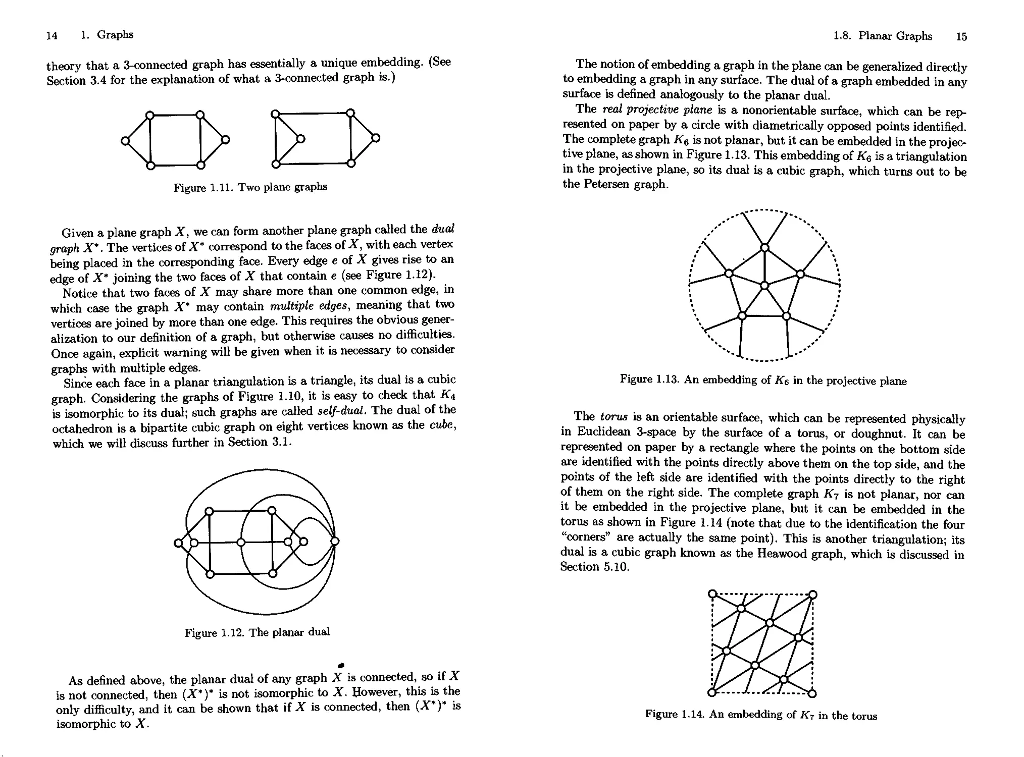
14 1. Graphs
theory that a 3-connected graph has essentially a unique embedding. (See
Section 3.4 for the explanation of what a 3-connected graph is.)
Figure 1.11. Two plane graphs
Given a plane graph X, we can form another plane graph called the dual
graph X*. The vertices of X* correspond to the faces of X, with each vertex
being placed in the corresponding face. Every edge e of X gives rise to an
edge of X* joining the two faces of X that contain e (see Figure 1.12).
Notice that two faces of X may share more than one common edge, in
which case the graph X" may contain multiple edges, meaning that two
vertices are joined by more than one edge. This requires the obvious gener-
generalization to our definition of a graph, but otherwise causes no difficulties.
Once again, explicit warning will be given when it is necessary to consider
graphs with multiple edges.
Since each face in a planar triangulation is a triangle, its dual is a cubic
graph. Considering the graphs of Figure 1.10, it is easy to check that K\
is isomorphic to its dual; such graphs are called self-dual. The dual of the
octahedron is a bipartite cubic graph on eight vertices known as the cube,
which we will discuss further in Section 3.1.
Figure 1.12. The planar dual
As defined above, the planar dual of any graph X is connected, so if X
is not connected, then (X*)* is not isomorphic to X. However, this is the
only difficulty, and it can be shown that if X is connected, then (X*)* is
isomorphic to X.
1.8. Planar Graphs 15
The notion of embedding a graph in the plane can be generalized directly
to embedding a graph in any surface. The dual of a graph embedded in any
surface is defined analogously to the planar dual.
The real protective plane is a nonorientable surface, which can be rep-
represented on paper by a circle with diametrically opposed points identified.
The complete graph K6 is not planar, but it can be embedded in the projec-
tive plane, as shown in Figure 1.13. This embedding of Kq is a triangulation
in the projective plane, so its dual is a cubic graph, which turns out to be
the Petersen graph.
Figure 1.13. An embedding of Ke in the projective plane
The torus is an orientable surface, which can be represented physically
in Euclidean 3-space by the surface of a torus, or doughnut. It can be
represented on paper by a rectangle where the points on the bottom side
are identified with the points directly above them on the top side, and the
points of the left side are identified with the points directly to the right
of them on the right side. The complete graph K7 is not planar, nor can
it be embedded in the projective plane, but it can be embedded in the
torus as shown in Figure 1.14 (note that due to the identification the four
"corners" are actually the same point). This is another triangulation; its
dual is a cubic graph known as the Heawood graph, which is discussed in
Section 5.10.
Figure 1.14. An embedding of K7 in the torus

16 1. Graphs
Exercises
1. Let X be a graph with n vertices. Show that X is complete or empty
if and only if every transposition of {1,..., n) belongs to Aut(X).
2. Show that X and X have the same automorphism group, for any
graph X.
3. Show that if x and y are vertices in the graph X and g e Aut(X),
then the distance between x and y in X is equal to the distance
between x9 and y9 in X.
4. Show that if / is a homomorphism from the graph X to the graph Y
and x\ and z2 are vertices in X, then
dx{xi,x2) >dY{f{xi),f{x2))-
5. Show that if Y is a subgraph of X and / is a homomorphism from
X to Y such that / \Y is a bijection, then Y is a retract.
6. Show that a retract Y of X is an induced subgraph of X. Then
show that it is isometric, that is, if x and y are vertices of Y, then
dx(z,y) = dy(x,j/).
7. Show that any edge in a bipartite graph X is a retract of X.
8. The diameter of a graph is the maximum distance between two dis-
distinct vertices. (It is usually taken to be infinite if the graph is not
connected.) Determine the diameter of J(v, k, k - 1) when v > 2k.
9. Show that Aut(/Cn) is not isomorphic to Aut(L(Kn)) if and only if
n = 2 or 4.
10. Show that the graph Ks \ e (obtained by deleting any edge e from
is not a line graph.
11. Show that /Ci,3 is not an induced subgraph of a line graph.
12. Prove that any induced subgraph of a line graph is a line graph.
13. Prove Krausz's characterization of line graphs (Theorem 1.7.2).
14. Find all graphs G such that L(G) ^ G.
15. Show that if X is a graph with minimum valency at least four, Aut(X)
and Aut(L(X)) are isomorphic.
16. Let 5 be a set of nonzero vectors from an m-dimensional vector space.
Let X(S) be the graph with the elements of S as its vertices, with
two vectors x and y adjacent if and only if xTy ^.0. (Call X(S) the
"nonorthogonality" graph of 5.) Show that any independent set in
X(S) has cardinality at most m.
1.8. Notes 17
17. Let X be a graph with n vertices. Show that the line graph of X is
the nonorthogonality graph of a set of vectors in 1",
18. Show that a graph is bipartite if and only if it contains no odd cycles.
19. Show that a tree on n vertices has n — 1 edges.
20. Let X be a connected graph. Let T(X) be the graph with the span-
spanning trees of X as its vertices, where two spanning trees are adjacent
if the symmetric difference of their edge sets has size two. Show that
T{X) is connected.
21. Show that if two trees have isomorphic line graphs, they are
isomorphic.
22. Use Euler's identity to show that K5 is not planar.
23. Construct an infinite family of self-dual planar graphs.
24. A graph is self-complementary if it is isomorphic to its complement.
Show that L{Kz$) is self-complementary.
25. Show that if there is a self-complementary graph X on n vertices,
then n = 0,1 mod 4. If X is regular, show that n = 1 mod 4.
26. The lexicographic product X[Y] of two graphs X and Y has vertex
set V{X) x V(Y) where {x, y) ~ (*', y1) if and only if
(a) x is adjacent to x' in X, or
(b) x = x' and y is adjacent to y1 in Y.
Show that the complement of the lexicographic product of X and Y
is the lexicographic product of X and Y.
Notes
For those readers interested in a more comprehensive view of graph theory
itself, we recommend the books by West [6] and Diestel [2].
The problem of determining whether two graphs are isomorphic has a
long history, as it has many applications—for example, among chemists
who wish to tabulate all molecules in a certain class. All attempts to find
a collection of easily computable graph parameters that are sufficient to
distinguish any pair of nonisomorphic graphs have failed. Nevertheless the
problem of determining graph isomorphism has not been shown to be NP-
complete. It is considered a prime candidate for membership in the class
of problems in NP that are neither NP-complete nor in P (if indeed NP ^
P)-
In practice, computer programs such as Brendan McKay's nauty [5] can
determine isomorphisms between most graphs up to about 20000 vertices,

18 References
though there are significant "pathological" cases where certain very highly
structured graphs on only a few hundred vertices cannot be dealt with.
Determining the automorphism group of a graph is closely related to de-
determining whether two graphs are isomorphic. As we have already seen, it
is often easy to find some automorphisms of a graph, but quite difficult
to show that one has identified the full automorphism group of the graph.
Once again, for moderately sized graphs with explicit descriptions, use of
a computer is recommended.
Many graph parameters are known to be NP-hard to compute. For ex-
example, determining the chromatic number of a graph or finding the size of
the maximum clique are both NP-hard.
Krausz's theorem (Theorem 1.7.2) comes from [4] and is surprisingly
useful. A proof in English appears in [6], but you are better advised to
construct your own. Beineke's result (Theorem 1.7.4) is proved in [1].
Most introductory texts on graph theory discuss planar graphs. For more
complete information about embeddings of graphs, we recommend Gross
and Tucker [3].
Part of the charm of graph theory is that it is easy to find interesting
and worthwhile problems that can be attacked by elementary methods,
and with some real prospect of success. We offer the following by way of
example. Define the iterated line graph Ln(X) of a graph X by setting
La(X) equal to L{X) and, if n > 1, defining Ln{X) to be L{Ln-l{X)). It
is an open question, due to Ron Graham, whether a tree T is determined
by the integer sequence
\V(Ln(T))\, „>!.
References
[1] L. W. Beineke, Derived graphs and digraphs, Beitrage zur Graphentheorie.
A968), 17-33.
[2] R. Diestel, Graph Theory, Springer-Verlag, New York, 1997.
[3] J. L. GROSS and T. W. Tucker, Topological Graph Theory, John Wiley &
Sons Inc., New York, 1987.
[4] J. Krausz, Demonstration nouvelle d'une theoreme de Whitney sur les
reseaux, Mat. Fiz. Lapok, 50 A943), 75-85.
[5] B. McKay, nauty user's guide (version 1.5), tech. rep., Department of
Computer Science, Australian National University, 1990.
[6] D. B. West, Introduction to Graph Theory, Prentice Hall Inc., Upper Saddle
River, NJ, 1996. *
2
Groups
The automorphism group of a graph is very naturally viewed as a group
of permutations of its vertices, and so we now present some basic informa-
information about permutation groups. This includes some simple but very useful
counting results, which we will use to show that the proportion of graphs
on n vertices that have nontrivial automorphism group tends to zero as
n tends to infinity. (This is often expressed by the expression "almost all
graphs are asymmetric") For a group theorist this result might be a disap-
disappointment, but we take its lesson to be that interesting interactions between
groups and graphs should be looked for where the automorphism groups
are large. Consequently, we also take the time here to develop some of the
basic properties of transitive groups.
2.1 Permutation Groups
The set of all permutations of a set V is denoted by Sym(Vr), or just Sym(n)
when [V| = n. A permutation group on V is a subgroup of Sym(V). If X
is a graph with vertex set V, then we can view each automorphism as a
permutation of V, and so Aut(X) is a permutation group.
A permutation representation of a group G is a homomorphism from G
into Sym(Vr) for some set V. A permutation representation is also referred
to as an action of G on the set V, in which case we say that G acts on V.
A representation is faithful if its kernel is the identity group.

20 2. Groups
A group G acting on a set V induces a number of other actions. If 5 is a
subset of V, then for any element g € G, the translate S9 is again a subset
of V. Thus each element of G determines a permutation of the subsets of V,
and so we have an action of G on the power set 2V. We can be more precise
than this by noting that \S9\ = \S\. Thus for any fixed fc, the action of G
on V induces an action of G on the fc-subsets of V. Similarly, the action of
G on V induces an action of G on the ordered A;-tuples of elements of V.
Suppose G is a permutation group on the set V. A subset 5 of V is G-
invariant if s9 € 5 for all points s of 5 and elements g of G. If 5 is invariant
under G, then each element g € G permutes the elements of 5. Let g ] S
denote the restriction of the permutation g to 5. Then the mapping
is a homomorphism from G into Sym(S), and the image of G under this
homomorphism is a permutation group on 5, which we denote by G\S. (It
would be more usual to use Gs.)
A permutation group G on V is transitive if given any two points x and
y from V there is an element g € G such that x9 = y. A G-invariant subset
5 of V is an orbit of G if G f 5 is transitive on 5. For any x € V, it is
straightforward to check that the set
x° := {x9:g€ G}
is an orbit of G. Now, if y € xa, then ya = xa, and if y ? xa, then
ya C\xc = 0, so each point lies in a unique orbit of G, and the orbits of G
partition V. Any G-invariant subset of V is a union of orbits of G (and in
fact, we could define an orbit to be a minimal G-invariant subset of V).
2.2 Counting
Let G be a permutation group on V. For any x € V the stabilizer Gx of x
is the set of all permutations g € G such that x9 = x. It is easy to see that
Gx is a subgroup of G. If X\,..., xr are distinct elements of V, then
r
GX1 Xr :=f]GXi.
t=i
Thus this intersection is the subgroup of G formed by the elements that
fix Xi for all i\ to emphasize this it is called the pointwise stabilizer of
{xi,... ,xr}- If 5 is a subset of V, then the stabilizer Gs of 5 is the set of
all permutations g such that S9 = S. Because here we are not insisting that
every element of 5 be fixed this is sometimes called the setwise stabilizer
of 5. If S = {xi,..., xr}, then GXl Xr is a subgroup of Gs-
Lemma 2.2.1 Let G be a permutation group acting on V and let S be an
orbit of G. If x and y are elements of S, the set of permutations in G that
2.2. Counting 21
map x toy is a right coset ofGx. Conversely, all elements in a right coset
of Gx map x to the same point in S.
Proof. Since G is transitive on 5, it contains an element, g say, such that
x9 = y. Now suppose that h € G and xh = y. Then x9 = xh, whence
xhg ' = x. Therefore, hg~l € Gx and h € Gxg. Consequently, all elements
mapping x to y belong to the coset Gxg.
For the converse we must show that every element of Gxg maps x to
the same point. Every element of Gxg has the form hg for some element
h e Gx. Since xh9 = {x'1)9 = x3, it follows that all the elements of Gxg
map x to x9. ?
There is a simple but very useful consequence of this, known as the
orbit-stabilizer lemma.
Lemma 2.2.2 (Orbit-stabilizer) Let G be a permutation group acting
on V and let x be a point in V. Then
\GX\ \xG\ = \G\
Proof. By the previous lemma, the points of the orbit xc correspond
bijectively with the right cosets of Gx. Hence the elements of G can be
partitioned into |xG| cosets, each containing \GX\ elements of G. ?
In view of the above it is natural to wonder how Gx and Gy are related
if x and y are distinct points in an orbit of G. To answer this we first need
some more terminology. An element of the group G that can be written in
the form g~:hg is said to be conjugate to h, and the set of all elements of
G conjugate to h is the conjugacy class of h. Given any element g € G, the
mapping rg : h >-> g~lhg is a permutation of the elements of G. The set
of all such mappings forms a group isomorphic to G with the conjugacy
classes of G as its orbits. If H C G and g € G, then g~lHg is defined to
be the subset
{g-'hg.heH}.
If H is a subgroup of G, then g~xHg is a subgroup of G isomorphic to H,
and we say that g~lHg is conjugate to H. Our next result shows that the
stabilizers of two points in the same orbit of a group are conjugate.
Lemma 2.2.3 Let G be a permutation group on the set V and let x be a
point in V. If g € G. then g~lGxg = Gx».
Proof. Suppose that x3 = y. First we show that every element oig~lGxg
fixes y. Let h € Gx. Then
and therefore g~xhg € Gy. On the other hand, if h € Gy, then ghg'1 fixes
x, whence we see that g~1Gxg = Gy. n

22 2. Groups
If g is a permutation of V, then fix(#) denotes the set of points in V
fixed by g. The following lemma is traditionally (and wrongly) attributed
to Burnside; in fact, it is due to Cauchy and Probenius.
Lemma 2.2.4 ("Burnside") Let G be a permutation group on the set
V. Then the number of orbits ofGonV is equal to the average number of
points fixed by an element of G.
Proof. We count in two ways the pairs (g, x) where g € G and a; is a point
in V fixed by g. Summing over the elements of G we find that the number
of such pairs is
which, of course, is \G\ times the average number of points fixed by an
element of G. Next we must sum over the points of V, and to do this we
first note that the number of elements of G that fix a; is \GX\. Hence the
number of pairs is
xev
Now, \GX\ is constant as x ranges over an orbit, so the contribution to this
sum from the elements in the orbit xa is \xa\ \GX\ = \G\. Hence the total
sum is equal to \G\ times the number of orbits, and the result is proved.O
2.3 Asymmetric Graphs
A graph is asymmetric if its automorphism group is the identity group.
In this section we will prove that almost all graphs are asymmetric, i.e..
the proportion of graphs on n vertices that are asymmetric goes to 1 as
n —» oo. Our main tool will be Burnside's lemma.
Let V be a set of size n and consider all the distinct graphs with vertex
set V. If we let Kv denote a fixed copy of the complete graph on the
vertex set V, then there is a one-to-one correspondence between graphs
with vertex set V and subsets of E{Kv)- Since Kv has (?) edges, the total
number of different graphs is
Given a graph X, the set of graphs isomorphic to X is called the iso-
isomorphism class of X. The isomorphism classes partition the set of graphs
with vertex set V. Two such graphs X and Y are isomorphic if there is a
permutation of Sym(V) that maps the edge set of X onto the edge set of
Y. Therefore, an isomorphism class is an orbit of Sym(V) in its action on
subsets of E(KV)-
2.3. Asymmetric Graphs 23
Lemma 2.3.1 The size of the isomorphism class containing X is
n!
|Aut(Jf)|'
Proof. This follows from the orbit-stabilizer lemma. We leave the details
as an exercise. ?
Now we will count the number of isomorphism classes, using Burnside's
lemma. This means that we must find the average number of subsets of
E(KV) fixed by the elements of Sym(V). Now, if a permutation g has r
orbits in its action on E(KV), then it fixes 2r subsets in its action on the
power set of E(KV). For any g e Sym(V), let orb2(?) denote the number
of orbits of g in its action on E(Ky)- Then Burnside's lemma yields that
the number of isomorphism classes of graphs with vertex set V is equal to
\ OOrD2(o) /ci i \
a! 1^ * ¦ \lA)
n!
9€Sym(V)
If all graphs were asymmetric, then every isomorphism class would
contain n! graphs and there would be exactly
2C)
isomorphism classes. Our next result shows that in fact, the number of
isomorphism classes of graphs on n vertices is quite close to this, and we
will deduce from this that almost all graphs are asymmetric. Recall that
o(l) is shorthand for a function that tends to 0 as n —> 00.
Lemma 2.3.2 The number of isomorphism classes of graphs on n vertices
is at most
2B)
A + 0A)) — .
Proof. We will leave some details to the reader. The support of a per-
permutation is the set of points that it does not fix. We claim that among
all permutations g € Sym(V) with support of size an even integer 2r, the
maximum value of orb2{g) is realized by the permutation with exactly r
cycles of length 2.
Suppose g e Sym(V) is such a permutation with r cycles of length two
and n-2r fixed points. Since g2 = e, all its orbits on pairs of elements from
V have length one or two. There are two ways in which an edge {x, y} €
E(KV) can be not fixed by g. Either both x and y are in the support of g,
but x9 ^ y, or x is in the support of g and y is a fixed point of g. There are
2r(r -1) edges in the former category, and 2r(n- 2r) is the latter category.
Therefore the number of orbits of length 2isr(r-l)+r(n-2r) = r(n-r-l),

24 2. Groups
and the total number of orbits of g on E{Kv) is
orb2(?) = \Vj -r(n-r- 1).
Now we are going to partition the permutations of Sym(V) into 3 classes
and make rough estimates for the contribution that each class makes to the
sum B.1) above.
Fix an even integer m < n - 2, and divide the permutations into three
classes as follows: C\ = {e}, C2 contains the nonidentity permutations with
support of size at most m, and C3 contains the remaining permutations.
We may estimate the sizes of these classes as follows:
|Ci| =
\CZ\ <n\<nn.
An element g € C2 has the maximum number of orbits on pairs if it is a
single 2-cycle, in which case it has Q) - (n — 2) such orbits. An element
g € C3 has support of size at least m and so has the maximum number of
orbits on pairs if it has m/2 2-cycles, in which case it has
m
nm
such orbits.
Therefore,
S€Sym(V)
= 2C) (l + nm2-(n-2) + nn2-nm/4)
The sum of the last two terms can be shown to be o(l) by expressing it as
2m log n—n+2 . <jnlogn—nm/4
and taking m = [clognj for c> 4. n
Corollary 2.3.3 Almost all graphs are asymmetric.
Proof. Suppose that the proportion of isomorphism classes of graphs on
V that are asymmetric is /i. Each isomorphism class of a graph that is not
asymmetric contains at most n!/2 graphs, whence the average size of an
isomorphism class is at most
n!
Consequently,
2.4. Orbits on Pairs 25
from which it follows that n tends to 1 as n tends to infinity. Since the
proportion of asymmetric graphs on V is at least as large as the proportion
of isomorphism classes (why?), it follows that the proportion of graphs on
n vertices that are asymmetric goes to 1 as n tends to 00. ?
Although the last result assures us that most graphs are asymmetric,
it is surprisingly difficult to find examples of graphs that are obviously
asymmetric. We describe a construction that does yield such examples. Let
T be a tree with no vertices of valency two, and with at least one vertex of
valency greater than two. Assume that it has exactly m end-vertices- We
construct a Halin graph by drawing T in the plane, and then drawing a
cycle of length m through its end-vertices, so as to form a planar graph.
An example is shown in Figure 2.1.
Figure 2.1. A Halin graph
Halin graphs have a number of interesting properties; in particular, it
is comparatively easy to construct cubic Halin graphs with no nonidentity
automorphisms. They all have the property that if we delete any two ver-
vertices, then the resulting graph is connected, but if we delete any edge, then
we can find a pair of vertices whose deletion will disconnect the graph.
(To use language from Section 3.4, they are 3-connected, but any proper
subgraph is at most 2-connected.)
2.4 Orbits on Pairs
Let G be a transitive permutation group acting on the set V. Then G acts
on the set of ordered pairs V x V, and in this section we study its orbits
on this set. It is so common to study G acting on both V and V x V that
the orbits of G on V x V are often given the special name orbitals.
Since G is transitive, the set
{{x,x):xe V}

26
2. Groups
is an orbital of G, known as the diagonal orbital. If fi C V x V, we define
its transpose fiT to be
It is a routine exercise to show that fiT is G-invariant if and only if fi is.
Since orbits are either equal or disjoint, it follows that if fi is an orbital of
G, either fi = fiT or finfiT = 0. If fi = fiT, we call it a symmetric orbital.
Lemma 2.4.1 Let G be a group acting transitively on the set V, and let
x be a point of V. Then there is a one-to-one correspondence between the
orbits of G on V xV and the orbits of Gx onV.
Proof. Let fi be an orbit of G on V x V, and let Ya denote the set
{y : (x, y) € fi}. We claim that the set Yq is an orbit of Gx acting on
V. If y and y' belong to Yq, then (x, y) and (x, y1) lie in fi and there is a
permutation g such that
This implies that g € Gx and y9 = y', and thus y and y1 are in the same
orbit of Gx. Conversely, if (x,y) € fi and y1 = y9 for some g € Gx, then
(x, ?/) e fi. Thus Yq is an orbit of Gx. Since V is partitioned by the sets
Yn, where fi ranges over the orbits of G on V x V, the lemma follows. ?
This lemma shows that for any x € V, each orbit fi of G on V x V is
associated with a unique orbit of Gx. The number of orbits of Gx on V is
called the rank of the group G. If fi is symmetric, the corresponding orbit
of Gx is said to be self-paired. Each orbit DofGonVxV may be viewed
as a directed graph with vertex set V and arc set fi. When fi is symmetric
this directed graph is a graph: (x, y) is an arc if and only if (y, x) is. If fi
is not symmetric, then the directed graph has the property that if (x, y) is
an arc, then (y, x) is not an arc. Such directed graphs are often known as
oriented graphs (see Section 8.3).
Lemma 2.4.2 Let G be a transitive permutation group on V and let fi be
an orbit ofGonVxV. Suppose (x, y) € fi. Then fi is symmetric if and
only if there is a permutation g in G such that x9 = y and y9 = x.
Proof. If (x, y) and (y, x) both lie in fi, then there is a permutation g €
G such that (x,y)9 = (x9,y9) = (y,x). Conversely, suppose there is a
permutation g swapping x and y. Since (x, y)9 = (y, x) € fi, it follows that
T0, andsofi = fiT. °
If a permutation g swaps x and y, then (xy) is a c^cle in g. It follows that
g has even order (and so G itself must have even order). A permutation
group G on V is generously transitive if for any two distinct elements x
and y from V there is a permutation that swaps them. All orbits of G on
VxKare symmetric if and only if G is generously transitive.
2.5. Primitivity 27
We have seen that each orbital of a transitive permutation group G on
V gives rise to a graph or an oriented graph. It is clear that G acts as a
transitive group of automorphisms of each of these graphs. Similarly, the
union of any set of orbitals is a directed graph (or graph) on which G acts
transitively. We consider one example. Let V be the set of all 35 triples
from a fixed set of seven points. The symmetric group SymG) acts on V
as a transitive permutation group G, and it is not hard to show that G is
generously transitive. Fix a particular triple x and consider the orbits of
Gx on V. There are four orbits, namely x itself, the triples that meet a; in 2
points, the triples that meet a; in 1 point, and those disjoint from x. Hence
these correspond to four orbitals, the first being the diagonal orbital, with
the remaining three yielding the graphs JG,3,2), JG,3,1), and JG,3,0).
It is clear that G is a subgroup of the automorphism group of each of these
graphs, but although it can be shown that G is the full automorphism
group of JG,3,2) and JG,3,0), it is not the full automorphism group of
.7G,3,1)!
Lemma 2.4.3 The automorphism group of JG,3,1) contains a group
isomorphic to Sym(8).
Proof. There are 35 partitions of the set {0,1,...,7} into two sets of
size four. Let X be the graph with these partitions as vertices, where two
partitions are adjacent if and only if the intersection of a 4-set from one
with a 4-set from the other is a set of size two. Clearly, Aut(A") contains
a subgroup isomorphic to Sym(8). However, X is isomorphic to JG,3,1).
To see this, observe that a partition of {0,1,..., 7} into two sets of size
four is determined by the 4-set in it that contains 0, and this 4-set in turn
is determined by its nonzero elements. Hence the partitions correspond to
the triples from {1,2,..., 7} and two partitions are adjacent in X if and
only if the corresponding triples have exactly one element in common. D
2.5 Primitivity
Let G be a transitive group on V- A nonempty subset 5 of V is a block of
imprimitivity for G if for any element g of G, either S9 = S or SC\ S9 = 0.
Because G is transitive, it is clear that the translates of 5 form a partition
of V. This set of distinct translates is called a system of imprimitivity for
G.
An example of a system of imprimitivity is readily provided by the
cube Q shown in Figure 2.2. It is straightforward to see that Aut(Q) acts
transitively on Q (see Section 3.1 for more details).
For each vertex x there is a unique vertex x' at distance three from
it; all other vertices in Q are at distance at most two. If 5 = {x,x'}
and g € Aut(Q), then either S9 = S or 5 D S9 = 0, so 5 is a block of
imprimitivity. There are four disjoint sets of the form S9, as g ranges over

28 2. Groups
Figure 2.2. The cube Q
the elements of Aut(Q), and these sets are permuted among themselves by
Aut(Q).
The partition of V into singletons is a system of imprimitivity as is
the partition of V into one cell containing all of V. Any other system of
imprimitivity is said to be nontrivial. A group with no nontrivial systems
of imprimitivity is primitive; otherwise, it is imprimitive. There are two
interesting characterizations of primitive permutation groups. We give one
now; the second is in the next section.
Lemma 2.5.1 Let G be a transitive permutation group on V and let x be
a point in V. Then G is primitive if and only ifGx is a maximal subgroup
ofG.
Proof. In fact, we shall be proving the contrapositive statement, namely
that G has a nontrivial system of imprimitivity if and only if Gx is not a
maximal subgroup of G. First some notation: We write H < G if H is a
subgroup of G, and H < G if H is a proper subgroup of G.
Suppose first that G has a nontrivial system of imprimitivity and that
B is a block of imprimitivity that contains x. Then we will show that
Gx < Gb < G and therefore that Gx is not maximal. If g € Gx, then
BC\B!I is nonempty (for it contains x) and hence B = B9. Thus Gx <Gb-
To show that the inclusion is proper we find an element in Gb that is not
in Gx.Lety^x be another element of B. Since G is transitive it contains
an element h such that xh = y. But then B = Bh, yet h & Gx, and hence
Gx < GB-
Conversely, suppose that there is a subgroup H such that Gx < H <G.
We shall show that the orbits of H form a nontrivial system of imprimi-
imprimitivity. Let B be the orbit of H containing x and let g € G. To show that
B is a block of imprimitivity it is necessary to show that either B = B9
or B n By = 0. Suppose that y € BC\Bf>. Tfien because y € B there
is an element he H such that y = xh. Moreover, because^ € B9 there
is some element h' € H such that y = xh'3. Then xh'9h = x, and so
h'gh''1 e Gx < H. Therefore, g € H, and because B is an orbit of H we
have B = B9. Because Gx < H, the block B does not consist of x alone,
2.6. Primitivity and Connectivity 29
and because H < G, it does not consist of the whole of V, and hence it is
a nontrivial block of imprimitivity. D
2.6 Primitivity and Connectivity
Our second characterization of primitive permutation groups uses the orbits
of G on V x V, and requires some preparation. A path in a directed graph
D is a sequence uo,..,,ur of distinct vertices such that (ui--[,Ui) is an
arc of D for i = 1...., r. A weak path is a sequence uo,...,ur of distinct
vertices such that for i = 1,. .,,r, either (ui-i,m) or (ui,Ui-^ is an arc.
(We will use this terminology in this section only.) A directed graph is
strongly connected if any two vertices can be joined by a path and is weakly
connected if any two vertices can be joined by a weak path. A directed
graph is weakly connected if and only if its "underlying" undirected graph is
connected. (This is often used as a definition of weak connectivity.) A strong
component of a directed graph is an induced subgraph that is maximal,
subject to being strongly connected. Since a vertex is strongly connected,
it follows that each vertex lies in a strong component, and therefore the
strong components of D partition its vertices.
The in-valency of a vertex in a directed graph is the number of arcs
ending on the vertex, the out-valency is defined analogously.
Lemma 2.6.1 Let D be a directed graph such that the in-valency and out-
valency of any vertex are equal. Then D is strongly connected if and only
if it is weakly connected.
Proof. The difficulty is to show that if D is weakly connected, then it is
strongly connected. Assume by way of contradiction that D is weakly, but
not strongly, connected and let Dx,..., Dr be the strong components of D.
If there is an arc starting in Dx and ending in ?>2, then any arc joining ?>i
to D2 must start in D\. Hence we may define a directed graph D' with the
strong components of D as its vertices, and such that there is an arc from
Di to Dj in D' if and only if there is an arc in D starting in A and ending
in Dj. This directed graph cannot contain any cycles. (Why?) It follows
that there is a strong component, D\ say, such that any arc that ends on
a vertex in it must start at a vertex in it. Since D is weakly connected,
there is at least one arc that starts in Dx and ends on a vertex not in D\.
Consequently the mimber of arcs in Z?i is less than the sum of the out-
valencies of the vertices in it. But on the other hand, each arc that ends
in Di must start in it, and therefore the number of arcs in Di is equal to
the sum of the in-valencies of its vertices. By our hypothesis on D, though,
the sum of the in-valencies of the vertices in D\ equals the sum of the
out-valencies. Thus we have the contradiction we want. ?

30 2. Groups
What does this lemma have to do with permutation groups? Let G act
transitively on V and let fi be an orbit of G on V x V that is not symmetric.
Then fi is an oriented graph, and G acts transitively on its vertices. Hence
each point in V has the same out-valency in fi and the same in-valency. As
the in- and out-valencies sum to the number of arcs in fi, the in- and out-
valencies of any point of V in fi are the same. Hence fi is weakly connected
if and only if it is strongly connected, and so we will refer to weakly or
strongly connected orbits as connected orbits.
Lemma 2.6.2 Let G be a transitive permutation group on V. Then G is
primitive if and only if each nondiagonal orbit is connected.
Proof. Suppose that G is imprimitive, and that B\,..., BT is a system of
imprimitivity. Assume further that x and y are distinct points in Si and fi
is the orbit of G (on V x V) that contains (x, y). If g € G, then x9 and y9
must lie in the same block; otherwise B9 contains points from two distinct
blocks. Therefore, each arc of 0 joins vertices in the same block, and so fi
is not connected.
Now suppose conversely that fi is a nondiagonal orbit that is not con-
connected, and let S be the point set of some component of fi. If g € G, then
B and B9 are either equal or disjoint. Therefore, B is a nontrivial block
and G is imprimitive. D
Exercises
1. Show that the size of the isomorphism class containing X is
n!
|Aut(Jf)|'
2. Prove that |Aut(Cn)| = 2n. (You may assume that 2n is a lower
bound on |Aut(Cn)|.)
3. If G is a transitive permutation group on the set V, show that there
is an element of G with no fixed points. (What if G has more than
one orbit, but no fixed points?)
4. If g is a permutation of a set of n points with support of size s,
show that ort>2(<7) is maximal when all nontrivial cycles of g are
transpositions.
5. The goal of this exercise is to prove Frobenius's lemma, which as-
asserts that if the order of the group G is divisible by the prime p,
then G contains an element of order p. Let fi denote the set of all
ordered p-tuples (x\,..., xp) of elements of G such that x\ ¦ ¦ ¦ xp = e.
Let 7T denote the permutation of Gv that maps (x\,X2, ¦. -,xp) to
(x2, • • •, Xp, xi). Show that n fixes fi as a set. Using the facts that n
2.6. Exercises 31
fixes (e,.. .,e) and |ft| = IG^, deduce that n must fix at least p
elements of fi and hence Frobenius's lemma holds.
6. Construct a cubic planar graph on 12 vertices with trivial auto-
automorphism group, and provide a proof that it has no nonidentity
automorphism.
7. Decide whether the cube is a Halin graph.
8. Let A" be a self-complementary graph with more than one vertex.
Show that there is a permutation g of V(X) such that:
(a) {x, y) € E(X) if and only if {x9,y9} € E{X),
(b) g2 € Aut(A) but g2 ^ e,
(c) the orbits of g on V(X) induce self-complementary subgraphs
oiX.
9. If G is a permutation group on V, show that the number of orbits of
G on V x V is equal to
1
and derive a similar formula for the number of orbits of G on the set
of pairs of distinct elements from V.
10. If H and K are subsets of a group G, then HK denotes the subset
{hk.heH, ke K}.
If H and K are subgroups and g € G, then HgK is called a double
coset. The double coset HgK is a union of right cosets of H and a
union of left cosets of K, and G is partitioned by the distinct double
cosets HgK, as g varies over the elements of G. Now (finally) suppose
that G is a transitive permutation group on V and H < G. Show
that each orbit of if on V corresponds to a double coset of the form
GxgH. Also show that the orbit of Gx corresponding to the double
coset GxgGx is self-paired if and only if GxgGx = Gxg~lGx.
11. Let G be a transitive permutation group on V. Show that it has a
symmetric nondiagonal orbit on V x V if and only if \G\ is even.
12. Show that the only primitive permutation group on V that contains
a transposition is Sym(V).
13. Let A" be a graph such that Aut(X) acts transitively on V(X) and let
B be a block of imprimitivity for Aut(X). Show that the subgraph
of X induced by B is regular.
14. Let G be a generously transitive permutation group on V and let B
be a block for G. Show that G\B and the permutation group induced
by G on the translates of B are both generously transitive.

32 References
15. Let G be a transitive permutation group on V such that for each
element v in V there is an element of G with order two that has
t; as its only fixed point. (Thus |V| must be odd.) Show that G is
generously transitive.
16. Let X be a nonempty graph that is not connected. If Aut(A") is
transitive, show that it is imprimitive.
17. Show that Aut( JDn-1,2n—1, n—1)) contains a subgroup isomorphic
to SymDn). Show further that w( JDn - 1,2n - 1, n - 1)) < 4n - 1,
and characterize the cases where equality holds.
Notes
The standard reference for permutation groups is Wielandt's classic [5]. We
also highly recommend Cameron [1]. For combinatorialists these are the
best starting points. However, almost every book on finite group theory
contains enough information on permutation groups to cover our modest
needs. Neumann [3] gives an interesting history of Burnside's lemma.
The result of Exercise 15 is due to Shult. Exercise 17 is worth some
thought, even if you do not attempt to solve it, because it appears quite
obvious that Aut( JDn—1,2n-l, n—1)) should be SymDn - 1). The second
part will be easier if you know something about Hadamard matrices.
Call a graph minimal asymmetric if it is asymmetric, but any proper in-
induced subgraph with at least two vertices has a nontrivial automorphism.
Sabidussi and Nesetfil [2] conjecture that there are finitely many isomor-
isomorphism classes of minimal asymmetric graphs. In [4], Sabidussi verifies this
for all graphs that contain an induced path of length at least 5, finding that
there are only two such graphs. In [2], Sabidussi and Nesetfil show that
there are exactly seven minimal asymmetric graphs in which the longest
induced path has length four.
References
[lj P. J. Cameron, Permutation Groups, Cambridge University Press, Cam-
Cambridge, 1999.
[2] J. Nesetril and G. Sabidussi, Minimal asymmetric graphs of induced length
4, Graphs Combin., 8 A992), 343-359.
[3] P. M. Neumann, A lemma that is not Burmide's, Math. Sci., 4 A979),
133-141.
[4] G. Sabidussi, Clumps, minimal asymmetric graphs, and involutions, J.
Combin. Theory Ser. B, 53 A991), 40-79.
[5] H. WlELANDT, Finite Permutation Groups, Academic Press, New York, 1964.
Transitive Graphs
We are going to study the properties of graphs whose automorphism group
acts vertex transitively. A vertex-transitive graph is necessarily regular.
One challenge is to find properties of vertex-transitive graphs that are not
shared by all regular graphs. We will see that transitive graphs are more
strongly connected than regular graphs in general. Cayley graphs form an
important class of vertex-transitive graphs; we introduce them and offer
some reasons why they are important and interesting.
3.1 Vertex-Transitive Graphs
A graph X is vertex transitive (or just transitive) if its automorphism group
acts transitively on V(X). Thus for any two distinct vertices of X there is
an automorphism mapping one to the other.
An interesting family of vertex-transitive graphs is provided by the k-
cubes Qk. The vertex set of Qk is the set of all 2k binary fe-tuples, with
two being adjacent if they differ in precisely one coordinate position. We
have already met the 3-cube Q3, which is normally just called the cube (see
Figure 2.2), and Figure 3-1 shows the 4-cube Q4,.
Lemma 3.1.1 The k-cube Qk is vertex transitive.
Proof. If v is a fixed fc-tuple, then the mapping
pv : x >—» x + v

34 3. Transitive Graphs
Figure 3.1. The 4-cube Q*
(where addition is binary) is a permutation of the vertices of Qk. This map-
mapping is an automorphism because the fc-tuples x and y differ in precisely
one coordinate position if and only if a; + v and y + v differ in precisely
one coordinate position. There are 2k such permutations, and they form a
subgroup H of the automorphism group of Qk- This subgroup acts transi-
transitively on V(Qk) because for any two vertices x and y, the automorphism
Py-X maps x to y. ?
The group H of Lemma 3.1.1 is not the full automorphism group of Qk-
Any permutation of the fc coordinate positions is an automorphism of Qk,
and the set of all these permutations forms a subgroup K of Aut(Qfc), iso-
morphic to Sym(fc). Therefore, Aut(<2fc) contains the set HK. By standard
group theory, the size of HK is given by
\iF7\k\-
It is straightforward to see that H O K is the identity subgroup, whence
we conclude that |Aut(Qfc)| > 2kk\.
Another family of vertex-transitive graphs that we have met before are
the circulants. Any vertex can be mapped to any other vertex by using a
suitable power of the cyclic permutation described in Section 1.5.
The circulants and the fc-cubes are both examples of a more general
construction that produces many, but not all, fertex-transitive graphs.
Let G be a group and let C be a subset of G that is closed under taking
inverses and does not contain the identity. Then the Cayley graph X(G, C)
is the graph with vertex set G and edge set
3.2. Edge-Transitive Graphs 35
If C is an arbitrary subset of G, then we can define a directed graph
X(G, C) with vertex set G and arc set {(g, h): hg~l € C). If C is inverse-
closed and does not contain the identity, then this graph is undirected and
has no loops, and the definition reduces to that of a Cayley graph. Most
of the results for Cayley graphs apply in the more general directed case
without modification, but we explicitly use directed Cayley graphs only in
Section 3.8.
Theorem 3.1.2 The Cayley graph X(G, C) is vertex transitive.
Proof. For each g € G the mapping
pg : x h-» xg
is a permutation of the elements of G. This is an automorphism of X(G, C)
because
{yg){x9)~l = ygg~lx~l = yx~\
and so xg ~ yg if and only if x ~ y. The permutations pg form a subgroup
of the automorphism group of X{G, C) isomorphic to G. This subgroup
acts transitively on the vertices of X(G, C) because for any two vertices g
and h, the automorphism Pg-^h maps g to h. ?
The fc-cube is a Cayley graph for the elementary abelian group {%>2)k,
and a circulant on n vertices is a Cayley graph for the cyclic group of order
n.
Most small vertex-transitive graphs are Cayley graphs, but there are
also many families of vertex-transitive graphs that are not Cayley graphs.
In particular, the graphs J(v,k,i) are vertex transitive because Sym(v)
contains permutations that map any fc-set to any other fc-set, but in general
they are not Cayley graphs. We content ourselves with a single example.
Lemma 3-1.3 The Petersen graph is not a Cayley graph.
Proof. There are only two groups of order 10, the cyclic group Zio and the
dihedral group Diq. You may verify that none of the cubic Cayley graphs
on these groups are isomorphic to the Petersen graph (Exercise 2). D
We will return to study Cayley graphs in more detail in Section 3.7.
3.2 Edge-Transitive Graphs
A graph X is edge transitive if its automorphism group acts transitively
on E(X). It is straightforward to see that the graphs J(v, fc, i) are edge
transitive, but the circulants are not usually edge transitive.
An arc in X is an ordered pair of adjacent vertices, and X is arc transitive
if Aut(X) acts transitively on its arcs. It is frequently useful to view an edge
in a graph as a pair of oppositely directed arcs. An arc-transitive graph is

36 3. Transitive Graphs
necessarily vertex and edge transitive. In this section we will consider the
relations between these various forms of transitivity.
The complete bipartite graphs Km,n are edge transitive, but not vertex
transitive unless m = n, because no automorphism can map a vertex of
valency m to a vertex of valency n. The next lemma shows that all graphs
that are edge transitive but not vertex transitive are bipartite.
Lemma 3.2.1 Let X be an edge-transitive graph with no isolated vertices.
If X is not vertex transitive, then Aut(X) has exactly two orbits, and these
two orbits are a bipartition of X.
Proof. Suppose X is edge but not vertex transitive. Suppose that {x, y} €
E(X). If w € V(X), then w lies on an edge and there is an element of
Aut(A') that maps this edge onto {x,y}. Hence any vertex of X lies in
either the orbit of x under Aut(A'), or the orbit of y. This shows that
Aut(A') has exactly two orbits. An edge that joins two vertices in one orbit
cannot be mapped by an automorphism to an edge that contains a vertex
from the other orbit. Since X is edge transitive and every vertex lies in an
edge, it follows that there is no edge joining two vertices in the same orbit.
Hence X is bipartite and the orbits are a bipartition for it. D
Figure 3.2 shows a regular graph that is edge transitive but not vertex
transitive. The colouring of the vertices shows the bipartition.
Figure 3.2. A regular edge-transitive graph that is not vertex transitive
An arc-transitive graph is, as we noted, always1 vertex and edge transitive.
The converse is in general false; see the Notes at the end of the chapter for
more. We do at least have the next result.
Lemma 3.2.2 // the graph X is vertex and edge transitive, but not arc
transitive, then its valency is even.
3.3. Edge Connectivity 37
Proof. Let G = Aut(A'), and suppose that a; € V(X). Let y be a vertex
adjacent to x and fi be the orbit of G on V x V that contains (x, y). Since
X is edge transitive, every arc in X can be mapped by an automorphism to
either (a;, y) or (y, x). Since X is not arc transitive, (y, x) ^ O, and therefore
Q is not symmetric. Therefore, X is the graph with edge set f2ufir. Because
the out-valency of x is the same in fi and flT, the valency of X must be
even. Q
A simple corollary to this result is that a vertex- and edge-transitive
graph of odd valency must be arc transitive. Figure 3.3 gives an example
of a vertex- and edge-transitive graph that is not arc-transitive.
Figure 3.3. A vertex- and edge- but not arc-transitive graph
3.3 Edge Connectivity
An edge cutset in a graph X is a set of edges whose deletion increases the
number of connected components of X. For a connected graph X, the edge
connectivity is the minimum number of edges in an edge cutset, and will
be denoted by ki(X). If a single edge e is an edge cutset, then we call
e a bridge or a cut-edge. As the set of edges adjacent to a vertex is an
edge cutset, the edge connectivity of a graph cannot be greater than its
minimum valency. Therefore, the edge connectivity of a vertex-transitive
graph is at most its valency. In this section we will prove that the edge
connectivity of a connected vertex-transitive graph is equal to its valency.

38 3. Transitive Graphs
If A C V(X), then we define dA to be the set of edges with one end in
A and one end not in A. So if A = 0 or A = V(X), then dA = 0, while the
edge connectivity is the minimum size of dA as A ranges over the proper
subsets of V(X).
Lemma 3.3.1 Let A and B be subsets of V(X). for some graph X. Then
\d(A U B)\ + \d(A n B)\ < \dA\ + \dB\.
Proof. The details are left as an exercise. We simply note here that the
difference between the two sides is twice the number of edges joining A\B
to B\A. d
Define an edge atom of a graph X to be a subset 5 such that \dS\ =
Ki(X) and, given this, \S\ is minimal. Since OS = dV\S, it follows that if
S is an atom, then 2|5| < \V(X)\.
Corollary 3.3.2 Any two distinct edge atoms are vertex disjoint.
Proof. Assume k = k\(X) and let A and B be two distinct edge atoms in
X. If A U B = V(X), then, since neither A nor B contains more than half
the vertices of X, it follows that
\A\ = \B\ = \\V(X)\
and hence that Af)B = 0. So we may assume that AuB is a proper subset
of V(X). Now, the previous lemma yields
\d(Al)B)\ + \d(AnB)\ <2k,
and, since AuB ^ V(X) and AnB^B, this implies that
\d(Al)B)\ = \d(AnB)\=K.
Since Af) B is a. nonempty proper subset of the edge atom A, this is
impossible. We are forced to conclude that A and B are disjoint. ?
Our next result answers all questions about the edge connectivity of a
vertex-transitive graph.
Lemma 3.3.3 If X is a connected vertex-transitive graph, then its edge
connectivity is equal to its valency.
Proof. Suppose that X has valency fe. Let A be an edge atom of X. If A is
a single vertex, then \dA\ = fc and we are finished. Suppose that \A\ > 2. If
g is an automorphism of X and B = A9, then |B| = \A\ and \dB\ = \dA\.
From the previous lemma we see that either ? = B or AC\B = 0. Therefore,
A is a block of imprimitivity for Aut(^), and by Exercise 2.13 it follows
that the subgraph of X induced by A is regular.
Suppose that the valency of this subgraph is (.. Then each vertex in A
has exactly k — I neighbours not in A, and so
3.4. Vertex Connectivity 39
Since X is connected, I < fc, and so if \A\ > k, then \dA\ > k. Hence we
may assume that \A\ < k. Since ? < \A\ — 1, it follows that
\dA\>\A\(k+l-\A\).
The minimum value of the right side here occurs if \A\ = 1 or fe, when it is
equal to fe. Therefore, \dA\ > fe in all cases. ?
3.4 Vertex Connectivity
A vertex cutset in a graph X is a set of vertices whose deletion increases
the number of connected components of X. The vertex connectivity (or just
connectivity) of a connected graph X is the minimum number of vertices
in a vertex cutset, and will be denoted by kq(X). For any fe < «o(^) we
say that X is k-connected. Complete graphs have no vertex cutsets, but
it is conventional to define Ko(Kn) to be n — 1. The fundamental result
on connectivity is Menger's theorem, which we state after establishing one
more piece of terminology. If u and v are distinct vertices of X, then two
paths P and Q from u to v are openly disjoint if V(P\{u, v}) and V(Q\
{u, v}) are disjoint sets.
Theorem 3.4.1 (Menger) Let u and v be distinct vertices in the graph
X. Then the maximum number of openly disjoint paths from u to v equals
the minimum size of a set of vertices S such that u and v lie in distinct
components of X\S. Q
We say that the subset 5 of the theorem separates u and v. Clearly, two
vertices joined by m openly disjoint paths cannot be separated by any set of
size less than m. The significance of this theorem is that it implies that two
vertices that cannot be separated by fewer than m vertices must be joined
by m openly disjoint paths. A simple consequence of Menger's theorem is
that two vertices that cannot be separated by a single vertex must lie on
a cycle. This is not too hard to prove directly. However, to prove that two
vertices that cannot be separated by a set of size two are joined by three
openly disjoint paths seems to be essentially as hard as the general case.
Nonetheless, this is possibly the most important case. (It is the one that
we make use of.)
There are a number of variations of Menger's theorem. In particular, two
subsets A and B of V(X) of size m cannot be separated by fewer than m
vertices if and only if there are m disjoint paths starting in A and ending in
B. This is easily deduced from the result stated; we leave it as an exercise.
We have a precise bound for the connectivity of a vertex-transitive
graph, which requires much more effort to prove than determining its edge
connectivity did.

40 3. Transitive Graphs
Theorem 3.4.2 A vertex-transitive graph with valency k has vertex
connectivity at least |(fe + 1).
Figure 3.4 shows a 5-regular graph with vertex connectivity four, showing
that equality can occur in this theorem.
Figure 3.4. A 5-regular graph with vertex connectivity four
Before proving this result we need to develop some theory. If A is a set
of vertices in X, let N(A) denote the vertices in V(X)\A with a neighbour
in A and let A be the complement of A U N(A) in V(X). A fragment of
X is a subset A such that A±$ and |iV(.<4.)| = Ko(X). An atom of X is
a fragment that contains the minimum possible number of vertices. Note
that an atom must be connected and that if X is a fc-regular graph with
an atom consisting of a single vertex, then kq(X) = k. It is not hard to
show that if A is a fragment, then N(A) = N{A) and A = A.
The following lemma records some further useful properties of fragments.
Lemma 3.4.3 Let A and B be fragments in a graph X. Then
(a) N(A n B) C (A n N(B)) U (N(A) n B) U (N(A) n N(B)).
(b) N{A uB) = (In N{B)) U (N(A) flB)U {N{A) n N{B)).
(c) AUBC A~h~B.
(d) AUB = AnB.
Proof. Suppose first that x € N{A n B). Since AnB and N(A n B) are
disjoint, if x € A, then x ? B, and therefore it must lie in N(B). Similarly,
if x € B, then x € iV(A). If x does not lie in A or B, then x € N{A)C\N{B).
Thus we have proved (a). •
Analogous arguments show that N(A U B) is contained in the union of
A n N{B), N{A)_r\ B, and N(A) n iV(B). To obtain the reverse inclusion,
note that if x € A n N(B), then x does not lie in A or B. Since x € N(B),
it follows that x € AT(A U B). Similarly, we see that if x € N(A) n B or
N{A) n #(#). then x € iV(A U B).
3.4. Vertex Connectivity 41
Next, iix € A, then x does not lie in A or iV(.<4), and therefore does not
lie inAnBor N(A n B). So a; € AC\B. This proves (c). We leave the
proof of (d) as an exercise. ?
B N(B) B
N(A)
b
a
c
e
d
Figure 3.5. Intersection of fragments
Theorem 3.4.4 Let X be a graph on n vertices with connectivity k. Sup-
Suppose A and B are fragments of X and An B ^ 0. // \A\ < \B\, then AC\B
is a fragment.
Proof. The intersections of A, N(A), and A with the sets B, N(B), and B
partition V(X) into nine pieces, as shown in Figure 3.5. The cardinalities
of five of these pieces are also denned in this figure. We present the proof
as a number of steps.
(a) \A\JB\ <n-n.
Since \F\ + \F\ = n - k. for any fragment F of X,
\A\<\B\ = n-K-\B\,
and therefore |A\ + \B\ < n- k. Since AnB is nonempty, the claim follows.
(b) \N{AUB)\ <k.
From Lemma 3.4.3 we find that \N(AC\B)\ < a + b + c and \N(AU B)\ =
c + d + e. Consequently,
2K=\N(A)\ + \N{B)\ = a+b+2c+d+e>\N(AnB)\ + \N{AuB)\. C.1)
Since \N(A n B)\ > k, this implies that \N(A U B)\ < k.
(c) A n B ^ 0.
From (a) and (b) we see that \A(J B\ + \N(AU B)\ < n. Hence AUB ^ 0,
and the claim follows from Lemma 3.4.3(d).
(d) \N(AUB)\=k.

42 3. Transitive Graphs
For any fragment F we have N(F) = N(F). Using part (a) of Lemma 3.4.3
and (b) we obtain
N(AnB) cCnN(B))u{BnN(A))u(jv(S)nJVE))
= (An N(B)) u (B n jv(A)) u (N(A) n iV(B))
Since InB is nonempty, \N{AC\B)\ > k and therefore \N(AUB)| > k.
Taken with (b), we get the claim.
(e) The set An B is a fragment.
From C.1) we see that \N{A n B)\ + \N(A U B)\ < 2k, whence (d) yields
that N{A nB)<K. D
Corollary 3.4.5 // A is an atom and B is a fragment of X, then A is a
subset of exactly one of B, N(B), and B.
Proof. Since A is an atom, \A\ < \B\ and \A\ < \B\. Hence the intersection
of A with B or B, if nonempty, would be a fragment. Since A is an atom,
no proper subset of it can be a fragment. The result follows immediately. D
Now, we can prove Theorem 3.4.2. Suppose that X is a vertex-transitive
graph with valency fc, and let A be an atom in X. If A is a single vertex,
then |iV(A)| = fc, and the theorem holds. Thus we may assume that | A\ > 2.
If g € Aut(X), then A9 is also an atom, and so by Corollary 3.4.5, either
A = A9 or A n A9 = 0. Hence A is a block of imprimitivity for Aut(X),
and its translates partition V(X). Corollary 3.4.5 now yields that N(A) is
partitioned by translates of A, and therefore
\N{A)\ = t\A\
for some integer t. Suppose w is a vertex A. Then the valency of w is at
most
and from this it follows that fe + 1 < {t + 1)\A\ and ko{X) > j^k. To
complete the proof we show that t > 2.
This is actually a consequence of Exercise 20, but since X is vertex transi-
transitive and the atoms are blocks of imprimitivrty for Aut(X), there is a shorter
argument. Suppose for a contradiction that t = 1. By Corollary 3.4.5, N(A)
is a union of atoms, and so N(A) is an atom. Since Aut(Jf) acts transitively
on the atoms of X, it follows that |iV(iV(A))| = |4j, and since AnN{N(A))
is nonempty, A = N(N(A)). This implies that A = 0, and so A is not a
fragment.
3.5. Matchings 43
3.5 Matchings
A matching M in a graph X is a set of edges such that no two have a
vertex in common. The size of a matching is the number of edges in it.
A vertex contained in an edge of M is covered by M. A matching that
covers every vertex of X is called a perfect matching or a 1-factor. Clearly,
a graph that contains a perfect matching has an even number of vertices.
A maximum matching is a matching with the maximum possible number
of edges. (Without this convention there is a chance of confusion, since
matchings can be partially ordered by inclusion or by size.)
We will prove the following result. It implies that a connected vertex-
transitive graph on an even number of vertices has a perfect matching, and
that each vertex in a connected vertex-transitive graph on an odd number
of vertices is missed by a matching that covers all the remaining vertices.
Theorem 3.5.1 Let X be a connected vertex-transitive graph. Then X has
a matching that misses at most one vertex, and each edge is contained in
a maximum matching.
We first verify the claim about the maximum size of a matching. This
requires some preparation, including two lemmas. If M is a matching in X
and P is a path in X such that every second edge of P lies in M, we say
that P is an alternating path relative to M. Similarly, an alternating cycle
is a cycle with every second edge in M.
Suppose that M and N are matchings in X, and consider their symmetric
difference M ® JV. Since M and N are regular subgraphs with valency
one, M © N is a subgraph with maximum valency two, and therefore each
component of it is either a path or a cycle. Since no vertex in M © N lies
in two edges of M or of JV, these paths and cycles are alternating relative
to both M and N. In particular, each cycle must have even length.
Suppose P is a path in M © N with odd length. We may assume without
loss that P contains more edges of M than of N, in which case it follows
that N © P is a matching in X that contains more edges than N. Hence, if
M and N are maximum matchings, all paths in M © N have even length.
Lemma 3.5.2 Let u and v be vertices in X such that no maximum match-
matching misses both of them. Suppose that Mu and Mv are maximum matchings
that miss u and v, respectively. Then there is a path of even length in
Mu © Mv with u and v as its end-vertices.
Proof. Our hypothesis implies that w and v are vertices of valency one in
Mu © Mv so, by our ruminations above, both vertices are end-vertices of
paths in Mu ® Mv. As Mu and Mv have maximum size, these paths have
even length. If they are end-vertices of the same path, we are finished.
Assume that they lie on distinct paths and let P be the path on w. Then
P is an alternating path relative to Mv with even length, and Mv ® P is

44 3. Transitive Graphs
a matching in X that misses w and v and has the same size as Mv. This
contradicts our choice of w and v. D
We are almost ready to prove the first part of our theorem. We call a
vertex w in X critical if it is covered by every maximum matching. If X
is vertex transitive and one vertex is critical, then all vertices are critical,
whence X has a perfect matching. Given this, the next result implies the
first claim in our theorem.
Lemma 3.5.3 Let u and v be distinct vertices in X and let P be a path
from u to v. If no vertex in V(P) \{u,v} is critical, then no maximum
matching misses both u and v.
Proof. The proof is by induction on the length of P. If w ~ v, then no
maximum matching misses both w and v; hence we may assume that P has
length at least two.
Let i be a vertex oil P distinct from w and v. Then u and x are joined
in X by a path that contains no critical vertices. This path is shorter than
P, so by induction, we conclude that no maximum matching misses both
w and x. Similarly, no maximum matching misses both v and x.
Since x is not critical, there is a maximum matching Mx that misses
it. Assume by way of contradiction that AT is a maximum matching that
misses w and v. Then, by Lemma 3.5.2 applied to the vertices u and x,
there must be a path in Mx © N with w and x as its end-vertices. Applying
the same argument to v and x, we find that Mx © N contains a path with
v and x as its end-vertices. This implies that w = v, a contradiction. D
We noted above that a vertex-transitive graph that contains a critical
vertex must have a perfect matching. By the above lemma, if X is vertex-
transitive and does not contain a critical vertex, then no two vertices are
missed by a maximum matching, and therefore a maximum matching covers
all but one vertex of X.
It remains for us to show that every edge of X lies in a maximum
matching. We assume inductively that this claim holds for all connected
vertex-transitive graphs with fewer vertices or edges than X. If X is edge
transitive, we are finished, so we assume it is not. Suppose e is an edge that
does not lie in a maximum matching. Let Y be the subgraph of X with
edge set consisting of the orbit of e under the action of Aut(X). Thus Y is
a vertex-transitive spanning subgraph of X. Since X is not edge transitive,
Y has fewer edges than X. We shall show that X has a matching contain-
containing an edge of Y that misses at most one vertex. This can be mapped to a
matching containing e that misses at most one vertex.
If Y is connected, then by induction, each edge in it lies in a match-
matching that misses at most one vertex. So suppose Y is not connected. The
components of Y form a system of imprimitivity for Aut(X), and are pair-
wise isomorphic vertex-transitive graphs. If the number of vertices in a
component of Y is even, then by induction, each component has a perfect
3.6. Hamilton Paths and Cycles 45
matching and the union of these perfect matchings is a perfect matching
inF.
Assume then that the number of vertices in a component of Y is odd. Let
Y\,...,Yr denote the distinct components of Y. Consider the graph Z with
the components of Y as its vertices, with Yi adjacent to Yj if and only if
there is an edge in X joining some vertex in Yi to a vertex in Yj. Then Z is
a vertex-transitive graph and so, by induction, contains a matching N that
misses at most one vertex. Suppose (Yi,Yj) is an edge in this matching.
Since Yi is adjacent to Yj in Z, there are vertices j/i in Yi and yj in Yj such
that yi is adjacent to yj in X. Because Yi and Yj are vertex transitive and
have an odd number of vertices, there is a matching in F, that misses only
yi and, similarly, a matching in Yj that misses only yj. The union of these
two matchings, together with the edge y^yj, is a matching in X that covers
all vertices in Yi U Yj. Thus each edge of N determines a matching that
covers the vertices in two components of Y.
If the number of components of Y is even, it follows that X has a per-
perfect matching. If the number is odd, we still have a matching in X that
covers all the vertices outside one of the components, Y\ say, of Y. Taken
together with a matching of Y\ that misses exactly one vertex of Y\, we get
a matching of X that misses exactly one vertex.
3.6 Hamilton Paths and Cycles
A Hamilton path in a graph is a path that meets every vertex, and a Hamil-
Hamilton cycle is a cycle that meets every vertex. A graph with a Hamilton cycle
is called hamiltonian. All known vertex-transitive graphs have Hamilton
paths, and only five are known that do not have Hamilton cycles. We
consider these five graphs.
Clearly, K2 is vertex transitive and does not have a Hamilton cycle.
We pass on. A more interesting observation is that the Petersen graph
JE,2,0) does not have a Hamilton cycle. This can be proved by a suitable
case argument; in Chapter 8 we will offer an algebraic proof. The Coxeter
graph, an arc-transitive cubic graph on 28 vertices that we will discuss in
Section 4.6, also has no Hamilton cycle. For references to proofs of this, see
the Notes at the end of this chapter.
The remaining two graphs are constructed from the Petersen and Coxeter
graphs, by replacing each vertex with a triangle (see Figure 3.6).
We give a more formal definition of what this means, using subdivision
graphs. The subdivision graph S(X) of a graph X is obtained by putting
one new vertex in the middle of each edge of X. Therefore, the vertex set of
S{X) is actually V(X)l)E{X), where two vertices of S(X) are adjacent if
they form an incident vertex/edge pair in X. The subdivision graph S(X)
is bipartite, with the two colour classes corresponding to V'(X) and E(X).

46 3. Transitive Graphs
Figure 3.6. The Petersen graph with each vertex replaced by a triangle
The vertices in the "edge class" of S{X) all have valency two. If X is
regular with valency fe, then the vertices in the "vertex class" of S(X) all
have valency fe. Thus S{X) is a semiregular bipartite graph.
The proof of the next result is left as an exercise.
Lemma 3.6.1 Let X be a cubic graph. Then L(S(X)) has a Hamilton
cycle if and only if X does. O
If X is arc transitive and cubic, it follows that L(S{X)) is vertex transitive.
Hence we obtain the last two of the five known vertex-transitive graphs
without Hamilton cycles. Of these five graphs, only K2 is a Cayley graph.
Despite this somewhat limited evidence it has been conjectured that all
Cayley graphs (other than K-i) are hamiltonian, and even more strongly
that all vertex-transitive graphs other than these five are hamiltonian. The
two conjectures have been quite intensively studied, and although some
positive results are known, both conjectures seem to be wide open. (The
conjecture is false for directed graphs.)
It is natural to look for sensible lower bounds on the length of a longest
cycle in a vertex-transitive graph X. Some measure of our inadequacy is
provided by the fact that the best known bound is of order O(y/\V(X)\).
Since this is all we have, we derive it here ajiyway. We need one further
result about permutation groups.
Lemma 3.6.2 Let G be a transitive permutation group on a set V, let S
be a subset of V, and set c equal to the minimum value of \S n S9\ as g
ranges over the elements of G. Then \S\ > \/<W\-
Proof. We count the pairs (g, x) where g € G and x € 5 n S9. For each
element of G there are at least c such points in 5, and therefore there are
at least c\G\ such pairs. On the other hand, the elements of G that map x
3.7. Cayley Graphs 47
to y form a coset of Gx, and so there are exactly \S\ \GX\ elements g~* of
G such that x9'1 € 5, i.e., x € S9. Hence
c\G\ < \S\2\GX\,
and since G is transitive,
|G|/|GX| = \V\
by the orbit stabilizer lemma. Consequently, \S\ > y/c\V\, as claimed. D
The proof of the next result depends on the fact that in a 3-connected
graph any two maximum-length cycles must have at least three vertices in
common.
Theorem 3.6.3 A connected vertex-transitive graph on n vertices contains
a cycle of length at least VSn.
Proof. Let X be our graph and let G be its automorphism group. First
we need to know that a connected vertex-transitive graph with valency at
least three is at least 3-connected. This is a consequence of Theorem 3.4.2.
Now we let C be a maximum-length cycle of X. Then by Exercise 19,
|CnCs| > 3 for any automorphism g of X, and the result follows from the
previous lemma. D
In fact, we can find a cycle through all but one vertex in both the Petersen
and Coxeter graphs (see Figure 3.7 for the Petersen graph).
Figure 3.7. A cycle through nine vertices of the Petersen graph
3.7 Cayley Graphs
We now develop some of the basic properties of Cayley graphs. First we
need some more terminology about permutation groups. A permutation
group G acting on a set V is semiregular if no nonidentity element of G
fixes a point of V. By the orbit-stabilizer lemma it follows that if G is

48 3. Transitive Graphs
semiregular, then all of its orbits have length equal to \G\. A permutation
group is regular if it is semiregular and transitive. If G is regular on V,
then \G\ = \V\.
Given any group G we can always find a set on which it acts regularly—
namely G itself. For each g € G recall that pg is the permutation of the
elements of G that maps x to xg. The mapping g *-*¦ pg is a permutation
representation of G (called the right regular representation). This group is
isomorphic to G and acts transitively 011 G, hence is regular. Therefore, the
proof of Theorem 3.1.2 implies the following result.
Lemma 3.7.1 Let G be a group and let C be an inverse-closed subset of
G\e. Then Aut(X(G,C)) contains a regular subgroup isomorphic toG. ?
There is a converse to this lemma.
Lemma 3.7.2 // a group G acts regularly on the vertices of the graph X,
then X is a Cayley graph for G relative to some inverse-closed subset of
G\e.
Proof. Choose a fixed vertex u of X. Now, if v is any vertex of X, then
since G acts regularly on V(X), there is a unique element, gv say, in G
such that u9v = v. Define
C := {gv : v ~ u}.
If x and y are vertices of X, then since gx € Aut(Jf), we see that x ~ y if
and only if x9* ~ y9* . But x9* = u and
and therefore x and y are adjacent if and only if gygx l € C. It follows
therefore that if we identify each vertex x with the group element gx, then
X = X{G,C). Since X is undirected and has no loops, the set C is an
inverse-closed subset of G\e. Q
There are many Cayley graphs for each group. It is natural to ask when
Cayley graphs for the same group are isomorphic. The next lemma provides
a partial answer to this question. If G is a gr^up, then an automorphism
of G is a bijection
e.G^G
such that
0(gh) = 0(gH(h)
for all g,heG.
Lemma 3.7.3 If 6 is an automorphism of the group G, then X(G, C) and
X(G,0(C)) are isomorphic.
3.8. Directed Cayley Graphs with No Hamilton Cycles 49
Proof. For any two vertices x and y of X(G, C) we have
0(y)e(x)-1 =
and so 6{y)e(x)-1 € 0(C) if and only if yx~l € C. Therefore, 0 is an
isomorphism from X(G, C) to X(G, 6{C). ?
The converse of this lemma is not true. Two Cayley graphs for a group
G can be isomorphic even if there is no automorphism of G relating their
connection sets.
A subset C of a group G is a generating set for G if every element of
G can be written as a product of elements of C. Equivalently, the only
subgroup of G that contains C is G itself. The proof of the following is left
as an exercise.
Lemma 3.7.4 The Cayley graph.X(G,C) is connected if and only ifCis
a generating set for G. D
3.8 Directed Cayley Graphs with No Hamilton
Cycles
In this section we show that it is relatively easy to find vertex-transitive
directed graphs that are not hamiltonian, and in fact our examples are even
directed Cayley graphs.
Theorem 3.8.1 Suppose that distinct group elements a and 13 generate
the finite group G, and that X = X(G, {a, /?}) is the directed Cayley graph
ofG with connection set {a,/3}. Suppose further that a and f3 have k and i
cycles, respectively, in their action by left multiplication on G. If ft~la has
odd order and V(X) has a partition into r disjoint directed cycles, then r,
k, and i all have the same parity.
Proof. Suppose that V(X) has a partition into r directed cycles. Define
a permutation 7r of G by i" = y if the arc (x, y) is in one of the directed
cycles. If we define
P = {xe V(X) : x* = ax}, Q = {x € V(X) : xn = ,3x},
then P and Q partition V(X).
Let t be the permutation of G defined by
xT = /r1z\
Clearly, r fixes every element of Q, and thus it fixes P setwise. Moreover,
for any element x € P we have xT = P~1ax, and since /3~'a has odd order,
so does t. Therefore, t is an even permutation. (An element of odd order
is the square of some element in the cyclic group it generates, and so is
even.)

50 3. Transitive Graphs
Now, "recall" that the parity of a permutation of n elements with exactly
r cycles equals the parity of n + r. Since left multiplication by /3 followed
by 7T is an even permutation, we see that & + r is even. Exchanging a and
C in the above argument yields that fe + r is even, and the result follows.D
The two permutations a = A,2) and /3 = A,2,3,4) generate the sym-
symmetric group SymD); the Cayley graph X = X(SymD), {<*,/?}) is shown
in Figure 3.8 (where undirected edges represent arcs in both directions).
Now,
p~xa = A,4,3),
which has odd order, and since SymD) has order 24, a and 0 have 12
and 6 cycles, respectively, in their action on SymD) by left multiplication.
Therefore, V{X) can only be partitioned into an even number of directed
cycles, and so in particular does not have a directed Hamilton cycle.
Figure 3.8. A nonhamiltonian directed Cayley graph
This example can be generalized to an infinite family X(n) of directed
Cayley graphs, where
Corollary 3.8.2 // n is even and n > 4, then the directed Cayley graph
X{n) is not hamiltonian. O
It is known that XC) and XE) are hamiltonian, but it is unknown whether
X(n) is hamiltonian for odd n > 7.
3.9. Retracts 51
3.9 Retracts
Recall that a subgraph Y of X is a retract if there is a homomorphism /
from X to Y such that the restriction / \ Y of / to Y is the identity map.
In fact, it is enough to require that / \ Y be a bijection, in which case it is
an automorphism of Y. (See Exercise 1.5.)
The main result of this section is a proof that every vertex-transitive
graph is a retract of a Cayley graph. Let G be a group acting transitively
on the vertex set of X, and let a; be a vertex of X. If y is a vertex of X,
then by Lemma 2.2.1, the set of elements of G that map x to y is a right
coset of Gx. Therefore, there is a bijection from V{X) to the right cosets of
Gx, and so we can identify each vertex of X with a right coset of Gx. The
action of G on V(X) coincides with the action of G by right multiplication
on the cosets of Gx. (You ought to verify this.)
Theorem 3.9.1 Any connected vertex-transitive graph is a retract of a
Cayley graph.
Proof. Suppose X is a connected vertex-transitive graph and let x be a
vertex of X. Let C be the set
C:={ge G:x~x9}.
Then C is a union of right cosets of Gx, and since x is not adjacent to itself
C n G = 0 Furthermor a b if d l if b
g
C n Gx = 0. Furthermore, x
if and only if ba~l € C.
UgeC and h, h' € Gx, then
xb if and only if x
~ x
ba
, which is true
= xh'3h,
and thus h'gh € C. Therefore, GXCGX C C, and since it is clear that
C C GXCGX, we have C = GXCGX.
Let G be the subgroup of Aat(X) generated by the elements of C. An
elementary induction argument on the diameter of X yields that G acts
transitively on V(X).
Now, let Y be the Cayley graph X(G, C). The right cosets of Gx partition
V(Y), so we can express every element of G in the form ga for some g € Gx.
If g and h lie in Gx, then the two vertices ga and hb are adjacent if and
only if
hb(ga)~l =hba~lg~l € C,
which happens if and only if 6a € C. Therefore, any two distinct right
cosets either have no edges between them or are completely joined, and
since e ^ C, the subgraph of Y induced by each right coset is empty.
Thus the subgraph of Y induced by any complete set of coset represen-
representatives of Gx is isomorphic to X. The map sending the vertices in Y in a
given right coset of Gx to the corresponding right coset, viewed as a vertex
of X, is a homomorphism from Y to X. Its restriction to a complete set

52 3. Transitive Graphs
of coset representatives is a Injection, and thus we have the retraction we
need. a
A careful reading of the above proof reveals that the Cayley graph Y
can be obtained from X by replacing each vertex in X by an independent
set of size \GX\- The graph induced by a pair of these independent sets is
empty when the vertices in X are not adjacent, or is a complete bipartite
subgraph if they are adjacent. It follows that
\V(X)\ = \V(Y)\
a(X) a(Y) •
We will make use of this in Section 7.7.
3.10 Transpositions
We consider some special Cayley graphs for the symmetric groups. A set
of transpositions from Sym(n) can be viewed as the edge set of a graph on
n vertices (the transposition (ij) corresponding to the edge {i, j}). Every
permutation in Sym(n) can be expressed as a product of transpositions,
whence the transpositions form a generating set for Sym(n). A generating
set C is minimal if C\g is not a generating set for any element g of C.
Lemma 3.10.1 Let T be a set of transpositions from Sym(n). Then T is
a generating set for Sym(n) if and only if its graph is connected.
Proof. Let T be the graph of T, which has vertex set {1,..., n}. Let G
be the group generated by T. If (li) and (ij) are elements of T, then
Consequently, a simple induction argument shows that if there is a path
from 1 to i in T. then (li) e G. It follows that if fc and ? lie in the same
component, then (k?) S G. (Repeat the above argument with fc in place
of 1.) Hence the transpositions belonging to a particular component of T
generate the symmetric group on the vertice's of that component.
Since no transposition can map a vertex in one component of T to a
vertex in a second component, it follows that the components of T are the
orbits of G. a
Lemma 3.10.2 Let T be a set of transpositions from Sym(n). Then the
following are equivalent:
(a) T is a minimal generating set for Sym(n).
(b) The graph of T is a tree.
(c) The product of the elements of T in any order is a cycle of length
n.
3.10. Transpositions 53
Proof. A connected graph on n vertices must have at least n - 1 edges,
and has exactly n - 1 edges if and only if it is a tree. Thus (a) and (b) are
equivalent. The equivalence of (b) and (c) is left as an exercise. ?
There are (n — 1)! possible products of n — 1 transpositions, and if (c)
holds, then these will be distinct, i.e.. every cycle of length n will arise
exactly once.
If T is a set of transpositions, then the Cayley graph X(Sym(n),T) has
no triangles: If {e,g, h) were a triangle, then g, h, and hg would all be
in T, which is impossible because no transposition is a product of two
transpositions. (In fact, it is almost as easy to prove that X(Sym(n), T) is
bipartite.)
From Lemma 3.10.2 we see that each tree on n vortices determines a
Cayley graph of Sym(n). We will use the next result to show that the
Cayley graph is determined by the tree.
Lemma 3.10.3 Let T be a set of transpositions from Sym(n) and let g
and h be elements of T. If the graph of T contains no triangles, then g and
h have exactly one common neighbour in X(Sym(n), T) if gh ^ hg, and
exactly two common neighbours otherwise.
Proof. The neighbours of a vertex g of X(Sym(n),T) have the form xg,
where x e T. So suppose xg = yh is a common neighbour of g and h. Then
yx = hg, and any solution to this equation yields a common neighbour.
If h and g commute, then they have disjoint support, and without loss
of generality we may take h = A2) and g = C4). Then
hg = A2)C4) = C4)A2) = gh,
and there are two solutions to the above equation, yielding the two common
neighbours e and hg.
If h and g do not commute, then they have overlapping support, and
without loss of generality we may take h = A2) and g = A3). Then hg =
A23), and the only way in which this can be factored into transpositions
is
A23) = A2)A3) = A3)B3) = B3)A2).
However, since both A2) and A3) lie in T and the graph of T contains no
triangles, then B3) does not lie in T, and hence there is only one possible
factorization of hg, yielding e as the only common neighbour of g and h.o
Theorem 3.10.4 Let T be a minimal generating set of transpositions for
Sym(n). // the graph of T is asymmetric, then
Aut(X(Sym(n),T)) SS Sym(n).
Proof. Let T be the graph of T. Since T is a minimal generating set, T is a
tree and hence contains no cycles. Then by Lemma 3.10.3 we can determine
from X(Sym(n),T) which pairs of transpositions in T do not commute, or

54 3. Transitive Graphs
equivalently, which have overlapping support. Thus X(Sym(n),T) deter-
determines the line graph of T. By Exercise 1.21, the tree T is determined by
its line graph.
Any element g of Aut(X(Sym(n), T))e induces a permutation of T. Since
automorphisms preserve paths of length two, it follows that the restriction
of g to T is an automorphism of T. Therefore, it is trivial.
Now, suppose that g is an automorphism of X(Sym(n),T) fixing at
least one vertex. We wish to show that g is the identity and hence that
Aut(X(Sym(n),T)) acts regularly. Suppose for a contradiction that g is
not the identity. Then since X(Sym(n),T) is connected, there is a vertex
v fixed by g adjacent to a vertex w that is not fixed by it. Then pv9PZl
fixes e and moves the adjacent vertex wv~1. This is impossible, and so we
are forced to conclude that g is the identity. Therefore, the automorphism
group acts regularly. ?
It is often quite difficult to determine the full automorphism group of a
Cayley graph, which makes Theorem 3.10.4 more interesting.
Exercises
1. We describe a construction for the Folkman graph in Figure 3.2. Con-
Construct a multigraph by doubling each edge in S(Ks), then replace each
vertex of valency eight by two vertices of valency four with identical
neighbourhoods. (This description is somewhat ambiguous, resolving
this forms part of the problem.) Show that the result is the Folkman
graph and prove that it is edge transitive but not vertex transitive.
2. Show that the Petersen graph is not a Cayley graph.
3. Show that the dodecahedron (Figure 1.4) is not a Cayley graph.
4. Prove that a Cayley graph X(G, C) is connected if and only if C
generates the group G.
5. If T is a set of transpositions from 9ym(n), show that the Cayley
graph X(Sym(n),T) is bipartite.
6. Prove that any vertex-transitive graph on a prime number of vertices
is a Cayley graph. (Use Frobenius's lemma; see Exercise 2.5.)
7. Let G be a transitive permutation group on V, let 5 be a nonempty
proper subset of V, and let c be the minimum value of |Sn S9\ as g
ranges over the elements of G. Can \V\ be equal to c|S|2?
8. Prove that a transitive abelian permutation group is regular.
9. Let G be an abelian group and let C be an inverse-closed subset of
G\e. Show that if \C\ > 3, then X(G, C) has girth at most four.
3.10. Exercises 55
10. Let C be an inverse-closed subset of G\e. Show that if G is abelian and
contains an element of order at least three, then |Aut(X(G,C))| >
2|G|.
11. Let G be a group. If g € G, let \g be the permutation of G such
that Xg(h) = gh for all h in G. Then {Xg : g e G} is a subgroup
of Sym(G). Show that each element of this subgroup commutes with
the group {pg : g € G}, and then determine when these two groups
are equal.
12. Let a and b be two elements that generate the group G. Let A and B
respectively denote the nonidentity elements of the cyclic subgroups
generated by a and b. If A n B = 0, show that the Cayley graph
X(G, A U B) is a line graph.
13. Show that S(X) is edge transitive if and only if X is arc transitive
and is vertex transitive if and only if X is a union of cycles of the
same length.
14. If X is a cubic vertex-transitive graph with a triangle and is not K4,
show that X can be obtained by replacing each vertex of a cubic
arc-transitive graph with a triangle. (This smaller graph may have
multiple edges).
15. Let X be a connected arc-transitive graph with valency four and girth
three. If X is not complete, show that it is the line graph of a cubic
graph.
16. Prove that the vertex connectivity of a connected edge-transitive
graph is equal to its minimum valency.
17. Let X be a graph. Show that two subsets A and B of V(X) of size
m cannot be separated by fewer than m vertices if and only if there
are m disjoint paths starting in A and ending in B.
18. Show that any two paths of maximum length in a connected graph
must have at least one vertex in common.
19. Show that any two cycles of maximum length in a 3-connected graph
have at least three vertices in common.
20. If A is an atom and B is a fragment of X such that A C N{B), show
that \A\ < |iV(B)|/2.
21. Show that if a vertex-transitive graph with valency fe has connectivity
|(fe + 1), then the atoms induce complete graphs.
22. Prove that if X is cubic, then L(S(X)) has a Hamilton cycle if and
only if X does.
23. A Cayley graph X(G, C) for the group G is minimal if C generates
G but for any element c of C the set C\{c,c~1} does not generate

56 3. Transitive Graphs
G. Show that the connectivity of a minimal Cayley graph is equal to
its valency.
24. The alternating group Alt E) is generated by the two permutations
a = A,2,3), 0= C,4,5).
Show that the directed Cayley graph X(AltE),{a,/3}) is not
hamiltonian.
25. If G is a group of order 2mfc where k is odd, then G has a single
conjugacy class of subgroups of order 2m called the Sylow 2-subgroups
of G. Suppose that G is generated by two elements a and /3, where
C has odd order. Show that if the Sylow 2-subgroups of G are not
cyclic, then the directed Cayley graph
X(G,{a,a{3})
is not hamiltonian.
Notes
The example in Figure 3.3 comes from Holt [6]. It follows from Alspach et
al. [1], and earlier work reported there, that there are no smaller examples.
(The smallest known examples with primitive automorphism group, found
by Praeger and Xu [10], have 253 vertices and valency 24.)
The fact that the edge connectivity of a vertex-transitive graph equals
its valency is due to Mader [9]. Our derivation of the lower bound on the
connectivity of a vertex transitive graph follows the treatment in Chap-
Chapter VI of Graver and Watkins [5]. The result is due independently to
Mader [8] and Watkins [15]. For more details oil the matching structure
of vertex-transitive graphs, see [7, pp. 207-211].
Theorem 3.6.3 is due to Babai [2]. Exercise 19, which it uses, is due to
Bondy. Our inability to improve on Babai'st>ound is regrettable evidence of
our ignorance. Biggs [3] notes that there exactly six 1-factors in the Petersen
graph, all equivalent under the action of its automorphism group. He also
shows that the Coxeter graph has exactly 84 1-factors, all equivalent under
its automorphism group. Deleting any one of them leaves 2Cu, whence
the Coxeter graph is not hamiltonian, but is 1-factorable. For the original
proof that the Coxeter graph has no Hamilton cycle, see Tutte [14]. In
Section 9.2, we will provide another proof that the Petersen graph does not
have a Hamilton cycle.
Sabidussi [12] first noted that if G acts as a regular group of automor-
automorphisms of a graph X, then X must be a Cayley graph for G. The fact that
each vertex-transitive graph is a retract of a Cayley graph is also due to
him.
Exercise 23 is based on [4].
3.10. References 57
Lovasz has conjectured that every connected vertex-transitive graph has
a Hamilton path. This is open even for Cayley graphs. Witte [16] has shown
that directed Cayley graphs of groups of prime-power order have Hamilton
cycles.
There is a family of examples, due to Milnor, of directed Cayley graphs
of metacyclic groups that do not have Hamilton paths. (A group G is
metacyclic if it has a cyclic normal subgroup H such that G/H is cyclic.)
These are described in Section 3.4 of Witte and Gallian's survey [17].
Our discussion of nonhamiltonian directed Cayley graphs in Section 3.8
follows Swan [13]. Ruskey et al. [11] prove that the directed Cayley graph
XE) is hamiltonian.
References
A] B. Alspach, D. Marusic, and L. Nowitz, Constructing graphs which are
X/2-transitive, J. Austral. Math. Soc. Ser. A, 56 A994), 391-402.
[2] L. BABAI, Long cycles in vertex-transitive graphs, J. Graph Theory, 3 A979),
301-304.
[3] N. Biggs, Three remarkable graphs, Canad. J. Math., 25 A973), 397-411.
[4] C. D. Godsil, Connectivity of minimal Cayley graphs, Arch. Math. (Basel),
37 A981), 473-476.
E] J. E. Graver and M. E. Watkins, Combinatorics with Emphasis on the
Theory of Graphs, Springer-Verlag, New York, 1977.
[6] D. F. Holt, A graph which is edge transitive but not arc transitive, J. Graph
Theory, 5 A981), 201-204.
[7] L. Lovasz and M. D. Plummer, Matching Theory, North-Holland
Publishing Co., Amsterdam, 1986.
[8] W. Mader, Uber den Zusammenhang symmetrischer Graphen, Arch. Math.
(Basel), 21 A970), 331-336.
[9] , Minimale n-fach kantenzusammenhdngende Graphen, Math. Ann.,
191 A971), 21-28.
[10] C. E. Praeger and M. Y. Xu, Vertex-primitive graphs of order a product
of two distinct primes, J. Combin. Theory Ser. B, 59 A993), 245-266.
[11] F. Ruskey, M. Jiang, and A. Weston, The Hamiltonicity of directed a-t
Cayley graphs (or: A tale of backtracking), Discrete Appl. Math., 57 A995),
75-83.
[12] G. Sabidussi, On a class of fixed-point-free graphs, Proc. Amer. Math. Soc,
9 A958), 800-804.
[13] R. G. Swan, A simple proof of Rankin's campanological theorem, Amer.
Math. Monthly, 106 A999), 159-161.
[14] W. T. Tutte, A non-Hamiltonian graph, Canad. Math. Bull., 3 A960), 1-5.
[15] M. E. Watkins, Connectivity of transitive graphs, J. Combinatorial Theory,
8 A970), 23-29.

58
References
[16] D. WittE, Cayley digraphs of prime-power order are Hamiltonian, J.
Combin. Theory Ser. B, 40 A986), 107-112.
[17] D. WittE AND J. A. GalliAN, A survey: Hamiltonian cycles in Cayley
graphs, Discrete Math., 51 A984), 293-304.
Arc-Transitive Graphs
An arc in a graph is an ordered pair of adjacent vertices, and so a graph is
arc-transitive if its automorphism group acts transitively on the set of arcs.
As we have seen, this is a stronger property than being either vertex tran-
transitive or edge transitive, and so we can say even more about arc-transitive
graphs. The first few sections of this chapter consider the basic theory
leading up to Tutte's remarkable results on cubic arc-transitive graphs. We
then consider some examples of arc-transitive graphs, including three of
the most famous graphs of all: the Petersen graph, the Coxeter graph, and
Tutte's 8-cage.
4.1 Arc-Transitive Graphs
An s-arc in a graph is a sequence of vertices (vo,---,vs) such that consec-
consecutive vertices are adjacent and Vi-i ^ Vi+\ when 0 < i < s. Note that an
s-arc is permitted to use the same vertex more than once, although in all
cases of interest this will not happen. A graph is s-arc transitive if its auto-
automorphism group is transitive on s-arcs. If s > 1, then it is both obvious and
easy to prove that an s-arc transitive graph is also (s — l)-arc transitive.
A 0-arc transitive graph is just another name for a vertex-transitive graph,
and a 1-arc transitive graph is another name for an arc-transitive graph. A
1-arc transitive graph is also sometimes called a symmetric graph.
A cycle on n vertices is s-arc transitive for all s, which only shows that
truth and utility are different concepts. A more interesting example is pro-

60 4. Arc-Transitive Graphs
vided by the cube, which is 2-arc transitive. The cube is not 3-arc transitive
because 3-arcs that form three sides of a four-cycle cannot be mapped to
3-arcs that do not (see Figure 4.1).
Figure 4.1. Inequivalent 3-arcs in the cube
A graph X is s-arc transitive if it has a group G of automorphisms such
that G is transitive, and the stabilizer Gu of a vertex u acts transitively on
the s-arcs with initial vertex u.
Lemma 4.1.1 The graphs J(v,k,i) are at least arc transitive.
Proof. Consider the vertex {l,...,fc}. The stabilizer of this vertex con-
contains Syrn(fc) x Sym(v - k). Clearly, any two fc-sets meeting this initial
vertex in an i-sot can be mapped to each other by this group. O
Lemma 4.1.2 The graphs JBk + l,fc,0) are at least 2-arc transitive. D
The girth of a graph is the length of the shortest cycle in it. Our first result
implies that the subgraphs induced by s-arcs in s-arc transitive graphs are
paths.
Lemma 4.1.3 (Tutte) // X is an s-arc transitive graph with valency at
least three and girth g, then g > 2s — 2.
Proof. We may assume that s > 3, since the condition on the girth is
otherwise meaningless. It is easy to see that X contains a cycle of length
g and a path of length g whose end-verticdl are not adjacent. Therefore X
contains a g-axc with adjacent end-vertices and a g-arc with nonadjacent
end-vertices; clearly, no automorphism can map one to the other, and so
s < g. Since X contains cycles of length g, and since these contain s-
arcs, it follows that any s-arc must lie in a cycle of length g. Suppose that
vq, ..., vs is an s-arc. Denote it by a. Since vs-\ has valency at least three,
it is adjacent to a vertex w other than v9-2 and vs, and since the girth of
X is at least s, this vertex cannot lie in a. Hence we may replace vs by w,
obtaining a second s-arc 0 that intersects a in an (s - l)-arc. Since 0 must
lie in a circuit of length g, we thus obtain a pair of circuits of length g that
have at least s - 1 edges in common.
If we delete these s - 1 edges from the graph formed by the edges of the
two circuits of length g, the resulting graph still contains a cycle of length
at most 2g - 2s + 2. Hence 2g -2s + 2> g, and the result follows. a
4.2. Arc Graphs 61
Given this lemma, it is natural to ask what can be said about the s-arc
transitive graphs with girth 2s - 2. It follows from our next result that
these graphs are, in the language of Section 5-6, generalized polygons. It is
a consequence of results we state there that s < 9.
Lemma 4.1.4 (Tutte) If X is an s-arc transitive graph with girth 2s - 2,
it is bipartite and has diameter s - 1.
Proof. We first observe that if X has girth 2s - 2, then any s-arc lies in at
most one cycle of length 2s - 2, and so if X is s-arc transitive, it follows that
every s-arc lies in a unique cycle of length 2s - 2. Clearly, X has diameter
at least s - 1, because opposite vertices in a cycle of length 2s - 2 are at
this distance. Now, let u be a vertex of X and suppose for a contradiction
that v is a vertex at distance s from it. Then there is an s-arc joining u to
v, which must lie in a cycle of length 2s - 2. Since a cycle of this length has
diameter s - 1, it follows that v cannot be of distance s from u. Therefore,
the diameter of X is at most s - 1 and hence equal to s - 1.
If X is not bipartite, then it contains an odd cycle; suppose C is an odd
cycle of minimal length. Because the diameter of X is s - 1, the cycle must
have length 2s - 1. Let u be a vertex of C, and let v and v' be the two
adjacent vertices in C at distance s - 1 from u. Then we can form an s-arc
(u,...,v, v'). This s-arc lies in a cycle C of length 2s - 2. The vertices of
C and C" not internal to the s-arc form a cycle of length less than 2s - 2,
which is a contradiction. ?
In Section 4.5 we will use this lemma to show that s-arc transitive graphs
with girth 2s - 2 are distance transitive.
4.2 Arc Graphs
If s > 1 and a = (xo, ¦ ¦ ¦, xs) is an arc in X, we define its head head(a)
to be the (s - l)-arc {x\,.. .,xs) and its tail tail(a) to be the (s - l)-arc
(xq, . ¦ •, xs-i). If a and ft are s-arcs, then we say that ft follows a if there
is an (s+ l)-arc 7 such that headG) = ft and tailG) = a. (Somewhat more
colourfully, we say that a can be shunted onto /?, and envisage pushing a
one step onto 0.) Let s be a nonnegative integer. We use X^ to denote
the directed graph with the s-arcs of X as its vertices, such that (a, 0) is
an arc if and only if a can be shunted onto C. Any automorphisms of X
extend naturally to automorphisms of X^, and so if X is s-arc transitive,
then X^ is vertex transitive.
Lemma 4.2.1 Let X and Y be directed graphs and let f be a homomor-
phism from X onto Y such that every edge inY is the image of an edge in
X. Suppose yo,...,yr is a path in Y. Then for each vertex x0 in X such
that f{xo) — y0, there is a path xo,---,xr such that f{xi) = y4.

62 4. Arc-Transitive Graphs
Proof. Exercise. E
Define a "spindle" in X to be a subgraph consisting of two given vertices
joined by three paths, with any two of these paths having only the given
vertices in common. Define a "bicycle" to be a subgraph consisting either of
two cycles with exactly one vertex in common, or two vertex-disjoint cycles
and a path joining them having only its end-vertices in common with the
cycles. We claim that if X is a spindle or a bicycle, then X^ is strongly
connected. We leave the proof of this as an easy exercise. Nonetheless, it is
the key to the proof of the following result.
Theorem 4.2.2 If X is a connected graph with minimum valency two that
is not a cycle, then X^ is strongly connected for all s > 0.
Proof. First we shall prove the result for s = 0 and s = 1, and then by
induction on s. If s = 0, then Xo is the graph obtained by replacing each
edge of X with a pair of oppositely directed arcs, so the result is clearly
true. If s = 1, then we must show that any 1-arc can be shunted onto
any other 1-arc. Since X is connected, we can shunt any 1-arc onto any
edge of X, but not necessarily facing in the right direction. Therefore, it is
necessary and sufficient to show that we can reverse the direction of any
1-arc, that is, shunt xy onto yx.
Since X has minimum valency at least two and is finite, it contains a
cycle, C say. If C does not contain both x and y, then there is a (possibly
empty) path in X joining y to C It is now easy to shunt xy along the path,
around C. then back along the path in the opposite direction to yx.
If x and y are in V{C) but xy ? E(C), then C together with the edge
xy is a spindle, and we are done.
Hence we may assume that xy e E(C). Since X is not a cycle, there is a
vertex in C adjacent to a vertex not in C. Suppose w in V(C) is adjacent
to a vertex z not in C. Let P be a path with maximal length in X, starting
with w and z, in this order. Then the laJt vertex of P is adjacent to a
vertex in P or a vertex in C. If it is adjacent to a vertex in C other than
w, then xy is an edge in a spindle. If it is adjacent to w or to a vertex of P
not in C, then xy is an edge in a bicycle. In either case we are done.
Now, assume that JfW is strongly connected for some s > 1. It is easy
to see that the operation of taking the head of an (s + l)-arc is a homomor-
phism from X^+1) to JfW. Since X has minimum valency at least two,
each s-arc is the head of an (s + l)-arc, and it follows that every edge of
X W is the image of an edge in X^s+1^>. Let a and C be any two (s +1 )-arcs
in X. Since X^ is strongly connected, there is a path in it joining head(a)
to tail(/3). By the lemma above, this path lifts to a path in X(s+V from a
to a vertex 7 where headG) = tail(/3). Since s > 1 and X has minimum
valency at least two, we see that 7 can be shunted onto 0. Thus a can be
shunted to C via 7, and so there is a path in X^s+i) from a to /?. D
4.3. Cubic Arc-Transitive Graphs 63
In the next section we will use this theorem to prove that an arc-transitive
cubic graph is s-arc regular, for some s. This is a crucial step in Tutte's
work on arc-transitive cubic graphs.
4.3 Cubic Arc-Transitive Graphs
In 1947 Tutte showed that for any s-arc transitive cubic graph, s < 5. This
was, eventually, the stimulus for a lot of work. One outcome of this was a
proof, by Richard Weiss, that for any s-arc transitive graph, s < 7. This is
a very deep result, the proof of which depends on the classification of the
finite simple groups.
We used a form of the next result in proving Theorem 3.10.4.
Lemma 4.3.1 Let X be a strongly connected directed graph, let G be a
transitive subgroup of its automorphism group, and, ifu e V{X), let N(u)
be the set of vertices v in V(X) such that (u,v) is an arc of X. If there is
a vertex u of X such that Gu \ N(u) is the identity, then G is regular.
Proof. Suppose u e V(X) and Gu \ N{u) is the identity group. By
Lemma 2.2.3, if v e V(X), then Gv is conjugate in G to Gu. Hence Gv \N(v)
must be the identity for all vertices v of X.
Assume, by way of contradiction, that Gu is not the identity group. Since
X is strongly connected, we may choose a directed path that goes from u to
a vertex, w say, that is not fixed by Gu. Choose this path to have minimum
possible length, and let v denote the second-last vertex on it. Thus v is fixed
by Gu, and (v,w) is an arc in X. Since Gu fixes all vertices in N(u), we
see that v ^ u.
Since Gu fixes v, it fixes N(v) but acts nontrivially on it, because it does
not fix w. Hence Gv \N(v) is not the identity. This contradiction forces us
to conclude that Gu = (e). D
A graph is s-arc regular if for any two s-arcs there is a unique
automorphism mapping the first to the second.
Lemma 4.3.2 Let X be a connected cubic graph that is s-arc transitive,
but not (s + \)-arc transitive. Then X is s-arc regular.
Proof. We note that if X is cubic, then JfM has out-valency two. Now let
G be the automorphism group of X, let a be an s-arc in X, and let H be the
subgroup of G fixing each vertex in a. Then G acts vertex transitively on
J?W, and H is the stabilizer in G of the vertex a in X^K If the restriction
of H to the out-neighbours of a is not trivial, then H must swap the two
s-arcs that follow a. Now, any two (s + l)-arcs in X can be mapped by
elements of G to (s + l)-arcs that have a as the "initial" s-arc; hence in this
case we see that G is transitive on the (s + l)-arcs of X, which contradicts
our initial assumption.

64 4. Arc-Transitive Graphs
Hence the restriction of H to the out-neighbours of a is trivial, and it
follows from Lemma 4.3.1 that H itself is trivial. Therefore, we have proved
that Ga = (e), and so G acts regularly on the s-arcs of X. D
If X is a regular graph with valency k on n vertices and s > 1, then
there exactly nk(k - I)8 s-arcs. It follows that if X is s-arc transitive
then |Aut(X)| must be divisible by nk(k - l)s~l, and if X is s-arc regular,
then |Aut(X)| = nk(k — I)*. In particular, a cubic arc-transitive graph
X is s-arc regular if and only if
|Aut(JC)|=CnJ»-1.
For an example, consider the cube. The alternative drawing of the cube
in Figure 4.2 makes it clear that the stabilizer of a vertex contains SymC),
and therefore its automorphism group has size at least 48. We observed
earlier that the cube is not 3-arc transitive, so by Lemma 4.3.2 it must be
precisely 2-arc regular, with full automorphism group of order 48.
Figure 4.2. The cube redrawn
Finally, we state Tutte's theorem.
Theorem 4.3.3 If X is an s-arc regular cubic graph, then s < 5. O
The smallest 5-arc regular cubic graph is Tutte's 8-cage on 30 vertices,
which we shall meet in Section 4.7. #
Corollary 4.3.4 // X is an arc-transitive cubic grajh, v € V(X), and
G = Aut(X), then \GV\ divides 48 and is divisible by ihree. D
4.4 The Petersen Graph
The Petersen graph is one of the most remarkable of all graphs. Despite
having only 10 vertices, it plays a central role in so many different aspects
of graph theory that almost any graph theorist will automatically be forced
to give it special consideration when forming or testing new theorems. We
have already met the Petersen graph in several guises: as .7E,2,0) or L(K5)
in Section 1.5, as the dual of K6 in the projective plane in Section 1.8, and
4.4. The Petersen Graph 65
as one of the five nonhamiltonian vertex-transitive graphs in Section 3.6.
Two different drawings of it are shown in Figure 4.3.
Figure 4.3. Two more drawings of the Petersen graph
The Petersen graph can also be constructed from the dodecahedron,
which is shown in Figure 1.4. Every vertex v in the dodecahedron has a
unique vertex v' at distance five from it. Consider the graph whose vertex
set is the ten pairs of the form {v, v1}, where {u, u'} is adjacent to {v, v1} if
and only if there is a perfect matching between them. The resulting graph
is the Petersen graph. In this situation we say that the dodecahedron is a
2-fold cover of the Petersen graph. We consider covers in more detail in
Section 6.8.
Since SymE) acts on JE,2,0), we see that the automorphism group of
the Petersen graph has order at least 120, and therefore it is at least 3-arc
transitive (also see Exercise 5). Because the Petersen graph has girth five,
by Lemma 4.1.3 it cannot be 4-arc transitive. Hence it is 3-arc regular,
and its automorphism group has order exactly 120. Therefore, SymE) in
its action on the 2-element subsets of a set of five elements is the full
automorphism group of the Petersen graph.
The Petersen graph plays an important role in one of the most famous
of all graph-theoretical problems. The four colour problem asks whether
every plane graph can have its faces coloured with four colours such that
faces with a common edge receive different colours. It can be shown that
this is equivalent to the assertion that a cubic planar graph with edge
connectivity at least two can have its edges coloured with three colours
such that incident edges receive different colours (that is, has a proper 3-
edge colouring). The Petersen graph was the first cubic graph discovered
that did not have a proper 3-edge colouring.
Theorem 4.4.1 The Petersen graph cannot be 3-edge coloured.
Proof. Let P denote the Petersen graph, and suppose for a contradiction
that it can be 3-edge coloured. Since P is cubic, each colour class is a 1-
factor of P. A simple case argument shows that each edge lies in precisely
two 1-factors (Figure 4.4 shows the two 1-factors containing the vertical

66
4. Arc-Transitive Graphs
"spoke" edge). For each of these 1-factors, the remaining edges form a
graph isomorphic to 2C5 that cannot be partitioned into two 1-factors.
Since P is edge transitive, this is true for all 1-factors of P, and thus P is
not 3-edge colourable. ?
Figure 4.4. Two 1-factors through an edge of P
Thus the Petersen graph made the first of its many appearances as a
counterexample. Since it is not planar, it is not a counterexample to the
four colour problem, which was eventually proved in 1977, thus becoming
the four colour theorem.
We have already observed that there is a cycle through any nine vertices
in the Petersen graph. Let X \ v denote the subgraph of X induced by
V(X) \ {v}. A nonhamiltonian graph X such that X \ v is hamiltonian for
all v is called hypohamiltonian. The Petersen graph is the unique smallest
hypohamiltonian graph; the next smallest have 13 and 15 vertices, respec-
respectively, and are closely related to the Petersen graph. We will see two more
hypohamiltonian graphs in Section 13.6.
So far, we have only scratched the surface of the many ways in which the
Petersen graph is special. It will reappear in several of the remaining sec-
sections of this book. In particular, the Petersen graph is a distance-transitive
graph (Section 4.5), a Moore graph (Sectidh 5.8), and a strongly regular
graph (Chapter 10).
4.5 Distance-Transitive Graphs
A connected graph X is distance transitive if given any two ordered pairs
of vertices (u, u') and {v,v') such that d{u,u') = d(v,v'), there is an auto-
automorphism g of X such that (v, v') = (u, u')9. A distance-transitive graph is
always at least 1-arc transitive. The complete graphs, the complete bipartite
graphs with equal-sized parts, and the circuits are the cheapest examples
available. A more interesting example is provided by the Petersen graph.
It is not hard to see that this is distance transitive, since it is arc transitive
and its complement, the line graph of K5, is also arc transitive.
4.5. Distance-Transitive Graphs 67
Another family of examples is provided by the fc-cubes described in Sec-
Section 3.7. If d(u, u') = d(v, v') = i, then by adding u to the first pair and
v to the second pair, we can assume that u = v = 0. Then u' and v' are
simply different vectors with i nonzero coordinates that can be mapped to
one another by Sym(fc) acting on coordinate positions.
Lemma 4.5.1
The graph J(v, k, k — 1) is distance transitive.
Proof. The key is to prove that two vertices u and v have distance i in
J(v, k, k - 1) if and only if |u D v\ = k — i (viewing u and v as fc-sets). We
leave the details as an exercise. ?
Lemma 4.5.2 The graph JBk + 1, k + 1,0) is distance transitive. ?
There is an alternative definition of a distance-transitive graph that often
proves easier to work with. If u is a vertex of X, then let X^u) denote the
set of vertices at distance i from u. The partition {u, Xx(u),..., Xd(u)} is
called the distance partition with respect to u. Figure 4.5 gives a drawing
of the dodecahedron that displays the distance partition from a vertex.
Figure 4.5. The dodecahedron
Suppose G acts distance transitively on X and u € V(X). If v and v'
are two vertices at distance i from u, there is an element of G that maps
(u, v) to (u, v'), i.e., there is an element of Gu that maps v to v', and so
G acts transitively on Xi(u). Therefore, the cells of the distance partition
with respect to u are the orbits of Gu. If X has diameter d, then it follows
that G acts distance transitively on X if and only if it acts transitively and,
for any vertex urn X, the vertex stabilizer Gu has exactly d+ 1 orbits. In
other words, the group G is transitive with rank d+l.
Since the cells of the distance partition are orbits of Gu, every vertex in
X{(u) is adjacent to the same number of other vertices, say Oi, in X^u).
Similarly, every vertex in Xi(u) is adjacent to the same number, say bi, of
vertices in Xi+i(u) and the same number, say a, of vertices in Xi-i(u).
Equivalently, the graph induced by any cell is regular, and the graph in-
induced by any pair of cells is semiregular. The graph X is regular, and its

68 4. Arc-Transitive Graphs
valency is given by 60, so if the diameter of X is d, we have
Ci + ai + bi = bo, t = 0, l,...,d.
These numbers are called the parameters of the distance-transitive graph,
and determine many of its properties. We can record these numbers in the
3 x (d + 1) intersection array
—
a0
bo
Cl
a\
h
... Cd-\
... a,i-i
..• bd-1
Cd
ad
-
Since each column sums to the valency of the graph, it is necessary to
give only two rows of the matrix to determine it entirely. It is customary
to use the following abbreviated version of the intersection array:
{
For example, consider the dodecahedron. It is easy to see that every
vertex in X-z(u) is adjacent to one vertex in X\(u), one in ^(w), and one
in X-i(u), and therefore 02 = 62 = C2 = 1. Continuing similarly we find
that the intersection array for the dodecahedron is
- 1 1 1 2 3
0 0 110 0
3 2 111-
Lemma 4.5.3 A connected s-arc transitive graph with girth 2s — 2 is
distance-transitive with diameter s — 1.
Proof. Let X satisfy the hypotheses of the lemma and let (u, u') and (v, 1/)
be pairs of vertices at distance i. Since X has diameter s-1 by Lemma 4.1.4,
we see that i < s—1. The two pairs of vertices are joined by paths of length
i, and since X is transitive on i-arcs, there is an automorphism mapping
(u.u1) to (v,v'). • ?
Distance transitivity is a symmetry property in that it is defined in terms
of the existence of certain automorphisms of a graph. These automorphisms
impose regularity properties on the graph, namely that the numbers ai,
bi, and q are well-defined. There is an important combinatorial analogue
to distance transitivity, which simply asks that the numerical regularity
properties hold, whether or not the automorphisms exist. Given any graph
X we can compute the distance partition from any vertex u, and it may
occur "by accident" that every vertex in Xi(u) is adjacent to a constant
number of vertices in AVi(u), Xi(u), and Xi+i{u), regardless of whether
there are any automorphisms that force this to occur. (Looking forward
to Section 9.3 this is saying that the distance partition is an equitable
partition.) If the intersection array is well-defined and is the same for the
distance partition from any vertex, then X is said to be distance regular.
4.6. The Coxeter Graph 69
It is immediate that any distance-transitive graph is distance regular, but
the converse is far from true.
We provide one class of distance-regular graphs that includes many
graphs that are not distance transitive. A Latin square of order n is an
n x n matrix with entries from {1,..., n} such that each integer i occurs
exactly once in each row and exactly once in each column. Given an n x n
Latin square L, wo obtain a set of n2 triples of the form
Let X(L) be the graph with these triples as vertices, and where two triples
are adjacent if they agree on the first, second, or third coordinate. (In fact,
two triples can agree on at most one coordinate.) Alternatively, we may
view X(L) as the graph whose vertices are the n2 positions in L, and two
"positions" are adjacent if they lie in the same row or column, or contain
the same entry. The graph X(L) has n2 vertices, diameter two, and is
regular with valency 3(n - 1). It is distance regular, and is in general not
distance transitive. The proof that X(L) is distance regular is left as an
exercise. We will encounter these graphs again in Chapter 10.
4.6 The Coxeter Graph
The Coxeter graph is a 28-vertex cubic graph with girth seven. It is shown
in Figure 4.6. From the picture we see that it is constructed from circulants
based on Z7. Start with the three circulants X(Z7, {1, -1}), X(Z7, {2, -2}).
X(Zr, {3, -3}) and then add seven more vertices, joining each one to the
same element of Z7 in each of the three circulants.
We describe another construction for the Coxeter graph, which identifies
it as an induced subgraph of 7G,3,0). The vertices of 7G,3,0) are the
35 triples from the set Q = {1,..., 7}. Two triples are adjacent if they
are disjoint, at distance two if they intersect in two points and at distance
three if they have exactly one point in common. A heptad is a set of seven
triples from Q such that each pair of triples meet in exactly one point, and
there is no point in all of them. In graph theoretic terms, a heptad is a set
of seven vertices of 7G,3,0) such that each pair of distinct vertices is at
distance three. The following seven triples are an example of a heptad:
124, 235, 346, 457, 561, 672, 713.
This set of triples is invariant under the action of the 7-cycle A234567);
denote this permutation by o. It is easy to verify that the four triples
357, 367, 567, 356
lie in distinct orbits under a. The orbit of 356 is another heptad. The
orbits of the first three triples are isomorphic, in the order given, to
X(Z7, {1, -1}), X(Z7, {2, -2}), and X(Z7, {3, -3}), respectively. It is easy

70 4. Arc-Transitive Graphs
Figure 4.6. The Coxeter graph
to check that 357, 367 and 567 are the unique triples in their orbits that are
disjoint from 124, and somewhat more tedious to see that no triple from
one of these orbits is disjoint from a triple in one of the other two. Thus,
by a minor miracle, we infer that the orbits of the triples
124, 357, 367, 567
induce a subgraph of JG,3,0) isomorphic to the Coxeter graph. We also
see that the vertices not in this Coxeter graph form a heptad.
We use the embedding of the Coxeter graph in JG,3,0) to show that its
girth is seven. First we determine the girth of JG,3,0).
Lemma 4.6.1 The diameter of JG,3,0) is three and its girth is six.
Proof. If we denote JG,3,0) by Y, then Y\(u) consists of the triples dis-
disjoint from u, while Y2{u) consists of the triples that meet u in two points,
and Y$(u) consists of the triples that meet u in one point. Therefore, there
are no edges in Yi(u) or Y2(u), so the girth of JG,3,0) is at least six. Since
it is easy to find a six-cycle, its girth is exactly six. D
An easy argument shows that every triple from ?2 that is not in a heptad
is disjoint from precisely one triple of the heptad. Therefore, deleting a
heptad from JG,3,0) results in a 28-vertex cubic graph X. To show that
X has girth seven we must demonstrate that every heptad meets every
six-cycle of JG,3,0). To this end, we characterize the six-cycles.
Lemma 4.6.2 There is a one-to-one correspondence between six-cycles in
JG,3,0) and partitions of Q, of the form {abc, de, fg}.
4.7. Tutte's 8-Cage 71
Proof. The partition {abc, de, fg} corresponds to the six-cycle ade, bfg,
cde, afg, bde, cfg. To show that every six-cycle has this form, it suffices to
consider six-cycles through 123. Without loss of generality we can assume
that the neighbours of 123 in the six-cycle are 456 and 457. The vertex at
distance three from 123 has one point in common with 123, say 1, and two in
common with 456 and 457 and hence must be 145. This then determines the
partition {167,23,45}, and it is straightforward to verify that the six-cycle
must be of the type described above. D
Lemma 4.6.3 Every heptad meets every six-cycle in JG,3,0).
Proof. The seven triples of a heptad contain 21 pairs of points; since two
distinct triples have only one point in common, these pairs must be distinct.
Hence each pair of points from {1,..., 7} lies in exactly one triple from the
heptad. If the point i lies in r triples, then it lies in 2r pairs. Therefore,
each point lies in exactly three triples.
Without loss of generality, we consider the six-cycle determined by the
partition {123,45,67}. Each heptad has a triple of the form o45 and one
of the form 667. At least one of a and b must be 1, 2, or 3, or else the
two triples would meet in two points. Hence this six-cycle has a triple in
common with every heptad. O
We will see in Section 5.9 that all heptads in JG,3,0) are equivalent
under the action of SymG).
The automorphism group of the Coxeter graph is at least the size of the
stabilizer in SymG) of the heptad. The heptad we used above is fixed by
the permutations
B3)D7), B347)E6), B35)D76), A234567).
The first two permutations generate a group of order eight, so the group
generated by all four permutations has order divisible by 8, 3, and 7, and
therefore its order is at least 168.
This implies that the Coxeter graph is at least 2-arc transitive. In fact,
there is an additional automorphism of order two (see Exercise 5.4), so its
full automorphism group has size 336, and acts 3-arc regularly.
4.7 Tutte's 8-Cage
Another interesting cubic arc-transitive graph is Tutte's 8-cage on 30 ver-
vertices. In 1947Tutte gave (essentially) the following two-sentence description
of how to construct this graph. Take the cube and an additional vertex oo.
In each set of four parallel edges, join the midpoint of each pair of opposite
edges by an edge, then join the midpoint of the two new edges by an edge,
and finally join the midpoint of this edge to oo. The resulting graph is
shown in Figure 4.7.

72 4. Arc-Transitive Graphs
Figure 4.7. Tutte's 8-cage
An alternative description of this graph makes use of the edges and 1-
factors of the complete graph K6. There are fifteen edges in K&. Each of
these edges lies in three 1-factors, and as each 1-factor contains three edges,
this implies that there are fifteen 1-factors.
Construct a bipartite graph T with the fifteen edges as one colour class
and the fifteen 1-factors as the other, where each edge is adjacent to the
three 1-factors that contain it. This is a cubic graph on 30 vertices, which
is Tutte's 8-cage again. One advantage of this description is that is easy to
see that SymF) acts as a group of automorphisms with the two parts of
the bipartition as its two orbits.
However, we have not yet established why the two descriptions are equiv-
equivalent. At the end of this section we sketch a proof that there is a unique
bipartite cubic graph on 30 vertices with girth eight. First we will verify
that T has girth eight. For reasons that we will reveal in Section 5.4, we
do this by first establishing the following lemma.
Lemma 4.7.1 Let F be a l-factor of K§ and let e be an edge of K6 that
is not contained in F. Then there is a unique 1-factor on e that contains
an edge of F.
Proof. Two edges of K6 lie in a 1-factor if and only if they are disjoint,
and two disjoint edges lie in a unique 1-factor. Since e ^ F, it meets two
distinct edges of F, and hence is disjoint from precisely one edge of F, with
which it lies in a unique 1-factor. D
4.7. Tutte's 8-Cage 73
Since T is bipartite, if its girth is less than eight, then it must be four or
six. Since you should not just sit here reading, you may eliminate the possi-
possibility that the girth is four. Having completed that we shall now eliminate
the possibility that the girth is six. Suppose to the contrary that there is a
6-cycle
ei, Fi, e2, F2, e3, F3.
This implies that F? and F3 are distinct 1-factors on e3 that contain the
edges e-i and e\, respectively, contradicting the previous lemma. Hence we
are forced to conclude that the graph has girth at least eight. There are a
number of ways by which you might show that the girth is equal to eight.
Now, we shall show that T is arc transitive. It is easy to see that if e\
and e2 are edges of Kq, then there is a permutation of SymF) mapping
e\ to ei. It is also clear that the stabilizer of e\ in SymF) is transitive
on the three neighbours of ex in T. Therefore, we conclude that SymF)
is transitive on 1-arcs starting at an "edge vertex." Similarly, SymF) is
transitive on 1-arcs starting at a -factor vertex".
The sole remaining task is to show that there is an automorphism that
exchanges the two classes of vertices, and this requires some prepara-
preparation. Although this argument is quite long, it is not atypical for such
computations done by hand.
A 1-factorization of a graph is a partition of its edge set into 1-factors.
Given a 1-factor F of K6, there are six 1-factors that share an edge with
F, and hence eight that are edge-disjoint from F. The union of two disjoint
1-factors is a 6-cycle, and hence the remaining edges of Kq form a 3-prism
(see Figure 4.8). It is straightforward to check that the 3-prism has four
1-factors and a unique 1-factorization (see Figure 4.8). Therefore, any two
disjoint 1-factors lie in a unique 1-factorization. Counting triples (F, G,-F)
where F and G are 1-factors contained in the 1-factorization F, we see
that there are six 1-factorizations of K$. Since each 1-factor lies in the
same number of 1-factorizations, this implies that each 1-factor lies in two
1-factorizations. There are fifteen pairs of distinct 1-factorizations, and so
any two distinct 1-factorizations have a unique 1-factor in common.
Figure 4.8. The 3-prism together with its unique 1-factorization
We will use the six 1-factorizations to determine a bijection between
the edges of K6 and the 1-factors of K6, and show that this bijection is

74 4. Arc-Transitive Graphs
an automorphism of T. Arbitrarily label the six 1-factorizations of K6 as
Ji,..., F$. Then define a map xp as follows. If e = ij is an edge of K&, then
let V(e) be the 1-factor that Ti and Jj have in common. The five edges
of K§ containing i are mapped by ip to the five 1-factors contained in Ti.
If e and / are incident edges of K$, then ip(e) and ip{f) are edge-disjoint
1-factors. Since there are only eight 1-factors disjoint from a given one, this
shows that if e and / are not incident, then tp(e) and xp(f) have an edge in
common.
Therefore, three independent edges of Kq are mapped by ip to three 1-
factors, any two of which have an edge in common. Any such set must
consist of the three 1-factors on a single edge. So, if F = {e, /, g} is a 1-
factor, then define ip(F) to be the edge of K$ common to ip(e), ip(f), and
(9).
All that remains is to show that V> is an automorphism of T. Suppose that
the edge e is adjacent to the 1-factor F = {e, /, g}. Then ip(F) is the edge
that tp(e), tp(f), and xp(g) have in common. In particular, ip(F) is an edge
in ip{e), and so tp(e) ~ ip(F) in T. Consequently, xp is an automorphism
of T that swaps its two colour classes. Therefore, T is vertex transitive
and hence arc transitive with an automorphism group of order at least
2x6! = 1440. If T is s-arc transitive, then s > 5, and Lemma 4.1.3 (or
Theorem 4.3.3) yields that s = 5. From Lemma 4.5.3 we conclude that T
is distance transitive with diameter four.
Now we sketch a proof that there is a unique cubic bipartite graph on
30 vertices with girth eight, thus showing that both descriptions above
are equivalent. So let X be a cubic bipartite graph on 30 vertices with
girth eight. Let v be any vertex of X and consider the graph induced
by X^{v) U Xi(v). The eight vertices of Xt(v) have valency three, and the
twelve vertices of Xs(v) all have valency two and join two vertices of Xi(v).
Therefore, this graph is a subdivision of a cubic graph Y, that has girth
four. The fact that X has girth eight implies that it must be possible to
partition E(Y) into pairs of edges at distance three. The cube is the unique
graph on eight vertices with these properties, and therefore Xs(v) U Xi(v)
is the subdivision graph of the cube. It is now straightforward to check that
the only way to extend a subdivision of the cube to a bipartite cubic graph
on 30 vertices with girth eight is by following Tutte's original description
of the 8-cage (see Exercise 15).
Exercises
1. Show that the graph JBk + 1, k, 0) is at least 2-arc transitive.
2. Prove that if X is a spindle or a bicycle, then X^.is strongly
connected.
4.7. Exercises 75
3. Define the directed line graph DL(X) of a directed graph X to be the
directed graph with the arcs of X as its vertices. If a and /? are arcs
in X, then (a, /?) is an arc in DL(X) if and only if head(a) = tail(/?)
and tail(a) ^ head(/?). (Thus (a, /?) is an arc if and only if a is the
tail and /? the head of a 2-arc in X.) Prove that if s > 1, then X(s+1~>
is the directed line graph of X^.
4. Let X be a vertex-transitive cubic graph on n vertices and let G be
its automorphism group. If 3 divides the order of the stabilizer Gu of
a vertex u, show that X is arc transitive.
5. Show directly (without using Tutte's theorem) that the automor-
automorphism group of the Petersen graph has one orbit on 3-arcs, and hence
that P is 3-arc transitive.
6. Show that each edge of the Petersen graph lies in exactly two 1-
factors. Conclude that it contains precisely six 1-factors, and that
these 1-factors are equivalent under the action of the automorphism
group. Deduce from this that the Petersen graph does not have a
Hamilton cycle.
7. Find the intersection arrays of the Petersen graph, the Coxeter graph,
and Tutte's 8-cage.
8. Prove that J(v, k, k — 1) is distance transitive, and determine its
intersection array.
9. Prove that JBk + 1, k, 0) is distance transitive, and determine its
intersection array.
10. The multiplication table of a group is a Latin square. Show that its
Latin square graph is a Cayley graph.
11. There are two distinct groups of order four, and their multiplication
tables can be viewed as Latin squares. Show that the graphs of these
Latin squares are not isomorphic. (One approach is to determine the
value of x(X) for both graphs.)
12. Show that an automorphism of Coxeter's graph that fixes two ver-
vertices at distance three is necessarily the identity, and conclude that
Coxeter's graph is not 4-arc transitive.
13. Show that a distance-transitive graph with girth at least five is 2-arc
transitive. Determine a relation between the girth and degree of arc
transitivity.
14. Show that an s-arc transitive graph with girth 2s — 1 has diameter s
and is distance transitive.
15. Let the edges of the graph K$ be given as pairs (i,j) where 1 < i <
j < 6. By labelling the vertices of a cube with the edges A,3), A,4),

76 References
A,5), A,6), B,3), B,4), B,5), B,6) and labelling the point oo with
A,2), reconcile Tutte's one-sentence description of the 8-cage with
the description in terms of edges and 1-factors of K§.
Notes
Theorem 4.2.2 is based on unpublished notes by D. G. Wagner.
Biggs [1] shows that there are exactly six 1-factors in the Petersen graph,
all equivalent under the action of its automorphism group. He also shows
that the Coxeter graph has exactly 84 1-factors, all eq\iivalent under its
automorphism group. Deleting any one of them leaves 2Cu, whence the
Coxeter graph is not hamiltonian, but is 1-factorable. Coxeter gave a geo-
geometric construction for Tutte's graph, and so it is sometimes referred to as
the Tutte-Coxeter graph.
Biggs [2] provides a proof of Tutte's theorem on arc-transitive cubic
graphs, which loosely follows Tutte's treatment. Weiss provides a more
succinct proof of a slightly more general result in [3]. (The advantages of
his approach will be lost if you do not read German, unfortunately.)
References
[1] N. BiGGS, Three remarkable graphs, Canad. J. Math., 25 A973), 397-411.
[2] , Algebraic Graph Theory^ Cambridge University Press, Cambridge,
second edition, 1993.
[3] R. M. Weiss, Uber s-regulare Graphen, J. Combinatorial Theory Ser. B, 16
A974), 229-233.
Generalized Polygons and Moore
Graphs
A graph with diameter d has girth at most 2d + 1, while a bipartite graph
with diameter d has girth at most 2d. While these are very simple bounds,
the graphs that arise when they are met are particularly interesting. Graphs
with diameter d and girth Id + 1 are known as Moore graphs. They were
introduced by Hoffman and Singleton in a paper that can be viewed as
one of the prime sources of algebraic graph theory. After considerable de-
development, the tools they used in this paper led to a proof that a Moore
graph has diameter at most two. They themselves proved that a Moore
graph of diameter two must be regular, with valency 2, 3, 7, or 57. We
will provide the machinery to prove this last result in our work on strongly
regular graphs in Chapter 10.
Bipartite graphs with diameter d and girth 2d are known as general-
generalized polygons. They were introduced by Tits in fundamental work on the
classification of finite simple groups. The complete bipartite graphs, with
diameter two and girth four, are the only examples we have met already.
Surprisingly, generalized polygons are related to classical geometry; in fact,
a generalized polygon with diameter three is another manifestation of a pro-
jective plane. When d = 4 they are known as generalized quadrangles, and
many of the known examples are related to quadrics in projective space.
In this chapter we consider these two classes of graphs. We develop
some of the basic theory of generalized polygons proving that "nondegener-
ate" generalized polygons are necessarily semiregular bipartite graphs. We
present the classical examples of generalized triangles and generalized quad-
quadrangles, and the smallest generalized hexagons. We show that the Moore
graphs are distance regular, which is surprising, because it is not even

78 5. Generalized Polygons and Moore Graphs
immediate that they are regular. We give a construction of the Hoffman-
Singleton graph, the unique Moore graph of diameter two and valency
seven, which along with the Petersen graph and the 5-cycle completes the
list of known Moore graphs of diameter two. The chapter concludes with
a brief introduction to designs, which provide another source of highly
structured graphs.
5.1 Incidence Graphs
An incidence structure consists of a set V of points, a set C of lines (disjoint
from V), and a relation
called incidence. If (p, L) e /, then we say that the point p and the line L are
incident. Ifl = (P,C,I) is an incidence structure, then its dual incidence
structure is given by I* = (?,P,/*), where /* = {(L,p) \ (p,L) € /}.
Informally, this simply corresponds to interchanging the names of "points'*
and "lines."
The incidence graph X(X) of an incidence structure 1 is the graph with
vertex set V U C, where two vertices are adjacent if and only if they are in-
incident. The incidence graph of an incidence structure is a bipartite graph.
Conversely, given any bipartite graph we can define an incidence struc-
structure simply by declaring the two parts of the partition to be points and
lines, respectively, and using adjacency to define incidence. Since we can
choose either half of the partition to be the points, any bipartite graph
determines a dual pair of incidence structures. This shows us that the
definition of incidence stnicture is not very strong, and to get interesting
incidence structures (and hence interesting graphs) we need to impose some
additional conditions.
A partial linear space is an incidence structure in which any two points
are incident with at most one line. This implies that any two lines are
incident with at most one point.
Lemma 5.1.1 The incidence graph X of a partial linear space has girth
at least six.
Proof. If X contains a four-cycle p, L, q, M, then p and q are incident to
two lines. Since the girth of X is even and not four, it is at least six. ?
When referring to partial linear spaces we will normally use geometric
terminology. Thus two points are said to be joined by a line, or to be
collinear, if they are incident to a common line. Similarly, two lines meet
at a point, or are concurrent, if they are incident to a common point.
5.2. Projective Planes 79
An automorphism of an incidence structure (P,C,I) is a permutation a
oiVUC such that V =V,C<T = C, and
This yields an automorphism of the incidence graph that preserves the two
parts of the bipartition. An incidence-preserving permutation a of V U C
such that V = C and Cf — V is called a duality. An incidence structure
with a duality is isomorphic to its dual, and called self-dual.
5.2 Projective Planes
One of the most interesting classes of incidence structures is that of pro-
projective planes. A projective plane is a partial linear space satisfying the
following three conditions:
A) Any two lines meet in a unique point.
B) Any two points lie in a unique line.
C) There are three pairwise noncollinear points (a triangle).
The first two conditions are duals of each other, while the third is self-
dual, so the dual of a projective plane is again a projective plane.
The first two conditions are the important conditions, with the third
serving to eliminate uninteresting -dimensional" cases, such as partial
linear spaces where all the points lie on a single line or all the lines on a
single point.
Finite geometers normally use a stronger nondegeneracy condition, in-
insisting on the existence of a quadrangle (four points, no three collinear).
Figure 5.1 shows a projective plane that a geometer would regard as
degenerate. The reasons for this will become apparent in Section 5.6.
Figure 5.1. A degenerate projective plane
Theorem 5.2.1 Let X be a partial linear space that contains a triangle.
Then lisa (possibly degenerate) projective plane if and only if its incidence
graph X(X) has diameter three and girth six.

80 5. Generalized Polygons and Moore Graphs
Proof. Let I be a projective plane that contains a triangle. Any two points
lie at distance two in XB), similarly for any two lines. Now, consider a line
L and a point p not on L. Any line M through p must meet L in a point
p', and thus L, p', M, p is a path of length three from L to p. Hence any
two vertices are at distance at most three, and the existence of the triangle
guarantees one pair at distance exactly three, so the diameter of XB) is
three. Since I is a partial linear space, the girth of X(J) is at least six, and
the existence of the triangle guarantees that it is exactly six.
Conversely, let X(l) be the incidence graph of an incidence structure
and suppose that it has diameter three and girth six. Then one half of
the bipartition corresponds to the points of I and the other to the lines
of 1. Any two points are at an even distance from each other, and since
this distance is at most three, it must be two. There must be a unique
path of length two between the two points; else there would be a four-
fourcycle in X(l). Hence there is a unique line between any two points. A dual
argument shows that any two lines meet in a unique point, and hence we
have a projective plane. C
5.3 A Family of Projective Planes
Let V be the three-dimensional vector space over the field IF with q ele-
elements. We can define an incidence structure PGB, q) as follows: The points
of PGB,q) are the 1-dimensional subspaces of V, and the lines are the 2-
dimensional subspaces of V. We say that a point p is incident with a line L
if the 1-dimensional subspace p is contained in the 2-dimensional subspace
L. A A;-dimensional subspace of V contains qk — 1 nonzero vectors. There-
Therefore, a line L contains q2 - 1 nonzero vectors, while each 1-dimensional
subspace contains q - 1 nonzero vectors. Therefore, each line contains
(q2 - l)/(q — 1) = q + 1 distinct points. Similarly, the entire projective
plane contains (q3 -l)/(q-l) = q2 + q + l points. It is also not hard to see
that there are q2 + q + 1 lines, with q + 1 lines passing through each point.
Each point may be represented by a vector a in K, where a and Aa
represent the same point if A ^ 0. A line can be represented by a pair of
linearly independent vectors, or by a vector aT. He« the understanding is
that a line is the subspace of dimension two formed by the vectors x such
aTx = 0. Of course, if A ^ 0, then \aT and aT determine the same line.
Then the point represented by a vector 6 lies on the line represented by a
if and only if arb = 0.
Two one-dimensional subspaces of V lie in a unique two-dimensional sub-
subspace of V, so there is a unique line joining two points. Two two-dimensional
subspaces of V intersect in a one-dimensional subspace, so any two lines
meet in a unique point. Therefore, PGB, q) is a projective plane.
5.4. Generalized Quadrangles 81
By Theorem 5.2.1, the incidence graph X of PGB, q) is a bipartite graph
with diameter three and girth six. It has 2(q2 +q+1) vertices and is regular
of valency q +1. However, we can say more. We aim to prove that it is 4-arc
transitive. To start with we must find some automorphisms of it.
We denote the group of all invertible 3x3 matrices over IF by GLC, q). It
is called the 3-dimensional linear group over F. Each element of it permutes
the nonzero vectors in V and maps subspaces to subspaces, therefore giving
rise to an automorphism of X. By elementary linear algebra, there is an
invertible matrix that maps any ordered basis to any other ordered basis,
so GLC, q) acts transitively on the set of all ordered bases of V.
Let p V q denote the unique line joining the points p and q. If p, q, and
r are three noncollinear points, then
p, pVq, q, qVr, r, p\/r
is a hexagon in X. The sequence
(p, pVq, q, qVr, r)
is a 4-arc in X, and so it follows that Aut(X) acts transitively on the 4-arcs
that start at a "point-vertex" of X. The same argument shows that Aut(X)
acts transitively on 4-arcs starting at a "line-vertex" of X. Therefore, to
show that Aut(X) is 4-arc transitive, it remains only to prove that there
is an automorphism of X that swaps point-vertices and line-vertices of X.
This automorphism is easy to describe. For each vector a, it swaps the
point represented by a with the line represented by aT. Since aTb = 0 if
and only if bTa = 0, this maps adjacent vertices to adjacent vertices, and
hence is an example of a duality.
Given this, it follows that X is a 4-arc transitive graph. In addition, from
Lemma 4.5.3, X is distance transitive.
5.4 Generalized Quadrangles
A second interesting class of incidence structures is provided by generalized
quadrangles. A generalized quadrangle is a partial linear space satisfying
the following two conditions:
A) Given any line L and a point p not on L there is a unique point p'
on L such that p and p' are collinear.
B) There are noncollinear points and nonconcurrent lines.
These conditions are self-dual, so the dual of a generalized quadrangle is
again a generalized quadrangle.
Once again, the first condition is the important one, with the second
condition serving to eliminate the uninteresting -dimensional" cases with
all points on one line or all lines through one point.

82 5. Generalized Polygons and Moore Graphs
We have already seen a generalized quadrangle. Lemma 4.7.1 showed
that the incidence structure defined on the edges and 1-factors of K§ is a
generalized quadrangle with Tutte's 8-cage as its incidence graph.
Two simple generalized quadrangles, called the grid and its dual are
shown in Figure 5.2. In a grid, every point is on two lines, while in a dual
grid, every line contains two points. For reasons that will become apparent
in Section 5.6, finite geometers also sometimes regard these as degenerate.
Figure 5.2. A grid and a dual grid
Theorem 5.4.1 Let X be a partial linear space that contains noncollinear
points and nonconcurrent lines. Then X is a generalized quadrangle if and
only if its incidence graph X(X) has diameter four and girth eight.
Proof. Let I be a generalized quadrangle, and consider the distances in
X(X) from a point p. A line is distance one from p if it contains p, and
at distance three otherwise (by the condition defining a generalized quad-
quadrangle). A point is at distance two from p if it is collinear with p, and at
distance four otherwise. The existence of noncollinear points guarantees
the existence of a pair of points at distance four. A dual argument for lines
completes the argument, showing that the diameter of X(X) is indeed four.
The girth of XB) is at least six. If it were exactly six, then the point and
line opposite each other in a six-cycle would violate the condition defining
a generalized quadrangle. To show that there is an 8-cycle we let p and
q be two noncollinear points. Then there is a line Lp on p that does not
contain q, and a line Lg on q that does not contain p. But then there is a
unique point on Lp incident to q and a unique point on Lq incident to p.
These eight elements form a cycle of length eight in the incidence graph,
and hence the girth is eight.
Conversely, suppose X (X) is the incidence graph of some partial linear
space, and that it has diameter four and girth eight. Then one part of the
bipartition corresponds to the points of I, and the other part to the lines of
X. Consider a line L and point p at distance three. Since the girth is eight,
there is a unique path L, p\ L', p from L to p. This provides the unique
point p' satisfying the condition defining a generalized quadrangle. ?
5.5. A Family of Generalized Quadrangles 83
5.5 A Family of Generalized Quadrangles
In this section we describe an infinite class of generalized quadrangles. The
smallest member of this family has Tutte's graph as its incidence graph.
Let V be the vector space of dimension four over the field F with order
q. The protective space PGC,q) is the system of one-, two- and three-
dimensional subspaces of V. We will refer to these as the points, lines, and
planes, respectively of PGC,q). There are qA — 1 nonzero vectors in V,
and each 1-dimensional subspace contains q — 1 nonzero vectors, so there
are exactly {qi — \)/{q - 1) = (q + 1)(<72 + 1) points. We will construct an
incidence structure using all of these points, but just some of the lines of
PGC,q).
Let H be the matrix defined by
H =
0 1 0
-10 0 0
0 0 0 1
0 0-10/
(If the field has characteristic 2 or, equivalently, q is even, then —1 = 1.)
A subspace 5 of V is totally isotropic if uTHv = 0 for all u and v in 5. It
is easy to see that uTHu = 0 for all u, so all the 1-dimensional subspaces
of V are totally isotropic. We will be concerned with the 2-dimensional
totally isotropic subspaces of V. Our first task is to count them. A 2-
dimensional subspace of V spanned by u and v is totally isotropic if and
only if uTHv = 0. For a nonzero vector u, define the set u1- as follows:
u
± _
= {v € V | uTHv = 0} .
The determinant of H is one, so H is invertible, and the vector uTH is
nonzero. Since uL consists of all the vectors orthogonal to uTH, it is a 3-
dimensional subspace of V that contains u. We count the number of pairs of
vectors u, v such that {u, v) is a 2-dimensional totally isotropic subspace.
There are qi - 1 choices for the vector u and then q3 — q choices for a
vector v that it is in uL but not in the span of u. Therefore, there are
(q4 - 1)(<73 - q) pairs of vectors spanning 2-dimensional totally isotropic
subspaces. Each 2-dimensional subspace is spanned by (q2 - I)(q2—q) pairs
of vectors, so the total number of 2-dimensional totally isotropic subspaces
B )(
Using the language of geometry, we say that PGC, q) contains (^)(^
1) totally isotropic points and (q2 + l)(q + 1) totally isotropic lines. A 2-
dimensional space contains q+1 subspaces of dimension one, so each totally
isotropic line contains q + 1 totally isotropic points. Because the numbers
of points and lines arc equal, this implies that each totally isotropic point
is contained in q +1 totally isotropic lines. Now, let W(q) be the incidence
structure whose points and lines are the totally isotropic points and totally
isotropic lines of PGC, q).

84 5. Generalized Polygons and Moore Graphs
Lemma 5.5-1 Let W(q) be the point/line incidence structure whose points
and lines are the totally isotropic points and totally isotropic lines of
PGC,q). Then W(q) is a generalized quadrangle.
Proof. We need to prove that given a point p and a line L not containing
p, there is a unique point on L that is collinear with p. Suppose that the
point p is spanned by the vector u. Any point collinear with p is spanned by
a vector in u1-. The 3-dimensional subspace ux intersects the 2-dimensional
subspace L in a subspace of dimension one, and hence there is a unique
point on L that is colliriear with p. ?
If X is the incidence graph of W(q), then it is a bipartite graph on
2(G2 + l)(G+l) vertices that is regular with valency q+1. By Theorem 5.4.1,
it has diameter four and girth eight. As will become apparent in Section 5.6,
it is also distance regular.
Applying the construction to the field of order two, we obtain a gener-
generalized quadrangle with fifteen points and fifteen lines; this is the same as
the generalized quadrangle on the edges and 1-factors of K$.
The matrix H we used can be replaced by any invertible 4x4 matrix
over F with all diagonal entries zero such that HT = —H. However, this
does not change the generalized quadrangle that results.
Although the construction described in this section yields generalized
quadrangles that are regular, it should be noted that there are many that
are not regular. We will not present any general constructions, although an
example will arise later.
5.6 Generalized Polygons
In Section 5.2 and Section 5.4 we saw that two classes of interesting (and
highly studied) incidence structures are equivalent to bipartite graphs with
diameter d and girth 2d, for d = 3 and d — 4. This motivates us to define a
generalized polygon to be a finite bipartite graph with diameter d and girth
2d. When it is important to specify the diameter, a generalized polygon of
diameter d is called a generalized d-gon, and the normal names for small
polygons (triangle for 3-gon. quadrangle for 4-gon, etc.) are used.
A vertex in a generalized polygon is called thick^ if its valency is at least
three. Vertices that are not thick are thin. A generalized polygon is called
thick if all its vertices are thick. Although on the face of it the defini-
definition of a generalized polygon is not very restrictive, we will show that the
thick generalized polygons are regular or semiregular, and that the general-
generalized polygons that are not thick arise purely as subdivisions of generalized
polygons.
The argument proceeds by a series of simple structural lemmas. The first
such lemma is a trivial observation, but we will use it repeatedly.
5.6. Generalized Polygons 85
Lemma 5.6.1 If d(v,w) = m < d, then there is a unique path of length
m from v tow. ?
Lemma 5.6.2 If d(v, w) = d, then v and w have the same valency.
Proof. Since X is bipartite of diameter d, any neighbour v' of v has dis-
distance d — 1 from w. Therefore, there is a unique path of length d— 1 from v'
to w that contains precisely one neighbour of w. Each such path contains a
different neighbour of w, and therefore w has at least as many neighbours
as v. Similarly, v has at least as many neighbours as w, and hence they
have equal valency. ?
Lemma 5.6.3 Every vertex in X has valency at least two.
Proof. Let C be a cycle of length 2d in X. Clearly, the vertices of C have
valency at least two. Let x be a vertex not on C, let P be the shortest path
joining x to C, and denote the length of P by i. Travelling around the cycle
for d — i steps we arrive at a vertex x' at distance d from x. Then x has
the same valency as x', which is at least two. ?
Lemma 5.6.4 Any two vertices lie in a cycle of length 2d.
Proof. Let v and w be any two vertices of X. Let P be the shortest path
between them. By repeatedly choosing any neighbour of an endpoint of P
not already in P, we can extend P to a geodesic path of length d with
endpoints x and y. Then x has a neighbour x' not in P, and hence it has
distance d - 1 from y, and by following the unique path of length d - 1
from x' to y we extend P into a cycle of length 2d as required. ?
The next series of lemmas shows that generalized polygons that are not
thick are largely trivial modifications of those that are thick.
Lemma 5.6.5 Let C be a cycle of length 2d. Then any two vertices at the
same distance in C from a thick vertex in C have the same valency.
Proof. Let v be a thick vertex contained in C and let w be its antipode in
C (that is, the unique vertex in C at distance d from v). Now, because v
is thick, it has at least one further neighbour v', and hence there is a path
P from v' to w that is disjoint from C except at w. Therefore, C together
with P forms three internally vertex-disjoint paths of length d from v to w.
Consider two vertices v\, vi in C both at distance h from v. Let x be the
vertex in P at distance d-h from v. Then x is at distance d from both v\
find V2, and hence v\ and V2 both have the same valency as x, and so they
have equal valencies. ?
Lemma 5.6.6 The minimum distance k between any pair of thick vertices
in X is a divisor ofd. Ifd/k is odd, then all the thick vertices have the same
valency; if it is even, then the thick vertices share at most two valencies.
Moreover, any vertex at distance k from a thick vertex is itself thick.

86 5. Generalized Polygons and Moore Graphs
Proof. Let v and w be two thick vertices of X such that d(v, w) — k, and
let x be any other thick vertex of X. By extending the path from x to the
closer of v and w, we can form a cycle C of length 2d containing v, w and x.
Repeatedly applying the previous lemma to the thick vertices of C starting
at v, we see that every kth vertex of C is thick. Since the antipode v' of
v in C is thick, k must divide d. Again using the previous lemma we see
that every second thick vertex in C has the same valency, and therefore
every thick vertex in C has the same valency as either v or w. Thus our
arbitrarily chosen thick vertex x has one of these two valencies, and the
set of all thick vertices shares at most two valencies. If d/k is odd, then if
has the same valency as w, so the valency of v is equal to the valency of w.
However, if d/k is even, then v and w may have different valencies. Finally,
consider any vertex x' at distance k from x. If x' € C, then the argument
above shows that it is thick. If x' ^ C, then we can form a new cycle of
length 2d that includes x', x, and one of the vertices of C at distance k
from x. Then repeating the above argument with the new cycle yields that
x' is itself thick. Q
We have already defined the subdivision graph S(X) as being the graph
obtained from X by putting a vertex in the middle of each edge. We could
also regard this as replacing each edge by a path of length 2. Taking this
point of view we define the fc-fold subdivision of a graph X to be the graph
obtained from X by replacing each edge by a path of length k.
Theorem 5.6.7 A generalized polygon X that is not thick is either a cycle,
the k-fold subdivision of a multiple edge, or the k-fold subdivision of a thick
generalized polygon.
Proof. If X has no thick vertices at all, then it is a cycle. Otherwise,
the previous lemma shows that any path between two thick vertices of
X has length a multiple of k with every kth vertex being thick and the
remainder thin. Therefore, we can define a graph X' whose vertices are
the thick vertices of X, and where two vertices are adjacent in X' if they
are joined by a path of length k in X. Clearly, X is the A;-fold subdivision
of X'. If k = d, then two thick vertices at maximum distance are joined
by a collection of A;-vertex paths of thin vertices. This collection of paths
contains all the vertices of X, so X contains only two thick vertices and
is just a subdivided multiple edge. (If we are willing to accept a multiple
edge as a thick generalized 2-gon, then we eliminate the necessity for this
case altogether.) If k < d, then X' has diameter d' := d/k because a path
of length d between two thick vertices in X is a fc-fold subdivision of a path
of length d' between two vertices of X'. Similarly, a cycle of length Id in
X is a fc-fold subdivision of a cycle of length 2d/k in X'. Therefore, X'
has diameter d' and girth 2d'. It is clear that X' must be bipartite, for if it
contained an odd cycle, then any A;-fold subdivision of such a .cycle would
have a thin vertex at distance at least kd' + 1 from some thick vertex,
5.6. Generalized Polygons 87
contradicting the fact that X has diameter d. Therefore, X' is a thick
generalized polygon. ?
Therefore, the study of generalized polygons reduces to the study of thick
generalized polygons, with the remainder being considered the degenerate
cases. The degenerate projective plane of Figure 5.1 is a 3-fold subdivision
of a multiple edge. The grids and dual grids are 2-fold subdivisions of the
complete bipartite graph, which is a generalized 2-gon.
Although the proofs of the main results about thick generalized polygons
are beyond our scope, the results themselves are easy to state. The following
famous theorem shows that in a thick generalized polygon, the diameter d
is severely restricted.
Theorem 5.6.8 (Feit and Higman) If a generalized d-gon is thick, then
de {3,4,6,8}. • ?
We have already seen examples of thick generalized triangles (d — 3) and
thick generalized quadrangles (d — 4). In fact generalized triangles and
generalized quadrangles exist in great profusion. Generalized hexagons and
octagons do exist, but only a few families are known. Unfortunately, even
the simplest of these families are difficult to describe.
Since a projective plane is a thick generalized triangle, it is necessarily
regular. If all the vertices have valency s+1, then we say that the projective
plane has order s. The other thick generalized polygons may be regular or
semiregular. If the valencies of the vertices of a thick generalized polygon
X are s + I and t + 1, then X is said to have order (s, t) (where « may
equal t).
We leave as an exercise the task of establishing the following result.
Lemma 5.6.9 If a generalized polygon is regular, then it is distance
regular. ?
The order of a thick generalized polygon satisfies certain inequalities
due to Higman and Haemers. We will prove the first of these later, as
Lemma 10.8.3.
Theorem 5.6.10 Let X be a thick generalized d-gon of order (s, t).
(a) Ifd = 4, then s<t2 andt<s2.
(b) // d — 6, then st is a square and s <t3 and t < s3.
(c) If d = S, then 2st is a square and s <t2 and t < s2. ?
Note that it is possible to take a generalized polygon of order («, s) and
subdivide each edge exactly once to form a generalized polygon of order
A, s). Therefore, it is possible to have a generalized 12-gon that is neither
thick nor a cycle.

88 5. Generalized Polygons and Moore Graphs
5.7 Two Generalized Hexagons
Although it is known that an infinite number of generalized hexagons exist,
it is not straightforward to present an elementary construction of an infinite
family. Therefore, we content ourselves with a construction of the smallest
thick generalized hexagon.
The smallest thick generalized hexagon has order B,2), and hence is
a cubic graph with girth 6 and diameter 12. By Exercise 5 it is distance
regular with intersection array
{3,2,2,2,2,2; 1,1,1,1,1,3}.
Given the intersection array we can count the number of vertices in each
cell of the distance partition from any vertex u. For example, it is clear that
|Ai(u)| = 3. Therefore, there are six edges between Xx(u) and X^iu), and
since each vertex of X2(u) is adjacent to one vertex in Xi(u), we conclude
that I-Xzfa)! = 6. Continuing similarly we see that the cells of the distance
partition from u have 1, 3, 6, 12, 24, 48, and 32 vertices, respectively.
Lemma 5-7.1 If X is a generalized hexagon of order B, 2), then the graph
Xs(u) U Xq(u) is the subdivision S(Y) of a cubic graph Y on 32 vertices.
Proof- It is straightforward to confirm that the 48 vertices of X$(u) are
each adjacent to two vertices of Xq(u), and each vertex of Xe(u) is adjacent
to three from Xs(m). D
We will describe the generalized hexagon by giving the cubic graph Y
on 32 vertices, and explaining which vertex of X5(u) subdivides each edge
of Y. First we give a simple encoding of the 48 vertices in X$(u). Let the
three vertices adjacent to u be called r, g, and 6. Then each of these has
two neighbours in X^iu): We call them rO, rl, 60, 61, gO, and g\. Similarly,
we denote the two neighbours of rO in Xz{u) by rOO and rOl. Continuing
in this fashion, every vertex of X^{u) is labelled by a word of length 5 with
first entry r, g, or 6 and whose remaining four entries are binary.
Lemma 5-7.2 For c € {r, g,b}, the 16 edges of Y subdivided by the 16
vertices of Xs(u) with first entry c form a one-factor of Y.
Proof- The distance from c € {r,g,b} to any vgrtex of X$(u) with first
entry c is four, and so there is a path of length at most eight between any
two such vertices. Since X has no cycles of length 10, two such vertices
cannot subdivide incident edges of Y. ?
Figure 5.3 shows a bipartite cubic graph with 32 vertices, along with
a 1-factorization given by the three different edge colours. This graph is
drawn on the torus, but in an unusual manner. Rather than identifying
points on the opposite sides of a square, this diagram identifies points on
the opposite sides of a hexagon.
5.7. Two Generalized Hexagons 89
Figure 5.3. Building block for the generalized hexagon
Temporarily define the distance between two edges of a graph Z to be
the distance that the corresponding vertices have in the subdivision S{Z).
(Thus incident edges of Y are deemed to have distance two.)
Theorem 5.7.3 Let Y be the graph of Figure 5.3 and let R be the set of
edges in one of the colour classes. Then for every edge e € R, there is a
unique edge e' € R at distance 10 from e. Moreover,
(a) There is a unique partition of the eight pairs {e, e'} into four quartets
of edges with pairwise distance at least eight, and
(b) There is a unique partition of these four quartets into two octets of
edges with pairwise distance at least six.
Proof- A few minutes with a photocopy of Y and a pencil will be far more
convincing than any written proof, so this is left as an exercise. ?
Now, it should be clear how we will subdivide the edges of Y to form a
generalized hexagon. The edges in R are assigned to the vertices of X$(u)
with first element r. The two octets of edges are assigned to the two octets
of vertices whose codes agree in the first two positions, the four quartets
of edges are assigned to the quartets of vertices whose codes agree in the
first three positions, and the eight pairs of edges are assigned to the pairs
of vertices whose codes agree in the first four positions. Then the two edges
of a pair are subdivided arbitrarily by the two vertices to which the pair is

90 5. Generalized Polygons and Moore Graphs
assigned. The same procedure is followed for the other two colour classes
of edges.
It is clear that the resulting graph is bipartite, and the assertions of
Theorem 5.7.3 are enough to show that it has no cycles of length less than
12, and that its diameter is six.
The automorphism group of this generalized hexagon does not act tran-
transitively on the vertices, but rather it has two orbits that are the two halves
of the bipartition. If we calculate the distance partition from a vertex of
the opposite colour to u, say v, then X$(v) U Xq(v) is a subdivision of a
different graph. In fact, it is the subdivision of a disconnected graph, each
of whose components is isomorphic to the graph shown in Figure 5.4.
Figure 5.4. Building block for the dual generalized hexagon
Although we shall not do so here, it can be shown that the two graphs of
Figure 5.3 and Figure 5.4 are the only possibilities for Y, and hence there
is a unique dual pair of generalized hexagons of order B, 2).
5.8 Moore Graphs
A Moore graph is a graph with diameter d and gifth 2d + 1. We already
know two examples: C$ and the Petersen graph. Unfortunately, there are
at most two more Moore graphs. (The proof of this is one of the major
achievements in algebraic graph theory.) In this section we prove that a
Moore graph must be distance regular, and in the next section we provide
the third known example.
Lemma 5.8.1 Let X be a graph with diameter d and girth 2d+ 1. Then
X is regular.
5.8. Moore Graphs 91
Proof. First we shall show that any two vertices at distance d have the
same valency, and then we shall show that this implies that all vertices have
the same valency. Let v and w be two vertices of X such that d(v, w) = d.
Let P be the path of length d joining them. Consider any neighbour v' of v
that is not on P. Then the distance from v' to w is exactly d; hence there
is a unique path from v' to w that contains one neighbour of w. Each such
path uses a different neighbour of w, and hence w has at least as many
neighbours as v. Similarly, v has at least as many neighbours as w, and
so they have equal valency. Let C be a cycle of length Id + 1. Starting
with any given vertex v and taking two d-step walks around C shows that
the neighbours of v have the same valency as v- Therefore, all vertices of
C have the same valency. Given any vertex x not on C, form a path of
length i from x to C. The vertex x' that is d — i further steps around C
has distance d from x, and hence x has the same valency as x'. Therefore,
all the vertices of X have the same valency, and X is regular. ?
Theorem 5.8.2 A Moore graph is distance regular.
Proof. Let X be a Moore graph of diameter d. By the previous lemma, X
is regular, so denote its valency by k. In order to show that X is distance
regular it is sufficient to show that the intersection numbers aubi, and Cj of
Section 4.5 are well-defined. Let v be a vertex of the Moore graph and let
Xi(v), ..., Xd{v) be the cells of the distance partition. The arguments are
straightforward, relying on the simple fact that for each vertex w € Xi(v)
there is a unique path of length i from vtow.
For any 1 < i < d a vertex w in Xi{v) cannot have two neighbours in
Xi-\{v) because if so, there would be a cycle of length at most 2i containing
v and w. On the other hand, w must have at least one neighbour in Xi-i (v),
and so Cj = 1 for all 1 < i < d.
For any 1 < i < d— la vertex w in Xi(v) cannot have a neighbour w' in
the same cell, because if so, there would be a cycle of length at most 2i +1
containing v, w, and w'. Therefore, a{ = 0 for all 1 < i < d — 1.
By the previous lemma X is regular, and hence this is enough to show
that 6o = fc, 6j = fc-lforl<i<d-l and ad = k - 1. Therefore, the
intersection numbers are well-defined and hence X is distance regular, n
The theory of distance-regular graphs can be used to show that Moore
graphs of diameter greater than two do not exist, and that if a Moore graph
of diameter two does exist, then its valency is either 2, 3, 7, or 57. We will
develop enough of this theory in our work on strongly regular graphs in
Chapter 10 to determine the possible valencies of a Moore graph of diameter
two. (In fact, it will become a fairly routine exercise: Exercise 10.7.) We
construct a Moore graph of valency seven in the next section; the existence
of a Moore graph of valency 57 is a long-standing and famous open problem
in graph theory.

92 5. Generalized Polygons and Moore Graphs
5.9 The Hoffman-Singleton Graph
In this section we show that there is a Moore graph of diameter two and
valency seven and study some of its properties. This graph is known as the
Hoffman-Singleton graph after its discoverers. By counting the number of
vertices at distance one and two from a fixed vertex, we find that it has
1 + 7 + 42 = 50 vertices.
Lemma 5.9.1 An independent set C in a Moore graph of diameter two
and valency seven contains at most 15 vertices. If \C\ = 15, then every
vertex not in C has exactly three neighbours in C.
Proof. Let X be a Moore graph of diameter two and valency seven. Sup-
Suppose that C is an independent set in X with c vertices in it. Without loss of
generality we may assume that the vertices are labelled so that the vertices
{1,..., 50 - c} are the ones not in C. If i is a vertex not in C, let ki denote
the nvimber of its neighbours that lie in C. Since no two vertices in C are
joined by an edge, we have
50-c
t=i
Now, consider the paths of length two joining two vertices in C. Since
every pair of nonadjacent vertices in X has exactly one common neighbour,
counting these in two ways yields
©¦!#)¦
From these last two equations it follows that for any real number m>
50-c
ki - mJ = E0 - c)fi2 - Ucfi + c2 + 6c. E.1)
The right side here must be nonnegative for all values of (i, so regarding it
as a quadratic in m, we see that it must have at most one zero. Therefore,
the discriminant
196c2 - 4E0 - c)(c2 + 6c) = 4c(c - 15j(c + 20)
of the quadratic must be less than or equal to 0. It follows that c < 15.
If c = 15, then the right side of E.1) becomes
35m2 - 210m + 315 = 35(m - 3J,
and so setting fi equal to three in E.1) yields that
35
5.9. The Hoffman-Singleton Graph 93
Therefore, ki = 3 for all i, as required. ?
We will now describe a construction of the Hoffman-Singleton graph,
using the heptads of Section 4.6. Once again we consider the 35 triples
from the set fi! = {1,..., 7}. A set of triples is concurrent if there is some
point common to them all, and the intersection of any two of them is this
common point. A triad is a set of three concurrent triples. The remainder
of the argument is broken up into a number of separate claims.
(a) No two distinct heptads have three nonconcurrent triples in common.
It is enough to check that for one set of three nonconcurrent triples, there
is a unique heptad containing them.
(b) Each triad is contained in exactly two heptads.
Without loss of generality we may take our triad to be 123, 145, and 167.
By a routine calculation one finds that there are two heptads containing
this triad:
123
145
167
246
257
347
356
123
145
167
247
256
346
357
Note that the second of these heptads can be obtained from the first by
applying the permutation F7) to each of its triples.
(c) There are exactly 30 heptads.
There are 15 triads on each point, thus we obtain 210 pairs consisting of
a triad and a heptad containing it. Since each heptad contains exactly 7
triads, it follows that there must be 30 heptads.
(d) Any two heptads have 0, 1, or 3 triples in common.
If two heptads have four (or more) triples in common, then they have three
nonconcurrent triples in common. Hence two heptads can have at most
three triples in common. If two triples meet in precisely one point, there
is a unique third triple concurrent with them. Any heptad containing the
first two triples must contain the third. (Why?)
(e) The automorphism group of a heptad has order 168, and consists of
even permutations.
Firstly, we note that SymG) acts transitively on the set of heptads, as it
acts transitively on the set of triads and there are permutations mapping
the two heptads on a triad to each other. Since there are 30 heptads, we

94 5- Generalized Polygons and Moore Graphs
deduce that the svibgroup of SymG) fixing a heptad has order 168, and in
Section 4.6 we exhibited such a group consisting of even permutations.
(f) The heptads form two orbits of length 15 under the action of the alter-
alternating group AltG). Any two heptads in the same orbit have exactly one
triple in common.
Since the subgroup of AltG) fixing a heptad has order 168, the number of
heptads in an orbit is 15. Let II denote the first of the heptads above. The
permutations A23) and A32) lie in AltG) and map II onto two distinct
heptads having exactly one triple in common with II. (Check it!) From each
triple in II we obtain two 3-cycles in AltG); hence we infer that there are
14 heptads in the same orbit as II under AltG) each with exactly one triple
in common with II. Since there are only 15 heptads in an AltG) orbit, and
since all heptads in an AltG) orbit are equivalent, it follows that any two
heptads in such an orbit have exactly one triple in common.
(g) Each triple from fi lies in exactly six heptads, three from each AltG)
orbit.
Simple counting.
We can now construct the Hoffman-Singleton graph. Choose an AltG)
orbit of heptads from il. Take the vertices of our graph to be these heptads,
together with the 35 triples in fi. We join a heptad to a triple if and only if it
contains the triple. Two triples are adjacent if and only if they are disjoint.
The resulting graph is easily seen to have valency seven and diameter two.
Since it has 50 = 72 + 1 vertices, it is a Moore graph. The collection of 15
heptads forms an independent set of size 15 as considered in Lemma 5.9.1.
5.10 Designs
Another important class of incidence structures is the class of i-designs. In
general, i-designs are not partial linear spaces, and design theorists tend to
use the word "block" rather than "line", and to identify a block with the
svibset of points to which it is incident.
In this language, a t-(v, k, Xt) design is a set V of v points, together with
a collection B of fc-subsets of points, called 6<ocfe*such that every i-set
of points lies in precisely At blocks. The projective planes PGB. q) have
the property that every two points lie in a unique block, and so they are
2-{q2 + q + 1, q + 1,1) designs.
Now, suppose that T> is a t-{v, k, Xt) design and let S be an s-set of points
for some s < t. We will count the number of blocks Xs of V containing 5.
We will do this by counting in two ways the pairs (T, B) where T is a i-set
containing S and B is a block containing T. Firstly, S lies in Q'l*) i-subsets
T, each of which lies in Xt blocks. Secondly, for each block containing S
there are (*_*) possible choices for T. Hence
510. Designs 95
E.2)
and since the number of blocks does not depend on the particular choice
of S, we see that V is also an s-(v, k, Xa) design. This yields a necessary
condition for the existence of a i-design in that the values of Xs must be
integers for all s < t.
The parameter Ao is the total number of blocks in the design, and is
normally denoted by 6. Putting s = 0 into E.2), we get
<:)-(:)¦
The parameter Ai is the number of blocks containing each point, and it is
normally called the replication number and denoted by r. Putting t = 1 in
the previous equation yields that
bk = vr.
If At = 1, then the design is called a Steiner system, and a 2-design with
A2 = 1 and k = 3 is called a Steiner triple system. The projective plane
PGB,2) is a 2-G,3,1) design, so is a Steiner triple system. It is usually
called the Fano plane and drawn as shown in Figure 5.5, where the blocks
are the straight lines and the central circle.
Figure 5.5. The Fano plane
The incidence matrix of a design is the matrix N with rows indexed by
points and columns by blocks such that Ntj = 1 if the ith point lies in the
jth block, and Nij = 0 otherwise. Then the matrix N has constant row
sum r and constant column sum fc, and satisfies the equation
NNT = (r - A2)/ + A2J,
where J is the all-ones matrix. Conversely, any 01-matrix with constant row
sum and constant column sum satisfying this equation yields a 2-design.
The proof of the next result relies on some results from linear algebra
that will be covered in Chapter 8.
Lemma 5.10.1 In a 2-design with k <v we have b>v.

96 5. Generalized Polygons and Moore Graphs
Proof. Putting t = 2 and s = 1 into E.2) we get that r(k -1) = (y- 1)A2,
and so k < v implies that r—A2 > 0. By the remark at the end of Section 8.6,
it follows that NNT is invertible. It follows that the rows of N are linearly
independent, and therefore that b> v. ?
A 2-design with 6 = v is called symmetric. The dual of a 1-design is a
1-design, but in general the dual of a 2-design is not a 2-design. The next
result shows that symmetric designs are exceptional.
Lemma 5.10.2 The dual T>* of a symmetric design T> is a symmetric
design with the same parameters.
Proof. If N is the incidence matrix of V, then NT is the incidence matrix
of V*. Since V is a 2-design, we have NNT = (r — A2)/ + A2J, and thus
NT = N~l((r - A2)/ + A2J). Since V is symmetric, r = k, and so N
commutes with both / and J. Therefore, NTN = (r — A2)/ + A2J, showing
that V is a 2-design with the same parameters as V. ?
Theorem 5.10.3 A bipartite graph is the incidence graph of a symmetric
2-design if and only if it is distance regular with diameter three-
Proof. Let V be a symmetric 2-(v, k, A2) design with incidence graph X.
Any two points lie at distance two in X, and similarly for blocks. Therefore,
a block lies at distance three from a point not on the block, and this is the
diameter of X. Now, consider the distance partition from a point. Clearly,
X is bipartite, so we have a\ = a2 = a$ = 0. Since two points lie in A2
blocks, we have a. = A2, and (using r = k) it is straightforward to verify
that the intersection numbers are
1 A2 A;
0 0 0 0
A; A:-l A; - A2 -
Since the dual of V is a design with the same parameters, the distance
partition from a line yields the same intersection numbers.
Conversely, suppose that X is a bipartite distance-regular graph with
diameter three. Declare one part of the bipartition to be points, and the
other to be blocks. Considering the distance partition from a point we
see that every point lies in 60 blocks, and every two points lie in c2 blocks,
hence we have a 2-design with r = 60 and A2 = a.. Considering the distance
partition from a block, we see that every block contains 60 points and every
two blocks meet in c2 blocks. Thus we have a 2-design with A; = 60 = r and
hence 6 = v. ?
Since projective planes are symmetric designs, this provides another
proof of Lemma 5.6.9 for the case of generalized polygons with diame-
diameter three. The incidence graph of the Fano plane is called the Heawood
graph, and shown in Figure 5.6.
5.10. Exercises 97
Figure 5.6. The Heawood graph
Another way to form a graph from a design V is to consider the block
graph whose vertices are the blocks of X>, where two vertices are adjacent
if the corresponding blocks intersect. More generally, blocks in a design
may meet in differing numbers of points, and interesting graphs can often
be found by taking two blocks to be adjacent if they meet in some fixed
number of points.
Theorem 5.10.4 The block intersection graph of a Steiner triple system
with v > 7 is distance regular with diameter two.
Proof. Let V be a 2-(v,3,1) design, and let X be the block intersection
graph of V. Every point lies in (v — l)/2 blocks, and so X is regular with
valency 3(v - 3)/2. If we consider two blocks that intersect, then there are
(v — 5)/2 further blocks through that point of intersection, and four blocks
containing a pair of points, one from each block, other than the point of
intersection. Therefore,
If we now consider two blocks that do not intersect, then we see that there
are nine blocks containing a pair of points, one from each block, and so
C2 = 9. This also shows that the diameter of X is two. From these it is
straightforward to compute the remaining intersection numbers and hence
show that X is distance regular. D
Exercises
1. Find the degenerate projective planes (those that do not contain a
triangle).
2. Determine the degenerate generalized quadrangles (those without
noncollinear points and nonconcurrent lines).
3. Let G be a group of automorphisms of an incidence structure 1 and
consider the set of points and lines fixed by G. Show that this is:

98 5. Generalized Polygons and Moore Graphs
A) A partial linear space if I is a partial linear space.
B) A projective plane if I is a projective plane.
C) A generalized quadrangle if I is a generalized quadrangle.
4. Consider the projective plane PGB,2). An antiftag in PGBi 2) is a
pair (p, L) where p is not on L. If L and M are two lines, then let
L n M denote the unique point incident with both L and M. Define
a graph whose vertex set is the set of antiflags, and where (p, L) and
(q, M) are adjacent if the point L n M is on the line p V q. Show that
this graph is the Coxeter graph and that the duality gives rise to an
automorphism of order two additional to the automorphism group of
PGB,2). (We discussed the Coxeter graph at length in Section 4.6.)
5. Show that a generalized hexagon of order B,2) is distance regular
with intersection array {3,2,2,2,2,2; 1,1,1,1,1,3}.
6. Determine how to subdivide the edges of two copies of the graph of
Figure 5.4 to form a generalized hexagon.
7. The Shrikhande graph can be embedded as a triangulation on the
torus as shown in Figure 5.7. Show that the graph of Figure 5.3 is
the dual of the Shrikhande graph.
Figure 5.7. The Shrikhande graph on tBe torus
8. Let Y denote the graph of Figure 5.4. Show that every vertex v €
V(Y) has a unique vertex v' at distance 4 from it. Define a graph Y'
whose vertex set is the eight pairs of vertices, and where two pairs
are adjacent if there are any edges between them in Y. What graph
is Y'l (It will follow from our work in Section 6.8 that Y is a cover
of Y'.)
5.10. Exercises
99
9. Show that the graph of Figure 5.4 is the unique cubic graph of girth
six on 16 vertices. Show further that the Heawood graph is the only
smaller cubic graph of girth six.
10. Show that if a Moore graph of valency 57 and diameter two exists,
then an independent set in it has size at most 400.
11. Suppose that X is a Moore graph with diameter two and valency
k. Show that there are exactly k(k - lJ/2 5-cycles through a given
vertex of X. Deduce from this that 5 divides (k2 + l)k(k - IJ, and
hence that k ^ 4 mod 5.
12. Show that a Moore graph with diameter two and valency seven con-
contains a subgraph isomorphic to the Petersen graph with an edge
deleted. Show further that the subgraph induced by this is isomorphic
to the Petersen graph.
13. Let X be the incidence graph of a projective plane of order n. (See
Section 5.3 for details.) Let Y be the graph obtained from X by
deleting an adjacent pair of vertices and all their neighbours. Show
that the resulting graph is distance regular.
14. Let X be a Moore graph with diameter two and valency seven. If
u € V(X), show that the graph induced by the vertices at distance
two from u is distance regular.
15. Let X be a Moore graph with diameter two and valency seven, and
let Y be an induced subgraph of X isomorphic to the Petersen graph.
Show that each vertex in V(X) \ V(Y) has exactly one neighbour in
Y. (It follows that the partition (V(Y),V(X)\V(Y)) of V(X) is an
example of an equitable partition. We will study these in Section 9.3.)
16. Let X be a Moore graph with diameter two and suppose G is a group
of automorphisms of X. Let Y be the subgraph of X induced by the
fixed points of G. Show that Y is isomorphic to either K\, K\tT for
some r, or a Moore graph of diameter two.
17. In Section 1.8 we saw that the Petersen graph is the dual of K6
embedded in the projective plane. This embedding determines a set
of 5-cycles such that each edge lies in exactly two of them. We build
an incidence structure as follows. Let V be the set {0,1,..., 10} and
let V \ 0 be the vertices of a copy of the Petersen graph. The first
six blocks of the incidence structure are the vertex sets of the six 5-
cycles given by the embedding of this graph in the projective plane.
There are five further blocks, consisting of a set of four independent
vertices in the Petersen graph, together with 0. (You might wish to
verify that the Petersen graph has exactly five independent sets of size
four.) Show that the 11 points in V arid the 11 blocks just described
form a 2-(ll, 5,2) design.

100 References
Notes
Feit and Higinan proved their theorem in [8]. A number of alternative
proofs of this result are known now. For one of these, and more details,
see Section 6.5 of [3]. The study of Moore graphs began with the work of
Hoffman and Singleton [9]. Biggs [2] presents a proof that a Moore graph
has diameter at most two. His treatment follows Damerell [7]; this result
was proved independently by Bannai and Ito [1].
Although generalized triangles and generalized quadrangles had previ-
previously been studied, the concept of a generalized polygon is due to Tits [11],
Our proof that a generalized polygon is semiregular is based on Yanushka
[12], while our proof that a Moore graph is necessarily regular follows Sin-
Singleton [10]. The construction of the generalized hexagon in Section 5.7 is
essentially the same as that offered by Cohen and Tits in [6]. There they
also prove that there is a unique dual pair of generalized hexagons with
order B,2).
The construction of the Hoffman-Singleton graph we presented is related
to the projective geometry PGC,2) of dimension three over GFB). We
may take the heptads in one Alt G) orbit to be the points, the triples as
the lines, and the remaining AltG) orbit of heptads as the planes. The
resulting collection of points, lines, and planes is PGC,2).
An independent set C in a Moore graph of valency 57 and diameter two
has size at most 400. (See Exercise 10.) If such a set C exists, then each of
2850 vertices not in it is adjacent to exactly eight vertices in C. This gives
us a 2-D00,8,l) design. The projective geometry PGC,7) has 400 points
and 2850 lines. It is perhaps tempting to use this to construct a Moore
graph of valency 57, with these points and lines as its vertices. A point will
be adjacent to a line if it is on it; the unresolved difficulty is to decide how
to define a suitable adjacency relation on the lines of PGC,7).
G. Higman [4] showed that if a Moore graph with valency 57 and diameter
two exists, it cannot be vertex transitive. This improved on earlier work
of Aschbacher, who showed that the automorphism group of such a graph
could not be a rank-three group.
A solution to Exercise 12 will be found in Chapter 6 of [5].
We do not seem to be at all close to deciding whether there is a Moore
graph with diameter two and valency 57. This is one of the most famous
open problems in graph theory.
References
[1] E. Bannai and T. Ito, On finite Moore graphs, J. Fac. Sci. Univ. Tokyo
Sect. IA Math., 20 A973), 191-208.
[2] N. BiGGS, Algebraic Graph Theory, Cambridge University Press, Cambridge,
second edition, 1993.
References 101
[3] A. E. Brouwer, A. M. Cohen, and A. Neumaier, Distance-Regular
Graphs, Springer-Verlag, Berlin, 1989.
[4] P. J. Cameron, Permutation Groups, Cambridge University Press, Cam-
Cambridge, 1999.
[5] P. J. Cameron and J. H. van Lint, Designs, Graphs, Codes and their
Links, Cambridge University Press, Cambridge, 1991.
[6] A. M. Cohen and J. Tits, On generalized hexagons and a near octagon
whose lines have three points, European J. Combin., 6 A985), 13-27.
[7] R. M. Damerell, On Moore graphs, Proc. Cambridge Philos. Soc, 74
A973), 227-236.
[8] W. Feit and G. Higman, The nonexistence of certain generalized polygons,
J. Algebra, 1 A964), 114-131.
[9] A. J. Hoffman and R. R. Singleton, On Moore graphs with diameters 2
and 3, IBM J. Res. Develop., 4 (I960), 497-504.
[10] R. Singleton, There is no irregular Moore graph, Amer. Math. Monthly
75 A968), 42-43.
[11] J. TITS. Buildings of spherical type and finite BN-pairs, Springer-Verlag
Berlin, 1974.
[12] A. Yanushka, On order in generalized polygons, Geom. Dedicata. 10 A981)
451-458.

6
Homomorphisms
Although any isomorphism between two graphs is a homomorphism, the
study of homomorphisms between graphs has quite a different flavour to
the study of isomorphisms. In this chapter we support this claim by intro-
introducing a number of topics involving graph homomorphisms. We consider
the relationship between homomorphisms and graph products, and in par-
particular a famous unsolved conjecture of Hedetniemi, which asserts that if
two graphs are not n-colourable, then neither is their product. Our second
major topic is the exploration of the core of a graph, which is the minimal
subgraph of a graph that is also a homomorphic image of the graph. Study-
Studying graphs that are equal to their core leads us to an interesting class of
graphs first studied by Andrasfai. We finish the chapter with an exploration
of the cores of vertex-transitive graphs.
6.1 The Basics
If X, Y, and Z are graphs and there are homomorphisms / from X to Y
and g from Y to Z, then the composition go f is a. homomorphism from X
to Z. (This needs a line of proof, which is a task for the reader.) Note that
we have go f and not / og, an unfortunate consequence of the fact that
it is traditional to write homomorphisms on the left rather than the right.
Now, define a relation "—»¦" on the class of all graphs by X —* Y if there
is a homomorphism from X to Y. (It may help if you read "—>" as "has
a homomorphism into.") Since the composition of two homomorphisms is

104 6. Homomorphisms
a homoinorphism, "—>" is a transitive relation. Since the identity map is
a homomorphisrn, we have X —> X for any graph X% and therefore —» is
reflexive as well. Most reflexive transitive relations you have met have been
partial orders such as:
(a) < on the reals,
(b) m divides n on the integers, or
(c) C on the subsets of a set.
Our new relation is not a partial order because it is not antisymmetric,
that is to say, if X —> Y and Y —> X, it does not necessarily follow that
X = Y. (Take X to be any bipartite graph and Y to be an edge.)
If X and Y are graphs such that there is a homomorphism from X to
Y and a homomorphism from Y to X, we say they are homomorphicxUly
equivalent. A homomorphism from X to Y is surjective if every vertex of Y
is the image of a vertex of X. If there is a surjective homomorphism from
X to Y and from Y to X, then X and Y arc isomorphic (this implicitly
uses the fact that X and Y are finite).
If / is a homomorphism from X to Y, then the preimages f~1(y) of
each vertex y in Y are called the fibres of /. The fibres of / determine a
partition n of V(X) called the kernel of /. If Y has no loops, then the
kernel is a partition into independent sets. Given a graph X together with
a partition 7r of V(X), define a graph X/n with vertex set the cells of tt and
with an edge between two cells if there is an edge of X with an endpoint
in each cell (and a loop if there is an edge within a cell). There is a natural
homomorphism from X to X/n with kernel 7r.
Although it is generally a hard task to show that there is no homomor-
homomorphism from one graph to another, there are two parameters that can be
useful. Recall from Lemma 1.4.1 that a graph Y can be properly coloured
with r colours if and only if there is a homomorphism from Y to KT. There-
Therefore, if there is a homomorphism from X to Y, we have X —> Y —> Kr, and
so x{X) ^ x(Y)- Hence if x(JQ > x(Y"), then there can be no homomor-
homomorphism from X to Y. Second, if X has an induced odd cycle of length t and
any induced odd cycle in Y has length greater than (, then there cannot
be a homomorphism from X to V, because the homomorphic image of an
odd cycle must be an odd cycle of no greater length. We call the length
of a shortest odd cycle in X the odd girth of X; the odd girth of X is an
upper bound on the odd girth of any homomorphic image of X.
6.2 Cores
A graph X is a core if any homomorphism from X to itself is a bijection or,
equivalently, if its endomorphism monoid equals its automorphism group.
The simplest examples of cores are the complete graphs. A subgraph Y of
6.2. Cores
105
X is a core of X if Y is a core and there is a homomorphism from X to
Y. We will see below that every graph has a core, and that all its cores are
isomorphic. We denote the core of X by X*. If Y is a core of X and / is a
homomorphism from X to Y, then / f Y must be an automorphism of Y.
The composition of / with the inverse of this automorphism Ls the identity
mapping on Y; hence any core of X is a retract (see Exercise 1.5).
A graph X is x-critical (or just critical) if the chromatic number of
any proper subgraph is less than x(-^0- A x-critical graph cannot have a
homomorphism to any proper subgraph, and hence must be its own core.
This provides a wide class of cores, including all complete graphs and odd
cycles.
The next lemma implies that —> is a partial order on isomorphism classes
of cores.
Lemma 6.2.1 Let X and Y be cores. Then X and Y are homomorphically
equivalent if and only if they are isomorphic.
Proof. Suppose X and Y are homomorphically equivalent and that / :
X —> Y and g : Y —> X are the homomorphisms between them. Then
because both fog and go f must be surjective, we see that both / and g
are surjective, so X and Y are isomorphic. ?
Lemma 6.2.2 Every graph X has a core, which is an induced subgraph
and is unique up to isomorphism-
Proof. Since X is finite and the identity mapping is a homomorphism, the
family of subgraphs of X to which X has a homomorphism is finite and
nonempty and hence has a minimal element with respect to inclusion. Since
a core is a retract, it is clearly an induced subgraph. Now, suppose that Y\
and Yj are cores of X and let /» be a homomorphism from X to Yj. Then
/i f Yi is a homomorphism from Yj to Y\, and fc \Y\ is a homomorphism
from Y\ to Yi- Therefore, by the previous lemma, Y\ and Yg &re isomorphic.
?
Lemma 6.2.3 Two graphs X and Y are homomorphically equivalent if
and only if their cores are isomorphic.
Proof. If there is a homomorphism / : X —*Y, then we have a sequence
of homomorphisms
which composes to give a homomorphism from X* to Y*. Hence, if X and
Y are homomorphically equivalent, so are X* and Y*.
On the other hand, if / : X* —> Y* is a homomorphism, then we have a
sequence of homomorphisms
X -»x* -» y* -»y,

106 6. Homomorphisms
which composes to yield a homomorphism from X to Y, and so X and Y
are homomorphically equivalent if X* and V* are.
Hence two graphs are homomorphically equivalent if and only if their
cores are. By Lemma 6.2.1, two cores are homomorphically equivalent if
and only if they are isomorphic. Hence the proof is complete. ?
If we view "—>" as a relation on the set of isomorphism classes of cores,
then the above results have the following consequence.
Corollary 6.2.4 The relation "—>" is a partial order on the set of
isomorphism classes of cores.
Proof. We have already seen that "—>" is a transitive and reflexive relation
on the set of isomorphism classes of graphs, whence it follows that it is
transitive and reflexive on isomorphism classes of cores. By Lemma 6.2.1, if
X and Y are cores and X —> Y and Y —> X, then X and Y are isomorphic.
Hence "—>" is antisymmetric, and a transitive, reflexive, antisymmetric
relation is a partial order. ?
We will learn more about this partial order in the next section.
6.3 Products
If X and Y are graphs, then their product X xY has vertex set V(X) x
V(Y), and (x, y) ~ (x', y') if and only if x ~ x' and y ~ y1. The map that
sends (x, y) to (y, x) is an isomorphism from X x Y to Y x X, and it is no
harder to describe an isomorphism from (X x Y) x Z to X x (Y x Z), so
this product behaves in much the way we might expect. However,
K2 x 2K3 Si 2C6 ^ K2 x C6
(as you are invited to verify), and so if X x Yi = X x Y2, it does not follow
that Yi = Y2. The product of connected graphs is connected if and only
if at least one of the factors is not bipartite. (Another exercise.) We also
point out that the product X x K\ is the empty graph, which is possibly
not what you expected.
For fixed x in V(X), the vertices of the form (x, y) in X x Y form an
independent set. Therefore, the mapping
Px ¦ (x, y)*-*x
is a homomorphism from X x Y to X. It is dignified by calling it the
projection from X x Y to X. Similarly, there is a projection py from XxY
toy.
Theorem 6.3.1 Let X, Y, and Z be graphs. If f : Z —> X and g : Z —>
Y, then there is a unique homomorphism <fr from Z to X x Y such that
f = Px ° 4> und g — py ° <$>¦
6.3. Products 107
Proof. Assume that we are given homomorphisms / : Z —> X and g :
Z ->• Y. The map
4>:z~(f(z),g(z))
is readily seen to be a homomorphism from Z to XxY. Clearly, px°4> = f
and py °4> = 9, and furthermore, 4> is uniquely determined by / and g. ?
If X and Y are graphs, we use Hom(JV, Y) to denote the set of all
homomorphisms from X to Y.
Corollary 6.3.2 For any graphs X, Y, and Z,
\Rom(Z,X x Y)\ = \Uom(Z,X)\ |Hom(Z,y)|. a
Our last theorem allows us to derive another property of the set of isomor-
isomorphism classes of cores. Recall that a partially ordered set is a lattice if each
pair of elements has a least upper bound and a greatest lower bound.
Lemma 6.3.3 The set of isomorphism classes of cores, partially ordered
by "-*", is a lattice.
Proof. We start with the least upper bound. Let X and Y be cores. For
any core Z, if X -^ Z and Y -> Z, then XuY ^ Z. Hence (X U Y)* is
the least upper bound of X and Y.
For the greatest lower bound we note that by the previous theorem, if
Z ->• X and Z -» Y, then Z -» X x Y. Hence {X x Y)' is the greatest
lower bound of X and Y. ?
It is probably a surprise that the greatest lower bound (XxY)' normally
has more vertices than the least upper bound. Life can be surprising.
If X is a graph, then the vertices (x, x), where x ? V(X), induce a
subgraph of X x X isomorphic to X. We call it the diagonal of the product.
In general, XxY need not contain a copy of X; consider the product
K2 x K3, which is isomorphic to Cq and thus contains no copy of K3.
To conclude this section we describe another construction closely related
to the product. Suppose that X and Y are graphs with homomorphisms
/ and <?, respectively, to a graph F. The subdirect product of (X, /) and
(y, g) is the subgraph of X x Y induced by the set of vertices
{(x,y)?V(X)xV(Y):f(x)=g(y)}.
(The proof is left as an exercise.) If X is a connected bipartite graph, then it
has exactly two homomorphisms /1 and f2 to K2. Suppose Y is connected
and g is a homomorphism from Y to K2. Then the two subdirect products
of (X, fi) with (y g) form the components of X x Y. (Yet another exercise.)

108 6. Homomo|jj>hisms
6.4 The Map Graph
Let F and -X" be graphs. The map graph Fx has the set of functions from
V(X) to V(F) as its vertices; two such functions / and g are adjacent in
Fx if and only if whenever u and v are adjacent in X, the vertices f(u)
and g(v) are adjacent in F. A vertex in Fx has a loop on it if and only
if the corresponding function is a homomorphism. Even if there are no
homomorphisms from X to F, the map graph Fx can still be very useful,
as we will see.
Now, suppose that t/> is a homomorphism from X to Y. If / is a function
from V(Y) to V(F), then the composition / oi/> is a function from V(X)
to V(F). Hence i> determines a map from the vertices of FY to Fx, which
we call the adjoint map to ip.
Theorem 6.4.1 If F is a graph and t/> is a homomorphism from X toY,
then the adjoint of i> is a homomorphism from FY to Fx.
Proof. Suppose that / and g are adjacent vertices of FY and that xj
and X2 are adjacent vertices in X. Then t/>(ii) ~ t/>(?2), and therefore
/(t/>(xi)) ~ <?(t/>(x2). Hence / o t/> and gotp are adjacent in Fx. D
Theorem 6.4.2 For any graphs F, X, and Y, we have FXxY ^ (FX)Y.
Proof. It is immediate that FXxY and {FX)Y have the same number of
vertices. We start by denning the natural bijection between these sets, and
then we will show that it is an isomorphism.
Suppose that g is a map from V(X x Y) to F. For any fixed y ? V(Y)
the map
gy:x^ g(x, y)
is an element of Fx. Therefore, the map
$9 : V >-> 9y
is an element of (FX)Y¦ The mapping g *-* $g is the bijection that we need.
Now, we must show that this bijection is in fact an isomorphism. So let
/ and g be adjacent vertices of FXxY. We must show that $/ and $g are
adjacent vertices of (FX)Y. Let yi and 2/2 be adjacent vertices in Y, For
any two vertices xi ~ X2 in X we have
and since / ~ g,
and so
A similar argument shows that if / + g, then */ / *„ and hence the
result follows.
6.5. Counting Homomorphisms 109
Corollary 6.4.3 For any graphs F, X, and Y, we have
|Hom(Jt x Y,F)\ = |Hom(y,F*)|.
Proof. We have just seen that FXxY = (FX)Y, and so they have the
same number of loops, which are precisely the homomorphisms. ?
Since there is a homomorphism from X x F to F, the last result implies
that there is a homomorphism from F into Fx. We can be more precise,
although we leave the proof as an exercise.
Lemma 6.4.4 // X has at least one edge, the constant functions from
V(X) to V(F) induce a subgraph of Fx isomorphic to F. ?
6.5 Counting Homomorphisms
By counting homomorphisms we will derive another interesting property
of the map graph.
Lemma 6.5.1 Let X and Y be fixed graphs. Suppose that for all graphs Z
we have
\Hom{Z,X)\ = \Kom(Z,Y)\.
Then X and Y are isomorphic.
Proof. Let Inj(/l, B) denote the set of injective homomorphisms from a
graph A to a graph B. We aim to show that for all Z we have |Inj(Z, X)\ =
\lnj(Z,Y)\. By taking Z equal to X and then Y, we see that there are
injective homomorphisms from X to Y and Y to X. Since X and Y must
have the same number of vertices, an injective homomorphism is surjective,
and thus X is isomorphic to Y.
"We prove that |Inj(Z,X)\ = |Inj(Z, Y)\ by induction on the num-
number of vertices in Z. It is clearly true if Z has one vertex, because any
homomorphism from a single vertex is injective.
We can partition the homomorphisms from Z into any graph W
according to the kernel, so we get
where ir ranges over all partitions. A homomorphism is an injection if and
only if its kernel is the discrete partition, which we shall denote by S.
Therefore,
, W)\ = \Hom(Z, W)\ ~
7r, W)\.

110 6. Homomorphisms
Now, by the induction hypothesis, all the terms on the right hand side of
this sum are the same for W = X and W — Y. Therefore, we conclude
that
\laj(Z,X)\=\Ini{Z,Y)\,
and the result follows. Q
Lemma 6.5.2 For any graphs F, X, and Y we have
fxuy g^px xFy
Proof. For any graph Z, we have
|Hom(Z,FXuy)| = |Hom(Zx {XVY),F)\
= |Hom((Z x X) U (Z x Y),F)\
= \Eom{Z x X,F)\\Oata(Z x Y,F)\
= |Hom(Z,Fx)||Hom(Z,Fy)|.
By Corollary 6.3.2, the last product equals the number of homomorphisms
from Z to Fx x Fv. Now, the previous lemma completes the argument.D
It is not hard to find a direct proof of the last result, but the argument
we have given has its own charm.
6.6 Products and Colourings
We recall that if X -» V, then x(X) < x(Y)- Since both X and Y are
homomorphic images of X x Y (using the projection homomorphisms), we
have that
X(XxY)<min{x(X),x(Y)}.
S. Hedetniemi has conjectured that for all graphs X and Y equality occurs
in the above bound and hence that x(X x Y) = min{x(-X')>xQ0}-
An equivalent formulation of Hedetniemi's conjecture is that if X and
Y are graphs that are not n-colourable, then the product X x Y is not
rc-colourable. When n = 2 we can prove this by showing that the product
of two odd cycles contains an odd cycle. For n = 3, the conjecture was
proved by El-Zahar and Sauer in 1985. The remaining cases are still open.
Our first result uses the map graph to simplify the study of Hedetniemi's
conjecture.
Theorem 6.6.1 Suppose x(X) > n. Then K% is n-colourable if and only
ifx(X xY)>n for all graphs Y such that \{Y) > n.
Proof. By Corollary 6.4.3,
x K%, Kn)\ =
0,
6.6. Products and Colourings 111
and therefore X x K% is n-colourable. Consequently, if x(X) > n and
X(X xY) > n whenever xQO > n> tnen K% must be n-colourable.
Assume conversely that xi^n ) ^ n and 'et ^ be a graph such that
X{Y) > n. Then there are no homomorphisms from Y into any n-colourable
graph, and therefore
0 = \Uoni{Y,KZ)\ = |Hom(X x Y,Kn)\.
Hence x(X xY)>n. a
This theorem tells us that we can prove Hedetniemi's conjecture by prov-
proving that x(K%) < " if x(X) > n. The next few results summarize the
limited number of cases where the conjecture is known to be true.
Theorem 6.6.2 The map graph Kn"+l is n-colourable.
Proof. We construct a proper n-colouring <p of Kn"+1 ¦ For any / e Knn+1,
there are two distinct vertices i and j such that f(i) = f(j). Define 4>{f)
to be the least value in the range of / that is the image of at least two
vertices. If <p(f) = 4>{g), then for some distinct vertices i' and / we have
Because i is not equal to both i' and f, this implies that / / g. Therefore,
4> is a proper n-colouring of Kn "+1 • D
Corollary 6.6.3 Suppose that the graph X contains a clique of size n +1.
Then K* is n-colourable.
Proof. Since Kn+i -» X, by Theorem 6.4.1
By the theorem, Kn"+1 is n-colourable, and so K% is n-colourable. D
Theorem 6.6.4 All loops in K%n are isolated vertices. The subgraph of
K^" induced by the vertices without loops is n-colourable.
Proof. Suppose / G K%n and / is a proper n-colouring of Kn. If g is
adjacent to /, then g{i) ^ f(j) for j in V(Kn)\i. This implies that g(i) =
f(i) and hence that g = f.
For any / in the loopless part of K%n, there are at least two distinct
vertices i and j such that f(i) = f{j), and we can define a proper n-
colouring of this part of K^" as in Theorem 6.6.2. D
The next result is remarkably useful.
Theorem 6.6.5 IfX is connected and not n-colourable, then K% contains
a unique n-clique, namely the constant functions.
Proof. By Lemma 6.4.4, the subgraph of K% induced by the constant
functions is an n-clique. We need to prove this is the only n-clique.

112 6. Homomorphisms
If x(X) > n and / is a homomorpliism from X to Kffn, then, by the
previous theorem, / must map each vertex of X onto the same loop of
K%n. Since Kn has exactly n! proper n-colourings, K%n has exactly n!
loops and therefore
n! = |Hom(*,lf*«)|
= \Uom(KnxX,Kn)\
= |Hom(A-xlifn,lifn)|
Thus there are exactly n! homomorphisms from Kn into K*, and therefore
K% contains a unique n-clique. ?
The above proof shows that if x(X) > n> then there are exactly n! ho-
homomorphisms from X x Kn to Kn. Hence X x Kn is uniquely n-colourable.
(For more about this, see the next section.)
Theorem 6.6.6 Suppose n > 2 and let X and Y be connected graphs, each
containing an n-clique. If X and Y are not n-colourable, neither is X xY.
Proof. Let xi,...,xn and yi,. ¦ -,yn be the respective n-cliques in X and
Y and suppose, by way of contradiction, that there is a homomorphism /
from XxY into Kn. Consider the induced homomorphism from Y into K%.
By Theorem 6.6.5, the image of y\,..., yn in K% consists of the constant
maps. In other words, f(x,yj), viewed as a function of x, is constant for each
yj. A similar argument yields that f(xi, y) is constant as a function of y.
Then /(xi ,yx) = /(xi, 2/2) = f(x2, J/2), so the adjacent vertices (xi, yi) and
(•^2,3/2) are mapped to the same vertex of Kn, contradicting the assumption
that / is a homomorphism. ?
One consequence of this theorem is that if X and Y are not bipartite,
then neither is X x Y.
Corollary 6.6.7 Let X be. a graph such that every vertex lies in an n-
clique and x(X) > n. If Y is a connected graph with x(Y) > n, then
X(X xY)>n.
Proof. Suppose by way of contradiction that there is a homomorphism /
from XxY into Kn. Then consider the induced mapping $/ from X into
K%. Because K% has no loops, every n-clique in X is mapped injectively
onto the unique n-clique in K%. Every vertex of X lies in an n-clique,
and so every vertex of X is mapped to this n-clique. Therefore, $/ is a
homomorphism from X into Kn, which is a contradiction. ' ?
6.7. Uniquely Colourable Graphs 113
6.7 Uniquely Colourable Graphs
If X is a graph with chromatic number n, then each n-colouring of X
determines a partition of V(X) into n independent sets; conversely, each
partition of V(X) into n independent sets gives rise to exactly n! proper
n-colourings. We say that a graph is uniquely n-colourable if it has chro-
chromatic number n, and there is a unique partition of its vertex set into n
independent sets. It is not hard to see that if a graph X has at least n
vertices, then it is uniquely n-colourable if and only if there are exactly n!
homomorphisms from X to Kn. The simplest examples are the connected
bipartite graphs with at least one edge, which are uniquely 2-colourable.
There are a number of conjectures concerning uniquely colourable graphs
related to Hedetniemi's conjecture. The connections arise because of our
next result, which is implicit in the proof of Theorem 6.6.5, as we noted
earlier.
Theorem 6.7.1 If X is a connected graph with x(X) > n, then X x Kn
is uniquely n-colourable. D
We have the following generalization of the first part of Theorem 6.6.4.
Lemma 6.7.2 If X is uniquely n-colourable, then each proper n-colouring
of X is an isolated vertex in K*.
Proof. Let / be a proper n-colouring of X and let x be a vertex in X.
Since X is uniquely n-colourable, each of the n - 1 colours other than /(x)
must occur as the colour of a vertex in the neighbourhood of x. It follows
that if g ~ /, then g(x) = /(x), and so the only vertex of K% adjacent to
/ is / itself. ?
Let \{K%) denote the subgraph of K* induced by its loopless vertices.
We can state the following conjectures:
(Bn) If X is uniquely n-colourable and Y is a connected graph that is not
n-colourable, then X x Y is uniquely n-colourable.
(Dn) If X is uniquely n-colourable, then the subgraph of K% induced by
its loopless vertices is n-colourable.
(Hn) If x(X) = x(Y) = n + 1, then X(XxY) = n + 1.
The conjecture that (Hn) holds for all positive integers n is equivalent
to Hedetniemi's conjecture. We will show that
{Bn) «• (A,) =* (Hn).
Suppose that (Bn) holds, and let X be uniquely n-colourable. If Y is any
subgraph of \(K*), then there are more than n! homomorphisms from Y
into K* (there is one homomorphism for each of the n! loops, along with
the identity map), and so
|Hom(JT x y,Kn)\ = |Hom(y, K*)\ > n! + 1.

114 6. Homomorphisms
This shows that X x Y is not uniquely n-colourable. whence (Bn) implies
that x(Y) < n- Hence (Bn) implies (Dn).
But {Dn) implies (Bn) too. For if Y is connected and x(Y) > » and
\(K%) is n-colourable, then the only homomorphisms from Y to K% are
the maps onto the loops. Therefore,
n! =
= |Hom(X x YKn)\,
with the implication that X x Y is uniquely n-colourable.
We will use the next lemma to show that (Dn) implies (Hn) (which, we
recall, is Hedetniemi's conjecture).
Lemma 6.7.3 // x(x) > n> tfien tflere *s a homomorphism from K% to
the. subgraph of K%*K" induced by the loopless vertices.
Proof. Let px be the projection homomorphism from X x Kn to X, and
let tp be the induced mapping from K* to K?xKn. (See Theorem 6.4.1,
where this was introduced.) If g e K%, then g is not a proper colouring of
X, and so there are adjacent vertices u and v in X such that g(u) = g(v).
Now, <p(g) = gopx, whence <p(g) maps (u,i) and (v, j) to g(u), for any
vertices i and j in #„. Hence <p(g) is not a proper colouring of X x Kn,
which means that it is not a loop. a
So now suppose that (Z>n) holds and let X be a graph with x(x) > n-
By Theorem 6.7.1, X x Kn is uniquely n-colourable, and so (Dn) implies
that \{K%*Kn) is n-colourable. Hence, by the lemma, K% is n-colourable,
and Hedetniemi's conjecture holds.
6.8 Foldings and Covers
We call a homomorphism from X to Y a simple folding if it has one fibre
consisting of two vertices at distance two, and all other fibres are singletons.
For example, the two homomorphisms from the path on three vertices to
K2 are simple foldings. A homomorphism is a folding if it is the composition
of a number of simple foldings.
Lemma 6.8.1 If f is a retraction from a connected graph X to a proper
subgraph Y, then it is a folding.
Proof. We proceed by induction on the number of vertices in X. Suppose
/ is a retraction from X to Y, that is, / is a homomorphism from X to Y
and / f Y is the identity. If X = Y, we have nothing to prove. Otherwise,
since X is connected, there is a vertex y in Y adjacent to a vertex x not in
Y. Now, / fixes y and maps x to some neighbour, z say, of y in Y.
Let 7T be the partition of V(X) with {x, z} as one cell and with all other
cells singletons. There is a homomorphism /i from X to a graph X\ with
kernel n. Since the kernel of /i is a refinement of the kernel of /, there is
6.8. Foldings and Covers 115
a homomorphism /2 from X\ to Y such that /2o/] = /. Since fi maps
each vertex in Y to itself, it follows that Y is a subgraph of Xx, and f2 is a
retraction from Xi to Y. Finally, fi is a simple folding, and by induction,
we may assume that f2 is a folding. This proves the lemma. D
We call a homomorphism a local injection if the minimum distance
between two vertices in the same fibre is at least three. Clearly, any
automorphism is a local injection.
Lemma 6.8.2 Every homomorphism h from XtoY can be expressed as
the composition fog, where g is a folding and f a local injection.
Proof. Let n be the kernel of h. If u and v are vertices of X, write u&v
if u and v lie in the same cell of n and are equal or at distance two in X.
This is a symmetric and reflexive.relation on the vertices of X. Hence its
transitive closure is an equivalence relation, which determines a partition
¦k' of V(X). There is a homomorphism g from X to X/w' with kernel -n'
and a homomorphism / from X/tt' to Y such that h = / o g.
Clearly, g is a folding. We complete the proof by showing that / is a local
injection. Assume by way of contradiction that a and /? are vertices in X/tt'
at distance two such that /(a) = /(/?). Let 7 be a common neighbour of a
and /? in Xj-n'. There must be a vertex u of X in g~l(a) adjacent (in X)
to a vertex u' in g~l(i), and a vertex v of X in g~l@) adjacent (in X)
to a vertex 1/ in g~l{y). But u' and v' are joined in X by a walk of even
length, hence this holds true for u and v as well. This implies that u and v
must lie in the same cell of it', a contradiction that completes the proof.?
A homomorphism / from X to Y is a local isomorphism if for each
vertex y in Y, the induced mapping from the set of neighbours of a vertex
in f~1(y) to the neighbours of y is bijective. We call / a covering map if
it is a surjective local isomorphism, in which case we say that X covers
Y. If / is a local isomorphism, then each fibre is an independent set of
vertices in X, and between each fibre there are either no edges or there is
a matching. If the image of X is connected, then each fibre has the same
size. This number is called the index r of the cover, and X is said to be an
r-fold cover of Y. There may be more than one covering map from a graph
X to a graph Y, so we define a covering graph X of Y to be a pair (X, /),
where / is a local isomorphism from X to Y.
If (X, /) is a cover of Y and Yi is an induced subgraph of Y, then /-x (Yi)
covers Y\. This means that questions about covers of Y can be reduced to
questions about the covers of its components. If Y is a connected graph
and (X, /) is a cover of Y, then each component of X covers Y. (We leave
the proof of this as an exercise.)
Our next result is a simple but fundamental property of covering maps.
Lemma 6.8.3 If X covers Y and Y is a tree, then X is the disjoint union
of copies ofY.

116 6. Homomorphisms
Proof. Suppose / is a covering map from X to Y. Since / is a local
isomorphism, if x G V(X), then the valency of /(x) in Y equals the valency
of x in X. This implies that the image of any cycle in A" is a cycle in Y,
and hence the girth of X cannot be less than the girth of Y. Thus, since Y
is acyclic, so is A".
A local isomorphism is locally surjective; hence if /(x) = y, then each
edge on y is the image under / of an edge on x. It follows that any path
in Y that starts at y is the image under / of a path in X that starts at
x (and this is also true for walks). Therefore, there is a tree T in X such
that / is an isomorphism from T to Y. Hence Y is a retract of X, and as
each component of X covers Y, it follows from Lemma 6.8.1 that X is the
disjoint union of copies of Y. D
We say that a cover (X, /) of index r over Y is trivial if X is isomorphic
to r vertex disjoint copies of Y and the restriction of / to any copy of Y
is an isomorphism. The previous lemma implies that any cover of a tree is
trivial.
Interesting covers are surprisingly common. The cube Q has the property
that for each vertex x there is a unique vertex in Q at distance three from
x. Thus V(Q) can partitioned into four pairs, and these pairs are the fibres
of a covering map from Q onto Ka, (see Figure 6.1).
Figure 6.1. The cube is a 2-fold cover of K\
Similarly, the dodecahedron covers the Petersen graph and the line graph
of the Petersen graph covers Ks. The 42 vertices at distance two from a
fixed vertex in the Hoffman-Singleton graph form a 6-fold cover of K7. For
any graph X, the product X x K2 is a 2-fold cover of X. In Chapter 11 we
will study two-graphs, which can be defined as 2-fold covers of complete
graphs.
If (A,/) and (Y,g) are covers of F, then so is their subdirect prod-
product. (The proof is left as an exercise. We defined the subdirect product in
Section 6.3.)
6.9 Cores with No Triangles
We showed in Section 6.2 that every graph has a core, but despite this,
it is not trivial to provide examples of cores. Critical graphs provide one
6.9. Cores with No Triangles 117
such class. So far, the only critical graphs we have identified are the odd
cycles and the complete graphs. There are many critical graphs known
that are more interesting, but we do not consider them here, since we have
nothing to say about them from an algebraic viewpoint. Since any homo-
morphism must map triangles to triangles, it would seem comparatively
easy to construct examples of cores that contain many triangles. In this
section we therefore take a more difficult route, and construct examples of
cores without triangles.
We begin by deriving a simple sufficient condition for a graph to be a
core.
Lemma 6.9.1 Let X be a connected nonbipartite graph. If every 2-arc lies
in a shortest odd cycle of X, then X is a core.
Proof. Let / be a homomorphism from A" to A\ This necessarily maps a
shortest odd cycle of X onto an odd cycle of the same length, so any two
vertices in the cycle have different images under /. Since every 2-arc lies
in a shortest odd cycle, this shows that / is a local injection, and hence by
Lemma 6.8.1, it cannot map X onto a proper subgraph of itself. ?
If two vertices u and v in a graph X have identical neighbourhoods, then
X is certainly not a core, for there is a retraction from X to X \ u. This
motivates the following definition: A graph is reduced if it has no isolated
vertices and the neighbourhoods of distinct vertices are distinct.
Now, suppose that A" is a triangle-free graph. If u and v are two vertices
in A at distance at least three, then the graph obtained by adding the edge
uv is also triangle free. Continuing this process, we see that any triangle-
free graph A is a spanning subgraph of a triangle-free graph with diameter
two.
We note a useful property of reduced triangle-free graphs with diameter
two.
Lemma 6.9.2 Let X be a reduced triangle-free graph with diameter two.
For any pair of distinct nonadjacent vertices u and v, there is a vertex
adjacent to u but not to v.
Proof. Suppose for a contradiction that N(u) C N(v). Since X is reduced,
there is some vertex w adjacent to v but not to u. Since A has no triangles,
w is not adjacent to any neighbour of u, which implies that the distance
between u and w is at least three. O
This last result enables us to characterize a class of cores.
Lemma 6.9.3 Let X be a triangle-free graph with diameter two. Then X
is a core if and only if it is reduced.
Proof. Our comments above establish that a graph that is not reduced is
not a core. So we assume that A is reduced and show that each 2-arc in A
lies in a 5-cycle, whence the result follows from Lemma 6.9.1.

118 6. Homom6rphisins
Assume that («, v, w) is a 2-arc. Then w is at distance two from u. Since
N(w) is not contained in N(u), there is a neighbour, vJ say, of u> at distance
two from u. Now, w' must have a neighbour, v' say, adjacent to w. Since X
has no triangles, V1 ^v, and therefore («, v,«?,«/, i/) is a 5-cycle. Q
It follows immediately that any reduced triangle-free graph of diameter
two is a core. The graph obtained by deleting a vertex from the Petersen
graph is triangle free with diameter three, but any proper homomorphic
image of it contains a triangle, thus showing that the condition in the
lemma is not necessary.
6.10 The Andrasfai Graphs
We define a family of Cayley graphs And(ft), each of which is a reduced
triangle-free graph with diameter two. For any integer ft > 1, let G =
Zzk-i denote the additive group of integers modulo 3ft - 1 and let C be
the subset of "Lzk-i consisting of the elements congruent to 1 modulo 3.
Then we denote the Cayley graph X{G,C) by And(ft). The graph AndB)
is isomorphic to the 5-cycle, And C) is known as the Mobius ladder (see
Exercise 44), and AndD) is depicted in Figure 6.2.
Figure 6.2. AndD) = X(Xn, {1,4.7,10})
Lemma 6.10.1 For ft > 2, the Cayley graph And(ft) is a reduced triangle-
free graph with diameter two.
Proof. First we show that And (ft) is reduced. If And (ft) has two distinct
vertices with the same neighbours, then there must be an element g in G
such that g^0zndg + C = C. It follows that both g + 1 and g - 1 lie in
C, which is impossible, since they are not both congruent to 1 modulo 3.
Next we show that And(ft) has no triangles containing the vertex 0. Let
g and h be two neighbours of 0. Then g and h are in C, and so g - h is zero
modulo 3. Thus g - h ? C, and so g is not adjacent to h. Since And(ft) is
transitive, this suffices to show that it is triangle-free.
6.11. Colouring Andrasfai Graphs 119
Finally, we show that And (ft) has diameter two, by showing that there
is a path of length at most two from 0 to any other vertex. If g = 3i, then
the path @,3i + 1,3t) has length two, and if g = 3i + 2, then the path
@,3i + 1,3t + 2) has length two. Every other vertex is adjacent to 0, and
so the result follows. D
Let X be a reduced triangle-free graph with diameter two, and let 5
be an independent set in X. If 5 is an independent set that is maximal
under inclusion, then every vertex of X is adjacent to at least one vertex
in 5. The graph we get by taking a new vertex and joining it to each
vertex of 5 is triangle-free with diameter two. Provided that 5 is not the
neighbourhood of a vertex, this new graph is also reduced. This gives us
a procedure for embedding each reduced triangle-free graph with diameter
two as an induced subgraph of a reduced triangle-free graph with diameter
two with one more vertex—unless each independent set in X is contained in
the neighbourhood of a vertex. This observation should make the following
result more interesting.
Lemma 6.10.2 Each independent set of vertices of And(ft) is contained
in the neighbourhood of a vertex.
Proof. Consider the ft — 1 pairs of adjacent vertices of the form {3i, 3i — 1}
for 1 < i < ft. Now, any vertex g €C has the form 3g + 1. If q > i, then g
is adjacent to 3i, but not to 3i -1. If q < i, then g is adjacent to 3i -1, but
not to 3i. Therefore, every vertex in C is adjacent to precisely one vertex
from each pair.
Suppose now that there is an independent set not contained in the neigh-
neighbourhood of a vertex. Then we can find an independent set 5 and an
element x such that 5 U x is independent, 5 is in the neighbourhood of a
vertex, but SUx is not in the neighbourhood of a vertex. By the transitivity
of And(ft) we can assume that 5 is in the neighbourhood of 0. Since x is
not adjacent to 0, either x = 3i or x = 3i - 1 for some i. If x = 3i, then
every vertex of 5 is not adjacent to x, and so is adjacent to x — 1, which
implies that 5 U x is in the neighbourhood of x - 1. Finally, if x = 3i - 1,
then every vertex of 5 is not adjacent to x and so is adjacent to x + 1,
which implies that SUx is in the neighbourhood of x + 1. Therefore, SUx
is in the neighbourhood of some vertex, which is a contradiction. ?
6.11 Colouring Andrasfai Graphs
In the next section we will use the following properties of Andrasfai graphs
to characterize them.
Lemma 6.11.1 If k > 2, then the number of 3-colourings of And(ft) is
6Cft — 1), and they are all equivalent under its automorphism group.

120 6. Homomorphisms
Proof. In any 3-colouring of And(fc), the average size of a colour class is
k — |. Since the maximum size of a colour class is k, two colour classes have
size k, and the third has size k - 1. By Lemma 6.10.2, the two big colour
classes are neighbourhoods of vertices.
Suppose that we have a 3-colouring of And(fc) and that one of the big
colour classes consists of the neighbours of 0; this colour class may be any
of the three colours.
Now, consider the set of vertices not adjacent to 0. This can be
partitioned into the two sets
A := {2,5,..., 3k - 4}, B := {3,6,..., 3k - 3}.
It is immediate that A and B are independent sets and that the ith vertex
of A is adjacent to the last k — i vertices of B (Figure 6.3 shows this
for AndD)). Hence AU B induces a connected bipartite graph, and can
therefore be coloured in exactly two ways with two colours.
There are now two choices for the colour assigned to 0, and so in total
there are 12 distinct colourings with the neighbours of 0 as a big colour
class. Since And(fc) is transitive with 3k - 1 vertices, and each 3-colouring
has two big colour classes, the first claim follows.
The permutation that exchanges i and —i modulo 3k — 1 is an auto-
automorphism of And(fc) that exchanges A and B, and hence the second claim
follows. n
Figure 6.3. Another view of AndD)
We note another property of the Andrasfai graphs. The subgraph of
And(fc) induced by {0,1,..., 3(k - 1) - 2} is And(fc - 1). Therefore, we can
get And(fc - 1) from And(fc) by deleting the path Ck -4,3k- 3,3k - 2).
Lemma 6.11.2 Let X be a triangle-free regular graph with valency k > 2,
and suppose that P is a path of length two in X. If X\P = And(fc - 1),
thenX ^ And(fc).
Proof. Let P be the path (u, v, w) and let Y denote X \ P. Since X is
triangle-free and regular, the neighbours of u, v, and w that are in Y form
independent sets of size k - 1, k - 2, and k - 1 respectively. Since Y is
6.12. A Characterization 121
regular of valency k — 1, each vertex of Y is adjacent to precisely one
vertex of P. Therefore, these independent sets are a 3-colouring of Y. Since
all 3-colourings of Y are equivalent under Aut(y), the result follows. ?
6.12 A Characterization
The condition that each independent set lies in the neighbourhood of a
vertex is very strong: We show that a reduced triangle-free graph with
this property must be one of the Cayley graphs And(fc). This is surprising,
because we know very few interesting cases where a simple combinatorial
condition implies so much symmetry.
Theorem 6.12.1 If X is a reduced triangle-free graph such that each in-
independent set in X is contained in the neighbourhood of a vertex, then X
is an Andrasfai graph.
Proof. We break the proof into a number of steps.
(a) // u and v are distinct nonadjacent vertices, then there is a unique
vertex au(v) adjacent to v but not u and such that
= X1(u)\(X1(u)nX1(v)).
The set of vertices
is independent and, by Lemma 6.9.2, contains at least one vertex of Xi(u).
Therefore, it is contained in the neighbourhood of some vertex, w say,
not adjacent to u. We will take au(v) to be w, but must show that it is
unique. Suppose for a contradiction that there is another vertex w' such
that w' is adjacent to all the vertices in the above set. Then w and w'
are not adjacent, and so there is a vertex x that is adjacent to w but not
w'. However, this implies that {u, x,w'} is an independent set. Any vertex
adjacent to u and w' is adjacent to w, and therefore it cannot be adjacent
to x (because w is). Thus we have an independent set that is not contained
in the neighbourhood of a vertex, which is the required contradiction. This
implies that au is a fixed-point-free involution on the set of vertices at
distance two from u.
(b) X is a k-regular graph on 3k — 1 vertices.
Let u be a vertex of X, and consider the edges between Xi (u) and X2(u).
Every vertex of Xi(u) is adjacent to exactly one vertex from each pair
{v,au(v)}. Therefore, every vertex in Xi(u) has the same valency, which
implies that every pair of vertices at distance two has the same valency.
Consequently, either X is bipartite or it is regular of valency k. If X has

122 6. Homomorphisms
two distinct nonadjacent vertices u and v, then u, v, and au(v) lie in a 5-
cycle, and so X is not bipartite. Therefore, if X is bipartite, it is complete
and thus equal to K2, which is And(l). If it is regular of valency k, then
for any vertex u, there are k - 1 pairs {v.au(v)} in ^(u), and hence
|Jfa(«)|=2(fc-l).
(c) If k > 2, then for each vertex u in X there is a vertex w such that u
and w have a unique common neighbour.
First we show that there is a vertex v such that u and v have k -1 common
neighbours. Let v be a vertex with the largest number of common neigh-
neighbours with u, and suppose that they have k-s common neighbours, where
s > 1. Let U denote Xi(u)\Xi(v) and V denote Xi(v)\Xi{u). Then both
U and V contain s vertices; moreover, U contains av(u) and V contains
If s > 1, then V contains a vertex v' other than au{v). Since au(v) is
the unique vertex adjacent to v and everything in U, it follows that there
is some vertex u' €U not adjacent to v'. Then
is independent and hence contained in the neighbourhood of a vertex w ^u.
Therefore, u and w have at least k—s+1 common neighbours. By the choice
of v, this cannot occur, and therefore s = 1, and u and v have k— 1 common
neighbours.
If u and v have k - 1 common neighbours, then u and w = au(v) have
one common neighbour, and the claim is proved.
(d) Let k > 2, and suppose that P = (u, v, w) is a path in X such that
v is the unique common neighbour of u and w. Then X \P is a reduced
triangle-free graph such that every independent set is in the neighbourhood
of a vertex.
If Y denotes X\P, then it is immediate that Y is a triangle-free graph, and
so we must show that every independent set of Y lies in the neighbourhood
of a vertex, and that it is reduced.
Let U, V, and W be the neighbours of u, v, and w, respectively, in Y.
Since no vertex of Y is in two of these sets, and they have sizes k - 1, k — 2,
and k - 1, respectively, these three sets partition V(Y).
Suppose that S is an independent set in Y, and hence an independent set
in X. Then S lies in the neighbourhood of a vertex, x say, in X. If x is not
in {u, v, w}, then it is a vertex of Y, and there is nothing to prove. If x = u,
then S CU and since the vertex au(v) is adjacent to everything in U, the
set S is in the neighbourhood of au(v). An analogous argument deals with
the case where x = w. For the final case, where x = v, note that v and
au(w) have w as their unique common neighbour, and therefore av(au(w))
lies in U and is adjacent to everything in V. Therefore, we conclude that
in every case S lies in the neighbourhood of a vertex in Y.
6.13. Cores of Vertex-Transitive Graphs 123
Finally, we prove that Y is reduced, by showing that any two vertices
x and y have different neighbourhoods. If x and y are both in U, then
since they have different neighbourhoods in X, they have different neigh-
neighbourhoods in Y. The same argument applies if they are both in V or both
in W. So suppose that x and y are in different sets from {{/, V, W}, and
without loss of generality we assume that x € U. Then aw(u) is in U and
is adjacent to everything in W, and av(au(w)) is in U and is adjacent to
everything in V. Therefore, every vertex in V(Y)\U is adjacent to a vertex
in U and so cannot have the same neighbourhood as x.
(e) X is an Andrdsfai graph.
It is easy to check that AndB) is the unique reduced triangle-free graph
with valency two such that every independent set is in the neighbourhood
of a vertex. The result follows by induction using (d) and Lemma 6.11.2.a
6.13 Cores of Vertex-Transitive Graphs
In this section we consider some further simple techniques that allow us
to identify classes of cores. Although these techniques use the theory of
homomorphisms that we have developed in a relatively elementary way,
we can get some quite strong results that would be difficult to prove
without using homomorphisms. The first result is quite surprising, as it
provides a somewhat unexpected connection between homomorphisms and
automorphisms.
Theorem 6.13.1 If X is a vertex-transitive graph, then its core X* is
vertex transitive.
Proof. Let x and y be two distinct vertices of X*. Then there is an auto-
automorphism of X that maps x to y. The composition of this automorphism
with a retraction from X to X* is a homomorphism / from X to X*. The
restriction / \ X* is an automorphism of X* mapping x toy. D
The graph of Figure 6.4 is an example of a quartic vertex-transitive graph
whose core is the vertex-transitive graph C5.
Theorem 6.13.2 If X is a vertex-transitive graph, then |V(X*)| divides
\V(X)\.
Proof. We show that the fibres of any homomorphism from X to X* have
the same size. Let / be a homomorphisni from X to X whose image Y is a
core of X. For any element g of Aut(X), the translate Y9 is mapped onto
Y by /, and therefore Y9 has one vertex in each fibre of /.
Now, suppose v e V(X) and let F be the fibre of / that contains v.
Since X is vertex transitive, the number of automorphisms g such that Y9

124 6. Homomorphisms
Figure 6.4. Quartic vertex-transitive graph with core
contains v is independent of our choice of v. If we denote this number by
N, then since every image Y3 of Y meets F,
|AutpO| = \F\N.
Since N does not depend on F, this implies that all fibres of / have the
same size. ?
This result has an immediate corollary that provides us with further large
classes of cores.
Corollary 6.13.3 If X is a nonempty vertex-transitive graph with a prime
number of vertices, then X is a core. ?
More surprisingly, it also yields an elegant proof of a result in graph
colouring theory.
Corollary 6.13.4 Let X be a vertex-transitive graph on n vertices with
chromatic number three. Ifn is not a multiple of three, then X is triangle-
free.
Proof. Since X is 3-colourable, it has a homomorphism onto K%. If X
contained a triangle, then the core of X would be a triangle and n would
be a multiple of three, contradicting the hypothesis. Therefore, X has no
triangles. ?
This result can easily be generalized to other chromatic numbers, as you
axe asked to show in Exercise 41.
To complete this section, we note another application of Lemma 6.9.1.
Theorem 6.13.5 If X is a connected 2-arc transitive nonbipartite graph,
then X is a core.
Proof. Since X is not bipartite, it contains an odd cycle; since X is 2-arc
transitive, each 2-arc lies in a shortest odd cycle. ' ?
6.14. Cores of Cubic Vertex-Transitive Graphs 125
This provides a simple proof that the Petersen graph and the Coxeter
graph are cores; alternative proofs seem to require tedious case arguments.
By Lemma 4.1.2 and the previous theorem, we see that the Kneser graphs
JBk + 1, fc, 0) are cores; in Chapter 7 we will show that all Kneser graphs
are cores.
6.14 Cores of Cubic Vertex-Transitive Graphs
The cycles are the only connected vertex-transitive graphs of valency two,
so cubic vertex-transitive graphs are the first interesting vertex-transitive
graphs, and as such, they have been widely studied. In this section we
consider cores of cubic vertex-transitive graphs, strengthen some of the
results of Section 6.13, and provide some interesting examples.
We start by showing that a connected cubic graph is a core if it is arc
transitive, thus strengthening Theorem 6.13.5.
Theorem 6.14.1 // X is a connected arc-transitive nonbipartite cubic
graph, then X is a core.
Proof. Let C be a shortest odd cycle in X, and let x be a vertex in C
with three neighbours Xj, z2, and x$, where x\ and x-i are in C. If G is
the automorphism group of X, then the vertex stabilizer Gx contains an
element g of order three, which can be taken without loss of generality to
contain the cycle (xiX2Xz). The 2-arc ft = (xi,x,X2) is in a shortest odd
cycle, and therefore so are 03 = (x2, i, Z3) and 0" = (xz, x, xi). Hence any
2-arc with x as middle vertex lies in a shortest odd cycle, and because X
is vertex transitive, the same is true for every 2-arc. Thus by Lemma 6.9.1,
X is a core. ?
We note in passing that there are cubic graphs that satisfy the condition
of Lemma 6.9.1 that are not arc transitive. For example, Figure 6.5 shows
two such graphs that are not even vertex transitive.
Figure 6.5. Two cubic cores that are not vertex transitive

126 6. Homomorphisms
It is easy to show that a graph with maximum valency A can be properly
coloured with A -+¦ 1 colours. The following useful strengthening of this
observation is a standard result from graph theory, known as Brooks's
theorem.
Theorem 6.14.2 (Brooks) If X is a connected graph of maximum va-
valency A that is neither complete nor an odd cycle, then the chromatic
number of X is at most A. Q
Theorem 6.14.3 If X is a connected vertex-transitive cubic graph, then
X* is Ki, an odd cycle, or X itself.
Proof. The proof of this is left as Exercise 42. D
This theorem raises the question as to whether we can identify cubic
vertex-transitive graphs whose cores are odd cycles. We content ourselves
with presenting an interesting example, which is the smallest cubic vertex-
transitive graph after the 10-vertex ladder that has core C5. First some
notation: Given a graph X, a truncation of X is a graph Y obtained by
replacing each vertex v of valency k with k new vertices, one for each
edge incident to v. Pairs of vertices corresponding to the edges of X are
adjacent in Y, and the k vertices of Y corresponding to a single vertex of
X are joined in a cycle of length k. If k — 3, then there is only one way to
do this, but otherwise the order in which the k vertices are joined must be
specified. If the graph X is embedded in a surface, then there is a "natural"
truncation obtained by joining the k vertices in the cyclic order given by
the embedding (see Figure 6.6).
¦*¦
rx
Figure 6.6. Truncating a vertex of valency k
The graph K§ can be embedded in the real projective plane as we saw
in Figure 1.13. Truncating this graph yields the vertex-transitive graph on
30 vertices shown in Figure 6.7 (also drawn in the real projective plane).
The odd girth of this graph is five, so by Theorem 6.14.3, it is either a core
or has a homomorphism onto C5. In fact, it can be shown that it has a
homomorphism onto C5, as given by the colouring of the vertices in the
figure. It is the second-smallest cubic vertex-transitive graph with core Cs
after the 10-vertex ladder (see Exercise 44).
6.14. Cores of Cubic Vertex-Transitive Graphs 127
Figure 6.7. Cubic vertex-transitive graph with core
Truncating the icosahedron embedded in the plane (Figure 6.8) yields a
cubic vertex-transitive graph on 60 vertices (see Figure 9.5). The truncated
icosahedron is well known because it describes the structure of the molecule
C60 (here C stands for carbon not cycle!) known as buckminsterfullerene.
Like the cube, the truncated icosahedron is antipodal; it is a 2-fold cover
of the graph of Figure 6.7. One consequence of this is that the truncated
icosahedron also has core C$. We will meet the truncated icosahedron once
again when we study fullerenes in Section 9.8.
Figure 6.8. The icosahedron

128 6- Homomorphisms
Exercises
1. Show that in a bipartite graph, every isometric path is a retract.
2. Show that in a bipartite graph, any cycle of length equal to the girth
is a retract.
3. Show that any bipartite graph is an isometric subgraph of a product
of paths.
4. If 5 C V(X) and \(X\S) < xPO, show that every retract of X
contains at least one vertex of 5.
5. If X is arc transitive and C is a core of X, show that C is axe
transitive. What if X is s-arc transitive?
6. Show that the product of two connected graphs X and Y (with
at least two vertices) is not connected if and only if X and Y are
bipartite.
7. Let X and Y be two graphs. Show that u(X x Y) is the minimum of
u>{X) arid u(Y). Show that the odd girth of X x Y is the maximum
of the odd girths of X and Y. (This implies that if X and Y are not
bipartite, then neither is X x Y.)
8. Show that K2 x JBk - 1, fc - 1,0) =* JBk, k,k- 1). (See Section 1.6
if you have forgotten the notation.)
9. For i = 1,2, let A* and Yi be graphs and let /* be a honiomorphism
from Xi to Yi. Show that the mapping that sends a vertex (x\, x2) in
Xi x X2 to (fi(xi), 72(^2)) is a homomorphism to Y\ x Yz-
10. Suppose that for each pair of distinct vertices u and v in X, there
is an r-colouring of X where u and v have different colours. Show
that X is a subgraph of the product of some number of copies of Kr.
Deduce that And(fc) is a subgraph of a product of copies of Kz-
11. Let X and Y be fixed graphs. Show that if |Hom(X,Z)| =
|Hom(y, Z)\ for all Z, then X arid Y are isomorphic.
12. Show that if X x X s Y x Y, then X s Y.
13. Show that there is a homomorphism from X into X x Y if and only
if there is a homomorphism from X into Y.
14. Show that the constant functions from V(X) to V(F) induce a
subgraph of Fx isomorphic to F.
15. If X is not bipartite, show that Kx is the disjoint union of Ki with
some (usually large) number of isolated vertices. Using this deduce
that if X x Y is bipartite, then X or Y is bipartite.
6.14. Exercises 129
16. Show that there is bijection between the arcs of Fx and the set of
homomorphisms from X x K2 to F.
17. Show that for any graph X, the product X x Kx is n-colourable. (In
fact, construct an explicit n-colouring, then prove the result again by
counting homomorphisms.)
18. Suppose that there are graphs X and Y, neither n-colourable, such
that x(X x Y) = n. Show there are subgraphs X' and Y' of X and Y,
respectively, such that x(x') = x(Y') = n + 1 and x{x> x Y') = n.
19. If X and Y are connected graphs, then show that Kn is a retract of
X xY only if it is a retract of X or a retract of Y.
20. Show that Hedetniemi's conjecture is equivalent to the statement that
Kn is a retract of the product X x Y of two graphs only if it is a
retract of X or a retract of Y.
21. Show that the subdirect product of two covers of Y is a cover of Y.
22. If X and Y are connected bipartite graphs, show that the two
components of X x Y arc subdirect products of X and Y.
23. Show that if (X, f) is a cover of the connected graph Y, then each
component of X covers Y.
24. Show that a nontrivial automorphism of a connected cover that fixes
each fibre must be fixed-point free.
25. Let X be a Moore graph of diameter two and valency m. Show that
the m2 — m vertices at distance two from a fixed vertex in X form
an (m — l)-fold cover of Km.
26. Let X be the incidence graph of a projective plane of order n. (See
Section 5.3 for details.) Let Y be the graph obtained from X by
deleting an adjacent pair of vertices and all their neighbours. Show
that the resulting graph is an n-fold cover of Kn,n.
27. A homomorphism / from a graph X to a graph Y determines a map,
/' say, from L(X) to L(Y). Show that the following are equivalent:
(a) / is a local injection,
(b) /' is a homomorphism,
(c) /' is a local injection.
28. Show that if / is a local injection from X to itself, then / is an
automorphism.
29. Suppose the Cayley graph X(G, C) for the group G is triangle-free.
Show that there is a subset D of G\e such that C C D and X(G, D)
is triangle-free and has diameter two.

130 6. Homomorphisms
30. The complement of And(fc) (see Section 6.9) has the property that
the neighbourhood of each vertex is covered by two vertex-disjoint
cliques. Prove or disprove that it is a line graph.
31. Show that the graph we get by deleting a vertex from the Petersen
graph has the property that each proper homomorphic image contains
a triangle.
32. Let X be a reduced triangle-free graph with diameter two. If u and
v are nonadjacent vertices in X, show that there is a unique vertex
v' adjacent to v such that each neighbour of u is adjacent to v or v'.
33. Show that the Cayley graph And(fc) does not contain an induced copy
ofC6.
34. Show that a triangle-free graph X on n vertices that contains a
subgraph isomorphic to the Mobius ladder on eight vertices (see Ex-
Exercise 44 for the definition of Mobius ladder) has minimum valency at
most 3n/8. (Hint: Any independent set in AndC) contains at most
three vertices. Hence if AndC) is a subgraph of X, then any vertex
not in this subgraph has at most three neighbours in it.)
35. Show that a triangle-free graph on n vertices with minimum valency
greater than [3n/8] has a homomorphism into C5.
36. Let r and k be integers such that r > 3 and k > 2. Let
denote the Cayley graph for Z(jt_i)r+2 with connection set
Show that {0,1,2,..., r — 1} induces a path and
Andr(fc) \ {0,1,2,..., r - 1} 2 Andr(fc - l).
37. Suppose X = And(fc), with vertex set {0,1,.. .,3fc - 2}. Show that
<7i(i + 2) = i + 3, where addition is modulo 3fc — 1.
38. Prove or disprove: If k > r, then x(Andr(fc)) = r.
39. Let Hk be the graph defined as follows. The vertices of Hk are the 3fc—
1 vertices of a regular Ck — l)-gon inscribed in a circle. Two vertices
are adjacent if and only if their distance is greater than the side of
the regular triangle that can be inscribed in the circle. Show that Hk
is a Cayley graph for Z3fc_i, and then show that Hk is isomorphic to
And(fc).
40. Show that the icosahedron is a core.
41. We saw (in Corollary 6.13.4) that if X is a vertex-transitive graph
with x(X) = 3 and \V(X)\ is not divisible by three, then X is
triangle-free. Find and prove an analogue of this result for graphs
with chromatic number k.
6.14. Exercises
131
42. Prove that if X is cubic and vertex transitive, then X* is K2, an odd
cycle, or X itself. (Hint: Consider the odd girth of X).
43. Show that if X is a quartic vertex-transitive graph on an odd number
of vertices, then its core is either complete, an odd cycle, or itself.
What about quartic graphs 011 2n vertices?
44. The ladder LBn) is the cubic graph constructed as follows: Take
two copies of the cycle Cn on disjoint vertex sets {oi,...,on} and
{61,..., 6n}, and join the corresponding vertices o<6j for 1 < i < n.
The Mobius ladder MBn) is obtained from the ladder by deleting
the edges O1O2 and 6162 and then inserting edges O162 and 0261. Find
the cores of LBn) and MBn) for all n.
45. Consider the cubic graph obtained by subdividing every edge of the
cube and joining pairs of vertices corresponding to opposite edges
(the first step in the construction of Tutte's 8-cage). Show that this
graph is a core.
46. Let X be a graph and let C be a subset of E(X). Construct a graph
Y with vertex set
V(X)x{0,\}
as follows. If uv e C, then (u, 0) ~ (v, l) and (u, l) ~ (v, 0) (in Y).
If uv € E{X)\C, then (u,0) ~ (u,0) and (u, 1) ~ (v, 1). Show that
Y is a double cover of X, and that the girth of Y is greater than r
if and only if each cycle of X with length at most r contains an odd
number of edges from C.
47. Let X be a graph and let C be a subset of E(X). If u € V(X), let
S(u) denote the set of edges in X that are incident with u. Show that
the double cover determined by C is isomorphic to the double cover
determined by the symmetric difference of C and S(u).
48. The aim of this exercise is to show that if n > 2, then there is a
unique double cover of the n-cube with girth six. For n = 2, this is
immediate, so assume n > 2. View the n-cube Qn as consisting of a
top and bottom copy of Qn-\ with a perfect matching consisting of
vertical edges joining the two copies. Now, proceed as follows:
(a) If C C E(Qn), then there is a subset C" of E(Qn) that contains
no vertical edges, but determines a double cover isomorphic to
the one given by C.
(b) Suppose C is a subset of E(Qn) that contains no vertical edges.
For any edge e in the top copy of E(Qn-i), let e' denote the
corresponding edge in the bottom copy. Show that the double
cover determined by C has girth at least six if and only if C
contains precisely one edge from each pair {e, e'}.

132 6. Homomorphisms
(c) Prove that up to isomorphism there is a unique double cover
of Qn with girth six.
Notes
The survey by Hahn and Tardif [11] is an excellent source of information on
graph homomorphisms, and has had a strong influence on our treatment.
Many of the questions about homomorphisms we have considered can be
extended naturally to directed graphs. See, e.g., [10].
The theory of graph homomorphisms can be presented naturally in terms
of the category with graphs as its objects and homomorphisms as its maps.
Then X x Y is the categorical product; the subdirect product is the natural
product for the category formed by the covers of a fixed graph Y, with local
isomorphisms as mappings. Imrich and Izbicki enumerate all the natural
graph products in [15). The products used most frequently in graph theory
are the "product," the strong product and the Cartesian product, all of
which we have considered in this chapter. Imrich and Klavzar [16] provide
an extensive treatment of graph products.
The map graph K* was introduced by El-Zahar and Sauer and extended
to Fx by Haggkvist et al. in [10]. Our treatment has been influenced by
Duffus and Sauer's treatment in [6]. Lemma 6.5.1 is due to Lovasz, as is
Exercise 12. (See Section 5 of [18].)
The strongest result concerning Hedetniemi's conjecture is due to El-
Zahar and Sauer [7], who proved that if X and Y are not 3-colourable,
then neither is their product X xY. Their paper is elegant and accessible.
Greenwell and Lovasz first proved that Kn x X is uniquely n-colourable
when \{X) > n or X is uniquely n-colourable. Burr, Erdos, and Lovasz [4]
proved that \{X x Y) = n + 1 if x{X) = x(V) = n + 1 and each vertex
of X lies in an n-clique. Welzl [21] and, independently, Duffus, Sands, and
Woodrow [5] proved that if x(X) = x{Y) = n + 1 and both X and Y
contain an n-clique, then x{X xY) = n+ I.
The comparison between the conclusions in Exercise 19 and Exercise 20
is very surprising. Most of the interesting results in graph theory that
hold for connected graphs hold for all graphs, but the essential difficulty
of Hedetniemi's conjecture lies in establishing it for graphs that are not
necessarily connected! For further information related to this, see Larose
and Tardif [17].
Covers play a significant role in the theory of graph embeddings, dis-
disguised as "voltage graphs". (See [8].) The theory of covering graphs can be
viewed a special case of the theory of covering spaces in topology. If this
approach is taken, it is more natural to allow our graphs to have multiple
edges and loops, and our definition of a covering map needs adjustment.
6.14. References 133
It would be useful to have a combinatorial development of the theory and
applications of covering graphs, but we do not know of one.
Hell and Nesetfil [14] prove that if Y is not bipartite, then the problem
of deciding whether there is a homomorphism from a given graph X into
Y is NP-complete.
The Cayley graphs And(fc) were first used by Andrasfai in [1], and also
appear in his book [2]. Pach [20] showed that a reduced triangle-free graph
of diameter two such that each independent set lies in the neighbourhood of
a vertex must be isomorphic to one of the Cayley graphs And(fc). Brouwer
C) has a second proof. Exercise 39 provides the original description of the
Andrasfai graphs.
Exercise 1 and Exercise 3 are from Hell [12] and [13], respectively, while
Exercise 2 is an unpublished observation due to Sabidussi. Exercise 27 and
Exercise 28 are due to Nesetfil [19]. Exercise 34 and Exercise 35 come from
[9].
Without a doubt, Hedetniemi's conjecture remains one of the most
important unsolved problems in this area.
References
[1] B. Andrasfai, Graphentheoretische Extremalprobleme, Acta Math. Acad.
Sci. Hungar, 15 A964), 413-438,
[2] B. Andrasfai, Introductory Graph Theory, Pergamon Press Inc., Elmsford,
N.Y., 1977.
[3] A. E. Brouwer, Finite graphs in which the point neighbourhoods are the
maximal independent sets, in Prom universal morphisms to megabytes: a
Baayen space odyssey, Math. Centrum Centrum Wisk. Inform., Amsterdam,
1994, 231-233.
[4] S. A. Burr, P. Erdos, and L. Lovasz, On graphs of Ramsey type, Ars
Combinatoria, 1 A976), 167-190.
[5] D. Duffus, B. Sands, and R. E. Woodrow, On the chromatic number
of the product of graphs, J. Graph Theory, 9 A985), 487-495.
[6] D. Duffus and N. Sauer, Lattices arising in categorial investigations of
Hedetniemi's conjecture,, Discrete Math., 152 A996), 125-139.
[7] M. El-Zahar and N. W. Sauer, The chromatic number of the product of
two A-chromatic graphs is 4, Combinatorica, 5 A985), 121-126.
[8] J. L. Gross and T. W. Tucker, Topological Graph Theory, John Wiley
& Sons Inc., New York, 1987-
[9] R. Haggkvist, Odd cycles of specified length in nonbipartite graphs, in
Graph Theory, North-Holland, Amsterdam, 1982, 89-99.
[10] R. Haggkvist, P. Hell, D. J. Miller, and V. Neumann Lara, On
multiplicative graphs and the product conjecture, Combinatorica, 8 A988),
63-74.

134 References
[11] G. Hahn and C. Tardif, Graph homomorphisms: structure and symmetry,
in Graph symmetry (Montreal, PQ, 1996), Kluwer Acad. Publ., Dordrecht,
1997, 107-166.
A2] P. Hell, Absolute retracts in graphs, Lecture Notes in Math., 406 A974),
291-301.
[13] P. Hell, Subdirect products of bipartite graphs, Colloq. Math. Soc. Janos
Bolyai, 10 A975), 857-866.
[14] P. Hell and J. Nesetril, On the complexity of H-coloring, J. Combin.
Theory Ser. B, 48 A990), 92-110.
[15] W. Imrich and H. Izbicki, Associative products of graphs, Monatsh. Math.,
80 A975), 277-281.
[16] W. Imrich and S. Klavzar, Product Graphs: Structure and Recognition,
Wiley, 2000.
[17] B. Larose and C. Tardif, Hedetniemi's conjecture and the retracts of a
product of graphs, Combinatorica, 20 B000), 531-544.
[18] L. Lovasz, Combinatorial Problems and Exercises, North-Holland Publish-
Publishing Co., Amsterdam, 1979.
[19] J. Nesetril, Homomorphisms of derivative graphs, Discrete Math.. 1
A971/72), 257-268.
B0] J. Pach, Graphs whose every independent set has a common neighbour,
Discrete Math., 37 A981), 217-228.
[21] E. Welzl, Symmetric graphs and interpretations, J. Combin. Theory Ser.
B, 37 A984), 235-244.
Kneser Graphs
The Kneser graph Kv:r is the graph with the r-subsets of a fixed u-set
as its vertices, with two r-subsets adjacent if they are disjoint. We have
already met the complete graphs Kv:l, while Kv.2 is the complement of
the line graph of Kv. The first half of this chapter is devoted to fractional
versions of the chromatic number and clique number of a graph. We dis-
discover that for the fractional chromatic number, the Kneser graphs play
a role analogous to that played by the complete graphs for the ordinary
chromatic number. We use this setting to provide a proof of the Erdos-
Ko-Rado theorem, which is a famous result from extremal set theory. In
the remainder of the chapter, we determine the chromatic number of the
Kneser graphs, which surprisingly uses a nontrivial result from topology,
and study homomorphisms between Kneser graphs.
7.1 Fractional Colourings and Cliques
We will use T(X) to denote the set of all independent sets of X, and X(X, u)
to denote the independent sets that contain the vertex u.
A fractional colouring of a graph X is a nonnegative real-valued function
/ on J(X) such that for any vertex x of X,

136 7. Kneser Graphs
The weight of a fractional colouring is the sum of all its values, and the
fractional chromatic number X* (X) of the graph X is the minimum possi-
possible weight of a fractional colouring. (We address the question of why this
minimum exists in a later section.) We call a fractional colouring regular
if, for each vertex x of X, we have
?
The colour classes of a proper fc-colouring of X form a collection of fc
pairwise disjoint independent sets Vi,...,Vjt whose union is V(X). The
function / such that f(Vi) = 1 and f(S) = 0 for all other independent sets
S is a fractional colouring of weight k. Therefore, it is immediate that
X*(X)<x(X).
Conversely, suppose that X has a 01-valued fractional colouring / of weight
k. Then the support of / consists of fc independent sets Vj,..., Vjt whose
union is V(X). If we colour a vertex x with the smallest i such that x e Vj.
then we have a proper fc-colouring of X. Thus the chromatic number of X
is the minimum weight of a 01-valued fractional colouring.
The five-cycle C5 has exactly five independent sets of size two, and each
vertex lies in two of them. Thus if we define / to take the value \ on each of
these independent sets and 0 on all others, then / is a fractional colouring
of C5 with weight |. Of course, x(Cs) = 3, and thus we see that x*P0
can be strictly less than x(X)- (Despite this, X*(X) is no easier to compute
than x(X)> m general.)
For a second example, consider the Kneser graph Kv-T. The r-sets that
contain a given point i form an independent set of size ("l|)> and each
vertex lies in exactly r of these independent sets. The function with value
1/r on each of these sets, and zero elsewhere, is a fractional colouring with
weight v/r, and so x'(^v.r) < v/r.
The empty set is an independent set, and so if / is a fractional colouring,
then /@) is defined. However, if /@) / 0, then we may adjust / by declar-
declaring it to be zero on 0 (and leaving its value on all nonempty independent
sets unaltered). The resulting function is a still a fractional colouring, but
its weight is less than that of /. Thus we can usually assume without loss
that /@) = 0.
7.2 Fractional Cliques
A fractional clique of a graph X is a nonnegative real-valued function on
V(X) such that the sum of the values of the function on the vertices of any
independent set is at most one. The weight of a fractional clique is the sum
of its values. The fractional clique number of X is the maximum possible
7.3. Fractional Chromatic Number 137
weight of a fractional clique, and it is denoted by u*(X). The characteristic
function of any clique of size fc in X is a 01-valued fractional clique of weight
fc, and thus
u{X) < u*(X).
The function with value | on each vertex of C5 is a fractional clique with
weight |, and thus we see that lj*(X) can be strictly greater than u(X).
More generally, if a(X) denotes the maximum size of an independent set in
X, then g := a(X)"! is a fractional clique. Hence we have the following.
Lemma 7.2.1 For any graph X,
\V(X)\
a(X) ¦
There is one important case where we can determine the fractional clique
number.
Lemma 7.2.2 // X is vertex transitive, then
\V{X)\
' <*{X)
and a(X)-1l is a fractional clique with this weight.
Proof. Suppose g is a nonzero fractional clique of X. Then g is a function
on V(X). If 7 e Aut(X), define the function g1 by
Then g1 is again a fractional clique, with the same weight as g. It follows
that
9-=
?
is also a fractional clique with the same weight as g. If X is vertex transitive,
then it is easy to verify that g is constant on the vertices of X. Now, cl is
a fractional clique if and only if c < a(X)'1, and so the result follows. D
So far we have not indicated why the fractional chromatic number and
fractional clique number are well-defined, that is, why fractional colourings
of minimum weight and fractional cliques of maximum weight must exist.
We remedy this in the next section.
7.3 Fractional Chromatic Number
Let B be the 01-matrix with rows indexed by the vertices of X and with
the characteristic vectors of the independent sets of X as columns. Then a
nonnegative vector / such that Bf > 1 (that is, each coordinate of Bf is

138 7. Kneser Graphs
at least one) is the same thing as a fractional colouring, and a nonnegative
vector g such that gTB < 1 is a fractional clique- Our first lemma shows
that if / is a fractional colouring, then there is a regular fractional colouring
/' of no greater weight than /.
Lemma 7.3.1 // o graph X has a fractional colouring f of weight w, then
it has a fractional colouring f with weight no greater than w such that
Bf = 1.
Proof. If Bf ^ 1, then we will show that we can perturb / into a function
/' of weight no greater than / such that Bf has fewer entries not equal to
one. The result then follows immediately by induction.
Suppose that some entry of Bf is greater than 1; say (Bf)j = b > 1.
Let Si,..., St be the independent sets in the support of / that contain Xj.
Choose values oi,..., at such that
t=t
ai<f(Si) and
t=i
Then define /' by
- Oi, if S = S*;
f(S)={ f(S)+ah HS = Si\
otherwise.
Then /' is a fractional colouring with weight no greater than w svich that
{Bf')j = 1 and (Bf')i = (Bf)i for all i^j. O
The next result is extremely important, as it asserts that the fractional
chromatic number of a graph is a well-defined rational number. It is possible
to provide a reasonably short and direct proof of this result. However, it is
a direct consequence of the basic theory of linear programming, and so we
give only the statement, leaving the details of the direct proof as Exercise 1.
Theorem 7.3.2 Any graph X has a regular rational-valued fractional
colouring with weight \*(X)- °
Similarly, the fractional clique number is also well-defined and rational
valued.
7.4 Homomorphisms and Fractional Colourings
We have already seen two graph parameters, namely the chromatic num-
number and the odd girth, that can be used to demonstrate that there is no
homomorphism from one graph to another. We show that the fractional
chromatic number can also fill this role.
7.4. Homomorphisms and Fractional Colourings 139
First, we make some remarks about the preimages of independent sets
in Y. If f is a homomorphism from X to Y and S is an independent set
in Y, then the preimage (p~l(S) is an independent set in X, as is easily
verified. If T is a second independent set in Y and
then <p~1(S) = ip~*{T). It follows that the preimage of an independent set
S of Y is determined by its intersection with <p(X).
Now, suppose that <p is a homomorphism from X to Y and / is a
fractional colouring of Y. We define a function / on 2{X) by
and say that / is obtained by lifting f. The support of / consists of in-
independent sets in X of the form f~1(S), where S e 1(Y). If two or more
independent sets in Y have the same intersection with f(X), then they
have the same preimage S, and so all contribute to the value f(S). As ev-
every independent set in Y makes a contribution to /, the weight of / is the
same as the weight of /.
Theorem 7.4.1 // there is a homomorphism from X to Y and f is a
fractional colouring of Y, then the lift f of f is a fractional colouring of
X with weight equal to the weight of f. The support of f consists of the
preimages of the independent sets in the support of f.
Proof. ItueV(X), then
/(T)= ? f(S)
?
It follows that / is a fractional colouring. ?
Corollary 7.4.2 If there is a homomorphism from X to Y, then x*(X) <
X'(Y). a
If there is an independent set in the support of / that does not inter-
intersect <p(X), then its preimage is the empty set. In this situation /@) ^ 0,
and there is a fractional colouring that agrees with / on all nonempty
independent sets and vanishes on 0. Hence we have the following:
Corollary 7.4.3 Let X and Y be two graphs with the same fractional chro-
chromatic number. If <p is a homomorphism from XtoY and f is a fractional
colouring of Y with weight X*(^)> then the image of X in Y must meet
every independent set in the support of f. ?

140 7. Kneser Graphs
Lemma 7.4.4 If X is vertex transitive, then x*(X) < \V(X)\/a(X).
Proof. We saw in Section 7.1 that x*{Kvr) < v/r. If X is vertex tran-
transitive, then by Theorem 3.9.1 and the remarks following its proof, it is
a retract of a Cayley graph Y where \V(Y)\/a(Y) = \V(X)\/a(X). By
Corollary 7.4.2 we see that x*(X) = X*(Y). If n = \V(Y)\ and a = a(Y),
then we will show that there is a homomorphism from Y into Kn:a.
Thus suppose that Y is a Cayley graph X(G,C) for some group G of
order n. As in Section 3.1, we take the vertex set of Y to be G. Let 5 be
an independent set of size a(Y) in Y, and define a map
where 5 = {s : s e 5}. Now, suppose that g ~ h and consider
<p(g)r\<p(h). If y e <p(g)r\<p(h), then y = a~lg = b~lh where a,b&S. But
then 6a = hg~l e C, and so a ~ 6, contradicting the fact that 5 is an
independent set. Thus <p(g) is disjoint from <p(h), and y is a homomorphism
from Y to /fn:Q. D
In the previous proof we used the existence of a homomorphism into Kv-r
to bound \*{X). Our next result shows that in fact the Kneser graphs play
the same central role in fractional graph colouring as the complete graphs
in graph colouring.
Theorem 7.4.5 For any graph X we have
Proof. We have already seen that x*(Kv.r) < v/r, and so by Corol-
Corollary 7.4.2, it follows that if X has a homomorphism into KvlT, then it
has a fractional colouring with weight at most v/r.
Conversely, suppose that X is a graph with fractional chromatic number
X*{X). By Theorem 7.3.2, x*(X) 1S a rational number, say ra/n, and X
has a regular fractional colouring / of this weight. Then there is a least
integer r such that the function g = rf is integer valued. The weight of g
is an integer v, and since / is regular, the sum of the values of g on the
independent sets containing x is r.
Now, let A be the |V(X)| x v matrix with rows indexed by V(X), such
that if 5 is an independent set in X, then A has g(S) columns equal to
the characteristic vector of 5. Form a copy of the Kneser graph Kv:r by
taking fi to be the set of columns of A. Each vertex x of X determines
a set of r columns of A—those that have a 1 in the row corresponding
to x—and since no independent set contains an edge, the sets of columns
corresponding to adjacent vertices of X are disjoint. Hence the map from
vertices of X to sets of columns is a homomorphism from X into Kv:r. ?
The proof of Lemma 7.4.4 emphasized the role of Kneser graphs, but
there are several alternative proofs. One of the shortest is to observe that
if X is vertex transitive and 5 is an independent set of maximum size
7.5. Duality 141
cx(X), then the translates of S under the action of Aut(X) are the support
of a fractional colouring with weight \V(X)\/a(X). We will offer another
argument in the next section.
7.5 Duality
We give an alternative description of x*{X) and w*(X), which will prove
very useful.
Let B be the 01-matrix whose columns are the characteristic vectors of
the independent sets in X. The fractional chromatic number x* (X) is equal
to the value of the following linear optimization problem:
min lTf
Bf>l
/>0.
Similarly, w*(X) is the value of the optimization problem
max gTl
9TB<1
9>0.
These are both linear programming problems; in fact, they form a dual
pair.
We use the formulations just given to prove the following result. Since
(jj{X) < oj*{X) and x*(X) < x(X), this could be viewed as a strengthening
of the simple inequality cj(X) < x(X)-
Lemma 7.5.1 For any graph X we have v*(X) < x*(X).
Proof. Suppose that / is a fractional colouring and g a fractional clique
of X. Then
1*7 _ gTx = 1r/ _ gTBf + gTBf _ gTl
T
)
Since g is a fractional clique, lT~gTB > 0. Since / is a fractional colouring,
/ > 0, and consequently AT - gTB)f > 0. Similarly, g and Bf - 1 are
nonnegative, and so gT(Bf - 1) > 0. Hence we have that lTf ~ gTl is
the sum of two nonnegative numbers, and therefore lTf > gTl for any
fractional colouring / and fractional clique g. ?
The above argument is essentially the proof of the weak duality theorem
from linear programming. We point out that the strong duality theorem
from linear programming implies that X*(X) = w*(X) for any graph X.
For vertex-transitive graphs we can prove this now.

142 7. Kneser Graphs
Corollary 7-5.2 If X is a vertex-transitive graph, then
_ \V{X)\
a{X)
Proof. Lemma 7.2.1, Lemma 7.5.1, and Lemma 7.4.4 yield that
a
and so the result follows. D
The odd circuit CWi is vertex transitive and a(C2m+i) = m, so we see
atx(C2m+i) 2 + ?
We extract two consequences of the proof of Lemma 7.5.1, tor later use.
Corollary 7.5-3 For any graph X we have
\V(X)\
>
a(X)
D
Proof. Use Lemma 7.2.1.
Lemma 7.5-4 Let XandYbe vertex-transitive graphs with the same frac-
fractional chromatic number, and suppose <p is a homomorphism from X to
Y. If S is a maximum independent set in Y, then <p~l(S) is a maximum
independent set in X.
Proof. Since X and Y are vertex transitive,
Let / be a fractional colouring of weight x*(x) and let g = a(X) ll. By
Lemma 7.2.2 we have that g is a fractional clique of maximum weight. From
the proof of Lemma 7.5.1
Since the sum of the values of g on any independent set of size less than
a(X) is less than 1, this implies that f{S) = 0 if 5 is an independent set
with size less than a(X). On the other hand, Theorem 7.4.1 yields that
X has a fractional colouring of weight x*(X) with <p~l(s) in its support.
Therefore, \V~l{S)\ = «( °
7.6 Imperfect Graphs
It is a trivial observation that x(Jf) > «(*)• We caU- a S^P*1 X ^^
if for any induced subgraph Y of X we have x(V) = u(Y). A graph that
is not perfect is called imperfect. The simplest examples of perfect graphs
7.6. Imperfect Graphs 143
are the bipartite graphs, while the simplest examples of imperfect graphs
are the odd cycles.
A much larger class of perfect graphs, known as comparability graphs,
arise from partially ordered sets. If 5 is a set, partially ordered by "<",
then we say that two elements a and b are comparable if a < b or b < a.
The comparability graph of 5 is the graph with vertex set 5, where two
vertices are adjacent if they are distinct and comparable. An induced sub-
subgraph of a comparability graph is also a comparability graph. A clique in
a comparability graph corresponds to a chain in the partially ordered set,
and an independent set to an antichain. A famous theorem of Dilworth as-
asserts that the minimum number of antichains needed to cover the elements
of a partially ordered set equals the maximum size of a chain. Equivalently,
comparability graphs are perfect. Every bipartite graph is a comparability
graph, and so this result generalizes the observation that bipartite graphs
are perfect.
Dilworth also proved that the minimum number of chains needed to
cover the elements of a poset equals the maximum size of an antichain.
Expressed graph-theoretically, this result states that the complement of a
comparability graph is perfect. Lovasz settled a long-standing open problem
by proving that the complement of any perfect graph is perfect, and we will
present a short proof of this fact.
A graph is minimally imperfect if it is not perfect but each induced proper
subgraph is perfect. The odd cycles are the simplest examples of minimally
imperfect graphs. If X is minimally imperfect, then x(X) = w(X) + 1 and
X(X\v) = v(X), for each vertex v of X. Let us say that an independent
set 5 in a graph X is big if \S\ = a(X), and that a clique is big if it has
size
Lemma 7.6.1 Let X be a minimally imperfect graph. Then any indepen-
independent set is disjoint from at least one big clique.
Proof. Let 5 be an independent set in the minimally imperfect graph X.
Then X\S is perfect, and therefore x(x\S) = w{X\5). If 5 meets each
big clique in at least one vertex, it follows that u(X \ S) < w(X) - 1.
Consequently,
which is impossible.
D
Suppose X is a minimally imperfect graph on n vertices, and let a and w
denote a(X) and w(X), respectively. If v e V(X), then X\v has a partition
into u(X) independent sets. Each of these sets contains a neighbour of v,
for otherwise we could extend the colouring to a proper colouring of X
with w colours. Thus these independent sets are maximal in X. We now
define a collection S of independent sets in X. First choose an independent
set So of size a. For each vertex v in So, take w independent sets in X\v

144 7. Kneser Graphs
that form an w-colouring of X \ v. This gives a collection of N = 1 + aw
independent sets So,..., 5jv_i.
Lemma 7.6.2 Each vertex of X lies in exactly a members o/S, and any
big clique of X is disjoint from exactly one member of S.
Proof. We leave the first claim as an exercise.
Let if be a big clique of X, let v be an arbitrary vertex of X, and suppose
that X \ v is coloured with w colours. Then K has at most one vertex in
each colour class, and so either v ^ K and K meets each colour class in
one vertex, or v € K and K is disjoint from exactly one colour class.
We see now that if K is disjoint from So, then it must meet each of
S\,. •.. Sn-i in one vertex. If K is not disjoint from So, then it meets it in
a single vertex, u say. If v e So \ «, then K meets each of the independent
sets we chose in X\v. However, K misses exactly one of the independent
sets from X\u. D
Let A be the N x n matrix whose rows are the characteristic vectors of
the independent sets in 5. By Lemma 7.6.1 we may form a collection C of
big cliques d such that dC)Si = 0 for each i. Let B be the N x n matrix
whose rows are the characteristic vectors of these big cliques. Lemma 7.6.2
implies that Si is the only member of S disjoint from d. Accordingly, the
following result is immediate.
Lemma 7.6.3 ABT = J-I. D
Theorem 7.6.4 The complement of a perfect graph is perfect.
< x{X)a(X),
Proof. For any graph X we have the trivial bound (
and so for perfect graphs we have | V(X)| < a(X)w(X).
Since .7—7 is invertible, the previous lemma implies that the rows of A are
linearly independent, and thus N <n. On the other hand, |V(X\i;)| < aw,
and therefore n < N. This proves that N = n, and so
n = \V(X)\ = 1 + a(X)w(X) = 1 + w(X)a(X).
Therefore, X cannot be perfect.
If X is imperfect, then it contains a minimally imperfect induced sub-
subgraph Z. The complement Z is then an induced subgraph of X that is
not perfect, and so X is imperfect. Therefore, the complement of a perfect
graph is perfect. Q
We extract further consequences from the above proof. If X is minimally
imperfect and n = l+aw, the w independent sets that partition a subgraph
X \ v must all have size a. Therefore, all members of S have size a.
We can define a function / on the independent sets of X by declaring / to
have value I/a on each element of S and to be zero elsewhere. By the first
part of Lemma 7.6.2, this is a fractional colouring. Since |5| = n, its weight
7.7. Cyclic Interval Graphs 145
is n/a, and therefore X*{X) < n/tx. On the other hand, Corollary 7.5.3
asserts that \V(X)\/a(X) < x*(X), for any graph X. Hence we find that
a(X)
a(xy
For any graph,
< w*(X) < X*(X) < X(X),
and so whenever Y is an induced subgraph of a perfect graph we have
X*00 = xiX)- Therefore, we deduce that a graph X is perfect if and only
if X*{Y) = x(Y) for any induced subgraph Y of X.
We note one final corollary of these results. Suppose that if is a big
clique of X, and let x be its characteristic vector. By the second part of
Lemma 7.6.2, we see that b = Ax, has one entry zero and all other entries
equal to one. Hence b is a column of J - I, Since ABT = J - I and A
is invertible, this implies that x must be a column of BT, and therefore
K € C. Thus C contains all big cliques of X. It follows similarly that 5
contains all big independent sets of X.
7.7 Cyclic Interval Graphs
The cyclic interval graph Civ, r) is the graph whose vertex set is the set of
all cyclic shifts, modulo v, of the subset {1,.. .,r} of Q = {1,...,«}, and
where two vertices are adjacent if the corresponding r-sets are disjoint. It
is immediate that C(v, r) is an induced subgraph of the Kneser graph Kvir
and that C(v, r) is a circulant, and hence vertex transitive.
If v < 2r, then every two vertices intersect and C(v, r) is empty, and
therefore we usually insist that v > 1r, In this case we can determine
the maximum size of an independent set in C(v, r) and characterize the
independent sets of this size.
Lemma 7.7.1 For v > 1r, an independent set in Civ, r) has size at most
r. Moreover, an independent set of size r consists of the vertices that
contain a given element of {1,..., v}.
Proof. Suppose that 5 is an independent set in C(v,r), Since C(v,r) is
vertex transitive, we may assume that S contains the r-set 0 = {l,...,r},
Let Si and Sr be the r-sets in S that contain the points 1 and r, respectively.
Let j be the least integer that lies in all the r-sets in Sr- The least element
of each set in Sr is thus at most j, and since distinct sets in Sr have distinct
least elements, it follows that |Sr| < j. On the other hand, each element of
Si has a point in common with each element of Sr. Hence each element of
Si contains j, and consequently, \Si\ <r-j + i. Since v > 2r this implies
that Si fl Sr = {0}, and so we have
\S\ = \Sl\ + \Sr\-l<{r-j + l)+j-i= r.

146 7. Kneser Graphs
If equality holds, then 5 consists of the vertices in C(v, r) that contain j.D
Corollary 7.7.2 If v > 2r, then x'(C(w,r)) = v/r. D
Corollary 7.7.3 For v > 2r, the fractional chromatic number of the
Kneser graph Kv:r is v/r.
Proof. Since C(v,r) is a subgraph of Kv:r, it follows that
v
r > — •
and we have already seen that x*(Kv.r) < v/r. D
Corollary 7.7.4 Ifv> 2r, then the shortest odd cycle in Kv..r has length
at least v/(v - 2r).
Proof. If the odd cycle Cim+i is a subgraph of Kv:T, then
2 + A = v*(C2m+1)<-,
which implies that m>r/(v- 2r), and hence that 2m + 1 > v/(v - 2r).D
The bound of this lemma is tight for the odd graphs K^T+i:r.
7.8 Erdos-Ko-Rado
We apply the theory we have developed to the Kneser graphs. The following
result is one of the fundamental theorems in extremal set theory.
Theorem 7.8.1 (Erdos-Ko-Rado) If v > 2r, then a(Kv:r) = (vrl\)-
An independent set of size ("l{) consists of the r-subsets of{l,...,v} that
contain a particular point.
Proof. From Corollary 7.7.3 and Corollary 7.5.2, it follows that
Suppose that 5 is an independent set in Kv:r with size (*_|). Given any
cyclic ordering of {1,.. .,v}, the graph C induced by the cyclic shifts of
the first r elements of the ordering is isomorphic to C(v,r). The inclusion
mapping from C to Kv.r is a homomorphism, and Sf\V{C) is the preimage
of 5 under this homomorphism. Therefore, by Lemma 7.5.4 we have that
\S n V(C)\ = r and 5 n V(C) consists of the r cyclic shifts of some set of
r consecutive elements in this ordering.
First consider the natural (numerical) ordering {1,..., v}. Relabelling if
necessary, we can assume that 5 contains the sets
7.8. Erdos-Ko-Rado 147
that is, all the r-subsets that contain the element r. To complete the proof
we need to show that by varying the cyclic ordering appropriately, we can
conclude that 5 contains every r-subset containing r. First note that since
5 contains precisely r cyclic shifts from any cyclic ordering, it does not
contain {x, 1,..., r - 1} for any x e {2r,..., v}.
Now, let g be any element of Sym(w) that fixes {1,..., r -1} setwise and
consider any cyclic ordering that starts
where x e {2r,..., v}. Then 5 contains /? = {1», 2»,..., (r - 1)9, r} but
not {x, Is,..., (r - IK}, and so 5 must contain the r right cyclic shifts of
/?. For any r-subset a containing r, there is some cyclic ordering of this
form that has a as one of these r cyclic shifts unless a contains all of the
elements {2r,. ,.,v} (for then there is no suitable choice for x).
For any y e {r + 1,..., 2r - 1}, the same argument applies if we con-
consider the natural cyclic ordering with 2r interchanged with y (with v as
x). Therefore, every r-subset containing r is in 5 except possibly those
containing all the elements of {y, 2r,..., v}. By varying y, it follows that if
there is any r-subset containing r that is not in 5, then it contains all of
the elements of {r + 1,..., v}. Since v > 2r, there are no such subsets and
the result follows. D
Corollary 7.8.2 The automorphism group of Kv:r is isomorphic to the
symmetric group Sym(w).
Proof. Let X denote Kv:r and let X(i) denote the maximum independent
set consisting of all the r-sets containing the point i from the underlying set
fi. Any automorphism of X must permute the maximum independent sets
of X, and by the Erdos-Ko-Rado theorem, all the maximum independent
sets are of the form X(i) for some i € fi. Thus any automorphism of X
permutes the X(i), and thus determines a permutation in Sym(w). It is
straightforward to check that no nonidentity permutation can fix all the
X(i), and therefore Aut(X) ? Sym(w). D
The bound in Theorem 7.8.1 is still correct when v = 2r; the maximum
size of an independent set is
But K2r.r is isomorphic to (^I/) vertex-disjoint copies of K2, and therefore
it has
maximum independent sets, not just the 2r described in the theorem.

148 7. Kneser Graphs
7.9 Homomorphisms of Kneser Graphs
In this section we consider homomorphisms between Kneser graphs. Our
first result shows that Kneser graphs are cores.
Theorem 7.9.1 Ifv > 2r, then Kv:r is a core.
Proof. Let X denote Kv.r, and let X(i) denote the maximum independent
set consisting of all the r-sets containing the point i from the underlying
set H. Let <p be a homomorphism from X to X. We will show that it is
onto. If /3 = {1,..., r}, then 0 is the unique element of the intersection
X(i)nx{2)n-'-nx(r).
By Lemma 7.5.4, the preimage <p~l(X(i)) is an independent set of maxi-
maximum size. By the Erdos-Ko-Rado theorem, this preimage is equal to X(i'),
for some element i' of n. We have
v-i{0) = <p-\X{\)) n <p-\x{2)) n • • • n vr1 W*0).
from which we see that <p~l{0) is the intersection of at most r distinct sets
of the form X(i'). This implies that <p~x{&) i1 0> and hence H> is onto. ?
Our next result implies that Kv:r —¦ Kv-2r+2a\ since Kv-2r+2-.i is the
complete graph on v — 2r + 2 vertices, this implies that x(Kv.r) < v — 2r + 2.
In the next section we will see that equality holds.
Theorem 7.9.2 Ifv>2r and r > 2, there is a homomorphism from KV.T
tO Kv-2;r-l-
Proof. If v = 2r, then Kv,r = f^1)/^, which admits a homomorphism
into any graph with an edge. So we assume v > 2r, and that the under-
underlying set Q is equal to {1,...,«}. We can easily find a homomorphism <p
from Kv-i-.r to Kv-2-.r-i- Map each r-set to the (r - l)-subset we get by
deleting its largest element. We identify Kv-i,r with the subgraph of Kv:r
induced by the vertices that do not contain v, and try to extend <p into a
homomorphism from Kv:r into Kv-2:r-i-
We note first that the vertices in Kv-T that axe not in our chosen KV-\..T
all contain v, and thus they form an independent set in Kv:r. Denote this
set of vertices by 5 and let Si denote the subset of 5 formed by the r-sets
that contain v,v - 1,.. .,v-i + l, but not v—i. The sets Si,...,Sr form
a partition of 5. If a € Si, define (p{a) to be a\v. If i > 1 and a e Si,
then v - i ? a. In this case let <p(a) be obtained from a by deleting v and
replacing v -1 by v - i. It is now routine to check that <p is a homomorphism
from Kvr into Kv-2:r-i- D
Lemma 7.9.3 Suppose that v > 2r and v/r = w/s. There is a
homomorphism from Kv.r to Kw:s if and only ifr divides s.
Proof. Suppose r divides s; we may assume s = mr and w = mv. Let W
be a fixed set of size w and let w be a partition of it into v cells of size
7.10. Induced Homomorphisms 149
m. Then the s-subsets of W that are the union of r cells of it induce a
subgraph of Kw.s isomorphic to Kv.r.
Assume that the vertices of X are the r-subsets of the t>-set V, and for
i in V, let X(i) be the maximum independent set formed by the r-subsets
that contain i. Similarly, assume that the vertices of Y are the s-subsets of
W, and for j in W, let Y(j) be the maximum independent set formed by
the s-subsets that contain j. The preimage <p~1(Y(J)) is equal to X(i), for
some i.
Let Vi denote the number of elements j of W such that <p~1(Y(j)) =
X(i). Let a be an arbitrary vertex of X. Then <p~l(Y(j)) = X(i) for some
i e a if and only if (p-1(Y(j)) contains a if and only if j e <p(cx). Therefore,
= «- G.1)
Moreover, i/* is independent of i. Suppose a and /? are vertices of X such
that |a n /3| = r - 1. Then, if a\0 = {fc} and 0\a = {<}, we have
0 = S — S = 2_j vi ~ /J v% = Vk — Vi.
i€a i€/3
Thus vk = ve, and therefore i>i is constant. By G.1) it follows that r divides
s, as required. D
7.10 Induced Homomorphisms
We continue our study of homomorphisms between Kneser graphs by show-
showing that in many cases a homomorphism from KV.T to Kw.e induces a
homomorphism from Kv-i:r to Kw-2.e.
For this we need to consider the independent sets of the Kneser graphs.
We have already seen that the maximum independent sets of X = Kv:r are
the sets X(l), ..., X(v) where X(i) comprises all the subsets that contain
the point i. More generally, let S be an independent set in Kv:T. An element
of the underlying set ft is called a centre of S if it lies in each r-set in S. If
an independent set in Kv:r has a centre i, then it is a subset of X(i). Let
hv,r denote the maximum size of an independent set in Kv:r that does not
have a centre.
Theorem 7.10.1 (Hilton-Milner) If v > 2r, the maximum size of an
independent set in Kv:r with no centre is
>-r-l\
Lemma 7.10.2 Suppose there is a homomorphism from Kv:r to Kw:e. If

150 7. Kneser Graphs
then there is a homomorphism from Kv-\.r to Kw-2.t-
Proof. Suppose that / is a homomorphism from X = Kv-r to Y = Kw:e-
Consider the preimages f~1(Y(i)) of all the maximum independent sets
of Y, and suppose that two of them, say fl(Y(i)) and f-l(Y(j)), have
the same centre c. Then / maps any r-set that does not contain c to an
^-set that does not contain i or j, and so its restriction to the r-sets not
containing c is a homomorphism from Kv-i-.r to Kw-2-.e-
Counting the pairs (a, Y(i)) where a € V(Kv:r) and Y(i) contains the
vertex f(a) we find that
If no two of the preimages /"' (Y(i)) have the same centre, then at most v
of them have centres and the remaining w - v do not have centres. In this
case, it follows that
?ir
and thus the result holds. D
By way of illustration, suppose that there were a homomorphism from
K7:2 to /Til*. The inequality of the lemma holds, and so this implies the
existence of a homomorphism from Ke.2 to K9.3. This can be ruled out
either by using Lemma 7.9.3 or by applying the lemma one more time, and
seeing that there would be an induced homomorphism from K5.2 to K>:3,
which can be directly eliminated as
This argument can be extended to show that there is a homomorphism
from Kv.2 to Kw-.z if and only if w > 2v - 2, but we leave the proof of this
as an exercise.
7.11 The Chromatic Number of the Kneser Graph
We will use the following theorem from topology, known as Borsuk's the-
theorem, to determine x(Kv-T). A pair of points {x, y) on the unit sphere in
W1 is antipodal \iy = —x.
Theorem 7.11.1 // the unit sphere in Rn is expressed as the union of n
open sets, then one of the sets contains an antipodal pair of points. ?
At first (and second) glance, this bears no relation to colouring graphs. We
therefore present Borsuk's theorem in an alternative form. If a is a nonzero
vector, the open half-space H(a) is the set of vectors x such that aTx > 0.
7.11. The Chromatic Number of the Kneser Graph 151
Lemma 7.11.2 Let C be a collection of closed convex subsets of the unit
sphere in Mn. Let X be the graph with the elements of C as its vertices,
with two elements adjacent if they are disjoint. If for each unit vector a the
open half-space H(a) contains an element of C, then X cannot be properly
coloured with n colours.
Proof. Suppose X has been coloured with the n colours {1,.. .,n}. For
i € {1,..., n}, let d be the set of vectors a on the unit sphere such that
H(a) contains a vertex of colour i. If 5 e V(X), then the set of vectors a
such that aTx > 0 for all x in 5 is open, and C» is the union of these sets
for all vertices of X with colour i. Hence d is open.
By our constraint on C, we see that U"=1Ct is the entire unit sphere.
Hence Borsuk's theorem implies that for some i, the set C» contains an
antipodal pair of points, a and -a.say. Then both H(a) and H(-a) contain
a vertex of colour i; since these vertices must be adjacent, our colouring
cannot be proper. D
To apply this result we need a further lemma. The proof of this involves
only linear algebra, and will be presented in the next section.
Theorem 7.11.3 There is a set Q. of v points in Rv~2r+l such that each
open half-space H(a) contains at least r points from tt. Q
Theorem 7.11.4 x{Kv:r) =v-2r + 2.
Proof. We have already seen that v -2r+2 is an upper bound on x{Kv.r)',
we must show that it is also a lower bound.
Assume that SI = {xi,..., xv} is a set of v points in JRt)-2r+1 such that
each open half-space H(a) contains at least r points of n. Call a subset
5 of n conical if it is contained in some open half-space. For each conical
r-subset a of n, let S(a) be the intersection with the sphere with the cone
generated by a. (In other words, let S{a) be the set of all unit vectors
that are nonnegative linear combinations of the elements of a.) Then let
X be the graph with the sets S(a) as vertices, and with two such vertices
adjacent if they are disjoint. If S(a) is disjoint from 5(/3), then clearly a is
disjoint from /?, and so the map
<p : S{a) —¦ a
is an injective homomorphism from X to Kv:r. Thus by Lemma 7.11.2, the
chromatic number of Kv:r is at least v - 2r + 2. D
Since the fractional chromatic number of KVT is only v/r, this shows that
the difference between the chromatic number and the fractional chromatic
number can be arbitrarily large.

152 7. Kneser Graphs
7.12 Gale's Theorem
We have already used the following to determine x(Kv.r)', now we prove it.
Theorem 7.12.1 If v > 2r, then there is a set ft of v points in uv~2r+1
such that each open half-space H(a) contains at least r points from Q.
Proof. Let a\,..., av be any v distinct real numbers, and let G be the
Bm + 1) x v matrix
1 1 ¦•• 1
a\ ai • • • av
G =
,2m
Jim
a2
,2m
for any integer to such that v > 2m + 2.
We claim that the rank of G is 2to+1. We shall show that for any vector
/ = (/o, • • •, f2m)T we have fTG ^ 0, and hence the 2m + 1 rows of G are
linearly independent. If f(t) is the polynomial of degree at most 2m given
by
2m
then
t=0
fTG= (f(ai),..., /K)),
and so fTG has at most 2m entries equal to 0; thus fTG ^ 0.
Now, consider the null space of G. We shall show that any vector x ^ 0
such that Gx = 0 has at least m + 1 negative entries and at least m + 1
positive entries. Suppose for a contradiction that Gx = 0 and that x has
at most m negative entries. Then
g(t) := J] (x - ai)
Xi<0
is a polynomial of degree at most to, and f(t) := g(tJ is a polynomial of
degree at most 2to. Then y = fTG is a vector in the row space of G such
that y > 0 and y» = 0 if and only if Xj < 0. Since yTx = 0, it follows that
x can have no positive entries, and since Gx = 0, we have found a set of
at most m linearly dependent columns, contradicting the fact that G has
rank 2to + 1. Hence x has at least to + 1 negative entries, and because -x
is also in the null space of G, we see that x has at least to + 1 positive
entries.
Now, let N be the (v - 2m - 1) x v matrix whose rows are a basis for
the null space of G. The columns of N form a set of v vectors in M*"™-1
such that for any vector a there are at least m+ 1 positive entries in aTN.
Therefore, the open half-space H(a) in Rt)-2m-1 contains at least to + 1
columns of N. Taking to equal to r - 1, the theorem follows. ?
7.13. Welzl's Theorem 153
7.13 Welzl's Theorem
The rational numbers have the property that between any two distinct
rational numbers there is a third one. More formally, the usual order on
the rationals is dense. It is amazing that the lattice of cores of nonbipartite
graphs is also dense.
Theorem 7.13.1 (Welzl) Let X be a graph such that x{X) > 3, and let
Z be a graph such that X —¦ Z but Z ¦/* X. Then there is a graph Y such
that X->Y andY ->Z,butZ-f*Y andY -h X.
Proof. Since X is not empty or bipartite, any homomorphism from X
to Z must map X into a nonbipartite component of Z. If we have homo-
morphisms X —¦ Y and Y —¦ Z,.it follows that the image of Y must be
contained in a nonbipartite component of Z. Since Y cannot be empty, there
is a homomorphism from any bipartite component of Z into Y. Hence it will
suffice if we prove the theorem under the assumption that no component
of Z is bipartite.
Let m be the maximum value of the odd girths of the components of
Z and let n be the chromatic number of the map-graph X2. Let L be
a graph with no odd cycles of length less than or equal to to and with
chromatic number greater than n. (For example, we may take L to be a
suitable Kneser graph.) Let Y be the disjoint union XU(Z x L).
Clearly, X —¦ Y. If there is a homomorphism from Y to X, then there
must be one from Z x L to X, and therefore, by Corollary 6.4.3, a ho-
homomorphism from L to Xz. Given the chromatic number of L, this is
impossible.
Since there are homomorphisms from X to Z and from Z x L to Z, there
is a homomorphism from Y to Z. Given the value of the odd girth of L,
there cannot be a homomorphism that maps a component of Z into L.
Therefore, there is no homomorphism from Z to L, and so there cannot be
one from Z into Z x L. ?
An elegant illustration of this theorem is provided by the Andrasfai
graphs. Each Andrasfai graph is 3-colourable, and so And(fc) —¦ #3, but
And(fc) is triangle-free, and so if3 /* And(fc). The theorem implies the
existence of a graph Y such that And(fc) —¦ Y —¦ K-s, and from our work
in Section 6.11 we see that we can take Y to be And(fc + 1). Therefore, we
get an infinite sequence
AndB) - AndC)
K*.
The fractional chromatic number of And(fc) is CA; - l)/fc, and so the frac-
fractional chromatic numbers of the graphs in this sequence form an increasing
sequence tending to 3.

154 7. Kneser Graphs
7.14 The Cartesian Product
We introduce the Cartesian product of graphs, and show how it can be used
to provide information about the size of r-colourable induced subgraphs of
a graph.
If X and Y are graphs, their Cartesian product X DY has vertex set
V(X) x V(Y), where (xi,j/i) is adjacent to (x2,j/2) if and only if xi = y\
and X2 ~ j/2i or xj ~ y\ and X2 = J/2- Roughly speaking, we construct the
Cartesian product of X and Y by taking one copy of Y for each vertex
of X, and joining copies of Y corresponding to adjacent vertices of X by
matchings of size | V(V)|. For example, Km OKn = L(Km,n).
Let ar(X) denote the maximum number of vertices in an r-colourable
induced subgraph of X.
Lemma 7.14.1 For any graph X, we have ar(X) = a(X ? Kr).
Proof. Suppose that 5 is an independent set in X ? KT. If v € V(Kr),
then the set Sv, defined by
is an independent set in X. Any two distinct vertices of X ? KT with
the same first coordinate are adjacent, which implies that if v and w are
distinct vertices of Kr, then Sv (~\ Sw = 0. Thus an independent set in
X D KT corresponds to a set of r pairwise-disjoint independent sets in X.
The subgraph induced by such a set is an r-colourable subgraph of X. For
the converse, suppose that X' is an r-colourable induced subgraph of X.
Consider the set of vertices
5 = {(x, i) : x € V(X') and x has colour i}
in XOKr. All vertices in 5 have distinct first coordinates so can be adjacent
only if they share the same second coordinate. However, if both (x, i) and
(y, i) are in 5, then x and y have the same colour in the r-colouring of X',
so are not adjacent in X. Therefore, 5 is an independent set in X O Kr.D
In Section 9.7 we will use this result to bound the size of the largest
bipartite subgraphs of certain Kneser graphs.
If X and Y are vertex transitive, then so is their Cartesian product (as
you are invited to prove). In particular, if X is vertex transitive, then so is
XUKr.
Lemma 7.14.2 If Y is vertex transitive and there is a homomorphism
from X toY, then
\V(X)\ \V(Y)\
ar(X) - ar(Y) '
Proof. If there is a homomorphism from X toy, then there is a homo-
homomorphism from XDKrtoFD Kr. Therefore, \*{X D Kr) < x*{Y D Kr).
7.15. Strong Products and Colourings
Using Corollary 7.5.3 and Corollary 7.5.2 in turn, we see that
155
\V(XUKr)\ ^.yvnjfw^ynjiM-inraKr)!
and then by the previous lemma
\V(XaKr)\ \V{YUKr)\
ar(X) ~ ar(Y) '
which immediately yields the result.
We offer a generalization of this result in Exercise 25.
?
7.15 Strong Products and Colourings
The strong product X * Y of two graphs X and Y is a graph with vertex
set X x Y; two distinct pairs (xi,y\) and (x2,3/2) are adjacent in X * Y if
Xi is equal or adjacent to X2, and y\ is equal or adjacent to yi-
In the strong product X * Y any set of vertices of the form
induces a subgraph isomorphic to X. Similarly, the sets
{(x,y):y?V(Y)}
induce copies of Y, and so it follows that
X(X*Y)>maX{X(X),x(Y)}.
This bound is not tight if both X and Y have at least one edge, as will be
proved later.
We define the n-colouring graph Cn{X) of X to be the graph whose
vertices are the n-colourings of X, with two vertices / and g adjacent if
and only if there is an n-colouring of X * Ki whose restrictions to the
subsets V{X) x {1} and V(X) x {2} of V(X * K2) are / and g respectively.
Notice that unlike the map graph K%, the vertices of Cn{X) are restricted
to be proper colourings of X.
Lemma 7.15.1 For graphs X and Y,
|Hom(X * Y, Kn)\ = \Eom(Y,Cn(X))\.
Proof. Exercise. D
Applying this lemma with X = KT we discover that
|Hom(Kr * F, Kn)\ = \Hom{Y,Cn(Kr))\.

156 7. Kneser Graphs
Recall that the lexicographic product X[Y] of two graphs X and Y is the
graph with vertex set V(X) x V(Y) and where
¦(
xi =x2 andt/i ~t/2, or
x\ ~ X2 and t/i = 1/2, or
x\ ~ X2 and t/i ~ t/2-
Theorem 7.15.2
= Knir\Kr(\.
Proof. Each vertex of Cn(Kr) is an n-colouring of Kr, and so its image
(as a function) is a set of r distinct colours. Partitioning the vertices of
Cn(Kr) according to their images gives (") cells each containing r! pair-
wise nonadjacent vertices. Any two cells of this partition induce a complete
bipartite graph if the corresponding r-sets are disjoint, and otherwise in-
induce an empty graph. It is straightforward to see that this is precisely the
description of the graph Kn:r[Kri]. ?
Corollary 7.15.3 Kn-r and Cn{Kr) are homomorphically equivalent. ?
Corollary 7.15.4 There is an n-colouring of Kr * X if and only if there
is a homomorphism from X into Kn:T. ?
A more unusual application of these results is the determination of the
number of proper colourings of the lexicographic product Cn[Kr],
Lemma 7.15.5 The number of v-colourings of the graph Cn[Kr\ is equal
to
\Eom{Cn,Kv..T[K^})\.
Proof. The lexicographic product Cn[Kr] is equal to the strong product
Kr * Cn, and therefore we have
\Hom(Cn[Kr],Kv)\ = |Hom(^r * Cn, Kv)\
= \Eom{Cn,Cv(Kr))\
= \Eom(Cn,Kv..r[K^})\-
?
In Exercise 8.1 we will see how this last expression can be evaluated in
terms of the eigenvalues of a suitable matrix.
Exercises
1. Let / be a fractional colouring of the graph X, and let B be the matrix
with the characteristic vectors of the independent sets of X as its
columns. Show that if the columns in supp/ are linearly dependent,
there is a fractional colouring /' such that supp(/') c supp(/) and
7.15. Exercises 157
the weight of /' is no greater than that of /. Deduce that there is a
fractional colouring / with weight x*(X), and that X*(X) must be a
rational number.
2. Prove that u>*(X) is rational.
3. Show that Kv:r is isomorphic to a subgraph of the product of enough
copies of Kv-2:r-i- (Hint: First, if / is a homomorphism from jFiTt,^
to KV-2;T-1 a^d 7 € Aut(Kv-r), then / 07 is a homomorphism from
Kv:r to Kv-2:r-i, second, the number of copies needed is at most
\Aut(Kv:r)\.)
4. Prove that C(v,r) is a core. (Hint: It is possible to use the proof of
Theorem 7.9.1 as a starting point.)
5. Show that x(C(v,r)) = \^~\.
6. Suppose v > 2r, w > 2s, and v/r < w/s. Show that there is a
homomorphism from C(v,r) into C(w, s).
7. The circular chromatic number of a graph X is defined to be the
minimum possible value of the ratio v/r, given that there is a homo-
homomorphism from X to C(v, r). Denote this by X°(X)- Show that this is
well-defined and that for any X we have x(X) - 1< X°(X) < x(X)-
8. If X is vertex transitive, show that a(X)u>(X) < \V(X)\. Deduce
that if X is vertex transitive but not complete and |V(X)| is prime,
then w(X) < (*)
9. Let X be a minimally imperfect graph and let A and B respectively
be the incidence matrices for the big independent sets and big cliques
of A", as defined in Section 7.6. Show that BJ = JB = wJ and that
A and BT commute. Deduce that each vertex of X lies in exactly
big cliques.
10. Let X be a minimally imperfect graph, and let 5 and C be the col-
collections of big independent sets and big cliques of X, as defined in
Section 7.6. Let Si and 5, be two members of 5, and let d be the
corresponding members of C. Show that if neither Si<~)Sj nor dC\Cj
is empty, then some entry of BTA is greater than 1. Deduce that for
each vertex v in X there is a partition of X\v into a cliques from C.
11. Let 5 be a subset of a set of v elements with size 2? — 1. Show
that the fc-sets that contain at least ? elements of 5 form a maximal
independent set in Kv:r, although the intersection of this family of fc
sets is empty.
12. Show that there are no homomorphisms from Ke.2 or K$.z to ^15:5,
but there is a homomorphism from K$2 x ^3 to #15:5.
13. Show that a(X *Y)> a(X)a(Y) and w(X * Y) = w(A>(y).

158 7. Kneser Graphs
14. Show that x{X * Y) < x(X)x(Y), and that this bound is sharp for
graphs whose chromatic and clique numbers are equal.
15. Show that x(C5 * C5) = 5.
16. If X is a graph on n vertices, show that a(X * X) > n.
17. Show that C5 is homomorphically equivalent to C$(C<i). (Hence x(X *
C5) = 5 if and only if there is a homomorphisin from X to C5.)
18. Let X* be the graph obtained from X by replacing each edge of X
by a path of length three. (So X* is a double subdivision of X, but
not a subdivision of S(X).) Show that there is a hornomorphism from
X* into C5 if and only if there is a homoinorphism from X into K5.
19. Convince yourself that if Ly denotes the loop on one vertex, then
X x Lx S X. Show that the subgraph of FXUY induced by the
homomorphisms is, essentially, the strong product of the subgraphs
of Fx and FY induced respectively by the homomorphisms from X
and Y into F. (And explain why we wrote "essentially" above.)
20. The usual version of Borsuk's theorem asserts that if the unit sphere
in W1 is covered by n closed sets, then one of the sets contains an
antipodal pair of points. The aim of this exercise is to show that
this version implies the one we used. Suppose that Si,...,Sk axe
open sets covering the unit sphere in Kn. Show that there is an open
set T\ whose closure is contained in S\ such that T\, together with
52, •. -,Sk, covers the unit sphere; using this deduce the version of
Borsuk's theorem from Section 7.11. [Hint: Let Ri be the complement
of 52 U • • • U 5^; this is a closed set contained in 5i. The boundary of
Ri is a compact set, hence can be covered by a finite number of open
disks on the sphere, each of which is contained in 5i.]
21. Show that if X and Y are vertex transitive, then so is their Cartesian
product.
22. Show that if there is a hornomorphism from X to Y, then there is a
homomorphisin from X O Kr to Y D KT.
23. Show that if X has n vertices, then a(X ? C5) < 2n and equality
holds if and only if there is a homomorphism from X into C5. Hence
deduce that if X has an induced subgraph Y onm vertices such that
there is a homomorphism from Y into C5, then 2|K(y)| < c^XDCs).
24. Show that Ki-z O C$ contains an independent set of size 61.
25. Let u(X, K) denote the maximum number of vertices in a subgraph
of X that admits a homomorphism to K. If Y is vertex transitive and
there is a homomorphism from X to Y, show that
\V(X)\
u{X,K)
7.15. Notes
159
(Hint: Do not use the Cartesian product.)
26. If Y and X are graphs, let Y[X] be the graph we get by replacing each
vertex of Y by a copy of X, and each edge of Y by a complete bipartite
graph joining the two copies of X. (For example, the complement of m
vertex-disjoint copies of X is isomorphic to Km[X\.) If v > 2r+l and
Y = Kv:r, show that x(X) < r if and only if x(Y[X}) < v. If x(X) >
r, show that any n-colouring of Y determines a homomorphism from
Kv.r to Knxr+\.
27. Show that there is a homomorphism from KV12 to Kw-z if and only if
w > 2v - 2.
28. Using the Hilton-Milner theorem (Theorem 7.10.1), prove that for
v > 7 there is a homomorphism from KVI$ to Kw-a if and only if
w > 2v — 4.
29. Let V be a set of size v, let a be a fc-subset of V, and suppose 1 G V\a.
Let Ti denote the set of all fc-subsets of V that contain 1 and at least
one point from a, together with the set a. Show that any two elements
of Ti have at least one point in common, but the intersection of the
elements of H is empty. (Note that \H\ = 1 + (?lj) - C^1)-)
30. Let V be a set of size v that contains {1,2,3}. Show that the set
of triples that contain at least two elements from {1,2,3} has size
1 + 3(t» - 3). (Note that 3v - 9 = {v~l) - (v~4).)
Notes
The theory of the fractional chromatic number provides a convincing
application of linear programming methods to graph theory.
The idea of using the fractional chromatic number to restrict the exis-
existence of homomorphisms is apparently due to Perles. It is an extension of
the "no homomorphism lemma" of Albertson and Collins, which appears
in [1]. The results in Section 7.14 are also based on this paper.
The study of perfect graphs has been driven by two conjectures, due
to Berge. The first, the so-called weak perfect graph conjecture, asserted
that the complement of a perfect graph is perfect. This was first proved
by Lovasz, although it was subsequently realized that Fulkerson had come
within easy distance of it. The proof we give is due to Gaspaxian [7]. The
second conjecture, the strong perfect graph conjecture, asserts that a mini-
minimally imperfect graph is either an odd cycle or its complement. This is still
open. Inventing new classes of perfect graphs has been a growth industry
for many years.
The circular chromatic number of a graph, which we introduced in Ex-
Exercise 7, was first studied by Vince [12], who called it the star chromatic

160 References
number. See Bondy and Hell [4] and Zhu [14] for further work on this
parameter.
For a treatment of the Erdos-Ko-Rado theorem from a more traditional
viewpoint, see [3].
The chromatic number of the Kneser graphs was first determined by
Lovasz [8], thus verifying a 23-year-old conjecture due to Kneser. A shorter
proof was subsequently found by Barany [2], and this is what we followed.
The proof of Theorem 7.13.1 is due independently to Perles and Nesetfil.
It is a significant simplification of Welzl's original argument, in [13].
The strong product X * Kr is isomorphic to the lexicographic product
X[Kr] (see Exercise 1.26). Theorem 7.9.2 and Lemma 7.9.3 are due to Stahl
[10]. Section 7.15 is based on Vesztergombi [11], which in turn is strongly
influenced by [10].
Reinfeld [9] uses the result of Lemma 7.15.5 together with the spectrum
of the Kneser graph to find the chromatic polynomial of the graphs Cn[Kr]
(see Chapter 15 for the definition of chromatic polynomial).
The truths expressed in Exercise 23 and Exercise 24 were pointed out to
us by Tardif. In Section 9.7 we will present a technique that will allow us
to prove that a(.KY:3 D C5) = 61. (See Exercise 9.18.) Tardif observes that
this implies that an induced subgraph of .K7..3 with a homomorphism into
C5 must have at most 30 vertices; he has an example of such a subgraph
with 29 vertices, and this can be shown by computer to be the largest such
subgraph. For the solution to Exercise 25, see Bondy and Hell [4],
Exercise 26 is based on Garey and Johnson [6]. They use it to show
that if a polynomial-time approximate algorithm for graph colouring ex-
exists, then there is a polynomial-time algorithm for graph colouring. (The
expert consensus is that this is unlikely.) For information related to the
Hilton-Milner theorem (Theorem 7.10.1), see Frankl [5]. Exercise 29 and
Exercise 30 give all the families of fc-sets without centres that realize the
Hilton-Milner bound.
It would be interesting to find more tools for determining the existence
of homomorphisms between pairs of Kneser graphs. We personally cannot
say whether there is a homomorphism from Kio:4 to #13:5. The general
problem is clearly difficult, since it contains the problem of determining
the chromatic numbers of the Kneser graphs.
References
[1] M. O. Albertson and K. L. Collins, Homomorphisms of 3-chromatic
graphs, Discrete Math., 54 A985), 127-132.
[2] I. Barany, A short proof of Kneser's conjecture, J. Combin. Theory Ser. A,
25 A978), 325-326.
[3] B. Bollobas, Combinatorics, Cambridge University Press, Cambridge,
1986.
References
161
[4] J. A. Bondy and P. Hell. A note on the star chromatic number, J. Graph
Theory, 14 A990), 479-482.
[5] P. Frankl, Extremal set systems, in Handbook of Combinatorics, Vol. 1, 2,
Elsevier, Amsterdam, 1995, 1293-1329.
[6] M. R. Garey and D. S. Johnson, The complexity of near-optimal graph
coloring, J. Assoc. Comp. Mach., 23 A976), 43-49.
[7] G. S. Gasparian, Minimal imperfect graphs: a simple approach, Combina-
torica, 16 A996), 209-212.
[8] L. Lovasz, Kneser's conjecture, chromatic number, and homotopy, J.
Combin. Theory Ser. A, 25 A978), 319-324.
[9] P. Reinfeld, Chromatic polynomials and the spectrum of the Kneser graph,
tech. rep., London School of Economics, 2000. LSE-CDAM-2000-02.
[10] S. Stahl, n-tuple colorings and associated graphs, J. Combinatorial Theory
Ser. B, 20 A976), 185-203.
[11] K. Vesztergombi, Chromatic number of strong product of graphs, in Al-
Algebraic methods in graph theory, Vol. I, II (Szeged, 1978), North-Holland,
Amsterdam, 1981, 819-825.
[12] A. Vince, Star chromatic number, J. Graph Theory, 12 A988), 551-559.
[13] E. Welzl, Symmetric graphs and interpretations, J. Combin. Theory Ser.
B, 37 A984), 235-244.
[14] X. Zhu, Graphs whose circular chromatic number equals the chromatic
number, Combinatorica, 19 A999), 139-149.

8
Matrix Theory
There are various matrices that are naturally associated with a graph, such
as the adjacency matrix, the incidence matrix, and the Laplacian. One of
the main problems of algebraic graph theory is to determine precisely how,
or whether, properties of graphs are reflected in the algebraic properties of
such matrices.
Here we introduce the incidence and adjacency matrices of a graph, and
the tools needed to work with them. This chapter could be subtitled "Linear
Algebra for Graph Theorists," because it develops the linear algebra we
need from fundamental results about symmetric matrices through to the
Perron-Probenius theorem and the spectral decomposition of symmetric
matrices.
Since many of the matrices that arise in graph theory are 01-matrices,
further information can often be obtained by viewing the matrix over the
finite field GFB). We illustrate this with an investigation into the binary
rank of the adjacency matrix of a graph.
8.1 The Adjacency Matrix
The adjacency matrix A(X) of a directed graph X is the integer matrix
with rows and columns indexed by the vertices of X, such that the w-entry
of A(X) is equal to the number of arcs from utoi; (which is usually 0 or
1). If X is a graph, then we view each edge as a pair of arcs in opposite
directions, and A(X) is a symmetric 01-matrix. Because a graph has no

164 8. Matrix Theory
loops, the diagonal entries of A(X) are zero. Different directed graphs on
the same vertex set have different adjacency matrices, even if they are
isomorphic. This is not much of a problem, and in any case we have the
following consolation, the proof of which is left as an exercise.
Lemma 8.1.1 Let X and Y be directed graphs on the same vertex set.
Then they are isomorphic if and only if there is a permutation matrix P
such that PTA(X)P = A(Y). ?
Since permutation matrices are orthogonal, PT = P~l, and so if X and Y
are isomorphic directed graphs, then A(X) and A(Y) are similar matrices.
The characteristic polynomial of a matrix A is the polynomial
) = det(xI-A),
and we let <p(X,x) denote the characteristic polynomial of A(X). The
spectrum of a matrix is the list of its eigenvalues together with their multi-
multiplicities. The spectrum of a graph X is the spectrum of A(X) (and similarly
we refer to the eigenvalues and eigenvectors of A(X) as the eigenvalues and
eigenvectors of X). Lemma 8.1.1 shows that <p(X,x) = 4>(Y,x) if X and
Y are isomorphic, and so the spectrum is an invariant of the isomorphism
class of a graph.
However, it is not hard to see that the spectrum of a graph does not
determine its isomorphism class. Figure 8.1 shows two graphs that are not
isomorphic but share the characteristic polynomial
(i + 2){x + lJ(x - lJ(x2 - 2s - 6),
and hence have spectrum
(where the superscripts give the multiplicities of eigenvalues with multi-
multiplicity greater than one). Two graphs with the same spectrum are called
cospectral.
Figure 8.1. Two cospectral graphs
The graphs of Figure 8.1 show that the valencies of the vertices are not
determined by the spectrum, and that whether a graph is planar is not
determined by the spectrum. In general, if there is a cospectral pair of
graphs, only one of which has a certain property P, then P cannot be
8.2. The Incidence Matrix 165
determined by the spectrum. Such cospectral pairs have been found for a
large number of graph-theoretical properties.
However, the next result shows that there is some useful information that
can be obtained from the spectrum. A walk of length r in a directed graph
X is a sequence of vertices
Vq ~ V\ ~ • " ~ Vr-
A walk is closed if its first and last vertices are the same. This definition is
similar to that of a path (Section 1.2), with the important difference being
that a walk is permitted to use vertices more than once.
Lemma 8.1.2 Let X be a directed graph with adjacency matrix A. The
number of walks from u to v in X with length r is (Ar)uv.
Proof. This is easily proved by induction on r, as you are invited to do.Q
The trace of a square matrix A is the sum of its diagonal entries and
is denoted by tr A. The previous result shows that the number of closed
walks of length r in X is tr Ar, and hence we get the following corollary:
Corollary 8.1.3 Let X be a graph with e edges and t triangles. If A is the
adjacency matrix of X, then
(a)
(b) tr A2 = 2e,
(c) tr>l3 =6t. D
Since the trace of a square matrix is also equal to the sum of its eigen-
eigenvalues, and the eigenvalues of Ar are the rth powers of the eigenvalues of
A, we see that tr Ar is determined by the spectrum of A. Therefore, the
spectrum of a graph X determines at least the number of vertices, edges,
and triangles in X. The graphs K\^ and K\ U C4 are cospectral and do
not have the same number of 4-cycles, so it is difficult to extend these
observations.
8.2 The Incidence Matrix
The incidence matrix B(X) of a graph X is the 01-matrix with rows and
columns indexed by the vertices and edges of X, respectively, such that the
«/-entry of B(X) is equal to one if and only if the vertex u is in the edge
/. If X has n vertices and e edges, then B{X) has order n x e.
The rank of the adjacency matrix of a graph can be computed in poly-
polynomial time, but we do not have a simple combinatorial expression for it.
We do have one for the rank of the incidence matrix.

166 8. Matrix Theory
Theorem 8.2.1 Let X be a graph with n vertices and c0 bipartite con-
connected components. If B is the incidence matrix of X, then its rank is
given by rk B = n — Cq.
Proof. We shall show that the null space of B has dimension c0, and hence
that rk B = n - c0. Suppose that z is a vector in IK" such that zTB = 0. If
uv is an edge of X, then zu + zv = 0. It follows by an easy induction that if
u and v are vertices of X joined by a path of length r, then zu = (—l)rzv.
Therefore, if we view z as a function on V(X), it is identically zero on any
component of X that is not bipartite, and takes equal and opposite values
on the two colour classes of any bipartite component. The space of such
vectors has dimension cq. d
The inner product of two columns of B(X) is nonzero if and only if the
corresponding edges have a common vertex, which immediately yields the
following result.
Lemma 8.2.2 Let B be the incidence matrix of the graph X, and let L be
the line graph ofX. Then BTB = 21 + A(L). a
If X is a graph on n vertices, let A(X) be the diagonal nx n matrix with
rows and columns indexed by V(X) with uu-entry equal to the valency
of vertex u. The inner product of any two distinct rows of B(X) is equal
to the number of edges joining the corresponding vertices. Thus it is zero
or one according as these vertices are adjacent or not, and we have the
following:
Lemma 8.2.3 Let B be the incidence matrix of the graph X. Then BBT =
A(X) + A(X). a
When X is regular the last two results imply a simple relation between the
eigenvalues of L(X) and those of X, but to prove this we also need the
following result.
Lemma 8.2.4 // C and D are matrices such that CD and DC are both
defined, then detG - CD) = detG - DC).
Proof. If
C\ Y_( I 0
D I )> Y ~ \-D
then
XY
(I-CD C\ YXl
\ 0 I)' ~\0 I-DC
and since det XY = det YX, it follows that detG - CD) = detG - DC).a
This result implies that detG - x~lCD) = detG - x~lDC), from which
it follows that CD and DC have the same nonzero eigenvalues with the
same multiplicities.
8.3. The Incidence Matrix of an Oriented Graph 167
Lemma 8.2.5 Let X be a regular graph of valency k with n vertices and
e edges and let L be the line graph of X. Then
4>(L, x) = (x + 2)e-n4>(X, x-k + 2).
Proof. Substituting C = x~1BT and D = B into the previous lemma we
get
det Ge - x~1BTB) = det (In - x~lBBT) ,
whence
det (xle - BTB) = xe~n det (xln - BBT) .
Noting that A(X) = kl and using Lemma 8.2.2 and Lemma 8.2.3, we get
det((x - 2Oe - A(L)) = xe-"det((x - k)In - A(X))}
and so
<t>(L,x-2)=xe-n4>(X,x-k),
whence our claim follows. ?
8.3 The Incidence Matrix of an Oriented Graph
An orientation of a graph X is the assignment of a direction to each edge;
this means that we declare one end of the edge to be the head of the edge
and the other to be the tail, and view the edge as oriented from its tail
to its head. Although this definition should be clear, we occasionally need
a more formal version. Recall that an arc of a graph is an ordered pair of
adjacent vertices. An orientation of X can then be denned as a function a
from the arcs of X to {—1,1} such that if (u, v) is an arc, then
a(u,v) = -a(v,u).
If o{u, v) = 1, then we will regard the edge uv as oriented from tail u to
head v.
An oriented graph is a graph together with a particular orientation. We
will sometimes use X" to denote the oriented graph determined by the
specific orientation a. (You may, if you choose, view oriented graphs as a
special class of directed graphs. We tend to view them as graphs with extra
structure.) Figure 8.2 shows an example of an oriented graph, using arrows
to indicate the orientation.
The incidence matrix D(X") of an oriented graph X" is the {0, ±1}-
matrix with rows and columns indexed by the vertices and edges of X,
respectively, such that the u/-entry of D(X") is equal to 1 if the vertex u
is the head of the edge /, -1 if u is the tail of /, and 0 otherwise. If X

168 8. Matrix Theory
Figure 8.2. An oriented graph
has n vertices and e edges, then D{X") has order n x e. For example, the
incidence matrix of the graph of Figure 8.2 is
/-I 1 0
1 0 -1
0 0 1
0 0 0
0 0 0\
1 0 0
0 1 -1
o-io
V 0 -1 0-1 0 1/
Although there are many different ways to orient a given graph, many
of the results about oriented graphs are independent of the choice of
orientation. For example, the next result shows that the rank of the in-
incidence matrix of an oriented graph depends only on X, rather than on the
particular orientation given to X.
Theorem 8.3.1 Let X be a graph with n vertices and c connected compo-
components. If a is an orientation of X and D is the incidence matrix of X",
then rk D = n — c.
Proof. We shall show that the null space of D has dimension c, and hence
that rkD = n - c. Suppose that z is a vector in R" such that zTB = 0. If
uv is an edge of X, then zu — zv = 0. Therefore, if we view ;asa function
on V(X), it is constant on any connected component of X. The space of
such vectors has dimension c. ?
We note the following analogue to Lemma 8.2.3.
Lemma 8.3.2 If a is an orientation of X and D is the incidence matrix
ofX", then DDT = A(X) - A(X). ?
If X is a plane graph, then each orientation of X determines an orientation
of its dual. This orientation is obtained by viewing each edge of X* as
arising from rotating the corresponding edge of X through 90° clockwise
(as in Figure 8.3). We will use a to denote the orientation of both X and
X*.
8.4. Symmetric Matrices 169
Figure 8.3. Orienting the edges of the dual
Lemma 8.3.3 Let X and Y be dual plane graphs, and let a be an orien-
orientation of X. If D and E are the incidence matrices of X" and Y". then
DET = 0.
Proof. If u is an edge of X and F is a face, there are exactly two edges
on u and in F. Denote them by g .and ft and assume, for convenience, that
g precedes h as we go clockwise around F. Then the wF-entry of DET is
equal to
If the orientation of the edge g is reversed, then the value of the product
DugEjF does not change. Hence the value of the sum is independent of the
orientation a, and so we may assume that g has head u and that / has tail
u. This implies that the edges in Y corresponding to g and h both have
head F, and a simple computation now yields that the sum is zero. ?
8.4 Symmetric Matrices
In this section we review the main results of the linear algebra of symmetric
matrices over the real numbers, which form the basis for the remainder of
this chapter.
Lemma 8.4.1 Let A be a real symmetric matrix. If u and v are
eigenvectors of A with different eigenvalues, then u and v are orthogonal.
Proof. Suppose that Au = Am and Av = tv. As A is symmetric, uTAv =
(vTAu)T. However, the left-hand side of this equation is tutv and the
right-hand side is \uTv, and so if t ^ A, it must be the case that uTv = 0.
?
Lemma 8.4.2 The eigenvalues of a real symmetric matrix A are real
numbers.
Proof. Let u be an eigenvector of A with eigenvalue A. Then by taking
the complex conjugate of the equation Au = Am we get Au = Am, and
so u is also an eigenvector of A. Now, by definition an eigenvector is not
zero, so uTu > 0. By the previous lemma, u and u cannot have different
eigenvalues, so A = A, and the claim is proved. ?

170 8. Matrix Theory
We shall now prove that a real symmetric matrix is diagonalizable. For
this we need a simple lemma that expresses one of the most important
properties of symmetric matrices. A subspace U is said to be A-invariant
if Au G U for all u G U.
Lemma 8.4.3 Let A be a real symmetric n x n matrix. If U is an A-
invariant subspace of Mn, then U1- is also A-invariant.
Proof. For any two vectors u and v, we have
vT(Au) = (Avfu.
If u G U, then Au G U\ hence if v G {/x, then vTAu = 0. Consequently,
(Av)Tu = 0 whenever u G U and v G {/x. This implies that Av G U1
whenever v G UL, and therefore U1 is ^-invariant. D
Any square matrix has at least one eigenvalue, because there must be at
least one solution to the polynomial equation det(x/—^4) = 0. Hence a real
symmetric matrix A has at least one real eigenvalue, 0 say, and hence at
least one real eigenvector (any vector in the kernel of A—01, to be precise).
Our next result is a crucial strengthening of this fact.
Lemma 8.4.4 Let A be annxn real symmetric matrix. If U is a nonzero
A-invariant subspace ofRn, then U contains a real eigenvector of A.
Proof. Let R be a matrix whose columns form an orthonormal basis for
U. Then, because U is ^-invariant, AR = RB for some square matrix B.
Since RTR = /, we have
RTAR = RTRB = B,
which implies that B is symmetric, as well as real. Since every symmetric
matrix has at least one eigenvalue, we may choose a real eigenvector u of
B with eigenvalue A. Then ARu = RBu = \Ru, and since u ^ 0 and
the columns of R are linearly independent, Ru i=- 0. Therefore, Ru is an
eigenvector of A contained in U. D
Theorem 8.4.5 Let A be a real symmetric nxn matrix. Then Rn has an
orthonormal basis consisting of eigenvectors of A.
Proof. Let {ui,..., um} be an orthonormal (and hence linearly indepen-
independent) set of to < n eigenvectors of A, and let M be the subspace that
they span. Since A has at least one eigenvector, to > 1. The subspace M
is ^.-invariant, and hence Mx is ^.-invariant, and so Mx contains a (nor-
(normalized) eigenvector um+i • Then {ui,..., um, um+i} is an orthonormal set
of to -I- 1 eigenvectors of A. Therefore, a simple induction argument shows
that a set consisting of one normalized eigenvector can be extended to an
orthonormal basis consisting of eigenvectors of A. . D
8.5. Eigenvectors 171
Corollary 8.4.6 If A is an n x n real symmetric matrix, then there are
matrices L and D such that LTL — LLT = I and LALT = D, where D is
the diagonal matrix of eigenvalues of A.
Proof. Let L be the matrix whose rows are an orthonormal basis of eigen-
eigenvectors of A. We leave it as an exercise to show that L has the stated
properties. D
8.5 Eigenvectors
Most introductory linear algebra courses impart the belief that the way to
compute the eigenvalues of a matrix is to find the zeros of its characteristic
polynomial. For matrices with order greater than two, this is false. Gener-
Generally, the best way to obtain eigenvalues is to find eigenvectors: If Ax = Ox,
then 0 is an eigenvalue of A.
When we work with graphs there is an additional refinement. First, we
stated in Section 8.1 that the rows and columns of A(X) are indexed by
the vertices of X. Formally, this means we are viewing A(X) as a linear
mapping on R^W, the space of real functions on V(X) (rather than on
the isomorphic vector space 1", where n = \V(X)\). If / G MVW and
A = A(X), then the image Af of / under A is given by
(Af)(u)= ? Auvf(v);
since A is a 01-matrix, it follows that
In words, the value of Af at u is the sum of the values of / on the neighbours
of w. If we suppose that / is an eigenvector of A with eigenvalue 0, then
Af = 0f, and so
In words, the sum of the values of / on the neighbours of u is equal to
0 times the value of / at u. Conversely, any function / that satisfies this
condition is an eigenvector of X. Figure 8.4 shows an eigenvector of the
Petersen graph. It can readily be checked that the sum of the values on
the neighbours of any vertex is equal to the value on that vertex; hence we
have an eigenvector with eigenvalue one. (The viewpoint expressed in this
paragraph is very fruitful, and we will make extensive use of it.)
Now, we will find the eigenvalues of the cycle Cn. Take the vertex set of
Cn to be {0,1,..., n — 1}. Let r be an nth root of unity (so r is probably

172 8. Matrix Theory
0 0
Figure 8.4. An eigenvector of P with eigenvalue 1
not a real number) and define f(u) := tu. Then for all vertices u,
and therefore r ' 4- r is an eigenvalue of Cn. Note that this is real, even if
r is not. By varying our choice of r we find the n eigenvalues of Cn. This
argument is easily extended to any circulant graph.
By taking r = 1 we see that the vector with all entries equal to one is an
eigenvector of Cn with eigenvalue two. We shall denote this eigenvector by
1. It is clear that 1 is an eigenvector of a graph X with eigenvalue k if and
only if X is regular with valency k. We can say more about regular graphs.
Lemma 8.5.1 Let X be a k-regular graph on n vertices with eigenvalues
k, 02,.. -,0n. Then X and its complement X have the same eigenvectors,
and the eigenvalues of X are n - k — 1, —1 — 02,..., -1 — 0n.
Proof. The adjacency matrix of the complement X is given by
A(X) = J-I- A{X),
where J is the all-ones matrix. Let {1, u2, ¦ • ¦, un} be an orthonormal basis
of eigenvectors of A(X). Then 1 is an eigenvector of X with eigenvalue
n - k - 1. For 2 < i < n, the eigenvector Ui is orthogonal to 1, and so
A(X)Ui = (J - / - A(X))ui = (-1 - O^ui.
Therefore, u, is an eigenvector of A(X) with eigenvalue -1-0*. ?
Finally, suppose that X is a semiregular bipartite graph with bipartition
V(X) = Vi U V2, and let k and I be the valencies of the vertices in V\ and
V2, respectively. Assume that «i is a vertex with valency k, and u2 is a
vertex with valency 1. We look for an eigenvector / that is constant on the
two parts of the bipartition. If / is such an eigenvector and has eigenvalue
8.6. Positive Semidefinite Matrices 173
0, then
Because an eigenvector is a nonzero vector, we can multiply the two
equations just given to obtain
02 = kt
Thus, if 0 = ±Vkl, then defining / by
1, ifitCVi,
0/k, if«eV2,
yields two eigenvectors of X.
We comment on a feature of the last example. If A is the adjacency
matrix of a graph X, and / is a function on V(X), then so is Af. If X is a
semiregular bipartite graph, then the space of functions on V(X) that are
constant on the two parts of the bipartition is j4-invariant. (Indeed, this is
equivalent to the fact that X is bipartite and semiregular.) By Lemma 8.4.4,
an ^-invariant subspace must contain an eigenvector of A; in the above
example this subspace has dimension two, and the eigenvector is easy to
find. In Section 9.3 we introduce and study equitable partitions, which
provide many further examples of ^-invariant subspaces.
8.6 Positive Semidefinite Matrices
A real symmetric matrix A is positive semidefinite if uTAu > 0 for all
vectors u. It is positive definite if it is positive semidefinite and uTAu = 0
if and only if u = 0. (These terms are used only for symmetric matrices.)
Observe that a positive semidefinite matrix is positive definite if and only
if it is invertible.
There are a number of characterizations of positive semidefinite matrices.
The first we offer involves eigenvalues. If u is an eigenvector of A with
eigenvalue 0, then
uTAu = 0uTu,
and so we see that a real symmetric matrix is positive semidefinite if and
only if its eigenvalues are nonnegative.
Out second characterization involves a factorization. If A = BTB for
some matrix B, then
uTAu = uTBTBu = {Bu)TBu > 0,
and therefore A is positive semidefinite. The Gram matrix of vectors
«!,...,«„ from Rm is the n x n matrix G such that d, = ufuj. Note
that BTB is the Gram matrix of the columns of B, and that any Gram

174 8. Matrix Theory
matrix is positive semidefinite. The next result shows that the converse is
true.
Lemma 8.6.1 If A is a positive semidefinite matrix, then there is a matrix
B such that A = BTB.
Proof. Since A is symmetric, there is a matrix L such that
A = LTAL,
where A is the diagonal matrix with ith entry equal to the ith eigenvalue
of A. Since A is positive semidefinite, the entries of A are nonnegative, and
so there is a diagonal matrix D such that D2 = A. If B = LTDL, then
B = BT and A = B2 = BTB, as required. D
We can now establish some interesting results about the eigenvalues of
graphs, the first being about line graphs.
Let 0ratlx(X) and 9min(X) respectively denote the largest and smallest
eigenvalues of A(X).
Lemma 8.6.2 If L is a line graph, then 0m\n{L) > -2.
Proof. If L is the line graph of X and B is the incidence matrix of X, we
have
A{L)+2I = BTB.
Since BTB is positive semidefinite, its eigenvalues are nonnegative and all
eigenvalues of BTB - 21 are at least -2. D
What is surprising about this lemma is how close it comes to
characterizing line graphs. We will study this question in detail in
Chapter 12.
Lemma 8.6.3 Let Y be an induced subgraph of X. Then
Proof. Let A be the adjacency matrix of X and abbreviate 0max(X) to
0. The matrix 91 - A has only nonnegative eigenvalues, and is therefore
positive semidefinite. Let / be any vector that is zero on the vertices of X
not in Y, and let /y be its restriction to V(Y). Then
0 < f(BI - A)f = fiFI - A(Y))fy,
from which we deduce that 91 - A(Y) is positive semidefinite. Hence
Jmax(F) < 0. A similar argument applied to A-0min(X)I yields the second
claim of the lemma. a
It is actually true that if Y is any subgraph of X, and not just an induced
subgraph, then 0max(Y) < 0max(Jt). Furthermore, when Y is a proper
subgraph, equality can hold only when X is not connected. We return
8.7. Subharmonic Functions 175
to this when we discuss the Perron-Frobenius theorem in the next two
sections.
Finally, we clear a debt incurred in Section 5.10. There we claimed that
the matrix
(r - A)/ + \J
is invertible when r > A > 0. Note that (r - A)/ is positive definite: All
its eigenvalues are positive and \J = A11T is positive semidefinite. But
the sum of a positive definite and a positive semidefinite matrix is positive
definite, and therefore invertible.
8.7 Subharmonic Functions
In this section we introduce subharmonic functions, and use them to
develop some properties of nonnegative matrices. We will use similar tech-
techniques again in Section 13.9, when we show how linear algebra can be used
to construct drawings of planar graphs.
If A is a square matrix, then we say that a nonnegative vector x is A-
subharmonic for A if x ^ 0 and Ax > Ax. When the value of A is irrelevant,
we simply say that x is subharmonic. We note one way that subharmonic
vectors arise. Let |A| denote the matrix obtained by replacing each entry
of A with its absolute value. If x is an eigenvector for A with eigenvalue 0,
then
|0| \x{\ = \0Xi\ = \(Ax)t\ =
*H*i
H
i\ <
from which we see that |x| is |0|-subharmonic for \A\.
Let A be an n x n real matrix. The underlying directed graph of A has
vertex set {1,.. .,n}, with an arc from vertex i to vertex j if and only if
Aij 5^ 0. (Note that this directed graph may have loops.) A square matrix
is irreducible if its underlying graph is strongly connected.
Lemma 8.7.1 Let A be an n x n nonnegative irreducible matrix. Then
there is a maximum real number p such that there is a p-subharmonic vector
for A. Moreover, any p-subharmonic vector x is an eigenvector for A with
eigenvalue p, and all entries of x are positive.
Proof. Let
F(x) = min
be a function defined on the set of nonnegative vectors, and consider the
values of F on the vectors in the set
S={x:x>0, lTx = l}.

176 8. Matrix Theory
It is clear that any nonnegative vector x is F(x)-subharmonic, and so we
wish to show that there is some vector y € S such that F attains its
maximum on y. Since S is compact, this would be immediate if F were
continuous on S, but this is not the case at the boundary of S. As A is
irreducible, Lemma 8.1.2 shows that the matrix (/ + A)n~l is positive.
Therefore, the set
contains only positive vectors, and F is continuous on T. Since T is also
compact, it follows that F attains its maximum value p at a point z e T.
If we set
then y e S and F(y) = F(z) = p. Moreover, for any vector x we have
A)n-\x))>F(x),
and therefore by the choice of z, there is no vector x e S with F(x) > p.
We now prove that any p-subharmonic vector is an eigenvector for A,
necessarily with eigenvalue p. If x is p-subharmonic, define a{x) by
a{x) = {i : {Ax)i > px,}.
Clearly, x is an eigenvector if and only if a{x) = 0. Assume by way of
contradiction that a{x) ^ 0. The support of a vector v is the set of nonzero
coordinates of v and is denoted by supp(v). Let h be a nonnegative vector
with support equal to a{x) and consider the vector y = x + eh.
We have
(Ay)i -pyi =
e(Ah)i - t
If i € <t(x), then (Ax)i > pxit and so for all sufficiently small values of e,
the right side of (8.7) is positive. Hence
(Ay)i > pyi-
If i $ a(x), then (Ax)i = px{ and hi = 0, so (8.7) yields that
{Ay)i -m = e(Ah)i.
Provided that e > 0, the right side here is nonnegative. Since A is irre-
irreducible, there is at least one value of i not in a{x) such that (Ah)i > 0,
and hence <r(y) properly contains a{x).
If |o-(j,)| = n, it follows that y is p'-subharmonic, where p' > p, and this
is a contradiction to our choice of p. Otherwise, y is p-subharmonic but
W(y)\ > W(x)\, and we may repeat the above argument with y in place
of x. After a finite number of iterations we will arrive at a p'-subharmonic
vector, with p' > p, again a contradiction.
8.7. Subharmonic Functions 177
Finally, we prove that if x is p-subharmonic, then x > 0. Suppose instead
that Xi = 0 for some i. Because a{x) = 0, it follows that (Ar),- = 0, but
(Ax)i =
and since A > 0, this implies that Xj = 0 if j4,j ^ 0. Since A is irreducible,
a simple induction argument yields that all entries of x must be zero, which
is the required contradiction. Therefore, x must be positive. n
The spectral radius p(A) of a matrix A is the maximum of the moduli of
its eigenvalues. (If A is not symmetric, these eigenvalues need not be real
numbers.) The spectral radius of a matrix need not be an eigenvalue of it,
e.g., if A = —I, then p(A) = 1. One consequence of our next result is that
the real number p from the previous lemma is the spectral radius of A.
Lemma 8.7.2 Let A be annxn nonnegative irreducible matrix and let p
be the greatest real number such that A has a p-subharmonic vector. If B
is annxn matrix such that \B\ < A and Bx = 9x, then \9\ < p. If \9\ = p.
then \B\ = A and \x\ is an eigenvector of A with eigenvalue p.
Proof. If Bx = 9x, then
|0||z| = \9x\ = \Bx\ < \B\ \x\ < A\x\.
Hence \x\ is |0|-subharmonic for A, and so |0| < p. If |0| = p, then A\x\ =
\B\\x\ = p\x\, and by the previous lemma, |x| is positive. Since A - \B\ > 0
and (A - \B\)\x\ = 0, it follows that A = \B\. O
Lemma 8.7.3 Let Abe a nonnegative irreducible nxn matrix with spectral
radius p. Then p is a simple eigenvalue of A, and if x is an eigenvector
with eigenvalue p, then all entries ofx are nonzero and have the same sign.
Proof. The p-eigenspace of A is 1-dimensional, for otherwise we could
find a p-subharmonic vector with some entry equal to zero, contradicting
Lemma 8.7.1. If x is an eigenvector with eigenvalue p, then by the previous
lemma, |x| is a positive eigenvector with the same eigenvalue. Thus |x| is a
multiple of x, which implies that all the entries of x have the same sign.
Since the geometric multiplicity of p is 1, we see that K = ker(j4 — pi)
has dimension 1 and the column space C of A— pi has dimension n — 1. If
C contains x, then we can find a vector y such that x = (A — pI)y. For any
k, we have (A - pl){y + kx) = x, and so by taking k sufficiently large, we
may assume that y is positive. But then y is p-subharmonic and hence is a
multiple of x, which is impossible. Therefore, we conclude that KC\C = 0,
and that 1" is the direct sum of K and C. Since K and C are .A-invariant,
this implies that the characteristic polynomial <p(A, t) of A is the product
of t - p and the characteristic polynomial of A restricted to C. As x is not
in C, all eigenvectors of A contained in C have eigenvalue different from
p, and so we conclude that p is a simple root of tp(A, t), and hence has
algebraic multiplicity one. D

178 8. Matrix Theory
8.8 The Perron-Probenius Theorem
The Perron-Frobenius theorem is the most important result on the
eigenvalues and eigenvectors of nonnegative matrices.
Theorem 8.8.1 Suppose A is a real nonnegative n x n matrix whose
underlying directed graph X is strongly connected. Then:
(a) p(A) is a simple eigenvalue of A. If x is an eigenvector for p, then
no entries of x are zero, and all have the same sign.
(b) Suppose A\ is a real nonnegative n x n matrix such that A — A\
is nonnegative. Then p(A\) < p{A), with equality if and only if
Ai =A.
(c) If 9 is an eigenvalue of A and \9\ = p{A), then Ojp(A) is an mth root
of unity and e2irir/mp(A) is an eigenvalue of A for all r. Further,
all cycles in X have length divisible by m. D
The first two parts of this theorem follow from the results of the previous
section. We discuss part (c), but do not give a complete proof of it, since
we will not need its full strength.
Suppose A is the adjacency matrix of a connected graph X, with spectral
radius p, and assume that 0 is an eigenvalue of A such that \0\ = p. If 6 ^ p,
then 9 = -p, and so 0/p is a root of unity. If z0 and Z\ are eigenvectors with
eigenvalues 6 and p, respectively, then they are linearly independent, and
therefore the eigenspace of A2 with eigenvalue p2 has dimension at least
two. However, it is easy to see that p2 is the spectral radius of A2. As A2
is nonnegative, it follows from part (a) of the theorem that the underlying
graph of A2 cannot be connected, and given this, it is easy to prove that
X must be bipartite.
It is not hard to see that if X is bipartite, then there is a graph isomorphic
to X with adjacency matrix of the form
A =
B
for a suitable 01-matrix B. If the partitioned vector (x, y) is an eigenvector
of A with eigenvalue 0, then it is easy to verify that (x, -y) is an eigenvector
of A with eigenvalue -9. It follows that 0 and -9 are eigenvalues with the
same multiplicity. Thus we have the following:
Theorem 8.8.2 Let A be the adjacency matrix of the graph X, and let p
be its spectral radius. Then the following are equivalent:
(a) X is bipartite.
(b) The spectrum of A is symmetric about the origin, i.e., for any 0, the
multiplicities of 0 and -9 as eigenvalues of A are the same.
(c) — p is an eigenvalue of A. n
8.9. The Rank of a Symmetric Matrix 179
There are two common applications of the Perron-Frobenius theorem
to connected regular graphs. Let X be a connected fc-regular graph with
adjacency matrix A. Then the spectral radius of A is the valency k with
corresponding eigenvector 1, which implies that every other eigenspace of
A is orthogonal to 1. Secondly, the graph X is bipartite if and only if -k
is an eigenvalue of A.
8.9 The Rank of a Symmetric Matrix
The rank of a matrix is a fundamental algebraic concept, and so it is natural
to ask what information about a graph can be deduced from the rank of its
adjacency matrix. In contrast to what we obtained for the incidence matrix,
there is no simple combinatorial expression for the rank of the adjacency
matrix of a graph. This section develops a number of preliminary results
about the rank of a symmetric matrix that will be used later.
Theorem 8.9.1 Let A be a symmetric matrix of rank r. Then there is a
permutation matrix P and a principal r xr submatrix M of A such that
4A RT).
Proof. Since A has rank r, there is a linearly independent set of r rows
of A. By symmetry, the corresponding set of columns is also linearly inde-
independent. The entries of A in these rows and columns determine an r x r
principal submatrix M. Therefore, there is a permutation matrix P such
that
PTAP-(M NT\
Since the first r rows of this matrix generate the row space of PTAP, we
liave that N = RM for some matrix R, and hence H = RNT = RMRT.
Therefore,
PTAP =
M MR \ _
RM RMRT
"(i)
RT)
as claimed. ?
We note an important corollary of this result.
Corollary 8.9.2 If A is a symmetric matrix of rank r. then it has a
principal r xr submatrix of full rank. ?
If a matrix A has rank one, then it is necessarily of the form A = xyT for
some nonzero vectors x and y. It is not too hard to see that if a matrix
can be written as the sum of r rank-one matrices, then it has rank at most

180 8. Matrix Theory
r. However, it is less well known that a matrix A has rank r if and only if
it can be written as the sum of r rank-one matrices, but no fewer. If A is
symmetric, the rank-one matrices in this decomposition will not necessarily
be symmetric. Instead, we have the following.
Lemma 8.9.3 Suppose A is a symmetric matrix with rank r over some
field. Then there is an integer s such that A is the sum ofr-2s symmetric
matrices with rank one and s symmetric matrices with rank two.
Proof. Suppose A is symmetric. First we show that if A has a nonzero
diagonal entry, then it is the sum of a symmetric rank-one matrix and a
symmetric matrix of rank r — 1. Let e* denote the ith standard basis vector,
and suppose that a = ejAei ^ 0. Let x = Aei and define B by
B:=A-a-1xxT.
Then B is symmetric, and a~lxxT has rank one. Clearly, Bu = 0 whenever
Au = 0, and so the null space of B contains the null space of A. This
inclusion is proper because e* lies in the null space of B, but not A, and so
rk(B) < t\l(A) -1. Since the column space of A is spanned by the columns
of B together with the vector x, we conclude that rk(B) = rk(.A) - 1.
Next we show that if there are two diagonal entries An = Ajj = 0
with Aij 7^ 0, then A is the sum of a symmetric rank-two matrix and a
symmetric matrix of rank r - 2. So suppose that ejAei = ejAej = 0 but
that 0 = ejAej ^ 0. Let y = Aa, z = Aej and define B by
B:=A-0-1(yzT+zyT).
Then B is symmetric and 0~l (yzT + zyT) has rank two. The null space of
B contains the null space of A. The independent vectors e* and ej lie in the
null space of B but not in the null space of A, and so rk(B) < ik(A) - 2.
Since the column space of A is spanned by the columns of B together with
the vectors y and z, we conclude that rk(B) = ik(A) — 2.
Therefore, by induction on the rank of A, we may write
r-2s
a=
(8.1)
and thus we have expressed A as a sum of s symmetric matrices with rank
two and r — 2s with rank one. CD
Corollary 8.9.4 Let A be a real symmetric rax n matrix of rank r. Then
there is annx r matrix C of rank r such that
A = CNCT,
where N is a block-diagonal rxr matrix with r — 2s diagonal entries equal
to ±1, and s blocks of the form
8.10. The Binary Rank of the Adjacency Matrix 181
Proof. We note that
Therefore, if we take C to be the n x r matrix with columns
/Jj^, and Zj, then
A = CNCT,
where N is a block-diagonal matrix, with each diagonal block one of the
matrices
@), (±1),
(Ji)-
The column space of A is contained in the space spanned by vectors Xj,
yj and Zj in (8.1); because these two spaces have the same dimension, we
conclude that these vectors are a basis for the column space of A. Therefore,
rk(C) = r. ?
The previous result is an application of Lemma 8.9.3 to real symmetric
matrices. In the next section we apply it to symmetric matrices over GFB).
8.10 The Binary Rank of the Adjacency Matrix
In general, there is not a great deal that can be said about a graph given the
rank of its adjacency matrix over the real numbers. However, we can say
considerably more if we consider the binary rank of the adjacency matrix,
that is, the rank calculated over GF{2). If X is a graph, then rk2(X)
denotes the rank of its adjacency matrix over GFB).
First we specialize the results of the previous section to the binary case.
Theorem 8.10.1 Let A be a symmetric n x n matrix over GF{2) with
zero diagonal and binary rank m. Then m is even and there is an m x n
matrix C of rank m such that
A = CNCT,
where N is a block diagonal matrix with ra/2 blocks of the form
CO-
Proof. Over GFB), the diagonal entries of the matrix yzT + zyT are
zero. Since all diagonal entries of A are zero, it follows that the algorithm
implicit in the proof of Lemma 8.9.3 will express A as & sum of symmetric
matrices with rank two and zero diagonals. Therefore, Lemma 8.9.3 implies
that rk(.A) is even. The proof of Corollary 8.9.4 now yields the rest of the
theorem. n

182 8. Matrix Theory
Next we develop a graphical translation of the procedure we used to
prove Lemma 8.9.3. If u € V(X), the local complement <ru(X) of X at u is
defined to be the graph with the same vertex set as X such that:
(a) If v and w are distinct neighbours of u, then they are adjacent in Y
if and only if they are not adjacent in X.
(b) If v and w are distinct vertices of X, and not both neighbours of u,
then they are adjacent in Y if and only if they are adjacent in X.
Less formally, we get Y from X by complementing the neighbourhood
Xi (u) of u in X. If we view au as an operator on graphs with the same
vertex set as X, then a\ is the identity map. If u and t; are not adjacent
in X, then auav{X) = <tv<tu(X). We leave the proof of this as an exercise,
because our concern will be with the case where u and v are adjacent. One
consequence of the following theorem is that {auavK is the identity map if
u and t; are adjacent.
Theorem 8.10.2 Let X be a graph and suppose u and v are neighbours in
X. Then auavau(X) = avauav{X). IfY is the graph obtained by deleting
u and v from auavau{X), then ^{X) = rk2(V) + 2.
Proof. Let A be the adjacency matrix of X. Define o to be the character-
characteristic vector of the set of neighbours of u that are not adjacent to v. Define
b to be the characteristic vector of the set of the neighbours of v, other
than «, that are not adjacent to u. Let c denote the characteristic vector
of the set of common neighbours of u and v. Finally, let eu and ev denote
the characteristic vectors of u and v.
The characteristic vector of the neighbours of u is a + c + ev, and so the
off-diagonal entries of A(<ru(X)) are equal to those of
Ai = A + (a + c + ev)(a + c + ev)T.
Similarly, as a + b + eu is the characteristic vector of the neighbours of v
in <ru(X), the off-diagonal entries of A{ovou(X)) are equal to those of
A2 = Al + (a + b + eu)(a + b + eu)T.
Finally, the characteristic vector of the neighbours of u in avau{X) is b +
c + ev, and so the off-diagonal entries of A{auavau(X)) are equal to those
of
A3 = A2 + (b + c + ev)(b + c + ev)T.
After straightforward manipulation we find that
A3 = A + abT + baT + acT + caT + bcT + cbT
+ (a + b)(eu + ev)T + (eu + ev)(a + b)T + eueTu.
The only nonzero diagonal entry of this matrix is the u«-entry, and so we
conclude that A{auavOv,{X)) = A3 + eueru. The previous equation shows
8.11. The Symplectic Graphs 183
that Az + eue? is unchanged if we swap a with b and eu with ev. Therefore,
<7u<7v&u(X) = avaucrv(X), as claimed.
The «-column of A is a + c + ev, the t;-column of A is b + c + eu, and
e^Aev = 1. Therefore, the proof of Lemma 8.9.3 shows that the rank of
the matrix
A + (a + c + ev)(b + c + eu)T + (b + c + eu)(a + c + ev)T
is equal to rk2(.A) — 2. The u- and v-rows and columns of this matrix are
zero, and so if A' is the principal submatrix obtained by deleting the u-
and v-rows and columns, then rk2(.A') = rk2(.A) — 2.
To complete the proof we note that since
(a + c)F + c)T + (b + c)(a + bf
= abT + baT + acT + caT + bcT + cbT,
it follows that the matrix obtained by deleting the u- and v-rows and
columns from .A3 is equal to A'. This matrix is the adjacency matrix of Y,
and hence the second claim follows. ?
We will say that the graph Y in the theorem is obtained by rank-two
reduction of X at the edge uv.
By way of example, if X is the cycle Cn and n > 5, then the rank-two
reduction of X at an edge is Cn_2- When n = 4 it is 2K\, and when n = 3
it is K\. It follows that rk2(Cn) is n — 2 when n is even and n — 1 when n
is odd. Clearly, we can use Theorem 8.10.2 to determine the binary rank of
the adjacency matrix of any graph, although it will not usually be as easy
as it was in this case.
8.11 The Symplectic Graphs
If a graph X has two vertices with identical neighbourhoods, then deleting
one of them does not alter its rank. Conversely, we can duplicate a vertex
arbitrarily often without changing the rank of a graph. Similarly, isolated
vertices can be added or deleted at will without changing the rank of X.
Recall that a graph is reduced if it has no isolated vertices and the neigh-
neighbourhoods of distinct vertices are distinct. It is clear that every graph is a
straightforward modification of a reduced graph of the same rank. We are
going to show that there is a unique maximal graph with binary rank 2r
that contains every reduced graph of binary rank at most 2r as an induced
subgraph.
Suppose that X is a reduced graph with binary rank 2r. Relabelling
vertices if necessary, Theorem 8.9.1 shows that the adjacency matrix of X
can be expressed in the form
M(I

184 8. Matrix Theory
where M is a 2r x 2r matrix of full rank. Therefore, using Lemma 8.9.3 we
see that
^(I RT),
where N is a block diagonal matrix with r blocks of the form
0 1
This provides an interesting vectorial representation of the graph X. The
vertices of X are the columns of the matrix CT (I RT), and adjacency
is given by
u ~ t; if and only if uTNv = 1.
Therefore, X is entirely determined by the set fi of columns of CT (/ RT ).
Since C has full rank, H is a spanning set of vectors. Conversely, if O is a
spanning set of nonzero vectors in GFBJr and X is the graph with vertex
set fi and with adjacency defined by
u ~ t;
H h
then X is a reduced graph with binary rank 2r.
We give an example in Figure 8.5; this graph has binary rank 4, and
therefore can be represented by eight vectors from GFBL. It is easy to
check that it is represented by the set
n = {looo, oioo, ooio, 0001, mo, 1101, ion, 0111}.
Figure 8.5. Graph with binary rank 4
Let SpBr) be the graph obtained by taking Q, to be GFBJr \ 0. We
call it the symplectic graph, for reasons to be provided in Section 10.12.
The next result shows that we can view SpBr) as the universal graph with
binary rank 2r.
Theorem 8.11.1 A reduced graph has binary rank at most 2r if and only
if it is an induced subgraph o/SpBr).
8.12. Spectral Decomposition 185
Proof. Any reduced graph X of binary rank 2r has a vectorial representa-
representation as a spanning set of nonzero vectors in GFBJr. Therefore, the vertex
set of X is a subset of the vertices of SpBr), where two vertices are ad-
adjacent in X if and only if they are adjacent in SpBr). Therefore, X is an
induced subgraph of SpBr). The converse is clear. D
This implies that studying the properties of the universal graph SpBr)
can yield information that applies to all graphs with binary rank 2r. A
trivial observation of this kind is that a reduced graph with binary rank
2r has at most 22r — 1 vertices. A more interesting example will be given
when we return to the graphs SpBr) in Section 10.12. Finally, we finish
with an interesting property of the symplectic graphs.
Theorem 8.11.2 Every graph on 2r — 1 vertices occurs as an induced
subgraph o/SpBr).
Proof. We prove this by induction on r. It is true when r = 1 because a
single vertex is an induced subgraph of a triangle. So suppose that r > 1,
and let X be an arbitrary graph on 2r — 1 vertices. If X is empty, then it is
straightforward to see that it is an induced subgraph of SpBr). Otherwise,
X has at least one edge uv. Let Y be the rank-two reduction of X at the
edge uv. Then Y is a graph on 2r — 3 vertices, and hence by the inductive
hypothesis can be represented as a set fi of nonzero vectors in GFBJr~2.
If z is a vector in Q representing the vertex y e V(Y), then define a vector
z' 6 GFBJr as follows:
for 1 < i < 2r - 2;
if i = 2r — 1 and y ¦
otherwise.
• u in X, or i = 2r and y ~ t; in X;
Then the set of vectors
n/={«/:ze5}u{e2r_i,e2r}
is a set of 2r vectors in GFBJr. Checking that the graph defined by fi'
is equal to X requires examining several cases, but is otherwise routine, so
we leave it as Exercise 28. D
8.12 Spectral Decomposition
Let A be an n x n real symmetric matrix and let ev(A) denote the set of
eigenvalues of A. If 6 is an eigenvalue of A, let Eg be the matrix representing
orthogonal projection onto the eigenspace of 6. These are sometimes called
the principal idempotents of A. Then
El = Ee,

186 8. Matrix Theory
and since distinct eigenspaces of A are orthogonal, it follows that if 6 and
r are distinct eigenvalues of A,
EeET = 0.
Since Mn has a basis consisting of eigenvectors of A, we have
/= ? Ee.
From this equation we see that
0eev(A)
this is known as the spectral decomposition of A.
More generally, if p is any polynomial, then it follows from the above
that
p(A)=
p(e)Ee
(8.2)
Since we may choose p so that it vanishes on all but one of the eigenvalues
of A, it follows from (8.2) that E8 is a polynomial in A. The matrices Eg
are linearly independent: If ?e a$Ee = 0, then
0=
= aTET.
Therefore, the principal idempotents form a basis for the vector space of
all polynomials in A, and therefore this vector space has dimension equal
to the number of distinct eigenvalues of A.
Lemma 8.12.1 If X is a graph with diameter d, then A(X) has at least
d + 1 distinct eigenvalues.
Proof. We sketch the proof. Observe that the w-entry of (A + 7)r is
nonzero if and only if u and t; are joined by a path of length at most
r. Consequently, the matrices (A + I)r for r = 0,..., d form a linearly
independent subset in the space of all polynomials in A. Therefore, d+1
is no greater than the dimension of this space, which is the number of
primitive idempotents of A. ?
A rational function is a function that can be expressed as the ratio q/r
of two polynomials. It is not too hard to see that (8.2) still holds when p
is a rational function, provided only that it is defined at each eigenvalue of
A. Hence we obtain that
(xI-A)-1 =
{x-6)-lE6.
(8.3)
8.13. Rational Functions 187
8.13 Rational Functions
In this section we explore some of the consequences of (8.3); these will be
crucial to our work on interlacing in the next chapter.
Lemma 8.13.1 Let A be a real symmetric nxn matrix and let B denote
the matrix obtained by deleting the ith row and column of A. Then
where e* is the ith standard basis vector.
Proof. Prom the standard determinantal formula for the inverse of a
matrix we have
((xl A) U-
det{xI_Ay
so noting that
((xl - A)-1)* = ej(xl - A)-\i
suffices to complete the proof.
Corollary 8.13.2 For any graph X we have
Proof. By (8.3),
tr(x/ -.
By the lemma, the left side here is equal to
E<j>{X\u,x)
E
<P(X,x)
If me denotes the multiplicity of 6 as a zero of <j>(X, x), then a little bit of
calculus yields the partial fraction expansion
4>'(X,x)
-Ett
0'
Since Eq is a symmetric matrix and E$ = Eg, its eigenvalues are all 0 or 1,
and tr Eg is equal to its rank. But the rank of E$ is the dimension of the
eigenspace associated with 6, and therefore tr Eg = rug. This completes the
proof. ?
If / = p/q is a rational function, we say that / is proper if the degree of
p is less than the degree of q. Any proper rational function has a partial

188 8. Matrix Theory
fraction expansion
Here m* is a positive integer, and Pi(x) is a nonzero polynomial of degree
less than m,. We call the numbers 6i the poles of /; the integer m, is the
order of the pole at 0j. A simple pole is a pole of order one. If the rational
function / has a pole of order m, then f2 has a pole of order at least 2m.
(You are invited to prove this.)
Theorem 8.13.3 Let A be a real symmetric nxn matrix, let b be a vector
of length n, and define ip{x) to be the rational function bT(xI - A)~lb.
Then all zeros and poles of ip are simple, and ip' is negative everywhere it
is defined. If 6 and r are consecutive poles of ip, the closed interval [0, r]
contains exactly one zero ofip.
Proof. By (8.3),
bT(xI-A)->b=
bTE9b
x-0'
(8.4)
This implies that the poles of ip are simple. We differentiate both sides of
(8.4) to obtain
and then observe, using (8.3), that the right side here is -bT(xI - A)~2b.
Thus
ip'{x) = -bT(xI-A)-2b.
Since bT(xI - A)~2b is the squared length of (xl - A)~lb, it follows that
ip'{x) < 0 whenever x is not a pole of ip. This implies that each zero of ip
must be simple.
Suppose that 6 and r are consecutive poles of ip. Since these poles are
simple, it follows that ip is a strictly decreasing function on the interval
[0, t] and that it is positive for values of x in this interval sufficiently close
to 6, and negative when x is close enough to r. Accordingly, this interval
contains exactly one zero of ip. ?
Exercises
1. Show that |Hom(Cn, X)\ equals the number of closed walks of length
n in X, and hence that |Hom(Cn,X)| is the sum of the nth powers
of the eigenvalues of X.
8.13. Exercises
189
2. Let B and D be respectively the incidence and an oriented incidence
matrix for the graph X. Show that X is bipartite if and only if there
is a diagonal matrix M, with all diagonal entries equal to 1 or —1,
such that MD = B. Show that X is bipartite if and only if A + A(X)
and A — A(X) are similar matrices.
3. Show that cospectral graphs have the same odd girth.
4. Show that the sum of two positive semidefinite matrices is positive
semidefinite, and that the sum of a positive definite and positive
semidefinite matrix is positive definite.
5. Let /i ,...,/„ be a set of vectors in an inner product space V and let
G be the n x n matrix with Gy equal to the inner product of /* and
fj. Show that G is a symmetric positive semidefinite matrix.
6. Show that any principal submatrix of a positive semidefinite matrix
is positive semidefinite.
7. Let A be a symmetric positive semidefinite matrix. Show that the ith
row of A is zero if and only if An =0.
8. Let X be a regular graph on n vertices with valency k and let 6 be
an eigenvalue of X. If u is an eigenvector for A(X) with eigenvalue
6 and Ju = 0, show that u is an eigenvector for X with eigenvalue
-1-6. Use this to give an expression for <p(X, x) in terms of <p(X, x).
9. Determine the eigenvalues of L(P) in the following stages:
(a) Determine the eigenvalues of Kn.
(b) Find the eigenvalues of L(K$).
(c) Find the eigenvalues of P = L(Ks).
(d) Find the eigenvalues of L(P).
10. Determine the eigenvalues of Km,n and their multiplicities.
11. Let Pn be the path with n vertices with vertex set {vi,..., t;n}, where
Vi ~ Vi+i for i = 1,..., n — 1. Suppose that / is an eigenvector for X
with eigenvalue 6 such that f(vi) = 1. If we define polynomials pr(x)
recursively by po(x) = 1, Pi(x) = x, and
Pr+\(X) = Xpr(x) - pr-l(x),
then show that /(t;r) = pr-i@). Deduce from this that pn(x) is the
characteristic polynomial of Pn.
12. Show that when n is odd, <j>{C2n, x) = — <j>{Cn, x) <j>{Cn, —x).
13. If Y is a subgraph of X, show that p(A(Y)) < p(A(X)). If X is
connected, show that equality holds if and only if Y = X.
14. Let X be a graph with maximum valency a. Show that
y/a < p(A(X)) < a

190 8. Matrix Theory
and characterize the cases where equality holds.
15. Let A be a symmetric matrix with distinct eigenvalues $i,..., 6n, and
for each i, let Xi be an eigenvector with length one and eigenvalue
6i- Show that the principal idempotent Ei corresponding to 6i equals
T
XiXl .
16. A graph X is walk regular if for all nonnegative integers r, the di-
diagonal entries of A(X)r are equal. (The simplest examples are the
vertex-transitive graphs. Strongly regular graphs, which we study in
Chapter 10, provide another less obvious class.) Show that a regular
graph with at most four distinct eigenvalues is walk regular.
17. If / is a rational function with a pole of order ra, show that f2 has a
pole of order at least 2m.
18. Let B be the submatrix of the symmetric matrix A obtained by delet-
deleting the ith row and column of A. Show that if x is an eigenvector
for A such that xt = 0, then the vector y we get by deleting the ith
coordinate from x is an eigenvector for B. We call y the restriction
of x, and x the extension of y. Now, suppose that 6 is a common
eigenvalue of A and B, and that its multiplicity as an eigenvalue of
A is to. If the multiplicity of $ as an eigenvalue of B is m — 1, show
that each ^-eigenvector of B extends to an eigenvector for A. Using
the spectral decomposition, prove that if the multiplicity of 0 as an
eigenvalue of B is at least m and x is a ^-eigenvector x of A, then
Xi = 0.
19. If
A =
then show that an eigenvector of B extends to an eigenvector of A if
and only if it is orthogonal to b.
20. If
_/0 b?\
~{b B)'
then show that
i o yl(x -e \
0 xI-BJ \-b xI-Bj
_(l -bT\(x-bT{xI-B)-lb 0\
-\0 I )\ -{xI-B)-lb I)'
Hence deduce that
det(x/ - A)
det(xl - B)
8.13. Exercises
191
21. Let X be a regular graph on 2to vertices and suppose S C V(X) such
that \S\ = ra. Let X1 be the graph we get by taking a new vertex
and joining it to each vertex in S. Let X2 be the graph we get by
taking a new vertex and joining it to each vertex in V(X)\S. Use the
previous exercise to show that X1 and X2 are cospectral. Construct
an example where X1 and X2 are not isomorphic.
22. Let A be an irreducible nonnegative matrix, and let L be the set of
all real numbers A such that there is a A-subharmonic vector for A.
Show directly that L is closed and bounded, and hence contains a
maximum element p.
23. Show that an ra x n matrix over a field F has rank r if and only if it
can be written as the sum .of r matrices with rank one.
24. Show that if a graph has two vertices with identical neighbourhoods,
then deleting one of them does not alter its rank.
25. Show that if X is bipartite and Y is obtained from X by rank-two
reduction at an edge, then Y is bipartite.
26. Suppose we consider graphs with loops, but at most one loop per
vertex. Define a rank-one reduction operation, similar to local com-
complementation at a vertex, that converts a given vertex to an isolated
vertex and reduces the rank of the adjacency matrix.
27. Let A be the adjacency matrix of the Petersen graph. Compute rk2(.A)
and rkz(A + I) using rank-one and rank-two reductions.
28. Complete the details in the proof of Theorem 8.11.2 that every graph
on 2r - 1 vertices occurs as an induced subgraph of SpBr).
29. A matrix A over a field of odd characteristic is skew symmetric if
A = —AT. (In even characteristic, we must add the requirement
that the diagonal entries of A be zero.) An oriented graph can be
represented naturally by a skew symmetric matrix over GF(S). Show
that there is a universal oriented graph of rank r that contains each
reduced oriented graph of rank at most r as an induced subgraph.
30. Let A be the adjacency matrix of the graph X over some field F. If
c e F and c ^ 0, show that a(X) < rk(A + cl). If c e F and c ^ 1,
show that 1 -I- u(X) < rk(A + cl).
31. Let A be the adjacency matrix of the graph X over some field F. If
c e F\ {0,1} and r = rkD + cl), show that \V(X)\ < 2r + r.

192 References
Notes
Detailed information and further references concerning the eigenvalues of
the adjacency matrix of a graph will be found in [4, 3,2]. Another approach,
placing more emphasis on the characteristic polynomial, is presented in [5].
Most books on matrix theory include material on the Perron-Frobenius
theorems (for example [8, 9]), and Mine [10] gives a detailed treatment of
nonnegative matrices. We have covered some material not in the standard
sources; we refer in particular to our discussions of rank and binary rank
(in Section 8.9 and Section 8.10), and rational functions (in Section 8.13).
The observation that a reduced graph with binary rank 2r is an induced
subgraph of SpBr) is due to Rotman [11], and this is explored further in
Godsil and Royle [7]. A graph is called n-full if it contains every graph
on n vertices as an induced subgraph. Vu [12] observed that SpBr) is
Br — l)-full and gave the proof presented in Theorem 8.11.2. Bollobas
and Thomason [1] proved that the Paley graphs, which we will meet in
Section 10.3, also contain all small graphs as induced subgraphs. More
information on walk-regular graphs appears in [6].
References
[I] B. Bollobas and A. Thomason, Graphs which contain all small graphs,
European J. Combin., 2 A981), 13-15.
[2] D. Cvetkovic, P. Rowlinson, and S. Simic, Eigenspaces of Graphs,
Cambridge University Press, Cambridge, 1997.
[3] D. M. Cvetkovic, M. Doob, I. Gutman, and A. Torgasev, Recent
Results in the Theory of Graph Spectra, North-Holland, Amsterdam, 1988.
[4] D. M. Cvetkovic, M. Doob, and H. Sachs, Spectra of Graphs, Academic
Press Inc., New York, 1980.
[5] C. D. Godsil, Algebraic Combinatorics, Chapman k Hall, New York, 1993.
[6] C. D. Godsil and B. D. McKay, Feasibility conditions for the existence
of walk-regular graphs, Linear Algebra Appl., 30 A980), 51-61.
[7] C. D. Godsil and G. F. Royle, Binary rank and the chromatic number
of a graph, J. Combin. Theory Ser. B, (To appear).
[8] R. A. Horn and C. R. Johnson, Matrix Analysis, Cambridge University
Press, Cambridge, 1990.
[9] P. Lancaster and M. TiSmenetsky, The Theory of Matrices, Academic
Press Inc., Orlando, Fla., second edition, 1985.
[10] H. Minc, Nonnegative Matrices, John Wiley & Sons Inc., New York, 1988.
[II] J. J. Rotman, Projective planes, graphs, and simple algebras, J. Algebra,
155 A993), 267-289.
[12] V. H. Vu, A strongly regular n-full graph of small order, Combinatorica, 16
A996), 295-299.
9
Interlacing
If M is a real symmetric n x n matrix, let 6\(M) > $2(M) > ¦ ¦ ¦ > 0n(M)
denote its eigenvalues in nonincreasing order. Suppose A is a real symmetric
nxn matrix and B is a real symmetric mxm matrix, where m < n. We say
that the eigenvalues of B interlace the eigenvalues of A if for i = 1,..., m,
0n-m+i(A)<0i(B)<0i(A).
We will see that the eigenvalues of an induced subgraph of X interlace the
eigenvalues of X. It follows that if we know enough about the spectrum of
X, we can derive constraints on the subgraphs of X. We develop the theory
of interlacing, equitable partitions, and generalized interlacing, and present
a range of applications. These applications range from bounding the size of
an independent set in a graph, and hence bounding its chromatic number,
through to results related to the chemistry of the carbon molecules known
as fullerenes.
9.1 Interlacing
We derive the interlacing inequalities as a consequence of our work on
rational functions (in Section 8.13).
Theorem 9.1.1 Let A be a real symmetric n x n matrix and let B be a
principal submatrix of A with order mxm. Then, for i= 1,..., m,

194 9. Interlacing
Proof. We prove the result by induction on n. If m = n, there is nothing
to prove. Assume m = n - 1. Then, by Lemma 8.13.1, for some i we have
Denote this rational function by ip. By Theorem 8.13.3, ip(x) has only
simple poles and zeros, and each consecutive pair of poles is separated by
a single zero. The poles of ip are zeros of A, the zeros of ip are zeros of B.
For a real symmetric matrix M and a real number A, let n(A, M) denote
the number of indices i such that 6i{M) > A. We consider the behaviour
of n(A, A) - n(A, B) as A decreases. If A is greater than the largest pole of
ip, then the difference n(A, A) - n(A, B) is initially zero. Since each pole
is simple, the value of this difference increases by one each time A passes
through a pole of ip, and since each zero is simple, its value decreases by one
as it passes through a zero. As there is exactly one zero between each pair
of poles, this difference alternates between 0 and 1. Therefore, it follows
that $i+i(A) < e{(B) < $i(A) for all *.
Now, suppose that m < n - 1. Then B is a principal submatrix of a
principal submatrix C of A with order (n - 1) x (n - 1). By induction we
have
By what we have already shown,
and it follows that the eigenvalues of B interlace the eigenvalues of A. ?
We will use Theorem 8.13.3 again in Chapter 13 to derive an interlac-
interlacing result for the eigenvalues of the Laplacian matrix of a graph. (See
Theorem 13.6.2.)
We close this section with an example. Let P be the Petersen graph
and Pi denote the subgraph obtained by deleting a single vertex. Then by
Exercise 8.9, the characteristic polynomial of P is given by
Mtp x) = (x — 3)(x — lM(x-|- 2L.
By Corollary 8.13.2, we have
<j>'(P,x) = 10<t>{P\l,x),
and so
</>(Plt x) = (x2 - 2s - 2)(x - lL(x + 2K.
Therefore,
(x2_2x-2)(x-lL(x + 2K _ 1/10 1/2- 2/5
WO- (~ _<jw~_i\5<~_i_o\4 (x-3) (x-1) (x + 2)'
9.2. Inside and Outside the Petersen Graph 195
The zeros of this are 1 ± y/3, and the poles are 3, 1, and -2. Hence there
is a zero between each pole, and given this it Is not at all difficult to verify
the the eigenvalues of P\ 1 interlace the eigenvalues of P.
9.2 Inside and Outside the Petersen Graph
We noted in Chapter 4 that the Petersen graph has no Hamilton cycle. We
now give a proof of this using interlacing.
Lemma 9.2.1 There are no Hamilton cycles in the Petersen graph P.
Proof. First note that there is a Hamilton cycle in P if and only if there
is an induced C10 in L(P).
Now, L(P) has eigenvalues 4, 2, -1, and -2 with respective multiplic-
multiplicities 1, 5, 4, and 5 (see Exercise 8.9). In particular, S7(L(P)) = -1. The
eigenvalues of Cjo are
'
1+V5" -
1- y/b -l-y/5
' '
2 ' 2 ' 2 ' 2
where 2 and -2 are simple eigenvalues and the others all have multiplicity
two. Therefore, 07{C10) % -0.618034. Hence 07(ClO) > 87(L(P)), and so
Cio is not an induced subgraph of L(P).
It would be very interesting to find further applications of this argument.
For example, there is no analogous proof that the Coxeter graph has no
Hamilton cycle.
Lemma 9.2.2 The edges of Km, cannot be •partitioned into three copies of
the Petersen graph.
Proof. Let P and Q be two copies of Petersen's graph on the same vertex
set and with no edges in common. Let R be the subgraph of Kw formed
by the edges not in P or Q. We show that R is bipartite.
Let Up be the eigenspace of A(P) with eigenvalue 1, and let Uq be the
corresponding eigenspace for A(Q). Then Up arid Uq are 5-dimensional
subspaces of E10. Since both subspaces lie in I-1, they must have a nonzero
vector u in common. Then
A(R)u = (J -I- A(P) - A{Q))u = (J - I)u - 2u = -3u,
and so -3 is an eigenvalue of A(R). Since R is cubic, it follows from
Theorem 8.8.2 that it must be bipartite. a
9.3 Equitable Partitions
In this section we consider partitions of the vertex set of a graph. We say
that a partition n of V(X) with cells Ci,..., CT is equitable if the number

196 9. Interlacing
of neighbours in Cj of a vertex u in d is a constant bij, independent of
u. An equivalent definition is that the subgraph of X induced by each cell
is regular, and the edges joining any two distinct cells form a semiregular
bipartite graph. The directed graph with the r cells of w as its vertices and
b^ arcs from the ith to the jth cells of n is called the quotient of X over
7T, and denoted by X/w. Therefore, the entries of the adjacency matrix of
this quotient are given by
One important class of equitable partitions arises from automorphisms of
a graph. The orbits of any group of automorphisms of X form an equitable
partition. (The proof of this is left as an exercise.) An example is given
by the group of rotations of order 5 acting on the Petersen graph. The
two orbits of this group, namely the 5 "inner" vertices and the 5 "outer"
vertices, form an equitable partition Wi with quotient matrix
A(X/wi)
¦ao-
Another class arises from a mild generalization of the distance partitions
of Section 4.5. If C is a subset of V(X), let C* denote the set of vertices in
X at distance i from C. (So Co = C.) We call a subset C completely regular
if its distance partition is equitable. Any vertex of the Petersen graph is
completely regular, and the corresponding distance partition iz2 has three
cells and quotient matrix
If tt is a partition of V with r cells, define its characteristic matrix P to
be the | V| x r matrix with the characteristic vectors of the cells of n as its
columns. Then PTP is a diagonal matrix where {PTP)u = \d\. Since the
cells are nonempty, the matrix PTP is invertible.
Lemma 9.3.1 Let w be an equitable partition of the graph X, with char-
characteristic matrix P. and let B = A(X/n). Then AP = PB and B =
{PTP)-lPTAP.
Proof. We will show that for all vertices u and cells Cj we have
(AP)ui = (PB)uj.
The uj-entry of AP is the number of neighbours of u that lie in Cj. If
« E Cj, then this number is b^. Now, the uj-entry of PB is also 6^,
because the only nonzero entry in the it-row of P is a 1 in the i-column.
Therefore, AP = PB, and so
PTAP = PTPB;
9.3. Equitable Partitions 197
since PTP is invertible, the second claim follows. ?
We can translate the definition of an equitable partition more or less
directly into linear algebra.
Lemma 9.3.2 Let X be a graph with adjacency matrix A and let ir be a
partition of V(X) with characteristic matrix P. Then n is equitable if and
only if the column space of P is A-invariant.
Proof. The column space of P is ^-invariant if and only if there is a
matrix B such that AP = PB. If n is equitable, then by the previous
lemma we may take B = A(X/n). Conversely, if there is such a matrix B,
then every vertex in cell C\ is adjacent to 6y vertices in cell Cj, and hence
¦n is equitable. ?
If AP = PB, then ArP = PBT for any nonnegative integer r, and
more generally, if f(x) is a polynomial, then f{A)P = Pf(B). If / is a
polynomial such that f(A) = 0, then Pf{B) = 0. Since the columns of
P are linearly independent, this implies that f(B) = 0. This shows that
the minimal polynomial of B divides the minimal polynomial of A, and
therefore every eigenvalue of B is an eigenvalue of A.
In fact, we can say more about the relationship between eigenvalues of
B and eigenvalues of A. The next result implies that the multiplicity of 6
as an eigenvalue of B is no greater than its multiplicity as an eigenvalue of
A.
Theorem 9.3.3 If n is an equitable partition of a graph X, then the char-
characteristic polynomial of A(X/ir) divides the characteristic polynomial of
A(X).
Proof. Let P be the characteristic matrix of tt and let B = A(X/n). If
X has n vertices, then let Q be an n x (n — \n\) matrix whose columns,
together with those of P, form a basis for Mn. Then there are matrices C
and D such that
AQ = PC + QD,
from which it follows that
A(P
Since (P Q) is invertible, it follows that det(x/ - B) divides det(x/ - A)
as asserted. D
We can also get information about the eigenvectors of X from the eigen-
eigenvectors of the quotient X/n. Suppose that AP = PB and that v is an
eigenvector of B with eigenvalue 6. Then Pv ^ 0 and
APv = PBv = OPv;

198 9. Interlacing
hence Ft; is an eigenvector of A. In this situation we say that the eigenvector
v of B "lifts" to an eigenvector of A.
Alternatively, we may argue that if the column space of P is /1-iiivariant,
then it must have a basis consisting of eigenvectors of A. Each of these
eigenvectors is constant on the cells of P, and hence has the form Pv,
where v ^ 0. If APv = OPv, then it follows that Bv = 6v. ?
If the column space of P is /1-invariant, then so is its orthogonal com-
complement; from this it follows that we may divide the eigenvectors of A into
two classes; those that are constant on the cells of n, which have the form
Pv for some eigenvector of B, and those that sum to zero on each cell of
For the two equitable partitions of the Petersen graph described above
we have
,, *) = (*- 3)(*-l)
and
2),
and therefore we can conclude that —2, 1, and 3 are eigenvalues of the
Petersen graph.
We conclude this section with one elegant application of Theorem 9.3.3.
A perfect e-code in a graph X is a set of vertices S such that for each vertex
v of X there is a unique vertex in S at distance at most e from v.
Lemma 9.3.4 If X is a regular graph with a perfect 1-code. then -1 is an
eigenvalue of A(X).
Proof. Let S be a perfect 1-code and consider the partition w of V(X) into
5 and its complement. If X is fc-regular, then the definition of a perfect
1-code implies that w is equitable with quotient matrix
@ k \
[l k-l)'
which has characteristic polynomial
x(x-(k-l))-k=(x-k)(x + l).
Therefore, -1 is an eigenvalue of the quotient matrix, and hence an
eigenvalue of A(X). D
We have already seen an example of a perfect 1-code in Section 4.6: A
heptad in JG,3,0) forms a perfect 1-code, because every vertex either lies
in the heptad or is adjacent to a unique vertex in the heptad. In the next
section we show that the eigenvalues of JG,3,0) = K7:3 are
-3, -1, 2, 4,
which is reassuring.
9.4. Eigenvalues of Kneser Graphs 199
9.4 Eigenvalues of Kneser Graphs
If X is a graph, and n an equitable partition, then in general the eigenvalues
of X/n will be a proper subset of those of X. However, in certain special
cases X/n retains all the eigenvalues of X, and we can get a partial converse
to Theorem 9.3.3.
Theorem 9.4.1 Let X be a vertex-transitive graph and n the orbit par-
partition of some subgroup G of Aut(X). If w has a singleton cell {u}, then
every eigenvalue of X is an eigenvalue of X/n.
Proof. If / is a function on V(X), and g e Aut(X), then let f9 denote
the function given by
f9(x) = f(x9).
It is routine to show that if / is an eigenvector of X with eigenvalue 0, then
so is f9.
If / is an eigenvector of X with eigenvalue 0, let / denote the average
of f9 over the elements g € G. Then / is constant on the cells of n, and
provided that it is nonzero, it, too, is an eigenvector of X with eigenvalue
6.
Now, consider any eigenvector h of X with eigenvalue 6. Since h ^ 0,
there is some vertex v such that h(v) ^ 0. Let g e Aut(X) be an element
such that u9 = v and let / = h9. Then f(u) ^ 0, and so
/(«) = f(u) ± 0.
Thus / is nonzero and constant on the cells of w. Therefore, following the
discussion in Section 9.3, this implies that / is the lift of some eigenvector
of X/n with the same eigenvalue. Therefore, every eigenvalue of X is an
eigenvalue of X/n. D
We shall use this result to find the eigenvalues of the Kneser graphs.
Assume that v > 2r, let X be the Kneser graph Kv:r, and assume that
the vertices of X are the r-subsets of the set Cl = {1,..., v}. Let a be the
fixed r-subset {1,..., r} and let d denote the r-subsets of Q, that meet a
in exactly r - i points. The partition n with cells Co, ¦ ¦ ¦, CT is the orbit
partition of the subgroup of Sym(ft) that fixes a setwise, and hence tt is
an equitable partition satisfying the conditions of Theorem 9.4.1.
Now, we determine A(X/w). Let C be an r-set meeting a in exactly r - i
points. Then the ij-entry of A{X/n) is the number of r-subsets of Q, that
are disjoint from C and meet a in exactly r — j points. Hence

200 9. Interlacing
For example, if r = 3, then
0 (V)
To determine the eigenvalues of A{X/n), we need to carry out some
computations with binomial coefficients; we note one that might not be
familiar.
Lemma 9.4.2 We have
Proof. Denote the sum in the statement of the lemma by /(a, h, k). Since
we have
/(a, h, k) = /(a - 1, h, k) + /(a - 1, h, k - 1).
We have /(fc, h, k) = (-1)", while /(a, h, 0) = 0 if h > 0 and /(a, 0,0) = 1.
Thus it follows by induction that
as claimed. n
Theorem 9.4.3 The eigenvalues of the Kneser graph KV.T are the integers
Proof. If h(i, j) is a function of i and j, let [h(i,j)] denote the (r+1) x (r +
1) matrix with ij-entry h(i,j), where 0 < i,j < r. Let ?> be the diagonal
matrix with ith diagonal entry
We will prove the following identity:
Here
9.4. Eigenvalues of Kneser Graphs 201
and hence this identity implies that A(X/n) is similar to the product
¦^[(r-j)]- Since [(^Ij)] is upper triangular with all diagonal entries equal
to 1, it follows that the eigenvalues of X/ir are the diagonal entries of D,
and this yields the theorem.
We prove (9.1). The ifc-entry of the product
[CT0 WHO]
equals
Since
we can rewrite this sum as
Y^ /v - r - A /v - r - fc - A / i
?0\ k J\ j-k )\r-j
_ (v - r - A y^ (v - r - k - A / i \
"v k 'hS j~k >v-"
_ (v - r - A (v - r - k\
~\k)\ r-k )¦
(The last equality follows from the Vandermonde identity.)
Given this, the /ifc-entry of the product
(-I)*"'
equals
which by Lemma 9.4.2 is equal to
where the last equality follows from (9.2) by taking a = v-r-h, b = r-h,
and c = k — h. This value is equal to the hk-entry of
»[(;:;)]¦
and so the result is proved.

202 9. Interlacing
9.5 More Interlacing
We establish a somewhat more general version of interlacing. This will
increase the range of application, and yields further information when some
of the inequalities are tight.
We will use a tool from linear algebra known as Rayleigh's inequalities.
Let A be a real symmetric matrix and let Ui,.. .,Uj be eigenvectors for
A such that Aui = 6i(A)iii. Let Uj be the space spanned by the vectors
{ui,..., Uj}. Then, for all u in Uj
~>ej{A),
u1 u
with equality if and only if u is an eigenvector with eigenvalue Oj(A). If
ueUf, then
uTAu
uTu
with equality if and only if u is an eigenvector with eigenvalue Oj+i(A). If
you prove these inequalities when A is a diagonal matrix, then it is easy
to do the general case; we invite you to do so. Also, the second family of
inequalities follows from the first, applied to -A.
Suppose that the eigenvalues of B interlace the eigenvalues of A, so that
9n-m+i(A) < 6i{B) <
Then we say the interlacing is tight if there is some index j such that
0n-m+i(A), for i = j + 1,..., m.
Informally this means that the first j eigenvalues of B are as large as
possible, while the remaining m — j are as small as possible.
Theorem 9.5.1 Let A be a real symmetric n x n matrix and let R be an
nxm matrix such that RTR ~ Im. Set B equal to RTAR and letvi,...,vm
be an orthogonal set of eigenvectors for B such that Bvi = 6i(B)Vi. Then:
(a) The eigenvalues of B interlace the eigenvalues of A.
(b) If$i(B) = 0i(A), then there is an eigenvector y of B with eigenvalue
Qi(B) such that Ry is an eigenvector of A with eigenvalue 9i(A).
(c) Ifdi(B) = $i(A) for i — 1,...,(, then Rvi is an eigenvector for A
with eigenvalue 6i(A) for i~ 1,..., (..
(d) If the interlacing is tight, then AR = RB.
Proof. Let in,..., un be an orthogonal set of eigenvectors for A such that
Aui = 0i{A)Ui. Let Uj be the span of u\,..., Uj and let Vj be the span of
vi,...,Vj. For any i, the space Vi has dimension i, and the space (RTUi-i)
has dimension at most i — 1. Therefore, there is a nonzero vector y in the
intersection of Vt and
and therefore Ry € U±.
9.6. More Applications 203
-i)-1. Then yTRTuj = 0 for j = 1,..., i - 1,
. By Rayleigh's inequalities this yields
We can now apply the same argument to the symmetric matrices —A and
-B and conclude that $i(-B) < ^(—^4), and hence that 0n-m+i(A) <
9i(B). Therefore, the eigenvalues of B interlace those of A, and we have
proved (a).
If equality holds in (9.3), then y must be an eigenvector for B and Ry
an eigenvector for A, both with eigenvalue 6i(A) = 0i(B). This proves (b).
We prove (c) by induction on 1. If i = 1, we may take y in (9.3) to be
vi, and deduce that ARvi = 0\(A)Rvi. So we may assume that ARvi =
6i(A)Rvi for all i < t, and hence we may assume that Ui = Rvi for all
i < t But then ve lies in the intersection of Vg and (R^Ue-i)-1, and thus
we may choose y to be vg, which proves (c).
If the interlacing is tight, then there is some index j such that $i (B) =
0i(A) for i < j and 0i(—B) = ^(-^4) for i < m — j. Applying (c), we see
that for all i,
?
vi = 9i{B)Rvi =
and since v\,..., vm is a basis for RTO, this implies that RB = AR.
If we take R to have columns equal to the standard basis vectors e» for i
in some index set /. then R7 AR is the principal submatrix of A with rows
and columns indexed by /. Therefore, this result provides a considerable
generalization of Theorem 9.1.1. We present an important application of
this stronger version of interlacing in the next section, but before then we
note the following consequence of the above theorem, which will be used in
Chapter 13.
Corollary 9.5-2 Let M be a real symmetric nxn matrix. If R is an nxm
matrix such that RTR = Im, then tr RTMR is less than or equal to the sum
of the m largest eigenvalues of M. Equality holds if and only if the column
space of R is spanned by eigenvectors belonging to these eigenvalues. D
9.6 More Applications
Let X be a graph with adjacency matrix A, and let n be a partition,
not necessarily equitable, of the vertices of X. If P is the characteristic
matrix of ir, then define the quotient of A relative to n to be the matrix
(PTP)~lPTAP, and denote it by A/n. We will show that the eigenvalues
of A/tv interlace the eigenvalues of A, and then we will give examples to
show why this might be of interest.

204 9. Interlacing
Lemma 9.6.1 If P is the characteristic matrix of a partition -k of the
vertices of the graph X, then the eigenvalues of (PTP)~1PTAP interlace
the eigenvalues of A. If the interlacing is tight, then ir is equitable.
Proof. The problem with P is that its columns form an orthogonal set,
not an orthonormal set, but fortunately this can easily be fixed. Recall that
PTP is a diagonal matrix with positive diagonal entries, and so there is a
diagonal matrix D such that D2 = PTP. If .ft = PD~l, then
RTAR = D-1PTAPD~1 = D{D-2PTAP)D-1,
and so RTAR is similar to {PTP)-lPTAP. Furthermore,
RTR = D-\PTP)D-1 = D-l{D2)D~l = I,
and therefore by Theorem 9.5.1, the eigenvalues of RTAR interlace the
eigenvalues of A. If the interlacing is tight, then the column space of R is
^-invariant, and since R and P have the same column space, it follows that
7T is equitable. ?
The ij-entry of PTAP is the number of edges joining vertices in the ith
cell of 7T to vertices in the jth cell. Therefore, the ij-entry of (PTP)~1PTAP
is the average number of edges leading from a vertex in the ith cell of -n to
vertices in the jth cell.
We show how this can be used to find a bound on the size of an inde-
independent set in a regular graph. Let X be a regular graph on n vertices
with valency k and let 5 be an independent set of vertices. Let -k be the
partition with two cells 5 and V(X) \ S and let B be the quotient matrix
A/ir. There are \S\k edges between S and V(X)\S, and hence each vertex
not in 5 has exactly \S\k/(n - \S\) neighbours in 5. Therefore,
0 k
Both rows of B sum to k, and thus k is one of its eigenvalues. Since
n — k
and tr B is the sum of the eigenvalues of B, we deduce that the second
eigenvalue of B is -k\S\/{n -\S\). Therefore, if r is the smallest eigenvalue
of A, we conclude by interlacing that
t< -
k\S\
(9.4)
~n-\S[
Lemma 9.6.2 Let X be a k-regular graph on n vertices with least
eigenvalue r. Then
9.6. More Applications 205
// equality holds, then each vertex not in an independent set of size a(X)
has exactly —r neighbours in it.
Proof. The inequality follows on unpacking (9.4). If 5 is an independent
set with size meeting this bound, then the partition with 5 and V(X)\S as
its cells is equitable, and so each vertex not in 5 has exactly k\S\/(n— \S\) =
—t neighbours in 5. ?
The Petersen graph P has n = 10, k = 3, and t = -2, and hence
a(P) < 4. The Petersen graph does have independent sets of size four, and
so each vertex outside such a set has exactly two neighbours in it (and
thus the complement of an independent set of size four induces a copy of
3^2 )• The Hoffman-Singleton graph has n = 50, k = 7, and as part of
Exercise 10.7 we will discover that it has t = — 3. Therefore, the bound on
the size of a maximum independent set is 15, and every vertex not in an
independent set of size 15 has exactly three neighbours in it. Thus we have
another proof of Lemma 5.9.1.
We saw in Section 9.4 that the least eigenvalue of Kv:r is
Since Kv:r has valency ("rr), we find using Lemma 9.6.2 that the size of
an independent set is at most
(V)
r-i
thus providing another proof of the first part of the Erdos-Ko-Rado theo-
theorem (Theorem 7.8.1). As equality holds, each vertex not in an independent
set of this size has exactly (""I71) neighbours in it.
We can use interlacing in another way to produce another bound on
the size of an independent set in a graph. If A is a symmetric matrix, let
n+(A) and n~(A) denote respectively the number of positive and negative
eigenvalues of A.
Lemma 9.6.3 Let X be a graph on n vertices and let A be a symmetric
n x n matrix such that Auv = 0 if the vertices u and v are not adjacent.
Then
< min{n — n+(A),n - n
Proof. Let 5 be the subgraph of X induced by an independent set of size
s, and let B be the principal submatrix of A with rows and columns indexed
by the vertices in 5. (So B is the zero matrix.) By interlacing,
But of course, Qi{B) = 0 for all i; hence we infer that
0 < 9S(A)

206 9. Interlacing
and that n" {A) < n - s. We can apply the same argument with -A in
place of A to deduce that n+ D) < n — s. n
We can always apply this result to the adjacency matrix A of X, but
there axe times when other matrices are more useful. One example will be
offered in the next section.
9.7 Bipartite Subgraphs
We study the problem of bounding the maximum number of vertices in a
bipartite induced subgraph of a Kneser graph K2r+i:r. (The Kneser graphs
with these parameters are often referred to as odd graphs.)
We use ar(X) to denote the maximum number of vertices in an
r-colourable subgraph of X. By Lemma 7.14.1, we have that
from which it follows that any bound on the size of an independent set
in X O Kr yields a bound on ar(X). We will use the bound we derived
in terms of the number of nonnegative (or nonpositive) eigenvalues. For
this we need to determine the adjacency matrix of the Cartesian product.
Define the Kronecker product A <8> B of two matrices A and B to be the
matrix we get by replacing the ij-entry of A by AijB, for all i and j. If X
and Y are graphs and X x Y is their product, as denned in Section 6.3,
then you may show that
= A(X)®A{Y).
For the Cartesian product XDY -we have
A(X DY) = A{X) ® /
A{Y).
We attempt to justify this by noting that A(X) ® / is the adjacency matrix
of \V(Y)\ vertex-disjoint copies of X, and that / ® A{Y) is the adjacency
matrix of \V{X)\ vertex-disjoint copies of Y, but we omit the details.
The Kronecker product has the property that if A, B, C, and D are four
matrices such that the products AC and BD exist, then
(A ® B){C ®D) = AC® BD.
Therefore, if x and y are vectors of the correct lengths, then
{A® B){x ®y) = Ax® By.
If x and y are eigenvectors of A and S, with eigenvalues 0 and r,
respectively, then
9.7. Bipartite Subgraphs 207
whence x <g> y is an eigenvector of A <g> B with eigenvalue 6r. In particular,
if x and y are eigenvectors of X and F, with respective eigenvalues 6 and
r, then
This implies that if 0 and r have multiplicities a and 6, respectively, then
6 + t is an eigenvalue of XDY with multiplicity ab. We also note that if
r and s are real numbers, then rO + st is an eigenvalue of
with multiplicity ab.
We are now going to apply Lemma 9.6.3 to the Kneser graphs K2r+i:r.
As we saw in Section 9.4, the eigenvalues of these graphs are the integers
the multiplicities are known to be
2r+l\ /2r+l\ . n
with the understanding that the binomial coefficient (_^) is zero. (We have
not computed these multiplicities, and will not.)
We start with the Petersen graph K5:2. Its eigenvalues are 3,-2 and
1 with multiplicities 1, 4, and 5. The eigenvalues of K2 are -1 and 1, so
K5:2 D K2 has eight negative eigenvalues, seven positive eigenvalues, and
five equal to zero. This yields a bound of at most 12 vertices in a bipartite
subgraph, which is certainly not wrong! There is an improvement available,
though, if we work with the matrix
A' = A{K2r+1:r)
3
2J
A{K2).
For the Petersen graph, this matrix has seven positive eigenvalues and 13
negative eigenvalues, yielding a2{X) < 7. This can be realized in two ways,
shown in Figure 9.1.
Figure 9.1. Bipartite subgraphs of

208 9. Interlacing
Applying the same modification to K7:3, we find that
a2(tf7:3) < 26,
which is again the correct bound, and again can be realized in two different
ways. In general, we get the following, but we leave the proof as an exercise.
Lemma 9.7.1 We have a2{K2r+v.r) < Brr) + Cir2)- a
For Kq-a this gives an upper bound of 98. The exact value is not known,
but Tardif has found a bipartite subgraph of size 96.
9.8 Fullerenes
A fullerene is a cubic planar graph with all faces 5-cycles or 6-cycles.
Fullerenes arise in chemistry as molecules consisting entirely of carbon
atoms. Each carbon atom is bonded to exactly three others, thus the ver-
vertices of the graph represent the carbon atoms and the edges the bonded
pairs of atoms. An example on 26 vertices is shown in Figure 9.2.
Figure 9.2. A fullerene on 26 vertices
Lemma 9.8.1 A fullerene has exactly twelve 5-cycles.
Proof. Suppose F is a fullerene with n vertices, e edges, and / faces. Then
n, e, and / are constrained by Euler's relation, n — e + / = 2. Since F is
cubic, 3n = 2e. Let /r denote the number of faces of F with size r. Then
3 1
/5 + /6 = / = 2 + e-n = 2 + -n-n = 2 + -n.
Since each edge lies in exactly two faces,
5/5 + 6/6 = 2e = 3n.
9.8. Pullerenes 209
D
Solving these equations implies that /s = 12.
It follows from the argument above that
n = 2/6 + 20.
If /6 = 0, then n = 20, and the dodecahedron is the unique fullerene on 20
vertices.
Most fullerene graphs do not correspond to molecules that have been
observed in nature. Chemists believe that one necessary condition is that no
two 5-cycles can share a common vertex—such fullerenes are called isolated
pentagon fullerenes. By Lemma 9.8.1, any isolated pentagon fullerene has at
least 60 vertices. There is a unique example on 60 vertices, which happens
to be the Cayley graph for AltE) relative to the generating set
{A2)C4), A2345), A5342)}.
This example is shown in Figure 9.5 and is known as buckminsterfullerene.
We describe an operation on cubic planar graphs that can be used to
construct fullerenes. If X is a cubic planar graph with n vertices, m = 3n/2
edges and / faces, then its line graph L(X) is a planar 4-regular graph
with m vertices and n + f faces; the reason it is planar is clear from a
drawing such as Figure 9.3. The n + f faces consist of n triangular faces
each containing a vertex of X, and / faces each completely inscribed within
a face of X of the same length.
Figure 9.3. A cubic planar graph X and its line graph L{X)
The leapfrog graph F{X) is formed by taking each vertex of L(X) and
splitting it into a pair of adjacent vertices in such a way that every trian-
triangular face around a vertex of X becomes a six-cycle; once again, a drawing
such as Figure 9.4 is the easiest way to visualize this. Then F(X) is a cubic
planar graph on 2m vertices with n faces of length six and / faces of the
same lengths as the faces of X. In particular, if X is a fullerene, then so is
F(X).

210 9. Interlacing
Figure 9.4. The leapfrog graph
The edges joining each pair of newly split vertices form a perfect match-
matching M in F(X). The n faces of length six around the vertices of X each
contain three edges from M and three other edges, and we will call these
faces the special hexagons of F(X). The remaining faces, those arising from
the faces of X, contain no edges of M. Therefore, regardless of the start-
starting fullerene, F(X) is an isolated pentagon fuUerene. Buckminsterfullerene
arises by performing the leapfrog operation on the dodecahedron.
There is an alternative description of the leapfrog operation that is more
general and more formal. Suppose a graph X is embedded on some surface
in such a way that each edge lies in two distinct faces. We construct a
graph F(X) whose vertices are the pairs (e, F), where e is an edge and F
a face of X that contains e. If Fx and F2 are the two faces that contain e,
we declare (e, Fx) and (e, F2) to be adjacent. If ei and e2 are two edges on
F, then (d, F) is adjacent to (e2, F) if and only if ei and e2 have a single
vertex in common. We say that F(X) is obtained from X by leapfrogging.
The edges of the first type form a perfect matching M in F(X), and the
edges of the second type form a disjoint collection of cycles, one for each
face of X. We call M the canonical perfect matching of F(X).
9.9 Stability of Fullerenes
In addition to the isolated pentagon rule, there is evidence that leads some
chemists to believe that a necessary condition for the physical existence of a
9.9. Stability of Fullerenes 211
Figure 9.5. Buckminsterfullerene
particular fullerene is that the graph should have exactly half its eigenvalues
positive, and half negative. In this section we use interlacing to show that
a fullerene derived from the leapfrog construction has exactly half of its
eigenvalues positive and half negative. Other than the leapfrog fullerenes,
there are very few other fullerenes known to have this property.
Lemma 9.9.1 If X is a cubic planar graph with leapfrog graph F(X), then
F(X) has at most half of its eigenvalues positive and at most half of its
eigenvalues negative.
Proof. Let tt be the partition whose cells are the edges of the canonical
perfect matching M of F(X). Since X is cubic, two distinct cells of n are
joined by at most one edge. The graph defined on the cells of -k where two
cells are adjacent if they are joined by an edge is the line graph L(X) of
Let P be the characteristic matrix of tt, let A be the adjacency matrix of
F(X), and let L be the adjacency matrix of L{X). Then a straightforward
calculation shows that
PTAP = 2I+L.

212 9. Interlacing
Because the smallest eigenvalue of L is — 2, it follows that PTAP is positive
semidefinite. If R = P/\/2, then RTAR is also positive semidefinite, and
its eigenvalues interlace the eigenvalues of A. Therefore, if F(X) has 2m
vertices, we have
0 < 6m{RTAR) < 6m{A).
Next we prove a similar bound on 0m+i D). We use an arbitrary orienta-
orientation a of X to produce an orientation of the edges of the canonical perfect
matching M. Suppose e e E{X) and Fi and Fi are the two faces of X
that contain e. Then (e, F\) and (e, F2) are the end-vertices of an edge of
M. We orient it so that it points from (e, F\) to (e, F2) if F2 is the face on
the right as we move along e in the direction determined by a. Denote this
oriented graph by M".
Let Q be the incidence matrix of M" and let D be the incidence matrix
oiXa. Then
QTAQ = -DTD,
which implies that QTAQ is negative semidefinite. If R = Q/y/2, then
RTAR is also negative semidefinite, and the eigenvalues of RTAR interlace
those of A. Therefore,
9m+x(A)<91(RTAR)<0,
and the result is proved.
?
Theorem 9.9.2 If X is a cubic planar graph, then its leapfrog graph F(X)
has exactly half of its eigenvalues negative. If, in addition, X has a face of
length not divisible by three, then its leapfrog graph F(X) also has exactly
half of its eigenvalues positive.
Proof. By the lemma, the first conclusion follows if 9m+l(A) ^ 0, and the
second follows if 9m(A) ^ 0.
Suppose to the contrary that 9m+i{A) = 0. Then by Theorem 9.5.1,
there is an eigenvector / for A with eigenvalue 0 that sums to zero on
each cell of ir. Let F = v0, ¦. ¦, vr be a face of F{X) that is not a special
hexagon. Thus each vertex Vi is adjacent to v»-i, t>i+i, and the other vertex
Wi in the same cell of ir. Since / sums to zero on the cells of ir, we have
f(wi) = -f(vi). Since / has eigenvalue 0, the sum of the values of / on
the neighbours of Vi+X is 0, and similarly for vi+2- Therefore (performing
all subscript arithmetic modulo r + 1), we get
+2) = 0,
/(t;i+3) = 0,
and hence
9.9. Exercises 213
If the length of F is not divisible by six, then / is constant, and therefore
zero, on the vertices of F. Any cubic planar graph has a face of length less
than six, and therefore F(X) has a face that is not a special hexagon on
which / is zero. Every edge of M lies in two special hexagons, and if / is
determined on one special hexagon, the values it takes on any "neighbour-
"neighbouring" special hexagon are also uniquely determined. If / is zero on a special
hexagon, then it is routine to confirm that it is zero on any neighbouring
special hexagon, and therefore zero on every vertex of F(X). Otherwise,
by starting with a special hexagon H sharing an edge with F and inferring
the values that / must take on the special hexagons neighbouring H and
so on, it is possible to show that there is a "circuit" of special hexagons
such that / takes increasingly large absolute values on every second one;
we leave the details as an exercise. This, of course, is impossible, and so we
conclude that there is no such eigenvector.
Next we suppose that 0m(A) = 0, in which case there is an eigenvector
for A with eigenvalue 0 that is constant on each cell of ir. An analogous
argument to the one above yields that for a face F = vo, ¦ ¦ •, vr that is not
a special hexagon, we have
f(vi+3) = f(vi).
If F has length not divisible by three, then / is constant, and hence zero
on every vertex of F. It is left as an exercise similar to the case above to
show that this implies that / = 0. ?
Exercises
1. What goes wrong if we apply the argument of Lemma 9.2.1 in an
attempt to prove that the Petersen graph has no Hamilton path?
2. Show that the orbits of a group of automorphisms of X form an
equitable partition.
3. If it is an equitable partition of the vertex set of the graph X, show
that the spectral radius of A(X/k) is equal to the spectral radius of
A(X).
4. Determine the graphs with 0mjn > — 1.
5. Let X be a vertex-transitive graph with valency k, and let 9 be a
simple eigenvalue of its adjacency matrix A. Show that either 9 =
k, or |V(X)| is even and k - 9 is an even integer. (Hint: If P is a
permutation matrix representing an automorphism of X and u is an
eigenvector of A, then Pu is an eigenvector with the same eigenvalue.)
6. Let X be an arc-transitive graph with valency k. Show that if 9 is a
simple eigenvalue of A{X), then 9 = ±k.

214 9. Interlacing
7. Let X be a vertex-transitive graph with two simple eigenvalues,
neither equal to the valency. Show that |V(X)| is divisible by four.
8. Let X be a graph and -k an equitable partition of V(X). Show that
the spectral radius of X is equal to the spectral radius of X/ir.
9. Let X be a graph with largest eigenvalue 0\ and average valency k.
Use interlacing to prove that 6\ < k, with equality if and only if X
is regular.
10. Let X be the Kneser graph Kvr, with the r-subsets of fi as its
vertices. If 1 € fi, let -k be the partition of X with two cells, one
consisting of the r-subsets that contain 1, and the other of those that
do not. Show that this partition is equitable, and that -("^-T1) 's
an eigenvalue of the quotient.
11. Let X and Y be graphs with respective equitable partitions a and tt.
If A(X/a) = A{Y/ir), show that there is a graph Z that covers both
X and Y.
12. Let A be a symmetric n x n matrix and let R be an n x m matrix
such that RTR = I. Show that there is an orthogonal matrix Q whose
first to columns coincide with R, and hence deduce that RTAR is a
principal submatrix of a symmetric matrix similar to A.
13. Let X be a graph on n vertices and let -k be an equitable partition
of X. Let Q be the normalized characteristic matrix of n and assume
that B is the quotient matrix, given by
AQ = QB.
If 0 is an eigenvalue of A with principal idempotent Eg, define Fg by
EgP = PF9.
(Note that Fg might be zero.) Show that Fg is symmetric and F$ =
Fg. Show further that Fg is one of the principal idempotents of B. If
the first cell of -k consists of the first vertex of X> show that
(E9)u = (F9)u-
14. Suppose X is a walk-regular graph on n vertices and tt is an equitable
partition of X with the first vertex of X as a cell. Assume B =
A{X/ir) and 6 is a simple eigenvalue of B; let xg be an eigenvector of
B with eigenvalue 9. If mg is the multiplicity of 0 as an eigenvalue of
X, show that mg = n(xg)'f/\\xg\\2, where ||x|| denotes the Euclidean
length of a vector x. (Hint: Use the previous exercise.)
15. Suppose X is a graph on n vertices and tt is an equitable partition of
X with the first vertex of X as a cell. Show how to determine n from
9.9. Notes 215
16. Let A be a real symmetric n x n matrix. A subspace U of Mn is
isotropic if xTAx = 0 for all vectors x in U. Let V(+) be the subspace
of Mn spanned by the eigenvectors of A with positive eigenvalues, and
let V(—) be the subspace spanned by the eigenvectors with negative
eigenvalues. Show that
and if U is isotropic, then
V{+) nu = v{-) nu = {o}.
Using this, deduce that a{X) cannot be greater than n — n+{A) or
n -n~(A).
17. Compute the eigenvalues of And(fc) and then use an eigenvalue bound
to show that its independence number is bounded above by its
valency. (See Section 6.9 for the definition of these graphs.)
18. Use a weighted adjacency matrix to prove that a{Kr.z ? C5) < 61.
19. Find an expression for the eigenvalues of the lexicographic product
X [Km ] in terms of the eigenvalues of X.
20. Let X be a cubic planar graph with leapfrog graph F(X), and let /
be an eigenvector of F(X) with eigenvalue 0 that sums to zero on the
cells of the canonical perfect matching. Show that / = 0 if and only
if / is zero on the vertices of a face that is not a special hexagon.
21. Let X be a cubic planar graph with leapfrog graph F(X), and let /
be an eigenvector of F(X) with eigenvalue 0 that is constant on the
cells of the canonical perfect matching. Show that / = 0 if and only
if / is zero on the vertices of a face that is not a special hexagon.
22. Define a generalized leapfrog operation as follows. If X is a graph,
then define a graph F'(X) on the vertex set {(e,i) : e € E(X),i =
0,1}. All the pairs of vertices (e, 0) and (e, 1) are adjacent, and there
is a single edge between {(e,0), (e, 1)} and {(/,0), (/, 1)} if and only
if e and / are incident edges in X. Show that any generalized leapfrog
graph has at most half its eigenvalues positive and at most half
negative.
Notes
The full power of interlacing in graph theory was most convincingly demon-
demonstrated by Haemers, in his doctoral thesis. He has exhausted his supply of
copies of this, but [1] is a satisfactory substitute.
The proof that Kx0 cannot be partitioned into three copies of the
Petersen graph is based on Lossers and Schwenk [3].

216 References
The bound on a(X) involving the least eigenvalue of X is due to Hoffman,
although inspired by a bound, due to Delsarte, for strongly regular graphs.
The bound on a(X) in terms of n+ (A) and n~ {A) is due to Cvetkovic. This
bounds seems surprisingly useful, and has not received a lot of attention.
Our treatment of the stability of fullerenes follows Haemers [1], which is
based in turn on Manolopoulos, Woodall, and Fowler [4].
More information related to Exercise 11 is given in Leighton [2].
The proof, in Section 9.2, that the Petersen graph has no Hamilton cycle
is based on work of Mohar [5]. Some extensions to this will be treated in
Section 13.6. In the notes to Chapter 3 we discussed two proofs that the
Coxeter graph has no Hamilton cycle. Because we have only a very limited
selection of tools for proving that a graph has no Hamilton cycle, we feel
it could be very useful to have a third proof of this, using interlacing.
References
(lj W. H. Haemers, Interlacing eigenvalues and graphs, Linear Algebra Appl.,
226/228 A995), 593-616.
[2] F. T. Leighton, Finite common coverings of graphs, J. Combin. Theory Ser.
B, 33 A982), 231-238.
[3] O. LosserS and A. SchwenK, Solutions to advanced problems, 6434,
American Math. Monthly, 94 A987), 885-886.
[4] D. E. Manolopoulos, D. R. Woodall, and P. W. Fowler, Electronic
stability of fullerenes: eigenvalue theorems for leapfrog carbon clusters, J.
Chem. Soc. Faraday Trans., 88 A992), 2427-2435.
[5] B. Mohar, A domain monotonidty theorem for graphs and Hamiltonicity,
Discrete Appl. Math., 36 A992), 169-177.
10
Strongly Regular Graphs
In this chapter we return to the theme of combinatorial regularity with the
study of strongly regular graphs. In addition to being regular, a strongly
regular graph has the property that the number of common neighbours
of two distinct vertices depends only on whether they are adjacent or
nonadjacent. A connected strongly regular graph with connected comple-
complement is just a distance-regular graph of diameter two. Any vertex-transitive
graph with a rank-three automorphism group is strongly regular, and we
have already met several such graphs, including the Petersen graph, the
Hoffman-Singleton graph, and the symplectic graphs of Section 8.11.
We present the basic theory of strongly regular graphs, primarily using
the algebraic methods of earlier chapters. We show that the adjacency
matrix of a strongly regular graph has just three eigenvalues, and develop
a number of conditions that these eigenvalues satisfy, culminating in an
elementary proof of the Krein bounds. Each of these conditions restricts
the structure of a strongly regular graph, and most of them yield some
additional information about the possible subgraphs of a strongly regular
graph.
Although many strongly regular graphs have large and interesting
groups, this is not at all typical, and it is probably true that "almost
all" strongly regular graphs are asymmetric. We show how strongly regular
graphs arise from Latin squares and designs, which supply numerous exam-
examples of strongly regular graphs with no reason to have large automorphism
groups.

218 10. Strongly Regular Graphs
10.1 Parameters
Let X be a regular graph that is neither complete nor empty. Then X is
said to be strongly regular with parameters
{n,k,a,c)
if it is fc-regular, every pair of adjacent vertices has a common neighbours,
and every pair of distinct nonadjacent vertices has c common neighbours.
One simple example is the 5-cycle C5, which is a 2-regular graph such that
adjacent vertices have no common neighbours and distinct nonadjacent ver-
vertices have precisely one common neighbour. Thus it is a E,2,0,1) strongly
regular graph.
It is straightforward to show that if X is strongly regular with parameters
(n, k, a, c), then its complement X is also strongly regular with parameters
(n,k,a,c), where
k = n — k — 1,
a = n-2-2fc + c,
c = n - 2k + a.
A strongly regular graph X is called primitive if both X and its com-
complement are connected, otherwise imprimitive. The next lemma shows that
there is only one class of imprimitive strongly regular graphs.
Lemma 10.1.1 Let X be an (n, k, a, c) strongly regular graph. Then the
following are equivalent:
(a) X is not connected,
(b) c = 0,
(c) a = k-l,
(d) X is isomorphic to mKk+i for some m > 1.
Proof. Suppose that X is not connected and let X\ be a component of X.
A vertex in X\ has no common neighbours with a vertex not in X\, and
so c = 0. If c = 0, then any two neighbours of a vertex u € V(X) must
be adjacent, and so a = k — 1. Finally, if a = k — 1, then the component
containing any vertex must be a complete graph Kk+i, and hence X is a
disjoint union of complete graphs. D
Two simple families of examples of strongly regular graphs are provided
by the line graphs of Kn and Kn>n. The graph L{Kn) has parameters
(n(n-l)/2, 2n-4, n - 2, 4),
while L(Kn,n) has parameters
(n2, 2n-2, n - 2, 2).
10.2. Eigenvalues 219
These graphs are sometimes referred to as the triangular graphs and the
square lattice graphs, respectively.
The parameters of a strongly regular graph are not independent. We can
find some relationships between them by simple counting. Every vertex u
has k neighbours, and hence n — k — 1 non-neighbours. We will count the
total number of edges between the neighbours and non-neighbours of u
in two ways. Each of the k neighbours of u is adjacent to u itself, to a
neighbours of u, and thus to k — a — 1 non-neighbours of u, for a total of
k{k — a — I) edges. On the other hand, each of the n — k — 1 non-neighbours
of u is adjacent to c neighbours of u for a total of (n - k — l)c edges.
Therefore,
k{k-a-l) = {n-k-l)c. A0.1)
The study of strongly regular- graphs often proceeds by constructing a
list of possible parameter sets, and then trying to find the actual graphs
with those parameter sets. We can view the above equation as a very simple
example of a feasibility condition that must be satisfied by the parameters
of any strongly regular graph.
10.2 Eigenvalues
Suppose A is the adjacency matrix of the (n, k, a, c) strongly regular graph
X. We can determine the eigenvalues of the matrix A from the parameters
of X and thereby obtain some strong feasibility conditions.
The w-entry of the matrix A2 is the number of walks of length two from
the vertex u to the vertex v. In a strongly regular graph this number is
determined only by whether u and v are equal, adjacent, or distinct and
nonadjacent. Therefore, we get the equation
which can be rewritten as
A2 - (a - c)A -{k- c)/ = cJ.
We can use this equation to determine the eigenvalues of A. Since X
is regular with valency k, it follows that k is an eigenvalue of A with
eigenvector 1. By Lemma 8.4.1 any other eigenvector of A is orthogonal to
1. Let z be an eigenvector for A with eigenvalue 0 ^ k. Then
A2z - (a - c)Az - (k - c)Iz = cJz = 0,
so
62 - (a - cH - {k - c) = 0.
Therefore, the eigenvalues of A different from k must be zeros of the
quadratic x2 - (a - c)x - {k - c). If we set A = (a - cJ + 4(jfc - c) (the

220 10. Strongly Regular Graphs
discriminant of the quadratic) and denote the two zeros of this polynomial
by 6 and r, we get
0 =
- (a ~ c)
T =
(a - c) - •y/A
Now, 6t = (c - k), and so, provided that c < k, we get that 6 and r
are nonzero with opposite signs. We shall usually assume that 6 > 0. We
see that the eigenvalues of a strongly regular graph are determined by its
parameters (although strongly regular graphs with the same parameters
need not be isomorphic).
The multiplicities of the eigenvalues are also determined by the parame-
parameters. To see this, let me and mT be the multiplicities of 6 and r, respectively.
Since k has multiplicity equal to one and the sum of all the eigenvalues is
the trace of A (which is 0), we have
me + mT = n — 1, me6 + mTr = —k.
Hence
Now,
me = —
(n -
mr =
6-T
A0.2)
F - tJ = F + rf - 40r = (o - cJ + 4(Jfc - c) = A.
(n-l)(a-c)
Substituting the values for 6 and r into the expressions for the multiplici-
multiplicities, we get
2k + (n - l)(a - c)
l)^
and
This argument yields a powerful feasibility condition. Given a parame-
parameter set we can compute me and mT using these equations. If the results
are not integers, then there cannot be a strongly regular graph with these
parameters. In practice this is a very useful condition, as we shall see in Sec-
Section 10.5. The classical application of this idea is to determine the possible
valencies for a Moore graph with diameter two. We leave this as Exercise 7.
Lemma 10.2.1 A connected regular graph with exactly three distinct
eigenvalues is strongly regular.
10.3. Some Characterizations 221
Proof. Suppose that X is connected and regular with eigenvalues k, 6,
and r, where k is the valency. If A = A(X), then the matrix polynomial
M:=
1
;(A-9I)(A-rI)
(k-9)(k-rY
has all its eigenvalues equal to 0 or 1. Any eigenvector of A with eigenvalue
6 or r lies in the kernel of M, whence we see that the rank of M is equal to
the multiplicity of A; as an eigenvalue. Since X is connected, this multiplicity
is one, and as Ml = 1, it follows that M = ?«/.
We have shown that J is a quadratic polynomial in A, and thus A2 is a
linear combination of /, J, and A. Accordingly, X is strongly regular. ?
10.3 Some Characterizations
We begin this section with an important class of strongly regular graphs.
Let q be a prime power such that q = 1 mod 4. Then the Paley graph P(q)
has as vertex set the elements of the finite field GF(q), with two vertices
being adjacent if and only if their difference is a nonzero square in GF(q).
The congruence condition on q implies that —1 is a square in GF(q), and
hence the graph is undirected. The Paley graph P(q) is strongly regular
with parameters
By using the equations above we see that the eigenvalues 0 and r are
(—1 ± \fq)/2 and that they have the same multiplicity (q - l)/2.
Lemma 10.3.1 Let X be strongly regular with parameters (n, k, o, c) and
distinct eigenvalues k, 6, and t. Then
nkk
Proof. The proof of this lemma is left as an exercise. n
Lemma 10.3.2 Let X be strongly regular with parameters (n, k, a, c) and
eigenvalues k, 9, and r. If me = mT, then k = (n— l)/2, a = (n — 5)/4,
and c = (n - l)/4.
Proof. If me = mT, then they both equal (n - l)/2, which we denote
by m. Then m is coprime to n, and therefore it follows from the previous
lemma that m2 divides kk. Since k + k = n - 1, it must be the case that
kk < (n - lJ/4 = m2, with equality if and only if k = k. Therefore, we
must have equality, and so k = k = m. Since m{6 + t) = —k, we see that
0 + t = o-c = -1, and so a = c - 1. Finally, because k(k - a - 1) = kc we
see that c = k - a - 1, and hence c = k/2. Putting this all together shows
that X has the stated parameters. a

222 10. Strongly Regular Graphs
A graph with mo = mT is called a conference graph. Therefore, all Pa-
ley graphs axe conference graphs (but the converse is not true; there are
conference graphs that are not Paley graphs).
The difference between me and mT is given by
2k + (n - l)(o - c)
mT-me = -—7=^ -.
VA
If the numerator of this expression is nonzero, then A must be a perfect
square, and the eigenvalues 6 and r are rational. Because they are the roots
of a monic quadratic with integer coefficients, they are integers. This gives
us the following lemma.
Lemma 10.3.3 Let X be strongly regular with parameters (n, k, a, c) and
eigenvalues k, 6, and r. Then either
(a) X is a conference graph, or
(b) F — tJ is a perfect square and 6 and r are integers. ?
The graph L(Kz,z) satisfies both (a) and (b), and more generally, all Paley
graphs P(q) where q is a square satisfy both these conditions.
We can use our results to severely restrict the parameter sets of the
strongly regular graphs on p or 2p vertices when p is prime.
Lemma 10.3.4 Let X be a strongly regular graph with p vertices, where p
is prime. Then X is a conference graph.
Proof. By Lemma 10.3.1 we have
pkk
A0.3)
If X is not a conference graph, then F - rJ is a perfect square. But since
k, k, mg, and mT are all nonzero values smaller than p, the right-hand side
of A0.3) is not divisible by p2, which is a contradiction. ?
Lemma 10.3.5 Let X be a primitive strongly regular graph with an eigen-
eigenvalue 6 of multiplicity n/2. If k < n/2, then the parameters of X
are
(B0 + lJ + l, 0B0 + 1), 02-l, 02).
Proof. Since me = n — 1 — mT, we see that me ^ mT, and hence that 0
and r are integers.
First we will show by contradiction that 0 must be the eigenvalue of
multiplicity n/2. Suppose instead that mT = n/2. Prom above we know
that mT = (n6 + k - 6)/F - r), and because mT divides n, it must also
divide k - 6. But since X is primitive, 0 < 0 < k, and so 0 < k - 6 < n/2,
and hence mT cannot divide k - 6. Therefore, we conclude that me = n/2.
10.4. Latin Square Graphs 223
Now, me = (nr + k — t)/(t — 0), and since mo divides n, it must also
divide k - r. But since — k < t, we see that k — r < n, and hence it must
be the case that mo — k — r.
Set m = mo — n/2. Then mT = m—1, and since tr A = 0 and tr A2 = nk,
we have
Jfc + m0 + (m-l)T = O, k2 + m62 + (m - 1)t2 = 2mk.
By expanding the terms (m - l)r and (m — l)r2 in the above expressions
and then substituting k — m for the second occurrence of r in each case we
get
0 + T = 0, 62 +t2 =
m,
respectively. Combining these we get that m = 62 + F + IJ, and hence
that k = 6B6 + 1). Finally, we know that c - k = 6t = -F2 + 6), and so
c = 62; we also know that a — c = 6 + t = —1, so a = 62 - 1. Hence the
result is proved. ?
Corollary 10.3.6 Let X be a primitive strongly regular graph with 2p
vertices where p is prime. Then the parameters of X or its complement
are
(B6 + IJ + 1, 6B6 + 1), 62 - 1, 62) .
Proof. By taking the complement if necessary, we may assume that
k < (n - l)/2. The graph X cannot be a conference graph (because for
a conference graph n = 2mT + 1 is odd), and hence 6 and r are integers.
Since F — TJm$mT = 2pkk, we see that either p divides F — rJ or p
divides memT. If p divides F — rJ, then so must p2, and hence p must
divide kk. Since k < Bp - l)/2, this implies that p must divide k, and
hence k = p and k = p — 1. It is left as Exercise 1 to show that there are
no primitive strongly regular graphs with k and k coprime. On the other
hand, if p divides memT, then either me = p or mT = p, and the result
follows from Lemma 10.3.5. ?
Examples of such graphs can be obtained from certain Steiner systems. In
particular, if D is a 2 - B6F+1) +1,6 +1,1) design, then the complement
of the block graph of D is a graph with these parameters. Such designs
are known only for 6 < 4. However, there are many further examples of
strongly regular graphs with these parameters.
10.4 Latin Square Graphs
In this section we consider an extended example, namely the graphs arising
from Latin squares. Recall from Section 4.5 that a Latin square of order n
is an n x n matrix with entries from a set of size n such that each row and

224 10. Strongly Regular Graphs
column contains each symbol precisely once. Here are three examples:
'1 2 3 4\ /I 3 4 2\ /I 2 3 4
2143) ._ I 4 2 1 3 1 , _ I 4 1 2 3
3 4 12' L2 12431' 3 412
,4 3 2 1/ \3 1 2 4/ \2 3 4 1.
Two Latin squares L — (kj) and M = (my) are said to be orthogonal if
the n2 pairs
(hj,mij), where 1 < i, j < n,
are all distinct. The Latin squares L\ and ?2 shown above are orthogonal,
as can easily be checked by "superimposing" the two squares and then
checking that every ordered pair of elements from {1,2,3,4} occurs twice
in the resulting array:
V
A set S of Latin squares is called mutually orthogonal if every pair of
squares in S is orthogonal.
An orthogonal array with parameters k and n is a k x n2 array with
entries from a set N of size n such that the n2 ordered pairs defined by
any two rows of the matrix are all distinct. We denote an orthogonal array
with these parameters by OA(k, n). A Latin square immediately gives rise
to an OAC, n) by taking the three rows of the orthogonal array to be "row
number," "column number," and "symbol":
1111222233334444
1234123412341234
1234214334124321
Conversely, any OAC,n) gives rise to a Latin square (or in fact several
Latin squares) by reversing this procedure and regarding two of the rows
of the orthogonal array as the row and column indices of a Latin square.
In an analogous fashion an OA(k, n) gives rise to a set of k - 2 Latin
squares. It is easy to see that these Latin squares are mutually orthogonal,
and hence we have one half of the following result. (The other half is easy,
and is left to the reader to ponder.)
Theorem 10.4.1 An OA(k, n) is equivalent to a set of k - 2 mutually
orthogonal Latin squares. ?
Given an OA(k, n), we can define a graph X as follows: The vertices of X
are the n2 columns of the orthogonal array (viewed as column vectors of
length k), and two vertices are adjacent if they have the same entries in
one coordinate position.
10.4. Latin Square Graphs 225
Theorem 10.4.2 The graph defined by an OA(k, n) is strongly regular
with parameters
(n2, (n - l)Jfe, n - 2 + (k - l)(k - 2), k(k - 1)).
?
Notice that the graph defined by an OAB, n) is isomorphic to L(Knin). We
can say more about the structure of strongly regular graphs arising from
orthogonal arrays.
Lemma 10.4.3 Let L be a Latin square of order n and let X be the graph
of the corresponding OA C, n). Then the maximum number of vertices a(X)
in an independent set of X is n, and the chromatic number x(X) of X is
at least n. If L is the multiplication table of a group, then \{X) = n if and
only ifa(X) = n.
Proof. If we identify the n2 vertices of X with the n2 cells of the Latin
square ?, then it is clear that an independent set of X can contain at
most one cell from each row of L. Therefore, a(X) < n, which immediately
implies that x(X) > n-
Assume now that L is the multiplication table of a group G and denote
the ij-entry of ? by ioj. An independent set of size n contains precisely one
cell from each row of L, and hence we can describe such a set by giving for
each row the column number of that cell. Therefore, an independent set of
size n is determined by giving a permutation it of N := {1,2,..., n} such
that the map i i-» i o i* is also a permutation of N. But if k € N, then the
permutation Tr* which maps i to koiK will also provide an independent set
either equal to or disjoint from the one determined by ?r. Thus we obtain
n independent sets of size n, and so X has chromatic number n. ?
Lemma 10.4.4 Let L be a Latin square arising from the multiplication
table of the cyclic group G of order 2n and let X be the graph of the
corresponding CM C,2n). Then X has no independent sets of size 2n.
Proof. Suppose on the contrary that X does have an independent set of
2n vertices, described by the permutation ?r. There is a unique element r
of order two in G, and so all the remaining nonidentity elements can be
paired with their inverses. It follows that the product of all the entries in
G is equal to r. Hence
?
i€G i&G i&G
This contradiction shows that such a permutation ?r cannot exist.
An orthogonal array OA(k,n) is called extendable if it occurs as the first
k rows of an OA(k + 1, n).
Theorem 10.4.5 An OA(k,n) is extendable if and only if its graph has
chromatic number n.

226 10. Strongly Regular Graphs
Proof. Let X be the graph of an OA(k,n). Suppose first that \{X) = n.
Then the n2 vertices of X fall into n colour classes V(X) = Vi U • • • U Vn.
Define the (k + l)st row of the orthogonal array by setting the entry to i
if the column corresponds to a vertex in Vj. Conversely, if the orthogonal
array is extendible, then the sets of columns on which the (k + l)st row is
constant form n independent sets of size ninX D
Up to permutations of rows, columns, and symbols there are only two
Latin squares of order 4, one coming from the group table of the cyclic
group of order 4 and the other from the group table of the noncyclic group
of order 4. Of the three Latin squares above, L\ is the multiplication table
of the noncyclic group, Li a permuted version of the same thing, and Lz the
multiplication table of the cyclic group. Prom Lemma 10.4.4 the orthogonal
array corresponding to L3 is not extendible (and hence we cannot find a
Latin square orthogonal to L3). However, L\ and Li are orthogonal, and
hence give us an Oj4D, 4). The graph corresponding to this orthogonal ar-
array is the complement of 4/?T4, and hence is 4-colourable. Thus the CMD,4)
can be extended to an CME,4) whose graph is the complete graph K\§.
This shows that the graph of L\ is the complement of the graph defined by
just two rows of the orthogonal array, which is simply L(K^\).
10.5 Small Strongly Regular Graphs
In this section we describe the small primitive strongly regular graphs,
namely those on up to 25 vertices. First we construct a list of the param-
parameter sets that satisfy equation A0.1) and for which the multiplicities of
the eigenvalues are integral. This is not hard to do by hand; indeed, we
recommend it.
The parameter sets in Table 10.1 pass this test. (We list only those where
k < n/2.)
Graphs that we have already met dominate this list. Paley graphs occur
on 5, 9, 13, 17, and 25 vertices. The Petersen graph is a strongly regu-
regular cubic graph on 10 vertices, isomorphic to L(K5). The complement of
L(Kg) is a 6-valent graph on 15 vertices, while L(K7) and its complement
are strongly regular graphs with parameters B1,10,5,4) and B1,10,3,6),
respectively. There are two nonisomorphic Latin squares of order four, and
the complements of their associated graphs provide two A6,6,2,2) strongly
regular graphs. The line graph L(K5,5) is a B5,8,3,2) strongly regular
graph. It is possible to show that the parameter vector A6,6,2,2) is re-
realized only by the two Latin square graphs, and that each of the other
parameter vectors just mentioned is realized by a unique graph.
There is a A6,5,0,2) strongly regular graph called the Clebsch graph,
shown in Figure 10.1. We will discuss this graph, and prove that it is
unique, in Section 10.6. There are two Latin squares of order 5, yielding
10.6. Local Eigenvalues 227
n
5
9
10
13
15
16
16
17
21
21
21
25
25
k
2
4
3
6
6
5
6
8
10
10
10
8
12
a
0
1
0
2
1
0
2
3
3
4
5
3
5
c
1
2
1
3
3
2
2
4
6
5
4
2
6
(-1-
(-H
(-1H
(-H
e
? v/5)/2
1
1
-a/13)/2
1
1
2
1
h\/21)/2
3
3
2
(-1
(-1
(-1
(-1
r
->/5)/2
-2
-2
-\/l3)/2
-3
-3
-2
-\/l7)/2
-4
-V2l)/2
-2
-2
-3
me
2
4
5
6
9
10
6
8
14
10
6
8
12
mT
2
4
4
6
5
5
9
8
6
10
14
16
12
Table 10.1. Parameters of small strongly regular graphs
two B5,12,5,6) strongly regular graphs. An exhaustive computer search
has shown that there are 10 strongly regular graphs with these parameters.
Such exhaustive computer searches have also been performed for a very lim-
limited number of other parameter sets. The smallest parameter set for which
the exact number of strongly regular graphs is unknown is C7,18,8,9).
The only parameter set remaining from Table 10.1 is B1,10,4,5). A
graph with these parameters would be a conference graph. However, it is
known that a conference graph on n vertices exists if and only if n is the
sum of two squares. Therefore, there is no strongly regular graph with these
parameters.
10.6 Local Eigenvalues
Let X be a strongly regular graph and choose a vertex u € V(X). We can
write the adjacency matrix A oi X in partitioned form:
A =
Here A\ is the adjacency matrix of the subgraph of X induced by the neigh-
neighbours of m, and A2 is the adjacency matrix of the subgraph induced by the
vertices at distance two from u. We call these two subgraphs respectively
the first and second subconstituents of X relative to u. Our goal in this

228 10. Strongly Regular Graphs
Figure 10.1. The Clebsch graph
section is to describe the relation between the eigenvalues of X and the
eigenvalues of its subconstituents.
Suppose that X has parameters (n,k,a,c). Then
A2 - (a - c)A - (k - c)I = cJ.
On the other hand, we also have
k 1TA1 1TBT
i4,l J + A\
B1 BAx
and so, comparing these expressions, we obtain the following three
conditions:
A\-(a- c)Ai -{k- c)I + BTB = (c - 1)J,
Al-(a- c)A2 - (k - c)I + BBT = cJ,
+ A2B = (a - c)B + cJ.
We say that an eigenvalue of Ai is local if it is not equal to an eigen-
eigenvalue of A and has an eigenvector orthogonal to 1. We have the following
characterization.
Lemma 10.6.1 Let X be strongly regular with eigenvalues k > 6 > r.
Suppose that x is an eigenvector of Ai with eigenvalue o\ such that lTx =
0. If Bx =0, then o\ € {0, r}, and if Bx ^ 0, then t <oi<6.
Proof. Since lTx = 0, we have
04? - (o - c)Ai - (k - c)I)x = -BTBx,
10.6. Local Eigenvalues 229
and since X is strongly regular with eigenvalues k, 9, and r, we have
{A\ -{a- c)Ai - (k - c)I)x = (Ai - 6I){Al - tI)x,
Therefore, if x is an eigenvector of A\ with eigenvalue o\,
- t)x = -BTBx.
If Bx = 0, then (<ri - 0){cn - r) = 0 and o\ e {0,t}, If Bx ^ 0, then
BT Bx ^ 0, and so x is an eigenvector for the positive semidefinite matrix
BTB with eigenvalue -(oi -6)(oi -r). It follows that (<ri -6){oi -r) < 0,
whence t <O\ <6. E
Either using similar arguments to those above or taking complements we
obtain the following result.
Lemma 10.6.2 Let X be a strongly regular graph with eigenvalues k >
9 > t. Suppose that y is an eigenvector of A2 with eigenvalue a2 such that
lTy = 0. IfBTy = 0, thena2 e {6,r}, and ifBTy ^ 0, them < a2<9.O
Theorem 10.6.3 Let X be an (n, k, a, c) strongly regular graph. Then a
is a local eigenvalue of one subconstituent of X if and only if a — c — a is
a local eigenvalue of the other, with equal multiplicities.
Proof. Suppose that <7i is a local eigenvalue of Ai with eigenvector x.
Then, since lTx = 0,
implies that
x + A2B = (a - c)B + cJ
A2Bx = (a- c)Bx — o\Bx = (a— c — o\)Bx.
Therefore, since Bx ^ 0, it is an eigenvector of A2 with eigenvaluea—c—oi.
Since 1TB = (k - 1 - o)lT, we also have lTBx = 0, and so a — c — o\ is a
local eigenvalue for A2.
A similar argument shows that if a2 is a local eigenvalue of A2 with
eigenvector y, then a - c - a2 is a local eigenvalue of A\ with eigenvector
BTy.
Finally, note that the mapping B from the <7i-eigenspace of A\ into the
(a- c- <7!)-eigenspace of A2 is injective and the mapping BT from the
(a- c — <7i)-eigenspace of A2 into the <7i-eigenspace of A\ is also injective.
Therefore, the dimension of these two subspaces is equal. ?
These results also give us some information about the eigenvectors of
A. Since the distance partition is equitable, the three eigenvectors of the
quotient matrix yield three eigenvectors of A that are constant on u, V(Xi),
and V(X2). The remaining eigenvectors may all be taken to sum to zero
on u, V(Xi), and V(X2). If x is an eigenvector of A\ with eigenvector a\

230 10. Strongly Regular Graphs
that sums to zero on V(X\), then define a vector z by
z =
We will show that for a suitable choice for a, the vector z is an eigenvector
of A. If Bx = 0, then it is easy to see that z is an eigenvector of A with
eigenvalue a\, which must therefore be equal to either 6 or r.
If Bx ^ 0, then
/ 0 \ / 0
Az = I a\x + aBTBx = I {o\ — a(o\ —0){o\ —t))x
\Bx + aA2Bx) \ Bx + aA2Bx
Now, A2BX = (a—c—a\)Bx, and so by takinga = (<7i -r) and recalling
that 6 = a — c — r, we deduce that
Therefore, z is an eigenvector of A with eigenvalue 6. Taking a = (<7t — 8)~l
yields an eigenvector of A with eigenvalue r.
We finish with a result that uses local eigenvalues to show that the
Clebsch graph is unique.
Theorem 10.6.4 The Clebsch graph is the unique strongly regular graph
with parameters A6,5,0,2).
Proof. Suppose that X is a A6,5,0,2) strongly regular graph, which
therefore has eigenvalues 5, 1, and —3. Let Xi denote the second subcon-
subconstituent of X. This is a cubic graph on 10 vertices, and so has an eigenvalue
3 with eigenvector 1. All its other eigenvectors are orthogonal to 1, Since 0
is the only eigenvalue of the first subconstituent, the only other eigenvalues
that X% can have are 1, —3, and the local eigenvalue —2. Since —1 is not
in this set, Xi can not have K± as a component, and so X2 is connected.
This implies that its diameter is at least two; therefore, X2 has at least
three eigenvalues. Hence the spectrum of X2 is not symmetric about zero,
and so X2 is not bipartite. Consequently, —3 is not an eigenvalue of X2.
Therefore, X2 is a connected cubic graph with exactly the three eigenvalues
3, 1, and —2. By Lemma 10.2.1 it is strongly regular, and hence isomorphic
to the Petersen graph. The neighbours in X2 of any fixed vertex of the first
subconstituent form an independent set of size four in X2. Because the
Petersen graph has exactly five independent sets of size four, each vertex
of the first subconstituent is adjacent to precisely one of these indepen-
independent sets. Therefore, we conclude that X is uniquely determined by its
parameters. ' O
10.7. The Krein Bounds
231
10.7 The Krein Bounds
This section is devoted to proving the following result, which gives in-
inequalities between the parameters of a strongly regular graph. The bounds
implied by these inequalities are known as the Krein bounds, as they apply
to strongly regular graphs. (There are related inequalities for distance-
regular graphs and, more generally, for association schemes.) The usual
proof of these inequalities is much less elementary, and does not provide
information about the cases where equality holds.
Theorem 10.7.1 Let X be a primitive (n,k,a,c) strongly regular graph,
with eigenvalues k, 6, and r. Let m$ and mT denote the multiplicities of 6
and t, respectively. Then
9r2
92r
-202t
-26t2
-e2-
-t2-
k0-\
kr-
-Jfer2H
hJW2-
h2Jfer
\-2k6
>o,
> 0.
// the first inequality is tight, then k>mo, and if the second is tight, then
k > mT. If either of the inequalities is tight, then one of the following is
true:
(a) X is the 5-cycle C5.
(b) Either X or its complement X has all its first subconstituents empty,
and all its second subconstituents strongly regular.
(c) All subconstituents of X are strongly regular. ?
Our proof is long, and somewhat indirect, but involves nothing deeper than
an application of the Cauchy-Schwarz inequality. We break the argument
into a number of lemmas. First, however, we introduce some notation which
is used throughout this section. Let X be a primitive (n, k, a, c) strongly
regular graph with eigenvalues k, 6, and r, where we make no assumption
concerning the signs of 6 and r (that is, either 6 or r may be the positive
eigenvalue). Let u be an arbitrary vertex of X and let Xi and X2 be the
first and second subconstituents relative to u. The adjacency matrix of X\
is denoted by A\. We use m for m$ where needed in the proofs, but not
the statements, of the series of lemmas.
Lemma 10.7.2 If k > me, then r is an eigenvalue of the first
subconstituent of X with multiplicity at least k — me-
Proof. Let U denote the space of functions on V(X) that sum to zero on
each subconstituent of X relative to u. This space has dimension n — 3.
Let T be the space spanned by the eigenvectors of X with eigenvalue r
that sum to zero on V(X\); this has dimension n — m — 2 and is contained
in U. Let N denote the space of functions on V(X) that sum to zero and
have their support contained in V{X\); this has dimension k - 1 and is
also contained in U. If k > m, then dim N + dim T > dim U, and therefore

232 10. Strongly Regular Graphs
dim N n T > k — m. Each function in N n T is an eigenvector of X with
eigenvalue r, and its restriction to V(Xi) is an eigenvector of X\ with the
same eigenvalue. D
The next result is the heart of the theorem. It is essentially the first of
the two Krein inequalities.
Lemma 10.7.3 Ifk>m$, then
(me - l)(Jfeo - a2 - (k - me)r2) -{a + (k- me)rf > 0.
Proof. We know that o is an eigenvalue of Ai with multiplicity at least
one, and that r is an eigenvalue with multiplicity at least k — m. This leaves
to — 1 eigenvalues as yet unaccounted for; we denote them by <7i,..., <7m-i•
Then
0 = tr(.4i) = a + (k - to)t + ^Oj
i
and
ka = tr(A\) = a? + {k - to)t2 + ^o2-
i
By the Cauchy-Schwarz inequality,
with equality if and only if the to — 1 eigenvalues <7j are all equal. Using
the two equations above, we obtain the inequality in the statement of the
lemma. n
Lemma 10.7.4 If k < mg, then
(me - l)(ka -a2 -(k- me)r2) - (a + (k- me)rJ > 0.
Proof. Define the polynomial p(x) by
p(x) := (m - l)(ka - a2 - (k - m)x2) -(a+(k- m)xJ.
Then
p(x) = (m - l)ka - ma2 + 2a(m - k)x + (k - 1)(to - k)x2,
and after some computation, we find that its discriminant is
-4o(m - k)(m - l)k(k - 1 - a).
Since k < m and 1 < m, we see that this is negative unless a = 0. If o = 0,
then
p(x) = (k-l)(m-k)x2,
and consequently p(r) ^ 0, unless r = 0.
10.7. The Krein Bounds 233
If a = 0 and r = 0, then X is the complete bipartite graph Kk,k with
eigenvalues k, 0, and —k. However, if r = 0, then 6 = — k and m = 1, which
contradicts the condition that k < m. D
Note that the proof of Lemma 10.7.4 shows that if k < me, then p(x) > 0
for any choice of x, while the proof of Lemma 10.7.3 shows that if k > m$,
then the eigenvalue r must satisfy p(r) > 0. Therefore, only Lemma 10.7.3
provides an actual constraint on the parameters of a strongly regular graph.
We have now shown that whether or not k >me,
(me - l)(ka -c?-{k- m9)r2) -(a + (k- m6)rJ > 0.
Using Exercise 5, we can write this in terms of k, 0, and r, obtaining
+*> Be2r + 02 - Or2 + kd- kr2 - 2kr) > 0. A0.4)
(Don't try this at home on your own! Use Maple or some approximation
thereto.) Also from Exercise 5 we find that
is the number of vertices of X2, and since X is primitive, this is strictly
positive. Therefore,
kr(T +!)(<? + !) It
(k + 6r)F-T) ~ 6-t'
Since X is primitive, r ^ 0, and so tF-t)~1 < 0. Therefore, A0.4) implies
that
202T + 62 - 6t2 + kO- kr2 - 2kr < 0.
Thus we have proved the first inequality in the statement of our theorem.
Because our proofs made no assumption about which eigenvalue was the
positive one, the second inequality follows immediately from the first by
exchanging 6 and r.
Next we consider the case where one of the inequalities is tight.
Lemma 10.7.5 //
(m9 - l)(ka -a2-(k- m6)r2) -(a + (k- me)rJ = 0,
then k > me. In addition, either each first subconstituent of X is strongly
regular, or k = me and a = 0.
Proof. By Lemma 10.7.4, equality cannot occur if k < me, and so
k > me- If equality holds in the Cauchy-Schwarz bound in the proof of
Lemma 10.7.3, then the eigenvalues Oi must all be equal; we denote their
common value by a. Therefore, X\ has at most three distinct eigenvalues
o, <r, and r.

234 10. Strongly Regular Graphs
If k = m, then
0 = {k - l)(ka - a2) - a2 = k2a - ka2 - ka = ka(k - a - 1).
Since X is neither empty nor complete, k ^ 0 and k ^ a +1, which implies
that a = 0.
Therefore, we assume that k > m and consider separately the cases where
X\ has one, two, or three distinct eigenvalues. If X\ has just one eigenvalue,
then it is empty, and so o = a = t = 0. Since 9t = c — k, this implies that
c = k and X is a complete bipartite graph, which is not primitive.
If X\ has exactly two distinct eigenvalues, then by Lemma 8.12.1, each
component of X\ has diameter at most 1, and so X\ is a union of cliques.
Since X is not complete, there are at least two cliques, and since X± has two
eigenvalues, these cliques have size at least two. Therefore, X\ is strongly
regular.
If Xi has three distinct eigenvalues, then X\ is a regular graph whose
largest eigenvalue is simple. By the Perron-Probenius theorem the mul-
multiplicity of the largest eigenvalue of a regular graph equals the number
of components, and so it follows that X\ is connected. Therefore, by
Lemma 10.2.1, X\ is strongly regular. ?
To complete our proof we consider the complement of X, which is
strongly regular with parameters
(n, n — 1 — k, n-2 — 2k + c, n — 2k + a)
and has eigenvalues n - k — 1, -1 — r, and —1 — 0 with multiplicities 1,
mT, and mo, respectively. If we set I equal to n — 1 — k and 6 equal to
n - 2 - 2k + c, then
(me - l)(tb -b2-{t- me)(T + IJ) -(b + (t- me)(-r - I)J > 0.
If we write the left-hand side of this in terms of k, 9, and r (Maple again!),
then the surprising conclusion is that it is also equal to
Therefore, if equality holds for X, it also holds for X, andjve conclude
that either l = m» and b = 0 or the first subconstituent of X is strongly
regular. Consequently, the second subconstituent of X is either complete
or strongly regular.
Therefore, when equality holds, Xx is empty or strongly regular, and -X2
is complete or strongly regular. It is straightforward to see that C$ is the
only primitive strongly regular graph with X1 empty and X2 complete. The
Clebsch graph provides an example where X\ is empty and X2 is strongly
regular, and we will discuss a graph with both subconstituents strongly
regular in the next section.
vVe give one example of using the Krein bound to show that certain
feasible parameter sets cannot be realized.
10.8. Generalized Quadrangles 235
Corollary 10.7.6 There is no strongly regular graph with parameter set
B8,9,0,4).
Proof. The parameter set B8,9,0,4) is feasible, and a strongly regular
graph with these parameters would have spectrum
{9, 1<21>, -5<6>}.
But if k = 9, 9 = 1, and r = -5, then
92r - 29t2 -r2-kr + k92 + 2k9 = -8,
and hence there is no such graph. ?
Although we cannot go into the matter in any depth here, the case where
a = 0 and k = m$ is extremely interesting. If k = me (or k = mT), then
X is said to be formally self-dual. Mesner has shown that other than the
conference graphs, there are just two classes of such graphs. The first are the
strongly regular graphs constructed from orthogonal arrays, and these are
not triangle-free. The second are known as negative Latin square graphs,
and the Clebsch graph is an example.
10.8 Generalized Quadrangles
We recall from Section 5.4 that a generalized quadrangle is an incidence
structure such that:
(a) any two points are on at most one line (and hence any two lines
meet in at most one point,
(b) if P is a point not on a line ?, then there is a unique point on I
collinear with P.
If every line contains s +1 points, and every point lies on (+1 lines, then
the generalized quadrangle has order (s, t). As we saw in Section 5.4, the
edges and one-factors of K& form a generalized quadrangle of order B,2).
The point graph of a generalized quadrangle is the graph with the points
of the quadrangle as its vertices, with two points adjacent if and only if
they are collinear. The point graph of the generalized quadrangle on the
edges and one-factors of K& is L(.K6)> which is strongly regular. This is no
accident, as the next result shows that the point graph of any nontrivial
generalized quadrangle is strongly regular.
Lemma 10.8.1 Let X be the point graph of a generalized quadrangle of
order (s, t). Then X is strongly regular with parameters
(E + l){st + 1), s(t + 1), 5-1, t + 1).
Proof. Each point P of the generalized quadrangle lies on t +1 lines of size
s + 1, any two of which have exactly P in common. Hence X has valency

236 10. Strongly Regular Graphs
s(t +1). The graph induced by the points collinear with P consists of t +1
vertex-disjoint cliques of size s, whence a = s — 1. Let Q be a point not
collinear with P. Then Q is collinear with exactly one point on each of the
lines through P. This shows that c = t + l.
Finally, we determine the number of vertices in the graph. Let I be a
line of the quadrangle. Each point not on C is collinear with a unique point
on l\ consequently, there are st points collinear with a given point of I and
not on I. This gives us exactly st(s +1) points not on I, and {s + \){st +1)
points in total. a
Lemma 10.8.2 The eigenvalues of the point graph of a generalized quad-
quadrangle of order (s, t) are s(t + 1), s — 1, and — t - 1, with respective
multiplicities
st{s + l)(t + l) s2(st + l)
' s+t ' s+t
Proof. Let X be the point graph of a generalized quadrangle of order
(s,t). From Section 10.2, the eigenvalues of X are its valency s(t + 1) and
the two zeros of the polynomial
x2-(a-c)x-(k-c) = x2-{s-t-2)x-{s-l)(t+l) = (x-s+l)(x+t+l).
Thus the nontrivial eigenvalues are s — 1 and —t — 1. Their multiplicities
now follow from A0.2). ?
The fact that these expressions for the multiplicities must be integers
provides a nontrivial constraint on the possible values of s and t. A further
constraint comes from the Krein inequalities.
Lemma 10.8.3 If Q is a generalized quadrangle of order (s, t) with s > 1
and t > I, then s <t2 and t < s2.
Proof. Let X be the point graph of Q. Substituting k = s(t + l), 6 = 5-1,
and r = —t — 1 into the second Krein inequality
62t - 26t2 - t2 - kr + kd2 + 2JW > 0
and factoring yields
Since s > 1, this implies that t < s2. Since we may apply the same argument
to the point graph of the dual quadrangle, we also find that s < t2. D
Generalized quadrangles with lines of size three will arise in the next
chapter, where we study graphs with smallest eigenvalue at least -2. There
we will need the following result.
Lemma 10.8.4 // a generalized quadrangle of order B, t) exists, then t €
{1,2,4}.
10.9. Lines of Size Three 237
Proof. If s = 2, then —t — 1 is an eigenvalue of the point graph with
multiplicity
8t + 4 _ 12
t + 2 ~ t+2'
Therefore, ? + 2 divides 12, which yields that t € {1,2,4,10}. The case
? = 10 is excluded by the Krein bound. D
Note that a generalized quadrangle of order B, t) has 6t + 3 points; thus
the possible number of points is 9, 15, or 27.
10.9 Lines of Size Three
At the end of the previous section we saw that if there is a generalized
quadrangle of order B, t), then ( e {1,2,4}. In this section we will show
that there is a unique example for each of these three values of t.
Lemma 10.9.1 Let X be a strongly regular graph with parameters
The spectrum of the second subconstituent of X is
where
x =
iD-t)
t+2 ' " t+2 '
Proof. The first subconstituent of X has valency one, and hence consists of
t+1 vertex-disjoint edges. Its eigenvalues are 1 and —1, each with multiplic-
multiplicity t+1, and so —1 is the unique local eigenvalue of the first subconstituent.
Therefore, the nonlocal eigenvalues of the second subconstituent of X are
t + 1 (its valency) and a subset of {1, —1 — t}. The only local eigenvalue of
the second subconstituent is 1 — (t+1) — (—1) = 1-t with multiplicity t+1.
We also see that t+1 is a simple eigenvalue, for if it had multiplicity greater
than one, then it would a local eigenvalue. Therefore, letting x denote the
multiplicity of 1 and y the multiplicity of -1 — t we get the spectrum as
stated.
Then, since the second subconstituent has 4t vertices and as its
eigenvalues sum to zero, we have
= 0.
Solving this pair of equations yields the stated expression for the
multiplicities. a

238 10. Strongly Regular Graphs
We will use these results to show that there is a unique strongly regular
graph with these parameters for t € {1,2,4}. Throughout we will let X be
the point graph of the generalized quadrangle, and X\ and X2 will denote
the first and second subconstituents of X relative to an arbitrary vertex.
The three proofs below all follow a common strategy. First we show that
the second subconstituent Xi is uniquely determined from its spectrum.
Then it remains only to determine the edges between X\ and Xi. Because
the first subconstituent of any vertex consists of t + 1 disjoint edges, each
vertex of X\ is adjacent to t vertex-disjoint edges in Xi. If xy is an edge
of X1, then the t edges adjacent to x together with the ? edges adjacent
to y form a one-factor of Xi. Since a = 1, the graph X has no induced
4-cycles. This implies that the endpoints of the ? edges adjacent to x have
vertex-disjoint neighbourhoods. We say that a one-factor of size 2i has a
proper partition if it can be divided into two sets of t edges such that the
endpoints of the edges in each set have vertex-disjoint neighbourhoods. If
Xi is connected, then a one-factor has at most one proper partition.
In each of the following proofs we show that every edge of X2 lies in
a unique one-factor with a proper partition, and thus find exactly t + 1
one-factors of Xi with proper partitions. Every way of assigning the t 4- 1
one-factors to the t + 1 edges of X1 is equivalent. The one-factor assigned
to the edge xy has a unique proper partition. It is clear that both ways
of assigning the two parts of the one-factor to x and y yield isomorphic
graphs.
Lemma 10.9.2 The graph L{Kz$) is the unique strongly regular graph
with parameters (9,4,1,2).
Proof. Let X be a strongly regular graph with parameters (9,4,1,2). Ev-
Every second subconstituent X2 is a connected graph with valency two on
four vertices, and so is C4. Every edge of d lies in a unique one-factor,
and so in a unique one-factor with a proper partition. O
Lemma 10.9.3 The graph L(Kq) is the unique strongly regular graph with
parameters A5,6,1,3).
Proof. The second subconstituent X2 is a connected cubic graph on 8
vertices. By Lemma 10.9.1 we find that its spectrum is symmetric, and
therefore Xi is bipartite. From this we can see that Xi cannot have diam-
diameter two, and therefore it has diameter at least three. By considering two
vertices at distance three and their neighbours, it follows quickly that Xi
is the cube.
Consider any edge e = uv of the cube. There is only one edge that
does not contain u or v or any of their neighbours. This pair of edges can
be completed uniquely to a one-factor, and so every edge lies in a unique
one-factor with a proper partition. D
10.10. Quasi-Symmetric Designs 239
In Section 11.7 we will see a strongly regular graph with parameters
B7,16,10,8) known as the Schlafli graph.
Lemma 10.9.4 The complement of the Schlafli graph is the unique
strongly regular graph with parameters B7,10,1,5).
Proof. The second subconstituent X2 is a connected graph on 16 vertices
with valency 5. Using Lemma 10.9.1 we find that X2 has exactly three
eigenvalues, and so is strongly regular with parameters A6,5,0,2). We
showed in Section 10.6 that the Clebsch graph is the only strongly regular
graph with these parameters, and so Xi is the Clebsch graph.
Let uv be an edge of the Clebsch graph. The non-neighbours of u form a
copy P of the Petersen graph, and the neighbours of v form an independent
set 5 of size four in P. This leaves three edges, all in P, that together with
uv form a set of four vertex-disjoint edges. This set of four edges can be
uniquely completed to a one-factor of the Clebsch graph by taking the four
edges each containing a vertex of 5, but not lying in P. Therefore, every
edge lies in a unique one-factor with a proper partition. D
Corollary 10.9.5 There is a unique generalized quadrangle of each order
B,1), B,2), and B,4).
Proof. We have shown that the point graph of a generalized quadrangle
of these orders is uniquely determined. Therefore, it will suffice to show
that the generalized quadrangle can be recovered from its point graph. If
X is a strongly regular graph with parameters Fi + 3,2t + 2,1, t + 1), then
define an incidence structure whose points are the vertices of X and whose
lines are the triangles of X. It is routine to confirm that the properties of
the strongly regular graph imply that the incidence structure satisfies the
axioms for a generalized quadrangle. Therefore, the previous three results
imply that there is a unique generalized quadrangle of each order B,1),
B,2), and B,4). D
We will use the results of the section in Chapter 12 to characterize the
graphs with smallest eigenvalue at least —2.
10.10 Quasi-Symmetric Designs
A 2-design V is quasi-symmetric if there are constants l\ and li such that
any two distinct blocks of T> have exactly l-y or l2 points in common. For
example, a Steiner triple system is a quasi-symmetric design with (^1,^2)
equal to @,1). We call the integers d the intersection numbers of the
design. Our next result provides the reason we wish to consider this class
of designs.
Lemma 10.10.1 Let V be a quasi-symmetric 2-(v, k, A) design with inter-
intersection numbers Ci and l2. Let X be the graph with the blocks of V as its

240 10. Strongly Regular Graphs
vertices, and with two blocks adjacent if and only if they have exactly (.\
points in common. If X is connected, then it is strongly regular.
Proof. Suppose that T> has b blocks and that each point lies in r blocks. If
N is the v xb incidence matrix of 2>, then from the results in Section 5.10
we have
NNT = (r - X)I + XJ
and
NJ = rJ, NTJ = fcJ.
Let A be the adjacency matrix of X. Since D is quasi-symmetric, we have
ntn = ki + e^A + e2{j -i-A) = {k- t2)i + (tx - e2)A + e2j.
Since NTN commutes with J, it follows that A commutes with J, and
therefore X is a regular graph.
We now determine the eigenvalues of NTN. The vector 1 is an
eigenvector of NTN with eigenvalue rk, and so
rfel = (fc - l2 + W2)l + (/i - ?2)A1,
from which we see that 1 is an eigenvector for A, and hence the valency of
Xis
rk - k +l2 - bt2
Because NTN is symmetric, we can assume that the remaining eigen-
eigenvectors are orthogonal to 1. Suppose that x is such an eigenvector with
eigenvalue 6. Then
Ox = (fc - I2)x + (?i - e2)Ax,
and so x is also an eigenvector for A with eigenvalue
9 - k +l2
h-b '
By Lemma 8.2.4, the matrices NNT and NTN have the same nonzero
eigenvalues with the same multiplicities. Since NNT = (r—X)I+XJ, we see
that it has eigenvalues rk with multiplicity one, and r-X with multiplicity
v - 1. Therefore, NTN has eigenvalues rk, r - X, and 0 with respective
multiplicities 1, v - 1, and b — v.
Hence the remaining eigenvalues of A are
r - X - k + (.2 I2~fc
/i-/a ' /i-V
with respective multiplicities v — 1 and b — v.
We have shown that X is a regular graph with at most three eigenvalues.
If X is connected, then it has exactly three eigenvalues, and so it is strongly
regular by Lemma 10-2.1. ?
10.11. The Witt Design on 23 Points 241
It is possible that a graph obtained from a quasi-symmetric design is
not connected. This occurs when the valency of X coincides with one of
the other eigenvalues, and so is not simple. If D is the design obtained
by taking two or more copies of the same symmetric design, then X is
complete multipartite or a disjoint union of cliques.
10.11 The Witt Design on 23 Points
The Witt design on 23 points is a 4-B3,7,1) design. It is one of the most
remarkable structures in all of combinatorics.
The design can be described as follows. Over GFB), the polynomial
x23 - 1 factors as
where
and
(x - l)g(x)h(x),
g(x) = x11 + x9 + x7 + x6 + x5 + x + 1
h(x) = xng(x~l) = x11 + x10 + x6 + x5 + x4 + x2.
Both g(x) and h(x) are irreducible polynomials of degree 11. Let R denote
the ring of polynomials over GFB), modulo x23 — 1, and let C be the ideal
in this ring generated by g(x), that is, all the polynomials in R divisible by
g{x). (In this case, though not in general, it suffices to take just the powers
of <?(x) modulo x23 - 1.) Each element of R is represented by a polynomial
over GFB) with degree at most 22. In turn, any such polynomial / can be
represented by a vector of length 23 over GFB) with the ith coordinate
position (counting from 0) being the coefficient of x* in /. Though we
will not prove it, the ideal C contains 2048 polynomials, whose associated
vectors form the binary Golay code. Exactly 253 of these vectors have
support of size 7, and the supports of these vectors form a 4-B3,7,1)
design known as the Witt design on 23 points.
It is known that the Witt design is the only design with these parameters,
but we will not need this fact and shall not prove it. However, we will prove
that this design is quasi-symmetric with intersection numbers 1 and 3.
First, as in Section 5.10, we compute that a 4-B3,7,1) design has 253
blocks, 77 blocks on each point and 23 blocks on each pair of points; that
is,
6 = 253, r = 77, A2 = 21.
Let B be an arbitrarily chosen block of the 4-B3,7,1) design V. By rela-
relabelling the points if necessary, we may assume that B = {1,2,3,4,5,6,7}.
For i + j < 7, define the parameter Xij to be the number of blocks of V

242 10. Strongly Regular Graphs
that contain the first i — j points of B, but none of the next j points. Thus
we have
Ao,o = 253, Ai(o = 77, A2,o — 21, A3,o = 5,
and A^o = 1 if 4 < i < 7, since no two distinct blocks have four points in
common.
Given these values, we can compute the remaining ones, because if i, j >
1 and i + j < 7, then
Aj,j = \i-ij-i — Ai,j_i,
the proof of which we leave as an exercise. For any chosen initial block B,
the values of Xij are given by the following lower triangular matrix:
\
/253
1 77
21
5
1
1
1
V 1
176
56
16
4
0
0
0
120
40
12
4
0
0
80
28
8
4
0
52
20
4
4
32
16 16
0 16
... 0/
We note that for a general t-design, the values A<j are guaranteed to be
independent of the initial block only when i + j < t. However, the Witt
design has A4 = 1, and this is sufficient for the result to hold as stated.
From the last row we infer that any two blocks meet in either one or three
points, and therefore T> is quasi-symmetric. By the results of the previous
section, the graph on the blocks of V where two blocks are adjacent if they
intersect in one point is strongly regular with parameters
B53,112,36,60)
and eigenvalues 112, 2, and —26.
In the next chapter we show how to use the Witt design to construct a
strongly regular graph on 275 vertices with strongly regular subconstituents
on 112 and 162 vertices.
10.12 The Symplectic Graphs
In this section we examine an interesting family SpBr) of strongly regular
graphs known as the symplectic graphs; we first encountered these graphs
in Section 8.10.
For any r > 0, let N be the 2r x 2r block diagonal matrix with r blocks
of the form
@ 1\
Vi <V
10.12. The Symplectic Graphs 243
The symplectic graph SpBr) is the graph whose vertex set is the set of all
nonzero vectors in GFBJr, with adjacency defined by
x ~ y if and only if xTNy = 1
with all calculations over GF{2). The name "symplectic graph" arises
because the function
f{x, y) = xTNy
is known as a symplectic form. Two vectors x and y are orthogonal with
respect to / if f(x, y) = 0. Therefore, SpBr) is the nonorthogonality graph
of GFBJr\0 with respect to the symplectic form /.
Lemma 10.12.1 The graph SpBr) is strongly regular with parameters
B2r - 1, 22-1, 22r~2, 22'-2),
and it has eigenvalues
22r-\ 2r-\ and -2r~\
Proof. In GFBJr, the number of vectors orthogonal to a given vector y
is the number of solutions to the equation yTNx = 0. Now, if y is nonzero,
the rank of yTN is one, and hence its null space has dimension 2r - 1.
Therefore, the number of nonzero vectors that are not orthogonal to y is
22r _ 22r-i _ 22r-i If x and z are distinct nonzero vectors in OFBJr,
then the vectors mutually orthogonal to both form a subspace of dimension
2r — 2, which leaves 22r~2 vectors mutually nonorthogonal to both x and
y. Therefore, SpBr) has parameters as given. The eigenvalues of SpBr)
follow directly from the results of Section 10.2. ?
By Theorem 8.11.1, every reduced graph X of binary rank 2r is an in-
induced subgraph of SpBr). One implication of this is that the chromatic
number of X is no more than the chromatic number of SpBr). We will
use the algebraic techniques of Section 9.6 to bound the chromatic number
of SpBr). We start by bounding the size of an independent set in SpBr).
The graph SpBr) is fc-regular with k = 22r~1 and has minimum eigenvalue
t = -2r~l. By Lemma 9.6.2 we have
<*(SpBr)) <
< n(-r) _ Ba- - 1J
ir-l
= 2r - 1.
k-r 22r-J + 21-1
We can easily find independent sets of this size. Any set of r linearly in-
independent mutually orthogonal vectors generates a subspace that contains
2r - 1 mutually orthogonal nonzero vectors (check this!). One such set is
given by the standard basis vectors e-z, e\, ..., e^r-
Therefore, the chromatic number of SpBr) satisfies the inequality
x(SpBr)) > n/a(SpBr)) = 2r + 1.
The chromatic number of SpBr) is equal to 2r + 1 if and only if the vertex
set can be partitioned into independent sets of this maximum size.

244 10. Strongly Regular Graphs
The graph SpD) is a A5,8,4,4) strongly regular graph, and therefore
isomorphic to L(Kq). An independent set of size three in L(K^) is a 1-factor
of K$, and a partition into independent sets of size three is a 1-factorization
of K$. The results of Section 4.7 show that 1-factorizations of Kq exist, and
hence x(SpD)) = 5. Although we shall not prove it, there is always such a
partition, and so we get the following result.
Theorem 10.12.2 The chromatic number o/SpBr) is 2r + 1. ?
Corollary 10.12.3 Let X be a graph with binary rank 2r. Then x(X) S
2r + l.
Proof. Duplicating vertices or adding isolated vertices does not alter the
chromatic number of a graph. Therefore, we can assume without loss of
generality that X is a reduced graph. Thus it is an induced subgraph of
SpBr) and can be coloured with at most 2r + 1 colours. ?
Exercises
1. If X is a strongly regular graph with k and k = n — k — 1 coprime,
show that X is imprimitive. Deduce that if p is a prime, all strongly
regular graphs on p + 1 vertices are imprimitive.
2. What are the parameters of mKn and mfCn?
3. Determine the strongly regular graphs with c = k.
4. Prove that momTF — rJ = nkk.
5. Let X be an (n, k, a, c) strongly regular graph with eigenvalues k, 6,
and t. Let ? be n - k - 1, which is the number of vertices in the
second subconstituent of X. The following identities express various
parameters of X as functions of the eigenvalues. Verify them.
a = k + e + T + 0r,
c = k + 0r,
„_ (fc-0)(fc-r)
_ k(k - t){t + 1)
m" ~ {k+0r){T-9)'
6. Let X be a fc-regular graph on n vertices and, if u € V(X), let tu
denote the number of triangles that contain u. Let v be a fixed vertex
in X and let w be the partition of V(X) with three cells: {v}, the
10.12. Exercises 245
neighbours of v, the vertices distinct from and not adjacent to v. If
A = A(X), show that the quotient A/n is given by
0
0
nk-2ki+2U,
n-l-fc
n-l-fc
If 0i,..., 6n axe the eigenvalues of X in nonincreasing order, show
that
7r) < k920n.
—r— =
it X /C
Deduce from this that
2tv < 2fc2 - nk - 62en{n - 1 - k)
and that if equality holds for each vertex, then X is strongly regular.
7. Let X be a Moore graph of diameter two and valency k. Compute
the multiplicities of the eigenvalues of X, and hence show that k 6
{2,3,7,57}.
8. Prove that an orthogonal array OA(k, n) is equivalent to a set of k—2
mutually orthogonal Latin squares.
9. Prove that the graph of an OA(k, n) is strongly regular with
parameters
(n2, (n - l)fc, n - 2 + (fc - l)(fe - 2), k{k - 1)) .
10. Let X be the graph of an OA(k, n). Show that the size of a maximum
clique in X is n.
11. Let X be the graph of an OA(k,n). If X has no independent sets of
size n, then show that x(-?0 >n + 2.
12. Call two triples from a fixed set of v points adjacent if they have
exactly one common point, and let X denote the resulting graph on
the triples of a set of size v. Show that X is strongly regular if v = 5,
v = 7, or v = 10, and determine its parameters.
13. Let fi denote the set of all partitions of a set of nine elements into
three triples. If it and a axe two of these partitions, define their
product to be the partition whose cells are all possible nonempty
intersections of the cells of w with those of <r. Define two elements
of fi to be adjacent if their product contains exactly five cells. Show
that the graph on O with this adjacency relation is strongly regular,
and determine its parameters.
14. Show that C5 is the only primitive strongly regular graph with all
first subconstituents empty and all second subconstituents complete.

246 10. Strongly Regular Graphs
15. Show that if there is a thick generalized quadrangle of order C, t),
thenie {3,5,6,9}.
16. Show that if there is a thick generalized quadrangle of order D,i),
then t € {2,4,6,8,11,12,16}.
17. If X is the point graph of a generalized quadrangle of order (s,t),
then show that the second subconstituent X<i has spectrum
where
X =
s + t
— * —
-1) _ t(s - l)(s2 - t)
y r~i •
Under what conditions is the second subconstituent strongly regular?
18. Suppose we have a finite group of people such that any two have
exactly one friend in common. Show that there must be a politi-
politician. (A politician is a person who is everyone's friend. Friendship is
understood to be a symmetric, irreflexive relation.)
19. Show that if there exists a quasi-symmetric 2-(v, k, X) design with
intersection numbers ?\ and ?i, then ?1 - ?2 divides r — X.
20. Determine the parameters of the strongly regular graphs obtained
from the blocks of the Witt design on 23 points.
21. There are 77 blocks in the Witt design on 23 points that contain
a given point. Show that the set of blocks we get by deleting the
common point from each of these 77 blocks is a 3-B2,6.1) design.
Show that this is a quasi-symmetric design with intersection num-
numbers 0 and 2, and determine the parameters and eigenvalues of the
associated strongly regular graphs.
Notes
Further information on strongly regular graphs can be found in [2, 3, 5].
Our treatment of the Krein bounds in Section 10.7 is equivalent to that
offered by Thas in [8].
Quasi-symmetric designs are studied at length in [7].
The solution to Exercise 13 is in [6]. Exercise 6 is based on Theorem 7.1 in
[4]. The result of Exercise 18 is sometimes called the "friendship theorem."
It is easily seen to be equivalent to the fact, due to Baer [1], that a polarity of
a finite projective plane must have absolute points. (The adjacency matrix
of the friendship relation is the incidence matrix of a projective plane, where
each line is the set of friends of some person.)
10.12. References 247
We do not know whether the number of primitive triangle-free strongly
regular graphs is finite. The largest known such graph is the Higman-Sims
graph, with parameters A00,22,0,6).
References
[1] R. Baer, Polarities in finite projective planes, Bull. Ainer. Math. Soc, 52
A946), 77-93.
[2] A. E. Brouwer and J. H. van Lint, Strongly regular graphs and partial
geometries, in Enumeration and design (Waterloo, Ont., 1982), Academic
Press, Toronto, Ont., 1984, 85-122.
[3] P. J. Cameron and J. H. van Lint, Designs, Graphs, Codes and their
Links, Cambridge University Press, Cambridge, 1991.
[4] W. H. Haemers, Interlacing eigenvalues and graphs, Linear Algebra Appl.,
226/228 A995), 593-616.
[5] X. L. Hubaut, Strongly regular graphs, Discrete Math., 13 A975), 357-381.
[6] R. Mathon and A. Rosa, A new strongly regular graph, J. Combin. Theory
Ser. A, 38 A985), 84-86.
[7] M.S. Shrikhande and S. S. Sane, Quasi-Symmetric Designs, Cambridge
University Press, Cambridge, 1991.
[8] J. A. Thas, Interesting pointsets in generalized quadrangles and partial
geometries, Linear Algebra Appl., 114A15) A989), 103-131.

11
Two-Graphs
The problem that we are about to discuss is one of the founding problems
of algebraic graph theory, despite the fact that at first sight it has little
connection to graphs. A simplex in a metric space with distance function d
is a subset 5 such that the distance d(x, y) between any two distinct points
of 5 is the same. In lRd, for example, a simplex contains at most d + 1
elements. However, if we consider the problem in real projective space then
finding the maximum number of points in a simplex is not so easy. The
points of this space are the lines through the origin of Rd, and the distance
between two lines is determined by the angle between them. Therefore, a
simplex is a set of lines in Wd such that the angle between any two distinct
lines is the same. We call this a set of equiangular lines. In this chapter we
show how the problem of determining the maximum number of equiangular
lines in Md can be expressed in graph-theoretic terms.
11.1 Equiangular Lines
We can represent a line in Md by giving a unit vector x that spans it,
and so a set of lines can be represented by a set 0, = {x1;..., xn} of unit
vectors. Of course, — x represents the same line as x, so Q is not unique. If
Q represents an equiangular set of lines where the angle between any two
distinct lines is 0, then for i j= j,
xjx}- = ± cos 0.

250 11- Two-Graphs
We can get an example by taking the 28 unit vectors in R8 of the form
xj = \/l724 C,3,-1,-1,-1,-1,-1,-1)
with two entries equal to 3 and the remaining six equal to — 1. For i ^ j,
we have xfxj = ±|, where the positive sign is taken if and only if x, and
Xj have an entry of 3 in the same coordinate. Therefore, we have a set of 28
equiangular lines in IX 8. Since all of the vectors are orthogonal to 1, they
lie in the 7-dimensional subspace 1L, so in fact there are 28 equiangular
lines in K7.
Given a set fi = {xi,..., xn} of vectors in !S:d, let U be the dxn matrix
with the elements of Q, as its columns. Then
G = UTU
is the Gram matrix of the vectors in il. Thus G is a symmetric positive
semidefinite matrix with the same rank as U. Conversely, given a symmetric
positive semidefinite nxn matrix G of rank d, it is possible to find a dxn
matrix U such that G = UTU (see the proof of Lemma 8.6.1). Therefore,
for our purposes it suffices to represent $2 by its Gram matrix G.
If Q is a set of unit vectors representing a set of equiangular lines with
xj Xj = ±a, then its Gram matrix G has the form
G = I + aS,
where 5 is a symmetric @, ±l)-matrix with all diagonal entries zero and all
off-diagonal entries nonzero. By taking -1 to represent adjacent and 1 to
represent nonadjacent we can view this as a kind of nonstandard "adjacency
matrix" of a graph X. This matrix is called the Seidel matrix of X and is
related to the usual adjacency matrix A(X) by
S{X) = J-I -2A(X).
Suppose now that we start with a graph X on n vertices and form its
Seidel matrix 5. Then since tr 5 = 0 and 5^0, the least eigenvalue of 5
is negative. If this eigenvalue is —a, then
I+'-S
a
is a positive semidefinite matrix. If its rank is d, then it is the Gram matrix
of a set of n equiangular lines in P:d with mutual cosine ±\/a. Therefore,
the geometric problem of finding the least integer d such that there are n
equiangular lines in Md is equivalent to the graph-theoretic problem of find-
finding graphs X on n vertices such that the multiplicity of the least eigenvalue
of S(X) is as large as possible.
We describe one example. If X = L(Ks), then by Lemma 8.2.5, the
eigenvalues of A(X) are 15, 1, and -5 with multiplicities 1, 7, and 20,
respectively. Hence the eigenvalues of S(X) are 9 and -3 with multiplicities
11.2. The Absolute Bound 251
7 and 21, respectively. Therefore,
is the Gram matrix of a set of 28 equiangular lines in ffi7. It is easy to see
that the 28 lines given at the start of this section yield the graph L(K$),
and we will see later that this is the maximum number possible in M7.
Choosing different sets of vectors to represent the set of equiangular lines
(that is, replacing some of the Xi with — Xi) will yield different graphs. This
is explored in more depth in Section 11.5.
11.2 The Absolute Bound
In this section we will derive an upper bound on the number of equiangu-
equiangular lines in Rd. It is called the absolute bound because the expression is
independent of the angle between the lines.
Let a; be a unit vector in Rd and let X = xxT. Then X is a symmetric dxd
matrix and X2 = X. Therefore, X represents orthogonal projection onto
its column space, which is the line spanned by x. Furthermore, replacing x
by —x does not change the matrix X (in general, the form of a projection
onto a subspace does not depend on the basis chosen for the subspace).
If y is a second unit vector in !Rd and Y = yyT. then
and so
XY = xx yy = (x y)xy
= i;sTv?-
Therefore, the trace of XY is the square of the cosine of the angle between
the lines spanned by x and y. Also,
tr(X) = tr(ixr) = tr(a:ra:) = 1.
Theorem 11.2.1 (The Absolute Bound) Let Xu....Xn be the pro-
projections onto a set of n equiangular lines in Rd. Then these matrices
form a linearly independent set in the space of symmetric matrices, and
consequently n < (d^1).
Proof. Let a be the cosine of the angle between the lines. If Y = ?]V CiXi}
then
E

252 11. Two-Graphs
It follows that tr(y2) = 0 if and only if a = 0 for all i, so the Xt are
linearly independent. The space of symmetric d x d matrices has dimension
C**1), so the result follows. D
11.3 Tightness
We have just seen that if there is a set of n equiangular lines in Md, then
n < ( 21) • ^ equality holds, then the projections X\,..., Xn onto the lines
form a basis for the space of symmetric dx d matrices. In particular, this
means that there are scalars C\,..., cn such that
The fact that / is in the span of the projections X\,..., Xn has significant
consequences whether or not the absolute bound is met.
Lemma 11.3.1 Suppose that Xi,..., Xn are the projections onto a set of
equiangular lines inM.d and that the cosine of the angle between the lines
is a. If I = ^Zi ciXi, then Ci = d/n for all i and
_d-da2
n~ I-da2'
The Seidel matrix determined by any set of n unit vectors spanning these
lines has eigenvalues
_1_ n-d
a' da
with multiplicities n — d and d, respectively. Ifn^ 2d, then a is an integer.
Proof. For any j we have
j = y cjXjXj,
and so by taking the trace we get
= A - a2)Cj
A1.1)
The first consequence of this is that all the q's are equal. Since d = tr / =
J2i Q, we see that q = d/n for all i. Substituting this back into A1.1) gives
the stated expression for d.
Now, let Xi,..., xn be a set of unit vectors representing the equiangular
lines, so Xi = XixJ. Let U be the d x n matrix with Xi,...,xn as its
11.4. The Relative Bound
253
columns. Then
and
UTU = I + aS.
By Lemma 8.2.4, UUT and UTU have the same nonzero eigenvalues with
the same multiplicities. We deduce that / + aS has eigenvalues 0 with
multiplicity n-d and n/d with multiplicity d. Therefore, the eigenvalues of
5 are as claimed. Since the entries of 5 are integers, the eigenvalues of 5 are
algebraic integers. Therefore, either they are integers or are algebraically
conjugate, and so have the same multiplicity. If n ^ 2d, the multiplicities
are different, so I/a is an integer. ?
Now, suppose the absolute bound is tight and that there is a set of
n = (d^1) equiangular lines in IRd. Then the previous result shows that
d + 2 = I/a2. If d ^ 3, then n ^ 2d, and so d + 2 must be a perfect square.
So we get the following table:
d
3
7
14
23
n
6
28
105
276
I/a
v/5
3
4
5
Six equiangular lines in R3 can be constructed by taking the six diagonals
of the icosahedron. We have already seen a collection of 28 equiangular lines
in R7, and in Section 11.8 we will see a collection of 276 equiangular lines
in R23. Later we will see that I/a must be an odd integer, so there cannot
be a set of 105 equiangular lines in M14. Are there further examples where
the absolute bound is tight? We do not know.
11.4 The Relative Bound
In this section we consider the relative bound, which bounds the maximum
number of equiangular lines in Rd as a function of both d and the cosine
of the angle between the lines.
Lemma 11.4.1 Suppose that there are n equiangular lines in
a is the cosine of the angle between them. If a > d, then
ld and that
n<
d-da2
I-da2'

254 11. Two-Graphs
If X\,.... Xn are the projections onto these lines, then equality holds if and
Proof. Put
n t-
Because Y is symmetric, we have tr(F2) > 0. with equality if and only if
Y = 0. Now,
-'-*E* + 5 E* •
so
tr(F2) = d-2d+^(
^
This reduces to
d-da2>n(l-da2),
which, provided that 1 - da2 is positive, yields the result. Equality holds
if and only if tr(F2) = 0, in which case Y = 0 and ?. X{ = (n/d)l. D
The Peterson graph provides an example where the relative bound is
tight. The eigenvalues of the Seidel matrix of the Petersen graph are ±3
with equal multiplicity 5. Thus we can find 10 equiangular lines in 1R5 where
the cosine of the angle between the lines is equal to — ?. This meets the
relative bound, but not the absolute bound.
If equality holds in the relative bound, then / is in the span of the
projections Xi, and so the results of Lemma 11.3.1 hold. In particular,
the Seidel matrix determined by the set of lines has only two eigenvalues.
Conversely, if 5 is a Seidel matrix with two eigenvalues, then the set of
equiangular lines that it determines meets the relative bound.
11.5 Switching
Given a set of n equiangular lines, there are 2n possible choices for the set
Q = {x\,.. .,xn} of unit vectors representing those lines. Different choices
for Q may have different Gram matrices, hence yield different graphs. In
this section we consider the relationship between these graphs. Let a be a
subset of {1,..., n) and suppose that we form fi' from O by replacing each
vector Xi by —Xi if i € a. The Gram matrix for Q' is obtained from the
Gram matrix for O by multiplying the rows and columns corresponding to
<t by — 1. If X is the graph obtained from ft, and X' is the graph obtained
from ft', then X' arises from X by changing all the edges between a and
11.5. Switching 255
V(X) \<r to nonedges, and all the nonedges between a and V(X) \<r to
edges. This operation is called switching on the subset a.
If X is a graph and a C V(X), then X" denotes the graph obtained
from X by switching on a. If a, r C V(X), then
X" =
and
{xay = {xTy = x
<tAt
where A is the symmetric difference operator.
The collection of graphs that can be obtained from X by switching on
every possible subset of V(X) is called the switching class of X. A switching
class of graphs is also known as a two-graph. It may seem unnecessary to
have two names for the same thing, but "two-graph" is also used to refer
to other combinatorial objects that are equivalent to a switching class of
graphs. Thus a set of equiangular lines in Erf determines a two-graph.
Certain graph-theoretical parameters are constant across all the graphs
in a two-graph, and hence can usefully be regarded as parameters of the
two-graph itself. For example, the next result shows that the Seidel matrices
of all the graphs in a two-graph have the same eigenvalues; we call these
the eigenvalues of the two-graph.
Lemma 11.5.1 If X is a graph and a is a subset ofV(X), then S(X) and
S(X'T) have the same eigenvalues.
Proof. Let D be the diagonal matrix with Duu = — 1 if u € a and 1
otherwise. Then D2 = I, so D is its own inverse. Then
S(Xa) = DS(X)D,
so S{X) and S(X") are similar and have the same eigenvalues.
D
If Y is isomorphic to X" for some <r, we say that X and Y are switching
equivalent. If N(v) denotes the neighbourhood of the vertex v, then XN(-V}
is a graph with the vertex v isolated. We denote by Xv the graph on
n — 1 vertices obtained from Xv<"' by deleting the isolated vertex v, and
say that Xv is obtained by switching off v. For any vertex v, there is a
unique graph in the switching class with v isolated, so the collection of
graphs {Xv : v € V(X)} is independent of the choice of X. Therefore,
this collection of graphs is determined only by the two-graph; we call these
graphs the neighbourhoods of the two-graph. This shows that determining
switching equivalence is polynomially reducible to the graph isomorphism
problem.
Given a graph X, we define the switching graph Sw(X) of X as follows:
The vertex set of Sw(X) is V(X) x {0,1}. If u ~ v in X, then join (u, 0)
to (v, 0) and (u, 1) to (v, 1), and if u ¦/¦ v, then join (u, 0) to (u, 1) and
(u, 1) to (v, 0). The neighbourhoods of the vertices {v,0) and (v, 1) are

256
11. Two-Graphs
both isomorphic to Xv. Since Sw(X) is determined completely by any one
of its neighbourhoods, we see that the switching graph is determined only
by the two-graph, rather than the particular choice of X used to construct
it. Therefore, X and Y are switching equivalent if and only if Sw(X) is
isomorphic to Sw(F). _
If we consider the complement X of a graph X, it is straightforward to
see that S(X) = -S(X). The neighbourhoods of the two-graph containing
X are the complements of the neighbourhoods of the two-graph containing
X.
11.6 Regular Two-Graphs
If a set of equiangular lines meets the absolute bound or the relative bound,
then the associated two-graph has only two eigenvalues. This is a very
strong condition: A symmetric matrix with only one eigenvalue must be a
multiple of the identity. Motivated by this, we define a regular two-graph
to be a two-graph with only two eigenvalues. The switching classes of the
complete graph and the empty graph are regular two-graphs; the neighbour-
neighbourhoods of these two-graphs are all complete or empty, respectively. We refer
to these two-graphs as trivial, and usually exclude them from discussion.
Theorem 11.6.1 Let $ be a nontrivial two-graph on n+ 1 vertices. Then
the following are equivalent:
(a) <I> is a regular two-graph.
(b) All the neighbourhoods of $ are regular graphs.
(c) All the neighbourhoods of $ are (n.fc,a,c) strongly regular graphs
with k = 2c.
(d) One neighbourhood o/<I> is an (n, fc, a, c) strongly regular graph with
k = 2c.
Proof, (a) => (b) Let 5 be the Seidel matrix of any neighbourhood of $.
Then the matrix
T =
0
1 5
has two eigenvalues, and so it satisfies an equation of the form
T2 + aT + bl = 0
for some constants a and b. Since
bl =
n + b
we see that 51 = -al, which implies that 5 has constant row sum -a.
Therefore, S is the Seidel matrix of a regular graph.
11.6. Regular Two-Graphs 257
(b) => (c) Let X be a neighbourhood of $ and let
V(X) = {v}UJV(v)UJV»,
where N(v) and N(v) are nonempty. Then (X U /Ci);V» = Y U /Ci, and
both X and V are fc-regular.
Let w be the isolated vertex in X\J K\. Then in Y U /Cj, the vertex v
is_now isolated, w is adjacent to N(v), and the edges between N(v) and
7V(v) have been complemented.
Consider a vertex in N(v), and suppose that it is adjacent to r vertices
of N(v) in X. Then its valency in Y is
k+ |7V(v)| - 2r,
and so r = \N(v) |/2. Therefore;, every vertex in N(t>) is adjacent to the same
number of vertices in N(v), and hence to the same number of vertices in
N(v).
Now, consider a vertex in N(v), and suppose that it is adjacent to s
vertices of N(v) in X. Then its valency in Y is
and so s = |iV(u)|/2 = fc/2. Therefore, every vertex in N(v) is adjacent to
fc/2 vertices in AT(t').
As v was an arbitrarily chosen vertex of X, this shows that X is a strongly
regular graph with c = fc/2, and the claim follows.
(c) => (d) This is obvious.
(d) => (a) Let X be an (n, fc, a, c) strongly regular graph with k = 2c.
Let A be the adjacency matrix of X with eigenvalues fc, 0 and t, and let
S = J — I - 2A be the Seidel matrix of X. Now, we wish to consider the
eigenvalues of
¦G *)¦
If z is an eigenvector of 5 orthogonal to 1, then (°) is an eigenvector
of T with the same eigenvalue. Therefore, T has n - 1 eigenvectors with
eigenvalues —20 - 1 or -2t - 1.
The above partition of the matrix T is equitable, with quotient matrix
V1 n-\-2k)-
Therefore, any eigenvector of Q yields an eigenvector of T that is constant
on the two cells of the partition, and so in particular is not among the
n - 1 eigenvectors that we have already found. Therefore, the remaining
eigenvalues of T are precisely the two eigenvalues of Q.

258 11. Two-Graphs
Using k - c = —Or, k = 2c, and a - c = 6 + r we can express all the
parameters of X in terms of 6 and t, yielding
n = -B0
A: = -20t,
a = 6 + t-6t,
c = -6r.
Therefore,
0 -2@+l)Br + l)
which has eigenvalues —26-1 and — 2t — 1, and so we can conclude that
T has precisely two eigenvalues. ?
Corollary 11.6.2 A nontrivial regular two-graph has an even number of
vertices.
Proof. From the above proof, it follows that n = -D6r + 2F + r) + 1).
Because both 6r and 6 + r are integers, this shows that n is odd; hence
n + 1 is even. ?
The Paley graphs are strongly regular graphs with A: = 2c, so they provide
a family of examples of regular two-graphs. Although the corresponding set
of equiangular lines meets the relative bound, this yields only 4k+ 2 lines in
M2fc+1. More generally, any conference graph will yield a regular two-graph.
Finally, we note that Theorem 11.6.1 can be used to find strongly regular
graphs. Suppose we start with a strongly regular graph X with A: = 2c.
Then by forming the graph XuK\ and switching off every vertex in turn, we
construct other strongly regular graphs with k — 2c, which are sometimes
nonisotnorphic to X.
11.7 Switching and Strongly Regular Graphs
There is another connection between regular two-graphs and strongly reg-
regular graphs. This arises by considering when a regular two-graph contains
a regular graph.
Theorem 11.7.1 Let X be a k-regular graph on n vertices not switching
equivalent to the complete or empty graph. Then S(X) has two eigenvalues
if and only if X is strongly regular and k - n/2 is an eigenvalue of A(X).
Proof. Any eigenvector of A(X) orthogonal to 1 with eigenvalue 6 is an
eigenvector of S{X) with eigenvalue —26-1, while 1 itself is an eigenvector
of S(X) with eigenvalue n -1 - 2k. Therefore, if X is strongly regular with
k - n/2 equal to 6 or t, then S(X) has just two eigenvalues.
11.7. Switching arid Strongly Regular Graphs 259
For the converse, suppose that X is a graph such that S(X) has two
eigenvalues. First we consider the case where X is connected. Since X is
not complete, A(X) has at least three distinct eigenvalues (Lemma 8.12.1).
Since S(X) has only two eigenvalues, this implies that A(X) must have
precisely three eigenvalues A:, 6. and r and also that n— I — 2k must equal
either -29 - 1 or -2r - 1. Therefore, by Lemma 10.2.1, X is strongly
regular, and A: — n/2 is either 6 or t.
Now, suppose that X is not connected. Then there is an eigenvector of
A(X) with eigenvalue A: orthogonal to 1. Hence n — 1 — 2k and — 1 — 2A;
are the two eigenvalues of S(X). Therefore, every component of X has
at most one eigenvalue 6 other than A:, and this eigenvalue must satisfy
n-l-2A: = -1-26. Since X is nonempty, every component of X has exactly
one further eigenvalue 0, and so is complete. Thus 6 = —1, A: = (n/2) - 1
and X = 2K(n/2)-i, which is easily seen to be switching equivalent to the
complete graph. ?
If X = L(KS), then X is a B8,12,6,4) strongly regular graph with
eigenvalues 6 = 4 and r = —2, so the two-graph $ containing X
is regular. Switching off a vertex yields the Schldfli graph, which is a
B7,16,10,8) strongly regular graph whose uniqueness was demonstrated
in Lemma 10.9,4.
Does $ contain any regular graphs other than L(K$)'t To answer this we
need to find all the proper subsets a of V(X) such that X" is regular. If a
vertex in <j is adjacent to a vertices in a, then it is adjacent to A: — a vertices
in V(X) \a. After switching, its valency increases by n - \cr\ - 2(k - a).
Since this must be the same for every vertex in cr, we conclude that a
is independent of the choice of vertex. Arguing similarly for V(X) \a we
conclude that the partition {a, V(X)\a} is equitable.
The partition of the vertices of L(Kg) into a and its complement is
equivalent to a partition of the edges of K« into two graphs X\ and X2.
The partition is equitable if and only if both L(X\) and L(X2) are reg-
regular graphs. From Lemma 1.7.5 we see that this implies that Xx and X2
are regular or bipartite and semiregular. However, if X\ is bipartite and
semiregular. then L(X-z) consists of two cliques of different sizes. Hence
both Xi and X2 are regular. Conversely, if X\ is an r-regular graph on 8
vertices, then \a\ = 4r, a = 2(r — 1), and routine calculations show that
X" is 12-regular.
We can assume that |<r| < 14. and hence r < 3. If r = 1, then we can take
X = 4K2; if r = 2, then Xl is one of C8, C5 UC3, and C4 UC4; and if r = 3,
there are six possible cubic graphs on eight vertices. Some of these choices
give isomorphic graphs. It is relatively straightforward to show that L(K$)
and the three graphs obtained by taking Xx = Cs, C5 U C3, and C4 U C4
are pairwise nonisomorphic. These latter three graphs are called the Chang
graphs. It is a little harder to show that every other choice for X\ leads to
a graph isomorphic to one of the three Chang graphs.

260 11. Two-Graphs
11.8 The Two-Graph on 276 Vertices
The Witt design on 23 points is a 4-B3,7,1) design, which we studied in
Section 10.11. There we found that if N is the incidence matrix of this
design, then
NNT = 567 + 21.7
and
NJ = 77 J, NTJ = 77, NTNJ = 5397.
Further, this design is quasi-symmetric, with intersection numbers 1 and
3. Hence there is a 01-matrix A such that
NTN =
3(J-I-A)=4I-2A + 3,7.
Define the matrix 5 by
S-{j-2NT
J-2N
NTN - 57 - 27
Since NTN - 57 - 27 = -2A - 7 + 7 is a Scidel matrix, it follows that
5 is a Seidel matrix. To prove that 5 determines a regular two-graph, we
aim to show that it has only two eigenvalues. The obvious approach, which
is to show that S2 can be expressed as a linear combination of 5 and 7,
rapidly leads to unpleasant algebraic manipulations. Rather than this, we
use a method similar to that used in Section 10.6 to find local eigenvectors,
and determine a complete collection of eigenvectors of 5.
Theorem 11.8.1 The matrix S defined above has two eigenvalues, which
are -5 with multiplicity 253 and 55 with multiplicity 23.
Proof. We work with partitioned vectors of the form
where x has length 23 and y length 253. First we compute
q(al\ _ /22al + 99l\
* V 1 ) ~ \ 9al + 281 J '
Hence we get an eigenvector for 5 with eigenvalue 9 if and only if
22 99
9 2b
The eigenvalues of this 2x2 matrix are -5 and 55, and a simple calculation
shows that
are eigenvectors for 5 with eigenvalues -5 and 55, respectively.
11.8. The Two-Graph on 276 Vertices 261
Next we look for eigenvectors of 5 orthogonal to the pair we have just
found. Suppose y € M253 and lTy = 0. Then lTNy = 0, and hence
-Ny - 20Ny \
-2NTNy + 0NTNy-5t3y)
-{\+2&)Ny
0 - 2)NTNy - ,
Ny\
If we take y to be an eigenvector of NTN with eigenvalue 9, then
(@-2)9-50)y)>
and therefore, if we select 0 such that /3(-l - 2/3) = @ - 2)9 - 5/3, we will
find an eigenvector of 5. Solving this last equation implies that we must
select 0 = 2 or 0 = -9/2.
Now, we need to know the eigenvalues of NTN in order to find the eigen-
eigenvectors that are orthogonal to 1. By Lemma 8.2.4, the nonzero eigenvalues
of NTN equal the nonzero eigenvalues of NNT, and have the same mul-
multiplicities. Since NNT = 567 + 217, its eigenvalues are 539 and 56, with
multiplicities 1 and 22, respectively. Hence NTN has eigenspaces of dimen-
dimension 1, 22, and 230, with the latter two consisting of eigenvectors orthogonal
to 1.
Now, if we take 0 = 2, then we get 252 linearly independent eigenvectors
of 5 of the form
Ny
all of which have eigenvalue — 1 — 2/3 = -5.
In addition, NTN has 22 linearly independent eigenvectors with eigen-
eigenvalue 9 = 56, and so taking /? = -9/2 yields 22 eigenvectors of the
form
Ny
-2Sy
all with eigenvalue -1 - 2(-28) = 55. These are necessarily independent
of the 252 eigenvectors with eigenvalue -5. The 230 eigenvectors of NTN
with eigenvalue 0 do not produce any further eigenvectors of 5 because
both Ny and 0y are zero for all of these. This is just as well, because
the 274 eigenvectors that we have just found, together with the two initial
eigenvectors, form a set of 276 linearly independent eigenvectors. Therefore,
there are no further eigenvectors of 5, and it has just two eigenvalues -5
and 55. q
By Theorem 11.6.1, the neighbourhoods of a regular two-graph on 276
vertices are strongly regular graphs. If X is such a neighbourhood with

262 11. Two-Graphs
eigenvalues k, 0, and r, then we must have
-1 -20 = -5,
-1 -2t = 55,
and so 6 = 2 and r = —28. Using the expressions given in the proof
of Theorem 11.6.1, we see that X has parameters B75.112,30,56). These
values give equality in the second Krein bound, whence we deduce from
Theorem 10.7.1 that both subconstitucnts of X are strongly regular. It
can also be shown that the subconstituents of these subconstitucnts are
strongly regular too, but we leave this an exercise.
Exercises
1. If n is odd, show that a switching class of graphs on n vertices contains
a unique graph in which all vertices have even valency.
2. Show that the strongly regular graph that arises by switching a vertex
off the Petersen graph is
3. Let 5 be the Seidel matrix for C$ U K\. Show that S has only two
eigenvalues and that there is no regular graph in its switching class.
4. Let X be the block graph of a Steiner triple system on v points.
Show that the switching class of X is a regular two-graph if and
only if v = 13. Show that the switching class of X U K\ is a regular
two-graph if and only if v = 15.
5. Let X be a strongly regular graph constructed from a Latin square
of order n. Show that the switching class of X U K\ is a regular two-
graph if and only if n = 5. Show that the switching class of X is a
regular two-graph if and only if n = 6.
6. Let X be a A;-regular graph on n vertices. If there is a nontrivial
switching a such that X" is A;-regular, show that k— | is an eigenvalue
o!A(X).
7. Show that the Petersen graph can be switched into its complement.
8. Let X be the neighbourhood of a vertex in the regular two-graph on
276 vertices. Determine the eigenvalues and their multiplicities for
each of the subconstituents of X, and show that the subconstituents
of the subconstituents are strongly regular.
11.8. Notes
263
Notes
Seidel's selected works [3] contains a number of papers on two-graphs,
including two surveys.
The regular two-graph on 276 vertices is a remarkable object. Its au-
automorphism group is Conway's simple group -3. Goethals and Seidel [2]
provide a short proof that there is a unique regular two-graph on 276 ver-
vertices; their proof reduces to the uniqueness of the ternary Golay code. The
switching class of this two-graph contains a strongly regular graph with
parameters B76,135,78,54).
One of the oldest open problems concerning two-graphs is the ques-
question of whether there exist regular two-graphs on 76 and 96 vertices.
The corresponding strongly regular graphs have parameters G5,32,10,16)
and (95,40,12. 20). The switching classes of the two-graphs could contain
strongly regular graphs on 76 or 96 vertices.
It would be interesting to have better information about the maximum
number of equiangular lines in Mn. The absolute bound gives an upper
bound of order n2/2. Dom de Caen [1] has a class of examples that provides
a set of size 2q2 in M39, where q = 22t~1. These examples do not form
regular two-graphs, which makes them even more interesting. It would be
very surprising if there was a further set of lines realizing the absolute
bound.
References
[l) D. de Caen, Large equiangular sets of lines in Euclidean space, Electron. J.
Combin., 7 B000), Research Paper 55, 3 pp. (electronic).
[2] J.-M. Goethals and J. J. Seidel, The regular two-graph on 276 vertices,
Discrete Math., 12 A975), 143-158.
[3] J. J. Seidel, Geometry and Combinatorics, Academic Press Inc., Boston,
MA, 1991.

12
Line Graphs and Eigenvalues
If AT is a graph with incidence matrix B, then the adjacency matrix of its
line graph L(X) is equal to BTB-2I. Because BTB is positive semidefinite,
it follows that the minimum eigenvalue of L{X) is at least —2. This chapter
is devoted to showing how close this property comes to characterizing line
graphs. The main result is a beautiful characterization of all graphs with
minimum eigenvalue at least -2. One surprise is that the proof uses sev-
several seemingly unrelated combinatorial objects. These include generalized
quadrangles with lines of size three and root systems, which arise in con-
connection with a number of important problems, including the classification
of Lie algebras.
12.1 Generalized Line Graphs
Suppose that A is a symmetric matrix with zero diagonal such that A+2I is
positive semidefinite. Then A+2I = UUT for some matrix U, and thus A +
21 is the Gram matrix of a set of vectors, each with length \/2. Conversely,
given a set of vectors with length \/2 and pairwise inner products 0 and
1, we can construct a graph with minimum eigenvalue at least -2. Our
eventual aim is to characterize all such sets of vectors, and hence the graphs
with minimum eigenvalue at least -2. However, it is necessary to approach
this task by first considering sets of vectors of length V2 whose pairwise
inner products are allowed to be 0, 1, or —1. We begin by defining an
important set of vectors with this property.

266 12. Line Graphs and Eigenvalues
Let ei,..., en be the standard basis for Wl and let Dn be the set of all
vectors of the form
All vectors in Dn have squared length 2, and the inner product of two
distinct vectors from Dn is 0, 1, or -1. Hence if S is a subset of Dn such
that the inner product of any two elements of 5 is nonnegative, then the
Gram matrix of 5 determines a graph with minimum eigenvalue at least
-2.
Since Dn contains all the vectors e* + ej, it follows that the columns of
the incidence matrix of any graph on n vertices lie in Dn, and so all line
graphs can be obtained in this way. This motivates us to call a graph X a
generalized line graph if 2/ -I- A{X) is the Gram matrix of a subset of Dn
for some n.
All line graphs are generalized line graphs, but there are many generalized
line graphs that are not line graphs. A simple example is given by the graph
&K.2 which has adjacency matrix A satisfying A + 21 = DTD, where D is
the matrix
(I
1
0
0
U
i
-l
0
0
0
1
0
1
0
0
1
0
-1
0
0
1
0
0
1
0
1
0
0
-1
0
1
0
0
0
1
0
0
0
-\)
Since 4/^2 contains a copy of K5 with an edge removed as an induced
subgraph, it is not a line graph. This example is easily generalized (sorry!)
to yield that rKv is a generalized line graph for all r > 4. (The graph 3.K2
is the line graph of K4.)
12.2 Star-Closed Sets of Lines
If x is a vector in En, let {x) denote the line spanned by x. Suppose that
5 is a set of vectors in IRm of length \/2 such that their pairwise inner
products lie in {-1,0,1}. Then the set of lines ? = {(x) : x e 5} has the
property that any two distinct lines are at an angle of 60° or 90°. Our aim
is to classify such sets of lines.
We call such a set maximal if there is no way to add a new line at 60° or
90° to those already given. All maximal sets are finite. To see this, consider
the points formed by the intersection of the lines with the unit sphere in
I". Since the angle formed at the origin by any two points is at least 60°,
the distance in i" between any two points is at least 1. Since the unit
sphere has finite area, this means we can have only finitely many points.
Thus it suffices to classify the maximal sets of lines at 60° and 90°.
12.3. Reflections 267
A star is a set of three coplanar lines, with any two at an angle of 60°.
A set of lines ? is star-closed if for any star ?, ro, and n such that t and
m lie in ?, the line n also lies in ?. The star-closure of a set of lines ?
is the intersection of all the star-closed sets of lines that contain ?. It is
immediate that the star-closure of a set of lines is itself star-closed.
Theorem 12.2.1 A maximal set of lines at 60c
closed.
and 90° in P." is star-
Proof. Let ? be a set of lines at 60° and 90°, and suppose that (a),
(b) e ? are two lines at 60°. We can assume that a and b have length \/2
and choose b such that (a,b) = — 1. Then a + b has length \/2, and (a + b)
forms a star with (a) and (b). We show that (a -I- b) is either in ? or is
at 60° or 90° to every line in ?. Let x be a vector spanning a line of ?.
Then (x,a + b) = (x,a) + (x,b), and so (x,a + b) e {-2,-1,0,1,2}. If
(x,a + b} = ±2. then x = ±(a + b), and so (a + b) € C. Otherwise, it is at
60° or 90° to every line of ?, and so can be added to ? to form a larger set
of lines. ?
We note that the converse of Theorem 12.2.1 is false: For example, the
four vectors e\ ±e2 and e$ ±e4 in D4 are pairwise orthogonal, and therefore
span a star-closed set of lines at 60° and 90°.
We record a result that we will need later; the proof is left as an exercise.
Lemma 12.2.2 The set of lines spanned by the vectors of Dn is star-
closed. ?
12.3 Reflections
We can characterize star-closed sets of lines at 60° and 90° in terms of their
symmetries. If h is a vector in ]Rn, then there is a unique hyperplane through
the origin perpendicular to h. Let ph denote the operation of reflection in
this hyperplane. Simple calculations reveal that for all x.
We make a few simple observations. It is easy to check that ph{h) = —h.
Also, ph(x) = x if and only if (h, x) = 0. The product papb of two reflections
is not in general a reflection. It can be shown that papt = pbpa if &n<l °nly
if either (a) = (b) or (a, b) = 0.
Lemma 12.3.1 Let C be a set of lines at 60° and 90° in !Rn. Then C
is star-closed if and only if for every vector h that spans a line in ?. the
reflection ph fixes C.

268 12. Line Graphs and Eigenvalues
Proof. Let h be a vector of length y/2 spanning a line in ?. From our
comments above, ph fixes (h) and all the lines orthogonal to (h). So suppose
that (a) is a line of ? at 60° to (h). Without loss of generality we can assume
that a has length y/2 and that (h, a) = -1. Now,
ph(a) = a
= a + h,
and {a + h) forms a star with (a) and (h). This implies that ph fixes ? if
and only if ? is star-closed. n
A root system is a set 5 of vectors in IS" such that
(a) iiheS, then (h) D 5 = {h, -h}\
(b) if h e S, then ph(S) = S.
Lemma 12.3.1 shows that if ? is a star-closed set of lines at 60° and 90°
in Rm, then the vectors of length \/2 that span these lines form a root
system. For example, the set Dn is a root system.
The group generated by the reflections ph, for h in 5, is the reflection
group of the root system. The symmetry group of a set of lines or vectors in
Rn is the group of all orthogonal transformations that take the set to itself.
The symmetry group of a root system or of a set of lines always contains
multiplication by — 1.
12.4 Indecomposable Star-Closed Sets
A set ? of lines at 60° and 90° is called decomposable if it can be partitioned
into two subsets ?i and C2 such that every line in ?i is orthogonal to every
line in ?2. If there is no such partition, then it is called indecomposable.
Lemma 12.4.1 Forn > 2, the set of lines ? spanned by the vectors in Dn
is indecomposable.
Proof. The lines (ei + ei) for i > 2 have pairwise inner products equal
to 1, and hence must be in the same part of any decomposition of ?. It
is clear, however, that airy other vector in Dn has nonzero inner product
with at least one of these vectors, and so there are no lines orthogonal to
all of this set. D
Theorem 12.4.2 Let ? be a star-closed indecomposable set of lines at 60°
and 90°. Then the reflection group of ? acts transitively on ordered pairs
of nonorthogonal lines.
Proof. First we observe that the reflection group acts transitively on the
lines of ?. Suppose that (a) and (b) are two lines that are not orthogonal,
and that (a, b) = -1. Then c= -a-b spans the third line in the star with
(a) and (b), and the reflection pc swaps (a) and (b). Therefore, (a) can be
12.4. Indecomposable Star-Closed Sets 269
mapped on to any Hue not orthogonal to it. Let ?' be the orbit of (a) under
the reflection group of ?. Then every line in ? \ ?' is orthogonal to every
line of ?'. Since ? is indecomposable, this shows that ?' = ?.
Now, suppose that ((a), (b)) and ((a),(c)) are two ordered pairs of
nonorthogonal lines. We will show that there is a reflection that fixes (a)
and exchanges (b) and (c). Assume that a, b, and c have length >/2 and
that (a, b) = (a, c) = -1. Then the vector -a-b has length >/2 and spans
a line in ?. Now,
If c = b or c = -a - b, then (c) and (b) are exchanged by the identity
reflection or pa, respectively. Otherwise, c has inner product 1 with precisely
one of the vectors in {/;, -a-b}, and is orthogonal to the other. Exchanging
the roles of b and -a - b if necessary, we can assume that (c, b) = 1. Then
(b - c) € ?, and the reflection pb-r. fixes (a) and exchanges (b) and (c). ?
Now, suppose that X is a graph with minimum eigenvalue at least —2.
Then A(X) + 2/ is the Gram matrix of a set of vectors of length \f2 that
span a set of lines at 60° and 90°. Let C(X) denote the star-closure of this
set of lines. Notice that the Gram matrix determines the set of vectors lap
to orthogonal transformations of the underlying vector space, and therefore
C(X) is uniquely determined up to orthogonal transformations.
Lemma 12.4.3 // X is a graph with minimum eigenvalue at least -2.
then the star-closed set of lines C(X) is indecomposable if and only if X is
connected.
Proof. First suppose that X is connected. Let ?' be the lines spanned
by the vectors whose Gram matrix is A(X) + 21. Lines corresponding to
adjacent vertices of X are not orthogonal, and hence must be in the sarnie
part of any decomposition of C(X). Therefore, all the lines in ?' are in the
same part. Any line lying in a star with two other lines is not orthogonal
to either of them, and therefore lies in the same part of any decomposii-
tion of C(X). Hence the star-closure of ?' is all in the same part of aay
decomposition, which shows that C(X) is indecomposable.
If X is not connected, then ?' has a decomposition into two parts. Any
line orthogonal to two lines in a star is orthogonal to all three lines of the
star, and so any line added to ?' to complete a star can be assigned to onie
of the two parts of the decomposition, eventually yielding a decompositiom
of?. a
Therefore, we see that any connected graph with minimum eigenvalue a.t
least -2 is associated with a star-closed indecomposable set of lines. Ou;r
strategy will be to classify all such sets, and thereby classify all the graphs
with minimum eigenvalue at least —2.

270 12. Line Graphs and Eigenvalues
12.5 A Generating Set
We now show that any indecomposable star-closed set of lines C at 60° and
90° is the star-closure of a special subset of those lines- Eventually, we will
sec that the structure of this subset is very restricted.
Lemma 12.5.1 Let C be an indecomposable star-closed set of lines at 60°
and 90°, and let (a), (b), and (c) form a star in C. Everxj other line of C
is orthogonal to either one or three lines in the star.
Proof. Without loss of generality we may assume that a, b, and c all have
length \/2 and that
It follows then that c = -a — b, and so for any other line (x) of C we have
(x, a) + {r... b) + {x. c) = 0.
Because each of the terms is in {0. ±1}, we see that either all three terms
are zero or the three terms are 1, 0, and —1 in some order. ?
Now, fix a star (a), {b}, and (c), and as above choose a. b, and c to be
vectors of length y/2 with pairwise inner products — 1. Let D be the set of
lines of C that are orthogonal to all three lines in the star. The remaining
lines of C are orthogonal to just one line of the star, so can be partitioned
into three sets A, B, and C, consisting of those lines orthogonal to (a), (b),
and (c), respectively.
Lemma 12.5.2 The set C is the star-closure of (a), (b), and C.
Proof. Let M denote the set of lines {(a), (b)} uC. Clearly, (c) lies in the
star-closure of M, and so it suffices to show that every line in A, B, and
D lies in a star with two lines chosen from M. Suppose that (x) E A, and
without loss of generality, select x such that (b, x) = — 1. Then -b - x E C
and straightforward calculation shows that (—b — x) E C Thus (x) is in
the star containing (b) and (-b - x). An analogous argument deals with
the case where (x) E B, leaving only the lines in D. Let x be & line in D,
and first suppose that there is some line in C. call it z, not orthogonal to
x. Then we can assume that (x, z) = —1, and hence that -x — z E C. Once
again, straightforward calculations show that -x - z 6 C, and so (x) lies in
a star with two lines from C. Therefore, the only lines remaining are those
in D that are orthogonal to every line of C. Let D' denote this set of lines.
Every line in D' is orthogonal to every line in M, and hence to every line
in the star-closure of M. which we have just seen contains C\D'. Since C
is indecomposable, this implies that D' is empty. ?
Clearly, an analogous proof could be used to show that C is the star-
closure of (a), B, and (c) and that C is the star-closure of A, (b), and (c).
12.6. The Classification 271
However, it is not necessary to do so because Theorem 12.4.2 implies that
all choices of a pair of lines are equivalent under the reflection group of C.
12.6 The Classification
We now need to select a spanning vector for each of the lines in A, B, and
C. We assume that every vector chosen has length \/2, but this still leaves
us two choices for each line. We fix the choice of one vector from each line
by defining A*, B*. and C* as follows:
A* = {x: (x) E C, (a,x) = 0, (b,x) = 1, (c,x) = -1};
B* = {x : (x) 6 C, {a,x) = -l, {b,x) = 0, <c,x) = 1},
C* = {x : (x) 6 C, (a./x) = 1, F,x) = -1, <c,s> = 0}.
With these definitions, it is routine to confirm that
A* =Pb(C*) = C* + b,
B* = pc(A') = A* + c,
C* = pa(B*) = B* + a.
Lemma 12.6.1 // x and y are orthogonal vectors in C*, then there is a
unique vector in C* orthogonal to both of them.
Proof. Suppose that vectors x, y 6 C* are orthogonal. Then by our com-
comments above, we see that x + b E A* and that y — a 6 B* and that
{x + b, y - a) = — 1. Therefore, (a -b — x — y) EC, and calculation shows
that a-b-x-yeC*. Now,
(a - b - x - y, x) = {a - b - x - y, y) = 0,
and so a-b- x — y is orthogonal to both x and y. If z is any other vector
in C* orthogonal to x and y, then
(z, a - b - x - y) ~ {z, a) - {z, b) = 2,
and hence z = a-b-x-y. ?
Using this lemma we see that C* has a very special structure. Define
the incidence structure Q to have the vectors of C* as its points, and the
orthogonal triples of vectors as its lines. The previous lemma shows that
any two points lie in at most one line, and hence Q is a partial linear space.
However, we can say more about Q.
Theorem 12.6.2 Let Q be the incidence structure whose points are the
vectors of C*, and whose lines are triples of mutually orthogonal vectors.
Then either Q has no lines, or Q is a generalized quadrangle, possibly
degenerate, with lines of size three.

272 12. Line Graphs and Eigenvalues
Proof. A generalized quadrangle has the property that given any line I
and a point P off that line, there is a unique point on ? collinear with P.
We show that Q satisfies this axiom.
Suppose that x, y, and a — b — x — y are the three points of a line of
Q, and let z be an arbitrary vector in C"\ not equal to any of these three.
Then
(z, x) + (z, y) + (z,a-b-x- y) = {z,a-b) = 2.
Since each of the three terms is either 0 or 1, it follows that there is a
unique term equal to 0, and hence z is collinear with exactly one of the
three points of the line.
Therefore, Q is a generalized quadrangle with lines of size three. ?
From our earlier work on generalized quadrangles with lines of size three,
we get the following result.
Corollary 12.6.3 IfQ is the incidence structure arising from a star-closed
indecomposable set of lines at 60° and 90°, then one of the following holds:
(a) Q has no lines;
(b) Q is a set of concurrent lines of size three;
(c) Q is the unique generalized quadrangle of order B,1), B,2), or
B,4). ' D
In the next section we will describe families of lines that realize each of the
five cases enumerated above.
12.7 Root Systems
In this section we present five root systems, known as Z)n, An, Ea, Ej,
and Eq. We will show that the corresponding sets of lines are indecom-
indecomposable and star-closed, and that they realize the five possibilities of
Corollary 12.6.3.
We have already denned Dn, and shown that the corresponding set of
lines is star-closed and indecomposable. We leave it as an exercise to confirm
that the corresponding incidence structure Q is a set of concurrent lines of
size three.
The next root system is An, which consists of all nonzero vectors of the
form ei — ej, where e* and e, run over the standard basis of S"+1. This is
a subset of Dn+1, and in fact is the set of all vectors orthogonal to 1. We
leave the proof of the next result as an exercise.
Lemma 12.7.1 The set of lines corresponding to the root system An is
star-closed and indecomposable. The incidence structure Q has no lines. ?
12.7. Root Systems 273
Our next root system is called Es, and lives in 38. It contains the vectors of
Dg. together with the 128 vectors x such that Xi e {-5,5} for i = 1,..., 8
and the number of positive entries is even.
Theorem 12.7.2 The root system Es contains exactly 240 vectors. The
lines spanned by these vectors form an indecomposable star-closed set of
lines at 60° and 90° in 38. The generalized quadrangle Q associated with
this set of lines is the unique generalized quadrangle of order B,4).
Proof. This is immediate, since D8 contains 112 vectors, and there are
128 further vectors.
First we show that the set of lines spanned by E$ is indecomposable.
Since the set of lines spanned by D$ is indecomposable, any decomposition
will have all the lines spanned by Dg in one part. Any vector in Es \ D$
that is orthogonal to eT + e2 has its first two entries of opposite sign, while
any vector orthogonal to ex - ei has its first two entries of the same sign.
Therefore, there are no vectors in E% \ Ds orthogonal to all the vectors in
Ds.
To show that Eg is star-closed, we consider pairs of vectors x, y that
have inner product — 1, and show that in all cases —x — y € E8. Observe
that permuting coordinates and reversing the sign of an even number of
entries are operations that fix E% and preserve inner products, and so we
can freely use these to simplify our calculations. Suppose firstly that x and
y are both in E$\D%. Then we can assume that x = jl, and so y has six
entries equal to -5 and two equal to \. Therefore, —x — y € A?, and so
this star can be closed. Secondly, suppose that x is in E% \ D% and that
y e D%. Once again we can assume that x = 5I, and therefore y has two
entries equal to — 1. Then —x — y has two entries of | and six equal to —A.
and so lies in E%\D%. Finally, if a; and y arc both in Ds, then we appeal
to the fact that D$ is star-closed.
By Theorem 12.4.2 we can select any pair of nonorthogonal lines as (a)
and (b), so choose a = e\ + e.2 and b = —ei + e$, which implies that
c = -e-2 - e.3. We count the number of lines orthogonal to this star. A
vector x is orthogonal to this star if and only if its first three coordinates
are xx = a, x2 = -a, x$ = a. Therefore, if x € Z)g, we have a = 0, and
there are thus 4(g) = 40 such vectors. If x e E»\DS, then the remaining
five coordinates have either 1, 3, or 5 negative entries, and so there arc
(l) + C) + E) = 16 Slicn vectors. Because a can be ±i, this yields 32
vectors. Therefore, there are 72 vectors in Es orthogonal to the star, or 36
lines orthogonal to the star. Since there are 120 lines altogether, this means
that the star together with A, B, and C contain 84 lines. Since A, B, and
C have the same size, this shows that they each contain 27 lines. Thus Q is
a generalized quadrangle with 27 points, and so is the unique generalized
quadrangle of order B,4). D

274 12. Line Graphs arid Eigenvalues
We define two further root systems. First E7 is the set of vectors in Es
orthogonal to a fixed vector, while ?6 is the subset of Es formed by the
set of vectors orthogonal to a fixed pair of vectors with inner product ±1.
The next result outlines the properties of these root systems; the proofs
are similar to those for Eg, and so are left as exercises.
Lemma 12.7.3 The root systems Eq and Ej contain 72 and 126 vectors
respectively. The sets of lines spanned by the vectors of Ec, and Et are star-
cloned and indecomposable. The associated generalized quadrangles art the
unique generalized quadrangles of order B.1) and B,2), respectively.
Theorem 12.7.4 An indecomposable star-closed set of lines at 60° and
90° is the set of lines spanned by the vectors in one of the root systems Eg,
E7, Es, An, or Dn (for some n).
Proof. The Gram matrix of the vectors in C* determines the Gram matrix
of the entire collection of lines in ?, which in turn determines C up to
an orthogonal transformation. Since these five root systems give the only
five possible Gram matrices for the vectors in C*, there are no further
indecomposable star-closed sets of lines at 60° and 90°. ?
We summarize some of the properties of our five root systems in the
following table.
Name
Dn
An
Es
E7
E6
Size
nBn-
n(n +
240
126
72
2)
1)
\C*
2n-
n —
27
15
9
1
5
2
12.8 Consequences
We begin by translating Theorem 12.7.4 into graph theory, then determine
some of its consequences.
Corollary 12.8.1 Let X be a connected graph with smallest eigenvalue at
least —2, and let A be its adjacency matrix. Then either X is a generalized
line graph, or A+ 21 is the Gram matrix of a set of vectors in E%.
Proof. Let 5 be a set of vectors with Gram matrix 21+A. Then the star-
closure of S is contained in the set of lines spanned by the vectors in Es or
Dn. ?
This implies that a connected graph with minimum eigenvalue at least
—2 and more than 120 vertices must be a generalized line graph. We can
be more precise than this, at the cost of some effort.
12.8. Consequences 275
Theorem 12.8.2 Let X be a graph with least eigenvalue at least -2. If
X has more than 36 vertices or maximum valency greater than 28, it is a
generalized line graph.
Proof. If X is not a generalized line graph, then A(X) + 21 is the Gram
matrix of a set of vectors in ?8. So let 5 be a set of vectors from Eg with
nonnegative pairwise inner products. First we will show that \S\ < 36. For
any vector i 6 E8. let Px be the 8 x 8 matrix xxT. The matrices Px span a
subspace of the real vector space formed by the 8 x 8 symmetric matrices,
which has dimension (?) = 36. To prove the first part of the lemma, it will
suffice to show that the matrices Px for x e S are linearly independent.
Suppose that there are real numbers ax such that
Then we have
0 = tr
The last sum can be written in the form aTDa, where D is the matrix
obtained by replacing each entry of the Gram matrix of 5 by its square.
This Gram matrix is equal to 2/ + A(X), and since A(X) is a 01-matrix,
it follows that D = 4/ + A(X). But as 2/ + A(X) is positive semidefinite.
D is positive definite, and so a = 0. Therefore, the matrices Px are linearly
independent, and so \S\ < 36.
It remains for us to prove the claim about the maximum valency. Suppose
that a € 5, and let (a), (b), and (c) be a star containing (a). The vectors
whose inner product with a is 1 are the vectors -b, -c, and the vectors in
C* and -B*. If x € C*, then x - a € B*. and so a - x e -B*. Then
{x,a-x) = 1 -2= -1.
and so 5 cannot contain both x and a -x. Similarly, 5 cannot contain both
-b and -c, because their inner product is -1, Thus 5 can contain at most
one vector from each of the pairs {x, a - x} for x e C*, together with at
most one vector from {-b, -c}. Thus S contains at most 28 vectors with
positive inner product with a. and so any vertex of X has valency at most
28. D

276 12. Line Graphs and Eigenvalues
12.9 A Strongly Regular Graph
Finally, we show how to construct a strongly regular graph from the root
system Eg.
Let ? be the set of lines spanned by the vectors in E8. Let X be the
graph with the lines of ? as its vertices, with two lines adjacent if they
are distinct and are not perpendicular. We will prove that X is a strongly
regular graph with parameters A20,56,28,24).
Choose one vector from each pair of vectors {x, — x} in Eg, and let V
be the collection of matrices Px. The map that takes a pair of symmetric
matrices A and B to tv{AB) is an inner product on the space of symmetric
matrices. Using this inner product, we can form the Gram matrix D of the
elements of V. Then
D = 4I+A,
where A is the adjacency matrix of X. To show that X is strongly regular
we will determine the eigenvalues of D.
For each vector x in E& there are 56 = 2{27 + 1) vectors y in Es such
that (x,y) = 1; hence X has valency 56, and the row sum of D is 60. This
provides one eigenvalue of D.
The span of V has dimension at most 36, and so the rank of the Gram ma-
matrix of V is at most 36. Therefore, D has 0 as an eigenvalue with multiplicity
at least 120 - 36 = 84.
Now, we have found at least 85 eigenvalues of D. Let 0i,..., #35 denote
the remaining ones, which may also be equal to 0 or 60. Then
480 = tr?> = 60
and
Since tr D2 is the sum of the squares of the entries of D, we have
tvD2 = 120A6 + 56) = 8640.
Thus our two equations yield that
0i = 420, ]T0?
35
Now,
with equality if and only if the eigenvalues 0< are all equal. But in this case
both sides equal D20J, whence 6i = 12 for all i.
12.9. Exercises 277
Therefore, the eigenvalues of D are 60, 12, and 0 with respective multi-
multiplicities 1, 35, and 84. The eigenvalues of A = D - 4/ arc 56, 8, and -4,
which shows that X is a regular graph with exactly three eigenvalues. Since
the largest eigenvalue is simple, X is connected, and so by Lemma 10.2.1,
we find that X is strongly regular. Given the eigenvalues of X, we can
compute that the parameter vector for X is A20,56,28,24). Note that
k - ^ = 56 - 60 = -4;
hence the switching class of X is a regular two-graph, by Theorem 11.7.1.
Each second subconstituent of X is a strongly regular graph on 63
vertices, namely the graph SpF).
Exercises
1. Let a and b be two nonzero vectors in Em. Show that papi, = pbpa if
and only if either (a) = (b) or aTb = 0.
2. Show that the set of lines spanned by the vectors of Dn is star-closed
and indecomposable.
3. If ? is a set of lines, then select a pair {x, —x} of vectors of length \/2
spanning each line. Define a graph Y on this set of vectors where ad-
adjacency is given by having inner product 1. If ? is an indecomposable
star-closed set of lines 60° and 90°, then find the diameter of Y.
4. Let Y be the graph defined on an indecomposable set of lines at 60°
and 90° as in Exercise 3. Let a be a vertex of Y and let N be the set
of neighbours of a. Show that each vector in N is adjacent to exactly
one vector in —N.
5. Let 5 be a set of vectors in An. If the inner product of any pair of
vectors in 5 is nonnegative, then show that the Gram matrix of 5 is
equal to 21+ A, where A is the adjacency matrix of the line graph of
a bipartite graph.
6. Let X be the orthogonality graph of C*. Let u and v be two nonad-
jacent vertices in X. Show that there is an automorphism of X that
swaps u and t;, but fixes all vertices adjacent to both u and v and all
vertices adjacent to neither.
7. Let X be a graph with minimum eigenvalue at least —2. Show that
if a{X) > 9. then X is a generalized line graph.
8. If X is a line graph and u and v are vertices in it with the same set
of neighbours, show that u = v.
9. If X is a generalized line graph, but not a line graph, show that there
must be a pair of vertices in X with the same neighbours.

278 References
10. Show that Petersen's graph is neither a line graph nor a generalized
line graph.
11. In which of the root systems ?V,. ?7. and Eg is Peterson's graph
contained, and in which is it not? (It is contained in at least one, and
it is not necessary to construct an embedding.)
12. Show that the set of lines spanned by the vectors in Ej is star-closed
and indecomposable.
13. Show that the set of lines spanned by the vectors in E$ is star-closed
and indecomposable.
14. Let X be a graph with least eigenvalue greater than -2. Show that
if X is not a generalized line graph, then ^(X)! < 8.
15. Determine the graphs with largest eigenvalue at most 2.
Notes
The results in this chapter are based on the fundamental paper by Cameron
et al [2]. Alternative expositions are given in [1, 3]. These place less em-
emphasis on the role of the generalized quadrangles with lines of size three.
There is still scope for improvement in the results: In [4] Hoffman shows
that if the minimum valency of X is large and 9m\n{X) > —1 - \/2. then
9mm(X) > -2 and X is a generalized line graph. Neumaier and Woo [5]
completely determine the structure of the graphs with 0rnjn (X) > -1 - \/2
and with sufficiently large minimum valency.
References
[1] A. E. Brouwer. A. M. Cohen, and A. Neumaier, Distance-Regular
Graphs, Springer-Verlag, Berlin. 1989.
[2] P. J. Cameron. J.-M. Goethals. J. J. Seidel. and E. E. Shult, Line
graphs, root systems, and elliptic geometry, J. Algebra, 43 A976), 305-327-
[3] P. J. Cameron and J. H. van Lint, Designs, Graphs, Codes and their
Links, Cambridge University Press, Cambridge, 1991.
[4] A. J. Hoffman, On graphs whose least eigenvalue exceeds — 1 — \/2, Lihear
Algebra and Appl., 16 A977), 153-165.
[5] R. Woo and A. Neumaier, On graphs whose, smallest eigenvalue is at least
-1 - s/2, Linear Algebra Appl., 226/228 A995), 577 591.
13
The Laplacian of a Graph
The Laplacian is another important matrix associated with a graph, and
the Laplacian spectrum is the spectrum of this matrix. We will consider
the relationship between structural properties of a graph and the Laplacian
spectrum, in a similar fashion to the spectral graph theory of previous
chapters. We will meet Kirchhoff's expression for the number of spanning
trees of a graph as the determinant of the matrix we get by deleting a row
and column from the Laplacian. This is one of the oldest results in algebraic
graph theory. We will also see how the Laplacian can be used in a number
of ways to provide interesting geometric representations of a graph. This is
related to work on the Colin de Verdiere number of a graph, which is one
of the most important recent developments in graph theory.
13.1 The Laplacian Matrix
Let a be an arbitrary orientation of a graph X, and let D be the incidence
matrix of X". Then the Laplacian of X is the matrix Q(X) = DDT. It is
a consequence of Lemma 8.3.2 that the Laplacian does not depend on the
orientation a, and hence is well-defined.
Lemma 13.1.1 Let X be a graph with n vertices and c connected
components. IfQ is the Laplacian of X, then rkQ = n — c.
Proof. Let D be the incidence matrix of an arbitrary orientation of X.
We shall show that rk?> = rkDT = rk?>?>T, and the result then follows
from Theorem 8.3.1. If z 6 Rn is a vector such that DDTz = 0, then

280
13. The Laplacian of a Graph
zTDDI z = 0. But this is the squared length of the vector DTz, and hence
we must have DTz = 0. Thus any vector in the null space of DDT is in the
null space of DT, which implies that rk DDT = rk D. Q
Let X be a graph on n vertices with Laplacian Q. Since Q is symmetric,
its eigenvalues are real, and by Theorem 8.4.5, Sra has an orthogonal basis
consisting of eigenvectors of Q. Since Q = DDT, it is positive semidefinite,
and therefore its eigenvalues are all nonnegative. We denote them by A] (Q),
..., \n(Q) with the assumption that
A,(C?)<A2(Q)<-<An(Q).
We use Xi(X) as shorthand for Xi(Q(X)), or simply A, when Q is clear
from the context or unimportant. We will also use Aoo to denote An. For
any graph, Ai = 0, because Ql = 0. By Lemma 13.1.1, the multiplicity
of zero as an eigenvalue of Q is equal to the number of components of X,
and so for connected graphs, A2 is the smallest nonzero eigenvahie. Much
of what follows will concentrate on the information determined by this
particular eigenvalue.
If X is a regular graph, then the eigenvalues of the Laplacian are
determined by the eigenvalues of the adjacency matrix.
Lemma 13.1.2 Let X be a regular graph with valency k. If the adjacency
matrix A has eigenvalues Qt,..., 9n. then the Laplacian Q has eigenvalues
k-eu...,k-en.
Proof, it A is /c-regular, then
eigenvector of A with eigenvalu
k-6.
...... k-Vn.
'. If X is fc-regular, then Q = A(X) - A = kl - A. Thus every
ector of A with eigenvahie 6 is an eigenvector of Q with eigenvalue
a
This shows that if two regular graphs are cospectral, then they also have
the same Laplacian spectrum. However, this is not true in general; the two
graphs of Figure 8.1 have different Laplacian spectra.
The next result describes the relation between the Laplacian spectrum
of X and the Laplacian spectrum of its complement X.
Lemma 13.1.3 If X is a graph on n vertices and 2 < i <n, then A.;(X) =
n- \n-i-\2(X).
Proof. We start by observing that
Q(X)+Q(X) =nI-J.
A3.1)
The vector 1 is an eigenvector of Q(X) and Q(X) with eigenvalue 0. Let
x be another eigenvector of Q{X) with eigenvalue A; we may assume that
x is orthogonal to 1. Then Jx = 0, so
nx = (nl - J)x = Q{X)x + Q{X)x = Xx + Q(X)x.
Therefore, Q(X)x = (n - \)x, and the lemma follows. Q
13.2. Trees 281
Note that nl - J = Q(Kn): thus A3.1) can be rewritten as
= Q(Kn).
From the proof of Lemma 13.13 it follows that the eigenvalues of Q{Kn)
are n, with multiplicity n - 1, and 0, with multiplicity 1. Since Km,n is the
complement of Km U Kn, we can use this fact, along with Lemma 13.1.3,
to determine the eigenvalues of the complete bipartite graph. We leave the
pleasure of this computation to the reader, noting only the result that the
characteristic polynomial of Q(Km,n) is
t{t-m)n-'i{t-n)m~]-{t-m-n).
We note another useful consequence of Lemma 13.1.3.
Corollary 13.1.4 If X is a graph on n vertices, then Xn{X) < n. If X
has c connected components, then the multiplicity of n as an eigenvalue of
Q(X) isc-1. D
Our last result in this section is a property of the Laplaeian that will provide
us with a lot of information about its eigenvalues.
Lemma 13.1.5 Let X be a graph on n vertices with Laplacian Q. Then
for any vector x,
xTQx= ^^ (xu-xvJ.
uv€E{X)
Proof. This follows from the observations that
xTQx = xTDDTx = (DTxf(DTx)
and that if uv € E(X), then the entry of DTx corresponding to uv is
±{xu - xv). D
13.2 Trees
In this section we consider a classical result of algebraic graph theory, which
shows that the number of spanning trees in a graph is determined by the
Laplacian.
First we need some preparatory definitions. Let X be a graph, and let
e = uv be an edge of X. The graph X \e with vertex set V(X) and edge
set E(X) \ e is said to be obtained by deleting the edge e. The graph
X/e constructed by identifying the vertices u and v and then deleting
e is said to be obtained by contracting e. Deletion and contraction are
illustrated in Figure 13.1. If a vertex x is adjacent to both u and v, then
there will be multiple edges between x and the newly identified vertex in
X/e. Furthermore, if X itself has multiple edges, then any edges between

282 13. The Laplacian of a Graph
u and v other than e itself become loops on the newly identified vertex in
X/e. Depending on the situation, it is sometimes possible to ignore loops,
multiple edges, or both.
Figure 13.1. Graph Y, deletion Y\e, and contraction Y/e
If M is a symmetric matrix with rows and columns indexed by the set
V and if S C V, then let M[S\ denote the submatrix of M obtained by
deleting the rows and columns indexed by elements of S.
Theorem 13.2.1 Let X be a graph with Laplacian matrix Q. If u is an
arbitrary vertex of X, then det Q[u] is equal to the number of spanning trees
ofX.
Proof. We prove the theorem by induction on the number of edges of X.
Let t(X) denote the number of spanning trees of X. If e is an edge
of X, then every spanning tree either contains e or does not contain e,
so we can count them according to this distinction. There is a one-to-one
correspondence between spanning trees of X that contain e and spanning
trees of X/e, so there are r(X/e) such trees. Any spanning tree of X that
does not contain e is a spanning tree of X \e, and so there are t(X \e) of
these. Therefore,
T(X)=T(X/e)+r(X\e).
A3.2)
In this situation, multiple edges are retained during contraction, but we
may ignore loops, because they cannot occur in a spanning tree.
Now, assume that e = uv, and let E be the n x n diagonal matrix with
Evv equal to 1, and all other entries equal to 0. Then
[u] = Q(X\e)[u]+E,
from which we deduce that
A3.3)
det Q[u] = det Q(X\e)[u} +det Q{X\a)[u,v\.
Note that Q(X\e)[u,v] = Q\u,v).
Assume that in forming X/e we contract u onto v, so that V(X/e) =
V(X)\u. Then Q(X/e)[v] has rows and columns indexed by V(X)\{u,v}
with the zy-entry being equal to Qxy, and so we also have that Q(X/e)[v] =
Q[u,v}.
13.2. Trees
283
Thus we can rewrite A3.3) as
det Q[u] = detQ(X \ e) [u] + det Q(X/e) [v].
By induction, det Q{X\e)[u] - r(X\e) and det Q(X/e)[v] - r(X/e); hence
A3.2) implies the theorem. ?
It follows from Theorem 13.2.1 that detQ[w] is independent of the choice
of the vertex u.
Corollary 13.2.2 The number of spanning trees of Kn is nn~2.
Proof. This follows directly from the fact that Q[u] = nln-i — J for any
vertex u. O
If M is a square matrix, then denote by M(i,j) the matrix obtained by
deleting row i and column j from M. The ij-cofactor of M is the value
(-l)i+j det M(Lj).
The transposed matrix of cofactors of M is called the adjugate of M and
denoted by adj M. The ij-entry of adj M is the ji-cofactor of M. The most
important property of the adjugate is that
Madj(Af) = (det M)J.
If M is invertible, it implies that M~l = (detM)~1adj(M). Theo-
Theorem 13.2.1 implies that if Q is the Laplacian of a graph, then the diagonal
entries of adj(Q) are all equal. The full truth is somewhat surprising: All
of the entries of adj(Q) are equal.
Lemma 13.2.3 Letr(X) denote the number of spanning trees in the graph
X and let Q be its Laplacian. Then adj(Q) = t(X)J.
Proof. Suppose that X has n vertices. Assume first that X is not con-
connected, so that t(X) =0. Then Q has rank at most n — 2, so any submatrix
of Q of order (n - 1) x (n — 1) is singular and adj(Q) = 0.
Thus we may assume that X is connected. Then adj(Q) ^ 0, but nonethe-
nonetheless Qadj(Q) = 0. Because X is connected, kerQ is spanned by 1, and
therefore each column of adj(Q) must be a constant vector. Since adj(Q)
is symmetric, it follows that it is a nonzero multiple of J; now the result
follows at once from Theorem 13.2.1. ?
To prove the next result we need some information about the character-
characteristic polynomial of a matrix. If A and B are square n x n matrices, then
det(>4 + B) may be computed as follows. For each subset S of {1,..., n), let
As be the matrix obtained by replacing the rows of A indexed by elements
of S with the corresponding rows of B. Then
det (.4 + B) = ^ det As.

284 13. The Laplacian of a Graph
Applying this to tl + (—A), we deduce that the coefficient of tn~k in
det(?/ - A) is (-l)fc times the sum of the determinants of the principal
k x k submatrices of A. (This is a classical result, due to Laplace.)
Lemma 13.2.4 Let X be a graph on n vertices, and let \\..... Xn be the
eigenvalues of the Laplacian of X. Then the number of spanning trees in
Proof. The result clearly holds if X is not connected, so we may assume
without loss that X is connected. Let <j>(t) denote the characteristic poly-
polynomial det(i/ - Q) of the Laplacian Q of X. The zeros of <p(t) are the
eigenvalues of Q. Since Ai = 0, its constant term is zero and the coefficient
of t is
i=2
On the other hand, by our remarks just above, the coefficient of the linear
term in <j>(t) is
uev{x)
This yields the lemma immediately.
13.3 Representations
Define a representation p of a graph X in !R.m to be a map p from V(X) into
Mm. Informally, we think of a representation as the positions of the vertices
in an ra-dimensional drawing of a graph. Figure 13.2 shows a representation
of the cube in E3.
(i-i.i)
(-l.-i.i)
(-1,-1,-1)
A,1,1)
(-1,1,-1)
Figure 13.2. The cube in
13.3. Representations 285
We regard the vectors p(u) as row vectors, and thus we may represent
p by the (V(-X")l x m matrix R with the images of the vertices of X as its
rows.
Suppose then that p maps V(X) into Mm. We say p is balanced if
/>(«) = o.
ueV(X)
Thus p is balanced if and only if 1TR = 0. The representation of Fig-
tire 13.2 is balanced. A balanced representation has its "centre of gravity"
at the origin, and clearly we can translate any representation so that it is
balanced without losing any information. Henceforth we shall assume that
a representation is balanced.
If the columns of the matrix R are not linearly independent, then the
image of X is contained in a proper subspace of Km, and p is just a
lower-dimensional representation embedded in Sm. Any maximal linearly
independent subset of the columns of R would suffice to determine all the
properties of the representation. Therefore, we will furthermore assume
that the columns of R are linearly independent.
We can imagine building a physical model of X by placing the vertices
in the positions specified by p and connecting adjacent vertices by identical
springs. It is natural to consider a representation to be better if it requires
the springs to be less extended. Letting ||x|| denote the Euclidean length
of a vector x, we define the energy of a representation p to be the value
?(p)=
and hope that natural or good drawings of graphs correspond to represen-
representations with low energy. (Of course, the representation with least energy is
the one where each vertex is mapped to the zero vector. Tims we need to
add further constraints, to exclude this.)
We can go further by dropping the assumption that the springs are iden-
identical. To model this, let u> be a function from the edges of X to the positive
real numbers, and define the energy S(p) of a representation p of X by
?{p)= Y, "uv\\p{u)-p{v)\\\
uv&E(X)
where uvv denotes the value of ui on the edge uv. Let W be the diagonal
matrix with rows and columns indexed by the edges of X and with the
diagonal entry corresponding to the edge uv equal to uiuv.
The next result can be viewed as a considerable generalization of
Lemma 13.1.5.
Lemma 13.3.1 Let p be a representation of the edge-weighted graph X,
given by the \V(X)\ x m matrix R. If D is an oriented incidence matrix

286
13. The Laplacian of a Graph
for X, then
= trRTDWDTR.
Proof. The rows of DTR are indexed by the edges of X, and if uv € E(X),
then the uv-row of DTR is ±(p(u) - p(v)). Consequently, the diagonal
entries of D1 RRTD have the form \\p{u) - p(«)l|2* where uv ranges over
the edges of X. Hence
?(p) = tr WDTRRTD = tvRTDWDTR
as required. D
We may view Q — DWDT as a weighted Laplacian. If uv € E{X). then
Quv = -wOT, and for each vertex u in X,
Thus Ql = 0. Conversely, any symmetric matrix Q with nonpositive off-
diagonal entries such that Ql = 0 is a weighted Laplacian.
Note that RTDWDTR. is an m x m symmetric matrix; hence its eigen-
eigenvalues are real. The sum of the eigenvalues is the trace of the matrix, and
hence the energy of the representation is given by the sum of the eigenvalues
of RTDWDTR.
For the normalized representation of the cube we have (with W — I)
1 /
Rr = -^= 1
V
/ 3
Q =
-1
0
-1
-1
0
0
\ 0
which implies that
1
1 -
1
-1
3
-1
0
0
-1
0
0
R
1 -1
1 -1
1 1
0
-1
3
-1
0
0
-1
0
TQR =
-1
0
-1
3
0
0
0
-1
/
V
-1
1
1
2
0
0
—
-1
0
0
0
3
-1
0
-1
0
2
0
1 1
1 -1
1 -1
0
-1
0
0
-1
3
-1
0
°\
°
2
-1
-1
-1
0
0
-1
0
0
-1
3
-1
-1
1
-1
°\
0
0
-1
-1
0
-1
3/
and ?{p) = 6. This can be confirmed directly by noting that each of the 12
edges of the cube has length l/\/2.
13.4. Energy and Eigenvalues 287
13.4 Energy and Eigenvalues
We now show that the energy of certain representations of a graph X are
determined by the eigenvalues of the Laplacian of X. If M is an invertible
to x to matrix, then the map that sends u to p(u)M is another represen-
representation of X. This representation is given by the matrix RM and provides
as much information about X as does p. From this point of view the rep-
representation is determined by its column space. Therefore, we may assume
that the columns of R are orthogonal to each other, and as above that each
column has norm 1. In this situation the matrix R satisfies RTR = 7m, and
the representation is called an orthogonal representation.
Theorem 13.4.1 Let X be a graph on n vertices with weighted Laplacian
Q. Assume that the eigenvalues of Q are Ai < • • ¦ < Xn and that A2 > 0.
The minimum energy of a balanced orthogonal representation of X in Km
equals J^^ ^i-
Proof. By Lemma 13.3.1 the energy of a representation is tr RTQR. From
Corollary 9.5.2, the energy of an orthogonal representation in R( is bounded
below by the sum of the t smallest eigenvalues of Q. We can realize this
lower bound by taking the columns of R to be vectors x\,...,xe such that
Since A2 > 0, we must have xi = 1, and therefore by deleting x\ we ob-
obtain a balanced orthogonal representation in IR^, with the same energy.
Conversely, we can reverse this process to obtain an orthogonal represen-
representation in S? from a balanced orthogonal representation in IB.* such that
these two representations have the same energy. Therefore, the minimum
energy of a balanced orthogonal representation of X in Rm equals the min-
minimum energy of an orthogonal representation in R'n+1, and this minimum
equals A2 + • • • + Xm+\. O
This result provides an intriguing automatic method for drawing a
graph in any number of dimensions. Compute an orthonormal basis of
eigenvectors x\... .,xn for the Laplacian Q and let the columns of R
be X2, ¦ ¦ ¦ .xm+\. Theorem 13.4.1 implies that this yields an orthogonal
balanced representation of minimum energy. The representation is not nec-
necessarily unique, because it may be the case that Am+i = Am+2, in which
case there is no reason to choose between xm+\ and ^m+2-
Figure 13.3 shows that such a representation (in IR2) can look quite
appealing, while Figure 13.4 shows that it may be less appealing.
Both of these graphs are planar graphs on 10 vertices, but in both cases
the drawing is not planar. Worse still, in general there is no guarantee that
the images of the vertices are even distinct. The representation of the cube
in K3 given above caii be obtained by this method.
More generally, any pairwise orthogonal triple of eigenvectors of Q pro-
provides an orthogonal representation in IR3, and this representation may have

288 13. The Laplacian of a Graph
Figure 13.3. A planar triangulation represented in 1
O
Figure 13.4. A planar triangulation represented in R2
pleasing properties, even if we do not choose the eigenvectors that minimize
the energy.
We finish this section with a corollary to Theorem 13.4.1.
Corollary 13.4.2 Let X be a graph on n vertices- Then the minimum
value of
EX2 '
as x ranges over all nonzero vectors orthogonal to 1, is \2{X). The
maximum value is AP D
13.5 Connectivity
Our main result in this section is a consequence of the following bound.
Theorem 13.5.1 Suppose that S is a subset of the vertices of the graph
X. ThenX2{X)<X2{X\S) + \S\.
13.5. Connectivity 289
Proof. Let z be a unit vector of length n such that (when viewed as a
function on V(X)) its restriction to S is zero, and its restriction to V(X)\S
is an eigenvector of Q(X\S) orthogonal to 1 and with eigenvalue 0. Then
by Corollary 13.4.2
uv€B{X)
Hence by dividing the edges into those with none, one, or two endpoints in
X\Sve get
a2w < J2 ? ? + ? (*» -z*J ^ w +e-
u€Sv~u uv€E(X\S)
We may take 0 = X-z{X\S), and hence the result follows. ?
If S is a vertex-cutset, then X \ S is disconnected, so A2 (X \ S) — 0, and
we have the following bound on the vertex connectivity of a graph.
Corollary 13.5.2 For any graph X we have A2PO < ko(X). ?
It follows from our observation in Section 13.1 or from Exercise 4 that the
characteristic polynomial of Q(Ki,n) is t(t - l)n~1(t — n — 1). This provides
one family of examples where A2 equals the vertex connectivity.
Provided that X is not complete, the vertex connectivity of X is bounded
above by the edge connectivity, which, in turn, is bounded above by the
minimum valency S(X) of a vertex in X. We thus have the following useful
inequalities for noncomplete graphs:
X2(X)<k0(X) <ki(X) <S(X).
Note that deleting a vertex may increase A2- For example, suppose X = Kn,
where n > 3, and Y is constructed by adding a new vertex adjacent to two
distinct vertices in X. Then X2(Y) < 2, since S(Y) = 2, but A2(^") = n.
Recall that a bridge is an edge whose removal disconnects a graph, and
thus a graph has edge-connectivity one if and only if it has a bridge. In
this case, the above result shows that X2(X) < 1 unless X = K2- It has
been noted empirically that A2 seems to give a fairly natural measure of
the "shape" of a graph. Graphs with small values of A2 tend to be elon-
elongated graphs of large diameter with bridges, whereas graphs with larger
values of A2 tend to be rounder with smaller diameter, and larger girth and
connectivity.
For cubic graphs, this observation can be made precise, at least as regards
the minimum values for X2. If n > 10 and n = 2 mod 4, the graphs shown
in Figure 13.5 have the smallest value of A2 among all cubic graphs on
n vertices. If n > 12 and n = 0 mod 4, the graphs shown in Figure 13.6
have the smallest value of A2 among all cubic graphs on n vertices. In both
cases these graphs have the maximum diameter among all cubic graphs on
n vertices.

290 13. The Laplacian of a Graph
Figure 13.5. Cubic graph with minimum A2 on n = 2 mod 4 vertices
Figure 13.6. Cubic graph with minimum A2 onn = 0 mod 4 vertices
13.6 Interlacing
We now consider what happens to the eigenvalues of Q(X) when we add
an edge to X.
Lemma 13.6.1 Let X be a graph and let Y be obtained from X by adding
an edge joining two distinct vertices of X. Then
X2(X) <X2(Y) <X2(X)+2.
Proof. Suppose we get Y by joining vertices r and s of X. For any vector
z we have
ZTQ(Y)Z= J2 (*» -*>? = & ~ Z'J + Z (•z»-2»J-
uv€E{Y) uv€E(X)
If we choose z to be a unit eigenvector of Q{Y), orthogonal to 1, and with
eigenvalue X2(Y), then by Corollary 13.4.2 we get
X2(Y) > X2(X) + (zr - ztJ. A3.4)
On the other hand, if we take z to be a unit eigenvector of Q(X),
orthogonal to 1, with eigenvalue Xi(X), then by Corollary 13.4.2 we get
X2(Y) < X2(X) + (zr - zsf. A3.5)
It follows from A3.4) that X2(X) < X2(Y). We can complete the proof
by appealing to A3.5). Since z? + z\ < 1, it is straightforward to see that
(zr - z$J < 2, and the result is proved. D
A few comments on the above proof. If we add an edge joining the two
vertices in 2Ki (to get K2), then A2 increases from 0 to 2. Although this
example might not be impressive, it does show that the upper bound can
be tight. The full story is indicated in Exercise 8.
Next, the reader may well have thought that we forgot to insist that the
edge added to X in the lemma has to join two distinet and nonadjacent
vertices. In fact, the proof works without alteration even if the two ver-
vertices chosen are adjacent. We say no more, because here we are not really
interested in graphs with multiple edges.
13.6. Interlacing 291
Theorem 13.6.2 Let X be a graph with n vertices and let Y be obtained
from X by adding an edge joining two distinct vertices of X. Then Xi{X) <
Xi(Y), for all i, and Xi(Y) < Xi+i(X) ifi < n.
Proof. Suppose we add the edge uv to X to get Y. Let z be the vector
of length n with u-entry and ¦u-entry 1 and — 1, respectively, and all other
entries equal to 0. Then Q(Y) = Q(X) + zzT, and if we use Q to denote
Q(X), we have
tl - Q(Y) = tI-Q-zzT = (tl - Q)(I - (tl - Q)-lzzT).
By Lemma 8.2.4,
det(J - (tl - Q)-lzzT) = 1 - zT(U - Q)~lz,
and therefore
det(tI-Q(Y)) T x
det(tl - Q(X)) {t Q)
The result now follows from Theorem 8.13.3, applied to the rational
function ip(t) = 1 - zT(t,I - Q)^, and the proof of Theorem 9.1.1. D
One corollary of this and Theorem 13.4.1 is that if X is a spanning
subgraph of V, then the energy of any balanced orthogonal representation
of Y can never be less than the energy of the induced representation of X.
As another corollary of the theorem, we prove again that the Petersen
graph does not have a Hamilton cycle. The eigenvalues of the adjacency
matrix of the Petersen graph are 3, 1, and -2, with multiplicities 1, 5, and
4, respectively. Therefore, the eigenvalues of the Laplacian matrix for the
Petersen graph are 0, 2, and 5. with multiplicities 1, 5, and 4. respectively.
The eigenvalues of the adjacency matrix of C\o are 2cos(tit/5), for r =
0,1,..., 9. It follows that
A6(Cio) = C + >/5)/2 > X6(P) = 2.
Consequently, the eigenvalues of the Laplacian matrix of C10 do not in-
interlace the eigenvalues of the Laplacian matrix of the Petersen graph, and
therefore the Petersen graph does not have a Hamilton cycle.
We present two further examples in Figure 13.7: we can prove that these
graphs are not hamiltonian by considering their Laplacians in this fash-
fashion. These two graphs are of some independent interest. They are cubic
hypohamiltonian graphs, which are somewhat rare. The first graph, on 18
vertices, is one of the two smallest cubic hypohamiltonian graphs after the
Petersen graph. Like the Petersen graph it cannot be 3-edge coloured (it is
one of the Blanusa snarks). The second graph, on 22 vertices, belongs to
an infinite family of hypohamiltonian graphs.
It is interesting to note that the technique described in Section 9.2 using
the adjacency matrix is not strong enough to prove that these two graphs
are not hamiltonian. However, there are cases where the adjacency matrix
technique works, but the Laplacian technique does not.

292 13. The Laplacian of a Graph
Figure 13.7. Two nonhamiltonian graphs
13.7 Conductance and Cutsets
We now come to some of the most important applications of A2. If X is a
graph and $ C V(X), let dS denote the set of edges with one end in 5 and
theotherin V(X)\5.
Lemma 13.7.1 Let X be a graph on n vertices and let S be a subset of
V(X). Then
; |5|(n-|5|)'
Proof. Suppose |5| = a. Let z be the vector (viewed as a function on
V(X)) whose value is n — a on the vertices in 5 and —a on the vertices not
in 5. Then z is orthogonal to 1, so by Corollary 13.4.2
A2(X) < ^ ,2
The lemma follows immediately from this.
a(n - «J + (n- a)a2'
By way of a simple example, if 5 is a single vertex with valency k, then the
lemma implies that A2 (X) < kn/(n— 1). This is weaker than Fiedler's result
that A2 is no greater than the minimum valency of X (Theorem 13.5.1),
although not by much.
Our next application is much more important. Define the conductance
(X) of a graph X to be the minimum value of
\s\'
where S ranges over all subsets of V(X) of size at most | V(X)|/2. (Many
authors refer to this quantity as the isoperimetric number of a graph. We
follow Lovasz, which seems safe.) From Lemma 13.7.1 we have at once the
following:
Corollary 13.7.2 For any graph X we have $(X) > \2(X)/2. D
13.8. How to Draw a Graph 293
The real significance of this bound is that A2 can be computed to a given
number of digits in polynomial time, whereas determining the conductance
of a graph is an NP-hard problem. A family of graphs with constant valency
and conductance bounded from below by a positive constant is called a
family of expanders. These are important in theoretical computer science,
if not in practice.
The bisection width of a graph on n vertices is the minimum value of
\dS\, for any subset $ of size [n/2j. Again, this is NP-hard to compute,
hut we do have the following:
Corollary 13.7.3 The bisection width of a graph X on 2m vertices is at
least rnX2(X)/2. ?
We apply this to the fe-cube Q*. In Exercise 13 it is established that
\2(Qk) = 2, from which it follows that the bisection width of the fc-cube
is at least 2k~1. Since this value is easily realized, we have thus found the
exact value.
Let bip(X) denote the maximum number of edges in a spanning bipartite
subgraph of X. This equals the maximum value of \dS\, where S ranges
over all subsets of V(X) with size at most \V(X)\/2.
Lemma 13.7.4 If X is a graph withn vertices, thenbip(X) < n\(X(X)/4.
Proof. By applying Lemma 13.7.1 to the complement of X we get
\dS\ < \S\(n ~ \S\)Xoo{X)/n < nX
which is the desired inequality.
13.8 How to Draw a Graph
We will describe a remarkable method, due to Tutte, for determining
whether a 3-connected graph is planar.
Lemma 13.8.1 Let S be a set of points in Wn. Then the vector x in
minimizes J2ves \\x ~v\\2 */ an<^ on^ /
Proof. Let y be the centroid of the set S, i.e.,
1
Then
yes
(y -
yes

294 13. The Laplacian of a Graph
= |S|||*-y||2 +
y€S
yeS
yes
Therefore, this is a minimum if and only if x = y. ?
We say that a representation p of X is barycentric relative to a subset
F of V(X) if for each vertex u not in F, the vector p{u) is the centroid of
the images of the neighbours of u. A barycentric representation can easily
be made balanced, but will normally not be orthogonal. If the images of
the vertices in F are specified, then a barycentric embedding has minimum
energy. Our next result formalizes the connection with the Laplacian.
Lemma 13.8.2 Let F be a subset of the vertices of X, let p be a repre-
representation of X, and let R be the. matrix whose rows are the images of the
vertices of X. Let Q be the Laplacian of X. Then p is barycentric relative
to F if and only if the rows of QR corresponding to the vertices in X\F
are all zero.
Proof. The vector x is the centroid of the vectors in S if and only if
yes
If u has valency d, the u-row of QR is equal to
p(v) = 52 p(u) - p{v).
The lemma follows. a
Lemma 13.8.3 Let X be a connected graph, let F be a subset of the ver-
vertices of X, and let a be a map from F into 3:m. If X\F is connected,
there is a unique m-dimensional representation p of X that extends a and
is barycentric relative to F.
Proof. Let Q be the Laplacian of X. Assume that we have
•i BT
3 Q2
where the rows and columns of Q\ are indexed by the vertices of F. Let R
be the matrix describing the representation p. We may assume
where i?i gives the values oftronF. Then p extends a and is barycentric
(relative to F) if and only if
(Q\ B
\ B Q
13.9. The Generalized Laplacian 295
Then BR\ + Q2R2 = 0, and so if Q2 is invertible, this yields that
R2 = -Q2lBRu Yi = (Qi - BTQ2B)Rl.
We complete the proof by showing that since X \ F is connected, Qi is
invertible. Let Y — X\F. Then there is a nonnegative diagonal matrix A2
such that
Since X is connected, A2
have
Q2 = Q{Y) + A2.
0. We prove that
is positive definite. We
xTQ2x = xTQ(Y)x +
Because xTQ(Y)x = J2ijeE<Y)(xi ~ xj)'2> we see *na* xTQ(Y)x > 0
and that xTQ(Y)x = 0 if and only if x = cl for some c. But now
xTA2x = c2lTA2l, and this is positive unless c = 0. Therefore, xTQ2x > 0
unless x = 0; in other words, Q2 is positive definite, and consequently it is
invertible. Q
Tutte showed that each edge in a 3-connected graph lies in a cycle C
such that no edge not in C joins two vertices of C and X\C is connected.
He called these peripheral cycles. For example, any face of a 3-connected
planar graph can be shown to be a peripheral cycle.
Suppose that C is a peripheral cycle of size r in a 3-connected graph X
and suppose that we are given a mapping a from V(C) to the vertices to
a convex r-gon in R2, such that adjacent vertices in C are adjacent in the
polygon, It follows from Lemma 13.8.3 that there is a unique barycentric
representation p of X relative to F. This determines a drawing of X in the
plane, with all vertices of X \ C inside the image of C. Tutte proved the
truly remarkable result that this drawing has no crossings if and only if X
is planar.
Peripheral cycles can be found in polynomial time, and given this,
Lemma 13.8.3 provides an automatic method for drawing 3-connected pla-
planar graphs, Unfortunately, from an aesthetic viewpoint, the quality of the
output is variable. Sometimes there is a good choice of outside face, maybe
a large face as in Figure 13.8 or one that is preserved by an automorphism
as in Figure 13.9.
However, particularly if there are a lot of triangular faces, the algorithm
tends to produce a large number of faces-within-faces, many of which are
minuscule.
13.9 The Generalized Laplacian
The rest of this chapter is devoted to a generalization of the Laplacian
matrix of a graph, There are many generalized Laplacians associated with

296 13. The Laplaeian of a Graph
Figure 13.8. Tutte embeddings of cubic planar graphs
Figure 13.9. Different Tutte embeddings of the same graph
each graph, which at first sight seem only tenuously related. Nevertheless,
graph-theoretical properties of a graph constrain the algebraic properties of
the entire class of generalized Laplacians associated with it. The next few
sections provide an introduction to this important and recent development.
Let X be a graph with n vertices. We call a symmetric nxn matrix Q a
generalized Laplaeian of X if Quv < 0 when u and v are adjacent vertices
of X and Quv = 0 when u and v are distinct and not adjacent. There are
no constraints on the diagonal entries of Q\ in particular, we do not require
that Ql = 0. The ordinary Laplaeian is a generalized Laplaeian, and if A
is the adjacency matrix of X, then —A is a generalized Laplaeian.
As with the usual Laplaeian, we will denote the eigenvalues of a
generalized Laplaeian Q by
We will be concerned with the eigenvectors in the A2-eigenspace of Q- If
Q is a generalized Laplaeian of X, then for any c, the matrix Q — cl is a
13.9. The Generalized Laplaeian 297
generalized Laplaeian with the same eigenvectors as Q. Therefore, we can
freely assume that X%(Q) = 0, whenever it is convenient to do so.
Lemma 13.9.1 Let X be a graph with a generalized Laplaeian Q. If X is
connected, then \\ (Q) is simple and the corresponding eigenvector can be
taken to have all its entries positive.
Proof. Choose a constant c such that all diagonal entries of Q — cl are
nonpositive. By the Perron- Frobenius theorem (Theorem 8.8.1), the largest
eigenvalue of — Q+cI is simple and the associated eigenvector may be taken
to have only positive entries. ?
If x is a vector with entries indexed by the vertices of X, then the positive
support supp+(ar) consists of the vertices u such that xu > 0, and the
negative support supp_(:r) of the vertices u such that xu < 0. A nodal
domain of a; is a component of one of the subgraphs induced by supp+ (x)
or supp_(ar). A nodal domain is positive if it is a component of supp+(:r);
otherwise, it is negative.
If Y is a nodal domain of x, then xy is the vector given by
, otherwise.
If Y and Z are distinct nodal domains with the same sign, then since no
edges of X join vertices in Y to vertices in Z,
= 0.
A3.6)
Lemma 13.9.2 Let x be an eigenvector of Q with eigenvalue A and let Y
be a positive nodal domain of x. Then (Q — XI)xy < 0.
Proof. Let y denote the restriction of x to V(Y) and let z be the restriction
of x to V(X) \supp+(ar). Let Qy be the submatrix of Q with rows and
columns indexed by V(Y), and let By be the submatrix of Q with rows
indexed by V(Y) and with columns indexed by V(X) \ supp+(a;). Since
Qx = Xx, we have
A3.7)
y
Since By and z are nonpositive, By z is nonnegative, and therefore
QyV < Aj/.
It is not necessary for x to be an eigenvector for the conclusion of this
lemma to hold; it is sufficient that (Q - XI)x < 0. Given our discussion in
Section 8.7, we might say that it suffices that x be X-superharmonic.
Corollary 13.9.3 Let x be an eigenvector of Q with eigenvalue X, and
let U be the subspace spanned by the vectors xy, where Y ranges over the
positive nodal domains of x. Ifu€U, then uT(Q - XI)u < 0.

298 13. The Laplaciaa of a Graph
Proof. If u = J2y aYXy, then using A3.6), we find that
uT{Q - XI)u =
and so the claim follows from the previous lemma. Q
Theorem 13.9.4 Let X be a connected graph, let Q be a generalized Lapla-
Laplacian of X, and let x be an eigenvector for Q with eigenvalue. \i{Q). Ifx has
minimal support, then supp+ (x) and sapp_(x) induce connected subgraphs
of X.
Proof. Suppose that v is a A2-eigenvector with distinct positive nodal
domains Y and Z. Because X is connected, Ai is simple and the span of
vy and vz contains a vector, u say, orthogonal to the Ai-eigenspace.
Now, u can be expressed as a linear combination of eigenvectors of Q
with eigenvalues at least A2; consequently, uT(Q — \2l)u > 0 with equality
if and only if u is a linear combination of eigenvectors with eigenvalue A2.
On the other hand, by Corollary 13.9.3, we have uT(Q - X^I)u < 0, and
so uT(Q — A2-0u = 0. Therefore, u is an eigenvector of Q with eigenvalue
A2 and support equal to V(Y) U V(Z).
Any A2-eigenvector has both positive and negative nodal domains, be-
because it is orthogonal to the Ai-eigenspace. Therefore, the preceding
argument shows that an eigenvector with distinct nodal domains of the
same sign does not have minimal support. Therefore, since x has minimal
support, it must have precisely one positive and one negative nodal domain.
D
Lemma 13.9.5 Let Q be a generalized Laplacian of a graph X and let
x be an eigenvector of Q. Then any vertex not in supp(ar) either has no
neighbours in supp(ar), or has neighbours in both supp+(:r) and supp_(ar).
Proof. Suppose that u <? supp(:r), so xu = 0. Then
0 = {Qx)u = QUUXU
Since Quv < 0 when v is adjacent to u, either xv = 0 for all vertices adjacent
to u, or the sum has both positive and negative terms. In the former case
it is not adjacent to any vertex in supp(ar); in the latter it is adjacent to
vertices in both supp+(ar) and supp_(:r). a
13.10 Multiplicities
In this section we show that if X is 2-conneeted and outerplanar, then
A2 has multiplicity at most two, and that if X is 3-connected and planar,
then A2 has multiplicity at most three. In the next section we show that if
13.10. Multiplicities 299
equality holds in the latter case, then the representation provided by the
A2-eigenspace yields a planar embedding of X.
Lemma 13.10.1 Let Q be a generalized Laplacian for the graph X. If X
is Z-connected and planar, then no eigenvector of Q with eigenvalue \2(Q)
vanishes on three vertices in the same face of any embedding of X.
Proof. Let x be an eigenvector of Q with eigenvalue A2, and suppose that
u, v, and w are three vertices not in supp(ar) lying in the same face. We
may assume that x has minimal support, and hence supp+ (x) and supp_ (x)
induce connected subgraphs of X. Let /; be a vertex in supp+(a:). Since X
is 3-connected, Menger's theorem implies that there are three paths in X
joining p to u, v\ and w such that any two of these paths have only the
vertex p in common. It follows that there are three vertex-disjoint paths
Pu, Pv, and Pu, joining u, v, and w, respectively, to some triple of vertices
in iV(supp+(a;)). Each of these three vertices is also adjacent to a vertex in
supp_ (x). Since both the positive and negative support induce connected
graphs, we may now contract all vertices in supp+ (x) to a single vertex, all
vertices in supp_(a:) to another vertex, and each of the paths Pu, Pv, and
Pw to u. v. and 11;, respectively. The result is a planar graph which contains
a copy of /f2.3 with its three vertices of valency two all lying on the same
face. This is impossible. Q
Corollary 13.10.2 Let Q be a generalized Laplacian for the graph X. If
X is 3-connected and planar, then \2(Q) has multiplicity at most three.
Proof. If A2 has multiplicity at least four, then there is an eigenvector in
the associated eigenspace whose support is disjoint from any three given
vertices. Thus we conclude that A2 has multiplicity at most three. ?
The graph A^.n is 2-connected and planar. Its adjacency matrix A has
eigenvalues ±\/2n, both simple, and 0 with multiplicity n — 2. Taking Q ~
—A, we see that we cannot drop the assumption that X is 3-connected in
the last result.
Lemma 13.10.3 Let X be a 2-connected plane graph with a generalized
Laplacian Q, and let x be an eigenvector of Q with eigenvalue MiQ) and
with minimal support. If u and v are adjacent vertices of a face F such that
J'u = %v = 0, then F does not contain vertices from both the positive and
negative support of x.
Proof. Since X is 2-connected, the face F is a cycle. Suppose that F
contains vertices p and q such that xp > 0 and xq < 0. Without loss
of generality we can assume that they occur in the order u, v. q, and
p clockwise around the face F. and that the portion of F from q to p
contains only vertices not in supp(j;). Let v' be the first vertex not in
supp(x) encountered moving anticlockwise around F from q, and let u' be
the first vertex not in supp(ar) encountered moving clockwise around F

300
13. The Laplacian of a Graph
from p. Then u', v1. q, and p are distinct vertices of F and occur in that
order around F. Let P be a path from v' to p all of whose vertices other
than v' are in supp+(z), and let N be a path from u' to q all of whose
vertices other than u' are in supp_(x). The existence of the paths P and
N is a consequence of Corollary 13.9.4 and Lemma 13.9.5. Because F is a
face, the paths P and N must both lie outside F, and since their endpoints
are interleaved around F, they must cross. This is impossible, since P and
N are vertex-disjoint, and so we have the necessary contradiction. ?
We call a graph outerplanar if it has a planar embedding with a face
that contains all the vertices. Neither #2,3 nor JCi is outerplanar, and it is
known that a graph is outerplanar if and only if it has no minor isomorphic
to one of these two graphs. (A minor of a graph X is a graph obtained by
contracting edges in a subgraph of X.)
Corollary 13.10.4 Let X be a graph on n vertices with a general-
generalized Laplacian Q. If X is 2-connected and outerplanar. then \2{Q) has
multiplicity at most two.
Proof. If X2 had multiplicity greater than two, then we could find an
eigenvector x with eigenvalue A2 such that x vanished on two adjacent
vertices in the sole face of X. However, since x must be orthogonal to
the eigenvector with eigenvalue Ai, both supp+(x) and supp_(x) must be
nonempty. ?
The tree KitJl is outerplanar, but if A is its adjacency matrix, then —A
is a generalized Laplacian for it with A2 having multiplicity greater than
two. Hence we cannot drop the assumption in the corollary that X be
2-connected.
13.11 Embeddings
We have seen that if X is a 3-conneeted planar graph and Q is a generalized
Laplacian for X, then \2{Q) has multiplicity at most three. The main
result of this section is that if A2(Q) has multiplicity exactly three, then
the representation p provided by the A2-eigenspace of Q provides a planar
embedding of X on the unit sphere.
As a first step we need to verify that in the case just described, no vertex
is mapped to zero by p. This, and more, follows from the next result.
Lemma 13.11.1 Let X be a 3-connected planar graph with a generalized
Laplacian Q such that \t(Q) has multiplicity three. Let p be a representa-
representation given by a matrix U whose columns form a basis for the \i-eigenspace
ofQ. If F is a face in some planar embedding of X, then the images under
p of any two vertices in F are linearly independent.
13.11. Embeddings 301
Proof. Assume by way of contradiction that u and v are two vertices in a
face of X such that p(u) = ap{v) for some real number a, and let wbea
third vertex in the same face. Then we can find a linear combination of the
columns of U that vanishes on the vertices u, v, and w, thus contradicting
Lemma 13.10.1. a
If p i.s a representation of X that maps no vertex to zero, then we define
the normalized representation p by
i>=\\p{u)\\-lp{u).
Suppose that X is a 3-connected planar graph with a generalized Laplacian
Q such that A2 (Q) has multiplicity three, and let p be the representation
given by the A2-eigenspace. By the previous lemma, the corresponding nor-
normalized representation p is well-defined and maps every vertex to a point of
the unit sphere. If u and v are adjacent in X, then p(u) ^ ±p(t>), so there
is a unique geodesic on the sphere joining the images of u and v. Thus we
have a well-defined embedding of the graph X on the unit sphere, and our
task is to show that this embedding is planar, i.e., distinct edges can meet
only at a vertex.
If C C Kn, then the convex cone generated by C is the set of all nonneg-
ative linear combinations of the elements of C. A subset of the unit sphere
is spherically convex if whenever it contains points u and v, it contains all
points on any geodesic joining u to v. The intersection of the unit sphere
with a convex cone is spherically convex. Suppose that F is a face in some
planar drawing of X. and consider the convex cone C generated by the
images under p of the vertices of F. This meets the unit sphere in a convex
spherical polygon, and by Lemma 13.10.3, each edge of F determines an
edge of this polygon.
This does not yet imply that our embedding of X on the sphere has no
crossings; for example, the images of distinct faces of X could overlap. Our
next result removes some of the difficulty.
Lemma 13.11.2 Let X be a 2-connected planar graph. Suppose it has a
planar embedding where the neighbours of the vertex u are, in cyclic order,
vi,...,Vk- Let Q be a generalized Laplacian for X such that Xz(Q) has
multiplicity three. Then the planes spanned by the pairs {p(u),p(vi)} are
arranged in the same cyclic order around the line spanned by p(u) as the
vertices Vi are arranged around u.
Proof. Let x be an eigenvector with eigenvalue A2 with minimal support
such that x(u) = x(v\) = 0. (Here we are viewing a; as a function on V(X).)
By Lemma 13.10.1, we see that neither x(vz) nor x(vk) can be zero, and
replacing x by ~x if needed, we may suppose that ar(f2) > 0. Given this,
we prove that x(vk) < 0.
Suppose that there are some values h, i, and j such that 2<h<i<j<
k and x(vh) > 0, x(vj) > 0, and x(vi) < 0. Since supp+(z) is connected, the

302
13. The Laplacian of a Graph
vortices Vh and Vj arc joined in X by a path with all vertices in supp+ (x).
Taken with u, this path forms a cycle in X that separates v\ from v». Since
X is 2-connected, there are two vertex-disjoint paths Py and Pi joining vi
and Vi respectively to vertices in Ar(supp+(a:)). The end-vertices of these
paths other than vi and v< are adjacent to vertices in supp_(a:), and thus
we have found two vortices in supp_(x) that are separated by vertices in
supp+(a:). This contradicts the fact that supp_(x) is connected.
It follows that there is exactly one index i such that x(vi) > 0 and
x(vi+i) < 0. Since x(u) = 0 and x(v2) > 0, it follows from Lemma 13.9.5
that u has a neighbour in supp_(a:), and therefore x{vk) must be negative.
From this we see that if we choose x such that x(u) = x(vi) = 0 and
x(vi+i) > 0, then x(^_i) < 0 (where the subscripts are computed modulo
k). The lemma follows at once from this. D
We now prove that the embedding provided by p has no crossings. The
argument is topological.
Suppose that X is drawn on a sphere Sa without crossings. Let Sj be
a unit sphere, with X embedded on it using p, as described above. The
normalized representation p provides an injective map from the vertices of
X in Sa to the vertices of X in Sj, By our remarks preceding the previous
lemma, this map extends to a continuous map ip from Sa to Sj, which
injectively maps each face on Sa to a spherically convex region on Sj. From
Lemma 13.11.2, it even follows that ij> is injective on the union of the faces
of X that contain a given vertex. Hence ?/> is a continuous locally injective
map from Sa to Sj,
It is a standard result that such a map must be injective; we outline a
proof. First, since ip is continuous and locally injectivc, there is an integer
k such that |^-1(x)| = k for each point x on Sj. Let Y be any graph
embedded on Sb, with v vertices, a edges, and / faces. Then i/j~1(Y) is
a plane graph on Sa with kv vertices, ke edges, and kf faces. By Euler's
formula,
2 = kv -ke + kf = k(v -e + f)=2k,
and therefore k = 1.
Thus wo have shown that i!> is injective, and therefore it is a
homeomorphisin. We conclude that p embeds X without crossings.
Exercises
1. If D is the incidence matrix of an oriented graph, then show that any
square submatrix of D has determinant 0, 1, or -1.
2. Show that the determinant of a square submatrix of B(X) is equal
to 0 or ±2r, for some integer r.
13.11. Exercises 30^
3. If M is a matrix, let M(i\j) denote the submatrix we get by deleting
row i and column j. Define a 2-forest in a graph to be a spanning
forest with exactly two components. Let Q be the Laplacian of X. If
u, p, and q are vertices of X and p ^ q, show that det Q[u)(p\q) is
equal to the number of 2-forests with u in one component and p and
q in the other.
4. Determine the characteristic polynomial of Q(Km<n).
5. An arborescencc is an acyclic directed graph with a root vertex u
such that u has in-valency 0 and each vertex other than u has in-
valency 1 and is joined to u by a directed path. (In other words,
it is a tree oriented so that all arcs point away from the root.) Let
Y be a directed graph with adjacency matrix A and let D be the
diagonal matrix with zth diagonal entry equal to the in-valency of
the ith vertex of Y. Show that the number of spanning arborescences
in Y rooted at a given vertex u is equal to det((D — A)[u\).
6. Show that if X is connected and has n vertices, then
~xj)
E,<y(l,-If),
where the minimum is taken over all nonconstarit vectors x.
7. Show that if T is a tree with at least three vertices, then \2(T) < 1,
with equality if and only if T is a star (i.e., is isomorphic to Kl!n).
8. Let r and s be distinct nonadjacent vertices in the graph X. If e ?
E(X), show that \2{X\e) = \-2{X) - 2 if and only if X is complete.
9. Let D be an oriented incidence matrix for the graph X. Let di denote
the valency of the vertex i in X. Show that the largest eigenvalue of
DTD is bounded above by the maximum value of di + dj, for any
two adjacent vertices i and j in X. Deduce that this is also an upper
bound on A^. (And for even more work, show that this bound is tight
if and only if X is bipartite and semiregular.)
10. Let X be a connected graph on n vertices. Show that there is a subset
of V(X) such that 2|5| < n,
\9S\
\S\
= *(*),
and the subgraphs induced by S and V \ S are both connected
I- Let* bea graph on „ vertices with diameter d. Show that A2 > 1/nd
\ fl? *he Cartesian Prod«ct of two graphs Y and 7 k u
MX) is the minimum of X2(Y) and \fz7mL T f '-Sh°W that
for X, and hence determine UeigenvalS of inT' "TF*0"
its factors.) rvalues of X in terms of those of

304
13. The Laplacian of a Graph
13. Use Exercise 12 to show that A2(Qfc) = 2.
14. If X is an arc-transitive graph with diameter d and valency r, show
that *(X) > r/2d.
15. Show that a cycle in a 3-connected planar graph is a peripheral cycle
if and only if it is a face in every planar embedding of the graph.
16. Let X be a connected graph and let z be an eigenvector of Q(X) with
eigenvalue A2. Call a path m,. ...ur strictly decreasing if the values
of 2 on the vertices of the path form a strictly decreasing sequence.
Show that if u € V(X) and zu > 0, then u is joined by a strictly
decreasing path to some vertex v such that zv < 0.
17. Let X be a connected graph. Show that if Q(X) has exactly three
distinct eigenvalues, then there is a constant fi such that any pair
of distinct nonadjacent vertices in X have exactly fi common neigh-
neighbours. Show further that there is a constant jx such that any pair
of distinct nonadjacent vertices in X have exactly Ji common neigh-
neighbours. Find a graph X with this property that is not regular. (A
regular graph would be strongly regular.)
18. Let Q be a generalized Laplacian for a connected graph X. If x is an
eigenvector for Q with eigenvalue A2 and u is a vertex in X such that
xu is maximal, prove that
Quu + ^ Quv < A2-
19. Let Q be a generalized Laplacian for a connected graph X and con-
consider the representation p provided by the A2-eigenspace. Show that
if p(u) does not lie in the convex hull of the set
then there is a vector a such that aTp(u) > aTp(v), for any neighbour
v of u. (Do not struggle with this; quote a result from optimization.)
Deduce that if p(u) does not lie in the convex hull of N, then
20. Let Q be a generalized Laplacian for a path. Show that all the
eigenvalues of Q arc simple.
21. Let Q be a generalized Laplacian for a connected graph X and let x
be an eigenvector for Q with eigenvalue A2. Show that if no entries
of x are zero, then both supp+(x) and supp_(z) are connected.
22. Let Q be a generalized Laplacian for a connected graph X, let x be
an eigenvector for Q with eigenvalue A2 and let C be the vertex set
of some component of supp(z). Show that N(C) = iV(supp(x)).
13.11. Notes 305
Notes
Theorem 13.4.1 comes from Pisaiiski and Shawe-Taylor [8], and our dis-
discussion in Section 13.3 ^nd Section 13.4 follows their treatment. Fiedler
[2] introduced the studv of A2. He called it the algebraic connectivity of a
graph. In [3], Fiedler proves that if z is an eigenvector for the connected
graph X with eigenvalue A2 and c < 0, then the graph induced by the set
{« e V(X) : zu > c}
is connected. Exercise 16 shows that it suffices to prove this when c = 0.
Our work in Section 13.6 is a modest extension of an idea due to Mo-
Mohar. which we treated in Section 9.2. Van den Heuvel [11] offers further
applications of this type.
Alon uses Lemma 13.7.4 to show that there is a positive constant c such
that for every e there is a triangle-free graph with e edges and
bip(X) < l+ce4/5.
Lovasz devotes a number »" exercises in Chapter 11 of [4] to conductance.
Section 13.8 is, of course, based on [9], one of Tutte's many masterpieces.
The final sections are based on work of van der Hoist, Schrijver, and
Lovasz [12], [13], [5], Thes<? papers are motivated by the study of the Colin
de Verdiere number of a graph. This is defined to be the maximum corank
of a generalized Laplacian Q that also satisfies the additional technical
condition that there is no nonzero matrix B such that QB = 0 and Buv = 0
when u is equal or adjacent to v. For an introduction to this important
subject we recommend [I3j-
For a solution to Exercise 5, see [4]. The result in Exercise 9 comes from
[1]. Exercise 10 comes from Mohar [6]. B. D. McKay proved that if X
has n vertices and diameter d, then d > 4/n\2. This is stronger than the
result of Exercise 11. and is close to optimal for trees. For a proof of the
stronger result, see Mohar [7]; for the weaker bound, try [4]. It might appear
that we do not need lower bounds on the diameter, as after all, it can be
computed in polynomial tirne. The problem is that this is polynomial time
in the number of vertices of a graph. However, we may wish to bound the
diameter of a Cayley graph given by its connection set; in this case we need
to compute the diameter in time polynomial in the size of the connection
set, i.e., the valency of the graph. Exercise 17 is based on van Dam and
Haemers [10].
The Colin de Verdiere number of a graph is less than or equal to three if
and only if the graph is plariar> and m this case, we can find a generalized
Laplaeian of maximum cora^k. The null space of this generalized Laplacian
then yields a planar representation of the graph, using the method described
in Section 13.11. However, frr a general graph X. we do not know how to
find a suitable generalized laplacian with corank equal to the Colin de

306 References
Verdiere number of X, nor do we know any indirect method to determine
it.
References
[1] W. N. Anderson Jr. and T. D. Morley, Eigenvalues of the Laplacian of
a graphs Linear and Multilinear Algebra, 18 A985), 141-145.
[2] M. Fiedler, Algebraic connectivity of graphs, Czechoslovak Math. J., 23(98)
A973), 298-305.
-, A pmperty of eigenvectors of nonnegative symmetric matrices and its
13]
[4]
application to graph theory, Czechoslovak Math. J., 25A00) A975), 619-633.
L. LOVASZ, Combinatorial Problems and Exe.rcises, North-Holland Publish-
Publishing Co., Amsterdam, second edition, 1993.
[5] L. LovAsz and A. Schrijver, On the null space of a Colin de Verdiere
matrix, Ann. Inst. Fourier (Grenoble), 49 A999), 1017-1026.
F] B. Mohar, Isoperimetric numbers of graphs, 3. Combin. Theory Ser. B, 47
A989), 274291.
[7] , Eigenvalues, diameter, and mean distance in graphs, Graphs Combin.,
7 A991), 53-64.
[8] T. PisanSKI and J. Shawe-Taylor, Characterising graph drawing with
eigenvectors,]. Chem. Inf. Comput. Sci, 40 B000), 567-571.
[9] W. T. Tutte, How to draw a graph, Proc. London Math. Soc. C), 13 A963),
743-767.
[10] E. R. van Dam and W. H. Haemers, Graphs with constant n and ju,
Discrete Math., 182 A998), 293-307.
[11] J. van den Heuvel, Hamilton cycles and eigenvalues of graphs, Linear
Algebra Appl., 226/228 A995), 723-730.
[12] H. VAN DER HOLST, A short proof of the planarity characterization of Colin
de. Verdiere, J. Combin. Theory Ser. B, 65 A995), 269-272.
[13] H. van der HOLST, L. LovAsz, and A. Schrijver, The Colin de Verdiere
graph parameter, in Graph theory and combinatorial biology (Balatonlelle,
1996), Janos Bolyai Math. Soc, Budapest, 1999, 29-85.
14
Cuts and Flows
Let X be a graph with an orientation a and let D be the incidence matrix
of X°. In this chapter we continue the study of how graph-theoretic prop-
properties of X are reflected in the algebraic properties of D. As previously,
the orientation is merely a device used to prove; the results, and the results
themselves are independent of which particular orientation is chosen. Let
'akE and Rv denote the real vector spaces with coordinates indexed by the
edges and vertices of X, respectively. Then the column space of DT is a
subspace of IEE, called the cut space of X. The orthogonal complement of
this vector space is called the flow space of X.
One of the aims of this chapter is to study the relationship between the
properties of X and its cut space and flow space. In particular, we observe
that there are significant parallels between the properties of the cut space
and the flow space of X, and that if X is planar, this extends to a formal
duality.
We also study the set of integral vectors in the cut space and the flow
space; these form a lattice, and the geometric properties of this lattice yield
further information about the structure of X.
We may also choose to view D as a matrix over a field other than the real
numbers, in particular the finite field GFB). Since the cut space and the
flow space are orthogonal, they intersect trivially when considered as vector
spaces over the real numbers. Over GFB), however, their intersection may
be iiontrivial; it is known as the bicycle space, of X, and will play a role in
our work on knots in Chapter 17.

308
14. Cuts and Flows
14.1 The Cut Space
Let X be a graph with an orientation ct, and let D be the incidence matrix
of Xa. The column space of DT is known as the cut space of the oriented
graph. Clearly, the cut space depends not only on X, but also on the orien-
orientation assigned to X. However, the results in this chapter are independent
of the particular orientation, and so we abuse notation by referring simply
to the cut space of X with the understanding that a is some fixed, but
arbitrarily chosen, orientation.
The first result is an immediate consequence of Theorem 8.3.1:
Theorem 14.1.1 If X is a graph with n vertices arid c connected
components, then its cut space has dimension n — c. ?
Next we shall examine the elements of the cut space of X that justify its
name. If ([/, V) is a partition of V(X) into two nonempty subsets, the set
of edges uv with u in U and v in V is a cut. We call U and V the shores
of the cut. A nonempty cut that is minimal (with respect to inclusion) is
called a bond. If X is connected, then the shores of a bond are connected.
An oriented cut is a cut with one shore declared to be the positive shore
V(+), and the other the negative shore V(-). Using the orientation of X,
an oriented cut determines a vector z € ME as follows:
{0. if e is not in C;
1, if the head of e is in V(+);
-1, if the head of c is in V(-).
We refer to z as the signed characteristic vector of the cut C. The sign on
an edge in the cut is +1 if the edge is oriented in the same sense as the
cut, and -1 otherwise.
Now, each vertex u determines an oriented cut C(u) with positive shore
{u} and negative shore V(X)\u. The u-column of DT is the signed char-
characteristic vector of the cut C(u), and so these vectors lie in the cut space
of X. In fact, we can say much more.
Lemma 14.1.2 If X is a graph, then the signed characteristic vector of
each cut lies in the cut space of X. The nonzero elements of the cut
space with minimal .support are scalar multiples of the signed characteristic
vectors of the bonds of X.
Proof. First let C be a cut in X and suppose that V(+) and V(—) are its
shores. Let y be the characteristic vector in Mv of V(+) and consider the
vector DTy. It takes the value 0 on any edge with both ends in the same
shore of C and is equal to ±1 on the edges C; its value is positive on e if
and only if the head of e lies in V(+). So DTy is the signed characteristic
vector of C.
Now, let x be a nonzero element of the cut space of X. Then x = DTy
for some nonzero vector y € 1RV. The vector y determines a partition of
14.1. The Cut Space
309
V(X) with cells
S(a) = {ue V(X) | yu = a}.
An edge is in supp(x) if and only if its endpoints lie in distinct cells of
this partition, so the support of x is determined only by this partition.
If there are edges between more than one pair of cells, x does not have
minimal support, because a partition created by merging two of the cells
would determine an element x' with supp(a;/) C supp(z).
Therefore, if x has minimal support, the only edges between distinct
cells all lie between two cells $(a) and $@). This implies that # is a scalar
multiple of the signed characteristic vector of the cut with shores S(a) and
V(X)\S(n). Finally, we observe that if a: is the signed characteristic vector
of a cut, then it has minimal support if and only if that cut is a bond. ?
There are a number of natural bases for the cut space of X. If X has
c connected components, then we can form a basis for the; cut space by
taking the signed characteristic vectors of the cuts C(u), as u ranges over
every vertex but one in each component. This yields n — c. independent
vectors, which therefore form a basis.
There is a second class of bases that will also prove useful. First we con-
consider the case where X is connected. Let T be a spanning tree of X and let
e. be an edge of T. Then T\e has exactly two connected components, so
we can define an oriented cut C(T, e) whose positive shore is the compo-
component containing the head of e and whose negative shore is the component
containing the tail of e.
Lemma 14.1.3 Let X be a connected graph and let T be. a spanning tree
of X. Then the signed characteristic vectors of the n — 1 cuts C(T, e), for
e € E(T), form a basis for the cut space of X.
Proof. An edge e € E(T) is in the cut C(T, e) but not in any of the cuts
C(T, f) for / 7^ e. Therefore, the signed characteristic vectors of the cuts
are linearly independent, and since there are n — 1 vectors, they form a
basis. D
Figure 14.1. An oriented graph X, spanning tree T, and cut C(T,l

310
14. Cuts and Flows
Figure 14.1 shows a graph, together with a spanning tree T and a cut
defined in this fashion.
This result is easily extended to the case where X is not connected. Recall
that in a graph with c connected components, a maximal spanning forest is
a spanning forest of c trees, each spanning one connected component. If F
is a maximal spanning forest and e is an edge in F, then F\e has exactly
c+1 components. Define a cut whose positive shore; contains the component
containing the head of c. and whose negative shore contains the component
containing the tail of e. Denote the resulting cut (which is independent of
which shore the other components are assigned to) by C(F,e). Then the
signed characteristic vectors of the n — c cuts C(F, e) form a basis for the
cut space of X.
14.2 The Flow Space
The flow space of a graph X is the orthogonal complement of its cut space,
so therefore consists of all the vectors x such that Dx = 0. The dimension
of the flow space of X follows directly from elementary linear algebra.
Theorem 14.2.1 If X is a graph withn vertices, m edges, and c connected
components, then its ftoiv space has dimension m — n + c. ?
Let C be a cycle in a graph X. An oriented cycle is obtained by choosing a
particular cyclic order u\..... uT for the vertices of C. Using the orientation
of X. each oriented cycle C determines an element z € JRK as follows:
{0, if e is not in C:
1, if e, = UiUi+j and Ui+i is the head of e;
—1, if e = UiUi+i and Ui+i is the tail of e.
We will refer to z as the signed characteristic vector of the oriented cycle
C. The sign on an edge in the cycle is +1 if the edge is oriented in the same
sense as the cycle, and -1 otherwise.
Theorem 14.2.2 // X is a graph, then the signed characteristic vector of
each cycle lies in the flow space of X. The nonzero elements of the flow
space with minimal support are scalar multiples of the signed characteristic
vectors of the cycles of X.
Proof- If C is a cycle with signed characteristic vector z, then it is a
straightforward exercise to verify that Dz = 0.
Suppose, then, that y lies in the flow space of X and that its support is
minimal. Let Y denote the subgraph of X formed by the edges in supp(|/)-
Any vertex that lies in an edge of Y must lie in at least two edges of Y.
Hence Y has minimum valency at least two, and therefore it contains a
cycle.
14.2. The Flow Space 311
Suppose that C is a cycle formed from edges in Y. Then, for any real
number or, the vector
y' = y + az
is in the flow space of X and has support contained in Y.
By choosing a appropriately, we can guarantee that there is an edge of C
not in supp(y'). But since y has minimal support, this implies that y' = 0,
and hence y is a scalar multiple of z. ?
If x and y are vectors with the same support S, then either a; is a scalar
multiple of y, or there is a vector in the span of x and y with support
a proper subset of S. This implies that the set of minimal supports of
vectors in a finite-dimensional vector space is finite, and that the vectors
with minimal support in a subspace must span it. This has the following
consequence:
Corollary 14.2.3 The flow space of X is spanned by the signed charac-
characteristic vectors of its cycles. D
There are also a number of natural bases for the flow space of a graph. If
F is a maximal spanning forest of X, then any edge not in F is called a
chord of F. If e is a chord of F, then e together with the path in F from
the head of e to the tail of e is a cycle in X. If X has n vertices, m edges,
and c connected components, then this provides us with m — n + c cycles.
Since each chord is in precisely one of these cycles, the signed characteristic
vectors of these cycles are linearly independent in 1R?, and hence they form
a basis for the flow space of X.
The spanning tree depicted in Figure 14.1 has three chords; Figure 14.2
shows the cycles corresponding to these chords.
Figure 14.2. The cycles associated with chords d, e, and /
R)

312 14. Cuts and Flows
form a basis for the cut space of X. Then the. rov>s of the (m — n + c) x e
matrix
N = (-RT I)
form a basis for the flow space of X.
Proof. It is obvious that MNT = 0. Therefore, the rows of N are in the
flow space of X, and since they are linearly independent, they form a basis
for the flow space of X. ?
Let F be a maximal spanning forest of X, and label the edges of X so
that the edges of F come first. Then the matrix whose rows are the signed
characteristic vectors of the cuts C(F,e) has the form M = (I R). By
Theorem 14.2.4, the rows of the matrix N = ( -RT I) are a basis for the
flow space. In fact, they are the signed characteristic vectors of the cycles
corresponding to the chords of F.
14.3 Planar Graphs
The results in the previous sections indicate that there are a number of
similarities between properties of the cut space and properties of the flow
space of a graph. For planar graphs we can show that these similarities arc
not accidental. Our next result provides the basic reason.
Theorem 14.3.1 If X is a plane graph, than a set of edges is a cycle in
X if and only if it is a bond in the dual graph X*.
Proof. We shall show that a set of edges D C E(X) contains a cycle of X
if and only if it contains a bond of X* (here we are identifying the edges
of X and X*). If D contains a cycle C, then this forms a closed curve in
the plane, and every face of X is either inside or outside C. So C is a cut
in X* whose shores are the faces inside C and the faces outside C. Hence
D contains a bond of X*. Conversely, if D does not contain a cycle, then
D docs not enclose any region of the plane, and there is a path between
any two faces of X* that uses only edges not in D. Therefore, D does not
contain a bond of X*. D
Corollary ..14.3.2 The flow space of a plane graph X is equal to the cut
space of its dual graph X*. D
The full significance of the next result will not become apparent until the
next chapter.
Lemma 14.3.3 If X is a connected plane, graph and T a spanning tree of
X, then E(X)\E(T) is a spanning tree of X*.
14.4. Bases and Ear Decompositions 313
Proof. The tree T contains no cycle of X, and therefore T contains no
bond of X*. Therefore, the graph with vertex set V{X*) and edge set
E{X) \ E{T) is connected. Euler's formula shows that \E(X) \ E(T)\ =
\V(X*)\ - 1, and the result follows. D
14.4 Bases and Ear Decompositions
Let C be a set of cycles in the graph X and let H be the matrix with the
signed characteristic vectors of these cycles as its rows. We say that C is
triangular if, possibly after permuting some of the rows and columns of H,
some set of columns of H forms an upper triangular matrix. Clearly, the
set of signed characteristic vectors of a triangular set of cycles is linearly
independent. An example is provided by the set of cycles determined by
the chords of a spanning tree. This is a triangular set because the identity
matrix is upper triangular. In this section we present a large class of graphs
with triangular bases for the flow space.
Let Y be a graph and let P be a path with at least one edge. If the
graph X is produced by identifying the end-vertices of P with two vertices
in Y, we say that X comes from adding an ear to Y. The path P may have
length one, in which case we have just offered a complicated description
of how to add an edge to Y. The end-vertices of P may be identified with
the same vertex of Y, but if the two vertices from Y are distinct, we say
that the ear is open. Any graph that can be constructed from a single
vertex by successively adding ears is said to have an ear decomposition. An
oar decomposition is open if all of its ears after the initial one are open.
Figure 14.3 shows an open ear decomposition of the cube.
Figure 14.3. An open ear decomposition of the cube

314
14. Cuts and Flows
If Y' is obtained by adding an ear to the connected graph Y, then
\E(Y')\-\V(Y')\ = \E(Y)\-\V(Y)\ + 1.
Therefore, there are exactly \E(X)\ - |V(X)| + 1 ears in any ear
decomposition of a connected graph X.
Ear decompositions can be used to construct triangular bases, but be-
before we can see this, we need some information about graphs with ear
deamipositions. Recall that a cut-edge in a connected graph X is an edge
whose removal disconnects X. An edge is a cut-edge if and only if it is not
contained in a cycle.
Lemma 14.4.1 Let Y be a graph with no cut-edges and let X be a graph
obtained by adding an ear to Y. Then X has no cut-edges.
Proof. Assume that X is obtained from Y by adding a path P and suppose
c € E(X). If e € E(P), then X\e is connected. If e € Y, then Y\e is
connected (because Y has no cut-edges), and hence X\e is connected. This
shows that X has no cut-edges. ?
Suppose that X is a graph with an ear decomposition, and that the paths
Pq. .... Pr are the successive ears. Let Yi be the graph obtained after the
addition of ear P*. (So Yo is a cycle and Yr = X.) Choose an edge eo in Yo,
and for i = 1,..., r, let e, be an edge in Pi that is not in E{Yi-y). For each
i. the graph Yi has no cut-edges, so it has a cycle C, containing the edge e*.
Clearly, if j > i, then e-j ^ d. If we form a matrix with the signed charac-
characteristic vectors of these cycles as the rows, then the columns corresponding
to the edges eo,..., er form a lower triangular matrix. Therefore, the set of
cycles Co,... Cr is a triangular set of cycles. Since an ear decomposition
of X contains exactly |?(X)| - |V(X)| + 1 ears, it follows that the signed
characteristic vectors of these cycles form a basis for the flow space.
The next theorem provides a converse to Lemma 14.4.1 and shows that
the class of graphs with ear decompositions is very large.
Theorem 14.4.2 A connected graph X has an ear decomposition if and
only if it has no cut-edges.
Proof. It remains only to prove that X has an ear decomposition if it has
no cut-edges. In fact, we will prove something slightly stronger, which is
that X has an ear decomposition starting with any cycle. Let Yo be any
cycle of X and form a sequence of graphs Yq, Yi, ... as follows. If Yi ^ X.
then there is an edge e = uv € E(X)\E(Yi), and because X is connected,
we may assume that u e V(Yi). Since e is not a cut-edge, it lies in a cycle
of X, and the portion of this cycle from u along e until it first returns to
V(Yi) is an ear; this may be only one edge if v € V(Yi). Form Yj+i from Yt
by the addition of this ear. Because X is finite, this process must terminate,
yielding an ear decomposition of X. ?
14.5. Lattices 315
14.5 Lattices
Up till now we have worked with the row space of the incidence matrix
over the rationals. From the combinatorialist's point of view, the most
interesting vectors in this row space are likely to be integer vectors. The
set of integer vectors in a subspace forms an abelian group under addition,
and is a prominent example of a lattice. We turn to the study of these
objects.
Let V be a finite-dimensional vector space over !S. Then V is an abelian
group under addition. A subgroup C of V is discrete if there is a positive
constant e such that if a; € ? and x ^ 0, then (x, x) > e. We define a lattice
to be a discrete subgroup of V. The rank of a lattice in V is the dimension
of its span. A sublattice M of a lattice C is simply a subgroup of C; we call
it a full sublattice if it has the same rank as C. The set 7Ln of all vectors in
Mn with integer coordinates provides a simple example of a lattice, and the
subset B2)n of all vectors with even integer coordinates is a full sublattice
ofZn.
Lemma 14.5.1 The set of all integer linear combinations of a set of
linearly independent vectors in V is a lattice.
Proof. Suppose that M is a matrix with linearly independent columns.
It will be enough to show that there is a positive constant e such that if
y is a nonzero integer vector, then yTMTMy > e. But if y is an integer
vector, then yTy > 1. Since M1 M is positive definite, its least eigenvalue
is positive; and since it equals
min rjTMTMy,
Il3/ll>l'
we may take e. to be least eigenvalue of MT M. ?
We state without proof two important results about lattices. An integral
basis for a lattice C of rank r is a set of vectors x\,...,xr from C such
that each vector in C is an integral linear combination of x,\,... ,xr. The
standard basis vectors e\...., er form an integral basis for 7LT. It is by no
means clear in advance that a lattice should have an integral basis, but in
fact, this is always the case.
Theorem 14.5.2 Every lattice has an integral basis. ?
One consequence of this result is that every lattice in V is the set of all
integer linear combinations of a set of linearly independent vectors in V.
This is often used as the definition of a lattice.
Theorem 14.5.3 Suppose A is a matrix whose columns form, an integral
basis for C, and B is a matrix whose columns form an integral basis for a
full sublattice M of C. Then there is an integer matrix G such that AG = D.
The absolute value ofdetG is equal to the number of cosets of M in C ?

316
14. Cuts and Flows
This result implies that the index of M in C must be finite; hence the
quotient group CjM is a finite abelian group of order det G.
14.6 Duality
If ? is a lattice, then the dual ?* of ? is defined by
?* = [x € span(?) : (x,y) € Z.Vy € ?}.
We say that ? is an integral lattice if it is contained in its dual. Therefore,
a lattice is integral if and only if {x, y) € Z for all x, y € ?. Any sublattice
of Zn is certainly integral, but in general, the vectors in an integral lattice
need not be integer vectors. The dual of a lattice is again a lattice. To see
this, suppose that M is a matrix whose columns form an integral basis for
?. Then ?* consists of the vectors x in the column space of M such that
xTM is an integer vector. It is easy to write down an integral basis for ?*.
Lemma 14.6.1 // the columns of the matrix M form an integral basis for
the lattice C, then the columns of M(MTM)~l are an integral basis for its
dual, ?*.
Proof. Let a,,..., ar denote the columns of M and bi,..., bT the columns
of M(MTM)~l. Clearly, the vectors bx,..., br lie in the column space of
M, and because MTM(MTM)~~l = I we have
, otherwise.
Therefore, the vectors bi, ¦ ¦ ¦, bT lie in ?*.
Now, consider any vector x € ?*, and define
Then x is an integer linear combination of the vectors bi. Since {x — x, a*} =
0, we have that (x-x)TM = 0. Therefore, x -5J belongs to both the column
space of M and its orthogonal complement, and so x - x = 0. Therefore, x
is an integer linear combination of the basis vectors xi,...,xr. Q
As an example of this result, consider the lattice with integral basis given
by the columns of the matrix
Then we have
MTM =
M = [ -1 1
0 -1
( 2/3 1/3^
= -1/3 1/3
\—1/3 -2/3
14.7. Integer Cuts and Flows 317
If ? is an integral lattice, then by Theorem 14.5.3, with A = M(MTM)~l
and G = MTM, the index of C in C* is equal to det MTM. This may ex-
explain why this index is called the determinant of C. A lattice is unimodular
if its determinant is 1, in which case it is equal to its dual. Note in addition
that an integral lattice is a full sublattice of its dual.
For the next results, we need a preliminary result from linear algebra.
Theorem 14.6.2 If M is a matrix with linearly independent columns, then
projection onto the column space of M is given by the matrix
P=M(MTM)-1MT.
This matrix has the properties that P = PT and P2 = P. ?
Suppose that ? is a lattice in V = IR™ and that M is an integer matrix
whose columns form an integral basis for C, If P is the matrix representing
orthogonal projection onto the column space of M, then for any vector x
in V and any vector y in C we have
(Px, y) = (Pxfy = xTPTy = xT(Py) = {x, Py) = {x, y).
If x is an integer vector in V, then (x, y) € Z, and it follows that Px € C*.
Thus P maps Z" into C. We will show that in many important cases this
map is onto.
Theorem 14.6.3 Suppose that M is an nxr matrix whose columns form
an integral basis for the lattice. C. Let P be the matrix representing orthogo-
orthogonal projection from 1R" onto the column space of M. If the greatest common
divisor of the r x r minors of M is 1. then C* is generated by the columns
of P.
Proof. From Theorem 14.6.2 we have that P = M(MTM)-lMT, and
from Lemma 14.6.1 we know that the columns of M(MTM)~1 form an
integral basis for C*. Therefore, it is sufficient to show that if y € Z-r, then
y = MTx for some integer vector x. Equivalently, we must show that the
lattice generated by the rows of M is Zr.
Let M denote the lattice generated by the rows of M. There is an r x r
matrix N whose rows form an integral basis for M. The rows of N are
an integral basis, so there is some integer matrix X such that XN = M.
Because N is invertible, we have X = MN-1, so we conclude that MAT
has integer entries. If M' is any r x r submatrix of M, then M'N~l is
also an integer matrix; hence det N must divide det M'. So our hypothesis
implies that detiV = 1, and therefore M = 7LT. D
14.7 Integer Cuts and Flows
The set of all integer vectors in the cut space of a graph is a lattice; we
call it the lattice of integer cuts or the cut lattice. If x is an integer cut and

318 14. Cuts and Flows
D is the incidence matrix of X, then x = DTy for some vector y. Hence,
if uv G E(X), then yu — yv is an integer, and it follows that there is an
integer vector, ?/ say, such that x = DTy'. Thus the lattice of integer cuts
of X is the set of all integer linear combinations of the columns of DT. If
X is connected with n vertices, then any set of n — 1 columns of DT forms
an integral basis for this lattice.
The set of all integer vectors in the flow space of a graph is the lattice
of integer flows, or the flow lattice. The bases for the flow space of X that
we described in Section 14.2 and Section 14.4 are integral bases for this
lattice.
The norm of a vector lina lattice is (x, x) (which, we admit, would be
called the square of the norm in most other contexts). A vector is even if
it has even norm. An integral lattice C is even if all its elements are even;
it is doubly even if the norm of each element is divisible by four. A graph
is called even if each vertex has even valency.
Lemma 14.7.1 The flow lattice of a graph X is even if and only if X is
bipartite. The cut lattice of X is even if and only if X is even.
Proof. If x and y are even vectors, then
(x +y,x+y} = (x, x) + 2(x, y) + (y, y),
and so x + y is also even. If X is bipartite, then all cycles in it have even
length. It follows that the flow lattice of integer flows is spanned by a set
of even vectors; therefore, it is even. If X is even, then each column of DT
is even, so the cut lattice is also spanned by a set of even vectors.
The converse is trivial in both cases. ?
Theorem 14.7.2 The determinant of the cut lattice of a connected graph
X is equal to the number of spanning trees of X.
Proof. Let D be the oriented incidence matrix of X, let u be a vertex of
X, and let Du be the matrix obtained by deleting the row corresponding
to u from D. Then the columns of D^ form an integral basis for the lattice,
and so its determinant is det(DuDl[). By Theorem 13.2.1, this equals the
number of spanning trees of X. ?
Theorem 14.7.3 The determinant of the flow lattice, of a connected graph
X is equal to the number of spanning trees of X.
Proof. Suppose the rows of the matrix
M = (l R)
form a basis for the cut space of X (the existence of such a basis is guar-
guaranteed by the spannirig-tree construction of Section 14.1). Then the rows
of the matrix
N=(-RT I)
14.8. Projections and Duals 319
form a basis for the flow space of X.
The columns of MT and NT form integral bases for the cut lattice and
the flow lattice, respectively. Therefore, the determinant of the cut lattice
is det MMT, and the determinant of the flow lattice is detNNT.
But
MMT = 1 + RRT, NNT = 1 + RTR,
and so by Lemma 8.2.4,
detMMT = det./VJVT,
and the result follows from Theorem 14.7.2. D
We leave to the reader the task of showing that for a disconnected graph
X, the determinant of the cut lattice and the flow lattice is equal to the
number of maximal spanning forests of X.
14.8 Projections and Duals
In the previous section we saw that the cut lattice C and flow lattice T of
a graph have the same determinant. This means that the quotient groups
C*/C and T* jT have the same order. In fact, they are isomorphic, and this
can be proved using the theory we have already developed. But we take an
alternative approach.
Assume that X is connected and has n vertices and in edges- Let u be
a vertex in X and put M = D%. Every (n — 1) x (n — 1) minor of M is
either 0, 1, or — 1, and since the columns of M are linearly independent, at
least one of them is nonzero. Therefore, the greatest common divisor of the
minors is 1. By Theorem 14.6.3 we conclude that if P represents orthogonal
projection onto the column space of M, then the columns of P generate
We note that the kernel of P is the flow space of X; hence P maps %mjT
onto C*. Since Px = x for each x in the cut space of X. it follows that P
maps Zm/(C ® T) onto C*/C. It is not hard to see that this mapping is
injective; hence we conclude that
Zm _ C*
Turning to flows, we note that I - P represents orthogonal projection
onto the flow space of X, and a straightforward modification of the pr
argument yields that
srevious
7//'
Therefore, the groups C*/C and T*jT are isomorphic.

320
14. Cuts and Flows
Now, we derive an expression for the matrix P that represents orthogonal
projection onto the cut space of a graph X. First we need some notation. If
T is a spanning tree of X, then define the matrix Nt with rows and columns
indexed by E(X) as follows: The e-column of Nt is zero if e ? E(T) and
is the signed characteristic vector of the cut C(T, e) if e € E(T).
Theorem 14.8.1 If X is a connected graph, then the matrix
p
represents orthogonal projection onto the cut space of X.
Proof. To prove the result we will show that P is symmetric, that Px = x
for any vector in the cut space of X, and that Px = 0 for any vector in the
flow space of X.
Now,
(NT)ef(NT)f3,
f€E(X)
and (NT)fg can be nonzero only when / € E(T), but then (NT)fg = 0
unless g = f. Hence the sum reduces to (^Vt)c9(-^t)p9 = (^r)eg, and so
NT = Nt- Because the column space of Nt is the cut space of X, we
deduce from this that Ntx = x for each vector in the cut space of X, and
thus that Px = x.
Next we prove that the sum of the matrices Nt over all spanning trees
of X is symmetric. Suppose e and / are edges of X. Then (NT)ef is zero
unless / e E(T) and e € C(T,f). Let Tf denote the set of trees T such
that / e E(T) and e € C(T, /); let Te denote the set of trees T such that
e € E(T) and / e C(T,e). Let 7)(+) and 7)(-) respectively denote the
set of trees in Tf such that the head of e lies in the positive or negative
shore of C(T,f), and define Te(+) and %(-) similarly. Note next that if
T eTf, then (T\f) U e is a tree in Te. This establishes a bijection from Te
to Tf, and this bijection maps Te(+) to Tf(+).
Since (Nr)ef equals 1 or -1 according as the head of e is in the positive
or negative shore of C(T, /), it follows that
T
and therefore that P is symmetric.
Finally, if x lies in the flow space, then xtNt = 0, for any tree T, and
so xTP = 0, and taking the transpose we conclude that Px = 0. D
14.9 Chip Firing
14.9. Chip Firing 321
We are going to discuss some games on graphs; the connection to latticas
will only slowly become apparent. We start with a connected graph X and
a set of N chips, which are placed on the vertices of the graph. One step
of the game is taken by choosing a vertex that has at least as many chips
as its valency, then moving oik; chip from it to each of its neighbours. We
call this firing a vertex. The game can continue as long as there is a vertex
with as many chips on it as its valency. The basic question is, given an
initial configuration, whether the game must terminate in a finite number
of steps. We start with a simple observation.
Lemma 14.9.1 In an infinite chip-firing game, every vertex is fired
infinitely often.
Proof. Since there are only a finite number of ways to place N chips on
X, some configuration, say s, must reappear infinitely often. Let a be the
sequence of vertices fired between two occurrences of s. If there is a vertex
v that is not fired in this sequence, then the neighbours of v are also not
fired, for otherwise the number of chips on v would increase. Since X is
connected, either a is empty or every vertex occurs in a. ?
Before we prove the next result we need some additional information
about orientations of a graph. An orientation of a graph X is called acyclic
if the oriented graph contains no directed cycles. It is easy to see that every
graph has an acyclic orientation.
Theorem 14.9.2 Let X be a graph with n vertices and m edges and
consider the chip-firing games on X with N chips. Then
(a) If N > 2m — n, the game is infinite.
(b) Ifm<N< 2m — n. the game may be finite or infinite.
(c) // N < in, the game is finite.
Proof. Let d{v) be the valency of the vertex v. If each vertex has at most
d(v) — 1 chips on it, then
So, if Ar > 2m - n, there is always a vertex with as least as many chips
on it as its valency. We also see that for N < 2m - n there are initial
configurations where no vertex can be fired.
Next we show that if TV > m. there is an initial configuration that
leads to an infinite game. It will be enough to prove that there are infi-
infinite games when N = m. Suppose we are given an acyclic orientation of
X, and let d+(v) denote the out-valency of the vertex v with respect to
this orientation. Every acyclic orientation determines a configuration with
N = e obtained by placing d+{v) chips on each vertex v- If an orientation is

322 14. Cuts and Flows
acyclic, there is a vertex u such that d+(u) = d(u); this vertex can be fired.
After u has been fired it has no chips, and every neighbour of u has one
additional chip. However, this is simply the configuration determined by
another acyclic orientation, the one obtained by reversing the orientation
of every edge on u. Therefore, the game can be continued indefinitely.
Finally, we prove that the game is finite if N < m. Assume that the chips
are distinguishable and let an edge capture the first chip that uses it. Once
a chip is captured by an edge, assume that each time a vertex is fired, it
either stays fixed, or moves to the other end of the edge it belongs to. Since
N < m, it follows that there is an edge that never has a chip assigned to
it. Hence neither of the vertices in this edge is ever fired, and therefore the
game is finite. ?
Now, consider a chip-firing game with N chips where m < N < 2m — n.
We will show that whether the game is finite or infinite depends only on
the initial configuration, and not on the particular sequence of moves that
are made.
First we need some additional terminology. At any stage in a chip-firing
game, the state is the vector indexed by V(X) giving the number of chips
on each vertex; we will also use this term as a synonym for configuration.
The score of a sequence of firings is the vector indexed by V{X) that gives
the number of times each vertex has been fired. If a chip-firing game is in
state s, then after applying a firing sequence a with score x, the resulting
state is t = s - Qx, where Q is the Laplacian of X. In this situation we say
that a is a firing sequence leading from s to t.
If x and y are two scores, then we define the score x V y by
If a and r are two sequences, then we construct a new sequence a \ r as
follows: For each vertex u, if u is fired i times in r, then delete the first i
occurrences of u from a (deleting all of them if there are fewer than i).
Theorem 14.9.3 Let X be a connected graph and let a and r be two firing
sequences starting from the same state s with respective scores x and y.
Then r followed by a\r is a firing sequence starting from s having score
Proof. We leave the proof of this result as a useful exercise. D
Corollary 14.9.4 Let X be a connected graph, and s a given initial state.
Then either every chip-firing game starting from s is infinite, or all such
games terminate in the same state.
Proof. Let r be the firing sequence of a terminating game starting from
s, and let a be the firing sequence of another game starting from s. Then
by Theorem 14.9.3, a\r is necessarily empty, and hence a is finite.
Now, suppose that a is the firing sequence of another terminating game
starting from s. Then both a \ r and r \ a are empty, and hence a and r
14.10. Two Bounds 323
have the same score. Since the state of a chip-firing game depends only on
the initial state and the score of the firing sequence, all terminating games
must end in the same state. ?
14.10 Two Bounds
We consider two bounds on the length of a terminating chip-firing game.
Lemma 14.10.1 Suppose u and v are adjacent vertices in the graph X. At
any stage of a chip-firing game on X with N chips, the difference between
the number of times that u has been fired and the number of times that v
has been fired is at most N.
Proof. Suppose that u has been fired a times and v has been fired b times,
and assume without loss of generality that a < b. Let H be the subgraph of
X induced by the vertices that have been fired at most a times. Consider the
number of chips currently on the subgraph H. Along every edge between
H and V(X)\H there has been a net movement of chips from V(X)\H to
H, and in particular, the edge uv has contributed b-a chips to this total.
Since H cannot have more than N chips on it, we have b - a < N. ?
Theorem 14.10.2 If X is a connected graph withn vertices, e edges, and
diameter D. then a terminating chip-firing game on X ends within 2neD
moves.
Proof. If every vertex is fired during a game, then the game is infinite, and
so in a terminating game there is at least one vertex v that is never fired. By
Lemma 14.10.1, a vertex at distance d from v has fired at most dN times,
and so the total number of moves is at most nDN. By Theorem 14.9.2,
N < 2c, and so the game terminates within 2naD moves. ?
Next we derive a bound on the length of a terminating chip-firing game,
involving the eigenvalue A2. This requires some preparation.
Lemma 14.10.3 Let M be a positive semidefinite matrix, with largest
eigenvalue p. Then, for all vectors y and z.
\yTMz\ < p\\y\\ \\z\\.
Proof. Since M is positive semidefinite, for any real number t we have
(y + tz)TM(y + tz) > 0.
The left side here is a quadratic polynomial in t, and the inequality implies
that its discriminant is less than or equal to zero. This yields the following
extension of the Cauchy-Schwarz inequality.
(yTMzJ < yTMy zTMz.

324 14. Cuts and Flows
Since pi - M is also positive semidefinite, for any vector x,
0 < xT(pI - M)x,
and therefore
xTMx < pxTx.
The lemma now follows easily. D
Theorem 14.10.4 Let X be a connected graph with n vertices and let Q
be the Laplacian of X. IfQx = y and xn = 0. then
|iT*l < f IMI.
Proof. Since Q is a symmetric matrix, the results of Section 8.12 show
that Q lias spectral decomposition
0€ev(Q)
Since X is connected, kerQ is spanned by 1, and therefore
Eo = -J.
n
Define the matrix Q^ by
The eigenvalues of Qf are 0, together with the reciprocals of the nonzero
eigenvalues of Q. Therefore, it is positive semidefinite, and its largest
eigenvalue is X^1. Since the idempotents E& are pairwise orthogonal, we
have
QiQ =
Therefore, if Qx = y, then
= I - Eo = I - ^J.
Multiplying both sides of this equality on the left by i
d^x = 0, we get
It t ^+
, and recalling that
By Lemma 14.10.3,
from which the theorem follows.
14.11. Recurrent States
325
Corollary 14.10.5 Let X be a connected graph with n vertices. A
terminating chip-firing game on X with N chips has length at most
V2nN/\2.
Proof. Let s be the initial state and t the final state of a chip-firing game
with score x. Since the game uses TV chips, we have ||s|| < N and ||?|| < TV,
and since both s and t arc nonnegative, \\s -1\\ < \/2N. Because the game
is finite, some vertex is not fired, and we may assume without loss that it
is the last vertex. Since Qx = s — i, the result follows directly by applying
the theorem with s — t in place of y. ?
14.11 Recurrent States
We say that a state * is recurrent if there is some firing sequence leading
from state s back to s. Clearly, a chip-firing game is infinite if and only if
there is some firing sequence leading from the initial state to a recurrent
state. A state s is diffuse if and only if for every induced subgraph Y C. X
there is some vertex of Y with at least as many chips as its valency in Y.
Theorem 14.11.1 A state is recurrent if and only if it is diffuse.
Proof. Suppose that s is a recurrent state, and that a is a firing sequence
leading from s back to itself. Let Y C X be an induced subgraph of X,
and let v be the vertex of Y that first finishes firing. Then every neighbour
of v in Y is fired at least once in the remainder of a, and so by the time s
recurs, v has at least as many chips as its valency in Y.
For the converse, suppose that the state s is diffuse. Then we will show
that some permutation of the vertices of X is a firing sequence from s.
Since X is an induced subgraph of itself, some vertex is ready to fire. Now,
consider the situation after some set W of vertices has been fired exactly
once each. Let U be the subgraph induced by the unfired vertices. In the
initial state s, some vertex u 6 U has at least as many chips on it as its
valency in U. After the vertices of W have been fired, u has gained one chip
from each of its neighbours in W. Therefore, u now has at least as many
chips as its valency in X, and hence is ready to fire. By induction on \W\,
some permutation of the vertices is a firing sequence from *. ?
One consequence of the proof of this result is that it is easy to identify
diffuse states. Given a state, simply fire vertices at most once each in any
order. This process terminates in at most n steps, with the state being
diffuse if and only if every vertex has been fired.
Theorem 14.11.2 Let X be a connected graph with rn edges. Then there
is a one-to-one correspondence between diffuse states with m chips and
acyclic orientations of X.

326
14. Cuts and Flows
Proof. Let s be a state given, as in the proof of Theorem 14.9.2, by an
acyclic orientation of X. If V is an induced subgraph of X, then the re-
restriction of the acyclic orientation of X to Y is an acyclic orientation of Y.
Hence there is some vertex whose out-valency in Y is equal to its valency
in Yy and so this vertex has at least as many chips as its valency in Y.
Therefore, s is diffuse.
Conversely, let s be a diffuse state with m chips, and let the permutation
a of V(X) be a firing sequence leading from s to itself. Define an acyclic
orientation of X by orienting the edge ij from i to j if i precedes j in a. For
any vertex v, let U and W denote the vertices that occur before and after
v in a, respectively, and let ntj and nw denote the number of neighbours
of v in U and W, respectively. When v fires it has at least d(v) = ny + nw
chips on it, of which nu were accumulated while the vertices of U were
fired. Therefore, in the initial state, v has at least % = d+(y) chips on it.
This is true for every vertex, and since N = m= X^«^T(U)' every vertex
v has exactly d+(v) chips on it. D
14.12 Critical States
We call a state q-stable if q is the only vertex ready to be fired, and q-
critical if it is both (/-stable arid recurrent. By Theorem 14.9.2, the number
of chips in a (/-critical state is at least the number of edges. Applying
Theorem 14.11.2 and the fact that q is the only vertex ready to be fired, we
get the following characterization of the (/-critical states with the minimum
number of chips.
Lemma 14.12.1 Let X be a connected graph withm edges. There is a one-
to-one correspondence between q-critical states with m chips and acyclic
orientations of X with q as the unique source. d
Lemma 14.12.2 Let X be a connected graph with m edges, and let t be
a q-critical state. Then there is a q-critical state s with m chips such that
&v < tv for every vertex v.
Proof. The state t is recurrent if and only if there is a permutation a of
V(X) that is a legal firing sequence from t. Suppose that during this firing
sequence, v is the first vertex with more than d(v) chips on it when fired.
Then the state obtained from t by reducing the number of chips on v by
the amount of this excess is also (/-critical. If every vertex has precisely d(v)
chips on it when fired, then there are m chips in total.
This result shows that the g-critical states with m chips are the "min-
"minimal" (/-critical states. Every (/-critical state with more than m chips1
obtained from a minimal q-critical state by increasing the number of cnlfis
on some of the vertices.
14.13. The Critical Group 327
Although the number of chips on q in ^-critical state can be arbitrarily
large, the number of chips on any other vertex v is at most d(v) - 1. This
implies that the number of (/-critical states with d(q) chips on q is finite,
and also yields the following bounds.
Lemma 14.12.3 Let X be a connected graph on n vertices with m edges.
The number of chips N in a q-critical state with d(q) chips on q satisfies
m < N < 2m-n+ 1. D
Suppose that we call two states equivalent if they differ only in the num-
number of chips on q. Then we have proved that there are only finitely many
equivalence classes of (/-critical states. In the next section we prove that
the number of equivalence classes of (/-critical states equals the number of
spanning trees of X.
14.13 The Critical Group
In this section we will investigate the number of equivalence classes of q-
critical states in the chip-firing game. One problem is that two equivalent
states may lead to inequivalent games, one terminating and the other in-
infinite. However, this problem can be overcome by introducing a slightly
modified game known as the dollar game. We arrive at the dollar game by
introducing a separate rule for firing the special vertex q:
(a) Vertex q can be fired if and only if no other vertex can be fired.
An immediate consequence of this rule change is that every game is
infinite. If q has fewer than d{q) chips on it when no other vertex can be
fired, then it is fired anyway and just ends up with a negative number of
chips. The second important consequence of this is that the possible games
leading from one state to another are now independent of the initial number
of chips on g, and so are determined by the equivalence classes of the two
states.
It is straightforward to verify that a state is (/-critical in the dollar game
if and only if it is equivalent to a (/-critical state in the chip-firing game.
We will select one representative state from each equivalence class of states
in the dollar game. Define a state s to be balanced if its entries sum to
zero, that is, ,9T1 = 0, and it is nonnegative on V{X) \q. It is immediate
that each equivalence class of states in the chip-firing game contains a
unique balanced state. If the dollar game starts from a state s, then after
a sequence of firings the new state is represented by t = s - Qx, and so t is
balanced if and only s is balanced. Therefore, we can view the dollar game
as a game on balanced states only, with the property that g-critical states
in the dollar game correspond precisely to equivalence classes of ^-critical

328 14. Cuts and Plows
states in the chip-firing game. Henceforth we adopt this view, and so any
state in the dollar game is balanced.
Now, let X be a connected graph on n vertices with Laplacian Q, and
let C(Q) denote the lattice generated by the columns of Q. Every column
of Q is orthogonal to 1, so this is a sublattiee of Snn I1-. Hence we deduce
that s and all the states reachable from s lie in the same coset of C(Q)
in TLnC\ I. We will show that the ^-critical states form a complete set of
coset representatives for C(Q).
Suppose we play the dollar game on X. Prom a g-stable state, vertex q
is fired a number of times and then the game is played under the rules of
the chip-firing game until another ^-stable state is reached. We can view
one of these portions of a dollar game as a terminating chip-firing game,
which by Corollary 14.9.4 ends in the same g-stable state regardless of
the moves chosen. Therefore, every dollar game from a given initial state
passes through the same infinite sequence of (/-stable states. Since there are
finitely many ^-stable states, some of them recur, and so every game from
s passes through the same infinite sequence of (/-critical states. Our next
result implies that there is only one (/-critical state in this sequence.
Lemma 14.13.1 In the dollar game, after q has been fired, no other vertex
can be fired twice before q is fired again.
Proof. Suppose that no vertex has yet been fired twice after q and consider
the number of chips on any vertex u that has been fired exactly once since
q. Immediately before q was last fired, u had at most d(u) — 1 chips on it.
Since then, u has gained at most d(u) chips, because no vertex has been
fired twice, and has lost d(u) chips when it was fired. Therefore, u is not
ready to fire. O
Now, suppose that s is a (/-critical state and that a is a nonempty firing
sequence with score x that starts and finishes at s. Then we have
s — Qx = s,
which implies that Qx = 0. Since X is connected, the kernel of Q is spanned
by 1, and hence x = ml, for some positive integer m. By the previous
lemma, each vertex must be fired exactly once between each firing of q,
so 1 is a legal firing sequence from 5. Since all games starting at s pass
through the same sequence of (/-stable states, no (/-stable states other than
s can be reached.
Lemma 14.13.2 // s and t are q-critical states such that s - t = Qx for
some integer vector x, then s = t.
Proof. We shall show that x is necessarily a constant vector, so Qx = 0,
and hence s = t. Assume for a contradiction that x is not constant. Then,
exchanging s and t if necessary, we may assume that xq is not a maximum
coordinate of x. Let the permutation r be a legal firing sequence starting
14.14. Voronoi Polyhedra 329
and ending at t, and let v ^ q be the first vertex in r such that xv is one of
the maximum coordinates of x. Let W be the neighbours of v that occur
before v in t. Then
sv = tv + xvd(v) - ^^ xw
> d(v).
This contradicts the fact that .s is a (/-critical configuration, because v is
ready to be fired. ?
Theorem 14.13.3 Let X be a connected graph on n vertices. Each coset
of C(Q) in I/1 n lx contains a unique q-critical state for the dollar game.
Proof. Given a coset of C(Q), choose an element s in the coset that repre-
represents a valid initial state for the dollar game. By the discussion above, every
game with initial state s eventually falls into a loop containing a unique
^-critical state. Therefore, each coset of C(Q) contains a ^-critical state,
and by Lemma 14.13.2 no coset contains more than one (/-critical state. D
Thus we have shown that the (/-critical states form a complete set of
coset representatives for C(Q). The determinant of C(Q) is equal to the
number of spanning trees of X. Therefore, the number of ^-critical states
is equal to the number of spanning trees of X, regardless of the choice of
vertex q.
We can now consider the quotient group
to be an abolian group defined on the (/-critical states. If s and t are q-
critical states, then their sum is the unique ^-critical state in the same
coset as s + t. It asms necessary to actually play the dollar game from s + t
in order to identify this ^-critical state in any particular instance!
We leave as an exercise the task of showing that this quotient group is
isomorphic to C/C and T* IT, and therefore independent of q. It is known
as the critical group of X.
14.14 Voronoi Polyhedra
Let ? be a attice m a vector space V and let a be an element of C. The
Voronoi cell of a ,s the set of all vectors in V that are as close to a as
they are to any other point of ?. The Voronoi cells of distSc elements of

330
14. Cuts and Flows
? differ only by a translation, so we will usually consider only the Voronoi
cell of the origin, which we denote by V. This consists of the vectors x in
V such that for all vectors a in ?,
(x,x) < (x-a,x-a). A4.1)
Let H(a) denote the half-space of V defined by the inequality
(x,a) < -{a,a).
Since (x - a,x - a) = (x,x) - 2{x,a) + (a,a), A4.1) implies that V is
the intersection of the half-spaces H(a), where a ranges over the nonzero
elements of ?. One consequence of this is that the Voronoi cells of a lattice
are closed convex sets; one difficulty with this description is that it uses an
infinite set of half-spaces.
Our next result will eliminate this difficulty.
Lemma 14.14.1 Let a and b be elements of the lattice ? with (a,b) > 0.
Then H(a) n H(b) C H(a + b).
Proof. Suppose x e H(a) n H(b). Then
(x, a + b} = (x, a) + (x, b) < ±<a, a) + i(&, b).
Since (a, b) > 0. we have that
(a + b,a + b}> (a,a) + (b,b).
It follows that x e H(a + b). ?
Define an element a of ? to be indecomposable if it is nonzero and cannot
be written as b + c, where b and c are nonzero elements of ? and (b, c) > 0.
Then our last result implies that V is the intersection of the half-spaces
H(a), where a runs over the indecomposable elements of ?.
We first show that indecomposable elements exist, then that there are
only finitely many.
Any element of minimum norm is indecomposable: If a = b + c, then
(a, a) = (b + c, b + c) = (b, b) + <c, c) + 2(b, c);
if {b, c) > 0 and b, c ^ 0, this implies that the norm of a is not minimal.
Lemma 14.14.2 An element a of ? is indecomposable if and only if a and
—a are the two elements of minimum norm in the coset a + 2?.
Proof. Suppose a € ?. If x e ?, then a = a - x + x, whence we see that
a is indecomposable if and only if
(a-x,x)<0
for all elements of ? \ {0, a}. Since
(a - 2a:, a - 2x) = (a, a) - 4((o, x) - (x, x}),
14.14. Voronoi Polyhedra 331
this condition holds if and only if for any x in ? \ {0, a},
(a-2x,a~2x) > (a, a),
which implies that any other elements of the coset have greater norm than
a. D
If ? has rank n, then 2? has index 2n in ?. In particular, there are only
finitely many distinct cosets of 2? in ?. It follows that V is the intersec-
intersection of a finite number of closed half-spaces, and therefore it is a convex
polytope.
A face of a convex polytope is the intersection of the polytope with a
supporting hyperplane. Informally, a hyperplane is supporting if it contains
points of the polytope, but does not divide it into two parts. Formally, we
may define a hyperplane H to be supporting if whenever p and q are two
points in the polytope and the line segment joining p to q meets H, then
p or q (or both) lie in H. A facet of a polytope is a face with dimension
one less than the dimension of the polytope. It is not hard to show that
if a polytope is presented as the intersection of a finite number of closed
half-spaces, then each face must be contained in a hyperplane bounding
one of the half-spaces.
Theorem 14.14.3 Let V be the Voronoi cell of the origin in the lattice ?.
Then V is the intersection of the dosed half-spaces H(a), where a ranges
over the indecomposable elements of ?. For each such a, the intersection
V fi H(a) is a facet.
Proof. We must show that V n H(a) has dimension one less than the
dimension of the polytope. So let a be a fixed indecomposable element of
? and let u be any vector orthogonal to a. If b is a second indecomposable
element of ?, then
If 6 t^ ±a, then (a, b) < (b. b); hence for all sufficiently small values of e
have
we
This shows that for all vectors u orthogonal to a and all sufficiently small
values of e, the vector |(a + eu) lies in the face H(a) O V. Therefore, this
face is a facet. ?
The next theorem identifies the indecomposable vectors in the flow lattice
of a connected graph.
Theorem 14.14.4 The indecomposable vectors in the flow lattice of a
connected graph X are the signed characteristic vectors of the cycles.

332
14. Cuts and Flows
Proof. Let ? be a lattice contained in Z", and let x be an element of ?
of minimal support which has all its entries in {-1,0,1}. For any element
y € ? we have (x+2y)i ^ 0 whenever Xi ^ 0, and so (x+2y, x+2y) > (x, x).
Equality holds only if supp(y) = supp(x), and then y is a multiple of
x. Therefore, by Lemma 14.14.2, x is indecomposable. Since the signed
characteristic vectors of the cycles of X have minimal support, they are
indecomposable elements of the flow lattice.
Conversely, suppose that x is a vector in the flow lattice T of X. Since x
is a flow, there is a cycle C that supports a flow c such that cexe > 0 for all
e € E(C). (Prove this.) Then (z,e) > 0, and so either x is decomposable,
or x = ±c. Q
14.15 Bicycles
We consider some properties of the cut and flow spaces of a graph X over
GF{2). This topic is interesting in its own right, and the information we
present will be needed in our work on knots in Chapter 17. Some aspects
of our work are simplified by working over GFB). Firstly, there is no need
to introduce orientations, since the oriented incidence matrix D is equal
to the ordinary incidence matrix B. Secondly, every vector in GFB)E is
the characteristic vector of a subset of the edges of X. Therefore, we can
easily visualize any vector as a subgraph of X- The binary addition of two
vectors in GF{2)E corresponds to taking the symmetric difference of the
edge-sets of two subgraphs of X.
Lemma 14.15.1 Let X be a graph with n vertices and c components, with
incidence matrix B. Then the 2-rank of B is n — c.
Proof. The argument given in Theorem 8,3.1 remains valid over GFB).
(The argument in Theorem 8.2.1 implicitly uses the fact that -1 ^ 1, and
hence fails over GFB).) ?
Let X be a graph with incidence matrix B and let S be a subset of E{X)
with characteristic vector x. Then Bx = 0 if and only if each vertex of X
lies in an even number of edges from S. Equivalently, each vertex in the
subgraph of X formed by the edges in S has even valency. Therefore, the
flow space of X consists of the characteristic vectors of the even subgraphs.
We say that S is a bicycle if the characteristic vector x of S lies in both
the flow space and cut space of X. Thus S is an edge cutset that is also
an even subgraph. We admit the empty subgraph as a bicycle, and provide
two more interesting examples in Figure 14.4, where the bicycles are shown
with thick edges.
Let C denote the cut space of X and F its flow space. Then each element
of C O F is the characteristic vector of a bicycle; conversely, the character-
characteristic vector of a bicycle lies inCnF. Therefore, we call C n F the bicycle
14.15. Bicycles 333
Figure 14.4. Bicycles in the Petersen graph arid the cube
space of X. If X has no nonempty bicycles, then it is called pedestrian-
Trees provide simple examples of pedestrian graphs, as do the complete
graphs on an odd number of vertices.
Now,
dim(C + F) = dim(C) + dim(F) - dim(C n F),
whence we see that C + F is the space of all binary vectors of length \E(X)\
if and only if C n F is the empty subspace.
Lemma 14.15.2 A graph X is pedestrian if and only if each subgraph of
X is the symmetric difference of an even subgraph and an edge cutset.
Proof. A subgraph of X is the symmetric difference of an even subgraph
and an edge cutset if and only if its characteristic vector lies in C + F. ?
Lemma 14.15.3 Let X be a graph with c components on n vertices, and
let Q be its Laplacian. Then the dimension of the bicycle space of X is
n — c — rk2 Q.
Proof. Since we are working over GFB), we have Q — BBT. The bicycle
space of X may be identified with the set of vectors BTx such that BBTx =
0. In other words, it is the image of the null space of BBT under BT. Hence
the dimension of the bicycle space is
- dimker5T.
Since dimker BBT = n - rk2(<9) and dimker Bl = c, the result follows. ?
Theorem 14.15.4 For a connected graph X on n vertices, the following
assertions are equivalent:
(a) X is pedestrian.
(b) The Laplacian Q of X has binary rank n — 1.
(c) The number of spanning trees of X is odd-
Proof. It follows at once from the previous lemma that (a) and (b) are
equivalent.

334
14. Cuts and Flows
We will prove that (b) and (c) are equivalent. If rh.2{Q) = n - 1, then
by Theorem 8.9.1, Q has a principal (n - 1) x (n - 1) submatrix of full
rank. If we denote this submatrix by Q[u], then detQM 0 0 mod 2, and
so over the integers, detQ[u] is odd. By Theorem 13.2.1, we conclude that
the number of spanning trees of X is odd.
Conversely, if the number of spanning trees of X is odd. then by The-
Theorem 13.2.1, any principal (n — 1) x (n — 1) submatrix of Q has odd
determinant over Z, Therefore, it has nonzero determinant over GFB),
which implies that rk2(Q) > n — 1. ?
14.16 The Principal Tripartition
We can use the bicycles of a graph to determine a natural partition of its
edges into three classes, called the principal tripartition.
Suppose e € E{X), and identify e with its characteristic vector in
GFB)E. If a lies in a bicycle with characteristic vector b, then bTe ^ 0,
and therefore
e i (C n F)x = (Cx + F^) = F + C.
If e does not lie in a bicycle, then e is orthogonal to all vectors in C n F,
and so e. € F + C. In other words, either e is contained in a bicycle, or e is
the symmetric difference of a cut and an even subgraph.
Figure 14.5. A cut and an even subgraph
Figure 14.5 shows a cut and an even subgraph whose symmetric difference
is a single edge. In this figure we see that the edge is in the even subgraph,
but not in the cut. There may be more than one way of representing a
particular edge as the symmetric difference of a cut and an even subgraph,
but we claim that in any such representation the edge will either always lie
in the cut, or always lie in the even subgraph. For suppose that e = c + f —
c' + f, where a and d lie in C and / and /' lie in F. Then c + c' 6 C and
/ + /' € F, and so c: + c! = f + f is a bicycle. Since e does not lie in a
bicycle, we see that it must lie in both or neither of c and c', and similarly
for / and /'. This can be summarized in the following result:
14.16. The Principal Tripartition 335
Theorem 14.16.1 Let e be an edge in the graph X- Then precisely one of
the following holds:
(a) e is contained in a bicycle,
(b) e lies in a cut S such that S\e is an even subgraph, or
(c) e lies in an even subgraph T such that T\e is a cut. ?
This provides us with a partition of the edges of X into three classes:
bicycle-type, cut-type, and flow-type according as case (a), (b), or (c), re-
respectively, holds. This is known as the principal tripartition of the edges of
X. Figure 14.6 shows the principal tripartition of the graph of Figure 14.5.
Figure 14.6. Bicycle-type (thick), cut-type (light), and flow-type (dashed) edges
If X is a plane graph, then clearly the bicycles of X are bicycles of its
dual graph, and it is not hard to see that edges of cut-type in X correspond
to edges of flow-type in X*.
It is not difficult to find the principal tripartition of the edge set of
a graph. The next result shows that it can be determined by solving a
system of linear equations over GF{2) with augmented matrix (Q B),
and therefore can be found using Gaussian elimination.
Theorem 14.16.2 Let y be the column of the incidence matrix B corre-
corresponding to the edge e, and consider the system of linear equations Qx = y.
Then:
(a) If Qx = y has no solution, then e is of bicycle-type.
(b) If Qx = y has a solution x, where xTQx ^ 0, then e is of cut-type.
(c) IfQ% = V has a solution x, where xTQx = 0, then t is of flow-type.
Proof. Identify e with its characteristic vector in GFB)B, and suppose
that there is a vector x such that Qx = y. Then BBTx = y = Be. and as
ker B — F, we have
BTx ? F + e.

336
14. Cuts and Flows
Now, BTx is a cut, and so this provides us with a representation of e as
the symmetric difference of a cut and an even subgraph. Therefore, if e is
of bicycle-type, the system of linear equations has no solution. If there is
a solution, then the additional condition merely checks whether e is in the
cut or not, ?
Theorem 14.16.3 In a pedestrian graph X, the union of the cut-type
edges is a cut, and the union of the flow-type edges is a flow-
Proof. Since X is pedestrian, any edge e has a unique expression of the
form
e = c(e) + /(e),
where c(e) € C and f{e) € F. Define c* and /* by
Then c* is the characteristic vector of a cut, /* is the characteristic vector
of a flow, and
Using the fact that the characteristic vector of any cut is orthogonal
to the characteristic vector of any flow, we obtain the following string of
equalities:
c(c)Te = c(e)T(c(e) + /(e)) = c(e)Tc(e)
= c(efl
= c(e)T(c* + n
= c(e)V
= (e + /(e))V
= eV.
Now, c(e)Tc = 1 if and only if e is of cut-type, and therefore eTc* = 1 if
and only if e is of cut-type, E
Exercises
1. If z is the signed characteristic vector of a cycle of X, show that
Dz = 0.
2. Show that a graph has an open ear decomposition if and only if it
contains no cut-vertex.
3. Show that if X is connected and has no cut-vertices and e € E(X),
then there is a cycle basis consisting of cycles that contain e. (You
14.16. Exercises 337
may need to use the fact that in a graph without cut-vertices any two
edges lie in a cycle.)
4, A strong orientation is an orientation of a graph such that the re-
resulting directed graph is strongly connected. Show that a connected
graph with no cut-edge has a strong orientation,
5. Determine the rank over GF(p) of the incidence matrix D of a graph
X.
6. Let X be a connected plane graph with n vertices and e edges, and
with faces F\,..., FK-n+2- Each face F; is a cycle in X, and hence
determines an element x, of its flow space. Show that the cycles can be
oriented so that ?f x» = 0, and that there is no other linear relation
satisfied by these vectors, (Hence, if we drop any one of them, the
remaining e — n+l form a basis for the flow space.)
7, Show that if x belongs to the flow lattice T of X, then there is a
signed circuit with characteristic vector c such that xece > 0 for each
edge e of X. Prove similarly that if x 6 C, then there is a signed bond
with characteristic vector b such that xeK. > 0 for all edges e.
8, A source in an oriented graph is a vertex with d+(u) = d(u), and a
sink is a vertex with d~(u) = d(u). Show that a graph with an acyclic
orientation has at least one sink and at least one source.
9. In the chip-firing game, show that a game is infinite if and only if
every vertex is fired at least once,
10. Let X be a pedestrian graph. Then the number t(X) of spanning trees
of X is odd, and so exactly one of t(X\e) and r(X/e) is odd. Show
that if e is of cut-type, then r(X/e) is odd, and if e is of flow-type,
then t(X \ e) is odd.
11. Show that if X is an oven graph on n vertices, then the dimension
of the bicycle space of X is congruent to {n - 1) mod 2. (So an even
graph on an even number of vortices must have a nonempty bicycle.)
12. If X is an even graph, show that it has no edges of cut-type. If X is
bipartite, show that it has no edges of flow-type,
13. Show that each subgraph obtained from the Petersen graph by delet-
deleting a vertex has two cycles of length nine in it (i.e., two Hamilton
cycles). Show that the Petersen graph contains at least 12 pentagons,
10 hexagons, 15 octagons, 20 nonagons, and 6 subgraphs formed from
two vertex-disjoint pentagons. Verify that the even subgraphs just
listed are all the nonempty even subgraphs of the Petersen graph.
Which even subgraphs form the bicycle space? (You may use any
standard facts about automorphisms of the Petersen graph to shorten
your work,]

338 References
14. Let X be a pedestrian graph with t{X) spanning trees, and let P be
the matrix representing orthogonal projection onto the real cut space
of X (as in Section 14.8). Show that the edge e is of cut-type if and
only if the diagonal ee-entry of t(X)P is odd.
15. Suppose e is an edge of X, and e = c -I- /, where c is a cut and / is
a flow in X. Show that if e is of cut-type, then \c\ is odd and |/| is
even, and if e is of flow-type, then \c\ is even and |/| is odd.
Notes
The material in the first four sections of this chapter is quite standard. Our
results on lattices come mostly from Bacher, de la Harpe, and Nagnibeda
[1] and the related work of Biggs [2]. Section 14.14 is based on [1].
Chip firing is a topic with a surprising range of ramifications. There is
a considerable physics literature on the subject, in the guise of "abelian
sandpiles." For graph theorists, the natural starting points are Bjorner
and Lovasz [4], Bjorner, Lovasz, and Shor [5], and Lovasz and Winkler
[8]. The bound on the length of a terminating chip-firing game given as
Theorem 14.10.2 is due to G. Tardos [9]. The eigenvalue bound, given as
Corollary 14.10.5, is from [5].
Biggs [3] establishes a connection between chip-firing and the rank poly-
polynomial. We treat the rank polynomial at length in the next chapter, but
unfortunately, we will not be able to discuss this work.
Our treatment of chip firing generally follows the work of Biggs. The very
useful concept of a diffuse state comes from Jeffs and Seager [6] though.
Our approach in Section 14.13 is based in part on ideas from Ahn-Louise
Larscn's Master's thesis [7].
Bicycles and the principal tripartition will play a useful role in our work
on knots and links in Chapter 17.
References
[1] R. Bacher. P. de la Harpe, and T. Nagnibeda, The lattice of integral
flows and the lattice of integral cuts on a finite graph, Bull. Soc. Math. Prance,
125 A997), 167-198.
[2] N. BiGGS, Algebraic potential theory on graphs, Bull. London Math. Soc., 29
A997), 641-682.
[3] N. L. BiGGS, Chip-firing and the critical group of a graph, J. Algebraic
Combin., 9 A999), 25-45.
[4] A. Bjorner and L. Lovasz, Chip-firing games on directed graphs, J.
Algebraic Combin., 1 A992), 305-328.
[5) A. Bjorner, L. Lovasz, and P W S
European J. Combin., 12 ATO1), 283 29f
References
339
171 tL?7L°Z,fiZ9am"
18] L. I.OVASZ AND P. WlNKLEH, Mixing „/ rmdm walk, „„
**"

15
The Rank Polynomial
One goal of this chapter is to introduce the rank polynomial of a signed
graph, which we will use in the next chapter to construct the Jones poly-
polynomial of a knot. A second goal is to place this polynomial in a larger
context. The rank polynomial is a classical object in graph theory, with a
surprising range of ramifications. We develop its basic theory and provide
an extensive description of its applications.
We treat the rank polynomial as a function on matroids, rather than
graphs. This certainly offers greater generality at a quite modest cost, but
the chief advantage of this viewpoint is that there is a natural theory of ma-
troid duality which includes, as a special case, the duality theory of planar
graphs. This duality underlies many properties of the rank polynomial.
15.1 Rank Functions
Let Q be a finite set. A function rk on the subsets of f2 is a rank function
if it is nonnegative, integer-valued, and satisfies the following conditions:
(Rl) If A and B are subsets of Q and A C B, then rk(A) < rk(B).
(R2) For all subsets A and B of Q,
rk(A DB) + rk(A U B) < rk{A) + rk{B).
(R3) If A C Q, then rk(,4) < \A\.
Functions satisfying Rl are called monotone, and functions satisfying R2
are called submodular. These are the important properties; Section 15.15

342
15. The Rank Polynomial
shows that any integer-valued monotone submodular function can be
modified to produce a rank function.
A rather uninteresting example of a rank function is the function rk(A) =
\A\, which clearly satisfies the three conditions. The following result gives
a family of more interesting examples.
Lemma 15.1.1 Let D be an m x n matrix with entries from .some field
?, and let SI index the columns of D. For any subset A C Q, view the
columns corresponding to the elements of A as vectors in iF™ and let
rk(A) = dim(span(j4)). Then rk is a rank function. D
There are two particularly important special cases of this result, arising
from graphs and from codes.
Let X be a graph with an arbitrary orientation a and let D be the
incidence matrix of the oriented graph X". Reversing the orientation on an
edge only multiplies the corresponding column of D by —1, and hence does
not alter the rank function. Therefore, the rank function is independent of
the orientation, and so is determined only by the graph X.
A linear coda is a subspace of a vector space IF™. A generator matrix for
a linear code C is a k x n matrix whose rows form a basis for C. Although
a linear code may have many generator matrices, the rank function is inde-
independent of which matrix is chosen, and hence we refer to the rank function
determined by a code C.
All of these examples have the property that the elements of Q are vec-
vectors in a vector space and the rank of a subset is the dimension of its
span. However, there are rank functions that are not of this form, and we
present one example. Consider the configuration of points and lines shown
in Figure 15.1. Let SI be the set of points, and define a function as follows:
(\A\, if\A\<2;
rk(A) = < 2, if -4 is the 3 points of a line:
I 3, otherwise.
Figure 15.1. A configuration of points and lines
15.2. Matroids 343
15.2 Matroids
A matroid is a set SI together with a rank function rk on the subsets of
SI. The theory of matroids is an abstraction of the theory of dependence
and independence in linear algebra, with the rank function playing the
role of "dimension." Therefore, much of the language of matroid theory
is analogous to that of linear algebra. A subset A C Q is independent
if rk(A) = \A\, and dependent otherwise. A maximal independent set is
called a basis. As well as the language, some of the fundamental properties
of linear algebra also hold in the more abstract matroid setting.
Lemma 15.2.1 If A Q Q, then the rank of A is the size of any maximal
(with respect to inclxision) independent set contained in A.
Proof. If A is itself independent, then the result follows immediately. So
let A' be any maximal independent set properly contained in A. Then for
every element x € A\A' we have rk(A' U {x}) = rk(A). Now, consider any
subset B such that A' C B C A, and let x € B \ A'. Then by applying the
submodularity property to B \ {x} and A' U {x} we get
rk(A') + rk(B) < rk(B\{x}) + rk(A' U {*}),
and so rk(i?) = rk(J3\{a;}), which in turn implias that rkB?) = rk(A'). By
taking B = A this yields that rk(,4) = rk(A') = \A'\. O
An important consequence of this result is that the collection of indepen-
independent sets determines the rank function, and hence the matroid. Therefore,
a matroid M can be specified just by listing its independent sets. In fact,
since any subset of an independent set is independent, it is sufficient to list
just the bases of M. Alternatively, a matroid can be specified by listing the
minimal dependent sets of M\ these are called the circuits of M.
Corollary 15.2.2 If M is a matroid, then all bases of M have the same
size rk(fi). a
The common size of all the bases of M is called the rank of the matroid,
and denoted by rk(M). This is again reminiscent of linear algebra, where
all bases of a vector space have the same size.
Now, we consider the matroid determined by a graph in more detail. Let
X be a graph on n vertices and D be the incidence matrix of an arbitrary
orientation of X. The columns of D can be identified with the edges of
X, and therefore the rank function determined by X yields a matroid on
Q = E{X). This matroid is called the cycle, matroid of X and denoted by
We identify a subset A C E(X) with the subgraph of X with vertex set
V(X) and edge set A. If A has c components, then by Theorem 8.3.1,
rk(j4) = n — c.

344 15. The Rank Polynomial
If A does not contain any cycles, then c = n-\A\, and so A is independent.
Conversely, if A does contain a cycle, then the corresponding columns of D
are linearly dependent, and so A is a dependent set of M(X). Therefore,
the independent sets of M{X) are precisely the sets of edges that contain
no cycles. The bases of M (X) are the maximal spanning forests of X—
spanning trees if X is connected—and the circuits of M(X) are the cycles
of X.
A loop in a matroid is an element e such that rk({e}) = 0. If a graph
contains a loop, then the corresponding column of its incidence matrix D
is defined to be zero. Therefore, this column forms a dependent set on its
own, and so is a loop in the cycle matroid.
Distinct graphs may have the same cycle matroid. For example, any tree
on n vertices has a cycle matroid with n - 1 elements where every subset
of fi is independent. More generally, if X and Y are two graphs on disjoint
vertex sets, then the disconnected graph X U Y has the same cycle matroid
as the graph obtained by identifying a single vertex of X with a vertex of
Y. However, it is known that the cycle matroid determines the graph if it
is 3-cormected.
15.3 Duality
An important secret of elementary linear algebra is that the concepts "span-
"spanning set" and "independent set" are dual. Thus the fact that a minimal
spanning set is a basis is dual to the assertion that a maximal independent
set is a basis. This is a reflection of the result that if M is a matroid on a
set fi, then the complements of the bases of M are the bases of a second
matroid on fi. _
We will denote the complement in 0 of the set A by A. If / is a function
on the subsets of fi, define its dual to be the function fx, given by
A little thought shows that if /@) = 0, then (f-1)-1 = f, which provides
some justification for the notation.
Theorem 15.3.1 // rk is a rank function on 12, then the function rk
given by
rk^iA) := \A\ + rk(J) - rk(Q)
is also a rank function on 12.
Proof. If / is a function on the subsets of fi, let / be the function (on
subsets of fi) defined by
f(A) := f(A).
15.3. Duality 345
If A and B are subsets of Q and / is submodular, we have
f(A) + f(B) > f(A nB) + f(A UB) = f(A UB) + f(A n B),
which implies that / is submodular. It is immediate that the sum of two
submodular functions is submodular. Since the size of a set is a submodular
function, it follows that, if / is submodular, then so is / + | • |.
Next we show that if / is a rank function on ?2, then the function mapping
a subset A to f(A) + \A\ is monotone. If A C B, then
f(A) = f(Bu(B\A)) < f(B) + f(B\A) < f{B) + \B\A\.
Hence
f(A) + \A\ < f(B) + \B\A\ + \A\ = f(B) + \B\.
Thus we have established that rk" is monotone and submodular, and it
remains only to show that rk is nonnegative and satisfies rk±(A) < \A\.
Because rk is submodular and monotone,
rk(ft) < rk(A) + ik(A),
and so
0 < rk(n) - rk(A) < rk(A) < \A\.
Therefore, if we rewrite rk as
rk^) = \A\ - (rk(fi) - rk(A)),
we see that
0 < rk-'-(yl) < \A\.
Therefore, rk is a rank function. D
If rk is the rank function of a matroid M, we call the matroid with rank
function rk the dual of M and denote it by M. The rank of the dual
matroid is rk±(n) = |Q| - rk(n).
Lemma 15.3.2 The bases of Mx are the complements of the bases of M.
Proof. If A is a subset of SI, then
and so if A is an independent set in M, then A is a spanning set in Mx.
Conversely, if A is a spanning set in Mx, then A is independent in M. By
duality, A is a spanning set in M if and only if A is independent in M1.
Therefore, A is a base of M if and only if A is a base of Mx. D
The dual of the cycle matroid of a graph X is called the bond matroid
of X. For a subset A C E{X), let c bejhe number of components of the
spanning subgraph of X with edge set A. Then
rk"L(.4) = \A\ + (n-c)-(n-l) = \A\-c+l.

346 15. The Rank Polynomial
Thus A is independent in Mx if and only if c = 1 or, equivalently, if A
does not contain a set of edges whose removal disconnects X. Therefore,
the circuits of Mx are the minimal edge cuts, or bonds, of X; hence justi-
justifying the name bond matroid. This also holds true for disconnected graphs,
provided that we consider an edge-cut to be a set of edges whose removal
increases the number of components of the graph.
If X is a graph embedded in the plane, then the cycle matroid of X is
the bond matroid of the dual graph of X. A matroid is graphic if it can be
expressed as the cycle matroid of a graph. The bond matroid of a graph X
is known to be graphic if and only if X is planar.
An element e of a matroid M such that e is a loop in Mx is called a
coloop in M. In general, we see that e is a coloop if and only if
In a graphic matroid, this implies that e is a coloop if and only if it is a
cut-edge, or bridge.
15.4 Restriction and Contraction
Suppose that M is a matroid with rank function rk defined on a set SI. If X
is a subset of $2, then the restriction of rk to subsets of T is a rank function
on T. Hence we have a matroid on T, denoted by M \ T, and called the
restriction of M to T. Sometimes this is also called the deletion of T from
M. In particular, if e € SI, we usually denote M \ (SI \ e) by M \e, and say
that it is obtained by deleting e-
Now. let p denote the function on subsets of T given by
p(A) =
- rk(T).
Then p is a rank function, and hence determines a matroid on T. This can
be shown directly by showing that p satisfies the three conditions for a
rank function, but we get more information if we proceed by considering
fr1. Then
p±(A) = \A\+p(T\_A)-p(T)
= \A\ + rk((T\ A) U T) - rk(T) + rk(T) - rk(Q)
= rk^A).
Consequently, px is a rank function on T, and therefore p is a rank function
on T. The corresponding matroid is called the contraction of T from M,
and is denoted by MjT- Our argument has also shown that
= Mx \T
15.5. Codes 347
and, by duality,
(M\T)± = M±/T.
You are invited to verify that if e and / are distinct elements of M, then
(M\e)// = (M//)\e.
Our next result implies that for the cycle matroids of graphs, the termi-
terminology just introduced is consistent with the graph-theoretic terminology
defined in Section 13.2.
Theorem 15.4.1 Let X be a graph, and let e € E(X). Then M(X)\e =
M(X\e) and M(X)/e = M(X/e).
Proof. The result for deletion is a direct consequence of the definitions
of deletion, so we need only consider the result for contraction. If e is a
loop, then Xje = X \e, and it is easy to see that M(X)je = M(X) \e,
and so the result follows from the result for deletion. So suppose that e is
not a loop. From the definition of p. a set A C E(X) \ e is independent in
M(X)je if and only if A U e is independent in M(X). It is not hard to see
that A U e contains no cycles of X if and only if A contains no cycles of
Xje, Therefore, M(X)/e and M(X/e) have the same independent sets, D
If there is a subset T of SI with 0 < |T| <
such that for all subsets A
rk(A) = rk(A n T) + rkD n T),
then we say that M is the direct sum of the matroids M \ T and M \
T, A matroid is connected if it is not a direct sum. If the graph X is
not connected, then the cycle matroid M(X) is a direct sum of the cycle
matroids of each connected component. If X is connected but has a cut-
vertex, then M(X) is again not connected; it is the direct sum of the cycle
matroids of the maximal cut-vertex-free subgraphs, or blocks, of X. If e is
a loop or a coloop in a matroid M, then M is the direct sum of M \ {e}
and M\e = M/e.
15.5 Codes
Recall that a linear code of length n is simply defined to be a subspace of
a vector space IF™. Let C be a linear code with generator matrix G, and
consider the rank function defined on the columns of G. The rank function
is independent of the choice of generator matrix, and so we denote the
corresponding matroid by M(C). The columns of G correspond to the
coordinate positions of vectors in IF", so we may assume that M(C) is a
matroid on the set SI = {1,,.,, n}.

348 15. The Rank Polynomial
An element i € $2 is a loop in M{C) if and only if the ith column of
G is zero. An element i is a coloop if the rank of the matrix obtained by
deleting column i from G is less than the rank of G. If M(C) has a coloop
i, then by using row operations on G if necessary, we can assume that C
has a generator matrix of the form
A5.1)
From this we see that if i is a coloop, then C contains the ith standard
basis vector e,. It is not hard to verify the converse, and thus we conclude
that i is a coloop if and only if e, G C.
If C is a code, then its dual code. Cx, is defined by
Cx := {v € Fn : (u, v) = 0 for all u in C}.
If C is the row space of the generator matrix G, then
ofG.
Lemma 15.5.1 If the linear code C has a generator matrix
is the null space
then the matrix
H = (-MT In-k)
is a generator matrix for C .
Proof. Clearly, GHT = 0, so the columns of HT are in the null space of
G. Since G has rank k and HT has rank n - k, the columns of HT form a
basis for the null space of G. D
The next result shows that matroid duality corresponds to duality in
codes as well as graphs.
Lemma 15.5.2 If C is a code of dimension k in F1, then
Proof. Suppose that A C fi is a base of M{C). Then there is a generator
matrix for C such that the matrix formed by the columns corresponding
to A is h- Hence by Lemma 15.5.1, there is a generator matrix H for
C-1 where the matrix formed by the columns corresponding to A is In~k-
Therefore, A is a base of M{CX). By duality, if A is a base of M(C ),
then A is a base of M{C). Hence the bases of M{CX) are precisely the
complements of the bases of M{C), and the result follows. D
A coding theorist punctures a code C at coordinate i by deleting the ith
entry of each codeword. The resulting code is denoted by C\i. It is clear
15.6. The Deletion-Contraction Algorithm 349
that puncturing a code corresponds to deleting an element, and that the
matroid of the resulting code is M{C) \i.
A code is shortened at coordinate i by taking the subcode formed by the
vectors x such that x, = 0 and then puncturing the resulting subcode at
i. The resulting code is denoted by C/i, and the next result justifies this
choice of terminology.
Theorem 15.5.3 If C/i is the code obtained by shortening C at coordinate
position i, then M{Cji) = M{C)/i.
Proof. Let G be the generator matrix for C. If i is a loop, then the ith
column of G is zero, and puncturing and shortening the code are the same
thing, and so M{C/i) = M(C)\i = M{C)/i. So suppose that i is not a
loop. Using row operations if necessary, we can assume that the ith column
of G contains a single nonzero entry in the first row and that the remaining
k - 1 rows of G form a generator matrix for C/i. Recall that if rk is the
rank function for M(C), then ik(AUi) - 1 is the rank function for M(C/i).
Then it is clear that A is independent in M{C)/i if and only if A U i is
independent in M{C) if and only if A is independent in M{C/i). Hence
D
A matroid is called F-linear if it is determined by the columns of a
matrix over F, and binary if it is determined by the columns of a matrix
over GFB). By Lemma 14.15.1 the cycle matroid of a graph is binary, and
thus Lemma 15.5.1 implies that the bond matroid is also binary.
15.6 The Deletion-Contraction Algorithm
In this section we will consider several graph parameters that can be
computed using a similar technique: the deletion-contraction algorithm.
We start with one that we have seen several times already. In Section 13.2
we gave an expression for the number of spanning trees t(X) of a graph
X:
{t(X \e), if e is a loop;
r{X/e), if e is a cut-edge;
t(X \e)+ r(X/e); otherwise.
Since both X\e and X/e are smaller graphs than X, this yields a recursive
algorithm for computing t(X) by applying this equation until the only
graphs in the expression are trees (which of course have one spanning tree).
This algorithm is called the deletion contraction algorithm.
The deletion contraction algorithm is not a good algorithm for comput-
computing the number of spanning trees of a graph, because it can take exponential
time, while the determinant formula given in Section 13.2 can be computed
in polynomial time. However, there are other graph parameters for which

350 15. The Rank Polynomial
the deletion-contraction algorithm is essentially the only available algo-
algorithm. Let k(X) denote the number of acyclic orientations of X. Then we
can find an expression for k(X) that depends on whether an edge is a loop,
coloop, or neither.
Theorem 15.6-1 // X is a graph, then the number k(X) of acyclic
orientations of X is given by
!0. if X contains a loop;
2«;(X/e), if e is a cut-edge;
K,(X\e) + K,(X/e); if e is not a loop or a cut-edge.
Proof. If X contains a loop, then this loop forms a directed cycle in any
orientation. If e is a cut-edge in X. then any acyclic orientation of X can
be formed by taking an acyclic orientation of Xje and orienting e in either
direction. Suppose, then, that c = uv is neither a loop nor a cnt-edge. If a is
an acyclic orientation of X, then r = a\(V(X)\e) is an acyclic orientation
of X \ e. We partition the orientations of X \ e according to whether or
not there is a path respecting the orientation joining the end-vertices of e
(either from u to v, or v to u; clearly, there cannot be both). If there is no
path joining the end-vertices of e, then r is an acyclic orientation of X/e,
and so there; are k(X/c) such acyclic orientations, leaving n,(X\e) — K(X/e)
remaining acyclic orientations. If r is in the former category, then it is the
restriction of two acyclic orientations of X (because e may be oriented in
either direction), and if it is in the latter category, then it is the restriction
of one acyclic orientation of X (since e is oriented in the same direction as
the directed path joining its end-vertices). Therefore,
k(X) = 2K(X/e) + (n(X\e) - n(X/e)) = n
k(X \e),
as claimed.
?
Consider now the number of acyclic orientations k(X, v) with a particular
vertex v as the unique source. It is not at all obvious that this is independent
of v. However, this is in fact true, and is a consequence of the following
result-
Theorem 15.6.2 // X is a graph, then the number k(X, v) of acyclic
orientations of X where v is the unique source is given by
{0, if X contains a loop;
K(X/e,v), if e is a cut-edge;
K,(X\e,v) + k(X/c,,v); ife is not a loop or a cut-edge.
Proof. This is left as Exercise 8. n
15.7. Bicycles in Binary Codes 351
15.7 Bicycles in Binary Codes
If C is a code over a finite field F, then the intersection C n Cx may be
nontrivial. Coding theorists call it the hull of the code. If C is the binary
code formed by the row space of the incidence matrix B of a graph X,
then the hull of C is just the bicycle space of X. In this section we consider
only binary codes, and therefore call C n C1 the bicycle space of C, and
its elements the bicycles of C (or of C1).
We start by extending the tripartition of Section 14.16 to binary codes.
Theorem 15.7.1 Assume that C is a binary code, of length n and let e«
denote the ith standard basis vector of GFB)n. Then exactly one of the
following holds:
(a) i lies in the support of a bicycle,
(b) i lies in the support of a codeword 7 such that 7 + e, € C1-, or
(c) i lies in the support of a word ip in C1- such that ip + ei € C.
Proof. If i does not lie in the support of a bicycle, then (ej,/?) = 0 for
each element E of C n C1, and consequently
eie(CnCL)± = C± + C
Thus d = 7 + ip, where 7 € C and <p € Cx.
Suppose we also have ei = -/' + ip', where -/ € C and ip' € C1-. Then
' 1
7
7' =
Therefore, i is in the support of both or neither of 7 and 7', and similarly
for ip and ip'. Hence precisely one of the last two conditions holds. ?
We say that an element i is of bicycle-type, cut-type, or flow-type accord-
according as (a), (b), or (c) respectively holds. This classification therefore gives
us a tripartition of the elements of the rnatroid M(C). It is straightforward
to check that any loop is of flow-type, and any coloop is of cut-type.
Our next aim is to relate the dimension of the bicycle space of C with
that ofC\iand C/i.
Theorem 15.7.2 Let C be a binary code with a bicycle space of dimension
b. If i is an element of M(C), then the following table gives the dimension
of the bicycle space ofC\i and C/i.
Type of i
Loop or coloop
Bicycle-type
Cut-type, not coloop
Flow-type, not loop
C\i
b
6-1
6+1
6
C/i
b
6-1
6
6 + 1

352 15. The Rank Polynomial
Proof. To verify this table, we need only consider the effect of deletion,
since once we know what happens in this case, the effect of contraction is
determined by duality.
First we consider loops and coloops. Deleting a loop clearly does not
affect the dirriension of the bicycle space. If i is a coloop, then no bicycle
of C has i in its support. Any bicycle of C is a bicycle of C\i once the ith
coordinate is deleted, and conversely, any bicycle of C\i yields a bicycle of
C by inserting an ith coordinate with value 0.
For any codeword a € C, let d denote the codeword in C \ i obtained
by deleting the ith coordinate of a. Provided that i is not a coloop, every
codeword in C \i is the image under the map «H>aofa unique codeword
in C. We will analyze when a is a bicycle, which depends both on a and
the type of i.
If « is a bicycle in C, then a is a bicycle in C \i if and only if a-i = 0. If
a is not a bicycle and at = 0, then a is not a bicycle. However, if a is not
a bicycle but a* = 1, then a is a bicycle if and only if a + ej € C-
Therefore, the map a >-> a may map both bicycles and non-bicycles of C
to bicycles and non-bicycles of C\i. For each type of edge we must account
for the bicycles lost and gained.
If i is of bicycle type, then only the bicycles of C with a; = 0 map to
bicycles of C\i, and therefore the dirriension of the bicycle space drops by
one.
If i is not of bicycle type, then every bicycle of C maps to a bicycle of
C\i, and so the only question is whether any bicycles are gained. If i is of
flow-type, then there are no codewords a for which a + d € Cx, and so
the dimension of the bicycle space of C \i is equal to the dimension of the
bicycle space of C. However, if i is of cut-type, then there is a codeword a,
with i in its support, such that a + e, € Cx. Therefore, d is a bicycle in
C\i. Now, if 3 is another codeword such that ,8 is a bicycle in C\i, then
0 + e.i € C-1, and so a + 8 € C, and so is a bicycle. Therefore, every vector
with i in its support that maps to a bicycle has the form 7 + <*> where 7
is a bicycle. Hence the dimension of the bicycle space of C\i is just one
greater than the dimension of the bicycle space of C. a
We can use the information we have just obtained to show that the di-
dimension of the bicycle space can be obtained by deletion and contraction. If
C is a binary code, let ?(C) denote its length and let b(C) be the dimension
of its bicycle space. Define the parameter bike(C) by
bike(C) = (-1)'<C>(-2)»<C>.
Up to sign, this is simply the number of bicycles in C.
15.8. Two Graph Polynomials 353
Lemma 15.7.3 Let i be an element of the code C. Then
( (-l)bike(C\i),
I ()kC/
bike(C) = I (-l)bike(C/0,
[ bike(C \ i) + bike(C/i),
if Us a loop;
ifi is a coloop;
otherwise.
Proof. If i is a loop or a coloop, then b(C\i) = b(C/i) = b(C), whence
the first two claims follow. So suppose that i is neither a loop nor coloop,
and assume that ?(C) = n and b(C) = d. If i is of cut-type, then
If i is of flow-type, then
7;) = (-l)re~1(-2)
re~1B)rf
Finally, if i lies in the support of a bicycle, then
Thus in all cases, bike(C\i) + bike(C/i) = bike(C). D
Although the dimension of the bicycle space can be calculated by the
deletion-contraction algorithm, this leads to an exponential algorithm. In
practice, the dimension of the bicycle space can be computed more easily
using Gaussian elimination. Along with the number of spanning trees, this
provides an example showing that evaluating the rank polynomial at a
specific point can be easy, whereas finding the rank polynomial itself is
NP-hard.
15.8 Two Graph Polynomials
Numerical parameters are not the only graphical parameters that can be
calculated by the deletion-contraction algorithm. In this section we con-
consider two graph polynomials: the chromatic polynomial and the reliability-
polynomial of a graph.
Given a graph X. let P(X, t) be the number of proper colourings of the
vertices of X with t colours. For some graphs we can compute this function
easily. If X = Kn, then it is easy to see that
because there are t choices of colour for the first vertex, t -1 for the second
vertex, and so on. If T is a tree, then there are t choices of colour for the

354 15. The Rank Polynomial
first vertex, and then t—1 choices for each of its neighbours, t - 1 choices
for each of their neighbours, and so on. Therefore,
P(T, t) = t(t -I)".
The function P(X, t) is called the chromatic polynomial of the graph X.
For complete graphs and trees we have just seen that the function actually
is a polynomial in t. The next result shows that this is true for all graphs.
Theorem 15.8.1 Let P(X,t) denote the number of proper colourings of
X with t colours. Then
{0, if X contains a loop;
P{X \ a, t) - P{X/e, t), if e is not a loop.
Proof. If X is empty, then P{X, t) = tn. If X contains a loop, then it
has no proper colourings. Otherwise, suppose that u and v are the ends of
the edge e. Any ^-colouring of X \ e where u and v have different colours
is a proper ^-colouring of X, while colourings where u and v are assigned
the same colour are in one-to-one correspondence with colourings of Xje.
Therefore,
P(X\e, t) = P{X,t) + P{X/e,t),
and the result follows. ?
This result shows that the chromatic polynomial of a graph can be
computed by deletion and contraction, and therefore that it actually is a
polynomial in t. Using the deletion-contraction algorithm on the Petersen
graph yields the chromatic polynomial
t(t-l){t- 2) (t7 - m6 + 67 i5 - 23014 + 52913 - 8l4t2 + 775t- 352).
Our next example is based on the idea of using a graph to represent
a computer network, where the edges represent possibly unreliable links
that may fail with some probability. Let X be a graph and suppose we
independently delete each edge of X with fixed probability p where 0 <
p < 1. Let C(X, p) denote the probability that no connected component of
X is disconnected as a result—the probability that the network "survives."
For example, if T is a tree on n vertices, then it remains connected if and
only if every edge survives, so
The function C(X, p) is called the reliability polynomial of X. As with
the chromatic polynomial, we justify its name by showing that it actually
is a polynomial.
Theorem 15.8.2 Let C(X,p) denote the probability that no component
of X is disconnected when each edge of X is deleted independently with
15.9. Rank Polynomial 355
probability p. Then
(C{X\e,p), if e is a loop;
A - p)C(X/e,p), if e is a cut-edge;
pC{X \e,p) + (l- p)C{X/e, p), otherwise.
Proof. In each case we consider the two possibilities that e is deleted or
not deleted and sum the conditional probabilities that no component of X
is disconnected given the fate of e. For example, if e is a cut-edge, then
the number of components of X remains the same if and only if a survives
(probability A — p)) and the deleted edges do not form a cut in the rest
of the graph (probability C{X/e,p)). Arguments for the other cases are
broadly similar. ?
Using the deletion-contraction algorithm on the Petersen graph yields
the reliability polynomial
G04/ + 696/ + 390/ + 155/ + 45/ + 9/> + l) A - pf.
Figure 15.2 shows a plot of the reliability polynomial for the Petersen graph
over the range 0 < p < 1.
0 0.2 0.4 0.S 0.8 1
Figure 15.2. Plot of the reliability polynomial of the Petersen graph
15.9 Rank Polynomial
The similarity of the deletion-contraction formulas for the parameters and
polynomials introduced in the previous sections strongly suggests that we

356 15. The Rank Polynomial
should search for a common generalization. This generalization is the rank
polynomial, which we introduce in this section.
The rank polynomial of a matroid M on SI with rank function rk is the
polynomial
R(M;x,y) =
From this we see at once that
R{M±;x,y) = R(M;y,x).
Since rkJ-(n\^) = \Sl\A\ -ik{A) - rk(tt) and rk^Q) = \Sl\ - rk(Q), it
also follows that
R(M:x,y) = ? xM^)-MA)y\A\-MA)_
Acn
This shows that the rank polynomial is essentially a generating function
for the subsets of SI, enumerated by size and rank.
We have the following important result.
Theorem 15.9.1 If M is a matroid on SI and e € SI, then
{A + y)R(M \e\ x, y), if e is a loop;
A + x)R(M/e; x,y), if e is a coloop;
R(M \e: x, y) + R{M/e: x, y), otherwise.
Proof. If e is a loop or coloop, then this follows directly from the definition
of the rank polynomial. If e is neither a loop nor a coloop, then the subsets
of SI that do not contain e contribute R(M\e] x, y) to the rank polynomial,
while the subsets that do contain e contribute R(M/e; x,y). ?
Therefore, the rank polynomial of any matroid can be calculated using
the deletion-contraction algorithm. The coefficients of the rank polynomial
of the cycle matroid of the Petersen graph are
R(P;x,y)=
/20OO
4680
5805
4875
2991
1365
455
105
15
\ 1
y1
2172
2765
1725
630
130
12
0
0
0
0
y2
1230
816
240
30
0
0
0
0
0
0
r
445
135
15
0
0
0
0
0
0
0
105
10
0
0
0
0
0
0
0
0
15
0
0
0
0
0
0
0
0
0
1
0
0
0
0
0
0
0
0
0
15.10. Evaluations of the Rank Polynomial 357
Lemma 15.9.2 Suppose that M is a matroid on Si. Then
(a) fi(M;l,l) = 2'nl.
(b) R(M;0,0) is the number of bases of M.
(c) R(M; 1,0) is the number of independent sets in M.
(d) R(M: 0,1) is the number of spanning sets in M. D
This result shows that various properties of a matroid can be found as
evaluations of its rank polynomial at specific points. However, we can say
something much stronger: The rank polynomial is the most general matroid
parameter that can be computed by deletion-contraction. The key to this
observation is the following converse of Theorem 15.9.1. Despite the power
of this result, the proof is quite straightforward, and so we leave it as an
exercise.
Theorem 15.9.3 Let T be a function defined on matroids such that for
the empty matroid 0, we have ^"@) = 1, and for all other matroids
a(l + y)J:(M \ e), if e is a loop;
= { b{l +x)f(M/e), if e is a coloop;
aF{M \e) + bF{Mje), otherwise.
IfM is a matroid on SI, then F{M) = a^-Tk^bTk^R(M;x, y).
D
15.10 Evaluations of the Rank Polynomial
In this section we present several applications of Theorem 15.9.3, showing
that all of the parameters that we have considered in the last few sections
are evaluations of the rank polynomial.
Lemma 15.10.1 The number of spanning trees in a connected graph X is
t(X) = R(M(X);0,0). D
Lemma 15.10.2 The number of acyclic orientations of a graph X is
Proof. Using Theorem 15.9.3 and the deletion-contraction expression
given in Theorem 15.6.1, we see that
o(l + y) = 0,
6A + *) = 2,
0 = 1,
and so x = 1 and y = —1.
D

358 15. The Rank Polynomial
Theorem 15.10-3 Let C be a binary code of length n, with a bicycle space
of dimension d. Then
{-l)n{-2)d =
);-2,-2).
Proof. This follows directly from Theorem 15.9.3 and Lemma 15.7.3. ?
Theorem 15-10.4 If X is a graph with n vertices, c components, and
chromatic polynomial P(X,t), then
P(X, t) = (-l)n-ctcR(M(X): -t, -1).
Proof. We cannot work directly with P(X, t) because it does not satisfy
the conditions of Theorem 15.9.3. Instead, consider the function
P(X,t):=rcP(X,t),
which takes the value 1 on the empty matroid, that is, on a graph with
no edges. If e is a coloop, then some thought shows that P(X \e,t) =
t,P(X/e. t), and therefore putting P into Theorem 15.9.3, we get
a(l + y) = 0,
6A + x) = (t- 1),
0=1,
b= -1,
and therefore y = — 1 and x = — t. Multiplying by tc to recover P(X,t)
gives the stated result. a
We leave the proof of the final result as an exercise.
Theorem 15.10.5 If X is a graph with n vertices, e edges, c components,
and reliability polynomial C(X,p), then
C{X,p) = (l-
m(X);0, ^ -
a
15.11 The Weight Enumerator of a Code
The weight of a codeword is the number of nonzero entries in it. If C is a
code of length n over a finite field, then the number of codewords of any
weight is finite. For a code C over a finite field, the weight enumerator of
the code is the polynomial
i=0
where n, is the number of codewords of weight i in C.
15.12. Colourings and Codes 359
Theorem 15.11.1 Let C be a linear code over the finite field GF{q) with
weight enumerator W (C\t). Then
W{C\i,t),
W(C, t)=}(l + (q- l)t)W(C/i, t),
[ tW(C\i, t) + A - t)W{C/i, t),
ifi is a loop in M{C);
if Us a coloop in M{C);
otherwise.
Proof. The result is clear if i is a loop. If i is a coloop, then consider a
generator matrix G in the form of A5.1). Any codeword of C is either zero
or nonzero in coordinate position i. The codewords that are zero in this po-
position contribute W(C/i, t) to the weight enumerator. All other codewords
consist of a codeword in C/i plus a nonzero multiple of the first row of G.
These codewords contribute (q - l)tW(C/i, t) to the weight enumerator.
Now, suppose that * is neither a loop nor a coloop, and so there is a one-to-
one correspondence between codewords of C \ i and C. If every codeword
of C had nonzero ith coordinate, then the weight enumerator of C would
be tW(C\i, t). However, every codeword does not have nonzero ith coordi-
coordinate, and those with ith coordinate zero actually contribute W(C/i, t) to
the weight enumerator rather than tW(C/i,t). Subtracting the overcount
gives the stated result. O
Therefore, the weight enumerator of a code is an evaluation of the rank
polynomial of the associated matroid.
Theorem 15.11.2 Let C be a code of dimension k and length n over the
finite field GF{q) and let M be the matroid determined by C. Then
kR (m- -*L, Lil\.
a
Given that R(M:x.y) = R(Mx:y,x), this result implies the following
important theorem from coding theory.
Theorem 15.11.3 (MacWilliams) Let C be a code of length n and
dimension k over the finite field GF{q). Then
±, t) =
- 1)t)nW
a
15.12 Colourings and Codes
Let D be the incidence matrix of an arbitrarily oriented graph X° We can
choose to view the row space of D as a code over any field, although this
does not change the associated matroid.
So suppose that we take D to be a matrix over the finite field GF(a) If
on WxVThl?Vthen TyrT°r X € GF{q)n Can be viewed « a Action
on V{X). The entries of xTD are all nonzero if and only if x takes distinct

360 15. The Rank Polynomial
values on each pair of adjacent vertices, and so is a proper g-colouring of
X. Therefore, if X has e edges, the row space of D contains vectors of
weight e if and only if X has a g-colouring. (This shows that determining
the maximum weight of a code is as difficult a problem as determining the
chromatic number of a graph; hence it is NP-hard.)
By Theorem 15.10.4, the number of q-colourings of a graph is an evalua-
evaluation of the rank polynomial, and hence we can find the number of codewords
of weight e in the row space of D. Our next result extends this to all codes.
Lemma 15.12.1 If M is the matroid of a linear code C of length n and
dimension k over the field GF{q), then the number of codewords of weight
n in C is
Proof. Let cr(C) denote the number of codewords with no zero entries in
a code C. It is straightforward to see from Theorem 15.11.1 that
{0, if i is a loop in M{C)\
(q - l)a{C/i), if i is a coloop in M{C)\
<t(C\i) - <r{Cji), otherwise.
The result then follows immediately from Theorem 15.9.3. D
Suppose C is a code of dimension k and length n over GF(q), with
generator matrix G. Then we may view G as a matrix over GF(qT). in
which case it generates a code C" with the same dimension k, and so
|C'| = qrk = \C\r.
Even though C and C" are different codes, M(C) = M(C). Hence, if
M = M(C), then \R(M; —qr. —1)| equals the number of words of weight n
in C.
There is a second interpretation of \R(M:—qr,—l)\. Suppose that D
is the incidence matrix of an oriented graph as above. If X has c con-
connected components, then the number of proper ^''-colourings of X is
(qr)c\R(M: -qr. —1)|, because (qr)c vectors x in GF(qr)n map onto each
word xTD of weight e. Since GF(qr) and GF(q)r are isomorphic as vector
spaces over GF(q), there is a one-to-one correspondence between vectors
x 6 GF(qr)n and r x n matrices A over GF(q) such that xTD has no
zero entries if and only if AD has no zero columns. Therefore, the num-
number of such matrices is qrc\R(M: —qr, —1)|. Interpreting this in terms of an
arbitrary code yields the following result.
Lemma 15.12.2 Let C be a code of length n over a field q and let M be
the matroid of C. Then the number of ordered r-tuples of codewords in C
such that the union of the supports of the codewords in the r-tuple has size
n is
15.13. Signed Matroids 361
Applying this to the incidence matrix of an oriented graph, we conclude
that a graph X is q' -colourable if and only if it is the union of r graphs, each
G-colourable. This may appear surprising, but is very easy to prove directly,
without any reference to matroids. (Algebraic methods often allow us access
to results we cannot prove in any other way; still, there are occasions svich
as this where they provide elephantine proofs of elementary results.)
We have established a relation between colouring problems on graphs and
a natural problem in coding theory. We now go a step further by describing
a geometric view. Let G be n kx n matrix of rank k over GF(q) and let M
be the matroid on its columns. The columns of G may be viewed as a set
Q of points in projective space of dimension k — 1. Each vector x 6 GF(q)k
determines a hyperplane
{yeGF(q)k:xTy = 0},
which is disjoint from fi if and only if no entry of xTG is zero. All nonzero
scalar multiples of a: determine the same hyperplane; hence Lemma 15.12.1
yields that the number of hyperplanes disjoint from Q is
(Thus we might say that the GF^-linear matroid M is g-colourable if and
only if there is a hyperplane disjoint from it.) Further, there Ls an r x k
matrix A over GF{q) such that no column of AG is zero if and only if there
are r hyperplanes whose intersection has dimension k — r and is disjoint
from fl. Therefore, \R(M; —qr. -1)| ^ 0 if and only if there is a space of
dimension k — r disjoint from il.
We note one interesting application of this. Let Q be the set of all nonzero
vectors with weight at most d in GF(q)k. Then a subspace disjoint from Q
is a linear code with minimum distance at least d + 1. If M is the matroid
associated with fi, then the smallest value of r such that R(M; -qr: —1)^0
is the minimum possible codimension of such a linear code. Determining
this value of r is, of course, a central problem in coding theory.
15.13 Signed Matroids
Let il = il{+) U il{-) be a partition of Ji into two parts. In this situation
we call Q a signed set, and refer to the positive and negative elements of
Q. If M is a matroid on il, then its rank polynomial counts the subsets of
Q according to their size and rank. In this section we consider a general-
generalization of the rank polynomial that counts subsets of il according to their
size, rank, and number of positive elements. This polynomial will play an
important role in our work on knots in the next chapter.
If A C Q, then define A(+) to be AC\il(+) and A(-) to be Anfi(-). As
visual, A refers to il\ A. Then if M is a matroid on Q and a and 0 are two

362 15. The Rank Polynomial
commuting variables, we define the rank polynomial of the signed matroid
M by
R{M:a,0,x,y)
:= V al^(+)l+l^(-)ligl^(+)l+l^(-)lx'-k(fi)-rk(A)?/rkJ-(n)-rkJ-(^)_
ACfi
If e is a loop, then
_
{a + 0y), e 6
(ay + 0), ee
If e is a coloop, then
Theorem 15.13.1 Let M be a matroid on the signed set Q and let e be
an element ofil. If e is neither a loop nor a coloop, then
(aR{M\e) + 0R{M/e), e e
\ ), e e fi(-).
If e is a loop, then R(M) = R(e)R(M\e), and if e is a coloop, R(M) =
R{e)R(M/e). ?
The signing of Q provides a new parameter for each subset of fi, but leaves
the rank function unchanged. If il is a signed set, then we define the dual
of M to be ML, but swap the signs on fi. With this understanding, we
obtain the following:
Corollary 15.13.2 If M is a matroid on a signed set and M1- its dual,
then
R(ML;a,0,x,y) = R(M;a,8,y,x). ?
If M~ is the matroid obtained from M simply by swapping the signs on fi
but leaving the rank function unchanged, then
R{M~; a, 0, x, y) = R{M; 0, a, y, x).
If M is the cycle matroid of a graph and e is a coloop, then M\e = M/e,
but X \ e ?? X/e. It X is a signed graph with c components, define the
modified polynomial R{X) by
R{X;a,0,x,y):=xc-lR(M(X);a,0,x,y).
If X is a connected planar graph, then R{X; a, 0, x, y) = R(X*; a, 0, y, x),
where as above, the sign on an edge is reversed on moving to the dual.
15.14. Rotors 365
Theorem 15.13.3 Let R(X) be the modified rank polynomial of the signed
graph X. Then
{R{e)R(X\e), if e is a loop;
aR(X \ e) + 0R(X/e), if e is positive and not a loop;
0R(X\e) + aR(X/e), if e is negative and not a loop.
Proof. If e is a coloop in X, then
xr<:R{X\e) = R(X\e) = R{X/e) = x~c+1R{X/e),
and so R(X\e) = xR{X/e). Since R(X) = R(e)R(X/e), it follows that if
e is a positive coloop, then R(X) = (ax + &)R(Xje), and so
R(X) = aR(X\e) + 0R(X/e).
Similarly, if e is a negative coloop, then
R\X) = 0R{X \ e) + aR{X/e).
It is easy to verify that the last two recurrences hold true for positive and
negative edges that are neither loops nor coloops. ?
Wo conclude with two small examples, both based on the graph Kz- If
all three edges are positive, then
R{K3; a, 0, x, y) = 3a02 + Za20x + 0*y + a3x2,
while if two are positive and one negative, we get
f, a, 0, x, y) = 0* + 2a20 + Ba,32 + a'6)x + a02y + a20x2.
15.14 Rotors
Although the rank polynomial of the cycle matroid of a graph X contains a
lot of information about X, it does not determine the graph. This can easily
be demonstrated by selecting noriisoniorphic graphs with isoniorphic cycle
matroids, which obviously must yield the same rank polynomial. However,
it is also possible to find noriisoniorphic pairs of 3-connected graphs with
cycle matroids—necessarily not isoniorphic— having the same rank poly-
polynomial. An example is provided in Figure 15.3, which shows the smallest
cubic planar 3-connected graphs whose cycle matroids have the same rank
polynomial. We describe a method of constructing such pairs of graphs.
For n > 3, a rotor of order n is a graph R together with a set N of n
vertices that is an orbit of a cyclic subgroup of Ant(R) of order n. Therefore,
there is some element <? e Aut(R) of order n and some vertex x0 e N such
that
N = {xO,...,Xn-l},

364 15. The Rank Polvnomial
Figure 15.3. Two graphs with the same rank polynomial
where xi+l = x\. The first graph in Figure 15.4 is a rotor of order five with
the five vertices of N highlighted.
Figure 15.4. The rotor R and graph S
Let 5 be an arbitrary graph with vertex set disjoint from V(R), together
with a set N' = {y0.. ...yn-i) of distinguished vertices. Then define two
graphs X and Xv, where X is obtained from Ru S by identifying vertices
Xi and pi for all i, and Xv is obtained from RliS by identifying vertices Xi
and yn-i for all i. If 5 is the second graph of Figure 15.4, then Figure 15.5
shows the graph X.
For obvious reasons, we say that Xv is obtained from X by flipping the
rotor R; this is shown in Figure 15.6.
Theorem 15.14.1 If R is a rotor of order less than six, then the cycle
matroids of X and Xv have the same, rank polynomial.
Proof. We describe a bijection between subsets of edges of X and subsets
of edges of Xv that preserves both size and rank.
Let A = Ar U As be a subset of E{R) U E(S), where AR C E{R) and
As Q E(S). The connected components of the subgraph of R with edge-set
15.14, Rotors 365
Figure 15.5. The graph X obtained from R and S
Ar induce a partition p on the vertices {xq, .. .,xn-i), and the connected
components of the subgraph of 5 with edge-set As induce a partition a on
the vertices {j/0, • • -, yn-i}-
The number of connected components of A depends on the number of
components that do not contain any vertices of N, and the number of cells
in the join pV a.
It is straightforward to check that any partition of a set of size five or
less is invariant under at least one of the "reflections"
(If n = 4, then it may be necessary to take i to be nonintegrah in this case
i will be an odd multiple of |, which causes no difficulty.) Therefore, there
is at least one i such that a is invariant under r(i). Choose the smallest
such i, set h = g~2\ and define
A' = AhRliAs.
We claim that the rank of A in the cycle matroid of X is equal to the rank
of A' in the cycle matroid of Xv. Establishing this claim will prove the
theorem, because since the same r(i) is chosen every time a particular As
is used, the mapping from .4 to A' is a bijection between subsets of E(X)
and subsets of E{X^).
Let p' be the partition determined by A\ on {xo,...,?n-i}- It is clear
that A and A' have the same number of components that do not contain
any vertices of Ar. Therefore, to show that they have the same rank, we
need to show that p' V a and pVc have the same number of cells.
In Xv the vertex *7_2» is identified with
yn-u-2i) =
j = yjw,

366 15. The Rank Polynomial
Figure 15.6. The graph X* obtained from X by flipping the rotor
and therefore expressed as a partition of {j/o> • • •, Vn-i},
p'=pT{i)-
Since a is invariant under r(i), we have
p' v a = pT^ V aT« = (pV ct)tW,
and so the two partitions have the same number of cells. Clearly, A and A'
contain the same number of edges, and so the claim is proved. Q
If R and 5 are chosen so that neither has an automorphism of order two,
then usually X and X* will not be isomorphic.
We can define a signed rotor—a rotor with signed edges- in an analo-
analogous fashion to a rotor, with the vinderstanding that an automorphism is a
mapping that preserves both sign and incidence. The rank polynomial of a
signed graph counts subsets of edges according to rank and the number of
positive edges. The bisection given in Theorem 15.14.1 preserves the num-
number of positive edges, and so can be used unchanged to prove the following
result.
Theorem 15.14.2 If X and Y are signed graphs such that Y is obtained
from X by flipping a signed rotor of order less than six, then the rank
polynomial of X is equal to the rank polynomial ofY. O
15.15 Submodular Functions
Suppose that / is an integer-valued function on the subsets of Q that is
monotone and submodular. Although / may not be a rank function itself,
15.15. Submodular Functions 367
we can nevertheless as-sociate a matroid with / by devising a rank function
based on /.
By adding a constant function to /, we can assume that it is nonnegative
and that /@) = 0. The final modification requires more work.
Theorem 15.15.1 Let f be an integer-valued monotone submodular func-
function on the subsets of fi such that /@) = 0. The function f on the subsets
o/fi defined by
f{A) := min{f{A\B) + \B\ : B C A}
is a rank function.
Proof. Clearly, / is nonnegative. We show that it is monotone, submodular
and that f(A) < \A\. First, suppose that AC Ai.lf BCAlt then A\B C
A\ \ B, and since / is monotone,
f(A1\B) + \B\>f(A\B) + \AnB\.
Therefore, f{A\) > f(A), which shows that / is monotone.
Now, let A and B be subsets of fi. Suppose that CCA and D C B are
the subsets that provide the values for f(A) and f(B), respectively. Let
W = (C\B) U (D\A) U (C n D) and X = (CuD)n(AnB). and observe
that |C| + |D| = |W| + |X|. Then
f(A) + f(B) = f(A\C) + f(B\D) + \C\ + \D\
>f((A\C)U(B\D)) + f((A\C)n(B\D)) + \C\ + \D\
= f{(A UB)\W) + f((A HB)\X) + \W\ + \X\
> f(AuB)+f(Ar\B),
and so / is submodular.
Finally, by taking B equal to A in the definition of /, we see that f(A) <
\A\, and therefore / is a rank function. ?
Therefore, any integer-valued monotone submodular function / such that
/@) = 0 determines a matroid M whose rank function is /. We can describe
the independent sets of M directly in terms of the original function /.
Corollary 15.15.2 Let f be an integer-valued monotone submodular func-
function on the subsets of Q such that /@) = 0, and let M be the matroid
determined by the rank function f. A subset A of Q is independent in M
if and only if f(B) > \B\ for all subsets B of A. ?
Proof. A subset A of Q is independent in M if and only if f(A\B) + \B\ >
\A\ for all subsets D of A, or, equivalently. if and only if f(A\B) > \A\B\
for all subsets B. O
We consider some examples of rank functions arising in this manner. It
is reassuring to observe that if rk is a rank function already, then rk = rk.

368 15. The Rank Polynomial
Let X be a bipartite graph and let (ft, <J>) be a bipartition of its vertex
set. If A C fi, define N(A) to be the set of vertices in 4> adjacent to a vertex
in -4. Define f(A) to be |JV(A)|. It is easy to see that / is submodular (and
monotone and integer-valued and that /@) = 0), so / is a rank function
determining a matroid on ft. By the corollary, a subset A is independent
in this matroid if and only if \N{B)\ > \B\ for all subsets B C A. The
following result, known as Hall's theorem, shows that this happens if and
only if there is a matching (X)vering the vertices in A.
Lemma 15.15.3 Let X be a bipartite graph with bipartition (Q. 4>), and
let A C ft. There is a matching in X that covers the vertices in A if and
only if \N{B)\ > \B\ for all subsets B of A. D
(It shovild be clear that Hall's condition for the existence of a matching
that covers A is necessary; the point of the result is that this condition is
sufficient.)
The last example can be generalized. Suppose that X is a bipartite graph
as above and that r is the rank function of a matroid M on $. If we
define f(A) to be r(N(A)), once again we find that / is an integer-valued
monotone submodular function with /@) = 0. and so / is the rank function
of a matroid M' on ft. We say that M' is the matroid induced from M
by X. A subset A C ft is independent in M' if and only if there is a
matching that covers A and pairs the vertices of A with the vertices of
an independent set of M'. (This claim is a modest, but nonetheless very
significant, generalization of Hall's theorem due to Rado.)
If rki and rk2 are the respective rank fvinctions of rnatroids Mi and M2 on
the same set ft, then their sum rk: + rk2 is a monotone nonnegative integer-
valued submodular function on ft. Hence, by the theorem, it determines a
rank function; the corresponding matroid is called the nnion of Mi and M2
and denoted by Mi V M2.
Lemma 15.15.4 Let M be the union of the rnatroids Mi and M2 on ft.
A subset A of ft is independent in M if and only if A = A\ U A2, where. Ai
is independent in Mi.
Proof. Let rki and rk2 be the rank functions of Mi and M2 respectively.
Suppose that A is the union of the sets Ai and A2, where A{ is independent
in M{. For any B C A, set Bi := B n A». Then
\B\ <\B,\ + \B2\ =
i) +rk2(B2) < ik1(B)+ik2(B),
and by Corollary 15.15.2. A is independent in Mi V M2.
The converse takes more work. Let iV denote the direct sum Mi © M2,
with ground set $ consisting of two disjoint copies of ft. Let T denote a
third copy of ft and let X be the bipartite graph with bipartition (F, $),
where the ith element of F is joined to the ith elements in each of the two
copies of ft in $. This is not a very interesting graph, but the matroid
15.15. Exercises 3(9
induced from Mi ©M2 by X is MiVM2. From this it follows that a subsc*
A of F is independent in M\ V M2 if and only if there is a matching f1
X that pairs the vertices of A with an independent set in <?. whence we
infer that A is independent if and only if it is the union of two sets, one
independent in Mi and the other in M2. C3
We use this to prove a graph-theoretic result whose alternative proof
seem to require rather detailed arguments. If tt is a partition of the verte?
set of X, then let e(X, n) denote the number of edges going between distinc
Cells Of 7!\
Theorem 15.15.5 A connected graph X has k edge-disjoint spanning trti
if and only if for every partition ir of the, vertices,
e(X,ir)>k(\v\-l).
Proof. For any partition n, it is easy to see that a spanning tree contributed
at least \ir\ — 1 edges to e(X, tt), and so if X has k edge-disjoint spanning
trees, the inequality holds.
For the converse, suppose that X has n vertices, and that rk is the rank
function of the cycle matroid M(X). Let kM = M(X)V- ¦ -VM(X) denote'
the fc-fold union of M(X) with itself. By the previous result, X has A; edge-
disjoint spanning trees if and only if the rank of kM is k(n - 1). By the
definition of the rank function of kM, this is true if and only if for all
A C E(X),
kik(A) + \A\ >k(n-l).
If A is a subset of E(X), then let -n be the partition whose cells are the
connected components of the graph with vertex set V(X) and edge set A.
Then rk(A) = n- |tt| and e(X,ir) = \A~\, and so
kr\i(A) + \A\ > k(n - |*r|) +
and thus the result follows. ?
| - 1) = k(n - 1),
Exercises
1. Suppose that A and B are independent sets in a matroid with \A\ <
\B\. Show that there is an element x & B\A such that Au {x} is
independent.
2. Suppose that C and D are distinct circuits in a matroid on VI, and
that xeCDD. Prove that there is a circuit in C U D that does not
contain x.
3. A subset A in a matroid M is a flat if rk(A U x) > tk(A) for all
x € O \ A. Show that the set of flats ordered by inclusion forms a

370 15. The Rank Polynomial
lattice (that is, a partially ordered set in which every set of elements
has a least upper bound and a greatest lower bound).
4. A hyperplane is a maximal proper flat. Show that the rank of a hy-
perplane is rk(fi) - 1, and that a subset is a hyperplane if and only
if its complement is a circuit in ML.
5. If M is a matroid defined on the columns of a matrix D, then show
that the complements of the supports of the words in the row space
of D are flats.
6. Show that a matroid is connected if and only if each pair of elements
lies in a circuit.
7. If the matroid M is the direct sum of matroids M\ and M2, show
that R{M) = R{Mi)R{M2).
8. Derive the expression given in Theorem 15.6.2 for the number of
acyclic orientations of a graph with a given vertex as the unique
source. Express this as an evaluation of the rank polynomial, and
find the number of such orientations for the Petersen graph.
9. For any e € E(X), show that
|Hom(X,Y)| = |Hom(X\e,r)| - |Hom(X/e, Y)|.
10. Use the results of this chapter to prove that a connected graph X has
no bicycles if and only if it has an odd number of spanning trees.
11. Prove the converse to the deletion-contraction formula for the rank
polynomial, as given in Theorem 15.9.3.
12. Let X be a graph with a fixed orientation a, and let D be the incidence
matrix of the oriented graph X"'. Then for any integer q > 1, a
nowhere-zero g-flow on X is a vector x € (Zg)?'x) such that xe ^ 0
for any e € E(X) and
Dx = 0 (mod q).
Show that the number F(X, q) of nowhere-zero g-flows satisfies the
equation
{(q-l)F{X\e,q), if e is a loop;
0, if X contains a bridge;
F{X/e, q) - F(X\e, q), if e is not a loop or a bridge.
The fvinction F(X, q) is known as the flow polynomial of a graph.
13. Use the results of the previous exercise to express F(X,q) as an
evaluation of the rank polynomial.
14. An eulerian orientation of an even graph is an orientation such that
the in-valency of every vertex is equal to its out-valency. Show that
15.15. Notes 371
if X is 4-regular, then there is a one-to-one correspondence between
eulerian orientations of X and nowhere-zero 3-flows of X. Use the
result of the previous exercise to obtain an expression for the number
of eulerian orientations of a 4-regular graph.
15. Let X be a connected graph with edge set E, and assume we are
given a total ordering of E. Let T be a spanning tree of X. An edge g
of X is internally active relative to T if it is contained in T and is the
least element in the cut of X determined by g and T. It is externally
active if it is not contained in T and it is the least edge in the unique
cycle in T U g. Let Uj(X) denote the number of spanning trees of X
with exactly i internally active edges and j externally active edges.
If edge e immediately precedes / in the order, show that swapping
e and / does not change the numbers tij(X). (Hence these numbers
are independent of the ordering used,)
16. We continue with the notation of the previous exercise. If / is the
last edge relative to the given ordering, and is not a loop or a bridge,
show that
tij(X)=tij(X\e)+tij(X/t).
(Note that a bridge lies in each spanning tree and is always internally
active, while a loop does not lie in any spanning tree and is always
externally active.)
17. Define the Tutte polynomial T(X;x,y) of the graph X by
id
Use the previous exercise to determine the relation between the Tutte
and rank polynomials.
18. If M is a matroid on the signed set fi, then show that R(M \?l(+))
and R(M \Q(-)) can both be determined from R{M).
19. If M\ and Mi are matroids on i\ with rank functions rki and rk2,
respectively, then show that the rank in M = M\ V M2 of a subset
A C Q is given by
max{rki(tf) +ik2(A\B) : B C A}.
Notes
One of the most useful references for the material in this chapter is BiKKs fll
Two warnings are called for. If M is the cycle matroid of a graph, then our
rk is not what Biggs calls the corank. Secondly, our rank polynomial is his

372 References
modified rank polynomial (see p. 101 of [1]) and not his rank polynomial.
Our usage follows Welsh [10]. Oxley's book [7] is an interesting and current
reference for background on matroid theory.
Theorem 15.9.3 is encoded as Theorem 3.6 in Brylawski [4]. It is strongly
foreshadowed by work of Tutte [8. 9].
The Tutte polynomial is the rank polynomial with a simple coordinate
change, and so any results about one can immediately be phrased in terms
of the other. Oxley and Brylawski [3] give an extensive survey of applica-
applications of the Tutte polynomial including many open problems. Welsh [11]
considers several questions related to the complexity of evaluating the Tutte
polynomial at specific points, or along specific curves.
The rank polynomial of a matroid on a signed set is based on the
graph polynomial introduced by Murasugi in [5, 6]. Perhaps the ultimate
generalization of this approach is given in [2].
We offer a warning that the solution of Exercise 15 requires a large
number of cases to be considered.
We will use the rank polynomial of a signed matroid in the next chap-
chapter to obtain a knot invariant. It would be interesting to find further
combinatorial applications for this polynomial.
References
[1] N. Biggs, Algebraic Graph Theory, Cambridge University Press, Cambridge,
second edition, 1993.
[2] B. BollOBAS AND O. RlORDAN, A Tutte polynomial for coloured graphs,
Cornbin. Probab. Comput., 8 A999), 45-93.
[3] T. Brylawski and J. Oxley, The Tutte polynomial and its applications,
in Matroid applications, Cambridge Univ. Press, Cambridge, 1992, 123-225.
[4] T. H. Brylawski, A decomposition for combinatorial geometries, Trans.
Amer. Math. Soc, 171 A972), 235-282.
[5] K. Murarugi, On invariants of graphs with applications to knot theory,
Trans. Amer. Math. Soc, 314 A989), 1-49.
-, Classical numerical invariants in knot theory, in Topics in knot theory
16]
[7]
(Erzurutn, 1992), Kluwer Acad. Publ., Dordrecht, 1993, 157-194.
J. G. Oxley, Matroid Theory, The Clarendon Press Oxford University
Press, New York, 1992.
[8] W. T. Ti;tte, A ring in graph theory, Proc. Cambridge Philos. Soc, 43
A947), 26 40.
[9] , The dichromatic polynomial, Congressus Numeratium. XV A976),
605-635.
[10] D. J. A. Welsh, Matroid Theory, Academic Press, London, 1976.
A1] , Complexity: Knots, Colourings and Counting, Cambridge University
Press, Cambridge, 1993.
16
Knots
A knot is a closed curve of finite length in IR3 that does not intersect itself.
Two knots are equivalent if one can be deformed into the other by moving
it around without passing one strand through another, (We will define
equivalence more formally in the next section). One of the fundamental
problems in knot theory is to determine whether two knots are equivalent.
If two knots are equivalent, then this can be demonstrated: For example,
we could produce a video showing one knot being continuously deformed
into the other. Unfortunately, if two knots are not equivalent, then it is not
at all clear how to prove this. The main approach to this problem has been
the development of knot invariants: values associated with knots such that
equivalent knots have the same value. If such an invariant takes different
values on two knots, then the two knots are definitely not equivalent.
Until very recently, most work on knots was carried out using topological
tools, particularly fundamental groups and homology. One notable excep-
exception to this was some important early work of Alexander, which has a
highly combinatorial flavour. More recently Vaughan Jones discovered the
object now known as the Jones polynomial, a new knot invariant that has
stimulated much research and has been used to answer a number of old
questions about knots.
In this chapter we derive the Jones polynomial from the rank polynomial
of a signed graph. Thus we have a graph-theoretical construction of an
important invariant from knot theory.

374
16. Knots
Figure 16.1. A knot diagram ami a link diagram
16.1 Knots and Their Projections
A knot is a piecewise-linear closed curve in iK3. A link is a collection of pair-
wise disjoint knots; the knots constituting a link are called its components.
The assumption that a curve is piecewise linear ensures that it consists of a
finite number of straight line segments. In practice, we will draw our links
with such a large number of small straight liue segments that they look
like continuous curves, and there is no harm in viewing a knot as a smooth
curve. (It is easier to work rigorously in the pieccwisc-linear category.)
Although knots and links live in E3, we usually represent them by link
diagrams, which live in M2. Figure 16.1 provides examples. We can view
a diagram as the shadow that a link would cast onto a wall if a light was
shone through it. together with extra "under-and-over" information at the
crossings indicating which strand is further from the light. Some care is
needed, we insist:
(a) That at most two points on the link correspond to a given point in
its diagram; neither of these points can be the end of a segment.
(b) That only finitely many points in the diagram correspond to more
than one point on the link.
If a diagram has at least one crossing, then we may represent it by a
4-rcgular plane graph, together with information about over- and under-
crossings at each vertex. For obvious reasons, we call this plane graph the
shadow of the link diagram; an example is shown in Figure 16.2. A knot or
link has infinitely many diagrams, and hence shadows associated with it.
A homeomorphism is a piecewise-linear bisection. Two links L\ and Lz
are equivalent if there is an orientation-preserving homeomorphism 4> from
E3 U oo to itself that maps Lx onto L^. (Topologists prefer to view links
as sitting in the unit sphere S3 in K4, which is equivalent to K3 U oo.)
The map d> is necessarily an isotopy. This means that there is a family 4>t
of piecewise linear hoineomorphisms where t € [0,1] such that d>o is the
identity, 4>i = 4>.. and the map
16.1. Knots and Their Projections 375
Figure 16.2. A knot diagram and its shadow
Figure 16.3. Two projections of the unknot
is a piecewise-linear homeomorphism from S3 x [0,1] to itself. (This justifies
our analogy with the video in the introduction above.)
A knot is the unknot if it is isotopic to a circle lying in a plane.
The fundamental problem of knot theory is to determine when two links
are equivalent. As we are primarily interested in the way a link is tangled,
rather than its location in M3, we will often informally refer to links as
being the 'same' if they are equivalent. Given a diagram of a link L, it
is straightforward to construct a link equivalent to L. The difficulty (and
challenge) of knot theory arises from the fact that a link can have several
diagrams that look quite different. It is far from obvious that the two dia-
diagrams of Figure 16.3 are both diagrams of the unknot. (Convince yourself
that they are by using a piece of string!) Even recognizing whether a given
knot is the unknot is an important problem.
Given a link L, we can form its mirror image L' by reflecting L in a plane
through the origin. Although such a reflection is a bijective linear map, it is
not orientation preserving. (A bijective linear map is orientation preserving
if and only if its determinant is positive.) Therefore, it may happen that
L and V are inequivalent. A diagram of V can be obtained by reflecting
a diagram of L in a line in the plane or, equivalently, by swapping all the
under-crossings and over-crossings. A link that is equivalent to its mirror

376 16. Knots
Figure 16.4. The right-handed and left-handed trefoil
RI
RII
RIII
Figure 16.5. The three Reidemeister moves
image is called achiral. Figure 16.4 shows the trefoil and its mirror image.
In Section 16.3 we will see how to prove that the trefoil is not achiral.
16.2 Reidemeister Moves
If two diagrams are related by an isotopy of the plane to itself, then they de-
determine the same knot. In addition, there are three further operations that
can be applied to a link diagram without changing the knot it represents,
even though they do alter the number of crossings. These operations are
known as the Reidemeister moves of types I, II, and III, and are shown in
Figure 16.5. Each involves replacing a configuration of strands and cross-
crossings in a link diagram with a different configuration, while leaving the
remainder of the link diagram unchanged.
It should be intuitively clear that diagrams related by a Reidemeister
move represent the same link. Therefore, any two link diagrams related by
a sequence of Reidemeister moves and planar isotopies are diagrams of the
same link. Much more surprising is the fact that the converse is true.
16.2. Reidemeister Moves 377
Figure 16.6. An arc in a link projection
Theorem 16.2.1 Two link diagrams determine the same link if and only
if one can be obtained from the other by a sequence of Reidemeister moves
and planar isotopies. Q
We omit the proof of this because it is entirely topological; nonetheless, it
is neither long nor especially difficult. This result shows that equivalence
of links can be determined entirely from consideration of link diagrams.
We regard this as justification for our focus on link diagrams, which are
2-dimensional combinatorial objects, rather than links themselves, which
are 3-dimensional topological objects. Therefore, to show that two links
are equivalent it is sufficient to present a sequence of Reidemeister moves
leading from a diagram of one link to a diagram of the other.
Demonstrating that two links are not equivalent requires showing that
there is no sequence of Reidemeister moves relating the two link diagrams.
Doing this directly, for example by systematically trying all possible se-
sequences, is not even theoretically possible because there is no known limit
to how many moves may be required. A more promising approach is to find
properties of link diagrams that are not affected by Reidemeister moves.
Such a property is then shared by every diagram of a link, and so de-
determines a link invariant. If a link invariant takes different values on two
link diagrams, then the diagrams represent different links. We consider one
important example of a link invariant.
Define an arc of a link diagram to be a piece that is maximal subject to
having no under-crossing; one is shown in Figure 16.6. At each crossing one
arc starts and another arc ends, so the number of arcs equals the number
of crossings. (The unknot, as usual, provides an anomaly, which, as usual,
we ignore.)
A 3-colouring of a link diagram is an assignment of one of three colours
to each arc such that the three arcs at each crossing are all the same

378
16. Knots
Figure 16.7. RII preserves a 3-colouring
Figure 16.8- A 3-colouring of a knot diagram
colour or use all three colours. (See Figure 16.8.) Clearly, any link diagram
has a 3-colouring where all the arcs receive the same colour, but not all
link diagrams have proper (that is, nonconstant) 3-colourings. Moreover,
if a link diagram has a proper 3-colouring, then so does any link diagram
obtained after performing a single Reiderneister move. Figure 16.7 shows a
pictorial proof of this for RII; we leave the proof for moves RI and RIII as
an exercise.
Therefore, the property of having a proper 3-colouring is a link invariant.
In particular, the unknot does not have a proper 3-colouring, and so the
knot of Figure 16.8 is actually knotted. We can use 3-colourings to show
that large classes of knots are knotted, but there are knots with no 3-
colourings that are not equivalent to the unknot.
This idea can be generalized to colourings with n colours for any odd
integer n. An n-colouring of a link diagram is a map 7 from its ^^ to the
set {0,1,..., n - 1} such that if the arc x goes over the crossing where arcs
y and z end, then
2^y{x) = 7C/) + 7B) (mod n).
It is an interesting exercise to show that the number of proper n-colourings
of a link diagram is invariant under Reidemeister moves.
16.3. Signed Plane Graphs 379
Figure 16.9. The graph on the black faces of a 4-valent plane graph
16.3 Signed Plane Graphs
The shadow of a knot diagram is a connected 4-regular plane graph, and
hence its dual graph is bipartite. Thus we may 2-colour the faces of the
shadow of a knot diagram with two colours, say black and white. Given
such a colouring, we can define two graphs, one on the faces of each colour.
Let D denote the graph with the black faces as its vertices, and the vertices
of the shadow as its edges, with adjacency given as follows. Every vertex
v of the shadow yields an edge of D joining the black faces that contain v.
If v lies in only one black face, then the corresponding vertex of B has a
loop, while if distinct black faces share more than one common vertex, then
the corresponding vertices of B are joined by a multiple edge. Figure 16.9
shows a 4-regular plane graph, together with the graph on its black faces.
We define the graph W on the white faces of the shadow analogously.
The two graphs B and W are called the face graphs of the shadow. Since
the shadow of a knot diagram is connected, the graphs B and W are also
connected, and it is not hard to see that W = B* and B — W*, that is, the
two face graphs are planar duals of each other. We will study the relation
between the shadow of a knot diagram and its face graphs in some detail
in the next chapter. For now, we content ourself with the observation that
it is not hard to convince oneself (if not someone else) that a connected
4-regular plane graph is determined by either of its face graphs.
If L is a link diagram of a link with more than one component, then the
shadow of L may not be connected. If X is a disconnected shadow, then we
can still colour the faces of X with two colours. However, if we were to define
the face graphs precisely as above, then one of them would be connected,
and we would be unable to reconstruct X uniquely from it. To overcome
this, we consider each component of X separately, and define the black face
graph B of X to be the union of the black face graphs of its components,
and analogously for W. In this way, any 4-regular plane graph is determined
by either of its face graphs. If Y is a plane graph, then the componentwise

380
16. Knots
Figure 16.10. A positive and a negative crossing relative to the black faces
\^VT~N
Figure 16.11. A knot diagram and one of its signed face graphs
planar dual Y* of Y is the graph whose connected components are the
planar duals of the components of Y considered separately. With this notion
of planar duality, once again we have W = B* and B = W*.
Now. let L be a link diagram and let X be the shadow of L, with a face
graph Y. Then L is determined by X, together with the under-and-over
information at the crossings. Therefore, since X is determined by its face
graph Y (or Y*), it is natural to consider a way of representing the link
diagram by adding the under-and-over information to Y. Given a crossing
in a link diagram, consider rotating the over-crossing anticlockwise until it
lies parallel to the under-crossing. In doing this, the over-crossing moves
over two faces of the same colour, and we define the crossing to be positive
relative to the faces of this colour, and negative relative to the faces of the
other colour. For example, Figure 16.10 shows crossings that are positive
and negative with respect to the black faces.
Each crossing in the link diagram L is a vertex of X and an edge in each
of the face graplis of X. If the crossing is positive relative to the black faces,
then the corresponding edge is declared to be positive in B arid negative
in W. Therefore, in this fashion, a link diagram determines a dual pair
of signed plane graphs, where the dual is the componentwise planar dual
and signs are swapped on moving to the dual. The link diagram can be
recovered uniquely from either of these signed plane graphs.
16.4. Rcidemeister moves on graphs 381
Figure 16.12. An alternating knot and a nonalternating knot
A knot is alternating if it has a knot diagram such that each of the
signed face graphs has edges of only one sign. If it seems that this is the
opposite of alternating, consider the knots in Figure 16.12 and observe that
in the first knot, following the strand results in using over-crossings and
under-crossings alternately.
16.4 Reidemeister moves on graphs
Since a link diagram can be represented as a dual pair of signed plane
graphs, the Reidemeister moves on link diagrams can be described purely
as operations on signed plane graphs.
Let L be a link diagram and Y and Y* the two signed face graphs
determined by L. Each Reidemeister move corresponds to an operation
and its inverse, since the configuration on either side of the arrow can be
replaced by the other.
A Reidemeister move of type I corresponds to deleting a positive loop
from a vertex of Y or adding a positive loop to a vertex of Y, In the dual
graph Y*, this corresponds to contracting a negative coloop incident with a
vertex of valency one, or adding a negative coloop attached to a new vertex
of valency one.
We say that two edges are parallel if they are not loops, but share the
same end-vertices. Then RII corresponds to deleting a pair of parallel edges
of opposite sign, or adding a pair of parallel edges of opposite sign between
two vertices of Y. In the dual graph, this operation is more complicated to
describe, and involves either contracting or inserting a path of length two.
A path uvw of length two can be contracted to a single vertex if uv and vw
have opposite sign and v is a vertex of valency two. After contraction, v is
adjacent to the neighbours of both u and w. The inverse operation involves
replacing a vertex x with a path uvw of length two, where uv and vw have

382
Figure 16.13. The star-triangle operation
RI'
\
Figure 16.14. The mirror images of RI and RIII
opposite sign, v has valency two, and the edges that were incident to x are
made incident to either u or w, in such a way that a plane graph results.
The operation RIII corresponds to replacing a star with two negative
edges with a triangle with two positive edges, or replacing a triangle with
star. In replacing a star with a triangle, the centre vertex and three edges
e, /, and g are removed, and the triangle e, /, and g inserted. The edges
e. /, and g have opposite sign to e, /, and g respectively, and join the two
vertices of the triangle not incident with e, /, and g, respectively. (We offer
Figure 16.13 to aid in decoding this description.) In the dual graph, this
corresponds to replacing a triangle with two positive edges with a star with
two negative edges.
Reidemeister moves RI and RIII have mirror images RI' and RIII' as
shown in Figure 16.14. In graphical terms, RI' corresponds to deleting or
adding a negative loop, or dually, contracting or adding a positive end-
edge. The move RIII' is the star-triangle operation where the star has
two positive edges, and the triangle two negative edges. It is a worthwhile
exercise to show that RI' and RIII' are consequences of the Reidemeister
moves. Once you have convinced yourself of this, you can freely use RI' and
RIII' as additional "moves" in trying to show Reidemeister equivalence of
two knots or signed plane graphs.
The. next result shows that, at least in theory, it does not matter which
face graph you choose to work with.
Theorem 16.4.1 There is a sequence of Reidemeister moves leading from
any signed plane graph Y to its componentwise dual Y*. D
16.5. Reidemeister Invariants 383
16.5 Reidemeister Invariants
In the remainder of this chapter we develop a link invariant based on the
rank polynomial of a signed graph. In this section we show that a suitable
evaluation of the modified rank polynomial of the signed face graph asso-
associated with a link diagram is invariant under the Reidemeister moves RII
and RIII. Although not invariant under RI, it is not hard to see the effect
of moves of type RI, and Section 16.7 describes how to account for these.
Lemma 16.5.1 Let Y be a signed graph and let e and f be parallel edges
of opposite sign, not loops. If ad = 1 and y = —(a2 + a~2), then R(Y) —
}
Proof. Without loss of generality, suppose that e is positive. Then by
Theorem 15.13.3,
R(Y) = aR(Y\e) + 0R(Y/e).
Since / has the opposite sign to e and is an edge in V\e and a loop in Y/e,
we have
R(Y) = a(W(Y\{e,f})+aR((Y\e)/f)+0(ay+0)R((Y/e)\f).
Since (Y \ e)/f = (Y/e) \ f, the lemma follows, provided that a/3 = 1 and
a2 + P2 + afly = 0,
which follow from the given conditions. O
A similar argument also yields the following result:
Lemma 16.5.2 Let Y be a signed graph and let e and f be edges of opposite
sign having a common vertex of valency two. If a0 = 1 and x = — (a2 +
a-2),thenR(Y) =
Therefore, we have shown that if a/? = 1 and x = y = -(a2 + a~2),
then the modified rank polynomial of a signed plane graph is invariant
under Reidemeister moves of type II. It is extremely surprising that these
conditions are sufficient for R to be invariant under type-Ill moves as well.
Lemma 16.5.3 IfY is a signed graph, a,8 = 1, and x = y = -(a2 + a~2),
then R(Y; a, 0, x, y) is invariant under Reidemeister moves of type III.
Proof. Let Y be a graph containing a star with two negative legs and a
positive leg, and Y' the graph obtained by performing the star-triangle
move on Y as shown in Figure 16.13. Let Z be the graph we get from Y\e
by contracting / and g. Alternatively, it is the graph obtained from Y' by
contracting e and deleting / and g.
By applying Theorem 15.13.3 to the edge e in Y we find that
R{Y) = 0R(Y \e)+ aR(Y/e).

384
16. Knots
Applying Lemma 16.5.2 to the edges / and g in Y\e, we see that R(Y\e) =
R(Z), and therefore
= 0R(Z)+aR(Y/e).
By applying Theorem 15.13.3 to the edge e in Y' we find that
R(Y') = a.R(Y'\e) + 0R(Y'/e).
In Y'/e, the edges / and g are parallel with opposite sign. Hence
Lemma 16.5.1 yields that R(Y'/e) = R(Z). Since Y'\e = Y/e, we conclude
that R(Y) = R(Y'). D
Let L be a link diagram with signed face graph Y. Then the Kauffman
bracket of L is defined to be
[L] := R(Y:a,a~l, -(a2 + a~2), -(a2 + a~2)).
An operation on link diagrams that is a combination of planar isotopy
and Reidemeister moves of types II and III is known as a regular isotopy.
Therefore, the results above show that the Kauffman bracket of a link
diagram is invariant under regular isotopies.
Although a link diagram has two signed face graphs, the Kauffman
bracket is well-defined, because using either Y or Y" gives the same result.
If Y is connected, this follows immediately because
and Y* is connected. If Y is not connected and has components Yi and Y2,
then
and so we get
R(Y) = R(Yl)R(Y2),
R(Y) = xR(Y1)R(Y2).
If Y* is the componentwise dual of Y, and x = y, then R(Y*) = R(Y).
Now, consider the knot diagrams for the right-handed trefoil and its
mirror image, the left-handed trefoil, shown in Figure 16.4. The diagram of
the right-handed trefoil has K3 with all edges positive as a face graph, and
the diagram of the left-handed trefoil K3 with all edges negative. Using
the expression given at the end of Section 15.13 yields that the Kauffman
brackets of these two diagrams are
a7 - a3 - a~5
and
respectively.
16.6. The Kauffman Bracket 385
Figure 16.15. A crossing in standard position
Figure 16.16. Link diagrams L, L , and iJ, respectively
Even though the Kauffman bracket of a link diagram is not a full Rei-
Reidemeister invariant, it can still be useful. Reidemeister moves of type I
correspond to adding or deleting a positive loop in one of the face graphs.
By Theorem 15.13.3, if e is a loop in the signed graph Y, then
= R(e)R(Y\e).
If e is a positive loop, afi = 1, and x = y = —(a2 + a~2), then
R(e) = a
= -a.
We conclude that if two signejd graphs Y and Z are related by a sequence
of Reidemeister moves, then R(Y)/R(Z) is ±1 times a power of a-3. Since
the Kauffman brackets of the link diagrams of the trefoil and its mirror
image are not related in this fashion, we deduce that there is no sequence
of Reidemeister moves that takes the right-handed trefoil to the left-handed
trefoil. Therefore, the trefoil knot is not aehiral.
16.6 The Kauffman Bracket
In this section we provide another approach to the Kauffman bracket as
developed in the previous section. We show that the deletion-contraction
recurrence for the rank polynomial can be described directly in terms of
the link diagram.
Let L be a link diagram with signed face graphs Y and Y*. Given a
crossing, the link diagram can be rotated (a planar isotopy) so that the
crossing has the form shown in Figure 16.15.
Let L= and L11 denote the link diagrams obtained by replacing the
crossing with two noncrossing strands, as shown in Figure 16.16.

386
16. Knots
[xl-IXHM
Figure 16.17. Recurrence for the Kauffman bracket
Let Y be the face graph containing the north arid south faces and Y*
the face graph containing the east and west faces. If e is the edge of Y and
Y* corresponding to the crossing, then e is positive in Y and negative in
Y*. The link diagram lr has Y\e and Y*je as its two face graphs, and
the link diagram Z,H has Y/e and Y*\e as its face graphs. If e is not a loop
in Y, then by Theorem 15.13.3, we get
[L] = aR(Y\e)+{3R(Y/e) = a[L=\ + cT^L11].
If e is a loop in Y, then it is not a loop in Y*, and so by Theorem 15.13.3,
we get
[L] = aR(Y*/e) + a-lR(Y* \e) = a[L=\ + a'1^}.
Therefore, in all cases we have
A6.1)
This expression is usually presented in picturesque fashion, as shown in
Figure 16.17. The second relation is equivalent to the first (rotate the page
through a quarter turn) and given only for convenience.
Since both L= and L" have fewer crossings than L, it follows that re-
repeated application of A6.1) yields an expression where every term is the
Kauffman bracket of a link diagram with no crossings, that is, a diagram
whose components are all isotopic to circles. If L is such a diagram with d
components, then
[L] = (-a2-a-2)d-1.
Figure 16.18 shows one step of this process on the knot diagram for the
right-handed trefoil. In this case, the second recurrence from Figure 16.17
applies, and so [L] = a~l[L=] + a[L"].
16.7 The Jones Polynomial
In this section we show how to convert the Kauffman bracket of a link
diagram L into a link invariant.
16.7. The Jones Polynomial 387
Figure 16.18. Link diagrams L, L~, and
Figure 16.19. Left-hand, and right-hand, crossings
We start by introducing another parameter that is invariant under Rei-
demeister moves of type II and III, but not under type-I moves. We are
obliged to work with oriented links—links in which a direction has been
assigned to each component—but will show that the particular choice of
orientation does not affect the result when the link is a knot. In a link
diagram of an oriented link, define a crossing to be left-handed if when we
move along the under-crossing branch in the direction of the orientation,
the over-crossing runs from left to right. If a crossing is not left handed it is
right-handed. The writhe of a link diagram L is the number of left-handed
crossings, less the number of right-handed crossings; we denote it by wr(L).
The diagrams of the trefoil and its mirror image shown in Figure 16.4
have writhes 3 and -3. respectively.
It is not difficult to verify that the writhe of a link diagram is invariant
under regular isotopy, but we leave the proof of this as an exercise. If the
orientation of every component of a link is reversed, then the writhe of
its link diagram does not change. Hence the writhe of a knot diagram is
independent of the orientation.
A Iteidemeister move of type I that is equivalent to deleting a positive
loop decreases the writhe by one. because the number of left-handed cross-
crossings goes down by one. Adding a positive loop increases the writhe by
one.
Theorem 16.7.1 Let L be a link diagram of an oriented link. Then
(-a3)wr<L>[L]
is invariant under all Reidemeister moves, and hence is an invariant of the
oriented link.

388
16. Knots
Proof. The expressions [L] and (—a 3)wr(L) are both regular isotopy in-
invariants. A Reidemeister move of type I has the same effect on both
expressions, and hence their ratio is invariant under all three Reidemeister
moves. D
If L is a link diagram of an oriented link, then
is an integral linear combination of the indeterminates
We define the Jones polynomial of an oriented link to be the polyno-
polynomial in t obtained by substituting t = a'/4 into this expression. Although
this is standard terminology, it is somewhat cavalier with the use of the
term "polynomial". Since the Jones polynomial is an expression in the
indeterminates
it is a Laurent polynomial rather than a polynomial. Nevertheless, the
standard terminology causes no difficulty, and we continue to use it.
As an example, consider the knot diagram L for the right-handed trefoil
as shown in Figure 16.4. We have seen that [L] = a7 — a3 — a~5 and that
wr(L) = 3. Therefore, the Jones polynomial of the right-handed trefoil is
(-a3K(a7 - a3 - a) = -it4 +t3 +t.
The Jones polynomial of the left-handed trefoil is
and in general the Jones polynomial of the mirror image of a knot is ob-
obtained by substituting t~l for t into the Jones polynomial for the knot.
Therefore, any knot with a Jones polynomial that is not invariant under
this substitution is not achiral.
Although the Jones polynomial is a powerful knot invariant, it is not a
complete invariant, because there are pairs of distinct knots that it cannot
distinguish. We will see examples of this in the next section.
16.8 Connectivity
A link is split if it has a link diagram whose shadow is not connected. De-
Deciding whether a particular shadow is connected is easy, but it appears to
be a hard problem to determine whether a link is split or not. Thus, it is
difficult to determine if a signed planar graph is Reidemeister equivalent to
a disconnected graph. (It is also difficult to determine whether a signed pla-
planar graph is Reidemeister equivalent to Ky. This is the problem of deciding
16.8. Connectivity 389
Figure 16.20. The sum of two knots
whether a knot is the unknot.) In this section we are going to study the
relationship between the connectivity properties of 4-valent plane graphs
and the links they represent.
First we introduce an operation on knots that allows us to build "com-
"composite" knots from smaller ones. Suppose that K\ and Ki are two knot
diagrams, which we shall assume are oriented. Then their sum K = K\ +K2
is the oriented knot diagram obtained by cutting one strand of K\ and Ki,
and joining them up to form one component in such a way that the orien-
orientations match up. It is necessary to use orientations to ensure that the sum
is well-defined, because if K'2 is obtained by reversing the orientation on
K2, then it may occur that K\ + if2 is not equivalent to Kx-\-K'2. However,
for our current purposes, the orientation plays no role, and can safely be
ignored. Figure 16.20 shows one of the knot diagrams that results when
two trefoils are added.
Despite its name, the sum of two knots behaves more like a product, and
topologists define a knot to be prime if it does not have a knot diagram
that is the sum of two nontrivial knot diagrams. Most published tables of
knots list only prime knots. The shadow of the sum of two nontrivial knot
diagrams has an edge cutset of size two, and therefore has edge connectivity
two. Conversely, if the shadow of a knot diagram has edge connectivity two,
then it is the sum of two smaller knot diagrams.
Recall that ko(X) denotes the vertex connectivity of X and that «i(X)
denotes the edge connectivity of X. We leave the proof of the following
result as an exercise.
Lemma 16.8.1 LetX be a connected 4-valent plane graph, with face graph
Y. Then ki(X) = 2 if and only if ko(Y) = 1. a
It follows from this result that the Kauffman bracket, of the sum of two
knots is the product of the Kauffman brackets of the components.
The edge connectivity of any eulerian graph is even, and since the shadow
of a knot diagram is 4-valent, the set of edges incident with any one vertex
is an edge cutset of size four. Therefore, the shadow of a knot diagram has

390
16. Knots
edge connectivity either two or four. We call the set of edges incident with
a single vertex a star.
Lemma 16.8.2 Let X be a connected A-valent plane graph with no edge
cutset of size two, and let Y be the face graph of X. Then X has an edge
cutset of size four that is not a star if and only if kq(Y) = 2. ?
Suppose Z and Z' are distinct graphs, possibly with signed edges, and that
{u\. W2} and {v\. v?} are pairs of distinct vertices in Z and Z', respectively.
Let Yi be the graph obtained by identifying Wj with t>i and «2 with t'2,
and let Y2 be the graph obtained by identifying u\ with «2 and u2 with
vi. Then both Yi and Y2 have a vertex cutset of size two, and any graph
with a vertex cutset of size two can be constructed in this fashion. In this
situation we say that Y\ and Y2 are related by a Whitney flip. If there is an
automorphism of Z that swaps «i and u2> then Yl and Yj. are isomorphic,
and similarly for Z'. In general, though, Yi and Y2 are not isomorphic. We
provide one example in Figure 16.21, where the shaded vertices form the
pair {ui,u2} - {vi,v2}.
Figure 16.21. The Whitney flip
Theorem 16.8.3 Let Y\ and Y2 be signed graphs that are related by a
Whitney flip. Then their rank polynomials are equal.
Proof. The graphs Y\ and Y2 have the same edge set, and it is clear that
a set S C E(Yi) is independent in M(Yi) if and only if it is independent
in M(Y2). Therefore, the two graphs have the same cycle matroid. Q
Two knot diagrams whose face graphs are related by a Whitney flip are
said to be mutants of one another. Mutant knots have the same Kauffman
bracket, and hence the same Jones polynomial. Figure 16.22 shows a famous
mutant pair of knots.
If we view a Whitney flip as flipping a "rotor of order two," then flipping
rotors of order n > 2 can be viewed as a generalization of knot mutation.
Rotor-flipping permits the construction of many pairs of knots with the
same Jones polynomial. However, we note that in general it is not easy to
determine whether the resulting knots are actually inequivalent.
16.8. Exercises 391
Figure 16.22. Two knots with the same Jones polynomial
Exercises
1. Show that the number of n-colourings of a link diagram is invariant
under the Rcidemeister moves,
2. Do the knots of Figure 16.22 have 3-colourings?
3. We label the arcs of an oriented knot diagram with elements of a
group G by assigning elements of G to the arcs, subject to the fol-
following condition. Suppose that at a given crossing the arc ending
at the crossing is labelled h and the arc starting at it is labelled it.
Then, if the crossing is left-handed, the label g of the overpass must
be chosen so that k = g~ihg; if the crossing is right-handed, then we
require h = g~lkg. Thus all elements used in a proper labelling must
be conjugate in G. Show that the property of having a labelling using
a given conjugacy class of G is invariant under Reidemeister moves.
4. Show that the moves RI' and RIII' are consequences of planar isotopy
and the Reidemeister moves RI, RII, and RIII. Why is there no move
RII'?
5. Prove Theorem 16.4,1.
6. Prove Lemma 16.5.2.
7. Show that the writhe of a link is invariant under regular isotopy.
8. Show that the Jones polynomial, when expressed in terms of a,
involves only powers of a4.
9. Show that the Jones polynomial of a knot evaluated at t = 1 has
absolute value 1.

392 References
Notes
There are now a number of excellent references on knots. The books of
Adams [1], Livingston [6], and Gilbert and Porter [3] all provide interesting
elementary treatments of the subject, including the Alexander and Jones
polynomial. The books by Lickorish [5] and Prasolov and Sossinsky [7]
provide more advanced treatments, but are still quite accessible. Lickorish
treats all the polynomials we have mentioned, while Prasolov and Sossin-
Sossinsky offer a nice treatment of braids. Kanffrnan's paper [4] is a fascinating
introduction to his bracket polynomial.
There are a number of approaches to the Jones polynomial. Kauffman's
is the simplest, and is highly combinatorial. Our approach has been chosen
to emphasize that this polynomial is a close relative of the rank polynomial,
which is a central object in algebraic graph theory. There is also an algebraic
approach, based on representations of the braid group. This is, essentially,
Jones's original approach, and has proved the most fruitful.
There are other useful knot polynomials of combinatorial interest that
we have not discussed. In particular, the Alexander polynomial is quite ac-
accessible and would fit in well with what we have done. Alexander's original
paper on his polynomial is very readable, and has a highly combinatorial
flavour. Then there is the HOMFLY polynomial, a polynomial in two vari-
variables that is more or less the least common multiple of the Alexander and
Jones polynomials. The most convenient reference for these polynomials is
Lickorish [5].
The term "mutant" was coined by Conway, and the two knots of Fig-
Figure 16.22 are called the Conway knot and the Kinoshita-Terasaka knot.
Anstee, Przytycki, and Rolfsen [2] consider some generalizations of mu-
mutation that are based essentially on rotor-flipping. Their aim was to see
whether the unknot. which has a Jones polynomial equal to 1, could be
mutated into a knot. This would provide an answer to the unsolved ques-
question of whether the Jones polynomial can be used to determine knottedness.
A resolution of this question, at least in the affirmative, would be a major
advance in knot theory.
References
[1] C. C. Adams, The Knot Book, W. H. Freeman and Company, New York,
1994.
[2] Ft. P. Anstee. .1. H. Przytycki, and D. Rolfsen, Knot polynomials and
generalized mutation, Topology Appl., 32 A989), 237-249.
[3] N. D. Gilbert and T. Porter, Knots and Surfaces, The Clarendon Press
Oxford University Press, New York, 1994.
[4] L. H. Kauffman, New invariants in the theory of knots, Amer. Math.
Monthly, 95 A988), 195-242.
References 393
[5] W. B. R. Hckorish, An Introduction to Knot Theory, Springer-Verlae New
York, 1997. "
[6] C. Livingston, Knot Theory, Mathematical Association of America Wash-
Washington, DC, 1993.
[7] V. V. Prasolov and A. B. Sossinsky, Knots, Links, Braids and
3-manifolds, American Mathematical Society, Providence, RI. 1997.

17
Knots and Eulerian Cycles
This chapter provides an introduction to some of the graph theory asso-
associated with knots and links. The connection arises from the description of
the shadow of a link diagram as a 4-valent plane graph. The link diagram
is determined by a particular eulerian tour in this graph, and consequently
many operations on link diagrams translate to operations on eulerian tours
in plane graphs. The study of eulerian tours in 4-valent plane graphs leads
naturally to the study of a number of interesting combinatorial objects,
such as double occurrence words, chord diagrams, circle graphs, and maps.
Questions that are motivated by the theory of knots and links can often
be clarified or solved by being reformulated as a question in one of these
different contexts.
17.1 Eulerian Partitions and Tours
We defined walks in graphs earlier, but then we assumed that our graphs
had no loops and no multiple edges. We now need to consider walks on
the shadow of a link diagram, and so we must replace our earlier definition
by a more refined one: A walk in a graph X is an alternating sequence of
vertices and edges that starts and finishes with a vertex, with the property
that consecutive vertices are the end-vertices of the edge between them. A
walk is closed if its first and last elements arc equal, and eulerian if it uses
each edge at most once.

396
17. Knots and Eulerian Cycles
We will be concerned with closed eulerian walks, but first we consider
two operations on this set. A rotation of a closed eulerian walk is the closed
eulerian walk obtained by cyclically shifting the sequence of vertices and
edges. A reversal of a closed eulerian walk is obtained by reversing the
sequence of vertices and edges. For our purposes, only the cyclic ordering
of vertices and edges determined by a closed eulerian walk is important,
rather than the starting vertex. Therefore, we wish to regard all rotations
of a closed eulerian walk as being the same. Usually, the direction of a
closed eulerian walk is also not important, and so we define an eulerian
cycle to be an equivalence class of closed eulerian walks under rotation and
reversal. We normally treat an euleriaii cycle as a specific closed eulerian
walk, but with the understanding that any other member of the equivalence
class could equally well be used.
Note that the subgraph spanned by the set of vertices and edges of an
eulerian cycle need not be a cycle in the usual sense, but will be an eulerian
subgraph of X.
An eulerian partition of X is a collection of eulerian cycles such that
every edge of X occurs in exactly one of them. An eulerian tour of X is an
eulerian cycle of X that uses every edge of X or, equivalently, an eulerian
partition with only one eulerian cycle. If X is a 4-valent plane graph, then
an eulerian cycle is straight if it always leaves a vertex by the edge opposite
the edge it entered by.
Figure 17.1. A straight euleriaii cycle and a straight eulerian partition
Given a link, choose a starting point and imagine following the strand
(in a fixed, but arbitrarily chosen, direction) until we return to the starting
position. Visualizing this same process on the link diagram, it is easy to see
that it corresponds to tracing out a straight eulerian cycle in the shadow
of the link diagram. Therefore, each component of a link determines a
straight eulerian cycle, and the link itself determines an eulerian partition
into straight eulerian cycles. We call this the straight eulerian partition.
If the link has only one component, then it determines a straight eulerian
tour.
17.1. Euleriaii Partitions and Tours 397
Suppose now that we are given an eulerian partition of a 4-valent graph.
This eulerian partition induces a partition on the four edges incident to any
given vertex into two pairs of consecutive edges. Conversely, an eulerian
partition can be specified completely by giving the induced partition at
each vertex. (So a 4-valent graph with n vertices has exactly 3™ eulerian
partitions.) We say that two eulerian partitions differ at x if they do not
determine the same partition at x: if they do not differ at x, we say that
they agree there. An eulerian partition that differs at each vertex from the
straight eulerian partition of a 4-valent plane graph is said to be bent.
Lemma 17.1.1 Let, T be an eulerian tour of the 4-valent graph X. Ifu?
V(X), then there is unique eulerian tourT' in X that differs from Tatu
and agrees with T at all other vertices of X.
Proof. There arc; three eulerian partitions that agree with T at the vertices
in V(X) \ u. We show that one of these is an eulerian tour and that the
other has two eulerian cycles.
Suppose that u € V(X) and that a, b, c, and d are the edges on u and
that T contains the subsequence (a, u, b, S, c, u, d), where S is an alternating
sequence of incident edges and vertices. Thus T partitions the edges on u
into the pairs {a, b} and {c,d}. Let S' be the reverse of the eulerian walk
S. If we replace the subsequence (b, S, c) of T by its reversal (c, S', b), the
result is a new eulerian tour that partitions the edges on u into the pairs
{a,c} and {b, d).
There is a unique eulerian partition that agrees with T at each vertex
other than u, and partitions the edges at u into the pairs {a, d} and {b, c).
But this euleriaii partition has two components, one of which is the eulerian
cycle (u, b, S, c, u). D
If T' is the unique eulerian tour that differs from T only at u, then we
say that T is obtained from T by flipping at u.
Lemma 17.1.2 Let S and T be two eulerian tours in the 4-valent graph
X. Then there is a sequence of vertices such that T can be obtained from
S by flipping at each vertex of the sequence in turn.
Proof. Suppose S and T are two eulerian tours that do not agree at a
vertex u. Let S' and T' denote the tours obtained from S and T, respec-
respectively, by flipping at u. Since there are only three partitions of the edges
on u into two pairs, and since S and T do not agree at u, one of the three
pairs of tours
must agree at u, and therefore differ at one fewer vertex than {S, T}. A
straightforward induction on the nuniber of vertices at which two tours
differ yields the result. D

398
17. Knots and Eulerian Cycles
Let ?{X) denote the graph on the eulerian tours of X. where two eulerian
tours are adjacent if and only if they are obtained from each other by
flipping at a vertex. The previous result shows that ?(X) is connected.
17.2 The Medial Graph
The shadow of a link diagram is a 4-valent plane graph, which gives rise
to a dual pair of face graphs. In Section 16.3 we asserted that this graph is
determined by either of its face graphs, and now we formalize the procedure
that takes us from a face graph back to the 4-valent plane graph.
Given a connected plane graph Y, its medial graph M(Y) is denned as
follows. The vertices of M(Y) are the edges of Y. Each face F = ei,..., er
of length r in Y determines r edges
of M{Y). In this definition, a loop e that bounds a face is viewed as a face
of length one, and so determines one edge of M{Y), which is a loop on
e. If Y has an edge e adjacent to a vertex of valency one, then the face
containing that edge is viewed as having two consecutive occurrences of e,
and so once again there is a loop on e. Figure 17.2 gives an example of a
plane graph and its medial graph.
Figure 17.2. A plane graph and its medial graph
There are two important consequences of this definition. Firstly, it is
clear that M(Y) is a 4-valent graph. Secondly, if two edges are consecutive
in some face of Y. then they are consecutive in some face of Y", and hence
M(Y) = M(Y*). Finally, we note that Y and Y* are the face graphs of
There is a more topological way to approach this rather awkward def-
definition of a medial graph. Consider placing a small disk of radius t\ over
each vertex, and a thin strip of width €2 over each edge, where €2 is much
17.2. The Medial Graph 399
smaller than ej. The union of the disks and the strips forms a region of the
plane. At the midpoint of each thin strip, pinch the two sides of the strip
together to a single point. Then the boundary of this region is a collection
of curves meeting only at the points where the strips were pinched together.
The medial graph is the graph whose; vertices are these points, and whose
edges are these; curves. Figure 17.3 should help convince you that these two
definitions are equivalent. Although this is straightforward, care is needed
with edges adjacent to a vertex of valency one and loops that bound a face.
Figure 17.3. Disks, strips, and the medial graph
We now consider a special kind of walk in a plane graph Y. As above,
view each vertex of Y as a small disk, and each edge as a thin strip. Since
each edge is a strip, it has two distinct skies, and we can visualize travelling
along the side of an edge. Select a starting point on the graph where the
side of a strip meets the boundary of a disk. We call such a vertex-edge-
side triple a flag. From there, walk along the side of the edge crossing to the
opposite side of the edge when you reach the point on the edge halfway be-
between its endpoints. On reaching the neighbouring vertex, walk around the
boundary of the disk representing the vertex, leaving the vertex along the
side of the edge lying in the same face as the side of the edge you have just
arrived on. Extend the walk by using the same rules for negotiating edges
and vertices, A left-right walk is the alternating sequence of vertices and
edges encountered during such a walk, together with the starting flag. (This
definition can be given more formally— but less intuitively—purely in terms
of flags; we develop some of the necessary machinery in Section 17.10.)
The underlying sequence of vertices and edges in a left-right walk is a
walk in the usual sense, but distinct left-right walks may have the same
underlying walk if they start at flags on opposite sides of the same edge. A
flag in the plane graph Y determines a flag in its dual graph Y", and with
the usual identification between the edges of Y and its dual Y", a left-right
walk in Y is also a left-right walk in Y*.

400 17. Knots and Eulerian Cycles
A closed left-right walk is a left-right walk that starts and ends at the
same flag. A left-right cycle is an equivalence class of closed left-right walks
under rotation and reversal; an example is shown in Figure 17.4. Thus hi
a left-right cycle, the cyclic order of the vertices and edges is important
and which sides of the edges are used is important, but the direction and
starting vertex are not.
O
Figure 17.4. A left-right cycle
After these definitions have been mastered, the following result is
immediate.
Lemma 17.2.1 Let Y be a connected plane graph and let X be its medial
graph. Then there is a bisection between straight eulerian cycles in X and
left right cycles inY. ?
17.3 Link Components and Bicycles
If X is the shadow of a link diagram, then the number of components of
the link is the number of eulerian cycles in the straight eulerian partition
of X. In this section we relate the number of components of a link to the
dimension of the bicycle space of the face graph of X.
Let Y be a plane graph, and let P be a left-right cycle in Y. If P uses an
edge, then it uses it at most twice. The set of edges that are used exactly
once is called the core of P.
Lemma 17.3.1 The core of a left-right cycle in a plane graph Y is a
bicycle ofY.
Proof. Let P be a left-right cycle and let Q be its core. Let u be a vertex
of Y, and consider the edges on u. The total number of occurrences of these
edges in P is even, and so the total number of these edges in Q is also even.
Therefore, Q determines an even subgraph of Y, Since P is also a left-right
17.3. Link Components and Bicycles 401
cycle in Y*, it follows that Q is also an even subgraph of Y*. Therefore, Q
is a bicycle of Y. O
Every edge of Y either occurs once in each of two left -right cycles or
occurs twice in one left right cycle. Therefore, each edge of Y lies either in
two cores or no cores at all.
Lemma 17.3.2 Let Y be a connected plane graph and let V be the set of
all the left-right cycles ofY. Each edge of Y occurs in an even number of
members of V, but no proper subset of V covers every edge an even number
of times.
Proof. The first claim follows directly from the comments preceding this
result. For the second claim, suppose that V is a proper subset of V con-
containing every edge an even number of times. Then there is at least one edge
that does not occur at all in the walks in V. Since Y is connected, we can
find a face of Y containing two consecutive edges e and /, where e does not
occur in the walks in V but / occurs twice. This, however, is impossible,
because one of the left-right cycles through / must use the neighbouring
edge e. ?
An immediate consequence of this result is that if any left-right cycle
has an empty core, then it contains every edge an even number of times,
and so is the only left -right cycle in Y.
Lemma 17.3.3 Let Y be a connected plane graph with exactly c left-
right cycles. Then the subspace ofGF{2)E^ spanned by the characteristic
vectors of the cores has dimension c — 1.
Proof. Let V = {Pi,...,Pc} be the set of left right cycles in Y, and
let Q = {Qi,..., Qc} be the corresponding cores. Identify a core with its
characteristic vector, and suppose that there is some linear combination of
the cores equal to the zero vector. Let Q! be the set of cores with nonzero
coefficients in this linear combination, and let V be the corresponding left-
right cycles. Then Q' covers every edge an even number of times, and so
V covers every edge an even number of times. By the previous result V
is either empty or V' = V- Therefore, there is a unique nontrivial linear
combination of the cores equal to the zero vector, and so the subspace they
span has dimension c — 1. ?
We now consider a partition of the edges of a plane graph Y into three
types. An edge is called a crossing edge if some left right cycle of Y uses
it only once. Any edge e that is not a crossing edge is used twice by some
left-right cycle P. If P uses it twice in the same direction, we say that e is
a parallel edge, and otherwise it is a skew edge. Any coloop in Y is a skew
edge, any loop is a parallel edge, and any edge is parallel in Y if and only
if it is skew in Y*. We let c{Y) denote the number of left-right cycles in a
graph Y.

402 17, Knots and Eulerian Cycles
Lemma 17.3.4 IfY is a plane graph, and e is an edge ofY, then
(a) If e is a loop or coloop. then c(Y\e) = c(Y/e) = c(Y).
(b) If e is a parallel edge, then c(Y\e) = c(Y) = r.(Y/a) - 1.
(c) Ife is a skew edge, then c(Y/e) = c(Y) = c{Y\e) - 1.
(d) Ife is a crossing edge, then c(Y\e) = c(Y/e) = c(Y) — 1.
Proof. We leave (a) as an exercise.
If e = uv is a parallel edge, then we can assume that the left right cycle
containing e has the form P — (u, e, %\ S, u, e, v, T). The graph Y\e contains
all the left right cycles of Y except for P, and in addition the left right
cycle (u, S', v, T) where 5' is the reverse of 5. The graph Y/e has also lost
P, but it has gained two new left-right cycles, namely (x,S) and (x,T).
where x is the vertex that resulted from merging u and v.
If c is a skew edge, then it is parallel in Y*, and the result follows directly
from (b).
Finally, if e is a crossing edge, then the two left-right cycles through e
are merged into a single walk in both Y/e and Y\e. Therefore, both graphs
have one fewer left-right cycle than Y. ?
Theorem 17.3.5 IfY is a connected plane graph with exactly c left-right
cycles, then the bicycle space has dimension c — 1 and is spanned by the
cores ofY.
Proof. We prove this by induction on the number of left right cycles in
Y. First we consider the case where Y has a single left-right cycle. Assume
by way of contradiction that Y has a nonempty bicycle B. Then D is both
an even subgraph and an edge cutset whose shores we denote by L and
R. Since B is even, it divides the plane into regions that can be coloured
black and white so that every edge in B has a black side and a white side,
and every other edge of Y has two sides of the same colour. Consider a
left-right cycle starting from a vertex in L on the black side of an edge in
B. After it uses this edge, it is on the white side of the edge at a vertex
in R. Every time the walk returns to L it uses an edge in B, and therefore
returns to the black side of that edge. Therefore, the edges in B are used
at most once by this walk, contradicting the assumption that Y has only
one left-right cycle.
Now. let Y be a plane graph with c > 1 left- right cycles. The dimension
of its bicycle space is at least o — 1 by Lemma 17.3.3. If e is a crossing edge
of Y, then Y\e has e- 1 left-right cycles and by the inductive hypothesis,
a bicycle space of dimension c - 2. Since deleting an edge cannot reduce
the dimension of the bicycle space by more than one, the bicycle space of
Y has dimension at most c — 1, and the result follows. C
Corollary 17.3.6 // a link has c components, then the face graphs of any
link diagram L have a bicycle space of dimension c — 1. In particular, the
face graphs of a knot diagram, are pedestrian. ?
17.4. Gauss Codes 403
Figure 17.5. Grassing eulerian tour of a knot shadow
In addition, the results of this section imply that the partition of the edges
of a plane graph into crossing edges, parallel edges, and skew edges is
actually the principal tripartition of Section 14.16 in disguise, The crossing
edges are the bicycle edges, the parallel edges are the flow-type edges, and
the skew edges are the cut-type edges. We finish with one application of
this observation to knot diagrams.
Theorem 17.3.7 Let Y be the signed face graph of a knot diagram K.
Let I be the number of negative cut-type edges plus the number of positive
flow-type edges ofY, and letr be the number of positive cut-type edges plus
the number of negative flow-type edges ofY. Then the writhe of K is equal
tol-r. D
17.4 Gauss Codes
We have seen that the face graphs of a link diagram provide a way to
represent the link, and also yield useful information about the link it-
itself. However, as representations of link diagrams, face graphs are not
particularly simple. In dealing with knots there is a useful alternative
representation that goes back to the work of Gauss.
Consider a knot diagram where the crossings arc arbitrarily labelled,
The shadow of the knot diagram has a unique straight eulerian tour, which
can be recorded simply by writing down the crossing points in the order
in which they are visited by the tour. The resulting string of symbols is
called the Gauss code of the shadow, and unsurprisingly, it is determined
only up to rotation and reversal. The shadow of the knot diagram shown
in Figure 17.5 has Gauss code 12345165234 6.

404 17. Knots and Eulerian Cycles
We emphasize that the Gauss code determines only the shadow of a
knot diagram. If the knot is alternating, then the Gauss code is sufficient to
determine the knot up to reflection, because the crossings alternate between
under-crossings and over-crossings. Otherwise, it is necessary to distinguish
between under-crossings and over-crossings in some fashion. One method
would be to sign the entries in the Gauss code so that over-crossings receive
a positive label and under-crossings a negative label.
A word w of length 2n in a set of n symbols is called a double occurrence
word if each symbol occurs twice. Each such word determines a 4-valent
graph with a distinguished eulerian tour. The vertices of the graph are the
symbols. The edges of the graph are the subsequences of length two in the
word, and a vertex is incident with an edge if it is contained in it. (So our
graph is undirected even though each edge is associated with an ordered
pair of symbols.) It is immediate that the word itself describes an eulerian
tour. Conversely, an eulerian tour in a 4-valent graph determines a double
occurrence word on the vertices of the graph.
Our ultimate aim is to characterize the double occurrence words that
arise as the straight eulerian tour of the shadow of a knot diagram. For the
moment we note two useful properties of such words.
Lemma 17A.I If w is the Gauss code of the shadow of a knot diagram,
then
(a) Each symbol occurs twice in u.
(b) The two occurrences of each symbol are separated by an even number
of other symbols.
Proof. The Gauss code gives the unique straight eulerian tour of the knot
shadow, and since an eulerian tour of a 4-valent graph visits each vertex
twice, the first part of the claim follows immediately.
The two occurrences of the symbol v partition the Gauss code into two
sections. The edges of the shadow of the knot diagram determined by one
of these sections form a closed curve C in the plane starting and ending
at the crossing labelled v. The edges determined by the other section form
another closed curve starting and ending at t1, and the first and last edges
of this curve are both inside or both outside C. Therefore, by the Jordan
curve theorem these two curves intersect in an even number of points other
than v. a
A double occurrence word is called even if the two occurrences of each
symbol are separated by an even number of other symbols. If X is a 4-
valent graph embedded in any surface, then it has a unique straight eulerian
partition. If this has only one component, then it is a double occurrence
word. Our next result indicates when a double occurrence word obtained
in this manner is even.
An embedding of a graph in a surface is called a 2-cell embedding if every
face is homeomorphic to an open disk; for the remainder of this chapter
17.5. Chords and Circles 405
we will assume that all embeddings are 2-cell embeddings. If X is a graph
embedded in a surface, then we orient a cycle of X by giving a cyclic
ordering of its vertices. If the surface is the sphere, for example, we can
orient each face of X clockwise about a nonzero vector pointing outwards
from the centre of the face. By orienting a cycle we also give an orientation
to each edge in it. The orientations of two cycles are compatible if no edge
in their union occurs twice with the same orientation. We say that an
embedding of X in a surface is orientable if there is an orientation of the
faces of X such that every pair of faces is compatibly oriented. Finally, a
surface is orientable if there is an orientable embedding of some graph in
it. (It can be shown that if one graph has an orientable embedding in a
surface, then all embeddings are orientable. Thus orientability is a global
property of a surface;.)
Theorem 17.4.2 Let X be a 4-valent graph embedded in a surface and
suppose lj is the double occurrence word corresponding to a straight eulerian
tour of X. If the surface is orientable and X* is bipartite, thenw is even.
Proof. Assume that the surface is orientable. Since X* is bipartite, we
may partition the faces of X into two classes, so that two faces in the same
class do not have an edge in common. Choose one of these classes and
call the faces in it white; call the other faces black. The straight eulerian
tour given by w has the property that as we go along it, the faces on the
left alternate in colour. Since the embedding is orientable, we can orient
the white faces. This gives an orientation of the edges of X so that at
each vertex there are two edges pointing in and two pointing out. This
orientation has the further property that any two consecutive edges in u)
point in opposite directions, which implies that u> is even. ?
This result shows that merely being even is not sufficient to guaran-
guarantee that a double occurrence word is the Gauss code of the shadow of a
knot diagram. We provide a complete characterization of Gauss codes in
Section 17.7.
17.5 Chords and Circles
We will use a pictorial representation of a double occurrence word, known
as a chord diagram. The chord diagram of w is obtained by arranging the
2n symbols of the word on the circumference of a circle and then joining
the two occurrences of each symbol by a chord of the circle. Figure 17.6
shows the chord diagram corresponding to the Gauss code given above.
We may also view a chord diagram as a graph in its own right. It is a cubic
graph with a distinguished perfect matching (the chords); the remaining
edges form a hamilton cycle called the rim of the chord diagram. If we write

406 17. Knots and Bulcrian Cycles
Figure 17.6. Chord diagram of a double occurrence word
down the sequence of vertices in the rim in order, we recover the double
occurrence word.
If we contract each chord in a chord graph, we get a 4-valent graph, and
the image of the rim in this is the eulerian tour from which the chord graph
was constructed. Also, we can represent a signed Gauss code by orienting
each chord in its chord diagram. For example, a chord could always be
oriented from the over-crossing to the under-crossing.
A circle graph is a graph whose vertices are the chords of a circle, where
two vertices are adjacent if the corresponding chords intersect. The chord
diagram of any double occurrence word therefore immediately yields a circle
graph, as shown in Figure 17.7. Two double occurrence words related by
rotation and/or reversal determine the same circle graph. See Exercise 8
for an example indicating that the converse of this statement is not true.
6 4
Figure 17.7. Chord diagram and associated circle graph
Lemma 17.5.1 A chord diagram is a planar graph if and only if its circle
graph is bipartite.
Proof. Let Z be a chord diagram with a bipartite circle graph. We can
map the rim of Z onto a circle in the plane. The chords in one colour class
of the circle graph can be embedded inside the circle without intersecting,
17.6. Flipping Words 407
and the chords in the other colour class similarly embedded outside the
circle.
Conversely, suppose we have an embedding of a chord diagram in the
plane. The rim of the chord diagram is a continuous closed curve in the
plane, which divides the plane into two disjoint parts: inside and outside.
Thus there are two classes of chords, those embedded on the inside and
those on the outside, and no two chords in the same class are adjacent in
the circle graph. Hence the circle graph of Z is bipartite. ?
17.6 Flipping Words
If u is a double occurrence word, then we flip it at the symbol v by reversing
the subsequence between the two occurrences of v. You might object that
there are two such sequences, since double occurrence words are cyclically
ordered. But since we do not distinguish between u> and its reversal, both
choices yield the same result. If u> corresponds to an eulerian tour in a
graph X, then the word we get by flipping at v corresponds to the euleiian
tour we get by flipping at the vertex v in the sense of Section 17.1. Thus
it is the unique euleiian tour that differs from the original eulerian tour at
v, and agrees with it everywhere else.
We can also interpret a flip in terms of the associated chord diagram
and circle graph. In the chord diagram, flipping at the chord joining the
two occurrences of v can be viewed as cutting out the section of the rim
between the two occurrences of t;, flipping it over (with any other chords
still attached), and then replacing it in the rim (see Figure 17.8). The rim
of the flipped chord diagram is the flipped double occurrence word.
In the circle graph, flipping at the vertex v has the effect of replacing all
the edges in the neighbourhood of v with nonedges, and all the nonedges
in the neighbourhood of v with edges. Recall that this operation is known
as local complementation at v (see Figure 17.9).
6 ' - t
Figure 178. Flipping on chord 1

408 17. Knots and Eulerian Cycles
1
4 4
Figure 17.9. Local complementation at vertex 1
Figure 17.10. Overpass, one-way, and two-way vertices
The vertices in an arbitrary eulcrian tour of a 4-valent plane graph may
be classified into three types: overpass, one-way, and two-way. A vertex v is
an overpass if the eulerian tour enters and leaves v through opposite edges.
A vertex is one-way if the two portions of the eulerian tour are oriented in
the same direction as they pass through v, and two-way if they are oriented
in opposite directions as they pass through v. Figure 17.10 should help in
interpreting this.
Flipping an eulerian tour at a vertex alters the types of the vertices
in a predictable manner. Suppose that cj is the double occurrence word
describing an euleriau tour of a 4-valent plane graph- We consider the
effect of flipping at v, first on the type of v, and then on the types of the
remaining vertices. If v is an overpass, then flipping at v changes it to a
two-way vertex, and vice versa. If v is a one-way vertex, then its type is
not changed by nipping at v. The type of any vertex other than v changes
only if it is adjacent to v in the circle graph determined by w. If w is a one-
oneway or two-way vertex adjacent to v in the circle graph, then nipping at v
changes its type to two-way or one-way, respectively. If it is an overpass,
then its type does not change.
17.7 Characterizing Gauss Codes
We now have the necessary tools to characterize which double occurrence
words are Gauss codes. Any double occurrence word describes an eulerian
17.7. Characterizing Gauss Codes 409
Figure 17.11. Plane chord diagram of a bent eulerian tour
tour in some 4-valent graph (possibly with multiple edges and loops). If
the 4-valent graph is not the shadow of a knot diagram or the eulerian tour
is not the straight eulerian tour, then the double occurrence word is not
a Gauss code. Lemma 17.4.1 shows that a Gauss code is necessarily even,
but this condition is not sufficient; any attempt to reconstruct a shadow
with Gauss code 1234534125 will not succeed. We describe another
property of Gauss codes, which will enable us to provide a characterization.
If we flip on each symbol of a Gauss code in some order, the double
occurrence word that results corresponds to an eulerian tour with no over-
overpasses, and so it is a bent tour. Suppose that we draw this bent tour
on the shadow of the knot diagram, split each vertex into two vertices a
short distance apart, and join each pair with a short edge. The resulting
graph is clearly a plane graph. The bent tour does not cross itself, and the
newly introduced edges are so short that no problems arise. Moreover, this
plane graph is actually the chord diagram of the bent eulerian tour—just
embedded in an unusual manner.
For example, if we start with the word 12345165234 6, associated
with the knot of Figure 17.5. then nipping at the symbols 1 through 6 in
order results in the double occurrence word 152345643216. This is
a bent tour of the shadow pictured in Figure 17.5, and its chord diagram
is shown in Figure 17.11.
Recall that a chord diagram is planar if and only if its associated circle
graph is bipartite. We conclude that if w is a Gauss code and w' is the
double occurrence word obtained from u> by nipping once on "each symbol,
then the circle graph of w is even and the circle graph of u/ is bipartite.
The surprise is that this easily checked condition is sufficient to characterize
Gauss codes.
Theorem 17.7.1 Let u be a double occurrence word with circle graph X.
Let w' be the double occurrence word obtained by flipping once at each

410 17. Knots and Eulerian Cycles
symbol of u> in some order, and let X' be its circle graph. Then u> is the
Gauss code of the shadow of a knot diagram, if and only if X is even and
X' is bipartite.
Proof. It remains only to prove that if X is even and X' is bipartite, then
u) is a Gauss code. We shall demonstrate this by explicitly constructing the
shadow of a knot diagram with a straight eulerian tour given by ui.
We work with circle graphs, rather than double occurrence words. As-
Assume that X has vertex set {1,..., n}, and that the local complementations
are carried out in numerical order. Let u?o = u) and u>i be the double oc-
occurrence word obtained after locally complementing at vertices {1,... ,i}.
Similarly, let Xo = X and Xt be the circle graph associated with uii- Since
X' = Xn is bipartite, the chord diagram of u)n has a planar embedding,
and by shrinking the chords we can find a plane 4-valent graph with a bent
eulerian tour Cn given by wn. By considering what happens to the rim of
a chord diagram as each chord is shrunk to a vertex, it is easy to see that
every vertex is two-way in Cn.
Now, we aim to construct a series of eulerian tours Cn, Cn-i, ¦ ¦., Co,
where C, has double occurrence word wi5 so that the final eulerian tour is
straight. The first condition is easy to satisfy: Starting with Cn we merely
need to flip on the vertices n to 1 in reverse numerical order to get the
eulerian tours Cn-\ to Co. The only remaining question is whether this
necessarily creates a straight eulerian tour. Since each flip can create at
most one overpass, Co is a straight eulerian tour if and only if every one of
the n flips creates one overpass each. This occurs if and only if the vertex
i is two-way in C,, for all i.
Since every vertex in Cn is two-way, the type of i in d depends on
whether its type has been changed an even or odd number of times as a
consequence of the flips at vertices {n,..., i + 1}. Now, X is even, and an
easy induction argument shows that for all i. the subgraph of Xi induced
by {i + l,..., n} is also even. Therefore, i is adjacent to an even number
of vertices of {i + 1 , n} in X{.
Now, we claim that for all j > i, either i is two-way in Cj and is adjacent
to an even number of vertices from {j + 1,..., n} in Xj or i is one-way in
Cj and is adjacent to an odd number of vertices from {j + 1,..., n} in Xj.
This is true when j = n, and since i changes type when j is flipped if and
only if i ~ j in Xj, it is true for j = n - 1, ..., j = i. Since we know that
i is adjacent to an even number of vertices from {i + 1,. •., n) in Xu we
conclude that i is two-way in Cis and the result follows. °
17.8 Bent Tours and Spanning Trees
In this section we consider some more properties of eulerian tours of 4-
valent plane graphs. In particular, we determine a relationship between the
17.8. Bent Tours and Spanning Trees 411
bent eulerian tours of a 4-valcnt plane graph and the spanning trees of its-
face graphs.
Suppose that X is a 4-valent plane graph and that its faces are coloured
black and white. There are three partitions of the four edges at a vertex
v 6 V(X) into two pairs of edges. We will call the partition at a vertex
straight if the two cells are pairs of opposite edges, black if the two edges
in each cell lie in different black faces, and white if the two edges in each
cell lie in different white faces (see Figure 17.12).
Figure 17.12. Straight, black, and white partitions at a vertex
A bent eulerian partition of X induces a partition at each vertex that
is either black or white. Conversely, by specifying at each vertex whether
the black or white partition is to be used, we determine a beiit eulerian
partition. (Thus if X has n vertices, then it has 2" bent eulerian partitions.)
Lemma 17.8.1 Let X be a 4-valent plane graph with face graph Y. Then
there is a bijection between the bent eulerian tours of X and the spanning
trees ofY.
Proof. Suppose that Y is the graph on the white faces, and that Y* is
the graph on the black faces. Let T be a spanning tree of Y, and then
T = E(Y)\T is a spanning tree of Y*. We can identify E(Y) and E(Y*)
with V(X), and so T U T is a partition of V(X). Now, define an culm an
partition of X by taking the whitejwirtition at every vertex in T and the
black partition at every vertex in T. (That is, take the white partition for
every edge in the white spanning tree, and the black partition for every
edge in the black spanning tree.) From our earlier remarks this is a bent
eulerian partition, so it remains to show that it has just one component.
Consider an adjacency relation on the faces of X, with two white faces
being adjacent if they meet at a vertex where the induced partition is
white, and two black faces being adjacent if they meet at a vertex where
the induced partition is black. It_follows immediately that this adjacency
relation is described by T and T, and so has two components^ being all
the white faces and all the black faces. An eulerian cycle of X determines
a closed curve C in the plane, and so has an inside and an outside. The
adjacency relation cannot connect a face inside C to a face outside C. If
the bent eulerian partition has more than one component, then there are
either two white or two black faces on opposite sides of an eulerian cycle,
which is a contradiction.

412 17. Knots and Eulcrian Cycles
Conversely, given a bent eulerian tour, partition the vertices into two
sets T and T, according to whether the bent eulerian partition induces the
white partition or the black partition, respectively, at that vertex. Then T
is a spanning tree of Y, and T is a spanning tree of Y*. ?
Figure 17.13 shows a 4-valent plane graph, together with a spanning tree
on the white faces, and Figure 17.14 shows the corresponding bent eulerian
tour.
Figure 17.13. A 4-valent plane graph and spanning tree on the white faces
Figure 17.14. Spanning tree and associated bent eulerian tour
In Section 17.7 we saw that flipping once on each vertex of the straight
eulerian tour of X yields a bent eulerian tour. The next result shows that
every bent eulerian tour of X arises in this fashion.
Lemma 17.8.2 Suppose that X is a 4-valent plane graph with a straight
eulerian tour S. For every bent eulerian tourT of X, there is a sequence a
containing each vertex of X once such that T is obtained from S by flipping
on the elements of a in turn.
17,9, Bont Partitions and the Rank Polynomial 413
Proof. See Exercise 7. ?
Now, suppose that Y is a plane graph, and that X is its medial graph.
Any spanning tree of Y determines a bent eulerian tour of X, which deter-
determines a planar chord diagram, which in turn has a bipartite circle graph.
Therefore, any plane graph Y determines a collection of bipartite circle
graphs.
The adjacency matrix of any bipartite graph can be written in the form
A =
0
M
0
)¦
However, when A is the adjacency matrix of a bipartite; circle graph arising
from a spanning tree of a plane graph, then it can be described in terms
of the spanning tree T. We declare that the rows of M are indexed by the
edges of Y in T and the columns of M are indexed by the edges of Y not in
T. Every edge / of Y that is not in T determines a unique cycle in TU{/}.
We claim that if e € T and / g T, then the e/-entry of M is 1 if and only
if e lies on the unique cycle in T U {/}.
This implies that the rows of the matrix
(/ MT)
are a basis for the flow space of Y (over GF{2)). We described this basis
earlier in Section 14.2; from our work there it follows that the rows of
(M /)
are a basis for the cut space. It follows that the kernel of A + I is the
intersection of the cut space and flow space of Y. In other words, it is
the bicycle space of Y. Therefore, the rank of A + I depends only on the
dimension of the bicycle space of Y, and in particular A + I is invertible
over GFB) if and only if Y is pedestrian.
17.9 Bent Partitions and the Rank Polynomial
In the last section we saw that the number of bent eulerian tours in a 4-
valent plane graph is equal to the number of spanning trees of one of its
face graphs. The number of spanning trees is an evaluation of the rank
polynomial, and a bent eulerian tour is a bent eulerian partition with one
component. Our next task is to show that the rank polynomial actually
counts the bent eulerian partitions with any number of components.
Lemma 17.9.1 Let X be a 4-valent plane graph with face graphs Y and
Y*. and let T be a bent eulerian partition of X with c components. Then
T determines a net of edges S in Y and the complementary set of edges S
inY*. If cw is the number of components in the subgraph ofY with edge

414 17. Knots and Eulerian Cycles
set S, and ct> the number of components in the subgraph of Y* with edge
set S, then
Cw -
Proof. The eulerian cycles of the bent eulerian partition T form a collec-
collection of disjoint closed cycles in the plane, and hence divide the plane into
c + 1 regions. Every face of X lies completely within one of these regions,
and each region contains faces of only one colour. Two white faces of X
lie in the same region if and only if there is a path in Y connecting them
using only edges of 5, and two black faces lie in the same region if and
only if there is a path joining them in Y* using only edges of 5. Therefore,
the partition into regions is the same as the partition into components of
Y and Y*. Hence c + 1 = Cf, + cw, and the result follows. ?
Corollary 17.9.2 Let X be a 4-valent plane graph with face graph Y. Let
R{Y;x,y) be the rank polynomial ofY. Then the number of bent eulerian
partitions of X with c components is the coefficient of xc~l in R(Y;x,x).
Proof. Let E denote the edge set of Y, and identify it with the edge set
of Y*. By the definition of the rank polynomial we see that
R{Y;x,x) = V
SCB
From the results of Section 15.2, the expression rk(E) - rkE) is equal
to the number of components of the subgraph of Y with edge set S, and
rkx(E) - rk± (E\S) is the number of components of the subgraph of Y*
with edge set 5. ?
?
17.10 Maps
In previous sections we have been content to use an intuitive topologically
based notion of the embedding of a graph in a surface. We are going to
present a purely combinatorial approach, which describes maps by ordered
triples of suitable permutations.
Before giving the formal definition, we present an extended example
showing how our usual concept of a graph embedded in a surface leads to
three permutations. We will use the Cartesian product K$ ? Kj embedded
in the torus as shown in Figure 17.15.
Define a flag to be an ordered triple consisting of a vertex, an edge,
and a face such that the vertex is contained in the edge, which in turn is
contained in the face. Let $ denote the set of flags in our embedding of
K3OK3. If (v, e, f) e *, then there are unique flags A/, e, /), (v, e', /), and
(v, e, /') that each differ from (v, e, f) in only one element. We define three
17.10. Maps 415
O
I
Figure 17.15. K3 ? K3 embedded in the torus
involutions r0, t\, and r2 on $ as follows:
to : (v, e, f) *-* (v, e, /),
n : (v,e,f) <-> (v,e',f),
r2 ¦ (v,e,f) <-» (v,e,f).
We can visualize these permutations on a drawing of the graph by rep-
representing each flag (v, e, /) as a small vertex near v, towards the end of e
and inside /. If two flags are exchanged by to, Tlt or T2, then join the corre-
corresponding vertices with an edge of colour 0,1, or 2, respectively. Figure 17.16
shows such a representation for our example.
Now, we take a more formal stance, and give a combinatorial definition
of a map purely in terms of the action of three permutations. Let $ be an
arbitrary set whose elements we call flags, and let (r0, ti, 75) be an ordered
triple of permutations of $. We say that M = (to,ti,t-2) is a map if:
I. ro, ti, and t2 are fixed-point-free involutions,
II. tot2 = t2T(), and tot2 is fixed-point free,
III. {to,ti,t2} is transitive.
The vertices, edges, and faces of the map M are denned to be the
respective orbits on $ of the subgroups
<n,7-2>, (ro,r2), {to,^).
A vertex is incident with an edge or a face if the corresponding orbits have
a flag in common; similarly, an edge and face are incident if they have a
flag in common.
Given a map M, we can also define an edge-coloured cubic graph Z with
vertex set $, where two vertices are joined by an edge of colour 0, 1 or 2 if
they are exchanged by to, tx , or t2) respectively. The edges of a given colour
form a perfect matching in Z, and so the union of the edges of two colours is
a 2-regular subgraph whose components are even cycles. If the two colours

416 17. Knots and Eulerian Cycles
Figure 17.16. The three permutations as an edge-coloured graph
concerned are i and j, then these components are called ij-cycles. We can
interpret the axioms above in terms of Z. For example, Axiom II above is
equivalent to the requirement that each 02-cycle should have length four,
and Axiom III is equivalent to requiring that Z be connected. It would
be quite reasonable to use these conditions as the definition of a map. We
define M to be orientable if Z is bipartite.
The dual of the map M = (r0, t1v r2) is the map specified by the triple
(^t^to); it is easy to see that this coincides with our intuitive notion of
the dual of a graph embedded in a surface.
The medial graph of M has the edges of M as its vertices and has the
orbits of T\ as its edges. An orbit of ti contains two flags, and so joins the
edges of M that contain those flags. (Each edge is an orbit of (to,t2) and
consists of four flags.)
If M = (to, ti, T2) is a map, then
G0T2,T1,r2)
is also a map, called the Petrie map of M. The Pctrie map of M has the
same vertices and edges as M, but its faces are the orbits of the subgroup
(toT2,ti). which are the left right cycles of M. Since the left-right cycles
are the faces of the Petrie map, it follows that they cover each edge of the
map exactly twice, but no proper subset covers each edge an even number
of times. Thus we have a generalization of Lemma 17.3.2.
17.11. Orientable Maps 417
17.11 Orientable Maps
For orientable maps, we can simplify our machinery: Only two permutations
are needed. Let 5 be a set of size 2m, with elements
Let 0 be the fixed-point-free involution of 5 that exchanges i and i' for
all i. and let a be a permutation of S such that {a, 0) is transitive. Then
M = (<t, 9) is a map whose vertices, edges, and faces are the respective
orbits on 5 of the subgroups
(a), (9),. {<rO).
Two elements of the map arc incident if they have an element of S in
common.
We consider an example. Suppose that a and 0 are given by
a = A,2,3,4X1', 3', 4', 2'),
9 = A,1')B,2')C!3')D,4/).
Since the group (a, 0) is transitive, these permutations determine an
orientable map M. whose faces are the orbits of
If n, e. and / are the numbers of vertices, edges, and faces of M, then we
see that n = 2, e = 4, and / = 2. Putting these values into the left-hand
side of Euler's formula, we s<;e that
n - e + / = 0,
and so this is not a map on the plane. However, Figure 17.17 shows this
map on the torus. In general, the value n — e + / determines the surface in
which an orientable map can be embedded.
Figure 17.17. A map on the torus
It is not too difficult to translate between the two definitions of an ori-
orientable map. Let M = (to,ti,t2) be an orientable map according to the

418 17. Knots and Eulerian Cycles
definition given using three permutations. Then the edge 3-coloured cubic
graph associated with M is bipartite, and we can define S to be one of the
two colour classes. If we take
¦= TlT2)
9 := t0t2,
then it is not hard to see that a and 9 satisfy the requirements for a map
under the second definition. Moreover, the vertices, edges, and faces of this
map are the intersections of the vertices, edges, and faces of M with S.
It is a worthwhile exercise to show that any map according to this second
definition is a map according to the first definition.
There is also a natural way to represent an orientable map in terms
of a cubic graph. If M is an orientable map, then we can form a cubic
graph Z by truncating the vertices of the map (in the same sense as in
Section 6.14). Then the vertices of Z can be identified with the elements of
5. The distinguished perfect matching of Z consisting of the original edges
of the map is the permutation 9. The remaining edges of Z form a collection
of disjoint cycles, and if these are oriented consistently (all clockwise or
all anticlockwise), then they form the cycles of a. The embedding of the
map obviously leads directly to an embedding of Z in the same surface.
Figure 17.18 shows this for the map of Figure 17.17.
Figure 17.18. Truncation of a map on the torus
Conversely, suppose that Z is a connected cubic graph with a distin-
distinguished perfect matching F. Label the two ends of the ith edge of F with
i and i', and set 9 to be the involution exchanging all such pairs. The
edges not in this matching form a disjoint union of cycles, and if each of
these is oriented, then they determine a permutation a of V(Z). Since Z
is connected, the group generated by these permutations is transitive, and
so {a, 9) is an orientable map. The faces of the map associated with Z can
easily be identified in Z itself. Define an alternating cycle to be an oriented
cycle in Z that alternately uses edges from Z \ F in the direction in which
17.12. Seifert Circles 419
they are oriented, and edges from the perfect matching F. There is a bi-
jection between the faces of the map (a. 9) and the alternating cycles of
Z.
Note that we can form a cubic graph by truncating a map on any sur-
surface, but the map itself can be reconstructed from the graph, the perfect
matching, and the orientation of the cycles only if the surface is orientable.
17.12 Seifert Circles
In this section we give a connection between an important invariant of an
oriented link and the faces of an associated map.
Before we start this, however, we need to extend our terminology to
account for the orientation of the link. Define an oriented eulerian cycle
to be an equivalence class of closed eulerian walks under rotation only.
Thus we are now viewing an eulerian cycle and its reversal as different.
If Xp is an oriented graph, then an oriented eulerian partition of Xp is
a collection of oriented eulerian cycles such that each edge of X occurs—
correctly oriented—in exactly one of the oriented eulerian cycles.
Lemma 17.12.1 // X is a 4-valent plane graph and p is an orientation
such that every vertex is the head of two edges and the tail of two edges,
then Xp has a unique straight, oriented eulerian partition S and a unique
bent oriented eulerian partition S*. Q
The conditions of this lemma are satisfied if X is the shadow of the link
diagram of an oriented link and p is the orientation of X inherited from the
orientation of the link. Since S* is bent, it forms a collection of noncrossing
closed curves in the plane, which are known as the Seifert circles of the
link diagram. The minimum number of Seifert circles in any diagram of an
oriented link is an important invariant in knot theory.
A knot can be oriented in only two ways, and both orientations yield the
same collection of Seifert circles up to reversal. In particular, the number
of Seifert circles is an invariant of the knot diagram. Figure 17.19 shows
the shadow of a knot diagram and its Seifert circles.
17.19. The shadow of a knot diagram and its Seifert circles

420
17. Knots and Eulerian Cycles
The oriented eulerian cycles of <S use each vertex of X twice. If we arbi-
arbitrarily label one occurrence of each vertex x with x\ then 5 determines a
permutation a of the set
S=
If we take 0 to be the usual involution exchanging i and i', then since X is
connected, M = (a, 6) is an oricntable map. The faces of M are the Seifert
circles of the oriented link diagram. Similarly, S" determines an orientable
map; this map is the dual of M.
17.13 Seifert Circles and Rank
We can say more about Seifert circles if we restrict our attention to knot
diagrams. In particular, we will show that the number of Seifert circles of
a knot diagram is determined by the binary rank of the associated circle
graph.
Suppose that X is the shadow of a knot diagram, and let Z be the
chord diagram whose rim is the straight eulerian tour of X, and where for
convenience we assume that the rim is oriented clockwise. For each vertex
x. arbitrarily relabel oik; of its two occurrences with x'. Then Z is a cubic
graph where the chords form the distinguished perfect matching, and the
rim is a single oriented cycle. The Seifert circles of X are the faces of the
associated orientable map, and so are determined by the alternating cycles
of Z.
Each alternating cycle of Z alternately uses rim edges in a clockwise
direction and chords. The collection of all alternating cycles of Z uses each
rim edge once in the clockwise direction, and each chord twice, once in each
direction. If C is an alternating cycle of Z, then define its core, to be the
set of chords that it uses once only.
Our remaining results are based on the following simple property of an
alternating cycle. Say that an alternating cycle crosses the chord aa' if
successive rim edges are on opposite sides of aa'. It is straightforward to
verify that an alternating cycle can cross aa' only if the chord separating
the successive rim edges is a chord that crosses aa'.
Lemma 17.13.1 Let Z be a chord diagram with associated circle graph Y,
and let A(Y) be the adjacency matrix ofY. Then the. characteristic vector
of the core of any alternating cycle is in the kernel of A(Y) over GFB). If
Z has s alternating cycles, then the cores of these cycles span a subspace
of dimension s - 1 in ker(A(Y)).
Proof. Let C be an alternating cycle of Z, and let aa' be an arbitrary
chord of Z. Since C is a cycle, it starts and ends on the same side of aa',
and so crosses aa' an even number of times in total. A chord not in the
core of C is used exactly twice, and so the number of chords in the core of
17.13. Seifert Circles and Rank 421
C that cross aa' is even. Hence the core of C contains an even number of
neighbours of any vertex a, and so its characteristic vector is in ker(A(Y)).
Let C\,..., Cs be the collection of alternating cycles of Z, and
let C\....,cs be the characteristic vectors of the cores of Ci,...,Cs,
respectively. Clearly,
Ci + C2 + • • • + Cs = 0,
and so we must show that no other linear combination of the vectors is
equal to zero. So suppose instead for a contradiction that there is some set
of indices / C {1, ...,*¦} such that
Them the corresponding set of alternating cycles Ci = {Ci : i € /} contains
every chord an even number of times. As this collection of alternating cycles
does not contain every chord twice, there is a pair of chords aa' and 00'
with a: and 8 successive vertices of the rim of Z. and such that aa' occurs
twice in Cj and ,80' does not occur at all. This is clearly impossible, because;
00' must be the chord used immediately after a'a in an alternating cycle,
and so we have the desired contradiction. D
Lemma 17.13.2 Let Z be a chord diagram with associated circle graph Y.
If Z has only one alternating cycle, then A(Y) is invertible over GFB).
Proof. If C is an alternating cycle, then form a word uj' by listing the
vertex at the end of each "chord" step. Since C is the only alternating
cycle of Z, it uses every chord twice, and so w' is the rim of another chord
diagram Z' on the same set of vertices as Z. If Y' is the circle graph of Z',
then we claim that over GFB),
A(Y)A(Y') = I,
which clearly suffices to show that A(Y) is invertible.
Let Ny(a) denote the set of vertices adjacent to a in Y: we identify this
set of vertices with the corresponding set of chords of Z. Then the (a, 0\-
entry of A(Y)A(Y') is determined by the parity of the set /Vy (a) fl/Vy'(.#)¦
We aim to show that this is odd if a = 0 and even if a ^ 0. Let C be the
portion of C that leaves 0 along a rim edge and ends at 0' having used the
chord 00'. This determines the subword of <J between 0 and 0'. Therefore,
the neighbours of/? in Y' are the chords that are used exactly once in C,
other than 0 itself. Every time C" uses a chord from Ny (a) it crosses from
oik; side of aa' to the other.
First suppose that a = 0. Then C crosses aa' an odd number of times
(because the first rim edge used is the one immediately clockwise of a,
while the last rim edge used is the one immediately anticlockwise of a),
and so \Ny(a) n Ny{a)\ is odd.

422 17. Knots and Eulerian Cycles
Now, suppose that a ^ /3. The number of times that C" crosses aa'
depends on whether /3 and /3' are on the same side of aa'. If /? and /3' are
on the same side, then C" crosses aa' an even number of times, and so
\Ny (<*) n /Vy/ (/3)| is even. If /3 and /3' are on opposite sides of aa', then C"
crosses aa' an odd number of times. However, one of the chords used by
C" is /3/3' itself, which is not in Ny'(P), and so again \NY(a) D NY>@)\ is
even. D
To illustrate this result consider the chord diagram with rim
w = l 34 2 1' 2' 3' 4'.
This has a single alternating cycle
C = 1 3 3' 4' 4 2 2' 3' 3 4 4' 1 1' 2' 2 1',
and so
J = 1 3' 4 2' 3 4' 1' 2.
Exercise 10 asks you to verify that the adjacency matrices of the circle
graphs associated with u) and u/ are indeed the inverses of each other.
Theorem 17.13.3 Let Z be a chord diagram with n chords, and with as-
associated circle graph Y. If Z has s alternating cycles, then rk2(^4(F)) =
n + l — s.
Proof. We will prove this by induction; our previous result shows that- it
is true when ,s = 1.
So suppose that Z has .s > 2 alternating cycles Ci,...,Cs. Select a
chord aa' that is in two distinct cores, say Cs_i and Cs, and consider
the chord diagram Z \ aa' obtained by deleting a and a' from the rim
of Z. The alternating cycles of this chord diagram are Ct,..., Cs-2 and
an alternating cycle obtained by merging Cs_i and C», whose core has
characteristic vector ca_i + cs. Therefore, Z\aa' has s — 1 alternating
cycles, and by induction
rk2(A(Y\a)) = (n - 1) + 1 - (s - 1) = n + 1 - s.
Since ,4(F\a) is a principal submatrix of A(Y), we see that ik2(A(Y)) is
at least n + 1 - s. By Lemma 17.13.1, rk2(A(Y) is at most n+l - s, and
so the result follows. D
Corollary 17.13.4 Let Y be the circle graph associated with the diagram
of a knot. If the diagram has n crossings and s Seifert circles, then
s=l
D
17.13. Exercises 423
Exercises
The goal of this exercise is to present Tutte's proof of Smith's result:
Each edge in a cubic graph lies in an even number of Hamilton cycles.
Let X be a cubic graph and let S be the set of subgraphs formed by
the disjoint union of two perfect matchings. Each 3-edge colouring of
X gives rise to three elements of <S; we call them a balanced triple.
Let us use the same symbol for a subset of E(X) and its characteristic
vector over GFB). If Si, S2, and 53 form a balanced triple, then
= 0.
A7.1)
If S € S, let c(S) denote the number of components of S. We see that
S can be expressed as the disjoint union of two perfect matchings in
exactly 2^s)~1* ways. Since the set of edges not in 5 is a perfect
matching, this means that 5 gives rise to 2(-c(-s^~1^ distinct balanced
triples. Given all this, use A7.1) to show that
where the sum is over all Hamilton cycles in X.
2. Show that a cubic graph with a Hamilton cycle has at least three
Hamilton cycles.
3. Show that a planar graph is hamiltonian if and only if the vertex set
of its dual can be partitioned into two sets, each of which induces a
tree.
4. Let X be a cubic plane graph on n vertices. Show that there is a
bijection between the perfect matchings of the medial graph of X
and the orientations of X such that each vertex has odd out-valency.
Hence deduce that the number of perfect matchings in the medial
graph of X is 2n/2+l if n = 0 mod 4, and 0 otherwise.
5. Show that the embedding of Kq in the projective plane is not
orientable.
6. Let X be a 4-valent graph embedded in a surface and suppose w is a
double occurrence word corresponding to a straight eulerian tour in
X. Prove that any two of the following assertions imply the third:
(a) The surface is orientable.
(b) X* is bipartite.
(c) w is even.
7. Let X be a 4-valent plane graph with a straight eulerian tour S. If
Y and Y* are the face graphs of X, show that every vertex of X
determines an edge of either Y or Ym, according to whether flipping
at that vertex would result in the white or the black partition at that

424 17. Knots and Eulerian Cycles
vertex. Use this to prove the assertion of Lemma 17.8.2 that every
bent eulerian tour can be obtained from <S by flipping at each vertex
in some order.
8. Consider the two mutant knots of Figure 16.22. Show that the asso-
associated double occurrence words are not related by rotation, reversal,
or relabelling, but that they yield isomorphic circle graphs.
9. Let Z be the truncation of an orientable map, with associated perfect
matching F, and with the cycles of Z \ F oriented clockwise. If we
contract the edges in F, the graph Z/F that results is 4-valent. and
has an oriented eulerian partition, S say. Describe how to recover the
original map from Z/F and the partition. If S* is the partition dual
to <S, show that the map determined by Z/F and S* is the dual of
the original map. Show that S* is straight.
10. Show that the circle graphs that arise from the double occurrence
words
1342 1234
and
134 234 12
have adjacency matrices that are inverses over GF{2).
11. Let X be the 4-valent plane graph shown in Figure 17.19. Draw the
chord diagram Z corresponding to the straight eulerian partition of
X, and find the associated circle graph Y. Show that Z has three
alternating cycles and that the core of each is in kci(A(Y)).
Notes
There arc; several definitions of medial graph in the literature, some of
which do not account for the subtleties raised by face-bounding loops or
vertices of valency one. In evaluating any proposed definition, a useful rule
of thumb is to try it on the "tadpole"—a two-vertex graph equal to Ki
with a loop on one vertex—which encapsulates the difficulties.
Section 17.3 is based on Shank's paper [8]. The main result—the relation
between the bicycle space and the cores—is ascribed there to J. D. Horton.
A number of papers have presented characterizations of Gauss codes. The
fundamental idea of flipping words is due to Dehn, but was extended by
Rosenstiehl and Read [7], and then given in a manner essentially equivalent
to ours by de Fraysseix and Ossona de Mendez [3].
Although lists of knots could be given by Gauss codes, it is not usual to do
so. The Gauss code is essentially a description of the rim of a chord diagram,
from which the chords are implicit. However, it is quite possible to describe
17.13. References 425
the chords instead, leaving the rim implicit. This is done by labelling the
symbols on the rim 1 through 2n in order as wo move clockwise around the
rim. Then the chords give a perfect matching on the set {1 2»}. If the
chord diagram comes from a Gauss code, then this matching pairs each odd
integer with an even integer: hence we can describe it by listing the even
integers paired with 1, 3. 5. etc. The latter is known to topologists as the
Dowker code and appears to be their preferred numerical representation.
The correspondence between bent eulerian tours and spanning trees in
Section 17.8 is due to de Fraysseix [2], Our work in Section 17.9 largely
follows Las Vergnas [5], The relationship between the alternating cycles of
a chord diagram and the binary rank of a circle graph is due to Bouchet
For treatments of maps along the lines we followed, see the work of
Lins [6] and Vince [9]. Graph theorists tend to prefer using two permuta-
permutations (and much baroque terminology) to describe maps, rather than three
involutions.
Exercise 4 is a slight extension of an observation from Section VI B of
Kuperberg [4].
References
[1] A. Bouchet, Unirnodularity and circle graphs. Discrete Math., 66 A987),
203-208.
[2j H. de Fraysseix, Local complementation and interlacement graphs, Discrete
Math., 33 A981), 29-35.
[3) H. de Fraysseix and P. Ossona de Mendez, On a characterization of
Gauss codes, Discrete Comput. Geom., 22 A999), 287-295.
[4] G. Kui'ERBERG, An exploration of the permanent-determinant method,
Electron. J. Combin., 5 (J998), Research Paper 46, 34 pp. (electronic).
[5] M. Las Vergnas, Eulerian circuits of 4-valent graphs imbedded in surfaces, in
Algebraic methods in graph theory, Vol. I, II (Szeged, 1978), North-Holland,
Amsterdam, 1981, 451-477.
[6] S. Lins, Graph-encoded maps, J. Combin. Theory Ser. B. 32 A982), 171-181.
[7) R. C. Read and P. Rosenstiehi.. On the Gauss crossing problem, in
Combinatorics (Proc. Fifth Hungarian Colloq., Keszthely, 1976), Vol. II,
North-Holland, Amsterdam, 1978, 843 876.
[8| H. Shank, The theory of left-right paths. Lecture Notes in Math., 452 A975),
42 54.
[9] A. Vince, Combinatorial map.% J. Combin. Theory Ser. B, 34 A983), 1-21.

Glossary of Symbols
The entries in this index are divided into two lists. Entries such as A(X)
and x(X) that have fixed letters as part of their representation occur in the
first list, in alphabetic order (phonetically for Greek characters). Entries
such as X* that involve only variables and mathematical symbols occur in
the second list, grouped somewhat arbitrarily.
A(X) adjacency matrix of X, 163
An root system, 272
adj M the adjugate of M, 283
a(X) size of largest independent set in X. 3
AltG) alternating group, 94
And(fc) Andrasfai graph, 118
Aut(X) automorphism group of X, 4
B{X) incidence matrix of X, 165
C(T, e) cut defined by spanning tree T and edge e, 309
C(X,p) reliability polynomial of X, 354
C(u) cut with positive shore u, 308
Cn cycle with n vertices, 8

428 Glossary of Symbols
Glossary of Symbols 429
x*(x)
X°(X)
C(v,r)
Cn(X)
X(X)
Dn
A(X)
dim U
d(v)
d+(v)
dA
deti4
d{x, y)
dx(x,rj)
E(X)
Ee
E7
Es
Eo
e,:
ov{A)
F(X,q)
fix(fl)
GLC,q)
fractional chromatic number of X. 136
circular chromatic number of X, 157
cylic interval graph, 145
n-colouring graph of X, 155
chromatic number of X, 7
root system, 266
diagonal matrix of valencies, 166
dimension of U, 231
valency of vertex v, 321
out-valency of vertex v, 321
set of edges with one end in A, 38
determinant of .4, 187
distance from x to y, 5
distance from x to y in X, 5
edge set of X, 1
root system, 272
root system, 272
root system, 272
principal idempoteut, 185
ith standard basis vector, 180
eigenvalues of A. 185
flow polynomial of X, 370
fixed points of permutation g. 22
general linear group, 81
Hom(X, Y) set of homomorphisms from X to Y, 107
J all-ones matrix, 95
J(v, k, i) generalized Johnson graph, 9
Kn complete graph on n vertices, 2
Ki,n star graph, 10
Km,n complete bipartite graph, 12
k.(X) number of acyclic orientations of X, 350
kq(X) vertex connectivity of X, 39
m(X) edge connectivity of X, 37
ker A kernel of A, 177
Kv-.r Knesev graph, 135
L{X) line graph of X.. 10
Xi{Q{X)) ith smallest eigenvalue of Q(X), 280
M(C) matroid denned by code C, 347
M(X) cycle matroid of X, 343
M/T matroid obtained by contracting T, 346
M\e matroid obtained by deleting e, 346
M(Y) medial graph of Y, 398
mo multiplicity of eigenvalue 0, 220
JV(z) neighbours of x, 5
n+(A) number of positive eigenvalues of A. 205
n~(A) number of negative eigenvalues of A, 205
OA(k,n) orthogonal array, 224
size of largest clique of X, 3
fractional clique number of X, 137
P(X. t) chromatic polynomial of X, 353
PGB.q) classical projective plane, 80
PGC. q) 3-dimensional projective space, 83
Pn path on n vertices, 10
conductance of X, 292
, x) characteristic polynomial of A, 164
<t>(X,x) characteristic polynomial of X, 164
Q(X) Laplacian of X, 279
Qk fc-dimeusional cube, 33
R(M: x, y) rank polynomial of M, 356
rk rank function, 341

430 Glossary of Symbols
Glossary of Symbols 431
rkB
rk2(X)
P(A)
S(X)
S(X)
supp(t')
0'it ( y*. J
Sw(X)
Sym(V)
SpBr)
t(X)
Oi(A)
OmA,(X)
emiO(x)
tr,4
V(X)
W(C,t)
wr(L)
X(G,C)
X(Zn,C)
X(X)
rank of B, 166
binary rank of X, 181
spectral radius of A, 177
Seidel matrix of X, 250
subdivision graph of X, 45
support of v. 176
local complement of X at u, 182
switching graph of X, 255
symmetric group. 4
symplectic graph. 184
number of spanning trees of X, 282
itli largest eigenvalue of A, 193
maximum eigenvalue of X, 174
minimum eigenvalue of X, 174
trace of A, 165
vertex set of X, 1
weight enumerator of C, 358
writhe of L, 387
Caylcy graph for G, 34
circulant graph. 8
incidence graph of X, 78
H < G H is a proper subgroup of G, 28
H < G H is a subgroup of G, 28
x ~ ?/ a; is adjacent to y, 1
[L] Kauffinan bracket of L, 384
X complement of X, 5
go f composition of homomorphisms, 103
X* dual incidence structure, 78
C dual lattice, 316
C1 dual code, 348
ux subspace of vectors orthogonal to u, 83
X* dual graph, 14
||x|| Euclidean length of x, 285
Fx the map graph, 108
{x) subspace spanned by x, 266
X = Y X is isomorphic to Y, 2
(n. k, a, c) parameters of a strongly regular graph, 218
t-(v, k, At) parameters of a ^-design, 94
A <g> B Kronecker product, 206
X * Y strong product, 155
X[Y] lexicographic product, 17
XOY Cartesian product, 154
X x Y product of X and Y, 106
Q[u] matrix Q with row and column u deleted, 282
A/n quotient matrix, 203
X/tt quotient graph, 104
XJ-k quotient graph, 196
RVW space of functions from V(X) -> K, 171
f\Y restriction of / to Y, 7
Gs stabilizer of 5 in G, 20
Gx stabilizer of x in G, 20
K? space of real-valued functions on E, 307
vg image of v under mapping g, 4
xG orbit of x under G. 20
Y9 image of Y under mapping g, 5
fiT transpose of orbital ft, 26
X/e graph obtained from X by contracting e, 281
X* core of X, 105
X\e graph obtained from X by deleting e, 281

X ->Y
Xa
xa
Xi(u)
there is a hoinomorphisin from X to Y, 103
oriented graph with orientation a, 167
graph obtained from X by switching on ex, 255
vertices at distance i from uinX, 67
Index
achiral, 376
action, 19
acyclic graph, 4
acyclic orientation, 321
adjacency matrix, 163
adjacent, 1
adjoint, 108
adjugate, 283
algebraic connectivity, 305
alternating
cycle, 418
alternating knot. 381
arborescence, 303
arc, 35
s-arc, 59
s-arc transitive, 59
in a graph, 2
of a link diagram, 377
regular, 63
transitive, 35
asymmetric, 22
atom, 40
automorphism
of a graph, 4
of a group, 48
automorphism group
of a graph, 4
balanced representation, 285
barycentric representation, 294
basis
of a matroid, 343
bent eulerian partition, 397
bicycle, 332
bicycle space, 333
of a code, 351
bicycle-type, 335, 351
binary matroid, 349
bipartite graph, 6
bisection width, 293
block
of a design. 94
of a graph, 347
of imprimitivity. 27
block graph, 97
bond,308
bond matroid. 345
bridge, 37
Cartesian product, 154

434 Index
Cayley graph, 34
Chang graphs, 259
characteristic matrix, 196
characteristic polynomial, 164
X-critical, 105
chip firing, 321
chord, 311
chord diagram, 405
chromatic number, 7
chromatic polynomial, 354
circle graph, 406
circuit of a matroid, 343
circulant graph, 8
circular chromatic number, 157
Clebsch graph, 226
clique, 3
closed
left-right walk, 400
walk, 165, 395
cofactor, 283
Colin de Verdiere number, 305
collinear, 78
coloop, 346
colour class, 7
colouring, 6
of a link diagram, 378
comparability graph, 143
complement, 5
complete
bipartite graph, 12
graph, 2
completely regular, 196
component
of a graph, 4
of a link, 374
concurrent, 78
conductance, 292
conference graph, 222
conjugacy class, 21
conjugate, 21
connected
component, 4
graph, 4
matroid, 347
connection set
of a circulant, 8
connectivity, 39
contraction, 346
core, 104
of a graph, 105
cospectral, 164
covering graph. 115
covering map, 115
critical, 105
^-critical, 326
critical group, 329
cube, 14, 33
A;-cube Qk, 33
cubic, 5
cut, 308
cut lattice, 317
cut space, 308
cut-edge, 37
cut-type, 335, 351
cycle, 4
Co
n; o
cycle matroid, 343
cyclic interval graph, 145
decomposable, 268
deletion, 346
deletion-contraction algorithm,
349
dependent set, 343
determinant, 317
diagonal
of a product, 107
orbital, 26
diameter, 16
diffuse state, 325
direct sum, 347
directed edge, 2
directed graph, 2
disconnected, 4
disjoint union, 4
distance, 5
distance partition, 67
distance regular, 68
distance transitive, 66
dollar game, 327
Index 435
double occurrence word, 404
Dowker code, 425
dual
code, 348
function, 344
graph, 14
incidence structure, 78
lattice, 316
map, 416
matroid, 345
duality, 79
ear decomposition, 313
edge, 1
atom, 38
colouring, 65
connectivity, 37
cutset, 37
transitive, 35
empty graph, 2
endomorphism, 8
endomorphism monoid, 8
energy, 285
equiangular lines, 249
equitable partition, 195
equivalent links, 374
eulerian
cycle, 396
partition, 396
tour, 396
eulerian orientation. 370
eulerian walk, 395
even
double occurrence word, 404
graph, 318
expander. 293
external face, 13
face
of a plane graph, 13
face graph, 379
faithful, 19
Fano plane, 95
feasibility condition, 219
fibre
of a homomorphism, 104
finite graph, 2
firing
chip firing, 321
5-prism, 7
flag, 414
flat, 369
flip
a double occurrence word, 407
an eulerian tour, 397
flipping the rotor, 364
flow lattice, 318
flow polynomial, 370
flow space, 310
flow-type, 335, 351
folding, 114
forest, 4
fractional
chromatic number, 136
clique, 136
clique number, 136
colouring, 135
fragment, 40
n-full. 192
fullerene. 208
Gauss code, 403
generalized
Laplacian, 296
line graph, 266
polygon, 84
quadrangle, 81
generating set, 49
generator matrix, 342
generously transitive, 26
G-invariant. 20
girth, 60
Gram matrix, 173
graph, 1
graphic matroid, 346
grid, 82
Halin graph, 25
Hamilton cycle, 45
Hamilton path, 45

436 Index
hamiltonian, 45
head of an edge, 167
heptad, 69
Hoffman-Singleton graph. 92
liomeomorphism, 374
homomorphically equivalent, 104
homomorpliism. 6
hull
of a code, 351
hyperplane, 370
hypohamiltonian. 66
icosahedron, 127
imperfect, 142
imprimitive
graph. 218
group, 28
in-valency, 29
incidence, 78
incidence graph, 78
incidence matrix
of a design, 95
of a graph, 165
of an oriented graph, 167
incidence structure, 78
incident
point and line, 78
vertex and edge, 1
indecomposable, 268
independent set, 343
of vertices, 3
index
of a cover, 115
induced subgraph. 3
infinite face, 13
integral basis, 315
integral lattice, 316
interlace, 193
intersection array, 68
intersection numbers, 239
invariant, 170
G-invariant, 20
irreducible, 175
isometric, 16
isomorphic, 1
isomorphism. 2
isomorphism class, 22
isoperimetric number, 292
isotopy, 374
isotropic, 215
Johnson graph, 9
Jones polynomial, 388
Kauffman bracket, 384
fc-connected, 39
kernel
of a homomorpliism, 104
Kneser graph, 9
knot, 374
fc-rcgular. 5
Krein bound, 231
Kronecker product, 206
ladder, 131
Laplacian, 279
Latin square. 69
lattice, 107, 315
Laurent polynomial, 388
leapfrog graph, 209
left right cycle, 400
left-right walk, 399
lexicographic product, 17, 156
line graph, 10
linear
code, 342
group, 81
matroid, 349
link, 374
link diagram, 374
link invariant, 377
local
complement, 182
eigenvalue, 228
injection, 115
isomorphism, 115
loop
in a graph, 8
in a matroid, 344
Index
437
Mobius ladder, 118
map, 415
map graph, 108
matching, 43
matroid. 343
maximal planar graph, 13
maximal spanning forest. 4
maximum matching. 43
medial graph, 398
minimal asymmetric graph, 32
minimally imperfect, 143
minor, 300
mirror image, 375
monoid, 8
monotone, 341
Moore graph, 90
multiple edge, 14
mutant knots, 390
n-colouring graph, 155
neighbour, 1
nodal domain, 297
normalized representation, 301
null graph, 2
octahedron, 13
odd girth, 104
odd graph, 206
1-factor. 43
1-factorization, 73
orbit, 20
orbital, 25
order
of generalized polygon, 87
orientable map, 416
orientable surface, 405
orientation, 167
oriented
cut, 308
cycle, 310
eulerian cycle, 419
eulerian partition, 419
graph. 167
link, 387
orthogonal array, 224
orthogonal representation, 287
out-valency, 29
outcrplanar, 300
Paley graph, 221
parameters, 218
partial linear space. 78
path, 4
pedestrian, 333
perfect code, 198
perfect graph, 142
perfect matching, 43
peripheral cycle, 295
permutation group, 19
permutation representation, 19
Petersen graph, 9
Petrie map, 416
planar, 12
planar embedding, 13
planar triangulation. 13
plane graph, 13
point graph, 235
pointwise stabilizer, 20
positive definite, 173
positive semidefinite, 173
prime knot, 389
primitive
graph, 218
group, 28
principal idempotents, 185
principal tripartition, 334
prism
5-prisin, 7
product, 106
projective plane, 79
projective space. 83
proper colouring, 6
puncturing a code, 348
(/-critical, 326
^-stable, 326
quartic, 5
quasi-symmetric design, 239
quotient graph, 196
quotient matrix, 203

438 Index
rank
function, 341
of a group, 26
of a lattice, 315
polynomial, 356
rank-two reduction, 183
rational function, 186
Rayleigh's inequalities, 202
real projective plane, 15
recurrent state, 325
reduced, 117
reflection group, 268
regular
fc-regular, 5
fractional colouring. 136
graph, 5
group, 48
isotopy, 384
two-graph, 256
Rcidemeister moves, 376
reliability polynomial, 354
replication number, 95
representation
of a graph, 284
restriction, 346
retract, 7
retraction, 7
r-fold cover, 115
right regular representation, 48
rim, 405
root system, 268
rotor, 363
.9-arc, 59
Schlafli graph, 259
score, 322
Seidel matrix, 250
Seifert circles, 419
self-complementary, 17
self-dual, 14
graph, 14
incidence structure, 79
self-paired orbital, 26
semiregular
bipartite graph, 12
group, 47
setwise stabilizer, 20
shadow, 374
shore, 308
shortening a code, 349
signed characteristic vector, 308
signed rotor, 366
signed set, 361
simple folding, 114
simple graph, 2
simplex, 249
sink, 337
skew symmetric, 191
source, 337
spanning subgraph, 3
spanning tree, 4
spectral decomposition, 186
spectral radius, 177
spectrum, 164
split link, 388
square lattice graph, 219
stabilizer, 20
^-stable, 326
star, 267
Ki,n, 10
star-closed, 267
star-closure, 267
state, 322
Steiner system, 95
Steiner triple system, 95
straight eulerian cycle, 396
straight eulerian partition, 396
strong component, 29
strong orientation, 337
strong product, 155
strongly connected, 29
strongly regular, 218
subconstituents, 227
subdirect product, 107
subdivision graph, 45
subgraph, 3
induced, 3
spanning, 3
subharmonic, 175
sublattice, 315
Index 439
submodular, 341
sum
of two knots, 389
support
of a permutation, 23
of a vector, 176
switching, 255
class, 255
equivalent, 255
graph, 255
off a vertex, 255
symmetric
design, 96
graph, 59
group, 4
orbital, 26
symmetry group, 268
symplectic form, 243
symplectic graph, 184, 242
system of imprimitivity, 27
tail of an edge, 167
thick
generalized polygon, 84
vertex, 84
thin
vertex, 84
tight interlacing, 202
torus, 15
totally isotropic, 83
trace, 165
transitive
graph, 33
group, 20
tree, 4
triad, 93
triangle, 11
triangular graph, 219
triangulation, 13
truncation, 126
Tutte polynomial, 371
2-eell embedding, 404
two-graph. 255
uniquely n-colourable, 113
unknot, 375
valency, 5
vertex, 1
connectivity, 39
cutset, 39
transitive, 33
walk, 165, 395
walk regular, 190
weak path, 29
weakly connected, 29
weight
of a codeword, 358
of a fractional clique. 136
of a fractional colouring, 136
weight enumerator, 358
weighted Laplacian, 286
Whitney flip, 390
Witt design, 241
writhe, 387
unimodular, 317

Graduate Texts in Mathematics
(continuedfrom page ii)
66 Waterhoush. Introduction to Affine
Group Schemes.
67 Serrk. Local Fields.
68 Weidmann. Linear Operators in Hilbert
Spaces.
69 Lang. Cyclotomic Fields II.
70 MaSSEy. Singular Homology Theory.
71 Farkas/Rra. Riemann Surfaces. 2nd ed.
72 Stillwell. Classical Topology and
Combinatorial Group Theory. 2nd ed.
73 I Iungerj-ord. Algebra.
74 Davenport. Multiplicative Number
Theory. 3rd ed.
75 Hochschii.d. Basic Theory of Algebraic
Groups and Lie Algebras.
76 Iitaka. Algebraic Geometry.
77 Hecke. Lectures on the Theory of
Algebraic Numbers.
78 Burris/Sankappanavar. A Course in
Universal Algebra.
79 Walters. An Introduction to Ergodic
Theory.
80 Robinson, a Course in the Theory of
Groups. 2nd ed.
81 Forster. Lectures on Riemann Surfaces.
82 Borr/Tu. Differential Forms in Algebraic
Topology.
83 Washington. Introduction to Cyclotomic
Fields. 2nd ed.
84 Iriu.and/Rosen. A Classical Introduction
to Modern Number Theory. 2nd ed.
85 Edwards. Fourier Series. Vol. II. 2nd ed.
86 van Lint. Introduction to Coding Theory.
2nd ed.
87 Brown. Cohomology of Groups.
88 Pierce. Associative Algebras.
89 Lang. Introduction to Algebraic and
Abclian Functions. 2nd ed.
90 Brondsted. An Introduction to Convex
Polytopes.
91 BeaRDON. On the Geometry of Discrete
Groups.
92 Diestel. Sequences and Series in Banach
Spaces.
93 Dijbrovin/Fomenko/Novikov. Modem
Geometry—Methods and Applications.
Part I. 2nd ed.
94 Warner. Foundations of Diffcrentiable
Manifolds and Lie Groups.
95 Shiryaev. Probability. 2nd ed.
96 Conway. A Course in Functional
Analysis. 2nd ed.
97 Koblitz. Introduction to Elliptic Curves
and Modular Forms. 2nd ed-
98 BrOcker/Tom Dieck. Representations of
Compact Lie Groups.
100 Berg/Chrjstensen/Resski.. Harmonic
Analysis On Semigroups: Theory of
Positive Definite and Related Functions.
101 Edwards. Galois Theory.
102 Varadarajan. Lie Groups, Lie Algebras
and Their Representations.
103 Lang. Complex Analysis. 3rd cd.
104 Dubrovin/Fomenko/Novikov. Modern
Geometry—Methods and Applications.
Part II.
105 Lang. SL2(R).
106 Silverman. The Arithmetic of Elliptic
Curves.
107 Olver. Applications of Lie Groups to
Differential Equations. 2nd ed.
108 Range. Holomorphic Functions and
Integral Representations in Several
Complex Variables.
109 Lehto. Univalent Functions and
Tcichmuller Spaces.
110 Lang. Algebraic Number Theory.
111 HusemOller. Elliptic Curves.
112 Lang. Elliptic Functions.
113 Karatzas/Shreve. Brownian Motion and
Stochastic Calculus. 2nd ed.
114 Koblitz. A Course in Number Theory and
Cryptography. 2nd ed.
115 Berger/Gostiaux. Differential Geometry:
Manifolds, Curves, and Surfaces.
116 Keli.ey/Srinivasan. Measure and
Integral. Vol. 1.
117 Serre. Algebraic Groups and Class
Fields.
118 PederSEN. Analysis Now.
119 Rotman. An Introduction to Algebraic
Topology.
120 Ziemer. Weakly Differentiable Functions:
Sobolev Spaces and Functions of
Bounded Variation.
121 Lang. Cyclotomic Fields I and II.
Combined 2nd ed.
122 Remmert. Theory of Complex Functions.
Readings in Mathematics
123 Ebbinghaus/Hermes et al. Numbers.
Readings in Mathematics
124 Dubrovin/Fomenko/Novikov. Modern
Geometry—Methods and Applications.
Part III.
125 Bernstein/Gay. Complex Variables: An
Introduction.
126 Borel. Linear Algebraic Groups. 2nd ed.
127 Massey. A Basic Course in Algebraic
Topology.
128 Rauch. Partial Differential Equations.
129 Fulton/Harris. Representation Theory:
A First Course.

131 Lam. A First Course in Noncommutative
Rings.
132 BeardOn. Iteration of Rational Functions.
133 Harms. Algebraic Geometry: A First
Course.
134 Roman. Coding and Information Theory.
135 Roman. Advanced Linear Algebra.
136 Adkins/Weintraub. Algebra: An
Approach via Module Theory.
137 Axler/Bourdon/Ramey. Harmonic
Function Theory. 2nd ed.
138 Cohen. A Course in Computational
Algebraic Number Theory.
139 Bredon. Topology and Geometry.
140 AuBrN. Optima and Equilibria. An
Introduction to Nonlinear Analysis.
141 BeckerAVeispfenning/Kredel. Grobner
Bases. A Computational Approach to
Commutative Algebra.
142 Lang. Real and Functional Analysis.
3rded.
!43 DOOB. Measure Theory.
144 Dennis/Farb. Noncommutative
Algebra.
145 ViCK. Homology Theory. An
Introduction to Algebraic Topology.
2nd ed.
146 Bridges. Computabiiity: A
Mathematical Sketchbook.
147 ROSENBERG. Algebraic ^-Theory
and Its Applications.
148 ROTMAN. An Introduction to the
Theory of Groups. 4th ed.
149 RATCLIFFE. Foundations of
Hyperbolic Manifolds.
150 ElSENBUD. Commutative Algebra
with a View Toward Algebraic
Geometry.
151 Silverman. Advanced Topics in
the Arithmetic of Elliptic Curves.
152 ZlEGLER. Lectures on Polytopes.
153 Fulton. Algebraic Topology: A
First Course.
154 BROWN/PEARCY. An Introduction to
Analysis.
155 KaSSEL. Quantum Groups.
156 KJECHRIS. Classical Descriptive Set
Theory.
157 MALLlAvrN. Integration and
Probability.
158 ROMAN. Field Theory.
159 CONWAY. Functions of One
Complex Variable II.
160 Lang. Differential and Riemannian
Manifolds.
161 BORWErN/ERDELYl. Polynomials
and Polynomial Inequalities.
162 Alperjn/Bell. Groups and
Representations.
163 DlXON/MORTlMER. Permutation
Groups.
164 NATHANSON. Additive Number Theory:
The Classical Bases.
165 NATHANSON. Additive Number Theory:
Inverse Problems and the Geometry of
Sumsets.
166 SHARPE. Differential Geometry: Cartan's
Generalization of Klein's Erlangen
Program.
167 MORANDi. Field and Galois Theory.
168 EwalD. Combinatorial Convexity and
Algebraic Geometry.
169 BHATIA. Matrix Analysis.
170 Bredon. Sheaf Theory. 2nd ed.
171 Petersen. Riemannian Geometry.
172 REMMERT. Classical Topics in Complex
Function Theory.
173 DlESTEL. Graph Theory. 2nd ed.
174 BRIDGES. Foundations of Real and
Abstract Analysis.
175 LICKORISH. An Introduction to Knot
Theory.
176 Lee. Riemannian Manifolds.
177 Newman. Analytic Number Theory.
178 Clarke/Ledyaev/SteRN/Wolenski.
Nonsmooth Analysis and Control
Theory.
179 DOUGLAS. Banach Algebra Techniques in
Operator Theory. 2nd ed.
180 SrivaSTaVa. A Course on Borel Sets.
181 KRESS. Numerical Analysis.
182 WALTER. Ordinary Differential
Equations.
183 MEGGrNSON. An Introduction to Banach
Space Theory.
184 BOLLOBAS. Modem Graph Theory.
185 COX/LlTTLE/O'SHEA. Using Algebraic
Geometry.
186 Ramakrishnan/Valenza. Fourier
Analysis on Number Fields.
187 Harris/Morrison. Moduli of Curves.
188 GolDBLaTT. Lectures on the Hyperreals:
An Introduction to Nonstandard Analysis.
189 LAM. Lectures on Modules and Rings.
190 ESMONDE/MURTY. Problems in Algebraic
Number Theory.
191 Lang. Fundamentals of Differential
Geometry.
192 HlRSCH/LACOMBE. Elements of
Functional Analysis.
193 Cohen. Advanced Topics in
Computational Number Theory.
194 Engel/NaGEL. One-Parameter Semigroups
for Linear Evolution Equations.
195 Nathanson. Elementary Methods in
Number Theory.
196 OSBORNE. Basic Homological Algebra.
197 Eisenbud/Harris. The Geometry of
Schemes.
198 ROBERT. A Course in jc-adic Analysis.
199 Hedenmalm/Korenblum/ZHU. Theory
of Bergman Spaces.
200 Bao/Chern/Shen. An Introduction to
Riemann-Finsler Geometry.
201 HINDRY/Silverman. Diophantine
Geometry: An Introduction.
202 LEE. Introduction to Topological
Manifolds.
203 SaGan. The Symmetric Group:
Representations, Combinatorial
Algorithms, and Symmetric Function.
2nd ed.
204 ESCOFIER Galois Theory.
205 FELIx/Halperin/Thomas. Rational
Homotopy Theory.
206 Murty. Problems in Analytic Number
Theory.
Readings in Mathematics
207 GODSIL/ROYLE. Algebraic Graph Theory.