/


Теги: military affairs engineering design handbook
Год: 1969
Похожие


Текст
AMC PAMPHLET
АМСР 706-11 3
STATEMENT «2 UNCLASSIFIED
This document is subject to special export
controls and each transmittal to foreign
governments nr . b
i . , or foreign nationals may be m-Hp
only With prior approval of- Army Materiel
2O3imgnd’ ?ttn AMCRD-TV, Washington, D.C.
ENGINEERING DESIGN
HANDBOOK
EXPERIMENTAL STATISTICS
SECTION 4
SPECIAL TOPICS
REPRODUCED BY
NATIONAL TECHNICAL
INFORMATION SERVICE
U. S. DEPARTMENT OF COMMERCE
HEADQUARTERS, U.S. ARMY MATERIEL COMMAND ECEMDER 1969
HEADQUARTERS
UNITED STATES ARMY MATERIEL COMMAND
WASHINGTON, D.C. 20315
AMC PAMPHLET 16 Deceir
No. 706-113*
ENGINEERING DESIGN H >OOK
EXPERIMENTAL STATISTICS (SEC 4)
Paragraph ^a9e
DISCUSSION OF TECHNIQUES IN CHAPTERS 15
THROUGH 23........................................................... xi
CHAPTER 15
SOME SHORTCUT TESTS FOR SMALL SAMPLES
FkOM NORMAL POPULATIONS
15-1 GENERAL...................................................... 15-1
15-2 COMPARING THE AVERAGE OF A NEW PRODUCT
WITH THAT OF A STANDARD............................ 15-1
15-2.1 Does the Average of the New Product Differ From the
Standard?.......................................... 15-1
15-2.2 Does the Average of the New Product Exceed the Standard ? 15-2
15-2.3 Is the Average of the New Product Less Than the Standard ? 15-3
15-3 COMPARING THE AVERAGES OF TWO PRODUCTS.. 15-4
15-3.1 Do the Products A and В Differ In Average Performance ? .. 15-4
15-3.2 Does the Average of Product A Exceed the Average of
Product В ?.............................................. 15-5
15-4 COMPARING THE AVERAGES OF SEVERAL PROD-
UCTS, DO THE AVERAGES OF t PRODUCTS DIFFER ?. 15-6
15-5 COMPARING TWO PRODUCTS WITH RESPECT TO
VARIABILITY OF PERFORMANCE......................... 15-7
15-5.1 Does the Variability of Product A Differ From that of
Product В ?........................................ 15-7
15-5.2 Does the Variability of Product A Exceed that of Product
B?................................................. 15-8
*This pamphlet supersedes AMCP 706-113, 10 March 1966.
/
АМСР 706-113
SPECIAL TOPICS
Paragraph Page
CHAPTER 16
SOME TESTS WHICH ARE INDEPENDENT OF THE
FORM OF THE DISTRIBUTION
16-1 GENERAL......................................... 16-1
16-2 DOES THE AVERAGE OF A NEW PRODUCT DIFFER
FROM A STANDARD?..................................... 16-2
16-2.1 Does the Average of a New Product Differ From a Stand-
ard ? The Sign Test.................................. 16-2
16-2.2 Does the Average of a New Product Differ From a Stand-
ard ? The Wilcoxon Signed-Ranks Test................. 16-3
16-3 DOES THE AVERAGE OF A NEW PRODUCT EXCEED
THAT OF A STANDARD?.................................. 16-4
16-3.1 Does the Average of a New Product Exceed that of a
Standard? The Sign Test.............................. 16-4
16-3.2 Does the Average of a New Product Exceed that of a
Standard? The Wilcoxon Signed-Ranks Test............. 16-5
16-4 IS THE AVERAGE OF A NEW PRODUCT LESS THAN
THAT OF A STANDARD ?................................. 16-6
16-4.1 Is the Average of a New Product Less Than that of a
Standard? The Sign Test.............................. 16-6
16-4.2 Is the Average of a New Product Less Than that of a
Standard ? The Wilcoxon Signed-Ranks Test............ 16-7
16-5 DO PRODUCTS A AND В DIFFER IN AVERAGE
PERFORMANCE?......................................... 16-8
16-5.1 Do Products A and В Differ in Average Performance?
The Sign Test For Paired Observations...... 16-8
16-5.2 Do Products A and В Differ in Average Performance?
The Wilcoxon-Mann-Whitney Test For Two Independent
Samples..................................... 16-9
16-6 DOES THE AVERAGE OF PRODUCT A EXCEED THAT
OF PRODUCT B?....................................... 16-10
16-6.1 Does the Average of Product A Exceed that of Product В ?
The Sign Test For Paired Observations..... 16-11
16-6.2 Does the Average of Product A Exceed that of Product В ?
The Wilcoxon-Mann-Whitney Test For Two Independent
Samples............................................. 16-11
16-7 COMPARING THE AVERAGES OF SEVERAL PROD-
UCTS, DO THE AVERAGES OF I PRODUCTS DIFFER ?. 16-13
11
TABLE OF CONTENTS
AMCP 706-113
Paragraph Page
CHAPTER 17
THE TREATMENT OF OUTLIERS
17-1 THE PROBLEM OF REJECTING OBSERVATIONS. . . 17-1
17-2 REJECTION OF OBSERVATIONS IN ROUTINE
EXPERIMENTAL WORK......................................... 17-2
17-3 REJECTION OF OBSERVATIONS IN A SINGLE
EXPERIMENT................................................ 17-2
17-3.1 When Extreme Observations In Either Direction are
Considered Rejectable.................................... 17-3
17-3.1.1 Population Mean and Standard Deviation Unknown —
Sample in Hand is the Only Source of Information........... 17-3
17-3.1.2 Population Mean and Standard Devia1 :on Unknown —
Independent External Estimate of Stam. .rd Deviation is
Available................................................. 17-3
17-3.1.3 Population Mean Unknown — Value for Standard Devia-
tion Assumed............................................. 17-..
17-3.1.4 Population Mean and Standard Deviation Known...... 17-4
17-3.2 When Extreme Observations In Only One Direction are
Considered Rejectable.......................... 17-4
17-3.2.1 Population Mean and Standard Deviation Unknown —
Sample in Hand is the Only Source of Information........... 17-4
17-3.2.2 Population Mean and Standard Deviation Unknown —
Independent External Estimate of Standard Deviation is
Available................................................. 17-5
17-3.2.3 Population Mean Unknown — Value for Standard Devia-
tion Assumed.............................................. 17-5
17-3.2.4 Population Mean and Standard Deviation Known...... 17-6
CHAPTER 18
THE PLACE OF CONTROL CHARTS
IN EXPERIMENTAL WORK
18-1 PRIMARY OBJECTIVE OF CONTROL CHARTS....... 18-1
18-2 INFORMATION PROVIDED BY CONTROL CHARTS. . 18-1
18-3 APPLICATIONS OF CONTROL CHARTS .......... 18-2
iii
Al’CP 706-113
SPECIAL TOPICS
Paragraph Page
CHAPTER 19
STATISTICAL TECHNIQUES FOR ANALYZING
EXTREME-VALUE DATA
19-1 EXTREME-VALUE DISTRIBUTIONS................ 19-1
19-2 USE OF EXTREME-VALUE TECHNIQUES............ 19-1
19-2.1 Largest Values............................. 19-1
19-2.2 Smallest Values............................ 19-3
19-2.3 Missing Observations....................... 19-4
CHAPTER 20
THE USE OF TRANSFORMATIONS
20-1 GENERAL REMARKS ON THE NEED FOR TRANS-
FORMATIONS........................................... 20-1
20-2 NORMALITY AND NORMALIZING TRANSFORMA-
TIONS................................................ 20-1
20-2.1 Importance of Normality..................... 20-1
20-2.2 Normalization By Averaging.................. 20-2
20-2.3 Normalizing Transformations................. 20-2
20-3 INEQUALITY OF VARIANCES, AND VARIANCE-
STABILIZING TRANSFORMATIONS.......................... 20-4
20-3.1 Importance of Equality of Variances......... 20-4
20-3.2 Types of Variance Inhomogeneity............. 20-5
20-3.3 Variance-Stabilizing Transformations........ 20-6
20-4 LINEARITY, ADDITIVE1"', AND ASSOCIATED
TRANSFORMATIONS...................................... 20-9
20-4.i Definition and Importance of Linearity and Additivity. . .. 20-9
20-4.2 Transformation of Data To Achieve Linearity and
Additivity.......................................... 20-11
20-5 CONCLUDING REMARKS............................. 20-11
iv
TABLE OF CONTENTS
AMCP 706-113
Paragraph Page
।
CHAPTER 21
THE RELATION BETWEEN CONFIDENCE INTERVALS
AND TESTS OF SIGNIFICANCE
21-1 INTRODUCTION......................... 21-1
21-2 A PROBLEM IN COMPARING AVERAGES...... 21-2
21-3 TWO WAYS OF PRESENTING THE RESULTS..... 21-2
21-4 . ADVANTAGES OF THE CONFIDENCE-INTERVAL
APPROACH............................. 21-4
21-5 DEDUCTIONS FROM THE OPERATING CHARAC-
TERISTIC (ОС) CURVE.................. 21-6
21-6 RELATION TO THE PROBLEM OF DETERMINING
SAMPLE SIZE.......................... 21-6
21-7 CONCLUSION........................... 21-6
CHAPTER 22
NOTES ON STATISTICAL COMPUTATIONS
22-1 CODING IN STATISTICAL COMPUTATIONS............. 22-1
22-2 ROUNDING IN STATISTICAL COMPUTATIONS. 22-2
22-2.1 Rounding of Numbers.................. 22-2
22-2.2 Rounding the Results of Single Arithmetic Operations.... 22-3
22-2.3 Rounding the Results of a Series of Arithmetic Operations. . 22-4
v
АМСР 706-113
SPECIAL TOPICS
Paragraph Page
CHAPTER 23
EXPRESSION OF THE UNCERTAINTIES
OF FINAL RESULTS
23-1 INTRODUCTION....'........................ 23-1
23-2 SYSTEMATIC ERROR AND IMPRECISION BOTH
NEGLIGIBLE (CASE 1). . . ............... 23-2
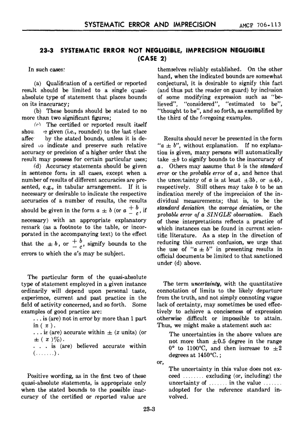
23-3 SYSTEMATIC ERROR NOT NEGLIGIBLE, IMPRECI-
SION NEGLIGIBLE (CASE 2)........................ 23-3
23-4 NEITHER SYSTEMATIC ERROR NOR IMPRECISION
NEGLIGIBLE (CASE 3)................... 23-4
23-5 SYSTEMATIC ERROR NEGLIGIBLE, IMPRECISION
NOT NEGLIGIBLE (CASE 4)................. 23-5
vi
LIST OF ILLUSTRATIONS AND TABLES
AMCP 706-113
LIST OF ILLUSTRATIONS
Fig. No. Title Page
19-1 Theoretical distribution of largest values.................. 19-2
19-2 Annual maxima of atmospheric pressure, Bergen, Norway,
1857-1926............................................... 19-3
20-1 Normalizing effect of some frequently used transformations.. 20-3
20-2 'Variance-stabilizing effect of some frequently used trans-
formations .............................: .............. 20-7
21-1 Reprint of Figure 3-1. ОС curves for the two-sided t-test
(a = .05)......................................................... 21-3
21-2 Reprint of Figure 1-8. Computed confidence intervals for
100 samples of size 4 drawn at random from a normal popula-
tion with m = 50,000 psi, a = 5,000 psi. Case A shows 50%
confidence intervals; Case В shows 90% confidence intervals. . 21-5
LIST OF TABLES
Table No. Title Page
16-1 Work table for Data Sample 16-7........................... 16-13
18-1 Tests for locating and identifying specific types of assignable
causes.......................................................... 18-2
18-2 Factors for computing 3-sigma control limits........... 18-3
20-1 Some frequently used transformations................... 20-5
vii
FOREWORD
INTRODUCTION
This is one of a group of handbooks covering
the engineering information and quantitative
data needed in the design, development, construc-
tion, and test of military equipment which (as a
group) constitute the Army Materiel Command
Engineering Design Handbook.
PURPOSE OF HANDBOOK
The Handbook on Experimental Statistics has
been prepared as an aid to scientists and engi-
neers engaged in Army research and develop-
ment programs, and especially as a guide and
ready reference for military and civilian person-
nel who have responsibility for the planning and
interpretation of experiments and tests relating
to the performance of Army equipment in the
design and developmental stages of production.
SCOPE AND USE OF HANDBOOK
This Handbook is a collection of statistical
procedures and tables. It is presented in five
sections, viz:
AMCP 706-110, Section 1, Basie Concepts
and Analysis of Measurement Data (Chapters
1-6)
AMCP 706-111, Section 2, Analysis of Enu-
inerative and Classificatory Data (Chapters
7-10)
AMCP 706-112, Section 3, Planning and
Analysis of Comparative Experiments (Chapters
11-14)
AMCP 706-113, Section 4, Special Topics
(Chapters 15-23)
AMCP 706-114, Section 5, Tables
Section 1 provides an elementary introduc-
tion to basic statistical concepts and furnishes
full details on standard statistical techniques
for the analysis and interpretation of measure-
ment data. Section 2 provides detailed pro-
cedures for the analysis and interpretation of
enumerative and classificatory data. Section 3
has to do with the planning and analysis of com-
parative experiments. Section 4 is devoted to
consideration and exemplification of a number
of important but as yet non-standard statistical
techniques, and to discussion of various other
special topics. An index for the material in all
four sections is placed at the end of Section 4.
Section 5 contains all the mathematical tables
needed for application of the procedures given
in Sections 1 through 4.
An understanding of a few basic statistical
concepts, as given in Chapter 1, is necesssary;
otherwise each of the first four sections is largely
independent of the others. Each procedure, test,
and technique described is illustrated by means
of a worked example. A list of authoritative
references is included, where appropriate, at the
end of each chapter. Step-by-step instructions
are given for attaining a stated goal, and the
conditions under which a particular procedure is
strictly valid are stated explicitly. An attempt is
made to indicate the extent to which results ob-
tained by a given procedure are valid to a good
approximation when these conditions are not
fully met. Alternative procedures are given for
handling eases where the more standard proce-
dures cannot be trusted to yield reliable results.
The Handbook is intended for the user with
an engineering background who, although he has
an occasional need for statistical techniques, does
not have the time or inclination to become an ex-
pert on statistical theory and methodology.
The Handbook has been written with three
types of users in mind. The first is the person
who has had a course or two in statistics, and
who may even have had some practical experi-
ence in applying statistical methods in the past,
but who does not have statistical ideas and tech-
niques at his fingertips. For him. the Handbook
wilt provide a ready reference source of once
familiar ideas and techniques. The second is the
viii
АМСР 706-113
person who feels, or has been advised, that some
particular problem can be solved by means of
fairly simple statistical techniques, and is in need
of a book that will enable him to obtain the so-
lution to his problem with a minimum of outside
assistance. The Handbook should enable such a
person to become familiar with the statistical
ideas, and reasonably adept at the techniques,
that are most fruitful in his particular line of re-
search and development work. Finally, there is
the individual who, as the head of, or as a mem-
ber of a service group, has responsibility for ana-
lyzing and interpreting experimental and test
data brought in by scientists and engineers en-
gaged in Army research and development work.
This individual needs a ready source of model
work sheets and worked examples corresponding
to the more common applications of statistics, to
„free him from the need of translating textbook
. discussions into step-by-step procedures that can
be followed by individuals having little or no
previous experience with statistical methods.
It is with this last need in mind that some
of the procedures included in the Handbook have
been explained and illustrated in detail twice:
once for the ease where the important question
is whether the performance of a new material,
product, or process exceeds an established stan-
dard; and again for the ease where the important
question is whether its performance is not up to
the specified standards. Small but serious errors
are often made in changing “greater than” pro-
cedures into “less than” procedures.
AUTHORSHIP AND ACKNOWLEDGMENTS
The Handbook on Experimental Statistics
was prepared in the Statistical Engineering Lab-
oratory, National Bureau of Standards, under a
contract with the Department of Army. The
project was under the general guidance of
Churchill Eisenhart, Chief, Statistical Engineer-
ing Laboratory.
Most of the present text is by Mary G. Na-
trella, who had overall responsibility for the com-
pletion of the final version of,the Handbook.
The original plans for coverage, a first draft of
the text, and some original tables were prepared
by Paul N. Somerville. Chapter 6 is by Joseph
M. Cameron; most of Chapter 1 and all of Chap-
ters 20 and 23 are by Churchill Eisenhart; and
Chapter 10 is based on a nearly-final draft by
Mary L. Epling.
Other members of the staff of the Statistical
Engineering Laboratory have aided in various
ways through the years, and the assistance of all
who helped is gratefully acknowledged. Partic-
ular mention should be made of Norman C.
Severo, for assistance with Section 2, and of
Shirley Young Lehman for help in the collection
and computation of examples.
Editorial assistance and art preparation were
provided by John 1. Thompson & Company,
Washington, D. C. Final preparation and ar-
rangement for publication of the Handbook were
performed by the Engineering Handbook Office,
Duke University.
Appreciation is expressed for the generous
cooperation of publishers and authors in grant-
ing permission for the use of their source materi-
al. References for tables and other material,
taken wholly or in part, from published works,
are given on the respective first pages.
Elements of the U. S. Army Materiel Com-
mand having need for handbooks may submit
requisitions or official requests directly to the
Publications and Reproduction Agency, Letter-
keiuiy Army Depot, Chambersburg, Pennsyl-
vania 17201. Contractors should submit such
requisitions or requests to their contracting of-
ficers.
Comments and suggestions on this handbook
are welcome and should be addressed to Army
Research Office-Durham, Box CM, Duke Station,
Durham, North Carolina 27706.
AMCP 706-113
PREFACE
This listing is a guide to the Section and Chapter subject coverage in all Sections of the Hand-
book on Experimental Statistics.
Chapter Title
No.
AMCP 706-110 (SECTION 1) — BASIC STATISTICAL CONCEPTS AND
STANDARD TECHNIQUES FOR ANALYSIS AND INTERPRETATION OF
MEASUREMENT DATA
1 —Some Basie Statistical Concepts and Preliminary Considerations
2 — Characterizing the Measured Performance of a Material, Product, or Process
3 — Comparing Materials or Products with Respect to Average Performance
4 — Comparing Materials or Products with Respect to Variability of Performance
5 — Characterizing Linear Relationships Between Two Variables
6 — Polynomial and Multivariable Relationships, Analysis by the Method of Least Squares
AMCP 706-111 (SECTION 2) —ANALYSIS OF ENUMERATIVE AND
CLASSI Fl CATORY DATA
7 — Characterizing the Qualitative Performance of a Material, Product, or Process
Я — Comparing Materials or Produces with Respect to a Two-Fold Classification of Performance
(Comparing Two Percentages)
9 — Comparing Materials or Products with Respect to Several Categories of Performance (Chi-Square
Tests)
10 — Sensitivity Testing
AMCP 706-112 (SECTION 3) —- THE PLANNING AND ANALYSIS OF
COMPARATIVE EXPERIMENTS
11 — General Considerations in Planning Experiments
12 — Factorial Experiments
13 — Randomized Blocks, Latin Squares, and Other Special-Purpose Designs
14 — Experiments to Determine Optimum Conditions or Levels
AMCP 706-113 (SECTION 4) — SPECIAL TOPICS
15 — Some “Short-Cut” Tests for Small Samples from Normal Populations
16 — Some Tests Which Are Independent of the Form of the Distribution
17 — The Treatment of Outliers
IK — The Place of Control Charts in Experimental Work
1!»—Statistical Techniques for Analyzing Extreme-Valne Data
20 — The Use of Transformations
21 —The Relation Between Confidence' Intervals and Tests of Significance
22 — Notes on Statistical Computations
23 — Expression of the Uncertainties of Final Results
Index
AMCP 706-114 (SECTION 5) —TABLES
Tables Л-1 through Л-37
X
AMCP 706-11,3
SPECIAL TOPICS
DISCUSSION OF TECHNIQUES IN CHAPTERS 15 THROUGH 23
In this Section, a number of important but as yet non-standard
techniques are presented for answering questions similar to those
considered in AMCP 706-110, Section 1. In addition, various spe-
cial topics, such as transformation of data to simplify the statis-
tical analysis, treatment of outlying observations, expression of
uncertainties of final results, use of control charts in experi-
mental work, etc., are discussed in sufficient detail to serve as
an introduction for the reader who wishes to pursue these topics
further in the published literature.
All А-Tables referenced in these Chapters are contained in AMCP
706-114, Section 5.
xi
ANCP 706-113
CHAPTER 15
SOME SHORTCUT TESTS FOR SMALL SAMPLES
FROM NORMAL POPULATIONS
15-1 GENERAL
Shortcut tests are characterized by their nplicity. The calculations are simple, and often may
be done on a slide rule. Further, they are easily learned. An additional advantage in their use
is that their simplicity implies fewer errors, and this may be important where time spent in checking
is costly. i,
The main disadvantage of the shortcut tests as compared to the tests given in AMCP 706-110,
Chapters 3 and 4, is that with the same values of a and n, the shortcut test will, in general, have a
larger , — i.e., it will result in a higher proportion of errors of the second kind. For the tests
given in this chapter, this increase in error will usually be rather small if the sample sizes involved
are each of the order of 10 or less.
Unlike the nonparametric tests of Chapter 16, these tests require the assumption of normality of
the underlying populations. Small departures from normality, hov/ever, will usually have a
negligible effect on the test — i.e., the values of a and /9, in general, will differ from their intended
values by only a slight amount.
No descriptions of the operating characteristics of the tests or of methods of determining sample
size are given in this chapter.
15-2 COMPARING THE AVERAGE OF A NEW PRODUCT WITH THAT
OF A STANDARD
15*2.1 DOES THE AVERAGE OF THE NEW PRODUCT DIFFER FROM THE STANDARD?
Data Sample 15-2.1 — Depth of Penetration
Ten rounds of a new t ype of shell are fired into a target, and the depth of penetration is measured
for each round. The depths of penetration are;
10.0, 9.8, 10.2, 10.5, 11.4, 10.8, 9.8, 12.2, 11.6, 9.9 cms.
The average penetration depth, mn, of the standard comparable shell is 10.0 cm.
15-1
AMCP 706-113
SHORTCUT TESTS
The question to be answered is: Does the new type differ from the standard type with respect
to average penetration depth (either a decrease, or an increase, being of interest)?
Procedure Example
(1) Choose a, the significance level of the test. (1) Let « = .01
(2) Look up in Table A-12 for the appro- priate n. (2) n = 10 ^.996 “ 0.333
(3) Compute X, the mean of the n observa- tions. (3) X = 10.62
(4) Compute w, the difference between the largest and smallest of the n observations. (4) w = 2.4
(5) Compute <p = (X - m0)/w (5) 10.62 - 10.00 v " 2.4 = 0.258
(6) If | > >pi-ai2, conclude that the average performance of the new product differs from that of the standard; otherwise, there is no reason to believe that they differ. (6) Since 0.258 is not larger than 0.333, there is no reason to believe that the new type shell differs from the standard.
15-2.2 DOES AVERAGE OF THE NEW PRODUCT EXCEED THE STANDARD?
In terms of 1. a Sample 15-2.1, let us suppose chat — in advance of looking at the data — the
important question is: Does the average of the new type exceed that of the standard?
Procedure
(1) Choose a, the significance level of the test.
(2) Look up in Table A-12, for the appro-
priate n.
(3) Compute X, the mean of the n observa-
tions.
(4) Compute w, the difference between the
largest and smallest of the n observations.
(5) Compute <p = (Jf — тЦ)/к
(6) If tp > , conclude that the average of
the new product exceeds that of the stand-
ard; otherwise, there is no reason to believe
that the average of the new product
exceeds the standard.
Exomple
(1) Let a = .01
(2) n 10
^.98 — 0.288
(3) X = 10.62
(4) w - 2.4
10.62 - 10.00
(5) <₽ =-----------2Л — -
= 0.258
(6) Since 0.258 is not larger than 0.288, there
is no reason to believe that the average of
the new type exceeds that of the standard.
15-2
COMPARING AVERAGE PERFORMANCE
АИСР 706-113
15-2.3 IS THE AVERAGE OF THE NEW PRODUCT LESS THAN THE STANDARD?
In terms of Data Sample 15-2.1, let us suppose that advance of looking at the data — the
important question is: Is the average of the new type le-,-- //.an that of the standard?
Procedure
Example
(1) Choose a, the significance level of the test. (1) Let a = .01
(2) Look up in Table A-12, for the appro- priate n. (2) n = 10 = 0.288
(3) Compute X, the mean of the n observa- tions. (3) X = >.
(4) Compute w, the difference between the largest and smallest of the n observations. (4) w = 2.4
(5) Compute <p = (m0 - X)/iv (5) ,0.00 - 10.62 ” " 2.4 = - 0.258
(6) If > <pt-a, conclude that the average of
the new product is less than that of the
standard; otherwise, there is no reason to
believe that the average of the new product
is less than that of the standard.
(6) Since - 0.258 is not larger than 0.288,
there is no reason to believe that the
average of the new type is less than that of
the standard.
15-3
AMCP 706-113
SHORTCUT TESTS
15-3 COMPARING THE AVERAGES OF TWO PRODUCTS
15-3.1 20 THE PRODUCTS A AND В DIFFER IN AVERAGE PERFORMANCE?
Data Sample 15-3.1 — Capacity ~>t Batteries
Form: A set of n measurements is available from each of two materials or products. The proce-
dure* given requires that both sets contain the same number of measurements (i.e., пл - n« = n).
Example: There are available two independent sets of measurements of battery capacity.
Set A Set В
138 140
143 141
136 139
141 143
140 138
142 140
142 142
146 139
137 141
135 138
Procedure Example
(1) Choose a, the significance level of the test. (1) Let a = .01
(2) Look up ^i_a/2 in Table A-13, for the appro- (2) n = 10
priate n. -• 0.419
(3) Compute , XH, the means of the two (3) Хл = 140.0
samples. Хн = 140.1
(4) Compute wA , wti, the ranges (or difference (4) = 146 - 135
between the largest and smallest values) = 11
for each sample. wH = 143 - 138
= 5
(5) Compute , 140.0 - 140.1 (5) <P - 8
, XA — Хц = - 0.0125
~ i (w,i + wt)
(6) If <p' | > </i-a/2, conclude that the aver- (6) Since 0.0125 is not larger than 0.419,
ages of the two products differ; otherwise, there is no reason to believe that the
there is no reason to believe that the average of A differs from the average of B.
averages of A and В differ.
* Thia procedure is not appropriate when the observations are "paired”, i.e., when each measurement from A is
associated with a corresponding measurement from В (see Paragraph 3-3.1.4). In the paired observation case, the
question may be answered by the following procedure: compute X,i as shown in Paragraph 3-3.1.4 and follow the
procedure of Paragraph 15-2.1, using X = and т„ » 0 .
15-4
COMPARING AVERAGE PERFORMANCE
АМСГ 706-113
15-3.2 DOES THE AVERAGE OF PRODUCT A EXCEED THE AVERAGE OF PRODUCT B?
In terms of Data Sample 15-3.1, let us suppose that — in advance of looking at the data — the
important question is: Does the average of A exceed the ave <e of B?
Again, as in Paragraph 15-3.1, the procedure is appropriate when two independent sets of
measurements are available, each containing the same number of observations (пл = n# - n),
but is not appropriate when the observations are paired (see Paragraph 3-3.1.4). In the paired
observation case, the question may be answered by the following procedure: compute Xd as shown
in Paragraph 3-3.2.4, and follow the procedure of Paragraph 15-2.2, using X = Xrt and m0 = 0.
Procedure
Example
(1) Choose a, the significance level of the test.
(2) Look up <pi^a in Table A-13, for the appro-
priate n.
(3) Compute , Xu, the means of the two
samples.
(4) Compute it'A , , the ranges (or difference
between the largest and smallest values)
for each sample.
(5) Compute
' — ~ X H
i (w.i + w’y?
(6) If v?' > ip'i_a, conclude that the average of
A exceeds that of B; otherwise, there is no
reason to believe that the average of A
exceeds that of B.
(1) Let a = .05
(2) n = 10
= .250
(3) = 140.0
XH = 140.1
(4) wA = 11
wlt = 5
... , 140.0 - 140.1
(5) v =------------g--------
= - 0.0125
(6) Since - 0.0125 is not larger than 0.250,
there is no reason to believe that the
average of A exceeds the average of B.
15-5
AMCP 706-113
SHORTCUT TESTS
15-4 COMPARING THE AVERAGES OF SEVERAL PRODUCTS
DO THE AVERAGES OF t PRODUCTS DIFFER?
Data Sample 15-4 — Breaking-Strength of Cement Briquette*
The following data relate to breaking-strength of cement briquettes (in pounds per square
inch).
Group
1 2 1 co I Li 4 5
518 508 554 555 536
560 574 598 567 492
538 528 579 550 528
510 534 538 535 572
544 538 544 540 506
2X, 2670 2682 2813 2747 2634
n, 5 5 5 5 5
Xi 534.0 536.4 562.6 549.4 526.8
Excerpted with permission from SlaiiMical Exercises, "Part II, Analysis of Variance and Associated Techniques," by N. L. Johnson, Ccpyri^nf,
1057, Department of Statistics, University College. London.
The question to be answered is: Does the average breaking-strength differ for the different
groups?
Procedure
Example
(1) Choose a , the significance level of the test. (1) Let a = .01
(2) Look up La in Table A-15, corresponding to t and n. n — П1 = n,2 = . . . = n i, the number of observations on each product. (2) f = 5 n = 5 La = 1.02
(3) Compute Wi, ,. .. , wt, the ranges of the n observations from each product. (3) -- 50 Wi — 66 w, = 60 Wi = 32 wb = 80
(4) Compute Xlt X2, .. . , Xt, the means of the observations from each product. (4) X, = 534.0 Xs = 536.4 X3 = 562.6 Xi = 549.4 Xb = 526.8
(5) Comp e w' ~ Wi + w2 + ... + wt. Comp e w", the difference between the la <est and the smallest of the means X, . (5) w’ = 288 w" = 562.6 - 526.8 = 35.8
15-6
AMCP 706-113
COMPARING VARIABILITY OF PERFORMANCE
Procedure (Cont)
(6) Compute L = гм"/w'
(7) If L > La, conclude that the averages of
the t products differ; otherwise, there is no
reason to believe that the averages differ.
Example (Cont)
(6) L = 179/288
= 0.62
(7) Since L is less than La, there is no reason to
believe that the group averages differ.
15-5 COMPARING TWO PRODUCTS WITH RESPECT TO VARIABILITY
OF PERFORMANCE
15-5.1 DOES THE VARIABILITY OF PRODUCT A DIFFER FROM THAT OF PRODUCT B?
The data of Data Sample 15-3.1 are used to illustrate the procedure.
The question to be answered is: Does the variability of A differ from the variability of B?
Procedure
Example
(1) Choose a, the significance level of the test. (1) Let
a = .01
(2) Look up Fa/г (nA , nlt) and
F\-ai2 (nA , nH) in Table A-ll*.
(2) пл = 10
Пи = 10
F'.aab (10, 10) : .37
(10, 10) - 2.7
(3) Compute wA , wh, the ranges (or difference (3)
between the largest and smallest observa-
tions) for A and B, respectively.
Wa = H
Wu = 5
(4) Compute F' - wA/wu
(4) F' = 11/5
= 2.2
(5) If F' < F^/i (пл , nH) or
F' > Fl-a/ztn.t, nu), conclude that the
variability in performance differs; other-
wise, there is no reason to believe that the
variability differs.
(5) Since F' is not less than .37 and is not
greater than 2.7, there is no reason to
believe that the variability differs.
* When using Table A-ll, sample sizes need not be equal, but cannot be larger than 10.
15-7
АМОР 706-113
SHORTCUT TESTS
15-5.2 DOES THE VARIABILITY OF PRODUCT A EXCEED THAT OF PRODUCT B?
In terms of Data Sample 15-3.1, the question to be answered is: Does the variability of A exceed
the variability of B?
Procedure
Example
(1) Choose a, the significance level of the test.
(2) Look up F'i_a (пл , пя) in Table A-ll*.
(3) Compute шл , Wn , the ranges (or difference
between the largest and smallest observa-
tions) for A and B, respectively.
(4) Computed' = Wa/h>h
(5) If F1 > F{_a (пл , пн), conclude that the
variability in performance of A exceeds the
variability in performance of В; otherwise,
there is no reason to believe that the vari-
ability in performance of A exceeds that of
B.
(1) Let a = .01
(2) nA = 10
nH - 10
(10, 10) = 2.4
(3) wA = 11
wH = 5
(4) F' = 11/5
= 2.2
(5) Since F' is not larger than F%9, there is no
reason to believe that the variability of set
A exceeds that of set B.
* When using Table A-ll, sample sizes need not be equal, but cannot be larger than 10.
15-8
АМОР 706-113
CHAPTER 16
SOME TESTS WHICH ARE INDEPENDENT OF THE FORM OF
THE DISTRIBUTION
16-1 GENERAL
This chapter outlines a number of test procedures in which very little is assumed about the
nature of the population distributions. In particular, the population distributions are not assumed
to be “normal”. These tests are often called “nonparametric” tests. The assumptions made
here are that the individual observations are independent* and that all observations on a given
material (product, or process) have the same underlying distribution. The procedures are strictly
correct only if the underlying distribution is continuous, and suitable warnings in this regard are
given in each test procedure.
In this chapter, the same wording is used for the problems as was used in AMCP 706-110,Chapter 3
(e.g., “Does the average differ from a standard?”), because the general import of the questions is the
same. The specific tests employed, however, are fundamentally different.
If the underlying populations are indeed normal, these tests are poorer than the ones given in
Chapter 3, in the sense that /9, the probability of the second kind of error, is always larger for given
a and n. For some other distributions, however, the nonparametric tests actually may have a
smaller error of the second kind. The increase in the second kind of error, when nonparametric
tests are applied to normal data, is surprisingly small and is an indication that these tests should
receive more use.
Operating characteristic curves and methods of obtaining sample sizes are not given for these
tests. Roughly speaking, most of the tests of this chapter require a sample size about 1.1 times that
required by the tests given in Chapter 3 (see Paragraphs 3-2 and 3-3 for appropriate normal sample
size formulas). For the sign test (Paragraphs 16-2.1, 16-3.1, 16-4.1, 16-5.1, and 16-6.1), a factor
of 1.2 is more appropriate.
For the problem of comparing with a standard (Paragraphs 16-2, 16-3, and 16-4), two methods
of solution are given and the choice may be made by the user. The sign test (Paragraphs 16-2.1,
16-3.1, and 16-4.1) is a very simple test which is useful under very general conditions. The Wil-
coxon signed-ranks test (Paragraphs 16-2.2, 16-3.2, and 16-4.2) requires the assumption that the
underlying distribution is symmetrical. When the assumption of symmetry can be made, the
signed-ranks test is a more powerful test than the sign test, and is not very burdensome for fairly
small samples.
For the problem of comparing two products (Paragraphs 16-5 and 16-6), two methods of solution
are also given, but each applies to a specific situation with regard to the source of the data.
The procedures of this chapter assume that the pertinent question has been chosen before taking
the observations.,
* Except for certain techniques which are given for “paired observations”; in that case, the pairs are assumed to be
independent.
16-1
AMCP 706-113
DISTRIBUTION-FREE TESTS
16-2 DOES THE AVERAGE OF A NEW PRODUCT DIFFER
FROM A STANDARD?
Data Sample 16-2 — Reverce-Bla* Collector Current of Ten franeletor*
The data are measurements of Icho for ten transistors of the same type, where Icho is the reverse-
bias collector current recorded in microamperes.
The standard value ?n(1 is 0.28да.
Transistor Icho
1
2
3
4
5
6
7
8
9
10
0.28
.18
.24
.30
.40
.36
.15
.42
.23
.48
16-2.1 DOES THE AVERAGE OF A NEW PRODUCT DIFFER FROM A STANDARD? THE SIGN TEST
Procedure
(1) Choose a, the significance level of the test.
Table A-33 provides for values of a = .25,
.10, .05, and .01 for this two-sided test.
(2) Discard observations which happen to be
equal to m0, and let n be the number of
observations actually used. (If more than
20% of the observations need to be dis-
carded, this procedure should not be used).
(3) For each observation Xi, record the sign of
the difference X, - m0.
Count the number of occurrences of the less
frequent sign. Call this number r.
(4) Look up r (a, n), in Table A-33.
(5) If r is less than, or is equal to, r (a, n), con-
clude that the average of the new product
differs from the standard; otherwise, there
is no reason to believe that the averages
differ.
Example
(1) Let a = .05
(2) In Data Sample 16-2, ma = .28. Discard
the first observation.
n = 9
(3) The less frequent sign is - .
Since there are 4 minus signs,
r = 4
(4) r (.05, 9) = 1
(5) Since r is not less than r (.05,9), there is no
reason to believe that the average current
differs from m0 = ,28pa.
16-2
COMPARING AVERAGE PERFORMANCE
AMCP 706-113
16-2.2 DOES THE AVERAGE OF A NEW PRODUCT DIFFER FROM A STANDARD? THE WILCOXON
SIGNED-RANKS TEST
Procedure
Example
(1) Choose a, the significance level of the test.
Table A-34 provides for values of a = .05,
.02, and .01 for this two-sided test. Dis-
card any observations which happen to be
equal to m0, and let n be the number of
observation's actually used.
(2) Look up T„ (n), in Table A-34.
(3) For each observation X,-, compute
x: = X,- - m0
(1) Let a = .05
In Data Sample 16-2, m(1 = .28. Discard
the first observation.
n = 9
(2) T.o6(9) = 6
(4) Disregarding signs, rank the X' according
to their numerical value, i.e., assign the
rank of 1 to the X; which is numerically
smallest, the rank of 2 to the X; which is
next smallest, etc. In case of ties, assign
the average of the ranks which would have
been assigned had the X’’s differed only
slightly. (If more than 20% of the ob-
servations are involved in ties, this proce-
dure should not be used.)
To the assigned ranks 1, 2, 3, etc., prefix a
+ or a - sign, according to whether the
corresponding X' is positive or negative.
(5) Sum the ranks prefixed by a + sign, and
the ranks prefixed by a - sign. Let T be
the smaller (disregarding sign) of the two
sums.
(3) (4)
X,- — ma Signed rank
- .10 -5
- .04 —2
+ .02 + 1
+ .12 +6
+ .08 +4
- .13 — 7
+ .14 +8
- .05 -3
+ .20 +9
(5) Sum + = 28
Sum - = 17
T = 17
(6) If T < Ta (n), conclude that the average
performance of the new type differs from
that of the standard; otherwise, there is no
reason to believe that the averages differ.
(6) Since T is not less than T.M(9). there is no
reason to believe that the average current
differs from m0 = .28ga.
16-3
AMCP 706-113
DISTRIBUTION-FREE TESTS
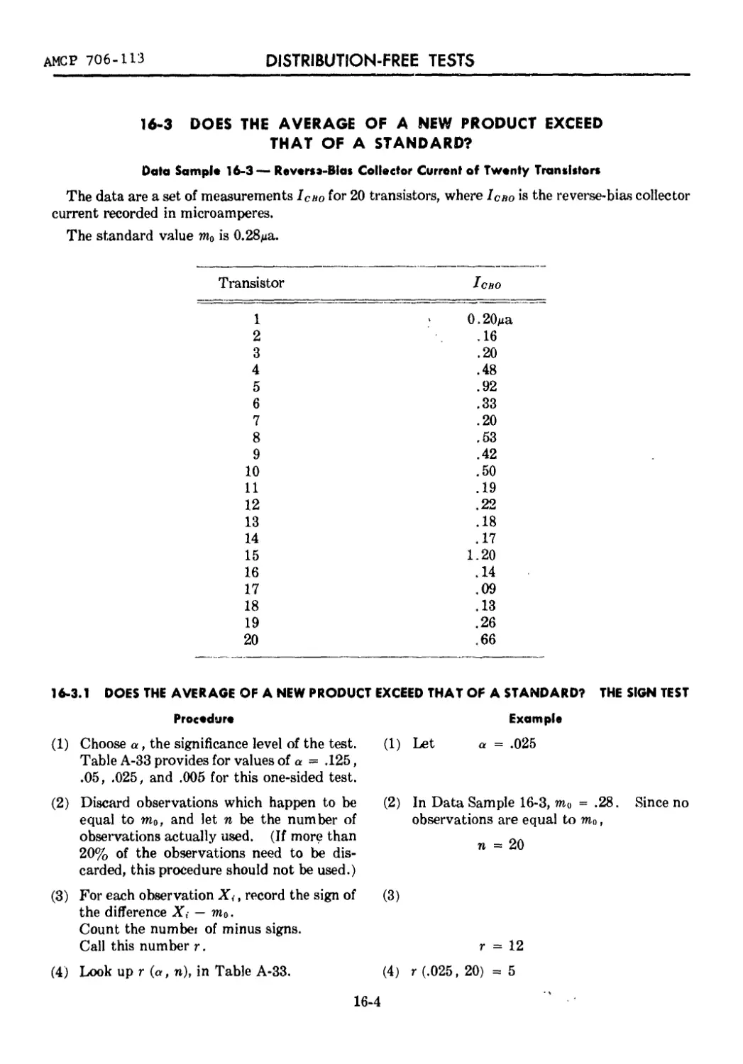
16-3 DOES THE AVERAGE OF A NEW PRODUCT EXCEED
THAT OF A STANDARD?
Data Sample 16-3— Reverce-Biat Collector Current of Twenty Transition
The data are a set of measurements Icno for 20 transistors, where Icbo is the reverse-bias collector
current recorded in microamperes.
The standard value m0 is 0.28да.
Transistor Icbo
1 > 0.20да
2 .16
3 .20
4 .48
5 .92
6 .33
7 .20
8 .53
9 .42
10 .50
11 .19
12 .22
13 .18
14 .17
15 1.20
16 .14
17 .09
18 .13
19 .26
20 .66
16-3.1 DOES THE AVERAGE OF A NEW PRODUCT EXCEED THAT OF A STANDARD? THE SIGN TEST
Procedure Example
(1) Choose a, the significance level of the test.
Table A-33 provides for values of a = .125,
.05, .025, and .005 for this one-sided test.
(2) Discard observations which happen to be
equal to wi0, and let n be the number of
observations actually used. (If more than
20% of the observations need to be dis-
carded, this procedure should not be used.)
(3) For each observation X<, record the sign of
the difference X,- — m0.
Count the numbei of minus signs.
Call this number r.
(4) Look up r (a, n), in Table A-33.
(1) Let a = .025
(2) In Data Sample 16-3, m0 = .28. Since no
observations are equal to ,
n = 20
(3)
r = 12
(4) r (.025, 20) = 5
16-4
AMCP 706-113
COMPARING AVERAGE PERFORMANCE
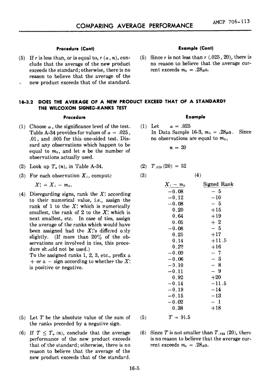
Procedure (Cont)
(5) If r is less than, or is equal to, r (a, n), con-
clude that the average of the new product
exceeds the standard; otherwise, there is no
reason to believe that the average of the
. new product exceeds that of the standard.
Example (Cont)
(5) Since r is not less than r (.025,20), there is
no reason to believe that the average cur-
rent exceeds m0 = .28ga.
16-3.2 DOES THE AVERAGE OF A NEW PRODUCT EXCEED THAT OF A STANDARD?
THE WILCOXON SIGNED-RANKS TEST
Procedure
(1) Choose a, the significance level of the test.
Table A-34 provides for values of a = .025,
.01, and .005 for this one-sided test. Dis-
card any observations which happen to be
equal to m0, and let n be the number of
observations actually used.
(2) Look up Ta (n), in Table A-34.
(3) For each observation X, , compute
X' = X,- - ma.
(4) Disregarding signs, rank the X' according
to their numerical value, i.e., assign the
rank of 1 to the X' which is numerically
smallest, the rank of 2 to the X! which is
next smallest, etc. In case of ties, assign
the average of the ranks which would have
been assigned had the X'’s differed oily
slightly. (If more than 20% of the ob-
servations are involved in ties, this proce-
dure should not be used.)
To the assigned ranks 1, 2, 3, etc., prefix a
4- or a - sign according to whether the X;
is positive or negative.
Example
(1) Let a = .025
In Data Sample 16-3, ma - .28да. Since
no observations are equal to m0,
n = 20
(5) Let T be the absolute value of the sum of
the ranks preceded by a negative sign.
(6) If T < Ta (n), conclude that the average
performance of the new product exceeds
that of the standard; otherwise, there is no
reason to believe that the average of the
new product exceeds that of the standard.
(2) T.o2b (20) — 52
(3) (4)
X,- - mB Signed Rank
-0.08 - 5
-0.12 -10
-0.08 - 5
0.20 + 15
0.64 + 19
0.05 + 2
-0.08 - 5
0.25 + 17
0.14 + 11.5
0.22 + 16
-0.09 - 7
-0.06 — 3
-9.10 - 8
-0.11 - 9
0.92 +20
-0.14 -11.5
-0.19 -14
-0.15 -13
-0.02 - 1
0.38 +18
(5) T = 91.5
(6) Since T is not smaller than T(20), there
is no reason to believe that the average cur-
rent exceeds m„ = ,28pa.
16-5
AMCP 706-113
DISTRIBUTION-FREE TESTS
16-4 IS THE AVERAGE OF A NEW PRODUCT LESS THAN
THAT OF A STANDARD?
Data Sample 16-4 — Tensile Strength of Aluminum Alloy
The data are measurements of ultimate tensile strength (psi) for twenty test specimens of alu-
minum alloy.. The standard value for tensile strength is ma = 27,000 psi.
Specimen Ultimate Tensile Strength (psi)
1 24,200
2 25,900
3 26,000
4 26,000
5 26,300
6 26,450
7 27,250
8 27,450
9 27,550
10 28,550
11 29,150
12 29,900
13 30,000
14 30,400
15 30,450
16 30,450
17 31,450
18 31,600
19 32,400
20 33,750
16-4.1 IS THE AVERAGE OF A NEW PRODUCT LESS THAN THAT OF A STANDARD? THE SIGN TEST
Procedure
(1) Choose a, the significance level of the test.
Table A-33 provides for values of a = .125 ,
.05, .025, and .005 for this one-sided test.
(2) Discard observations which happen to be
equal to m0, and let n be the number of
observations actually used. (If more than
20% of the observations need to be dis-
carded, this procedure should not be used.)
(3) For each observation X,, record the sign
of the difference X, — wic.
Count the number of plus signs. Call this
number r.
(4) Look up r (a, и), in Table A-33.
Exomple
(1) Let a = .025
(2) In Data Sample 16-4, m0 ~ 27,000. Since
no observations are equal to m»,
n = 20
(3)
There are 14 plus signs.
r = 14
(4) r (.025, 20) = 5
16-6
AMCP 706-113
COMPARING AVERAGE PERFORMANCE
Procedure (Cont)
(5) If r is less than, or is equal to, r (a, n), con-
clude that the average of the new product
is less than the standard; otherwise, there
is no reason to believe that the average of
the new product is less than the standard.
Example (Cont)
(5) Since r is not less than r (.025,20), there is
no reason to believe that the average tensile
strength is less than m0 - 27,000 psi.
16-4.2 IS THE AVERAGE OF A NEW PRODUCT I ESS THAN THAT OF A STANDARD?
THE WILCOXON SIGNED-RANKS TEST
Procedure
(1) Choose a, the significance level of the test.
Table A-34 provides for values of a = .025,
.01, and .005 for this one-sided test. Dis-
card any observations which happen to be
equal to mn, and let n be the number of
observations actuallv used.
(2) Look up Ta (n), in Table A-34.
(3) For each observation Xi, compute
X', = Xi — mu.
(4) Disregarding signs, rank the X\ according
to their numerical value, i.e., assign the
rank of 1 to the X- which is numerically
smallest, the rank of 2 to the X- which is
next smallest, etc. In case of ties, assign
the average of the ranks which would have
been assigned had the X-’s differed only
slightly. (If more than 20% of the ob-
servations are involved in ties, this proce-
dure should not be used.)
To the assigned ranks 1, 2, 3, etc., prefix a
+ or a - sign according to whether the
corresponding X', is positive or negative.
(5) Let T be the sum of the ranks preceded by
a + sign.
(6) If T < Ta (n), conclude that the average of
the new product is less than that of the
standard; otherwise, there is no reason to
believe that the average of the new product
is less than that of the standard.
Example
(1) Let a = .025
In Data Sample 16-4,
mo = 27,000.
Since no observations are equal to m0,
n = 20
(2) T,„26 (20) = 52
(3)
X,-
-2800
-1100
-1000
-1000
- 700
- 550
250
450
550
1550
2150
2900
3000
3400
3450
3450
4450
4600
5400
6750
(5) T = 169.5
Signed Rank
-11
- 8
- 6.5
- 6.5
- 5
- 3.5
+ 1
+ 2
+ 3.5
+ 9
+ 10
+ 12
+ 13
+ 14
+15.5
+ 15.5
+ 17
+ 18
+ 19
+20
(6) Since T is not less than T,oii (20), there is
no reason to believe that the average tensile
strength is less than ma = 27,000 psi.
16-7
AMCP 706-113
DISTRIBUTION-FREE TESTS
16-5 DO PRODUCTS A AND В DIFFER IN AVERAGE PERFORMANCE?
Two procedures are given to answer this question. Each of the procedures is applicable to a
different situation, depending upon how the data have been taken.
Situation 1 (for which the sign test of Paragraph 16-5.1 is applicable) is the case where observa-
tions on the two things being compared have been obtained in pairs. Each of the two observations
on a pair has been obtained under similar conditions, but the different pairs need not have been
obtained under similar conditions. Specifically, the sign test procedure tests whether the median
difference between A and В can be considered equal to zero.
Situation 2 (for which we use the Wilcoxon-Mann-Whitney test of Paragraph 16-5.2) is the case
where two independent samples have been drawn — one from population A and one from popula-
tion B. This test answers the following kind of questions — if the two distributions are of the
same form, are they displaced with respect to each other? Or, if the distributions are quite different
in form, do the observations on A systematically tend to exceed the observations on B?
16-5.1 DO PRODUCTS A AND В DIFFER IN AVERAGE PERFORMANCE? THE SIGN TEST FOR PAIRED
OBSERVATIONS
Data Sample 16-5.1 —Reverse-Bias Collector Currents of Two Types of Transistors
Ten pairs of measurements of leno on two types of transistors are available, as follows:
Type A Type В
.19 .21
.22 .27
.18 .15
.17 .18
1.20 .40
.14 .08
.09 .14
.13 .28
.26 .30
.66 .68
16-8
COMPARING AVERAGE PERFORMANCE
AMCP 706-113
Procedure
(1) Choose a, the significance level of the test.
Table A-33 provides for values of a = .25,
.10, .05, and .01 for this two-sided test.
(2) For each pair, record the sign of the differ-
ence X4 — Xu. Discard any difference
which happens to equal zero. Let n be the
number of differences remaining. (If more
than 20% of the observations need to be
discarded, this procedure should not be
used.)
(3) Count the number of occurrences of the less
frequent sign. Call this r.
(4) Look upr(«, n), in Table A-33.
(5) If r is less than, or is equal to, r (a, n), con-
clude that the averages differ; otherwise,
there is no reason to believe that the
averages differ.
Example
(1) Let a = .10
(2) In Data Sample 16-5.1,
n = 10
(3) There are 3 plus signs,
r = 3
(4) r (.10, 10) = 1
(5) Since r is not less than r (.10, 10), there is
no reason to believe that the two types
differ in average current.
Note: The Wilcoxon Signed-Ranks Test also may be used to compare the averages of two
products in the paired-sample situation; follow the procedure of Paragraph 16-2.2, substituting
X'i = XA - Xi, for Х\ - Xj — m0 in step (3) of that procedure.
16-5.2 DO PRODUCTS A AND В DIFFER IN AVERAGE PERFORMANCE? THE WILCOXON-MANN-
WHITNEY TEST FOR TWO INDEPENDENT SAMPLES
Data Sample 16-5.2 — Forward Current Transfer Ratio of Two Type* of Transistor*
The data are measurements of hfc for two independent groups of transistors, where hf. is the
small-signal short-circuit forw; ird current transfer ratio.
Group A
Group В
50.5 (9)* 57.0 (17)
37.5 (1) 52.0 (11)
49.8 (7) 51.0 (10)
56.0 (15.5) 44.2 (3)
42.0 (2) 55.0 (14)
56.0 (15.5) 62.0 (19)
50.0 (8) 59.0 (18)
54.0 (13) 45.2 (5)
48.0 (6) 53.5 (12)
44.4 (4)
* The numbers shown in parentheses are the ranks, from lowest to highest, for all observations combined, as required
in Step (2) of the following Procedure and Example.
16-9
AMCP 706-113
DISTRIBUTION-FREE TESTS
Procedure
(1) Choose a, the significance level of the test.
Table A-35 provides for values of a ~ .01,
.05, .10, and .20 for this two-sided test
when nA , пн < 20.
Example
(1) Let a = .10
(2) Combine the observations from the two
samples, and rank them in order of in-
creasing size from smallest to largest.
Assign the rank of 1 to the lowest, a rank
of 2 to the next lowest, etc. (Use algebraic
size, i.e., the lowest rank is assigned to the
largest negative number, if there are nega-
tive numbers). In case of ties, assign to
each the average of the ranks which would
have been assigned had the tied observa-
tions differed only slightly. (If more than
20% of the observations are involved in
ties, this procedure should not be used.)
(3) Let: 7ii = smaller sample
n2 = larger sample
n - «j + n2
(2) In Data Sample 16-5.2, the ranks of the
nineteen individual observations, from low-
est to highest, are shown in parentheses
beside the respective observations. Note
that the two tied observations (56.0) are
each given the rank 15.5 (instead of ranks
15 and 16), and that the next larger obser-
vation is given the rank 17.
(3) nt = 9
n2 = 10
n = 19
(4) Compute R, the sum of the ranks for the
smaller sample. (If the two samples are
equal in size, use the sum of the ranks for
either sample.)
(4) R = 77
Compute R' = nt (n + 1) — R
R' = 9 (20) - 77
= 103
(5) Look up Ra (тц, n2), in Table A-35.
(6) If either R or R' is smaller than, or is equal
to, Ra (n1( n2), conclude that the averages
of the two products differ; otherwise, there
is no reason to believe that the averages of
the two products differ.
(5) R.,„ (9, 10) = 69
(6) Since neither R nor R1 is smaller than
R.io (9, 10), there is no reason to believe
that the averages of the two groups differ.
16-6 DOES THE AVERAGE OF PRODUCT A EXCEED THAT OF PRODUCT B?
Two procedures are given to answer this question. In order to choose the procedure that is
appropriate to a particular situation, read the discussion in Paragraph 16-5.
16-10
COMPARING AVERAGE PERFORMANCE
AMCP 706-113
16-6.1 DOES THE AVERAGE OF PRODUCT A EXCELD THAT OF PRODUCT B? THE SIGN TEST
FOR PAIRED OBSERVATIONS
In terms of Data Sample 16-5.1, assume that we had asked in advance (not after looking at the
data) whether the average Icho was larger for Type A than for Type B.
Procedure
(1) Choose a, the significance level of the test.
Table A-33 pr ovides for values of a = .125,
.05, .025, and .005 for this one-sided test.
(2) For each pair, record the sign of the differ-
ence Хл — Xu. Discard any difference
which happens to equal zero. Let n be the
number of differences remaining. (If more
than 20% of the observations need to be
discarded, this procedure should not be
used.)
(3) Count the number of minus signs. Call
this number r.
(4) Look up r (a, n), in Table A-33.
(5) If r is less than, or is equal to, r («, n), con-
clude that the average of product A ex-
ceeds the average of product B; otherwise,
there is no reason to believe that e aver-
age of product A exceeds that of product B.
Example
(1) Let a = .025
(2) In Data Sample 16-5.1,
n = 10
(3) There are 7 minus signs.
r = 7
(4) r (.025, 10) = 1
(5) Since r is not less than r (.025, 10), there is
no reason to believe that the average of
Type A exceeds the average of Type B.
Note: The Wilcoxon Signed-Ranks Test also may be used to compare the averages of two
products in the paired-sample situations; follow the procedure of Paragraph 16-3.2, substituting
X' - Хл - Xu for X', = X,- - mu in Step (3) of that Procedure.
16-6.2 DOES THE AVERAGE OF PRODUCT A EXCEED THAT OF PRODUCT B? THE WILCOXON-
MANN-WHITNEY TEST FOR TWO INDEPENDENT SAMPLES
Data Sample 16-6.2 — Output Admittance of Two Types of Transistor*
The data are observations of k„i> for two types of transistors, where = small-signal open-circuit
output admittance.
Type A Type В
.291 (5)* .246 (1)
.390 (10) .252 (2)
.305 (7) .300 (6)
.331 (9) .289 (4)
.316 (8) .258 (3)
* The numbers shown in parentheses are the ranks, from lowest to highest, for all observations combined, as required
in Step (2) of the following Procedure and Example.
16-11
AMCP 706-113
DISTRIBUTION-FREE TESTS
Does the average hob for Type A exceed that for Type B?
Procedure
Example
(1) Choose a, the significance level of the test.
Table A-35 provides for values of
a = .005, .025, .05, and .10 for this one-
sided test, when nA , nB < 20.
(2) Combine the observations from the two
populations, and rank them in order of
increasing size from smallest to largest.
Assign the rank of 1 to the lowest, a rank
of 2 to the next lowest, etc. (Use alge-
braic size, i.e., the lowest rank is assigned
to the largest negative number if there are
negative numbers). In case of ties, assign
to each the average of the ranks which
would have been assigned had the tied
observations differed only slightly. (If
more than 20% of the observations are
involved in ties, this procedure should not
be used.)
(3) Let: = smaller sample
n2 = larger sample
n = nt + n2
(4) Look up Ra (ni, n2), in Table A-35.
(5a) If the two samples are equal in size, or if
nH is the smaller, compute RB the sum of
the ranks for sample B. If RB is less
than, or is equal to, Ra (ги, n2), conclude
that the average for product A exceeds
that for product В; otherwise, there is no
reason to believe that the average for
product A exceeds that for product B.
(5b) If nA is smaller than nB, compute RA the
sum of the ranks for sample A, and com-
pute R'a = nA (n + 1) - Ra .
If R'a is less than, or is equal to, Ra (и,, n2),
conclude that the average for product A
exceeds that for product B; otherwise,
there is no reason to believe that the
two products differ.
(1) Let a = .05
(2) In Data Sample 16-6.2, the ranks of the
ten individual observations, from lowest
to highest, are shown beside the respective
observations.
(3) nt 5
n2 = 5
n = 10
(4) 2?,M(5,5) = 19
(5a) RB = 16
Since RB is less than R,№ (5, 5), conclude
that the average for Type A exceeds that
for Type B,
16-12
COMPARING AVERAGE PERFORMANCE
AMCP 706-113
16-7 COMPARING THE AVERAGES OF SEVERAL PRODUCTS
DO THE AVERAGES OF t PRODUCTS DIFFER?
Data Sample 16-7 — Life Tests of Three Types of Stopwatches
Samples from each of three types of stopwatches were tested. The following data are thousands
of cycles (on-off-restart) survived until some part of the mechanism failed.
Type 1 Type 2 Type 3
1.7 (1)* 13.6 (6) 13.4 (5)
1.9 (2) 19.8 (8) 20.9 (9)
6.1 (3) 25.2 (12) 25.1 (10.5)
12.5 (4) 46.2 (16.5) 29.7 (13)
16.5 (7) 46.2 (16.5) 46.9 (18)
25.1 (10.5) 61.1 (19)
30.5 (14)
42.1 (15)
82.5 (20)
* The numbers shown in parentheses are the ranks, from lowest to highest, for all observations combined, as required
in Step (3) of the following Procedure and Example.
TABLE 16-1. WORK TABLE FOR DATA SAMPLE 16-7
Rank* Type 1 Rank* Type 2 Rank* Type 3
1 6 5
2 8 9
3 12 10.5
4 16.5 13
7 16.5 18
10.5 19
14
15
20
Ri /?, = 76.5 R2 = 78.0 Rt = 55.5
w, 9 6 5
Я.’/п,- 650.25 1014.00 616.05
16-13
AMCP 706-113
DISTRIBUTION-FREE TESTS
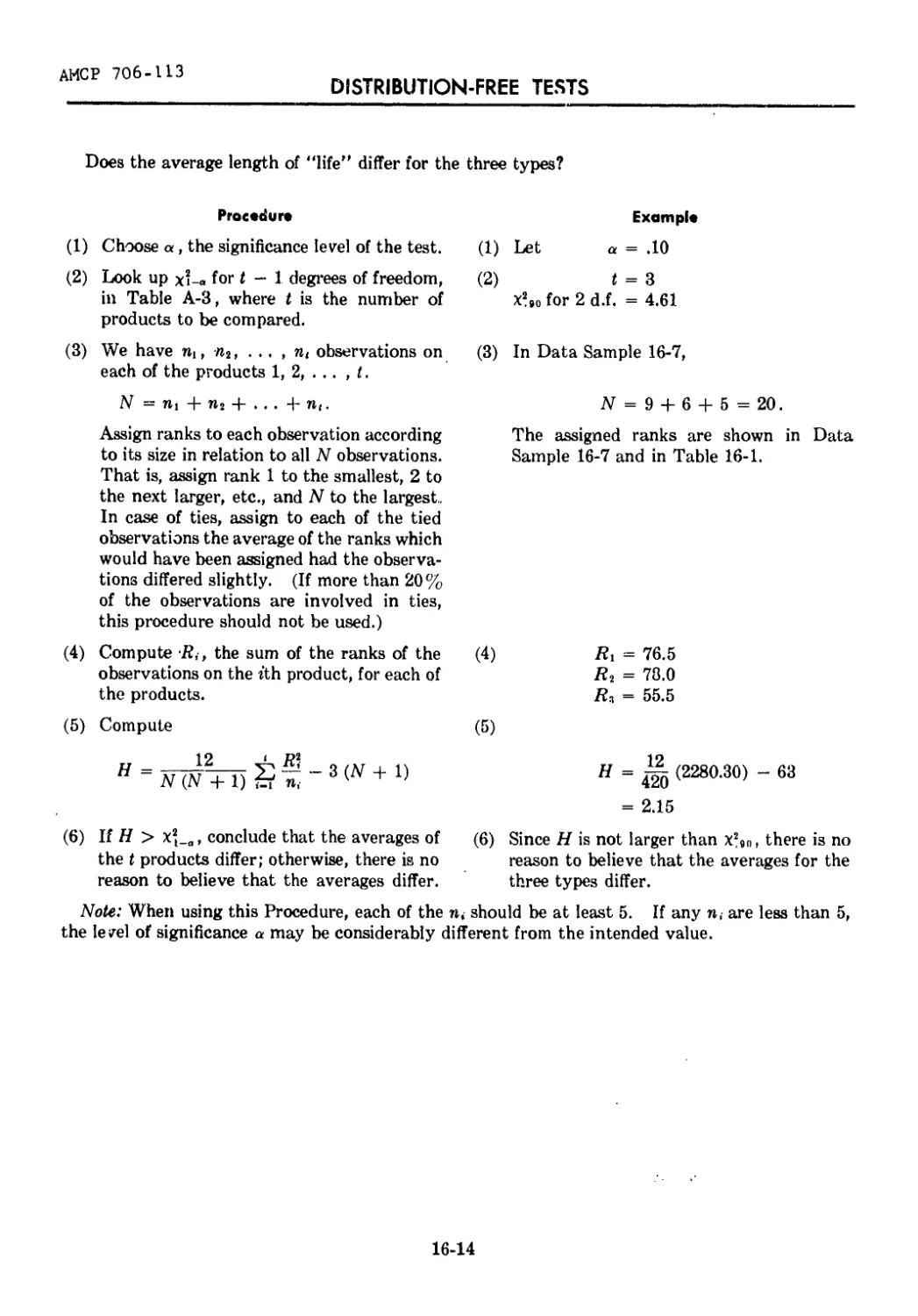
Does the average length of “life” differ for the three types?
Procedure Example
(1) Choose a, the significance level of the test.
(2) Look up xi-a for t — 1 degrees of freedom,
in Table A-3, where t is the number of
products to be compared.
(3) We have nt, , . .. , nt observations on
each of the products 1,2,... , t.
N - П1 + Пг + . . . + nt.
Assign ranks to each observation according
to its size in relation to all N observations.
That is, assign rank 1 to the smallest, 2 to
the next larger, etc., and N to the largest..
In case of ties, assign to each of the tied
observations the average of the ranks which
would have been assigned had the observa-
tions differed slightly. (If more than 20%
of the observations are involved in ties,
this procedure should not be used.)
(4) Compute Я, , the sum of the ranks of the
observations on the (th product, for each of
the products.
(5) Compute
(1) Let a = .10
(2) t = 3
x%0 for 2 d.f. = 4.61
(3) In Data Sample 16-7,
N = 9 + 6 + 5 = 20.
The assigned ranks are shown in Data
Sample 16-7 and in Table 16-1.
(4) Ri = 76.5
R2 = 78.0
R, = 55.5
(6) If H > №(_a, conclude that the averages of
the t products differ; otherwise, there is no
reason to believe that the averages differ.
H = (2280.30) - 63
= 2.15
(6) Since H is not larger than x2en, there is no
reason to believe that the averages for the
three types differ.
Note: When using this Procedure, each of the n, should be at least 5. If any n, are less than 5,
the level of significance a may be considerably different from the intended value.
16-14
AMGO 706-113
CHAPTER 17
THE TREATMENT OF OUTLIERS
17-1 THE PROBLEM OF REJECTING OBSERVATIONS
Every experimenter, at some time, has obtained a set of observations, purportedly taken under
the same conditions, in which one observation was widely different, or an outlier from the rest.
The problem that confronts the experimenter is whether hp should keep the suspect observation
in computation, or whether he should discard it as being a faulty measurement. The word reject
will mean reject in computation, since every observation should be recorded. A careful experi-
menter will want to make a record of his "rejected” observations and, where possible, detect and
carefully analyze their cause (s).
It should be emphasized that we are not discussing the case where we know that the observation
differs because of an assignable cause, i.e., a dirty test-tube, or a change in operating conditions.
We are dealing with the situation where, as far as we are able to ascertain, all the observations are
on approximately the same footing. One observation is suspect however, in that it seems to be
set apart from the others. We wonder whether it is not so far from the others that we can reject
it as being caused by some assignable but thus far unascertained cause.
When a measurement is far-removed from the great majority of a set of measurements of a
quantity, and thus possibly reflects a gross error, the question of whether that measurement should
have a full vote, a diminished vote, or no vote in the final average — and in the determination of
precision — is a very difficult question to answer completely in general terms. If on investigation,
a trustworthy explanation of the discrepancy is found, common sense dictates that the value con-
cerned should be excluded from the final average and from the estimate of precision, since these
presumably are intended to apply to the unadulterated system. If, on the other hand, no explana-
tion for the apparent anomalousness is found, then common sense would seem to indicate that it
should be included in computing the final average and the estimate of precision. Experienced
investigators differ in this matter. Some, e.g., J. W. Bessel, would always include it. Others
would be inclined to exclude it, on the grounds that it is better to exclude a possibly "good” measure-
ment than to include a possibly "bad” one. The argument for exclusion is that when a “good"
measurement is excluded we simply lose some of the relevant information, with consequent decrease
in precision and the introduction of some bias (both being theoretically computable); whereas,
when a truly anomalous measurement is included it vitiates our results, biasing both the final average
and the estimate of precision by unknown, and generally unknowable, amounts.
There have been many criteria proposed for guiding the rejection of observations. For an excel-
lent summary and critical review of the classical rejection procedures, and some more modern
ones, see P. R. Rider'1'. One of the more famous classical rejection rules is "Chauvenet's criterion,"
which is not recommended. This criterion is based on the normal distribution and advises rejection
of an extreme observation if the probability of occurrence of such deviation from the mean of the n
measurements is less than Un. Obviously, for small n, such a criterion rejects too easily.
17-1
AMCP 706-113
TREATMENT OF OUTLIERS
A review of the history of rejection criteria, and the fact that new criteria are still being proposed,
leads us to realize that no completely satisfactory rule can be devised for any and all situations.
We cannot devise a criterion that will not reject a predictable amount from endless arrays of per-
fectly good data; the amount of data rejected of course depends on the rule used. This is the price
we pay for using any rule for rejection of data. No available criteria are superior to the judgment
of an experienced investigator who is thoroughly familiar with his measurement process. For an
excellent discussion of this point, see E. B. Wilson, Jr.<2). Statistical rules are given primarily for
the benefit of inexperienced investigators, those working with a new process, or those who simply
want justification for what they would have done anyway.
Whatever rule is used, it must bear some resemblance to the experimenter’s feelings about the
nature and possible frequency of errors. For an extreme example — if the experimenter feels that
about one outlier in twenty reflects an actual blunder, and he uses a rejection rule that throws out
the two extremes in every sample, then his reported data obviously will be “clean” with respect
to extreme blunders — but the effects of “little" blunders may still be present. The one and only
sure way to avoid publishing any “bad” results is to throw away all results.
With the foregoing reservations, Paragraphs 17-2 and 17-3 give some suggested procedures for
judging outliers. In general, the rules to be applied to a single experiment (see Paragraph 17-3)
reject only what would be rejected by an experienced investigator anyway.
17-2 REJECTION OF OBSERVATIONS IN ROUTINE EXPERIMENTAL WORK
The best tools for detection of errors (e.g., systematic errors, gross errors) in routine work are the
control charts for the mean and range. These charts are described in Chapter 18, which also
contains a table of factors to facilitate their application, Table 18-2.
17-3 REJECTION OF OBSERVATIONS IN A SINGLE EXPERIMENT
We assume that our experimental observations (except for the truly discordant ones) come from
a single normal population with mean m and standard deviation <r. Ina particular experiment,
we have obtained n observations and have arranged them in order from lowest to highest
(Xi < Хг < . . . < X„). We consider procedures applicable to two situations: when observa-
tions which are either too large or too small would be considered faulty and rejectable, see Para-
graph 17-3.1; when we consider rejectable those observations that are extreme in one direction
only (e.g., when we want to reject observations that are too large but never those that are too
small, or vice versa), see Paragraph 17-3.2. The proper choice between the situations must be
made on a priori grounds, and not on the basis of the data to be analyzed.
For each situation, procedures are given for four possible cases with regard to our knowledge of
m and <r.
17-2
PROBLEM OF REJECTING OBSERVATIONS
AMCP 706-113
17-3.1 WHEN EXTREME OBSERVATIONS IN EITHER DIRECTION ARE CONSIDERED REJECTABLE
17-3.1.1 Population Moan and Standard Deviation Unknown — Sample in Hand it the Only Source
of Information.
[The Dixon Criterion]
Procedure
(1) Choose a, the probability or risk we are willing to take of rejecting an observation that really belongs in the group.
(2) If: 3 < n < 7 8 < n < 10 11 < n < 13 14 < n < 25 where r,7 is computed as follows: r,7 If X„ is Suspect Compute Гю Compute r 11 Compute Г21 Compute Г22, If X, is Suspect
Гю {Xn — Xn-t)/(Xn — xj (X, - Xi)/(Xn - X,)
т 11 (X„ — X„_,)/(X„ — X,) ex, - хж-> - x,)
Г21 (X n — Хп—г)/{Хп X2) (X3 - X1)/(X„_I - X,)
Г22 (Xn — — X3) (X3 - X1)/(Xn_2 - X,)
(3) Look up r^a/2 for the r,7 from Step (2), in Table A-14.
(4) If r,7 > ri-o/s, reject the suspect observation; otherwise, retain it.
17-3.1.2 Population Mean and Standard Deviation Unknown — Independent External Estimate of
Standard Deviation Is Available.
[The Studentized Range]
Procedure
(1) Choose a, the probability or risk we are willing to take of rejecting an observation that really
belongs in the group.
(2) Look up g,_„ (n, v) in Table A-10. n is the number of observations in the sample, and v is
the number of degrees of freedom for e, the independent external estimate of the standard
deviation obtained from concurrent or past data — not from the sample in hand.
(3) Compute w = qi-as.
(4) If X„ - X, > w, reject the observation that is suspect; otherwise, retain it.
17-3.1.3 Population Mean Unknown — Value for Standard Deviation Assumed.
Procedure
(1) Choose a, the probability or risk we are willing to take of rejecting an observation that really
belongs in the group.
(2) Look up qi_„ (n, «) in Table A-10.
(3) Compute w = qX-a a.
(4) If X„ - Xt > w, reject the observation that is suspect; otherwise, retain it.
17-3
AMCP 706-113
TREATMENT OF OUTLIERS
17-3.1.4 Population Mean and Standard Deviation Known.
Procedure Example
(1) Choose «, the probability or risk we are willing to take of rejecting an observation when all n really belong in the same group. (1) Let a = .10, for example.
(2) Compute a = 1 — (1 - a)l/n (We can compute this value using loga- rithms, or by reference to a table of frac- tional powers.) (2) If n = 20, for example, a! = 1 - (1 - .10)1/20 = 1 - (.90)1/20 = 1 - .9947 = .0053
(3) Look up 21-,,'/! in Table A-2. (Interpolation in Table A-2 may be re- quired. The recommended method is graphical interpolation, using probability paper.) (3) 1 - tt'/2 = 1 - (.0053/2) = .9974 2.997J = 2.80 /
(4) Compute: G/ — Tit — CrZi—a'/2 Ь = Ш -|- <721— a'/2 (4) \ a = m - 2.80 a b - m + 2.80 a
(5) Reject any observation that does not lie in the interval from a to b. (5) Reject any observation that does not lie in the interval from m — 2.80 <r to m + 2.80 <r.
17-3.2 WHEN EXTREME OBSERVATIONS IN ONLY ONE DIRECTION ARE CONSIDERED REJECT ABLE
17-3.2.1 Population Mean and Standard Deviation Unknown — Sample in Hand it the Only Source
of information.
[The Dixon Criterion]
Procedure
(1) Choose a, the probability or risk we are willing to take belongs in the group. of rejecting an observation that really \
(2) If: 3 < n < 7 8 < n < 10 11 < n < 13 14 < n < 25 Compute Гц, Compute Гц Compute rti Compute r22,
where r„ is computed as follows:
If Only Large Values Гц are Suspect If Only Small Values are Suspect
Гк> (X„ — Хп-|)/(Х„ — Xi) гн (X„ — X ,,-i)/(X„ — Xi) Tn (X„ — X„^)/(Xn — X2) Ta (X„ — X „-i) /(Xn — X2) (X2 - Xi)/(X„ - Xi) (X2 — X!)/(X,,_l — Xi) (X, - XO/fXn-, - X,) (X;, - Xl)/(Xn-2 - Xi)
(3) Look up Г1-„ for the r,, from Step (2), in Table A-14.
(4) If r„ > Г1_„, reject the suspect observation; otherwise, retain it.
17-4
PROBLEM OF REJECTING OBSERVATIONS
AMCP 706-113
17-3.2.2 Population Mean and Standard Deviation Unknown — Independent External Estimate of
Standard Deviation i* Available.
[Extreme Studentized Deviate From Sample Mean; The Nair Criterion]
Procedure
(1) Choose a, the probability or risk we are willing to take of rejecting an observation that really
belongs in the group.
(2) Look up ta (n, v) in Table A-16. n is the number of observations in the sample, and v is the
number of degrees of freedom for s, the independent external estimate of the standard deviation
obtained from concurrent or past data — not from the sample in hand.
(3) If only observations that are too large are considered rejectable, compute
t„ = (Xn - X)/s,.
Or, if only observations that are too small are considered rejectable, compute
f. = (X - X,)/s„
(4) If tn (or ti, as appropriate) is larger than ta (n, r), reject the observation that is suspect;
otherwise, retain it.
17-3.2.3 Population Mean Unknown — Value for Standard Deviation Assumed.
[Extreme Standardized Deviate From Sample Mean]
Procedure
(1) Choose a, the probability or risk we are willing to take of rejecting an observation that really
belongs in the group.
(2) Look up L (n, oc) in Table A-16.
(3) If observations that are too large are considered rejectable, compute
t„ = (xn — X)/o.
Or, if observations that are too small are considered rejectable, compute
ti = (X — x о / <r.
(4) If t„ (or ii, as appropriate) is larger than ta (n, x), reject the observation that is suspect;
otherwise, retain it.
17-5
AMCP 706-113
TREATMENT OF OUTLIERS
17-3.2.4 Population Mean and Standard Deviation Known.
Procedure
(1) Choose a, the probability or risk we are
willing to take of rejecting an observation
when all n really belong in the same group.
(2) Compute a /2 = 1 — (1 - a)!/n.
(We can compute this value using loga-
rithms, or by reference to a table of frac-
tional powers.)
(3) Look up Zi-.a'i2 in Table A-2.
(Interpolation in Table A-2 may be re-
quired. The recommended method is
graphical interpolation using probability
paper.)
(4) Compute:
fl =~ 7W " (TiS'i_a'/2
b = rn + aZi-а'/г
(5) Reject any observation that does not lie in
the interval from a to b.
Example
(1) Let a = .10,
for example.
(2) If n = 20,
for example,
a'/2 = 1 - (1 - .10)1/20
= 1 - (.90)1/20
= 1 - .9947
= .0053
(3) 1 - a'/2 = 1 - .0053
= .9947
z. 99-17 = 2.55
(4)
a = m — 2.55 o-
b = m + 2.55 <r
(5) Reject any observation that does not lie in
the interval from
m — 2.55 a to
m + 2.55 <r.
REFERENCES
1. P. R. Rider, “Criteria for Rejection of Observations,” Washington Uni-
versity Studies -- Neu> Series, Science and Technology, No. 8, October 1933.
2. E. B. Wilson, Jr., An Introduction to Scientific Research, pp. 256-258,
McGraw-Hill Book Co., Inc., New York, N. Y., 1952.
ADDITIONAL READING
W. J. Dixon, “Processing Data for Outliers,” Biometrics, Vol. 9, No. 1, pp. 74-89,
March 1953.
F. E. Grubbs, “Sample Criteria for Testing Outlying Observations,” Annals
of Mathematical Statistics, Vol. 21, No. 1, pp. 27-58, March 1950.
A. Hald, Statistical Theory with Engineering Applications, pp, 333-336, John
Wiley & Sons, Inc., New York, N. Y., 1952.
F. Proschan, "Testing Suspected Observations,” Industrial Quality Control,
Vol. XIII, No. 7, pp. 14-19, January 1957.
17-6
AMCP 706-113
CHAPTER 18
THE PLACE OF CONTROL CHARTS IN EXPERIMENTAL WORK
18-1 PRIMARY OBJECTIVE OF CONTROL CHARTS
Control charts have very important functions
in experimental work, although their use in
laboratory situations has been discussed only
briefly by most textbooks. Control charts can
be used as a form of statistical test in which the
primary objective is to test whether or not the
process is in statistical control. The process is in
statistical control when repeated samples from
the process behave as random samples from a
stable probability distribution; thus, the under-
lying conditions of a process in control are such
that it is possible to make predictions in the
probability sense.
The control limits are usually computed by
using formulas which utilize the information
from the samples themselves. The computed
limits are placed as lines on the specific chart,
and the decision is made that the process was in
control if all points fall within the control limits.
If all points are not within the limits, then the
decision is made that the process is not in control.
The basic assumption underlying most sta-
tistical techniques is that the data are a random
sample from a stable probability distribution,
which is another way of saying that the process
is in statistical control. It is the validity of this
basic assumption which the control chart is
designed to test. The control chart is used to
demonstrate the existence of statistical control,
and to monitor a controlled process. As a
monitor, a given control chart indicates a par-
ticular’type of departure from control.
18-2 INFORMATION PROVIDED BY CONTROL CHARTS
Control charts provide a running graphical
record of small subgroups of data taken from a
repetitive process. Control charts may be kept
on any of various characteristics of each small
subgroup — e.g., on the average, standard de-
viation, range, or proportion defective. The
chart for each particular characteristic is de-
signed to detect certain specified departures in
the process from the assumed conditions. The
process may be a measurement .process as well
as a production process. The order of groups is
usually with respect to time, but not necessarily
so. The grouping is such that the members of
the same group are more likely to be alike than
are members nf different groups.
Primarily, control charts can be used to
demonstrate whether or not the process is in
statistical control. When the charts show lack
of control, they indicate where or when the
trouble occurred. Often they indicate the na-
ture of the trouble, e.g., trends or runs, sudden
shifts in the mean, increased variability, etc.
In addition to serving as a method of testing
for control, control charts also provide addi-
tional and useful information in the form of
estimates of the characteristics of a controlled
process. This information is altogether too-
frequently overlook, .1. For example, one very
important piece of information which can be
obtained from a control chart for the range or
standard deviation is an estimate of the varia-
bility a of a routine measurement or production
process. It should be remembered that many
of the techniques of Section 1, Chapter 3, are
given in parallel for known a and unknown a.
Most experimental scientists have very good
18-1
AMCP 706-113
CONTROL CHARTS
knowledge of the variability of their measure-
ments, but hesitate to assume known a without
additional justification. Control charts can be
used to provide the justification.
Finally, as was pointed out in Chapter 17,
Paragraph 17-2, a control chart is the most
satisfactory criterion for rejection of observa-
tions in a routine laboratory operation. An ex-
cellent discussion of the use of control charts to
detect particular kinds of trouble is given by
OlmsteadThe three most important types
of control charts in this connection are the
charts for the average X, range R, and stand-
ard deviation <r. The order of usefulness of
each tyj of. chart in particular situations is
shown in fable 18-1, where a “1” meat "ost
useful, “2” is the next best, and dots lote
“not appropriate”.
As can be seen from Table 18-1, the X and R
charts are the most useful of the three types.
The R chart is preferred to the <r chart because
of its simplicity and versatility; and, unless
there are compelling reasons to use the <r chart,
the R chart is the method of choice.
TABLE 18-1. TESTS FOR LOCATING AND
IDENTIFYING SPECIFIC TYPES OF
ASSIGNABLE CAUSES
Type of Assignable Cause Control Charts*
X R cr
Gross Error (Blunder) 1 2
Shift in Average 1
Shift in Variability 1 2
Slow Fluctuation (Trend) 1
Fast Fluctuation (Cycle) 1 2
Combination:
(a) Production 1 2
(b) Research
’ wariation 1
* The numeral 1 denotes the most useful type of chart;
2 denotes the next best; and, . . denote charts which are
not appropriate for the particular cause.
Adapted with permission from /na^ Arial Quality Control, Vol. IX,
No. 3, (November, 1962) and No. 4, (January, 1953) from article
entitled “How to Detect the Type of an Assignable Cause” by P. S.
Olmstead.
18-3 APPLICATIONS OF CONTROL CHARTS
Table 18-2 is a summary table of factors for
control charts for Jf, R, and <r, when equal size
samples are involved. Note carefully the foot-
note to Table 18-2, beginning “When using
s = ... ”, because s is so defined
v n — 1
in this Handbook. The last column of Table
18-2 gives values of for convenience in
V n
using the Table factors with values of s.
The most explicit details of application to a
variety of possible situations, e.g., to samples of
unequal size, are given in the ASTM Manual<2);
in using that Manud, however, the reader again
must be wary of thi difference between the defi-
nition of <r given therein, and the definition of s
given in this Handbook.
Actual examples of laboratory applications in
the chemical field can be found in a series of
comprehensive bibliographies published in Ana-
lytical Chemistry<3 4 6 6). These four articles
are excellent reviews that successively bring
up-to-date the recent developments in statis-
tical theory and statistical applications that
are of interest in chemistry. Further, these
bibliographies are divided by subject matter,
and thus provide means for locating articles on
control charts in the laboratory. They are not
limited to control chart applications, however.
Industrial Quality Control0', the monthly
journal of the American Society for Quality
Control, is the most comprehensive publication
in this field.
For a special technique with ordnance exam-
ples, see Grubbs<sl.
18-2
APPLICATION OF CHARTS
AMCP 706-113
ТАШ IM. FACTORS FOR COMFUTNO 3-SMM A CONTROL LIMITS
1 I Chart far Avarage* Chart far Standatd Davtaftoat Chart tef Rangaa
Number af
Ob*ntv*4ten* fatten tef fatten te< Fatten tef Facten tef Fatten tef In — 1
ta Snmgta, a Cnnfcni UmWt Central Una CaaWal Umftt CaMral Una Central limit* \ Й
A A. A. Cl l/«. Bi I. 9< A >/A A 01 D. Oi Di
2 2.121 3.760 1.880 0.5642 1.7725 0 1.843 0 3.267 1.128 0.8865 0.853 0 3.686 0 3.267 .70711
3 1.732 2.394 1.023 0.7236 1.3820 о 1.858 о 2.568 1.693 0.5907 0.888 о 4.858 о 2.575 .81650
4 1.500 1.880 0.729 0.7979 1.2533 0 1.808 0 2.266 2.059 0.4857 0.880 0 4.698 0 2.282 .86603
& 1.342 1.596 0.577 0.8407 1.1894 о 1.756 о 2.089 2.326 0.4299 0.864 о 4.918 о 2.115 .89443
6 1.225 1.410 0.483 0.8686 1.1512 0.026 1.711 0.030 1.970 2.534 0.3946 0.848 0 5.078 0 2,004 ,91287 .92582
7 1.134 1.277 0.419 0.8882 1.1259 0.105 1.672 0.118 1.882 2.704 0.3698 0.833 0.205 5.203 0.076 1.924
8 i.oei 1.175 0.373 0.9027 1.1078 0.167 1.638 0.185 1.815 2.847 6.3512 0.820 0.387 5.307 0.136 1.864 .93541
9 1.000 1.094 0.337 0.9139 i.0942 0.219 1.609 0.239 1.761 2.970 0.3367 0.808 0.546 5.394 0.184 1.816 .94281
10. . 0.949 1.028 0.303 0.9227 1.0837 0.262 1.584 0.284 1.716 3.078 0.3249 0.797 0.687 5.469 0.223 1.777 .94868
11 0.905 0.973 0.285 0.9300 1.0753 0.299 1.561 0.321 1.679 3.178 0.3152 0.737 0.812 5.534 0.256 1.744 .95346
12 0.866 0.925 0.266 0.9359 1.0684 0.381 1.541 0.354 1.646 3.258 0.3069 0.778 0.924 5.592 0.284 1.716 .95743
13.. . 0.832 0.884 0.848 0.249 0.235 0.9410 0.9453 1.0627 1.0571- 0.859 1.523 1.507 0.382 0.406 1.618 3.336 0.2998 0.770 1.026 5.646 0.308 1.692 1.671 .96077 .96362
14 0.802 '384 1.594 3.40"/ 0.2935 0.762 1.121 5.693 0.329
15 0.775 0.816 0.223 0.9490 06 1.492 0.428 1.572 3.472 0.2880 0.755 1.207 5.737 0.848 1.652 OAAAQ . MrvUV
16 0.750 0.728 0.707 0.788 0.762 0.788 0.212 0 9523 0 1.478 0.448 0.466 0.482 0.497 0.510 1.552 1.534 1.518 1.503 1.490 8.532 3.588 3.640 0.2831 0.749 1.285 5.779 0.364 1.636 1.621 .96825 .97014 .97183 .97833 .97468
17 0.203 0.194 0.9551 0.9576 0.9599 1.0470 1.0442 1.0418 1.0396 0 445 1.465 0.2787 0.743 1.359 5.817 5.854 0.379
18 0.46. 0.477 0.491 1.454 1.443 0.2747 0.788 1.426 0.392 1.608
19 0.688 0.717 0.697 0.187 3.689 3.735 0.2711 0.733 1.490 5.888 0 404 1.596 1.586
20 0.671 0.180 0.9619 1.433 0.2677 0.729 1.548 5.922 0.414
21 0.655 0.640 0.679 0.662 0.647 0.178 0.9638 1.0376 0.504 0.516 0.527 1.424 0.523 0.534 0.545 1.477 3.778 0.2647 0.724 1.606 5.950 0.425 1.575 .97590
22 0.167 0.9655 0.9670 1.0358 1.0342 1.415 1.466 1.455 3.819 3.858 0.2618 0.2592 0.720 0.716 1.659 1.710 5.979 6.006 0.434 0.443 1.566 .97701 .97802
23 0.626 0.162 1.407 1.557
24 0.612 0.632 0.619 0 157 0.9684 0.9696 1.0327 1.0313 0.538 0.548 1.399 1.392 0.555 0.565 1.445 1.435 3.895 3.931 0.2567 0.112 0.709 1.759 1.804 6.031 0.462 1.548 .97895 .97980
25 0.600 0.153 0.2544 6.058 0.459 1.541
AtepcW pinnMa* from АЯТЫ Меем/ n QieB/p Ceorief е/ Meteriob, р. lit, copyright. IHi, AnwteM Мну for Тшй« MeuriAta.
FORMULAS*
Purpose of Chari For analyzing past data for control (J?, s, R are average values for the data being analyzed) 3-Sigma Chart for Central Line Control Limitf ( Averages J? J? ± Arf, or J ft. ± A2R | Standard deviations a B2a and BtS [ Ranges R DJi and DJi
For controlling performance to standard Averages J?' X' ± Aa' , ОГ
values (Jf', <r', Rn' are selected stand- ft' rfc A2Rn'
ard values; R,,' = d2a’ for samples of Standard deviations C2a' Bia' and B2a'
size n) Ranges d2a', ОГ Dia' and D2a',
R„' D3R„' and DiR
• When using s = A—JL)2 for the standard "deviation of a sample instead of a =
V n — 1
make the following changes in the formulas for the central line and for the 3-sigma limits:
(1) Replace Ai by A, ; replace s by 3 ; make no change in B3 and ;
(2) Replace с,, B,, B2 by . C1t n в, and B,, respectively.
, one must
This material is reproduced from the American Standard Control Chart M ft hod of Controlling Quality During Production, Z1.8—1958, copyrixht
1959 by ASA, copiee of which may be purchased from the American Standards Association at 10 East 40th Street, New York 16, N. Y.
18-3
AMCP 706-113
CONTROL CHARTS
REFERENCES
1. P. S. Olmstead, "How to Detect the Type of
an Assignable Cause,” Parts I and II,
Industrial Quality Control, Vol. IX, Nos. 3,
pp. 32-38 (November 1952) and 4, pp. 22-
32 (January 1953).
2. ASTM Manual on Quality Control of Ma-
terials, American Society for Testing Ma-
terials, 1916 Race St., Philadelphia 3, Pa.,
1951.
3. G. Wernimont, "Statistics Applied to Anal-
ysis”, Analytical Chemistry, Vol. 21, p.
115, 1949.
4. R. J. Hader and W. J. Youden, “Experi-
mental Statistics”, Analytical Chemistry,
Vol. 24, p. 120, 1952.
5. J. Mandel and F. J. Linnig, "Statistical
Methods in Chemistry”, Analytical Chem-
istry, Vol. 28, p. 770, 1956.
6. Ibid., Vol. 30, p. 739, 1958.
7. Industrial Quality Control, Monthly Journal,
The American Society for Quality Con-
trol, 161 W. Wisconsin Ave., Milwaukee
3, Wis.
8. F. E. Grubbs, “The Difference Control
Chart with Example of Its Use”, Indus-
trial Quality Control, Vol. Ill, No. 1,
pp. 22-25, July 1946.
SOME RECOMMENDED GENERAL TEXTS
American Standard Z 1.3-1958, Control Chart
Method of Controlling Quality During Pro-
duction, available from American Standards
Association, Inc., 10 East Fortieth St.,
New York 16, N. Y.
D. J. Cowden, Statistical Methods in Quality
Control, Prentice-Hall, Inc., Englewood Cliffs,
N. J., 1957.
A. J. Duncan, Quality Control and Industrial
Statistics, Richard D. Irwin, Inc., Chicago,
Ill., 1952.
E. L. Grant, Statistical Quality Control, (2d edi-
tion), McGraw-Hill Book Co., New York,
N. Y., 1952.
W. A. Shewhart, Economic Control of Quality of
Manufactured Product, Van Nostrand Inc.,
New York, N. Y., 1931. (The first and still a
very significant book in the field).
18-4
AMCP 706-113
CHAPTER 19
STATISTICAL TECHNIQUES FOR ANALYZING EXTREME-VALUE DATA*
19-1 EXTREME-VALUE DISTRIBUTIONS
Classical applications of statistical methods,
which frequently concern average values and
other quantities following the symmetrical nor-
mal distribution, are inadequate when the quan-
tity of interest is the largest or the smallest in a
set of magnitudes. Applications of the tech-
niques described in this Chapter already have
been made in a number of fields. Meteorologi-
cal phenomena that involve extreme pressures,
temperatures, rainfalls, wind velocities, etc.,
have been treated by extreme-value techniques.
The techniques are also applicable in the study
of floods and droughts.
Other examples of extreme-value problems
occur in the fracturing of metals, textiles, and
other materials under applied force, and in
fatigue phenomena. In these instances, the
observed strength of a specimen often differs
from the calculated strength, and depends,
among other things, upon the length and vol-
ume. An explanation is to be found in the
existence of weakening flaws assumed to be dis-
tributed at random in the body and assumed
not to influence one another in any way. The
observed strength is determined by the strength
of the weakest region — just as no chain is
stronger than its weakest link. Thus, it is
apparent that whenever extreme observations
are encountered it will pay to consider the use of
extreme-value techniques.
19-2 USE OF EXTREME-VALUE TECHNIQUES
19-2.1 LARGEST VALUES
A simplified account is given here. Primary
sources for the detailed theory and methods are
References 1, 2, 3, which also contain extensive
bibliographies. References 4 through 10, also
given at the end of this Chapter, provide addi-
tional information and examples of applications.
Figure 19-1 illustrates the frequency form of a
typical curve for the distribution of largest
observations.
The curve in Figure 19-1 is tl derivative of the
function
Ф(у) = exp [-exp ( )].
Unlike the normal distribution, this curve is
skewed, with its maximum to the left of the
mean and the longer of its tails extending to the
right. The outstanding feature of such a dis-
tribution is that very large values are much
more likely to occur than are very small values.
This agrees with common experience. Very
low maximum values are most unusual, while
very high ones do occur occasionally. Theo-
retical considerations lead to a curve of this
nature, called the distribution of largest values or
the extreme-value distribution.
In using the extreme-value method, all the
observed maxima, such as the largest wind
velocity observed in each year during a fifty-
* Adapted with permiaalon from The American Statistician, Vol. 8, No. 5, December 1954. from article entitled “Some Applications of Extreme-
Value Methods" by E, J. Gumbel and J. Lieblein; and, from National Bureau of Standards Technical Nsm-b Bulletin 38, No, 2, pp. 29-81, February
1954, from article entitled "Extreme-Value Methods for Engineering Problems".
19-1
AMCP 706-113
ANALYZING EXTREME-VALUE DATA
Figure 19-1. Theoretical distribution of largest values.
Adapted with permission from The American Statistician, Vol. A, No. 5. December 1954, from article entitled “Some Applications of Extreme-
Value Methbda’’ by E. J. Gumbel and J. Lieblein.
year period, are first ranked in order of size from
the smallest to the largest,
X. < Xt < . .. < X,- < . .. < X,..
A plotting position (X,-, P,) is obtained for each
observation by associating with X, the proba-
bility coordinate P, = i/(n + 1), where i is the
rank of the observation, counting from the
smallest. The data are plotted on a special
graph paper, called extreme-value probability
paper*, designed so that the "ideal” extreme-
value distribution will plot exactly as a straight
line. Consequently, the closeness of the plotted
points to a straight line is an indication of how
well the data fit the theory.
* Extreme-value probability paper may be obtained
from three sources: (a) U. S. Department of Commerce,
Weather Bureau; (bl Environmental Protection Section,
Research and Development Branch, Military Planning
Division, Office of the Quartermaster General ;(e) Techni-
cal and Engineering Aids for Management, 104 Belrose
Ave., Lowell, Mass.
Extreme-value probability paper has a uni-
form scale along one axis, usually the vertical,
which is used for the observed values as shown
in Figure 19-2. The horizontal axis then serves
as the probability scale, and is marked accord-
ing to the doubly-exponential formula. Thus,
in Figure 19-2, the space between 0.01 and 0.5 is
much less than the space between 0.5 and 0.99.
The limiting values zero and one are. never
reached, as is true of any probability paper de-
signed for an unlimited variate.
An extreme-value plot (Figure 19-2) of the
maximum atmospheric pressures in Bergen,
Norway, for the period between 1857 and 1926,
showed by inspection that the observed data
satisfactorily fitted the theory. Fitting the line
by eye may be sufficient. Details of fitting a
computed line are given in Gumbel.From
the fitted straight line, it is possible to predict,
for example, that a pressure of 793 mm corre-
sponds to a probability of 0.994; that is, pres-
19-2
USE OF TECHNIQUES
AMCP 706-113
RETURN PERIOD
Figure 19-2. Annual maxima of atmospheric pressure, Bergen, Norway, 1857-1926.
Adapted with per.nlMlon from The American Statistician, Vol, 8, No. 6, December 1954, from article enlithu r Applications of Extreme*
Value Methods" by E. J. Gumbel and J. Lieblein.
sures of this magnitude have less than one
chance in 100 of being exceeded in any par-
ticular year.
In studies of the normal acceleration incre-
ments experienced by an airplane flying through
gusty air, see Gumbel and Carlson/4' page 394,
an instrument was employed that indicated only
the maximum shocks. Thus, only one maxi-
mum value was obtained from a single flight.
A plot representing 26 flights of the same air-
craft indicated that the probability that the
largest recorded gust will not be exceeded in any
other flight was 0.96; i.e., a chance of four in 100
of encountering a gust more severe than any
recorded. A more recent study, Lieblein/61
presents refinements especially adapted to very
small samples of extreme data, and also to
larger samples where it is necessary to obtain
the greatest amount of information from a
limited set of costly data.
19-2.2 SMALLEST VALUES
Extreme-value theory can also be used to
study the smallest observations, since the corre-
sponding limiting distribution is simply related
to the distribution of largest values. The steps
in applying the "smallest-value” theory are
very similar to those for the largest-value case.
For example, engineers have long been inter-
ested in the problem of predicting the tensile
strength of a bar or specimen of homogeneous
material. One approach is to regard the s»
men as being composed of a large numbei ..i
pieces of very short length. The tensile strength
of the entire specimen is limited by the strength
of the weakest of these small pieces. Thus, the
tensile strength at which the entire specimen
will fail is a smallest-value phenomenon. The
smallest-value approach can be used even
though the number and individual strengths of
the “small pieces” are unknown.
19-3
AMCP 706-113
ANALYZING EXTREME-VALUE DATA
This method has been applied with consider-
able success by Kase*” in studying the tensile
testing of rubber, Using 200 specimens ob-
tained so as to assure as much homogeneity as
possible, he found that the observed distribution
of their tensile strengths could be fitted remark-
ably well by the extreme-value distribution for
smallest values. The fitted curve given by this
data indicates that one-half of a test group of
specimens may be expected to break under a
tensile stress of 105 kg./cm.2 or more, while only
one in 1,000 will survive a stress exceeding
126 kg./cm.2.
Other examples of applications are given by
Epstein and Brooks*” and by Freudenthal and
Gumbel*”*”.
19-2.3 MISSING OBSERVATIONS
It has been found that fatigue life of speci-
mens under fixed stress can be treated in the
same manner as tensile strength — by using the
theory of smallest values. An extensive appli-
cation of this method is given in Lieblein and
Zelen*10’.
In such cases, tests may be stopped before all
specimens have failed. This results in a sample
from which some observations are missing — a
“censored” sample. Methods for handling
such data are included in Lieblein and Zelen*11”.
REFERENCES
1. E. J. Gumbel, Statistical Theory of Extreme
Values and Some Practical Applications,
National Bureau of Standards Applied
Mathematics Series No. 33, U. S. Gov-
ernment Printing Office, Washington,
D. C., 1954.
2. National Bureau of Standards, Probability
Tables for the Analysis of Extreme-Value
Data, Applied Mathematics Series No.
22, U. S. Government Printing Office,
Washington, D. C., 1953.
3. E. J. Gumbel, Statistics of Extremes,
Columbia University Press, New York,
N. Y., 1958.
4. E. J. Gumbel and P. G. Carlson, “Extreme
Values in Aeronautics”, Journal of the
Aeronautical Sciences, Vol. 21, No. 6, pp.
389-398, June 1954.
5. J. Lieblein, "A New Method for Analyzing
Extreme-Value Data”, NACA Technical
Note 3053, National Advisory Com-
mittee for Aeronautics, January 1954.
6. S. Kase, “A Theoretical Analysis of the
Distribution of Tensile Strength of Vul-
canized Rubber,” Journal of Polymer
Science, Vol. 11, No. 5, pp. 425-431,
November 1953.
7. B. Epstein and H. Brooks, “The Theory of
Extreme Values and Its Implications in
the Study of the Dielectric Strength of
Paper Capacitors”, Journal of Applied
Physics, Vol. 19, pp. 544-550, 1948.
8. A. M. Freudenthal and E. J. Gumbel, "On
the Statistical Interpretation of Fatigue
Tests”, Proceedings of the Royal Society
A, Vol. 216, pp. 309-332, 1953.
9. A. M. Freudenthal and E. J. Gumbel,
“Minimum Life in Fatigue”, Journal of
the American Statistical Association, Vol.
49, pp. 575-597, September 1954.
10. J. Lieblein and M. Zelen, “Statistical
Investigation of the Fatigue Life of
Deep-Groove Ball Bearings”, Journal of
Research, of the National Bureau of
Standards, Vol. 57, No. 5, pp. 273-316,
November 1956.
19-4
AMCP 706-113
CHAPTER 20
THE USE OF TRANSFORMATIONS
20-1 GENERAL REMARKS ON THE NEED FOR TRANSFORMATIONS
The scale on which a property is usually measured (that is, the units in which is ordinarily ex-
pressed) may not be the most suitable for statistical analysis and interpretation. Statistical tech-
niques are always based on assumptions. The validity of results obtained through their use in practice
always depends, sometimes critically, on the assumed conditions being met, at least to a sufficient
degree of approximation. Essentially all of the standard techniques for the statistical analysis
and interpretation of measurement data (e.g., those given in AMCP 706-1 Bisection 1, Chapters 1
through 6) are based upon assumed normality of the underlying distribution involved; and many
(e.g., the majority of those considered in Chapters 5 and 6) also require (at least approximate)
equality of variances from group to group. Furthermore, the analysis-of-variance tests considered
in AMCP 706-112,Section 3, depend not only on normality and equality of variances among sub-
groups, but also on additivity of the "effects” that characterize real differences of interest among
the materials, processes, or products under consideration; see Eisenhart.(l)
Real-life data do not always conform to the conditions required for the strict, or even approxi-
mate, validity of otherwise appropriate techniques of statistical analysis. When this is the case,
a transformation (change of scale) applied to the raw data may put the data in such form that the
appropriate conventional analysis can be performed validly. Bartlett'2’ provides a good general
survey of the practical aspects of transformations, together with a fairly complete bibliography
of the subject to 1947.
20-2 NORMALITY AND NORMALIZING TRANSFORMATIONS
20-2.1 IMPORTANCE OF NORMALITY
The dependence of many standard statistical techniques on normality of the underlying dis-
tribution is twofold. First, standard statistical techniques are in the main based on the sample
mean X, and the sample estimate s of the population standard deviation. A normal distribution
is completely determined by its mean m and its standard deviation <r; and in sampling from a normal
distribution, X and s together summarize all of the information available in the sample about the
parent distribution. This 100% efficiency of X and s in samples from a normal distribution does
not carry over to non-normal distributions. Consequently, if the population distribution of a
characteristic of interest, is markedly non-normal, confidence intervals for the population mean m
and standard deviation a based on and e will tend to be wider, and tests of hypotheses regarding
m or tf will have less power, (han those based on the particular functions of the sample values that
are the efficient estimators of the location and dispersion parameters of the non-normal distribution
concerned. In other words, use of X and s as sample measures of the location and dispersion
characteristics of a population distribution may result in an intrinsic loss of efficiency in the case
of markedly non-normal distributions, even if the correct sampling distributions of x2, t, F, etc.,
appropriate to the non-normal distribution concerned aie employed.
20-1
AMCP 706-113
USE OF TRANSFORMATIONS
Second, the customary tables of percentage points of x2, t, F, and of factors for confidence
intervals, tolerance limits, and so forth, are based on the assumption of sampling from a normal
distribution. These percentage points, tolerance-limit factors, and so forth, are not strictly valid
when sampling from non-normal distributions. The distribution of s'2, which is identically that
of x2ff2/v for v degrees of freedom in the case of sampling from a normal distribution, is especially
sensitive to departures from normality. Consequently, the actual significance levels, confidence
coefficients, etc., associated with the procedures of Chapter 4 may differ somewhat from their
nominal values when sampling from only moderately non-normal material is involved. Fortu-
nately, the percentage points of t- and F-tests of hypotheses about means are not so sensitive to
departures from normality, so that the standard tests of hypotheses about, and confidence intervals
for, population means will be valid to a good approximation for moderately non-normal populations
— but there may be some loss of efficiency, as noted above.
20-2.2 NORMALIZATION BY AVERAGING
Many physical measurement processes produce approximately normally-distributed data; some
do not. Even when measurement errors are approximately normally distributed, sampling of a
material, product, or process may be involved, and the distribution of the characteristic of interest
in the sampled population may be definitely non-normal — or, at least, it may be considered risky
to assume normality. In such cases, especially when the basic measurements are plentiful or easy
to obtain in large numbers, an effective normalization almost always can be achieved — except
for extremely non-normal distributions — if the questions of interest with respect to the population
concerned can be rephrased in terms of the parameters of the corresponding sampling distribution
of the arithmetic means of random samples of size four or more. This normalizational trick is of
extremely wide applicability; but results, of course,, in a substantial reduction in the number of
observations available for statistical analysis. Consequently, it should not be applied when the
basic measurements themselves are few in number and costly to obtain. In such cases, if assump-
tion of normality of the population distribution of the basic observations is considered risky, or
definitely is known to be false, then we may take recourse in available distribution-free techniques;
see Chapter 16.
20-2.3 NORMALIZING TRANSFORMATIONS
If we know from theoretical considerations or previous experience that some simple transforma-
tion will approximately normalize the particular kind of data in hand, then, both for convenience
and in the interest of efficiency, we may prefer to use normal-based standard techniques on the
transformed data, rather than use distribution-free techniques on the data in their original form.
For example, certain kinds of data are quite definitely known to be approximately normal in logs,
and the use of a log transformation in these cases may become routine. Indeed, this transformation
is the subject of an entire book which is devoted to its theoretical and empirical bases, and its uses
and usefulness in a wide variety of situations; see Aitchison and Brown.'”
Table 20-1 gives a selection of transformations that are capable of normalizing a wide variety
of non-normal types. They are arranged in groups according as the range of variation of the original
variable X is from 0 to « , from 0 to 1, or from -1 to +1. Their “normalizing power” is exempli-
fied in Figure 20-1. For the theoretical bases of these and other normalizing transformations, the
advanced reader is referred to the papers of Curtiss'” and Johnson.<6)
20-2
NORMALIZING TRANSFORMATIONS
AMCP 706-113
Original Distribution*
Transformed Distribution*
(b)
yorCtinvT"
Г to—
(e)
|M ME AN «MEDIAN
•MOCt-O
А /\ (2)МОС>€-)ЗвЗ
../ \ a./ \ MEBAN-I.I67
/ \/ \ MEAN-1169
/ Л V _
д-7" 1—.r^-TlTTb
Figure 20-1. Normalizing effect of some frequently used transformations.
20-8
AMCP 706-113
USE OF TRANSFORMATIONS
20-3 INEQUALITY OF VARIANCES, AND VARIANCE-STABILIZING
TRANSFORMATIONS
20-3.1 IMPORTANCE OF EQUALITY OF VARIANCES
Many standard statistical techniques for the analysis and comparison of two or more materials,
products, or processes with respect to average performance depend on equality of variabilitjr within
groups. When the magnitude of the common within-groups variance <r2 is unknown, it is cus-
tomary (as in Procedures of Paragraphs 3-3.1.1, 3-3.2.1, and 3-4) to combine the sample evidence
on variability of performance within the respective groups, to obtain a pooled estimate of <r2. The
advantages of pooling are: the resultant pooled estimate s2 is a more precise estimate of <r2 than is
available from data of any of the individual groups alone; it leads to narrower confidence
intervals for each of the individual group means, and for differences between them; and hence, it
leads to more powerful tests of significance for differences between group means. If, however,
the assumption of equality of within-group variances is false, then the resultant pooled s2 does not
provide a valid estimate of the standard error of any of the group averages, or of any of the differ-
ences between them. When marked inequalities exist among the true within-group variances, the
standard errors of individual group averages and of differences between them, derived from a
pooled s2, may be far from the true values; and confidence intervals and tests of significance based
on the pooled s2 may be seriously distorted.
Thus, in Chapter 3, we emphasized that the standard (-tests for the comparison of averages of
two groups of unpaired observations (Paragraphs 3-3.1.1 and 3-3.2.1) are based on the assumption
of equal variances within the two groups. Furthermore, we noted that if the two samples involved
are of equal size, or of approximately equal size, then the significance levels of the two sided (-test
of the difference of two means (Paragraph 3-3.1.1) will not be seriously increased (Figure 3-9,
curve (A)); but the power of the test may be somewhat lessened if the two variances are markedly
unequal. Similarly, two-sided confidence intervals derived from ( for the difference between the
two population means will tend to be somewhat narrower than if proper allowance were made for
the inequality of the variances, but the effective confidence coefficient will not be seriously less
than the value intended. These remarks carry over without change to one-sided (-tests (Para-
graph 3-3.2.1) and to the corresponding one-sided confidence intervals. In other words, the com-
parison of averages of two groups by means of the standard two sample (-test procedures and
associated confidence intervals results only in some loss of efficiency when the samples from the two
groups are of equal size, and the reduction in efficiency will be comparatively slight unless the two
variances are markedly different.
In contrast, if the samples from the two groups differ appreciably in size, then not only may the
significance levels of standard two-sample (-tests be seriously affected (Figure 3-9, curve (B)) but
their power (i.e., the entire ОС curve) also may be altered considerably, especially if the smallest
sample comes from the group having the larger variance. Hence, in the case of samples of unequal
size, inequality of variances may invalidate not only a standard two-sample (-test for comparison
of averages, but also the associated confidence-interval procedures for estimating the difference
between the corresponding population means.
The foregoing remarks carry over without modification to the Studentized-range techniques
given in Paragraph 3-4 for the comparison of averages of several groups, and in AMCP 706-112,
Section 3, Chapters 12 and 13, for the comparison of averages and groups of averages in complex
and more specialized forms of comparative experiments. In all of these cases, if the true within-
group variances differ appreciably from one group to another (or from subgroups to subgroups),
there ordinarily will be a loss of efficiency in the estimation of, say, product means, or treatment
differences. Similarly, there will be a loss of power in tests of significance. If the samples from
the respective groups are of unequal sizes and the true within-group variances are markedly un-
20-4
VARIANCE-STABILIZING TRANSFORMATIONS
AMCP 706-113
equal, these losses may be substantial. Some of the estimates of group means and differences
between group means may have much smaller or much larger standard errors than others, so that
pair-wise /-tests, or Studentized-range tests, derived from a pooled standard-deviation estimate e
may correspond to significance levels far from those intended; and the actual effective confidence
sSpefficients associated with the corresponding confidence intervals may differ substantially from
<?ne another, and from their nominal values.
20-3.2 TYPES OF VARIANCE INHOMOGENEITY
The situations in which variance inhomogeneity may present a problem can be divided into
two types:
(a) Situations in which there is a functional dependence of the variance of an observation
on the mean of the group to which it belongs. Functional dependence of the variance of an obser-
vation on its mean or expected value is an intrinsic characteristic of many non-normal distributions.
The second column of Table 20-1 gives some specific examples. Or, it may be a basic property of
the phenomena under investigation quite apart from the form of the underlying distribution
involved. Thus, in studies of various types of “growth” phenomena, the amount of variation
present at any given stage of the "growth,” as measured by the standard deviation of observations
at that stage, is apt to be proportional to the average size characteristic of that stage.
ТАШ Ж». SOMI MMMMMIY US» ШАМЫЮвМАПОШ
Tumliiai Ulla r-im Apyrayrtaoa tbialia Араи|м1тв0о VnrtaiMe aampitief Myiif lita WiMhiRi и
VediMi СМимйиМм of XiMIHia emi Ы Appraaimtfn Vaden tn an
VX 0 SX S . Vartaaea proportional to tto mana Var - x* • mana V/4 СаЫммми Gamma dtataibuttaoa Mana - H Var-pT l/4p
Duenfc Poiaoon dtataibuttaa* X - 0.1.t,... Maan - a* Var - m 1/4
or X OSXS « Standard deviation proper* ttanal to tnaaa Var - x’ (moan)’ F>4o<., x’ For tagi*. 0.1» X» DtatribuUoaa of •• la aamptaa of atae • (or normal dtatributtaa Mona - e’ V*r - Л1 - (Hi) Гог lot, ж Sj Fork»,.,—j
la*, ppj - 1 U»h-' OX - 1) or 0SXS1 Гуна Mean - • Var - x»m (t - ) F'orU«-«(T’^ Ma ЖмНЬиЧош V" *'.»+<>•*+<+ I)
TyprB Mana - • Var - X» (1 - •)» Fork<«, X» For log,., 0.18» x* Empirical
raria VX (radiaaa) or arttaa y/T • SISI Mana - » Var - X’ (1 - ) For radiaaa, X‘/4 For dagrwa, ttl V BaU dbuibata. »***-•, “+l
Рйегай Binomial dtatribuUoM| X - 0, l/n, 1/n n/n Moan - p Var - p(l - pl/n For rndlaM, 1/4* For dogma, Mln
- uak-’X or -1 s X S +1 Var - X‘|l - (monn)’i' For | Io*,, x« Fortagi*.O.7M X* Dtatributtaa of owrotattaa iwiflhiiat i in aamptaa from a normal dirtributiaa M~-4i-Ls/’+•] Vm - (1 - [; + jjr - • ] | lot., j/tj
Probit BenaiUvity TmUm ftoe ORDP Ю-Ill, Chaptar 10
•Pwl < Г -К/Ъ vTT+1).
t For fnatar мммму. ампНГГ* iMutl»,
0» X - У - y-T/ta _
•MX - l. У
20-5
AMCP 706-113
USE OF TRANSFORMATIONS
(b) Situations in which there is present incidental desultory heterogeneity of variance, arising
from inadequate control of conditions or procedure; from differences or shortcomings of equipment
or personnel; from use of inhomogeneous material or inadequate sampling methods; or from other
disturbing features (e.g., partial failure of one or more of the products or treatments) that tend to
produce less, or greater, variability among observations in some groups than in others in an irregular
manner.
Situations of the first type, in which the variance inhomogeneity present is simply the conse-
quence of a functional dependence of the variance of an observation on its mean or expected value,
are most easily handled statistically by employing an appropriate variance-stabilizing transforma-
tion. Details are given in Paragraph 20-3.3. Statistical analyses of data arising from the second
irregular type of variance heterogeneity should be left to experts. Variance-stabilizing transforma-
tions are of little or no help in such situations. Helpful advice, illustrated by worked examples,
can be found in two papers by Cochran.<B' 7) Recourse usually must be made to subdividing the
experimental observations into approximately homogenous subgroups; or to omission of parts
of the experiment that have yielded data very different from the rest. An overall analysis may be
impossible. Combination of the pertinent evidence from the respective subdivisions of the data
may involve complex weighting and laborious arithmetic. Various procedures for the combination
of evidence from different experiments, or from separately analyzed parts of a single experiment,
have been examined and evaluated in a later paper by Cochran.(8) Irregular heterogeneity of
variance should be avoided whenever possible, by adequate design of experiments and careful
attention to the control of conditions, procedures, etc.
20-3.3 VARIANCE-STABILIZING TRANSFORMATIONS
When experimentally determined values Xi, X2, . . . , are such that their variances <r.?-, are
functionally dtpendent on their mean values m.v, in accordance with a common functional relation-
ship, say
= g (wi.vj ,(i=l,2,...), (20-1)
then we may gain the advantages of variance homogeneity in the statistical analysis of such data
by replacing the original values Xlt X2, . . . , by transformed values У1 = f (X,), Y2 - f (X2), ,
whose variances <r?,. are (at least, to a good approximation) functionally independent of their mean
values m r.. Five such variance-stabilizing transformations У ~ f (X) are given in the first column
of Table 20-1; the “situations” (i.e., the range of X and the form of the function g (m) in equation
(20-1)) for which each is appropriate* are indicated in the second column; and the third column
shows the approximate variances of the corresponding transformed values Y, as given by the
approximate formula
<rf-~[/'(w)M, (20-2)
where /'(m) denotes the derivative of the function у - f (X) evaluated at X = m, the mean value
of the original variable X.
Figure 20-2 presents comparisons of the actual values of the variances <r?- of the transformed
values У and the corresponding approximate values given by formula (20-2), for four of the trans-
formations listed in Table 20-1.
* The third transformation in the first column of Table 20-1, log , is variance-stabilizing only for "situations”
of type B.
20-6
VARIANCE-STABILIZING TRANSFORMATIONS
AMCP 706-113
Panel
(1)
Panel
(2)
Dependence of the variances of two functions of a sample
value X from a Poisson distribution on the Poisson
parameter, m. (1) Variance of %/X; (2) Variance of
2 | + VX + 11
The ratio of the variance of log,s’ to its approximate
value 2/(n — 1) in samples of size n from a normal
distribution.
Panel
(3)
Panel
(4)
Dependence of the variances of three functions of a sample
proportion X/n on the population proportion p when
the sample sine is 10 . (1) 40 Var (X/n) ;
(2) 40 Var (sin1 \/X/n) ; (3) 40 Var (v>3), where
i^sin-1 VT/4 n for X =0
sin-1 y/X /n for X = 1,2,... , n — 1
sin-1 v'ii n - 1 )/4 n for X = n
Dependence of the variances of three functions of a sample
proportion X /n on the population proportion p when
the sample size is 20. (1) 80 Var (X/n) ;
(2) 80 Var (sin-1 vX'n) ; (3) 80 Var , where
!sin-1 VlTJ n for X =0
sin-1 \TX/n for X = 1, 2, .. . , n — 1
sin-1 V(4 n — T for X = n
Panel
(5)
Panel
(6)
Dependence of the variance of the sample correlation
coefficient r and of the variance of the transformation
z' = ~ log on the true correlation coefficient p
for sample size n = 5 . (1) Variance of z‘ ;
(2) Variance of r .
Dependence of the variance of the sample correlation
coefficient r and of the variance of the transformation
z’ = | log (p—) on the true correlation coefficient p
for sample size n - 11 . (1) Variance of z' ;
(2) Variance of r .
Figure 20-2. Variance-stabilizing effect of some frequently used transformations.
20-7
AMCP 706-113
USE OF TRANSFORMATIONS
The logari, transformation log s2 is "variance-stabilizing ' for all values of n, since the
variance of log s is functionally independent of its mean for all values of n; and, as is evident from
2
panel 2 of Figure 20-2, the variance of log s2 is close to its limiting value -----r for all values of
n — 1
n > 5, say. For further details on this transformation, see Bartlett and Kendall/9’
The other four transformations depicted in Figure 20-2 are variance-stabilizing (to a good
approximation at least), only for favorable combinations of the parameters concerned. Thus, in
the case of the Poisson distribution (panel 1), we see that the variance of y/X is independent of mx
to a good approximation only for m > 10, say; but the variance of the more sophisticated trans-
formation J (VX + -x/X + 1), devised by Freeman and Tukey<10), is nearly constant for n > 3,
say. A table to facilitate the use of this transformation has been published by Mosteller et al(l'- l2).
Similarly, for the binomial distribution: from panel 3 we see that when n = 10, the variance of
arcsin y/X/n is no more stable as p ranges from 0 to 1, than is the variance of X/n itself; but
with Bartlett’s modifications"я’’ <l4) for X = 0 and X = 1, the variance is essentially constant
^at from p = 0.25 to p = 0.75. On the other hand, when n = 20 (panel 4), the variance
of the unmodified transformation is nearly constant from p = 0.25 to p = 0.75, so that the un-
modified transformation is quite adequate for this range of p. However, by adopting Bartlett’s
modifications, the range of variance constancy ^at can be extended to p = 0.12 and
о = 0.88. When n = 30, the unmodified transformation is adequate from p = 0.18 to p = 0.82,
and with Bartlett’s modifications, nearly constant variance ^at is achieved from p — 0.08
I I 1*
to p = 0.92. Finally, panels 5 and 6 show the variance-stabilizing power of the log ,----------trans-
1 — r
formation of the correlation coefficient r, due to Fisher/16’ for n = 5 and n = 10.
Figure 20-2 and the foregoing discussion serve to bring out a very important feature of variance
stabilizing transformations: over any range of favorable circumstances for which a particular
variance-stabilizing transformation Y has an essentially constant and known variance a-?-, we also
have, in addition to the advantages of variance constancy, all of the attendant advantages of
"а-known” techniques. However, in practice, before proceeding on the assumption that <r'f- has a
particular theoretical value, we should always evaluate an estimate of af-, say s?-, from the data
on hand, and check to see vhtther s? is consistent with the presumed theoretical value of <r?-. If
it is, then "<r-known” tecA lues should be used in the interest of greater efficiency. On the other
hand, if the magnitude ‘ « indicates that the effective value of <r2 is substantially greater than
its theoretical value, ti -unknown” techniques, based on sr, must be used. Tn such cases,
the excess of s?- over the theoretical value of </>• indicates the amount of additional va. ation present
in the data, which, in principle at least, could be eliminated in future experiments of the same
kind by improved experiment design an< measurement-error control.
20-8
LINEARITY AND ADDITIVITY
AMCP 706-113
20-4 LINEARITY, ADDITIVITY, AND ASSOCIATED TRANSFORMATIONS
20-4.1 DEFINITION AND IMPORTANCE OF LINEARITY AND ADDITIVITY
Experimental data are much easier to interpret when the effects of the variables concerned are
linear and additive.
When only a single independent variable x is involved, then linearity of the phenomena under
investigation means that the response у corresponding to input x can be expressed in the form
у — 0o + 013; (20-3)
when x and у are expressed on appropriate scales. Equation (20-3) is the equation of a straight
line in the x, {/-plane. The analysis and interpretation of such linear relationships derived from
experimental data are considered in detai’ Chapter 5.
In the case of two independent or input , iables, say x and z, if the dependence of the response у
on these two variables is of the form
у = 0o + 013? + 02z + 03xz
= (00 + 022) + (01 + 0jz)x (20-4)
= (0o + 01^) + (02 + 03^)2
then clearly the response у depends linearly on x for fixed values of z, and linearly on z for fixed
values of x; but the effect of changes in x and z will be additive if and only if the cross product
term is missing (i.e., 03 = 0). Only in this case will a given change in x, say Sx, produce the same
change in у regardless of the value of z, and a given change in z, say Sz, produce the same change
in у regardless of the value of x; and hence together produce the same total change in у, irrespective
of the “starting values” of x and z. In other words, for linearity and additivity in the case of two
independent variables, the -esponse surface must be of the form
У = 0o + 01Я 4" 02Z (20-5)
which is the equation oi ane in the three-dimensional x, z, {/-space.
Similar remarks extend . the case of three or more independent variables, in which case for
linearity and additivity the response surface must be of the form
у = 0o + 013: + 02z + 03u + 04r + 06w + . . . (20-6)
which is the equation of a hyperplane in the (г, z, u, v, w, .. ., {/)-space.
When, as in equation (20-4), the cross-product term 03zz is present, the effect of a given change
in x, say йг, will depend upon the corre nig value of z; the effect of a given change in z,
say <5z, will depend upon the corresponding value of x; and the joint effect of and 6z will depend
on the "starting values” of x and z. In such cases, we say that there is an interaction between the
factors x and z with respect to their effect on the response у. Hence, in the contrary case, when
the changes in у resulting from changes in the two variables x and z are additive, it is customary
to say that there is no interaction between x and z with respect to their effect on the response у.
Many of the standard techniques of statistical analysis, especially analysis-of-variance tech-
niques, depend explicitly on linearity and additivity of the phenomenon under investigation. Thus,
the usual analysis of randomized-block experiments (Paragraph 13-3.2) is based on the assumption
that the response {/,, of the zth treatment in the /th block can be expressed in the form
Ун = <p,- + 0,, (20-7)
where serves to characterize the expected response of the zth treatment, and may be regarded
as the average response of the tth treatment over all of the blocks of the experiment; and 0, charac-
terizes the effect of the /th block, and is the amount by which the response in the /th block of any
20-9
AMCP 706-113
USE OF TRANSFORMATIONS
one of the treat ments may be expected to differ from its a erage response over all blocks. Similarly,
in the analysis of Latin-square experiments (Paragraph 13-5.2.1), it usually is assumed that yijm,
the response of the ith treatment under conditions corresponding to the /th row and the with column,
can be represented in the form
Vijm = (pi + /' I- ' , (20-8)
where, as before, serves to characterize the ill, atment, and may be regarded as the expected
response for the ith treatment averaged over all combinations of conditions (corresponding to the
rows and columns) included in the experiment; p, serves to characterize the /th row, and may be
regarded as the amount by which the response of any one of the treatments may be expected to
differ under the conditions of the /th row from its response averaged over al) of the experiment;
and Km serves to characterize the with column, and may be regarded as the amount by which the
response of any treatment may be expected to differ under the conditions of the with column from
its response averaged over the entire experiment.
In the case of factorial-type experiments involving many factors (.Chapter 12), complete addi-
tivity as defined by equation (20-6) is rarely realistic. However, if internal estimates of experimental
error are to be obtainable from the experimental data in hand (Paragraph 12-1.2.1), then at least
some of the higher-order interaction terms, involving, say, three or more factors (e.g., terms in
xzw, xzu, . . . ; xzw и xzwuv, . . .) must either be absent or at least of negligible magnitude
in comparison to <r, the actual standard deviation of the measurements involved.
Thus the importance of additivity in the analysis and interpretation of randomized-block, Latin-
square, and other multi-factor experiments is seen to be twofold: first, only when the effects of
treatments and blocks, or treatments and rows and columns, etc., are strictly additive can we use
a single number w to represent the effect of the ith treatment under the range of conditions included
in the experiment; and second, only when strict additivity prevails will the residual deviations of
the observed responses Y from response surfaces of the form of equation (20-5), (20-6), (20-7), or
(20-8), provide unbiased estimates e2 of the actual experimental-error variance <r2 associated with
the experimental setup concerned. In the absence of strict additivity, for example, when “inter-
action" cross-product terms (,p0)„ need to be added to equation (20-7), the actual effect of the ith
treatment will depend upon the conditions corresponding to the particular block concerned, being
ip,- + (<pf})it for the first block, <p>t + (^j8)12 for the second block, etc. Furthermore, if the experi-
mental data are analyzed on the supposition that equation (20-7) holds, whereas the cross-product
terms actually are necessary to describe the situation accurately, then the resulting residual sum
of squares will contain a component dr.e to the sum of the squares of the interaction terms
(<р0)ц. Consequently, the resulting variance estimates s2 will tend to exceed the true experimental-
error variance <r2, to reduce the apparent "significance” of experimental estimates of the actual
treatment effects <pit and to yield unnecessarily wide confidence interval estimates for the <pi, and
for differences between them. Worse, the customary distribution theory will no longer be strictly
applicable, so that the resulting tests for significance and confidence interval estimates will, at best,
be only approximately valid.
Therefore, it is highly desirable that the effects of treatments and other factors involved in a
complex experiment, if not additive, at least have negligible interactions, in the sense that the
corresponding terms needed to depict the situation accurately be individually and collectively
negligible in comparison with the corresponding main effects (^, , /3,, etc.) and also with respect
to the true experimental-error variance <r2.
20-10
LINEARITY AND ADDITIVITY
AMCP 706-113
90-4.2 TRANSFORMATION OF DATA TO ACHIEVE LINEARITY AND ADDITIVITY
It should be noted that in connection with the linear relationship in equation (20-3) we added a
qualifying phrase "when x and у are expressed on appropriate scales.” This qualification was
added because, if a response у depends non-linearly on the corresponding input x and the form of
this non-linear relationship is known, then sometimes it is possible to make a transformation of one
or both df the variables so that the relationship between the transformed variables y' and x' is of
the form of equation (20-3) with y' in place of у and x' in place of x. A number of such linearizing
transformations are considered in Paragraph 5-4.4, and are summarized in Table 5-4.
The art of transformation of data to achieve additivity is far less well developed than are the arts
of transformation t: achieve normality, constancy of variance, and linearity. The only situation
that comes to mind for which the exact transformation needed to achieve additivity is obvious,
is the case where, say, treatment, row, and column effects are multiplicative in the original units,
so that instead of equation (20-8) we have
УЦт = (20-9)
On taking logarithms this becomes
log Унт = log + log pj 4- log кт, (20-10)
which clearly is of the form given in equation (20-8) in terms of the variables
У Off* “ log yijmi <p i 10g Ipi , p j = 10g pj f and К m = log Km •
Fortunately, it often happens that a transformation chosen for the purpose of achieving con-
stancy of variance also improves the situation to some extent with respect to linearity and addi-
tivity. But, this will not always be the case. In some situations, if ve can find a transformation
that improves linearity or additivity we may choose to forego the . dvantages of constancy of
variance. Such is the case, for example, when we adopt the probit transformation (Chapter 10)
in order to achieve linearity, with the consequent necessity of performing weighted analyses of the
transformed data to allow for non-constancy of variance. In other cases, variance constancy may
be so advantageous that we are willing to proceed on the assumption that additivity also is achieved
by the transformation to stabilize variance — a situation explored by Cochran*1” for the cases of
binomial or Poisson-distributed data.
20-5 CONCLUDING REMARKS
One important characteristic of all of the transformations given in Table 20-1 is that they all
are order preserving: the relative rank order (with respect to magnitude) of the original individual
measurements Xit Хг, ... is strictly preserved in their transforms f (Xi), Y2 = f (X2) .. . .
Consequently, the relative rank order of subgroup means X(d, X(2), . . of the original measure-
ments will usually — but not necessarily* — be preserved in the corresponding subgroup means
У(1>, P<2), . . . evaluated from the transformed data. When these subgroup means on the У-scale
are transformed back to the X-scale by the inverse transformation X = g (У), their transforms
X'iiy “ 0 <i>), X'm = g (P(2i),. . . will always be in the same relative rank order as the subgroup
* For example, let the original data consist of the following two groups of two observations each: 1, 10 and 5,5.
Then, X = 5.5 , X} = 5, and X< > Хг. If now we change to Y = login X, the data become 0, 1 and 0.699,0.699
so that У, = 0.5 , P, = 0.699 , and Pi < Ps.
20-11
AMCP 706-113
USE OF TRANSFORMATIONS
/
means P(1), P(2), . . . on the У-scale; and hence, usually — but not always — in the same relative
rank order as the original subgroup means Я(1), X(2), ... on the X-scale. In other words, by
using one of these transformations, we ordinarily will not seriously distort the relative magnitudes
of treatment effects, of block effects, etc.
The “transformed-back” subgroup means , X'(2), . . . , will, of course, not have the same
meaning as the "straight-forward” subgroup means Zv, ... Thus, in the case of the
logarithmic transformation у - log X, if the subgroup means P(1), £<»,... on the transformed
scale (У) are arithmetic means of the corresponding У values, then the "transformed-back” sub-
group means Jf'(D = anti-log P(i), X'm = anti-log F(n...........are estimates, not of the corre-
sponding population arithmetic means д(1) , .... but rather of the corresponding population
geometric means у(п, y{2}, . On the other hand, if instead of considering subgroup means, we
were to consider subgroup medians ^(1), ^(2), . . . , then the corresponding subgroup medians
, ^(2) , • • • , on the У-scale will always be in the same relative rank order as the original sub-
group medians on the X-scale; and the “transformed-back” subgroup medians = g
X'(2) = g (F<2>), . • • , will be identically equal to the original subgroup medians X(2>, . . . .
Consequently, if there is some danger of (’ Portion through the use of a transformation to achieve
normality, constancy of variance, linearity, or additivity, then consideration should be given to:
(a) whether, for the technical purposes at issue, discussion might not be equally or perhaps even
more conveniently conducted in terms of the transformed values У, thus obviating the necessity
of transforming back to the original У-scale; or,
(b) whether, P purposes of discussion, population medians rather than population means
might well be equ. у or perhaps more meaningful.
In this connection, it must be pointed out that confidence limits for means, differences between
means (medians, differences between medians) etc., evaluated in terms of the transformed values У
can be "transformed back” directly into confidence limits for the corresponding magnitudes* on
the original X-scale. On the other hand, estimated standard errors of means (medians), differences
between means (differences between medians), etc., evaluated on the transformed scale У cannot
be “transformed-back” directly into standard errors of the corresponding "transformed-back”
magnitudes on the original scale X. Hence, if standard errors of final results are to be given as a
way of indicating their respective imprecisions, such standard errors must be evaluated for, and
stated as being applicable only to, final results expressed on the transformed scale У.
As so eloquently remarked by Acton<17 »i> 22|-222):
“These three reasons for transforming . . . (i.e., to achieve normality, constancy of variance, or additivity) have no
obvious mathematical compulsion tone compatible; a transformation to introduce additivity might well throw out
normality and mess up the constancy of variance beyond all recognition. Usually, the pleasant cloak of obscurity
hides knowledge of all but one property from us — and so we cheerfully transform to vouchsafe unto ourselves this
one desirable property while carefully refraining from other considerations about which query is futile. But there
is a brighter side to this picture. The gods who favor statisticians have frequently ordained that the world be well
behaved, and so we often And that a transformation to obtain one of these desiderata in fact achieves them all (well,
almost achieves them!).”
Nevertheless, the following sobering advice from Tippett11"' 344’346) should not go unheeded: —
“If a transformed variate Igj, having convenient statistical properties, can be substituted for x in the technical argu-
ments from the results and in their applications, there is everything to be said for making the transformation. But
otherwise the situation can become obscure. Suppose, for example, that there is an interaction between treatments
and looms when the measure is warp breakage rate and that the interaction disappears for the logarithm of the warp
breakage rate. It requires some clear thinking to decide what this signifies technically; and the situation becomes
somewhat obscure when, as so often happens, the effects are not overwhelmingly significant, and it is remembered that
a verdict ‘no significant interaction’ is not equivalent to ‘no interaction.’ If the technical interpretation has to be in
terms of the untransformed variate x, and after the statistical analysis has been performed on (y), means and so on
have to be converted back to x, statistical difficulties arise and the waters deepen. Readers are advised not to make
transformations on statistical grounds alone unless they are good swimmers and have experience of the currents.”
• E.g., for geometric means on the Y-scale, if the transformation involved is У = log X and arithmetic means are
employed on the У-scale.
20-12
REFERENCES
AMCP 706-113
REFERENCES
1. C. Eisenhart, “The Assumptions Underly-
ing the Analysis of Variance,” Biometrics,
Vol. 3, No. 1, pp. 1-21, March 1947.
2. M. S. Bartlett, “The Use of Transforma-
tions,” Biometrics, Vol. 3, No. 1, pp.
39-52, March 1947.
3. J. Aitchison and J. A. C. Brown, The Log-
normal Distribution, Cambridge Uni-
versity Press, Cambridge, England, 1957.
4. J. H. Curtiss, “On Transformations Used
in the Analysis of Variance,” Annals of
Mathematical Statistics, Vol. 14, No. 2,
pp. 107-122, June 1943.
5. N. L. Johnson, “Systems of Frequency
Curves Generated by Methods of Trans-
lation,” Biometrika, Vol. 36, Pts. 1 and 2,
pp. 149-176, June 1949.
6. W. G. Cochran, “Some Difficulties in the
Statistical Analysis of Replicated Experi-
ments,” Empire Journal of Experimental
Agriculture, Vol. VI, No. 22, pp. 157-175,
April 1938.
7. W. G. Cochran, “Some Consequences
When the Assumptions for the Analysis
of Variance Are Not Satisfied,” Bio-
metrics, Vol. 3, No. 1, pp. 22-38, March
1947.
8. W. G. Cochran, "The Combination of Esti-
mates from Different Experiments,” Bio-
metrics, Vol. 10, No. 1, pp. 101-129,
March 1954.
9. M. S. Bartlett and D. G. Kendall, “The
Statistical Analysis of Variance — Het-
erogeneity and the Logarithmic Trans-
formation,” Journal of the Royal Sta-
tistical Society, Supplement Vol. VIII,
No. 1, pp. 128-138, 1946.
10, M. F. Freeman and J. W. Tukey, “Trans-
formations Related to the Angular and
the Square Root,” Annals of Mathe-
matical Statistics, Vol. 21, No. 4, pp. 607-
611, December 1950.
11. F. Mosteller and R. R. Bush, "Selected
Quantitative Techniques,” Ch. 8 of
Handbook of Social Psychology (Edited
by G. Lindzey), Addison-Wesley Pub-
lishing Co., Inc., Reading, Mass., 1954.
12. F. Mosteller and C. Youtz, “Tables of the
Freeman-Tukey Transformations for the
Binomial and Poisson Distributions,”
Biometrika, Vol. 48, Pts. 3 and 4, pp.
433-440, December 1961.
13. M. S. Bartlett, “Some Examples of Statis-
tical Methods of Research in Agriculture
and Applied Biology,” Journal of the
Royal Statistical Society, Supplement Vol.
IV, No. 2, pp. 137-170, 1937; especially
second footnote on p. 168.
14. C. Eisenhart, “Inverse Sine Transforma-
tion of Proportions,” Ch. 16 of Selected
Techniques of Statistical Analysis (Edited
by C. Eisenhart, M. W. Hastay, and
W. A. Wallis), McGraw-Hill Book Co.,
Inc., New York, N. Y., 1947.
15. R. A. Fisher, “On the 'Probable Error’ of a
Coefficient of Correlation Deduced from
a Small Sample,” Metron, Vol. 1, No. 4,
pp. 1-32, 1921.
16. W. G. Cochran, “The Analysis of Variance
When Experimental Errors Follow the
Poisson or Binomial Laws,” Annals of
Mathematical Statistics, Vol. 11, No. 3,
pp. 335-347, September 1940.
17. F. S. Acton, Analysis of Straight-Line Data,
John Wiley and Sons, Inc., New York,
N. Y., 1959.
18. L. H. C. Tippett, The Methods of Statistics
(4th edition), John Wiley and Sons, Inc.,
New York, N. Y,, 1952.
20-13
AMCP 706-113
CHAPTER 21
THE RELATION BETWEEN CONFIDENCE INTERVALS
AND TESTS OF SIGNIFICANCE*
21-1 INTRODUCTION
Several chapters in this Handbook are con-
cerned with statistical tests of significance —
see, for example,AMCP 706-110,Chapters 3 and
4. In Paragraph 3-2.1.1, the problem is that
of deciding whether the average of a new
product differs from the known or specified
average ma of the standard product. The test
procedure involves computing a quantity и and
comparing и with the difference between the ob-
served average X and the standard average m0.
This comparison is the test of significance. A
further step in the procedure, however, notes
that the interval X ± u is in fact a confidence
interval estimate of the true mean of the new
product.
In AMCP 706-111, Chapter 8, the problem of
comparing an observed proportion with a stand-
ard proportion is done directly in terms of the
confidence interval for the observed proportion,
completely omitting the test-of-significance step
given in Chapter 3 for comparisons involving
quantitative data. Tables and charts that give
confidence intervals for an observed proportion
are used, and we “test” whether the observed
proportion differs from the standard by noting
whether or not the standard proportion is in-
cluded in the appropriate interval.
Many statistical consultants, when analyzing
an experiment for the purpose of testing a
statistical hypothesis, e.g., when comparing
means of normal populations, find that they
prefer to present results in terms of the appro-
priate confidence interval.
It must be noted of course that not every
statistical test can be put in the form of a con-
fidence interval. In general, tests that are
direct tests of the value- of a parameter of the
parent population can be expressed in terms of
confidence intervals.
When the results of a statistical test can
alternatively be stated in terms of a confidence
interval for a parameter, why would we prefer
the confidence interval statement? Some au-
thorities have stressed the point that experi-
menters are not typically engaged in disproving
things, but are looking for evidence for affirma-
tive conclusions; after rejecting the null hypoth-
esis, the experimenter will look for a reasonable
hypothesis to accept. The relation between
confidence intervals and tests of significance is
mentioned only briefly in most textbooks, and
ordinarily no insight is given as to which con-
clusion might be more appropriate. (A notable
exception is Wallis and Roberts* ”.)
* Adapted with permlMlon from Tfa Лтлвпсая S/a/fetician, Vol. 14. No. 1, I960, from article entitle^ “The Relation Between Confidence
Intervale and Teata of Significance — A Teaching Aid" by Mary G. Natrella.
21-1
AMCP 706-113
CONFIDENCE INTERVALS
21-2 A PROBLEM IN COMPARING AVERAGES
In this Chapter, we review both procedures
with reference to a numerical example, which
was given in Paragraph 3-2.1.1.
For a certain type of shell, specifications state
that the amount of powder should average 0.735
lb. In order to determine whether the average
for the present stock meets the specification,
twenty shells are taken at random and the
weight of powder is determined. The sample
average X is 0.710 lb. The estimated standard
deviation e is 0.0504 lb. The question to be
answered is whether or not the average of
present stock differs from the specification
value. In order to use a two-sided test of sig-
nificance at the (1 — a) probability level, we
compute a critical value, to be called u. Let
where t* is the positive number exceeded by
100 % of the t-distribution with n — 1
degrees of freedom. (See Table A-4.)
In the above example with a = .05, t*
equals 2.09 and и equals 0.0236 lb. The test of
significance says that if |X — 0.7351 > u, we
decide that the average for present stock differs
from the specified average. Since
|0.710 - 0.735| > 0.0236,
we decide that there is a difference.
From the same data, we also can compute a
95% confidence interval for the average of
present stock. This confidence interval is
X ± и = 0.710 ± 0.0236, or the interval from
0.686 to 0.734 lb. The confidence interval can
be used for a test of significance; since it does
NOT include the standard value 0.735, we con-
clude that the average for the present stock
DOES differ from the standard.
Comparisons of two materials (see Paragraph
3-3.1.1 for the case of both means unknown and
equal variances) may be made similarly. In
computing a test of significance, we compare the
difference between sample means, | XA — Хд|,
with a computed critical quantity, again called
ii. If |Xx — Хд| is larger than u, we declare
that the means differ significantly at the chosen
level. We also note that the interval
(Хл — Xe) ± и
is a confidence interval for the difference be-
tween the true means (mA — mB); if the com-
puted interval does not include zero, we conclude
from the experiment that the two materials
differ in mean value.
21-3 TWO WAYS OF PRESENTING THE RESULTS
Here then are two ways to answer the original
question. We may present the result of a test
of significance, or we may present a confidence
interval. The significance test is a go no-go
decision. We compute a critical value и, and
we compare it with an observed difference. If
the observed difference exceeds и, we announce
a significant difference; if it does not, we
announce that there is NO difference. If we
had no ОС curve for the test, our decision
would be a yes-no proposition with no shadow-
land of indifference. The significance test may
have said NO, but only the ОС curve can
qualify this by showing that this particular
experiment had only a ghost of a chance of
saying YES to this particular question. For
example, see Figure 21-1. If the true value of
m — m0
CT
were equal to 0.5, a sample of 10
is not likely to detect a difference, but a sample
of 100 is almost certain to detect such a
difference.
Using a rejection criterion alone is not the
proper way to think of a significance test; we
should always think of the associated ОС curve
as part and parcel of the test. Unfortunately,
this has not always been the case. As a matter
of fact, many experimenters who use signifi-
cance tests are using them as though there were
no such thing as an ОС curve.
d =
21-2
RELATION TO SIGNIFICANCE TESTS
AMCP 706-113
- PROBABILITY OF NOT DETECTING A DIFFERENCE 8
Figure 21-1. Reprint of Figure 3-1. ОС curves for the two-sided t-test (a = .05).
Adapted with permission from ЛнпаЬ of Mathematical Statistics, Vol, 17, No. 2, June 1946, pp. 178-197, from article entitled "Operating Charac-
teristics for the Common Statistical Tests of Significance” by C. D. Ferris, F, E. Grubbs, and C. L. Weaver.
21-3
AMCP 706-113
CONFIDENCE INTERVALS
21-4 ADVANTAGES OF THE CONFIDENCE-INTERVAL APPROACH
A confidence-interval procedure contains in-
formation similar to the appropriate ОС curve,
and, at the same time, is intuitively more ap-
pealing than the combination of a test of sig-
nificance and its ОС curve. If the standard
value is contained in the confidence interval, we
can announce NO difference. The width of the
confidence interval gives a good idea of how firm
is the Yes or No answer; however, there is a
caution in this regard which is explained in the
following paragraphs.
Suppose that the standard value for some
property is known to be 0.735, and that a
100 (1 - a) % confidence interval for the same
property of a possibly different material is de-
termined to be the interval from 0.600 to 0.800.
It is true that the standard value does lie within
this interval, and that we would declare no
difference. All that we really know about the
new product, however, is that its mean probably
is between 0.6 and 0.8. If a much more exten-
sive experiment gave a 100 (1 - a) % confi-
dence interval of 0.60 to 0.70 for the new mean,
our previous decision of no difference would be
reversed.
multiple of s, the estimate of <r from the sample),
we occasionally can be misled by unusually
short or long intervals. But the average width
of the entire family of intervals associated with
a given confidence-interval procedure is a defi-
nite function of the appropriate dispersion
parameter, so that on the average the random
widths do give similar information. For a
graphical illustration of confidence intervals
computed from 100 random samples of n = 4
(actually random normal deviates), see Figure
21-2. Despite the fluctuation in size and posi-
tion of the individual intervals, a proportion of
intervals which is remarkably close to the speci-
fied proportion do include the known popula-
tion average. If a were known rather than esti-
mated from the individual sample, the intervals
would fluctuate in position only, of course.
On the other hand, if the computed confi-
dence interval for the same confidence coeffi-
cient had been 0.710 to 0.750, our answer would
still have been no difference, but we would have
said NO more loudly and firmly. The confi-
dence interval not only gives a Yes or No
answer, but, by its width, also gives an indica-
tion of whether the answer should be whispered
or shouted.
The significance test gives the same answer,
and a study of the ОС curve of the test indicates
how firm is the answer. If the test is dependent
on the value of a, the ОС curve has to be given
in terms of the unknown a. In such a situa-
tion, we must use an upper bound for a in order
to interpret the ОС curve, and again we may be
misled by a poor choice of this upper bound.
On the other hand, the width of the confidence
interval is part and parcel of the information
provided by that method. No a priori esti-
mates need be made of <r as would be necessary
to interpret the ОС curve. Furthermore, a
great advantage of confidence intervals is that
the width of the interval is in the same units as
the parameter itself. The experimenter finds
this information easy to grasp, and easy to com-
pare with other information he may have.
This is certainly true when the width of the
interval for a given confidence coefficient is a
function only of n and the appropriate disper-
sion parameter (e.g., known <r). When the
width itself is a random variable (e.g., is a fixed
The most striking illustration of information
provided by confidence intervals is shown in the
charts of confidence limits for a binomial param-
eter. In this case, the limits depend only on n
and the parameter itself, and we cannot be mis-
led in an individual sample.
1
21-4
RELATION TO SIGNIFICANCE TESTS
AMCP 706-113
Suppose that a new item is being tested for
comparison with a standard. We observe two
defectives in a sample of 10, and we estimate the
proportion defective for the new item as 0.20.
The 95% confidence interval given in Table
A-22, corresponding to an observed proportion
of 0.20 (n = 10), is 0.04 to 0.60. Assume that
the known proportion defective for the standard
Po is 0.10. Our experiment with a sample of 10
gives a confidence interval which includes Po;
and, therefore, we announce no difference be-
tween the new item «nd the standard in this
regard. Intuitively, however, we feel that the
interval 0.04 to 0.60 is so wide that our experi-
ment was not very indicative. Suppose that
we test 100 new items and observe 20 defectives.
The observed proportion defective again is 0.20.
The confidence interval from Table A-24 is
0.13 to 0.29, and does not include Po = 0.10.
This time, we are forced to announce that the
new item is different from the standard; and the
narrower width of the confidence interval (0.13
to 0.29) gives us some confidence in doing so.
60,000
5 0,000
40,000
CASE A,50 % CONFIDENCE INTERVALS
Figure 21-2. Reprint of Figure 1-8. Computed confidence intervals for 100 samples of size 4
drawn at random from a normal population with m - 50,000 psi, <r = 5,000 psi.
Case A shows 50% confidence intervals; Case В shows 90% confidence intervals.
Adapted wllh permiaiion from ASTM Manual of Quality Control of Material*, Copyright, 1961, American Society for Testing Materials.
21-5
AMCP 706-113
CONFIDENCE INTERVALS
21-5 DEDUCTIONS FROM THE OPERATING CHARACTERISTIC (ОС) CURVE
The foregoing paragraphs have shown that it
is possible to have some notion of the discrimin-
atory power of the test from the size of confi-
dence intervals. Is it also possible, in reverse,
to deduce from the ОС curve what kind of con-
fidence interval we would get for the new mean?
Although we cannot deduce the exact width of
the confidence interval, we can infer the order of
magnitude. Suppose that: we have measured
100 items; we have performed a two-sided i-test
(does the average m differ from wi(,?); and we
have obtained a significant result. Look at the
curve for n = 100 in Figure 21-1, which plots
the probability of accepting Ho (the null hy-
pothesis) against d = ----—° . From the
(T
curve, we see that when d is larger than 0.4, the
probability of accepting the null hypothesis is
practically zero. Since our significance test did
reject the null hypothesis, we may reasonably
assume that our d — —--------— is larger than
(Г (
0.4, and may perhaps infer a bound for the true
value of [m — wi0| —in other words, some
‘confidence interval” for m.
On the other hand, suppose that only 10
items were tested and a significant result was
obtained. If we look at the curve for n = 10,
we see that the value of d which is practically
certain to be picked up on a significance test is
d = 1.5 or larger. As expected, a significant
result from an experiment which tested only 10
items corresponds to a wider confidence inter-
val for m than the interval inferred from the
test of 100 items. A rough comparison of the
relative widths may be made. More quantita-
tive comparisons could be made, but the pur-
pose here is to show a broad general relation-
ship.
21-6 RELATION TO THE PROBLEM OF DETERMINING SAMPLE SIZE
The problem of finding the sample size re-
quired to detect differences between means can
be approached in two ways also. We can
specify tolerable risks of making either kind of
wrong decision (errors of the first or the second
kind) — thereby fixing two points on the ОС
curve of the pertinent test. Matching these
two points with computed curves for various n,
enables us to pick the proper sample size for the
experiment.
Alternatively, we can specify the magnitude
of difference between means which is of impor-
tance. We then compute the sample size re-
quired to give a confidence interval of fixed
length equal to the specified difference.
21-7 CONCLUSION
Presentation of results in terms of confidence
intervals can be more meaningful than is the
presentation of the usual tests of significance (if
the test result is not considered in connection
with its ОС curve). Things are rarely black or
white; decisions are rarely made on one-shot
tests, but usually in conjunction with other
information. Confidence intervals give a feel-
ing of the uncertainty of experimental evidence,
and (very important) give it in the same units,
metric or otherwise, as the original observa-
tions. A recent development in statistical
theory that stems from the intuitive preference
for confidence intervals is given in Birnbaum
REFERENCES
1. W. A. Wallis and H. V. Roberts, Statistics, A New Approach, pp. 461-463,
The Free Press, Glencoe, III., 1956.
2. A. Birnbaum, "Confidence Curves: An Omnibus Technique for Estimation
and Testing Statistical Hypotheses,” Journal of the American Statistical
Association, Vol. 56, No. 294, pp. 246-249, June 1961.
21-6
AMCP 706-113
CHAPTER 22
NOTES ON STATISTICAL COMPUTATIONS
22-1 CODING IN STATISTICAL COMPUTATIONS
CcJ\ig is the term used when arithmetical
operations are applied to the original data in
order to make the numbers easier to handle in
computation. The possible coding operations
are:
(a) Multiplication (or its inverse, division) to
change the order of magnitude of the recorded
numbers for computing purposes.
(b) Addition (or its inverse, subtraction) of a
constant — applied to recorded numbers which
are nearly equal, to reduce the number of figures
which need be carried in computation.
When the recorded results contain non-signifi-
cant zeros, (e.g., numbers like .000121 or like
11,100), coding is clearly desirable. There ob-
viously is no point in copying these zeros a large
number of times, or in adding additional useless
zeros when squaring, etc. Of course, these re-
sults could have been given as 121 X 10-4 or
il.l X 103, in which case coding for order of
magnitude would not be necessary.
The purpose of coding is to save labor in
computation. On the other hand, the process
of coding and decoding the results introduces
more opportunities for error in computation.
The decision of whether to code or not must be
considered carefully, weighing the advantage of
saved labor against the disadvantage of more
likely mistakes. With this in mind, the follow-
ing five rules are given for coding and decoding.
1. The whole set of observed results must be
treated alike.
2. The possible coding operations are the two
general types of arithmetic operations:
(a) addition (or subtraction); and,
(b) multiplication (or division). Either
(a) or (b), or both together, may be used as
necessary to make the original numbers more
tractable.
3. Careful note must be kept of how the data
have been coded.
4. The desired computation is performed on
the coded data.
5. The process of decoding a computed re-
sult depends on the computation that has been
performed, and is indicated separately for
several common computations, in the following
Paragraphs (a) through (d).
(a) The mean is affected by every coding
operation. Therefore, we must apply the in-
verse operation and reverse the order of opera-
tions used in coding, to put the coded mean
back into original units. For example, if the
data have been coded by first multiplying by
10,000 and then subtracting 120, decode the
mean by adding 120 and then dividing by
10,000.
Observed Coded
Results Results
.0121 1
.0130 10
.0125 5
Mean .0125 Coded mean 5
,. ,, Coded mean + 120
Decoding: Mean =---------цГ обо------
125
= 10,000
= .0125
(b) A standard deviation computed on
coded data is affected by multiplication or divi-
sion only. The standard deviation is a measure
of dispersion, like the range, and is not affected
by adding or subtracting a constant to the
whole set of data, Therefore, if the data have
22-1
амср 706-113 NOTES ON STATISTICAL COMPUTATIONS
been coded by addition or subtraction only, no
adjustment is needed in the computed standard
deviation. If the coding has involved multi-
plication (or division), the inverse operation
must be applied to the computed standard
deviation to bring it back to original units.
(c) A variance computed on coded data
must be: multiplied by the square of the coding
factor, if division has been used in coding; or
divided by the square of the coding factor, if
multiplication was used in coding.
(d) Cgding which involves loss of significant
figures: The kind of coding thus far discussed
has involved no loss in significant figures.
There is another method of handling data, how-
ever, that involves both coding and rounding,
and is also called “coding”. This operation is
sometimes used when the original data are con-
sidered to be too finely-recorded for the purpose.
Observed Weights
Units: lbs.
Coded Data
Units: 100 lbs.
7,123 71
10,056 101
100,310 1003
5,097 51
543 5
etc. etc.
For example, suppose that the data consist of
weights (in pounds) of shipments of some bulk
material. If average weight is the character-
istic of interest, and if the range of the data is
large, we might decide to work with weights
coded to the nearest hundred pounds, as follows:
Whether or not the resulting average of the
coded data gives us sufficient information will
depend on the range of the data and the in-
tended use of the result. It should be noted
that this “coding” requires ?, b’^her older of
judgment than the strictly an a) ~ouing
discussed in previous exampk iuce some
loss of information does occur. e decision to
“code” in this way should be made by someone
who understands the source of the data and the
intended use of the computations. The group-
ing of data in a frequency distribution is coding
of this kind.
22-2 ROUNDING IN STATISTICAL COMPUTATIONS
22-2.1 ROUNDINC OF NUMBERS
Rounded numbers are inherent in the process
of reading and recording data. The readings of
an experimenter are rounded numbers to start
with, because all measuring equipment is of
limited accuracy. Often he records results to
even less accuracy than is attainable with the
available equipment, simply because such re-
sults are completely adequate for his immed
purpose. Computers often are requin <i
round numbers — either to simplify iu
metic calculations, or because i' „ be
avoided, as when 3.1416 is used fi >i .414 is
used for -y/2.
When a number is to be rounded to a specific
number of significant figures, the rounding
procedure should be carried out in accordance
with the following three rules.
1. When the figure next beyond the last place
to be retained is less than 5, the figure in the last
place retained should be kept unchanged.
For example, .044 is rounded to .04.
2. When the figure next beyond the last fig-
ure or place to be retained is greater than 5, the
figure in the last place retained should be in-
creased by 1.
For example, .046 is rounded to .05.
When the figure next beyond the last fig-
° retained is 5, and,
ere are no figures or are only zeros
и . >ih< ciiis 5, an odd figure in the last place to
be retained should be increased by 1, an even
figure should be kept unchanged.
22-2
ROUNDING
AMCP 706-113
For example, .045 or .0450 is rounded to
.04; ;055 or .0550 is rounded to .06.
(b) if the 5 is followed by any figures oti,
than zero, the figure in the last place to b
retained should be increased by 1, whether odd
or even.
For example, in rounding to two deci-
mals, .0451 is rounded to .05.
A number should always be rounded off in one
step to the number of figures that are to be
recorded, and should not be rounded in two or
more steps of successive roundings.
22-2.2 ROUNDING THE RESULTS OF SINGLE
ARITHMETIC OPERATIONS
Nearly all numerical calculations arising in
the problems of everyday life are in some way
approximate. The aim of the computer should
be to obtain results consistent with the data,
with a minimum of labor. We can be guided in
the various arithmetical operations by some
basic rules regarding significant figures and the
rounding of data:
1. Addition. When several approximate num-
bers are to be added, the sum should be rounded
to the number of decimal places (not significant
figures) no greater than in the addend which
has the smallest number of decimal places.
Although the result is determined by
the least accurate of the numbers en-
tering the operation, one more decimal
place in the more-accurate numbers
should be retained, thus eliminating
inherent errors in the numbers.
For example:
4.01
.002
.623
4.635
The sum should be rounded to and recorded
as 4.64.
2. Subtraction. When one approximate num-
ber is to be subtracted from another, they must
both be rounded off to the same place before
subtracting.
Errors arising from the subtraction of
nearly-equal approximate numbers are
frequent and troublesome, often mak-
ing the computation practically worth-
less. Such errors can be avoided when
the two nearly-equal numbers can be
approximated to more significant
digits.
3. Multiplication. If the less-accurate of two
approximate numbers contains n significant
digits, their product can be relied upon for n
digits at most, and should not be >it ten with
more.
As a practical working plan, carry in-
termediate computations out in full,
and round off the final result in ac-
cordance with this rule.
4. Division. If the less-accurate of either the
dividend or the divisor contains n significant
digits, their quotient can be relied upon for n
digits at most, and should not be written with
more.
Carry intermediate computations out
in full, and round off the final result in
accordance with this rule.
5. Powers and Roots. If an approximate num-
ber contains n significant digits, its power can be
relied upon for n digits at most; its root can be
relied upon for at least n digits.
6. Logarithms. If the mantissa of the loga-
rithm in an n-place log table is not in error by
more than two units in the last significant
figure, the antilog is correct to n — 1 significant
figures.
The foregoing statements are working rules
only. More complete explanations of the
rules, together with procedures for determining
explicit bounds to the accuracy of particular
computations, are given in Scarborough11’, and
the effects of rounding on statistical analyses of
large numbers of observations are discussed in
Eisenhart*-1;
22-3
AMCP 706-113
NOTES ON STATISTICAL COMPUTATIONS
22-2.3 ROUNDING THE RESULTS OF A SERIES
OF ARITHMETIC OPERATIONS
Most engineers and physical scientists are
well acquainted with the rules for reporting a
result to the proper number of significant fig-
ures. From a computational point of view,
they know these rules too well. It is perfectly
true, for example, that a product of two num-
bers should be reported to the same number of
significant figures as the least-accurate of the
two numbers. It is not so true that the two
numbers should be rounded to the same num-
ber of significant figures before multiplication.
A better rule is to round the more-accurate
number to one more figure than the less-accu-
rate number, and then to round the product to
the same number of figures as the less-accurate
one. The great emphasis against reporting
more figures than are reliable has led to a
prejudice against carrying enough figures in
computation.
Assuming that the reader is familiar with the
rules of the preceding Paragraph 22-2.2, regard-
ing significant figures in a .ingle arithmetical
operation, the following paragraphs will stress
the less well-known difficulties which arise in a
computation consisting of a long series of dif-
ferent arithmetic operations. In such a com-
putation, strict adherence to the rules at each
stage can wipe out all meaning from the final
results.
For example, in computing the slope of a
straight line fitted to observations containing
three significant figures, we would not report
the slope to seven significant figures; but, if we
round to three significant figures after each
necessary step in the computation, we might
end up with no significant figures in the value
of the slope.
It is easily demonstrated by carrying out a
few computations of this nature that there is
real danger of losing all significance by too-
strict adherence to rules devised for use at the
final stage. The greatest trouble of this kind
comes where we mus ubtract two nearly-
equal numbers, and many statistical computa-
tions involve such subtractions.
The rules generally given for rounding-off,
were given in a period when the average was the
only property of interest in a set of data.
Reasonable rounding does little damage to the
average. Now, however, we almost always cal-
culate the standard deviation, and this statistic
does suffer from too-strict rounding. Suppose
we have a set of numbers:
3.1
3.2
3.3
Avg. = 3.2
If the three numbers are rounded off to one sig-
nificant figure, they are all identical. The
average of the rounded figures is the same as the
rounded average of the original figures, but all
information about the variation in the original
numbers is lost by such rounding.
The generally recommended procedure is to
carry two or three extra figures throughout the
computation, and then to round off the final
reported answer (e.g., standard deviation, slope
of a line, etc.) to a number of significant figures
consistent with the original data. However, in
some special computations such as the fitting of
equations by least squares methods given in
AMCP 706-110, Chapters 5 and 6, one should
carry extra decimals in the intermediate steps
— decimals sufficiently in excess of the number
considered significant to insure that the com-
putational errors in the final solutions are
negligible in relation to their statistical impreci-
sion as measured by their standard errors. For
example, on a hand-operated computing ma-
chine, use its total capacity and trim the figures
off as required in the final results. (See
Chapter 23.)
REFERENCES
1. J. B. Scarborough, Numerical Mathematical Analysis, Chapter 1, (3d edi-
tion), The Johns Hopkins Press, Baltimore, Md., 1955.
2. C. Eisenhart, Techniques of Statistical Analysis, Chapter 4, McGraw-Hill
Book Co., New York, N. Y., 1947.
22-4
AMCP 706-113
CHAPTER 23
EXPRESSION OF THE UNCERTAINTIES OF FINAL RESULTS
23-1 INTRODUCTION
Measurement of some property of a thing in
practice always takes the form of a sequence of
steps or operations that yield as an end result a
number that serves to represent the amount or
quantity of some particular property of a
thing — a number that indicates how much of
this property the thing has, for someone to use
for a specific purpose. The end result may be
the outcome of a single reading of an instru-
ment, with or without corrections for departures
from prescribed conditions. More often, it is
some kind of average; e.g., the arithmetic mean
of a number of independent determinations of
the same magnitude, or the final result of a least
squares “reduction” of measurements of a num-
ber of different magnitudes that bear known
relations with each other in accordance with a
definite experimental plan. In general, the
purpose for which the answer is needed deter-
mines the precision or accuracy of measurement
required, and ordinarily also determines the
method of measurement employed.
Although the accuracy required of a reported
value defends primarily on the use, or uses, for
which it is intended, we should not ignore the
requirements of other uses to which the re-
ported value is likely to be put. A certified or
reported value whose accuracy is entirely un-
known is worthless.
Strictly speaking, the actual error of a re-
ported value, that is, the magnitude and sign of
its deviation from the truth, is usual!}- un-
knowable. Limits to this error, however, can
usually be inferred — with some risk of being
incorrect — from the precision of the measure-
ment process by which the reported value was
obtained, and from reasonable limits to the pos-
sible bias of the measurement process. The
bias, or systematic error, of a measurement proc-
ess is the magnitude and direction of its tend-
ency to measure something other than what was
intended; its precision refers to the typical
closeness together of successive independent
measurements of a single magnitude generated
by repeated applications of the process under
specified conditions; and, its accuracy is deter-
mined by the closeness to the true value charac-
teristic of such measurements.
Precision and accuracy are inherent charac-
teristics of the measurement process employed,
and not of the particular end result obtained.
From experience with a particular measurement
process and knowledge of its sensitivity to un-
controlled factors, we can often place reasonable
bounds on its likely systematic error (bias). It
also is necessary to know how well the particular
value in hand is likely to agree with other values
that the same measurement process might have
provided in this instance, or might yield on re-
measurement of the same magnitude on another
occasion. Such information is provided by the
standard error of the reported value, which
measures the characteristic disagreement of re-
peated determinations of the same quantity by
the same me'hod, and thus serves to indicate
the precision (.strictly, the imprecision) of the
reported value.
The uncertainty of a reported value is indi-
cated by giving credible limits to its likely inac-
curacy. No single form of expression for these
limits is universally satisfactory. In fact, dif-
ferent forms of expression are recommended, the
choice of which will depend on the relative
magnitudes of the imprecision and likely bias;
and on t heir relative importance in relation to
the intended use of the reported value, as well as
to other possible uses to which it may be put.
23-1
AMCP 706-113
EXPRESSING UNCERTAINTIES OF RESULTS
Four distinct cases need to be recognized:
1. Both systematic error and imprecision
negligible, in relation to the requirements of the
intended and likely uses of the 'ilt.
2. Systematic error not negligible, but im-
precision negligible, in relation to the require-
ments.
3. Neither systematic error nor imprecision
negligible in relation to the requirements.
4. Systematic error negligible, but impreci-
sion not negligible in relation to the require-
ments.
Specific recommendations are made below
with respect to each of these four cases, sup-
plemented by further discussion of each case in
Paragraphs 23-2 through 23-5. These recom-
mendations may be summarized as follows:
(a) Two numerics, respectively expressing
the imprecision and bounds to the systematic
error of the result, should be used whenever:
(1) the margin is narrow between ability to
measure and the accuracy or precision require-
ments of the situation; or, (2) the imprecision
and the bounds to the systematic error are
nearly equal in indicating possible differences
from the true value. Such instances come under
Case 3.
(b) A quasi-absolute type of statement with
one numeric, placing bounds on the inaccuracy
of the result, should be used whenever: (1) a
wide or adequate margin exists between ability
to measure and the accuracy requirements of
the situation (Case 1); (2) the imprecision is
negligibly small in comparison with the bounds
placed on the systematic error (Case 2); or,
(3) the control is so satisfactory that the extent
of error is known.
(c) A single numeric expressing the impreci-
sion of the result should be used whenever the
systematic error is either zero by definition or
negligibly small in comparison with the impreci-
sion (Case 4).
(d) Expressions of uncertainty should be
given in sentence form whenever feasible.
(e) The form “a =t b” should be avoided as
much as possible; and never used without ex-
plicit explanation of its connotation.
23-2 SYSTEMATIC ERROR AND IMPRECISION BOTH NEGLIGIBLE
(CASE 1)
In this case, the certified or reported result
should be given correct to the number of sig-
nificant figures consistent with the accuracy
requirements of the situation, together with an
explicit statement of its accuracy or correctness.
For example:
... the wavelengths of the principal visible
lines of mercury 198 have been measured
relative to the 6057.802106 A (Angstrom
units) line of krypton 98, and their values
in vacuum are certified to be
5792.2685 A
5771.1984 A
5462.2706 A
4359.5625 A
4047.7146 A
correct to eight significant figures.
It must be emphasized that when no state-
meni of accuracy or precision accompanies a
certified or reported number, then, in accord-
ance with the usual conventions governing
rounding, this number will be interpreted as
being accurate within unit in the last sig-
nificant figure given; i.e., it will be understood
that its inaccuracy before rounding was less
than ±5 units in the next place.
23-2
SYSTEMATIC ERROR AND IMPRECISION
AMCP 706-113
23-3 SYSTEMATIC ERROR NOT NEGLIGIBLE, IMPRECISION NEGLIGIBLE
(CASE 2)
In such cases:
(a) Qualification of a certified or reported
result should be limited to a single quasi-
absolute type of statement that places bounds
on its inaccuracy;
(b) These bounds should be stated to no
more than two significant figures;
(>'' The certified or reported result itself
shou. >e given (i.e., rounded) to the last place
affec by the stated bounds, unless it is de-
sired lo indicate and preserve such relative
accuracy or precision of a higher order that the
result may possess for certain particular uses;
I'd) Accuracy statements should be given
in sentence form in all cases, except when a
number of results of different accuracies are pre-
sented, e.g., in tabular arrangement. If it is
necessary or desirable to indicate the respective
accuracies of a number of results, the results
should be given in the form a ± b (or a + &, if
necessary) with an appropriate explanatory
remark (as a footnote to the table, or incor-
porated in the accompanying text) to the effect
that the ± b, or + , signify bounds to the
errors to which the a’s may be subject.
The particular form of the quasi-absolute
type of statement employed in a given instance
ordinarily will depend upon personal taste,
experience, current and past practice in the
field of activity concerned, and so forth. Some
examples of good practice are:
... is (are) not in error by more than 1 part
in ( x ).
... is (are) accurate within ± (x units) (or
±( x )%).
... is (are) believed accurate within
(......)•
Positive wording, as in the first two of these
quasi-absolute statements, is appropriate only
when the stated bounds to the possible inac-
curacy of the certified or reported value are
themselves reliably established. On the other
hand, when the indicated bounds are somewhat
conjectural, it is desirable to signify this fact
(and thus put the reader on guard) by inclusion
of some modifying expression such as "be-
lieved”, “considered”, “estimated to be”,
"thought to be”, and so forth, as exemplified by
the third of the foregoing examples.
Results should never be presented in the form
“a ± b”, without explanation. If no explana-
tion is given, many persons will automatically
take ±6 to signify bounds to the inaccuracy of
a. Others may assume that b is the standard
error or the probable error of a, and hence that
the uncertainty of a is at least ±36, or ±46,
respectively. Still others may take 6 to be an
indication merely of the imprecision of the in-
dividual measurements; that is, to be the
standard deviation, the average deviation, or the
probable error of a SINGLE observation. Each
of these interpretations reflects a practice of
which instances can be found in current scien-
tific literature. As a step in the direction of
reducing this current confusion, we urge that
the use of “a ± 6” in presenting results in
official documents be limited to that sanctioned
under (d) above.
The term uncertainty, with the quantitative
connotation of limits to the likely departure
from the truth, and not simply connoting vague
lack of certainty, may sometimes be used effec-
tively to achieve a conciseness of expression
otherwise difficult or impossible to attain.
Thus, we might make a statement such as:
The uncertainties in the above values are
not more than ±0.5 degree in the range
0° to 1100°C, and then increase to ±2
degrees at 1450°C.;
or,
The uncertainty in this value does not ex-
ceed ........excluding (or, including) the
uncertainty of........in the value.........
adopted for the reference standard in-
volved.
23-3
AMCP -706-ИЗ
EXPRESSING UNCERTAINTIES OF RESULTS
Finally, the following forms of quasi-absolute
statements are considered poor practice, and
should be avoided:
The accuracy 01 ......is 5 percent.
The accuracy of.......is ±2 percent.
These statements are presumably intended to
mean that the result concerned is not inaccu-
rate, i.e.; not in error, by more than 5 percent
or 2 percent, respectively; but they explicitly
state the opposite.
23-4 NEITHER SYSTEMATIC ERROR NOR IMPRECISION NEGLIGIBLE
(CASE 3)
In such cases:
(a) A certified or reported result should be
qualified by: (1) a quasi-absolute type of state-
ment that places bounds on its systematic
error; and, (2) a separate statement of its
standard error or its probable error, explicitly
identified, as a measure of its imprecision;
(b) The bounds to its systematic error and
the measure of its imprecision should be stated
to no more than two significant figures;
(c) The certified or reported result itself
should be stated, at most, to the last place
affected by the finer of the two qualifying state-
ments, unless it is desired to indicate and pre-
serve such relative accuracy or precision of a
higher order that the result may possess for
certain particular uses;
(d) The qualification of a certified or re-
ported result, with respect to its imprecision and
systematic error, should be given in sentence
form, except when results of different precision
or with different bounds to their systematic
errors are presented in tabular arrangement.
If it is necessary or desirable to indicate their
respective imprecisions or bounds to their re-
spective systematic errors, such information
may be given in a parallel column or columns,
with appropriate identification.
Here, and in Paragraph 23-5, the term stand-
ard error is to be understood as signifying the
standard deviation of the reported value itself,
not as signifying the standard deviation of a
single determination (unless, of course, the re-
ported value is the result of a single determina-
tion only).
The above recommendations should not be
construed to exclude the presentation of a
quasi-absolute type of statement placing bounds
on the inaccuracy, i.e., on the overall uncer-
tainty, of a certified or reported value, provided
that separate statements of its imprecision and
its possible systematic error are included also.
Bounds indicating the overall uncertainty of a
reported value should not be numerically less
than the corresponding bounds placed on the
systematic error outwardly increased by at least
two times the standard error. The fourth of
the following examples of good practice is an
instance at point:
The standard errors of these values do not
exceed 0.000004 inch, and their systematic
errors are not in excess of 0.00002 inch.
The standard errors of these values are less
than (x units), and their systematic errors
are thought to be less than ± (y units).
. . . with a standard error of (x units), and
a systematic error of not more than
± (y units).
. . . with an overall uncertainty of ±3 per-
cent based on a standard error of 0.5 per-
cent and an allowance of ±1.5 percent for
systematic error.
When a reliably established value for the
relevant standard error is available, based on
considerable recent experience with the meas-
urement process or processes involved, and the
dispersion of the present measurements is in
keeping with this experience, then this estab-
lished value of the standard error shnuld be
used. When experience indicates that the rele-
vant standard error is subject to fluctuations
greater than the intrinsic variation of such a
measure, then an appropriate upper bound
23-4
SYSTEMATIC ERROR AND IMPRECISION
AMCP 706-113
should be given, e.g., as in the first two of the
above examples, or by changing “a standard
error . . .” in the third and fourth examples to
“an upper bound to the standard error . . .”.
When there is insufficient recent experience
with the measurement processes involved, an
estimate of the standard error must of necessity
be computed, by recognized statistical proce-
dures, from the same measurements as the certi-
fied or reported value itself. It is essential that
such computations be carried out according to
an agreed-upon standard procedure, and that
the results thereof be presented in sufficient
detail to enable the reader to form his own judg-
ment and make his own allowances for their
inherent uncertainties. To avoid possible mis-
understanding in such cases:
(a) the term computed standard error should
be used;
(b) the estimate of the standard error em-
ployed should be that obtained from the relation
estimate of standard error
= [sum of squared residuals
V nv ’
where n is the (effective) number of completely
independent determinations of which a is the
arithmetic mean (or, other appropriate least
squares adjusted value) and v is the number of
degrees of freedom involved in the sum of
squared residuals (i.e., the number of residuals
minus the number of fitted constants and/or
other independent constraints); and,
(c) the number of degrees of freedom v
should be explicitly stated.
If the reported value a is the arithmetic
mean, then:
estimate of standard error = 4/~
V n
where s2 is computed as shown in AMCP 706-110,
Chapter 2, Paragraph 2-2.2, and n is the num-
ber of completely independent determinations
of which a is the arithmetic mean.
For example:
The computed probable error (or, standard
error) of these values is (x units), based on
( v ) degrees of freedom, and the system-
atic error is estimated to be less than
± (y units).
. . . which is the arithmetic mean of ( n )
independent determinations and has a com-
puted standard error of..........
. . . with an overall uncertainty of ±5.2
km/sec based on a standard error of 1.5
km/sec and bounds of ±0.7 km/sec on the
systematic error. (The figure 5.2 equals
0.7 plus 3 times 1.5).
Or, if based on a computed standard error:
. . . with an overall uncertainty of ±7
km/sec derived from bounds of ±0.7
km/sec on the systematic error and a com-
puted standard error of 1.5 km/sec based
on 9 degrees of freedom. (The figure 7 is
approximately equal to 0.7 4-4.3(1.5),
where 4.3 is the two-tail 0.002 probability
value of Student's t for 9 degrees of free-
dom. As V —> OO , t.m W —> 3.090.)
23-5 SYSTEMATIC ERROR NEGLIGIBLE, IMPRECISION NOT NEGLIGIBLE
(CASE 4)
In such cases:
(a) Qualification of a certified or reported
value should be limited to a statement of its
standard error or of an upper bound thereto,
whenever a reliable determination of such value
or bound is available. Otherwise, a computed
value of the standard error so designated should
be given, together with a statement of the num-
ber of degrees of freedom on which it is based;
(b) The standard error or upper bound
thereto, should be stated to not more |than two
significant figuies;
23-5
AMCP 706-113
EXPRESSING UNCERTAINTIES OF RESULTS
(c) The certified or reported result itself
should be stated, at most, to the last place
affected by the stated value or bound to its im-
precision, unless it is desired to indicate and
preserve such relative precision of a higher order
that the result may possess for certain par-
ticular uses;
(d) The qualification of a certified or re-
ported result with respect to its imprecision
should be given in sentence form, except when
results of different precision are presented in
tabular arrangement and it is necessary or de-
sirable to indicate their respective imprecisions,
in which event such information may be given
in a parallel column or columns, with appro-
priate identification.
The above recommendations should not be
construed to exclude the presentation of a quasi-
absolute type of statement placing bounds on
its possible inaccuracy, provided that a sepa-
rate statement of its imprecision is included also.
Such bounds to its inaccuracy should be nu-
merically equal to at least two times the stated
standard error. The fourth of the following
examples of good practice is an instance at
point:
The standard errors of these values are less
than (x units).
. . . with a standard error of (a; units).
. . . with a computed standard error of
(x units) based on ( v ) degrees of freedom.
. . . with an overall uncertainty of ±4.5
km/stc derived from a standard error of
1.5 km/sec. (The figure 4.5 equals 3 times
1.5).
Or, if based on a computed standard error:
. . . with an overall uncertainty of ±6.5
km/sec derived from a computed standard
error of 1.5 km/sec (based on 9 degrees of
freedom). (The figure 6.5 equals 4.3 times
1.5, where 4.3 is the two-tail 0.002 proba-
bility value of Student’s t for 9 degrees of
freedom. As v —> » , Z.002 W —> 3.090.
The remarks with regard to a computed
standard error in Paragraph 23-4 apply with
equal force to the last two of the above examples.
23-6 -
AMCP 706-113
INDEX
The following alphabetical listing includes all topics from the entire Handbook, Sections 1
through 5, inclusive.
Page references have double numerals, identifying both the chapter and page within the
chapter. Page numbers for Section 5 (А-Tables) are identified as T-l, T-2, etc., as numbered
in that Section to avoid confusion with the pages of Chapter 5. Roman numeral page refer-
ences indicate pages of the same number in every Section.
A
Acknowledgments, iii
Acton, F. S., Б-46, 20-13
Addison-Wesley Publishing Co., Inc., 20-13
Additivity
(See Transformations)
Aitchison, J., 20-13
Allowances
table, critical values of L for Link-Wallis test, T-28
a, chosen significance level value, discussion of use and choice of, 3-2
a, error of the first kind, 3-1
Alphabet, Greek, T-l
Alternative Hypothesis
(See also, Hypotheses)
definition, 1-16
Aluminum alloy, tensile strength of, data sample, 16-6
American Ceramic Society. 14-7
American Cyanamid Company, T-79 ,
American Society for Quality Control, 14-4, -Б, -7, -8
American Society for Testing Materials (ASTM), 1-12; 18-3, -4; 21-Б
American Soil Sciences Society, 14-7
American Standards Association, 18-3. -4
American Standard Control Chart Method of Controlling Quality During Production
Z 1.3-1958, 18-3, -4
American Statistical Association, 1-19, 2-12, Б-46, 10-24, 19-4
The American Statistician, 19-1, -2, -3; 21-1
Analysis
(See also: Experiments, Planning and Analysis of; Statistical Analysis)
Karber Method, 10-3
Probit method, 10-8
Analyst, 14-Б
Analytical Chemistry, 18-4
Andersen, S. L., 14-5
Anderson, R. L., 6-42, 11-6, 14-5
Anderson, T. W., 10-24
Annuls of Mathematical Statistics, 3-6, -11; 4-4, -6, -11, -12, -13; 14-5, -6, -7; 17-6;
20-13; 21-3; T-75, -76, -77
Arc sine Transformation
(See Tr«nsformations)
ASTM
(See American Society for Testing Materials)
Authorship, i, iii
Averages
(See: Performance, Average; Tests, Distribution-free; Tests, Shortcut)
Average Performance
(See: Performance, Average; Tests, Distribution-free; Tests, Shortcut)
1-1
AMCP 706-113
EXPERIMENTAL STATISTICS
В
Bancroft, T. A., 6-42, 11-6
Bands, Confidence
(See Linear Relationships)
Bartlett, M. S., 5-46, 20-14
Basic Engineering, 14-5
Batteries, capacity of, data sample, 3-32, 4-1, 15-4
Behnken, D. W., 14-5, -6
Berkson, J., 5-46, 10-24
fl , error of the second kind, 3-1
B(8) , probability of failure to detect a specified difference, 3-2
Biometrics, 5-46; 10-24; 14-5, -6, -7; 17-6; 20-13
Biometrika, 3-25, -42; 14-5, -6; 20-13; T-18, -26, -34, -46
Biometrika Tables for Statisticians, T-7, -30, -31
Birnbaum, A., 21-6
Blocked Designs
(See also: Block Plans, Chain, Incomplete, and Randomized; Latin Square Plans;
Randomized Plans; Youden Square Plans)
discussion, general, 13-1
Blocked Factorials
(See Factorial Experiments)
Block Plans
(See also: Latin Square Plans; Randomized Plano; Youden Square Plans)
chain block plans
analysis, 13-21
data sample, 13-22
estimating treatment and block effects, 13-24
example, 13-25
procedure, 13-24
symbols, definitions of, 13-21
table, schematic representation of plan of data sample, 13-22
table, three blocks with data sample determinations coded, 13-23
testing and estimating differences in treatment effects, 13-28
example, 13-29
procedure, 13-28
planning, 13-19
table, schematic presentation of two plans, 13-19
incomplete block plans
discussion, general, 13-6
balanced plans, 13-7
analysis, 13-14
data sample, 13-14
estimating block effects, 13-17
estimating treatment effects, 13-15
symbols, definitions of, 13-7
table, schematic representation of results, 13-13
testing and estimating differences in block effects, 13-18
procedure and example. 13-18
testing and estimating differences in treatment effects, 13-16
procedure and example, 13-16
planning, 13-7
table showing 19 plans, 13-8
randomized block plans
analysis, 13-3
data sample, 13-4
estimation of block effects, 13-5
procedure and example, 13-6
estimation of treatment effects, 13-4
procedure and example, 13-5
table, schematic presentation of results, 13-3
testing and estimating differences in block effects, 13-6
procedure and example, 13-6
testing and estimating differences in treatment effects, 13-5
procedure and example, 13-5
discussion, general, 13-1
planning 13-2
Blocks:
(See: Block Plans, Chain, Incomplete, and Randomized; Randomized Plans)
Bose, R. C„ 13-46, 14-5
Bowker, A. H„ 1-7, -19; 3-7, -12, -13, -14, -18; 4-14
Box, G. E. P., 14-4, -5, -6
Bradley, R. A., 14-4, -5
1-2
INDEX
AMCP 706-113
Brooks, H., 19-4
Brooks, S., 14-6
Brooks, S. H., 14-6
Brown, D. S., 14-7
Brown, J. A. C., 20-13
Brown, W. G., 14-8
Brownlee, K. A., 10-24
Buckland, W. R., 2-16, 6-42
Bureau of Ordnance, U. S. Navy, 10-24
Bush, R. R., 20-13
c
Cambridge University Press. Cambridge, England, 1-19: 3-42: 6-42: 10-24: 20-13: T-6,
-30, -31
Cameron, J. M., iii
Carlson, P. G., 19-4
Carr, N. L„ 14-7
Carter, R. L., 14-6, -6
Castings, metal, causes of rejection, data sample, 9-6
Cells, chemical, temperature reference, data sample, 13-33
Cement Iriquettes, breaking-strength of, data sample, 3-41, 16-6
Cestoni, L'. J., 14-7
Chand, Uttam, 4-14
Chang, C. D., 14-7
Charts
(See Control Charts)
Chemical Engineering Progress, 14-7, -8
Chew, V., 11-6; 14-4, -6, -7
x}, table, values of corresponding to P, T-4
Chi-square tests, 9-1
Clatworthy, W. H„ 13-46
Clelland, R. С., T-80
Cochran, W. G., 1-4, -6, -19; 11-6; 12-21; 13-46; 14-4, -6; 20-13
Cochran, W. O., 14-7
Colorimetric methods, relation of two, data sample, Б-27
Columbia University Press, 19-4
Comparing Average Performance
(See: Performance, average; Performance, several categories; Performance, two-
fold classification; Tests, Distributior.-fiee; Tests, Shortcut)
Comparing Materials or Products
(See: Performance, average; Performance, measured; Performance, several cate-
gories; Performance, two-fold classification; Performance, variability of;
Tests, Distribution-free; Tests, Shortcut)
Comparing Several Products
(See: Performance, average; Performance, variability of; Tests, Distribution-free;
Tests, Shortcut)
Computations
(See also, discussions, and the procedures and examples for specific topics of interest)
formula for s2, 1-10
table, factors for computing one-sided confidence limits for a , T-36
table, factors for computing two-sided confidence limits for a, T-34
Computations, Statistical
notes on, 22-1 through 22-4
coding, 22-1
observed and coded results, tabulated example of, 22-1, -2
rounding, 22-2
of numbers, 22-2
of results of a series of arithmetic operations. 22-4
of results of single arithmetic operations, 22-3
Conclusions
(See also. Decisions)
risks involved with exceedingly small samples, 1-19
Concrete, compressive strength of, data sample, 3-26
Confidence Bands
(See Linear Relationships)
1-3
AMCP 706-113
EXPERIMENTAL STATISTICS
Confidence Belts
(See also: Correlation coefficient; Linear Relationships)
table of, for the correlation coefficient, T-31
table of, for proportions, sample sizes greater than 30, Т-4Б
Confidence coefficient
у, proportion of samples n for which computed intervals may be expected to bracket
m or a , 1-11
Confidence Interval Estimates
(See also: Performance, average; Performance, variability of)
of average performance, 2-1
differences in procedure results for variability known and unknown, 2-5
example of, 1-11
when variability is known
general remarks, 2-4
procedure and example, two-sided interval, 2-5
Confidence Intervals
advantages of, 21-4
figure showing confidence intervals, 21-5
basic concepts, 1-11
definition of term, as difference from statistical tolerance limits and engineering
limits, 1-15
ОС curves, deductions from, 21-6
determining sample size, relation to problem of, 21-6
figure showing 50%, with less variation as sample size increases, 1-13
figure showing 50% and 90% intervals, 1-12
for population mean, knowledge of variability cannot be assumed
one-sided interval Xu or XL , 2-3
procedure and example, 2-4
two-sided interval Xi- and Xi., 2-2
procedure and example, 2-2
remarks, concluding, 21-6
and tests of significance, relation between, 21-1 through 21-6
comparing averages, a problem in, 21-2
figure showing ОС curves for two-sided t-test (a = .05), 21-3
introduction, discussion of, 21-1
presenting results, two ways of, 21-2
Confidence Levels
(See also, Confidence Limits)
choice of t and z values, variability known and unknown, discussion, 2-5
tables, one-sided distribution-free tolerance limits, T-76
tables, two-sided distribution-free tolerance limits, Т-7Б
table, confidence associated with a tolerance limit statement, T-77
Confidence Limits
(See also: Confidence Intervals; Confidence Interval Estimates; Confidence Levels)
one-sided
table, factors for computing limits for a , T-36
table of, for a proportion, sample sizes less than 30, T-41
two-sided
table, factors for computing limits for a , T-34
table of, for a proportion, sample sizes less than 30, T-37
Contrasts, table of minimum required for significance in 2 x 2 tables with equal sample
sizes, T-55
Cornfield, J„ 10-24
Control Charts
place of, in experimental work, 18-1 through 18-4
applications of, 18-2
table of factors for computing 3-sigma control limits, 18-3
table of formulas for, 18-3
information provided by, 18-1
table of tests for locating and identifying specific types of assignable causes, 18-2
primary objective of, 18-1
Control Limits
(See Control Charts)
Correlation coefficient, table, confidence belts for, T-31
Cowden, D. J., 18-4
Cox, D. R., 11-6
Cox, G. M„ 11-6; 12-21; 13-46; 11-4, -5
Crew, E. L., 2-12; T-37, -41
Culling, H. P„ 10-24
Curtis, J. M., 10-24
Curtiss, J. H., 20-13
1-4
INDEX
AMCP 706-113
Curves
(See also: Control Charts; Operational Characteristic (ОС) Curves)
figure showing degrees of freedom required to estimate standard deviation with
stated precision, 2-12
figure showing three different normal distributions, 1-8
figure showing various shapes of, with regard to frequency distributions, 1-8
normal
table, values of P corresponding to z? , T-2
table, values of Zr corresponding to P , T-3
use of ОС curves to depict discriminatory power of a statistical statement, 8-2
D
d. allowable margin of error in estimates, 2-9
Data
(See also: Conclusions; Data Samples; Decisions; Extreme-Value Data)
cautions concerning interpretation of, 1-18
figure showing plot of linear relationships between two variables, 5-2
plotting, for linear relationships of two variables, Б-1
Data Sampler,
aluminum alloy, tensile strength of, 16-6
batteries, croacity of, 1Б-4
breakdown > of electricity meters, 9-4
burning time of rocket powder, 2-6
causes of rejection of metal castings, 9-6
cement briquettes, breaking-strength of, 15-f.
chemical cells, temperature reference, 13-33
defectives in sample of new product, 8-1
field trials of two types of mine fuzes, 8-16
flame tests of fire-retardant treatments
for factorial experiments, 12-4
assuming fractional factorial design, 12-19
inspections and tests of clinical thermometers, 9-2
nickel, spectographic determination of, 13-22
peak-voltage test of fuzes, 10-2
performance of new type of mine fuze, 8-2
resistors, conversion gain of, 13-4
resistors, noise measurement of, 13-14
resistors, reverse-bias collector current of 10, 16-2
shells, penetration depth of, 16-1
small-scale comparison test of two types of artillery fuzes. 8-12
small-scale comparison test of two types of mine fuzes, 8-10
stopwatches, life tests of three types, 16-13
thermometers, intercomparison of, 13-14
thickness >f mica washers, 2-1
transi ;tors, forward current transfer ratio of two types, 16-9
transistors output admittance of two types. 16-11
transistors, reverse-bias collector current of 20, 16-4
transistors, reverse-bias collector currents of two types, 16-8
vacuum tube failures, 9-9
weight of shell powder, 3-3
Davies, O. L., 6-42; 11-6; 12-21; 14-2, -4, -Б
Davis. F. A., 2-12; T-37, -41
Day, В. B„ 9-9, -10
DeBaun, R. M., 14-6, -7
Decisions
(See also: Conclusions; Data; Statistical Tests; Uncertainties, Expression of)
approach to a problem, 1-1Б
procedure, general remarks on factors involved, 3-2
using statistics to make, 1-15
Deckman, D. A., 14-7
Defectives, in sample of new product, data sample, 8-1
Degrees of Freedom
definition of uses in statistics, quote from “A Dictionary of Statistical Terms," 2-3
figure showing d.f. required to estimate standard deviation with stated precision, 2-12
3 , sign of difference, 3-1
DeLury, D. B., 6-42
Deming, W. E„ 1-11. -13, -14; 2-9
U. S. Department of Agriculture, 1-13, -14
1-5
AMCP 706-113
EXPERIMENTAL STATISTICS
Deviates
(See also: Normal Deviates; Random normal deviates)
table, percentage points of extreme studentized deviate from sample mean, T-30
Deviation
(See also: Deviation, Standard; Performance, Variability of)
table, factors for computing one-sided confidence limits for a , T-36
cable, factors for computing two-sided confidence limits for a, T-34
Deviation Standard
(See also: Deviation; Performance, Variability of)
figure showing degrees of freedom required to estimate with stated precision, 2-12
of some simple distributions, figure showing, 2-9
estimating when no sample data are available, 2-8
number of measurements (sample size) required to estimate with stated precision, 2-12
procedure and example, 2-12
sample range as an estimate of, 2-6
table, factors for converting range of a sample to an estimate of a, 2-6
sample size required to estimate with stated precision, 2-12
Dextrons, molecular weight of, data sample, 3-38
A Dictionary of Statistical Terms, quotes from, 2-3, 6-2
Distribution
(See also: Curves; Disrrii: > • ; Sampling Distribution)
bivariate, discussion of, 1
of a characteristic
not completely defined until methods of measurement or unumeration are fully
specified, 1-2
witnin a population, 1-2
of one, two, three, or more characteristics in the population, 1-2
of F, table of percentiles, T-6
of the t distribution, table of percentiles, T-5
Distribution-free Techniques
(See also, Tests, Distribution-free)
table, confidence associated with a tolerance limit statement, T-77
tables for distribution-free tolerance limits
one-sided, T-76
two-sided, T-75
table, critical values of smaller rank sum for Wilcoxon-Mann-Whitney test, T-80
table, critical values of r for the sign test, T-78
table, critical values of Ta(n) for Wilcoxon signed-ranks test, T-79
Distribution-free Tests
(See Tests, Distribution-free)
Distribution-free Tolerance Limits
(See Tolerance Limits)
Distribution Mean
methods for determining measurements and sample size required to establish with
prescribed accuracy, discussion of, 2-9
Distribution, multivariate, discussion of, 1-2
Distribution, Normal
cumulative
values of z„ corresponding to P for normal curve, T-3
values of P corresponding to tor normal curve, T-2
figure showing three different curves for, 1-8
determined by m and a , 1-8
table, factors for one-sided tolerance limits, T-14
table, factors for two-sided tolerance limits, T-10
figure showing percentage of population in various intervals of, 1-9
Distribution, trivariate, discussion of, 1-2
Distribution, univariate, discussion of, 1-2
Distributions
(See also, Extreme-value Data)
basic concepts, 1-1
frequency, figure showing various shapes of, 1-8
properties of
basic concepts, 1-6
use ot histograms, 1-6
D.- bombing, methods, data sampie, 4-8
Du .<*, W. J., 1-19; 10-24; 17-6; Т-4, -Б. -24, -27, -45, -78
Dover Publications, Inc., 2-12
Draper, N. R., 14-6
Duke University, iif
Duncan, A. J., 18-4
Dwytr, P. S.. 12
Dykstra, O. >
1-6
INDEX
AMCP 706-113
E
East, D. A., T-34
Eisenhart, C., iii, 1-19, 4-14, 5-46, 14-6, 20-13, 22-4, T-10
Empire Journal of Experimental Agriculture, 20-13
The Engineer, 9-10
Engineering Tolerance Limits
(See Tolerance Limits, Engineering)
Epling, Mary L., iii
Epstein, B., 19-4
Equations and Formulas
(See also: discussions, and the procedures and examples for specific topics of interest)
analysis of polynomial and multivariable relationships by method of least squares,
6-1 through 6-42
Errors, definitions of the two types, 1-17
Estimates
(See also: Confidence Interval Estimates; Distribution Mean; Population Mean)
footnote, tabulation showing situation where s is unbiased estimator of er, in samples
of size n , 1-10
Estimation, of mean and deviation, basic concepts, 1-10
Experimental Designs, 13-1 through 13-46
(See also: Blocked Designs; Block Plans, Chain, Incomplete, and Randomized; Ex-
periments, Planning and Analysis of; Latin Square Plans; Randomized Plans;
Youden Square Plans)
in determining optimum conditions and levels, 14-3
Experimental Situation
(See Sensitiv v Testing)
Experimentation
(See Experiments, Planning and Analysis of)
Experiments
(See also, Factorial Experiments)
planning and analysis of 11-1 through 14-8
experimental design, language of, discussion, 11-5
experimental pattern, discussion, 11-3
general considerations in planning, 11-1
nature of experimentation, discussion, 11-1
planned grouping, discussion, 11-3
randomization, need for, discussion, 11-4
replication; purpose of, discussion, 11-4
table, requisites and tools for sound experimentation, 11-2
Expressions of Uncertainties
(See Uncertainties, Expression of)
Extreme-value Data
analyzing statistical techniques, for, 19-1 through 19-4
distributions of values, discussion of, 19-1
techniques, use of, 19-1
largest values, 19-1
figure showing theoretical distributions oi largest values, 19-2
figure sho-dng an extreme-value plot of maximum atmospheric pressures in
Bergen, Norway, 1857-1926, 19-3
missing observations, 19-4
smallest values, 19-3
Ezekial, M., 5-46
F
Factors
table of, for one-sided tolerance limits for normal distributions, T-14
table of, for two-sided tolerance limits for normal distributions, T-10
Factorials
(See Factorial Experiments)
1-7
AMCP 706-113
EXPERIMENTAL STATISTICS
Factorial Experiments
(See also, Response Function)
planning and analysis of, 12-1 through 12-21
terminology, discussions and definitions of, 12-1
each factor at two levels
analysis, 12-5
analysis of main effects and interactions
estimation by Yates method, discussion, 12-5
procedure and example, 12-6
table, analysis of data from data sample, 12-8
testing for significance of, procedure and example, 12-8
data sample, 12-4
estimates of experimental error for factorial-type designs, 12-3
internal estimates, discussion, 12-3
estimates from past experience, discussion, 12-3
figure, examples of response curves showing presence or absence of interactions,
12-2
fractional factorial experiments
applications and designs, discussion, 12-14
data sample, 12-19
table, fractional factorial plans, 8 factors, 12-16
analysis of main effects and interactions, 12-19
Yates’ procedure for estimating, discussion, 12-19
table, Yates’ method using data from data sample, 12-20
testing for significance of, procedure and example, 12-21
figures showing: a one-half, a one-quarter, and a one-eighth replicate of a 21
factorial, 12-15
tables, reported observations, using data from data sample, 12-4, -19
when uniform conditions cannot be maintained
analysis of blocked factorial experiments, 12-13
main effects and interactions, 12-13
testing for significance of, procedure, 12-13
table, blocked factorial plans for 3, 4, 5, 6, and 7 factors, 12-10
experimental design arrangements, discussion, 12-19
symbols used, definitions, 12-3
F distribution, table, percentiles of, T-6
Federer, W. T., 11-6
Ferris, C. D., 3-6, -11; 4-4, -6, -11, -12, -13; 21-3
Finney, D, J., 10-24
Fire-retardant treatments, flame tests of, data sample, 12-4, -19
Fisher, R, A., 6-9, -42; 10-24; 11-6; 13-46; 20-13; T-5, -32, -33
Flame tests of fire-retardant treatments, data samples
for factorial experiments, 12-4
assuming fractional factorial design, 12-19
Folks, J. L., 14-7
Formulas and Equations
(See also, discussions, and the procedures and examples for specific topics of
interest)
examples, using 2 as shorthand for “the sum of,’’ 1-10
of s2 , 1-10
Fractional Factorials
(See Factorial Experiments)
Franklin, R. E., Jr., 14-7
Freeman, M. F., 20-13
The Free Press, 1-19; 21-6; T-82, -86
Frequency Distributions
(See Distributions, Frequency)
Freudenthal, A. M., 19-4
Friedman, M., 14-6
Functional Relationships
(See also. Linear Relationships)
FI and FIT as system of linear relationships, 5-3
FI
when only one of two variables are affected by errors of measurement, 5-3
figure showing distribution of pointer readings, 5-4
FII
when both variables are subject to errors of measurement, 5-3
figure showing joint distribution of p-inter readings, 5-5
Fuzes
artillery, small-scale comparison test of two types of, data sample, 8-12
mine
field trials of two types of, data sample, 8-16
performance of new type, data sample, 8-2
small-scale comparison test of two types of, data sample, 8-10
peak-voltage test of, data sample, 10-2
proportion of defective, data sample, 7-1
1-8
INDEX
AMCP 706-11
G
у , confidence coefficient, 2-12
у , confidence levels corresponding to values of a, 2-2
у, proportion of samples n for which computed intervals may be expected to bracket
m or <r, 1-11
Gardiner, D. A., 14-6
Geary, R. C., 6-46
Glaser, R. H., 14-7
Glinski, Anna M., T-69
Goldin, J., 14-8
Golub, A„ 10-24
Goode, H. P., 1-7
Grandage, A. H. E., 14-6
Grant, E. L., 18-4
Graph papers, probit, normal deviate, and normal ruling, use of to plot probit solution,
10-10
Graybill, F. A., 11-6
Greek alphabet, T-l
Greenwood, J. A., 2-12
Grohskopf, H., 14-7
Grubbs, F. E., 3-6, -11; 4-4,-6, -11, -12, -13; 10-24; 17-6; 18-4; 21-3
Gumbel, E. J., 19-1, -2, -3, -4
H
h , harmonic mean, 4-14
Hackler, W. C., 14-7
Hader, R. J., 14-6, -7; 18-4
Hafner Publishing Company, Inc., 10-24; 11-6; 12-21; 13-46; 14-4, -6; T-32, -33
Hald, A., 17-6
Hamilton, P. A., T-34
Handbook series, ORDP 20-110 through 20-114
purpose of, ii
scope of, ii
topical coverage in individual Sections, iv
Hartley, H. O., 3-42; 6-42; 14-7; T-6, -30, -31
Harvard University Press, T-48, -61
Hastay, M. W., 4-14, 14-6, 20-13, T-10
Heady, E. O., 14-8
Herrera, L., Т-ББ
Hickman, J. B., 14-8
Histograms
figure showing. 1-7
steps required in preparing, 1-6
use of for revealing general nature of population distribution, 1-6
Hodges, J. !>., Jr., 10-24
Hoerl, A. E., 14-8
Holt, Rinehart, and Winston, Inc., 6-7
Hotelling, H., 14-7
Houghton Mifflin Company, 6-46
Hooke’s law, 6-3
Houseman, E. E., 6-42
Hunt, G. A., 9-6
Hunter, J. S., 14-4, -6, -6, -7
Hypotheses, choice of null and alternative, 1-16
1-9
AMCP 706-1 3
EXPERIMENTAL STATISTICS
I
Ice, latent heat of fusion of, data sample, 3-23, -30
Imperial Bureau of Soil Science, Harpenden, England, 12-21
Inductive Statistics
(See Statistics, Inductive)
Industrial and Engineering Chemistry, 14-7, -8
Industrial Quality Control, 9-6; 14-4, -5; 17-6; 18-2, -4; T-14
Institute of Radio Engineers, 14-7
Institute of Statistics, Raleigh, N. C., 13-46, 14-6
International Statistical Institute, 9-9, -10; 14-7
Interpretations
(See also: Conclusions; Data; Decisions; Uncertainties, Expression of)
of data
cautions to be observed in statistical tests, 1-18
risks involved in conclusions from small samples, 1-19
Interstate Printers and Publishers, Inc., T-80
Iowa State College, 6-42, 14-8
Richard D. Irwin, Inc., 18-4
J
James, G. S., 3-42
The Johns Hopkins Press, 5-46, 22-4
Johns Hopkins University, Baltimore, Md., 14-6
Johnson, N. L., 15-6, 20-13
Journal of the Aeronautical Sciences, 19-4
Journal, American Ceramic Society, 14-7
Journal, American Statistical Association, 14-5, -6; 21-6
Journal of Applied Physics, 19-4
Journal of Industrial Engineering, 14-8
Journal of Polymer Science, 19-4
Journal of Research, National Bureau of Standards, 19-4
Joi nal of the Royal Statistical Society, 14-6, 20-13
К
fc , number of categories of classification, 9-6
К, factor in approximating limits when m and a are unknown (form, X — Kb and
X + Kb , based on sample statistics X and s) , 1-14
К, factors, for tolerance limits, normal distributions
one-sided limits, T-14
two-sided limits, T-10
К , multiple of s used in setting tolerance limits, 1-14
Kase, S„ 19-4
Karber method of analysis, 10-3
Kempthorne, O., 11-6
Kendall, M. G„ 2-15, 6-42, 20-13
Kenworthy, О. O., 14-8
Kern, D. Q„ 14-8
Knudsen, L. F., 10-24
Kononenko, О. K., 14-7
Kriegel, W. W„ 14-7
T-10
INDEX
AMCP 706-113
L
Latin Square Plans
analysis, 13-32
data sample, 13-33
estimation of row (or column) effects, 13-35
estimation of treatment effects, 13-33
symbols, definitions of, 13-32
testing and estimating differences in row (or column) effects, 13-35
procedure and example, 13-35
testing and estimating differences in treatment effects, 13-34
procedure and example, 13-34
discussion, general, 13-1
planning, 13-30
table of selected Latin squares, 13-31
Least squares theorem, discussion and example equations, 6-3
Lehman, S. Y., iii
Lev, J., 5-7
Levels of Confidence
(See Confidence Levels)
Lieberman, G. J., 1-19; 3-7, -12,-13, -14, -18, -19; 4-14; T-14, -59
Lieblein, J., 19-1, -2, -3, -4
Limits
(See: Confidence Inter' »' •; Tolerance Limits)
Lind, E. E., 4-8
Lindley, D. V., T-34
Lindzey, G., 20-13
Linearity
(See: Linear Relationships; Transformations)
Linear Relationships
between two variables
characterizing, discussion, 5-1
determining form of empirically, procedures for plotting on graph, semilog, and
log-log papers, 5-30
figure showing plotted data, 5-1
plotting the data, 5-1
two important systems of, discussion and definitions, 5-3
table, summary of FI, FII, SI, SII, 5-9
table, linearizing transformations, changes of variables and formulas to convert
resulting constants to original form, 5-31
transformations, non-linear to linear, discussion and procedures, 5-30
basic worksheet for all types, 5-10
functional relationships FI and FII, discussion and definitions, 5-3-
FI relationships
figure showing, 5-4
problems and procedures, 5-11
figure showing Young’s modulus of sapphire rods as function of temperature,
5-12
procedure, best line to be used for estimating у from given values of x, 5-12
worksheet example of Young’s modulus as function of temperature, 5-13
procedure, confidence interval estimates for: line as a whole; a point on the
line; future value of У corresponding to given value of x , discussion, 5-15
procedure, predicting (1-a) confidence band for line as a whole, 5-16
table, computational arrangement for procedure and example calculations,
5-16
procedure, estimating (1-a) confidence interval for a single point on the line,
5-18
procedure, estimating (1-a) confidence interval for future value of У corre-
sponding to given value of x , 5-19
procedure, estimating confidence interval for slope of true line, 5-19
procedure, using fitted regression line to obtain interval estimate of x that
produced observed new values of У , 5-20
procedure, using fitted regression line to choose value of X expected with
confidence (1-a) to produce a value У not less than a specified Q, 5-21
testing assumption of linear regression, discussion, 5-22
table, computational arrangement for test of linearity, 5-22
procedure, testing assumption of linear regression, 5-23
when intercept is known equal to zero, lines through the origin, discussion, 5-24
procedure, variance of Y’a independent of x , 5-24
worksheet example, 5-25
procedure, variance proportional to x , 5-25
procedure, errors of У’в cumulative (cumulative errors), 5-26
1-11
AMCP 706-113
EXPERIMENTAL STATISTICS
Linear Relationships (cont)
between two variables (cont)
FII relationship
distinguishing features of, discussion, 5-27
figure showing, 5-5
procedure, simple method of fitting the line (general case), 5-27
data sample, 5-27
figure showing relationship between two methods of determining a chemical
constituent, 5-28
important exceptional case, discussion and examples, 5-29
statistical relationships SI and SII, discussion and definitions, 5-5
SI relationship
discussion with example, 5-6
figure showing normal bivariate frequency surface, 5-6
figure showing six contour ellipses for normal bivariate distributions having
different values of five parameters, 5-7
SII relationships
discussion and example, 5-7
figure showing effect of restrictions of X or У on regression of У on X, 5-8
Link, R. F., T-28
Link-Wallace test, table of critical values of L for, T-28
Linnig, F. J., 18-4
Lipka, J., 5-46
Lord, E., T-26
M
re 'hmetic mean (or "the mean’’) of the distribution, 1-8
m., a age of new material, product, or process, (unknown), 3-3
m , center of gravity of a distribution, 1-8
m , location parameter of a normal distribution, 1-8
m , median of a curve (the center of gravity), 1-8
m , number of materials, etc., to be compared, 9-6
m», average performance of a standard material, product, or process (known), 3-3
The Macmillan Company, 11-6
Madhava, К. B„ 14-7
Mainland, D., T-55
Mandel, J., 5-46, 18-4
Mantel, N., 10-24
Massey, F. J., Jr., 1-19; 10-24; T-4, -5, -24, -27, -45, -78
Matrix Methods, 6-87
formulas using triangular factorization of normal equations, 6-37
triangularization of matrices, 6-38
Maxfield, M. W„ 2-12; T-37, -41
McCarthy, P. J., 10-24
McGraw-Hill Book Company, Inc., 1-7, -19; 4-14; 6-42; 10-24; 11-6; 14-6; 17-6; 20-13;
22-4; T-4, -5, -10, -24, -27, -45, -78
Mean, Population
(See Population Mean)
Measured Performance
(See Performance, Measured)
Measurements
(See also: Performance, Measured; Samples)
number required to establish distribution mean with prescribed accuracy, discussion
of methods for determining, 2-9
number required to establish variability with stated precision, 2-12
Metal castings, causes of rejection, data sample, 9-6
Meters, electricity, breakdowns of, data sample, 9-4
Methods of inductive statistics, 1-2
Metron, 20-13
Mickey, M. R., 14-6
Mooney, R. B., 14-8
Moroney, M. J., 1-19
Mosteller, F., 1-4, -5, -19; 20-13
Multivariable Relationships
(See Polynomial and Multivariable Relationships)
1-12
INDEX
AMCP 706-113
N
n, total number of items, 9-6
n , total number of observations, 1-10
П1, degrees of freedom for numerator, T-6
, degrees of freedom for denominator, T-6
n<, size of sample for the ith material, product, or process, 9-6
National Bureau of Standards, 4-14, 6-42,12-21; 19-1, -4; Т-Б9
Natrella, Mary G., Title pages, iii, 21-1
Nature, 14-6
National Advisory Committee for Aeronautics, Technical Note, 19-4
Naval Ordnance Laboratory, White Oak, Md., 10-24
Naval Ordnance Test Station, China Lake, Calif., 2-13; T-37, -41
New York Academy of Science, 14-7
New York University, 14-6, -7; T-55
Neyman, J., 4-14
New products, defectives in sample of, data sample, 8-1
Nickel, spectographic determination of, data sample, 13-22
Non-linear Relationships
(See- also, Linear Relationships)
between two variables, transformation to linear, 6-30
Normal Deviates, random, short table of, T-86
Normal Distribution
(See also, Distribution, Normal)
determined by m and a , 1-8
North Carolina Agricultural Experiment Station, 13-46
North Carolina State College, 14-4, -6, -7, -8
>> , degrees of freedom, 2-10
Null Hypothesis
(See also, Hypotheses)
definition, 1-16
Numbers
(See Random Numbers)
О
Observations, table of, criteria for rejection of outlying, T-27
ОС Curves
(See: Curves: Operating Characteristic (ОС) Curves; Performance Average; Per-
formance, Variability of; Statistical Analysis; Statistical Tests)
Oliver and Boyd, London, 2-16; 6-29, -42; T-6, -32, -33
Oliver and Boyd, Ltd., Edinburgh, 11-6; 13-46; 14-2, -4, -6
Olmstead, P. 8., 18-2, -4
Olson, L. R., 14-7
Operating Characteristics
(See: Operating Characteristic (ОС) Curves; Performance Average; Performance,
Variability of; Statistical Analysis; Statistical Tests)
Operating Characteristic (ОС) Curves
(See also: Curves; Performance, Average; Performance Variability of; Statistical
Analysis; Statistical Tests)
of a statistical test, 1-17
figures showing curves for
one-sided x2 test, to determine whether ai exceeds <n (a — .06) , 4-4
one-sided x2 test, to determine whether ai is less than (a = .06) , 4-6
one-sided F-test, to determine whether <гл exceeds an (a = .06; nt = n>) , 4-11
one-sided F-test, to determine whether at exceeds a* (a — .06; nt = n>,
Зпл = 2n>, 2пл = пи) , 4-12
one-sided F-test, to determine whether at exceeds an (a = .06; nt — n*, 2nt = 3n> ;
Пл = 2n«) , 4-13
one-sided normal test (a = .01) , 3-19
one-sided normal test (a = .06) , 3-18
two-sided normal test (a = .01) , 3-2
tw--sided normal test (a = .06) , 3-11
on< -uided t-test (a - .01) , 3-16
one-sided f-test (a = .06) , 3-14
two-sided t-test (a - .01) , 3-7
two-sided t-test (i = .05) , 3-6, 21-3
1-13
AMCP 706-113
EXPERIMENTAL STATISTICS
Optimum Conditions or Levels
(See also, Response Function)
discussion, general, 14-1
experimental designs to determine, 14-3
experiments to determine, 14-1 through 14-8
finding the optimum, 14-3
recommended sources for further study, 14-4
Orthogonal Polynomials
(See Polynomial and Multivariable Relationships)
Outliers, Treatment of, 17-1 through 17-6
rejecting observations
discussion of problem, 17-1
in routine experimental work, 17-2
in a single experiment
extreme observations in only one direction considered rejectable, 17-4
mean and standard deviation unknown, sample is only source of information,
17-4
Dixon criterion, procedure, 17-4
mean unknown, value of standard deviation assumed, 17-5
extreme standardized deviate from sample mean, procedure, 17-5
mean and standard deviation unknown, independent external estimate of devi-
ation available, 17-5
extreme studentized deviate from sample mean; the Nair criterion, proce-
dure, 17-5
mean and standard deviation known, 17-6
procedure and example, 17-6
extreme observations in either direction considered rejectable, 17-3
mean unknown, value for standard deviation assumed, 17-3
procedure, 17-3
mean and standard deviation unknown, sample is only source of information,
17-3
Dixon criterion, procedure and example, 17-3
mean and standard deviation unknown, independent external estimate of devi-
ation available, 17-3
studentized range, procedure, 17-3
mean and standard deviation known, 17-4
procedure and example, 17-4
table, criteria for rejection of outlying observations, T-27
Owen, D. B., 2-15, T-59
P
P, proportion of elements in a population, 1-8, -9
Pacnares, J., T-18
Pearson, E. S., 3-42; 4-14; 6-42; T-6, -30, -31
Penguin Books, Inc., 1-19
Percentages 4
(See also: Performance, Average; Performance, Variability of)
figure showing percentage of population in various intervals of normal distribution,
1-9
table, percentage points of extreme studentized deviate from sample mean, T-30
table, percentiles of the x1 distribution, T-4
table, F distribution, T-6
table, F' = — , T-24
W„
table, for 0 , T-26
table, for 0', T-26
table, for the studentized range, q , T-18
table, for the t-distribution, T-5
Performance Average
(See alee: Tests, Distribution-free; Tests, Shortcut)
best single estimate of, 2-1
procedure and example, 2-2
comparing materials or products
discussion, 3-1
statistical tests, discussion of uses in testing for differences, 3-1
confidence interval estimates of, 2-1
general remarks, 2-2
1-14
INDEX
AMCP 706-113
Performance, Average (cont)
estimating from a sample, discussion, 2-1
comparing new product with a standard
discussion, 3-3
table, summary of Chapter 3 techniques for comparing, 3-4
does new product differ from a standard
(a known) two-sided normal test
operating characteristics of test, 3-9
figure showing ОС curves (a = .01) , 3-12
figure showing ОС curves (a = .06) , 3-11
procedure ana example, 3-8
selection of sample size n , 3-9
(<r unknown) two-side t-test
operating characteristics of test, 3-6
figure showing ОС curves (a = .01) , 3-7
figure showing ОС curves (a = .06) , 3-6
procedure and example, 3-4
selection of sample size n , 3-6
does ne w product exceed a standard
(v known) one-sided normal test
operating characteristics of test, 3-17
figure showing ОС curves (a ~ .01) , 3-19
figure showing ОС curve (a = .06) , 3-18
procedure ana example, 3-16
selection of sample size n , 3-17
does new product exceed a standard (cont)
(a unknown) one-sided t-test
operating characteristics of test, 3-13
figure showing ОС curves (a = .01) , 3-16
figure showing ОС curves (a ~ .06) , 3-14
procedure and example, 3-13
selection of sample size n , 3-16
is new product less than a standard
(a known) one-sided normal test
operating characteristics of test, 3-21
figure showing ОС curves (a = .01) , 3-19
figure showing ОС curves (a = .05) , 3-18
procedure and example, 3-21
selection of sample size n , 3-22
(a unknown) one-sided t-test
operating characteristics of test, 3-20
figure showing ОС curves (a - .01) , 3-16
figure showing ОС curves (a = .06) , 3-14
procedure and example, 3-20
selection of sample size n , 3-21
comparing two materials, products, or processes
discussion, 3-22
table, summary of Chapter 3 techniques for comparing, 3-22
do products A and В differ
ал and os known, two-sided normal test
operating characteristics of test, 3-31
figure showing ОС curves (a - .06) , 3-11
procedure and example, 3-30
selection of sample size n , 3-31
ax and ав unknown, but assumed equal, two-sided t-test
operating characteristics of test, 3-24
figure showing probability of rejection of hypothesis тл — л , 3-26
procedure and example, 3-24
selection of sample size n , 3-26
ал and ав unknown, cannot be assumed equal, two-sided t-test
discussion of test procedure, 3-28
figure showing ОС curves (a = .06) , 3-6
procedure and example, 3-27
paired observations
discussion, 3-31
operating characteristics of test, 3-32
procedure and example, 3-32
selection of number of pairs n , 3-33
1-15
AMCP 706-113
EXPERIMENTAL STATISTICS
Performance, Average (cont)
comparing two materials, products, or processes (cont)
does product A exceed В
ал and ав known, one-sided normal test
operating characteristics of test, 3-38
figure showing ОС curves (a = .01) , 3-19
figure showing ОС curves (a = .05) , 3-18
procedure and example, 3-37
selection of sample size n, 3-38
paired observations
discussion, 3-38
operating characteristics of test, 3-39
procedure and example, 3-39
selection of number of pairs n , 3-40
ал and ав unknown, but assumed equal, one-sided t-test
operating characteristics of test, 3-35
figure showing ОС curves (a = .01) , 3-16
figure showing ОС curves (a = .06) , 3-14
procedure and example, 3-34
selection of sample size n , 3-36
ал and ав unknown, cannot be assumed equal
procedure and example, 3-36
comparing several products
do t products differ, equal sample sizes
discussion, 3-40
procedure and example, 3-41
Performance, Measured
characterizing of a material, product, or process, 2-1
Performance, Qualitative
characterizing of
data sample, 7-1
discussion, 7-1
one-sided confidence intervals, 7-3
approximate limits for n > 30 (one-sided), procedure and example, 7-3
exact limits for n 30 (one-sided), 7-3
exact limits for n > 30 (one-sided), 7-3
best single estimate of true proportion, procedure and example, 7-1
confidence interval estimates of true proportion, 7-2
two-sided intervals, 7-2
approximate limits for n > 30 (two-sided), procedure and example, 7-2
exact limits for n 30 (two-sided), 7-2
exact limits for n > 30 (two-sided), 7-2
sample size required to estimate true proportion;
discussion, 7-4
with a specified limit of error in both directions (— 8) , 7-4
graphical method
discussion, 7-4
procedure and example, 7-4
numerical method
discussion, 7-5
procedure and example, 7-6
with a specified limit in only one direction (+ 8 or — 8)
discussion, 7-6
procedure and example, 7-6
Performance, Several Categories
comparing materials or products with respect to (chi-square test)
discussion of classification scheme, 9-1
test of association between two methods of classification
data sample, 9-9
discussion, 9-8
procedure and example, 9-9
table, computational arrangement for data sample on vacuum tube failures, 9-10
comparing with a standard
data sample, 9-2
procedure and example, 9-3
table, computational arrangement for data sample on clinical thermometers, 9-3
comparing with a theoretical standard
data sample, 9-4
procedure and example, 9-6
table, computational arrangement for data sample on electricity meters, 9-5
comparing two or more products
data sample, 9-6
definitions of symbols used, 9-6
procedure and example, 9-6
simplified computation for m = 2, 9-8
simplified computation for m = 2 when я, = Я:, 9-8
table, computational arrangement for data sample on metal castings, 9-7
1-16
INDEX
AMCP 706-113
Polynomial and Multivariable Relationships (cont)
multivariable functio tai relationships (cont)
standard deviation of a linear function of the (3’8, Step (6)
example, 6-13
procedure, 6-12
standard deviation of a predicted point, Step (7)
example, 6-13
procedure, 6-12
analysis of variance test of significance of group of p < к of coefficients, Step (8),
procedure, 6-14
analysis of variance test of significance of last coefficient, Step (8), example, 6-15
confidence interval estimates, Step (9)
example, 6-17
procedure, 6-16
polynomial fitting, 6-18
discussion and example equations, 6-18
use of orthogonal polynomials with equally spaced x values, 6-26
discussion of procedures and examples, 6-26
equations showing B’s as a function of a’s for polynomials up to Sth degree, 6-36
sample table of orthogonal polynomials, 6-28
Step (1), example, 6-31
procedure, 6-31
Step (2), example, 6-31
procedure, 6-30
Step (3), example, 6-33
procedure, 6-32
Step (4), example, 6-33
procedure, 6-32
Step (5), example, 6-33
procedure, 6-32
Step (6), example, 6-ЗБ
procedure, 6-34
polynomials, up to Sth degree, equation showing (3’s as a function of a’s , 6-36
Population Mean, Estimation of
using a single sample
procedure and example for determining sample size required, 2-10
using sample taken in two stages
discussion of method, 2-10
procedure and example for determining sample size required, 2-11
Populations
concepts, 1-1
examples of, 1-1
importance of knowing “parent” population from which sample is taken, 1-5
types of “parent" populations, 1-5
Powder
(See also, Rocket powder)
weight of for shells, data sample, 3-3
Prentice-Hall, Inc., 1-19; 3-7, -12, -13, -14, -18, -19; 4-14; 18-4
Princeton University, T-28
Probability Level
one-sided and two-sided tests
tables for testing significance in 2 x 2 tables with unequal sample sizes, T-59
Probit Method of Analysis, 10-8
(See also, Sensitivity Testing)
table, maximum and minimum working probits and range, T-33
table, weighting coefficients for, T-32
Probit paper, use of to plot probit solution, 10-10
Probits
(See Probit Method of Analysis)
Proportion
table, arc sine transformation for, T-54
table, confidence belts for (sample sizes greater than 30), T-45
table, one-sided confidence limits for (sample sizes less than 30), T-41
table, two-sided confidence limits for (sample sizes less than 30), T-37
table, cumulative normal distribution, values of P corresponding to xf for normal
curve, T-2
table, sample sizes required for comparing with a standard, sign of difference is im-
portant, T-51
table, sample sizes required for comparing with a standard, sign of difference ia not
important, T-48
Proschan, F., 17-6
Publications, referenced for adapted, reproduced, quoted, or recommended statistical
works
American Standard Control Chart Method of Controlling Quality During Production,
Z 1.3 - 1958, 18-3, -4
1-19
AMCP 706-113
EXPERIMENTAL STATISTICS
Publications (Cont)
The American Statistician, 19-1, -2, -3; 21-1
Analyst, 14-6
Analytical Chemistry, 18-4
Annals of Mathematical Statistics, 3-6, -11; 4-4, -6, -11, -12, -13; 14-Б, -6, 7; 17-6;
20-13; 21-3; T-75, -76, -77
ASTM Manual of Quality Control of Materials, 18-3, -4; 21-5
Basic Engineering, 14-5
Biometrics, Б-46; 14-5, -6, -7; 17-6; 20-13
Biometrika, 3-25, -42; 14-5, -6; 20-13; T-18, -26, -34, -46
Biometrika Tables for Statisticians, T-7, -30, -31
Chemical Engineering Progress, 14-7, -8
A Dictionary of Statistical Terms, 2-3, 6-2
Empire Journal of Experimental Agriculture, 20-13
The Engineer, 9-10
Industrial and Engineering Chemistry, 14-7, -8
Industrial Quality Control, 9-6; 14-4, -5; 17-6; 18-2, -4; T-14
Journal of the Aeronautical Sciences, 19-4
Journal, American Ceramic Society, 14-7
Journal of American Statistical Association, 1-19; 2-12; 5-46; 10-24; 14-5, -6; 19-4;
21-6
Journal of Applied Physics, 19-4
Journal of Industrial Engineering, 14-8
Journal of Polymer Science, 19-4
Journal of Research, National Bureau of Standards, 19-4
Journal of the Royal Statistical Society, 14-6, 20-13
Metron, 20-13
National Bureau of Standards Applied Mathematics Series, 19-4
National Bureau of Standards News Bulletin 38, 19-1
Nature, 14-6
Proceedings of The Royal Society A, 19-4
Review, International Statistical Institute, 14-7
Rubber Age, 5-46
Tappi, 14-7
Technometrics, 14-5, -6, -7
Washington University Studies, New Series, Science and Technology, 17-6
Publishers, of adapted, reproduced, or recommended statistical works
Addison-Wesley Publishing Co., Inc., 20-13
American Cyanamid Company, T-79
American Society for Quality Control, 14-4, -5, -7, -8
American Society for Testing Materials (ASTM), 1-12; 18-3, -4; 21-5
American Soil Sciences Society, 14-7
American Standards Association, 18-3, -4
American Statistical Association, 1-19, 2-12, 5-46, 10-24, 19-4
Cambridge University Press, 1-19; 3-42; 6-42; 10-24; 20-13; T-6, -30, -31
Columbia University Press, 19-4
Dover Publications, Inc., 2-12
The Free Press, 1-19; 21-6; T-82, -86
Hafner Publishing Company, Inc., 10-24; 11-6; 12-21; 13-46; 11-4, -5; T-32, -33
Harvard University Press, T-48, -51
Holt, Rinehart, and Winston, Inc., 5-7
Houghton Mifflin Company, 5-46
International Statistical Institute, 9-9, -10; 14-7
Interstate Printers and Publishers, Inc., T-80
Institute of Radio Engineers, 14-7
Institute of Statistics, Raleigh, N. C., 13-46, 14-6
Iowa State College, 6-42, 14-8
Richard D. Irwin, Inc., 18-4
The Johns Hopkins Press, 5-46, 22-4
Johns Hopkins University, Baltimore, Md., 14-6
McGraw-Hill Book Company, Inc., 1-7, -19; 4-14; 6-42; 10-24; 11-6; 14-6; 17-6; 18-4;
20-13; 22-4; T-4, -5, -10, -24, -27, -45, -78
National Advisory Committee for Aeronautics, 19-4
New York Academy of Science, 14-7
New York University, 14-6, -7; T-55
North Carolina Agricultural Experiment Station, 13-46
North Carolina State College, 14-4, -6, -7, -8
Oliver and Boyd, Ltd., Edinburgh, 11-6; 13-46; 14-2, -4, -5
Oliver and Boyd, Ltd., London, 2-15; 6-29; T-5, -32, -33
Penguin Books, Inc., 1-19
Prentice-Hall, Inc., 1-19; 3-7, -12, -13, -14. -18, -19; 4-14; 18-4
Princeton University, T-28
The Rand Corporation, 1-6, -19; T-82, -86
Sandia Corporation, 2-15
Stanford University, T-59
1-20
INDEX
AMCP 706-113
Performance, Two-fold Classification
comparing materials or product with respect to, discussion, 8-1
comparing observed proportion with a standard
does new product differ from a standard
procedure for n 30, 8-1
data sample, 8-1
procedure and example, 8-2
procedure for n > 30, 8-2
data sample, 8-2
procedure and example, 8-3
does new product exceed a standard
procedure for n 30, 8-3
procedure and example, 8-3
procedure for n > 30, 8-4
procedure and example, 8-4
is new product less than a standard
procedure for n — 30, 8-5
procedure and example, 8-5
procedure for n > 30, 8-5
procedure and example, 8-5
sample size required to detect a difference of prescribed magnitude
when sign of difference is important, 8-7
procedure and example, 8-8
when sign of difference is not important, 8-6
procedure and example, 8-6
comparing two observed proportions
discussion, 8-9
table, observed frequencies from two samples from two mutually-exclusive cate-
gories, 8-9
table, rearranged for use with Table A-29, 8-12
when sample sizes are equal
data sample, 8-10
discussion, 8-9
does product A differ from B, 8-10
procedure and example, 8-10
does product A exceed B, 8-11
procedure and example, 8-11
when sample sizes are large
does product A differ from B, 8-16
data sample, 8-16
procedure and example, 8-16
does product A exceed B, 8-18
procedure and example, 8-18
when sample sizes are unequal and small
does product A differ from B, 8-12
data sample, 8-12
data, rearranged for use with Table A-29, 8-13
procedure and example, 8-12
does product A exceed B, 8-14
data sample, 8-14
data, rearranged for use with Table A-29, 8-15
procedure and example, 8-14
sample size required to detect a difference of prescribed magnitude
when the sign of difference is important, 8-20
procedure and example, 8-20
when sign of difference is not. important, 8-18
procedure and example, 8-19
Performance, Variability of
estimating, general discussion, 2-6
estimating when no sample data are available, discussion, 2-8
single estimates of s2 and s, procedure and example, 2-6
one-sided confidence interval estimates for (s,. or s, ) , discussion, 2-7
procedure and example, 2-8
two-sided confidence interval estimates for (st and su) , procedure and example, 2-7
1-17
AMCP 706-113
EXPERIMENTAL STATISTICS
Performance, Variability of (cont)
comparing new material or product with a standard
discussion, 4-1
does new product differ from a standard, 4-1
operating characteristics of test, 4-2
procedure and example, 4-2
does new product exceed a standard, 4-3
operating characteristics of test, 4-3
figure showing ОС curves of one-sided x2-test (a - .06) and various n values, 4-4
procedure and example, 4-3
selection of sample size, 4-4
is new product less than a standard, 4-5
operating characteristics of test, 4-8
figure showing ОС curves of one-sided x2-test (a = .05) and various n values, 4-6
procedure and example, 4-5
selection of sample size, 4-7
comparing two materials or products
discussion, 4-8
does product A differ from B, 4-8
operating characteristics of test, 4-9
procedure and example, 4-9
does product A exceed B, 4-9
operating characteristics of test, 4-10
figure showing ОС curves of one-sided F-test (a = .05; пл = nB) , 4-11
figure showing ОС curves of one-sided F-test (a = .65; пл = n« , 3nA = 2n« ,
2пл - Пл) , 4-12
figure showing ОС curves of one-sided F-test (a = .05; = nB , 2nA = 3nB ,
«л = 2пя) , 4-13
procedure and example, 4-10
selection of sample size, 4-11
Pesek, J. T., 14-8
Planning
(See Experiments, Planning and Analysis of)
Pike, F. P., 14-8
Plates, surface hardness of, data sample, 3-34
Plotting
(See: Data: Histograms; Linear Relationships; Plotting paper)
Plotting paper, procedures for use of to determine form of a relationship empirically,
5-30
Polynomial and Multivariable Relationships
analysis by method of least squares, 6-1
discussion of many-variable relationships and analysis techniques, 6-1
correlated measurement errors, 6-22
discussion of procedures and examples, 6-22
examples, 6-23
procedures, 6-22
inequality of variance, 6-19
discussion of procedures and examples, 6-19
examples, 6-21
procedures, 6-20
least squares theorem, discussion and example equations, 6-3
matrix methods, 6-37
formulas using triangular factorization of normal equations, 6-37
remarks on values needed for computations, 6-41
triangularization of matrices, 6-38
multiple measurements at o- or more points, 'scussion and example equations, 6-17
multivariable functional re ionships, 6-4
discussion of procedures < examples, with data sample and equations, 6-5
use and assumptions, discus.ion and sample of tabulated data and equations, 6-4
formation of normal equations, Step (1)
example, 6-7
procedure, 6-6
solution of normal equations, Step (2)
example, 6-9
procedure, 6-8
calculation of deviation between predicted and observed ' ies of F’s, Step (3)
example, 6-11
procedure, 6-10
estimation of <z2, Step (4)
example, 6-11
ocedure, 6-10
nation standard deviations of the coefficients, Step (5)
nple, 6-13
ndure, 6-12
1-18
INDEX
АЙСР 706-113
Publishers (Cont)
University College, London, 3-41
University of London, 4 44
University of Toronto Press, 6-42
U. S. Government Printing Office, 6-4
Van Nostrand, Inc., 18-4
John Wiley & Sons, Inc., 1-8, -11, -9; 5-46; 6-42; 11-6; 12-21; 13-40; 14-4, -5,
-6, -7; 17-6
Q
Qualitative Performance
(See Performance, Qualitative)
Quenouille, M. H., 11-6
R
r, table, critical values of, for sign test (one-sided and two-sided tests), T-78
R , range (difference between largest and smallest), 1-2
Ri, (=1,2,...) as sample distribution of muzzle velocities in samples of size 10, 1-2
Ri , w ere i = 1, 2.....collectively determine sampling distribution of range, 1-2
The Rand Corporation, 1-6, -19; T-82, -86
Randomization
(See: Block Plans, Randomized; Experiments, Planning and Analysis of; Randomized
Plans; Random Sampling)
Randomized Plans
analysis, 13-2
completely-randomized plans, 13-1
discussion, general, 13-1
table, schematic presentation of results, 13-2
Random normal deviates, short table of, T-86
Random numbers, short table of, T-82
Random Sampling
basic concepts, 1-4
simple (or unrestricted), 1-4
selection of sample
basic concepts, 1-6
discussion of methods, 1-6
use of tables of random numbers, 1-6
Range
table, factors for converting to estimate of a (= Range/d.) , 2-6
table, maximum and minimum working probits and range, T-33
of n observations, defined as difference between highest and lowest of the n values, 2-6
table, percentiles of the studentized range q , T-18
sampl' range as an estimate of standard deviation, 2-6
Rank s.i. i, table of critical values of smaller, for the Wilcoxon-Mann-Whitney test
(one-sided and two-sided), T-80
Read, D. R., 14-7
Rejecting Observations
(See Outliers, Treatment of)
Rejection
(See also: Outliers, Treatment of)
of outlying observations, table of criteria for, T-27
figure showing probability of rejection of hypothesis тл = Mi when true, plotted
agaim s, 3-25
Relationships
(See: Functional Relationships; Linear Relationships; Polynomial and Multivariable
Relationships; Statistical Relationships)
Replication
(See Experiments, Planning and Analysis of)
Resistors
conversion gain of, data sample, 13-4
noise measurement of, data sample, 13-14
reverse-bias collector current of 10, data sample, 16-2
1-21
AMCP 706-113
EXPERIMENTAL STATISTICS
Response Function, 14-1
In a factorial experiment, 14-1
figure showing a response surface, 14-2
figure showing contours for a response surface with 2! factorial sign, 14-2
Results, Final
(See Uncertainties, Expression of)
Review, International Statistical Institute, 14-7
Richey, G. G., 5-46
Rider, P, R,, 17-6
Rietz, H. L., 5-46
Ringelman, R. E., 14-7
Roberts, H. V., 1-19, 21-6
Rocket powder, burning time of, data sample, 2-6
Rockwell hardness table, for use in preparing histograms, 1-7
Rosenblatt, M., 10-24
Roth, P. B., 14-8
The Royal Society A, Proceedings of, 19-4
Rubber Age, 5-46
s
в, standard deviation estimate computed from n measurements on new product (used
where a is unknown), 8-8
s , unbiased estimator of a , 1-10
s2 , best unbiased sample estimate of variant in estimate of a, 1-10
s2 , formula of, for computational purposes, 1-10
SI, statistical relationship, when errors of measurement are negligible compared to
variation of each item, 5-6
SII, statistical relationship, when range of one or two variables is preselected or re-
stricted, 5-6
Samples, concepts, 1-1
Sample mean, table, percentage points of extreme deviate, T-30
Sample Range
(See Range)
Sample Size
(See also: Measurements; Population mean; and selection of sample size, under
specific topics of interest)
number required to establish distribution mean with prescribed accuracy, discussion
of methods for determining, 2-9
table, sizes required to detect prescribed differences in averages, when sign of differ-
ence IS important, T-17
table, sizes required to detect prescribed differences in averages, when sign of differ-
ence IS NOT important, T-16
table, sizes required for comparing a proportion with a standard, when sign of differ-
ence IS important, T-48
table, sizes required for comparing a proportion with a standard, when sign of differ-
ence IS NOT important, T-48
Sampling
(See also, Random Sampling)
importance of knowing the “parent" population from which sample is taken, 1-5
principles of, 1-4
quote on randomization, 1-5
techniques, 1-4
Sampling Distribution
of X for samples of size 10, 1-2
figure showing distribution of sample mean X for samples of various sizes from same
normal distribution, 1-11
figure showing distribution of sample variance s2 for samples of various sizes from
same normal distribution, 1-11
Sampling, Random
(See Random Sampling)
Sampling scheme, conditions to be insured by, 1-4
Sanderson, B. S., 14-8
Sandia Corporation, 2-15
Sandomire, M. M., 2-12
Sapphire rods, Young’s modulus vs., temperature for, data sample, 5-11
Savage, L. J., 14-6
Scarborough, J. B., 5-30, -46; 22-4
ScheffS, H., 11-6
1-22
INDEX
AMCP 706-113
Schneider, A. M., 14-7
Sensitivity Testing
applications of term, 10-1
data, collecting and analyzing, discussion of methods, 10-2
data sample, 10-2
experimental situation, discussion and examples, 10-1
Karber method of analysis
discussion, 10-3
selection of stimulus levels, 10-3
general solution for, 10-4
example, 10-5
procedure, 10-4
table, example analysis data, 10-5
simplified solution for special case, test levels equally spaced, equal numbers of
items tested at each level, 10-6
example, 10-7
procedure, 10-6
table, example analysis data, 10-7
probit method of analysis
discussion, 10-8
method, basis of, discussion and formulas, 10-9
selection of stimulus level, 10-8
solutions, discussion, 10-9
exact probit solution, discussion, 10-16
example, 10-17
procedure, 10-16
table, example analysis data, 10-17
example for additional iteration, 10 19
procedure for additional iteration 10-18
table, example analysis data for ond iteration, 10-19
graphical solutions, discussion, 10-lv
example, 10-11
procedure, 10-10
table, example analysis data, 10-11
figure showing probit regression line, fitted by eye, 10-13
using probit regression line for prediction, 10-21
estimate of proportion expected to respond at specified levels, 10-21
estimates of stimulus levels, 10-21
testing whether line is adequate representation of data, 10-20
example, 10-20
procedure, 10-20
table, test of linearity, example final probit equation, 10-20
when stimulus levels cannot be controlled, discussion, 10-24
up-and-down design, 10-22
discussion of method, 10-22
procedure, 10-23
Severo, N. C., iii
Shells, penetration depth of, data sample, 15-1
Shewell, С. T., 14-8
Shewhart, W. A., 1-13; -14; 18-4
Shrikhande, S. S., 13-46
Shortcut Tests
(See Tests, Shortcut)
a, distance from m to either of two inflection points on normal distribution curve
("radius of gyration” of distribution about m) , 1-8
a, measure of the spread, scatter, or dispersion of a normal distribution, 1-8
a, standard deviation (or population mean; population standard deviation), 1-8
a, known standard deviation of new product, 3-3
, known variability of a standard, measured by its standard deviation, 4-1
v2, second moment about m , 1-8
v2, variance of the distribution, 1-8
S , example formulas, using as shorthand for “the sum of," 1-10
Signed-ranks Test
table, critical values of smaller rank sum for Wilcoxon-Mann-Whitney test (one-
sided and two-sided), T-80
table, critical values of Ta (n) for, (one-sided and two-sided), T-79
Significance
(See, Tests of Significance)
Significance Level
of a statistical test, 1-17
choice oi, for statistical tests, 1-17
table, minimum contrasts required for, in 2 x 2 tables with equal sample sizes, T-55
Т-5Б
tables, for testing significance in 2 x 2 tables with unequal sample sizes (one-sided
and two-sided tests), T-59
1-23
AMCP 706-113
EXPERIMENTAL STATISTICS
Significant Contrasts
(See, Contrasts)
Sign Test
(See also, Tests, Distribution-free)
table, critical values of r for (one-sided and two-sided tests), T-78
Skewness
figure showing frequency distributions of various shapes, 1-8
Smith, A. C., 14-7
Smith, W. N., 14-7
Square Plans
(See: Latin Square Plans; Youden Square Plans)
Somerville, P. N., iii; Т-7Б, -76, -77
Staircase Methods
(See, Sensitivity Testing, Up-and-Down Designs)
Standard Deviation
(See Deviation, Standard)
Stanford University, T-59
Statement of Tolerance Limits
(See Tolerance Limits)
Statistical Analysis
(See also: Distribution-free Technique; Sensitivity Testing; Tests of Significance)
Karber method, 10-3
probit method, 10-8
table, percentiles of the у2 distribution, T-4
of samples from binomial distributions
table, arc sine transformations for proportions, Т-Б4
table, confidence belts for proportions for n > 30 (confidence coefficients .90, .95,
.99) , T-45
table, confidence limits for a proportion (one-sided), T-41
table, confidence limits for a proportion (two-sided), T-37
table, minimum contrasts required for significance in 2 x 2 tables with equal
samples, Т-Б5
table, sample size required for comparing proportion with a standard, sign of
difference NOT important, T-48
, sign of difference IS important, Т-Б1
table for testing significance in 2 x 2 tables with unequal samples, T-59
of samples from normal distributions
table, confidence belts for correlation coefficient (confidence coefficient .96), T-31
table, criteria for rejection of outlying observations, T-27
table, critical values of L for Link-Wallace test, T-28
table, factors for one-sided tolerance limits, T-14
table, factors for two-sided tolerance limits, T-10
table, factors for computing one-sided confidence limits for a , T-36
table, factors for computing two-sided confidence limits for a , T-34
table, maximum and minimum working probits and range, T-33
table, percentiles of F', T-24
table, percentiles for 0 , T-26
table, percentiles for 0', T-26
table, percentage points of extreme studentized deviate from sample mean, T-30
table, percentiles of the studentized range q , T-18
table, sample sizes required to detect prescribed differences in averages, sign of
difference NOT important, T-16
, sign of difference IS important, T-17
table, weighting coefficients for probit analysis, T-32
Statistical Computations
(See Computations, Statistical)
Statistical concepts, basic, 1-1, -19
Statistical Inferences
discussion, definition, and examples of, 1-3
as estimates of magnitude of population characteristics, 1-3
as tests of hypotheses regarding population characteristics, 1-3
Statistical methods, inductive, 1-1
Statistical Relationships
(See also, Linear Relationships)
between two variables
problems and icedures for, Б-31
SI relationsh
data samp. - , 5-33
discussion and examples, 5-31
estimating confidence band for line as a whole,
procedure and example, Б-36
table, computational arrangement for, 5-37
confidence interval estimate for slope of true regression line, procedure and
example, 5-38
1-24
INDEX
AMCP 706-113
Statistical Relationships (cont)
between two variables (cont)
SI relationships (cont)
confidence interval estimate for single (future) value of Y corresponding to
chosen value of X, procedure and example, 5-38
estimating confidence interval for single point on line, procedure and example,
6-37
confidence interval estimates for line as a whole, a point on the line, single Y
corresponding to new value of X, 5-36
figure showing the line and confidence limit for the line, using relationship be-
tween two methods of estimating tread life, 5-35
degree of relationship of X and Y as measured by correlation coefficient; proce-
dure and example, 5-40
procedure, best line for estimating Ух from given values of X , 5-33
worksheet example, 5-34
best line for predicting Xv from given values of Y, procedure and example, 5-39
figure showing relationship between two methods of estimating tire tread life,
5-32
figure showing two regression lines, using relationship between two methods
of estimating tread life, 5-39
using regression line for prediction; using fitted line equation; and example of
predicted values, 5-35
SII relationships
data sample, 5-40
discussion, 5-40
example worksheet, 5-41
confidence band for line as a whole, procedure and example, 5-43
table, computational arrangement and example calculations for, 5-44
confidence interval estimates for: line as a whole; a point on the line; a single
Y corresponding to new value of X , 5-42
confidence interval for slope of true line, procedure and example, 5-45
confidence interval for a single point on the line, procedure and example, 5-44
confidence interval for a single (future) value of Y corresponding to chosen
value of X , procedure_and example, 5-45
best line for estimating Ух from given value of X, procedure, 5-41
figure showing relationship between two methods, range of one method restricted,
5-42
Statistical Techniques
(See Extreme-value Data)
Statistical Tests
application to experimental results in making decisions, 3-1
cautions concerning interpretations of data, 1-18
use of ОС curve to depict discriminatory power of, 3-2
uses in testing for differences in average performance, discussion, 3-1
Statistical Tolerance Limits
(See Tolerance limits, Statistical)
Statistics
preliminary considerations, 1-1
using to make decisions, 1-15
Statistics, Inductive
methods of, discussion, 1-2
use of inductive methods to learn about population characteristics from study of
samples, 1-2
Stiehler, R. D., 5-46
Stopwatches, life tests of three types, data sample, 16-13
Studentized Range
(See Range)
Sutcliffe, M., T-55
Swan, A. W., 9-10
Sweeney, R. F., 14-8
Switlyk, G., 14-8
Symbols
(See also: discussions, and the procedures and examples for specific topics of inter-
est)
definitions for m , m, , X , в , and a , 3-3
Systems
(See Linear Relationships)
1-25
AMCP 706-113
EXPERIMENTAL STATISTICS
T
Tables
(See alto, specific topic of interest)
arrangement of А-Tables, discussion, T-l
referenced А-Tables, T-l through T-89
of random numbers, T-82
example of use of, 1-6
Rockwell hardness reading as first step in preparing a histogram, 1-7
Tappi, 14-7
Tate, M. W„ T-80
Taussky, O., 6-42
t-distribution, table of percentiles, T-5
Techniques
(See: Discussions of, in front of Sections 1 through 4; Distribution-free Techniques)
Technometrics, 14-6, -6, -7
Testing, Sensitivity
(See, Sensitivity Testing)
Tests
(See also: Significance Level; Statistical Tests)
of significance
table, cumulative normal distribution, values of P, T-2
table, cumulative normal distribution, values of , T-3
table, minimum contrast required for significance in 2 x 2 tables with equal sam-
Sles, Т-ББ
e, percentiles of F distribution, T-6
table, percentiles of t distribution, T-5
table, percentiles of x1 distribution, T-4
Tests, Distribution-free, 16-1 through 16-14
discussion, general, 16-1
comparing average of new product with a standard, 16-2
data sample, 16-2
does new differ from standard
the sign test, 16-2
procedure and example, 16-2
the Wilcoxon signed-ranks test, 16-3
procedure ana example, 16-3
does new exceed standard, 16-4
data sample, 16-4
the sign test, 16-4
procedure and example, 16-4
the Wilcoxon signed-ranks test, 16-5
procedure ana example, 16-5
is new less than standard, 16-6
data sample, 16-6
the sign test, 16-6
procedure and example, 16-6
the Wilcoxon signed-ranks test, 16-7
procedure and example, 16-7
comparing averages of several products, 16-13
do t products differ, 16-13
data sample, 16-13
procedure and example, 16-14
work table for data sample, 16-13
comparing averages of two products, 16-8
discussion, general, 16-8
does A differ from В , 16-8
the sign test for paired observations, 16-8
data sample, 16-8
the Wilcoxon-Mann-Whitney test for two independent samples, 16-9
data sample, 16-9
procedure and example, 16-10
does A exceed В , 16-10
the sign test for paired observations, 16-11
procedure and example, 16-11
the Wilcoxon-Mann-Wnitney test for two independent samples, 16-11
data Sample, 16-11
procedure and example, 16-12
1-26
INDEX
AMCP 706-113
Testa, Shortcut
shortcut for small samples from normal populations, 16-1 through 15-8
discussion, general, 15-1
comparing average of new product with a standard, 16-1
does new differ from standard, 15-1
data sample, 15-1
procedure and example, 15-2
does new exceed standard, 15-2
procedure and example, 16-2
is new less than standard, 15-8
procedure and example, 15-8
comparing averages of several products, 15-6
do t products differ, 15-6
data Sample, 16-6
procedure and example, 15-6
comparing averages of two products, 15-4
does A differ from В , 16-4
data sample, 15-4
procedure and example, 15-4
does A exceed В, 15-5
procedure and example, 15-5
comparing variability of performance, 15-7
does A differ from В , 16-7
procedure and example, 15-7
does A exceed В , 15-8
procedure and example, 15-8
Tests of Significance
(See also: Confidence Intervals)
and confidence intervals, relation between, 21-1
introduction, discussion of, 21-1
comparing averages, a problem in, 21-2
figure snowing ОС curves for two-sided t-test (a = .05) , 21-3
presenting results, two ways of, 21-2
Thermometers, clinical, inspections and tests of, data sample, 9-2
Thermometers, intercomparison of, data sample, 13-40
9 , ratio of variances, 3-28
Thompson, John I. and Co., iii
Tidwell, P. W.; 14-8
Tippett, L. H. C., 1-6, -11, -19; 20-13
Tires
estimated tread wear of, two methods, data sample, 5-38
estimated tread wear of, 5-40
Tolerance Limits
(See also, Distribution-free Techniques)
table, confidence associated with a statement of, T-77
tables, one-sided distribution-free limits, T-76
tables, two-sided distribution-free limits, T-75
table, factors for normal distributions, T-14
table, factors for normal distributions (two-sided), T-10
engineering, definition of term, as different from confidence intervals and statisticci
tolerance limits, 1-15
statistical
basic concepts and examples, 1-14
definition of term, as different from confidence intervals and engineering tolerance
limits, 1-15
two-sided and one-sided values, discussion of, 2-13
figure showing computed limits for 99.7% of population, with intervals tending
to a fixed size as sample size increases, 1-14
determining one-sided limits with stated precision (Xv or XL) , procedure and
example, 2-14
determining two-sided limits with stated precision (Xu and Xu) , procedure and
example, 2-14
determining limits independent of form of distribution (distribution-free), dis-
cussion of methods, 2-15
one-sided limits (distribution-free), procedure, 2-15
two-sided limits (distribution-free), procedure, 2-15
one-sided limits for normal distribution, discussion, 2-14
two-sided limits for normal distribution, discussion, 2-13
1-27
AMCP 706-113
EXPERIMENTAL STATISTICS
Transformations
table, arc sine for proportions, Т-Б4
of non-linear to linear relationships between two variables, 5-30
use of, 20-1 through 20-13
need for, discussion of, 20-1
normality and normalizing
normality, importance ox, 20-1
normalization by averaging, 20-2
normalizing transformations, 20-2
figure showing examples of normalizing effect of frequently used transformations,
20-3
inequality of variances, variance-stabilizing transformations, 20-4
equality of variances, importance of, 20-4
linearity; additivity, and associated transformations, 20-9
definition and importance of, 20-9
remarks, concluding, 20-11
transformation of data to achieve, 20-11
variance inhomogeneity, types of, 20-5
table showing some frequently used transformations, 20-5
variance-stabilizing transformations, 20-6
figure showing six examples of variance-stabilizing effect of frequently used
transformations, 20-7
Transistors, forward current transfer ratio of two types, data sample, 16-9
Transistors, output admittance of two types, data sample, 16-11
Transistors, reverse-bias collector current of 20, data sample, 16-4
Transistors, reverse-bias collector currents of two types, data sample, 16-8
Treatment of Outliers
(See Outliers, Treatment of)
Treloar, A. E., 1-8
Trickett, W. H., 3-42
Tubes
cutoff bias of, data sample, 4-5
vacuum, failures of, data sample, 9-9
Tukey, J. W„ 1-4, -5, -19; 10-24 : 20-13
Turner, W. R., 14-7
Two-fold Classification
(See, Performance, Two-fold Classification)
u
u, computed test criterion, 3-4
Umland, A. W., 14-7
Uncertainties, Expression of
of final results, 23-1 through 23-6
definitions of four distinct cases, 23-2
example::
of case 1, 23-2
of case 2, 23-3
of case 3, 23-4
of case 4, 23-5
discussion of problem, 23-1
Universities
Cambridge, 1-19; 3-42; 6-42; 10-24; T-6, -30, -31
Columbia, N. Y., 19-4
Duke, iii
Johns Hopkins, 5-46, 14-6
Iowa State, 6-42, 14-8
of London, 4-14
New York, 14-6, -7; T-55
Princeton, T-28
Stanford, T-59
of Toronto. 6-42
Washington, 17-6
University College, London, 3-41, 15-6
University of Toronto Press, 6-42
Up-and-Down Design, 10-22
(See aleo, Sensitivity Testing, Up-snd-Down design)
1-28
INDEX
AMCP 706-ИЗ
U. S. Government
Department of Agriculture, 1-13, -14
National Bureau of Standards, 4-14; 6-42; 12-21; 19-1, -4; Т-Б9
Naval Ordnance Laboratory, White Oak, Md., 10-24
Naval Ordnance Test Station, China Lake, Calif., 2-12; T-37, -41
Navy Bureau of Ordnance, 10-24
Printing Office, 6-42, 12-21, 19-4
V
Vacuum tubes, failures, data sample, 9-9
VanDyke, J., T-59
Van Nostrand, Inc., 18-4
Van Winkle, M., 14-7
Variability
(See also: Deviation, Standard; Performance, Variability of; Tests, Shortcut)
number of measurements required to establish with stated precision, 2-12
Variables
(See Linear Relationships)
Variances, Inequality of
(See Transformations)
Variance-stabilizing Transformations
(See Transformations)
Vaswani, R., 14-8
w
Washers, mica, thickness of, data sample, 2-1
Washington University, 17-6
Walker, H. M., 5-7
Wallace, D. L., T-28
Wallis, W. A., 1-19, 4-14, 14-6, 20-13, 21-6, T-10
Weaver, C. L., 3-6, -11; 4-4, -6, -11, -12, -13; 21-3
Weighting, table of coefficients for probit analyjis, T-32
IVelch, B. L., 3-25, -42
Werimont, G., 18-4
Whidden, P., 3-25, -42
Wilcoxon, F., 2-79
Wilcoxon-Mann-Whitnev Test
(See Tests, Distribution-free)
Wilcoxon-Signed ranks Test
(See Tests, Distribution-free)
Jonn Wiley & Sons, Inc., 1-8, -11, -19; 2-9; 5-46; 6-42; 11-6; 12-21; 13-40; 144 -5, -6,
-7; 17-6; 20-13
Wilson, К. B„ 14-6
Wilson, E. B., Jr., 11-6, 17-6
Worksheets
basic, for all types of linear relationships, 5-10
example of FI relationship, Young’s modulus as function of temperature, 5-13
for FI relationships, intercept known to be zero, variance of Y’s independent of « ,
b-25
example of SI relationship, 5-34
example of SII relationship, 5-41
1-29
AMCP 706-113
EXPERIMENTAL STATISTICS
X
X, representing any value in a population, 1-8
different sets of observations of any element in a population sample, 1-10
observations taken at random from normal population, 1-10
X : average muzzle velocity of 10 rounds, 1-2
best unbiased sample estimate of m, 1-10
average of sample of n measurements on new product, 3-3
sample mean, 1-10
Xi : average of measurements of n , 1-2
average muzzle velocity of each of many sets of 10 rounds, 1-2
Y
Yates, F., 6-29, -42; 10-24; 12-21; 13-46; T-5, -32, -33
Yates’ method for obtaining estimates of main effects and interactions for two-level
factorials, 12-5 through 12-21
Youden, W. J., 11-6, 13-40, 18-4
Youden Square Plans
analysis, 13-40
data sample, 13-40
estimation of column effects, 13-44
estimation of row effects, 13-45
estimation of treatment effects, 13-41
symbols, deflnitions of, 13-36
testing and estimating differences in column effects, 13-44
procedure and example, 13-44
testing and estimating differences in row effects, 13-45
procedure and example, 13-45
testing and estimating differences in treatment effects, 13-43
procedure and example, 13-43
planning, 13-36
table showing arrangement of eight plans, 13-37
Youle, P. V., 14-6
Young’s modulus, as example data, 5-20, -21
Young's modulus vs. temperature for sapphire rods
data sampla, 5-11
figure showing (FI). 5-12
example worksheet (FI), 5-13
figure showing computed regression line and confidence interval for the line, 5-14
table, computational arrangement for test of linearity, 5 22
Youtz, C., 20-13
z , distance from population mean in units of the standard deviation, 1-8
z , the standard normal variable, T-2, -3
Zelen, M., 19-4
1-30