Probability and Measure
Third Edition
PATRICK BILLINGSLEY
The University of Chicago
A Wiley-Interscience Publication
JOHN WILEY & SONS
New York · Chichester · Brisbane · Toronto · Singapore

This text is printed on acid-free paper.
Copyright © 1995 by John Wiley & Sons, Inc.
All rights reserved. Published simultaneously in Canada.
Reproduction or translation of any part of this work beyond
that permitted by Section 107 or 108 of the 1976 United
States Copyright Act without the permission of the copyright
owner is unlawful. Requests for penrussioa oxiuxthejL-
information should be addressed tMthe Permissrons~b)e#artment,
John Wiley & Sons, Inc., 605 ThirfrAvenue, New Yori<|NY
10158-0012.
Library of Congress Cataloging in Publication Data:
Billingsley, Patrick.
Probability and measure / Patrick-Billingsley. —3tfJ ed.
p. cm. —(Wiley series in probability and mathematical
statistics. Probability and mathematical statistics)
"A Wiley-Interscience publication."
Includes bibliographical references and index.
ISBN 0-471-00710-2
1. Probabilities. 2. Measure theory. I. Title. II. Series.
QA273.B575 1995
519.2—dc20
94-28500
Printed in the United States of America
10 9

Preface
Edwaid Davenant said he "would have a man knockt in the head that should
write anything in Mathematiques that had been written of before." So
reports John Aubrey in his Brief Lives. What is new here then?
To introduce the idea of measure the book opens with Borel's normal
number theorem, proved by calculus alone, and there follow short sections
establishing the existence and fundamental properties of probability
measures, including Lebesgue measure on the unit interval. For simple random
variables—ones with finite range—the expected value is a sum instead of an
integral. Measure theory, without integration, therefore suffices for a
completely rigorous study of infinite sequences of simple random variables, and
this is carried out in the remainder of Chapter 1, which treats laws of large
numbers, the optimality of bold play in gambling, Markov chains, large
deviations, the law of the iterated logarithm. These developments in their
turn motivate the general theory of measure and integration in Chapters 2
and 3.
Measure and integral are used together in Chapters 4 and 5 for the study
of random sums, the Poisson process, convergence of measures, characteristic
functions, central limit theory. Chapter 6 begins with derivatives according to
Lebesgue and Radon-Nikodym—a return to measure theory—then applies
them to conditional expected values and martingales. Chapter 7 treats such
topics in the theory of stochastic processes as Kolmogorov's existence
theorem and separability, all illustrated by Brownian motion.
What is new, then, is the alternation of probability and measure,
probability motivating measure theory and measure theory generating further
probability. The book presupposes a knowledge of combinatorial and discrete
probability, of rigorous calculus, in particular infinite series, and of
elementary set theory. Chapters 1 through 4 are designed to be taken up in
sequence. Apart from starred sections and some examples, Chapters 5, 6, and
7 are independent of one another; they can be read in any order.
My goal has been to write a book I would myself have liked when I first
took up the subject, and the needs of students have been given precedence
over the requirements of logical economy. For instance, Kolmogorov's exis-
v

vi
PREFACE
tence theorem appears not in the first chapter but in the last, stochastic
processes needed earlier having been constructed by special arguments
which, although technically redundant, motivate the general result. And the
general result is, in the last chapter, given two proofs at that. It is instructive,
I think, to see the show in rehearsal as well as in performance.
The Third Edition. The main changes in this edition are two For the
theory of Hausdorff measures in Section 19 I have substituted an account of
Lp spaces, with applications to statistics. And for the queueing theory in
Section 24 I have substituted an introduction to ergodic theory, with
applications to continued fractions and Diophantine approximation. These sections
now fit better with the rest of the book, and they illustrate again the
connections probability theory has with applied mathematics on the one hand
and with pure mathematics on the other.
For suggestions that have led to improvements in the new edition, I thank
Raj Bahadur, Walter Philipp, Michael Wichura, and Wing Wong, as well as
the many readers who have sent their comments.
Envoy. I said in the preface to the second edition that there would not be
a third, and yet here it is. There will not be a fourth. It has been a very-
agreeable labor, writing these successive editions of my contribution to the
river of mathematics. And although the contribution is small, the river is
great: After ages of good service done to those who people its banks, as
Joseph Conrad said of the Thames, it spreads out "in the tranquil dignity of a
waterway leading to the uttermost ends of the earth."
Patrick Billingsley
Chicago, Illinois
December 1994

Contents
CHAPTER 1. PROBABILITY 1
1. Borel's Normal Number Theorem, 1
The Unit Interval—The Weak Law of Large Numbers—The Strong
Law of Large Numbers—Strong Law Versus Weak—Length—
The Measure Theory of Diophantine Approximation*
2. Probability Measures, 17
Spaces—Assigning Probabilities—Classes of Sets—Probability
Measures—Lebesgue Measure on the Unit Interval—Sequence
Space*—Constructing σ-Fields*
3. Existence and Extension, 36
Construction of the Extension—Uniqueness and the ττ-λ Theorem
—Monotone Classes—Lebesgue Measure on the Unit Interval—
Completeness—Nonmeasurable Sets—Two Impossibility Theorems*
4. Denumerable Probabilities, 51
General Formulas—Limit Sets—Independent Events—
Subfields—The Borel-Cantelli Lemmas—The Zero-One Law
5. Simple Random Variables, 67
Definition—Convergence of Random Variables—Independence—
Existence of Independent Sequences—Expected Value—Inequalities
6. The Law of Large Numbers, 85
The Strong Law—The Weak Law—Bernstein's Theorem—
A Refinement of the Second Borel-Cantelli Lemma
*Stars indicate topics that may be omitted on a first reading.
vii

viii
CONTENTS
7. Gambling Systems, 92
Gambler's Ruin—Selection Systems—Gambling Policies—
Bold Play*—Timid Play*
8. Markov Chains, 111
Definitions—Higher-Order Transitions—An Existence Theorem—
Transience and Persistence—Another Criterion for Persistence—
Stationary Distnbutions—Exponential Convergence*—Optimal
Stopping *
9. Large Deviations and the Law of the Iterated Logarithm,* 145
Moment Generating Functions—Large Deviations—Chernojfs
Theorem—The Law of the Iterated Logarithm
CHAPTER 2. MEASURE 158
10. General Measures, 158
Classes of Sets—Conventions Involving °o—Measures—
Uniqueness
11. Outer Measure, 165
Outer Measure—Extension—An Approximation Theorem
12. Measures in Euclidean Space, 171
Lebesgue Measure—Regularity—Specifying Measures on the
Line—Specifying Measures in Rk—Strange Euclidean Sets*
13. Measurable Functions and Mappings, 182
Measurable Mappings—Mappings into Rk—Limits
and Measureability—Transformations of Measures
14. Distribution Functions, 187
Distribution Functions—Exponential Distributions—Weak
Convergence—Convergence of Types*—Extremal Distributions*
CHAPTER 3. INTEGRATION 199
15. The Integral, 199
Definition —Nonnega tive Functions—Uniqueness

CONTENTS
16. Properties of the Integral, 206
Equalities and Inequalities—Integration to the Limit—Integration
over Sets—Densities—Change of Variable—Uniform Integrability
—Complex Functions
17. The Integral with Respect to Lebesgue Measure, 221
The Lebesgue Integral on the Line—The Riemann Integral—
The Fundamental Theorem of Calculus—Change of Variable—
The Lebesgue Integral in Rk—Stieltjes Integrals
18. Product Measure and Fubini's Theorem, 231
Product Spaces—Product Measure—Fubini's Theorem—
Integration by Parts—Products of Higher Order
19. The L" Spaces,* 241
Definitions—Completeness and Separability—Conjugate Spaces
—Weak Compactness—Some Decision Theory—The Space
L2—An Estimation Problem
CHAPTER 4. RANDOM VARIABLES
AND EXPECTED VALUES
20. Random Variables and Distributions, 254
Random Variables and Vectors—Subfields—Distributions—
Multidimensional Distributions—Independence —Sequences
of Random Variables—Convolution—Convergence in Probability
—The Glivenko-Cantelli Theorem*
21. Expected Values, 273
Expected Value as Integral—Expected Values and Limits—
Expected Values and Distributions—Moments—Inequalities—
Joint Integrals—Independence and Expected Value—Moment
Generating Functions
22. Sums of Independent Random Variables, 282
The Strong Law of Large Numbers—The Weak Law and Moment
Generating Functions—Kolmogorov's Zero-One Law—Maximal
Inequalities—Convergence of Random Series—Random Taylor
Series *

χ
23. The Poisson Process, 297
Characterization of the Exponential Distribution—The Poisson
Process—The Poisson Approximation—Other Characterizations
of the Poisson Process—Stochastic Processes
24. The Ergodic Theorem,* 310
Measure-Preserving Transformations—Ergodicity—Ergodicity
of Rotations—Proof of the Ergodic Theorem—The Continued-
Fraction Transformation—Diophantine Approximation
CHAPTER 5. CONVERGENCE OF DISTRIBUTIONS
25. Weak Convergence, 327
Definitions—Uniform Distribution Modulo Γ—Convergence
in Distribution—Convergence in Probability—Fundamental
Theorems—Helly's Theorem—Integration to the Limit
26. Characteristic Functions, 342
Definition—Moments and Derivatives—Independence—Inversion
and the Uniqueness Theorem—The Continuity Theorem—
Fourier Series*
27. The Central Limit Theorem, 357
Identically Distributed Summands—The Lindeberg
and Lyapounov Theorems—Dependent Variables *
28. Infinitely Divisible Distributions,* 371
Vague Convergence—The Possible Limits—Characterizing
the Limit
29. Limit Theorems in Rk, 378
The Basic Theorems—Characteristic Functions—Normal
Distributions in Rk—The Central Limit Theorem
30. The Method of Moments,* 388
The Moment Problem—Moment Generating Functions—Central
Limit Theorem by Moments—Application to Sampling Theory—
Application to Number Theory

CONTENTS
CHAPTER 6. DERIVATIVES AND CONDITIONAL
PROBABILITY
31. Derivatives on the Line,* 400
The Fundamental Theorem of Calculus—Derivatives of Integrals
—Singular Functions—Integrals of Derivatives—Functions
of Bounded Variation
32. The Radon-Nikodyni Theorem, 419
Additive Set Functions—The Hahn Decomposition—Absolute
Continuity and Singularity—The Main Theorem
33. Conditional Probability, 427
The Discrete Case—The General Case—Properties of Conditional
Probability—Difficulties and Curiosities—Conditional Probability
Distributions
34. Conditional Expectation, 445
Definition—Properties of Conditional Expectation—Conditional
Distributions and Expectations—Sufficient Subfields*—
Minimum-Variance Estimation *
35. Martingales, 458
Definition-Submartingdales—Gambling—Functions
of Martingales—Stopping Times —Inequalities —Convergence
Theorems—Applications: Derivatives—Likelihood Ratios—
Reversed Martingales—Applications: de Finetti's Theorem—
Bayes Estimation—A Central Limit Theorem*
CHAPTER 7. STOCHASTIC PROCESSES
36. Kolmogorov's Existence Theorem, 482
Stochastic Processes —Finite-Dimensional Distributions—Product
Spaces—Kolmogorov's Existence Theorem—The Inadequacy
of &T—A Return to Ergodic Theory*—The Hewitt-Savage
Theorem*
37. Brownian Motion, 498
Definition—Continuity of Paths—Measurable Processes—
Irregularity of Brownian Motion Paths—The Strong Markov
Property—The Reflection Principle—SkorohodEmbedding*—
Invariance"

xii
CONTENTS
38. Nondenumerable Probabilities,* 526
Introduction —Definitions—Existence Theorems—Consequences
of Separability
APPENDIX 536
NOTES ON THE PROBLEMS 552
BIBLIOGRAPHY 581
LIST OF SYMBOLS 585
INDEX 587

Probability and Measure

CHAPTER 1
Probability
SECTION 1. BOREL'S NORMAL NUMBER THEOREM
Although sufficient for the development of many interesting topics in
mathematical probability, the theory of discrete probability spaces1 does not go far
enough for the rigorous treatment of problems of two kinds: those involving
an infinitely repeated operation, as an infinite sequence of tosses of a coin,
and those involving an infinitely fine operation, as the random drawing of a
point from a segment. A mathematically complete development of
probability, based on the theory of measure, puts these two classes of problem on the
same footing, and as an introduction to measure-theoretic probability it is the
purpose of the present section to show by example why this should be so.
The Unit Interval
The project is to construct simultaneously a model for the random drawing of
a point from a segment and a model for an infinite sequence of tosses of a
coin. The notions of independence and expected value, familiar in the
discrete theory, will have analogues here, and some of the terminology of the
discrete theory will be used in an informal way to motivate the development.
The formal mathematics, however, which involves only such notions as the
length of an interval and the Riemann integral of a step function, will be
entirely rigorous. All the ideas will reappear later in more general form.
Let il denote the unit interval (0,1]; to be definite, take intervals open on
the left and closed on the right. Let ω denote the generic point of Ω. Denote
the length of an interval / = (a, b] by |/|:
(1.1) \I\ = \(a,b]\ = b-a.
For the discrete theory, presupposed here, see for example the first half of Volume I of Feller.
(Names in capital letters refer to the bibliography on p. 581 )
1

2
PROBABILITY
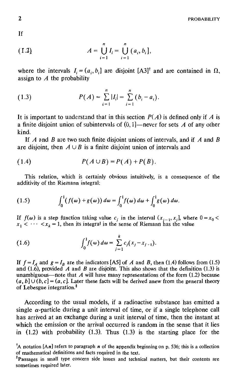
If
(ΐ·3) a=\ji,= ύκΛ],
1=1 1=1
where the intervals /, = (a,-, 6,] are disjoint [Α3Ϋ and are contained in Ω,
assign to A the probability
(ΐ·3) p(a)= £i/,i= £(&,.-«,).
ί=1 /=I
It is important to understand that in this section P(A) is defined only if A is
a finite disjoint union of subintervals of (0,1]—never for sets A of any other
kind.
If Л and β are two such finite disjoint unions of intervals, and if A and В
are disjoint, then A U В is a finite disjoint union of intervals and
(1.4) P(AUB)=P(A)+P(B).
This relation, which is certainly obvious intuitively, is a consequence of the
additivity of the Riemann integral:
(1.5) (\f{a>)+g{a>))dcu= Cf(io)du>+ Cg(u>)dio.
Jo Jo -Ό
If /(ω) is a step function taking value c; in the interval (x _ l5 jc;], where 0=дго<
X\ < · · · <X/i = 1, then its integral in the sense of Riemann has the value
к
(1.6) j !{ω)άω= Σ c,(*,.-*,_,).
'° /=1
If f = IA and g = IB are the indicators [A5] of A and B, then (1.4) follows from (1.5)
and (1.6), provided A and В are disjoint. This also shows that the definition (1.3) is
unambiguous—note that A will have many representations of the form (1.2) because
(a, b] U (b, с] = (а, с]. Later these facts will be derived anew from the general theory
of Lebesgue integration.*
According to the usual models, if a radioactive substance has emitted a
single α-particle during a unit interval of time, or if a single telephone call
has arrived at an exchange during a unit interval of time, then the instant at
which the emission or the arrival occurred is random in the sense that it lies
in (1.2) with probability (1.3). Thus (1.3) is the starting place for the
fA notation [An] refers to paragraph η of the appendix beginning on p. 536; this is a collection
of mathematical definitions and facts required in the text.
*Passages in small type concern side issues and technical matters, but their contents are
sometimes required later.

SECTION 1. BOREL'S NORMAL NUMBER THEOREM
3
description of a point drawn at random from the unit interval: Ω is regarded
as a sample space, and the set (1.2) is identified with the event that the
random point lies in it.
The definition (1.3) is also the starting point for a mathematical
representation of an infinite sequence of tosses of a coin. With each ω associate its
nonterminating dyadic expansion
(1.7) «= Σ -ψ1 = Α(")<12(ω)...,
n = l Δ
each dn(w) being 0 or 1 [A31]. Thus
(1.8) (<*,(«),<*,(«),...)
is the sequence of binary digits in the expansion of ω. For definiteness, a
point such as |=.1000... =.0111..., which has two expansions, takes the
nonterminating one; 1 takes the expansion .111... .
1
1
0 10 1
Graph of (1,(ω) Graph of d2(u)
Imagine now a coin with faces labeled 1 and 0 instead of the usual heads
and tails. If ω is drawn at random, then (1.8) behaves as if it resulted from an
infinite sequence of tosses of a coin. To see this, consider first the set of ω
for which ίί,-(ω) = w, for i = Ι,.,.,η, where u,,...,u„ is a sequence of O's
and l's. Such an ω satisfies
n и "и- 1
γ4ΐτ<ω< УЦ+ У Л,
1—1 г)1 — 1—1 г\1 1—1 П1 '
1-1 Δ i= l z i=n+\ Δ
where the extreme values of ω correspond to the case ά^ω) = 0 for i > η and
the case dt((o) = 1 for i > n. The second case can be achieved, but since the
binary expansions represented by the ά^ω) are nonterminating—do not end
in O's—the first cannot, and ω must actually exceed Σ"=1μ,/2'. Thus
(1.9) [«:^.(«) = Ы<>1 = 1,...,/1] = (е|, Σ^ί + ψ ■

4
PROBABILITY
The interval here is open on the left and closed on the right precisely
because the expansion (1,7) is the nonterminating one. In the model for coin
tossing the set (1.9) represents the event that the first η tosses give the
outcomes w,,...,w„ in sequence. By (1.3) and (1.9),
(1.10) P[w.di(co) = ui,i=l,...,n] = ±,
which is what probabilistic intuition requires.
oo . ci , io , и
OOP t 001 , 010 , 0Ί [ 100 , 101 , 110 , 111
Decompositions by dyadic intervals
The intervals (1.9) are called dyadic intervals, the endpcints being
adjacent dyadic rationale k/2r and (k + l)/2" with the same denominator, and
η is the rank or order of the interval. For each η the 2" dyadic intervals of
rank η decompose or partition the unit interval. In the passage from the
partition for η to that for η + 1, each interval (1.9) is split into two parts of
equal length, a left half on which ί/π + ,(ω) is 0 and a right half on which
ί/„ + ](ω) is 1. For и = 0 and for и = 1, the set [ω: ί/„ + 1(ω) = и] is thus a
disjoint union of 2" intervals of length l/2" + 1 and hence has probability \:
Ρ[ω: dn(w) = u] = \ for all n.
Note that ί/,(ω) is constant over each dyadic interval of rank / and that for
η > i each dyadic interval of rank η is entirely contained in a single dyadic
interval of rank :'. Therefore, ά((ω) is constant over each dyadic interval of
rank η if i < n.
The probabilities of various familiar events can be written down
immediately. The sum Σ"= λά^ω) is the number of l's among ί/,(ω),..., dn(w), to be
thought of as the number of heads in η tosses of a fair coin. The usual
binomial formula is
(1.11)
ω: Ε^,(ω) = к
/=1
ΐ)ψ> °*k*»·
This follows from the definitions: The set on the left in (1.11) is the union of
those intervals (1.9) corresponding to sequences и,,...,«„ containing к l's
and n-k O's; each such interval has length 1/2" by (1.10) and there are \"A
of them, and so (1.11) follows from (1.3).

SECTION 1. BOREL's NORMAL NUMBER THEOREM
5
The functions άη{ω) can be looked at in two ways. Fixing η and letting ω
vary gives a real function dn = dn(·) on the unit interval. Fixing ω and letting
η vary gives the sequence (1.8) of O's and l's. The probabilities (1.10) and
(1.11) involve only finitely many of the components d-<ia). The interest here,
however, will center mainly on properties of the entire sequence (1.8). It will
be seen that the mathematical properties of this sequence mirror the
properties to be expected of a coin-tossing process that continues forever.
As the expansion (1.7) is the nonterminating one, there is the defect that
for no ω is (1.8) the sequence (1,0,0,0,...), for example. It seems clear that
the chance should be 0 for the coin to turn up heads on the first toss and tails
forever after, so that the absence of (1,0,0,0,...)—or of any other single
sequence—should not matter. See on this point the additional remarks
immediately preceding Theorem 1.2.
The Weak Law of Large Numbers
In studying the connection with coin tossing it is instructive to begin with a
result that can, in fact, be treated within the framework of discrete
probability, namely, the weak law of large numbers:
Theorem 1.1. For each e?
(1.12)
lim Ρ
ω:
1 " 1
-£>,.(ω)- J
>e
= 0.
Interpreted probabilistically, (1.12) says that if η is large, then there is
small probability that the fraction or relative frequency of heads in η tosses
will deviate much from \, an idea lying at the base of the frequency
conception of probability. As a statement about the structure of the real
numbers, (1.12) is also interesting arithmetically.
Since άι(ω) is constant over each dyadic interval of rank η if i <n, the
sum Σ"=1ίί,(ω) is also constant over each dyadic interval of rank n. The set in
(1.12) is therefore the union of certain of the intervals (1.9), and so its
probability is well denned by (1.3).
With the Riemann integral in the role of expected value, the usual
application of Chevyshev's inequality will lead to a proof of (1.12). The
argument becomes simpler if the dn(w) are replaced by the Rademacher
functions,
(1.13)
r„(«) = 2rf„(«)-l =
+ 1 ifrf„(«) = l,
-1 ifrf„(«)=0.
+The standard e and δ of analysis will always be understood to be positive.

6
PROBABILITY
Graph of r,fcjj
1
0
1
1
Graph of r3(tj)
Consider the partial sums
(1.14) i„(«)= Ση{ω).
i=l
Since Σ"=,ίί,(ω) = (sn(w) + n)/2, (1.12) with e/2 in place of e is the same
thing as
(1.15)
lim Ρ
η ->oo
ω:
«5«(ω>
> e
= 0.
This is the form in which the theorem will be proved.
The Rademacher functions have themselves a direct probabilistic
meaning. If a coin is tossed successively, and if a particle starting from the origin
performs a random walk on the real line by successively moving one unit in
the positive or negative direction according as the coin falls heads or tails,
then rf(<a) represents the distance it moves on the ith step and 5„(ω)
represents its position after η steps. There is also the gambling
interpretation: If a gambler bets one dollar, say, on each toss of the coin, r,(w)
represents his gain or loss on the ith play and sn(w) represents his gain or
loss in η plays.
Each dyadic interval of rank /' - 1 splits into two dyadic intervals of rank /;
Γ,(ω) has value - 1 on one of these and value + 1 on the other. Thus r/ω) is
— 1 on a set of intervals of total length { and + 1 on a set of total length \.
Hence }^η(ω)άω = 0 by (1.6), and
(1.16)
/ 5„(ω) άω = 0
by (1.5). If the integral is viewed as an expected value, then (1.16) says that
the mean position after η steps of a random walk is 0.
Suppose that i <j. On a dyadic interval of rank /- 1, r,(w) is constant
and r (ω) has value -1 on the left half and +1 on the right. The product

SECTION 1. BOREL's NORMAL NUMBER THEOREM
7
Γι(ω)η(ω) therefore integrates to 0 over each of the dyadic intervals of rank
j — 1, and so
(1.17)
( η(ω)η(ω)άω = 0, i Φ].
This corresponds to the fact that independent random variables are
uncorrected. Since rf (ω) = 1, expanding the square of the sum (1.14) shows that
(1.18)
j 5^(ω) άω = п.
This corresponds to the fact that the variances of independent random
variables add. Of course (1.16), (1.17), and (1.18) stand on their own, in no
way depend on any probabilistic interpretation.
Applying Chebyshev's inequality in a formal way to the probability in
(1.15) now leads to
(1.19) Ρ[ω: |*„(ω)| > ne] < -~-2 f\2n(w) dw = -^.
The following lemma justifies the inequality.
Let / be a step function as in (1.6): /(w) = c; for ω e(x;._,, хД where
0 =x0 < · · · <xk = 1.
Lemma. If fis a nonnegative step function, then [ω: /(ω) > a] is for a > 0
a finite union of intervals and
(1.20)
P[<o:f(a,)>a]<lff(w)dw.
The shaded region
has area
αΡ[ω: /(ω)» α}.
Proof. The set in question is the union of the intervals (χ;_,,χ;] for
which Cj > a. If Σ denotes summation over those / satisfying c; > a, then
Ρ[ω: f(w)>a] = L'(Xj-Xj_]) by the definition (1.3). On the other hand,

8
PROBABILITY
since the c; are all nonnegative by hypothesis, (1.6) gives
f /(ω) άω = Σ Cj(Xj ~Xj.,) > Е'сДXj -Xj-i)
Hence (1.20). ■
Taking a = n2e2 and /(ω)-ί^(ω) in (1.20) gives (1.19). Clearly, (1.19)
implies (1.15), and as already observed, this in turn implies (1.12).
The Strong Law of Large Numbers
It is possible with a minimum of technical apparatus to prove a stronger
result that cannot even be formulated in the discrete theory of probability.
Consider the set
(1.21) N =
1 " 1
ω: Urn - £<(ω)
η ^лш> 2
consisting of those ω for which the asymptotic relative frequency* of 1 in the
sequence (1.8) is \. The points in (1.21) are called normal numbers. The idea
is to show that a real number ω drawn at random from the unit interval is
"practically certain" to be normal, or that there is "practical certainty" that 1
occurs in the sequence (1.8) of tosses with asymptotic relative frequency \. It
is impossible at this stage to prove that P(N) = 1, because N is not a finite
union of intervals and so has been assigned no probability. But the notion of
"practical certainty" can be formalized in the following way.
Define a subset Л of Ω to be negligible^ if for each positive e there exists
a finite or countable* collection /,, /2,... of intervals (they may overlap)
satisfying
(1.22) Aa\JIk
к
and
(1.23) ΣΙ/*Ι<*.
к
A negligible set is one that can be covered by intervals the total sum of
whose lengths can be made arbitrarily small. If P(A) is assigned to such an
*The frequency of 1 (the number of occurrences of it) among d,(c<j),...,dn{m) is Σ,"=ιίί,(ω), the
lelatiue frequency is η-1Σ,"=1£*,(ω), and the asymptotic relative frequency is the limit in (1.21).
+The term negligible is introduced for the purposes of this section only. The negligible sets will
reappear later as the sets of Lebesgue measure 0.
%СоиШаЫу infinite is unambiguous. Countable will mean finite or countably infinite, although it
will sometimes for emphasis be expanded as here to finite or countable.

SECTION 1. BOREL'S NORMAL NUMBER THEOREM
9
A in any reasonable way, then for the Ik of (1.22) and (1.23) it ought to be
true that P(A) < ZkP(Ik) = Zk\Ik\ < e, and hence P(A) ought to be 0. Even
without any assignment of probability at all, the definition of negligibility can
serve as it stands as an explication of "practical impossibility" and "practical
certainty": Regard it as practically impossible that the random ω will lie in A
if A is negligible, and regard it as practically certain that ω will lie in A if its
complement Ac [Al] is negligible.
Although the fact plays no role in the next proof, for an understanding of
negligibility observe first that a finite or countable union of negligible sets is
negligible. Indeed, suppose that AX,A2,... are negligible. Given e, for each
η choose intervals lnl, In2,... such that An с (J*. Ink and Zk\Ink\ < e/2". All
the intervals Ink taken together form a countable collection covering (J„ An,
and their lengths add to ZnZk\lnk\ < E„e/2" = e. Therefore, U„ An is
negligible.
A set consisting of a single point is clearly negligible, and so every countable
set is also negligible. The rationale for example form a negligible set. In the
coin-tossing model, a single point of the unit interval has the role of a single
sequence of 0's and l's, or of a single sequence of heads and tails. It
corresponds with intuition that it should be "practically impossible" to toss a
coin infinitely often and realize any one particular infinite sequence set down
in advance. It is for this reason not a real shortcoming of the model that for
no ω is (1.8) the sequence (1,0,0,0,...). In fact, since a countable set is
negligible, it is not a shortcoming that (1.8) is never one of the countably
many sequences that end in 0's.
Theorem 1.2. The set of normal numbers has negligible complement.
This is Borel's normal number theorem,1' a special case of the strong law of
large numbers. Like Theorem 1.1, it is of arithmetic as well as probabilistic
interest.
The set Nc is not countable: Consider a point ω for which
(ί/,(ω),ά2(ω),...) = (1,1,ы3,1,1,ы6,...)—that is, a point for which d,(w) = 1
unless i is a multiple of 3. Since n~lZ"=]dj(w) > f, such a point cannot be
normal. But there are uncountably many such points, one for each infinite
sequence (u3,u6,...)oi 0's and l's. Thus one cannot prove Nc negligible by
proving it countable, and a deeper argument is required.
Proof of Theorem 1.2. Gearly (1.21) and
(1.24) N =
ω: lim -5„(ω)=0
П
tEmiIe Borel: Sur les probabilites denombrables et leurs applications arithmetiques, Circ. Mat
d. Palermo, 29 (1909), 247-271. See Dudley for excellent historical notes on analysis and
probability.

10
PROBABILITY
define the same set (see (1.14)). To prove Nc negligible requires constructing
coverings that satisfy (1.22) and (1.23) for A =NC. The construction makes
use of the inequality
(1.25) P[a>:\s„(a>)\>ne]i^-ifs*n(a>)d<».
This follows by the same argument that leads to the inequality in (1.19)—it is
only necessary to take /(ω) = s*(a)) and α = nAeA in (1.20). As the integral in
(1.25) will be shown to have order n2, the inequality is stronger than (1.19).
The integrand on the right in (1.25) is
(1.26) 5π4(ω)= Σ''α(ω)Λβ(ω)^(ω)Λδ(ω),
where the four indices range independently from 1 to л. Depending on how
the indices match up, each term in this sum reduces to one of the following
five forms, where in each case the indices are now distinct:
r,» = l,
г,2(«)г/(«) = 1,
(1.27) {г,2(«)гД«К(«) = г;(«)гк(«),
г/(«)гД«)=г1.(«)г/(й»),
/,(ω)>';(ωΚ(ω)Λ,(ω).
If, for example, к exceeds /, j, and /, then the last product in (1.27)
integrates to 0 over each dyadic interval of rank к - I, because η(ω)η(ω)η(ω)
is constant there, while rk(w) is -1 on the left half and +1 on the right.
Adding over the dyadic intervals of rank к — 1 gives
f rl-(u»)r/(ftl)rfc(ftl)r,(ftl)rfftl=0.
yo
This holds whenever the four indices are distinct. From this and (1.17) it
follows that the last three forms in (1.27) integrate to 0 over the unit interval;
of course, the first two forms integrate to 1.
The number of occurrences in the sum (1.26) of the first form in (1.27) is
n. The number of occurrences of the second form is Ъп{п — 1), because there
are η choices for the α in (1.26), three ways to match it with β, y, or δ, and
n-1 choices for the value common to the remaining two indices. A term-by-
term integration of (1.26) therefore gives
(1.28) [1sl(a>)da> = n + 3n(n-l) <3n2,

SECTION 1. BOREL's NORMAL NUMBER THEOREM
11
and it follows by (1.25) that
(1.29)
ω:
-*„(")
> e
П2€А
Fix a positive sequence {e„} going to 0 slowly enough that the series
Е„е~4и-2 converges (take en = n~,/s, for example). If An = [ω: |«_15„(ω)|>
e„], then P(A„) < 3e;4«"2 by (1.29), and so ΣπΡ(Αη) < oo.
If, for some m, ω lies in Acn for all η greater than or equal to m, then
\n~ 'ί„(ω)| < en for n>m, and it follows that ω is normal because en -> 0 (see
(1.24)). In other words, for each m, f) ™-mAc„ c^» which is the same thing as
/Vе с U°n=m A„. This last relation leads to the required covering: Given e,
choose m so that YTn=mP(An) <e. Now Ar is a finite disjoint union \Jk Ink of
intervals with Lk\Ink\ = P(An\ and therefore U^=m An is a countable union
iX~m U* Ink °^ intervals (not disjoint, but that does not matter) with
L~=mLk\Ink\ = L'"n,mP(AJ<e. The intervals Ink (n>m, k>\) provide a
covering of /Vе of the kind the definition of negligibility calls for. ■
Strong Law Versus Weak
Theorem 1.2 is stronger than Theorem 1.1. A consideration of the forms of the two
propositions will show that the strong law goes far beyond the weak law.
For each η let /„(ω) be a step function on the unit interval, and consider the
relation
(1.30)
lim P[«: |/„(«)| 2:e]=0
together with the set
(1.31)
«: lim/„(«)= 0].
n-»°° J
If /„(ω) = Η_15„(ω), then (1.30) reduces to the weak lav/ (1.15), and (1.31) coincides
with the set (1.24) of normal numbers. According to a general result proved below
(Theorem 5.2(ii)), whatever the step functions /„(ω) may be, if the set (1.31) has
negligible complement, then (1.30) holds for each positive e. For this reason, a proof
of Theorem 1.2 is automatically a proof of Theorem 1.1.
The converse, however, fails: There exist step functions /„(ω) that satisfy (1.30) for
each positive e but for which (1.31) fails to have negligible complement (Example 5.4).
For this reason, a proof of Theorem 1.1 is not automatically a proof of Theorem 1.2;
the latter lies deeper and its proof is correspondingly more complex.
Length
According to Theorem 1.2, the complement /Vе of the set of normal numbers
is negligible. What if N itself were negligible? It would then follow that
(0,1] = /V U /Vе was negligible as well, which would disqualify negligibility as
an explication of "practical impossibility," as a stand-in for "probability
zero." The proof below of the "obvious" fact that an interval of positive

12
PROBABILITY
length is not negligible (Theorem 1.3(ii)), while simple enough, does involve
the most fundamental properties of the real number system.
Consider an interval I = (a,b] of length \I\ = b-a; see (1.1). Consider
also a finite or infinite sequence of intervals Ik = (ak,bk]. While each of
these intervals is bounded, they need not be subintervals of (0,1].
Theorem 1.3. (i) // (J^ Ik c/, and the Ik are disjoint, then Lk\Ik\ < |/|.
(ii) /// с \J( Ik {the Ik need not be disjoint), then |/| < Σ J/J.
(iii) /// = Ok Ik, and the lk are disjoint, then \l\ = *Lk\Ik\.
Proof. Of course (iii) follows from (i) and (ii).
Proof of (i): Finite case. Suppose there are η intervals. The result
being obvious for η = 1, assume that it holds for η - 1. If an is the largest
among au...,an (this is just a matter of notation), then U"Z\(ak,bk]<z
(a,an\ so that L"kZ.\(bk ~ak) <an -a by the induction hypothesis, and
hence Lk=](bk - ak) < (an - a) + (bn -an)<b-a.
Infinite case. If there are infinitely many intervals, each finite subcollection
satisfies the hypotheses of (i), and so L"k = i(bk - ak) < b - a by the finite case.
But as η is arbitrary, the result follows.
Proof of (ii): Finite case. Assume that the result holds for the case of
η - 1 intervals and that (a,b]c \Jk = l(ak,bk]. Suppose that an <b <bn
(notation again). If an < a, the result is obvious. Otherwise, (а, ап] с
UkZ\(ak,bk], so that Z"kZ\(bk-ak)>an-a by the induction hypothesis
and hence L"k= ,(b*. - ak) > (an -a) + (bn -an)>b -a. The finite case thus
follows by induction.
Infinite case. Suppose that (a, b] с \J*k = i(ak,bk]. If 0 <e <b -a, the open
intervals (ak, bk + el~k) cover the closed interval [a + e,b], and it follows by
the Heine-Borel theorem [A13] that [a + e,b]a \J"k=l(ak,bk +e2~k) for
some n. But then (a +e,b]c U"k=l(ak,bk + e2~k], and by the finite case,
b -(a+e)<L"k = i(bk + e2~k -ak)<Lk'=l(bk-ak) + e. Since e was
arbitrary, the result follows. ■
Theorem 1.3 will be the starting point for the theory of Lebesgue measure
as developed in Sections 2 and 3. Taken together, parts (i) and (ii) of the
theorem for only finitely many intervals Ik imply (1.4) for disjoint A and B.
Like (1.4), they follow immediately from the additivity of the Riemann
integral; but the point is to give an independent development of which the
Riemann theory will be an eventual by-product.
To pass from the finite to the infinite case in part (i) of the theorem is
easy. But to pass from the finite to the infinite case in part (ii) involves
compactness, a profound idea underlying all of modern analysis. And it is
part (ii) that shows that an interval / of positive length is not negligible: |/| is

SECTJON 1. BOREL'S NORMAL NUMBER THEOREM
13
a positive lower bound for the sum of the lengths of the intervals in any
covering of /.
The Measure Theory of Diophantine Approximation*
Diophantine approximation has to do with the approximation of real numbers χ by
rational fractions p/q. The measure theory of Diophantine approximation has to do
with the degree of approximation that is possible if one disregards negligible sets of
real x.
For each positive integer q, χ must lie between some pair of successive multiples
of 1 /q, so that for some p, \x— p/q\< 1 /q. Since for each q the intervals
^ (f-£■?♦£]
decompose the line, the error of approximation can be further reduced to \/2q: For
each q there is a p such that \x -p/q\< l/2q. These observations are of course
trivial. But for "most" real numbers χ there will be many values of ρ and q for which
x lies very near the center of the interval (1.32), so that p/q is a very sharp
approximation to x.
Theorem 1.4. If χ is irrational, there are infinitely many irreducible fractions ρ / q
such that
(i.33) μ-J
ι
This famous theorem of Dirichlet says that for infinitely many ρ and q, χ lies in
(p/q ~ 1/q2, P/q + l/<72) and hence is indeed very near the center of (1.32).
Proof. For a positive integer Q, decompose [0,1) into the Q subintervals
[(/- l)/Q,i/Q), i = l,...,Q. The points (fractional parts) {qx} = qx -[qx\ for q =
0,1,...,Q lie in [0,1), and since there are Q + 1 points1 and only Q subintervals, it
follows (Dirichlet's drawer principle) that some subinterval contains more than one
point. Suppose that {q'x} and {q"x} lie in the same subinterval and 0 < q' < q" < Q.
Take q=q"-q' and ρ = [q"x\ -\q'x\; then \<q<Q and \qx-p\ = \{q"x)-{q'x}\
<\/Q:
(1.34)
1 1
< -TT <
q
qQ J -2
If ρ and q have any common factors, cancel them; this will not change the left side of
(1.34), and it will decrease q.
For each Q, therefore, there is an irreducible p/q satisfying (1.34).* Suppose
there are only finitely many irreducible solutions of (1.33), say P\/ q\,---,pm /qm·
Since χ is irrational, the I* — pk /qk\ are all positive, and it is possible to choose Q so
that Q~l is smaller than each of them. But then the p/q of (1.34) is a solution of
(1.33), and since |* -p/q\ < 1/Q, there is a contradiction. ■
*This topic may be omitted.
+Although the fact is not technically necessary to the proof, these points are distinct: (q'x) = (q"x)
implies iq" - q')x = [q"x J - [q'x], which in turn implies that χ is rational unless q' = q".
*This much of the proof goes through even if χ is rational.

14
PROBABILITY
In the measure theory of Diophantine approximation, one looks at the set of real χ
having such and such approximation properties and tries to show that this set is
negligible or else that its complement is. Since the set of rationals is negligible,
Theorem 1.4 implies such a result: Apart from a negligible set of x, (1.33) has
infinitely many irreducible solutions.
What happens if the inequality (1.33) is tightened? Consider
(1.35)
1
<
<72<K<7) '
and let A consist of the real χ for which (1.35) has infinitely many irreducible
solutions. Under what conditions on φ will Αψ have negligible complement? If
cp(q)< 1, then (1.35) is weaker than (1.33): <p(<7)> 1 in the interesting cases. Since χ
satisfies (1.35) for infinitely many irreducible p/q if and only if χ - [χ J does, Αφ may
as well be redefined as the set of χ in (0,1) (or even as the set of irrational χ in (0, D)
for which (1.35) has infinitely many solutions.
Theorem 1.5. Suppose that ψ is positive and nondecreasing. If
(1.36) Σ—7~τ=^
V , Ml)
then Αφ has negligible complement.
Theorem 1.4 covers the case cp(q) = 1. Although this is the natural place to state
Theorem 1.5 in its general form, the proof, which involves continued fractions and the
ergodic theorem, must be postponed; see Section 24, p. 324. The converse, on the
other hand, has a very simple proof.
Theorem 1.6. Suppose that ψ is positive. If
q Ml)
then Αφ is negligible.
Proof. Given e, choose <70 so that Σ, b(? 1 /q<p(q) < e/A. If χ ^Αφ, then (1.35)
holds for some q S: q0, and since 0 < χ < 1, the corresponding ρ lies in the range
0 <p < q. Therefore,
ArcU и(|-йгг.#-
The right side here is a countable union of intervals covering Αφ, and the sum of
their lengths is
Σ Σ-*-- Σ ^i±i>-< L^~<e
яъяо p-0 «Ml) дъд0<1М<1) чъЧоМ<1)
Thus A satisfies the definition ((1.22) and (1.23)) of negligibility. ■

SECTION 1. BOREL'S NORMAL NUMBER THEOREM 15
If <pi(q)=l, then (1.36) holds and hence Αφ has negligible complement (as
follows also from Theorem 1.4). If φ2(ΐ) = <7£, however, then (1.37) holds and
Αφ itself is negligible Outside the negligible set A^UA , therefore, \x-p/q\<
\/q2 has infinitely many irreducible solutions but |* —p/q\ < l/q2+c has only
finitely many. Similarly, since Lqi/(q log q) diverges but Lql/(q log1+£<7) converges,
outside a negligible set \x-p/q\<l/(q2 \ogq) has infinitely many irreducible
solutions but \x —p/q\ < l/(q2 \og1+tq) has only finitely many.
Rational approximations to χ obtained by truncating its binary (or decimal)
expansion are very inaccurate: see Example 4.17. The sharp rational approximations
to χ come from truncation of its continued-fraction expansion: see Section 24.
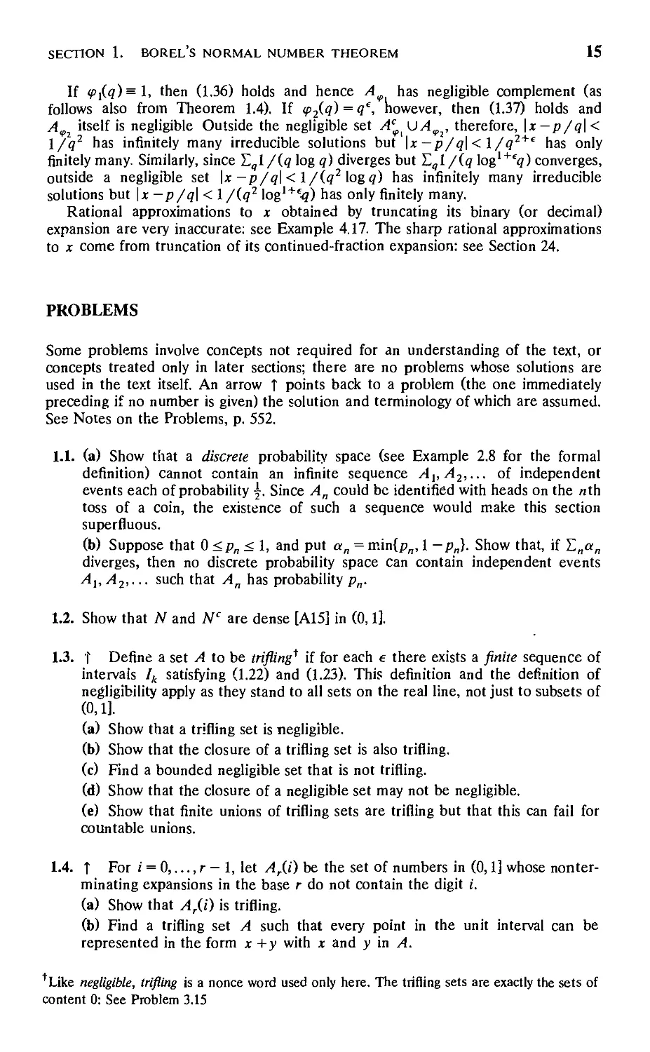
PROBLEMS
Some problems involve concepts not required for an understanding of the text, or
concepts treated only in later sections; there are no problems whose solutions are
used in the text itself. An arrow Τ points back to a problem (the one immediately
preceding if no number is given) the solution and terminology of which are assumed.
See Notes on the Problems, p. 552.
1.1. (a) Show that a discrete probability space (see Example 2.8 for the formal
definition) cannot contain an infinite sequence A1,A2,... of independent
events each of probability \. Since An could be identified with heads on the nth
toss of a coin, the existence of such a sequence would make this section
superfluous.
(b) Suppose that 0 <pn < 1, and put a„ = min{pn, 1 -p„]. Show that, if Σ„α„
diverges, then no discrete probability space can contain independent events
Al,A2,... such that An has probability pn.
1.2. Show that N and Nc are dense [A15] in (0,1].
1.3. ΐ Define a set A to be trifling* if for each e there exists a finite sequence of
intervals /,. satisfying (1.22) and (1.23). This definition and the definition of
negligibility apply as they stand to all sets on the real line, not just to subsets of
(0,11
(a) Show that a trifling set is negligible.
(b) Show that the closure of a trifling set is also trifling.
(c) Find a bounded negligible set that is not trifling.
(d) Show that the closure of a negligible set may not be negligible.
(e) Show that finite unions of trifling sets are trifling but that this can fail for
countable unions.
1.4. Τ For i = 0,..., r - 1, let Ar(i) be the set of numbers in (0,1] whose nonter-
minating expansions in the base r do not contain the digit i.
(a) Show that Ar(i) is trifling.
(b) Find a trifling set A such that every point in the unit interval can be
represented in the form χ +y with χ and у in A.
tLike negligible, trifling is a nonce word used only here. The trifling sets are exactly the sets of
content 0: See Problem 3.15

16
PROBABILITY
(с) Let Ar(iu ■■■,ik) consist of the numbers in the unit interval in whose base-r
expansions the digits г',,..., ik nowhere appear consecutively in that order.
Show that it is trifling. What does this imply about the monkey that types at
random?
1.5. Τ The Cantor set С can be defined as the closure of /1,(1)
(a) Show that С is uncountable but trifling.
(b) From [0,1] remove the open middle third ({, f); from the remainder, a
union of two closed intervals, remove the two open middle thirds (£, §) and
(|, §). Show that С is what remains when this process is continued ad infinitum.
(c) Show that С is perfect [A15]
1.6. Put M(t) = lle's"Mdm, and show by successive differentiations under the
integral that
(1.38) M<*>(0)- flskn(<o)da>
Over each dyadic interval of rank n, sn(a>) has a constant value of the form
± 1 + 1 + ■ ■ ■ + 1, and therefore M(t) = 2~Texp t(± 1 + 1 ± · ■ ± 1), where
the sum extends over all 2" л-long sequences of + l's and — l's. Thus
(1.39) M(t) = (e'+2e '] = (cosh г)"
Use this and (1.38) to give new proofs of (1.16), (1.18), and (1.28). (This, the
method of moment generating functions, will be investigated systematically in
Section 9.)
1.7. Τ By an argument similar to that leading to (1.39) show that the Rademacher
functions satisfy
L
1
exp
о
k=\
^ ~ 11 2
k=\ Δ
η
= Π cosak.
k=\
Take ak = tl k, and from Σ^=1^(ω)2 * = 2ω — 1 deduce
(1.40) «Ji-noos'
k=\ ^
by letting η -»oo inside the integral above. Derive Vieta's formula
2.
π
J2 yjl + ΐϊ д/2 + J2 + fi
1.8. A number ω is normal in the base 2 if and only if for each positive e there exists
an n0(e, ω) such that |η-1Σ7=1^,(ω) - -jl<e for all η exceeding n0(e, ω).

SECTION 2. PROBABILITY MEASURES
17
Theorem 1.2 concerns the entire dyadic expansion, whereas Theorem 1.1
concerns only the beginning segment. Point up the difference by showing that
for e < j the n0(e, ω) above cannot be the same for all ω in N—in other words,
η-1Σ"„ι^,·(ω) converges to \ for all ω in N, but not uniformly. But see
Problem 13.9.
1.9. 1.3 Τ (a) Using the finite form of Theorem 1.3(ii), together with Problem
1.3(b), show that a trifling set is nowhere dense [A15].
(b) Put В = \J„(r„ -2~n~2, rn + 2~n~2], where rl,r2,... is an enumeration of
the rationals in (0,1]. Show that (0,1] — В is nowhere dense but not trifling or
even negligible.
(c) Show that a compact negligible set is trifling
1.10. Τ A set of the first category [A15] can be, represented as a countable union of
nowhere dense sets; this is a topological notion of smallness, just as negligibility
is a metric notion of smallness. Neither condition implies the other:
(a) Shov that the nonnegligible set N of normal numbers is of the first category
by proving that Am = Γ\"^η[ω- \n~lsn(a>)\ < \] is nowhere dense and Nc
(b) According to a famous theorem of Baire, a nonempty interval is not of the
first category. Use this fact to prove that the negligible set Nc = (0,1] - N is not
of the first category.
1.11. Prove:
(a) If χ is rational, (1.33) has only finitely many irreducible solutions
(b) Suppose that <p(q)> 1 and (1.35) holds for infinitely many pairs p,q but
only for finitely many relatively prime ones. Then χ is rational.
(c) If φ goes to infinity too rapidly, then Αφ is negligible (Theorem 1.6). But
however rapidly φ goes to infinity, A is nonempty, even uncountable. Hint-
Consider χ = ΣΧ=11/2α<Α:) for integral a(k) increasing very rapidly to infinity.
SECTION 2. PROBABILITY MEASURES
Spaces
Let Ω be an arbitrary space or set of points ω. In probability theory Ω
consists of all the possible results or outcomes ω of an experiment or
observation. For observing the number of heads in η tosses of a coin the
space Ω is {0,1,..., n); for describing the complete history of the η tosses Ω
is the space of all 2" л-long sequences of H's and T's; for an infinite
sequence of tosses Ω can be taken as the unit interval as in the preceding
section; for the number of α-particles emitted by a substance during a unit
interval of time or for the number of telephone calls arriving at an exchange
Ω is {0,1,2,...}; for the position of a particle Ω is three-dimensional
Euclidean space; for describing the motion of the particle Ω is an
appropriate space of functions; and so on. Most Ω'β to be considered are interesting
from the point of view of geometry and analysis as well as that of probability.

18
PROBABILITY
Viewed probabilistically, a subset of Ω is an event and an element ω of Ω
is a sample point.
Assigning Probabilities
In setting up a space Ω as a probabilistic model, it is natural to try and assign
probabilities to as many events as possible. Consider again the case Ω = (0,1]
—the unit interval. It is natural to try and go beyond the definition (1.3) and
assign probabilities in a systematic way to sets other than finite unions of
intervals. Since the set of nonnormal numbers is negligible, for example, one
feels it ought to have probability 0. For another probabilistically interesting
set that is not a finite union of intervals, consider
oo
(2.1) (J [ω: -a <s,(<u),..., 5„_,(ω) <b,sn(a>)= -a],
n = \
where a and b are positive integers. This is the event that the gambler's
fortune reaches —a before it reaches +b; it represents ruin for a gambler
with a dollars playing against an adversary with b dollars, the rule being that
they play until one or the other runs out of capital.
The union in (2.1) is countable and disjoint, and for each η the set in the
union is itself a union of certain of the intervals (1.9). Thus (2.1) is a
countably infinite disjoint union of intervals, and it is natural to take as its
probability the sum of the lengths of these constituent intervals. Since the set
of normal numbers is not a countable disjoint union of intervals, however,
this extension of the definition of probability would still not cover all the
interesting sets (events) in (0,1].
It is, in fact, not fruitful to try to predict just which sets probabilistic
analysis will require and then assign probabilities to them in some ad hoc
way. The successful procedure is to develop a general theory that assigns
probabilities at once to the sets of a class so extensive that most of its
members never actually arise in probability theory. That being so, why not
ask for a theory that goes all the way and applies to every set in a space Ω?
In the case of the unit interval, should there not exist a well-defined
probability that the random point ω lies in A, whatever the set A may be?
The answer turns out to be no (see p. 45), and it is necessary to work within
subclasses of the class of all subsets of a space Ω. The classes of the
appropriate kinds—the fields and σ-fields—are defined and studied in this
section. The theory developed here covers the spaces listed above, including
the unit interval, and a great variety of others.
Classes of Sets
It is necessary to single out for special treatment classes of subsets of a space
il, and to be useful, such a class must be closed under various of the

SECTION 2. PROBABILITY MEASURES
19
operations of set theory. Once again the unit interval provides an instructive
example.
Example 2.1* Consider the set N of normal numbers in the form (1.24),
where 5„(ω) is the sum of the first η Rademacher functions. Since a point ω
lies in N if and only if lim„ «-ι5„(ω) = 0, N can be put in the form
(22) N = Π U П [ω:\η-\(ω)\<^\.
к=1т=1п=т
Indeed, because of the very meaning of union and of intersection, ω lies in
the set on the right here if and only if for every к there exists an m such that
\ri~xsn(b>)\<k~l holds for all n>m, and this is just the definition of
convergence to 0—with the usual e replaced by k~l to avoid the formation
of an uncountable intersection. Since s„(w) is constant over each dyadic
interval of rank n, the set [ω: «_15η(ω)| </с-1] is a finite disjoint union of
intervals. The formula (2.2) shows explicitly how N is constructed in steps
from these simpler sets. ■
A systematic treatment of the ideas in Section 1 thus requires a class of
sets that contains the intervals and is closed under the formation of
countable unions and intersections. Note that a singleton [Al] {x} is a countable
intersection f\n(x -n'1, x] of intervals. If a class contains all the singletons
and is closed under the formation of arbitrary unions, then of course it
contains all the subsets of Ω. As the theory of this section and the next does
not apply to such extensive classes of sets, attention must be restricted to
countable set-theoretic operations and in some cases even to finite ones.
Consider now a completely arbitrary nonempty space Ω. A class OF of
subsets of Ω is called a field1 if it contains Ω itself and is closed under the
formation of complements and finite unions:
(i) fieJ;
(ii) /4ef implies Ac <ξ <F;
(iii) А,В<еЗг implies ЛиВе^
Since Ω and the empty set 0 are complementary, (i) is the same in the
presence of (ii) as the assumption 0 e JF". In fact, (i) simply ensures that ^
is nonempty: If A <= !F, then Ac <ξ S^ by (ii) and Ω = A UAC <ξ S^ by (iii).
By DeMorgan's law, Α Π В = (Ac U Bc)c and A U В = (Ac Π BCY. If У is
closed under complementation, therefore, it is closed under the formation of
finite unions if and only if it is closed under the formation of finite intersec-
Many of the examples in the book simply illustrate the concepts at hand, but others contain
definitions and facts needed subsequently
The term algebra is often used in place of field

2U
PROBABILITY
tions. Thus (iii) can be replaced by the requirement
(iii') Л,Вё^ implies АСЛВ<е&.
A class if of subsets of Ω is a σ-field if it is a field and if it is also closed
under the formation of countable unions:
(iv) AX,A2,. . <= if implies Л, UA2L) ·■■ &if.
By the infinite form of DeMorgan's law, assuming (iv) is the same thing as
assuming
(iv') Л,, Л2,... £ if implies Л, Г\А2П ·· · e if.
Note that (iv) implies (iii) because one can take AY=A and An = В for
η > 2. A field is sometimes called a finitely additive field to stress that it need
not be a σ-rield. A set in a given class if is said to be measurable if or to be
an S^set. A field or σ-field of subsets of Ω will sometimes be called a field or
σ-field in Ω.
Example 2.2. Section 1 began with a consideration of the sets (1.2), the
finite disjoint unions of subintervals of Ω = (0,1]. Augmented by the empty
set, this class is a field ^0: Suppose that A = (a],a\]u ··· U(am,a'm],
where the notation is so chosen that a, < ··· <am. If the (a(,a';] are
disjoint, then Ar is (0, a,] L)(a\,a2] U ··· u(a'm_,,am] u(a'm, 1] and so lies
in ^0 (some of these intervals may be empty, as d-t and ai + i may coincide).
If B = (b1,b\]u ·· u(bn,b'„], the (Ь^Ь-] again disjoint, then AnB =
U/li U"=ii(fl,·, fl/]n(fcy, by]}; each intersection here is again an interval or
else the empty set, and the union is disjoint, and hence А Г) В is in @0. Thus
&ϋ satisfies (i), (ii), and (iii').
Although S8{) is a field, it is not a σ-field: It does not contain the
singletons {jc}, even though each is a countable intersection Π„(ϊ — η~\ x]
of i$()-sets. And ί$() does not contain the set (2.1), a countable union of
intervals that cannot be represented as a finite union of intervals. The set
(2.2) of normal numbers is also outside &ϋ. ■
The definitions above involve distinctions perhaps most easily made clear
by a pair of artificial examples.
Example 2.3. Let ^consist of the finite and the cofinite sets (Л being
cofinite if Л' is finite). Then if is a field. If Ω is finite, then ^contains all
the subsets of Ω and hence is a σ-field as well. If Ω is infinite, however, then
if is not a σ-field. Indeed, choose in Ω a set Л that is countably infinite and
has infinite complement. (For example, choose a sequence ωλ,ω2,... of
distinct points in Ω and take Л = {ω2,ω4,...}.) Then /iiJ, even though

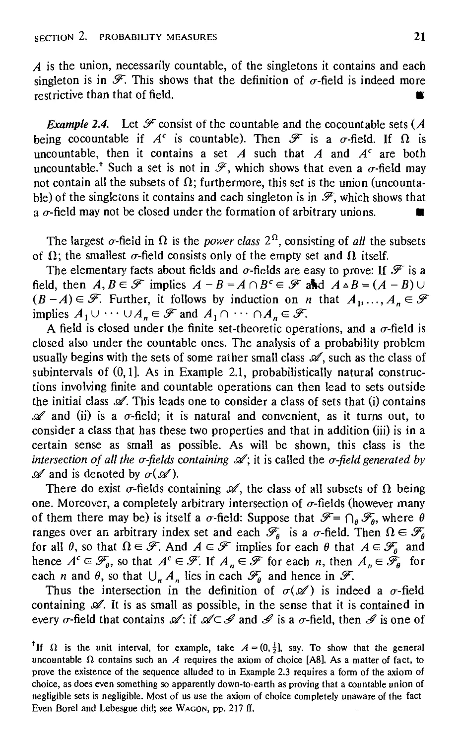
SECTION 2. PROBABILITY MEASURES
21
A is the union, necessarily countable, of the singletons it contains and each
singleton is in ^. This shows that the definition of σ-field is indeed more
restrictive than that of field. ■
Example 2.4. Let & consist of the countable and the cocountable sets (A
being cocountable if Ac is countable). Then F is a σ-field. If Ω is
uncountable, then it contains a set A such that A and Ac are both
uncountable.1 Such a set is not in &, which shows that even a σ-field may
not contain all the subsets of Ω; furthermore, this set is the union
(uncountable) of the singletons it contains and each singleton is in &~, which shows that
a σ-field may not be closed under the formation of arbitrary unions. ■
The largest σ-fieid in Ω is the power class 2Ω, consisting of all the subsets
of Ω; the smallest σ-field consists only of the empty set and Ω itself.
The elementary facts about fields and σ-fields are easy to prove: If ^ is a
field, then ^Se-J implies А -В=АпВс<в S? aiid A*B = (A - 5) и
(B-A)<e.!F. Further, it follows by induction on η that Αν...,Αη^^
implies AX\J ··· иЛ„Ё ^and Axn · ·· пАп <ξ <F.
A field is closed under the finite set-theoretic operations, and a σ-field is
closed also under the countable ones. The analysis of a probability problem
usually begins with the sets of some rather small class stf, such as the class of
subintervals of (0,1]. As in Example 2.1, probabilistically natural
constructions involving finite and countable operations can then lead to sets outside
the initial class &/. This leads one to consider a class of sets that (i) contains
sxf and (ii) is a σ-field; it is natural and convenient, as it turns out, to
consider a class that has these two properties and that in addition (iii) is in a
certain sense as small as possible. As will be shown, this class is the
intersection of all the σ-fields containing &/; it is called the σ-field generated by
sf and is denoted by σ(&/).
There do exist σ-fields containing &/, the class of all subsets of Ω being
one. Moreover, a completely arbitrary intersection of σ-fields (however many
of them there may be) is itself a σ-field: Suppose that &~= Πβ -^, where θ
ranges over an arbitrary index set and each J^ is a σ-field. Then Пе^
for all 0, so that Oef. And A e <F implies for each θ that Ле^ and
hence Ac <ξ S^e, so that Ac <ξ &\ If An e &~ for each n, then A„ e S^ for
each η and Θ, so that (J„ An lies in each 5^ and hence in ^.
Thus the intersection in the definition of σ(&/) is indeed a σ-field
containing «of. It is as small as possible, in the sense that it is contained in
every σ-field that contains &/: if &/a^ and ^ is a σ-field, then ^ is one of
If Ω is the unit interval, for example, take A = (0,5], say. To show that the general
uncountable Ω contains such an A requires the axiom of choice [A8]. As a matter of fact, to
prove the existence of the sequence alluded to in Example 2.3 requires a form of the axiom of
choice, as does even something so apparently down-to-earth as proving that a countable union of
negligible sets is negligible. Most of us use the axiom of choice completely unaware of the fact
Even Borel and Lebesgue did; see Wagon, pp. 217 ff.

22
PROBABILITY
the σ-fields in the intersection defining σ(.οΟ, so that a(^f)<z^f. Thus
σ(&ί) has these three properties:
(i) icff(j/);
(ii) a(stf) is a σ-field;
(iii) if £f<z^f and £ is a σ-field, then a(snf) c/
The importance of σ-fields will gradually become clear.
Example 2.5. If fF is a σ-field, then obviously a(S^) = $*~.H ssf consists
of the singletons, then a(ssf) is the σ-field in Example 2.4. If ssf is empty or
sf= {0} or sf= {SI}, then σ(&/) = {0,Sl}. If sf<isf\ then a(j*)<za(j*').
If ^c/C(t(/), then а(я/) = аШ'). ■
Example 2.6. Let J^ be the class of subintervais of SI = (0,1], and define
6B = a{if). The elements of 9$ are called the Borel sets of the unit interval.
The field 9$Q of Example 2.2 satisfies J^c 9$Q с ^, and hence a(9SQ) = 60.
Since ί# contains the intervals and is a σ-field, repeated finite and
countable set-theoretic operations starting from intervals will never lead
outside 98. Thus 98 contains the set (2.2) of normal numbers. It also contains
for example the open sets in (0,1]: If G is open and xeG, then there exist
rationale ax and bx such that χ ^(ax,bx\<^G. But then G = Ox^G(ax,bx];
since there are only countably many intervals with rational endpoints, G is a
countable union of elements of J^ and hence lies in 98.
In fact, 9$ contains all the subsets of (0,1] actually encountered in
ordinary analysis and probability. It is large enough for all "practical"
purposes. It does not contain every subset of the unit interval, however; see
the end of Section 3 (p. 45). The class 9$ will play a fundamental role in all
that follows. ■
Probability Measures
A set function is a real-valued function defined on some class of subsets of
SI. A set function Ρ on a field !F is a probability measure if it satisfies these
conditions:
(i) 0<P(A)< lfor A e^;
(ii) P(0) = 0, P(Sl) = 1;
(iii) if Ai,A2,... is a disjoint sequence of J^sets and if \J^^iAke &~,
then1
(2.3) p[\jAk)= LP(Ak).
fAs the left side of (2 3) is invariant under permutations of the An, the same must be true of the
right side. But in fact, according to Dirichlet's theorem [A26], a nonnegative series has the same
value whatever order the terms are summed in.

SECTION 2. PROBABILITY MEASURES
23
The condition imposed on the set function Ρ by (iii) is called countable
additivity. Note that, since & is a field but perhaps not a σ-field, it is
necessary in (iii) to assume that U"= ι Ak lies in &. If A,,..., An are disjoint
^sets, then Ok = iAk is also in & and (2.3) with An + l =An,2 = ··· = 0
gives
(2-4) p[ U^)= LP(Ak).
\k=l I L-_l
The condition that (2.4) holds for disjoint ^sets is finite additivity; it is a
consequence of countable additivity. It follows by induction on η that Ρ is
finitely additive if (2.4) holds for η = 2—if P(A и 5) = P(A) +P(B) for
disjoint ^sets A and β.
The conditions above are redundant, because (i) can be replaced by
P(A) > 0 and (ii) by Ρ(Ω,) = 1. Indeed, the weakened forms (together with
(iii)) imply that P(il) = Р(Щ + P(0) + P(0) + · · · , so that P(0) = 0, and
1 = Ρ(Ω) = P(A) + P(AC), so that P(A) < 1.
Example 2.7. Consider as in Example 2.2 the field бёй of finite disjoint
unions of subintervals of Ω = (0,1]. The definition (1.3) assigns to each
^0-set a number—the sum of the lengths of the constituent intervals—and
hence specifies a set function Ρ on ^0. Extended inductively, (1.4) says that
Ρ is finitely additive. In Section 1 this property was deduced from the
additivity of the Riemann integral (see (1.5)). In Theorem 2.2 below, the
finite additivity of Ρ will be proved from first principles, and it will be shown
that Ρ is, in fact, countably additive—is a probability measure on the field
бёй. The hard part of the argument is in the proof of Theorem 1.3, already
done; the rest will be easy. ■
If & is a σ-field in Ω and Ρ is a probability measure on &, the triple
(Ω, &, P) is called a probability measure space, or simply a probability space.
A support of Ρ is any ^set A for which P(A) = 1.
Example 2.8. Let & be the σ-field of all subsets of a countable space Ω,
and let ρ(ω) be a nonnegative function on Ω. Suppose that Σω(Ξίιρ(ω) = 1,
and define P(A) = Σω^Αρ(ω); since ρ(ω)>_0, the order of summation is
irrelevant by Dirichlet's theorem [A26]. Suppose that A = U"=i A{, where
the Aj are disjoint, and let ωη, ωί2,... be the points in At. By the theorem
on nonnegative double series [A27], P(A) = Σ4ρ(ωα) = Σ,Σ,/Κω,·,) =
LjPiAj), and so Ρ is countably additive. This (Ω, &, P) is a discrete
probability space. It is the formal basis for discrete probability theory. ■
Example 2.9. Now consider a probability measure Ρ on an arbitrary
σ-field & in an arbitrary space Ω; Ρ is a discrete probability measure if there
exist finitely or countably many points ωΙ( and masses mk such that P(A) =
Σω e Amk for A in &. Here Ρ is discrete, but the space itself may not be. In

24
PROBABILITY
terms of indicator functions, the defining condition is P(A) = LkmkIA(wk)
for A e &. If the set [ων ω2,...} lies in &, then it is a support of P.
If there is just one of these points, say ω0, with mass m0 = 1, then Ρ is a
unit mass at ω0. In this case P(A) = ΙΑ(ω0) for A e ^". ■
Suppose that Ρ is a probability measure on a field ^", and that Л,Ве^
and ЛсВ. Since P(A) + P(B -A) = P(B), Ρ is monotone:
(2.5) P(A)<P(B) if ЛсВ.
It follows further that P(B - A) = P(B) - P(A), and as a special case,
(2.6) P(AC) = 1-P(A).
Other formulas familiar from the discrete theory are easily proved. For
example,
(2.7) P(A) +P(B)=P(AuB)+P(Af)B),
the common value of the two sides being P(A U Bc) + 2P(A C\B) + P(AC Π
В). Subtraction gives
(2.8) P(A ufi) =P(A) +P(B)-P(AnB).
This is the case η = 2 of the general inclusion-exclusion formula:
(2.9) ρίυΛ^Σ^ΛΟ-Σ^^η^)
+ Σ Р(Л/ПЛ;ПЛ,)+---+(-])" + 1Р(Л,П---пЛ„).
i<j<fc
To deduce this inductively from (2.8), note that (2.8) gives
p\RAk )=p(piAk)+p(A»+i)-p(yyknA»+i))-
Applying (2.9) to the first and third terms on the right gives (2.9) with η + 1
in place of n.
If Βλ =Αλ and Bk =Ak СлА\ П · · · Г\Ак_и then the Bk are disjoint and
\JUxAk=\J"k = xBk, so that P{\JUxAk) = ZUxP{Bk). Since P(Bk) <
P{Ak) by monotonicity, this establishes the finite subadditivity of P:
(2.10) Ρ\(jAk)< LP(Ak).

SECTION 2. PROBABILITY MEASURES
25
Here, of course, the Ak need not be disjoint. Sometimes (2.10) is called
Boole's inequality.
In these formulas all the sets are naturally assumed to lie in the field $*~.
The derivations above involve only the finite additivity of P. Countable
additivity gives further properties:
Theorem 2.1. Let Ρ be a probability measure on a field ^.
(i) Continuity from below: If An and A lie in & and* An1 A, then
P(An)TP(A).
(ii) Continuity from above: If An and A lie in & and An\ A, then
P(An)iP(A).
(iii) Countable subadditivity: IfAx,A2,··· and \Tks,\Ak lie in S*~(theAk
need not be disjoint), then
(OO \ 00
\jAk\< LP(Ak).
k=l I k=l
Proof. For (i), put Bx = AX and Bk=Ak-Ak_x. Then the Bk are
disjoint, A = \J^^iBk, and An = Wk = \Bk, so that by countable and finite
additivity, P(A) = Е"к = 1Р(Вк) = lim„ Znk = xP(Bk) = lim„ P(An). For (ii),
observe that An i A implies Acn Τ Ac, so that 1-Р(Ап)П~ Р(А).
As for (iii). increase the right side of (2.10) to L°^=iP(Ak) and then apply
part (i) to the left side. ■
Example 2.10. In the presence of finite additivity, a special case of (ii)
implies countable additivity. // Ρ is a finitely additive probability measure on
the field $*~, and if An 10 for sets An in 5? implies P(An)iO, then Ρ is
countably additive. Indeed, if В = \Jk Bk for disjoint sets Bk (B and the Bk in
F), then Cn=Ok>nBk = B- \Jk<nBk lies in the field $?, and C„|0- The
hypothesis, together with finite additivity, gives P(B) - Σ^,^ίβ^.) =
P(Cn) ^ 0, and hence P(B) = Σ"„ ,/>(£*)· ■
Lebesgue Measure on the Unit Interval
The definition (1.3) specifies a set function on the field 080 of finite disjoint
unions of intervals in (0,1]; the problem is to prove Ρ countably additive. It
will be convenient to change notation from Ρ to Λ, and to denote by ^ the
class of subintervals (a, b] of (0,1]; then A(/) = \I\ = b - a is ordinary length.
Regard 0 as an element of J^ of length 0. If A = (J"= ι /,, the /, being
fFor the notation, see [A4] and [A10].

26
PROBABILITY
disjoint J^sets, the definition (1.3) in the new notation is
(2.12) λ(Α)= Σλ(/,.)= ΣΙ/,Ι·
ί-1 (=1
As pointed out in Section 1, there is a question of uniqueness here, because
A will have other representations as a finite disjoint union U"'= ι Jj of J^-sets.
But Jf is closed under the formation of finite intersections, and so ihe finite
form of Theorem 1.3(iii) gives
η η m m
(2.13) El/,l= Σ Σΐ/,η/,ΐ= ΣΙ-',Ι·
(Some of the /, n/ may be empty, but the corresponding lengths are then 0.)
The definition is indeed consistent.
Thus (2.12) defines a set function A on ^(), a set function called Lebesgue
measure.
Theorem 2.2. Lebesgue measure A is a (countably additive) probability
measure on the field &0.
Proof. Suppose that A = U£=i Ak, where A and the Ak are ^0-sets
and the Ak are disjoint. Then A = U"„i /,· and Ak = Uy"=( Л/ are disjoint
unions of j^-sets, and (2.12) and Theorem 1.3(iii) give
(2.14) \(А)= ΣΙ/,·Ι= Σ Σ Σΐ/,·η7„.|
ί=1 ί-1 fc=l /=1
οο tV ^ со
= Σ L\h<\= ΣΑ(Λ). ■
ft-lj-l k=l
In Section 3 it is shown how to extend A from 98ϋ to the larger class
98 - σ(&0) of Borel sets in (0,1]. This will complete the construction of A as
a probability measure (countably additive, that is) on &8. and the construction
is fundamental to all that follows. For example, the set N of normal numbers
lies in SB (Example 2.6), and it will turn out that A(/V) = 1, as probabilistic
intuition requires. (In Chapter 2, A will be defined for sets outside the unit
interval as well.)
It is well to pause here and consider just what is involved in the
construction of Lebesgue measure on the Borel sets of the unit interval. That length
defines a finitely additive set function on the class J^ of intervals in (0,1] is a
consequence of Theorem 1.3 for the case of only finitely many intervals and
thus involves only the most elementary properties of the real number system.
But proving countable additivity on J^ requires the deeper property of

SECTION 2. PROBABILITY MEASURES
27
compactness (the Heine-Borel theorem). Once λ has been proved countably
additive on J^, extending it to ^0 by the definition (2.12) presents no real
difficulty: the arguments involving (2.13) and (2.14) are easy. Difficulties again
arise, however, in the further extension of Λ from бёй to & = σ(^0), and
here new ideas are again required. These ideas are the subject of Section 3,
where it is shown that any probability measure on any field can be extended
to the generated σ-field.
Sequence Space*
Let 5 be a finite set of points regarded as the possible outcomes of a simple
observation or experiment. For tossing a coin, 5 can be {H,T} or {0,1); for
rolling a die, 5 = {1,... ,6}; in information theory, 5 plays the role of a finite
alphabet. Let Ω = S°° be the space of all infinite sequences
(2.15) ω = (ζ1(ω),ζ2(ω),...)
of elements of 5: zk((o)^S for all ω eS°° and к > 1. The sequence (2.15)
can be viewed as the result of repeating infinitely often the simple
experiment represented by S. For 5 = {0,1}, the space 5°° is closely related to the
unit interval; compare (1.8) and (2.15).
The space 5°° is an infinite-dimensional Cartesian product. Each zk(·) is a
mapping of 5°° onto 5; these are the coordinate functions, or the natural
projections. Let S" = S x · · · x 5 be the Cartesian product of η copies of 5;
it consists of the л-long sequences (u,,...,u„) of elements of 5. For such a
sequence, the set
(2.16) [ω: (ζ1(ω),...ίζ,Ι(ω)) = («„...,«„)]
represents the event that the first η repetitions of the experiment give the
outcomes ul,...,u„ in sequence. A cylinder of rank л is a set of the form
(2.17) Α = \ω:{ζλ{ω),...,ζη{ω))^Η],
where Я с 5". Note that A is nonempty if Η is. If Я is a singleton in 5",
(2.17) reduces to (2.16), which can be called a thin cylinder.
Let €Q be the class of cylinders of all ranks. Then ifQ is a field: S°° and
the empty set have the form (2.17) for Η = S" and for Η = 0. If Η is
replaced by 5" -H, then (2.17) goes into its complement, and hence if0 is
*The ideas that follow are basic to probability theory and are used further on, in particular in
Section 24 and (in more elaborate form) Section 36. On a first reading, however, one might
prefer to skip to Section 3 and return to this topic as the need arises.

28
PROBABILITY
closed under complementation As for unions, consider (2.17) together with
(2.18) Β=[ω:(ζι(ω),...,ζ„(ω))<Ξΐ],
a cylinder of rank m. Suppose that η < m (symmetry); if H' consists of the
sequences («„...,«„) in 5'" for which the truncated sequence (и„...,и„)
lies in Я, then (2.17) has the alternative form
(2.19) Α = [ω:(ζι(ω),...,ζ„(ω))<=Η'].
Since it is now clear that
(2.20) /lUfl=[«:(z.(ft»),...,zm(fti))eH'u/]
is also a cylinder, tf0 is closed under the formation of finite unions and hence
is indeed a field.
Let pu, ueS, be probabilities on 5—nonnegative and summing to 1.
Define a set function Ρ on tf0 (it will turn out to be a probability measure)
in this way: For a cylinder A given by (2.17), take
(2-21) Ρ(Α)=Σρ„ι···Ρ^
η
the sum extending over all the sequences (и,,..., un) in H. As a special case,
(2.22) />[ω:(ζ,(ω),...,ζ„(ω)) = («,,...,«„)] =pUi · · · р„я.
Because of the products on the right in (2.21) and (2.22), Ρ is called product
measure; it provides a model for an infinite sequence of independent
repetitions of the simple experiment represented by the probabilities pu on 5. In
the case where 5 = {0,1} and p0=/7, = 5, it is a model for independent
tosses of a fair coin, an alternative to the model used in Section 1.
The definition (2.21) presents a consistency problem, since the cylinder A
will have other representations. Suppose that A is also given by (2.19). If
η —m, then Η and H' must coincide, and there is nothing to prove. Suppose
then (symmetry) that η <m. Then H' must consist of those (u,,...,um) in
Sm for which (u„...,u„) lies in Η: Η' = HxSm-". But then
(2.23) Zpu, ■ ■ ■ Pu,pu^ · ■ ■ pu„ = Lpu, ■ ■ ■ pu„ Σ pU)i+i ■ · ■ pu„
Η' η s"'-"
= ΣΡ«, ■■■Pu,,·
Η
The definition (2.21) is therefore consistent. And finite additivity is now easy:
Suppose that A and В are disjoint cylinders given by (2.17) and (2.18).

SECTION 2. PROBABILITY MEASURES
29
Suppose that η <m, and put A in the form (2.19). Since A and В are
disjoint, H' and / must be disjoint as well, and by (2.20),
(2.24) P(AuB) = Σ Pui---pUm = P(A)+P{B).
Η'ΌΙ
Taking H = S" in (2.21) shows that Ρ(5°°) = 1. Therefore, (2.21) defines a
finitely additive probability measure on the field ifQ.
Now, Ρ is countably additive on €Q, but this requires no further argument,
because of the following completely general result.
Theorem 2.3. Every finitely additive probability measure on the field ifQ of
cylinders in Sx is in fact countably additive.
The proof depends on this fundamental fact:
Lemma. If Anl A, where the An are nonempty cylinders, then A is
nonempty.
Proof of Theorem 2.3. Assume that the lemma is true, and apply
Example 2.10 to the measure Ρ in question: If Anl0 for sets in tf0
(cylinders) but P(An) does not converge to 0, then P(An) > e > 0 for some
6. But then the An are nonempty, which by the lemma makes An 10
impossible. ■
Proof of the Lemma.* Suppose that A, is a cylinder of rank mn say
(2.25) At = [a:(z^),...,zm^))^Ht],
where H, c5m'. Choose a point ωη in An, which is nonempty by assumption.
Write the components of the sequences in a square array:
ζ,(ω,) ζ,(ω2) ζ,(ω3) ··■
(2.26) ζ2(ω,) ζ2(ω2) ζ2(ω3) ■■■
The «th column of the array gives the components of ωη.
Now argue by a modification of the diagonal method [A14]. Since 5 is
finite, some element w, of 5 appears infinitely often in the first row of (2.26):
for an increasing sequence {л, k) of integers, ζ,(ωη ) = ы, for all k. By the
same reasoning, there exist an increasing subsequence {n2 k) of {л, к) and an
The lemma is a special case of Tychonov's theorem: If S is given the discrete topology, the
topological product S°° is compact (and the cylinders are closed).

30
PROBABILITY
element u2 of 5 such that ζ2(ωη ) = u2 for all k. Continue. If nk = nk k,
then zr{u)nk) = ur for k>r, and hence (ζ,(ω^),..., zr(wni)) = (ы,,...,ыг)
for k>r.
Let ω° be the element of 5°° with components ur: ω° = (ы,,ы2,...) =
(ζ,(ω°), ζ2(ω°),...). Let t be arbitrary. If к > t, then (nk is increasing) и*. > t
and hence ω„ еЛ„ с Л,. It follows by (2.25) that, for k>t,H, contains the
point (ζ,(ω„ ),-.., ζ„#(ω)) of 5m'. But for k>m,, this point is identical
with (ζ,(ω0),...,ζΜ(ω0)), which therefore lies in Hr Thus ω° is a point
common to all the A,. ■
Let € be the σ-field in 5°° generated by €ϋ. By the general theory of the
next section, the probability measure Ρ defined on tf0 by (2.21) extends to
if The term product measure, properly speaking, applies to the extended P.
Thus (5°°, €, P) is a probability space, one important in ergodic theory
(Section 24).
Suppose that S = {0,1} and p0 =P] = \. In this case, (5", ■&, P) is closely related to
((0,l],i@, λ), although there are essential differences. The sequence (2.15) can end in
O's, but (1.8) cannot. Thin cylinders are like dyadic intervals, but the sets in if0 (the
cylinders) correspond to the finite disjoint unions of intervals with dyadic endpoints, a
field somewhat smaller than ^0. While nonempty sets in ^c (for example, (5,5 +
2""]) can contract to the empty set, nonempty sets in if0 cannot. The lemma above
plays here the role the Heine-Borel theorem plays in the proof of Theorem 1.3. The
product probability measure constructed here on if0 (in the case 5 = {0,1b Ρο=ίΊ
= I, that is) is analogous to Lebesgue measure on 9§й But a finitely additive
probability measure on ^0 can fail to be countably additive/ which cannot happen
in if0.
Constructing σ-Fields*
The σ-field σ($έ) generated by stf was defined from above or from the outside, so to
speak, by intersecting all the σ-fields that contain srf (including the σ-field consisting
of all the subsets of Ω). Can a(s>f) somehow be constructed from the inside by
repeated finite and countable set-theoretic operations starting with sets in stfl
For any class JV of sets in Ω let c№* consist of the sets in at?, the complements
of sets in c№, and the finite and countable unions of sets in ai°. Given a class .я/, put
sxf{) = srf and define si^, srf2,... inductively by
(2.27) < =<*-!·
That each sxfn is contained in a(sxf) follows by induction. One might hope that
&fn -=a{snf) for some n, or at least that U"=0^ = a(sxf). But this process applied to
the class of intervals fails to account for all the Borel sets.
Let J^q consist of the empty set and the intervals in Ω = (0,1] with rational
endpoints, and define ^n =J*-\ for η = 1,2,... . It will be shown that υ"=0^· "
strictly smaller than e8 = a(J?0).
+See Problem 2.15.
*This topic may be omitted.

SECTION 2. PROBABILITY MEASURES
31
If a„ and b„ are rationals decreasing to a and ft, then (a,ft] = Um n„(flm,ftn] =
Um(U „(am,bn¥Y e j^. The result would therefore not be changed by including in
,/Ό all Ihe intervals in (0,1].
To prove \J™=Qy„ smaller than S§, first put
(2.28) Ψ(Αι,Α2,...)=Α'[υΑ2υΑ3υΑ4Ό ···.
Since J^_! contains Ω = (0,1] and the empty set, every element of J? has the form
(2.28) for some sequence Al,A2,... of sets in J^_]. Let every positive integer
appear exactly once in the square array
mn mn ■■·
mn m22 ■■■
Inductively define
(2.29) Φ0(Αι,Α2, ..)=ΑΧ,
Фп{АиА2,.. )=Ψ(Φπ-1(Αηΐιι,Αη,π,...),Φη_ι(Αη,2ί,Αηΐ22,...), ..),
« = 1,2,....
It follows by induction that every element of J? has the form Фп(АиА2,...) for
some sequence of sets in ^0. Finally, put
(2.30) Ф(А1,А2,...)=Ф1(Ати,Ат„,...)иФ2(Ат21,Ат22,...)и ■■·.
Then every element of U"=0^ has the form (2.30) for some sequence AUA2,..
of sets in J?0.
If AUA2,... are in ^, then (2.28) is in ^; it follows by induction that each
Ф„(АиА2,...) is in & and therefore that (2.30) is in (%.
With each ω in (0,1] associate the sequence (ω,, ω2,...) of positive integers such
that u>]+ ··· +a>k is the position of the fcth 1 in the nonterminating dyadic
expansion of ω (the smallest η for which L]=idj(w) = k). Then ω +*(ω1,ω2,...) is a
one-to-one correspondence between (0,1] and the set of all sequences of positive
integers. Let /,,/2,... be an enumeration of the sets in j^,put φ(ω) = Φ(/ω ,/ш ,...),
and define Β = [ω: ω £ <ρ(ω)]. It will be shown that ΰ is a Borel set out is not
contained in any of the J?.
Since ω lies in В if and only if ω lies outside ψ(ω), Β Φ φ(ω) for every ω. But
every element of OZ=o-?„ has the form (2.30) for some sequence in J^J, and hence
has the form φ(ω) for some ω. Therefore, В is not a member of и"=0^·
It remains to show that Л is a Borel set. Let Dk =[ω: ω e Ιω ]. Since Lk(n) = [ω:
ω, + ··· +<ak =η] = [ω: Е"Г,Ц(ш) < fc = Σ;=1^/ω)] is a Borel set, so are [ω: wk =
"]= Um = 1i-A_,(m)nLA(m+n) and
0* = [«:«εΛ,4]= UO:t**="]n/n)·

32
PROBABILITY
Suppose that it is shown that
(2.31) [ω·ωεΦη(/ω(|,/ωΐ2...)]=ΦΛ(0Μ|,0Μ2,...)
for every η and every sequence ui,u2,... of positive integers. It will then follow from
the definition (2.30) that
Β'=[ω:ω<=φ(ω)]= (J [ω: ω e Φ„(/^ ,/ω^,.. )]
η = 1
со
= иФ«(°|.,я!.0Ив2.-)=Ф(01.°2.···)·
But as remarked above, (2.30), is a Borel set if the An are. Therefore, (2.31) will imply
that Bc and В are Borel sets.
If η =0, (2.31) holds because it reduces by (2.29) to [ω: ω е/ш ] = DU . Suppose
that (2.31) holds with η - 1 in place of n. Consider the condition
"I I
(2.32) ωεΦη_,(/ ,/
\ "raj |
By (2.28) and (2.29), a necessary and sufficient condition for ω e Ф„(/ш ,/,...) is
that either (2.32) is false for к = 1 or else (2.32) is true for some к exceeding 1. But by
the induction hypothesis, (2.32) and its negation can be replaced by ω e
Φ„_](Ομ ,D„ ,...) and its negation. Therefore, ω еф;;(/Ш1,/ш ,...) if and only if
Thus U „У„ Ф ё&, and there are Borel sets thai cannot be arrived at from the
intervals by any finite sequence of set-theoretic operations, each operation being finite
or countable. It can even be shown that there are Borel sets that cannot be arrived at
by any countable sequence of these operations. On the other hand, every Borel set
can be arrived al by a countable ordered set of these operations if it is not required
that they be performed in a simple sequence. The proof of this statement—and
indeed even a precise explanation of its meaning—depends on the theory of infinite
ordinal numbers.+
PROBLEMS
2.1. Define χ V у = тах{дг, у), and for a collection {xj define V„ xa = supa xa;
define χ Λ у = minU, у) and Λ „xa = infβ xa. Prove that IA u B = IA V /B, IAnB
= /4 /\IB, IA. =1 —IA, and IA&B = \IA - IB\, in the sense that there is equality
at each point of Ω. Show that A <zB if and only if IA <IB pointwise. Check
the equation χ Λ (у Vz) = (jt л у) V (χ л ζ) and deduce the distributive law
'See Problem 2.22.

SECTION 2. PROBABILITY MEASURES
33
АГ\(ВиС) = (АГ\В)и(АГ\ С). By similar arguments prove that
A\J(BnC) = (AuB)n(AuC),
AACcz(AAB)U(BAC),
(lM„) = Г\А<„,
η ' η
2.2. Let A1,...,A„ be arbitrary events, and put Uk = U(^,- η · · · (ΊΑ,) and
/λ = П(Л; U · · · U Л; ), where the union and intersection extend over all the
fc-tuples satisfying 1 < г, < ··· <ik <n. Show that Uk -I„_k + l.
2.3. (a) Suppose that Ω e & and that /Ι,ίε^ implies Л -В =Л n#f e 5*".
Show that & is a field.
(b) Suppose that Ω £ У and that У is closed under the formation of
complements and finite disjoint unions. Show that S^ need not be a field.
2.4. Let ^,^2'- ■ be classes of sets in a common space Ω.
(a) Suppose that 5*~n are fields satisfying 5Jc^ + l. Show that U*_i^ is a
field.
(b) Suppose that 5^ are σ-fields satisfying Уп с 5^ + 1. Show by example that
lC = ii^ need not be a σ-field.
2.5. The field f{snf) generated by a class suf in Ω is defined as the intersection of all
fields in Ω containing stf.
(a) Show that /(ja/) is indeed a field, that stfczfisnf), and that f(stf) is
minimal in the sense that if £ is a field and ja/c^, then /(.я/) с^.
(b) Show that for nonempty ,af, /(ja/) is the class of sets of the form
U/Ιι Π]LiAjj, where for each ί and ;' either Л,7 e ja/ or Л;; е ja/, and where
the m sets η^ύ,/1ι7, 1 <i<m, are disjoint. The sets in f(sxf) can thus be
explicitly presented, which is not in general true of the sets in a(s>f).
2.6. Τ (a) Show that if ja/ consists of the singletons, then f(s>f) is the field in
Example 2.3.
(b) Show that /(ja/) ca(ja/), that f(srf) = a(sif) if suf is finite, and that
σ(/(Λ^))=σ(ΛΤ).
(c) Show that if ja/ is countable, then f{snf) is countable.
(d) Show for fields ^j and J^ that /(^j U У2) consists of the finite disjoint
unions of sets Ax Г\А2 with At e &[. Extend.
2.7. 2.5 Τ Let Я be a a set lying outside У, where У is a field [or σ-field]. Show
that the field [or σ-field] generated by &\J {Н} consists of sets of the form
(2.33) (НПА)и(НспВ), A,B^SF.

34
PROBABILITY
2.8. Suppose for each A in srf that Ac is a countable union of elements of .я/. The
class of intervals in (0,1] has this property. Show that a(sxf) coincides with the
smallest class over stf that is closed under the formation of countable unions
and intersections.
2.9. Show that, if В е<г(,я/), then there exists a countable subclass JnfB of ssf such
that flea(j/fi),
2.10. (a) Show that if a(&f) contains every subset of Ω, then for each pair ω and ω'
of distinct points in Ω there is in $f an A such that ΙΑ{ω) Φ ίΑ(ω')
(b) Show that the reverse implication holds if Ω is countable.
(c) Show by example that the reverse implication need not hold for
uncountable Ω
2.11. A σ-field is countably generated, or separable, if it is generated by some
countable class of sets.
(a) Show that the σ-field 98 of Borel sets is countably generated.
(b) Show that the σ-field of Example 2.4 is countably generated if and only if Ω
is countable.
(c) Suppose that ^j and &г are σ-fields, .^ с 5^, and ^ 1S countably
generated. Show by example that S^ may not be countably generated.
2.12. Show that a σ-field cannot be countably infinite—its cardinality must be finite
or else at least that of the continuum. Show by example that a field can be
countably infinite.
2.13. (a) Let У be the field consisting of the finite and the cofinite sets in an infinite
Ω, and define Ρ on & by taking P(A) to be 0 or 1 as A is finite or cofinite.
(Note that Ρ is not well defined if fl is finite.) Show that Ρ is finitely additive.
(b) Show that this Ρ is not countably additive if Ω is countably infinite.
(c) Show that this Ρ is countably additive if Ω is uncountable.
(d) Now let У be the σ-field consisting of the countable and the cocountable
sets in an uncountable Ω, and define Ρ on У by taking P(A) to be 0 or 1 as A
is countable or cocountable. (Note that Ρ is not well defined if Ω is countable.)
Show that Ρ is countably additive.
2.14. In (0,1] let JF be the class of sets that either (i) are of the first category [A15] or
(ii) have complement of the first category. Show that &~ is a σ-field. For A in
У, take P(A) to be 0 in case (i) and 1 in case (ii). Show that Ρ is countably
additive.
2.15. On the field SSU in (0, lj define P( A) to be 1 or 0 according as there does or
does not exist some positive eA (depending on A) such that A contains the
interval {{,{ +eA]. Show that Ρ is finitely but not countably additive. No such
example is possible for the field ifn in S°° (Theorem 2.3).
2.16. (a) Suppose that Pisa probability measure on a field &~. Suppose that A, e У
for г>0, that AscAt for s <t, and that A — \Jt>0A, e <F. Extend Theorem
2.1(i) by showing that P(A,)1 P(A) as t -»<». Show that A necessarily lies in У
if it is a σ-field.
(b) Extend Theorem 2.1(ii) in the same way.

SECTION 2. PROBABILITY MEASURES
35
2.17. Suppose that Ρ is a probability measure on a field &, that Al,A2,..., and
A = (J „Л„ lie in &~, and that the An are nearly disjoint in the sense that
Р(АтГ\Ап) = 0 for тФп. Show that />(Л) = Σ„/>(An).
2.18. Stochastic arithmetic. Define a set function Pn on the class of all subsets of
П = {1,2,...}Ьу
(2.34) Pn{A)=^#[m: \ <m <n,m<EA];
among the first η integers, the proportion that lie in A is just P„(A). Then P„ is
a discrete probability measure. The set A has density
(2.35) D(A)=\imP„(A),
η
provided this limit exists. Let 3 be the class of sets having density.
(a) Show that D is finitely but not countably additive on 3.
(b) Show that 3 contains the empty set and Ω and is closed under the
formation of complements, proper differences, and finite disjoint unions, but is
not closed under the formation of countable disjoint unions or of finite unions
that are nol disjoint.
(c) Let Л consist of the periodic sets Ma = [ka: к = 1,2,...]. Observe that
(2.36) Pn{Ma)=l-\l\^\=D{Ma).
Show that the field /(*#) generated by ^(see Problem 2.5) is contained in 3.
Show that D is completely determined on f(~#) by the value it gives for each a
to the event that m is divisible by a.
(d) Assume that Σρ_1 diverges (sum over all primes; see Problem 5.20(e)) and
prove that D, although finitely additive, is not countably additive on the field
f(M).
(e) Euler's function φ{η) is the number of positive integers less than η and
relatively prime to it. Let pl,...,pr be the distinct prime factors of n; from the
inclusion-exclusion formula for the events [m: ρ,-lm], (2.36), and the fact that
the ρ, divide n, deduce
<"" ^-йИ)-
(f) Show for 0 < χ < 1 that D(A) =jc for some A.
(g) Show that D is translation invariant: If В = [m + l: m e/1], then В has a
density if and only if A does, in which case D(A) =D(B).
2.19. A probability measure space (Ω,&~,Ρ) is nonatomic if P(A)>0 implies that
there exists а В such that Be A and 0<P(B)<P(A) (A and Β in &, of
course).
(a) Assuming the existence of Lebesgue measure λ on SS, prove that it is
nonatomic.
(b) Show in the nonatomic case that P(A) > 0 and e > 0 imply that there exists
а В such that В с A and 0 < P(B) < e.

36
PROBABILITY
(c) Show in the nonatomic case that 0 <x <P(A) implies that there exists a B
such that BcA and P(B):=x. Hint: Inductively define classes J%, numbers
A„, and sets Hn by <ЯГй = {0} = {//„}, сГп = [Н: HcA -Uk<nHk,
PiUk<nHk) + P(H)^xl hn = sup[P(H)- //ε/Д and Ρ(Ηη)>ηη-η-χ.
Consider (J kHk.
(d) Show in the nonatomic case that, if pb p2,--- are nonnegative and add to 1,
then A can be decomposed into sets B{,B2,... such that P(Bn) =pnP(A).
2.20. Generalize the construction of product measure: For η = 1,2,..., let S„ be a
finite space with given probabilities p„tl, и е£„ Let 5, Χ 52 Χ · be the space
of sequences (2.15), where now ζΑ(ω) ^Sk. Define Ρ on the class of cylinders,
appropriately defined, by using the product pUl ■ ■ pnu on the right in (2.21)
Prove Ρ countably additive on if0, and extend Theorem 2.3 and its lemma to
this more general setting. Show that the lemma fails if any of the Sa are infinite
2.21. (a) Suppose that J3/={A{,A2,.. } is a countable partition of Ω Show (see
(2.27)) that ja/] = &f* = .of* coincides with a(sxf). This is a case where a(snf)
can be constructed "from the inside."
(b) Show that the set of normal numbers lies in Jb.
(c) Show that <^F* = Ж if and only if Jf is a σ-field. Show that J^_, is
strictly smaller than j£ for ац п
2.22. Extend (2.27) to infinite ordinals a by defining snfa =(υί<σ^)*- Show that, if
Ω is the first uncountable ordinal, then \Ja<n^a =σ(&/\ Show that, if the
cardinality of srf does not exceed that of the continuum, then the same is true
of a(&f). Thus &§ has the power of the continuum.
2.23. Τ Extend (2.29) to ordinals a < Ω as follows. Replace the right side of (2.28)
by υ"=ι(Λ2„-ι u^2„)· Suppose that Φ„ is defined for β < a Let
βα(1),βα(2),... be a sequence of ordinals sucn that βα(η) <ot and such that if
β <ot, then β =βα(η) for infinitely many even η and for infinitely many odd n;
define
(2.38) Φ„(Λ1;Λ2,...)
ж%.|(/,.„./|. J-W^,"4"»-·)····)·
Prove by transfinite induction that (2.38) is in 98 if the An are, that every
element of j^ has the form (2.38) for sets An in .X,, and that (2.31) holds with
a in place of n. Define φα(ω) = Φ„(/ωι, /ш,,...), and show that Βα = [ω:
ω g φα(ω)] lies in 98 - j^ for a < Ω. Show that J^ is strictly smaller than j^
for α < β < Ω.
SECTION 3. EXISTENCE AND EXTENSION
The main theorem to be proved here may be compactly stated this way:
Theorem 3.1. A probability measure on a field has a unique extension to
the generated σ-field.
In more detail the assertion is this: Suppose that Ρ is a probability
measure on a field ^ of subsets of Ω, and put Sr=a(Sr0). Then there

SECTION 3. EXISTENCE AND EXTENSION
37
exists a probability measure Q on & such that Q(A) = P{A) for A e &~0.
Further, if Q' is another probability measure on & such that Q'(A) = P(A)
for A e= ^o, then Q'(A) = Q(A) for Α<ξ&.
Although the measure extended to fF is usually denoted by the same
letter as the original measure on &~0, they are really different set functions,
since they have different domains of definition. The class S^0 is only assumed
finitely additive in the theorem, but the set function Ρ on it must be assumed
countably additive (since this of course follows from the conclusion of the
theorem).
As shown in Theorem 2.2, Λ (initially defined for intervals as length:
A(/) = |/|) extends to a probability measure on the field ^0 of finite disjoint
unions of subintervais of (0,1]. By Theorem 3.1, λ extends in a unique way
from ^0 to ^ = σ(^0), the class of Borel sets in (0,1]. The extended Λ is
Lebesgue measure on the unit interval. Theorem 3.1 has many other
applications as well.
The uniqueness in Theorem 3.1 will be pioved iater; see Theorem 3.3. The
first project is to prove that an extension does exist.
Construction of the Extension
Let Ρ be a probability measure on a field S*~0. The construction following
extends Ρ to a class that in general is much larger than σ($*~0) but
nonetheless does not in general contain all the subsets of Ω.
For each subset A of Ω, define its outer measure by
(3.1) Ρ*(Α) = ΜΣΡ(Αη),
η
where the infimum extends over all finite and infinite sequences Au A2,...
of ^"0-sets satisfying A<z\Jn A„. If the A„ form an efficient covering of A,
in the sense that they do not overlap one another very much or extend much
beyond A, then Σ„Ρ(Αη) should be a good outer approximation to the
measure of A if A is indeed to have a measure assigned it at all. Thus (3.1)
represents a first attempt to assign a measure to A.
Because of the rule P(AC) = 1 - P(A) for complements (see (2.6)), it is
natural in approximating A from the inside to approximate the complement
Ac from the outside instead and then subtract from 1:
(3.2) P^{A) = \-P*{AC).
This, the inner measure of A, is a second candidate for the measure of A? A
plausible procedure is to assign measure to those A for which (3.1) and (3.2)
An idea which seems reasonable at first is to define Pt(A) as the supremum of the sums
Σ„Ρ(Αη) for disjoint sequences of ^-sets in A. This will not do. For example, in the case
where Ω is the unit interval, Уй is S80 (Example 2.2), and Ρ is λ as defined by (2.12), the set N
of normal numbers would have inner measure 0 because it contains no nonempty elements of
^0; in a satisfactory theory, N will have both inner and outer measure 1.

38
PROBABILITY
agree, and to take the common value P*(A) = P*{A) as the measure. Since
(3.1) and (3.2) agree if and only if
(3.3) P*{A)+P*{AC) = \,
the procedure would be to consider the class of A satisfying (3.3) and use
P*(A) as the measure.
It turns out to be simpler to impose on A the more stringent requirement
that
(3.4) Р*(АГ)Е)+Р*(АСПЕ)=Р*(Е)
hold for every set E; (3.3) is the special case Ε = Ω,, because it v/ill turn out
that Ρ*(Ω.) - V A set A is called P*-measurable if (3.4) holds for all E; let
J( be the class of such sets. What will be shown is that JK contains σ(5^)
and that the restriction of P* to σ(5^) is the required extension of P.
The set function P* has four properties that will be needed:
(i) />*(0) = O;
(ii) P* is nonnegative: P*(A) > 0 for every А с Ω;
(iii) Ρ* is monotone: A<zB implies P*(A) <P*(B);
(iv) P* is countably subadditive: P*(\J„ An) < Σ„Ρ*(Αη).
The others being obvious, only (iv) needs proof. For a given e, choose
^o-sets Bnk such that Ana\JkBnk and ZkP(Bnk) <P*(An) + el'",
which is possible by the definition (3.1). Now UnAn<z\JnkBnk, so that
P*iU„ A„) < ZnkP{Bnk) < LnP*(An) + e, and (iv) follows.* Of course, (iv)
implies finite subadditivity.
By definition, A lies in the class *d of P*-measurable sets if it splits each
Ε in 2n in such a way that P* adds for the pieces—that is, if (3.4) holds.
Because of finite subadditivity, this is equivalent to
(3.5) Р*(АПЕ)+Р*(АСПЕ)<Р*(Е).
Lemma 1. The class JZ is a field.
fIt also turns out, after the fact, that (3.3) implies that (3.4) holds for aii Ε anyway, see Problem
3.2.
*Сотраге the proof on p. 9 that a countable union of negligible sets is negligible.

SECTION 3. EXISTENCE AND EXTENSION
39
Proof. It is clear that ftei" and that J( is closed under
complementation. Suppose that Л,5е/ and £cft. Then
P*(E) = Р*(ВпЕ)+Р*(ВсГ\Е)
= Р*(АпВпЕ)+Р*(АсПВпЕ)
+ Р*(АГ)ВСПЕ) + Р*(АСПВСПЕ)
>Р*(АГ)ВпЕ)
+ Р*((АС Π Β Π Ε) U (А П Вс Π Ε) и(АсПВсПЕ))
= Р*(( А ПВ) П Ε) + Р*((А П В)с П Ε),
the inequality following by subadditivity. Hence* Α Π β e ^, and ^ is a
field. ■
kmma 2. // Л,, Л 2,... is a finite or infinite sequence of disjoint JK-sets,
then for each £cft,
(3.6) P*[En^\jAk^ = EP*(EnAk).
Proof. Consider first the case of finitely many Ak, say η of them. For
η = 1, there is nothing to prove. In the case η = 2, if Л, L)A2 = Ω, then (3.6)
is just (3.4) with Л, (or A2) in the role of A. If Л, UA2 is smaller than Ω,
split £П(Л, иЛ2) by Л, and Л^ (or by A2 and Л2) and use (3.4) and
disjointness.
Assume (3.6) holds for the case of η - 1 sets. By the case η = 2, together
with the induction hypothesis, P*(E n((JJ[_, Лл)) = />*(£ η (U£:} Λ*)) +
/3*(ЕПЛ) = Е^ = 1/'*(£ПЛЛ).
Thus (3.6) holds in the finite case. For the infinite case use monotonicity:
P*(En(\Jk> = lAk))>P4En(\J"k=lAk))=L"k = lP*(EnAk). Let n-*«,
and conclude that the left side of (3.6) is greater than or equal to the right.
The reverse inequality follows by countable subadditivity. ■
Lemma 3. The class JK is a σ-field, and P* restricted to Jif is countabfy
additive.
Proof. Suppose that Ax, Л2)... are disjoint ^sets with union A. Since
F„= UJ[-,/4* lies in the field jf, P*(E) = P*(EnFn) + P*(Ef)Fnc). To the
This proof does not work if (3.4) is weakened to (3.3).

40
PROBABILITY
first term on the right apply (3.6), and to the second term apply monotonicity
(F„c эАс): P*(E) > Znk = lP*(E f)Ak) + P*(E f)Ac). Let η -+ oo and use (3.6)
again: P*(E) > Zmk = lP*(EnAk) + P*(E f)Ac) = P*(E f)A) + P*(E f)Ac).
Hence A satisfies (3.5) and so lies in J%, which is therefore closed under the
formation of countable disjoint unions.
From the fact that J( is a field closed under the formation of countable
disjoint unions it follows that J% is a σ-field (for sets Bk in JK, let Л, = Bx
and Ak= ВкГ\Вх П · · · П Bk_t; then the Ak are disjoint ^sets and
(J*. Bk = \JkAk^J?). The countable additivity of P* on Jf follows from
(3.6): take Ε = Ω. ■
Lemmas 1, 2, and 3 use only the properties (i) through (iv) of P* derived
above. The next two use the specific assumption that P* is defined via (3.1)
from a probability measure Ρ on the field 5^.
Lemma 4. If P* is defined by (3.1), then S^0 <^J(.
Proof. Suppose that A e S^0. Given Ε and e, choose ^-sets An such
that Ecz \JnAn and Σ„Ρ(Α„) <Ρ*(Ε) + e. The sets Bn=A„nA and Cn =
An C\AC lie in $*~0 because it is a field. Also, Ε Г) А с \jn Bn and Ε C\AC с
U„C„; by the definition of P* and the finite additivity of Ρ, Ρ*(Ε η A) +
P*(E ПАС) < ΣηΡ(Βη) + Z„P(C„) = ΣηΡ(Αη) < P*(E) + e. Hence >4e^0
implies (3.5), and so ^, c^. ■
Lemma 5. //f* й defined by (3.1), {Леи
(3.7) />*(Л)=/>(Л) forA&y0.
Proof. It is obvious from the definition (3.1) that P*(A) < P(A) for A
in ^0. If А с U„ /4„, where Л and the An are in J^, then by the countable
subadditivity and monotonicity of Ρ on ^"0, P(A) <ΣηΡ(Α nAn) <
ΣηΡ(Αη). Hence (3.7). ■
Proof of Extension in Theorem 3.1. Suppose that P* is defined via
(3.1) from a (countably additive) probability measure Ρ on the field ^,. Let
У= σ{&~0). By Lemmas 3 and 4,*
By (3.7), Р*Ш) = Ρ(Ω) = 1. By Lemma 3, P* (which is defined on all of 2Ω)
restricted to Λ is therefore a probability measure there. And then P*
further restricted to & is clearly a probability measure on that class as well.
fIn the case of Lebesgue measure, the relation is ^c^c^ci10'11, and each of the three
inclusions is strict; see Example 2.2 and Problems 3.14 and 3.21

SECTION 3. EXISTENCE AND EXTENSION
41
This measure on & is the required extension, because by (3.7) it agrees with
Ρ on &0. ■
Uniqueness and the ττ-λ Theorem
To prove the extension in Theorem 3.1 is unique requires some auxiliary
concepts. A class &> of subsets of Ω is a ir-system if it is closed under the
formation of finite intersections:
(тг) A,B<e&> implies AnB^g».
A class ^f is a λ-system if it contains Ω and is closed under the formation of
complements and of finite and countable disjoint unions:
(A,) fie/;
(A2) A <E^tf implies Ac <E^f\
(λ,) А1,Аг,..., е_г^ and AnC\Am = 0 for m Φ η imply \JnAn<E^f.
Because of the disjointness condition in (λ3), the definition of Λ-system is
weaker (more inclusive) than that of σ-field. In the presence of (A,) and (A2),
which imply 0 е_г^, the countably infinite case of (A3) implies the finite one.
In the presence of (A,) and (A3), (A2) is equivalent to the condition that S
is closed under the formation of proper differences:
(A'2) A, B ^^f and Ad В imply В -А еУ.
Suppose, in fact, that ^f satisfies (A2) and (A3). If Л,5еУ and A <zB,
then .^ contains B:, the disjoint union A VBC, and its complement (A U
Bc)c = B -A. Hence (A'2). On the other hand, if ^f satisfies (A,) and (A'2),
then /4e/ implies / = П-Ле/ Hence (A2).
Although a σ-field is a Α-system, the reverse is not true (in a four-point
space take S to consist of 0, Ω, and the six two-point sets). But the
connection is close:
Lemma 6. A class that is both a ττ-system and a λ-system is a σ-field.
Proof. The class contains Ω by (A,) and is closed under the formation
of complements and finite intersections by (A2) and (тг). It is therefore a
field. It is a σ-field because if it contains sets An, then it also contains the
disjoint sets Bn =АпСлА\С\ ■ ■ · Г\Асп_х and by (A 3) contains ΌηΑη = \JnBn.

42
PROBABILITY
Many uniqueness arguments depend on Dynkin's тг-А theorem:
Theorem 3.2. // & is a π-system and ^f is a λ-system, then &<z^f
implies a{&)<i-if.
Proof. Let jf{) be the Α-system generated by &— that is, the
intersection of all Λ-systems containing &>. It is a Α-system, it contains &, and it is
contained in every A-system that contains & (see the construction of
generated σ-fields, p. 21). Thus &<z^?K) <z^f. If it can be shown that _г^() is also a
тг-system, then it will follow by Lemma 6 that it is a σ-field. From the
minimality of σ(^) it will then follow that a(&>)<Zjf0, so that Λσ(^) с
^f0 <z^f. Therefore, it suffices to show that „/J, is a тг-system.
For each Л, let _^, be the class of sets В such, that А ПВ ^jf{). If A is
assumed to lie in &, or even if A is merely assumed to lie in jf{), then jfA
is a λ-system: Since ΑΓ)Ω=Α ^^?α by the assumption, _^, satisfies (A,).
If ZJ,,#2e_^ and Bx<zB2, then the λ-system _^, contains AnBx and
Af)B2 and hence contains the proper difference (А Г\В2) - (Α ηβ,) =
AC\(B2- B{), so that -έ?Α contains B2-Bx: ^fA satisfies (A'2). If Bn are
disjoint _^-sets, then -г^, contains the disjoint sets А Г) Вп and hence
contains their union Α Π (U„ Bn): ^fA satisfies (A3).
If A<^& and βε^, then {&> is a тг-system) ^ПВе^сУ0, or
В e_^. Thus Л e ^ implies ^c_^, and since ^ is a Α-system,
minimality gives _^0с_г^.
Thus Л е ^ implies _г^0 с_^, or, to put it another way, Ле^ and
βεΞ_^0 together imply that B^jfA and hence Л e_^B. (The key to. the
proof is that Be^ if and only if A e_^B.) This last implication means that
В е./',, implies &<ZjfB. Since .ifB is a Α-system, it follows by minimality
once again that Be^J, implies _^() c_^B. Finally, Be^, and Ce^,
together imply СеУй, or BnC^^f0. Therefore, _^, is indeed a тг-
system. ■
Since a field is certainly a тг-system, the uniqueness asserted in Theorem
3.1 is a consequence of this result:
Theorem 3.3. Suppose that f, and P2 are probability measures on σ(&),
where & is a v-system. ///>, and P2 agree on 3s, then they agree on σ({?).
Proof. Let ^f be the class of sets Л in σ{&) such that />,(Л) = P2(A).
Clearly ОеУ. If ^e7, then />,ЫС) = 1 - Ρ,Μ) = 1 - P2(A) = P2(AC),
and hence Ac <E^f. If An are disjoint sets in .£, then P1(UnAn) =
Σ„Ρι(Α„) = ΣηΡ2(Αη) = P2(\Jn A„), and hence U„ A„ e^. Therefore J1 is
a Α-system. Since by hypothesis &><^^f and Φ is a тг-system, the ττ-λ
theorem gives σ(^) с_г^, as required. ■

SECTION 3. EXISTENCE AND EXTENSION
43
Note that the π-λ theorem and the concept of Λ-system are exactly what
are needed to make this proof work: The essential property of probability
measures is countable additivity, and this is a condition on countable disjoint
unions, the only kind involved in the requirement (A3) in the definition of
Α-system. In this, as in many applications of the π-λ theorem, ~ι?<ζσ{&) and
therefore a(&)=jf, even though the relation a(&)<Zjf itself suffices for
the conclusion of the theorem.
Monotone Classes
A class Jf of subsets of Ω is monotone if it is closed under the formation of
monotone unions and intersections:
(i) Αχ,Α2,... e^and A„"\ A imply Ле/;
(ii) Ax, A2, .. s^ and An J, A imply ^e/.
Halmos's monotone class theorem is a close relative of the π-λ theorem but will be
less frequently used in this book.
Theorem 3.4. // Уа is a field and Л is a monotone class, then ^0<ζΛ implies
Proof. Let m(^0) be the minimal monotone class over 5^,—the intersection of
all monotone classes containing У0. It is enough to prove ^(^ст^); this will
follow if /?i(5^,) is shown to be a field, because a monotone field is a σ-field.
Consider the class <0= [A: Ac e m(5^0)]. Since m(^0) is monotone, so is <f. Since
5^, is a field, У0с^, and so т(5^0) <zJ?. Hence т(У0) is closed under
complementation.
Define ^, as the class of A such that Α υβ e т(У0) for all βε^,. Then Jx is
a monotone class and ^c^j; from the minimality of m(^()) follows »i(^)c^j.
Define J2 as the class of В such that A U В e mKS^) for all A e т(^0). Then J2
is a monotone class. Now from m{^a)<z^l it follows that A e m(^0) and В е ^
together imply that /1 υβεηιί^); in other words, fie^0 implies that β s^2.
Thus F0c^2; by minimality, m(5r0)<z^2-> a"d hence A,B em(^Q) implies that
Lebesgue Measure on the Unit Interval
Consider once again the unit interval (0,1] together with the field ^0 of
finite disjoint unions of subintervals (Example 2.2) and the σ-field £8 = аШ0)
of Borel sets in (0,1]. According to Theorem 2.2, (2.12) defines a probability
measure Л on ^0. By Theorem 3.1, A extends to Ш, the extended A being
Lebesgue measure. The probability space ((0,1],^, A) will be the basis for
much of the probability theory in the remaining sections of this chapter. A
few geometric properties of A will be considered here. Since the intervals in
(0,1] form a T7-system generating Ш, λ is the only probability measure on &§
that assigns to each interval its length as its measure.

44
PROBABILITY
Some Borel sets are difficult to visualize:
Example 3.1. Let {r,, r2,...} be an enumeration of the rationale in (0,1).
Suppose that e is small, and choose an open interval /„ = (an, bn) such that
r„ e /„ с (0,1) and Л(/„) = b„ - an < e2~n. Put A = L£ =, /„. By subadditivity,
0<\(A)<e.
Since A contains all the rationale in (0,1), it is dense there. Thus A is an
open, dense set with measure near 0. If / is an open subinterval of (0,1),
then / must intersect one of the /tt, and therefore λ(Α Π /) > 0.
If В ■= (0,1) -A then 1-е < λ(Β) < 1. The set В contains no interval and
is in fact nowhere dense [A 15]. Despite this, В has measure nearly 1. ■
Example 3.2. There is a set defined in probability terms that has
geometric propenies similar to those in the preceding example. As in Section 1, let
άη{ω) be the nth digit in the dyadic expansion of ω; see (1.7). Let /1„ = [ω e
(0,1]: d/ίω) = dn+i(w) = d2n+i{w\ i = 1,..., n], and let A = ΐχ=, Α„.
Probabilistically, A corresponds to the event that in an infinite sequence of tosses
of a coin, some finite initial segment is immediately duplicated twice over.
From Λ(/1„) = 2"·2-1" it follows that 0 < λ(Α) < Σ"_,2"2" = \. Again A is
dense in the unit interval; its measure, less than \, could be made less than e
by requiring that some initial segment be immediately duplicated к times
over with к large. ■
The outer measure (3.1) corresponding to A on ^() is the infimum of the
sums Σ„λ(Αη) for which An e £8{) and А с U„ An. Since each A„ is a finite
disjoint union of intervals, this outer measure is
(3.8) A*(/l) = inf£lU
where the infimum extends over coverings of A by intervals /„. The notion of
negligibility in Section 1 can therefore be reformulated: A is negligible if and
only if λ*(A) = 0. For A in ^, this is the same thing as λ(Α) = 0. This ravers
the set /V of normal numbers: Since the complement /Vе is negligible and lies
in (8, A(/vrc) = 0. Therefore, the Borel set N itself has probability 1:
A(/V)=l.
Completeness
This is the natural place to consider completeness, although it enters into probability
theory in an essential way only in connection with the study of stochastic processes in
continuous time; see Sections 37 and 38.

SECTION 3. EXISTENCE AND EXTENSION
45
A probability measure space (Ω, &~, P) is complete if A<zB, В e &, and P(B) = 0
together imply that A e ^"(and hence that P(A) = 0). If (Ω, &~, P) is complete, then
the conditions /fe^, ^M'cfie/, and Ρ(β) = 0 together imply that /e^
and P(A') = P(A).
Suppose that (Ω, &, P) is an arbitrary probability space. Define P* by (3.1) for
&0 = &=σ{5Γ0), and consider the σ-field Jf of P*-measurable sets. The arguments
leading to Theorem 3.1 show that P* restricted to J( is a probability measure. If
/>*(B) = 0 and Ac B, then Р*(А С\Е) + Р*(АС ПЕ) <P*(B) + P*(E) = P*(E) by
monotonicity, so that A satisfies (3.5) and hence lies in JK. Thus (Ω,Λ,Ρ*) is a
complete probability measure space. In any probability space it is therefore possible to
enlarge the σ-field and extend the measure in such a way as to get a complete space.
Suppose that ((0,1], 98, λ) is completed in this way. The sets in the completed
σ-field Л are called Lebesgue sets, and λ extended to J( is still called Lebesgue
measure.
Nonmeasurable Sets
There exist in (0,1] sets that lie outside £8. For the construction (due to Vitali) it is
convenient to use addition modulo 1 in (0,1]. For x, у e (0,1] take χ ®y to be χ +y
or χ +y - 1 according as χ -Vy lies in (0,1] or not.f Put A ®x = [a ®x: a eA].
Let S be the class of Borel sets A such that A®x is a Borel set and
λ(Α ®χ) = λ(Α). Then ^f is a λ-system containing the intervals, and so ^c_/ by
the тг-λ theorem. Thus A&S8 implies that /Iffijce^ and λ(Α ®x) = λ(Α). In this
sense, λ is translation-invariant.
Define χ and у to be equivalent (x~y) if x®r=y for some rational r in (0,1].
Let Я be a subset of (0,1] consisting of exactly one representative point from each
equivalence class; such a set exists under the assumption of the axiom of choice [A8].
Consider now the countably many sets H®r for rational r
These sets are disjoint, because no two distinct points of Η are equivalent. (If
H®rx and Η ®r2 share the point hi®r1=h2®r2, then h{ ~h2; this is impossible
unless h{ =h2, in which case rt =r2.) Each point of (0,1] lies in one of these sets,
because Η has a representative from each equivalence class. (If x~heH, then
x=h ® reH®r for some rational r.) Thus (0,1]= \Jr(H® /), a countable disjoint
union.
If Η were in &, it would follow that λ(0,1] = ErA(#©r). This is impossible: If
the value common to the X(H®r) is 0, it leads to 1 = 0; if the common value is
positive, it leads to a convergent infinite series of identical positive terms (a +a + · · ·
< oo and a > 0). Thus Η lies outside ^. ■
Two Impossibility Theorems*
The argument above, which uses the axiom of choice, in fact proves this: There exists
on 2(0·1] no probability measure Ρ such that P(A®x) = P(A) for all A e 2(0·1] and all
χ e (0,1]. In particular it is impossible to extend λ to a translation-invariant
probability measure on 2(0,1l
This amounts to working in the circle group, where the translation у-»лФу becomes a
rotation (1 is the identity). The rationals form a subgroup, and the set Η defined below contains
one element from each coset.
This topic may be omitted. It uses more set theory than is assumed in the rest of the book.

46
PROBABILITY
There is a stronger result There exists on 2((ul no probability measure Ρ such that
P[x} = 0 for each x. Since А{д:} = 0, this implies that it is impossible to extend λ to
2<°·4 at all.*
The proof of this second impossibility theorem requires the well-ordering principle
(equivalent to the axiom of choice) and also the continuum hypothesis. Let S be the
set of sequences (s(l),s(2),...) of positive integers. Then S has the power of the
continuum. (Let the nth partial sum of a sequence in S be the position of the nth 1 in
the nonterminating dyadic representation of a point in (0,1]; this gives a one-to-one
correspondence.) By the continuum hypothesis, the elements of S can be put in a
one-to-one correspondence with the set of ordinals preceding the first uncountable
ordinal. Carrying the well ordering of these ordinals- over to S by means of the
correspondence gives to 5 a well-ordering relation <w with the property that each
element has only countably many predecessors.
For s, t in 5 write s < t if s(i) < t(i) for all i > 1. Say that t rejects s if t <w s and
s < t, this is a transitive relation. Let Τ be the set of unrejected elements of S. Let Vs
be the set of elements that reject s, and assume it is nonempty. If t is the first
element (with respect to <w) of Vs, then t e Τ (if t' rejects t, then it also rejects s,
and since t <w t, there is a contradiction). Therefore, if s is rejected at all, it is
rejected by an element of Γ.
Suppose Τ is countable and let tl,t2,... be an enumeration of its elements. If
t*(k) = tk(k) + 1, then t* is not rejected by any tk and hence lies in T, which is
impossible because it is distinct from each tk. Thus 7' is uncountable and must by the
continuum hypothesis have the power of (0,1].
Let χ be a one-to-one map of Τ onto (0,1]; write the image of i as xr Let
A\ = [x,: t(i) = k] be the image under χ of the set of г in Γ for which t(.i) = k. Since
t(i) must have some value k, (J* = ( A'k = (0,1]. Assume that Ρ is countably additive
and choose и in S in such a way that P(\JfL\ A'k)>l - l/2, + 1 for ί > 1. If
oo u(i) oo
Λ= Π ΙΜ'*= i)[x.-t(i)^u(i)] = [xl:t<u]t
i**l k = l ;=i
then P(A) > 0. HA is shown to be countable, this will contradict the hypothesis that
each singleton has probability 0.
Now, there is some г() in Τ such that и < t0 (if и e T, take t0 = u, otherwise, и is
rejected by some t0 in T). If t < и for a ι in T, then t < t0 and hence t <w t0 (since
otherwise г0 rejects t). This means that [t: t <u] is contained in the countable set [t.
t <w г(;], and A is indeed countable.
PROBLEMS
3.1. (a) In the proof of Theorem 3.1 the assumed finite additivity of Ρ is used twice
and the assumed countable additivity of Ρ is used once. Where?
(b) Show by example that a finitely additive probability measure on a field may
not be countably subadditive. Show in fact that if a finitely additive probability
measure is countably subadditive, then it is necessarily countably additive as
well.
+This refers to a countably additive extension, of course. If one is content with finite additivity,
there is an extension to 2(0 ''; see Problem 3.8.

SECTION 3. EXISTENCE AND EXTENSION
47
(c) Suppose Theorem 2.1 were weakened by strengthening its hypothesis to the
assumption that У is a σ-field. Why would this weakened result not suffice for
the proof of Theorem 3.1?
3.2. Let Ρ be a probability measure on a field 5^ and for every subset A of Ω
define P*(A) by (3.1). Denote also by Ρ the extension (Theorem 3.1) of Ρ to
(a) Show that
(3.9) P*(A) = M[P(B): AcB, В е ^]
and (see (3.2))
(3.10) P*(A) = sup[P(C):CcA,C<E^},
and show that the infimum and supremum are always achieved.
(b) Show that A is P*-measurable if and only if />*(/!) = P*(A).
(c) The outer and inner measures associated with a probability measure Ρ on a
σ-field & are usually defined by (3.9) and (3.10). Show that (3.9) and (3.10) are
the same as (3.1) and (3.2) with & in the role of 3^0.
3.3. 2.13 2.15 3.2 Τ For the following examples, describe P* as defined by (3.1)
and Λ=Λ(Ρ*) as defined by the requirement (3.4). Sort out the cases in which
P* fails to agree with Ρ on ^Q and explain why.
(a) Let ^o consist of the sets 0,{1},{2,3}, and Ω= {1,2,3}, and define
probability measures P, and P2 on У0 by P,{1}=0 and P2[2,3) = 0. Note that
Ж Pt) and ЖР?) differ.
(b) Suppose that Ω is countably infinite, let 3*~0 be the field of finite and
cofinite sets, and take P(A) to be 0 or 1 as A is finite or cofinite.
(c) The same, but suppose that Ω is uncountable.
(d) Suppose that Ω is uncountable, let 5^0 consist of the countable and the
cocountable sets, and take P(A) to be 0 or 1 as A is countable or accountable.
(e) The probability in Problem 2.15.
(f) Let P(A) = ΙΑ(ω0) for A e &~0, and assume {ω0} e σ(3*~0).
3.4. Let / be a strictly increasing, strictly concave function on [0,oo) satisfying
/(0) = 0. For Ac(0,1], define P*(A)=f(X*(A)l Show that P* is an outer
measure in the sense that it satisfies P*(0) = 0 and is nonnegative, monotone,
and countably subadditive. Show that A lies in Л (defined by the requirement
(3.4)) if and only if λ*(Α) or X*(AC) is 0. Show that P* does not arise from the
definition (3.1) for any probability measure Ρ on any field У0.
3.5. Let Ω be the unit square [(x, y): 0 <x, у < 1], let У be the class of sets of the
form [(x, y): χ еЛ, 0 <y < 1], where /leJ, and let Ρ have value λ(Α) at :his
set. Show that (Ω, &~, P) is a probability measure space. Show for A = [(x, y):
0 <x < 1, у = 4] that PJA) = 0 and P*(A) = 1.

48
PROBABILITY
3.6. Let Ρ be a finitely additive probability measure on a field ^0 For А с Ω, in
analogy with (3.1) define
(3.11) P°(/l) = infX;P(/ln),
where now the infimum extends over all finite sequences of ^,-sets An
satisfying А с (J„ A„. (If countable coverings are allowed, everything is
different. It can happen that Ρ°(Ω) = 0; see Problem 3.3(e)) Let Л° be the class of
sets A such that P°(£) = P°(A П E) + P°(AC Π Ε) for all Ε с Ω.
(a) Show that P°(0) = 0 and that P° is nonnegative, monotone, and finitely
subadditive Using these four properties of P°, prove: Lemma 1°- Л° is a field.
Lemma 2°: If A{, A-,, is a finite sequence of disjoint ^°-sets, then for each
£сП,
(3.12) ^£п(ил)) = Е^И)-
Lemma 3°: P° restricted to the fieid JK° is finitely additive.
(b) Show that if P° is defined by (3.11) (finite coverings), then: Lemma 4°-
^"0 c^°. Lemma 5°: P°(A) = P(A) for A e &0.
(c) Define P0(A)= \-P°(Ac). Prove that if Ε с A e J2,,, then
(3.13) Po(E)=P(A)-P°(A-E).
3.7. 2.7 3.6 Τ Suppose that Η lies outside the field &~0, and let ^ be the field
generated by У0и{Я}, so that 5*j consists of the sets (Η Π /1)и(Яг η β) with
Α,Β е У0. The problem is to show that a finitely additive probability measure
Ρ on ^ has a finitely additive extension to ^. Define β on 5^ by
(3.14) Q((Hr\A)\J(HcnB))=P°(HnA)+Po(HcnB)
for A, Be У0.
(a) Show that the definition is consistent.
(b) Shows that Q agrees with Ρ on 5?~0.
(c) Show that Q is finitely additive on &x. Show that Q(H) = P°(H).
(d) Define Q by interchanging the roles of P° and Po on the right in (3 14).
Show that Q' is another finitely additive extension of Ρ to SFV The same is true
of any convex combination Q" of Q and Q. Show that Q"(H) can take any
value between P0(H) and P°(#).
3.8. Τ Use Zorn's lemma to prove a theorem of Tarski: A finitely additive
probability measure on a field has a finitely additive extension to the field of all
subsets of the space.
3.9. Τ (a) Let Ρ be a (countably additive) probability measure on a σ-field &~.
Suppose that Η€&~, and let ^ = a{3F\j {#}). By adapting the ideas in
Problem 3.7, show that Ρ has a countably additive extension from У to 5^.

SECTION 3. EXISTENCE AND EXTENSION
49
(b) It is tempting to go on and use Zorn's lemma to extend Ρ to a completely
additive probability measure on the σ-field of all subsets of Ω. Where does the
obvious proof break down?
3.10. 2.17 3.2 Τ As shown in the text, a probability measure space (Ω, У, P) has a
complete extension—that is, there exists a complete probability measure space
(Ω, Уи P{) such that Fc yt and P, agrees with Ρ on У.
(a) Suppose that (Ω, ^2, P2) is a second complete extension Show by an
example in a space of two points that P, and P2 need not agree on the σ-field
^пУ2.
(b) There is, however, a unique minimal complete extension: Let У+ consist
of the sets A for which there exist J^sets В and С such that A&BczC and
P(C) = 0. Show that ^+ is a σ-field. For such a set A define P+(A) = P(B).
Show that the definition is consistent, that P+ is a probability measure on У+,
and that (Ω, У+, F+) is complete. Show that, if (Ω, У1гР{) is any complete
extension of (Ω, ^ P), then Sr+cz^rl and P, agrees with P+ on SF+\
(Ω, F+, F+) is the completion of (Ω, ^ F).
(c) Show that ,4εΓ if and only if P*(A) = P*(A), where P* and F* are
defined by (3.9) and (3.10), and that P+(A) = P*(A) = P*(/l) in this case. Thus
the complete extension constructed in the text is exactly the completion.
3.11. (a) Show that a Α-system satisfies the conditions
(A4) A,Be^f ana ΛηΒ = 0 imply /1иВеУ,
(A5) Л,,/12,... еУ and /1„ T /1 imply А еУ,
(λ6) AVA2,... e^and Λ„ J, /1 imply /1 ёУ.
(b) Show that _/ is a Α-system if and only if it satisfies (A,), (A'2), and (A5).
(Sometimes these conditions, with a redundant (A4), are taken as the definition.)
3.12. 2.5 3.11 Τ (a) Show that if &> is a π-system, then the minimal Α-system over
&> coincides with σ(&>).
(b) Let &> be a π-system and J( a monotone class. Show that &<zJK does not
imply a(&)dJf.
(c) Deduce the π-Α theorem from the monotone class theorem by showing
directly that, if a Α-system ^ contains a π-system &, then ^ also contains the
field generated by &>.
3.13. 2.5 Τ (a) Suppose that &~Q is a field and P, and P2 are probability measures
on σ(^,). Show by the monotone class theorem that if P, and F2 agree on 5*,,,
then they agree on σ(^0).
(b) Let ^o be the smallest field over the π-system &. Show by the inclusion-
exclusion formula that probability measures agreeing on &> must agree also on
^q. Now deduce Theorem 3.3 from part (a).
3.14. 1.5 2.22T Prove the existence of a Lebesgue set of Lebesgue measure 0 that
is not a Borel set.
3.15. 1.3 3.6 3.14Τ The outer content of a set A in (0,1] is c*(A) = infE„|/,,|,
where the infimum extends over finite coverings of A by intervals /„. Thus A is

50
PROBABILITY
trifling in the sense of Problem 1.3 if and only if c*(A) = 0. Define inner content
by cJ).(A)= 1 -c*(Ac). Show that c*(A) = supEJ/J, where the supremum
extends over finite disjoint unions of intervals /„ contained in A (of course the
analogue for λ* fails) Show that c*(A) <c*(A); if the two are equal, their
common value is taken as the content c(A) of A, which is then Jordan
measurable Connect all this with Problem 3.6.
Show that c*(A) = c*(A~\ where A' is the closure of A (the analogue for
λ* fails).
A trifling set is Jordan measurable Find (Pioblem 3.14) a Jordan measurable
set that is not a Borel set.
Show that c*(A) <\*(А) <λ*(Α) <c*(A). What happens in this string of
inequalities if A consists of the rationals in (0, \] together with the irrationals in
(i.iP
3.16. 1 5 Τ Deduce directly by countable additivity that the Cantor set has Lebesgue
measure 0.
3.17. From the fact that λ(χ®Α) = λ(Α), deduce that sums and differences of
normal numbers may be nonnormal.
3.18. Let Η be the nonmeasurable set constructed at the end of the section.
(a) Show that, if A is a Borel set and A<zH, then λ(Α) = 0—that is, λ *(//) =
0.
(b) Show that, if A*(£) > 0, then Ε contains a nonmeasurable subset.
3.19. The aim of this problem is the construction of a Borel set A in (0,1) such that
0 <λ(Α Π G) < A(G) for every nonempty open set G in (0,1).
(a) It is shown in Example 3.1 how to construct a Borel set of positive Lebesgue
measure that is nowhere dense. Show that every interval contains such a set.
(b) Let {/„} be an enumeration of the open intervals in (0,1) with rational
endpoints. Construct disjoint, nowhere dense Borel sets Ai,Bl,A2,B2,... of
positive Lebesgue measure such that An US,, c7„.
(c) Let A = \Jk Ak. A nonempty open G in (0,1) contains some /„. Show that
0 < k{A„) < AM nG)< \(A DG) + \(B„) < A(G).
3.20. Τ There is no Borel set A in (0,1) such that αλ(Ι)<λ(Α Dl)<b\(I) for
every open interval / in (0,1), where 0 < a < b < 1. In fact prove:
(a) If \(A П I) <b\(I) for all / and if b < 1, then A(/1)=0. Hint. Choose an
open G such that А с G c(0,1) and A(G) <b-,A(/l); represent G as a disjoint
union of intervals and obtain a contradiction.
(b) If αλ(Ι)<λ(Α η I) for all / and if a > 0, then A(/l)= 1.
3.21. Show that not every subset of the unit interval is a Lebesgue set. Hint: Show
that A* is translation-invariant on 2((>,1); then use the first impossibility theorem
(p. 45). Or use the second impossibility theorem.

SECTION 4. DENUMERABLE PROBABILITIES
51
SECTION 4. DENUMERABLE PROBABILITIES
Complex probability ideas can be гщае clear by the systematic use of
measure theory, and probabilistic ideas of extramathematical origin, such as
independence, can illuminate problems of purely mathematical interest. It is
to this reciprocal exchange that measure-theoretic probability owes much of
its interest.
The results of this section concern infinite sequences of events in a
probability space.1 They will be illustrated by examples in the unit interval.
By this will always be meant the triple Ш, &~, P) for which Ω is (0,1], & is
the σ-field Ш of Borel sets there, and P(A) is for A in &~ the Lebesgue
measure λ(Α) of A. This is the space appropriate to the problems of Section
1, which will be pursued further. The definitions and theorems, as opposed to
the examples, apply to all probability spaces. The unit interval will appear
again and again in this chapter, and it is essential to keep in mind that there
are many other important spaces to which the general theory will be applied
later.
General Formulas
The formulas (2.5) through (2.11) will be used repeatedly. The sets involved
in such formulas lie in the basic σ-field S*~ by hypothesis. Any probability
argument starts from given sets assumed (often tacitly) to lie in tF; further
sets constructed in the course of the argument must be shown to lie in J^as
well, but it is usually quite clear how to do this.
If P(A)>0, the conditional probability of В given A is defined in the
usual way as
(4.1) Р(ЩЛ)^ЛЛ^1.
There are the chain-rule formulas
P(AnB) =P(A)P(B\A),
(4.2) Р(АпВпС)=Р(А)Р(В\А)Р(С\АГ)В),
If у4,,у42,... partition Ω, then
(4.3) Ρ(Β) = ΣΡ(Αη)Ρ(Β\Αη).
η
They come under what Borel in his first paper on the subject (see the footnote on p. 9) called
probability denombrables, hence the section heading

52
PROBABILITY
Note that for fixed A the function P(B\A) defines a probability measure as
В varies over &~.
If P(An) = 0, then by subadditive P(\jnAj = 0. If P(A„) = l, then
П„ An has complement U„ Ac„ of probability 0. This gives two facts used over
and over again:
//Л,, A2, - - - are sets of probability 0, so is \Jn A„. IfAx, Аг,... are sets of
probability 1, so is C\„A„.
Limit Sets
For a sequence Al,A2,··- of sets, define a set
oo oo
(4.4) \imsupA„ = П \jAk
η л = 1 k-=n
and a set
(4.5) liminf^= (J f)Ak.
" л=1к=п
These setsf are the limits superior and inferior of the sequence {An}. They lie
in &~ if all the An do. Now ω lies in (4.4) if and only if for each η there is
some к > η for which ω ^Ak; in other words, ω lies in (4.4) if and only if it
lies in infinitely many of the A„. In the same way, ω lies in (4.5) if and only if
there is some η such that ω e Ak for all /c > n; in other words, ω lies in (4.5)
if and only if it lies in all but finitely many of the An.
Note that VCk=nAk Tliminf„ An and \J°*k=nAk J,limsupn An. For every m
and n, Г\™=тАк с иХ^Лд., because for / > max{m, л}, At contains the first
of these sets and is contained in the second. Taking the union over m and
the intersection over η shows that (4.5) is a subset of (4.4). But this follows
more easily from the observation that if ω lies in all but finitely many of the
An then of course it lies in infinitely many of them. Facts about limits inferior
and superior can usually be deduced from the logic they involve more easily
than by formal set-theoretic manipulations.
If (4.4) and (4.5) are equal, write
(4.6) lim An = lim inf An = lim supAn.
" " η
To say that An has limit A, written An-^A, means that the limits inferior
and superior do coincide and in fact coincide with A. Since lim inf„ Л„ с
limsup„/4„ always holds, to check whether An->A is to check whether
limsup„ An <zA climinf„ An. From Л„е J^and An -»Л follows Ле^".
See Problems 4 1 and 4 2 for the analogy between set-theoretic and numerical limits superior
and inferior.

SECTION 4. DENUMERABLE PROBABILITIES
53
Example 4.1. Consider the functions άη(ω) denned on the unit interval by
the dyadic expansion (1.7), and let Ιη(ω) be the length of the run of O's
starting at άη(ω): /„(ω) =/c if ά„(ω)= ■■· = ά„+Ιί_1(ω) = 0 and dn+k(w) = 1;
here /„(ω) = 0 if άη(ω)= 1. Probabilities can be computed by (1.10). Since
[ω: /„(ω) = к] is a union of 2"~l disjoint intervals of length 2~n~k, it lies in
& and has probability 2~*-1. Therefore, [ω: /„(ω) > r] = [ω: ά^ω) = 0,
л <i < л + r] lies also in & and has probability ЕЛгг2~*_|:
(4.7) Ρ[ω;/η(ω-)>Λ]=2-
If An is the event in (4.7), then (4.4) is the set of ω such that Ιη(ω) > ι for
infinitely many n, or, η being regarded as a time index, such that /„(ω) > r
infinitely often. В
Because of the theory of Sections 2 and 3, statements like (4.7) are valid in
the sense of ordinary mathematics, and using the traditional language of
probability—"heads," "runs," and so on—does not change this.
When η has the role of time, (4.4) is frequently written
(4.8) \imsupAn = [Ani.o.],
η
where "i.o." stands for "infinitely often."
Theorem 4.1. (i) For each sequence [An),
(4.9) p(limMAn)<liminfP(An)
<lim sup P(An) </41im sup/4 J.
η η
(ii) IfAn-+A, then P(An)-^P(A).
Proof. Clearly (ii) follows from (i). As for (i), if Bn = C\1=nAk and
C„= U1=nAk, then B„Tliminf„ An and C„ JJimsup,, An, so that, by parts
(i) and (ii) of Theorem 2.1, P(An)> P(B„) -^ P(\imMn A„) and P(An) <
P(Cn) ^ P(\im supn An). Ш
Example 4.2. Define /„(ω) as in Example 4.1, and let An = [ω: /„(ω) > г]
for fixed r. By (4.7) and (4.9), Ρ[ω: l„(a))>r i.o.]>2~r. Much stronger
results will be proved later. Ш
Independent Events
Events A and В are independent if P(A Π Β) = P(A)P(B). (Sometimes an
unnecessary mutually is put in front of independent.) For events of positive

54
PROBABILITY
probability, this is the same thing as requiring P(B\A) = P(B) or P(A\B) =
P(A). More generally, a finite collection Л,,■ ■ ■, Лп of events is independent
if
(4.10) P(Akin-nAkt)=P(Aki)---P(Akj)
for 2 <j < η and 1 < &, < · ■ ■ <kj <n. Reordering the sets clearly has no
effect on the condition for independence, and a subcollection of independent
events is also independent. An infinite (perhaps uncountable) collection of
events is defined to be independent in each of its finite subcollections is.
If η = 3, (4.10) imposes for j = 2 the three constraints
(4.11) Р(А1ПА2)=Р(А1)Р(А2)> Р(А,пА3) = />( Л,)/>( Л3),
Р(А2Г,А3)=Р(А2)Р(А3)>
and for j = 3 the single constraint
(4.12) P(AlnA2nA3)=P(Al)P(A2)P(A3).
Example 4.3. Consider in the unit interval the events BUL =[ω: ίίΜ(ω) =
ίί,(ω)]—the wth and uth tosses agree—and let Л, = Bn, A2 = B13, A3 = B23.
Then Av A2, A3 are pairwise independent in the sense that (4.11) holds (the
two sides of each equation being \). But since Л, пА2 сЛ3, (4.12) does not
hold (the left side is \ and the right is |), and the events are not
independent. ■
Example 4.4. In the discrete space Ω = {1,..., 6} suppose each point has
probability | (a fair die is rolled). If Л, ={1,2,3,4} and A2 =A3 = {4,5,6},
then (4.12) holds but none of the equations in (4.11) do. Again the events are
not independent. ■
Independence requires that (4.10) hold for each j = 2,...,n and each
choice of /c,,...,/cy, a total of Σ"^!"^2"- ! ~n constraints. This
requirement can be stated in a different way: If Bu..., Bn are sets such that for
each i = 1,..., и either В, = Л, or β, = Ω, then
(4.13) P(Bt ПВ2 П · · · ПВЯ) = P{B,)P{B2) ■ · · Р(ВЯ).
The point is that if Β. = Ω, then Bt can be ignored in the intersection on the
left and the factor P{Bt) = 1 can be ignored in the product on the right. For
example, replacing A2 by Ω reduces (4.12) to the middle equation in (4.11).
From the assumed independence of certain sets it is possible to deduce
the independence of other sets.

SECTION 4. DENUMERABLE PROBABILITIES
55
Example 4.5. On the unit interval the events H„ = [ω: άη(ω) = 0], η =
1,2,..., are independent, the two sides of (4.10) having in this case value 2~J.
It seems intuitively clear that from this should follow the independence, for
example, of [ω: d2(w) = 0] = H2 and [ω: ίί,(ω) = 0, ά3(ω) = 1] = Я, Г\Н^,
since the two events involve disjoint sets of times. Further, any sets A and
В depending, respectively, say, only on even and on odd times (like
[ω: ά2η(ω) = 0 i.o.] and [ω: ά2η + ](ω) = 1 i.o.]) ought also to be independent.
This raises the general question of what it means for A to depend only on
even times. Intuitively, it requires that knowing which ones among H2, H4,...
occurred entails knowing whether or not A occurred—that is, it requires that
the sets H2,H4,... "determine" A. The set-theoretic form of this
requirement is that A is to lie in the cr-field generated by H2,H4,... . From
Α^σ(Η2,Η4,...) and 5еа(Я,,Я3, ..) it ought to be possible to deduce
the independence of A and В. Ш
The next theorem and its corollaries make such deductions possible.
Define classes sxfb...,sin in the basic σ-field !F to be independent if for
each choice of At from J3^, / = 1,..., n, the events Ab...,An are
independent. This is the same as requiring that (4.13) hold whenever for each /',
1 < i < n, either В, е j^ or Β, = Ω.
Theorem 4.2. If stfy,...,stfn are independent and each ^ is a π-system,
then σ(^ι),..., σ(&ίη) are independent.
Proof. Let ^ be the class j^ augmented by Ω (which may be an
element of J^ to start with). Then each Ш{ is a T7-system, and by the
hypothesis of independence, (4.13) holds if Β,-^Щ, i = l,...,n. For fixed
sets B2,...,B„ lying respectively in £82,...,£8п, let Л be the class of J^sets
Bx for which (4.13) holds. Then ^ is a λ-system containing the T7-system Шх
and hence (Theorem 3.2) containing σ(^,) = a{ssfx). Therefore, (4.13) holds
if BvB2,...,Bn lie respectively in σ(^,),Q82,...,£8n, which means that
σ(^,),srf2,-..,£f„ are independent. Clearly the argument goes through if 1
is replaced by any of the indices 2,..., n.
From the independence of σ($#γ), &f2,...,sxfn now follows that of
σ(^), σ(^2), ^3, ...,J^,, and soon. ■
If si= {Ay,..., Ak) is finite, then each A in a(&f) can be expressed by a
"formula" such as A =A2nAc5 or A =(A2nA7) u(A3nAc7r\As). If ssi is
infinite, the sets in a(&f) may be very complicated; the way to make precise
the idea that the elements of stf "determine" A is not to require formulas,
but simply to require that A lie in σ(^).
Independence for an infinite collection of classes is defined just as in the
finite case: \stfe: θ e Θ] is independent if the collection [Αθ: θ e Θ] of sets is
independent for each choice of Ae from &fe. This is equivalent to the
independence of each finite subcollection sf9,...,sf9 of classes, because of

56
PROBABILITY
the way independence for infinite classes of sets is defined in terms of
independence for finite classes. Hence Theorem 4.2 has an immediate
consequence:
Corollary 1. // sxfe, θ e Θ, are independent and each sxfe is a π-system,
then σ(&ίθ), йе0, are independent.
Corollary 2. Suppose that the array
An Ai2
(4.14) A2l A22 ···
of events is independent; here each row is a finite or infinite sequence, and there
are finitely or infinitely many rows. If ^ is the σ-field generated by the ith row,
then ^χ,^2,... are independent.
Proof. If s^i is the class of all finite intersections of elements of the / th
row of (4.14), then j^ is a T7-system and aissfj) = «9^. Let / be a finite
collection of indices (integers), and for each / in / let /, be a finite collection
of indices. Consider for i e / the element C, = П; <= }.AV of £/(. Since every
finite subcollection of the array (4.14) is independent (the intersections and
products here extend over : e / and j e/;),
p{ Π c,)-p( Π Π Au) = Π YIp(au) = ГИп,л„)
= Пр(с,)-
i
It follows that the classes ssfx,ssf2,... are independent, so that Corollary 1
applies. ■
Corollary 2 implies the independence of the events discussed in Example
4.5. The array (4.14) in this case has two rows:
H2 H4 H6
Hi H3 H5
Theorem 4.2 also implies, for example, that for independent Al,...,An,
(4.15) P(A\n---nAlnAk + ln---nAn)
= P(A)-P(Al)P(Ak+l)--P(A„).

SECTION 4. DENUMERABLE PROBABILITIES
57
To prove this, let j^ consist of A; alone; of course, /1[е(г(^). In (4.15)
any subcollection of the Л, could be replaced by their complements.
Example 4.6. Consider as in Example 4.3 the events BUI that, in a
sequence of tosses of a fair coin, the wth and v\h outcomes agree. Let srfx
consist of the events B12 and B13, and let sf2 consist of the event B23. Since
these three events are pairwise independent, the classes srfx and stf2 are
independent. Since B23 = (Βι2*Β]3Υ lies in σ(·0^,), however, σ(^,) and
a(&f2) are not independent. The trouble is that s/x is not a тг-system, which
shows that this condition in Theorem 4.2 is essential. ■
Example 4.7. If stf= {Av A2,...} is a finite or countable partition of Ω
and Ρ(Β\Α,) = p for each A, of positive probability, then P(B) =p and В is
independent of a(&f): If Σ' denotes summation over those i for which
P(Ai)>0, then Р(В) = ЕР(А,пВ) = ГР(А<)р=р, and so Β is
independent of each set in the T7-system stfV) {0}. ■
Subfields
Theorem 4.2 involves a number of σ-fields at once, which is characteristic of
probability theory; measure theory not directed toward probability usually
involves only one all-embracing σ-field &. In proability, σ-fields in ^—that
is, sub-a-fields of .9^—play an important role. To understand their function it
helps to have an informal, intuitive way of looking at them.
A subclass sf of & corresponds heuristically to partial information.
Imagine that a point ω is drawn from Ω according to the probabilities given
by Ρ: ω lies in A with probability P(A). Imagine also an observer who does
not know which ω it is that has been drawn but who does know for each A in
sf whether ω еЛ or ω <£A—that is, who does not know ω but does know
the value of ΙΑ(ω) for each A in &f. Identifying this partial information with
the class stf itself will illuminate the connection between various measure-
theoretic concepts and the premathematical ideas lying behind them.
The set В is by definition independent of the class &f if P(B\A) = P(B)
for all sets A in of for which P(A)>0. Thus if B is independent of suf,
then the observer's probability for В is P(B) even after he has received the
information in stf; in this case sxf contains no information about B. The
point of Theorem 4.2 is that this remains true even if the observer is given
the information in a{ssf), provided that sxf is a T7-system. It is to be stressed
that here information, like observer and know, is an informal, extramathe-
matical term (in particular, it is not information in the technical sense of
entropy).
The notion of partial information can be looked at in terms of partitions.
Say that points ω and ω are ^equivalent if, for every A in sxf, ω and ω' lie

58
PROBABILITY
either both in A or both in Ac—that is, if
(4.16) ΙΑ{ω)=ΙΑ{ω'), A^s/.
This relation partitions Ω into sets of equivalent points; call this the &f-
partition.
Example 4.8. If ω and ω are a(,af )-equivalent, then certainly they are
^equivalent. For fixed ω and ω', the class of A such that ΙΑ(ω) = ΙΑ(ώ) is a
σ-field; if ω and ω are ^equivalent, then this σ-field contains &f and hence
a(&f), so that ω and ω' are also a(.aO-equivalent. Thus ^equivalence
and a(.aO-equivalence are the same thing, and the ^partition coincides
with the σ(&/)-partition. Ш
An observer with the information in σ(&/) knows, not the point ω drawn,
but only the equivalence class containing it. That is exactly the infoima-
tion he has. In Example 4.6, it is as though an observer with the items
of information in ΰ/χ were unable to combine them to get information
about #23.
Example 4.9. If Ηη = [ω: άη(ω) = 0] as in Example 4.5, and if &/=
{Hx, #3, H5,...}, then ω and ω satisfy (4.16) if and only if άη(ω) = άη(ω) for
all odd n. The information in a(sf) is thus the set of values of άη(ω) for η
odd. ■
One who knows that ω lies in a set A has more information about ω the smaller
A is. One who knows ΙΑ(ω) for each A in a class s/, however, has more information
about ω the larger si is. Furthermore, lo have the information in srfx and the
information in $i2 is to have the information in $fx \Jsaf7, not that in $#x Π sf2.
The following example points up the informal nature of this interpretation of
σ-fields as information.
Example 4.10. In the unit interval (Ω, &~, Ρ) let <0 be the σ-field consisting of the
countable and the cocountable sets. Since P(G) is 0 or 1 for each G in <0, each set Η
in У is independent of <0. But in this case the ^partition consists of the singletons,
and so the information in <0 tells the observer exactly which ω in Ω has been drawn,
(i) The σ-field <0 contains no information about Η—in the sense that Η and J are
independent, (ii) The σ-field ^ contains all the information about Η—in the sense
that it tells the observer exactly which ω was drawn. ■
In this example, (i) and (ii) stand in apparent contradiction. But the mathematics is
in (i)—Η and <0 are independent—while (ii) only concerns heuristic interpretation.
The source of the difficulty or apparent paradox here lies in the unnatural structure of
the σ-field <0 rather than in any deficiency in the notion of independence.1 The
heuristic equating of σ-fields and information is helpful even though it sometimes
fSee Problem 4.10 for a more extreme example

SECTION 4. DENUMERABLE PROBABILITIES
59
breaks down, and of course proofs are indifferent to whatever illusions and vagaries
brought them into existence.
The Borel-Cantelli Lemmas
This is the first Borel-Cantelli lemma:
Theorem 4.3. // Σ„Ρ(Α„) converges, then f(limsup„ An) = 0.
Proof. From lim sup„ An с \Jt = mAk follows P(l\m sup„ An) <
P(U°°k = „,Ak)<Lu°k^mP(Ak), and this sum tends to 0 as m->oo if Σ„Ρ(Αη)
converges. ■
By Theorem 4.1, P(An)-^0 implies that P(\imini„ /4„) = 0; in Theorem
4.3 hypothesis and conclusion are both stronger.
Example 4.11. Consider the run length /„(ω) of Example 4.1 and a
sequence {r„} of positive reals. If the series El/2r" converges, then
(4.17) P[(o:ln((o)>r„ i.o.] = 0.
To prove this, note that if sn is r„ rounded up to the next integer, then by
(4.7), Ρ[ω: /„(ω)> rj = 2^« < 2~Ч Therefore, (4.17) follows by the first
Borel-Cantelli lemma.
If rn = (1 + e)log2η and e is positive, there is convergence because
2'r"= l/«1+e. Thus
(4.18) P[w:l„(w)^(l+e)log2n\.o] =0.
The limit superior of the ratio /n(w)/log2" exceeds 1 if and only if ω
belongs to the set in (4.18) for some positive rational e. Since the union of
this countable class of sets has probability 0,
(4.19) Ρ
To put it the other way around,
/„(ω)
ω: limsup , > 1
= 0.
(4.20) Ρ
/„(ω)
ω: limsup , < 1
= 1.
Technically, the probability in (4.20) refers to Lebesgue measure.
Intuitively, it refers to an infinite sequence of independent tosses of a fair coin. ■
In this example, whether limsup„ /n(w)/log2" < 1 holds or not is a
property of ω, and the property in fact holds for ω in an J^set of probability

60
PROBABILITY
1. In such a case the property is said to hold with probability 1, or almost
surely. In nonprobabilistic contexts, a property that holds for ω outside a
(measurable) set of measure 0 holds almost everywhere, or for almost all ω.
Example 4.12. The preceding example has an interesting arithmetic consequence.
Truncating the dyadic expansion at η gives the standard (n - l)-place approximation
LkZ\dk(a>)2~k to ω; the error is between 0 and 2~" + 1, and the error relative to the
maximum is
(421) e,(a>)= ;—n = L4.+/-i(»)2 .
which lies between 0 and 1. The binary expansion of e„(a>) begins with /,,(ω) O's, and
then comes a 1 Hence .0 . 01 <en(w)< .0...0111..., where there are /„(ω) O's in
the extieme terms. Therefore,
(4·22) £>*TT^e«(«)^^).
so that results on run length give information about the eiror of approximation.
By the left-hand inequality in (4.22), е„(ш)<х„ (assume that 0 <xn < 1) implies
that /„(ω)> -log2.r„-l; since E2~r"<<» implies (4.17), Σ*„<°° implies P[a>:
e„(w) <xn i.o.] = 0. (Clearly, [ω: ε„(ω) <χ] is a Borel set) In particular,
(4.23) P[a>:en(a>)< I/ni+e i.o.) =0.
Technically, this probability refers to Lebesgue measure; intuitively, it refers to a
point drawn at random from the unit interval. ■
Example 4.13. The final step in the proof of the normal number theorem
(Theorem 1.2) was a disguised application of the first Borel-Cantelli lemma.
If Αη = [ω: |«_15„(ω)|>«-1/8], then ΣΡ(Α„)<«>, as follows by (1.29), and
so P[An i.o.] = 0. But for ω in the set complementary to [An i.o.], n~lsn(w)
-*0.
The proof of Theorem 1.6 is also, in effect, an application of the first
Borel-Cantelli lemma. ■
This is the second Borel-Cantelli lemma:
Theorem 4.4. If{An) is an independent sequence of events and ΣηΡ(Αη)
diverges, then f(limsup„ An) = 1.
Proof. It is enough to prove that P(\Tn = i П^=„Л^) = 0 and hence
enough to prove that />(П£=„ Ack) = 0 for all n. Since 1 - χ < e~x,
Ρ \Γ\ΑΙ = П(1-Р(Ак))<схр
\k=n / k^"
n+j
LP(Ak)

SECTION 4. DENUMERABLE PROBABILITIES
61
Since ZkP(Ak) diverges, the last expression tends to 0 as /-»oo, and hence
P(Crk=nAck) = UmJP(nnkt/nAl) = 0. Ш
By Theorem 4.1, limsup„ P(An) > 0 implies P(\imsupn An) > 0; in
Theorem 4.4, the hypothesis ΣηΡ(Αη) = oo is weaker but the conclusion is stronger
because of the additional hypothesis of independence.
Example 4.14. Since the events [ω: /„(ω) = 0] = [ω: άη(ω) = 1], η =
1,2,..., are independent and have probability \, Ρ[ω: /„(ω) = 0 i.o.] = 1.
Since the events An = [ω: /,,(ω) = 1] = [ω: dn(w) = 0, άη + 1(ω) = 1], η =
1,2,..., are not independent, this argument is insufficient to prove that
(4.24) Ρ[ω:!η(ω)-1\.ο.] = 1.
But the events A2, A4, A6,... are independent (Theorem 4.2) and their
probabilities form a divergent series, and so Ρ[ω: /2„(ω) = 1 i.o.] = 1, which
implies (4.24). ■
Significant applications of the second Borel-Cantelli lemma usually
require, in order to get around problems of dependence, some device of the
kind used in the preceding example.
Example 4.15. There is a complement to (4.17): If rn is nondecreasing and
Y2~r"/rn diverges, then
(4.25) Ρ[ω:Ιη(ω)>Γηι.ο.]=1.
To prove this, note first that if /■„ is rounded up to the next integer, then
Y2~r"/rn still diverges and (4.25) is unchanged. Assume then that rn = r(n) is
integral, and define {nk} inductively by и, = 1 and nk + i = nk + rn , к > 1. Let
Ak = [ω: /„(ω)> r„ ] = [ω: ίί,·(ω) = 0, nk<i <nk + 1]; since the Ak involve
nonoverlapping sequences of time indices, it follows by Corollary 2 to
Theorem 4.2 that Л,, A2, ■ ■ ■ are independent. By the second Borel-Cantelli
lemma, P[Ak i.o.] = 1 if ZkP(Ak) = ΣΑ.2_,'("<) diverges. But since r„ is
nondecreasing,
E2-*"i>= Z2-^rl(nk)(nk + l-nk)
k>l k>l
±Σ Σ 2-ч„-'-Е2л-'.
Аг>1 nt<n<nt + l л>1
Thus the divergence of L„2~r"r~l implies that of Lk2~r("k\ and it follows
that, with probability 1, /„ (ω) > rn for infinitely many values of k. But this is
stronger than (4.25).
The result in Example 4.2 follows if r„ = r, but this is trivial. If r„ = log2 n,
then L2~r"/rn = Σΐ/(η log2 n) diverges, and therefore
(4.26)
Ρ[ω: /„(ω) > log2 η i.o.] = 1.

62
PROBABILITY
By (4.26) and (4.20),
(4.27)
ω: hmsup
log, л
= 1
= 1.
Thus for ω in a set of probability 1, log2 л as a function of л is a kind of
"upper envelope" for the function /„(ω). ■
Example 4.16. By the right-hand inequality in (4.22), if /,,(w)>log2n, then
е„(ш) < 1 /п. Hence (4.26) gives
(4.28)
ι ч l ·
1.
This and (4.23) show that, with probability 1, εη(ω) has 1/nasa "lower envelope."
The discrepancy between ω and its (n — l)-place approximation L"Z\dk(<o)2~k will
fall infinitely often below l/(n2n_1) but not infinitely often below !/(n1+e2"-'). ■
Example 4.17. Examples 4.12 and 4.16 have to do with the approximation of real
numbers by rationals: Diophantine approximation. Change the xn = \/nl+c of (4.23)
to l/((n - l)log2)1+i. Then Σχ„ still converges, and hence
Ρ[ω: e„(w) < l/(log 2"-')'+i i.o.] = 0.
And by (4.28),
P[e:e„(»)<l/log2"_l i.o.] = 1.
The dyadic rational L"kZ\dk(a>)2~k =p/q has denominator q = 2"~l, and en(<o) =
q(<o -p/q). There is therefore probability 1 that, if q is restricted to the powers of 2,
then 0 <ω -p/q < 1/0? log 4) holds for infinitely many p/q but 0<a>-p/q<
1 /(q log1+£<j) holds only for finitely many.f But contrast this with Theorems 1.5 and
1.6: The sharp rational approximations to a real number come not from truncating its
dyadic (or decimal) expansion, but from truncating its continued-fraction expansion;
see Section 24. ■
The Zero-One Law
For a sequence Al,A2,·.. of events in a probability space Ш, &, P)
consider the σ-fields σ(Αη, Αη +,,...) and their intersection
(4.29)
n = l
+This ignores the possibility of even ρ (reducible p/q); but see Problem 1.11(b). And rounding
ω up to (p + \)/q instead of down to p/q changes nothing; see Problem 4.13.

SECTION 4. DENUMERABLE PROBABILITIES
63
This is the tail σ-field associated with the sequence {An}, and its elements are
called tail events. The idea is that a tail event is determined solely by the An
for arbitrarily large n.
Example 4.18. Since limsupm^4m = nk2.„U i>kAt and liminfm^4m =
U ^>„П/>^,· are both in cr(An, An +,,...), the limits superior and inferior
are tail events for the sequence {Л„}. ■
Example 4.19. Let /„(ω) be the run length, as before, and let Hn = [ω:
άη(ω) = 0]. For each nQ,
[w:ln(w)>rn\.o.] = f] (J [ω: lk(w) > rk]
n>n0 tin
= П U^n//t+1n-nHt+rrl.
Thus [ω: Ι „(ω) > rn i.o.] is a tail event for the sequence {#„}. ■
The probabilities of tail events are governed by Kolmogorou's zero-one
law:1'
Theorem 4.5. If Ax, A2,-·· is an independent sequence of events, then for
each event A in the tail σ-field (4.29), P(A) is either 0 or 1.
Proof. By Corollary 2 to Theorem 4.2, σ(Λ,), .. . , σ(Λ„_,),
σ(Αη,Αη + 1,...) are independent. If A e У", then A <Ea(An,An + i,...) and
therefore Au.. ,An_l,A are independent. Since independence of a
collection of events is defined by independence of each finite subcollection, the
sequence A,A1,A2,--- is independent. By a second application of Corollary
2 to Theorem 4.2, σ(Α) and σ(Λ„Λ2,...) are independent. But A e Ус
σ(Λ,, Л2,..·); from Α ^σ(Α) and Л εσ(^,, A2,...) it follows that Л is
independent of itself: Р(АПА) = P(A)P(A). This is the same as P(A) -
(/ЧЛ))2 and can hold only if />Ы) is 0 or 1. ■
Example 4.20. By the zero-one law and Example 4.18, f(limsup„ An) is
0 or 1 if the An are independent. The Borel-Cantelli lemmas in this case go
further and give a specific criterion in terms of the convergence or divergence
of ΣΡ(Αη). Ш
Kolmogorov's result is surprisingly general, and it is in many cases quite
easy to use it to show that the probability of some set must have one of the
extreme values 0 and 1. It is perhaps curious that it should so often be very
difficult to determine which of these extreme values is the right one.
For a more general version, see Theorem 22.3

64
PROBABILITY
Example 4.21. By Kolmogorov's theorem and Example 4.19, [ω: /„(ω) > r„
i.o.] has probability 0 or 1. Call the sequence {r„} an outer boundary or an
inner boundary according as this probability is 0 or 1.
In Example 4.11 it was shown that {r„} is an outer boundary if Σ2~Γ" <°°.
In Example 4.15 it was shown that {rn} is an inner boundary if rn is
nondecreasing and Y2~r"r~l = oo. By these criteria r„ = 01og2« gives an
outer boundary if θ > 1 and an inner boundary if θ < 1.
What about the sequence rn = log2 η + θ log2 log2 л? Here Σ2-Γ" =
El//z(iog2 n)e, and this converges for θ > 1, which gives an outer boundary.
Now 2~r"/~1 is of the order l/«(log2 л)1 +θ, and this diverges if θ < 0, which
gives an inner boundary (this follows indeed from (4.26)). But this analysis
leaves the range 0 < θ < 1 unresolved, although every sequence is either an
inner or an outer boundary This question is pursued further in Example 6.5.
PROBLEMS
4.1. 2.1 Τ The limits superior and inferior of a numerical sequence {xn} can be
denned as the supremum and infimum of the set of limit points—that is, the set
of limits of convergent subsequences. This is the same thing as defining
CO CO
(4.30) lim sup.*„ = Д V **
" n=\ k=n
and
oo то
(4.31) liminfx„= V Л хк-
" n=\ k=n
Compare these relations with (4.4) and (4.5) and prove that
'limsup„,4„ = ''"Ι Sup/^ , hmM„A„ = lim miIAn-
η "
Prove that lim„ An exists in the sense of (4.6) if and only if lim„/4 (ω) exists for
each ω.
4.2. Τ (a) Prove that
(lim sup/l„)nllim supBJ Dlim sup(Anr\Bn),
I lim sup/l„jullim supBJ = lim sup(AnuBn),
π η η
(lim inf/ljnilim ΊηΐΒ„) =lim Μ(ΑηΓ\Βη),
(lim inf/l„)u(lim infB„)clim M(An\JBn).
Show by example that the two inclusions can be strict.

SECTION 4. DENUMERABLE PROBABILITIES
65
(b) The numerical analogue of the first of the relations in part (a) is
lim sup*„j л llim supy„) > lim sup(jcn лу„).
η η η
Write out and verify the numerical analogues of the others.
(c) Show that
lim supAcn = (lim inf/ln) ,
η "
lim intAc„ = (lim sup/ln) ,
lim sup/ln - lim inf/ln = lim sup(/ln Π/1^ + 1)
η " η
= limsup(/Tnn/l„+1)
η
(d) Show that An-+A and Bn-+B together imply that AnUBn-*A υ β and
ΑηΓ\Βη^>ΑΓ\Β.
4.3. Let An be the square [(x, y): \x\< 1, |y|< 1] rotated through the angle 2-πηθ.
Give geometric descriptions of limsup„ An and liminf An in case
(a) θ = |;
(b) θ is rational;
(c) θ is irrational. Hint: The 2-πηθ reduced modulo 2π are dense in [0,2тг] if θ
is irrational.
(d) When is there convergence is the sense of (4.6)?
4.4. Find a sequence for which all three inequalities in (4.9) are strict.
4.5. (a) Show that lim„ F(lim infk An Π Ack) = 0. Hint: Show that lim sup„
liminfA An Г)Аск is empty.
Put A* = lim sup„ An and A * = lim inf„ An.
(b) Show that P(An -A*)-* 0 and P(A* -A„)-*0.
(c) Show that An->A (in the sense that A=A*=A^) implies Ρ(/1Δ/1η) -» 0.
(d) Suppose that An converges to A in the weaker sense that Ρ(ΑΔΑ*) =
Р(ААА*) = 0 (which implies that P(A* -Ajf) = 0). Show that Ρ(/1Δ/1η)^0
(which implies that P(An)-+P(A)).
4.6. In a space of six equally likely points (a die is rolled) find three events that are
not independent even though each is independent of the intersection of the
other two.
4.7. For events Al,...,An, consider the 2" equations Ρ{Βγ(Λ ■■■ Γ\Βη) =
Ρ(β,) ··· P(Bn) with В,=А{ or £,·=/!' for each i. Show that /*,,...,/!„ are
independent if all these equations hold.
4.8. For each of the following classes stf, describe the ^partition defined by (4.16).
(a) The class of finite and cofinite sets.
(b) The class of countable and cocountable sets.

66
PROBABILITY
(c) A partition (of arbitrary cardinality) of Ω.
(d) The level sets of sin χ (Ω = R1).
(e) The σ-field in Problem 3.5.
4.9. 2.9 2.10 Τ In connection with Example 4.8 and Problem 2 10, prove these
facts:
(a) Every set in σ(β/) is a union of ^equivalence classes.
(b) If snf=[Ae: 0e0], then the ^equivalence classes have the form Γ\βΒθ,
where for each Θ, Be is Ae or Ace.
(c) Every finite σ-field is generated by a finite partition of Ω.
(d) If 5^ is a field, then each singleton, even each finite set, in σ(^ΰ) is a
countable intersection of J^-sets.
4.10. 3.2 Τ There is in the unit interval a set Η that is nonmeasurable in the
extreme sense that its inner and outer Lebesgue measures are 0 and 1 (see (3.9)
and (3.10)): A*(tf) = 0 and X*{H) = 1. See Problem 12.4 for the construction
Let Ω = (0,1], let ^ consist of the Borel sets in Ω, and let Η be the set just
described. Show that the class ^"of sets of the form (ЯпС,)и(ЯспС2) for
G, and G2 in J is a σ-field and that F[(tfn G,)u(tfc nG2)]= |A(G,) +
jA(G2) consistently defines a probability measure on У. Show that P(H) = {
and that P(G) = A(G) for Ge/, Show that £ is generated by a countable
subclass (see Problem 2.11). Show that ^contains all the singletons and that Η
and ^ are independent.
The construction proves this: There exist a probability space (ίϊ,^,Ρ), a
σ-field ^ in tF, and a set Η in ZF, such that P(H) = \, Η and J are
independent, and ^ is generated by a countable subclass and contains all the
singletons.
Example 4.10 is somewhat similar, but there the σ-fieid £ is not countably
generated and each set in it has probability either 0 or 1. In the present example
^ is countably generated and P(G) assumes every value between 0 and 1 as G
ranges over <&. Example 4.10 is to some extent unnatural because the ^ there
is not countably generated. Tne present example, on the other hand, involves
the pathological set H. This example is used in Section 33 in connection with
conditional probability; see Problem 33.11.
4.11. (a) If Al,A2,... are independent events, then P(f]™=lAn) = Π^= \Ρ(Α„)and
P(\J°°n=iAn)= 1 - Π^=1(1 -P(An)). Prove these facts and from them derive
the second Borel-Cantelli lemma by the well-known relation between infinite
• series and products.
(b) Show that F(limsup„/1„) = 1 if for each к the series En>kP(An\AckC\
• · C\Ac„_l) diverges. From this deduce the second Borel-Cantelli lemma once
again.
(c) Show by example that F(limsup„ An)= 1 does not follow from the
divergence of Σ„Ρ(Αη\Α\ η · · · (~)Acn_i) alone.
(d) Show that F(limsup„ An) = 1 if and only if ΣηΡ(Α Γ\Αη) diverges for each
A of positive probability.
(e) If sets An are independent and P(An) < 1 for all n, then P[An i.o.] = 1 if
and only if F(U nAn)= 1.
4.12. (a) Show (see Example 4.21) that log2 η + log2 log2 η + θ log2 log2 log2 η is an
outer boundary if θ > 1. Generalize.
(b) Show that log2 η + log2 log2 log2 η is an inner boundary.

SECTION 5. SIMPLE RANDOM VARIABLES
67
4.13. Let φ be a positive function of integers, and define Βφ as the set of χ in (0,1)
such that \x-p/2'\< \/2'φ{2') holds for infinitely many pairs p,i. Adapting
the proof of Theorem 1.6, show directly (without reference to Example 4.12)
that Σ,1Λ>(2') < °° implies λ(Βφ) = 0.
4.14. 2.19Τ Suppose that there are in (Ω, &~, P) independent events Al,A2,---
such that, if a„ = mm{P(An), 1 -P(An)), then Σα„ = °°. Show that Ρ is
nonatomic.
4.15. 2.18 Τ Let F be the set of square-free integers—those integers not divisible by
any perfect square. Let F, be the set of m such that p2\m for no ρ </, and
show that D(F,) = npi,(l -p~2\ Show that Pn(F,-F) <Lp>,p~2, and
conclude that the square-free integers have density Π„(1 -p~2) = 6/тг2.
4.16. 2.18 Τ Reconsider Problem 2.18(d). If D were countably additive on f(Jf\ it
would extend to σ(Λ). Use the second Borel-Cantelli lemma.
SECTION 5. SIMPLE RANDOM VARIABLES
Definition
Let (Ω, !F, P) be an arbitrary probability space, and let X be a real-valued
function on Ω; Χ is a simple random variable if it has finite range (assumes
only finitely many values) and if
(5.1) [ω:Χ(ω)=χ] e^
for each real x. (Of course, [ω: Χ(ω) = χ] = 0 <ξ & for χ outside the range
of X.) Whether or not X satisfies this condition depends only on &, not on
P, but the point of the definition is to ensure that the probabilities Ρ[ω:
Χ(ω) = χ] are defined. Later sections will treat the theory of general random
variables, of functions on Ω having arbitrary range; (5.1) will require
modification in the general case.
The άη(ω) of the preceding section (the digits of the dyadic expansion) are
simple random variables on the unit interval: the sets [ω: άη(ω) = 0] and [ω:
άη(ω) = 1] are finite unions of subintervals and hence lie in the σ-field &8 of
Borel sets in (0,1]. The Rademacher functions are also simple random
variables. Although the concept itself is thus not entirely new, to proceed
further in probability requires a systematic theory of random variables and
their expected values.
The run lengths /„(ω) satisfy (5.1) but are not simple random variables,
because they have infinite range (they come under the general theory). In a
discrete space, ^"consists of all subsets of Ω, so that (5.1) always holds.
It is customary in probability theory to omit the argument ω. Thus X
stands for a general value ΛΧω) of the function as well as for the function
itself, and [X = x] is short for [ω: ΛΧω) = χ]

68
PROBABILITY
A finite sum
(5.2) X= Σ,χ,Ιλ,
i
is a random variable if the A, form a finite partition of Ω into 5^sets.
Moreover, every simple random variable can be represented in the form
(5.2): for the jc, take the range of X, and put Л, = [X = x,]. But X may have
other such representations because XjIA can be replaced by Σ^χ,/^.. if the
A,j form a finite decomposition of Л,· into ^sets.
If ^ is a sub-a-field of !F, a simple random variable X is measurable ^,
or measurable with respect to cf, if [Z = jc] e «^ for each jc. A simple random
variable is by definition always measurable &. Since [X^H]= \j[X = x],
where the union extends over the finitely many χ lying both in Η and in the
range of X, [X^H]^cf for every HaR1 if X is a simple random variable
variable measurable ^.
The σ-field σ(Χ) generated by X is the smallest σ-field with respect to
which X is measurable; that is, σ(Χ) is the intersection of all σ-fields with
respect to which X is measurable. For a finite or infinite sequence Xv X2, ■ ■.
of simple random variables, a(Xu X2,...) is the smallest σ-field with respect
to which each X, is measurable. It can be described explicitly in the finite
case:
Theorem 5.1. Let Xx,..., Xn be simple random variables.
(i) The σ-field σ(Χν..., Xn) consists of the sets
(5.3) [(*„...,*„) 6Я] = [ω: (Χχ{ω),...,Χη{ω)) е=Я]
for Η с R"; H in this representation may be taken finite.
(ii) A simple random variable Υ is measurable σ(Χν..., XJ if and only if
(5.4) Y = f(Xl,...,Xn)
for some f: R"-*R1.
Proof. Let J% be the class of sets of the form (5.3). Sets of the form
[(*„ ...,Xn) = (xlt..., x„)] = П ,"_,[*, = χ,] must lie in σ(Χν...,Xn); each
set (5.3) is a finite union of sets of this form because (A',,...,Xn), as a
mapping from Ω to R", has finite range. Thus J?<za(Xx,...,Xn).
On the other hand, J( is a σ-held because Ω = [(Xv..., Xj&R"],
[и1,...Д„)еЯГ = [а1)...Д„)бЯс], and иД,...Д„)е^] =
[(Xv..., Хп)Г\ U jHj]. But each X-, is measurable with respect to J?,
because [X,=x] can be put in the form (5.3) by taking Η to consist of those
(jc ,,..., jc„) in Λ" for which x,=x. It follows that σ(Χχ,...,Χη) is contained

SECTION 5. SIMPLE RANDOM VARIABLES
69
in J( and therefore equals JK. As intersecting Η with the range (finite)
of (Xv...,Xn) in R" does not affect (5.3), Η may be taken finite. This
proves (i).
Assume that Υ has the form (5.4)—that is, Υ(ω) =/(Ζ,(ω),..., Χη(ω))
for every ω. Since [У = y] can be put in the form (5.3) by taking Η to consist
of those x = (xl,...,x„) for which f(x) = y, it follows that Υ is measurable
σ{Χχ,- ■ ■, Xn)-
Now assume that Υ is measurable a(Xt,..., Xn). Let yv--,yr be the
distinct values Υ assumes. By part (i), there exist sets Hx,...,Hr in R" such
that
[ω:Υ(ω)=νί}=[ω:(Χι(ω),...,Χη(ω))^Ηί}.
Take / = Σ;= j >',-/w. Although the //,■ need not be disjoint, if tf,- and Hj
share a point of the form (Χχ(ω),..., Χ„(ω)\ then Κ(ω) = >', and Κ(ω) = yy,
which is impossible if i Φ-j. Therefore each (Χχ(ω),..., Χη(ω)) lies in exactly
one of the H-„ and it follows that /(Χχ(ω),..., Χη(ω)) = Υ(ω). Μ
Since (5.4) implies that Υ is measurable σ(Χχ,..., Xn), it follows in
particular that functions of simple random variables are again simple random
variables. Thus X2, e'x, and so on are simple random variables along with X.
Taking / to be Σ"=1·*,, Y\"=ix;, or max,-<„ xt shows that sums, products, and
maxima of simple random variables are simple random variables.
As explained on p. 57, a sub-a-field corresponds to partial information
about ω. From this point of view, σ(Χν...,Χη) corresponds to a knowledge
of the values Χ^ω),...,Χη(ω). These values suffice to determine the value
Κ(ω) if and only if (5.4) holds. The elements of the σ(Χν..., A'J-partition
(see (4.16)) are the sets [Xx =xv...,Xn =xn] for jc, in the range of Xr
Example 5.1. For the dyadic digits άη(ω) on the unit interval, d3 is not
measurable a(dv d2); indeed, there exist ω' and ω" such that ίί,(ω') = ίί,(ω")
and ά2(ω') = ά2(ω") but ά3(ω) Φ ά3(ω"), an impossibility if ά3(ω) =
/(ίί,(ω), ά2{ω)) identically in ω. If such an / existed, one could unerringly
predict the outcome ά3(ω) of the third toss from the outcomes ίί,(ω) and
ά2(ω) of the first two. - ■
Example 5.2. Let 5„(ω) - L"k=irk(a)) be the partial sums of the
Rademacher functions—see (1.14). By Theorem 5.1(H) sk is measurable
a(r,,...,r„) for k<n, and rk = sk- sk_l is measurable a(s,,...,s„) for
к < п. Thus a(r,,..., r„) = σ(ί,,...,ί„). In random-walk terms, the first η
positions contain the same information as the first η distances moved. In
gambling terms, to know the gambler's first η fortunes (relative to his initial
fortune) is the same thing as to know his gains and losses on each of the first
η plays. ■

70
PROBABILITY
Example 5.3. An indicator lA is measurable £ if and only if A lies in £.
And A e oi Av..., A„) if and only if IA = f(IAj,..., IA) for some /: Rn -* Rl.
Convergence of Random Variables
It is a basic problem, for given random variables X and XVX2,... on a
probability space Ш, &, P), to look for the probability of the event that
lim„ Χ„(ω) =Χ(ω). The normal number theorem is an example, one where
the probability is 1. It is convenient to characterize the complementary event:
Χ„(ω) fails to converge to Χ(ω) if and only if there is some e such that for no
m does |Χη{ω) - Χ(ω)\ remain below e for all η exceeding m—that is to say,
if and only if, for some e, \Χ„(ω) -Χ(ω)\ > e holds for infinitely many values
of n. Therefore,
(5.5) [lim *„=*]' = \J[\Xn-X\>ei.o.],
where the union can be restricted to rational (positive) e because the set in
the union increases as e decreases (compare (2.2)).
The event [lim„ Xn - X] therefore always lies in the basic σ-field 3*~, and
it has probability 1 if and only if
(5.6) P[\Xn-X\>ei.o.]=0
for each e (rational or not). The event in (5.6) is the limit superior of the
events [|Xn -X\> e], and it follows by Theorem 4.1 that (5.6) implies
(5.7) limP[\Xn-X\>e]=0.
η
This leads to a definition: If (5.7) holds for each positive e, then Xn is said to
converge to X in probability, written Xn -*p X.
These arguments prove two facts:
Theorem 5.2. (i) There is convergence limn Xn = X with probability 1 if
and only if (5.6) holds for each e.
(ii) Convergence with probability 1 implies convergence in probability.
Theorem 1.2, the normal number theorem, has to do with the convergence
with probability 1 of л_1Е"=1^,(ы) to \. Theorem 1.1 has to do instead with
the convergence in probability of the same sequence. By Theorem 5.2(ii),
then, Theorem 1.1 is a consequence of Theorem 1.2 (see (1.30) and (1.31)).
The converse is not true, however—convergence in probability does not
imply convergence with probability 1:

SECTION 5. SIMPLE RANDOM VARIABLES
71
Example 5.4. Take X = 0 and Xn = lA Then Xn -*P X is equivalent to
P(An)-*0, and [lim„ Xn =X]c = [An i.o.]. Any sequence {An} such that
P(An)-*0 but P[An i.o.]>0 therefore gives a counterexample to the
converse to Theorem 5.2(H).
Consider the event An = [ω: /„(ω) > log2 η] in Example 4.15. Here,
P(An)< \/n ->0, while P[An i.o.] = 1 by (4.26), and so this is one
counterexample. For an example more extreme and more transparent, define
events in the unit interval in the following way. Define the first two by
^i=(<U], A2 = (±,l].
Define the next four by
^3=(0'4ji ^4=(?'lJ' J^5=\li'i\> -^6 = (ϊ' 1J -
Define the next eight, A7, .., Au, as the dyadic intervals of rank 3. And so
on. Certainly, P(A„)-*0, and since each point ω is covered by one set in
each successive block of length 2k, the set [An i.o.] is all of (0,1]. ■
Independence
A sequence Xl,X2,... (finite or infinite) of simple random variables is by
definition independent if the classes σ(Χι),σ(Χ2),... are independent in the
sense of the preceding section. By Theorem 5.1(i), a(Xt) consists of the sets
[X-^H] for H<zRl. The condition for independence of Xb...,Xn is
therefore that
(5.8) P[XltEHl,...,XntEHn]=P[X1*EHi]---P[XntEHn]
for linear sets #,,..., Hn. The definition (4.10) also requires that (5.8) hold if
one or more of the [Xt e Hs] is suppressed; but taking #, to be Rl eliminates
it from each side. For an infinite sequence XX,X2,..., (5.8) must hold for
each n. A special case of (5.8) is
(5.9) Ρ[Χι=χι,...,Χη=χη]=Ρ[Χι=χι]·-·Ρ[Χη=χη].
On the other hand, summing (5.9) over jc, e #„..., xn e Hn gives (5.8). Thus
the X; are independent if and only if (5.9) holds for all jc,,..., jc„.
Suppose that
(5.10) Xn
is an independent array of simple random variables. There may be finitely or
X,
12
x.
22

72
PROBABILITY
infinitely many rows, each row finite or infinite. If snf-t consists of the finite
intersections ПДА^-е//.] with Hj(zR\ an application of Theorem 4.2
shows that the σ-fields σ(Χη,Χί2,...\ /'=1,2,... are independent. As a
consequence, YX,Y2,... are independent if Vj is measurable σ(Χη, Xi2,...)
for each /'.
Example 5.5. The dyadic digits άλ(ω), ά2(ω),... on the unit interval are
an independent sequence of random variables for which
(5.11) P[dn = Q\=P[dn = \] = {.
It is because of (5 11) and independence that the dn give a model for tossing
a fair coin.
The sequence (ίί,(ω), ά2(ω\...) and the point ω determine one another.
It can be imagined that ω is determined by the outcomes άη{ω) of a
sequence of tosses. It can also be imagined that ω is the result of drawing a
point at random from the unit interval, and that ω determines the άη{ω). In
the second interpretation the άη(ω) are all determined the instaflt ω is
drawn, and so it should further be imagined that they are then revealed to
the coin tosser or gambler one by one. For example, σ(άι, d2) corresponds to
knowing the outcomes of the first two tosses—to knowing not ω but only
ίί,(ω) and ά2(ω)—and this does not help in predicting the value ά3(ω),
because a{dx,d2) and a(d3) are independent. See Example 5.1. ■
Example 5.6. Every permutation can be written as a product of cycles.
For example,
[11 ι tit з7Н15«Н">«>·
This permutation sends 1 to 5, 2 to 1, 3 to 7, and so on. The cyclic form on
the right shows that 1 goes to 5, which goes to 6, which goes to 2, which goes
back to 1; and so on. To standardize this cyclic representation, start the first
cycle with 1 and each successive cycle with the smallest integer not yet
encountered.
Let Ω consist of the n\ permutations of 1,2,..., n, all equally probable; &~
contains all subsets of Ω, and P(A) is the fraction of points in A. Let Xk(a>)
be 1 or 0 according as the element in the /cth position in the cyclic
representation of the permutation ω completes a cycle or not. Then 5(ω) =
Σ£=1Λ^(ω) is the number of cycles in ω. In the example above, η = 7,
Xl=X2 = X3 = X5 = О, ХЛ = X6 = X7= 1, and 5 = 3. The following argument
shows that Xx,..., Xn are independent and P[Xk = 1] = l/(« - к + 1). This
will lead later on to results on P[S^H].

SECTION 5. SIMPLE RANDOM VARIABLES
73
The idea is this: Λ\(ω) = 1 if and only if the random permutation ω sends
1 to itself, the probability of which is \/n. If it happens that Χ[ω) = 1—that
ω fixes 1—then the image of 2 is one of 2,..., n, and Χ2(ω) = 1 if and only if
this image is in fact 2; the conditional probability of this is l/(n - 1). If
Χ[ω) = 0, on the other hand, then ω sends 1 to some / φ 1, so that the image
of / is one of 1,...,/ - 1, /' + Ι,.,.,η, and Χ2(ω) = 1 if and only if this image
is in fact 1; the conditional probability of this is again l/(n - 1). This
argument generalizes.
But the details are fussy Let Υ,(ω),..., ϊ„(ω) be the integers in the successive
positions in the cyclic representation of ω Fix k, and let At be the set where
(Xl,...,Xk_i,Y1,...,Yk) assumes a specific vector of values u = (xl,...,xk_l,
yx, ..,yk) The /1, form a partition si of Ω, and if P\Xk = \\A\ = \/(n-k + 1)
for each υ, then by Example 4.7, P[Xk = 1] = l/(n - к + 1) and Xk is independent of
a(sf) and hence of the smaller σ-field σ(Χχ,..., Xk_x). It will follow by induction
that Xx,..., Xn are independent.
Let j be the position of the rightmost 1 among xl,...,xk_l (;' = 0 if there are
none). Then ω lies in A, if and only if it permutes у,,..., y} among themselves (in a
way specified by the values x,,..., д:у_,, л:у=1, у1;..., у,) and sends each of
ν,+ ι,..., Ук-\ t0 the у just to its right. Thus Af contains (n - к + 1)! sample points.
And Хк(ш)= 1 if and only if ω also sends yk to yj + l. Thus At C\[Xk = 1] contains
(n - k)l sample points, and so the conditional probability of Xk = 1 is 1 /{n - к + 1).
Existence of Independent Sequences
The distribution of a simple random variable X is the probability measure μ
defined for all subsets A of the line by
(5.12) μ(Α)=Ρ[Χ(ΞΛ].
This does define a probability measure. It is discrete in the sense of Example
2.9: If χ^.-.,χ, are the distinct points of the range of X, then μ has mass
Pi = P[X = x;] = μ{χ;} at xh and μ(Α) = Σρ,-, the sum extending over those i
for which X; eA. As μ(Α) = 1 if Л is the range of X, not only is μ discrete,
it has finite support.
Theorem 5.3. Let {μη} be a sequence of probability measures on the class
of all subsets of the line, each having finite support. There exists on some
probability space (Ω,&~,Ρ) an independent sequence {XJ of simple random
variables such that Xn has distribution μη.
What matters here is that there are finitely or countably many
distributions μη. They need not be indexed by the integers; any countable index set
will do.

74
PROBABILITY
Proof. The probability space will be the unit interval. To understand
the construction, consider first the case in which each μη concentrates its
mass on the two points 0 and 1. Put pn = μη{0} and qn = 1 -p„ = μη{1}. Split
(0,1] into two intervals /0 and /, of lengths px and qx. Define Χχ(ω) = 0 for
ω e /0 and Χχ(ω) = 1 for ω e /,. If Ρ is Lebesgue measure, then clearly
P[XX = 0]=p1 and P[XX = 1] = qx, so that Xx has distribution μ.,.
ΑΊ=0 ΑΊ = 1 '
« a β
ΑΊ =0 ΑΊ=0 A", = l A", = l
Χ2 = 0 Χ2=\ Χ2 = 0 Χ2 = 1
. 1 , 1 #
Ρΐί>2 Ρί42 Ч\Рг Ч^у
Now split /0 into two intervals /00 and /0l of lengths pxp2 and pxq2, and
split /, into two intervals /10 and /,, of lengths q\P2 and qxq2- Define
Χ2(ω) --= 0 for ω e /00 и /10 and Χ2(ω) = 1 for ω e /01 U /,,. As the diagram
makes clear, P[XX = 0, X2 = 0]=pxp2, and similarly for the other three
possibilities. It follows that Xx and X2 are independent and X2 has
distribution μ2. Now X3 is constructed by splitting each of /00, /0!, /10, /,, in
the proportions p3 and q3. ^d so on.
If pn = qn = 2 for all n, then the successive decompositions here are the
decompositions of (0,1] into dyadic intervals, and Χη(ω) = άη(ω).
The argument for the general case is not very different. Let xnX,..., xnl
be the distinct points on which μη concentrates its mass, and put pni = μη{χηι)
for 1 < i < /„.
Decompose1 (0,1] into /, subintervals /,(1),...,//" of respective lengths
pxx,...,pxl[. Define Xx by setting Χχ(ω) = χΧί for ω e//1', 1 <i </,. Then (P
is Lebesgue measure) Ρ[ω: Χγ(ω) = xxi] = Ρ(//υ) =ρχί, 1 <ί </,.Thus Χχ is
a simple random variable with distribution μχ.
Next decompose each //" into /2 subintervals Iff\ ■. ■, Iff] of respective
lengths PuPn,»-tPuPiif Define Χ2(ω) = χ2] for we \J';LXI^\ l<j<l2.
Then Ρ[ω: Χχ(ω) = χχί, Χ2(ω) = x2j] = PUjf) =РиРг;· Adding out /shows
that Ρ[ω: Χ2(ω) =x2j] =p2J, as required. Hence P[Xx=xxh X2 = x2J] =
P\iPij~P[Xi = хи]Р[Хг =x2j\ and X\ and X2 are independent.
The construction proceeds inductively. Suppose that (0,1] has been
decomposed into /]···/„ intervals
(5.13) //;\, ι </,</„...,! <;„</„,
+If ί>-α = δ,+ ··- +δ, and δ,-> 0, then /; = (α + Σί<ίδ/, α + Σ>£,δ;] decomposes (a, b] into
subintervals Ix,...,li with lengths of δ, Of course, /,■ is empty if δ,- = 0.

SECTION 5. SIMPLE RANDOM VARIABLES
75
of lengths
(5-14) />(///%,)=/>.,,, ••■/ν,ν
Decompose /,■"',ir into /n + 1 subintervals //"+/)„..., I}"*]], of respective
lengths PUf^'iYpn +1.1, ■ ■ ·, PUi"] ,·„)/>„ + u„+r these are the+intervals of the
next decomposition. This construction gives' a sequence of decompositions
(5.13) of (0,1] into subintervals; each decomposition satisfies (5.14), and each
refines the preceding one. If μ„ is given for 1 < η < Ν, the procedure
terminates after N steps; for an infinite sequence it does not terminate at all.
For 1 </'</„, put Χη(ω) = χηί if ω«Ξ (J,, ,-п.|//"> ,-„.,,· Since each
decomposition (5.13) refines the preceding, Xk(a)) = xkj for ω€Ξ//η)(. . .
Therefore, each element of (5.13) is contained in the element with the same
label /', ...:'„ in the decomposition
Α-, ,·„ = [ω:^,(ω)=Λ1/ι>...,Λ'„(ω)=Λ„|.Β]. 1 <:/,</„..., l<i„</„.
The two decompositions thus coincide, and it follows by (5.14) that
P[Xl=xUi,...,X„=xniJ=Pi,ir--Pnj„- Adding out the indices /„...,:„_,
shows that Xn has distribution μη and hence that Xu...,Xn are
independent. But η was arbitrary. ■
In the case where the μ„ are all the same, there is an alternative construction
based on probabilities in sequence space. Let S be the support (finite) common to the
μ„, and let pu, и e S, be the probabilities common to the μ„. In sequence space 5°°,
define product measure Ρ on the class if0 of cylinders by (2.21). By Theorem 2.3, Ρ is
countably additive on tf0, and by Theorem 3.1 it extends to if=a(if0). The
coordinate functions zk(·) are random variables on the probability space (S°°, €, F); take
these as the Xk. Then (2.22) translates into P[Xl=ul,...,X„=un\=pu · · · pu,
which is just what Theorem 5.3 requires in this special case.
Probability theorems such as those in the next sections concern
independent sequences {Xn} with specified distributions or with distributions having
specified properties, and because of Theorem 5.3 these theorems are true not
merely in the vacuous sense that their hypotheses are never fulfilled. Similar
but more complicated existence theorems will come later. For most purposes
the probability space on which the Xn are defined is largely irrelevant.
Every independent sequence {Xn} satisfying P[X„ = 1] =p and P[X„ = 0] =
\-p is a model for Bernoulli trials, for example, and for an event like
υ^=1[Σ" = 1Α^ > an], expressed in terms of the Xn alone, the calculation of
its probability proceeds in the same way whatever the underlying space
(Ω, J2",/') may be.

76
PROBABILITY
It is, of course, an advantage that such results apply not just to some
canonical sequence {Xn} (such as the one constructed in the proof above) but
to every sequence with the appropriate distributions. In some applications of
probability within mathematics itself, such as the arithmetic applications of
run theory in the preceding section, the underlying Ω does play a role.
Expected Value
A simpie random variable in the form (5.2) is assigned expected value or
mean value
(5.15) E[X]=E
Σ*Λ
= Σ*ΛΑί)-
There is the alternative form
(5.16) Ε[Χ]=Σ*Ρ[Χ = *],
X
the sum extending over the range of X; indeed, (5.15) and (5.16) both
coincide with Σ,Σ,■. x .=fXjP(At). By (5.16) the definition (5.15) is consistent:
different representations (5.2) give the same value to (5.15). From (5.16) it
also follows that E[X] depends only on the distribution of X; hence
E[X] = E[Y] if P[X=Y]=1.
If X is a simple random variable on the unit interval and if the Л, in (5.2)
happen to be subintervals, then (5.15) coincides with the Riemann integral as
given by (1.6). More general notions of integral and expected value will be
studied later. Simple random variables are easy to work with because the
theory of their expected values is transparent and free of technical
complications.
As a special case of (5.15) and (5.16),
(5-17) E[IA]=P(A).
As another special case, if a constant a is identified with the random variable
Χ(ω) = a, then
(5.18) E[a]=a.
From (5.2) follows f(X) = Z;fix,)IAl, and hence
(5.19) E[f(X)] = Zf(*i)P(A,) = Lf(*)P[X = x]>
i χ
the last sum extending over the range of X. For example, the kth moment
E[Xk] of X is defined by E[Xk] = LvyP[Xk = y], where у varies over the

SECTION 5. SIMPLE RANDOM VARIABLES 77
range of Xk, but it is usually simpler to compute it by E[Xk] = LxxkP[X = x],
where χ varies over the range of X.
If
(5.20) X= Σ*,Ια,, Υ= ЕуД-
' j
are simple random variables, then αΧ + βΥ= Συ(αχι>+ j8y-)/4.nB. has ex"
pected value Σ,/ajc,- + /3y;)/>U,- П Bj) = αΣ,χ,ΡίΛ^ + βΣ^Ρ(Β}).
Expected value is therefore linear:
(5.21) Ε[αΧ + βΥ] = αΕ[Χ]+βΕ[Υ].
If Χ(ω)<Υ(ω) for all ω, then *[<У; if AjCiBj is nonempty, and hence
1LijxiP{AiC\Bj) < Lijy]-P(Aj C\Bj). Expected value therefore preserves
order:
(5.22) E[X]<E[Y] ifX<Y.
(Ii is enough that X < Υ on a set of probability 1.) Two applications of (5.22)
give £[--|*l] <£[*]<£[I* 13, so that by linearity,
(5.23) \E[X]\<E[\X\].
And more generally,
(5.24) \E[X-Y]\<E[\X-Y\].
The relations (5.17) through (5.24) will be used repeatedly, and so will the
following theorem on expected values and limits. If there is a finite К such
that \Χη(ω)\<Κ for ail ω and n, the Xn are uniformly bounded.
Theorem 5.4. // {Xn} is uniformly bounded, and if X = limn Xn with
probability 1, then E[X] = lim„ E[Xn].
Proof. By Theorem 5.2(H), convergence with probability 1 implies
convergence in probability: Xn -*P X. And in fact the latter suffices for the
present proof. Increase К so that it bounds \X\ (which has finite range) as
well as all the \Xn\; then \X-Xn\<2K. If A = [\X-Xn\> e], then
\Χ(ω)-Χη(ω)\< 2ΚΙΑ(ω)+€ΐΑ*>) ^ 2ΚΙΑ(ω)+€
for all ω. By (5.17), (5.18), (5.21), and (5.22),
E[\X-Xn\] <2KP[\X-Xn\>e] +e.

78
PROBABILITY
But since Xn ~*p X, the first term on the right goes to 0, and since e is
arbitrary, E[\X- Xn\] -+ 0. Now apply (5.24). ■
Theorems of this kind are of constant use in probability and analysis. For
the general version, Lebesgue's dominated convergence theorem, see
Section 16.
Example 5.7. On the unit interval, take Χ(ω) identically 0, and take
A;(w)tobe n2 if 0<ω<η'1 and 0 if η'1 <ω < 1. Then Χη(ω)-*Χ(ω) for
every ω, although E[Xn] = η does not converge tc E[X] = 0. Thus theorem
5.4 fails without some hypothesis such as that of uniform boundedness. See
also Example 7.7. ■
An extension of (5.21) is an immediate consequence of Theorem 5.4:
Corollary. If Χ=ΣηΧη on an tF-set of probability 1, and if the partial
sums of ΣηΧη are uniformly bounded, then E[X\ = ΣηΕ[Χη].
Expected values for independent random variables satisfy the familiar
product law. For X and Υ as in (5.20), XY = Σ,,-κ,ν^.ηβ. If the jc, are
distinct and the y; are distinct, then Ai = [X = xi] and Bj = [Y = yj\·, for
independent X and Y, P(AS nB;) = PiAjPiBj) by (5.9), and so E[XY] =
ZijXiyjPiAjPiBj) = E[X]E[Y]. If Χ,Υ,Ζ are independent, then XY and
Ζ are independent by the argument involving (5.10), so that E[XYZ] =
E[XY]E[Z] = E[X]E[Y]E[Z). This obviously extends:
(5.25) E[Xl--Xn] = E[Xi]--E[Xn]
if Xu.·, Xn are independent.
Various concepts fiom discrete probability carry over to simple random
variables. If E[X] = m, the variance of X is
(5.26) Уш[Х]=Е[{Х-т)2\ =Е[Х2]-т2;
the left-hand equality is a definition, the right-hand one a consequence of
expanding the square. Since αΧ + β has mean am + β, its variance is
E[((aX + β) - (am + β))2] = E[a2(X - m)2]:
(5.27) Var[ff* + /3]=<*2Var[Z].
If Xu...,Xn have means m,,...,m„, then 5 = E"„iAr/ has mean m =
Σ?../я,-, and E[(S - m)2] = Е[(Ц= ,U,. - m,-))2] = Ц= ,£[U,. - m;)2] +
2Σ]&ί<]^ηΕ[(Χι - m^Xj - ntj)]. If the X; are independent, then so are the
X; - m,, and by (5.25) the last sum vanishes. This gives the familiar formula

SECTION 5. SIMPLE RANDOM VARIABLES
79
for the variance of a sum of independent random variables:
(5.28)
Var
/■=1
= Σ Var[*,.].
/'= 1
Suppose that X is nonnegative; order its range: 0 <x, <x2 < · · · <xk.
Then
= Σχι{Ρ[Χ>χ:\-ηχ^ι+Λ)+4Ρ[Χ^4]
к
= χιΡ[Χ>χχ] + £(*,-*,_,№>*,].
i'=2
Since /J[Ar>jc] = /5[Ar>jc1]forO<jc<jCi and P[X> x] = P[X>xs] for x,_l
<x < jc,, it is possible to write the final sum as the Riemann integral of a step
function:
(5.29)
E[X]= fp[X>x]dx.
This holds if X is nonnegative. Since P[X>x] = 0 for χ >xk, the range of
integration is really finite.
There is for (5.29) a simple geometric argument involving the "area over
the curve." If p, =P[X = x;], the area of the shaded region in the figure is
the sum pxxx + · · · +pkxk = E[X] of the areas of the horizontal strips; it is
also the integral of the height P[X>x] of the region.
A
1
^
1.»
'"' 1
\
■ 1
I;-. ,
'
l"
Pk
1
ι ^
X-, X X-,
l*-l

80
PROBABILITY
Inequalities
There are for expected values several standard inequalities that will be
needed. If X is nonnegative, then for positive a (sum over the range of X)
Ε[Χ] = ΣχχΡ[Χ = χ]>Σχ χ>αχΡ[Χ = χ]>αΣχ χ>„/>[X = χ]. Therefore,
(5.30) P[X>oc}<^E[X]
if X is nonnegative and a positive. A special case of this is (1.20). Applied to
IX\\ (5.30) gives Markov's inequality,
(5.31) P[\X\>a]<-^E[\X\k],
valid for positive a. If к = 2 and m = E[X] is subtracted from X, this
becomes the Chebysheu (or Chebyshev-Bienayme) inequality:
(5.32) P[\X-m\>a] <^Var[X].
a
A function φ on an interval is convex [A32] if <p(px + (1 -p)y) <ρφ(χ) +
(1 -ρ)φ(γ) for 0 <p < 1 and χ and у in the interval. A sufficient condition
for this is that φ have a nonnegative second derivative. It follows by
induction that <ρ(Σί„ ,/?,*,) < Σί·„,/?,·<ρ(χ,·) if the pt are nonnegative and add
to 1 and the x{ are in the domain of φ. If X assumes the value x, with
probability pt, this becomes Jensen's inequality,
(5.33) φ(Ε[Χ])<Ε[φ(Χ)],
valid if φ is convex on an interval containing the range of X.
Suppose that
(5.34) p + q=1' P>1' q>1·
Holder's inequality is
(5.35) E[\XY\]<El/p[\X\"]-El/q[\Y\q].
If, say, the first factor on the right vanishes, then X=0 with probability 1,
hence AY = 0 with probability 1, and hence the left side vanishes also.
Assume then that the right side of (5.35) is positive. If a and b are positive,
there exist s and t such that a =ep~'s and b = eq~''. Since ex is convex,

SECTION 5. SIMPLE RANDOM VARIABLES
81
ep-'s+4 '· <p-les + q-le',OT
L ap b"
ab< — + —.
Ρ Я
This obviously holds for nonnegative as well as for positive a and b. Let и
and υ be the two factors on the right in (5.35). For each ω,
Χ(ω)Υ(ω)
uv
<
1
Χ (ω)
+
1
Υ(ω)
Taking expected values and applying (5.34) leads to (5.35).
If ρ = q = 2, Holder's inequality becomes Schwarz's inequality:
(5.36)
E[\XY\]<El/2[X2]El/2[Y2].
Suppose that 0<α<β. In (5.35) take ρ = β/α, q = β/(β-a), and
Υ(ω) = 1, and replace X by \X\". The result is Lyapounou's inequality,
(5.37)
£1/а[|ЛГ]<£1//3[|Л'|/3], 0<<*</3.
PROBLEMS
5.1. (a) Show that X is measurable with respect to the σ-field <& if and only if
a(X)c<#. Show that X is measurable σ(Υ) if and only if σ(Χ)<ζσ(Υ).
(b) Show that, if ^={0,Ω}, then X is measurable ^ if and only if X is
constant.
(c) Suppose that P(A) is 0 or 1 for every A in ^. This holds, for example, if ^
is the tail field of an independent sequence (Theorem 4.5), or if £ consists of
the countable and cocountable sets on the unit interval with Lebesgue measure.
Show that if X is measurable ^, then P[X= c] = 1 for some constant с
5.2. 2.19 Τ Show that the unit interval can be replaced by any nonatomic
probability measure space in the proof of Theorem 5.3.
5.3. Show that m =E[X] minimizes E[(X - m)2].
5.4. Suppose that X assumes the values m—a,m,m+a with probabilities p, 1 —
2p,p, and show that there is equality in (5.32). Thus Chebyshev's inequality
cannot be improved without special assumptions on X.
5.5. Suppose that X has mean m and variance σ2.
(a) Prove Cantelli's inequality
P[X-m>a]<
σ2 + α2'
a>0.

82
PROBABILITY
(b) Show that P[\X~m\>a] <2σ2/(σ2 + a2). When is this better than
Chebyshev's inequality?
(c) By considering a random variable assuming two values, show that Cantelli's
inequality is sharp.
5.6. The polynomial £[(ί|ΛΊ + \Υ\)2] in t has at most one real zero. Deduce
Schwarz's inequality once more.
5.7. (a) Write (5.37) in the form Εβ/α[\Χ\α]<Ε[\Χ\α)β/α] and deduce it directly
from Jensen's inequality.
(b) Prove that E[l/X"]> l/E"[X] for ρ > 0 and X a positive random
variable.
5.8. (a) Let / be a convex real function on a convex set С in the plane Suppose
that (Χ(ω), Y(co)) e С for all ω and prove a two-dimensional Jensen's
inequality:
(5.38) f(E[X],E[Y])<E[f(X,Y)].
(b) Show that / is convex if it has continuous second derivatives that satisfy
(5-39) /M>0, /22>0, fufnbfh-
5.9. Τ Holder's inequality is equivalent to E[Xl/pYi/q]<El/p[X]Ei/ci[Y]
(p~l + q~x = 1), where X and Υ are nonnegative random variables. Derive this
from (5.38).
5.10. Τ Minkowski's inequality is
(5.40) El/°[\X+Y\p]<Ei/p[\X\p]+El/p[\Y\p],
valid for p> 1. It is enough to prove that E[(Xi/p + Υ [/p)p] <(E[/p[X] +
Ei/p[Y])p for nonnegative X and У. Use (5.38).
5.11. For events Al,A2,..., not necessarily independent, let Nn = YJjl_liA be the
number to occur among the first n. Let
(5-41) *n=l- i.P(Ak)> βη--^—^ Σ P(AjnAk).
k = l \ ' \<,j<k<n
Show that
(5.42) E[n~%] =«„, Var[n-4] =^„-«„2+ ^^-
Thus Var[n-'Nn]->0 if and only if /3„-«;;->0, which holds if the An are
independent and P(An)=p (Bernoulli trials), because then an=p and βη =
P2 = <*2n-

SECTION 5. SIMPLE RANDOM VARIABLES
83
5.12. Show that, if A' has nonnegative integers as values, then E[X] = T%=iP[X>n].
5.13. Let /f = IA, be the indicators of η events having union A. Let Sk = Σ/, ··*/,·,
where the summation extends over all fc-tuples satisfying 1 </, < · · · <ik<n.
Then sk = E[Sk] are the terms in the inclusion-exclusion formula P{A) = sx -
s2+ · ■· ±sn. Deduce the inclusion-exclusion formula from /,,=5,-52 +
• · · ± 5„. Prove the latter formula by expanding the product Π"_ι(1 - /,·)
■ ι
«-'<
5.14. Let fn(x) be n2x or In -ηλχ or 0 according as 0<*<η~' or
χ <2n~x or 2n~l <x<\. This gives-a standard example of a sequence of
continuous functions, that converges to 0 but not uniformly. Note that Ι^η(χ)άχ
does not converge to 0; relate to Example 5.7.
5.15. By Theorem 5.3, for any prescribed sequence of probabilities pn, there exists
(on some space) an independent sequence of events An satisfying P(An)=pn.
Show that if pn -»0 but Σρη =■ °°, this gives a counterexample (like Example 5.4)
to the converse of Theorem 5.2(ii).
5.16. Τ Suppose that 0 <pn < 1 and put an = min{pn, 1 ~p„). Show that, if Σ«„
converges, then on some discrete probability space there exist independent
events An satisfying P(An)=pn. Compare Problem 1.1(b).
5.17. (a) Suppose that X„ ->P X and that / is continuous. Show that f(Xn) ->P f(X).
(b) Show that E[\X~Xn\]-
false.
• 0 implies Xn -+P X. Show that the converse is
5.18. 2.20 Τ The proof given for Theorem 5.3 for the special case where the μη are
all the same can be extended to cover the general case: use Problem 2.20.
5.19. 2.18 Τ For integers m and primes p, let ap(m) be the exact power of ρ in the
prime factorization of m: m = Прр""(т). Let Sp(m) be 1 or 0 as ρ divides m or
not. Under each Pr
for distinct primes p{,...,pu,
(see (2.34)) the ap and δρ are random variables. Show that
(5.43)
and
(5.44)
Similarly,
(5.45)
Рп[ар/>к„1<и] = ±
ρί' •••Pu"
p*....p*.
ι = ι \ fi Pi I
P„[8p-l,izu\-±
P\---Pu
Pi'"P«'
According to (5.44), the ap are for large η approximately independent under
P„, and according to (5.45), the same is true of the δρ.

PROBABILITY
For a function / of positive integers, let
(5-46) £„[/]=£ £/(™)
m= 1
be its expected value under the probability measure Pn. Show that
(5.47)
lPki
P-1'
this says roughly that (p - 1) ' is the average power of ρ in the factorization of
large integers.
Τ (a) From Stirling's formula, deduce
(5.48) E„[log] = logn + 0(l).
From this, the inequality En[ap] <2/p, and the relation log m = Epap(m)\og p,
conclude that Σρρ~[ log ρ diverges and that there are infinitely many primes,
(b) Let log*m = LpSp(m)\ogp. Show that
(5.49)
£„[log*] = Σ
log ρ = log и + 0(1).
(с) Show that [2n/p\ — 2[n/p\ is always nonnegative and equals 1 in the
range η <p < In. Deduce £2„[log*] - £„[log*] = 0(1) and conclude that
(5.50)
Σ \ogP=0(x).
Use this to estimate the error removing the integral-part brackets introduces
into (5.49), and show that
(5.51)
Σ p-'logp = log* + 0(l).
p<x
(d) Restrict the range of summation in (5.51) to θχ <p <x for an appropriate
Θ, and conclude that
(5.52)
Σ log ρ xx,
p<,x
in the sense that the ratio of the two sides is bounded away from 0 and <».
(e) Use (5.52) and truncation arguments to prove for the number π(χ) of
primes not exceeding χ that
(5.53)
π(χ)~ΈΪΪ·

SECTION 6. THE LAW OF LARGE NUMBERS
85
(By the prime number theorem the ratio of the two sides in fact goes to 1.)
Conclude that the rth prime pr satisfies pr ^ r log r and that
(5-54) Σ^=»-
Ρ
ρ
SECTION 6. THE LAW OF LARGE NUMBERS
The Strong Law
Let Xu X2,■ · · be a sequence of simple random variables on some
probability space (Ω, &~, P). They are identically distributed if their distributions (in
the sense of (5.12)) are all the same. Define 5„ =XX + · · · \-Xn. The strong
law of large numbers:
Theorem 6.1. // the Xn are independent and identically distributed and
E[Xn] = m. then
(6-1)
lim η [S„ =m\ = 1.
Proof. The conclusion is that n~lSn-m = n~l'Z"„l(Xj-m)-*Q with
probability 1. Replacing Xi by Xt - m shows that there is no loss of
generality in assuming that m = 0. The set in question does lie in fF (see
(5.5)), and by Theorem 5.2(i), it is enough to show that P[\n ~~ lSn\ > e i.o.] = 0
for each e.
Let E[X?\ = σ2 and E[Xf] = ξ4. The proof is like that for Theorem 1.2.
First (see (1.26)), E[S*] = ΣΕ[ΧαΧβΧΎΧδ], the four indices ranging
independently from 1 to n. Since E[Xt] = 0, it follows by the product rule (5.25)
for independent random variables that the summand vanishes if there is one
index different from the three others. This leaves terms of the form E[Xf] =
ξ\ of which there are n, and terms of the form E\X}Xf\ = E\X}\E\Xf\ = σ4
for / Φ}, of which there are 3n(n - 1). Hence
(6.2) £[S„4] =ηξ4 + 3η(η-\)σ4<Κη2,
where К does not depend on n.
By Markov's inequality (5.31) for к = 4, P[\Sn\ > ne] < Kn~2e~4, and so by
the first Borel-Cantelli lemma, P[\n~lSn\ > e i.o.] = 0, as required. ■
Example 6.1. The classical example is the strong law of large numbers for
Bernoulli trials. Here P[X„ = 1] =p, P[X„ = 0] = 1 -p, m =p; Sn represents
the number of successes in η trials, and n~lSn ~*p with probability 1. The
idea of probability as frequency depends on the long-range stability of the
success ratio S /n. ■

86
PROBABILITY
Example 6.2. Theorem 1.2 is the case of Example 6.1 in which Ш, !F, P)
is the unit interval and the Χη(ω) are the digits άη(ω) of the dyadic
expansion of ω. Here p=\. The set (1.21) of normal numbers in the unit
interval has by (6.1) Lebesgue measure 1; its complement has measure 0 (and
so in the terminology of Section 1 is negligible). ■
The Weak Law
Since convergence with probability 1 implies convergence in probability
(Theorem 5.2(ii)), it follows under the hypotheses of Theorem 6.1 that
n~ '5„ -*ρ т. But this is of course an immediate consequence of Chebyshev's
inequality (5.32) and the rule (5.28) for adding variances:
П € Π €
This is the weak law of large numbers.
Chebyshev's inequality leads to a weak law in other interesting cases as
well:
Example 6.3. Let Ωπ consist of the n\ permutations of 1,2,...,n, all
equally probable, and let Xnk(w) be 1 or 0 according as the kth element in
the cyclic representation of ω e Ω„ completes a cycle or not. This is Example
5.6, although there the dependence on η was suppressed in the notation. The
Xnl,...,Xnn are independent, and Sn=Xnl + ··· +Xnn is the number of
cycles. The mean mnk of Xnk is the probability that it equals 1, namely
(n - к + l)-1, and its variance is σ„\ = mnk(l - mnk).
If Ln = Zk = lk~l, then Sn has mean T,nk = lmnk = Ln and variance
L"k=slmnk(l - mnk) <Ln. By Chebyshev's inequality,
\Sn-Ln
[ L»
>€
Of the n\ permutations on η letters, a proportion exceeding 1 - e~2L~l thus
have their cycle number in the range (l+e)L„. Since Ln = log η + 0(1),
most permutations on η letters have about log η cycles. For a refinement, see
Example 27.3.
Since Ωπ changes with и, it is the nature of the case that there cannot be
a strong law corresponding to this result. ■
Bernstein's Theorem
Some theorems that can be stated without reference to probability
nonetheless have simple probabilistic proofs, as the last example shows. Bernstein's
approach to the Weierstrass approximation theorem is another example.

SECTION 6. THE LAW OF LARGE NUMBERS
87
Let / be a function on [0,1]. The Bernstein polynomial of degree η
associated with / is
(6.3) Bn(x) = Д/(£)(«)х*(1_х)-*
Theorem 6.2. If f is continuous, Bn(x) converges to f(x) uniformly on
[0,1]·
According to the Weierstrass approximation theorem, / can be uniformly
approximated by polynomials; Bernstein's result goes further and specifies an
approximating sequence.
Proof. Let Μ = sup,, |/(x)|, and let 5(e) = sup[|/(x) -f(y)\: \x - y\ <e]
be the modulus of continuity of /. It will be shown that
Ί Μ
(6.4) sup|/(x)-B„(x)|<S(£) + —.
χ K€
By the uniform continuity of /, lim£^05(e) = 0, and so this inequality (for
e = n~l/3, say) will give the theorem.
Fix η > 1 and χ e [0,1] for the moment. Let Xl:..., Xn be independent
random variables (on some probability space) such that P[X,= 1] = * and
/>[*, = 01= 1-х; put S = *,+ ·· +Xn. Since />[S = k] = ("k)xk(\ -x)n~k,
the formula (5.19) for calculating expected values of functions of random
variables gives E[f(S/n)] = Bn(x). By the law of large numbers, there should
be high probability that S/n is near χ and hence (/ being continuous) that
f(S/n) is near f(x); E[f(S/n)] should therefore be near f(x). This is the
probabilistic idea behind the proof and, indeed, behind the definition (6.3)
itself.
Bound |/(«"'5)-/(x)|by 5(e) on the set [\n"lS - x\<e] and by 2M on
the complementary set, and use (5.22) as in the proof of Theorem 5.4. Since
E[S] = nx, Chebyshev's inequality gives
\Bn(x)-f(x)\<E[\f(n-lS)-f(x)\]
<5(e)P[|«-15-x|<e] + 2M/5[|«-'5-x!>e]
<8(e)+2M Var[S]/rtV;
since Var[5] = nx(l - x) < n, (6.4) follows. ■
A Refinement of the Second Borel-Cantelli Lemma
For a sequence Al:A2,... of events, consider the number Nn = IA
+ ··· +IA of occurrences among Av...,An. Since [An i.o.] = [ω:
supn Νη(ω) = o°], P[An i.o.] can be studied by means of the random
variables JV„.

88 PROBABILITY
Suppose that the An are independent. Put pk = P(Ak) and mn = pl
+ ·■■ +pn. From E[IAt]=pk and Var[/J = Pk{\ - pk) <pk follow E[N„] =
mn and Vai[iV„] = Σ£ = , Varf/^J <m„. If mn >x, then
(6.5) />[/Vn<x]</>[|/Vn-mJ>m„-x]
Var[/V„] ^ m„
<
(m„-x)2 (mn-x)2
If Σ/?„ = oo, so that m„ -»oo, it follows that lim„ P[Nn <x] = 0 for each x.
Since
(6.6)
sup Nk<x
zP[N„<x],
ftsup^. Nk <x] = 0 and hence (take the union over χ = 1,2,...) ftsup^ Nk <
oo] = 0. Thus P[An i.o.] = /5[sup„ /V, = oo] = 1 if the An are independent and
Σρη = oo, which proves the second Borel-Cantelli lemma once again.
Independence was used in this argument only to estimate Var[/V„]. Even
without independence, E[Nn] = mn and the first two inequalities in (6.5)
hold.
Theorem 6.3. // ΣΡ(Αη) diverges and
Σ Р(А;ПАк)
(6.7) liminf^-^ — < 1,
" (Σρ(α,))
Kk<n '
then Р[АП i.o.] = 1.
As the proof will show, the ratio in (6.7) is at least 1; if (6.7) holds, the
inequality must therefore be an equality.
Proof. Let θη denote the ratio in (6.7). In the notation above,
Var[JVj=£[jV„2]-^= Σ E\lAlA\-m\
J, k<n
= Σ Р{А}пАк)-т2„ = (вп-1)т2п
J, k<n
(and 0„-l>O). Hence (see (6.5)) P[Nn <x] <(0„ - l)m2n/(mn -x)2 for
χ <mn. Since m2n/(mn -x)2 ~> 1, (6.7) implies that liminf„ P[Nn <x] = 0. It
still follows by (6.6) that P[supk Nk<x] = 0, and the rest of the argument is
as before. ■

SECTION 6. THE LAW OF LARGE NUMBERS
89
Example 6.4. If, as in the second Borel-Cantelli lemma, the An are
independent (or even if they are merely independent in pairs), the ratio in
(6.7) is 1 + Lk <„( pk-p\)/m2n, so that ΣΡ(Αη) = οο implies (6.7). ■
Example 6.5. Return once again to the run lengths /π(ω) of Section 4. It
was shown in Example 4.21 that {rn} is an outer boundary (P[ln > rn i.o.] = 0)
if Σ2_Γ"<ο°. It was also shown that {rj is an inner boundary (P[ln>rn
i.o.] = 1) if rn is nondecreasing and Σ2"Γτ~1 = οο, but Theorem 6.3 can be
used to prove this under the sole assumption that Σ2~Γη = oo.
As usual, the rn can be taken to be positive integers. Let An = [ln > rn] =
[dn = ■ ■ ■ = dn+r _j = 0]. If j + η < к, then Aj and Ak are independent. If
j<k<j + rj, then P(Aj\Ak)<P[dj= ·■· =dk_i = 0\Ak] = P[dJ= ■■■ =
d'*_, = 0]= 1/2*4 and so Р(А;Г)Лк) <PUk)/2k~j. Therefore,
Σ P{Aj^Ak)
j, к <п
< EP(Ak)+2 Σ P{Aj)P(Ak) + 2 Σ 2-<k-»P(Ak)
k<n i<k<n j<k <n
j + r^k k<jJrrj
* LP(Ak) + (ZP(Ak)) +2ΣΡ(ΑΙζ).
k<n k<n ' k<,n
If ΣΡ(Α„) = Σ2~Γ- diverges, then (6.7) follows.
Thus {rr} is an outer or an inner boundary according as Σ2~Γ" converges or
diverges, which completely settles the issue. In particular, rn = log2" +
01og2log2rt gives an outer boundary for 0> 1 and an inner boundary for
0<1. ■
Example 6.6. It is now possible to complete the analysis in Examples 4.12 and
4.16 of the relative error επ(ω) in the approximation of ω by LnkZ\dk(a))2~k. If
/„(ω) > - log2 xn (0 <xn < 1), then en(<o) <xn by (4.22). By the preceding example
for the case rn = -log2^„, Σ*π = °° implies that Ρ[ω: еп{ш)<хп i.o.]= 1. By this
and Example 4.12, [ω: en(a>) <xn i.o.] has Lebesgue measure 0 or 1 according as Σχπ
converges or diverges. U
PROBLEMS
6.1. Show that Zn-*Z with probability 1 if and only if for every positive e there
exists an n such that P[\Zk~Z\<e, n <k <m\> \ —e for all m exceeding n.
This describes convergence with probability 1 in "finite" terms.
6.2. Show in Example 6.3 that P[\S„ - L„\ 2: L'/2+£] -* 0.
6.3. As in Examples 5.6 and 6.3, let ω be a random permutation of 1,2,..., n Each
k, 1 <k <n, occupies some position in the bottom row of the permutation ω;

90
PROBABILITY
let XnkM be the number of smaller elements (between 1 and к - 1) lying to
the right of к in the bottom row. The sum S„ = Xni+ ··· +Xnn is the total
number of inversions—the number of pairs appearing in the bottom row in
reverse order of size. For the permutation in Example 5.6 the values of
Χη,...,ΧΊΊ are 0, 0, 0, 2, 4, 2, 4, and 57 = 12. Show that A",,,,.. ,Xnn are
independent and P[Xnk = i] = k~' for 0 < i < k. Calculate E[S„] and Var[5„].
Show that S„ is likely to be near n2/A.
6.4. For a function / on [0,1] write ll/ll = supj/(*)|. Show that, if / has a
continuous derivative /', then \\f - B„\\<e\\f'\\ + 2\\f\\ /ne2. Conclude that
\\f~Bn\\ = 0(n-^\
6.5. Prove Poisson's theorem: If Al,A2,... are independent events, pn =
«"'Σ?.,ΡΚ·), and ,У = Е;'=1/Л|, then n-lN„-pn-*P0.
In the following problems S„=Xi + ■ ■ ■ +Xr
6.6. Prove Cantelli's theorem. If A",, A';,... are independent, E[Xn] = 0, and E[X*]
is bounded, then n~ lS„ -» 0 with probability 1. The Xn need not be identically
distributed
6.7. (a) Let xbx2,... be a sequence of real numbers, and put sn=xl + · ·· +xn.
Suppose that n~2sn2 -* 0 and that the xn are bounded, and show that n~ xsn -* 0.
(b) Suppose that n~zS„: -* 0 with probability 1 and that the Xn are uniformly
bounded (sup,, ω\Χη(ω)\ <<»). Show that n~[Sn-->0 with probability 1 Here
the Xn need not be identically distributed or even independent.
6.8. Τ Suppose that A",, A"2>... are independent and uniformly bounded and
E[X„] = 0. Using only the preceding result, the first Borel-Cantelli lemma, and
Chebyshev's inequality, prove that n~lSn -* 0 with probability 1.
6.9. Τ Use the ideas of Problem 6.8 to give a new proof of Borel's normal number
theorem, Theorem 1.2. The point is to return to first principles and use only
negligibility and the other ideas of Section 1, not the apparatus of Sections 2
through 6; in particular, P(A) is to be taken as defined only if A is a finite,
disjoint union of intervals.
6.10. 5.11 6.7Τ Suppose that (in the notation of (5.41)) β„ ~a2 = 0(1 /ή). Show
that η lNn -an->0 with probability 1. What condition on βη - a2 will imply a
weak law? Note that independence is not assumed here.
6.11. Suppose that ΑΊ, X2,... are m-dependent in the sense that random variables
more than m apart in the sequence are independent. More precisely, let
ja^* =a(Xj,...,Xk), and assume that ja^*',...,sxf^1 are independent if fc,_, +
m </,· for i = 2,...,/. (Independent random variables are 0-dependent.)
Suppose that the Xn have this property and are uniformly bounded and that
E[X„] = 0. Show that n"'Sn->0. Hint: Consider the subsequences
X/, -^i+m + i» Xi+%m+1), for 1 < ί < m + 1.
6.12. Τ Suppose that the Xn are independent and assume the values xx,..., x, with
probabilities p(x,),.. .,ρ(χ,). For ux,...,uk a fc-tuple of the x,\ let

SECTION 6. THE LAW OF LARGE NUMBERS
91
N„(ult...,uk) be the frequency of the fc-tuple in the first n+k- 1 trials, that
is, the number of t such that 1 <t <n and X, = ul,..., Xl+k_{ = uk. Show that
with probability 1, all asymptotic relative frequencies are what they should
be—that is, with probability 1, n~'JV„(h„ ..., uk) -*p(ux) ■ ■ ■ p(uk) for every к
and every fc-tuple u{,...,uk.
6.13. Τ A number ω in the unit interval is completely normal if, for every base b
and every к and every fc-tuple of base-b digits, the fc-tuple appears in the base-b
expansion of ω with asymptotic relative frequency b~k. Show that the set of
completely normal numbers has Lebesgue measure 1.
6.14. Shannon's theorem. Suppose that XhX2,... are independent, identically
distributed random variables taking on the values l,...,r with positive
probabilities ρ „..., pr If pn(ix,...,in) = ph ..p, and ρ„(ω) = ρ„(Χ[(ω),. .,Χ„(ω)),
then ρ„(ω) is the probability that a new sequence of η trials would produce the
particular sequence Xt(<a),..., Χ„(ω)οίoutcomes that happens actually to have
been observed. Show that
1 r
- log ρ„(ω) -» A = - £ p,. log p,
; = i
with probability 1.
In information theory 1, — r are interpreted as the letters of an alphabet,
Xl,X2,..- are the successive letters produced by an information source, and h
is the entropy of the source. Prove the asymptotic equipartition property: For
large η there is probability exceeding 1-е that the probability ρ,,(ω) of the
observed и-long sequence, or message, is in the range e~"(h±*\
6.15. In the terminology of Example 6.5, show that log2 η + log2 log2 η +
θ log2 log2 log2 η is an outer or inner boundary as θ > 1 or θ < 1. Generalize.
(Compare Problem 4.12.)
6.16. 5.20? Let g(m) = Lp8p(m) be the number of distinct piime divisors of m. For
an = En[g] (see (5.46)) show that an -> <». Show that
(6.8) еАъ-1- ι \U~l- MLJ- + .L
L\ n[p\)\ п[Я \j\~ np nq
for ρ Φ q and hence that the variance of g under Pn satisfies
(6-9) Var„[g]<3 £ -i
p<1
Prove the Hardy-Ramanujan theorem:
(6.10)
limP
m:
g("0
- 1
^€
Since απ ~ loglogn (see Problem 18.17), most integers under η have something
like log log η distinct prime divisors. Since log log 107 is a little less than 3, the
typical integer under 107 has about three prime factors—remarkably few.

92
PROBABILITY
6.17. Suppose that Xt,X2,... are independent and P[Xn = 0]=p. Let Ln be the
length of the run of O's starting at the nth place: Ln = к if Xn = ■ ■ ■ = Xn+k_i
= О Φ Хп + к. Show that P[Ln > rn i.o.] is 0 or 1 according as L„pr" converges or
diverges. Example 6.5 covers the case ρ = γ.
SECTION 7. GAMBLING SYSTEMS
Let Xl,X2,--- be an independent sequence of random.variables (on some
(Ω, JF", />)) taking on the two values +1 and -1 with probabilities P[X„ =
+ l]=p and P[X„= -\\ = q = \-p. Thioughout the section, Xn will be
viewed as the gambler's gain on the nth of a series of plays at unit stakes.
The game is favorable to the gambler if ρ > {-, fair if ρ = {, and unfavorable
if ρ < {-. The case ρ < {- will be called the subfair case.
After the classical gambler's ruin problem has been solved, it will be
shown that every gambling system is in certain respects without effect and
that some gambling systems are in other respects optimal. Gambling
problems of the sort considered here have inspired many ideas in the
mathematical theory of probability, ideas that carry far beyond their origin.
Red-and-Ыаск will provide numerical examples. Of the 38 spaces on a
roulette wheel, 18 are red, 18 are black, and 2 are green. In betting either on
red or on black the chance of winning is Щ.
Gambler's Ruin
Suppose that the gambler enters the casino with capital a and adopts the
strategy of continuing to bet at unit stakes until his fortune increases to с or
his funds are exhausted. What is the probability of ruin, the probability that
he will lose his capital, a? What is the probability he will achieve his goal, c?
Here a and с are integers.
Let
(7.1) Sn=Xl+---+Xn, 50 = 0.
The gambler's fortune after η plays is a +Sn. The event
n-l
(7.2) Aan = [a + Sn = c]n f][0<a + Sk<c]
k=l
represents success for the gambler at time n, and
n- 1
(7.3) Bafn = [a+Sa = 0]n C\[0<a + Sk<c]
k=l

SECTION 7. GAMBLING SYSTEMS
93
represents ruin at time n. If sc(a) denotes the probability of ultimate success,
then
(7.4)
*c(«)-1 ΙΜ..« - ΣΡ(Λα,η)
> л = 1 / n = l
for 0 < a < с
Fix с and let a vary. For η > 1 and 0 <a <c, define Aa n by (7.2), and
adopt the conventions Aa 0 = 0 for 0<a<c and Лс0 = П (success is
impossible at time 0 if a < с and certain if a = c), as well as A0 n = Ac „ = 0
for η > 1 (play never starts if α is 0 or c). By these conventions, sc(0) = 0 and
sc(c)=h
Because of independence and the fact that the sequence X2,X3,... is a
probabilistic replica of XbX2,..., it seems clear that the chance of success
for a gambler with initial fortune a must be the chance of winning the first
wager times the chance of success for an initial fortune a + 1, plus the
chance of losing the first wager times the chance of success for an initial
fortune a - 1. It thus seems intuitively clear that
(7.5)
sc(a) =psc(a + 1) +qsc(a - 1), 0<a<c.
For a rigorous argument, define A'an just as Aa „ but with S'n=X2
+ ■■■ +χη + ι in Place of 5„ in (7.2). Now />[*,. = *,·, Ί" < n] =P[Xi+l =*,-,
i < n] for each sequence x,,...,x„ of +l's and -l's, and therefore
Ρ[(Χι,...,Χη)<ΞΗ] = Ρ[(Χ2,...,Χη + ι)(ΞΗ]ΐοτ Я с Л". Take Η to be the
set of χ = (*,,...,*„) in R" satisfying x, = ±1, a +x, + · · · +xn = c, and
+xk <c for к < п. It follows then that
0<a +x, +
(7.6)
P(AaJ=P(A'aJ.
Moreover, Aa<n = ([*, = +1]пЛ'й + 1 ,„_,)u([Z, = - 1]пЛ'й_, „.,) for и
> 1 and 0<a<c. By independence and (7.6), P(Aan) =pP(Aa + l n_r) +
qP(Aa_x „_!); adding over и now gives (7.5). Note that this argument
involves the entire infinite sequence Xx, X2,...
It remains to solve the difference equation (7.5) with the side conditions
5C(0) = 0, sc(c) = 1. Let ρ = q/p be the odds against the gambler. Then [A19]
there exist constants A and В such that, for 0<a < c, sc(a)=A + Bp" if
ρ Φ q and sc(a) = A + Ba if ρ = q. The requirements sc(0) = 0 and sc(c) = 1
determine A and B, which gives the solution:
The probability that the gambler can before ruin attain his goal of с from an
initial capital of a is
(7.7)
sc(a)
^—[> 0<a<c, ifp=J#l,
-, 0<a<c, ifp=J = l.

94
PROBABILITY
Example 7.1. The gambler's initial capital is $900 and his goal is $1000. If
ρ = \, his chance of success is very good: s1000(900) = .9. At red-and-black,
ρ = з| and hence ρ = Щ; in this case his chance of success as computed by
(7.7) is only about .00003. ' ■
Example 7.2. It is the gambler's desperate intention to convert his $100
into $20,000. For a game in which ρ = 5 (no casino has one), his chance of
success is 100/20,000 = .005; at red-and-black it is minute—about 3 X 10 ~911
In the analysis leading to (7.7), replace (7.2) by (7.3). It follows that (7.7)
with ρ and q interchanged (p goes to p_1) and a and с-a interchanged
gives the probability rc(a) of ruin for the gambler: rc(a) = (p_(c ~a) - 1)/
(p_c-l) if ρ φ 1 and rc(a) = (c - a)/c if ρ = 1. Hence sc(a) -J- rc(a) = 1
holds in all cases: The probability L· 0 that play continues forever.
For positive integers a and b, let
На,ъ= U [[Sn = b]n"r\[-a<Sk<b]\
n-1\ fc=l /
be the event that 5„ reaches +b before reaching -a. Its probability is simply
(7.7) with c = a+b: P(HaJ,) = sa+b(a). Now let
Hb= UHa<b= \J[Sn = b] =
a=l n=l
sup Sn>b
be the event that 5„ ever reaches +b. Since Ha h Τ #fe as a -»oo, it follows
that /4#6) = !ima 50+ί)(α); this is 1 if ρ = 1 or ρ < 1, and it is \/pb if ρ > 1.
Thus
(7.8)
sup Sn>b
1 iip>q,
(p/q)b ifp<q.
This is the probability that a gambler with unlimited capital can ultimately gain
b units.
Example 7.3. The gambler in Example 7.1 has capital 900 and the goal of
winning b = 100; in Example 7.2 he has capital 100 and b is 19,900. Suppose,
instead, that his capital is infinite. If ρ = \, the chance of achieving his goal
increases from .9 to 1 in the first example and from .005 to 1 in the second.
At red-and-black, however, the two probabilities .9100 and .919900 remain
essentially what they were before (.00003 and 3 X 10~911). ■

SECTION 7. GAMBLING SYSTEMS
95
Selection Systems
Players often try to improve their luck by betting only when in the preceding
trials the wins and losses form an auspicious pattern. Perhaps the gambler
bets on the nth trial only when among Xv..., Χη_λ there are many more
+ l's than - l's, the idea being to ride winning streaks (he is "in the vein").
Or he may bet only when there are many more -l's than +l's, the idea
being it is then surely time a +1 came along (the "maturity of the chances").
There is a mathematical theorem that, translated into gaming language, says
all such systems are futile.
It might be argued that it is sensible to bet if among Xl,...,X„_l there is an
excess of + l's, on the ground that it is evidence of a high value of p. But it is
assumed throughout that statistical inference is not at issue: ρ is fixed—at Щ, for
example, in the case of red-and-black—and is known to the gambler, or should be.
The gambler's strategy is described by random variables B-^ B2,... taking
the two values 0 and 1: If Bn = 1, the gambler places a bet on the nth trial; if
Bn = 0, he skips that trial. If Bn were (Xn + l)/2, so that Bn = 1 for Xn = + 1
and Bn = 0 for Xn = -1, the gambler would win every time he bet, but of
course such a system requires he be prescient—he must know the outcome
Xn in advance. For this reason the value of Bn is assumed to depend only on
the values of Xl,...,Xn_[: there exists some function bn: Rn~l -* Rl such
that
(7-9) 5„ = &„(*„...,*„_,).
(Here β] is constant.) Thus the mathematics avoids, as it must, the question
of whether prescience is actually possible.
Define
mm /$>*(*„...,*„), n-1,2,...,
и'Ш) \^Ο = {0,Ω}.
The σ-field 5^_, generated by X1,...,Xn_1 corresponds to a knowledge of
the outcomes of the first η - 1 trials. The requirement (7.9) ensures that Bn
is measurable 5^_! (Theorem 5.1) and so depends only on the information
actually available to the gambler just before the nth trial.
For η = 1,2,..., let iV„ be the time at which the gambler places his nth
bet. This nth bet is placed at time к or earlier if and only if the number
Ef=1B, of bets placed up to and including time к is η or more; in fact,
N„ is the smallest к for which Y%=lBt = n. Thus the event [Nn<k]
coincides with [Ef„i£;>n]; by (7.9) this latter event lies in σ(β,,..., Bk)(z
σ(*„...,Xk_{)= Ук_х. Therefore,
(7.11) [Nn = k] = [Nn<k]-[Nn<k-l]tESrk_l.

96
PROBABILITY
(Even though [Nn = k] lies in ^k_1 and hence in &~, Nn is, as a function on
Ω, generally not a simple random variable, because it has infinite range. This
makes no difference, because expected values of the Nn will play no role;
(7.11) is the essential property.)
To ensure that play continues forever (stopping rules will be considered
later) and that the N„ have finite values with probability 1, make the further
assumption that
(7.12)
P[B„ = I i.o.] = l.
A sequence {Bn} of random variables assuming the values 0 and 1, having the
form (7.9), and satisfying (7.12) is a selection system.
Let Yn be the gambler's gain on the nth of the trials at which he does bet:
Y„ = XNn. It is only on the set [Bn = 1 i.o ] that all the N„ and hence all the Y„
are well defined. To complete the definiiion, set Yn= -1, say, on [Bn= 1
i.o.]c; since this set has probability 0 by (7.12), it really makes no difference
how YH is defined on it.
Now Yn is a complicated function on Ω because Υη(ω) = ΧΝ (ω)(ω).
Nonetheless,
[ω: Υ„(ω) = l] = (J {[ω: Ν„(ω) = к] η [ω: Хк{а>) = l])
lies in JF, and so does its complement [ω: Υη(ω) = - 1]. Hence Y„ is a simple
random variable.
Example 7.4. An example will fix these ideas. Suppose that the rule is
always to bet on the first ti ail, to bet on the second trial if and only if
Xx= +1, to bet on the third trial if and only if X{ = X2, and to bet on all
subsequent trails. Here Bx = 1, [B2= \] = [Xl = +1], [B3 = 1] = [Х{ =Х2],
and B4 = B5= · · · = 1. The table shows the ways the gambling can start out.
A dot represents a value undetermined by Xu X2, X3. Ignore the rightmost
column for the moment.
Χι
-1
-1
-1
-1
+ 1
+ 1
+ 1
+ 1
*2
-1
-1
+ 1
+ 1
-1
-1
+ 1
+ 1
x3 в, в2
-1
+ 1
-1
+ 1
-1
+ 1 ]
-1 ]
+ 1
I 0
I 0
I 0
I 0
I 1
1
1
I 1
B3 N, N2
1 1
1 ]
0 1
0 1
0 1
0 1
1 1
1 1
3
3
4
4
2
2
2
2
^3
4
4
5
5
4
4
3
3
#4
5
5
6
6
5
5
4
4
Yi
-1
-1
-1
-1
+ 1
+ 1
+ 1
+ 1
y2
-1
+ 1
-1
-1
+ 1
+ 1
^3
-1
+ 1
τ
1
1
1
1
2
2
3

SECTION 7. GAMBLING SYSTEMS
97
In the evolution represented by the first line of the table, the second bet is
placed on the third trial (N2 = 3), which results in a loss because Y2 = XN =
X3 = -1. Since X3 = -1, the gambler was "wrong" to bet. But remember
that before the third trial he does not know Χ3(ω) (much less ω itself); he
knows only Χ^ω) and Χ2(ω). See the discussion in Example 5.5. ■
Selection systems achieve nothing because {Yn} has the same structure as
Theorem 7.1. For every selection system, {YJ is independent and P[Y„~
+ l]=P,P[Yn=-l] = 1.
Proof. Since random variables with indices that are themselves random
variables are conceptually confusing at first, the w's here will not be
suppressed as they have been in previous proofs.
Relabel ρ and q as p( + l) and p(- 1), so that Ρ[ω: Хк(со) = x] = p(x) for
χ = ±1. If A e &k_1, then A and [ω: Xk(a>) = x] are independent, and so
Ρ(Αί)[ω: Xk(<o) = xl) = P(A)p(x). Therefore, by (7.11),
Ρ[ω:Υη(ω)=χ]=Ρ[ω:ΧΝι(ω)(ω)=χ]
oo
= LP[<o:N^)=k,Xk(w)=x]
k = l
00
= P(x)·
More generally, for any sequence xv...,xn of + l's,
Ρ[ω:Υ,{ω)=χ.„Ί^η] = Ρ[ω: ΧΝ^(ω) = χ;, i <n]
Σ Р[о:Щ(о.)=к.„Хк1(а>)=Х;,1<п],
*ι< ■··<*„
where the sum extends over и-tuples of positive integers satisfying /c, < · · ·
< kn. The event [ω: /ν,(ω) = kh i < η] η [ω: Xk((o) = xh i < n] lies in &~k ,
(note that there is no condition on Xk (ω)), and therefore
/>[ω:^( ω) =*,,/<«]
= Σ /,([a>:tfi(<U)=*|.,i<n]
Γ»[ω: ХкЦ(о)=хп i<n])p(x„).

98
PROBABILITY
Summing kn over kn_l + l, k„_l + 2,... brings this last sum to
Σ Ρ[ω: Ν,(ω) = k„ Χ,ί,ω) = x„ ι < η] ρ(χη)
= />[ω: ΧΝι<ω)(ω)=Χί,ΐ<η]ρ(χη)
= Ρ[ω:^.(ω)=χ|.,ί<η]ρ(χη).
It follows by induction that
Ρ[ω: ^(ω) =x,., i <n] = Пр(^) = ГИ*»: Ή") = *,].
and so the У) are independent (see (5.9)). ■
Gambling Policies
There are schemes that go beyond selection systems and tell the gambler not
only whether to bet but how much. Gamblers frequently contrive or adopt
such schemes in the confident expectation that they can, by pure force of
arithmetic, counter the most adverse workings of chance. If the wager
specified for the nth trial is in the amount Wn and the gambler cannot see
into the future, then Wn must depend only on Xl,...,X„_1. Assume
therefore that Wn is a nonnegative function of these random variables: there is an
/„: R"~l-+Rl such that
(7.13) Wn=fn(Xl,...,Xn_l)>0.
Apart from nonnegativity there are at the outset no constraints on the /„,
although in an actual casino their values must be integral multiples of a basic
unit. Such a sequence {Wn} is a betting system. Since Wn = 0 corresponds to a
decision not to bet at all, betting systems in effect include selection systems.
In the double-or-nothing system, Wn = 2n~' if Xl = · · · = Xn_, = - 1 (W, =
1) and Wn = 0 otherwise.
The amount the gambler wins on the nth play is WnXn. If his fortune at
time η is Fn, then
(7-14) Fn = Fn_x + WnXn.
This also holds for η = 1 if F0 is taken as his initial (nonrandom) fortune. It
is convenient to let W„ depend on F0 as well as the past history of play and
hence to generalize (7.13) to
(7.15)
K = 8„(F0,Xl,...,X„_l)^0

SECTION 7. GAMBLING SYSTEMS
99
for a function gn: R"->Rl. In expanded notation, \¥η(ω) = g„(F0, Χλ(ω),
... ,Ar„_ ι(ω)). The symbol Wn does not show the dependence on ω or on F0,
either. For each fixed initial fortune F0, Wn is a simple random variable; by
(7.15) it is measurable &n_v Similarly, F„ is a function of F0 as well as of
Χ^ω),..., Χ„(.ωϊ Fn = Fn(F0, ω).
If F0 = 0 and g„ = 1, the Fn reduce to the partial sums (7.1).
Since ^_, and σ(Χη) are independent, and since Wn is measurable
&'n_x (for each fixed F0), Wn and Z„ are independent. Therefore, E[WnXn\
= E[W„]-E\X„l Now E[Xn]=p-q<0 in the subfair case (p<j), with
equality in the fair case (p = {). Since E[Wn] > 0, (7.14) implies that E[Fn] <
£[F„_,]. Therefore,
(7Л6) fo^^il* ■ >E[Fn]> ■■■
in the subfair case, and
(7.17) ίΌ = Ε[*Ί]= ··" =^[f„l= ···
in the fair case. (If p<q and f[^Fn>0]>0, there is strict inequality in
(7.16).) Thus no betting system can convert a subfair game into a profitable
enterprise.
Suppose that in addition to a betting system, the gambler adopts some
policy for quitting. Perhaps he stops when his fortune reaches a set target, or
his funds are exhausted, or the auguries are in some way dissuasive. The
decision to stop must depend only on the initial fortune and the history of
play up to the present.
Let t(F0, ω) be a nonnegative integer for each ω in Ω and each F0 > 0. If
τ = η, the gambler plays on the nth trial (betting tyn) and then stops; if τ = 0,
he does not begin gambling in the first place. The event [ω: t(F0, ω) = η]
represents the decision to stop just after the nth trial, and so, whatever value
F0 may have, it must depend only on Λ',,...,Xn. Therefore, assume that
(7.18) [W:r(F0,w)=n]e^, n = 0,l,2,...
Α τ satisfying this requirement is a stopping time. (In general it has infinite
range and hence is not a simple random variable; as expected values of τ
play no role here, this does not matter.) It is technically necessary to let
t(F0,o)) be undefined or infinite on an ω-set of probability 0. This has no
effect on the requirement (7.18), which must hold for each finite n. But it is
assumed that τ is finite with probability 1: play is certain to terminate.
A betting system together with a stopping time is a gambling policy. Let π
denote such a policy.
Example 7.5. Suppose that the betting system is given by Wn =β„, with
Bn as in Example 7.4. Suppose that the stopping rule is to quit after the first

100
PROBABILITY
loss of a wager. Then* [τ = η] = \Jk= ,[i%. = и, У, = · · · = Ук_, = + 1, Yk =
-1]. For j <k <n, [Nk = n, Yj = x]= U"m = i[Nk = n, Nj = m, Xm = x\ lies in
^ by (7.11); hence τ is a stopping time. The values of τ are shown in the
rightmost column of the table. ■
The sequence of fortunes is governed by (7.14) until play terminates, and
then the fortune remains for all future time fixed at Fr (with value FT(F ω)(ω)).
Therefore, the gambler's fortune at time η is
(7.19) F„* =
F„ Ίίτ>η,
F. if τ <η.
Note that the case τ = η is covered by both clauses here If η - 1 < η < τ,
then F„* = F„ = F„_1 + ^„Z„=F„*_1 + H;Z„; if r<n-Kn, then Fn* =
FT = F„*_,. Therefore, if W* = I[Tin]Wn, then
(7.20) F„* = Fn*-i+I[r>n]KXn = F«*-i + ^Xn.
But this is the equation for a new betting system in which the wager placed
at time η is W*. If τ>η (play has not already terminated), W* is the old
amount IV„; if τ < η (play has terminated), W* is 0. Now by (7.18), [τ > η] =
[τ < л]с lies in &n_x. Thus /(r >n] is measurable <^_l5 so that И^* as well as
И^ is measurable ^_i, and {W^*} represents a legitimate betting system.
Therefore, (7.16) and (7.17) apply to the new system:
(7.21) F0 = F*>E[F,*]> ··· >E[Fn*]> ■■■
if ρ < j, and
(7.22) F0 = F0*=-F[Fr]= ··· =£[/?]=...
The gambler's ultimate fortune is FT. Now lim„ F* = FT with probability 1,
since in fact F* = FT for л > т. If
(7.23) limF[F„*]=F[Fr],
then (7.21) and (7.22), respectively, imply that E[FT]<F0 and £[Fr]=F0.
According to Theorem 5.4, (7.23) does hold if the F* are uniformly bounded.
Call the policy bounded by Μ (Μ nonrandom) if
(7.24) 0<F„*<M, «=0,1,2,....
If F* is not bounded above, the gambler's adversary must have infinite
capital. A negative F* represents a debt, and if F* is not bounded below,

SECTION 7. GAMBLING SYSTEMS
101
the gambler must have a patron of infinite wealth and generosity from whom
to borrow and so must in effect have infinite capital. In case F* is bounded
below, 0 is the convenient lower bound—the gambler is assumed to have in
hand all the capital to which he has access. In any real case, (7.24) holds and
(7.23) follows. (There is a technical point that arises because the general
theory of integration has been postponed: FT must be assumed to have finite
range so that it will be a simple random variable and hence have an expected
value in the sense of Section 5.f) The argument has led to this result:
Theorem 7.2. For every policy, (7.21) holds if ρ < \ and (7.22) holds if ρ =
j. If the policy is bounded (and FT has finite range), then E[FT] < F0 for ρ < \
and E[FT] = F0 for ρ = {.
Example 7.6. The gambler has initial capital a and plays at unit stakes
until his capital increases to с (0 < a < c) or he is ruined. Here F0 = a and
Wn = 1, and so Fn = a + Sn. The policy is bounded by c, and FT is с or 0
according as the gambler succeeds or fails. If ρ = \ and if s is the probability
of success, then a = F0 = FfF, ] = sc. Thus s = a/c. This gives a new
derivation of (7.7) for the case p=\. The argument assumes however that play is
certain to terminate. If ρ <\, Theorem 7.2 only gives s <a/c, which is
weaker than (7.7). ■
Example 7.7. Suppose as before that F0 = a and Wn = 1, so that F„ = a +
5„, but suppose the stopping rule is to quit as soon as F„ reaches a +b. Here
F* is bounded above by a + b but is not bounded below. If ρ = \, the
gambler is by (7.8) certain to achieve his goal, so that FT = a + b. In this case
F0 = a <a +b = F[Fr]. This illustrates the effect of infinite capital. It also
illustrates the need for uniform boundedness in Theorem 5.4 (compare
Example 5.7). ■
For some other systems (gamblers call them "martingales"), see the
problems. For most such systems there is a large chance of a small gain and a
small chance of a large loss.
Bold Play*
The formula (7.7) gives the chance that a gambler betting unit stakes can
increase his fortune from α to с before being ruined. Suppose that a and с
happen to be even and that at each trial the wager is two units instead of
TSee Problem 7.11.
*This topic may be omitted.

102
PROBABILITY
one. Since this has the effect of halving a and c, the chance of success is now
pa/1- 1 pa-\ pc/2+l q
,c/2_j рс-1ра/2+Г Ρ
= ρΦ\.
If p> 1 (p< \), the second factor on the right exceeds 1: Doubling the
stakes increases the probability of success in the unfavorable case ρ > 1. In
the case ρ = 1, the probability remains the same.
There is a sense in which large stakes are optimal. It will be convenient to
rescale so that the initial fortune satisfies 0 < F0 < 1 and the goal is 1. The
policy of bold play is this: At each stage the gambler bets his entire fortune,
unless a win would carry him past his goal of 1, in which case he bets just
enough that a win would exactly achieve that goal:
1^2'
1 -F„. if ^ <F„_, < 1
2
(It is convenient to allow even irrational fortunes.) As for stopping, the policy
is to quit as soon as Fn reaches 0 or 1.
Suppose that play has not terminated by time к - 1; under the policy
(7.25), if play is not to terminate at time k, then Xk must be +1 or - 1
according as Fk_l < \ or Fk_l > \, and the conditional probability of this is
at most m -= max{/?, q). It follows by induction that the probability that bold
play continues beyond time η is at most m", and so play is certain to
terminate (τ is finite with probability 1).
It will be shown that in the subfair case, bold play maximizes the
probability of successfully reaching the goal of 1. This is the Dubins-Sauage theorem.
It will further be shown that there are other policies that are also optimal in
this sense, and this maximum probability will be calculated. Bold play can be
substantially better than betting at constant stakes. This contrasts with
Theorems 7.1 and 7.2 concerning respects in which gambling systems are
worthless.
From now on, consider only policies π that are bounded by 1 (see (7.24)).
Suppose further that play stops as soon as F„ reaches 0 or 1 and that this is
certain eventually to happen. Since FT assumes the values 0 and 1, and since
[Fr = x] = O^=0[r:=n]n[Fn =x] for χ = 0 and χ = 1, FT is a simple random
variable. Bold play is one such policy -π.
The policy π leads to success if FT = 1. Let Q^ix) be the probability of
this for an initial fortune F0 =x:
(7.26) Q*(x)=P[FT=l] ■ forF0=x.

SECTION 7. GAMBLING SYSTEMS
103
Since F„ is a function tf>„(F0, Χ^ω),..., Χη(ω)) = Ψη(Ρ0,ω), (7.26) in
expanded notation is Qu(x) = Ρ[ω: %(κ,ω)(χ,ω)= 1]. As π specifies that play
stops at the boundaries 0 and 1,
r7?7, QM = o, β„(ΐ) = ι,
{ ' 0<<2π(χ)<1, 0<χ<1.
Let Q be the Qu for bold play. (The notation does not show the dependence
of Q and Qn on p, which is fixed.)
Theorem 7.3. In the subfair case, QJLx) < Q(x) for all π and all x.
Proof. Under the assumption ρ < q, it will be shown later that
(7.28) Q(x)>pQ(x + t)+qQ(x-t), 0 <x - t <x <x + t < 1.
This can be interpreted as saying that the chance of success under bold play
starting at χ is at least as great as the chance of success if the amount t is
wagered and bold play then pursued from χ +1 in case of a win and from
χ -1 in case of a loss. Under the assumption of (7.28), optimality can be
proved as follows.
Consider a policy π, and let Fn and F* be the simple random variables
defined by (7.14) and (7.19) for this policy. Now Q(x) is a real function, and
so Q(F*) is also a simple random variable; it can be interpreted as the
conditional chance of success if π is replaced by bold play after time n. By
(7.20), F* - χ + tX„ if F„*_, = χ and W* - t. Therefore,
x,t
where χ and t vary over the (finite) ranges of F„*_, and W*, respectively.
For each χ and t, the indicator above is measurable Srn_l and Q(x + tXn)
is measurable σ(Χη); since the Xn are independent, (5.25) and (5.17) give
(7.29) E[Q(Fn*)\ = Y,P[Fn*-^x,Wn* = t}E{Q{x + tXn)\
x,t
By (7.28), E[Q(x + tXn)] < Q(x) if 0 < χ - t < χ < χ + t < 1. As it is assumed
of π that F* lies in [0,1] (that is, W* < min{F„*_„ 1 - F*_,}), the probability

104
PROBABILITY
in (7.29) is 0 unless χ and t satisfy this constraint. Therefore,
e[Q(f;)} < £/>[/?_, =χ, ^„* = ί]β(χ)
= Lp[f:-x=aq(x)-e[q(f:_x)\
This is true for each n, and so E[Q(F*)] < E[Q(Fp] = <2(F0). Since Q(F*)
= £?(^r) for " > τ, Theorem 5.4 implies that E[Q(FT)] < Q(F0). Since χ = 1
implies that β(χ)= 1, />[Fr = 1] <E[<2(FT)] < <2(F0). Thus G^Fq)^ <2(F0)
for the policy π, whatever F0 may be.
It remains to analyze Q and prove (7.28). Everything hinges on the
functional equation
(7.30) 0^'\р + т2х-^ Ux£l.
For χ = 0 and χ = 1 this is obvious because <2(0) = 0 and Q(\) = 1. The idea
is this: Suppose that the initial fortune is x. If χ < \, the first stake under
bold play is x; if the gambler is to succeed in reaching 1, he must win the first
trial (probability p) and then from his new fortune x+x = 2x go on to
succeed (probability Q(2x)); this makes the first half of (7.30) plausible. If
χ > \, the first stake is 1-х; the gambler can succeed either by winning the
first trial (probability p) or by losing the first trial (probability q) and then
going on from his new fortune χ-(1 -x) = 2x - 1 to succeed (probability
Q(2x - 1)); this makes the second half of (7.30) plausible.
It is also intuitively clear that Q(x) must be an increasing function of χ
(0 < χ < 1): the more money the gambler starts with, the better off he is.
Finally, it is intuitively clear that Q(x) ought to be a continuous function of
the initial fortune x.
A foimal proof of (7.30) can be constructed as for the difference equation (7.5). If
β(χ) is χ for χ < \ and 1 -x for χ > \, then under bold play Wn = /3(F„_,). Starting
from /o(x) =x, recursively define
/„(x;xi,...,x„) =/„_1(χ;χ1,...,χ„_1) +^(/„_ι(χ;χ!,...,χ„_ι))χ„.
Then Fn=fn(FQ;Xh...,Xn). Now define
g„(x;x,,...,x„)= max fk(x;xx,...,xk).
0<k<n
If Fq^x, then Tn(x):=[gn(x;Xl,...,Xn) = 1] is the event that bold play will by time
η successfully increase the gambler's fortune to 1. From the recursive definition it

SECTION 7. GAMBLING SYSTEMS
105
follows by induction on η that for n^l, fn(x;xl,...,xn)=fn_i(x + fi(x)xl;
x2,...,x„) and hence that g„( л:; *„...,*„)== тах{д:^п_1(д: + /3(д:)д:1;д:2,...,д:„)}.
Since д:= 1 implies g„_iU + β(χ)χ1;x2,...yχη)^χ + β(χ)χ1 = 1, Tn(x) = [gn_i(x +
β{χ)Χχ\ X2, ■ ■ ■, Xn) - 1]. and since the Xi are independent and identically
distributed, P(Tn(x)) = F([Z, = + 1] η Γ„(*)) + F([Z, = -1] η Г„Ы) =
pF[gn_1U+/3U);Z2,...,^n) = l]+<7F[^n_1(jc-/3U);^2,...,^n)=pF(rn_1U +
/3(jt))) + <7F(r„_ ,(jc - /3(jc))). Letting η -» oo now gives g(jc) = pQ(jc + /3(jc))
+<72(jc - )3(jc)), which reduces to (7.30) because 2(0) = 0 and Q(\) = 1.
Suppose that у =f„-i(x',xi, ,xn-i) is nondecreasing in x. If xn= +1, then
f„{x\Xi, ■ ,x„)is2y if0<>< 5 and 1 if \<v< 1; if x„ = - 1, then /„(*;jc,,...,jc„)
is 0 if 0<у<5 and 2y - 1 if у<><1. In any case, fn(x;*,,...,xj is also
nondecreasing in x, and by induction this is true for every n. It follows that the same
is true of g„(x;χ^.-.,χ,,), of P(Tn(x)\ and of Q(x). Thus Q(x) is nondecreasing.
Since 2(1) = 1, (7.30) implies that βφ = ρβ(1)=ρ, β(£)=ρβφ = ρ2, QO =
/?+<72(р =P + P<7 More generally, if p0 =p and /?, =<7, then
(7.31) β(£)-Σ
/=1 z
0<fc<2", n>l,
the sum extending over и-tuples (ы,,...,ып) of 0's and l's satisfying the condition
indicated. Indeed, it is easy to see that (7.31) is the same thing as
(7.32)
Q(.ul...un + 2-"')-Q(.ul. .un)=pn
Pu.
for each dyadic rational .ы,... un of rank n. If .ы, ...ы„ + 2 " < }, then ut = 0 and by
(7.30) the difference in (7.32) is p0[Q(.u2...u„ + 2~n+l) -Q(.u2...un)]. But (7.32)
follows inductively from this and a similar relation for the case .ы,... ы„ > |.
Therefore Q(k2~n) — Q((k - 1)2"") is bounded by max{p", a"), and so by mono-
tonicity 2 is continuous. Since (7.32) is positive, it follows that Q is strictly increasing
over [0,1].
Thus Q is continuous and increasing and satisfies (7.30). The inequality
(7.28) is still to be proved. It is equivalent to the assertion that
4r,s) = Q(a)-pQ(s)-qQ(r)2:0
if 0<r<5 < 1, where a stands for the average: a = {-(r + s). Since Q is
continuous, it suffices to prove the inequality for r and s of the form k/2",
and this will be done by induction on n. Checking all cases disposes of и =0.
Assume that the inequality holds for a particular n, and that r and s have
the form /c/2" + 1. There are four cases to consider.
Case 1. s <{. By the first part of (7.30), A(r,s) =/?A(2r,2s). Since 2r and
2s have the form k/2", the induction hypothesis implies that A(2r,2s)>0.

106
PROBABILITY
Case 2. \ < r. By the second part of (7.30),
Д(г,5)=<7Д(2г-1,25-1)>0.
Case 3. r < a < \ < s. By (7.30),
Hr,s) =pQ(2a) -p[p + qQ(2s - 1)] -q[pQ(2r)].
From \<s <r + s = 2a <\, follows Q(2a) = p + qQ(4a - 1); and from
0 < 2a - \ < \, follows Q(2a - {) =pQ(4a - 1). Therefore, pQ(2a) =p2 +
qQ(2a - j), and it follows that
4r,s) =q[Q(2a - {) -pQ(2s - 1) -PQ(2r)}.
Since p<q, the right side does not increase if either of the two /?'s is
changed to q. Hence
A(r,s)>qmax[A(2r,2s- l),A(2s- l,2r)].
The induction hypothesis applies to 2r < 2s - 1 or to 2s - 1 < 2r, as the case
may be, so one of the two A's on the right is nonnegative.
Case 4. r < \ < a < s. By (7.30),
A(r,s) =pq + qQ(2a - 1) -pqQ(2s - 1) -pqQ(2r).
From 0<2a-l = r + s-l<j, follows Q(2a - 1) = pQ(4a - 2); and from
\<2a-\-=r + s-\<\, follows β(2α - \) = p + qQ(4a - 2). Therefore,
qQ(2a - 1) =pQ(2a - |) -/?2, and it follows that
A(r,s) =p[q -p + Q(2a - {) - qQ(2s - \)-qQ(2r)\.
If 2s - 1 < 2r, the right side here is
Р[(Я-Р)(1 -Q(2r)) + A(2s - l,2r)] > 0.
If 2r < 2s - 1, the right side is
Р[(Я -P)(l - <2(2s - 1)) + Д(2г,25 - 1)] > 0.
This completes the proof of (7.28) and hence of Theorem 7.3. ■

SECTION 7. GAMBLING SYSTEMS
107
The equation (7.31) has an interesting interpretation. Let Z,,Z2,... be
independent random variables satisfying P[Ztl = 0] = p0 =/? and P[Z„ = 1] =
px=q. From P[Z„=\ i.o.] = 1 and Σ,·>ΠΖ,·2-'< 2~" it follows that
/>[Σ°1,Ζ,2-' < A:2-"] < PtE^.Z^"' < £2""] < Р\ТГЫ^{1~1 < k2~n}. Since
by (7.31) the middle term is Q(k2~n),
(7.33) Q(x)=P
ΣΖ,2-'<χ
holds for dyadic rational χ and hence by continuity holds for all x. In Section
31, Q will reappear as a continuous, strictly increasing function singular in
the sense of Lebesgue. On p. 408 is a graph for the case p0 = .25.
Note that Q(x) = x in the fair case p= \. In fact, for a bounded policy
Theorem 7.2 implies that E[FT] = F0 in the fair case, and if the policy is to
stop as soon as the fortune reaches 0 or 1, then the chance of successfully
reaching 1 is P[FT =■ 1] = E[FT] = F0. Thus in the fair case with initial fortune
x, the chance of success is χ for every policy that stops at the boundaries,
and χ is an upper bound even if stopping earlier is allowed.
Example 7.8. The gambler of Example 7.1 has capital $900 and goal
$1000. For a fair game (p = |) his chance of success is .9 whether he bets
unit stakes or adopts bold play. At red-and-black (p =■ Щ), his chance of
success with unit stakes is .00003; an approximate calculation based on (7.31)
shows that under bold play his chance Q(.9) of success increases to about .88,
which compares well with the fair case. ■
Example 7.9. In Example 7.2 the capital is $100 and the goal $20,000. At
unit stakes the chance of successes is .005 for p=-\ and 3x 10~911 for
ρ = Щ. Another approximate calculation shows that bold play at red-and-black
gives the gambler probability about .003 of success, which again compares
well with the fair case.
This example illustrates the point of Theorem 7.3. The gambler enters the
casino knowing that he must by dawn convert his $100 into $20,000 or face
certain death at the hands of criminals to whom he owes that amount. Only
red-and-black is available to him. The question is not whether to gamble—he
must gamble. The question is how to gamble so as to maximize the chance of
survival, and bold play is the answer. ■
There are policies other than the bold one that achieve the maximum
success probability Q(x). Suppose that as long as the gambler's fortune χ is
less than { he bets χ for χ < | and \ -x for £ <x < \. This is, in effect, the

108
PROBABILITY
bold-play strategy scaled down to the interval [0, \], and so the chance he
ever reaches \ is Q(2x) for an initial fortune of x. Suppose further that if he
does reach the goal of \, or if he starts with fortune at least \ in the first
place, then he continues, but with ordinary bold play. For an initial fortune
χ > τ, the overall chance of success is of course Q(x), and for an initial
fortune x< \, it is Q(2x)Q(±) = pQ(2x) = Q(x). The success probability is
indeed Q(x) as for bold play, although the policy is different. With this
example in mind, one can generate a whole series of distinct optimal policies.
Timid Play*
The optimality of bold play seems reasonable when one considers the effect
of its opposite, timid play. Let the e-timid policy be to bet Wn =
min{e, Fn_x, 1 -F„_x} and stop when Fn reaches 0 or 1. Suppose that ρ <q,
fix an initial fortune χ = F0 with 0 <x < 1, and consider what happens as
e -> 0. By the strong law of large numbers, lim„ n~lSn = E[XX] ^ ρ -q < 0.
There is therefore probability 1 that sup^ Sk < o° and lim„ 5„ = -oo. Given
η >0, choose e so that P[s\ipk(x + eSk)< 1] > 1 -η. Since P(\J°°n=x[x + eSn
< 0]) = 1, with probability at least 1 - η there exists an n such that χ + eSn
< 0 and ma\k<n(x + eSk) < 1. But under the e-timid policy the gambler is in
this circumstance ruined. If Qe(x) is the probability of success under the
e-timid policy, then lime _0 Qe(x) = 0 for 0 < χ < 1. The law of large numbers
carries the timid player to his ruin.1
PROBLEMS
7.1. A gambler with initial capital a plays until his fortune increases b units or he is
ruined. Suppose that p>\. The chance of success is multiplied by 1 + θ
if his initial capital is infinite instead of a. Show that 0 < θ < (pa - l)~l <
(a(p - I))"1; relate to Example 7.3.
7.2 As shown on p. 94, there is probability 1 that the gambler either achieves his
goal of с or is ruined. For ρ Φ q, deduce this directly from the strong law of
large numbers. Deduce it (for all p) via the Borel-Cantelli lemma from the fact
that if play never terminates, there can never occur с successive +l's.
7.3. 6 12Τ If V„ is the set of и-long sequences of ±l's, the function b„ in (7.9)
maps И„_, into {0,1}. A selection system is a sequence of such maps. Although
there are uncountably many selection systems, how many have an effective
'This topic may be omitted
fFor each e, however, there exist optimal policies under which the bet never exceeds e; see
Dubins & Savage.

SECTION 7. GAMBLING SYSTEMS
109
description in the sense of an algorithm or finite set of instructions by means of
which a deputy (perhaps a machine) could operate the system for the gambler?
An analysis of the question is a matter for mathematical logic, but one can see
that there can be only countably many algorithms or finite sets of rules
expressed in finite alphabets.
Let Υ}σ),Υ^σ\... be the random variables of Theorem 7.1 for a particular
system σ, and let С be the ω-set where every fc-tuple of + l's (k arbitrary)
occurs in Υ,<σ)(ω),Υ2<σ)(ω),... with the right asymptotic relative frequency (in
the sense of Problem 6.12). Let С be the intersection of Ca over all effective
selection systems σ. Show that С lies in У (the σ-field in the probability space
(Ω, &~, P) on which the Xn are defined) and that P(C)=1. A sequence
(Χ£ω),Χ2{ω),...) for ω in С is called a collective: a subsequence chosen by any
of the effective rules σ contains all fc-tuples in the correct proportions
7.4. Let D„ be 1 or 0 according as X2n _, Φ Χ2π or not, and let Mk be the time ot
the fcth 1—the smallest η such that E"=1D,- = fc. Let Zk = X2M. In other
words, look at successive nonoverlapping pairs (X2n-i> ^гД discard accordant
(X2n-i ~^2^ Pai'rs, and keep the second element of discordant (A,2n_, ФХ2п)
pairs. Show that this process simulates a fair coin: ZUZ2,... are independent
and identically distributed and P[Zk = +1] = P[Zk = -1] = 5, whatever ρ may
be. Follow the proof of Theorem 7.1.
7.5. Suppose that a gambler with initial fortune 1 stakes a proportion θ (0 < θ < 1)
of his current fortune: F0 = 1 and Wn = 6F„_X. Show that Fn = П£„,(1 + 0Хк)
and hence that
Og К = 7
£logi±!+lQg(l-fl2)
Show that Fn-*0 with probability 1 in the subfair case.
7.6. In "doubling," W{ = 1, Wn - 2W„_l, and the rule is to stop after the first win.
For any positive p, play is certain to terminate. Here FT = F0+ 1, but of course
infinite capital is required. If F0 = 2k — 1 and Wn cannot exceed Fn_l. the
probability of FT = F0 + 1 in the fair case is 1 - 2~k. Prove this via Theorem 7.2
and also directly.
7.7. In "progress and pinch," the wager, initially some integer, is increased by 1
after a loss and decreased by 1 after a win, the stopping rule being to quit if the
next bet is 0. Show that play is certain to terminate if and only if ρ > 5. Show
that FT = F0 + {-Wf + =ί(τ - 1). Infinite capital is required.
7.8. Here is a common martingale. Just before the nth spin of the wheel, the
gambler has before him a pattern xh...,xk of positive numbers (k varies with
n). He bets jc, +xk, or jc, in case к = 1. If he loses, at the next stage he uses the
pattern xh...,xk,xl +xk (x\,X[ in case к = 1). If he wins, at the next stage he
uses the pattern x2,...,xk_{, unless к is 1 or 2, in which case he quits. Show

по
PROBABILITY
that play is certain to terminate if ρ > у and that the ultimate gain is the sum of
the numbers in the initial pattern. Infinite capital is again required.
7.9. Suppose that Wk = \, so that Fk=F0 + Sk. Suppose that p>.q and τ is a
stopping time such that 1 <τ <η with probability 1. Show that E[FT] <E[Fn],
with equality in case ρ = q. Interpret this result in terms of a stock option that
must be exercised by time n, where Fu + Sk represents the price of the stock at
time k.
7.10. For a given policy, let A* be the fortune of the gambler's adversary at time n.
Consider these conditions on the policy, (i) W* <F*_X; (ii) W* <A*n_x\ (iii)
F* +A* is constant. Interpret each condition, and show that together they
imply that the policy is bounded in the sense of (7.24).
7.11. Show that FT has infinite range if FQ = 1, W„ = 2~", and τ is the smallest η for
which X„= +1.
7.12. Let μ be a real function on [0,1], u(x) representing the utility of the fortune x.
Consider policies bounded by 1; see (7.24). Let Q„(F0) = E[u(FT)]; this
represents the expected utility under the policy ττ of an initial fortune F0. Suppose of
a policy 7г0 that
(7.34) и(х)<ОщЦх), 0<л:<1,
and that
(7.35) Q^x) >pQ^x + t)+ qQ^x-t),
0<x-t<x<x + t<l.
Show that Q„(x) < £?„ (x) for all χ and all policies it. Such a тг0 is optimal.
Theorem 7.3 is the special case of this result for ρ < \, bold play in the role
of 7Гц, and u(x) = 1 or u(x) = 0 according as χ = 1 or χ < 1.
The condition (7.34) says that gambling with policy тг0 is at least as good as
not gambling at all; (7.35) says that, although the prospects even under 7г0
become on the average less sanguine as time passes, it is better to use тг0 now
than to use some other policy for one step and then change to тг0.
7.13. The functional equation (7.30) and the assumption that Q is bounded suffice to
determine Q completely. First, Q(0) and Q(\) must be 0 and 1, respectively, and
so (7.31) holds. Let T0x = \x and Txx = \x + \\ let f0x=px and /,jc =p + qx.
Then Q(TU[ ■■■ Tux)=fu ■ ■ ■ fu Q(x). If the binary expansions of χ and у
both begin with the digits м„...",ип, they have the form x = Tu ...Tux' and
У = TUx " ' Tuy. If К bounds Q and if m = max{p, q), it follows that
\Q(x) ~ Q(y)\<Km". Therefore, Q is continuous and satisfies (7.31) and (7.33).

SECTION 8. MARKOV CHAINS
HI
SECTION 8. MARKOV CHAINS
As Markov chains illustrate in a clear and striking way the connection
between probability and measure, their basic properties are developed here
in a measure-theoretic setting.
Definitions
Let 5 be a finite or countable set. Suppose that to each pair / and / in 5
there is assigned a nonnegative number prj and that these numbers satisfy
the constraint
(8.1) Σα-, = 1. ''eS-
Let X0, X1,X2,... be a sequence of random variables whose ranges are
contained in 5. The sequence is a Markov chain or Markov process if
(8.2) P[Xn+l=j\X0 = i0,...,Xn=in]
= Р[Х„ + 1=]\Х„=^]=Р!я}
for every η and every sequence /0,...,/'„ in 5 for which P[X0 =i0,...,Xn =
in] > 0. The set 5 is the state space or phase space of the process, and the ptj
are the transition probabilities. Part of the defining condition (8.2) is that the
transition probability
(8.3) P[Xn+l=j\Xn=i]=P,;
does not vary with n.1
The elements of 5 are thought of as the possible states of a system, Xn
representing the state at time n. The sequence or process X0, Xv X2, ■ ■ ■ then
represents the history of the system, which evolves in accordance with the
probability law (8.2). The conditional distribution of the next state Xn + l
given the present state Xn must not further depend on the past X0,..., X„_i.
This is what (8.2) requires, and it leads to a copious theory.
The initial probabilities are
(8.4) a, = P[X0 = i].
The a-, are nonnegative and add to 1, but the definition of Markov chain
places no further restrictions on them.
Sometimes in the definition of the Markov chain P[Xn+ \ =-j\X„ = '] is allowed to depend on n.
A chain satisfying (8.3) is then said to have stationary transition probabilities, a phrase that will be
omitted here because (8 3) will always be assumed.

112
PROBABILITY
The following examples illustrate some of the possibilities. In each one,
the state space 5 and the transition probabilities ptj are described, but the
underlying probability space Ш, &, P) and the Xn are left unspecified for
now: see Theorem 8.1.*
Example 8.1. The Bernoulli-Laplace model of diffusion. Imagine r black
balls and r white balls distributed between two boxes, with the constraint
that each box contains r balls. The state of the system is specified by the
number of white balls in the first box, so that the state space is 5 =■ {0,1,..., r).
The transition mechanism is this: at each stage one ball is chosen at random
from each box and the two are interchanged. If the present state is /, the
chance of a transition to / - 1 is the chance i/r of drawing one of the i white
balls from the first box times the chance i/r of drawing one of the / black
balls from the second box. Together with similar arguments for the other
possibilities, this shows that the transition probabilities are
ll\2 (r~i\2 Лг~1)
Pu-i =■ [~r J · P«,,-+1 = [ — J > P„ = 2—~2— >
the others being 0. This is the probablistic analogue of the model for the flow
of two liquids between two containers. ■
The pu form the transition matrix Ρ = [/?,·■] of the process. A stochastic
matrix is one whose entries are nonnegative and satisfy (8.1); the transition
matrix of course has this property.
Example 8.2. Random walk with absorbing barriers. Suppose that 5 =
{0,l,...,r}and
1
A
я
0
0
0
0
0
0
я
0
0
0
0
Ρ
0
0
0
0
0
0
Ρ
0
0
0
0
0
0
я
0
0
0
0
0
0
я
0
0
0
0
Ρ
0
0
о'
0
0
0
Ρ
1
That is, p!J+, =p and piJ_l = ^ = 1 -p for 0 < i < r and p00 =prr = 1. The
chain represents a particle in random walk. The particle moves one unit to
the right or left, the respective probabilities being ρ and q, except that each
of 0 and r is an absorbing state—once the particle enters, it cannot leave.
The state can also be viewed as a gambler's fortune; absorption in 0
fFor an excellent collection of examples from physics and biology, see Feller, Volume 1,
Chapter XV.

SECTION 8. MARKOV CHAINS
113
represents ruin for the gambler, absorption in r ruin for his adversary (see
Section 7). The gambler's initial fortune is usually regarded as nonrandom, so
that (see (8.4)) ai = 1 for some /. ■
Example 8.3. Unrestricted random walk. Let S consist of all the integers
i = 0, ± 1, ± 2,...,and take p: +i =p and /?,,_, =q = 1 -p. This chain
represents a random walk without barriers, the particle being free to move
anywhere on the integer lattice. The walk is symmetric if ρ = q. Ш
The state space may, as in the preceding example, be countably infinite. If
so, the Markov chain consists of functions Xn on a probability space
(Ω, &~, P), but these will have infinite range and hence will not be random
variables in the sense of the preceding sections. This will cause no difficulty,
however, because expected values of the Xn will not be considered. All that
is required is that for each /gS the set [ω: Χη(ω) = ϊ\ lie in 3^ and hence
have a probability.
Example 8.4. Symmetric random walk in space. Let 5 consist of the
integer lattice points in Ar-dimensional Euclidean space Rk; x = (xl,...,xk)
lies in 5 if the coordinates are all integers. Now χ has 2k neighbors, points
of the form у = (χ,,..., χ, ± 1,..., xk)\ for each such у let pxy = (2k)~l.
The chain represents a particle moving randomly in space; for к = 1 it
reduces to Example 8.3 with ρ = q = \. The cases к < 2 and к > 3 exhibit an
interesting difference. If к < 2, the particle is certain to return to its initial
position, but this is not so if к > 3; see Example 8.6. ■
Since the state space in this example is not a subset of the line, the
X0,XU... do not assume real values. This is immaterial because expected
values of the Xn play no role. All that is necessary is that Xn be a mapping
from Ω into 5 (finite or countable) such that [ω: Χη(ω) = i] e S*~ for / e 5.
There will be expected values E[f(Xn)] for real functions f on S with finite
range, but then f(Xn(oj)) is a simple random variable as defined before.
Example 8.5. A selection problem. A princess must chose from among r suitors.
She is definite in her preferences and if presented with all r at once could choose her
favorite and could even rank the whole group. They are ushered into her presence
one by one in random order, however, and she must at each stage either stop and
accept the suitor or else reject him and proceed in the hope that a better one will
come along. What strategy will maximize her chance of stopping with the best suitor
of all?
Shorn of some details, the analysis is this. Let 5„S2,.-.,Sr be the suitors in order
of presentation; this sequence is a random permutation of the set of suitors. Let
Xt—l and let X2, X3,... be the successive positions of suitors who dominate (are
preferable to) all their predecessors. Thus X2 = 4 and ^3=6 means that 5,
dominates S2 and S3 but 54 dominates S,, S2, 53, and that S4 dominates S5 but 56
dominates 5,,...,55. There can be at most r of these dominant suitors; if there are
exactly m, Xm +, = Xm + 2= ··· =r+lby convention.

114
PROBABILITY
As the suitors arrive in random order, the chance that 5, ranks highest among
5,,..., S; is (i - l)!/i! = 1/i. The chance that 5^ ranks highest among 5„..., 5- and
5,- ranks next is (;' - 2)!//! = 1//'(;' - 1). This leads to a chain with transition
probabilities1
(8.5) P[xn + I=j\xn = i} = —L—, \<i<j<r.
If Xn = i, then Xn + l=r + I means that 5, dominates Si+U. , 5r as well as S{,. .,S;,
and the conditional probability of this is
(8.6) P[Jf„+1=r+l|Jf„ = /] = i, \<i<r
As downward transitions are impossible and r+l is absorbing, this specifies a
transition matrix for 5 = {1,2,..., r + 1}.
It is quite clear that in maximizing her chance of selecting the best suitor of all, the
princes>s should reject those who do not dominate their predecessors. Her strategy
therefore will be to stop with the suitor in position XT, where τ is a random variable
representing her strategy. Since her decision to stop must depend only on the suitors
she has seen thus far, the event [τ=η] must lie in σ(Χ,..., Xn) If XT = i, then by
(8.6) the conditional probability of success is f(i) = i/r. The probability of success is
therefore b[f(XT)], and the problem is to choose the strategy τ so as to maximize it.
For the solution, see Example 8 17.* ■
Higher-Order Transitions
The properties of the Markov chain are entirely determined by the transition
and initial probabilities. The chain rule (4.2) for conditional probabilities
gives
P[^0 = i0,Jf1=i11^2=i2]
= P[Jf0 = i0]P[^1=i1|^0 = i0]P[^2 = i2|Jf0 = i0,^1=i!]
= ai0Pi0ilPili1·
Similarly,
(8.7) P[X=it, 0 <i <m] = a,, p, , ■■■ η ,
v Lit' J '(I ^'O'l r'm-l'm
for any sequence iQ,il,...,im of states.
Further,
(8.8) P\Xm + t =)tA<t< n\Xs = i„ 0<s<m] =PimhPhh ■ ■ ■ Pin_-ln,
+Тпе details can be found in Dynkin & Yushkevich. Chapter III.
*With the princess replaced by an executive and the suitors by applicants for an office job, this is
known as the secretary problem

SECTION 8. MARKOV CHAINS
115
as follows by expressing the conditional probability as a ratio and applying
(8.7) to numerator and denominator. Adding out the intermediate states now
gives the formula
(8.9) p^ = P[Xm+n-=j\Xm = i]
= Σ PikiPkik2'--Pkn_ii
(the k[ range over 5) for the nth-order transition probabilities.
Notice that p\p is the entry in position (:',;) of P", the nth power of the
transition matrix P. If 5 is infinite, Ρ is a matrix with infinitely many rows
and columns; as the terms in (8.9) are nonnegative, there are no convergence
problems. It is natural to put
рда-в..-/1 ifiW'
Then P° is the identity /, as it should be. From (8.1) and (8.9) follow
(8.10) /7<™+"> = Σρ^ΡΪ"\ Σρ^=1·
" j
An Existence Theorem
Theorem 8.1. Suppose that Ρ = [ρ/;·] is a stochastic matrix and that a; are
nonnegative numbers satisfying E/eSar,- = 1. There exists on some (Ω, 5*", P) a
Markov chain X0, Xx, X2, ■.. with initial probabilities a-, and transition
probabilities pu.
Proof. Reconsider the proof of Theorem 5.3. There the space (Ω, &,P)
was the unit interval, and the central part of the argument was the
construction of the decompositions (5.13). Suppose for the moment that 5 = {1,2,...}.
First construct a partition /}0), Z^0',... of (0,1] into countably many1 subinter-
vals of lengths (P is again Lebesgue measure) F(//0)) = a;. Next decompose
each //0) into subintervals //;> of lengths PU№) = a;pij. Continuing
inductively gives a sequence of partitions {//"' ;: i0,...,i„ = 1,2,...} such that
each refines the preceding and P(Ifn) ·. ) = a; p, ,· · · · p, ;.
r ° Ό ιη Ό ΌΊ ^'л-1'л
Put Χη(ω) = i if ω <ξ (J, .,· //"> in_ ,. It follows just as in the proof of
Theorem 5.3 that the set [XQ = i0,...,Xn = in] coincides with the interval
Я?■ ■:'„■ Thus P[X0 = i0,...,Xn = ij = ainpi{jii · · · /?;„_,;„· From this it
follows immediately that (8.4) holds and that the first and third members of
U S, + S2+ · =b -a and θ, > 0, then /, ={b - Σ;£,·θ;, b - Σ,<(·θ·], i = 1,2,..., decompose
(a, b] into intervals of lengths θ;.

116
PROBABILITY
(8.2) are the same. As for the middle member, it is P[Xn=in, X„ + l =
j\/P[Xn=in\, the numerator is EarioP/o/| ■'' Pi„.{i„Pij the Sum extending
over all i0, ...,/„_,, and the denominator is the same thing without the factor
Pj j, which means that the ratio is pt;, as required.
That completes the construction for the case 5 = {1,2,...}· For the
general countably infinite 5, let g be a one-to-one mapping of {1,2,...} onto 5,
and replace the Xn as already constructed by g(X„); the assumption 5 =
{1,2,...} was merely a notational convenience. The same argument obviously
works if S is finite.1 ■
Although strictly speaking the Markov chain is the sequence X0,
X,,..., one often speaks as though the chain were the matrix Ρ together with
the initial probabilities ai or even Ρ with some unspecified set of at.
Theorem 8.1 justifies this attitude: For given Ρ and a, the corresponding Xn
do exist, and the apparatus of probability theory—the Borel-Cantelli
lemmas and so on—is available for the study of Ρ and of systems evolving in
accordance with the Markov rule.
From now on fix a chain X0, Χλ,... satisfying a-t > 0 for all i. Denote by f,
probabilities conditional on [X0 = /]: Ρ/LA) = P[ A \X0 = /]. Thus
(8.11) P,[X, = i„ 1 < t < n] =PUlP,li2 ■ ■ ■ Pin_iln
by (8.8). The interest centers on these conditional probabilities, and the
actual initial probabilities a-, are now largely irrelevant.
From (8.11) follows
(8.12) /f[/L,=/,,..., Xm = im, Xm+i =7ц- · ·, Xm+n = ]n\
-Pi[Xl=il,...,Xm=i„]Pim[Xl=j\,...,Xn=Jn].
Suppose that / is a set (finite or infinite) of m-long sequences of states, / is a
set of л-long sequences of states, and every sequence in / ends in /. Adding
both sides of (8.12) for (/l5..., im) ranging over / and (;',,..., ;'„) ranging over
/ gives
(8.13) P![(Xl,...,Xm)^I,{Xm,l,...,Xm,n)^J]
= P![(Xl,...,Xm)cEl]Pj[(Xl,...,Xn)fEj].
For this to hold it is essential that each sequence in / end in ;'. The formulas
(8.12) and (8.13) are of central importance.
For a different approach in the finite case, see Problem 8.1.

SECTION 8. MARKOV CHAINS
117
Transience and Persistence
Let
(8.14) f^ = Pi[xl*J\--,xn-l*i,x„=f]
be the probability of a first visit to j at time η for a system that starts in /',
and let
(8-15) /„=/>,( U [**=/])= tfir
be the probability of an eventual visit. A state i is persistent if a system
starting at /' is certain sometime to return to /':/,·,· = 1. The state is transient
in the opposite case: /„· < 1.
Suppose that nl,...,nk are integers satisfying 1<и,< ··· <nk and
consider the event that the system visits ; at times nl...nk but not in
between; this event is determined by the conditions
л, #./,..., Χηι_ιΦ], X„t=j,
Χη,+ι ^ ],·■■■> xni-\^h Xni=j>
Xnk_l+i*tji---i Xnk-i^ii Xnk=i-
Repeated application of (8.13) shows that under />, the probability of this
event is ftf°f}f2~n,) ■ · ■ f}"k~"k-l). Add this over the fc-tuples и„..., nk: the
/^-probability that Xn=) for at least к different values of η is /;,/;*"'.
Letting к -»oo therefore gives
(8.16) />[*n=/i.0.] =
Recall that i.o. means infinitely often. Taking / = / gives
(8.17) />,[*„= ι i.e.] =
Thus Pi[X„ = i io.] is either 0 or 1; compare the zero-one law (Theorem 4.5),
but note that the events [Xn = i] here are not in general independent.+
0 if/,.,·<!,
0 if/,<l,
1 if/„=l.·
fSee Problem 8.35

118
PROBABILITY
Theorem 8.2.
(i) Transience of i is equivalent to P,{Xn = i i.o.] = 0 and to Σηρ^ < °°.
(ii) Persistence of i is equivalent to P;[X„ = i i.o.] = 1 and to Σηρ^ = °°.
Proof. By the first Borel- Cantelli lemma, Σηρ\Ρ < °° implies P,[X„ = i
i.o.] = 0, which by (8.17) in turn implies fu < 1. The entire theorem will be
proved if it is shown that /„ < 1 implies Σπ/?·,η) < °°.
The proof uses a first-passage argument: By (8.13),
n-\
= £^[^1^' ^-^a,-ri№=i]
5 = 0
Therefore,
ί>ί/>= Σ Σ/Τ^/'
l-1 ί=1ί=0
-ςΊ*1 ς rr^ twin-
s=0 i=s+\ s=0
Thus (1 -βα)Σ"^ιΡ(ιΡ<^ι, and if /,, < 1, this puts a bound on the partial
sums Σ?„ ,/?,<;>. ■
Example 8.6. Polya's theorem. For the symmetric /c-dimensional random
walk (Example 8.4), all states are persistent if к = 1 or к = 2, and all states
are transient if к > 3. To prove this, note first that the probability pW of
return in η steps is the same for all states i\ denote this probability by a*f' to
indicate the dependence on the dimension k. Clearly, α^'+ι = 0· Suppose
that к = 1. Since return in In steps means η steps east and η steps west,
By Stirling's formula, αψη ~ (irn)"i/2. Therefore, Σ„α(ηι) = oo, and all states
are persistent by Theorem 8.2.

SECTION 8. MARKOV CHAINS
119
In the plane, a return to the starting point in 2n steps means equal
numbers of steps east and west as well as equal numbers north and south:
fl(2,= у (2")! 1
2n и~0и!и!(л-и)!(л-и)! 42"
= 4^( η J^Q[uj[n-uJ-
It can be seen on combinatorial grounds that the last sum is 12н"1, and so
a<2n ~ (fl2n)2 ~ (""и)-1. Again, Σηα(2) = oo and every state is persistent.
For three dimensions,
в(э,_у l^i1 L
2" ^ M'.M!u!u!(n-u-u)!(n-M-u)! 62" '
the sum extending over nonnegative и and υ satisfying и + и < п. This
reduces to
(8-18) αψη= t (22;)(^)2"~2'(|)VU*£\
as can be checked by substitution. (To see the probabilistic meaning of this
formula, condition on there being 2n - 2/ steps parallel to the vertical axis
and 2/ steps parallel to the horizontal plane.) It will be shown that a^l =
0(n~3/2\ which will imply that Σηαψ < °°. The terms in (8.18) for / = 0 and
l = n are each 0(n~3/2) and hence can be omitted. Now a(u° <Ku~l/2 and
a(2) <Ku~\ as already seen, and so the sum in question is at most
^^(^^(^"""(jf^n-20-^(20-·.
Since (2n - 2/)-1/2 < 2ni/2(2n - 2/Γ1 < 4ni/2(2n -21+ l)"1 and (2/)"1 <
2(2/ + 1)_1, this is at most a constant times
„1/2
ДгеИПГ-^)·
Thus Σ„α(„3) < °°, and the states are transient. The same is true for к = 4,5,...,
since an inductive extension of the argument shows that α(„Λ) = 0(n ~k/2). ■
It is possible for a system starting in i to reach / (f{j > 0) if and only if
p\V > 0 for some n. If this is true for all i and ;', the Markov chain is
irreducible.

120
PROBABILITY
Theorem 8.3. If the Markov chain is irreducible, then one of the following
two alternatives holds.
(i) All states are transient, Pj(\Jj[X„ =j i.o.]) = 0 for all i, and Σ„ρ\ρ < °°
for all i and j.
(ii) All states are persistent, Pi(f\j[X„ =j i.o.]) = 1 for all i, and Σηρ\Ρ = °°
for all i and j.
The irreducible chain itself can accordingly be called persistent or
transient. In the persistent case the system visits every state infinitely often. In
the transient case it visits each state only finitely often, hence visits each
finite set only finitely often, and so may be said to go to infinity.
Proof. For each / and j there exist r and s such thai p\0 > 0 and
pf > 0. Now
(8.19) ΡΪΓ'^ΖρΡρΡρΪΡ,
and from p\pp]p > 0 it follows that Σ„ρ£ι)<°° implies Σ„ p'jp <°°: if one
state is transient, they all are. In this case (8.16) gives Pj[X„ =j i.o.] = 0 for
all i and j, so that />((J/*„=;' i.o.]) = 0 for all i. Since ΣΤηα1ρ^ =
Σ:=ιΣ:=ι^ρ^-ν)-Σ:^^Σΐ=οΡ^<κ^ρ^ii follows that if jis
transient, then (Theorem 8.2) Σηρ\Ρ converges for every :'.
The other possibility is that all states are persistent. In this case P.[X„ = j
i.o.] = 1 by Theorem 8.2, and it follows by (8.13) that
/?jf> = />;([*„,=*] П [*„=/i.o.])
^ Σ Р>[Хт = 1, Xm + l*i,...,X„-l*j, X„=i]
n>m
= ЦрТУГт)=рТ%·
There is an m for which p),"" > 0, and therefore fn = 1. By (8.16), Pi[X„=j
i.o.] =/,.. = 1. If Σηρ)Ρ were to converge for some : and /, it would follow by
the first Borel-Cantelli lemma that P.[Xn =j i.o.] = 0. ■
Example 8.7. Since Σ}ρ\Ρ = 1, the first alternative in Theorem 8.3 is
impossible if 5 is finite: a finite, irreducible Markov chain is persistent. ■
Example 8.8. The chain in Polya's theorem is certainly irreducible. If the
dimension is 1 or 2, there is probability 1 that a particle in symmetric random
walk visits every state infinitely often. If the dimension is 3 or more, the
particle goes to infinity. ■

SECTION 8. MARKOV CHAINS
121
Example 8.9. Consider the unrestricted random walk on the line
(Example 8.3). According to the ruin calculation (7.8), /0l = p/q for p<q. Since
the chain is irreducible, all states are transient. By symmetry, of course, the
chain is also transient if ρ > q, although in this case (7.8) gives /01 = 1. Thus
/;· = 1 0 *tj) is possible in the transient case.1
If ρ = q = \, the chain is persistent by Polya's theorem. If η and / - i have
the same parity,
Pf =
η \
η +j - i
~2~ ,
_1
2"'
™-, \j-i\<n.
This is maximal if j = /' or j =:' ± 1, and by Stirling's formula the maximal
value is of order n~l/2. Therefore, lim„ pj"} = 0, which always holds in the
transient case but is thus possible in the persistent case as well (see Theorem
8.8). ■
Another Criterion for Persistence
Let Q = [<7,y] be a matrix with rows and columns indexed by the elements of a
finite or countable set U. Suppose it is substochastic in the sense that qu > 0
and Σ;0,7 < 1. Let Q" = [qW] be the nth power, so that
(8.20)
ίίΤ1)-ΣΧΦ}. €-su.
Consider the row sums
(8.21)
^"}=Σίί;}·
From (8.20) follows
(8.22)
o-/-+l)=EiW}.
Since Q is substochastic σ,·(1) < 1, and hence σ/"+1) = LjLvq^")qvj
Zvqj")ay) < σ/η). Therefore, the monotone limits
(8.23)
σ-limEC
But for each j there must be some i Φ] for which /,-· < 1; see Problem 8.7.

122
PROBABILITY
exist. By (8.22) and the Weierstrass M-test [A28], σι■ = Σ^,,σ,, Thus the a-t
solve the system
[xi= Σ QijXj, 'eL/>
(8.24) i*u
(0<Jt,<l, ie(/.
For an arbitrary solution, xt = Σ,-<?,·,.*,■ < Σ,<?,·,· = σ,(|), and χ, < σ/'0 for all i
implies χ,<Σ#„-σ}η) = σ}" + 1) by (8.22). Thus x,■. < σ/'!) for all η by
induction, and so Xj < σ,. Thus the σ, give the maximal solution to (8.24):
Lemma 1. For a substochastic matrix Q the limits (8.23) are the maximal
solution of (8.24).
Now suppose that U is a subset of the state space 5. The pu for i and j in
U give a substochastic matrix β. The row sums (8.21) are σ/η) = Σρ,7 ρ,· ·,
• · · pin , where the /,,...,j„ range over i/, and so σ/η) = f,[X, e ί/, ί <и]".
Let л -»oo:
(8.25) σ, = Ρ,.[Ζ, et/,i= 1,2...], ίεί/.
In this case, σ(· is thus the probability that the system remains forever in U,
given that it starts at /'. The following theorem is now an immediate
consequence of Lemma 1.
Theorem 8.4. For U с 5 the probabilities (8.25) are the maximal solution
of the system
[xi= Σ Ρ/,-*/» ' e U,
(8.26) i^u
[0<jc,<1, /εΙ/.
The constraint jc,· > 0 in (8.26) is in a sense redundant: Since xi = 0 is a
solution, the maximal solution is automatically nonnegative (and similarly for
(8.24)). And the maximal solution is xt- = 1 if and only if Σ;·ε6,ρ,·;· = 1 for all i
in U, which makes probabilistic sense.
Example 8.10. For the random walk on the line consider the set U =
{0,1,2,...}. The System (8.26) is
xi=P*i+i+Qxi-i> '^1.
χο=Ρχι-
It follows [A19] that xn =A +An if ρ =q and jc„ =A -A(q/p)" + l if p¥=q.
The only bounded solution is xn = 0 if <?>/?, and in this case there is

SECTION 8. MARKOV CHAINS
123
probability 0 of staying forever among the nonnegative integers. If q <p,
A = 1 gives the maximal solution xn = 1 -(q/p)" + l (and 0 <A < 1 gives
exactly the solutions that are not maximal). Compare (7.8) and Example 8.9.
■
Now consider the system (8.26) with U = S - {i0} for an arbitrary single
state /0:
(·*,= Σ PijX,, i'^'o»
(8.27) J+O
[o<jc,<1, ΐΦί0-
There is always the trivial solution—the one for which xi = 0.
Theorem 8.5. An irreducible chain is transient if and only if (8.27) has a
nontrivial solution.
Proof. The probabilities
(8.28) 1 -/,,o = />,.[*„ Φ i0, η > 1], ι Φ i0,
are by Theorem 8.4 the maximal solution of (8.27). Therefore (8.27) has a
nontrivial solution if and only if /,,· < 1 for some : Φ i0. If the chain is
persistent, this is impossible by Theorem 8.3(ii).
Suppose the chain is transient. Since
//ο,ο = ρ.ο[^=,·0]+ Σ LPlo[Xi=i,X2*io>->Xn-i*io,Xn = io]
η = 2 ι*ί„
— ^'o'o L· ΡίυίΙίία>
ίφίυ
and since /, , < 1, it follows that /,,· < 1 for some /" Φ /η. ■
Since the equations in (8.27) are homogeneous, the issue is whether they
have a solution that is nonnegative, nontrivial, and bounded. If they do,
0 < jc, < 1 can be arranged by rescaling.1
fSee Problem 8.9.

124
PROBABILITY
Example 8.11. In the simplest of queueing models the state space is
{0,1,2,...} and the transition matrix has the form
"ίο
ίο
0
0
0
ίι
ίι
ίο
0
0
ί2
h
ίι
ίο
0
0
0
ί2
ίι
ίο
0
0
0
ί2
ίι
0 ···
0 ···
0 ···
0 ··
ί2 ···
If there are i customers in the queue and I > 1, the customer at the head of
the queue is served and leaves, and then 0, 1, or 2 new customers arrive
(probabilities t0,tl,t2), which leaves a queue of length /'- 1, /', or /'+1. If
i = 0, no one is served, and the new customers bring the queue length to 0, 1,
or 2. Assume that i0 and t2 are positive, so that the chain is irreducible.
For /0 = 0 the system (8.27) is
(8.29)
Xl — tiXi + t2X2,
xk^ {oxk-i+tixk +t2xk + i' k>2.
Since t0,tut2 have the form q(l - ί), t, p(l -t) for appropriate p,q,t, the
second line of (8.29) has the form xk =pxk + i + qxk_i, k>2. Now the
solution [Al9] is A + B(q/p)k =A + B(t0/t2)k if f0 Φ t2 (pφq)аnd A+Bk
if i0 = t2 (p = q), and A can be expressed in terms of В because of the first
equation in (8.29). The result is
β((ίο/ί2)*-ΐ) if Ό*'2.
Bk
if f0 = f2.
There is a nontrivial solution if i0 < t2 but not if t0>t2.
If i0 <t2, the chain is thus transient, and the queue size goes to infinity
with proability l.lit0^t2, the chain is persistent. For a nonempty queue the
expected increase in queue length in one step is t2 - i0, and the queue goes
out of control if and only if this is positive. ■
Stationary Distributions
Suppose that the chain has initial probabilities π,· satisfying
(8.30)
ΣπιΡα = π],
Уе5.
iei

SECTION 8. MARKOV CHAINS
125
It then follows by induction that
(8.31) Ет,Х?) = 17-у, /eS, «=0,1,2,....
If π,· is the probability that X0 = i, then the left side of (8.31) is the
probability that Xn =_/, and thus (8.30) implies that the probability of [ Xn =j]
is the same for all n. A set of probabilities satisfying (8.30) is for this reason
called a stationary distribution. The existence of such a distribution implies
that the chain is very stable.
To discuss this requires the notion of periodicity. The state / has period t
if pjp > 0 implies that t divides η and if t is the largest integer with this
property. In other words, the period of j is the greatest common divisor of
the set of integers
(8.32) {n:n>\,p)p>Q\.
If the chain is irreducible, then for each pair / and / there exist r and s
for which p\p and ρψ are positive, and of course
(8.33) PJr^^PiPtfVP-
Let i; and i; be the periods of i and /. Taking η = 0 in this inequality shows
that t-, divides r + s; and now it follows by the inequality that p)p > 0 implies
that i, divides r + s +n and hence divides n. Thus i, divides each integer in
the set (8.32), and so i, < f ■. Since i and / can be interchanged in this
argument, i and / have the same period. One can thus speak of the period of
the chain itself in the irreducible case. The random walk on the line has
period 2, for example. If the period is 1, the chain is aperiodic
Lemma 2. In an irreducible, aperiodic chain, for each i and j, p\p > 0 for
all η exceeding some n0(i, j).
Proof. Since p)p+n)>p)p)p)p, if Μ is the set (8.32) then m eM and
η e Μ together imply m + η e M. But it is a fact of number theory [A21] that
if a set of positive integers is closed under addition and has greatest common
divisor 1, then it contains all integers exceeding some и,. Given / and /,
choose r so that pjp > 0. If η > n0 = η, + r, then p\f> >pjpp}"~r) > 0. ■
Theorem 8.6. Suppose of an irreducible, aperiodic chain that there exists a
stationary distribution—a solution of (8.30) satisfying π, > 0 and Σ,-ττ,·= 1.
Then the chain is persistent,
(8.34) limpj^ir,·
П
for all i andj, the π. are all positive, and the stationary distribution is unique.

126
PROBABILITY
The main point of the conclusion is that the effect of the initial state wears
off. Whatever the actual initial distribution {a-,} of the chain may be, if (8.34)
holds, then it follows by the M-test that the probability Σ,-α,-pfj0 of [Ar„=;]
converges to iry.
Proof. If the chain is transient, then pW -» 0 for all i and / by Theorem
8.3, and it follows by (8.31) and the M-test that тг- is identically 0, which
contradicts Σ^ = 1. The existence of a stationary distribution therefore
implies that the chain is persistent.
Consider now a Markov chain with state space 5x5 and transition
probabilities p(ij,kl) =PikPji (it is easy to verify that these form a stochastic
matrix). Call this the coupled chain; it describes the joint behavior of a pair of
independent systems, each evolving according to the laws of the original
Markov chain. By Theorem 8.1 there exists a Markov chain (Xn,Y„), n =
0,1,...,having positive initial probabilities and transition probabilities
^(*„μΛ + ι) = (Μ)|(*„Λ) = (μ)]=ρ(«.*0·
For η exceeding some n0 depending on i.;, k, /, the probability
p("\ij, kl) <= ΡίΖ)ρ}") is positive by Lemma 2. Therefore, the coupled chain is
irreducible. (This proof that the coupled chain is irreducible requires only the
assumptions that the original chain is irreducible and aperiodic, a fact
needed again in the proof of Theorem 8.7.)
It is easy to check that тг(//) = тг,-тг· forms a set of stationary initial
probabilities for the coupled chain, which, like the original one, must
therefore be persistent. It follows that, for an arbitrary initial state (/',/) for the
chain {(X„,Y„)} and an arbitrary t0 in 5, one has />iy[(A'„,Y„) = (/0,/0)
i.o.] = 1. If τ is the smallest integer such that XT = YT = /0, then τ is finite
with probability 1 under Pu. The idea of the proof is now this: Xn starts in i
and Yn starts in /; once Xn = Y„ = :0 occurs, Xn and Yn follow identical
probability laws, and hence the initial states i and ;' will lose their influence.
By (8.13) applied to the coupled chain, if m < n, then
PlMxn,Yn)=(k,l),r = m]
= Pu[(X»Yi)*(i0,io),t<'n>(Xn„Ym) = (io,io)]
= Ри[т = т]р$-"р%-»\
Adding out / gives Ри[Х„ = к, τ = m] = ΡιΊ[τ = m]pfy~m\ and adding out к
gives Ри[Уп = 1, r = m] = Plj[T = m]pj"l~m). Take к = I, equate probabilities,
and add over m = l,...,n:
Pu[Xn = k,r <n] = ΡιΊ[Υη = k, τ <n].

SECTION 8. MARKOV CHAINS
127
From this follows
Ри[Хп = к]<Ри[Хп = к,т<:п]+Ри[т>п]
<Ри[У„ = к]+Ри[т>п].
This and the same inequality with X and Υ interchanged give
\p\V-P^\ = \Pii[Xn=k\-Pii[Yn = k\\^Pij[r>nl
Since τ is finite with probability 1,
(8.35) \im\p\p-p)i>\ = Q.
η
(This proof of (8.35) goes through as long as the coupled chain is irreducible
and persistent— no assumptions on the original chain are needed. This fact
is used in the proof of the next theorem.)
By (8.31),ттк -ρ)? = Σ,ττ,ί/?^ -ρ)Ρ\ and this goes to 0 by the M-test if
(8.35) holds. Thus lim„ p^) = irk. As this holds for each stationary
distribution, there can be only one of them.
It remains to show that the тг· are all strictly positive. Choose r and s so
that p\p and pjp are positive. Letting η ~* o° in (8.33) shows that тг,· is
positive if тг· is; since some тг· is positive (they add to 1), all the тг,· must be
positive. ■
Example 8.12. For the queueing model in Example 8.11 the equations
(8.30) are
77 о :=7roio + 77iio»
π1 =7Г0{1 +7Г1{1 +7Γ2ί0>
·π2 = π0ί2 + πιί2 + π2ίι +ττ3ί0,
TTk =7r*-li2+'nVl +7r/t + li0' к>Ъ.
Again write t0,tut2, as q(l -1), t, p(l -f). Since the last equation here is
тгк = qirk + l +ртгл_„ the solution is
^ \A +B(p/q)k =A +B(t2/t0)k iff0#f2,
""* \A+Bk ifi0 = f2
for к > 2. If r0 < t2 and Σττ^. converges, then тг^. = О, and hence there is no
stationary distribution; but this is not new, because it was shown in Example
8.11 that the chain is transient in this case. If tQ = t2, there is again no

128
PROBABILITY
stationary distribution, and this is new because the chain was in Example 8.11
shown to be persistent in this case.
If t0> t2, then Lvk converges, provided /4 = 0. Solving for Т70 and π, in
the first two equations of the system above gives Τ70 = Bt2 and π, = Bt2(l -
ί0)/ί0. From Lkvk = 1 it now follows that Β = (ί0 - t2)/t2, and the irk can
be written down explicitly. Since irk = B(t2/t0)k for k>2, there is small
chance of a large queue length. ■
If ί0 = ί2 ш this queueing model, the chain is persistent (Example 8.11)
but has no stationary distribution (Example 8.12). The next theorem
describes the asymptotic behavior of the pjp in this case.
Theorem 8.7. If an irreducible, aperiodic chain has no stationary
distribution, then
(8.36) limpid = 0
for all i and j.
If the chain is transient, (8.36) follows from Theorem 8.3. What is
interesting here is the persistent case.
Proof. By the argument in the proof of Theorem 8.6, the coupled chain
is irreducible. If it is transient, then Ln(pjp)2 converges by Theorem 8.2, and
the conclusion follows.
Suppose, on the other hand, that the coupled chain is (irreducible and)
persistent. Then the stopping-time argument leading to (8.35) goes through
as before. If the pj-n) do not all go to 0, then there is an increasing sequence
{nj of integers along which some pjp is bounded away from 0. By the
diagonal method [A14], it is possible by passing to a subsequence of {nj to
ensure that each p\"u) converges to a limit, which by (8.35) must be
independent of i. Therefore, there is a sequence {nj such that limu p\"u) = tj exists
for all i and /, where ί · is nonnegative for all / and positive for some /. If Μ
is a finite set of states, then E;(=Mi, = limu E;eMp,("u) < 1, and hence 0<
t = Ljtj < 1. Now LkfEMPik")Pkj <PJ"" + l) = ^kPikPknj"\ it is possible to pass
to the limit (u -»oo) inside the first sum (if Μ is finite) and inside the second
sum (by the M-test), and hence T.k<=Mtkpkj<'Zkpiktj = tj. Therefore,
Lktkpkj <tj-, if one of these inequalities were strict, it would follow that
Lktk = LjLktkpkj < Zjtj, which is impossible. Therefore Lktkpkj = tj for all
j, and the ratios Vj = tj/t give a stationary distribution, contrary to the
hypothesis. ■
The limits in (8.34) and (8.36) can be described in terms of mean return
times. Let
oo
(8.37) μ-i-Znf^;
n= 1

SECTION 8. MARKOV CHAINS
129
if the series diverges, write μ, = °°. in the persistent case, this sum is to be
thought of as the average number of steps to first return to j, given that
Lemma 3. Suppose that j is persistent and that lim„ /?)"' = u. Then u> 0 if
and only if μι < °°, in which case и = 1 /μ-.
Under the convention that 0 =■ l/°o, the case и = 0 and μ, = o° is
consistent with the equation и = \/μ}.
Proof. For к > 0 let pk = Hn>kfj"); the notation does not show the
dependence on /, which is fixed. Consider the double series
W+ff+f$>+■■■
+ ...
The &th row sums to pk (k > 0) and the nth column sums to nfjp (n > 1),
and so [A27] the series in (8.37) converges if and only if Zkpk does, in which
case
00
(8.38) Hj=Zpk-
k=Q
Since j is persistent, the /y-probability that the system does not hit / up to
time η is the probability that it hits / after time n, and this is p„. Therefore,
l-p^ = P,[Xn*j]
n-l
= Р;[х1Ф]\...,хпфП+ ZPj[xk=J,Xk+i*J,-,Xn*J]
n-l
=pn+ Σ Pjppn-k,
and since p0 = 1,
l=PoPJ")+PiPJr1)+-"+P"-i^) + P"i#)-
Keep only the first к + 1 terms on the right here, and let η ~* o°; the result is
1 > (p0 + · ■ · +pk)u. Therefore и > 0 implies that Zkpk converges, so that
/X; < 00.
^ince in general there is no upper bound to the number of steps to first return, it is not a simple
random variable. It does come under the general theory in Chapter 4, and its expected value is
indeed μ; (and (8 38) is just (5.29)), but for the present the interpretation of μ, as an average is
informal See Problem 23.11

130
PROBABILITY
Write xnk = pk p)1 ~k) for 0 < к < η and xnk = 0 for η < к. Then 0 < xnk <
pk and lim„ xnk = pku. If μ; < <», then Σ^,ρ* converges and it follows by the
M-test that 1 = Σ£=0χ„Λ -» Σ*=0ρ*«. By (8.38), 1 = /x;u, so that u > 0 and
и = \/μ}. Μ
The law of large numbers bears on the relation и = \/μι in the persistent
case. Let Vn be the number of visits to state / up to time n. If the time from
one visit to the next is about μ.;, then V„ should be about η/μ}: Vn/n ~ l/μ. .
But (if X0 =j) Vn/n has expected value п~1И"к = 1р]р, which goes to и under
the hypothesis of Lemma 3 [A30].
Consider an irreducible, aperiodic, persistent chain. There are two
possibilities. If there is a stationary distribution, then the limits (8.34) are positive,
and the chain is called positive persistent. It then follows by Lemma 3 that
μι < oo and πj = Ι/μ for all /. In this case, it is not actually necessary to
assume persistence, since this follows from the existence of a stationary
distribution. On the other hand, if the chain has no stationary distribution,
then the limits (8.36) are all 0, and the chain is called null persistent It then
follows by Lemma 3 that μ; = с» for all j. This, taken together with Theorem
8.3, provides a complete classification:
Theorem 8.8. For an irreducible, aperiodic chain there are three
possibilities:
(i) The chain is transient; then for all i and j, lim„ pjp = 0 and in fact
(ii) The chain is persistent but there exists no stationary distribution (the null
persistent case); then for all i and j, pjp goes to 0 but so slowly that
ZnPi") = co, and /*; = °°-
(iii) There exist stationary probabilities π- and (hence) the chain is persistent
(the positive persistent case); then for all i and j, lim„ р}") = тгу> О and
μ; = 1/π,. <».
Since the asymptotic properties of the ρψ are distinct in the three cases,
these asymptotic properties in fact characterize the three cases.
Example 8.13. Suppose that the states are 0,1,2,... and the transition
matrix is
<7o
Qi
Qi
Po
0
0
0
Pi
0
0 ··· "
0 ··
Рг ■■■
where p-t and qt are positive. The state / represents the length of a success

SECTION 8. MARKOV CHAINS
131
run, the conditional chance of a further success being pL. Clearly the chain is
irreducible and aperiodic.
A solution of the system (8.27) for testing for transience (with /0 = 0) must
have the form xk=xx/py ■■pk_v Hence there is a bounded, nontrivial
solution, and the chain is transient, if and only if the limit a of p0 · · ■ pn is
positive. But the chance of no return to 0 (for initial state 0) in η steps is
clearly p0 ■ ■ ■ pn_,; hence fm = 1 - a, which checks: the chain is persistent if
and only if a = 0.
Every solution of the steady-state equations (8.30) has the form vk = π0ρ0
■ ■ ■ pk_x- Hence there is a stationary distribution if and only if Σ/(ρ0 ■ · ■ Pk
converges; this is the positive persistent case. The null persistent case is that
in which p0 ■ ■ ■ pk~* 0 but Lkp0 ■ · · pk diverges (which happens, for
example, if qk = \/k for к > 1).
Since the chance of no return to 0 in л steps is p0 ···/?„_,, in the
persistent case (8.38) gives μ0 = Σ^=0/?0 · · ■ Pk-\. In the null persistent case
this checks with μ0 =«; in the positive persistent case it gives μ0 =
Σ*~ο7Γ*/7Γο = l/^o» which again is consistent. ■
Example 8.14. Since Ey/$° = 1, possibilities (i) and (ii) in Theorem 8.8
are impossible in the finite case: A finite, irreducible, aperiodic Markov chain
has a stationary distribution. ■
Exponential Convergence*
In the finite case, pjp converges to тг,- at an exponential rate:
Theorem 8.9. // the state space is finite and the chain is irreducible and
aperiodic, then there is a stationary distribution {тг,-}, and
\pf-7rj\<Ap",
where A > 0 and 0 < ρ < 1.
Proof.1 Let m<n) = min, pW and Mjn) = max,- pW. By (8.10),
mj" + "=min EAvPiy^min ZPtMP = rn\n\
M}" + »= max ΣΡίνΡΐΤ* max ΣΡιΜ") = Μΐη)'
This topic may be omitted.
fFor other proofs, see Problems 8.18 and 8 27.

132
PROBABILITY
Since obviously m*n) < Mjn),
(8.39) Q<m(p<mf< ·■· <MJ2) <MJV) < 1.
Suppose temporarily that all the ptj are positive. Let s be the number of
states and let δ = min,7 /?,-,·. From Σ;/?,7 > s8 follows 0 < δ < s~'. Fix states и
and υ for the moment; let Σ' denote the summation over / in 5 satisfying
puj >pL.j and let Σ" denote summation over / satisfying puj <pvj- Then
(8-40) E'( Puj-P.j) + Σ"( Puj-Puj) = 1-1=0.
Since L'paj + FpttJ > sS.
(8-41) L'(Puj-P,j) = 1 - Σ'ρ,ΐ-Σ'ρ^ίΙ-'δ.
Apply (8.40) and then (8.41):
Puk Pi. к L·\Puj PujjPjk
j
* L'(pUJ-p,j)Mr + r(puj-P4Xn)
= Е'(ри,-^)(мГ-<))
<(l-s8)(Mln)-m(kn)).
Since и and υ are arbitrary,
Ml"+ 1) - m(k"+l) < (1 -sS)(Mln) - m(kn)).
Therefore, M(k") - mkn) < (1 -s8)n. It follows by (8.39) that m<-n) and Mjn>
have a common limit Τ7;· and that
(8.42) \p\p-irj\^(l-sS)n.
Take Л = 1 and ρ = 1 - s8. Passing to the limit in Zip(v")piJ = pl]+1) shows
that the ttl are stationary probabilities. (Note that the proof thus far makes
almost no use of the preceding theory.)
If the Pjj are not all positive, apply Lemma 2: Since there are only finitely
many states, there exists an m such that /?^m) > 0 for all /' and /. By the case
just treated, Mjmt) -m<.m,) <p'. Take A=p~l and then replace ρ by p1/m.
■

SECTION 8. MARKOV CHAINS
133
Example 8.15. Suppose that
Po
Ps-l
Pi
Pi ■
Po ■
Рг ■
·· Ps-\~
·· Ps-i
■ Po
The rows of Ρ are the cyclic permutations of the first row: pij=pJ-i, j -i
reduced modulo s. Since the columns of Ρ add to 1 as well as the rows, the
steady-state equations (8.30) have the solution ir; = j_1. If the pt are all
positive, the theorem implies that /?}"' converges to Γ1 at an exponential
rate. If X0,Y1,Y2,·-- are independent random variables with range
{0,1,.. ,5-1}, if each Yn has distribution {p0,---,ps-i}, and if Xn =
X0 +F, -r - · · + Yn, where the sum is reduced modulo s, then P[X„ =j] ~*
s~l. The Xn describe a random walk on a circle of points, and whatever the
initial distribution, the positions become equally likely in the limit. ■
Optimal Stopping*
Assume throughout the rest of the section that 5 is finite. Consider a function
τ on Ω for which τ(ω) is a nonnegative integer for each ω. Let ^ =
σ(Χ0,Χι,...,Χη);τ is a stopping time or a Markov time if
(8.43) \ω:τ(ω) = η] e ^
for η = 0,1,... . This is analogous to the condition (7.18) on the gambler's
stopping time. It will be necessary to allow τ(ω) to assume the special value
oo; but only on a set of probability 0. This has no effect on the requirement
(8.43), which concerns finite η only.
If / is a real function on the state space, then f(X0), f(X\),■■■ are simple
random variables. Imagine an observer who follows the successive states
X0, Xb... of the system. He stops at time τ, when the state is XT (or
Ζτ(ω)(ω)), and receives an reward or payoff f(XT)- The condition (8.43)
prevents prevision on the part of the observer. This is a kind of game, the
stopping time is a strategy, and the problem is to find a strategy that
maximizes the expected payoff E[f(XT)]. The problem in Example 8.5 had
this form; there 5 = {1,2,..., r + 1}, and the payoff function is /(/) = i/r for
i<r (set /(r+l) = 0).
If P(A) > 0 and Υ = Y,jysIB. is a simple random variable, the B- forming a
finite decomposition of Ω into ^sets, the conditional expected value of Υ
*This topic may be omitted.

134
PROBABILITY
given A is defined by
E[Y\A] = Zy!P(Bj\A).
j
Denote by Ei conditional expected values for the case A = [ X0 = /']:
Ei[Y]=E{Y\X0=i] = ZyjPi(B}).
J
The stopping-time problem is to choose τ so as to maximize simultaneously
E;[f(XT)] for all initial states /. If χ lies in the range of /, which is finite, and
if τ is everywhere finite, then [ω:β(ΧτΜ(ω)) =χ]= υ™=,0[ω:τ(ω) = n,
f(Xn(o))) = x] lies in ^, and so f(XT) is a simple random variable. In order
that this always hold, put /(^τ(ω)(ω)) =■ 0, say, if τ(ω) = ο° (which happens
only on a set of probability 0).
The game with payoff function / has at / the value
(8.44) v(i)=supEi[f(XT)},
the supremum extending over all Markov times т. It will turn out that the
supremum here is achieved: there always exists an optimal stopping time. It
will also turn out that there is an optimal τ that works for all initial states i.
The problem is to calculate v(i) and find the best т. If the chain is
irreducible, the system must pass through every state, and the best strategy is
obviously to wait until the system enters a state for which / is maximal. This
describes an optimal τ, and v(i) = max / for all i. For this reason the
interesting cases are those in which some states are transient and others are
absorbing (/?„· =1).
A function φ on 5 is excessive or superharmonic, iff
(8.45) φν)*Σρ,Μί)> 'eS.
1
In terms of conditional expectation the requirement is φ(ί)>Ε![φ(Χι)].
Lemma 4. The value function ν is excessive.
Proof. Given e, choose for each У in 5 a "good" stopping time r,·
satisfying E}[f(XT)]>v(j)-€. By (8.43), [η = n] = [(X0,...,Xn)eI]n] for
some set JJn of (n + l)-long sequences of states. Set τ = η + 1 (η > 0) on the
set [Xx =j\ Π [(Xt,...,Xn + l)e/;J; that is, take one step and then from the
new state X{ add on the "good" stopping time for that state. Then τ is a
fCompare the conditions (7.28) and (7.35).

SECTION 8. MARKOV CHAINS
135
stopping time and
oo
£,[/(*,)]= Σ ЕЕ^,=М^ ^,)e/;„j„+1=i]/(i)
л=0 j ft
00
= Σ ΣΣΡ^·[(*ο>·--.*π)ε//π.*„ = *]/(*)
л=0 ; ft
= Σρ,·Λ·[/(^)]·
j
Therefore, v(i)>Et[f(XT))>Z;Pij(v(j)-e) = Z;Pijv(j)-e. Since e was
arbitrary, υ is excessive. ■
Lemma 5. Suppose that φ is excessive.
(i) For all stopping times τ, <ρ(/) > Ε([φ(Χτ)].
(ii) For all pairs of stopping times satisfying σ < τ, Ε;[φ(Χσ)] > Ε;[φ(Χτ)].
Part (i) says that for an excessive payoff function, τ = 0 represents an
optimal strategy.
Proof. To prove (i), put τΝ = min{r, N). Then τΝ is a stopping time,
and
(8.46) EI[4>(XJ]= Σ ЕФ = «Д» = *]?(*)
n=0 ft
ft
Since [r>iV] = [t</V]c eFw_|, the final sum here is by (8.13)
LLPl[r^N,XN.l=j,XN = k^(k)
к J
= ΣΣΡ^>Ν,ΧΝ_ι=}]ρ1Ι(φ(Ιί)<ΣΡ^>Ν,ΧΝ_ι=}]φα).
к j j
Substituting this into (8.46) leads to Ε;[φ(ΧΤΝ)] <Ε;[φ(ΧΤΝ )]. Since τ0 = 0
and Ε;[φ(Χ0)] = φ(Ο, it follows that Ε;[φ(ΧΤΝ)] <φ(ί) for"all N. But for
τ(ω) finite, φ(Χτ^ω)(ω)) ~* φ(ΧΗω)(ω)) (there is equality for large N), and so
4<P(XJ] ~* £/[*>UT)] ЬУ Theorem 5.4.

136
PROBABILITY
The proof of (ii) is essentially the same. If rN = πιίη{τ, σ + Ν), then τΝ is a
stopping time, and
Ει[φ{ΧΤΗ)]= Σ Σ LPi[<r = m,T = m + n,Xm+n = k]<p(k)
m=0 л = 0 к
oo
+ Σ Е/5,[^ = т,т>т+Лг, Zm+A, = /c]<p(/c).
т = 0 fc
Since [a = m, τ > m + Ν] =[a = m] - [σ = m, τ <m +N]e SrmJrN_v again
E^XTn)\<E;^XTn_)\<E^{XTi)1 Since τ0 = σ, part (ii) follows from
part (i) by another passage to the limit. ■
Lemma 6. // an excessive function φ dominates the payoff function f, then
it dominates the value function ν as well.
By definition, to say that g dominates h is to say that g(i) > MO for all i.
Proof. By Lemma 5, <p(0 > Et[(p(XT)] > E:[f(XT)] for all Markov times
τ, and so <p(i) > v(i) for all /'. ■
Since τ = 0 is a stopping time, ν dominates /. Lemmas 4 and 6
immediately characterize v:
Theorem 8.10. The value function ν is the minimal excessive function
dominating f.
There remains the problem of constructing the optimal strategy τ. Let Μ
be the set of states i for which v(i) =/(/); M, the support set, is nonempty,
since it at least contains those : that maximize /. Let A = П"=0[^п ^^1 be
the event that the system never enters M. The following argument shows that
P;(A) = 0 for each /'. As this is trivial if M = S, assume that Μ Φ S. Choose
δ > 0 so that /(/) < ϋ(ί) - δ for i <= S - M. Now Et[f(XT)] = Е"=0Ц Ph = n,
X„ = k]f(k); replacing the f(k) by v(k) or v(k) - δ according as к εΜ or
k(ES-M gives E:[f(XT)] <; E,[v(XT)] - 8Р,[ХТ eS-M]< ЕДиОД] -
δΡ;(Α) < v(i) - SPt(A), the last inequality by Lemmas 4 and 5. Since this
holds for every Markov time, taking the supremum over τ gives P;(A) = 0.
Whatever the initial state, the system is thus certain to enter the support
set M.
Let T0(io) = min[n:In(u))eM] be the hitting time for M. Then τ0 is a
Markov time, and τ0 = 0 if I0eM. It may be that Χη(ω)£Μ for all n, in
which case τ0(ω) = с», but as just shown, the probability of this is 0.

SECTION 8. MARKOV CHAINS
137
Theorem 8.11. The hitting time τ0 is optimal: Е[/(ХТ )] = v(i) for all i.
Proof. By the definition of т0, f(XTfj) = υ(ΧΤ()). Put <p(i) = £,[/(*Гц)] =
Е([и(Хт )]. The first step is to show that φ is excessive. If τλ = min[«:
η ^ 1 Д„ e M], then τ, is a Markov time and
oo
Ε{ν{Χτ)}= Σ Σ P-[X^M,...,Xn_^M,Xn = k]v(k)
л=1keM
oo
= Σ Σ Σρ^[*ο*Λ/,···,*π-2«Μ.*η-. =*]«(*)
η = 1 keM jeS
-LpuEjHxJ].
J
Since т0 < τ,, £'1[y(Arr())] > E,[y(Arri)] by Lemmas 4 and 5.
This shows that φ is excessive. And φ(ϊ) < v(i) by the definition (8.44). If
(p(i)>f(i) is proved, it will follow by Theorem 8.10 that φ(ί)>υ(0 and
hence that φ(ί) = v(i). Since τ0 = 0 for X0 e M, if ieM then φ(ί) =
^/[Д^о)1 ^/(O. Suppose that <p(0 </(:') for some values of : in S - M, and
choose /0 to maximize /(:') - φϋ). Then </>(') = <p(i) +/('O) ""^(''о) dominates
/ and is excessive, being the sum of a constant and an excessive function. By
Theorem 8.10, ψ must dominate υ, so that </»(/0) > v(i0), or /(/„) > υ(υ0). But
this implies that i0 e M, a contradiction ■
The optimal strategy need not be unique. If / is constant, for example, all
strategies have the same value.
Example 8.16. For the symmetric random walk with absorbing barriers at
0 and r (Example 8.2) a function ψ on 5 = {0,1,..., r) is excessive if
φ(ί) > -\φ(ί - 1) ■+ \φ(ί + 1) for 1 < i < r - 1. The requirement is that φ give
a concave function when extended by linear interpolation from 5 to the
entire interval [0, r]. Hence υ thus extended is the minimal concave function
dominating /. The figure shows the geometry: the ordinates of the dots are
the values of / and the polygonal line describes v. The optimal strategy is to
stop at a state for which the dot lies on the polygon.

138
PROBABILITY
If f(r) = 1 and /(/) = 0 for i < r, then у is a straight line; v(i) = i/r. The
optimal Markov time т0 is the hitting time for Μ = {0, r), and v(i) =
Ei[f(XT )] is the probability of absorption in the state r. This gives another
solution of the gambler's ruin problem for the symmetric case. ■
Example 8.17. For the selection problem in Example 8.5, the pn are given by (8.5)
and (8.6) for \<i<r, while pr+lr+1= 1. The payoff is f(i) = i/r for i <r and
f(r f 1) = 0. Thus u(r + 1) = 0, and since υ is excessive,
г
(8.47) o(i)>g(i)= Σ ТТТТТГКЛ. l~i<r-
By Theorem 8.10, υ is the smallest function satisfying (8.47) and u(i)>f(i) = i/r,
1 <i <r. Since (8.47) puts no lower limit on u(r), it follows that u(r)=f(r) = 1, and r
lies in the support set M. By minimality,
(8.48) i>(i)=max{/(i),*(i)}. l<i<r.
If ieM, then f(i) =_u(i) > g(i) > Σ^ί+ιΓι(] - 1)_1ДЛ =/(/)£;_,+ιΟ - l)"1, and
hence Σ.Γ=,·+1(/ - 1) ' < 1. On the other hand, if this inequality holds and i+l,...,r
all lie in M, then g(0 = Е;„/+1г>*"Чу- 1)"'/(;') =/(0E^/+1(/- l)"1 </(/), so that
ίεΜ by (8.48). Therefore, M= {ir, ir + l,.. ,r,r+ 1}, where ir is determined by
(8-49) ГЩ + -+7Ч^<]Я + Ь-+7Ч
If / < ir, so that ι ί Μ, then v(i)>f(i) and so, by (8.48),
It follows by backward induction starting with i = ir — \ that
(8-50) lj(f)_Pr_kZi(_lT + ...+_lT)
is constant for 1 < i < ir.
In the selection problem as originally posed, Xx = \. The optimal strategy is to
stop with the first Xn that lies in M. The princess should therefore reject the first
ir — 1 suitors and accept the next one who is preferable to all his predecessors (is
dominant). The probability of success is pr as given by (8.50). Failure can happen in
two ways. Perhaps the first dominant suitor after ir is not the best of all suitors; in this
case the princess will be unaware of failure. Perhaps no dominant suitor comes after
i ; in this case the princess is obliged to take the last suitor of all and may be well

SECTION Ь. MARKOV CHAINS
139
aware of failure. Recall that the problem was to maximize the chance of getting the
best suitor of all rather than, say, the chance of getting a suitor in the top half.
If r is large, (8.49) essentially requires that log r - log ir be near 1, so that ir ~ r/e.
In this case, pr = l/e.
Note that although the system starts in state 1 in the original problem, its
ν resolution by means of the preceding theory requires consideration of all possible
initial s*ates. ■
This theory carries over in part to the case of infinite 5, although this
requires the general theory of expected values, since f{XT) may not be a
simple random variable. Theorem 8.10 holds for infinite 5 if the payoff
function is nonnegative and the value function is finite.1 But then problems
arise: Optimal strategies may not exist, and the probability of hitting the
support set Μ may be less than 1. Even if this probability is 1, the strategy of
stopping on first entering Μ may be the worst one of all.*
PROBLEMS
8.1. Prove Theorem 8.1 for the case of finite S by constructing the appropriate
probability measure on sequence space S°°: Replace the summand on the right
in (2.21) by au pu u ■ ■ pu _ u , and extend the arguments preceding Theorem
2.3. If Α',,(-) = £„(■), then X{,X7,. . is the appropriate Markov chain (here
time is shifted by 1).
8.2. Let У0,У,,... be independent and identically distributed with Р[У„=1]=р,
P[Yn = 0] = q = 1 -ρ,ρ Φ q. Put Xn = Yn + Yn+, (mod2). Show that X0, Xv...
is not a Markov chain even though Р[А'п+1 =/|А'п_1 =г'] = Р[А'п+1 =/]. Does
this last relation hold for all Markov chains? Why?
8.3. Show by example that a function f{Xn\f(Xx),... of a Markov chain need not
be a Markov chain.
8.4. Show that
and prove that if / is transient, then Σηρ\"} <°° for each г (compare Theorem
8.3(0). If ;' is transient, then
The only esseniial change in the argument is that Fatou's lemma (Theorem 16.3) must be used
in place of Theorem 5 4 in the proof of Lemma 5.
*See Problems 8 36 and 8.37

140
PROBABILITY
Specialize to the case i =;: in addition to implying that ί is transient (Theorem
8.20)), a finite value for t^.ipj"'* suffices to determine fu exactly.
8.5. Call {jc,} a subsolution of (8.24) if xi < E;<7,;JC, and 0 <jc,< 1, i e U. Extending
Lemma 1, show that a subsolution {jc,} satisfies ·*,<σ,: The solution {σ,} of
(8.24) dominates all subsolutions as well as all solutions. Show that if jc, = E;<7,;JC
and -1 <jc( < 1, then {|.r,|} is a subsolution of (8.24).
8.6. Show by solving (8.27) that the unrestricted random walk on the line (Example
8.3) is persistent if and only if ρ = \
8.7. (a) Generalize an argument in the proof of Theorem 8.5 to show that fjk =
Pik + ^j*kPafjk- Generalize this further to
/W,V> + ■■+№
+ Σ ад **.....*„-> **.*„=л/;*
(b) Take k=i. Show that /(>>0 if and only if РДЛГ,*г,. .,Χ„.χΦ'ι,
Xn =j] > 0 for some n, and conclude that г is transient if and only if fsi < 1 for
some / Ψ i such that ftj > 0.
(c) Show that an irreducible chain is transient if and only if for each г there is a
; Φι such thai />( < 1.
8.8. Suppose that S = [0,1,2,...}, p00 = 1, and /,0 > 0 for all i.
(a) Show that ^.(U"=,[*„ =/ i.o.]) = 0 for all i.
(b) Regard the state as the size of a population and interpret the conditions
Poo = 1 and fi0 > 0 and the conclusion in part (a).
8.9. 8.5 Τ Show for an irreducible chain that (8.27) has a nontrivial solution if and
only if there exists a nontrivial, bounded sequence {jc,·} (not necessarily nonnega-
tive) satisfying xi, = Σ,·„, ,op/y·xjt i*i0. (See the remark following the proof of
Theorem 8.5.)
8.10. Τ Show that an irreducible chain is transient if and only if (for arbitrary г0)
the system y( = E;p,yyy, ί Φ i0 (sum over all j), has a bounded, nonconstant
solution {у,, г e S).
8.11. Show that the Ρ,-probabilities of ever leaving U for i e U are the minimal
solution of the system.
[zi= Σ Pi,zj+ Σ Pir i^U,
(8.51) I i^u i*u
(о<г,<1, i<=U.
The constraint zt < 1 can be dropped: the minimal solution automatically
satisfies it, since z, = 1 is a solution.
8.12. Show that sup,--n0(i,/) = oo is possible in Lemma 2.

SECTION 8. MARKOV CHAINS
141
8.13. Suppose that {π,·} solves (8.30), where it is assumed that Σ,·Ιπ,Ι < °°, so that the
left side is well defined. Show in the irreducible case that the тг1 are either all
positive or all negative or all 0. Stationary probabilities thus exist in the
irreducible case if and only if (8.30) has a nontrivial solution {π,} (Σ,-ττ,
absolutely convergent).
8.14. Show by example that the coupled chain in the proof of Theorem 8.6 need not
be irreducible if the original chain is not aperiodic.
8.15. Suppose that S consists of all the integers and
Ρο,-ι = ίΌ,ο=Ρο,+ ι = I.
Pk,k-\=4> Pk,k + l=P>
Pk,k-\ =P' Pk.k + l =4>
Show that the chain is irreducible and aperiodic. For which p's is the chain
persistent? For which p's are there stationary probabilities?
8.16. Show that the period of / is the greatest common divisor of the set
(8.52) [n:n>l,f^>0].
8.17. Τ Recurrent events. Let fx, /2,... be nonnegative numbers with /= Σ^„ι/„ <
1. Define м,,м2,... recursively by u{ = /j and
(8.53) "»=/i"„-i + ··· +/„-i«i+/„■
(a) Show that /< 1 if and only if L„un < <».
(b) Assume that /= 1, set μ = Σ^ι/ι/,,, and assume that
(8.54) gcdfn: л > 1,/„ > 0] = 1.
Prove the renewal theorem. Under these assumptions, the iimit и = limn un
exists, and и > 0 if and only if μ < », in which case и = Ι/μ.
Although these definitions and facts are stated in purely analytical terms,
they have a probabilistic interpretation: Imagine an event <? that may occur at
times 1,2,.... Suppose fn is the probability <f occurs first at time n. Suppose
further that at each occurrence of £ the system starts anew, so that /„ is the
probability that <f next occurs η steps later. Such an £ is called a recurrent
event. If un is the probability that <? occurs at time n, then (8.53) holds. The
recurrent event <? is called transient or persistent according as /< 1 or /= 1, it
is called aperiodic if (8.54) holds, and if /= 1, μ is interpreted as the mean
recurrence time
8.18. (a) Let τ be the smallest integer for which XT = i0. Suppose that the state space
is finite and that the pif are all positive. Find a p such that max,(l -p,·,·) <p < 1
and hence РДт>и]^р" for all i.
(b) Apply this to the coupled chain in the proof of Theorem 8.6: \pj^ ~Рд"| <
ρ". Now give a new proof of Theorem 8.9.
*<-l,
fc>l.

142
PROBABILITY
8.19. A thinker who owns r umbrellas wanders back and forth between home and
office, taking along an umbrella (if there is one at hand) in rain (probability p)
but not in shine (probability q). Let the state be the number of umbrellas at
hand, irrespective of whether the thinker is at home or at work. Set up the
transition matrix and find the stationary probabilities. Find the steady-state
probability of his getting wet, and show that five umbrellas will protect him at
the 5% level against any climate (any p).
8.20. (a) A transition matrix is doubly stochastic if Σ,-ρ,- = 1 for each ;. For a finite,
irreducible, aperiodic chain with doubly stochastic transition matrix, show that
the stationary probabilities are all equal.
(b) Generalize Example 8.15: Let 5 be a finite group, let p(i) be probabilities,
and put Pjj =p(j i~'), where product and inverse refer to the group operation.
Show that, if all p(i) are positive, the states are all equally likely in the limit.
(c) Let 5 be the symmetric group on 52 elements. What has (b) to say about
card shuffling?
8.21. A set С in 5 is closed if L:<EcPij= * f°r 'e^: once the system enters С it
cannot leave. Show that a chain is irreducible if and only if S has no proper
closed subset.
8.22. Τ Let Τ be the set of transient states and define persistent states ί and / (if
there are any) to be equivalent if /)· > 0. Show that this is an equivalence
relation on S — Τ and decomposes it into equivalence classes C{,C2,..., so that
S = TO C, U С, U · · Show that each Cm is closed and that ftj = 1 for i and j
in the same Cm.
8.23. 8.11 8.21 Τ ' Let Γ be the set of transient states and let С be any closed set of
persistent states. Show that the ^-probabilities of eventual absorption in С for
i £ Τ are the minimal solution of
У, = Σ Pijyj + Σ Pij, ' e T,
j<ET ye С
0<у,<1, ier.
8.24. Suppose that an irreducible chain has period t> 1. Show that S decomposes
into sets S0,...,S,_, such that pt] > 0 only if г'е£„ and j^Sv+1 for some ν
{ν + 1 reduced modulo /)- Thus the system passes through the Sv in cyclic
succession.
8.25. Τ Suppose that an irreducible chain of period t > 1 has a stationary
distribution {ttj}. Show that, if i e S„ and j^Sv+a (v + a reduced modulo t), then
lim„p((;'+<" = 7r;, Show that lim„ «-^_,p,if,=ir>// for all i and ;.
8.26. Eigenvalues. Consider an irreducible, aperiodic chain with state space {1, ..,s).
Let i-0 = (ir1,...,irJ) be (Example 8.14) the row vector of stationary
probabilities, and let c0 be the column vector of l's; then r0 and c0 are left and right
eigenvectors of Ρ for the eigenvalue λ = 1.
(a) Suppose that r is a left eigenvector for the (possibly complex) eigenvalue λ:
rP = kr. Prove: If λ = 1, then r is a scalar multiple of rQ (λ = 1 has geometric
(8.55)

SECTION 8. MARKOV CHAINS
143
multiplicity 1). If λ Φ 1, then |λ| < 1 and rc0 = 0 (the 1 X 1 product of 1 X s and
s X 1 matrices).
(b) Suppose that с is a right eigenvector: Pc = Ac. If λ = 1, then с is a scalar
multiple of c0 (again the geometric multiplicity is 1). If λ Φ 1, then again |λ| < 1,
and r0c = 0.
8.27. Τ Suppose Ρ is diagonalizable; that is, suppose there is a nonsingular С such
that C~1PC = \, where Л is a diagonal matrix. Let λ,,.,.,λ^ be the diagonal
elements of Λ, let ch...,cs be the successive columns of C, let R = C~l, and
let ri,...,rs be the successive rows of R.
(a) Show that c, and r; are right and left eigenvectors for the eigenvalue Aj,
i = l,...,s. Show that τ-,ο, = δ(;. Let At = cjri (s Xs). Show that Λ" is a diagonal
matrix with diagonal elements \",..., Xns and that P" = CK"R = Lsu = xX"uAu,n>\.
(b) Part (a) goes through under the sole assumption that Ρ is a diagonalizable
matrix. Now assume also that it is an irreducible, aperiodic stochastic matrix,
and arrange the notation so that A, = 1. Show that each row of /4, is the vector
(it,, ..., irs) of stationary probabilities. Since
(8.56) Г"=А1+ ΣΚΑ„
и=-2
and | A J < 1 for 2 < и < s, this proves exponential convergence once more.
(c) Write out (8.56) explicitly for the case 5 = 2.
(d) Find an irreducible, aperiodic stochastic matrix that is not diagonalizable.
8.28. Τ (a) Show that the eigenvalue A = 1 has geometric multiplicity 1 if there is
only one closed, irreducible set of states; there may be transient states, in which
case the chain itself is not irreducible.
(b) Show, on the other hand, that if there is more than one closed, irreducible
set of states, then A = 1 has geometric multiplicity exceeding 1.
(c) Suppose that there is only one dosed, irreducible set of states. Show that
the chain has period exceeding 1 if and only if there is an eigenvalue other than
1 on the unit circle.
8.29. Suppose that {Xn) is a Markov chain with state space 5, and put Yn = (Хп, А'я + 1).
Let Τ be the set of pairs (/,;') such that ptj > 0 and show that {Yn) is a Markov
chain with state space T. Write down the transition probabilities. Show that, if
{Xn} is irreducible and aperiodic, so is {Yn}. Show that, if π,· are stationary
probabilities for {X„), then π,ρ,; are stationary probabilities for {Yn}.
830. 6.10 8.29 Τ Suppose that the chain is finite, irreducible, and aperiodic and
that the initial probabilities are the stationary ones. Fix a state /, let An = [A", =
i], and let Nn be the number of passages through ί in the first η steps. Calculate
an and βη as defined by (5.41). Show that βη-α2η = 0(1/η), so that n~lNn^> ττ-ι
with probability 1. Show for a function / on the state space that я"'Σ* = i/(■£*)
-> Σ,ττ,/Ο) with probability 1. Show thai n~1L"k=ig(Xk, Xk + 1) ->
LjjTTjPjjgQ, j) for functions g on S X 5.

144
PROBABILITY
8.31.6.14 8.30Τ If Χ0(ω) = ϊ0,...,ΧηΜ = ΐ„ for states i0,...,i„, put ρ„(ω) =
■""ί Pi i " ' Pi . i у so triat ρ„(ω) is the probability of the observation observed.
Show that -n-1 logp„(u>) -*h = -Σ,,π,ρ,; logp,; with probability 1 if the
chain is finite, irreducible, and aperiodic. Extend to this case the notions of
source, entropy, and asymptotic equipartition.
8.32. A sequence [Xn] is a Markov chain of second order if Ρ[ΛΓ„ + , =j|AT0 =
/0,...,А'п = гл] = Р[А'п+1=;|ЛГп_1=гп_1,А'л = гп]=р,.1_1,л). Show that
nothing really new is involved because the sequence of pairs (Xn,Xn+1) is an
ordinary Markov chain (of first order). Compare Problem 8.29. Generalize this
idea into chains of order r.
8.33. Consider a chain on S = {0,1, .., r), where 0 and r are absorbing states and
piJ+1 =Pj > 0, ρ,·,_ ι = q,:= 1 -Pj > 0 for 0 < i < r. Identify state i with a point
ζ ι on the line, where 0 = z0 < · · · < zr and the distance from z, to zj+ j is <7,/p,
times that from z,_j to z,. Given a function ψ on 5, consider the associated
function φ on [0, zr] defined at the z, by <£(z,) = φ(0 and in between by linear
interpolation. Show that φ is excessive if and only if ψ is concave. Show that
the probability of absorption in r for initial state ί is tj_l/tr_i, where t,■ =
Σ'* = ο9ι ' ' Чк/Р\ "" Ρ к- Deduce (7.7). Show that in the new scale the expected
distance moved on each step is 0.
8.34. Suppose that a finite chain is irreducible and aperiodic. Show by Theorem 8.9
that an excessive function must be constant.
8.35. A zero-one law. Let the state space S contain s points, and suppose that
e„ = sup;y|pf"' - ir-l —» 0, as holds under the hypotheses of Theorem 8.9. For
a<b, let J?% be the σ-field generated by the sets [Xa =ua,..., Xb = ub].
Let ^ - σ(υU.f,b) and &= n:_i^· Show that \P(A ПB) - P(A)P(B)\ <
s(en+eb+n) for A^c?o and йе^"1; the eb + n can be suppressed if the
initial probabilities are the stationary ones. Show that this holds for A e <&£
and 5еУн„. Show that Се У implies that P(C) is either 0 or 1.
8.36+ Alter the chain in Example 8.13 so that q0 = 1 -p0 = 1 (the other p, and <7, still
positive). Let β = limn pl ■ ■ ■ pn and assume that β > 0. Define a payoff
function by /(0)=1 and f(i) = 1 -/,„ for />0. If X0,...,Xn are positive, put
ση = η; otherwise let ση be the smallest к such that Xk = 0. Show that
£,[/(A'<7n)] -> 1 as η -> oo, so that и(г') = 1. Thus the support set is Μ = {0}, and
for an initial state i> 0 the probability of ever hitting Μ is fm < 1.
For an arbitrary finite stopping time τ, choose η so that Ρ,·[τ <«=σπ]> 0.
Then £,[/(A'T)]< 1 -/;+„ 0Ρ,·[τ<η =σ„]< 1. Thus no strategy achieves the
value u(i) (except of course for г = 0).
8.37. Τ Let the chain be as in the preceding problem, but assume that /3 = 0, so
that //0= 1 for all i. Suppose that λ,,λ2,... exceed 1 and that λ, · ·· λ„->λ <
oo; put /(0) = 0 and /(г') = А, ··· A,_,/pi •••p/_1. For an arbitrary (finite)
stopping time τ, the event [τ = η] must have the form [(X0,...,X„)eIn] for
some set /„ of (n + l)-long sequences of states. Show that for each i there is at
fThe final three problems in this section involve expected values for random variables with
infinite range.

SECTION 9. LARGE DEVIATIONS AND THE ITERATED LOGARITHM 145
most one η > 0 such that (i,i + 1,...,/ + n)e In. If there is no such n, then
E]if(XT)] = 0. If there is one, then
£,[/(*r)]=^[(*o.· .,*„) = (i,...,i + n)]/(i + n),
and hence the only possible values of E[f(XT)] are
0, /(i), p./O'+l) =/(')*,-, р,р, + 1/(г + 2)=/(ОА;А;+1,....
Thus o(i) =/(/)λ/λ, · · · λ,_, for ί > 1; no strategy this value. The support set
is Μ = {0}, and the hitting time τ0 for Μ is finite, but ЕЦ(ХТо)] = О.
8.38. 5.12 Τ Consider an irreducible, aperiodic, positive persistent chain. Let τ,- be
the smallest η such that X„=j, and let /и,у = Е,[тД Show that there is an r
such that ρ = Ρ-[ΧιΦ},...,ΧΓ_ιΦ}, Xr = i] is positive; from f}jn + r) >pf^ and
mj,<co> conclude that mit < со and /и,7 = 1^=0^[т,>п]. Starting from pjy'' =
ς;_ιΛ?>ρ)Γ,>· show that
1 = 1 m = 0
Use the M-test to show that
CO
n= 1
If г =;, this gives m- = 1/ttj again; if г Ф], it shows how in principle m,; can be
calculated from the transition matrix and the stationary probabilities.
SECTION 9. LARGE DEVIATIONS AND THE LAW
OF THE ITERATED LOGARITHM*
It is interesting in connection with the strong law of large numbers to
estimate the rate at which S„/n converges to the mean m. The proof of the
strong law used upper bounds for the probabilities P[\Sn — m\ > a] for large
a. Accurate upper and lower bounds for these probabilities will lead to
the law of the iterated logarithm, a theorem giving very precise rates for
Sn/n -»m.
The first concern will be to estimate the probability of large deviations
from the mean, which will require the method of moment generating
functions. The estimates will be applied first to a problem in statistics and then to
the law of the iterated logarithm.
This section may be omitted
\

146
PROBABILITY
Moment Generating Functions
Let X be a simple random variable asssuming the distinct values χ,,..., xt
with respective probabilities ρ,,.,.,ρ,. Its moment generating function is
(9.1) Μ(ί)=Ε[β,χ]=ΣΡ,-''χ'·
(See (5.19) for expected values of functions of random variables.) This
function, denned for all real t, can be regarded as associated with X itself or
as associated with its distribution—that is, with the measure on the line
having mass p, at x, (see (5.12)).
If с = max,-!*,-!, the partial sums of the series c'x ■= Y%=0tkXk/k\ are
bounded by e|,|c, and so the corollary to Theorem 5.4 applies:
(9.2) M(i)= Σ ^E[Xk].
Thus M(t) has a Taylor expansion, and as follows from the general theory
[A29], the coefficient of tk must be М(Ч0)Д! Thus
(9.3) E[Xk]=Mw(0).
Furthermore, term-by-term differentiation in (9.1) gives
M(k\t) = Σ Pix*e,x-=E[Xke'x];
i=l
taking t = 0 here gives (9.3) again. Thus the moments of X can be calculated
by successive differentiation, whence M{t) gets its name. Note that M(0) = 1.
Example 9.1. If X assumes the values 1 and 0 with probabilities ρ and
q = \—p, as in Bernoulli trials, its moment generating function is M(t) =
pe'+q. The first two moments are M'(0)=p and M"(0) =p, and the
variance is ρ —p2 =pq. ■
If Xv...,Xn are independent, then for each t (see the argument
following (5.10)), e'x\...,e'x" are also independent. Let Μ and M,,..., M„ be the
respective moment generating functions of S=Xl+---+X„ and of
J\f,,...,J\f„; of course, e'5 = П/е'Л/. Since by (5.25) expected values multiply
for independent random variables, there results the fundamental relation
(9.4)
M{t)=Ml(t)---M„(t).

SECTION 9. LARGE DEVIATIONS AND THE ITERATED LOGARITHM 147
This is an effective way of calculating the moment generating function of
the sum 5. The real interest, however, centers on the distribution of 5, and
so it is important to know that distributions can in principle be recovered
from their moment generating functions.
Consider along with (9.1) another finite exponential sum iV(i) = H-q-e'**,
and suppose that M{t) = N{t) for all t. If х1ц = max xi and yy = max yjt then
M{t) ~pifje'x'f> and N(t) ~ qJoe'yio as t -»oo, and so xt = y,- and p,- = qt. The
same argument now applies to ΣίΦίοΡιβ'χ' = Υ,ίΦ- q^^·, and it follows
inductively that with appropriate relabeling, x, = y; and p( = ^ for each /. Thus
the function (9.1) does uniquely determine the x; and pt.
Example 9.2. If A"j,..., J\f„ are independent, each assuming values 1 and
0 v/ith probabilities ρ and g, then S=J\f,+ ··· +Z„ is the number of
successes in η Bernoulli trials. By (9.4) and Example 9.1, 5 has the moment
generating function
£[е<Л=(ре' +q)"= t (?)pV-V*.
The right-hand form shows this to be the moment generating function of a
distribution with mass ί "k \pkq"~k at the integer k, 0 < к < п. The uniqueness
just established therefore yields the standard fact that P[S = k] = [nk]pkq"~k.
The cumulant generating function of X (or of its distribution) is
(9.5) C(r) = log M(i) = log £[e'*].
(Note that M{t) is strictly positive.) Since C = M'/M and C"-{MM" -
(M')2)/M2, and since M(0)= 1,
(9.6) ;C(0)=0, C(0)=E[X], C"(0) = Var[*].
Let mk = E[Xk]. The leading term in (9.2) is m0=l, and so a formal
expansion of the logarithm in (9.5) gives
(9-7) Ф)=Е^ЕМ·
υ=1 \fc=l ' /
Since M{t) -»1 as t -»0, this expression is valid for ί in some neighborhood
of 0. By the theory of series, the powers on the right can be expanded and

148
PROBABILITY
terms with a common factor t' collected together. This gives an expansion
(9.8)
ОД= Σ^«',
i'-l
valid in some neighborhood of 0.
The c( are the cumulants of X. Equating coefficients in the expansions
(9.7) and (9.8) leads to ct =m, and c2 = m2-m2, which checks with (9.6).
Each c, can be expressed as a polynomial in m1,...,mi and conversely,
although the calculations soon become tedious. If E[X] = 0, however, so that
m.
c, = 0, it is not hard to check that
_ τ.
im%
(9.9) c3=m3, cA = m.
Taking logarithms converts the multiplicative relation (9.4) into the
additive relation
(9.10)
C(r)=C1(i) + ---+Cll(i)
for the corresponding cumulant generating functions; it is valid in the
presence of independence. By this and the definition (9.8), it follows that
cumulants add for independent random variables.
Clearly, M"(t) = E[X2e'x) > 0. Since (M'(O)2 = E2[Xe,x] < E[e,x] ■
E[X2e,x] = M(t)M"(t) by Schwarz's inequality (5.36), C"(t)>0. Thus the
moment generating function and the cumulant generating function are both
convex.
Large Deviations
Let Υ be a simple random variable assuming values y; with probabilities p,.
The problem is to estimate P[Y>a] when Fhas mean 0 and a is positive. It
is notationally convenient to subtract a away from Υ and instead estimate
P[Y> 0] when Υ has negative mean.
Assume then that
(9.11)
E[Y]<0, P[Y>0]>0,
the second assumption to avoid trivialities. Let M{t) = ZjPj-e'y' be the
moment generating function of Y. Then M'(0) < 0 by the first assumption in
>~t

SECTION 9. LARGE DEVIATIONS AND THE ITERATED LOGARITHM 149
(9.11), and M{t) -»oo as t -»oo by the second. Since M(t) is convex, it has its
minimum ρ at a positive argument τ:
(9.12) infM(i) =м(т)=р, 0<р<1, т > 0.
Construct (on an entirely irrelevant probability space) an auxiliary random
variable Ζ such that
(9.13) />[Z=y,]=^/>[r = y,]
for each y; in the range of Y. Note that the probabilities on the right do add
to 1. The moment generating function of Ζ is
(9.14) ψ*]-££?>,-iiiliil.
and therefore
г τ Μ'(τ) 1 Г ,1 Μ" (τ)
(9.15) Ε[Ζ] = —— =0, s2 = £[Z2]= ^->0.
For all positive t, P[Y> Q] = P[e'Y> 1] <M{t) by Markov's inequality
(5.31), and hence
(9.16) P[Y>0]<p.
Inequalities in the other direction are harder to obtain. If Σ denotes
summation over those indices / for which y;· > 0, then
(9.17) P[Y>0]=ZPj = pL'e-TyjP[Z=yj].
Put the final sum here in the form e~e, and let ρ = P[Z > 0]. By (9.16), θ > 0.
Since log χ is concave, Jensen's inequality (5.33) gives
-Θ = logZ'e~ryiP~lP[Z = yj] +\ogp
>L'(-Tyj)p-lP[z = yj}+\ogP
= -T^-1E'7^[Z = yy]+logp.
By (9.15) and Lyapounov's inequality (5.37),

150
PROBABILITY
The last two inequalities give
(9.18) 0<fl< ρ[ζ°>0] -logP[Z>0].
This proves the following result.
Theorem 9.1. Suppose that Υ satisfies (9.11). Define ρ and τ by (9.12), let
Ζ be a random variable with distribution (9.13J, and define s2 by (9.15). Then
P[Y>0]=pe~e, where Θ satisfies (9.18).
To use (9.18) requires a lower bound for P[Z > 0].
Theorem 9.2. IfE[Z] = 0, E[Z2] = s2, and E[Z4] = £4 > 0, then P[Z > 0]
> i4/4fV
Proof. Let Z + = Z/[Z>0] and Z~= -ΖΙ,Ζ<0]. Then Z+ and Z~ are
nonnegative, Z = Z + -Z~,Z2 = (Z+)2 + (Z~Y, and
(9.19) j2 = e[(Z + )2]+e[(Z-)2].
Let ρ = P[Z > 0]. By Schwarz's inequality (5.36),
e[(z+)2]=e[/[2,0]z2]
<E^2\l2z^'2\Z*\=p^2e·
By Holder's inequality (5.35) (for ρ = f and g = 3)
£[(Z-)2]=£[(Z-)2/3(Z-)4/3]
<£2/3[z-]£'/3[(z-)4] <£2/3[z~]£4/3.
Since E[Z] = 0, another application of Holder's inequality (for p = 4 and
q=\) gives
E[Z-]=E[Z+]=E[ZI[Z^0]]
<E./4[Z4]E3/4[/v3o]]=^3/4
Combining these three inequalities with (9.19) gives s2 < ρι/2ξ2 +
(^3/4)2/3^4/3 = 2ρΙ/2ξ2 ,
fFor a related result, see Problem 25.19.

SECTION 9. LARGE DEVIATIONS AND THE ITERATED LOGARITHM 151
Chernoffs Theorem1
Theorem 9.3. Let Xl,X2,... be independent, identically distributed simple
random variables satisfying E[Xn]<0 and P[Xn > 0]> 0, let M(t) be their
common moment generating function, and put ρ = inf, M(t). Then
(9.20) lim -log/>[*,+ ··· +Xn>0]=\ogp.
Π -^ oo ft
Proof. Put Yn =Xt + ■ ■ ■ +Xn. Then E[YJ<0 and P[Yn > 0] >
P"[XX > 0] > 0, and so the hypotheses of Theorem 9 1 are satisfied. Define
pn and τ„ by inf, Mn(t) = Мя(тя) =ри, where Μ„(ί) is the moment generating
function of Yn. Since Mn(t)=M"(t), it follows that pn =p" and τ„ = τ, where
Μ(τ)=ρ.
Let Z„ be the analogue for Yn of the Ζ described by (9.13). Its moment
generating function (see (9.14)) is Μ„(τ + t)/p" = (М(т + t)/p)". This is also
the moment generating function of Vx + · · · + Vn for independent random
variables Vb...,Vn each having moment generating function M(r + t)/p.
Now each Vt has (see (9.15)) mean 0 and some positive variance σ2 and
fourth moment ξ4 independent of i. Since Z„ must have the same moments
as V{ + ·- · +V„, it has mean 0, variance s2n = na2, and fourth moment
ξ* = ηξ4 + Зп(п - 1)σ4 = 0(n2) (see (6.2)). By Theorem 9.2, P[Zn>0]>
54/4ξ4 > a for some positive a independent of n. By Theorem 9.1 then,
P[Y„> Q] = p"e~e", where 0 <en<rnsna~l - log α = τα"χσ^η - log α. This
gives (9.20), and shows, in fact, that the rate of convergence is 0(n~1/2). ■
This result is important in the theory of statistical hypothesis, testing. An informal
treatment of the Bernoulli case will illustrate the connection.
Suppose Sn=Xl+ · · · +Xn, where the A', are independent and assume the values
1 and 0 with probabilities ρ and q. Now P[Sn ^na] = P[Lnk=i{Xk -a) ^01, and
Chernoffs theorem applies if ρ < a < 1. In this case M(t) = £te'(*1-e)] = e~'"(pe' +
<7). Minimizing this shows that the ρ of Chernoffs theorem satisfies
-\og ρ = K(a, p) = a\og - +blog-,
where b = 1 - a. By (9.20), n"' log P[Sn ^ na] -> -K(a, p); express this as
(9.21) P[Sn>na]«e'nK(a-p\
Suppose now that ρ is unknown and that there are two competing hypotheses
concerning its value, the hypothesis #, that p=px and the hypothesis H2 that
This theorem is not needed for the law of the iterated logarithm, Theorem 9.5.

152
PROBABILITY
Ρ = P2> where ρλ <р2. Given the observed results Xlt. .,Xn of η Bernoulli trials,
one decides in favor of H2 if Sn > na and in favor of #, if Sn < na, where a is some
number satisfying px <a <p2. The problem is to find an advantageous value for the
threshold a.
By (9.21),
(9.22) P[Sn>na\Hl]=e-nK(a-p>\
where the notation indicates that the probability is calculated for ρ =ρ,—that is,
under the assumption of #,. By symmetry,
(9 23) P[Sn<na\H2]=e-"K^^\
The left sides of (9.22) and (9 2?) are the probabilities of erroneously deciding in favor
of #2 when #, is, in fact, true and of erroneously deciding in favor of #, when H2
is, in fact, true—the probabilities describing the level and power of the test.
Suppose a is chosen so that K(a,P\)-=K{a,p2), which makes the two error
probabilities approximately equal. This constraint gives for a a linear equation with
solution
(9.24) * = «(P,,P2)=log(p2M) + log(9i/92),
where q-, = l -p; The common error probability is approximately β~ηΚ<·α·Ρθ for this
value of a, and so the larger K(a,px) is, the easier it is to distinguish statistically
between pt and p2.
Although K(a(ph p2), p,) is a complicated function, it has a simple approximation
for p, near p2. As χ -> 0, log(l +x) =x - \хг + 0(x3). Using this in the definition of
К and collecting terms gives
(9.25) K(p+x,p) = ^+0(x3), x^O.
Fix p, =p, and let p2 —p + t; (9.24) becomes a function ψ(ί) of t, and expanding the
logarithms gives
(9.26) ιρ(ί)=ρ + \ί + θ(ίζ), г->0,
after some reductions. Finally, (9.25) and (9.26) together imply that
(9.27) К(ф(0,р) = ^+О(Р), *-0.
In distinguishing pt=p from p2=p + t for small t, if α is chosen to equalize the
two error probabilities, then their common value is about е~п,г/Ърч. For t fixed, the
nearer ρ is to 2, the larger this probability is and the more difficult it is to distinguish
ρ from p+t. As an example, compare ρ = Λ with ρ = .5. Now .36n/2/8UX-^ =
иг2/8(.5)(.5). With a sample only 36 percent as large, Л can therefore be
distinguished from Л+1 with about the same precision as .5 can be distinguished from
.5+г.

SECTION 9. LARGE DEVIATIONS AND THE ITERATED LOGARITHM 153
The Law of the Iterated Logarithm
The analysis of the rate at which S„/n approaches the mean depends on the
following variant of the theorem on large deviations.
Theorem 9.4. Let Sn = Xl + ■ · · +Xn, where the Xn are independent and
identically distributed simple random variables with mean 0 and variance 1. //
an are constants satisfying
(9.28) e„-»oo, -^-»0,
then
(9.29) P[Sn>an^\ =e-«S> + W/2
for a sequence ζη going to 0.
Proof. Put Yn --= S„ - ajn~ = Znk=l{Xk- aj{n~). Then E[Yn] < 0. Since
λ', has mean 0 and variance 1, Р[Х{>0]>0, and it follows by (9.28)
that P[XX > an/Jn] > 0 for η sufficiently large, in which case P[Yn > 0] >
Ρ"[Α'1-β„/^">01>0. Thus Theorem 9.1 applies to Yn for all large
enough n.
Let Mn(t),pn,rn, and Z„ be associated with Yn as in the theorem. If m(t)
and c(t) are the moment and cumulant generating functions of the Xn, then
Mn(t) is the nth power of the moment generating function e~'an/^"m{t) of
Xi - an/4n , and so Yn has cumulant generating function
(9.30) Cn(t)=-tan^^nc{t).
Since τ„ is the unique minimum of Cn(t), and since Cn(t)= -ajn +
nc'(t), τ„ is determined by the equation с'(т„) = an/4n . Since Xx has mean
0 and variance 1, it follows by (9.6) that
(9.31) c(0) = c'(0) = 0, c"(0) = l.
Now c'(t) is nondecreasing because c(t) is convex, and since с'(т„) = an/4n
goes to 0, т„ must therefore go to 0 as well and must in fact be 0{an/Jn).
By the second-order mean-value theorem for c'(t), an/4n = с'(т„) = тя +
0(т„2), from which follows
a„ „ /a2
(9.32) - T» = t+°W

154
PROBABILITY
By the third-order mean-value theorem for c(t),
logpn = Cn(Tn)= -tnajn~ +nc(r„)
Applying (9.32) gives
(9.33) log p„=-\al + o(a2„).
Now (see (9.14)) Z„ has moment generating function Μη(τ,, + t)/pn and
(see (9.30)) cumulant generating function Dn{t) = Сп{тп + t) - log p„ = -(т„
+ t)anJn + nc(t + т„) - log p„. The mean of Z„ is £>ή(0) = 0· Its variance s;j
is D;'(0); by (9.31), this is
(9.34) s2n = nc"{rn) = n(c"(0) + 0(r„)) = n(l + o(l)).
The fourth cumulant of Z„ is DJ"(0) = nc""(T„) = O(n). By the formula (9.9)
relating moments and cumulants (applicable because E[Zn] = 0), E[Z*] =
3s^ +Д,"'(0). Therefore, E[Z^]/s4n-*3, and it follows by Theorem 9.2 that
there exists an a such that />[Z„ > 0] > a > 0 for all sufficiently large n.
By Theorem 9.1, P[Yn > 0] = pne~K with 0 < θη < τ„5„α_1 + loga. By
(9.28), (9.32), and (9.34), θ„ = 0(an) = o{a2r), and it follows by (9.33) that
P[Yn>0] = e-a"ii+o(1))/2. Ш
The law of the iterated logarithm is this:
Theorem 9.5. Let Sn=Xi+ ··· +X„, where the Xn are independent,
identically distributed simple random variables with mean 0 and variance 1.
Then
(9.35)
lim sup . " =■ = l
„ V2«loglog«
= 1.
Equivalent to (9.35) is the assertion that for positive e
(9.36) P[Sn>(l +e)V2nloglogni.o.] =0
and
(9.37) /5[5„>(l-e)y2nloglogrti.o.] =1.
The set in (9.35) is, in fact, the intersection over positive rational e of the sets
in (9.37) minus the union over positive rational e of the sets in (9.36).

SECTION 9. LARGE DEVIATIONS AND THE ITERATED LOGARITHM 155
The idea of the proof is this. Write
(9.38)
φ(η) = ]/2n log log ίΓ
If A± = [5„ > (1 ± е)ф(п)], then by (9.29), P(A±) is near (log «)"(1 ±6)2. If
nk increases exponentially, say nk ~ вк for θ > 1, then P(A *) is of the order
k'{i±() . Now Lkk~° ±e) converges if the sign is + and diverges if the sign
is -. It will follow by the first Borel-Cantelli lemma that there is probability
0 that A* occurs for infinitely many k. In providing (9.36), an extra
argument is required to get around the fact that the A* for пФпк must also
be accounted for (this requires choosing θ near 1). If the A~ were
independent, it would follow by the second Borel-Cantelli lemma that with
probability 1, A~ occurs for infinitely many k, which would in turn imply (9.37). Ал
extra argument is required to get around the fact that the An are dependent
(this requires choosing θ large).
For the proof of (9.36) a preliminary result is needed. Put Mk =
max{50,5,,..., Sk), where 50 = 0.
Theorem 9.6. // the Xk are independent simple random variables with
mean 0 and variance 1, then for a > v2.
(9.39)
>a
<2P
Proof. If As = [My_,, < a\fn <Mf], then
4η-
>a
<P
n-l
^<a-yf2
Since 5„ - Sj has variance η -), it follows by independence and Chebyshev's
inequality that the probability in the sum is at most
PlA.n " ' >y/2
\ [ vn
= P{Aj)P
\n
Since и"Г/Лус[М„>а\/«],
*Цл1)Чг**рМ·
^а
<P
Vn
+ \p
^a

156
PROBABILITY
Proof of (9.36). Given e, choose 0 so that 0 > 1 but 02 < I + e. Let
nk = [вк\ and xk = 0(21oglogrt,)1/2. By (9.29) and (9.39),
M„
^'*
< 2exp
(xk-Jl)\\+tk)
where £A -»0. The negative of the exponent is asymptotically 02log/c and
hence for large к exceeds 0 log k, so that
M„
>Xi
<
,0 ·
Since 0 > 1, it follows by the first Borel-Cantelli lemma that there is
probability 0 that (see (9.38))
(9.40) М„к>вф(пк)
for infinitely many k. Suppose that nk_l<n <nk and that
(9.41) S„>(1+£)(/>(«).
Now ф(п) >ф(пк_1)~в~1/2ф(пк); hence, by the choice of Θ, (1 +е)ф(п)>
вф(пк) if к is large enough. Thus for sufficiently large k, (9.41) implies (9.40)
(if nk_l <n <nk), and there is therefore proability 0 that (9.41) holds for
infinitely many n. ■
Proof of (9.37). Given e, choose an integer θ so large that 30"1/2 <e.
Take η k = вк. Now nk - η k _, -*«>, and (9.29) applies with n=nk- nk_l and
an =xk/ynk ~ nk-\ > where xk = (1 - в~1)ф(пк). It follows that
Ψ-.-V,***]-'IV-.-,***]-«*
2 nk-nk_l
(1+&)
where £ft -» 0. The negative of the exponent is asymptotically (1 - 0_1)log к
and so for large к is less than log k, in which case P[Sn - Sn >*J >k~l.
The events here being independent, it follows by the second Borel-Cantelli
lemma that with probability 1, 5„ - 5 >xk for infinitely many k. On the
other hand, by (9.36) applied to (-X$, there is probability 1 that -S <
2ф(пк_1) < 2в~1/2ф(пк) for all but finitely many k. These two inequalities
give 5„t >xk - 2в~1/2ф(пк) > (1 - е)ф(пк), the last inequality because of the
choice of 0. ■
That completes the proof of Theorem 9.5.

SECTION 9. LARGE DEVIATIONS AND THE ITERATED LOGARITHM 157
PROBLEMS
9.1. Prove (6.2) by using (9.9) and the fact that cumulants add in the presence of
independence.
9.2. In the Bernoulli case, (9.21) gives
P[Sn>np+xn] = txp -ηκ(ρ+^,ρ)(1+ο(1)) ,
where ρ < a < 1 and xn = n(a -p). Theorem 9.4 gives
P[Sn>np+xn]=e.xp
x2
-^-=-(1+0(1))
2npQ v v 'I
where xn=any/npq. Resolve the apparent discrepancy. Use (9.25) to compare
the two expressions in case xn/r. is small. See Problem 27.17.
9.3. Relabel the binomial parameter ρ as θ =/(ρ), where / is increasing and
continuously differentiable. Show by (9.27) that the distinguishability of θ from
0 + ΔΘ, as measured by K, is (Δθ)2/8ρ(1 -pXf'(p))2 + Ο(Δ0)3. The leading
coefficient is independent of θ if f(p) = arcsiny'p .
9.4. From (9.35) and the same result for {—X„}, together with the uniform bounded-
ness of the Xn, deduce that with probability 1 the set of limit points of the
sequence {5„(2nloglogn)_1/2} is the closed interval from -1 to +1.
9.5. Τ Suppose X„ takes the values +1 with probability \ each, and show that
P[Sn = 0 i.o.] = 1. (This gives still another proof of the persistence of symmetric
random walk on the line (Example 8.6).) Show more generally that, if the Xn are
bounded by M, then P[\S„\ <M i.o.] = 1.
9.6. Weakened versions of (9.36) are quite easy to prove. By a fourth-
moment argument (see (6.2)), show that />[5„>n3/4(logn)(1 + °/4i.o.] = 0. Use
(9.29) to give a simple proof that P[Sn > On log n)1/2i.o.] = 0.
9.7. Show that (9.35) is true if 5„ is replaced by |5„| or maxkunSk or maxkun\Sk\.

CHAPTER 2
Measure
SECTION 10. GENERAL MEASURES
Lebesgue measure on the unit interval was central to the ideas in Chapter 1.
Lebesgue measure on the entire real line is important in probability as well
as in analysis generally, and a uniform treatment of this and other examples
requires a notion of measure for which infinite values are possible. The
present chapter extends the ideas of Sections 2 and 3 to this more general
setting.
Classes of Sets
The σ-field of Borel sets in (0, l] played an essential role in Chapter 1, and it
is necessary to construct the analogous classes for the entire real line and for
A;-dimensional Euclidean space.
Example 10.1. Let χ = (xl,...,xk) be the generic point of Euclidean
/c-space Rk. The bounded rectangles
(10.1) [x = (xl,...,xk):ai<xi<bi,i=l,...,k]
will play in Rk the role intervals (a, b] played in (0,1]. Let &k be the σ-field
generated by these rectangles. This is the analogue of the class &
of Borel sets in (0,1]; see Example 2.6. The elements of &k are the k-
dimensional Borel sets. For к = 1 they are also called the linear Borel sets.
Call the rectangle (10.1) rational if the a, and £>, are all rational. If G is an
open set in Rk and yeG, then there is a rational rectangle Ay such that
ye/4ycG. But then G= Ό y^GAy, and since there are only countably
many rational rectangles, this is a countable union. Thus 3lk contains the
open sets. Since a closed set has open complement, &k also contains the
closed sets. Just as QB contains all the sets in (0,1] that actually arise in
158

SECTION 10. GENERAL MEASURES
159
ordinary analysis and probability theory, 3$k contains all the sets in Rh that
actually arise.
The σ-field &k is generated by subclasses other than the class of
rectangles. If An is the x-set where a; <x; < b; + n~l, i = 1,..., k, then An is
open and (10.1) is Π nAn. Thus 32k is generated by the open sets. Similarly, it
is generated by the closed sets. Now an open set is a countable union of
rational rectangles. Therefore, the {countable) class of rational rectangles
generates &k. ■
The σ-field & on the line Rl is by definition generated by the finite
intervals. The σ-field 98 in (0,1] is generated by the subintervals of (0,1]. The
question naturally arises whether the elements of 98 are the elements of &
that happen to lie inside (0,1], and the answer is yes. If sai is a class of sets in
a space Ω and Ω0 is a subset of Ω, let stff\ il0 = [An Ω0·. A e s/\.
Theorem 10.1. (i) If S^ is a σ-field in Ω, then &T\ Ω0 is a σ-field in Cl0.
(ii) // &f generates the σ-field & in Ω, then ^ΠΩ0 generates the σ-field
&Τ\ Ω0 in Ω0: σ(^η Ω0) = σ(^) Π Ω0.
Proof. Of course Ω0 = Ω η Ω0 lies in &Ή Ω0. If Β lies in ^n Ω0, so
that Β = Α ΠΩ0 for an A <= ^", then Ω0 -В = (Ω - Α)η Ω0 lies in Jnfi0.
If Bn lies in &T\ Ω0 for all n, so that Bn=Ann Ω0 for an An e &~, then
υ„β„ = (υ„/4„)ηΩ0 liesin^r^0. Hence part (i).
Let S^ be the σ-field sz?C\ Ω0 generates in Ω0. Since s/d Ω0 с 3*~Γ\ Ω0
and Fn Ω0 is a σ-field by part (i), &~0 с ^"n Ω0.
Now S^n Ω0 с $*~0 will follow if it is shown that Ле^ implies ΑΓ\Ω,0
e ^q, or, to put it another way, if it is shown that & is contained in
d?= [А с Ω: Α η Ω0 e ^0]. Since Ле/ implies that ЛпП0 lies in sfc\ Ω0
and hence in &~C\ Ω0, it follows that .ofc ^. It is therefore enough to show
that £ is a σ-field in Ω. Since Ω Π Ω0 = Ω0 lies in 3*~0, it follows that
Ω<= d? If Α <ξ d?, then (П-Л)пО0 = О0-(Лп Ω0) lies in ^0 and hence
Ω-Ле/ If Л„е^ for all n, then (и„Л„)П Ω0 = υ„(Λ„ηΩ0) lies in
^o and hence \JnAn<E^. ■
If Ωο^^, then Fnft0=[^: ЛсП0, Л е ^"]. If Ω = Λ\ Ω0 = (0,1],
and &r=£%\ and if J^ is the class of finite intervals on the line, then s/C\ Ω0
is the class of subintervals of (0,1], and 9$ = σ(^Γι Ω0) is given by
(10.2) &=[A: Лс(0,1], /lej1].
A subset of (0, l] is thus a Borel set (lies in 9S) if and only if it is a linear
Borel set (lies in &l), and the distinction in terminology can be dropped.

160
MEASURE
Conventions Involving °°
Measures assume values in the set [0,°°] consisting of the ordinary nonnegative reals
and the special value <», and some arithmetic conventions are called for.
For x, у е [Ο,οο], χ <y means that у = °° or else χ and у are finite (that is, are
ordinary real numbers) and χ <y holds in the usual sense. Similarly, χ <y means that
у = 0° and χ is finite or else χ and у are both finite and χ <y holds in the usual
sense.
For a finite or infinite sequence x, xv x2,··· in [Ο,οο],
(юз) *=Σ**
к
means that either (i) χ = oo and xk = oo for some k, or (ii) χ = oo and jcfc < oo for all к
and Lkxk is an ordinary divergent infinite series, or (iii) χ <<χ> and xk<°° for all к
and (10.3) holds in the usual sense for Lkxk an ordinary finite sum or convergent
infinite series. By these conventions and Dirichlet's theorem [A26], the order of
summation in (10.3) has no effect on the sum.
For an infinite sequence x, *,, x2,... in [Ο,οο],
(10.4) xkU
means in the first place that xk<xk+l<x and in the second place that either (i)
χ < oo and there is convergence in the usual sense, or (ii) xk =oo for some k, or (iii)
χ = oo and the xk are finite reals converging to infinity in the usual sense.
Measures
A set function μ on a field ^ in Ω is a measure if it satisfies these
conditions:
(i) /х(Л)е [Ο,οο] for /|еУ;
(ii) /t(0) = 0;
(iii) if Л,, Л2,... is a disjoint sequence of ^sets and if \J1=lAk<E. &,
then (see (10.3))
(oo \ oo
The measure μ is finite or infinite as μ(Ω)<°° or μ.(Ω) = οο; 4t is a
probability measure if μ,(Ω) = 1, as in Chapter 1.
If Ω = Л, UЛ2 U ... for some finite or countable sequence of J^sets
satisfying μ{ΑΙζ) < oo, then μ. is σ-finite. The significance of this concept will
be seen later. A finite measure is by definition σ-finite; a σ-finite measure
may be finite or infinite. If si is a subclass of &, then μ is σ-finite on stf if
Ω = U ftЛл for some finite or infinite sequence of .onsets satisfying μ(Αι<) <
oo. It is not required that these sets Ak be disjoint. Note that if Ω is not a
finite or countable union of .onsets, then no measure can be σ-finite on si/. It

SECTION 10. GENERAL MEASURES
161
is important to understand that σ-finiteness is a joint property of the space
Ω, the measure μ, and the class stf.
If μ is a measure on a σ-field & in Ω, the triple (Ω, $*~,μ) is a measure
space. (This term is not used if F is merely a field.) It is an infinite, a
σ-finite, a finite, or a probability measure space according as μ has the
corresponding property. If μ( Ac) = 0 for an ^set Л, then A is a support of
/x, and /x is concentrated on Л. For a finite measure, Л is a support if and
only if μ(Α) = μ(ίϊ).
The pair (ft, $*~) itself is a measurable space if 5*" is a σ-field in il. To say
that μ is a measure on (il, 5*~) indicates clearly both the space and the class
of sets involved.
As in the case of probability measures, (iii) above is the condition of
countable additivity, and it implies finite additivity: If A,,..., An are disjoint
J^sets, then
m(lM*]= t^(Ak).
As in the case of probability measures, if this holds for л = 2, then it extends
inductively to all n.
Example 10.2. A measure μ on (il, F) is discrete if there are finitely or
countably many points ω, in Ω and masses mi in [0,oo] such that μ(Α) =
Σω <EAmi f°r Л е ^". It is an infinite, a finite, or a probability measure as
L!m! diverges, or converges, or converges to 1; the last case was treated in
Example 2.9. If F contains each singleton {ω,}, then μ is σ-finite if and only
if mi < oo for all i ■
Example 10.3. Let F be the σ-field of all subsets of an arbitrary Ω, and
let μ(Α) be the number of points in Л, where μ(Α) = oo if Л is not finite.
This μ is counting measure; it is finite if and only if Ω is finite, and is σ-finite
if and only if Ω is countable. Even if &~ does not contain every subset of Ω,
counting measure is well defined on &. ■
Example 10.4. Specifying a measure includes specifying its domain. If μ
is a measure on a field F and FQ is a field contained in F, then the
restriction μ0 of μ to 5^ is also a measure. Although often denoted by the
same symbol, μ0 is really a different measure from μ unless $*~0 = F. Its
properties may be different: If μ is counting measure on the σ-field F of all
subsets of a countably infinite Ω, then μ is σ-finite, but its restriction to the
σ-field Fo = {0, Ω} is not σ-finite. ■

162
MEASURE
Certain properties of probability measures carry over immediately to the
general case. First, μ is monotone: μ(Α) < μ(Β) if Л с β. This is derived,
just like its special case (2.5), from μ(Α) + μ(Β -Л) = μ(Β). But it is
possible to go on and write μ(Β -Α) = μ(Β) -μ(Α) only if μ(Β)<χ. If
μ(Β) = οο and μ( A) < oo, then μ(Β - A) = oo; but for every a e [0, oo] there
are cases where μ(Α) = μ{Β) = oo and μ(Β -Α) = α. The inclusion-exclusion
formula (2.9) also carries over without change to ^sets of finite measure:
(10.5) μ[ (J АЛ = Ε/*(Λ·) - Σμ(Α,ПА,) +■■■
+ (-1)" + 1/х(Л1П---ПЛ„).
The proof of finite subadditwity also goes through just as before:
μ1 \JaA< ΣΜ4);
\k=\ I k=\
here the Ak need not have finite measure.
Theorem 10.2. Let μ be a measure on a field 5*~.
(i) Continuity from below: If An and A lie in & and An\ Л, then*
μ(Αη)\μ(Α).
(ii) Continuity from above: If An and A lie in & and An I A, and if
/х(Л,)<оо, then μ(Αη)Ιμ(Α).
(iii) Countable subadditwity: If Av Л2,... and \J1=iAk lie in &~, then
(oo \ oo
\jAk\< Σμ(Α,).
(iv) If μ is σ-finite on &, then & cannot contain an uncountable, disjoint
collection of sets of positive μ-measure.
Proof. The proofs of (i) and (iii) are exactly as for the corresponding
parts of Theorem 2.1. The same is essentially true of (ii): If /х(Л,)<°°,
subtraction is possible and Л, - Л„ Τ Αχ- A implies that /х(Л,) -/х(Л„) =
μ(Αι-Αη)ϊμ(Αι-Α) = μ(Αι)-μ(Α).
There remains (iv). Let [Ββ: ίεθ] be a disjoint collection of J^sets
satisfying μ(Ββ)> 0. Consider an ^set Л for which μ(Α) < oo. If вь...,в„
are distinct indices satisfying μ(А Г\Вв)>е>0, then ne < Σ"=]μ(Α ηΒβ.)
< μ(Α), and so n < μ(Α)/β. Thus the index set [θ: μ(Α Γ\ΒΘ) > e] is finite,
+See (10.4).

SECTION 10. GENERAL MEASURES
163
and hence (take the union over positive rational e) [θ: μ(ΑΓ\Βθ)>0] is
countable. Since μ is σ-finite, il=\JkAk for some finite or countable
sequence of J^sets Ak satisfying /x(/4fc) < oo. But then %k = [Θ: ^{АкСЛВе)
> 0] is countable for each k. Since μ(Ββ) > 0, there is а к for which
μ{Αίι Π Βθ) > 0, and so Θ = \Jk®k: Θ is indeed countable. ■
Uniqueness
According to Theorem 3.3, probability measures agreeing on a 77-system &>
agree on σ(£Ρ). There is an extension to the general case.
Theorem 10.3. Suppose that μ1 and μ2 are measures on σ(£Ρ), where &
is a π-system, and suppose they are σ-finite on &. If μλ and μ2 agree on &,
then they agree on σ(&).
Proof. Suppose that fie^ and μ^Β) = μ2(Β) < °°, and let ^fB be
the class of sets A in σ(&) for which μλ(Β η Α) = μ2(ΒηΑ). Then ^fB is a
Λ-system containing &> and hence (Theorem 3.2) containing σ(&).
By σ-finiteness there exist ^sets Bk satisfying Ω = Uk Bk and μϊ(ΒΙζ) =
μ2(Β/<.) < oo. By the inclusion-exclusion formula (10.5),
μα[ϋ(ΒίΠΑ)\= Σ ИМПЛ)- Σ μα(ΒίηΒ}ηΑ)+···
for a = 1,2 and all п. Since &> is a ir-system containing the Bt, it contains
the BjDBj, and so on. For each σί^-βεί A, the terms on the right above
are therefore the same for a = 1 as for a = 2. The left side is then the same
for a = 1 as for a = 2; letting η -* oo gives μ.,(/4) = μ2( А). Ш
Theorem 10.4. Suppose μ, and μ2 are finite measures on σ(£Ρ), where &
is a тг-system and Ω is a finite or countable union of sets in &. If μχ and μ2
agree on &, then they agree on σ(£Ρ).
Proof. By hypothesis, Ω = UkBk for ^sets Bk, and of course
Va(Bk) ^ μα(Ω) < oo, cr=l,2. Thus μ, and μ2 are σ-finite on &>, and
Theorem 10.3 applies. ■
Example 10.5. If &> consists of the empty set alone, then it is a 77-system
and σ{&>) = {0, Ω}. Any two finite measures agree on &, but of course they
need not agree on σ(&). Theorem 10.4 does not apply in this case, because
Ω is not a countable union of sets in &>. For the same reason, no measure on
σ(&) is σ-finite on @>, and hence Theorem 10.3 does not apply. ■

164
MEASURE
Example 10.6. Suppose that (D,,Sr) = (Rl,&1) and &> consists of the
half-infinite intervals (-00, χ]. By Theorem 10.4, two finite measures on &
that agree on & also agree on ^. The ^sets of finite measure required in
the definition of σ-finiteness cannot in this example be made disjoint. ■
Example 10.7. If a measure on (Ω, &) is σ-finite on a subfield 3^ of 5^
then Ω = (Jk Bk for disjoint 5^,-sets β^ of finite measure: if they are not
disjoint, replace Bk by Bk Π B{ ■ ■ ■ Π β£_,. ■
The proof of Theorem 10.3 simplifies slightly if Ω = U^ Bk for disjoint
^sets with μ.,(βΑ) = μ.2(β*) <°°, because additivity itself can be used in
place of the inclusion-exclusion formula.
PROBLEMS
10.1. Show that if conditions (i) and (iii) in the definition of measure hold, and if
μ(Α) < oo for some /1 e JF, then condition (ii) holds.
10.2. On the σ-field of all subsets of Ω = {1,2,...} put μ(Α) = T.k^A2"k if A is
finite and μ(/0 = °° otherwise. Is μ finitely additive? Countably additive7
10.3. (a) In connection with Theorem 10.2(ii), show that if An J, A and μ(/1Α) < oo
for some k, then μ(Αη)1 μ(Α).
(b) Find an example in which An J, Α, μ(Απ) = oo, and A = 0.
10.4. The natural generalization of (4.9) is
(10.6) μ liminf/ln) < lim Ίηϊμ(Αη)
<lim supμ(Αη) <μ\\ίτη supAn\.
π π
Show that the left-hand inequality always holds. Show that the right-hand
inequality holds if μ(υ* гп Ак) < <χ> for some η but can fail otherwise.
10.5. 3.10 A measure space (Ω, JF, μ) is complete if А с В, fie^ and μ(Β)= Ο
together imply that A e &— the definition is just as in the probability case. Use
the ideas of Problem 3.10 to construct a complete measure space (Ω, 5Γ+, μ+)
such that JFc ^ and μ and μ+ agree on У.
10.6. The condition in Theorem 10.2(iv) essentially characterizes σ-finiteness.
(a) Suppose that (Ω, JF, μ) has no "infinite atoms," in the sense that for every
A in У-, if μ(Α) = oo, then there is in & а В such that В cA and 0 <μ(Β) <οο.
Show that if JF does not contain an uncountable, disjoint collection of sets of
positive measure, then μ is σ-finite. (Use Zorn's lemma.)
(b) Show by example that this is false without the condition that there are no
"infinite atoms."
10.7. Example 10.5 shows that Theorem 10.3 fails without the σ-finiteness condition.
Construct other examples of this kind.

SECTION 11. OUTER MEASURE
165
SECTION 11. OUTER MEASURE
Outer Measure
An outer measure is a set function μ* that is denned for all subsets of a space
Ω and has these four properties:
(i) μ*(Α) e [0, oo] for every AcO,;
(ii) μ*(0) = 0;
(iii) μ* is monotone: A <zB implies μ*(Α) <μ*(Β);
(iv) μ* is countably subadditive: /x*(U„ An) < Σ„μ*(Απ).
The set function P* defined by (3.1) is an example, one which generalizes:
Example 11.1. Let ρ be a set function on a class srf in Ω. Assume that
0e^ and p(0) = O, and that p(A)<E [0,oo] for Лё/; р and j/ are
otherwise arbitrary. Put
(11.1) μ*(Α) = ϊα£Σρ(Α„),
where the infimum extends over all finite and countable coverings of A by
.onsets An. If no such covering exists, take μ*(Α) = oo in accordance with the
convention that the infimum over an empty set is oo.
That μ* satisfies (i), (ii), and (iii) is clear. If μ*(Αη) = oo for some n, then
obviously /x*(U„ An) < Σπμ*(Απ). Otherwise, cover each An by .onsets Bnk
satisfying EkP(Bnk) < μ*(Αη) + e/2"; then ^*(U„ An) < Ln,kp(Bnk) <
Σημ*(Αη) + €. Thus μ* is an outer measure. ■
Define A to be μ*-measurable if
(11.2) μ*(ΑηΕ)+μ*(Α':ηΕ)=μ*(Ε)
for every E. This is the general version of the definition (3.4) used in Section
3. By subadditivity it is equivalent to
(11.3) μ*(ΑηΕ)+μ*(Α'ΠΕ)<μ*(Ε).
Denote by Λ(μ*) the class of /x*-measurable sets.
The extension property for probability measures in Theorem 3.1 was
proved by a sequence of lemmas the first three of which carry over directly to
the case of the general outer measure: If P* is replaced by μ* and JK by
*Ж/х*) at each occurrence, the proofs hold word for word, symbol for symbol.

166
MEASURE
In particular, an examination of the arguments shows that oo as a possible
value for μ* does not require any changes. Lemma 3 in Section 3 becomes
this:
Theorem 11.1. If μ* is an outer measure, then ^(μ*) is a σ-field, and μ*
restricted to «^(μ*) is a measure.
This will be used to prove an extension theorem, but it has other
applications as well.
Extension
Theorem 11.2. A measure on a field has an extension to the generated
σ-field.
If the original measure on the field is σ-finite, then it follows by Theorem
10.3 that the extension is unique.
Theorem 11.2 can be deduced from Theorem 11.1 by the arguments used
in the proof of Theorem 3.1.f It is unnecessary to retrace the steps, however,
because the ideas will appear in stronger form in the proof of the next result,
which generalizes Theorem 11.2.
Define a class &f of subsets of Ω to be a semiring if
(i) 0 e #f;
(ii) А, В е of implies AnB<Esf;
(iii) if A, B<es/ and A <zB, then there exist disjoint .onsets C,,...,C„
such that B-A={Jnk = lCk.
The class of finite intervals in D, = Rl and the class of subintervals of
Ω = (0,1] are the simplest examples of semirings. Note that a semiring need
not contain Ω.
Theorem 11.3. Suppose that μ is a set function on a semiring &f. Suppose
that μ has values in [0, oo], that μ(0) = 0, and that μ is finitely additive and
countably subadditive. Then μ extends to a measure on a(&f).
This contains Theorem 11.2, because the conditions are all satisfied if stf
is a field and μ is a measure on it. If Ω = (Jk Ak for a sequence of .onsets
satisfying μ(ΑΙζ) < oo, then it follows by Theorem 10.3 that the extension is
unique.
See also Problem 11.1.

SECTION 11. OUTER MEASURE
167
Proof. If A, B, and the Ck are related as in condition (iii) in the
definition of semiring, then by finite additivity μ(Β) = μ(Α) + L"k = ^(Ck) >
μ(Α). Thus μ is monotone.
Define an outer measure μ* by (11.1) for ρ = μ:
(11-4) μ*(Α)=ΐηίΣμ(Αη),
η
the infimum extending over coverings of A by .onsets.
The first step is to show that ,afc^(/x*). Suppose that /jeu If
μ*(Ε) = oo, then (11.3) holds trivially. If μ*(Ε) < oo, for given e choose .onsets
An such that Ε с (J„ An and Σημ(Αη) <μ*(Ε) + e. Since of is a semiring,
Bn=AnAn lies in sf and AcnAn=An-Bn has the form \J™ixC„k for
disjoint .onsets Cnk. Note that An= BnU (JknilCnk, where the union is
disjoint, and that Α Π Ε с U„ β„ and Лс Π £ с U„ U™=i С„л. By the
definition of /x* and the assumed finite additivity of μ,
и,
μ*(ΑηΕ)+μ*(Α<ΠΕ)<Σμ(Βη)+Σ Σ и(Слк)
η π к = \
= Σν(Αη)<μ*(Ε)+€.
Π
Since € is arbitrary, (11.3) follows. Thus .я^сДд*).
The next step is to show that μ* and μ agree on ssf. If А с (J„ /4„ for
.onsets Л and Λη, then by the assumed countable subadditivity of μ and the
monotonicity established above, μ(Α) < Σ„μ(Α ΠΑΠ) < Σ„μ(Απ).
Therefore, Ле# implies that μ(Α) <μ*(Α) and hence, since the reverse
inequality is an immediate consequence of (11.4), μ(Α) = μ*(Α). Thus μ*
agrees with μ on stf.
Since £/<ζΛ(μ*) and Λ(μ*) is a σ-field (Theorem 11.1),
j/Cff(j/)c/(M*)c2"
Since μ* is countably additive when restricted to Λ(μ*) (Theorem 11.1
again), μ* further restricted to σ{·ΰ/) is an extension of μ on of, as required.
Example 11.2. For srf take the semiring of subintervals of Ω = (0,1]
(together with the empty set). For μ take length Λ: A(a,b] = b - a. The finite
additivity and countable subadditivity of Λ follow by Theorem 1.3.f By
Theorem 11.3, Λ extends to a measure on the class a(szf) = (8 of Borel sets
in (0,1]. ■
On a field, countable additivity implies countable subadditivity, and λ is in fact countably
additive on si/— but st/ is merely a semiring. Hence the separate consideration of additivity and
subadditivity; but see Problem 11.2.

168
MEASURE
This gives a second construction of Lebesgue measure in the unit interval.
In the first construction Λ was extended first from the class of intervals to the
field SSQ of finite disjoint unions of intervals (see Theorem 2.2) and then by
Theorem 11.2 (in its special form Theorem 3.1) from 6$ϋ to & = σ(&0).
Using Theorem 11.3 instead of Theorem 11.2 effects a slight economy, since
the extension then goes from &f directly to & without the intermediate stop
at ί$0, and the arguments involving (2.13) and (2.14) become unnecessary.
Example 11.3. In Theorem 11.3 take for &/ the semiring of finite
intervals on the real line Rl, and consider Xl(a,b] = b -a. The arguments for
Theorem 1.3 in no way require that the (finite) intervals in question be
contained in (0,1], and so A, is finitely additive and countably subadditive on
this class &/. Hence A, extends to the σ-field ^" of linear Borel sets, which
is by definition generated by si. This defines Lebesgue measure A, over the
whole real line. ■
A subset of (0,1] lies in & if and only if it lies in &l (see (10.2)). Now
Л,(Л) = Л(Л) for subintervals A of (0.1], and it follows by uniqueness
(Theorem 3.3) that k^A) = λ(Α) for all A in S8. Thus there is no
inconsistency in dropping A! and using Λ to denote Lebesgue measure on &y as well
as on 98.
Example 11.4. The class of bounded rectangles in Rk is a semiring, a fact
needed in the next section. Suppose that A = [x: jc, e /15 / < k] and В = [*:
jc, e/(., i <k] are nonempty rectangles, the /, and /, being finite intervals. If
А с В, then /,-c/,., so that /,·-/,· is a disjoint union /,'U/" of intervals
(possibly empty). Consider the 3* disjoint rectangles [x: jc, e Ц, i <k], where
for each /, Ц is /, or // or /". One of these rectangles is A itself, and В -А
is the union of the others. The rectangles thus form a semiring. ■
An Approximation Theorem
If &f is a semiring, then by Theorem 10.3 a measure on σ(&/) is determined
by its values on &/ if it is σ-finite there. Theorem 11.4 shows more explicitly
how the measure of a a(&f)-set can be approximated by the measures of
.onsets.
Lemma 1. If A,Ax,...,An are sets in a semiring &f, then there are
disjoint stf-sets C,,..., Cm such that
ΑηΑ\η ■■■ n^^=C,U ··· UCm.
Proof. The case η = 1 follows from the definition of semiring applied to
А Г\А\=А -(ADAi). If the result holds for n, then A nA\n ·· · nAcn + l
= UJLi(Cy η Acn + l); apply the case η = 1 to each set in the union. ■

SECTION 11. OUTER MEASURE
169
Theorem 11.4. Suppose that si is a semiring, μ is a measure on &= σ( si),
and μ is σ-finite on si.
(i) //fie^ and e > 0, there exists a finite or infinite disjoint sequence
Ax, A2,... of si-sets such that В a \Jk Ak and μ(((Jk Ak)- B)<e.
(ii) If B<e $r and e > 0, and if μ(Β) < oo, then there exists a finite disjoint
sequence A{,...,An of subsets such that /x(Z?a(|J£ = 1 Ak)) <e.
Proof. Return to the proof of Theorem 11.3. If μ* is the outer measure
defined by (11.4), then ^сЖ/х*) and μ* agrees with μ on si, as was
shown. Since μ* restricted to & is a measure, it follows by Theorem 10.3
that μ* agrees with μ on & as well.
Suppose now that В lies in & and μ(Β) = μ*{Β) < oo. There exist .onsets
Ak such that В с \Jk Ak and μ(Ό/ί Ak) < Σkμ(Ak) <μ(Β) + e; but then
μ((Όι<: Ak)-B) <€. To make the sequence {Ak} disjoint, replace Ak by
АкГ\А\Г\ ··· Г\Аск_{, by Lemma 1, each of these sets is a finite disjoint
union of sets in si.
Next suppose that В lies in &~ and μ(Β) = μ*(Β) = oo. By σ-finiteness
there exist .assets Cm such that Ω = Um Cm and /x(Cm) < oo. By what has just
been shown, there exist .onsets Amk such that В nCma(JkAmk and
μ((ΐΛ Amk) - (Β Π CJ)<e/2m. The sets Amk taken all together provide a
sequence AX,A2,... of .onsets satisfying B<z (Jk Ak and μ((Ό/ζΑΙζ)-Β) <e.
As before, the Ak can be made disjoint.
To prove part (ii), consider the Ak of part (i). If В has finite measure, so
has A = (Jk Ak, and hence by continuity from above (Theorem 10.2(ii)),
μ(Α - (Jk<nAk)<e for some n. But then /x(£a(|J£ = 1 Ak)) < 2e. Ш
If, for example, β is a linear Borel set of finite Lebesgue measure, then
Α(β δ (U"k = iAk)) < ε for some disjoint collection of finite intervals
Αγ,..., Αη.
Corollary 1. // μ is a finite measure on a σ-field &generated by afield ^0, then
for each &-set A and each positive e there is an S^-set В such that μ(Α δ Β) < е.
Proof. This is of course an immediate consequence of part (ii) of the theorem,
but there is a simple direct argument. Let ^ be the class of ^sets with the required
property. Since AC^BC =A *B, ^ is closed under complementation. If A = (J„ An,
where An&^, given e choose n0 so that μ(Α— Unan An)<e, and then choose
^-sets Bn, n<n0, so that μ(Απ*Βπ)<ε/η0. Since i\Jn£nuA„)*(\Jn£„uB„)c
^n<,n№n Δ #Д the ^o"set S=U„S„ Bn satisfies μ(Α δ Β) <2e. Of course &0 с J;
since ^ is a σ-field, JFc <£, as required. a
Corollary 2. Suppose that si is a semiring, Ω is a countable union of sisets, and
μ-ι,μι are measures on S^=a(si). If μ[(Α)<μ2(Α)<<χ> for A e si, then μ^Β)<
μ2(Β) for Be Sr.

170
MEASURE
Proof. Since μ2 is σ-finite on srf, the theorem applies. If μ2(Β)<°°, choose
disjoint .assets Ak such that β с \JkAk and Σ/ιμ2(ΑΙι) <μ2(Β) + e. Then μ{(Β)<
Σ^ι(ΑΙι)<Σιιμ2(ΑΙ()<μ2(Β) + ε. Ш
A fact used in the next section:
Lemma 2. Suppose that μ is a nonnegative and finitely additive set function on a
semiring stf, and let A, A{,..., An be sets in S>f.
(i) // U"^ι Λ, C/1 and tne Ai are disjoint, then Σ"^ιμ(Αί)<μ{Α).
(ii) If А с U"_, A„ then μ(Α)<Σ^ιμ(Αί).
Proof. For part (i), use Lemma 1 to choose disjoint .assets CJ such that
A - U"=|/l,= U™=|C Since μ is finitely additive and nonnegative, it follows that
μ(Α) = Σ^ ιμ(Α,) + t% ,μ(ς·) > E?_ ,μ(Λ,).
For(ii), take β, =Α Π Ax and Β, =Α Π Α,η Α\ Π · · П/^_, for i> 1. By Lemma
1, each β, is a finite disjoint union of .assets C,--. Since the β, are disjoint,
/1 = UjB,= LLC,, and U;C,;c/l;., it follows by finite additivity and part (i) that
μ(Α) = Е,Е;м(С,,) < Σ,μΜ,)· ■
Compare Theorem 1.3.
PROBLEMS
11.1. The proof of Theorem 3.1 obviously applies if the probability measure is
replaced by a finite measure, since this is only a matter of rescaling. Take as a
starting point then the fact that a finite measure on a field extends uniquely to
the generated σ-field. By the following steps, prove Theorem 11.2—that is,
remove the assumption of finiteness.
(a) Let μ be a measure (not necessarily even σ-finite) on a field J^, and let
^=σ(^ο). If A is a nonempty set in J^J, and μ(Α)<<χ>, restrict μ to a finite
measure μΑ on the field З^ПА, and extend μΑ to a finite measure μΑ on the
σ-field JFh/1 generated in A by У0 Г\А.
(b) Suppose that £t^ If there exist disjoint ^-sets An such that Ε с (J„ An
and μ(/1π)<<», put μ(Ε)= Ε„μ/(ι(£Γΐ/1π) and prove consistency. Otherwise
put /2(E) = oo.
(c) Show that β is a measure on JF and agrees with μ on J^.
11.2. Suppose that μ is a nonnegative and finitely additive set function on a
semiring $1?.
(a) Use Lemmas 1 and 2, without reference to Theorem 11.3, to show that μ is
countably subadditive if and only if it is countably additive.
(b) Find an example where μ is not countably subadditive.
11.3. Show that Theorem 11.4(ii) can fail if μ(β) = со.
11.4. This and Problems 11.5, 16.12, 17.12, 17.13, and 17.14 lead to proofs of the
Daniell-Stone and Riesz representation theorems.

SECTION 12. MEASURES IN EUCLIDEAN SPACE
171
Let Λ be a real linear functional on a vector lattice J? of (finite) real
functions on a space Ω. This means that if / and g lie in _/, then so do / ν g
and f Ag (with values max{/(ω), g(w)}and min{/(w), g(w)}), as well as af + fig,
and A(a/ + /3g) = aA(/) + /3A(g). Assume further of J' that /e_/ implies
/Λΐε^ (where 1 denotes the function identically equal to 1). Assume further
of Л that it is positive in the sense that /> 0 (pointwise) implies Л(/) > 0 and
continuous from above at 0 in the sense that /„ J, 0 (pointwise) implies Л(/„) -» 0.
(a) If/<g (/,gey), define in ΩχΛ1 an "interval"
(U5) {f,g] = [(a>,t):f{a>)<t<g(a>)].
Show that these sets form a semiring snf0.
(b) Define a set function v0 on я/0 by
(П.6) "о(/.*]=Л(*-/).
Show that vn is finitely additive and countably subadditive on ja/0.
11.5. Τ (a) Assume /ε/ and let /„ = («(/-/л 1)) л 1. Show that
/(ω)<1 implies /π(ω) = 0 for all η and /(ω)>1 implies /π(ω)=1 for all
sufficiently large n. Conclude that for χ > 0,
(11.7) (0,^„]τ[«./(«)>1]χ(0,λ].
(b) Let JF be the smallest σ-field with respect to which every / in ^f is
measurable: ^=a[f{H: f<E^f, Ней1]. Let ^ be the class of A in ^ for
which A X (0,1] 6E σ(^/0). Show that 3^ is a semiring and that 52"=σ(52ο).
(c) Let ν be the extension of v0 (see (11.6)) to a{saf0), and for /1 e J^ define
μ0(A) = v(A x(0,1]). Show that μ0 is finitely additive and countably
subadditive on the semiring ^0.
SECTION 12. MEASURES IN EUCLIDEAN SPACE
Lebesgue Measure
In Example 11.3 Lebesgue measure Λ was constructed on the class &l of
linear Borel sets. By Theorem 10.3, Λ is the only measure on £%x satisfying
λ(α, b] = b - a for all intervals. There is in /c-space an analogous k-
dimensional Lebesgue measure \k on the class &k of /c-dimensional Borel
sets (Example 10.1). It is specified by the requirement that bounded
rectangles have measure
(12.1) Ak[x:ai<xi<bi,i=l,...,k]=U(bi-ai).
1 = 1
This is ordinary volume—that is, length (k = 1), area (k = 2), volume (k = 3),
or hypervolume (k > 4).

172
MEASURE
Since an intersection of rectangles is again a rectangle, the uniqueness
theorem shows that (12.1) completely determines Xk. That there does exist
such a measure on 3lk can be proved in several ways. One is to use the ideas
involved in the case к = 1. A second construction is given in Theorem 12.5. A
third, independent, construction uses the general theory of product
measures; this is carried out in Section 18.f For the moment, assume the
existence on &k of a measure Xk satisfying (12.1). Of course, Xk is σ-finite.
A basic property of Xk is translation invariance*
Theorem 12.1. If A<E&k, then A +x = [a +x: a<EA]<E&k and
Xk(A) = Xk(A + x) for all x.
Proof. If £ is the class of A such that A +x is in &k for all x, then cf
is a σ-field containing the bounded rectangles, and so ^Z)&k. Thus A +x e
For fixed χ define a measure μ on 3&k by μ(Α) = Xk(A + x). Then μ and
Xk agree on the T7-system of bounded rectangles and so agree for all Borel
sets. ■
If Л is a (k - l)-dimensional subspace and χ lies outside A, the hyper-
planes A + tx for real t are disjoint, and by Theorem 12.1, all have the same
measure. Since only countably many disjoint sets can have positive measure
(Theorem 10.2(iv)), the measure common to the A + tx must be 0. Every
(k - \)-dimensional hyperplane has k-dimensional Lebesgue measure 0.
The Lebesgue measure of a rectangle is its ordinary volume. The following
theorem makes it possible to calculate the measures of simple figures.
Theorem 12.2. // T: Rk -»Rk is linear and nonsingular, then Ле^4
implies that ТА е &k and
(12.2) Xk(TA)=\detT\-Xk(A).
Since a parallelepiped is the image of a rectangle under a linear
transformation, (12.2) can be used to compute its volume. If Г is a rotation or a
reflection—an orthogonal or a unitary transformation—then det7"=+l,
and so Xk(TA)=-Xk(A). Hence every rigid transformation or isometry (an
orthogonal transformation followed by a translation) preserves Lebesgue
measure. An affine transformation has the form Fx = Tx + x0 (the general
+See also Problems 17.14 and 20.4
*An analogous fact was used in the construction of a nonmeasurable set on p. 45

SECTION 12. MEASURES IN EUCLIDEAN SPACE
173
linear transformation Τ followed by a translation); it is nonsingular if Τ is. It
follows by Theorems 12.1 and 12.2 that Xk(FA) = \detT\-Xk(A) in the
nonsingular case.
Proof of the Theorem. Since Τ U„ An = U„ TAn and TAC = (TA)C
because of the assumed nonsingularity of T, the class £= [A: TA^ &k\ is a
σ-field. Since ТА is open for open A, it follows again by the assumed
nonsingularity of Τ that £ contains all the open sets and hence (Example
10.1) all the Borel sets. Therefore, A<E&k implies TA<z&k.
For A<a&k, set μι(Α) = λΙζ(ΤΑ) and /x2(^) = |det T\- Ak(A). Then μ{
and μ2 are measures, and by Theorem 10.3 they will agree on &k (which is
the assertion (12.2)) if they agree on the T7-system consisting of the rectangles
[x: a, <*,<&,, /=l,...,/c] for which the a, and the b,- are all rational
(Example 10.1). It suffices therefore to prove (12.2) for rectangles with sides
of rational length. Since such a rectangle is a finite disjoint union of cubes
and Xk is translation-invariant, it is enough to check (12.2) for cubes
(12.3) ^ = [jc:0<Jc,<c,i = l,...,A:]
that have their lower corner at the origin.
Now the general Τ can by elementary row and column operationst be
represented as a product of linear transformations of these three special
forms:
(Γ) T(x1,...,xk):=(xv.i,.,.,xv.k), where π is a permutation of the set
{1,2,..., A:};
(2°) T(xi,..., χk) = (axt, χ2,..., χk);
(3°) T(x и..., xk) = (xl +x2,x2,...,xk).
Because of the rule for multiplying determinants, it suffices to check (12.2)
for Τ of these three forms. And, as observed, for each such Τ it suffices to
consider cubes (12.3).
(Γ): Such а Г is a permutation matrix, and so det T= ± 1. Since (12.3) is
invariant under T, (12.2) is in this case obvious.
(2°): Here det Τ = a, and TA = [x: jc, еЯ, 0 <x, < c, i = 2,..., k], where
Η = (0, ас] if a > 0, Η = {0} if a = 0 (although a cannot in fact be 0 if Γ is
nonsingular), and # = [ac,0)if a<0. In each case, λk(TA) = \a\ · ck = \a\ ·
Ak(A).
Birkhoff & Mac Lane, Section 8.9

174
MEASURE
(3°): Here detT = 1. Let B = [x: 0<jc,<c, i = 3,...,*], where B=Rk if
к < 3, and define
β, = [x:0<jc, <x2<c]nB,
B2=[jc:0<jc2<jc, <c]nB,
B3 = [x: с <x, <c +x2,0<x2<c] nB.
Then Λ = β, Uβ2, TA=B2UB3, and β, + (с,О,...,0) = β3· Since Лк(В,) =
ΛΛ(β3) by translation invariance, (12.2) follows by additivity. ■
If Τ is singular, then detr = 0 and ТА lies in a (k - l)-dimensional subspace.
Since such a subspace has measure 0, (12.2) holds if A and ТА lie in 32k. The
surprising thing is that A e ^ need not imply that ТА e ^ if Г is singular. Even
for a very simple transformation such as the projection r(jc,,jc2) = (^1,0) in the
plane, there exist Borel sets A for which ТА is not a Borel set.
Regularity
Important among measures on &k are those assigning finite measure to
bounded sets. They share with Kk the property of regularity:
Theorem 12.3. Suppose that μ is a measure on &k such that μ(Α) <οο if
A is bounded.
(i) For A&3lk and e > 0. there exist a closed С an open G such that
C<^A <zG and μ(ϋ-0<β.
(ii) If μ(Α) <co, then μ{Α) = βυρμ(Α'), the supremum extending over the
compact subsets К of A.
Proof. The second part of the theorem follows form the first: μ(Α) < oo
implies that μ(Α~Α0) <e for a bounded subset A0 of A, and it then
follows from the first part that μ(Α0-Κ)<β for a closed and hence
compact subset К of A0.
See Hausdorff, p. 241.

SECTION 12. MEASURES IN EUCLIDEAN SPACE
175
To prove (i) consider first a bounded rectangle A = [x: a, < jc, < b,·, i <k].
The set G„ = [*: α, <xi <b,,+ n~\ i </c]isopen and G„ I A. Since ^(G^is
finite by hypothesis, it follows by continuity from above that /x(G„ -A) <e
for large n. A bounded rectangle can therefore be approximated from the
outside by open sets.
The rectangles form a semiring (Example 11.4). For an arbitrary set A in
<%k, by Theorem 11.4(i) there exist bounded rectangles Ak such that А с
\JkAk and p((\JkAk)-A)<e. Choose open sets Gk such that AkcGk
and μ(0Ιζ-ΑΙζ)< e/2k. Then G = \JkGk is open and /x(G -Л)< 2е. Thus
the general /c-dimensional Borel set can be approximated from the outside by
open sets. To approximate from the inside by closed sets, pass to
complements. ■
Specifying Measures on the Line
There are on the line many measures other than Л that are important for
probability theory. There is a useful way to describe the collection of all
measures on 3&x that assign finite measure to each bounded set.
If μ is such a measure, define a real function F by
( μ(0,χ] ifjc^O,
С") "(Χ)"{-μ(*.0] if^O.
It is because μ(Α) < °° for bounded A that F is a finite function. Clearly, F
is nondecreasing. Suppose that xn I x. If χ ^ 0, apply part (ii) of Theorem
10.2, and if χ < 0, apply part (i); in either case, F(xn)i F(x) follows. Thus F
is continuous from the right. Finally,
(12.5) /i(fl,b]=F(b)-F(e)
for every bounded interval (a, b]. If μ is Lebesgue measure, then (12.4) gives
FU)=jc.
The finite intervals form a T7-system generating &l, and therefore by
Theorem 10.3 the function F completely determines μ through the relation
(12.5):But (12.5) and μ do not determine F: if F{x) satisfies (12.5), then so
does F(x) + с On the other hand, for a given μ, (12.5) certainly determines
F to within such an additive constant.
For finite μ, it is customary to standardize F by defining it not by (12.4)
but by
(12.6) F(x)=n(-«>,x\;
then \imx^_caF(x) = 0 and limx^oc F(x) = μ(Κ1). If μ is a probability
measure, F is called a distribution function (the adjective cumulative is
sometimes added).

176
MEASURE
Measures μ are often specified by means of the function F. The following
theorem ensures that to each F there does exist a μ.
Theorem 12.4. If F is a nondecreasing, right-continuous real function on
the line, there exists on &1 a unique measure μ satisfying (12.5) for all a
and b.
As noted above, uniqueness is a simple consequence of Theorem 10.3. The
proof of existence is almost the same as the construction of Lebesgue
measure, the case F(x)=x. This proof is not carried through at this point,
because it is contained in a parallel, more general construction for k-
dimensional space in the next theorem. For a very simple argument
establishing Theorem 12.4, see the second proof of Theorem 14.1.
Specifying Measures in Я*
The σ-field &k of к -dimensional Borel sets is generated by the class of
bounded rectangles
(12.7) A = [x: a; <*,<&,·, i = l,...,k]
(Example 10.1). If /,· = (a,·, b,·], A has the form of a Cartesian product
(12.8) A =/,X ··· XV
Consider the sets of the special form
(12.9) Sx = [y:yi<xi,i = l,...,k];
Sx consists of the points "southwest" of χ = (χ,,..., xk); in the case к = 1 it
is the half-infinite interval (-«>, x]. Now Sx is closed, and (12.7) has the form
(12.10) v4 = 5(ft, w-[W.*.>u5<*.«2 Mu'"uS№ «*)]·
Therefore, the class of sets (12.9) generates &k. This class is a ^-system.
The objective is to find a version of Theorem 12.4 for /c-space. This will in
particular give /c-dimensional Lebesgue measure. The first problem is to find
the analogue of (12.5).
A bounded rectangle (12.7) has 2fc vertices—the points x = (xu...,xk)
for which each xt is either at or b;. Let sgn^ x, the signum of the vertex, be
+ 1 or - 1, according as the number of i (1 < i < k) satisfying jc,- = at is even
or odd. For a real function F on Rk, the difference of F around the vertices
of Л is &AF= Esgn^ χ ■ F(x), the sum extending over the 2k vertices χ of
A. In the case к = 1, A = (a, b] and AAF = F(b) - F(a). In the case к = 2,
Ay4F = F(b1,b2)-F(b1,fl2)-F(a1,b2) + F(a1>a2).

SECTION 12. MEASURES IN EUCLIDEAN SPACE 177
Since the fc-dimensional analogue of (12.4) is complicated, suppose at first
that μ is a finite measure on 3&k and consider instead the analogue of (12.6),
namely
(12.11) F(x)=n[y\ y,<x,,i = l,...,/c].
Suppose that Sx is defined by (12.9) and A is a bounded rectangle (12.7).
Then
(12.12) μ(Α)=ΑΑΡ.
To see this, apply to the union on the right in (12.10) the inclusion-exclusion
formula (10.5). The к sets in the union give 2k - 1 intersections, and these
are the sets Sx for χ ranging over the vertices of A other than (ft,,..., bk).
Taking into account the signs in (10.5) leads to (12.12).
Suppose x(n) i χ in the sense that дс(л) J, χ,, as η -»<χ> for each i = 1,..., k.
Then Sr(„, I Sx, and hence F(xin))-> F(x) by Theorem 10.2(ii). In this sense,
F is continuous from above.
Theorem 12.5. Suppose that the real function F on Rk is continuous from
above and satisfies AAF>0 for bounded rectangles A. Then there exists a
unique measure μ on &k satisfying (12.12) for bounded rectangles A.
The empty set can be taken as a bounded rectangle (12.7) for which a, = b;
for some i, and for such a set A, AAF = 0. Thus (12.12) defines a
finite-valued set function μ on the class of bounded rectangles. The point of the
theorem is that μ extends uniquely to a measure on &k. The uniqueness is
an immediate consequence of Theorem 10.3, since the bounded rectangles
form a T7-system generating &k.
If F is bounded, then μ will be a finite measure. But the theorem does not
require that F be bounded. The most important unbounded F is F(x) =jc,
• · · xk. Here AAF = {bl -a,) · · · (bk -ak) for A given by (12.7). This is the
ordinary volume of A as specified by (12.1). The corresponding measure
extended to &k is fc-dimensional Lebesgue measure as described at the
beginning of this section.

178
MEASURE
Proof of Theorem 12.5. As already observed, the uniqueness of the extension
is easy to prove. To prove its existence it will first be shown that μ as defined by
(12.12) is finitely additive on the class of bounded rectangles. Suppose that each side
/,=(a;, b,-] of a bounded rectangle (12.7) is partitioned into n, subintervals J(] =
(i,,>-i, tu], j = 1, · ·,«,, where a, = </0 < tn < ··· < *,„ = b,. The nxn2 · · nk
rectangles
(12ЛЗ) Bh t=V" X7*A' l£Ji£nt,.. ,\<jk<nk,
then partition A Call such a partition regular. It will first be shown that μ adds for
regular partitions:
(12-14) μ(Λ) = Σ Л (Я/, J-
The right side of (12.14) is ΣΡΣΧ sgnB χ F(x), where the outer sum extends over
the rectangles В of the form (12.13) and the inner sum extends over the vertices χ of
B. Now
(12.15) Σ Σ sgnB x-F(x) -= ΣΗχ) Σ sgnB Jt,
Βλ- χ Β
where on the right the outer sum extends over each χ that is a vertex of one or more
of the B's, and for fixed χ the inner sum extends over the B's of which it is a vertex.
Suppose that χ is a vertex of one or more of the B's but is not a vertex of A. Then
there must be an i such that x,- is neither a,- nor b,-. There may be several such i, but
fix on one of them and suppose for notational convenience that it is i= 1. Then
Jt, = tXj with 0 <j < nv The rectangles (12.13) of which χ is a vertex therefore come
in pairs B'=BJj2 ; and B" = BJ+, J2 j7 and sgnB. jc= -sgnB»Jt. Thus the inner
sum on the right in (12.15) is 0 if χ is not a vertex of A.
On the other hand, if χ is a vertex of A as well as of at least one B, then for each
i either jc, = a,- - tj0 or jc;. = b, - i/n.. In this case χ is a vertex of only one В of the
form (12.13)—the one for which ;',■ = 1 or;', = n,-, according as jc, = a,- or jc,- = b,— and
sgnB д: = sgn^ x. Thus the right side of (12.15) reduces to kAF, which proves (12.14).
Now suppose that A = \}nu^xAu, where A is the bounded rectangle (12.8),
Au = Ли x ''- x4« f°r и = 1,...,«, and the Au are disjoint. For each / (1 <i <k),
the intervals /„,...,/,.„ have /, as their union, although they need not be disjoint. But
their endpoints split /,. into disjoint subintervals 7;1,...,7,„. such that each Iiu is the
union of certain of the Jr The rectangles В of the form (12.13) are a regular
■>
I
I
1

SECTION 12. MEASURES IN EUCLIDEAN SPACE
179
partition of A, as before; furthermore, the fi's contained in a single Au form a
regular partition of Au. Since the Au are disjoint, it follows by (12.14) that
Μ>0 = ΣΜ«)=Σ Σμ(β)=ΣΜΛ)·
β u=l B<ZA„ u=l
Therefore, μ is finitely additive on the class J?k of bounded fc-dimensional
rectangles.
As shown in Example 114, J? is a semiring, and so Theorem 11.3 applies. If
A, A{,..·, An are sets in J^k, then by Lemma 2 of the preceding section,
η n
(12.16) μ(Α)< Σμ(Α„) if А с (J/1,,.
;; =■ 1 u =■ 1
To apply Theorem 11.3 requires showing that μ is countably subadditive on J^k.
Suppose then that А с Ц^=, Au. where A and the Au are in J2^. The problem is ю
prove that
CO
(12.17) μ(Α)< Σμ{Αα).
и = 1
Suppose that e > 0. If A is given by (12.7) and В = [*· α; + δ <x, <b:, i <к], then
μ(Β) > μ(Α) - e for small enough positive δ, because μ is defined by (12.12) and F is
continuous from above. Note that A contains the closure B~=[x: α,. + δ <xt <bt,
i < к] of B. Similarly, for each и there is in J?k a set Bu = [x: aju <jc; < bju + Su,
i<k] such that μ(ΒΝ) <μ{Αιι) + €/2" and /1„ is in the interior B° =[x: aiu <jc, <
biu + S,„i<k] of B„
Since B~<zA с U"=i Au с υζ„, θ°, it follows by the Heine-Borel theorem that
BcB'c υ^,β° с \Jnn=!iB„ for some n. Now (12.16) applies, and so μ(Α)-€ <
μ(Β)<Σ",^ιμ(Β„) <ZZ^i^(Au) + e. Since e was arbitrary, the proof of (12.17) is
complete.
Thus μ as defined by (12.12) is finitely additive and countably subadditive on the
semiring J^k. By Theorem 11.3, μ extends to a measure on 3lk =a(^k). ■
Strange Euclidean Sets*
It is possible to construct in the plane a simple curve—the image of [0,1] under a
continuous, one-to-one mapping—having positive area. This is surprising because the
curve is simple: if the continuous map is not required to be one-to-one, the curve can
even fill a squared
Such constructions are counterintuitive, but nothing like one due to Banach and
Tarski: Two sets in Euclidean space are congruent if each can be carried onto the
other by an isometry, a rigid transformation. Suppose of sets A and В in Rk that A
can be decomposed into sets A{,...,An and В can be decomposed into sets
Bt,...,B„ in such a way that Ai and Bi art congruent for each i=l,...,n. In this
case A and В are said to be congruent by dissection. If all the pieces A, and β, are
Borel sets, then of course kk{A) = E"=,,A/t(y4/) = Е|'=,λ*(£,·) = \k(B). But if nonmea-
This topic may be omitted.
A Peano curve see HAUSDORrr, ρ 231 For the construction of simple curves of positive area,
see GriUAUM & Oi MSTri), pp. 135 ff.

180
MEASURE
surable sets are allowed in the dissections, then something astonishing happens: If
k>3, and if A and В are bounded sets in Rk and have nonempty interiors, then A and В
are congruent by dissection. (The result does not hold if к is 1 or 2.)
This is the Banach-Tarskiparadox. It is usually illustrated in 3-space this way: It is
possible to break a solid ball the size of a pea into finitely many pieces and then put
them back together again in such a way as to get a solid ball the size of the sun.f
PROBLEMS
12.1. Suppose that μ is a measure on £%x that is finite for bounded sets and is
translation-invariant: μ(Α + χ) = u(A). Show that μ(Α) = αλ(Α) for some
a > 0. Extend to Rk
12.2. Suppose that A e &1, λ(Α) > 0, and 0 < 0 < 1. Show that there is a bounded
open interval / such that k(A Π/)> 0λ(/). Hint: Show that X(A) may be
assumed finite, and choose an open G such that AcG and λ(Α)>θλ(0.
Now G=U„/„ for disjoint open intervals /π [Α12], and Σ„λ(Λ n/J>
0Σ„λ(/π); use an /„.
12.3. Τ If Л е&1 and \(A)>0, then the origin is interior to the difference set
D(A) = [x -y: χ, ye A]. Hint Choose a bounded open interval / as in
Problem 12.2 for 0 = f. Suppose that \z\< λ(/)/2; since А П/ and (Α Π/) + ζ
are contained in an interval of length less than 3λ(/)/2 and hence cannot be
disjoint, zeD(A).
12.4. Τ The following construction leads to a subset Η of the unit interval that is
nonrr.easurable in the extreme sense that its inner and outer Lebesgue
measures are 0 and 1: λ*(#) = 0 and λ*(#) = 1 (see. (3.9) and (3.10)). Complete
the details. The ideas are those in the construction of a nonmeasurable set at
the end of Section 3. It will be convenient tc work in G = [0,1); let θ and θ
denote addition and subtraction modulo 1 in G, which is a group with
identity 0.
(a) Fix an irrational θ in G and for η = 0, ± 1, ± 2,... let θη be ηθ reduced
modulo 1. Show that 0„ θ 0m = 0n+m, 0„e0m=0„_m, and the 0„ are distinct.
Show that [θ2η: η = 0, ± 1,...} and {02π + 1: η = 0, ± 1,...} are dense in G.
(b) Take χ and у to be equivalent if xGy lies in {0П: и = 0, + 1,...}, which is
a subgroup. Let S contain one representative from each equivalence class
(each coset). Show that G= U„(5e0„), where the union is disjoint. Put
H= U„(5e02n)and show that G-H = H®6.
(c) Suppose that A is a Borel set contained in H. If k(A) > 0, then D(A)
contains an interval (0,e); but then some 62k + l lies in (0,e)cD(A)cD(H),
and so 02* + ,=/?, -h2 = hi θh2 = isi ® θ2π)θ(s2® в2пг) for some hi,h2 in
Η and some sl,s2 in S. Deduce that st=s2 and obtain a contradiction.
Conclude that A*(#) = 0.
(d) Show that АДЯе 0) = 0 and А*(Я) = 1.
See Wagon for an account of these prodigies.

SECTION 12. MEASURES IN EUCLIDEAN SPACE
181
12.5. Τ The construction here gives sets Hn such that #„ ί G and λ*(#„) = 0. If
Jn = G- Hn, then Jn 10 and A*(7„) = 1.
(a) Let Hn = U£= _„(5 θ вк), so that H„ Τ G. Show that the sets H„ θ 0(2и + 1),
are disjoint for different υ.
(b) Suppose that A is a Borel set contained in Hn. Show that A and indeed
all the Α θ 0(2Π+|), have Lebesgue measure 0.
12.6. Suppose that μ is nonnegative and finitely additive on &k and that μ(/?*) < °°.
Suppose further that μ(Α) = $ιιρμ(Κ\ where К ranges over the compact
subsets of A. Show that μ is countably additive (Compare Theorem 12.3(ii).)
12.7. Suppose μ is a measure on 32k such that bounded sets have finite measure.
Given A, show that there exist an /^-set U (a countable union of closed sets)
and a Gg-set V (a countable intersection of open sets) such that U с А с К and
μ(Υ-υ) = 0.
12.8. 2.19ΐ Suppose that μ is a nonatomic probability measure on (Rk,&k) and
that μ(Α)>0. Show that there is an uncountable compact set K such that
KcA and μ(Κ) = 0.
12.9. The minimal closed support of a measure μ on 3ik is a closed set С such that
СцсС for closed С if and only if С supports μ. Prove its existence and
uniqueness. Characterize the points of CM as those χ such that μ(ί/) > 0 for
every neighborhood U of x. If к = 1 and if μ and the function F(x) are
related by (12.5), the condition is F(x - e) < F(x + e) for all e; χ is in this case
called a poini of increase of f.
12.10. Of minor interest is the fc-dimensional analogue of (12.4). Let /, be (0, t] for
t> 0 and (г,0] for t < 0, and let Ax =lx χ · · · χ lx . Let ip(jt) be + 1 or -1
according as the number of i, 1 < i < fc, fOr which xi < 0 is even or odd. Show
that, if F(x) = φ(χ)μ(Αx), then (12.12) holds for bounded rectangles /1.
Call F degenerate if it is a function of some к — 1 of the coordinates, the
requirement in the case к = 1 being that F is constant. Show that kAF = 0 for
every bounded rectangle if and only if F is a finite sum of degenerate
functions; (12.12) determines F to within addition of a function of this sort.
12.11. Let С be a nondecreasing, right-continuous function on the line, and put
F(x, y) = min{G(jc), y]. Show that F satisfies the conditions of Theorem 12.5,
that the curve С = [(x,G(x)Y. χ e R{] supports the corresponding measure,
and that A2(C) = 0.
12.12. Let F{ and F2 be nondecreasing, right-continuous functions on the line and
put /r(jc1,jc2) = /:'i(^i)/:'2(jc2^ Show that F satisfies the conditions of Theorem
12.5. Let μ,μ{,μ2 be the measures corresponding to F, F{,F2, and prove that
μ(Αι ΧΑ2) = μ[(Α[)μ2(Α2) for intervals A{ and A2. This μ is the product of
μ! and μ2; products are studied in a general setting in Section 18.

182
MEASURE
SECTION 13. MEASURABLE FUNCTIONS AND MAPPINGS
If a real function AOnil has finite range, it is by the definition in Section 5
a simple random variable if [ω: Χ(ω) = χ] lies in the basic σ-field &~ for
each x. The requirement appropriate for the general real function X is
stronger; namely, [ω: Χ(ω)^Η] must lie in У for each linear Borel set H.
An abstract version of this definition greatly simplifies the theory of such
functions.
Measurable Mappings
Let (Ω,^) and (Ω', У) be two measurable spaces. For a mapping T.
Ω -» Ω', consider the inverse images T~lA = [ω e Ω: Τω еЛ'] for А с Ω'
(See [A7] for the properties of inverse images.) The mapping Τ is measurable
У/У if T~lA e= У for each A e f.
For a real function /, the image space Ω' is the line R1, and in this case
&[ is always tacitly understood to play the role of У. A real function / on
Ω is thus measurable У (or simply measurable, if it is clear from the context
what У is involved) if it is measurable SF/3$X—that is, if f~[H =
[ω: /(ω) eHje^ for every Η g^1. In probability contexts, a real
measurable function is called a random variable. The point of the definition is to
ensure that [ω: /(и)ей] has a measure or probability for all sufficiently
regular sets Η of real numbers—that is, for all Borel sets H.
Example 13.1. A real function / with finite range is measurable if
/~'{·*} ^ У for each singleton {x}, but his is too weak a condition to impose
on the general /. (It is satisfied if (Ω, У) = (R1, &x) and / is any one-to-one
map of the line into itself; but in this case f~lH, even for so simple a set Η
as an interval, can for an appropriately chosen / be any uncountable set, say
the non-Borel set constructed in Section 3.) On the other hand, for a
measurable / with finite range, f~xH e У for every Η cR1; but this is too
stiong a condition to impose on the general /. (For (Ω, У) = (R\ &l), even
f(x)=x fails to satisfy it.) Notice that nothing is required of fA; it need not
lie in ^' for A in &~. ■
If in addition to (Ω, S?), (Ω', У), and the map Τ: Ω -» Ω', there is a third
measurable space (Ω", У") and a map Τ': Ω' -» Ω", the composition T'T =
T'° Τ is the mapping Ω -» Ω" that carries ω to Τ'(Τ(ω)).
Theorem 13.1. (i) // T~ lA' e У for each A e sf and sf generates S?\
then Τ is measurable У/ У.
(ii) // Τ is measurable У/У and Γ is measurable У/У then T'T is
measurable У/У".

SECTION 13. MEASURABLE FUNCTIONS AND MAPPINGS
183
Proof. Since T~l(fl' - A ') = Ω, - T'^A' and T~l(\Jn A'n) = ΌπΤ~ιΑ'η,
and since 5? is a σ-field in Ω, the class [A': T~lA' e <F\ is a σ-field in Ω'. If
this σ-field contains of', it must also contain σ(αί'), and (i) follows.
As for (ii), it follows by the hypotheses that A" e S^" implies that
(TTlA" e &*, which in turn implies that (ГТГ'Л" = [ω: T'Tw<eA"] =
[ω: Γω е(Г)-'Л"] = Г"'((Г)"'Л") е ^ ■
By part (i), if / is a real function such that [ω: F(w) <jc] lies in &~ for all
a, then / is measurable &~. This condition is usually easy to check.
Mappings into Rk
For a mapping /: Ω-* Rk carrying il into /c-space, 3&k is always understood
to be the σ-field in the image space. In probabilistic contexts, a measurable
mapping into Rk is called a random vector. Now / must have the form
(13.1) /(«) = (/i(*>),···,/*(«))
for real functions /;·(ω). Since the sets (12.9) (the "southwest regions")
generate 3lk, Theorem 13.10) implies that / is measurable &~ if and only if
the set
к
(13.2) [<o:f1(co)<x1,...,fk(co)<xk]= f| [«: /y(«) <*,·]
lies in ^ for each (*,,..., xk). This condition holds if each f-s is measurable
&~. On the other hand, if Xj = χ is fixed and jc, = ■ ■ · =·*,·_! = Jty+i = · ■ ■ =
xk = η goes to oo, the sets (13.2) increase to [ω: //ω) <*]; the condition thus
implies that each f] is measurable. Therefore, f is measurable S^ if and only
if each component function /. is measurable &~. This provides a practical
criterion for mappings into Rk.
A mapping /: R'~* Rk is defined to be measurable if it is measurable
3$l /0$k. Such functions are often called Borel functions. To sum up, T:
a -* Ω' is measurable ^/^' if 7_U' e= У for all Л' е S^'\ f: fl-+Rk is
measurable &~ if it is measurable S^/ffi; and /: Λ' -»Λ* is measurable (a
Borel function) if it is measurable 0$l /0$k. If Η lies outside 0$\ then IH
(i = k = 1) is not a Borel function.
Theorem 13.2. ///: R' -* Rk is continuous, then it is measurable.
Proof. As noted above, it suffices to check that each set (13.2) lies in
3$'. But each is closed because of continuity. ■

184
MEASURE
Theorem 13.3. // f/. D,~*R[ is measurable S^, j=l,...,k, then
g(fi(o)), ■ ■■, fk(o))) is measurable SF if g: Rk -» R[ is measurable—in
particular, if it is continuous.
Proof. If the /. are measurable, then so is (13.1), so that the result
follows by Theorem 13.1(H). ■
Taking g(x,, ..,xk) to be Σ^ιχί, Π,*,,*,·, and max{jt,,...,xk) in turn
shows that sums, products, and maxima of measurable functions are
measurable. If /(ω) is real and measurable, then so are sin/(ω), e'f(a), and so on,
and if /(ω) never vanishes, then 1//(ω) is measurable as well.
Limits and Measurability
For a real function / it is often convenient to admit the artificial values oo
and -oo—to work with the extended real line [-00,00]. Such an / is by
definition measurable &~ if [ω: /(ω) <ξ Η] lies in &~ for each Borel set Η of
(finite) real numbers and if [ω: /(ω) = oo] and [ω: /(ω) = - oo] both lie in &~.
This extension of the notion of measurability is convenient in connection with
limits and suprema, which need not be finite.
Theorem 13.4. Suppose that fl,f2,..- are real functions measurable &~.
(i) The functions supn /„, inf„/n, limsupn /„, and liminfn /„ are
measurable &.
(ii) // limn fn exists everywhere, then it is measurable &~.
(iii) The ω-set where {/„(ω)} converges lies in &~.
(iv) If f is measurable JF, then the ω-set where /„(ω) -»/(ω) lies in S^.
Proof. Clearly, [sup„ fn<x]= fl„ [/„ <·*] lies in & even for χ = °° and
χ = - oo, and so sup,, fn is measurable. The measurability of inf „ /„ follows
the same way, and hence limsup„ fn = ΐηίπ8υρΛ>π fk and liminf„/„ =
supn inik^„fk are measurable. If limn/„ exists, it coincides with these last
two functions and hence is measurable. Finally, the set in (iii) is the set where
limsup„ /„(ω) = liminf„ /„(ω), and that in (iv) is the set where this common
value is /(ω). ■
Special cases of this theorem have been encountered before—part (iv), for
example, in connection with the strong law of large numbers. The last three
parts of the theorem obviously carry over to mappings into Rk.
A simple real function is one with finite range; it can be put in the form
(13.3)
/= Σ*Λ,,

SECTION 13. MEASURABLE FUNCTIONS AND MAPPINGS 185
where the Л, form a finite decomposition of Ω. It is measurable !F if each
Л, lies in &~. The simple random variables of Section 5 have this form.
Many results concerning measurable functions are most easily proved first
for simple functions and then, by an appeal to the next theorem and a
passage to the limit, for the general measurable function.
Theorem 13.5. If f is real and measurable &~, there exists a sequence {/„}
of simple functions, each measurable JF, such that
(13.4) 0</„(ω)ί/(ω) iff(co)>0
and
(13.5) 0>/„(ω)|/(ω) ί//(ω)<0.
Proof. Define
if -oo </(ω) < -η,
if -kl'n </(ω) < -(к- 1)2-",
1<к<п2",
if (A: - 1)2-" </(ω) <k2'",
1 <k<n2",
if η </(ω) < oo.
This sequence has the required properties. ■
Note that (13.6) covers the possibilities /(ω) = oo and /(ω) = -oo.
If A e &~, a function / defined only on A is by definition measurable if
[ωε/4: /(ω) etf] lies in У for Яе^1 and for Η = Π and tf = {-oo}.
Transformations of Measures
Let (Ω, &~) and (IT, J^7) be measurable spaces, and suppose that the
mapping Τ: Ω -» Ω' is measurable S^/ S^'. Given a measure μ. on 5*", define
a set function μΤ'1 on ^ by
(13.7) μΊ-1(Α')=μ(Τ-ιΑ'), A' e ^'.
That is, /χΓ-1 assigns value /х(Г"14') to the set Л'. If A'^F', then
T~XA' Gl &~ because Г is measurable, and hence the set function μΤ~ι is
well denned on &*. Since Γ~! U„ Л'„ = U„ Г- lA'n and the Γ~',4'„ are disjoint
(13.6) /„(«) =
- л
-(Л- 1)2-"
(it-l)2_n

186
MEASURE
sets in Ω if the A'n are disjoint sets in Ω', the countable additivity of μΤ~'
follows from that of μ. Thus μΤ~ι is a measure. This way of transferring a
measure from Ω to IT will prove useful in a number of ways.
If μ is finite, so is μΤ~ι; if μ is a probability measure, so is μΤ'1.1
PROBLEMS
13.1. Functions are often defined in pieces (foi example, let f(x) be χλ or x~[ as
χ > 0 or jc < 0), and the following result shows that the function is measurable
if the pieces are.
Consider measurable spaces (Ω, 5*") and (Ω', У) and a map Γ Ω -* Ω'
Let Al,A2,... be a countable covering of Ω by J^sets. Consider the σ-field
Srn = [A: AcAn, Ae ^]'m An and the restriction Tn of Τ lo An. Show that
Τ is measurable &~/ SF' if and only if Tn is measurable &~η/&' for each n.
13.2. (a) For a map Γ and σ-fields & and ^', define Γ-1^' = 17~'/1': Α'<=&~']
and Г^= [/Г: Г-1/*' е 5*"]· Show that T1^' and 7\^" are σ-fields and that
measurability ^/^' is equivalent to T'1^' с &~ and to 5*"' с Т&.
(b) For given 5*"', T~l&~\ which is the smallest σ-field for which Τ is
measurable ^/^', is by definition the σ-field generated by 7\ For simple
random variables describe σ{Χχ,...,Xn) in these terms.
(c) Let a'W) be the σ-field in Ω' generated by srf'. Show that σ(Τ~ι£/') =
T~l(a'{szf)). Prove Theorem 10.1 by taking Τ to be the identity map from Ω0
to Ω.
13.3. Τ Suppose that /: Ω -*Rl. Show that / is measurable T~l&~' if and only if
there exists a map φ: Ω' -»R[ such that ψ is measurable У and /= <pT. Hint:
First consider simple functions and then use Theorem 13.5.
13.4. Τ Relate the result in Problem 13.3 to Theorem 5.1(ii).
13.5. Show of real functions / and g that f(a>) + g(a>) <x if and only if there exist
rationals r and s such that r + s<x, /(w)<r, and g(a>)<s. Prove directly
that f+g is measurable & if / and g are.
13.6. Let У be a σ-field in R}. Show that 31х с У if and only if every continuous
function is measurable fF. Thus & is the smallest σ-field with respect to
which all the continuous functions are measurable.
13.7. Consider on R[ the smallest class ST (that is, the intersection of all classes) of
real functions containing all the continuous functions and closed under point-
wise passages to the limit. The elements of ST art called В aire functions. Show
that Baire functions and Borel functions on Rl are the same thing.
13.8. A real function / on the line is upper semicontinuous at χ if for each e there
is a δ such that \x-y\<8 implies that f(y) <f(x) + e. Show that, if/ is
everywhere upper semicontinuous, then it is measurable.
fBut see Problem 13.14.

SECTION 14. DISTRIBUTION FUNCTIONS
187
13.9. Suppose that /„ and / are finite-valued, ^measurable functions such that
/,,(ω) ->/(ω) for ω еЛ, where μ(Α) < <χ> (μ a measure on 5*"). Prove Egoroff's
theorem: For each e there exists a subset В oi A such that μ(Β) <e and
/„(ω)->/(ω) uniformly on /1 - β. Яшг; Let β^*> be the set of ω in /1 such
that |/(ω) -/,(ω)| > к'' for some ί > п. Show that B(nk) 1/0 as и Т °°, choose
nk so that μ(β<*>) <e/2*, and put В=Щш1 B(nk\
13.10. Τ Show that Egoroffs theorem is false without the hypothesis μ(Α) <°°.
13.11. 2.9? Show that, if / is measurable a{snf), then there exists a countable
subclass suff of suf such that / is measurable a{srf\
13.12. Circular Lebesgue measure Let С be the unit circle in the complex plane, and
define T: [0,1) -» С by Γώ = e2l,iw. Let ^ consist of the Borel subsets of [0,1),
and let λ be Lebesgue measure on S8. Show that -€=\A\ T'lA e 6§\ consists
of the sets in £%2 (identify R2 with the complex plane) that are contained in
С Show that ■€ is generated by the arcs of C. Circular Lebesgue measure is
defined as μ = λΤ~ι. Show that μ is invariant under rotations: μ[θζ: ζ ε/1] =
μ(Α) for Ae if and θ e С.
13.13. Τ Suppose thai the circular Lebesgue measure of A satisfies μ(Α) > I— n'1
and that В contains at most η points. Show that some rotation carries В into
Α ΘΒ czA foi some θ in С
13.14. Show by example that μ σ-finite does not imply μΤ~ι σ-finite.
13.15. Consider Lebesgue measure λ restricted to the class 98 of Borel sets in (0,1].
For a fixed permutation n,,n2>··· of the positive integers, if χ has dyadic
expansion .xlx2···, take Tx = .xn *„,... . Show that Τ is measurable $/&
and that λΤ~ι =λ.
13.16. Let Hk be the union of the intervals (d- l)/2k,i/2k] for i even, 1 <i<2k.
Show that if 0</(ω)<1 for all ω and Ak=f'l{Hk\ then /(ω) =
Σ*=μΛι (ω)/2*, an infinite linear combination of indicators.
13.17. Let S = {0,1}, and define a map Τ from sequence space 5" to [0,1] by
Γω = Σ^=1β/ι(ω)/2*. Define a map i/of [0,1] to 5" by Ux = (di(x),d2(x\...),
where the dk(x) are the digits of the nonterminating dyadic expansion of х
(and dk(0) = 0). Show that Τ is measurable -€/98 and that U is measurable
&/if. Let Ρ be the measure specified by (2.21) for p0=P\ = \. Describe
PT'1 and AIT1.
SECTION 14. DISTRIBUTION FUNCTIONS
Distribution Functions
A random variable as defined in Section 13 is a measurable real function X
on a probability measure space Ш, У, f). The distribution or /aw of the

188
MEASURE
random variable is the probability measure μ on (R\ &l) defined by
(14.1) μ(Α) = Ρ[ΧεΑ], Ле^1.
As in the case of the simple random variables in Chapter 1, the argument ω
is usually omitted: P[X<=A] is short for Ρ[ω:Χ(ω) еЛ]. In the notation
(13.7), the distribution is PX~ '.
For simple random variables the distribution was defined in Section
5—see (5.12). There μ was defined for every subset of the line, however;
from now on μ will be defined only for Borel sets, because unless X is
simple, one cannot in general be sure that [.Ye/l] has a probability for A
outside ^".
The distribution function of X is defined by
(14.2) F(x) =μ(-οο,χ] =Ρ[Χ<χ]
for real x. By continuity from above (Theorem 10.2(ii)) for μ, F is right-
continuous. Since F is nondecreasing, the left-hand limit F(x - ) =
limyTj F(y) exists, and by continuity from below (Theorem 10.2(iJ) tor μ,
(14.3) F(x-)=p(-oo,x)=P[X<x].
Thus the jump or saltus in F at χ is
F(x) -F(jc-)=/x{jc} =/>[* = *].
Therefore (Theorem 10.2(iv)) F can have at most countably many points of
discontinuity. Clearly,
(14.4) lim F(x) =0, lim F(x) = l.
X-* —oo X—>°°
A function with these properties must, in fact, be the distribution function
of some random variable:
Theorem 14.1. If F is a nondecreasing, right-continuous function satisfying
(14.4), then there exists on some probability space a random variable X for
which F(x) = P[X<x].
First Proof. By Theorem 12.4, if F is nondecreasing and
right-continuous, there is on (R1,^1) a measure μ for which μ(α^] = Ρ&) - F(a). But
\imx__a,F(x) = 0 implies that μ(-°°,χ] = F(x), and limx^a,F(x) = l
implies that μ(Λ') = 1. For the probability space take Ш, S?, Ρ) = (Λ1, @\μ\
and for X take the identity function: Χ(ω) = ω. Then P[X <x\ = μ[ω<ΞRl■.
ω <x] = F(x). m

SECTION 14. DISTRIBUTION FUNCTIONS
189
Second Proof. There is a proof that uses only the existence of Lebesgue
measure on the unit interval and does not require Theorem 12.4. For the
probability space take the open unit interval: Я is (0,1), ^"consists of the
Borel subsets of (G, 1), and P(A) is the Lebesgue measure of A.
To understand the method, suppose at first that F is continuous and
strictly increasing. Then F is a one-to-one mapping of Rl onto (0,1); let φ:
(0,1) —»/?' be the inverse mapping. For 0 <ω < 1, let Χ(ω} = φ(ω). Since φ
is increasing, certainly X is measurable &~. If 0 < и < 1, then <p(u) <x if and
only if u<F(x). Since Ρ is Lebesgue measure, P[X<x] = Ρ[ω e (0,1):
φ(ω) <x] - Ρ[ω e(0,1): ω <F(x)] = F(x), as required.
F(x)
I·
»—>■
(u) φ(ν)
If F has discontinuities or is not strictly increasing, define1
(14.5) <p(u) =inf[jt.-M <F(x)]
for 0 < и < I. Since F is nondecreasing, [x: и < F(x)] is an interval stretching
to o°; since F is right-continuous, this interval is closed on the left. For
0 <u < 1, therefore, [x: и <F(x)] = [<p(w),o°), and so <p(u) <x if and only if
u<F(x). If Χ(ω) = φ(ω) for 0<ω<1, then by the same reasoning as
before, X is a random variable and P[X <x] = F(x). ■
This second argument actually provides a simple proof of Theorem 12.4
for a probability distribution* F: the distribution μ (as defined by (14.1)) of
the random variable just constructed satisfies μ(-<χ,χ] = F(x) and hence
/i(a,b] = F(b)-F(a).
Exponential Distributions
There are a number of results which for their interpretation require random
variables, independence, and other probabilistic concepts, but which can be
discussed technically in terms of distribution functions alone and do not
require the apparatus of measure theory.
This is called the quantile function
For the general case, see Problem 14 2.

190
MEASURE
Suppose as an example that F is the distribution function of the waiting
time to the occurrence of some event—say the arrival of the next customer at
a queue or the next call at a telephone exchange. As the waiting time must be
positive, assume that F(0) = 0. Suppose that F(x) < 1 for all x, and
furthermore suppose that
The right side of this equation is the probability that the waiting time exceeds
y; by the definition (4.1) of conditional probability, the left side is the
probability thai the waiting time exceeds χ + у given that it exceeds x. Thus
(14.6) attributes to the waiting-time mechanism a kind of lack of memory or
aftereffect: If after a lapse of χ units of time the event has not yet occurred,
the waiting time stili remaining is conditionally distributed just as the entire
waiting time from the beginning. For reasons that will emerge later (see
Section 23), waiting times often have this property.
The condition (14.6) completely determines the form of F. If U(x) =
l-F(jt), (14.6) is U(x+y) = U(x)U(y). This is a form of Cauchy's
equation [A20], and since U is bounded, U(x):=e~ax for some a. Since
lim^. _„£/(*) = 0, a must be positive. Thus (14.6) implies that F has the
exponential form
(14-7) ^(*)"f? -« 'iX~°n
K ' w (1-е °' ifx>0,
and conversely.
Weak Convergence
Random variables Xl,...,Xn are defined to be independent if the events
[A", ^Al],...,[Xn^An] are independent for all Borel sets Α^.,.,Α^so
that P[Xt e A„ ί = 1,..., η] = Π?_, P[X{ e A,]. To find the distribution
function of the maximum Mn = max{ Xb..., Xn), take /4,= ··· = An = (-<», x].
This gives P[Mn <x] = Π"=1Ρ[Χι <x]. If the X{ are independent and have
common distribution function G and Mn has distribution function F„, then
(14.8) Fn(x) = G»(x).
It is possible without any appeal to measure theory to study the real
function Fn solely by means of the relation (14.8), which can indeed be taken
as defining F„. It is possible in particular to study the asymptotic properties
of F„:

SECTION 14. DISTRIBUTION FUNCTIONS
191
Example 14.1. Consider a stream or sequence of events, say arrivals of
calls at a telephone exchange. Suppose that the times between successive
events, the interarrival times, are independent and that each has the
exponential form (14.7) with a common value of a. By (14.8) the maximum Mn
among the first η interarrival times has distribution function F„(jc) = (1 -
e~aXY, χ > 0. For each x, lim„ Fn(x) = 0, which means that Mn tends to be
large for η large. But P[Mn - a~l log η <x] = Fn(x + a"' log n). This is the
distribution function of Mn -a"1 log n, and it satisfies
(14.9) F„(jt + ff-1logrt)-(l-e-(<"+,ogn))"^<?-e"'" -
as η -»o°; the equality here holds if log η > -ax, and so the limit holds for
all x. This gives for large η the approximate distribution of the normalized
random variable Mn - a~] log п. т
If F„ and F are distribution functions, then by definition, F„ converges
weakly to F, written F„ =» F, if
(14.10) limF„(jc)=F(jc)
for each χ at which F is continuous.' To study the approximate distribution
of a random variable Yn it is often necessary to study instead the normalized
or rescaled random variable (Yn -bn)/an for appropriate constants an and
bn. If Yn has distribution function Fn and if an > 0, then P[(Yn ~bn)/an <x\
= P[Yn<anx +bn], and therefore (Yn -bn)/an has distribution function
Fn(anx +bn). For this reason weak convergence often appears in the form*
(14.11) Fn(anx+bn)~F(x).
Ал example of this is (14.9): there an = 1, bn~ a~l log n, and F(x) = e'e "".
Example 14.2. Consider again the distribution function (14.8) of the
maximum, but suppose that G has the form
r( \ /° ifjc<l,
G(*) = \l-;c-« if,*!,
where a > 0. Here Fn(nl/ax) = (1 - η'ιχ-α)" for χ > n'i/a, and therefore
.. r- / \/a \ /0 if JC < 0,
limFJ ηl/ax) = {
η пУ ' \e'x ifjc > 0.
This is an example of (14.11) in which an = nl/a and bn = 0. ■
fFor the role of continuity, see Example 14.4.
*To write Fn(anx + bn) => F(x) ignores the distinction between a function and its value at an
unspecified value of its argument, but the meaning of course is that Fn(anx + bn) -»F(x) at
continuity points χ of F.

192
MEASURE
Example 14.3. Consider (14.8) once more, but for
[0 ifjc<0,
G(x)= I-(I-jc)" if0<jc<l,
U if jc > 1,
where a > 0. This time Fn(n'l/ax + 1) = (1 - n-1(-*)")" if -n1/a<x<0.
Therefore,
limFn(n-^ax + l) = {e~(~X)° {icx£°>
η nK ' \l if jc > 0,
a case of (14.11) in which an = n~l/a and i»„ = 1. ■
Let Δ be the distribution function with a unit jump at the origin:
04-12) A(x)-('J ^<J·
If Χ(ω) = 0, then X has distribution function Δ.
Example 14.4. Let XlX2,... be independent random variables for which
P[Xk = l] = P[Xk = -1] = j, and put 5„ = Xx + · · · +*„. By the weak law
of large numbers,
(14.13) P[\n-%\>e]^0
for e > 0. Let Fn be the distribution function of n~lSn. If jc > 0, then
F„(jt) = l-/,[n_lSil>Al-»l; if jc<0, then F„(jc) ^P[|n_1SJ > I jc Π -» 0. As
this accounts for all the continuity points of Δ, Fn => Δ. It is easy to turn the
argument around and deduce (14.13) from F„ =» Δ. Thus the weak law of
large numbers is equivalent to the assertion that the distribution function of
n~lSn converges weakly to Δ.
If η is odd, so that Sn = 0 is impossible, then by symmetry the events
[S„ < 0] and [Sn > 0] each have probability \ and hence F„(0) = {. Thus F„(0)
does not converge to Δ(0) = 1, but because Δ is discontinuous at 0, the
definition of weak convergence does not require this. ■
Allowing (14.10) to fail at discontinuity points jc of F thus makes it
possible to bring the weak law of large numbers under the theory of weak
convergence. But if (14.10) need hold only for certain values of jc, there

SECTION 14. DISTRIBUTION FUNCTIONS
193
arises the question of whether weak limits are unique. Suppose that Fn=>F
and F„ =» G. Then F(x) = lim„ Fn(x) = G(x) if F and G are both
continuous at x. Since F and G each have only countably many points of
discontinuity/ the set of common continuity points is dense, and it follows by right
continuity that F and G are identical. A sequence can thus have at most one
weak limit.
Convergence of distribution functions is studied in detail in Chapter 5.
The remainder of this section is devoted to some weak-convergence theorems
which are interesting both for themselves and for the reason that they require
so little technical machinery.
Convergence of Types*
Distribution functions F and G are of the same type if there exist constants
a and b, a > 0, such that F(ax + b) = G(x) for all x. A distribution function
is degenerate if it has the form Δ(* -.r0) (see (14.12.)) for some xQ; otherwise,
it is nondegenerate.
Theorem 14.2. Suppose that Fn(unx +υη) => F(x) and Fn{anx +6„)=>
G(x), where un > 0, an > 0, and F and G are nondegenerate. Then there exist a
and b, a > 0, such that an/un -»a, (bn - vn)/un -» b, and F{ax + b) = G{x).
Thus there can be only one possible limit type and essentially only one
possible sequence of norming constants.
The proof of the theorem is for clarity set out in a sequence of lemmas. In
all of them, a and the an are assumed to be positive.
Lemma 1. If Fn =» F, an~* a, and bn -»b, then Fn(anx + bn) =» F(ax + b).
Proof. If χ is a continuity point of F(ax + b) and e > 0, choose
continuity points и and υ of F so that u<ax + b<v and F(v)-F(u)<e;
this is possible because F has only countably many discontinuities. For large
enough n, u<anx + bn<u, \Fn{u) - F{u)\<e, and \Fn(v) - F(v)\ <e; but
then F(ax + b)-2e< F(u) -e< F„(u) < Fn{anx + b„) < F„(v) <F(v) + e<
F(ax+b) + 2e. ■
Lemma 2. If Fn=* F and an -»°o, then Fn(anx) =» A(x).
Proof. Given e, choose a continuity point и of F so large that F(u) >
1 - €. If χ > 0, then for all large enough n, anx > и and \Fn(u) - F(u)\ < e, so
fThe proof following (14.3) uses measure theory, but this is not necessary If the saltus
σ{χ) = F{x) — F{x -) exceeds e at л:, < · · <x„, then F(x,)- F(x,_ x)> e (take jt0 <*,), and
so ne <F(x„)- F{xn)< 1; hence [д:· σ(χ)> e] is finite and [д:: σ(χ)> 0] is countable
*This topic may be omitted.

194
MEASURE
that F„(a„x) > Fn(u) > F{u) - e > 1 - 2e. Thus lim„ F„(a„x) = 1 for χ > 0;
similarly, lim„ Fn(anx) = 0 for jc <0. ■
Lemma 3. If Fn=*F and bn is unbounded, then Fn(x + bn) cannot
converge weakly.
Proof. Suppose that bn is unbounded and that bn -> oo along some
subsequence (the case bn-> -oo is similar). Suppose that Fn(x +bn) => G(x).
Given e, choose a continuity point и of F so that F(u)> 1-е. Whatever χ
may be, for η far enough out in the subsequence, χ +bn> и and Fn(u) > 1 -
2e, so that F„U + 6„) > 1 - 2e. Thus G(jc) = lim„ Fn(x + b„)=l for all
continuity points χ of G, which is impossible. ■
Lemma 4. If F„(x) =» F(jc) α«ίί F„(a„a: + i>„) =» G(*), tv/iere Τ7 α«ίί G are
nondegenerate, {Леи
(14.14) 0 < inf a„ < sup a„ < oo, sup|6„|<oo.
Proof. Suppose that a„ is not bounded above. Arrange by passing to a
subsequence that an *-» oo. Then by Lemma 2,
(14.15) Fn(a„x)=>b(x).
Since
(14.16) Fn{a„(x + bn/an))=Fn(anx+bn)=>G(x),
it follows by Lemma 3 that bn/an is bounded along this subsequence. By
passing to a further subsequence, arrange that b„/an converges to some c. By
(14.15) and Lemma 1, Fn(an(x + b„/a„)) => Δ(χ +c) along this subsequence.
But (14.16) now implies that G is degenerate, contrary to hypothesis.
Thus an is bounded above. If Gn(x) =FJLanx + b„), then Gn(x)=*G(x)
and Gn(a~lx - a~lbn) = Fn(x) => F(x). The result just proved shows that a~ '
is bounded.
Thus an is bounded away from 0 and oo. If bn is not bounded, neither is
bn/an; pass to a subsequence along which bn/an -> +oo and an converges to
a positive a. Since, by Lemma 1, Fn(anx)=> F(ax) along the subsequence,
(14.16) and bn/an ~* +oo stand in contradiction (Lemma 3 again). Therefore
bn is bounded. ■
Lemma 5. // F(x) = F(ax + b) for all χ and F is nondegenerate, then
a = 1 and i> = 0.
Proof. Since F(x) = F(a"x + (a"'1 + ■ ■ ■ +a + l)b), it follows by
Lemma 4 that a" is bounded away from 0 and oo, so that a = 1, and it then
follows that nb is bounded, so that 6 = 0. ■

SECTION 14. DISTRIBUTION FUNCTIONS
195
Proof of Theorem 14.2. Suppose first that un = 1 and vn = 0. Then
(14.14) holds. Fix any subsequence along which an converges to some positive
a and bn converges to some b. By Lemma 1, Fn(anx + bn) => F(ax +b) along
this subsequence, and the hypothesis gives F(ax + 6) = G(x).
Suppose that along some other sequence, an -»и > 0 and bn -> v. Then
F(ux + v) = G(x) and F(ax + b) = G(x) both hold, so that и = a and υ = b
by Lemma 5. Every convergent subsequence of {(an,bn)} thus converges to
(a, b), and so the entire sequence does.
For the general case, let Hn(x) = Fn{unx + u„). Then Hn{x)=> F(x) and
Ηη(αηιι~[χ +(bn - un)u~l) => G(^), and so by the case already treated, anu~x
converges to some positive a and (bn - vn)u~' to some b, and as before,
F(ax + 6) = G(jt). ■
Extremal Distributions*
A distribution function F is extremal if it is nondegenerate and if, for some
distribution function G and constants an (an > 0) and bn,
(14.17) G"(a„x + b„)~F(x).
These are the possible limiting distributions of normalized maxima (see (14.8)), and
Examples 14.1, 14.2, and 14.3 give three specimens. The following analysis shows that
these three examples exhaust the possible types.
Assume that F is extremal. From (14.17) follow G"k(anx + bn) => Fk(x) and
Gnk(ankx + bnk) => F(x), and so by Theorem 14.2 there exist constants ck and dk
such that ck is positive and
(14.18) Fk(x)=F(ckx + dk).
From F(cjkx + djk) = FJk(x) = F'(ckx + dk) = F(cfckx + dk) + dj) follow (Lemma
5) the relations
(14.19) cjk = CjCk, djk=cjdk+dj = ckdj + dk.
Of course, Cj = 1 and dx = 0. There are three cases to be considered separately.
Case 1. Suppose that ck = 1 for all fc. Then
(14.20) Fk(x)=F(x + dk), Fl/k(x) = F(x-dk).
This implies that Fi/k(x) =F(x + d — dk). For positive rational r=j/k, put 8r=d:
~dk; (14.19) implies that the definition is consistent, and Fr(x) = Fix + Sr). Since F
is nondegenerate, there is an χ such that 0 < F(x) < 1, and it follows by (14.20) that
dk is decreasing in k, so that 8r is strictly decreasing in r.
This topic may be omitted.

196
MEASURE
For positive real t let ^(i) = inf0<r</ Sr (r rational in the infimum). Then <p(t) is
decreasing in t, and
(14.21) F,(x)=F(x + 9(t))
for all χ and all positive t. Further, (14.19) implies that cpist) = cpis) + cp(t), so that by
the theorem on Cauchy's equation [A20] applied to <p(ex\ <p(t)= —β log t, where
β > 0 because cp(t) is strictly decreasing. Now (14.21) with t = ex/p gives Fix) =
exp{e~x/l3 log /40)}, and so F must be of the same type as
(14.22) f,(*)=«-'"'.
Example 14.1 shows that this distribution function can arise as a limit of distributions
of maxima—that is, Fl is indeed extremal.
Case 2. Suppose that ck Φ 1 for some k0, which necessarily exceeds 1. Then there
exists an x' such that ckix'"+dk=x'; but (14.18) then gives Fk»(x') = Fix'), so that
Fix') is 0 or 1. (In Case 1, F has the type (14.22) and so never assumes the values 0
and 1.)
Now suppose further that, in fact, /r(jc'):=0. Let xQ be the supremum of those χ
for which F(x) = 0. By passing to a new F of the same type one can arrange that
x0 = 0; then Fix) =- 0 for χ < 0 and Fix) > 0 for x> 0. The new F will satisfy (14.18),
but with new constants dk.
If a (new) dk is distinct from 0, then there is an χ near 0 for which the arguments
on the two sides of (14.18) have opposite signs. Therefore, dk = 0 for all k, and
(14.23) Fk(x)=F(ckx), Fx/k(*)=F(lr)
for all к and x. This implies that Fi/kix) =F(xcj/ck). For positive rational r=j/k,
put yr = Cj/ck. The definition is again consistent by (14.19), and Frix) = Fiyrx).
Since 0 <F(jc)< 1 for some x, necessarily positive, it follows by (14.23) that ck is
decreasing in k, so that y, is strictly decreasing in r. Put φ(ί) = inftl<r<l yr for
positive real t. From (14.19) follows i/i(st) = ψ(ε)ψθ), and by the corollary to the
theorem on Cauchy's equation [A20] applied to ф(ех\ it follows that ψ(ί) = t~( for
some ξ > 0. Since F'(x) = F(<l/(t)x) for all χ and for t positive, Fix) =
ехр{д:_ l/( log FiD) for χ > 0. Thus (take α = Ι/ξ) F is of the same type as
Example 14.2 shows that this case can arise.
Case 3. Suppose as in Case 2 that ck Φ 1 for some k0, so that Fix') is 0 or 1 for
some x', but this time suppose that Fix ) = 1. Let xx be the infimum of those χ for
which Fix)^= 1. By passing to a new F of the same type, arrange that jc, = 0; then
Fix) < 1 for χ < 0 and Я·*) = 1 for jc > 0. If dk Φ 0, then for some χ near 0, one side
of (14.18) is 1 and the other is not. Thus dk = 0 for all k, and (14.23) again holds. And

SECTION 14. DISTRIBUTION FUNCTIONS
197
again jj/k^Cj/Ck consistently defines a function satisfying Fr(x) = F(yrx). Since F
is nondegenerate, 0 < F(x) < 1 for some x, but this time χ is necessarily negative, so
that ck is increasing.
The same analysis as before shows that there is a positive ξ such that F'(x) =
F(t(x) for all χ and for t positive. Thus F(x) = exp{(-xy/t log F(-l)} for χ < 0,
and F is of the type
(.4.25) ^W=(f""' ΪΑΪ
Example 14 3 shows that this distribution function is indeed extremal.
This completely characterizes the class of extremal distributions:
Theorem 14.3. The class of extremal distribution functions consists exactly of the
distribution functions of the types (14.22), (14.24), and (14.25).
It is possible to go on and characterize the domains of attraction. That is. it is
possible for each extremal distribution function F to describe the class of G satisfying
(14.17) for some constants a„ and bn—the class of G attracted to /*".*
PROBLEMS
14.1. The general nondecreasing function F has at most countably many
discontinuities. Prove this by considering the open intervals
(supf(ii), inff(u))
—each nonempty one contains a rational.
14.2. For distribution functions F, the second proof of Theorem 14.1 shows how to
construct a measure μ on (R1,^1) such that μ(α, b] = F(b) - F(a).
(a) Extend to the case of bounded F.
(b) Extend to the general case. Hint: Let F„(x) be —n or F(x) or η as
F(x) < —n or —n < F(x) < η or η < F(x). Construct the corresponding μη and
define μ(Α) = lim„μπ(Α).
14.3. (a) Suppose that X has a continuous, strictly increasing distribution function
F. Show that the random vaiiable F(X) is uniformly distributed over the unit
interval in the sense that P[F(X)<u] = u for 0<ы<1. Passing from X to
F(X) is called the probability transformation.
(b) Show that the function ^(м) defined by (14.5) satisfies F(<p(u) — )<
и < /Ч(р(м)) and that, if F is continuous (but not necessarily strictly increasing),
then F(^(m)) = и for 0 < и < 1.
(c) Show that P[F(X) < и] = /г(^(и) - ) and hence that the result in part (a)
holds as long as F is continuous.
fThis theory is associated with the names of Fisher, Frechet, Gnedenko, and Tippet. For further
information, see Galambos.

198
MEASURE
14.4. Τ Let С be the set of continuity points of F.
(a) Show that for every Borel set A, P[F(X) ^A, A'sC] is at most the
Lebesgue measure of A.
(b) Show that if F is continuous at each point of F~lA, then
P[F(X)eA] is at most the Lebesgue measure of A.
14.5. The Levy distance d(F,G) between two distribution functions is the infimum of
those e such that G(x - e) - e <F(x) < G(x + e) + e for all x. Verify that this
is a metric on the set of distribution functions. Show that a necessary and
sufficient condition for Fn => F is that d(Fnl F) -» 0.
14.6. 12.3 Τ A Borel function satisfying Cauchy's equation [A20] is automatically
bounded in some interval and hence satisfies fix) =jc/(1). Hint: Take К large
enough that k[x\ χ > s, \f(x)\ < K] > 0. Apply Problem 12.3 and conclude that
/ is bounded in some interval *o the right of 0
14.7. Τ Consider sets S of reals that are linearly independent over the field of
rationals in the sense that nixi + ■ ■ · +nkxk — 0 for distinct points jc,- in 5 and
integers «,· (positive or negative) is impossible unless «, = 0.
(a) By Zorn's lemma find a maximal such S. Show that it is a Hamel basis. That
is, show that each real χ can be written uniquely as χ = ηχχλ + · · · +nkxk for
distinct points xt in 5 and integers nt.
(b) Define / arbitrarily on 5, and define it elsewhere by f(nlxl + ■ · ■ +nkxk)
= n,/(jc,) + ■·· +nkf(xk). Show that / satisfies Cauchy's equation but need
not satisfy fix) =jc/(1).
(c) By means of Problem 14.6 give a new construction of a nonmeasurable
function and a nonmeasurable set.
14.8. 14.5 Τ (a) Show that if a distribution function F is everywhere continuous,
then it is uniformly continuous.
(b) Let Sf.(e) = sup[F(x) — F(y): |л:-у|<е] be the modulus of continuity of
F. Show that d(F, G)<e implies that supx \F(x) - G(x)\ <e+ 8F(e).
(c) Show that, if Fn=>F and F is everywhere continuous, then F„(x)-*F(x)
uniformly in x. V/hat if F is continuous over a closed interval?
14.9. Show that (14.24) and (14.25) are everywhere infinitely differentiable, although
not analytic

CHAPTER 3
Integration
SECTION 15. THE INTEGRAL
Expected values of simple random variables and Rieinann integrals of
continuous functions can be brought together with other related concepts under a
general theory of integration, and this theory is the subject of the present
chapter.
Definition
Throughout this section, /, g, and so on will denote real measurable
functions, the values ±00 allowed, on a measure space (Ω, ^,μ).* The object
is to define and study the definite integral
/*№ = /7(«)M«) = (ί(ω)μ(άω).
1 Jn Jn
Suppose first that / is nonnegative. For each finite decomposition {Л,·} of
Ω into ^sets, consider the sum
(15.1)
inf /(ω)
β(Α,).
In computing the products here, the conventions about infinity are
0·οο=οο·0=0,
(15.2) χ ■ 00 = oo-jc = 00 if0<jc<oo,
00 · 00 = 00.
^Although the definitions (15.3) and (15.6) apply even if / is not measurable &, the proofs of
most theorems about integration do use the assumption of measurability in one way or another.
For the role of measurability, and for alternative definitions of the integral, see the problems.
199

200
INTEGRATION
The reasons for these conventions will become clear later. Also in foice are
the conventions of Section 10 for sums and limits involving infinity; see (10.3)
and (10.4). If A; is empty, the infimum in (15.1) is by the standard convention
oo; but then μ.(/4(·) = 0, so that by the convention (15.2), this term makes no
contribution to the sum (15.1).
The integral of / is defined as the supremum of the sums (15.1):
(15.3) //<*/* = sup Σ
inf /(ω)
ω<Ξ/4,
H(A,).
The supremum here extends over all finite decompositions {Αέ} of Ω into
^sets.
For general /, consider its positive part,
(15.4) Π«) =
and its negative part,
(15.5) ГЫН
ί/(ω) ΐί0</(ω)<οο,
,0 ίί-°ο<^(ω)<0
-/(ω) if -°ο</^(ω) <0,
0 ΐί0</(ω)<οο.
These functions are nonnegative and measurable, and / = /+—/ . The
general integral is defined by
(15.6) (/α·μ=(/+άμ-(Γάμ,
unless //+ άμ = //" άμ =■ oo, in which case / has no integral.
If //+ άμ and //_ άμ are both finite, then / is integrable, or integrable μ,
or summable, and has (15.6) as its aefinite integral. If //+ άμ = °° and
//" άμ < oo, then / is not integrable but in accordance with (15.6) is assigned
oo as its definite integral. Similarly, if //+ άμ < °o and //" άμ = oo, then / is
not integrable but has definite integral -oo. Note that / can have a definite
integral without being integrable; it fails to have a definite integral if and only
if its positive and negative parts both have infinite integrals.
The really important case of (15.6) is that in which //+ άμ and //" άμ are
both finite. Allowing infinite integrals is a convention that simplifies the
statements of various theorems, especially theorems involving nonnegative
functions. Note that (15.6) is defined unless it involves "oo - oo"; if one term
on the right is oo and the other is a finite real x, the difference is defined by
the conventions oo - χ = oo and χ - oo = - oo.
The extension of the integral from the nonnegative case to the general
case is consistent: (15.6) agrees with (15.3) if / is nonnegative, because then
Г-0.

SECTION 15. THE INTEGRAL
201
Nonnegative Functions
It is convenient first to analyze nonnegative functions.
Theorem 15.1. (i) ///= Σ,·*,/^ is a nonnegative simple function, {Л(}
being a finite decomposition of Ω into &-sets, then \$άμ = Σίχίμ(Αί).
(ii) // 0 </(ω) <g(w) for all ω, then \$άμ < ^άμ.
(in) // 0 </„(ω)Τ /(ω) for all ω, then 0 < //„ άμ | \$άμ.
(iv) For nonnegative functions f and g and nonnegative constants a and β,
|(af + βg)dμ=aJfdμ+β|gdμ.
In part (iii) the essential point is that \$άμ = lim„ //„ άμ, and it is
important to understand that both sides of this equation may be oo. If fn ■= lA
and f = IA, where An | A, the conclusion is that μ is continuous from below
(Theorem 10.2(0): Ιϊτηημ(Αη) = μ(Α); this equation often takes the form
oo — oo.
Proof of (i). Let {β·} be a finite decomposition of ii and let /3, be the
infimum of / over Br If Α,Γ\Β;Φ 0, then β} <x,; therefore, Σ]β]μ(Β]) =
Σ,^Μ(Λ,ηβρ)<Ε,νχ,·μ(Λ,ι~>β;·)= Σ,-χ,-μί/Ι,·). On the other hand, there
is equality here if {Bj) coincides with {А). Ш
Proof of (ii). The sums (15.1) obviously do not decrease if / is replaced
byg. ■
Proof of (iii). By (ii) the sequence //„ άμ is nondecreasing and bounded
above by jfdn. It therefore suffices to show that \$άμ < lim„ //„ άμ, or that
m
(15.7) Пт//„^>5= Χ>,μ(Λ,.)
" i=\
if Ax,...,Am is any decomposition of Ω into ^sets and vt = ϊηίω(Ξ/4./(ω).
In order to see the essential idea of the proof, which is quite simple,
suppose first that S is finite and all the y,- and /х(Л;) are positive and finite.
Fix an € that is positive and less than each f,, and put Ain = [ω еЛ,:
/„(ω) > у,· - е). Since /„ Τ f, Ain Τ Л;. Decompose Ω into A,„,..., Amn and
the complement of their union, and observe that, since μ is continuous from
below,
m m
(15.8) ί/ηάμ> Σ(νί~€)μ(Αίη)^ Σ(ν,-€)μ(Α1)
ί=1 i=l
m
= 5-бЕд(Л,).
\=\
Since the /х(Л,·) are all finite, letting e -> 0 gives (15.7).

202
INTEGRATION
Now suppose only that 5 is finite. Each product ι>,·μ.(/4,·) is then finite;
suppose it is positive for i<m0 and 0 for i>m0. (Here m0<m; if the
product is 0 for all i, then 5 = 0 and (15.7) is trivial.) Now y, and μ.(/4,) are
positive and finite for i < m0 (one or the other may be oo for i > m0). Define
Ain as before, but only for i <m0. This time decompose Ω into Ain,..., Am n
and the complement of their union. Replace m by mQ in (15.8) and complete
the proof as before.
Finally, suppose that S = <χ. Then υίιμ(Αί ) = oo for some i0, so that vt
and μ(Α( ) are both positive and at least one is oo. Suppose 0 <x < y, < oo
and 0<y <μ(Αίί)<οο, and put Л(> = [ω еЛ/и: fn(w)>x]. From /„ Τ /
follows Ain\At; hence μ(Αίη)>γ for η exceeding some n0. But then
(decompose Ω into A{ and its complement) }/„άμ>χμ(Αι n) >xy for
η > n0, and therefore lim„ //„ άμ > xy. If v-t = oo, let χ -»oo, and if μ(Α^) =
oo, let у -> oo. in either case (15.7) follows: lim„ //„ άμ = oo. ■
Proof of (iv). Suppose at first that /=Σ,χ,·//4 and g = Y,jyjIB. are
simple. Then af + βg = Συ(αχι+βγί)1Α.ηΒ., and so
{(α/ + β8)άμ=Σ(<ΧΧί + βν])μ(ΑίηΒί)
ij
= «LxiH(Ai)+fiLyjV(Bj)=<xff<*H+fifg<in-
' i
Note that the argument is valid if some of α, β, xh yj are infinite. Apart from
this possibility, the ideas are as in the proof of (5.21).
For general nonnegative / and g, there exist by Theorem 13.5 simple
functions /„ and gr such that 0 </„ Τ / and 0 <gn Τ g. But then 0 <afn +
βδη Τ осf + j8g and j(af„ + /3g„) d/x = <*//„ ^Д + Э/§„ ^Д>so that (iv) follows
from (iii). ■
By part (i) of Theorem 15.1, the expected values of simple random
variables in Chapter 1 are integrals: E[X) = (Χ(ω)Ρ(άω). This also covers
the step functions in Section 1 (see (1.6)). The relation between the Riemann
integral and the integral as defined here will be studied in Section 17.
Example 15.1. Consider the line (Λ',^',Α) with Lebesgue measure.
Suppose that - oo < α0 < α, < · · · < am < oo, and let / be the function with
nonnegative value x,- on (ai_l, a,·], / = 1,... ,.m, and value 0 on (- oo, a0] and
(flm,oo). By part (i) of Theorem 15.1, jfdk = Σ^,χ,ία,- - «,_,) because of the
convention 0 · oo = о—see (15.2). If the "area under the curve" to the left of
a0 and to the right of am is to be 0, this convention is inevitable. From
oo · 0 = 0 it follows that jfdk = 0 if / is oo at a single point (say) and 0
elsewhere.

SECTION 15. THE INTEGRAL
203
If /=/(β,Μ). the area-under-the-curve point of view makes }/άμ = <χ>
natural. Hence the second convention in (15.2), which also requires that the
integral be infinite if / is oo on a nonempty interval and 0 elsewhere. ■
Recall that almost everywhere means outside a set of measure 0.
Theorem 15.2. Suppose that f and g are nonnegative.
(i) ///=0 almost everywhere, then {/άμ = 0.
(ii) // μ[ω: /(ω) > 0] > 0, then {/άμ > 0.
(iii) // {/άμ < oo, then / < oo almost everywhere.
(iv) If '/<g almost everywhere, then {/άμ < ^άμ.
(ν) ///= g almost everywhere, then {ίάμ = fgdμ.
Proof. Suppose that /= 0 almost everywhere. If Л, meets [ω: /(ω) = 0],
then the infimum in (15.1) is 0; otherwise, μ(/4,) = 0. Hence each sum (15.1)
is 0, and (i) follows.
If Ae = [ω: /(ω)> e], then Ae Τ[ω: /(ω) > 0] as e j.0, so that under the
hypothesis of (ii) there is a positive e for which μ(Α() > 0. Decomposing Ω
into Ae and its complement shows that f/άμ > βμ(Αε) > 0.
If μ[/= oo] > 0, decompose Ω into [/= oo] and its complement: f/άμ >
oo · μ[/= oo] = oo by the conventions. Hence (iii).
To prove (iv), let G = [f<g]. For any finite decomposition {Л,,..., Am}
of Ω,
inf/
A:
^Σ
inf/
μ(ΑίηΟ)<Σ\ inf /
A,nG
μ(ΑίΠθ)
inf g
AtnG
μ(AlnG)^fgdμ,
where the last inequality comes from a consideration of the decomposition
A, Π G,..., Am Π G, Gc. This proves (iv), and (v) follows immediately. ■
Suppose that f = g almost everywhere, where / and g need not be
nonnegative. If / has a definite integral, then since /+ = g+ and /" = g~~
almost everywhere, it follows by Theorem 15.2(v) that g also has a definite
integral and j/άμ = ^άμ.
Uniqueness
Although there are various ways to frame the definition of the integral, they are all
equivalent—they all assign the same value to ί/άμ. This is because the integral is
uniquely determined by certain simple properties it is natural to require of it.
It is natural to want the integral to have properties (i) and (iii) of Theorem 15.1.
But these uniquely determine the integral for nonnegative functions: For /
nonnegative, there exist by Theorem 13.5 simple functions fn such that 0</„T/; by (iii),
{/άμ must be lim„ //„ άμ, and (i) determines the value of each // άμ.

204
INTEGRATION
Property (i) can itself be derived from (iv) (linearity) together with the assumption
that \1Αάμ = μ(Α) for indicators lA. /(Σ,·*,/^)^ = Τ.ϊΧ-,\1Α.άμ = Σ,·^,μ(/1,).
If (iv) of Theorem 15.1 is to persist when the integral is extended beyond the class
of nonnegative functions, )/άμ must be /(/+-/~Ыд = //+ άμ — }f~ άμ, which
makes the definition (15.6) inevitable.
PROBLEMS
These problems outline alternative definitions of the integral and clarify the role
measurability plays. Call (15.3) the lower integral, and write it as
(15 9)
[ /<^=sup£
inf /(ω)
μ(Α,)
to distinguish it from the upper integral
(15.10)
/74* = inf Σ
sup /(ω)
μ(Λ,)·
The infimum in (15 10), like the supremum in (15.9), extends over all finite partitions
[Aj] of il into insets.
15.1. Suppose that / is measurable and nonnegative. Show that }*/άμ = °χ> if μ[ω:
/(ω) > 0] = oo or if μ[ω: /(ω) > a] > 0 for all a
There are many functions familiar from calculus that ought to be integrable but
are of the types in the preceding problem and hence have infinite upper integral.
Examples are x~2I{l ^(x) and ·*~ι/2/(0,ι)(■*)· Therefore, (15.10) is inappropriate as a
definition of {/άμ for nonnegative /. The only problem with (15.10), however, is that
it treats infinity the wrong way. To see this, and to focus on essentials, assume that
μ(Ω) < oo and that / is bounded, although not necessarily nonnegative or
measurable &.
15.2. Τ (a) Show that
E[ inf /(«)]μ(Λ)^Σ
inf /(ω)
*W
if {Bj} refines {/!,}. Prove a dual relation for the sums in (15.10) and conclude
that
(15.11)
Ι/α·μ<Ι*/άμ.
(b) Now assume that / is measurable & and let Μ be a bound for |/|.
Consider the partition Λ,. = [ω: ie </(ω) <(ί + l)e], where ι ranges from -N

SECTION 15. THE INTEGRAL
205
to N and N is large enough that Ne > M. Show that
sup /(ω)
μ(Α,)-Σ\ inf/(«)
μ(Λ,)<6μ(Ω).
Conclude that
(15.12)
Ι/άμ=/*/άμ.
To define the integral as the common value in (15.12) is the Darboux-Ycung
approach. The advantage of (15.3) as a definition is that (in the nonnegative
case) it applies at once to unbounded / and infinite μ
15.3. 3.2 15.2T For AcQ,, define μ*{Α) and μ*(Α) by (3.9) and (3.10) with μ in
place of P. Show that \*1Αάμ = μ*(Α) and \*1Αάμ =μίι.{Α) for every A.
Therefore, (15.12) can fail if / is not measurable &. (Where was measurability
used in the proof of (15.12)?)
The definitions (15.3) and (15.6) always make formal sense (for finite μ(Ω) and
supi/|), but they are reasonable—accord with intuition—only if (15.12) holds. Under
what conditions does it hold?
15.4. 10.5 15.3 Τ (a) Suppose of / that there exist an S^-set A and a function g,
measurable fF, such that μ(/1) = 0 and [fl=g]^A. This is the same thing as
assuming that μ*[fΦg] = 0, or assuming that / is measurable with respect to 5r
completed with respect to μ. Show that (15.12) holds.
(b) Show that if (15.12) holds, then so does the italicized condition in part (a).
Rather than assume that / is measurable JF, one can assume that it satisfies the
italicized condition in Problem 15.4(a)—which in case (Ω, &, μ) is complete is the
same thing anyway. For the next three problems, assume that μ(Ω) < <» and that / is
measurable У and bounded.
15.5. Τ Show that for positive e there exists a finite partition {/!,·} such that, if {Bj}
is any finer partition and ω, еВр then
//4* "Σ/(«>(*;)
<e.
15.6. Τ Show that
j/άμ = lim Σ -^ϊϊ-μ
\k\<n2"
к-1 .. . к
The limit on the right here is Lebesgue's definition of the integral.

206
INTEGRATION
15.7. Τ Suppose that the integral is defined for simple nonnegative functions by
/(Σ,-jc,-/^ )ί/μ = LjX^iAj). Suppose that /„ and g„ are simple and nondecreas-
ing and have a common limit: 0 <fn Τ / and 0 <g„ Τ /· Adapt the arguments
used to prove Theorem 15.1(iii) and show that lim„ //„ άμ = lim„ fg„ άμ. Thus,
in the nonnegative case, f/άμ can (Theorem 13.5) consistently be defined as
lim„ //„ άμ for simple functions for which 0 </„ Τ /·
SECTION 16. PROPERTIES OF THE INTEGRAL
Equalities and Inequalities
By definition, the requirement for integrability of / is that //+ άμ and
//" άμ both be finite, which is the same as the requirement that //+ άμ +
jf~ άμ < oo and hence is the same as the requirement that /(/+ + /")ti/x < oo
(Theorem 15.1(iv)). Since /++/"= i/l, / is integrable if and only if
(16.1) /|/|d/*<oo.
it follows that if |/|<|g| almost everywhere and g is integrable, then / is
integrable as well. If μ,(Ω) < oo, a bounded / is integrable.
Theorem 16.1. (i) Monotonicity: If f ana g are integrable ana f <g almost
everywhere, then
(16.2) //άμ<Ι8άμ.
(ii) Linearity: If f ana g are integrable and α, β are finite real numbers, then
af + β8 is integrable ana
(16.3) ((α/+β8)άμ = αΙ/άμ+βΙ§άμ.
Proof of (i). For nonnegative / and g such that f<g almost
everywhere, (16.2) follows by Theorem 15.2(iv). And for general integrable / and
g, if f <g almost everywhere, then /+<g+ and f~>g~ almost everywhere,
and so (16.2) follows by the definition (15.6). ■
Proof of (ii). First, af + fig is integrable because, by Theorem 15.1,
/k/ + /3gk/z</(|tf|-|/l + l/3HgH/x
= W/l/|rf/* + |j8|/|g|rf/*<oo.

SECTION 16. PROPERTIES OF THE INTEGRAL
207
By Theorem 15.1(iv) and the definition (15.6), }(α/)άμ = α{/άμ—consider
separately the cases a > 0 and a < 0. Therefore, it is enough to check (16.3)
for the case a = β = I. By definition, (f + g)+-(f + g)~ = f+g =f+-f~ +
g+-g~ and therefore (f + g)+ + f~ + g~ = (f + g)~ + f+ + g+. All these
functions being nonnegative, /(/ + g)+ άμ + ff~ άμ + fg~ άμ = f(f + g)~ άμ +
ff+ άμ + fg+ άμ, which can be rearranged to give f(f + g)+dμ-f(f +
g)~ άμ = ff+ άμ - ff άμ + jg+ άμ - fg~ άμ. But this reduces to (16.3). ■
Since -|/| </< l/l, it follows by Theorem 16.1 that
(16 4)
f/άμ <{\/\άμ
for integrable /. Applying this to integrable / and g gives
(16.5)
ffdμ-fgdμ <.j\f-g\dii.
Example 16.1. Suppose that Ci is countable, that & consists of all the
subsets of Ω, and that μ is counting measure: each singleton has measure 1.
To be definite, take Ω ■-= {1,2,...}. A function is then a sequence xx, x2,·.· ·
If xnm is xm or 0 as m < η or m> n, the function corresponding to
xnl, xn2,··· has integral Yfm = xxm by Theorem 15.1(0 (consider the
decomposition {1},...,{«}, [n + I,n +2,...}). It follows by Theorem I5.1(iii) that in
the nonnegative case the integral of the function given by [xm] is the sum
Lmxm (finite or infinite) of the corresponding infinite series. In the general
case the function is integrable if and only if E^, = 1|jcm| is a convergent infinite
series, in which case the integral is Σ™ =1x^ ~^m^\x~m·
The function xm - (- l)m + 1m_1 is not integrable by this definition and
even fails to have a definite integral, since YTm = xxJ'm = YTm = xx^n = °°. This
invites comparison with the ordinary theory of infinite series, according to
which the alternating harmonic series does converge in the sense that
lim^ Σ^=1(- l)m + 1m_1 = log2. But since this says that the sum of the first
Μ terms has a limit, it requires that the elements of the space Ω be ordered.
If Ω consists not of the positive integers but, say, of the integer lattice points
in 3-space, it has no canonical linear ordering. And if Zmxm is to have the
same finite value no matter what the order of summation, the series must be
absolutely convergent.1 This helps to explain why / is defined to be
integrable only if //+ άμ and //" άμ are both finite. ■
Example 16.2. In connection with Example 15.1, consider the function
/= 3/(a «,) - 2I(_x<a). There is no natural value for jfaX (it is "<» - oo"), and
none is assigned by the definition.
^UDINj, p. 76.

208
INTEGRATION
If a function / is bounded on bounded intervals, then each function
/„=//(_„„) is integrable with respect to Λ. Since /=lim„/„, the limit of
//„ dX, if it exists, is sometimes called the "principal value" of the integral of
/. Although it is natural for some purposes to integrate symmetrically about
the origin, this is not the right definition of the integral in the context of
general measure theory. The functions g„=fl(-„,n + \) for example also
converge to /, and jgn άΧ may have some other limit, or none at all; f(x) = x
is a case in point. There is no general reason why /„ should take precedence
over g„.
As in the preceding example, /= E* = t(- l)kk'4(k k + X) has no integral,
even though the //„ d\ above converge. ■
Integration to the Limit
The first result, the monotone convergence theorem, essentially restates
Theorem 15.1(iii).
Theorem 16.2. // 0 </„ Τ f almost everywhere, then jfn άμ | {/άμ.
Proof. If 0 </„ Τ / on a set A with μ(Α€) = 0, then 0 <fnIA Τ flA holds
everywhere, and it follows by Theorem 15.1(iii) and the remark following
Theorem 15.2 that //„ άμ = //„ IA άμ \ }fIA άμ = f/άμ. Ш
As the functions in Theorem 16.2 are nonnegative almost everywhere, all
the integrals exist. The conclusion of the theorem is that lim„ //„ άμ and
(/άμ are both infinite or both finite and in the latter case are equal.
Example 16.3. Consider the space {1,2,...} together with counting
measure, as in Example 16.1. If for each m one has 0 <xnm Τ xm as η -»oo, then
lim„ Lmxnm = Emxm, a standard result about infinite series. ■
Example 16.4. If μ is a measure on 5^ and S^ is a σ-field contained in
5^ then the restriction μ0 of μ to ^ is another measure (Example 10.4). If
f=IA and A <= &~0, then
j/άμ = f/άμο,
the common value being μ(Α) = μ0(Α). The same is true by linearity for
nonnegative simple functions measurable 3^. It holds by Theorem 16.2 for
all nonnegative / that are measurable 5^ because (Theorem 13.5) 0 <fn | /
for simple functions fn that are measurable S^. For functions measurable
S^, integration with respect to μ is thus the same thing as integration with
respect to μ0. ■

SECTION 16. PROPERTIES OF THE INTEGRAL 209
In this example a property was extended by linearity from indicators to
nonnegative simple functions and thence to the general nonnegative function
by a monotone passage to the limit. This is a technique of very frequent
application.
Example 16.5. For a finite or infinite sequence of measures μη on &~,
μ(Α) = Σημη(Α) defines another measure (countably additive because [A27]
sums can be reversed in a nonnegative double series). For indicators /,
jfdn=Zffdnn,
η
and by linearity the same holds for simple /> 0. If 0 < fk t / for simple fk,
then by Theorem 16.2 and Example 16.3, //άμ = lim^ jfk άμ =
lim^ Lnffk άμη = Ση Уапк ffk άμη = Ση{/άμη. The relation in question thus
holds for all nonnegative /. ■
An important consequence of the monotone convergence theorem is
Fatou's lemma:
Theorem 16.3. For nonnegative fn,
(16.6) I liminf/„ άμ < liminf (/„ άμ.
Proof. If gn = Ык >nfk, then 0 <g„ Τ g = liminf„ /„, and the
preceding two theorems give //„ άμ > fgn άμ -* ^άμ. ■
Example 16.6. On (Λ',^',Λ), the functions /„ = "2/(0,„-') and f=Q
satisfy /„(*) -*f(x) for each x, but jfa\ = 0 and //„ άλ = η -»oo. This shows
that the inequality in (16.6) can be strict and that it is not always possible to
integrate to the limit. This phenomenon has been encountered before; see
Examples 5.7 and 7.7. ■
Fatou's lemma leads to Lebesgue's aominatea convergence theorem:
Theorem 16.4. // |/„| < g almost everywhere, where g is integrable, ana if
fn -»/ almost everywhere, then f ana the fn are integrable ana ffn άμ -> f/άμ.
Proof. Assume at the outset, not that the fn converge, but only that
they are dominated by an integrable g, which implies that all the fn as well

210
INTEGRATION
as /* = limsupn/„ and /* = liminffn are integrable. Since g+/„ and
g - f„ are nonnegative, Fatou's lemma gives
^άμ + ff* άμ = fliminf (g +/„) άμ
< lim inf f(g+f„) άμ = (gd/x + lim inf ffn άμ,
and
Jgcf/x - ff*d\i = Jliminf (g -/„) cf/x
<liminf J(g-/r)d/x = Jgάμ -hmsup j/,,άμ.
" η
Therefore
(16.7) \\ιχηιηίΙηάμ<\\νΛΜ\ϊηάμ
< lim sup Jfn άμ < Aim sup/„ άμ.
η η
(Compare this with (4.9).)
Now use the assumption that f„-*f almost everywhere: / is dominated by
g and hence is integrable, and the extreme terms in (16.7) agree with f/άμ.
■
Example 16.6 shows that this theorem can fail if no dominating g exists.
Example 16.7. The Weierstrass M-test for series. Consider the space
{1,2....} together with counting measure, as in Example 16.1. If \xnm\<Mm
and LmMm < oo and if lim„ x„m =xm for each m, then lim„ Zmx„m = Zmxm.
mm7 η rim τη * η τη nm τη τη
This follows by an application of Theorem 16.4 with the function given by the
sequence M,,M2,... in the role of g. This is another standard result on
infinite series [A28]. ■
The next result, the boundea convergence theorem, is a special case of
Theorem 16.4. It contains Theorem 5.4 as a further special case.
Theorem 16.5. // μ,(Ω) < oo and the fn are uniformly bounaea, then fn ->/
almost everywhere implies jfn άμ -» \$άμ.
The next two theorems are simply the series versions of the monotone and
dominated convergence theorems.

SECTION 16. PROPERTIES OF THE INTEGRAL
211
Theorem 16.6. ///„ > 0, then / Σ„ /„ άμ = Σ„ //„ άμ.
The members of this last equation are both equal either to oo or to the
same finite, nonnegative real number.
Theorem 16.7. // Σ„/„ converges almost everywhere and \L"k = ifk\<g
almost everywhere, where g is integrable, then Σ„/„ and the fn are integrable
and {Σηί„άμ = Ση}/„άμ.
Corollary. // Σ„{\/η\άμ <°°, then Σ„/„ converges absolutely almost
everywhere and is integrable, and /Σ„/„ άμ = Σ„//„ άμ.
Proof. The function g = Σn\fn\ is integrable by Theorem 16.6 and is
finite almost everywhere by Theorem 15.2(iii). Hence Σ„|/„| and Σ„/„
converge almost everywhere, and Theorem 16.7 applies. ■
In place of a sequence {/„} of real measurable functions on (Ω, У, μ), consider a
family [/,: t > 0] indexed by a continuous parameter t. Suppose of a measurable /
that
(16 8) lim/,(«)=/(»)
on a set A, where
(16.9) Aef, μ(Ω-Α) = 0.
A technical point arises here, since У need not contain the ω-set where (16.8) holds:
Exampie 16.8. Let У consist of the Borel subsets of Ω = [0,1), and let Η be a
nonmeasurable s>et—a subset of Ω that does not lie in У (see the end of Section 3).
Define /,(ω) = 1 if ω equals the fractional part t — [t\ of t and their common value
lies in Hc; define /,(ω) = 0 otherwise. Each /, is measurable У, but if /(ω) = 0, then
the ω-set where (16.8) holds is exactly H. Ш
Because of such examples, the set A above must be assumed to lie in У. (Because
of Theorem 13.4, no such assumption is necessary in the case of sequences.)
Suppose that / and the /, are integrable. If /, = //, άμ converges to / = j/άμ as
t -»oo, then certainly /, -»/ for each sequence [tn] going to infinity. But the converse
holds as well: If /, does not converge to /, then there is a positive e such that
I/, -/|>e for a sequence Un) going to infinity. To the question of whether /,_
converges to / the previous theorems apply.
Suppose that (16.8) and \f,(u>)\<g((u) both hold for и£/1, where A satisfies
(16.9) and g is integrable. By the dominated convergence theorem, / and the /, must
then be integrable and /, -»/ for each sequence [tn} going to infinity. It follows that
//, άμ -» j/άμ. In this result t could go continuously to 0 or to some other value
instead of to infinity.

212
INTEGRATION
Theorem 16.8. Suppose that /(ω, t) is a measurable and integrable function of ω
for each t in (a,b). Let φ(ί) = //(ω, ί)μ(άω).
(i) Suppose that for ω еЛ, where A satisfies (16.9), /(ω, t) is continuous in t at t0;
suppose further that Ι/(ω, г)| < g(<u) for ω e A and \t —10\ < δ, where δ is independent
of ω and g is integrable. Then φ(ί) is continuous at tQ.
(ii) Suppose that for ω еЛ, where A satisfies (16.9), /(ω, t) has in (a, b) a deriuatiue
/'(ω, г); suppose further that \f'(u>,t)\<g(cu) for ω еЛ and ί e (a, 6), where g is
integrable. Then φ(ί) has deriuatiue jf'ioy, ί)μ(άω) on (a, b).
Proof Part (i) is an immediate consequence of the preceding discussion. To
prove part (ii), consider a fixed t. If ω e/1, then by the mean-value theorem,
f((Q,t+h)-f(eu,t)
Jj =J (ω,ί),
where s lies between / and t + h. The ratio on the left goesf to /'(ω, t) as h -» 0 and
is by hypothesis dominated by the integrable function g(w). Therefore,
/J = J 1 μ(άω)-* Ι/(ω,ί)μ(άω). U
The condition involving g in part (ii) can be weakened. It suffices to assume that
for each t there is an integrable g(o>,t) such that |/'(ω, s)\ <g(cj,t) for ω eA and all
s in some neighborhood of t.
Integration over Sets
The integral of / over a set A in &~ is defined by
(16.10) /άμ= ΙΑ/άμ.
JA J
The definition applies if / is defined only on A in the first place (set /=0
outside Л). Notice that fAfd[i = 0 if μ( A) = 0.
All the concepts and theorems above carry over in an obvious way to
integrals over A. Theorems 16.6 and 16.7 yield this result:
Theorem 16.9. If Αλ, A2,... are disjoint, and if f is either nonnegative or
integrable, then \^ηΑηίάμ = Σ„{Α^άμ.
+Letting h go to 0 through a sequence shows that each /'(·, t) is measurable 5*"on A; take it to
be 0, say, elsewhere.

SECTION 16. PROPERTIES OF THE INTEGRAL
213
The integrals (16.10) usually suffice to determine /:
Theorem 16.10. (i) If f and g are nonnegative and {Α/άμ = \Α%άμ for all
A in &~, and if μ is σ-finite, then f = g almost everywhere.
(ii) If f and g are integrable and \Α$άμ = \^άμ for all A in ^, then f= g
almost everywhere.
(iii) If f and g are integrable and \Α}άμ = \^άμ for all A in &, where &>
is a TT-system generating ^ and Ω is a finite or countable union of &-sets, then
f=g almost everywhere.
Proof. Suppose that / and g are nonnegative and that {Α/άμ < \Αξάμ
for all A in !F. If μ is σ-finite, there are J^sets An such that A„ Τ Ω
and /х(Л„)<о°. If B„ = [0<g</, g<n], then the hypothesized
inequality applied to AnnBn implies ΙΑηηΒ„ί<ίμ < \ΑηΓλΒβάμ <°ο (finite
because ΑηΓ\Βη has finite measure and g is bounded there) and hence
fIA nB(/-g)ii/x = 0. But then by Theorem 15.2(H), the integrand is 0
almost everywhere, and so μ(Αη Γ. Βη) = 0. Therefore, μ[0 < g </, g < ooj =
0, so that f <g almost everywhere; (i) follows.
The argument for (ii) is simpler: If / and g are integrable and }Afdμ <
Ι^άμ for all A in ,9*", then fl[g<f](f - g)dμ = 0 and hence μ[g </] = 0 by
Theorem 15.2(H).
Part (iii) for nonnegative / and g follows from part (ii) together with
Theorem 10.4. For the general case, prove that f+ + g~ = f~ + g+ almost
everywhere. ■
Densities
Suppose that δ is a nonnegative measurable function and define a measure ν
by (Theorem 16.9)
(16.11) ν{Α)=\δάμ, A&F;
JA
δ is not assumed integrable with respect to μ. Many measures arise in this
way. Note that μ(Α) = 0 implies that v( A) = 0. Clearly, ν is finite if and only
if δ is integrable μ. Another function δ' gives rise to the same ν if δ = δ'
almost everywhere. On the other hand, v(A) = jA8'άμ and (16.11) together
imply that δ = δ' almost everywhere if μ is σ-finite, as follows from Theorem
16.100).
The measure ν defined by (16.11) is said to have density 8 with respect
to μ. A density is by definition nonnegative.
Formal substitution dv = δάμ gives the formulas (16.12) and (16.13).

214
INTEGRATION
Theorem 16.11. If ν has density δ with respect to μ, then
(16.12) jfdv = ffSdii
holds for nonnegatwe f. Moreover, f (not necessarily nonnegatwe) is integrable
with respect to ν if and only if f8 is integrable with respect to μ, in which case
(16.12) and
(16.13) ίfdv=[fδdμ
} A 3 A
both hold. For nonnegative f, (16.13) always holds.
Here /δ is to be taken as 0 if /= 0 or if δ = 0; this is consistent with the
conventions (15.2). Note that ν[δ = 0] = 0.
Proof. If f = IA, then jfdv = v(A), so that (16.12) reduces to the
definition (16.11). If / is a simple nonnegative function, (16.12) then follows
by linearity. If / is nonnegative, then jfndv = \$ηδάμ for the simple
functions /„ of Theorem 13.5, and (16.12) follows by a monotone passage to the
limit—that is, by Theorem 16.2. Note that both sides of (16.12) may be
infinite.
Even if / is not nonnegative, (16.12) applies to |/|, whence it follows that
/ is integrable with respect to ν if and only if /δ is integrable with respect to
μ. And if / is integrable, (16.12) follows from differencing the same result for
/+ and /". Replacing / by flA leads from (16.12) to (16.13). ■
Example 16.9. If v(A) = μ(Α ПА0), then (16.11) holds with δ = 1Ац, and
(16.13) reduces to \Afdv = fAnA fdμ. ■
Theorem 16.11 has two features in common with a number of theorems
about integration:
(i) The relation in question, (16.12) in this case, in addition to holding for
integrable functions, holds for all nonnegative functions—the point being
that if one side of the equation is infinite, then so is the other, and if both are
finite, then they have the same value. This is useful in checking for integrabil-
ity in the first place.
(ii) The result is proved first for indicator functions, then for simple
functions, then for nonnegative functions, then for integrable functions. In
this connection, see Examples 16.4 and 16.5.
The next result is Scheffe's theorem.

SECTION 16. PROPERTIES OF THE INTEGRAL
215
Theorem 16.12. Suppose that vn(A) = \Αδηάμ and v(A) = \Αδάμ for
densities 8n and 8. If
(16.14) vn(f\) = v(i\)«», « = 1,2,...,
and if δη~* δ except on a set of μ-measure 0, then
(16.15) sup \V(A) -νη{Α)\<\\δ-δη\άμ-+ 0.
AeF Jil
Proof. The inequality in (16.15) of course follows from (16.5). Let
gn = δ - δη. The positive part g* of gn converges to 0 except on a set of
μ,-measure 0. Moreover, 0 < g+ < δ and δ is integrable, and so the
dominated convergence theorem applies: /g+ άμ -» 0. But jgn άμ = 0 by (16.14),
and therefore
ί\8η\άμ=ί 8„άμ-ί gn άμ
•Ώ J[gn>0] •/fg„<0]
= 2/ 8ηάμ=2(8;άμ-*0. Ш
J[g„>0] Jn
A corollary concerning infinite series follows immediately—take μ as
counting measure on Ω = {1,2,...}.
Corollary. // Emx„m = E„.xm < oo, the terms being nonnegatwe, and if
lim„ xnm =xm for each m, then lim„ Lm\xnm -xm\ = 0. Ifym is bounded, then
\imnLmymxnm = Lmymxm.
Change of Variable
Let (Ω, ,90 and (Ω', ,90 be measurable spaces, and suppose that the
mapping Τ: Ω ~* Ω' is measurable F/' F'. For a measure μ on ,9% define a
measure μΤ~' on J*"' by
(16.16) μΤ-ι(Α')=μ(Τ'ιΑ'), A'eF',
as at the end of Section 13.
Suppose / is a real function on Ω' that is measurable F\ so that the
composition fT is a real function on Ω that is measurable F (Theorem
13.1(ii)). The change-of-variable formulas are (16.17) and (16.18). If A' = W,
the second reduces to the first.

216
INTEGRATION
Theorem 16.13. If f is nonnegatiue, then
(16.17) ( /(Τω)μ(άω) = ( ί{ω')μΤ~\άω').
Jfi ·/Ω'
A function f (not necessarily nonnegatiue) is integrable with respect to μΤ~ι if
and only iffTis integrable with respect to μ, in which case (16.17) and
(16.18) f /(Τω)μ(άω)= ί /(ω·)μΤ-\άω·)
hold. For nonnegatiue f, (16.18) always holds.
Proof. If f = IA, then fT = IT-iA, and so (16.17) reduces to the
definition (16.16). By linearity, (16.17) holds for nonnegative simple functions. If fn
are simple functions for which 0</„T/, then 0 <f„T Τ /Τ, and (16.17)
follows by the monotone convergence theorem.
Ал application of (16.17) to |/| establishes the assertion about integrabil-
ity, and for integrable /, (16.17) follows by decomposition into positive and
negative parts. Finally, if / is replaced by fIA, (16.17) reduces to (16.18). ■
Example 16.10. Suppose that (Ω', У) = (Л1, «#') and T= φ is an
ordinary real function, measurable SF. If f(x) =x, (16.17) becomes
(16.19) { φ(ω)μ(άω)= { χμφ-\άχ).
If φ = Σ,'-ϊ,·/^. is simple, then ιιφ~ι has mass /х(Л,) at x,·, and each side of
(16.19) reduces to Σ,χ,-Μ^;)· ■
Uniform Iniegrability
If / is integrable, then l/U[|/|Sct] g°es to 0 almost everywhere as «-><» and is
dominated by |/|, and hence
(16.20) lim f \/\άμ = 0.
α-»<»·'[|/|>α]
A sequence {/„} is uniformly integrable if (16.20) holds uniformly in n:
(16.21) lim supf |/„|d/i = 0.
α->0° η JUfn\Ha]

SECTION 16. PROPERTIES OF THE INTEGRAL
217
If (16.21) holds and μ(Ω) < °°, and if a is large enough that the supremum in
(16.21) is less than 1, then
(16.22) /|/„|Λμ<αμ(Ω) + 1,
and hence the /„ are integrable. On the other hand, (16.21) always holds if the /„ are
uniformly bounded, but the /„ need not in that case be integrable if μ(Ω) =°°. For
this reason the concept of uniform integrability is interesting only for μ finite
If h is the maximum of |/| and \g\, then
f \! + Β\άμ<ΐί ϊΐάμ<2\ \/\άμ + 2ί \8\άμ
J\f+g\>2a Jh>a J\P>a J\g\>c
Therefore, if {/„} and [gn} are uniformly integrable, so is {/„ + g„).
Theorem 16.14. Suppose that μ(Ω) < <» and fn -»/ almost everywhere.
(i) If the fn are uniformly integrable, then f is integrable and
(16.23) //„^μ-//^μ.
(ii) If f and the fn are nonnegatwe and integrable, then (16.23) implies that the fn
are uniformly integrable.
Proof. If the fn are uniformly integrable, it follows by (16.22) and Fatou's
lemma that / is integrable. Define
(α)=μ ifi/j<«, (a)j> ifi/i<«,
Jn \0 if|/„l>a, У \0 ifl/l>a.
If μ[|/|=α] = 0, then f{na) ->/<a) almost everywhere, and by the bounded
convergence theorem,
(16.24) {№>άμ->{/Μάμ.
Since
(16-25) ί/„άμ-ί^άμ=ί ίηάμ
and
(16.26) (ϊάμ-(ϊΜάμ=( ίάμ,
J J J\f\^a

218
INTEGRATION
it follows from (16.24) that
limsup
//„ άμ - ffdn < Sup f \f„\dp+f \ί\άμ.
1 J л J\f„\-Za J\f\>c
And now (16.23) follows from the uniform integrability and the fact that μ[|/| = a] = 0
for all but countably many a.
Suppose on the other hand that (16.23) holds, where / and the /„ are nonnegative
and integrable. If μ[/ = α] = 0, then (16.24) holds, and from (16.25) and (16.26)
follows
(16.27) / /„«/μ-»/ ίάμ.
Jf„>a Jf>a
Since / is integrable, there is, for given e, an a such that the limit in (16 27) is less
than e and μ[/=α] = 0. But then the integral on the left is less than e for all η
exceeding some n0. Since the /„ are individually integrable, uniform integrability
follows (increase a). ■
Corollary. Suppose that μ(Ω)<°°. If f and the /„ are integrable, and if f„~*f
almost everywhere, then these conditions are equivalent:
(i) /„ are uniformly integrable;
(ϋ)/Ι/-/„Ι^μ-0;
(iii) /|/„|Λμ-*/|/|Λμ.
Proof. If (i) holds, then the differences I/-/J are uniformly integrable, and
since they converge to 0 almost everywhere, (ii) follows by the theorem. And (ii)
implies (iii) because 11/| -1/„| | < I/-/„I· Finally, it follows from the theorem that (iii)
implies (i). ■
Suppose that
(16.28) sup/|/„|1+erfM<~
tt
for a positive e. If К is the supremum here, then
/ \ίη\άμ<^( |/„|'+^μ<£,
Jl\fn\*a) a Jl\f„)>«) a
and so {/„} is uniformly integrable.
Complex Functions
A complex-valued function on Ω has the form f(u)) = g(<u) + ih(u)\ where g and h
are ordinary finite-valued real functions on Ω. It is, by definition, measurable У if g
and h are. If g and h are integrable, then / is by definition integrable, and its
integral is of course taken as
(16.29) /(*+0ΐ)</μ = |ί</μ+ι]"Λ</μ.

SECTION 16. PROPERTIES OF THE INTEGRAL
219
Since max{|g|, \h\) <\f\ <\g\ + \h\, f is integrable if and only if /|/| άμ <<», just as in
the real case.
The linearity equation (16.3) extends to complex functions and coefficients—the
proof requires only that everything be decomposed into real and imaginary parts.
Consider the inequality (16.4) for the complex case:
(16.30)
f/άμ <\\ί\άμ.
If f'= g +ih and g and h are simple, the corresponding partitions can be taken to be
the same (g = LkxkIAi and h = YLkykIA ), and (16.30) follows by the triangle
inequality. For the general integrable /, represent g and h as limits of simple functions
dominated by |/|, and pass to the limit.
The results on integration to the limit extend as well. Suppose that fk =gk +ihk
are complex functions satisfying Lkf\fk\ άμ < °°. Then Lkf\gk\ άμ < oo, and so by the
corollary to Theorem 16.7, Lkgk is integrable and integrates to Lkjgk άμ. The same
is true cf the imaginary parts, and hence ~Lkfk is integrable and
(16 31) /Σ/*4*=Σ//*4*.
PROBLEMS
16.1. 13.9 Τ Suppose that μ(Ω)<<» and /„ are uniformly bounded.
(a) Assume fn ->/ uniformly and deduce //„ άμ -»j/άμ from (16.5).
(b) Use part (a) and Egoroffs theorem to give another proof of Theorem 16.5.
16.2. Prove that if 0 </„ ->/ almost everywhere and j/,,άμ <A<<*>, then / is
integrable and j/άμ <A. (This is essentially the same as Fatou's lemma and is
sometimes called by that name.)
16.3. Suppose that fn are integrable and sup„ //„ άμ < <χ>. Show that, if /„ Τ /, then
/ is integrable and //„ άμ -» j/άμ. This is Beppo Levi's theorem.
16.4. (a) Suppose that functions an,bn,fn converge almost everywhere to
functions a,b,f, respectively. Suppose that the first two sequences may be
integrated to the limit—that is, the functions are all integrable and jan άμ -> {αάμ,
jbn άμ -» ^άμ. Suppose, finally, that the first two sequences enclose the third:
an </„ <bn almost everywhere. Show that the third may be integrated to the
limit.
(b) Deduce Lebesgue's dominated convergence theorem from part (a).
16.5. About Theorem 16.8:
(a) Part (i) is local: there can be a different set A for each t0. Part (ii) can be
recast as a local theorem. Suppose that for ω eA, where A satisfies (16.9),

220
INTEGRATION
/(ω, t) has derivative /'(ω, г0) at tQ; suppose further that
/(ω,ί0+Α) -/(ω, ί0)
(16.32)
**ι(ω)
for ω еЛ and 0<|Λ|<δ, where δ is independent of ω and gj is integrable.
Then φ'(ί0) = ΙΓ(ω,ί0)μ,(άω).
The natural way to check (16.32), however, is by the mean-value theorem,
and this requires (for ω ε/1) a derivative throughout a neighborhood of t0
(b) If μ is Lebesgue measure on the unit interval CI, (a, b) = (0,1), and
/(ω, t) = 1{Q 0(ω), then part (i) applies but part (ii) does not. Why? What about
(16.32)?
16.6. Suppose that /(ω, ·) is, for each ω, a function on an open set W in the
complex plane and that /(,z) is for ζ in W measurable У and integrable.
Suppose that A satisfies (16.9), that /(ω, ·) is analytic in W for ω in A, and
that for each z0 in W there is an integrable g(-,z0) such that |/'(ω,ζ)|<
g(u>,zQ) for all ω eA and all ζ in some neighborhood of z0. Show that
//(ω, ζ)μ(άω) is analytic in W.
16.7. (a) Show that if \f„\ <g and g is integrable, then {/„} is uniformly integrable.
Compare the hypotheses of Theorems 16.4 and 16.14
(b) On the unit interval with Lebesgue measure, let /„ =(n/\ogn)I(0 n-i} for
η > 3. Show that the /„ are uniformly integrable (and //„ άμ -> 0) although
they are not dominated by any integrable g.
(c) Show for /„ =nl(0 ,ri0)-nl(n-i 2n->) that the fn can be integrated to the
limit (Lebesgue measure) even though the fn are not uniformly integrable.
16.8. Show that if / is integrable, then for each e there is a δ such that μ(Α)<δ
implies {Α\/\άμ < e.
16.9. Τ Suppose that μ(Ω) < <». Show that {/„} is uniformly integrable if and only
if (i) /|/„Μμ is bounded and (ii) for each e there is a δ such that μ(Α)<8
implies ΙΑ\/η\άμ <e for all n.
16.10. 2.19 16.9 Τ Assume μ(ίΙ)<°°.
(a) Show by examples that neither of the conditions (i) and (ii) in the
preceding problem implies the other.
(b) Show that (ii) implies (i) for all sequences. {/„} if and only if μ is
nonatomic.
16.11. Let / be a complex-valued function integrating to re'e, r > 0. From /(|/(ω)|-
ε'ιβ/(ω))μ(άμ) = ί\/\άμ-Γ, deduce (16.30).
16.12. 11.5 Τ Consider the vector lattice _/ and the functional Λ of Problems 11.4
and 11.5. Let μ be the extension (Theorem 11.3) to 5r=a(5J0) of the set
function μ0 on £Fq.
(a) Show by (11.7) that for positive jc,y,,y2 one has "([/> 1]x(0,jc]) =
χμ0[/> \]=χμ[!> l]and ν([γχ<[<γ2]χ(0,χ])=χμ[γι <f<y2].

SECTION 17. THE INTEGRAL WITH RESPECT TO LEBESGUE MEASURE 221
(b) Show that if /е_г^, then / is integrable and
Λ(/) = //^μ.
(Consider first the case />0.) This is the Daniell-Stone representation
theorem.
SECTION 17. THE INTEGRAL WITH RESPECT TO LEBESGUE
MEASURE
The Lebesgue Integral on the Line
A real measurable function on the line is Lebesgue integrable if it is
integrable with respect to Lebesgue measure Λ, and its Lebesgue integral
jfdk is denoted by jf(x)dx, or, in the case of integration over an interval, by
faf(x)dx. The theory of the preceding two sections of course applies to the
Lebesgue integral. It is instructive to compare it with the Riemann integral.
The Riemann Integral
A real function / on an interval (a,b] is by definition1 Riemann integrable,
with integral r, if this condition holds: For each e there exists a δ with the
property that
(17.1)
'-Σ/(*..)Λ(/,·)
<e
if {/,} is any finite partition of (a, b] into subintervals satisfying Λ(/;) < δ and
if x,e/, for each i. The Riemann integral for step functions was used in
Section 1.
Suppose that / is Borel measurable, and suppose that / is bounded, so
that it is Lebesgue integrable. If / is also Riemann integrable, the r of (17.1)
must coincide with the Lebesgue integral J„f(x) dx. To see this, first note
that letting xt vary over /, leads from (17.1) to
(17.2)
r-Esup/(x)-A(/()
.re/,
<e.
Consider the simple function g with value supxe; f(x) on /,. Now f<g, and
the sum in (17.2) is the Lebesgue integral of g. By monotonicity of the
fFor other definitions, see the first problem at the end of the section and the Note on
terminology following it.

222
INTEGRATION
Lebesgue integral, j„f(x)dx<j^g(x)dx<r + €. The reverse inequality
follows in the same way, and so f^f(x)dx = r. Therefore, the Riemann integral
when it exists coincides with the Lebsegue integral.
Suppose that / is continuous on [a, b]. By uniform continuity, for each e
there exists a δ such that \f(x) -f(y)\ <e/(b -a) if \x-y\<8. If Λφ < δ
and χ(· <ξ /(·, then g = Σ,/(χ,)//. satisfies \f - g\ < e/(b - a) and hence
\Safdx - jabgdx\ < e. But this is (17.1) with r replaced (as it must be) by the
Lebesgue integral S„fdx: A continuous function on a closed interval is
Riemann integrable.
Example 17.1. If / is the indicator of the set of rationals in (0,1], then the
Lebesgue integral /0'(х)Л is 0 because /= 0 almost everywhere. But for an
arbitrary partition {/,·} of (0,1] into intervals, Σ,/(χ,)Λ(/,) with jc,e/. is 1 if
each x, is taken from the rationals and 0 if each xt is taken from the
irrationals. Thus / is not Riemann integrable. ■
Example 17.2. For the / of Example 17.1, there exists a g (namely, g = 0)
such that f = g almost everywhere and g is Riemann integrable. To show
that the Lebesgue theory is not reducible to the Riemann theory by the
casting out of sets of measure 0, it is of interest to produce an / (bounded
and Borel measurable) for which no such g exists.
In Examples 3.1 and 3.2 there were constructed Borel subsets A of (0,1]
such that 0 < Λ( A) < 1 and such that Λ( Α Π /) > 0 for each subinterval / of
(0,1]. Take f=IA. Suppose that f = g almost everywhere and that {/,·} is a
decomposition of (0,1] into subintervals. Since λ(ΙιΓ\Α D[/=g]) = Л(/,ПЛ)
> 0, it follows that g(y,) = /(y;) = 1 for some y,· in /,· C\A, and therefore,
(17.3) Е*(У,-)Л(/,) = 1>Л(Л).
If g were Riemann integrable, its Riemann integral would coincide with the
Lebesgue integrals jgdx = jfdx = Л(/4), in contradiction to (17.3). ■
It is because of their extreme oscillations that the functions in Examples
17.1 and 17.2 fail to be Riemann integrable. (It can be shown that a bounded
function on a bounded interval is Riemann integrable if and only if the set of
its discontinuities has Lebesgue measure 0.f) This cannot happen in the case
of the Lebesgue integral of a measurable function: if / fails to be Lebesgue
integrable, it is because its positive part or its negative part is too large, not
because one or the other is too irregular.
fSee Problem 17.1.

SECTION 17. THE INTEGRAL WITH RESPECT TO LEBESGUE MEASURE 223
Example 17.3. It is an important analytic fact that
/,-, α ι· f sin χ , π
(17.4) hm / ——dx = T.
I—ma Jq X *·
The existence of the limit is simple to prove, because Ι"ηπ_1)πχ~ι sin xdx
alternates in sign and its absolute value decreases to 0; the value of the limit
will be identified in the next section (Example 18.4). On the other hand,
x"'sinx is not Lebesgue integrable over (0,oo), because its positive and
negative parts integrate to oo. Within the conventions of the Lebesgue theory,
(17.4) thus cannot be written fix'1 sin xdx = it/2—although such
"improper" integrals appear in calculus texts. It is, of course, just a question of
choosing the terminology most convenient for the subject at hand. ■
The function in Example 17.2 is not equal almost everywhere to any
Riemann integrable function. Every Lebesgue integrable function can,
however, be approximated in a certain sense by Riemann integrable functions of
two kinds.
Theorem 17.1. Suppose that /|/| dx < oo and e > 0.
(i) There is a step function g = Т^=хх^А , with bounded intervals as the A,·,
such that j\f- g\dx <e.
(ii) There is a continuous integrable h with bounded support such that
j\f-h\dx<€.
Proof. By the construction (13.6) and the dominated convergence
theorem, (i) holds if the Л, are not required to be intervals; moreover, Л(Л,) < oo
for each г for which xi,Φ 0. By Theorem 11.4 there exists a finite disjoint
union Bj of intervals such that A(/4,A£,) < e//c|x,|. But then Σ,·χ,·/β. satisfies
the requirements of (i) with 2e in place of e.
To prove (ii) it is only necessary to show that for the g of (i) there is a
continuous h such that f\g - h\dx<e. Suppose that Ai = (.ahbi\, let /г,(х)
be 1 on (a,·, b;] and 0 outside (a, - δ, bt + δ], and let it increase linearly from
0 to 1 over (α,--δ,α,·] and decrease linearly from 1 to 0 over (6„£>,· + δ].
Since j\IA. — h;\ dx -»0 as δ -» 0, h = Σχ,/г, for sufficiently small δ will
satisfy the requirements. ■
The Lebesgue integral is thus determined by its values for continuous
functions.1
This provides another way of defining the Lebesgue integral on the line. See Problem 17.13.

224
INTEGRATION
The Fundamental Theorem of Calculus
Adopt the convention that /,f = - jg if a > β. For positive h,
1 rx+ft
1 /-Χ+Λ,
if*+ f(y)dy-f(x) *i£+\f(y)-f(x)\dy
<sup[|/(y) -/(x)|: x<y <x + h],
and the right side goes to 0 with h if / is continuous at x. The same thing
holds for negative h, and therefore f„f(y)dy has derivative f(x):
(17.5) ^fj(y)dy=f(x)
if / is continuous at x.
Suppose that F is a function with continuous derivative F'=f; that is,
suppose that F is a primitive of the continuous function /. Then
(17.6) fbf(x) dx = fbF'(x)dx = F(b)- F(a),
a a
as follows from the fact that F(x) - F(a) and ///(уЫу agree at χ = α and
by (17.5) have identical derivatives. For continuous /, (17.5) and (17.6) are
two ways of stating the fundamental theorem of calculus. To the calculation
of Lebesgue integrals the methods of elementary calculus thus apply.
As will follow from the general theory of derivatives in Section 31, (17.5) holds
outside a set of Lebesgue measure 0 if / is integrable—it need not be continuous. As
the following example shows, however, (17.6) can fail for discontinuous /.
Example 17.4. Define Fix) =jc2sin x~2 for 0 <x < { and F(x) = 0 for χ <0 and
for jc > 1. Now for \<x<l define F(x) in such a way that Γ is continuously
differentiable over (0,oo). Then F is everywhere differentiable, but F'(0) = 0 and
F'(x) = 2* sin jc-2- 2jc_1 cosjc-2 for 0 <x < \. Thus F' is discontinuous at 0; F' is,
in fact, not even integrable over (0,1], which makes (17.6) impossible for a = 0.
For a more extreme example, decompose (0,1] into countably many subintervals
(an, bn]. Define G(x) = 0 for χ < 0 and χ > 1, and on (a„, bn] define G(x) = F((x -
an)/(bn —an)). Then G is everywhere differentiable, but (17.6) is impossible for G if
(a, b] contains any of the (an, bn], because G is not integrable over any of them. ■
Change of Variable
For
(17.7) [a,b]^[u,u]^Rl,

SECTION 17. THE INTEGRAL WITH RESPECT TO LEBESGUL MEASURE 225
the change-of-variable formula is
(17.8) (bf{Tx)T\x)dx= fnf(y)dy.
J π •'TV,
If Τ exists and is continuous, and if / is continuous, the two integrals are
finite because the integrands are bounded, and to prove (17.8) it is enough to
let b be a variable and differentiate with respect to it.f
With the obvious limiting arguments, this applies to unbounded intervals
and to open ones:
Example 17.5. Put T(x) = tan χ on {-ττ/Ι,ττ/ΐ). Then 7"(x)=l +
T2(x\ and (17.8) for f(y) = (1 + y2)~ ' gives
(17.9) / -
— 00 J.
dy
+ У2
= π.
The Lebesgue Integral in Rk
The /c-dimensional Lebesgue integral, the integral in (Rk,&k,\k\ is
denoted ff(x) dx, it being understood that χ = (*,,..., xk). In low-dimensional
cases it is also denoted fjAf(x\, x2)dxl dx2, and so on.
As for the rule for changing variables, suppose that T: U -> Rk, where U is
an open set in Rk. The map has the form Tx = (i,(x),...,tk(x)); it is by
definition continuously differentiable if the partial derivatives ί,--(χ) = dtjdx.
exist and are continuous in U. Let Dx = [ί,7(χ)] be the Jacobian matrix, let
J(x) = det Dx be the Jacobian determinant, and let V= TO.
Theorem 17.2. Let Τ be a continuously differentiable map of the open set U
onto V. Suppose that Τ is one-to-one and that J(x) Φ 0 for all x. If f is
nonnegative, then
(17.10) ff(Tx)\J(x)\dx=ff(y)dy.
By the inverse-function theorem [A35], V is open and the inverse point
mapping Γ-1 is continuously differentiable. It is assumed in (17.10) that /:
V-* Rl is a Borel function. As usual, for the general /, (17.10) holds with |/|
in place of /, and if the two sides are finite, the absolute-value bars can be
removed; and of course / can be replaced by flB or fITA.
See Problem 17.11 for extensions.

226
INTEGRATION
Example 17.6. Suppose that Γ is a nonsingular linear transformation on
U = V=Rk. Then Dx is for each χ the matrix of the transformation. If Τ is
identified with this matrix, then (17.10) becomes
(17.11) \dztT\[f(Tx)dx=[f(y)dy.
Ju Jv
If f=ITA, this holds because of (12.2), and then it follows in the usual
sequence for simple / and for the general nonnegative /: Theorem 17.2 is
easy in the linear case. ■
Example 17.7. In R2 take U = [(p, 0): ρ > 0, 0 < θ< 2π] and T(p, θ) =
(ρ cos θ, ρ sin θ). The Jacobian is Др,0) = р, and (17.10) gives the formula
for integrating in polar coordinates:
(17.12) ffp>Q f(pcose,psine)Pdpde = ff f(x,y)dxdy.
0<β<2ττ
Here V is R2 with the ray [(χ,Ο): χ > 0] removed; (17.12) obviously holds
even though the ray is included on the right. If the constraint on θ is
replaced by 0 < θ < Αττ, for example, then (17.12) is false (a factor of 2 is
needed on the right). This explains the assumption that Τ is one-to-one. ■
Theorem 17.2 is not the strongest possible; it is only necessary to assume that Τ is
one-to-one on the set t/0 = [xe U: Κχ)Φϋ\. This is because, by Sard's theorem/
А*(К-Шо) = 0.
Proof of Theorem 17.2. Suppose it is shown that
(17.13) [f(Tx)\J(x)\dx>[f(y)dy
Ju Jv
for nonnegative /. Apply this to Γ"1: V-* U, which [A35] is continuously differen-
tiable and has Jacobian J~l(T~1y) at y:
jg{T-ly)\r\T-ly)\dy> j g{x)dx
for nonnegative g on V. Taking g(x)=f(Tx)\J(x)\ here leads back to (17.13), but
with the inequality reversed. Therefore, proving (17.13) will be enough.
For f = ITA, (17.13) reduces to
(17.14) f\J(x)\dx>\k(TA).
fSpivAK, p. 72.

SECTION 17. THE INTEGRAL WITH RESPECT TO LEBESGUE MEASURE 227
Each side of (17.14) is a measure on <&= Uc\3lk. If srf consists of the rectangles A
satisfying A~czU, then ja^ is a semiring generating <%, U is a countable union of
.assets, and the left side of (17.14) is finite for A in sf (sup^-Щ <°°). It follows by
Corollary 2 to Theorem 11.4 that if (17.14) holds for A in ja/, then it holds for A in
<%. But then (linearity and monotone convergence) (17.13) will follow.
Proof of (17.14) for A in stf. Split the given rectangle A into finitely many
subrectangles Qt satisfying
(17.15) diamg^S,
'8 to be determined. Let xt be some point of β,. Given e, choose δ in the first place
so that \J(x) - J(x')\ <e if x,x' eA~ and U-jc'I <δ. Then (17.15) implies
(17.16) Σί'(*/)Ιλ*(β,·) ^ / \Ч*)\ dx + e\k(A).
Let β/+Ε be a rectangle that is concentric with β, and similar to it and whose edge
lengths are those of Q, multiplied by 1 + e. For χ in U consider the affine
transformation
(17.17) φχζ = Ωχ(ζ-χ)+Τχ, z<ERk;
φχζ will [A34] be a good approximation to Tz for ζ near x. Suppose, as will be
pioved in a moment, that for each e there is a δ such that, if (17.15) holds, then, for
each i, φχ approximates Τ so well on Qt that
(17.18) TQi^x.Qf-
By Theorem 12.2, which shows in the nonsingular case how an affine
transformation changes the Lebesgue measures of sets, λΑ(ψχ.βί+ί) = ΙΛ^)ΙλΑ(β/+£)· If (17.18)
holds, then
(17.19) \k(TA) = ЕЛ*(Л2,) < Σ^{Φχ&Γ)
i i
= ΣΐΑ*/)ΐλ*(βη=(ΐ + θ*Σΐ^,)ΐλ*(β,).
/ i
(This, the central step in the proof, shows where the Jacobian in (17.10) comes from.)
If for each e there is a δ such that (17.15) implies both (17.16) and (17.19), then
(17.14) will follow. Thus everything depends on (17.18), and the remaining problem is
to show that for each e there is a δ such that (17.18) holds if (17.15) does.
Proof of (17.18). As (x, z) varies over the compact set A~x[z: \z\ = 1], \D~lz\ is
continuous, and therefore, for some c,
(17.20) \D~1z\<c\z\ for xe A, z <ERk.
Since the tjt are uniformly continuous on A ~, 8 can be chosen so that \tjt(z) - iy/(jc)|
<e/k2c for all ;,/ if z,x&A and \z—x\<8. But then, by linear approximation
[A34: (16)], \Tz-Tx-Dx(z-x)\<ec-1\z-x\<ec-l8. If (17.15) holds and δ<1,
then by the definition (17.17),
(17.21)
\Тг-фх.г\<е/с for ζ eg,.

228
INTEGRATION
To prove (17.18), note that ζ e Q. implies
\φ-ιΤζ-ζ\ = \φ-ιΤζ-φ-ιφΧιζ\ = \0-\ϋ-φΧιζ)\
<β\Τζ-φΧιΖ\<€,
where the first inequality follows by (17.20) and the second by (17.21). Since φχιΤζ is
within e of the point ζ of Q„ it lies in g,+ £: φχχΤζ e β,+£, or Γζ e <£,.(2,+£. "Hence
(17.18) holds, which completes the proof. ' ■
Stieltjes Integrals
Suppose that F is a function on Rk satisfying the hypotheses of Theorem
12.5, so that there exists a measure μ such that μ(Α) = AAF for bounded
rectangles A. In integrals with respect to μ, μ(άχ) is often replaced by
dF(x):
(17.22) jf(x)dF(x) = [/(χ)μ(άχ).
J A J A
The left side of this equation is the Stieltjes integral of / with respect to F;
since it is defined by the right side of the equation, nothing new is involved.
Suppose that / is uniformly continuous on a rectangle A, and suppose
that A is decomposed into rectangles Am small enough that \f(x) -f(y)\ <
€/μ(Α) for x, у еЛт. Then
/.
f(x)dF(x)-Zf(xm)^f
<€
for xm £/lm. In this case the left side of (17.22) can be defined as the limit of
these approximating sums without any reference to the general theory of
measure, and for historical reasons it is sometimes called the
Riemann-Stieltjes integral; (17.22) for the general / is then called the
Lebesgue-Stieltjes integral. Since these distinctions are unimportant in
the context of general measure theory, ff(x)dF(x) and ffdF are best
regarded as merely notational variants for }/(χ)μ(άχ) and {/άμ.
PROBLEMS
Let / be a bounded function on a bounded interval, say [0,1]. Do not assume that /
is a Borel function. Denote by L^f and L*f (L for Lebesgue) the lower and upper
integrals as defined by (15.9) and (15.10), where μ is now Lebesgue measure λ on the
Borel sets of [0,1]. Denote by R^f and R*f(R for Riemann) the same quantities but
with the outer supremum and infimum in (15.9) and (15.10) extending only over finite
partitions of [0,1] into subintervals. It is obvious (see (15.11)) that
(17.23) Riff<Liff<L*f<R*f.

SECTION 17. THE INTEGRAL WITH RESPECT TO LEBESGUE MEASURE 229
Suppose that / is bounded, and consider these three conditions:
(i) There is an r with the property that for each e there is α δ such that (17.1) holds
if {/,} partitions [0,1] into subinteruals with λ(/,) < δ and if xt e /,.
(ii) К*/=«*/.
(iii) If Dj is the set of points of discontinuity off, then \(Df) = 0.
The conditions are equivalent.
17.1. Prove:
(a) Df is a Borel set.
(b) (i) implies (ii).
(c) (ii) implies (iii).
(d) (iii) implies (i).
(e) The r of (i) mast coincide with the Rjf,f=R*f of (ii).
A note on terminology. An / on the general (Ω, &,μ) is defined to be integrable
not if (15.12) holds, but if (16.1) does. And an / on [0,1] is defined to be integrable
with respect to Lebesgue measure not if L^f^Lff holds, but, rather, if
(17.24) f\f(x)\dx <co
does. The condition L*/ = L*f is not at issue, since for bounded / it always holds if
/ is a Borel function, and in this book / is always assumed to be a Borel function
unless the contrary is explicitly stated. For the Lebesgue integral, the question is
whether / is small enough that (17.24) holds, not whether it is sufficiently regular that
L*/ = L*f. For the Riemann integral, the terminology is different because Riff<R*f
holds for all sorts of important Borel functions, and one way to define Riemann
integrability is to require RJff:=R*f. In the context of general integration theory, one
occasionally looks at the Riemann integral, but mostly for illustration and
comparison.
17.2. 3.15 17.1 Τ (a) Show that an indicator lA for А с [0,1] is Riemann
integrable if and only if A is Jordan measurable.
(b) Find a Riemann integrable function that is not a Borel function.
17.3. Extend Theorem 17.1 to Rk.
17.4. Show that if / is integrable, then
lim f\f(x + t)-f(x)\dx = 0.
Use Theorem 17.1.
17.5. Suppose that μ is a finite measure on 92k and A is closed. Show that
μ(χ+Α) is upper semicontinuous in χ and hence measurable.
17.6. Suppose that /™|/(jc)| dx < °°. Show that for each e, λ[χ: x>ot, \f(x)\ > e] -»0
as a -»oo. Show by example that fix) need not go to 0 as χ -»oo (even if / is
continuous).

230
INTEGRATION
17.7. Let f(x)=x"-l-2x2"-1. Calculate and compare /ο'Σ^,/„(*)<& and
T£=.lflf„{x)dx. Relate this to Theorem 16.6 and to the corollary to Theorem
16.7.
17.8. Show that (1+y2)"1 has equal integrals over (-<»,- 1),(- 1,0),(0,1),(1,°°).
Conclude from (17.9) that /„'(1 + y2)~l dy = ir/4. Expand the integrand in a
geometric series and deduce Leibniz's formula
4 _1 3 T 5 7 +
by Theorem 16.7 (note that its corollary does not apply).
17.9. Show that if / is integrable, there exist continuous, integrable functions g„
such thatgn(jc) -*f(x) except on a set of Lebesgue measure 0. (Use Theorem
17.1(H) with e=n~2.)
17.10. 13.9 17.9 Τ Let / be a finite-valued Borel function over [0,1] By the
following steps, prove Lusin's theorem: For each e there exists a continuous
function g such that λ[χ e (0,1): fix) Φ g(x)] < e.
(a) Show that / may be assumed integrable, or even bounded.
(b) Let g„ be continuous functions converging to / almost everywhere.
Combine EgorofPs theorem and Theorem 12.3 to show that convergence
is uniform on a compact set К such that λ((0,1) - К) <е. The limit
lim„ g„(x)=/(x) must be continuous when restricted to K.
(c) Exhibit (0,1) - К as a disjoint union of open intervals Ik [A12], define g as
/ on K, and define it by linear interpolation on each Ik.
17.11. Suppose in (17.7) that 7" exists and is continuous and / is a Borel function,
and suppose that fa\f(Tx)T'(x)\ dx < <». Show in steps that /т-(0,ь)1/(y)l dy < <χ>
and (17.8) holds. Prove this for (a) / continuous, (b) /=/[Si,|, (c) f—IB,
(d) / simple, (e) f> 0, (f) / general.
17.12. 16.12 Τ Let ^f consist of the continuous functions on Rl with compact
support. Show that _/ is a vector lattice in the sense of Problem 11.4 and has
the property that /еУ implies /л1е/ (note that 1 ^J"\ Show that the
σ-field ^generated by ^ is &ίχ. Suppose Λ is a positive linear functional on
_/; show that Λ has the required continuity property if and only if /„(jc) J. 0
uniformly in χ implies Λ(/„) -» 0. Show under this assumption on Л that there
is a measure μ on ^" such that
(17.25) A(/) = //dM, /e^.
Show that μ is σ-finite and unique. This is a version of the Riesz representation
theorem.
17.13. Τ Let Λ(/) be the Riemann integral of /, which does exist for / in ^f.
Using the most elementary facts about Riemann integration, show that the μ
determined by (17.25) is Lebesgue measure. This gives still another way of
constructing Lebesgue measure.
17.14. Τ Extend the ideas in the preceding two problems to Rk.

SECTION 18. PRODUCT MEASURE AND FUBINl's THEOREM 231
SECTION 18. PRODUCT MEASURE AND FUBINI'S THEOREM
Let (A\ 3F) and (У, $/) be measurable spaces. For given measures μ and ν
on these spaces, the problem is to construct on the Cartesian product XxY
a product measure π such that π(Α XB) = μ(Α)ν(Β) for A cJi and В с У.
In the case where μ and ν are Lebesgue measure on the line, π will be
Lebesgue measure in the plane. The main result is Fubini's theorem,
according to which double integrals can be calculated as iterated integrals.
Product Spaces
It is notationally convenient in this section to change from (Ω, &) to (X, 8£)
and (У, 3/). In the product space Α'χ Υ a measurable rectangle is a product
Лх В for which ^ef and Be^. The natural class of sets in Χ Χ Υ to
consider is the σ-field 3£x 3/ generated by the measurable rectangles. (Of
course, 8£x 3/ is not a Cartesian product in the usual sense.)
Example 18.1. Suppose that X = У = R1 and 3T= &= &l. Then a
measurable rectangle is a Cartesian product A X В in which A and В are linear
Borel sets. The term rectangle has up to this point been reserved for
Cartesian products of intervals, and so a measurable rectangle is more
general. As the measurable rectangles do include the ordinary ones and the
latter generate ^2, it follows that &2 <z&1 χ &l. On the other hand, if A
is an interval, [B: A xB<e&2] contains Rl (A X Rl = Ό „(Α χ (-«,«])<=
&2) and is closed under the formation of proper differences and countable
unions; thus it is a σ-field containing the intervals and hence the Borel sets.
Therefore, if β is a Borel set, [A: Ax В е^2] contains the intervals and
hence, being a σ-field, contains the Borel sets. Thus all the measurable
rectangles are in &2, and so &xx3ll = &2 consists exactly of the two-
dimensional Borel sets. ■
As this example shows, 3£x З/ is in general much larger than the class of
measurable rectangles.
Theorem 18.1. (i) If Ε <e S£x &, then for each χ the set [у: (х, у) е Е]
lies in "3/ and for each у the set [x: (x, y) e E] lies in 8E.
(ii) /// is measurable 8£x З/, then for each fixed χ the function f(x, ·) is
measurable 3/, and for each fixed у the function f(-,y) is measurable 8£.
The set [y: (x, y) e E] is the section of Ε determined by x, and f(x, ■) is
the section of / determined by x.
Proof. Fix x, and consider the mapping Tx: У-♦А'х У defined by
Txy = (x, y). If E=AxB is a measurable rectangle, T~lE is β or 0

232
INTEGRATION
according as A contains χ or not, and in either case Tx XE e $/. By Theorem
13.10), Tx is measurable &/ЗГХ. &. Hence [y: (x,y)e£] = 77'Ее & for
Ε e ^x S'. By Theorem 13.1(H), if / is measurable 2Гх &/Я\ then fTx is
measurable %//{%х. Hence f(x,-)=fTx(·) is measurable S^. The symmetric
statements for fixed у are proved the same way. ■
Product Measure
Now suppose that (Χ, 8£, μ) and (У, 5/, y) are measure spaces, and suppose
for the moment that μ and ν are finite. By the theorem just proved v[y:
(x, y) <= E] is a well-defined function of x. If ^f is the class of Ε in <2"x ^
for which this function is measurable 3£, it is not hard to show that ^f is a
λ-system. Since the function is IA(x)v(B) for E=AxB, ^f contains the
T7-system consisting of the measurable rectangles. Hence _^ coincides with
STY & by the T7-A theorem. It follows without difficulty that
(18.1) ir'(£)= [ v[y: (x,y) ^ Ε]μ(άχ), Е&ЗГХ&,
Jx
is a finite measure on S£x З/, and similarly for
(18.2) ir'(E)= [p[x:(x,y)e=E]v(dy), Е^ЗГх&.
JY
For measurable rectangles,
(18.3) ττ'(ΑχΒ)=ττ"(ΑχΒ)=μ(Α)ν(Β).
The class of Ε in S£x %/ for which тг'(Е) = тг"(Е) thus contains the
measurable rectangles; since this class is a λ-system, it contains 3£x $/. The
common value π'(Ε) = π"(Ε) is the product measure sought.
To show that (18.1) and (18.2) also agree for σ-finite μ and v, let {A J and
{Bn} be decompositions of X and Υ into sets of finite measure, and put
μ„(.Α) = μ(Α DAJ and i/„(5) = ι>(Β η 5„). Since KB) = Em^m(B), the
integrand in (18.1) is measurable £T in the σ-finite as well as in the finite case;
hence π' is a well-defined measure on 8£x $/ and so is it". If ir'mn and тг"тп
are (18.1) and (18.2) for μη and ^„,-then by the finite case, already treated
(see Example 16.5), тг'(Е) = L„y„n(E) = Σ„„ιτ*„η(.Ε) = π"(Ε). Thus (18.1)
and (18.2) coincide in the σ-finite case as well. Moreover, v'(AxB) =
Σηιημηι(Α>η(Β) = μ(Α)ν(Β).
Theorem 18.2. // (X, ££, μ) and (У, %/, v) are σ-finite measure spaces,
77(E) = тг'(Е) = тг"(Е) defines a σ-finite measure on 3£x ty; it is the only
measure such that π(Α Χ Β) = μ(Α) ■ v(B) for measurable rectangles.

SECTION 18. PRODUCT MEASURE AND FUBINl's THEOREM
233
Proof. Only σ-finiteness and uniqueness remain to be proved. The
products AmxBn for {Am} and {Bn} as above decompose Λ'χ У into
measurable rectangles of finite T7-measure. This proves both σ-finiteness and
uniqueness, since the measurable rectangles form a ^-system generating
STx ^(Theorem 10.3). ■
The π thus defined is called product measure; it is usually denoted μΧν.
Note that the integrands in (18.1) and (18.2) may be infinite for certain χ and
y, which is one reason for introducing functions with infinite values. Note
also that (18.3) in some cases requires the conventions (15.2).
Fubini's Theorem
Integrals with respect to π are usually computed via the formulas
(18.4) / /(uMi(i,y))=i ff(x,y)v(dy)
JXxY
and
H{dx)
(18.5) / /(x,yMrf(x,y)) = / [/(χ,ν)μ(άχ)
JXXY
v(dy).
The left side here is a double integral, and the right sides are iterated
integrals. The formulas hold very generally, as the following argument shows.
Consider (18.4). The inner integral on the right is
(18.6) fYf(x,yHdy).
Because of Theorem 18.1(ii), for / measurable 8£x & the integrand here is
measurable 'З/; the question is whether the integral exists, whether (18.6) is
measurable 8£ as a function of x, and whether it integrates to the left side
of (18.4).
First consider nonnegative /. If /=/£, everything follows from Theorem
18.2: (18.6) is v[y: (x, у) е £], and (18.4) reduces to π(Ε) = π'(Ε). Because
of linearity (Theorem 15.1(iv)), if / is a nonnegative simple function, then
(18.6) is a linear combination of functions measurable SC and hence is itself
measurable 8£; further application of linearity to the two sides of (18.4)
shows that (18.4) again holds. The general nonnegative / is the monotone
limit of nonnegative simple functions; applying the monotone convergence
theorem to (18.6) and then to each side of (18.4) shows that again / has the
properties required.
Thus for nonnegative /, (18.6) is a well-defined function of χ (the value °°
is not excluded), measurable 3F, whose integral satisfies (18.4). If one side of

234
INTEGRATION
(18.4) is infinite, so is the other; if both are finite, they have the same finite
value.
Now suppose that /, not necessarily nonnegative, is integrable with
respect to v. Then the two sides of (18.4) are finite if / is replaced by |/|.
Now make the further assumption that
(18.7) [\f(x,y)\v(dy)<«>
JY
for all x. Then
(18.8) ff(x,y)V(dy)= ff+(x,y)v(dy)- [r(x,y)v(dy).
Jy Jy Jy
The functions on the right here are measurable S£ and (since f+,f~< \f\)
integrable with respect to μ, and so the same is true of the function on the
left. Integrating out the χ and applying (18.4) to /+ and to Γ gives (18.4)
for / itself.
The set A0 of χ satisfying (18.7) need not coincide with X, but
μ(Χ — A0) = 0 if / is integrable with respect to π, because the function in
(18.7) integrates to f\f\dv (Theorem 15.2(iii)). Now (18.8) holds on A0,
(18.6) is measurable ЙГоп А0, and (18.4) again follows if the inner integral
on the right is given some arbitrary constant value on X - A0.
The same analysis applies to (18.5):
Theorem 18.3. Under the hypotheses of Theorem 18.2, for nonnegative f
the functions
(18.9) ff(x,y)»(dy),ff(x,yMdx)
are measurable 8£ and 'З/, respectively, and (18.4) and (18.5) hold. If f (not
necessarily nonnegative) is integrable with respect to π, then the two functions
(18.9) are finite and measurable on A0 and on B0, respectively, where μ(Χ -
A0) = v(Y-B0) = 0, and again (18.4) and (18.5) hold.
It is understood here that the inner integrals on the right in (18.4) and
(18.5) are set equal to 0 (say) outside A0 and B0J
This is Fubini's theorem; the part concerning nonnegative / is sometimes
called Tonelli's theorem. Application of the theorem usually follows a two-step
procedure that parallels its proof. First, one of the iterated integrals is
computed (or estimated above) with |/| in place of /. If the result is finite,
^ince two functions that are equal almost everywhere have the same integral, the theory of
integration could be extended to functions that are only defined almost everywhere; then A0 and
fi0 would disappear from Theorem 18.3.

SECTION 18. PRODUCT MEASURE AND FUBlNl'S THEOREM
235
then the double integral (integral with respect to π) of |/| must be finite, so
that / is integrable with respect to π; then the value of the double integral of
/ is found by computing one of the iterated integrals of /. If the iterated
integral of I /I is infinite, / is not integrable тт.
Example 18.2. Let Dr be the closed disk in the plane with center at the
origin and radius r. By (17.12),
А2(Я) = ffdxdy = ff ράράθ.
0<p<r
0<0<2i7
The last integral can be evaluated by Fubini's theorem:
A2(Dr) = 2π( ρ dp = vr2. ■
•Ό
Example 18.3. Let / = jl^e"" dx. By Fubini's theorem applied in the
plane and by the polar-coordinate formula,
I2= ffe-<x2+y2)dxdy= ff e-e'pdpde.
R1 P>0
Ο<0<2Τ7
The double integral on the right can be evaluated as an iterated integral by
another application of Fubini's theorem, which leads to the famous formula
(18.10) Γβ-χ2άχ = ντ7.
As the integrand in this example is nonnegative, the question of integrability
does not arise. ■
Example 18.4. It is possible by means of Fubini's theorem to identify the
limit in (17.4). First,
[ e_"*sin xfitc= A\ -e~"'(usini + cos t)],
J0 \+u21 K n
as follows by differentiation with respect to t. Since
ri г00 ri
I I \e~ux sin x\ du dx= I |sin x\ x~ ' dx <t <o°,
Λ) l/o J Jo

236
INTEGRATION
Fubini's theorem applies to the integration of e ux sin χ over (0, ί) χ (0, oo):
dx
j dx = / sin χ j e ux du
J0 X J0 I/O
~ j I e~"xs'm xdx
r°° du r°° e~"'
= / τ-/ ? ( μ sin t +cosi) du.
h l+u2 J0 1 + ы2
du
The next-to-last integral is π/2 (see (17.9)), and a change of variable ut = s
shows that the final integral goes to 0 as t -»<». Therefore,
(18.11)
/■I Sin X , 77
lim | or = у.
ί-»οο-0
Integration by Parts
Let F and G be two nondecreasing, right-continuous functions on an interval
[a,b], and let μ and ν be the corresponding measures:
n{x,y] = F{y)-F(x), i>(x,y}---G(y)-G(x), a<x<y<b.
In accordance with the convention (17.22) write dF(x) and dG(x) in place of
μ(άχ) and y(<±r).
Theorem 18.4. // F and G have no common points of discontinuity in
(a, b], then
(18.12) f G(x)dF(x)
J(a,b ]
= F(b)G(b) - F(a)G(a) - f F(x)dG(x).
J(a,b]
In brief: jGdF = AFG - jFdG. This is one version of the partial
integration formula.
Proof. Note first that replacing F(x) by F(x)-C leaves (18.12)
unchanged—it merely adds and subtracts Cv(a, b] on the right. Hence (take
С = F(a)) it is no restriction to assume that F(x) = μ(α, χ] and no restriction
to assume that G(x) = v(a, x]. If π = μ χ ν is product measure in the plane,

SECTION 18. PRODUCT MEASURE AND FUBlNl'S THEOREM 237
then by Fubini's theorem,
(18.13) тг[(х, у): a <y<x<b]
= ί ν(α,χ]μ(άχ)= f G(x)dF(x)
J(a,b] J(a,b]
and
(18.14) ir[(x,y):a <x<y<b]
= ( μ(α,ν]ν(άν) = [ F(y)dG(y).
J(a,b] J(a,b]
The two sets on the left have as their union the square 5 = (a,b]x (a,b].
The diagonal of 5 has T7-measure
тг[(х,у): a <x=y <b] = [ ν{χ}μ(άχ) = 0
J(.a,b\
because of the assumption that μ and ν share no points of positive measure.
Thus the left sides of (18.13) and (18.14) add to ir(S) = μ(α,^\ν(α^] =
F(b)G(b). Ш
Suppose that ν has a density g with respect to Lebesgue measure and let
G(x) = c + f*g(t)dt. Transform the right side of (18.12) by the formula
(16.13) for integration with respect to a density; the result is
(18.15) [ G(x)dF(x)
J(a,b]
= F(b)G(b)-F(a)G(a) - fbF(x)g(x) dx.
A consideration of positive and negative parts shows that this holds for any g
integrable over (a, b].
Suppose further that μ has a density / with respect to Lebesgue measure,
and let F(x) = c' + JaxfU)dt. Then (18.15) further reduces to
(18.16) fbG(x)f(x) dx = F(b)G(b) - F(a)G(a) - iV(x)g(x) dx.
Ja Ja
Again, / can be any integrable function. This is the classical formula for
integration by parts.
Under the appropriate integrability conditions, (a,b] can be replaced by
an unbounded interval.

238
INTEGRATION
Products of Higher Order
Suppose that (Χ,8£,μ), (Υ, 3^,u), and (Ζ,^,η) are three σ-finite measure
spaces. In the usual way, identify the products XxYxZ and (XxY)xZ.
Let 8£x &X φ be the σ-field in XxYxZ generated by the AxBxC
with A,B,C in 8£, ^,^, respectively. For С in Z, let ^c be the class of
Ε e QTx <& for which ExCe ЗГх %/χ φ. Then d?c is a σ-field containing
the measurable rectangles in XxY, and so ^c = ^x ^· Therefore, (£Tx
30 x ^c ЙГх g^x g. But the reverse relation is obvious, and so (ЙГх %/)
x $= STx <3/x $.
Define the product μΧ^Χη on STx %/X $ as (μ Χ ν) Χ η. It gives to
AxBxC the value (μ Χ ν) (Л χ β) · 77(C) = μ(Α)ι>(Β)η(€), and it is the
only measure that does. The formulas (18.4) and (18.5) extend in the obvious
way.
Products of four or more components can clearly be treated in the same
way. This leads in particular to another construction of Lebesgue measure in
Rk = Λ1 X · · · X Д1 (see Example 18.1) as the product Λ X · · · Χ λ (к
factors) on &k = &x x ■ ■ ■ x&1. Fubini's theorem of course gives a practical
way to calculate volumes:
Example 18.5. Let Vk be the volume of the sphere of radius 1 in Rk; by
Theorem 12.2, a sphere in Rk with radius r has volume rkVk. Let A be the
unit sphere in Rk, let В = [(xl,x2): x*+xj<l], and let C(x1,x2) =
[(x3,-..,xk): Lk=,3...xf < 1 -x\-x\\. By Fubini's theorem,
Vk= fdxl ■dxk= fdxldx2[ dx3-dxk
JA JB JC(xl,x2)
= \аххахгУк_г{\-х\-х$к-гШ
JB
-K-2 // (i-P2f~2)/2pdpde
0<θ<2ττ
0</><l
If V0 is taken as 1, this holds for к = 2 as well as for к > 3. Since Vl = 2, it
follows by induction that
V 2(2π)'-' _ (2π)'
1 Χ 3x5 Χ ··· χ(2ι- 1) ' 2! 2Χ4Χ ■■■ Χ(2ι)
for / = 1,2,... . Example 18.2 is a special case.

SECTION 18. PRODUCT MEASURE AND FUBlNl'S THEOREM
239
PROBLEMS
18.1. Show by Theorem 18.1 that if A Χ Β is nonempty and lies in Six @/, then
/fe^'andfieg'.
18.2. 2.9Τ Suppose that X=Y is uncountable and S£= ^consists of the
countable and the cocountable sets. Show that the diagonal Ε = [(χ, у): х = у] does
not lie in 9Tx &, even though [y: U,y)£E]e & and [x: (x, y) e E] e Й"
for all jc and y.
18.3. 10.5 18.1 Τ Let (Χ,3Τ,μ) = (Υ,3^,ν) be the completion of (R\&\k).
Show that UxV, ЙГх ^,/4Ху) is not complete.
18.4. The assumption of o--finiteness in Theorem 18.2 is essential: Let μ be Lebesgue
measure on the line, let ν be counting measure on the line, and take
Ε = [(jc, y): x = y]. Then (18.1) and (Ί8.2) do not agree.
18.5. Example 18.2 in effect connects π as the area of the unit disk D, with the π
of trigonometry.
(a) A second way: Calculate A2(D1) directly by Fubini's theoiem: X2(Di) =
/1(2(1 -x2)l/2dx. Evaluate the integral by trigonometric substitution.
(b) A third way: Inscribe in the unit circle a regular polygon of η sides. Its
interior consists of η congruent isosceles triangles with angle 2π/η at the
apex; the area is ns\n(n/n)cos(n/n), which goes tc π.
18.6. Suppose that / is nonnegative on a σ-finite measure space (Ω, &, μ). Show
that
f /άμ = (μΧλ)[(ω,ν)<ΕςΐΧΐΙ[:ϋ<γ</(ω)].
a
Prove that the set on the right is measurable. This gives the "area under the
curve." Given the existence of μ Χ A on Ωχ R\ one can use the right side of
this equation as an alternative definition of the integral.
18.7. Reconsider Problem 12.12.
18.8. Suppose that v[y. (jc, y)e E]= v[y: (x,y)eF] for all x, and show that
(μ Χν)(Ε) = (μΧ vXF). This is a general version of Caualieri's principle.
18.9. (a) Suppose that μ is σ-finite, and prove the corollary to Theorem 16.7 by
Fubini's theorem in the product of (Π,^,μ) and {1,2,...} with counting
measure.
(b) Relate the series in Problem 17.7 to Fubini's theorem.

240
INTEGRATION
18.10. (a) Let μ = ν be counting measure on X= Υ = {1,2,...}· If
l2-2~x ifjt = y,
f(x,y) = j -2 + 2-χ ifjt = y + l,
\0 otherwise,
then the iterated integrals exist but are unequal. Why does this not contradict
Fubini's theorem?
(b) Show that xy/(x2 + y2)2 is not integrable over the square [(*, y) \x\,\y\ <
1] even though the iterated integrals exist and are equal
18.11. Exhibit a case in which (18.12) fails because F and G have a common point of
discontinuity.
18.12. Prove (18.16) for the case in which all the functions are continuous by
differentiating with respect to the upper limit of integration.
18.13. Prove for distribution functions F that fl^Fix + c) - F(x))dx = с
18.14. Prove for continuous distribution functions that }1„F(x)dF(x) = j.
18.15. Suppose that a number /„ is defined for each η > n0 and put F(x) =
L„o<„<,/„. Deduce from (18.15) that
(18.17) Σ G{n)fn = F(x)G{x)-jXF{t)g{t)
dt
if G(y)- G(x)= f/g(t)dt, which will hold if G has continuous derivative g.
First assume that the /„ are nonnegative.
18.16. Τ Take л0= I, Д = 1, and G(x)= l/x, and derive Σπ<χη~ι = log χ +y +
0{\/x\ where γ = 1 - /J°(f - [t\)t~2 di is Euler's constant.
18.17. 5.20 18.15 Τ Use (18.17) and (5.51) to prove that there exists a constant с
such that
(18.18) . Σ ^loglog^ + c + θί^Μ.
18.18. Euler's gamma function is defined for positive t by Γ(ί)= \^x'~xe~x dx.
(a) Prove that T<k\t)= /J*'-"(log x)ke~xdx.
(b) Show by partial integration that Г(г + 1) = tT(t) and hence that T(n + 1)
= n\ for integral n.
(c) From (18.10) deduce Гф = ^.
(d) Show that the unit sphere in Rk has volume (see Example 18.5)
(18.19) Vk =
it '
Г((*/2) + 1)"

SECTION 19. THE Lp SPACES
241
18.19. By partial integration prove that /"(sin x)/x)2 dx = тг/2 and /™Jl-
cos jc)jc~2<ic = тт.
18.20. Suppose that μ is a probability measure on (X, S£) and that, for each x in X,
vx is a probability measure on (У, SO. Suppose further that, for each В in S^,
ν,(Β) is, as a function of x, measurable 3Γ. Regard the μ(Α) as initial
probabilities and the vx(B) as transition probabilities:
(a) Show that, if Ε e ЗГх &, then ^[y: (x, у) е £] is measurable #".
(b) Show that π(Ε) = lxvx[y: {x, у) е £]μ(ώ:) defines a probability measure
on ^"x S^. If ι^ = ι- does not depend on x, this is just (18.1).
(c) Show that if / is measurable S'xS' and nonnegative, then fYf(x, y)vx(dy)
is measurable SC. Show further that
/ f(x,yMd(x,y))=f jf{x,y)vx{dy)
JXXY
μ(άχ),
which extends Fubini's theorem (in the probability case). Consider also /'s that
may be negative.
(d) Let v(B)= [χνχ(Β)μ(άχ). Show that тг{Хх В) = v{B) and
(Яу)К*) = /]//(уК(*)
μ{άχ).
SECTION 19. THE L" SPACES*
Definitions
Fix a measure space Ш, ^", μ). For 1 </? < oo, let Lp = LP(H. ^", /χ) be the
class of (measurable) real functions / for which \f\p is integrable, and for /
in Lp, write
(19.1)
\\ί\ράμ
Up
There is a special definition for the case ρ = °°: The essential supremum of /
is
(19.2)
, = inf[a: μ[ω: |/(ω)|>α] = О];
take L°° to consist of those / for which this is finite. The spaces Lp have a
geometric structure that can usefully guide the intuition. The basic facts are
laid out in this section, together with two applications to theoretical statistics.
*The results in this section are used nowhere else in the book. The proofs require some
elementary facts about metric spaces, vector spaces, and convex sets, and in one place the
Radon-Nikodym theorem of Section 32 is used. As a matter of fact, it is possible to jump ahead
and read Section 32 at this point, since it makes no use of Chapters 4 and 5

242
INTEGRATION
For 1 <p,q <oo, ρ and q are conjugate indices if p~l + q~l = 1, ρ and q
are also conjugate if one is 1 and the other is oo (formally, 1-1 + oo-1 = 1).
Holder's inequality says that if ρ and q are conjugate and if /e Lp and
g <= Lq, then fg is integrable and
(19.3)
\&diL </|/g|^<||/IUIg|
τ
This is obvious if ρ = 1 and q = °°. If 1 </?, g < oo and μ. is a probability
measure, and if / and g are simple functions, (19.3) is (5.35). But the proof
in Section 5 goes over without change to the general case.
Minkowski's inequality says that if f,g^Lp (l <p < oo), then f+g^Lp
and
(19.4)
11/ + *Н„£ 11/11,+ 1Ы1,.
This is clear if ρ = 1 or ρ = oo. Suppose that 1 <p < oo. Since \f + g\< 2(| /Ί
+ IgD1^, /" + § does lie in Lp. Let q be conjugate to p. Since ρ - 1 =ρ/ς
Holder's inequality gives
ll/ + g||£ = /l/ + *l"d/*
<\\f\\P-\\\f+g\p/ql+\\g\\P-\\\f+g\p/ql
(11/11, Hlgll,)
j\f + g\"dn
ll/9
= (ll/ll„ + llgll„)ll/+g|
Since ρ - p/<7 = 1, (19.4) follows.1
If a is real and f^Lp, then obviously af^Lp and
(19.5)
|a/ll„ = kHI/ll„.
Define a metric on Lp by rfp(/, g) = ll/~g||p. Minkowski's inequality
gives the triangle inequality for dp, and dp is certainly symmetric. Further,
dpif,g) = Q if and only if \f-g\p integrates to 0, that is, f=g almost
everywhere. To make Lp a metric space, identify functions that are equal
almost everywhere.
fThe Holder and Minkowski inequalities can also be proved by convexity arguments, see
Problems 5.9 and 5.10.

SECTION 19. THE LP SPACES
243
If ll/-/Jp-»0 and ρ < oo, so that j\f-fn\"dp -»0, then /„ is said to
converge to / in the mean of order p.
If /=/' and g = g' almost everywhere, then f + g=f +g' almost
everywhere, and for real a, af = af almost everywhere. In Lp, f and /' become
the same function, and similarly for the pairs g and g', f + g and f + g', and
af and af. This means that addition and scalar multiplication are
unambiguously defined in Lp, which is thus a real vector space. It is a normed
vector space in the sense that it is equipped with a norm || · ||p satisfying (19.4)
and (19.5).
Completeness and Separability
A normed vector space is a Banach space if it is complete under the
corresponding metric. According to the Riesz-Fischer theorem, this is true
of L":
Theorem 19.1. The space Lp is complete.
Proof. It is enough to show that every fundamental sequence contains a
convergent subsequence. Suppose first that ρ < °°. Assume that \\fm -f„\\p -*
0 as m, η -»oo; and choose an increasing sequence {nk} so that \\fm - fnVp <
2-(p+l)k for m,n>nk. Since j\fm-fn\p άμ>αρμ[^η-fn\>a] (this is
just a general version of Markov's inequality (5.31)), μ[\/η-fm\>2~k]<
2pk\\fm-fn\\pP<2-k for m,n>nk. Therefore, Ud\f„k+i "/J * 2"*] <°o,
and it follows by the first Borel-Cantelli lemma (which works for arbitrary
measures) that, outside a set of μ,-measure 0, Lk\fn ,-f„k\ converges.
But then fn converges to some / almost everywhere, and by Fatou's
lemma, /I/-/„J" άμ < lirninf,- /|/„.-/„J" άμ. <2'k. Therefore, /eL" and
II/ - fnk \\p -* 0. as required.
If ρ = oo, choose {nk} so that \\fm -/„IL < 2~k for m,n>nk. Since
l/„ -/„ |< 2~k almost everywhere,/„ converges to some/, and I/-/ I <
2"* almost everywhere. Again, ΙΙΖ-^.ΙΙρ-^Ο. ■
The next theorem has to do with separability.
Theorem 19.2. (i) Let U be the set of simple functions Е"=,а,-/Я. for a-,
and μ,(β,) finite. For 1 <p < <», t/ й rfenie /и L^.
(ii) If μ is σ-finite and 5? is countably generated, and if ρ < oo, then Lp is
separable.
Proof. Proof of (i). Suppose first that ρ < <». For f^Lp, choose
(Theorem 13.5) simple functions /„ such that /„ -*f and |/J < |/|. Then fn eL",
and by the dominated convergence theorem, j\f - fn\p άμ -» 0. Therefore,

244
INTEGRATION
\\f~~fn\\p<e f°r some n; but each fn is in U. As for the case ρ = », if
n2">||/IL then the /„ defined by (13.6) satisfies ||/-/„|U < 2"" (<e for
large «).
/Voo/ of («). Suppose that ,9*" is generated by a countable class € and
that Ω is covered by a countable class 2) of J^sets of finite measure. Let
EX,E2,... be an enumeration of €\J3i; let &>n (n > 1) be the partition
consisting of the sets of the form F, η · · · nF„, where f) is £,- or E,c; and let
S^ be the field of unions of the sets in &>n Then 5^= U" = 1<^ is a
countable field that generates ,9*", and /χ is σ-finite on 3^. Let ^ be the set
of simple functions LJL [aiIAj for a, rational, Л, е 5^, and μ(Λ,) < <».
Let g = Σ,"1 ,α,/β. be the element of £/ constructed in the proof of part (i).
Then ||/- g||p <e, the at are rational by (13.6), and any a,· that vanish can
be suppressed. By Theorem 11.4(H), there exist sets A, in ^ such that
μ{ΒίΑΑί) <(e/m\a,\)p, provided ρ < oo, and then Λ-Σ^,α,-/^. lies in V
and ||/ - Λ|!p < 2e. But V is countable.1 ' ■
Conjugate Spaces
A linear functional on Lp is a real-valued function γ such that
(19.6) у(«/ + «'/')=«У(Я+«'у(П-
The functional is bounded if there is a finite Л/ such that
(19.7) Ιγ(/)Ι<Λί·||/ΙΙΡ
for all / in Lp. A bounded linear functional is uniformly continuous on Lp
because \\f-f'\\p<e/M implies |y(/)- γ(/')| <e (if M>0; and M = 0
implies γ(/) s 0). The norm \\γ\\ of γ is the smallest Μ that works in (19.7):
Hyll = sup[|y(/)|/||/||p:/#0].
Suppose ρ and q are conjugate indices and g e Lq. By Holder's inequality,
(19.8) ygU)=jfgdn
is defined for f^Lp and satisfies (19.7) if M>||g||9; and γ is obviously
linear. According to the &'esz representation theorem, this is the most general
bounded linear functional in the case ρ <<χ·_
Theorem 19.3. Suppose that μ is σ-finite, that 1 <p < o°, and that q is
conjugate to p. Every bounded linear functional on Lp has the form (19.8) for
some g e Lq; further,
(19.9) UyJ = llglU,
and g is unique up to a set of μ-measure 0.
fPart (ii) definitely requires ρ < χ; see Problem 19.2.

SECTION 19. THE Lp SPACES
245
The space of bounded linear functionals on Lp is called the dual space, or
the conjugate space, and the theorem identifies Lq as the dual of Lp. Note
that the theorem does not cover the case ρ = oo.t
Proof. Case Ι: μ finite. For A in &~, define φ(Α)= y(IA). The linearity
of у implies that φ is finitely additive. For the Μ of (19.7), \φ{Α)\ < Μ · \\ΙΑ\\Ρ
= Μ-\μ{Α)\ι/ρ. If A = U„An, where the An are disjoint, then φ{Α) =
Σ^ΜΑη)+φωη>ΝΑη), and since |φ(υ „>NAJ <Μμ^ρω я>л,А>->
0, it follows that ψ is an additive set function in the sense of (32.1).
The Jordan decomposition (32.2) represents φ as the difference of two
finite measures φ+ and φ~ with disjoint supports A+ and A~. If μ(Α) = 0,
then φ + (Α) = φ{Α Γ)Α + )<Μμι/ρ(Α) = 0. Thus φ+ is absolutely
continuous with respect to μ. and by the Radon-Nikodym theorem (p. 422) has an
integrable density g + : φ+(Α)= fAgJr άμ. Together with the same result for
φ~, this shows that there is an integrable g such that y{IA) = φ{Α) =
\Αξάμ = \ΙΑ%άμ. Thus γ(/) = ^άμ for simple functions / in Lp.
Assume that this g lies in Lq, and define yg by the equation (19.8). Then
у and у are bounded linear functionals that agree for simple functions;
since the latter are dense (Theorem 19.2(0), it follows by the continuity of у
and yg that they agree on all of Lp. It is therefore enough (in the case of
finite μ) to prove g eL'. It will also be shown that ||g||9 is at most the Μ of
(19.7); since ||g||, does work as a bound in (19.7), (19.9) will follow. If
yg{f) = 0, (19.9) will imply that g = 0 almost everywhere, and for the general
у it will follow further that two functions g satisfying yg{f) = y{f) must
agree almost everywhere.
Assume that 1 <p, q < <». Let gn be simple functions such that 0 <gn t \g\q,
and take hn ^g^sgng. Then hng = gln/p\g\>gln/pgyq = gn, and since hn
is simple, it follows that /g,. άμ < \η^άμ = yg(hn) = y(hr) <M-\\h,\\p =
M[fg„dp]x/p. Since l-l/p=l/q, this gives [^,,άμ]1/" <M. Now the
monotone convergence theorem gives g^Lp and even ||g||9 <M.
Assume that ρ = 1 andq = v>. In this case, l//gifyi| = lyg(/)| = Ιγ(/)Ι<Μ·
||/||i for simple functions / in L'.Take /= sgng ·7[|ί;|>α]. Then a/x[|g| >q] <
fI[ш>a■^■\g\dμ = ffgdμ<M■\\f\\^ = Mμ[\g\>a]. If α > M, this inequality
gives /4|g|>a] = 0; therefore ||g||o= = llgll, <M and g<ELT = Lq.
Case II: μσ-finite. Let Ля be sets such that An1 Ω, and μ.(Λ„)<°°. If
μη(Α) = μ(Α^Αη), then lyi/Z^UM-ll/^JI^M-t/l/r^J1/" for/e
L"(fIA eL^/^cL" (μ„)). By the finite case, Λ„ supports a g„ in L9 such
that y(fIA ) = ///^ g„ άμ for f^Lp, and ||g„||9 < M. Because of uniqueness,
gn + 1 can be taken to agree with g„ on An (L/'(/xn + 1)cL/'(/xn)). There is
therefore a function g on Ω such that g = gn on Λ„ and Ц/^ g\\q<M. It
follows that ||g||9<M and g^Lq. By the dominated convergence theorem
and the continuity of y, f e L^ implies //g d/x = limn ffIA g άμ =
limn γί//^ ) = γ(/). Uniqueness follows as before. ■
Problem 19 3

246
INTEGRATION
Weak Compactness
For /eLp. and g eL', where ρ and q are conjugate, write
(19.10) (f,8)-ffgdv.
For fixed / in Lp, this defines a bounded linear functional on V; for fixed g
in Lq, it defines a bounded linear functional on Lp. By Holder's inequality,
(19.11) l(/,g)l<ll/IUigll,.
Suppose that / and fn are elements of Lp. If (/, g) = lim„(/„ g) tor each
g in L9, then /„ converges weakly to /. If ||/-/„ilp ~* 0, then certainly /„
converges weakly to /, although the converse is false.1
The next theorem says in effect that if p>\, then the unit ball Bp =
[/ eLp: ||/||p < 1] is compact in the topology of weak convergence.
Theorem 19.4. Suppose that μ is σ-finite and &~ is countably generated. If
1 <p < °°, then eveiy sequence in Bp contains a subsequence converging weakly
to an element of Bp.
Suppose of elements fn, f, and f of Lp that f„ converges weakly both to f
and to f. Since, by hypothesis, μ is σ-finite and ρ > 1, Theorem 19.3 applies if
the ρ and q there are interchanged. And now, since ('/, g) = (/', g) for all g in
Lq, it follows by uniqueness thatf = f. Therefore, weak limits are unique under
the present hypothesis. The assumption ρ > 1 is essential}
Proof. Let q be conjugate to ρ (1 <q <°°). By Theorem 19.2(ii), Lq
contains a countable, dense set G. Add to G all finite, rational linear
combinations of its elements; it is still countable. Suppose that {fn} <zBp.
By (19.11), K/„,g)l^llgli, ior g^U. Since {(/„,g)} is bounded, it is
possible by the diagonal method [A14] to pass to a subsequence of {/„} along
which, for each of the countably many g in G, the limit lim„(/„,g) = y(g)
exists and |y(g)| < ||g||,. For g, g' e G, |y(g) - y(g')| = lira J(/„, g - g')l < \\g
— g'\\q. Therefore, γ is uniformly continuous on G and so has a unique
continuous extension to all of Lq. For g, g' e G, y(g+g') = lim„(/„, g +g')
- y(g) + y(g'); by continuity, this extends to all of L9. For g^G and α
rational, y(ag) = a lim„(/„, g) = ay(g); by continuity, this extends to all real
a and all g in L9: γ is a linear functional on Lq. Finally, |y(g)| < \\g\\q
extends from G to Lq by continuity, and γ is bounded in the sense of (19.7).
+ProbIem 19.4
*Problem 19.5.

SECriON 19. THE Lp SPACES
247
By the Riesz representation theorem (1 <q <oo); there is an / in Lp (the
space adjoint to Lq) such that y(g) = (/, g) for all g. Since γ has norm at
most 1, (19.9) implies that ||/||p < 1: / lies in Bp.
Now (/, g) = lim„(/„, g) for g in G. Suppose that g' is an arbitrary
element of Lq, and choose g in G so that \\g' -g\\q <e. Then
\(f,g')-(fn,g')\
^l(/,g,)-(/.?)l + l(/,g)-(/„.?)l + l(/„.g)-(/„.g,)l
< ll/Ulg' -gll, +1(/, g) - (/„, g)l + ll/JUIg -g'll,
<2e+\{f,g)-(fn,g)\.
Since g eG, the last term here goes to 0, and hence lim„(/n. g') = (/, g') for
all g' in Lq. Therefore, /„ converges weakly to /. ■
Some Decision Theory
The weak compactness of the unit ball in L°° has interesting implications for statistical
decision theory. Suppose that μ is σ-finite and & is countably generated. Let
/,,...,Д be probability densities with respect to μ—nonnegative and integrating to
1. Imagine that, for some i, ω is drawn from Ω according to the probability measure
Pj(A) = jAft άμ. The statistical problem is to decide, on the basis of an observed ω,
which /, is the right one.
Assume that if the right density is /,, then a statistician choosing / incurs a
nonnegative loss L(j\i). A decision rule is a vector function δ(ω) = (δ,(ω),..., δΑ(ω)),
where the δ,(ω) are nonnegative and add to 1: the statistician, observing ω, selects /,
with probability δ,(ω). If, for each ω, δ,(ω) is 1 for one ί and 0 for the others, δ is a
nonrandomized rule; otherwise, it is a randomized rule. Let D be the set of all rules.
The problem is to choose, in some more or less rational way that connects up with the
losses L(j\i\ a rule δ from D.
The risk corresponding to δ and /, is
?;(«) = /
Ев;(«)ЦЛ0
/ι(ω)μ(άω),
which can be interpreted as the loss a statistician using δ can expect if /; is the right
density. The risk point for δ is R(S) = (Rl(S\...,Rk(8)). If Κ,(δ') <Κ;(δ) for all i
and Λ,(δ') < Κ,·(δ) for some г—that is, if the point R(S') is "southwest" of R(8)—then
of course δ' is taken as being better than δ. There is in general no rule better than all
the others. (Different rules can have the same risk point, but they are then
indistinguishable as regards the decision problem.)
The risk set is the collection 5 of all the risk points; it is a bounded set in the first
orthant of Rk. To avoid trivialities, assume that S does not contain the origin (as
would happen for example if the L(j\i) were all 0).
Suppose that δ and δ' are elements of D, and λ and λ' are nonnegative and add to
1. If δ;'(ω) = λδ,(ω) + λ'δ;(ω), then δ" is in D and Λ(δ") = λ/?(δ) + λ'Λ(δ').
Therefore, 5 is a convex set.
Lying much deeper is the fact that S is compact. Given points x(n) in S, choose
rules δ"" such that R(S(n)) =x(n). Now «]"»(·) is an element of L°°, in fact of B", and
so by Theorem 19.4 there is a subsequence along which, for each ;'= l,...,fc, δ,·"'

248
INTEGRATION
converges weakly to a function δ in B™. If μ(Α) < °°, then jSjIA άμ =
lim„ /δ)")/^ άμ > 0 and /(1 - LjSj)Ia άμ = lim„ /(1 - Σ,8)η))ίΑ άμ = 0, so that δ, > О
and Σ;δ;= ] almost everywhere on A. Since μ is σ-finite, the δ;· can be altered on a
set of μ-measure 0 in such a way as to ensure that δ = (δ,,..., 8k) is an element of D.
But, along the subsequence, x(n) -> R(8). Therefore: The risk set is compact and
convex.
The rest is geometry. For χ in Rk, let Qx be the set cf x' such that 0 <x) <xt for
all ('. If χ = R(8) and *' = Λ(δ'), then δ' is better than δ if and only if x' e Qx and
χ' Φ χ. A rule δ is admissible if there exists no δ' better than δ; it makes no sense to
use a rule that is not admissible. Geometrically, admissibility means that, for χ = R(S),
S П Q consists of χ alone.
A f
s
^Ш///Л
X'
Qx
X \
>■
Let χ = R(8) be given, and suppose that δ is not admissible. Since S Π Qx is
compact, it contains a point x' nearest the origin (x' unique, since S η Qx is convex as
well as compact); let δ' be a conesponding rule: x' = R(S'). Since δ is not admissible,
χ' Φχ, and δ' is better than δ. If S Π Qx- contained a point distinct from x', it would
be a point of S η Qx nearer the origin than x', which is impossible. This means that
Qx. contains no point of S other than x' itself, which means in turn that δ' is
admissible. Therefore, if δ is not itself admissible, there is a δ' that is admissible and
is bettei than δ. This is expressed by saying that the class of admissible rules is
complete.
Let ρ = (Pi,..-,pk) be a probability vector, and view pi as an a priori probability
that fi is the correct density. A rule δ has Bayes risk R(p,8) = Σ,ρ,/?,(δ) with
respect to p. This is a kind of compound risk: /( is correct with probability /?,·, and the
statistician chooses jj with probability δ;(ω). A Bayes rule is one that minimizes the
Bayes risk for a given p. In this case, take a =/?(/?, δ) and consider the hyperplane
(19.12)
and the half space
Η
ζ· ΣΡίζί=α
(19.13)
Я+ =
z'· Σρ,ζ^«
Then χ = R(8) lies on H, and S is contained in H+: χ is on the boundary of S, and

SECTION 19. THE Lp SPACES
249
Я is a supporting hyperplane. If /?, > 0 for all /, then Qx meets S only at x, and so δ
is admissible.
Suppose now that δ is admissible, so that χ = R(8) is the only point in S Π Qx and
χ lies on the boundary of S. The problem is to show that δ is a Bayes rule, which
means finding a supporting hyperplane (19.12) corresponding to a probability vector
p. Let Τ consist of those у for which Qy meets S. Then Τ is convex: given a convex
combination y" = λ у + к'у' of points in Τ, choose in S points ζ and z' southwest of у
and y', respectively, and note that ζ" = λζ + λ'ζ' lies in S and is southwest of y".
Since S meets Qx only in the point x, the same is true of T, so that χ is a boundary
point of Τ as well as of S. Let (19.12) (ρ Φ 0) be a supporting hyperplane through χ-
χ e Η and Τ с H+. If ρ, < 0, take ζ, = *, +1 and take ζ, = *; for the other i; then ζ
lies in Γ but not in H+, a contradiction. (The right-hand figure shows the role of T:
the planes H{ and H2 both support S, but only tf2 supports Τ and only tf2
corresponds to a probability vector.) Thus /?, > 0 for all i, and since Σ,ρ, = 1 can be
arranged by normalization, δ is indeed a Bayes rule. Therefore The admissible rules
are Bayes rules, and they form a complete class.
The Space L2
The space L2 is special because ρ = 2 is its own conjugate index. If /, g e L2,
the inner product (/, g) = //gd/x is well defined, and by (19.11)—write ||/|l in
place of ||/||2—K/, g)\ < 11/11 · llgl!· This is the Schwarz (or Cauchy-Schwarz)
inequality. If one of / and g is fixed, (/, g) is a bounded (hence continuous)
linear functional in the other. Further, (/, g) = (g,/), the norm is given by
II/II2 = (/»/), and L2 is complete under the metric d(f, g) = ||/-g||. A
Hilbert space is a vector space on which is defined an inner product having all
these properties.
The Hilbert space L2 is quite like Euclidean space. If (/, g) = 0, then /
and g are orthogonal, and orthogonality is like perpendicularity. If /,,.. .,/„
aie orthogonal (in pairs), then by linearity, (Σ,/^,Σ,/,) = Σ,Σ;(/,,/;) =
Zi(fitfi): !ΙΣ,·/;||2 = Σ,ΙΙ/,ΙΙ2. This is a version of the Pythagorean theorem. If
/ and g are orthogonal, write /±g. For every /, /1 0.
Suppose now that μ is σ-finite and ^" is countably generated, so that L?
is separable as a metric space. The construction that follows gives a sequence
(finite or infinite) φι,ψ2,... that is orthonormal in the sense that ||<p„|| = 1 for
all η and (<pm, ψη) = 0 for m Φ η, and is complete in the sense that (/, φη) = 0
for all η implies /= 0—so that the orthonormal system cannot be enlarged.
Start with a sequence /,,/2,··· that is dense in L2. Define g,,g2,...
inductively: Let g, =/,. Suppose that g,,...,g„ have been defined and are
orthogonal. Define g„+1 =/„ + 1 - Σ?_,<*„,£„ where «„,· is (/„ + 1,g,)/l|g,||2 if
g,#0 and is arbitrary if g, = 0. Then g„ + 1 is orthogonal to g,,...,g„, and
/„ +, is a linear combination of g,,..., g„ +,. This, the Gram-Schmidt method,
gives an orthogonal sequence g1,g2,··- with the property that the finite
linear combinations of the g„ include all the /„ and are therefore dense in
L2. If gn Φ 0, take φη = g„/||gj; if g„ = 0, discard it from the sequence. Then
φι,φ2,-.. is orthonormal, and the finite linear combinations of the φη are
still dense. It can happen that all but finitely many of the g„ are 0, in which

250
INTEGRATION
case there are only finitely many of the φη. In what follows it is assumed that
φι,φ2,... is an infinite sequence; the finite case is analogous and somewhat
simpler.
Suppose that / is orthogonal to all the φη. If ai are arbitrary scalars, then
/,αιφί,...,αηφη is an orthogonal set, and by the Pythagorean property,
\\f - L?=lai(Pi\\2 = \\f\\2 + Σ?=ια* >\\f\\2. If 11/11 > 0, then / cannot be
approximated by finite linear combinations of the φη, a contradiction: φί,φ2,.--
is a complete orthonormal system.
Consider now a sequence a,, a2,... of scalars for which Σ°°= ,α2 converges.
U sn = Σ"=Ια,<ρ,·, then the Pythagorean theorem gives \\sn - sm\\2 = Em</<„a2.
Since the scalar series converges, {sj is fundamental and therefore by
Theorem 19.1 converges to some g in L2. Thus g = limn Σ"ι = ιαιψι, which it is
natural to express as g = Σ%ίαίφί. The series (that is to say, the sequence of
partial sums) converges to g in the mean of order 2 (not almost everywhere).
By the following argument, every element of L2 has a unique representation
in this form.
The Fourier coefficients of / with respect to {φ,) are the inner products
«, = (/, φ(). For each n, 0 < ||/ - Σ^,α^ΙΙ2 = ll/ll2 - 2Σ,«;(/, Ψι) +
Σ,7α,·α/<ρ,·, <py) = ll/ll2 - Σ"=ια2, and hence, η being arbitrary, Σ?=ια2 < ||/||2.
By the argument above, the series Σ™=ιαίφί therefore converges. By linearity,
(f-Σ"„^aiφi,φj) = 0 for n>j, and by continuity, (/- Σ°=ιαίψί,φί) = 0.
Therefore, /— Е°°=1я,<р, is orthogonal to each <py and by completeness must
beO:
со
(19-14) /= Σ (/,*>,>,-
This is the Fourier representation of /. It is unique because if / = Σ^,ι^,-ιρ; is
0 (Σα,2 <o°), then a, = (/, <py) = 0. Because of (19.14), {φη} is also called an
orthonormal basis for L2.
A subset Μ of L2 is a subspace if it is closed both algebraically (/, /' eM
implies af + a'f'^M) and topological^ (fn eM, /„ -»/ implies f^M). If
L2 is separable, then so is the subspace M, and the construction above
carries over: Μ contains an orthonormal system [φη] that is complete in M, in
the sense that / = 0 if (/, φη) = 0 for all η and iff e M. And each f in Μ has
the unique Fourier representation (19.14). Even if / does not lie in M,
Σ7= ι(/> ψ)2 converges, so that Σ7=ι(/, <ρ,)<ρ,- is well defined.
This leads to a powerful idea, that of orthogonal projection onto M. For an
orthonormal basis {φ,) of M, define PMf= Σ7=ι(/,<Ρ,-)<Ρ/ for all / in L2 (not
just for / in M). Clearly, PMf^M. Further, /- Σ"=1(/, <р,)<р, 1 φ; for η >j
by linearity, so that f-PMf±_ φ] by continuity. But if f—PMf is orthogonal
to each <p,, then, again by linearity and continuity, it is orthogonal to the
general element Σ]=φ}φ; of M. Therefore, FM/eM and f-PMf±M. The
map f~*PMf is the orthogonal projection on M.

SECTION 19. THE Lp SPACES
251
The fundamental properties of PM are these:
(i) g<EM and f-g±M together imply g = PMf;
(ii)/eM implies PMf = f;
(Hi) g^M implies ll/-g||^||/-PM/ll;
(iv) PM(af + «'/') = aPMf + a'PMf.
Property (i) says that PMf is uniquely determined by the two conditions
PMf^M and f-PM±M. To prove it, suppose that g,g'<EM, f-g±M,
and f-g'lM. Then g -g' eM and g -g' ±M, so that g -g' is
orthogonal to itself and hence Hg-g'll =0: g = g'- Thus the mapping PM is
independent of the particular basis {<p,}; it is determined by Μ alone.
Clearly, (ii) follows from (i); it implies that PM is idempotent in the sense
that Puf= PMf. As for (iii), if g lies in M, so does PMf-g, so that, by the
Pythagorean relation, \\f-g\\2 = \\f-PMf\\2 + \\PMf-g\\2>\\f-PMf\\2; the
inequality is strict if g*PMf- Thus PMf is the unique point of Μ lying
nearest to /. Property (iv), linearity, follows from (i).
An Estimation Problem
First, the technical setting: Let (Ω, У, u) and (Θ,<?,π) be a σ-finite space and a
probability space, and assume that У and £ are countably generated. Let /θ(ω) be a
nonnegative function on Θ Χ Ω, measurable (fx &~, and assume that /Ω/θ(ω)μ(^ω)
= 1 for each 0 e Θ. For some unknown value of 0, ω is drawn from Ω according to
the probabilities ΡΘ(Α) = {Α/β(ω)μ(άω), and the statistical problem is to estimate the
value of g(0), where g is a real function on Θ. The statistician knows the functions
/(-) and g(-), as well as the value of ω; it is the value of 0 that is unknown.
For an example, take Ω to be the line, /(ω) a function known to the statistician,
and fe(w)=af(aw + β), where θ=(α,β) specifies unknown scale and location
parameters; the problem is to estimate g(0)=a, say. Or, more simply, as in the
exponential case (14.7), take /θ(ω) = af(aa>\ where θ = g(0) = a.
An estimator of g(0) is a function ί(ω). It is unbiased if
(19.15) ίί(ω)ίθ(ω)μ(άω)=8(θ)
J!l
for all θ in Θ (assume the integral exists); this condition means that the estimate is on
target in an average sense. A natural loss function is (ί(ω) -g(d))2, and if fe is the
correct density, the risk is taken to be /Ω(ί(ω)^(0))2/θ(ω)μ(^0).
If the probability measure π is regarded as an a priori distribution for the
unknown 0, the Bayes risk of t is
(19.16) R(n,t)= f f (f(«) -g(0))2/e(«)M(^)7r(^0);
JeJii
this integral, assumed finite, can be viewed as a joint integral or as an iterated integral
(Fubini's theorem). And now t0 is a Bayes estimator of g with respect to π if it
minimizes R(ir, t) over t. This is analogous to the Bayes rules discussed earlier. The

252
INTEGRATION
following simple projection argument shows that, except in trivial cases, no Bayes
estimator is unbaised f
Let Q be the probability measure on (fx & having density /θ(ω) with respect to
7Γ χ μ, and let Lr be the space of square-integrable functions on (Θ Χ Ω, gx iF, Q).
Then Q is finite and &x !F is countably generated. Recall that an element of L2 is
an equivalence class of functions that are equal almost everywhere with respect to Q.
Let G be the class of elements of L2 containing a function of the form g(e,w) = g(w)
—functions of 0 alone Then G is a subspace. (That G is algebraically closed is clear;
if /„ e G and ll/„-/l|-*0, then—see the proof of Theorem 19.1—some
subsequence converges to / outside a set of β-measure 0, ?nd it follows easily that /e G.)
Similarly, let Τ be the subspace of functions of ω alone: /(0, ω) = ί(ω). Consider only
functions g and their estimators t for which the corresponding g and 1 are in L2.
Suppose now that t0 is both an unbiased estimator of gn and a Bayes estimator of
g0 with respect to тт. By (19 16) for g0, R(ir, t) = \\1 -g0|l , and since t0 is a Bayes
estimator of gQ, it follows that l|f0-goll2 <||?-foil7 for all 1 in T. This means that ?„
is the orthogonal projection of g0 on the subspace Τ and hence that g0 - 10 _L 10. On
the other hand, from the assumption that t0 is an unbiased estimator of g0, it follows
that, for every g(0, ω) = g(6) in G,
('0 -g0, g) = / {(ΐ0(ω)-80(θ))ί(θ)/β(»)μ(άω)ΐΓ(άθ)
■Ώ-Ό
■'Θ-'Ω
= fg(0) f(to(")-go(<>))fe("Md*>)
ττ(άθ)=0.
This means that ?() — g0±G: g0 is the orthogonal projection of ?0 on the subspace G
But g0-/0_L/0 and ~t0-g0jLg0 together imply that t0-g0 is orthogonal to itself:
~t0 = g0. Therefore, t0M = ί0(θ, ω) = §0(θ, ω) = gQ(d) for (θ,ω) outside a set of Q-
measure 0.
This implies that tQ and g0 are essentially constant. Suppose for simplicity that
/θ(ω)>0 for all (θ,ω), so that (Theorem 15.2) (πΧμΜθ,ω): /O(w)^g0(fl)] = 0. By
Fubini's theorem, there is a θ such that, if a =g0(e), then μ[ω: ί0(ω)Φα] = 0; and
there is an ω such that, if b = t0(<u), then π[θ: gu(e)*b] = 0. It follows that, for
(θ,ω) outside a set of (v Хд)-теа5иге О, ί0(α>) and go(0) have the common value
a = ft: tt[0: go(0) = α] = 1 and Ρθ[ω: ί0(ω) - α] = 1 for all 0 in Θ.
PROBLEMS
19.1. Suppose that μ(ίϊ) < °° and /e L°°. Show that ||/||„ Τ ll/IL
19.2. (a) Show that Lx((0,1],^,λ) is not separable.
(b) Show that L "((0,1], 9§, μ) is not separable if μ is counting measure (μ is
not σ-finite).
(c) Show that Lp(fl, SF, P) is not separable if (Theorem 36.2) there is on the
space an independent stochastic process [X,: 0 <t < 1] such that X, takes the
values ±1 with probability | each (У is not countably generated).
+This is interesting because of the close connection between Bayes rules and admissibility; see
Berger, pp. 546 ff.

SECTION 19. THE LP SPACES
253
19.3. Show that Theorem 19.3 fails for ЦЩ, \\@,\\ Hint: Take y(/) to be a
Banach limit of п{У"/(х)ах.
19.4. Consider weak convergence in Lp((0,1], ё&, λ).
(a) For the case ρ = <», find functions f„ and / such that /n goes weakly to /
but \\f-f,,\\P does not go to 0.
(b) Do the same for ρ = 2.
19.5. Show that the unit ball in L'((0,1], £8, λ) is not weakly compact.
19.6. Show that a Bayes rule corresponding to p=(pt, -,P^ таУ not be admissible
if p, = 0 for some ί But there will be a better Bayes rule that is admissible
19.7. The Neyman-Pearson lemma. Suppose /, and /, are rival densities and L(j\i) is
0 or 1 as j = i or j Φ i, so that Λ,-(ό) is the probability of choosing the opposite
density when ft is the right one. Suppose of δ that δ2(ω) = 1 if f2M > ί/ι(ω)
and δ2(ω) = 0 if /2(ω) < ί/,(ω), where t > 0 Show that δ is admissible: For any
rule δ', /δ'2/, άμ < /δ2/, άμ implies /δ',/2 άμ > /δ,/2 άμ. Hint. /(δ2 - δ2)
(/2 — t/^άμ > 0, since the integrand is nonnegative.
19.8. The classical orthonormal basis for L2[0,2π] with Lebesgue measure is the
trigonometric system
(19.17) (2тг)~\ 7r-,/2sinm:, 7r_1/2cosm:, n=l,2,..
Prove orthonormality. Hint: Express the sines and cosines in terms of e'"x ±
e~"'x, multiply out the products, and use the fact that j^e""xdx is Ιττ or 0 as
m = 0 or m Φ 0. (For the completeness of the trigonometric system, see Problem
26.26.)
19.9. Drop the assumption that L2 is separable. Order by inclusion the orthonormal
systems in L2, and let (Zorn's lemma) Φ = [φγ: γ e Γ] be maximal.
(a) Show that I}= [y: (/, φγ) Φ 0] is countable. Hint- Use £?_,(/, <ΡΎ )2 < ll/ll2
and the argument for Theorem 10.2(iv).
(b) Let Ρ/=Σγε1·(/,φΎ)φΎ- Show that f-P/ΐΦ and hence (maximality)
f=Pf. Thus Φ is an orthonormal basis.
(c) Show that Φ is countable if and only if L2 is separable.
(d) Now take Φ to be a maximal orthonormal system in a subspace M, and
define Puf=Lyerr(f,<p1)<pr Show that PMfeM and /-ΡΜ/ΐΦ, that g =
PMg if geM, and that f-PMf±M. This defines the general orthogonal
projection.

CHAPTER 4
Random Variables
and Expected Values
SECTION 20. RANDOM VARIABLES AND DISTRIBUTIONS
This section and the next cover random variables and the machinery for
dealing with them—expected values, distributions, moment generating
functions, independence, convolution.
Random Variables and Vectors
A random variable on a probability space (Ω, &~, Ρ) is a real-valued function
X = Χ(ω) measurable &~. Sections 5 through 9 dealt with random variables of
a special kind, namely simple random variables, those with finite range. All
concepts and facts concerning real measurable functions carry over to
random variables; any changes are matters of viewpoint, notation, and
terminology only.
The positive and negative parts X+ and X~ of X are denned as in (15.4)
and (15.5). Theorem 13.5 also applies: Define
i(k-l)2-" if(k-l)2-"<x<k2-",
(20.1) Ф„(х) = \ 1<к<п2",
\n if χ > n.
If X is nonnegative and Xn = ψη(Χ), then 0 < Xn Τ Χ. If X is not necessarily
nonnegative, define
( ψ(Χ) ifZ>0,
<20'2) *■-(-«-*> **-<»■
(This is the same as (13.6).) Then 0<Ζ„(ω)Τ*(ω) if Χ(ω)>0 and 0>
254

SECTION 20. RANDOM VARIABLES AND DISTRIBUTIONS
255
Χη(ω)ΐΧ(ω) if Χ(ω) < 0; and |Α"„(ω)|Τ \Χ(ω)\ for every ω. The random
variable Xn is in each case simple.
A random vector is a mapping from Ω to Rk that is measurable J^ Any
mapping from Ω to /?* must have the form ω -»ΑΧ ω) = (Χ{(ω),..., Xk((o)),
where each Χ;(ω) is real; as shown in Section 13 (see (13.2)), X is
measurable if and only if each Xt is. Thus a random vector is simply a /c-tuple
X= (Xt,..., Xk) of random variables.
Subfields
If ^ is a σ-field for which c^c ^ a /c-dimensional random vector X is of
course measurable £ if [ω: Χ(ω)ЁЯ)е^ for every Η in ^,Ar. The σ-field
σ(Χ) generated by X is the smallest σ-field with respect to which it is
measurable. The σ-field generated by a collection of random vectors is the
smallest σ-field with respect to which each one is measurable.
As explained in Sections 4 and 5, a sub^r-field corresponds to partial
information about ω. The information contained in σ(Χ) = σ(Χ{,..., Xk)
consists of the к numbers Α',(ω),..., Xk(a>).< The following theorem is the
analogue of Theorem 5.1, but there are technical complications in its proof.
Theorem 20.1. Let X = (X{,...,Xk) be a random vector.
(i) The σ-field σ(Χ) = a(Xu ..,Xk) consists exactly of the sets [Л'еЯ]
forH^32k.
(ii) In order that a random variable Υ be measurable σ(Χ) = a(Xu..., Xk)
it is necessary and sufficient that there exist a measurable map f: Rk -»Rl such
that Υ(ω)=/(Χι(ω),..., ХкЫУ) for all ω.
Proof. The class £ of sets of the form [X^H] for //gJ* is a
σ-field. Since X is measurable σ(Λ'), ^Ca(I). Since X is measurable ^f,
σ(Χ)α^. Hence part (i).
Measurability of / in part (ii) refers of course to measurability &k/&1.
The sufficiency is easy, if such an / exists, Theorem 13.1(H) implies that Υ is
measurable σ(Λ').
To prove necessity,* suppose at first that Υ is a simple random variable,
and let у,,...,ym be its different possible values. Since At = [ω: yr(w) = y,·]
lies in σ(X), it must by part (i) have the form [ω: Χ(ω) e #.] for some #,· in
&k. Put /= E,y,/H.; certainly / is measurable. Since the At are disjoint, no
X(ω) can lie in more than one H, (even though the latter need not be
disjoint), and hence /(Χ(ω)) = Υ(ω).
+The partition defined by (4.16) consists of the sets [ω. ΧΜ = χ] for χ e Rk.
*For a general version of this argument, see Problem 13.3.

256
RANDOM VARIABLES AND EXPECTED VALUES
To treat the general case, consider simple random variables Yn such that
Υη(ω)-* Υ(ω) for each ω. For each n, there is a measurable function fn:
Rk->Rl such that Υη(ω) = /η(Χ(ω)) for all ω. Let Μ be the set of χ in Rk
for which {/„(*)} converges; by Theorem 13.4(iii), Μ lies in &k. Let
/(*) = limn/„(x) for χ in M, and let /(x) = 0 for χ in Rk-M. Since
/= limn /„/M and /я/м is measurable, / is measurable by Theorem 13.4(ii).
For each ω, Κ(ω) = limn /η(Χ(ω)); this implies in the first place that Χ(ω)
lies in Μ and in the second place that Κω) = lim„ /η(Χ(ω)) = /(Χ(ω)). ■
Distributions
The distribution or law of a random variable X was in Section 14 denned as
the probability measure on the line given by μ = PX~' (see (13.7)), or
(20.3) μ(Α)=Ρ[ΧεΑ], /lej1.
The distribution function of X was denned by
(20.4) Ρ(χ)=μ(-™,χ]=Ρ[Χ<χ]
for real x. The left-hand limit of F satisfies
Ρ(χ-)=μ(~°ο,χ)=Ρ[Χ<χ],
' } F(x)-F(x-) = /,{*} =/>[* = *],
and F has at most countably many discontinuities. Further, F is nondecreas-
ing and right-continuous, and lim^^ F(x) = 0, lim^,,, F(x)= 1. By
Theorem 14.1, for each F with these properties there exists on some probability
space a random variable having F as its distribution function.
A support for μ is a Borel set 5 for which /a(5)= 1. A random variable,
its distribution, and its distribution function are discrete if μ has a countable
support S = {*,, x2,- .·}· In this case μ is completely determined by the
values μ{χι},μ{χ2},... .
A familiar discrete distribution is the binomial:
(20.6) Ρ[Χ=Γ]=μ{Γ} = ^ρΓ(1-ρ)"'Γ, r-0,l,...,n.
There are many random variables, on many spaces, with this distribution: If
{Xk} is an independent sequence such that P[Xk= l]=p and P[Xk = 0] = 1
-p (see Theorem 5.3), then X could be Z"=iX,; or Σ^,Λ',·, or the sum of
any η of the X,-, Or Ω could be {0,1,---,"} if & consists of all subsets,
P{r] = μ{ή, r = 0,!,...,«, and X(r) = r. Or again the space and random
variable could be those given by the construction in either of the two proofs
of Theorem 14.1. These examples show that, although the distribution of a

SECTION 20. RANDOM VARIABLES AND DISTRIBUTIONS 257
random variable X contains all the information about the probabilistic
behavior of X itself, it contains beyond this no further information about the
underlying probability space (Ω,^, Ρ) or about the interaction of X with
other random variables on the space.
Another common discrete distribution is the Poisson distribution with
parameter Λ > 0:
(20.7) ρ[Χ=Γ)=μ{Γ}=ε-^, - r = 0,l,....
A constant с can be regarded as a discrete random variable with Χ(ω) = с.
In this case P[X = c] = μ{ο) = 1. For an artificial discrete example, let
{*,, x2,...} be an enumeration of the rationale, and put
(20.8) μ{χΓ}=2-';
the point of the example is that the support need not be contained in a
lattice.
A random variable and its distribution have density f with respect to
Lebesgue measure if / is a nonnegative Borel function on Rl and
(20.9) Ρ[Χ&Α] = μ(Α)= [ f(x)dx, /lei?1.
3 A
In other words, the requirement is that μ have density / with respect to
Lebesgue measure Λ in the sense of (16.11). The density is assumed to be
with respect to Λ if no other measure is specified.
Taking A = Rl in (20.9) shows that / must integrate to 1. Note that / is
determined only to within a set of Lebesgue measure 0: if f=g except on a
set of Lebesgue measure 0, then g can also serve as a density for X and μ.
It follows by Theorem 3.3 that (20.9) holds for every Borel set A if it holds
for every interval—that is, if
F(b)-F(a) = ff(x)dx
a
holds for every a and b. Note that F need not differentiate to / everywhere
(see (20.13), for example); all that is required is that / integrate
properly—that (20.9) hold. On the other hand, if F does differentiate to /
and / is continuous, it follows by the fundamental theorem of calculus that /
is indeed a density for F.f
+The general question of the relation between differentiation and integration is taken up in
Section 31

258
RANDOM VARIABLES AND EXPECTED VALUES
For the exponential distribution with parameter a > 0, the density is
(20.10)
f( \ = / ° lf x<
RX) \ae-"x ifx>
if χ < 0,
0.
The corresponding distribution function
(20.11)
/0
if χ < 0,
F(X) \l-e-°< if > 0
was studied in Section 14.
For the normal distnbution with parameters m and σ, σ > 0,
(20.12) /(*) =
/2ττσ
exp
(χ - m)
2σ2
-oo <χ < oo;
a change of variable together with (18.10) shows that / does integrate to 1.
For the standard normal distribution, m = 0 and σ = 1.
For the uniform distribution over an interval (a, b],
(20.13)
if a <x < b,
otherwise.
The distribution function F is useful if it has a simple expression, as in
(20.11). It is ordinarily simpler to describe μ by means of a density f(x) or
discrete probabilities μ{χΓ).
If F comes from a density, it is continuous. In the discrete case, F
increases in jumps; the example (20.8), in which the points of discontinuity
are dense, shows that it may nonetheless be very irregular. There exist
distributions that are not discrete but are not continuous either. An example
is μ(Α)= j/i,,(/4) + \μ2(Α) for μ, discrete and μ2 coming from a density;
such mixed cases arise, but they are few. Section 31 has examples of a more
interesting kind, namely functions F that are continuous but do not come
from any density. These are the functions singular in the sense of Lebesgue;
the Q(x) describing bold play in gambling (see (7.33)) turns out to be one of
them. See Example 31.1.
If X has distribution μ and g is a real function of a real variable,
(20.14)
Ρ[8(Χ)*ΞΑ]=Ρ[ΧςΕ8-*Α]=μ(8-*Α).
Thus the distribution of g(X) is /xg ' in the notation (13.7).

SECTION 20. RANDOM VARIABLES AND DISTRIBUTIONS
259
In the case where there is a density, / and F are related by
(20.15) F(x) = f f(t)dt.
J — CO
Hence / at its continuity points must be the derivative of F. As noted above,
if F has a continuous derivative, this derivative can serve as the density /.
Suppose that / is continuous and g is increasing, and let T = g~l. The
distribution function of g(X) is P[g(X) <x] = P[X< T(x)] = F(T(x)). If Τ
is differentiable, this differentiates to f(T(x))T'(x), which is therefore the
density for g(X). If g is decreasing, on the other hand, then P[g(X) <x] =
P[X> T(x)] = 1 - F(T(x)\ and the derivative is equal to -f(T(x))T'(x) =
f(T(x))\T'(x)\. In either case, g(X) has density
(20.16) Шр[ё(х) <χ\ =f(T(x))\T'(x)\.
If X has the normal density (20.12) and a > 0, (20.16) shows that aX + b
has the normal density with parameters am Yb and ασ. Finding the density
of g(X) from first principles, as in the argument leading to (20.16), often
works even if g is many-to-one:
Example 20.1. If X has the standard normal distribution, then
P[X*<x] = ^=\ΓΧ e-'2/*dt= -jL· ft-*»dt
for χ > 0. Hence X2 has density
if χ < 0,
χ
'/V*/2 ifx>0.
Multidimensional Distributions
For a /c-dimensional random vector A'=(A'1,..., Xk), the distribution μ (a
probability measure on &k) and the distribution function F (a real function
on Rk) are defined by
(20 17) ii{A)=P\{Xx,...,Xk)*A], Ae&,
Ρ(χι,...,χΙζ)=Ρ[Χι<χι,...,ΧΙί<χΙζ) = μ(5χ),
where 5x = [y: y, <x,, / = l,...,k] consists of the points "southwest" of x.

260
RANDOM VARIABLES AND EXPECTED VALUES
Often μ and F are called the joint distribution and joint distribution
function of X1,...,Xk.
Now F is nondecreasing in each variable, and AAF>0 for bounded
rectangles A (see (12.12)). As h decreases to 0, the set
sx,h = [y- У,<х,+/г,/= l,...,k]
decreases to Sx, and therefore (Theorem 2.1(H)) F is continuous from above
in the sense that limAi0 F(x, + h,..., xk + h) = F(x,,..., xk). Further,
F(x,,..., xk) -»0 if jc,- -» - oo for some / (the other coordinates held fixed),
and F(x,,..., xk) -» 1 if jc,- -»oo for each /. For any F with these properties
there is by Theorem 12.5 a unique probability measure μ on &k such that
μ(Α) = &AF for bounded rectangles A, and μ(Ξχ) = F(x) for all x.
As h decreases to 0, Sx_h increases to the interior S°=[y: y,<xh
i = 1,..., k] of Sx, and so
(20.18) limF(x, -h,...,xk-h) = /x(S°).
h 10
Since F is nondecreasing in each variable, it is continuous at χ if and only if
it is continuous from below there in the sense that this last limit coincides
with F(x). Thus F is continuous at χ if and only if F(x) = μ(Ξχ) = /x(S°),
which holds if and only if the boundary dSx = SX-S°X (the y-set where y,- < jc,-
for all / and у,=х, for some i) satisfies μ(35χ) = 0. If к > 1, F can have
discontinuity points even if μ has no point masses: if μ corresponds to a
uniform distribution of mass over the segment В = [(x,0): 0 <x < 1] in the
plane (μ(Α) = λ[χ: 0<χ< 1, (х,0)еЛ1), then F is discontinuous at each
point of B. This also shows that F can be discontinuous at uncountably many
points. On the other hand, for fixed χ the boundaries dSx h are disjoint for
different values of h, and so (Theorem 10.2(iv)) only countably many of them
can have positive μ,-measure. Thus χ is the limit of points (x, + h,..., xk + h)
at which F is continuous: the continuity points of F are dense.
There is always a random vector having a given distribution and
distribution function: Take (Ω.,3Γ,Ρ) = (ΚΙζ,&Ιζ,μ) and Χ(ω) = ω. This is the
obvious extension of the construction in the first proof of Theorem 14.1.
The distribution may as for the line be discrete in the sense of having
countable support. It may have density / with respect to /c-dimensional
Lebesgue measure: μ(Α) = JAf(x)dx. As in the case к = 1, the distribution
μ is more fundamental than the distribution function F, and usually μ is
described not by F but by a density or by discrete probabilities.
If X is a /c-dimensional random vector and g: Rk -»R' is measurable,
then g(X) is an /-dimensional random vector; if the distribution of X is μ,
the distribution of g(X) is μg'~', just as in the case к = 1—see (20.14). If g;:
Rk ~*Rl is denned by gj(xlt...,xk)= x-, then gj(X) is Xj, and its
distribution μj = μgJl is given by μ;(Α) = μ[(χ„ ..., xk): Xj еЛ] = P[Xj <eA] for

SECTION 20. RANDOM VARIABLES AND DISTRIBUTIONS 261
/le^'. The μι are the marginal distributions of μ. If μ has a density / in
Rk, then μj has over the line the density
(20.19)
f;(x) = f kif(xl,...,xJ_l,x,xJ + l,...,xk)dxl ··· dxJ_1dxj + l ··· dxk,
since by Fubini's theorem the right side integrated over A comes to
/Ж*,,...,**): Xj^A].
Now suppose that g is a one-to-one, continuously differentiable map of V
onto U, where £/ and К are open sets in Rk. Let Τ be the inverse, and
suppose its Jacobian J(x) never vanishes. If X has a density / supported by
V, then for Лс£/, />[g(Z) ёЛ] =/*[Ze ГЛ] = }TAf(y)dy, and by (17.10),
this equals /^/(Тх^Дл:)! dx. Therefore, g(X) has density
/(7x)|7(x)| forxei/,
0 for χ £ (/.
This is the analogue of (20.16).
Example 20.2. Suppose that (Л",, A^) has density
/(x1,x2) = (277)-1exp[-i(x12 + x22)],
and let g be the transformation to polar coordinates. Then U, V, and Τ are
as in Example 17.7. If R and Θ are the polar coordinates of (Xu X2\ then
(R,®) = g(Xi,X2) has densitv (2тгУ1ре~р2/2 in K. By (20.19), R has density
pe-p /2on (0, «О, and Θ is uniformly distributed over (0,2 π). ■
For the normal distribution in Rk, see Section 29.
Independence
Random variables Xlt...,Xk are denned to be independent if the σ-fields
σ(ΛΊ),...,a(Xk) they generate are independent in the sense of Section 4.
This concept for simple random variables was studied extensively in Chapter
1; the general case was touched on in Section 14. Since a(Xt) consists of the
sets [А',еЯ]йгЯе^'1, Х1,...,Хк are independent if and only if
(20.21) P[Xl<EHl,...,XkeHk]=P[XleHl}---P[XkeHk}
for all linear Borel sets Hu...,Hk. The definition (4.10) of independence
requires that (20.21) hold also if some of the events [A',· e #,·] are suppressed
on each side, but this only means taking H,- = Rl.
(20.20)
d(x) =

262
RANDOM VARIABLES AND EXPECTED VALUES
Suppose that
(20.22) P[Xl<xi,...,Xk<xk] = P[Xl<xi]-P[Xk<xk]
for all real xlt...,xk; it then also holds if some of the events [A^x,] are
suppressed on each side (let *,■-»<»). Since the intervals (-00, χ] form a
T7-system generating &, the sets [Xt <x] form a ^-system generating a(Xt).
Therefore, by Theorem 4.2, (20.22) implies that Xl,...,Xk are independent.
If, for example, the Xt are integer-vaiued, it is enough that P\XX =
nl,...,Xk = nk]=P[Xl=n1]---P[Xk = nk] for integral nv...,nk (see
(5.9)).
Let (Xv...,Xk) have distribution μ and distribution function F, and let
the Xt have distributions μ., and distribution functions Ft (the marginals). By
(20.21), X1,...,Xk are independent if and only if μ is product measure in
the sense of Section 18:
(20.23) μ = μιΧ ··· ΧμΙζ.
By (20.22), X},...,Xk are independent if and only if
(20.24) F(xi,...,xk)=Fi(xi)-Fk(xk).
Suppose that each μ. has density /,; by Fubini's theorem, /,(y,) · · · fk(yk)
integrated over (-00, χ,] χ ··· χ (-oo, xk] is just F,(x,) · · · Fk(xk), so that
μ has density
(20.25) /(*)=/,(*i) ···/*(**)
in the case of independence.
If cflt...,cfk are independent «--fields and Xt is measurable ^, / =
1,..., k, then certainly Xx,..., Xk are independent.
If X{ is a ίί,-dimensional random vector, : = 1,...,k, then Xx,..., Xk are
by definition independent if the σ-fields σ(Χχ),...,a(Xk) are independent.
The theory is just as for random variables: Xu...,Xk are independent if and
only if (20.21) holds for tf, e &d>, ...,Hk& &dk. Now (*„ ...,Xk) can be
regarded as a random vector of dimension d = Ef=1rf,; if μ is its distribution
in Rd = Rd[ X · · X Rd" and /x,- is the distribution of Xt in Rd', then, just as
before, Xu...,Xk are independent if and only if μ = μ., Χ · · · X ju.^. In none
of this need the di components of a single X{ be themselves independent
random variables.
An infinite collection of random variables or random vectors is by
definition independent if each finite subcollection is. The argument following (5.10)

SECTION 20. RANDOM VARIABLES AND DISTRIBUTIONS
263
extends from collections of simple random variables to collections of random
vectors:
Theorem 20.2. Suppose that
(20.26) *2i *22 "·
is an independent collection of random vectors. If ^ is the σ-field generated by
the ith row, then ^j, &~2,... are independent.
Proof. Let s^i consist of the finite intersections of sets of the form
[Xjj&H] with Η a Borel set in a space of the appropriate dimension, and
apply Theorem 4.2. The σ-fields ^= a(szf), i = l,...,n, are independent
for each n, and the result follows. ■
Each row of (20.26) may be finite or infinite, and there may be finitely or
infinitely many rows. As a matter of fact, rows may be uncountable and there
may be uncountably many of them.
Suppose that X and Υ are independent random vectors with distributions
μ and ν in R> and Rk. Then (X, Y) has distribution μ Χ ν in R> X Rk = Ri+k.
Let χ range over R' and у over Rk. By Fubini's theorem,
(20.27) (μχν)(Β)= ( v[y:(x,y)(=BU(dx), BeJi+i.
JRl
Replace В by (AxRk)nB, where Α<ξ&> and BeJ'+i. Then (20.27)
reduces to
(20.28) (μ X v)((A xRk) ПВ) = f v\y: (x, y) εί]μ(ώ),
Ae&>, ВеЯ'+к.
If Bx = [y: U,y)eB] is the x-section of B, so that Bx^&k (Theorem
18.1), then P[(x,Y) (Ξ B] = Ρ[ω: (χ,Υ(ω)) εβ] = Ρ[ω: Υ(ω) е Вх] = ι>(Βχ).
Expressing the formulas in terms of the random vectors themselves gives this
result:
Theorem 20.3. // X and Υ are independent random vectors with
distributions μ and ν in R' and Rk, then
(20.29) Ρ[(Χ,Υ)(ΞΒ] = f Ρ[(χ,Υ)(ΞΒ]μ(άχ), βε#Λ
JRJ

264
RANDOM VARIABLES AND EXPECTED VALUES
and
(20.30) P[XeA,(X,Y)f=B] = Ρ[(χ,Υ)^Β)μ(άχ),
JA
A<e&', B<B&i+k.
Example 20.3. Suppose that X and Υ are independent exponentially
distributed random variables. By (20.29), P[Y/X > ζ] = βΡ[Υ/χ >
z]ae~axfitc = jQe-aXZae~axΛ = (1+ζ)_1. Thus Y/X has density (1 + ζΓ2
for z>0. Since P[X>zx, Y/X>z2] = j;P[Y/x>z2\ae'axdx by (20.30),
the joint distribution of X and Y/X can be calculated as well. ■
The formulas (20.29) and (20.30) are constantly applied as in this example.
There is no virtue in making an issue of each case, however, and the appeal
to Theorem 20.3 is usually silent.
Example 20.4. Here is a more complicated argument of the same sort. Let
Xx,...,Xn be independent random variables, earh uniformly distributed over [0,f].
Let Yk be the fcth smallest among the Xt-, so that 0 < У, < ■ ■ · < Y„ < t. The Xt
divide [0,f] into n+ 1 subintervals of lengths Yl,Y2-Yl,...,Yn-Yn_l,t -Y„; let Μ
be the maximum of these lengths. Define t]/n(t,a) = P[M < a]. The problem is to show
that
(20.31) ic^EVi)')";1)!!-^",
where x + = (x + \x\)/2 denotes positive part.
Separate consideration of the possibilities 0<a<t/2, t/2 <a <t, and t <a
disposes of the case η = 1. Suppose it is shown that the probability ψη(ί,α) satisfies
the recursion
(20.32) ^(Г|в) = и^я_1(г-лг,в)(1=£)Л '^.
Now (as follows by an integration together with Pascal's identity for binomial
coefficients) the right side of (20.31) satisfies this same recursion, and so it will follow
by induction that (20.31) holds for all n.
In intuitive form, the argument for (20.32) is this: If [M < a] is to hold, the smallest
of the Xt must have some value χ in [0, a]. If XY is the smallest of the X„ then
Χ2,···,Χ„ must all lie in [x, f] and divide it into subintervals of length at most a; the
probability of this is (1 -χ/ί)"~)ψη_ι(ί -χ,ά), because X2,..., Xn have probability
(1 — x/t)"~l of all lying in [x,t], and if they do, they are independent and uniformly
distributed there. Now (20.32) results from integrating with respect to the density for
Xt and multiplying by η to allow for the fact that any of Xx,...,Xn may be the
smallest.
To make this argument rigorous, apply (20.30) for j= 1 and к = η - 1. Let A be
the interval [0, a], and let В consist of the points (jc„ ..., xn) for which 0 < xt < t, xl
is the minimum of д:,,..., хп, and x2,...,xn divide [xx,t] into subintervals of length
at most a. Then P[Xx = m\nX„ M< a] = P[XX eA, (*„..., X„) efl]. Take Xx for

SECTION 20. RANDOM VARIABLES AND DISTRIBUTIONS 265
X and (X2,...,X„) for У in (20.30). Since Xx has density \/t,
(20.33) F[*1=min*,,M<a] = /<?F[(*,*2,. ,Дл)ей]у.
If С is the event that χ < Xt < t for 2 < ί < л, then F(C) = (1 - jt/f)"~ '· A simple
calculation shows that P[Xi - χ < s„ 2 < ι < n\C] = П?„2(·*;/^ ~~ *)); in other words,
given C, the random variables X2~x,...,Xn-χ are conditionally independent and
uniformly distributed over [0,ί -χ]. Now Л'г,..., Х„ are random variables on some
probability space (Ω, У, F); replacing F by F(|C) shows that the integrand in
(20.33) is the same as that in (20.32). The same argument holds with the index 1
replaced by any к (1 < к < η), which gives (20.32). (The events [Xk = min Xt, Υ <a]
are not disjoint, but any two intersect in a set of probability 0.) ■
Sequences of Random Variables
Theorem 5.3 extends to genera! distributions μη.
Theorem 20.4. // {μη} is a finite or infinite sequence of probability
measures on &\ there exists on some probability space (Ω, 3*~, Ρ) an independent
sequence {Xn) of random variables such that Xn has distribution μη.
Proof. By Theorem 5.3 there exists on some probability space an
independent sequence Z„ Z2,... of random variables assuming the values 0
and 1 with probabilities P[Zn =0] = P[Zn = 1] = {. As a matter of fact,
Theorem 5.3 is not needed: take the space to be the unit interval and the
Ζ„(ω) to be the digits of the dyadic expansion of ω—the functions άπ(ω) of
Sections and 1 and 4.
Relabel the countably many random variables Z„ so that they form a
double array,
Zu Z12
■^21 ^22
All the Znk are independent. Put Un = YTkalZnk2~k The series certainly
converges, and Un is a random variable by Theorem 13.4. Further, £/,, U2,...
is, by Theorem 20.2, an independent sequence.
Now P[Zni = zt, 1 < i < k) = 2~k for each sequence z„..., zk of 0's and
1's; hence the 2k possible values j2'k, 0<j<2k, of Snk = EfDlZ„,2"'' all
have probability 2"k. If 0 <x < 1, the number of the j2~k that lie in [0, x] is
[2kx\ + 1, and therefore P[Snk<x] - ([2kx\ + \)/2k. Since 5πΛ(ω)Τ ί/„(ω) as
A; T00, it follows that [Snk <x]l[Un <x] as M00, and so P[Un<x] =
hmk P[Snk<x] = \\mk([2kx\ + \)/2k=x for 0 <x < 1. Thus U„ is uniformly
distributed over the unit interval.

266
RANDOM VARIABLES AND EXPECTED VALUES
The construction thus far establishes the existence of an independent
sequence of random variables Un each uniformly distributed over [0,1]. Let
Fn be the distribution function corresponding to μη, and put <p„(w) = inf[x:
и <Fn(x)] for 0 <u < 1. This is the inverse used in Section 14—see (14.5).
Set <p„(u) = 0, say, for и outside (0,1), and put Χ„(ω) = <ρ„(£/π(ω)). Since
φ „(и) <x if and only if и <Fn(x)—see the argument following (14.5)—P[X„
<x] = P[Un<Fn(x)] = Fn(x). Thus Xn has distribution function Fn. And by
Theorem 20.2, Xx, X2,... are independent. ■
This theorem of course includes Theorem 5.3 as a special case, and its
proof does not depend on the earlier result. Theorem 20.4 is a special case of
Kolmogorov's existence theorem in Section 36.
Convolution
Let X and Υ be independent random variables with distributions μ and v.
Apply (20.27) and (20.29) to the planar set B = [(x,y): x + y^H] with
(20.34) P[X+Y*=H]= Γ ν{Η-χ)μ{άχ)
J — oo
= Γ Ρ[Υ(ΞΗ-χ]μ(άχ).
"* — OO
The convolution of μ and ν is the measure μ * ν defined by
(20.35) {μ*ν){Η)= Γ ν{Η-χ)μ{άχ), Ζ/eJ1.
"* — 00
If X and Υ are independent and have distributions μ and v, (20.34) shows
that X+Y has distribution μ * v. Since addition of random variables is
commutative and associative, the same is true of convolution: μ * ν = ν * μ
and μ *(ν * η) = (μ * ν)* η.
If F and G are the distribution functions corresponding to μ and v, the
distribution function corresponding to μ * ν is denoted F *G. Taking Η =
(-oo,у] in (20.35) shows that
(20.36) (f*G)(y)= Г G(y-x)dF(x).
(See (17.22) for the notation dF(x).) If G has density g, then G(y -x) =
jrjg(s)ds = fy_ocg(t--x)dt, and so the right side of (20.36) is fiJfZ^U
-x)dF(x)]dt by Fubini's theorem. Thus F *G has density F * g, where
(20.37) (F*g)(y)= Г g(y-x)dF(x);

SECTION 20. RANDOM VARIABLES AND DISTRIBUTIONS
267
this holds if G has density g. If, in addition, F has density /, (20.37) is
denoted f * g and reduces by (16.12) to
(20.38)
(f*8)(y) = fg(y-x)f(x)dx.
This defines convolution for densities, and μ * ν has density f * g if μ and ν
have densities / and g. The formula (20.38) can be used for many explicit
calculations.
Example 20.5. Let Xx,...,Xk be independent random variables, each
with the exponential density (20.10). Define gk by
,k-l
(20.39) ^(xj-aif^L^e-*,
put gk(x) = 0 for χ < 0. Now
x>0, fc = l,2,...;
U*-i*Si)(30 = f 8k-i(y-x)8i(x)dx>
which reduces to gk(y). Thus gk=gk_1*g1, and since g, coincides with
(20.10), it follows by induction that the sum A", + · · · +Xk has density gk.
The corresponding distribution function is
(20.40) Gt(x)-l-e-"*£^= £e — -^, *>0,
fM '
1 = 0
i-ft
i!
as follows by differentiation. ■
Example 20.6. Suppose that X has the normal density (20.12) with m — 0
and that У has the same density with r in place of σ. If X and У are
independent, then X + Υ has density
1
Ίττστ
f
exp
(y-x) __ j^_
2σ2 2τ2
dx.
A change of variable и = χ(σ2 + τ2)ι/2/στ reduces this to
, 2
1
1
г
]/2ττ(σ2 + τ2) ^т ·>_
_ 1
exp
^|и-У
τ/σ
vWt2 / 2(σ2 + τ2)
du

268
RANDOM VARIABLES AND EXPECTED VALUES
Thus X+Y has the normal density with m = 0 and with σ2 + τ2 in place of
σ\ ■
If μ and ν are arbitrary finite measures on the line, their convolution is
defined by (20.35) even if they are not probability measures.
Convergence in Probability
Random variables Xn converge in probability to X, written Xn ~>P X, if
(20.41) limP[\Xn-X\>c]=0
η
for each positive e.f This is the same as (5.7), and the proof of Theorem 5.2
carries over without change (see also Example 5.4)
Theorem 20.5. (i) IfXn-*X with probability I, then Xn ~>p X.
(ii) Λ necessary and sufficient condition for Xn ~*P X is that each
subsequence {Xn } contain a further subsequence {X„k ) such that Xnt. ~*X vAth
probability 1 as i -»°°
Proof. Only part (ii) needs proof. If Xn -*p X, then given {nk}, choose a
subsequence {nkU)} so that k>k(i) implies that Р[\ХПк~Х\^Г1] <2"'. By
the first Borel-Cantelli lemma there is probability 1 that \Xn - X\<i"1 for
all but finitely many /'. Therefore, lim, Xn = X with probability 1.
If Xn does not converge to X in probability, there is some positive e for
which P[\Xn - ΛΊ > e] > e holds along some sequence [nk]. No subsequence
of {X„ } can converge to X in probability, and hence none can converge to X
with probability 1. ■
It follows from (ii) that if X„ -*p X and Xn ~>P Y, then X=Y with
probability 1. It follows further that if / is continuous and Xn ~*p X, then
f(Xn) -*P f(X).
In nonprobabilistic contexts, convergence in probability becomes
convergence in measure: If fn and / are real measurable functions on a measure
space Ш, 3*~,μ), and if μ[ω: |/(ω) -/π(ω)|> e] -»0 for each e > 0, then fn
converges in measure to /.
The Glivenko-Cantelli Theorem*
The empirical distribution function for random variables Xv...,Xn is the
distribution function F„(x, ω) with a jump of и-1 at each ^(ω):
(20.42) Ρη(χ,ω) = ± £/(-.„(**(«))·
+This is often expressed plimn Хл = X
*This topic may be omitted

SECTION 20. RANDOM VARIABLES AND D1STRJBUTIONS
269
If the Xk have a common unknown distribution function F(x), then Fn(x, ω)
is its natural estimate. The estimate has the right limiting behavior, according
to the Glivenko-Cantelli theorem:
Theorem 20.6. Suppose thatXvX2,■■■ are independent and have a
common distribution function F; put £>„(ω) = sup, \Fn(x, ω) - F{x)\. Then Dn~*0
with probability 1.
For each x, Fn(x, ω) as a function of ω is a random variable. By right
continuity, the supremum above is unchanged if χ is restricted to the
rationals, and therefore Dn is a random variable.
The summands in (20.42) are independent, identically distributed simple
random variables, and so by the strong law of large numbers (Theorem 6.1),
for each χ there is a set Ax of probability 0 such that
(20.43) \imFn(x,w) = F(x)
η
for ω <£AX. But Theorem 20.6 says more, namely that (20.43) holds for ω
outside some set A of probability 0, where A does not depend on χ—as
there are uncountably many of the sets Ax, it is conceivable a priori that
their union might necessarily have positive measure. Further, the
convergence in (20.43) is uniform in x. Of course, the theorem implies that with
probability 1 there is weak convergence Fn(x, ω) => F(x) in the sense of
Section 14.
Proof of the Theorem. As already observed, the set Ax where (20.43)
fails has probability 0. Another application of the strong law of large
numbers, with /(_«,,,) in place of /(_«,,,] in (20.42), shows that (see (20.5))
lim„ Fn(x - ,ω) = F(x - ) except on a set Bx of probability 0. Let <p(w) =
inf[x: и <F(x)] for 0 <u < 1 (see (14.5)), and put x)n k = (p(k/m), m > 1,
1 < к < т. It is not hard to see that F(tp{u) - ) < и < F(<p(w)); hence F(xm k
-)-F(xmk_i)<m-\ F{xmA-)<m-\ and F(xm J > 1 - τη \ Let
Dmn{w) be the maximum of the quantities \Fn(xm k,oi) - F{xmk)\ and
\Fn(xm,k- >ω)~ ЯхтД- )l for k= l,...,m.
If 'x„ik.i <x<xmik, then Fn(x, ω) < Fn(xmk - , ω) < F(xmk - ) +
DmJw)<F{x) + m-l+DmJw) and Fn{x,w)> Fn{xmΛ_„ω)> F(xm,M)
- Dm „(ω) > F(x) - m ' - Dm „(ω). Together with similar arguments for the
cases χ <xm , and χ > xm m, this shows that
(20.44) , Dn(w)<DmJw)+m-i.
If ω lies outside the union A of all the Ar and Br , then lim„ Dm „(ω)
л тк л тк " "Ί"
= 0 and hence lim„ £>„(ω) = 0 by (20.44). But A has probability 0. ■

270
RANDOM VARIABLES AND EXPECTED VALUES
PROBLEMS
20.1. 2.11 Τ A necessary and sufficient condition for a σ-field ^ to be countably
generated is that ^=σ(Χ) for some random variable X. Hint: If £=
σ{Αν A2,...), consider X = ITk^if(IAt)/10k, where f(x) is 4 for χ = 0 and 5
for χ Φ 0.
20.2. If Λ" is a positive random variable with density /, then X'1 has density
f(l/x)/x2. Prove this by (20.16) and by a direct argument.
20.3. Suppose that a two-dimensional distribution function F has a continuous
density/. Show that f(x,y) = d2F(x,y)/dxdy.
20.4. The construction in Theorem 20.4 requires only Lebesgue measure on the unit
interval. Use the theorem to prove the existence of Lebesgue measure on Rk.
First construct \k restricted to (-η,η] χ · · x(-n,n], and then pass to the
limit (n -»oo). The idea is to argue from first principles, and not to use previous
constructions, such as those in Theorems 12.5 and 18.2.
20.5. Suppose that A, B, and С are positive, independent random variables with
distribution function F. Show that the quadratic Azi + Bz + С has real zeros
with probability {^F(x2/4y)dF(x)dF(y).
20.6. Show that Xi,X2,... are independent if σ(Χι,...,Χ„_ι) and σ(Χ„) are
independent for each n.
20.7. Let X0, A",,... be a persistent, irreducible Markov chain, and for a fixed state
/ let Γ],Γ2,... be the times of the successive passages through /. Let Zx = 7\
and Z„ = T„-Tn_l, n>2. Show that Z1,Z2)... are independent and that
P[Z„=k]=ffjk) for η > 2.
20.8. Ranks and records. Let X1,X2,... be independent random variables with a
common continuous distribution function. Let В be the ω-set where
XmM = Χ„(ω) for some pair m, η of distinct integers, and show that P( B) = 0.
Remove В from the space Ω on which the X„ are defined. This leaves the
joint distributions of the Xn unchanged and makes ties impossible.
Let Τ(η\ω)^{Τ\η\ω),...,Τ^ηΚω)) be that permutation (ί,,...,ίη) of
(1,..., n) for which Λ^ω) <Χ,±ω)< ■■■ < Χ, (ω). Let Yn be the rank of Xn
among Xu...,Xn·. Yn = r if and only if X,-<X„ for exactly r- 1 values of г
preceding n.
(a) Show that Г(п) is uniformly distributed over the n\ permutations.
(b) Show that P[Yn = /·] = \/n, \<r<n.
(c) Show that Yk is measurable σ(Γ(π)) for к < п.
(d) Show that У,,У2,... are independent.
20.9. Τ Record values. Let An be the event that a record occurs at time n:
max^„ Xk<X„.
(a) Show that AUA2,... are independent and P(A„)= \/n.
(b) Show that no record stands forever.
(c) Let Nn be the time of the first record after time n. Show that P[Nn=n +
k] = n(n+k-irl(n+k)-1.

SECTION 20. RANDOM VARIABLES AND DISTRIBUTIONS
271
20.10. Use Fubini's theorem to prove that convolution of finite measures is
commutative and associative.
20.11. Suppose that X and Υ are independent and have densities. Use (20.20) to find
the joint density for (X+ Y, X) and then use (20.19) to find the density for
X+Y. Check with (20.38).
20.12. If F(x - e)<F(x + e) for all positive e, then χ is a point of increase of F (see
Problem 12.9). If F(x - )<F(x), then χ is an atom of F.
(a) Show that, if χ and у are points of increase of F and G, then χ + y is a
point of increase of F *G.
(b) Show that, if χ and у are atoms of F and G, then χ +y is an atom of
F*G.
20.13. Suppose that μ and ν consist of masses an and /3„ at η, η = 0,1,2,... . Show
thai μ * ν consists of a mass of Σ£ = 0α>/3Π_Α at η, η = 0,1,2,... . Show that
two Poisson distributions (the parameters may differ) convolve to a Poisson
distribution.
20.14. The Cauchy distribution has density
(20.45) Св(х) =!_£_, -oo<*<oo,
for и > 0. (By (17.9), the density integrates to 1.)
(a) Show that cu*ct =cu+l. Hint: Expand the convolution integrand in
partial fractions.
(b) Show that, if Xu...,Xn are independent and have density c„, then
(A", + · · · +Xn)/n has density cu as well.
20.15. Τ (a) Show that, if X and Υ are independent and have the standard normal
density, then X/Y has the Cauchy density with и = 1.
(b) Show that, if X has the uniform distribution over (-π/2,π/2), then
tan X has the Cauchy distribution with и = 1.
20.16. 18.18T Let Xh...,Xn be independent, each having the standard normal
distribution Show that
has density
(20.46) —^ _x<»/2)-ie-*/2
over (0, °°). This is called the chi-squared distribution with η degrees of freedom.

272 RANDOM VARIABLES AND EXPECTED VALUEC
e
20.17. Τ The gamma distribution has density
(20.47) /(x;a;M)=_i!_x«-.e —
over (0, °°) for positive parameters a and u. Check that (20.47) integrates to 1
Show that
(20.48) /( ,a,u)*f( ;a,u)=f(-;a,u+u).
Note that (20.46) is /(*; {-,n/2), and from (20.48) deduce again that (20.46) is
the density of χ*. Note that the exponential density (20 10) is fix; a, 1), and
from (20 48) deduce (20 39) cnce again.
20.18. Τ Let N,Xl,X2,... be independent, where P[N = n] = q"~xp, n>\, and
each Xk has the exponential density f(x;a, 1). Show that X, + · · +ХЫ has
density f(x;ap,l).
20.19. Let A„Je) = [\Zk ~Z\<e, η <k<m]. Show that Zn->Ζ with probability 1
if and only if limn limm P(Anm(e)) = 1 for all positive e, whereas Z„ -»,, Ζ if
and only if lim„ P(Ann(e)) = 1 for all positive e.
20.20. (a) Suppose that /: R2 -» Rl is continuous. Show that X„ -*P X and Yn -*P Υ
imply f(Xn,Y„)^Pf(X,Y).
(b) Show that addition and multiplication preserve convergence in probability.
20.21. Suppose that the sequence {Xn} is fundamental in probability in the sense that
fore positive there exists an Λ^ such that P[\Xm-Xn\>e]<e for m,n>Ne.
(a) Prove there is a subsequence {X„ } and a random variable X such that
nk
limA Xn =X with probability 1. Hint: Choose increasing nk such that
P[\Xm-X„\ > 2'k] < 2~k for m,n^nk. Analyze P[\X„k„ -X„t\ > 2"*].
(b) Show that Xn-*P X.
20.22. (a) Suppose that Xt<X2< ■■■ and that X„ ->P X. Show that X„-*X with
probability 1.
(b) Show by example that in an infinite measure space functions can converge
almost everywhere without converging in measure.
20.23. If X„->0 with probability 1, then n~XrL'kalXk -> 0 with probability 1 by the
standard theorem on Cesaro means [A30]. Show by example that this is not so
if convergence with probability 1 is replaced by convergence in probability.
20.24. 2.19 Τ (a) Show that in a discrete probability space convergence in
probability is equivalent to convergence with probability 1.
(b) Show that discrete spaces are essentially the only ones where this
equivalence holds: Suppose that Ρ has a nonatomic part in the sense that there is a
set A such that P(A)>0 and P( \A) is nonatomic. Construct random
variables X„ such that Xn -+p 0 but Xn does not converge to 0 with
probability 1.

SECTION 21. EXPECTED VALUES 273
0.25. 20.21 20.24Τ Let d(X,Y) be the infimum of those positive e for which
P[\X-Y\ >e]<e.
(a) Show that d(X,Y) = 0 if and only if X=Y with probability 1. Identify
random variables that are equal with probability 1, and show that d is a metric
on the resulting space.
(b) Show that X„ ->P X if and only if d(X„, X) -> 0.
(c) Show that the space is complete.
(d) Show that in general there is no metric d0 on this space such that Xn->X
with probability 1 if and only if d0(Xn, X) -* 0.
20.26. Construct in Rk a random variable X that is uniformly distributed over the
surface of the unit sphere in the sense that |A"| = 1 and UX has the same
distribution as X for orthogonal transformations U. Hint Let Ζ be uniformly
distributed in the unit ball in Rk, define ψ(χ) =χ/\χ\ (ψ(0) = (1,0, ,0), say),
and take Χ = φ(ΖΥ
20.27. Τ Let θ and Φ be the longitude and latitude of a random point on the
surface of the unit sphere in R3. Show that Θ and Φ are independent, Θ is
uniformly distributed over [0,27г), and Φ is distributed over [-it/2, +тг/2]
with density γ cos φ
SECTION 21. EXPECTED VALUES
Expected Value as Integral
The expected value of a random variable X on (Ω, &~, P) is the integral of X
with respect to the measure P:
E[X] = [XdP= f Χ(ω)Ρ(άω).
J Jn
All the definitions, conventions, and theorems of Chapter 3 apply. For
nonnegative X, E[X] is always defined (it may be infinite); for the general
X, £[X] is defined, or X has an expected value, if at least one of E[X+] and
E[X~\ is finite, in which case E[X] = E[X+] ~ E[X~\, and X is integrable if
and only if Ε[|ΑΊ]<<». The integral jAXdP over a set A is defined, as
before, as E[IAX]. In the case of simple random variables, the definition
reduces to that used in Sections 5 through 9.
Expected Values and Limits
The theorems on integration to the limit in Section 16 apply. A useful fact: If
random variables Xn are dominated by an integrable random variable, or if
they are uniformly integrable, then E[Xn] -» E[X] follows if Xn converges to
X in probability—convergence with probability 1 is not necessary. This
follows easily from Theorem 20.5.

274
RANDOM VARIABLES AND EXPECTED VALUES
Expected Values and Distributions
Suppose that X has distribution μ. If g is a real function of a real variable,
then by the change-of-variable formula (16.17),
(21.1) E[g(X)]= Γ 8(χ)μ(άχ).
J —oo
(In applying (16.17), replace Τ: Ω, -> Ω' by Χ: Ω, -* R\ μ by Ρ, μΤ'1 by μ,
and / by g.) This formula holds in the sense explained in Theorem 16.13: It
holds in the nonnegative case, so that
(212) E[\g(X)\]^r \8(χ)\μ(άχ);
J — 00
if one side is infinite, then so is the other. And if the two sides of (2).2) are
finite, then (21.1) holds.
If μ is disciete and μ{χν x2,...} = 1, then (21.1) becomes (use Theorem
16.9)
(21-3) E[g(*)]=E*(xr)/*{xr}.
г
If X has density /, then (21.1) becomes (use Theorem 16.11)
(21.4) E[g(X)]=f g(x)f(x)dx.
J — 00
If F is the distribution function of X and μ, (21.1) can be written E[g(X)]
= FL„g(x)dF(x) in the notation (17.22).
Moments
By (21.2), μ and F determine all the absolute moments of X:
(21.5) E[\X\k]= Γ\χ\"μ(άχ)= r\x\kdF(x), it = 1,2,....
^ — 00 ^ — 00
Since j <k implies that |jc|y < 1 + |jc|*, if X has a finite absolute moment of
order k, then it has finite absolute moments of orders 1,2,...,k - 1 as well.
For each к for which (2.15) is finite, X has fcth moment
(21.6) E[xk\ = Γ χ"μ((Ιχ)= Γ xkdF{x).
These quantities are also referred to as the moments of μ and of F. They
can be computed by (21.3) and (21.4) in the appropriate circumstances.

SECTION 21. EXPECTED VALUES
275
Example 21.1. Consider the normal density (20.12) with m = 0 and σ = 1.
For each k, xke~x /2 goes to 0 exponentially as x-> ±o°, and so finite
moments of all orders exist. Integration by parts shows that
■^Γι*ί-'!/2ώ~ί"ι*-2Γ'2/2ώ, it = 2,3,....
v2t7 •'-oo V2t7 ■'-co
(Apply (18.16) to g(x)=x*-2 and f{x) = xe~"2/2, and let α -» -oo, b-*«>.)
Of course, Ε[λΊ = 0 by symmetry and E[X°]= 1. It follows by induction
that
(21.7) E[X2k] = 1x3x5 X ··· x(2k-l), Λ = 1,2,...,
and that the odd moments all vanish. ■
If the first two moments of X are finite and E[X] = m, then just as in
Section 5, the variance is
(21.8) V<\r[X] = E\(X-m)2] = f (χ-ηι)2μ(άχ)
* — ου
= E[X2]-m2.
From Example 21.1 and a change of variable, it follows that a random
variable with the normal density (20.12) has mean m and variance σ2.
Consider for nonnegative X the relation
(21.9) E[X]= fp[X>t]dt = fp[X>t]dt.
Since P[X= t] can be positive for at most countably many values of t, the
two integrands differ only on a set of Lebesgue measure 0 and hence the
integrals are the same. For X simple and nonnegative, (21.9) was proved in
Section 5; see (5.29). For the general nonnegative X, let Xn be simple
random variables for which 0 < Xn Τ Χ (see (20.1)). By the monotone
convergence theorem EtA'Jt E[X\; moreover, P[Xn> t]\ P[X> t], and therefore
j^P[Xn >t]df\ JqP[X> t]dt, again by the monotone convergence theorem.
Since (21.9) holds for each Xn, a passage to the limit establishes (21.9) for X
itself. Note that both sides of (21.9) may be infinite. If the integral on the
right is finite, then X is integrable.
Replacing X by XI[X>a] leads from (21.9) to
(21.10) f XdP = aP[X>a]+ [°°P[X>t]dt, a>0.
J[X>a] Ja
As long as a > 0, this holds even if X is not nonnegative.

276
RANDOM VARIABLES AND EXPECTED VALUES
Inequalities
Since the final term in (21.10) is nonnegative, aP[X> a] < f[X>a]XdP <
E[X]. Thus
(21.11) P[X>a]< -f XdP<-E[X], a>0,
01 J[X>a] a
for nonnegative X. As in Section 5, there follow the inequalities
(21.12) P[\X\>a] <\( \X\kdP<^E\\X\k\.
It is the inequality between the two extreme terms here that usually goes
under the name of Markov; but the left-hand inequality is often useful, too.
As a special case there is Chebyshev's inequality,
(21.13) P[\X-m\>a] <-^Var[Z]
a
{m=E[X]l
Jensen's inequality
(21.14) φ(Ε[Χ])<Ε[φ(Χ)]
holds if φ is convex on an interval containing the range of X and if X and
φ(Χ) both have expected values. To prove it, let l(x) = ax + b be a
supporting line through (E[X],cp(E[X]))—a line lying entirely under the graph of φ
[A33]. Then aX{co) + b <φ(Χ(ω)), so that aE[X] + b <E[cp(X)]. But the
left side of this inequality is φ(Ε[Χ]).
Holder's inequality is
(21.15) E[\XY\] ^'/'[lATJE'/^liT], - + - = 1.
For discrete random variables, this was proved in Section 5; see (5.35). For
the general case, choose simple random variables Xn and Yn satisfying
0<|ZJTI*I and 0<|rjiin see (20.2). Then (5.35) and the monotone
convergence theorem give (21.15). Notice that (21.15) implies that if \X\"
and \Y\'' are integrable, then so is XY. Schwarz's inequality is the case
ρ = q = 2:
(21.16) E[\XY\] <Εχ/2\Χ2]Εχ/2\Υ2].
If X and Υ have second moments, then XY must have a first moment.

SECTION 21. EXPECTED VALUES
277
The. same reasoning shows that Lyapounov's inequality (5.37) carries over
from the simple to the general case.
Joint Integrals
The relation (21.1) extends to landom vectors. Suppose that (A',,..., Xk) has
distribution μ in /c-space and g: Rk ->/?'. By Theorem 16.13,
(21.17) E[g{Xlt...,Xk))=i β(χ)μ(άχ),
J Rk
with the usual provisos about infinite values. For example, £[A",A"y] =
/K*X;X;/x(iic). If E[Xi] = mi, the couariance of A"; and A"; is
Cov[4^] =£[(i-m,.)(^-W/)] =/ (χ,.-Μί)(ίΓίη>(ώ).
Random variables are uncorrelated if they have covariance 0.
Independence and Expected Value
Suppose that X and Υ are independent. If they are also simple, then
E\XY] = E[X]E[Y], as proved in Section 5—see (5.25). Define Xn by (20.2)
and similarly define Yn = ψη(Υ+)- ψη{Υ~). Then Xn and Yn are independent
and simple, so that E[\XnYn\\ = E[\Хп\ШЮ1 and 0 < \Xn\1 IX\, 0 < !Г„|Т ΙΠ
If X and У are integrable, then E[\XnYn\] = E[\Xn\]E[\Yn\]1 E[\X\]-E[\Y\],
and it follows by the monotone convergence theorem that E[\XY\\ < oo; since
XnYn ~>XY and \XnYn\<\XY\, it follows further by the dominated
convergence theorem that £[AT] = lim„ E[XnYn] = \imn EiXn]E[Yn] = E[X]E[Y].
Therefore, XY is integrable if X and Υ are (which is by no means true for
dependent random variables) and E[XY\ = E[X]E[Y].
This argument obviously extends inductively: If X1,...,Xk are
independent and integrable, then the product A", · · · Xk is also integrable and
(21.18) £[Α-1···Α-,]=£[Α-1]···Ε[Α-,].
Suppose that ^λ and ^2 are independent σ-fields, A lies in cfl,Xl is
measurable ^,, and X2 is measurable ^f2- Then lAXx and X2 are
independent, so that (21.18) gives
(21.19) \ XxX2dP= \ XxdP-E{X2\
}A JA
if the random variables are integrable. In particular,
(21.20) f X2dP = P(A)E[X2].
3 A

278
RANDOM VARIABLES AND EXPECTED VALUES
From (21.18) it follows just as for simple random variables (see (5.28)) that
variances add for sums of independent random variables. It is even enough
that the random variables be independent in pairs.
Moment Generating Functions
The moment generating function is defined as
(21.21) M(s) = E\esX\ = Γ ε"μ(άχ) = Г е"dF(x)
J — oo ^ —oo
for all s for which this is finite (note that the integrand is nonnegative).
Section 9 shows in the case of simple random variables the power of moment
generating function methods. This function is also called the Laplace
transform of μ, especially in nonprobabilistic contexts.
Now Ι^'χμ(άχ) is finite for s < 0, and if it is finite for a positive s, then it
is finite for all smaller s. Together with the corresponding result for the left
half-line, this shows that M(s) is defined on some interval containing 0. If X
is nonnegative, this interval contains (-*>,()] and perhaps part of (0, oo); if X
is nonpositive, it contains [0,°°) and perhaps part of (-oo,0). It is possible
that the interval consists of 0 alone; this happens, for example, if μ is
concentrated on the integers and μ{η] = μ{-η) = С/η2 for η = 1,2,... .
Suppose that M(s) is defined throughout an interval (-s0,s0), where
50 > 0. Since e1"1 < esx + e~sx and the latter function is integrable μ for
|s|<s0, so is Lk'=0\sx\k/k\ = e]sxK By the corollary to Theorem 16.7, μ has
finite moments of all orders and
00 к °° к
(21.22) M(s)- Σ πΦ"]= Σ πΓ xkit{dx), \s\<s0.
Thus M(s) has a Taylor expansion about 0 with positive radius of
convergence if it is defined in some (-s(),.s()), s()>0. If M(s) can somehow be
calculated and expanded in a series Zkaksk, and if the coefficients ak can be
identified, then, since ak must coincide with E[Xk]/k\, the moments of X
can be computed: E[Xk] = akk\ It also follows from the theory of Taylor
expansions [A29] that akk\ is the kth derivative M(k\s) evaluated at s =0:
(21.23) M(k\0) =E[xk] = Γ xkii.(dx).
This holds if M(s) exists in some neighborhood of 0.
Suppose now that Μ is defined in some neighborhood of s. If ν has
density esx/M(s) with respect to μ (see (16,11)), then ν has moment
generating function N(u) = M(s + u)/M(s) for и in some neighborhood of 0.

SECTION 21. EXPECTED VALUES
279
But then by (21.23), JV(Ar)(0) = r_„xkv(dx) = /:„χ^"μ(ώ)/Μ(ί), and since
/V(Ar)(0) = M(Ar)(s)/M(s),
(21.24) Mik)(s) = Γ xkes^(dx).
This holds as long as the moment generating function exists in some
neighborhood of s. If s = 0, this gives (21.23) again. Taking к = 2 shows that M(s)
is convex in its interval of definition.
Example 21.2. For the standard normal density,
M(s) = -jL· Г e"e-*2/2dx= -^e*2/2 f
-ix-s)2/2
dx,
'.tt J-oo \Ίττ
and a change of variable gives
(21.25) M(s)=ei2/2.
The moment generating function in this case defined for all s. Since es /2
has the expansion
^/2- f J_f£l]*_ f 1Χ3χ-·-Χ(2/:-1)
~£о*!12' "£„ (2*)!
the moments can be read off from (21.22), which proves (21.7) once more. ■
Example 21.3. In the exponential case (20.10), the moment generating
function
(21.26) M(s) = fesxae-axdx=-^- = Σ ^
•Ό α ό k = oa
is defined for s <a. By (21.22) the kth moment is k\a~k. The mean and
variance are thus a~l and a~2. ■
Example 21.4. For the Poisson distribution (20.7),
(21.27) M(s)= ierse-k^=e^-'\
r = Q
Since M'(s) = Xe'M(s) and M"(s) = (A2e2i + ke')M(s), the first two
moments are M'(0) = Λ and M"(0) = Λ2 + Λ; the mean and variance are both A.

280 RANDOM VARIABLES AND EXPECTED VALUES
Let Xv..., Xk be independent random variables, and suppose that each
Xt has a moment generating function M,(s) = E[esXi] in (-s0,s0). For
|s|<s0, each expisZ,) is integrable, and, since they are independent, their
product exp(sEf=, A",·) is also integrable (see (21.18)). The moment generating
function of Xj + · · · +Xk is therefore
(2128) M(s)=Ml(s)··-Mk(s)
in (-50,50). This relation for simple random variables was essential to the
arguments in Section 9.
For simple random variables it was shown in Section 9 that the moment
generating function determines the distribution. This will later be proved for
general random variables; see Theorem 22.2 for the nonnegative case and
Section 30 for the general case.
PROBLEMS
21.1. Prove
differentiate к times with respect to t inside the integral (justify), and derive
(21,7) again.
21.2. Show that, if X has the standard normal distribution, then Е[|ЛГ|2л + |] =
2nn\yJ2/^.
21.3. 20.9 Τ Records. Consider the sequence of records in the sense of Problem
20.9. Show that the expected waiting time to the next record is infinite.
21.4. 20.14 Τ Show that the Cauchy distribution has no mean.
21.5. Prove the first Borel-Cantelli lemma by applying Theorem 16.6 to indicator
random variables. Why is Theorem 16.6 not enough for the second
Borel-Cantelli lemma?
21.6. Prove (21.9) by Fubini's theorem.
21.7. Prove for integrable X that
E[X]= Γρ[χ>ί]ώ- f° P[X<t]dt.

SECTION 21. EXPECTED VALUES
281
21.8. (a) Suppose that X and У have first moments, and prove
E[Y]-E[X] = f (P[X<t<Y]-P[Y<t<X])dt.
J —со
(b) Let (А", У] be a nondegenerate random interval Show that its expected
length is the integral with respect to t of the probability that it covers t.
21.9. Suppose that X and У are random variables with distribution functions F
and G.
(a) Show that if F and G have no common jumps, then E[F(Y)] + E[G(X)]
= 1.
(b) If F is continuous, then E[F(X)] = f.
(c) Even if F and G have common jumps, if X and Υ are taken to be
independent, then E[F(Y)] + E[G(X)] = 1 -rP[X = Y].
(d) Even if F has jumps, E[F(X)]= { f \JLxP2[X=x]
21.10. (a) Show that uncorrelated variables need not be independent.
(b) Show that VarfE^, A",] = Ц,_, Covf*,, Xf] = E?_, Varf*,] +
2E];S,</s„Cov[A';, X]. The cross terms drop out if the A", are uncorrelated,
and hence drop out if they are independent.
21.11. Τ Let X, У, and Ζ be independent random variables such that X and У
assume the values 0,1,2 with probability \ each and Ζ assumes the values 0
and 1 with probabilities \ and \. Let X'= X and У =X+ Ζ (mod 3).
(a) Show that А", У, and A" -f У have the same one-dimensional
distributions as X, У, and X+Y, respectively, even though (А",У) and (X,Y) have
different distributions.
(b) Show that A" and У are dependent but uncorrelated
(c) Show that, despite dependence, the moment generating function of A" + У
is the product of the moment generating functions of A" and У.
21.12. Suppose that X and У are independent, nonnegative random variables and
that Ε[ΑΊ = οο and £[У] = 0. What is the value common to E[XY] and
E[X]E[Y]? Use the conventions (15.2) for both the product of the random
variables and the product of their expected values. What if £[A"] = oo and
0<Е[У]<оо?
21.13. Suppose that X and У are independent and that f(x,y) is nonnegative. Put
g(x) = E[f(x,Y)] and show that E[g(X)] = E[f(X,Y)]. Show more generally
that fxeAg(X)dP = fxeAf(X, Y)dP. Extend to / that may be negative.
21.14. Τ The integrability of A" + y does not imply that of X and У separately.
Show that it does if X and У are independent.
21.15. 20.25 Τ Write dx{X,Y) = E[|Ar- У 1/(1 +\X- У I)]. Show that this is a metric
equivalent to the one in Problem 20.25.
21.16. For the density Cexp(~U|1/2), -°° <x <°°, show that moments of all orders
exist but that the moment generating function exists only at 5 = 0.

282 RANDOM VARIABLES AND EXPECTED VALUES
21.17. 16.6 Τ Show that a moment generating function M(s) defined in (— % sn),
s0 > 0, can be extended to a function analytic in the strip [z: -sa < Re ζ < s0].
If A/(s) is defined in [0, sQ), s0 > 0, show that it can be extended to a function
continuous in [z: 0 < Re ζ <s0] and analytic in [z· 0 < Re ζ < s0].
21.18. Use (21.28) to find the generating function of (20.39).
21.19. For independent random variables having moment generating functions, show
by (21.28) that the variances add.
21.20. 20.17 Τ Show that the gamma density (20.47) has moment generating function
(I —s/a)~" for s<a. Show that the fcth moment is u(u + 1) ••(u+k —
\)/ak Show that the chi-squared distribution with η degrees of freedom has
mean η and variance In.
21.21. Let A",, X2,... be identically distributed random variables with finite second
moment. Show that ηΡ[\Χλ\> e\fn] ->0 and n'i/2maxki„\Xk\ -*P 0.
SECTION 22. SUMS OF INDEPENDENT RANDOM VARIABLES
Let XX,X2,... be a sequence of independent random variables on some
probability space. It is natural to ask whether the infinite series Σ^,Λ^
converges with probability 1, or as in Section 6 whether n~lY."k=lXk
converges to some limit with probability 1. It is to questions of this sort that the
present section is devoted.
Throughout the section, Sn will denote the partial sum L"k=lXk (50 = 0).
The Strong Law of Large Numbers
The central result is a general version of Theorem 6.1.
Theorem 22.1. If X],X2,... are independent and identically distributed
and have finite mean, then Sn/n -» E[X{] with probability 1.
Formerly this theorem stood at the end of a chain of results. The following
argument, due to Etemadi, proceeds from first principles.
Proof. If the theorem holds for nonnegative random variables, then
n-lS„ = n-lZnk,lX^-n-lZnk.iXk-*^.^i]-E[X;] = ElXl] with
probability 1. Assume then that Xk > 0.
Consider the truncated random variables Yk =XkI[X sk] and their partial
sums 5* = Σ£= {Yk. For a > 1, temporarily fixed, let u„ = [a"\. The first step
is to prove
s'--e^ >; <..
(22.1)
Σρ
n=l

SECTION 22, SUMS OF INDEPENDENT RANDOM VARIABLES
283
Since the Xn are independent and identically distributed,
Var[S„*]= Σ Var[r,]< £ e[y*]
k=\ k~ 1
iE[XtIlXlSk]\znE[XtllXiSa]\.
k= 1
It follows by Chebyshev's inequality that the sum in (22.1) is at most
n= 1
V"K] 1-
—— < — F
2 2 — 2
1
xi L ,. I[x,<;„
n= 1
U \.χι£"η)
Let K= 2a/(a - 1), and suppose χ > 0. If N is the smallest η such that
u„ >x, then aN>x, and since у < 2[y\ for у > 1,
Σ "π_1<2 Σ α-" = *<*""<: ЯГ1.
U„>X /TSlN
Therefore, Σ£=,Μ~'/[ιν 511 ]</lY["' for Xx > 0, and the sum in (22.1) is at
most Ke~2E[Xl]<oo. '
From (22.1) it follows by the first Borel-Cantelli lemma (take a union over
positive, rational e) that (5*n - E[S*])/u„ -»0 with probability 1. But by the
consistency of Cesaro summation [A30], n~lE[S%] = n~lZ"k=lE[Yk] has the
same limit as E[Y„], namely. Ε[Χλ). Therefore S* /u„ ->£[Z,] with
probability 1. Since
00 °° 00
another application of the first Borel-Cantelli lemma shows that (5* - Sn)/n
-»0 and hence
(22.2)
■ВД]
with probability 1.
If u„<k <u +l, then since A',. > 0,

284
RANDOM VARIABLES AND EXPECTED VALUES
But u„ + i/un -»a, and so it follows by (22.2) that
ι 5 5
-E[ Xx ] < lim inf -jr < lim sup -£ < ff£[ A", ]
with probability 1. This is true for each a > 1. Intersecting the corresponding
sets over rational o- exceeding 1 gives lim* Sk/k = E[Xt] with probability 1.
Although the hypothesis that the Xn all have the same distribution is used
several times in this proof, independence is used only through the equation
Var[5*] = Σ'Ι^ι VarfFj, and for this it is enough that the Xn be
independent in pairs. The proof given for Theorem 6.1 of course extends beyond the
case of simple random variables, but it requires £[ A^4] < oo.
Corollary. Suppose that Xl,X2,... are independent and identically
distributed and £[Λ7]<οο, £[*,+] = οο (so that £[*,] = oo). Then n''Z"k^Xk
-»oo with probability 1.
Proof. By the theorem, и^Е^Л^-»E[A7l with probability 1, and so
it suffices to prove the corollary for the case A^ =X*> 0. If
[X„ ifO<X<u,
" \0 ifXn>u,
then η" 'Σ£=,Xk > n' lLU tXj·'0 -»E[X\U)\ by the theorem. Let и -»oo. ■
The Weak Law and Moment Generating Functions
The weak law of large numbers (Section 6) carries over without change to the
case of general random variables with second moments—only Chebyshev's
inequality is required. The idea can be used to prove in a very simple way
that a distribution concentrated on [0, oo) is uniquely determined by its
moment generating function or Laplace transform.
For each Л, let YK be a random variable (on some probability space)
having the Poisson distribution with parameter Л. Since Υλ has mean and
variance Λ (Example 21.4), Chebyshev's inequality gives

SECTION 22. SUMS OF INDEPENDENT RANDOM VARIABLES
285
Let GA be the distribution function of FA/A, so that
k = 0
The result above can be restated as
(22.3) HmGA(0 = (i ί^ί'
v ; A-. AV ; \0 ifi<l.
In the notation of Section 14, GA(x) => A(x - 1) as A -»oo.
Now consider a probability distribution μ concentrated on [0,oo). Let F be
the corresponding distribution function. Define
(22.4) M(s)= Γβ~"μ(άχ), s>0;
Jo
here 0 is included in the range of integration. This is the moment generating
function (21.21), but the argument has been reflected through the origin. It is
a one-sided Laplace transform, defined for all nonnegative s.
For positive s, (21.24) gives
(22.5) MikXs) = (-l)k Гуке-'Щау).
Therefore, for positive χ and s,
lsxi (-l)k r°°[sxi (sv)k
(22.6) Σ ^-skM«\s) = / Ъе-'уЩ-^)
-jTc„(i)M(*).
Fix χ > 0. If* 0 <y <x, then Gsy(x/y) -» 1 as 5 -»oo by (22.3); if у >х, the
limit is 0. If μ{χ) = 0, the integrand on the right in (22.6) thus converges as
s -»oo to /[0л.](у) except on a set of μ,-measure 0. The bounded convergence
theorem then gives
l«J /_J4*
(22.7) lim Σ LTTZ-5A:M(Ar)(5)=/x[0,x]=F(x).
fIf у = 0, the integrand in (22.5) is 1 for к = 0 and 0 for λ 2 1, hence for >> = 0, the integrand in
the middle term of (22 6) is 1.

286
RANDOM VARIABLES AND EXPECTED VALUES
Thus M(s) determines the value of F at χ if χ > 0 and μ{χ) =■ 0, which
covers all but countably many values of χ in [0,°°), Since F is
right-continuous, F itself and hence μ are determined through (22.7) by M(s). In fact μ is
by (22,7) determined by the values of M(s) for s beyond an arbitrary s0:
Theorem 22.2. Let μ and ν be probability measures on [0, °o). If
Γβ-"μ(άχ)= Γβ-"ι·(άχ), s>s0,
where s0 > 0, then μ = v.
Corollary. Let fi and f2 be real functions on [0,°o), If
f"'e-"fl(x)dx= fe-sxf2{x)dx, s>s0,
where s0 > 0, then /, = f2 outside a set of Lebesgue measure 0.
The fj need not be nonnegative, and they need not be integrable, but
e ""/,·(x) must be integrable over [0,oo) for s > s0.
Proof. For the nonnegative case, apply the theorem to the probability
densities g,(x) = e~s"xf(x)/m, where m = fZe~s°xfi(x)dx, / = 1,2. For the
general case, prove that /Γ+/^ = /^ + /Γ almost everywhere. ■
Example 22.1. If μ] * μ2 = μ3, then the corresponding transforms (22.4)
satisfy Λ/,(5)Λ/2(ί) = M3(s) for s > 0. If μ., is the Poisson distribution with
mean A,-, then (see (21.27)) M,(s) = exp[A,(e-i - 1)]. It follows by Theorem
22.2 that if two of the μ., are Poisson, so is the third, and Α, Ι- Α2 = A3. ■
Kolmogorov's Zero-One Law
Consider the set Α οί ω for which Μ_ιΣ£ = |Λ^(ω) -»0 as η -»οο. For each
m, the values of Χ](ω),...,Χηι_](ω) are irrelevant to the question of
whether or not ω lies in A, and so A ought to lie in the σ-field
σ(Χιη, Xm + l,...). In fact, lim„ n~ 1Σ™Γ()1Λ'Λ(ω) = 0 for fixed m, and hence ω
lies in A if and only if lim„ n~lZ"k=s,„Xk(w) = 0. Therefore,
(22.8)
a= Π U Π
e N>mn>N
ω:
«-' £**(«)
k = m
<e
the first intersection extending over positive rational e. The set on the inside

SECTION 22. SUMS OF INDEPENDENT RANDOM VARIABLES
287
lies in a(Xm,Xm + i,,,,\ and hence so does A. Similarly, the ω-set where the
series ΣηΧη(ω) converges lies in each a(Xm, Xm + ],,..).
The intersection У~= Γ\°°η^]σ(Χη,Χη + ι,...) is the tail σ-field associated
with the sequence XVX2,...; its elements are tail events. In the case
Xn = lA , this is the σ-field (4.29) studied in Section 4. The following general
form of Kolmogorov's zero-one law extends Theorem 4,5.
Theorem 22.3. Suppose that {Xn} is independent and that A e У~=
ГС-,*(*„,*„ + „...). Then either P(A) = 0 or P(A)=l.
Proof. Let S^ = (J ^=la(Xt,,,,, Xk). The first thing to establish is that
S^ is a field generating the σ-field a(Xt, X2,...). If В and С lie in S%,
then Β εσ(ΛΊ,..., Xj) and С (Ea(Xx,...,Xk) for some ; and k; if m =
max{/,/c}, then β and С both lie in σ(Λ'1,..., Л^Д so that BuCe
σίΖ,,..., Xm) с 5^. Thus 5^ is closed under the formation of finite unions;
since it is similarly closed under complementation, 5^ is a field. For
H<e&\ [Ine//)e ^σσ(^), and hence Xn is measurable σ^); thus
5^ generates a(XuX2,...) (which in general is much larger than &~0).
Suppose that A lies in &. Then A lies in a(Xk + l, Xk+2,...) for each /с.
Therefore, if В e σ(.Υ,,..., Xk), then v4 and β are independent by Theorem
20.2. Therefore, A is independent of 3^ and hence by Theorem 4.2 is also
independent of σ(Χν X2,...). But then A is independent of itself: P(A Π
A) = P(A)P(A). Therefore, P(A) = P\A\ which implies that P(A) is
either 0 or 1. ■
As noted above, the set where ΣηΧη(ω) converges satisfies the hypothesis
of Theorem 22.3, and so does the set where n~iY.nk-xXk{.ai) -»0. In many
similar cases it is very easy to prove by this theorem that a set at hand must
have probability either 0 or 1. But to determine which of 0 and 1 is, in fact,
the probability of the set may be extremely difficult.
Maximal Inequalities
Essential to the study of random series are maximal
inequalities—inequalities concerning the maxima of partial sums. The best known is that of
Kolmogorov.
Theorem 22.4. Suppose that X],...,Xn are independent with mean 0 and
finite variances. For a > 0,
(22.9) Ρ max \Sk\>a < \ Var[S„].
]<,k<,n

288
RANDOM VARIABLES AND EXPECTED VALUES
Proof. Let Ak be the set where \Sk\>a but |5;| <a for j <k. Since the
Ak are disjoint,
E\s2n\> Σ/ sup
k = 1 Ak
= Σ/ [s,2 + 2S,(Sn-Sj+(S„-Sj2]^
*= ι
Since Ak and 5^ are measurable a(Xu...,Xk) and Sn-Sk is measurable
σ(Λ^ +,,..., Л'Д and since the means are all 0, it follows by (21.19) and
independence that jAS,,(Sn- Sk)dP = 0. Therefore,
E[S2n\> ΣΙ S2kdP> Z«2P(Ak)
k=l Ak · ·
*=i
- ™2
alP
max |SJ > a
\<k<n
By Chebyshev's inequality, P[\Sn\ > a] <a~2 VarfSj. That this can be
strengthened to (22.9) is an instance of a general phenomenon: For sums of
independent variables, if maxk£n \Sk\ is large, then |5„| is probably large as
well. Theorem 9.6 is an instance of this, and so is the following result, due to
Etemadi.
Theorem 22.5. Suppose that Xt,...,X„ are independent. For a>0,
(22.10)
max \Sk\> 3a
1 <k <n
<3 max /5[|SJ>a'].
1 <k<n
Proof. Let Bk be the set where \Sk\ > 3a but |5;| < 3a for / <k. Since
the Bk are disjoint,
max \Sk\ > 3a
. 1 <,k<n
<P[\Sn\>a] + "iP(Bkn[\Sn\<a})
<P[\Sn\>a] + "i P{Bkn[\Sn-Sk\>2a])
= P[\Sn\>a] + "i P(Bk)P[\Sn-Sk\>2a]
k=\
<P[\Sn\>a] + max P[\S„ - Sk\ >2a]
1 <k <n
^P[\Sn\>a]+ max (P[\Sn\>a]+P[\Sk\>a])
\<k^n
<3 max P[\Sk\>a].
1 <k<n

SECTION 22. SUMS OF INDEPENDENT RANDOM VARIABLES
289
If the Xk have mean 0 and Chebyshev's inequality is applied to the right
side of (22.10), and if a is replaced by a/3, the result is Kolmogorov's
inequality (22.9) with an extra factor of 27 on the right side. For this reason,
the two inequalities are equally useful for the applications in this section.
Convergence of Random Series
For independent Xn, the probability that ΣΧη converges is either 0 or 1. It is
natural to try and characterize the two cases in terms of the distributions of
the individual Xn.
Theorem 22.6. Suppose that {Xn) is an independent sequence and E[Xn] =
0. // EVartZj <oo, then ΣΧη converges with probability 1.
Proof. By (22.9),
Ρ
1
max \Snl.k-S„\>e <— Σ Var[*„+fc].
. l<k<r J
k= 1
Since the sets on the left are nondecreasing in r, letting r -»oo gives
sup|S„+k-SJ>6
U>i
<— Σ Уят[х„+к].
k= 1
Since Σ Уат[Х„] converges,
(22.11)
UmP
η
sup|Sn+A-
.*>!
-Sn\>e
= 0
for each e.
Let E(n,e) be the set where sup; k>n \Sj -Sk[> 2e, and put E(e) =
Г\„Е(п,е). Then E(n,e)lE(e), and (22.11) implies P(£(e)) = 0. Now
U eE(e), where the union extends over positive rational e, contains the set
where the sequence {5„} is not fundamental (does not have the Cauchy
property), and this set therefore has probability 0. ■
Example 22.2. Let Χη(ω) = rn(w)an, where the r„ are the Rademacher
functions on the unit interval—see (1.13). Then Xn has variance a2n, and so
Σα2η <οο implies that Er„(w)an converges with probability 1. An interesting
special case is an = n~l. If the signs in Σ + η~ι are chosen on the toss of a
coin, then the series converges with probability 1. The alternating harmonic
series l-2_1+3~'+--is thus typical in this respect. ■
If ΣΧη converges with probability 1, then Sn converges with probability 1
to some finite random variable 5. By Theorem 20.5, this implies that

290
RANDOM VARIABLES AND EXPECTED VALUES
Sn ~*p S. The reverse implication of course does not hold in general, but it
does if the summands are independent.
Theorem 22.7. For an independent sequence {Xn}, the Sn converge with
probability 1 if and only if they converge in probability.
Proof. It is enough to show that if Sn -*p S, then {5„} is fundamental
with probability 1. Since
11W
Sn ~*F S implies
(22.12)
But by (22.10),
~Sn\>€]<P
lim supf
\S - VI > -
+ P
15 -5|>
max \S„ +j-Sn\>e
\<i<k
< 3 max Ρ
1 <j < к
ls„+,-s„l>T
and therefore
sup|S„+*-S„|>e
til
<3sup/> |5n+,-5„|> 3
til L
It now follows by (22.12) that (22.11) holds, and the proof is completed as
before. ■
The final result in this direction, the three-series theorem, provides
necessary and sufficient conditions for the convergence of ΣΑ',, in terms of the
individual distributions of the Xn. Let A^c) be X„ truncated at c: X^c) =
XnIl\x„\^cy
Theorem 22.8. Suppose that {Xn} is independent, and consider the three
series
(22.13) ZP[\X.\>c], ΣΕ[Χ^], EVar[*r].
In order that ΣΧη converge with probability 1 it is necessary that the three
series converge for all positive с and sufficient that they converge for some
positive с

SECTION 22. SUMS OF INDEPENDENT RANDOM VARIABLES
291
Proof of Sufficiency. Suppose that the series (22.13) converge, and
put m(„c) = E[X(nc)]. By Theorem 22.6, L(X(nc) - m(„c)) converges with
probability 1, and since E/w(„c) converges, so does ZXj,c). Since Р[ХпфХ11с) i.o.] = 0
by the first Borel-Cantelli lemma, it follows finally that ΣΧη converges with
probability 1. ■
Although it is possible to prove necessity in the three-series theorem by
the methods of the present section, the simplest and clearest argument uses
the central limit theorem as treated in Section 27. This involves no circularity
of reasoning, since the three-series theorem is nowhere used in what follows.
Proof of Necessity. Suppose that ΣΧη converges with probability 1,
and fix с > 0. Since Xn ~* 0 with probability 1, it follows that ΣA^c)
converges with probability 1 and, by the second Borel-Cantelli lemma, that
LP[\XJ>c]<™.
Let M(nc) and s(nc) be the mean and standard deviation of S{nc) = L"k = lX(kc).
If s(nc) -»oo, then since the Xj,c) - m(„c) are uniformly bounded, it follows by
the central limit theorem (see Example 27.4) that
(22.14)
UmP
X ,(c) - У
1
/2 77
fe-2/4t.
And since ΣΧ(η€) converges with probability 1, s(nc) -»oo also implies S(nc)/s(nc)
-»0 with probability 1, so that (Theorem 20.5)
(22.15) limP[\Sic)/sic)\>e] =0.
η
But (22.14) and (22.15) stand in contradiction: Since
x<sJlz^ll<y
X^ c(c) ~y>
sic)
,(c)
<e
is greater than or equal to the probability in (22.14) minus that in (22.15), it is
positive for all sufficiently large η (if χ <y). But then
x-e< -M^c)/s^<y + €,
and this cannot hold simultaneously for, say, (x - e, у +е) = (-1,0) and
(x - €, у + e) = (0,1). Thus s(nc) cannot go to °°, and the third series in (22.13)
converges.
And now it follows by Theorem 22.6 that L(X^C) - m(„c)) converges with
probability 1, so that the middle series in (22.13) converges as well. ■
Example 22.3. If Xn = rnan, where r„ are the Rademacher functions,
then Σα2π < oo implies that ΣΧη converges with probability 1. If ΣΧη
converges, then an is bounded, and for large с the convergence of the third

292
RANDOM VARIABLES AND EXPECTED VALUES
series in (22.13) implies Σα\ < oo: If the signs in Σ ± an are chosen on the toss
of a coin, then the series converges with probability 1 or 0 according as Σα2η
converges or diverges. If Σα\ converges but Σ\α„\ diverges, then Σ ± an is
with probability 1 conditionally but not absolutely convergent. ■
Example 22.4. If an J.0 but Σα\ = oo, then Σ + an converges if the signs
are strictly alternating, but diverges with probability 1 if they are chosen on
the toss of a coin. ■
Theorems 22.6, 22.7, and 22.8 concern conditional convergence, and in the
most interesting cases, ΣΧη converges not because the Xn go to 0 at a high
rate but because they tend to cancel each other out. In Example 22.4, the
terms cancel well enough for convergence if the signs are strictly alternating,
but not if they are chosen on the toss of a coin.
Random Taylor Series*
Consider a power series Σ±ζ", where the signs are chosen on the toss of a
coin. The radius of convergence being 1, the series represents an analytic
function in the open unit disk D0 = [z: \z\ < 1] in the complex plane. The
question arises whether this function can be extended analytically beyond
D0. The answer is no: With probability 1 the unit circle is the natural
boundary.
Theorem 22.9. Let {Xn} be an independent sequence such that
(22.16) />[*„ = 1]=/>[X,= -I] = i, „-0,1,....
There is probability 0 that
oo
(22.17) F(w,z)= ΣΧη(")ζη
coincides in D0 with a function analytic in an open set properly containing D0.
It will be seen in the course of the proof that the ω-set in question lies in
σ(Χ0, Χχ,...) and hence has a probability. It is intuitively clear that if the set
is measurable at all, it must depend only on the Xn for large η and hence
must have probability either 0 or 1.
Proof. Since
(22.18) |*„(«)| = 1, η = 0,1,.··
This topic, which requires complex variable theory, may be omitted.

SECTION 22. SUMS OF INDEPENDENT RANDOM VARIABLES 293
with probability 1, the series in (22.17) has radius of convergence 1 outside a
set of measure 0.
Consider an open disk D = [z: \z — ζ\ < r], where ζ <ξ D0 and r > 0. Now
(22.17) coincides in D0 with a function analytic in D0UD if and only if its
expansion
F(*,z)~ Σ ^F<m>(a,,0(z-Om
about ζ converges at least for \z - ζ\ < r. Let AD be the set of ω for which
this holds. The coefficient
π =m \ '
is a complex-valued random variable measurable a(Xm,Xm + l,...). By the
root test, ω e AD if and only if Iimsupm \am(w)\l/m < r_1. For each m0, the
condition for ω еЛс can thus be expressed in terms of am (ω), am H ,(a>),...
alone, and so Л0 е.а(Хт ,Хт +,,...). Thus Л0 has a probability, and in
fact P(AD) is 0 or 1 by the zero-one law.
Of course, P(AD) = 1 if D cD0. The central step in the proof is to show
that P(AD) = 0 if D contains points not in D0. Assume on the contrary that
P(AD) = 1 for such a D. Consider that part of the circumference of the unit
circle that lies in D, and let к be an integer large enough that this arc has
length exceeding 2тт/к. Define
Ι Χη(ω) if и £0 (mod*),
π(ω) \-Χ„(ω) if nsO(modJt).
Let BD be the ω-set where the function
oo
(22.19) G(w,z)= Σ^„(ω)ζ"
coincides in D0 with a function analytic in D0 U D.
The sequence {Y0, У,,...} has the same structure as the original sequence:
the Yn are independent and assume the values ± 1 with probability \ each.
Since BD is defined in terms of the Yn in the same way as AD is defined in
terms of the Xn, it is intuitively clear that P(BD) and P(AD) must be the
same. Assume for the moment the truth of this statement, which is somewhat
more obvious than its proof.
If for a particular ω each of (22.17) and (22.19) coincides in D0 with a
function analytic in D0 U D, the same must be true of
oo
(22.20) F(«,z)-G(fti,z)=2 Σ Xmk{<»)zmk.
m=0

294
RANDOM VARIABLES AND EXPECTED VALUES
Let D, = [ze2rrll/k: z<eD]. Since replacing ζ by ze2nl/k leaves the function
(22.20) unchanged, it can be extended analytically to each D0 U D,, / =
1,2,... . Because of the choice of k, it can therefore be extended analytically
to [z: |z| < 1 + e] for some positive e; but this is impossible if (22.18) holds,
since the radius of convergence must then be 1.
Therefore, ADC\BD cannot contain a point ω satisfying (22.18). Since
(22.18) holds with probability 1, this rules out the possibility P(AD) = P(BD)
= 1 and by the zero-one law leaves only the possibility P(AD) = P(BD) = 0.
Let A be the ω-set where (22.17) extends to a function analytic in some open
set larger than D0. Then ω еЛ if and only if (22.17) extends to D0U D for
some D = [z: \ζ-ζ\<τ] for which D -D0¥= 0, r is rational, and ζ has
rational real and imaginary parts; in other words, A is the countable union of
AD for such D. Therefore, A lies in сг(Х0,Х{,...) and has probability 0.
It remains only to show that P(AD) = P(BD), and this is most easily done
by comparing {Xn} and {Yn} with a canonical sequence having the same
structure. Put Ζ„(ω) = (Χη(ω)+1)/2> and let Τω be ΥΤη=ύΖη{ω)2'η'χ on
the ω-set A* where this sum lies in (0,1]; on Ω,-Α* let Τω be 1, say.
Because of (22.16) P(A*)=l. Let У=а(Хй,Хи...) and let Я be the
σ-field of Borel subsets of (0,1]; then Τ: Ω -»(0,1] is measurable F/Qe. Let
rn(x) be the «th Rademacher function. If M--=[x: r,(x) = u,, / = 1—,n],
where w,- = ±1 for each /', then P(T~ lM) = Ρ[ω: Χ^ω) = u,-,: = 0,1,..., η -
1] = 2"", which is the Lebesgue measure λ(Μ) of M. Since these sets form a
77-system generating @, P(T~lM) = λ(Μ) for all Μ in & (Theorem 3.3).
Let MD be the set of χ for which E"=0r„ + 1(x)z" extends analytically to
D0 UD. Then MD lies in SB, this being a special case of the fact that AD lies
in tF. Moreover, if ω e#, then ω ^AD if and only if Τω eMe: Л* C\AD =
Α* η Γ-'Λ/д. Since P(A*) = 1, it follows that P(AD) = λ(Μ0).
This argument only uses (22.16), and therefore it applies to {Yn} and BD as
weil. Therefore, P(BD) = λ(Μ0) = P(AD). ■
PROBLEMS
22.1. Suppose that Xv X2,... is an independent sequence and Υ is measurable
σ(Χη,Χη+ι,...) for each n. Show that there exists a constant a such that
P[F=a]=l.
22.2. Assume [Xn] independent, and define Xj,c) as in Theorem 22.8. Prove that for
Σ\Χη\ to converge with probability 1 it is necessary that EPtlA'Jx:] and
ΣΕ[\Xbc)\] converge for all positive с and sufficient that they converge for some
positive c. If the three series (22.13) converge but ΣΕ[\X^c)\] = °°, then there is
probability 1 that ΣΧη converges conditionally but not absolutely.
22.3. Τ (a) Generalize the Borel-Cantelli lemmas: Suppose Xn are nonnegative
If ΣΕ[Χη] < oo, then ΣΧ„ converges with probability 1. If the Xn are indepen
dent and uniformly bounded, and if Σ£'[Α'π] = οο) then ΣΧΠ diverges witi
probability 1.

SECTION 22. SUMS OF INDEPENDENT RANDOM VARIABLES 295
(b) Construct independent, nonnegative Xn such that ΣΧΠ converges with
probability 1 but ΣΕ[Χη] diverges For an extreme example, arrange that
P[Xn > 0 i.o.] = 0 but E[X„] = oo.
22.4. Show under the hypothesis of Theorem 22.6 that ΣΧη has finite variance and
extend Theorem 22.4 to infinite sequences.
22.5. 20.14 22.1 Τ Suppose that Xt,X2,... are independent, each with theCauchy
distribution (20.45) for a common value of u.
(a) Show that n~lL"k = iXk does not converge with probability 1. Contrast with
Theorem 22.1.
(b) Show that F[n"'max^„ Xk <*]->е~"/1ГДГ for χ > 0. Relate to Theorem
14.3.
22.6. If Xit X2,... are independent and identically distributed, and if P[XX > 0] = 1
and Ρ[ΑΊ>0]>0, then Σ„Χ„ = <Χ> with probability 1. Deduce this from
Theorem 22.1 and its corollary and also directly: find a positive e such that
Xr >c infinitely often with probability 1.
22.7. Suppose that Xl,X2,... are independent and identically distributed and
£[!*,!] = oo. Use (21.9) to show that ΣηΡ[\Χη\>αη] = °ο for each a, and
conclude that sup„ n~ l\Xn\ = <x> with probability 1. Now show that supnn~:|5J
= oo with probability 1. Compare with the corollary to Theorem 22.1.
22.8. Wald's equation. Let X{,X2,... be independent and identically distributed
with finite mean, and put S„=Xl + ··· +Xn- Suppose that τ is a stopping
time: τ has positive integers as values and [τ = η] e a(Xu..., Xn); see Section
7 for examples. Suppose also that Ε[τ] < oo.
(a) Prove that
(22.21) E[ST]=E[Xl]E[r].
(b) Suppose that Xn is ± 1 with probabilities ρ and q, ρ Φ q, let τ be the first
η for which Sn is — a or b (a and b positive integers), and calculate Ε[τ]. This
gives the expected duration of the game in the gambler's ruin problem for
unequal ρ and q.
22.9. 20.9 Τ Let Z„ be 1 or 0 according as at time η there is or is not a record in
the sense of Problem 20.9. Let Rn = Z, + · · · +Zn be the number of records
up to time n. Show that Rn/\ogn ->P 1.
22.10. 22.1 Τ (a) Show that for an independent sequence {Xn} the radius of
convergence of the random Taylor series ΣηΧ„ζ" is r with probability 1 for some
nonrandom r.
(b) Suppose that the Xn have the same distribution and P[A", Φ 0] > 0. Show
that r is 1 or 0 according as log^A^I has finite mean or not.
22.11. Suppose that X0, A",,... are independent and each is uniformly distributed
over [0,27г]. Show that with probability 1 the series Σηε'χ"ζ" has the unit
circle as its natural boundary.
22.12. Prove (what is essentially Kolmogorov's zero-one law) that if A is independent
of a 7r-system &> and A e σ(&\ then P(A) is either 0 or 1.

296
RANDOM VARIABLES AND EXPECTED VALUES
22.13. Suppose that srf is a semiring containing Ω.
(a) Show that if P(A C\B)< bP(B) for all В e sf, and if b < 1 and A e σ(^),
then РЫ) = 0.
(b) Show that if P(AnB) <P(A)P(B) for all flej/, and if /ίεσ(^),
then P(A) is 0 or 1.
(c) Show that if aP(B) < P(A Π Β) for all B&snf, and if α > 0 and A e σ(^),
then Р(Я)=1.
(d) Show that if P(A)P(B) < P(A Γ)Β) for all fie< and if /Ιεσ(^),
then P(A) is 0 or 1.
(e) Reconsider Problem 3.20
22.14. 22.12 Τ Burstings theorem. Let / be a Borel function on [0,1] with arbitrarily
small periods: For each e there is a ρ such that 0 <p <e and fix) =f(x +p)
for 0 <x < 1 -p. Show that such an / is constant almost everywhere:
(a) Show that it is enough to prove that P(f~lB) is 0 or 1 for every Borel set
B, where Ρ is Lebesgue measure on the unit interval.
(b) Show that f~lB is independent of each interval [0, x], and conclude that
P(/-'£)is0or 1.
(c) Show by example that / need not be constant.
22.15. Assume that Xx,...,Xn are independent and s,t,a are nonnegative Let
L(s)= maxP[|SJ>s],/?(s)= maxP[|5„ -Sk\ >s],
k<.n k&n
M(s) = P\ max|S,| >s], T(s) = P[\S„\ >s].
I k£n 1
(a) Following the first part of the proof of (22.10), show that
(22.22) M(s + t)<T(t)+M(s + t)R(s).
(b) Take s = 2a and f = a; use (22.22), together with the inequalities T(s) <
L(s) and R(2s) <2L(s), to prove Etemadi*s inequality (22.10) in the form
(22.23) M(3a)<BE(a)~lA3L(a).
(c) Carry the rightmost term in (22.22) to the left side, take s = t=a, and
prove Ottaviani's inequality:
(22.24) M(2a)<B0(a) = lA ^a) ■
(d) Prove
Be(a) < ЪВ0(а/2), В0(а) < 3BE(a/6).
This shows that the Etemadi and Ottaviani inequalities are of the same power
for most purposes (as, for example, for the proofs of Theorem 22.7 and (37.9)).
Etemadi's inequality seems the more natural of the two. Neither inequality can
replace (9.39) in the proof of the law of the iterated logarithm.

SECTION 23. THE POISSON PROCESS
297
SECTION 23. THE POISSON PROCESS
Characterization of the Exponential Distribution
Suppose that X has the exponential distribution with parameter a:
(23.1) P[X>x]=e-ax, x>0.
The definition (4.1) of conditional probability then gives
(23.2) P[X>x+y\X>x]=P[X>y], x,y>0.
Image X as the waiting time for the occurrence of some event such as the
arrival of the next customer at a queue or telephone call at an exchange. As
observed in Section 14 (see (14.6)), (23.2) attributes to the waiting-time
mechanism a lack of memory or aftereffect. And as shown in Section 14, the
condition (23.2) implies that X has the distribution (23.1) for some positive
a. Thus if in the sense of (23.2) there is no aftereffect in the waiting-time
mechanism, then the waiting time itself necessarily follows the exponential
law.
The Poisson Process
Consider next a stream or sequence of events, say arrivals of calls at an
exchange. Let Xx be the waiting time to the first event, let X2 be the waiting
time between the first and second events, and so on. The formal model
consists of an infinite sequence Xi,X2,··· of random variables on some
probability space, and Sn=Xl+ · · · +Xn represents the time of occurrence
of the nth event; it is convenient to write S0 = 0. The stream of events itself
remains intuitive and unformalized, and the mathematical definitions and
arguments are framed in terms of the Xn.
If no two of the events are to occur simultaneously, the Sn must be strictly
increasing, and if only finitely many of the events are to occur in each finite
interval of time, Sn must go to infinity:
(23.3) 0 = 50(ω)<5,(ω)<52(ω) < ···, supS„(co) = °o.
This condition is the same thing as
(23.4) *,(«)> 0, Χ2(ω)>0,..., Σ*„(ω) = <».
η
Throughout the section it will be assumed that these conditions hold
everywhere—for every ω. If they hold only on a set A of probability 1, and if
Χη(ω) is redefined as Χη(ω)= 1, say, for ωί/4, then the conditions hold
everywhere and the joint distributions of the X and Sn are unaffected.

298
RANDOM VARIABLES AND EXPECTED VALUES
Condition 0°. For each ω, (23.3) and (23.4) hold.
The arguments go through under the weaker condition that (23.3) and
(23.4) hold with probability 1, but they then involve some fussy and
uninteresting details. There are at the outset no further restrictions on the Xt; they
are not assumed independent, for example, or identically distributed.
The number JV, of events that occur in the time interval [0, i] is the largest
integer η such that Sn < t:
(23.5)
JV, = тах[и: Sn <t].
Note that JV, = 0 if t < 5, = A",; in particular, JV0 = 0. The number of events
in (s, t] is the increment JV, - Ns.
3 -
ι -
So = 0
N,
= 0
Nt
J
- 1
Nt = 2
I
1
s3 = x, +x2 + x3
From (23.5) follows the basic relation connecting the JV, with the Sn:
(23.6) [Nt>n] = [Sn<t].
From this follows
(23.7) [N, = n] = [Sn*t<S„ + 1].
Each JV, is thus a random variable.
The collection [JV,: i^O] is a stochastic process, that is, a collection of
random variables indexed by a parameter regarded as time. Condition 0° can
be restated in terms of this process:
Condition 0°. For each ω, Ν,(ω) is a nonnegative integer for t > 0, JV0(c<j) = 0,
and ит,_„ JV,(w) = oo; further, for each ω, Ν,(ω) as a function of t is
nondecreasing and right-continuous, and at the points of discontinuity the saltus
Ν,(ω) - sup^ <t Ns((o) is exactly 1.
It is easy to see that (23.3) and (23.4) and the definition (23.5) give random
variables JV, having these properties. On the other hand, if the stochastic

SECTION 23. THE POISSON PROCESS
299
process [JV,: t ^ 0] is given and does have these properties, and if random
variables are defined by 5„(ω) = ίηί[ί: Ν,(ω)>η] and Χπ(ω) = Sn(w) -
5„_,(ω), then (23.3) and (23.4) hold, and the definition (23.5) gives back the
original JV,. Therefore, anything that can be said about the Xn can be stated
in terms of the JV,, and conversely. The points 5,(ω),52(ω),... of (0,o°) are
exactly the discontinuities of Ν,(ω) as a function of t; because of the
queueing example, it is natural to call them arrival times.
The program is to study the joint distributions of the JV, under conditions
on the waiting times Xn and vice versa. The most common model specifies
the independence of the waiting times and the absence of aftereffect:
Condition Γ. The Xtl are independent, and each is exponentially distributed
with parameter a.
In this case P[Xn > 0] = 1 for each η and n~xSn -»a~l by the strong law
of large numbers (Theorem 22.1), and so (23.3) and (23.4) hold with
probability 1; to assume they hold everywhere (Condition 0°) is simply a convenient
normalization.
Under Condition Γ, S„ has the distribution function specified by (20.40),
so that P[N, >n] = Z%ne-a'{aty/i\ by (23.6), and
, . η
(23.8) P[N, = n]=e-a'^-, η =0,1,.-.
Thus JV, has the Poisson distribution with mean at. More will be proved in a
moment.
Condition 2°. (i) For 0 < t, < · · · < tk the increments JV, ,N, - N,,..., Nt
- JV, _ are independent.
(ii) The individual increments have the Poisson distribution:
(23.9) P[N,-Ns = n] = e-«'-s)(a<<tn~S" , « = 0,1,..., 0<s<i.
Since JV0 = 0, (23.8) is a special case of (23.9). A collection [JV,: t > 0] of
random variables satisfying Condition 2° is called a Poisson process, and a is
the rate of the process. As the increments are independent by (i), if r < s < t,
then the distributions of Ns - Nr and JV, - Ns must convolve to that of
JV, - Nr. But the requirement is consistent with (ii) because Poisson
distributions with parameters и and ν convolve to a Poisson distribution with
parameter и + v.
Theorem 23.1. Conditions Г and 2° are equivalent in the presence of
Condition 0°.

300
RANDOM VARIABLES AND EXPECTED VALUES
Proof of Γ -» 2°. Fix t, and consider the events that happen after time
t. By (23.5), SN <t <SN + l, and the waiting time from t to the first event
following t is SN +, - i; the waiting time between the first and second events
following t is XN +2; and so on. Thus
(23.10) Xl'> = SNi+l-t, X^ = XNi + 2, XP = XNi + 3,...
define the waiting times following t. By (23.6), Nl+i - Nt>m, or Nt+S > N, +
m, if and only if SN +m < t + s, which is the same thing as X^ + ■ ■ ■ +Х„) <
s. Thus
(23.11) JV,+i-JV, = max[m: X\l) + ■■■ +X^^s].
Hence [Nl+S - N, = m] = [X\!) + ■■■ +*,<„'> < s < X\» + ■■■ +X«)+ll A
comparison of (23.11) and (23.5) shows that for fixed t the random variables
Nt+S - N, for s > 0 are defined in terms of the sequence (23.10) in exactly the
same way as the Ns are defined in terms of the original sequence of waiting
times.
The idea now is to show that conditionally on the event [N,=n] the
random variables (23.10) are independent and exponentially distributed.
Because of the independence of the Xk and the basic property (23.2) of the
exponential distribution, this seems intuitively clear. For a proof, apply
(20.30). Suppose у > 0; if Gn is the distribution function of Sn, then since
Xn +, has the exponential distribution,
P[Sn<t<Sn^,Sn+l-t>y] = P[Sn<t,Xn + l>t+y-Sn]
= / P[Xn + i>t+y-x]dGn(x)
= e-^'\ P[Xn + l>t-x]dGn(x)
x<t
= e-ayp[Sn<t,Xn+l>t-Sn].
By the assumed independence of the Xn,
P[S„ + ,-t>yl,Xn + 2>y2,...,X„+}>yj,Snzt<Sn + l]
= P[Sn,i-t>yl,Sn<t<Sn+l]e-yi ■ ■ ■ e-»
= P[Sn<t<Sn + l]e-ay* ■■■€-"*.
If # = (y,,°°)x ··· x(yy,°°), this is
(23.12) P[N, = n,(X\'\...,Xy)tEH}=P[Nt = n]P[(X1,...,Xj)<EH].

SECTION 23. THE POISSON PROCESS
301
By Theorem 10.4, the equation extends from Η of the special form above to
all Η in &'.
Now the event [Ns. = w„ 1 < i < u] can be put in the form [(X{, ...,Xj)<^
H], where j = mu + \ and Η is the set of χ in R' for which x, + · · ■ +xm. <
ί,<χι+ ■·■ +x„l+i, l<i<u. But then [(X\'\..., X}1)) еЯ] is by (23.11)
the same as the event [Nt+S. -Nt = mt, 1 < /' < и]. Thus (23.12) gives
P[N, = n, Nl+Sj - JV, = mh l<i<u]=P[N,= n]P[Ns. = mh 1 <ι <u].
From this it follows by induction on к that if 0 = i0 < i, < · · ■ <tk, then
к
(23.13) P[Nli-Nli_i = ni,liiik] = YlP[N,i-,i.l = ni]·
i= 1
Thus Condition Г implies (23.13) and, as already seen, (23.8). But from
(23.13) and (23.8) follow the two parts of Condition 2°. ■
Proof of 2° -» 1°. If 2° holds, then by (23.6), Р[Х{ >t] = P[N, = 0] =
e~°", so that Xx is exponentially distributed. To find the joint distribution of
Ζ, and X2, suppose that 0 <s, < i, < s2 < t2 and perform the calculation
P[s, <5, <ί,, 52<52<ί2]
= F[iVii = 0,iV,|-iVii = l,iVi2-A',| = 0,iV,2-iVii>l]
= e~aSi Χ α(ί, - ί1)β_α(''-ί') χ е-а^2-'|) χ (! _ е-«с2-*2))
= α(ί1-51)(^αί2-^α'2)=-ίί a2e-a^dy,dy2.
i2<y2</2
Thus for a rectangle Л contained in the open set G = [(у,, у2): О <y, <y2]-
P[(S1,S2)tEA} = [a2e-a»dyidy2.
JA
By inclusion-exclusion, this holds for finite unions of such rectangles and
hence, by a passage to the limit, for countable ones. Therefore, it holds for
A = G Π G if G' is open. Since the open sets form a T7-system generating the
Borel sets, (5,,52) has density а2е~"У2 on G (of course, the density is'O
outside G).
By a similar argument in Rk (the notation only is more complicated),
(5],...,Sk) has density ake~ayk on [y: 0 <y, < ··· <ук]. If a linear
transformation g(y) = χ is defined by x, =y,-y,_i, then (Λ",,...; Xk) =
g(Slt...,Sk) has by (20.20) the density Ylk=iae'ax· (the Jacobian is
identically 1). This proves Condition Г. ■

302
RANDOM VARIABLES AND EXPECTED VALUES
The Poisson Approximation
Other characterizations of the Poisson process depend on a generalization of
the classical Poisson approximation to the binomial distribution.
Theorem 23.2. Suppose that for each n, Znl,...,Znr are independent
random variables and Znk assumes the values 1 and 0 with probabilities pnk
and \-pnk. If
(23.14)
Σ Pnk -»λ ^ 0, max pnk -» 0,
k=l
l<Lk<r
then
(23.15)
L znk
k=l
->.A'
fM '
i!
i = 0,l,2,.
If λ = 0, the limit in (23.15) is interpreted as 1 for / = 0 and 0 for / > 1. In
the case where rn = η and pnk = λ/η, (23.15) is the Poisson approximation to
the binomial. Note that if λ > 0, then (23.14) implies rn -»oo.
,1 /o:1"p I
hP
-И
Jn:e-P
«/,-c-Pp/l!
Proof. The argument depends on a construction like that in the proof of
Theorem 20.4. Let t/„t/2,... be independent random variables, each
uniformly distributed over [0,1). For each p, 0 <p < 1, split [0,1) into the two
intervals I0(p) = [0,1 - p) and /,(p) = \\-p, 1), as well as into the sequence
of intervals /f(p) = \£%\*-ρρ'>/j\, Σ)= xe~pp j/j\), / = 0,1 Define Vnk = 1
if Uk&I(pnk) and V„k = 0 if Uk^I0(pnk). Then Vnl,...,V„re are
independent, and Vnk assumes the values 1 and 0 with probabilities P[Uk e Ix(pnk)\ =
pnk and P[Uk<ElQ(pNk)]= l -Pnk. Since VnX,...,Vnrn have the same joint
distribution as Znl,..., Znr, (23.15) will follow if it is shown that Vn = Σ£"= У„к
satisfies
(23.16)
P[Vn = i]^e-
λ[
ι! ·
Now define Wnk = i if Uk^J,.(pnk), i = 0,1 Then P[Wnk = i} =
e~Pnkp'nk/rt—Wnk has the Poisson distribution with mean pnk. Since the Wnk

SECTION 23. THE POISSON PROCESS
303
are independent, Wn = Yfkn= ^Vnk has the Poisson distribution with mean
A„ = Ek"=, pnk. Since 1 - ρ < e~p, /,(p») с /,(р) (see the diagram). Therefore,
Р[Кк*Кк) = Р[К,с = 1*Кк]=Р[икеЧр„1с) -Чр«к)\
= Pnk-e~PnkPnk^P2nk>
and
Ρ[νηΦ\Υη\< ΣρΙ,^Κ max p„t-» 0
by (23.14). And now (23.16) and (23.15) follow because
P[W„ = i] = e~x»)iji\ -» e-AA'/i! В
Other Characterizations of the Poisson Process
The condition (23.2) is an interesting characterization of the exponential
distribution because it is essentially qualitative. There are qualitative
characterizations of the Poisson process as well.
For each ω, the function Ν,(ω) has a discontinuity at t if and only if
5„(ω) = t for some η > 1; t is a fixed discontinuity if the probability of this is
positive. The condition that there be no fixed discontinuities is therefore
(23.17) p[sn = t]=0, i>0, «>l;
that is, each of 5,,52,... has a continuous distribution function. Of course
there is probability 1 (under Condition 0°) that Ν,(ω) has a discontinuity
somewhere (and indeed has infinitely many of them). But (23.17) ensures that
a t specified in advance has probability 0 of being a discontinuity, or time of
an arrival. The Poisson process satisfies this natural condition.
Theorem 23.3. // Condition 0° holds and [Nt: t > 0] has independent
increments and no fixed discontinuities, then each increment has a Poisson
distribution.
This is Prekopa's theorem. The conclusion is not that [Nr: t > 0] is a
Poisson process, because the mean of JV, - Ns need not be proportional to
t - s. If φ is an arbitrary nondecreasing, continuous function on [0, oo) and
<p(0) = 0, and if [Nt: t > 0] is a Poisson process, then Νφ(ι) satisfies the
conditions of the theorem.1
Proof. The problem is to show for t' <t" that /V,« - N,, has for some
λ > 0 a Poisson distribution with mean A, a unit mass at 0 being regarded as
a Poisson distribution with mean 0.
+This is in fact the general process satisfying them; see Problem 23.8

304
RANDOM VARIABLES AND EXPECTED VALUES
The procedure is to construct a sequence of partitions
(23.18) ί' = ί„ο<ί„ι< ■■■<'-- ='-"
nr„
of [i', t"] with three properties. First, each decomposition refines the
preceding one: each tnk is a tn + lJ. Second,
(23.19) EP[J4n4-A^_,>l]tA
for some finite λ and
(23.20) max P\N. - N. >ll-+0.
Third,
(23.21) p\ max (N. - N. )>2
Once the partitions have been constructed, the rest of the proof is easy:
Let Z„k be 1 or 0 according as N. - N. is positive or not. Since [N:
- nk 'л,к-I '
ί > 0] has independent increments, the Znk are independent for each n. By
Theorem 23.2, therefore, (23.19) and (23.20) imply that Zn = Zrk"=xZnk
satisfies P[Zn = i] -» e~kk'/i\ Now Nr - Nt, > Z„, and there is strict inequality if
and only if N, t- N, t i > 2 for some k. Thus (23.21) implies P[N,„ - Ν,, Φ
Z„] -» 0, and therefore'FtA/;,, - /v> = i] = е_АА'/Л
To construct the partitions, consider for each t the distance D, = infm > ,
|i - Sm\ from t to the nearest arrival time. Since Sm -»oo, the infimum is
achieved. Further, D, = 0 if and only if Sm = t foi some m, and since by
hypothesis there are no fixed discontinuities, the probability of this is 0:
P[D, = 0] = 0. Choose δ, so that 0<δ, <«"' and P[D, < δ,] <η~ι. The
intervals (i -o,,t + δ,) for t' < t < t" cover [i', t"]. Choose a finite subcover,
and in (23.18) take the tnk for 0 < к < rn to be the endpoints (of intervals in
the subcover) that are contained in (i', t"). By the construction,
(23.22) max (i„k-i„,k_,)-»0,
and the probability that Un k_l,tnk] contains some Sm is less than n~l. This
gives a sequence of partitions satisfying (23.20). Inserting more points in a
partition cannot increase the maxima in (23.20) and (23.22), and so it can be
arranged that each partition refines the preceding one.
To prove (23.21) it is enough (Theorem 4.1) to show that the limit superior
of the sets involved has probability 0. It is in fact empty: If for infinitely many
n, Nl/tt(u)) - Ν,η 4_/ω) ^ 2 holds for some к < r„, then by (23.22), Ν,(ω) as a

SECTION 23. THE POISSON PROCESS
305
function of t has in [i', t"] discontinuity points (arrival times) arbitrarily close
together, which requires 5m(w) e [i', t"\ for infinitely many m, in violation of
Condition 0°.
It remains to prove (23.19). If Znk and Z„ are defined as above and
Pnk = P\-Zr,k = U then the sum in (23·19)is ^kPnk = E[Zn]. Since Z„+ x > Z„,
Ek pnk is nondecreasing in n. Now
P[Nr-N, = Q\=P[Znk = Q,k<rn]
= ПО -P„j<exp
k=\
Σ рПк
k=\
If the left-hand side here is positive, this puts an upper bound on T,kpnk, and
(23.19) follows. But suppose P[Nr - JV,, = 0] = 0. If s is the midpoint of t'
and t", then since the increments are independent, one of P[ Ns - Nt. = 0]
and P[Nt> - Ns = 0J must vanish. It is therefore possible to find a nested
sequence of intervals [um,vn] such that vm - um -»0 and the event Am =
[N, - Nu > 1] has probability 1. But then P(PlmA)= 1, and if t is the
1 m um mm
point common to the [um,vm], there is an arrival at t with probability 1,
contrary to the assumption that there are no fixed discontinuities. ■
Theorem 23.3 in some cases makes the Poisson model quite plausible. The
increments will be essentially independent if the arrivals to time s cannot
seriously deplete the population of potential arrivals, so that Ns has for t > s
negligible effect on JV, - Ns. And the condition that there are no fixed
discontinuities is entirely natural. These conditions hold for arrivals of calls
at a telephone exchange if the rate of calls is small in comparison with the
population of subscribers and calls are not placed at fixed, predetermined
times. If the arrival rate is essentially constant, this leads to the following
condition.
Condition 3°. (i) For 0 < i, < ··· <tk the increments Ν,,Ν, -Ν,,...,
Λ/, - Λ/, are independent.
(ii) The distribution of JV, - Ns depends only on the difference t - s.
Theorem 23.4. Conditions Γ, 2°, and 3° are equivalent in the presence of
Condition 0°.
Proof. Obviously Condition 2° implies 3°. Suppose that Condition 3°
holds. If J, is the saltus at t (J, = Λ/, - sups<tNs), then [N, - N,_„-i > Щ
[/, > 1], and it follows by (ii) of Condition 3° that P[J, > 1] is the same for all
t. But if the value common to P[J, > 1] is positive, then by the independence
of the increments and the second Borel-Cantelli lemma there is probability 1
that J, > 1 for infinitely many rational t in (0,1), for example, which
contradicts Condition 0°.

306
RANDOM VARIABLES AND EXPECTED VALUES
By Theorem 23.3, then, the increments have Poisson distributions. If /(f)
is the mean of Nt, then JV, - Ns for s <t must have mean /(f) -f(s) and
must by (ii) have mean f(t-s); thus f(t)=f(s)+f(t-s). Therefore, /
satisfies Cauchy's functional equation [A20] and, being nondecreasing, must
have the form /(f) = at for a > 0. Condition 0° makes a = 0 impossible. ■
One standard way of deriving the Poisson process is by differential
equations.
Condition 4°. // 0 < f ,<···< f*. and ifnl,...,nk are nonnegative integers,
then
(23.23) P[N,k,h-N,r\\N,=n1,j<k\=ah+o{h)
and
(23.24) P[Nlk+h-Nh>2\N,i = nj,j<k]=o(h)
as h i0. Moreover, [Nt: f > 0] has no fixed discontinuities.
The occurrences of o(h) in (23.23) and (23.24) denote functions, say <£,(/z),
and <£2(/z), such that h~ ^t(h) -* 0 as h J.0; the <£, may depend a priori on
k,ti,...,tk, and n1,...,nk as well as on h. It is assumed in (23.23) and
(23.24) that the conditioning events have positive probability, so that the
conditional probabilities are well defined.
Theorem 23.5. Conditions Γ through 4° are all equivalent in the presence
of Condition 0°.
Proof of 2° -» 4°. For a Poisson process with rate a, the left-hand sides
of (23.23) and (23.24) are e~ahah and 1 - e~ah - e~ahah, and these are
ah + o(h) and o(h), respectively, because e~ah = 1 - ah + o(h). Ana by the
argument in the preceding proof, the process has no fixed discontinuities. ■
Proof of 4° -»2°. Fix k, the tp and the n·, denote by A the event
[Nt) = nj, j<k]; and for f>0 put pn(t) = P[N,k + t-N,t = n\A). It will be
shown that
(23.25) Pn(t)=e-a'^-, « = 0,1,....

SECTION 23. THE POISSON PROCESS
307
This will also be proved for the case in which pn(t) = P[N, = n]. Condition 2°
will then follow by induction.
If ί > 0 and \t -s\<n~l, then
|Р[^ = п]-Р[Л^ = п]|<Р[^#^]<Р[^+„--^_„->1].
As η -* oo, the right side here decreases to the probability of a discontinuity
at t, which is 0 by hypothesis. Thus P[Nt = n] is continuous at t. The same
kind of argument works for conditional probabilities and for ί = 0, and so
pn(t) is continuous for t > 0.
To simplify the notation, put D, = N,k + I - N,k. If Dl+h = n, then D, = m
for some m < n. If t > 0, then by the rules for conditional probabilities,
Pn(t + h) =Pn{t)P[D,,h -D, = 0\An[D, = n]]
+ P«-i(t)P[Dl+h -D, = l\An[D, = n-l]]
n-2
+ Σ Pm{t)P[D,+h-Dt = n-m\An[Dt = m}}.
For η < 1, the final sum is absent, and for η = 0, the middle term is absent as
well. This holds in the case pn(t) = P[N, = n] if D, = N, and A = Ω. (If t = 0,
some of the conditioning events here are empty; hence the assumption t > 0.)
By (23.24), the final sum is o(h) for each fixed n. Applying (23.23) and (23.24)
now leads to
PnO + h)=P„(t)(l-ah)+pn.l(t)ah+o(h),
and letting h 10 gives
(23.26) p'n(t)=-apn{t)+apn_i(t).
In the case η = 0, take p_ ,(i) to be identically 0. In (23.26), ί > 0 and p'n(t) is
a right-hand derivative. But since pn(t) and the right side of the equation are
continuous on [0, oo), (23.26) holds also for ί = 0 and p'n(t) can be taken as a
two-sided derivative for ί > 0 [A22].
Now (23.26) gives [A23]
Pn(t)=e-
PnW+af'Pn-iW"*
Since pn(0) is 1 or 0 as η = 0 or η > 0, (23.25) follows by induction on n.

308
RANDOM VARIABLES AND EXPECTED VALUES
Stochastic Processes
The Poisson process [N,: t > 0] is one example of a stochastic process—that
is, a collection of random variables (on some probability space (Ω, & P))
indexed by a parameter regarded as representing time. In the Poisson case
time is continuous. In some cases the time is discrete: Section 7 concerns the
sequence {Fn} of a gambler's fortunes; there η represents time, but time that
increases in jumps.
Part of the structure of a stochastic process is specified by its
finite-dimensional distributions. For any finite sequence f,,..., ffc of time points, the
/c-dimensional random vector (N,,..., N,k) has a distribution μ, t over Rk.
These measures μ, , are the finite-dimensional distributions of the
process. Condition 2° of this section in effect specifies them for the Poisson case:
* (ait -t \\η'~">-1
(23.27) f[w!,-.J,/a*]-n.-B--"-'v ν,,-';;",),—
if 0 <л, <, ··· <nk and 0<f, < ·· · <tk (take n0 = t0 = 0).
The finite-dimensional distributions do not, however, contain all the
mathematically interesting information about the process in the case of
continuous time. Because of (23.3), (23.4), and the definition (23.5), for each
fixed ω, Λ/,(ω) as a function of t has the regularity properties given in the
second version of Condition 0°. These properties are used in an essential way
in the proofs.
Suppose that /(f) is f or 0 according as t is rational or irrational. Let N
be defined as before, and let
(23.28) Μ,(ω)=Ν,(ω)+/(ί+Χι(ω)).
If R is the set of rationale, then Ρ[ω: f(t +Ζ,(ω)) Φ 0] = Ρ[ω: Χ{(ω) <=
R - t) = 0 for each t because R-t is countable and X} has a density. Thus
P[Mt=Nt] = 1 for each t, and so the stochastic process [M,: t > 0] has the
same finite-dimensional distributions as [N,: t > 0]. For ω fixed, however,
Μ,(ω) as a function of f is everywhere discontinuous and is neither
monotone nor exclusively integer-valued.
The functions obtained by fixing ω and letting f vary are called the path
functions or sample paths of the process. The example above shows that the
finite-dimensional distributions do not suffice to determine the character of
the path functions. In specifying a stochastic process as a model for some
phenomenon, it is natural to place conditions on the character of the sample
paths as well as on the finite-dimensional distributions. Condition 0° was
imposed throughout this section to ensure that the sample paths are nonde-
creasing, right-continuous, integer-valued step functions, a natural condition
if JV, is to represent the number of events in [0, f]. Stochastic processes in
continuous time are studied further in Chapter 7.

SECTION 23. THE POISSON PROCESS
309
PROBLEMS
Assume the Poisson processes here satisfy Condition 0° as well as Condition Γ.
23.1. Show that the minimum of independent exponential waiting times is again
exponential and that the parameters add.
23.2. 20.17T Show that the time Sn of the nth event in a Poisson stream has the
gamma density f(x;a,n) as defined by (20.47). This is sometimes called the
Erlang density.
23.3. Let A,=t — SN be the time back to the most recent event in the Poisson
stream (or to 0), and let B, = SN + j — t be the time forward to the next event.
Show that A, and B, are independent, that B, is distributed as Xl
(exponentially with parameter a), and that A, is distributed as minfA".,?}: P[A, <t] is
0, 1 -e~ax, or 1 as χ <0, 0 <x <t, or x> t.
23.4. Τ Let L,=A, + Bl = SNi+l-SN be the length of the interarrival interval
covering t.
(a) Show that L, has density
d( ) = ja2xe'ax if 0 <jc < ί,
'W~\a(l+ai)e-"x ifx>r.
(b) Show thai E[L,] converges to 2E[XX] as t -»<». This seems paradoxical
because L, is one of the Xn. Give an intuitive resolution of the apparent
paradox.
23.5. Merging Poisson streams. Define a process {N,) by (23.5) for a sequence {Xn} of
random variables satisfying (23.4). Let {X'n} be a second sequence of random
variables, on the same probability space, satisfying (23.4), and define {jV/} by
Л/,' = тах[л: X\+ ··· +X'„<t\ Define {Д"} by N'; = Nt+N't. Show that, if
σ(Χχ,X?,...) and σ(Χ[, X'2,...) are independent and {N,} and {N',} are
Poisson processes with respective rates a and β, then {N") is a Poisson process
with rate a + β.
23.6. Τ The nth and (n + l)st events in the process {N,} occur at times Sn and
S/r + l-
(a) Find the distribution of the number N* — jVO of events in the other
. . ... . , 3»+i 3"
process during this time interval.
(b) Generalize to Щ - Ni.
23.7. Suppose that Xl,X2,... are independent and exponentially distributed with
parameter a, so that (23.5) defines a Poisson process [N,}. Suppose that
Y,,Y2,... are independent and identically distributed and that a(XuX2,...)
and σ(Υ,,Υ2,...) are independent. Put Z, = LkiNYk. This is the compound
Poisson process. If, for example, the event at time Sn in the original process

310
RANDOM VARIABLES AND EXPECTED VALUES
represents an insurance claim, and if Yn represents the amount of the claim,
then Z, represents the total claims to time t.
(a) If Yk = 1 with probability 1, then {Z,} is an ordinary Poisson process.
(b) Show that {Z,} has independent increments and that ZSJr,-Zs has the
same distribution as Z,.
(c) Show that, if Yk assumes the values 1 and 0 with probabilities ρ and 1 — ρ
(0 <p < 1), then {Z,} is a Poisson process with rate pa.
23.8. Suppose a process satisfies Condition 0° and has independent, Poisson-distrib-
uted increments and no fixed discontinuities. Show that it has the form {Νφ(ί)},
where {N,} is a standard Poisson process and φ is a nondecreasing, continuous
function on [0, oo) with φ(0) = 0.
23.9. If the waiting times Xn are independent and exponentially distributed with
parameter a, then Sn/n ->a_1 with probability 1, by the strong law of large
numbers. From \\m,^„N, = <» and SN <t <SN +1 deduce that lim, ^,^Ν,/t =
a with probability 1.
23.10. Τ (a) Suppose that XVX2,... are positive, and assume directly that
Sn/n -»m with probability 1, as happens if the X„ are independent and
identically distributed with mean m. Show that lim, N,/t = \/m with
probability 1.
(b) Suppose now that Sn/n -»°° with probability 1, as happens if the Xn are
independent and identically distributed and have infinite mean. Show that
lim, N,/t =0 with probability 1.
The results in Problem 23.10 are theorems in renewal theory: A component of
some mechanism is replaced each time it fails or wears out The Xn are the lifetimes
of the successive components, and N, is the number of replacements, or renewals, to
time t.
23.11. 20.7 23.10 Τ Consider a persistent, irreducible Markov chain, and for a fixed
state j let Nn be the number of passages through j up to time n. Show that
Nn/n -»\/m with probability 1, where m = T%=ikfjjk) is the mean return lime
(replace \/m by 0 if this mean is infinite). See Lemma 3 in Section 8.
23.12. Suppose that X and У have Poisson distributions with parameters a and β.
Show that \P[X= i] - P[Y = i]\ < \a - β\. Hint: Suppose that a < β, and
represent У as X+ D, where X and D are independent and have Poisson
distributions with parameters a and β - a.
23.13. Τ Use the methods in the proof of Theorem 23.2 to show that the error in
(23.15) is bounded uniformly in / by |λ -A„| + AnmaxA pnk.
SECTION 24. THE ERGODIC THEOREM*
Even though chance necessarily involves the notion of change, the laws
governing the change may themselves remain constant as time passes: If time
"This section may be omitted. There is more on ergodic theory in Section 36.

SECTION 24. THE ERGODIC THEOREM
311
does not alter the roulette wheel, the gambler's fortunes fluctuate according
to constant probability laws. The ergodic theorem is a version of the strong
law of large numbers general enough to apply to any system governed by
probability laws that are invariant in time.
Measure-Preserving Transformations
Let (ίϊ, &, Ρ) be a probability space. A mapping Τ: Ω -»Ω is a
measure-preserving transformation if it is measurable &/'& and P(T~lA) = P(A) for all
A in &, from which it follows that P(T~"A) = P(A) for η > 0. If, further, Τ
is a one-to-one mapping onto Ω and the point mapping T~l is measurable
&/'& (ТА <= & for Α <ξ &\ then Г is inuertible; in this case Г"1
automatically preserves measure: P(A) = P(J"lTA) = P(TA).
The first result is a simple consequence of the π-λ theorem (or Theorems
13.1(0 and 3.3).
Lemma 1. If & is a π-systcm generating S^, and if Г'^е ^ and
P(J~XA) = P(A) for A e {?, then Τ is a measure-preserving transformation.
Example 24.1. The Bernoulli shift. Let 5 be a finite set, and consider the
space S°° of sequences (2.15) of elements of 5. Define the shift Τ by
(24.1) 7fti = (z2(«),z3(fti),...);
the first element of ω = (ζ,(ω), ζ2(ω),...) is lost, and Τ shifts the remaining
elements one place to the left: zk(JTo)) = zk + l(u>) for к > 1. If A is a cylinder
(2.17), then
(24.2) T~lA = [ω: (ζ2(ω),..., ζη + ι(ω)) е=я]
= [ft>:(z1(ft,),...,zll+1(ft>))eSxtf]
is another cylinder, and since the cylinders generate the basic σ-field if, Τ is
measurable ■£/ €.
For probabilities pu on 5 (nonnegative and summing to 1), define product
measure Ρ on the field ifQ of cylinders by (2.21). Then Ρ is consistently
defined and countably additive (Theorem 2.3) and hence extends to a
probability measure on € = a(tf0). Since the thin cylinders (2.16) form a
T7-system that generates if, Ρ is completely determined by the probabilities it
assigns to them:
(24.3) />[ω:(ζ1(ω),...,ζπ(ω)) = (Μ1, ...,uj] =p ---p

312
RANDOM VARIABLES AND EXPECTED VALUES
If A is the thin cylinder on the left here, then by (24.2),
(24.4) P(TlA) = ZPuPUl-PUn=PUl--PUn = P{A),
ueS
and it follows by the lemma that Τ preserves P. This Τ is the Bernoulli shift.
If A = [ω: ζ,(ω) = u](u£: S), then IA{Tk~lw) is 1 or 0 according as zk(w)
is и or not. Since by (24.3) the events [ω: гк(а>) = и] are independent, each
with probability p„, the random variables IA(Tk~lw) are independent and
take the value 1 with probability pu = P(A). By the strong law of large
numbers, therefore,
(24.5) lim± Σ'ΛΤ*-*ω)=Ρ(Α)
" k=\
with probability 1. ■
Example 24.1 gives a model for independent trials, and that Τ preserves Ρ
means the probability laws governing the trials are invariant in time. In the
present section, it is this invariance of the probability laws that plays the
fundamental role; independence is a side issue.
The orbit under Τ of the point ω is the sequence (ω, Τω, Τ2ω,...), and
(24.5) can be expressed by saying that the orbit enters the set A with
asymptotic relative frequency P(A). For Α=[ω: (ζ,(ω), ζ2(ω)) = (uuu2)],
the IA(Tk~lw) are not independent, but (24.5) holds anyway. In fact, for the
Bernoulli shift, (24.5) holds with probability 1 whatever A may be (/ief).
This is one of the consequences of the ergodic theorem (Theorem 24.1).
What is more, according to this theorem the limit in (24.5) exists with
probability 1 (although it may not be constant in ω) if Τ is an arbitrary
measure-preserving transformation on an arbitrary probability space, of which
there are many examples.
Example 24.2. The Markov shift. Let Ρ = [ρ,·-] be a stochastic matrix with
rows and columns indexed by the finite set 5, and let π, be probabilities on
S. Replace (2.21) by P(A) = Lhttu pu u · ■ · pu _ u . The argument in Section
2 showing that product measure is consistently defined and finitely additive
carries over to this new measure: since the rows of the transition matrix add
to 1,
"n+l "m
and so the argument involving (2.23) goes through. The new measure is again

SECTION 24. THE ERGOD1C THEOREM
313
countably additive on €й (Theorem 2.3) and so extends to €. This
probability measure Ρ on € is uniquely determined by the condition
(24.6) P[w:(zl(w),...,zn(w)) = (ui,. ..,«„)] = ^,Ρ„,„2 · · · Ρ„π_,„π·
Thus the coordinate functions zn() are a Markov chain with transition
probabilities p,·· and initial probabilities тг,-.
Suppose that the π, (until now unspecified) are stationary: Σ,-ττ,-ρ,-· = тг,·.
Then
L· 7ruPuuiPuiu2 Pu„_]U„~ πιιιΡιιιυ2 Pun.iU„>
uGS
and it follows (see (24.4)) that Τ preserves P. Under the measure Ρ specified
by (24.6), Τ is the Markov shift. Ш
The shift T, qua point transformation on S°°, is the same in Examples 24.1
and 24.2. A measure-preserving transformation, however, is the point
transformation together with the σ-field with respect to which it is measurable and
the measure it preserves.
Example 24.3. Let Ρ be Lebesgue measure λ on the unit interval, and take
Τω = 2ω (modi):
\ΐω ίΐΟ<ω<{-,
\2ω-\ \ί{<ω<\.
If ω has nonterminating dyadic expansion ω = .ά^ω)ά2(ω)... , then To> =
.ά2(ω)ά3(ω)...: Τ shifts the digits one place to the left—compare (24.1). Since
Γ_1(0, jc] = (0, yjc]u(^, j + jjc], it follows by Lemma 1 that T preserves Lebesgue
measure. This is the dyadic transformation. ■
Example 24.4. Let Ω be the unit circle in the complex plane, let У be the σ-field
generated by the arcs, and let Ρ be normalized circular Lebesgue measure: map [0,1)
to the unit circle by ф(х) = е27г1х and define Ρ by P(A) =λ(φ~ιΑ). For a fixed с in
Ω, let Τω = co>. Since Τ is effectively the rotation of the circle through the angle
argc, Τ preserves P. The rotation turns out to have radically different properties
according as с is a root of unity or not. ■
Ergodicity
The ^set A is invariant under Τ if T~XA =A\ it is a nontrivial invariant set
if 0 <P(A)<1. And Τ is by definition ergodic if there are in JF no

314
RANDOM VARIABLES AND EXPECTED VALUES
nontrivial invariant sets. A measurable function / is invariant if /(Τω) =/(ω)
for all ω; A is invariant if and only if lA is.
The ergodic theorem:
Theorem 24.1. Suppose that Τ is a measure-preserving transformation on
(Ω, &~, P) and that f is measurable and integrable. Then
(24.7) lim^ Σ/(74-'ω)=/(ω)
" k = \
with probability 1, where f is invariant and integrable and E[f] = E[f]. If Τ is
ergodic, then f = E[f] with probability 1.
This will be proved later in the section. In Section 34, / will be identified
as a conditional expected value (see Example 34.3).
If /= IA, (24.7) becomes
(24.8) lim± Σ/ΛΓ*-1") =£(«).
and in the ergodic case,
(24.9) ΐΑ(ω)=Ρ(Α)
with probability 1. If A is invariant, then ΙΑ(ω) is 1 on Л and 0 on Ac, and
so the limit can certainly be nonconstant if Τ is not ergodic.
Example 24.5. Take Ω = [a, b, c, d, e) and &= 2Ω. If Τ is the cyclic
permutation T = (a,b,c,d,e) and Τ preserves P, then Ρ assigns equal
probabilities to the five points. Since 0 and Ω are the only invariant sets, Τ
is ergodic. It is easy to check (24.8) and (24.9) directly.
The transformation Γ= (a, b,c\d, e), a product of two cycles, preserves Ρ
if and only if a, b, с have equal probabilities and d, e have equal
probabilities. If the probabilities are all positive, then since {a,b, c] is invariant, Τ is
not ergodic. If, say, A = {a, d), the limit in (24.8) is j on {a, b, c] and \ on
[d, e). This illustrates the essential role of ergodicity. ■
The coordinate functions zn(·) in Example 24.1 are independent, and
hence by Kolmogorov's zero-one law every set in the tail field У~=
Π„σ(ζπ, z„ + 1,...) has probability 0 or 1. (That the zn take values in the
abstract set 5 does not affect the arguments.) If A e σ(ζ,,..., zk), then
T~"A εσ(ζ„ +,,..., zn + k)<Za(zn + i, zn+2,...); since this is true for each k,
A<e Sfr=a{zl,z2,...) implies (Theorem 13.1(0) Г"Леа(г1 + „гл+2,„.).
For A invariant, it follows that A<e T: The Bernoulli shift is ergodic. Thus

SECTION 24. THE ERGODIC THEOREM
315
the ergodic theorem does imply that (24.5) holds with probability 1, whatever
A may be.
The ergodicity of the Bernoulli shift can be proved in a different way. If
A = [(z,,..., z„) = u] and B = [(zi,...,zk) = v] for an л-tuple и and a k-
tuple v, and if Ρ is given by (24.3), then P{A Π T~nB) = P(A)P(B) because
T~"B = [(z„ +,,..., zn + k) = υ]. Fix л and Л, and use the тг-λ theorem to
show that this holds for all В in &. If В is invariant, then P(AnB) =
P(A)P(B) holds for the A above, and hence (π-λ again) holds for all A.
Taking' В =A shows that P(B) = (P(B))2 for invariant B, and Ρ(β) is 0 or
1. This argument is very close to the proof of the zero-one law, but a
modification of it gives a criterion for ergodicity that applies to the Markov
shift and other transformations.
Lemma 2. Suppose that ^"c &~0 с &~, where S*~0 is afield, every set in &~0
is a finite or countable disjoint union of &-sets, and &~Q generates ^. Suppose
further that there exists a positive с with this property: For each A in & there is
an integer nA such that
(24.10) P(AnT-"*B)>cP(A)P(B)
for all В in &>. Then Т~1С = С implies that P{C) is 0 or 1.
It is convenient not to require that Τ preserve P; but if it does, then it is
an ergodic measure-preserving transformation. In the argument just given, &
consists of the thin cylinders, nA=n if A = [(z,,..., zn) = и], с = 1, and
$*~0 = €ϋ is the class of cylinders.
Proof. Since every ^g-set is a disjoint union of ^-sets, (24.10) holds for
Be^0 (and A <= &>). Since for fixed A the class of В satisfying (24.10) is
monotone, it contains & (Theorem 3.4). If В is invariant, it follows that
Р(АПВ) > cP(A)P(B) for A in &>. But then, by the same argument, the
inequality holds for all A in &. Take A = Bc: If В is invariant, then
P(BC)P(B) = 0 and hence P(B) is 0 or 1. Ш
To treat the Markov shift, take $*~0 to consist of the cylinders and & to
consist of the thin ones. If A = [(zl,..., zn) = (и,,...,«„)], nA = η + m - 1,
and B = [(zl,...,zk) = (v1,...,vk)], then
P(A)P(B) = 7rUipUiU2 · · · PUn_iUjrliPlil2 ■ ■ ■ plt_ilt,
(24.11)
P(Α Π T~n*B) = iru pu „ · · · pu u p(um? PLL ·■■ pL , ■
The lemma will apply if there exist an integer m and a positive с such that
pi™) > ciTj for all i and /. By Theorem 8.9 (or Lemma 2, p. 125), there is in
the irreducible, aperiodic case an m such that all p\^ are positive; take с

316
RANDOM VARIABLES AND EXPECTED VALUES
less than the minimum. By Lemma 2, the corresponding Markov shift is
ergodic.
Example 24.6. Maps preserve ergodicity. Suppose that φ: Ω -» Ω is measurable
3^/3^ and commutes with Τ in the sense that ψΤω = Τψω. If Τ preserves F, it also
preserves Ρψ~ι: Ρψ-ι(Τ~ιΑ) = Ρ(Τ~1ψ-1Α) = Ρφ~χ(Α). And if T is ergodic under
P, it is also ergodic under Ρψ~χ: if A is invariant, so is ψ~ιΑ, and hence Ρψ~ι(Α) is
0 or 1. These simple observations are useful in studying the ergodicity of stochastic
processes (Theorem 36.4). ■
Ergodicity of Rotations
The dyadic transformation, Example 24.3, is essentially the same as the Bernoulli
shift. In any case, it is easy to use the zero-one law or Lemma 2 to show that it is
ergodic. From this and the ergodic theorem, the normal number theorem follows once
again.
Consider the rotations of Example 24.4. If the complex number с defining the
rotation (Τω =βω) is — 1, then the set consisting of the first and third quadrants is a
nontrivial invariant set, and hence Τ is not ergodic. A similar construction shows that
Τ is nonergodic whenever с is a root of unity.
In the opposite case, с is ergodic. In the first place, it is an old number-theoretic
fact due to Kronecker that if с is not a root of unity then the orbit (ω,εω,ε2ω,...) of
every ω is dense. Since the orbits are rotations of one another, it suffices to prove that
the orbit (1, c, c2,...) of ! is dense. But if с is not a root of unity, then the elements of
this orbit are all distinct and hence by compactness have a limit point ω0. For
arbitrary e, there are distinct points c" and cn + k within e/2 of ω0 and hence within
e of each other (distance measured along the arc). But then, since the distance from
cn+'k to cn + (;+1|t is the same as that from c" to cn+k, it is clear that for some m the
points cn,cn + k,...,cn + mk form a chain which extends all the way around the circle
and in which the distance from one point to the next is less than e. Thus every point
on the circle is within e of some point of the orbit (1, c, c2,...), which is indeed dense.
To use this result to prove ergodicity, suppose that A is invariant and P(A) > 0.
To show that P(A) must then be 1, observe first that for arbitrary e there is an arc /,
of length at most e, satisfying P(A Π /) > (1 - е)Р(Л). Indeed, A can be covered by
a sequence /,, /2,... of arcs for which P(A)/(l - e) > E„F(/n); the arcs can be taken
disjoint and of length less than e. Since ΣηΡ(Α Γ\Ιη) = Ρ(Α)> (1 -e)E„F(/„), there
is an η for which P(A Π /„) > (1 - e)F(/„): take / = /„. Let / have length a; a <e.
Since A is invariant and 2" is invertible and preserves F, it follows that P(A Π
T"I)> (1 -e)P(T"I). Suppose the arc / runs from a to b. Let n, be arbitrary and,
using the fact that {T"a} is dense, choose n2 so that T"4 and T"2I are disjoint and
the distance from Γ"<6 to T"*a is less than ea. Then choose пъ so that Г"'/, Т"21, Т"Ч
are disjoint and the distance from T"2b to T"^a is less than ea. Continue until T"kb
is within a of T"la and a further step is impossible. Since the T"'I are disjoint,
ka < 1; and by the construction, the T"'I cover the circle to within a set of measure
kea +a, which is at most 2e. And now by disjointness,
к к
P(A)> Σ Ρ(Α Π Γ"'/) > (1 -e) Σ Ρ(Τ"Ί) > (1 -e)(l-2e).
Since e v/as arbitrary, P(A) must be 1: Τ is ergodic if с is not a root of unity.f
For a simple Fourier-series proof, see Problem 26.30.

SECTION 24. THE ERGODIC THEOREM
317
Proof of the Ergodic Theorem
The argument depends on a preliminary result the statement and proof of
which are most clearly expressed in terms of functional operators. For a real
function / on Ω, let Uf be the real function with value (£//)(ω) =/(Γω) at
ω. If / is integrable, then by change of variable (Theorem 16.13),
(24.12) E[Uf] = ff(Tw)P(da>) = f f(co)PT-\dco) = E[f].
And the operator U is nonnegative in the sense that it carries nonnegative
functions to nonnegative functions; hence f<g (pointwise) implies Uf < Ug.
Make these pointwise definitions: S0f=0, Snf=f+Uf + ■■■ + U"~lf,
M„f=max0£k£nSkf, and MJ=sup„3.0S„f=supni0M„f. The maximal
ergodic theorem:
Theorem 24.2. If f is integrable, then
(24.13) f fdP>0.
Proof. Since Bn = [Mnf> 0]|[М00/> О], it is enough, by the dominated
convergence theorem, to show that {BfdP>0. On Bn, Mnf =
max, <£<.„ S^/. Since the operator U is nonnegative, Skf = f+USk_lf<
f+ UMJ forl<k<n, and therefore MJ<f+ UMJ on Bn. This and the
fact that the function UMnf is nonnegative imply
JMJdP= { MJdP<f (f+UMnf)dP
Jn jb„ jb„
< [ fdP+ f UMjdP = f fdP+ f MJdP,
jb„ Ja jb„ Jn
where the last equality follows from (24.12). Hence fB fdP > 0. ■
Replace / by fIA. If A is invariant, then S„(fIA) = (SJ)IA, and M£fIA)
= (M0O/)//4, and therefore (24.13) gives
(24.14) f fdP>0 HT~lA=A.
JAn[Myif>0]
Now replace / here by /- Л, Л a constant. Clearly [M„(/- Л) > 0] is the set

318
RANDOM VARIABLES AND EXPECTED VALUES
^A =
«: supi Ε/(Γ*-1«)>λ
лЫ к = \
where for some η > 1, S„(f- A) > 0. or л 'S„/> A. Let
(24.15)
it follows by (24.14) that /„ nFa(/-X)dP> 0, or
(24.16) \P(AnFx)<[ fdP if T~lA= A.
The Л here can have either sign.
Proof of Theorem 24.1. To prove that the averages α „(ω) =
n~lL'l^if(Tk~lw) converge, consider the set
Α·.β =
ω: lim ίηίαπ(ω) <α <β < lim supa„(w)
for <*</?. Since Aa β=Αα βΓ\Ρβ and /4α ^ is invariant, (24.16) gives
βΡ(Αα β) < \A fdP. The same result with -/, -β, -α in place of /, α, β is
\A fdP <aP(Aa β). Since α<β, the two inequalities together lead to
P(Aa β) = 0. Take the union over rational a and β: The averages α„(ω)
converge, that is,
(24.17)
lime„(fti)=/(«)
with probability 1, where / may take the values + °o at certain values of ω.
Because of (24.12), E[an]=E[f]; if it is shown that the απ(ω) are
uniformly integrable, then it will follow (Theorem 16.14) that / is integrable
and £[/] = £[/]·
By (24.16), AP(FX) < E[\f\]. Combine this with the same inequality for -/:
If GA = [ω: sup>„(«)| > A], then \P(GX) < 2E[\f\] (trivial if Λ < 0).
Therefore, for positive a and λ,
/ K\dP<\t ί \ί{Τ*-ιω)\Ρ{άω)
•V,I>a] n k.iJc,
*iHf tl \f(Tk-lw)\P(dw)+aP(Gk)\
П к=1У\Г(Тк-1о,)\>а j
= / \f(w)\P(dw)+aP(Gx)
<( \f(w)\P(dw) + 2jE[\f\].
•Ί/(ω)|>α Λ
Take α = Λ1/2; since / is integrable, the final expression here goes to 0 as

SECTION 24. THE ERGODIC THEOREM
319
Λ -»οο. The αη(ω) are therefore uniformly integrable, and E[f] = E[f]. The
uniform integrability also implies E[\an -/|] -»0.
Set /(ω) = 0 outside the set where the α„(ω) have a finite limit. Then
(24.17) still holds with probability 1, and /(Τω) =/(ω). Since [ω: /(ω) <x] is
invariant, in the ergodic case its measure is either 0 or 1; if x0 is the infimum
of the χ for which it is 1, then /(ω)=χ0 with probability 1, and from
x0 = E[f] = E[f] it follows that /(ω) = E[f] with probability 1. ■
The Continued-Fraction Transformation
Let Ω consist of the irrationals in the unit interval, and for χ in Ω let
Tx = {l/x} and a,(x) = [l/x\ be the fractional and integral parts of 1/x. This
defines a mapping
(24.18) Γ,= {!} = !-[
1 , \
of Ω into itself, a mapping associated with the continued-fraction expansion
of χ [Α36]. Concentrating on irrational χ avoids some trivial details
connected with the rational case, where the expansion is finite; it is an inessential
restriction because the interest here centers on results of the almost-every-
where kind.
For χεΩ and η > 1 let an(x) = α,(Τ"~ιχ) be the nth partial quotient,
and define integer-valued functions pn(x) and qn(x) by the recursions
(24.19)
p_1(.x)=l, p0(x) = 0, P„(x) = an(x)pn_l(x)+pn_2(x), n>\,
q_1(x)--=0, q0(x)=l, qn(x) = an(x)qn_i(x) + qn_2(x), n>\.
Simple induction arguments show that
(24.20) P„'-l(x)qn(x)-pn(x)qn.l(x) = (-l)\ n>0,
and [A37: (27)]
(24.21) x = JJa,(jc)+ ■·· +l}an_l(x) + l]an(x) + T"x, n>\.
It also follows inductively [A36: (26)] that
(24.22) ljaji) +··· +l]an_l(x) + \\an(x)+t
P»(x) + tPn-i(*)
<7„(*)+'<7„-i(*)'
η > 1, 0<ί < 1.

320
RANDOM VARIABLES AND EXPECTED VALUES
Taking ί = 0 here gives the formula for the nth convergent:
(24.23) ΐ№)+···+ΐ№)=^|, η>1,
where, as follows from (24.20), pn(x) and qn(x) are relatively prime. By
(24.21) and (24.22),
p„(x)-t (T"x)pn_,(x)
(24.24) х=Щ-А—L„ i ; ν, ">0,
which, together with (24.20), implies1
(2425) *-^ = ^ «>0
<?„(*) qn{x)({TnxYXqn{x)+qn^{x)Y
Thus the convergents for even η fall to the left of x, and those for odd η
fall to the right. And since (24.19) obviously implies that qn(x) goes to infinity
with n, the convergents pn(,x)/qn(x) do converge to x: Each irrational χ in
(0,1) has the infinite simple continued-fraction representation
(24.26) χ = \JaJx) + lje2(x) + · · ■ .
The representation is unique [A36: (35)], and Tx = lja2(x) + lja3(x) + ■ ■' ■ :
7" shifts the partial quotients in the same way the dyadic transformation
(Example 24.3) shifts the digits of the dyadic expansion. Since the continued-
fraction transformation turns out to be ergodic, it can be used to study the
continued-fraction algorithm.
Suppose now that α,,α2>... are positive integers and define pn and qn by
the recursions (24.19) without the argument x. Then (24.20) again holds
(without the x), and so pjqn -pn-Jqn-\ = (- 1)"+Ά„_ι4„, "> 1. Since
qn increases to infinity, the right side here is the «th term of a convergent
alternating series. And since p0/q0 = 0, the nth partial sum is P„/q„, which
therefore converges to some limit: Every simple infinite continued fraction
converges, and [A36: (36)] the limit is an irrational in (0,1).
^t Δα,. .an be the set of χ in Ω such that ak(x) = ak for 1 < к < η; call it
a fundamental set of rank n. These sets are analogous to the dyadic intervals
and the thin cylinders. For an explicit description of Δα α —necessary for
the proof of ergodicity—consider the function
(24.27) ^ι...β„(0=ΐΚ+··-+ΐΚΓί + ΐΚΤί·
Theorem 1.4 follows from this.

SECTION 24. THE ERGOD1C THEOREM
321
If χ <ξ Δαι fln, then χ = φαι ..α(.Τ"χ) by (24.21); on the other hand, because
of the uniqueness of the partial quotients [A36: (33)], if t is an irrational in
the unit interval, then (24.27) lies in Δ0ι α . Thus Δα α is the image under
(24.27) of Ω itself. '" ' "
Just as (24.22) follows by induction, so does
(24.28) φα fl(0=P"tf""'·
And ψα α (t) is increasing or decreasing in t according as η is even or odd,
as is clear from the form of (24.27) (or differentiate in (24.28) and use
(24.20)). It follows that
Δ«,
Pn Pn+Pn-l
η Ω if л is even,
(Pn+Pn-\ Pn\r,n if · ^AA
; ,— nil if η is odd.
By (24.20), this set has Lebesgue measure
(24·29) *(Aa a)= ι 1 7-
V ' V °' ""' Qnidn+Яп-д
The fundamental sets of rank η form a partition of Ω, and their unions
form a field У„; let ^= U"=,^· Then ^ is the field generated by the
class 3s of all the fundamental sets, and since each set in ^, is in some ^,
each is a finite or countable disjoint union of ^-sets. Since qn>2qn_2 by
(24.19), induction gives qn > 2("~1)/2 for η > 0. And now (24.29) implies that
&~0 generates the σ-field & of linear Borel sets that are subsets of Ω (use
Theorem 10.1(H)). Thus &, $*~0, $*~ are related as in the hypothesis of Lemma
2. Clearly Τ is measurable iF/ iF.
Although Τ does not preserve Λ, it does preserve Gauss's measure,
defined by
(24.30) P(A) = —J АЫ.
In fact, since
7-'((0,ί)ηΩ)= U((^,i)nn),

322
RANDOM VARIABLES AND EXPECTED VALUES
it is enough to verify
dx Д rl/k dx Д rl/k dx
f ax _ v1 V' — V il/tk l
Jn 1 + χ J /(b ,« 1 + χ J, ,,. . 1
Gauss's measure is useful because it is preserved by Τ and has the same sets
of measure 0 as Lebesgue measure does.
Proof that Τ is ergodic. Fix ax,...,an, and write φη for φα α and An for
Δα 0я. Suppose that η is even, so that <Д„ is increasing, if хеД„, then
(since χ = \pn{T"x))s < T"x < t if and only if ψ„(ί) <χ < ψ„(ί); and this last
condition implies χ e Δ„. Combined with (24.28) and (24.20), this shows that
Λ(Δ„ П [χ: s < Τ" χ < ί]) = ψ(ί) - ώ (j) = -. ^ Γ.
If β is an interval with endpoints s and t, then by (24.29),
Λ(Δ„ηΓ-"β)=λ(Δ„)Λ(β)
(<7„ + s<7n_i)(<?„ + i<?„_i)
A similar argument establishes this for η odd. Since the ratio on the right lies
between \ and 2,
(24.31) 12λ(Αη)λ(Β) <Λ(Δ„ П Г-5) < 2λ(Δ„)λ(5).
Therefore, (24.10) holds for 0,^^ as defined above, Α = Δ„, ηΑ = η,
с = \, and λ in the role of P. Thus T~lC = С implies that Л(С) is 0 or 1, and
since Gauss's measure (24.30) comes from a density, P(C) is 0 or 1 as well.
Therefore, 7" is an ergodic measure-preserving transformation on (Ω, 9^,Ρ).
It follows by the ergodic theorem that if / is integrable, then
(24.32, ϊίΣΛΓ'-χ)-^/'^*
holds almost everywhere. Since the density in (24.30) is bounded away from 0
and oo, the "integrable" and "almost everywhere" here can refer to Ρ or to λ
indifferently.
Taking / to be the indicator of the x-set where al(x) = k shows that the
asymptotic relative frequency of к among the partial quotients is almost
everywhere equal to
_!_/■'/* dx _ 1 (£+l)2
log2JI/a + 1)l+x _ log2logA:(A: + 2)·
In particular, the partial quotients are unbounded almost everywhere.

SECTION 24. THE ERGOD1C THEOREM
323
For understanding the accuracy of the continued-fraction algorithm, the
magnitude of an(x) is less important than that of q„(x). The key relationship
is
(24.33)
9π(*)(*π(*)+9« + ι(*))
<
Ρ«{χ)
Яп(х)
<
1
яп(х)яп+1(х)'
which follows from (24.25) and (24.19). Suppose it is shown that
1
77
(24.34) Hm_l0g^(x) = __
almost everywhere; (24.33) will then imply that
Pn(x)
(24.35)
lim — log
77
Q„(x) 61og2
The discrepancy between χ and its nth convergent is almost everywhere of
the order e""17 /(6l0g2).
To prove (24.34), note first that since pj+l(x) = qj(Tx) by (24.19), the
product nnk=ip„_k + i(Tk~lx)/qn_k + l(Tk~lx) telescopes to l/qn(x):
(24.36)
**^=Σ***-'+ΑΤ"1χ)
As observed earlier, qn(x) > 2("~l)/2 for η > 1. Therefore, by (24.33),
Рп(х)/Я„(х)
-1
1
qn + 1(x) ~ 2"/2
1
<ГГп. П>\.
Since HoeCl +ί)|<4|ί| if |ί|< 1//2,
log χ - log
Pn{x)
Qn{x)
2n/2
Therefore, by (24.36),
1
Σ logr^'x-log
k=\ Чп\л)
k=l
log Tk lx - log
ρ„-*+.σ*-1*)
<7n-*+l(^ *)

324
RANDOM VARIABLES AND EXPECTED VALUES
By the ergodic theorem, then,1
1 /-ilogx
lim — log
1 1 /-ι log* -1 /-ι fi&
1 £ (-1»
-77
log2*=0 (A: + l)2 121°^2'
Hence (24.34).
Diophantine Approximation
The fundamental theorem of the measure theory of Diophantine approximation, due
to Khinchine, is Theorem 1.5 together with Theorem 1.6. As in Section 1, let <p(q) be
a positive function of integers and let A be the set of χ in (0,1) such that
(24.37)
x-P-
<
q ч>(ч)
has infinitely many irreducible solutions p/q. If Σ1/<7<ρ(<?) converges, then A has
Lebesgue measure 0, as was proved in Section 1 (Theorem 1.6). It remains to prove
that if φ is nondecreasing and Tl/q<p(q) diveiges, then Αφ has Lebesgue measure 1
(Theorem 1.5). It is enough to consider irrational x.
Lemma 3. For positive an, the probability (P or λ) of [x\ an(x) > an i.o.] is 0 or 1
as Σί/α„ converges or diverges.
Proof. Let En = [x: an(x) > an]. Since P(£„) = P[x: a{(x) > an] is of the order
l/an, the first Borel-Cantelli lemma settles the convergent case (not needed in the
proof of Theorem 1.5).
By (24.31),
λ(Δ„Π£„+1) > ^А(Д„)А[д:: «,(*) >an+l] > ±λ(Δ„)
1
αη+ι + 1
Taking a union over certain of the Δη shows that for m <n,
к(ЕстП ■■■ П£,;П£„+1)>А(£^П ··· ПЕС„)
1
2(«„+i + l)
By induction on n,
" 1
<exp - £ -τ- —p-
as in the proof of the second Borel-Cantelli lemma.
f Integrate by parts over (a, 1) and then let a 10. For the series, see Problem 26.28. The specific
value of the limit in (24.34) is not needed for the application that follows.

SECTION 24. THE ERGOD1C THEOREM
325
Proof of Theorem 1.5. Fix an integer N such that log N exceeds the limit in
(24.34). Then, except on a set of measure 0,
(24.38) ?„(*)<#"
holds for all but finitely many n. Since #\s nondecreasing,
^ 1 N
<
Nn<,q<Nn + i ^^^J rv I
and ΣΙ/φ(Ν") diverges if Ll/q<p(q) does. By the lemma, outside a set of measure 0,
a„ + l(x)> φ(Ν") holds for infinitely many n. If this inequality and (24.38) both hold,
then by (24.33) and the assumption that φ is nondecreasing,
Pn(x)
<?„(·*)
1 1
<In{x)<In + \(x) an + l(x)ql(x)
1 1
-<p(N")q2n(x) 9{qn{x))q2„(x)'
But p„(x)/qn(x) is irreducible by (24.20). ■
PROBLEMS
24.1. Fix (Ω, &~) and a T measurable 3^/9". The probability measures on (Ω, 3^)
preserved by Τ form a convex set C. Show that Τ is ergodic under Ρ if and only
if Ρ is an extreme point of С—cannot be represented as a proper convex
combination of distinct elements of C.
24.2. Show that Τ is ergodic if and only if n~lZ"KZ\P{A Π T~kB) -» P(A)P(B) for
all A and В (or all A and В in a 7r-system generating 5е).
24.3. Τ The transformation Τ is mixing if
(24.39) P{ACiT-"B)^P{A)P(B)
for all /1 and B.
(a) Show that mixing implies ergodicity.
(b) Show that Τ is mixing if (24.39) holds for all A and β in a 7r-system
generating 5е.
(c) Show that the Bernoulli shift is mixing.
(d) Show that a cyclic permutation is ergodic but not mixing.
(e) Show that if с is not a root of unity, then the rotation (Example 24.4) is
ergodic but not mixing.

326
RANDOM VARIABLES AND EXPECTED VALUES
24.4. Τ Write r_"^= [TnA: Α ε У], and call the σ-field ^ = П "„,Γ""^
trivial if every set in it has probability either 0 or 1. (If Γ is invertible, ^ is У and
hence is trivial only in uninteresting cases.)
(a) Show that if 5£ is trivial, then Τ is ergodic. (A cyclic permutation is
ergodic even though ^ is not trivial.)
(b) Show that if the hypotheses of Lemma 2 are satisfied, then 5^ is trivial.
(c) It can be shown by martingale theory that if 5£ is trivial, then Τ is mixing;
see Problem 35.20. Reconsider Problem 24.3(c)
24.5. 8.35 24.4 ΐ (a) Show that the shift corresponding to an irreducible, aperiodic
Markov chain is mixing. Do this first by Problem 8 35, then by Problem 24.4(b),
(c).
(b) Show that if the chain is irreducible but has period greater than 1, then the
shift is ergodic but not mixing.
(c) Suppose the state space splits into two closed, disjoint, nonempty subsets,
and that the initial distribution (stationary) gives positive weight to each. Show
that the corresponding shift is not ergodic.
24.6. Show that if Τ is ergodic and if / is nonncgative and Elf] — 00, then
η-'Σ"=ι/(Γ*_1ω)^οο with probability 1.
24.7. 24.3 ΐ Suppose that PQ(A) = {A8dP for all A (8>0) and that Τ is mixing
with respect to Ρ (T need not preserve F0). Use (21.9) to prove
P0(T"A)= ( 8dP->P{A).
JT-"A
24.8. 24.6 Τ (a) Show that
and
1 "
*=i
ViK^..^x)-n(1 + iry
\(log*)/(log2)
almost everywhere,
(b) Show that
1
log <?„(·*)
Pn(x)
Qn(x)
12 log 2'
24.9. 24.4 24.7 Τ (a) Show that the continued-fraction transformation is mixing,
(b) Show that
\[x:T"x<t]
log(l + Q
log 2
0 < ί < 1.

CHAPTER 5
Convergence of Distributions
SECTION 25. WEAK CONVERGENCE
Many of the best-known theorems in probability have to do with the
asymptotic behavior of distributions. This chapter covers both general methods for
deriving such theorems and specific applications. The present section
concerns the general limit theory for distributions on the real line, and the
methods of proof use in an essential way the order structure of the line. For
the theory in Rk, see Section 29.
Definitions
Distribution functions Fn were defined in Section 14 to converge weakly to
the distribution function F if
(25.1) limF„(x)=F(x)
η
for every continuity point χ of F; this is expressed by writing Fn =» F.
Examples 14.1, 14.2, and 14.3 illustrate this concept in connection with the
asymptotic distribution of maxima. Example 14.4 shows the point of allowing
(25.1) to fail if F is discontinuous at x; see also Example 25.4. Theorem 25.8
and Example 25.9 show why this exemption is essential to a useful theory.
If μ„ and μ are the probability measures on (Λ\ «^') corresponding to Fn
and F, then Fn=>F if and only if
(25.2) 1\πΐμη(Α)=μ(Α)
η
for every A of the form A = (-<», x] for which μ{χ) = 0—see (20.5). In this
case the distributions themselves are said to converge weakly, which is
expressed by writing μη =>μ. Thus Fn=>F and μη=>μ are only different
expressions of the same fact. From weak convergence it follows that (25.2)
holds for many sets A besides half-infinite intervals; see Theorem 25.8.
327

328
CONVERGENCE OF DISTRIBUTIONS
Example 25.1. Let Fn be the distribution function corresponding to a unit
mass at n: Fn=I[na>). Then lim„ F„(jc) = 0 for every x, so that (25.1) is
satisfied if F(x) = 0. But Fn=*F does not hold, because F is not a
distribution function. Weak convergence is defined in this section only for functions
Fn and F that rise from 0 at -oo to 1 at +°°—that is, it is defined only for
probability measures μη and μ..* ■
Example 25.2. Poisson approximation to the binomial. Let μη be the
binomia! distribution (20.6) for ρ = Л/л and let μ be the Poisson distribution
(20.7). For nonnegative integers k,
"Гс-(:)Ш'КГ
1 * "I / · \
A*(l-A/n)
Η (1-Α/π)'
if η > к. As η -» oo the second factor on the right goes to 1 for fixed k, and so
μ„{Α:} -»μ,ί/c}; this is a special case of Theorem 23.2. By the series form of
Scheffe's theorem (the corollary to Theorem 16.12), (25.2) holds for every set
A of nonnegative integers. Since the nonnegative integers support μ and the
μη, (25.2) even holds for every linear Borel set A. Certainly μη converges
weakly to μ in this case. ■
Example 25.3. Let μη correspond to a mass of n~l at each point k/n,
к = 0,1,..., η - 1; let μ be Lebesgue measure confined to the unit interval.
The corresponding distribution functions satisfy Fn(x) = fl/ucj + \)/n -» F(x)
for 0 <x < 1, and so Fn => F. In this case (25.1) holds for every x, but (25.2)
does not, as in the preceding example, hold for every Borel set A: if A is the
set of rationale, then μ „(A) = 1 does not converge to μ(Α) = 0. Despite this,
μη does converge weakly to μ. Ш
Example 25.4. If μη is a unit mass at xn and μ is a unit mass at x, then
μη => μ if and only if xn -»x. If xn > χ for infinitely many n, then (25.1) fails
at the discontinuity point of F. Ш
Uniform Distribution Modulo 1*
For a sequence xvx2,... of real numbers, consider the corresponding sequence of
their fractional parts {jcn} =xn - [xn\. For each n, define a probability measure μη by
(25.3) μ„(Α) = £#[*: 1 < к <п, {хк) eA];
fThere is (see Section 28) a related notion of vague convergence in which μ may be defective in
the sense that μ(Λ') < 1. Weak convergence is in this context sometimes called complete
convergence.
*This topic, which requires ergodic theory, may be omitted.

SECTION 25. WEAK CONVERGENCE
329
μη has mass n~l at the points {*,},...,{·*„}, and if several of these points coincide,
the masses add. The problem is to find the weak limit of {μη} in number-theoretically
interesting cases.
If the μ„ defined by (25.3) converge weakly to Lebesgue measure restricted to the
unit interval, the sequence x{,x2,... is said to be uniformly distributed modulo 1. In
this case every subinterval has asymptotically its proportional share of the points {*„};
by Theorem 25.8 below, the same is then true of every subset whose boundary has
Lebesgue measure 0.
Theorem 25.1. For 0 irrational, 0, 20,30,... is uniformly distributed modulo 1.
Proof. Since {«0} = {л{0}}, 0 can be assumed to lie in [0,1]. As in Example 24.4,
map [0,1) to the unit circle in the complex plane by ф(х) = е2тг'х. If 0 is irrational,
then с = φ(θ) is not a root of unity, and so (p. 000) Τω=εω defines an ergodic
transformation with respect to circular Lebesgue measure P. Let j^ be the class of
open arcs with endpoints in some fixed countable, dense set. By the ergodic theorem,
the orbit {Τ"ω} of almost every ω enters every / in ,/ with asymptotic relative
frequency P(I). Fix such an ω. If /] c7c/2, where J is a closed arc and /,, /2 are in
J?, then the upper and lower limits of n~xY."kw,lIJ{Tk~ia) are between F(/,) and
F(/2), and therefore the limit exists and equals P(J). Since the orbits and the arcs are
rotations of one another, every orbit enters every closed arc J with frequency P(J).
This is true in particular of the orbit {c") of 1.
Now carry all this back to [0,1) by φ"1: For every χ in [0,1), {«0} = ф~1(с") lies in
[0, x] with asymptotic relative frequency x. и
For a simple proof by Fourier series, see Example 26.3.
Convergence in Distribution
Let Xn and A' be random variables with respective distribution functions Fn
and F. If Fn =» F, then Xn is said to converge in distribution or in law to X,
written Xn =*X. This dual use of the double arrow will cause no confusion.
Because of the defining conditions (25.1) and (25.2), Xn =» X if and only if
(25.4) \imP[Xn<x]=P[X<x]
for every χ such that P[X = x] = 0.
Example 25.5. Let XX,X2,·· be independent random variables, each
with the exponential distribution: P[Xn >x] = e~ax, x>0. Put M„ =
max{Xx,..., Xn) and bn = a~l log n. The relation (14.9), established in
Example 14.1, can be restated as P[Mn - bn <x]~> e~e "". If X is any random
variable with distribution function e~e "', this can be written M„ - bn=>X.
■
One is usually interested in proving weak convergence of the distributions
of some given sequence of random variables, such as the M„ - bn in this
example, and the result is often most clearly expressed in terms of the
random variables themselves rather than in terms of their distributions or

330
CONVERGENCE OF DISTRIBUTIONS
distribution functions. Although the M„ - bn here arise naturally from the
problem at hand, the random variable X is simply constructed to make it
possible to express the asymptotic relation compactly by M„ - bn =» X. Recall
that by Theorem 14.1 there does exist a random variable for any prescribed
distribution.
Example 25.6. For each n, let Ω„ be the space of л-tuples of 0's and l's,
let Уп consist of all subsets of Ω„, and let Pn assign probability (А/и)*(1 -
Л/л)""* to each ω consisting of к l's and η -к 0's. Let Χη(ω) be the
number of l's in ω; then Xn, a random variable on (Ωη, &n, Pn), represents
the number of successes in η Bernoulli trials having probability λ/η of
success at each.
Let I bea random variable, on some (Ω, &, P), having the Poisson
distribution with parameter A. According to Example 25.2, Xn => X. ■
As this example shows, the random variables Xn may be defined on
entirely different probability spaces. To allow for this possibility, the Ρ on the
left in (25.4) really should be written Pn. Suppressing the η causes no
confusion if it is understood that Ρ refers to whatever probability space it is
that Xn is defined on; the underlying probability space enters into the
definition only via the distribution μη it induces on the line. Any instance of
Fn =» F or of μη => μ can be rewritten in terms of convergence in distribution:
There exist random variables Xn and X (on some probability spaces) with
distribution functions Fn and F, and Fn => F and Xn => X express the same
fact.
Convergence in Probability
Suppose that X, Xx, X2,... are random variables all defined on the
same probability space Ш, 5% P). If Xn->X with probability 1, then
P[\Xn -X\ > € i.o.] = 0 for € > 0, and hence
(25.5) limP[\Xn-X\>e]=0
η
by Theorem 4.1. Thus there is convergence in probability Xn -*P X; see
Theorems 5.2 and 20.5.
Suppose that (25.5) holds for each positive e. Now P[X <x - e] - P[\Xn -
X\>e]<P[Xn <x] <P[X<x + e] + P[\Xn -x\> e]; letting η tend to » and
then letting e tend to 0 shows that P[X <x] < liminf„ P[Xn <x] <
limsup„/>[*„<*] </>[*<;<:]. Thus P[X„ <x]-^P[X<x] if P[X = x] = 0,
and so Xn => X:
Theorem 25.2. Suppose that Xn and X are random variables on the same
probability space. If Xn-^> X with probability 1, then Xn-^p X.· If Xn -*P X,
thenXn=>X.

SECTION 25. WEAK CONVERGENCE
331
Of the two implications in this theorem, neither converse holds. Because
of Example 5.4, convergence in probability does not imply convergence with
probability 1. Neither does convergence in distribution imply convergence
in probability: if X and Υ are independent and assume the values 0 and 1
with probability \ each, and if Xn = Y, then Xn => X, but Xn -*p X cannot
hold because P[\X - Y\] = 1 = \. What is more, (25.5) is impossible if X and
the Xn are defined on different probability spaces, as may happen in the case
of convergence in distribution.
Although (25.5) in general makes no sense unless X and the Xn are
defined on the same probability space, suppose that X is replaced by a
constant real number a—that is, suppose that Χ(ω) = α. Then (25.5)
becomes
(25.6) limP[\Xn-a\>e] =0,
r.
and this condition makes sense even if the space of Xn does vary with n.
Now a can be regarded as a random variable (on any probability space at all),
and it is easy to show that (25.6) implies that Xn => a: Put e = \x—a\; if
x>a, then P[Xn<x]>P[\Xn-a\<e]-> I, and if x<a, then P[Xn<x]<
P[\Xn - a\> e]-> 0. If a is regarded as a random variable, its distribution
function is 0 for χ < a and 1 for χ > a. Thus (25.6) implies that the
distribution function of Xn converges weakly to that of a.
Suppose, on the other hand, that Xn =» a. Then P[\Xn - a\ > e] < P[Xn <
a-e] + l~P[Xn<a+e]^0,so that (25.6) holds:
Theorem 25.3. The condition (25.6) holds for all positive e if and only if
Xn => a, that is, if and only if
(0 ifx<a,
If (25.6) holds for all positive e, Xn may be said to converge to a in
probability. As this does not require that the Xn be defined on the same
space, it is not really a special case of convergence in probability as defined
by (25.5). Convergence in probability in this new sense will be denoted
Xn => a, in accordance with the theorem just proved.
Example 14.4 restates the weak law of large numbers in terms of this
concept. Indeed, if Xx, X2,. ■ ■ are independent, identically distributed
random variables with finite mean m, and if 5„ = X{ + · · · +Xn, the weak law of
large numbers is the assertion «_15„=>m. Example 6.3 provides another
illustration: If 5„ is the number of cycles in a random permutation on η
letters, then 5„/log η =» 1.

332
CONVERGENCE OF DISTRIBUTIONS
Example 25.7. Suppose that Xn => X and δ„ -»0. Given e and η, choose
χ so that Ρ[\Χ\>χ]<η and P[X = ±x] = 0, and then choose n0 so that
n>n0 implies that \8„\<e/x and \P[X„ <y] - P[X <y]\ <η for y = +x.
Then F[!5„Ar„| > e] < 3η for n > n0. Thus Z^Iam/ δ„ -» 0 imp/y ί/ιαί
δ„Α'η =» 0, a restatement of Lemma 2 of Section 14 (p. 193). ■
The asymptotic properties of a random variable should remain unaffected
if it is altered by the addition of a random variable that goes to 0 in
probability. Let (Xn> Yn) be a two-dimensional random vector.
Theorem 25.4. // Xn =» X and Xn-Yn=> 0, then Yn =» X.
Proof. Suppose that y'<x<y" and P[X = y'] = P[X = y"\ = 0. If y'<
x-€<x<x + e<y", then
(25.7) P[Zn <y'] - P[\Xn - Yn\> e] <P[Yn <x]
<Р[Хя<У>]+Р[\Хп-¥п\*е].
Since Xn => X, letting n -»c» gives
(25.8) /5[A'<y']^liminf/5[r„<x]
^limsupF[r„<x]<F[A'<y"].
Since f[Ar = y] = 0 for all but countably many y, if P[X = x] = 0, then у'
and y" can further be chosen so that P[X <y'] and P[X <,y"] are arbitrarily
near P[X<x]; hence Ρ[Κ„ <x]-*P[Ar <x]. ■
Theorem 25.4 has a useful extension. Suppose that (Χ^,Υ^ is a two-dimensional
random vector.
Theorem 25.5. //, for each и, Х(„и)=*Х(и) as n -> oo, i/Ar<") =>Xasu->oo, and if
(25.9) limlimsupF[|A'iu)-yJ>e] =0
" n
for positive e, ί/ien Yn =>X.
Proof. Replace ^„ by X(nu) in (25.7). If P[X = y'] = 0 = ΡΐΑ"'"» =y'] and FtA'
= y"] = 0 =P[X(u) = y"l letting и -»°° and then и -»oo gives (25.8) once again. Since
P[A' = y] = 0 = P[Ar(u) =y] for all but countably many y, the proof can be completed
as before. ■

SECTION 25. WEAK CONVERGENCE
333
Fundamental Theorems
Some of the fundamental properties of weak convergence were established in
Section 14. It was shown there that a sequence cannot have two distinct weak
limits: If Fn=* F and Fn => G, then F = G. The proof is simple: The
hypothesis implies that F and G agree at their common points of continuity, hence at
all but countably many points, and hence by right continuity at all points.
Another simple fact is this: // lim„ Fn(d) = F(d) for d in a set D dense in Rl,
then Fn =» F. Indeed, if F is continuous at x, there are in D points d' and d"
such that d'<x<d" and F(d") - F(d') <e, and it follows that the limits
superior and inferior of Fn(x) are within e of F(x).
For any probability measure on (R\&x) there is on some probability
space a random variable having that measure as its distribution. Therefore,
for probability measures satisfying μη =>μ, there exist landom variables Yn
and Υ having these measures as distributions and satisfying Yn =» Y.
According to the following theorem, the Yn and Υ can be constructed on the same
probability space, and even in such a way that Υη(ω) -» Υ(ω) for every ω—a
condition much stronger than Yn ^> Y. This result, Skorohod's theorem,
makes possible very simple and transparent proofs of many important facts.
Theorem 25.6. Suppose that μη and μ are probability measures on
(Rl,&1) and μη=>μ. There exist random variables Yn and Υ on a common
probability space Ш, !F, P) such that Yn has distribution μη, Υ has distribution
μ, and Υη(ω) -» Υ(ω) for each ω.
Proof. For the probability space Ш, &, P), take Ω = (0,1), let &
consist of the Borel subsets of (0,1), and for P(A) take the Lebesgue measure
of A.
The construction is related to that in the proofs of Theorems 14.1 and
20.4. Consider the distribution functions Fn and F corresponding to μη and
μ. For 0 < ω < 1, put Υ„(ω) = inf[x: ω < Fn(x)] and Υ(ω) = inf[x: ω < F(x)].
Since ω < Fn(x) if and only if Υη(ω) <χ (see the argument following (14.5)),
Ρ[ω: Υη(ω)<χ] = Ρ[ω: ω <Fn(x)] = Fn(x). Thus Yn has distribution function
Fn; similarly, Υ has distribution function F.
It remains to show that Υη(ω) -» Υ(ω). The idea is that Yn and Υ are
essentially inverse functions to Fn and F; if the direct functions converge, so
must the inverses.
Suppose that 0 <ω < 1. Given e, choose χ so that Υ(ω) - e <x < Υ(ω)
and μ(χ} = 0. Then F(x) < ω; Fn(x) -»F(x) now implies that, for η large
enough, Fn(x)<w and hence Υ(ω) - e <x < Υη(ω). Thus liminf„ Υη(ω)>
Υ(ω). If ω < ω and e is positive, choose а у for which Υ(ω') <y < Υ(ω') + e
and д{у} = 0. Now ω <ω <F(Y(a)')) <F(y), and so, for n large enough,
(a<Fn(y) and hence Υη(ω) <у < Υ(ω') + e. Thus limsup„r„(w) < Υ(ω') if
ω < ω. Therefore, Υη(ω) -» Υ(ω) if Y is continuous at ω.

334
CONVERGENCE OF DISTRIBUTIONS
Since Υ is nondecreasing on (0,1), it has at most countably many
discontinuities. At discontinuity points ω of Y, redefine Υη(ω) = Υ(ω) = 0. With this
change, Υη(ω) -» Κω) for every ω. Since Υ and the Yn have been altered
only on a set of Lebesgue measure 0, their distributions are still μη and μ. Ш
Note that this proof uses the order structure of the real line in an essential
way. The proof of the corresponding result in Rk is more complicated.
The following mapping theorem is of very frequent use.
Theorem 25.7. Suppose that h: Rl -»Rl is measurable and that the set Dh
of its discontinuities is measurable* If μη=> μ and μ(Οίι) = 0, then μ„Α~' =»
μ-Α"1.
Recall (see (13.7)) that μΑ_1 has value μ(Α-1/ί) at A.
Proof. Consider the random variables Yn and Υ of Theorem 25.6. Since
У„Ы-» УС*»), if Y(w)£Dh then Α(Κ„(ω))-»Α(Κ(ω)). Since Ρ[ω: Υ(ω) e
Dh] = μ(ΩΗ) = 0, it follows that h(Yn(a>)) -»Л(У(«)) with probability 1. Hence
h(Y„) =»Л(К)by Theorem 25.2. Since P[h(Y) &A] = P[Yeh-lA] = μ(Α-!/l),
Λ(Υ) has distiibution μΑ-1; similarly, A(F„) has distribution μ„Α_1. Thus
A(Fn) =» A(F) is the same thing as μ„Α ~' =» μΑ ~'. ■
Because of the definition of convergence in distribution, this result has an
equivalent statement in terms of random variables:
Corollary 1. IfXn=>XandP[XeDh] = 0, then h(X„) => h(X).
Take X = a:
Corollary 2. IfX„ =» a and h is continuous at a, then h(Xn) => h(a).
Example 25.8. From Xn=*X it follows directly by the theorem that
aXn + b =» aX + b. Suppose also that an-^a and bn -»b. Then (a„ - fl)^ => 0
by Example 25.7, and so (a„X„ + b„) - (aXn + b) => 0. And now a„X„ + bn=*
aX + b follows by Theorem 25.4: If Xn=*X, an->a, and bn-^b, then
anXn + bn => aX + b. This fact was stated and proved differently in Section 14
—see Lemma 1 on p. 193. ■
By definition, μ„ =» μ means that the corresponding distribution functions
converge weakly. The following theorem characterizes weak convergence
fThat Dh lies in 3ix is generally obvious in applications. In point of fact, it always holds (even if
h is not measurable): Let A(e,S) be the set of л: for which there exist у and ζ such that
|jt-y|<«, U-z|<«, and \h{y)-h{z)\>t. Then A(e,S) is open and Dh = U£ Г\цА(е, δ),
where e and δ range over the positive rationals.

SECTION 25. WEAK CONVERGENCE
335
without reference to distribution functions. The boundary dA of A consists
of the points that are limits of sequences in A and are also limits of
sequences in Ac; alternatively, dA is the closure of A minus its interior. A
set A is a μ-continuity set if it is a Borel set and μ(3Α) = 0.
Theorem 25.8. The following three conditions are equivalent.
(i) μ„=»μ;
(ii) \$άμη -» f/άμ for every bounded, continuous real function f;
(iii) μ „(Α) -»μ(Α) for every μ-continuity set A.
Proof. Suppose that μη => μ. and consider the random variables Yn
and Υ of Theorem 25.6. Suppose that / is a bounded function such
that /x(Df) = 0, where Df is the set of points of discontinuity of F. From
P[YeDf] = /*(£,) = 0 it follows that f(Yn) ->/(*/) with probability 1, and so
by change of variable (see (21.1)) and the bounded convergence theorem,
\fdnn = E[f(Yn)} -»E[f(Y)] = f/άμ. Thus μη =» μ and /ДЯ,) = 0 together
imply that jfdpn -»//d/x if / is bounded. In particular, (i) implies (ii).
Further, if f=IA, then Df = dA, and from μ(3Α) = 0 and μη=*μ follows
μη(Α) ■= //ίίμ„ -» //ίίμ = μ(/4). Thus (i) also implies (iii).
Since d(-<x,x] = {x}, obviously (iii) implies (i). It therefore remains only
to deduce μη =» μ from (ii). Consider the corresponding distribution
functions. Suppose that x<y, and let f(t) be 1 for t<x, 0 for t>y, and
interpolate linearly on [x,y]: f(t) = (y - t)/(y -x) for x<t<y. Since
Fn(x)< ^άμη and (fdμ <F(y\ it follows from (ii) that limsup„ Fn(x) <
F(y); letting у J, χ shows that limsup„ F„(x) <F(x). Similarly, F(u)<
liminf„F„(x) for и <x and hence F(x - ) < liminf„ F„(x). This implies
convergence at continuity points. ■
The function / in this last part of the proof is uniformly continuous.
Hence μη =» μ follows if \$άμη -» \$άμ for every bounded and uniformly
continuous /.
Example 25.9. The distributions in Example 25.3 satisfy μη=*μ, but
μ „(A) does not converge to μ(Α) if A is the set of rationale. Hence this A
cannot be a μ,-continuity set; in fact, of course, dA = Rl. ■
The concept of weak convergence would be nearly useless if (25.2) were
not allowed to fail when μ(3Α) > 0. Since F(x) - F(x - ) = μ[χ) =
μ,(<9(-οο, χ]), it is therefore natural in the original definition to allow (25.1) to
fail when χ is not a continuity point of F.

336
CONVERGENCE OF DISTRIBUTIONS
Helly's Theorem
One of the most frequently used results in analysis is the Helly selection
theorem:
Theorem 25.9. For every sequence {F„} of distribution functions there exists
a subsequence {Fn } and a nondecreasing, right-continuous function F such that
Hrr^ Fn/(x) = F(x) at continuity points χ of F.
Proof. Ал application of the diagonal method [A14] gives a sequence
[nk] of integers along which the limit G(r) = l\mk Fnt(r) exists for every
rational r. Define F(x) = inf[GO): χ <r]. Clearly F is nondecreasing.
To each χ and e there is an r for which x<r and G(r) <F(x) + e. If
x<y<r, then F(y) < GO) <F(x) + e. Hence F is continuous from the
right.
If F is continuous at x, choose у < χ so that F(x) - e < F(y); now choose
rational r and s so that у < r <x < s and G(s) < F(x) J,- e. From F(x) - e <
G(r) < G(s) <F(x) + e and F„0) < Fn(x) < F„(s) it follows that as к goes to
infinity Fn (x) has limits superior and inferior within e of F(x). Ш
The F in this theorem necessarily satisfies 0 < F(x) < 1. But F need not
be a distribution function: if Fn has a unit jump at n, for example, F(x) = 0
is the only possibility. It is important to have a condition which ensures that
for some subsequence the limit F is a distribution function.
A sequence of probability measures μη on (Rl,&1) is said to be tight if
for each e there exists a finite interval (a, b] such that μη(α, b] > 1 - e for all
n. In terms of the corresponding distribution functions Fn, the condition is
that for each e there exist χ and у such that F„(x) < e and F„(y) > 1 - e for
all n. If μ.„ is a unit mass at η, [μη] is not tight in this sense—the mass of μ„
"escapes to infinity." Tightness is a condition preventing this escape of mass.
Theorem 25.10. Tightness is a necessary and sufficient condition that for
every subsequence {μη } there exist a further subsequence {μ,4 } and a
probability measure μ such that μ„ =>uaj/-» o°.
Only the sufficiency of the condition in this theorem is used in what
follows.
Proof. Sufficiency. Apply Helly's theorem to the subsequence [Fn/} of
corresponding distribution functions. There exists a further subsequence
{F„ } such that lim;. Fn (x) = F(x) at continuity points of F, where F is
nondecreasing and right-continuous. There exists by Theorem 12.4 a measure
μ on (Λ1, ^") such that μ(α, b] = F(b) - F(a). Given e, choose a and b so
that μη(α, b] > 1 - e for all n, which is possible by tightness. By decreasing a

SECTION 25. WEAK CONVERGENCE
337
and increasing b, one can ensure that they are continuity points of F. But
then μ.(α,6]> 1-е. Therefore, μ is a probability measure, and of course
Necessity. If [μη] is not tight, there exists a positive e such that for each
finite interval (a, b], μη(α, b] < 1 - e for some n. Choose nk so that
μη(~k,k]< 1-е. Suppose that some subsequence {μη .} of {μη } were to
converge weakly to some probability measure μ. Choose (a,b] so that
μ{α) = μ{6) = 0 and μ(α, b] > 1 - e. For large enough /, (a, b] с
(-k(j), k(j)], and so 1 - e > /x„t(.(-k(j), k(j)] > μηΐι(.(α, b] ->μ(α, b]. Thus
μ(α, b] < 1 - e, a contradiction. ■
Corollary. // {μη} is a tight sequence of probability measures, and if each
subsequence that converges weakly at all converges weakly to the probability
measure μ, then μη =» μ.
Proof. By the theorem, each subsequence {μη } contains a further
subsequence {μη } converging weakly (/ -»°o) to some limit, and that limit
must by hypothesis be μ. Thus every subsequence {μη } contains a further
subsequence {μη } converging weakly to μ.
Suppose that μη => μ is false. Then there exists some χ such that μ{χ} = 0
but μ.η(-οο, χ] does not converge to μ.(-ο°, χ]. But then there exists a
positive e such that \μη(-°°, χ]- μ( — °°, x]\>e for an infinite sequence {nk}
of integers, and no subsequence of {μη } can converge weakly to μ. This
contradiction shows that μη =» μ. ■
If μ.„ is a unit mass at x„, then {μη} is tight if and only if {*„} is bounded.
The theorem above and its corollary reduce in this case to standard facts
about real line; see Example 25.4 and A10: tightness of sequences of
probability measures is analogous to boundedness of sequences of real
numbers.
Example 25.10. Let μη be the normal distribution with mean mn and
variance σ„2. If mn and σ„2 are bounded, then the second moment of μη is
bounded, and it follows by Markov's inequality (21.12) that [μη] is tight. The
conclusion of Theorem 25.10 can also be checked directly: If {nk(j)} is chosen
sothatlim,m„ =mandlim,a„2 = σ2, then u„ =» u, where μ is normal
J nk(» J nk(j) nkU)
with mean m and variance σ2 (a unit mass at m if σ2 = 0).
If mn > b, then /x„(fr, «0 > \; if mn<a, then μη( - oo, a] > \. Hence {μη}
cannot be tight if mn is unbounded. If mn is bounded, say by K, then
μ.„(-οο,α] > ι/(-οο,(α — Κ)σ~ι\, where ν is the standard normal
distribution. If a„is unbounded, then i/(-°°,(fl - /Οσ,,-1]-* 5 along some
subsequence, and {/x„} cannot be tight. Thus a sequence of normal distributions is
tight if and only if the means and variances are bounded. ■

338
CONVERGENCE OF DISTRIBUTIONS
Integration to the Limit
Theorem 25.11. IfXn =»X, then E[\X\] < liminf„ E[\Xnt
Proof. Apply Skorohod's Theorem 25.6 to the distributions of Xn and
X: There exist on a common probability space random variables Yn and Υ
such that Y= lim„ Yn with probability 1, Yn has the distribution of Xn, and Υ
has the distribution of X. By Fatou's lemma, E[|F|]< liminf„ £[Щ]. Since
\X\ and \Y\ have the same distribution, they have the same expected value
(see (21.6)), and similarly for \Xn\ and \Yn\. ■
The random variables Xn are said to be uniformly integrable if
(25.10) lim sup f \Xn\dP = 0;
«-*00 η J[\X„\>oc]
see (16.21). This implies (see (16.22)) that
(25.11) sup£[|Z„|] <oo.
η
Theorem 25.12. If Xn=>X and the Xn are uniformly integrable, then X is
integrable and
(25.12) E[Xn}-+E[X].
Proof. Construct random variables Yn and Υ as in the preceding proof.
Since Yn -» Υ with probability 1 and the Yn are uniformly integrable in the
sense of (16.21), E[Xn] = E[Yn]-+E[Y) = E[X] by Theorem 16.14. ■
If sup„ ZTflA'J +i]<oc for some positive e, then the Xn are uniformly
integrable because
(2513) bjJW'Mwi
Since Xn =*X implies that Xrn=*Xr by Theorem 25.7, there is the following
consequence of the theorem.
Corollary. Let r be a positive integer. If Xn =*X and sup„ EllA^I1"1"*] < °°5
where e > 0, then E[\X\r] < oo and E[Xrn\ -»E[Xr\.
The X„ are also uniformly integrable if there is an integrable random
variable Ζ such that P[\X„\ >t]< P[\Z\ > t] for t > 0, because then (21.10)

SECTION 25. WEAK CONVERGENCE
339
( \X„\dP<( \Z\dP.
Jl\X„\>a] Ji\Z\>a]
From this the dominated convergence theorem follows again.
PROBLEMS
25.1. (a) Show by example that distribution functions having densities can converge
weakly even if the densities do not converge: Hint: Consider f„(x) = 1 +
cos27rn* on [0,1].
(b) Let /n be 2" times the indicator of the set of χ in the unit interval for
which dn+l(x) = · · ■ = d2n(x) = 0, where dk(x) is the fcth dyadic digit. Show
that /„(·*) -» 0 except on a set of Lebesgue measure 0; on this exceptional set,
redefine f„(x) = 0 for all n, so that f„(x) -»0 everywhere. Show that the
distributions corresponding to these densities converge weakly to Lebesgue
measure confined to the unit interval.
(c) Show that distributions with densities can converge weakly to a limit that
has no density (even to a unit mass).
(d) Show that discrete distributions can converge weakly to a distribution that
has a density.
(e) Construct an example, like that of Example 25.3, in which μ „(Α) -»μ(Α)
fails but in which all the measures come from continuous densities on [0,1].
25.2. 14.8 Τ Give a simple proof of the Gilvenko-Cantelli theorem (Theorem 20.6)
under the extra hypothesis that F is continuous.
25.3. Initial digits, (a) Show that the first significant digit of a positive number χ is d
(in the scale of 10) if and only if {log10 x) lies between log10 d and \ogl0(d + 1),
d — 1,..., 9, where the braces denote fractional part.
(b) For positive numbers xl,x2,..., let Nr(d) be the number among the first
η that have initial digit d. Show that
(25.14) lim^N„(i/) = log10(i/+l)-log1oi/, d=l,...,9,
if the sequence log10 xn, η = 1,2,..., is uniformly distributed modulo 1. This is
true, for example, of xn =#" if log10 τ? is irrational.
(c) Let Dn be the first significant digit of a positive random variable Xn. Show
that
(25.15) \imP[D„=d] = \ogl0(d+l)-\ogl0d, d=l,...,9,
η
if {log1() Xn) =» U, where U is uniformly distributed over the unit interval.
25.4. Show that for each probability measure μ on the line there exist probability
measures μη with finite support such that μη => μ. Show further that μη[χ} can

340
CONVERGENCE OF DISTRIBUTIONS
be taken rational and that each point in the support can be taken rational.
Thus there exists a countable set of probability measures such that every μ is
the weak limit of some sequence from the set. The space of distribution
functions is thus separable in the Levy metric (see Problem 14.5).
25.5. Show that (25.5) implies that P([X<x]*[Xn <x]) -> 0 if P[X-x] = 0.
25.6. For arbitrary random variables Xn there exist positive constants an such that
25.7. Generalize Example 25.8 by showing for three-dimensional random vectors
(A„,B„,X„) and constants a and b, a > 0, that, if An=>a, Bn=*b, and
X„=>X, then A„X„+B„=>aX+b Hint: First show that if Y„=>Y and
D„ => 0, then D„Yn =» 0.
25.8. Suppose that Xn => X and that hn and h are Borel functions. Let Ε be the set
of χ for which hnxn-*hx fails for some sequence xn-*x. Suppose that
£e^' and P[X(=E] = 0. Show that h„Xn=*hX.
25.9. Suppose that the distributions of random variables Xn and X have densities
/„ and /. Show that if f„(x) -*f(x) for χ outside a set of Lebesgue measure 0,
then Xn =» X.
25.10. Τ Suppose that Xn assumes as values yn + k8n, к = 0, + 1,..., where 8„ > 0.
Suppose that δ„ -» 0 and that, if kn is an integer varying with η in such a way
that Уп + кп8п^х, then Ρ[Χ„ = ύ„ +Α:ηδη]δ„_1 ->/(*), where / is the density
of a random variable X. Shew that Xn =*X.
25.11. Τ Let Sn have the binomial distribution with parameters η and p. Assume as
known that
(25.16) p[Sn=/cn](«p(l-p))1/2^-i=e-*2/2
V27T
if (kn - np)(np(l -р))~1/2->л:. Deduce the DeMoivre-Laplace theorem: (S„
-npXnpil -p))~l/2 =>N, where N has the standard normal distribution.
This is a special case of the central limit theorem; see Section 27.
25.12. Prove weak convergence in Example 25.3 by using Theorem 25.8 and the
theory of the Riemann integral.
25.13. (a) Show that probability measures satisfy μ„ ==> μ if μ„(«, b] -» μ(α, b]
whenever μ{α) = μ{6} = 0.
(b) Show that, if //ίίμ„-»\fd\i for all continuous / with bounded support,
then μη =>μ.

SECTION 25. WEAK CONVERGENCE
341
25.14. Τ Let μ be Lebesgue measure confined to the unit interval; let μ„
correspond to a mass of ■*„,,·-*„,,■_! at some point in (x„ ,_ j, jc .], where 0 = xn0
<xn\< ·■· <xn„=l. Show by considering the distribution functions that
μ„=>μ if тах(<„(л„,-jc„ ,-_,)-» 0. Deduce that a bounded Borel function
continuous almost everywhere on the unit interval is Riemann integrable. See
Problem 17.1.
25.15. 2.18 5.19 Τ A function / of positive integers has distribution function F if F
is the weak limit of the distribution function Pn[m: f(m) <x] of / under the
measure having probability \/n at each of I,...,n (see 2.34)). In this case
D[m: f(m)<x]=F(x) (see (2.35)) for continuity points χ of F. Show that
<p(m)/m (see (2.37)) has a distribution:
(a) Show by the mapping theorem that it suffices to prove that f(m) =
logdp(m)/m) = EpSp(m)log(l - l/p) has a distribution.
(b) Let fu(m) = LpStti:(m)log(l- l/p), and shew by (5.45) that /„ has
distribution function Fu(x) = P[Lp^uXp log(l - l/p) <*], where the Xp are
independent random variables (one for each prime p) such that P[Xp = 1] =
l/p and P[Xp = 0] = l-l/p.
(c) Show that ΣρΧρ log(l - l/p) converges with probability 1. Hint: Use
Theorem 22.6.
(d) Show that lim„_0Osupn E„[\f-fu\] = 0 (see (5.46) for the notation).
(e) Conclude by Markov's inequality and Theorem 25.5 that / has the
distribution of the sum in (c).
25.16. For /Ιεί?1 and T> 0, put λτ(Α) = λ([-7\Γ] Γ\Α)/2Τ, where λ is Lebesgue
measure. The relative measure of A is
(25.17) P(A)= lim λτ(Α),
7"-.oo
provided that this limit exists. This is a continuous analogue of density (see
(2.35)) for sets of integers. A Borel function / has a distribution under λ^; if
this converges weakly to F, then
(25.18) p[x:f(x)<u]=F(u)
for continuity points и of F, and F is called the distribution function of /.
Show that all periodic functions have distributions.
25.17. Suppose that sup„//d/in <<» for a nonnegative / such that /(*)-» oo as
χ -» ±oo. Show that {μ„} is tight.
25.18. 23.4Τ Show that the random variables A, and L, in Problems 23.3 and 23.4
converge in distribution. Show that the moments converge.
25.19. In the applications of Theorem 9.2, only a weaker result is actually needed:
For each К there exists a positive a = a(K) such that if E[X] = 0, E[X2] = 1,
and E[X4]<K, then P[X>0]>a. Prove this by using tightness and the
corollary to Theorem 25.12.
25.20. Find uniformly integrable random variables Xn for which there is no
integrable Ζ satisfying />[|A;|>i]<P[|Z|>i]for t > 0.

342
CONVERGENCE OF DISTRIBUTIONS
SECTION 26. CHARACTERISTIC FUNCTIONS
Definition
The characteristic function of a probability measure μ on the line is defined
for real t by
φ(ί)=Γβ"'μ(άχ)
J — 00
00 00
= / cos ίχμ(άχ) +i / ύηίχμ(άχ);
J -oo J — oo
see the end of Section 16 fcr integrals of complex-valued functions.1 A
random variable X with distribution μ has characteristic function
<p(t)*=E[e',x]= Γ β'"μ(άχ).
"* — 00
The characteristic function is thus defined as the moment generating function
but with the real argument s replaced by it; it has the advantage that it
always exists because e"x is bounded. The characteristic function in nonprob-
abilistic contexts is called the Fourier transform.
The characteristic function has three fundamental properties to be
established here:
(i) If μ, and μ2 have respective characteristic functions φχ(.ί) and <p2(t),
then μ, *μ2 has characteristic function φι(ί)φ2(ί). Although convolution is
essential to the study of sums of independent random variables, it is a
complicated operation, and it is often simpler to study the products of the
corresponding chaiacteristic functions.
(ii) The characteristic function uniquely determines the distribution. This
shows that in studying the products in (i), no information is lost.
(iii) From the pointwise convergence of characteristic functions follows
the weak convergence of the corresponding distributions. This makes it
possible, for example, to investigate the asymptotic distributions of sums of
independent random variables by means of their characteristic functions.
Moments and Derivatives
It is convenient first to study the relation between a characteristic function
and the moments of the distribution it comes from.
+Ргот complex variable theory only De Moivre's formula and the simplest properties of the
exponential function are needed here.

SECTION 26. CHARACTERISTIC FUNCTIONS
343
Of course, φ(0) = 1, and by (16.30), |<p(i)l < 1 for all t. By Theorem 16.8(0,
<p(i) is continuous in t. In fact, |<p(i + h) - φ(ί)\ < j\eihx - 1\μ(άχ), and so it
follows by the bounded convergence theorem that cp(t) is uniformly
continuous.
In the following relations, versions of Taylor's formula with remainder, χ
is assumed real. Integration by parts shows that
(26.1) ((i-OVi-^^^-fV·*,
and it follows by induction that
(26.2)
for η > 0. Replace η by η - 1 in (26.1), solve for the integral on the right,
and substitute this for the integral in (26.2); this gives
" (ix)
>'" rX
(26.3) β"= Σ^ + 7Γ4τ/(χ-ί)"ν-ΐ)ώ.
Estimating the integrals in (26.2) and (26.3) (consider separately the cases
χ > 0 and χ < 0) now leads to
(26.4)
fc = 0
("Г
it!
< min
in+l
2UT
(« + !)!' n!
for η > 0. The first term on the right gives a sharp estimate for |jc| small, the
second a sharp estimate for |jc| large. For η = 0,1,2, the inequality
specializes to
(26.40)
(26.4.)
(26.42)
|e/j:-l|<min{|x|,2},
\e'x - (1 + ix)\ <min{{x2,2\x\),
\eix-(l+ix-{x2)\<min{i\x\\x2}.
If X has a moment of order n, it follows that
(26.5)
9(t)~ t^~E[Xk]
k = 0
<E
min
|ίΛΊ" + 1 2\tX\"
(" + !)!'

344
CONVERGENCE OF DISTRIBUTIONS
For any t satisfying
t\"E[\X\n]
(26.6) lim „, = 0,
φ(ί) must therefore have the expansion
(26-7) φ(ί)= Σ^Ε[Χ*];
compare (21.22). If
fc = 0 '
then (see (16.31)) (26.7) must hold. Thus (26.7) holds if X has a moment
generating function over the whole line.
Example 26.1. Since E[e|,Jf|] < oo if X has the standard normal
distribution, by (26.7) and (21.7) its characteristic function is
(26.8)
9(0- έ^ΐΧ3χ·-·Χ(2*-1)- £^(-£)* = e-'V2.
This and (21.25) formally coincide if s = it. Ш
If the power-series expansion (26.7) holds, the moments of X can be read
off from it:
(26.9) cp(h\0)=ikE[Xk].
This is the analogue of (21.23). It holds, however, under the weakest possible
assumption, namely that EflA^O < oo. Indeed,
*(' + *)-*) _E[iXei,x] = E
h
,ltXeihx-l-ihX
h
By (26.4,), the integrand on the right is dominated by 2\X\ and goes to0 with
h; hence the expected value goes to 0 by the dominated convergence
theorem. Thus φ'(ί) = E[iXe"x]. Repeating this argument inductively gives
(26.10) <pw{t) = E[{iX)kei,x\

SECTION 26. CHARACTERISTIC FUNCTIONS
345
if E[|**0 < oo. Hence (26.9) holds if E[\Xk\] < oo. The proof of uniform
continuity for <p(i) works for cp(kKt) as well.
If E[X2] is finite, then
(26.11) φ(ί) = \+itE[X]-\t2E[X2] +o(t2), i-»0.
Indeed, by (26.42), the error is at most i2E[min{|r| |ΛΊ3, X2)], and as t -»0
the integrand goes to 0 and is dominated by Z2. Estimates of this kind are
essential for proving limit theorems.
The more moments μ has, the more derivatives φ has. This is one sense in
which lightness of the tails of μ is reflected by smoothness of ψ. There are
results which connect the behavior of φ(ί) as |f|-><» with smoothness
properties of μ. The Riemann-Lebesgue theorem is the most important of
these:
Theorem 26.1. // μ has a density, then φ(ί) -» 0 as \t\ -» oo.
Proof. The problem is to prove for integrable / that Jf(x)e"xdx -»0 as
|i| -»oo. There exists by Theorem 17.1 a step function g = LkackIA/r, a finite
linear combination cf indicators of intervals Ak = (ak,bk], for which /!/ —
g\dx<€. Now ff(x)e"xdx differs by at most e from fg(x)e"xdx =
Lkak(ei,bk - e'""k)/it, and this goes to 0 as |i| -»oo. ■
Independence
The multiplicative property (21.28) of moment generating functions extends
to characteristic functions. Suppose that Xx and X2 are independent random
variables with characteristic functions <p, and φ2. If Y; = cos Xj and Z, =
sin tXj, then (Y^Z^ and (Y2, Z2) are independent; by the rules for
integrating complex-valued functions,
φι(ί)φ2(ί) = (Е[У,] +iE[Zl])(E[Y2] +iE[Z2})
= E[y,]E[y2]-£[Z1]£[Z2]
+ i(E[Yl]E[Z2]+E[Zi]E[Y2])
= E[r,r2-Z1Z2 + /(riZ2 + Zir2)]=E[e"№+^].
This extends to sums-of three or more: If X1,...,Xn are independent, then
(26.12) Ε[β"«-Λ] = f\E[e"Xk].

346
CONVERGENCE OF DISTRIBUTIONS
If X has characteristic function <p(i), then aX + b has characteristic
function
(26.13) E[eh(aX+b)] =e"V(ei)·
In particular, -X has characteristic function cp(-t), which is the complex
conjugate of φ(ί).
Inversion and the Uniqueness Theorem
A characteristic function φ uniquely determines the measure μ it comes
from. This fundamental fact will be derived by means of an inversion formula
through which μ can in principle be recovered from φ.
Define
S(T)*r^dx, Т.О.
In Example 18.4 it is shown that
(26.14) limS(T) = y;
S(T) is therefore bounded. If sgn# is +1, 0, or -1 as θ is positive, 0, or
negative, then
(26.15) iT^^-dt=sgneS(T\e\), T>0.
Theorem 26.2. // the probability measure μ has characteristic function ψ,
and if μ{α) = μ{6} = 0, then
(26.16) μ(α^]= \\m^fT^e "" ue "\{t)dt.
Distinct measures cannot have the same characteristic function.
Note: By (26.4,) the integrand here converges as t -» 0 to b - a, which is
to be taken as its value for t = 0. For fixed a and b the integrand is thus
continuous in t, and by (26.40) it is bounded. If μ is a unit mass at 0, then
cp(t) = 1 and the integral in (26.16) cannot be extended over the whole line.
Proof. The inversion formula will imply uniqueness: It will imply that if
μ and ν have the same characteristic function, then μ(α, b] = v(a, b] if
μ{α) = v{a) = μ{6} = v{b) = 0; but such intervals (a, b] form a 77-system
generating 31K

SECTION 26. CHARACTERISTIC FUNCTIONS
347
Denote by IT the quantity inside the limit in (26.16). By Fubini's theorem
1
(26,17)
7^^LL—*—dt
It
μ(άχ).
This interchange is legitimate because the double integral extends over a set
of finite product measure and by (26.40) the integrand is bounded by \b - a\.
Rewrite the integrand by DeMoivre's formula. Since sin s and cos s are odd
and even, respectively, (26.15) gives
-f
sgn(x -a)
π
S(T\x-a\)
sgn(x-fr)
77
S(T\x-b\)
μ(άχ).
The integrand here is bounded and converges as Τ -»oo to the function
(26.18)
ΦαΛ*)
Ό ifx<a,
\ if x = a,
1 Ha<x<b,
\ if χ = b,
β ifixx.
Thus IT-> (фаЬ άμ, which implies that (26.16) holds if μ{α) = μ{6) = 0.
The inversion formula contains further information. Suppose that
(26.19)
Гш\
dt <oo.
In this case the integral in (26.16) can be extended over R1. By (26.40),
|β"<6-«>-1|
β-ίι6_β-Λβ
:ί
Ul
<|6-el;
therefore, μ{α^)<^ - a)j1^{.t)\dt, and there can be no point masses.
By (26.16), the corresponding distribution function satisfies
F(x+h)-F(x) _ J_ Г e~i,x - e-"ix+h)
h
ίττ
/
ith
<p(t) dt
(whether h is positive or negative). The integrand is by (26.40) dominated by
\φ{ί)\ and goes to e"xq>(t) as h -»0. Therefore, F has derivative
(26.20)
/(*) = а/"в~"М')л.

348
CONVERGENCE OF DISTRIBUTIONS
Since / is continuous for the same reason φ is, it integrates to F by the
fundamental theorem of the calculus (see (17,6)). Thus (26.19) implies that μ
has the continuous density (26,20). Moreover, this is the only continuous
density. In this result, as in the Riemann-Lebesgue theorem, conditions on
the size of <p(i) for large |i| are connected with smoothness properties of μ.
The inversion formula (26.20) has many applications. In the first place, it
can be used for a new derivation of (26.14). As pointed out in Example 17.3,
the, existence of the limit in (26.14) is easy to prove. Denote this limit
temporarily by π0/2—without assuming that π0 = π. Then (26.16) and
(26.20) follow as before if π is replaced by π0. Applying the latter to the
standard normal density (see (26.8)) gives
(26.21) —Le-*2/2= _L Γ e-^e-<2/2dt
where the π on the left is that of analysis and geometry—it comes ultimately
from the quadrature (18.10). An application of (26.8) with χ and t
interchanged reduces the right side of (26.21) to (^2ττ /2v0)e~x2/2, and therefore
T70 does equal π.
Consider the densities in the table. The characteristic function for the
normal distribution has already been calculated. For the uniform distribution
over (0,1), the computation is of course straightforward; note that in this case
the density cannot be recovered from (26.20), because <p(i) is not integrable;
this is reflected in the fact that the density has discontinuities at 0 and 1,
Distribution Density Interval
1 _ 2 /7
1. Normal ,— e x ' -оо<д;<оо
l/2ir
2. Uniform 1 0 <jc < 1
3. Exponential e~x 0<Jt<oo
4. Double
exponential |е_|лг| — oo<jc<<»
or Laplace
5. Cauchy r -oo<jc<oo
-"■ 1 +jc2
6. Triangular 1 - U| — 1 <jc < 1
1 1 - cos χ
7. ; — oo < jc < oo
IT j-2
Characteristic
Function
e~'2/2
e" - 1
it
1
1-/7
1
1+/2
е-"'·
,, 1 - cos /
- /2
(i-M)/(_U)a)

SECTION 26. CHARACTERISTIC FUNCTIONS
349
The characteristic function for the exponential distribution is easily
calculated; compare Example 21.3. As for the double exponential or Laplace
distribution, e-|JVx integrates over (0,«>) to (1 - /f)-1 and over (-°°,0) to
(1 +/f)_1, which gives the result. By (26.20), then,
W-oo 1+i2
For χ = 0 this gives the standard integral jx_mdt/{\ +t2) = π; see Example
17.5. Thus the Cauchy density in the table integrates to 1 and has
characteristic function e-1'1. This distribution has no first moment, and the
characteristic function is not differentiable at the origin.
A straightforward integration shows that the triangular density has the
characteristic function given in the table, and by (26.20),
(1-|xO/(-...)(*)-^/_"/","L=^£a-
For χ = 0 this is/IJl - cos t)t"2 dt = π; hence the last line of the table.
Each density and characteristic function in the table can be transformed
by (26.13), which gives a family of distributions.
The Continuity Theorem
Because of (26.12), the characteristic function provides a powerful means of
studying the distributions of sums of independent random variables. It is
often easier to work with products of characteristic functions than with
convolutions, and knowing the characteristic function of the sum is by
Theorem 26.2 in principle the same thing as knowing the distribution itself.
Because of the following continuity theorem, characteristic functions can be
used to study limit distributions.
Theorem 26.3. Let μ„,μ be probability measures with characteristic
functions φη, φ. A necessary and sufficient condition for μ„ =» μ is that <ρ„(ί) -»<ρ(ί)
for each t.
Proof. Necessity. For each t, eUx has bounded modulus and is
continuous in x. The necessity therefore follows by an application of Theorem 25.8
(to the real and imaginary parts of e"x).

350
CONVERGENCE OF DISTRIBUTIONS
Sufficiency. By Fubini's theorem,
χ> Γ ι /■" 1
1 г"
(26.22) _^(ι-φ|ΐ(ί))Λ = ^|-^(ι-β"*)Λ
*M„
ι ι 2
χ: χ > —
ы
(Note that the first integral is real.) Since φ is continuous at the origin and
<p(0) = 1, there is for positive e а и for which и"'/"„(! - q>(t))dt <e. Since
<p„ converges to φ, the bounded convergence theorem implies that there
exists an n0 such that «"'/"„(! -φη(ί))άί < 2e for n>n0. If α = 2/и in
(26.22), then μ„[χ: |x|>a]<2e for n>n0. Increasing a if necessary will
ensure that this inequality also holds for the finitely many η preceding n0.
Therefore, {μ„} is tight.
By the corollary to Theorem 25.10, μη =» μ will follow if it is shown that
each subsequence {μη/} that converges weakly at all converges weakly to μ.
But if μ„4 => ν as к -»oo, then by the necessity half of the theorem, already
proved, ν has characteristic function lim^ ψη (ί) = φ(ί). By Theorem 26.2, ν
and μ must coincide. ■
Two corollaries, interesting in themselves, will make clearer the structure
of the proof of sufficiency given above. In each, let μη be probability
measures on the line with characteristic functions φη.
Corollary 1. Suppose that limn <p„(i) = g(t) for each t, where the limit
function g is continuous at 0. Then there exists α μ such that μη => μ, and μ
has characteristic function g.
Proof. The point of the corollary is that g is not assumed at the outset
to be a characteristic function. But in the argument following (26.22), only
<p(0) = 1 and the continuity of φ at 0 were used; hence {μ„} is tight under the
present hypothesis. If μ„ => ν as &-»<», then ν must have characteristic
function limfc<p„t(i) = g(t). Thus g is, in fact, a characteristic function, and
the proof goes through as before. ■

SECTION 26. CHARACTERISTIC FUNCTIONS
351
In this proof the continuity of g was used to establish tightness. Hence if
{μ„} is assumed tight in the first place, the hypothesis of continuity can be
suppressed:
Corollary 2. Suppose that limn <pri(i) = g(f) exists for each t and that [μη]
is tight. Then there exists α μ such that μη => μ, and μ has characteristic
function g.
This second corollary applies, for example, if the μη have a common
bounded support.
Example 26.2. If μη is the uniform distribution over (-n,n), its
characteristic function is (nt)~l sin tn for t Φ 0, and hence it converges to /{0}(i)- In
this case {μ„} is not tight, the limit function is not continuous at 0, and μη
does not converge weakly. ■
Fourier Series*
Let μ be a probability measure on &x that is supported by [0,2·7γ]. Its Fouiier
coefficients are defined by
(26.23) cm= f2neimx,i(dx), m = 0, + l, + 2,...
These coefficients, the values of the characteristic function for integer arguments,
suffice to determine μ except for the weights it may put at 0 and 2π. The relation
between μ and its Fourier coefficients can be expressed formally by
(26.24) H(dx)~^= Σ c,e-"'dx:
/=-oo
if the μ,(άχ) in (26.23) is replaced by the right side of (26.24), and if the sum over / is
interchanged with the integral, the result is a formal identity.
To see how to recover μ from its Fourier coefficients, consider the symmetric
partial sums sm(t) = (2тг)~1Е?=-тс,е~''' and their Cesaro averages am(t) =
"ΐ_1Σ^'ί/(ί). From the trigonometric identity [A24]
s'm2\mx
(26.25) Σ Σ «№*-^£
/ = 0 к- -1 Sln 2х
it follows that
(26.26) am(t) = ^ / , ,2, v -μ(άχ).
*This topic may be omitted

352
CONVERGENCE OF DISTRIBUTIONS
If μ is (2π) ' times Lebesgue measure confined to [0,2тг\ then c0 = 1 and cm = 0
for m Φ 0, so that am(t) = sm(t) = (2тг)-1; this gives the identity
(26.27)
—r
vm J
r sin2 \ms
· 2~i
■π SHTjS
<fc = l.
Suppose that 0 <a <b <2π, and integrate (26.26) over (a,b). Fubini's theorem
(the integrand is nonnegative) and a change of variable lead to
(26.28) Ди(0Л_/Ч_1_/
ί-6-д: x sin2 jms
sin
2 1.
ds
μ(άχ).
The denominator in (26.27) is bounded away from 0 outside ( — δ, δ), and so as m goes
to oo with δ fixed (0 < δ < π\
TmJ8<ls\
2vm
%\x\2jms
\<тг sin2 2$
ds-»0,
sin2 {ms
ί
ώ-»1.
Therefore, the expression in brackets in (26.28) goes to OifO<i<a or b <x< 2π,
and it goes to 1 if a < χ < b; and because of (26.27), it is bounded by 1. It follows by
the bounded convergence theorem that
(26.29)
μ(α,δ] = Μιηί am(t)dt
m •'л
if μ{α) = μ{6} = 0 and 0 < a < b < 2π.
This is the analogue of (26.16). If μ and ν have the same Fourier coefficients, it
follows from (26.29) that μ(Α) = ν(Α) for /1с(0,2тг) and hence that μ{0,2ττ} =
v[0,2тг). It is clear from periodicity that the coefficients (26.23) are unchanged if μ{0}
and μ{2ττ) are altered but μ{0) + μ{2ττ) is held constant.
Suppose that μη is supported by [0,2v ] and has coefficients c*£\ and suppose that
lim„c^,) = cm for all m. Since {μη} is tight, μη=*μ will hold if μη/ι=>ν (fc-»oo)
implies ν = μ. But in this case ν and μ have the same coefficients cm, and hence
they are identical except perhaps in the way they split the mass ι/{0,2π} =
μ{0,2тг) between the points 0 and 2тг. But this poses no problem if μ{0,27τ} = 0: If
lim„ c^} = cm for all m and μ{0} = μ{27τ} = 0, then μη =» μ.
Example 26.3. If μ is (2π)-1 times Lebesgue measure confined to the intep/al
[0,2π], the condition is that limnc^I) = 0 for m Φ 0. Let xux2,... be a sequence of
reals, and let μ„ put mass n_1 at each point 2тг{хк), \<k <n, where {xk} =xk -[xk J
denotes fractional part. This is the probability measure (25.3) rescaled to [0,2π]. The
sequence x1,x2,.-. is uniformly distributed modulo 1 if and only if
1 " 1 "
± у е2ттЦхк)т _ J. V е2тг!хкт
k=\
k = \
for m Φ 0. This is Weyl's criterion.

SECTION 26. CHARACTERISTIC FUNCTIONS
353
If xk = кв, where 0 is irrational, then εχρ(2πίθπι) Φ 1 for m Φ 0 and hence
1 11
_ у „2irik6m _ _р2тг!вт±
- '■■' η ι
„2τγ ίηθ/η
к = \
σ 2 ττΐθηι
о.
Thus 0,20,30,... is uniformly distributed modulo 1 if 0 is irrational, which gives
another proof of Theorem 25.1. ■
PROBLEMS
26.1. A random variable has a lattice distribution if for some a and b, b > 0, the
lattice [a+nb: и = 0, ±1,...] supports the distribution of X. Let X have
characteristic function φ.
(a) Show that a necessary condition for X to have a lattice distribution is that
\(p{t)\= 1 for some t Φ$.
(b) Show that the condition is sufficient as well.
(c) Suppose that \tp(t.)\ = \(p(t')\ = 1 for incommensurable t and t' (t Φ 0,
t' Φ 0, t/t' irrational). Show that P[X= c] = 1 for some constant c.
26.2. If μ(-°°, χ] = μ[-χ,οο) for all χ (which implies that μ(Α) = μ(-Α) for all
A e £%x\ then μ is symmetric. Show that this holds if and only if the
characteristic function is real.
26.3. Consider functions ψ that are real and nonnegative and satisfy cp{ —1) =
<p(t) and ψ(0)= 1.
(a) Suppose that dx,d2,... are positive and T%=ldk = <», that s, >s2> ··· >
0 and \\mk sk = 0, and that T%=lskdk = 1. Let φ be the convex polygon whose
successive sides have slopes — slt — s2,--- and lengths di,d2,-.. when
projected on the horizontal axis: ψ has value 1 — L^=1s dj at tk=d] + ■ ■· +dk. If
sn = 0, there are in effect only η sides. Let φ0(ί) = (1 — ΙΗ)/(_ι,ΐ)(ί) be the
characteristic function in the last line in the table on p. 348, and show that ip(t)
is a convex combination of the characteristic functions <pQ(t/tk) and hence is
itself a characteristic function.
(b) Polya's criterion. Show that φ is a characteristic function if it is even and
continuous and, on [0,<»), nonincreasing and convex (φ(0) = 1).

354
CONVERGENCE OF DISTRIBUTIONS
26.4. Τ Let <p\ and φ2 be characteristic functions, and show that the set A =[t:
φχ(ΐ) = cp2(t)] is closed, contains 0, and is symmetric about 0. Show that every
set with these three properties can be such an A. What does this say about the
uniqueness theorem?
26.5. Show by Theorem 26.1 and integration by parts that if μ has a density / with
integrable derivative /', then <p(t) = o(t~') as И -»°°. Extend to higher
derivatives.
26.6. Show for independent random variables uniformly distributed over (-1, +1)
that Xt + ■■■ +Xn has density π" '/^((sin i)/i)"cos txdt for η > 2.
26.7. 21.17 Τ Uniqueness theorem for moment generating functions. Suppose thai F
has a moment generating function in (-s0,s0), s0>0. From the fact that
/™Me"dF(x) is analytic in the strip —s0 < Re ζ <s0, prove that the moment
generating function determines F. Show that it is enough that the moment
generating function exist in [0, s0), s0 > 0.
26.8. 21.20 26.7 Τ Show that the gamma density (20.47) has characteristic
function
;-.ц.-!)].
where the logarithm is the principal part. Show that j^e**fix; a, u) dx if
analytic for Re ζ < a.
26.9. Use characteristic functions for a simple proof that the family of Cauch·
distributions defined by (20.45) is closed under convolution; compare th
argument in Problem 20.14(a). Do the same for the normal distributic
(compare Example 20.6) and for the Poisson and gamma distributions.
26.10. Suppose that F„=* F and that the characteristic functions are dominated by
integrable function. Show that F has a density that is the limit of the densit
of the Fn.
26.11. Show for all a and b that the right side of (26.16) is μ(α, b) + \μ{α) + \μ
26.12. By the kind of argument leading to (26.16), show that
1 τ
(26.30) μ{α)=\\π\-~φ\ e~h\{t)dt.
7"-><» ll J-T
26.13. Τ Let *i>*2>··· be the points of positive μ-measure. By the following
prove that
(26.31) lim ±fT |^(0|2Λ= Σ(Μ**})2·
T~*oo **! J — f ,
1
Π -it/ty\
;r = exp

SECTION 26. CHARACTERISTIC FUNCTIONS
355
Let X and Υ be independent and have characteristic function ψ.
(a) Show by (26.30) that the left side of (26.31) is P[X- Y= 0].
(b) Show (Theorem 20.3) that P[X - Υ = 0] = jl^PlX = yfcidy) =
Σ*(μ{**))2.
26.14. Τ Show that μ has no point masses if <p2(t) is integrable.
26.15. (a) Show that if {μη} is tight, then the characteristic functions <p„(t) are
uniformly equicontinuous (for each e there is a δ such that |χ-ί|<δ implies
that \<pnis) - <pn(t)\ < e for all n).
(b) Show that μη => μ implies that <pn(t) -»φ(ί) uniformly on bounded sets.
(c) Show that the convergence in part (b) need not be uniform over the entire
line.
26.16. 14.5 26.15 Τ For distribution functions F and G, define d'(F,G) =
sup, \φ(ί) - ψ(ί)\/(1 + И), where φ and ψ are the corresponding characteristic
functions. Show that this is a metric and equivalent to the Levy metric.
26.17. 25.16 Τ A real function / has mean value
(26.32) M[f(x)]= lim ^ψ [Tf(x)dx,
7"-»°° ll J-T
provided that / is integrable over each [ — T,T] and the limit exists.
(a) Show that, if / is bounded and e"fix) has a mean value for each t, then /
has a distribution in the sense of (25.18).
(b) Show that
(26.33) "['"]-{;;;;:!!:
Of course, fix) =x has no distribution.
2( '8. Suppose that X is irrational with probability 1. Let μη be the distribution of
the fractional part {riX}. Use the continuity theorem and Theorem 25.1 to
show that «_1E" = iMA converges weakly to the uniform distribution on [0,1].
26"). 25.13 Τ The uniqueness theorem for characteristic functions can be derived
from the Weierstrass approximation theorem. Fill in the details of the
following argument. Let μ and ν be probability measures on the line. For continuous
/ with bounded support choose a so that μ(-α, a) and vi — a, a) are nearly 1
and / vanishes outside i-a, a). Let g be periodic and agree with / in i-a,a),
and by the Weierstrass theorem uniformly approximate gix) by a
trigonometric sum pix) = !L%=lake"kX. If μ and ν have the same characteristic function,
then $άμ ~ \%άμ = \ράμ = fpdv ~ fgdv = ffdv.
26.20. Use the continuity theorem to prove the result in Example 25.2 concerning the
convergence of the binomial distribution to the Poisson.

356
CONVERGENCE OF DISTRIBUTIONS
26.21. According to Example 25.8, if Xn => X, an -»a, and bn -»b, then anXn + bn =>
aJf + b. Prove this by means of characteristic functions.
26.22. 26.1 26.15 Τ According to Theorem 14.2, if *„=> X and anXn + b„=>Y,
where an > 0 and the distributions of X and У are nondegenerate, then
an -»a > 0, b„ -»b, and aX+b and У have the same distribution. Prove this
by characteristic functions. Let ψη,ψ,ψ be the characteristic functions of
*„,*,У
(a) Show that |^>n(ani)| -»\ψ(ί)\ uniformly on bounded sets and hence that an
cannot converge to 0 along a subsequence.
(b) Interchange the roles of φ and ф and show that an cannot converge to
infinity along a subsequence.
(c) Show that an converges to some a > 0.
(d) Show that e"b" -»ψ(ί)/φ(αί) in a neighborhood of 0 and hence that
/o'e'i6" ds -" Ιο(ψ(ε)/φ(α$)) ds. Conclude that bn converges.
26.23. Prove a continuity theorem for moment generating functions as defined by
(22.4) for probability measures on [0,oo). For uniqueness, see Theorem 22.2;
the analogue of (26.22) is
lf\l-M(s))ds>^u,co).
26.24. 26.4 Τ Show by example that the values <p(m) of the characteristic function at
integer arguments may not determine the distribution if it is not supported by
[0,277].
26.25. If / is integrable over [0,2π], define its Fourier coefficients as Q*e,mxf(x)dx.
Show that these coefficients uniquely determine / up to sets of measure 0.
26.26. 19.8 26.25 Τ Show that the trigonometric system (19.17) is complete.
26.27. The Fourier-series analogue of the condition (26.19) is Lm\cm\ <°°. Show that
it implies μ has density /(х)^(2п)~^тсте~'тх on [0,2ir], where / is
continuous and f(0)=f(2ir). This is the analogue of the inversion formula
(26.20).
26.28. Τ Show that
(it-x) = -~- +4 У. 7-, 0<*<2тг.
3 «-ι m
Show that Е^=11/ш2 = 7г2/6 and Г°т=1(- l)m + l/m2 = π2/\2.
26.29. (a) Suppose A" and X" are independent random variables with values in
[0,2ir], and let X be X' + X" reduced module 2π. Show that the
corresponding Fourier coefficients satisfy cm =c'mc"m.
(b) Show that if one or the other of A" and X" is uniformly distributed, so
is X.

SECTION 27. THE CENTRAL LIMIT THEOREM
357
26.30. 26.25 Τ The theory of Fourier series can be carried over from [0,2π] to the
unit circle in the complex plane with normalized circular Lebesgue measure P.
The circular functions eimx become the powers wm, and an integrable / is
determined to within sets of measure 0 by its Fourier coefficients cm =
Ιςϊω'η/(ω)Ρ(άω). Suppose that A is invariant under the rotation through the
angle argc (Example 24.4). Find a relation on the Fourier coefficients of IA,
and conclude that the rotation is ergodic if с is not a root of unity. Compare
the proof on p. 316.
SECTION 27. THE CENTRAL LIMIT THEOREM
Identically Distributed Summands
The central limit theorem says roughly that the sum of many independent
random variables will be approximately normally distributed if each sum-
mand has high probability of being small. Theorem 27.1, the Lindeberg-Levy
theorem, will give an idea of the techniques and hypotheses needed for the
more general results that follow.
Throughout, N will denote a random variable with the standard normal
distribution:
(27.1) Ρ[Ν(ΞΑ] = -β=ί£-χ2'2άχ.
V2t7 ja
Theorem 27.1. Suppose that [Xn) is an independent sequence of random
variables having the same distribution with mean с and finite positive variance
σ2. IfS„ = Xi+··· +Xn, then
(27.2) ^^jv.
ayn
By the argument in Example 25.7, (27.2) implies that л_15„=>с. The
central limit theorem and the strong law of large numbers thus refine the
weak law of large numbers in different directions.
Since Theorem 27.1 is a special case of Theorem 27.2, no proof is really
necessary. To understand the methods of this section, however, consider the
special case in which Xk takes the values +1 with probability 1/2 each.
Each Xk then has characteristic function φ(ί) = \e" + \e~a = cosi. By
(26.12) and (26.13), Sn/Jn has characteristic function φη(χ/4n\ and so, by
the continuity theorem, the problem is to show that cos" t/Jn -* E[ei,N] =
e~' /2, or that rtlogcosi/vn^ (well denned for large n) goes to - \t2. But
this follows by 1'HopitaPs rule: Let t/yfn =x go continuously to 0.

358
CONVERGENCE OF DISTRIBUTIONS
For a proof closer in spirit to those that follow, note that (26.5) for η = 2
gives \φ(ί) - (1 - \t2)\ < |i|3 (\X\ < 1). Therefore,
(27.3)
'Ш-(«-£)
и3
- «3/2·
Rather than take logarithms, use (27.5) below, which gives (n large)
(27.4)
φ
fi
1~Ъг
2 η" Чз
< -j= -»0.
But of course (1 - t2/2n)" ->e~' /2, which completes the proof for this
special case.
Logarithms for complex arguments can be avoided by use of the following
simple lemma.
Lemma 1. Let z,,..., zm and w1,...,wm be complex numbers of modulus
at most 1; then
(27.5)
Zl ■ ■ ■ Zm ~ W\ ■ ■ ■ W,
,1* ΣΙ
Zk-Wk\-
Proof. This follows by induction from z,
(z, - w,Xz2 ■■■ zj + w,(z2 ■■■ zm-w2---wj.
Two illustrations of Theorem 27.1:
Example 27.1. In the classical De Moivre-Laplace theorem, Xn takes the
values 1 and 0 with probabilities ρ and q = 1 - p, so that с =p, and σ2 =pq.
Here 5„ is the number of successes in η Bernoulli trials, and (Sn —
np)/^npq =>N. Ш
Example 27.2. Suppose that one wants to estimate the parameter α of an
exponential distribution (20.10) on the basis of an independent sample
Χι,..., Xn. As η ~* oo the sample mean Xn = n~lL"k=lXk converges in
probability to the mean 1 /a of the distribution, and hence it is natural to use
\/X„ to estimate a itself. How good is the estimate? The variance of the
exponential distribution being 1/a2 (Example 21.3), ar/n(Xn - 1/a) =>/V by
the Lindeberg-Levy theorem. Thus Xn is approximately normally distributed
with mean 1/a and standard deviation l/ajn .
By Skorohod's Jbeorem 25.6 there exist on a single probability space
random variables Y„_and Υ having the respective distributions of Xn and N
and satisfying α^/η(Υη(ω) - 1/a) -*_Υ(ω) foreach ω. Now Υη(ω)-> 1/a and
a'l)fn~(Yn(w)-1 -a) = aifn~(a-1 - Ϋη(ω))/αΥ„(ω)-* -Υ(ω). Since -Υ has

SECTION 27. THE CENTRAL LIMIT THEOREM
359
the distribution of N and Yn has the distribution of Xn, it follows that
a U„ '
thus \/X„ is approximately normally distributed with mean a and standard
deviation a/4n. In effect, 1/Xn has been studied through the local linear
approximation to the function 1/x. This is called the delta method. Ш
The Lindeberg and Lyapounov Theorems
Suppose that for each η
(27.6) X„i>~;XnrK
are independent; the probability space for the sequence may change with n.
Such a collection is called a triangular array of random variables. Put
Sn =■ Xnl + ■ ■ ■ +Xnr. Theorem 27.1 covers the special case in which rn = η
and Xnk =Xk. Example 6.3 on the number of cycles in a random
permutation shows that the idea of triangular array is natural and useful. The central
limit theorem for triangular arrays will be applied in Example 27.3 to the
same array.
To establish the asymptotic normality of Sn by means of the ideas in the
preceding proof requires expanding the characteristic function of each Xnk
to second-order terms and estimating the remainder. Suppose that the means
are 0 and the variances are finite; write
r„
(27.7) E[Xnk]=0, an2k = E[Xtk], s2n = £ о-Д.
The assumption that Xnk has mean 0 entails no loss of generality. Assume
si > 0 for large n. A successful remainder estimate is possible under the
assumption of the Lindeberg condition:
r" 1
(27.8) lim Σ ~[ *Л"^=0
for € > 0.
Theorem 27.2. Suppose that for each η the sequence Xni,...,Xnr
is independent and satisfies (27.7). // (27.8) holds for all positive e, then
Sn/sn=>N.

360 CONVERGENCE OF DISTRIBUTIONS
This theorem contains the preceding one: Suppose that Xnk = Xk and
rn = n, where the entire sequence [Xk] is independent and the Xk all have
the same distribution with mean 0 and variance σ2. Then (27.8) reduces to
(27.9) \\xa\i X?dP = 0,
which holds because [ΙΛ^Ι > eajn]l 0 as η Τ00·
Proof of the Theorem. Replacing Xnk by Xnk/sn shows that there is
no loss of generality in assuming
rn
(27.10) s2n= Ε<τΛ = 1·
By (26.42),
\e"x - (] + itx - ^t2x2)\ <mm[\tx\2,\tx\3}.
Therefore, the characteristic function ipnk of Xnk satisfies
(27.11) \<pnk(t) - (1 - ^2a2k)\<E[mm{\tXnk\2,\tXj3}].
Note that the expected value is finite.
For positive e the right side of (27.11) is at most
f \tXnk\3dP+\ \tXnk\2dP<e\t\3a2k + t2f X2kdP.
Since the a2k add to 1 and e is arbitrary, it follows by the Lindeberg
condition that
(27-12) Ek(0-0-W)h0
k = l
for each fixed t. The objective now is to show that
(27.13) ГЬ„*(0= Π(1-ϊ«42*)+*(1)
k=l k=l
rn
= rie-'V"'/2 + o(l)=e-'2/2 + o(l).

SECTION 27. THE CENTRAL LIMIT THEOREM
361
For € positive,
σ„2,<62 + / XlkdP,
and so it follows by the Lindeberg condition (recall that sn is now 1) that
(27.14) max σ„\-* 0.
\<,к<,гп
For large enough n, 1 - jt2a?k are all between 0 and 1, and by (27.5),
T\rk"=l<pnk(t) and Π£"=ιΟ - jt2a*k) differ by at most the sum in (27.12). This
establishes the first of the asymptotic relations in (27.13).
Now (27.5) also implies that
Пг'2^-П(1-А24)
k^l k=l
< Ek'42'/2-i + l'42J
k = l
For complex z,
(27.15) k*-l-z|<|z|2£ 1^-<|2|2еи.
k = 2
Using this in the right member of the preceding inequality bounds it by
ίν2Σ#_,σ„4*; by (27.14) and (27.10), this sum goes to 0, from which the
second equality in (27.13) follows. ■
It is shown in the next section (Example 28.4) that if the independent array {Xnk}
satisfies (27.7), and if Sn/sn =» N, then the Lindeberg condition holds, provided
maxA ur c2k/s2 -» 0. But this converse fails without the extra condition: Take Xnk =
Xk normal with mean 0 and variance a^k = ak, where σ,2 = 1 and σ„2 = rcs2_ j.
Example 27.3. Goncharov's theorem. Consider the sum Sn = ΣΊ=ιΧη/ζ in
Example 6.3. Here 5„ is the number of cycles in a random permutation on η
letters, the Xnk are independent, and
Ρ[Χ**-ΐ]= η-\ + 1 =i-P[*nk = o].
The mean mn is Ln = YTk=xk~l, and the variance i2 is Ln + 0(1). Lindeberg's
condition for Xnk - (n - к + I)-1 is easily verified because these random
variables are bounded by 1.
The theorem gives (5„ - Ln)/sn =» N. Now, in fact, Ln = log η + 0(1), and
so (see Example 25.8) the sum can be renormalized: (5„ - log n)/ /log η =» N.

362
CONVERGENCE OF DISTRIBUTIONS
Suppose that the \Xnk\ + are integrable for some positive δ and that
Lyapounov's condition
(27.16) lim i-hsEl\Xj2+s]=0
holds. Then Lindeberg's condition follows because the sum in (27.8) is
bounded by
k = \ Sn J\X„k\*es„ fi» €. k^lSn
Hence Theorem 27.2 has this corollary:
Theorem 27.3. Suppose that for each η the sequence Xnl,...,Xnr is
independent and satisfies (27.7). // (27.16) holds for some positive δ, then
Sn/sn=>N.
Example 27.4. Suppose that Xi,X2,... are independent and uniformly
bounded and have mean 0. If the variance s% of Sn = X{ + ·· · +Xn gees to
oo, then S„/s„ =» JV: If К bounds the Xn, then
which is Lyapounov's condition for 5 = 1. ■
Example 27.5. Elements are drawn from a population of size n, randomly and
with replacement, until the number of distinct elements that have been sampled is rn,
where 1 < rn < n. Let Sn be the drawing on which this first happens. A coupon
collector requires Sn purchases to fill out a given portion of the complete set. Suppose
that rn varies with η in such a way that rn/n -> p, 0 <p < 1. What is the approximate
distribution of 5„?
Let Yp be the trial on which success first occurs in a Bernoulli sequence with
probability ρ for success: P[Yp = k] = qk~lp, where q = \— p. Since the moment
generating function is pes/(l-qes), E[Yp]=p~l and Var[Yp] = qp~2. If k-l
distinct items have thus far entered the sample, the waiting time until the next distinct
one enters is distributed as Yp as ρ = (η - к + \)/n. Therefore, Sn can be
represented as Lk"=iXnk for independent summands Xnk distributed as Y(n-k + i)/n- Since
rn ~ pn, the mean and variance above give

SECTION 27. THE CENTRAL LIMIT THEOREM
363
and
Lyapounov's theorem applies for 8 = 2, and to check (27.16) requires the
inequality
(27.17) Ε[(Υρ-ρ-*)Α\<Κρ-<
for some К independent of p. A calculation with the moment generating function
shows that the left side is in fact qp~4(l + lq +q2). It now follows that
(*.-:=Ы4к!('-^)
Μ1
,lf
η ι
;o (1
и
dx
-x)4'
(27.18) £ £
Since (27.16) follows from this, Theorem 27.3 applies: (5„ — mn)/sn =» N.
Dependent Variables*
The assumption of independence in the preceding theorems can be relaxed
in various ways. Here a central limit theorem will be proved for sequences in
which random variables far apart from one another are nearly independent
in a sense to be defined.
For a sequence Xi,X2,... of random variables, let an be a number such
that
(27.19) \P(AnB)-P(A)P(B)\<an
for Α εσ(ΑΊ,...,Χλ), Β <=a(Xk+n, Xk+n + ls...), and к > 1, η > 1. Suppose
that ая -»0, the idea being that Xk and Xk+n are then approximately
independent for large n. In this case the sequence {XJ is said to be
α-mixing. If the distribution of the random vector (Xn,Xn + l,...,Xn +j) does
not depend on n, the sequence is said to be stationary.
Example 27.6. Let {YJ be a Markov chain with finite state space and
positive transition probabilities pip and suppose that Xn =f(Y„), where / is
some real function on the state space. If the initial probabilities /?, are the
stationary ones (see Theorem 8.9), then clearly {Xn} is stationary. Moreover,
by (8.42), \pf-Pl\<pn, where p<\. By (8.11), Ρ[Υ, =/„...,Yk =ik,
Ук+п =Jo,-, Yk+n+i =//! =А,Лу2 · · · Pi^iMPfrr·-^*' which differs
'This topic may be omitted.

364
CONVERGENCE OF DISTRIBUTIONS
from F[F, = i„..., Yk = ik]P[Yk+n = jQ,.. ·, Yk+n+i = Λ1 ЬУ at m°st
Ρ/,Ρ/,ίϊ · · · Pu-^Pjoi, · · · ph-iir h foIIows ЬУ addition that> if s is the number
of states, then for sets of the form A = [(Yl,...,Yk)^H] and B =
[(У4+ ,yi+11+,)6W'l (27.19) holds with a„ = sp". These sets (for к and
η fixed) form fields generating σ-fields which contain a(Xu...,Xk) and
<r(Xk+n,Xk+n + „...), respectively. For fixed Л the set of β satisfying (27.19)
is a monotone class, and similarly if A and В are interchanged. It follows by
the monotone class theorem (Theorem 3.4) that [XJ is α-mixing with
an = sp". ■
The sequence is m-dependent if (Xu...,Xk) and (Xk+n,---,Xk+n+i) are
independent whenever n> m. In this case the sequence is α-mixing with
an = 0 for η > т. In this terminology an independent sequence is 0-depen-
dent.
Example 27.7. Let YX,Y2,... be independent and identically distributed,
and put X4=fiY„,...,Y„+m) for a real function / on Rm + l. Then {Xn} is
stationary and m-dependent. ■
Theorem 27.4. Suppose that Χλ, X2,··· is stationary and α-mixing with
αη = 0(η~5) and that £[*„] = 0 and E[Xf]<oo. If Sn=Xl+ · ··+X„,
then
(27.20) n"1 Var[5„] -+σ2 = E{xf] + 2 Σ E[XtXl+k],
where the series converges absolutely. If σ> 0, then Sn/ajn =* N.
The conditions an = 0(n~5) and E[X*2] < c» are stronger than necessary;
they are imposed to avoid technical complications in the proof. The idea of
the proof, which goes back to Markov, is this: Split the sum X{+ · · · +Xn
into alternate blocks of length bn (the big blocks) and /„ (the little blocks).
Namely, let
(27.21) Uni=X(i_l)(bn+ln)+1+ ■■■ +Ха-1хьп+1п)+ьп> \^l^rn>
where rn is the largest integer i for which (i - 1)(6Я + /„) + bn<n. Further,
let
Ki=X(i-lXbn+ln) + bn+l+ '"' +ХцЬп+1п)> 1^'<ГЛ.
(27 22^
Then Sn = Lri'LiUni+Z'i"=iVnj, and the technique will be to choose the /„
small enough that Y.tVni is small in comparison with Σ;ί/„; but large enough

SECTION 27. THE CENTRAL LIMIT THEOREM
365
that the Uni are nearly independent, so that Lyapounov's theorem can be
adapted to prove Σ,·ί/η/ asymptotically normal.
Lemma 2. // Υ is measurable σ(Χχ,..., Xk) and bounded by C, and if Ζ is
measurable σ(ΧΙί +n, Xk+n +,,...) and bounded by D, then
(27.23)
\E[YZ]-E[Y]E[Z]\<4CDan.
Proof. It is no restriction to take С = D = 1 and (by the usual
approximation method) to take Y= Σ^/,,, and Ζ = Σ;ζ;/β simple (|y,|,|z;| < 1). If
du = P(A, η Bj) - P(At)P(Bj), the 'left side of (27.23) is ΙΣ,,,ν,ζ,ίί,,! Take ξ,
to be + 1 or - 1 as LjZjd^ is positive or not; new take η; to be + 1 or -1 as
Σ,£,ί/,; is positive or not. Then
Y,ytzidu < Σ Σ * A = Σ£·ΣζΑ
',;
^ Σ Σ&4υ = Σν;Σ^άί}= Σίί^/ο-
'■;
Let Л(0) [β(0)] be the union of the Л, [β;] for which ξ,, = +1 fy. = + 1]. and
let Л(1) = Ω - Л(0> [В<" = Ω - 5(0)]. Then
Σί,-'7/ιν< ΣΗ^Πβ*0)-^00)^0)!^"»· ■
', 1 Ч-,Ι-
Lemma 3. If Υ is measurable σ(Χχ,... > Xk) and E[F4] < С, and if Ζ is
measurable a(Xk+n,Xk+n + x,...) and E[Z4] < D, then
(27.24)
\E[YZ] - E[Y]E[Z]\ < 8(1 + С + D)a1/2.
Proof. Let Y0- Yl^f^a], /x — YI^Yl>a], Z0- ZI^z^aj, Zx-ZI^>ay
By Lemma 2, \E[Y0Z0] - E[Y0]E[Z0]\ < 4a2an. Further,
\E[Y0ZX]-E[Y0]E[ZX]\<E[\Y0-E[Y0]\-\ZX-E[ZX]\]
< 2a ■ 2E[\Zl\] < 4βΕ[|Ζ,| · \Zx/a\3] < 4D/a2.
Similary, \E[YXZ0] - E[YX]E[Z0]\ < AC /a2. Finally,
\E[YXZX] - E[YX]E[ZX]\ ^Var'/^FjVar'/^Z,] <E1/2[Y2]E1/2[Z2}
<E"2\Yt/a2\E"2\Z\/a2\<Cx/2D'/2/a2.
Adding these inequalities gives 4a2an + 4(C + D)a~2 + C1/2D1/2a~2 as a

366
CONVERGENCE OF DISTRIBUTIONS
bound for the left side of (27.24). Take a = a ~1/4 and observe that 4 + 4(C +
D) + C'/2£)i/2 < 4 + 4(CI/2 + D1/2)2 < 4 + 8(C + D). Ш
Proof of Theorem 27.4. By Lemma 3, \E[XxX1+n]\ < 8(1 +
2E[Xl4])a1/2 = 0(n'5/2), and so the series in (27.20) converges absolutely. If
pk = E[XlXl+k], then by stationary £[S2] = np0 + 2L"kZ\(n - k)pk and
therefore \σ2 - n-lE[S2]\ < 21Гк=п\Рк\ + 2п-^:11Гк=/\Рк\; hence (27.20).
By stationarity again,
^[5B4]^4!/iEH[^,^,+l-^,+i+y^.-i+>+*]|,
where the indices in the sum are constrained by /', j,k>0 and i+j + к <n.
By Lemma 3 the summand is at most
8(1 +E[xt] +E[X\¥iXUi+iXUl+i+k\)«\/1,
which is at most1
8(1 + E[Xt] + E[Xl2])aV2 = Kxa1/2.
Similarly, Kxa\/2 is a bound. Hence
£[S„4] <4!«2 Σ Кхттп{аУ2,а)/2}
I,fc2;0
i + k<n
<K2n2 Σ «V2 = Kin2i{k+\W2.
0<i<k 4 = 0
Since ak = 0(k~5), the series here converges, and therefore
(27.25) E[St]<Kn2
for some К independent of n.
Let bn = [n3/4\ and ln = IV/4J. If rn is the largest integer i such that
(i- \Xbn + ln) + bn<n, then
(27.26) К~пъ/\ /„~nI/4, г„~л1/4.
Consider the random variables (27.21) and (27.22). By (27.25), (27.26), and
*E\XYZ\ < Ε'^ΙΛΊ3 · E2/3|KZ|3/2 < Е'/3|л-|3 · E"W · Ε'/3|Ζ|3.

SECTION 27. THE CENTRAL LIMIT THEOREM
367
stationarity,
r„-l
-γ'ςκ, **
(27.25) and (27.26) also give
* Σρ
K\*
ea
^
^r.Kll
к
- eW " " eVV/4
0;
σ4η
\>e
К
e*aW2
0.
Therefore, Σ\η=ινηι/σ\[η => 0, and by Theorem 25.4 it suffices to prove that
EiLlL/,./^=*JV.
Let IT,, 1 < i < rn, be independent random variables having the
distribution common to the Unj. By Lemma 2 extended inductively the characteristic
functions of ΣΊη=ιυηί/σ^η and of Σ-^ ,£/„',/σ\/ίΓ differ by at most1 16/-„az.
Since an = 0(n~5), this difference is Oin"1) by (27.26).
The characteristic function of Υ.\η=ι\]ηί/σ4η will thus approach e~'1/2 if
that of YJ/LiU^/ayfn does. It therefore remains only to show that
Zi"-iUni/<rvn=>N. Now £[|L/',.|2] = E[Un\] ~ bna2 by (27.20). Further,
E[\UJ4] <Kb2 by (27.25). Lyapounov's condition (27.16) for δ = 2 therefore
follows because
'■„ψ;:.!4! e[wj\ _ K
МкыЧ)
r.b2a4 г„ал
0.
Example 27.8. Let {YJ be the stationary Markov process of Example 27.6.
Let / be a function on the state space, put m = Σ,.ρ,/0'), and define
X„=f(Yn)-m. Then {Xn) satisfies the conditions of Theorem 27.4. If
fiij = SuPi-piPj + 2piL1 = 1(p<ip-p/), then the σ2 in (27.20) is Σ,7/3,ν(/(0 -
mXf(j)-m), and L"k = lf(Yk) is approximately normally distributed with
mean nm and standard deviation σ4η .
If /(0 = 5:,, then Σ£„ι/(^) is the number of passages through the
state i0 in the first η steps of the process. In this case m
: D: and σ
2 _
Example 27.9. If the A^ are stationary and w-dependent and have mean
0, Theorem 27.4 applies and σ2 = E[X2] + 2Σ™_,£[*,*,+J. Example 27.7
is a case in point. Taking m = 1 and /(x, y) = χ — у in that example gives an
instance where σ2 = 0. ■
+ The 4 in (27.23) has become 16 to allow for splitting into real and imaginary parts.

368
CONVERGENCE OF DISTRIBUTIONS
PROBLEMS
27.1. Prove Theorem 23.2 by means of characteristic functions. Hint: Use (27.5) to
compare the characteristic function of Lkn=iZnk with exp[Lkpnk(e" - 1)].
27.2. If [Xn] is independent and the Xn all have the same distribution with finite
first moment, then n~lSn -*Е[ХХ\ with probability 1 (Theorem 22.1), so that
n~xSn =>E[XX]. Prove the latter fact by characteristic functions. Hint: Use
(27.5).
27.3. For a Poisson variable Υλ with mean λ, show that (УА - λ)/ \fk =» N as λ -> oo.
Show that (22.3) fails for / = 1.
27.4. Suppose that \Xnk\< Mn with probability 1 and Mn/sn -* 0 Verify Lyapounov's
condition and then Lindeberg's condition.
27.5. Suppose that the random variables in any single row of the triangular array are
identically distributed. To what do Lindeberg's and Lyapounov's conditions
reduce?
27.6. Suppose that Zl5 Z2,... are independent and identically distributed with mean
0 and variance 1, and suppose that Xnk=o-„kZk. Write down the Lindeberg
condition and show that it holds if maxA s a„k = ο(Σ£"=. i<r„k)·
27.7. Construct an example where Lindeberg's condition holds but Lyapounov's
does not.
27.8. 22.9 Τ Prove a central limit theorem for the number Rn of records up to
time n.
27.9. 6.3 Τ Let Sn be the number of inversions in a random permutation on η
letters. Prove a central limit theorem for Sn.
27.10. The 8-method. Suppose that Theorem 27.1 applies to [X„), so that
Vn σ~ι(Χ„ - c)=>N, where Xn = n~xlLnk = \Xk. Use Theorem 25.6 as in
Example 27.2 to show thatjjf fix) has a nonzero derivative at c, then /n(f(Xn) -
f(c))/a\f'(c)\=>N: Xn is approximately normal with mean с and standard
deviation σ/ijn, and f(Xn) is approximately normal with mean /(c) and
standard deviation \f'(c)\a/' 4n . Example 27.2 is the case f(x)= l/x.
27.11. Suppose independent Xn have density |jc|-3 outside (-1,+1). Show that
(n\ogn)~1/2Sn^N.
27.12. There can be asymptotic normality even if there are no moments at all.
Construct a simple example.
27.13. Let dn(<o) be the dyadic digits of a point ω drawn at random from the unit
interval. For a fc-tuple (ux,...,uk) of 0's and l's, let Nn(ux,...,uk; ω) be the
number of m<n for which (dm(a)),...,d)n+k_l(<o)) = (uu...,uk). Prove a
central limit theorem for Nn{ux,...,uk,w). (See Problem 6.12.)

SECTION 27. THE CENTRAL LIMIT THEOREM
369
27.14. The central limit theorem for a random number of summands. Let X{, X2,... be
independent, identically distributed random variables with mean 0 and
variance σ2, and let Sn =A"1 + · · · +Xn. For each positive t, let v, be a random
variable assuming positive integers as values; it need not be independent of the
Xn. Suppose that there exist positive constants a, and 0 such that
a,
as t -> со. Show by the following steps that
S S
(27.27) —%---=>N, p— =>N.
σ-yV, ay θα,
(a) Show that it may be assumed that 0 = 1 and the a, are integers.
(b) Show that it suffices to prove the second relation in (27.27).
(c) Show that it suffices to prove (S„ - S )/ fiT, => 0.
(d) Show that
P[|S„(-SJ*^]* Ρ[|ν,-β,| ;>£'«,]
+ P
max |5A -Sa\>€-^
\k-a,\<,e\.
and conclude from Kolmogorov's inequality that the last probability is at most
lea2
27.15. 21.21 23.10 23.14? A central limit theorem in renewal theory. Let
Xl,X2,... be independent, identically distributed positive random variables
with mean m and variance σ2, and as in Problem 23.10 let N, be the
maximum η for which Sn < t. Prove by the following steps that
N,-tm~l
'/2„,-з/2
at'^m
(a) Show by the results in Problems 21.21 and 23.10 that (SNi -1)/ fi => 0.
(b) Show that it suffices to prove that
N,-SNm-1 _ -(SNi-mN,)
at^m-3'2 vtV2m-"2
(c) Show (Problem 23.10) that N,/t=>m ', and apply the theorem in
Problem 27.14.

370
CONVERGENCE OF DISTRIBUTIONS
27.16. Show by partial integration that
(27.28)
1 1
Птт
as χ -> οο.
27.17. Τ Suppose that XUX2,... are independent and identically distributed with
mean 0 and variance 1, and suppose that an -> oo. Formally combine the
central limit theorem and (27.28) to obtain
(27.29)
P[Sn>anJn~] ~-^^Le-^/2 = e-aJ(i+i„)/2j
where ζη -* 0 if an -> oo. For a case in which this does hold, see Theorem 9.4.
27.18. 21.2 Τ Stirling's formula. Let Sn = A", + · · · +X„, where the Xn are
independent and each has the Poisson distribution with parameter 1. Prove
successively.
(a) Ε
*-<Λ vn )K-
n-k\nk nn + (l/2)e-n
(b) |^=^| -ΛΓ.
^
(с) Е
(Sn-n
->E[N~] =
(d) n!~y/2^n"+(l/2)e-n.
27.19. Let /η(ω) be the length of the run of O's starting at the nth place in the dyadic
expansion of a point ω drawn at random from the unit interval; see Example
4.1.
(a) Show that /j,/2,... is an α-mixing sequence, where an = 4/2".
(b) Show that Y.nk = llk is approximately normally distributed with mean η and
variance 6n.
27.20. Prove under the hypotheses of Theorem 27.4 that Sn/n -> 0 with probability 1.
Hint: Use (27.25).
27.21. 26.1 26.29T Let A"„ X2,... be independent and identically distributed, and
suppose that the distribution common to the Xn is supported by [0,2π] and is
not a lattice distribution. Let Sn=Xi+ ··· +X„, where the sum is reduced
modulo 2тг. Show that Sn => U, where U is uniformly distributed over [0,2π].

SECTION 28. INFINITELY DIVISIBLE DISTRIBUTIONS
371
SECTION 28. INFINITELY DIVISIBLE DISTRIBUTIONS*
Suppose that ZA has the Poisson distribution with parameter Λ and that
Xnl,...,Xnn are independent and P[Xnk = 1] = λ/η, P[Xnk = 0] = 1 - λ/η.
According to Example 25.2, Xni + · ■ ■ +Xnn => ZA. This contrasts with the
central limit theorem, in which the limit law is normal. What is the class of all
possible limit laws for independent triangular arrays? A suitably restricted
form of this question will be answered here.
Vague Convergence
The theory requires two preliminary facts about convergence of measures Let μη and
μ be finite measures on (Rl,&1). If μ„(α, b] ->μ(α.ί>] for every finite interval for
which μ{α) = μ{ύ) = 0, then μη converges vaguely to μ, written μη-*ι μ.Π μ„ and μ
are probability measures, it is not hard to see that this is equivalent to weak
convergence- μη =>μ. On the other hand, if μη is a unit mass at η and μ(/?') = 0,
then μη ->, μ, but μη -=> μ makes no sense, because μ is not a probability measure.
The first fact needed is this: Suppose that μη ->, μ and
(28.1) SUPM„(/?1)<oo;
Л
then
(28.2) ]>μ„ - //^μ
for every continuous real f that vanishes at + oo щ the sense that lim^, _(=о/(д:) = 0.
Indeed, choose Μ so that μ(/?')<Μ and μπ(/?')<Μ for all n. Given e, choose a
and b so that μ{α) = μ'φ) = 0 and |/(*)l < e/M if x£A= (a, b]. Then l/^/d/xJ < e
and \{ΑΙ/άμ\<ε. If μ(/1)>0, define ι/(β) = μ(#ηΛ)/μ(/0 and νη(Β) = μη(Βη
Α)/μη(Α). It is easy to see that u„ =>v, so that jfdvn -> //di/. But then \\Α$άμη-
ΙΑ/άμ\ < e for large n, and hence |//^μ„ - //^μΙ < 3e for large п. If μ(Λ)^= 0, then
//4/^μ„ -> 0, and the argument is even simpler.
The other fact needed below is this: // (28.1) holds, then there is a subsequence
{μ„ } and a finite measure μ such that μη ->t μ as к -> oo. Indeed, let /г„(д:) =
μ„(— 0°, дс]. Since the /*"„ are uniformly bounded because of (28.1), the proof of Helly's
theorem shows there exists a subsequence [Fn } and a bounded, nondecreasing,
right-continuous function F such that \\mk Fn (x) = ^(jc) at continuity points χ of F.
If μ is the measure for which μ(α,6] = F(b)-F(a) (Theorem 12.4), then clearly
The Possible Limits
Let Xnl,...,Xnr, η = 1,2,..., be a triangular array as in the preceding
section. The random variables in each row are independent, the means are 0,
*This section may be omitted.

372
CONVERGENCE OF DISTRIBUTIONS
and the variances are finite:
(28.3) E[Xnk] = 0, ση\ = Ε[Χ^\, s2n=fan\.
Assume s2 > 0 and put Sn = Xnl + · · · +Xnr. Here it will be assumed that
the total variance is bounded:
(28.4) sups„2<°o.
η
In order that the Xnk be small compared with S„, assume that
(28.5) limmax^ = 0.
η k<rn
The arrays in the preceding section were normalized by replacing Xnk by
Xnk/Sn- This has the effect of replacing sn by 1, in which case of course (28.4)
holds, and (28.5) is the same thing as maxA σ^/s2 -» 0.
A distribution function F is infinitely divisible if for each η there is a
distribution function Fn such that F is the л-fold convolution F„ * · · · * F„
(n copies) of Fn. The class of possible limit laws will turn out to consist of the
infinitely divisible distributions with mean 0 and finite variance.1 It will be
possible to exhibit the characteristic functions of these laws in an explicit
way.
Theorem 28.1. Suppose that
(28.6) <p(t) = exp/ (ei,x - 1 - ίίχ)^μ(άχ),
where μ is a finite measure. Then φ is the characteristic function of an infinitely
divisible distribution with mean 0 and variance /x(i?')·
By (26.42), the integrand in (28.6) converges to -t2/2 as χ -» 0; take this
as its value at χ = 0. By (26.4,), the integrand is at most t2/2 in modulus and
so is integrable.
The formula (28.6) is the canonical representation of φ, and μ is the
canonical measure.
Before proceeding to the proof, consider three examples.
Example 28.1. If μ consists of a mass of σ2 at the origin, (28.6) is
£-σ ι /2^ ^е characteristic function of a centered normal distribution F. It is
certainly infinitely divisible—take Fn normal with variance σ2/η. Ш
fThere do exist infinitely divisible distributions without moments (see Problems 28.3 and 28.4),
but they do not figure in the theory of this section

SECTION 28. INFINITELY DIVISIBLE DISTRIBUTIONS
373
Example 28.2. Suppose that μ consists of a mass of λχ2 at χ Φ 0. Then
(28.6) is exp A(e"x - 1 - /fit); but this is the characteristic function of x(ZA -
Λ), where ZA has the Poisson distribution with mean Λ. Thus (28.6) is the
characteristic function of a distribution function F, and F is infinitely
divisible—take Fn to be the distribution function of χ(Ζλ/η - λ/η). Ш
Example 283. If φ jit) is given by (28.6) with /xy for the measure, and if
μ = Σ*=1μι, then (28.6) is <p,(?)···<pДО- It follows by the preceding two
examples that (28.6) is a characteristic function if μ consists of finitely many
point masses. It is easy to check in the preceding two examples that the
distribution corresponding to φ(ί) has mean 0 and variance μiRl), and since
the means and variances add, the same must be true in the present example.
Proof of Theorem 28.1. Let μΙζ have mass д(/2_А,(/ + l)2_Ar] at j2~k
for / = 0, ±1,..., ± 22k. Then μκ -», μ. As observed in Example 28.3, if
<pk(t) is (28.6) with μίί in place of μ, then <pk is a characteristic function. For
each t the integrand in (28.6) vanishes at ±oo; since sup^ μ^-iR1) < oo,
ψ^ί) -»φ(ί) follows (see (28.2)). By Corollary 2 to Theorem 26.3, q>it) is
itself a characteristic function. Further, the distribution corresponding to
q>kit) has second moment /хДЛ1), and since this is bounded, it follows
(Theorem 25.11) that the distribution corresponding to <p(r) has a finite
second moment. Differentiation (use Theorem 16.8) shows that the mean is
<p'(0) = 0 and the variance is -q>"iO) = μϋί1). Thus (28.6) is always the
characteristic function of a distribution with mean 0 and variance μiRl).
If i/i„(f) is (28.6) with μ/η in place of μ, then <p(r) = ψ^ί), so that the
distribution corresponding to (pit) is indeed infinitely divisible. ■
The representation (28.6) shows that the normal and Poisson distributions
are special cases in a very large class of infinitely divisible laws.
Theorem 28.2. Every infinitely divisible distribution with mean 0 and finite
variance is the limit law of Sn for some independent triangular array satisfying
(28.3), (28.4), and (28.5). ■
The proof requires this preliminary result:
Lemma. // X and Υ are independent and X+Y has a second moment,
then X and Υ have second moments as well.
Proof. Since X2 + Y2 < iX + Y)2 + 2|AY|, it suffices to prove \XY\
integrable, and by Fubini's theorem applied to the joint distribution of X and
Υ it suffices to prove |ΛΊ and \Y\ individually integrable. Since |У|<|х| +
|x + F|, £[|yQ = °° would imply E[\x + Yft = a° for each x; by Fubini's

374
CONVERGENCE OF DISTRIBUTIONS
theorem again E[\Y\] = o° would therefore imply E[\X + F|] = <», which is
impossible. Hence E[\Y\1 < o°, and similarly E[\X\] < o°. ■
Proof of Theorem 28.2. Let F be infinitely divisible with mean 0 and
variance σ2. If F is the л-fold convolution of Fn, then by the lemma
(extended inductively) F„ has finite mean and variance, and these must be 0
and σ2/η. Take rn = n and take Xnl,..., Xnn independent, each with
distribution function Fn. ■
Theorem 28.3. // F is the limit law of Sn for an independent triangular
array satisfying (28.3), (28.4), and (28.5), then F has characteristic function of
the form (28.6) for some finite measure μ.
Proof. The proof will yield information making it possible to identify
the limit. Let φη/ζ(ί) be the characteristic function of Xnk. The first step is to
prove that
(28.7) ГЬп*(')-ехр Σ (*>„*(')-l)-0
for each t. Since \z\ < 1 implies that \ez~l\ = eRez~l < 1, it follows by (27.5)
that the difference 8n(t) in (28.7) satisfies |δ„(01 < Σ^,Ι^ίί) -
exp(<pnA.(0 - 1)|. Fix t. If <pnk(t) - 1 = впк, then \впк\ < t\2k/2, and it follows
by (28.4) and (28.5) that maxj0„J -* 0 and Zk\6nk\ = 0(1). Therefore, for
sufficiently large η, |δ„(ί)Ι < EJl + θηΙζ - ев"к\ < e2Zk\enk\2 <e2 тах.к\впк\ ·
Zk\enk\ by (27.15). Hence (28.7).
If Fnk is the distribution function of Xnk, then
E(*W(0-1)= Σ/ {eux - I) dFnk{x)
fc=l k=l R
= Σ f (ei,x-l-itx)dFnk(x).
fc-r «'
Let μη be the finite measure satisfying
(28.8) /*„(-<»,*]= Σ / y2dFnk{y),
k=l У^х
and put
(28.9) φη(ί) = exp/ (β'» - 1 - ία)^μ„(Λ).

SECTION 28. INFINITELY DIVISIBLE DISTRIBUTIONS
375
Then (28.7) can be written
(28.10) Π *>„*(')-*>„(')-0.
By (28.8), /χ„(Λ') = ί^, and this is bounded by assumption. Thus (28.1)
holds, and some subsequence {μη } converges vaguely to a finite measure μ.
Since the integrand in (28.9) vanishes at +o°, ψη (t) converges to (28.6). But,
of course, lim„ <p„(0 must coincide with the characteristic function of the
limit law F, which exists by hypothesis. Thus F must have characteristic
function of the form (28.6). ■
Theorems 28.1, 28.2, and 28.3 together show that the possible limit laws
are exactly the infinitely divisible distributions with mean 0 and finite
variance, and they give explicitly the form the characteristic functions of such
laws must have.
Characterizing the Limit
Theorem 28.4. Suppose that F has characteristic function (28.6) and that
an independent triangular array satisfies (28.3), (28.4), and (28.5). Then Sn has
limit law F if and only if μη -*c μ, where μη is defined by (28.8).
Proof. Since (28.7) holds as before, Sn has limit law F if and only if
φη(ί) (defined by (28.9)) converges for each t to φ(ί) (defined by (28.6)). If
μη -*υ μ, then cpn(t) ~* φ(ί) follows because the integrand in (28.9) and (28.6)
vanishes at ±°° and because (28.1) follows from (28.4).
Now suppose that <pn(t) -» φ(ί). Since //.„(Λ1) = si is bounded, each
subsequence {μη } contains a further subsequence [μη .} converging vaguely to
some v. If it can be shown that ν necessarily coincides with μ, it wil! follow
by the usual argument that μη -»t μ. But by the definition (28.9) of <p„(0, it
follows that φ(ί) must coincide with ψ(ί) = exp fRi(e"x - 1 - itx)x~2v(dx).
Now φ'(ί) = 1>(0/Я'(е'" - 1)χ~ιμ(άχ), and similarly for φ'(ί). Hence <p(r) =
(КО implies that fRl(ei,x - 1)χ~ιν(άχ) = }Rl(eiu - 1)χ~ιμ(.άχ). A further
differentiation gives Ικ·.ε"χμ(άχ) = JRie"xv(dx). This implies that μ,(Λ') =
viR1), and so μ = ν by the uniqueness theorem for characteristic functions.
Example 28.4. The normal case. According to the theorem, 5„ =» N if and
only if μη converges vaguely to a unit mass at 0. If s% = 1, this holds if and
only if Lrk"= ι{Μζεχ2 dFnk(x) -» 0, which is exactly Lindeberg's condition. ■
Example 28.5. The Poisson case. Let Z„,,...,Z„r be an independent
triangular array, and suppose Xnk = Znk - mnk satisfies the conditions of the

376
CONVERGENCE OF DISTRIBUTIONS
theorem, where mnk = E[Znk]. If ZA has the Poisson distribution with
parameter Λ, then Lk Xnk =» ZA - Λ if and only if μη converges vaguely to a
mass of Λ at 1 (see Example 28.2). If s%-*\, the requirement is μη[1 -e,
1 +e]-»A, or
(28.11) Σί (Znk-mnk)2dP-+0
к \2„к-тпк-\\>€
for positive e. If si and Lkmnk both converge to A, (28.11) is a necessary and
sufficient condition for LkZnk =» ZA. The conditions are easily checked under
the hypotheses of Theorem 23.2: Znk assumes the values 1 and 0 with
probabilities pnk and 1 - pnk, Lkpnk ~* A, and maxk pnk -» 0. ■
PROBLEMS
28.1. Show that μη ->( μ, implies μ(/?') < liminfn/in(/?'). Thus in vague
convergence mass can "escape to infinity" but mass cannot "enter from infinity."
28.2. (a) Show that μη ->( μ if and only if (28.2) holds for every continuous / with
bounded support.
(b) Show that if μη ->( μ but (28.1) does not hold, then there is a continuous /
vanishing at ±oo for which (28.2) does not hold.
28.3. 23.7Τ Suppose that N,YUY2,... are independent, the Yn have a common
distribution function F, and N has the Poisson distribution with mean a. Then
S = Yt+ · · · + YN has the compound Poisson distribution.
(a) Show that the distribution of 5 is infinitely divisible. Note that S may not
have a mean.
(b) The distribution function of S is r;,=0e~aa"F"*{x)/n\, where F"* is the
i-fold convolution of F (a unit jump at 0 for η = 0). The characteristic function
of S is expa/°Ue"* - l)dF(x).
(c) Show that, if F has mean 0 and finite variance, then the canonical measure
μ in (28.6) is specified by μ(Α) =ajAx2dF(x).
28.4. (a) Let ν be a finite measure, and define
(28.12) <p(f)-exp
where the integrand is -t2/2 at the origin. Show that this is the characteristic
function of an infinitely divisible distribution.
(b) Show that the Cauchy distribution (see the table on p. 348) is the case
where γ = 0 and ν has density 77-~'(l +x2)~' with respect to Lebesgue
measure.
28.5. Show that the Cauchy, exponential, and gamma (see (20.47)) distributions are
infinitely divisible.

SECTION 28. INFINITELY DIVISIBLE DISTRIBUTIONS
377
28.6. Find the canonical representation (28.6) of the exponential distribution with
mean 1:
(a) The characteristic function is \^e"xe~x dx = (1 - it)"1 = <p(t).
(b) Show that (use the principal branch of the logarithm or else operate
formally for the moment) d(logip(0)/df = i<p(t) = i\^eUxe~xdx. Integrate with
respect to t to obtain
(28.13) -4^ = ехр/°°(е<<*-1)£-^
Verify (28 13) after the fact by showing that the ratio of the two sides has
derivative 0.
(c) Multiply (28.13) by e~" to center the exponential distribution at its mean:
The canonical measure μ has density xe~x over (0,°°).
28.7. Τ If X and У are independent and each has the exponential density e~x,
then X-Y has the double exponential density \e~w (see the table on p. 348).
Show that its characteristic function is
—Ц-=ехр Г (e"*-l-itt)-^|jc|e-l"dr.
1+r ■'-«Л ' χ2
28.8. Τ Suppose Xlt X2,··· are independent and each has the double exponential
density. Show that Y?n=mXXn/n converges with probability 1. Show that the
distribution of the sum is infinitely divisible and that its canonical measure has
density |jt|e-|Jr|/(l -<Г|ДГ|) = ТГп=1\х\е^пхК
28.9. 26.8T Show that for the gamma density е~хх"~1/Г(и) the canonical
measure has density uxe~x over (0,oo).
The remaining problems require the notion of a stable law. A distribution function
F is stable if for each η there exist constants an and bn, an > 0, such that, if
Xu. .,Xn are independent and have distribution function F, then α~ι(Χγ
+ · · · +Xn) + bn also has distribution function F.
28.10. Suppose that for all a, a', b, b' there exist a", b" (here a, a', a" are all positive)
such that F(ax + b)*F(a'x+b') = F(a"x+b"). Show that F is stable.
28.11. Show that a stable law is infinitely divisible.
28.12. Show that the Poisson law, although infinitely divisible, is not stable.
28.13. Show that the normal and Cauchy laws are stable.
28.14. 28.10 Τ Suppose that F has mean 0 and variance 1 and that the dependence
of a",b" on a,a',b,b' is such that
teMa-'i*
rl + vl
Show that F is the standard normal distribution.

378
CONVERGENCE OF DISTRIBUTIONS
28.15. (a) Let Ynk be independent random variables having the Poisson distribution
with mean cna/\k\ , where c>0 and 0<a<2. Let Z„ = n~lZf=_nikYnk
(omit к = 0 in the sum), and show that if с is properly chosen then the
characteristic function of Z„ converges to e-1'1".
(b) Show for 0 < a < 2 that e-1'1" is the characteristic function of a symmetric
stable distribution; it is called the symmetric stable law of exponent a. The case
a = 2 is the normal law, and a = 1 is the Cauchy law.
SECTION 29. LIMIT THEOREMS IN Rk
If Fn and F are distribution functions on Rk, then Fn converges weakly to F,
written F„=>F, if lim„ Fn(x) = F(x) for all continuity points χ of F. The
corresponding distributions μη and μ are in this case also said to converge
weakly: μη => μ. If Xn and X are /c-dimensional random vectors (possibly on
different probability spaces), Xn converges in distribution to X, written
Xn => X, if the corresponding distribution functions converge weakly. The
definitions are thus exactly as for the line.
The Basic Theorems
The closure A~ of a set in Rk is the set of limits of sequences in A; the
interior is A° = Rk - (Rk -АУ; and the boundary is ЗА =А~- A". A Borel
set Л is a μ-continuity set if μ(βΑ) = 0. The first theorem is the
/c-dimensional version of Theorem 25.8.
Theorem 29.1. For probability measures μη and μ on (Rk,&k), each of
the following conditions is equivalent to the weak convergence of μη to μ:
(i) lim„ \$άμη = //d/x for bounded continuous f;
(ii) limsup„ /x„(C) < μ(0 for closed C;
(iii) lim inf„ /x„(G) > /x(G) for open G;
(iv) lim„ μη(Α) = μ(Α) for μ-continuity sets A.
Proof. It will first be shown that (i) through (iv) are all equivalent,
(i) implies (ii): Consider the distance dist(x,C) = inf[|x - y\: у e C] from χ
to C. It is continuous in x. Let
(1 ifr<0,
v.^t) = h-jt if0<i<y_1,
(θ ify-'<i.

SECTION 29. LIMIT THEOREMS IN Rk
379
Then fj(x) = ^(distCxjC)) is continuous and bounded by 1, and fj(x)i /с(*)
as j T00 because С is closed. If (i) holds, then limsup„ μη(0 < lim„ //y άμη
= If; άμ. As j T°°, //; d/x i Pc dV- = β(0-
(ii) is equivalent to (iii). Take С = Rk - G.
(ii) α«ίί (iii) imply (iv): From (ii) and (iii) follows
μ( A°) < lim infμη{ A°) < lim infμη{ A)
η η
< Hmsup/хДЛ) < limsup/xn(/l_) <μ(Α~).
Clearly (iv) follows from this.
(iv) implies (i): Suppose that / is continuous and |/(дг)| is bounded by K.
Given e, choose reals aQ<ai< ··· <a, so that aQ< -K <K <a,, ar;-
a-,·.., <e, and μ[χ: f(x) = a;] = 0. The last condition can be achieved
because the sets [x: f(x) = a] are disjoint for different a. Put Л, = [х:
a!_l<f(x)<ai]. Since / is continuous, A~<z[x: ai_l <f(x) <at] and
A°, э[х: αί_ι <f(x) < α J. Therefore, &4; c[x: /(χ) = «._,] υ [χ: f(x) = α, J,
and therefore μ(8Α) = 0. Now \{/άμη - Σ^α^μ,,ίΛ,·)! < e and similarly for
/x, and L'i=la^n(A;)-* Σ'^α,-μίΛ,·) because of (iv). Since e was arbitrary,
(i) follows.
It remains to prove these four conditions equivalent to weak convergence.
(iv) implies μη => μ: Consider the corresponding distribution functions. If
Sx = [y- У;^хь '-I,-··»£], then F is continuous at χ if and only if
μ(95χ) = 0; see the argument following (20.18). Therefore, if F is continuous
at x, Fn(x) = μ„(Ξχ) -»/x(S^) = F(x), and F„ =* F.
μη => μ implies (iii): Since only countably many parallel hyperplanes can
have positive μ,-measure, there is a dense set D of reals such that μ[χ:
xt: = d] = 0 for d^D and / = !,...,&. Let .of be the class of rectangles
A = [x: at < X; < 6,·. i = 1,..., k] for which the a; and the b; all lie in D. All
2* vertices of such a rectangle are continuity points of F, and so Fn=>F
implies (see (12.12)) that μη(Α) = bAF„ ~> bAF = μ(Α). It follows by the
inclusion-exclusion formula that μη(Β)~* μ(Β) for finite unions В of
elements of &/. Since D is dense on the line, an open set G in Rk is a
countable union of sets Am in ssi. But μ(Όm£LMAm) = \imn μη(υ m£.MAm)
< lim inf„ μ„(ΰ). Letting Μ -*°o gives (iii). ■
Theorem 29.2. Suppose that h: Rk -» R' is measurable and that the set Dh
of its discontinuities is measurable.1 If μη => μ in Rk and /x(DA) = 0, then
μ.„Λ_1 =>μ.Λ_1 in R'.
tThe argument in the footnote on p. 334 shows that in fact Dh e 9ik always holds.

380
CONVERGENCE OF DISTRIBUTIONS
Proof. Let С be a closed set in R'. The closure (h lC) in Rk satisfies
(r'O'cD^ur'C If /*„=»/*, then part (ii) of Theorem 29.1 gives
lim sup/x„/r'(C) < lim sup/x„((/T'C)~) </x((/r'C)~)
<n{Dh)+n(h-lC).
Using (ii) again gives μ„Λ ~' => μ,Λ ~' if μ.(£>Α) = 0. ■
Theorem 29.2 is the /c-dimensional version of the mapping
theorem—Theorem 25.7. The two proofs just given provide in the case к = 1 a second
approach to the theory of Section 25, which there was based on Skorohod's
theorem (Theorem 25.6). Skorohod's theorem does extend to Rk, but the
proof is harder.1
Theorems 29.1 and 29.2 can of course be stated in terms of random
vectors. For example, Xn =*X if and only if P[X<eG] < liminf„ P[Xn e G]
for all open sets G.
A sequence {//.„} of probability measures on (Rk, &k) is tight if for every e
there is a bounded rectangle A such that μη(Α) > 1-е for all n.
Theorem 29.3. // {μπ} is a tight sequence of probability measures, there is a
subsequence [μπ) and a probability measure μ such that μη. =» μ as i-* °°.
Proof. Take Sx = [y: y;<Xj, ]<k] and F„(x) = p„(Sx). The proof of
Helly's theorem (Theorem 25.9) carries over: For points χ and у in Rk,
interpret x<y as meaning xu<yu, u = l,...,k, and χ <y as meaning
хи<Уи-> u = l,...,k. Consider rational points r—points whose coordinates
are all rational—and by the diagonal method [A14] choose a sequence {л;}
along which lim; Fn(r) = G(r) exists for each such r. As before, define
F(x) = inf[G(r): χ < r]. Although F is clearly nondecreasing in each
variable, a further argument is required to prove Δ^> 0 (see (12.12)).
Given e and a rectangle A =(a1,b1]x ·■■ X(ak,bk], choose a δ such
that if ζ = (δ,...,δ), then for each of the 2fc vertices χ of A, x <r <x +z
implies \F(x) - G(r)\ <e/2k. Now choose rational points r and s such that
a <r<a+z and b <s<b+z. If В = (r,,s,]X ··■ X(rk,sk], then \AAF -
ABG\<e. Since ABG^=lim;ABFn >0 and e is arbitrary, it follows that
Δ^>0.
With the present interpretation of the symbols, the proof of Theorem 25.9
shows that F is continuous from above and lim,- Fn(x) = F(x) for continuity
points χ of F.
fThe approach of this section carries over to general metric spaces; for this theory and its
applications, see BillingsleY] and Billingsley2. Since Skorohod's theorem is no easier in Rk
than in the general metric space, it is not treated here.

SECTION 29. LIMIT THEOREMS IN Rk
381
By Theorem 12.5, there is a measure μ on (Rk, &k) such that μ(Α) = A^F
for rectangles Л. By tightness, there is for given eat such that /x„[y:
-i <yy < ί, / < к] > 1 - e for all л. Suppose that all coordinates of χ exceed
t: If r>x, then Fn(r)> 1-е and hence (r rational) G(r)> 1 -e, so that
F(x) > 1 - e. Suppose, on the other hand, that some coordinate of χ is less
than — t: Choose a rational r such that x<r and some coordinate of r is
less than -1; then Fn(r) < e, hence G(r) < e, and so F(x) < e. Therefore, for
every € there is a t such that
> 1 - e if Xj>t for all j,
<e if jc ■ < -1 for some ;'.
If Bs = [y: -i<yy<xy, /<A:], then μ(Ξχ) = lim,/χ(β,) = lim, ABF. Of
the 2* teims in the sum ABF, all but F(x) go to 0 (s -»<») because of the
second part of (29.1). Thus /x(5^) = Fix).1 Because of the other part of
(29.1), μ is a probability measure. Therefore, Fn => F and μη =* μ. ■
Obviously Theorem 29.3 implies that tightness is a sufficient condition that
each subsequence of {μη} contain a further subsequence converging weakly
to some probability measure. (An easy modification of the proof of Theorem
25.10 shows that tightness is necessary for this as well.) And clearly the
corollary to Theorem 25.10 now goes through:
Corollary. // [μη] is α tight sequence of probability measures, and if each
subsequence that converges weakly at all converges weakly to the probability
measure μ, then μπ =*μ..
Characteristic Functions
Consider a random vector X = (Xv..., Xk) and its distribution μ in Rk. Let
t -x = Lk = 1tuxu denote inner product. The characteristic function of X and
of μ is defined over Rk by
(29.2) <p(t) = f e" χμ(άχ)=Ε[ε!ι χ].
jRk
To a great extent its properties parallel those of the one-dimensional
characteristic function and can be deduced by parallel arguments.
+This requires proof because there exist (Problem 12.10) functions F' other than F for which
/jl(A) = A^F' holds for all rectangles A.
(29.1) F(x)

382
CONVERGENCE OF DISTRIBUTIONS
The inversion formula (26.16) takes this form: For a bounded rectangle
A = [x: au <xu <bu, u<k] such that μ(3Α) = 0,
(29.3)
1
Г-»» (2Т7) JBTu=\
к е-""а
Н"|| _ £ "ll'll
it,.
4>(t)dt,
where BT= [t e Rk: \tu\ <T, и <k] and dt is short for dtx · · ■ rfik. To prove
it, replace <p(r) by the middle term in (29.2) and reverse the integrals as in
(26.17): The integral in (29.3) is
h =
(2π)'
l Ш
k e-""a
U"U — β "lAl
it,.
dt
μ(άχ).
The inner integral may be evaluated by Fubini's theorem in Rk, which gives
k rsgn(xu-au)
I.
JRku=\
sgn(xu-bu)
S(T-\xu-au\)
77
S(T-\xu-bJ)
μ(άχ).
Since the integrand converges to Пи=1Фа1гЬ(хи) (see (26.18)), (29.3) follows
as in the case к = 1.
The proof that weak convergence implies (iii) in Theorem 29.1 shows that
for probability measures μ and ν on Rk there exists a dense set D of reals
such that μ(3Α) = v(dA) = 0 for all rectangles A whose vertices have
coordinates in D. If μ(Α) = v(A) for such rectangles, then μ and ν are identical by
Theorem 3.3.
Thus the characteristic function φ uniquely determines the probability
measure μ Further properties of the characteristic function can be derived from
the one-dimensional case by means of the following device of Cramer and
Wold. For t<ERk: define A,: Rk ~> Rl by h,(x) = fx. For real a, [x:
t χ < a] is a half space, and its μ -measure is
(29.4) μ[χ:ίχ<α]=μ^\-™,α].
By change of variable, the characteristic function of μ.Α,_1 is
(29.5) [ el"nhj\dy) = ( eisU χ)μ(άχ)
JRl }Rk
= <ρ(ίί1,..·,ίίΑ.), S<ERl.
To know the μ,-measure of every half space is (by (29.4)) to know each μ.Α~'
and hence is (by (29.5) for s = 1) to know φ(ί) for every t; and to know the

SECTION 29. LIMIT THEOREMS IN Rk
383
characteristic function φ of μ is to know μ. Thus μ is uniquely determined by
the values it gives to the half spaces. This result, very simple in its statement,
seems to require Fourier methods—no elementary proof is known.
If μ„=>μ for probability measures on Rk, then <p„(r) -»(pit) for the
corresponding characteristic functions by Theorem 29.1. But suppose that the
characteristic functions converge pointwise. It follows by (29.5) that for each
t the characteristic function of /х„Л,~' converges pointwise on the line to the
characteristic function of μ.Λ~'; by the continuity theorem for characteristic
functions on the line then, /х„ЛГ' =*μh~l. Take the wth component of t to
be 1 and the others 0; then the /х„Л~' are the marginals for the uth
coordinate. Since {μη'η~1} is weakly convergent, there is a bounded interval
(au,bj such that μn[x<ERk^. au<xu <bu] = lL„h;\au,bu]> 1 -e/k for all
n. But then μη(Α)> 1-е for the bounded rectangle A =[x: au <xu <bu,
« = 1,...^]. The sequence {μη} is therefore, tight. If a subsequence [μη)
converges weakly to v, then φ „it) converges to the characteristic function of
v, which is therefore <p(r). By uniqueness, ν = μ, so that μη, =» μ. By the
corollary to Theorem 29.3, μη=*μ. This proves the continuity theorem for
A:-dimensional characteristic functions: μη => μ if and only if <p„(f) -»<p(0 for
allt.
The Cramer-Wold idea leads also to the following result, by means of
which certain limit theorems can be reduced in a routine way to the
one-dimensional case.
Theorem 29.4. For random vectors X„ = iXnl,..., Xnk) and Y =
(Y,,..., Yk), a necessary and sufficient condition for Xn=*Y is that Y,ku = ltu Xnu
=»££_,гиУи for each itt,...,tk) in Rk.
Proof. The necessity follows from a consideration of the continuous
mapping h, above—use Theorem 29.2. As for sufficiency, the condition
implies by the continuity theorem for one-dimensional characteristic
functions that for each it„..., tk)
for all real s. Taking s = 1 shows that the characteristic function of Xn
converges pointwise to that of Y. ■
Normal Distributions in Rk
By Theorem 20.4 there is (on some probability space) a random vector
X =iXv...,Xk) with independent components each having the standard
normal distribution. Since each Xu has density e~x /2/^2π, Χ has density

384
CONVERGENCE OF DISTRIBUTIONS
к
Π e""x"
u= 1
к
Ί2/2
(see (20.25))
(29.6) f(x)= Цт2е"и2/2·
where UI2=E*„,x^ denotes Euclidean norm. This distribution plays the
role of the standard normal distribution in Rk. Its characteristic function is
(29.7)
Let A = [aut ] be а к X к matrix, and put Y = AX. where X is viewed as a
column vector. Since E[ Xa Χβ] = δαβ, the matrix X = [aUL ] of the covariances
of Υ has entries aul = E[YUY, ] = Т,ка = хаиаа1а. Thus X =AA', where the
prime denotes transpose. The matrix X is symmetric and nonnegative
definite: Zu, aul xuxt = \A'x\2 > 0. View t also as a column vector with transpose
t', and note that t ·χ = t'x. The characteristic function of AX is thus
(29.8) E[ei,'(AX)] = E[ei(A',1x]=e^A'^/2 = e-''1'/2.
Define a centered normal distribution as any probability measure whose
characteristic function has this form for some symmetric nonnegative
definite Σ.
If Σ is symmetric and nonnegative definite, then for an appropriate
orthogonal matrix U, ί/'Σί/ = D is a diagonal matrix whose diagonal
elements are the eigenvalues of X and hence are nonnegative. If D0 is the
diagonal matrix whose elements are the square roots of those of D, and if
A = UD0, then X =AA. Thus for every nonnegative definite X there exists a
centered normal distribution (namely the distribution of AX) with covari-
ance matrix X and characteristic function exp(- \t'Xt).
If X is nonsingular, so is the A just constructed. Since X has density
(29.6), Υ = AX has, by the Jacobian transformation formula (20.20), density
/(/T'jOldet/r'l. From X=AA' follows Idet A~l\ = (detX)"1/2. Moreover,
X~l = (A')~iA~l, so that \A~lx\2 = x"l~lx. Thus the normal distribution
has density (2T7)Ar/2(detX)"1/2exp(- jx'X"^) if X is nonsingular. If X is
singular, the A constructed above must be singular as well, so that AX is
confined to some hyperplane of dimension к - 1 and the distribution can
have no density.
By (29.8) and the uniqueness theorem for characteristic functions in Rk, a
centered normal distribution is completely determined by its covariance matrix.
Suppose the off-diagonal elements of X are 0, and let A be the diagonal
matrix with the σ>/2 along the diagonal. Then X =AA', and if X has the
standard normal distribution, the components Xt are independent and hence
so are the components ai)/2Xi of AX. Therefore, the components of a

SECTION 29. LIMIT THEOREMS IN Rk
385
normally distributed random vector are independent if and only if they are
uncorrelated.
If Μ is a / X& matrix and Υ has in Rk the centered normal distribution
with covariance matrix Σ, then MY has in R' the characteristic function
exp(-\(M'tyi(M't)) = exp(- {t'(MlM')t) U^R'l Hence MY has the
centered normal distribution in R' with covariance matrix ΜΈ,Μ'. Thus a
linear transformation of a normal distribution is itself normal.
These normal distributions are special in that all the first moments vanish.
The general normal distribution is a translation of one of these centered
distributions. It is completely determined by its means and covariances.
The Central Limit Theorem
Let Xn - (Xni,..., Xnk) be independent random vectors all having the same
distribution. Suppose that E[X^U] < oo; let the vector of means be с =
(с,,...,ck), where cu = E[Xnu], and let the covariance matrix be Σ = [auJ,
where aU[ = E[{Xnu - cu\Xni - c, )1. Put 5„ = Xx + · · · +Xn.
Theorem 29.5. Under these assumptions, the distribution of the random
vector (Sn - nc)/ \fn converges weakly to the centered normal distribution with
covariance matrix Σ.
Proof. Let Y=(Yl,...,Yk) be a normally distributed random vector
with 0 means and covariance matrix Σ. For given t = (t,,...,tk), let Z„ =
L^ = itu(Xnu - cu) and Ζ = Zku = ltuYu. By Theorem 29.4, it suffices to prove
that η~l/2Z"=lZj => Ζ (for arbitrary t). But this is an instant consequence of
the Lindeberg-Levy theorem (Theorem 27.1). ■
PROBLEMS
29.1. A real function /on Rk is everywhere upper semicontinuous (see Problem
13.8) if for each χ and e there is a δ such that \x-y\<8 implies that
/(y) </(*) -1- e; f is lower semicontinuous if —/ is upper semicontinuous.
(a) Use condition (iii) of Theorem 29.1, Fatou's lemma, and (21.9) to show
that, if μ„ =» μ and / is bounded and lower semicontinuous, then
(29.9) liminf//<//i„>//<//i.
(b) Show that, if (29.9) holds for all bounded, lower semicontinuous functions
f, then μ„=>μ.
(c) Prove the analogous results for upper semicontinuous functions.

386
CONVERGENCE OF DISTRIBUTIONS
29.2. (a) Show for probability measures on the line that μ„ χ νη => μ Χ ν if and only
if μ„ =» μ and vn => v.
(b) Suppose that Xn and Yn are independent and that X and У are
independent. Show that, if Xn =*X and У„ => У, then (Л^.У,,) => (А', У) and hence that
Xn + Yn~X+Y.
(c) Show that part (b) fails without independence.
(d) If F„ =» F and G„ =» G, then F„ * G„ =» F * G. Prove this by part (b) and
also by characteristic functions.
29.3. (a) Show that {μ„} is tight if and only if for each e there is a compact set К
such that μ„(Κ) > 1 - e for all n.
(b) Show that {μη} is tight if and only if each of the к sequences of marginal
distributions is tight on the line.
29.4. Assume of (X„, Y„) that X,=>X and Y„ => с Show that (Xa, Yn) => (X, c). This
is an example of Problem 29.2(b) where Xn and Yr need not be assumed
independent.
29.5. Prove analogues for Rk of the corollaries to Theorem 26.3.
29.6. Suppose that f(X) and g(Y) are uncorrelated for all bounded continuous /
and g. Show that X and У are independent. Hint: Use characteristic
functions.
29.7. 20.16 Τ Suppose that the random vector X has a centered fc-dimensional
normal distribution whose covariance matrix has 1 as an eigenvalue of
multiplicity r and 0 as an eigenvalue of multiplicity k — r. Show that \X\ has the
chi-squared distribution with r degrees of freedom.
29.8. Τ Multinomial sampling. Let p1,...,pk be positive and add to 1, and let
Z,,Z2,... be independent fc-dimensional random vectors such that Z„ has
with probability pt a 1 in the tth component and 0's elsewhere. Then /„ =
(/„p..-,/„fc)= TTm=xZm is the frequency count for a sample of size η from a
multinomial population with cell probabilities p,. Put Xnj = (/,,,· — npj)/ фщ
and *„ = (*„„...,*„*).
(a) Show that Xn has mean values 0 and covariances σ/;· = (δ^ρ;· —
PiPi>/JpiFj-
(b) Show that the chi squared statistic Ef„,(/ni -np$l/npi has asymptotically
the chi-squared distribution with к — 1 degrees of freedom.
29.9. 20.26Τ A theorem of Poincare. (a) Suppose that Xn = (XJll,...,Xnn) is
uniformly distributed over the surface of a sphere of radius {n in R". Fix t,
and show that Xnl,...,Xnl are in the limit independent, each with the
standard normal distribution. Hint: If the components of У„ = (У„р--.,У„„)
are independent, each with the standard normal distribution, then Xn has the
same distribution as 4nYn/\Yn\.
(b) Suppose that the distribution of X„ = (Xnl,...,Xnn) is spherically
symmetric in the sense that Xn/\Xn\ is uniformly distributed over the unit sphere.
Assume that \Xn\ /n => 1, and show that Xni,...,Xnt are asymptotically
independent and normal.

SECTION 29. LIMIT THEOREMS IN Й*
387
29.10. Let X„ = (Xni,..., Xnk\ η = 1,2,..., be random vectors satisfying the mixing
condition (27.19) with an = 0(n~5). Suppose that the sequence is stationary
(the distribution of (Xn,..., Xn+j) is the same for all n), that E[Xm] = 0, and
that the Xnu are uniformly bounded. Show that if Sn = Xl + · · · +Xn, then
S„/ vn has in the limit the centered normal distribution with covariances
E[XiM+ LE[XluXl+ll}+ Σ E[Xl+huXu].
Hint: Use the Cramer-Wold device.
29.11. Τ As in Example 27.6, let {Yn) be a Markov chain with finite state space
S = {l,...,s}, say. Suppose the transition probabilities pui are all positive and
the initial probabilities pu are the stationary ones. Let fnu be the number of i
for which 1 <i <n and Yt = u. Show that the normalized frequency count
n~1/2(fm ~ «Pi.···> fnk - nPk)
has in the limit the centered normal distribution with covariances
К -Pupl + Σ (pH)-pup,)+ Σ {p['u-p,Pu)-
j=\ ;=i
29.12. Assume that
Σ= σιι σΐ2
σ,2 σ22
is positive definite, invert it explicitly, and show that the corresponding
two-dimensional normal density is
~Td(°"22*i _2о"12*1*2+о-пд:|) ,
where D = crua22 — ση.
29.13. Suppose that Ζ has the standard normal distribution in R1. Let μ be the
mixture with equal weights of the distributions of (Z, Z) and (Ζ, -Ζ), and let
(X, Y) have distribution μ. Prove:
(a) Although each of X and У is normal, they are not jointly normal.
(b) Although X and У are uncorrected, they are not independent.
(29.10) ftxi.Xi)-
1
27tD'/2
exp

388
CONVERGENCE OF DISTRIBUTIONS
SECTION 30. THE METHOD OF MOMENTS*
The Moment Problem
For some distributions the characteristic function is intractable but moments
can nonetheless be calculated. In these cases it is sometimes possible to
prove weak convergence of the distributions by establishing that the moments
converge. This approach requires conditions under which a distribution is
uniquely determined by its moments, and this is for the same reason that the
continuity theorem for characteristic functions requires for its proof the
uniqueness theorem.
Theorem 30.1. Let μ be a probability measure on the line having finite
moments ak = ρ_α>χΙζμ(άχ) of all orders. If the power series Y.kakrk/k\ has a
positive radius of convergence, then μ is the only probability measure with the
moments ax,a2,....
Proof. Let βΙζ = ρ_^\χ\Ιζμ(άχ) be the absolute moments. The first step is
to show that
(30.1) ^T^0' *-*00'
for some positive r. By hypothesis there exists an s, 0 < s < 1, such
that aksk/kl->0. Choose 0<r<s; then 2kr2k~l <s2k for large к. Since
\x\2k-l<\+\x\2k,
ft*-,'2*-' , г2*" , β^2'
(2*-l)! _ (2k-1)1 (2k)I
for large k. Hence (30.1) holds as к goes to infinity through odd values; since
βΙζ = ak for к even, (30.1) follows.
By (26.4),
, / ., " (ihx)k\
and therefore the characteristic function φ of μ satisfies
<p(t + h)- t £f(ir)V'>(a)
k=o J-°°
*This section may be omitted.
IM"+1
* (rt + 1)!'
~ (n + 1)! ·

SECTION 30. THE METHOD OF MOMENTS
389
By (26.10), the integral here is <p(k)(t). By (30.1),
(30.2)
00 a>{fc)(t)
<p(t + h)= Σ ^ЧН-л*. ΙΛΙ =^ ■
it!
If ν is another probability measure with moments ak and characteristic
function ψ(ί), the same argument gives
(30.3) Ψ(' + Λ)=Σ4-1^ \h\<r.
Take r = 0; since <pw(0) = ikak = i/rw(0) (see (26'.9)), φ and ψ agree in
( — r, r) and hence have identical derivatives there. Taking t = r~e and
t = -r + e in (30.2) and (30.3) shows that φ and ψ also agree in(-2r + e,2r
— e) and hence in (- 2r, 2r). But then they must by the same argument agree
in (-3r,3r) as well, and so on^ Thus φ and ψ coincide, and by the
uniqueness theorem for characteristic functions, so do μ and v. ■
A probability measure satisfying the conclusion of the theorem is said to
be determined by its moments.
Example 30.1. For the standard normal distribution, \ak\ < k\, and so the
theorem implies that it is determined by its moments. ■
But not all measures are determined by their moments:
Example 30.2. If N has the standard normal density, then eN has the
log-normal density
f^L,-e-<los*>2/2 ifx>0,
[θ ifx<0.
Put g(x) =/(xXl + sin(2T7 log x)). If
fxkf{ x) sin(2T7 log x) dx = 0, к = 0,1,2,...,
•Ό
then g, which is nonnegative, will be a probability density and will have the
same moments as /. But a change of variable log χ = s + к reduces the
This process is a version of analytic continuation.

390
CONVERGENCE OF DISTRIBUTIONS
integral above to
_Lek2/2f e-s2/2un2irsds,
which vanishes because the integrand is odd. ■
Theorem 30.2. Suppose that the distribution of X is determined by its
moments, that the Xn have moments of all orders, and that lim„ E[Xrn] =
E[Xr] for r= 1,2,.... Then Xn =>X.
Proof. Let μη and μ be the distributions of Xn and X. Since E[X2]
converges, it is bounded, say by K. By Markov's inequality, P[\Xn\>x] <
K/x2, which implies that the sequence [μJ is tight.
Suppose that /x„t ■=> v, and let Υ be a random variable with distribution v.
If и is an even integer exceeding r, the convergence and hence boundedness
of E\Xun\ implies that E\Xr„k] -+E\Yr], by the corollary to Theorem 25.12.
By the hypothesis, then, E[Yr] = E[Xr]—that is, ν and μ have the same
moments. Since μ is by hypothesis determined by its moments, ν must be the
same as μ, and so /x„t =*/x. The conclusion now follows by the corollary to
Theorem 25.10. * ■
Convergence to the log-normal distribution cannot be proved by
establishing convergence of moments (take X to have density / and the Xn to have
density g in Example 30.2). Because of Example 30.1, however, this approach
will work for a normal limit.
Moment Generating Functions
Suppose that μ has a moment generating function M(s) for s e[— a0,s0],
s0> 0. By (21.22), the hypothesis of Theorem 30.1 is satisfied, and so μ is
determined by its moments, which are in turn determined by M(s) via
(21.23). Thus μ is determined by M(s) if it exists in a neighborhood of 0? The
version of this for one-sided transforms was proved in Section 22—see
Theorem 22.2.
Suppose that μη and μ have moment generating functions in a common
interval [-s0,s0], s0 > 0, and suppose that M„(s) -»M(s) in this interval.
Since μη[(-α,αΥ) < e~s»a(Mn(-s0) + M„(s0)\ it follows easily that {μη} is
tight. Since M(s) determines μ, the usual argument now gives μη =» μ.
tFor another proof, see Problem 26.7. The present proof does not require the idea of anaiyticity.

SECTION 30. THE METHOD OF MOMENTS
391
Central Limit Theorem by Moments
To understand the application of the method of moments, consider once
again a sum 5„ = XnX + ■·· +Xnka, where XnV..., Xnk are independent and
(30.4) E[Xnk) = 0, E[xtk\=aZk, s2n= Σ <U
к.
I
Suppose further that for each η there is an M„ such that \Xnk\<Mn,
к = 1,..., kn, with probability 1. Finally, suppose that
M„
(30.5) ---0.
All moments exist, and*
(30.6) 5; = Σ Σ' τττ^ ^ Σ" xrni · · · *;r.,
«-= ι ' "
where Σ' extends over the w-tuples (г,,...,ги) of positive integers satisfying
r\ + '" +ru = r an^ Σ" extends over the «-tuples (/,,...,/„) of distinct
integers in the range 1 < ia < kn.
By independence, then,
(30.7)
where
U") J ]:ргх\-:-ги\и\л^"--гЛ'
(30.8) An(rl,...,ru)= Σ"^Ε[Χ^]-·- Ε[Χχ],
and Σ' and Σ" have the same ranges as before. To prove that (30.7) converges
to the rth moment of the standard normal distribution, it suffices to show
that
(30.9) \imAn(rl,...,ru) = {1 if,bri = ."'=r" = 2'.
η \ 0 otherwise
Indeed, if r is even, all terms in (30.7) will then go to 0 except the one for
which и = r/2 and ra = 2, which will go to r\/(rx\ · · · rjul) =1x3x5
X · · · X (r - 1). And if r is odd, the terms will go to 0 without exception.
+To deduce this from the multinomial formula, restrict the inner sum to ы-tuples satisfying
1 S ι', < · · · <iu<,kn and compensate by striking out the \/u\.

392
CONVERGENCE OF DISTRIBUTIONS
If ra = 1 for some a, then (30.9) holds because by (30.4) each summand in
(30.8) vanishes. Suppose that ra>2 for each a and ra > 2 for some a. Then
r>2u, and since \Ε[Χ^]\<Μ^-"2)σ^, it follows that A„(rlt...,ru)<
(Mn/snY~2uAn(2,...,2). But this goes to 0 because (30.5) holds and because
An{2,.. .,2) is bounded by 1 (it increases to 1 if the sum in (30.8) is enlarged
to include all the «-tuples (/,,...,/„)).
It remains only to check (30.9) for r, = · · · = ru = 2. As just noted,
An(2,... ,2) is at most 1, and it differs from 1 by Ls~2"a2t■, the sum extending
over the (/,,...,/„) with at least one repeated index. Since σ„2<Μ„2, the
terms for example with /„ = <„_, sum to at most Μ„2ίηΓ2"Σσ„2 ■ ■ · σ„2 _ <
MX2. Thus 1 - A„(2,. ·.,2) < u2M2s-2 -* 0.
This proves that the moments (30 7) converge to those of the normal
distribution and hence that Sn/s„ => N
Application to Sampling Theory
Suppose that η numbers
Xnl' *η2> · ' · ' Xnn>
not necessarily distinct, are associated with the elements of a population of
size n. Suppose that these numbers are normalized by the requirement
η η
(30.10) Σχ„., = 0, Σχ*Α = 1, M„=max|x„J.
A-l A=l h^n
An ordered sample XnV..., Xnk is taken, where the sampling is without
replacement. By (30.10), E[Xnk] = 0 and E[X2k]=l/n. Let s2n = kn/n be
the fraction of the population sampled. If the Xnk were independent, which
they are not, S„ = Xnl -f · · · +Xnk would have variance s2. If kn is small in
comparison with n, the effects of dependence should be small. It will be
shown that Sn/s„ => N if
(30.li) *- = τ-°· 17-*0· k"-"°·
Since M2>n~x by (30.10), the second condition here in fact implies the
third.
The moments again have the form (30.7), but this time E\Xrn\ '"X^J
cannot be factored as in (30.8). On the other hand, this expected value is by
symmetry the same for each of the (&„)„ = kn(kn - 1) · · · (kn - и + 1) choices
of the indices ia in the sum Σ". Thus
An(rl,...,ru) = ^E[X^1---X^].
The problem again is to prove (30.9).

SECTION 30. THE METHOD OF MOMENTS
393
The proof goes by induction on u. Now An(r) = knsn rn~x^nh^lxrnh, so that
Л„(1) = 0 and Л„(2)= 1. If r > 3, then \xrJ <M^2x2nh, and so |Л„(г)|<
(MJsny-2-+0 by (30.11).
Next suppose as induction hypothesis that (30.9) holds with и - 1 in place
of u. Since the sampling is without replacement, E[Xr„\ ■ · ■ Xfo] = Lxr„'h · · ·
xr„l /(")„, where the summation extends over the «-tuples (hv...,hu) of
distinct integers in the range 1 < ha < n. In this last sum enlarge the range by
requiring of (hvh2,...,hu) only that h2,...,hu be distinct, and then
compensate by subtracting away the terms where hx = h2, where /z, =h3, and so
on. The result is
a=2 \П)"
This takes the place of the factorization made possible in (30.8) by the
assumed independence there. It gives
Л„(г,,...,гц) = „_и + 1 ~J1—£-n An(rx)An(r2,...,ru)
kn-u + \ »
~ n-U+T L An(r2r---,rl + ra,...,r,l).
By the induction hypothesis the last sum is bounded, and the factor in
front goes to 0 by (30.11). As for the first term on the right, the factor in front
goes to 1. If г, Ф2, then Л„(г,)-*0 and A„(r2,..., ru) is bounded, and so
An(rv. ..,ru)-*0. The same holds by symmetry if ra Φ 2 for some a other
than 1. If r, = · · · = ru = 2, then Л„(г,) = 1, and An(r2,..., rj -»1 by the
induction hypothesis.
Thus (30.9) holds in all cases, and Sn/sn =» N follows by the method of
moments.
Application to Number Theory
Let g(m) be the number of distinct prime factors of the integer m; for
example #(34x52) = 2. Since there are infinitely many primes, g(m) is
unbounded above; for the same reason, it drops back to 1 for infinitely many
m (for the primes and their powers). Since g fluctuates in an irregular way, it
is natural to inquire into its average behavior.
On the space Ω of positive integers, let Pn be the probability measure that
places mass \/n at each of 1,2,...,n, so that among the first η positive

394
CONVERGENCE OF DISTRIBUTIONS
integers the proportion that are contained in a given set A is just Pn( A). The
problem is to study Pn[m: g(m) <x] for large n.
If dp(m) is 1 or 0 according as the prime ρ divides m or not, then
(30.12) g(m)=ZSp(m).
Probability theory can be used to investigate this sum because under Pn the
Sp(m) behave somewhat like independent random variables. If pv..., pu are
distinct primes, then by the fundamental theorem of arithmetic, 8p(m) =
·· = Sp(m) = 1—that is, each /?, divides m—if and only if the product
ρ ι · · ■ pu divides m. The probability under Pn of this is just n~x times the
number of m in the range 1 < m < η that are multiples of p, · · · pu, and this
number is the integer part of n/pl · · · pu. Thus
(30.13) Pn[m:8p(m) = l,i = l,...,u] = ^
■■■Pu
for distinct P;.
Now let Xp be independent random variables (on some probability space,
one variable for each prime p) satisfying
If p1,...,pu are distinct, then
(30.14) ΡμΛ.1>/β lf...iM] = _L_.
For fixed pv..., pu, (30.13) converges to (30.14) as η -»oo. Thus the behavior
of the X can serve as a guide to that of the Sp(m). If m <n, (30.12) is
Σρ<,„δρ(ητ), because no prime exceeding m can divide it. The ideaf is to
compare this sum with the corresponding sum Ep£LnXp.
This will require from number theory the elementary estimate*
(30.15) Σ ^ = loglogx + <9(l).
The mean and variance of Σρ^ηΧρ are Σριίηρ~ι and Σρ^ηρ~\ΐ -ρ"1);
since Σρρ~2 converges, each of these two sums is asymptotically log log n.
tCompare Problems 2.18, 5.19, and 6.16.
*See, for example, Problem 18.17, or Hardy&Wright, Chapter XXII.

SECTION 30. THE METHOD OF MOMENTS
395
Comparing Lp<nSp(m) with Σρ&ηΧρ then leads one to conjecture the
Erdos-Kac central limit theorem for the prime divisor function:
Theorem 30.3. For all x,
g(m) - loglogn
(30.16)
m:
Vloglogn
<x
/2 77
■f e-u*'2du.
Proof. The argument uses the method of moments. The first step is to
show that (30.16) is unaffected if the range of ρ in (30.12) is further
restricted. Let {<*„} be a sequence going to infinity slowly enough that
(30.17)
but fast enough that
(30.18)
log л
Σ - =o(loglog«)1/2.
a„<p£n
Because of (30.15), these two requirements are met if, for example, logan
(Iog«)/loglog«.
Now define
Sn(m)= Σ 8p(m).
(30.19)
For a function / of positive integers, let
E„[f] = n~l tf(m)
m = l
denote its expected value computed with respect to Pn. By (30.13) for и = 1,
En\ Σ δJ= Σ Pn[m:8p(m) = l]z Σ \-
p>an J an<p<n an<p^n
By (30.18) and Markov's inequality,
P„[m: \g(m)-gn(m)\>e(\og\ogn)l/2] -»0.
Therefore (Theorem 25.4), (30.16) is unaffected if gn(m) is substituted for
g(m).

396
CONVERGENCE OF DISTRIBUTIONS
Now compare (30.19) with the corresponding sum Sn = Lp&aXp. The
mean and variance of S„ are
cn= Σ ± *l= Σ ifi-i
PS«„
Pi«,
and each is loglog η + o(loglog n)i/2 by (30.18). Thus (see Example 25.8),
(30.16) with g(m) replaced as above is equivalent to
(30.20)
m:
Sn(m)
<x
/2π •'-α.
It therefore suffices to prove (30.20).
Since the X are bounded, the analysis of the moments (30.7) applies
here. The only difference is that the summands in 5„ are indexed not by the
integers к in the range к <kn but by the primes ρ in the range ρ < an; also,
Xp must be replaced by Xp-p~x to center it. Thus the rth moment of
(5„ - cn)/sn converges to that of the normal distribution, and so (30.20) and
(30.16) will follow by the method of moments if it is shown that as η -»oo,
(30.21)
*J»t C„
-E.
for each /·.
Now E[S'„] is the sum
(30-22) Σ Σ'-rrf^Tj ϊγγ Σ'Έ{ χχ ■ ■ ■ χ;·;\,
и = 1 '' "' '
where the range of Σ' is as in (30.6) and (30.7), and Σ" extends over the
«-tuples (pv...,pu) of distinct primes not exceeding an. Since Xp assumes
only the values 0 and 1, from the independence of the X and the fact that
the p; are distinct, it follows that the summand in (30.22) is
(30.23)
E\Xn ■■■ Xn] =
I Pi PuJ
1
P\'"P«
By the definition (30.19), En[gr„] is just (30.22) with the summand replaced
by Ε„[δΓ' ■ ■ ■ δΓ"]. Since δ (m) assumes only the values 0 and 1, from (30.13)
and the fact that the /?, are distinct, it follows that this summand is
(30.24)
E-[«
P\
' ' δΡ»\ - η
■ Pu

SECTION 30. THE METHOD OF MOMENTS
397
But (30.23) and (30.24) differ by at most 1/n, and hence E[Sr„) and En[grn]
differ by at most the sum (30.22) with the summand replaced by \/n.
Therefore,
(30.25) \E[S'H\-EH[g'H\\*U Σ lf<$.
Now
E{{Sn-cn)r]= iQ(rk)E[Skn}(-cny-k,
and En[(gn - cnY] has the analogous expansion. Comparing the two
expansions term for term and applying (30.25) shows that
(30.26) \E[(S„-cS]-E„[(g„-c„)'\\
Since c„ < a„, and since arn/n -» 0 by (30.17), (30.21) follows as required. ■
The method of proof requires passing from (30.12) to (30.19). Without
this, the an on the right in (30.26) would instead be n, and it would not
follow that the difference on the left goes to 0; hence the truncation (30.19)
for an an small enough to satisfy (30.17). On the other hand, an must be
large enough to satisfy (30.18), in order that the truncation leave (30.16)
unaffected.
PROBLEMS
30.1. From the central limit theorem under the assumption (30.5) get the full
Lindeberg theorem by a truncation argument.
30.2. For a sample of size kn with replacement from a population of size n, the
probability of no duplicates is Flfio'd -j'/n). Under the assumption
kn/ 4n -» 0 in addition to (30.10), deduce the asymptotic normality of S„ by a
reduction to the independent case.
30.3. By adapting the proof of (21.24), show that the moment generating function of
μ in an arbitrary interval determines μ.
30.4. 25.13 30.3 Τ Suppose that the moment generating function of μ„ converges
to that of μ in some interval. Show that μη => μ.

398
CONVERGENCE OF DISTRIBUTIONS
30.5. Let μ be a probability measure on Rk for which /Λ*|*,Γμ(ώί)< °° for i =
l,...,к and r = 1,2,... . Consider the cross moments
'Λ*
for nonnegative integers r,.
(a) Suppose for each i that
(30.27) Ljrft\*M<b)
has a positive radius of convergence as a power series in Θ. Show that μ is
determined by its moments in the sense that, if a probability measure ν
satisfies a(rlt...,rk) = fx^ · ■ xrkkv(dx) for all ι·,, — rk, then ν coincides
with μ.
(b) Show that a λ-dimensional normal distribution is determined by its
moments.
30.6. Τ Let μ„ and μ be probability measures on Rk. Suppose that for each i,
(30.27) has a positive radius of convergence. Suppose that
jRk jRk
for all nonnegative integers rt,...,rk. Show that μ„ =>μ.
30.7. 30.5T Suppose that X and У are bounded random variables and that Xm
and Y" are uncorrelated for m, η = 1,2,... . Show that A' and У are
independent.
30.8. 26.17 30.6 Τ (a) In the notation (26.32), show for λ Φ 0 that
(30.28) M[(cosA*)r] = (r/2)^
for even r and that the mean is 0 for odd r. It follows by the method of
moments that cos Ад; has a distribution in the sense of (25.18), and in fact of
course the relative measure is
(30.29) p[x: cos A* ^u] = 1 - -arccosu, -1<м<1.
(b) Suppose that A„ A2,... are linearly independent over the field of rationale
in the sense that, if η,Α, + · · · +nmkm = 0 for integers nv, then n, = · · · =
nm = 0. Show that
(30.30) Μ
к
IKcosA,,*/
v=\
к
ΠΛ/[(008λ„*)Γ·]
x=l
for nonnegative integers r,,..., rk.

SECTION 30. THE METHOD OF MOMENTS
399
(c) Let Xl,X2,... be independent and have the distribution function on the
right in (30.29). Show that
(30.31)
(d) Show that
(30.32) limp
χ: Σ cos kjX <u
= P[XX+--+Xk<u].
'■ui<VT Σ cos\jX <u2 = — / e ,2/2du.
v K , = , ι/2π Ju,
For a signal that is the sum of a large number of pure cosine signals with
incommensurable frequencies, (30.32) describes the relative amount of time
the signal is between u, and u2.
30.9. 6.16T From (30.16), deduce once more the Hardy-Ramanujan theorem (see
(6.10)).
30.10. Τ (a) Prove that (if Pn puts probability \/n at l,...,n)
log log m - log log и
(30.33)
limR,
>6
yJ\og log η
(b) From (30.16) deduce that (see (2.35) for the notation)
= 0.
(30.34) D
g(m) - loglog/я
m: ' = <x
yioglog)
30.11. Τ Let G(m) be the number of prime factors in m with multiplicity counted.
In the notation of Problem 5.19, G(m) = Lpap(m).
(a) Show for к > 1 that Pn[m: ap(m) - 8p(m) >k]< l/pk+l; hence En[ap -
Sp] < 2/p2.
(b) Show that En[G - g] is bounded.
(c) Deduce from (30.16) that
G(m) — log log и
г: , : <j
yloglogn
(d) Prove for G the analogue of (30.34).
30.12. Τ Prove the Hardy-Ramanujan theorem in the form
1=(Χ e-"2/2du.
D
log log m
1
> 6
= 0.
Prove this with G in place of g.

CHAPTER 6
Derivatives and
Conditional Probability
SECTION 31. DERIVATIVES ON THE LINE*
This section on Lebesgue's theory of derivatives for real functions of a real
variable serves to introduce the general theory of Radon-Nikodym
derivatives, which underlies the modern theory of conditional probability. The
results here are interesting in themselves and will be referred to later for
purposes of illustration and comparison, but they will not be required in
subsequent proofs.
The Fundamental Theorem of Calculus
To what extent are the operations of integration and differentiation inverse
to one another? A function F is by definition an indefinite integral of another
function / on [a, b] if
(31.1) F(x)-F(a)=ff(t)dt
Ja
for a < χ < b; F is by definition a primitive of / if it has derivative /:
(31.2) F'(x)=f(x)
for a <x < b. According to the fundamental theorem of calculus (see (17.5)),
these concepts coincide in the case of continuous /:
Theorem 31.1. Suppose that f is continuous on [a, b].
(i) An indefinite integral of f is a primitive off: if (31.1) holds for all χ in
[a,b], then so does (31.2).
(ii) A primitive of f is an indefinite integral of f: if (31.2) holds for all χ in
[a, b], then so does (31.1).
*This section may be omitted.
400

SECTION 31. DERIVATIVES ON THE LINE
401
A basic problem is to investigate the extent to which this theorem holds if
/ is not assumed continuous. First consider part (i). Suppose / is integrable,
so that the right side of (31.1) makes sense. If / is 0 for χ <m and 1 for
χ >m (a < m < b), then an F satisfying (31.1) has no derivative at m. It is
thus too much to ask that (31.2) hold for all x. On the other hand, according
to a famous theorem of Lebesgue, if (31.1) holds for all x, then (31.2) holds
almost everywhere—that is, except for χ in a set of Lebesgue measure 0. In
this section almost everywhere will refer to Lebesgue measure only. This
result, the most one" could hope for, will be proved below (Theorem 31.3).
Now consider part (ii) of Theorem 31.1. Suppose that (31.2) holds almost
everywhere, as in Lebesgue's theorem, just stated. Does (31.1) follow? The
answer is no: If / is identically 0, and if F(x) is 0 for χ < m and 1 for χ > m
(a <m <b), then (31.2) holds almost everywhere, but (31.1) fails for χ > т.
The question was wrongly posed, and the trouble is not far to seek: If / is
integrable and (31.1) holds, then
(31.3) F(x + h)-F(x)=(bI(x,x+h)(t)f(t)dt-*0
Ja
as h i 0 by the dominated convergence theorem. Together with a similar
argument for h |0 this shows that F must be continuous. Hence the question
becomes this: If F is continuous and / is integrable, and if (31.2) holds
almost everywhere, does (31.1) follow? The answer, strangely enough, is still
no: In Example 31.1 there is constructed a continuous, strictly increasing F
for which F'(x) = 0 except on a set of Lebesgue measure 0, and (31.1) is of
course impossible if / vanishes almost everywhere and F is strictly
increasing. This leads to the problem of characterizing those F for which (31.1) does
follow if (31.2) holds outside a set of Lebesgue measure 0 and / is integrable.
In other words, which functions are the integrals of their (almost everywhere)
derivatives? Theorem 31.8 gives the characterization.
It is possible to extend part (ii) of Theorem 31.1 in a different direction. Suppose
that (31.2) holds for every x, not just almost everywhere. In Example 17.4 there was
given a function F, everywhere differentiable, whose derivative / is not integrable,
and in this case the right side of (31.1) has no meaning. If, however, (31.2) holds for
every x, and if / is integrable, then (31.1) does hold for all x. For most purposes of
probability theory, it is natural to impose conditions only almost everywhere, and so
this theorem will not be proved here.*
The program then is first to show that (31.1) for integrable / implies that
(31.2) holds almost everywhere, and second to characterize those F for which
the reverse implication is valid. For the most part, / will be nonnegative and
F will be nondecreasing. This is the case of greatest interest for probability
theory; F can be regarded as a distribution function and / as a density.
fFor a proof, see Rudin2, ρ 179

402
DERIVATIVES AND CONDITIONAL PROBABILITY
In Chapters 4 and 5 many distribution functions F were either shown to
have a density / with respect to Lebesgue measure or were assumed to have
one, but such F's were never intrinsically characterized, as they will be in this
section.
Derivatives of Integrals
The first step is to show that a nondecreasing function has a derivative almost
everywhere. This requires two preliminary results. Let Λ denote Lebesgue
measure.
Lemma 1. Let A be a bounded linear Borel set, and let J^ be a collection
of open intervals covering A. Then J^ contains a finite, disjoint subcollection
I],...,Ik for which Σ?_,Λ(/,) > λ(Α)/6.
Proof. By regularity (Theorem 12.3) A contains a compact subset К
satisfying λ(Κ)>λ(Α)/2. Choose in J^ a finite subcollection J^0 covering
K. Let /, be an interval in J^ of maximal length; discard from J^0 the
interval /, and all the others that intersect It. Among the intervals remaining
in J^0, let /2 be one of maximal length; discard /2 and all intervals that
intersect it. Continue this way until J^0 is exhausted. The /, are disjoint. Let
J,- be the interval with the same midpoint as /, and three times the length. If
/ is an interval in J^0 that is cast out because it meets /,·, then /c/f. Thus
each discarded interval is contained in one of the Jh and so the 7, cover K.
Hence ΣΛ(//) = ΣΛ(/,)/3 > лШ/3 > λ(Α)/6. Ш
If
(31.4) Δ: α = a0<al < ■■ ■ <ak = b
is a partition of an interval [a, b] and F is a function over [a, b], let
(31.5) \\F\\A= E|F(fl()-F(e/_,)|.
1 = 1
Lemma 2. Consider a partition (31.4) and a nonnegative Θ. If
(31.6) F(a)<F(b),
and if
(31.7) Н',)-П*,-1)<_в
for a set of intervals [α,,,,,α,·] of total length d, then
\\F\\A>\F(b)-F(a)\ + 2ed.

SECTION 31. DERIVATIVES ON THE LINE
403
This also holds if the inequalities in (31.6) and (31.7) are reversed and -Θ is
replaced by θ in the latter.
Proof. The figure shows the case where к = 2 and the left-hand interval
satisfies (31.7). Here F falls at least θά over [a, a + d], rises the same amount
over [a + d, u], and then rises F(b) - F(a) over [u, b].
1 ι
I
ι ι
a a+i и b
For the general case, let Σ' denote summation over those / satisfying (31.7)
and let Σ" denote summation over the remaining i (1 <i <k). Then
IIF||A=E'(F(«/-.)-F(«/))+E"l^(«i)-F(a/_1)|
^Е,(^(в.--|)-^Ю) + |Е*И«*)-^(«.--.))|
= L'(F(ai_l)-F(ai))+\(F(b)-F(a)) + Z(F(ai_l)-F(ai))\.
As all the differences in this last expression are nonnegative, the absolute-
value bars can be suppressed; therefore,
l№*F(ft)-F(e) + 2E'(*■(«,_,)-*■( a,))
*F(4>)-F(a) + 2eZ'("i'-«,-,). ■
A function F has at each χ four derivates, the upper and lower right
derivatives
Dr(x) = hmsup—- τ *-^-,
η , ^ Γ · cF{x+h)-F{x)
and the upper and lower left derivatives
Fn, , ,. Fix)-F(x-h)
D(x) = limsup—^—И '-,
FD(x) = lim inf v —r^ -.

404
DERIVATIVES AND CONDITIONAL PROBABILITY
There is a derivative at χ if and only if these four quantities have a common
value. Suppose that F has finite derivative F'(x) at x. If и <x < v, then
F(v)-F(u)
ν - и
F'(x) <
υ-χ
<
ν — и
χ -
ν -
F
и
и
υ-χ
F(x)-F(M)
-F(x)
F(x)
Therefore,
(31.8)
F(v)-F(u)
ν - и
F'(x)
as и Τ χ and υ Ι χ; that is to say, for each e there is a δ such that и <x < ν
and 0 < ν - и < δ together imply that the quantities on either side of the
arrow differ by less than e.
Suppose that F is measurable and that it is continuous except possibly at
countably many points. This will be true if F is nondecreasing or is the
difference of two nondecreasing functions. Let Μ be a countable, dense set
containing all the discontinuity points of F; let rn(x) be the smallest number
of the form k/n exceeding x. Then
D (x) = Hm sup
"-,0° x<y<rn(x)
f(y)-F(x).
у -χ '
the function inside the limit is measurable because the x-set where it exceeds
a is
(J [x:x<y<r„(x),F(y)-F(x)>a(y-x)].
уем
Thus DF(x) is measurable, as are the other three derivates. This does not
exclude infinite values. The set where the four derivates have a common
finite value F' is therefore a Borel set. In the following theorem, set F' = 0
(say) outside this set; F' is then a Borel function.
Theorem 31.2. Л nondecreasing function F is differentiable almost
everywhere, the derivative F' is nonnegative, and
(31.9)
for all a and b.
fbF'(t)dt<F(b)-F(a)
•'л
This and the following theorems can also be formulated for functions over
an interval.

SECTION 31. DERIVATIVES ON THE LINE
405
Proof. If it can be shown that
(31.10) DF(x)<FD(x)
except on a set of Lebesgue measure 0, then by the same result applied to
G(x) = -F(-x) it will follow that FD(x) = DG(-x) <GD(-x) = DF(x)
almost everywhere. This will imply that DF(x) <DF(x) < FD(x) < FD(x) <
DF(x) almost everywhere, since the first and third of these inequalities are
obvious, and so, outside a set of Lebesgue measure 0, F will have a
derivative, possibly infinite. Since F is nondecreasing, F' must be nonnega-
tive, and once (31.9) is proved, it will follow that F' is finite almost
everywhere.
If (31.10) is violated for a particular x, then for some pair α, β of rationale
satisfying α<β, χ will lie in the set Ααβ = [χ: FD(x) <a <β < DF(x)].
Since there are only countably many of these sets, (31.10) will hold outside a
set of Lebesgue measure 0 if λ(Ααβ) = 0 for all a and β.
Put G(x) = F(x)- \(,α + β)χ and θ = \(β - a). Since differentiation is
linear, Λαβ = Be = [x: GD(x) < -θ<θ< DG(x)]. Since F and G have only
countably many discontinuities, it suffices to prove that Л(С9) = 0, where Ce
is the set of points in Be that are continuity points of G. Consider an interval
(a, b), and suppose for the moment that G(a)<G(b). For each χ in Ce
satisfying a <x <b, from GD(x) < -Θ it follows that there exists an open
interval (ax, bx) for which χ e (ax, bx) с (a, b) and
G(bx)-G(ax)
(31.11) h - < -Θ-
X X
There exists by Lemma 1 a finite, disjoint collection (ax.,bx) of these
intervals of total length Z(bx. - ax) > Λ((α, b) Π C9)/6. Let Δ be the
partition (31.4) of [a, b] with the points ax and bx_ in the role of the al,...,ak_l.
By Lemma 2,
(31.12) HGIU >\G(b)-G(a)\ + }0Λ((α, b) n Ce).
If instead of G(a) < G(b) the reverse inequality holds, choose ax and bx so
that the ratio in (31.11) exceeds Θ, which is possible because DG(x)> θ for
x e Ce. Again (31.12) follows.
In each interval [a, b] there is thus a partition (31.4) satisfying (31.12).
Apply this to each interval [α,_,, α,] in the partition. This gives a partition Δ,
that refines Δ, and adding the corresponding inequalities (31.12) leads to
1|С||Д1>||С||д + }0Л((а,Ь)ПС9).
Continuing leads to a sequence of successively finer partitions Δη such that
(31.13) ||G|U„ >«|a((«,£>) DCe).

406
DERIVATIVES AND CONDITIONAL PROBABILITY
Now ||G|U is bounded by \F(b) - F(a)\ + {\a + /3|(6 - a) because F is mono-
tonic. Thus (31.13) is impossible unless Λ((α, b) Π Ce) = 0. Since (a, b) can be
any interval, Л(С9) = О. This proves (31.10) and establishes the
differentiability of F almost everywhere.
It remains to prove (31.9). Let
(31.14)
fM-F(x+-?,-p(x)
Now fn is nonnegative, and by what has been shown, /„(*)-» F'(x) except
on a set of Lebesgue measure 0. By Fatou's lemma and the fact that F is
nondecreasing,
/V(x) dx < liin inf fbf„(x) dx
= lim inf η I F(x) dx - η ja+" F(x)dx
η [ Jb Ja
< lim inf [F(b + n'1) - F(a)] =F(b + ) -F(a).
η
Replacing b by b - e and letting e -»0 gives (31.9). ■
Theorem 31.3. Iffis nonnegative and integrable, and ifF(x) = fx_^f(t)dt,
then F'(x) = f(x) except on a set of Lebesgue measure 0.
Since / is nonnegative, F is nondecreasing and hence by Theorem 31.2 is
differentiable almost everywhere. The problem is to show that the derivative
F' coincides with / almost everywhere.
Proof for Bounded /. Suppose first that / is bounded by M. Define fn
by (31.14). Then fn(x) = nfxx+n~f(t)dt is bounded by Μ and converges
almost everywhere to F'(x), so that the bounded convergence theorem gives
(bF'(x)dx= lim (bfn(x)dx
Ja η ■'a
= lim n\ +" F(x) dx - η fa+" F(x)dx
Since F is continuous (see (31.3)), this last limit is F(b)~ F(a) = f^f(x)dx.
Thus fAF'(x)dx = fAf(x)dx for bounded intervals A = (a, b]. Since these
form a T7-system, it follows (Theorem 16.10(iii)) that F'=f almost
everywhere. ■

SECTION 31. DERIVATIVES ON THE LINE
407
Proof for Integrable /. Apply the result for bounded functions to /
truncated at n: If hnix) is fix) or η as fix) < η or fix) > n, then Hnix) =
jx-Jinit)dt differentiates almost everywhere to hnix) by the case already
treated. Now Fix) = Hnix) + /I„(/(i) - hnit))dt; the integral here is nonde-
creasing because the integrand is nonnegative, and it follows by Theorem
31.2 that it has almost everywhere a nonnegative derivative. Since
differentiation is linear, F'ix) > H'nix) = hnix) almost everywhere. As η was arbitrary,
F'ix) >fix) almost everywhere, and so fabF'ix)dx> Jabfix)dx = Fib) - Fia).
But the reverse inequality is a consequence of (31.9). Therefore", jbiF'ix) -
fix))dx = 0, and as before F' =f except on a set of Lebesgue measure 0. ■
Singular Functions
If fix) is nonnegative and integrable, differentiating its indefinite integral
fL^fiOdt leads back to fix) except perhaps on a set of Lebesgue measure
0. That is the content of Theorem 31.3. The converse question is this: If Fix)
is nondecreasing and hence has almost everywhere a derivative F'ix), does
integrating F'ix) lead back to Fix)! As stated before, the answer turns out
to be no even if Fix) is assumed continuous:
Example 31.1. Let Xl,X2,·.. be independent, identically distributed
random variables such that P[Xn = 0] = p0 and P[Xn = lj =p, = 1 -p0, and
let X= Σ°η = λΧη2-". Let Fix) = P[X<x] be the distribution function of X.
For an arbitrary sequence u,,u2,... of 0's and l's, P[X„ = un, η = 1,2,...] =
lim„ pu ■ · ■ pu = 0; since χ can have at most two dyadic expansions
χ = Lnun2~", P[X = x] = 0. Thus F is everywhere continuous. Of course,
F(0) = 0 and F(l) = l. For 0<A:<2", k2~" has the form Σ^,μ,-2-' for
some л-tuple (и,,...,w„) of 0's and l's. Since F is continuous,
(M.15) ,(*£!)-,(£)-,.
<X<
2" 2"
= P[Xi = ui,i<n]=pU[ ■■· PUn.
This shows that F is strictly increasing over the unit interval.
If Po=P\- \, the right side of (31.15) is 2"", and a passage to the limit
shows that Fix) = x for 0 <x < 1. Assume, however, that ρ0Φρν It will be
shown that F'ix) = 0 except on a set of Lebesgue measure 0 in this case.
Obviously the derivative is 0 outside the unit interval, and by Theorem 31.2 it
exists almost everywhere inside it. Suppose then that 0 < χ < 1 and that F
has a derivative F'ix) at x. It will be shown that F'ix) - 0.
For each η choose kn so that χ lies in the interval /„= ikn2~",
ikn + 1)2""]; /„ is that dyadic interval of rank η that contains x. By (31.8),
Pixel.] F{jkn+l)2-")-Fjkn2-")
2=7; = 2=" b \x>·

408
DERIVATIVES AND CONDITIONAL PROBABILITY
Graph of F(.x) for p0 = .25, p\ = .75. Because of the recursion (31.17), the part of the graph
over [0,.5] and the part over [.5,1] are identical, apart from changes in scale, with the whole
graph Each segment of the curve therefore contains scaled copies of the whole, the extreme
irregularity this implies is obscured by the fact that the accuracy is only to within the width of the
printed line. ,
If F'(x) is distinct from 0, the ratio of two successive terms here must go to 1,
so that
(31.16)
If /„ consists of the reals with nonterminating base-2 expansions beginning
with the digits «„...,«„, then P[XeIn]=pUi ■ · · plln by (31.15). But Ia + l
must for some u„ + , consist of the reals beginning u,,."..,u„,u„ + 1 (un + l is 1
or 0 according as χ lies to the right of the midpoint of /„ or not). Thus
P[X <^ In + i]/P[X <^ I„] = Pu n+l is either p0 or/?,, and (31.16) is possible only
if p0 =p„ which was excluded by hypothesis.
Thus F is continuous and strictly increasing over [0,1], but F'(x) = 0
except on a set of Lebesgue measure 0. For 0 < χ < j independence gives

SECTION 31. DERIVATIVES ON THE LINE
409
F(x) = P[Xl=0, L:=2Xn2-" + ]<2x]=p0F(2x). Similarly, F(x)-p0 =
p,F(2x- Dfor \<x<\. Thus
(31.17) F(x)-K(2X> !^*·
V ^ V ^ \p0+PiF(2x-l) й{<х<\.
In Section 7, F(x) (there denoted <2(*)) entered as the probability of success
at bold play; see (7.30) and (7.33). ■
A function is singular if it has derivative 0 except on a set of Lebesgue
measure 0. Of course, a step function constant over intervals is singular.
What is remarkable (indeed, singular) about the function in the preceding
example is that it is continuous and strictly increasing but nonetheless has
derivative 0 except on a set of Lebesgue measure 0. Note that there is strict
inequality in (31.9) for this F.
Further properties of nondecreasing functions can be discovered through
a study of the measures they generate. Assume from now on that F is
nondecreasing, that F is continuous from the right (this is only a
normalization), and that 0 = lim, _ _„,, F(x) < lim, _ +00 F(x) = m < oo. Call such an F
a distribution function, even though m need not be 1. By Theorem 12.4 there
exists a unique measure μ on the Borel sets of the line for which
(31.18) μ(β,&] =F(fc)-F(a).
Of course, μ,(Λ') = m is finite.
The larger F' is, the larger μ is:
Theorem 31.4. Suppose that F and μ are related by (31.18) and that F'(x)
exists throughout a Borel set A.
(i) IfF'(x)<aforx<EA, then μ(Α)<αλ(Α).
(ii) IfF'(x)>ot forx<EA, then μ(Α)>αλ(Α).
Proof. It is no restriction to assume A bounded. Fix e for the moment.
Let Ε be a countable, dense set, and let A„ = Γ\(Α Π /), where the
intersection extends over the intervals / = (и, υ] for which u, υ e E, 0 <Λ(/) <n~',
and
(31.19) μ(Ι)<{α + €)λ{ί).
Then An is a Borel set and (see (31.8)) An1 A under the hypothesis of (i).
By Theorem 11.4 there exist disjoint intervals Ink (open on the left, closed on

410
DERIVATIVES AND CONDITIONAL PROBABILITY
the right) such that An с (J kInk and
(31.20) Ea(/„J<A(>4„)+6.
It is no restriction to assume that each Ink has endpoints in E, meets An,
and satisfies \(I„k) <n~]. Then (31.19) applies to each Ink, and hence
/*(Λ)^ΣΜω^(«+ί)Σλ(υ^(«+ο(λ(^)+ί).
In the extreme terms here let η -»oo and then e -»0; (i) follows.
To prove (ii), let the countable, dense set Ε contain all the discontinuity
points of F, and use the same argument with μ(Ι) >{α - e)A(I) in place of
(31.19) and ΣΙζμ(ΙηΙζ)<μ(Α„) + € in place of (31.20). Since Ε contains all
the discontinuity points of F, it is again no restriction to assume that each Ink
has endpoints in E, meets An, and satisfies Α(/„Λ) <η~λ. It follows that
/*M„) + *> Ем(и^(«-«)ЕмиМ«-ОМЛ)-
к к
Again let η -»oo and then e -» 0. ■
and 5A such that
The measures μ. and Λ have disjoint supports if there exist Borel sets 5μ
= 0, Λ(Λ' -5Α) = 0,
(31.21)
Theorem 31.5. Suppose that F and μ are related by (31.18). A necessary
and sufficient condition for μ and A to have disjoint supports is that F'(x) = 0
except on a set of Lebesgue measure 0.
Proof. By Theorem 31.4, μ[χ: |χ|<α, F'(x) <e] < 2ae, and so (let
e->0 and then a -»oo) μ[χ: F'(x) = 0] = 0. If F'(x) = 0 outside a set of
Lebesgue measure 0, then 5A = [x: F'(x) = 0] and 5μ = R] - 5A satisfy (31.21).
Suppose that there exist 5μ and 5A satisfying (31.21). By the other half of
Theorem 31.4, e\[x: F'(x) >e] = еЛ[х: ieSA, F'(x)>e] </x(5A) = 0, and
so (let € -» 0) F'(x) = 0 except on a set of Lebesgue measure 0. ■
Example 31.2. Suppose that μ is discrete, consisting of a mass mk at each
of countably many points xk. Then F(x)= Lmk, the sum extending over the
к for which xk <x. Certainly, μ and Λ have disjoint supports, and so F' must
vanish except on a set of Lebesgue measure 0. This is directly obvious if the
xk have no limit points, but not, for example, if they are dense. ■

SECTION 31. DERIVATIVES ON THE LINE
411
Example 31.3. Consider again the distribution function F in Example
31.1. Here μ(Α) = P[X&A]. Since F is singular, μ and Λ have disjoint
supports. This fact has an interesting direct probabilistic proof.
For χ in the unit interval, let άλ(χ\ d2(x\... be the digits in its nontermi-
nating dyadic expansion, as in Section 1. If (k2~",(k+ 1)2""] is the dyadic
interval of rank η consisting of the reals whose expansions begin with the
digits u,,...,u„, then, by (31.15),
(31.22)
μ[ψ,
k + 1
2"
= μ[χ:ά;(χ) = uhi<n] = p ··
P»„
If the unit interval is regarded as a probability space under the measure μ,
then the d^x) become random variables, and (31.22) says that these random
variables are independent and identically distributed and μ[χ: d;(x) = 0] = p0,
μ[χ: d,(x)= l]=p].
Since these random variables have expected value pv the strong law of
large numbers implies that their averages go to px with probability 1:
(31.23)
μ
:(0,1]:НпД Ε4·(*)=Ρι
" ί-ι
= 1.
On the other hand, by the normal number theorem,
(31.24)
= (0,1]:ИпДЕ4(*) = 1
» П I = 1 Z
= 1.
(Of course, (31.24) is just (31.23) for the special case p0 = /?, = \; in this case
μ and Λ coincide in the unit interval.) If /?, Φ \, the sets in (31.23) and
(31.24) are disjoint, so that μ and Λ do have disjoint supports.
It was shown in Example 31.1 that if F'(x) exists at all (0 <x < 1), then it
is 0. By part (i) of Theorem 31.4 the set where F'(x) fails to exist therefore
has μ,-measure I; in particular, this set is uncountable. ■
In the singular case, according to Theorem 31.5, F' vanishes on a support
of Λ. It is natural to ask for the size of F' on a support of μ. If В is the x-set
where F has a finite derivative, and if (31.21) holds, then by Theorem 31.4,
μ[χ<ΕΒ: F'(x) < η] = μ[χ <e Β Γι 5μ: F'(x) < η] < «Λ(5μ) = 0, and hence
μ(Β) = 0. The next theorem goes further.
Theorem 31.6. Suppose that F and μ are related by (31.18) and that μ
and Λ have disjoint supports. Then, except for χ in a set of μ-measure 0,

412
DERIVATIVES AND CONDITIONAL PROBABILITY
If μ has finite support, then clearly FD(x) = oo if μ{χ) > 0, while DF(x) = 0
for all x. Since F is continuous from the right, FD and DF play different
roles.1
Proof. Let An be the set where FD(x)<n. The problem is to prove
that μiAn) = 0J and by (31.21) it is enough to prove that μiAnnS|1) = ϋ.
Further, by Theorem 12.3 it is enough to prove that μ(Κ) = 0 if К is a
compact subset of An Π 5μ.
Fix e. Since XiK) = 0, there is an open G such that K<zG and X(G) < e.
If χ e K, then χ ^Λη, and by the definition of FD and the right-continuity of
F, there is an open interval Ix for which xe/,cG and μ(Ιχ) <ηλ(Ιχ). By
compactness, К has a finite subcover Ix ,..., Ix . If some three of these have
a nonempty intersection, one of them must be contained in the union of the
ether two. Such superfluous intervals can be removed from the subcover, and
it is therefore possible to assume that no point of К lies in more than two of
the / . But then
μ(Κ)<μί^ύ^Σβ(ΐχ,)^ηΣλ(ΐΧι)
^ i l i i
< 2ηλί (J /r.) < 2nX{G) < 2ne.
ι
Since 6 was arbitrary, Л(/0 = О, as required. ■
Example 31.4. Restrict the F of Examples 31.1 and 31.3 to (0,1), and let g be the
inverse. Thus F and g are continuous, strictly increasing mappings of (0,1) onto itself.
If A = [x e (0,1): F(;c) = 0], then k(A) = 1, as shown in the examples, while μ(Α) =
0. Let Я be a set in (0,1) that is not a Lebesgue set. Since H-A is contained in a set
of Lebesgue measure 0, it is a Lebesgue set; hence HQ = HC\A is not a Lebesgue set,
since otherwise H = H0iJ(H-A) would be a Lebesgue set. If B = (0, x], then
λg-l(B) = λ(0, Fix)] = Fix) = μ(β), and it follows that λg-'(β) = μ(β) for all Borel
sets B. Since g~]H0 is a subset of g~lA and kig~lA) = μiΛ) = 0J g~lH0 is a
Lebesgue set. On the other hand, if g~lH0 were a Borel set, H0 = F~\g~]H0) would
also be a Borel set. Thus g~lH0 provides an example of a Lebesgue set that is not a
Borel set.1 ■
Integrals of Derivatives
Return now to the problem of extending part (ii) of Theorem 31.1, to the
problem of characterizing those distribution functions F for which F'
integrates back to F:
(31.25) F(x)= Γ F'(t)dt.
·' — re
+See Problem 31.8
For a different argument, see Problem 3.14.

SECTION 31. DERIVATIVES ON THE LINE
413
The first step is easy: If (31.25) holds, then F has the form
(31.26) F{x) = f f(t)dt
* — 00
for a nonnegative, integrable / (a density), namely / = F'. On the other hand,
(31.26) implies by Theorem 31.3 that F'=f outside a set of Lebesgue
measure 0, whence (31.25) foliows. Thus (31.25) holds if and only if F has the
form (31.26) for some /, and the problem is to characterize functions of this
form. The function of Example 31.1 is not among them.
As observed earlier (see (31.3)), an F of the form (31.26) with / integrable
is continuous. It has a still stronger property: For each e there exists a δ such
that
(31.27) (f(x)dx<e if\(A)<8.
JA
Indeed, if An = [x: f(x)>n], then A„10, and since / is integrable, the
dominated convergence theorem implies that jA f(x)dx <e/2 for large n.
Fix such an η and take δ = e/2n. If А(Л) < δ, then jAf(x)dx<
ίΑ-Αηί(χ)<ά + la /(*)dx <ηλ(Α) + 6/2 <e.
If "F is given by"(3l.26), then F(b) - F(a) = fabf(x)dx, and (31.27) has this
consequence: For every e theie exists a δ such that for each finite collection
[a,·, bj], i = 1,..., k, of nonoverlappingt intervals,
fc fc
(31.28) Σ \ПЬ) -F(«,)| <€ if Σ {bt-at)<8.
A function F with this property is said to be absolutely continuous* A
function of the form (31.26) (/ integrable) is thus absolutely continuous.
A continuous distribution function is uniformly continuous, and so for
every e there is a δ such that the implication in (31.28) holds provided that
к = 1. The definition of absolute continuity requires this to hold whatever к
may be, which puts severe restrictions on F. Absolute continuity of F can be
characterized in terms of the measure μ:
Theorem 31.7. Suppose that F and μ are related by (31.18). Then F is
absolutely continuous in the sense of (31.28) if and only if μ(Α) = 0 for every A
for which λ(Α) = 0.
f Intervals are nonoverlapping if their interiors are disjoint. In this definition it is immaterial
whether the intervals are regarded as closed or open or half-open, since this has no effect on
(31.28).
The definition applies to all functions, not just to distribution functions If F is a distribution
function as in the present discussion, the absolute-value bars in (31.28) are unnecessary

414
DERIVATIVES AND CONDITIONAL PROBABILITY
Proof. Suppose that F is absolutely continuous and that Л(Л) = 0.
Given e, choose δ so that (31.28) holds. There exists a countable disjoint
union В = \JkIk of intervals such that A cB and Λ(β)<δ. By (31.28) it
follows that μ((J £„]/*.) <e for each η and hence that μ(Α) <μ(Β) <e.
Since e was arbitrary, μ(Α) = 0.
If F is not absolutely continuous, then there exists an e such that for every
δ some finite disjoint union A of intervals satisfies λ(Α)<δ and μ(Α)>€.
Choose An so that λ(Αη) <n~2 and μ(Αη)>β. Then A(limsup„ An) = 0 by
the first Borel-Canielli lemma (Theorem 4.3, the proof of which does not
require Ρ to be a probability measure or even finite). On the other hand,
/x(limsup„ An) > e > 0 by Theorem 4.1 (the proof of which applies because μ
is assumed finite). ■
This result leads to a characterization of indefinite integrals.
Theorem 31.8. A distribution function F(x) has the form /1„/(ί)ώ for
an integrable f if and only if it is absolutely continuous in the sense of (31.28).
Proof. That an F of the form (31.26) is absolutely continuous was
proved in the argument leading to the definition (31.28). For another proof,
apply Theorem 31.7: if F has this form, then λ(Α) = 0 implies that μ(Α) =
fAf(t)dt = 0.
To go the other way, define for any distribution function F
(31.29) Fac(x)=f F'(t)dt
and
(31.30) Fs(x)=F(x)-Fac(x).
Then Fs is right-continuous, and by (31.9) it is both nonnegative and
nondecreasing. Since Fae comes form a density, it is absolutely continuous. By
Theorem 31.3, Fa'e = F' and hence Fs' = 0 except on a set of Lebesgue
measure 0. Thus F has a decomposition
(31.31) F(x)=Fac(x)+Fs(x),
where F3C has a density and hence is absolutely continuous and Fs is singular.
This is called the Lebesgue decomposition.
Suppose that F is absolutely continuous. Then Fs of (31.30) must, as the
difference of absolutely continuous functions, be absolutely continuous itself.
If it can be shown that Fs is identically 0, it will follow that F = Fae has the
required form. It thus suffices to show that a distribution function that is both
absolutely continuous and singular must vanish.

SECTION 31. DERIVATIVES ON THE LINE
415
If a distribution function F is singular, then by Theorem 31.5 there are
disjoint supports 5μ and SA. But if F is also absolutely continuous, then from
Λ(5μ) = 0 it follows by Theorem 31.7 that /χ(5μ) = 0. But then /х(Л') = О, and
so F(x) = 0. Ш
This theorem identifies the distribution functions that are integrals of their
derivatives as the absolutely continuous functions. Theorem 31.7, on the
other hand, characterizes absolute continuity in a way that extends to spaces
Ω without the geometric structure of the line necessary to a treatment
involving distribution functions and ordinary derivatives.* The extension is
studied in Section 32.
Functions of Bounded Variation
The remainder of this section briefly sketches the extension of the preceding theory to
functions that are not monotone. The results arc for simplicity given only for a finite
interval [a,b] and for functions F on [a,b] satisfying F(a) = 0.
If F(x) = j*f(t)dt is an indefinite integral, where / is integrable but not
necessarily nonnegative, then F(x) = j*f+(t)dt- j*f~(t)dt exhibits F as the difference of
two nondecreasing functions. The problem of characterizing indefinite integrals thus
leads to the preliminary problem of characterizing functions representable as a
difference of nondecreasing functions.
Now F is said to be of bounded variation over [a,b] if supA \\F\\& is finite, where
||Л1л is defined by (31.5) and Δ ranges over all partitions (31.4) of [a,b\ Clearly, a
difference of nondecreasing functions is of bounded variation. But the converse hold.s
as well: For every finite collection Γ of nonoverlapping intervals [*,, y,·] in [a,b], put
ΡΓ=Σ(ΡΜ-η*,))+> Nr=L(FM-n*,)V-
Now define
P(x) = sup Pr, N(x) = sup Nr,
г г
where the suprsma extend over partitions Г of [a, x]. If F is of bounded variation,
then P(x) and Mjc) are finite. For each such Г, Pr = Nr + F(x). This gives the
inequalities
Pr<N(x)+F(x), P(x)>Nr + F(x),
which in turn lead to the inequalities
P(x)<N(x)+F(x), P(x)itN(x)+F(x).
Thus
(31.32) F(x) = P(x)-N(x)
gives the required representation: A function is the difference of two nondecreasing
functions if and only if it is of bounded variation.
tTheorems 31.3 and 31 8 do have geometric analogues in Rk; see Rudin2, Chapter 8.

416
DERIVATIVES AND CONDITIONAL PROBABILITY
If Tr = Pr + Nr, then Tr = ΣΙ Я у,-) - F(x;)\. According to the definition (31.28), F
is absolutely continuous if for every e there exists a δ such that Tr < e whenever the
intervals in the collection Γ have total length less than δ. If F is absolutely
continuous, take the δ corresponding to an e of 1 and decompose [a,b] into a finite
number, say n, of subintervals [u]_uuj] of lengths less than δ. Any partition Δ of
[a, b] can by the insertion of the Uj be split into η sets of intervals each of total length
less than 8, and it follows* that ||Л|д<и. Therefore, an absolutely continuous
function is necessarily of bounded variation.
An absolutely continuous F thus has a representation (31.32). It follows by the
definitions that P(y) - P(x) is at most supr Tv, where Г ranges over the partitions of
[x,y]. If [х,-,У;] are nonoverlapping intervals, then L(P(y;) -Я*,)) is at most
suprrr, where now Г ranges over the collections of intervals that partition each of
the [*,·, y,] Therefore, if F is absolutely continuous, there exists for each e a δ such
that Е(у,·-*,) <δ implies that L(P(y,) -P(x,)) <e. In other words, Ρ is absolutely
continuous. Similarly, N is absolutely continuous.
Thus an absolutely continuous F is the difference of two nondecreasing absolutely
continuous functions. By Theorem 31.8, each of these is an indefinite integral, which
implies that F is an indefinite integral as well: For an F on [a,b] satisfying F(a) = 0,
absolute continuity is a necessary and sufficient condition for F to be an indefinite
integral—to have the form F(x) = j*f(t)dt for an integrablef.
PROBLEMS
31.1. Extend Examples 31.1 and 31.3: Let Ρο>···>Α—ι be nonnegative numbers
adding to 1, where r>2; suppose there is no i such that p,= l. Let Χγ,
X2,... be independent, identically distributed random variables such that
P[Xn = i]=p„ 0</ <r, and put X =L*=lX„r~n. Let F be the distribution
function of X. Show that F is continuous. Show that F is strictly increasing
over the unit interval if and only if all the p, are strictly positive. Show that
F(x)=x for 0<*<1 if p, = r~l and that otherwise F is singular; prove
singularity by extending the arguments both of Example 31.1 and of Exampie
31.3. What is the analogue of (31.17)?
31.2. Τ In Problem 31.1 take r = 3 and p0 =p2 = \, pl = 0. The corresponding F
is called the Cantor function. The complement in [0,1] of the Cantor set (see
Problems 1.5 and 3.16) consists of the middle third (},f), the middle thirds
(|, f) and (|, |), and so on. Show that F is \ on the first of these intervals, \
on the second, 4 on the third, and so on. Show by direct argument that F' = 0
except on a set of Lebesgue measure 0.
31.3. A real function / of a real variable is a Lebesgue function if [*: fix) <a] is a
Lebesgue set for each a.
(a) Show that, if /, is a Borel function and /2 is a Lebesgue function, then
the composition /,/2 is a Lebesgue function.
(b) Show that there exists a Lebesgue function /, and a Lebesgue (even Borel,
even continuous) function /2 such that /,/2 is not a Lebesgue function. Hint:
Use Example 31.4.
This uses the fact that ||F||i cannot decrease under passage to a finer partition.

SECTION 31. DERIVATIVES ON THE LINE
417
31.4. Τ An arbitrary function / on (0,1] can be represented as a composition of a
Lebesgue function /, and a Borel function /2. For χ in (0,1], let dn(x) be the
nth digit in its nonterminating dyadic expansion, and define /2(*) =
T^=i2dn(x)/3". Show that /2 is increasing and that /2(0,1] is contained in the
Cantor set. Take /,(*) to be fif^ix)) if χ e/2(0,1] and 0 if χ e (0,1] -/2(0,1].
Now show that /=/ι/2·
31.5. Let r,,r2)... be an enumeration of the rationale in (0,1) and put F(x) =
Σ* r <,x^-~k- Define φ by (14.5) and prove that it is continuous and singular.
31.6. Suppose that μ and F are related by (31.18). If F is not absolutely continuous,
then μ(Α) > 0 for some set A of Lebesgue measure 0. It is an interesting fact,
however, that almost all translates of A must have μ-measure 0. From Fubini's
theorem and the fact that λ is invariant under translation and reflection
through 0, show that, if λ(/1) = ϋ and μ is σ-finite, then μ(Α +*) = 0 for χ
outside a set of Lebesgue measure 0.
31.7. 17.4 31.6 Τ Show that F is absolutely continuous if and only if for each
Borel set Α. μ(Α + χ) is continuous in x.
31.8. Let F*(x) = 11тв_0 mf(F(u)-F(u))/(u- и), where the infimum extends
over и and υ such that и <x < υ and υ — и <δ. Define F*(x) as this limit with
the infimum replaced by a supremum. Show that in Theorem 31.4, F' can be
leplaced by F* in part (i) and by F+ in part (ii). Show that in Theorem 31.6,
FD can be replaced by F^ (note that F+(x) < FD(x)).
31.9. Lebesgue's density theorem. A point χ is a density point of a Borel set A if
Л((и,υ]Γ\Α)/(υ — и) -»1 as и Τ χ and υ Ι χ. From Theorems 31.2 and 31.4
deduce that almost all points of A are density points. Similarly, А((и,и]п
Α)/(υ — и) -» 0 almost everywhere on Ac.
31.10. Let /: [a,b]->Rk be an aic; f(t) = (f1U\...,fk(ty). Show that the arc is
rectifiable if and only if each /, is of bounded variation over [a, b].
31.11. Τ Suppose that F is continuous and nondecreasing and that F(0) = 0,
/41) = 1. Then fix) = (x, Fix)) defines an arc /: [0,1] -> R2. It is easy to see
by monotonicity that the arc is rectifiable and that, in fact, its length satisfies
L(f) < 2. It is also easy, given e, to produce functions F for which L(f) > 2 — e.
Show by the arguments in the proof of Theorem 31.4 that L(/)= 2 if F is
singular.
31.12. Suppose that the characteristic function of F satisfies limsup,_„I^O)|= 1.
Show that F is singular. Compare the lattice case (Problem 26.1). Hint: Use
the Lebesgue decomposition and the Rieman η-Lebesgue theorem.
31.13. Suppose that X{,X2,... are independent and assume the values ±1 with
probability \ each, and let X= TTn = \Xn/2n. Show that X is uniformly
distributed over [-1, +1]. Calculate the characteristic functions of X and Xn
and deduce (1.40). Conversely, establish (1.40) by trigonometry and conclude
that X is uniformly distributed over [-1, +1].

418
DERIVATIVES AND CONDITIONAL PROBABILITY
31.14. (a) Suppose that Xl,X2,... are independent and assume the values 0 and 1
with probability \ each. Let F and G be the distribution functions of
m = i*2„-i/2 and ϊ?π = ιΧ2π/22η. Show that F and G are singular but
that F * G is absolutely continuous.
(b) Show that the convolution of an absolutely continuous distribution
function with an arbitrary distribution function is absolutely continuous.
31.15. 31.2 Τ Show that the Cantor function is the distribution function of
Σ?, = ιΧπ/3", where the Xn are independent and assume the values 0 and 2
with probability \ each. Express its characteristic function as an infinite
product.
31.16. Show for the F of Example 31.1 that FD(l) = со and Df(0) = 0 if
p0< {. From (31 17) deduce that pD{x) = ^ and DF(x) = 0 for all dyadic
rationale x. Analyze the case p0 > j and sketch the graph
31.17. 6.14 Τ Let F be as in Example 31.1, and let μ be the corresponding
probability measure on the unit interval. Let dn(x) be the nth digit in the
nonterminating binary expansion of x, and let sn(x) = Lk1^idk(x). If /„(*) is
the dyadic interval of order η containing x, then
(31.33) -liogM(/„(i)) = -(l-^)logp0-^logp1.
(a) Show that (31.33) converges on a set of μ-measure l to the entropy
h = —p0 log p0 -p, log px. From the fact that this entropy is less than log2 if
p0 Φ \, deduce in this case that on a set of μ-measure l, F does not have a
finite derivative.
(b) Show that (31.33) converges to - jlog p() - {log p, on a set of Lebesgue
measure 1. If ρ0Φ \ this limit exceeds log2 (arithmetic versus geometric
means), and so μ(Ιη(χ))/2~η -> 0 except on a set of Lebesgue measure 0. This
does not prove that F(x) exists almost everywhere, but it does show that,
except for χ in a set of Lebesgue measure 0. if F'(x) does exist, then it is 0.
(c) Show that, if (31.33) converges to /, then
(31.34) .im^M: la>1/^'
K ' „ {!-") \0 if«<//log2.
If (31.34) holds, then (roughly) F satisfies a Lipschitz condition of (exact)
order //log 2. Thus F satisfies a Lipschitz condition of order h/log 2 on a set
of μ-measure 1 and a Lipschitz condition of order (- \\о%рй - ylogp,)/log2
on a set of Lebesgue measure 1.
31.18. van der Waerden's continuous, nowhere differentiable function is /(*) =
E£=0flA(jc), where a0(x) is the distance from χ to the nearest integer and
ak(x) = 2~ka0(2kx). Show by the Weierstrass M-test that / is continuous. Use
(31.8) and the ideas in Example 31.1 to show that / is nowhere differentiable.
+A Lipschitz condition of order a holds at χ if F{x + h) - F{x) = 0{\h\a) as h - 0, for a > 1
this implies F'(jt) = o, and for 0 <a < 1 it is a smoothness condition stronger than continuity
and weaker than differentiability.

SECTION 32. THE RADON-N1KODYM THEOREM
419
31.19. Show (see (31.31)) that (apart from addition of constants) a function can have
only one representation /*", + F2 with F{ absolutely continuous and F2
singular.
31.20. Show that the Fs in the Lebesgue decomposition can be further split into
Fd + Fcs, where Fa is continuous and singular and Fd increases only in jumps
in the sense that the corresponding measure is discrete. The complete
decomposition is then F = Fac + Fcs + Fd.
31.21. (a) Suppose that *1-<*2< ··· and Ln\F(xn)\ = <». Show that, if F assumes
the value 0 in each interval (xn, xn + i), then it is of unbounded variation.
(b) Define F over [0,1] by F(0) = 0 and F(x) = xa sin x~l for χ > 0. For
which values of a is F of bounded variation?
31.22. 14.4 Τ If / is nonnegative and Lebesgue integrable, then by Theorem 31.3
and (31.8), except for χ in a set of Lebesgue measure 0,
(31-35) ^fjO)dt-f(x)
if и < χ < υ, и < υ, and и, υ -> χ. There is an analogue in which Lebesgue
measure is replaced by a general probability measure μ: If / is nonnegative
and integrable with respect to μ, then as h |0,
<31·36> u(x I r + hll /('WO "»/(*)
μ(Χ -П,χ + П\ J{x-h,x+h]
on a set of μ-measure l. Let F be the distribution function corresponding to
μ, and put <p(u) = inff*: и < F(x)] for 0 < и < 1 (see (14.5)). Deduce (31.36)
from (31.35) by change of variable and Problem 14.4.
SECTION 32. THE RADON-NIKODYM THEOREM
If / is a nonnegative function on a measure space (Ω, $*~,μ), then i>(A) =
{Α/άμ defines another measure on !F. In the terminology of Section 16, ν
has density f with respect to μ; see (16.11). For each A in &, μ(Α)=0
implies that v(A) = 0. The purpose of this section is to show conversely that
if this last condition holds and и and μ are σ-finite on $*~, then ν has a
density with respect to μ. This was proved for the case (Λ',^',Λ) in
Theorems 31.7 and 31.8. The theory of the preceding section, although
illuminating, is not required here.
Additive Set Functions
Throughout this section, Ш, $*~) is a measurable space. All sets involved are
assumed as usual to lie in !F.

420
DERIVATIVES AND CONDITIONAL PROBABILITY
An additive set function is a function φ from & to the reals for which
(32-1) <p(\jAn) = L<P(An)
η η
if Al>A2,--- is a finite or infinite sequence of disjoint sets. A set function
differs from a measure in that the values φ(Α) may be negative but must be
finite—the special values + °° and — <» are prohibited. It will turn out that
the series on the right in (32.1) must in fact converge absolutely, but this need
not be assumed. Note that <p(0) = 0.
Example 32.1. If μ, and μ2 are finite measures, then φ(Α) = μχ(Α) —
μ2(Α) is an additive set function. It will turn out that the general additive set
function has this form. A special case of this if φ(Α) = {Α/άμ, where / is
integrable (not necessarily nonnegative). ■
The proof of the main theorem of this section (Theorem 32.2) requires
certain facts about additive set functions, even though the statement of the
theorem involves only measures.
Lemma 1. If Eu\ Ε or Eu I E, then cp(Eu) -»φ(Ε).
Proof. If Ε„Τ Ε, then <p(£) = <p(£, U U:=1(£u + 1-£„)) = <p(£,) +
ΪΖ-ΜΕ„ + ι ~ Ю = Hm Γφ(£,) + К11МЕи + 1 - Еи)] = lim, <p(EL) by
(32.1). If Eu i Ε, then Ecu Τ £c, and hence <p(Eu) = φ(Ω) - φ(ΕΖ)->φ(Ω) -
<p(Ec) = <p(E). Ш
Although this result is essentially the same as the corresponding ones for
measures, it does require separate proof. Note that the limits need not be
monotone unless φ happens to be a measure.
The Hahn Decomposition
Theorem 32.1. For any additive set function φ, there exist disjoint sets A +
and A ~ such that A + UA~= Ω, cp(E) > 0 for all Ε in A +, and φ(Ε) < 0 for
all Ε in A ~.
A set A is positive if φ(Ε)>0 for £сЛ and negative if <p(E) <0 for
£сЛ. The A+ and A~ in the theorem decompose Ω into a positive and a
negative set. This is the Hahn decomposition.
If φ(Α) = ΙΑ{άμ (see Example 32.1), the result is easy: take A + = [/> 0]
and A~=[f<0].

SECTION 32. THE RADON-N1KODYM THEOREM
421
Proof. Let a = sup[<p(/l): Ле^]. Suppose that there exists a set A +
satisfying φ(Α+) = α (which implies that a is finite). Let Α~=Ω~Α+. If
А сЛ+ and φ(Α)<0, then φ(Α + -Α)> a, an impossibility; hence A+ is a
positive set. If A <zA ~ and φ(Α) > 0, then φ(Α + L)A) > a, an impossibility;
hence A ~ is a negative set.
It is therefore only necessary to construct a set A + for which φ(Α +) = a.
Choose sets An such that φ(Αη)~>α, and let Л= (J nAn. For each «
consider the 2" sets β„; (some perhaps empty) that are intersections of the
iorm Г\пк = 1А'к, where each A'k is either Ak or else A - Ak. The collection
&n = t^m: 1 ^' ^ 2"] of these sets partitions A. Clearly, 9ёп refines &„_{.
each Bnj is contained in exactly one of the β„_,;.
Let C„ be the union of those Bni in &„ for which <ρ(β„,) > 0. Since A„ is
the union of certain of the β,,·, it follows that <рЫ„) < <р(С„). Since the
partitions (&и(&г,... are successively finer, m <η implies that (Cm U · · · U
C„_, U C„) - (Cm U · · · U C„_i) is the union (perhaps empty) of certain of
the sets Bni; the Bni in this union must satisfy <p(Bni) > 0 because they are
contained in Cn. Therefore, <p(Cm U · · · U C„_,) < <р(Сш и · · · U C„), so that
by induction φ(Α„) < <p(Cm) < «p(Cm U · · · U C„). If Dm - (J ;.иСя1 then by
Lemma 1 (take Et = C;n U · · · UCm+,) <p(Am) <«p(DJ. Let Л + = D; = 1Dm
(note that Л + --= limsup„C„), so that Dm I A+. By Lemma 1, a = limm <р(Лт)
< limm <p(Dm) = <р(Л + ). Thus /ί+ does have maximal <p-value. ■
If φ+(Α) = φ(Α ί)Α + ) and φ~(Α)= -φ(Α пА~), then φ+ and <p" are
finite measures. Thus
(32.2) φ(Α)=φ + (Α)-φ~(Α)
represents the set function φ as the difference of two finite measures having
disjoint supports. If Ε(zA, then φ(Ε) <φ + (Ε) <φ+(Α), and there is
equality if E=AnA+. Therefore, φ+(Α) = sup£.C/4 φ(Ε). Similarly, φ~(Α) =
-ΊηίΕ(ΖΑφ(Ε). The measures φ+ and φ" are called the upper and lower
variations of φ, and the measure |<p| with value φ+(Α) + φ~(Α) at A is
called the total variation. The representation (32.2) is the Jordan
decomposition.
Absolute Continuity and Singularity
Measures μ and и on Ш, &") are by definition mutually singular if they have
disjoint supports—that is, if there exist sets 5μ and S„ such that
μ(Ω-5μ)=0, *(Ω-5„)=0,
StinS„ = 0.
(32.3)

422
DERIVATIVES AND CONDITIONAL PROBABILITY
In this case μ is also said to be singular with respect to ν and ν singular with
respect to μ. Note that measures are automatically singular if one of them is
identically 0.
According to Theorem 31.5 a finite measure on R1 with distribution
function F is singular with respect to Lebesgue measure in the sense of
(32.3) if and only if F'(x) = 0 except on a set of Lebesgue measure 0. In
Section 31 the latter condition was taken as the definition of singularity, but
of course it is the requirement of disjoint supports that can be generalized
from Rl to an arbitrary Ω.
The measure ν is absolutely continuous with respect to μ if for each A in
&, μ(Α) = 0 implies v(A) = 0. In this case ν is also said to be dominated by
μ, and the relation is indicated by ν «: μ. If ν «: μ and μ<~-ν, the measures
are equivalent, indicated by ν = μ.
A finite measure on the line is by Theorem 31.7 absolutely continuous in
this sense with respect to Lebesgue measure if and only if the corresponding
distribution function F satisfies the condition (31.28). The latter condition,
taken in Section 31 as the definition of absolute continuity, is again not the
one that generalizes from Rl to Ω.
There is an e-8 idea related to the definition of absolute continuity given
above. Suppose that for every e there exists a δ such that
(32.4) v{A)<€ ϋμ{Α)<δ.
If this condition holds, μ(Α) = 0 implies that v(A)<e for all e, and so
y«)ii. Suppose, on the other hand, that this condition fails and that ν is
finite. Then for some e there exist sets An such that μ(Αη) <η~2 and
v(A„)>€. If Л = Нтьир„Л„, then μ(Α) = 0 by the first Borel-Cantelli
lemma (which applies to arbitrary measures), but v(A)>e> 0 by the right-
hand inequality in (4.9) (which applies because ν is finite). Hence ν «: μ fails,
and so (32.4) follows if ν is finite and ν «с μ. If ν is finite, in order that
ν <c μ it is therefore necessary and sufficient that for every e there exist α δ
satisfying (32.4). This condition is not suitable as a definition, because it need
not follow from ν <c μ if ν is infinite.*
The Main Theorem
If v(A) = \Α$άμ, then certainly ν <^μ. The Radon-Nikodym theorem goes
in the opposite direction:
Theorem 32.2. // μ and ν are σ-finite measures such that ν <^μ, then
there exists a nonnegative f, a density, such that u(A) = ίΑ}άμ for all A e &~.
For two such densities f and g, μ[fΦg] = 0.
+See Problem 32.3.

SECTION 32. THE RADON-NIKODYM THEOREM
423
The uniqueness of the density up to sets of μ -measure 0 is settled by
Theorem 16.10. It is only the existence that must be proved.
The density / is integrable μ if and only if ν is finite. But since / is
integrable μ over A if v(A)<°o, and since ν is assumed σ-finite, /<<»
except on a set of μ,-measure 0; and / can be taken finite everywhere. By
Theorem 16.11, integrals with respect to ν can be calculated by the formula
(32.5) \hdv= f h/άμ.
JA 3 A
The density whose existence is to be proved is called the Radon-Nikodym
derivative of ν with respect to μ and is often denoted dv/άμ. The term
derivative is appropriate because of Theorems 31.3 and 31.8: For an
absolutely continuous distribution function F on the line, the corresponding
measure μ has with respect to Lebesgue measure the Radon-Nikodym
derivative F'. Note that (32.5) can be written
(32.6) \hdv= \Η^άμ.
JA JA fl'X
Suppose that Theorem 32.2 holds for finite μ and ν (which is in fact
enough for the probabilistic applications in the sections that follow). In the
σ-finite case there is a countable decomposition of Ω into J^sets An for
which μ(Αη) and v(An) are both finite. If
(32.7) μ„{Α)=μ{Α ПА„), vn(A) = v{A ПА„),
then ν ·« μ implies vn «: μη, and so vn(A) = jAfn άμη for some density /„.
Since u„ has density IA with respect to μ (Example 16.9),
η η Λ η А
= j ΣυΑηάμ·
J л
Thus LnfnIA is the density sought.
It is therefore enough to treat finite μ and v. This requires a preliminary
result.
Lemma 2. // μ and ν are finite measures and are not mutually singular,
then there exists a set A and a positive e such that μ(Α) > 0 and €μ(Ε) < ι>(Ε)
for all Ε czA.

424
DERIVATIVES AND CONDITIONAL PROBABILITY
Proof. Let Α*ΌΑ~ be a Hahn decomposition for the set function
ν - η~ V; put Μ = U nA+, so that Mc = f\ nA~. Since Mc is in the negative
set A~ for ν - η~χμ, it follows that v(Mc) <η~ιμ(Μ€); since this holds for
all n, v(Mc) = 0. Thus Μ supports v, and from the fact that μ and ν are not
mutually singular it follows that Mc cannot support μ—that is, that μ(Μ)
must be positive. Therefore, μ(Α*)>0 for some n. Take A =A* and
e=n~l. Ш
Example 32.2. Suppose that Ш, &~) = (R\&1), μ is Lebesgue measure
Λ, and v(a, b] = F(b) - F(a). If ν and Λ do not have disjoint supports, then
by Theorem 31.5, Л[лг: F'(x) > 0] > 0 and hence for some e, A = [x: F'(x) >
e] satisfies λ(Α) > 0. If Ε = (a, b] is a sufficiently small interval about an χ in
A, then ν(Ε)/λ(Ε) = (F(b) - F(a))/(b -a)>e, which is the same thing as
e\(E)<v(E). Я
Thus Lemma 2 ties in with derivatives and quotients ν(Ε)/μ(Ε) for
"small" sets E. Martingale theory links Radon-Nikodym derivatives with
such quotients; see Theorem 35.7 and Example 35.10.
Proof of Theorem 32.2. Suppose that μ and ν are finite measures
satisfying ν ■« μ. Let ^ be the class of nonnegative functions g such that
\^άμ < v(E) for all E. If g and g' lie in ^, then max(g, g') also lies in £
because
( mаx(g,g')dμ = f gdμ + f g'άμ
JE JEn[g>e·) JEn[g'>g]
<v(En[g>g'])+V(En[g'>g])=v(E).
Thus ^ is closed under the formation of finite maxima. Suppose that
functions gn lie in £ and gn Τ g. Then \^άμ = lim„ fcgn άμ < v(E) by the
monotone convergence theorem, so that g lies in £. Thus £ is closed under
nondecreasing passages to the limit.
Let α = sup jgdμ for g ranging over £ (a <, v(£l)). Choose gn in £ so
that fgndμ>α- n~l. If /„ = max(g,,..., gn) and /=lim/„, then / lies in
cf and {/άμ = lim„//„ rf/x > limn fgn άμ = a. Thus / is an element of c0 for
which J/άμ is maximal.
Define vK by ^(E) = {Ε/άμ and *f by vt{E) = v(E) - i>JE). Thus
(32.8) v(E) = Vac(E) +»t(E) = f fd» + »t(E).
J Ε
Since / is in <£, v% as well as vac is a finite measure—that is, nonnegative. Of
course, vac is absolutely continuous with respect to μ.

SECTION 31. DERIVATIVES ON THE LINE
425
Suppose that vs fails to be singular with respect to μ. It then follows from
Lemma 2 that there are a set A and a positive e such that μ(Α) > 0 and
€μ(Ε) < vs(E) for all Ε <zA. Then for every Ε
\ (f + eIA) άμ = ί/άμ +€μ(ΕΠΑ) < ί/άμ + vs(Ei)A)
JE JE JE
= ( /άμ + ν,(ΕΠΑ) + [ /άμ
■Έπα je-a
= и(ЕГ)А) + [ /άμ<ν(ΕηΑ)+ν(Ε-Α)
JE-A
= V{E).
In other words, f + eIA lies in cf; since ((/+€ΐΑ)άμ = a + €μ(Α)>a, this
contradicts the maximality of /.
Therefore, μ and vs are mutually singular, and there exists an 5 such that
vt(S) = /x(5c) = 0. But since ν <«c μ, us(Sc) < v(Sc) = 0, and so *,(Ω) = 0. The
rightmost term in (32.8) thus drops out. ■
Absolute continuity was not used until the last step of the proof, and what
the argument shows is that ν always has a decomposition (32.8) into an
absolutely continuous part and a singular part with respect to μ. This is the
Lebesgue decomposition, and it generalizes the one in the preceding section
(see (31.31)).
PROBLEMS
32.1. There are two ways to show that the convergence in (32.1) must be absolute:
Use the Jordan decomposition. Use the fact that a series converges absolutely
if it has the same sum no matter what order the terms are taken in.
32.2. If A + UA~ is a Hahn decomposition of ψ, there may be other ones /l^U/lf.
Construct an example of this. Show that there is uniqueness to the extent that
<р(А+ьА?) = <р(А-ьА^) = 0.
32.3. Show that absolute continuity does not imply the e-δ condition (32.4) if ν is
infinite. Hint. Let У consist of all subsets of the space of integers, let ν be
counting measure, and let μ have mass n'2 at n. Note that μ is finite and ν is
σ-finite.
32.4. Show that the Radon-Nikodym theorem fails if μ is not σ-finite, even if ν is
finite. Hint: Let У consist of the countable and the cocountable sets in an
uncountable Ω, let μ be counting measure, and let v(A) be 0 or 1 as A is
countable or cocountable.

426
DERIVATIVES AND CONDITIONAL PROBABILITY
32.5. Let μ be the restriction of planar Lebesgue measure λ2 to the σ-field
&~= {AXR1: Ae &l) of vertical strips. Define ν on & by v(A XR1)=\2(A
X (0,1)). Show that ν is absolutely continuous with respect to μ but has no
density. Why does this not contradict the Radon-Nikodym theorem?
32.6. Let μ, I*, and ρ be σ-finite measures on (Ω, &\ Assume the Radon-Nikodym
derivatives here are everywhere nonnegative and finite.
(a) Show that ν «: μ and μ <κ ρ imply that ν <κ ρ and
dv _ dv άμ
dp άμ dp
(b) Show that v= μ implies
dv _. MM ~'
(c) Suppose that μ <s:p and ν «■[>, and let A be the set where dv/dp > 0 =
άμ/dp. Show that ν <s: μ if and only if p(A) = 0, in which case
dv _ dv/dp
Ίμ~ hdv-/dP>o\άμ/dp ■
32.7. Show that there is a Lebesgue decomposition (32.8) in the σ-finite as well as
the finite case. Prove that it is unique.
32.8. The Radon-Nikodym theorem holds if μ is σ-finite, even if ν is not. Assume
at first that μ is finite (and ν <κ μ).
(a) Let Θ be the class of Onsets) В such that μ(£) = 0 or v(E) = °° for each
Ε <ζΒ. Show that 9$ contains a set β0 of maximal μ-measure.
(b) Let if be the class of sets in Ω0 = Bq that are countable unions of sets of
finite i/-measure. Show that if contains a set C0 of maximal μ-measure. Let
D0 = Ω0 — C0.
(c) Deduce from the maximality of B0 and Q that μ(Ω0) = v(D0) = 0.
(d) Let vQ(A) = v(A Π Ω0). Using the Radon-Nikodym theorem for the pair
μ, vQ, prove it for μ, ν.
(e) Now show that the theorem holds if μ is merely σ-finite.
(f) Show that if the density can be taken everywhere finite, then ν is σ-finite.
32.9. Let μ and ν be finite measures on (Ω, У), and suppose that 5го is a σ-field
contained in .9*". Then the restrictions μ° and v° of μ and ν to 3го are
measures on (Ω, 5го). Let vac,vs, j/°c, v° be, respectively, the absolutely
continuous and singular parts of ν and v° with respect to a and μ". Show that
"«(£) ^ "«(£)and "s° (£) ^ "s(£) f°r £ e •^ro·
32.10. Suppose that μ,ν,νη are finite measures on (Ω, ^) and that v(A)= Σπνπ(Α)
for all Λ. Let vn(A) = fAfn άμ + v'n(A) and v(A) = {Α/άμ + v'(A) be the
decompositions (32.8); here v' and v'n are singular with respect to μ. Show that
/= Σ„/„ except on a set of μ-measure О and that ν'(Α) = Σ„ν'„(Α) for all A.
Show that ν <s: μ if and only if i/„ ■« μ for all n.

SECTION 33. CONDITIONAL PROBABILITY
427
32.11. 32.2T Absolute continuity of a set function φ with respect to a measure μ is
defined just as if φ were itself a measure: μ(Α) = 0 must imply that <p(A) = 0.
Show that, if this holds and μ is σ-finite, then φ(Α)= \Α$άμ for some
integrable /. Show that Α + =[ω: /(ω)>0] and Α~ = [ω: /(ω) < 0] give a
Hahn decomposition for ψ. Show that the three variations satisfy <p+(A) =
fAf+ άμ, φ~(Α) = fAf' άμ, and \φ\(Α) = fA\f\ άμ. Hint: To construct /, start
with (32.2).
32.12. Τ A signed measure φ is a set function that satisfies (32.1) if AX,A2,... are
disjoint and may assume one of the values +°° and — <» but not both. Extend
the Hahn and Jordan decompositions to signed measures
32.13. 31.22T Suppose that μ and ν are a probability measure and a σ-finite
measure on the line and that ν <κ μ. Show that the Radon-Nikodym derivative
/ satisfies
v(x-h,x + h]
lim — ; r4 =f(x)
n_c μ(χ-η,jc-f h\
on a set of μ-measure l.
32.14. Find on the unit interval uncountably many probability measures μρ, 0 <p < 1,
with supports Sp such that μμ{χ\ = 0 for each χ and ρ and the Sp are disjoint
in pairs.
32.15. Let 3^0 be the field consisting of the finite and the cofinite sets in an
uncountable Ω. Define φ on 5^ by taking ψ(Α) to be the number of points in
A if A is finite, and the negative of the number of points in Ac if A is cofinite.
Show that (32.1) holds (this is not true if Ω is countable). Show that there are
no negative sets for ψ (except the empty set), that there is no Hahn
decomposition, and that ψ does not have bounded range.
SECTION 33. CONDITIONAL PROBABILITY
The concepts of conditional probability and expected value with respect to a
σ-field underlie much of modern probability theory. The difficulty in
understanding these ideas has to do not with mathematical detail so much as with
probabilistic meaning, and the way to get at this meaning is through
calculations and examples, of which there are many in this section and the next.
The Discrete Case
Consider first the conditional probability of a set A with respect to another
set B. It is defined of course by P(A\B) = P(A nB)/P(B), unless P(B)
vanishes, in which case it is not defined at all.
It is helpful to consider conditional probability in terms of an observer in
possession of partial information.1 A probability space (Ω, &, P) describes
As always, observer, information, know, and so on are informal, nonmathematical terms; see the
related discussion in Section 4 (p. 57).

428
DERIVATIVES AND CONDITIONAL PROBABILITY
the working of a mechanism, governed by chance, which produces a result ω
distributed according to P; P(A) is for the observer the probability that the
point ω produced lies in A. Suppose now that ω lies in В and that the
observer learns this fact and no more. From the point of view of the observer,
now in possession of this partial information about ω, the probability that ω
also lies in A is P(A\B) rather than P(A). This is the idea lying back of the
definition.
If, on the other hand, ω happens to lie in Bc and the observer learns of
this, his probability instead becomes P(A\BC). These two conditional
probabilities can be linked together by the simple function
(P(A\B) if ω<Ξβ,
The observer learns whether ω lies in В or in Bc; his new probability for the
event ω^Α is then just /(ω). Although the observer does not in general
know the argument ω of /, he can calculate the value /(ω) because he knows
which of В and Bc contains ω. (Note conversely that from the value /(ω) it
is possible to determine whether ω lies in В от in Bc, unless P(A\B) =
P(A\BC)—that is, unless A and В are independent, in which case the
conditional probability coincides with the unconditional one anyway.)
The sets В and Bc partition Ω, and these ideas carry over to the general
partition. Let β,, β2,... be a finite or countable partition of il into J^sets,
and let £ consist of all the unions of the Br Then £ is the σ-field generated
by the Br For A in &, consider the function with values
(33.2) β(ω)=Ρ(Α\Βί)-Ρ(^ί) if ω£β,, / = 1,2,....
If the observer learns which element Bt of the partition it is that contains ω,
then his new probability for the event ω еЛ is /(ω). The partition {β,}, or
equivalent^ the σ-field ^, can be regarded as an experiment, and to learn
which β, it is that contains ω is to learn the outcome of the experiment. For
this reason the function or random variable / denned by (33.2) is called the
conditional probability of A given £ and is denoted P[A\\cf). This is written
Ρ[Α\\^]ω whenever the argument ω needs to be explicitly shown.
Thus P[A\\cf] is the function whose value on Bi is the ordinary
conditional probability P(A\Bt). This definition needs to be completed, because
P(A\B,) is not defined if F(B;) = 0. In this case P[A\№] will be taken to
have any constant value on Bt; the value is arbitrary but must be the same
over all of the set β,·. If there are nonempty sets B} for which Ρ(β,) = 0,
P[A\\^] therefore stands for any one of a family of functions on Ω. A
specific such function is for emphasis often called a version of the conditional

SECTION 33. CONDITIONAL PROBABILITY
429
probability. Note that any two versions are equal except on a set of
probability 0.
Example 33.1. Consider the Poisson process. Suppose that 0 < s < t, and
let A=[Ns = 0] and β; = [Λ/, = /], /=0,1,.... Since the increments are
independent (Section 23), Ρ(Λ|β,) = P[NS = 0]P[N, -NS = i]/P[N, = /], and
since they have Poisson distributions (see (23.9)), a simple calculation reduces
this to
(33.3) ρ[Ν5 = 0\\^]ω = (\-γ)' ifftiefi,, /==0,1,2,....
Since / = Ν,(ω) on B;, this can be written
(33.4) Ρ[Ν5 = 0№]ω = (\-Ί) .
Here the experiment or observation corresponding to {β,·} or c0
determines the number of events—telephone calls, say—occurring in the time
interval [0, t]. For an observer who knows this number but not the locations
of the calls within [0, t], (33.4) gives his probability for the event that none of
them occurred before time s. Although this observer does not known ω, he
knows Nt(w), which is all he needs to calculate the right side of (33.4). ■
Example 33.2. Suppose that X0, Xx,... is a Markov chain with state
space S as in Section 8. The events
(33.5) [XQ = iQ,...,Xn = in]
form a finite or countable partition of Ω as /0, ...,/„ range over 5. If c0n is
the σ-field generated by this partition, then by the defining condition (8.2) for
Markov chains, P[Xn + l =]'№„]„ =PinJ holds for ω in (33.5). The sets
(33.6) [Xn = i]
for / e 5 also partition Ω, and they generate a σ-field ^fn° smaller than £n.
Now (8.2) also stipulates Р[Хп+1=]~\\^п°]ш=Рц for ω in (33.6), and the
essence of the Markov property is that
(33.7) P[Xn + l =/U4] =P[Xn + l =j\\J„°]. ■
The General Case
If £ is the σ-field generated by a partition BX,B2,..., then the general
element of £ is a disjoint union β,- U β, U · · ·, finite or countable, of
certain of the Br To know which set β, it is that contains ω is the same thing

430
DERIVATIVES AND CONDITIONAL PROBABILITY
as to know which sets in £ contain ω and which do not. This second way of
looking at the matter carries over to the general σ-field £ contained in &.
(As always, the probability space is Ш, &, P).) The σ-field ^ will not in
general come from a partition as above.
One can imagine an observer who knows for each G in £ whether ω e G
or ω £ Gc. Thus the σ-field £ can in principle be identified with an
experiment or observation. This is the point of view adopted in Section 4; see
p. 57. It is natural to try and define conditional probabilities P[A\\cf] with
respect to the experiment cf. To do this, fix an A in & and define a finite
measure ν on £ by
v(G) = P(AnG), Ge/
Then P(G) = 0 implies that v(G) = 0. The Radon-Nikodym theorem can be
applied to the measures ν and Ρ on the measurable space (Ω, cf) because
the first one is absolutely continuous with respect to the second.1 It follows
that there exists a function or random variable /, measurable £ and
integrable with respect to P, such that1 P(Ai)G) --= v(G) = fGfdP for all G
in J.
Denote this function / by P[A\\cf]. It is a random variable with two
properties:
(i) P[A\\<#] is measurable £ and integrable.
(ii) P[A\\<#] satisfies the functional equation
(33.8) [ P[A\\J]dP = P(AnG), Ge/
JG
There will in general be many such random variables P[A\\cf], but any two
of them are equal with probability 1. A specific such random variable is
called a version of the conditional probability.
If £ is generated by a partition BUB2,... the function / defined by
(33.2) is measurable cf because [ω: /(ω) еЯ] is the union of those B, over
which the constant value of / lies in H. Any G in £ is a disjoint union
G = U kB,k, and P(A nG) = LkP(A\Blk)P(Blk), so that (33.2) satisfies (33.8)
as well. Thus the general definition is an extension of the one for the discrete
case.
Condition (i) in the definition above in effect requires that the values of
P[A\\cf] depend only on the sets in cf. An observer who knows the outcome
of £ viewed as an experiment knows for each G in £ whether it contains ω
or not; for each χ he knows this in particular for the set [ω': Р[А\\с?]ш. = х),
+Let P0 be the restriction of Ρ to ^ (Example 10.4), and find on (fl, <?) a density / for ν with
respect to P0. Then, for Cei, v{G) = jGfdP0 = jcfdP (Example 16.4). If g is another such
density, then P[f*g] = P0lf*g] = 0.

SECTION 33. CONDITIONAL PROBABILITY
431
and hence he knows in principle the functional value Ρ[Α\\^]ω even if he
does not know ω itself. In Example 33.1 a knowledge of /ν,(ω) suffices to
determine the value of (33.4)—ω itself is not needed.
Condition (ii) in the definition has a gambling interpretation. Suppose that
the observer, after he has learned the outcome of cf, is offered the
opportunity to bet on the event A (unless A lies in £, he does not yet know whether
or not it occurred). He is required to pay an entry fee of P[A\\cf] units and
will win 1 unit if A occurs and nothing otherwise. If the observer decides to
bet and pays his fee, he gains \ -P[A\\cf) if A occurs and -P[A\\cf]
otherwise, so that his gain is
{\-P[A\\J])IA + {-P[A\\<f])IA<=IA-P[A\\J].
If he declines to bet, his gain is of course 0. Suppose that he adopts the
strategy of betting if G occurs but not otherwise, where G is some set in £.
He can actually carry out this strategy, since after learning the outcome of
the experiment £ he knows whether or not G occurred. His expected gain
with this strategy is his gain integrated over G:
f(IA--P[A\\J?])dP.
But (33.8) is exactly the requirement that this vanish for each G in ^.
Condition (ii) requires then that each strategy be fair in the sense that the
observer stands neither to win nor to lose on the average. Thus P[A\\cf] is
the just entry fee, as intuition requires.
Example 33.3. Suppose that ^e^, which will always hold if £
coincides with the whole σ-field !F. Then IA satisfies conditions (i) and (ii), so
that P[A\\cf] = lA with probability 1. If A e^, then to know the outcome of
£ viewed as an experiment is in particular to know whether or not A has
occurred. ■
Example 33.4. If £ is {0, Ω}, the smallest possible σ-field, every function
measurable £ must be constant. Therefore, Р[А\\с?]ш =Р(А) for all ω in
this case. The observer learns nothing from the experiment £. Ш
According to these two examples, P[ Л||{0, Ω}] is identically P(A), whereas
IA is a version of P[A\\S^]. For any cf, the function identically equal to
P(A) satisfies condition (i) in the definition of conditional probability, whereas
lA satisfies condition (ii). Condition (i) becomes more stringent as £
decreases, and condition (ii) becomes more stringent as £ increases. The two
conditions work in opposite directions and between them delimit the class of
versions of P[A\\^].

432
DERIVATIVES AND CONDITIONAL PROBABILITY
Example 33.5. Let Ω be the plane R2 and let & be the class ^2 of
planar Borel sets. A point of Ω is a pair (x,y) of reals. Let cf be the σ-field
consisting of the vertical strips, the product sets ExR1 = [(jc, y): xe£],
where Ε is a linear Borel set. If the observer knows for each strip Ex Rl
whether or not it contains (x,y), then, as he knows this for each one-point
set E, he knows the value of x. Thus the experiment £ consists in the
determination of the first coordinate of the sample point. Suppose now that
Ρ is a probability measure on &2 having a density fix, y) with respect to
planar Lebesgue measure: P(A) = ffAf(x,y)dxdy. Let Л be a horizontal
strip R1 X F = [{x,y): y^F],F being a linear Borel set. The conditional
probability P[A\\cf] can be calculated explicitly.
Put
(33.9) Ч>(х,У) =
jf{x,t)dt
f f(x,t)dt
Set φ(χ, y) = 0, say, at points where the denominator here vanishes; these
points form a set of P-measure 0. Since φ(,χ, у) is a function of χ alone, it is
measurable £. The general element of £ being Ε XR\ it will follow that φ
is a version of P[A\\cf] if it is shown that
(33.10) / (p{x,y)dP{x,y)=P(An{ExR1)).
JExRl
Since A = Rl x F, the right side here is P(E χ F). Since Ρ has density /,
Theorem 16.11 and Fubini's theorem reduce the left side to
flfRi<P(x'y)f(x> У) dy) dx = /(//(*. t) dt\ dx
= {{ f(x,y)dxdy = P(ExF).
J JEXF
Thus (33.9) does give a version of P[Rl χ F\\J]. Ш
The right side of (33.9) is the classical formula for the conditional
probability of the event Rl χF (the event that yef) given the event
{x} xR1 (given the value of x). Since the event {χ} χ Rl has probability 0,
the formula P(A\B) = P(A η Β)/Ρ(Β) does not work here. The whole point
of this section is the systematic development of a notion of conditional
probability that covers conditioning with respect to events of probability 0.
This is accomplished by conditioning with respect to collections of
events—that is, with respect to σ-fields £.

SECTION 33. CONDITIONAL PROBABILITY
433
Example 33.6. The set A is by definition independent of the σ-field £ if
it is independent of each G in d?: P(AnG) = P(A)P(G). This being the
same thing as P(A r\G) = fGP(A)dP, A is independent of c0 if and only if
P[ A ||J] = P( A) with probability 1. ■
The σ-field σ(Χ) generated by a random variable X consists of the sets
[ω: 1(й)еЯ] for Яе^'; see Theorem 20.1. The conditional probability
of A given X is defined as P[A\\<r(X)] and is denoted P[A\\X]. Thus
/>[Л||ЛГ] = Ρ[Α\\σ(Χ)\ by definition. From the experiment corresponding to
the σ-field σ(Χ), one learns which of the sets [ω': Χ(ω') =χ] contains ω and
hence learns the value Χ(ω). Example 33.5 is a case of this: take X(x, y) = x
for (x, y) in the sample space Ω = R2 there.
This definition applies without change to random vector, or, equivalentiy,
to a finite set of random variables. It can be adapted to arbitrary sets of
random variables as well. For any such set [X,, ! e Γ], the σ-field σ[Χ,,
t e T] it generates is the smallest σ-field with respect to which each X, is
measurable. It is generated by the collection of sets of the form [ω: Χ,(ω) <ξ
Η] for t in 7 and Η in &. The conditional probability P[A\\X„ t e Τ]\ of A
with respect to this set of random variables is by definition the conditional
probability Ρ[Α\\σ[Χ„ t <= T]] of A with respect to the σ-field σ[Χ„ ie T].
In this notation the property (33.7) of Markov chains becomes
(33.11) P[*„ + 1=/||*0 Xn]=P[Xn + l=j\\Xn].
The conditional probability of [ Xn + i =j] is the same for someone who knows
the present state Xn as for someone who knows the present state Xn and the
past states X0,..., Xn_l as well.
Example 33.7. Let X and Υ be random vectors of dimensions / and k,
let μ be the distribution of X over R\ and suppose that X and Υ are
independent. According to (20.30),
P[X(eH,(X,Y)(eJ] = ί Ρ[(χ,Υ)^]μ(άχ)
JH
for WeJJ and J e &J+k. This is a consequence of Fubini's theorem; it has
a conditional-probability interpretation. For each χ in R' put
(33.12) f(x)=P[(x,Y) e=/] =Ρ[ω': (χ,Υ(ω')) e=/].
By Theorem 20.1(H), f(X(a))) is measurable σ(Χ), and since μ is the
distribution of X, a change of variable gives
f f(X(w))P(dw)= [ f(xMdx)=P([(X,Y)eJ]n[XeH]).

434
DERIVATIVES AND CONDITIONAL PROBABILITY
Since [1еЯ] is the general element of σ(Χ), this proves that
(33.13) /(Χ(ω))=Ρ[(Χ,Υ)^\\Χ]ω
with probability 1. ■
The fact just proved can be written
P[(.X,Y)eJ\\X]„-P[(X(<o),Y)ej]
= Р[б/:(*(б>),У(б/))еУ].
Replacing ω' by ω on the right here causes a notational collision like the one
replacing у by χ causes in f^f(x,y)dy.
Suppose that X and Υ are independent random variables and that У has
distribution function F. For J = [(u, υ): тах{ы, υ) < m], (33.12) is 0 for m < χ
and F(m) for m >x; if M = тах^Г}, then (33.13) gives
(33.14) P[Mim\\X]u = I[X!Sm{a>)F(m)
with probability 1. All equations involving conditional probabilities must be
qualified in this way by the phrase with probability 1, because the conditional
probability is unique only to within a set of probability 0.
The following theorem is useful for checking conditional probabilities.
Theorem 33.1. Let & be a ir-system generating the σ-field £, and suppose
that Ω, is a finite or countable union of sets in &. An integrable function f is a
version of P[A\\^] if it is measurable £ and if
(33.15) f fdP = P(Af)G)
JG
holds for all G in &>.
Proof. Apply Theorem 10.4. ■
The condition that Ω is a finite or countable union of ^sets cannot be
suppressed; see Example 10.5.
Example 33.8. Suppose that X and Υ are independent random variables with a
common distribution function F that is positive and continuous. What is the
conditional probability of [X<x] given the random variable Μ = maxfA', Y}7 As it should
clearly be 1 if Μ <x, suppose that M>x. Since X<x requires Μ =Y, the chance of
which is j by symmetry, the conditional probability of [X <x] should by
independence be jF(x)/F(m) = jP[X<x\X<m] with the random variable Μ substituted

SECTION 33. CONDITIONAL PROBABILITY
435
for m. Intuition thus gives
(33.16) Ρ[*<*ΙΙΜ]ω = /[Λ, ,„(*>) + \\м>*1«>р?щш)у
It suffices to check (33.15) for sets G = [M <m\ because these form a π-system
generating σ(Μ). The functional equation reduces to
(33.17) P[M<mm{x,m)] + \( ^)-dP = P[M<m, X<x].
Δ Jx<M<,m r(M )
Since the other case is easy, suppose that χ <m. Since the distribution of (X,Y) is
product measure, it follows by Fubini's theorem and the assumed continuity of F that
K<M<mF(M) JJU<1 F(u)
x<i <,m
+ fj<u T^dF(u)dF(o) = 2(F(m)-F(x)),
x<u <,m
which gives (33.17). ■
Example 33.9. A collection [A',: t > 0] of random variables is a Markov
process in continuous time if for к > 1, 0 < ί, < · · · <tk <u, and Η e ^',
(33.18) P\XueH\\Xl{,...,Xlt] =P[XueH\\Xlt]
holds with probability 1. The analogue for discrete time is (33.11). (The Xn
there have countable range as well, and the transition probabilities are
constant in time, conditions that are not imposed here.)
Suppose that t < u. Looking on the right side of (33.18) as a version of the
conditional probability on the left shows that
(33.19) ( P[XU eHWX,] dP=P([Xu^H] П G)
JG
if 0 < i, < · · · <tk = t<u and G e a(X,t,..., X,t). Fix i, u, and H, and let
к and tl,...,tk vary. Consider the class &= 1)σ(Χ, ,.,.,Χ, ), the union
extending over all к > 1 and all A>tuples satisfying 0 < i, < · · · <tk = t. If
A(Ea(Xu,...,Xtt) and В ^a(XSi,...,Xs), then AnB^a(Xri,...,Xrj),
where the ra are the sp and the ty merged together. Thus & is a 7r-system.
Since &> generates a[Xs: s<t] and P[Xu^H\\Xt] is measurable with
respect to this σ-field, it follows by (33.19) and Theorem 33.1 that P[XU <=
H\\X,] is a version of P[XU f=H\\Xs, s < t]:
(33.20) P[XueEH\\Xs,s<t}=P[XutEH\\X,}, t<u,
with probability 1.

436
DERIVATIVES AND CONDITIONAL PROBABILITY
This says that for calculating conditional probabilities about the future,
the present a(Xt) is equivalent to the present and the entire past a[Xs:
s < t]. This follows from the apparently weaker condition (33.18). ■
Example 33.10. The Poisson process [Nt: ί > 0] has independent
increments (Section 23). Suppose that 0 < i, < ··· <tk <u. The random vector
(N, ,Nt - N,,...,N, - /V, ) is independent of Nu- Nt, and so (Theorem
20.2) (iVf|, N ,..., N,t) is independent of Nu -Nlk. If / is the set of points
(x{,...,xk,y)in Rk + l such that xk + y еЯ, where Яе^1, and if ν is the
distribution of Nu-N.k, then (33.12) is PfU,,..., xk, Nu -N,t) e/] = P[xk
+ Nu - N,k e Я] = v(H - xk). Therefore, (33.13) gives P[NU e
Я||Л/',|....,Л',4] = 1'(Я-\). This holds also if к = 1, and hence P[NU e
Я||Л/...,Л/,4] = Р[Лг„еЯ||Лг^]. The Poisson process thus has the Markov
property (33.18); this is a consequence solely of the independence of the
increments. The extended Markov property (33.20) follows. ■
Properties of Conditional Probability
Theorem 33.2. With probability 1, P[&\^\ = 0, Ρ[Ω\\<0] = 1; and
(33.21) 0<P[A\\.^]<1
for each A. IfAu A2,--- is a finite or countable sequence of disjoint sets, then
(33.22)
with probability 1.
IMJ^
Σρ[αΜ]
Proof. For each version of the conditional probability, fGP[A\\^]dP =
P(A η G) > 0 for each G in cf; since P[A\\c&] is measurable ^f, it must be
nonnegative except on a set of P-measure 0. The other inequality in (33.21) is
proved the same way.
If the An are disjoint and if G lies in £, it follows (Theorem 16.6) that
/ (LP[An\\^])dP=Ef P[An\\J?]<ir=LP(AnnG)
(ил)
nG
Thus L„P[An\\cf}, which is certainly measurable cf, satisfies the functional
equation for P[(J nAn\\^}, and so must coincide with it except perhaps on a
set of /"-measure 0. Hence (33.22). ■

SECTION 33. CONDITIONAL PROBABILITY
437
Additional useful facts can be established by similar arguments. If А с В, then
(33.23) P[B-A\\S]=P[B\\S]-P[A\\S], P[A\\J>]<P[B\\J>].
The inclusion-exclusion formula
(33.24) Ρ
U A,\\S
holds. If An Τ A, then
(33.25) P[An\\^]] Ρ[Λ\\^},
and if An I A, then
(33.26) P[AJJ]IP[A\\S].
Further, P(A) = 1 implies that
(33.27) P[A\\S] = 1,
and P(A) = 0 implies that
(33.28) P[A\\J?]=0.
Of course (33.23) through (33.28) hold with probability 1 only.
Difficulties and Curiosities
This section has been devoted almost entirely to examples connecting the
abstract definition (33.8) with the probabilistic idea lying back of it. There are
pathological examples showing that the interpretation of conditional
probability in terms of an observer with partial information breaks down in certain
cases.
Example 33.11. Let (0-, &, P) be the unit interval Ω with Lebesgue
measure Ρ on the σ-field & of Borel subsets of Ω. Take £ to be the σ-field
of sets that are either countable or accountable. Then the function identically
equal to P(A) is a version of P[A\\cf]: (33.8) holds because P(G) is either 0
or 1 for every G in £. Therefore,
(33.29)
Ρ[Α\\^]ω = Ρ(Α)
with probability 1. But since £ contains all one-point sets, to know which

438
DERIVATIVES AND CONDITIONAL PROBABILITY
elements of £ contain ω is to know ω itself. Thus £ viewed as an
experiment should be completely informative—the observer given the
information in £ should know ω exactly—and so one might expect that
(33.30) ρμιι^]ω = |
This is Example 4.10 in a new form.
1 if ω e A,
0 if ω ίΛ.
The mathematical definition gives (33.29); the heuristic considerations
lead to (33.30). Of course, (33.29) is right and (33.30) is wrong. The heuristic
view breaks down in certain cases but is nonetheless illuminating and cannot,
since it does not intervene in proofs, lead to any difficulties.
The point of view in this section has been "global." To each fixed A in $*~
has been attached a function (usually a family of functions) Р[А\\с?]ш
defined over all of Ω. What happens if the point of view is reversed—if ω is
fixed and A varies over &Ί Will this result in a probability measure on 5?'}
Intuition says it should, and if it does, then (33.21) through (33.28) all reduce
to standard facts about measures.
Suppose that Bv...,Br is a partition of Ω into insets, and let J?=
σ(Βι Br). If Ρ(β,) = 0 and Ρ(β,) > 0 for the other i, then one version of
P[A\\cf] is
Ρ[Α№]ω =
Bx,
B„ i = 2,...,r.
With this choice of version for each Α, Ρ[Α\\^]ω is, as a function of A, a
probability measure on & if ω£ΰ2υ ··· U Br, but not if we β,. The
"wrong" versions have been chosen. If, for example,
iP(A) ifftiefi,,
P[A\\J]a={ P(AnBi)
P(B,)
if ω<Ξ β , i = 2,
then Ρ[Α\\^]ω is a probability measure in A for each ω. Clearly, versions
such as this one exist if £ is finite.
It might be thought that for an arbitrary σ-field ^ in & versions of the
various P[A\\^\ can be so chosen that Ρ[Α\\^]ω is for each fixed ω a
probability measure as A varies over &. It is possible to construct a

SECTION 33. CONDITIONAL PROBABILITY
439
counterexample showing that this is not so.f The example is possible because
the exceptional ω-set of probability 0 where (33.22) fails depends on the
sequence A1,A2,...; if there are uncountably many such sequences, it can
happen that the union of these exceptional sets has positive probability
whatever versions P[A\\cf] are chosen.
The existence of such pathological examples turns out not to matter.
Example 33.9 illustrates the reason why. From the assumption (33.18) the
notably stronger conclusion (33.20) was reached. Since the set [1„еЯ] is
fixed throughout the argument, it does not matter that conditional
probabilities may not, in fact, be measures. What does matter for the theory is
Theorem 33.2 and its extensions.
Consider a point ω0 with the property that P(G) > 0 for every G in £
that contains ω0. This will be true if the one-point set {ω0} lies in S*~ and has
positive probability. Fix any versions of the P[A\\cf]. For each A the set [ω:
Р[А\\с?]ш <0] lies in ^ and has probability 0; it therefore cannot contain
ω0. Thus Ρ[Α\υ>]ω >0. Similarly, Р[Щ^]Ш = 1, and, if the An are
disjoint, Ρ[Ό ηΑΜΐ[ = ^η-ρ[Α\\^]ωο. Therefore, Ρ[Α\\*]ωο is a probability
measure as A ranges over &.
Thus conditional probabilities behave like probabilities at points of
positive probability. That they may not do so at points of probability 0 causes no
problem because individual such points have no effect on the probabilities of
sets. Of course, sets of points individually having probability 0 do have an
effect, but here the global point of view reenters.
Conditional Probability Distributions
Let Ibea random variable on (Ω, 5?, P), and let ^ be a σ-field in &.
Theorem 33.3. There exists a function μ(Η, ω), defined for Η in &l and
ω in Ω, with these two properties:
(i) For each ω in Ω, μ(·, ω) is a probability measure on &1.
(ii) For each Η in <%\ μ(Η, ■) is a version of P[X^H\\^].
The probability measure μ(·, ω) is a conditional distribution of X given £'.
If £= σ(Ζ), it is a conditional distribution of X given Z.
Proof. For each rational r, let F(r, ω) be a version of P[X < г\\с?]ш. If
r < s, then by (33.23),
(33.31) F(r,iu) <^(ί,ω)
fThe argument is outlined in Problem 33.11. It depends on the construction of certain
nonmeasurable sets.

440
DERIVATIVES AND CONDITIONAL PROBABILITY
for ω outside a ^set Ars of probability 0. By (33.26),
(33.32) F(r,w)= limF(r + n-\w)
for ω outside a d?-set Br of probability 0. Finally, by (33.25) and (33.26),
(33.33) . lim F(r,w)=0, limF(r,co) = l
outside a c^set С of probability 0. As there are only countably many of these
exceptional sets, their union Ε lies in £ and has probability 0.
For ωί£ extend Fi-,ω) to all of Rl by setting F(jc,uj) = inffF(r,ω):
jc <r]. For ωε£ take F(jc,cu) = F(x), where F is some arbitrary but fixed
distribution function. Suppose that ωί£. By (33.31) and (33.32), F(x,cu)
agrees with the first definition on the rationals and is nondecreasing; it is
right-continuous; and by (33.33) it is a probability distribution function.
Therefore, there exists a probability measure μ(·,ω) on (Rl,&l) with
distribution function F(-,w). For ие£, let μ(·,ω) be the probability
measure corresponding to F(x). Then condition (i) is satisfied.
The class of Η for which μ(Η, ■) is measurable £ is a A-system
containing the sets H = (-°°,r] for rational r; therefore μ(Η, ■) is
measurable 4 for Η in ·#'.
By construction, μ((-°ο, r], ω) = P[X < г\\с?]ш with probability 1 for
rational r; that is, for Η = (- oo, r) as well as for Η = R\
/ μ(//,ω)Ρ(Λω) =/>([*£//] η G)
JG
for all G in £. Fix G. Each side of this equation is a measure as a function
of #, and so the equation must hold for all Η in &l. ■
Example 33.12. Let X and У be random variables whose joint
distribution ν in Л2 has density f(x, y) with respect to Lebesgue measure: P[(.Y, F)
(ΞΑ] = ι>(Α) = ffAf(x,y)dxdy. Let g(x,y)=f(x,y)/fRif(x,t)dt, and let
μ(Η,χ) = fHg(x,y)dy have probability density #(x, ·); if jRif(x,t)dt = Q,
let μ(·, jc) be an arbitrary probability measure on the line. Then μ(#, Χ(ω))
will serve as the conditional distribution of Υ given X. Indeed, (33.10) is the
same thing as fExRw(F, x)dv(x, y) = v(E X F), and a change of variable
gives flxeEp(.F,XM)PUa>) = P[XeE, YeF]. Thus M(F, Ζ(ω)) is a
version of P[Y^ F\\Χ]ω. This is a new version of Example 33.5. α

SECTION 33. CONDITIONAL PROBABILITY
441
PROBLEMS
33.1. 20.27 Τ BoreVs paradox. Suppose that a random point on the sphere is
specified by longitude Θ and latitude Φ, but restrict Θ by 0 < Θ < π, so that Θ
specifies the complete meridian circle (not semicircle) containing the point,
and compensate by letting Φ range over (-π,π].
(a) Show that for given Θ the conditional distribution of Φ has density
^|cos</>| over (-π, +тг]. If the point lies on, say, the meridian circle through
Greenwich, it is therefore not uniformly distributed over that great circle.
(b) Show that for given Φ the conditional distribution of θ is uniform over
(0, π). If the point lies on the equator (Φ is 0 or π), it is therefore uniformly
distributed over that great circle.
Since the point is uniformly distributed over the spherical surface and
great circles are indistinguishable, (a) and (b) stand in appaient contradiction.
This shows again the inadmissibility of conditioning with respect to an isolated
event of probability 0. The relevant σ-field must not be lost sight of.
33.2. 20.16 Τ Let X and У be independent, each having the standard normal
distribution, and let (/?,Θ) be the polar coordinates for (X,Y).
(a) Shew that X + Υ and А'- У are independent and that R2 = [(X+ У)2 +
(X— У)2]/2, and conclude that the conditional distribution of R2 given X—Y
is the chi-squared distribution with one degree of freedom translated by
(Л--У)2/2.
(b) Show that the conditional distribution of R2 given Θ is chi-squared with
two degrees of freedom.
(c) If X-Y=0, the conditional distribution of R2 is chi-squared with one
degree of freedom. If Θ = π/4 or Θ = 5π/4, the conditional distribution of
R2 is chi-squared with two degrees of freedom. But the events [Л"- У = 0] and
[Θ = π/4] U [Θ = 5π/4] are the same. Resolve the apparent contradiction.
33.3. Τ Paradoxes of a somewhat similar kind arise in very simple cases.
(a) Of three prisoners, call them 1, 2, and 3, two have been chosen by lot for
execution. Prisoner 3 says to the guard, "Which of 1 and 2 is to be executed?
One of them will be, and you give me no information about myself in telling
me which it is." The guard finds this reasonable and says, "Prisoner 1 is to be
executed." And now 3 reasons, "I know that 1 is to be executed; the other will
be either 2 or me, and so my chance of being executed is now only j, instead of
the | it was before," Apparently, the guard has given him information.
If one looks for a σ-field, it must be the one describing the guard's answer,
and it then becomes clear that the sample space is incompletely specified.
Suppose that, if 1 and 2 are to be executed, the guard's response is "1" with
probability ρ and "2" with probability 1 -p; and, of course, suppose that, if 3
is to be executed, the guard names the other victim. Calculate the conditional
probabilities.
(b) Assume that among families with two children the four sex distributions
are equally likely. You have been introduced to one of the two children in such
a family, and he is a boy. What is the conditional probability that the other is a
boy as well?

442
DERIVATIVES AND CONDITIONAL PROBABILITY
33.4. (a) Consider probability spaces (Π,^,Ρ) and (Ω', ^\ P')\ suppose that T:
Ω->Ω' is measurable &/&1 and P' = PT~l. Let J' be a σ-field in ^"', and
take <0 to be the σ-field [Т~1С: G' e J\ For /1' e &', show by (16.18) that
P[T-iA'\№]a> = P'[A'\\J!']Ta>mth F-probability 1.
(b) Now take (Ω', 5Γ',Ρ') = (Λ2,^2,μ), wheie μ is the distribution of a
random vector (X,Y) on (Ω, &~, P). Suppose that (X,Y) has density /, and
show by (33.9) that
P[YeF\\X]t
fj(X(a>),t)dt
/ f(X(o),t)U
with probability 1.
33.5. Τ (a) There is a slightly different approach to conditional probability. Let
(Ω, &~, P) be a probability space, (Ω', &') a measurable space, and T: il -»Ω'
a mapping measurable &/SF'. Define a measure ν on &' by j/( Л') = Р( Л П
Γ-1/4') for A' s У. Prove that there exists a function ρ(Α\ω') on Ω',
measurable $*~' andintegrable PT'\ such that //4.ρ(/ΐ|ω')ΡΓ-1(^ω') = Ρ(/1 η Γ_1/ί')
for all A' in У. Intuitively, ρ(/1|ω') is the conditional probability that ω eA
for someone who knows that Τω = ω'. Let <0= [T~ Ά': A' e У']; show that ^
is a σ-field and that ρ(Α\Τω) is a version of Ρ[Α\\^]ω.
(b) Connect this with part (a) of the preceding problem.
33.6. Τ Suppose that Τ = X is a random variable, (Ω',&~') = (ϋ1,&1\ and jc is
the general point of R1. In this case p(A\x) is sometimes written P[A \X = x].
What is the problem with this notation?
33.7. For the Poisson process (see Example 33.1) show that for 0 <s < t,
,ι,..„«,-((ϊ)(ί)'ΚΓ- -"■·
[θ, k>Nr
Thus the conditional distribution (in the sense of Theorem 33.3) of Ns given Nt
is binomial with parameters N, and s/t.
33.8. 29.12Τ Suppose that (Xu X2) has the centered normal distribution—has in
the plane the distribution with density (29.10). Express the quadratic form in
the exponential as

SECTION 33. CONDITIONAL PROBABILITY
443
integrate out the x2 and show that
f(Xi,x2) 1
f f{xut)dt
J _ CD
y/T,
exp
2тЬ σΖΧΊ
where τ = σ22 ~ог\г<т\\· Describe the conditional distribution of X2 given A",.
33.9. (a) Suppose that μ(Η,ω) has property (i) in Theorem 33.3, and suppose that
μ(Η, ·) is a version of P[XeH\\cf] for Я in a тг-system generating J?1. Show
that μ(·,ω) is a conditional distribution of X given ^.
(b) Use Theorem 12.5 to extend Theorem 33.3 from Rl to Rk.
(c) Show that conditional probabilities can be defined as genuine probabilities
on spaces of the special form {Ω,σ(Χ{,..., Xk\ P).
33.10. Τ Deduce from (33.16) that the conditional distribution of X given Μ is
I, / 1 μ(ΗП (-co, M(a>)])
2WH](«>)+2 μ(-οο,Μ(ω)]) '
where μ is the distribution corresponding to F (positive and continuous). Hint:
First check Я=( — °°, x].
33.11. 4.10 12.4 Τ The following construction shows that conditional probabilities
may not give measures. Complete the details.
In Problem 4.10 it is shown that there exist a probability space (Ω, SF, P), a
σ-field J in &, and a set Я in & such that P(H)= {-, Я and J are
independent, ^ contains all the singletons, and ^ is generated by a countable
subclass. The countable subclass generating ^ can be taken to be a 7r-system
&= {Bi,B2,...} (pass to the finite intersections of the sets in the original
class).
Assume that it is possible to choose versions P[A\\^] so that Ρ[Α\\^]ω is
for each ω a probability measure as A varies over fF. Let Cn be the ω-set
where Ρ[Βη\\^]ω = ΙΒ(ω); show (Example 33.3) that C= f)„Cn has
probability 1. Show that we't implies that Ρ[ΰ\\^]ω = /σ(ω) for all G in £ and
hence that Ρ[{ω}||^]ω = 1.
Now <о<вНГ)С implies that Ρ[Η\\^]ω>Ρ[{ω}\\^]ω= 1 and й><=НсГ)С
implies that Р[Я||^]Ш < Ρ[Ω - {ω}||^]ω = 0. Thus ω e С implies that
Ρ[Η\\^]ω = ΙΗ(ω). But since Я and J are independent, Р[Я||^]Ш =
P(H)= \ with probability 1, a contradiction.
This example is related to Example 4.10 but concerns mathematical fact
instead of heuristic interpretation.
33.12. Let a and β be σ-finite measures on the line, and let f(x, y) be a probability
density with respect to α Χβ. Define
(33.34) gx(y) = li^1
f μχ,ΐ)β(ώ)

444
DERIVATIVES AND CONDITIONAL PROBABILITY
unless the denominator vanishes, in which case take gx(y) = 0, say. Show that,
if (A", Y) has density / with respect to α Χβ, then the conditional distribution
of Υ given X has density gx(y) with respect to β. This generalizes Examples
33.5 and 33.12, where a and β are Lebesgue measure.
33.13. 18.20 Τ Suppose that μ and vx (one for each real x) are probability measures
on the line, and suppose that vx(B) is a Borel function in χ for each SeJ1.
Then (see Problem 18 20)
(33.35) r{E)=fvx[y{x,y)eE]p{dx)
defines a probability measure on (R2,&2).
Suppose that (X,Y) has distribution π, and show that vx is a version of the
conditional distribution of Υ given X.
33.14. Τ Let a and β be σ-finite measures on the line. Specialize the setup of
Problem 33.13 by supposing that μ has density f(x) with respect to a and ν
has density gx(y) with respect to β. Assume that gx(y) is measurable ^
in the pair (x, y), so that vx(B) is automatically measurable in x. Show
that (33.35) has density f(x)gx(y) with respect to a Χ β: π(Ε) =
}}Ef(x)gx(y)a(dx)fi(dy). Show that (33.34) is consistent with f(x,y) =
f(x)gx(y). Put
Py(x)=- ·
f f(s)gs(y)a(ds)
■Ή1
Suppose that (X,Y) has density f(x)gx(y) with respect to α Χβ, and show
that Py(x) is a density with respect to a for the conditional distribution of X
given Y.
In the language of Bayes, f(x) is the prior density of a parameter x, gx(y)
is the conditional density of the observation у given the parameter, and py(x)
is the posterior density of the parameter given the observation.
33.15. Τ Now suppose that a and β are Lebesgue measure, that f(x) is positive,
continuous, and bounded, and that gx(y) = e~{y~x) "/2/^2v/n. Thus the
observation is distributed as the average of η independent normal variables
with mean χ and variance 1. Show that
for fixed χ and y. Thus the posterior density is approximately that of a normal
distribution with mean у and variance \/n.
33.16. 32.13T Suppose that X has distribution μ. Now Ρ[/1||ΑΓ]ω=/(ΑΓ(ω)) for
some Borel function /. Show that limA_0 P[A\x—h <X<x +h]=f(x) for χ
in a set of μ-measure l. Roughly speaking, P[A\x — h <X<x +h]-*P[A\X
= x]. Hint: Take v(B) = P(An[X<=Bl> in Problem 32.13.

SECTION 34. CONDITIONAL EXPECTATION
445
SECTION 34. CONDITIONAL EXPECTATION
In this section the theory of conditional expectation is developed from first
principles. The properties of conditional probabilities will then follow as
special cases. The preceding section was long only because of the examples in
it; the theory itself is quite compact.
Definition
Suppose that X is an integrable random variable on Ш, !F, P) and that cf is
a σ-field in &. There exists a random variable E[X\\^], called the
conditional expected value of X given £, having these two properties:
(i) E[X\\^\ is measurable £ and integrable.
(ii) E[X\\^\ satisfies the functional equation
(34.1) [ E[X\\J]dP= (XdP, Ge/
JG JG
To prove the existence of such a random variable, consider first the case of
nonnegative X. Define a measure ν on £ by v(G) = fGXdP. This measure
is finite because X is integrable, and it is absolutely continuous with respect
to P. By the Radon-Nikodym theorem there is a function /, measurable ^f,
such that v(G) = \GfdP? This / has properties (i) and (ii). If X is not
necessarily nonnegative, E[X+\\^\ — E[X~\\cf] clearly has the required
properties.
There will in general be many such random variables E[X\\^]; any one of
them is called a version of the conditional expected value. Any two versions
are equal with probability 1 (by Theorem 16.10 applied to Ρ restricted to ^).
Arguments like those in Examples 33.3 and 33.4 show that £[ΛΊ|{0, Ω}] =
E[X] and that E[X\\&~]=X with probability 1. As £ increases, condition
(i) becomes weaker and condition (ii) becomes stronger.
The value Е[Х\\с?]ш at ω is to be interpreted as the expected value of X
for someone who knows for each G in £ whether or not it contains the point
ω, which itself in general remains unknown. Condition (i) ensures that
E[X\\^] can in principle be calculated from this partial information alone.
Condition (ii) can be restated as fG(X - E[X\\^])dP = 0; if the observer, in
possession of the partial information contained in cf, is offered the
opportunity to bet, paying an entry fee of E[X\\c?\ and being returned the amount
X, and if he adopts the strategy of betting if G occurs, this equation says that
the game is fair.
fAs in the case of conditional probabilities, the integral is the same on (Ω, 5*", P) as on (Ω, ^)
with Ρ restricted to £ (Example 16.4).

446
DERIVATIVES AND CONDITIONAL PROBABILITY
Example 34.1. Suppose that Bu B2,... is a finite or countable partition of
Ω generating the σ-field c0. Then E[X\\^] must, since it is measurable £,
have some constant value over Bit say or,-. Then (34.1) for G = β, gives
aiP(Bi) = (B/XdP. Thus
(34.2) Е[Х№]„ = -рщ{вХаР, ,6fi, P(B,)>0.
If P{Bt) = 0, the value of E[X\\£\ over β,· is constant but arbitrary. ■
Example 34.2. For an indicator IA the defining properties of E[IA\\^f]
and P[A\\<f\ coincide; therefore, E[IA№\ = P[A\\<#\ with probability 1. It
is easily checked that, more generally, E[X\\<#] = Σ,α^ΐΑ^] with pioba-
bility 1 for a simple function X = Σ,-α,·/^.. ■
In analogy with the case of conditional probability, if [Xn t e T] is a
collection of random variables, E[X\\Xt, t e T] is by definition E[X\\^f]
with σ[^,, t <ξ Γ] in the role of J?.
Example 34.3. Let J^ be the σ-field of sets invariant under a measure-
preserving transformation^ on (Ω,,^,Ρ). For / integrable, the limit / in
(24.7) is E[f\\^\. Since / is invariant, it is measurable «X If G is invariant,
then the averages an in the proof of the ergodic^theorem (p. 318) satisfy
E[IGan} = E[IGf]. But since the an converge to / and are uniformly
integrable, E[lJ\ = E[Icfl Ш
Properties of Conditional Expectation
To prove the first result, apply Theorem 16.10(iii) to / and E[X\\cf] on
Theorem 34.1. Let & be a v-system generating the σ-field .^, and suppose
that Ω is a finite or countable union of sets in d?. An integrable function fis a
version of E[X\\^\ if it is measurable £ and if
(34.3) ffdP = fxdP
G G
holds for all G in &.
In most applications it is clear that Пе^1.
All the equalities and inequalities in the following theorem hold with
probability 1.

SECTION 34. CONDITIONAL EXPECTATION
447
Theorem 34.2. Suppose that X, Y, Xn are integrable.
(i) IfX = a with probability 1, then E[X\\^] = a.
(ii) For constants a and b, E[aX + bY\\J>\ = aE[X\\^\ + bE[Y\\^\.
(iii) IfX< Υ with probability 1, then E[X\\cf] < E\Y\\^\.
Ы\Е\Х\\Л<Е\\Х\\\Л
(ν) // limn Xn = X with probability 1, \Xn\ < Y, and Υ is integrable, then
lim„ E[Xn\\cf] = E[X\\cf] with probability 1.
Proof. If X = a with probability 1, the function identically equal to a
satisfies conditions (i) and (ii) in the definition of E[X\\^\, and so (i) above
follows by uniqueness.
As for (ii), aE[X\\cf] + bE[Y\\cf) is integrable and measurable £, and
[ (aE[X\\c?]+bE[Y\\J?])dP = af E[X\\J?]dP + b( E[Y\\J?]dP
JG JG JG
= a[ XdP + b[ YdP = f (aX+bY) dP
JG JG JG
for all G in £, so that this function satisfies the functional equation.
If X<Y with probability 1, then fG(E[Y\\d?] - E[X\\J?])dP = fG(Y-
X)dP>0 for all G in J. Since E[Y\\^\ - E[X\\d?] is measurable d?, it
must be nonnegative with probability 1 (consider the set G where it is
negative). This proves (iii), which clearly implies (iv) as well as the fact that
E[X\\J\ = E[Y\\^\ \iX=Y with probability 1.
To prove (v), consider Z„ = sup^jA^ - X]. Now Z„ J.0 with probability
1, and by (ii), (iii), and (iv), \E[Xn\\^}- E[X\\d?]\<E[Zn\\cf]. It suffices,
therefore, to show that £[Ζ„||.^]10 with probability 1. By (iii) the sequence
E[Zn\\^\ is nonincreasing and hence has a limit Z; the problem is to prove
that Z = 0 with probability 1, or, Ζ being nonnegative, that E[Z] = Q. But
0<Z„<2F, and so (34.1) and the dominated convergence theorem give
E[Z] = fE[Z\\cf]dP < jE[Zn\WdP = E[Zn]-+ 0. ■
The properties (33.21) through (33.28) can be derived anew from Theorem
34.2. Part (ii) shows once again that Ε[Σ,·ο',·//4.||^'] = Σ,-α,ΡΜ,-Ц.^] for
simple functions.
If X is measurable cf, then clearly E[X\\^] = X with probability 1. The
following generalization of this is used constantly. For an observer with the
information in £, X is effectively a constant if it is measurable £:
Theorem 34 J. IfXis measurable ^f, and if Υ and XY are integrable, then
(34.4) E[XY\\J?]=XE[Y\\cf]
with probability 1.

448
DERIVATIVES AND CONDITIONAL PROBABILITY
Proof. It will be shown first that the right side of (34.4) is a version of
the left side if X = IG and G0^cf. Since IG E[Y\\^\ is certainly
measurable £, it suffices to show that it satisfies the functional equation
\GlGE\Y\\J?\dP = fGIGYdP, Gei. But this reduces to jGnG{E[Y\\^]dP
= fGnGYdP, which holds by the definition of E[Y\\J\. Thus (34.4) holds if
X is the indicator of an element of £.
It follows by Theorem 34.2(ii) that (34.4) holds if X is a simple function
measurable £. For the general X that is measurable <£, there exist simple
functions Xn, measurable £, such that |Xr\ < \X\ and limn Xn = X (Theorem
13.5). Since I^FI^IAYI and \XY\ is integrable, Theorem 34.2(v) implies
that lim„ E[XnY\\J?] = E[XY\\J?] with probability 1. But E[X„Y\\J] =
XnE[Y\\df] by the case already treated, and of course limn XnE[Y\\cf] =
XE[Y\\J?]. (Note that \X„E[Y\\J]\ = \E[X„Y\\J]\ < E[\XnY\ \\J\ <
E[\XY\\\d?], so that the limit XE[Y\\^\ is integrable.) Thus (34.4) holds in
general. Notice that X has not been assumed integrable. ■
Taking a conditional expected value can be thought of as an averaging or
smoothing operation. This leads one to expect that averaging X with respect
to £2 and then averaging the result with respect to a coarser (smaller)
σ-field ^x should lead to the same result as would averaging with respect to
^"i in the first place:
Theorem 34.4. If X is integrable and the σ-fields cfx and £2 satisfy
^,ci2, then
(34.5) Е[Е[Х\\^2]\\^] = Е[ХЩ]
with probability 1.
Proof. The left side of (34.5) is measurable cfv and so to prove that it is
a version of E[X\\JX\ it is enough to verify }αΕ[Ε[Χ\\^2]\\^]άΡ = jGXdP
for Ge/,. But if Gej?,, then Ge^ and the left side here is
(GE[X\\d?2]dP = fGXdP. Ш
If cf2 = F, then E[X\\J?2] = X, so that (34.5) is trivial. If J? = {0, Ω} and
cf2 = cf, then (34.5) becomes
(34.6) E[E[X\\J?]]=E[X],
the special case of (34.1) for G = Ω.
If £x c-^2, then Е[Х\\^{], being measurable ^,, is also measurable £2,
so that taking an expected value with respect to £2 does not alter it:
Е[Е[Х\\^]\\^2] = Е[Х\\^1 Therefore, if ^, c^2, taking iterated expected
values in either order gives Ε[Χ\\^].

SECTION 34. CONDITIONAL EXPECTATION
449
The remaining result of a general sort needed here is Jensen's inequality
for conditional expected values: If φ is a convex function on the line and X
and φ(Χ) are both integrable, then
(34.7) φ(Ε[Χ№])<Ε[φ(Χ)\\4\
with probability 1. For each x0 take a support line [A33] through (jc0, φ(χ0)):
φ(χ0) +A(x0Xx -x0) < φ(χ). The slope A(x0) can be taken as the right-hand
derivative of φ, so that it is nondecreasing in jc0. Now
<p{E[X\\J>}) + A{E[X\\J]){X- E[X\\J?}) <φ{Χ).
Suppose that E[X\\^\ is bounded. Then all three terms here are integrable
(if φ is convex on R1, then φ and A are bounded on bounded sets), and
taking expected values with respect to cf and using (34.4) on the middle term
gives (34.7).
To prove (34.7) in general, let G„ = [|£[Z||^]| < n]. Then E[IGX\\cf] =
IGnE[X\\cf] is bounded, and so (34.7) holds for ICX: cp(IG E[X\\J?]) <
E[cp(IG X)\\c?l Now Ε[φ(Ια X)\\J] = E[IG φ(Χ) + /Сс«р(0)||.Я =
IGE[<pCx)\\d?]+IGc<p(Q)-+E[<p(x")\\d?]. Since cp(IGE[X\\d?]) converges to
φ(Ε[Χ\\^]) by the continuity of φ, (34.7) follows. If φ(χ) = \x\, (34.7) gives
part (iv) of Theorem 34.2 again.
Conditional Distributions and Expectations
Theorem 34.5. Let μ(·,ω) be a conditional distribution with respect to £
of a random variable X, in the sense of Theorem 33.3. // φ: R1 -+R1 is a Borel
function for which φ(Χ) is integrable, then (κιφ(χ)μ(άχ,ω) is a version of
Ε[φ(Χ)\\^]ω.
Proof. If φ =ΙΗ and Яе^', this is an immediate consequence of the
definition of conditional distribution, and by Theorem 34.2(ii) it follows for φ
a simple function over R1. For the general nonnegative φ, choose simple φη
such that 0 <φη(χ)1 φ(χ) for each χ in R1. By the case already treated,
{κιφη(χ)μ(άχ, ω) is a version of Ε[φη(Χ)\\^]ω. The integral converges by the
monotone convergence theorem in (β',^',/Λ-,ω)) to (κιφ(χ)μ(άχ,ω) for
each ω, the value +00 not excluded, and Ε[φη(Χ)\\^]ω converges to
Ε[φ(Χ)\\^]ω with probability 1 by Theorem 34.2(v). Thus the result holds for
nonnegative φ, and the general case follows from splitting into positive and
negative parts. ■
It is a consequence of the proof above that }κιφ(χ)μ(άχ, ω) is measurable
£ and finite with probability 1. If X is itself integrable, it follows by the

450
DERIVATIVES AND CONDITIONAL PROBABILITY
theorem for the case φ(χ) =χ that
E[X\\J]a= Γ χμ(άχ,ω)
^ — 00
with probability 1. If φ(Χ) is integrable as well, then
(34.8) Ε[φ(Χ)№]ω= Γ ψ{χ)μ{άχ,ω)
^ — oo
with probability 1. By Jensen's inequality (21.14) for unconditional expected
values, the right side of (34.8) is at least φ(ρ_αχμ(άχ,ω)) if φ is convex. This
gives another proof of (34.7).
Sufficient Subfields*
Suppose that for each θ in an index set Θ, P6 is a probability measure on (Ω, У). In
statistics the problem is to draw inferences about the unknown parameter θ from an
observation ω.
Denote by Pe[A\\<f] and Ee[X\\<f] conditional probabilities and expected values
calculated with respect to the probability measure Pe on (Ω, У). A σ-field ^ in &~
is sufficient for the family [Ρβ: θ e Θ] if versions P0[A\\^] can be chosen that are
independent of θ—that is, if there exists a function ρ(Α,ω) of A e У and ω εΩ
such that, for each A e & and θ e Θ, p(A, ■) is a version of Pe[A\\^\ There is no
requirement that ρ(·,ω) be a measure for ω fixed. The idea is that although there
may be information in & not already contained in ^, this information is irrelevant to
the drawing of inferences about 0.+ A sufficient statistic is a random variable or
random vector Τ such that σ(Τ) is a sufficient subfield.
A family Jf of measures dominates another family JV if, for each A, from
μ(Α) = 0 for all μ in Л, it follows that v(A) = 0 for all ν in jV. If each of Л and J/
dominates the other, they are equivalent. For sets consisting of a single measure these
are the concepts introduced in Section 32.
Theorem 34.6. Suppose thai [Рв: 9еО]и dominated by the σ-finite measure μ. A
necessary and sufficient condition for £ to be sufficient is that the density fe of Pe with
respect to μ can be put in the form fe = geh for a ge measurable <#.
It is assumed throughout that ge and h are nonnegative and of course that h is
measurable IF. Theorem 34.6 is called the factorization theorem, the condition being
that the density fe splits into a factor depending on ω only through ^ and a factor
independent of Θ. Although ge and h are not assumed integrable μ, their product fe,
as the density of a finite measure, must be. Before proceeding to the proof, consider
an application.
Example 34.4. Let (Sl,Sr) = (Rk,^k), and for 6>0 let Pe be the measure
having with respect to fc-dimensional Lebesgue measure the density
f(x^-f(x хл-{е~к if°£*/*M = l.-.*>
Je\x)-Je\x\'--->xk)-\ n t,
0 otherwise.
*This topic may be omitted.
fSee Problem 34.19.

SECTION 34. CONDITIONAL EXPECTATION
451
If X, is the function on Rk defined by X,(x)=xh then under Pe, Xx,...,Xk are
independent random variables, each uniformly distributed over [0,0]. Let T(x) =
maxi£k Х{х). If ge(t) is в~к for 0<f <0 and 0 otherwise, and if h(x) is 1 or 0
according as all д:^ are nonnegative or not, then fe(x) = ge(T(x))h(x). The
factorization criterion is thus satisfied, and Г is a sufficient statistic.
Sufficiency is clear on intuitive grounds as well: 0 is not involved in the conditional
distribution of Xt,...,Xk given Τ because, roughly speaking, a random one of them
equals Τ and the others are independent and uniform over [0, T]. If this is true, the
distribution of Xt given Τ ought to have a mass of k~l at Τ and a uniform
distribution of mass 1 — fc"1 over [0, T], so that
(34.9) £e№]-£r+^I|-^r.
Foi a proof of this fact, needed later, note that by (21 9)
(34 10) ( XfdPe = f ΡΘ[Τ<t,X,.>u]du
JT<t -Ό
J0 θ \0j 20*
if 0 < t < Θ. On the other hand, Pe[T <t] = 0/0)*, so that under Pe the distribution
of Τ has density ktk'x/0* over [0,0]. Thus
n,.n r k+l k + l f, ,uk-1, tk + 1
(34.11) / ~, TdPe = ~. uk—т-аи = —r.
K ' h<t 2k 2k Jo вк 2вк
Since (34.10) and (34.11) agree, (34.9) follows by Theorem 34.1. ■
The essential ideas in the proof of Theorem 34.6 are most easily understood
through a preliminary consideration of special cases.
Lemma 1. Suppose that [Ρβ: θ e Θ] is dominated by a probability measure Ρ and
that each Pe has with respect to Ρ a density ge that is measurable <#. Then ^ is
sufficient, and P[A\\^] is a version of ΡΘ[Α\\^] for each 0 in Θ.
Proof. For G in <f, (34.4) gives
( P[A\\S]dP„= f E[lJS]gedP= f E[lAge\\S]dP
JG JG JG
= flA8edP = f gedP = Pe(AnG).
JG JAnG
Therefore, P[A\\<f]—the conditional probability calculated with respect to Ρ—does
serve as a version of Pe[A\\<f] for each 0 in Θ. Thus ^ is sufficient for the family

452
DERIVATIVES AND CONDITIONAL PROBABILITY
[Рв: 0 e Θ]—even for this family augmented by Ρ (which might happen to lie in the
family to start with). ■
For the necessity, suppose first that the family is dominated by one of its members.
Lemma 2. Suppose that [Ρθ: θ e Θ] is dominated by Pe for some eoe0. If ^ is
sufficient, then each Pe has with respect to Pe a density ge that is measurable <?.
Proof. Let p(A, ω) be the function in the definition of sufficiency, and take
Ρθ[Α\\^]ω=ρ(Α,ω) for all A e F, ω efi, and θ e Θ. Let de be any density of Pe
with respect to Pe . By a number of applications of (34.4),
JEe\de\\J] dPBo = flAEej[de\\S] dP,o
= fEeo{lAEeu[de\\J?]\\J?}dFetr lE4lA\\J)Ee£d№]dPeo
= JE„\ EeJ IA\\S)de\\S] dPeu = /EeJ IA\\S)de dP„,
= {PeSA\\^]dPe = fPe[A\\S]dPe = ΡΘ(Α),
the next-to-last equality by sufficiency (the integrand on either side being ρ (A,-)).
Thus ge = Ee[de№\, which is measurable <0, can serve as a density for Pe with
respect to Pe . и
To complete the proof of Theorem 34.6 requires one more lemma of a technical
sort.
Lemma 3. // [Pe\ θ εθ]ύ dominated by a σ-finite measure, then it is equivalent to
some finite or countably infinite subfamily.
In many examples, the Pe are all equivalent to each other, in which case the
subfamily can be taken to consist of a single Pe
Proof. Since μ is σ-finite, there is a finite or countable partition of Ω into
J^sets An such that 0 <μ(Αη) <°°. Choose positive constants an, one for each An,
in such a way that Σ„α„ <°°. The finite measure with value Σπαπμ(Α Γ)Αη)/μ(Αη)
at A dominates μ. In proving the lemma it is therefore no restriction to assume the
family dominated by a finite measure μ.
Each Pe is dominated by μ and hep.ce has a density fe with respect to it. Let
Se = [ω: /θ(ω) > 0]. Then ΡΘ(Α) = ΡΘ(Α Π Se) for all A, and ΡΘ(Α) = 0 if and only if
μ(Α oSe) = 0. In particular, Se supports Ρθ.
Call a set В in JF a kernel if BcSe for some Θ, and call a finite or countable
union of kernels a chain. Let a be the supremum of μ(0 over chains С Since μ is
finite and a finite or countable union of chains is a chain, a is finite and μ((7)= a for
some chain C. Suppose that C= U„ #„, wheie each β„ is a kernel, and suppose that
Bn с 5θπ.
The problem is to show that [Ρθ: θ e Θ] is dominated by [Ρθ: η= 1,2,...] and
hence equivalent to it. Suppose that Pe(A) = 0 for all n. Then μ(/1 nSe )=0, as
observed above. Since С с U„5e, μ(/1 hC)=0, and it follows that Pe(A"r\C) = 0

SECTION 34. CONDITIONAL EXPECTATION
453
whatever θ may be. But suppose that Pe(A-C)>0. Then Pe((A - C)nSe) =
Pe(A - C) is positive, and so (A —C)C\Se is a kernel, disjoint from C, of positive
μ-measure; this is impossible because of the maximality of C. Thus ΡΘ(Α - С) is 0
along with Рв(А П С), and so Pe(A) = 0. ■
Suppose that [Pe: θ e Θ] is dominated by a σ-finite μ, as in Theorem 34.6, so that,
by Lemma 3, it contains a finite or infinite sequence Ρβ ,ΡΘ ,... equivalent to the
entire family. Fix one such sequence, and choose positive constants c„, one for each
0„, in such a way that E„c„ = 1. Now define a probability measure Ρ on 3е by
(34.12) P(A)-Lc,MA)-
Clearly, Ρ is equivalent to [Ρθ, Ρβ ,.. ] and hence to [Ρβ: θ e Θ], and all three are
dominated by μ.
(34.13) Ρ^[Ρβ^Ρβ2,...]=[Ρβ:θε%]«μ.
Proof of Sufficiency in Theorem 34.6. If each Pe has density geh with
respect to μ, then by the construction (34.12), Ρ has density fh with respect to ,u,
where /=E„c„^. Put re = ge/f if />0, and re = 0 (say) if /=0. If each ge is
measurable ^, the same is true of / and hence of the re. Since P[f^ 0] = 0 and Ρ is
equivalent to the entire family, Pe[f= 0]= 0 foi all Θ. Therefore,
f r„dP= f Γββάμ= ί Γββάμ=ί ζ^άμ
JA J4 JAn[f>0] JAn[f>0]
= Pe(An[f>0])=Pe(A).
Each Pe thus has with respect to the probability measure Ρ a density measurable ^,
and it follows by Lemma 1 thai ^ is sufficient ■
Proof of Necessity in Theorem 34.6. Let p(A, ω) be a function such that, for
each A and 0, p(A,·) is a version of Pe[A\\^\ as required by the definition of
sufficiency. For Ρ as in (34.12) and G e.#",
(34.14) f ρ(Α,ω)Ρ(άω)=Σ(:„ί Ρ(Α,ω)Ρθι(άω)
JG „ JG
= Zcnf PeXA\\J]dPeii
JG
η υ
= LcnPe(AnG) = P(AnG).
Thus p(A, ■) serves as a version of P[A\\^] as well, and ^ is still sufficient if Ρ is
added to the family Since Ρ dominates the augmented family, Lemma 2 implies that
each Pe has with respect to Ρ a density ge that is measurable <?. But if h is the
density of Ρ with respect to μ (see (34.13)), then Pe has density geh with respect
to μ. ■

454
DERIVATIVES AND CONDITIONAL PROBABILITY
A sub-<r-field ^0 sufficient with respect to [Рв: 0e0] is minimal if, for each
sufficient ^, ^0 is essentially contained in ^ in the sense that for each A in ^0
there is а В in ^ such that ΡΘ(Α δ Β) = 0 for all θ in Θ. A sufficient £ represents a
compression of the information in fF, and a minimal sufficient ^0 represents the
greatest possible compression.
Suppose the densities fe of the Pe with respect to μ have the property that /θ(ω)
is measurable (fx У, where £ is a σ-field in Θ. Let π be a probability measure on
(f, and define Ρ as }βΡβπ(άθ\ in the sense that P(A)= }β}Α^(ω)μ(άω)π(άθ) =
{βΡθ(Α)ν(άθ). Obviously, Ρ<ζ[Ρθ: ве Θ]. Assume that
(34 15) [Рв:ве9]«:Р = f Ρθ-π(άθ).
If π has mass c„ at θη, then Ρ is given by (34.12), and of course, (35.15) holds if
(34.13) does. Let re be a density for Pe with respect to P.
Theorem 34.7. // (34.15) holds, then ^0 = a[re: 9εθ]ύα minimal sufficient
sub-σ-field.
Proof. That ^0 is sufficient follows by Theorem 34.6. Suppose that £ is
sufficient. It follows by a simple extension of (34.14) that £ is still sufficient if
Ρ is added to the family, and then it follows by Lemma 2 that each Pe has with
respect to Ρ a density ge that is measurable <#. Since densities are essentially unique,
P\.&e = re\= 1- ^l ^ be the class of A in ^0 such that P(A^B) = 0 for some В in
<&. Then Ж is a σ-field containing each set of the form A = [reeH] (take
β = [ge e #]) and hence containing ^0. Since, by (34.15), Ρ dominates each Pe, ^f0
is essentially contained in ^, in the sense of the definition. ■
Minimum-Variance Estimation*
To illustrate sufficiency, let g be a real function on Θ, and consider the problem of
estimating g(0). One possibility is that Θ is a subset of the line and g is the identity;
another is that Θ is a subset of Rk and g picks out one of the coordinates. (This
problem is considered from a slightly different point of view at the end of Section 19.)
An estimate of g(0) is a random variable Z, and the estimate is unbiased if
Ee[Z]=g(6) for all Θ. One measure of the accuracy of the estimate Ζ is Ee[(Z -
g(60)2].
If ^ is sufficient, it follows by linearity (Theorem 34.2(ii)) that Ee[X№] has for
simple X a version that is independent of Θ. Since there are simple Xn such that
\Xn\ < \X\ and Xn -»ΛΓ, the same is true of any X that is integrable with respect to
each Pe (use Theorem 34.2(v)). Suppose that cf is, in fact, sufficient, and denote by
E[X\\J?] a version of Ee[X\\^] that is independent of Θ.
Theorem 34.8. Suppose that Ee[(Z - g(0))2] < °o for all θ and that ^ is sufficient.
Then
(34.16) Ee[(E[Z\\J?]-g(6))2] <Εβ[(Ζ-8(θ))2]
for all Θ. If Ζ is unbiased, then so is E[Z\\<f].
*This topic may be omitted.

SECTION 34. CONDITIONAL EXPECTATION
455
Proof. By Jensens's inequality (34.7) for φ(χ) = (χ- g(0))2, {E\Z\\J\ - g(0))2
<Ee[(Z - g(e))2\\<f]. Applying Ee to each side gives (34.16). The second statement
follows from the fact that Ee[E[Z\\^]] = Ee[Z]. Ш
This, the Rao-Blackwell theorem, says that E[Z\\<f] is at least as good an estimate
as Ζ if £ is sufficient.
Example 34.5. Returning to Example 34.4, note that each A', has mean 0/2
under Ρθ, so that if A"= fc~'E?=i^, is the sample mean, then 2X is an unbiased
estimate of Θ. But there is a better one. By (34.9), Ee[2X\\T] = (k+ \)T/k = T, and
by the Rao-Blackwell theorem, Τ is an unbiased estimate with variance at most that
of IX.
In fact, for an arbitrary unbiased estimate Ζ, ΕΘ[(Γ - θ)2] < Εβ[(Ζ - Θ)2]. To
prove this, let δ = Γ - E[Z\\T]. By Theorem 20.1(ii), δ =/(Γ) for some Borel
function /, and Ee[f(T)] - 0 for all Θ. Taking account of the density for Τ leads to
1${(χ)χ1"1 dx = 0, so thai f(x)xk~l integrates to 0 over all intervals. Therefore,
fix) along with f(x)xk'1 vanishes for χ > 0, except on a set of Lebesgue measure 0,
and hence />Θ[/(Γ) = 0]= 1 and ΡΘ[Γ =£[Z||T]]= 1 for all Θ. Therefore, Ee[{T -
θ)2] = Εθ[(Ε[Ζ\\Τ]-θ)2]<Εβ[(Ζ-θ)2] for Ζ unbiased, and Γ has minimum
variance among all unbiased estimates of Θ. ■
PROBLEMS
34.1. Work out for conditional expected values the analogues of Problems 33.4, 33.5,
and 33.9.
34.2. In the context of Examples 33.5 and 33.12, show that the conditional expected
value of У (if it is integrable) given X is g(X), where
f(x,y)ydy
f(x,y)dy
34.3. Show that the independence of X and У implies that £[У||ЛГ] = £[У], which
in turn implies that E[XY] = E[X]E[Y]. Show by examples in an Ω of three
points that the reverse implications are both false.
34.4. (a) Let В be an event with P(B) > 0, and define a probability measure PQ by
P0(A) = P(A\B). Show that Р0[А\Ш = Р[АГ)В\\Л>]/Р[В\\^] on a set of
,P0-measure 1.
(b) Suppose that JV is generated by a partition β,, Β2,..., and let ^v <%f=
σ(^υ с^Г). Show that with probability 1,
ί^ί-ς:/.*^·

456
DERIVATIVES AND CONDITIONAL PROBABILITY
34.5. The equation (34.5) was proved by showing that the left side is a version of the
right side. Prove it by showing that the right side is a version of the left side.
34.6. Prove for bounded X and У that E[YE[X\\d?]] = E[XE[Y\\<f]].
34.7. 33.9 Τ Generalize Theorem 34.5 by replacing X with a random vector
34.8. Assume that X is nonnegative but not necessarily integrable. Show that it is
still possible to define a nonnegative random variable E[X\\^], measurable £,
such that (34.1) holds. Prove versions of the monotone convergence theorem
and Fatou's lemma.
34.9. (a) Show for nonnegative X that E[X\\^]= (qP[X> t\\^]dt with
probability 1.
(b) Generalize Markov's inequality: P[\X\ > a\\J\ <a'kE\\X\k\\J\ with
probability 1.
(c) Similarly generalize Chevyshev's and Holder's inequalities.
34.10. (a) Show that, if i,c/2 and E[X2]<oo, then E[(X-E[X\\j?2])2] <E[(X
- Ε[Χ\\^])2]. The dispersion of X about its conditional mean becomes
smaller as the σ-field grows.
(b) Define Var[X\\^] = E[(X - E[X\\^])2\\^\ Prove that Var[*] =
£[Var[ Jfll^D + УагШЛГМИ
34.11. Let JX,J2,J3 be σ-fields in &~, let ^ be the σ-field generated by ^U J?.,
and let At be the generic set in £r Consider three conditions:
(i) P[A3\\J>l2] = P[A,\\c?2] for allA3.
(ii) P[AlnA,\\j?2] = P[Ai]\j?2]P[A,\\<f2]forallAl and A3.
(iii) P[A1\\J23] = P[Ai\\J2]forallA1.
If <0X, £2, and ^з are interpreted as descriptions of the past, present, and
future, respectively, (i) is a general version of the Markov property: the
conditional probability of a future event Аъ given the past and present £X2 is
the same as the conditional probability given the present ^2 alone. Condition
(iii) is the same with time reversed. And (ii) says that past and future events A j
and Аъ are conditionally independent given the present ^2. Prove the three
conditions equivalent.
34.12. 33.7 34.11 Τ Use Example 33.10 to calculate P[NS = k\\Nu, и >t] (s <t) for
the Poisson process.
34.13. Let L2 be the Hubert space of square-integrable random variables on
(Ω, JF, P). For ^ a σ-field in JF, let Mj, be the subspace of elements of L2
that are measurable ^. Show that the operator P^ defined for XeL2 by
Pj?X = E[X\\<#] is the perpendicular projection on M^.
34.14. Τ Suppose in Problem 34.13 that ^= σ(Ζ) for a random variable Ζ in L2.
Let Sz be the one-dimensional subspace spanned by Z. Show that Sz may be
much smaller than M.Z), so that Ε[ΛΓ||Ζ] (for XeL2) is by no means the
projection of X on Z. Hint: Take Ζ the identity function on the unit interval
with Lebesgue measure.

SECTION 34. CONDITIONAL EXPECTATION
457
34.15. Τ Problem 34.13 can be turned around to give an alternative approach to
conditional probability and expected value. For a σ-field ^ in JF, let Pj, be
the perpendicular projection on the subspace Mj,. Show that P^X has for
XeL2 the two properties required of E[X\\<f]. Use this to define E[X\\<f]
for A"e L2 and then extend it to all integrable X via approximation by random
variables in L2. Now define conditional probability.
34.16. Mixing sequences. A sequence Ai,A2,... of J^sets in a probability space
(Ω, JF, P) is mixing with constant a if
(34.17) ПтР(АпГ)Е) = аР(Е)
π
for every Ε in JF. Then a = \imnP(An).
(a) Show that [4r) is mixing with constant a if and only if
(34.18) limf XdP = a(xdP
for each integrable X (measurable JF).
(b) Suppose that (34.17) holds for £e^, where &> is a тг-system, Πε^,
and An ea(i?) for ail n. Show that {/!„} is mixing. Hint: First check (34.18)
for X measurable σ(^) and then use conditional expected values with respect
to σ{&>).
(c) Show that, if P0 is a probability measure on (Ω, У) and P() <κ Ρ, then
mixing is preserved if Ρ is replaced by P{).
34.17. Τ Application of mixing to the central limit theorem. Let X1,X2,... be
random variables on (Ω, JF, P), independent and identically distributed with
mean 0 and variance σ2, and put Sn=Xx+ ■ ■ ■ +X„. Then Sn/a\fn =»N by
the Lindeberg-Levy theorem. Show by the steps below that this still holds if Ρ
is replaced by any probability measure P() en (Ω, JF) that Ρ dominates. For
example, the central limit theorem applies lo the sums ££„,ΓΛ(ω) of
Rademacher functions if ω is chosen according to the uniform density over the
unit interval, and this result shows that the same is true if ω is chosen
according to an arbitrary density.
Let Yv=Sn/a4n and Z„ = (5„ -5(10„π])/σ\/η, and take & to consist of
the sets of the form [(AT,,..., Xk) e #], k>\, Η e <%k. Prove successively:
(a) P[Yn<x]^P[N<x].
(b) P[\Yn-Zn\>e]^0.
(c) P[Zn<x]^P[N<x].
(d) P(E Π [Z„ <jc]) -»P(E)P[N <x] for £εΛ
(e) P(E Π[Ζ„ <jc]) -» P(E)P[N<x] for £ε^.
(f) P0[Zn<x]^P[N<x].
(g) />o[|Y„-Zn|>e]-0.
(h)P0[y„<Jc]^P[yV<Jc].
34.18. Suppose that ^ is a sufficient subfield for the family of probability measures
Ρβ> θ 6E Θ, on (Ω, JF). Suppose that for each θ and A, p(A, ω) is a version of
Рв[А\\<#]ш. and suppose further that for each ω, ρ(-,ω) is a probability

458
DERIVATIVES AND CONDITIONAL PROBABILITY
measure on JF. Define Qe on JF by Qe{A) = fnp(A, ω)Ρθ(άω), and show that
Qe=Pe-
The idea is that an observer with the information in £ (but ignorant of ω
itself) in principle knows the values ρ(Α,ω) because each p(A, ·) is
measurable ^. If he has the appropriate randomization device, he can draw an ω'
from Ω according to the probability measure ρ(-,ω), and his ω will have the
same distribution Qe = Pe that ω has. Thus, whatever the value of the
unknown Θ, the observer can on the basis of the information in £ alone, and
without knowing ω itself, construct a probabilistic replica of ω.
34.19. J4.13 Τ In the context of the discussion on p. 252, let JF be the σ-field of sets
of the form Θ X A for A e JF. Show that under the probability measure Q, i0
is the conditional expected value of g() given !F.
34.20. (a) In Example 34.4, take π to have density e~e over Θ = (0,°°). Show by
Theorem 34.7 that Γ is a minimal sufficient statistic (in the sense that σ(Τ) is
minimal).
(b) Let Ρθ be the distribution for samples of size η from a normal distribution
with parameter θ = (ιη,σ2\ σ2>0, and let π put unit mass at (0,1). Show
that the sampie mean and variance form a minimal sufficient statistic.
ι
SECTION 35. MARTINGALES
Definition
Let XUX2,... be a sequence of random variables on a probability space
(Ω, &~, P\ and let ^v^2,... be a sequence of σ-fields in 5?. The sequence
{(X„, ^n): η = 1,2,...} is a martingale if these four conditions hold:
(ii) Xn is measurable 5^;
(iii)E[|*„D<*>;
(iv) with probability 1,
(35.1) E[X„ + № ] =Xn.
Alternatively, the sequence Xl.X2,... is said to be a martingale relative to
the σ-fields $*~v S*~2,... . Condition (i) is expressed by saying the 5^ form a
filtration and condition (ii) by saying the X„ are adapted to the filtration.
If Xn represents the fortune of a gambler after the nth play and ^
represents his information about the game at that time, (35.1) says that his
expected fortune after the next play is the same as his present fortune. Thus
a martingale represents a fair game, and sums of independent random
variables with mean 0 give one example. As will be seen below, martingales
arise in very diverse connections.

SECTION 35. MARTINGALES
459
The sequence Xv X2,... is defined to be a martingale if it is a martingale
relative to some sequence ^j,^2,.... In this case, the σ-fields £n =
σ(Χχ,...,Χ^) always work: Obviously, ^,c^ + 1 and Xn is measurable ^,
and if (35.1) holds, then E[Xn + 1\\c?n} = E[E[Xn + 1\\3*-J\c?n] = Е[Х„\Ш =
Xn by (34.5). For these special σ-fields ^, (35.1) reduces to
(35.2) E[Xn + i\\Xl,...,Xn]=Xn.
Since a(Xu...,Xn)<z Уп if and only if Xn is measurable 5^ for each n,
the σ(Χΐ7..., Xn) are the smallest σ-fields with respect to which the X„ are a
martingale.
The essential condition is embodied in (35.1) and in its specialization
(35.2). Condition (iii) is of course needed to ensure that £[Arn + 1||5^] exists.
Condition (iv) says that X„ is a version of E[Xn + 1\\3^]; since X„ is
measurable 5^, the requirement reduces to
(35.3) fXn + ldP=fxndP, A<=&„.
JA J A
Since the 5^ are nested, A <= ^ implies that \AXndP= jAXn + ]dP =
■■■ = jAXn+kdP. Therefore, Xri, being measurable 5^, is a version of
Е[Хп+кШ-
(354) E[Xn+k\\^n]=Xn
with probability 1 for к > 1. Note that for A = Ω, (35.3) gives
(35.5) E[Xl]=E[X2]= ■■·.
The defining conditions for a martingale can also be given in terms of the
differences
(35.6) An=Xn-Xn_x
(Δ, =Χι). By linearity, (35.1) is the same thing as
(35.7) £[ΔΠ + 1||^]=0.
Note that, since Xk = Δ, + ■ ■ ■ +Ak and Ak =Xk- Xk_u the sets Xv ..., Xn
and Δ,,..., Δπ generate the same σ-field:
(35.8) σ(*1,...,*π)=σ(Δ1,...,Δ„).
Example 35.1. Let Δ,,Δ2,... be independent, integrable random
variables such that £[ΔΠ] = 0 for η > 2. If ^n is the σ-field (35.8), then by
independence £[ΔΠ + 1||5^] = £[ΔΠ + 1] = 0. If Δ is another random variable,

460
DERIVATIVES AND CONDITIONAL PROBABILITY
independent of the Δ„, and if &n is replaced by σ(Δ, Δ,,..., Δπ), then the
X„ = Δ, + · ■ ■ +ΔΠ are still a martingale relative to the 5^. It is natural and
convenient in the theory to allow σ-fields 5^ larger than the minimal ones
(35.8). ■
Example 35.2. Let (Ω, &~, Ρ) be a probability space, let ν be a finite
measure on &~, and let ^j,^,... be a nondecreasing sequence of σ-fields
in &. Suppose that Ρ dominates ν when both are restricted to 5^—that is,
suppose that A e &n and Р(Л)= О together imply that г>(Л) = 0. There is
then a density or Radon-Nikodym derivative Xn of ν with respect to Ρ
when both are restricted to 5^; Λ^ is a function that is measurable Уп and
integrable with respect to P, and it satisfies
(35.9) XndP = v(A), Ле^.
JA
If Л е 5^, then /1 e ^ + 1 as well, so that JAX„ + l dP = v(A); this and (35.9)
give (35.3). Thus the Xn are a martingale with respect to the 5^. ■
Example 35.3. For a specialization of the preceding example, lei Ρ be
Lebesgue measure on the σ-field <F of Borel subsets of Ω = (0,1], and let Уп
be the finite σ-field generated by the partition of Ω into dyadic intervals
0t2-", (k + 1)2-"], 0 < к < 2". If A e 5^ and />(Л) = 0, then Л is empty.
Hence f dominates every finite measure j/ on 5^. The Radon-Nikodym
derivative is
(35.10) Χπ(ω) = -^2~Π'^π+1)2~Π] iftuG(yt2-",(yt + l)2-"].
There is no need here to assume that Ρ dominates ν when they are
viewed as measures on all of !F. Suppose that ν is the distribution of
Σ£=1ΖΑ2~* for independent Zk assuming values 1 and 0 with probabilities ρ
and 1 - p. This is the measure in Examples 31.1 and 31.3 (there denoted by
μ), and for ρ Φ \, ν is singular with respect to Lebesgue measure P. It is
nonetheless absolutely continuous with respect to Ρ when both are restricted
to^. ■
Example 35.4. For another specialization of Example 35.2, suppose that ν
is a probability measure Q on & and that !Fn = σ(Κ1,..., Υη) for random
variables Yx, Y2,... on Ш, ^"). Suppose that under the measure Ρ the
distribution of the random vector (У-,,..., Fn) has density pn(y,,..., yn) with
respect to л-dimensional Lebesgue measure and that under Q it has density
Я„(Уи···■>УД Т° av°id technicalities, assume that pn is everywhere positive.

SECTION 35. MARTINGALES
461
Then the Radon-Nikodym derivative for Q with respect to f on ^ is
(3511) Xn Pn{r»-,Yn)·
To see this, note that the general element of 3^ is [(F,,..., Yn) еЯ],
Η e &n; by the change-of-variable formula,
1, XndP=J -j- rTP„(yi,...,y„)rfy, ■•■dy„
= β[(ίΊ П)ея].
In statistical terms, (35.11) is a likelihood ratio: p„ and qn are rival
densities, and the larger Xn is, the more strongly one prefers qn as an
explanation of the observation (F,,..., Yn). The analysis is carried out under
the assumption that Ρ is the measure actually governing the Yn\ that is, X„ is
a martingale under Ρ and not in general under Q.
In the most common case the Y„ are independent and identically
distributed under both Ρ and Q: p„(y1,...,y„) = p(y1)---p(y„) and
Яп(-У\> ■ ■ ■ > Уn> - я(У\)'' ' я(Уп) f°r densities p and q on the line, where ρ is
assumed everywhere positive for simplicity. Suppose that the measures
corresponding to the densities ρ and q are not identical, so that P[Yn &Η\φ
Q[Yn^H] for some Яе^1. If Z„ = IlY eH], then by the strong law of large
numbers, n~lL"k = lZk converges to P[Yl еЯ]опа set (in !F) of P-measure
1 and to Q[Yi еЯ]опа (disjoint) set of (2-measure 1. Thus Ρ and Q are
mutually singular on J^even though Ρ dominates Q on 5^. ■
Example 35.5. Suppose that Ζ is an integrable random variable on
Ш, &, P) and that Уп are nondecreasing σ-fields in &. If
(35.12) Xn = E\ZWn\>
then the first three conditions in the martingale definition are satisfied, and
by (34.5), Ε[Χπ + ι\\^-η]-Ε[Ε[Ζ\\^η+1]\\^-η]^Ε[Ζ\\^-η]^Χη. Thus X„ is a
martingale relative to 5^. ■
Example 35.6. Let Nnk, n, к = 1,2,..., be an independent array of
identically distributed random variables assuming the values 0,1,2,... . Define
Z0, Z,, Z2, . . . inductively by Ζ0(ω) = 1 and Ζ„(ω) = JV„ ,(ω)
+ · · · +Λ,π,ζ„_|(ω)(ω); Ζ„(ω) = 0 if Ζ„_,(ω) = 0. If N„k is thought of as the
number of progeny of an organism, and if Z„ _, represents the size at time
η - 1 of a population of these organisms, then Z„ represents the size at time
n. If the expected number of progeny is E[Nnk\ = m, then £[ZjZ„_,] =
Zn_]/n, so that Xn = Zn/m", η = 0,1,2,..., is a martingale. The sequence
Z0, Z,,... is a branching process. Ш

462
DERIVATIVES AND CONDITIONAL PROBABILITY
In the preceding definition and examples, η ranges over the positive
integers. The definition makes sense if η ranges over 1,2,...,JV; here
conditions (ii) and (iii) are required for 1 < η < N and conditions (i) and (iv)
only for 1 < η < N. It is, in fact, clear that the definition makes sense if the
indices range over an arbitrary ordered set. Although martingale theory with
an interval of the line as the index set is of great interest and importance,
here the index set will be discrete.
Submartingales
Random variables Xn are a submartingale relative to σ-fields 5^ if (i), (ii),
and (iii) of the definition above hold and if this condition holds in place of
(iv).
(iv') with probability 1,
(35.13) E\Xn + lWn]>Xn·
As before, the X„ are a submartingale if they are a submartingale with
respect to some sequence &n, and the special sequence 5^ = σ(Χχ,..., X„)
works if any does. The requirement (35.13) is the same thing as
(35.14) fXn + xdP>fXndP, A^Fn.
JA JA
This extends inductively (see the argument for (35.4)), and so
(35.15) Е[Х„+к\\Г„]>Х„
for к > 1. Taking expected values in (35.15) gives
(35.16) E[XX]<E[X2]< ···.
Example 35.7. Suppose that the Δπ are independent and integrable, as in
Example 35.1, but assume that Ε[ΔΠ] is for η > 2 nonnegative rather than 0.
Then the partial sums Δ, + · · · +ΔΠ form a submartingale. ■
Example 35.8. Suppose that the Xn are a martingale relative to the ^.
Then \Xn\ is measurable 5^ and integrable, and by Theorem 34.2(iv),
E[\Xn + x\Wn\ > \E[Xn+l\\&-„]\ = \X„\. Thus the \Xn\ are a submartingale
relative to the 5^. Note that even if Xv..., Xn generate Уп, in general
IXx\,..., |Xn\ will generate a σ-field smaller than &n. ■
Reversing the inequality in (35.13) gives the definition of a supermartin-
gale. The inequalities in (35.14), (35.15), and (35.16) become reversed as well.
The theory for supermartingales is of course symmetric to that of
submartingales.

SECTION 35. MARTINGALES
463
Gambling
Consider again the gambler whose fortune after the nth play is Xn and
whose information about the game at that time is represented by the σ-field
&„. If 5^ = σ(ΑΊ,..., Xn), he knows the sequence of his fortunes and
nothing else, but 5^ could be larger. The martingale condition (35.1)
stipulates that his expected or average fortune after the next play equals his
present fortune, and so the martingale is the model for a fair game. Since the
condition (35.13) for a submartingale stipulates that he stands to gain (or at
least not lose) on the average, a submartingale represents a game favorable
to the gambler. Similarly, a supermartingale represents a game unfavorable
to the gambler.f
Examples of such games were studied in Section 7, and some of the results
there have immediate generalizations. Start the martingale at η = 0, X0
representing the gambler's initial fortune. The difference Δ.π= Χπ- Χπ_λ
represents the amount the gambler wins on the nth play,* a negative win
being of course a loss. Suppose instead that Δπ represents the amount he
wins if he puts up unit stakes. If instead of unit stakes he wagers the amount
Wn on the rtth play, WnAn represents his gain on that play. Suppose that
Wn > 0, and that Wn is measurable 5^_, to exclude prevision: Before the
nth play the information available to the gambler is that in 5^_,, and his
choice of stake Wn must be based on this alone. For simplicity take Wn
bounded. Then №'„Α„ is integrable, and it is measurable 5^ if Δπ is, and if
Xn is a martingale, then E[WnAnl^n_,\ = WnE[An\Wn_,\ = 0 by (34.2). Thus
(35.17) X0+W^1+---+W^n
is a martingale relative to the &~η. The sequence Wi,W2,... represents a
betting system, and transforming a fair game by a betting system preserves
fairness; that is, transforming Xn into (35.17) preserves the martingale
property.
The various betting systems discussed in Section 7 give rise to various
martingales, and these martingales are not in general sums of independent
random variables—are not in general the special martingales of Example
35.1. If W„ assumes only the values 0 and 1, the betting system is a selection
system; see Section 7.
If the game is unfavorable to the gambler—that is, if Xn is a
supermartingale—and if Wn is nonnegative, bounded, and measurable 5^_1; then the
same argument shows that (35.17) is again a supermartingale, is again
unfavorable. Betting systems are thus of no avail in unfavorable games.
The stopping-time arguments of Section 7 also extend. Suppose that {Xn}
is a martingale relative to {5^}; it may have come from another martingale
There is a reversal of terminology here: a subfair game (Section 7) is against the gambler, while
a submartingale favors him.
The notation has, of course, changed. The Fn and Xn of Section 7 have become Xn and Δ„.

464
DERIVATIVES AND CONDITIONAL PROBABILITY
via transformation by a betting system. Let τ be a random variable taking on
nonnegative integers as values, and suppose that
(35.18) [т = п]Ы„.
If τ is the time the gambler stops, [τ = η] is the event he stops just after the
nth play, and (35.18) requires that his decision is to depend only on the
information 5^ available to him at that time. His fortune at time η for this
stopping rule is
(X„ if η < τ,
(35.19) Χ* = " .„
v ' " |I, ιί/ι>τ.
Here XT (which has value ΧΓ(ω)(ω) at ω) is the gambler's ultimate fortune,
and it is his fortune for all times subsequent to т.
The problem is to show that Xq, X*,... is a martingale relative to
^o,^,,.... First,
n-l
Σ
Since [τ > η] = Ω, - [τ < n] e ^,
E[\Xn*\\ = "if \Xk\dP+( \Xn\dP< ЁВД<'
[Xn*^H]= \J[T = k,XktEH]u[T>n,XntEH]tE&-„.
fc = 0
Moreover,
and
(Xn*dP = f XndP+f XTdP
JA -Άη[τ>π] ·ΆηΙτ<,η]
(Xn*+ldP=f Xn+idP+f XTdP.
Because of (35.3), the right sides here coincide if A e 5^; this establishes
(35.3) for the sequence X*,X*,·.·, which is thus a martingale. The same
kind of argument works for supermartingales.
Since X* = XT for η > τ, X* ~* XT. As pointed out in Section 7, it is not
always possible to integrate to the limit here. Let Xn =α + Δ, + · · · +Δ„,
where the Δπ are independent and assume the values ± 1 with probability \
(X0 = a), and let τ be the smallest η for which Δ, + · · · +Δ„ = 1. Then
EiX^^a and XT = a + l. On the other hand, if the X„ are uniformly
bounded or uniformly integrable, it is possible to integrate to the limit:
E[XT] = E[X0].

SECTION 35. MARTINGALES
465
Functions of Martingales
Convex functions of martingales are submartingales:
Theorem 35.1. (i) IfXi,X2,... is a martingale relative to ^,3^,..., if
φ is convex, and if the <p(X„) are integrable, then φ(Χ{),φ(Χ2),... is a
submartingale relative to ^χ,^2.
(ii) //Xx, X2,... is a submartingale relative to !FX, &~2,..., if φ is nonde-
creasing and convex, and if the φ(Χ„) яге integrable, then φ(Χ1), φ(Χ2), ...is
a submartingale relative to ^, S^,... .
Proof. In the submartingale case, Xn <E[Xn + l\\&n\, and if φ is non-
decreasing, then φ(Χπ)<φ(Ε[Χπ + 1\\^]). In the martingale case, Xn =
E[X„ + 1\\&^], and so <p(X„) = φ{Ε[Χη + ι\\3Γ„\). If ψ is convex, then by Jensen's
inequality (34.7) for conditional expectations, it follows that φ(Ε[Χπ + 1\\^]) <
EW„+l)\\r„l m
Example 35.8 is the case of part (i) for φ(χ) = \x\.
Stopping Times
Let τ be a random variable taking as values positive integers or the special
value oo. It is a stopping time with respect to {5^} if [т = к] е S^k for each
finite к (see (35.18)), or, equivalently, if [т<к]^ S^k for each finite k.
Define
(35.20) &τ = \Α<Ξ&\ Α Π [г <к] е Ук, 1 < к < oo].
This is a σ-field, and the definition is unchanged if [т<к] is replaced by
[t = k] on the right. Since clearly [r=j] e 3\ for finite j, τ is measurable
If τ(ω) < oo for all ω and ^n = σ(Χχ,...,X„), then ΙΑ(ω) = ΙΑ(ω') for all
A in ^ if and only if Χ,Χω) = Λ',(ω') for / ^ τ(ω) = τ(ω'): The information
in ^ consists of the values τ(ω), Χχ(ω),...,Χτ(ω)(ω).
Suppose now that τ, and τ2 are two stopping times and τ, < τ2. If
A <= 5^, then Λ η[τ, <A:]e 5^ and hence A n[r2<k]=A п[тх <k]n
[T2<kUsrk:5rT^5rTi.
Theorem 35.2. If Xx,...,Xn is a submartingale with respect to !FX,..., J^
and τγ,τ2 are stopping times satisfying 1 <τ,<τ2<«, then XT,XT is a
submartingale with respect to &~τ 3^2.

466
DERIVATIVES AND CONDITIONAL PROBABILITY
This is the optional sampling theorem. The proof will show that XT, XT is
a martingale if Xx,..., Xn is.
Proof. Since the XT. are dominated by E"k = i\Xk\, they are integrable. It
is required to show that E[XT2\\&~T ] > XTl, or
(35.21) f^{XT2-XTi)dP>0, AeFTi.
But A <= S^t implies that Α Π [τ, < к < т2] = (А Г) [т, < к - 1]) Г\[т2<к- 1]с
lies in ^_,. If Ak = Xk-Xk_l, then
f(xT2-xT[)dp = f ii[Ti<k,r2Adp
A Ak = l
Σί AkdP>0
fc = i ■/АП[т[<к<;т2]
by the submartingale property.
Inequalities
There are two inequalities that are fundamental to the theory of martingales.
Theorem 35.3. If Xu...,Xn is a submartingale, then for a > 0,
(35.22) МшахЛ^а] < -Е[ЦГ„|].
I<.n
a
This extends Kolmogorov's inequality: If 5,,52,... are partial sums of
independent random variables with mean 0, they form a martingale; if the
variances are finite, then S,2, S\,... is a submartingale by Theorem 35.1(i),
and (35.22) for this submartingale is exactly Kolmogorov's inequality (22.9).
Proof. Let τ2 = η; let τ, be the smallest к such that Xk > a, if there is
one, and η otherwise. If Mk = max/sk X„ then [Мп>а]п[т1<к] =
[Mk > α] <ξ <Fk, and hence [M„ > a] is in ^. By Theorem 35.2,
(35.23) αΡ[Λί„>α]< ί XT dP < f XndP
J[M„>a) ' •'lM^a]
</ Zn+^<£[Z„+]<£[|ZJ]. ■
This can also be proved by imitating the argument for Kolmogorov's
inequality in Section 23. For improvements to (35.22), use the other integrals

SECTION 35. MARTINGALES
467
in (35.23). If Xx,..., X„ is a martingale, |Xx\,..., \Xn\ is a submartingale, and
so (35.22) gives P[vaax.t&n\Xi\>α] <α~ιΕ[\Χχ
The second fundamental inequality requires the notion of an upcrossing.
Let [α,β] be an interval (α<β) and let Xx,...,Xn be random variables.
Inductively define variables τ,, τ2,...:
τ, is the smallest j such that 1 <j <n and X- <a, and is η if there is no
such j;
тк for even к is the smallest / such that тк_, <j <n and X}> β, and is η if
there is no such /;
тк for odd к exceeding 1 is the smallest / such that тк_1 <j <n and X- <a,
and is η if there is no such j.
The number U of upcrossings of [α,β] by Xv...,Xn is the largest / such
that Χτ <α <β <XT . In the diagram, η = 20 and there are three
upcrossings.
T7=T« =
Theorem 35.4. For α submartingale Xv..., Xn, the number U of
upcrossings of [α, β] satisfies
(35.24)
1 J β — a
Proof. Let Yk = max{0, Xk - α} and Θ = β - α. By Theorem 35.1(H),
F,,..., Yn is a submartingale. The тк are unchanged if in the definitions
Xj < a is replaced by Yt, = 0 and A^- Si )3 by ^- Si 0, and so £/ is also the
number of upcrossings of [0,0] by Yv...,Yn. If к is even and тл_, is a
stopping time, then for j <n,
;-i
[r*=/]= U [^-1='^ + ι<β,...,^_1<0,^>0]
1= 1

468
DERIVATIVES AND CONDITIONAL PROBABILITY
lies in ^ and [тк = η] = [τ,. < η - l]c lies in 5^, and so тк is also a stopping
time. With a similar argument for odd k, this shows that the тк are all
stopping times. Since the тк are strictly increasing until they reach η, τπ = n.
Therefore,
where Σ£ and Σ0 are the sums over the even к and the odd к in the range
2<k <n. By Theorem 35.2, 10 has nonnegative expected value, and
therefore, E[Y„] Ξ>£[ 1 Д
If Ут,._1 = 0 < θ ζ Υτ2_ (which is the same thing as XT2j_i <α<β <XTJ,
then the difference Y. - YT _ appears in the sum 1e and is at least Θ. Since
there are U of these differences, le>0U, and therefore E[Yn]>. 6E[U]. In
terms of the original variables, this is
(β-α)Ε[ϋ]<[ (Xn-a)dP<E[\Xrl\]+\a\. ■
J\X„>cc]
In a sense, an upcrossing of [α, β] is easy: since the Xk form a submartin-
gale, they tend to increase. But before another upcrossing can occur, the
sequence must make its way back down below a, which it resists. Think of
the extreme case where the Xk are strictly increasing constants. This is
reflected in the proof. Each of Xe and 10 has nonnegative expected value,
but for 2e the proof uses the stronger inequality E[le] > Ε[θίΙ].
Convergence Theorems
The martingale convergence theorem, due to Doob, has a number of forms.
The simplest one is this:
Theorem 35.5. Let XVX2,-.. be a submartingale. If К = sup„ £[| ЛГ„|] < oo,
then Xn -»X with probability 1, where X is a random variable satisfying
E[\X\]<K.
Proof. Fix a and β for the moment, and let U„ be the number of
upcrossings of [α,β] by Xu...,Xn. By the upcrossing theorem, E[Un]<
(Ε[\Χπ\] + \α\)/(β-α)<(Κ + \α\)/(β-α). Since U„ is nondecreasing and
E[Un] is bounded, it follows by the monotone convergence theorem that
supn£/„ is integrable and hence finite-valued almost everywhere.
Let X* and X* be the limits superior and inferior of the sequence
X1,X2,...; they may be infinite. If X^ <a <β <Χ*, then U„ must go to
infinity. Since U„ is bounded with probability 1, P[X* <a <β <Χ*) = 0.

SECTION 35. MARTINGALES
469
Now
(35.25) [*„<**]= U[**«*</3<**],
where the union extends over all pairs of rationale a and β. The set on the
left therefore has probability 0.
Thus X* and X^ are equal with probability 1, and Xn converges to their
common value X, which may be +oo. By Fatou's lemma, £[|ΛΊ]<
lim inf „ £[1^1] < K. Since it is integrable, X is finite with probability 1. ■
If the Xn form a martingale, then by (35.16) applied to the submartingale
IZJJA^I,... the E[\X„\] are nondecreasing, so that K = lim„ E[\X„\]. The
hypothesis in the theorem that К be finite is essential: If Xn = Δ, + · · · +ΔΠ,
where the Δπ are independent and assume values ±1 with probability \,
then X„ does not converge; ENA'J] goes to infinity in this case.
If the X„ form a nonnegative martingale, then EtiA'J] = E[Xn] = E[Xl]
by (35.5), and К is necessarily finite.
Example 35.9. The X„ in Example 35.6 are nonnegative, and so Xn =
Zn/m" ~*X, where X is nonnegative and integrable. If m < 1, then, since Z„
is an integer, Z„ = 0 for large n, and the population dies out. In this case,
X = 0 with probability 1. Since E[X„] = E[X0] = 1, this shows that E[Xn] -*
E[X] may fail in Theorem 35.5. ■
Theorem 35.5 has an important application to the martingale of Example
35.5, and this requires a lemma.
Lemma. // Ζ is integrable and !Fn are arbitrary σ-fields, then the random
variables E[Z\\&~n] are uniformly integrable.
For the definition of uniform integrability, see (16.21). The ^n must, of
course, lie in the σ-field 5*", but they need not, for example, be
nondecreasing.
Proof of the Lemma. Since \E[Z\\^]\ < E[\Z\ ||5^], Ζ may be assumed
nonnegative. Let Ααπ = [Ε[Ζ\\^„] > a]. Since Аап е &n
[ E[Z\\&-„]dP= [ ZdP.
nan si an
It is therefore enough to find, for given e, an a such that this last integral is
less than e for all n. Now jAZdP is, as a function of A, a finite measure
dominated by P; by the e-8 version of absolute continuity (see (32.4)) there
is a δ such that Ρ(Α)<δ implies that fAZdP <e. But Ρ[Ε[Ζ\\^„]^α]^
α-ιΕ[Ε[Ζ\\3Γη]] = α-1Ε[Ζ]<δ for large enough α. ■

470
DERIVATIVES AND CONDITIONAL PROBABILITY
Suppose that 5^ are σ-fields satisfying ^j с iF2 с · · ·. If the union
U„^i 5^ generates the σ-field J£, this is expressed by 5^ t &<*,■ The
requirement is not that ^ coincide with the union, but that it be generated by it.
Theorem 35.6. // 5^ f 5^ and Ζ й integrable, then
(35.26) E[Z||55;]-»E[Z||5L].
ΜίΛ probability 1.
Proof. According to Example 35.5, the random variables Xn = E[Z\\^]
form a martingale relative to the 5^. By the lemma, the Xn are uniformly
integrable. Since ZsflA'J] <£[|Z|], by Theorem 35.5 the X„ converge to an
integrable X. The problem is to identify X with E[Z\\3^\.
Because of the uniform integrability, it is possible (Theorem 16.14) to
integrate to the limit: jAXdP = lim„ fAXn dP. If A <= ^ and η >. к, then
fAX„ dP = fAEXZWn\dP = JAZdP. Therefore, jAXdP = }AZdP for all A in
the 77-system (J"=i S^k; since X is measurable 5^, it follows by Theorem 34.1
that X is a version of £[Z||^]. ■
Applications: Derivatives
Theorem 35.7. Suppose that Ш, ^,P) is a probability space, ν is a finite
measure on &~, and 5^|^c ^, Suppose that Ρ dominates ν on each &~n,
and let Xn be the corresponding Radon-Nikodym derivatives. Then Xn-*X
with probability 1, where X is integrable.
(i) // Ρ dominates ν on 5^,, then X is the corresponding Radon-Nikodym
derivative.
(ii) If Ρ and ν are mutually singular on 5^, then X=Q with probability 1.
Proof. The situation is that of Example 35.2. The density Xn is
measurable 5^ and satisfies (35.9). Since Xn is nonnegative, E[\Xn\]= E[Xn] =
ν(Ω), and it follows by Theorem 35.5 that Xn converges to an integrable X.
The limit X is measurable 5^.
Suppose that Ρ dominates ν on ^ and let Ζ be the Radon-Nikodym
derivative: Ζ is measurable 5^, and fAZdP^=v(A) for /le^. It follows
that JAZdP = JAX„dP for A in &„, and so Xn = E\Z\\&„\. Now Theorem
35.6 implies that X„ -* E[Z\\FJ = Z.
Suppose, on the other hand, that Ρ and ν are mutually singular on 3^,, so
that there exists a set 5 in J£ such that v(S) = 0 and P(S) = 1. By Fatou's
lemma jAXdP < \\muAnfAXn dP. If Λ e ^, then fAX„ dP = v(A) ίοτ η > к,
and so fAXdP < v(A) for A in the field U"= ι ^k. It follows by the monotone
class theorem that this holds for all A in ^. Therefore, jXdP = jsXdP<
v(S) = 0, and Ζ vanishes with probability 1. ■

SECTION 35. MARTINGALES
471
Example 35.10. As in Example 35.3, let ν be a finite measure on the unit
interval with Lebesgue measure (Ω, &~, P). For ^ the σ-field generated by
the dyadic intervals of rank n, (35.10) gives Xn. In this case <ί^ί5ζ = &·
For each ω and η choose the dyadic rationale απ(ω) = k2~" and bn(w) =
(A: + 1)2~" for which α „(ω) <ω < bn{w). By Theorem 35.7, if F is the
distribution function for v, then
V 6π(ω)-απ(ω)
except on a set of Lebesgue measure 0.
According to Theorem 31.2, F has a derivative F' except on a set of
Lebesgue measure 0, and since the intervals (α„(ω), 6„(ω)] contract to ω, the
difference ratio (35.27) converges almost everywhere to F'(w) (see (31.8)).
This identifies X. Since (35.27) involves intervals (α„(ω), 6„(ω)] of a special
kind, it does not quite imply Theorem 31.2.
By Theorem 35.7, X- F' is the density for ν in the absolutely continuous
case, and X = F' = 0 (except on a set of Lebesgue measure 0) in the singular
case, facts proved in a different way in Section 31. The singular case gives
another example where E[Xn] -»E[X] fails in Theorem 35.5. ■
Likelihood Ratios
Return to Example 35.4: v~Q is a probability measure, 5^ = σ(Υν..., Yn)
for random variables Yn, and the Radon-Nikodym derivative or likelihood
ratio Xn has the form (35.11) for densities pn and qn on R". By Theorem
35.7 the Xn converge to some X which is integrable and measurable
3^ = σ(ΥνΥ2,...\
If the Yn are independent under Ρ and under Q, and if the densities are
different, then Ρ and Q are mutually singular on σ(ΥνΥ2,···), as shown in
Example 35.4. In this case X = 0 and the likelihood ratio converges to 0 on a
set of P-measure 1. The statistical relevance of this is that the smaller Xn is,
the more strongly one prefers Ρ over Q as an explanation of the observation
{Yx,...,Yn), and Xn goes to 0 with probability 1 if Ρ is in fact the measure
governing the Yn.
It might be thought that a disingenuous experimenter could bias his results
by stopping at an Xn he likes—a large value if his prejudices favor Q, a
small value if they favor P. This is not so, as the following analysis shows. For
this argument Ρ must dominate Q on each 5^ = a(Yu...,Yn), but the
likelihood ratio Xn need not have any special form.
Let τ be a positive-integer-valued random variable representing the time
the experimenter stops. Assume that τ is finite, and to exclude prevision,
assume that it is a stopping time. The σ-field ^ defined by (35.20)
represents the information available at time τ, and the problem is to show that Χτ

472
DERIVATIVES AND CONDITIONAL PROBABILITY
is the likelihood ratio (Radon-Nikodym derivative) for Q with respect to Ρ
on &\. First, X, is clearly measurable 3\. Second, if A e ^, then Αη[τ =
/i]e^, and therefore
CO 00
[XTdP = Σ f XndP= Σ(2(Λη[τ = η])=βΜ),
JA n = iJAnlr = n] „ = l
as required.
Reversed Martingales
A left-infinite sequence..., A"_2, X-\ ls a martingale relative to σ-
fields..., ^L2, &_x if conditions (ii) and (iii) in the definition of martingale
are satisfied for η < - 1 and conditions (i) and (iv) are satisfied for η < - 1.
Such a sequence is a reversed or backward martingale.
Theorem 35.8. For a reversed martingale, lim„_0O X_n = X exists and is
integrable, and E[X] = E[X_n] for all n.
Proof. The proof is almost the same as that for Theorem 35.5. Let X*
and X^ be the limits superior and inferior of the sequence X_vX^2->·· ■ ■
Again (35.25) holds. Let Un be the number of upcrossings of [α, β] by
Ar_„,...,Ar_1. By the upcrossing theorem, £[{/„]< (E[|AL,|]+ |α|)/(/3-α).
Again E[Un] is bounded, and so sup„£/„ is finite with probability 1 and the
sets in (35.25) have probability 0.
Therefore, lim„_0OX_n —X exists with probability 1. By the property
(35.4) for martingales, X_n = ElALjI^J for η = 1,2,... . The lemma above
(p. 469) implies that the AL„ are uniformly integrable. Therefore, X is
integrable and E[X] is the limit of the E[X_n]\ these all have the same value
by (35.5). ■
If 5^ are σ-fields satisfying ^ э &~2 ..., then the intersection fl"= 15^ =
^o is also a σ-field, and the relation is expressed by 5^ i 3%.
Theorem 35.9. // Уп \ S^Q and Ζ is integrable, then
(35.28) E\ZWn\-*E\Z\\^\
with probability 1.
Proof. If X_n = E[Z\\&~n\, then ..., Х_г,Χ_λ is a martingale relative
to ..., ^2->^\· By tne preceding theorem, Ε[Ζ\\&~η\ converges as η -»oo to
an integrable X and by the lemma, the E[Z\\3^] are uniformly integrable. As
the limit of the E[Z\\!Fn\ for η > к, X is measurable ^k; к being arbitrary,
X is measurable 3*~Q.

SECTION 35. MARTINGALES
473
By uniform integrability, A e ^ implies that
[XdP= l\m [e[Z\\&„ ]dP=lim[E[E[Z\\&r„ ]\MdP
JA n Ja n J a
·= Vim ( E[Z\\F0]dP = [ E[Z\\y0]dP.
η JA JA
Thus X is a version of Ε[Ζ\\&~0]. ■
Theorems 35.6 and 35.9 are parallel. There is an essential difference
between Theorems 35.5 and 35.8, however. In the latter, the martingale has a
last random variable, namely A'_,, and so it is unnecessary in proving
convergence to assume the £[|A'J] bounded. On the other hand, the proof in
Theorem 35.8 that X is integrable would not work for a submartingale.
Applications: de Finetti's Theorem
Let Θ,ΧΧ,Χ2,... be random variables such that 0 < θ < 1 and, conditionally
on Θ, the Xn are independent and assume the values 1 and 0 with
probabilities θ and 1 - Θ: for и,,..., un a sequence of O's and ]'s,
(35.29) Р\Х1=щ,...,Хп = ипЩ = в'{\-в)п~\
where s = w, + · · · +u„.
To see that such sequences exist, let θ,Ζλ,Ζ2,··· be independent random
variables, where θ has an arbitrarily prescribed distribution supported by [0,1] and the Z„
are uniformly distributed over [0,1]. Put X„ = I,Z sS|. If, for instance, f(x) =x(l —x)
= P[Zx<x, Z2>x], then P[XX = 1, ΑΓ2=0!Ιβ]2=/(β(ω)) by (33.13). The obvious
extension establishes (35.29).
Integrate (35.29):
(35.30) Р[Х1=и1,...,Хп = ип]=Е[в\1-в)п-'].
Thus {Xn} is a mixture of Bernoulli processes. It is clear from (35.30) that the
Xk are exchangeable in the sense that for each η the distribution of
(Xlt...,X„) is invariant under permutations. According to the following
theorem of de Finetti, every exchangeable sequence is a mixture of Bernoulli
sequences.
Theorem 35.10. // the random variables Xv X2,... are exchangeable and
take values 0 and 1, then there is a random variable θ for which (35.29) and
(35.30) hold.

474
DERIVATIVES AND CONDITIONAL PROBABILITY
Proof. Let Sm = Xx + ··· +Xm. If t < m, then
P[Sm=t]= Σ P[Xl = ul,...,Xm=um],
where the sum extends over the sequences for which u, + · · · +um=t. By
exchangeability, the terms on the right are all equal, and since there are I m I
of them,
Suppose that s<n<m and u, + ··· +w„=5<i<m, add out the
Mn + i>·· >Mm that sum to t - s:
^.-«,.-.*.-».ι*.-Ί-(,;:;)/(Τ)
_ (Q,(m-Q„-, . f (j_\
(m)„ T"^m\m)'
where
s— 1 / · \ n—s— Ι ι · ^ In — 1 / · >
/.,..(*)-д(*-£) П (,-x-s)/ri(i-£).
The preceding equations still hold if further constraints 5m + , =tl,...,Sm+j
= i,- are joined to Sm = t. Therefore, P[XX = ux,...,X„ = u„\\Sm,..., Sm+j] =
fn,s,m(Sm/m).
Let .^-tf(Sm,Sm + 1,...)and.y= Г\т^т- Now fix η and u,,...,u„, and
suppose that и, + · · · +un = 5. Let / -»00 and apply Theorem 35.6: /'[A', =
M,,...,Ar„ = u„||ly^]=/„i m(Sm/m). Let m -» » and apply Theorem 35.9:
P[Z1=Ml,...,Z„=MJ|^]w=lim/„ii,m(^^-)
holds for ω outside a set of probability 0.
Fix such an ω and suppose that {Sm(w)/m} has two distinct limit points.
Since the distance from each Sm(w)/m to the next is less than 2/m, it
follows that the set of limit points must fill a nondegenerate interval. But
limkjcm =x implies lim4/^jm(xm ) =xs(l -x)"~s, and so it follows
further that xs(l -x)n~s must be constant over this interval, which is
impossible. Therefore, Sm(o))/m must converge to some limit θ(ω). This shows that
P[XX = щ,...,Х„ = mJIi/Ί = 0*(1 - θ)""5 with probability 1. Take a
conditional expectation with respect to σ(θ), and (35.29) follows. ■

SECTION 35. MARTINGALES
475
Bayes Estimation
From the Bayes point of view in statistics, the 0 in (35.29) is a parameter
governed by some a priori distribution known to the statistician. For given
XU...,X„, the Bayes estimate of 0 is Ε[θ\\Χν...,Χη]. The problem is to
show that this estimate is consistent in the sense that
(35.31) Е[в\\Х1г...,Х„]-*в
with probability 1. By Theorem 35.6, Ε[θ\\Χι,...,Χη}-+Ε[θ\\,'%\, where
3^ = σ(Χι, Χ2,...), and so what must be shown is that £[0||^] = 0 with
probability 1.
By an elementary argument that parallels the unconditional case, it follows
from (35.29) for £„=*,+ ··· +Xn that E[Sn\\e] = ne and E[(Sn - и0)2||0]
= «θ(1 -0). Hence E[(n~'Sn - 0)2] < n~\ and by Chebyshev's inequality
n~lSn converges in probability to 0. Therefore (Theorem 20.5), Vimkn^lSn
= 0 with probability 1 for some subsequence. Thus 0 = 0' with probability 1
for a 0' measurable S^, and Ε[θ\\3^\ = E[ff\\S^\ ■= 0' = 0 with probability 1.
A Central Limit Theorem*
Suppose Xl,X2,... is a martingale relative to !FV ^,..., and put Yn=Xn
-*„_,(?!=*,), so that
(35.32) E[U^-,]=0.
View F„ as the gambler's gain on the nth trial in a fair game. For example, if
Δ,,Δ7,... are independent and have mean 0, 5^ = σ(Δ,,...,Δ„), Wn is
measurable ^_„ and Yn = Η^Δ„, then (35.32) holds (see (35.17)). A
specialization of this case shows that Xn — Yfk-\^k пее(* not be approximately
normally distributed for large n.
Example 35.11. Suppose that Δ„ takes the values ± 1 with probability \
each and Wx = 0, and suppose that Wn = \ for η > 2 if Δ, = 1, while Wn = 2
for η > 2 if Δ, = -1. If Sn = Δ2 + · · · + Δ„, then Xn is 5„ or 25„ according
as Δ, is +1 or -1. Since Sn/4n has approximately the standard normal
distribution, the approximate distribution of Xn/ 4n is a mixture, with equal
weights, of the centered normal distributions with standard deviations 1
and 2. ■
To understand this phenomenon, consider conditional variances. Suppose
for simplicity that the Yn are bounded, and define
(35-33) °t = E[Y?\\*n-i\
*This topic, which requires the limit theory of Chapter 5, may be omitted.

476
DERIVATIVES AND CONDITIONAL PROBABILITY
(take ^o = {0, Ω}). Consider the stopping times
(35.34) y, = min
k=l
Under appropriate conditions, Xv /4t will be approximately normally
distributed for large t. Consider the preceding example. Roughly: If Δ, = +1,
then L"k = 1ak = η - 1, and so v,~t and Xv /4~t ~ S, /i/7; if Δ, = - 1, then
Σ£„,σ*2 = 4(n - 1), and so v, = i/4 and X^ /ft » 2St/jfi = S,/4/y774.
In either case, ^ /i/7 approximately follows the standard normal law.
If the rtth play takes σ„2 units of time, then v, is essentially the number of
plays that take place during the first / units of time. This change of the time
scale stabilizes the rate at which money changes hands.
Theorem 35.11. Suppose the Yn = Xn — Xn _, are uniformly bounded and
satisfy (35.32), and assume that Σ„σ„2 = °° with probability 1. Then Xv / -ft =* N.
This will be deduced from a more general result, one that contains the
Lindeberg theorem. Suppose that, for each n, Xnl, Xn2,... is a martingale
with respect to ^ι,·^2>··· · Define Kk=Xnk~Xn,k-i> suppose the Ynk
have second moments, and put σ„\ = E[Y*k\\&~„л -',](^0 = (0>Ω))· Tne
probability space may vary with л. If the martingale is originally defined only
for 1 < к < r„, take Ynk = 0 and Упк = 9~„tn for к > r„. Assume that Σ"=ιΥηΙζ
and Σ"„,σ„2Λ converge with probability 1.
Theorem 35.12. Suppose that
(35.35) Σ<τη\-*Ρ<τ2,
k-l
ννΛβ/ΐ σ й α positive constant, and thai
(36.36) EfiftiwJ-o
for each е. ГЛел Σ"=1^ =» σΝ.
Proof of Theorem 35.11. The proof will be given for t going to infinity
through the integers.1 Let Ynk =I[V ^k^k/fi and !Fnk = &k. From [v„>k]
= [Σ;*Γ,ν<η]ε^_2 follow E[Lll^-il = 0and о-Д-£[^11^,*-.]
= /κ^,σ>. If A: bounds the \Yk\, then 1 < Σ^_,σ„\ = «-'£*"_,σ* < 1 +
/£2/л, so that (35.35) holds for σ = 1. For л large enough that K/{n<€,
the sum in (35.36) vanishes. Theorem 35.12 therefore applies, and
rk"=lYk/Jn~ = Z:=1Ynk=>N. ш
fFor the general case, first check that the proof of Theorem 35.12 goes through without change
if η is replaced by a parameter going continuously to infinity.

SECTION 35. MARTINGALES
477
Proof of Theorem 35.12. Assume at first that there is a constant с such
that
(35.37)
which in fact suffices for the application to Theorem 35.11.
Write Sk = Z).xYn] (50 = 0), Sm = Z%lYnj, Σ* = Σ,*.,σ„2, (Σ0 = 0), and
Σοο = ^%\σηί'ι tne dependence on η is suppressed in the notation. To prove
E[e"s*] -*e~ ^2<T\ observe first that
|Ε[β'«*·-β-*«ν]|
= |£[β,ι5-(1-βϊ|2Σ-β-ϊ'ν)+β^ιν(^|2Σ-βίι5--1)]|
<E[\l -^'24r;'V|] +\E[e^W,s·- l]| =A +B.
The term A on the right goes to 0 as η -> <», because by (35.35) and (35.37)
the integrand is bounded and goes to 0 in probability.
The integrand in В is
ου
£е"5*-'(е"^-е-з'2<^)^'21*,
k = l
because the mth partial sum here telescopes to e"Sme'2' lm - 1. Since, by
(35.37), this partial sum is bounded uniformly in m, and since Sk_l and l,k
are measurable ^д_1; it follows (Theorem 16.7) that
В
f;£[e/,s*-«e5,2£*(e"y-*-e-i,2«r-*)]
= 1
k=l
k=l
To complete the proof (under the temporary assumption (35.37)), it is enough
to show that this last sum goes to 0.
By (26.42),
(35.38) β'ιΥ·* = 1+ίίΥηΙι-ϊ2Υη\ + θ,
where (write Ink = 1[\улк\ье\ an(* 'et K, bound t2 and |i|3)
|0|<min{|ir„J3, \tYnk\2}iK,(Yn\lnk + €Yn\).

478
DERIVATIVES AND CONDITIONAL PROBABILITY
And
(38.39) e " *'V"* = 1 - \t 2a2k + θ',
where (use (27.15) and increase K,)
\&\±{\^к)\^<№пке^<К^к.
Because of the condition E[Ynk\\!Fn k _ x\ = 0 and the definition of a2k, the
right sides of (35.38) and (35.39), minus θ and ff, respectively, have the same
conditional expected value given &„л-у By (35.37), therefore,
ft = l
*K, Σ {E[Yn2kfnk\ reE[an\] + Ε[ση\])
^Κ,ί Σ E[Yn2kInk] +€C + cE\Supan2k\).
Since ο£ < E[e2 + Y2kInk\\^k^\ <e2 + Σ^,Ε^Λ/ΙΙ^.,-ιΙ it follows by
(35.36) that the last expression above is, in the limit, at most K,(ec +ce2).
Since e is arbitrary, this completes the proof of the theorem under the
assumption (35.37).
To remove this assumption, take с > σ2, define Ank = [Σ*=1σ„2<c] and
Λ„οο = [Σ7=1σ„2,.<4 and take Znk = YnkIAnk. From Апк^^к_, follow
E[Znk\\^k.l} = 0 and T2nk = E\Z2nk\\^k_x\ = lAntfk. Since Σ;„τ„2, is
Σ;=1σ„2 on Ank--Ank+i and Σ7=ισ„2 on Ληοο, the Z-array satisfies (35.37).
Now P(AnJ-+ 1 by (35.35), and on Лпоо, т2к=а2к for all A, so that the
Z-array satisfies (35.35). And it satisfies (35.36) because \Znk\ <\Ynk\.
Therefore, by the case already treated, Σ"=ιΖηΙζ=*σΝ. But since Σ%α1ΥηΙζ
coincides with this last sum on An„, it, too, is asymptotically normal. ■
PROBLEMS
35.1. Suppose that Δ,,Δ2,... are independent random variables with mean 0. Let
Λ^Δ, and Xn+l=Xn + An+lfn(Xb...,Xn\ and suppose that the Xn are
integrable. Show that {Xn} is a martingale. The martingales of gambling have
this form.
35.2. Let У„ Y2,... be independent random variables with mean 0 and variance σ2.
Let X = (Σ"_ιΥ*)2 - ησ2 and show that {Xn} is a martingale.

SECTION 35. MARTINGALES
479
35.3. Suppose that [Yn} is a finite-state Markov chain with transition matrix [pu].
Suppose that LjPijx(j) = λχ(ϊ) for all ί (the д:(г) are the components of a right
eigenvector of the transition matrix). Put Xn = λ ~"x(Y„) and show that {A^} is
a martingale.
35.4. Suppose that Y1,Y2,... are independent, positive random variables and that
E[Y„]=l.Put X„ = Yl ■■■¥„.
(a) Show that {Xn} is a martingale and converges with probability 1 to an
integrable X.
(b) Suppose specifically that Yn assumes the values \ and § with probability \
each. Show that A"=0 with probability 1. This gives an example where
Ε[Π"^1Υ„]^Π"^ιΕ[Υ„] for independent, integrable, positive random
variables. Show, however, that Е[П"=1У„] < Π"=ι£[Υη] always holds.
35.5. Suppose that Xu X-,,... is a martingale satisfying E[X,] = 0 and E[X*] < oo.
Show that Ei(Xn+r-Xn)2]=Lrk = iE[(Xn+k-Xn+k_iY] (the variance of the
sum is the sum of the variances). Assume that ΣηΕ[(Χη — Xn_i)2]<<x> and
prove that Xn converges with probability 1. Do this first by Theorem 35.5 and
then (see Theorem 22.6) by Theorem 35.3.
35.6. Show that a submartingale Xn can be represented as Xn — Yn + Zn, where Yn
is a martingale and 0 < Zx < Z2 < · · ·. Hint· Take X0 = 0 and &n=Xn—Xn_u
and define Z„ = Ε2_,£[ΔΑ||^_,] (^ = {0,Ω}).
35.7. If XVX2,... is a martingale and bounded either above or below, then
sup„£[|*J]<°°·
35.8. Τ Let Xn = Δ, + · · · +Δη, where the Δη are independent and assume the
values ± 1 with probability { each. Let τ be the smallest η such that Xn = 1
and define X* by (35.19). Show that the hypotheses of Theorem 35.5 are
satisfied by {X*} but that it is impossible to integrate to the limit. Hint: Use
(7.8) and Problem 35.7.
35.9. Let Χγ, Χ2,... be a martingale, and assume that |ΛΓ,(ω)| and \Χη(ω) - ΛΤη_,(ω)|
are bounded by a constant independent of ω and n. Let τ be a stopping time
with finite mean. Show that XT is integrable and that E[XT\ = E[XX].
35.10. 35.8 35.9 Τ Use the preceding result to show that the τ in Problem 35.8 has
infinite mean. Thus the waiting time until a symmetric random walk moves one
step up from the starting point has infinite expected value.
35.11. Let Xx, X2,... be a Markov chain with countable state space S and transition
probabilities ptJ. A function ψ on S is excessive or superharmonic if <p(i) ^
LjP,j<p(j). Show by martingale theory that <p(X„) converges with probability 1
if ψ is bounded and excessive. Deduce from this that if the chain is irreducible
and persistent, then φ must be constant. Compare Problem 8.34.
35.12. Τ A function φ on the integer lattice in Rk is superharmonic if for each
lattice point χ, φ(χ)>(2Ιί)~ιΣφ()>), the sum extending over the 2k nearest
neighbors y. Show for к = 1 and к = 2 that a bounded superharmonic function
is constant. Show for к > 3 that there exist nonconstant bounded harmonic
functions.

480
DERIVATIVES AND CONDITIONAL PROBABILITY
35.13. 32.7 32.9 Τ Let (Ω, У, P) be a probability space, let ν be a finite measure
on У, and suppose that &~„Ί S^C &~. For η <<», let Xn be the Radon-
Nikodym derivative with respect to Ρ of the absolutely continuous part of ν
when Ρ and ν are both restricted to &η. The problem is to extend Theorem
35.7 by showing that Xn -* ΛΓ„ with probability 1.
(a) For η < α», let
р(А)=(х„аР + ая(А), /let
'/4
be the decomposition of e into absolutely continuous and singular parts with
respect to Ρ on &n. Show that Х1г Х2 is a supermartingale and converges
with probability 1.
(b) Let
σ£Α)=(ζ„άΡ + σ<η(Α), Ae^n,
J A
be the decomposition of σ„ into absolutely continuous and singular parts with
respect to Ρ on &n. Let Yn=E[Xj\&n\ and prove
f (Y„ + Z„)dP + a„(A)= f X„dP + a„(A), A^Fn.
1A JA
Conclude that Y„ + Z„=X„ with probability 1. Since Yn converges to X„, Z„
converges with probability 1 to some Z. Show that jAZdP <aJ,A) for A e 5£,
and conclude that Ζ = 0 with probability 1.
35.14. (a) Show that {X„} is a martingale with respect to {^} if and only if, for all η
and all stopping times τ such that τ <η, E[Xn\\^] = XT.
(b) Show that, if {Xn) is a martingale and τ is a bounded stopping time, then
E[XT] = E[Xl].
35.15. 31.9 Τ Suppose that &~„ Τ 5£ and /1 e 5£, and prove that Ρ[Α\\3*~„]-*ΙΑ
with probability 1. Compare Lebesgue's density theorem.
35.16. Theorems 35.6 and 35.9 have analogues in Hubert space. For η < <χ>, let P„ be
the perpendicular projection on a subspace Mn. Then Pnx -~* P„x for all χ if
either (a) M, cM2 с · · · and Mm is the closure of D„<aiMn or (b) M] эМ2
э ··· and M00= Пп<0ОМ„.
35.17. Suppose that θ has an arbitrary distribution, and suppose that, conditionally
on Θ, the random variables У,,У2>··· are independent and normally
distributed with mean θ and variance σ2. Construct such a sequence {θ, Yl,Y2,...}.
Prove (35.31).
35.18. It is shown on p. 471 that optional stopping has no effect on likelihood ratios
This is not true of tests of significance. Suppose that Xx, X2,··· are
independent and identically distributed and assume the values 1 and 0 with
probabilities ρ and I-p. Consider the null hypothesis that p= {- and the alternative
that ρ > {-. The usual .05-level test of significance is to reject the null

SECTION 35. MARTINGALES
481
hypothesis if
(35.40) -i(*,+ ···+*„-5/1) > 1.645.
For this test the chance of falsely rejecting the null hypothesis is approximately
P[N> 1.645] ~ .05 if η is large and fixed. Suppose that η is not fixed in
advance of sampling, and show by the law of the iterated logarithm that, even
if ρ is, in fact, 5, there are with probability 1 infinitely many η for which
(35.40) holds.
35.19. (a) Suppose that (35.32) and (35.33) hold. Suppose further that, for constants
si s;2ZLxat^Pl and J^EJ-.EltfW'J "* °' and show that
s^LUiYk => N. Hint: Simplify the proof of Theorem 35.11.
(b) The Lindeberg-Leuy theorem for martingales Suppose that
..., Υ-\, Vq,У],...
is stationary and ergodic (p. 494) and that
E[Yk2]<cc and E[Yk\\Yk_1,Yk_2,...] = 0.
Prove that Lk = iYk /{n is asymptotically normal. Hint: Use Theorem 36.4 and
the remark following the statement of Lindeberg's Theorem 27.2.
35.20. 24.4 Τ Suppose that the σ-field 9^ in Problem 24.4 is trivial. Deduce from
Theorem 35.9 that Ρ[Α\\Τ'η^]^ Ρ[Α\\$ζ>] = Ρ(Α) with probability 1, and
conclude that Τ is mixing.

CHAPTER 7
Stochastic Processes
SECTION 36. KOLMOGOROVS EXISTENCE THEOREM
Stochastic Processes
A stochastic process is a collection [X/. ;еГ] of random variables on a
probability space (Ω, $*~, P). The sequence of gambler's fortunes in Section 7,
the sequences of independent random variables in Section 22, the
martingales in Section 35—all these are stochastic processes for which Τ = {1,2,...}.
For the Poisson process [N,: t > 0] of Section 23, T = [0, «>). For all these
processes the points of Τ are thought of as representing time. In most cases,
Τ is the set of integers and time is discrete, or else Τ is an interval of the line
and time is continuous. For the general theory of this section, however, Τ can
be quite arbitrary.
Finite-Dimensional Distributions
A process is usually described in terms of distributions it induces in
Euclidean spaces. For each /c-tuple (f,,...,fk) of distinct elements of T, the
random vector (X, ,...,X, ) has over Rk some distribution μ1{ ,:
(36.1) βΐι lk(H)=P[{Xli,...,Xlk)tEH], Яе#.
These probability measures μ, , are the finite-dimensional distributions of
the stochastic process [X,: t e T]. The system of finite-dimensional
distributions does not completely determine the properties of the process. For
example, the Poisson process [N,: t > 0] as defined by (23.5) has sample paths
(functions /ν,(ω) with ω fixed and t varying) that are step functions. But
(23.28) defines a process that has the same finite-dimensional distributions
and has sample paths that are not step functions. Nevertheless, the first step
in a general theory is to construct processes for given systems of finite-
dimensional distributions.
482

SECTION 36. KOLMOGOROV'S EXISTENCE THEOREM
483
Now (36.1) implies two consistency properties of the system μ, , .
Suppose the Η in (36.1) has the form H = Hlx ··· xHk (H^^1), and
consider a permutation ν of (1,2,..., к). Since [(X,,..,, X, ) <= (#, χ · · · χ
Hk)] and [(Ζ, χ,...,Χ, k)<ξ(Яи1 χ · · · χЯ^)] are the same event, it follows
by (36.1) that"
(36.2) /z,, .„(Н.Х'-хЩ^,,, ..JH.iX'·' XffTt).
For example, if μΜ = cXi'', then necessarily μ., ^ = ι/ Χ v.
The second consistency condition is
(36.3) μ,, (1.,(Я,Х··· ХЯЛ_,)=Д|1 „^(Я.Х-ХЯ^ХЯ1).
This is clear because (A',,..., X, ) lies in Hx x · · · xHk_x if and only if
U(i,...,Z/4 _,,*,,) lies in Я,Х ■'■'хЯ^.хЛ'.
Measures μ., , coming from a process [Ζ,: ί e Γ] via (36.1) necessarily
satisfy (36.2) and (36.3). Kolmogorcv's existence theorem says conversely that
if a given system of measures satisfies the two consistency conditions, then
there exists a stochastic process having these finite-dimensional distributions.
The proof is a construction, one which is more easily understood if (36.2) and
(36.3) are combined into a single condition.
Define φπ: Rk -> Rk by
φπ applies the permutation π to the coordinates (for example, if π sends x3
to first position, then π~ι1 = 3). Since <p~'(#i X · · · xHk) = Hn, X ■ · · X
ΗπΙζ, it follows from (36.2) that
Mi., л^Л") =/*„..„(")
for rectangles H. But then
(36.4) **,,.,, = /*,„,. i^-1·
Similarly, if <p: Л*-»Л*"1 is the projection φ(χχ,. ..,xk) = (xu..., xk_x),
then (36.3) is the same thing as
(36·5) Μι,.. '*-, = Μι, . ι4<Ρ
■ ι
The conditions (36.4) and (36.5) have a common extension. Suppose that
(и,,..., um) is an m-tuple of distinct elements of Г and that each element of
(r,,...,ίΛ) is also an element of (и,,...,um). Then (r„...,tk) must be the
initial segment of some permutation of (и,,..., um); that is, к < т and there

484
STOCHASTIC PROCESSES
is a permutation π of (1,2,..., m) such that
{Ulr-il,...,Ulr-im)=(tl,...,tk,tk+x,...,tm),
where ik+],...,im are elements of (u,,...,um) that do not appear in
(f„.. ·, tk). Define φ: Rm -> Rk by
(36.6) ф(х1,...,хт) = (χπ-ιι,...,χπ-4ί);
ψ applies ж to the coordinates and then projects onto the first к of them.
Since ф(Хи1,...,Хит) = (Х,1,...,Х,к),
(36.7) μ,, ΐ4 = μΒι. „„Г1.
This contains (36.4) and (36.5) as special cases, but as ψ is a coordinate
permutation followed by a sequence of projections of the form (x,,..., x,) -*
(*!,...,*,_,), it is also a consequence of these special cases.
Product Spares
The standard construction of the general process involves product spaces.
Let Τ be an arbitrary index set, and let RT be the collection of all real
functions on Τ—all maps from Τ into the real line. If Τ = {1,2,..., к), a real
function on Τ can be identified with a /c-tuple (х{,...,хк) of real numbers,
and so RT can be identified with k-dimensional Euclidean space Rk. If
Τ = {1,2,...}, a real function on Γ is a sequence [xltx2,...} of real numbers.
If Τ is an interval, RT consists of all real functions, however irregular, on the
interval. The theory of RT is an elaboration of the theory of the analogous
but simpler space 5°° of Section 2 (p. 27).
Whatever the set Τ may be, an element of RT will be denoted x. The
value of χ at t will be denoted x(t) or x,, depending on whether χ is viewed
as a function of t with domain Γ or as a vector with components indexed by
the elements t of T. Just as Rk can be regarded as the Cartesian product of
к copies of the real line, RT can be regarded as a product space—a product
of copies of the real line, one copy for each t in T.
For each t define a mapping Z,: RT~* R1 by
(36.8) Z,(x)=x(t)=x,.
The Z, are called the coordinate functions or projections. When later on a
probability measure has been denned on RT, the Z, will be random variables,
the coordinate variables. Frequently, the value Z,(x) is instead denoted
Z(t,x). If jc is fixed, Z(,x) is a real function on Τ and is, in fact, nothing
other than x()—that is, χ itself. If t is fixed, Z(t, ·) is a real function on RT
and is identical with the function Z, denned by (36.8).

SECTION 36. KOLMOGOROV'S EXISTENCE THEOREM
485
There is a natural generalization to RT of the idea of the σ-field of
/c-dimensional Borel sets. Let &T be the σ-field generated by all the
coordinate functions Z,, (еГ: &T = σ[Ζ,: t e T]. It is generated by the sets
of the form
[x(ERT: Z,(i)eH] = [x^RT: х,ея]
for t e Τ and Η e ^". If Τ = {1,2,..., A:}, then &T coincides with Як.
Consider the class 3$l consisting of the sets of the form
(36.9) /l = [xe^:(Z,|(x),...,Z,i(x))eW]
-[xtERT:(Xli,...,xlk)tEH],
where к is an integer, (f,,...,fft) is a /c-tuple of distinct points of T, and
// e &k. Sets of this form, elements of @%, are called finite-dimensional sets,
or cylinders. Of course, .Й?^ generates ^r. Now &l is not a σ-field, does
not coincide with 3$T (unless Τ is finite), but the following argument shows
that it is a field.
A
<*1
'. h
If Τ is an interval, the cylinder [xeRT: αι<χ{ίι)<βι, a2<x{t?) </32] consists of the
functions that go through the two gates shown; у lies in the cylinder and ζ does not (they need
not be continuous functions, of course)
The complement of (36.9) is RT - A = [x <eRt: (xh,.. .,xlt)<=Rk - H],
and so &l is closed under complementation. Suppose that A is given by
(36.9) and В is given by
(36.10) B=[xceRt:(xSi,...,xs.)ceI],
where I^&J. Let (u,,...,um) be an m-tuple containing all the ta and all
the Sp. Now (f,,...,fA) must be the initial segment of some permutation of
(w,,...,wm), and if φ is as in (36.6) and Η' = ψ~ιΗ, then H' <E&m and A is

486
STOCHASTIC PROCESSES
given by
(36.11) A = [xtERT:(xUi,...,xuJtEH']
as well as by (36.9). Similarly, В can be put in the form
(36.12) B = [xeRT:(xUi,...,xUm)eI'\,
where /' e <%m. But then
(36.13) AuB = [хеЛг:(х||1,...,хИя)еЯ'и/'].
Since H' U /' e 3lm, AuB is a cylinder. This proves that 38% is a field such
that @T = аШо).
The Z, are measurable functions on the measurable space (RT, 3$т). If Ρ
is a probability measure on 3$τ, then [Z,: (e Γ] is a stochastic process on
(RT,&T,P), the coordinate-variable process.
Kolmogorov's Existence Theorem
The existence theorem can be stated two ways:
Theorem 36.1. If μ, , are a system of distributions satisfying the
consistency conditions (36.2) and (36.3), then there is a probability measure Ρ on &T
such that the coordinate-variable process [Z,: t e T] on (RT, &$T, P) has the
μι , as its finite-dimensional distributions.
Theorem 36.2. If μ, , are a system of distributions satisfying the
consistency conditions (36.2) and (36.3), then there exists on some probability space
(Ω,,^,Ρ) a stochastic process [X,: iei] having the μ, , as its finite-
dimensional distributions.
For many purposes the underlying probability space is irrelevant, the joint
distributions of the variables in the process being all that matters, so that the
two theorems are equally useful. As a matter of fact, they are equivalent
anyway. Obviously, the first implies the second. To prove the converse,
suppose that the process [X,: t^T] on Ш, &, P) has finite-dimensional
distributions μ, ,, and define a map ξ: D,~*RT by the requirement
(36.14) Z,(f («))=*,(«), fe=7\
For each ω, ξ(ω) is an element of RT, a real function on T, and the

SECTION 36. KOLMOGOROV'S EXISTENCE THEOREM
487
requirement is that Χ,(ω) be its value at t. Clearly,
(36.15) Γ'[^ΛΓ:(Ζ(1(χ) Ζ(ί(ι))ε//|
= [<oeCi:(Zli{t(<o)),...,ZltMa>)))eH\
= [^ίΐ:Κ(») W)^l;
since the X, are random variables, measurable $*~, this set lies in & if
Η e &k. Thus Γ'/ί e J for A ^&Q, and so (Theorem 13.1) ξ is
measurable Sf/&T. By (36.15) and the assumption that [X,: t <ξ Γ] has finite-
dimensional distributions μ, ,, Ρξ~ι (see (13.7)) satisfies
(36.16) Fr1[xe^:(Zii(x),...,Z,4(x))GH]
= Ρ[ω^η:(Χ,ϋω),...,Χ1ΐί(ω))^Η}=μ,ι ,/Я).
Thus the coordinate-variable process [Z,: (e Г] on (RT, &τ, Ρξ~ι) also has
finite-dimensional distributions μ, , .
Therefore, to prove either of the two versions of Kolmogorov's existence
theorem is to prove the other one as well.
Example 36.1. Suppose that Τ is finite, say Τ = {1,2,...,&}. Then
(RT,&T) is (Rk,&k), and taking Ρ = μλ2,.. ,k satisfies the requirements of
Theorem 36.1. ■
Example 36.2. Suppose that Τ = {1,2,...} and
(36-17) μ,,.,.,^μ,, x ··· χμ,,,
where μι,μ2,--· are probability distributions on the line. The consistency
conditions are easily checked, and the probability measure Ρ guaranteed by
Theorem 36.1 is product measure on the product space (RT,&T). But by
Theorem 20.4 there exists on some Ш, &, P) an independent sequence
XvX2,... of random variables with respective distributions μ,,μ2,...; then
(36.17) is the distribution of (X,t,..., X,). For the special case (36.17),
Theorem 36.2 (and hence Theorem 36.1) was thus proved in Section 20. The
existence of independent sequences with prescribed distributions was the
measure-theoretic basis of all the probabilistic developments in Chapters 4,
5, and 6: even dependent processes like the Poisson were constructed from
independent sequences. The existence of independent sequences can also be
made the basis of a proof of Theorems 36.1 and 36.2 in their full generality;
see the second proof below. ■

488
STOCHASTIC PROCESSES
Example 36.3. The preceding example has an analogue in the space 5°° of
sequences (2.15). Here the finite set 5 plays the role of R\ the z„() are
analogues of the Z„(), and the product measure defined by (2.21) is the
analogue of the product measure specified by (36.17) with μ; = μ. See also
Example 24.2. The theory for 5°° is simple because 5 is finite: see Theorem
2.3 and the lemma it depends on. ■
Example 36.4. If Γ is a subset of the line, it is convenient to use the order
structure of the line and take the μ5 Sk to be specified initially only for
/c-tuples (s,,..., sk) that are in increasing order:
(36.18) s}<s2< ■■■ <sk.
It is natural for example to specify the finite-dimensional distributions for the
Poisson processes for increasing sequences of time points alone; see (23.27).
Assume that the μ5{ Sk for A:-tuples satisfying (36.18) have the consistency
property
(36.19) μ„ Si^ St(HlX---xHi_lxHt+lX---xHk)
= /*,,. ,4(Я,Х ■■xHi_lxRlxHi+lX·· XHk).
For given s„..., sk satisfying (36.18), take (X ,..., XSk) to have distribution
μ5ι s. If t1,...,tk is a permutation of s,,...,sk, take μ/( ,t to be the
distribution of (X, ,...,X, ):
(36.20) Mli 1к{НхХ---хНк)=Р[Х:^Н,,1<к\.
This unambiguously defines a collection of finite-dimensional distributions.
Are they consistent?
If ίπ1,...,t^k is a permutation of i,,..., tk, then it is also a permutation of
sl,...,sk, and by the definition (36.20), μ, t ,пк is the distribution of
(Χ,ν,...,Χ,ν ), which immediately gives (36.2*), the first of the consistency
conditions. Because of (36.19), uc c c . is the distribution of
(XS],...,Xs._i, Xs.+[,...,XSk), and if tk = s-t, then r„..., tk_, is a permutation
of sl,...,si_l,si+l,...,sk, which are in increasing order. By the definition
(36.20) applied to tl,...,tk_l it therefore follows that μ,^ .,4_, is the
distribution of (X,,...,X, ). But this gives (36.3), the second of the
11 'ft—I
consistency conditions.
It will therefore follow from the existence theorem that if TczR1 and
μ5 Sk is defined for all /c-tuples in increasing order, and if (36.19) holds,
then there exists a stochastic process [ X,: геГ] satisfying (36.1) for
increasing i„..., tk. Ш

SECTION 36. KOLMOGOROV'S EXISTENCE THEOREM
489
Two proofs of Kolmogorov's existence theorem will be given. The first is
based on the extension theorem of Section 3.
First proof of Kolmogorov's theorem. Consider the first
formulation, Theorem 36.1. If A is the cylinder (36.9), define
(36.21) Ρ(Α)=β„. ,4(Я).
This gives rise to the question of consistency because A will have other
representations as a cylinder. Suppose, in fact, that A coincides with the
cylinder В defined by (36.10). As observed before, if (и,,..., um) contains all
the ta and sp, A is also given by (36.11), where Η' = φ~ιΗ and ψ is defined
in (36.6). Since the consistency conditions (36.2) and (36.3) imply the more
general one (36.7), Ρ(.Α)~μ,ι ι(.Η) = μιΙ{ иШ'). Similarly, (36.10) has
the form (36.12), and Ρ(Β) = μ, Xl) = ^u "'(/')· Since the и are dis-
tinct, for any real numbers ζ,,..., zm there are points χ of R for which
(xu,...,xu ) = (z,,..., zm). From this it follows that if the cylinders (36.11)
and (36.121 coincide, then H' = V. Hence A=B implies that P(A) =
u„ „ Ш') ·■= u„ „ (/') = P(B), and the definition (36.21) is indeed consis-
tent.
Now consider disjoint cylinders A and B. As usual, the index sets may be
taken identical. Assume then that A is given by (36.11) and В by (36.12), so
that (36.13) holds. If Η' Π /' were nonempty, then Α η Β would be nonempty
as well. Therefore, Н'пГ = 0, and
Ρ(ΑυΒ)=μ„ι ,JH'u/')
= μυι ^Η')+μ^^Ι')=Ρ(Α)+Ρ(Β).
Therefore, Ρ is finitely additive on &£. Clearly, P(RT) = 1.
Suppose that Ρ is shown to be countably additive on 3$%. By Theorem 3.1,
Ρ will then extend to a probability measure on &T. By the way Ρ was
defined on &l,
(36.22) p[xe/?7-:(Zli(x),...,Zfi(x))eW]=/*li ,,t(H),
and therefore the coordinate process [Z,: геГ] will have the required
finite-dimensional distributions.
It suffices, then, to prove Ρ countably additive on &£, and this will follow
if АпеЩ and A„ 10 together imply P(An)iO (see Example 2.10).
Suppose that Α ι эА2 э · · · and that P(An) > e > 0 f or all n. The problem is to
show that Π nAn must be nonempty. Since An e ^, and since the index set
involved in the specification of a cylinder can always be permuted and

490
STOCHASTIC PROCESSES
expanded, there exists a sequence ί,,ί2,... of points in Τ for which
Л„ = [хеЛ7':(д:,1,...,х,г])е//„],
wheret Hn <= 31".
Of course, Ρ(Αη) = μ, ...tn(Hn). By Theorem 12.3 (regularity), there
exists inside Hn a compact set Kn such that μ, ,(Ηη - Kn) <e/2" + 1. If
Д„=[хеЕЯг: (xlit...,Xl)eKni then F(/l„ -<) <e/2" + l. Put C„ =
Πί-ιθ*. Then С„сВлсЛ„ and P(A„ - C„) <e/2, so that P(C„)>e/2
> 0. Therefore, C„ cC„_, and C„ is nonempty.
Choose a point x(n) of RT in C„. If л > к, then х(п) е С„ с Cfc ^Bk and
hence (x<n),..., χ'ζ1) <= /CA. Since ^ is bounded, the sequence {x(^,χ'ξ\...}
is bounded for each k. By the diagonal method [A14] select an increasing
sequence «,, n2,... of integers such that lim, х,(п,) exists for each k. There is
in RT some point χ whose r^th coordinate is this limit for each k. But then,
for each k, (x.,..., x. ) is the limit as / -»c» of (xin,),..., xin/)) and hence lies
* I *k * I к ^^
in /Ck. But that means that χ itself lies in Bk and hence in Ak. Thus
*e Π λ = ι^αγ' which completes the proof.* ■
The second proof of Kolmogorov's theorem goes in two stages, first for countable
T, then for general T*
Second proof for countable T. The result for countable Τ will be proved in
its second formulation, Theorem 36.2. It is no restriction to enumerate Τ as {/j, t2,...)
and then to identify tn with n; in other words, it is no restriction to assume that
Γ ={1,2,...}. Write μ„ in place of μ, 2. ,„·
By Theorem 20.4 there exists on a probability space (Ω, У, F) (which can be taken
to be the unit interval) an independent sequence J7„ U2, · ■ · of random variables each
uniformly distributed over (0,1). Let Fl be the distribution function corresponding to
μ γ. If the "inverse" gl of Fl is defined over (0,1) by g,(s) = inffjc: χ </*"](*)], then
A", =gj(f/,) has distribution μ, by the usual argument: P[giWi) <x] = P[Ul <F](jc)]
= Fl(x).
The problem is to construct X2, A"3,... inductively in such a way that
(36.23) Xk=hk(Ult...,Uk)
for a Borel function hk and (Χ^.,.,Χ,,) has the distribution μη. Assume that
Xi,...,Xn_i have been defined (n > 2): they have joint distribution μη^ι and (36.23)
holds for к < η - 1. The idea now is to construct an appropriate conditional
distribution function Fn(x\xi,...,xn_l); here Ρη(χ\Χ,(ω),...,Χη_χ(ω)) will have the value
Ρ[Χη<χ\\Χι,...,Χη_ι]ω would have if Xn were already defined. If gniAx\,-..,x„-\)
+In general, An will involve indices tl7..., ta , where al<a2< ·■■. For notational simplicity a„ .
is taken as л. As a matter of fact, this can be arranged anyway: Take A'a =An, A'k = [x:
(xti,...,xlk)<=Rk] = RT for k<ai, and A'k = [x: (x, ,x,k)eHnxRk'a«]=An for an<
k<an + l. Now relabel A'„ as An.
*The last part of the argument is, in effect, the proof that a countable product of compact sets is
compact.
*This second proof, which may be omitted, uses the conditional-probability theory of Section 33.

SECTION 36. KOLMOGOROV'S EXISTENCE THEOREM
491
is the "inverse" function, then Χη(ω) = gn(Un(w)\Xx(w),...,Xn_x(w)) will by the
usual argument have the right conditional distribution given Xx,...,Xn_x, so that
(Xx,...,Xn_x,Xn) will have the right distribution over R".
To construct the conditional distribution function, apply Theorem 33.3 in
(/?",£%",μη) to get a conditional distribution of the last coordinate of (xx,...,xn)
given the first η - 1 of them. This will have (Theorem 20.1) the form
u(H; xx,..., x„-.\)', it is a probability measure as Η varies over 32х, and
L
ν(Η;χι *„-ιΗΜ·*ι> ···.·*„)
,λγ„_,)<ξΜ
= H„[x e *"■ (*i>·· ·, *„-.) eM, xn e H].
Since the integrand involves only x1,...,xn_1, and since μ,η by consistency projects to
μπ_, under the map (*,, ..., x„) -»(*,,.,.,*„_,), a change of variable gives
= li„[xeR»:(xu...,xn_l)eM,xneH].
Define /^(лтк,,..., *„_,) = 1/((-о°,л:]; *,,...,*„_,). Then Fn(-\xx,...,xn_x) is a
probability distribution function over the line, Fn(x\ ■) is a Borel function over Л"-1,
and
/ Fn{x\xx,...,xn_x) άμη_χ(χχ,...,χη_χ)
Μ
= μ„[χ<ΕΗη:(χχ,...,χπ__χ)<=Μ,χη<χ].
Put g„(u\xx,..., xn_x)= inf[x: и < Fn(x\xx,..., xn_x)] for 0 < и < 1. Since
Fn(x\xx,...,xn_x) is nondecreasing and right-continuous in x, gn(u\xx,...,xn_x)<x
if and only if и < Fn(x\xx,..., xn_x). Set ЛГ„ = gn(U„\Xx,..., Xn_x). Since
(A",,..., A^,) has distribution μ„_, and by (36.23) is independent of Un, an
application of (20.30) gives
P[(Xx,...,Xn_x)eM,Xn<x]
= P[(Xx,...,Xn_x)eM,Un<Fn(x\Xx,...,Xn_x)]
= f P[Un<Fn(x\xx,...,xn_x)]d^n_x{xx,...,xn_x)
Μ
= f Fn(x\xl,...,xn_x)dvn_l(xl,...,xn-l)
JM
= Hn[x<ER":(xx,...,xn_x)<=M,xn<x].
Thus (Xx,...,Xn) has distribution μ„. Note that Xn, as a function of XX,...,X„_X
and t/n, is a function of Ux,...,Un because (36.23) was assumed to hold for k<n.
Hence (36.23) holds for к = η as well. ■

492
STOCHASTIC PROCESSES
Second proof for general T. Consider (RT,&T) once again. If S с Т, let
^ = σ[Ζ,: teS]. Then fjC^^7'.
Suppose that S is countable. By the case just treated, there exists a process [X,:
is5] on some (Ω, У, F)—the space and the process depend on S—such that
(X,,..., X, ) has distribution μ, , for every fc-tuple (/,,...,/A) from S. Define a
map ξ: Ω -> RT by requiring that
г1(«.)>-(*'<-> :<;!*·
(о utes.
Now (36.15) holds as before if tl,...,tk all lie in S, and so ξ is measurable &/'5^s.
Further, (36.16) holds for /,,...,/* in S. Put Ρ5 = Ρξ'1 on S*~s Then Fy is a
probability measure on (Λ7", &s), and
(36,24) F4^e^:(Z,i(^),,,.,Z,t(^))eW]=M,i ,/tf)
if ί/ε^' and f],...,fA all lie in S. (The various spaces (Ω,,^,Ρ) and processes
[A",: t e 5] now become irrelevant.)
If 5U с5, and if A is a cylinder (36.9) for which the i1,...,tk lie in 50, then Fy(/1)
and PS(A) coincide, their common value being μ, , (Η). Since these cylinders
generate &s , Ру(Л) = PS(A) for all A in 5^ . If A 'lies*both in &~s and 5^ , then
F^/O-Fy uS(A) = Ps(.A). Thus P(A) = PS(A) consistently defines a set function
on the class (J s^S' 1^е uni°n extending over the countable subsets S of T. If /ln lies
in this union and Ane &~s (Sn countable), then 5 = U nSn is countable and (J „Л„
lies in &s. Thus U j^j is a σ-field and so must coincide with 3lT. Therefore, F is a
probability measure on £%T, and by (36.24) the coordinate process has under F the
required finite-dimensional distributions. ■
The Inadequacy of ^r
Theorem 36.3. Let [X,: t e T] be a family of real functions on Ω.
(i) IfA(Ea[X,:t(ET]and(u(EA, and if Χ,(ω) = ΧΧω') for all t e T,
then ω' G/4.
(ii) If A e σ[ X,: t e T], then A e σ[Χ,: t e 5] /or some countable subset S
of T.
Proof. Define £: Ω-»ΛΓ by Ζ,(ξ(ω)) = Χ,(ω). Let ^"=σ[Α'/: (еГ].
By (36.15), ξ is measurable !?/{%Τ and hence ^ contains the class [ξ~ΛΜ:
Μ e ^,Γ]. Ί he latter class is a σ-field, however, and by (36.15) it contains the
sets [ω<ΞίΙ: (Λ',(ω),..., Л^с^еЯ], HeJ*, and hence contains the
σ-field ^" they generate. Therefore
(36.25) σ[Χ,:ί^Τ] = [ξ-1Μ:Μ^^τ].
This is an infinite-dimensional analogue of Theorem 20.1(i).

SECTION 36. KOLMOGOROV'S EXISTENCE THEOREM
493
As for (i), the hypotheses imply that ω еЛ = ξ~λΜ and ξ(ω) = ξ(ω), so
that ω ^Α certainly follows.
For S<zT, let &~s = a[X,: ieS]; (ii) says that &= Э^т coincides with
£= U s^S' the union extending over the countable subsets 5 of T. If
Av A2,... lie in c0, An lies in &s for some countable 5„, and so U nAn lies
in cf because it lies in ^s for 5 = U nSn. Thus £ is a σ-field, and since it
contains the sets [X, e //], it contains the σ-field & they generate. (This part
of the argument was used in the second proof of the existence theorem.) ■
From this theorem it follows that various important sets lie outside the
class &T. Suppose that Г = [0,оо). Of obvious interest is the subset С of RT
consisting of the functions continuous over [0, <»). But С is not in &T. For
suppose it were. By part (ii) of the theorem (let fl = RT and put [Z,: t e T] in
the role of [X,: t e T]), С would lie in σ[Ζ,: t e 5] for some countable
5 с [0, oo). But then by part (i) of the theorem (let Ω = RT and put [Z,: t <ξ 5]
in the role of [X,: t e T]\ if x<eC and Z,(x) = Z,(y) for all t e 5, then
yeC. From the assumption that С lies in ^r thus follows the existence of a
countable set 5 such that, if χ e С and x(t) = y(i) for all t in 5, then yeC.
But whatever countable set 5 may be, for every continuous χ there obviously
exist functions у that have discontinuities but agree with χ on 5. Therefore,
cannot lie in &T.
What the argument shows is this: A set A in RT cannot lie in &T unless
there exists a countable subset 5 of Γ with the property that, if χ еЛ and
x(t)=y(t) for all t in 5, then y^A. Thus A cannot lie in &T if it
effectively involves all the points t in the sense that, for each χ in A and
each t in T, it is possible to move χ out of A by changing its value at t alone.
And С is such a set. For another, consider the set of functions χ over
Τ = [0,o°) that are nondecreasing and assume as values x(t) only nonnegative
integers:
(36.26) [xe#"): x(s) <x(t), χ < t; x(t) e {0,1,...}, t > θ].
This, too, lies outside SI1.
In Section 23 the Poisson process was defined as follows: Let Xv Хг,...
be independent and identically distributed with the exponential distribution
(the probability space Ω on which they are defined may by Theorem 20.4 be
taken to be the unit interval with Lebesgue measure). Put 50 = 0 and
S„ = Xt+ ··· +Xn. If 5„(ω) < 5„ + ι(ω) for η > 0 and 5„(ω) -* oo, put Mi, ω)
= Ν,(ω) = тах[л: 5„(ω) < ί] for t > 0; otherwise, put Mi, ω) = Ν,(ω) = 0 for
ί>0. Then the stochastic process [JV,: i>0] has the finite-dimensional
distributions described by the equations (23.27). The function Μ,ω) is the
path function or sample function1 corresponding to ω, and by the
construction every path function lies in the set (36.26). This is a good thing if the
+Other terms are realization of the process and trajectory.

494
STOCHASTIC PROCESSES
process is to be a model for, say, calls arriving at a telephone exchange: The
sample path represents the history of the calls, its value at t being the
number of arrivals up to time t, and so it ought to be nondecreasing and
integer-valued.
According to Theorem 36.1, there exists a measure Ρ on RT for Τ = [0,«0
such that the coordinate process [Z,: t > 0] on (RT,&T,P) has the finite-
dimensional distributions of the Poisson process. This time does the path
function Ζ(·,χ) lie in the set (36.26) with probability 1? Since Ζ(·,χ) is just
χ itself, the question is whether the set (36.26) has P-measure 1. But this set
does not lie in &T, and so it has no measure at all.
Ал application of Kolmogorov's existence theorem will always yield a
stochastic process with prescribed finite-dimensional distributions, but the
process may lack certain path-function properties that it is reasonable to
require of it as a model for some natural phenomenon. The special
construction of Section 23 gets around this difficulty for the Poisson process, and in
the next section a special construction will yield a model for Brownian
motion with continuous paths. Section 38 treats a general method for
producing stochastic processes that have prescribed finite-dimensional
distributions and at the same time have path functions with desirable regularity
properties.
A Return to Ergodic Theory*
Write R°°, 39%, S$T for RT, &%, &T in the case where the index set {0, ± 1, ± 2,...}
Gonsists of all the integers. Then R°° is analogous to S°° (Sections 2 and 24), except
that here the sequences are doubly infinite:
x=(...,Z_1(x),Z0(x),Z1(x),...).
Let Τ (not an index set) denote the shift: Zk(Tx) = Zk + £x), k = 0,±l,.... This is
like the shift in Section 24. Since A e <Щ implies ТА е <Щ, Τ is measurable
ЗГ/ЗГ. Clearly, it is invertible.
For a stochastic process X =(..., X_v X0,X1,...)on(O,,Sr, P), define ξ: Ω -* R°°
by (36.14): ξω=Χ(ω) = (...,Χ_1(ω),Χ0(ω),Χ1(ω),...). The measure Ρξ~ι=ΡΧ'λ
on (R°°,&°°) can be viewed as the distribution of X. Suppose that X is stationary in
the sense that, for each к > 1 and Иe £&k, P[(X„+1,..., Xn+k)e H]is the same for
all η = 0, ± 1,... . Then the shift preserves Ρξ~Λ (use (36.16) and Lemma 1, p. 311).
The process X is defined to be ergodic if under Ρξ~* the shift is ergodic in the sense
of Section 24.
In the ergodic case, it follows by the ergodic theorem that
(36.27) \if{Tkx)^j j(x)PC\dx)
*This topic, which requires Section 24, may be omitted.

SECTION 36. KOLMOGOROV'S EXISTENCE THEOREM
495
on a set of Ρξ '-measure 1, provided / is measurable &°° and integrable. Carry
(36.27) back to (Ω, &, P) by the inverse set mapping ξ'1. Then
(36.28) i Ε /(.··, Xk-i,Xk,Xk + i, ...)-»£[/(···, *-„*„,*„...)]
with probability 1: (36.28) holds al ω if and only if (36.27) holds at χ = ζω = Χ(ω). It
is understood that on the left in (36.28), Xk is the center coordinate (the Oth
coordinate) of the argument of /, and on the right, X0 is the center coordinate: For
stationary, ergodic X and integrable f, (36.28) holds with probability 1.
If the Xk are independent, then the Zk are independent under Ρξ'χ. In this case,
lim„ Ρξ-\ΑηΤ-"Β) = Ρξ-\Α)Ρξ-\Β) for A and В in &%, because for large
enough η the cylinders A and T'"B depend on disjoint sets of time indices and
hence are independent. But then it follows by approximation (Corollary 1 to Theorem
11.4) that the same limit holds for all A and В in &Г. But for invariant B, this
implies Ρξ'\Β€ Π Β) = Ρξ'1(Β':)Ρξ'\Β), so that Ρξ'\Β) is 0 or 1, and the shift is
ergodic under Ρξ'1: If X is stationary and independent, then it is ergodic.
If / depends on just one coordinate of x, then (36.28) is in the independent case a
consequence of the strong law of large numbers, Theorem 22.1. But (36.28) follows by
the ergodic theorem even if / involves all the coordinates in some complicated way.
Consider now a measurable real function φ on R". Define ψ: Λ°° ->Л°° by
ф(х) = (...,ф(Т'1х),ф(х),ф(Тх),...);
here ф(х) is the center coordinate: Zk(ip(x)) = ф(Ткх). It is easy to show that φ is
measurable &°°/&°° and commutes with the shift in the sense of Example 24.6.
Therefore, Τ preserves Ρξ'1φ'1 if it preserves Ρξ'1, and it is ergodic under
Ρξ'1ψ'1 if it is ergodic under Ρξ'1.
This translates immediately into a result on stochastic processes. Define Y =
(..., Υ_ j, Y0, Y],...) in terms of X by
(36.29) Υη = φ(...,Χπ_νΧη,Χπ+ι,. .),
that is to say, Υ(ω) = ψ(Χ(ω)) = ψξω. Since Ρξ'1 is the distribution of Χ, Ρξ'1^'1
= Ρ(φξ)'J = PY'J is the distribution of Y:
Theorem 36.4. If X is stationary and ergodic, in particular if the Xn are
independent and identically distributed, then Υ as defined by (36.29) is stationary and ergodic.
This theorem fails if Υ is not defined in terms of X in a time-invariant way—if the
φ in (36.29) is not the same for all n: If φη(χ) = Z_n(x) and φ is replaced by φπ in
(36.29), then Y„ = X0; in this case Υ happens to be stationary, but it is not ergodic if
the distribution of A"0 does not concentrate at a single point.
Example 36.5. The autoregress'we model. Let φ(χ) = ΣΙ=0βΙίΖ_Ι[(χ) on the set
where the series converges, and take φ(χ) = 0 elsewhere. Suppose that \β\ < 1 and
that the Xn are independent and identically distributed with finite second moments.
Then by Theorem 22.6, Y„ = Hk~ofikXn-k converges with probability 1, and by
Theorem 36.4, the process Υ is ergodic. Note that Y„+J = βΥη + Χη+1 and that Xn+1
is independent of У . This is the linear autoregressive model of order 1. ■

496
STOCHASTIC PROCESSES
The Hewitt-Savage Theorem*
Change notation: Let (K",^) be the product space with {1,2,...} as the index set,
the space of one-sided sequences. Let Ρ be a probability measure on 32™. If the
coordinate variables Z„ are independent under F, then by Theorem 22.3, P(A) is 0
or 1 for each A in the tail σ-field J. If the Z„ are also identically distributed under
F, a stronger result hofds.
Let Уп be the class of ^""-sets A that are invariant under permutations of the
first η coordinates: if π is a permutation of {l,...,n}, then χ lies in A if and only if
(Ζπ1(χ),...,Z„n(x),Zn+1(x),.··) does. Then Sn is a σ-field. Let S= VCn.vSn be
the σ-field of U^-sets invariant under all finite permutations of coordinates. Then .У
is larger than ST, since, for example, the дг-set where E£ = ]ZA(jt) > cn infinitely often
lies in У but not in 3~.
The Hewitt-Savage theorem is a zero-one law for У in the independent,
identically distributed case.
Theorem 36.5. // the Z„ are independent and identically distributed under F, then
F( A) is 0 or 1 for each A in У.
Proof. By Corollary 1 to Theorem 11.4, there are for giver. A and e an η and a
set y = [(Z, Z„)eW] (ffel") such that P(A ± U) < e. Let V =
[(Z„ + ],..., Z2„)e Я ]· If the Zk are independent and identically distributed, then
P(A δ U) is the same as
4(Z„ + I,...,Z2„,ZI,...,Z„)e//xKn]).
But if /1 e </2„, this is in turn the same as P(A * V). Therefore, P(A δ £/) = P(A δ V).
But then, P(A*V)<e and P(A*(Un V)) <P(A*U) + P(A δΚ) < 2c. Since t/
and К have the same probability and are independent, it follows that P(A) is within
e of F(£/) and hence P2(A) is within 2e of P2W) = P(U)P(V) = P(U Π V), which is
in turn within 2e of P(A). Therefore, \P2(A)-P(A)\ < 4e for all e, and so P(A)
must be 0 or 1. ■
PROBLEMS
36.1. Τ Suppose that [A',: t e T] is a stochastic process on (Ω, ^ F) and /1 e &.
Show that there is a countable subset S of Τ for which FMHA',, f еГ] =
Ff/lUA',, f e 5] with probability 1. Replace A by a random variable and prove
a similar result.
36.2. Let Τ be arbitrary and let K(s,t) be a real function over ГхГ. Suppose that
К is symmetric in the sense that K(s,t) = K(t,s) and nonnegative-definite in
the sense that Z'lj=!-lK{ti,tj)xixj> 0 for Ar^ 1, t1,...,tk in Г, and xv...,xk
real. Show that there exists a process [A",: /e T] for which (A",,..., X, ) has
the centered normal distribution with covariances K(tj,tj), i,j= l,...,к.
*This topic may be omitted.

SECTION 36. KOLMOGOROV'S EXISTENCE THEOREM
497
36.3. Let L be a Borel set on the line, let S consist of the Borel subsets of L, and
let LT consist of all maps from Τ into L. Define the appropriate notion of
cylinder, and let ST be the σ-field generated by the cylinders. State a version
of Theorem 36.1 for {lI,~fT). Assume Τ countable, and prove this theorem
not by imitating the previous proof but by observing that ll is a subset of RT
and lies in &T.
36.4. Suppose that the random variables XvX2,... assume the values 0 and 1 and
P[Xn = 1 i.o.] = 1. Let μ be the distribution over (0,1] of Σ°η^Χη /2". Show
that on the unit interval with the measure μ, the digits of the nonterminating
dyadic expansion form a stochastic process with the same finite-dimensional
distributions as Xv X2,
36.5. 36.3 Τ There is an infinite-dimensional version of Fubini's theorem. In the
construction in Problem 36.3, let L = I = (0,1), Τ = {1,2,...}, let J? consist of
the Borel subsets of /, and suppose that each Аг-dimensional distribution is the
Аг-fold product of Lebesgue measure over the unit interval. Then IT is a
countable product of copies of (0,1), its elements are sequences χ = (xv x2,···)
of points of (0,1), and Kolmogorov's theorem ensures the existence οη(Ιτ,^τ)
of a product probability measure v. v[x: *,·<«,·, i<n] = ai ■ ■ · an for
0 <a, < 1. Let /" denote the и-dimensional unit cube.
(a) Define φ: Ι" χ/7"-»/7" by
ф((х1,...,хп),(у1,у2,...)) = (х1,...,хп,у1,у2,...).
Show that φ is measurable J?" X J?T/J?T and φ'1 is measurable J^7Д/""
x/r. Show that ф~\кп Хтг) = π, where λ„ is η-dimensional Lebesgue
measure restricted to /".
(b) Let / be a function measurable J?T and, for simplicity, bounded. Define
/Π(·*Π+ΐ'*η+2>···)= f "· /'/(>Ί.···.>'η.·ϊη + ι.···)ί/>Ί ■■■(1Уп,
•Ό -Ό
in other words, integrate out the coordinates one by one. Show by Problem
34.18, martingale theory, and the zero-one law that
(36.30) fn(xn+1,xn+2,---)^fi7f(y)Tr(dy)
except for χ in a set of тг-measure 0.
(c) Adopting the point of view of part (a), let gn(xv...,xn) be the result of
integrating the variable (yn+i,yn + 2.···) out (w'tri respect to π) from
/(*],....,xn,yn + v...). This may suggestively be written as
e„(xi,---,xn)= f f •••/(*ι>···>*Π>:νΠ+ι,>'Π+2>···)4'Π+ι^Π+2 ···
■Ό -Ό
Show that g„(jtj,...,xn) ->f(x1,x2,...) except for χ in a set of π-measure 0.
36.6. (a) Let Τ be an interval of the line. Show that 32T fails to contain the sets of:
linear functions, polynomials, constants, nondecreasing functions, functions of
bounded variation, differentiable functions, analytic functions, functions con-

498
STOCHASTIC PROCESSES
tinuous at a fixed f0, Borel measurable functions. Show that it fails to contain
the set of functions that: vanish somewhere in T, satisfy x(s) <x(t) for some
pair with s <t, have a local maximum anywhere, fail to have a local maximum,
(b) Let С be the set of continuous functions опГ= [0,°°). Show that A e £%r
and Ac С imply that A = 0. Show, on the other hand, that Ae&T and
С о A do not imply that A = RT.
36.7. Not all systems of finite-dimensional distributions can be realized by stochastic
processes for which Ω is the unit interval. Show that there is on the unit
interval with Lebesgue measure no process [A",: t > 0] for which the X, are
independent and assume the values 0 and 1 with probability { each. Compare
Problem 1.1.
36.8. Here is an application of the existence theorem in which Τ is not a subset of
the line. Let (Ν,Λ,ν) be a measure space, and take Τ to consist of the ^sets
of finite ^-measure. The problem is to construct a generalized Poisson process,
a stochastic process [XA: A e T] such that (i) XA has the Poiss,on distribution
with mean v(A) and (ii) XA,...,XA are independent if Av...,An are
disjoint. Hint: To define the finite-dimensional distributions, generalize this
construction: For А, В in T, consider independent random variables YVY2, Y$
having Poisson distributions with means v(A Π Bc), u(A Π Β), v(Ac Π Β), take
μΑ B to be the distribution of (У, + Y2, Y2 + Y3).
SECTION 37. BROWNIAN MOTION
Definition
A Brownian motion or Wiener process is a stochastic process [Wt: t > 0], on
some Ш, &, P), with these three properties:
(i) The process starts at 0:
(37.1) P[wo = 0] = l.
(ii) The increments are independent: If
(37.2) 0<i0<ij< ··· <tk,
then
(37.3) P[w,-w,i^H.ni<k\ = Y\P{w,-w,i^H.\.
(iii) For 0 <s <t the increment Wl-Ws is normally distributed with mean
0 and vanance t - s:
(37.4) P[W,-WseH]= , l =( e-x2/*'-s)dx.
■\]2n{t-s) jh
The existence of such processes will be proved.
Imagine suspended in a fluid a particle bombarded by molecules in
thermal motion. The particle will perform a seemingly random movement

SECTION 37. BROWN1AN MOTION
499
first described by the nineteenth-century botanist Robert Brown. Consider a
single component of this motion—imagine it projected on a vertical axis—and
denote by W, the height at time t of the particle above a fixed horizontal
plane. Condition (i) is merely a convention: the particle starts at 0. Condition
(ii) reflects a kind of lack of memory. The displacements W, -W,,...,W,
-W, _ the particle undergoes during the intervals [i0, ti],...,[tk_2, tk_i] in
no way influence the displacement W, - W, _ it undergoes during [tk_vtk].
Although the future behavior of the particle depends on its present position,
it does not depend on how the particle got there. As for (iii), that W, - Ws
has mean 0 reflects the fact that the particle is as likely to go up as to go
down—there is no drift. The variance grows as the length of the interval
[s,t\, the particle tends to wander away from its position at time s, and
having done so suffers no force tending to restore it to that position. To
Norbert Wiener are due the mathematical foundations of the theory of this
kind of random motion.
A Brownian motion path.
The increments of the Brownian motion process are stationary in the
sense that the distribution of W, - Ws depends only on the difference t-s.
Since W0 = 0, the distribution of these increments is described by saying that

500
STOCHASTIC PROCESSES
W, is normally distributed with mean 0 and variance t. This implies (37.1). If
0 < s < t, then by the independence of the increments, £[^^,1 = E[(.WS(W,
- Ws)] + E[WS2] = E[WS]E[W, - Ws] + E[WS2] = s. This specifies all the
means, variances, and covariances:
(37.5) E[W,] = 0, E[w,2]=t, £[H^] = min{s,i}.
If 0 < f, < ··· <tk, the joint density of (W^W^- Wu,...,W,k- W,k_) is
by (20.25) the product of the corresponding normal densities. By the Jacobian
formula (20.20), (Wlt,..., W,t) has density
(37.6) /,, l4(xI,...,xk) = n-==_=exp
i = \ V277(i<_ii-i)
(*.--*.--i)2
2(^-^-0
where i0 = x0 = 0.
Sometimes W, will be denoted W(t), and its value at ω will be W(t, ω).
The nature of the path functions W(·, ω) will be of great importance.
The existence of the Brownian motion process follows from Kolmogorov's
theorem. For 0 <t1 < · ■ ■ <tk let μ, , be the distribution in Rk with
density (37.6). To put it another way, let μ, , be the distribution of
(5i,...,5k), where Si = X1+ ··· +Xt and where Xl,...,Xk are
independent, normally distributed random variables with mean 0 and variances
ti,t2-tu...,tk -tk-v If g(xv...,xk) = (xu...,xl_i,xi+l,...,xk), then
g(S1,...,Sk) = (S1,...,Si_1,Si+1,...,Sk) has the distribution prescribed for
μ, , , , . This is because X{ + Xj+1 is normally distributed with mean 0
and variance ti+1 - if_,; see Example 20.6. Therefore,
(37·7) ^, .',-'i+I. 4 = ^, ,kS~'-
The μ, , defined in this way for increasing, positive ti,...,tk thus
satisfy the conditions for Kolmogorov's existence theorem as modified in
Example 36.4; (37.7) is the same thing as (36.19). Therefore, there does exist
a process [W,: ί > 0] corresponding to the μ, , . Taking W, = 0 for ί = 0
shows that there exists on some (Ω,,^,Ρ) a process [W,: t > 0] with the
finite-dimensional distributions specified by the conditions (i), (ii), and (iii).
Continuity of Paths
If the Brownian motion process is to represent the motion of a particle, it is
natural to require that the path functions W(-,w) be continuous. But
Kolmogorov's theorem does not guarantee continuity. Indeed, for Τ = [0,°°),
the space (Ω, &~) in the proof of Kolmogorov's theorem is (RT, &T), and as
shown in the last section, the set of continuous functions does not lie in &J.

SECTION 37. BROWN1AN MOTION
501
A special construction gets around this difficulty. The idea is to use for
dyadic rational t the random variables Wt as already denned and then to
redefine the other Wt in such a way as to ensure continuity. To carry this
through requires proving that with probability 1 the sample path is uniformly
continuous for dyadic rational arguments in bounded intervals.
Fix a space Ш, ,9*", P) and on it a process [Wt: t > 0] having the finite-
dimensional distributions prescribed for Brownian motion. Let D be the set
of nonnegative dyadic rationals, let Ink = [k2~n,(k + 2)2""], and put
(37.8)
ΜπΙζ(ω)= sup \lV(i,w)- W(k2-",w)\
r<ElnknD
Μη(ω)= max Mnk{o>).
0<k<n2"
Suppose it is shown that ΣΡ[Μη > n~l] converges. The first Borel-Canielli
lemma will then imply that В = [M„>n~1 i.o.] has probability 0. But
suppose ω lies outside B. Then for every t and e there exists an η such that
t <n, 2п~л <€, and Μη(ω)<η~Λ. Take δ = 2"". Suppose that r and r' are
dyadic rationals in [0,i] and \r-r'\<8. Then r and r' must for some
к < til" lie in a common interval Ink (length 2 X 2""), in which case \W(r, ω)
- W(r',a))\ < 2M„>) < 2Μ„(ω) < 2л"1 < е. Therefore, ωίΰ implies that
W(r, ω) is for every t uniformly continuous as r ranges over the dyadic
rationals in [0, t], and hence it will have a continuous extension to [0, oo).
To prove ΣΡ[ΜΠ> η~1]<<χ, use Etemadi's maximal inequality (22.10),
which applies because of the independence of the increments. This, together
with Markov's inequality, gives
max|^Ci + 5i'2-m) - W{t)\> a
li<2m
3 maxP[| W(t + 5/2~т) -W(t)\> a/3]
■•<2
(a/3)
ΓΕ[(^(ί + δ)-^(ί))4]=4·3δ2 =
Κδ2
a
(see (21.7) for the moments of the normal distribution). The sets on the left
here increase with m, and letting m -»oo leads to
(37.9)
Therefore,
sup \W{t + r8)- W{t)\>a
0<r<\
reD
Κδ2
г n K(2x2-")2 4Kn5
(η ')
and ΣΡ[Μη > η J] does converge.

502
STOCHASTIC PROCESSES
Therefore, there exists a measurable set В such that P(B) = 0 and such
that for ω outside B, W(r,w) is uniformly continuous as r ranges over the
dyadic rationale in any bounded interval. If ω £Β and r decreases to t
through dyadic rational values, then W(r, ω) has the Cauchy property and
hence converges. Put
( UmW(r,w) if ω£β,
\ν;(ω) = W'{t,w) = гц
|θ if we β,
where r decreases to t through the set D of dyadic rationale. By
construction, W(t, ω) is continuous in t for each ω in Ω. If ω £ В, then W(r, ω) =
W(r,(u) for dyadic rationale, and W'{-, ω) is the continuous extension to all
of [0,oo).
The next thing is to show that the W't have the same joint distributions as
the Wr It is convenient to prove this by a lemma which will be used again
further on.
Lemma 1. Let Xn and X be k-dimensional random vectors, and let Fn(x)
be the distribution function of Xn. If Xn-> X with probability 1 and Fn(x) -»
F(x) for all x, then F(x) is the distribution function of X.
Proof.1 Let X have distribution function H. By two applications of
Theorem 4.1, if h > 0, then
F(xj,..., xk) = HmsupF„(x{,..., xk) < Н(хл,..., xk)
η
< HminfF„(;C] + h,...,xk + h)
η
=--F(x, +h,...,xk + h).
It follows by continuity from above that F and Η agree. ■
Now, for 0 < i, < · · · <tk, choose dyadic rationals r,(n) decreasing to the
t{. Apply Lemma 1 with (W (n),...,Wrki„^ and (W^,..., W,'k) in the roles of
Xn and X, and with the distribution function with density (37.6) in the role of
F. Since (37.6) is continuous in the ί(·, it follows by Scheie's theorem that
Fn(x) -»F(x), and by construction X„-*X with probability 1. By the lemma,
(W,',..., W, ) has distribution function F, which of course is also the
distribution function of (W^,..., Wlk).
Thus \W',: ί > 0] is a stochastic process, on the same probability space as
[W,, t > 0], which has the finite-dimensional distributions required for Brown-
ian motion and moreover has a continuous sample path W'{-, ω) for every ω.
fThe lemma is an obvious consequence of the weak-convergence theory of Section 29; the point
of the special argument is to keep the development independent of Chapters 5 and 6.

SECTION 37. BROWNIAN MOTION
503
By enlarging the set В in the definition of W't(ω) to include all the ω for
which W(0, ω)Φθ, one can also ensure that ^'(0, ω) = 0. Now discard the
original random variables Wt and relabel W, as Wr The new [W,\ t> 0] is a
stochastic process satisfying conditions (i), (ii), and (iii) for Brownian motion
and this one as well:
(iv) For each ω, W(t, ω) is continuous in t and W{Q, ω) = 0.
From now on, by a Brownian motion will be meant a process satisfying (iv)
as well as (i), (ii), and (iii). What has been proved is this:
Theorem 37.1. There exist processes [Wt: t > 0] satisfying conditions (i),
(ii), (iii), and (iv)—Brownian motion processes.
In the construction above, Wr for dyadic r was used to define W, in
general. Foi that reason it suffices to apply Kolmogorov's theorem for a
countable index set. By the second proof of that theorem, the space (Ω, JF, P)
can be taken as the unit interval with Lebesgue measure.
The next section treats a general scheme for dealing with path-function
questions by in effect replacing an uncountable time set by a countable one.
Measurable Processes
Let Γ be a Borel set on the line, let [Xt: t e Γ] be a stochastic process on an
(Ω, У, P), and consider the mapping
(37.10) (ί,ω)-+Χι(ω)=Χ(ί,ω)
carrying ΓχΩ into R1. Let У" be the σ-field of Borel subsets of T. The
process is said to be measurable if the mapping (37.10) is measurable
Ух &/&.
In the presence of measurability, each sample path Λν,ω) is measurable
У" by Theorem 18.1. Then, for example, j£(p(X(t,(o))dt makes sense if
(a, b) с Τ and ψ is a Borel function, and by Fubini's theorem
(\{X{t,-))dt =ibE[9{X,)\dt ■ujbE\W{Xl)\\dt<^.
/a J Ja Ja
Hence the usefulness of this result:
Theorem 37.2. Brownian motion is measurable.
Proof. If
W(n\t,o)) = W{k2-n,o>) for k2-"<t<(k + l)2-",
k = 0,l,2,...,

504
STOCHASTIC PROCESSES
then the mapping (t,o>) ~> W(nXt,w) is measurable У~Х fF. But by the
continuity of the sample paths, this mapping converges to the mapping
(37.10) pointwise (for every (ί, ω)), and so by Theorem 13.4(H) the latter
mapping is also measurable У~Х ^/^х. ■
Irregularity of Brownian Motion Paths
Starting with a Brownian motion [Wt: t > 0] define
(37.11) lv;(<tt) = c-llVci,(a>),
where с > 0. Since t -»c2t is an increasing function, it is easy to see that the
process [W',: i>0] has independent increments. Moreover, W't-W's =
c~\Wc2i - WC2S), and for s <t this is normally distributed with mean 0 and
variance c~2(c2t - c2s) = t -s. Since the paths W(-,w) all start from 0 and
are continuous, [W,1: t > 0] is another Brownian motion. In (37.11) the time
scale is contracted by the factor c2, but the other scale only by the factor c.
That the transformation (37.11) preserves the properties of Brownian
motion implies that the paths, although continuous, must be highly irregular.
It seems intuitively clear that for с large enough the path W(-, ω) must with
probability nearly 1 have somewhere in the time interval [0, c] a chord with
slope exceeding, say, 1. But then Wi-,ω) has in [0,c_l] a chord with slope
exceeding c. Since the Wt are distributed as the W,, this makes it plausible
that ΐν(-,ω) must in arbitrarily small intervals [0,δ] have chords with
arbitrarily great slopes, which in turn makes it plausible that W^-,ω) cannot
be differentiable at 0. More generally, mild irregularities in the path will
become ever more extreme under the transformation (37.11) with ever larger
values of c. It is shown below that, in fact, the paths are with probability 1
nowhere differentiable.
Also interesting in this connection is the transformation
(37.12) KW-[m"M in>°'
V ' \0 if t = 0.
Again it is easily checked that the increments are independent and normally
distributed with the means and variances appropriate to Brownian motion.
Moreover, the path W"{-, ω) is continuous except possibly at t = 0. But (37.9)
holds with W" in place of Ws because it depends only on the
finite-dimensional distributions, and by the continuity of W"(-,w) over (0,oo) the
supremum is the same if not restricted to dyadic rationals. Therefore,
P[supSiLn-W\> п'л]<К/п2, and it follows by the first Borel-Cantelli
lemma that W"(-,(o) is continuous also at 0 for ω outside a set Μ of
probability 0. For ω e M, redefine W(t, ω) = 0; then [W": ί > 0] is a
Brownian motion and (37.12) holds with probability 1.

SECTION 37. BROWN1AN MOTION
505
The behavior of W(-,w) near 0 can be studied through the behavior of
Wi-,ω) near oo and vice versa. Since (W" - W£)/t = Wx/„ W"(-, ω) cannot
have a derivative at 0 if W(-,w) has no limit at oo. Now, in fact,
(37.13)
inf Wn= - oo, sup Wn = + oo
with probability 1. To prove this, note that Wn= Xx +
%k = Wk - Wk_y are independent. Consider
+X„, where the
sup Wn < oo
oo oo
υ η
и = 1 m=\
max Wt< и
i<m
this is a tail set and hence by the zero-one law has probability 0 or 1. Now
-Χχ, -Χ2,... have the same joint distributions as Xl,X2,..., and so this
event has the same probability as
oo oo
inf Wn > - oo
L η
= (J Π max(-^)<«
If these two sets have probability 1, so has [supjH^I < oo], so that ftsuPnlH^I
<x]>0 for some x. But P[\Wn\ <x] = P[\WX\ <x/nl/2] ~> 0. This proves
(37.13).
Since (37.13) holds with probability 1, W'i-,ω) has with probability 1
upper and lower right derivatives of + oo and - oo at t = 0. The same must be
true of every Brownian motion. A similar argument shows that, for each fixed
t, ΐν(-,ω) is nondifferentiable at t with probability 1. In fact, 1¥(·,ω) is
nowhere differentiable:
Theorem 37.3. For ω outside a set of probability Ο, 1¥(·,ω) is nowhere
differentiable.
Proof. The proof is direct—makes no use of the transformations (37.11)
and (37.12). Let
(37.14) ^ = max||^(*±l)-^(A)|f|^^l2)_^^l)
By independence and the fact that the differences here have the distribution
of 2-n/2Wb P[Xnk < e] = P\\WX\ < 2"/2e]; since the standard normal
density is bounded by 1, P[Xnk < e] < (2 X 2"/2e)\ If Yn = min^„2,, Xnk, then
(37.15)
P[Yn<e]<n2n(2x2"/2e) .

506
STOCHASTIC PROCESSES
Consider now the upper and lower right-hand derivatives
Dw(t,w) = limsup —i τ - -,
n ... lV(t + h,a>)-W(t,w)
Dw{t,<a) = liminf—* ^ * -.
Define Ε (not necessarily in &~) as the set of ω such that Dw(i, ω) and
Dw{.t,o)) are both finite for some value of t. Suppose that ω lies in E, and
suppose specifically that
-K<Dw(t,w) <Dw(t,w) <K.
There exists a positive δ (depending on ω, t, and K) such that t < s < t + δ
implies \W(s, ω) - WU, ω)\ < K\s - t\. If η exceeds some n0 (depending on δ,
К, and ί), then
4χ2""<δ, SK<n, n>t.
Given such an n, choose k so that (к - Ш'п < t < к2~". Then \i2~" -t\<8
for i = k,k + l,k + 2,k + 3, and therefore ΧπΙζ(ω) <2Κ(4χ2~π) <η2~η.
Since к - 1 < ί2" < η2", Υη(ω) < η2~η.
What has been shown is that if ω lies in E, then ω lies in An = [Yn < nl~n\
for all sufficiently large η: Ε с liminf„ An. By (37.15),
P( A„) < n2n{2 Χ 2η/1 Χ η2~"γ -* 0.
By Theorem 4.1, liminf„ Лл has probability 0, and outside this set W(-,w) is
nowhere differentiable—in fact, nowhere does it have finite upper and lower
right-hand derivatives. (Similarly, outside a set of probability 0, nowhere does
W(-, ω) have finite upper and lower left-hand derivatives.) ■
If A is the set of ω for which W(·, ω) has a derivative somewhere, what
has been shown is that Л с β for a measurable В such that P(B) = 0;
P(A) = 0 if A is measurable, but this has not been proved. To avoid such
problems in the study of continuous-time processes, it is convenient to work
in a complete probability space. The space (Ω, 5*", P) is complete (see p. 44)
if A <zB, Be^, and P(B) = 0 together imply that A e <F (and then, of
course, P(A) = 0). If the space is not already complete, it is possible to
enlarge & to a new σ-field and extend Ρ to it in such a way that the new
space is complete. The following assumption therefore entails no loss of
generality: For the rest of this section the space (Ω, !F, P) on which the
Brownian motion is defined is assumed complete. Theorem 37.3 now becomes:
ΐν(-,ω) is with probability 1 nowhere differentiable.

SECTION 37. BROWNIAN MOTION
507
A nowhere-differentiable path represents the motion of a particle that at
no time has a velocity. Since a function of bounded variation is differentiable
almost everywhere (Section 31), ΐν(-,ω) is of unbounded variation with
probability 1. Such a path represents the motion of a particle that in its
wanderings back and forth travels an infinite distance in finite time. The
Brownian motion model thus does not in its fine structure represent physical
reality. The irregularity of the Brownian motion paths is of considerable
mathematical interest, however. A continuous, nowhere-differentiable
function is regarded as pathological, or used to be, but from the Brownian-motion
point of view such functions are the rule not the exception.1
The set of zeros of the Brownian motion is also interesting. By property
(iv), ί = 0 is a zero of W(-,w) for each ω. Now [W": ί > 0J as denned by
(37.12) is another Brownian motion, and so by (37.13) the sequence {W"\
η = 1,2,...} = [nWl/n: η = 1,2,...} has supremum +oo and infimum -oo for
ω outside a set of probability 0; for such an ω, W(-, ω) changes sign infinitely
often near 0 and hence by continuity has zeros arbitrarily near 0. Let Ζ(ω)
denote the set of zeros of Ψ(·,ω). What has just been shown is that
0 e Ζ(ω) for each ω and that 0 is with probability 1 a limit of positive points
in Ζ(ω). From (37.13) it also follows that Ζ(ω) is with probability 1
unbounded above. More is true:
Theorem 37.4. The set Ζ(ω) is with probability 1 perfect [A15],
unbounded, nowhere dense, and of Lebesgue measure 0.
Proof. Since Ψ{-,ω) is continuous, Ζ(ω) is closed for every ω. Let λ
denote Lebesgue measure. Since Brownian motion is measurable (Theorem
37.2), Fubini's theorem applies:
/ λ(Ζ(ω))Ρ(άω) = (λχΡ)[(ί,ω): W(t,a>)=0\
Jn
= Γρ[ω: W(t,o)) = 0]dt = 0.
•'о
Thus λ(Ζ(ω)) = 0 with probability 1.
If W(-,(o) is nowhere differentiable, it cannot vanish throughout an
interval / and hence must by continuity be nonzero throughout some subin-
terval of /. By Theorem 37.3, then, Ζ(ω) is with probability 1 nowhere dense.
It remains to show that each point of Ζ(ω) is a limit of other points of
Ζ(ω). As observed above, this is true of the point 0 of Ζ(ω). For the general
point of Ζ(ω), a stopping-time argument is required. Fix r>0 and let
For the construction of a specific example, see Problem 31.18.

508
STOCHASTIC PROCESSES
τ(ω) = inf[i: t > r, W(t, ω) = 0]; note that this set is nonempty with
probability- 1 by (37.13). Thus τ(ω) is the first zero following r. Now
[ω:τ(ω)<ί]= ω: inf \W{s,<a)\ = Q ,
I r<s<t \
and by continuity the infimum here is unchanged if s is restricted to
rationals. This shows that τ is a random variable and that
[ω. τ(ω) <t] <^a[Wu:u<t].
A nonnegative random variable with this property is a stopping time.
To know the value of τ is to know at most the values of Wu for и < т.
Since the inciements are independent, it therefore seems intuitively clear
that the process
(37.16) W?{o>) = WT{a)+l(w) - WT{a)(w) = WHa)+l(w), i > 0,
ought itself to be a Brownian motion. This is, in fact, true by the next result,
Theorem 37.5. What is proved there is that the finite-dimensional
distributions of [W*: t > 0] are the right ones for Brownian motion. The other
properties are obvious: IV*(·, ω) is continuous and vanishes at 0 by
construction, and the space on which [W*; t > 0] is defined is complete because it is
the original space (Ω, ,9*", P), assumed complete.
If [W*: t > 0] is indeed a Brownian motion, then, as observed above, for ω
outside a set Br of probability 0 there is a positive sequence {i„} such that
t„ -» 0 and W*(t„, ω) = 0. But then W(t(<o) + t„, ω) = 0, so that τ(ω), a zero
of ΐν(·,ω), is the limit of other larger zeros of Щ-,ω). Now τ(ω) was the
first zero following r. (There is a different stopping time τ for each r, but
the notation does not show this.) If В is the union of the Br for rational r,
the first point of Ζ(ω) following r is a limit of other, larger points of Ζ(ω).
Suppose that ωίβ and t e Ζ(ω), where t > 0; it is to be shown that t is a
limit of other points of Ζ(ω). If t is the limit of smaller points of Ζ(ω), there
is of course nothing to prove. Otherwise, there is a rational r such that r<t
and ΐν(·,ω) does not vanish in [r, i); but then, since ω £ Br, t is a limit of
larger points s that lie in Ζ(ω). This completes the proof of Theorem 37.4
under the provisional assumption that (37.16) is a Brownian motion. ■
The Strong Markov Property
Fix i0 > 0 and put
(37.17) w;=ivl<t+,-w,0, i>o.
It is easily checked that [IV,': t > 0] has the finite-dimensional distributions

SECTION 37. BROWNIAN MOTION
509
appropriate to Brownian motion. As the other properties are obvious, it is in
fact a Brownian motion.
Let
(37.18) y, = a[Ws:s<.t].
The random variables (37.17) are independent of ^. To see this, suppose
that 0 < 5, < · · · < Sj < t0 and 0 < i, < · · · <tk. Put u, = ί0 + ί,. Since the
increments are independent, (W!, W,'2 - W/,.. ., W't - W't ) = (Wu -
W,n,WU2-WUi,...,WUk-WUk_) is independent of (Щ'V,2 -WSi,.. .,WS -
W ). But then {.W;i,W,,2,...,W;k) is independent of (WSi,WSi,...,W). By
Theorem 4.2, (W,\,..'., W[k) is independent of ^ц. Thus
(37.19) P([K »;;)eH]n/i)
= P[(Wl'i,...,Wt'k)tEH]P(A)
= P[(Wli,...,Wlk)eH]P(A), /le^,
where the second equality follows because (37.17) is a Brownian motion. This
holds for all Η in Як.
The problem now is to prove all this when i0 is replaced by a stopping time
τ—a nonnegative random variable for which
(37.20) [ω: τ(ω) <t] ε^, ί > 0.
It will be assumed that τ is finite, at least with probability 1. Since [τ = ί] =
[τ<ί]- UJt<(- и-1], (37.20) implies that
(37.21) [ω:τ(ω)=ί] e ^ ί>0.
The conditions (37.20) and (37.21) are analogous to the conditions (7.18) and
(35.18), which prevent prevision on the part of the gambler.
Now 5*Ί contains the information on the past of the Brownian motion up
to time i0, and the analogue for τ is needed. Let ^ consist of all
measurable sets Μ for which
(37.22) Μη[ω:τ(ω)<ί] ej^
for all t. (See (35.20) for the analogue in discrete time.) Note that 3\ is a
σ-field and τ is measurable ^. Since ΜΓ\[τ = t]= Μη[τ = ί] η [τ < ί],
(37.23) Μη[ω:τ(ω) = ί] е ^
for Μ in ^. For example, r=inf[i: ^, = 1] is a stopping time and
[infsiTWs> - И is in &T.

510
STOCHASTIC PROCESSES
Theorem 37.5. Let τ be a stopping time, and put
(37.24) IV,*(ω) = WT{a)+l(a>) - Ψτ(ω){ω), t > 0.
Then [W*: t>] is a Brownian motion, and it is independent of ^—that is,
a[W*: t > 0] is independent of ^:
(37.25) p([(W,*,...,W,*)eH]nM)
= P[(Wl*,...,Wl*)eH]P(M)=P[(lV,l,...,Wlt)<=H]P(M)
for Η in @k and Μ in &;.
That the transformation (37.24) preserves Brownian motion is the strong
Markov property.* Part of .the conclusion is that the W* are random
variables.
Proof. Suppose first that τ has countable range V and let i0 be the
general point of V. Since
[w:W*(w)tEH]= (J [ω:^0+,(αι)-^0(αι)εΗ,τ(αι)=ί0],
,0eK
W* is a random variable. Also,
P([{W*,...,H>*)tEH\nM)
= Е/'([к,..д:)ея]пмп[г=4
,0eK
If Μ e $?, then Μ η [г = ί0] е ^ц by (37.23). Further, if τ = ί0, then И^*
coincides with И^' as defined by (37.17). Therefore, (37.19) reduces this last
sum to
Σ Ρ[(^..,^)εψ(Μη[τ = ι0])
ί0<ΞΚ
= />[(^,...,^)еЯ]/>(М).
This proves the first and third terms in (37.25) equal; to prove equality with
the middle term, simply consider the case Μ = Ω.
Since the Brownian motion has independent increments, it is a Markov process (see Examples
33.9 and 33.10); hence the terminology.

SECTION 37. BROWNIAN MOTION
511
Thus the theorem holds if τ has countable range. For the general τ, put
k2~a И(к-1)2-"<т<к2-л,к=1,2,...
(37.26) r„ = ,
1 ; " '0 ifr = 0
If k2~n < t <(k + 1)2"", then [r„ <t] = [r <к2~п] е &кг-л с &t. Thus each
тп is a stopping time. Suppose that Με^ and k2~" <t <(k + 1)2"".
Then Mn[r„<i] = Mn[T<i2""]E^r„c^. Thus ^c^. Let
И^Ы = ^Τπ(ω)+,(ω) - 0ςη(ω)(ω)— that is, let W,ln) be the W,*
corresponding to the stopping time т„. If Μ e ^ then Μ <= &~τ and by an application
of (37.25) to the discrete case already treated,
(37.27) P([(W,\"\...,Wlln))tEH]nM)=P{(Wh,...,Wlt)tEH]P(M).
But τ„(ω) -»τ(ω) for each ω, and by continuity of the sample paths,
\ν,(η\ω) -» И^/Чю) for each ω. Condition on Μ and apply Lemma 1 with
(IV™,..., W,ln)) for *„, (И-;*,..., W*) for X, and the distribution function of
(И^,..., W,n)foT F = Fn. Then(37.25) follows from(37.27). ■
The τ in the proof of Theorem 37.4 is a stopping time, and so (37.16) is a
Brownian motion, as required in that proof. Further applications will be
given below.
If У* = a[W*: t > 0], then according to (37.25) (and Theorem 4.2) the
σ-fields &\ and ^* are independent:
(37.28) P(AnB)=P(A)P(B), Ле^, ВеГ.
For fixed t define т„ by (37.26) but with i2"" in place of 2"" at each
occurrence. Then [WT <x] η [τ< ί] is the limit superior of the sets [WT <x]
Π [τ < t], each of which lies in 5*j. This proves that [WT <x] lies in ·!?' and
hence that WT is measurable 5*~τ. Since τ is measurable &~T,
(37.29) [(T,WT)etf]e.^
for planar Borel sets #.
The Reflection Principle
For a stopping time τ, define
(if, if t < τ,
The sample path for [W": ί > 0] is the same as the sample path for [W,: t > 0]
up to τ, and beyond that it is reflected through the point WT. See the figure.

512
STOCHASTIC PROCESSES
The process defined by (37.30) is a Brownian motion, and to prove it, one
need only check the finite-dimensional distributions: Р[(Щ ,..., Wk) eH] =
P[(Wt",..., W"k) eH]. By the argument starting with (37.26), it is enough to
consider the case where τ has countable range, and for this it is enough to
check the equation when the sets are intersected with [τ = ί0].
Consider for notational simplicity a pair of points:
(37.31) p[T = t0,(ws,wl)eH]=p[T = t0,(w;,wr)<=H].
If s < t < tu, this holds because the two events are identical. Suppose next
that s < t0 < t. Since [τ = ί0] lies in 5^ > lt follows by the independence of the
increments, symmetry, and the definition (37.30) that
P[r = t0,(Ws,lVlu)^I,Wi-Wl^j}
= P[r = t0,(Ws,Wj^I, -(Wt-WjtEj]
= p[r = t0, (w;,w,i) e=/, w;'-w;'^j].
If K = IXJ, this is
p[r = tQ,{ws,w,n,wt-wt^K]=p{r = tQ,{w;',w;i,w;'-w;i)^K],
and by T7-A it follows for all Κ(Ξ&3. For the appropriate K, this gives
(37.31). The remaining case, i0 < s < i, is similar.
These ideas can be used to derive in a very simple way the distribution of
M, = s\ips£lWs. Suppose that x>0. Let τ = inf[s: Ws>x], define W" by
(37.30), and put r" = inf[i: Wsn7>x] and M," = sup,s, Ws". Since r" = r and
W" is another Brownian motion, reflection through the point WT = x shows

SECTION 37. BROWNIAN MOTION
513
that
P[r<t]
P[r<t,Wt<x]+P[r<t,W,>x]
Ρ[τ" <t,W," <x]+P[r<t,W,>x]
P[r"<t,Wt>x]+P[r<t,Wt>x}
P[r<t,Wt>x]+P[r<t,lVl>x] = 2P[Wt>x].
P[Mt>x] = -^f e-"2/2du.
This argument, an application of the reflection principle? becomes quite
transparent when referred to the diagram.
Skorohod Embedding*
Suppose that Xv X2,... are independent and identically distributed random
variables with mean 0 and variance σ2. A powerful method, due to
Skorohod, of studying the partial sums Sn=Xi+ · · ■ +Xn is to construct an
increasing sequence τ0 = 0,τ,,τ2,... of stopping times such that W(t„) has
the same distribution as 5„. The differences тк-тк_1 will turn out to be
independent and identically distributed with mean σ2, so that by the law of
large numbers η~ιτη = п~1ТГк=1(тк — тк_1) is likely to be near σ2. But if τ„
is near ησ2, then by the continuity of Brownian motion paths W(t„) will be
near W(na2), and so the distribution of Sn/ai/n, which coincides with the
distribution of W(rn)/ajn, will be near the distribution of W{na2)/a^fn
—that is, will be near the standard normal distribution. The method will thus
yield another proof of the central limit theorem, one independent of the
characteristic-function arguments of Section 27.
But it will also give more. For example, the distribution of max^ £n Sk/ai/n
is exactly the distribution of max^^, W(Tk)/aJn , and this in turn is near the
distribution of supi£.no.2 W(t)/ajn, which can be written down explicitly
because of (37.32). It will thus be possible to derive the limiting distribution
of тах^ £„ 5^. The joint behavior of the partial sums is closely related to the
behavior of Brownian motion paths.
The Skorohod construction involves the class У" of stopping times for
which
(37.33) E[WT] = 0,
(37.34) E[t]=E[W2],
P[M,>x]
Therefore,
(37.32)
fSee Problem 37.18 for another application.
*The rest of this section, which requires martingale theory, may be omitted.

514
STOCHASTIC PROCESSES
and
(37.35) £[r2]<4£[^r4].
Lemma 2. All bounded stopping times are members of У.
Proof. Define Y9, = exp(6Wt - \d2t) for all 0 and for t > 0. Suppose
that s < t and А е ^s. Since Brownian motion has independent increments,
(Y9ldP= ( eew<-e2s/2 dP -E[e<*w>-^>-"2<'-*>/2]?
}A ' }A
and a calculation with moment generating functions (see Example 21.2)
shows that
(37.36) (YesdP= (YeidP, s<t, /le^.
} A JA '
This says that for 0 fixed, [Υθ,: t > 0] is a continuous-time martingale
adapted to the σ-fields &~r ^ IS tne moment-generating-function martingale
associated with the Brownian motion.
Let /(0, i) denote the right side of (37.36). By Theorem 16.8,
^f{6,t) = \\t{Wt-et)dP,
-^-2f(<>,t) = f/eMwi-et)2-t]dP,
°* f(6,t) = f Ye,,[{Wt - θί)4 -6{W,- etft + 3i2] dP.
4-
3Θ
Differentiate the other side of the equation (37.36) the same way and set
0 = 0. The result is
f WsdP= f W,dP, s<i, /le Fs,
}A }A
/ (Ws2-s)dP= [ (W,2-t)dP, s<t, Α(Ξ&;,
A A
f (Ws4-6W2s + 3s2)dP= f (Wt4-6W2t + 3t2)dP, s<t, /4e^,
A A
This gives three more martingales: If Z, is any of the three random variables
(37.37) W„ W2-t, W*-6W2t + 3t2,

SECTION 37. BROWNIAN MOTION
515
then Z0 = 0, Z, is integrable and measurable &„ and
(37.38) [ ZsdP= f Z,dP, s<t, A^FS.
}A JA
In particular, E[Z,] = [Z0] = 0.
If τ is a stopping time with finite range {i„...,im} bounded by t, then
(37.38) implies that
Ε[ΖΤ]=Σ{ ZtidP=Z( Z,dP = E[Z,] = 0.
i ■'[t-I,.] ,· Jlr-I,]
Suppose that τ is bounded by t but does not necessarily have finite iange.
Put Tn = k2-"t if (k-l)2-"t<T^k2-nt, l<k<2", and put T„ = 0 if
τ = 0. Then τ„ is a stopping time and E[Zr ] = 0. For each of the three
possibilities (37.37) for Z,. supiS.,|Zj is integrable because of (37.32). It
therefore follows by the dominated convergence theorem that E[Z ] =
lim„ E[ZJ = 0.
Thus E[ZT] = 0 for every bounded stopping time т. The three cases
(37.37) give
E[WT] = E[WT2 - r] = E[WT4 - 6WT2r + 3r2\ = 0.
This implies (37.33), (37.34), and
Q = E[W?\-6E[Wt2t\ +3E[t2]
*E[Wt*]-6EV2[IVt<]E1/2[t2] + 3E[t2].
If С = El/2[WT4] and χ = £1/2[r2], the inequality is 0 > q(x) = 3x2-6Cx +
C2. Each zero of q is at most 2C, and q is negative only between these two
zeros. Therefore, χ <, 2C, which implies (37.35). ■
Lemma 3. Suppose that τ and τη are stopping times, that each τ„ is a
member of У", and that τη~* τ with probability 1. Then τ is a member of 3~ if
(i) E[WT4] < E[WT4] < oo for all n, or if (ii) the WT4 are uniformly integrable.
Proof. Since Brownian motion paths are continuous, WT -» WT with
probability 1. Each of the two hypotheses (i) and (ii) implies that £[И^4] is
bounded and hence that Е[т2] is bounded, and it follows (see (16.28)) that
the sequences {т„}, [WT}, and {W2} are uniformly integrable. Hence (37.33)
and (37.34) for τ follow by Theorem 16.14 from the same relations for the τ„.
The first hypothesis implies that liminf„ Е[1У*] <E[WT4], and the second
implies that lim„ EiW*] = EiWf]. In either case it follows by Fatou's lemma
that E[t2] < lim inf„ e\t2] < 41iminf„ E[WT4] < 4E[WT4]. ■

516
STOCHASTIC PROCESSES
Suppose that a, b > 0 and a + b > 0, and let τ(α, b) be the hitting time for
the set {-a,b): т(а, b) = inf[i: W, e {-a,b)]. By (37.13), Λα, b) is finite with
probability 1, and it is a stopping time because τ(α, b) <t if and only if for
every m there is a rational r < t for which Wr is within m~l of -a or of b.
From If-Kminf-Ka, b), л})| < max{a, b) it follows by Lemma 3(ii) that т(а, b) is
a member of У. Since WT(a b) assumes only the values -a and b, E[WT^a b)]
= 0 implies that
(37.39) P\WT(aM=-a) = ^, P\Kiab)^b]=aJL·-.
This is obvious on grounds of symmetry in the case a = b.
Let μ be a probability measure on the line with mean 0. The program is to
construct a stopping time τ for which WT has distribution μ. Assume that
μ.{0} < 1, since otherwise τ = 0 obviously works. If μ consists of two point
masses, they must for some positive a and b be a mass of b/{a + b) at - a
and a mass of a/(a + b) at b; in this case т(а b) is by (37.39) the required
stopping time. The general case will be treated by adding together stopping
times of this sort.
Consider a random variable X having distribution μ. (The probability
space for X has nothing to do with the space the given Brownian motion is
defined on.) The technique will be to represent X as the limit of a martingale
Xi,X2,... of a simple form and then to duplicate the martingale by
WT, WT ,... for stopping times τ„; the τ„ will have a limit τ such that WT has
the same distribution as X.
The first step is to construct sets
Δ„: α(0")<<)< ··· <a<rnn)
and corresponding partitions
ί/0" = (-οο,α(«>],
&„: 4" = (в(^1,в(*я)],1^Л^„,
Let M(H) be the conditional mean:
Μ{Η) = ~μΤΗ)ίΗΧμ{άΧ) [ίμ(Η>>>0-
Let Aj consist of the single point M(Rl) = E[X] = 0, so that &x consists of
/о1 = (-oo,0] and l\ = (0,oo). Suppose that Δ„ and &>n are given. If μ((Ι"Τ)
>0, split 4" by adding to Δ„ the point МЩ), which lies in ЩТ; if
μ((Ι£Τ) = 0, /" appears again in &>n + l.

SECTION 37. BROWN1AN MOTION
517
Let c0n be the σ-field generated by the sets [Л'е/Д and put Xn =
E[X\№n]. Then Xv X2,... is a martingale and Xn = M(I£) on [Ze/;]. The
Xn have finite range, and their joint distributions can be written out
explicitly. In fact, [Xx = MUl),.. ·, Xn = M(I£)] = [X^ Ilky..., *£=/£], and this
set is empty unless l\ э ■ ■ ■ э1£, in which case it is [Xn = M(/£ )] = [ A"e
4"J. Therefore, if kn_\ = j and //"' = /£_, U 4",
Ρΐ^ = ^ι^)\\Χι=Μ(ιΙι),...,χ^1=Μ(ι^)] = ή^
and
p[xn = M(iD\\xl = M(ilki),...,xn_l = M(i?n-ji)} =
provided the conditioning event has positive probability. Thus the martingale
{Xn} has the Markov property, and if x = M(I"~l\ u = M(I£_l), and ν =
M(I£\ then the conditional distribution of Xn given Xn_x =x is
concentrated at the two points и and υ and has mean x. The structure of [Xj is
determined by these conditional probabilities together with the distribution
Ρ[Χι=Μ(ΐΙ)]=μ(ΐΙ), Ρ[Χι=Μ(ΙΙ)\=μ(ΐΙ).
of Xx.
If £= σ(υ „^„), then Xn -* E[X\\^] with probability 1 by the martingale
theorem (Theorem 35.6). But, in fact, Xn-*X with probability 1, as the
following argument shows. Let В be the union of all open sets of μ,-measure
0. Then β is a countable disjoint union of open intervals; enlarge В by
adding to it any endpoints of μ,-measure О these intervals may have. Then
μ(Β) = 0, and χίΰ implies that μ(χ - e, x] > 0 and μ[χ, χ + e) > 0 for all
positive e. Suppose that χ=Χ(ω)<£Β and let χη=Χη(ω). Let /£ be the
element of &„ containing x; then xn + l= M(I£) and 4" |/ for some
interval /. Suppose that xn+l<x - e for η in an infinite sequence N of
integers. Then xn+l is the left endpoint of /£*| for η in N and converges
along N to the left endpoint, say a, of /, and (x - e, x]c/. Further,
xn + l= M(I£)-* M(I) along N, so that M(I) = a. But this is impossible
because μ(χ - e, x] > 0. Therefore, xn >x - e for large n. Similarly, xn <x
+ € for large n, and so x„ —*x. Thus Χη(ω)~*Χ(ω) if Χ(ω)<£Β, the
probability of which is 1.
Now XY = Ε[Χ\\^λ] has mean 0, and its distribution consists of point
masses at -a = M(/0') and b = M(//). If τ, = τ(α,b) is the hitting time to

518
STOCHASTIC PROCESSES
{-a,b}, then (see (37.39)) τ, is a stopping time, a member of У, and WT
has the same distribution as Xy
Let τ2 be the infimum of those t for which ί > τ, and W, is one of the
points M(42), 0 < к < r2 + 1. By (37.13), т2 is finite with probability 1; it is a
stopping time, because т2 < t if and only if for every m there are rationale r
and s such that r<s + m_1, r<t, s<t, Wr is within m~l of one of the
points Μ(Ι;ι), and И^ is within m~l of one of the points M(l£). Since
|И/(тт{т2,«})| is at most the maximum of the values |М(/Л2)|, it follows by
Lemma 3(ii) that т2 is a member of У.
Define И^* by (37.24) with τ, for т. If χ = MUjX then χ is an endpoint
common to two adjacent intervals 42_, and l£; put u = M(42_,) and у =
M(l£). If И^ =x, then u and и are the only possible values of WT . If τ* is
the first time the Brownian motion [W*: t > 0] hits и - χ or у -х, then by
(37.39),
p\W% = u-x\ = ^—^, P[W% = υ - χ] = —"-.
lr Jy-«' lr Jy-u
On the set [WT =x], τ2 coincides with τ, + τ*, and it follows by (37.28) that
p[WTrx,WT2 = v\ =P[WTi=x,x+WT% = V\
= P[WT=x\P[WT% = v-x] = P[WT\^.
This, together with the same computation with и in place of y, shows that for
WT = χ the conditional distribution of WT is concentrated at the two points
и and υ and has mean x. Thus the conditional distribution of WT given WT
coincides with the conditional distribution of X2 given Xx. Since WT and Xx
have the same distribution, the random vectors (WT, WT ) and (Xb X2) also
have the same distribution.
Ал inductive extension of this argument proves the existence of a
sequence of stopping times т„ such that τι<τ2£ ■ · ·, each τ„ is a member of
У", and for each n, WT,...,WT have the same joint distribution as
Xv..., X„. Now suppose that X has finite variance. Since τ„ is a member of
У, £[r„] = E[WT2] = E[Xf] = E[E2[X\\^J]<E[X2] by Jensen's inequality
(34.7). Thus τ = lim„ τ„ is finite with probability 1. Obviously it is a stopping
time, and by path continuity, WT -» WT with probability 1. Since Xn ~* X with
probability 1, it is a consequence of the following lemma that WT has the
distribution of X.
Lemma 4. IfX„ ~* Xand Yn ~* Υ with probability 1, and if Xn and Yn have
the same distribution, then so do X and Y.

SECTION 37. BROWN1AN MOTION
519
Proof.1 By two applications of (4.9),
P[X <x] < P[X <x + e] <\im iniP[Xn <x + e]
η
<lim supP[Yn <x + e] <P[Y<x + e].
η
Let e -» 0: P[X <x] < P[Y<x]. Now interchange the roles of X and Y. Ш
Since X2 <E[X2\\cfn], the Xn are uniformly integrable by the lemma
preceding Theorem 35.6. By the monotone convergence theorem and
Theorem 16.14, E[r] = limnE[rn] = limnE[W2] = \imnE[X2] = E[X2]^E[W2].
If E[X*]<°o, then ElW?] = E[X*}<E[X*\ = E[W?\ (Jensen's inequality
again), and so τ is a member of &. Hence Ε[τ2] < 4E[WT4].
This construction establishes the first of Skorohod's embedding theorems:
Theorem 37.6. Suppose that X is a random variable with mean 0 and finite
variance. There is a stopping time τ such that WT has the same distribution as
X, E[t] = E[X2], and E[t2] < 4E[X4].
Of course, the last inequality is trivial unless E[X4] is finite. The theorem
could be stated in terms not of X but of its distribution, the point being that
the probability space X is defined on is irrelevant. Skorohod's second
embedding theorem is this:
Theorem 37.7. Suppose that Xl,X2,... are independent and identically
distributed random variables with mean 0 and finite variance, and put Sn = Xl
+ ■ ■ ■ +Xn- There is a nondecreasing sequence τ„ τ2,... of stopping times
such that the WT have the same joint distributions as the Sn and τ„ τ2 - τ1? τ3
- τ2,... are independent and identically distributed random variables satisfying
E[rn - τ„_,] = E[X2) and E[(t„ - r„_ ,)2] < 4E[X*].
Proof. The method is to repeat the construction above inductively. For
notational clarity write W, = W,w and put 3^0) = a[Ws(1): 0<s<i] and
Sr(l) = a[W,a): t > 0]. Let δ, be the stopping time of Theorem 37.6, so that
W£l) and Xl have the same distribution. Let ^1} be the class of Μ such
that Μ Π [δ, < ί] e ^(1) for all t.
Now put W™ = Wtfl, - Wg\ ^2) = a[W}2): 0<s<t], and ^(2) =
a[W^2): t > 0]. By another application of Theorem 37.6, construct a stopping
time δ2 for the Brownian motion [Wt(2): t > 0] in such a way that Wj;2) has the
same distribution as Xx. In fact, use for δ2 the very same martingale
construction as for δ„ so that (δ,, We(1)) and (δ2, W£2)) have the same
distribution. Since Щ{) and 5r(2) are independent (see (37.28)), it follows
(see (37.29)) that (δ„ W™) and (δ2, Wsf) are independent.
fThis is obvious from the weak-convergence point of view.

520
STOCHASTIC PROCESSES
Let jy2) be the class of Μ such that Μη[δ2<ί]<Ξ ^ for all t. If
W,0) = W^\, - Wg> and 5r(3) is the σ-field generated by these random
variables, then again 3^2) and J^3* are independent. These two σ-fields
are contained in IF^, which is independent of 5^(1). Therefore, the three
σ-fields 5g(1), 5^(2), 5r(3) are independent. The procedure therefore extends
inductively to give independent, identically distributed random vectors
(δ„, W^). If τ„ = δ, + · · · + δ„, then W™ = Wg> +■■■ + Ws[n) has the
distribution oi Xx+ ■■■ +Xn. " " ■
Invariance *
If E[X2] = σ2, then, since the random variables τ„ -τ„_, of Theorem 37.7
are independent and identically distributed, the strong law of large numbers
(Theorem 22.1) applies and hence so does the weak one:
(37.40)
Р[\п-1тп-а2\>е] -»0.
(If E[Xf]<«>, so that the τη-τη_λ have second moments, this follows
immediately by Chebyshev's inequality.) Now Sn has the distribution of
W(t„\ and τ„ is near ησ2 by (37.40); hence Sn should have nearly the
distribution of W(na2), namely the normal distribution with mean 0 and
variance ησ2.
To prove this, choose an increasing sequence of integers Nk such that
P[\n'1rn-a2\>k-1]<k-i for n> Nk, and put €n=k~l for Nk < η < Nk +,.
Then e„-*0and Ρ[\η~ιτη- σ2\> €„]<€„. By two applications of (37.32),
**(c)=P
\Щпа2) - W(rn)\
>e
στη
<p[\n-'rn-a2\>en)+p
<€n + 4P[\W(€nn)\^€CT^],
sup \W{t)~W(na2)\>eaTn
\t—na2\<,€„n
and it follows by Chebyshev's inequality that lim„ Sn(e) = 0. Since 5„ is
distributed as W(t„\
σνη
-δ„(6)<Ρ
<P
<x
σ4η
W(na2)
σνη
<x + e
+ δ„(0·
*This topic may be omitted.

SECTION 37. BROWNIAN MOTION
521
Here W(na2)/ajn can be replaced by a random variable N with the
standard normal distribution, and letting η -* oo and then e -»0 shows that
lim/5
σν«
<x
= P[N<x].
This gives a new proof of the central limit theorem for independent,
identically distributed random variables with second moments (the Lindeberg-Levy
theorem—Theorem 27.1). Observe that none of the convergence theory of
Chapter 5 has been used.
This proof of the central limit theorem is an application of the invariance
principle: Sn has nearly the distribution of W(na2\ and the distribution of
the latter does not depend on (vary with) the distribution common to the Xn.
More can be said if the Xn have fourth moments.
For each n, define a stochastic process [Yn(t): 0 <i < 1] by Yn(0,ω) = 0
and
(37.41) Yn(t,w) = ^rSk(w) if^-<i<£, k=l,...,n.
If k/n = t > 0 and η is large, then к is large, too, and Yn(t) = tx/1Sk/a{k is
by the central limit theorem approximately normally distributed with mean 0
and variance t. Since the Xn are independent, the increments of (37.41)
should be approximately independent, and so the process should behave
approximately as a Brownian motion does.
Let т„ be the stopping times of Theorem 37.7, and in analogy with (37.41)
put Z„(0) = 0 and
(37.42) Z„(i)--=^W(r,) \i^±<t<k-, k = l,...,n.
By construction, the finite-dimensional distributions of [Yn(t): 0 < t < 1]
coincide with those of [Zn(t)\ 0 < t < 1]. It will be shown that the latter process
nearly coincides with [W(tna2)/a]fn: 0 < t < 1], which is itself a Brownian
motion over the time interval [0,1]—see (37.11). Put Wn(.t) = W(tna2)/<rfn'.
Let Βη(δ) be the event that \тк — ka2\ > δησ2 for some k<n. By
Kolmogorov's inequality (22.9),
Varir 1 4£[Z,41
(37.43) ,(,.(,))* .^L^-^LUo.
If (k- On'1 <t <kn~x and η >δ ', then

522
STOCHASTIC PROCESSES
on the event (Bn(8))c, and so
\Zn(t)-Wn(t)\= Wn[^)-Wn{t) < sup \Wn{s) - Wn{t)\
\s-t\<2S
on (Bn(S))c. Since the distribution of this last random variable is unchanged
if the WnU) are replaced by W(t\
p\sup\Zn(t)-W„(t)\>e]
<Ρ(Βη(δ))+Ρ
sup sup \W(s) - W(t)\>e
l£l \s-t\&2S
Let η -» oo and then δ -» 0; it follows by (37.43) and the continuity of
Brownian motion paths that
(37.44)
limP
sup\Zn(t)-Wn(t)\>e
L l£l
= 0
for positive e. Since the processes (37.41) and (37.42) have the same finite-
dimensional distributions, this proves the following general invariance
principle or functional central limit theorem.
Theorem 37.8. Suppose that XX,X2,·-· are independent, identically
distributed random variables with mean 0, variance σ2, and finite fourth
moments, and define Y„(t) by (37.41). There exist {on another probability space),
for each n, processes [Z„(i): 0 < t < 1] and [Wn(t): 0 < t < 1] such that the first
has the same finite-dimensional distributions as [Yn(t): 0 < t < 1], the second is
a Brownian motion, and P[sup, <,|Z„(i) - WnU)\ > e] -» 0 for positive e.
As an application, consider the maximum Mn = maxk£.n Sk. Now
Μη/σ4η = sup, Yn(t) has the same distribution as sup, Z„(i), and it follows
by (37.44) that
supZn(t)-sup Wn(t)
i£l
t£l
>e
But P[suptalWn(0>x] = P[supt£.l W(t)>x] = 2P[N>x] for χ > 0 by
(37.32). Therefore,
(37.45)
σ{η
<x
2P[N<x], x>0.

SECTION 37. BROWN1AN MOTION
523
PROBLEMS
37.1. 36.2 Τ Show that K(s, t) = mm{s, t) is nonnegative-definite; use Problem 36.2
to prove the existence of a process with the finite-dimensional distributions
prescribed for Brownian motion.
37.2. Let X(t) be independent, standard normal variables, one for each dyadic
rational t (Theorem 20.4; the unit interval can be used as the probability
space). Let W(0) = 0 and W(n)= Enk = lX(k). Suppose that W(t) is already
defined for dyadic rationals of rank n, and put
Prove by induction that the W(t) for dyadic t have the finite-dimensional
distributions prescribed for Brownian motion. Now construct a Brownian
motion with continuous paths by the argument leading to Theorem 37.1. This
avoids an appeal to Kolmogorov's existence theorem.
37.3. Τ For each η define new variables Wn(t) by setting Wn(k/2") = W(k/2n) for
dyadics of order η and interpolating linearly in between. Set δ„ =
sup, s„|W„ + ,(i) - Wn(t)\, and show that
δη = max
0<,k<n2n
The construction in the preceding problem makes it clear that the difference
here is normal with variance 1/2"+ i. Find positive xn such that Σχη and
ΣΡ[δπ >x„] both converge, and conclude that outside a set of probability 0,
Wn(t, ω) converges uniformly over bounded intervals. Replace W(t,a>) by
limn Wn(t, ω). This gives another construction of a Brownian motion with
continuous paths.
37.4. 36.6 Τ Let Γ = [0,°°), and let Ρ be a piobability measure on (RT,&T) having
the finite-dimensional distributions prescribed for Brownian motion. Let С
consist of the continuous elements of RT.
(a) Show that /^(0 = 0, or P*(RT-C)=l (see (3.9) and (3.10)). Thus
completing (RT,&T,P) will not give С probability 1.
(b) Show that P*(C)=l.
37.5. Suppose that [Wt: t>0] is some stochastic process having independent,
stationary increments satisfying £[W,] = 0 and E[Pf,2] = i. Show that if the
finite-dimensional distributions are preserved by the transformation (37.11),
then they must be those of Brownian motion.
37.6. Show that Dt>0a[Ws: s>t] contains only sets of probability 0 and 1. Do the
same for П f >о^[Щ'· 0 < ί <e]; give examples of sets in this σ-field.
37.7. Show by a direct argument that W(-,a>) is with probability 1 of unbounded
variation on [0,1]: Let Yn = Lfl №02'n) - W((i-1)2-")\. Show that Yn
has mean 2"/2E[|W,|] and variance at most Var[|Pf,|]. Conclude that
ΣΡ[Υη <и]<».
*№)-ш^т

524
STOCHASTIC PROCESSES
37.8. Show that the Poisson process as defined by (23.5) is measurable.
37.9. Show that for Τ = [0,°°) the coordinate-variable process [Ζ,: ίε T]on(RT, &T)
is not measurable.
37.10. Extend Theorem 37.4 to the set [t: W(t,<u) = a].
37.11. Let τα be the first time the Brownian motion hits a > 0: T„=inf[i: W, >a].
Show that the distribution of τα has over (0,oo) the density
(37.46) Ae(0= » 1 -«V*
Show that E[ra] = oo. Show that τα has the same distribution as a2/N2, where
N is a standard normal variable.
37.12. Τ (a) Show by the strong Markov property that ra and τα+β-τα are
independent and that the latter has the same distribution as τβ. Conclude that
ha * hp :=ha+p. Show that βτα has the same distribution as τα /-.
(b) Show that each ha is stable—see Problem 28.10.
37.13. Τ Suppose that X1,X2,... are independent and each has the distribution
(37.46).
(a) Show that (A^ + ■ · · +Xn)/n2 also has the distribution (37.46). Contrast
this with the law of large numbers.
(b) Show that P[n~2 maxAin Xk <*]-» cxp(-a^2/vx) for χ > 0. Relate
this to Theorem 14.3.
37.14. 37.11 Τ Let p(s, t) be the probability that a Brownian path has at least one
zero in (s, t). From (37.46) and the Markov property deduce
2 IT
(37.47) p(s,t) = — arccos-J - .
Hint: Condition with respect to Ws.
37.15. Τ (a) Show that the probability of no zero in (г, 1) is (2/Tr)arcsiiiA/F and
hence that the position of the last zero preceding 1 is distributed over (0,1)
with density π_1(ί(1 -t)Yx/2.
(b) Similarly calculate the distribution of the position of the first zero
following time 1.
(c) Calculate the joint distribution of the two zeros in (a) and (b).
37.16. Τ (a) Show by Theorem 37.8 that infiSUS, Yn(u) and infsйu£, Z„(u) both
converge in distribution to \nfsSuslW(u) for 0<s<i<l. Prove a similar
result for the supremum.
(b) Let An(s, t) be the event that Sk, the position at time к in a symmetric
random walk, is 0 for at least one к in the range sn<k< tn, and show that
P(A„(s, Ο) -»(2/π) arccos yfs/t.

SECTION 37. BROWN1AN MOTION
525
(c) Let Tn be the maximum к such that к < η and Sk = 0. Show that T„/n has
asymptotically the distribution with density v~l(t(l -t))~l/2 over (0,1)· As
this density is larger at the ends of the interval than in the middle, the last time
during a night's play a gambler was even is more likely to be either early or late
than to be around midnight.
37.17. Τ Show that p(s,t) = p(t~\s~}) = p(cs,ct). Check this by (37.47) and also
by the fact that the transformations (37.11) and (37.12) preserve the properties
of Brownian motion.
37.18. Deduce by the reflection principle that (MnW,) has density
It
on the. set where y>0 and у >х. Now deduce from Theorem 37.8 the
corresponding limit theorem for symmetric random walk.
37.19. Show by means of the transformation (37.12) that for positive a and b the
probability is 1 that the process is within the boundary -at < W, <bt for all
sufficiently large t. Show that a/(a +b) is the probability that it last touches
above rather than below.
37.20. The martingale calculation used for (37.39) also works for slanting boundaries.
For positive a,b,r, let τ be the smallest t such that either W, = -a +rt or
W, = b +rt, and let p(a,b,r) be the piobability that the exit is through the
upper barrier—that WT = b + rr.
(a) For the martingale Ye, in the proof of Lemma 2, show that E[Ye ,]= 1.
Operating formally at first, conclude that
(37.48) Е[ев">-в2т/2] = 1.
Take 0 = 2r, and note that WT-\<d2r is then 2rb if the exit is above
(probability p(a, b, r)) and -Ira if the exit is below (probability 1 —p(a, b, r)).
Deduce
l-e2ra
p(a,b,r)= £2rb_e_2ra.
(b) Show that p(a,b,r) -»a/(a + b) as r -» 0, in agreement with (37.39).
(c) It remains to justify (37.48) for θ = 2r. From E[Ye,] = 1 deduce
(37.49) E[e2'<^-'2">] = 1
for nonrandom σ. By the arguments in the proofs of Lemmas 2 and 3, show
that (37.49) holds for simple stopping times σ, for bounded ones, for σ = τ Λ η,
for σ = т.
2(2y-jQ
ΐ}/2ττί
exp

526
STOCHASTIC PROCESSES
SECTION 38. NONDENUMERABLE PROBABILITIES*
Introduction
As observed a number of times above, the finite-dimensional distributions do
not suffice to determine the character of the sample paths of a process. To
obtain paths with natural regularity properties, the Poisson and Brownian
motion processes were constructed by ad hoc methods. It is always possible
to ensure that the paths have a certain very general regularity property called
separability, and from this property will follow in appropriate circumstances
various other desirable regularity properties.
Section 4 dealt with "denumerable" probabilities; questions about path
functions involve all the time points and hence concern "nondenumerable"
probabilities.
Example 38.1. For a mathematically simple illustration of the fact that
path properties are not entirely determined by the finite-dimensional
distributions, consider a probability space (Ω, ,9*", P) on which is defined a positive
random variable V with continuous distribution: P[V = x] = 0 for each x. For
t > 0, put X(t, ω) = 0 for all ω, and put
,1 iiV(o))=t,
Since V has continuous distribution, P[X, = Y,] = 1 for each t, and so [X,:
t>0] and [Y,: t > 0] are stochastic processes with identical finite-dimensional
distributions; for each t0...,tk, the distribution μ, , common to
(Xt,...,X,k) and (Yt,..., Yt) concentrates all its mass at the origin of Rk.
But what about the sample paths? Of course, Χ(·,ω) is identically 0, but
Υ(·,ω) has a discontinuity—it is 1 at t = ν(ω) and 0 elsewhere. It is because
the position of this discontinuity has a continuous distribution that the two
processes have the same finite-dimensional distributions. ■
Definitions
The idea of separability is to make a countable set of time points serve to
determine the properties of the process. In all that follows, the time set Τ
will for definiteness be taken as [0,°°). Most of the results hold with an
arbitrary subset of the line in the role of T.
As in Section 36, let RT be the set of all real functions over T= [0,°°). Let
D be a countable, dense subset of T. A function χ—an element of RT—is
separable D, or separable with respect to D, if for each t in Τ there exists a
*This section may be omitted.

SECTION 38. NONDENUMBERABLE PROBABILITIES
527
sequence i,, t2,... of points such that
(38.2) i„GD, f„-»f, x(i„)-»x(0·
(Because of the middle condition here, it was redundant to require D dense
at the outset.) For t in D, (38.2) imposes no condition on x, since tn may be
taken as t. An χ separable with respect to D is determined by its values at
the points of D. Note, however, that separability requires that (38.2) hold for
every t—an uncountable set of conditions. It is not hard to show that the set
of functions separable with respect to D lies outside &T.
Example 38.2. If χ is everywhere continuous or right-continuous, then it
is separable with respect ίο every countable, dense D.
Suppose that x(t) is 0 for t Φ υ and 1 for ί = υ, where υ > 0. Then χ is not
separable with respect to D unless υ lies in D. The paths Υ(·,ω) in Example
38.1 are of this form. ■
The condition for separability can be stated another way: χ is separable D
if and only if for every t and every open interval / containing t, x(t) lies in
the closure of [x(s): s e / nD].
Suppose that χ is separable D and that / is an open interval in T. If
€ > 0, then x(tQ) + e > sup/e/ x(t) = и for some i0 in /. By separability
\x(sQ) - x(tQ)\ < € for some sQ in I C\D. But then x(sQ) + 2e> u, so that
(38.3) supx(i) = sup x{t).
Similarly,
(38.4) inf.r(i)= inf x(t)
,is/ is/no
and
(38.5) sup |x(0-*('o)l= sup |x(f)-x(f0)|.
ι0^'<Ό + δ ι0£ΐ<ι0+δ
A stochastic process [X,: i>0] on (Ω,&~,Ρ) is separable D if D is a
countable, dense subset of 7"=[0,<») and there is an ^set N such that
P(N) = 0 and such that the sample path Χ(·,ω) is separable with respect to
D for ω outside N. Finally, the process is separable if it is separable with
respect to some D; this D is sometimes called a separant. In these definitions
it is assumed for the moment that X(t, ω) is a finite real number for each t
and ω.
Example 38.3. If the sample path ΑΧ-,ω) is continuous for each ω, then
the process is separable with respect to each countable, dense D. This covers
Brownian motion as constructed in the preceding section. ■

528
STOCHASTIC PROCESSES
Example 38.4. Suppose that [Wt: t> 0] has the finite-dimensional
distributions of Brownian motion, but do not assume as in the preceding section
that the paths are necessarily continuous. Assume, however, that [Wt: t > 0]
is separable with respect to D. Fix i0 and δ. Choose sets Dm = [tml,..., tmm)
of D-points such that tQ < tml < ■■■ < tmm < t0 + δ and Dm Τ D η (ί0, ί0 + 5).
By the argument leading to (37.9),
(38.6)
sup \Wt-W \>a
Κδ2
For sample points outside the N in the definition of separability, the
supremum in (38.6) is unaltered, because of (38.5), if the restriction t e D is
dropped. Since P(N) = 0,
sup \W,-W,o\>a
ioi'S/H + S
<
Κδ
α4
2
Define Mn by (37.8) but with r ranging over all the reals (not just over the
dyadic rationale) in [Jt2_",(* + 2)2_n]. Then P[Mn> n~[] <4Kn5/2n
follows just as before. But for ω outside В = [Mn> n~l i.o.], W(-,w) is
continuous. Since P(B) = 0, ^(-,ω) is continuous for ω outside an ^set of
probability 0. If Ш, Sr,P)is complete, then the set of ω for which W{-, ω) is
continuous is an ^set of probability 1. Thus paths are continuous with
probability 1 for any separable process having the finite-dimensional
distributions of Brownian motion—provided that the underlying space is complete,
which can of course always be arranged. ■
As it will be shown below that there exists a separable process with any
consistently prescribed set of finite-dimensional distributions, Example 38.4
provides another approach to the construction of continuous Brownian
motion. The value of the method lies in its generality. It must not, however,
be imagined that separability automatically ensures smooth sample paths:
Example 38.5. Suppose that the random variables Xt, t > 0, are
independent, each having the standard normal distribution. Let D be any countable
set dense in Τ = [0, °°). Suppose that / and J are open intervals with rational
endpoints. Since the random variables X, with t e D Π / are independent,
and since the value common to the P[X,^J] is positive, the second
Borel-Cantelli lemma implies that with probability 1, X,^J for some t in
D П I. Since there are only countably many pairs / and J with rational
endpoints, there is an ^set N such that P(N) = 0 and such that for ω
outside N the set [Χ(ί,ω): t^Dnl] is everywhere dense on the line for
every open interval / in T. This implies that [Xt: t > 0] is separable with
respect to D. But also of course it implies that the paths are highly irregular.

SECTION 38. NONDENUMBERABLE PROBABILITIES
529
This irregularity is not a shortcoming of the concept of separability—it is a
necessary consequence of the properties of the finite-dimensional
distributions specified in this example. ■
Example 38.6. The process [Yt: t > 0] in Example 38.1 is not separable:
The path Υ(·,ω) is not separable D unless D contains the point V(w). The
set of ω for which Υ(-,ω) is separable D is thus contained in [ω: V(w) e D],
a set of probability 0, since D is countable and V has a continuous
distribution. ■
Existence Theorems
It will be proved in stages that for every consistent system of
finite-dimensional distributions there exists a separable process having those
distributions. Define χ to be separable D at the point t if there exist points tn in D
such that tn -*t and x(tn) -*x(t). Note that this is no restriction on χ if t
lies in D, and note that separability is the same thing as separability at
every t.
Lemma 1. Let [X/. i>0] be a stochastic process on (Ω,,&~,Ρ). There
exists a countable, dense set D in [0, <»), and there exists for each t an t^-set
N(t), such that P(N(t)) = 0 andsuch that for ω outside N(t) the path function
Χ(·,ω) is separable D at t.
Proof. Fix open intervals / and J, and consider the probability
P(U)=p(f)[Xs£J])
yse(/ ;
for countable subsets U of / η Τ. As U increases, the intersection here
decreases and so does p(U). Choose Un so that p(Un) -»inf^ p(U). If
U(I,J)= U„t/„, then U(I,J) is a countable subset of ШТ making p(U)
minimal:
(38.7) p[ Π [*,*']UW П [*,*'])
for every countable subset U of / η Τ. If t e / η Τ, then
(38.8) p([X,<EJ]n Π [A,£/])=0,
because otherwise (38.7) would fail for U = U(I, J) U {i}.

530
STOCHASTIC PROCESSES
Let D = U U(I, J), where the union extends over all open intervals / and
J with rational endpoints. Then D is a countable, dense subset of T. For
each t let
(38.9) N(t)= \ji[X,^J)n Π [ЪеП),
where the union extends over all open intervals J that have rational end-
points and ovei all open intervals / that have rational endpoints and contain
t. Then MO is by (38.8) an ^set such that />(MO) = 0.
Fix t and ω £ MO. The problem is to show that Χ(·,ω) is separable with
respect to D at t. Given n, choose open intervals / and J that have rational
endpoints and lengths less than л-' and satisfy t e/ and ΛΧί,ω)^/. Since
ω lies outside (38.9), there must be an sn in £/(/,/) such that X(sn, ω)ε/.
But then s, eD, |s„ — f| <«-1, and \X(sn,(o) ~X(t,a>)\ < n~l. Thus sn -»ί
and AXsn, ω) -»ΑΌ, ω) for a sequence Sj, s2> · · · m D. Ш
For any countable D, the set of ω for which Χ(·,ω) is separable with
respect to D at ί is
oo
(38.10) p| (J [a>:\X(t,<o)-X(s,<o)\<n-1].
"=1 |j-i|<n"'
ssO
This set lies in fF for each t, and the point of the lemma is that it is possible
to choose D in such a way that each of these sets has probability 1.
Lemma 2. Let [X,: t > 0] be a stochastic process on (Ω, 5*", P). Suppose
that for all t and ω
(38.11) a<X(t,w)<b.
Then there exists on (Ω,&~,Ρ) a process [X't: t > 0] having these three
properties:
(i) P[X',=X,]=l for each t.
(ii) For some countable, dense subset D of [0,«0, Χ'(·,ω) is separable D
for every ω in Ω.
(iii) For all t and ω,
(38.12) a<X'(t,(o)<b.
Proof. Choose a countable, dense set D and ^sets MO of probability
0 as in Lemma 1. If t eD or if ωίΜΟ, define Χ'0,ω) = Χ(ί,ω). If iiD,

SECTION 38. NONDENUMBERABLE PROBABILITIES
531
fix some sequence {s*,0} in D for which limn s^ = t, and define Χ'(ί,ω) =
limsup„ X(s(n\ ω) for ω e JV(i). To sum up,
(38.13) X'(t,a>) = .
Χ(ί,ω) if ieDortuiiV(i),
limsupAr(i^'),w) if t £D and ω eJV(i).
Since /V(i) «ξ ^", Χ; is measurable ^" for.each t. Since P(N(t)) = 0, P[X, =
X\\ = \ for each i.
Fix t and ω. If ί εβ, then certainly Ζ'ί',ω) is separable D at f, and so
assume i£D. If ω<£Ν(ί), then by the construction of N(t), Χ(·,ω) is
separable with respect to D at i, so that there exist points sn in D such that
sn -*t and Ζ(ίπ,ω) -*X(t, ω). But X(sn,cu) =X'(sn, ω) because sn eE D, and
Χ(ί,ω)=Χ'(ί, ω) because ω£/ν(ί)- Hence X'(sn,w) ~* X'(t, ω), and so
Χ'(-,ω) is separable with respect to D at f. Finally, suppose that t <£D and
ω e JVO). Then X'U, ω) = lim^ Α'ίί^', ω) for some sequence [nk] of integers.
As A: ^oo, ,<£-^ and Χ'^,ω) = Χ^,ω) -*Χ'(ί,ω), so that again
Χ'(-,ω) is separable with respect to D at t. Clearly, (38.11) implies (38.12).
Example 38.7. One must allow for the possibility of equality in (38.12).
Suppose that ν(ω)> 0 for all ω and that V has a continuous distribution.
Define
/(0-fe""' ifi#0'
n ' \0 if ί = 0,
and put Λ4ί,ω) =/(ί - Κω)). If [A',': t > 0] is any separable process with the
same finite-dimensional distributions as [X,: t > 0], then Χ'(-,ω) must with
probability 1 assume the value 1 somewhere. In this case (38.11) holds for
a < 0 and 6 = 1, and equality in (38.12) cannot be avoided. ■
If
(38.14) sup|Z(i,tu)|<oo,
l,ω
then (38.11) holds for some a and 6. To treat the case in which (38.14) fails,
it is necessary to allow for the possibility of infinite values. If x(t) is °° or
-oo, replace the third condition in (38.2) by x(tn) -»oo or x(tn) -» -oo. This
extends the definition of separability to functions χ that may assume infinite
values and to processes [X,: t > 0] for which X(t, ω) = ±<χ> is a possibility.
Theorem 38.1. // [X,: t > 0] is a finite-valued process on Ш, &, P), there
exists on the same space a separable process [X[: t > 0] such that P[X't = X,] = 1
for each t.

532
STOCHASTIC PROCESSES
It is assumed for convenience here that X(t, ω) is finite for all t and ω,
although this is not really necessary. But in some cases infinite values for
certain X'(t, ω) cannot be avoided—see Example 38.8.
Proof. If (38.14) holds, the result is an immediate consequence of
Lemma 2. The definition of separability allows an exceptional set N of
probability 0; in the construction of Lemma 2 this set is actually empty, but it
is clear from the definition this could be arranged anyway.
The case in which (38.14) may fail could be treated by tracing through the
preceding proofs, making slight changes to allow for infinite values. A simple
argument makes this unnecessary. Let g be a continuous, strictly increasing
mapping of Rl onto (0,1). Let Y(t, ω) = g(X(t, ω)). Lemma 2 applies to [Yt:
i>0]; there exists a separable process [F/: i>0] such that P[Y,'= Y,] ■-= 1.
Since 0 < Y(t, ω) < 1, Lemma 2 ensures 0 < Y'(t, ω) ζ 1. Define
■oo if Y'(t,ω) =0,
X'{t,o>) = {g-\Y'{t,fJ>)) ίίΟ<Γ(ί,ω)<1,
+ oo HY'(t,w) = l.
Then [X't: t > 0] satisfies the requirements. Note thai P[X't = +oo] = 0 for
each t. Ш
Example 38.8. Suppose that V(w) > 0 for all ω and V has a continuous
distribution. Define
h(t) = lur if^o,
w \0 ifi = 0,
and put X(t,a)) = h(t - ν(ω)). This is analogous to Example 38.7. If [X't:
t > 0] is separable and has the finite-dimensional distributions of [X,: t > 0],
then X'( ■, ω) must with probability 1 assume the value oo for some t. Ш
Combining Theorem 38.1 with Kolmogorov's existence theorem shows that
for any consistent system of finite-dimensional distributions μ, , there exists a
separable process with the μ, , as finite-dimensional distributions. As shown
in Example 38.4, this leads to another construction of Brownian motion with
continuous paths.
Consequences of Separability
The next theorem implies in effect that, if the finite-dimensional distributions
of a process are such that it "should" have continuous paths, then it will in
fact have continuous paths if it is separable. Example 38.4 illustrates this.
The same thing holds for properties other than continuity.

SECTION 38. NONDENUMBERABLE PROBABILITIES
533
Let RT be the set of functions on Τ=[0,<χ>) with values that are ordinary
reals or else oo or -oo. Thus RT is an enlargement of the RT of Section 36, an
enlargement necessary because separability sometimes forces infinite values.
Define the function Z, on RT by Z,(x) =Z(t, x) =x(t). This is just an
extension of the coordinate function (36.8). Let &T be the σ-field in RT
generated by the Z„ t > 0. _ _
Suppose that A is a subset of RT, not necessarily in &T. For DcF=[0, oo),
let AD consist of those elements χ of RT that agree on D with some
element у of A:
(38.15) AD= (J Π [хе/гг:х(*)=У(0]·
Of course, A <^AD. Let 5D denote the set of χ in RT that are separable with
respect to D.
In the following theorem, [X,: t > 0] and [X't: t > 0] are processes on
spaces Ш, &, P) and (Ω', &', P'\ which may be distinct; the path functions
are Z(-,oj)and Χ'(-,ω').
Theorem 38.2. Suppose of A that for each countable, dense subset D of
Γ = [Ο,οο), the set (38.15) satisfies
(38.16) Ad<e&t, ADnSD<zA.
If [X,: t > 0] and [X't: t > 0] have the same finite-dimensional distributions, if
[ω: Χ(·,ω) ^A] lies in У and has P-measure 1, and if [X't: t > 0] is
separable, then [ω: Χ'(-,ω') еЛ] contains an S*~'-set of P'-measure 1.
If (ίϊ, ,Φ~', Ρ') is complete, then of course [ω': Χ'(-,ω') еЛ] is itself an
^"'-set of f"-measure 1.
Proof. Suppose that [X[: t > 0] is separable with respect to D. The
difference [ω': Ζ'(-,ω') eAD] - [ω': Χ'(-,ω') f=A] is by (38.16) a subset of
[ω': Χ'(-,ω') ейт- 5D], which is contained in an ^'-set of Л" of
P-measure 0. Since the two processes have the same finite-dimensional distributions
and hence induce the same distribution on (RT, &T), and since AD lies in
Шт, it follows that Ρ'[ω': Χ'(-,ω') (EAD] = Ρ[ω: Χ(·, ω) ^AD]> Ρ[ω:
Χ(-,ω)(ΞΑ] = 1. Thus the subset [ω': Χ'(-,ω') ^AD] ~Ν' of [ω': Χ'(-,ω')
^Α] lies in &' and has f'-measure 1. ■
Example 38.9. Consider the set С of finite-valued, continuous functions
on T. If χ e 5D and yeC, and if χ and у agree on a dense D, then χ and у
agree everywhere: x = y. Therefore, CD Π 5D с С. Further,
CD= Π U C\[xeRT:\x{s)\«»Ax{i)\<«>>\x{s)-x{t)\<e\,
€,t δ S

534
STOCHASTIC PROCESSES
where e and δ range over the positive rationale, t ranges over D, and the
inner intersection extends over the s in D satisfying \s —1\<8. Hence
CD<^MT. Thus С satisfies the condition (38.16).
Theorem 38.2 now implies that if a process has continuous paths with
probability 1, then any separable process having the same finite-dimensional
distributions has continuous paths outside a set of probability 0. In particular,
a Brownian motion with continuous paths was constructed in the preceding
section, and so any separable process with the finite-dimensional
distributions of Brownia? motion has continuous paths outside a set of probability 0.
The argument in Example 38.4 now becomes supererogatory. ■
Example 38.10. There is a somewhat similar argument for the step functions of
the Poisson process. Let Z+ be the set of nonnegative integers; let Ε consist of the
nonciecreasing functions χ in RT such that x(t)eZ+ for all t and such that for every
η e Z+ there exists a nonempty interval / such that x(t) = η for t e /. Then
ED= f\[x:x{t)^Z + }n Π [x:x(s)zx(t)]
fGD s,t<=.D,s<i
CO
η П U П [х:хО) = п],
η = 0 / iefin/
where / ranges over the open intervals with rational endpoints. Thus Εq g &?.
Clearly, £Dn5DcE, and so Theorem 38.2 applies.
In Section 23 was constructed a Poisson process with paths in E, and therefore any
separable process with the same finite-dimensional distributions will have paths in Ε
except for a set of probability 0. ■
Example 38.11. For Ε as in Example 38.10, let E0 consist of the elements of Ε
that are right-continuous; a function in Ε need not lie in EQ, although at each t it
must be continuous from one side or the other. The Poisson process as defined in
Section 23 by N, = max[«: Sn<t] (see (23.5)) has paths in E0. But if Nl = max[n:
Sn < t], then [Nf: t ^ 0] is separable and has the same finite-dimensional distributions,
but its paths are not in E0. Thus EQ does not satisfy the hypotheses of Theorem 38.2.
Separability does not help distinguish between continuity from the right and
continuity from the left. ■
Example 38.12. The class of sets A satisfying (38.16) is closed under the
formation of countable unions and intersections but is not closed under complementation.
Define Xt and Yt as in Example 38.1, and let С be the set of continuous paths. Then
[Yt: t > 0] and [X,: t^0] have the same finite-dimensional distributions, and the
latter is separable; Υ(·,ω) is in RT— С for each ω, and Χ(·,ω) is in RT-C for
no ω. ■
Example 38.13. As a final example, consider the set J of functions with
discontinuities of at most the first kind: χ is in J if it is finite-valued, if x(t + ) = limJ,, x(s)
exists (finite) for f> 0 and x(t - ) = limJT, s(s) exists (finite) for t> 0, and if *u)lies
between x(t +) and x(t — ) for t > 0. Continuous and right-continuous functions are
special cases.

SECTION 38. NONDENUMBERABLE PROBABILITIES
535
Let V denote the general system
(38.17) V: k;ri,...,rk;sl,...,sk;al,...,ak,
where к is an integer, where the /-,·, sh and a(. are rational, and where
0 = /-, <i, <r2 <s2 < · <rk<sk.
Define
к
J(D,V,e)= f) [*:a,<*(0<«,+e, te(ritS;)nD]
к
П f) [jc:min{a,_,,a,.} <x(t) < max{a,_ ,, α,.} + e, /1 ($,._,, r,) nfl]
i = 2
Let %m k & be the class of systems (38.17) that have a fixed value for к and satisfy
r,· — Sj_, < δ, ί = 2,..., fc, and sk > m. It will be shown that
CO CO
(38.18) ]υ- Π Π U Π U HD,V,e),
where e and δ range over the positive rationals. From this it will follow that JD e &T.
It will also be shown that JD(~)SD<zJ, so that J satisfies the hypothesis of Theorem
38.2.
Suppose that ye/. For fixed e, let Η be the set of nonnegative h for which there
exist finitely many points г, such that 0 = t0 <r, < · · · <tr = h and \y(t) -y(t')\ <e
for t and г' in the same interval (ί(·_,,ί,). If hneH and hn Τ h, then from the
existence of y{h —) follows h e #. Hence Я is closed. If /i e H, from the existence of
y(h + ) it follov/s that Я contains points to the right of h. Therefore, Η = [0,°°). From
this it follows that the right side of (38.18) contains JD.
Suppose that χ is a member of the right side of (38.18). It is not hard to deduce
that for each t the limits
(38.19) lim x(s), lim x(s)
slt,s£D s\t,s£D
exist and that x(t) lies between them if teD. For t eD take y(t) = x(t), and for
iiD take y(t) to be the first limit in (38.19). Then ye7 and hence xeJD. This
argument also shows that JD Π SD с J. и

Appendix
Gathered here for easy reference are certain definitions and results from set theory
and real analysis required in the text. Although there are many newer books,
Hausdorff (the early sections) on set theory and Hardy on analysis are still
excellent for the general background assumed here.
Set Theory
AL The empty set is denoted by 0. Sets are variable subsets of some space that is
fixed in any one definition, argument, or discussion; this space is denoted either
generically by Ω or by some special symbol (such as Rk for Euclidean fc-space). A
singleton is a set consisting of just one point or element. That A is a subset of В is
expressed by А с В. In accordance with standard usage, А с В does not preclude
A = B; A is a proper subset of В if А с В and Α Φ Β.
The complement of A is always relative to the overall space Ω; it consists of the
points of Ω not contained in A and is denoted by Ac. The difference between A and
B, denoted by A - B, is Α Π Bc; here В need not be contained in A, and if it is, then
A -B is a proper difference. The symmetric difference A*B = (A Г\Вс)и(АсПВ)
consists of the points that lie in one of the sets A and В but not in both.
Classes of sets are denoted by script letters. The power set of Ω is the class of all
subsets of Ω; it is denoted 2Ω.
A2. The set of ω that lie in A and satisfy a given property ρ(ω) is denoted [ω eA:
ρ(ω)]; if A = Ω, this is usually shortened to [ω: ρ(ω)].
A3. In this book, to say that a collection [Αβ: θ e Θ] is disjoint always means that it
is pairwise disjoint: ΑθΓ\Αθ' = 0 if θ and Θ' are distinct elements of the index set Θ.
To say that A meets B, or that В meets A, is to say that they are not disjoint:
Α Π Β Φ 0. The collection [Αθ: θ e Θ] covers β if β с (J ΘΑΘ. The collection is a
decomposition or partition of В if it is disjoint and В = U βΑβ.
A4. By An1 A is meant Al<zA2<z ■■■ and A = \JnAn; by Anl A is meant
Л,г>/12г> ··· and A = C\„An.
AS. The indicator, or indicator function, of a set A is the function on Ω that
assumes the value 1 on A and 0 on Ac; it is denoted lA. The alternative term
"characteristic function" is reserved for the Fourier transform (see Section 26).
536

APPENDIX
537
A6. De Morgan's laws are (\J вАв)с = Π eA% and (Г\вАвУ = \JeAce. These and the
other facts of basic set theory are assumed known: a countable union of countable
sets is countable, and so on.
A7. If Τ: Ω -»Ω' is a mapping of Ω into Ω' and A' is a set in Ω', the inverse image
of A' is T~lA' = [ω e Ω: Τω еЛ']. It is easily checked that each of these statements is
equivalent to the next: иеП-Г^иб Τ' ιΆ, Τω <£Α', Τω е Ω' -Α', ω е Γ" '(Ω'
- A'). Therefore, Ω - Τ' ιΑ' = Τ ι(Π' - A'). Simple considerations of this kind show
that ΌβΤ-ιΑ'β = Τι(ΌβΑ'β) and П вТ~1Л'в = Г'ЧПеЛ'Д and that A'nB' = 0
implies T~ lA' Π Τ'1 В' = 0 (the reverse implication is false unless ΓΩ = Ω')·
If / maps Ω into another space, /(ω) is the value of the function / at an
unspecified value of the argument ω. The function / itself (the rule defining the
mapping) is sometimes denoted /(·). This is especially convenient for a function
/(ω, t) of two arguments: For each fixed t, f{-,t) denotes the function on Ω with
value /(ω, г) at ω.
A8. The axiom of choice. Suppose that [Αβ: θ e Θ] is a decomposition of Ω into
nonempty sets. The axiom of choice says that there exists a set (at least one set) С
that contains exactly one point from each Ав: СГ\Ав is a singleton for each θ in Θ.
The existence of such sets С is assumed in "everyday" mathematics, and the axiom of
choice may even seem to be simply true. A careful treatment of set theory, however, is
based on an explicit list of such axioms and a study of the relationships between them;
see Halmos 2 or Dudley.
A few of the problems require Zorn's lemma, which is equivalent to the axiom of
choice; see Dudley or Kaplansky.
The Real Line
A9. The real line is denoted by Rl; χ ν у = maxU, у} and χ л у = min{*, у}. For
real χ, [χ\ is the integer part of x, and sgn χ is +1, 0, or -1 as χ is positive, 0, or
negative. It is convenient to be explicit about open, closed, and half-open intervals:
(a,b) = [x: a <x <b],
[a,b] = [x: a <x <b],
(a,b] = [x: a <x <b],
[a,b) = [*: a <x <b].
A10. Of course xn ->* means limn xn =x; xn t χ means xl <x2 <■■ ■ and i„->i;
xn I x means x^ > x2 > ■ ■' and xn -»*.
A sequence {*„} is bounded if and only if every subsequence {*„,) contains a further
subsequence {хПк .} that converges to some x: lim; *„ =x. If {*„} is not bounded,
then for each к there is an nk for which \xn \> k; no subsequence of {xn } can
converge. The implication in the other direction is a simple consequence of the fact
that every bounded sequence contains a convergent subsequence.
// {*„} is bounded, and if each subsequence that converges at all converges to x, then
lim„ xn =x. If xn does not converge to x, then \хПк — x\ > e for some positive e and
some increasing sequence {nk} of integers; some subsequence of {xn } converges, but
the limit cannot be x.
All. A set G is defined as open if for each χ in G there is an open interval / such
that χ e / с G. A set F is defined as closed if Fc is open. The interior of A, denoted

538
APPENDIX
A°, consists of the χ in A for which there exists an open interval / such that
χ s/<zA. The closure of A, denoted A', consists of the χ for which there exists a
sequence {*„} in A with xn -»x. The boundary of A is dA =A~-A°. The basic facts
of real analysis are assumed known: A is open if and only if A =A°; A is closed if
and only if A =A "; A is closed if and only if it contains all limits of sequences in it; χ
lies in dA if and only if there is a sequence {*„} in A and a sequence {y„} in Ac such
that x„->x and yn -»*; and so on.
A12. Every open set G on the line is a countable, disjoint union of open intervals.
To see this, define points χ and у of G to be equivalent if χ <y and [i,y]cG or
y<* and [j,j]cG. This is an equivalence relation. Each equivalence ciass is an
interval, and since G is open, each is in fact an open interval. Thus G is a disjoint
union of open (nonempty) intervals, and there can be only countably many of them,
since each contains a rational.
A13. The simplest form of ihe Heme-Borel theorem says that if [a,b]<z
\J^=\(ak,bk), then [a,b]c \j^ = l(ak,bk] for some n. A set A is defined to be
compact if each cover of it by open sets has a finite subcover—that is, if [Ge: θ e Θ]
covers A and each Ge is open, then some finite subcollection {Ge ,...,Ge} covers A.
Equivalent to the Heine-Borel theorem is the assertion that a bounded, closed set is
compact. Also equivalent is the assertion that every bounded sequence of real
numbers has a convergent subsequence.
A14. The diagonal method. From this last fact follows one of the basic principles of
analysis.
Theorem. Suppose that each row of the array
*1,1 *1,2 *1,3
(1) *2.1 *2,2 *2,3
is a bounded sequence of real numbers. Then there exists an increasing sequence
nltn2,... of integers such that the limit limA * exists for r= 1,2,... .
Proof. From the first row, select a convergent subsequence
(2) *1,Π|.|'*1,π, 2' *1.»»| ,>···'
here {/г, k} is an increasing sequence of integers and limA xl n exists. Look next at
the second row of (1) along the sequence nl l,nl 2,··-'-
(3) *2 π,.,»*2,π, 2> *2,Π| ,'··· ·
As a subsequence of the second row of (1), (3) is bounded. Select from it a convergent
subsequence
X2,n2 ,' *2,n2 2' Х2.пг ι'' '''
here {«2 *} is an increasing sequence of integers, a subsequence of {nl k}, and
lim**2,n'2i exists.

APPENDIX
539
Continue inductively in the same way. This gives an array
"l.i "1.2 "i,3 ···
(4) "2,1 "2,2 "2,3 ···
with three properties: (i) Each row of (4) is an increasing sequence of integers, (ii)
The rth row is a subsequence of the (r - l)st. (iii) For each r, linn xr „ exists. Thus
\ ) Xr,nr |> xr.n, 2' Xr,n, ,' ·
is a convergent subsequence of the rth row of (1).
Put nk = nk k. Since each row of (4) is increasing and is contained in the preceding
row, n,, n2, n3, ... is an increasing sequence of integers. Furthermore,
nr,nr+l,nr + 2,... is a subsequence of the rth row of (4). Thus *,_„_,* , xr n^ ,...
is a subsequence of (5) and is therefore convergent. Thus \\mk xr „ does exist. ' U
Since {nk} is the diagonal of the array (4), application of this theorem is called the
diagonal method.
A15. The set A is by definition dense in the set В if for each χ in В and each open
interval J containing x, J meets A. This is the same thing as requiring Β <ζΑ ~. The
set Ε is by definition nowhere dense if each open interval / contains some open
interval J that does not meet E. This makes sense: It / contains an open interval J
that does not meet E, then Ε is not dense in /; the definition requires that Ε be
dense in no interval /.
A set A is defined to be perfect if it is closed and for each χ in A and positive e,
there is а у in A such that 0 <|*-у|<е. An equivalent requirement is that A be
closed and for each χ in A there exist a sequence {*„} in A such that xn Φ χ and
xn -*x. The Cantor set is uncountable, nowhere dense, and perfect.
A set that is nowhere dense is in a sense small. If A is a countable union of sets
each of which -is nowhere dense, then A is said to be of the first category. This is a
weaker notion of smallness. A set that is not of the first category is said to be of the
second category.
Euclidean fc-Space
A16. Euclidean space of dimension к is denoted Rk. Points (ah...,ak) and
(bv...,bk) determine open, closed, and half-open rectangles in Rk:
[x: ai<x!<bt,i= l,...,fc],
[x: ai<xi<bi,i=l,...,k],
[x: a,<xl<bl-,i= l,...,fc].
A rectangle (without a qualifying adjective) is in this book a set of this last form.
The Euclidean distance (E,-=i(*,--}v)2)1/2 between x = (xu...,xk) and y =
(Уъ---,Ук^ 's denoted by U-yl.
A17. All the concepts in All carry over to Rk: simply take the / there to be an open
rectangle in Rk. The definition of compact set also carries over word for word, and
the Heine-Borel theorem in Rk says that a closed, bounded set is compact.

540
APPENDIX
Analysis
A18. The standard Landau notation is used. Suppose that {xn) and {yn) are real
sequences and yn > 0. Then xn = 0(yn) means xn/yn is bounded; xn = o(yn) means
хп/Уп->Ь *п~Уп means Хп/Уп^и хп~Уп means х„/У„ and у„Д„ are both
bounded. To write xn = zn + 0(yn), for example, means that xn = z„+un for some
(u„) satisfying un = 0(yn)—that is, that j„ -z„ = 0(yn).
A19. /1 difference equation. Suppose that a and b are integers and a < b. Suppose
that xn is defined for a < η < b and satisfies
(6) *„=P*n+i+<7*,,-i fora<n<b,
where ρ and q are positive and p+q= 1. The general solution of this difference
equation has the form
χ =(A+B(q/p)" toa<n<b \fp*q,
\A+Bn for a <n <b iip = q.
That (7) always solves (6) is easily checked. Suppose the values xn and xn are given,
where a < nl <n2<b. If ρ Φ q, the system
А+В(д/р)щ=хП1, A+B(q/p)"2=x„2
can always be solved for A and B. If ρ = q, the system
A+Bnx=xni, А+Вп2 = хПг
can always be solved. Take nl = a and n2 = a + 1; the corresponding A and β satisfy
(7) for η = a and for η = a + 1, ar.d it follows by induction that (7) holds for all n.
Thus any solution of (6) can indeed be put in the form (7). Furthermore, the equation
(6) and any pair of values xn and xn (nx Φ η2) suffice to determine all the xn.
If xn is defined for a < η < °° and satisfies (6) for a < η < <», then there are
constants A and В such that (7) holds for a < η < °°.
A20. Cauchy's equation.
Theorem. Let f be a real function on (0, °°), and suppose that f satisfies Cauchy's
equation: fix +y)=f(x) +f(y) for x, у > 0. // there is some internal on which f is
bounded above, then fix) = xf(l) for x>0.
Proof. The problem is to prove that g(x)=f(x) -xfW vanishes identically.
Clearly, g(l) = 0, and g satisfies Cauchy's equation and on some interval is bounded
above. By induction, g(nx) = ng(x); hence ng(m/n) = g(m) = mg(\) = 0, so that
g(r) = 0 for positive rational r. Suppose that g(xo)φ0 for some *0. If g(*0)<0,
then g(r0—xc)= — g(xo)>0 for rational г0>л:0. It is thus no restriction to assume
that g(x0) > 0. Let / be an open interval in which g is bounded above. Given a
number M, choose η so that ng(x0) > M, and then choose a rational r so that nxQ + r
lies in /. If r>0, then g(r + nx0) = g(r) + g(nx0) = g(nxQ) = ng(x0). If r<0, then
ng(x0)=g(nx0) = g((-r) + (nx0 + r)) = g(-r) + g(nx0 + r)=g(nx0 + r). In either

APPENDIX
541
case, g(nx0) + r) = ng(x0); of course this is trivial if r=0. Since g(nxQ + r) =
ng(x0) > Μ and Μ was arbitrary, g is not bounded above in /, a contradiction. ■
Obviously, the same proof works if / is bounded below in some interval.
Corollary. Let U be a real function on (0, °°) and suppose that U(x +y) = U(x)U(y)
for x, у > 0. Suppose further that there is some interval on which U is bounded above.
Then either U(x) = 0 for x > 0, or else there is an A such that U(x) = eAx for x>0.
Proof. Since U(x) = U2(x/2\ U is nonnegative. If U(x) = 0, then U(x/2n) = 0
and so U vanishes at points arbitrarily near 0. If U vanishes at a point, it must by the
functional equation vanish everywhere to the right of that point. Hence U is
identically 0 or else everywhere positive.
In the latter case, the theorem applies to f(x) = \ogU(x\ this function being
bounded above in some interval, and so fix) = Ax for A = log i/(l). И
A21. A number-theoretic fact.
Theorem. Suppose that Μ is a set of positive integers closed under addition and that
Μ has greatest common divisor 1. Then Μ contains all integers exceeding some n0.
Proof. Let Mx consist of all the integers m, —m, and m—m' with m and m' in
M. Then Mx is closed under addition and subtraction (it is a subgroup of the group of
integers). Let d be the smallest positive element of Mx. If η e Mx, write η =qd + r,
where 0 <r <d. Since r = n-qd lies in Mx, r must actually be 0. Thus Mx consists
of the multiples of d. Since d divides all the integers in Mx and hence all the integers
in M, and since Μ has greatest common divisor 1, d=\. Thus Mx contains all the
integers.
Write 1 = m — m' with m and m' in Μ (if 1 itself is in M, the proof is easy), and
take nQ = (m + m')2. Given η > nQ, write η = q(m + m') + r, where 0 < r < m + m'.
From η > n0 > (r + lXm + m') follows q = (n - r)/(m + m') > r. But η =
q(m+m') + r(m - m')=(q+r)m+(q-r)m', and since q+r>q-r>0, n lies
in M. U
A22. One- and two-sided derivatives.
Theorem. Suppose that f and g are continuous on [0, <») and g is the right-hand
derivative of f on (0,oo); f+(t) =g(t) for t > 0. Then /+(0) = g(0) as well, and g is the
two-sided derivative of f on (0, <»).
Proof. It suffices to show that F(t) =f(t) -/(0) - /0'g(i)rfi vanishes for t > 0.
By assumption, F is continuous on [0,°°) and F+(t)-0 for t > 0. Suppose that
F(t0)>F(tx), where 0<го<г,. Then G(t) = F(t)-(t-t0XF(tx)-F(t0))/(tx-t0)
is continuous on [0,<»)5 G(t0) = G(tx), and G + (t) > 0 on (0,oo). But then the maximum
of G over Uq,^] must occur at some interior point; since G + <0 at a local maximum,
this is impossible. Similarly F(t0) <F(tx) is impossible. Thus F is constant over (0,oo)
and by continuity is constant over [0, °°). Since F(0) = 0, F vanishes on [0, °o). ■
A23. A differential equation. The equation f'(t)=Af(t) +g(t) (t > 0; g continuous)
has the particular solution f0(t) = eA'jOg(s)e~Asds; for an arbitrary solution /,
(/(г)-/0(О)е_/" has derivative 0 and hence equals /(0) identically. All solutions
thus have the form f(t) = eA'[f(0) + flg(s)e-Asds].

542
APPENDIX
A24. A trigonometric identity. If ζ Φ 1 and ζ Φ 0, then
' 2/ J _z2/+i z-/_z/+i
Σ zk=z-'Zzk-z-'
k=-l k = 0
\-Z 1-2
and hence
1-2
l-2-w+l-2w _ (
l-z~m 1-2'
— 2-
m-1 / m-1 / /+1
Σ Σ ζ<= Σ^τ^
/=0 k = -I 1=0
7"i/2 _ _-m/2
1-2-1 1-г
(l-2)(l-2-1) (2l/2_2-l/2)2 "
Take 2 = е,дг. If * is not an integral multiple of 2π, then
/=o *=-/ (sin 5*)
If χ = 2πη, the left-hand side here is m2, which is the limit of the right-hand side as
χ -»2vn.
Infinite Series
A25. Nonnegative series. Suppose xux2,... are nonnegative. If Ε is a finite set of
integers, then £c{l,2,...,n) for some я, so that by nonnegativity Y.k^Exk < E"k=]xk.
The set of partial sums Σ£= \xk thus has the same supremum as the larger set of sums
Σ* <= Exk (^ finite). Therefore, the nonnegative series T^l-lxk converges if and only if
the sums EksExk for finite Ε are bounded, in which case the sum is the supremum:
Ц< = 1Хк =SUPE*~k(EExk·
A26. Dirichlet's theorem. Since the supremum in A25 is invariant under
permutations, so is Σ"=ι*£.' If the xk are nonnegative and yk=Xf(k) for some one-to-one
map / of the positive integers onto themselves, then ΣΑ*Α and £kyk diverge or
converge together and in the latter case have the same sum.
A27. Double series. Suppose that xi}, i,j= 1,2,..., are nonnegative. The ith row
gives a series Σ;*,7, and if each of these converges, one can form the series Σ,·Σ;*,7·
Let the terms xi; be arranged in some order as a single infinite series Σ,7*,7; by
Dirichlet's theorem, the sum is the same whatever order is used.
Suppose each Σ;*,7 converges and Σ,·Σ;*,7 converges. If Ε is a finite set of the
pairs (i,j), there is an η for which Σ(ί,;)ε£*,7 < £/<;„£JS„*l7 £ LiunL.xu < Σ/Σ;*,;;
hence Σ,·;*,7 converges and has sum at most Σ,·Σ;*,7·. On the other hand, if Σ,7*,7
converges, then Σ,·5„Σ;£Πί/7 < Σ,7*,·;; letting η -»°° and then m -»<» shows that
each Σ;*;; converges and that Σ,·Σ;*,7 < Σ,·;*,7·. Therefore, in the nonnegative case,
Σ,·;*,·, converges if and only if the Σ;*,7 all converge and Σ,·Σ;*,7 converges, in which
case 1^цХ^ = 2*,·2*.χ,7.
By symmetry, Σ,7*,7 = Σ,Σ,*,7·. Thus the order of summation can be reversed in a
nonnegative double series: Σ,·Σ;*,7= Σ;Σ,·*,7.
A28. The Weierstrass M-test.

APPENDIX
543
Theorem. Suppose that lim„ xnk = xk for each к and that \xnk\<Mk, where
Y.kMk < a». Then Y.kxk and all the t.kxnk converge, and limn Y.kxnk = Y.kxk.
Proof. The series of course converge absolutely, since iLkMk<&>. Now
fck*nk-'£kxk\<I.klikliUnk-xk\ + 2Zk>kliMk. Given e, choose k0 so that
Σ*>* Mk <e/3, and then choose n0 so that n>nQ implies \xnk - xk\ <e/3k0 for
к <k0'. Then η >n0 implies \Lkxnk ~Lkxk\<e. Ш
A29. Power series. The principal fact needed is this: If fix) = Т^=0акхк converges
in the range |*| <r, then it is differentiable there and
(8)
For a simple proof, choose r0 and rx so that |*| <r0<r{ <r. If \h\ <r0 — \x\, so that
\x ± h\ < r0, then the mean-value theorem gives (here 0 < Qh < 1)
(^)
(* + *)-*'
kx
k-l
= \k(x + ehh)
Л- 1 ι k-l
kxk-l\<2krS
k-\
Since 2кгц~1/гк goes to 0, it is bounded by some M, and if Mk = \ak\-Mrk, then
Y.kMk < oo and \ak\ times the left member of (9) is at most Mk for \h\ < r0 -\x\. By
the Λί-test [A28] (applied with h -» 0 instead of η -»oo),
. Д (x+hf-xk Д . ,
A^O
* = 0
* = 0
Hence (8).
Repeated application of (8) gives
fU\x)= L*(*"l) ···(*-/+!)«**
*-;
*=;
For χ = 0, this is aj=fuK0)/jl, the formula for the coefficients in a Taylor series.
This shows in particular that the values of fix) for |*| <r determine the coefficients
ak.
A30. Cesaro averages. If xn -*x, then n~lYLnk=\xk -*x. To prove this, let Μ bound
\xk\, and given e, choose fc0 so that \x— xk\<e/2 for k>kQ. If n>kQ and
и > 4fc0M/e, then
*d-l
-^Σ**4 Σ2Μ+Ι Σ |<
k=l
k = l
η — 2
A31. Dyadic expansions. Define a mapping Γ of the unit interval Ω = (0,1] into itself
by
Τω
2ω if 0 <ω < 5,
2ω - 1 if ч <ω < 1.

544
APPENDIX
Define a function dl on Ω by
/θ ίί0<ω<5,
and let d;M = d{(T'~ [ω). Then
(1°) L -,· <<■>< L -,· + τ7?
i-l 2 i=i 2
for all ω e ω and я > 1. To verify this for η = 1, check the cases ω < 5 and ω > 5
separately. Suppose that (10) holds for a particular η and for all ω. Replace ω by Τω
in (10) and use the fact that di(T<u) = di + l(a>); separate consideration of the cases
ω < j and ω > 5 now shows that (10) holds with η + 1 in place of η
Thus (10) holds for all η and ω, and it follows that ω = Σ7=ι^/ω)/2'. This gives
the dyadic representation of ω. If dl(w) = 0 for all i>n, then ω = Σ,"=1ίί,(ω)/2',
which contradicts the left-hand inequality in (10). Thus the expansion does not
terminate in 0's.
Convex Functions
A32. A function φ on an open interval / (bounded or unbounded) is convex if
(11) <p(tx + (l-t)y)<t<p(x)+(l-t)<p(y)
for x,y e I and 0 <t < 1. From this it follows by induction that
(12) Ψ Ep,*,U Σρ,<ρ(ϊ,·)
if the *, lie in / and the p; are nonnegative and add to 1.
If φ has a continuous, nondecreasing derivative φ' on /, then φ is convex. Indeed,
if a <b <c, the average of ψ' over (a,b) is at most the average over (b,c):
Щ^1 - ά/vw * * "<ч - Л/>) *
у(с)-у(Ь)
с-Ь
The inequality between the extreme terms here reduces to
(13) (c-a)<p(b) < (c-b)<p(a) + (b-a)<p(c),
which is (11) with χ = а, у = с, t = (с - b)/(c - a).
A33. Geometrically, (11) means that the point В in Figure (i) lies on or below the
chord AC. But then slope AB < slope AC; algebraically, this is (ip(W - cp(a))/(b - a)
< (<p(c) - <p(a))/(c - a), which is the same as (13). As В moves to A from the right,

APPENDIX
545
(О
(ii)
(ιϋ)
(iv)
slope AB is thus nonincreasing and hence has a limit. In other words, φ has a
right-hand derivative φ+. Figure (ii) shows that slope DE < slope EF < slope FG. Let
Ε move to D from the right and let С move to F from the right: The right-hand
derivative at D is at most that at F, and φ + is nondecreasing. Since the slope of XY
in Figure (iii) is at least as great as the right-hand derivative at X, the curve to the
right of X lies on or above the line through X with slope φ + (χϊ·
(14)
<р(у)><р(*) + (у-л:)<Р + (х), у>х.
Figure (iii) also makes it clear that φ is right-continuous.
Similarly, φ has a nondecreasing left-hand derivative <p~ and is left-continuous.
Since slope AB < slope ВС in Figure (i), φ~(ό) <φ^ (b). Since clearly <p+(b)<°°
and -oo<<p-(fo), φ+ and φ~ are finite. Finally, (14) and its right-sided analogue
show that the curve lies on or above each line through Ζ in Figure (iv) having slope
between φ~(ζ) and ψ + (ζ):
(15)
<p(x) >ψ(ζ) +m(x-z), φ (ζ) <ΤΠ <φ + (ζ)·
This is a support line.
Some Multivariable Calculus
A34. Suppose that U is an open set in Rk and T: U^>Rk is continuously differen-
tiable; let Dx = [tu(x)] and J(x) = det Dx be the Jacobian matrix and determinant, as
in Theorem 17.2. Let Q~ be a closed rectangle in U.
Theorem. // \tu(x') -i,;(*)l <a forx, x' e Q~ and all i,j, then
(16) \Tx'-Tx-Dx(x'-x)\<k2a\x'-x\, x,x'eQ-
Before proceeding to the proof, note that, since the t^ are continuous, a can be
taken to go to 0 as β contracts to the point x. In other words, (16) implies
(17)
lim
\Tx'-Tx-Dx(x'-x)\
\x'-x\
= 0.
This shows that Dx acts as a multivariable derivative. Suppose on the other hand that
(17) holds at χ for an initially unspecified matrix Dx. Take x) = x; + n and A = xi f°r
/ Φ), and let h go to 0. It follows that the entires of Dx must be the partial derivatives
tjjix): If (17) holds, then Dx must be the Jacobian matrix.

546
APPENDIX
(v) (vi)
Proof of (16). For j = 0,l,...,k, let z1 agree with x' in the first ;' places and
with χ in the last к -j places. Then z°=x, zk=x', and \zJ -z'~l\ = |(z;-z;_1);| =
\x'j — xj\ (Figure (v)). By the mean-value theorem in one dimension, there is a point
wu on the segment from z'~l to z' such that tt(z}) -ti(zi~l)=tij(w'iKzi-zi~l)j.
Since
(D,(z>-z^1))i.= i:i,./(,)(z^-^-1)/ = i,v(x)(z>-z>-1);,
/
it follows that
\Tx'-Tx-Dx(x'-x)\
*L\t,iz>)-t,{z>-*)-{Dx{z>-z>-%\
и
= L\^ii)-t!j(x)\-\(^-z^)]\
ϋ
< Y,a\x'j-Xj\<k2a\x'-x\. Ш
о
A35, The multwariable inverse-function theorem. Let *0 be a point of the open set U.
Theorem. If Κχ0)Φθ, then there are open sets X and Y, containing xQ and
y0 = TxQ, respectively, such that Τ is a one-to-one map from X onto Y= TX; further,
T~l: Y-*Xis continuously differentiable, and the Jacobian matrix of T~l at у is D^-\y.
This is a local theorem. It is not assumed, as in Theorem 17.2, that Τ is one-to-one
on U and J(x) never vanishes; but under those additional conditions, TU is open and
the inverse point mapping is continuously differentiable. To understand the role of
the condition Кх0)Ф 0, consider the case where к = 1, *0 = 0, and Tx is x2 or *3.
Proof. Let β be a rectangle such that *0e6°ci2_c£/ and 7(*)*0 for
*e(2~. As (x,u) ranges over the compact set Q~X[u: \u\ = 1], \Dxu\ is bounded
below by some positive β:
(18)
|Dxu|>/3|u| if x<EQ~,u<ERk.

APPENDIX
547
Making Q smaller will ensure that UtJ(x) -ti}{x')\ </3/2fc2 for all χ and x' in Q
and all /,;'. Then (16) and (18) give, for x, x' e Q~,
\Tx' - Tx\>\Dx(x' - x)\-\Tx' - Tx - Dx(x' - x)\
>\θχ(χ'-χ)\-{β\χ'-χ\>\β\χ'-χΙ
Thus
(19) \x' -x\<hTx'-Tx\ forx,x'<=Q-.
This shows that Τ is one-to-one on Q~.
Since x0 does not lie in the compact set dQ, inf^^ll* - Tx0\ = d > 0. Let У be
the open ball with center y0 = Tx0 and radius d/2 (Figure (vi)). Fix а у in У. The
problem is to show that у = Tx for some χ in Q°, which means finding an χ such that
φ(χ) = \γ — Tx\ = E;(y,- tj(x))2 vanishes. By compactness, the minimum of φ
on Q~ is achieved there. If χ edg(and у e Y), then 2|y -y0\<d <\Tx -y0| < |7*-
yl +ly -Уо1> so lhat Iу - 7*0| <|y- 7дс|. Therefore, <p(*0) <<p(*) for χ edg, and so
the minimum occurs in Q° rather than on dQ. At the minimizing point, дср/dxj =
-E,2(y; - i,(*))i;/*) = 0, and since Dx is nonsingular, it follows that у = Tx: Each у
in У is the image under Τ of some point χ in (2°. By (19), this χ is unique (although
it is possible that у =Tz for some ζ outside Q).
Let X= Q°Π Г_1У. ТЬгп A' is open and Г is a one-to-one map of X onto Y.
Now let T~] denote the inverse point transformation on У. By (19), T~l is
continuous.
To prove differentiability, consider in У a fixed point у and a variable point y'
such that y' -»y and y' =£y. Let jc = Г"'у and x' = T~ly'\ then jc' is a function of y',
x' -»*, and χ' =£ jc. Define d by Tx' -Tx = Dx(x' - χ) + υ; then υ is a function of jc'
and hence of y', and M/| *'- * I-» 0 by (17). Apply D~l: D;x{Tx' -Tx) = x' -x +
D;lu, or Г"У - T-xy=D;\y' -y) -D;1;;. By (18) and (19),
\T-ly'-T'ly-Dx-\y'-y)\ _ \D;lu\ \χ'-χ\ \υ\/β I
\y'-y\ U'-Jtl Iv'-yl ^ Ιχ'-χΙ β'
The right side goes to 0 as y' -»y.
By the remark following (17), the components of D~l must be the partial
derivatives of the inverse mapping. T'1 has Jacobian matrix Dj-\y at y. The
components of an inverse matrix vary continuous with the components of the original
matrix (think for example of the inverse as specified by the cofactors), and so T~l is
even continuously differentiable on У. ■
Continued Fractions
A36. In designing a planetarium, Christian Huygens confronted this problem: Given
the ratio χ of the periods of two planets, approximate it by the ratio of the periods of
two linked gears. If one gear has ρ teeth and the other has q, then the ratio of their
periods is p/q-, so that the problem is to approximate the real number χ by the
rational p/q. Of course x, being empirical, is already rational, but the numerator and
denominator may be so large that gears with those numbers of teeth are not practical:
in the approximation p/q, both ρ and q must be of moderate size.

548
APPENDIX
Since the gears play symmetrical roles, there is no more reason to approximate χ
by r=p/q than there is to approximate l/x by l/r = q/p. Suppose, to be definite,
that χ and r lie to the left of 1. Then
(20)
!*-/■
1
X
1
r
<f
1
X
1
r
xr < -
and the inequality is strict unless χ = r: If χ < 1, it is better to approximate l/x and
then invert the approximation, since that will control both errors.
For a numerical illustration, approximate χ = .127 by rounding it up to r = .13; the
calculations (to three places) are
(21)
r-x= .13-.127 =.003,
- - -=7.874-7.692 = .182.
The second error is large. So instead, approximate \/x = 7.874 by rounding it down to
l/r' = 7.87. Since 1/7.87 = .1271 (to four places), the calculations are
(22)
- - Д = 7.874 - 7.87 = .004,
χ r
r'-x = . 1271 -.127 =.0001.
This time, both errors are small, and the error .0001 in the new approximation to χ is
smaller than the corresponding .003 in (21). It is because χ lies to the left of 1 that
inversion improves the accuracy; see (20).
If this inversion method decreases the error, why not do another inversion in the
middle, in finding a rational approximation to l/x? It makes no sense to invert l/x
itself, since it lies to the right of 1 (and inversion merely leads back to χ anyway). But
to approximate l/x= 7.874 is to approximate the fractional part .874, and here a
second inversion will help, for the same reason the first one does. This suggests
Huygens's iterative procedure.
In modern notation, the scheme is this. For χ (rational or irrational) in (0,1), let
Tx = {l/x) and β^*) = H/jcJ be the fractional and integral parts of l/x; and set
TO = 0. This defines a mapping of [0,1) onto itself:
(23)
Tx-
χ ! χ
= --ai(x) if 0 <jc < 1,
if x = 0.
Then
(24)
fli(jt) + Tx
if0<jc<l.
What (20) says is that replacing Tx on the right in (24) by a good rational
approximation to it gives an even better rational approximation to χ itself.

APPENDIX
549
To carry this further requires a convenient notation. For positive variables z,
define the continued fractions
11^=7-' Ц*1 + Цъ = p.
z' + Γ
'2 + т:
and so on. It is "typographically" clear that
(25) ΐΓ^+···+ΐΡ^=ι/[2ι + №+'"+ΐΓ^)]
and
(26) \jrx+ ··· +ir^=lF7+ ··· +ι|ζ„_, + ια„-.
For a formal theory, use (25) as a recursive definition and then prove (26) by
induction (or vice versa). An infinite continued fraction is defined by
provided the limit exists. A continued fraction is simple if the z, are positive integers.
If Tn~lx>0, let ап(д;) = а1(Г""1д:); the an(x) are the partial quotients of *. If jc
and Tx are both positive, then (24) applies to each of them:
χ = 1]β,(*) + 7лг= lja,(jc) + ljfl2(jc) + T2jc.
If none of the iterates д:, Tx,...,T"~lx vanishes, then it follows by induction (use
(26)) that
(27) x = lfi£x)+ ■■■ +l]an_l(x) + ljan(x) + T"x.
This is an extension of (24), and the idea following (24) extends as well: a good
rational approximation to Tnx in (27) gives a still better rational approximation to x.
Even if T"x is approximated very crudely by 0, there results a sharp approximation
(28) ""ΐ№)+ ···+!№}
to χ itself. The right side here is the «th convergent to x, and it goes very rapidly to
x; see Section 24.
By the definition (23), χ and Tx are both rational or both irrational. For an
irrational x, therefore, T"x remains forever among the irrationals, and (27) holds for
all n. If χ is rational, on the other hand, T"x remains forever among the rationals,
and in fact, as the following argument shows, Tnx eventually hits 0 and stays there.

550
APPENDIX
Suppose that χ is a rational in (0,1): χ = dl/d0, where 0 < d{ < d0. If Tx > 0, then
Tx = Ыц/ат) = d2/db where 0 <d2<dl because 0 < Tx < 1. (If dx/d0 is irreducible,
so is d2/dl.) If T2x > 0, the argument can be repeated:
(29) x = ^, Tx=^, T2x = -£, d0>dl>d2>d3>0.
And so on. Since the dn decrease as long as the T"x remain positive, Tnx must
vanish for some n, and then Tmx = 0 for m > n. If nx is the smallest integer for which
Tnx = 0 (n r > 1 if x> 0), then by (27),
(30) х=1ЩТ)+ ■■+l^JF).
Thus each positive rational has a representation as a finite simple continued fraction.
If 0<x <1 and Tx = 0, then 1>χ=\/αλ{χ), so that α,ί*)^. Applied to Tn'~lx,
this shows that the a„(x) in (30) must be at least 2.
Section 24 requires*a uniqueness result. Suppose that
(31) x = \Ja[+ ··· +\\a„_x + \\an + t,
where the a, are positive integers and
(32) 0<*<1, 0<ί<1, a„ + t>l.
The last condition rules out an = 1 and t = 0 (which in the case η = 1 is also ruled out
by χ < 1). It follows from (31) and (32) that
(33) al(x)=al,...,an(x)=an, T"x = t.
The case η = 1 being easy, suppose the implication holds for η — 1, where η > 2.
Since 0<1/(β +ί)<1, the induction hypothesis (use (26)) gives ak(x) = ak for
k<n and Tn~[x= l/(an + t). Now apply the case η = 1 to T"~lx. (If an= 1 and
i = 0, then aA(jc) = aA for к <n-2, an_l(x) = an_l + 1, and Гп_1д: = 0.)
Consider now the infinite case. Assume that
(34) x = \Ja[+\Ja'2+ ■■■,
converges, where the a„ are positive integers. Then
(35) an(x) = an, T"x = lJ^T+ lj^+ · ■ ■, n>\.
To prove this, let η -»oo in (25): the continued fraction i=jja^ + jja^+ ···
converges and χ = l/(«i + i). It follows by induction (use (26)) that
(36) lja7> JJaT+ ··· +lja^^jja7+jr^, « > 2.
Hence 0 <x < 1, and the same must be true of t. Therefore, ax and t are the integer
and fractional parts of \/x, which proves (35) for η = 1. Apply the same argument to

APPENDIX
551
Tx, and continue. The χ defined by (34) is irrational: otherwise, Tnx = 0 for some n,
which contradicts (35) and (36).
Thus the value of an infinite simple continued fraction uniquely determines the
partial quotients. The same is almost true of finite simple continued fractions. Since
(31) and (32) imply (33), it follows that if χ is given by (30), then any continued
fraction of nx terms that represents χ must indeed match (30) term for term. But, for
example, 1_[3 + jJ3= 1_[3 + lj4 + lfT. This is always possible: replace an(x) in (30)
(where an {x) > 2) by an (*) - 1 + lfT. Apart from this ambiguity, the representation
is unique—and the representation (30) that results from repeated application of Τ to
a rational χ never ends with a partial quotient of l.f
See Rockett & Szusz for more on continued fractions.

Notes on the Problems
These notes consist of hints, solutions, and references to the literature. As a rule a
solution is complete in proportion to the frequency with which it is needed for the
solution of subsequent problems
Section 1
1.1. (a) Each point of the discrete space lies in one of the four sets Α[Γ\Α2,
А\Г\А2, А{Г)АС2, А\Г\АС2 and hence would have probability at most 2~2;
continue.
(b) If, for each i, B, is At or А% then B\ П · · · Π Βη has probability at most
Π,^α - а,) £ехр[-£?.,«,■]
1.3. (b) Suppose A is trifling and let A ~ be its closure. Given e choose intervals
(ak,bk\ k = \,...,n, such that Ac \Jnk = l(ak,bk] and Z"k = lbk-ak)<e/2. If
xk = ak -e/2n, then A~c U k = l(xk,bk] and Y."k = x(bk - xk) <e.
For the other parts of the problem, consider the set of rationals in (0,1).
1.4. (a) Cover Ar{i) by (r- 1)" intervals of length r~".
(c) Go to the base rk. Identify the digits in the base r with the keys of the
typewriter. The monkey is certain eventually to reproduce the eleventh edition
of the Britannka and even, unhappily, the fifteenth.
1.5. (a) The set A3{\) is itself uncountable, since a point in it is specified by a
sequence of 0's and 2's (excluding the countably many that end in 0's).
(b) For sequences ul,...,un of 0's, l's, and 2's, let Mu u consist of the points
in (0,1] whose nonterminating base-3 expansions start out with those digits.
Then A3(l) = (0,1]-L)M„ u , where the union extends over η > 1 and the
sequences щ,...,ип containing at least one 1. The set described in part (b) is
[0,1] - U M° u , where the union is as before, and this is the closure of A3(l).
From this representation of C, it is not hard to deduce that it can be defined
as the set of points in [0,1] that can be written in base 3 without any l's if
terminating expansions are also allowed. For example, С contains f = .1222 · · ·
= .2000... because it is possible to avoid 1 in the expansion.
(c) Given e and an ω in C, choose ω' in A3(l) within e/2 of ω; now define ω"
by changing from 2 to 0 some digit of ω' far enough out that ω" differs from ω
by at most e/2.
552

NOTES ON THE PROBLEMS
553
1.7. The interchange of limit and integral is justified because the series Т.кгк{ш)2~
converges uniformly in ω (integration to the limit is studied systematically
in Section 16). There is a direct derivation of (1.40): let n-*°° in sin t =
2"sin2""i · Π£=ι cos2"~*i, which follows by induction from the half-angle
formula.
1.10. (a) Given m and a subinterval (a, b] of (0,1], choose a dyadic interval / in
(a, b], and then choose in / a dyadic interval J of order η > m such that
\n~ [sn(w)\ > \ for ω ej. This is possible because to specify J is to specify the
first η dyadic digits of the points in J, choose the first digits in such a way that
7c / and take the following ones to be 1, with η so large that η ~ lsn(w) is near 1
for ω e J.
(b) A countable union of sets of the first category is also of the first category;
(0, l] = NUNC would be of the first category if Nc were. For Baire's theorem,
see Royden, ρ 139.
1.11. (a) If x=p0/q0ibp/q, then
lfV?-<?oPl J_
(c) The rational YTk = il/2a{k) has denominator 2a(n) and approximates χ to
within 2/2α(π + 1>.
Section 2
2.3. (b) Let Ω consist of four points, and let У consist of the empty set, Ω itself,
and all six of the two-point sets.
2.4. (b) For example, take Ω to consist of the integers, and let 5^ be the σ-field
generated by the singletons {k} with к <п. As a matter of fact, any example in
which 5^ is a proper subclass of 5^J+, for all η will do, because it can be
shown that in this case U n&~„ necessarily fails to be a σ-field; see A. Broughton
and B. W. Huff: A comment on unions of sigma-fields, Amer. Math. Monthly,
84 (1977), 553-554.
2.5. (b) The class in question is certainly contained in fisnf) and is easily seen to be
closer under the formation of finite intersections. But (Uili Π "'=ιΑηΥ =
nr=iU"Li^;, and U"Li^;= U"LiMf.n Г\[\\А-1к] has the required form.
2.8. If <%? is the smallest class over srf closed under the formation of countable
unions and intersections, clearly .Же а(з/). То prove the reverse inclusion, first
show that the class of A such that Ac е.Ж is closed under the formation of
countable unions and intersections and contains srf and hence contains J¥.
2.9. Note that U „B„ea(\J nsnfB).
2.10. (a) Show that the class of A for which ΙΑ(ω) = //ω') is a σ-field. See
Example 4.8.
2.11. (b) Suppose that У is the σ-field of the countable and the cocountable sets in
Ω. Suppose that У is countably generated and Ω is uncountable. Show that 3е

554
NOTES ON THE PROBLEMS
is generated by a countable class of singletons; if Ω0 is the union of these, then
У must consist of the sets В and BuO.c0 with йсП0, and these do not
include the singletons in flc0, which is uncountable because Ω is.
(c) Let 5?2 consist of the Borel sets in Ω = (0,1], and let JF, consist of the
countable and the cocountable sets there.
2.12. Suppose that AX,A2,... is an infinite sequence of distinct sets in a σ-field У,
and let £ consist of the nonempty sets of the form n"=i#„, where Bn =An or
Bn=Acn, η = 1,2,... . Each An is the union of the ^sets it contains, and since
the An are distinct, £ must be infinite. But there are uncountably many distinct
• countable unions of ^sets, and they all lie in &.
2.18. For this and the subsequent problems on applications of probability theory to
arithmetic, the only number theory required is the fundamental theorem of
arithmetic and its immediate consequences. The other problems on stochastic
arithmetic are 4.15, 4.16, 5.19, 5.20, 6.16, 18.17, 25.15, 30.9, 30.10, 30.11, and
30.12. See also Theorem 30.3.
(b) Let A consist of the even integers, let Ck = [m: uk <m < vk+x), and let В
consist of the even integers in C, U C3 U · · · together with the odd integers in
C2UC4U · · ·; take uk to increase very rapidly with к and consider Α Π Β.
(c) If с is the least common multiple of a and b, then Ma (~)Mb = Mc. From
Ma e 3 conclude in succession that Ma Π Мь e 3, Ma Π · · · Π
Ma Π Μ^ Π · · · ПМ6С( е 31, f(«4') с 3. By the same sequence of steps, show
how D on J? determines D on f(~#).
(d) If B, = Ma - U p<iMap, then a eB/ and (the inclusion-exclusion formula
requires only finite additivity)
ο(β,) = 1- Σ —+ Σ
v " a *·", ар ^ , ара
p<.l P<q<l
Choose la so that, if Ca = B,, then D(Ca) <2~"~l. If D were a probability
measure on f(~#), D(Q.) < \ would follow. See Problem 4.16 for a different
approach.
2.19. (a) Apply the intermediate-value theorem to the function fix) = λ(Α η(0, *]).
Note that this even proves part (c) for λ (under the assumption that λ exists).
(b) If 0<P(B)<P(A), then either 0 <P(B) <{PiA) or 0<P(B-A)
< \P(A). Continue.
(c) If P(\JkHk)<x, choose С so that CcA-\JkHk and 0<P(C)<x-
P(UkHk). If п~1<Р(С), then PO)k<nHk) + hn<P(Uk<nHk) + P(Hn) +
P(C)<P(Uk<nHk) + hn.
2.21. (c) If-^-i were a σ-field, @)с J?n_x would follow.
2.22. Use the fact that, if aba2,... is a sequence of ordinals satisfying απ <Ω, then
there exists an ordinal a such that α <Ω and an <a for all n.

NOTES ON THE PROBLEMS
555
2.23. Suppose that Bj e \Ja<aJ^, j= 1,2,... . Choose odd integers n} in such a way
that Bj ^J^a(n) and the ns are all distinct; choose J^-sets such that
*/8.(»J)(C«.Ji'C«.jl"")=B>:
for η not of the form n-p choose J^0-sets for which Φβ (п)(Сш ,Cm ,...) is 0 or
(0,1] as η is odd or even. Then U°°=1P; = Ф^С^С,,..."). Similarly, Bc =
Фв(С„С2,...) for J^-sets C„ ifjB e Up<ct^. The rest of the proof is
essentially the same as before.
Section 3
3.1. (a) The finite additivity of Ρ is used in the proof that S^c.^i and again (via
monotonicity; see (2.5)) in the proof of (3.7). The countable additivity of Ρ is
used (via countable subadditivity; see Theorem 2.1) in the proof of (3.7).
(b) For a specific example consider U „(2-1 +n~l, 1] in connection with
Problem 2.15. But an example is provided by every Ρ that is finitely but not countably
additive: If Ρ is finitely additive on a field &~0 and Ar are disjoint Уд-sets
whose union A also lies in ^Q, then monotonicity (which requires
finite additivity only) gives Zk <nP(Ak) = P(\Jk^nAk) <P(A) and hence
EkP(Ak) <P(A). Countable subadditivity will ensure that there is equality
here.
(c) The proof of (3.7) involves the countable subadditivity of Ρ on S*~0, which is
only assumed to be a field (that being the whole point of the theorem).
3.2. (a) Given e, choose yo-sets A„ such that А с U „A„ and ΣΡ(Α„)<Ρ*(Α) +
e; if В = U nAn, then А о В, BeF, and P(B) < P*(A) + e; hence the right
side of (3.9) is at most P*(A) On the other hand, А с В and В е SF imply
P*(A)<P*(B) = P(Bl Hence(3.9). UAcBk, Bk ε У, Р(Вк) <Р*(А)+ к\
and В = П kBk, then AoB, Be^y and Ρ*(A) = P(P). For (ЗЛО), argue by
complementation.
(b) Suppose that Р*(А) = Р*(А) and chose J^sets Al and A2 in such a way
that /1, c/1 <zA2 and ?(/!,) = F(/12). Given £, choose an J^set В in such a
way that £ с β and P*(E) = P(P). Then Р*Ы П £) + Р*ЫС П £) <
РЫ2 Г\В)+ Р(А\ Π £). Now use (2.7) to bound the last sum by P(B) + P(A2
-Al) = P*(E).
3.3. First note the general fact that P* agrees with Рол F0 if and only if Ρ is
countably, additive there, a condition not satisfied in parts (b) and (e). Using
Problem 3.2 simplifies the analysis of P* and JKi.P*') in the other parts.
Note in parts (b) and (e) that, if P* and P* are defined by (3.1) and (3.2),
then, since P*(A) = 0 for all A, (3.4) holds for all A and (3.3) holds for no A.
Countable additivity thus plays an essential role in Problem 3.2.
3.6 (c) Split Ec hy A: /»„(£) = 1 -P°(£c) = 1 -P°(A Г)ЕС)-Р°(АС n£c) = 1 -
P°(A Π Ec) - P(AC) = Pi A) - РЧА - £).
3.7, (b) Apply (3.13): For A e ^,, (2Ы) = Р°(ЯПЛ) +Ро(ЯсП/1) = Р°(НГ\А)
+ Ρ(Λ) - Р°Ы - (Яс ПИ)) = Р(Л).
(с) If Ax and Λ2 are disjoint J^-sets, then by (3.12),
P°(Hn(AlUA2))=P°(Hr\Al)+P°(HnA2).

556
NOTES ON THE PROBLEMS
Apply (3.13) to the three terms in this equation, successively using A, VA2, A
and A2 for A:
P0{H< η (AtUA2)) = P0(HC П/1,) +P0(H< nA2).
But for these two equations to hold it is enough that НГ\АХ Г\А2= 0 in the
first case and Hc Γ\ΑιΓ\Α2 = 0 in the second (replacing AX by ΑιΓ\Α2
changes nothing).
3.8. By using Banacli limits (Banach, p. 34) one can similarly prove that density D
on the class 3> (Problem 2.18) extends to a finitely additive probability on the
class of all subsets of Ω = {1,2,...}.
3.14. The argument is based on cardinality. Since the Cantor set С has Lebesgue
measure 0, 2C is contained in the class _/ of Lebesgue sets in (0,1]. But С is
uncountable: card 9ё=- card(0,1] < card2c < card _/.
3.18. (a) Since the Α θ r are disjoint Borel sets, ΣΓλ(Α θ г) < 1, and so the common
value λ(Α) of the λ(Α θ r) must be 0. Similarly, if A is a Borel set contained in
some # θ r, then k(A) = 0.
(b) If the £п(ЯФг) are all Borel sets, they all have Lebesgue measure 0, and
so £ is a Borel set of Lebesgue measure 0.
3.19. (b) Given ЛЬВ1,...,А„_ЬВ„,Ь note that their union Cn is nowhere dense,
so that /„ contains an interval Jn disjoint from Cn. Choose in Jn disjoint,
nowhere dense sets An and Bn of positive measure.
(c) Note that A and Bn are disjoint and that AnUBn<z G.
3.20. (a) If /„ are disjoint open intervals with union G, then b~l\(A) > Σ„λ(/Π)>
Lnb-lX(AC)In)>b-lX(A).
Section 4
4.1. Let r be the quantity on the right in (4.30), assumed finite. Suppose that χ < r;
then χ < V"=nxk for n>\ and hence х<хк for some k>n: x<xn i.o.
Suppose that x<xn i.o.; then χ < V"=„*A for η > 1: x<r. It follows that
r = sup[*: χ <xn i.o.], which is easily seen to be the supremum of the limit
points of the sequence. The argument for (4.31) is similar.
'4.10. The class & is the σ-field generated by ^U {#} (Problem 2.7(a)). If
(HnGi)U(Hc nG2) = (HnG'l)U(Hc oG'2\ then G^G\czHc and
С2дС2сЯ; consistency now follows because АДЯ) = Xji.(Hc)= 0. If A =
(Я η G[n)) U (Hc η G2n)) are disjoint, then G\m) η G\n) с Hc and G(2m) η G2"> с
Η for тФп, and therefore (see Problem 2.17) P(\JnAn)= \\(\J nG[n))
+ 5^(U ,,G2n)) = E„GA(G<n)) + JA(Gi,n))) = ΣηΡ(Αη). The intervals with
rational endpoints generate cf.
4.14. Show as in Problem 1.1(b) that the maximum of F(B, Π · · · Γ\Βη), where β, is
A, or Acf, goes to 0. Let Ax = [w. ΣηΙΑ(ω)2~" <χ\ show that PiAnAx) is
continuous in x, and proceed as in Problem 2.19(a).

NOTES ON THE PROBLEMS
557
4.15. Calculate D(F,) by (2.36) and the inclusion-exclusion formula, and estimate
P„(F!-F) by subadditive; now use 0 <P„(F,)-P„(F) = P„(Fl-F). For the
calculation of the infinite product, see Hardy & Wright, p. 246.
Section 5
5.5. (a) If m = 0, a > 0, and χ > 0, then P[X>a]< P[(X + x)2 ;> (a + x)2] < E[(X
+ x)2]/(a +x)2 = (σ2 +x2)/(a + x)2; minimize over x.
5.8. <b) It is enough to prove that φίί) =f(t(x', y') + (l -tXx, y)) is convex in t
(0 < t < 1) for (x, y) and (*', y') in C. If a = x' - χ and β = у' - у, then (if
/u>0)
φ"=ίηα2 + 2/12αβ+/22β2
1
7"(/n« +/12/З)2 + W/11/22 -/n)^2 21 0.
/11 /l! V
Examples like f(x,y) = y2 -2xy show that convexity in each variable
separately does not imply convexity.
5.9. Check (5.39) for fix, y) = -хЧ»уЧч.
5.10. Check (5.39) for f(x,y)= -(х^р + у^рУ.
5.19. For (5.43) use (2.36) and the fundamental theorem of arithmetic· since the p,-
are distinct, the p;< individually divide m if and only if their product does. For
(5.44) use inclusion-exclusion. For (5.47), use (5.29) (see Problem 5.12)).
5.20. (a) By (5.47), £„[«„]< ΣΓ-ιΡ~k <2/p. And, of course, n~l log/z! = E„[log] =
ΣρΕη[α p]\og p.
(b) Use (5.48j and the fact that En[ap - 8p] < ТГк=2р~к.
(c) By (5.49),
Σ OgP= Σ у" 2J 11°B Ρ
<2n(£2„[log*]-£„[log*]) = 0(n).
Deduce (5.50) by splitting the range of summation by successive powers of 2.
(d) If К bounds the 0(1) terms in (5.51), then
Σ \ο%Ρ^θχ Σ P~l\ogp^ex(\oge~l-2K).
p<x θχ<ρ<χ
(e) For (5.53)
use
Σ
ρ<χ
log p
log x
<тг(*)
<χι'2 +
* Σ
ρ <χ'
2
log χ
1 +
/2 χ
Σ log
ρ&χ
Σ
/2 <ρ ^дг
Ρ·
log ρ
log*1/2

558
NOTES ON THE PROBLEMS
By (5.53), π(χ)>χι/2 for large x, and hence \ogir(x) χ log χ and 7t(jc)x
jc/log 7t(jc). Apply this witfi x=pr and note that тг(рг) = г.
Section 6
6.3. Since for given values of Χη1(ω),..-, X„ik_£<·>) there are for Χπ(ω) the к
possible values 0,1,. -.,k - 1, the number of values of (Χη1(ω),...,Χηη{ω)) is
n\. Therefore, the map ω -»(Χηϊ(ω),..., Χη„(ω)) is one-to-one, and the Xnk(<o)
determine ω. It follows that if 0 <jc, <i for l</<fc, then the number of
permutations ω satisfying Χπ!(ω) = χ,-, 1 < ί < к, is just (к + lXfc + 2) · · ■ η, so
that P[Xni=Xj, I <i <k]= l/k\. It now follows by induction on к that
vnl'-
,Xnk are independent and P[Xnk =x] = k l (0 <x <k).
Now calculate
E[Xnk]
E[S„Y
k-l
0+1+ ■·· +(и-1) «(«-1)
η
Τ
02 + l2+ ·· + (*-!)
Var[Jf„t]= fc
Var[S„]=^L(fc2-l) =
fc2-l
-m-^
* = i
2я3 + 3я2-5я η
72
3
36·
Apply Chebyshev's inequality.
6.7. (a) If k2 < η < (к + l)2, let an = fc2; if Μ bounds the \xn\, then
I _ _L
я s" a„ s"
<
1
η
1
O-n
■nM+—(n-a„)M=2M-—— ->0.
6.16. From (5.53) and (5.54) it follows that an = Σρη Чп/р\ -*°°. The ieft side of
(6.8) is
IIJL _Ii» I|» <J__(I_I)(I_I)<J_ + J_.
η [ pq η [ ρ J η [ q J p<? \p η )\q η ) np nq
Section 7
7.3. If one grants that there are only countably many effective rules, the result is an
immediate consequence of the mathematics of this and the preceding sections:
С is a countable intersection of J^sets of measure 1. The argument proves in
particular the nontrivial fact that collectives exist.
7.7. If η <τ, then Wn = Wn__l -X„^i = Wt - S„_u and τ is the smallest η for which
5„_, = Wx. Use (7.8) for the question of whether the game terminates. Now
FT = F0+ L (W, -Sk_,)Xk =/=„ + ^5r_, - i(52_, -(τ- 1)).
ft-i

NOTES ON THE PROBLEMS
559
7.8. Let xb....Xj be the initial pattern and put X0 = jt,+ ··· +*,. Define X„ =
X„_j- WnXn, L0 = k, and ^„ = ^„.,-(3^+ l)/2. Then τ is the smallest «
such that Ln < 0, and τ is by the strong law finite with probability 1 if
E[3Xn+ l] = 6(p - \)> 0. For η < τ, X„ is the sum of the pattern used to
determine Wn+1. Since F„ - Fn_Y = X„ _,- X„, it follows that /Γ„ = /Γ0 + Σ0-Σπ
and /v^Fo + Xq.
7.9. Observe that £[/r„-fT] = £[EJ_I^/lT<A]]-EJi.1£[JfjP[T<*].
Section 8
8.8. (b) With probability 1 the population either dies out or goes to infinity. If, for
example, pkQ = 1 — Pk,k + i = V·2» 1^еп extinction and explosion each have
positive probability.
8.9. To prove that Xj = 0 is the only possibility in the persistent case, use Problem
8.5, or else argue directly: If x, = ΣίΦ!αρί)χ)., i * i0, and К bounds the U,|, then
Xj = LpUi...pjn_iJXjii.> where the sum is over /ι,--·»/„-ι distinct from г0, and
hence \x,\ < KP,[Xk Φ i0, к <η] -> 0.
8.13. Let Ρ be the set of i for which π,- > 0, let Μ be the set of i for which π, < 0,
and suppose that Ρ and N are both nonempty. For i0 e Ρ and j0 e /V choose η
so that p!"' > 0. Then
o< Σ Σ*,ρΤ = Σ*>- Σ Σ^ρΙΓ
= Σ^,ΣρΙ/^ο.
Transfer from N to Ρ any г for which π,· = 0 and use a similar argument.
8.16. Denote the sets (8.32) and (8.52) by Ρ and by F, respectively. Since Fc/>,
gcd Ρ < gcd /\ The reverse inequality follows from the fact that each integer in
Ρ is a sum of integers in F.
8.17. Consider the chain with states 0,1,... and a and transition probabilities
Р0У=/у+1 f0r J^°> P0a=}~f> P,,,-l = 1 f°r ΙΞϊ1> 3nd A«»=1 (» 'S ЗП
absorbing state). The transition matrix is
7i
1
0
0
/2
0
1
0
h ■
0 -
0 ·
о -
- W"
0
0
1
Show that /^ =/„ and p$ = un, and apply Theorem 8.1. Then assume /= 1,
discard the state a and any states / such that fk = 0 for k>j, and apply
Theorem 8.8.

560
NOTES ON THE PROBLEMS
In Feller, Volume 1, the renewal theorem is proved by purely analytic
means and is then used as the starting point for the theory of Markov chains.
Here the procedure is the reverse.
8.19. The transition probabilities are p0r = 1 and p,r_,+ !=p, p,r_,=i, 1<г<г;
the stationary probabilities are ul = ■· =ur = q~lun = (r + q)~l. The chance
of getting wet is u0p, of which the maximum is 2r+ I - 2y7(r + 1). For r= 5
this is .046, the pessimal value of ρ being .523. Of course, u0p < \/Ar. In more
reasonable climates fewer umbrellas suffice: if ρ = .25 and г = Ъ, then u0p =
.050; if ρ = .1 and r = 2, then uQp = .031. At the other end of the scale, if
ρ = .8 and r = 3, then uQp = .050; and if ρ = .9 and r = 2, then и0р = .043.
8.22. For the last part, consider the chain with state space Cm and transition
probabilities ptJ for г',/ eCm (show that they do add to 1).
8.23. Let С = 5-(ГиС), and take U= TUC in (8.51). The probability of
absorption in С is the probability of ever entering it, and for initial states г in TUC
these probabilities are the minimal solution of
У, = Σ P.jVj + Σ PU + Σ P,jV;> '" e ru C'-
0 <y,-< 1, геГиС.
Since the states in С (С = 0 is possible) are peisistent and С is closed, it is
impossible to move from С to C. Therefore, in the minimal solution of the
system above, y, = 0 for i e C. This gives the system (8.55). It also gives, for the
minimal solution, E;e7-p,7y; + Lj^cPj^O, г'еС This makes probabilistic
sense: for an г in C", not only is it impossible to move to a / in C, it is
impossible to move to a / in Τ for which there is positive probability of
absoiption in C.
8.24. Fix on a state i, and let S„ consist of those j for which pjp > 0 for some η
congruent to ν modulo /. Choose к so that p(k) > 0; if р)р and p)f are
positive, then t divides m+k and η + к, so that m and η are congruent
modulo t. The Sv are thus well defined.
8.25. Show that Theorem 8,6 applies to the chain with transition probabilities pty.
8.27. (a) From PC = СЛ follows Ρο,^λ,ς·, from RP=AR follows r,P = A,.r„ and
from RC = I follows ricJ = SiJ. Clearly Λ" is diagonal and Pn = CAnR. Hence
Pip = ZulClu\l8ul Rtj = Σ„λ"„(ν„),·,. = Σ„λ"„(Λ„)„,
(b) By Problem 8.26, there are scalars ρ and γ such that rx = pr0 = p(iru,,.,tts)
and ci=yc0, where c0 is the column vector of l's. From rxcx = 1 follows
ργ = 1, and hence /1, = c,r, = c0r0 has rows (irl,...,irs). Of course, (8.56) gives
the exact rate of convergence. It is useful for numerical work; see Cinlar, pp.
364 ff.
(c) Suppose all four pu are positive. Then 7Г] =p2i AP21 +Pn^ '""г ^РмАрн
+ pi2X the second eigenvalue is λ = 1 -р\2~Ргъ ап^
7Г, 7Г2
7Г, 7Г2
+ λ"
7Г2 -7Г2
-7Г, 7Г,

NOTES ON THE PROBLEMS
561
Note that for given η and e, A" > 1 - e is possible, which means that the p}"'
are not yet near the it,·. In the case of positive pip Ρ is always diagonalizable by
С
1 7Г2
1 -7Г,
R
-1
(d) For example, take t = \, 0 <e < t, and
t t t
t t t
1-е t+e t
In tliis case, 0 is an eigenvalue with algebraic multiplicity 2 and geometric
multiplicity 1.
8.30. Show that a„ = π,- and
-ο(4,έ <-*>•)-o(±).
where ρ is as in Theorem 8.9.
8.36. The definitions give
£,[/(XJ] =Ρ,[ση <n)f(0) + Ρ{ση = n]f(i + n)
= 1 - Ρ;[ση = η] +Ρ;[ση = й](1 -//+n,0)
= 1 -Ρ,···Ρ,·+π-ι +/Ί···Ρ,+π-ι(Ρ,·+πΡ,+π + ι·· ).
and this goes to 1. Since Ρ;[τ <n = σΠ]> Ρ{[τ <n}(~)[Xk> 0, fc>l])->l-
/,.„ > 0, there is an η of the kind required in the last part of the problem. And
now
£,·[/(*r)] zP,[T<n=an]f(i + n) + 1 -Ρ,[τ <η = σ„]
= 1-^[τ<π=σ„]//+„ι0.
8.37. If ί>1, ηί<η2, (i,...,i + nl)eln and 0\...,/+л2) e'„2> then ^-[τ = η,,
τ = «2]>/';[ΛΓΑ =ί + к, к <п2]> 0, which is impossible.
Section 9
9.3. See Bahadur.
9.7. Because of Theorem 9.6 there are for P[Mn >a] bounds of the same order as
the ones for P[Sn >ot] used in the proof of (9.36).

562
NOTES ON THE PROBLEMS
Section 10
10.7. Let μι be counting measure on the σ-field of all subsets of a countably infinite
Ω, let μ2 = 2μ^ and let & consist of the cofinite sets. Granted the existence
of Lebesgue measure λ on <ё?', one can construct another example: let μ, =λ
and μ2 = 2λ, and let & consist of the half-infinite intervals (-°°, jc].
There are similar examples with a field /5^ in place of 9*. Let Ω consist of
the rationals in (0,1], let μ{ be counting measure, let μ2 = 2μ1, and let &~0
consist of finite disjoint unions of "intervals" [r e Ω: a < r < b].
Section 11
11.4. (b) If (/,*] с U *(/*,**], then (/(»),*(»)] с и *(/*(»),/*(»)] for all ω, and
Theorem 1.3 gives g(ω)-/(ω) <Σk(gk(ω)-fk(ω)). If Лш =(g-/-Σ* <„
(g*~/*))v0> then Λ„ 4,0 and g-f<Lk<,,(gk-fk) + h„. The positivity and
continuity of Л now give v0(f,g]< HkvQ(fk,gk]· A similar, easier argument
shows that Lkv0(fk,gk]< v0(f,g] if (/*,gj are disjoint subsets of (/, g].
11.5. (b) From (11.7) it follows that [/> 1] e У0 for / in _/ Since _/ is linear,
[f>x] and [/< -jc] are in 5*~0 for /e_/ and x> 0. Since the sets (*,<») and
(-co, -jc) for χ > 0 generate &\ each / in -£ is measurable a(S*~0). Hence
.9*"- σ-(^ο).
It is easy to show that 3^ is a semiring and is in fact closed under the
formation of proper differences. It can happen that Ω£ 3^—for example, in
the case where Ω = {1,2} and-/ consists of the / with /(1)= 0. See Jiirgen
Kindler: A simple proof of the Daniell-Stone representation theorem. Amer.
Math. Monthly, 90 (1983), 396-397.)
Section 12
12.4. (a) If θη = θ„, then вп_т = 0 and n=m because θ is irrational. Split G into
finitely many intervals of length less than e; one of them must contain points θ2η
and в2т with θ2η < e2m. Uk = m-n, then 0 < θ2„ - θ2η = в2т θ θ2π = в2к <е,
and the points 62kl for 1 <1<{в2к\ form a chain in which the distance from
each to the next is less than e, the first is to the left of e, and the last is to the
right of 1 -e.
(c) If s1Qs2 = e2k + iQ62n ®θ2η lies in the subgroup, then s, =s2 and 62k_, ] =
12.5. (a) The S ® вт are disjoint, and (2л + ί)υ + к = (2« + 1)ϋ' + к' with |fc|, |fc'| <n
is impossible if κ Φ υ'.
(b) The /1 θ θ(2η+1)ι are disjoint, contained in G, and have the same Lebesgue
measure.
12.6. See Example 2.10 (which applies to any finite measure).
12.8. By Theorem 12.3 and Problem 2.19(b), A contains two disjoint compact sets of
arbitrarily small positive measure. Construct inductively compact sets Ku iU
(each м;. is 0 or 1) such that 0<μ(^„ ) <3"~" and KU[ 0 and Кщ иj'
are disjoint subsets of K„ .. . Take К = f] „ U ,, ,, Ku „ . The Cantor set is
, ΜΙ Μ η n M ( M ii " I " и
a special case.

NOTES ON THE PROBLEMS
563
Section 13
13.3. If /= Σ,χ,ΙΑ. and ^еГ1^, take A', in &' so that A^T'%, and set
φ = ILjXjIj.. For the general / measurable Г'У, there exist simple functions
/„, measurable Г_1У, such that /π(ω)-»/(ω) for each ω. Choose ψη,
measurable У, so that /„ = φηΤ. Let C" be the set of ω' for which φη(ω') has
a finite limit, and define φ(ω') = lim„ φη{ω) for w'eC and ψ(ω')=0 for
ω' € С. Theorem 20.1(ii) is a special case.
13.7. The class of Borel functions contains the continuous functions and is closed
under pointwise passages to the limit and hence contains 8£.
By imitating the proof of the тт-к theorem, show that, if / and g lie in S£,
then so do f + g, fg, f-g, /Vg (note that, for example, [g: / + ge 5Г] is
closed under passages to the limit). If fn(x) is 1 or 1 - nix - a) or 0 as χ < a
or a<x<a+n~x or a +n~x <x, then fn is continuous and f„(x)->
/,_„, a](x). Show that [A: IAe S£\ is a A-system. Conclude that 2£ contains
all indicators of Borel sets, all simple Borel functions, all Borel functions.
13.13. Let β = {ί>ι,...,Μ, where fc<«, Et = C-brlA, and E=U?=iE,·. Then
E = C— \J?=ib~lA. Since μ is invariant under rotations, μ(Ε,) = 1 - μ(Α) <
n~\ and hence μ(Ε) < 1. Therefore C-E= r\f=1bj~lA is nonempty. Use
any θ in С - Ε.
Section 14
14.3. (b) Since и < F(x) is equivalent to cp(u) <x, it follows that и <Fbp{u)). And
since F(x) < и is equivalent to χ < <р(м), it follows further that Fbpiu) - e)<u
for positive e.
14.4. (a) If 0<u<u<l, then P[u<F(X)<u, Х<вС] = Р[<р(и) <Χ <φ(υ), A'e
C]. If <p(u) e C, this is at most P[ <p{u) <Χ<ψ(υ)] = F(<p(u) - ) - F(f(«) - )
= F(<p(u)- )- Л<р(и)) <u-u; if <р(м)€ С, it is at most P[<p(u) <X<φ(υ)]
= F(<piu) - ) -F(<piu)) <u-u. Thus P[F(X)e [u,υ), Χe С] < А[м,и) if 0<
м<и < 1. This is true also for M=0(let «10 and note that Р[ЯА') = 0]=0)
and foi υ = 1 (let d Τ 1). The finite disjoint unions of intervals [u,u) in [0,1)
form a field there, and by addition P[F(X)eA, A'e C]<X(A) for /1 in this
field. By the monotone class theorem, the inequality holds for all Borel sets in
[0,1). Since P[F(X) =1ДеС] = 0, this holds also for A = {1}.
14.5. The sufficiency is easy. To prove necessity, choose continuity points x,- of F in
such a way that x0 <X\ < · · · <xk, F(x0) <e, F(xk)> 1-е, and *,·—■*,■_ι <
e. If η exceeds some n0, \F(x;) -F„(x;)\ <e/2 for all i. Suppose that ·*,·_]<
x<x;. Then Fll(x)<Fn(xi)<F(x!) + e/2<F(x + e)+e/2. Establish a
similar inequality going the other direction, and give special arguments for the
cases χ <x0 and х>хк·
Section 15
15.1. Suppose there is an ^partition such that Σ,-Isup^ /]μ(/1;·) <<». Then
a, = sup^ /<o° for / in the set / of indices for which μ(Αί)>0. If a =
max/a,·,'then μ[/> a] = Σ,μ(/1, Π [/> a]) < Σ,μ(/1,·η [/> a,]) = 0. And
Α ι Π [/> 0] = 0 for ι outside the set J of indices for which μ{Α-) < °°, so that
μ[/> 0] = 1μ(Αί Π [/> 0]) < 1]μ{Α;) < со.

564
NOTES ON THE PROBLEMS
15.4. Let (Ω, 5**, μ + ) be the completion (Problems 3.10 and 10.5) of (Ω, S*~, μ). If g
is measurable &,[f*g\^A, Л е &, μ(Α)=0, and He&\ then [/еЯ] =
(#п[/£Я])и(Лп[/еЯ]) = (#п[?еЯ])и(/(п[/еЯ]) lies in ^,
and hence / is measurable &*.
(a) Since / is measurable &~*, it will be enough to prove that for each (finite)
^"-partition {fly} there is an ^partition {/!,} such that Χ,-Ιϊηί^/]μ(/4,-)>
Σ;[ϊηίβ./]μ + (Α,), and to prove the dual relation for the upper sums. Choose
(Problem 3.2) 5^sets At so that А,сВ, and μ(Λ,) = μ*(Α,) = μ + (Α,·). For
the partition consisting of the /1, together with (U,/l,)c, the lower sum is at
least Σ,[ίηίβ//]μ(/1,) - Σ,[ϊηίβ./]μ +(fl,).
(b) Choose successively finer ^partitions {Am) in such a way that the
corresponding upper and lower sums differ by at most l/n3. Let g„ and /„ have
values inf^./ and sup^./ on Ani. Use Markov's inequality—since μ(Ω) is
finite, it may as well be 1—to show that μ[/„ - g„ > l/n] < l/n2, and then use
the first Borel-Cantelli lemma lo show that /„ - g„ -» 0 almost everywhere.
Take g - lim„ g„.
Section 16
16.3. 0 </„-/,?/-/,·
16.4. (a) By Fatou's lemma,
\ί<ίμ ~ \αάμ = j lim(/„ - β„) άμ
<lim inf J(/„ -απ)άμ = lim inf (/„άμ - ίαάμ
and
/Ьйл-//^ = /Нт(Ь„-/„)^
< lim inf /(b„ -/π)άμ= ^άμ- lim sup //„ ^μ.
Therefore
lim sup //„ ^μ < //^μ < lim inf //„ άμ.
16.6. For ω еЛ and small enough complex h,
|/(»,z0 + A)-/(»,z0)| =
<|/i|g(u>,z0).
16.8. Use the fact that /J/Ι^μ <αμ(Α) + Ιηη^α]\/\άμ.

NOTES ON THE PROBLEMS
565
16.9. If μ(Α)<δ implies (Α\ί„\άμ <e for all n, and if a"1 supjl/jd/ι. <δ, then
μ[\fn\>a]<a~l|\fn\dμ<δ and hence /[|/(|ϊ,α]|/π^μ <e for all n. For the
reverse implication adapt the argument in the preceding note.
16.10. (b) Suppose that /„ are nonnegative and satisfy condition (ii) and μ is
nonatomic. Choose δ so that μ(Α)<δ implies {Α/ηάμ<1 for all n. If
μ[fn = oo] > 0, there is an A such that A<z[fn = oo] and 0 < μ(Α) <δ; but then
)Α/ηάμ = oo. Since μ[/Γι = οο] = 0, there is an a such that μ[/η>α]<δ <
μ[/„>α]- Choose бс[/л=«] in such a way that A = [fn>a]UB satisfies
μ(Α) = δ. Then αδ=αμ(Α)<)Α/ηάμ< 1 and //„ Λμ < 1 +ад(/1с) < 1 +
δ'ιμ(Ω,).
16Л2. (b) Suppose that /еУ and />0. If /„ = (1 -«_1)/v0, then /„e/ and
/„ Τ /, so that </"„,/] = Λ(/-/„)10. Since «4/,,/] < °°, it follows that ν[(ω,ί):
/(ω) = t ] = 0. The disjoint anion
β·-μΡ
</^
/+1
X
(°f])
increases to β, where Bc(0,/] and (0,/]-Κ[(„),(): Λω) = /]. Therefore
л2" ·
A(/) = KO,/]=Hmi;(B„)=liin L 07?Μ
:=1
2" <·'- 2"
//^μ.
Section 17
17.1. (a) Let /1€ be the set of χ such that for every δ there are points у and ζ
satisfying |y -jtl <δ, \ζ -χ\<δ, and l/(y) -/(2)|> e. Show that Ae is closed
and Df is the union of the Ae.
(c) Given e and 77, choose a partition into intervals /, for which the
corresponding upper and lower sums differ by at most εη. By considering those Ϊ,
whose interiors meet Ae, show that er) >ek(Ae).
(d) Ixt Μ bound l/l and, given e, find an open G such that DfoG and
A(G) < e/M. Take С = [0,1] - G and show by compactness that there is a δ
such that \f(y) -f(x)\ <e if χ (but perhaps not y) lies in С and \y -x\ <δ. If
[0,1] is decomposed into intervals /, with λ(/,) < δ, and if x, e /,., let g be the
function with value /(·*,·) on /;. Let Σ' denote summation over those i for
which /: meets C, and let Σ" denote summation over the other i. Show that
(if(x)dx- E/(*,-)A(/,) zf\f(x)-g(x)\dx
■Ό -Ό
<E'2eA(/,)+ E"2MA(/,)<4e.
17.10. (c) Do not overlook the possibility that points in (0,1) - К converge to a point
in K.
17.11. (b) Apply the bounded convergence theorem to f„(x) = (1 - η dist(*,[i, t]))+.
(c) The class of Borel sets В in [u,u] for which f=IB satisfies (17.8) is a
λ-system.

566
NOTES ON THE PROBLEMS
(e) Choose simple /„ such that 0</„T/ To (17.8) for / = /„, apply the
monotone convergence theorem on the right and the dominated convergence
theorem on the left.
17.12. If g(x) is the distance from χ to [a,b], then /„ = (1 -ng) V Oj, I[a fc] and
fne.^f; since the continuous functions are measurable &x, it follows that
У~= &K. If /n(jc)iO for each x, then the compact sets [*: f„(x) > e] decrease
to 0 and hence one of them is 0; thus the convergence is uniform.
17.13. The linearity and positivity of Λ are certainly elementary facts, and for the
continuity property, note that if 0 <f<t and / vanishes outside [a,b], then
elementary considerations show that 0 < Λ(/) < e(b — a).
Section 18
18.2. First, ЗГх ST is generated by the sets ot the forms {χ) χ A' and Xx {x). If the
diagonal Ε lies in &У. S£, then there must be a countable 5 in A' such that Ε
lies in the σ-field iF generated by the sets of these two forms for χ in 5. If 3s
consists of Sc and the singletons in S, then &~ is the class of unions of sets in
the partition [P, X P2: Pu P2 e 3s]. But Ε e & is impossible.
18.3. Consider А У В, where A consists of a single point and В lies outside the
completion of ^' with respect to λ.
18.17. Put f„=p~[ logp, and put /„ = 0 if η is not a prime In the notation of
(18.17), Fix) = log χ + φ(χ\ where φ is bounded because of (5.51). If G(x) =
-1/log x, then
F(x) | fxF(t)dt
log·* J2 t\og2t
ψ(χ) cx dt r"4>(t)dt _ r«4p(t)dt
log χ J2 t log t J2 t iog21 jx t iog21 ■
Section 19
19.3. See Banach, p. 34.
19.4. (a) Take /= 0 and /,,=/(0,,/n)-
(b) Take /= 0, and let {/„} be an infinite orthonormal set. Use the fact that
En(/„,g)2<llgll2.
19.5. Take fn = nl(0[/n), and suppose that f„k converges weakly to some / in L1.
Integrate against the L°°-functions sgn/-/(€ 1} and conclude that /= 0 almost
everywhere; now integrate against the function identically 1 and get a
contradiction.
Section 20
20.4. Suppose Ux,...,Uk are independent and uniformly distributed over the unit
interval, put Vj = 2nUj-n, and let μ„ be (2n)k times the distribution of
Σ|
ρ<χ

NOTES ON THE PROBLEMS
567
(V{,...,Vk). Then μ„ is supported by Qn = (-n,n]x ·-· x(-n,n], and if
/ = («„b,]X'-'X(fli,i)i]cj2„1 then μ„(/) = Π^,(ί>ί-β1·). Further, if
А с Qn с Qm (n < m), then μ „(Α) = μ J. A). Define \k(A) = lim„ μ„(/1 η β„).
20.7. By the argument preceding (8.16),
/> [η = Й1,..., г, = пк ] =/#">/#"-'">... /,<·"- ■>.
For the general initial distribution, average over i.
20.8. (a) Use the π-λ theorem to show that P[{X^,■■■, Χπ„)e H] is the same for
all permutations тт.
(b) Use part (a) and the fact that Yn = r if and only if Trin) = n.
(c) If k<n, then Yk = r if and only if exactly r-l among the integers
1,.. , к - 1 precede к in the permutation Tin).
(d) Observe that Г(п) = (/„.. .,/„) and Y„+i=r if and oniy if Г(п + 1) =
('ι,■--,',_[,и + l,tr,... ,tn), and conclude that σ(Υπ+1) is independent of
σ(Γ(π)) and hence of σ(Υ„..., Y„)— see Problem 20.6.
20.12. If X and Υ are independent, then
P[\(X +Y) - (jt +y)|<c] >P[\X -x\< &]P[\Y-y\< ±e]
and
P[X+Y = x+y]>P[X = x]P[Y = y].
20.14. The partial-fraction expansion gives
cu(y-x)c,(x)= ^j(A+B + C + D),
where /? = (u2 - v2)2 + 2(u2 + v2)y2 +y4 and
y2 + u2-u2 2y(y-x)
A=— r, B =
u2 + (y -x) u2 + (y-x)
C-y2-u2 + u\ D-~2yX-
υ +x υ +x
After the fact this can of course be checked mechanically. Integrate over
[-/,/] and let / -»oo: f'_,Ddx = 0, j'_,Bdx->0, and {ZJ.A +C)dx = (y2 +
u2-u2)u~ V + (y2 - v2 + u2)u~ V = и~1и~ 1тг2Яси+1(у). There is a very
simple proof by characteristic functions; see Problem 26.9.
20.16. See Example 20.1 for the case η = 1, prove by inductive convolution and a
change of variable that the density must have the form Кпх(п/2)~1е~х/2, and
then from the fact that the density must integrate to 1 deduce the form of Kn.
20.17. Show by (20.38) and a change of variable that the left side of (20.48) is some
constant times the right side; then show that the constant must be 1.

568
NOTES ON THE PROBLEMS
20.20. (a) Given e choose Μ so that P[\X\>M]<e and P[\Y\>M]<e, and
then choose δ so that |jc|,|y|<A/, \χ-χ'\<δ, and \y-y'\<8 imply that
l/(jt',y')-/(jt,y)l<c Note that P[\f(Xn,Yn) -f(X,Y)\ >e] < 2e + P[\Xn-
X\>8] + P[\Yn-Y\>8].
20.23. Take, for example, independent Xn assuming the values 0 and я with
probabilities 1-я-1 and n~l. Estimate the probability that Xk=k for some к in
the range я/2 <к <n.
20.24. (b) For each m split A into 2m sets Amk of probability P(A)/2M. Arrange all
the Amk in one infinite sequence, and let X„ be the indicator of the nth set
in it.
20.27. To get the distribution of Ф, show by integration that for 0 < φ < 2π, the
intersection with the unit ball of the (xlt x2, Jt3)-set where 0 <Jt3 < (jt,2-f
jc2)1/2 tan φ has volume χττ sin φ.
Section 21
21.5. Consider ΣΙΑ ■ A random variable is finite with probability 1 if (but not only if)
it is integrable.
21.6. Calculate j^xdF(x) = /jf/*dydF(x) = ffl?dF(x)dy.
21.8. (a) Write E[Y-X] = fx<Yjx<l&Y dtdP-lY<xjY<l <xdtdP.
21.10. (a) The most important dependent uncorrelated random variables are the
trigonometric functions—the random variables sinlirnw and coslirnw on the
unit interval with Lebesgue measure. See Problem 19.8.
21.13. Use Fubini's theorem; see (20.29) and (20.30).
21.14. Even if X= -Y is not integrable, X+Y=0 is. Since |Y| <UI + U + У|,
E[\Y\] = oo implies that E[\x + Y\] = oo for each x; use Problem 21.13. See also
the lemma in Section 28.
21.21. Use (21.12).
Section 22
22.2. For sufficiency, use Ε[Σ\Χ^\]= ΣΕ[\Χ^\]. '
22.8. (a) Put U = LkI[kuT]Xt and V= Т<к1[к&г]Хк, so that ST = U-V. Since
[τ > fc] = Ω - [τ < fc - 1] lies in σ{Χλ,..., Xk_,), it follows that E[ /[т ^к]Х£] =
Е[11т^к]]Е[Х+] = Р[т>к]Е[Х{]. Hence E[U] = Σ^=ιΕ[Χ^]Ρ[τ > к] =
Е[Х{]Е[т]. Treat V the same way.
(b) To prove Е[т] <oo, show that P[r> (a +b)n] <(1 -pa+b)n. By (7.7), 5T
is b with probability (1 — p")/(l - pa+b) and -a with the opposite probability.
Since E[Xt]=p -q,
c-r ι a a+b 1 ~P" 4 -l ι
1 J q-p q-p ι -po+b' y Ρ

NOTES ON THE PROBLEMS
569
22.11. For each θ, Σπε'χ"(ε'βζ)η has the same probabilistic behavior as the original
series, because the Xn + ηθ reduced modulo 2v are independent and
uniformly distributed. Therefore, the rotation idea in the proof of Theorem 22.9
carries over. See Kahane for further results.
22.14. (b) Let A=f~lB and suppose ρ is a period of /. Let m=[x/p\ and
n=[l/p\. By periodicity, P(AC\[y,y +p]) is the same for all y;
therefore, \Р(Ап[0,х])-тР(АГ)[0,р])\<р, \P(A) - nP(A Г)[0, р])\<р, and
\P(A Π [0: x]) - P(A)x\ < 2p + \x - m/n\ < Ър. Since ρ can be taken
arbitrarily small, P(A Π [0, χ]) = P(A)x.
22.15. (a) By the inequalities Lis) < M(s) and (22.24),
BE{ls) = 1 л 3L(2s) < 3M(2s) < 3B0(s).
For the other inequality, note first that T(s) is nonincreasing and that R(2s) <
2 Us) and T(s) < Lis) < Mis). If BE(s) < 1/3, then
l-fi(6s) - l-2L(3s) _ l-2M(3s)
l-2B£(s)
<3£?t-(s).
On the other hand, if BF(s)> 1/3, then B0(6s) < 1 <3Bt-(s). In either case,
B0(6s) < 3BE(s).
Section 23
23.3. Note that A, cannot exceed t. If 0 < и <t and υ > 0, then P[A, >u,Bt> u] =
РЩ+1-И,_и = 0,] = е-аие-а1.
23.4. (a) Use (20.37) and the distributions of A, and B,.
(b) A long interarrival interval has a better chance of covering ' than a short
one does.
23.6. The probability that N's^k -ЩИ=] is
J η J-
-xk-le-axdx =
23.8. Let M, be the given process and put φ(ί) = E[M,]. Since there are no fixed
discontinuities, <p(t) is continuous. Let t/f(w) = inf[i: u<cp(t)], and show that
Nu = Мф(и) is an ordinary Poisson process and M, = Νφ(ι).
23.9. Let t -» oo in
$N, J_ $N,+ 1 N, + 1

570
NOTES ON THE PROBLEMS
23.11. Restrict t in Problem 23.10 to integers. The waiting times are the Z„ of
Problem 20.7, and account must be taken of the fact that the distribution of Zj
may differ from that of the other Z„.
Section 25
25.1. (e) Let G be an open set that contains the rationale and satisfies A(G) < j.
For к = 0,1,...,η — I, construct a triangle whose base contains k/n and is
contained in G: make these bases so narrow that they do not overlap, and
adjust the heights of the triangles so that each has area l/n. For the nth
density, piece together these triangular functions, and for the limit density, use
the function identically 1 over the unit interval.
25.2. By Problem 14.8 it suffices to prove that F„( , ω) => F with probability 1, and
for this it is enough that Fn(x, ω)-» Fix) with probability 1 for each rational x.
25.3. (b) It can be shown, for example, that (25.14) holds for xn=n\. See Persi
Diaconis: The distribution of leading digits and uniform distribution modi,
Ann. Prob., 5 (1977), 72-81.
(c) The first significant digits of numbers drawn at random from empirical
compilations such as almanacs and engineering handbooks seem approximately
to follow the limiting distribution in (25.15) rather than the uniform
distribution over 1,2,..., 9. This is sometimes called Benford's law. One explanation is
that the distribution of the observation X and hence of log10 X will be spread
over a large interval; if log10 X has a reasonably smooth density, it then seems
plausible that {log10 X) should be approximately uniformly distributed. See
Feller, Volume 2, p. 62.
25.9. Use Scheffe's theorem.
25.10. Put fn(x) = P[ Xn = yn + kdn]S;' for y„ + kS„ < χ < yn + (k + 1)S„. Construct
random variables Yn with densities /„, and first prove Y„=>X. Show that
Z„ = yn + [(Y„ - y„)/S„]5„ has the distribution of Xn and that Yn-Zn=> 0.
25.11. For a proof of (25.16) see Feller, Volume 1, Chapter 7.
25.13. (b) Follow the proof of Theorem 25.S, but approximate I(xy^ instead of
25.20. Let X„ assume the values η and 0 with probabilities pn=l/(nlogn) and
- 1 -P„-
Section 26
26.1. (b) Let μ be the distribution of X. If \φ(0\ = 1 and t Φ 0, then <p(i)=e"a for
some a, and 0 = fZJ.1 - eUix"a))ii(dx) = jZJ.1 - cos t(x - α))μ(άχ). Since the
integral vanishes, μ must confine its mass to the points where the nonnegative
integrand vanishes, namely to the points χ for which t(x — a) = 2π« for юте
integer n.
(c) The mass of μ concentrates at points of the form a + 2vn/t and also at
points of the form a' + 2πη/ί'. If μ is positive at two distinct points, it follows
that t/t' is rational.

NOTES ON THE PROBLEMS
571
263. (a) Let f0(x) = v~1x~2(l -cosx) be the density corresponding to φ0(ί). If
Pk = (sk _5* + 1)'*. then Σ^-ιΡ*= 1; s'nce Σ"=.ιΡ* *><)('/'*) = *>(') (check the
points t = tj), cp(t) is the characteristic function of the continuous density
Σϊ-ιΡ*'*/ο('*.*)·
(b) If lim, _„„ φ(ί) = 0, approximate ψ by functions of the kind in part (a), pass
to the limit, and use the first corollary to the continuity theorem. If φ does not
vanish at infinity, mix in a unit mass at 0.
26.12. On the right in (26.30) replace φ(ί) by the integral defining it and apply
Fubini's theorem; the integral average comes to
, , r sin ТУ*-a)
"{a]+Le T(x-a) '»(*>·
Now use the bounded convergence theorem.
26.15. (a) Use (26.40) to prove that \<pn{t +h)-(p„(t)\ <2μη(-α. af +a\h\.
(b) Use part (a).
26.17. (a) Use the second corollary to the continuity theorem.
26.19. For the Weierstrass approximation theorem, see Rudin,, Theorem 7.32.
26.22. (a) If an goes to 0 along a subsequence, then |ι/Ό)Ι=1; use part (c) of
Problem 26.1.
(c) Suppose two subsequences of (ял) converge to aQ and a, where 0 <a0 < a;
put θ = a0/a and show that \<p(t)\ = |^(fl*/)|.
(d) Observe that
-ι
[e"b"-l]
f'e"b' ds
26.25. First do the nonnegative case; then note that if / and g have the same
coefficients, so do f+ + g~ and g + + f~
Section 27
27.8. By the same reasoning as in Example 27.3, (Rn - log ή)/ )/\ogn =» N.
27.9. The Lindeberg theorem applies: (S„ - n2/4)/ y/n3/36 =» N.
27.11. Let Y„ be Xn or 0 according as \X} < n1/2 log η or not. Show that X„ = Yn for
large n, with probability 1, and that Lyapounov's theorem (δ = 1) applies to
the Y„.
27.12. For example, let the distribution of X„ be the mixture, with weights 1-й-2
and n~2, of the standard normal and Cauchy distributions.
27.16. Write fie'»'^du =χ-χβ~χ2'1 - jy^e""2^2du.

572
NOTES ON THE PROBLEMS
27.17. For another approach to large-deviation theory, see Mark Pinsky: An
elementary derivation of Khintchine's estimate for large deviations, Proc. Amer.
Math. Soc, 22 (1969), 288-290.
27.19. (a) Everything comes from (4.7). If A = [(/,, ...,lk)(=H] and Be
Ο^Α+ηΛ+η + Ι.···). then
\P(AnB)-P(A)P(B)\
zL\P(.[i«=iu,"zk]nB)-p[iu=iu,uzk]p(B)\,
where the sum extends~over the fc-tuples (ij,...,i'A) of nonnegative integers in
H. The summand vanishes if и + iu < к + η for и < к, the remaining terms add
to at most 2LkualP[l„ >k+n-u]< 4/2"
(b) To show that σ2 = 6 (see (27.20)), show that /, has mean 1 and variance 2
and that
k-n \p[it=i]i(i-n) \ii>n.
Section 28
28.2. (b) Pass to a subsequence along which μη(/?')-»°°, choose en so that it
decreases to 0 and en/i„(/?') -»<», and choose xn so that it increases to <» and
β„(-χ„,x„)> j^n{Rl)\ consider the / that satisfies f(±x„}^e„ for all η and
is defined by linear interpolation in between these points.
28.4. (a) If all functions (28.12) are characteristic functions, they are all certainly
infinitely divisible. Since (28.12) is continuous at 0, it need only be exhibited as
a limit of characteristic functions. If μ„ has density /(_n n](l +x2) with respect
to v, then
exp
J — ж l ~r X J —oo X
is a characteristic function and converges to (28.12). It can also be shown that
every infinitely divisible distribution (no moments required) has characteristic
function of the form (28.12); see Gnedenko &Kolmogorov, p. 76.
(b) Use (see Problem 18.19) - \t\ = w_1/"icos tx - 1)лГ2 dx.
28.14. If X1,X2,... are independent and have distribution function F, then (A-, +
• · · + X„)/Jn also has distribution function F. Apply the central limit
theorem.
28.15. The characteristic function of Zn is
^^о]^(в',4/""1Имрс^-|^л
; exp
. .„ r" 1 -cos^
-c\t\ \ r-—dx

NOTES ON THE PROBLEMS
573
Section 29
29.1. (a) If / is lower semicontinuous, [x: fix) > t] is open. If / is positive, which is
no restriction, then {/άμ = /£μ[/> t]dt < /^ Mm inf„ /i„[/> t]dt <
liminfn/^n[/> t]dt = 1ίπιίηί„//Λμη.
(b) If G is open, then /c is lower semicontinuous.
29.7. Let Σ be the covariance matrix. Let Μ be an orthogonal matrix such that the
entries of ΜΣΜ' are 0 except for the first r diagonal entries, which are 1. If
Y = MX, then У has covariance matrix ΜΣΜ', and so У=(У1,..-.-Уг,0,...,0),
where У,, .,Yr are independent and have the standard normal distribution.
But |*12 = Е?„,У,2.
29.8. By Theorem 29.5, Xn has asymptotically the centered normal distribution with
covariances σ-. Put χ = (p\/2,...,pk/2) and show that Σχ' = 0, so that 0 is an
eigenvalue of Σ. Show that Σ/ = y' if у is perpendicular to x, so that Σ has 1
as an eigenvalue of multiplicity к — I. Use Problem 29.7 together with
Theorem 29.2 (h(x) =\x\2).
29.9. (a) Note that л_1Е"=,У,*; => 1 and that (Xnl,...,Xnt) has the same
distribution as (^„...^/(η-'Σ^)'/2.
Section 30
30.1. Rescale so that s2n= 1, and put Ln(e) = Lkf\Xi \>eX2kdP. Choose increasing
nu so that Ln(u~l) <u~3 for n>nu, and put Mrl = u~1 for nu<n <nu + l.
Then Mn-0 and- Ln(Mn)<Mn3. Put У„, =^/[|X,ij£MJ. Show that
LkE[Ynk] -» 0 and LAE[y„J -» 1, and apply to LkY„k the central limit
theorem under (30.5). Show that LkP[Xnk * Y„k] -» 0.
30.4. Suppose that the moment generating function Mn of μ„ converges to the
moment generating function Μ of μ in some interval about s. Let vn have
density esx/Mn(s) with respect to /tn, and let ν have density e"/M(s) with
respect to μ. Then the moment generating function of vn converges to that of
ν in some interval about 0, and hence v„ => v. Show that {1χ/(χ)μη(άχ) -»
Ι°1αι/(χ)μ(άχ) if / is continuous and has bounded support; see Problem
25.13(b).
30.5. (a) By Holder's inequality ΙΣ^ι^.Γ < fc^'E^ili/Jt/, and so
Lrerj \i,jtjXj\^(dx)/r] has positive radius of convergence. Now
fj Σ'/*, n(dx)=Ltri,---tita(ri,...,rk),
where the summation extends over fc-tuples that add to r. Project μ to the line
by the mapping LjtjXj, apply Theorem 30.1, and use the fact that μ is
determined by its values on half-spaces.
30.6. Use the Cramer-Wold idea.

574
NOTES ON THE PROBLEMS
-M
30.8. Suppose that к = 2 in (30.30). Then
Μ [(cos A,Jc)r'(cos A2Jt)r2J
(е/А,дг + е-/А,дг \ Г| / е/А2ДГ + е-/А2ДГ\ '2
2 ) ( 2 )
= 2—2Е Ε Г' Г2 Лфхр^А^-г.Э+А^-,-,))*].
By (26.33) and the independence of A, and A2, the last mean here is 1 if
2;', —r{= 2j2 — r2 = 0 and is 0 otherwise. A similar calculation for к = 1 gives
(30 28), and a similar calculation for general к gives (30.30). The actual form of
the distribution in (30.29) is unimportant. For (30.31) use the multidimensional
method of moments (Problem 30.6) and the mapping theorem. For (30.32) use
the central limit theorem; by (30.28). Xl has mean 0 and variance ^.
30.10. If nX/2<m<n and the inequality in (30.33) holds, then loglogn1/2<
log log и -e(loglogn)1/2, which implies loglogn<e~2 log2 2. For large η the
probability in (30.33) is thus at most \/{n.
Section 31
31.1. Consider the argument in Example 31.1. Suppose that F has a nonzero
derivative at x, and let /n be the set of numbers whose base-r expansions
agree in the first η places with that of x. The analogue of (31.16) is P[Ze
/„ + ,]/P[^e/„] -> r~\ and the ratio here is one of pQ,...,pr. If pt* r~l for
some i, use the second Borel-Cantelli lemma to show that the ratio is p,
infinitely often except on a set of Lebesgue measure 0. (This last part of the
argument is unnecessary if r= 2.)
The argument in Example 31.3 needs no essential change. The analogue of
(31.17) is
/ i + 1
Hx)=Po+ ··" +Pi-\+PiF(rx-i), -<x<—j—, 0<i<r-l.
31.3. (b) Take fi=Ig-'H(l and f2=F; (/ι/2Γ'{1} =Я0 is not a Lebesgue set.
31.9. Suppose that A is bounded, define μ by μ(Β) = λ(Β Γ\Α\ and let F be the
corresponding distribution function. It suffices to show that F'(x)= 1 for χ in
A, apart from a set of Lebesgue measure 0. Let Ct be the set of χ in A for
which F'{x) < 1 - e. From Theorem 31.4(i) deduce that A(C6) = /a(C6) <(1 -
e)A(C6) and hence Л(Сб) = 0. Thus F'(x)> 1 -e almost everywhere on A.
Obviously, F'(x)< 1.
31.11. Let A be the set of χ in the unit interval for which F'(x) = 0, take a = 0, and
define An as in the first part of the proof of Theorem 31.4. Choose η so that
Α(Λ„)> 1-е. Split {1,2,..., л} into the set Μ of к for which ((k- l)/n,k/n]
meets An and the opposite set N. Prove successively that Lk ^ M[F(k/n)—
F((k-l)/n)]<e, LksN[F(k/n)-F((k-l)/n)]>l-e, LksMl/n>\(A„)
il-f, ΣΖ_,!/(*/«) -f«k ~ D/»)! * 2 - 2c

NOTES ON THE PROBLEMS
575
3i.i5. п:=1(^ + ;к2"/3").
31.18. For χ fixed, let un and un be the pair of successive dyadic rationals of order η
(υ„ — un = 2~") for which un <x < υη. Show that
/Ю-/К) уЧК)-ЫО "y'.T-r,.x
where ak is the left-hand derivative. Since ak~ix) = + Lior all χ and k, the
difference ratio cannot have a finite limit
31.22. Let A be the .r-set where (31.35) fails if / is replaced by /φ; then A has
Lebesgue measure 0. Let G be the union of all open sets of μ-measure 0;
represent G as a countable disjoint union of open intervals, and let В be G
together with any endpoints of zero μ-measure of these intervals. Let D be the
set of discontinuity points of F. If F(x)£A, x&B, and iiD, then F(x- h)
<Fix) <Fix + h\ Fix± Λ) -»Fix), and
1 fF(x+h)
rx+h)f(9(t))dt^f(9(F(x))).
J Ft r _ U \
F(x + h)-F(x-h)JFix„h)
Now x-e <<piFix))<x follows from Fix-e) <Fix), and hence <piF{x)) =
x. If λ is Lebesgue measure restricted to (0,1), then μ=λφ~\ and (31.36)
follows by change of variable. But (36.36) is easy if χ e D, and hence it holds
outside В U iDc Π F~ XA). But μiB) = 0 by construction and μiDc nF~1A)=0
by Problem 14.4.
Section 32
32.7. Define μη and v„ as in (32.7), and write ν = v^ + 4"\ where v™ is
absolutely continuous with respect to μπ and ν*η) is singular with respect to
μη. Take pK = Σ„ρ£ and v% = ΣΑ"'-
Suppose that vaciE) + vsiE)--= v'aciE) + i>'siE) for ail Ε in &~. Choose an S
in &~ that supports v% and v's and satisfies μiS) = 0. Then v.c(E) —
vJLE Π Sc) = vjE Π Sc) + vsiE Π Sc) = v'JE η Sc) + v'siE η Sc) = t'jE η
Sc) = 1/зС(£). A similar argument shows that us(E)=v's(E).
32.8. (a) Show that & is closed under the formation of countable unions, choose
^-sets Bn such that μ(Β„) -»sup^ μ(β) (<<»), and take B0 = UnBn.
(b) The same argument.
(c) Suppose μiD0)> 0. The maximality of B0 implies that B0UD0 contains
an Ε such that μiE) > 0 and v{E) < oo. Since B0 П Ε cfl0 e 0, μiB0 П E) = 0
iviE) < oo rules out j/(B0 Л Ε) = °°). Therefore, μiDof}E)>0 and
ι/(Ζ)0 Π Ε) < oo, which contradicts the maximality of C0.
(d) Take the density to be oo on Пс0.
32.9. Define / and us as in (32.8), and let f° and v° be the corresponding
function and measure for 3го: v{E) = }Ef° άμ + v°(E) for Ε e 5го, and there
is an 3го-set 5° such that ι/°(Ω-5°) = 0 and μ(5°) = 0. If Ε e 5го, it
follows that ίΕΓάμ=ΙΕ_^Ι° άμ= jE_^f° άμα =v0iE-S0) = viE-S0)>

576
NOTES ON THE PROBLEMS
It is instructive to consider the extreme case 5го = {0, Ω}, in which v° is
absolutely continuous with respect to μ° (provided μ(Ω)>0) and hence v°
vanishes.
Section 33
33.2. (a) To prove independence, check the covariance. Now use Example 33.7.
(b) Use the fact that R and Θ are independent (Example 20.2).
(c) As the single event [X = Y] = [X- Y= 0]= [Θ = π/4]υ [Θ = 5тг/4] has
probability 0, the conditional probabilities have no meaning, and strictly
speaking there is nothing to resolve But whether it is natural to regard the
degrees of freedom as one or as two depends on whether the 45° line through
the origin is regarded as an element of the decomposition of the plane into 45°
lines or whether it is regarded as the union of two elements of the
decomposition of the plane into rays from the origin.
Borel's paradox can be explained the same way: The equator is an element
of the decomposition of the sphere into lines of constant latitude; the
Greenwich meridian is an element of the decomposition of the sphere into great
circles with common poles. The decomposition matters, which is to say the
σ-field matters.
33.3. (a) If the guard says, "1 is to be executed," then the conditional probability
that 3 is also to be executed is 1/(1 + p). The "paradox" comes from assuming
that ρ must be 1, in which case the conditional probability is indeed j. But if
ρφ\, then the guard does give prisoner 3 some information.
(b) Here "one" and "other" are undefined, and the problem ignores the
possibility that you have been introduced to a girl. Let the sample space be
οι β γ δ
bbo j, bgo j, gbo j, ggo j,
,, 1-α 1-/3 l-> 1-Й
bby —4—, bgy —4—, gby —4—. 8ВУ —4— ·
For example, bgo is the event (probability β/4) that the older child is a boy,
the younger is a girl, and the child you have been introduced to is the older;
and ggy is the event (probability (1 - δ)/4) that both children are girls and the
one you have been introduced to is the younger. Note that the four sex'
distributions do have probability j. If the child you have been introduced to is
a boy, then the conditional probability that the other child is also a boy is
ρ = 1/(2 +β - у). If β = 1 and γ = 0 (the parents present a son if they have
one), then p = \. If β = γ (the parents are indifferent), then ρ = {. Any ρ
between \ and 1 is possible.
This problem shows again that one must keep in mind the entire
experiment the sub-<7--field £ represents, not just one of the possible outcomes of
the experiment.
33.6. There is no problem, unless the notation gives rise to the illusion that p(A\x)
is P(An[X = x])/P[X = x].
33.15. If N is a standard normal variable, then
N
i4+x)=7ir-'4+i)/f
ny+-fi.

NOTES ON THE PROBLEMS
577
Section 34
34.3. IK*, У Hakes the values (0,0), (1, - 1), and (1,1) with probability j each, then
X and У are dependent but £[У||Л"] = E[Y] = 0.
If (X,Y) takes the values (-1,1), (0, -2), and (1,1) with probability \ each,
then E[Al = E[Y] = E[AY] = Oandso E[XY] = E[X]E[Y\ but E[Y\\X] =
У^0=Е[У]. Of course, this is another example of dependent but
uncorrected random variables.
34.4. First show that jfdP0 = jBfdP/P(B) and that P[B\\^]> 0 on a set of F0-
measure 1. Let G be the general set in <?.
(a) Since
[ P0[A\\cf]P[B\\cf]dP= [ Pa[A\\cf]lBdP= [lcPa[A\\cf]dP
JG JG JB
= P(B)[ IcP0\A\\J?]dP0 = P(B)P0(AnG)
= ( P[AnB\\J?]dP,
JG
it follows that
P0[A\\S]P[B\\J]=P[AnB\\S]
holds on a set of F-measure 1.
(b) If Pi(A) = P(A\Bi), then
f Ρ{Α№] άΡ = F(Β,.) ί IcPiiAWJ?] dPt = P(B,)/>( AnG)
JGnB, Jil
= f P[A\\^v^]dP.
■One,
Therefore, jcIBP;[A\\^]dP = jcI? P\A\\Jv Jif]dP if C=GC\B„ and of
course this holds for C=Gr\Bj if ji=i. But C's of this form constitute a
тг-system generating <0V Jf, and hence ΙΒ.Ρ,[Α\\^] = IB,P[A\\^V Jf] on a
set of F-measure 1. Now use the result in part (a).
34.9. All such results can be proved by imitating the proofs for the unconditional
case or else by using Theorem 34.5 (for part (c), as generalized in Problem
34.7). For part (a), it must be shown that it is possible to take the integral
measurable cf.
34.10. (a) If Y = X-E[X\\^l], then X-E[X\\J>2] = Y-E\Y\\J2\ and E[(Y-
E[Y\\J?2])2\\J?2] = E[Y2\\J?2]-E2[Y\\J?2]<E[Y2\\J?2]. Take expected values.
34.11. First prove that
P[AinA3\\J?2]=E[lAiP[A3\\J?u]\\J?2].

578
NOTES ON THE PROBLEMS
From this and (i) deduce (ii). From
e[iap[a3\\^2]I^2]=p[a1\\^2]p[a3\\^2],
(ii), and the preceding equation deduce
[ P[A3\\J?2]dP = f P[A3\\Sl2]dP.
JAlnA2 JAlnA2
The sets AlC)A2 form a π-system generating cf12.
34.16. (a) Obviously (34.18) implies (34.17). If (34.17) holds, then clearly (34.18) holds
for X simple. For the general X, choose simple Xk such that liin A Xk - X and
\Xk\<\X\. Note that
f XdP-afXdP
j XkdP-a\xkdP
+ (\+\a\)E[\X-Xk\];
let η -»oo and then let к -»oo.
(b) If Ω e &>, then the class of Ε satisfying (34.17) is a λ-system, and so by
the ττ-λ theorem and part (a), (34.18) holds if X is measurable σ(&>). Since
Αη(Εσ{&>\ it follows that
j XdP= j E[X\\a(&>)]dP^afE[X\\a(&>)]dP
= afXdP.
(c) Replace X by XdP0/dP in (34.18).
34.17. (a) The Lindeberg-Levy theorem.
(b) Chebyshev's inequality.
(c) Theoiem 25.4.
(d) Independence of the Xn.
(e) Problem 34.16(b).
(f) Problem 34.16(c).
(g) Part (b) here and the e-δ definition of absolute continuity,
(h) Theorem 25.4 again.
Section 35
35.4. (b) Let S„ be the number of к such that l<fc<n and Yk = \. Then
Xn = 3s"/2". Take logarithms and use the strong law of large numbers.

NOTES ON THE PROBLEMS
579
35.9. Let К bound I*,! and the \X„ -*„_,!. Bound \X7\ by Κτ. Write jT&kXTdP =
Σ^ι/τ„Λ^ = Σ*„ι(/τ&,·Λ',ΛΡ-/τ&Ι.+1Λ',ΛΡ). Transform the last integral
by the martingale property and reduce the expression to £[ A", ] - /T > k Xk +, dP.
Now
<A:(fc + l)F[T>fc]<A:(fc + l)fc-1 f rdP^O.
JT>k
35.13. (a) By the result in Problem 32.9, ΛΊ, X2, .. is a supermartingale. Since
Ε[\Χη\] = Ε[Χ„]<ν(Ω), Theorem 35.5 applies.
(b) If Λ e ^, then lA(Y„ + Z„)dP + σ'η{Α) = jAXmdP + σ<£Α) = v(A) =
jAXndP + σπ(Α). Since the Lebesgue decomposition is unique (Problem 32.7),
Yn+Zn=Xn with probability 1. Since Xn and Y„ converge, so does Z„. If
/Ιε^ and η > к, then jAZ„dP < aJA), and by Fatou's lemma, the limit Ζ
satisfies jAZdP<aJiA). This holds for A in UA^ and hence (monotone
class theorem) for A in .$£. Choose /1 so that P(A) = 1 and aJ.A) = 0:
Ε[Ζ]=//4Ζ^Ρ<σ„Μ) = 0.
It can happen that ση(Ω) = 0 and ajil) = ι/(Ω) > 0, in which case ση does
not converge to σ^ and the A^ cannot be integrated to the limit.
35.17. For a very general result, see J. L. Doob: Application of the theory of
martingales, Le Calcul des Probabilites et ses Applications (Colloques Interna-
tionaux du Centre de la Recherche Scientifique, Paris, 1949).
Section 36
36.5. (b) Show by part (a) and Problem 34.18 that /n is the conditional expected
value of / with respect to the σ-field ^ + ] generated by the coordinates
x„ + i,x„ + 2 By Theorem 35.9, (36.30) will follow if each set in П „^ has
тг-measure either 0 or 1, and here the zero-one law applies.
(c) Show that g„ is the conditional expected value of / with respect to the
σ-field generated by the coordinates xh...,xn, and apply Theorem 35.6.
36.7. Let S be the countable set of simple functions Σ,αιΙΑ. for at rational and
[Aj] a finite decomposition of the unit interval into subintervals with rational
endpoints. Suppose that the X, exist, and choose (Theorem 17.1) Y, in ~tf so
that £[|Ar,-y,|]<i From £[1*, -X,\]= ±, conclude that E[\YS -Y,\]> 0 for
s Φ t. But there are only countably many of the Yr It does no good to replace
Lebesgue measure by some other measure on the unit interval. .
ψ
Section 37
37.1. If t tk are in increasing order and f0 = 0, then
min(/,y)
Σ*(',·.'/)*ί*/=Σ*ι«/ Σ (h-h-i)
i.i ij /-1
= Σ(<ί-',-ι)(Σ*,)2ϊ:0.
f X*+idP
JT>k

580
NOTES ON THE PROBLEMS
37.4 (a) Use Problem 36.6(b).
(b) Let Щ: t > 0] be a Brownian motion on (Ω, ^ P0\ where W(-, ω) e С
for every ω. Define £: Ω-»ΛΓ by Ζ,(£(ω)) = ^,(ω). Show that £ is
measurable &/& and Ρ = ?„£-'. If Cc/lei?7', then Ρ(Α) = Ρ0(ξ~ιΑ) =
P0(il)=l.
37.5. Consider W{\) = Znkal{W{k/n) - W((k - \)/n)) for notational convenience.
Since
nf W2[-)dP=( W2(l)dP->0,
the Lindeberg theorem applies.
37.14. By symmetry,
p(s,t) = 2P
Ws>0, inf (Wu-Ws)< -W,\\
Ws and the infimum here are independent because of the Markov property,
and so by (20.30) (and symmetry again)
P(s,t)=2fp[Txst-s]-7±=e-*2/2*dx
Jf\ 1/ / IT С
v2tts
= 2Γ(,-'-±=-±-€-*1/ι*-Λ=€-**π'ώιάχ.
x I c-x2/2u 1 __r2.
^o ^o y/lv u3/2 v^s"
Reverse the integral, use j^xe * r/2 dx = 1/r, and put υ = (s/(s + ы))1/2:
p(*.o = -/ τζιν**1

Bibliography
Halmos and Saks have been the strongest measure-theoretic and Doob and
Feller the strongest probabilistic influences on this book, and the spirit of
Kac's smali volume has been very important.
Aubrey: Brief Lives, John Aubrey; ed., O. L. Dick. Seker and Warburg,
London, 1949.
Bahadur: Some Limit Theorems in Statistics, R. R. Bahadur. SIAM,
Philadelphia, 1971.
Banach: Theone des Operations Lineaires, S. Banach. Monografje Matem-
atyczne, Warsaw, 1932.
Berger: Statistical Decision Theory, 2nd ed., James O. Berger. Springer-
Verlag, New York, 1985.
Bhattacharya & Waymire: Stochastic Processes with Applications, Rabi
N. Bhattacharya and Edward С Waymire. Wiley, New York, 1990.
Billingsley,: Convergence of Probability Measures, Patrick Billingsley.
t Wiley, New York, 1968.
Billingsley2: Weak Convergence of Measures: Applications in Probability,
+ Patrick Billingsley. SIAM, Philadelphia, 1971.
"Birkhoff & Mac Lane: A Survey of Modem Algebra, 4th ed., Garrett
BirkhofF and Saunders Mac Lane. Macmillan, New York, 1977.
Qnlar: Introduction to Stochastic Processes, Erhan (Jinlar. Prentice-Hall,
Englewood Cliffs, New Jersey, 1975.
Cramer: Mathematical Methods of Statistics, Harald Cramer. Princeton
University Press, Princeton, New Jersey, 1946.
" Doob: Stochastic Processes, J. L. Doob. Wiley, New York, 1953.
Dubins & Savage: How to Gamble If You Must, Lester E. Dubins and
Leonard J. Savage. McGraw-Hill, New York, 1965.
581

582
BIBLIOGRAPHY
Dudley: Real Analysis and Probability, Richard M. Dudley. Wadsworth
and Brooks, Pacific Grove, California, 1989.
Dynkin & Yushkevich: Markov Processes, English ed., Evgenii B. Dynkin
and Aleksandr A. Yushkevich. Plenum Press, New York, 1969.
Feller: An Introduction to Probability Theory and Its Applications, Vol. I.
3rd ed., Vol. II, 2nd ed., William Feller. Wiley, New York, 1968, 1971.
Galambos: The Asymptotic Theory of Extreme Order Statistics, Janos
Galambos. Wiley, New York, 1978.
Gelbaum & Olmsted: Counterexamples in Analysis, Bernard R. Gelbaum
and John M. Olmsted. Holden-Day, San Francisco, 1964.
Gnedenko & Kolmogorov: Limit Distributions for Sums of Independent
Random Variables, English ed., B. V. Gnedenko and A. N. Kolmogorov.
Addison-Wesley, Reading, Massachusetts, 1954.
Halmos,: Measure Theory, Paul R. Halmos. Van Nostrand, New York,
1950.
Halmos2: Naive Set Theory, Paul R. Halmos. Van Nostrand, Princeton,
1960.
Hardy: A Course of Pure Mathematics, 9th ed., G. H. Hardy. Macmillan,
New York, 1946.
Hardy & Wright: An Introduction to the Theory of Numbers, 4th ed.,
G. H. Hardy and Ε. Μ. Wright. Clarendon, Oxford, 1959.
Hausdorff: Set Theory, 2nd English ed., Felix Hausdorff. Chelsea, New
York, 1962.
Jech: Set Theory, Thomas Jech. Academic Press, New York, 1978.
Kac: Statistical Independence in Probability, Analysis and Number Theory,
Carus Math. Monogr. 12, Marc Kac. Wiley, New York, 1959.
Kahane: Some Random Series of Functions, Jean-Pierre Kahane. Heath,
Lexington, Massachusetts, 1968.
Kaplansky: Set Theory and Metric Spaces, Irving Kaplansky. Chelsea, New
York, 1972.
Karatzes & Shreve: Brownian Motion and Stochastic Calculus, Ioannis
Karatzis and Steven E. Shreve. Springer-Verlag, New York, 1988.
Karlin & Taylor: A First Course in Stochastic Processes, 2nd ed., A
Second Course in Stochastic Processes, Samuel Karlin and Howard M.
Taylor. Academic Press, New York, 1975 and 1981.
Kolmogorov: Grundbegriffe der Wahrscheinlichkeitsrechnung, Erg. Math.,
Vol. 2, No. 3, A. N. Kolmogorov. Springer-Verlag, Berlin, 1933.
Levy: Theorie de /'Addition des Variables Aleatoires, Paul Levy. Gauthier-
Villars, Paris, 1937.
Protter: Stochastic Integration and Differential Equations, Philip Protter.
Springer-Verlag, 1990.

BIBLIOGRAPHY
583
Riesz & Sz.-Nagy: Functional Analysis, English ed., Frigyes Riesz and
Bela Sz.-Nagy. Unger, New York, 1955.
Rockett & Szusz: Continued Fractions, Andrew M. Rockett and Peter
Sziisz. World Scientific, Singapore, 1992.
Royden: Real Analysis, 2nd ed., H. I. Royden. Macmillan, New York, 1968.
Rudin,: Principles of Mathematical Analysis, 3rd ed., Walter Rudin.
McGraw-Hill, New York, 1976.
Rudin2: Real and Complex Analysis, 2nd ed., Walter Rudin. McGraw-Hill
New York, 1974.
Saks: Theory of the integral, 2nd rev. ed., Stanislaw Saks. Hafner, New
York, 1937.
Spivak: Calculus on Manifolds, Michael Spivak. W. A. Benjamin, New
York, 1965.
Wagon: The Banach-Tarsky Paradox, Stan Wagon. Cambridge University
Press, 1985.

List of Symbols
Ω, 536
2Ω, 536
0,536
(а,Ы 537
lA, 536
Ш. ι
Я, 2, 22
d„(o>), 3
r„(«), 5
ί„(ω), 6
Λ/, 8, 357
[jcJ, 537
sgn л:, 537
A - B, 536
Ac, 536
ΑδΒ, 536
/4 с β, 536
5^set, 20
^0,20
σ(Λθ, 21
s,n
SS,21
(Ω, У, Я), 23
ΛηίΛ, 536
у4„4. ^4, 536
λ, 25, 43, 168
Л, 537
ν, 537
/(лО. 33
Я„Ы), 35
D{A\ 35
Я 35
Р*, 37, 47
Я», 37, 47
5", 27, 311
5»,41
^,41
λ*, 44
Я(ВЫ), 51
'imsupn /1„, 52
liminfn А„, 52
Нт„Л„, 52
i.o., 53
Т, 62, 287
Я1, 537
Я*, 539
[* = *], 67
с(ЛГ), 68, 255
μ, 73, 160, 256
Е[Х], 76, 273
Varl АГ], 78, 275
£Д/], 87
*Дя), 93
τ, 99, 133, 464, 508
Р:р Ш
5, Ш
«,, in
ir„ 124
МО), 146, 278,285
Як, 158
^ΓιΩ0, 159
хк\х, 160,537
* = Σ***, 160
μ*, 165
Ж μ*), 165
λ,, 168
А,, 171
F, 175, 177
hAF, 176
Г"'/4', 537
57^', 182
Я„=»Я, 191,327, 378
dfU), 228
XX Υ, 231
Й"Х ^, 231
μ Χυ, 233

586
LIST OF SYMBOLS
*,266
X„-*PX, 70,268,330
11/11, 249
II/IU 241
L", 241
μ„ ~ μ, 327, 378
X„ =* X, 329, 378
X„=>a, 331
a A, 538
φ(ί), 342
μ„-»,μ, 371
Fs, 414
FK, 414
ν <κ μ, 422
dv/d/u, 423
",. 424
"ac> «4
F\A\\<0\ 428, 430
Я[/1||ЛГ„ геГ], 433
E[X\\d?], 445
Rr, 484
i?7, 485
W„ 498

Index
Here Ал refers to paragraph η of the Appendix (p. 536): u.v refers to Problem ν in Section u,
or else to a note on it (Notes on the Problems, p. 552); the other references are to pages. Greek
letters are alphabetized by their Roman equivalents (m for μ, and so on). Names in the
bibliography are not indexed separately.
Absolute continuity, 413, 422
Absolutely continuous part, 425
Absolute moment, 274
Absoibing state, 112
Adapted σ-fields, 458
Additive set function, 420
Additivity:
countable, 23, 161
finite, 23, 161
Admissible, 248, 252
Affine transformation, 172
Algebra, 19
Almost everywhere, 60
Almost surely, 60
α-mixing, 363, 29.10
Aperiodic, 125
Approximation of measure, 168
Area over the curve, 79
Area under the curve, 203
Asymptotic equipartition property, 91, 144
Asymptotic relative frequency, 8
Atom, 271
Autoregression, 495
Axiom of choice, 21, 45
Beppo Levi theorem, 16.3
Bernoulli-Laplace model of diffusion, 112
Bernoulli shift, 311
Bernoulli trials, 75
Bernstein polynomial, 87
Betting system, 98
Binary digit, 3
Binomial distribution, 256
Blackwell-Rao theorem, 455
Bold play, 102
Boole's inequality, 25
Bore!, 9
Borel-Cantelli lemmas, 59, 60
Borel function, 183
Borel normal number theorem, 9
Borel paradox, 441
Borei set, 22, 158
Boundary, All
Bounded convergence theorem, 210
Bounded variation, 415
Branching process, 461
Britannica, 552
Brownian motion, 498
Burstin's theorem, 22.14
Baire category, 1 10, A15
Baire function, 13.7
Banach limits, 3.8, 19.3
Banach space, 243
Banach-Tarski paradox, 180
Bayes estimation, 475
Bayes risk, 248, 251
Benford law, 25.3
Canonical measure, 372
Canonical representation, 372
Cantelli inequality, 5.5
Cantelli theorem, 6.6
Cantor function, 31.2, 31.15
Cantor set, 1.5
Cardinality of σ-fieids, 2.12, 2.22
Cartesian product, 231

588
INDEX
Category, A15, 1 10
Cauchy distribution, 20 14, 348
Cauchy equation, A20, 14.7
Cavalieri principle, 18.8
Central limit theorem, 291, 357, 385, 391,
34 17,475
Cesaro averages, A30, 20.23
Change of variable, 215, 224, 225, 274
Characteristic function, 342
Chebyshev inequality, 5, 80, 276
Chernoff theorem, 151
Chi-squared distribution, 20.15
Chi-squared statistic, 29.8
Circular Lebesgue measure, 13 12, 313
Class of sets, 18
Closed set, Al 1
Closed set of states, 8 21
Closed support, 12.9
Closure, All
Cocountable set, 21
Cofinite set, 20
Collective, 109
Compact, A13
Complement, Al
Completely normal number, 6.13
Complete space or measure, 44, 10.5
Completion, 3 10, 10.5
Complex functions, integration of, 218
Compound Poisson distribution, 28.3
Compound Poisson process, 32.7
Concentrated, 161
Conditional distribution, 439, 449
Conditional expected value, 133, 445
Conditional probability, 51, 427, 33.5
Congruent by dissection, 179
Conjugate index, 242
Conjugate space, 244
Consistency conditions for finite-dimensional
distributions, 483
Content, 3.15
Continued·fraction transformation, 319, A36
Continuity from above, 25
Continuity of paths, 500
Continuum hypothesis, 46
Conventions involving °°, 160
Convergence in distribution, 329, 378
Convergence in mean, 243
Convergence in measure, 268
Convergence in probability, 70, 268, 330
Convergence with probability 1, 70, 330
Convergence of random series, 289
Convergence of types, 193
Convex functions, A32
Convolution, 266
Coordinate function, 27, 484
Coordinate variable, 484
Countable, 8
Countable additivity, 23, 161
Countable subadditivity, 25, 162
Countably generated σ-field, 2 11
Countably infinite, 8
Counting measure, 161
Coupled chain, 126
Coupon problem, 362
Covariance, 277
Cover, A3
Cramer-Wold theorem, 383
Cylinder, 27, 485
Danieii-Stone theorem, Π 14, 16 12
Darboux-Young definition, 15.2
Δ-distribution, 192
Decision theory, 247
Decomposition, A3
de Finetti theorem, 473
Definite integral, 200
Degenerate distribution function, 193
Delta method, 359
DeMoive-Laplace theorem, 25.11, 358
DeMorgan !aw, A6
Dense, A15
Density of measure, 213, 422
Density point, 31.9
Density of random variable or distribution,
257, 260
Density of set of integers, 2.18
Denumerable probabilities, 51
Dependent random variables, 363
Derivatives of integrals, 402
Diagonal method, 29, A14
Difference equation, A19
Difference set, Al
Diophantine approximation, 13, 324
Dirichlet theorem, 13, A26
Discontinuity of the first kind, 534
Discrete measure, 23, 161
Discrete random variable, 256
Discrete space, 1.1, 23, 5.16
Disjoint, A3
Disjoint supports, 410, 421
Distribution:
of random variable, 73, 187, 256
of random vector, 259
Distribution function, 175, 188, 256, 259, 409
Dominated convergence theorem, 78, 209
Dominated measure, 422
Double exponential distribution, 348
Double integral, 233

INDEX
589
Double series, A27
Doubly stochastic matrix, 8.20
Dual space, 245
Dubins-Savage theorem, 102
Dyadic expansion, 3, A31
Dyadic interval, 4
Dyadic transformation, 313
Dynkin's ir-A theorem, 42
e-δ definition of absolute continuity, 422
Egorov theorem, 13 9
Eigenvalues, 8.26
Empirical distribution function, 268
Empty set, Al
Entropy, 57, 6.14, 8.31, 31.17
Equicontinuous, 355
Equivalence class, 58
Equivalent measures, 422
Erdos-Kac central limit theorem, 395
Ergodic theorem, 314
Erlang density, 23.2
Essential supremum, 241
Estimation, 251, 452
Etemadi, 282, 288, 22.15
Euclidean distance, A16
Euclidean space, ΑΙ, Α16
Euler function, 2.18
Event, 18
Excessive function, 134
Exchangeable, 473
Existence of independent sequences, 73, 265
Existence of Markov chains, 115
Expected value, 76, 273
Exponential convergence, 131, 8.18
Exponential distribution, 189, 258, 297, 348
Extension of measure, 36, 166, 11.1
Extremal distribution, 195
Factorization and sufficiency, 450
Fair game, 92, 463
Fatou lemma, 209
Field, 19, 2.5
Filtration, 458
Finite additivity, 20, 23, 2.15, 3 8, 161
Finite or countable, 8
Finite-dimensional distributions, 308, 482
Finite-dimensional sets, 485
Finitely additive field, 20
Finite subadditivity, 24, 162
First Borel-Cantelli lemma, 59
First category, 1.10, A15
First passage, 118
fixed discontinuity, 303
Fourier representation, 250
Fourier series, 351, 26.30
Fourier transform, 342
Frequency, 8
Fubini theorem, 233
Functional central limit theorem, 522
Fundamental in probability, 20 21
Fundamental set, 320
Fundamental theorem of calculus, 224, 400
Fundamental theorem of Diophantine
approximation, 324
Gambling policy, 98
Gamma distribution, 20.17
Gamma function, 18 18
Generated σ· field, 21
Glivenko-Cantelli theorem, 269
Goncharov's theorem, 361
Hahn decomposition, 420
Hamel basis, 14 7
Hardy-Ramanujan theorem, 6.16
Heine-Borel theorem, A13, A17
Hewitt-Savage zero-one law, 496
Hubert space, 249
Hitting time, 136
Holder's inequality, 80, 5 9, 242, 276
Hypothesis testing, 151
Inadequacy of £%T, 492
Inclusion-exclusion formula, 24, 163
Indefinite integral, 400
Identically distributed, 85
Independent classes, 55
Independent events, 53
Independent increments, 299, 498
Independent random variables, 71, 261
Independent random vectors, 263
Indicator, A5
Infinitely divisible distributions, 371
Infinitely often, 53
Infinite series, A25
Information, 57
Initial digit problem, 25.3
Initial probabilities, 111
Inner boundary, 64
Inner measure, 37, 3.2
Integrable, 200, 206
Integral, 199
Integral with respect to Lebesgue measure,
221
Integrals of derivatives, 412
Integration by parts, 236
Integration over sets, 212
Integration with respect to a density, 214

590
INDEX
Interior, All
Interval, A9
Invariance principle, 520
Invariant set, 313
Inverse image, A7, 182
Inversion formula, 346
Irreducible chain, 119
Irregular paths, 504
Iterated integral, 233
Jacobian, 225, 261, 545
Jensen inequality, 80, 276, 449
Jordan decomposition, 421
Jordan measurable, 3.15
A:-dimensionaI Borel set, 158
A:-dimensionaI Lebesgue measure, 171, 177,
17 14, 20.4
Kolmogorov existence theorem, 483
Kolmogorov zero-one law, 63, 287
Landau notation, A18
Laplace distribution, 348
Laplace transform, 285
Large deviations, 148
Lattice distribution, 26.1
Law of the iterated logarithm, 153
Law of large numbers:
strong, 9, 11, 85,282
weak, 5, 11, 86,284
Lebesgue decomposition, 414, 425
Lebesgue density theorem, 31.9, 35.15
Lebesgue function, 31.3
Lebesgue integrable, 221, 225
Lebesgue measure, 25, 43, 167, 171, 177
Lebesgue set, 45
Leibniz formula, 17.8
Levy distance, 14.5, 25.4, 26.16
Likelihood ratio, 461, 471
Limit inferior, 52, 4.1
Limit of sets, 52
Lindeberg condition, 359
Lindeberg-Levy theorem, 357
Linear Borel set, 158
Linear functional, 244
Linearity of expected value, 77
Linearity of the integral, 206
Linearly independent reals, 14.7, 30.8
Lipschitz condition, 418
Log-normal distribution, 388
Lower integral, 204, 228
Lower semicontinuous, 29.1
Lower variation, 421
Z,p-space, 241
A-system, 41
Lusin theorem, 17.10
Lyapounov condition, 362
Lyapounov inequality, 81, 277
Mapping theorem, 344, 380
Marginal distribution, 261
Markov chain, 111, 363, 367, 29.11, 429
Markov inequality, 80, 276
Markov process, 435, 510
Markov shift, 312
Markov time, 133
Martingale, 101, 458, 514
Martingale central limit theorem, 475
Martingale convergence theorem, 468
Maximal ergooic theorem, 317
Maximal inequality, 287
Maximal solution, 122
μ.-continuity set, 335, 378
m-dependent, 6 11, 364
Mean value, 26.17
Measurable mapping, 182
Measurable process, 503
Measurable rectangle, 231
Measurable with respect to a a- field, 68, 225
Measurable set, 20, 38, 165
Measurable space, 161
Measure, 22, 160
Measure-preserving transformation, 311
Measure space, 161
Meets, A3
Method of moments, 388, 30.6
Minimal sufficient field, 454
Minimum-variance estimation, 454
Minkowski inequality, 5.10, 242
Mixing, 24.3, 363, 29.10, 34.16
Mixture, 473
p.*-measurable, 165
Moment, 274
Moment generating function, 1.6, 146, 278,
284, 390
Monotone, 24, 162, 206
Monotone class, 43, 3.12
Monotone class theorem, 43
Monotone convergence theorem, 208
M-test, 210, A28
Multidimensional central limit theorem, 385
Multidimensional characteristic function, 381
Multidimensional distribution, 259
Multidimensional normal distribution, 383
Multinomial sampling, 29.8
Negative part, 200, 254
Negligible set, 8, 1.3, 1.9, 44

INDEX
Neyman-Pearson lemma, 19.7
Nonatomic, 2.19
Nondenumerable probabilities, 526
Nonmeasurable set, 45, 12 4
Nonnegative series, A25
Norm, 243
Normal distribution, 258, 383
Normal number, 8, 1 8, 86, 6 13
Normal number theorem, 9, 6.9
Nowhere dense, A15
Nowhere differentiabie, 31.18, 505
Null persistent, 130
Number theory, 393
Open set, All
Optional sampling theorem, 466
Optimal stopping, 133
Ordei of dyadic interval, 4
Orthogonal projection, 250
Orthonormai, 249
Ottaviani inequality, 22.15
Outer boundary, 64
Outer measure, 37, 3.2, 165
Pairwise disjoint, A3
Partial-fraction expansion, 20.14
Partial information, 57
Partition, A3
Path function, 308, 493, 500
Payoff function, 133
Perfect set, A15
Peano curve, 179
Period, 125
Permutation, 72, 86, 361
Persistent, 117, 120
Phase space, 111
ΤΓ-Λ theorem, 42
/^-measurable, 38
Poincare theorem, 29.9
Point of increase, 12 9, 20.12
Poisson approximation, 302, 328
Poisson distribution, 257, 299, 375
Poisson process, 297, 436
Poisson theorem, 6.5
Polar coordinates, 226, 261
Polya criterion, 26.3
Polya theorem, 118
Positive part, 200, 254
Positive persistent, 130
Power class, 21, Al
Power series, A29
Prekopa theorem, 303
Primitive, 224, 400
Probability measure, 22
Probability measure space, 23
Probability transformation, 14 3
Product measure, 28, 12.12, 233, 487
Product space, 27, 231, 484
Projection, 27, 484
Proper difference, Al
Proper subset, Al
тг-system, 41
Rademacher functions, 5, 289, 291
Radon-Nykodym derivative, 423, 460, 470
Radon-Nykodym theorem, 422, 32.8
Random Taylor series, 292
Random variable, 67, 182, 254
Random vector, 183, 255
Random walk, 112
Rank, 4, 320
Ranks and records, 20.8
Rate of Poisson process, 299
Rational rectangle, 158
Realization of process, 493
Record values, 20.9, 21.3, 22.9, 27 8
Rectangle, 158, A16
Recurrent event, 8.17
Red-and-black, 92
Reflection principle, 511
Regularity, 174
Relative frequency, 8
Relative measure, 25.16
Renewal theory, 8.17, 310
Reversed martingale, 472
Riemann integral, 2, 12, 221, 228, 25 12
Riemann-Lebesgue lemma, 345
Riesz-Fischer theorem, 243
Riesz representation theorem, 17.12, 244
Right continuity, 175, 256
Rigid transformation, 172
Risk, 247, 251
Saitus, 188
Sample function, 188
Sample path, 188, 308
Sample point, 18
Sampling theory, 392
Scheffe theorem, 215
Schwarz inequality, 81, 5 6, 249, 276
Second Borel-Cantelli lemma, 60, 4.11, 88
Second category, 1.10, A15
Second-order Markov chain, 8.32
Secretary problem, 114
Section, 231
Selection problem, 113, 138
Selection system, 95, 7.3
Semicontinuous, 29 1

592
INDEX
Semiring, 166
Separable function, 526
Separable process, 527, 531
Separable σ-field, 2.11
Separant, 527
Sequence space, 27, 311
Set function, 22, 420
tr-fieid, 20
<r-field generated by a class of sets, 21
<r-field generated by a random variable, 68,
255
a- finite on a class, 160
<r-finite measure, 160
Shannon theorem, 6.14, 8 31
Signed measure, 32.12
Simple function, 184
Simple random variable, 67, 185, 254
Singleton, Al
Singular function, 407
Singularity, 421
Singular part, 425
Skorohod embedding, 513, 519
Skorohod theorem, 333
Southwest, 176, 247
Space, Al, 17
Souare-free integers, 4.15
Stable law, 377
Standard normal distribution, 258
State space, 111
Stationary distribution, 124
Stationary increments, 499
Stationary probabilities, 124
Stationary process, 363, 494
Stationary sequence of random variables, 363
Stationary transition probabilities, 111
Stieitjes integral, 228
Stirling formula, 27.18
Stochastic arithmetic, 2.18, 4.15, 4.16, 5.19,
6.16, 18.17, 25.15, 393, 30.9, 30.10, 30.11
Stochastic matrix, 112
Stochastic process, 298, 308, 482
Stopping time, 99, 133, 464, 465, 508
Strong law of large numbers, 8, 9, 11, 85, 6.8,
282, 312, 27.20
Strong Markov property, 508
Subadditivity:
countable, 25, 162
finite, 24, 162
Subfair game, 92, 102
Submartingale, 462
Subset, Al
Subsolution, 8.5
Sufficient subfield, 450
Superharmonic function, 134
Supermartingale, 462
Support line, A33
Support of measure, 23, 161
Symmetric difference, Al
Symmetric random walk, 113, 35.10
Symmetric stable law, 378
System, 111
Tail σ-fieid, 63, 287, 496
Tarski theorem, 3.8
Taylor series, A29, 292
Thin cylinders, 27
Three series theorem, 290
Tightness, 336, 380
Timid play, 108
Tonelli theorem, 234
Total variation, 421
Trajectory of process, 493
Transformation of measures, 185, 215
Transient, 117, 120
Transition probabilities, 111
Translation invariance, 45, 172
Triangular array, 359
Triangular distribution, 348
Trifling set, 1.3, 1.9,3.15
Type, 193
Unbiased estimate, 251, 454
Uncorrelated random variables, 7, 277
Uniform distribution, 258, 348
Uniform distribution modulo 1, 328, 352
Uniform integrability, 216, 338
Uniformly equicontinuous, 26.15
Uniqueness of extension, 36, 42, 163
Uniqueness theorem for characteristic
functions, 346, 382
Uniqueness theorem for moment generating
functions, 147, 284, 26.7, 390
Unit interval, 51
Unit mass, 24
Upcrossing, 467
Upper integral, 204, 228
Upper semicontinuous, 29.1
Upper variation, 421
Utility function, 7 12
Vague convergence, 371
Value of payoff function, 134
van der Waerden function, 31.18

INDEX
593
Variance, 78, 275
Version of conditional expected value, 445
Version of conditional probability, 430
Vieta formula, 1.7
Waid equation, 22.8
Weak convergence, 190, 327, 378
Weak law of large numbers, 5, 11, 86, 284
Weierstrass approximation theorem, 87, 26
Weierstrass M-test, 210, A28
Weiner process, 498
With probability 1, 60
Zeroes of Brownian motion, 507
Zero-one law, 63, 117, 8.35, 286, 22.12, 314,
496, 37.4
Zorn's lemma, A8