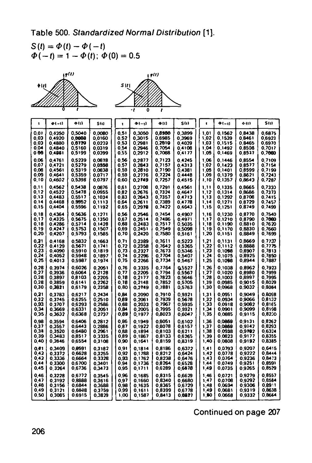
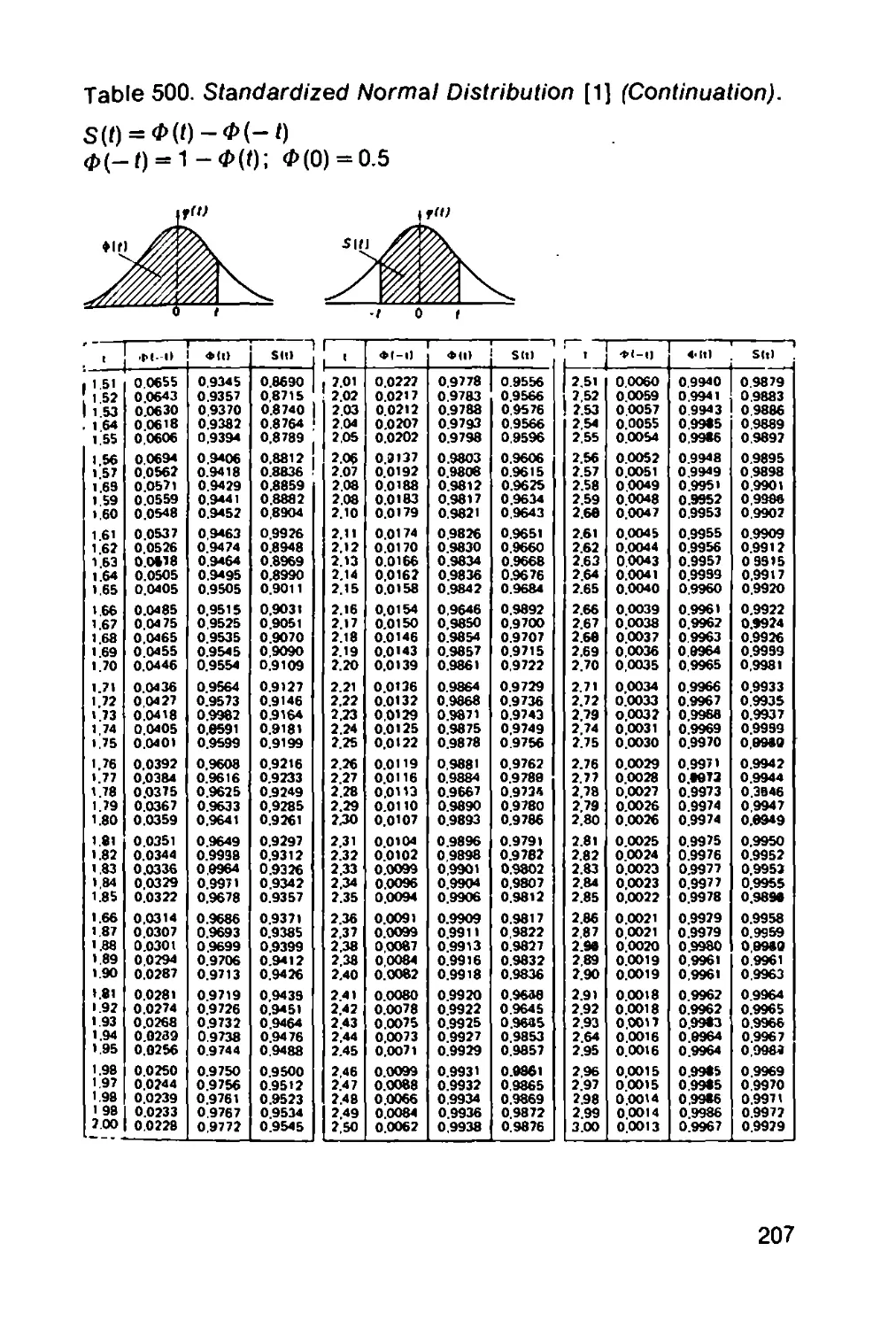
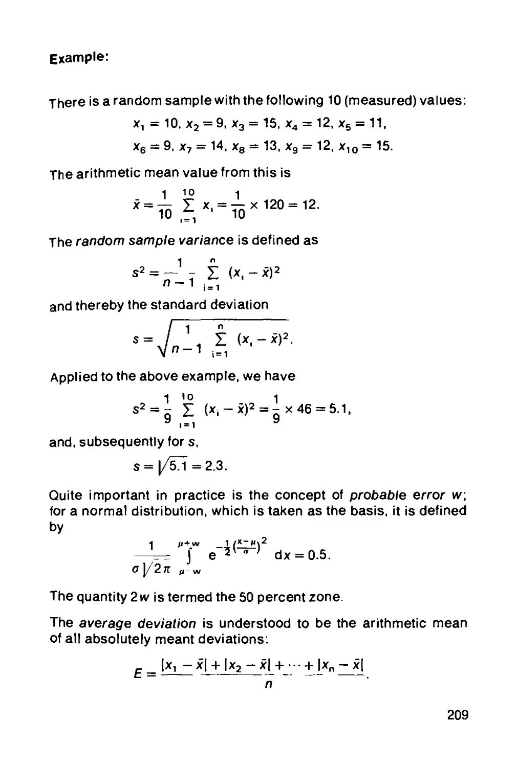
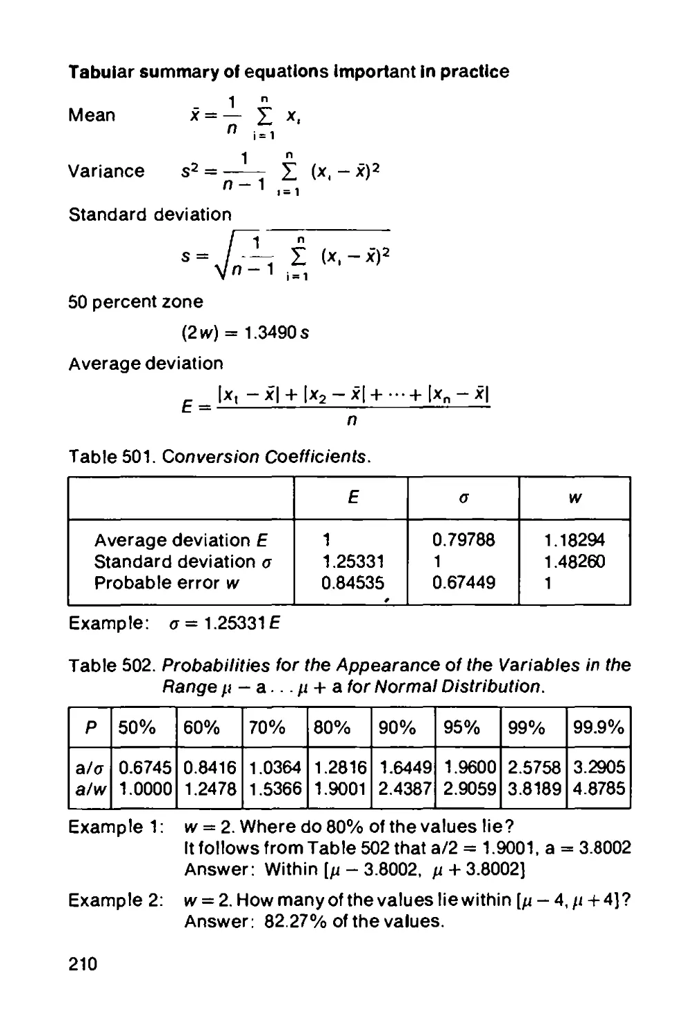
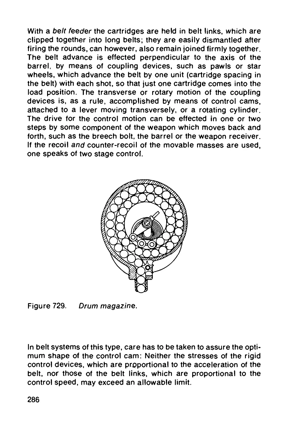
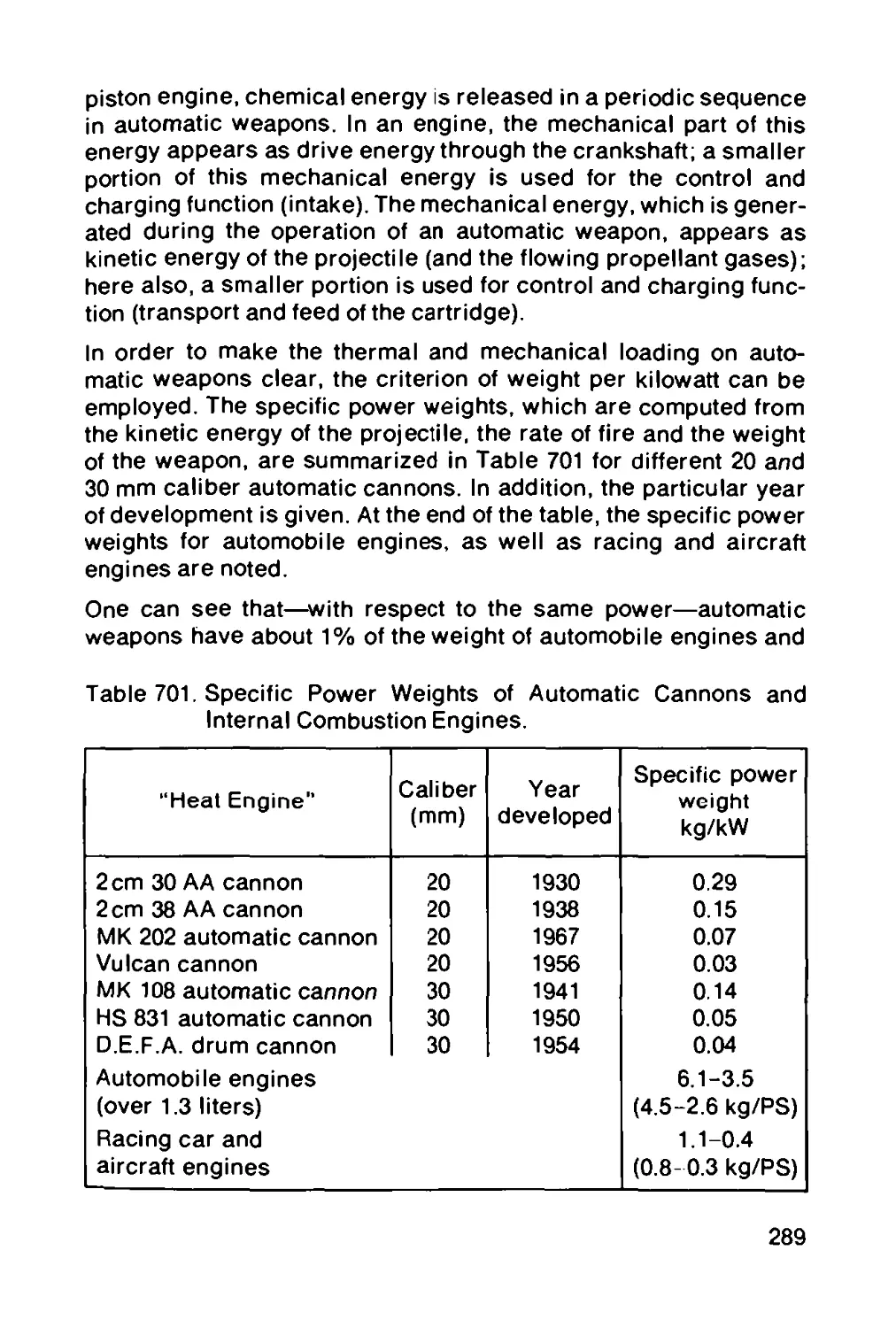
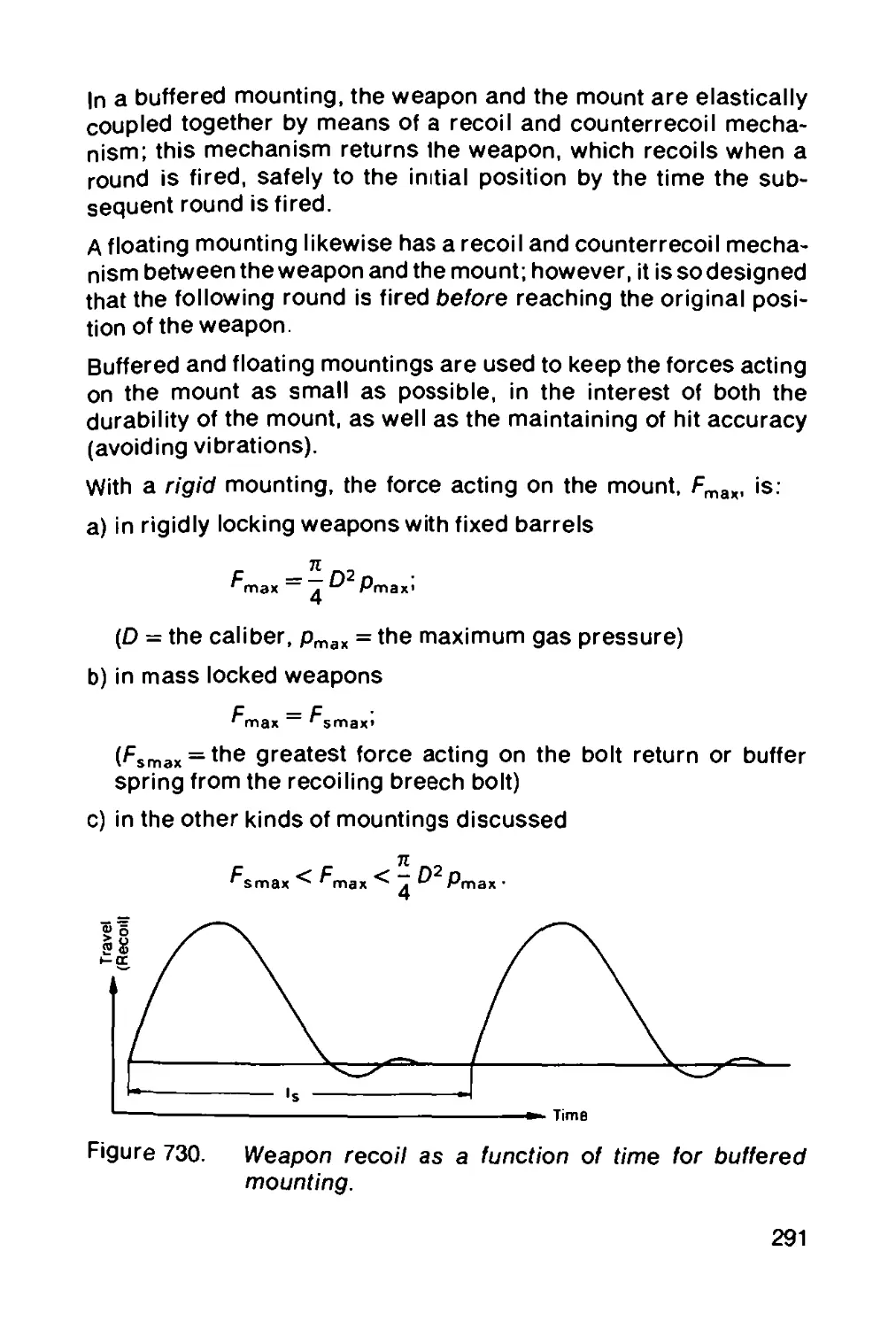
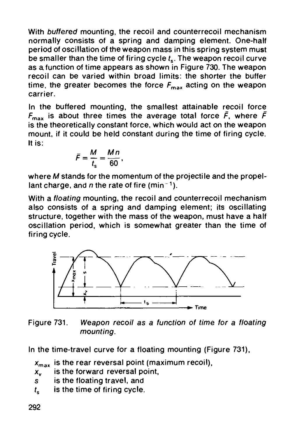
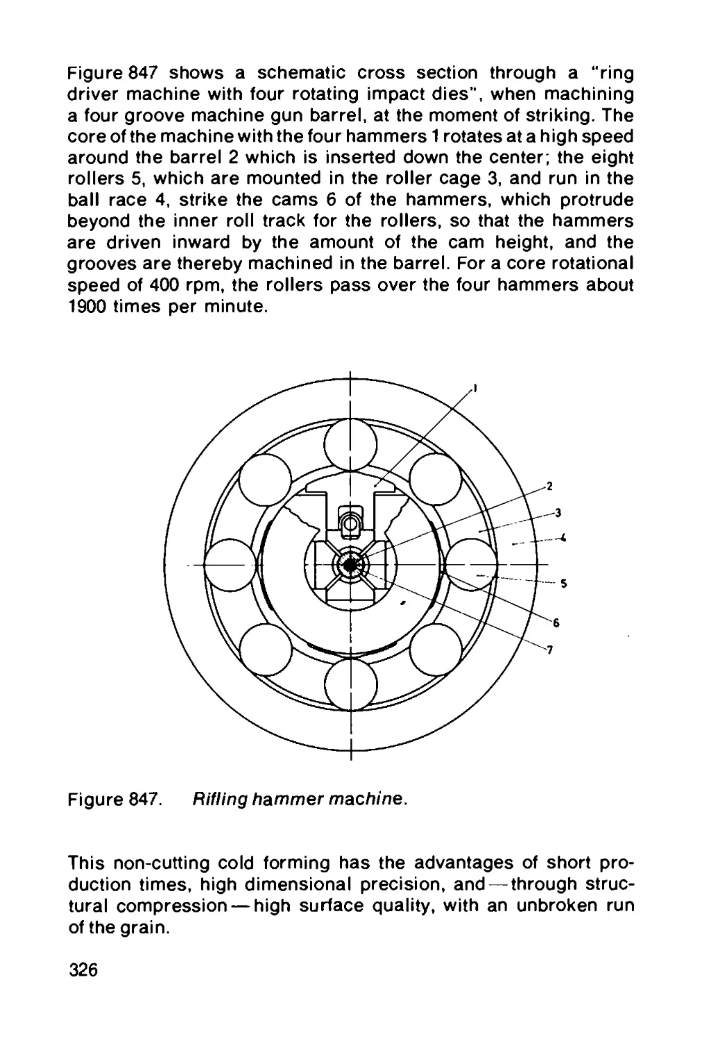
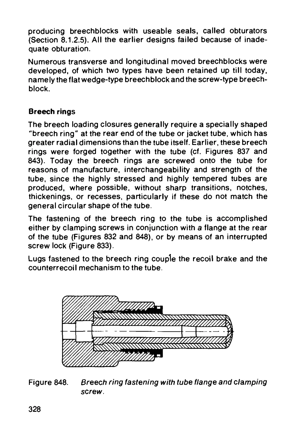
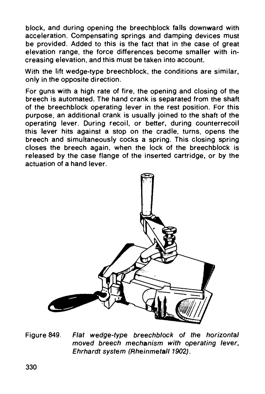
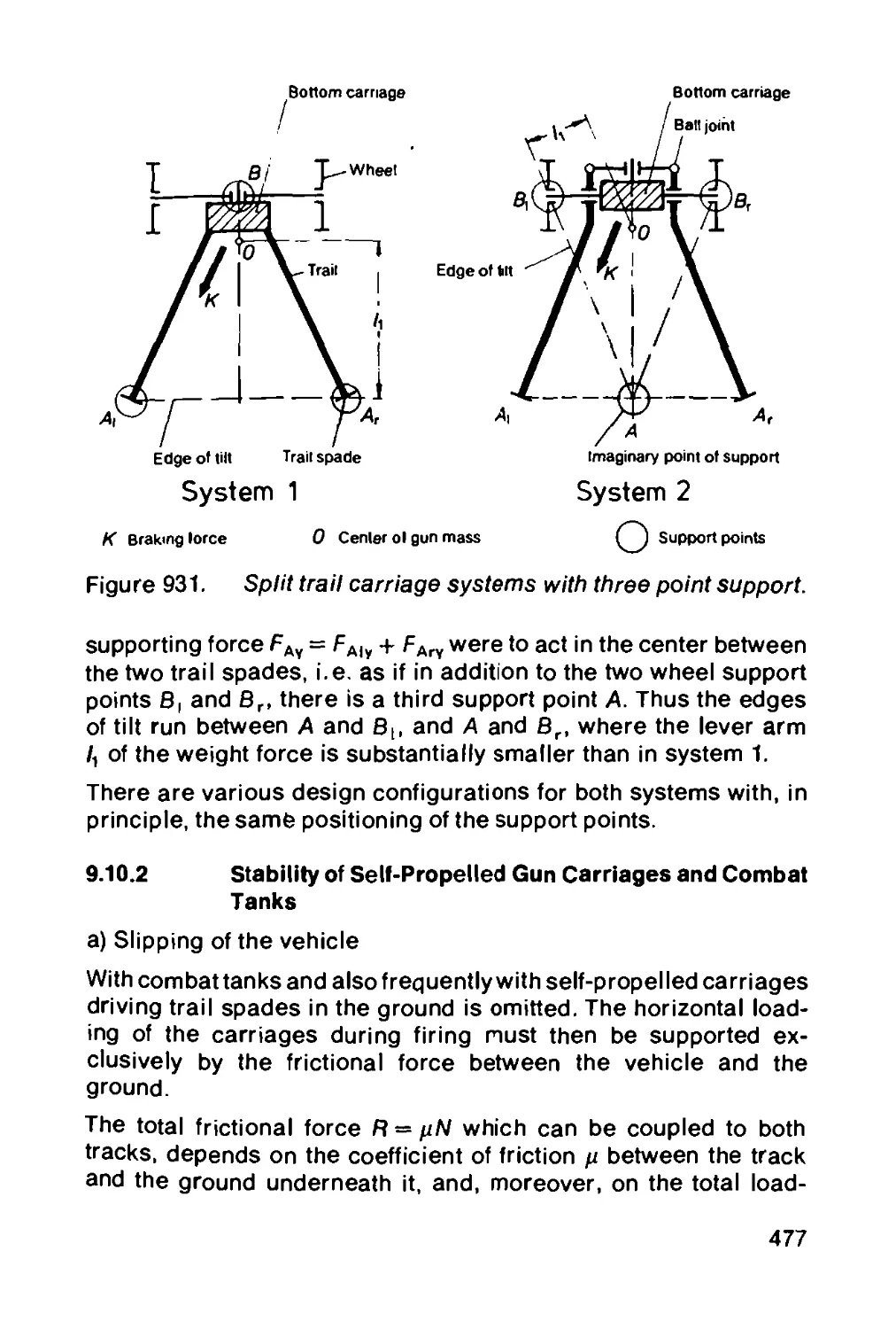
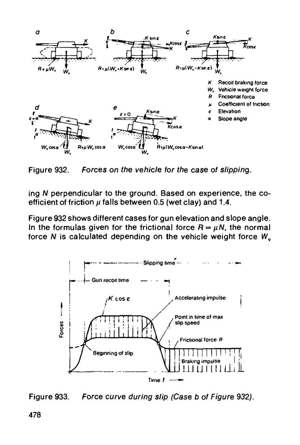
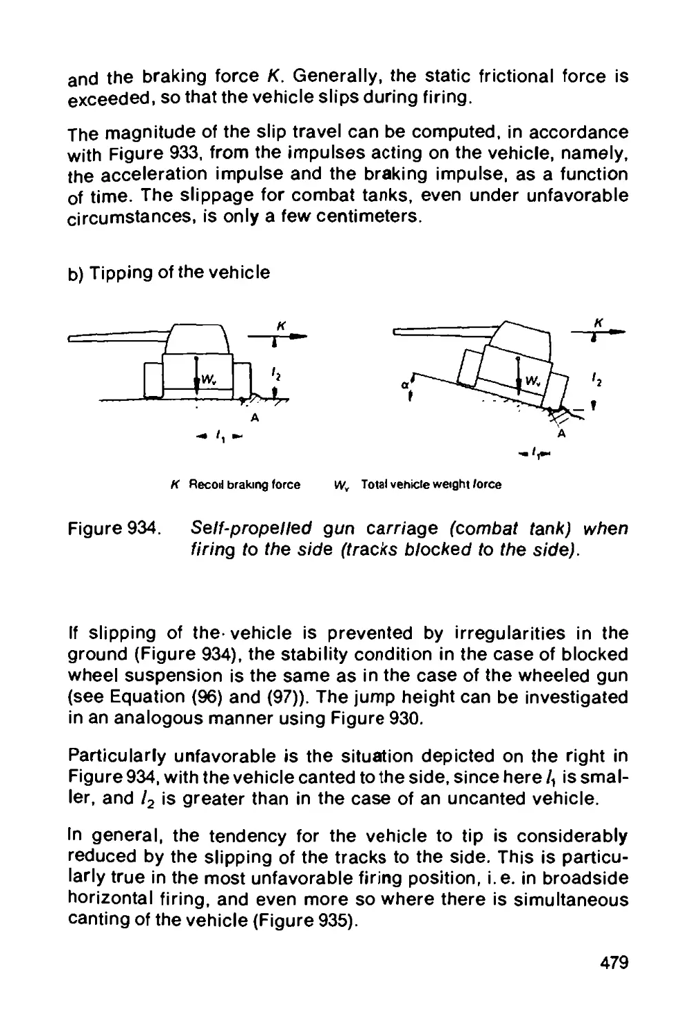
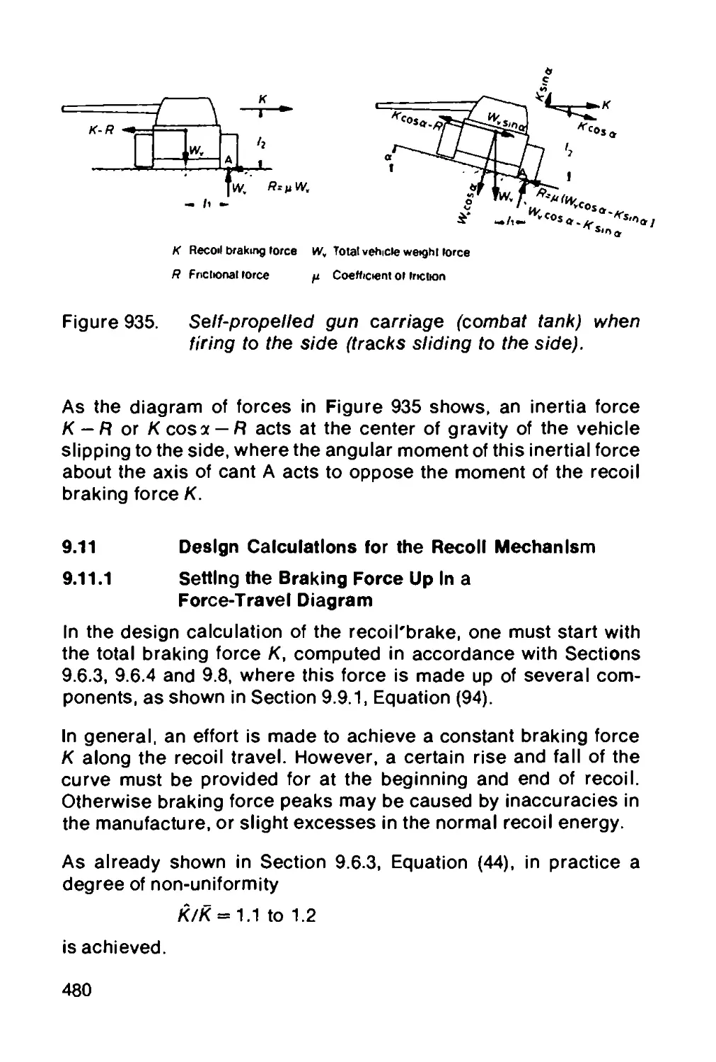
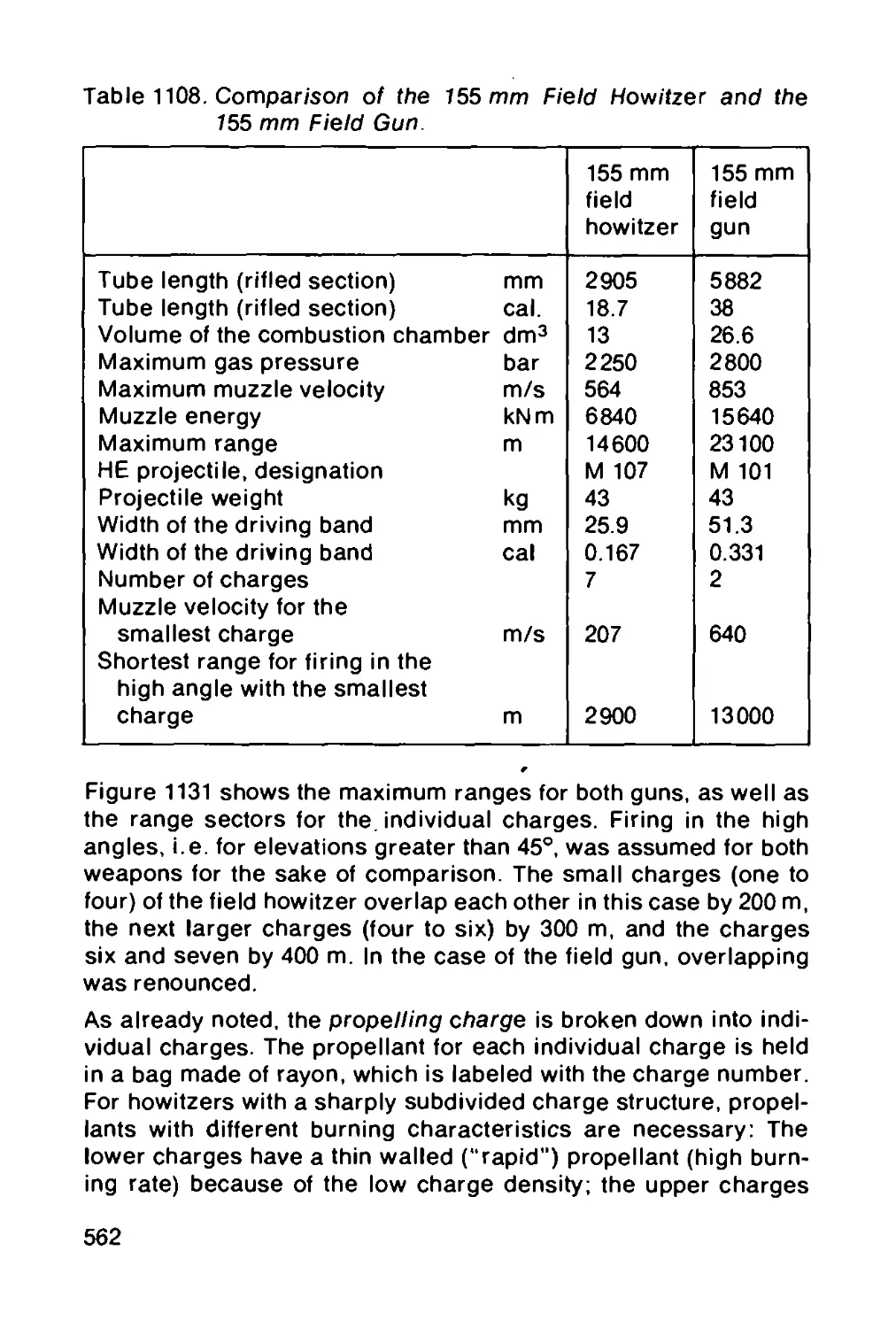
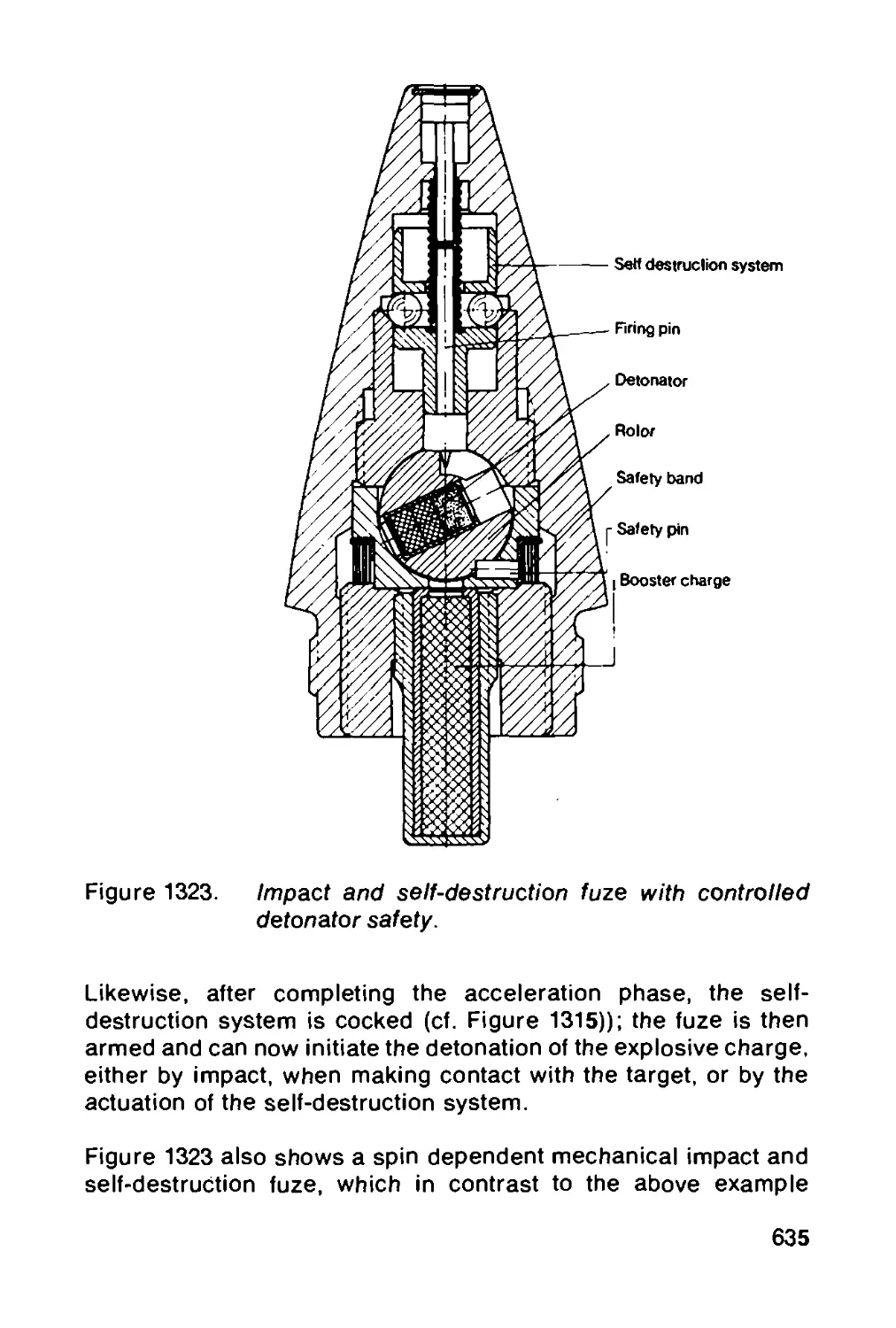
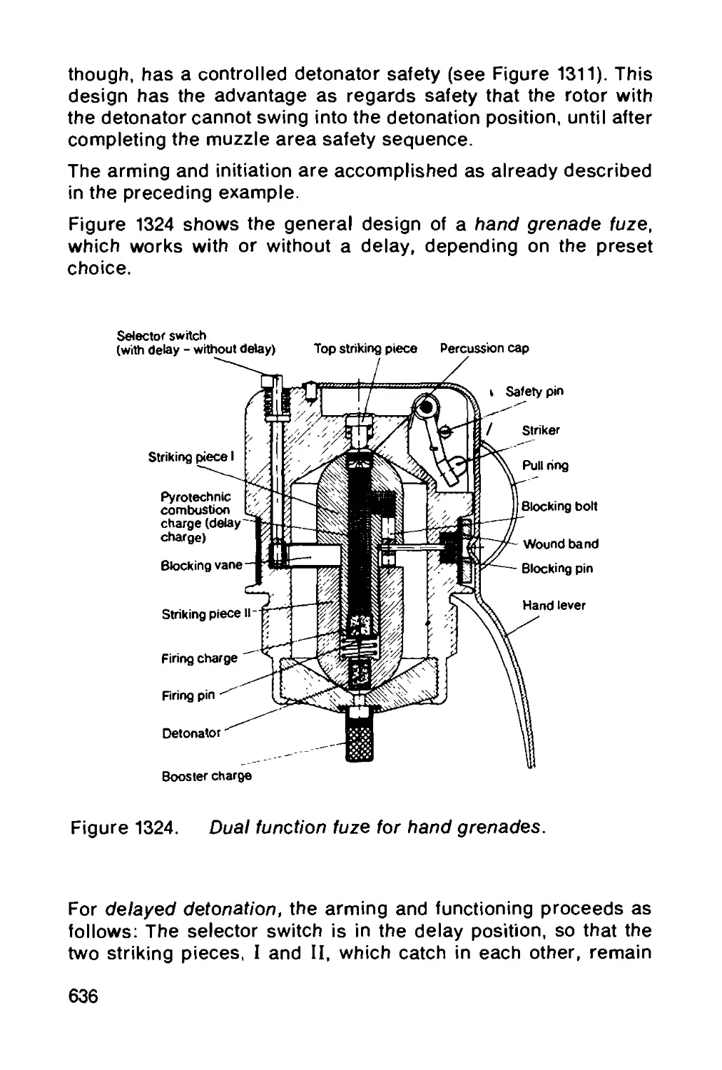
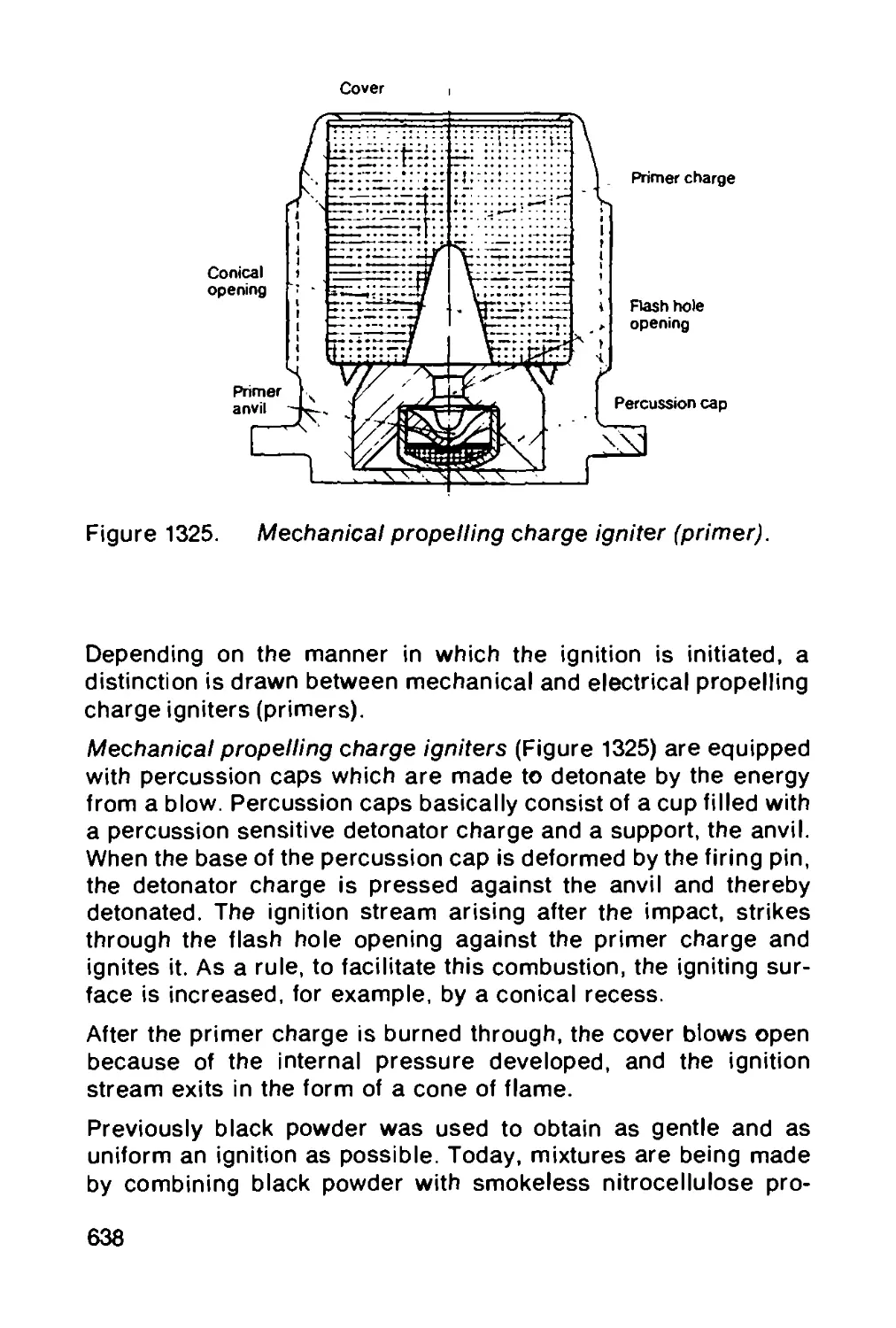
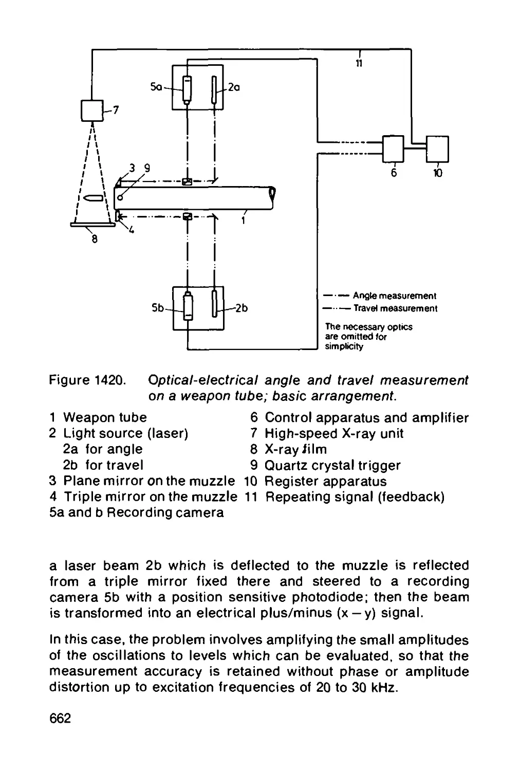
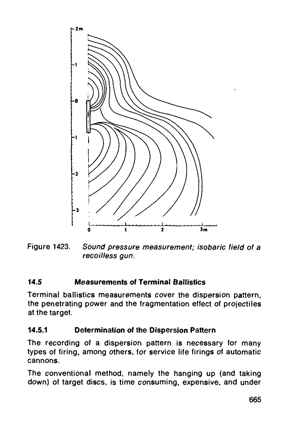
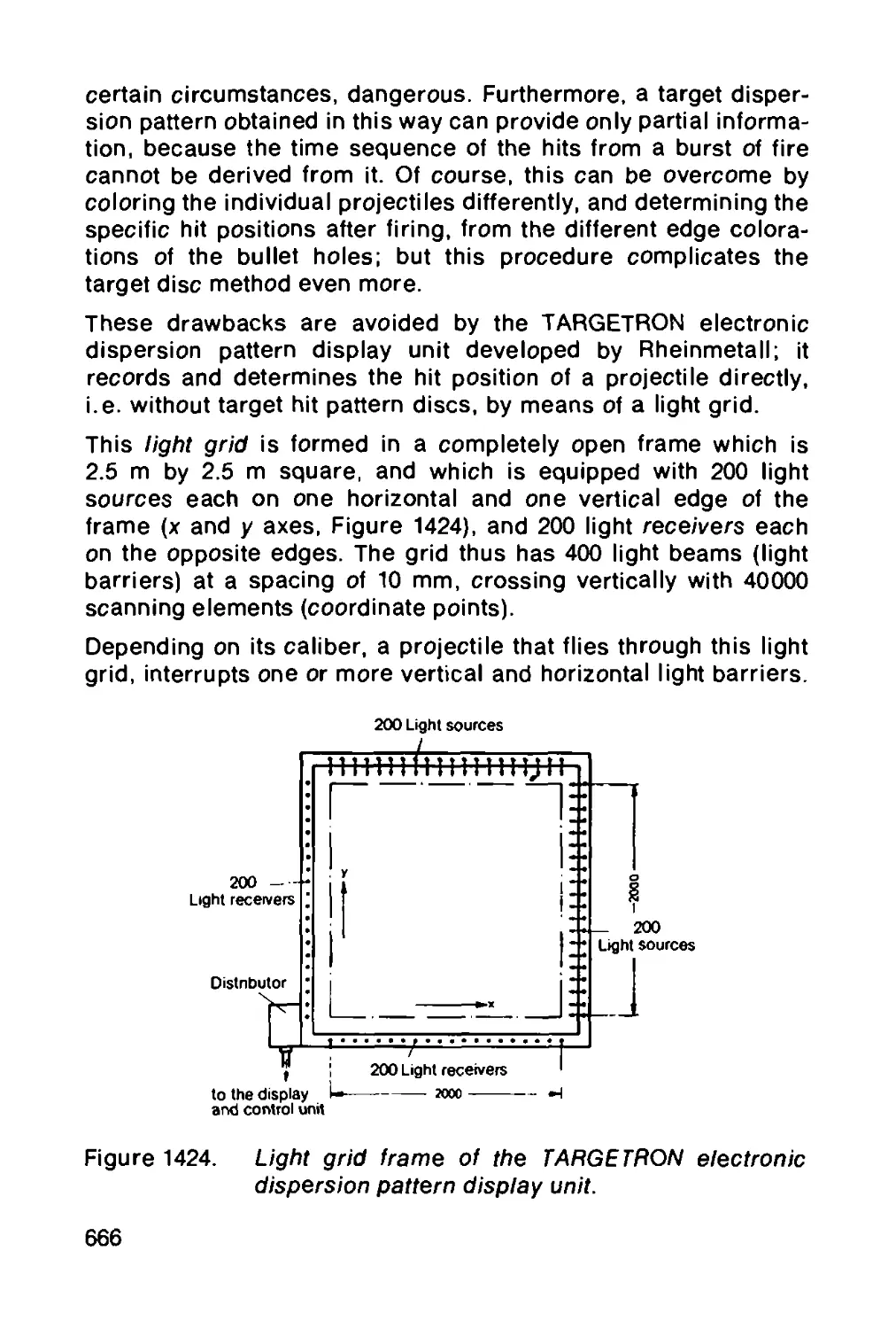
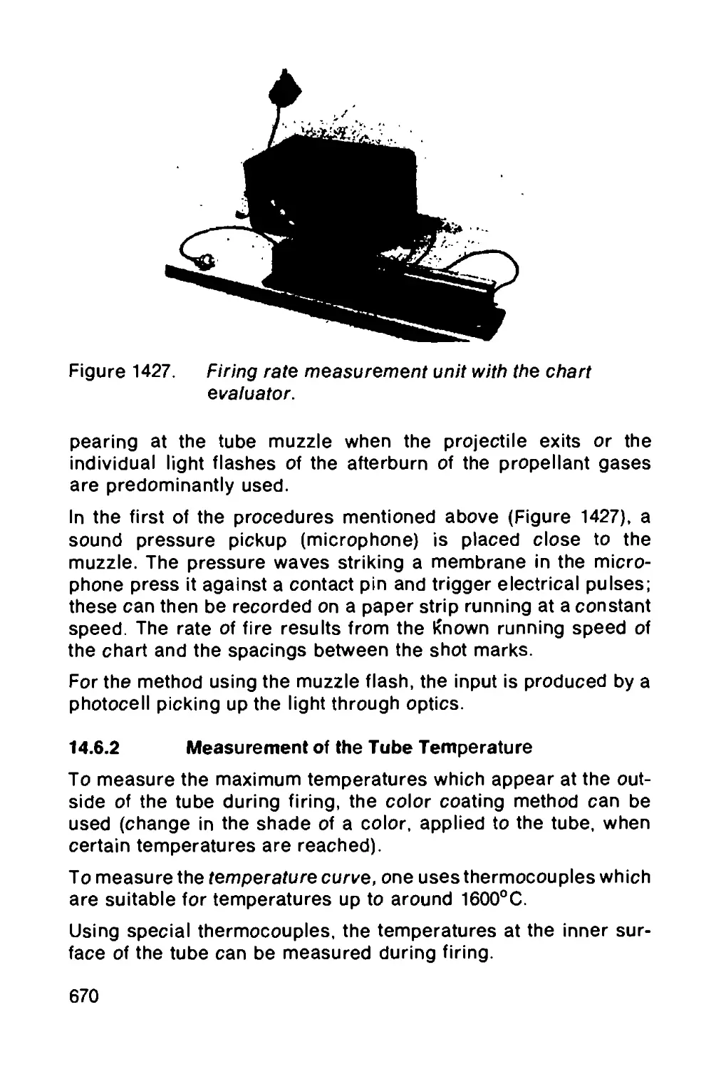
/


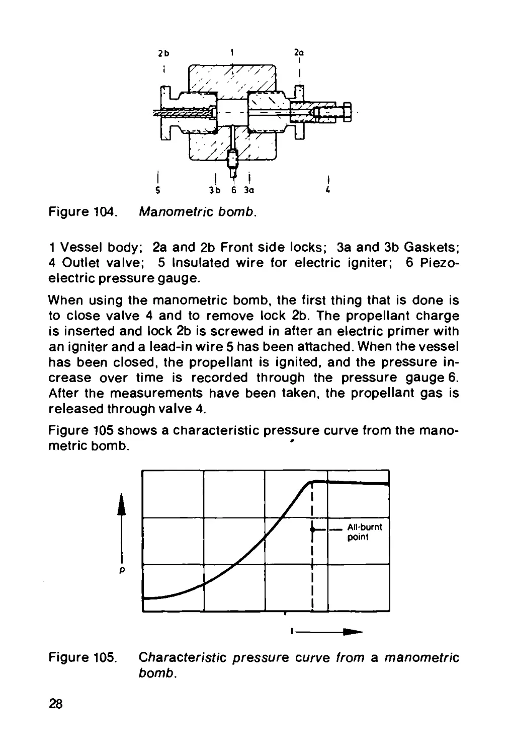
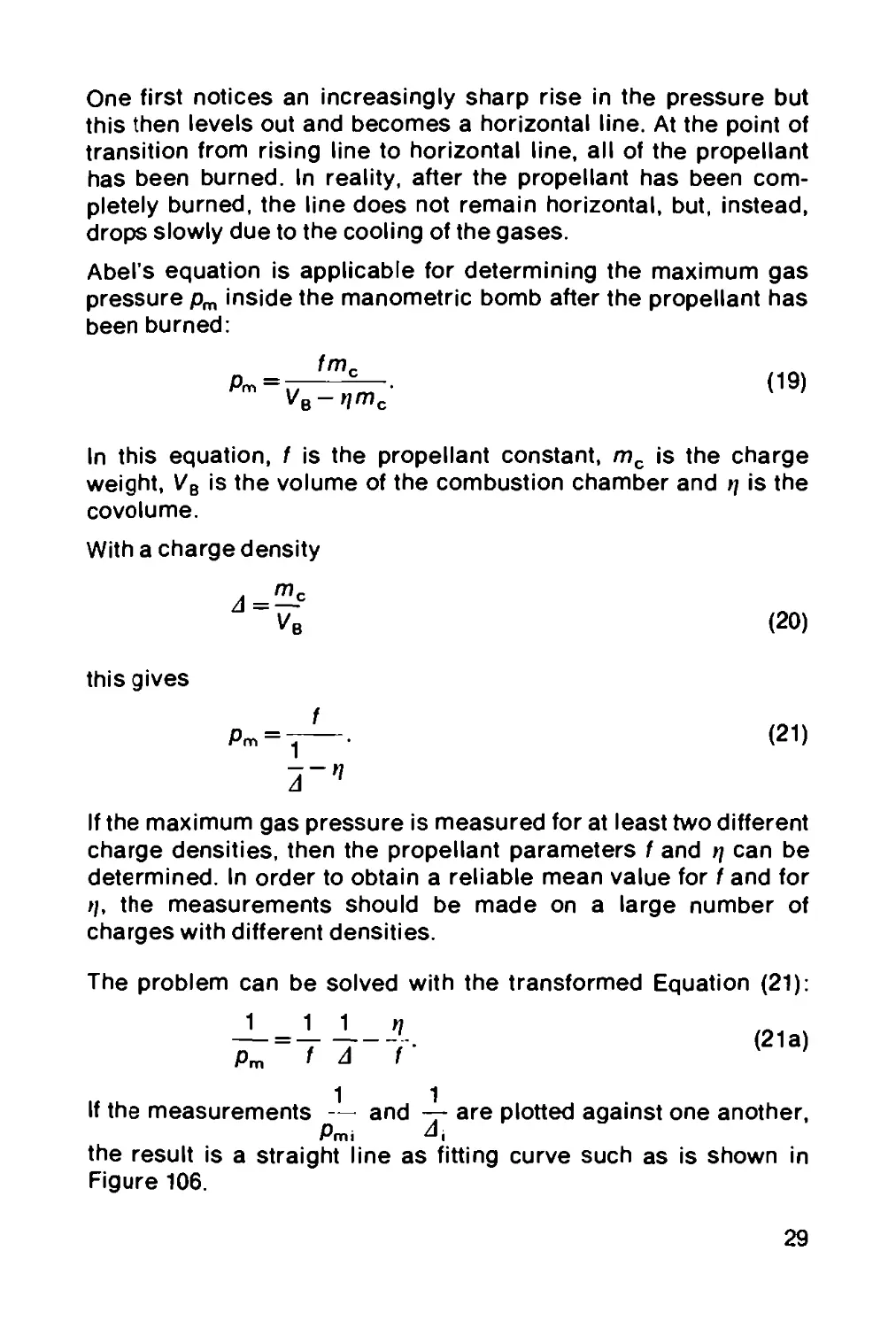


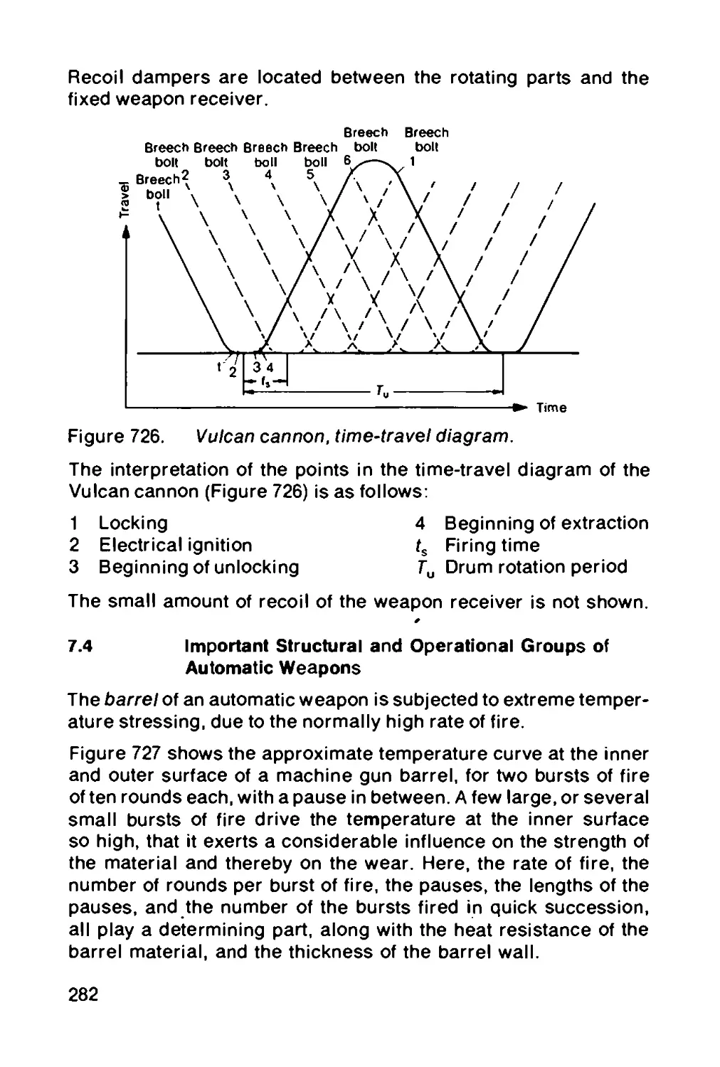


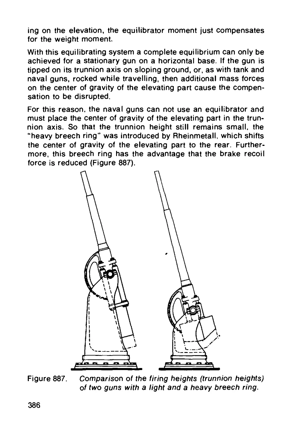
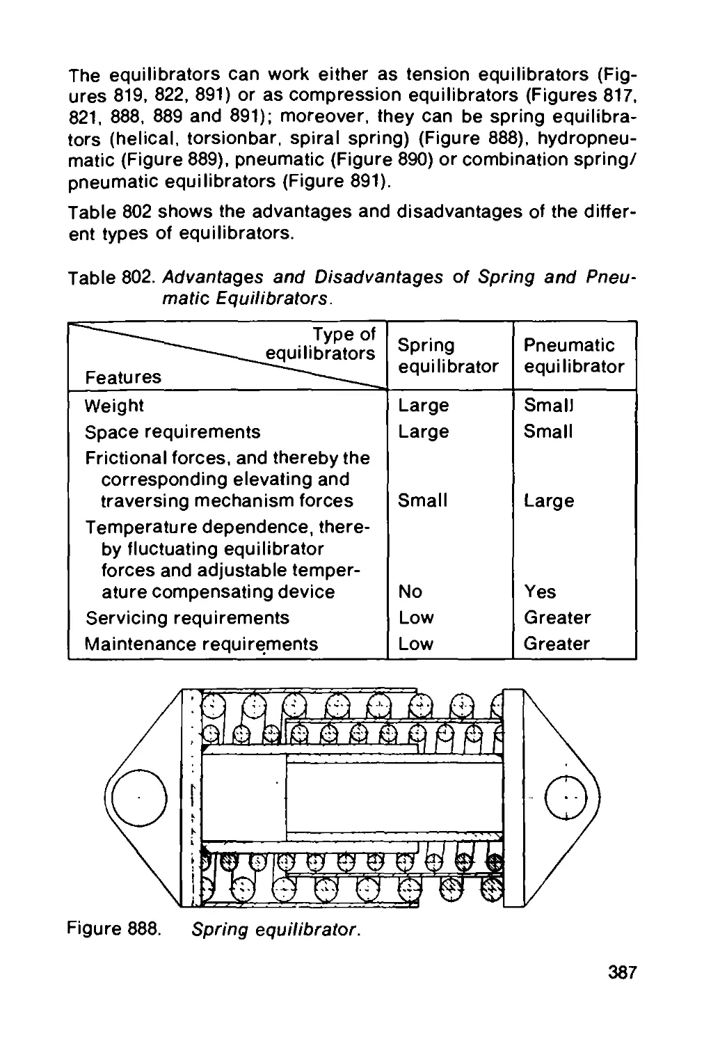
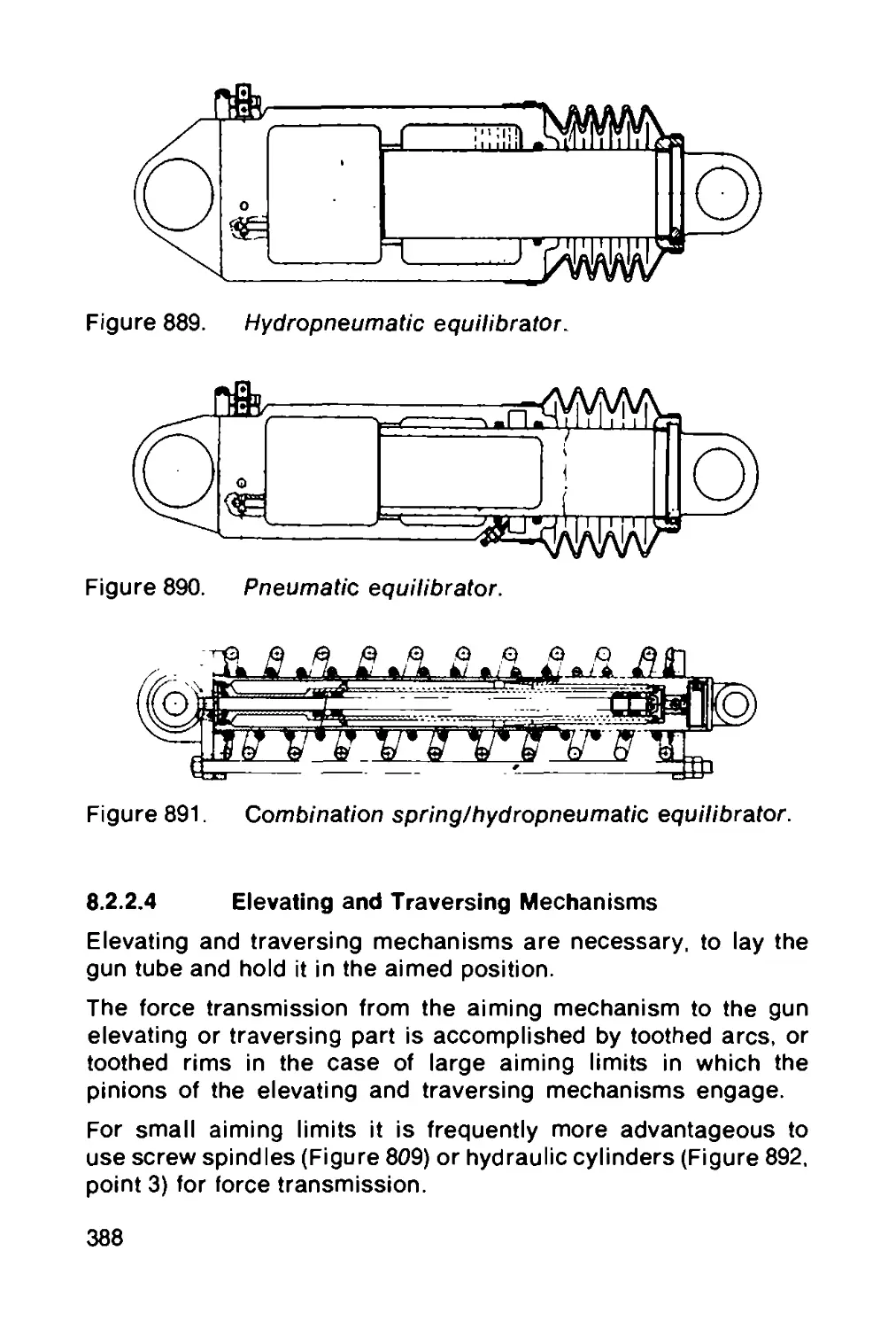


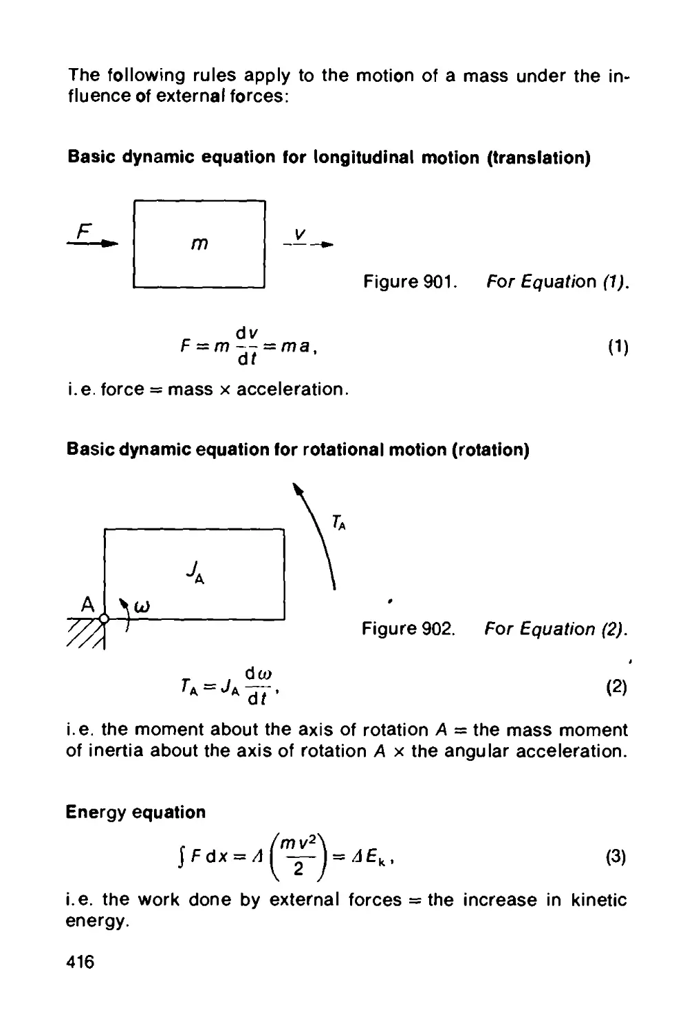


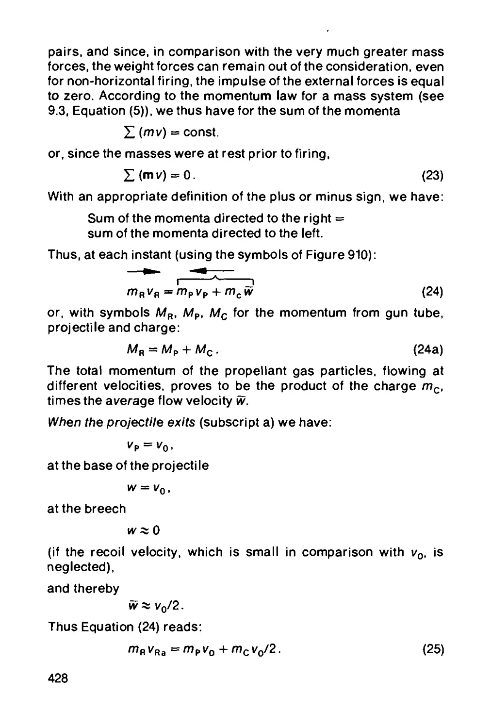


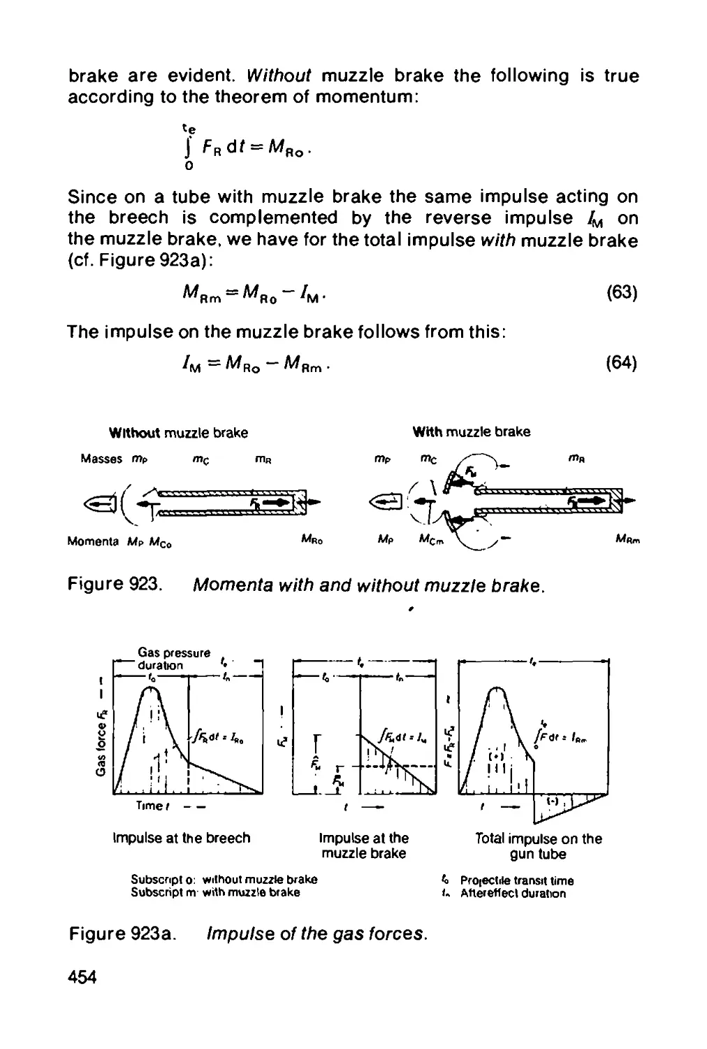
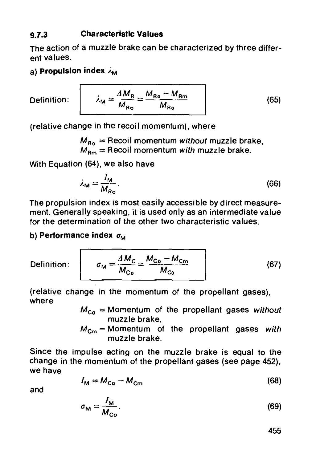


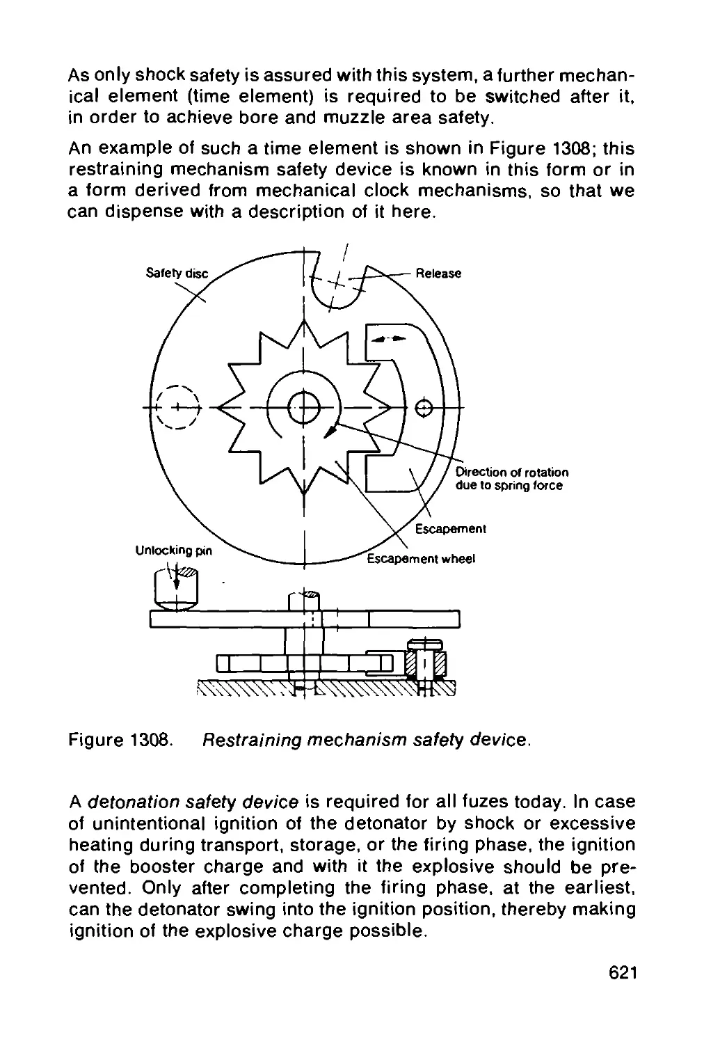
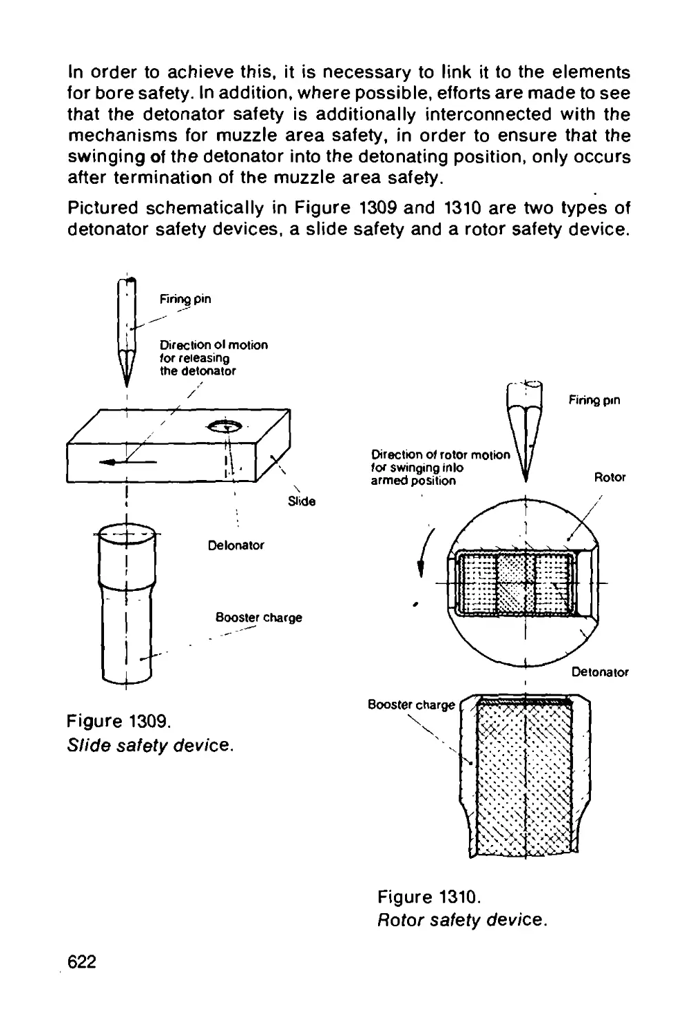
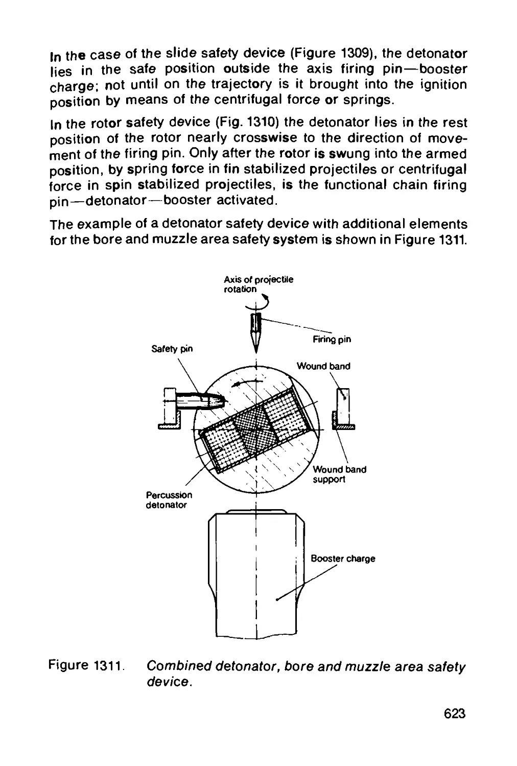
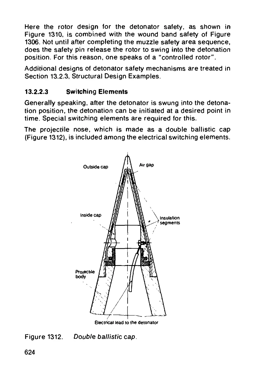


Текст
Handbook
и/ on
Weaponry
Authors (complete chapters or sections) and assistants.
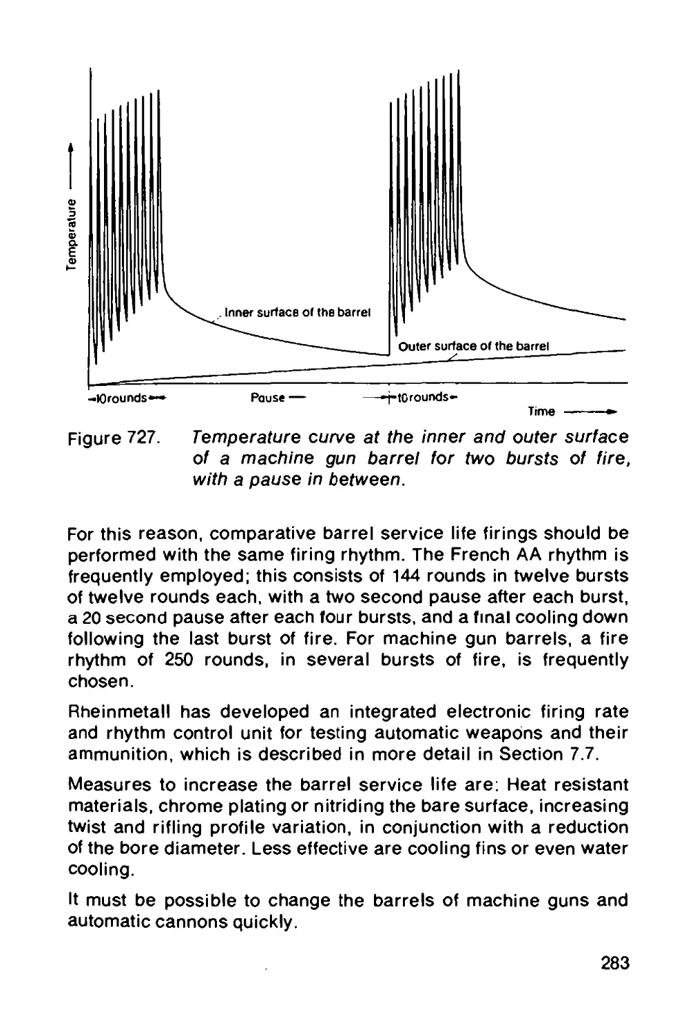
G. Backstein (13), P. Bettermann (14), B. Bisping, D. Boder (8.1.6,
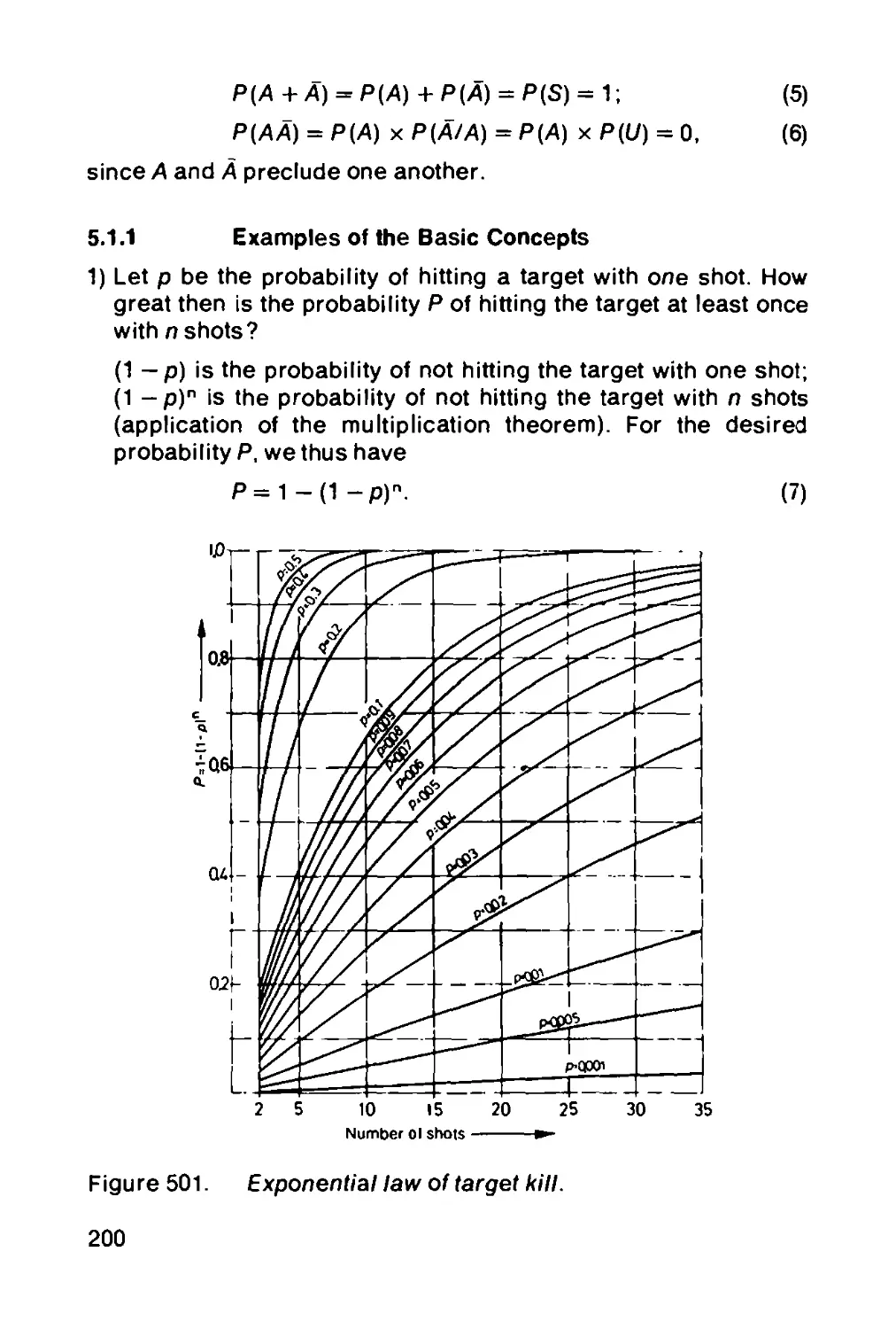
8.1.7, 8.1.8, 10), Dr. S. v. Boutteviiie (9), H. Dechow, A. Fabry,
S. Fischer, F. Flanhardt (7), E. Genter, Dr. R. Germershausen
(1, 2, 12), H. GroBschopf, K. Harbrecht (7), H.-D. Harnau (13),
Dr. S. Harris (6), F. Horn (8, 10), J. Hornfeck, H. Kantner,
D. Karius, Dr. E. Kokott (6), W. Kuppe (6), Dr. K. F. Leisinger,
F. Mayer (14), Dr. E. Melchior (2, 3, 15), M. Moll, J. Prochnow
(11.5), H. Renner, H. Reuschel (3, 4, 5), R. Romer (11), W. Rottges,
H.-J. Rubsam, E. Schaub, H.-J. Schiewer (5), D. Schuh, F. Woyt.
General direction: Dr. R. Germershausen
Readers and redactors: Dr. S. v. Boutteviiie, E. Schaub
IV
Handbook on Weaponry
First English Edition
All rights reserved
Copyright 1982 by Rheinmetall GmbH, Dusseldorf
Rheinmetall GmbH, P.O.B. 6609, D-4000 Dusseldorf
Design and presentation: riw Rheinmetall Industriewerbung
GmbH, Dusseldorf
Overall production: Bronners Druckerei Breidenstein GmbH,
Frankfurt a.M.
Preface
Following the tradition of the "Taschenbuch fur den Artilleristen",
which first appeared in 1936, we published in 1972 a new edition
entitled “Waffentechnisches Taschenbuch". Since then this hand-
book has been reprinted five times.
As a result of numerous requests by our partners abroad we
have decided to publish this book also in English as "Handbook
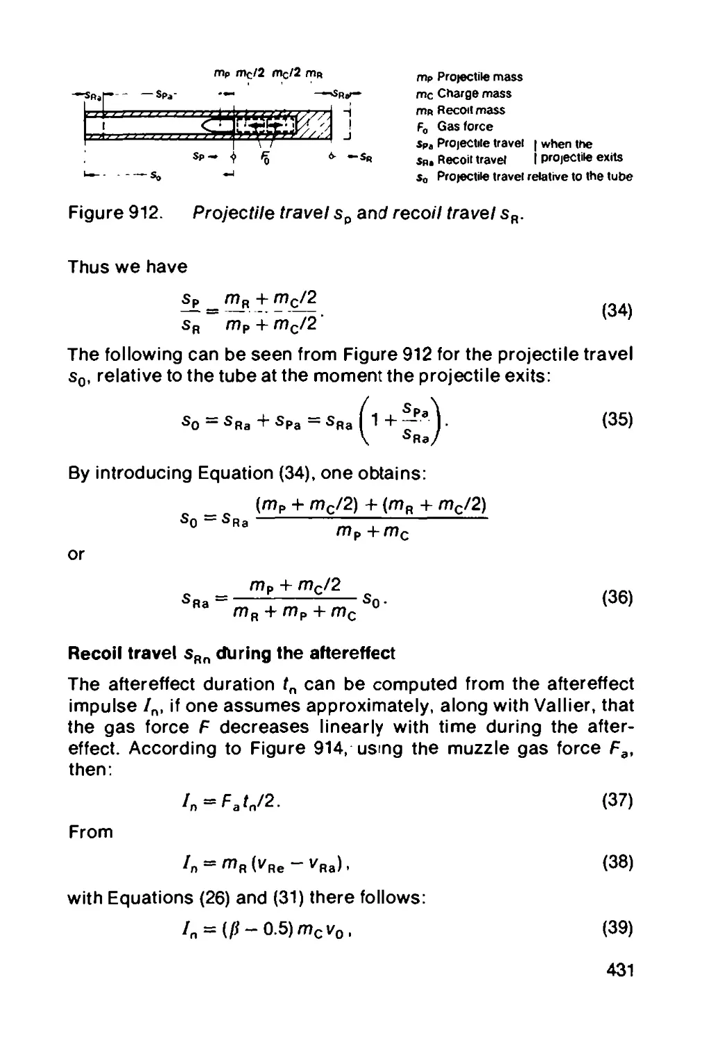
on Weaponry". The present English edition is a translation of the
fifth German edition of 1980, various passages of which were
revised as compared with the first edition. We have tried to adapt
the translation—in particular with regard to the technical terms—
to the expressions commonly used in the English-speaking
countries.
The progress made in the meantime in military engineering will
be taken into account in any further revised edition.
We hope that the English edition of our handbook will meet with
the same interest as has been found by the German editions.
Dusseldorf, February 1982
Rheinmetall GmbH
V
Table of Contents
RHEINMETALL—A Military Technology Company................ XIX
1 EXPLOSIVES.................................... 1
R. Germershausen
1.1 General....................................... 1
1.2 Classification of explosives.................. 5
1.3 Propellants................................... 9
1.3.1 Gun propellants.............................. 9
1.3.1.1 Nitrocellulose propellants................... 9
1.3.1.2 Propellants without a solvent............... 10
1.3.1.2.1 Double base propellants..................... 10
1.3.1.2.2 Triple base propellants..................... 11
1.3.2 Rocket propellants.......................... 12
1.3.2.1 Liquid propellants.......................... 12
1.3.2.2 Solid propellants........................... 16
1.3.2.3 Lithergols ................................. 18
1.3.3 Thermochemistry............................. 19
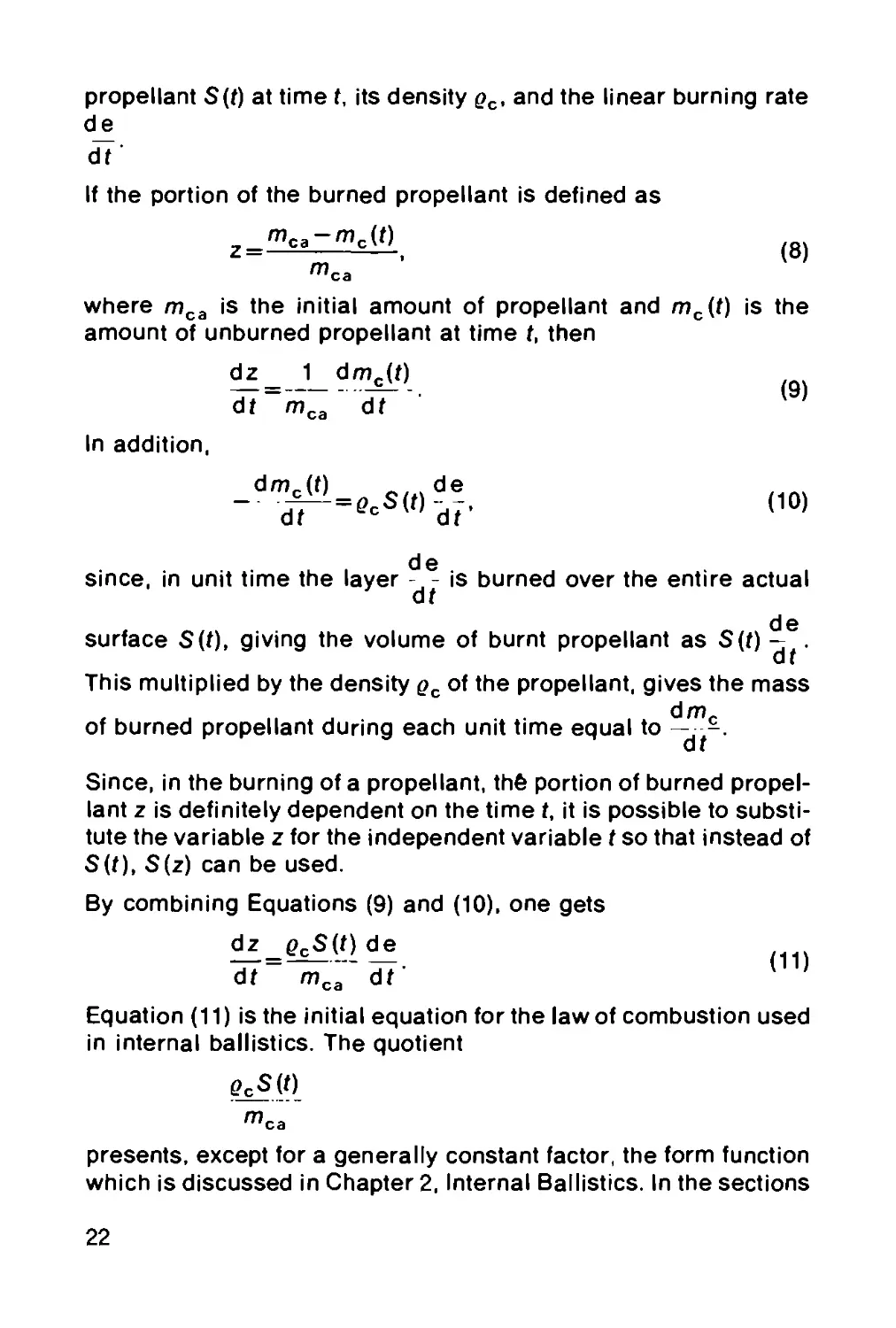
1.3.4 Burning characteristics of propellants..... 21
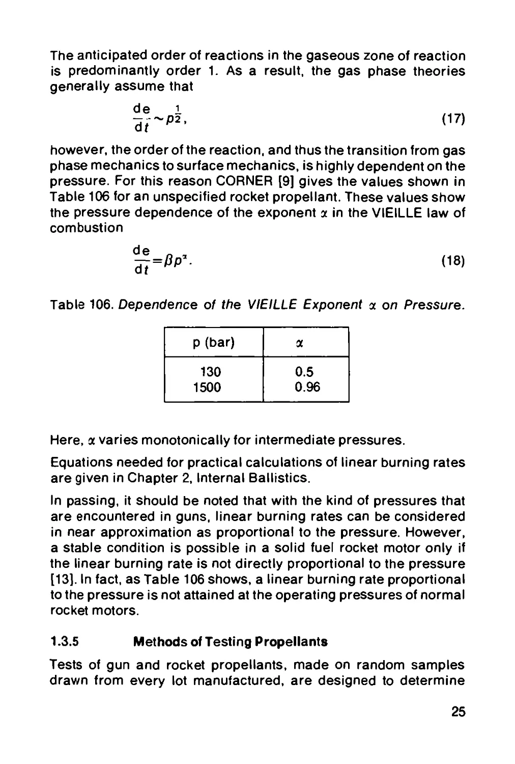
1.3.5 Methods of testing propellants.............. 25
1.4 Explosives................................. 32
1.4.1 Military explosives. ....................... 32
1.4.2 Commercial explosives ...................... 37
1.4.3 Initiating (detonating) explosives.......... 39
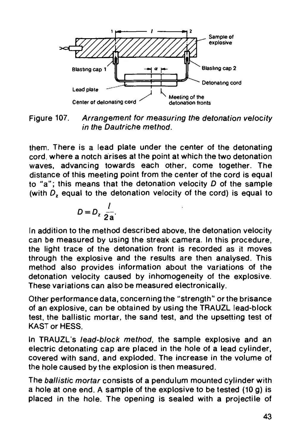
1.4.4 Testing methods for explosives.............. 41
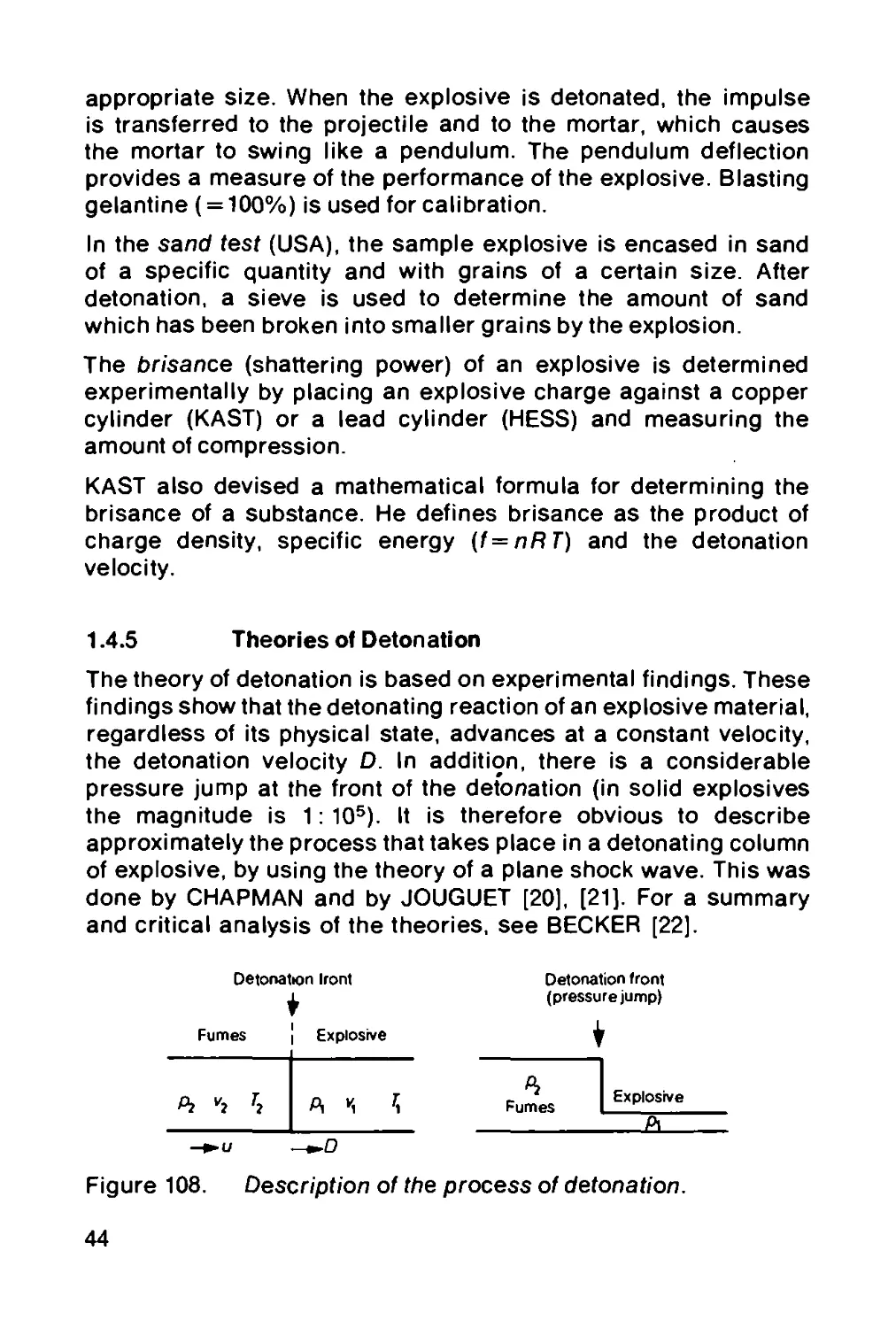
1.4.5 Theories of detonation ..................... 44
1.4.6 Military use of explosives.................. 48
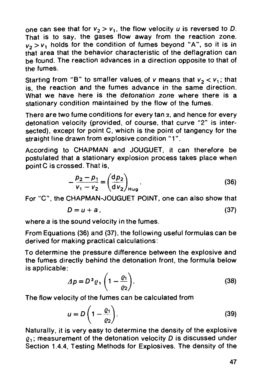
1.4.6.1 Pressure effects of explosive charges...... 48
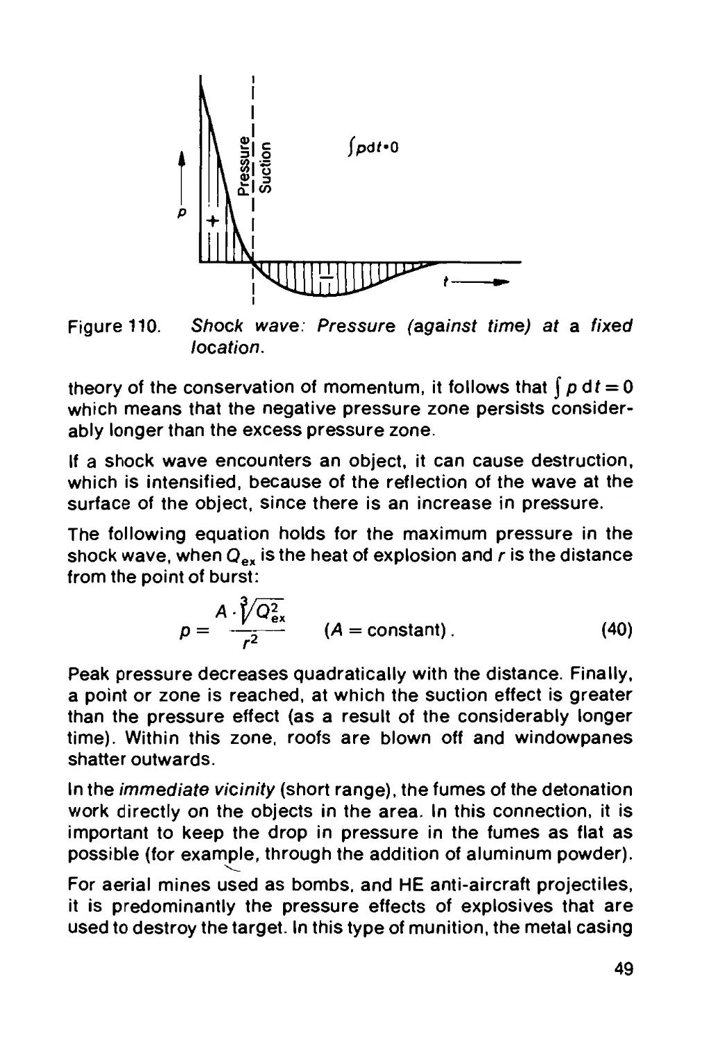
1.4.6.2 Fragmentation charges....................... 50
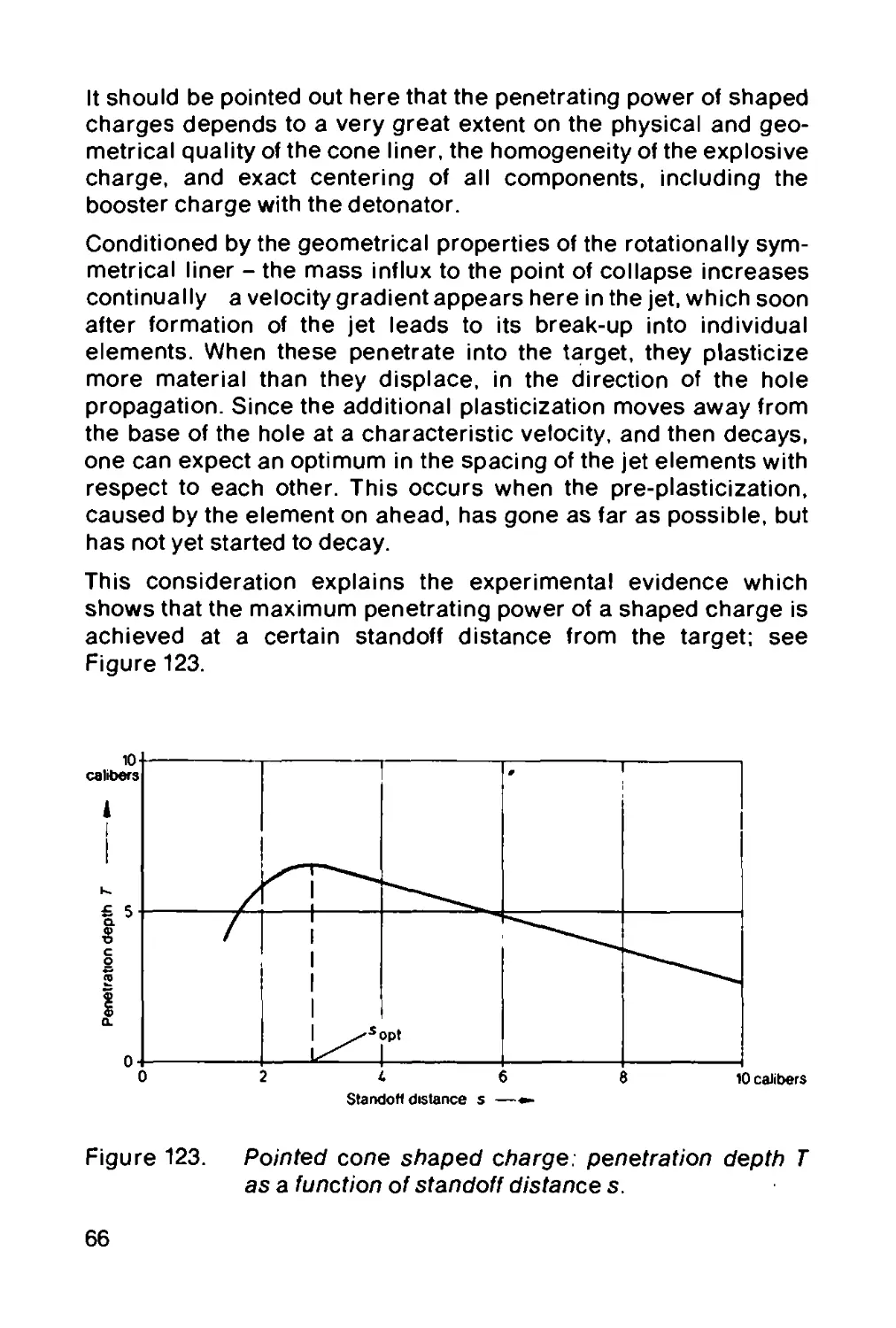
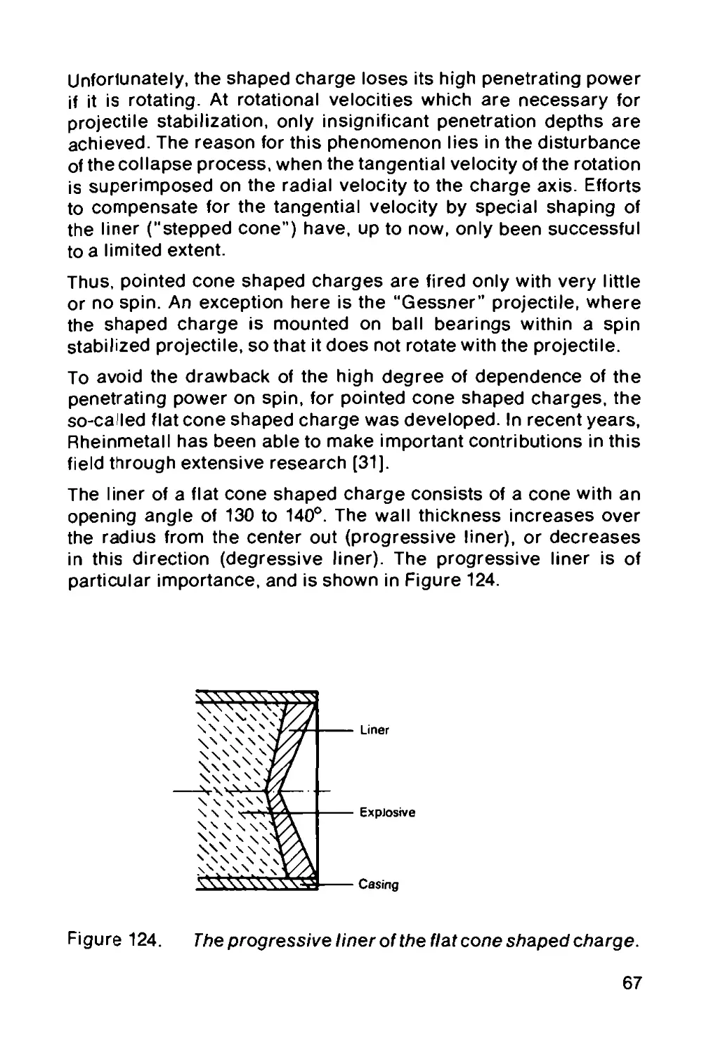
1.4.6.3 Shaped charges.............................. 60
1.5 Pyrotechnic compositions .................... 71
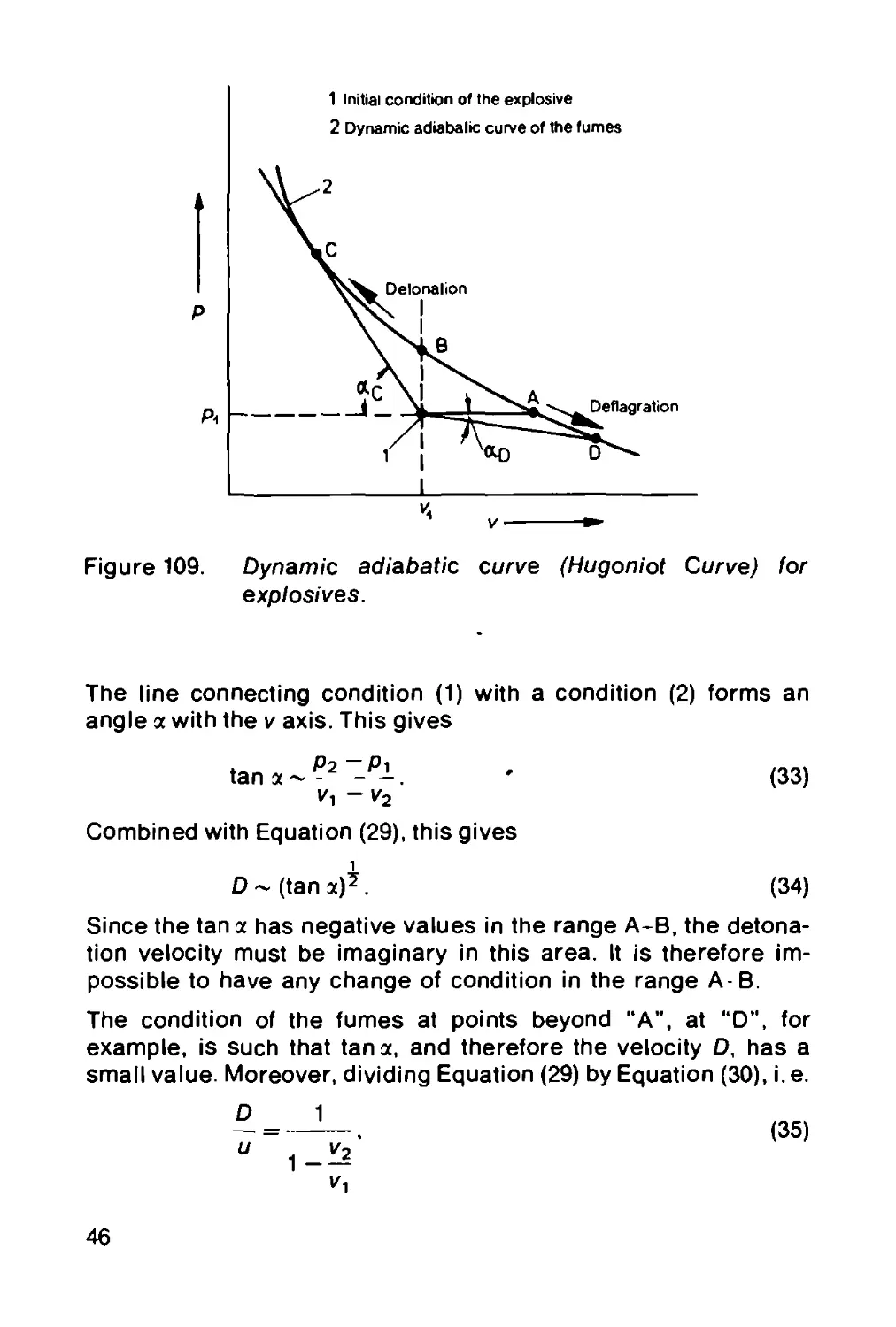
1.5.1 Illuminating compositions .................. 71
1.5.2 Signal and screening smoke generating
compositions............................... 72
1.5.3 Noise producing compositions................ 73
1.5.4 Incendiary compositions..................... 73
1.5.5 Other compositions.......................... 74
VI
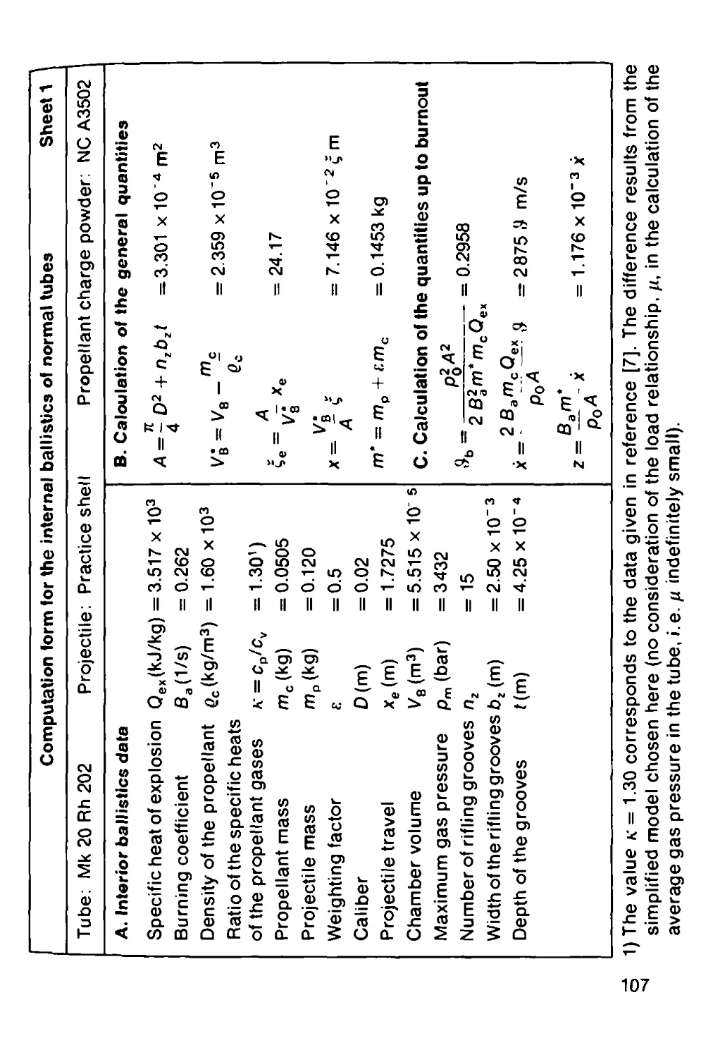
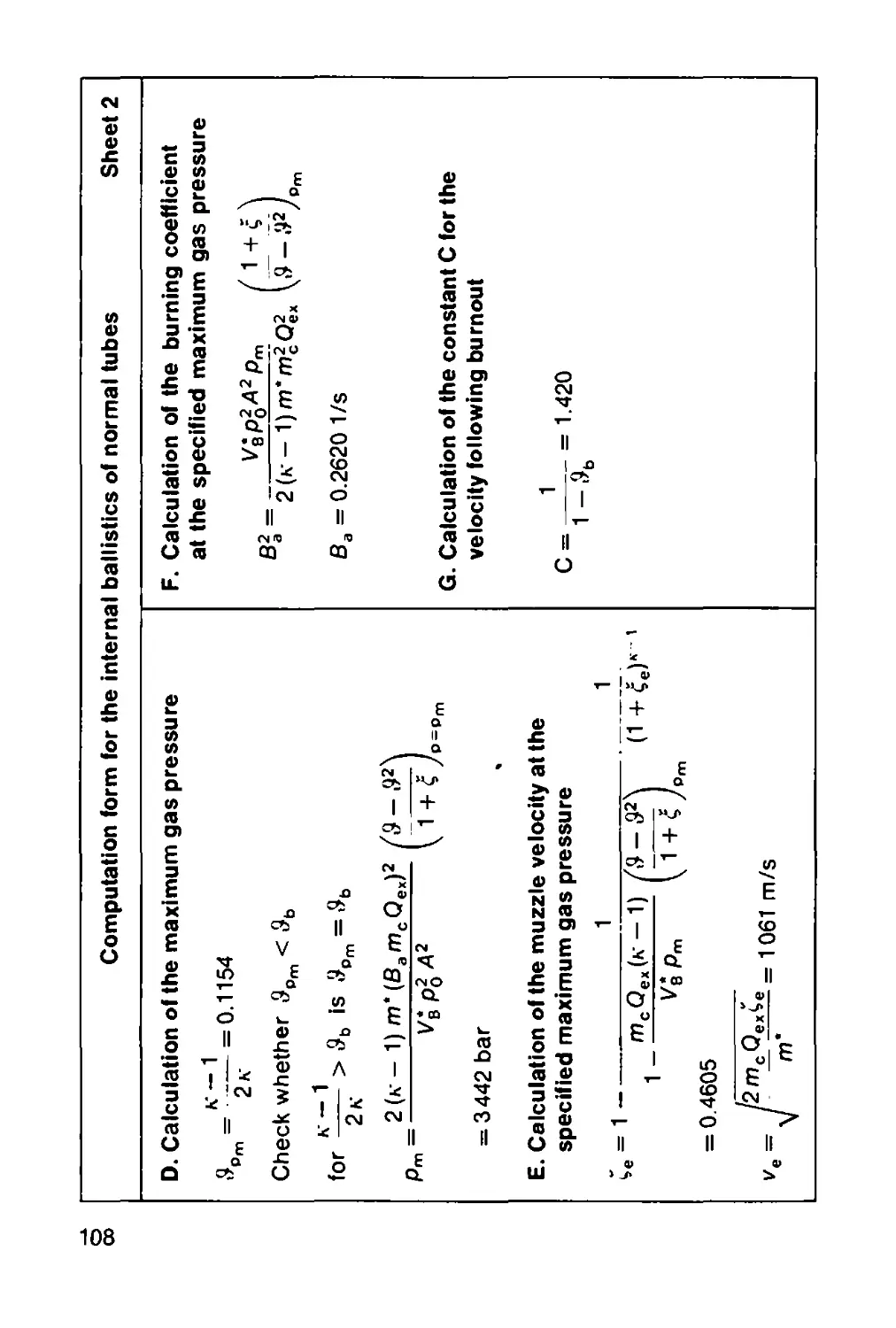
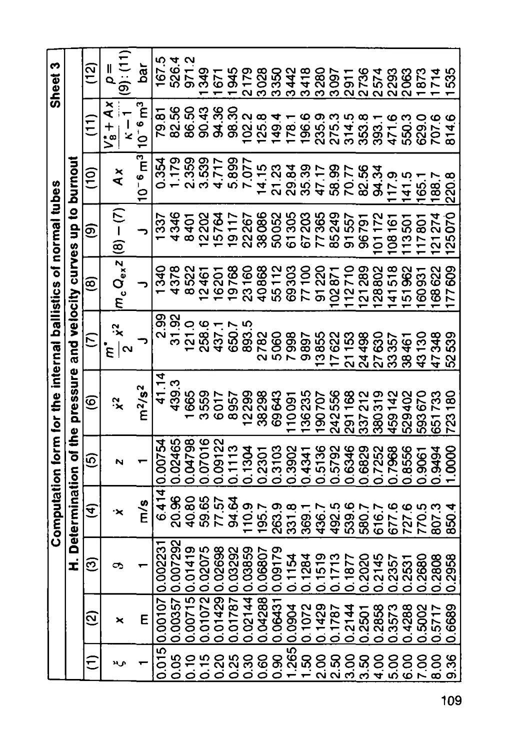
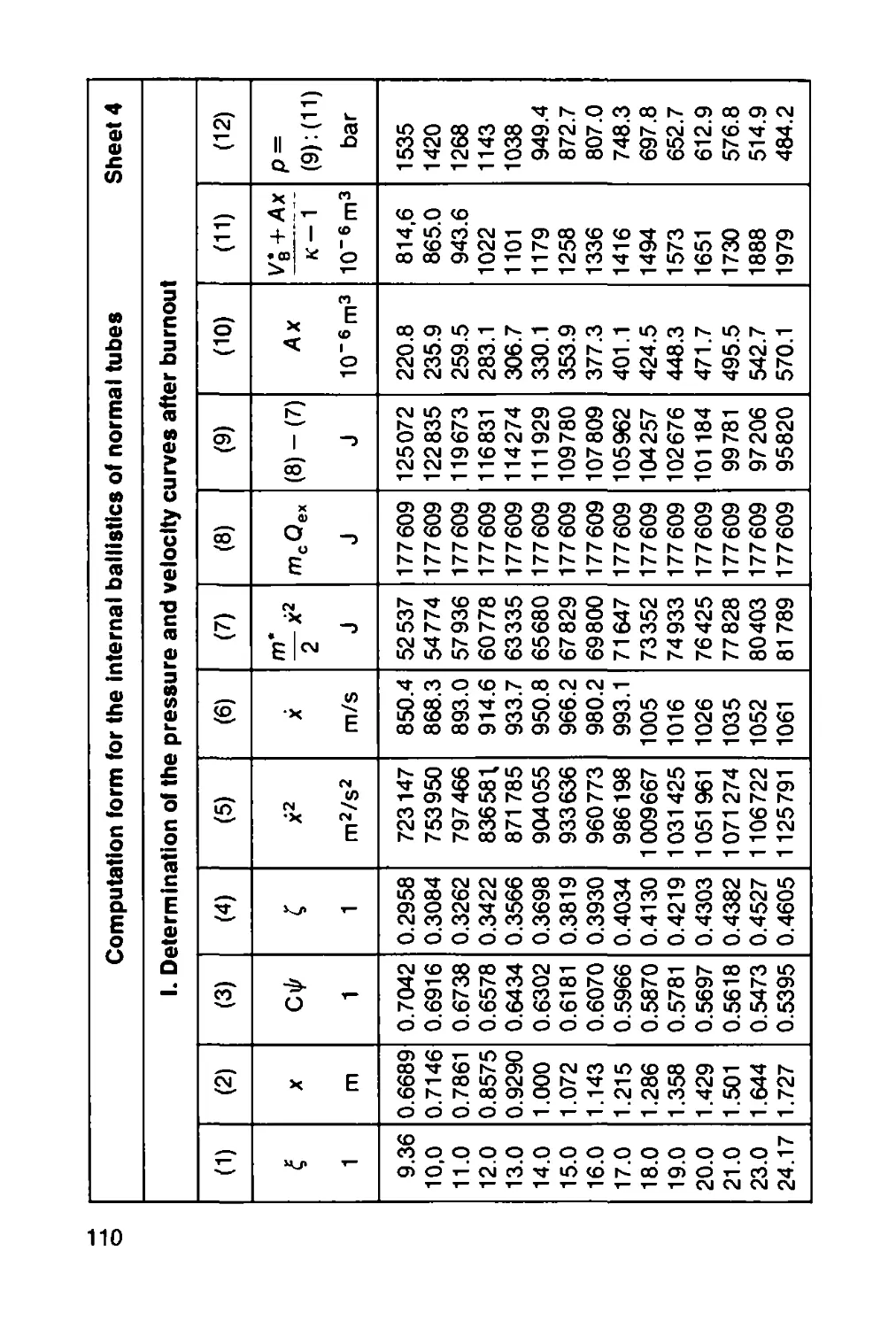
2 INTERNAL BALLISTICS ........................... 77
R. Germershausen and E. Melchior
2.1 Internal ballistics of guns.................... 77
2.1.1 Gun construction............................... 78
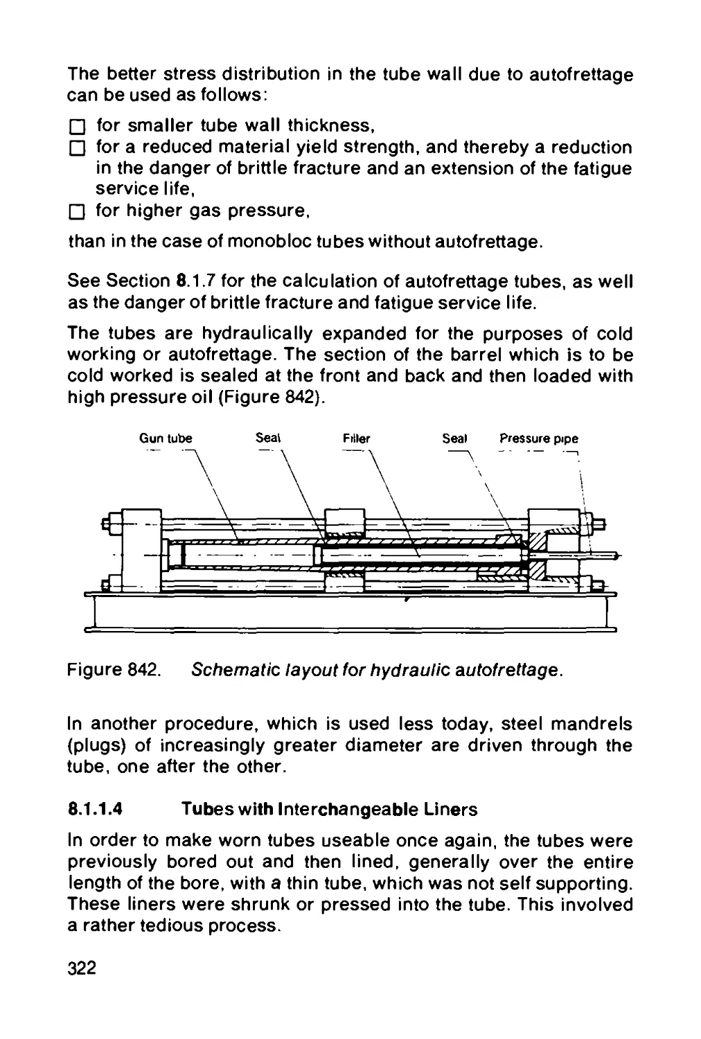
2.1.2 The firing process............................. 80
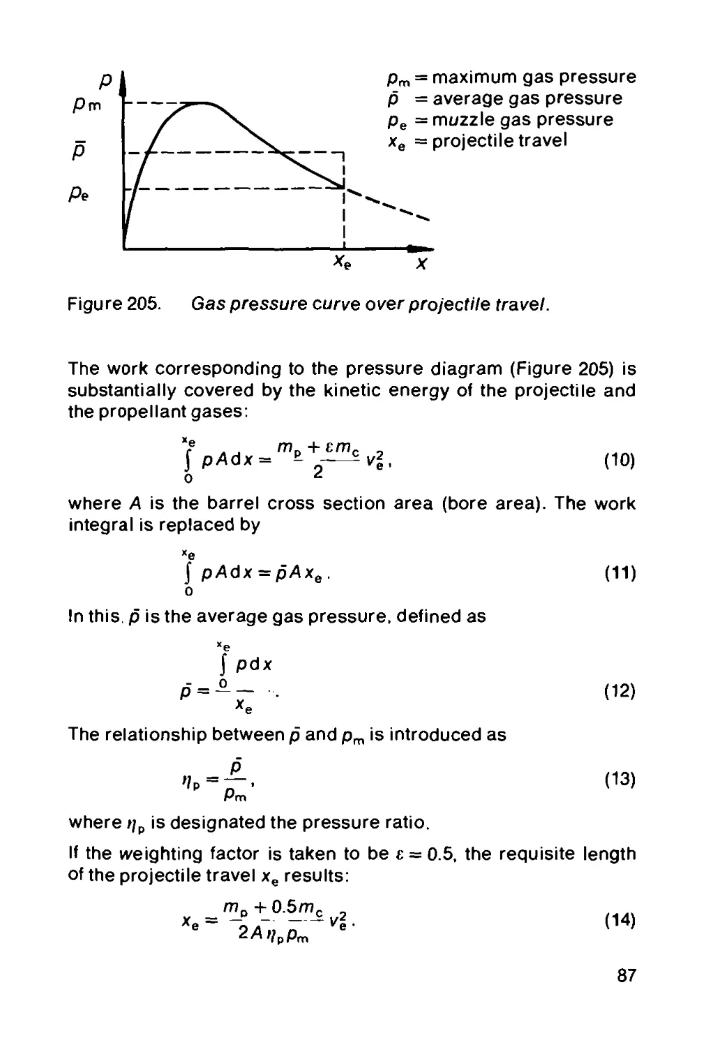
2.1.3 Energy relationships during firing............. 83
2.1.4 Gas pressure and tube design .................. 86
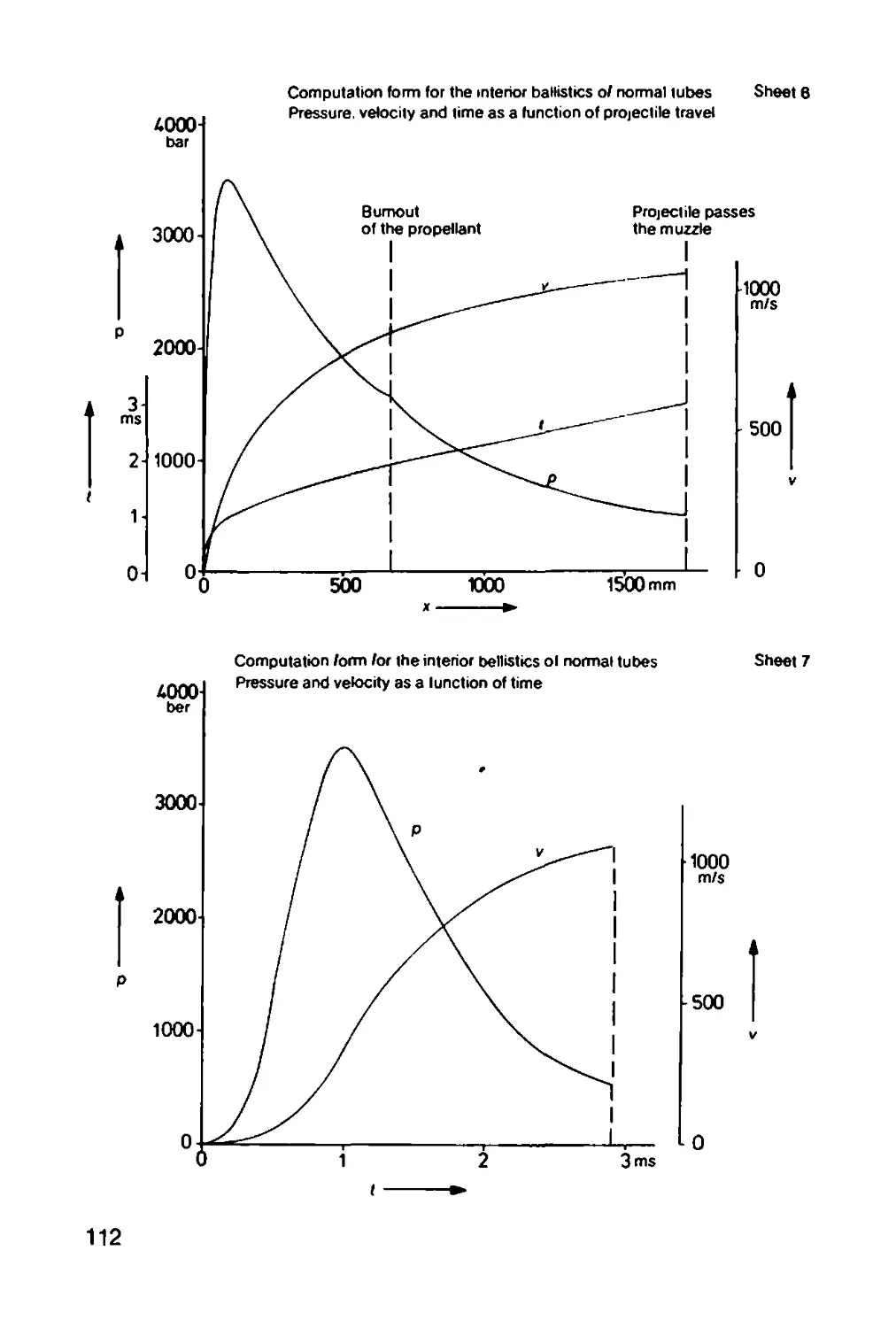
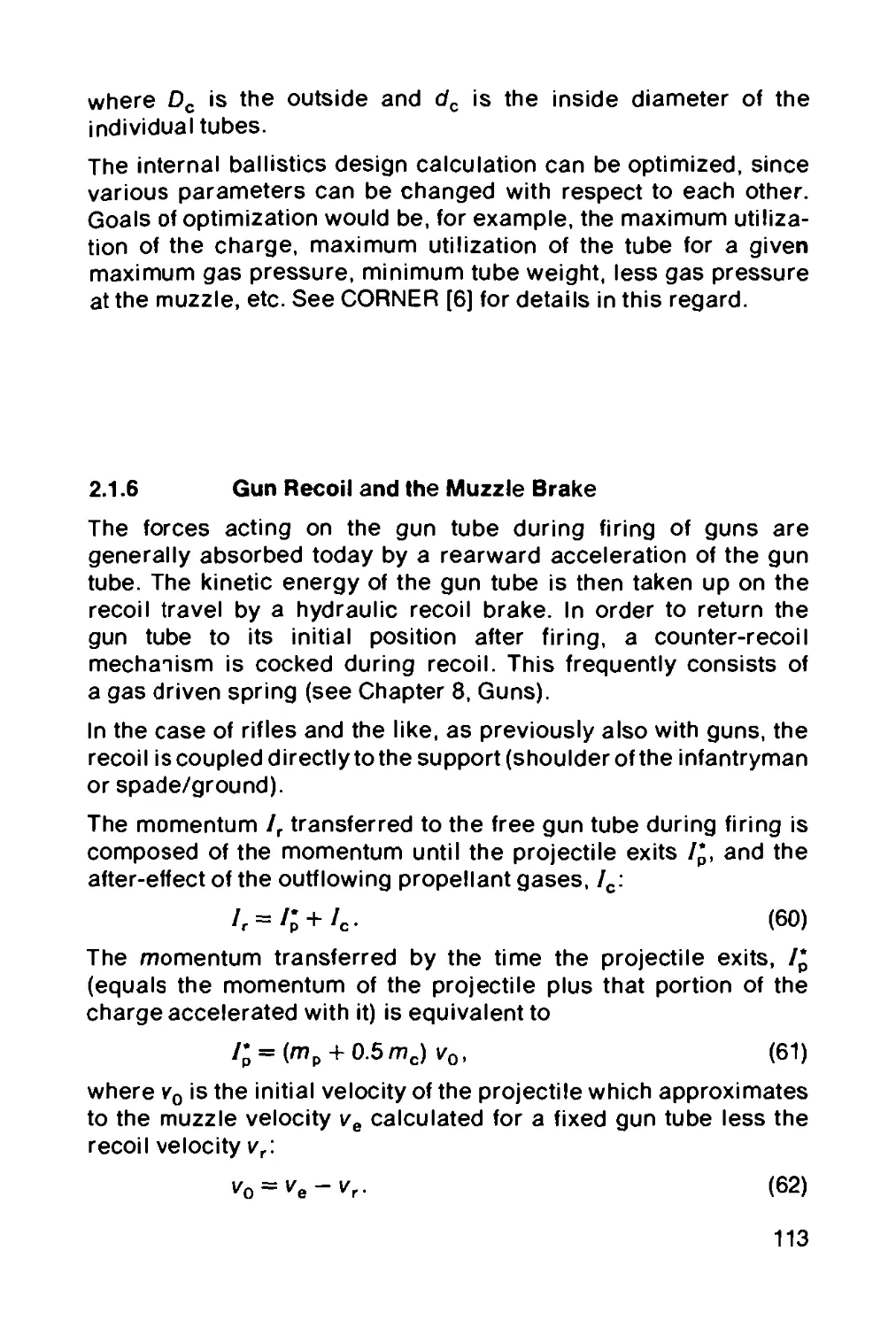
2.1.5 Procedures for internal ballistics calculations . 89
2.1.5.1 The Resal equation............................. 89
2.1.5.2 Pressure distribution in the tube.............. 92
2.1-5.3 Propellant burning............................. 94
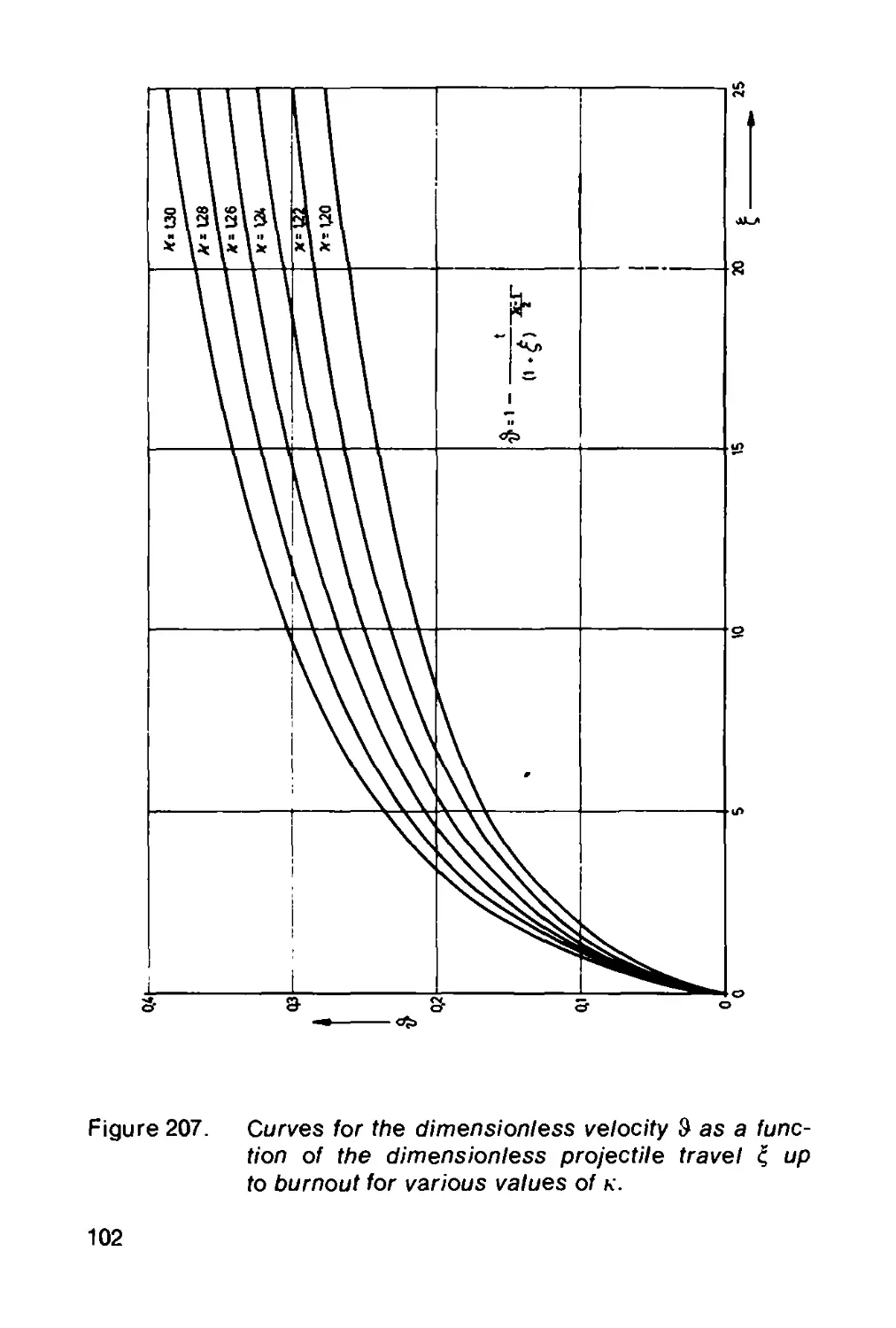
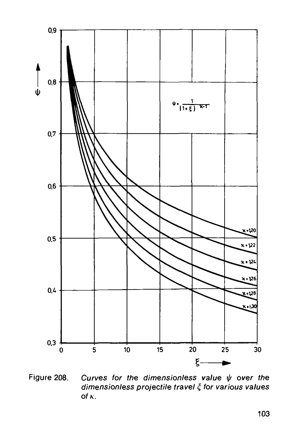
2.15.4 Pressure and projectile velocity in the tube ... 97
2.1.5.5 Computed example.............................. 104
2.1.5.6 Design calculations........................... 105
2.1.6 Gun recoil and the muzzle brake............... 113
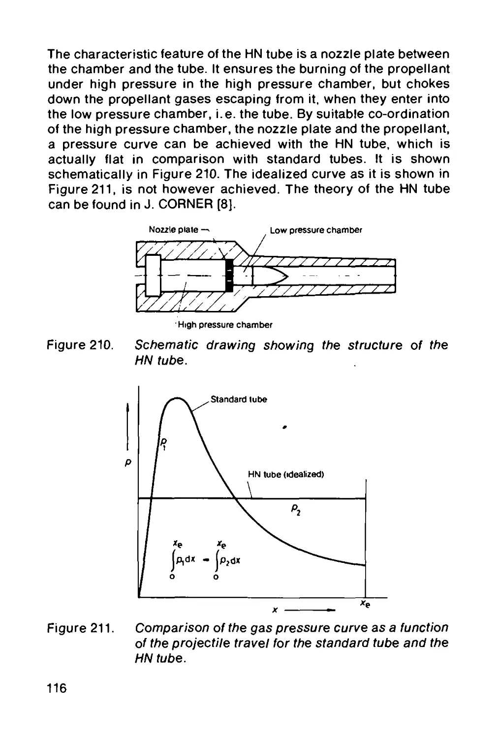
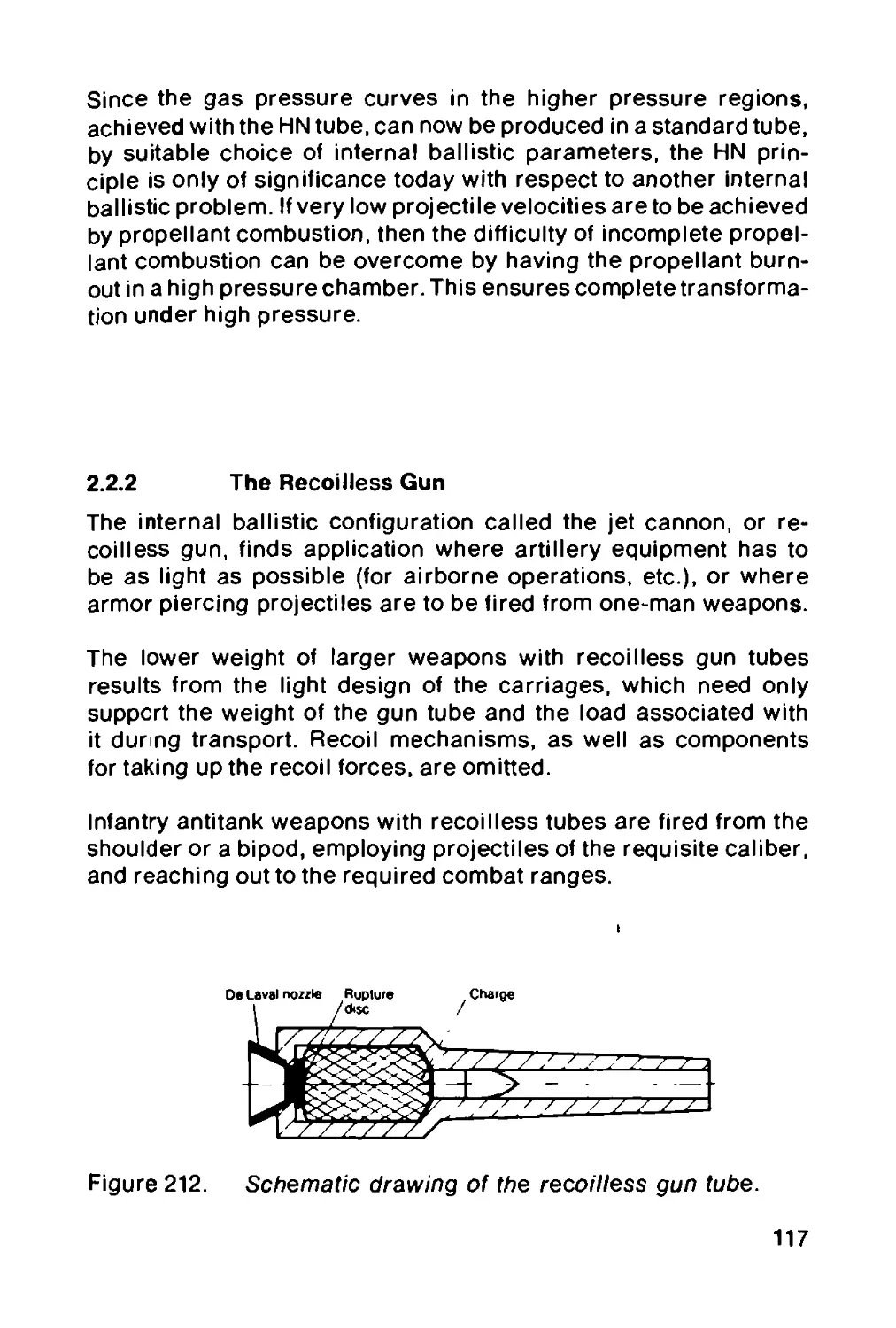
2.2 Special internal ballistic configurations.... 115
2.2.1 The high and low pressure tube................ 115
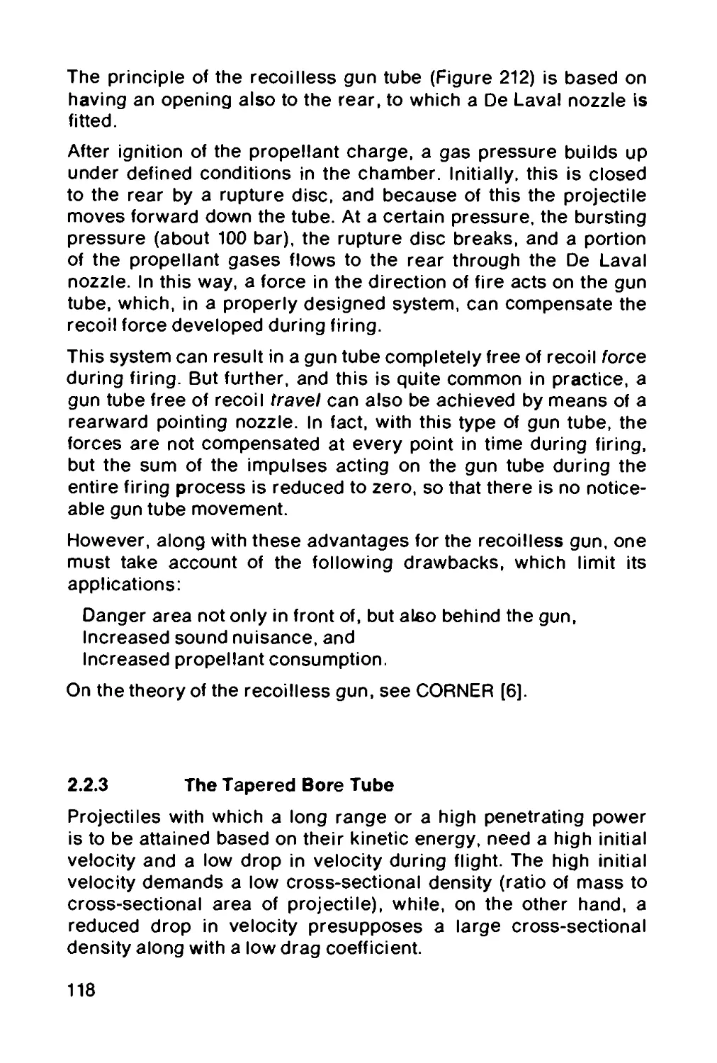
2.2.2 The recoilless gun............................ 117
2.2.3 The tapered bore tube......................... 118
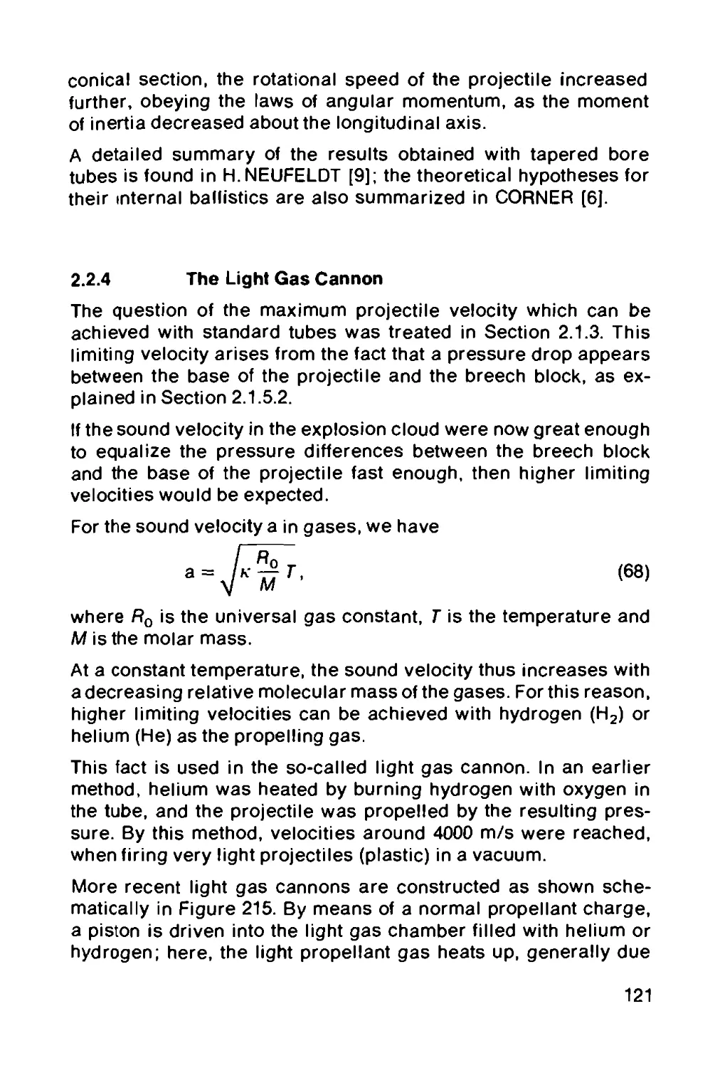
2.2.4 The light gas cannon.......................... 121
2.3 Internal ballistics of rockets................ 122
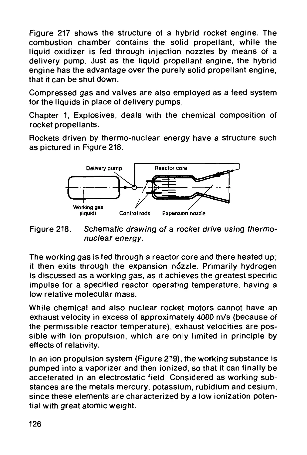
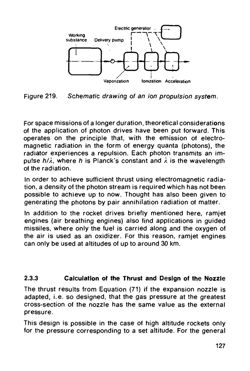
2.3.1 General information .......................... 123
2.3.2 Types of propulsion........................... 124
2.3.3 Calculation of the thrust and design of the
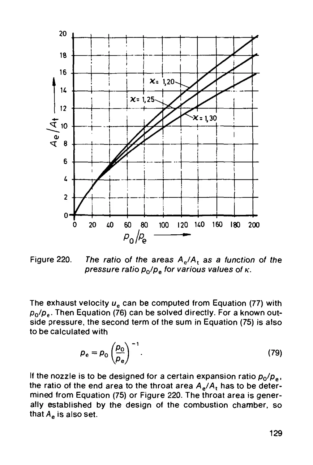
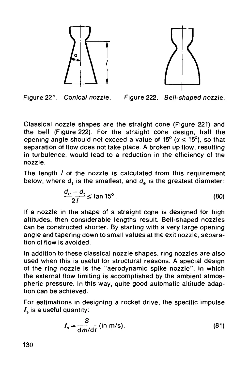
nozzle.................................................. 127
2.3.4 Calculation of the combustion chamber
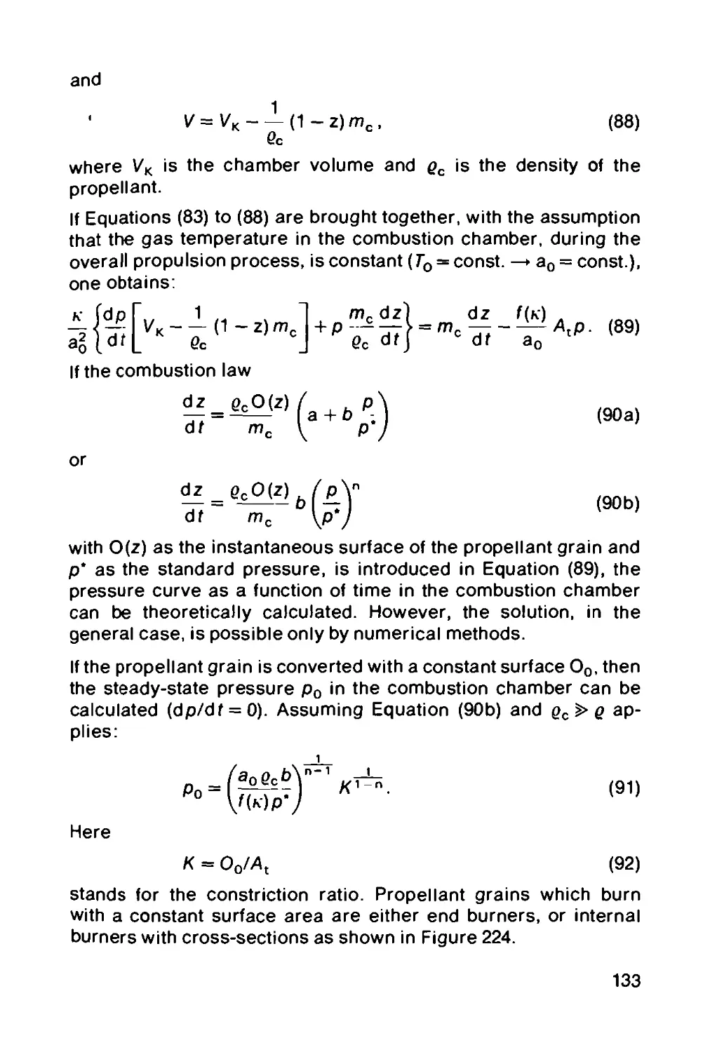
pressure for solid propellant rockets....... 131
2.3.5 Multi-stage rockets........................... 134
3 EXTERNAL BALLISTICS........................... 137
E. Melchior and H. Reuschel
3.1 The trajectory in a vacuum.................... 137
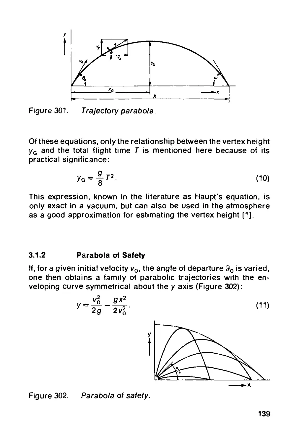
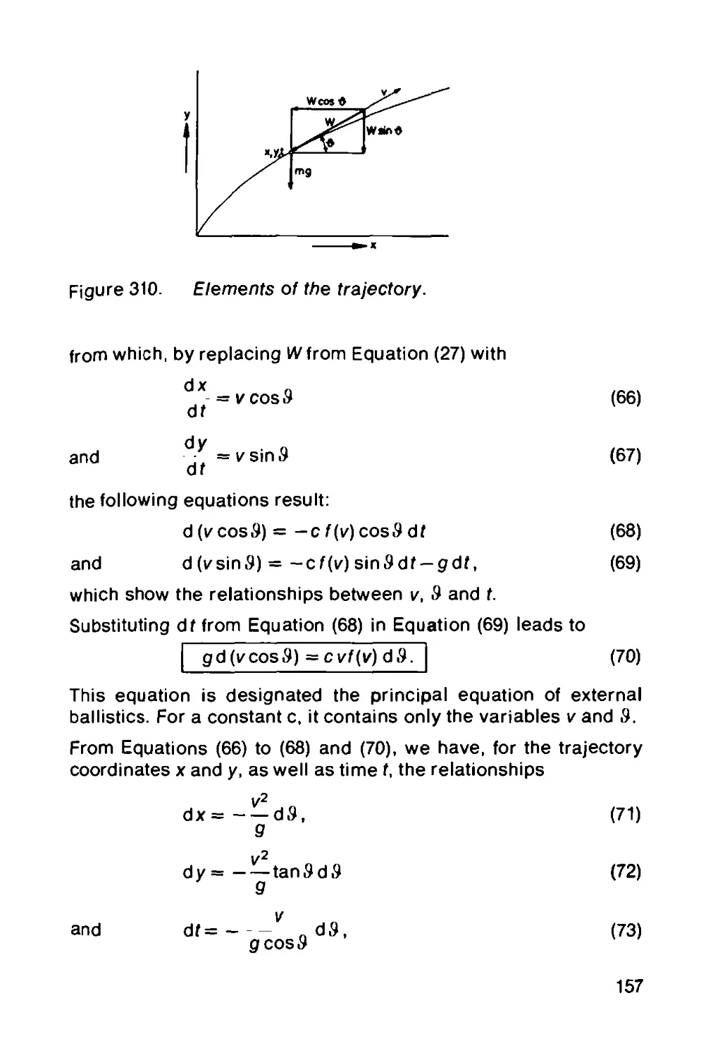
3.1.1 The trajectory................................ 137
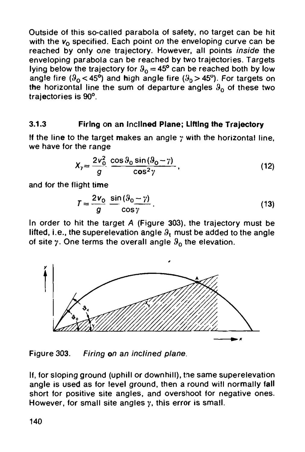
3.1.2 Parabola of safety............................ 139
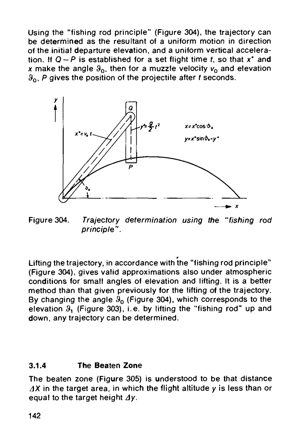
3.1.3 Firing on an inclined plane; lifting the trajectory 140
3.1.4 The beaten zone............................... 142
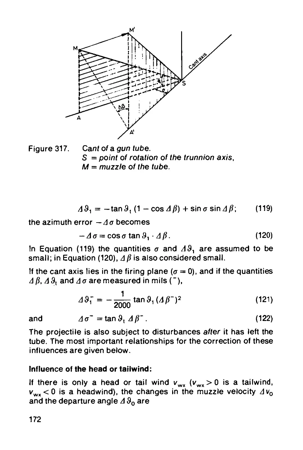
3.2 The trajectory in the atmosphere.............. 144
3.2.1 Aerodynamics of the projectile................ 144
VII
3.2.1.1 Air resistance (drag).............................
3.2.1.2 Aerodynamic forces in the case of non-axial
flow..............................................'........
3.2.1.3 Laws of similarity and modelling..................
3.2.1.4 The atmosphere....................................
3.2.2 Trajectory calculations.............................
3.2.2.1 The principal equation of external ballistics...
3.2.2.2 Integration of the principal equation ............
3.2.2.2.1 Calculation of the trajectory with a constant
resistance coefficient cw .................................
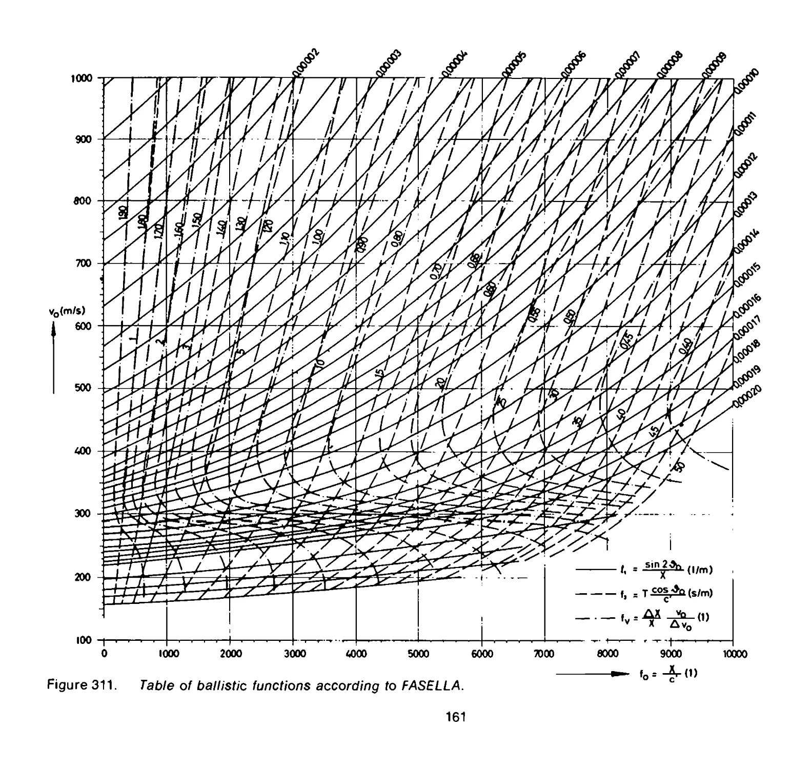
3.2.2.2.2 Trajectory calculation according to SIACCI ...
3.2.2.2.3 Calculation of the trajectory according to
d’ANTONIO..................................................
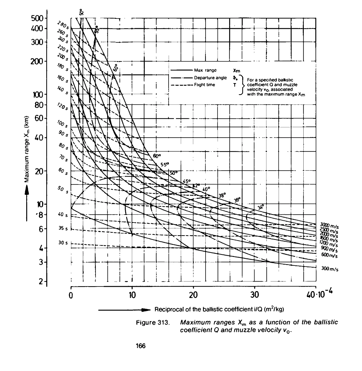
3.2.2.2.4 Maximum range for a known ballistic
coefficient and muzzle velocity............................
3.2.2.3 Approximation solutions.......................
3.2.2.3.1 Determination of trajectory parameters from
the range ratio...............................
3.2.2.3.2 Approximate graphical representation of the
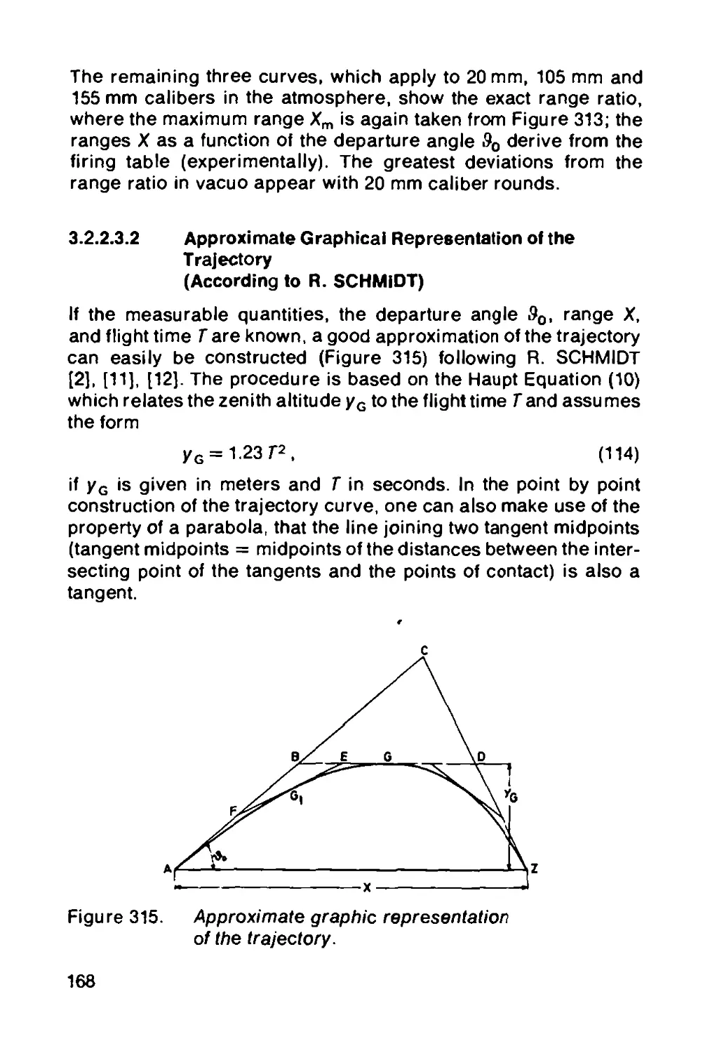
trajectory (according to R. SCHMIDT) .........
3.2.2.4 Perturbation calculation......................
3.2.3 Stability and tractability....................
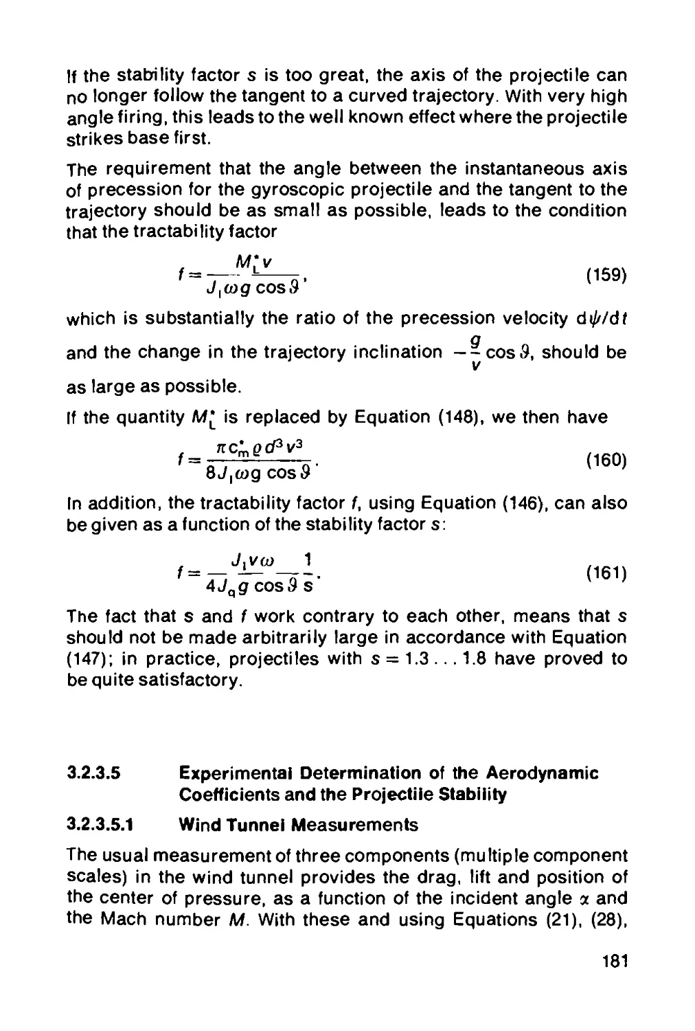
3.2.3.1 Oscillation of a spinning projectile..............
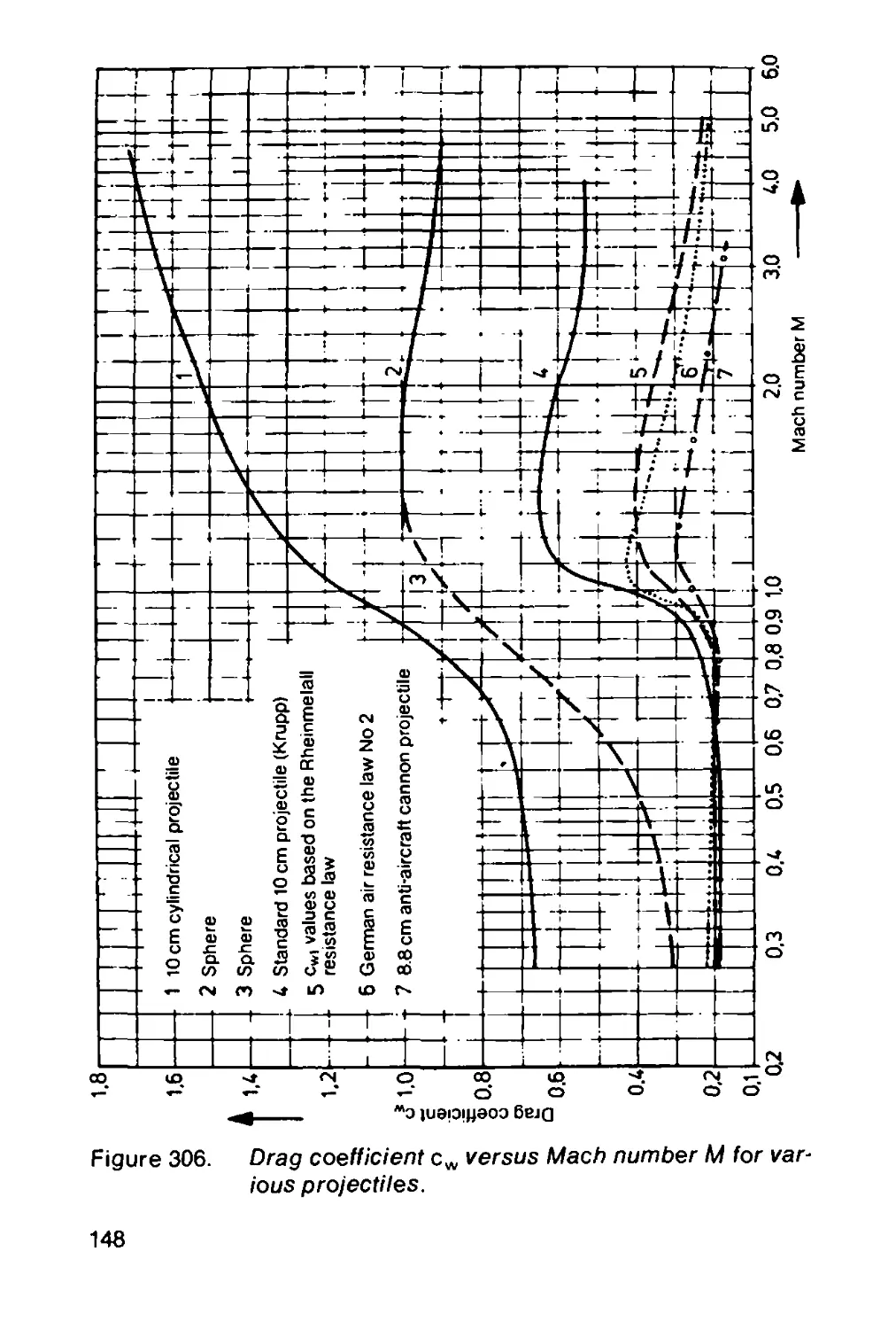
3.2.3.2 The oscillation equation......................
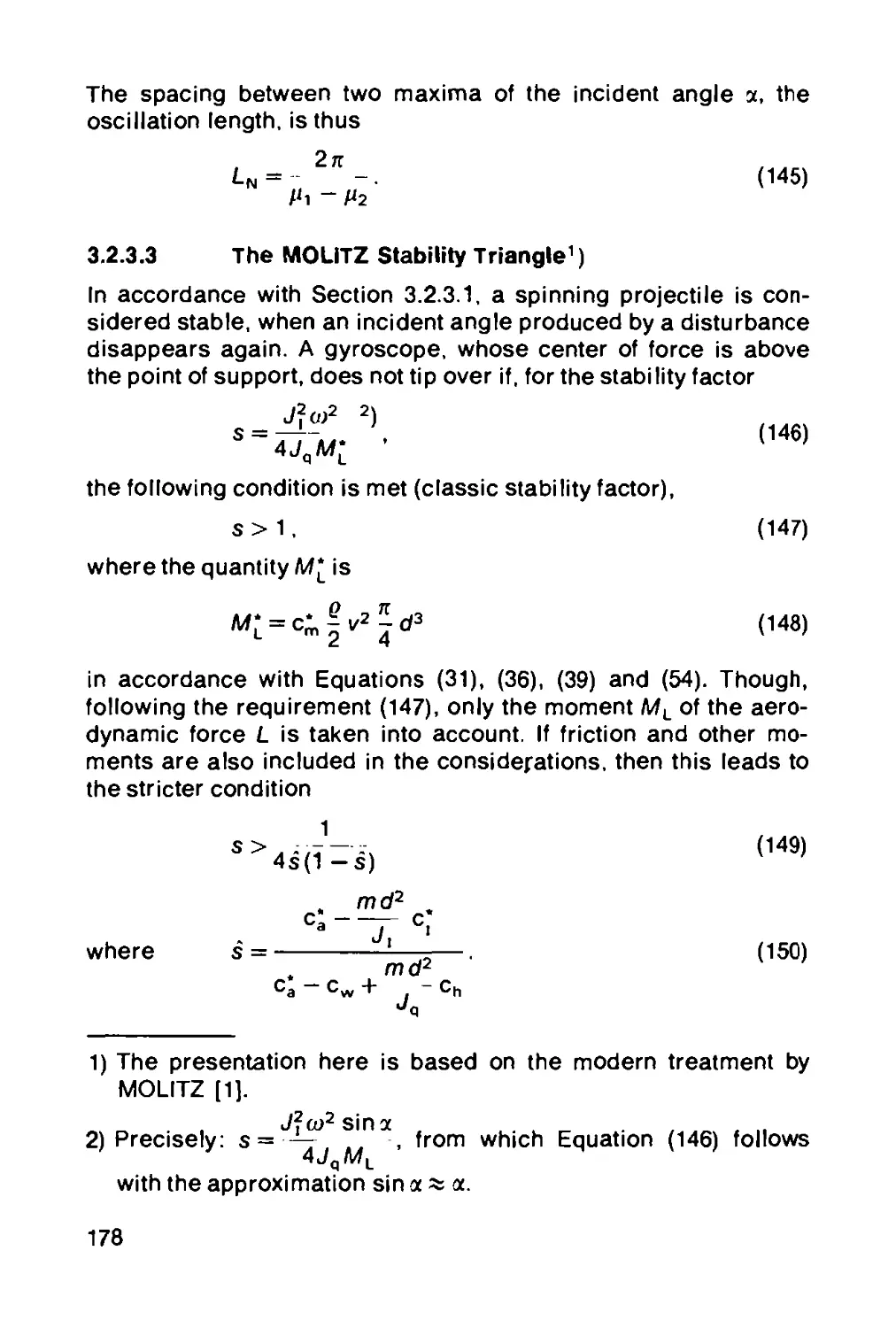
3.2.3.3 The MOLITZ stability triangle ................
3.2.3.4 The tractability factor ......................
3.2.3.5 Experimental determination of the aero-
dynamic coefficients and the projectile
stability ....................................
3.2.3.5.1 Wind tunnel measurements........................
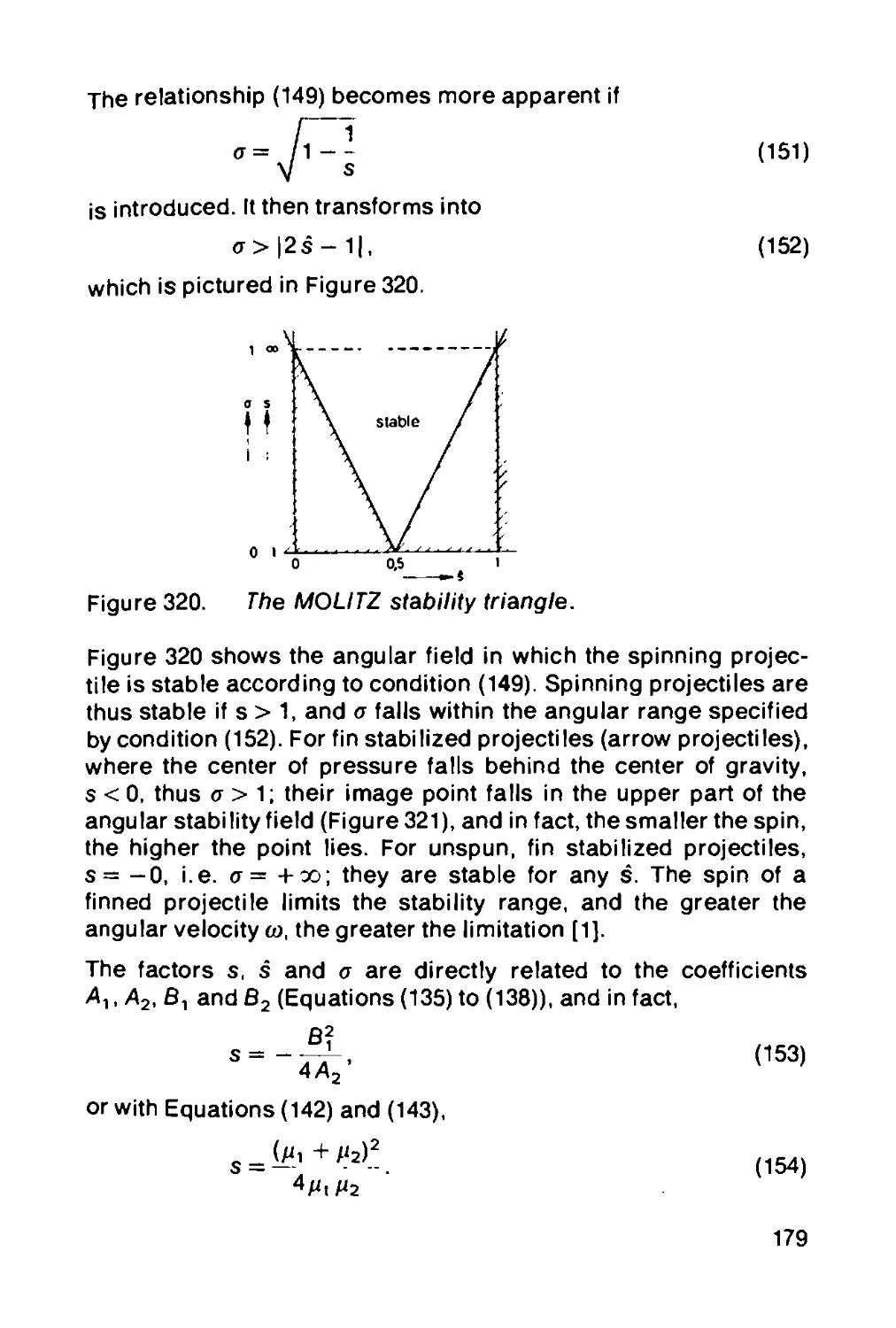
3.2.3.5.2 Measurement in a free flight test facility......
3.2.3.6 Fin stabilized projectiles ...................
3.3 External ballistics of rockets.................
3.3.1 The rocket trajectory in vacuo......................
3.3.2 The rocket trajectory in the atmosphere.............
3.3.2.1 Influence of crosswind and the "nose down”
effect on rockets..........................................
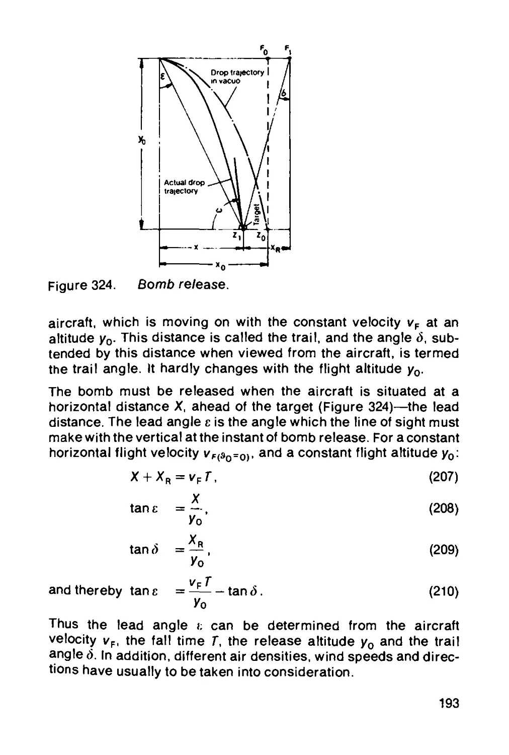
3.4 Bomb ballistics................................
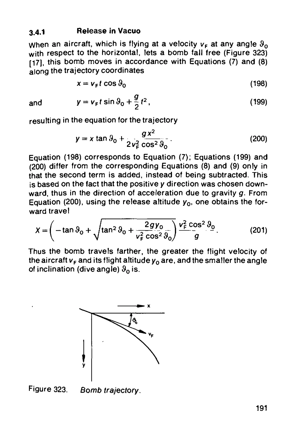
3.4.1 Release in vacuo....................................
3.4.2 Release under atmospheric conditions................
VIII
4 INTERMEDIATE BALLISTICS.................... 196
H. Reuschel
4.1 The jump error............................. 196
4.1.1 Causes of the jump error................... 196
4.1.2 Determination of the jump angle............ 197
5 THE APPLICATION OF PROBABILITY THEORY 199
H. Reuschel and H.-J. Schiewer
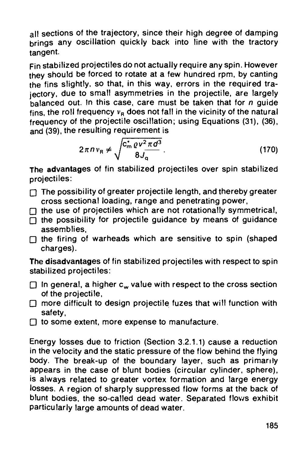
5.1 Basic concepts............................. 199
5.1.1 Examples of the basic concepts............. 200
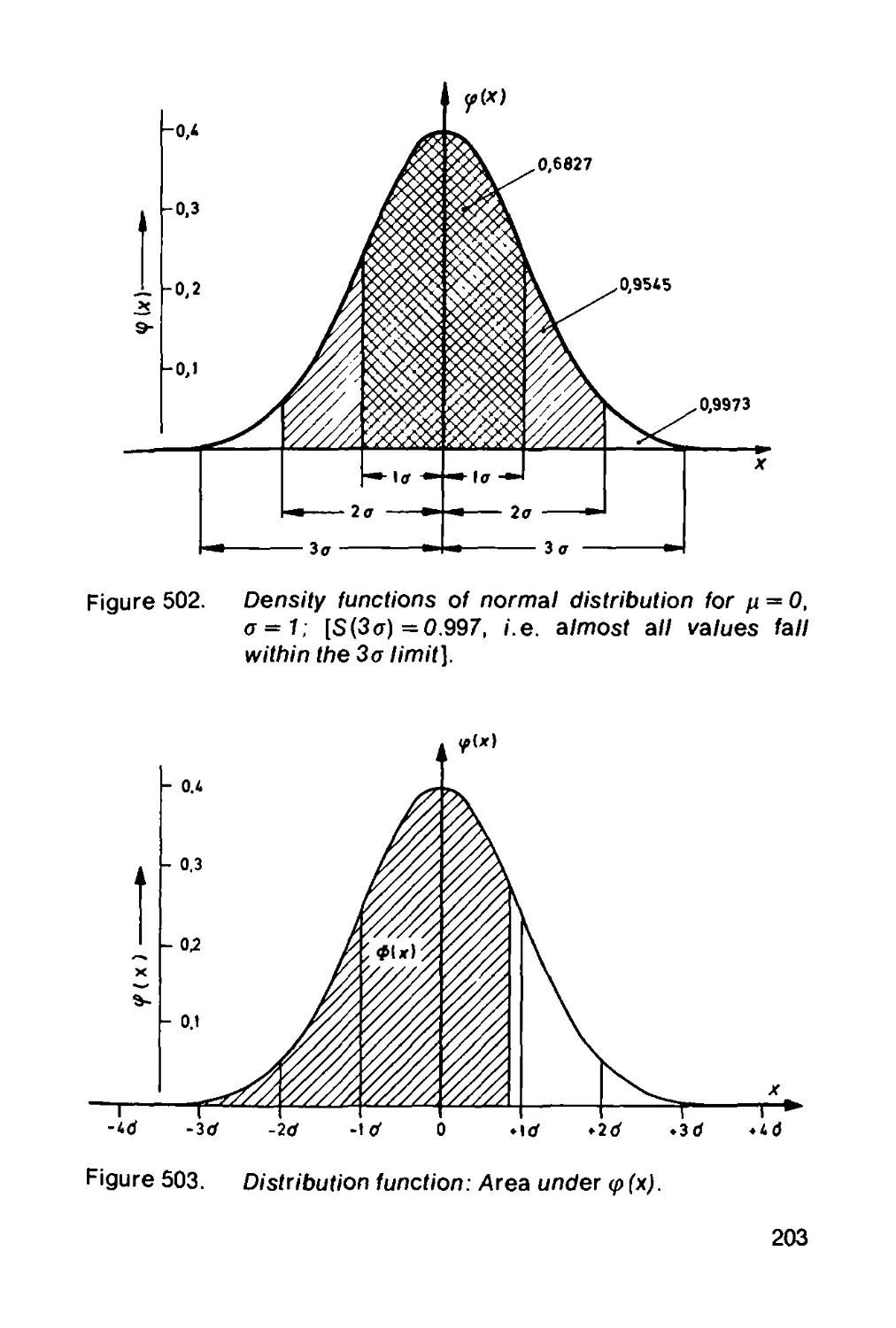
5.2 Distribution functions .................... 202
5.2.1 Normal distribution........................ 202
5.2.2 The binomial distribution.................. 205
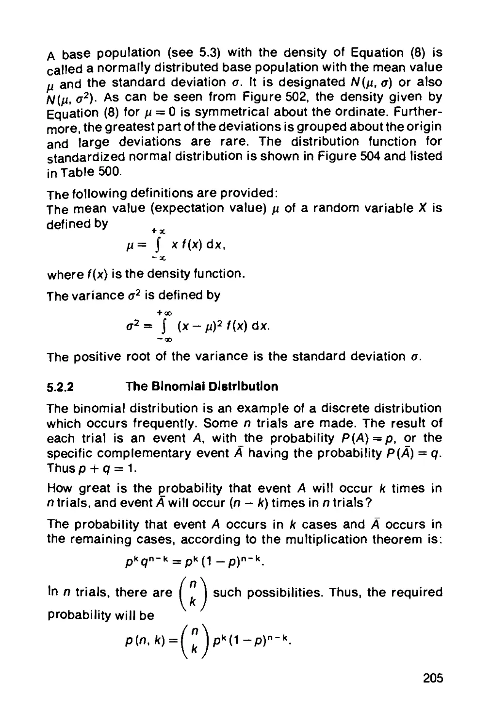
5.3 Random sampling and random sample
parameters............................... 208
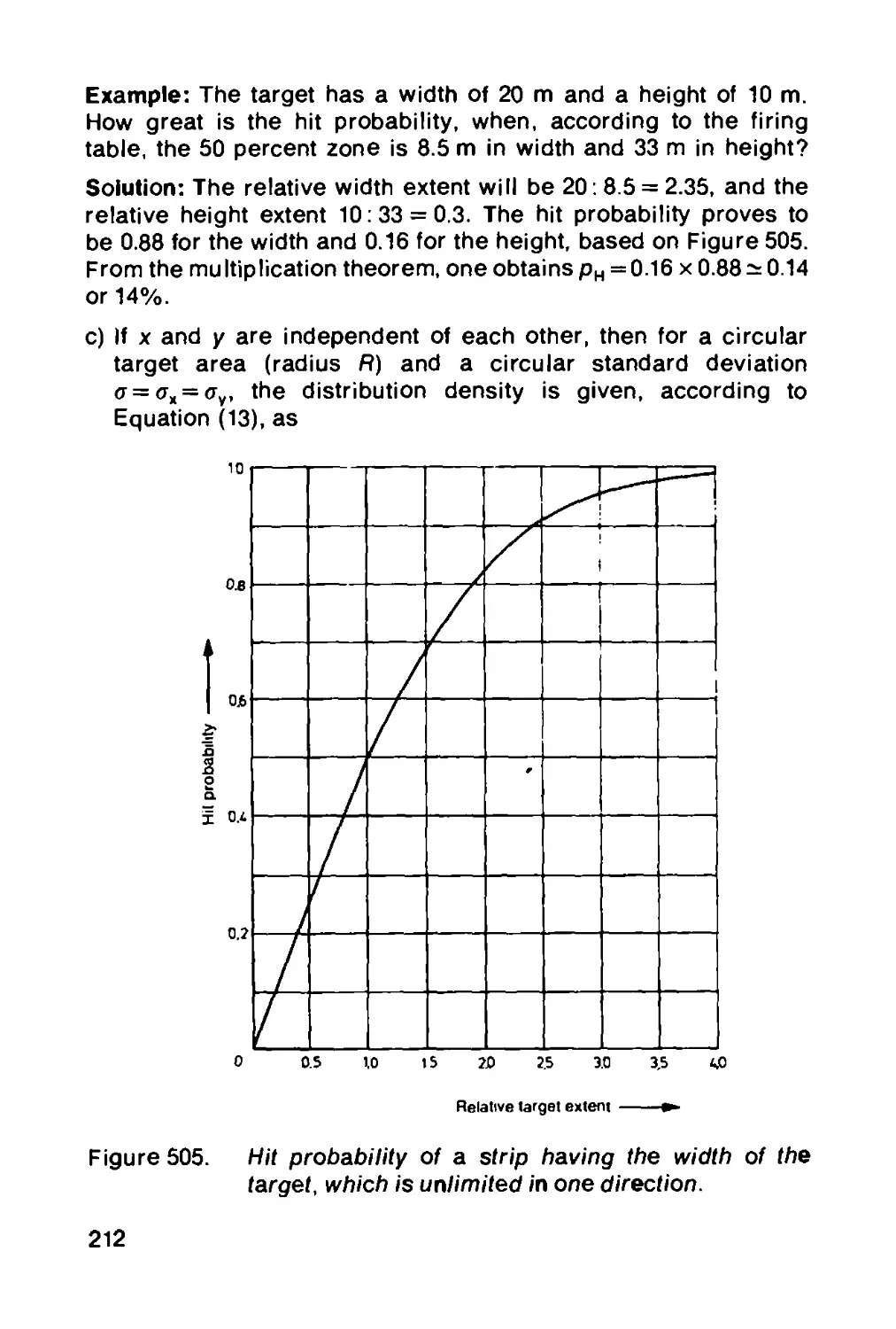
5.4 Ballistics applications.................... 211
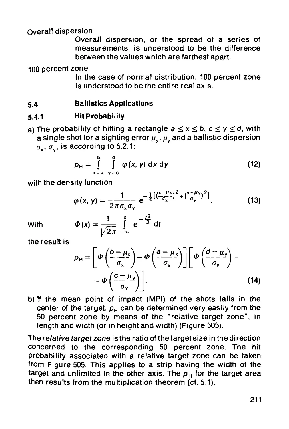
5.4.1 Hit probability............................ 211
5.4.2 Kill probability of к hits................. 213
5.4.3 Kill probability of n rounds............... 216
5.4.4 Ammunition consumption..................... 217
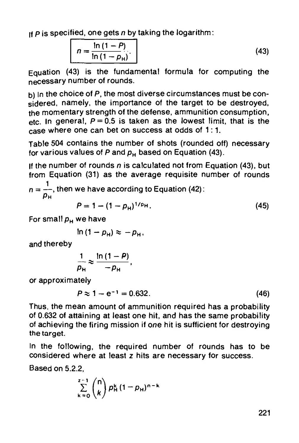
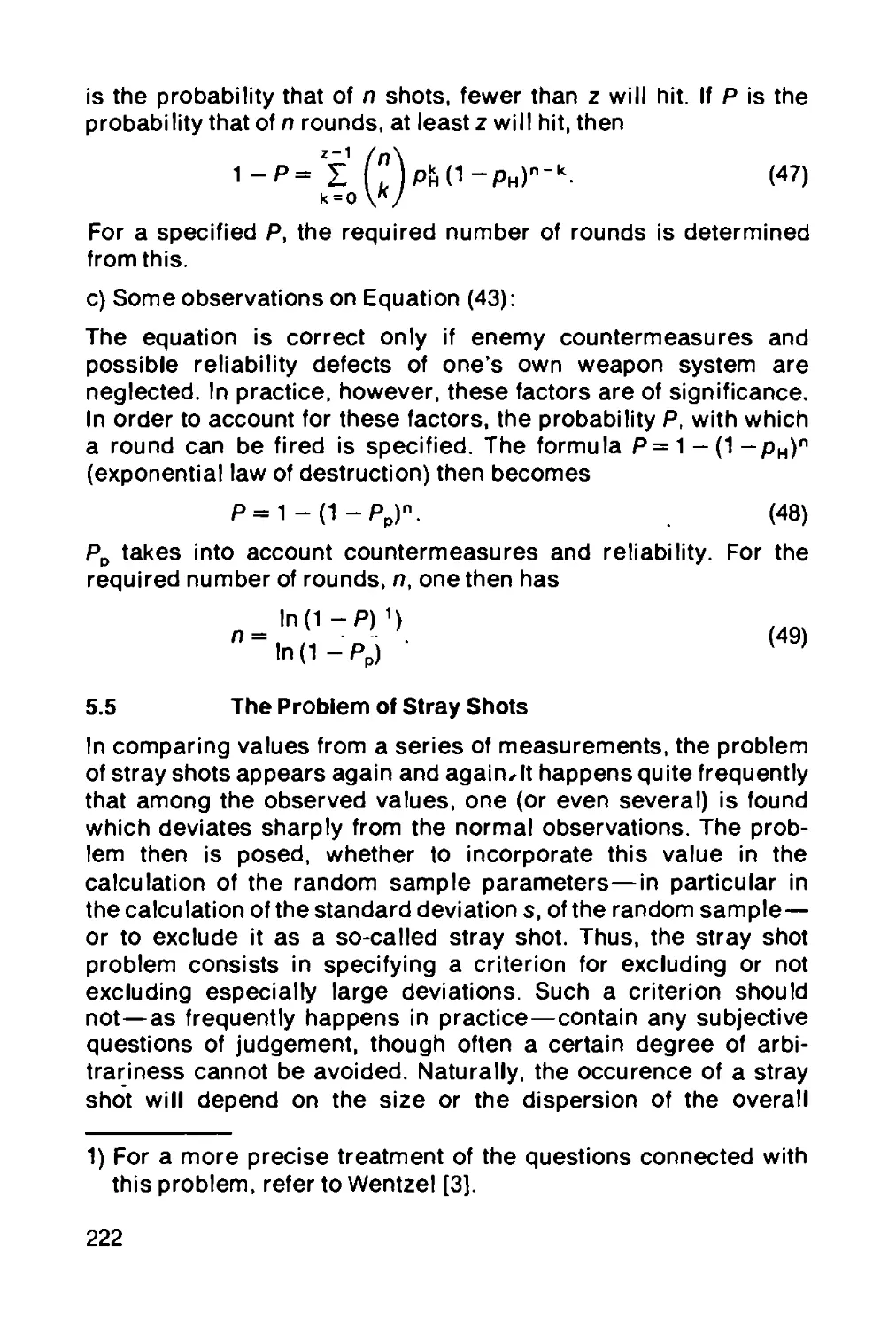
5.5 The problem of stray shots................. 222
5.5.1 The stray shot criterion according to
CHAUVENET................................ 223
5.5.2 The stray shot criterion according to STUDENT 225
5.5.3 The stray shot criterion according to GRAF
and HENNING.............................. 225
6 SIGHTING AND AIMING........................ 228
W. Kuppe, E. Kokott and S. Harris
6.1 General requirements for sighting and
aiming equipment......................... 228
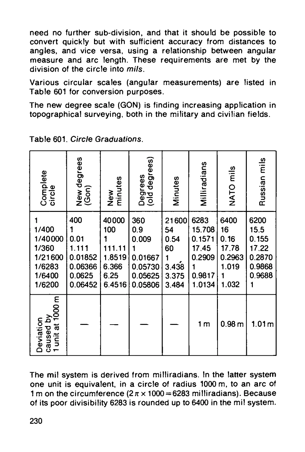
6.1.1 Angular measurement for artillery.......... 229
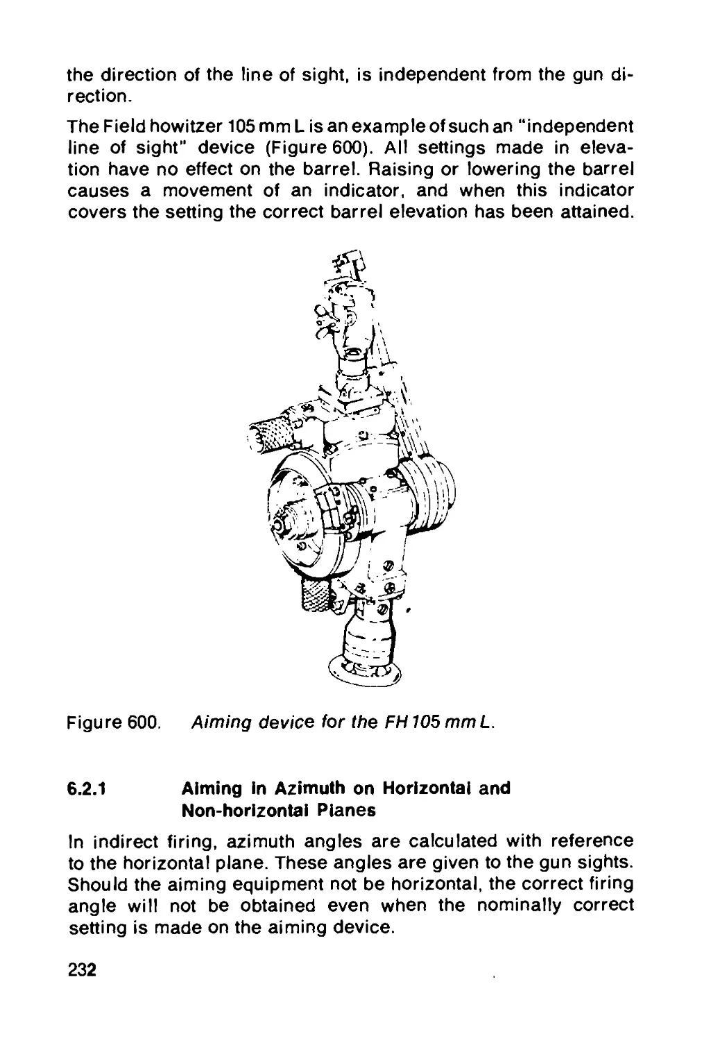
6.1.2 Aiming methods............................. 231
6.2 The sighting mechanisms.................... 231
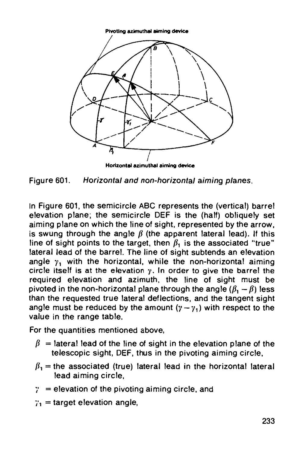
6.2.1 Aiming in azimuth on horizontal and non-
horizontal planes 232
IX
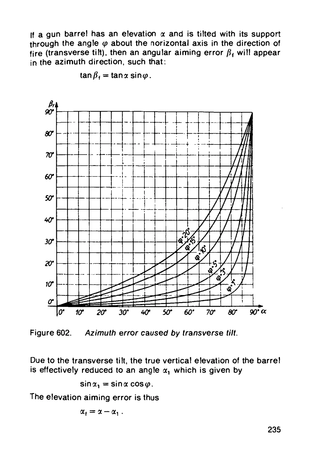
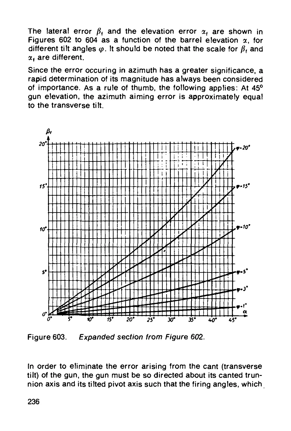
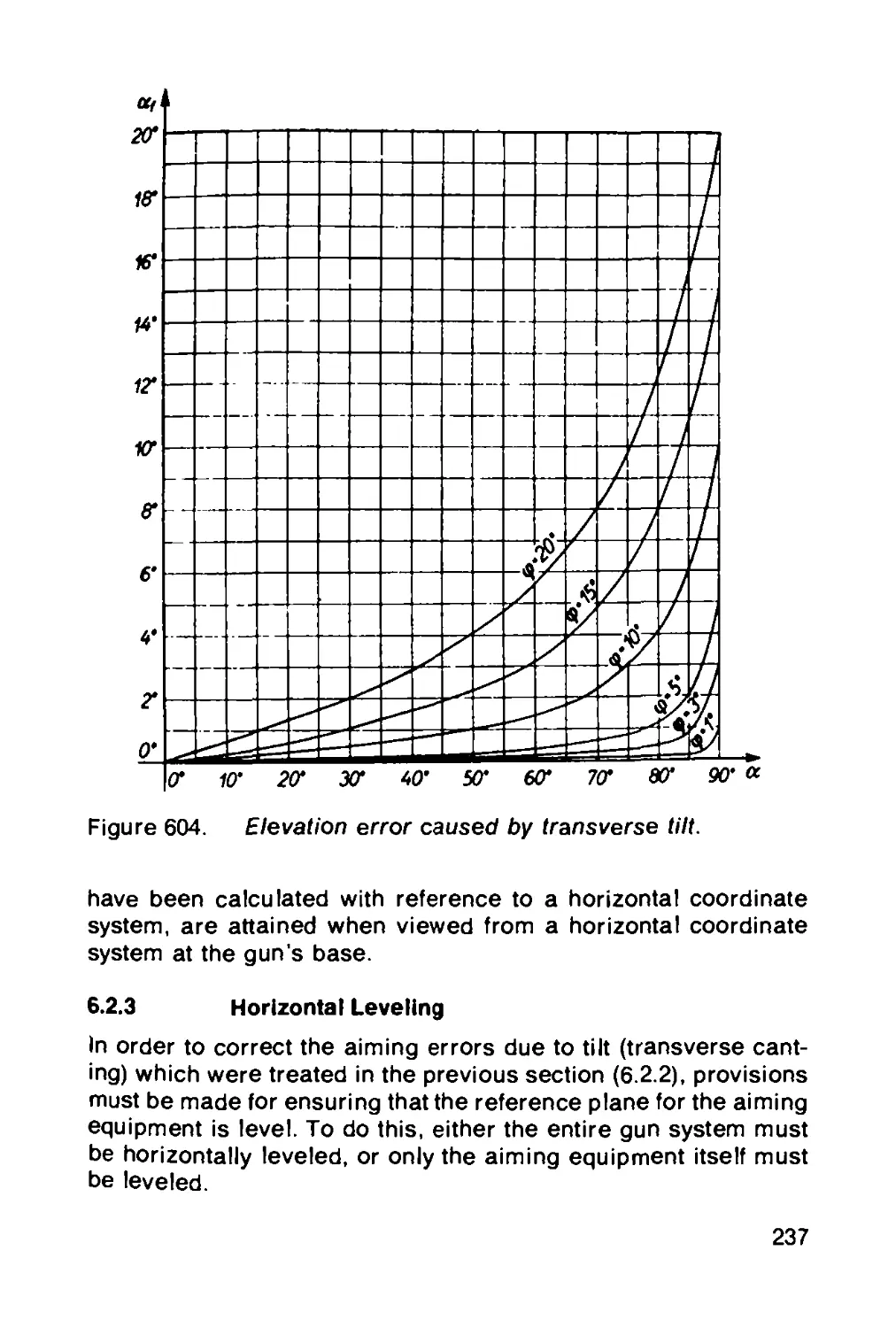
6.2.2 Trunnion tilt and the resulting aiming error ... 234
6.2.3 Horizontal leveling.......................... 237
6.2.4 The “dead spaces" and air defense limitations 239
6.3 The means for sighting and aiming............ 241
6.3.1 Optical and mechanical instruments and
equipment; sights for field and tank artillery .. 241
6.3.11 Optical means of reconnaissance.............. 241
6.3.1.2 Mechanical means of aiming................... 243
6.3.2 Fire control equipment for field and tank
artillery ............................................... 243
6.3.3 Sights and fire control equipment for AA guns 244
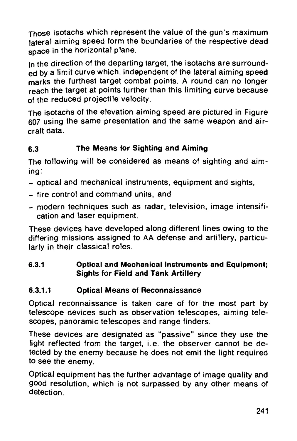
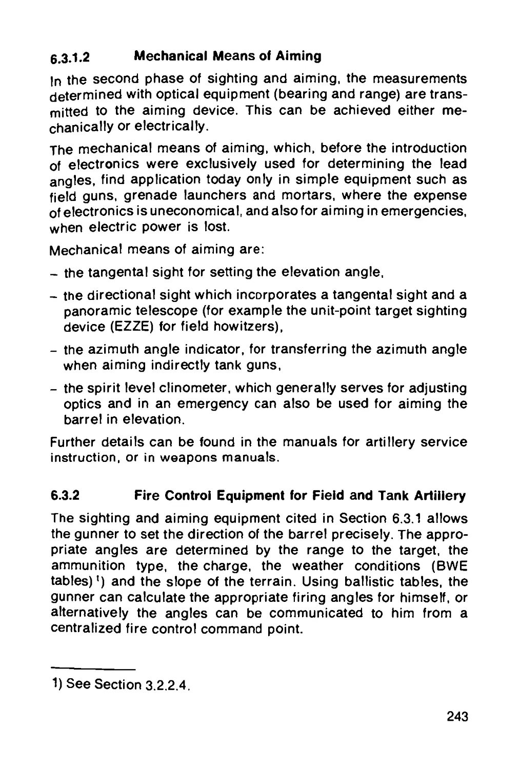
6.3.3.1 Antiaircraft sights.......................... 244
6.3.3.2 Fire control equipment for antiaircraft guns ... 248
6.3.4 Modern sighting and aiming techniques........ 251
6.3.4.1 Radar techniques............................. 251
6.3.4.2 Television technology........................ 252
6.3.4.3 Night vision technology...................... 253
6.3.4.3.1 Active infrared techniques .................. 253
6.3.4.3.2 Passive image intensifiers and low level light
television apparatus (LL LTV)................ 254
6.3.4.4 Thermal imaging technology................... 255
6.3.4.5 Laser techniques............................. 255
6.4 Stabilization ............................... 257
6.4.1 Stabilization on ships....................... 257
6.4.2 Stabilization in tanks....................... 258
6.5 Training equipment .•........................ 259
7 AUTOMATIC WEAPONS............................ 262
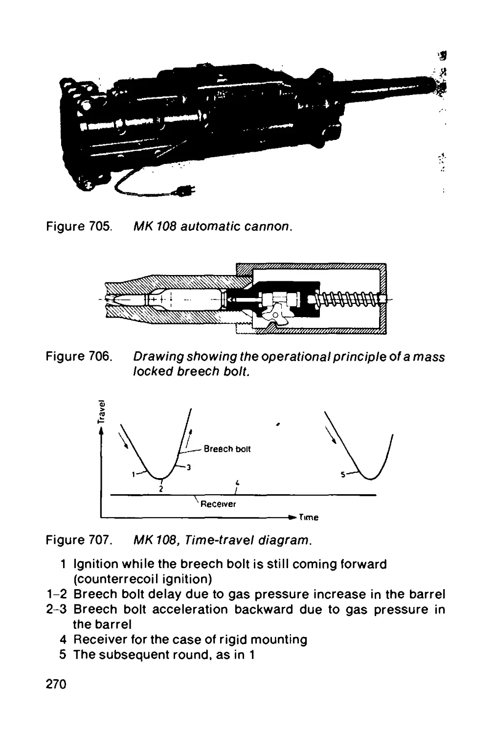
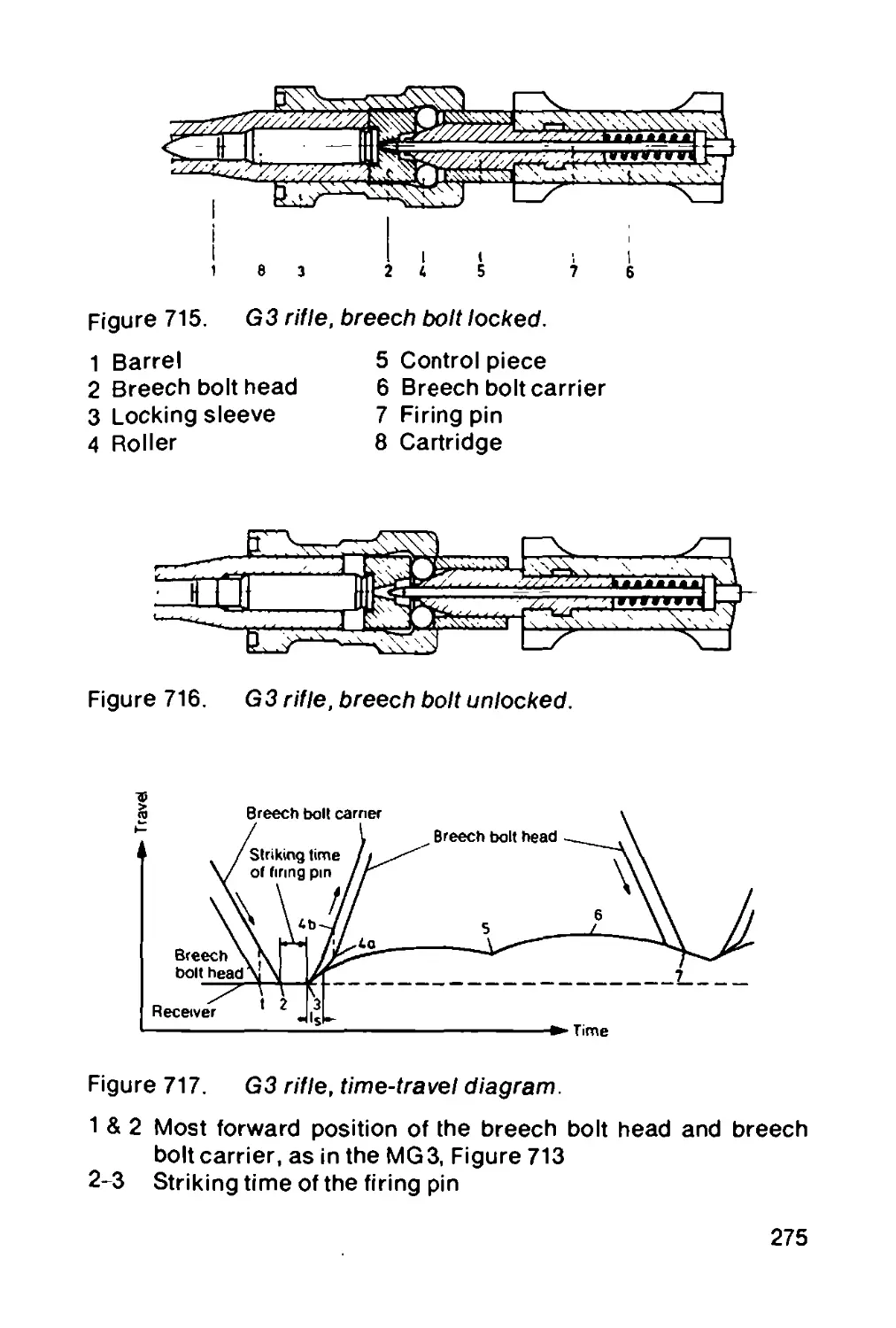
F. Flanhardt и nd K. Harbrecht
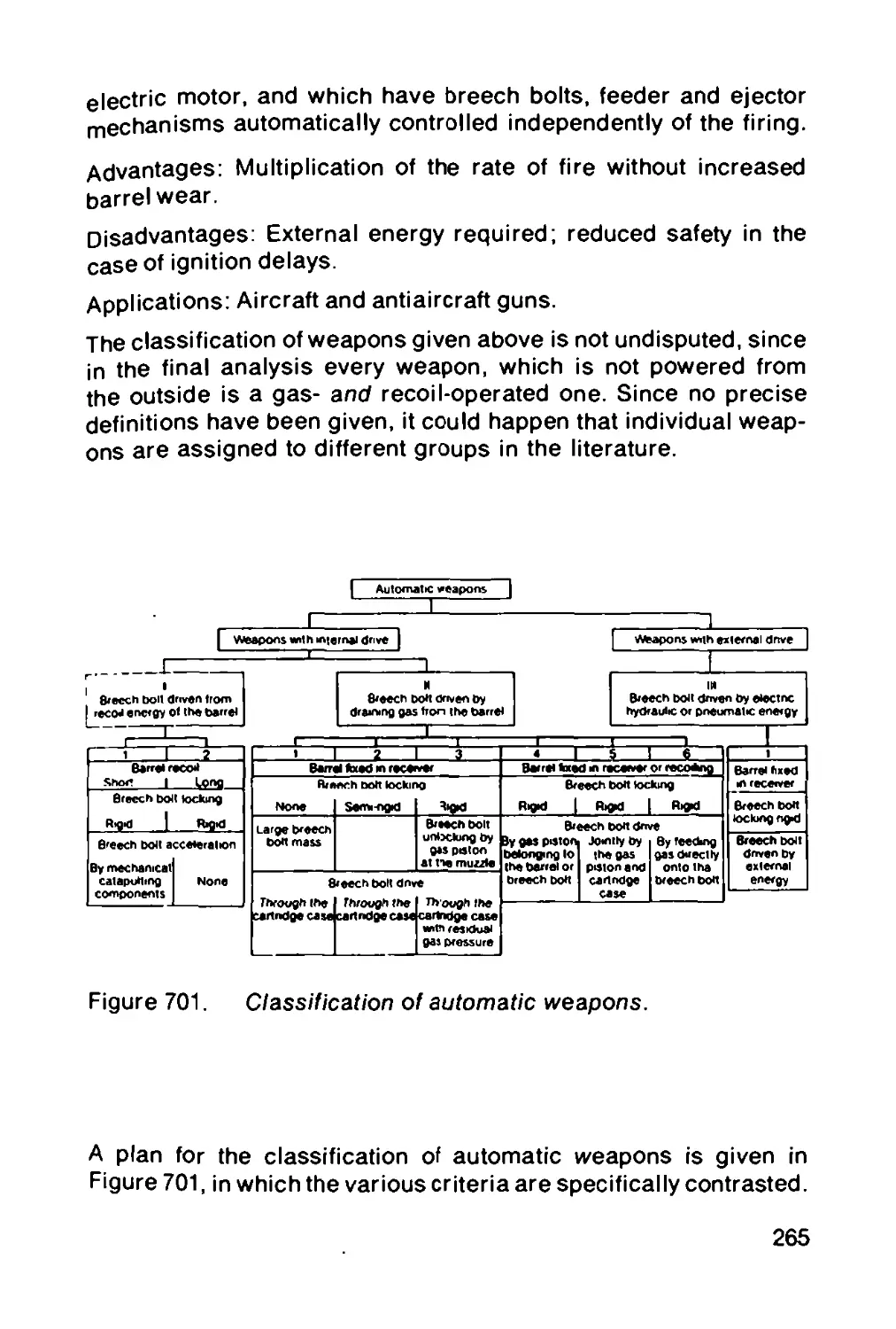
7.1 Classification of automatic weapons.......... 263
7.2 Operating sequences of an automatic weapon 266
7.3 Examples of automatic weapons and their
operational sequences........................ 269
7.4 Important structural and operational groups of
automatic weapons............................ 282
7.5 Performance considerations................... 288
7.6 Mounting automatic weapons; recoil and
counterrecoil mechanisms..................... 290
7.7 IKARUS electronic rate of fire and rhythm
control unit................................. 293
X
8 GUNS......................................... 295
F. Horn
8.1 Gun tubes................................... 298
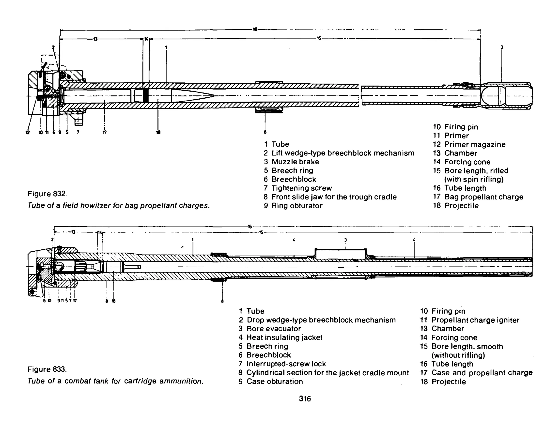
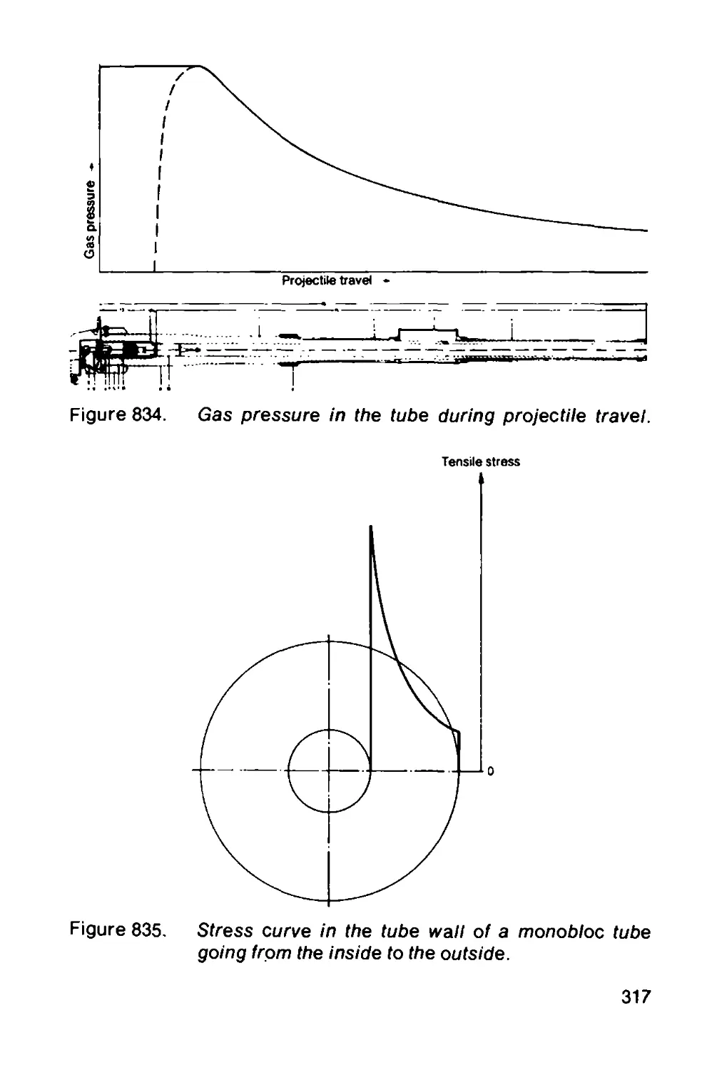
8.1.1 Tubes....................................... 315
8.1.1.1 Monobloc tubes.............................. 315
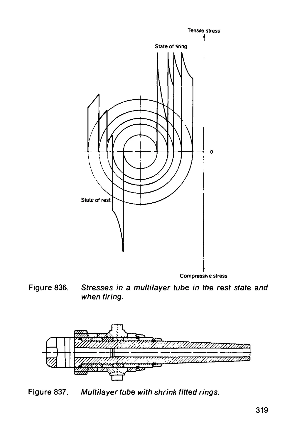
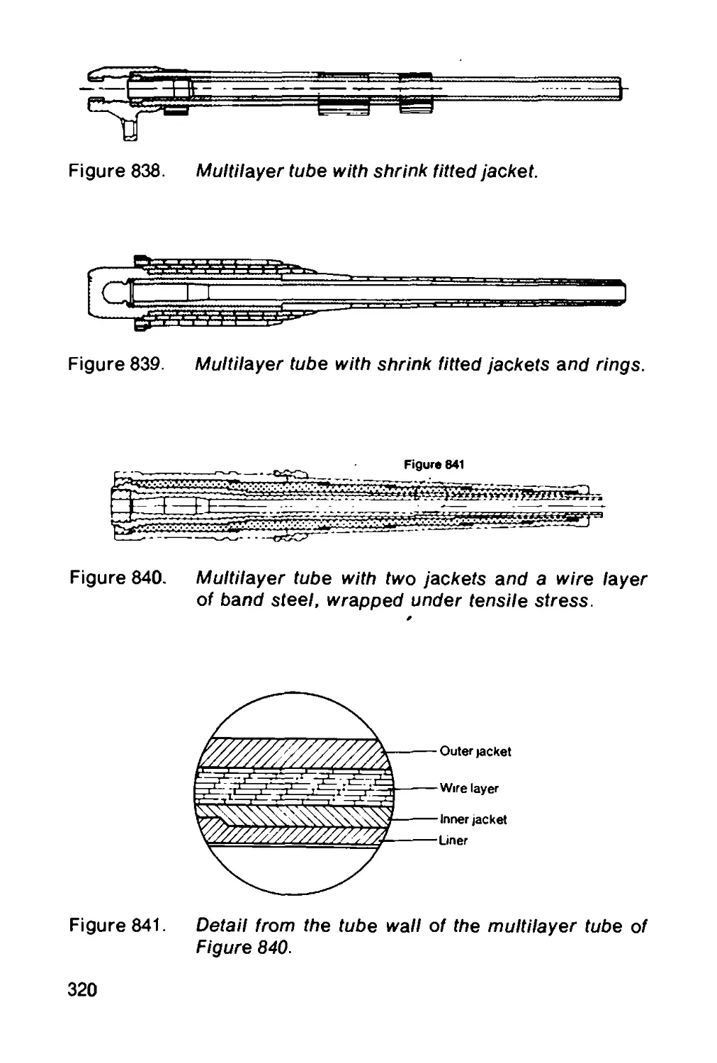
8.1.1.2 Multilayer tubes............................ 318
8.1.1.3 Monobloc tubes with autofrettage............ 321
8.1.14 Tubes with interchangeable liners........... 322
8.1.15 Removable tubes............................. 324
8.1.1.6 Manufacture of tubes........................ 324
8.1.2 Breechblock mechanisms...................... 327
8.1.2.1 Fixed closures.............................. 327
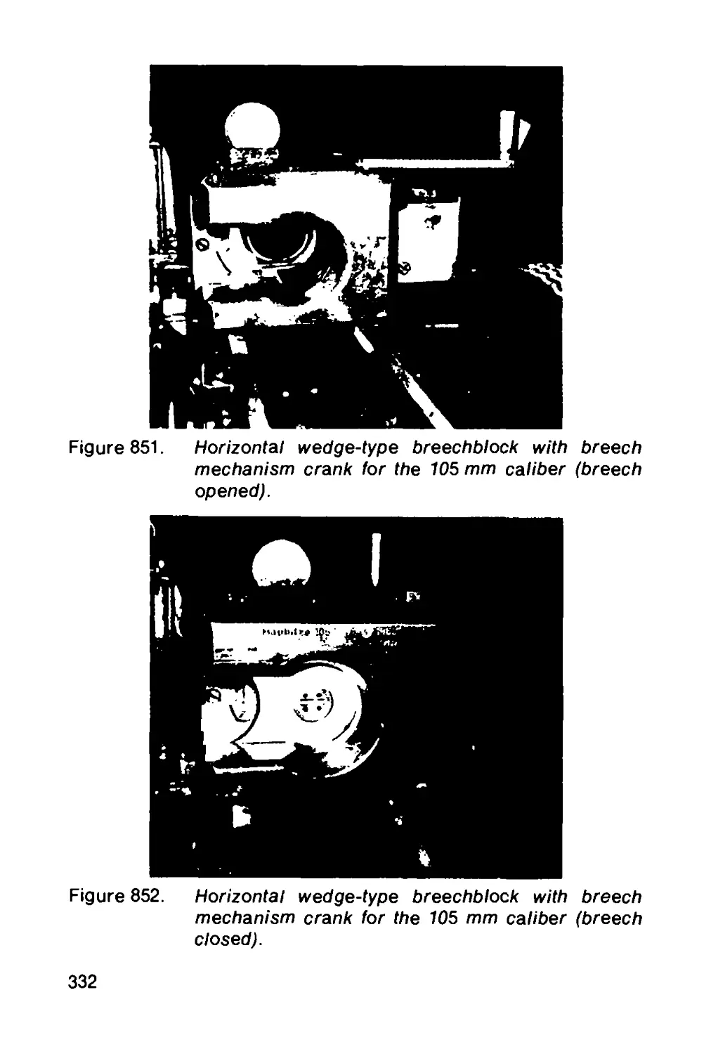
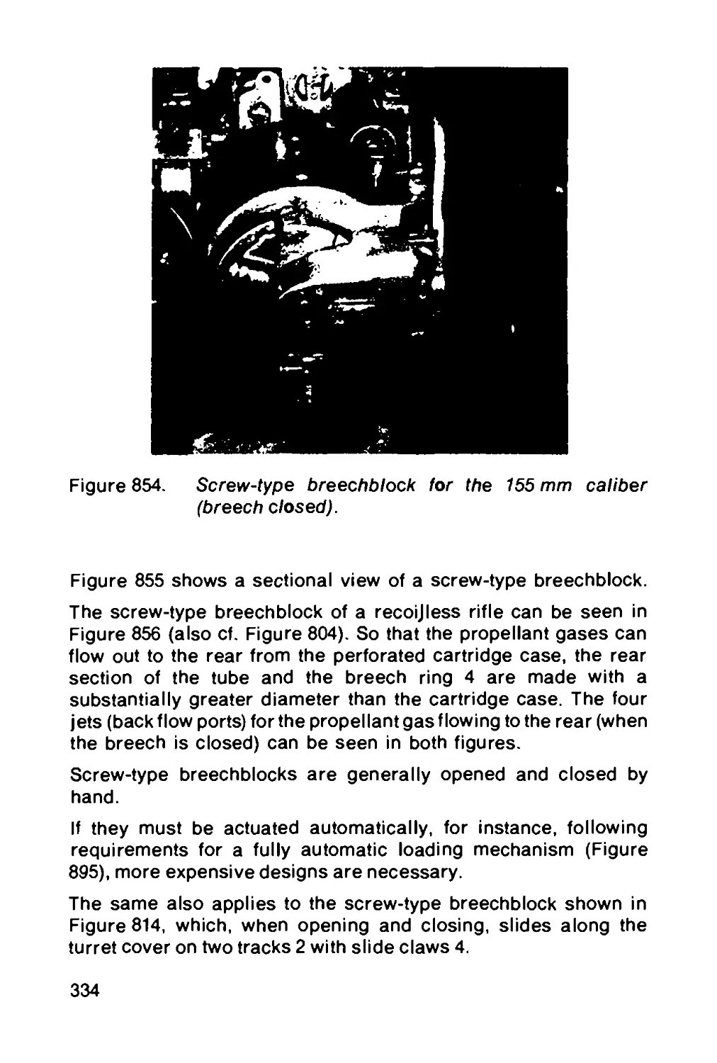
8.1.2.2 Wedge-type breechblocks and rings......... 327
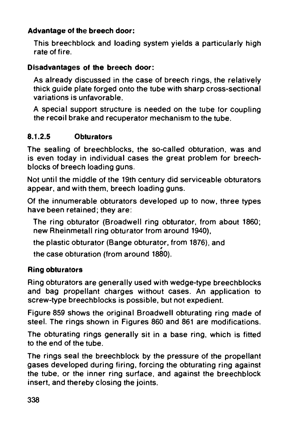
8.1.2.3 Screw-type breechblocks..................... 333
8.1.2.4 Breech door mechanism ................ 336
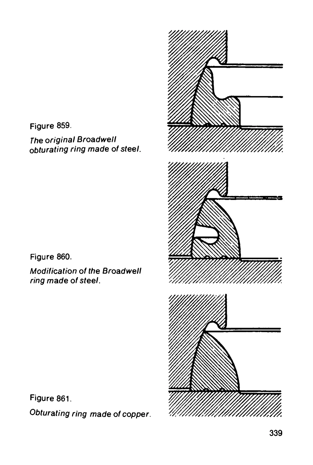
8.1.2.5 Obturators.................................. 338
8.1.2.6 Firing devices.............................. 343
8.1.2.7 Case ejector................................ 346
8.1.3 Muzzle brakes............................... 347
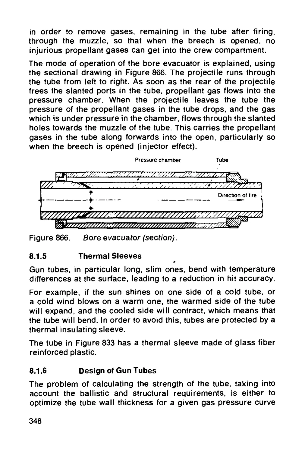
8.1.4 Bore evacuator.............................. 347
8.1.5 Thermal sleeves............................. 348
8.1.6 Design of gun tubes......................... 348
8.1.6.1 Stress-strain analysis of monobloc tubes
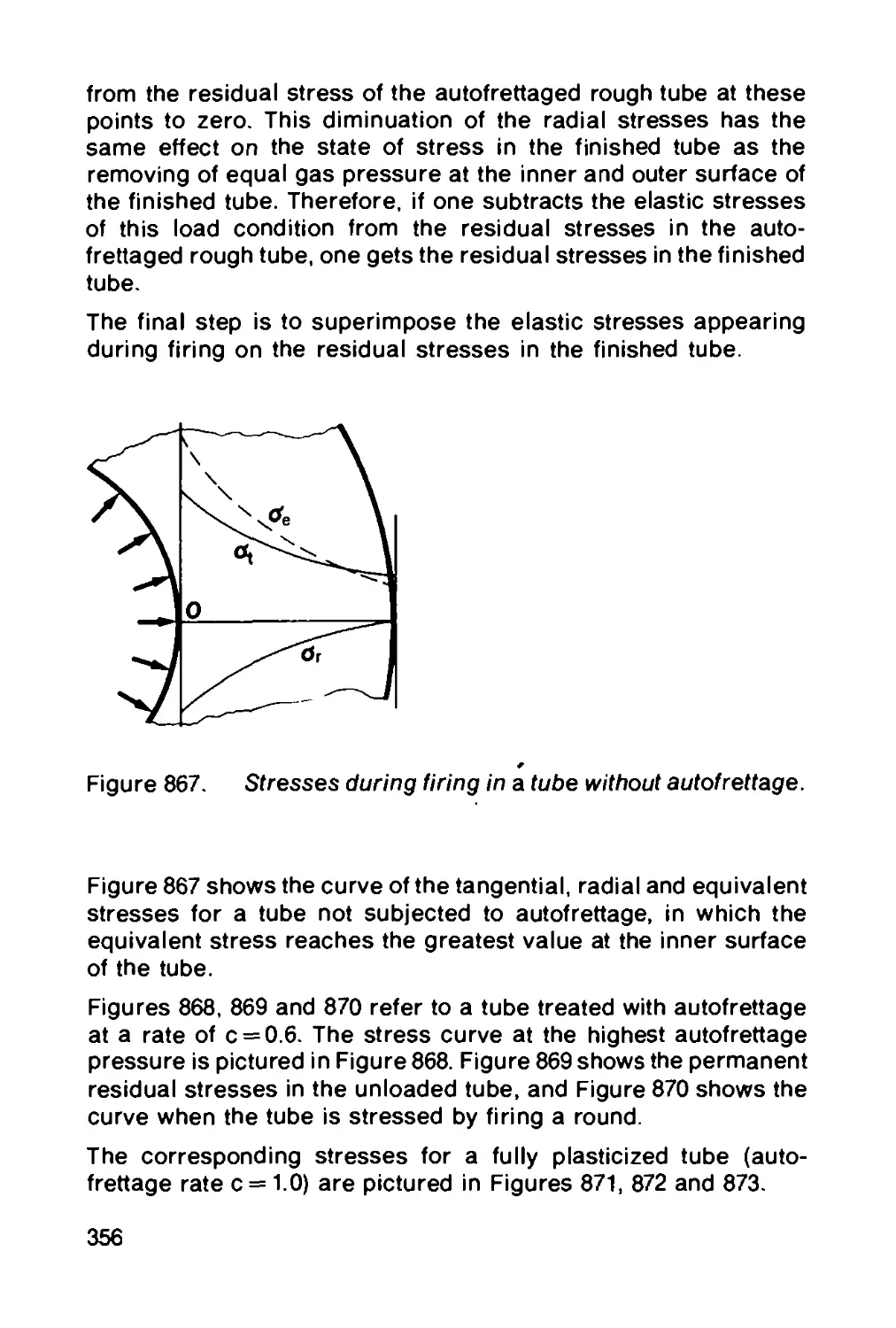
without autofrettage................................... 351
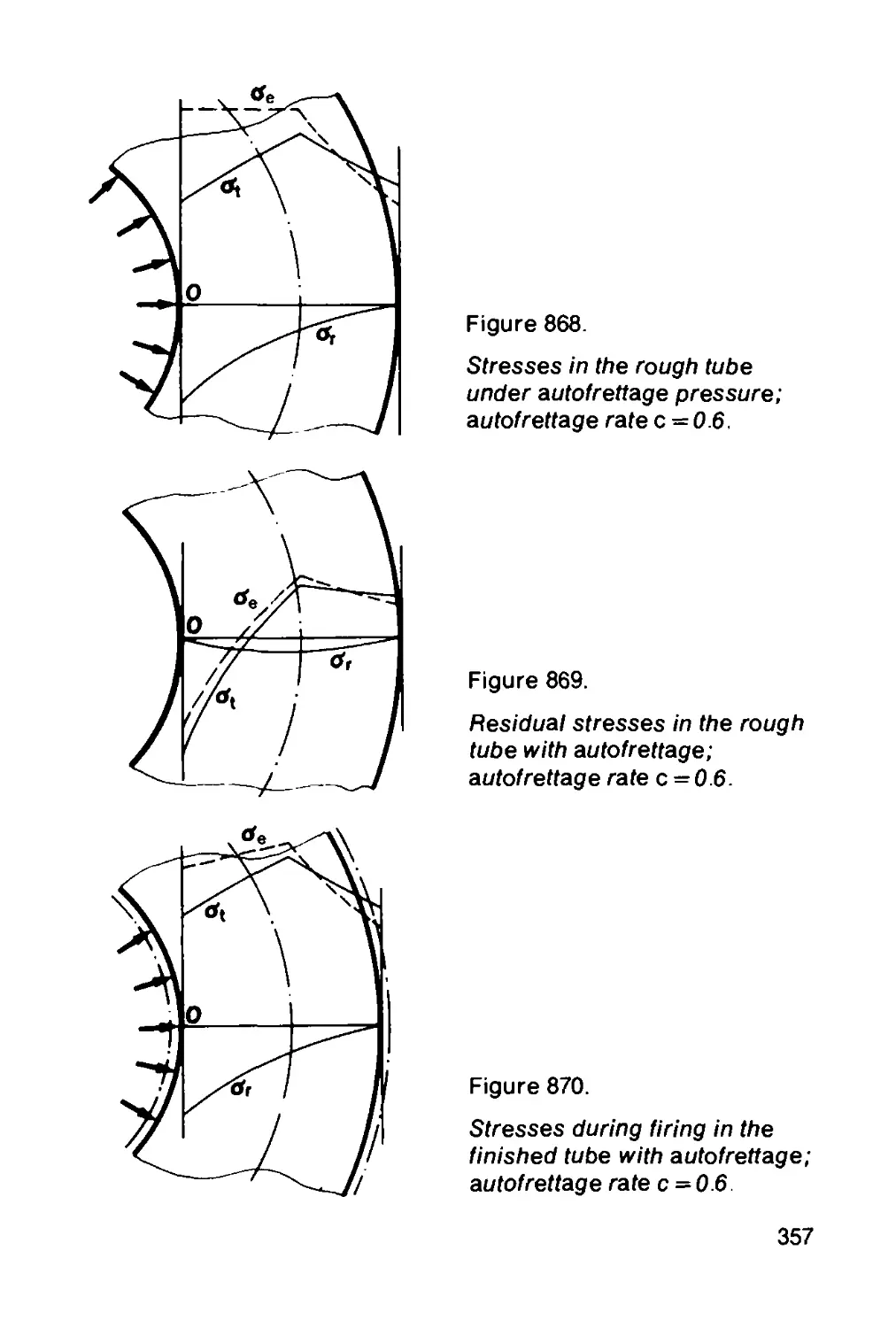
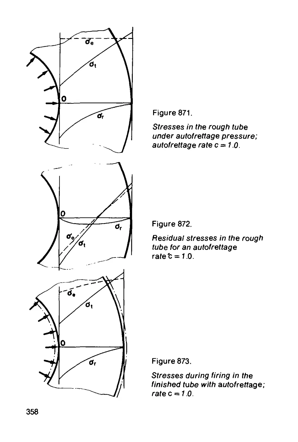
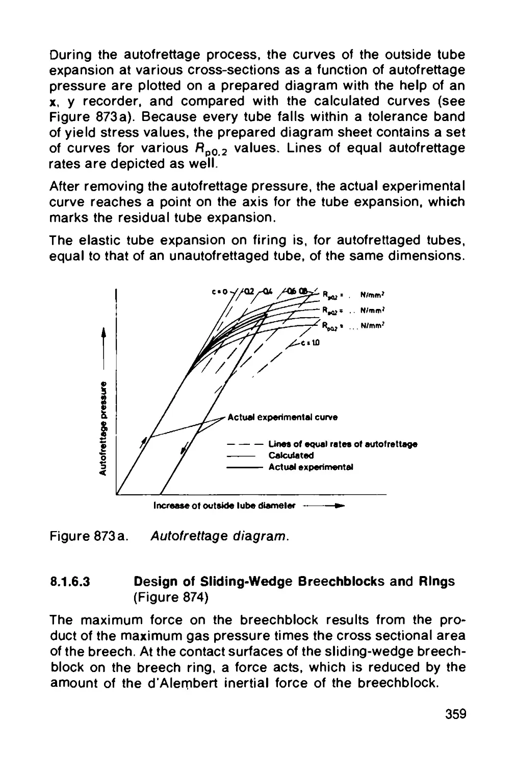
8.1.6.2 Design of monobloc tubes with autofrettage... 354
8.1.6.3 Design of sliding-wedge breechblocks and
rings.................................................. 359
8.1.7 Service life of gun tubes................... 362
8.1.7.1 Wear service life........................... 362
8.1.7.2 Fatigue service life........................ 363
8.1.8 Gun tube materials and their testing......... 365
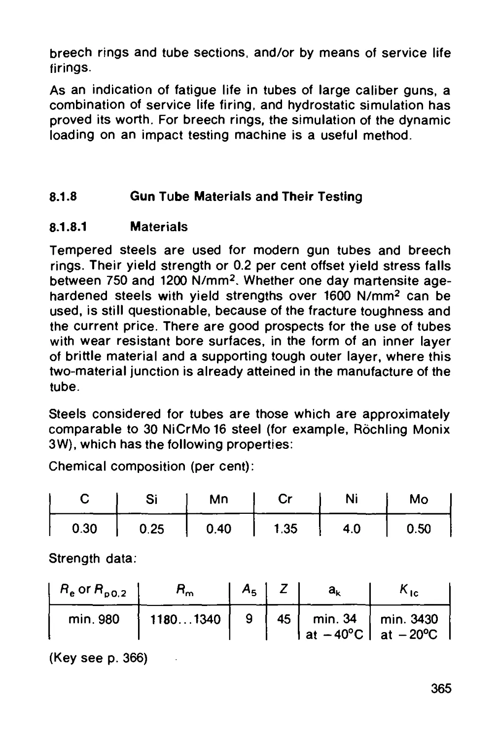
8.1.8.1 Materials................................... 365
8.1.8.2 Materials testing .......................... 366
8.2 Carriages and mounts........................ 367
8.2.1 Mounting of gun tubes and supporting the forces
during firing ............................. 367
8.2.1.1 Forces and their behavior during firing .... 368
8.2.1.2 Guidelines for avoiding additional, damaging
forces and torques......................... 370
8.2.1.3 Cradles .................................... 371
XI
8.2.1.4 Recoil brakes and recuperator mechanisms .. 374
8.2.2 Aiming, stabilizing and leveling............ 379
8.2.2.1 Aiming axes, elevating part, traversing part and
canting part........................................... 380
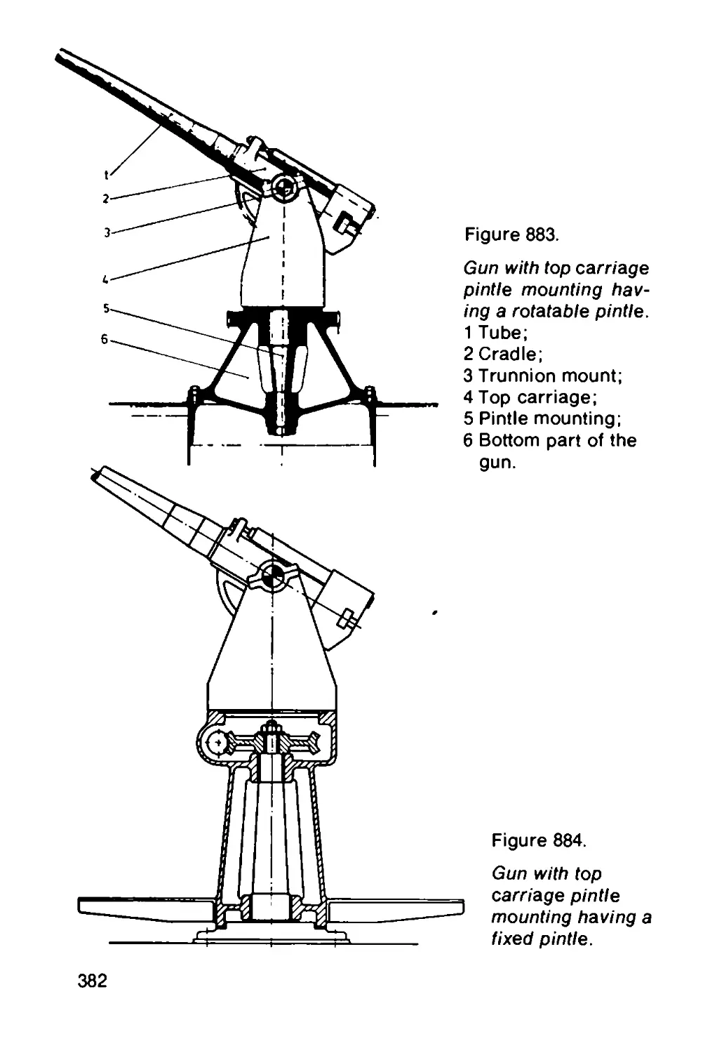
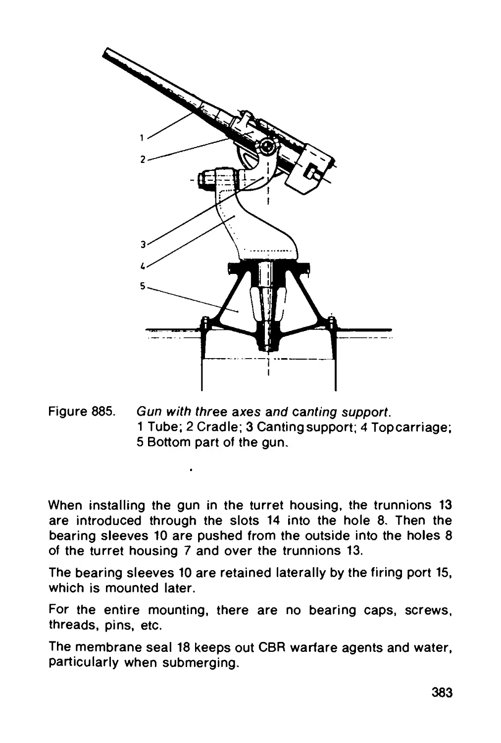
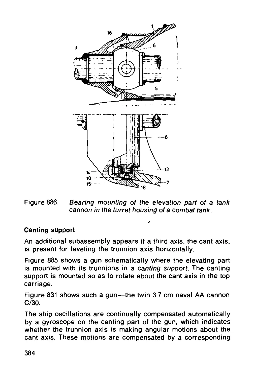
8.2.2.2 Top carriage and canting support............ 381
8.2.2.3 Equilibrators............................... 385
8.2.2.4 Elevating and traversing mechanisms.......... 388
8.2.2.5 Stabilization .............................. 391
8.2.2.6 Leveling.................................... 391
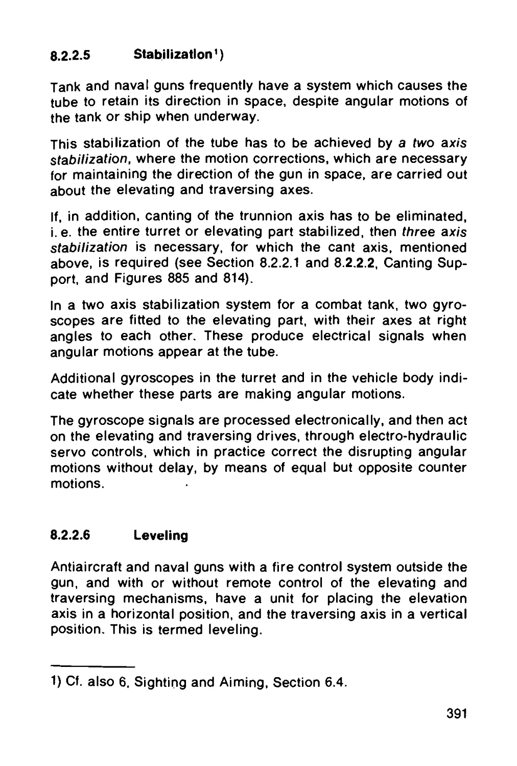
Э.2.2.7 Laying and fire range limitation ........... 393
8.2.3 Bottom part of the gun and arrangement for
movability............................................. 395
8.2.3.1 Wheeled mounts.............................. 395
8.2.3.2 Self-propelled carriages and tanks ....... 399
8.2.3.3 Fixed carriages ............................ 400
8.2.4 Special carriages........................... 400
8.2.5 Armor and CBR protection.................... 402
8.2.5.1 Protective armor on vehicles and carriages... 402
8.2.5.2 Protection against CBR agents............... 404
8.3 Loading mechanisms.......................... 405
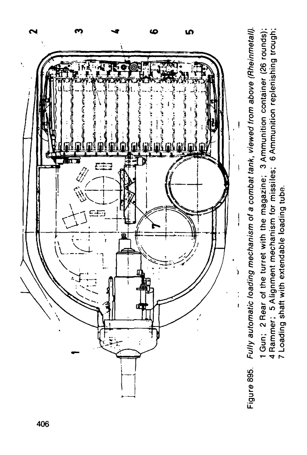
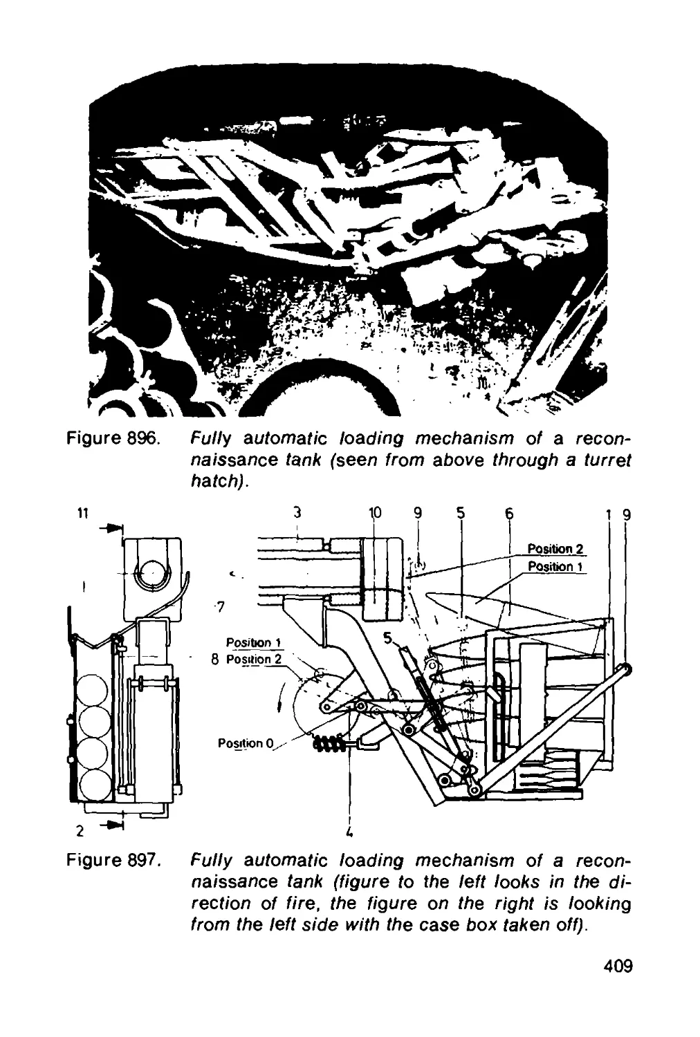
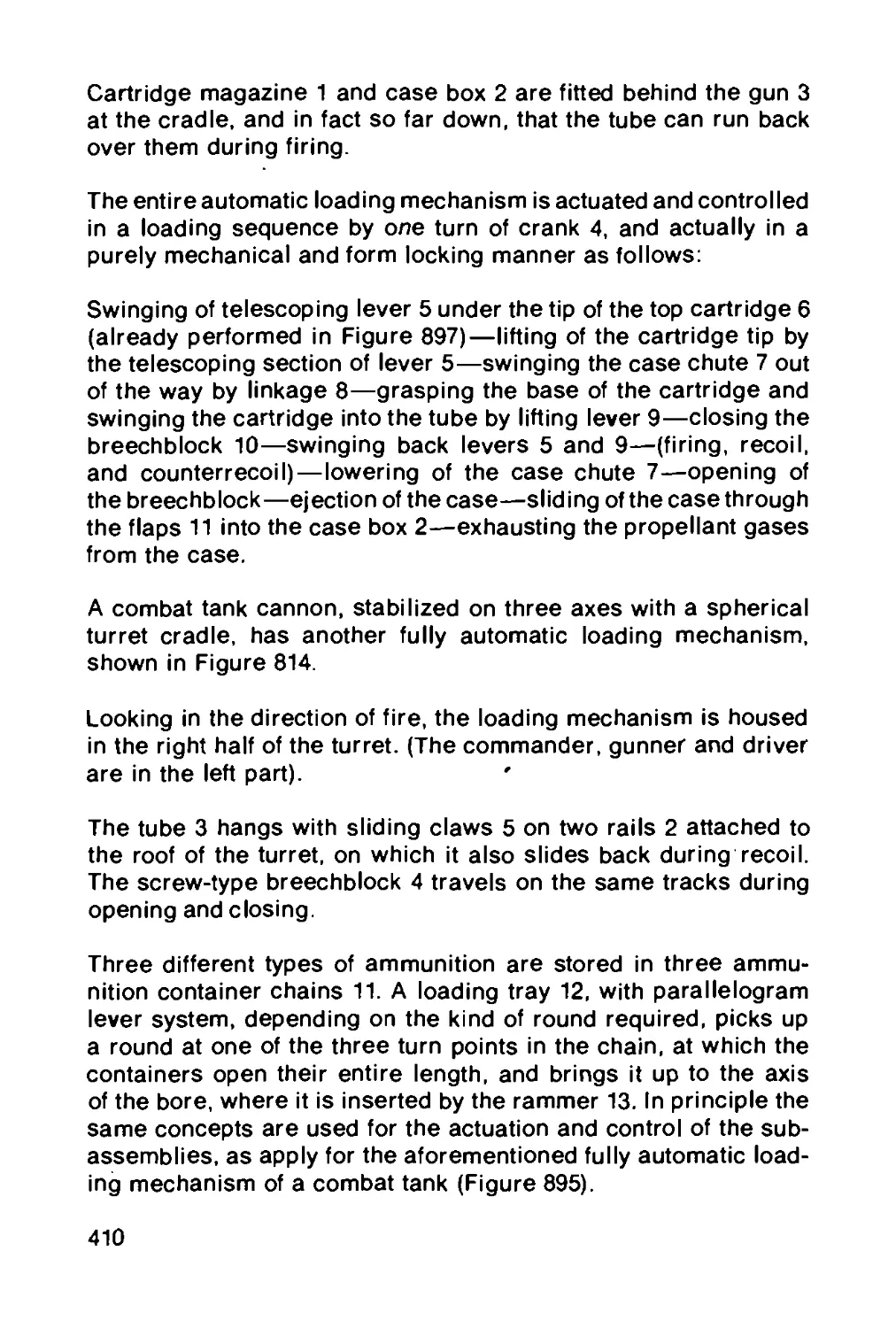
8.3.1 Fully automatic loading mechanisms........... 405
8.3.2 Automatic loading mechanisms................ 411
8.3.3 Semi-automatic loading mechanisms............ 411
9 GUN MECHANICS .............................. 413
S. v. Boutteville
9.1 Definition of gun mechanics................. 413
9.2 Symbols employed ........................... 413
9.3 Some important fundamental rules of
mechanics.................................. 415
9.4 Fundamental processes of firing a projectile .. 417
9.5 Load on the gun tube during firing.......... 419
9.5.1 Forces on a smooth tube for fin stabilized
projectiles............................................ 421
9.5.2 Forces on a rifled tube for spin stabilized
projectiles............................................ 421
9.6 Load on the carriage during firing.......... 425
9.6.1 Types of gun mounts......................... 425
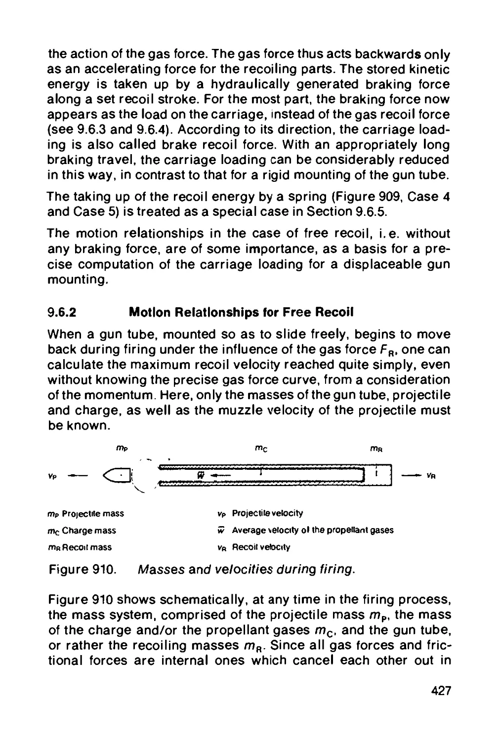
9.6.2 Motion relationships for free recoil........ 427
XII
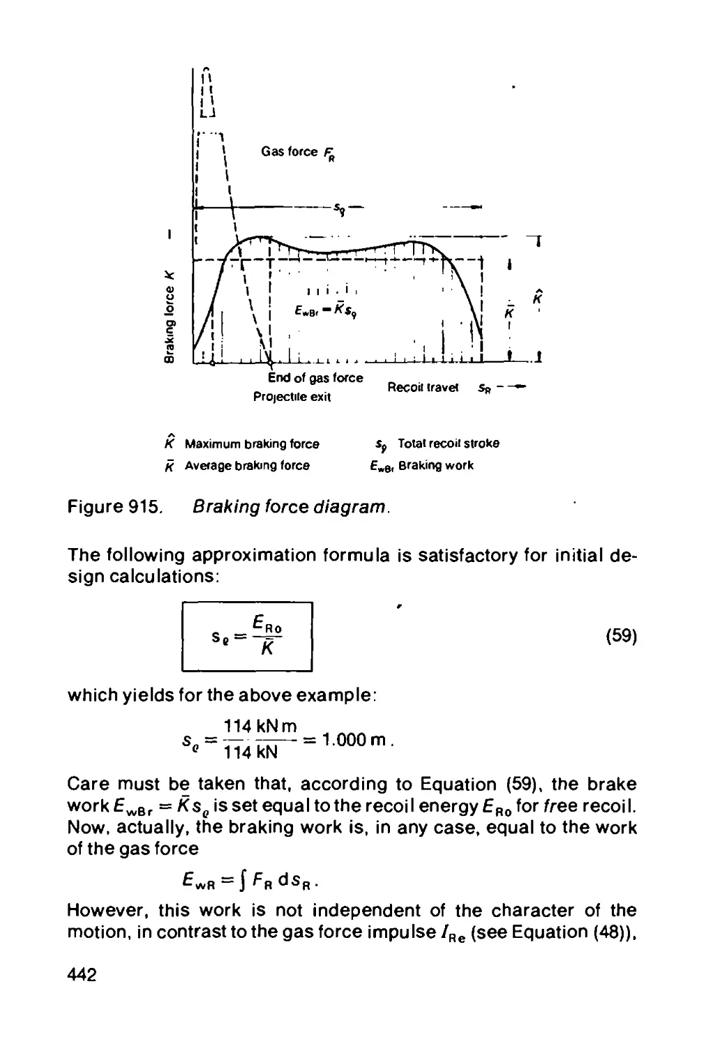
9.6.3 Requisite braking force for initially free recoil 433
9.6.4 Influence of initial braking on the recoil.. 437
9.6.5 Carriage load with spring type mount........ 443
9.6.6 Rigid mounting of the gun tube.............. 448
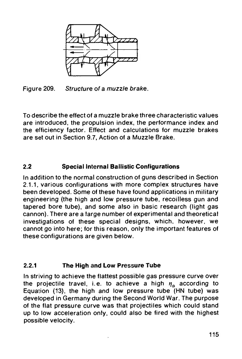
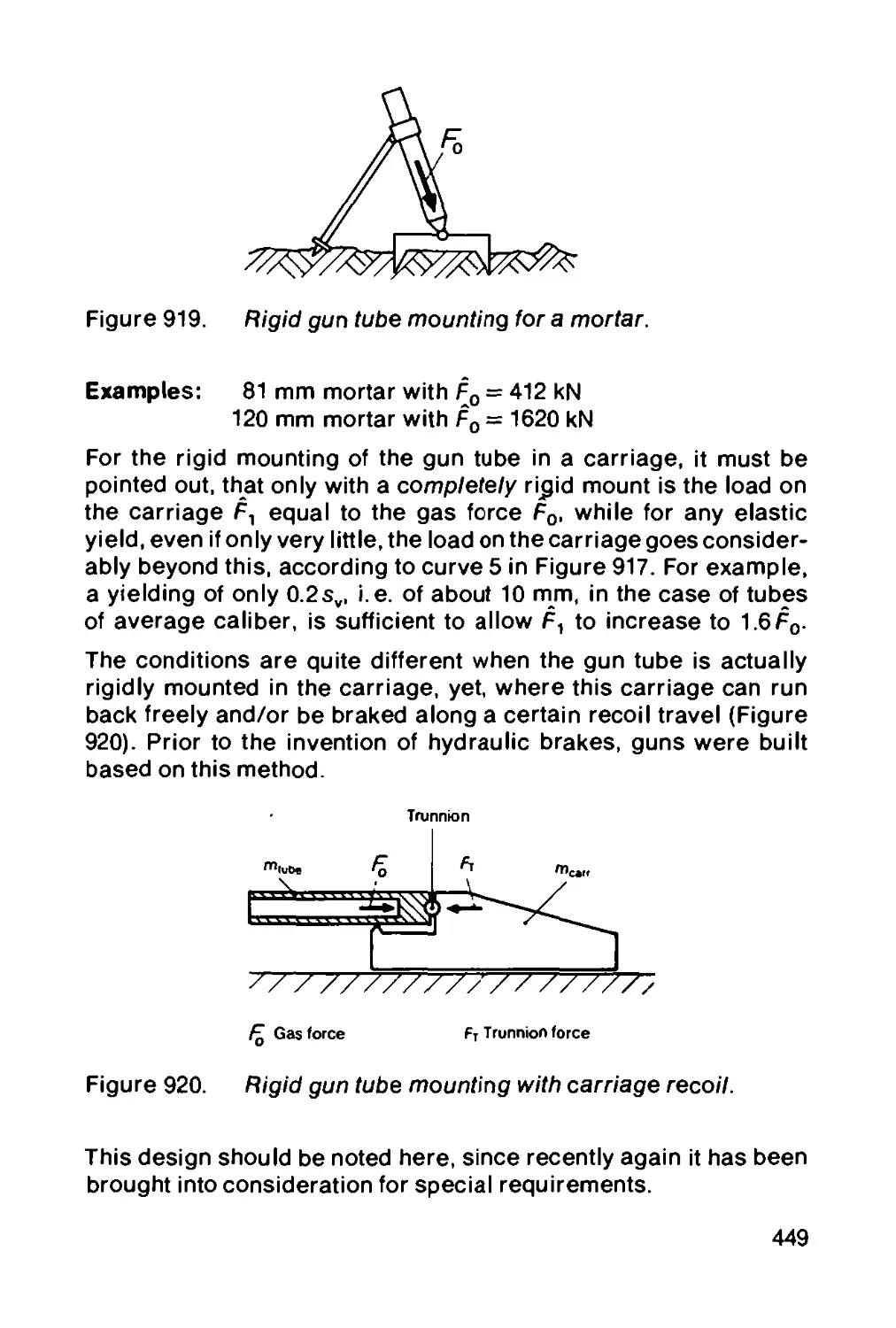
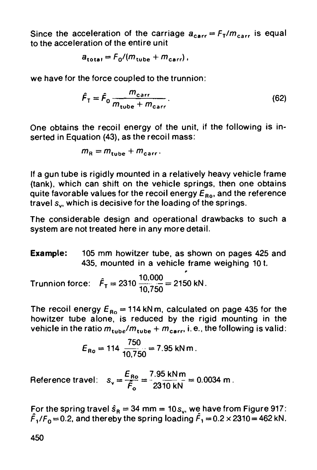
9.7 Action of a muzzle brake.................... 451
9.7.1 Basic manner of operation................... 451
9.7.2 Impulse magnitudes.......................... 453
9.7.3 Characteristic values ........................... 455
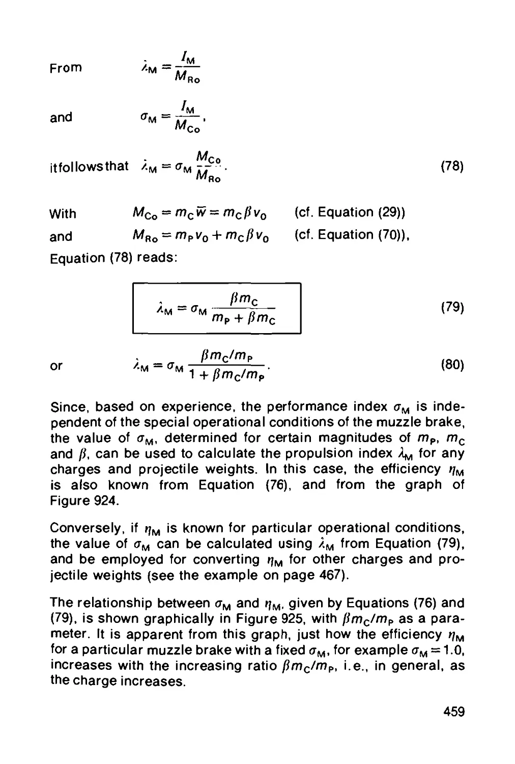
9.7.4 Relationships between the characteristic values 457
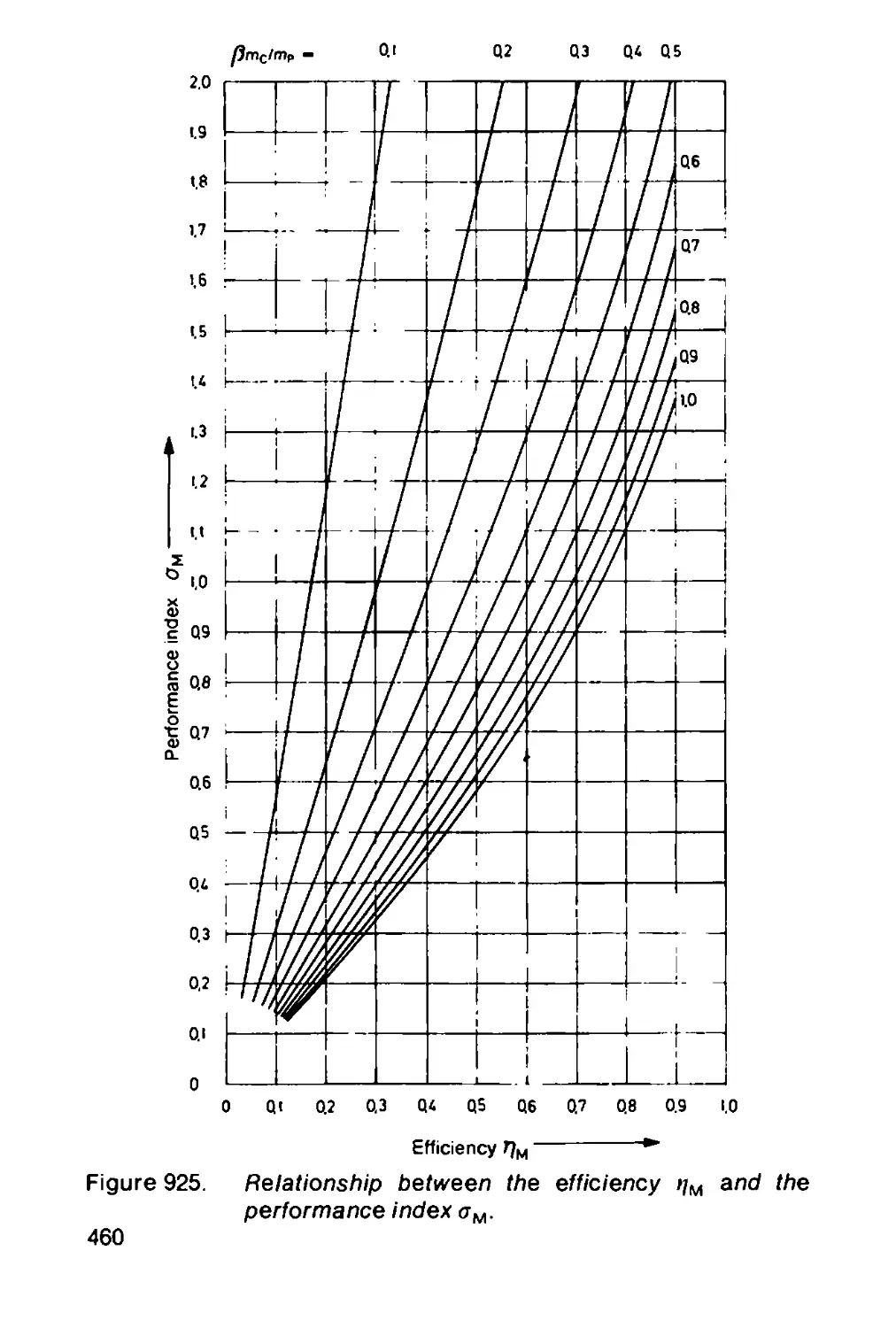
9.7.5 Measurement of the characteristic values .... 461
9.7.6 Load on the muzzle brake.................... 464
9.8 Required braking force with a muzzle brake .. 464
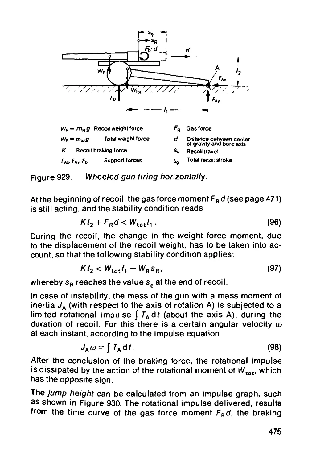
9.9 Forces on the gun with recoil ................... 468
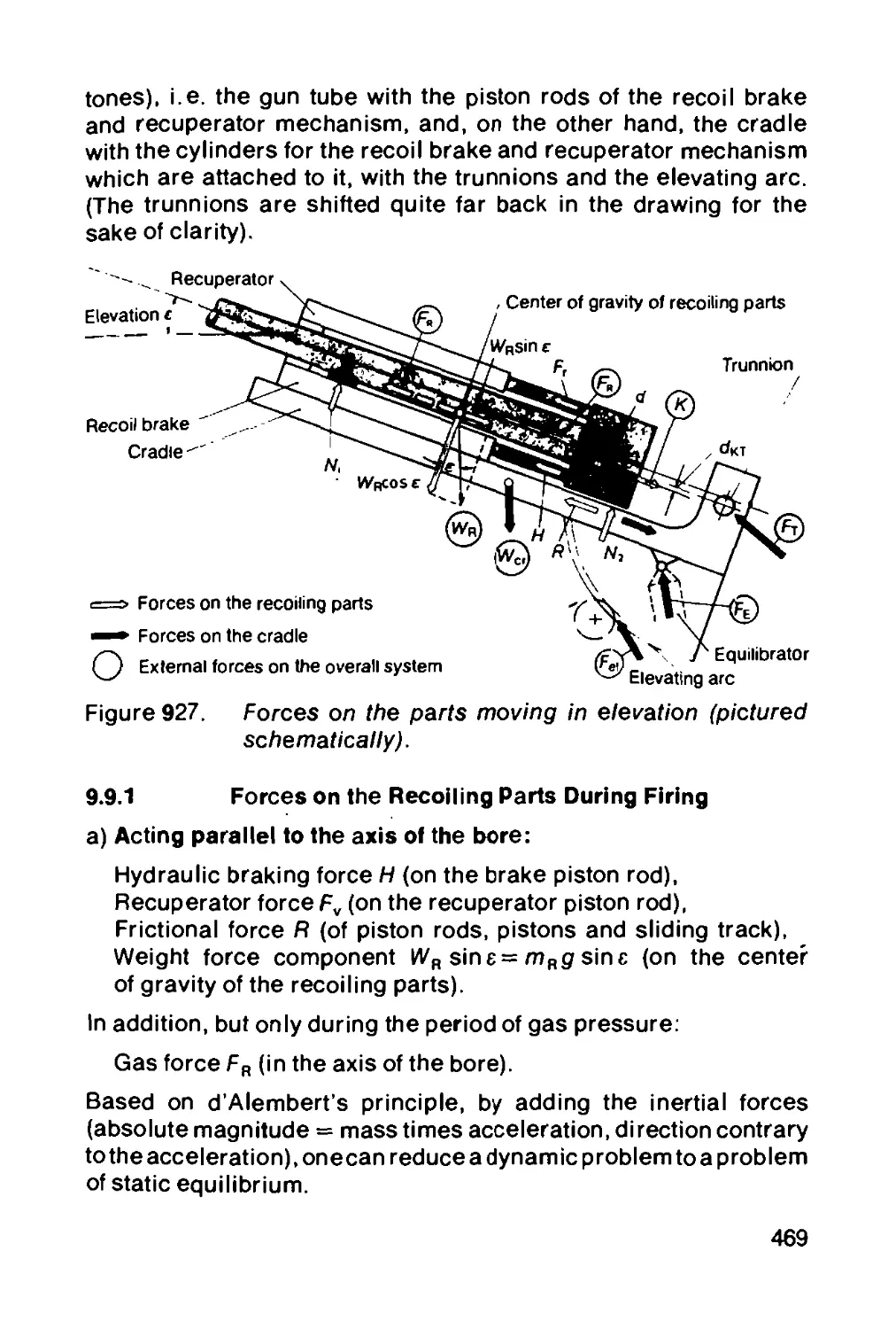
9.9.1 Forces on the recoiling parts during firing .... 469
9.9.2 Forces on the gun tube-cradle system........ 471
9.9.3 Forces on the entire gun.................... 473
9.10 Stability of the gun during firing.......... 474
9.10.1 Stability of wheeled guns................... 474
9.10.2 Stability of self-propelled gun carriages and
combat tanks............................................ 477
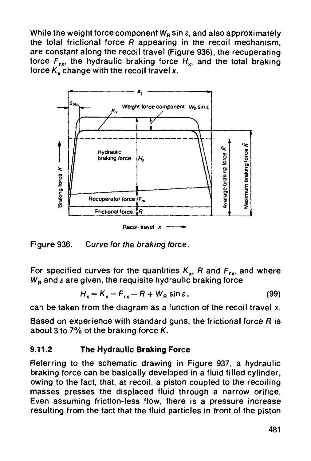
9.11 Design calculations for the recoil mechanism . 480
9.11.1 Setting the braking force up in a force-travel
diagram................................................. 480
9.11.2 The hydraulic braking force...................... 481
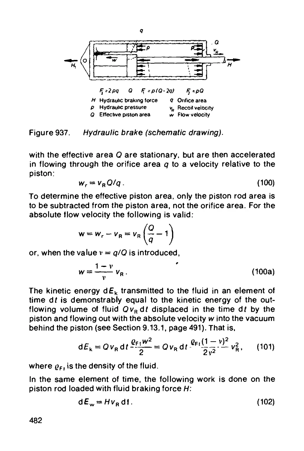
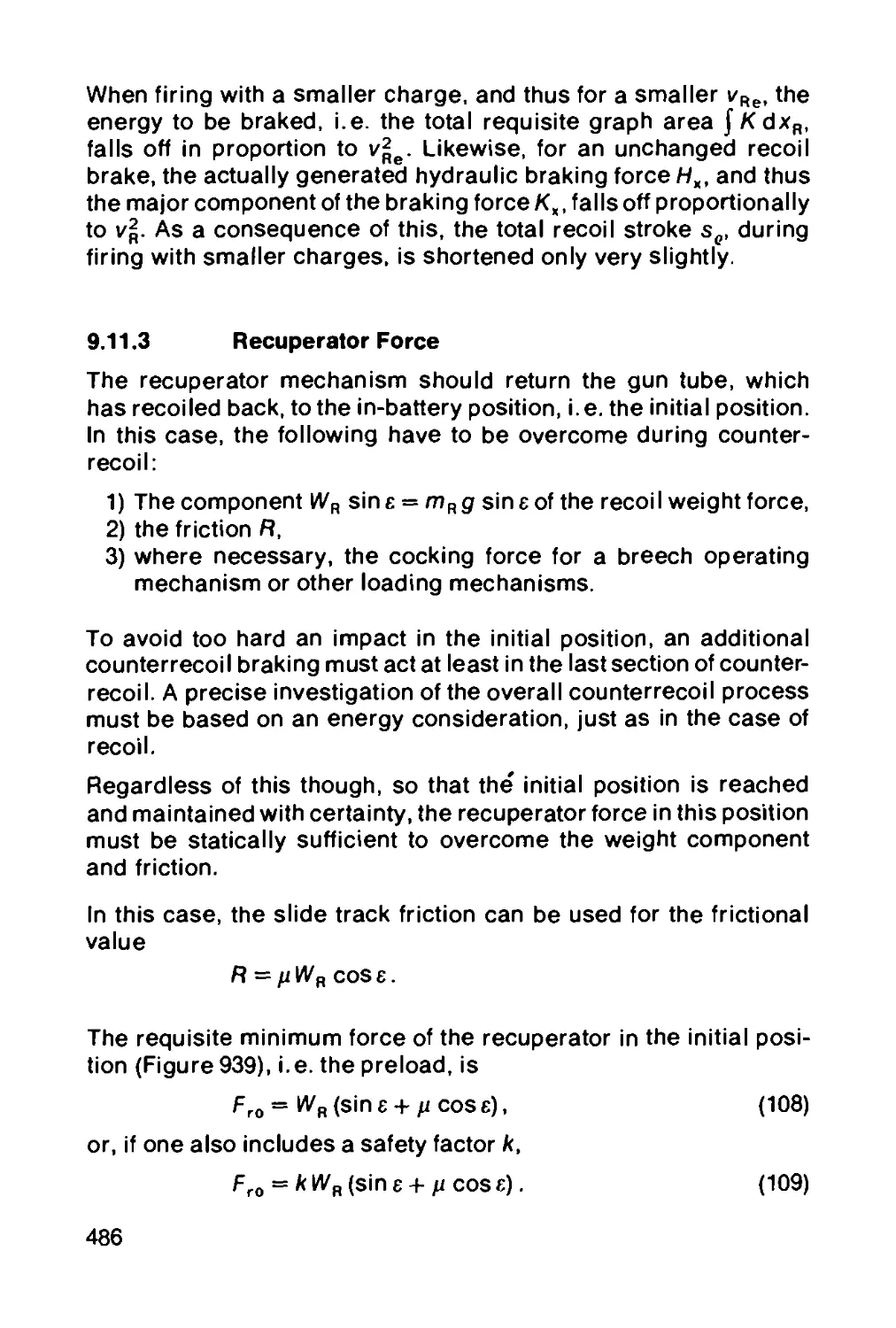
9.11.3 Recuperator force................................ 486
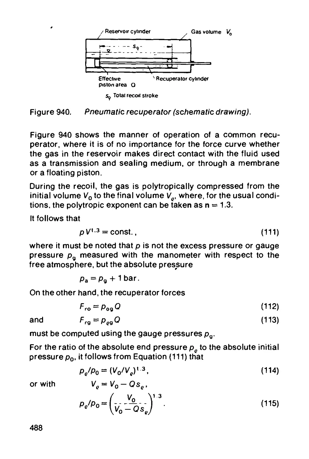
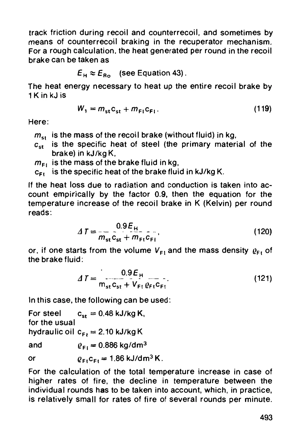
9.12 Basic design of common recoil mechanisms .. 489
9.13 Some special problems of hydraulic recoil
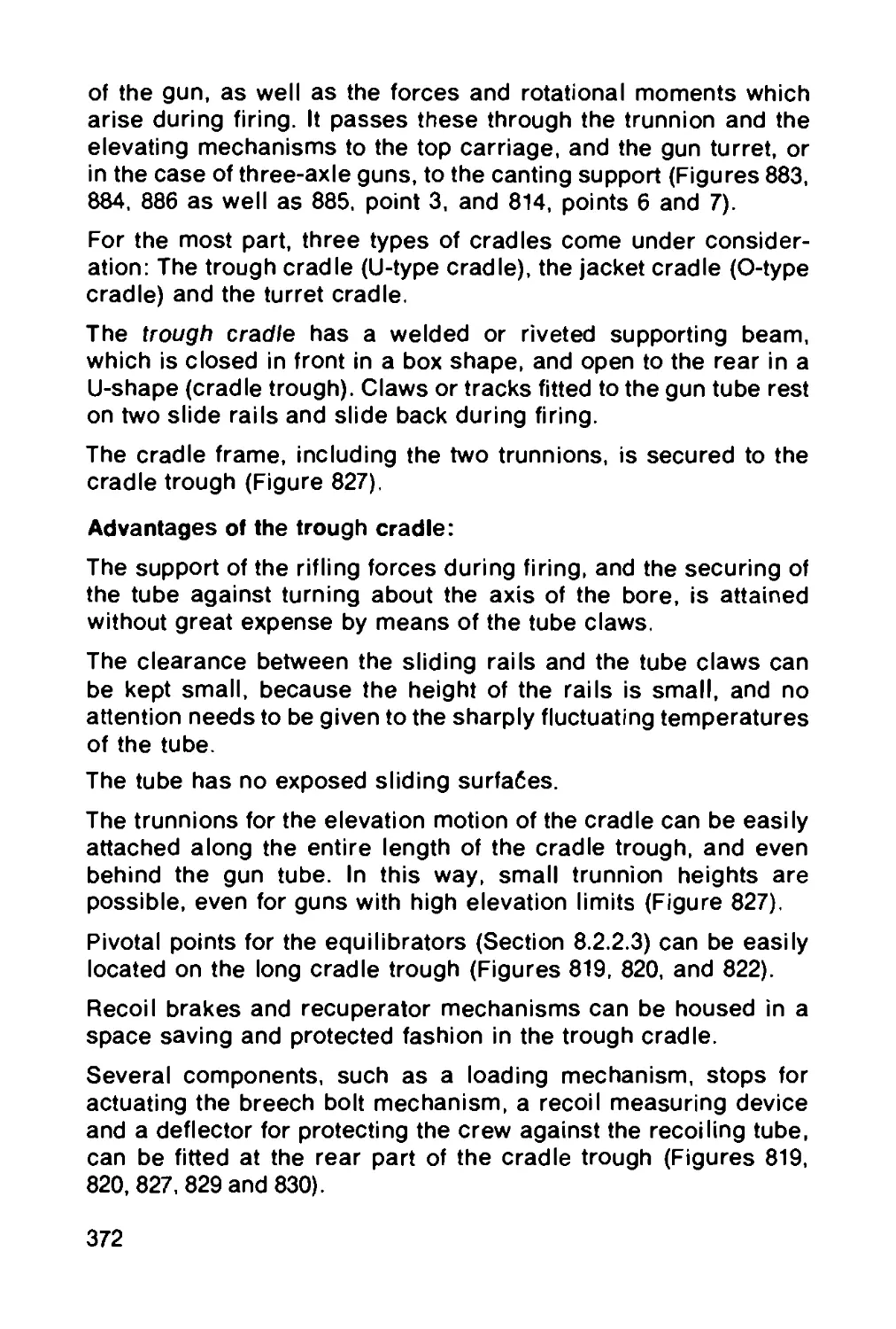
brakes........................................... 491
9.13.1 Formation of a vacuum............................ 491
9.13.2 Influence of heating............................. 492
9.13.3 Behavior of an air bubble in the pressure
chamber of a recoil brake............................... 495
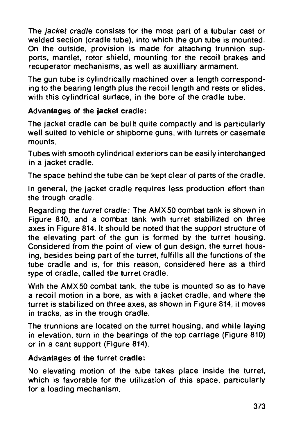
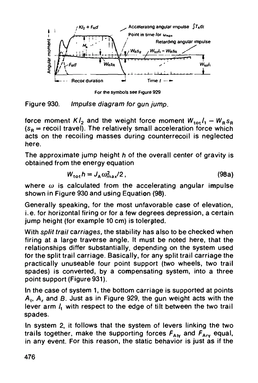
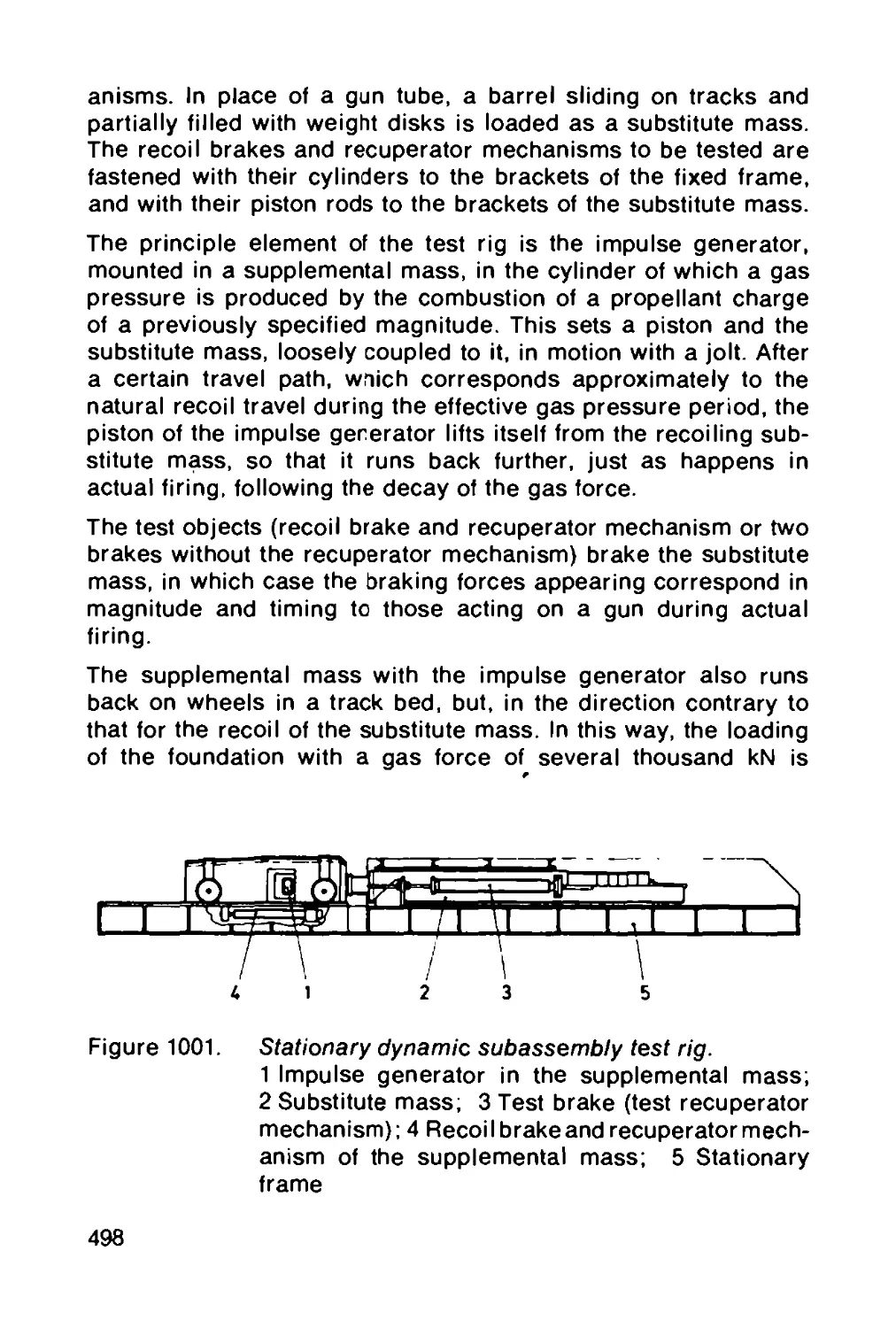
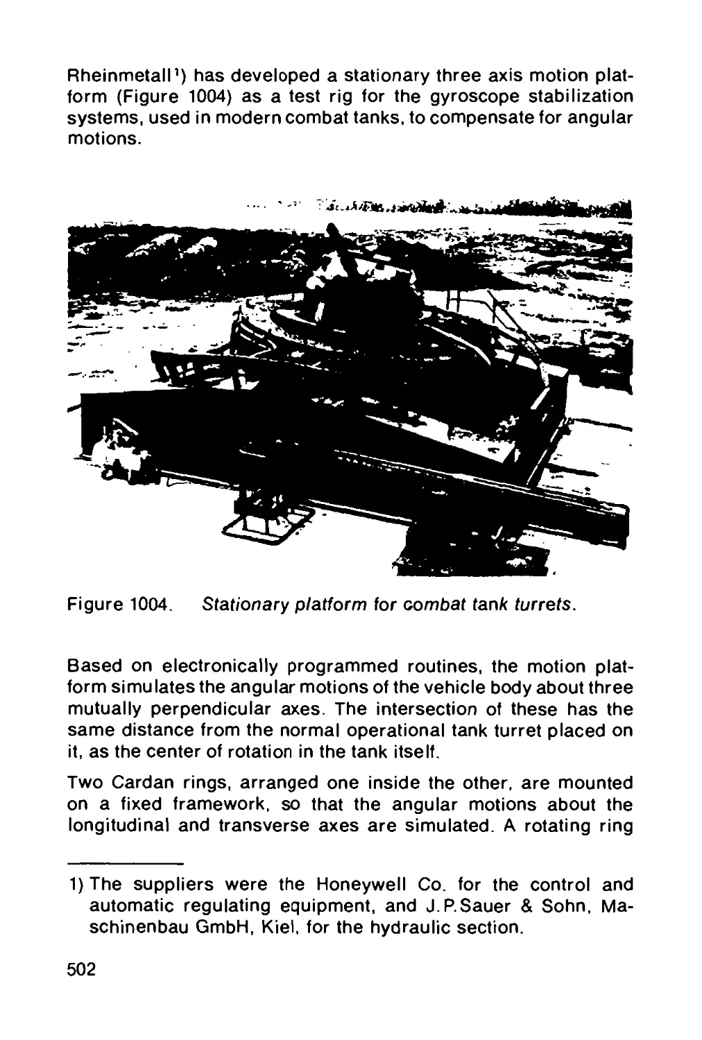
10 GUN AND GUN TURRET TEST RIGS... 497
F. Horn and D. Boder
10.1 Dynamic gun test rigs............................ 497
10.1.1 Stationary subassembly test rig.................. 497
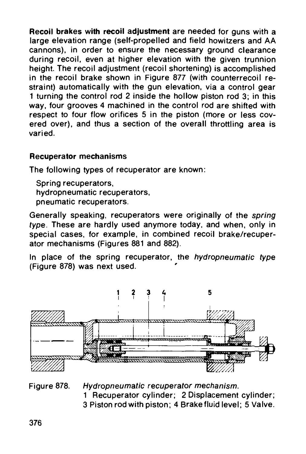
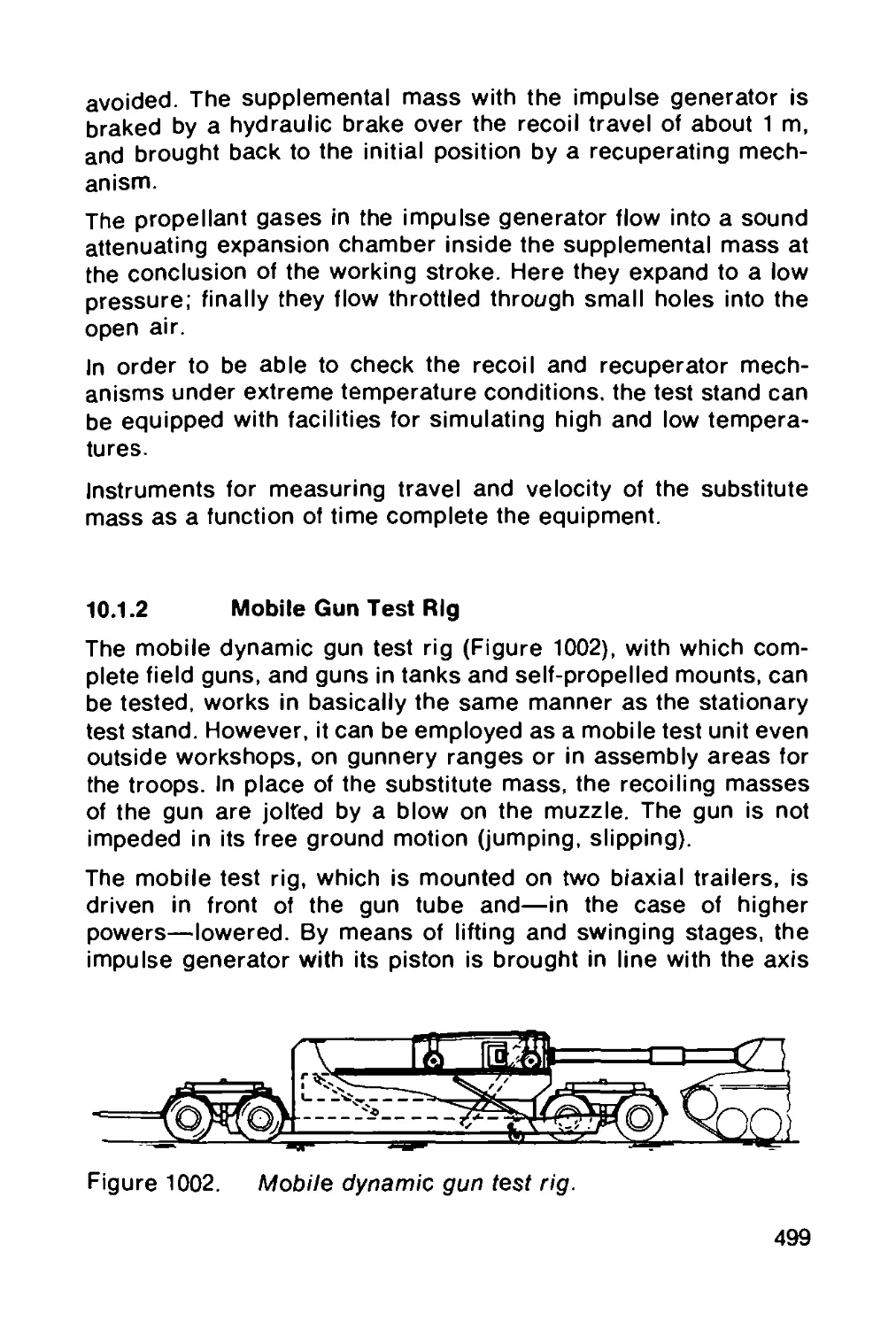
10.1.2 Mobile gun test rig.............................. 499
10.2 Rolling rigs for naval guns and fire control
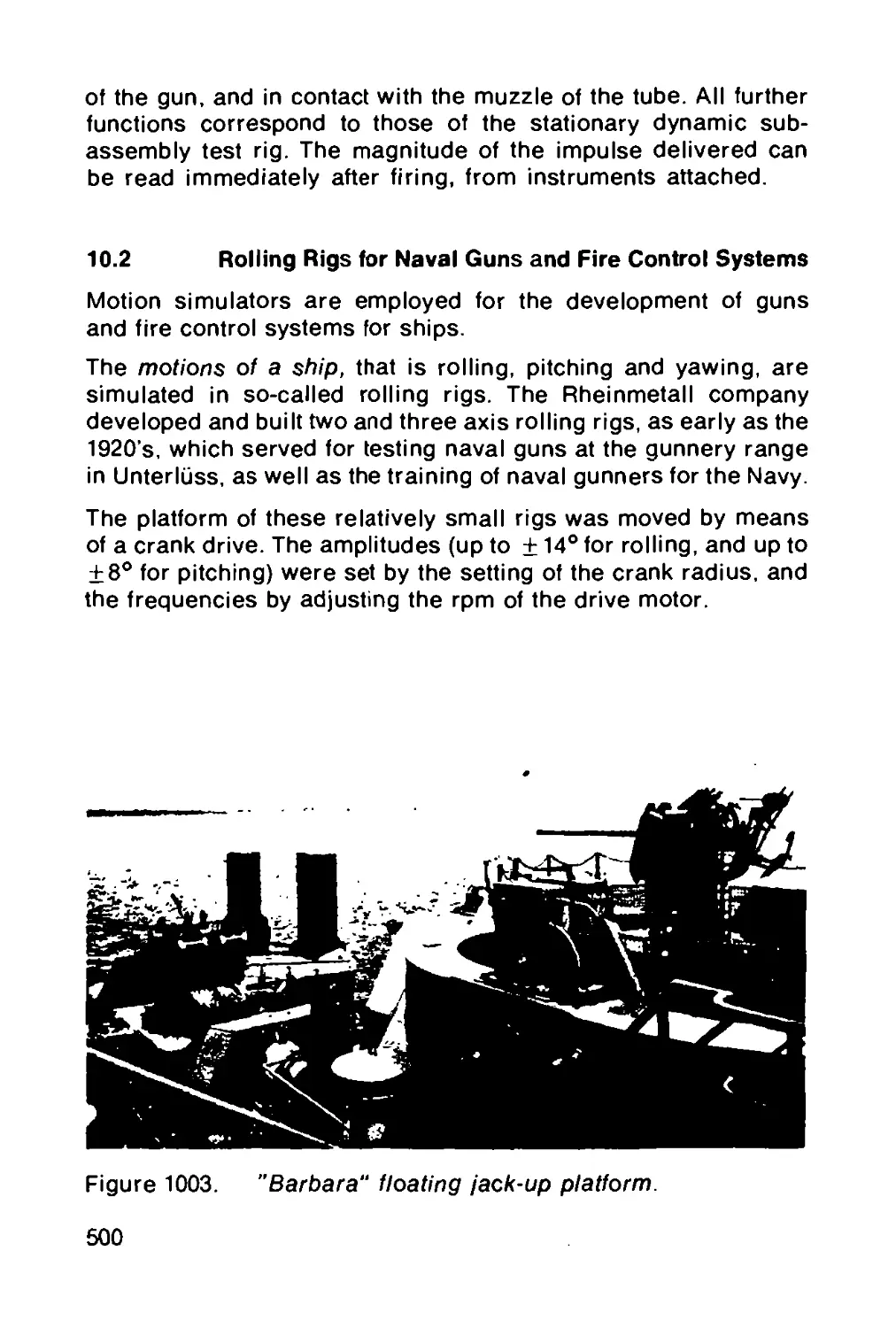
systems.......................................... 500
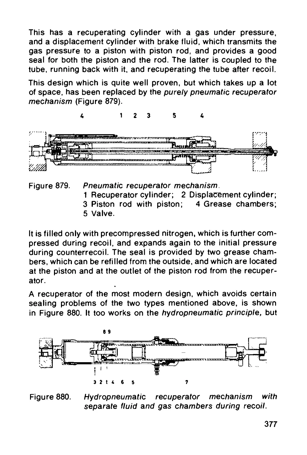
XIII
10.3 Stationary motion platform for combat tank
turrets.................................... 501
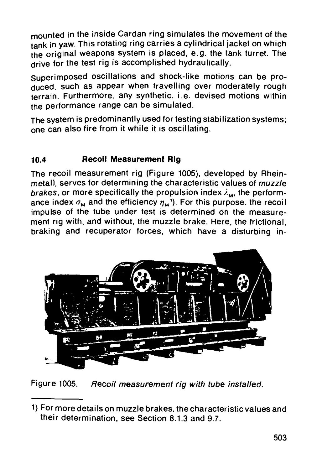
10.4 Recoil measurement rig....................... 503
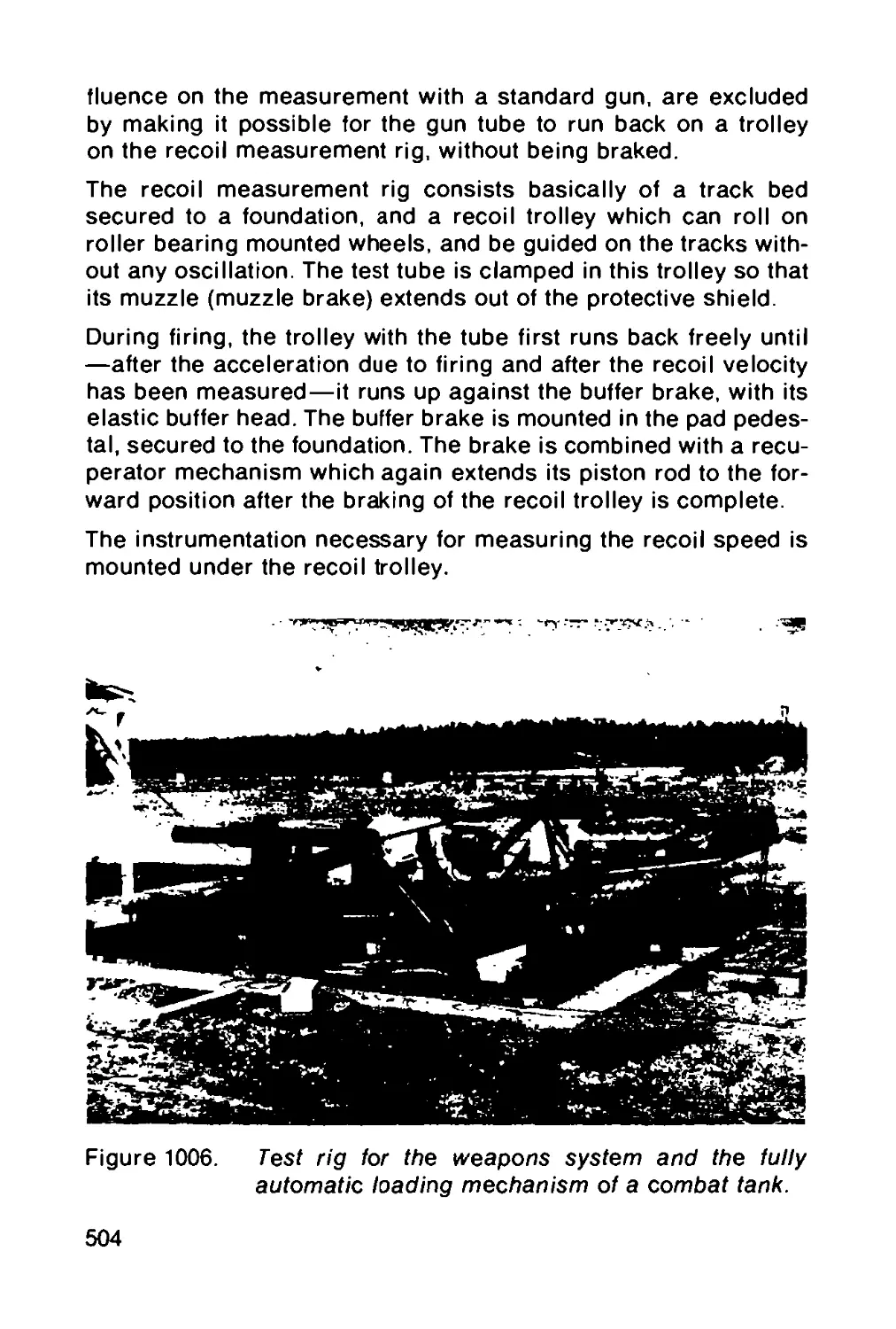
10.5 Test rigs for weapons systems................ 505
11 AMMUNITION.................................. 506
R. Romer
11.1 Ammunition design............................ 506
11.2 Projectiles.................................. 507
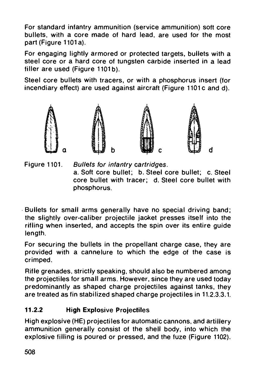
11.2.1 Projectiles for small arms.................. 507
11.2.2 High explosive projectiles.................. 508
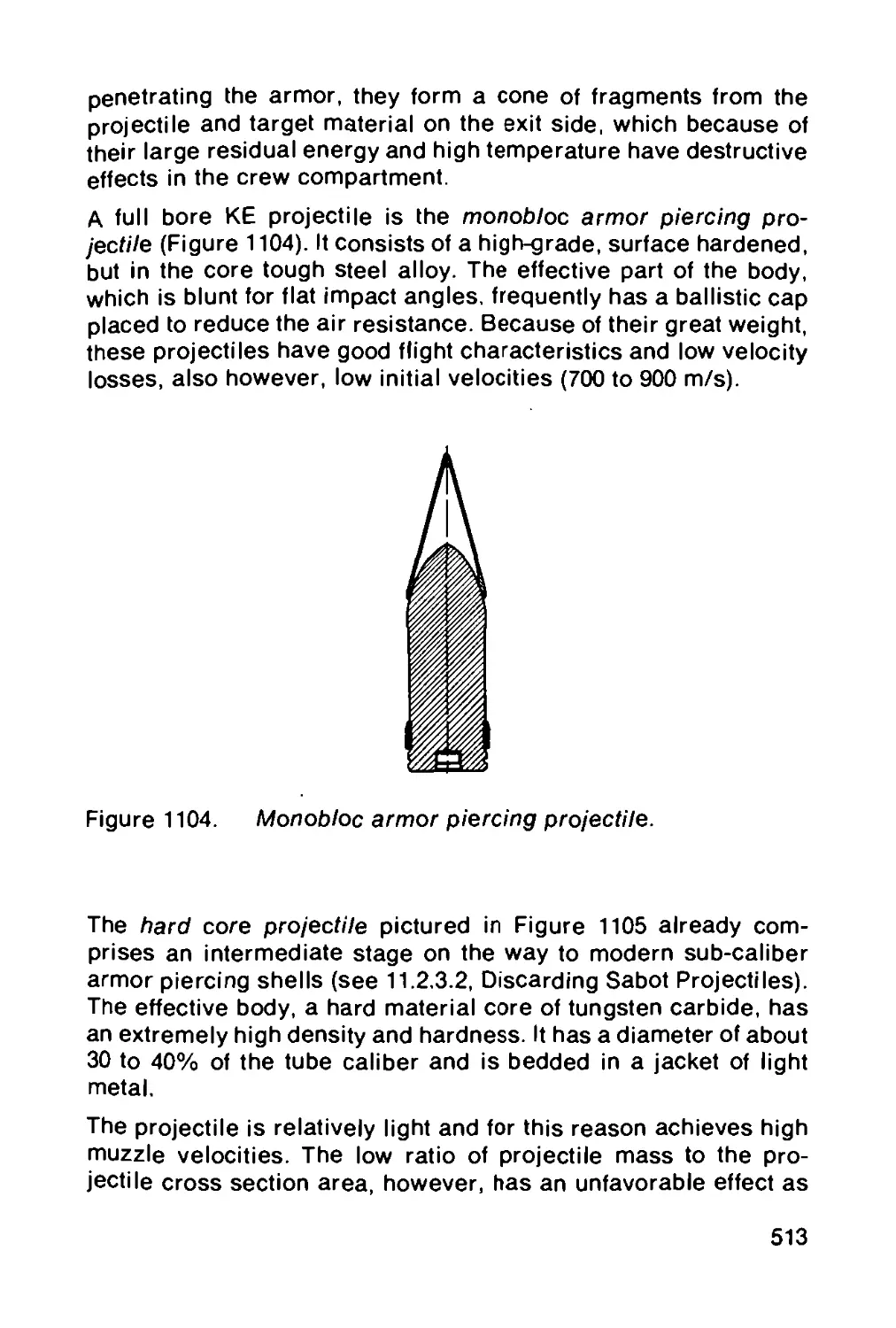
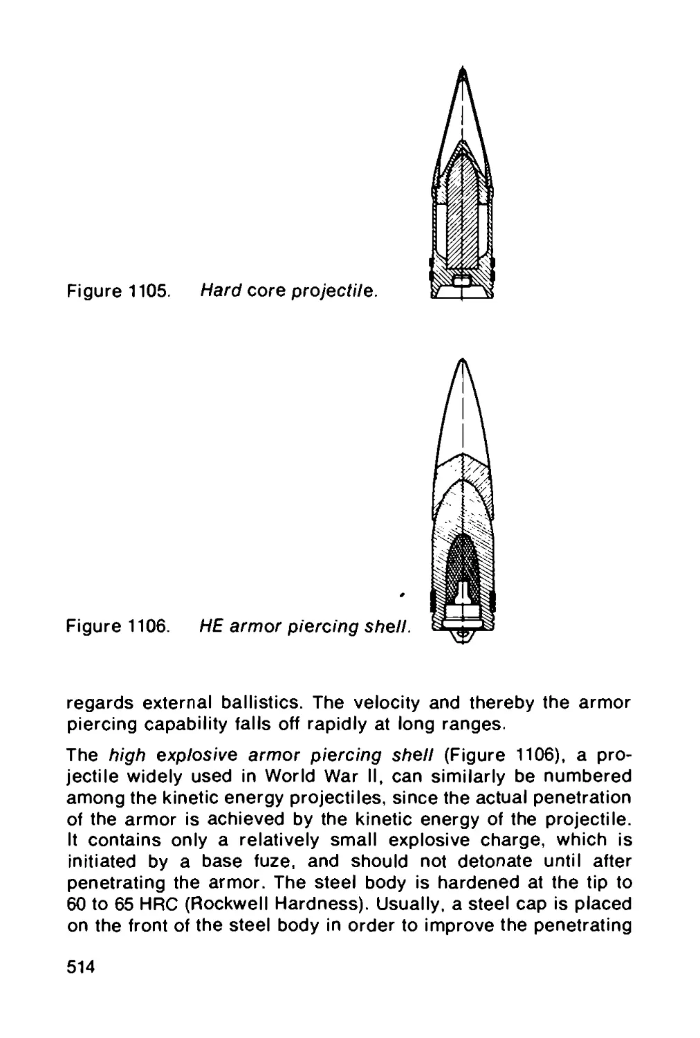
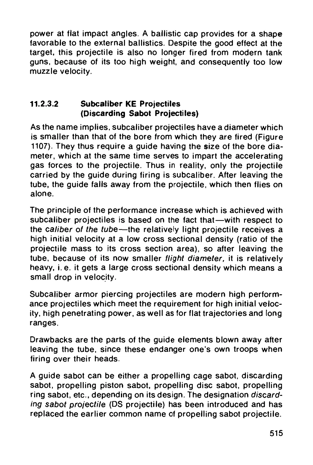
11.2.3 Armor piercing projectiles.................. 512
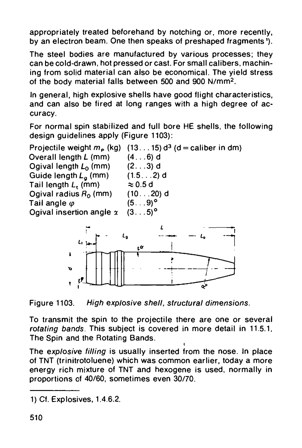
11.2.3.1 Full bore KE projectiles.................... 512
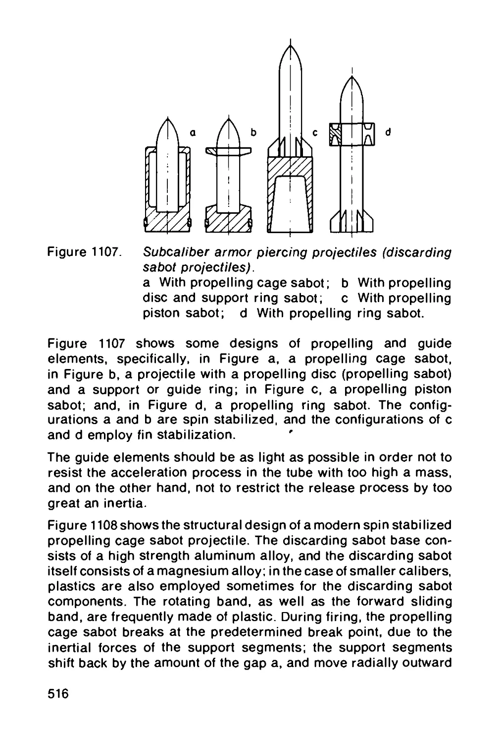
11.2.3.2 Subcaliber KE projectiles (discarding sabot
projectiles) ......................................... 515
11.2.3.3 Shaped charge projectiles................... 518
11.2.3.3.1 Fin stabilized shaped charge projectiles.... 519
11.2.3.3.2 Spin stabilized shaped charge projectile? .... 523
11.2.3.4 Squash head projectiles..................... 525
11.2.3.5 Flange projectiles for tapered bore tubes.... 527
11.2.4 Arrow projectiles........................... 528
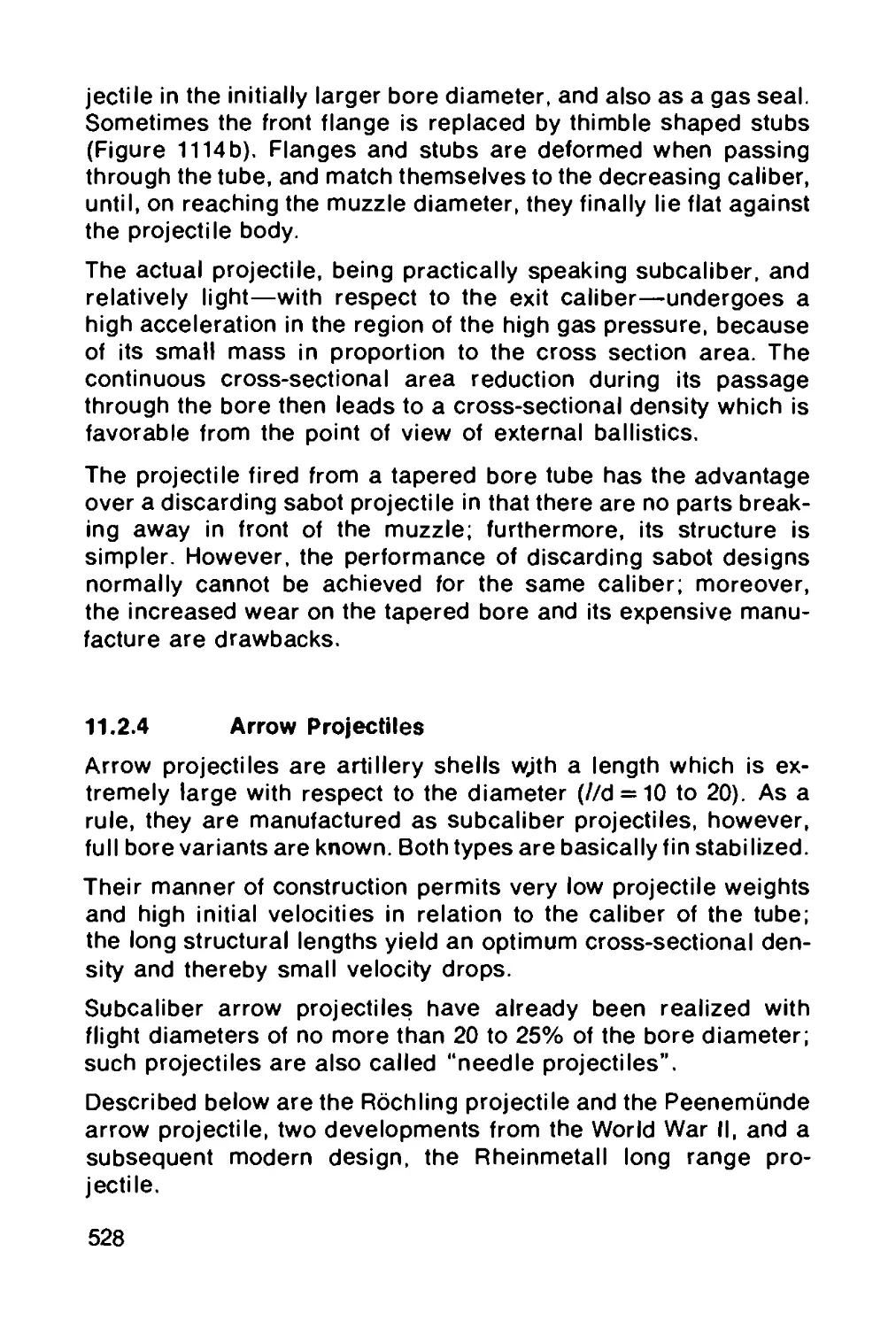
11.2.4.1 The Rochling projectile..................... 529
11.2.4.2 The PeenemOnde arrow projectile............. 530
11.2.4.3 The Rheinmetall long range projectile........ 532
11.2.5 Super-caliber projectiles................... 533
11.2.6 Rocket assisted projectiles................. 533
11.2.7 Carrier projectiles......................... 536
11.2.8 Special projectiles......................... 536
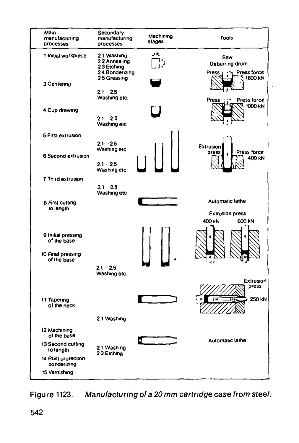
11.3 The cartridge case........................... 540
11.3.1 Manufacture of cartridge cases.............. 541
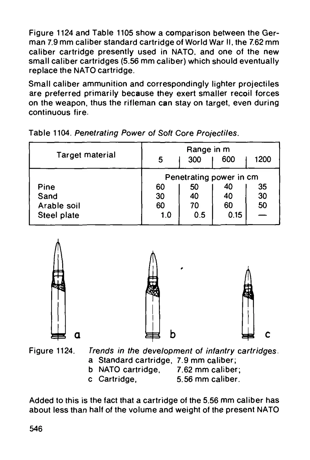
11.4 Types of ammunition.......................... 545
11.4.1 Ammunition for small arms................... 545
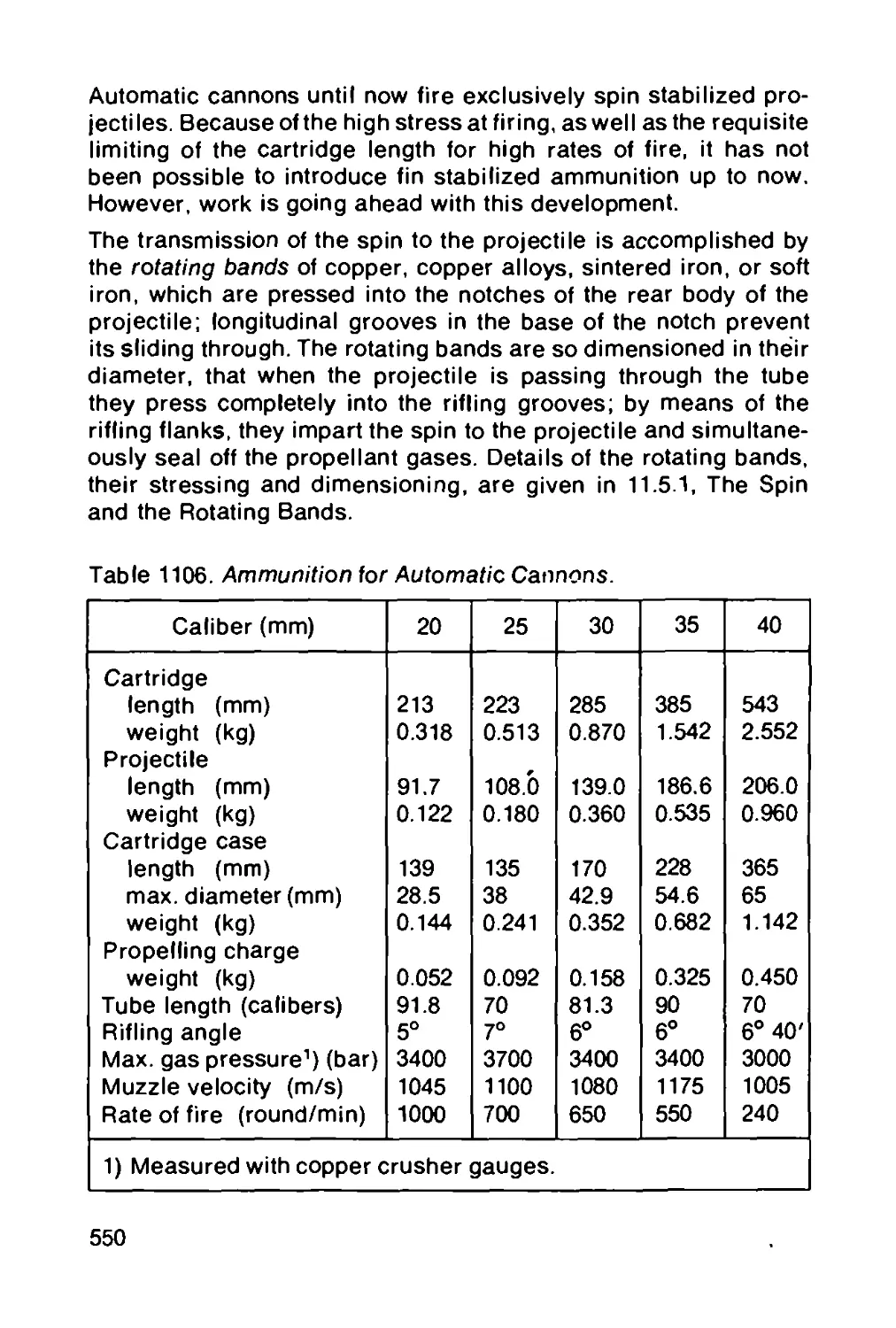
11.4.2 Ammunition for automatic cannons............ 548
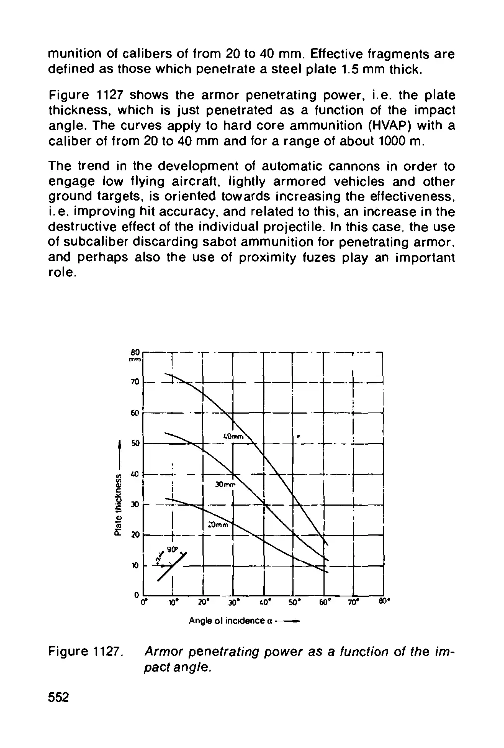
11.4.3 Armor piercing ammunition................... 553
11.4.3.1 The penetration behavior of armor piercing
projectiles................................ 559
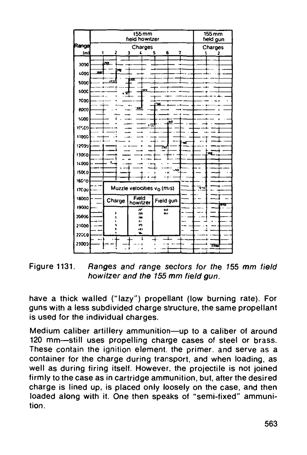
11.4.4 Artillery ammunition........................ 561
11.4.4.1 Ammunition for guns and howitzers........... 561
11.4.5 Mortar ammunition .......................... 565
XIV
11.4.6 Ammunition for training and control purposes 566
11.4.6.1 Practice ammunition........................ 567
11.4.6.2 Blank ammunition........................... 567
11.4.6.3 Drill ammunition........................... 570
11.4.6.4 Proof ammunition........................... 570
11.4.7 Hand grenades and air-dropped ammunition .. 571
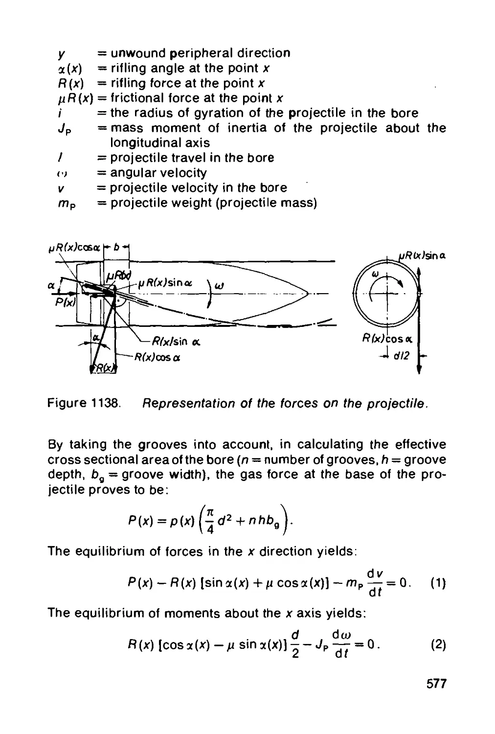
11.5 The stress on the projectiles during firing .... 571
11.5.1 The spin and the rotating bands............ 572
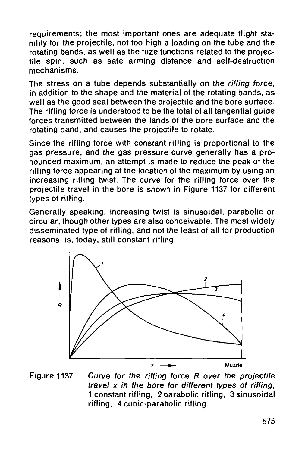
11.5.1.1 The rifling force.......................... 576
11.5.1.2 Surface pressure and frictional work of the
rotating bands...................................... 579
11.5.1.3 The rate of revolutions of the projectile... 580
11.5.2 The stress of the projectile body during firing 582
12 ROCKETS ................................... 587
R. Germershausen
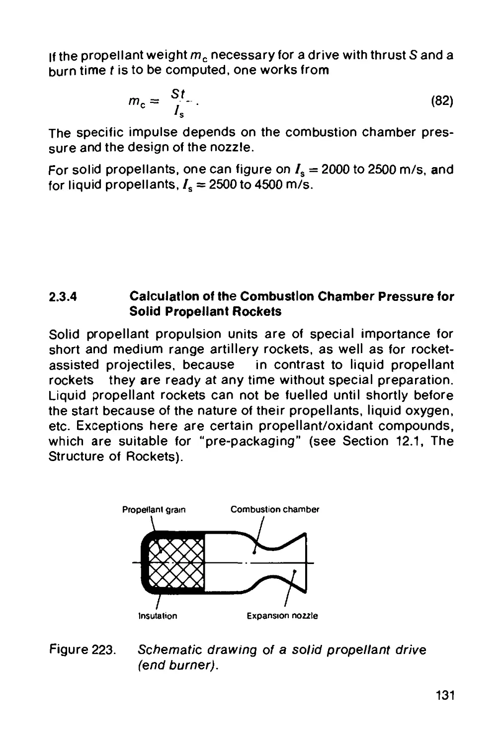
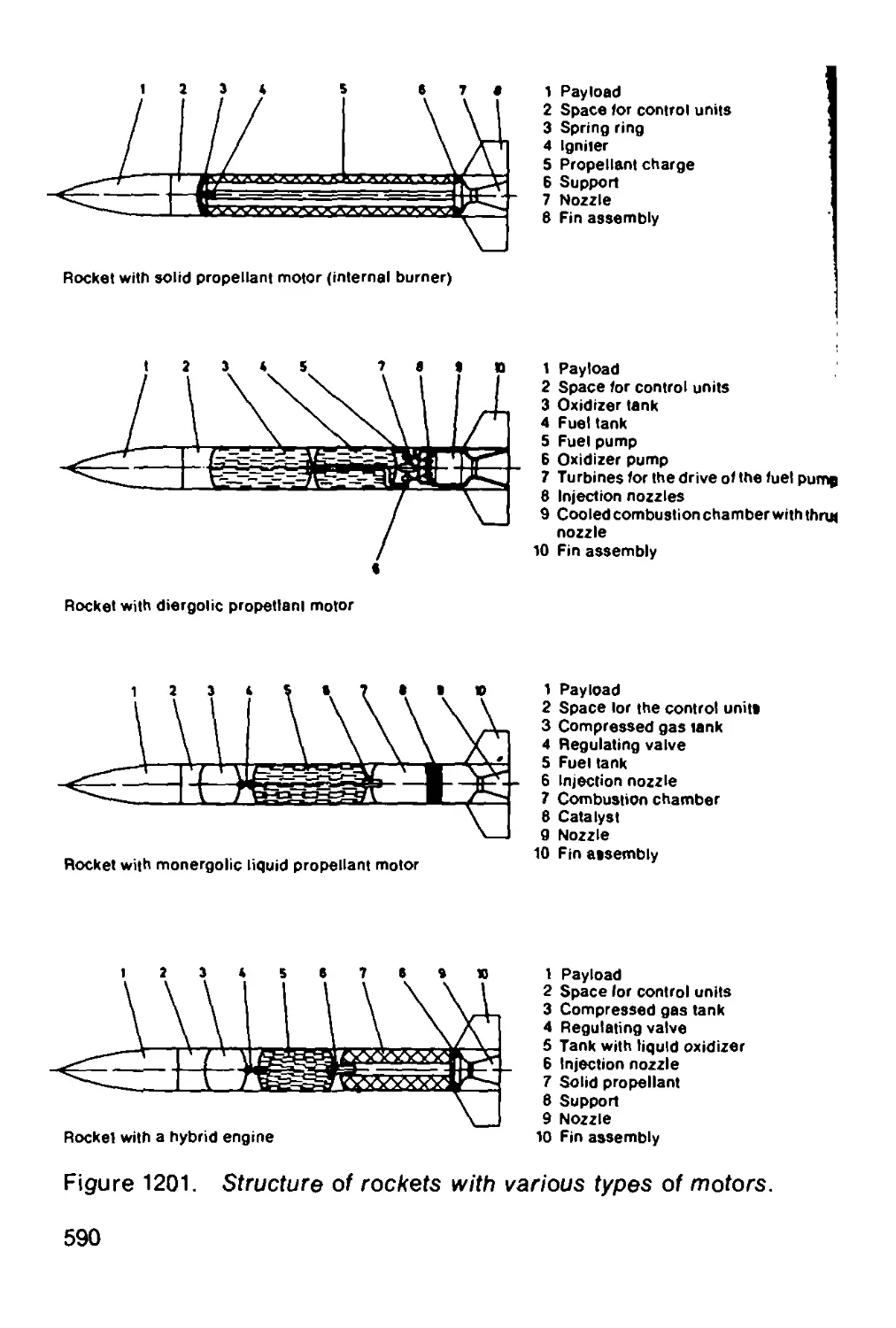
12.1 The structure of rockets................... 589
12.2 Unguided rockets........................... 591
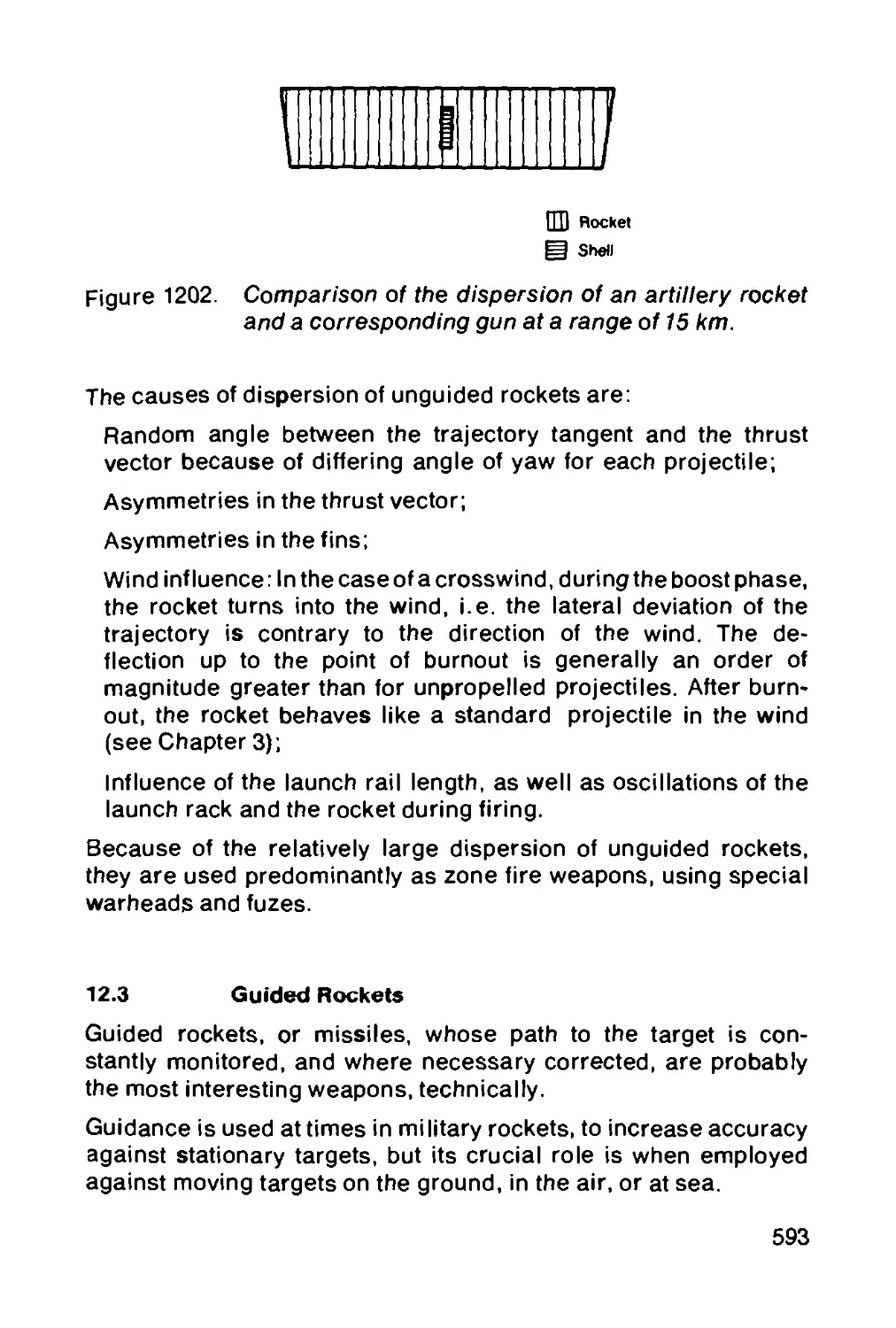
12.3 Guided rockets............................. 593
12.4 Warheads .................................. 598
12.5 Rocket launchers........................... 599
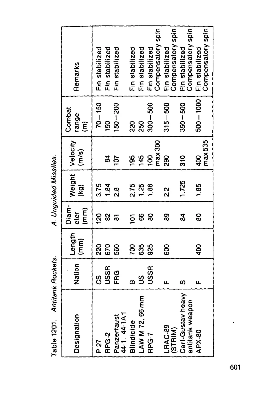
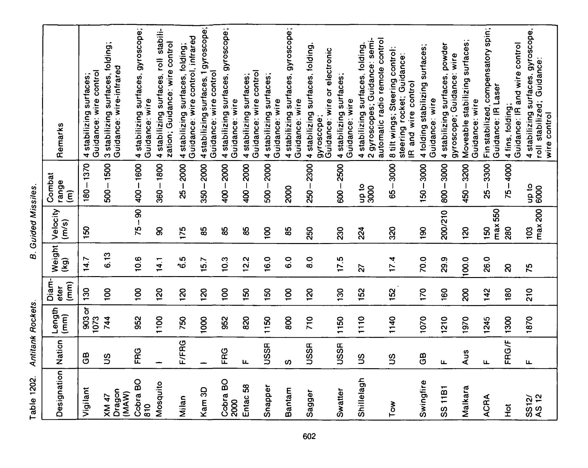
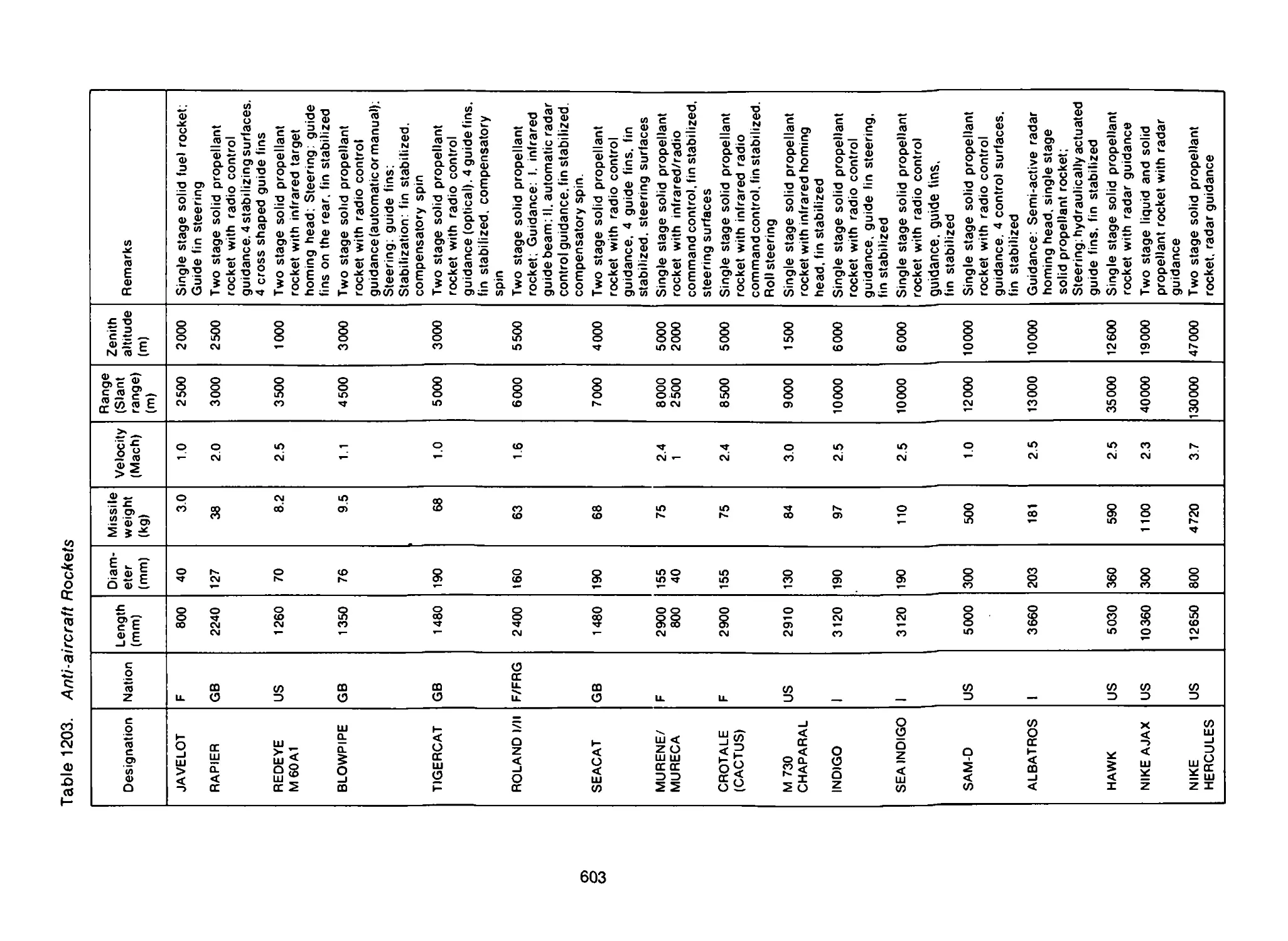
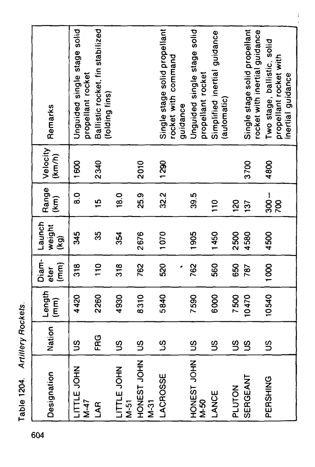
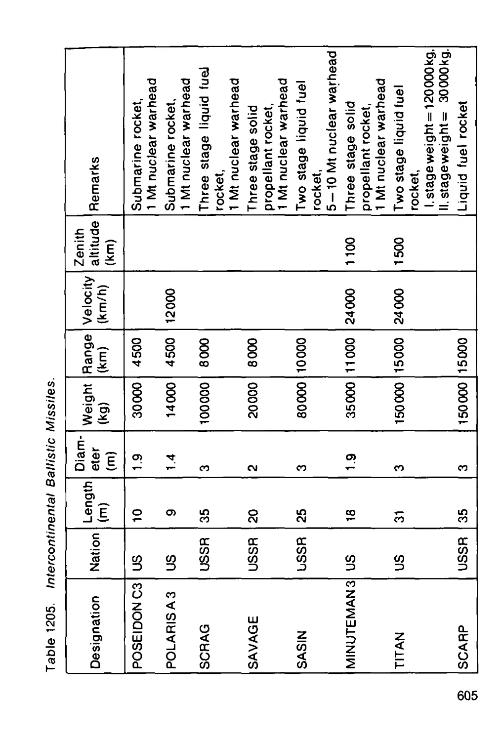
12.6 Data of known rocket weapons............... 600
13 FUZES AND PROPELLING CHARGE IGNITERS 607
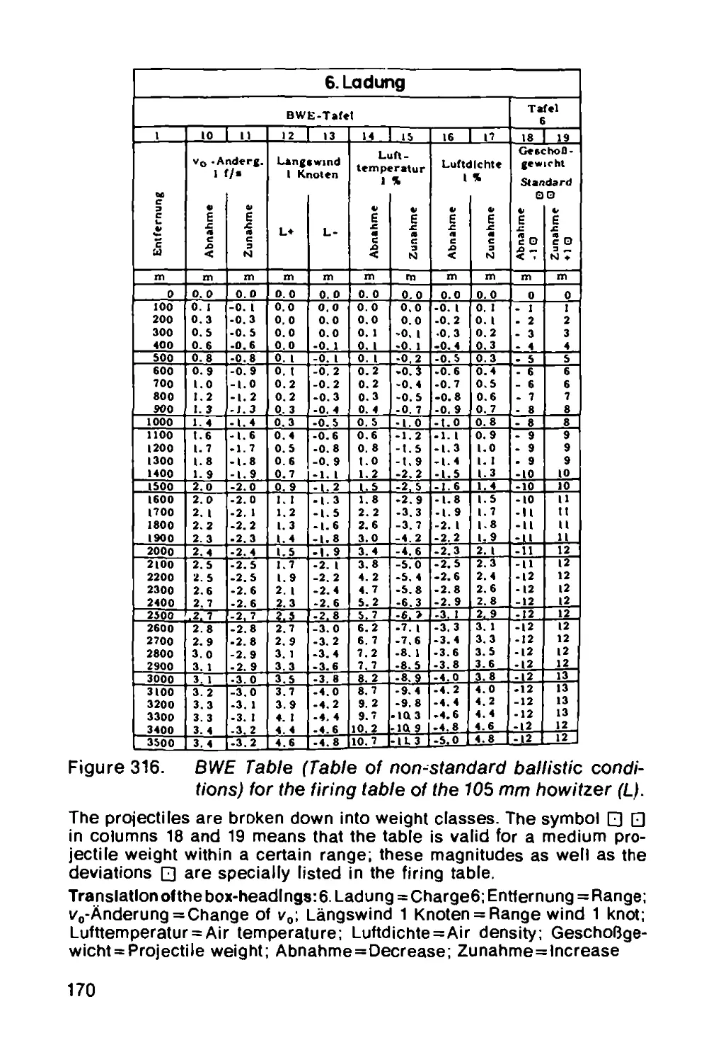
G. Backstein and H.-D. Harnau
13.1 Safety and tactical requirements ........... 607
13.2 Fuzes....................................... 608
13.2.1 Typesof fuzes.............................. 609
13.2.2 Fuze components............................. 613
13.2.2.1 Energy sources and accumulators............. 613
13.2.2.2 Safety systems.............................. 617
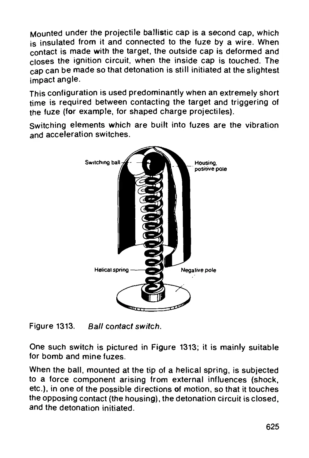
13.2.2.3 Switching elements.......................... 624
13.2.2.4 Means of initiation......................... 628
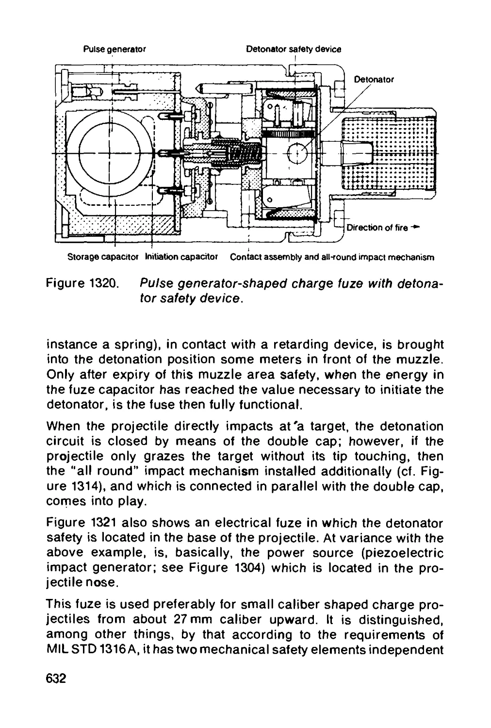
13.2.3 Structural design examples.................. 631
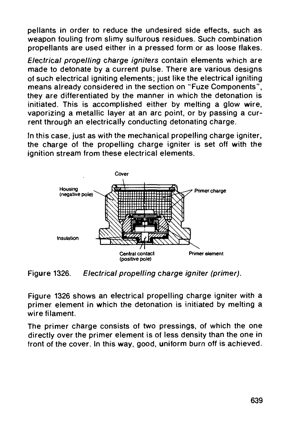
13.3 Propelling charge igniters.................. 637
XV
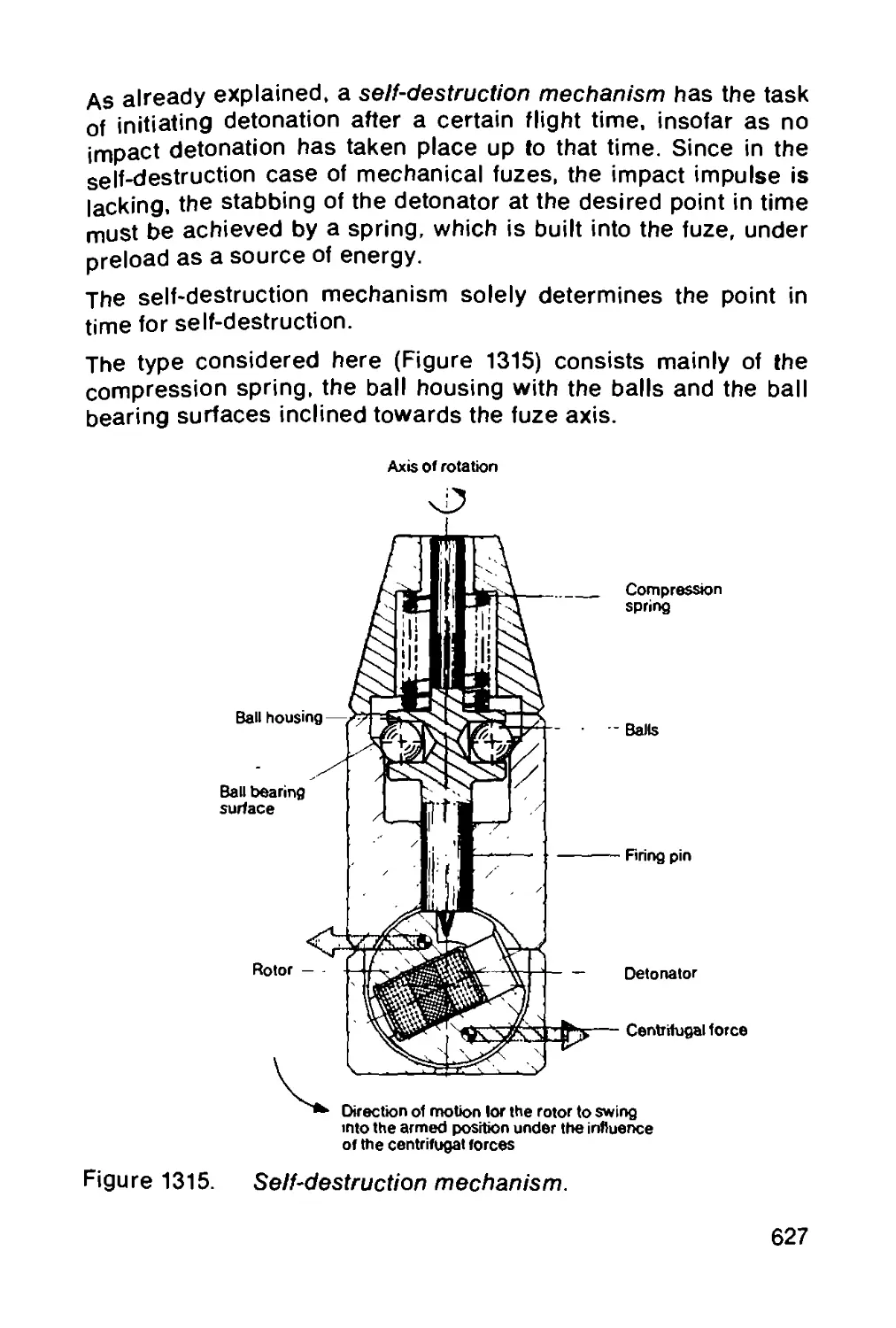
14 BALLISTICS AND WEAPONS TESTING
METHODS.................................. 640
P. Bettermann and F. Mayer
14.1 Time measurement, recording and evaluation 640
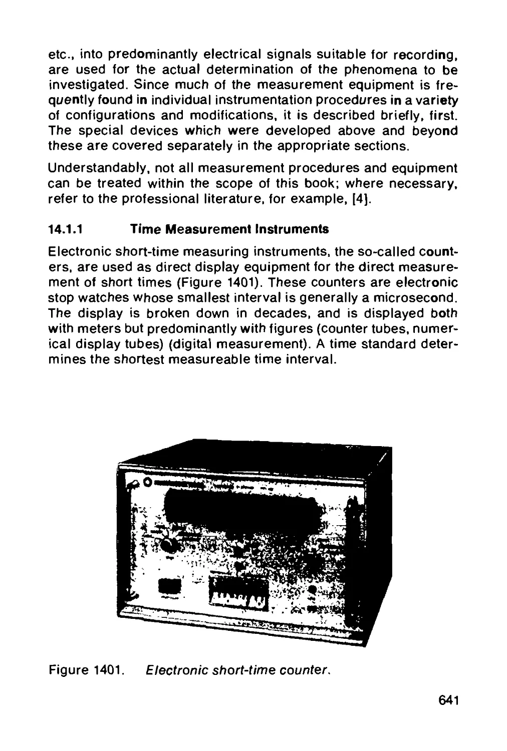
14.1.1 Time measurement instruments............. 641
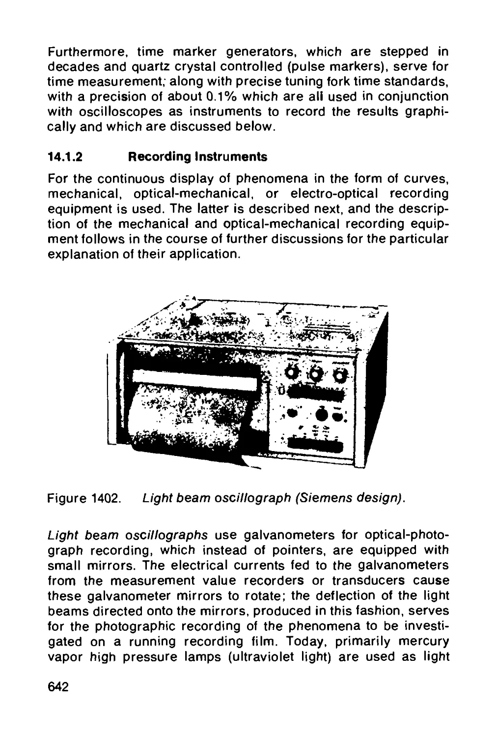
14.1.2 Recording instruments.................... 642
14.1.3 Image forming instruments for short-time
phenomena........................................ 644
14.2 Measurements for internal ballistics..... 644
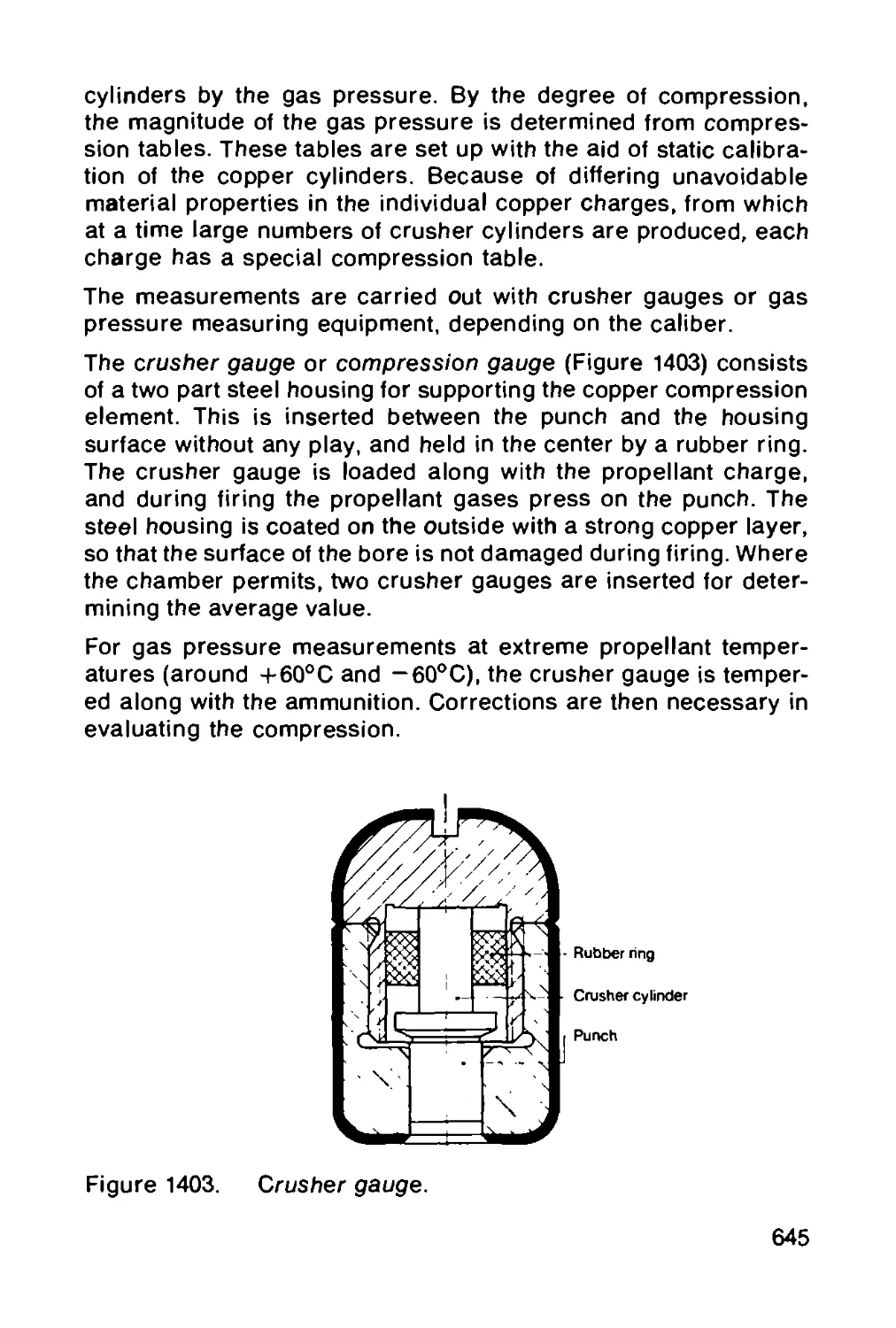
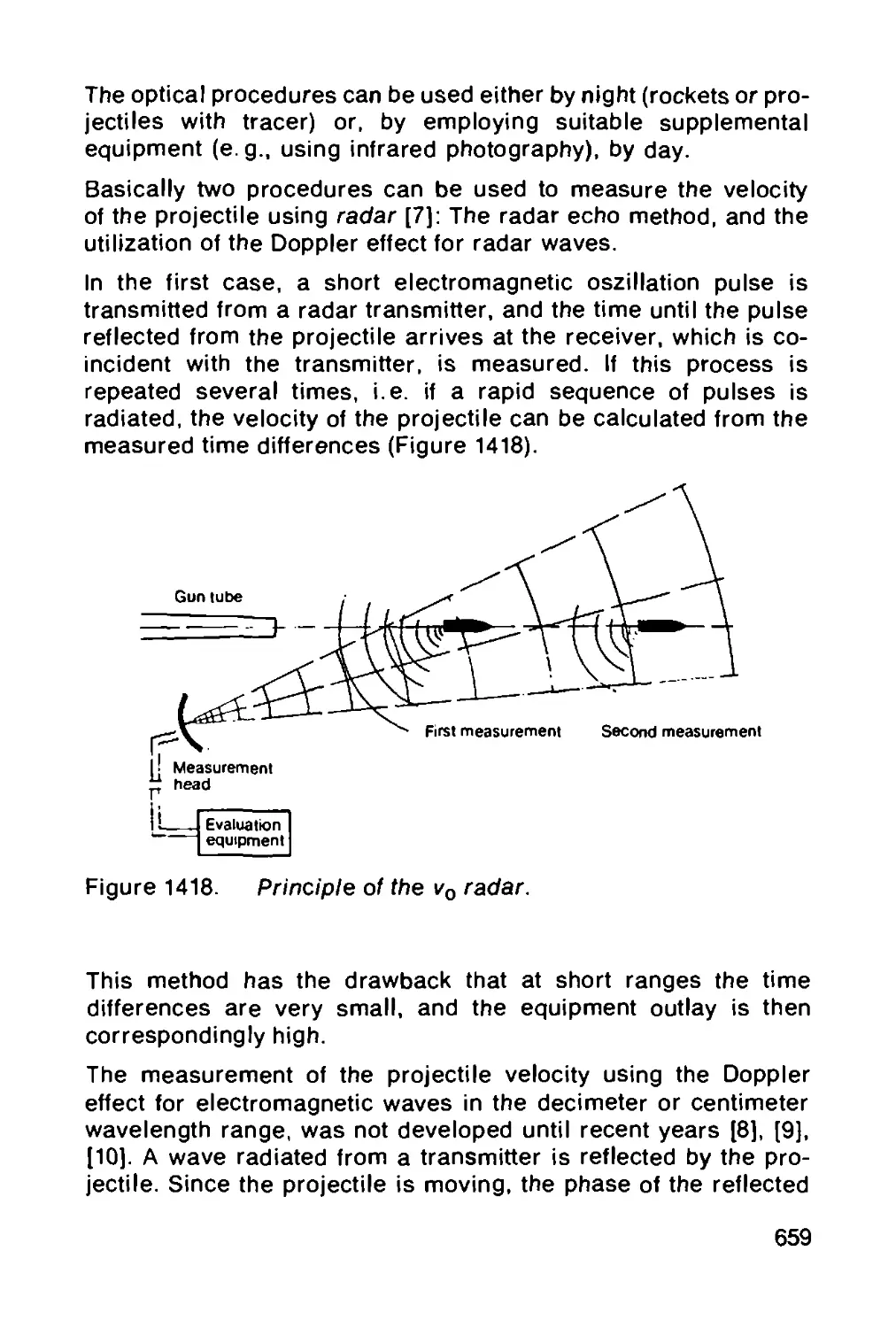
14.2.1 Measurement of the maximum gas pressure .. 644
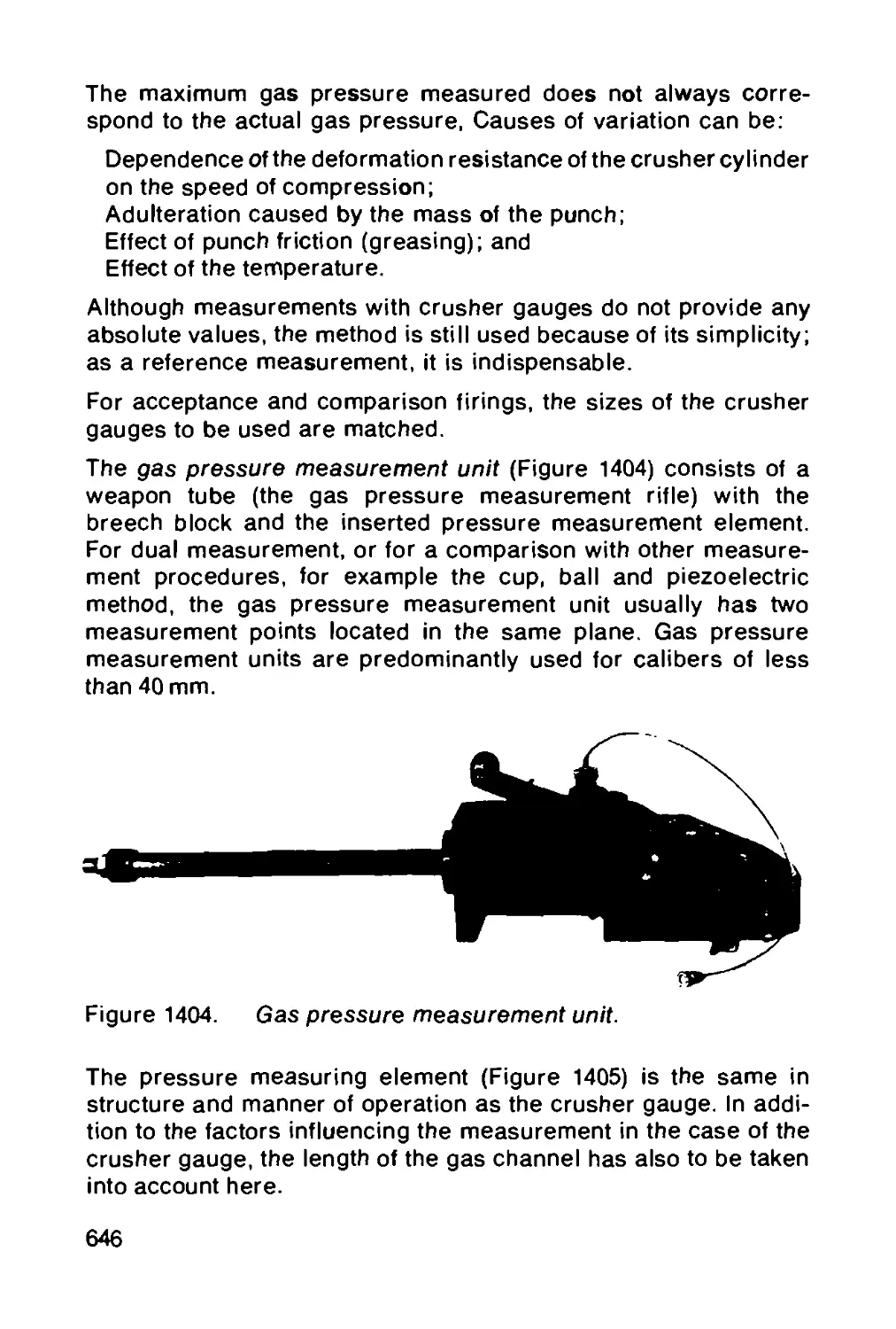
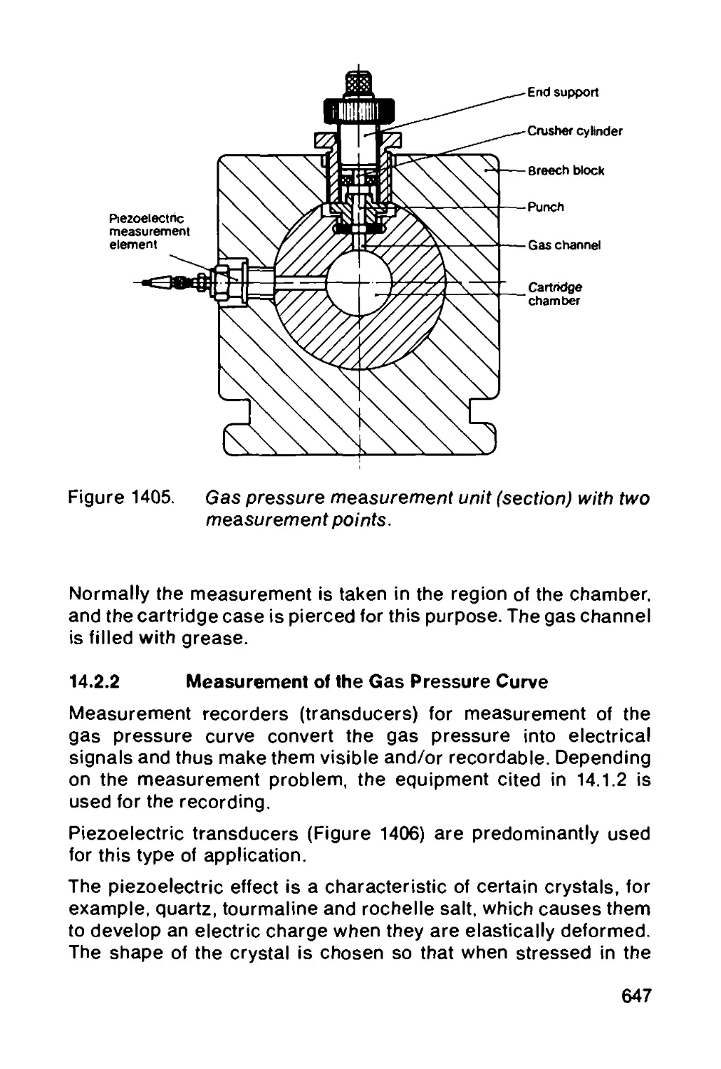
14.2.2 Measurement of the gas pressure curve... 647
14.3 Measurements for external ballistics..... 649
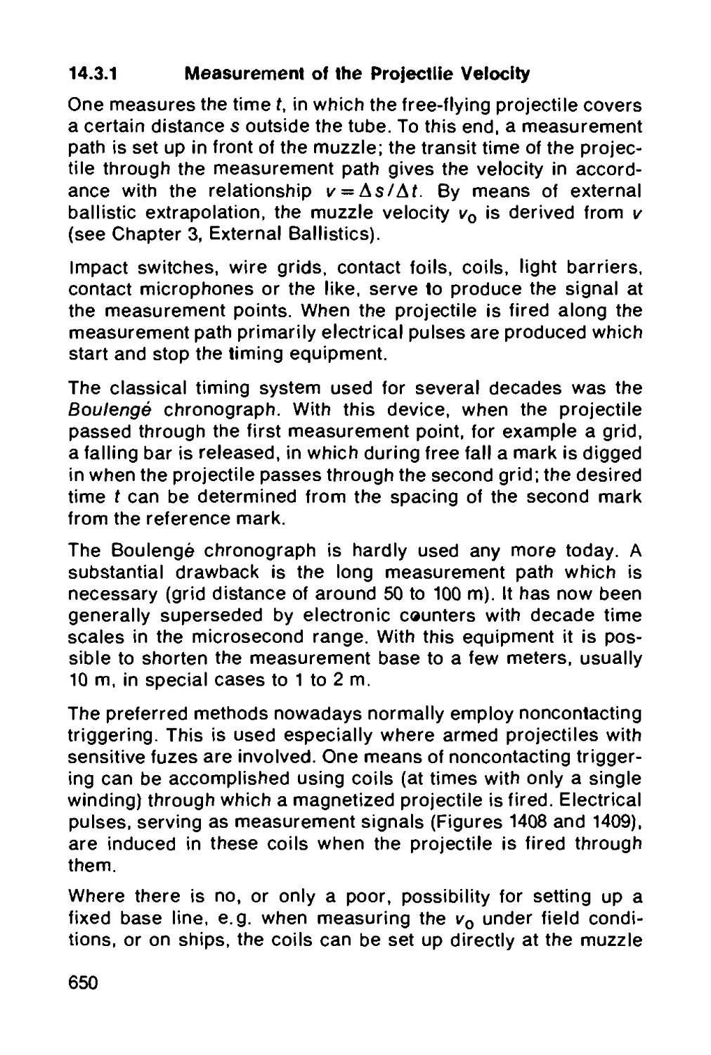
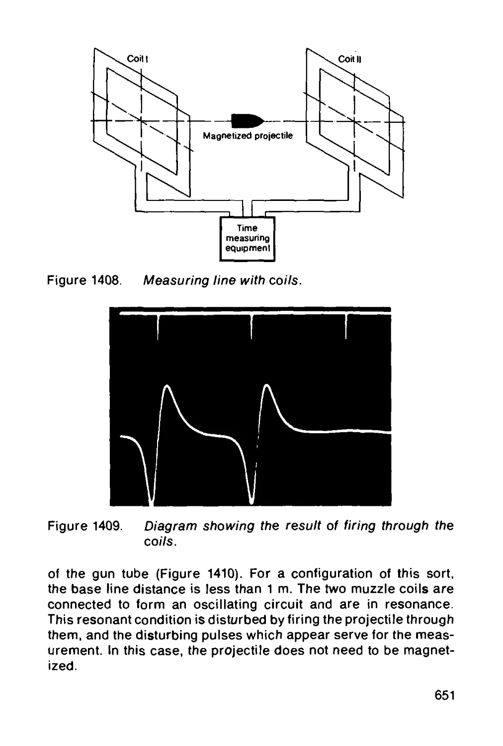
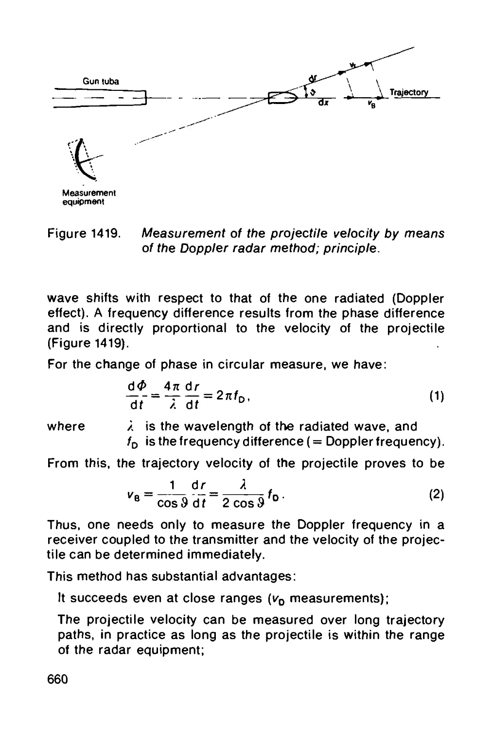
14.3.1 Measurement of the projectile velocity.. 650
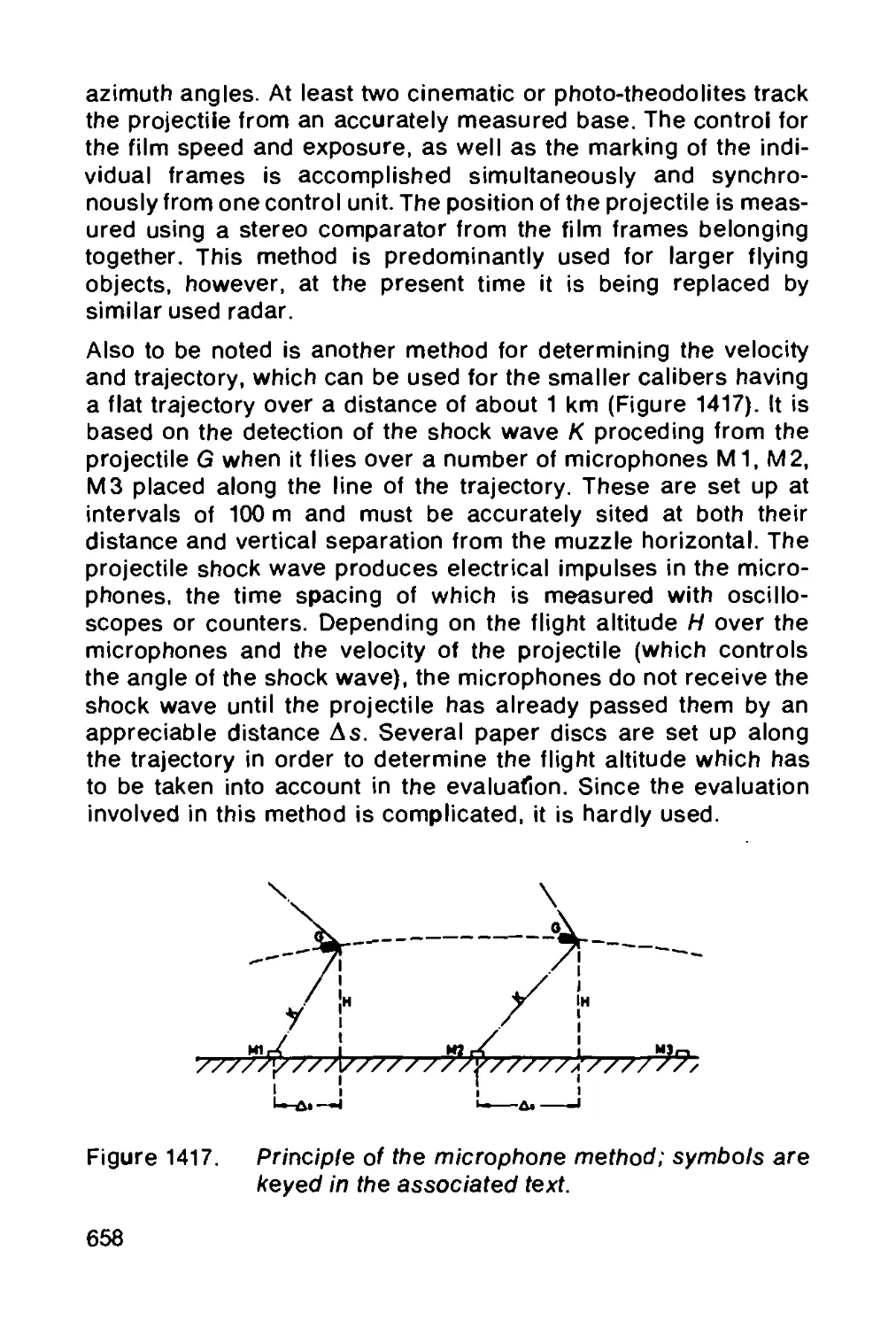
14.3.2 Determining the trajectory............... 653
14.4 Measurements for intermediate ballistics. 661
14.4.1 Measurement of the tube bending oscillations
and tube deviation............................... 661
14.4.2 Measurement of the sound pressure....... 663
14.5 Measurements of terminal ballistics...... 665
14.5.1 Determination of the dispersion pattern . 665
14.5.2 Measuring the penetration power.......... 668
14.5.3 Measuring the fragmentation effect....... 668
14.6 Weapons testing measurements.............. 668
14.6.1 Measuring the rate of fire............... 669
14.6.2 Measurement of the tube temperature..... 670
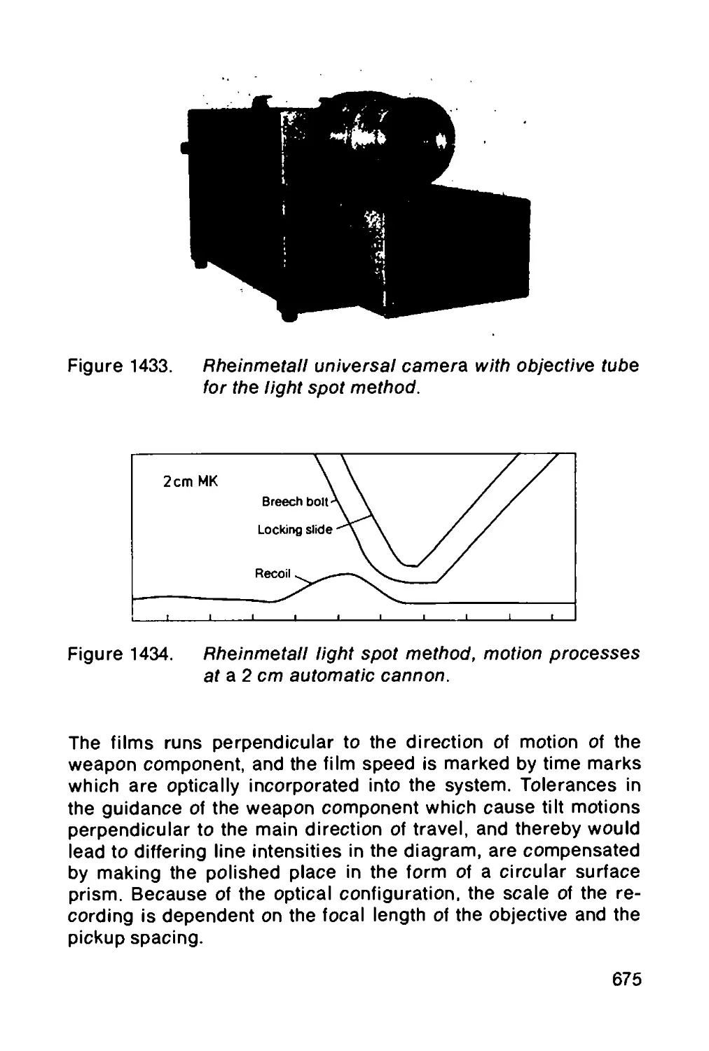
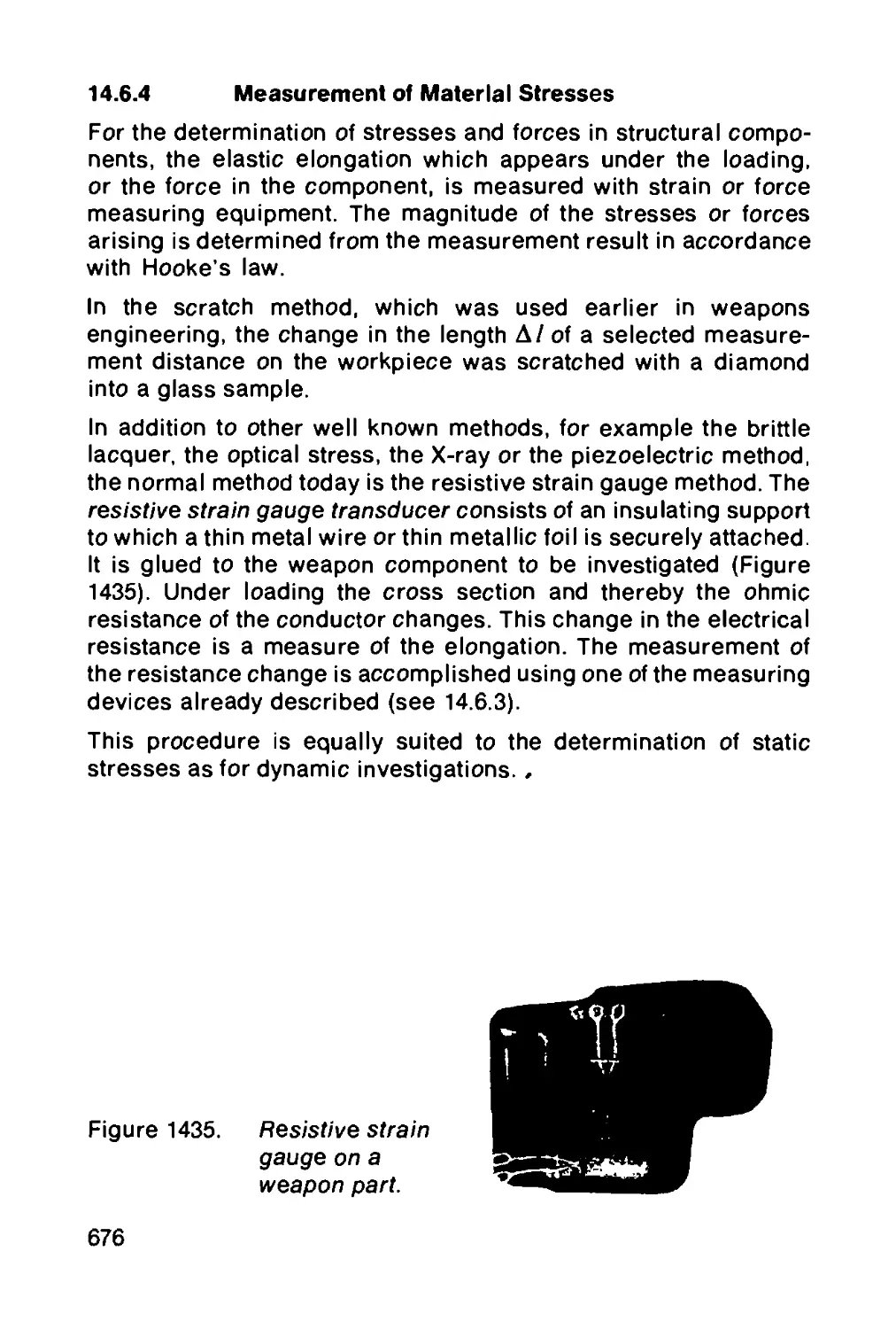
14.6.3 Measurement of motion phenomena.......... 671
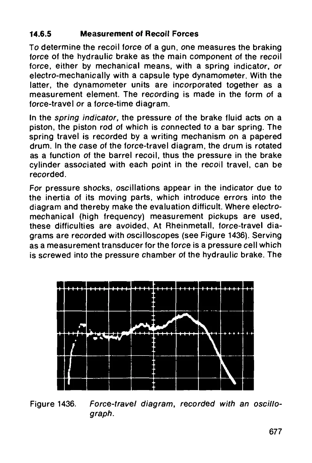
14.6.4 Measurement of material stresses......... 676
14.6.5 Measurement of recoil forces............. 677
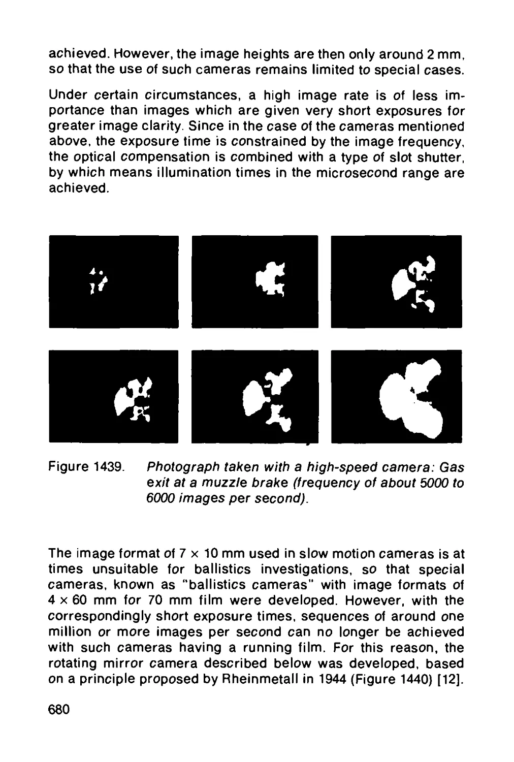
14.7 High-speed photography ................... 678
14.7.1 Slow motion (framing) cameras............ 678
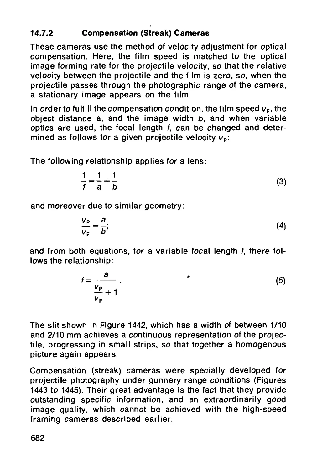
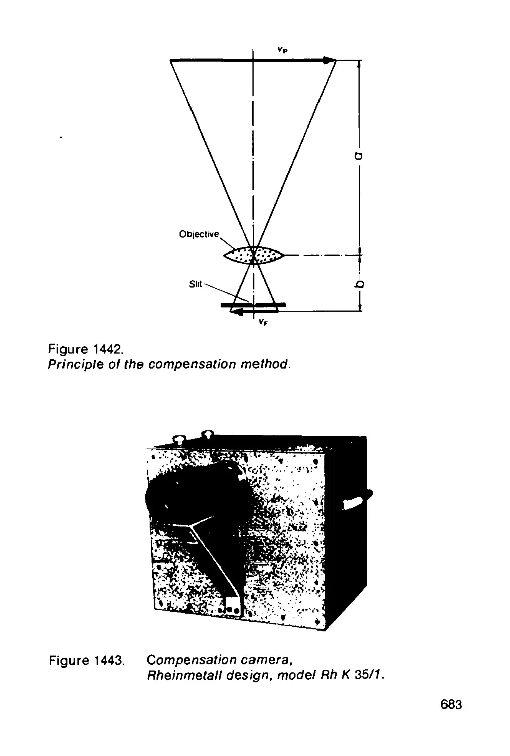
14.7.2 Compensation (streak) cameras............ 682
14.7.3 Spark flash equipment.................... 687
14.7.4 High-speed X-ray equipment............... 688
15 TABLES.................................... 691
E. Melchior
15.1 Mathematical relationships and tables... 691
15.1.1 The numbers я and e...................... 691
XVI
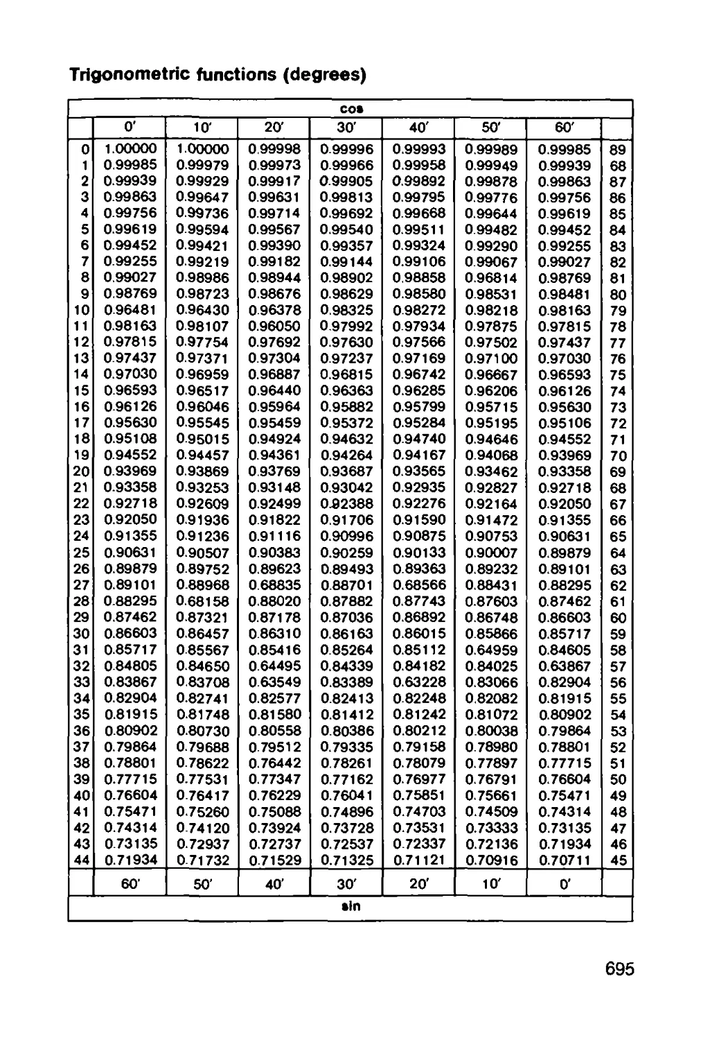
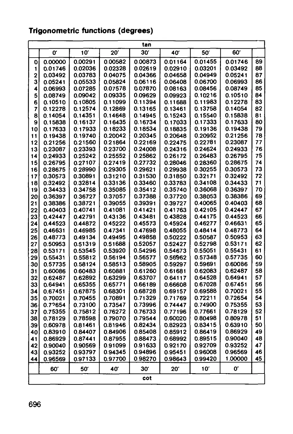
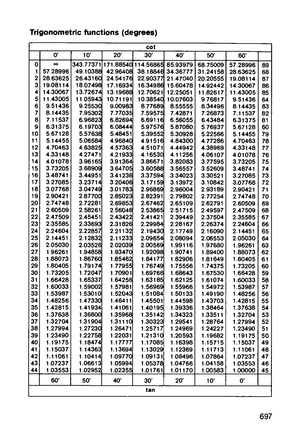
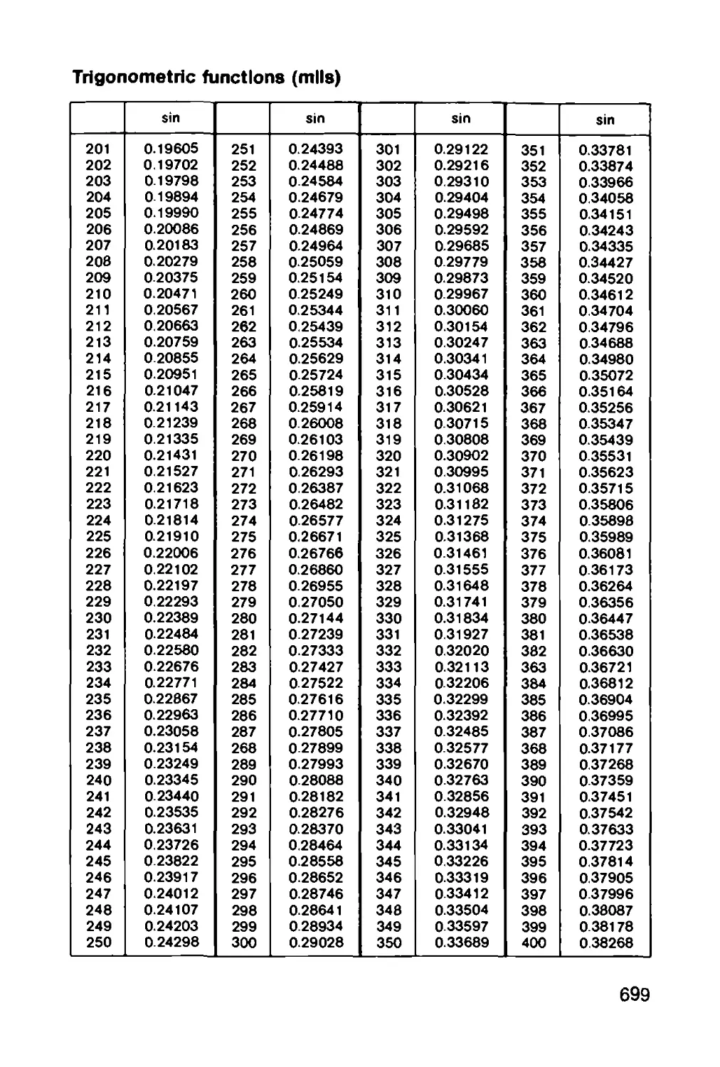
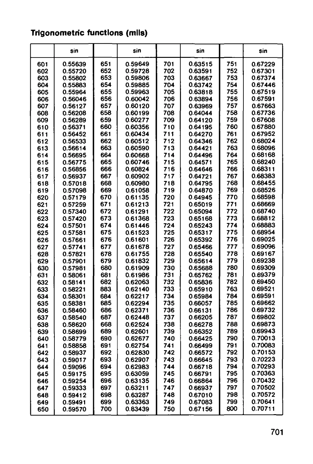
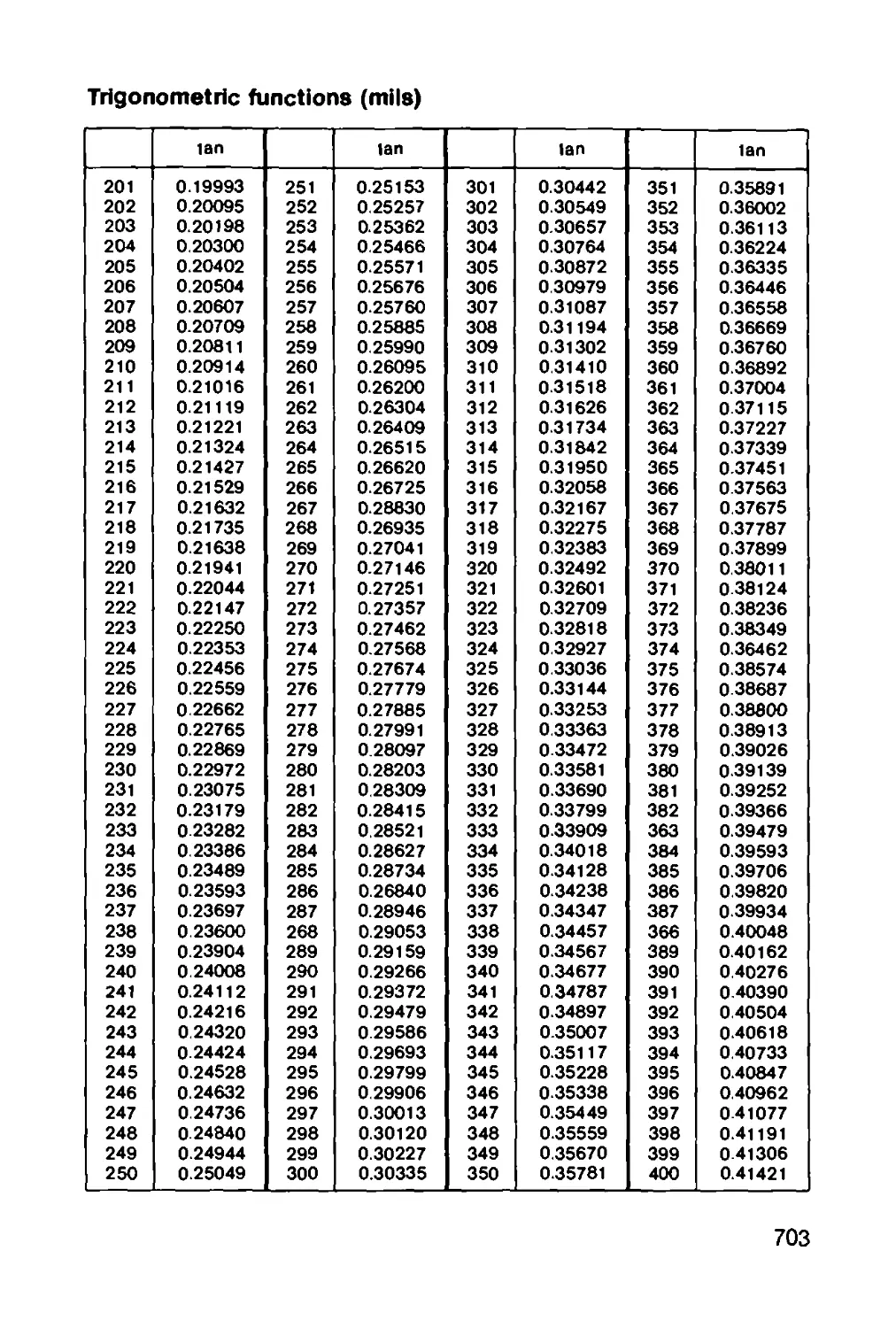
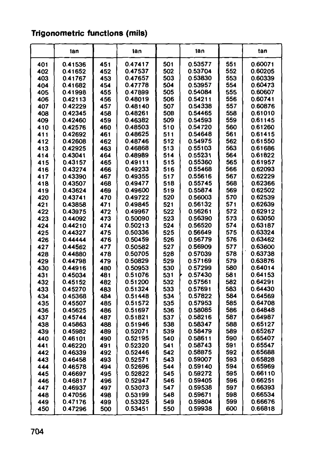
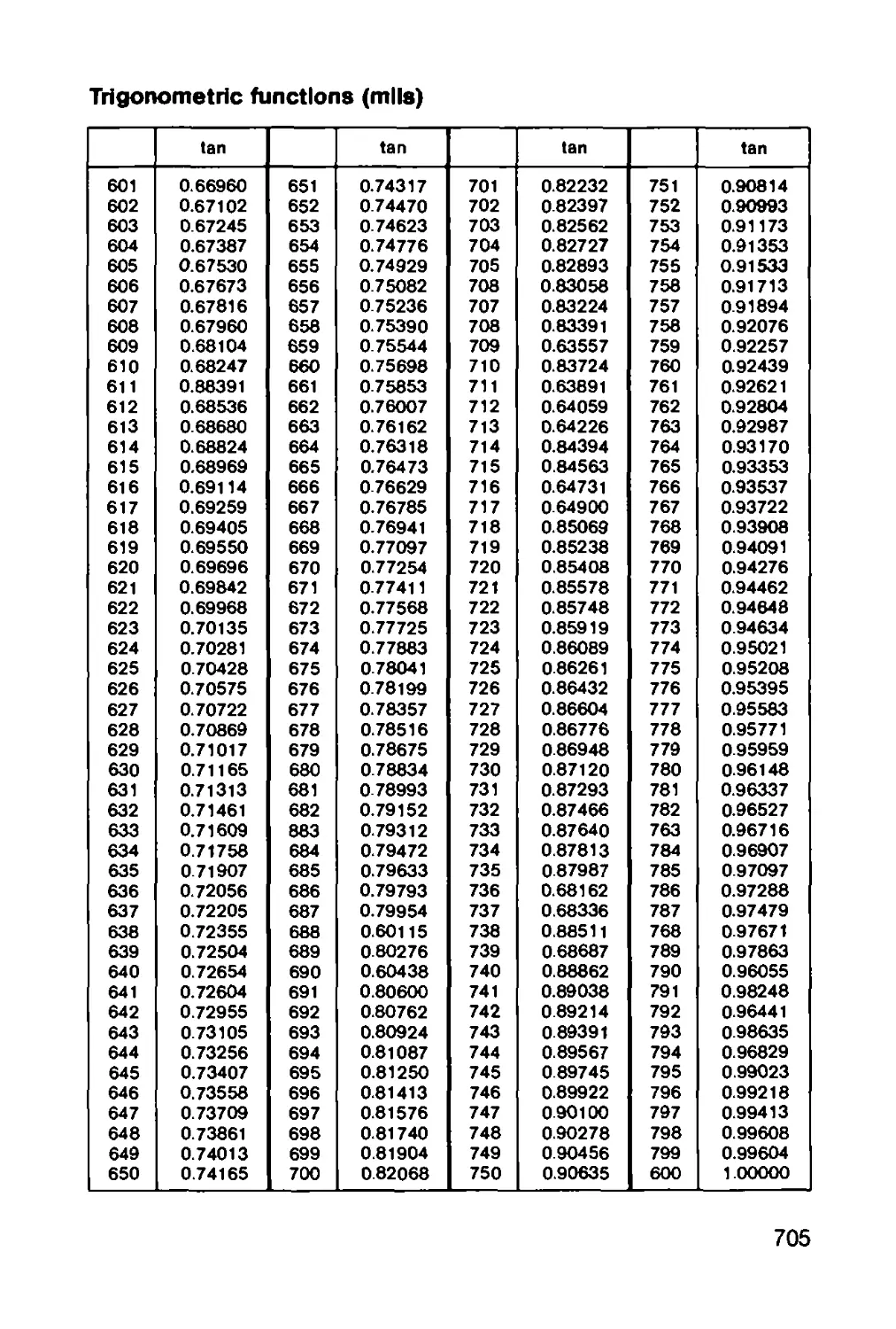
15-1.2 Trigonometric functions................... 692
15.13 Logarithms................................ 706
15.1.4 Exponential functions..................... 708
15.1.5 Reciprocals of the numbers from 1 to 100.. 710
15.1.6 The first 8 powers of the numbers from 1 to 20 710
15.2 Magnitudes and units, systems of units..... 711
15.2.1 The international system of units......... 712
15.2.2 The engineering system of units........... 712
15.2.3 Law concerning units of measurement........ 713
15.2.3.1 Important legally derived units .......... 714
15.2.3.2 Transitional regulations.................. 715
15-2.4 Important English units................... 715
15.2.5 Hardness measurement...................... 717
15.3 Conversion tables......................... 721
15.3.1 Units of energy.......................... 721
15.3.2 Units of power........................... 721
15.3.3 Units of pressure........................ 721
15.3.4 Temperature scales........................ 722
15.3.5 English units............................. 723
15.4 Miscellaneous ............................ 727
15.4.1 Chemical elements......................... 727
15.4.2 Greek alphabet............................ 729
INDEX OF SUBJECTS..................................... 731
XVII
RHEINMETALL
A Military Technology Company
Rheinmetall's tradition in weapons production goes back more
than 85 years. The German Bundeswehr and NATO partners are
familiar with the company through a series of innovative weapon
developments; above all, since its establishment, Rheinmetall
has been involved in the technological development of weapons,
many of which have proved pioneering.
Here is a short history of our company and an outline of our
production program.
Rheinmetall was founded in Dusseldorf on 7 May 1889, under the
name of “RheinischeMetallwaaren und MaschinenfabrikAkt.-Ges.”.
The objective was the re-equipment of the German army with the
jacketed infantry bullet M 88. The organisation and direction of the
company was entrusted to Heinrich Ehrhardt who steered the
company through the following 30 years and, not least through his
own pioneering technological weapon developments, built it into
a world wide recognized armaments company. Some important
steps on the way were: 1892 -Acquisition of a forge in Diisseldorf-
Rath and its development into a steel works producing far in
excess of internal requirements. 1899—Takeover of the “Nikolaus
Dreyse percussion cap and rifle company” in Sommerda and
development into a fuze factory with later expansion for the
production of sighting systems, infantry weapons and machine
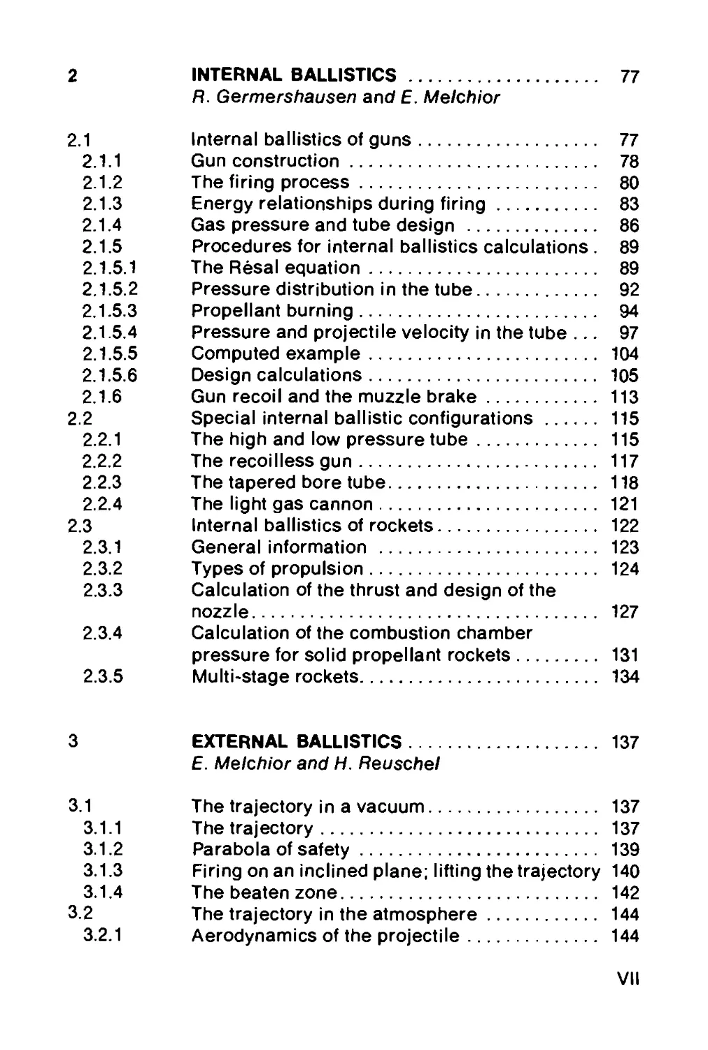
guns. Also in 1899—Acquisition of the Unterluss shooting range.
Figure 1. The cross section of a square steel ingot in a cylindrical
die became the Rheinmetall symbol.
XIX
The development and success of the company rested largely on
Heinrich Ehrhardt’s pressing and drawing process for the pro-
duction of seamless hollow bodies recognized as an important
invention in the history of technology. The process involved
inserting a red-hot steel ingot in a cylindrical die, piercing it with
a circular mandrel and hot-drawing the blanc to give seamless
tubes (shell casings) and steel pipes (see Figure 1).
In 1898 Ehrhardt produced the world’s first serviceable tube recoil
gun, a 75 mm field gun. This invention, after costly experiments
and lengthy discussions with obdurate opponents, was finally
approved and after first orders from foreign countries set the
ball rolling, the whole world's artillery was equipped within a few
years, the German army starting in 1904.
Figure 2. Heinrich Ehrhardt, founder of "Rheinische Metall-
waaren und Maschinenfabrik Akt.-Ges", later "Rhein-
metall", and inventor of the world's first serviceable
tube recoil gun with his 75 mm field gun.
During World War I, Rheinmetall supplied the army, navy and
air force with weapons of all kinds: cannons, howitzers, mortars,
mine throwers, antitank guns, anti-aircraft guns, ship-, submarine-
and aircraft guns, infantry weapons and all the requisite am-
munition. After the dismantling of all plant and equipment used
for military production, broad based civilian production began
XX
in 1920. The output included locomotives, wagons, steam ploughs
and other agricultural machinery, and mining and steel mill equip-
ment. The Sommerda factory started producing office machinery
and automotive parts (Cardan-shafts) and continued this success-
fully up to World War II.
Only after 1925 did the Allied Control Commission approves return
to weapons development. After the construction of a 75 mm field
gun, there followed the development of 150 mm triple turrets for
the five К class cruisers and also a fire control device, the
forerunner of the later AA fire control mechanisms.
In 1933, the A. Borsig company in Berlin-Tegel, with its wide
ranging machine building program, was taken over, and from
1936 the company used the name of “Rheinmetall-Borsig AG".
Weapon development and production in those days and up to the
end of World War II included weapons of all kinds for the three
armed services, including the required munitions, among other
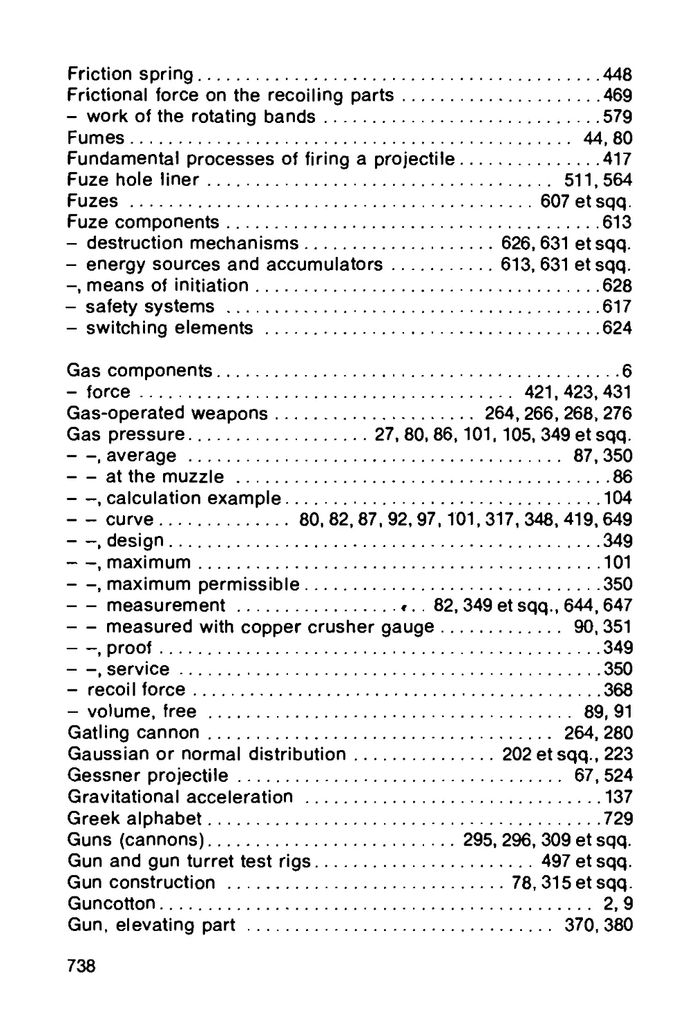
things tanks, heavy mortars (see Figure 3) and rockets.
Figure 3. "Karl" 600 mm mortar, still today the world's largest
gun of that caliber, suitable to be transported as a
complete unit. Development began at Rheinmetall in
1937 and it saw service in the attacks on Brest-Litowsk
in 1941 and Sebastopol in 1942.
XXI
In addition to the development and production of the “Karl" mortar,
(known to the troops as "Thor") and its 540 mm and 600 mm shells,
the company undertook the development of a remote controlled
surface-to-surface missile. The “Rheintochter" was a 2-stage
liquid propellant missile with a range of 40 km. The “Rheinbote"
was a 4-stage solid fuel missile with a 250 km range. "Fritz X",
a guided bomb, carried a 350 kg warhead.
The available production facilities were expanded and new
factories acquired: Berlin-Marienfelde, Alkett, Apolda, Guben and
Breslau.
1945 saw the complete destruction and dissolution of all pro-
duction facilities including the Unterluss firing range.
In contrast to many other firms, Rheinmetall could not immediately
consider rebuilding; for many years a prohibition order prevented
production. Only in autumn 1956 parts of the company were allowed
to resume production, and the revival began in a plant where all
but two of the buildings had been reduced to rubble and ashes.
Prior to this, the two major production units of Rheinmetall-Borsig
Holdings, Rheinmetall Dusseldorf and Borsig Berlin, were split
off into legally independent companies. In the course of de-
nationalization, the majority shareholding in the Berlin company,
Rheinmetall-Borsig, was acquired by the Rochling'sche Eisen-
und Stahlwerke GmbH in Volklingen/Saar, and subsequently real
rebuilding in Dusseldorf began. The former parent factory became
once again the heart of the organization. Also in 1956 development
started on weapons and equipment for the German Bundeswehr
and other NATO forces.
The first task was to provide a basis for weapons design and
manufacture. Technicians and specialists were scarce, but slowly
a core of former workers who had come back, was formed, which
provided the necessary base for the resumption of weapons
production. Already in January 1958 the company began prompt
delivery of the MG 1 machine gun, a continually improved version
of the pre-war MG 42 design, now modified to the NATO caliber
of 7.62 mm. Then followed series production of the 20 mm automatic
cannon MK 20-1 (licensed construction of the Hispano Suiza HS 820)
and the G 3 automatic rifle.
XXII
Figure 4. The MG 3, successor to the MG 42, is used today by
the German Bundeswehr and some NA TO countries.
Today Rheinmetall is one of the Federal Republic’s and NATO's
important partners in the development and production of weapons
systems and ammunition. In the field of military technology which
is represented by "Rheinmetall GmbH", there are its subsidiaries
“Rheinmetall Industrietechnik" in Dusseldorf, which is involved
in the planning of production facilities, “Nico-Pyrotechnik” in
Trittau, producing amongst other things illuminating and signal
material, maneuver and simulation products, colored smokes,
screening smoke and tear gas makers, and “NWM de Kruithoorn
B.V." in 's-Hertogenbosch (Netherlands).
A forward looking research and development program is a basic
requirement for working successfully on problems in military
technology, and this is fulfilled by management using modern
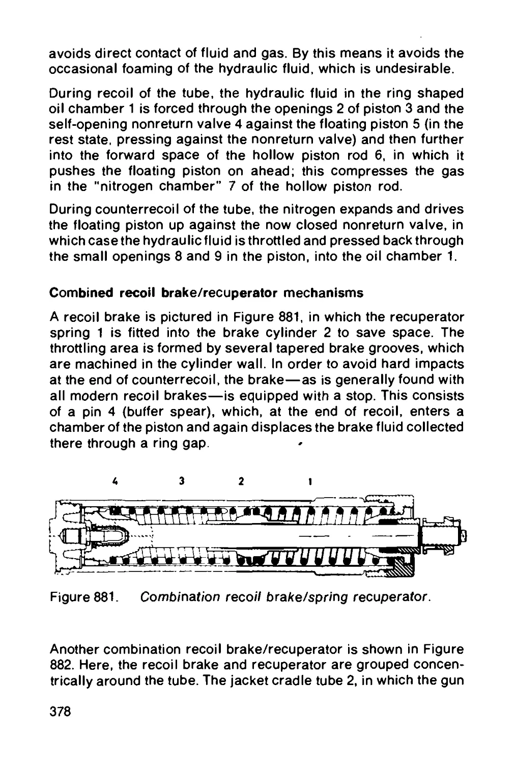
methods and planning techniques to control and supervise a
project.
Weapons today are often complex systems which, because of the
need for cost and technical effectiveness, require system analysis.
Production must include complete weapons systems as well as
XXIII
series production of components. Not the least requirement is a
trial and testing station such as Rheinmetall has in Unterluss in
the Luneburg Heath. This is the largest company-owned area in
the Federal Republik and provides a firing range 15 km long by
4 km wide, and also allows for a range of 35 km using external
firing stations. Part of the most modern ballistic and technological
equipment there has been developed by the company itself.
Immediately adjacent to the range there is a modern ammunition
factory for assembling 20 to 203 mm caliber ammunition.
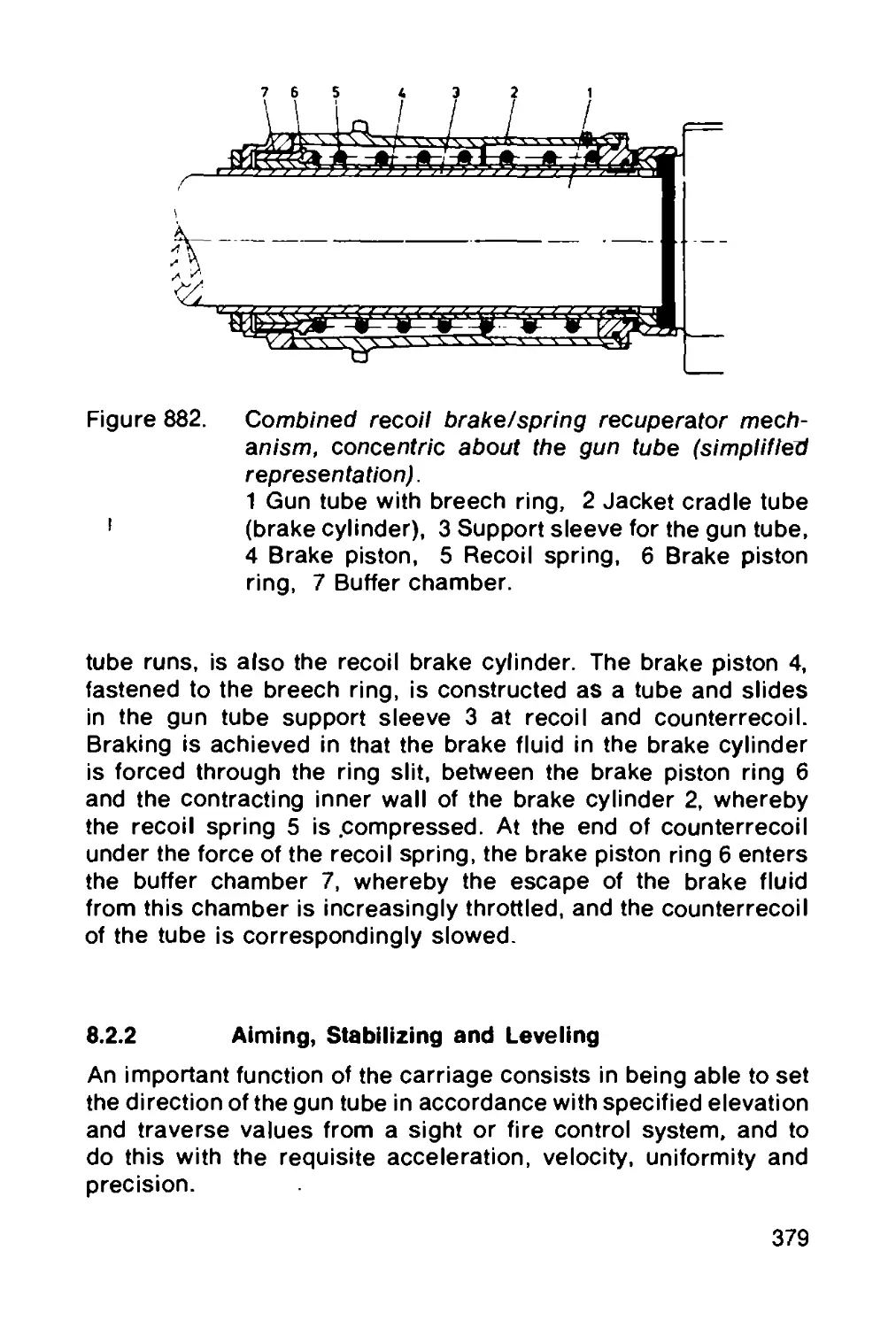
Current Points of Emphasis in the Military
Technology Program
MG 3 Machine Gun
The MG 3 machine gun (Figure 4; caliber 7.62 mm, fire rate
700-1300 rounds/min) is used by all units of the German Bundes-
wehr and is a modernized version of the MG 42 machine gun. It
is also used as coaxial machine gun, anti-aircraft machine gun
and a prow machine gun.
Under the internal designation of MG 3e, Rheinmetall have
developed a lightweight version of the MG 3. Through the choice
of alternative materials and through systematic material savings
the MG 3 has been lightened by 2.2 kg whilst retaining its previous
function, hitting accuracy and handling. The interchangeability
of assemblies and removable components with the corresponding
MG 3 assemblies and parts is guaranteed.
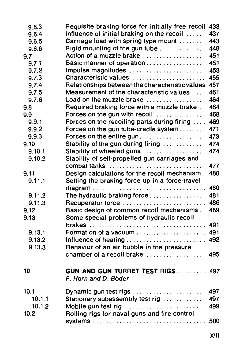
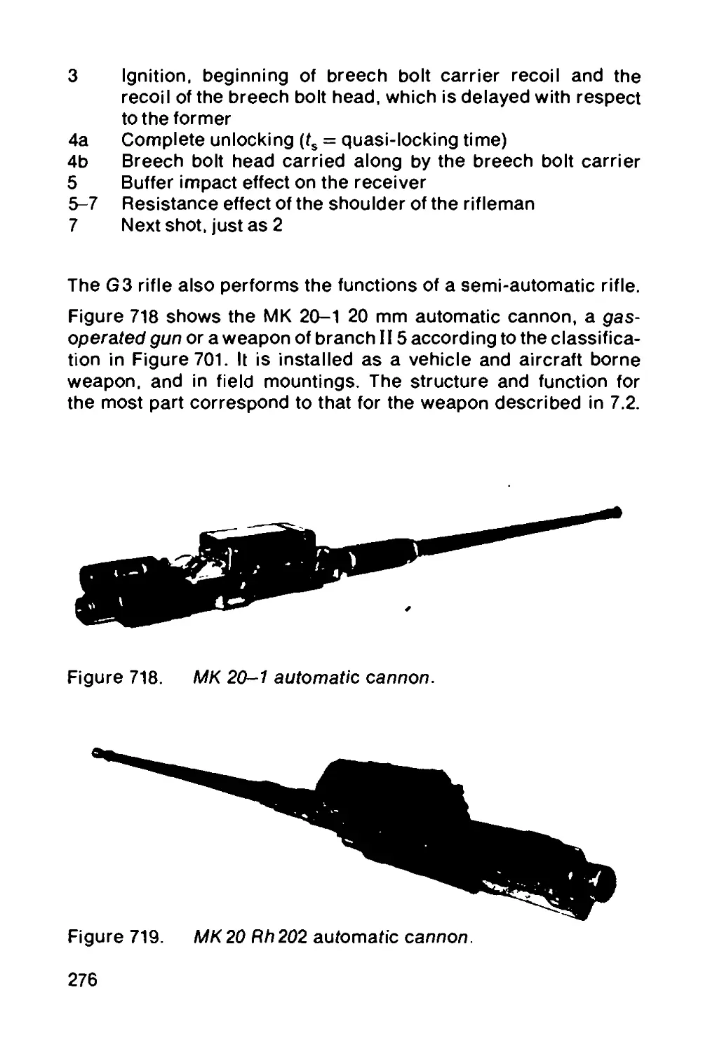
MK 20 Rh 202 Automatic Cannon
The MK 20 Rh 202, an automatic cannon developed and produced
by Rheinmetall, has been introduced into the German Bundeswehr
and, on various mountings, is used for low level air defense and
for ground target combating (Figure 5). The cannon is rigid locking,
gas operated. Its principal advantages are short construction, high
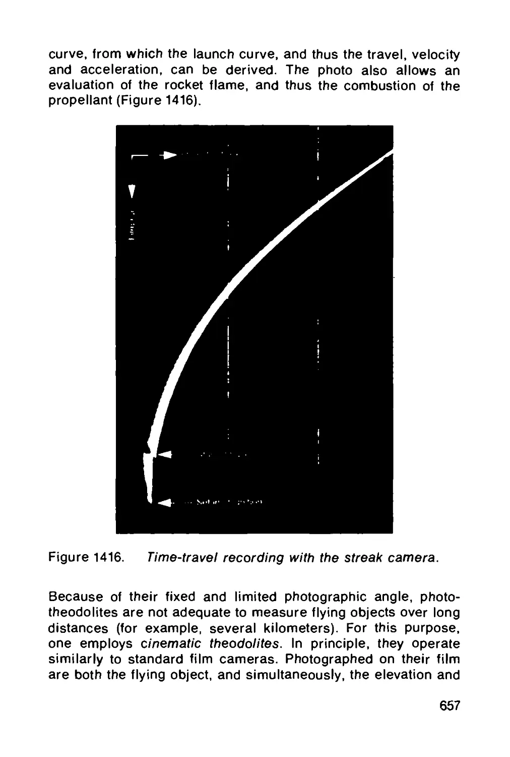
ballistic performance, reliability even under extreme conditions
and its low recoil forces.
Ammunition feed is via a belt feed device which is stored separately
from the cannon in a hinged frame on the carriage. The gun
XXIV
Figure 5. MK 20 Rh 202 automatic cannon.
offers a choice of two belt feeders, a two-way feeder with rapid
ammunition change-over, and a three-way feeder.
The variations offered by the belt feeders make the MK 20 Rh 202
similarly suitable against low flying aircraft and ground targets.
Due to its shortness, separation of the belt feeder from the gun
and its minimal recoil forces, the MK 20 Rh 202 is suitable for a broad
spectrum of weapon carriers and tactical deployment.
The cannon fires 20 mm x 139 ammunition with an approximate
muzzle velocity of 1100 m/s at a rate of 800 to 1000 rounds/min.
Maximum effective range is 2000 m.
XXV
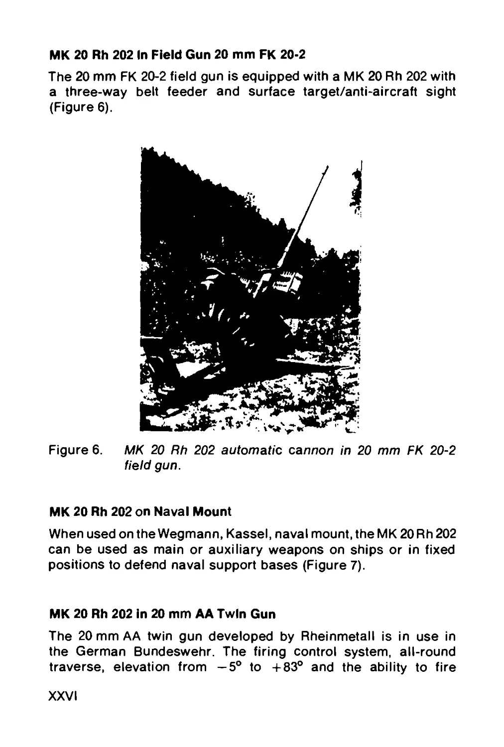
МК 20 Rh 202 In Field Gun 20 mm FK 20-2
The 20 mm FK 20-2 field gun is equipped with a MK 20 Rh 202 with
a three-way belt feeder and surface target/anti-aircraft sight
(Figure 6).
Figure 6.
MK 20 Rh 202 automatic cannon in 20 mm FK 20-2
field gun.
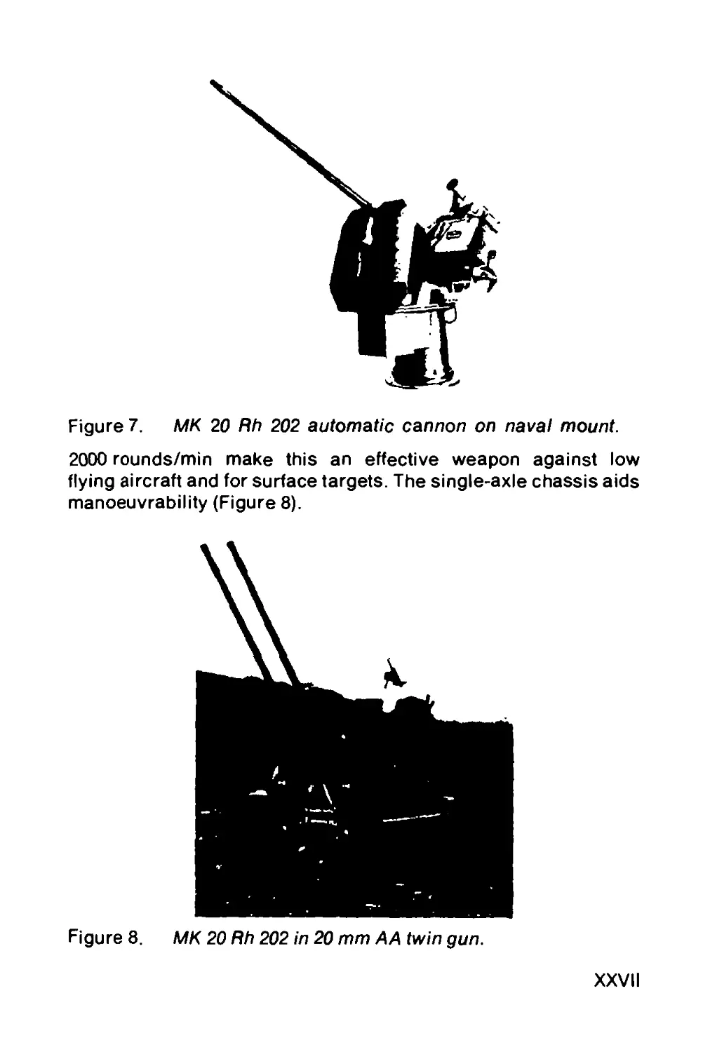
MK 20 Rh 202 on Naval Mount
When used on the Wegmann, Kassel, naval mount, the MK 20 Rh 202
can be used as main or auxiliary weapons on ships or in fixed
positions to defend naval support bases (Figure 7).
MK 20 Rh 202 in 20 mm AA Twin Gun
The 20 mm AA twin gun developed by Rheinmetall is in use in
the German Bundeswehr. The firing control system, all-round
traverse, elevation from —5° to +83° and the ability to fire
XXVI
Figure 7. MK 20 Rh 202 automatic cannon on naval mount.
2000 rounds/min make this an effective weapon against low
flying aircraft and for surface targets. The single-axle chassis aids
manoeuvrability (Figure 8).
Figure 8. MK 20 Rh 202 in 20 mm AA twin gun.
XXVII
MK 20 Rh 202 In the "Marder” Armored Personnel Carrier
The “Marder" armored personnel carrier is equipped with the
MK 20 Rh 202 in a top mounting as its main armament (Figure 9).
Figure 9. MK 20 Rh 202 automatic cannon on a "Marder" armored
personnel carrier.
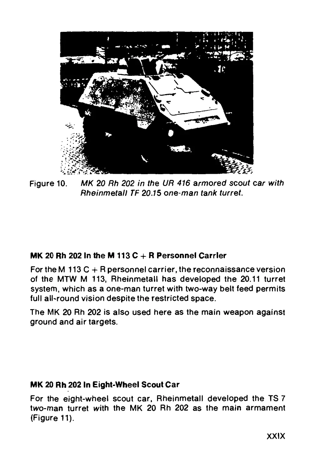
MK 20 Rh 202 in the UR 416 Armored Scout Car
The UR 416 armored scout car is equipped with the Rheinmetall
TF 20.15 one-man tank turret (Figure 10).
The TF 20.15 is armed with a MK 20 Rh 202; alternatively with
three- or two-way belt feeder. It is intended for wheeled vehicles
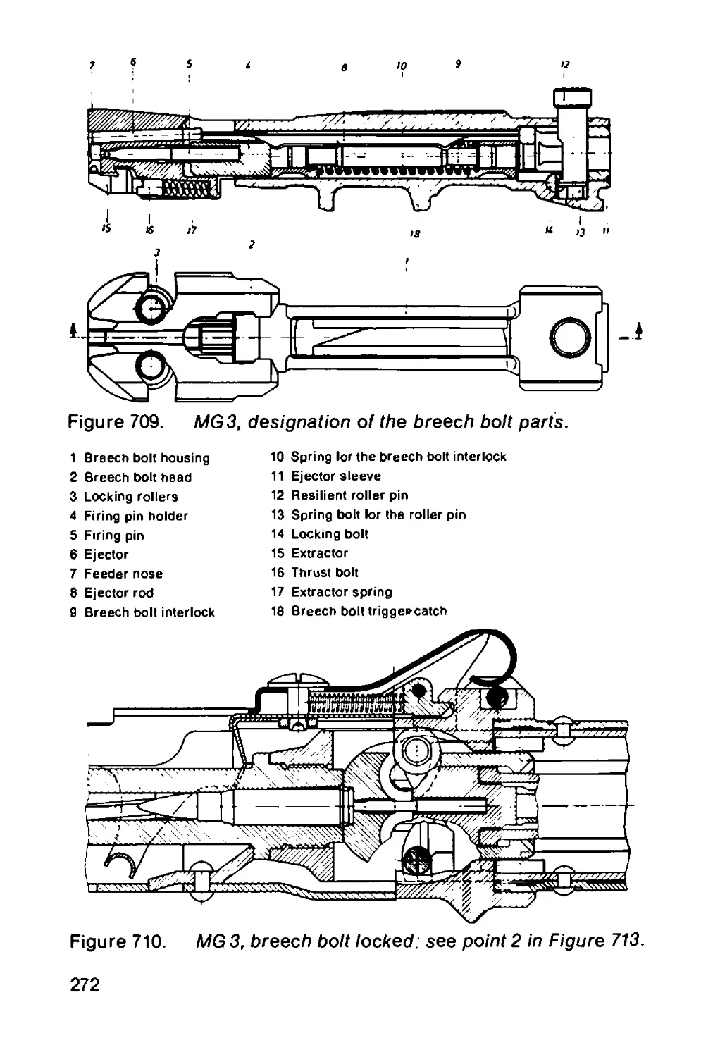
and light armored tracked vehicles, which can be used as
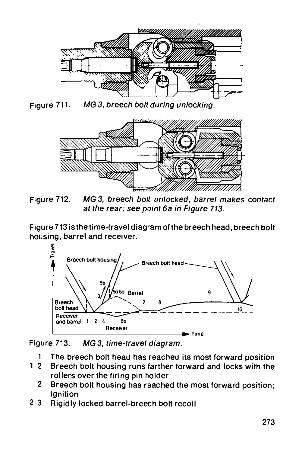
armored scout cars for reconnaissance duties and as escorting
vehicles when attacking ground targets and for defense against
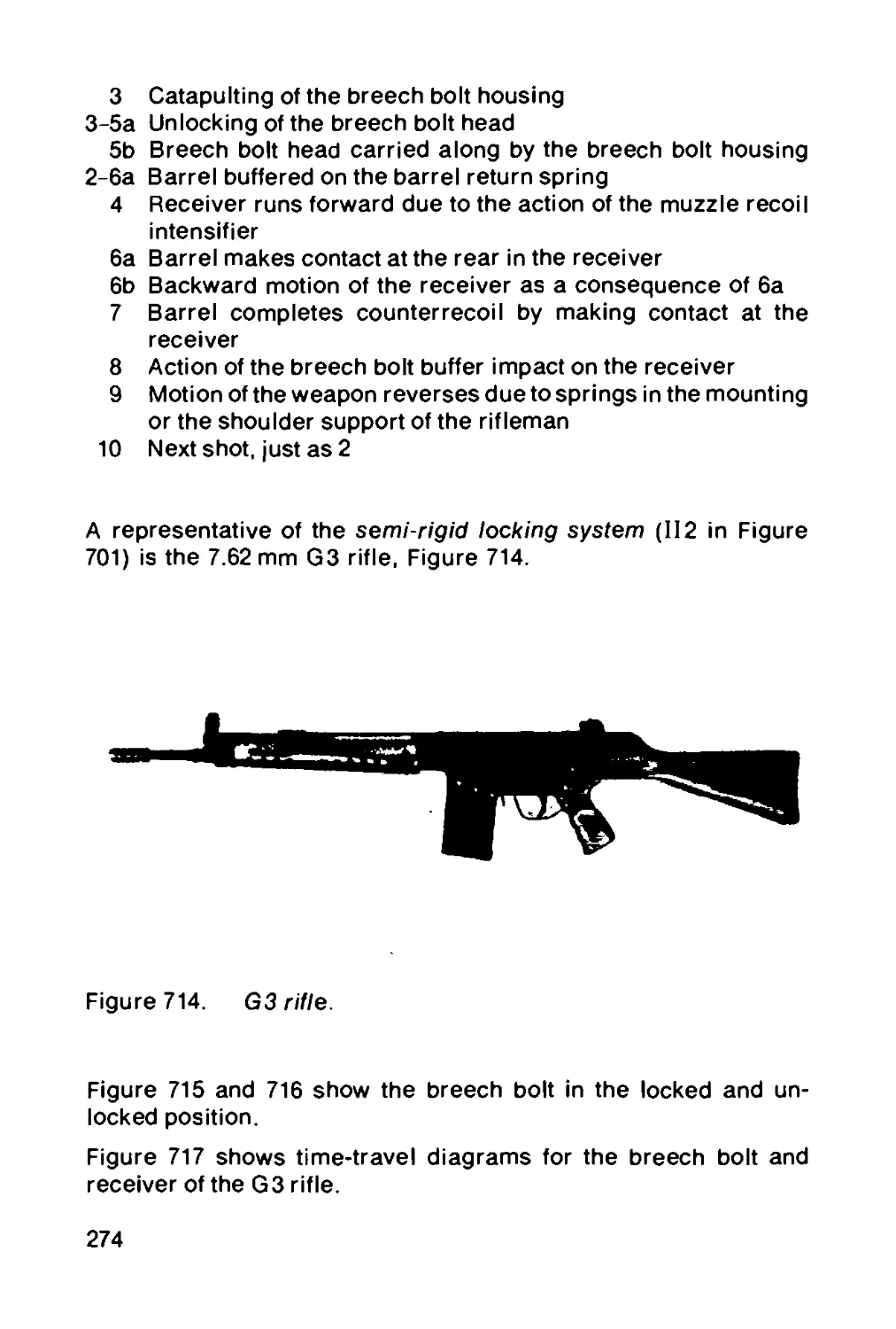
low flying aircraft.
MK 20 Rh 202 in the MTW M 113 Personnel Carrier
The Rheinmetall TF 20.15 one-man tank turret with the MK 20 Rh 202,
equipped with changeover belt feed, is also intended for the MTW
M 113 personnel carrier.
XXVIII
Figure 10. MK 20 Rh 202 in the UR 416 armored scout car with
Rheinmetall TF 20.15 one-man tank turret.
MK 20 Rh 202 In the M 113 C + R Personnel Carrier
For the M 113 C + R personnel carrier, the reconnaissance version
of the MTW M 113, Rheinmetall has developed the 20.11 turret
system, which as a one-man turret with two-way belt feed permits
full all-round vision despite the restricted space.
The MK 20 Rh 202 is also used here as the main weapon against
ground and air targets.
MK 20 Rh 202 In Eight-Wheel Scout Car
For the eight-wheel scout car, Rheinmetall developed the TS 7
two-man turret with the MK 20 Rh 202 as the main armament
(Figure 11).
XXIX
Figure 11. The MK 20 Rh 202 in the TS 7 two-man turret on the
eight-wheel scout car.
MK 20 Rh 202 as Helicopter Armament
For helicopters, Rheinmetall developed a mount for the MK 20
Rh 202 which is attached under the fuselage and remote-con-
trolled by the gunner in the helicopter.
Figure 12. Automatic cannon MK 20 Rh 202 as helicopter
armament.
Tank Destroyer with Cannon
The complete armament of the tank destroyer with cannon, con-
sisting of a 90 mm gun, a co-axial machine gun in the turret and an
AA machine gun, were developed, produced and installed by
Rheinmetall (Figure 13).
XXX
Figure 13. Tank destroyer with cannon.
Leopard 1 Battle Tank
Mounts for the 105 mm cannon and two machine guns on the
Leopard 1 battle tank were developed by Rheinmetall. Individual
parts are manufactured in the Rheinmetall plant at Dusseldorf,
and the complete turret is assembled there (Figures 14 and 15).
Rheinmetall also developed the requisite practice and illuminating
ammunition for the 90 mm cannon of the tank destroyer and the
105 mm cannon of the Leopard battle tank.
Figure 14. Leopard battle tank.
XXXI
Figure 15. Leopard 1 battle tank turret assembly in Rhein-
metall s Ddsseldorf plant.
M 109 G Armored Self-propelled Howitzer
Because of a new breech assembly developed by Rheinmetall,
the M 109 G self-propelled howitzer, used by the German Bundes-
wehr, can now achieve a considerably higher fire rate, increasing
its performance. In addition, a new sighting device was developed
for this weapon. Rheinmetall assembles the complete weapons
system (Figure 16).
Figure 16. M 109 G armored self-propelled howitzer.
XXXII
155 mm FH 70
The 155 mm field howitzer with its associated family of am-
munition is a trilateral development between the United Kingdom,
Germany and Italy. Rheinmetall played an important part in
developing the elevating components (gun and recoil system)
and the special ammunition.
155 mm PzH70
Rheinmetall also had an important part in the trilateral development
of the 155 mm armored self-propelled howitzer 70. The ammunition
developed for the FH 70 can be used in the armored self-propelled
howitzer.
New Generation of 105 mm/120 mm Tank Cannons
For subsequent generations of the Leopard 1 Rheinmetall has
developed 105 and 120 mm guns and ammunition (Figures 17 and
18). The development is noted for its smooth bore and fin
stabilized ammunition. The 105 mm smooth bore is particularly
suited for raising the fire power of tanks in current use.
The 120 mm gun is a very advanced weapon intended as tank
armament for the 80’s and beyond1).
Figure 17. 120 mm Rheinmetall smooth bore gun.
1) Meller, R.: Die 120-mm-Glattrohrkanone von Rheinmetall (The
120 mm smooth bore Rheinmetall cannon). Internationale Wehr-
revue (9), 1976, No. 4 (August), pp. 619-624.
XXXIII
Figure 18. 720 mm KE missile (Schlieren photograph).
Rockets
The development team at Rheinmetall is also involved in post
accelerated projectiles and rockets, especially in the anti-tank
sphere.
An example is the anti-tank weapon “Hellebarde”, a jet cannon
of 75 mm caliber which, when built into light armored vehicles,
can fire fin stabilized hollow charged rockets up to 1000 m
(Figure 19). As a result of following the principle of total drag
compensation in this development, the missile is insensitive to
all kinds of crosswinds. The resultant impact diagrams are similar
to those of a good tank cannon.
Figure 19. Rheinmetall anti-tank weapon "Hellebarde" mounted
on the "Marder" armored personnel carrier in the
act of being fired.
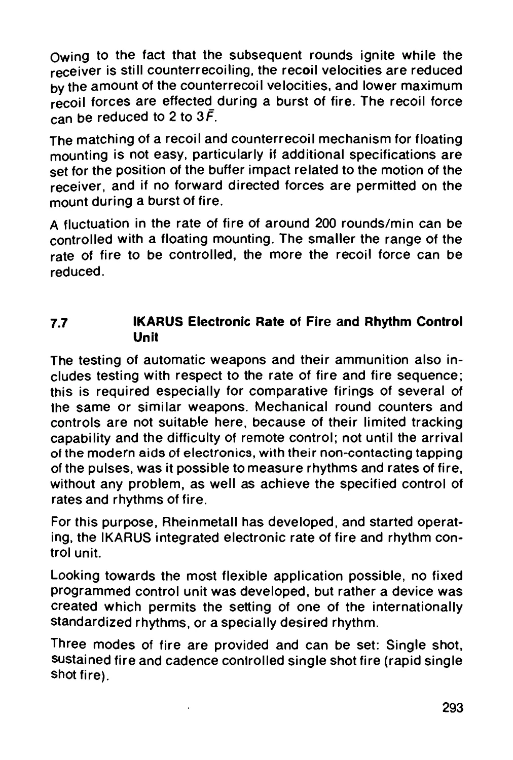
XXXIV
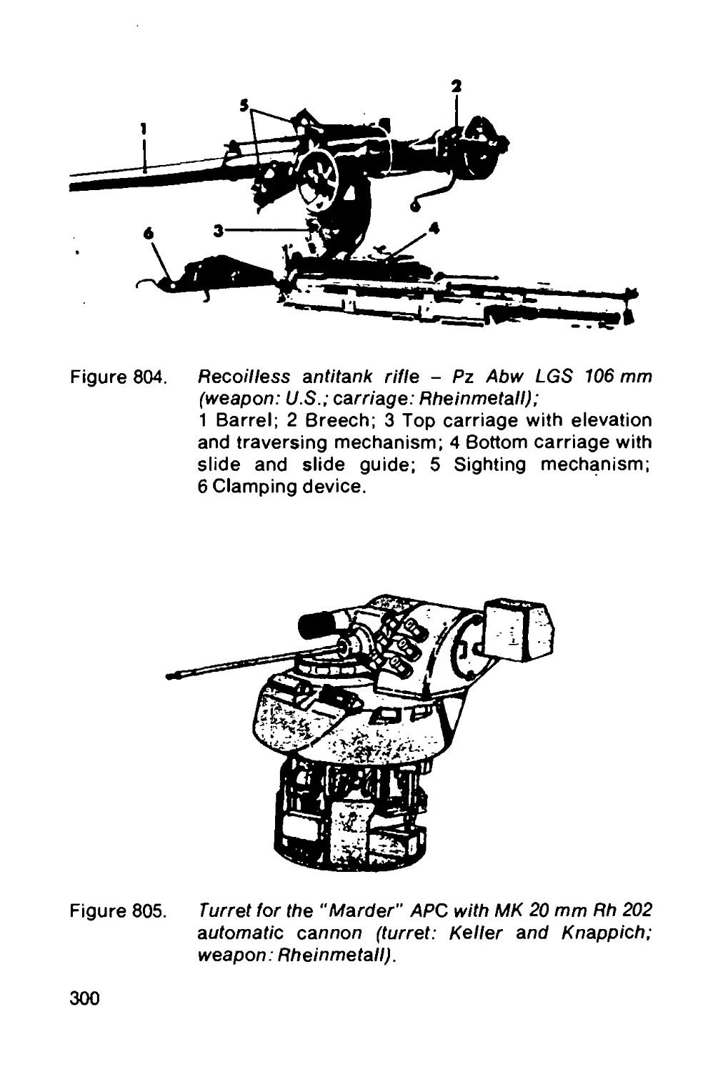
Military Technology and Production Design
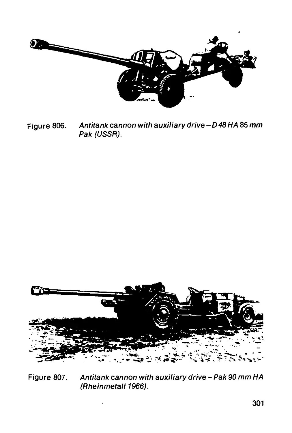
Turrets and gun systems for battle tanks and armored vehicles
Tank guns
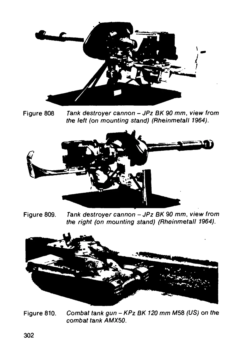
Armored self-propelled howitzers and artillery guns
AA systems
Rockets and rocket launching systems
Automatic cannons
Infantry weapons
Service and practice ammunition
Maneuver and simulator ammunition
Primers
Electrical firing and timing systems
Electronic measurement and control systems
Ballistic measurement systems
Performance of system studies
Planning and sale of production facilities
XXXV
1 EXPLOSIVES
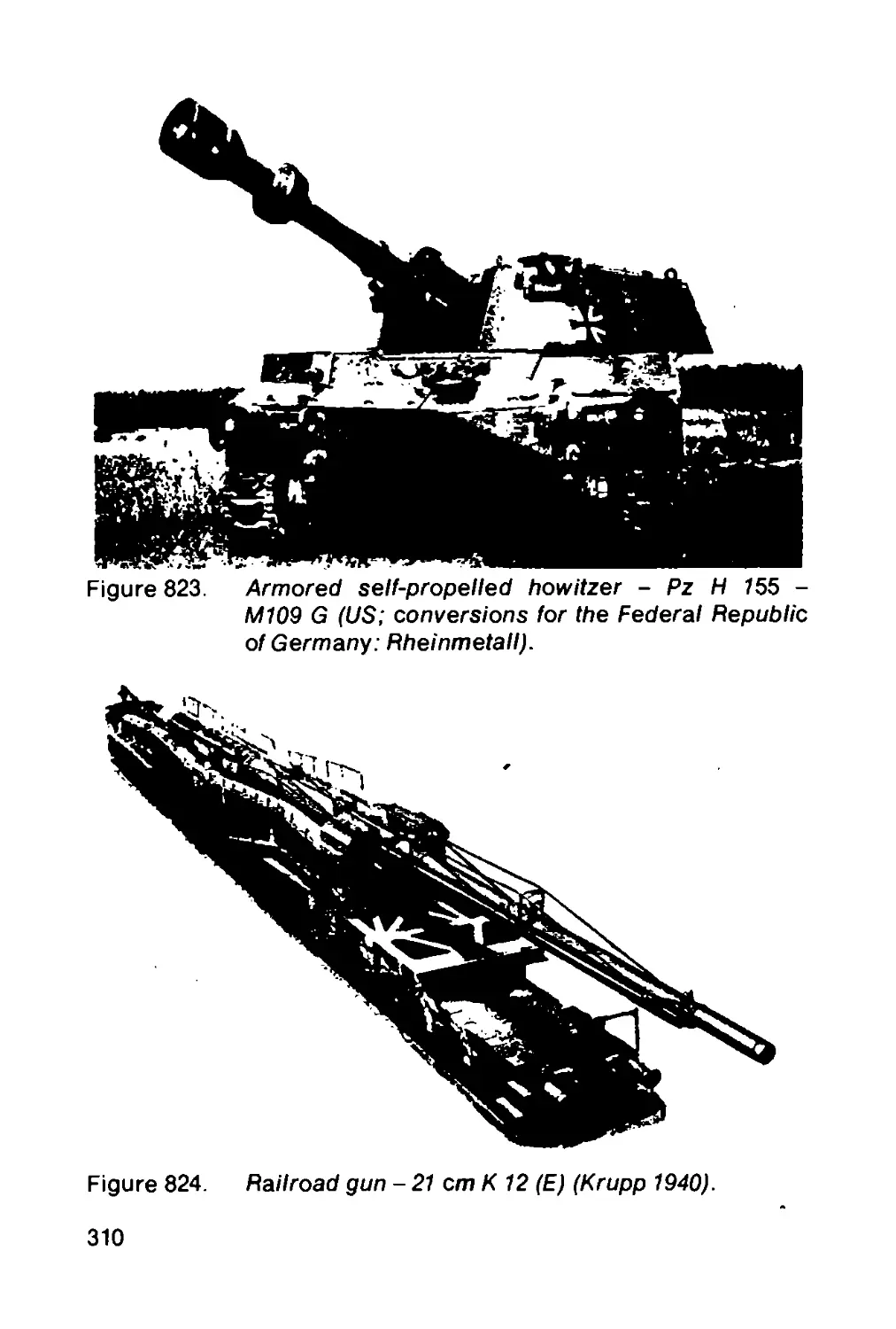
1.1 General
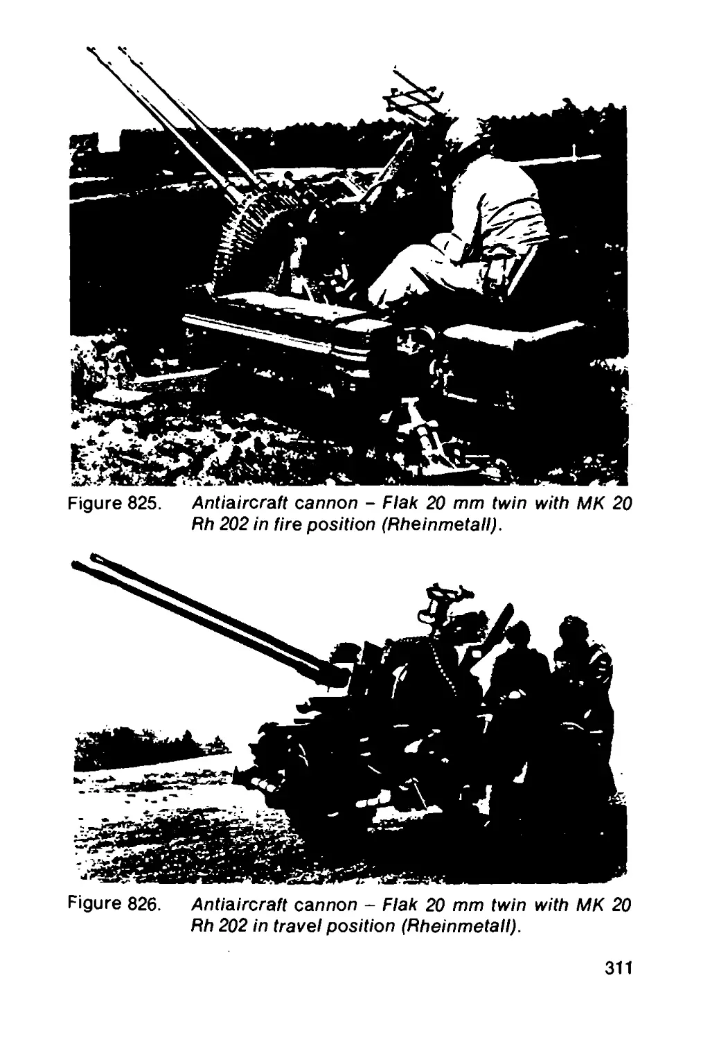
Explosives play a key role in military technology, both as propel-
lants for projectiles, and as agents to damage the target. Since
they are such important chemicals, it is worthwhile to look back at
their history.
Black powder was introduced into Europe in the thirteenth cen-
tury, having been discovered previously in China. Its first use is
attributed (without certainty) to one BERTHOLD SCHWARZ, who is
said to have used the powder to fire a shot from a ''musket" around
1300. Several centuries passed, and by the middle of the nine-
teenth century other explosive materials were discovered, which
were used aside from black powder and very soon had largely
replaced it.
A certain BERTHOLLET proved to be the first in this development.
In 1788 he undertook a series of experiments, in which he replaced
the saltpeter in the black powder by potassium chlorate, and dis-
covered "black” fulminating silver (AG3N). Other forerunners in-
clude HOWARD, who discovered mercury fulminate in 1799, and
BRUGNATELLI, who discovered fulminating silver (CNOAg) in
1802.
Modern explosives are all basically produced through the nitration
of hydrocarbons of different composition. This method began with
nitrobenzene (1834), nitronaphthalene (1835), and picric acid (tri-
nitrophenol) (1843). The most decisive stage in this development
1
took place in 1846, when SOBRERO discovered nitroglycerine,
and SCHONBEIN discovered guncotton. These discoveries were
followed by significant work on the part of A. NOBEL, who de-
veloped their characteristics towards a practical application. In
1867 he invented guhr-dynamite (75% nitroglycerine/25% dia-
tomite). In 1875 he invented blasting gelatine (92% nitroglycerine/
8% collodion cotton), and in 1888 he invented the first double base
propellant, “Ballistite” (nitroglycerine/nitrocellulose).
REID and JOHNSON (1882), DUTTENHOFER (1884) and VIEILLE
(1885) devised means of gelatinizing nitrocellulose into definite
shapes, through the use of appropriate solvents. VIEILLE’s product
was the so-called “Powder B".
In 1889, ABEL and DEWAR developed the double base "Cordite",
which proved to be more powerful than NOBEL’s "Ballistite".
Whereas the manufacturing process for both "Cordite" and
"Ballistite” required the use of solvents, a process was discovered
in Germany in 1909, of producing double base propellants without
solvents.
During the Second World War, “cool" propellants containing di-
ethyleneglycol dinitrate, and nitroguanidine were developed. They
are linked with the name of GALLWITZ.
In addition to NOBEL’s guhr-dynamite, any discussion on explo-
sives should mention trinitrophenol filled rounds. This process was
developed according to STETTBACHER[1] on the basis of work by
TURPIN (1885), and it led to the beginnings of high explosive
artillery rounds and bombs.
To avoid the disadvantages of trinitrophenol which was poisonous
and also produced salts sensitive to shocks, users turned to trini-
trotoluene (TNT) which had been known since 1863. Only at the start
of this century, did this compound become available in technical
quantities.
MERTENS found tetryl in 1877 and HENNING discovered hexogen
(trimethylene-trinitroamine) in 1898; the patent for the production
of nitropenta (pentaerytrol tetranitrate) dates from 1912.
In addition to the most frequently used explosives (TNT and hex-
ogen), octogen has become increasingly important in recent
years because of its greater energy/volume ratio compared to
hexogen.
2
The discovery of the classical explosives, operating on the release
of chemical energy, can be said to have reached a conclusion at the
start of this century.
The beginning of a new “era" in weapons technology, comparable
at least in historic consequences with the first ballistic use of black
powder, can be pinpointed to the summer of 1945, when the first
atomic bomb was detonated in New Mexico, USA. This technical
achievement was made possible by the research work of two
generations of nuclear physicists: especially RUTHERFORD who
carried out the first synthetic nuclear reaction in 1919; and O. HAHN
and F. STRASSMANN, who proved that uranium could be made to
decay as a result of bombardment with neutrons (1938).
If one considers the development of military equipment since 1945,
then, in the field of explosives, one can perceive:
Atomic and conventional weapons coexist.
Chemical propellants are still used to power the launching vehi-
cles for atomic warheads. Even for large intercontinental mis-
siles, it is still not practical to use an atomic reactor to provide the
propellant needed.
Conventional explosives are studied intensively in all their chem-
ical and physical dimensions and, where possible, they are
improved to provide optimal constructions and to increase the
performance of new weapons.
Having completed this short historical sketch, there are still a few
general comments which should be made.
Explosives are distinguished from common fuels, such as coal, pe-
troleum products or wood, by the fact that they contain as an inte-
gral part the oxidizing agent. Consequently, the energy released per
unit of mass (heat of explosion) for explosives, about 5x 10’ kJ/kg,
is considerably less than that for fuels (43x10’ kJ/kg for gas-
oline), which combine with oxygen from the atmosphere. On the
other hand, and this is the decisive property of explosives, the
chemical bond and finely dispersed oxygen (included or confined)
causes highly rapid combustion, which creates high energy den-
sities (pressures) in a short period of time.
STETTBACHER [1] gave a very instructive example, which is
shown here in modified form:
3
2500 kg of an explosive with a heat of explosion Oex = 6700 kJ/kg
explodes in 500 ps. This releases energy equal to 2500 x 6700
= 16.75 x 10⁶ kJ = 4650 kWh. The world's total energy production
in 1966 was 3.5 x 10¹² kWh. This is equivalent to the energy of the
explosive considered here being produced 7.35 x 10⁸ times in the
year. However, the power of the explosive charge is 4650 x 3600: 5
x 10"* = 3.35 x 10'° kW, while the total capacity of the world’s
power plants operating for 24 hours a day for 360 days is 4.05
x 10® kW. Thus, 82.7 times the 1966 production of energy would
be needed to achieve the same output as the explosive charge.
The classification of explosive materials into the two main groups,
propellants and explosives, is less fundamental; it is based on the
ranges of the combustion rate, for which the various combinations
or mixtures are most suitable. Explosives for gun propellant, dis-
integrate, depending on the heat of explosion, with sturdy depend-
ence on the pressure and with a linear burning rate of from 10 to
1000 mm/s (20 bar < p < 4000 bar). The detonation rate for explo-
sives is from 2 to nearly 9 km/s, that is up to 106 times as great.
The exothermic disintegration of explosives and propellants is the
result of a chemical reaction, i.e. changes in the condition of the
electron shell of the atoms involved. This decay/disintegration
reaction continues until atoms, molecular fragments, ions and
radicals form a stable end product.
The maximum heat of combustion for mixtures of chemical fuels
and oxidizing agents used for projectile and rocket propellants is
approximately 25,000 kJ/kg (Be + |O2 —» BeO + 23,950 kJ/kg;
|H2 4-|F2 —> HF + 13,500 kJ/kg). The maximum thermal output, as
the result of "chemical” action, would be the recombination heat
of two hydrogen atoms to the molecule, 2H—>H2 releasing
216,000 kJ/kg. This is the theoretical and practical limit for energy
release by a chemical reaction [2], [3], [4], [5].
The energy released by an atomic (or better, a nuclear) explosive
charge is produced by changes in the atomic nucleus. Since the
interaction forces between the nucleons (elementary particles
which form the nucleus of atoms) in the same vicinity are con-
siderably greater than the Coulomb forces between the electron
shell and the nucleus, nuclear reactions can produce enormous
amounts of heat.
4
Exothermal nuclear reactions are produced through the fission of
the nuclei of atoms with high atomic numbers (uranium and pluto-
nium bombs) and through the fusion of the nuclei of atoms with low
atomic number (hydrogen bombs). The fission of uranium releases
7.1 x1O10 kJ/kg and the fusion of ,T3 + ,D2—>2He4 + n produces
34.3 x Ю10 kJ/kg (T = tritium, D = deuterium, He = Helium, n =
neutron) [4].
The energy content of nuclear warheads is given in TNT equiv-
alents. Today intercontinental missiles carry warheads equivalent
to some 50 megatons of TNT.
The following sections deal with some details of chemical explo-
sives as far as possible. This handbook does not discuss nuclear
charges in further detail, since it is limited to the examination of
conventional weapons. For further information on nuclear
weapons, and particularly their effect, the book "The Effects of
Nuclear Weapons” [33] is recommended.
1.2 Classification of Explosives [6], [7]
On the suggestion of the Federal Office for Materials Testing
(BAM), Berlin, explosive matter or materials capable of exploding
are classified as shown in Figure 101.
Figure 101. Classification of materials capable of exploding.
5
The individual groups and subgroups include:
Under explosives, homogeneous:
a) nitric acid esters: nitroglycerine, nitropenta,
nitromannit, glycoldinitrate
b) secondary nitro compounds: trinitrophenol, trinitrotoluene
c) nitramine: hexogen (cyclonite), octogen
d) nitrosamine: trimethylentrinitrosamine
e) salts: ammonium picrate
Under explosives, explosive mixtures:
black powder
nitroglycerine explosives
ammonium nitrate explosives
chlorate explosives
liquid air explosives
Under Initiating explosives:
mercury fulminate
lead azide
lead trinitroresorcinate
diazodinitrophenol
silver fulminate
chlorate-phosphorous salts
Under gun propellant (smokeless):
a) made with volatile solvents: nitrocellulose powder
b) made without solvents (POL-Pulver): nitroglycerine or diglycol
powder
c) double base propellant with crystalline nitro compounds: ni-
troguanidine powder, guanidinenitrate powder
Under pyrotechnics:
illuminating and signal components
fire crackers
propellants
whistling components
screening smoke and gas components
flash components
The following compounds belong to the group of explosive ma-
terials manufactured by the chemical industry but not intended as
explosives:
6
ammonium nitrate for fertilizers - secondary nitro compounds,
inorganic nitrate and chlorate mixtures used as herbicides and
pesticides-azonitril, sulfohydrazide and dinitrosopentamethy-
lenetetramine in inflating agents for the synthetic and rubber
industries-organic per- and hydroperoxideas a polymerization
catalyst in the synthetics industry-secondary nitro compounds
and nitric acids for the pharmaceutical industry-azo and diazo
compounds in bleaching and washing products-nitrocellulose
for synthetic resin varnishes, synthetic films and synthetic silk-
explosive gases such as acetylene and chlordioxide, etc.
The following materials are manufactured as preparations not
intended for use as explosives:
ammonium bromate-ammonium chlorate-ammonium nitrate
- azidoamine - chromium salts - ether peroxide - ethylene
ozonide - lead bromate - lead acetate - lead tetracetate -
calcium azide - chlorheptoxide - nitrogen chloride - acetylene
dioiodide - halogen azides - halogenated hydrocarbons with
alkali or alkaline earth metals - hydrazine nitrate - nitrous
iodine - gold fulminate - platinum fulminate - silver fulminate
Ag3N - manganese heptoxide - metal picrates - metal salts of
the hydrazines - sodium nitromethane - organic chlorates and
perchlorates - 100% perchloric acid - mercury oxalate - mer-
cury oxinide-nitrogen sulfide-silver chlorate-silveroxalate-
silver persulfate - strontium azide - zinc chlorate, etc.
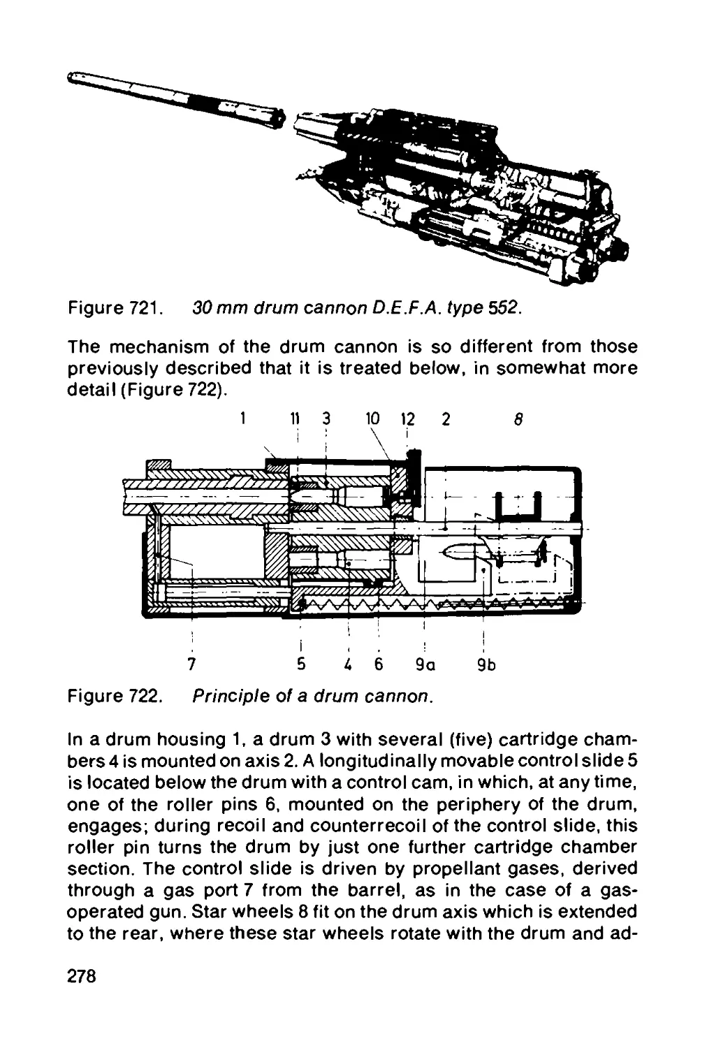
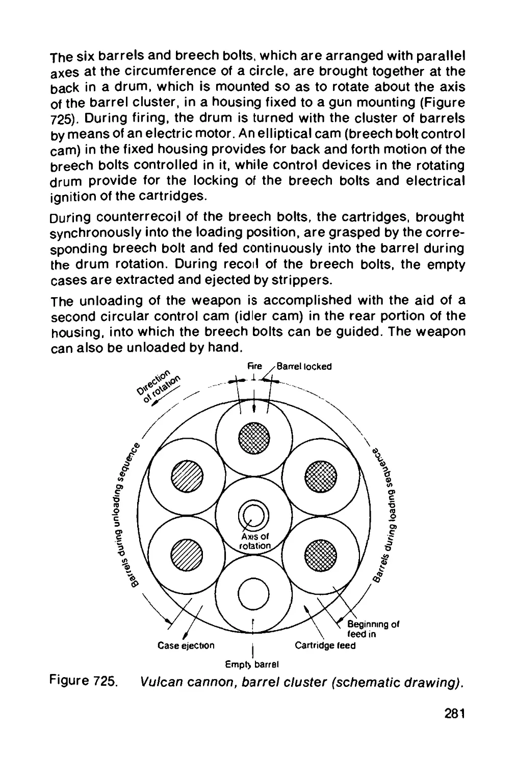
Figure 102. Subdivision of explosive devices.
7
Figure 102 depicts the subdivision of explosive devices produced
from explosives. The individual groups include:
Under blasting agents:
a) powder explosives: blasting powder, А-black blasting powder
b) rock blasting explosives: dynamite, В-black blasting powder,
ammonite, donarite, ammonium gelite, cloratite, oxyliquite
c) permitted explosives used in mining: Wetter nobelite, Wetter
wasagite, Wetter detonite, Wetter westfalite, Wetter astraline,
Wetter bicarbite, Wetter salite
d) well drilling cartridges: trinitrotoluol-hexogene (trixogen), am-
monium gelite, triamine, seismo-gelite, seismotolite
Under igniting agents:
a) explosive: blasting caps, electrical fuzes with blasting caps,
fuse cord
b) non-explosive: electrical fuzes without blasting caps, powder
fuses and igniters, igniting cords, percussion caps
In addition lothose listed above, there are: explosive rivets, Flobert
ammunition, igniting sheets, popping cork, and exploding puli-
cords.
Under firing agents:
cartridges for small arms
cartridges for illuminating and signal ammunition
cartridges for firing apparatus used for technical purposes
rockets
Under pyrolechnical devices:
fireworks
small fireworks
party fireworks
pyrotechnical devices for technical purpose
large fireworks
Under pyrolechnical igniters:
stoppine, igniting cord
Under inflammables:
matches
8
1.3 Propellants
As indicated in the introduction, chemical propellants are used to
hurl projectiles containing a warhead towards their target. These
projectiles may be shells, which are accelerated inside gun bar-
rels and then-depending on their departure velocity when they
leave the barrel-fly without further propulsion, or rockets which
receive additional thrust through all ora partoftheir trajectory. For
post accelerated projectiles, there is a combination of acceleration
in the barrel and by rocket propellants.
A distinction is made between gun and rocket propellants on the
basis of differences in chemical composition, in some cases other
phases (solid or liquid), and the manufacturing processes.
1.3.1 Gun Propellants
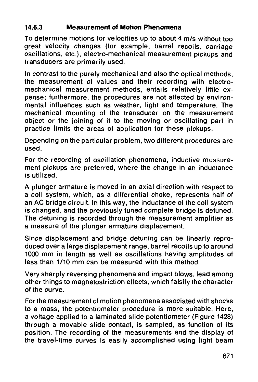
1.3.1.1 Nitrocellulose Propellants
Single base propellants made from nitrocellulose with traces of
additive are widely used in the ammunition for small arms, auto-
matic cannons, and in large caliber weapons. As a group, they are
called nitrocellulose or Nc propellants.
Nitrocellulose is a nitric acid ester of cellulose. It is produced by
adding nitrating acid (nitric acid and sulphuric acid) to cotton or
wood cellulose. The gross formula with complete nitration is
[C6H7O2(ONO2)3]n.
The degree of nitration depends on the nitrogen content. The gross
formula given above would show a nitrogen content of 14.14%; for
practical purposes, the content attained is only 13.4%. In the manu-
facture of the propellant, guncotton (nitrogen content 13.0 to
13.4%) and collodion cotton (12.0 to 12.6% nitrogen), are used.
In the course of the process of propellant manufacture [8], the
nitrocellulose is first gelatinized with a volatile solvent, usually an
ether and alcohol mixture. The gel is then pressed into strands of
the desired shape and size. These strands are cut into uniform
lengths (e. g., as tubes or flakes). The solvent is then volatized and
in the process there is considerable shrinkage. The final thickness
is not apparent until all of the solvent has been driven off. The
strand of propellant has a greater thickness when it leaves the
press than at the conclusion of the manufacturing process, and it is
only the final thickness which is ballistically effective. Here, con-
9
siderable experience is required for dimensioning of the molds
used in the press.
Stabilizing agents, such as acardite or centralite, are added to the
nitrocellulose, and this supports simultaneous gelatinization. The
stabilizing agents work by combining with free nitrous gases,
which would otherwise act as an automatic catalyst and cause the
compound to disintegrate.
In order to change the linear burning rate, to attain a progressive
burning, for example, the surface of the Nc propellant is treated.
Treatment of the surface consists in adding substances with low
vapor pressures, such as arcadite, centralite, diphenylamine,
dibutylphthalate or camphor, so that they can diffuse into the inte-
rior of the propellant. These additives reduce the heat of explosion
in the outer layers and thereby reduce the linear burning rate.
In order to prevent the accumulation of static electrical charges,
and to increase the bulk weight, graphite is added to the surface of
the Nc propellant.
1.3.1.2 Propellants without a Solvent
Solventless propellants (in German: POL-Pulver) areeitherdouble
base or triple base.
1.3.1.2.1 Double Base Propellants
Nitrocellulose can be gelatinized with the slightly volatile liquids
nitroglycerine and diglycoldinitrate.
The structure of these substances is:
CH2-O-NO2
CH —O-NO2 | Nitroglycerine
CH2-O-NO2
CH2-O-NO2
I
CH2 \
| /О ? Diglycoldinitrate
CH2 '
I
CH2-O-NO2
10
Nitroglycerine propellants are produced by submerging the nitro-
cellulose in water and adding the nitroglycerine when the solution
is agitated. When this is done, the nitroglycerine is absorbed by the
nitrocellulose. After being separated from the water, the com-
pound is gelatinized and re-worked again by rollers or screw type
presses. (In the USA and in England, the gelatinization is partly
achieved with the use of acetone as a volatile solvent.) Further
transformation of the gel into a propellant grain is accomplished by
putting it in an extrusion press or roller press at a elevated
temperature.
Nitroglycerine propellant containing 25 to 50% nitroglycerine has a
heat of explosion of from 2900 to 5200 kJ/kg. If lesser heats of
explosion are required, nitrocellulose containing a lower nitrogen
content is used.
If nitrocellulose is gelatinized with diglycoldinitrate, the result is
so-called "cool” propellant, which is characterized by low heat of
explosion and hence low explosion temperatures. This reduces the
amount of tube wear considerably. In addition, since the specific
gas volume of diglyc'oldinitrate propellant is greater than that of
nitrocellulose or nitroglycerine propellant, it retains still a suf-
ficient ballistic performance.
1.3.1.2.2 Triple Base Propellants
If nitroguanidine is added to diglycoldinitrate propellant as a third
component, the result is nitroguanidine propellant which is also a
“cool" propellant.
Nitroguanidine is a crystalline solid with the following structure:
NH2
NH = C \
X NHNO2
The content of nitroguanidine in the propellant varies between 25
and 50%.
Cool propellants were developed in Germany during the Second
World War. Because there is less tube erosion when nitro-
guanidine is used in conjunction with diglycoldinitrate, nitro-
guanidine propellant is used today for both tank and artillery
ammunition.
11
Another triple base propellant, ammonium powder, has failed to
achieve practical significance. This is a solventless propellant that
contains up to 55% ammonium nitrate (NH4NO3), but whose main
drawback is its high hygroscopicity.
1.3.2 Rocket Propellants1)
Rocket propellants [3], [4] are divided according to their phase as
follows:
Liquid propellants are those where the homogeneous propellant or
fuel and the oxidizer are deposited in tanks as separate fluids.
From there they are fed into the combustion chamber.
Solid propellants are those where the propellant as a homoge-
neous substance or as a mixture of substances is positioned inside
the combustion chamber in a solid state with definite surface.
Lithergols (hybrid propellants) are those where the fuel (normal
type) or the oxidizer (inverse type) are placed in the combustion
chamber in a solid state, and the oxidizer/fuel is introduced from a
tank into the combustion chamber as a liquid.
1.3.2.1 Liquid Propellants
The first group of liquid propellants is that known as monergoles. A
distinction is made between simple and composite monergoles;
simple monergoles are chemically pure substances while com-
posites are mixtures of propellants containing at least two different
components, capable of being stored. When igniting energy is
applied, the monergoles disintegrate spontaneously releasing
both heat and gas products.
Table 101 contains examples of monergoles; the data are drawn
from DADIEU-DAMM-SCHMIDT [4].
With the exception of nitromethane and mixtures of hydrazine and
hydrazine mononitrate, the monergoles have a relatively small
specific impulse-the criterion of a propellant’s ballistic perform-
ance (see Section 2.3.3 on the Internal Ballistics of Rockets, page
130). The values given in Table 101 are theoretical equilibrium
values.
1) See Section 2.3 on the Internal Ballistics of Rockets.
12
Table 101. Monergol Propellants.
Substance Chemical Composition Specific Impulse /s (m/s)
Nitromethane CN3NO2 2500
Hydrazine n2h4 1950
Hydrazine/Hydrazine nitrate N2H4 + 30%N2H5NO3 2160
Ethylene Oxide C2H4O 1950
Tetranitromethane C(NO2)4 1780
Hydrogen Peroxide H2O2 1620
Since nitromethane is highly explosive, it cannot be used as a
rocket propellant in its pure form. (The use of a hydrazine/hydra-
zine nitrate system is beingexamined.) The remaining monergoles
Table 102. Homogeneous Liquid Rocket Fuels.
Fuel Chemical Composition Boiling Point Ts (°C)
Hydrogen Kerosene (RP-1) Methane Ethylene Hydrazine Monomethylhydrazine (MMH) Unsymmetrical dimethylhydrazine (UDMH) Aniline Diethylenetriamine (DETA) Ammonia Ethyl alcohol Diborane Penta borane H2 Сц,7 H21,8 CH4 C2H4 n2h4 ch3nnh2 (CH3)2NNH2 c6h5nh2 h2nch2ch2nh ch2ch2nh2 NH3 C2H5OH B2H6 B5H9 -252.8 + 140 to +250 -161.7 -103.5 + 113.5 + 87.5 + 63 + 184.4 + 207 - 33.4 + 78.4 - 92.5 + 60.1
13
in the list, particularly hydrazine and hydrogen peroxide, are used
for guidance and booster systems.
Diergoles are propellants which require that the fuel and the oxi-
dizer be introduced into the combusion chamber separately.
Hydrogen, hydrocarbons, hydrazine and hydrazine derivatives,
amides, ammonia, alcohols and boranes are all used as fuels.
The most important oxidizers are oxygen, fluorine, nitric acid,
nitrogen oxide, hydrogen peroxide, and oxygen difluoride.
Table 102 gives the chemical composition and the boiling points Ts
of homogeneous liquid rocket fuels.
The fuels listed in Table 102 are used singly or in combination with
one another. Important mixtures of liquid fuels are:
Aerozine 50(50% UDMH+50% hydrazine)
Hydyne (60% UDMH+40% DETA).
The technically significant oxidizers are listed in Table 103.
Table 103. Liquid Oxidizers.
Oxidizer Chemical Composition Boiling Point Ts (°C)
Oxygen O2 -183
Fluorine f2 -188
Nitric acid HNO3 4- 84
Dinitrogentetroxide N2O4 + 21.1
Hydrogen peroxide H2O2 4-150
Oxygen difluoride of2 -145.3
Table 104 gives the specific impulses of various combinations of
fuels and oxidizers.
As shown in Table 104, the greatest specific impulses are attained
when fluorine, oxygen, and oxygen difluoride are used as oxi-
dizers, and the specific impulses with nitric acid and dinitrogen-
tetroxide are considerably lower. The highest specific impulse for
this type of system, reported in the literature, is 4480 m/s for the
system BeH2/O2.
14
Table. 104. Specific Impulses of Various Combinations of Fuels
and Oxidizers.
Fuel Specific Impulse /S(m/s)
O2 f2 of2 HNO3 H2O4
Hydrogen 3830 4020 4020 —. —
Kerosene RP-1 2950 3200 3420 2580 2710
Hydrazine 3070 3570 3380 2730 2850
MMH 3060 3390 3420 (2740)* 2820
UDMH 3040 3360 3440 (2710) 2800
Aerozine 3060 — — (2740) 2820
Hydyne —• — 3410 — —•
Diborane 3370 3640 —. — —.
Pentaborane 3140 3530 3530 — 2970
Ammonia 2890 3520 3300 — 2640
Ethyl alcohol 2810 3240 — — —
* Values in brackets are based on red fuming nitric acid HNO3 + 15%NO2.
The A4 (V2), developed at Peenemunde by Wernher von Braun
during the Second World War, used a combination of ethyl alcohol
(75%)/O2 (liquid) as the propellant. The propellant pumps were
driven by hydrogen peroxide. The American Saturn 5 moon rocket
used a combination of kerosene/O2 (liquid) in the first stage
boos'.er and used H2 (liquid)/O2 (liquid) in the second and third
stages.
These propellant combinations are known as cryogens, because at
least one of the components can only be liquified at very low
temperatures (see Tables 102 and 103). Propellant combinations
which are in the liquid state at room temperature are termed
storable. Storable propellants are important especially for medium
military rockets, because they eliminate the necessity to fuel the
rockets immediately prior to launch. On the contrary, the rocket
can be fueled ahead of time and held ready. This is known as pre-
packaged propellant. In this connection, the mixture of nitric acid
and nitrous oxide is particularly important as an oxidizer.
15
For the choice of propellant combinations, ignition behavior is of
great importance. A group of oxidizers and fuels ignite spon-
taneously when brought into contact with one another; this charac-
teristic is known as hypergolity. Some hypergolic combinations
can also be produced by the addition of a catalyst.
Table 105 gives the ignition behavior of various propellant com-
binations.
Table 105. Ignition Behavior of Various Propellant Combinations.
Oxidizer Fuel O2 liquid F2 liquid Н2О2 HNO3 N2O4 CiF3
Ammonia X О X □ □ О
Aniline X О X □ О О
Ethanol X О □ X X О
Hydrazine X О □ о о О
Kerosene RP-1 X О X X X О
H2 (liquid) X О X X X О
MMH X О X о о О
UDMH X О X о о О
О = hypergolic □ = hypergolic with catalyst x =non-hypergolic
Non-hypergoliccombinations are ignited either pyrotechnically or
by addition of a hypergolic fluid during the starting operation.
1.3.2.2 Solid Propellants
A distinction is made between
homogeneous propellants which contain both the oxygen and the
fuel in one compound,
and
heterogeneous propellants (or composite propellants) which
consist of a mixture of at least two compounds, the fuel and the
oxidizer.
Homogeneous propellants are based on nitrocellulose which has
been gelatinized with diglycolnitrate or nitroglycerine (see Section
16
1.3.1.2.1 on Double Base Propellants). Nitroglycerine is usually
employed as the second component. Homogeneous propellants
also contain additives to stabilize them, and to make them easier to
work with. The reasons for this are similar to those discussed in the
context of gun propellants. Their final form is arrived at after
pressing into strands in heated extruders, extrusion, final process-
ing and isolating.
In heterogeneous solid propellants, the oxidizer (in fine crystals) is
evenly distributed throughout a synthetic binding agent.
The following nitrates and perchlorates are used as oxidizers:
lithium nitrate
sodium nitrate
potassium nitrate
ammonium nitrate
lithium perchlorate
sodium perchlorate
potassium perchlorate
ammonium perchlorate
LiNO3
NaNO3
KNO3
NH4N03
LiCI04
NaCI04
KCI04
NH4CI04
The excess oxygen in these compounds ranges between 20% by
weight for ammonium nitrate, and 60% by weight for lithium per-
chlorate. Studies have recently been made on the feasibility of
using nitroniumperchlorate (NO2CIO4), which contains 66%
excess oxygen by weight.
When used as an oxidizer, ammonium nitrate produces a gas-rich
propellant with a relatively low temperature of combustion. The
linear burning rate is low, as is the specific impulse.
Potassium perchlorate also gives a low specific impulse, but the
linear burning rate is quite high. For this reason, potassium per-
chlorate composites make good propellants for launch motors.
Ammonium perchlorate delivers a relatively high specific impulse
- up to 2450 m/s. The linear burning rate lies in the middle
of the range, and is less dependent upon pressure and temperature
than the other oxidizers.
The following are used as binding agents:
Asphalt (with KCI04 for launch assisting rockets); asphalt com-
pounds have low performance and are unstable.
17
Polyisobutylene (with ammonium perchlorate); high perform-
ance but unstable.
Polyvinylchloride (with ammonium perchlorate); high perform-
ance but the high rate of shrinkage means that it can only attain
case bonding if the dimensions are small.
Cellulose acetate (with ammonium nitrate); produces large
amounts of gas at low temperatures, so it is well suited for use in
gas generators.
Polysulfide (with ammonium perchlorate); since a high degree of
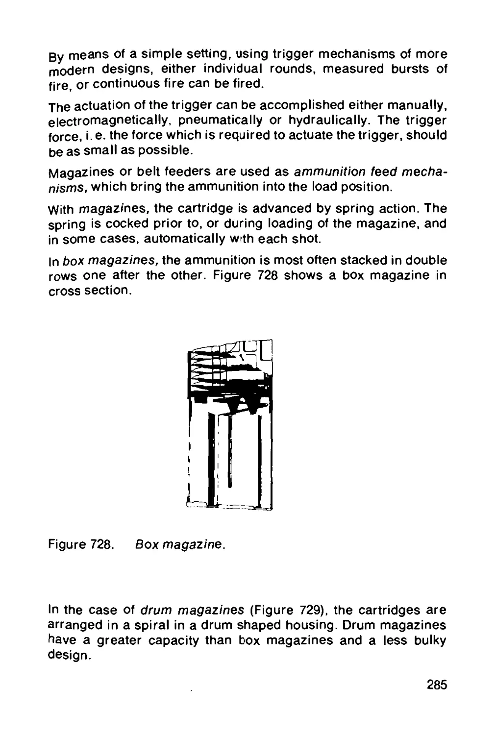
filling is possible (80%), it has a high level of performance. It is
highly elastic. Polysulfide composites are also known as
thiocole.
Polyurethane (with ammonium perchlorate); has a very high
performance.
Polybutadien - Acrylic acid polymers have a very high perform-
ance and good physical characteristics.
Propellants with polyvinylchloride (PVC) and cellulose acetate
are also known as plastisols.
To raise the specific impulse further, powdered light metals (Al,
Mg) or Bor/metal hydrides are added to the solid propellants.
To change the linear burning rate, catalysts, such as copper or
chromium oxide, are added as ballistidadditives (plateau burning
and mesa burning).
The burning rate of heterogeneous solid propellants is strongly
influenced by the particle size of the oxidizer.
The composites are prepared for use as propellants either by
shaping in molds or by compressing them. They are then placed
in the combustion chamber after partially isolating the surface.
However, they can also be poured directly into the combustion
chamber, using a central core in the case of an internal burning
grain. The mold core is then removed, after the propellant is
hardened.
1.3.2.3 Lithergols
In lithergol propulsion systems, which are also called hybrid sys-
tems, oxygen, hydrogen peroxide, dinitrotetraoxide, nitric acid,
18
chlorine trifluoride, and oxygen difluoride are all used as liquid
oxidizers.
The primary solid fuels are hydrocarbons [(CH2)„], some of which
use light metal powder as additives.
The particular problem in lithergol systems derives from the fact
that the relative flow rates through the combustion chamber must
be coordinated in such a way, that the oxidizer passing across the
surface of the solid fuel produces the optimal reaction.
1.3.3 Thermochemistry
The heat of explosion, explosion temperature, composition of re-
sultant gases and smoke, and the volume of the gases released by
the reaction of a propellant can be calculated rather precisely by
using the principles of thermochemistry. The basic considerations
involved can be summarized briefly as follows:
In reactions involving Nc or solventless propellants having the
general formula CaHbNcOd, primarily CO2, CO, H2O, H2 and N2
are released.
In addition, radicals such as H, OH, NO, and others, show up in
various arrangements. Subsequent reactions in the exhaust gases,
particularly of the ''cool" propellants, can produce C, NH3 and CH4.
Calculations begin with the five principal reaction products [9].
There is an exchange reaction envolving CO2, CO, H2O and H2; this
is the water-gas reaction:
CO2 + H2fc>CO + H2O.
The concentration [ ] or the partial pressure of the reaction ele-
ments taking part in the water-gas reaction is controlled by the law
of mass action:
[CO] [H2O]^
[CO2] [H2]
(D
k(T) is a function dependent only on the temperature T, which is
calculated for the water-gas equilibrium.
In addition, the molar number of the atoms of the propellant of the
general compound CaHbNcOd and that of the reaction products is
the same:
19
[С]: [СО] + [СО2] = а, (2)
[HJ: 2[Н2О] + 2[Н2]=Ь, (3)
[О]: [СО] 4-2[СО2] + [H2O] = d. (4)
Equations (1) to (4) depict an equation system with the molar
concentration of the four reacting elements. It can be solved with
the temperature dependent function k(T) when T=Tex (the explo-
sion temperature).
The explosion temperature itself is now also dependent on the
solution of the system by means of the four Equations (1) to (4). This
holds that for Tex:
Qsx = Qbg ~ Qbp = cvg 7"ex—c«p Лэ- (5)
In the above expression, the following values are used:
Qex = heat of explosion,
QBG =heat of formation of gaseous products of the
explosive,
QBP =heat of formation of the explosive,
cvP = specific heat of the explosive,
To = surrounding temperature of unburned explo-
sive.
cvG is the mean specific heat of the propellant gases:
SP,cvGi
where p, is the partial pressure and cvGi is the molar heat of the
reaction products (here CO2, CO, H2O, H2 and N2).
The values of cvG1 are also temperature dependent; they are also
available in tabular form for a large number of gases.
The heat of formation of the propellant gases can be calculated
from the concentrations of the individual molecules in the gas and
their individual heats of formation. These are also available in
tabular form.
In practice, one can carry out the calculations in such a way that the
equation system is first solved using Equations (1) to (4) with an
estimated temperature and the result is then checked using
20
Equation (5). The calculations can then be made again using the
more accurate value, provided that the condition
Obg-Qep = Qex
is met. The gas volume can be determined immediately from the
total number of moles of the gaseous reaction products.
Since it is known that there are other reaction products, which are
dependent on the temperature of the explosion, the calculations
can be further corrected by considering these compounds.
The reader is referred to the references [4], [9], [10], and [11] given
in the bibliography for further demonstration of the thermochem-
ical calculating procedures for gun or rocket propellants.
1.3.4 Burning Characteristics of Propellants
The burning of propellants is an extremely complex physical and
chemical process; even a less than complete discussion would
exceed the scope of this publication. For a more exhaustive treat-
ment of the problem, the reader is referred to books [4] and [9] in
the bibliography. These references deal with all the most important
experimental and theoretical work that has been done in this field.
As is discussed in Chapter 2, Internal Ballistics, the burning
characteristics of a propellant play a decisive role in determining
the propulsion of a projectile. In rocket propulsion systems which
use liquid propellants or lithergols, the rate at which the injection
pump operates determines the rate at which the hot gases are
produced. This rate can therefore be regulated during the propul-
sion process. By contrast, with propellants used in solid fuel rock-
ets or in guns, the combustion process is determined by the
geometry of the propellant grains and other factors of Internal
Ballistics.
For propellants which are either a homogeneous or heterogeneous
mixture, the rate of reaction is determined by the total exposed
surface and by the thermodynamic condition of the gas phase in the
combustion chamber.
dz
The rate of reaction — is derived from the free surface of the
df
21
propellant S(t) at time t, its density qc, and the linear burning rate
de
dt'
If the portion of the burned propellant is defined as
Z=mc.-M (8)
mca
where mca is the initial amount of propellant and mc(t) is the
amount of unburned propellant at time t, then
dz=_1dmjt) ,
dt mca dt ' 1 1
In addition,
de
since, in unit time the layer - - is burned over the entire actual
7 dt
de
surface S(t), giving the volume of burnt propellant as S(t) .
dt
This multiplied by the density qc of the propellant, gives the mass
of burned propellant during each unit time equal to
dt
Since, in the burning of a propellant, thfe portion of burned propel-
lant z is definitely dependent on the time t, it is possible to substi-
tute the variable z for the independent variable t so that instead of
S(t), S(z) can be used.
By combining Equations (9) and (10), one gets
dz=££S(t)de
dt mca df
Equation (11) is the initial equation for the law of combustion used
in internal ballistics. The quotient
mca
presents, except for a generally constant factor, the form function
which is discussed in Chapter 2, Internal Ballistics. In the sections
22
which follow, we shall look more closely at linear burning rates.
Greatly oversimplified, the process that occurs during the burning
of the propellant surface can be divided into three parts. These are
illustrated in Figure 103.
Ill Gas area, reaction
completed
II Gaseous zone
of reaction
I Surface of
propellant (solid
or liquid phase)
Figure 103. Reaction zones of burning propellant.
The transition from the solid or liquid state of the propellant into the
gaseous zone of reaction may be characterized by the reaction
velocity vi и: the transition from the gaseous zone of reaction to the
gas area, where the reaction is completed, takes place at the
reaction velocity vn hi.
The reaction velocity vt n is determined by the convection patterns
and the transfer of radiant heat on the surface of the propel-
lant. as well as by the energy of stimulation, such as, for example,
that needed to achieve pyrolysis of the macromolecules of nitrocel-
lulose or the vaporization/disintegration of the inorganic oxidizer
in composite propellants. In general, destruction of the binder in
composites does not affect the speed of reaction.
The vn in reaction velocity is dependent upon the chemical com-
position of the intermediate products. Reactions in zone II take
place in accordance with complicated radical mechanisms. If the
reaction proceeds according to the first order, then
£
Vll III~P2. (12)
If it is a second order reaction which determines the rate, then it
can be expected that the vn ш rate of reaction will be directly
proportional to the pressure in the gas phase:
vn in —p. (13)
23
Theories about linearburning rates can bedivided into twogroups:
vi. и < vii hi: surface theories,
vi h>vii in: gas phase theories.
In other words, in surface theories, the starting point is that the
transfer of heat on the surface of the propellant is the slowest and
therefore most decisive step in controlling the rate of burning.
According to the gas phase theories, it is the reactions in zone II
which determine the burning rate.
The semi-empirical evaluation of MURAOUR-AUNIS [12] is rep-
resentative of the surface theories
£q
with ^=conste *7®xp + a, (14)
df
where Eo = the stimulation energy of a molecule,
Tex = the temperature of the explosion,
p = the gas pressure,
к = Boltzmann's constant,
a = the contribution of radiation.
The amount a is such that at high pressures (roughly greater than
1000 bar) it can be disregarded when cojnpared to the first term of
the sum in Equation (14) which increases proportionally with the
pressure.
The combustion law of MURAOUR-AUNIS can be shortened to
de
~^ = a+bp. (15)
MURAOUR and AUNIS found, that, according to Equation (14), for
nitroglycerine powder with centralite, the equation
log Ь = с,+c2Tex (16)
holds for a wide range of nitroglycerine concentrations, within the
range 2000 K< Tex<4000 K. From this it must follow that the stimu-
lation energy Eo of this type of propellant is independent of the
nitroglycerine content.
24
The anticipated order of reactions in the gaseous zone of reaction
is predominantly order 1. As a result, the gas phase theories
generally assume that
however, the order of the reaction, and thus the transition from gas
phase mechanics to surface mechanics, is highly dependent on the
pressure. For this reason CORNER [9] gives the values shown in
Table 106 for an unspecified rocket propellant. These values show
the pressure dependence of the exponent a in the VIEILLE law of
combustion
(18)
Table 106. Dependence of the VIEILLE Exponent a on Pressure.
P (bar) a
130 0.5
1500 0.96
Here, a varies monotonically for intermediate pressures.
Equations needed for practical calculations of linear burning rates
are given in Chapter 2, Internal Ballistics.
In passing, it should be noted that with the kind of pressures that
are encountered in guns, linear burning rates can be considered
in near approximation as proportional to the pressure. However,
a stable condition is possible in a solid fuel rocket motor only if
the linear burning rate is not directly proportional to the pressure
[13]. In fact, as Table 106 shows, a linear burning rate proportional
to the pressure is not attained at the operating pressures of normal
rocket motors.
1.3.5 Methods of Testing Propellants
Tests of gun and rocket propellants, made on random samples
drawn from every lot manufactured, are designed to determine
25
chemical composition,
chemical stability,
physical characteristics,
ballistic behavior.
Chemical composition is determined through the normal methods
of analysis [14], including among others, such modern procedures
as thin-layer chromotography.
Technical terms of delivery prescribe that, as regards the chemical
composition, tests must be made to determine the total content
of volatile substances (remaining solvents), the moisture of the
propellant (using the desiccator or distillation method) and the
content of non-volatile and ether soluable substances.
Since nitrocellulose and nitroglycerine as nitric acid esters are
particularly inclined toward autocatalytic acid decomposition,
stability tests are required which speed up the separation by
raising the temperature. One must distinguish between tests at
high temperatures, carried out over a number of hours or even
days, and tests to ascertain the service life of the propellant,
which are carried out at lower temperatures, but over a period of
years. The Holland Test, conducted at +105°C over a period of
150 hours, or at + 110°C for 72 hours, with continuously recording
the weight loss of the propellant, is considered as the most reliable
testing method. The most important of the other tests are the Abel
Test, the Bergmann-Junk Test, and the Hansen Test. For details,
see KAST and METZ [14].
The hot storage test is used to determine service life. In general,
at +75°C, the time after which yellowish-red or reddish-brown
vapors appear, is determined.
Tests of the physical characteristics of a propellant include checks
of both shape and dimensions, density, bulk weight (in so far as
it is given), compression strength, deflagration point, the heat of
explosion, and hygroscopicity.
The deflagration point of nitrocellulose and nitroglycerine
propellants is determined by placing a sample in a paraffin bath,
and heating it at the rate of 5°C/min, and observing at what
temperature it ignites and explodes.
Heat of explosion is measured in a calorimetric bomb. In this
measurement procedure, the propellant sample is placed in a
26
sealed vessel under pressure (up to 2000 bar) and ignited. The
vessel is immersed in the liquid of a calorimeter. When the
propellant reacts, the heat raises the temperature of the liquid of the
calorimeter (water), and the rise in temperature is measured. By
considering the water equivalent of the calorimeter and the pressure
vessel, it is possible to calculate the heat of explosion. It is important
that the boiling point of water (the calorimeter liquid) should not
be surpassed, so that water produced by combustion will be
condensed. This enables the gross heating value to be measured.
The special problem of determining the heat of explosion in a
calorimetric bomb consists in the fact that at the lower (final)
temperature of the calorimeter measurement there is another
chemical reaction (equilibrium) established in the exhaust gases
than at the temperature of explosion, and which changes the
heating value.
Tests of the ballistic behavior of gun propellants are made usu-
ally by test firing rounds from guns with well defined ammuni-
tion components. The first thing is to determine the charge weight
which produces the required performance levels. Then a large
number of rounds of one propellant specimen are fired to
determine
the mean value of the muzzle velocity of the projectile and its
dispersion,
the mean value of the gas pressure (generally measured with
crusher gauges) and the highest level of gas pressure as
well as
the charge capacity.
In the development of propellants, but also for quality control
during the manufacturing process, considerable use is made of
the manometric bomb to determine ballistic values. This involves
using a closed pressure vessel in which the propellant can react
at constant chamber volume. Figure 104 presents a schematic
diagram of such a manometric bomb.
27
2b
I
2a
Figure 104.
1 Vessel body; 2a and 2b Front side locks; 3a and 3b Gaskets;
4 Outlet valve; 5 Insulated wire for electric igniter; 6 Piezo-
electric pressure gauge.
When using the manometric bomb, the first thing that is done is
to close valve 4 and to remove lock 2b. The propellant charge
is inserted and lock 2b is screwed in after an electric primer with
an igniter and a lead-in wire 5 has been attached. When the vessel
has been closed, the propellant is ignited, and the pressure in-
crease over time is recorded through the pressure gauge 6.
After the measurements have been taken, the propellant gas is
released through valve 4.
Figure 105. Characteristic pressure curve from a manometric
bomb.
28
One first notices an increasingly sharp rise in the pressure but
this then levels out and becomes a horizontal line. At the point of
transition from rising line to horizontal line, all of the propellant
has been burned. In reality, after the propellant has been com-
pletely burned, the line does not remain horizontal, but, instead,
drops slowly due to the cooling of the gases.
Abel’s equation is applicable for determining the maximum gas
pressure pm inside the manometric bomb after the propellant has
been burned:
fmc
— VB —r/mc'
(19)
In this equation, f is the propellant constant, mc is the charge
weight, VB is the volume of the combustion chamber and ц is the
covolume.
With a charge density
d = —c
VB (20)
this gives
(21)
d""
If the maximum gas pressure is measured for at least two different
charge densities, then the propellant parameters f and rj can be
determined. In order to obtain a reliable mean value for f and for
the measurements should be made on a large number of
charges with different densities.
The problem can be solved with the transformed Equation (21):
If the measurements — and — are plotted against one another,
Pm, A,
the result is a straight line as fitting curve such as is shown in
Figure 106.
29
Figure 106. Analysis of the measurements from the mano-
metric bomb.
The propellant constant f can be determined from the slope of
the line and the covolume z/ from the negative ordinate intercept.
In addition to f and >/, the pressure curve from the manometric
dz
bomb can be used to calculate the rate of reaction
dt
During burning, the expression
pm------------------------------- (22|
VB-^mcz(t)------mc(1 — z(t))
Qc
holds for the pressure, where z(t) is the portion of the charge
engaged in the reaction and oc is the density of the propellant.
If one assumes that >] = —, then Equation (22) can be rewritten as
вс
p(t) = —-±-z(t) (23)
VB-nmc
or, using Equation (19),
p(t)=pmz(t). (24)
If Equation (24) is further differentiated with respect to time, one
obtains
30
p(t)=pmz(t). (25)
Since the propellant burning can be written in general form, as
z(f)=Ba<p(z)₽(f) (26)
Po
(see Section 2.1.5.3, Propellant Burning), where Ba is the burning
coefficient, and <p(z) is the form function, then, using Equation (25),
Ba<p(z)=_p(n_
Po PmP(0 ’
p
gives the burning behavior of the propellant. The quotient
PmP
is referred to as the dynamic activity L.
The calculation of Ba<p(z) can be made for the general case
n# 1 , but the formula will, of course, be more complicated.
2c
A final comment should be made in conjunction with the
manometric bomb. According to Equation (26), the integration of
the pressure curve to time fb (all-burnt point)
f p(f)dt = f (28)
0 0 °a (Pt2)
must give a value, which is, due to the right side of Equation (28),
for a propellant characterized by Ba <p (z) independent of the charge
density at which the pressure curve was taken. In this connection,
O. SCHMITZ [15] has carried out a number of experiments involving
the range of pressures of interest to us here. His experiments
confirm the statements made above and the possibility of using
the law of combustion as is done in Equation (26). This is known
as the Krupp-Schmitz Law in the literature on the problem.
To measure the burning behavior of rocket propellants, one can
use either the Crawford bomb or the standard combustion chamber.
This has been introduced recently also for the testing of propellant
charges which generally burn at high pressure.
In the Crawford bomb, a sample of propellant is burned under
a constant pressure of nitrogen. The sample is 150 to 200 mm
long and 3 to 5 mm in diameter. The cylindrical side surface and
one end face of the sample are insulated with a synthetic film, so
31
that the sample will burn as an end-burning grain. Fuse wires are
passed through the sample at two specific points, they break when
the burning zone reaches them and this activates a recording
mechanism. This enables one to determine how long it takes to burn
a certain distance and thus to calculate the linear burning rate.
The Crawford bomb is constructed in such a way that the adjusted
pressure of the nitrogen is virtually unaffected by the propellant
gases released. One can therefore speak in terms of an isobaric
measurement. In order to determine the relationship between
pressure and the linear burning rate, Crawford measurements
should be made at a variety of different pressures.
1.4 Explosives [8], [16]
As already explained in the first section, there is no fundamental
difference between explosives and propellants. Depending upon
the type of ignition used, it is generally possible to take any
explosive material and have it burn as either a propellant (see
Section 1.3.4, Burning Characteristics of Propellants) or to have it
detonate. During burning the reaction that takes place is
dependent upon the pressure and temperature of the gas phase;
the linear burning rate has values of between 10'4 and 1 m/s.
During detonation, the reaction takes place as a steady process
with constant velocity, the detonation rate. The value of this rate
depends on the chemical composition of the explosive material,
and the charge density. For explosives this is between 2 x 10³
and 8 x 10³ m/s. Details regarding the physical and chemical
processes that take place during detonation are given under
Section 1.4.5.
The suitability of a material for use as an explosive depends
upon the specific characteristics required for particular appli-
cations. Thus one can list the differences between military, com-
mercial and initiating explosives.
1.4.1 Military Explosives
The following requirements apply to all military explosives:
high energy density,
firing safety, i.e. resistance to compression which, depending
on the height of the column of explosive, may occur during
accelerations up to several ten-thousand “g’s”,
32
safety in handling,
workability by pouring or pressing,
chemical stability even when stored for long periods.
In the pages which follow, the most important chemical com-
positions which meet these requirements are enumerated, and
their special characteristics stated. All of these materials are
solids at the temperatures at which they are used.
2, 4, 6-Trinitrotoluene (TNT, Tri, Tritol, Trilite, Tolit, Tutol, Trinol,
Triton, Trotyl)
Density: 1.64 g/cm3
Melting point: 80.8°C
Heat of explosion: 4310 kJ/kg
(H2O vaporous)
Detonation velocity: 6900 m/s
Deflagration point: 300°C
Trinitrotoluene is yellowish and crystalline in form, and is almost
completely insoluble in water. It dissolves slightly in alcohol and
is quite soluble in benzene, toluene and acetone. It is very stable
chemically and does not react with metals.
Due to its favorable melting point, trinitrotoluene is now one of
the most widely used military explosives. It is used both in the
pure form, and mixed with other explosives to form the explosive
agent for all types of weapons. Since there is a 12% loss of
volume when trinitrotoluene changes from the liquid to the solid
state, special steps must be taken to assure pouring free of
shrinkage cavities. Since TNT has a low level of mechanical
sensitivity, it lends itself to the pressing of charges.
Picric acid (2,4, 6-Trinitrophenol, Pertite, Picrinite, Melinite,
Ecrasite)
Density: 1.75 g/cm3
Melting point: 122.5°C
Heat of explosion: 4350 kJ/kg
(H2O vaporous)
Detonation velocity: 7350 m/s
Deflagration point: 300-310°C
Picric acid is given in the form of yellow sheets; it is poisonous
and soluble in hot water, alcohol, ether, benzene, and acetone.
33
In the past, picric acid was used in grenades. However, because
it is an acid, it formes metallic salts (picrates), i.e. highly impact
sensitive materials. As a result picric acid has practically no
significance today.
Nitropenta (Pentaerythritol tetranitrate, PETN, Pentryle, Penta,
Pentaryth)
CH2ONO2x. /CH2ONO2
CHjONOj^ ^CH2ONO2
Density: 1.76 g/cm3
Melting point: 141.3°C
Heat of explosion: 5860 kJ/kg
(H2O vaporous)
Detonation velocity: 8400 m/s
Deflagration point: 202 205°C
Nitropenta consists of colorless crystals. It is very stable chemically
and will not dissolve in water, but it is soluble in acetone and
methylacetate.
It is used for pressed shell and bomb charges, as well as for
booster charges. It is desensitized with a bit of wax.
Tetryl (Trinitrophenylmethylnitramine, Tetranitromethylaniline,
Pyronite, CE, Tetra, Tetralite, Tetralita)
Density: 1.73 g/cm3
Melting point: 131°C
Heat of explosion: 4900 kJ/kg
(H2O vaporous)
Detonation velocity: 7500 m/s
Deflagration point: 185°C
Tetryl is a fine yellow powder. It is poisonous, barely soluble in
water, but does dissolve well in benzene.
Because of its good initiation properties, tetryl is used mainly in
pressed booster charges. In addition, it is used together with
trinitrotoluene as the filler in shells and torpedos.
34
Hexogen (Cyclotrimethylenetrinitramine, Cyclonite, RDX, T 4,
Trimethylenetrinitramine) [17]
T2
N02\ r /NOj
N N
I I
н/уЧ
NOj
Density: 1.802 g/cm3
Melting point: 204°C
Heat of explosion: 5141 kJ/kg
(H2O vaporous)
Detonation velocity: 8700 m/s
Deflagration point: 230°C
Hexogen is a colorless, crystalline substance which dissolves
poorly in water but which is readily soluble in cyclohexane. Since
the deflagration point is close to the melting point, Hexogen can
only be processed in the solid state. Today, Hexogen is the most
important component of high explosive charges, e.g. shaped
charges. Hexogen is molded in melted trinitrotoluene (see Com-
position B), and recently it has also been molded in hardened
synthetic bonding agents or, desensitized with wax, pressed into
the desired form, partly with metallic additions (see Hexal).
Hexogen can be transported only after it has been desensitized
(with TNT, wax, and water).
Octogen (Homocyclonite, Tetramethylenetetranitramine, HMX,
Cyclotetramethylene-tetramine)
Density:
1.82 g/cm3 (a-modification)
1.90 g/cm3 (/(-modification)
35
Melting point:
1.76 g/cm3 (-/-modification)
1.80 g/cm3 (^-modification)
280° C
Heat of explosion: 5116 kJ/kg (H2O vaporous)
Detonation velocity: 9100 m/s
Deflagration point: 287°C
Appearance and solubility are much the same as for hexogen,
and both physical and chemical characteristics are almost
identical to those of hexogen. The one exception is the higher
density of octogen. Since the greater density of octogen also gives
a greater energy density, use of this material in high performance
shaped charges is currently being considered. Though, for the
present, the price of octogen is greater than that of hexogen,
since it must be separated from the hexogen that is formed with it.
As already indicated, the substances described above are also
used in mixtures as explosives.
Composition В (Compound B, Bonite) is a mixture of hexogen
and trinitrotoluene in ratios ranging from 60/40 to 40/60, which
is prepared together with melted TNT at temperatures from 85 to
100°C by using casting procedures. Today, Composition В is used
preponderately in shaped charges and in warheads of other types.
When the ratio between the two components is 60/40, a density
of greater than 1.7 g/cm3 can be attained, if it is poured free of
shrinkage cavities, and if a proper distribution of the grain sizes
of hexogen is obtained. The detonation velocity will then be
approximately 8000 m/s.
Hexotol (Hexolite) is made from hexogen desensitized with TNT
(80% hexogen and 20% TNT by weight). If hexogen is to be con-
verted into Composition B, then it is generally stored and
transported in the form of hexotol.
Hexal consists of a mixture of hexogen and aluminum powder,
which is desensitized with lignite wax and pressed into charges.
Hexal finds particular use in shells used in anti-aircraft defense,
because the aluminum gives a very high incendiary effect. In
addition, the aluminum produces "post heating" reactions in the
fumes of the explosive, which further raise the pressure (gas
impact). It is because of this action that aluminum is also used in
underwater explosives (e.g. hexogen/TNT/AI).
36
Trinallte is a mixture made from trinitrotoluene and aluminum
powder with characteristics similar to those of hexal. It is also
used in ways similar to hexal.
Plastic explosives are composed predominantly (80-90%) of
highly explosive materials such as nitropenta or hexogen held
together by a plastic. Wax or soft polymerized synthetics are
used as binding agents. The explosive charge of high-explosive
squash-head (HESH) projectiles frequently contain some plastic
explosive (HEP).
Holtex is similar to the solventless propellants and is made from
nitroglycerine, nitrocellulose, and nitropenta. This mixture is
gelatinized by the addition of metallic soaps. Holtex can be
formed thermoplastically and easily be worked mechanically. With
a detonation velocity of 7800 m/s, it is a highly explosive material.
Variations of this composition are known as Nipolite.
1.4.2 Commercial Explosives
Naturally military explosives can also be used for various civilian
purposes such as explosive forming and plating. For certain
civilian or industrial purposes, however, the need for special
characteristics, or the requirement to use less expensive sub-
stances than those used in military explosives, means that
materials are used other than those named under Section 1.4.1.
Two important groups in the commercial field are mining ex-
plosives and rock blasting explosives.
Mining explosives (permitted explosives), used in coal mines, must
not ignite mixtures of methane and air (firedamp) or of coal-dust
and air. That is to say, they must produce only very short flames
upon detonation. They are divided into three classes (I, II, and III)
on the basis of how safe they are. As one moves from Class I to
Class III, the substances become more safe, but the explosive
effect declines.
Class I includes gelatinous or powdered ammonium nitrate ex-
plosives containing up to 50% (by weight) inert salts. Trade
names used in Germany are: Wetter-Nobelit В and Wetter-
Wasagit В (both gelatinous), as well as Wetter-Detonit A and
Wetter-Westfalit A (both powdered).
37
Class II includes salt-paired permitted explosives (potassium or
sodium nitrate, ammonium chloride and nitroglycerine) and some
sheathed explosives (explosive core and jacket made of salts, such
as sodium bicarbonate which disintegrate endothermically). In
Germany, the following trade names are used: Wetter-Energit A
and Wetter-Roburit A (salt-paired explosives) as well as Wetter-
Nobelit В (M 1) and Wetter-Wasagit В (M 1) (sheathed explosives).
Explosives in Class III are similar to those in Class II except that
they are not as powerful. The difference in strength results from
differences in composition. Well-known trade names in Germany
include: Wetter-Carbonit and Wetter-Securit (salt-paired explo-
sives) as well as Wetter-Bikarbit and Wetter-Astralit (sheathed
explosives).
The safety of mining explosives is checked in so-called testing
galleries.
Rock blasting explosives are evaluated primarily on the basis of
handling safety and price. A distinction is made between powdered
rock blasting explosives (based on combinations of ammonium
nitrate and, in part, potassium chlorate) and gelatinous rock
blasting explosives. The last named group includes the blasting
gels, dynamite, and the ammonia gels.
Blasting gels consist of from 92 to 94% nitroglycerine by weight
and from 6 to 8% collodion cotton. When confined, detonation
velocities up to 7700 m/s can be attained.
Dynamites are nitroglycerine based explosives. The first dynamite
is attributed to Alfred NOBEL, who used a mixture of nitro-
glycerine and diatomite (75/25). Today dynamites are manufactured
by admixing sodium nitrate and wood dust or cereal meal to blasting
gelatine.
Ammongelites are distinguished from dynamites in that the nitro-
glycerine is at least partially replaced by nitroglycol, and the sodium
nitrate is replaced by ammonium nitrate. In addition, a mixture
of dinitrotoluene and trinitrotoluene is added. Ammongelites
are less inclined to freeze the embodied nitroglycerine than are
dynamites, and for this reason they are considered preferable
today.
Besides the industrial explosives named, mention should be made
of Oxyliquit which is very cheap, but hardly ever used today.
38
Here porous carbonic substances such a charcoal or cork meal
are soaked with liquid air, or, even better, liquid oxygen
(---180°C) immediately prior to use.
1.4.3 Initiating (Detonating) Explosives
The military and commercial explosives described above cannot
normally be made to explode by mechanical means, and they
generally will not explode if subjected to high temperatures; they
will merely burn or smoke.
In order to detonate explosive charges at all and above all at the
proper time, and with the proper geometry, highly sensitive
initiating explosives must be used. When subjected to mechanical
stresses, or upon the introduction of heat, these explosives will
go olf and thereby detonate sometimes through an intermediary
charge made from easily detonating explosives such as Tetryl —
the main explosive charge. Because they are so sensitive,
initiating explosives are kept in metal capsules to protect them from
external influences.
Initiation is achieved through a mechanical impact, through the
discharge of electrical energy over a wire resistor (bridgewire
detonator), through a spark discharge, or by means of an ex-
ploding wire. Chapter 13 contains information on the con-
struction of mechanical and electrical igniting and detonating
caps.
The following chemical compositions are used as initiating ex-
plosives1 *).
Mercury fulminate Hg = (ONC)2
Density: 4.42 g/cm3
Heat of explosion: 1486 kJ/kg
Detonation velocity: 5400 m/s
Deflagration point: 165-170°C
1) The following compositions are used by the German Bundes-
wehr: High effective: lead azide + lead trinitroresorzinate or
lead azide + tetrazene; low effective: lead trinitroresorzinate
+ tetrazene.
39
In the chemically pure form, mercury fulminate is colorless and
crystalline, but as a technical product it has a gray color
resulting from traces of the element mercury. It is insoluble in
water. Mercury fulminate is used in pressed form for igniting and
detonating caps (the caps themselves are made of copper).
Lead azide Pb(N3)2
Density: 4.8 g/cm3
Detonation velocity: 5100 m/s
Deflagration point: 330°C
Lead azide exists as colorless crystals, is insoluble in water and
quite heat-resistant. Partly, it is made more sensitive by the
addition of lead trinitroresorcinate, and is used in detonating caps
(the caps themselves are made of aluminum).
Silver azide AgN3
Density: 5.1 g/cm3
Melting point: 251°C
Deflagration point: 273°C
Silver azide is sensitive to light and insoluble in water, but it is
soluble in ammonia. It is difficult to proportionate, because it
takes amorphous forms during the manufacture. Although it has
better initiating properties than lead azide, it is not widely used
because of its difficulty in handling.
Lead trinitroresorcinate (Lead styphnate. Lead tricinate, Tricinate)
NO? (+1H20)
Density: 3.0 g/cm3
Heat of explosion: 1550 kj/kg (H2O vaporous)
Detonation velocity: 4900-5200 m/s
Deflagration point: 275-280°C
It occurs as yellow crystals, and is only slightly soluble in water.
Mixed with lead azide, it is used as the charge for detonating
capsules. In addition, it is mixed with a small amount of tetrazene
to form a component of the "sinoxide" charges.
40
Tetracene (Guanyl-nitrosamino-guanyl-tetrazene)
H,N- -C—NH NH— N-N—C NH NH-NO
II II
NH NH
Density: 1.7 g/cm3
Deflagration point: ca. 140°C
It has the form of fuzzy, colorless to pale yellow crystals, and is
practically insoluble in water or most organic solvents. Its
importance lies in its use in the "sinoxide" charges.
Diazodinitrophenol (Dinol, D.D.N.P., Diazol)
Density: 1.63 g/cm3
Detonation velocity: 6600-7100 m/s
Deflagration point: 180-200°C
It is a yellow to reddish yellow amorphous powder which is barely
soluble in water. It is used as an initiating explosive in the USA.
1.4.4 Testing Methods for Explosives
Explosives are tested to determine their chemical stability,
sensitivity, and level of performance.
The chemical stability of explosives is checked in the same
manner as is the chemical stability of propellants; the methods
involved are described in Section 1.3.5.
Checks of sensitivity are made with reference to friction, impact
and heat.
In tests of sensitivity to friction, the explosive to be tested is
placed between two rough porcelain surfaces, which move across
one another. The surfaces are pressed against one another with
increasing load until the explosive begins to react. The value of
the load applied at the time a reaction begins, serves as the
measurement of sensitivity to friction.
41
To determine sensitivity to impact, the drop hammer method is
used. Here, a hammer of definite weight is dropped on the explosive
to be tested from increasingly greater heights. The height from
which the hammer is dropped when the reaction begins, is
multiplied by the weight of the hammer, to give the value of
sensitivity to impact.
Sensitivity to heat is determined by means of the "steel sleeve test".
A certain amount of the explosive to be tested is placed in a steel
sleeve. The sleeve is closed with a cover that has a hole in it.
When the steel sleeve is heated with a gas burner, the material
explodes, and the exhaust gases escape through the hole in the
cover. The hole is made progressively smaller until the pressure
released by the reaction of the explosive becomes so great that
it destroys the walls of the sleeve. The diameter of the hole is
taken as the sensitivity to heat.
For a detailed description of these sensitivity tests—which were
developed by The Federal Office For Materials Testing, Berlin
the reader is referred to references [18] and [19] in the bibliography.
In terms of performance data, it is the detonation velocity which
is of primary interest. In homogeneous explosives the constant
detonation velocity is attained after a starting distance. The
measurement of velocity involves determining how long it takes
for the "front” of the detonation to travel a specified distance along
a column of the explosive. To avoid having too short a time
interval to measure the velocity with precision, it is necessary to
ensure that the measurement distance is not too short (i. e., it should
be between 100 and 300 mm). The elapsed time is measured with
electronic timers (counters). The counter is started and stopped
by open double wires placed in the explosive at the start and
finish of the measurement distance. The wires are closed when
the explosion wave passes across them.
The classic procedure is that developed by DAUTRICHE. He used
a detonating cord of precisely determined detonation velocity to
measure the time. The DAUTRICHE method is depicted schemati-
cally in Figure 107.
Blasting caps 1 and 2 are placed in the test sample at measuring
points 1 and 2 which are separated by the distance I. These caps
relay the explosion to the two ends of a detonating cord, when
the explosion front of the sample of the explosive passes across
42
Figure 107. Arrangement for measuring the detonation velocity
in the Dautriche method.
them. There is a lead plate under the center of the detonating
cord, where a notch arises at the point at which the two detonation
waves, advancing towards each other, come together. The
distance of this meeting point from the center of the cord is equal
to “a”; this means that the detonation velocity D of the sample
(with Dz equal to the detonation velocity of the cord) is equal to
In addition to the method described above, the detonation velocity
can be measured by using the streak camera. In this procedure,
the light trace of the detonation front is recorded as it moves
through the explosive and the results are then analysed. This
method also provides information about the variations of the
detonation velocity caused by inhomogeneity of the explosive.
These variations can also be measured electronically.
Other performance data, concerning the "strength" or the brisance
of an explosive, can be obtained by using the TRAUZL lead-block
test, the ballistic mortar, the sand test, and the upsetting test of
KAST or HESS.
In TRAUZL's lead-block method, the sample explosive and an
electric detonating cap are placed in the hole of a lead cylinder,
covered with sand, and exploded. The increase in the volume of
the hole caused by the explosion is then measured.
The ballistic mortar consists of a pendulum mounted cylinder with
a hole at one end. A sample of the explosive to be tested (10 g) is
placed in the hole. The opening is sealed with a projectile of
43
appropriate size. When the explosive is detonated, the impulse
is transferred to the projectile and to the mortar, which causes
the mortar to swing like a pendulum. The pendulum deflection
provides a measure of the performance of the explosive. Blasting
gelantine ( = 100%) is used for calibration.
In the sand test (USA), the sample explosive is encased in sand
of a specific quantity and with grains of a certain size. After
detonation, a sieve is used to determine the amount of sand
which has been broken into smaller grains by the explosion.
The brisance (shattering power) of an explosive is determined
experimentally by placing an explosive charge against a copper
cylinder (KAST) or a lead cylinder (HESS) and measuring the
amount of compression.
KAST also devised a mathematical formula for determining the
brisance of a substance. He defines brisance as the product of
charge density, specific energy (f=nRT) and the detonation
velocity.
1.4.5 Theories of Detonation
The theory of detonation is based on experimental findings. These
findings show that the detonating reaction of an explosive material,
regardless of its physical state, advances at a constant velocity,
the detonation velocity D. In addition, there is a considerable
pressure jump at the front of the detonation (in solid explosives
the magnitude is 1: 105). It is therefore obvious to describe
approximately the process that takes place in a detonating column
of explosive, by using the theory of a plane shock wave. This was
done by CHAPMAN and by JOUGUET [20], [21]. For a summary
and critical analysis of the theories, see BECKER [22].
Detonation Iront
i
Fumes । Explosive
Detonation front
(pressure jump)
P} v3 Ti A к I,
-*-u —D
Explosive
A
Figure 108. Description of the process of detonation.
44
The shock wave theory of detonation is also known as the
hydrodynamic theory.
The basic equations of the shock wave theory are obtained by
using the laws of conservation for mass, momentum and energy
with regard to the shock wave moving at a constant velocity, and
then converting them by speed transformation to the fixed reference
system.
By labelling the variables, p, v and T of the explosive ahead of
the detonation front, with the index 1 (as shown in Figure 108),
and the variables, p, v and T for the fumes directly behind the
detonation front, with the index 2, then, from hydrodynamic theory,
the following relationships are obtained for the detonation veloc-
ity D and the velocity и with which the fumes, being directly behind
the detonation front, make contact with the front:
D2 = v2 P^~—P—, (29)
v, - v2
u2 = (P2-p,)(v,-v2). (30)
For the energy difference E2 ~ where Q is the heat of explosion
of the material, and cv is the specific heat at a constant volume,
the equation to apply is:
E2-Ey = cv2T2-cvt T, -Q=|(p2 +Pi)(vi -v2).
(31)
The potential for condition "2" of the fumes is based on the follow-
ing relationship known as the Rankine-Hugoniot Relationship or
the Dynamic Adiabatic Curve:
Cv(r-D=|(p+p')(v-v'). (32)
If an equation of state is introduced into Equation (32), where
Abel’s equation (see Section 1.3.5) has proved valid regarding
the fumes from solid explosives, it becomes possible to define
the dynamic adiabatic curve in a p-v diagram such as that shown
in Figure 109 as curve 2.
Figure 109 also shows the initial condition (1) of the explosive
which lies below the Hugoniot Curve because of the difference in
energy due to the heat of explosion Q. When the explosive reacts,
there is a transition from point 1 to some point along the curve (2).
45
Figure 109. Dynamic adiabatic curve (Hugoniot Curve) for
explosives.
The line connecting condition (1) with a condition (2) forms an
angle a with the v axis. This gives
tan a
Рг ~ P±
v, - v2 '
Combined with Equation (29), this gives
D ~ (tan a)5.
(33)
(34)
Since the tan a has negative values in the range A-В, the detona-
tion velocity must be imaginary in this area. It is therefore im-
possible to have any change of condition in the range A-B.
The condition of the fumes at points beyond "A", at “D”, for
example, is such that tana, and therefore the velocity D, has a
small value. Moreover, dividing Equation (29) by Equation (30), i. e.
D 1
u ~ -i _K?
v'i
(35)
46
one can see that for v2 > v,, the flow velocity и is reversed to D.
That is to say, the gases flow away from the reaction zone.
v2 > v, holds for the condition of fumes beyond “A", so it is in
that area that the behavior characteristic of the deflagration can
be found. The reaction advances in a direction opposite to that of
the fumes.
Starting from “B" to smaller values, of v means that v2 < v,; that
is, the reaction and the fumes advance in the same direction.
What we have here is the detonation zone where there is a
stationary condition maintained by the flow of the fumes.
There are two fume conditions for every tan a, and hence for every
detonation velocity (provided, of course, that curve "2" is inter-
sected), except for point C, which is the point of tangency for the
straight line drawn from explosive condition “1”.
According to CHAPMAN and JOUGUET, it can therefore be
postulated that a stationary explosion process takes place when
point C is crossed. That is,
= (36)
v,-v2 \dv2/Hug
For "C", the CHAPMAN-JOUGUET POINT, one can also show that
D = и + a , (37)
where a is the sound velocity in the fumes.
From Equations (36) and (37), the following useful formulas can be
derived for making practical calculations:
To determine the pressure difference between the explosive and
the fumes directly behind the detonation front, the formula below
is applicable:
zlp = D22, ( 1-—) (38)
\ Qz)
The flow velocity of the fumes can be calculated from
и = D (1 - -6-1 ]. (39)
\ 02/
Naturally, it is very easy to determine the density of the explosive
6,; measurement of the detonation velocity D is discussed under
Section 1.4.4, Testing Methods for Explosives. The density of the
47
fumes q2 can be determined from the darkening of X-ray photos
of the exploding substance. The density of the gaseous fumes is
greater than that of the solid explosive. For trinitrotoluene,
q2/q,= 1.22 (see KUTTERER [13]).
1.4.6 Military Use of Explosives
Explosives are important militarily for the pressure effects caused
by them, and because they can be used to accelerate pieces of
casing material when detonating. The detonation pressure can be
transferred to an object either directly or through a medium such
as air or water, and then affect the object. The accelerated casing
materials can be, for example, projectile shells which split up into
fragments when the explosive is detonated. These fragments have
a considerable initial velocity. Other casings are metal liners,
which are placed at the front end, in the direction normal to that of
detonation velocity: the detonation accelerating them to an ex-
tremely high velocity (project! le-forming charges, shaped charges).
This type of warhead is used primarily to penetrate armor plate.
In addition to the effects of pressure, fragmentation and pene-
tration, explosives are important as incendiary materials (alu-
minum compositions). This use has already been mentioned in
the section on types of explosives.
1.4.6.1 Pressure Effects of Explosive Charges
When discussing the pressure effects of explosives, it is necessary
to distinguish between what happens in the immediate vicinity
and at a distance.
The long range effects are caused by the shock wave, initiated by
the explosion, moving through a transfer medium such as air or
water. However, the flow of fumes produced by the explosion is
not involved in this process. The behavior of the shock wave over
time is depicted in Figure 110.
A fixed point of reference is provided by the point at which there is
a transition from a zone of excess pressure to a zone of negative
pressure (suction). The maximum value of the excess pressure
can reach as high as several bar while the negative pressure
can, naturally, not have any value greater than 1 bar. From the
48
Figure 110. Shock wave: Pressure (against time) at a fixed
location.
theory of the conservation of momentum, it follows that f p df = 0
which means that the negative pressure zone persists consider-
ably longer than the excess pressure zone.
If a shock wave encounters an object, it can cause destruction,
which is intensified, because of the reflection of the wave at the
surface of the object, since there is an increase in pressure.
The following equation holds for the maximum pressure in the
shock wave, when QeM is the heat of explosion and r is the distance
from the point of burst:
a -J/qFx
p = — (Д = constant). (40)
Peak pressure decreases quadratically with the distance. Finally,
a point or zone is reached, at which the suction effect is greater
than the pressure effect (as a result of the considerably longer
time). Within this zone, roofs are blown off and windowpanes
shatter outwards.
In the immediate vicinity (short range), the fumes of the detonation
work directly on the objects in the area. In this connection, it is
important to keep the drop in pressure in the fumes as flat as
possible (for example, through the addition of aluminum powder).
For aerial mines used as bombs, and HE anti-aircraft projectiles,
it is predominantly the pressure effects of explosives that are
used to destroy the target. In this type of munition, the metal casing
49
surrounding the explosive is relatively thin (mexplosive: mprojectHe
= 0.25 to 0.30), so that as much explosive as possible can be
fitted into a given volume. HE shells with impact fuzes contain
aluminum additives in the explosive mixtures to increase the
impact of the fumes, by facilitating further reactions in the fumes
produced by the original detonation. (Also see Section 1.4.1,
Hexal and Trinalite.)
If an explosive charge is detonated when in direct contact with a
piece of armor plate, a shock wave will travel through the plate and
be reflected at the free surface. This leads to a superimposition
of stresses in the plate and causes to split away of a spall on the
back side (Hopkins or spalling effect). This material spalling with
high velocity causes destruction behind the armor plate.
This effect is utilized in squash head (HESH/HEP) projectiles1),
consisting of a light weight shell casing, a plastic explosive, and
a base fuze with delay. When the squash head projectile strikes
an armor plate, the explosive squashes against the outer surface of
the armor, giving it the optimal form for producing the Hopkins
effect, and then it is initiated.
1.4.6.2 Fragmentation Charges
Fragmentation charges consist of an explosive body, the surface
of which fits against a casing of metaf (usually steel). When the
explosive detonates, the metal casing is splitted up and the result-
ing fragments are accelerated at a relatively high velocity. This
charge is used in HE-projectiles, HE-bombs, HE-mines, hand
grenades, etc.
The metal casing is generally homogeneous, but it can be pro-
vided with predetermined fracture points or be composed of
separate elements. Predetermined fracture occurs through varia-
tion in wall thickness at specific points, or through a reduction
in material strength in certain narrow zones, e.g. through electron
beam treatment. Fragments resulting from predetermined fracture
during detonation are referred to as preshaped fragments.
1) See Section 11.2.3.4, Squash Head Projectiles.
50
Fragmentation charges work in the following way. The fragments
are hurled outward, and penetrate or perforate objects within a
certain distance from the point of burst. In this way damage to
the object is attained. The effects of a single fragment at a certain
distance from the point of burst are determined by the velocity
of the fragment, its mass, shape and position at the time of impact.
These characteristics are determined, in turn, by the fragmenta-
tion process (mass and shape), acceleration (initial velocity),
and the effects of aerodynamic forces (velocity of the fragment
when it strikes the object). This means that the fragmentation
effects can be divided into four phases, which, taken together,
are known as fragmentation ballistics:
Fragmentation of the casing,
acceleration of the fragments,
loss of speed due to aerodynamic forces (drag),
penetration of the object (damage to the object).
The fragmentation of the homogeneous metal casing or envelope
is dependent upon the type of explosive, the type of initiation, the
caliber, the ratio between the diameters of the explosive charge
and the entire charge (shell, grenade or bomb), and the quality
of the casing material. The fragmentation of the metal casing can
often be improved considerably by selecting the optimal quality
of steel for the task. The relationship between the weight of the
explosive and the total weight of the charge is between 0.1 and
0.2 for fragmentation charges; in HE-incendiary shells with tracer
(small caliber), this ratio can fall to 0.05.
Figure 111. Detonation pit.
51
Figure 111 shows how the size (that is the size distribution) of
fragments is determined using the detonation pit.
The fragmentation charge is surrounded by an air space inside a
sand lined pit. The pit is covered and the cover is weighted down
with sand bags to dampen the effects of the explosion. The initiation
is set off either electrically, or by means of a mechanical fuze
with a lanyard.
The air space between the charge and the sand, which is formed
by a cardboard cylinder, affects the amount of fragmentation if it
is too small. According to H. HANSEL [23]. the proper ratio should
be D s 5d.
The fragments produced by the detonation are trapped inside the
pit and can be removed from the sand by using a sieve. A magnet
is used to separate the fragments from non-metallic materials
(from the fuze or other components). The collected fragments are
weighed and sorted according to weight classes.
In order to avoid the sifting required after detonation in a sand
filled pit, LINDEIJER and LEEMANS [24] revived an old idea, which
called for detonating underwater, and collecting the fragments in
a net. Automatic selecting devices are being developed for the
sorting of fragments.
Figures 112, 113, 114 and 115 depict typical examples of the size
distribution of the fragments produced» when 30 mm shells are
detonated inside a detonation pit. Figure 112 is a photograph of
the fragments of a HE-incendiary shell (arranged according to
weight classes).
Figure 113 shows the fragments from a thin wall HE-shell (Minen-
geschoss) of the same caliber. Figure 114 and 115 illustrate the
number of fragments in each weight class produced by the two
projectiles.
The acceleration of the fragments produced when the shell body
explodes is largely dependent on the weight ratio h = mb0!jy:
^explosive- The impulse is transferred firstly by the shock wave
which is transmitted to the body and repeatedly reflected at its
inner surfaces, and then by the exposure of the fragments to the
flow of the expanding fumes. The direction of motion of the
fragments is roughly at right angles to the surface of the charge.
52
Figure 112.. Photograph of fragments from 30 mm HE-incendiary
shell.
X-ray photographs make it possible to analyse the acceleration of
individual fragments. According to new values obtained by
M. HELD [25] using a charge with steel balls (pellets), the accelera-
tion process is limited to approximately 6 ps for oblique incidence
of the detonation front. The greatest acceleration under the in-
fluence of the shock wave takes place within < 1 ps. Figure 116
shows the X-ray photograph of an exploding fragmentation charge.
53
Figure 113. Photograph of fragments from 30 mm thin wall
HE-shell (Minengeschoss).
At the end of the acceleration phase, the fragments attain velocities
of between 1000 and 1500 m/s. For rounds detonated in flight, this
velocity must be added (as a vector) to the velocity of the projectile.
Due to the velocity of the projectile at the time of detonation, the
trajectories of most of the fragments form a cone that opens away
from the projectile. The angle of the cone depends on the ratio of
the velocity of the projectile to the velocity of the fragments (deter-
mined when the projectile is at rest).
54
Number of fragments Number of fragments
Figure 114.
30 mm HE-incendiary
shell, number of fragments
by weight class.
Figure 115.
30 mm thin wall HE-shell
(Minengeschoss), number
of fragments by weight class.
55
It is difficult to estimate how much the fragments will be retarded
by air resistance, because the fragments have very complex
geometric shapes, and tumble several times during their flight
(since they do not fly with great stability). In any event, the decelera-
tion is so great, that small fragments (less than 0.5 g) lose their
effectiveness within a few meters, despite the high initial velocity.
The ability to penetrate the target or to damage the object is
characterized by the concept of the “effective fragment”, which is
defined as follows: A fragment is effective if it perforates a steel
sheet, 1.5 mm thick.
The number of effective fragments, dependent on the distance from
the point of burst, can be determined in a fragmentation test area.
Figure 116.
X-ray photograph of an exploding fragmentation
charge.
56
This device consists of several sheets of 1.5 mm steel plate ar-
ranged at various distances from a central point (as shown
schematically in Figure 117). Thefragmentation charge is detonated
in a lying position at the center.
By counting the number of fragments perforating each of the sheets,
one can derive the number of effective fragments at each of the
different distances, as well as their spatial distribution.
Since most fragmentation charges are symmetrical about their
axis of rotation but are shaped differently front and rear (e.g. an
HE-projectile), it is necessary to carry out two detonation tests.
In the second one, the nose and base of the projectile are reversed,
that is to say. the projectile is rotated 180° from the position shown
in Figure 117.
Figure 117. Fragmentation test area (schematically).
57
Figure 118 illustrates as an example the number of effective
fragments from a 30 mm HE-shell, as a function of the distance
from the burst point.
Figure 118. Number of effective fragments as a function of the
distance from the burst point for a 30 mm HE-shell.
Of particular importance in the effectiveness tests is the number
of effective fragments hitting per unit area as a function of the
distance from the point of burst. This number is known as the
fragmentation density.
58
The fragmentation density decreases with the distance, because
of the energy loss of the fragments due to air resistance and
because of the simple geometric fact, that the greater the distance
from the point of burst, the greater the area hit by the fragment
spray. The decrease in the fragment density determined geo-
metrically is proportional to r 1 for cylindrical charges with no
fragmenting material other than the cylindrical cover, and
proportional to r 2 for spherical charges initiated centrally.
The distance for fragment density “1” is often used as a simple way
for describing a charge effectiveness. The fragment density “1”
means that there is one effective fragment for each m2.
The effectiveness of fragmentation charges such as HE-projectiles
used in anti-aircraft defenses are of particular interest. Today,
low flying planes are engaged with 20 to 40 mm automatic guns
as well as rockets. These guns fire special projectiles which have
an impact fuze with a delay mechanism. The fuze is activated when
the 4helI hits the skin of the plane, but does not initiate the detona-
tion until the shell has penetrated to a depth of some 5 calibers.
The number of hits which are required to knock out a given plane
depends upon the projectiles fired, the type and size of the plane,
and the location of hits. In general, one can add up (accumulate)
the damage caused by individual hits to determine when the plane
will be knocked out; this means that the kill effect of each hit can
be defined by the following expression:
PklhXNk = 1. (41)
In this expression, pk|h stands for the kill probability of an indi-
vidual hit, and Nk is the number of hits required to achieve the
kill.
For pt|h, various functions have been stated depending on the
weight of the projectile, the weight of the explosive, and on the
type of aircraft involved. Here we shall use the function suggested
by MOLITZ [26] which takes the weight of the explosive as the
independent variable:
pk|h = 1-e-(m/mo’;, (42)
where m = weight of the explosive,
m0 = standardizing factor
and z >1.
59
Figure 119 plots the function described by Equation (42).
Figure 119. Relationship between the kill probability of a hit and
the weight of explosive per round.
Figure 119 shows that, according to Equation (42), with increasing
explosive weight, pk|h tends towards the saturation value of "1".
Just when this saturation value is reached, so that an increase in
the explosive weight per projectile would lead to ‘'overkill", re-
mains a matter of debate. The reason for the lack of reliable
values for pk|h can be traced to the extremely high costs involved
in carrying out the necessary trials. In addition, any such values,
as far as they are known, are likely to be regarded as military
secrets.
1.4.6.3 Shaped Charges
If the energy released by the detonation of an explosive charge is
carried by a shock wave, its destructive effects decrease sharply
as the distance increases. This is because the impulse per unit
of surface area (impulse density) is the important factor in the
destruction of an object, and this falls off as r~2 for spherical
detonations. However, if the explosive energy can be transferred
by a material covering the charge, then, despite the low level of
effectiveness of the transfer over large distances, the impulse
density is considerably higher for the cross sectional area of the
covering material. Quite naturally, this higher impulse density
exists only in a small portion of the total space surrounding the
charge. In the final analysis the fragmentation charge described
above, can best be understood in terms of the description of
shaped charges given below.
60
Charges can be divided roughly into three categories, depending
on the manner in which the energy of the explosion is transferred
to the covering material:
Projectiles accelerated by explosives,
flat cone shaped charges, and
pointed cone shaped charges.
In explosive accelerated projectiles (see page 69), the covering
material is accelerated at the time of the explosion without being
pre-shaped. The impulse density is the smallest in this category.
The lining of a flat cone shaped charge is designed so that a long
projectile is formed at the time of detonation; the cross sectional
area is therefore made somewhat smaller and the impulse density
is increased.
Finally, the pointed cone shaped charge has a lining which
"collapses” after the explosion, where a part of the lining gives up
most of its initial impulse to the remainder. The remainder of the
lining then has an extremely high velocity and hence a favorable
impulse density resulting from a small cross sectional area.
The mcst important characteristics of these charges, of which the
pointed cone shaped charge is the most widely used, will be dis-
cussed in the following pages.
Viewed historically, shaped charges can be traced to the discovery
of the so-called Munroe Effect, but this too had forerunners. In
1888, Munroe found that the impression made by a cylindrical
explosive charge, detonated perpendicular to a steel plate, was
considerably deeper if there was a cone shaped recess in the
side of the charge facing the steel plate. In the third decade of this
century, it was discovered, in Germany [27] and the USA [28],
that the surface of the hollow conical space could be lined. If the
recess is lined with a solid material, preferably copper, silver or
gold some 1 to 2 mm thick, then the depth of the hole produced by
the charge is many times greater than that purely using the Munroe
effect. This discovery led to considerable research and develop-
ment work, resulting in the great number of different armor
piercing projectiles used today.
The following designs are employed in the lining of rotationally
symmetrical shaped charges: calottes, bottle shaped linings and
straight cones. The most important today is the straight cone with
61
an included angle of less than 90°. The cone is made of copper,
covered with either zinc or cadmium to reduce the effects of
corrosion.
Figure 120 illustrates the principal components of a pointed cone
shaped charge.
The cone liner is surrounded by the main charge, which is normally
made from TNT/Hexogen or TNT/Octogen. This is attached to the
booster charge and the detonator. To optimize the directing of the
detonation waves, an inert body, having a lower sound velocity
or a good shock absorption, is frequently inserted in the charge.
Boosler charge
Main charge
Liner
Figure 120. Pointed cone shaped charge: basic design.
The design of the charge has to be matched to the specific require-
ments such as weight and exterior dimensions.
Figure 121 illustrates the operating principle of shaped charges,
by showing a schematic representation of a flash radiograph.
The oblique incident detonation wave accelerates the elements of
the liner, with a pressure of greater than 105 bar, so that they
come together on the charge axis. The area of the liner affected
by the detonation is bent (the lines of the bend being almost
62
straight) in such a manner, that the lines from the edges form the
angle ft with the charge axis. This angle remains almost constant
as it progresses through the charge as was shown by the flash
radiographs taken by TRINKS, among others. The elements of
the liner, which have been crushed together in the center, break
up into the jet, which emerges from the hollow area of the charge
at speeds of up to 105 m/s, and the slug moving in the same direc-
tion. but at a velocity of only several 100 m/s. The armor penetrat-
ing ability of the charge is due to the effects of the jet; the slug
makes no contribution in this respect.
x Oetonalion fronl
Figure 121. Mode of action of a shaped charge.
The explanation of the momentum distribution during “collapse”
of the liner element is given by BIRKHOFF, et al. [29]. based on
hydrodynamic considerations. A constant propagation velocity of
the point of collapse is assumed, i.e. the process is steady state
with respect to this point. The liner elements then flow into the
point of collapse, and distribute themselves so that the total
momentum is retained.
63
The results of this theory agree quite well with experimental
values. However, this should not lead to the incorrect view that
the liner material, in becoming the so-called "jet”, exists in the
fluid or even in the gaseous state.
The important formulas for the shaped charge are given as shown
here below, in terms of plane geometry. For rotationally sym-
metrical geometries, the relationships are analogous, though
more complex.
The velocities are given as
sin0 + cot^ + ,an^-o!) (43)
sin“cot I1 ~,an i 4s ~ a) ' (44)
where 0 is the detonation velocity of the explosive.
The masses are computed as
^let =^<n(1-cos/f) (45)
and mslu9=^m(1 4-cos/f). (46)
V)et =DSin(/i-°!)
1 cos a
, sin (fl-a)
and Vslu. = D------------
s cos a
where m is the total mass of the liner.
The angle P in these formulas can be obtained only by flash radio-
graphs; the difference angle p — x varies by 10°</f — a <20°.
The acceleration process for the lining due to the detonating
explosive is described by p. According to Equations (45) and (46),
when P = 40°, we have
^tjet^^slug = 0.13.
In the case of rotationally symmetrical shaped charges, the mass
ratio is greater, at the expense of the average jet velocity, which
is smaller than calculated using Equation (43).
The hydrodynamic approach has also been applied to the penetra-
tion process of the jet into the target material; see Figure 122.
The shaped charge jet, which impacts on the target material with
the velocity vjet, displaces this material and is consumed itself
in the process. The base of the hole progresses into the target at
64
a velocity и. This velocity of the hole’s base is again taken as a
constant, thus the penetration process is considered to be steady
state.
Figure. 122. The penetration process of the jet.
Then, to an observer moving with the base of the hole, the target
material flows from the right with a velocity u, and the jet material
from the left at viet — u. Thus, the following equation applies with
respect to the dynamic pressure at the base of the hole:
2 2jet (^jet U) 2 ^target » (47)
where gjet is the density of the jet material, and ^targetthat °*the
target material. According to Equation (47), using copper as
the liner material, and steel as the target material, results in
hole velocities of 2500 m/s <u <3000 m/s, depending on the
jet velocity. This range of values has also been experimentally
verified. EICHELBERGER [30] has expanded the right side of
Equation (47) by yet another additive term, which takes into
account the strength of the target material.
The overall penetration depth T of the jet is calculated, in accord-
ance with the hydrodynamic model, to be
1
T = l( (48)
target/
where L is the total length of the jet.
With mass produced shaped charges of modern design, more
than six liner diameters of armor steel are penetrated. There are
reports of penetrations of up to 10 liner diameters for precision
made experimental charges.
65
It should be pointed out here that the penetrating power of shaped
charges depends to a very great extent on the physical and geo-
metrical quality of the cone liner, the homogeneity of the explosive
charge, and exact centering of all components, including the
booster charge with the detonator.
Conditioned by the geometrical properties of the rotationally sym-
metrical liner - the mass influx to the point of collapse increases
continually a velocity gradient appears here in the jet, which soon
after formation of the jet leads to its break-up into individual
elements. When these penetrate into the target, they plasticize
more material than they displace, in the direction of the hole
propagation. Since the additional plasticization moves away from
the base of the hole at a characteristic velocity, and then decays,
one can expect an optimum in the spacing of the jet elements with
respect to each other. This occurs when the pre-plasticization,
caused by the element on ahead, has gone as far as possible, but
has not yet started to decay.
This consideration explains the experimental evidence which
shows that the maximum penetrating power of a shaped charge is
achieved at a certain standoff distance from the target; see
Figure 123.
Figure 123. Pointed cone shaped charge: penetration depth T
as a function of standoff distance s.
66
Unfortunately, the shaped charge loses its high penetrating power
if it is rotating. At rotational velocities which are necessary for
projectile stabilization, only insignificant penetration depths are
achieved. The reason for this phenomenon lies in the disturbance
of the collapse process, when the tangential velocity of the rotation
is superimposed on the radial velocity to the charge axis. Efforts
to compensate for the tangential velocity by special shaping of
the liner ("stepped cone”) have, up to now, only been successful
to a limited extent.
Thus, pointed cone shaped charges are fired only with very little
or no spin. An exception here is the “Gessner” projectile, where
the shaped charge is mounted on ball bearings within a spin
stabilized projectile, so that it does not rotate with the projectile.
To avoid the drawback of the high degree of dependence of the
penetrating power on spin, for pointed cone shaped charges, the
so-called flat cone shaped charge was developed. In recent years,
Rheinmetall has been able to make important contributions in this
field through extensive research [31].
The liner of a flat cone shaped charge consists of a cone with an
opening angle of 130 to 140°. The wall thickness increases over
the radius from the center out (progressive liner), or decreases
in this direction (degressive liner). The progressive liner is of
particular importance, and is shown in Figure 124.
Figure 124. The progressive liner of the flat cone shaped charge.
67
Under the action of the detonating explosive column, the liner
elements are accelerated. The central regions are struck first by
the detonation front, and gain the greatest velocity, because they
are of the least thickness. Thus they run ahead of the other liner
elements. Because of the angle of the cone, the off-center elements
receive a momentum component towards the center. The velocity
decreases steadily towards the rim. Because of the velocity gra-
dients and the motion of the charge to the center, a longitudinally
extended projectile appears, with the central region of the liner
at the tip, and the rim section at the rear. Practically the entire mass
of the liner is found again in the projectile. The velocity of the
projectile tip attains values of over 4000 m/s in well dimensioned
charges. Some 1300 to 1700 m/s is measured at the end of the pro-
jectile.
The velocity gradient leads to the breakup of the projectile after
a certain travel, which is disadvantageous for the penetrating
power. On the other hand, an extensive stretching out should be
achieved. Thus, for flat cone shaped charges, as for pointed cone
shaped charges, there is a standoff from the target which is an
optimum for penetration.
Penetration power for flat cone shaped charges, static detonated
without rotation, is about 3.5 liner diameters.
The flat cone shaped charge is substantially less spin dependent
than the pointed cone shaped charge, owing to the different
mechanism for the formation of the effective part of the charge.
For both types of charge, penetration, expressed in calibers, de-
creases with the peripheral velocity U, as shown in Figure 125.
One can see that for U greater than 25 m/s, the flat cone is superior
to the pointed one. Since for spin stabilized projectiles U is greater
than 25 m/s, there is an application for the flat cone shaped
charge.
The velocity of the shell before reaching the target, v2, is super-
imposed on the projectile velocity for static detonation, and
despite being a considerably smaller value, here represents a
noticeable percentage. Thus, for spin stabilized, multipurpose
projectiles (armor piercing and fragmentation), where the greatest
projectile cross-section can easily be taken advantage of for the
liner, reliable penetration of two shell calibers, against steel
armor, can be attained relatively independent of the combat
68
Figure 125. The penetration of rotating shaped charges as a
function of the peripheral velocity.
range. The outlet of the pierced hole and the effect behind the plate
are greater than for the pointed cone shaped charge.
In conclusion, two special features should also be mentioned
regarding the flat cone shaped charge. To increase penetration,
particularly with rotating charges, a metallic nozzle is fitted in front
of the liner. Furthermore, the charge should be adequately con-
fined to the side in the area of the liner.
Explosive accelerated (boosted) projectiles consist of sheets of
various metals, which, like the shaped charge liner, are preferably
fitted on the front face of explosive charges. In addition to diverse
military applications, appropriate charges are of importance for
supersonic research. With stable projectiles, velocities between
2000 and 6000 m/s can be reached, with which penetrations of
satellites by meteorites can be simulated, among other things.
69
An important aid in investigating shaped charges is high-speed
X-ray photography; shown in Figure 126 are examples of high-
speed flash radiographs depicting a pointed cone shaped charge,
a flat cone shaped charge, and an explosive accelerated projec-
tile.
Explosive accelerated projectile
Figure 126. Flash radiographs of shaped charges.
70
1.5 Pyrotechnic Compositions
Pyrotechnic compositions are also numbered among the explo-
sive substances listed under 1.2. The few of these having military
significance are to be described below. A detailed treatment can
be found in the book by ELLERN [32].
1.5.1 Illuminating Compositions
With illuminating compositions, a distinction is drawn between
compositions for tracers, and those for flare shells for battlefield
illumination (stars).
Depending on the color of the flame, tracer elements have the
following composition:
White: Barium nitrate 65% by weight
Al powder 20% by weight
Sulfur 12% by weight
Binder 3% by weight
Red: Potassium chlorate 65% by weight
Strontium oxalate 26% by weight
Binder 9% by weight
Yellow: Potassium nitrate 28% by weight
Sodium oxalate 28% by weight
Magnesium powder 42% by weight
Binder 2% by weight
Green: Barium chlorate 86% by weight
Binder 14% by weight
These recipes are only examples, which can vary quite a bit. The
grain size of the components is important for the light output. The
metallic salts contained are excited, and the metallic ions pro-
duced emit a characteristic light falling within the visible spectrum.
Flare elements are based on the oxidation of aluminum and/or
magnesium powder. Used as oxidizers are peroxides, nitrates,
chlorates or perchlorates of alkali or alkaline earth metals. The
metallic powder and oxidizer are mixed with a binder and pressed.
The criteria for evaluating a flare composition are the specific
surface light output and the burning time.
71
Since flare compositions experience considerable mechanical
stress (projectile acceleration and discharge), attention must also
be given to good strength properties.
The following composition, which burns without an illuminating
flame (dark tracer), has proved itself as an igniter charge for tracers
and also flare elements:
Potassium nitrate 59% by weight
Barium nitrate 10% by weight
Sulfur 15% by weight
Charcoal 6% by weight
Ground pyrotechnical aluminum (Pyroschliff) 6% by weight
Dextrin 4% by weight
1.5.2 Signal and Screening Smoke Generating
Compositions
Smoke generating compositions produce finely divided aerosols
of oxides or chlorides. The addition of dyes is also known. Signal
smoke compositions are used for position marking, and screening
smoke compositions for limiting the visibility in front of one’s own
or the enemy positions.
The following mixtures are often employed as signal smoke com-
positions:
Potassium chlorate 33% by weight
Tylose 3% by weight
Sudan orange 30% by weight
Sudan blue 9% by weight
Milk sugar 22% by weight
Diatomaceous earth 3% by weight
and
Sodium nitrate
Sulfur
Charcoal
Ground zinc
52% by weight
11% by weight
7% by weight
30% by weight
For screening smoke compositions, preferably zinc chloride is
released by the transposition of the chlorine of paraffin chlorine
compounds. The classic “Berger mixture" consists of hexachlor-
ethane, zinc dust and zinc oxide.
72
In addition, a so-called cold smoke composition, with the following
mixture, is known:
Red phosphorus 10% by weight
Potassium nitrate 30% by weight
Ammonium chloride 60% by weight
The aerosol produced here consists of phosphorus pentoxide and
vaporized ammonium chloride.
1.5.3 Noise Producing Compositions
These compositions are used to simulate firing or shell bursts,
for instance during maneuvers. A rapid exothermal reaction is
used to produce a shock wave in the air. The following mixture is
one o' a wide variety of possible recipes:
Potassium perchlorate 75% by weight
Aluminum powder 25% by weight
1.5.4 Incendiary Compositions
Pyrotechnic compositions in incendiary ammunition are to be
differentiated into two categories, according to their effects: They
can either ignite combustible material in the target, or they can
themselves be the combustible substance.
For igniting fires, it is a matter of generating high temperatures
in a limited space. Suitable for this task are compositions of
aluminum or magnesium, thermite mixtures (iron oxide and Al
powder) or phosphorus, with appropriate oxidizers.
Larger quantities of white phosphorus can also be considered as
a fuel in the second role noted above: the effect of this combustible
substance is just as devastating as that of napalm, which often
has been employed in more recent times. Napalm is benzene
(90 to 95%) gelatinized with aluminum soap.
73
1.5.5 Other Compositions
In addition to the compositions mentioned above, studies have
been made in recent years into mixtures of substances which
undergo a conversion free of gas, though developing quite high
temperatures. Such mixtures are, for example,
Magnesium/tellurium
Titanium/antimony/lead
Silicon/red lead (Pb3O4).
These substances are termed coruscatives in the literature. Among
other things, they are suitable as infrared light charges, or for
igniting propellant charges, when gas producing igniters are not
desired.
Bibliography
[1] Stettbacher, A.: Spreng- und SchieBstoffe [Explosive and
Gunnery Substances]. Zurich 1948.
[2] Behrens, H.: Grundlagen der Entwicklung neuer Raketen-
treibmittel in den USA [Fundamentals for the Development of
New Rocket Propellants in the U.S.]. Wehrtechnische Monats-
hefte 55 (1958), pp. 344 354.
[3] Sarner, S. F.: Propellant Chemistry. New York 1966.
[4] Dadieu, A.; Damm, R.; Schmidt, E.W.: Raketentreibstoffe
[Rocket Propellants], Wien 1968.
[5] Rocketdyne: Theoretical Performance of Rocket Propellant
Combinations. House publication.
[6] Berthmann, A.: Explosivstoffe [Explosives]. Winacker-Kuch-
ler, Chemische Technologie, Vol. 4. Munchen 1960.
[7] Treumann, H.: Explosive Stoffe [Explosive Substances]. Hutte,
Taschenbuch der Werkstoffkunde, 4th edition, pp. 1251-1259.
[8] Urbanski, T.: Chemie und Technologie der Explosivstoffe
[Chemistry and Technology of Explosives], Leipzig 1961.
[9] Corner, J.: Theory of the Interior Ballistics of Guns. New
York 1950.
74
[10] Cranz, C.: Lehrbuch der Ballistik [Manual of Ballistics], Vol. 2.
Berlin 1926.
[11] Spengler, G.; Buchner, E.: Brennstoff-Chemie44 (1963), p. 217.
[12] Muraour, H.; Aunis, G.: Explosivstoffe 2 [Explosives 2] (1954),
p. 154.
[13] Kutterer, R. E.: Ballistik [Ballistics], 3rd edition. Braunschweig
1959.
[14] Kast, H.; Metz, L.: Chemische Untersuchung der Spreng- und
Zundstoffe [The Chemical Investigation of Explosive and Det-
onating Substances]. 2nd edition. Braunschweig 1944.
[15] Schmitz, O.: Artilleristische Monatshefte 84 (1913), p. 489;
86 (1914), p. 85.
[16] Wasag-Chemie AG: Explosivstoffe [Explosives]. 1961, House
publication.
[17] Holston Army Ammunition Plant, Technical Data AD 665624;
April 1965.
[18] Koenen, H.; Ide, К. H.; Swart, K.H.: Explosivstoffe 9 (1961),
p. 4, p. 30.
[19] Ide, К. H.; Haeuseler, E.; Swart, К. H.: Explosivstoffe 9 (1961),
p. 195.
[20] Chapman, D. L.: Phil. Mag. 47 (1899), p. 90.
[21] Jouguet, E.: Journ. d. Math. 1 (1905), p. 347.
[22] Becker, R.: StoBwelle und Detonation [Shock Wave and Deto-
nation], Zeitschrift fur Physik 8 (1922), pp. 321 362.
[23] Hansel, H.: Wehrtechnische Monatshefte 60 (1963), pp. 97-107,
pp. 272-278.
[24] Lindeijer, E.W.; Leemans, J.S.: Explosivstoffe 16 (1968),
pp. 145-151.
[25] Held, M.: Explosivstoffe 15 (1967), p. 265; 16 (1968), p. 49.
[26] Molitz, H.: Wahrscheinlichkeitsrechnung und Statistik mit
ihren Anwendungen in der Ballistik [Probability Computation
and Statistics with Their Applications in Ballistics]. Weil,
CCG course, 11 February 1970.
[27] Trinks, W.: Rechnerische Untersuchungen uber die Abhangig-
keit der Wirkung verkleideter Hohlsprengkorper von ihren
BestimmungsgroBen [Numerical Investigations of the Action
of Lined Shaped Charges as a Function of Their Determining
Parameters]. Bericht des Bevollmachtigten fur Sprengstoff-
physik 43/6 [Report of the Authorized Agent for the Physics
of Explosives].
[28] Cook, M.A.: The Science of High Explosives. New York 1966.
75
[29] Birkhoff, D.P.; MacDougall; Pugh, E. M.; Taylor, Sir G.: Ex-
plosives with Lined Cavities. Journ. Appl. Phys. 19 (1948),
pp. 563-582.
[30] Eichelberger, R. J.: Journ. Appl. Phys. 27 (1956), p. 63.
[31] DBP 1137351 (Federal German Patent), Drallstabilisiertes
HohlladungsgeschoB [Spin Stabilized Shaped Charge Projec-
tile].
DBP 1234584 (Federal German Patent), Drallstabilisiertes
HohlladungsgeschoB mit Einlage [Spin Stabilized Shaped
Charge Projectile with Liner],
[32] Ellern, H.: Military and Civilian Pyrotechnics. New York 1968.
[33] Glasstone, S.: The Effects of Nuclear Weapons. Washington
1962. German translation: Leutz, H.: Die Wirkungen der Kern-
waffen. Koln 1964.
76
2 INTERNAL BALLISTICS
The science of internal ballistics is concerned with the propulsion
of a projectile along the tube of a weapon by the gas pressure
acting on the base of the projectile, or, for rockets, by the back-
ward exhaust of the gas jet.
The kinetic energy transmitted to the projectile, or the work to be
done against external forces such as air resistance in the case of
rockets, is normally produced in the system by an exothermic
reaction of solid or liquid chemical propellants. For this reason,
guns especially can be classed as heat engines.
In addition to chemical propellants, electrical and nuclear power
is also playing an increasing role in providing thrust for space
rockets.
The purpose of internal ballistics is to calculate the course of a
propulsive process in a gun or rocket, and thus, either determine
theoretically the velocity and gas pressure for given conditions,
or establish the parameters of a system, based on stated require-
ments for gas pressure and velocity.
A summary of calculations used in the design of guns is given
below, and following this, some information on the construction
of rocket motors.
2.1 Internal Ballistics of Guns
The firing process is very complex, as the complicated kinetic
reactions by the conversion of the propellant into hot gases are
linked with gas dynamic and thermodynamic processes. If one can
so compute the internal ballistic system, that the results are in
useable agreement with corresponding experiments, then this is
only possible because in practice the gas dynamic aspects
generally can be simplified, and the kinetics of propellant trans-
formation can be described by empirical formulae.
The first attempts at a mathematical treatment of internal ballistic
phenomena go back to RESAL (1864), SARRAU (1876), SEBERT
and HUGONIOT (1882), LIOUVILLE (1895) and CHARBONNIER
(1908). Semiempirical methods of calculation were produced by
77
VALLIER (1899) and HEYDENREICH (1900). Since then, a large
number of publications on internal ballistics have appeared,
centering today on the problems of gas dynamics.
2.1.1 Gun Construction
To understand later sections of this chapter, a brief explanation of
the concepts employed in the internal structure of guns is needed,
though more detailed descriptions are given elsewhere in appro-
priate chapters in this book.
Of interest here are:
The tube and breech,
the projectile, and
the propellant charge with primer and igniter.
A loaded gun tube is pictured schematically in Figure 201. It con-
sists of a rifled or smooth section down which the projectile travels
under the pressure of gas. This is the projectile travel. The inside
diameter along the projectile travel is the caliber of the tube. In
the case of rifled tubes, this is measured over the lands of the
rifling (see Figure 1136). At the rear is the chamber, whose dia-
meter is normally larger than that of the bore. The transition from
the chamber to the rifled section is formed in a cone shape, and
is called the forcing cone.
Figure 201. Schematic drawing of a loaded gun tube.
78
The designer determines the external shape of the tube from the
maximum gas pressures at various points along the tube, and the
strength of the material used (see Chapter 8, Guns).
The tube is sealed at the rear by the breech block, which can be
constructed in different ways to suit the type of ammunition to be
used. It must be designed to withstand the maximum pressure
encountered during firing. With fixed ammunition, having metallic
cartridges, the sealing of the breech is provided by the cartridge
case. Cartridges with combustible cases or separate ammunition
with bag charges, etc., require special seals (ring obturators,
plastic obturators) at the breech block (see Section 8.1.2.5,
Obturators).
Ammuntion loaded into the gun tube consists of the projectile, and
the propellant charge with igniter and detonating element (primer).
With fixed ammunition, the propellant charge is housed inside the
case together with the igniter and primer, and the case is attached
to the projectile by crimping or gluing. With separate ammunition
the propellant and igniter are sewn together into the charge bag,
or held together in some other way, while the primer is loaded
separately into a fixing on the breech block (see Chapter 11,
Ammunition).
In rifled tubes, the seal between projectile and tube is formed by
the rotating band, which also transmits spin to the projectile.
Smooth bores are sealed by rings of various designs, fitted round
the projectile (see Chapter 11, Ammunition).
In Section 11.5, The Stress on the Projectiles During Firing, more
details are to be found about rifling, type of rifling, rifling force
(i.e. the guide force which is transmitted by the rifling to the pro-
jectile on its circumference in the region of the rotating band),
the determination of the dimensions of the grooves and the rotat-
ing band, which governs the surface pressure on the sides of the
grooves, as well as details about the frictional work carried out
by the rotating band.
When loading separate ammunition, it is essential that the com-
bustion chamber length should always be the same, to give
constancy in the internal ballistics. This demands that the tube
and projectiles be accurately manufactured, so that the loaded
projectile always fits into a definite position.
79
2.1.2 The Firing Process
The firing process runs as follows: After loading the ammunition
and closing the breech block, the primer is activated, either
mechanically by a blow, or electrically. The stream of hot particles
released by the primer initiates the igniter charge, whose task is
to start ignition over the entire face of the propellant, simultane-
ously as far as possible (see Chapter 13, Fuzes and Propelling
Charge Igniters).
The time required between the impact of the firing pin on the cap,
or from the triggering of the electrical igniter, until the start of
burning of the propellant, is less than 1 millisecond for small caliber
weapons, and reaches several tens of milliseconds for larger
calibers. If the ignition takes more time, this indicates an insuffi-
cient igniter charge, and results in greater ballistic dispersion.
Depending on the choice of the composition of the igniter charge,
ignition of the propellant can be accomplished by hot gases (pres-
sure ignition), or by the emission of hot corpuscles (flame ignition).
Which type of ignition is chosen depends on the nature of the
propellant charge, its structure, and other considerations such
as fouling of the weapon, etc.
When the propellant is ignited, it starts its conversion into gaseous
products, the so-called explosion clouds, which reach temper-
atures of from 2000 to 4000 K, dependipg on the chemical compo-
nents. (This applies to the smokeless propellants which are used
almost exclusively today; with black powder however, the resultant
products consist partially of solid materials. The chemical compo-
sition of the powder, and its burning behaviour are treated in
Chapter 1, Explosives). The pressure generated in the tube by
the hot propellant gases, in the area between the breech block
and the base of the projectile, now drives the projectile, so that
it accelerates until it leaves the muzzle. Up until the point where
the propellant is all burnt, there is a characteristic pressure curve,
due to the following phenomena, which act counter to one an-
other:
The burning rate of the propellant increases sharply with in-
creasing pressure. This in turn, leads to further pressure in-
crease.
80
Under the influence of pressure, the projectile acquires kinetic
energy, which it gains from the propellant gases. At the same
time, the volume available to the propellant gases increases
with the movement of the projectile, and this leads to a pressure
drop.
Thus normally, as the projectile travels down the tube the pressure
rises to a maximum, and then falls off again, until the propellant
is all burnt (Figure 202a). It is, however, possible that the propel-
lant is all burnt, before the peak of the pressure curve has been
reached (Figure 202b). After all is burnt, the pressure drops off
steadily, corresponding to a polytropic expansion.
Figure 202a. Propellant all-burnt after reaching maximum
pressure.
Figure 202b. Propellant all-burnt before reaching maximum
pressure.
81
Care must be taken in designing the internal ballistics of a new
tube that the propellant is all burnt as far backward in the tube
as possible, by the appropriate choice of parameters. The actual
propulsion process for the projectile lasts only for a few milli-
seconds, with accelerations of up to 105 g. The muzzle velocity for
military purposes can reach values of over 1500 m/s, with a maxi-
mum gas pressure of over 5000 bar.
To master an internal ballistics system, it is necessary in addition
to theoretical calculations, to make measurements on all phe-
nomena to as great an extent as possible. Details of this can be
found in Chapter 14, Ballistics and Weapons Testing Methods.
As well as measurements of the muzzle velocity, measurements
of gas pressure play an important role. For this, chrusher gauges
can be used, from which a comparative maximum pressure may
be obtained. Because of its simplicity, and low susceptibility to
disturbance, this method is much used in the proof of ammunition,
before delivery is accepted. During development work, pressure
is usually measured with piezo-electric transducers, which allow
the pressure/time curve to be displayed on an oscilloscope.
Figure 203. Typical pressure/time curve, with definitions of time
intervals during the firing process.
0 = Impact of the firing pin
1 = Pressure begins in the percussion cap
2a = Region of pressure
beginning in the main charge
2 = 10% of the maximum gas pressure
3 = Projectile exit
t, = Percussion cap time
t2 = Ignition delay time
t3 = Transit time
t4 = Firing time
82
A typical gas pressure curve from a piezo-electric recording is
shown in Figure 203 (triggered by the impact of the firing pin on the
percussion cap). Also shown in this figure are the definitions of
the various time intervals during firing, as proposed by the Ballistic
Section of the Federal Office for Armaments Technology and Pro-
curement.
2.1.3 Energy Relationships During Firing
The chemical energy released by the conversion of the propellant
charge during firing is largely divided between the following:
□ Energy of the translational motion of the projectile,
□ Energy of projectile rotation,
□ Energy of the recoiling weapon parts,
□ Energy for driving automatic weapons (where necessary),
□ Flow energy of the propellant gases,
□ Internal energy of the propellant gases,
□ Heating the tube, projectile and case by friction and heat
transmission,
□ Work done against the extractor resistance in the case of
cartridge ammunition,
□ Work done in engraving the rotating band in the case of spin-
stabilized projectiles.
The percentage of the total energy which is used in projectile spin,
and weapon recoil, as well as that sometimes used in driving auto-
matic weapons, is quite small (overall, about 1%), and can thus
be neglected. The work done against the extraction resistance,
and in engraving the rotating band, is likewise, generally, neglected
in this calculation. However, the extraction and band engraving
force do play a part in maintaining the ballistics specifications of
the ammunition.
The energy lost due to the heating of the tube and the ammunition
parts during the firing process can be accounted for by con-
sidering a polytropic expansion. The flow energy of the propellant
gases can be taken into account in the calculations, by adding a
portion of the charge (weighting factor, Sdbert factor) to that of
the projectile mass which is being accelerated (see Section
2.1.5.2, Pressure Distribution in the Tube, for more details). Thus,
calculations are made with an effective mass, which is usual in
83
other branches of physics. It is also theoretically possible to in-
corporate the energy losses due to tube heating, particularly the
frictional losses, in the effective mass.
Of special interest for a rough estimation of an interior ballistics
system, is the percentage of the chemical energy of the powder
which is converted into the kinetic energy of the projectile, that is
the thermal efficiency i/th. We have
'lth 2mcOex'
(1)
where mp is the projectile mass (kg),
mc is the propellant mass (kg),
ve is the muzzle velocity (m/s),
Oe, is the specific heat of explosion (J/kg).
The specific heat of explosion of the average propellant ranges
between 3000and 5000 kJ/kg (see Chapter 1, Explosives).
The thermal efficiency is determined by the internal ballistics
parameters of the system. Values between 0.25 and 0.45 are
achieved for »,th, depending on the maximum gas pressure and
tube length.
Along with the thermal efficiency, the specific charge is calculated
using
where
denotes the muzzle energy (kinetic energy of the projectile at the
muzzle). A rough estimate of the specific charge is
mcs = 8x10 7 kg/J for ve = 1000 m/s. The relationship between
»/th and mcs is found in the equation
'/thmCs = Q^- (4)
Thus, using for the calculation of the kinetic energy attained on
firing, the previously determined effective mass
m’ = mp + emc,
(5)
84
where c is the weighting factor (e = 0.5), then a characteristic co-
efficient is obtained, subsequently designated £e:
m've
2mcOex'
(6)
For the automatic 20 mm cannon MK20 Rh202, for instance,
se = 0.44.
The muzzle velocity limit which can be achieved with a conventional
gun is often estimated using Equation (6). When the expression
used above for m‘ is introduced into this equation, the result is
or
(7)
(8)
It can be seen that, other parameters being constant, the muzzle
velocity increases as the ratio mp/mc decreases. A limiting value
is reached when the projectile mass is arbitrarily small in relation
to the propellant mass.
In Figure 204 the muzzle velocity curve from Equation (8) is plotted
over mc/mp with £e and r. constant. With £e = 0.46, e = 0.5 and
0ex = 3475 kJ/kg, a velocity limit of 2500 m/s results.
Figure 204. Muzzle velocity ve as a function of the ratio of the
propellant weight mz to the projectile weight m0.
85
A limit consideration for this kind of estimate is, however, not per-
missible for two reasons. Firstly, maximum velocities achievable
cannot be calculated using values for Se associated with normal
velocities, and secondly, the simple gas dynamic model, which
uses m' as the effective mass being accelerated, is no longer
valid in limiting conditions.
Based on non-steady gas dynamics H. SCHARDIN [1] has derived
2a
^emax ______ -| ’ (9)
where a is the sound velocity in the propellant gases. It is assumed
that the projectile acquires the highest velocity of the particles
in the gases, and that the pressure in front of the projectile is equal
to zero (evacuated barrel).
The velocity limit thus computed, v. m,x, equals about 8000 m/s,
depending on the type of propellant used.
The internal energy of the propellant gases, at the point in time
when the projectile leaves the muzzle, depends on the total
volume of the tube, and the gas pressure existing at this time, i. e.
the muzzle gas pressure. For a given tube, the higher the muzzle
gas pressure, the higher is the residual internal energy, at the
expense of the projectile energy. For this reason, a high muzzle
gas pressure is always an indication of poor thermal efficiency.
2.1.4 Gas Pressure and Tube Design
In the construction of a gun tube, in which a projectile is to achieve
a specified muzzle velocity, the gas pressure curve, and particu-
larly the maximum gas pressure, along the projectile travel must
be known. The precise determination of these quantities is cal-
culated by the methods shown in the following sections. However,
a quick summary of the design of a tube, with a required muzzle
energy, can be gained from the following consideration.
86
рт = maximum gas pressure
р
Pm
Р
Ре
р = average gas pressure
pe = muzzle gas pressure
xe = projectile travel
Figure 205. Gas pressure curve over projectile travel.
The work corresponding to the pressure diagram (Figure 205) is
substantially covered by the kinetic energy of the projectile and
the propellant gases:
'r . . mn + ernr _
f pAdx= (10)
о z
where A is the barrel cross section area (bore area). The work
integral is replaced by
xe
f pAdx = pAxe . (11)
о
In this, p is the average gas pressure, defined as
xe
f pdx
P=°~ • (12)
The relationship between p and pm is introduced as
(13)
rm
where >/p is designated the pressure ratio.
If the weighting factor is taken to be e = 0.5, the requisite length
of the projectile travel xe results:
87
In Equation (14) the values of qD and mc are undetermined. The
requisite propellant mass mc can be approximately determined
by reading the mc/mp value required for a specified muzzle
velocity ve from Figure 204. Values for generally fall between
0.4 and 0.6. However, it should not be overlooked that there is a
relationship between the required propellant mass and the pres-
sure ratio. The lower the value of r/p, the better the degree of
utilization of the charge, assuming similar gas curves.
From this one can see the limits of this simple approach. If the
relationships between m0/mc, >,p and ve are determined from
existing guns, and new designs computed from Equation (14), this
would lead to a considerable limitation on possible variations
offered by the internal ballistics. However, rough values are often
wanted quickly, and Equation (14) is helpful in this respect.
To obtain the overall length of the tube, the length of the chamber
is added to the projectile travel.
The values for the quantities appearing in Equation (14), as well
as those for se. lor guns of different calibers D, are summarized
in Table 201.
Table 201. Internal Ballistic Values for Guns of Different Calibers.
D mp Pm ve '/p
mm m kg kg bar m/s 1 1
20 1.728 0.120 0.052 3900 1055 0.38 0.44
30 2.315 0.360 0.160 3900 1080 0.40 0.46
90 3.062 5.74 3.92 4300 1145 0.60 0.30
105 4.791 5.83 5.54 4000 1478 0.57 0.45
155 3.004 43.09 9.231) 3200 684 0.62 0.35
1) Charge 8
88
2.1.5 Procedures for Internal Ballistics Calculations
A computational procedure for the firing sequence is given
briefly below, together with the formulae required for carrying
out the calculations. This procedure takes account of the propel-
lant combustion; in order to achieve a complete solution, it con-
tains certain simplifications which have proved to be permissible
in practice [2].
The goal of such theoretical investigations is the presentation of
the relationships between all the parameters of an internal bal-
listic system, the prime object being to optimise the design of a
new gun.
A summary of the symbols used and their meaning is found in
Table 202.
2.1.5.1 The Resal Equation
The theoretical treatment of the interior ballistics of guns is based
on the energy balance during firing, as first expounded by
H. RESAL [3]:
mcQexz = cvTmcz + ™ x2. (15)
This equation states that, at each point in time during firing, at
which some percentage z of the charge has been converted, the
chemical energy released is equal to the internal energy of the
propellant gases generated up to that time, plus the kinetic energy
of the effective mass. The following equation of state applies for
the propellant gases:
mcRTz = pV, (16)
where V is the free gas volume.
Considering Equation (16) as well as
R/cv = k-1, (17)
Equation (15) becomes
89
Table 202. Symbols Used in Internal Ballistics'}.
Symbol Dimension Meaning
A a Sa C„ D e f M m mc P Pcu Po Qex R = Ro/M «0 r = de/dt Г ^ex t U vB V X z X p A ~ mc/VB r. m2 m/s 1/s m2/s2 К m m m2/s2 kg/kmol kg kg kg kg/m s2 kg/m s2 kg/m s2 kJ/kg m2/s2 К kg m2/s2 kmol К m/s К К s m/s m3 m/s m 1 1 m/s kg/m3 1 Cross section area of the bore Sound velocity Burning coefficient Specific heat at constant volume Tube caliber Unilateral burnt propellant layer Propellant constant (f value) Molecular weight Mass (general) Propellant mass Projectile mass Gas pressure at the breech Pressure measured with copper crusher gauges Normal pressure Specific heat of explosion Special gas constant Universal gas constant Linear burning rate Gas temperature Explosion temperature Time Velocity of the propellant gases Volume of the geometric combustion chamber Projectile velocity Ordinate (general) Part of the burnt charge mass Linear combustion law constant Linear combustion law constant Load density Weighting factor
1) Symbols in accordance with the guidelines of the German
Federal Defense Minister.
90
Table 202. Symbols Used in Internal Ballistics (Continued).
Symbol Dimension Meaning
к ц = тс/тр в <P(2) m3/kg 1 1 kg/m3 1 Covolume of propellant gases Relationship of specific heats Load relationship Density Form function
Indices
c Charge p Projectile r Gun tube a Value at start of combustion m Value at maximum gas pressure b Value at end of combustion e Value at instant when the projectile leaves the muzzle
The free gas volume V has, at the point in time under consideration,
the value:
V = VB- — mc(1 -z) - »/mcz + Ax, (19)
Sc
or converted:
1 ( 1 \
V=VB-----------------mcz + Ax. (19a)
0c \ 0с/
For mathematical reasons, the following is assumed and gener-
ally justified in practice:
( 1 \ 1
I i]-mcz<V8----------mc + Ax, (20)
\ 0с/ 0c
so that
V % VB—- mc + Ax = V* + Ax (21)
0c
91
with
Vb = Vb- 1 mc. (22)
Qc
The Rdsal equation then reads
mcOexz = ^^- (Vb + Ax)+ у x2. (23)
Strictly, Equation (23) applies for a time dependent gas pressure,
p(t), averaged over the tube length. This is because the pressure,
and consequently the kinetic energy of the gases, varies between
the breech block and the base of the projectile, a factor which
will be considered in more detail in the following Section 2.1.5.2:
mc0H2 = k^(V;+Ax)+™ (23a)
2.1.5.2 Pressure Distribution in the Tube
During firing, the propellant charge and the gases resulting from
it are also accelerated along with the projectile and the gun tube
(recoil). As a result of the acceleration of the propellant gases,
there is a pressure difference between the base of the tube
(breech) and the base of projectile, because a portion of its inter-
nal energy is transformed into flow energy.
The first theoretical investigations of this problem go back to
LAGRANGE (1783). Since that time, a number of ballistics special-
ists, in particular, the English and French, have treated this
problem, and given solutions for considerably simplified models.
A comprehensive mathematical treatment for a constant velocity
gradient of the propellant gases from the breech block to the
projectile is found in K. OSWATITSCH [4]. However, this solution
applies only to lower projectile velocities, since for velocities
higher in comparison with the sound velocity in the propellant
gases, the velocity gradient in the gases increases towards the
projectile.
The question of the pressure differences, along the tube, up to a
set point in time during firing, is closely related to the question
of the portion of the charge which is also accelerated, as can be
92
seen from the following consideration (in this context, see also
R. E. KUTTERER [5]). According to the theorem of momentum
applied to the gun tube as a closed system, when firing, we have:
(mr+£,mc)xr=(mp + cmc)x, (24)
(mr + Ci mc) xr = (mp + smc) x, (24a)
in which the subscripts r refer to the gun tube, c to the propellant
charge and p to the projectile, e, is the portion of the charge
accelerated with the gun tube, s that portion of the charge acceler-
ated with the projectile.
Neglecting frictional forces, the following equations are valid:
mrxr = Apr, (25)
V =Ap0. (25a)
By combining Equations (24a), (25) and (25a) with
(mr + etmc)^mr (26)
the result is
zjp = pr-Pp = «2’- Pp. (27)
mp
zfp = --1 pr. (27a)
The relationship between the pressure difference in the tube Ap,
and the portion of the propellant charge e accelerated with the
projectile is given by Equation (27) or (27a). By measuring the
pressure at the breech and at the base of the projectile during
firing, the magnitude of e can be determined experimentally. Such
measurements have been reported by KUTTERER [5]. According
to him, values for t around 0.5 result, which have also proved
useful in design calculations. From the simple gas dynamic
models, values result of t = 0.5 for the momentum and к = 0.33
for the energy, where no energy losses due to heat transfer are
taken into account.
In the sections following, the gas pressure at the breech is
always considered, and the pressure difference in the tube is
taken into account by a portion of the charge being accelerated
with the effective mass.
93
2.1.5.3 Propellant Burning
Chapter 1, Explosives, goes into details of the transformation of
propellant charges, called propellant burning for short in ballis-
tics. Here, the following is stressed once again:
The transformation of the propellant occurs over the individual
grain, developing from its exposed surface, at the conversion
rate of the layer nearest the surface, i.e. the linear burning rate
which for the most part depends on the chemical composition of
the propellant, and the pressure of the gas phase.
The percentage of the charge which is transformed in unit time
depends on the linear burning rate, and the geometry of the
propellant.
Various pressure relationships are given in the literature for the
linear burning rate, which are partly derived from empirical
results, and are partly based on theoretical qualitative or quan-
titative hypotheses.
The ones important for gun propellants are:
de f о
according to VIEILLE: — = [i I — |, (28)
\PoJ
de p
according to MURAOUR-AUNIS: - = a + b —, (29)
df p0
and as a special case of Equation (28)', where a= 1, according
to KRUPP-SCHMITZ:
(30)
= ₽-
df p0
Here de/dt indicates the linear burning rate, a, (i, a and b being
constants which depend on the temperature of the propellant
gases, and p0 indicates the normal pressure.
The linear burning rate also depends to a certain extent on the
initial temperature of the powder (see Chapter 1, Explosives).
This explains the influence of the propellant temperature on
muzzle velocity and gas pressure (the v0 correction in firing
tables).
Equation (30) is primarily used in gunnery ballistics for mathe-
matical reasons; its justification arises from extensive measure-
94
ments by SCHMITZ, as well as from other practical experience.
J. CORNER [6] specifies a validity range of from 800 to 4000 bar,
for Equation (30).
The relationship between the percentage of the charge which is
transformed in unit time (dz/dt), and the geometry of the propel-
lant, can be expressed by the equation
d z A qc A, d e
d7=A;^rd7- (31)
Here Aa is the initial surface of the propellant and A is the surface
at the point in time under consideration. The fraction A/Aa is also
termed the form function <p(z), since a surface A can be assigned
to each value of z in the possible range of values between zero
and one.
Propellants are now manufactured in a wide variety of geometric
shapes. This is partly for the convenience of the production pro-
cess or the ease of working, but also to achieve a desirable burn-
ing behaviour. Thus bulk powder with cubical or spherical propel-
lant grains, solid cylinders, strip and tubular propellants with one
centra or several perforations (seven hole propellants etc.) are
all in use.
The curve for <p(z) is shown in Figure 206, for various propellant
geometries.
It can be seen from this figure, that tubular propellant burns with
a constant form function; the decline in the external surface of the
tube is compensated by the increase in the surface area of the
hole. In this case it is presupposed that tubular propellant is long
in comparison with its diameter.
Strip propellant behaves just as shown, if the width and length of
the strip are large with respect to its thickness. Cubical and
spherical propellants as well as propellants in the shape of solid
cylinders, show a sharply declining curve for the form function
(propellant with degressive burning), while with seven hole propel-
lant, the surface area first increases up to the point where the
individual webs of the grain are burned away; then the surface
area of the seven hole propellant also decreases (propellant with
predominantly progressive burning).
95
a = Cubical or spherical
propellant
b = Solid cylinder
propellant
c = Strip propellant
(<) = 1/10)’)
d = Tubular propellant
e = Seven hole propellant
(Dc = 10dc)2)
1) <i = Thickness/width of
the strip < 1/4
2) Dc = the outside diameter
of the propellant rod,
dc = the diameter of the
perforations
Figure 206. The form function <p(z) for various powder geome-
tries.
Propellants with progressive burning are used when a high muzzle
velocity for the projectile has to be attained with as little gas
pressure as possible.
The progressive aspect can also be achieved with single hole
tubular propellants by surface treating the propellant grain with
suitable inert chemicals. In this way, the caloric value, and thus
the explosion gas cloud temperature of the layers near the sur-
face, are reduced. This leads to a reduction in the linear burning
rate, so that without changing the geometry, the percentage of the
transformed charge is lower initially. With this desensitization of
the propellant at the surface, care has to be taken to provide
good physical stability, i.e. the applied substance must retain its
concentration within the propellant for many years; it must neither
evaporate nor diffuse farther into the propellant grain.
96
Using Equation (30), Equation (31) becomes
dz=A всА^0 p
df Aa mc p0
or
dz p
— =Ba<p(z)~, (33)
df Po
if the following value is substituted:
Sa is designated as the burning coefficient of the propellant.
2.1.5.4 Pressure and Projectile Velocity in the Tube
In order to transform the internal ballistics energy equation (18)
into a differential equation with one variable, two further equations
are used: the combustion law for the propellant charge as shown
in Equation (33) and the following equation for the motion of a
projectile
m'ii = Ap. (35)
Here A stands for the barrel cross section area as in Section 2.1.4.
Using Equation (35), Equation (33) becomes
dz Bam‘ , , ..
= -? - ip z x.
df P0A
(36)
It can be shown that the instances of the form function (z) given
below lead to closed integration of the energy equation:
<p(z) = 1, (37)
<p(z) = (1 + azp. (38)
Equation (37) means that the entire surface of the propellant re-
mains constant during burning. Depending on whether the constant
a is negative or positive, Equation (38) can represent progressive
or degressive propellant burning.
97
The mathematical treatment of the constant burning case (Equa-
tion (37)) is presented below [2], because simpler equations
result than for the general case based on Equation (38) [7].
Thus, we have from Equation (36) with the initial velocity x = 0
forz = 0:
B.m'
z= л
P0A
so that with Equation (21), (35) and (39), Equation (18) becomes:
during propellant burning:
8a mcQe> = (Ув + Дх)х x2
p0A X A(k-1) 2’
after the propellant is completely burned up:
mcQe> _ (Vb + Ax)x x2
m' A(k - 1) 2 ’
(39)
(40)
(41)
since in this case
z = 1.
(39а)
(42)
(43)
Introducing the following expression for x,
.. _dx_dxdx_dx .
X dt dx dt dx X’
then Equations (40) and (41) represent two differential equations
for the relationship between the projectile travel and velocity.
With the dimensionless variables
for the projectile travel, and
s = _
28amcOex
for the projectile velocity, the following relationship results from
Equation (40) up to the point where the propellant is all burnt:
9 = 1--------
(44)
(45)
98
After the propellant is all burnt, by integrating Equation (41), one
obtains the expression
= 1 ~ (1 -»b)(1 ’ (46)
where
is the dimensionless variable for the kinetic energy, and Sb is the
dimensionless velocity variable when the propellant is all burnt.
Thus, it is possible, with the given hypotheses, to compute the
velocity of the projectile at any point in the tube from a universally
valid relationship between two dimensionless quantities. Up to
propellant burnout, the adiabatic exponent of the propellant gases
is the single parameter of the dimensionless relationship between
the travel and velocity of the projectile; after the propellant is
completely burned out, the dimensionless velocity variable Sb
appears in the corresponding Equation (46) as a second para-
meter for the burnout, which has to be computed separately for
each internal ballistic system.
Since the burnout of the propellant is characterized by z = 1, the
velocity of the projectile at burnout, xb, can be calculated from
Equation (39) as
t - Po±
b Bo-
using Equation (48) one obtains, from Equation (44),
9 - P^2
b 2Blm‘ mcQex
(48)
(49)
Equation (49) defines:
a) the limits up to which the firing process is described by Equa-
tion (45).
Thus for
9< PoA2
2Blm'mcQex
99
Equation (45) applies, but for
P20A2
2Blm' mcQex
Equation (46) applies;
b) the constant .9b in Equation (46).
In this way, the projectile velocity at any point in the tube can be
calculated. Here for convenience, numerical tables or curves are
employed for the functions
3=1---------1-^ (45)
d +<;) 2
and
(50)
where к appears as a parameter. These functions are shown in
Figures 207 arid 208 for various values of к.
When it is a matter of calculating the course of pressure and
velocity for specified internal ballistic quantities, the projectile
travel is first transformed into the dimensionless location variable
up to <;e at the muzzle, in accordance with Equation (43). Up until
burnout, which is determined from Equation (49), the particular
value of 9 is read from Figure 207 against suitable steps Ac,, and
employing the к value taken from propellant data, and converted to
the projectile velocity, using Equation (44). The portion of the
charge transformed can be calculated from the velocity using
Equation (39).
Since x, x and z are to be calculated in the manner specified, the
specific pressure can be calculated directly from the Resal equa-
tion in the form of Equation (23).
After burnout, the procedure is similar. First the value of
c=A <51>
has to be determined using Equation (49).
100
Taking values of ф from Figure 208, and using Equation (46), in
the range cb<c<ce, corresponding values of C can be deter-
mined. From this, and Equation (47), the projectile velocity x can
be found.
The gas pressure over the projectile travel then follows from
Equation (23) with z = 1.
It is frequently desirable to have a correlation between the
projectile travel and time, for example, in order to compare the
computed gas pressure curves with the measured p(t) curve.
This correlation is achieved through the integral
the solution of which is accomplished numerically. The muzzle
is taken as the initial point for the integration, because the
correlation between travel and time at the beginning of the firing
process is uncertain due to additional effects. In the following
Section 2.1.5.5, the method of calculation is presented once more
in detail in an example.
The internal ballistics model used here also leads to a clear
formula for the maximum gas pressure:
2(к—1)m* (BamcQex)2 (9-P\
Pm </* 2 Л2 I 1 j. Г I (53)
vB p* A2 y1+<;yp = Pm
Here 9 and c, have the magnitudes assigned in Equation (45) for
the ocation of the maximum gas pressure. The location of
maximum gas pressure follows therefore from the simple relation-
ship
(54)
The appearance of a maximum gas pressure when using Equation
(53) presupposes that the gas pressure goes through a true
maximum, as given in Figure 202a. The condition for this is
»₽m < К (55)
If the inequality (55) is not met, then there is no real pressure
maximum, and the greatest gas pressure appears at burnout (see
Figure 202b).
101
Figure 207. Curves for the dimensionless velocity 9 as a func-
tion of the dimensionless projectile travel £ up
to burnout for various values of к.
102
0.9
Figure 208. Curves for the dimensionless value ф over the
dimensionless projectile travel <; for various values
of к.
103
A very useful difference formula for practical internal ballistics
follows from Equation (53): If it is asked how the charge mass must
be changed for a given gun in order to retain the previously
established gas pressure, while varying the projectile mass zfmp,
then an estimate using the following is possible:
2.1.5.5 Computed Example
The calculation of the projectile velocity and the gas pressure
down the projectile travel, and against time, is carried out on
a calculation form sheet using the MK 20 Rh 202 Automatic Gun
as an example.
This form contains a summary of the internal ballistics data on the
first sheet (page 107) under A. The propellant data are taken from
heat and pressure bomb measurements. There follows in В a
calculation of the general quantities which are necessary for further
evaluation. The quantities of interest up to burnout of the propellant
are calculated under C.
The second sheet (page 108) contains relationships in D, E, and F,
which are to be used for the design calculations (Section 2.1.5.6);
at the same time, it is checked in D, whether a true pressure
maximum exists. The constant C in Equation (51) is determined
as described and entered in G.
The third sheet (page 109) is subdivided into 12 columns for the
computation of the pressure and velocity up to burnout. Column 1
contains <;, the intervals of which are determined by the
required accuracy. In column 2. x from Equation (43) is entered.
Column 3 contains the t), associated with the c, from Equation (45)
or the diagram of Figure 207. The projectile velocity in column 4,
x, from Equation (44), follows from column 3. The percentage of
the charge consumed, z, (column 5) is computed from Equation
(39). In column 7 the effective kinetic energy is calculated using
column 6, while the propellant energy released is determined in
column 8. The difference between columns 8 and 7 (column 9)
divided by к-1, and the gas volume (column 11), calculated
from column 10, gives the gas pressure (column 12).
104
The calculation of the pressure and velocity behaviour over the
projectile travel following burnout of the propellant, is carried out
on the fourth sheet (page 110), which is also subdivided into 12
columns. This calculation with the corresponding formulas (£
instead of .9) is carried out in much the same manner as on the
third sheet.
The time associated with the travel is computed from Equation
(52) on the fifth sheet (page 111), by means of numerical integration
(Simpson’s rule).
The sixth and seventh sheets (page 112) are used for graphing the
pressure and velocity curves as a function of the projectile travel
or of time.
The calculation form discussed here can be considered a useable
aid if calculations are to be performed without greater effort. In
the case of a larger number of calculations, an electronic computer
is used, with the aid of which complex internal ballistics models
[7] can also be more easily processed.
2.1.5.6 Design Calculations
The dependence of the gas pressure and projectile velocity on the
internal ballistic parameters, for propellants which burn with a
constant surface area, was demonstrated in the preceding
sections. These relationships can be incorporated into one com-
prehensive formula for the most important result of the internal
ballistics, i.e. the muzzle velocity. It can be expressed in two forms,
one version which contains intrinsic parameters exclusively
(Equation (57)); and in the other version (Equation (58)), the
cons’.ant Sa for the combustion rate does not explicitly appear,
but instead of this there is the maximum gas pressure pm:
1 P2OA2 Г+С'еГ 1
(57)
2Blm' mcQe,
mcQe,(K-1) /SI - 9Л (1 + ёе)«- 1 _
VePm \ 1 + c /pm (58)
105
Contained in these equations are the internal ballistic parameters
mp, mc, A, VB, xe. Oex, к, Ba and pm.
For design calculations, the weight and caliber of the projectile
and with it the bore area are generally specified first. Further-
more, the maximum gas pressure results from the projectile
design because of the stress limit.
The composition of the propellant is chosen with respect to the
service life of the tube, and thus Oex and к are also established.
There thus remains the matching of mc. VB and xe to attain the
required muzzle velocity of the projectile in the internal ballistics
design calculation.
The projectile travel xe and thereby the tube length are frequently
only variable within narrow limits because of weapon engineering
considerations. The quantities to be determined are in the end
reduced principally to the charge weight and the chamber volume.
The charge weight is in a decisive manner a determining factor
for the muzzle velocity, while the chamber volume influences
the thermal efficiency (the expressions in brackets under the
square root sign in Equations (57) and (58)).
As a rule, the chamber volume is chosen as small as possible in
order to arrive at small cartridge dimensions, something which
is important for automatic guns. The lower limit of the chamber
volume is naturally the loading capacity of the propellant. Load
densities of up to 1050 kg/m3 are achieved.
In the case of a given projectile design (mp, A, pm), a required
muzzle velocity ve, and a set propellant composition (Oex, к), if
the projectile travel xe, the propellant mass mc, and the chamber
volume VB are established by Equation (58), then the burning
coefficient of the propellant Sa can be computed from Equation
(53). If the linear combustion velocity of the type of propellant
selected is known, then the requisite wall thickness of the pro-
pellant is determined using Equation (34) from
e--£ x1'- 'M>
We thus have for tubular propellant
106
Computation form for the internal ballistics of normal tubes Sheet A
Tube: Mk 20 Rh 202 Projectile: Practice she I Propellant charge powder. NC A3502
A. Interior ballistics data B. Calculation of the general quantities
Specific heat of explosion Qe«(kJ/kg) = 3.517 x 10³ A=~D2 + nzbzt = 3.301 x 10’4 m2
Burning coefficient Be(1/s) = 0.262 4
Density of the propellant Ratio of the specific heats ec(kg/m3) — 1.60 x 10³ VB = VB-^ = 2.359 x10'5 m3
of the propellant gases к = cp/cv = 1.30') A
Propellant mass mc(kg) = 0.0505 *эе — — 24.17
Projectile mass mp(kg) = 0.120 Vo
Weighting factor E = 0.5 x= / ; = 7.146 X 10'2;m
Caliber D(m) = 0.02
Projectile travel xe(m) = 1.7275 m‘ = mp + i:mc =0.1453 kg
Chamber volume V8(m3) = 5.515 x 10’ 5 C. Calculation of the quantities up to burnout
Maximum gas pressure Number of rifling grooves Pm (bar) = 3432 О2 Д2 .Q — ° П 20ЯЯ
15 "° 2 B2m*mcOex
Width of the rifling grooves bz (m) = 2.50 x 10’3 j.=2Bam QPX 9 = 2875 .9 m/s PoA г = В-^тл х = 1.176 x10"3x PoA
Depth of the grooves t(m) 4.25 x 10’4
о 1) The value к = 1.30 corresponds to the data given in reference [7]. The difference results from the
simplified model chosen here (no consideration of the load relationship, /r, in the calculation of the
average gas pressure in the tube, i.e. я indefinitely small).
Computation form for the internal ballistics of normal tubes Sheet 2
D. Calculation of the maximum gas pressure .9. =\—= 0.1154 pm 2k Check whether Эо < Эь F. Calculation of the burning coefficient at the specified maximum gas pressure s2 = VeP^2Pm /1+5 \ a 2 (« - 1) m* m2 Q2X ^.9 - »г)„т
fOr TT>9b iS ,9pm = '9b Sa = 0.2620 1/s
2 (к - 1) m* (SamcQex)2 (9-SP\
W \1 + «Л=рт = 3442 bar G. Calculation of the constant C for the velocity following burnout
E. Calculation of the muzzle velocity at the specified maximum gas pressure С = --V = 1.420
; ! J . . 1.
’e mcQex(K-1) (1+^ '
Pm \ 1 + i JOm
= 0.4605
ve= /2m^Q-^e = 1061 m/s V m
109
Computation form for the internal ballistics of normal tubes Sheet 3
H. Determination of the pressure and velocity curves up to burnout
(1) (2) (3) (4) (5) (6) (7) (8) (9) (Ю) (11) (12)
m* VJ + Ax p =
i X 3 X z X2 T* ^cQexZ (8)-(7) Ax (9): (11)
1 m 1 m/s 1 m2/s2 J J J 10’6m3 106m3 bar
0.015 0.00107 0.002231 6.414 0.00754 41.14 2.99 1340 1337 0.354 79.81 167.5
0.05 0.00357 0.007292 20.96 0.02465 439.3 31.92 4378 4346 1.179 82.56 526.4
0.10 0.00715 0.01419 40.80 0.04798 1665 121.0 8522 8401 2.359 86.50 971.2
0.15 0.01072 0.02075 59.65 0.07016 3559 258.6 12461 12202 3.539 90.43 1349
0.20 0.01429 0.02698 77.57 0.09122 6017 437.1 16201 15764 4.717 94.36 1671
0.25 0.01787 0.03292 94.64 0.1113 8957 650.7 19768 19117 5.899 98.30 1945
0.30 0.02144 0.03859 110.9 0.1304 12299 893.5 23160 22267 7.077 102.2 2179
0.60 0.04288 0.06807 195.7 0.2301 38298 2782 40868 38086 14.15 125.8 3028
0.90 0.06431 0.09179 263.9 0.3103 69643 5060 55112 50052 21.23 149.4 3350
1.265 0.0904 0.1154 331.8 0.3902 110091 7998 69303 61305 29.84 178.1 3442
1.50 0.1072 0.1284 369.1 0.4341 136235 9897 77100 67203 35.39 196.6 3418
2.00 0.1429 0.1519 436.7 0.5136 190707 13855 91 220 77365 47.17 235.9 3280
2.50 0.1787 0.1713 492.5 0.5792 242556 17622 102871 85249 58.99 275.3 3097
3.00 0.2144 0.1877 539.6 0.6346 291168 21153 112710 91557 70.77 314.5 2911
3.50 0.2501 0.2020 580.7 0.6829 337212 24498 121289 96791 82.56 353.8 2736
4.00 0.2858 0.2145 616.7 0.7252 380319 27630 128802 101172 94.34 393.1 2574
5.00 0.3573 0.2357 677.6 0.7968 459142 33357 141518 108161 117.9 471.6 2293
6.00 0.4288 0.2531 727.6 0.8556 529402 38461 151962 113501 141.5 550.3 2063
7.00 0.5002 0.2680 770.5 0.9061 593670 43130 160931 117801 165.1 629.0 1873
8.00 0.5717 0.2808 807.3 0.9494 651 733 47348 168622 121274 188.7 707.6 1714
9.36 0.6689 0.2958 850.4 1.0000 723180 52539 177609 125070 220.8 814.6 1535
110
Computation form for the internal ballistics of normal tubes Sheet 4
1. Determination of the pressure and velocity curves after burnout
(1) (2) (3) (4) (5) (6) (7) (8) (9) (Ю) (11) (12)
X Cl// X2 X m* 2 * ^cQex (8) - (7) Ax VJ + Ax P = (9):(11)
1 m 1 1 m2/s2 m/s J J J 10~6 m3 10-6m3 bar
9.36 0.6689 0.7042 0.2958 723147 850.4 52537 177609 125072 220.8 814,6 1535
10,0 0.7146 0.6916 0.3084 753950 868.3 54774 177609 122835 235.9 865.0 1420
11.0 0.7861 0.6738 0.3262 797466 893.0 57936 177609 119673 259.5 943.6 1268
12.0 0.8575 0.6578 0.3422 836581 914.6 60778 177609 116831 283.1 1022 1143
13.0 0.9290 0.6434 0.3566 871 785 933.7 63335 177609 114274 306.7 1101 1038
14.0 1.000 0.6302 0.3698 904055 950.8 65680 177609 111929 330.1 1179 949.4
15.0 1.072 0.6181 0.3819 933636 966.2 67829 177609 109780 353.9 1258 872.7
16.0 1.143 0.6070 0.3930 960773 980.2 69800 177609 107809 377.3 1336 807.0
17.0 1.215 0.5966 0.4034 986198 993.1 71647 177609 105962 401.1 1416 748.3
18.0 1.286 0.5870 0.4130 1009667 1005 73352 177609 104257 424.5 1494 697.8
19.0 1.358 0.5781 0.4219 1031425 1016 74933 177609 102676 448.3 1573 652.7
20.0 1.429 0.5697 0.4303 1 051 961 1026 76425 177609 101184 471.7 1651 612.9
21.0 1.501 0.5618 0.4382 1071 274 1035 77828 177609 99781 495.5 1730 576.8
23.0 1.644 0.5473 0.4527 1 106722 1052 80403 177609 97206 542.7 1888 514.9
24.17 1.727 0.5395 0.4605 1 125791 1061 81 789 177609 95820 570.1 1979 484.2
Computation form for the internal ballistics of normal tubes Sheets
J. Determination of the associated times by means of numerical integration
(1) (2) (3) (4) (5) (6) (7) (8) (9) (Ю) (11)
n 1 m *n m/s 1 10-3s/m *n+ 1 1 10'3 s/m _L o 0) 1 3 £ Г ёх(6) 10-3s/m (4) + (7) 10’3s/m Xn-i—xn+i m (8)x(9) 10“3s t = Z(10) 10-3s
1 2 3 4 5 6 7 8 9 10 11 12 13 14 15 16 17 18 19 20 21 22 23 24 25 26 27 28 29 30 31 32 33 1.727 1.644 1.501 1.429 1.358 1.286 1.215 1.143 1.072 1.000 0.9290 0.8575 0.7861 0.7146 0.5717 0.5002 0.4288 0.3573 0.2858 0.2501 0.2144 0.1787 0.1429 0.1072 0.06431 0.04288 0.02144 0.01787 0.01429 0.01072 0.007146 0.003573 0.001072 1061 1052 1035 1026 1016 1005 993.1 980.2 966.2 950.8 933.7 914.6 893.0 868.3 807.3 770.5 727.6 677.6 616.7 580.7 539.6 492.5 436.7 369.1 263.9 195.7 110.9 94.64 77.57 59.66 40.80 20.96 6.41 0.9425 0.9506 0.9662 0.9747 0.9843 0.9950 1.007 1.020 1.035 1.052 1.071 1.093 1.120 1.152 1.239 1.298 1.374 1.476 1.622 1.722 1.853 2.030 2.290 2.709 3.789 5.110 9.017 10.57 12.89 16.76 24.51 47.71 155.9 0.0081 0.0156 0.0085 0.0096 0.0107 0.012* 0.013 0.015 0.017 0.019 0,022 0.027 0.032 0.087 0.059 0.076 0.102 0.146 0.100 0.131 0.177 0.260 0.419 1.080 1.321 3.907 1.553 2.32 3.87 7.75 23.2 108.2 0.0075 0.0011 0.0013 0.002 0.002 0.005 0.055 0.017 0.044 0.031 0.083 0.661 2.586 0.767 3.88 85.0 0.00125 0.000183 0.000217 0.000333 0.000333 0.000833 0.00917 0.00283 0.00733 0.00517 0.0138 0.110 0.431 0.128 0.647 14.17 0.9519 0.9749 0.9952 1.020 1.052 1.094 1.161 1.301 1.483 1.727 2.044 2.819 5.541 10.70 17.41 61 88 0.226 0.143 0.143 0.143 0.143 0.1429 0.2144 0.1429 0.1430 0.0714 0.0715 0.0786 0.0429 0.00715 0.00714 0.00607 0.2151 0.1394 0.1423 0.1459 0.1504 0.1563 0.2489 0.1859 0.2121 0.1233 0.1461 0.2216 0.2377 0.0765 0.1243 0.3759 2.902 2.687 2.548 2.406 2.260 2.110 1.954 1.705 1.519 1.307 1.184 1.038 0.8164 0.5787 0.5022 0.3779
112
where Dc is the outside and dc is the inside diameter of the
individual tubes.
The internal ballistics design calculation can be optimized, since
various parameters can be changed with respect to each other.
Goals of optimization would be, for example, the maximum utiliza-
tion of the charge, maximum utilization of the tube for a given
maximum gas pressure, minimum tube weight, less gas pressure
at the muzzle, etc. See CORNER [6] for details in this regard.
2.1.6 Gun Recoil and the Muzzle Brake
The forces acting on the gun tube during firing of guns are
generally absorbed today by a rearward acceleration of the gun
tube. The kinetic energy of the gun tube is then taken up on the
recoil travel by a hydraulic recoil brake. In order to return the
gun tube to its initial position after firing, a counter-recoil
mechanism is cocked during recoil. This frequently consists of
a gas driven spring (see Chapter 8, Guns).
In the case of rifles and the like, as previously also with guns, the
recoil is coupled directly to the support (shoulder of the infantryman
or spade/ground).
The momentum /r transferred to the free gun tube during firing is
composed of the momentum until the projectile exits /*, and the
after-effect of the outflowing propellant gases, /c:
/r = /; + /c. (60)
The momentum transferred by the time the projectile exits, /*
(equals the momentum of the projectile plus that portion of the
charge accelerated with it) is equivalent to
/; = (mp + 0.5mc) v0, (61)
where v0 is the initial velocity of the projectile which approximates
to the muzzle velocity ve calculated for a fixed gun tube less the
recoil velocity vr:
Уо^е-Уг- (62)
113
The momentum transferred due to the after-effect of the propellant
gases, the magnitude of which is quite considerable, is computed
from
/c = 0.5 mc (u — v0) + 0.5 тсй. (63)
Here й is the average outflow velocity of the propellant gases from
the muzzle,
й = |/v2 + a2, (64)
and a is the average sound velocity at the muzzle cross section.
For approximations, a = 1000 m/s can be assumed.
The recoil energy Er, which results from
where mr is the gun tube mass, is usually calculated from
_ (m„ + 0mc)2
E'~ 2mr V°’
where
(65)
(66)
(67)
is a factor characterizing the after-effect.
The smallest loading of the recoil brake, and thereby the mount,
during the given recoil, then occurs if the braking force is constant
during the entire recoil. By a suitable design of the recoil brake
a nearly constant braking force can be achieved thoroughly in
practice. Details of this can be found in Section 9.6, Load on the
Carriage During Firing.
To keep recoil travel and braking force to a minimum, muzzle
brakes are used. These are devices fitted to the muzzle, which
direct a part of the exiting gases to the rear, so that a counter
force is exerted on the recoiling gun tube.
Figure 209 illustrates the basic structure of a muzzle brake.
114
Figure 209. Structure of a muzzle brake.
To describe the effect of a muzzle brake three characteristic values
are introduced, the propulsion index, the performance index and
the efficiency factor. Effect and calculations for muzzle brakes
are set out in Section 9.7, Action of a Muzzle Brake.
2.2 Special Internal Ballistic Configurations
In addition to the normal construction of guns described in Section
2.1.1, various configurations with more complex structures have
been developed. Some of these have found applications in military
engineering (the high and low pressure tube, recoilless gun and
tapered bore tube), and some also in basic research (light gas
cannon). There are a large number of experimental and theoretical
investigations of these special designs, which, however, we
cannot go into here; for this reason, only the important features of
these configurations are given below.
2.2.1 The High and Low Pressure Tube
In striving to achieve the flattest possible gas pressure curve over
the projectile travel, i.e. to achieve a high t]D according to
Equation (13), the high and low pressure tube (HN tube) was
developed in Germany during the Second World War. The purpose
of the flat pressure curve was that projectiles which could stand
up to low acceleration only, could also be fired with the highest
possible velocity.
115
The characteristic feature of the HN tube is a nozzle plate between
the chamber and the tube. It ensures the burning of the propellant
under high pressure in the high pressure chamber, but chokes
down the propellant gases escaping from it, when they enter into
the low pressure chamber, i.e. the tube. By suitable co-ordination
of the high pressure chamber, the nozzle plate and the propellant,
a pressure curve can be achieved with the HN tube, which is
actually flat in comparison with standard tubes. It is shown
schematically in Figure 210. The idealized curve as it is shown in
Figure 211, is not however achieved. The theory of the HN tube
can be found in J. CORNER [8].
' High pressure chamber
Figure 210. Schematic drawing showing the structure of the
HN tube.
Figure 211.
Comparison of the gas pressure curve as a function
of the projectile travel for the standard tube and the
HN tube.
116
Since the gas pressure curves in the higher pressure regions,
achieved with the HN tube, can now be produced in a standard tube,
by suitable choice of internal ballistic parameters, the HN prin-
ciple is only of significance today with respect to another internal
ballistic problem. If very low projectile velocities are to be achieved
by propellant combustion, then the difficulty of incomplete propel-
lant combustion can be overcome by having the propellant burn-
out in a high pressure chamber. This ensures complete transforma-
tion under high pressure.
2.2.2 The Recoilless Gun
The internal ballistic configuration called the jet cannon, or re-
coilless gun, finds application where artillery equipment has to
be as light as possible (for airborne operations, etc.), or where
armor piercing projectiles are to be fired from one-man weapons.
The lower weight of larger weapons with recoilless gun tubes
results from the light design of the carriages, which need only
support the weight of the gun tube and the load associated with
it during transport. Recoil mechanisms, as well as components
for taking up the recoil forces, are omitted.
Infantry antitank weapons with recoilless tubes are fired from the
shoulder or a bipod, employing projectiles of the requisite caliber,
and reaching out to the required combat ranges.
Figure 212. Schematic drawing of the recoilless gun tube.
117
The principle of the recoilless gun tube (Figure 212) is based on
having an opening also to the rear, to which a De Laval nozzle is
fitted.
After ignition of the propellant charge, a gas pressure builds up
under defined conditions in the chamber. Initially, this is closed
to the rear by a rupture disc, and because of this the projectile
moves forward down the tube. At a certain pressure, the bursting
pressure (about 100 bar), the rupture disc breaks, and a portion
of the propellant gases flows to the rear through the De Laval
nozzle. In this way, a force in the direction of fire acts on the gun
tube, which, in a properly designed system, can compensate the
recoil force developed during firing.
This system can result in a gun tube completely free of recoil force
during firing. But further, and this is quite common in practice, a
gun tube free of recoil travel can also be achieved by means of a
rearward pointing nozzle. In fact, with this type of gun tube, the
forces are not compensated at every point in time during firing,
but the sum of the impulses acting on the gun tube during the
entire firing process is reduced to zero, so that there is no notice-
able gun tube movement.
However, along with these advantages for the recoilless gun, one
must take account of the following drawbacks, which limit its
applications:
Danger area not only in front of, but also behind the gun,
Increased sound nuisance, and
Increased propellant consumption.
On the theory of the recoilless gun, see CORNER [6].
2.2.3 The Tapered Bore Tube
Projectiles with which a long range or a high penetrating power
is to be attained based on their kinetic energy, need a high initial
velocity and a low drop in velocity during flight. The high initial
velocity demands a low cross-sectional density (ratio of mass to
cross-sectional area of projectile), while, on the other hand, a
reduced drop in velocity presupposes a large cross-sectional
density along with a low drag coefficient.
118
These contradictory requirements can be reconciled by a so-called
discarding sabot projectile. Here, the flight projectile, with its
greater cross-sectional density, has its cross-sectional areas in-
creased during the acceleration phase in the tube, by means of
a very light propelling sabot. The propelling sabot separates from
the projectile in flight, after leaving the tube (see Section 11.2.3.2).
Another approach is the use of a tapered bore tube, as shown in
Figure 213; projectiles such as shown in Figure 214 are fired
from it
Figure 213. Tapered bore tube.
Figure 214. Projectile for the tapered bore tube:
above, before firing, below, after firing.
119
The tapered bore consists of a rear cylindrical section of a dia-
meter dt which abuts directly against the chamber; then the
tapered section follows, which represents the transition from the
greater diameter dt to the smaller diameter d2 of the forward
cylindrical section of the bore.
The projectile for the tapered bore tube has two deformable flanges
with a diameter d,, which are forced back in the conical section
of the bore, until they have reached the diameter d2.
Figure 1114 shows two projectile designs for tapered bore tubes,
of which one (model b) has thimble-like compressible pieces in
place of the front flange.
Thus, the projectile is primarily accelerated with a large diameter,
then undergoes deformation in the tube, and covers its trajectory
with a smaller diameter, which is more favorable for the external
ballistics.
The internal ballistics of the tapered bore tube deviate from that
of the standard tube, in that, on the one hand, a sharp deformation
of the projectile takes place during firing, and, on the other hand,
as the bore cross-section becomes smaller towards the front,
propellant gases expand more slowly over the projectile travel, at
the same time as there is an increase in the cross-sectional
density.
The energy loss due to projectile deformation for a taper of about
1:40 has been determined to be extraordinarily low, and can be
neglected in the calculations. Where the bore area is known as a
function of the projectile travel, the internal ballistics sequence
can then be computed in a manner analogous to that for the
standard tube.
For further data on tapered tubes and their projectiles, see Section
11.2.3.5, Flange Projectiles for Tapered BoreTubes.
In the first designs of tapered bore tubes, the coupling of the spin
to the projectiles was accomplished by rifling along the entire pro-
jectile travel, which entailed certain manufacturing difficulties.
Later developments provided for a rifling profile only in the rear
cylindrical section, while the conical section and the forward
cylindrical section were smooth (manufactured separately and
fitted on). The rifling angle in the rear cylindrical section was
greater than otherwise usual, but during its passage through the
120
conical section, the rotational speed of the projectile increased
further, obeying the laws of angular momentum, as the moment
of inertia decreased about the longitudinal axis.
A detailed summary of the results obtained with tapered bore
tubes is found in H.NEUFELDT [9]; the theoretical hypotheses for
their internal ballistics are also summarized in CORNER [6].
2.2.4 The Light Gas Cannon
The question of the maximum projectile velocity which can be
achieved with standard tubes was treated in Section 2.1.3. This
limiting velocity arises from the fact that a pressure drop appears
between the base of the projectile and the breech block, as ex-
plained in Section 2.1.5.2.
If the sound velocity in the explosion cloud were now great enough
to equalize the pressure differences between the breech block
and the base of the projectile fast enough, then higher limiting
velocities would be expected.
For the sound velocity a in gases, we have
I a
a=K-^T, (68)
where Ro is the universal gas constant, T is the temperature and
M is the molar mass.
At a constant temperature, the sound velocity thus increases with
a decreasing relative molecular mass of the gases. For this reason,
higher limiting velocities can be achieved with hydrogen (H2) or
helium (He) as the propelling gas.
This fact is used in the so-called light gas cannon. In an earlier
method, helium was heated by burning hydrogen with oxygen in
the tube, and the projectile was propelled by the resulting pres-
sure. By this method, velocities around 4000 m/s were reached,
when firing very light projectiles (plastic) in a vacuum.
More recent light gas cannons are constructed as shown sche-
matically in Figure 215. By means of a normal propellant charge,
a piston is driven into the light gas chamber filled with helium or
hydrogen; here, the light propellant gas heats up, generally due
121
to the compression waves proceeding from the piston. There is
a pressure increase, by which the projectile is accelerated.
In this way, projectile velocities of around 6000 m/s have been
achieved.
The importance of the light gas cannon is found particularly in its
applications to space research. Problems of flight stability and
the heating of the capsule, when re-entering the earth's atmos-
phere, were cleared up by extensive investigations using models
which were fired from light gas cannons. Details of light gas
cannons can be found in C. L.LECOMTE [10].
Figure 215. Light gas cannon, basic structure.
2.3 Internal Ballistics of Rockets
Rocket propulsion, i.e. the internal ballistics of the rocket, plays
a major role in space engineering, from which one of the most
modern branches of industry has developed. If success has been
achieved today in propelling space capsules and vehicles
weighing more than 10 t above and beyond the earth’s gravita-
tional field, and in giving them high velocities for interplanetary
travel, then this has been made possible by the development of
suitable rocket propulsion units.
The wide field of internal rocket ballistics can, naturally, only be
treated here in the form of a short summary, although solid propel-
lant rockets will be treated in somewhat more detail, because of
their particular importance to military engineering.
122
The general design principles of rockets, and the construction of
military rockets are covered in Chapter 12.
2.3.1 General Information
The thrust driving the rocket derives from the fact that a portion
of the rocket mass (the propellant) exits through a rear opening
(the nozzle) at a high velocity.
When a mass dm is ejected in one direction with the velocity ue((
from a closed system of mass m, such as a rocket, in a gravitation-
less vacuum, then the remaining mass of the system gets an in-
crease in velocity dv, in the opposite direction, according to the
law of momentum:
dmueff= -mdv.
It follows from Equation (69) that
dm d v
dt °e,,= ~m dt’
(69)
(70)
i.e., the product of the exhaust velocity and the mass leaving per
unit time is equal to the driving force acting on the rest of the
system. This product is designated the thrust S:
„ dm
S-Tf ueh.
(71)
For the simple case where no external forces act on the rocket,
the rocket velocity, v, at any point in time can be given directly by
integrating Equation (69):
(72)
where m0 is the initial mass and m(t) is the instantaneous mass
of the rocket.
The final velocity vE of the single stage rocket is
VE = ueiiln^, (73)
123
where mr is the mass of the rocket which has burned all its fuel, or,
the difference between the initial mass and the mass of the
propellant.
The term
is the mass ratio for the rocket.
One can see from Equation (73) that the greater the exhaust
velocity ueU on one hand, or the mass ratio ц on the other, the
greater is the final velocity which is reached.
2.3.2 Types of Propulsion
Various methods are possible to generate a mass jet of a rocket
which will exhaust to the rear, some of which have already been
realized technically, while others, particularly in space projects,
are still in the research stage.
The types of propulsion are broken down approximately as follows:
Rockets with chemical propulsion, specifically
solid propellant rockets,
liquid propellant rockets,
hybrid rockets;
Rockets with thermo-nuclear energy propulsion,
Rockets with ion propulsion, and
Rockets with photon propulsion.
In the case of rockets with chemical propulsion, gas at a temper-
ature of up to around 3000 К is produced in the combustion chamber
by the exothermal conversion of a solid fuel, liquid fuel, or a solid
fuel and a liquid oxidizing agent (hybrid rocket) at a pressure of up
to around 200 bar. This gas expands through a De Laval nozzle
(shockless pressure reduction) and there reaches supersonic
velocity.
Some particulars on solid propellant rockets are given for the
internal ballistics design in Section 2.3.4.
124
Delivery pumps Expansion nozzle
Figure 216. Schematic drawing of a liquid propellant rocket
engine.
Figure 216 shows schematically the structure of a liquid propellant
rocket engine.
The supplies of fuel and oxidizer are stored in separate tanks. By
means of delivery pumps, both components are brought into con-
tact in the combustion chamber through injection nozzles, where
they react with each other either spontaneously (hypergolic fuels)
or by means of external ignition. In this way, gaseous products
arise which exit through the throat, and expand in the attached
expansion nozzle. Depending on the chemical composition, the
fuel or the oxidizer is generally used for cooling the combustion
chamber wall prior to entering the injection nozzles.
Figure 217. Schematic drawing of a hybrid rocket engine.
125
Figure 217 shows the structure of a hybrid rocket engine. The
combustion chamber contains the solid propellant, while the
liquid oxidizer is fed through injection nozzles by means of a
delivery pump. Just as the liquid propellant engine, the hybrid
engine has the advantage over the purely solid propellant engine,
that it can be shut down.
Compressed gas and valves are also employed as a feed system
for the liquids in place of delivery pumps.
Chapter 1, Explosives, deals with the chemical composition of
rocket propellants.
Rockets driven by thermo-nuclear energy have a structure such
as pictured in Figure 218.
Figure 218. Schematic drawing of a rocket drive using thermo-
nuclear energy.
The working gas is fed through a reactor core and there heated up;
it then exits through the expansion ndzzle. Primarily hydrogen
is discussed as a working gas, as it achieves the greatest specific
impulse for a specified reactor operating temperature, having a
low relative molecular mass.
While chemical and also nuclear rocket motors cannot have an
exhaust velocity in excess of approximately 4000 m/s (because of
the permissible reactor temperature), exhaust velocities are pos-
sible with ion propulsion, which are only limited in principle by
effects of relativity.
In an ion propulsion system (Figure 219), the working substance is
pumped into a vaporizer and then ionized, so that it can finally be
accelerated in an electrostatic field. Considered as working sub-
stances are the metals mercury, potassium, rubidium and cesium,
since these elements are characterized by a low ionization poten-
tial with great atomic weight.
126
Figure 219. Schematic drawing of an ion propulsion system.
For space missions of a longer duration, theoretical considerations
of the application of photon drives have been put forward. This
operates on the principle that, with the emission of electro-
magnetic radiation in the form of energy quanta (photons), the
radiator experiences a repulsion. Each photon transmits an im-
pulse h/л, where h is Planck's constant and z is the wavelength
of the radiation.
In order to achieve sufficient thrust using electromagnetic radia-
tion, a density of the photon stream is required which has not been
possible to achieve up to now. Thought has also been given to
generating the photons by pair annihilation radiation of matter.
In addition to the rocket drives briefly mentioned here, ramjet
engines (air breathing engines) also find applications in guided
missiles, where only the fuel is carried along and the oxygen of
the air is used as an oxidizer. For this reason, ramjet engines
can only be used at altitudes of up to around 30 km.
2.3.3 Calculation of the Thrust and Design of the Nozzle
The thrust results from Equation (71) if the expansion nozzle is
adapted, i.e. so designed, that the gas pressure at the greatest
cross-section of the nozzle has the same value as the external
pressure.
This design is possible in the case of high altitude rockets only
for the pressure corresponding to a set altitude. For the general
127
case, the thrust equation must therefore be increased by one
term, which takes into account the difference between the end
pressure at the nozzle pe and the external pressure pa:
S = ^ ue + Ae(pe-pa). (75)
For the calculation of the thrust, knowledge of the temperature To
and the pressure p0 in the combustion chamber, as well as the
throat area At and the end area Ae of the nozzle, is required').
By means of the equations
(76)
(77)
and
(78)
the amount of the thrust can then be determined, where R is the
individual gas constant.
If the nozzle and the conditions in the combustion chamber are
specified, then the ratio polpe is determined from Equation (78).
This can be carried out using the family of curves in Figure
220, in which the relationship between AeMt and p0/pe is re-
presented for various values of к, according to Equation (78).
1) The calculation of the conditions in the combustion chamber of
a solid propellant motor is given in Section 2.3.4.
128
Figure 220. The ratio of the areas Ae/At as a function of the
pressure ratio p0/pe for various values of к.
The exhaust velocity ue can be computed from Equation (77) with
p0/pe. Then Equation (76) can be solved directly. For a known out-
side pressure, the second term of the sum in Equation (75) is also
to be calculated with
Pe =Po
\Pe
(79)
If the nozzle is to be designed for a certain expansion ratio p0/pe,
the ratio of the end area to the throat area AeMt has to be deter-
mined from Equation (75) or Figure 220. The throat area is gener-
ally established by the design of the combustion chamber, so
that Де is also set.
129
Figure 221. Conical nozzle. Figure 222. Bell-shaped nozzle.
Classical nozzle shapes are the straight cone (Figure 221) and
the bell (Figure 222). For the straight cone design, half the
opening angle should not exceed a value of 15° (a < 15°), so that
separation of flow does not take place. A broken up flow, resulting
in turbulence, would lead to a reduction in the efficiency of the
nozzle.
The length / of the nozzle is calculated from this requirement
below, where dt is the smallest, and de is the greatest diameter:
~ tan 15°' (80)
If a nozzle in the shape of a straight соле is designed for high
altitudes, then considerable lengths result. Bell-shaped nozzles
can be constructed shorter. By starting with a very large opening
angle and tapering down to small values at the exit nozzle, separa-
tion of flow is avoided.
In addition to these classical nozzle shapes, ring nozzles are also
used when this is useful for structural reasons. A special design
of the ring nozzle is the "aerodynamic spike nozzle", in which
the external flow limiting is accomplished by the ambient atmos-
pheric pressure. In this way, quite good automatic altitude adap-
tion can be achieved.
For estimations in designing a rocket drive, the specific impulse
/s is a useful quantity:
/s = dmS/dt(in m/s)- (81)
130
If the propellant weight mc necessary for a drive with thrust S and a
burn time t is to be computed, one works from
mc = . (82)
's
The specific impulse depends on the combustion chamber pres-
sure and the design of the nozzle.
For solid propellants, one can figure on /s = 2000 to 2500 m/s, and
for liquid propellants, /s = 2500 to 4500 m/s.
2.3.4 Calculation of the Combustion Chamber Pressure for
Solid Propellant Rockets
Solid propellant propulsion units are of special importance for
short and medium range artillery rockets, as well as for rocket-
assisted projectiles, because in contrast to liquid propellant
rockets they are ready at any time without special preparation.
Liquid propellant rockets can not be fuelled until shortly before
the start because of the nature of their propellants, liquid oxygen,
etc. Exceptions here are certain propellant/oxidant compounds,
which are suitable for "pre-packaging” (see Section 12.1, The
Structure of Rockets).
Figure 223. Schematic drawing of a solid propellant drive
(end burner).
131
The structure of a solid propellant drive is shown in Figure 223.
A propellant grain is placed in the combustion chamber, which
following ignition burns with a set surface area. Surfaces, where
no burning should take place, are insulated by suitable materials.
The pressure in the combustion chamber can be calculated from
the thermodynamic values of the propellant and from the geo-
metric dimensions of the nozzle.
The gas generated by the burning of the propellant leads on one
hand to a pressure build-up in the combustion chamber, and on
the other, to a portion of the gases flowing out through the nozzle,
because of a pressure difference between the internal and ex-
ternal space. The burning of the propellant is pressure dependent.
For this reason, in determining the relationships in the combustion
chamber, one works from a mass balance between the trans-
formed powder, the gas present in the combustion chamber and
the gas flowing out through the nozzle:
Here q stands for the density, V the volume, T the temperature
and p the pressure of the gases in the combustion chamber; mc is
the initial weight and z is the transformed portion of the propellant
charge.
The second term of the right side of Equation (83) is more ex-
pediently written in abbreviated form:
with the sound velocity
a = ]/kR T
and the dimensionless quantity
K+ 1
/ 2
There applies further
к
Q=a?P
(84)
(85)
(86)
(87)
132
and
U=VK- —(1-z)mc,
Qc
(88)
where VK is the chamber volume and qc is the density of the
propellant.
If Equations (83) to (88) are brought together, with the assumption
that the gas temperature in the combustion chamber, during the
overall propulsion process, is constant (Го = const. —»a0 = const.),
one obtains:
к (dp
^}dt
VK — — (1 — z)m,
Qc
mcdz| dz f(K) л
+ p - - — > = mc — - — .
Qc dt] dt a0
(89)
If the combustion law
dz=ecO(z)/ p\
dt mc у p'J
or
dz = ecO(z) b /p \"
dt mc \p‘J
(90a)
(90b)
with O(z) as the instantaneous surface of the propellant grain and
p* as the standard pressure, is introduced in Equation (89), the
pressure curve as a function of time in the combustion chamber
can be theoretically calculated. However, the solution, in the
general case, is possible only by numerical methods.
If the propellant grain is converted with a constant surface O0, then
the steady-state pressure p0 in the combustion chamber can be
calculated (dp/df = 0). Assuming Equation (90b) and gc > q ap-
plies:
= /ЧесЬ\п"1 кт^
\'M~py
(91)
Here
К = Oo/At (92)
stands for the constriction ratio. Propellant grains which burn
with a constant surface area are either end burners, or internal
burners with cross-sections as shown in Figure 224.
133
0® ое
Figure 224. Cross-sections of propellant grains which burn with
a constant surface area.
2.3.5 Multi-stage Rockets
The ideal terminal velocity of the rocket was considered in Section
2.3.1, and was calculated from
vE=ueffln/4- (93)
Since uef, < 4000 m/s for chemical engines, and other engines of
a sufficient size have not been available up to now, carrier rockets
for satellites, lunar vehicles or interplanetary probes would re-
quire mass ratios of p ~ 12, because of the requisite terminal
velocity of about 10,000 m/s. Such mass ratios can hardly be
realized technically, and apart from this, would be uneconomical
in comparison with rockets based on the multi-stage principle.
For multi-stage rockets, a first stage inifially accelerates the over-
all rocket until burnout, then the empty section of the first stage
is jettisoned, and the second stage ignited, etc. By means of
multi-stage rockets, substantially higher terminal velocities can
be achieved with an initially unfavorable mass ratio. This is be-
cause the components no longer necessary are jettisoned during
the drive phase after each stage burns out, thus, no more trans-
ported energy (propellant) is used for their acceleration.
The terminal velocity of the к-th stage is
vk= Z (ueff), ln/r, (94)
। -1
with
134
The launch mass of the rocket is mOt Jthe difference between the
launch mass m01 and the propellant mass of the first stage тс) is
mrt-mct. (96)
For the second stage, we have correspondingly
where mRt is the mass of the empty parts which are jettisoned,
including the burned out propellant mass of the first stage, and
mc2 is the propellant mass for the second stage.
This approach can be similarly continued for additional stages.
Bibliography
[1] Schardin, H.: Bemerkungen zum Druckausgleichsvorgang in
einer Rohrleitung [Observations on the Pressure Equalization
Process in a Pipe]. Physikalische Zeitschrift 33 (1932), p. 60.
[2] Germershausen, R.; Witt, W.; Melchior, E.: Thermodynami-
sches Modell der Innenballistik [Thermodynamic Model of
Internal Ballistics]. -1. Feste Treibstoffe, mit konstanter Ober-
flache abbrennend [Solid Propellants Burning with a Constant
Surface Area], Wehrtechnik 3 (1971), p. 281/288.
[3] R6sal, H.: Recherches sur le mouvement des projectiles dans
les armes a feu [Investigations of the Movement of Projectiles
in Firearms]. Paris 1864.
[4] Oswatitsch, K.: Gasdynamik [Gas Dynamics]. Wien 1952.
[5] Kutterer, R. E.: Ballistik[Ballistics], 3rd Edition. Braunschweig
1959.
[6] Corner, J.: Theory of the Interior Ballistics of Guns. New York
1950.
135
[7] Witt, W.; Melchior, E.: Thermodynamisches Modell der Innen-
ballistik [Thermodynamic Model of Internal Ballistics]. -
II. Feste Treibstoffe, progressiv Oder degressiv abbrennend
[Solid Propellants Burning Progressively or Degressively],
Wehrtechnik 6 (1974), pp. 222/225, 288/292.
[8] Corner, J.: A Theory of Internal Ballistics of the Hoch- und
Niederdruck-Kanone. J. Franklin Inst. 246 (1948), p. 233/248.
[9] Neufeldt, H.: Hochleistungswaffen mit konischen Rohren fur
die Deutsche Wehrmacht im 2. Weltkrieg [High Performance
Guns with Tapered Tubes for the German Wehrmacht in
WW II]. Wehrtechnische Monatshefte 64 (1967), No. 4, No. 5/6.
[10] Lecomte, C. L.: Lancement de Maquettes a Grande Vitesse.
In: Vollrath, K.; Thomer, G.: Kurzzeitphysik. Wien 1967.
136
3 EXTERNAL BALLISTICS
External ballistics deals with the description and measurement
of the motion of a body, which is projected at an angle .90, and
with an initial velocity v0. In a narrower sense, external ballistics
is understood to be the following of the trajectory, which a pro-
jectile (unpowered projectile), fired in the earth’s gravitational
field Ithe attraction of the earth) executes against air resistance
(Section 3.2). If the motion takes place under just the influence of
the acceleration due to gravity, then one speaks of vacuum
ballistics (Section 3.1). However, external ballistics also treats the
trajectories of rocket-assisted projectiles and rockets (Section 3.3)
and, as a special case, the dropping of a projectile in bomb
ballistics (Section 3.4).
Thus, if the whole process is divided up, external ballistics comes
between intermediate ballistics (Chapter 4) and terminal ballistics
(effect at the target).
3.1 The Trajectory In a Vacuum
If, in the simplest form, the gravitational acceleration g=9.81 m/s2 ')
is only considered, and the curvature and the rotation of the earth
are ignored, then results can still be obtained, which in some
cases, come close to reality. This is true, for example, for very
high altitudes, for small projectile velocities, or large projectile
weights. These calculations are particularly useful for rough
approximations. By neglecting air resistance, however, they lead
to overestimation of range.
3.1.1 The Trajectory
The trajectory can be computed from Newton's equation of motion
in the x and у direction
1) More precisely:
g = 9.780490 (1 + 0.0052884 sin2//- 0.0000059 sin2 2/?), where //
is the geographical latitude.
137
and т^2=-тЭ (2)
with the initial conditions (t = 0)
x = 0. (3)
y = 0, (4)
dx
-Y=v0cosJ0, (5)
dy
and ~= v0 sin.%, (6)
where
x is the horizontal coordinate of the trajectory,
у is the vertical coordinate of the trajectory,
t is the flight time to a point on the trajectory (x, y),
30 is the angle of departure,
m is the mass of the projectile.
By integrating Equations (1) and (2), and using the initial condi-
tions (3) and (4), one obtains the coordinates of any point on the
trajectory at a time t:
x = v0tcos.90 (7)
Q
and у = votsin.9o- t2, ' (8)
from which, after eliminating the time t, the equation for the trajec-
tory becomes:
„ gx2
y = xtan.9o.- —-5---— (9)
0 2v2cos2.90 1 ’
This is a parabola which is symmetrical about the ordinates yG of
the apex.
Figure 301 shows a trajectory parabola, indicating the most
important quantities.
The relationships between the quantities in Table 301 can be
obtained from Equations (7) to (9), (12) and (13).
138
Of these equations, only the relationship between the vertex height
yG and the total flight time Г is mentioned here because of its
practical significance:
(10)
This expression, known in the literature as Haupt’s equation, is
only exact in a vacuum, but can also be used in the atmosphere
as a good approximation for estimating the vertex height [1].
3.1.2 Parabola of Safety
If, for a given initial velocity v0, the angle of departure Эо is varied,
one then obtains a family of parabolic trajectories with the en-
veloping curve symmetrical about the у axis (Figure 302):
Figure 302. Parabola of safety.
139
Outside of this so-called parabola of safety, no target can be hit
with the v0 specified. Each point on the enveloping curve can be
reached by only one trajectory. However, all points inside the
enveloping parabola can be reached by two trajectories. Targets
lying below the trajectory for 90 = 45° can be reached both by low
angle fire (.9O<45°) and high angle fire (.% >45°). For targets on
the horizontal line the sum of departure angles 90 of these two
trajectories is 90°.
3.1.3 Firing on an Inclined Plane; Lifting the Trajectory
If the line to the target makes an angle у with the horizontal line,
we have for the range
_ 2vq cos30 sin(<90 —y)
Лу—----------------------- , ( l^l
g cos2у
and for the flight time
r _ 2v0 sinQo-y)
g cosy
In order to hit the target A (Figure 303), the trajectory must be
lifted, i.e., the superelevation angle ,9t must be added to the angle
of site y. One terms the overall angle 90 the elevation.
Figure 303. Firing on an inclined plane.
If, for sloping ground (uphill or downhill), the same superelevation
angle is used as for level ground, then a round will normally fall
short for positive site angles, and overshoot for negative ones.
However, for small site angles y, this error is small.
140
Table 301. Formula for Trajectory Calculations.
In vacuo In air 1) Identical to Equation (12) 5) a' = a/cos.9o; a comes from Equation (102) 2) Identical to Equation (13) 1 / /(T^a'X)2\ 3) Based on Section 3.2.2.2.3 6) A good approximation, to be exact: - |1-з/ - -- 4) V„o ~ v0 COS 30 ' 1 — a~ - f 2
Firing altitude = target altitude Firing altitude y0^ target altitude, (f. i. bomb dropping) Site angle ;/ 0 For flat trajectories after d’Antinio3) Mach number M> 1.5
x Abscissa of any point on the trajectory у Ordinate of any point on the trajectory t Flight time to a point on the trajectory (x, y) v, Component of the ve- locity v in the xdirection vv Component of the ve- locityvintheydirection v Velocity at a point on the trajectory (x, y) xG Abscissa of the vertex of the trajectory yG Ordinate of the vertex of the trajectory tG Flight time to the vertex (xG,yG) X Range Г Total flight time vE Final velocity Xm Maximum range ym Maximum altitude (vertical) IN T « X f ° О On' W =? =? съ° 0? 7 2 "Ol О) 0 о £ Й w с I * I cm c £ « x 2 8 « « ^O X 2? » 'o о .£ О У) £ NOl N, + o> o>|<n « ~ о _ “I" <3 =? £ « °> x 11 + •£ c -p o> o W n • O) 0? c*3 O? O) 1 8 Э Л “° c° " "° S « + S 8 » ч? *?_, ? » M — <«> -x + г ° s° ъ- =°|о> + - o> SL - o> £ vofcos.% xtan.9o- ~/x 2vjcos2y0 X v0cos30 ^£_os.2^(tan3 an j 1} g cosy ° 21,0 cos Эо (tan 30 - tan ;•) 2) 9 vl g(1 4 Sin; ) Ф X——x 1 oi C. .* « -x + * I * X 1 rv |co - IT Ч>. I . * to CQ I n • I ’ O.ICV X i l г <b « :— I 2 1 o (Q o ? -P X 1 1 съ I 1 1 X I* X e «в с ~ £ Л’-’-Р + S 9 "о Я 1 X > 2? * X CM O) CM
9 ° Ил -^Sin290 2V° Sin.% 9 vp 9 ^0 2g ''«о(1-е‘хс) -.б- Щ a \ Vt'xo/ X I'xoU-a’X) v0(1-a‘X)2
141
Using the “fishing rod principle" (Figure 304), the trajectory can
be determined as the resultant of a uniform motion in direction
of the initial departure elevation, and a uniform vertical accelera-
tion. If Q — P is established for a set flight time t. so that x* and
x make the angle Эо, then for a muzzle velocity v0 and elevation
Эо, P gives the position of the projectile after t seconds.
Figure 304. Trajectory determination using the “fishing rod
principle ".
Lifting the trajectory, in accordance with the "fishing rod principle"
(Figure 304), gives valid approximations also under atmospheric
conditions for small angles of elevation and lifting. It is a better
method than that given previously for the lifting of the trajectory.
By changing the angle (Figure 304), which corresponds to the
elevation .9, (Figure 303), i.e. by lifting the "fishing rod" up and
down, any trajectory can be determined.
3.1.4 The Beaten Zone
The beaten zone (Figure 305) is understood to be that distance
zfX in the target area, in which the flight altitude у is less than or
equal to the target height Ay.
142
The following considerations are interesting because, for a given
target height zly, they give a clue as to how precise the range
measurement X must be, and how great will be the hit probability
which is dependent on /IX.
Figure 305. The calculation of the beaten zone.
The general trajectory can be represented quite well by parabolic
curves. This is used to advantage for the last section of the curve.
From the trajectory Equation (9) (vacuum), one obtains the follow-
ing relationship:
Vc /Ус / Ve \
zjX = — sinwcosw— / cos2<o --sin2w—2/jy I, (14)
g v g \g )
with the velocity at the target vE and the impact angle w. By using
the vertex altitude yG (Equation (10)), this can be considerably
simplified to
z1X = 2yG cotw
(15)
For the case where zly <yG, which frequently occurs in practice,
this becomes
I /iy
zfX = zly cotw 1 + -—
\ 4 Ус
or, with the range X (Table 301),
JycotaA
JX = /lycotro 1 -I-—----- .
\ A /
(16)
(17)
143
These equations can be applied quite well under atmospheric
conditions, if, instead of 4yG in Equation (16), one uses the quantity
3yG (DUFRENOIS) [2]; Equations (16) and (17) then become the
Equations
/ zl v
zjX = /jycota>( 1 + —
\ 3yG
and
, „ A 4dycoto>
/IX = zlycotoil 1 + - эх -
(18)
(19)
or, based on the investigations of W. KRAUS [3],
„ A 3/Jycotw\
/1X = zlycotwl 1ч-— I-
3.2 The Trajectory In the Atmosphere
3.2.1 Aerodynamics of the Projectile
In addition to gravity, in the atmosphere additional air forces act
on the projectile, which unlike gravity are surface forces. The
projectile is surrounded by the atmosphere, which flows along the
surface of the projectile when in flight. Thus, a pressure force is
exerted perpendicular to each surface element; due to the adhesion
of air molecules to the surface, frictional forces arise in a tan-
gential direction, as a consequence of the internal friction of the
air.
3.2.1.1 Air Resistance (Drag)
The Prandtl expression for an air resistance law reads
W = v2 Jd2,
where
W is the air resistance (the drag),
cwis the dimensionless drag coefficient,
Q is the air density,
v is the projectile velocity,
d is the diameter of the projectile.
(21)
144
One can easily see from the basic structure of this law that the
drag W is proportional to the mass of air which the projectile
must displace per unit of time, thus,
W^qvF, (22)
where F is the cross-sectional area of the projectile.
Since in accordance with Newton’s law of motion, the force is
equal to the rate of change of momentum, the resistance is pro-
portional overall to the product of “air mass times velocity". With
the proportionality factor cw, one then obtains Equation (21).
The dimensionless drag coefficient cw is in no way constant, but
depends on the shape and velocity of the projectile, and the state
of the air through which the projectile must fly; it thus changes
along the trajectory.
From analyses using dimensionless quantities, according to which
Equation (21) can also be derived, one finds that the drag coeffi-
cient cw again depends on other dimensionless quantities, the
Mach number
v
M = - (23)
and the Reynolds number
(Section 3.2.1.3), where
/„ is a characteristic length dependent on the projectile’s geo-
metry (for example, the diameter d or the length /),
a is the sound velocity,
q is the air density,
»/ is the dynamic viscosity of the air.
The Mach number is a measure of how strong the inertial forces
are in comparison with forces which arise from compression of
the air through which the projectile flies. The Reynolds number
indicates the ratio of the inertial to the frictional forces.
If the tangent to the trajectory of a projectile coincides with its
axis, only one air force arises in the case of rotationally symmet-
rical bodies, which is comprised of the pressure or wave resist-
ance, the frictional resistance and the wake behind the base.
145
According to this, the drag coefficient is theoretically broken down
as
cw — + cwr -I- cwB (25)
where
cwW is the contribution of the wave resistance to the cw,
cwR is the contribution of the frictional resistance to the cw,
cwB is the contribution of the wake behind the base to the cw.
Estimates of these factors are found in I. SZABO [4], among others.
For subsonic speeds (M<1), the waves run ahead of the pro-
jectile; there thus exists a certain pressure equalization. For
supersonic speeds (M> 1), this is not possible; shock fronts are
formed. Thus, the pressure or shock wave resistance in the super-
sonic range makes a substantial contribution to the overall drag.
For subsonic velocities, friction and the wake behind the base are
the primary components of the drag.
Within a very thin layer, the Prandtl boundary layer, the air
molecules are carried along; they acquire a greater velocity than
those molecules which are farther away from the projectile. Only
at small Reynolds numbers Re are the flow lines nearly parallel
to the wall (laminar boundary layer), and at large Reynolds
numbers Re, vortices are formed within the boundary layer due to
the internal friction of the air (turbulence), which again break up
at the base of the projectile, and form a vortex path behind the
projectile base (Karman vortex path). They are, to a large extent,
responsible for the size of the wake behind the base. At subsonic
speeds, vortex formation can largely be suppressed by suitable
shaping of the projectile (dirigible shape). The practical realiza-
tion of the dirigible shape, however, is subject to certain diffi-
culties [5].
It proves to be the case that for thin pointed projectiles, the base
wake component can be up to half of the total drag, well up into
the supersonic range, while with increasingly blunter projectiles,
the shock wave resistance outweighs the frictional resistance.
In the normal case, where cw corresponds approximately to the
resistance coefficient cwl, based on the Rheinmetall resistance
law and/or the German resistance law Nr. 2 (Figure 306), at a
146
Mach number of 3 the breakdown of the individual coefficients is
as follows:
cww:cwB:cwB = 0.13 : 0.05 :0.11
= 45%: 17%: 38%.
Figure 306 shows the cw values for various projectile shapes as
a function of the Mach number M.
In solving the main equation in External Ballistics (Section 3.2.2)
special laws of resistance (SIACCl, d'ANTONlO) are used as well.
For instance, in this form, the equation
W = cn-jV20-"V'~d2 (26)
makes closed integration of the main equation possible (in d’AN-
TONIO л = 1.5). The coefficients cn remain dimensionless because
of the factor Vq-".
Numbered among these formulas of the laws of resistance is also
the relationship
W=mcf(v), (27)
where the drag W is determined as a function of the projectile
velocity v, by means of the function f(v). The quantity c is called
the ballistic coefficient.
3.2.1.2 Aerodynamic Forces in the Case of Non-axial Flow
In contrast to the hypotheses set up in Section 3.2.1.1, in reality,
the axis of the projectile always makes an angle to the direction
of flight (angle of incidence a, Figure 307). In oblique incident
flow the component of force acting perpendicular to the drag W is
called lift A. The resolving of the aerodynamic force in the direc-
tion of flow (flight direction) and perpendicular to it, i.e. into drag
and lift, can also be replaced by resolving in the direction of the
projectile axis, and perpendicular to it. In this way, one obtains the
tangential force T and the normal force N. Since the center of
pressure D does not normally coincide with the center of gravity
S, one obtains also a turning moment about the center of gravity,
the turning moment ML of the aerodynamic force. By analogy
147
мэ )иэ1Э1цэоэ 6ejq
Figure 306. Drag coefficient cM versus Mach number M for var-
ious projectiles.
Mach number M
Figure 307. Aerodynamic forces acting on the projectile.
v = incident flow velocity, a = incident flow angle
(angle of incidence), D = center of pressure, S =
center of gravity, d = projectile diameter, /= pro-
jectile length, /s = the spacing between the center
of gravity and the projectile tip, /D = the spacing of
the center of pressure from the projectile tip.
with the Prandtl expression (Equation (21)), using the correspond-
ing coefficients c( . one can then write:
W = cw-|v2 ?’• drag, (21)
A =ca-|v2 lift. (28)
7 = Ct^v2 ?’• tangential force, (29)
N =cn-^v2 normal force, (30)
4. = cm 2 V2 turning moment of the aerodynamic force. (31)
For reasons of symmetry, cw and ct must be even functions; ca, cn
and cm must be uneven functions of the angle of incidence a. For
149
small angles of incidence a, one thus obtains, by series expansion,
the relationships
Cw ~ (t'w)o’ (32)
Ct =(ct)o. (33)
( dca\ Ca = HF1 * “• \ da /0 (34)
c - (d_CrA a (35)
/dcm\ = a- \ dot Jo (36)
(37)
(38)
and
(39)
where the quantities marked with the 0 subscript refer to the
incidence angle a = 0.
For the sake of simplicity, the following symbols are introduced1):
. Zdca\
с*
n4da/o
с*
m Д da Jo
for which the equations below, based on geometrical relationships
(Figure 307), apply with the same approximation:
and
ct — cw,
Cn = ca + cw
« * (o ~ As
cm-cn d~
(40)
(41)
(42)
On top of this, due to spin and projectile oscillation, the following
forces and moments appear:
K = ck^va}^d3, Magnus force, (43)
1) The asterisk * indicates the particular derivative with respect
to a at the point a = 0.
150
E = ce~va^d3, damping force, (44)
/ = c,-^-vw-^-d4, roll braking moment, (45)
J = c,vw-^-d4, Magnus moment, (46)
H = ch-^vi d4, damping moment, (47)
where w is the angular velocity of the shell and a is the time
derivative of the angle of incidence a.
For practical reasons, R. E. KUTTERER [5] introduces the resist-
ance coefficients c( > as
_(Kutterer) _ _ я
- C(...) g '
so that Equation (43) assumes the more convenient form for
numerical calculations
(48)
К = C|<Kut<erer> Ovwd3.
(49)
The coefficients ck and c, are uneven functions of the incident flow
angle a. so that the following relationships can be given as above:
ck = ( d— ) a (50) \ dot Jq
and ' (51)
Corresponding to Equations (37) to (39), one can also define:
) • (52) < d« Jo
c; =| (53) ^da Jo
and = I <d/VfL\ L . (Section 3.2.3.3) (54) к da Jo
151
If /к is the distance of the center of pressure of the Magnus force
from the tip of the projectile, we have further
c‘ = c‘k(lK-ls)/d. (55)
In order to get an idea of the order of magnitude of the aerodynamic
coefficients, these are now given for a 20 mm projectile (Figure
308) [5].
Sd
Figure 308. 20 mm projectile (drawn schematically).
—- = 5 Mass of the projectile m = 0.1149 kg
d
Ic D
— = 2.81 — = 26.5 (D = rifling length = pitch of the
d d rifling)
With these dimensions, the following aerodynamic coefficients
result for the Mach number of M= 1.54:
cw = 0.40
c; = 2.35
с* = 2.75
Cm = 1.87
cj = 0.94
Ch =20
C* = 0.84
— = 2.091)
d
4.3.7 4
Ce 5.1
C,=s3x10 3 to 8x10*3
1) Cf. Section 3.2.3.5.2
152
3.2.1.3 Laws of Similarity and Modelling
If, in determining the aerodynamic coefficients, one is forced to
make a model to a scale different than that of the original, the
geometrical similarity of the bodies does not necessarily entail
the similarity of the flow processes around the projectile. Certain
laws of similarity must be observed between the model and the
original:
(1) If geometrical similarity is achieved, therefore, the ratio of
homologous pieces is constant
///' = z, (56)
furthermore, the following conditions must be met
ovl q'v'I'
(2) Re = —- = - (57)
'J >1
and
v v'
(3) M =- = -7, (58)
a a
where >] is the dynamic viscosity of, and a the sound velocity in
the corresponding gas. Here, the ' index indicates the model. The
quantity A designates the scale ratio.
The geometry of the model should also ensure a similar surface
character as far as possible, in order to attain similar boundary
layer behaviour.
Where the laws of similarity (56) to (58) between the model and
the original are met, the aerodynamic coefficients of the model
and the original are the same, so long as one remains below the
hypersonic range of M = 5. For M < 0.5, the laws of incompressible
flow are a good approximation, so that condition (58) can be
neglected (Section 3.2.1.1).
Often, for very large Reynolds numbers Re, only Equation (58)
must be fulfilled. So that similar boundary layers exist, however,
Re and Re' may not both be around Re|Se1061), since in this
range the boundary layer goes from laminar to turbulent flow.
1) Taken with reference to the projectile length I.
153
For flat plates and slender bodies of revolution, we have as the
coefficient of friction for laminar flow
c((lam,nar)= 1 328 Rer'/2 (59)
and for turbulent flow
z< (turbulent)= 0 074 Rej1/5, (60)
corresponding to boundary layer thicknesses of
^(laminar) = 5Rer,/2/ (61)
and ^(turbulent)= 0-38 Rej",/51. (62)
Those coefficients, which are for the most part a function of
frictional phenomena, as for example, the Magnus force, depend
primarily on the boundary layer behaviour. When converting
from the model to the original, for instance, in the case of
turbulent flow with Re>106, the result for these coefficients
using Equations (57) and (60) is
c(...) — • <63)
3.2.1.4 The Atmosphere
The troposphere, which is quite shallow in proportion to the radius
of the earth (6378 km at the equator), and the adjoining lower-
most layers of the stratosphere, are approximately the altitude
levels through which artillery fire will normally pass.
The standard values for the atmosphere have been introduced
into international civil aviation since 1952, and established in the
ICAO standard atmosphere1), which is used for most firing tables.
The established values for temperature, pressure, density and the
sound velocity in dry air, as a function of altitude, are summarized
in Table 302; they are shown in Figure 309, up to an altitude of
20 km.
1) International Civil Aviation Organisation
154
. Sound velocity a
____________XOky/nP
— » Density ф
Figure 309. ICAO Standard Atmosphere.
155
Table 302. Temperature, Air Pressure, Air Density and Sound
Velocity for the ICAO Standard Atmosphere.
Alti- tude H’) km Layer Temper- ature T К Pressurep mbar Density q kg/m3 Sound velocity a m/s
0 Sea level 288.16 1013.25 1.225 340.429
0-11 T ropo- To-0.0065H / J-\S,2561 / f\4.2S61 It
sphere ₽<w Mr
11 Tropo- pause 216.66 226.32 0.364 295.188
11 65 Strato- sphere 216.66 Hl H plX10M5U5 <?1 £ 295.188
(H and Hy in m)
The subscript 0 gives the values for zero altitude (sea level),
and the subscript 1 gives the values for 11 km altitude (tropo-
pause).
3.2.2 Trajectory Calculations
3.2.2.1 The Principal Equation of External Ballistics
To derive the principal equation, one starts again from Newton’s
equation of motion. After leaving the muzzle, the forces acting on
the projectile are the gravity mg and the drag W (Figure 310). To
describe the drag, which should only be effective in a direction
tangential to the trajectory, one works from Equation (27).
The equation of motion for the x direction then reads
x
m — = -IV cos 9 (64)
dt2
and for the у direction
d2v
m —*— = -Wsin9-mg, (65)
dt2
1) Precisely speaking, we are dealing here with the geopotential
altitude. A geometric altitude of 100 km corresponds to a geo-
potential altitude of 98.454 km [1].
156
Figure 310. Elements of the trajectory.
from which, by replacing W from Equation (27) with
d X- = v cos 9 (66)
dt
d у
and • = vsin9 (67)
dt
the following equations result:
d(vcos9) = — cf(v)cos9dt (68)
and d (vsin9) = -ct(v) sinSdt — gdt, (69)
which show the relationships between v, 9 and t.
Substituting dt from Equation (68) in Equation (69) leads to
| gd (vcos9) = c vt(v) d9. | (70)
This equation is designated the principal equation of external
ballistics. For a constant c, it contains only the variables v and 9.
From Equations (66) to (68) and (70), we have, for the trajectory
coordinates x and y, as well as time t, the relationships
v2
dx=- — d9, (71)
9
v2
dy=——-tanSdS (72)
9
v
and dt=------------ndS, (73)
geos 9
157
which can be integrated, since from Equation (70), the trajectory
velocity v is known as a function of the angular coordinate 9.
According to Equation (21), the drag W is proportional to the
cross-sectional area of the projectile — d2; in accordance with
4
this, and based on the equation of motion (64), the acceleration
d2x/dt2 of the projectile is inversely proportional to the mass
relative to its cross-sectional area, i.e. to the ballistic coefficient
O = - . (74)
7 d2
For similar projectiles, the ballistic coefficient based on Equa-
tion (74) is generally proportional to the caliber.
3.2.2.2 Integration of the Principal Equation
Analytical integration of the principal equation is only possible,
either with certain simplifying assumptions, or by basing the work
on a special analytical expression for the drag (Section 3.2.1.1).
The general integration has to be carried out on electronic com-
puter facilities, using approximation methods [1], (5], [7], [8], (for
example, based on RUNGE-KUTTA [9]), which solve the system
of differential Equations (70) to (73) in'a short time.
3.2.2.2.1 Calculation of the Trajectory with a Constant
Resistance Coefficient cw
For small velocity ranges, and thereby short flight paths, the
assumption
cw = const. (75)
is permissible. For short flight paths, moreover, the influence of
gravity, and thus the bending of the trajectory path [1] is small.
Generally beyond this, particularly for small caliber projectiles
(Equation (74)), the delay due to drag is considerably greater
than the acceleration due to gravity, or, With these
assumptions, and with the initial condition (x = 0),
v = v0, (76)
158
the following relationship can be derived for the trajectory veloc-
ity from the principal Equation (70):
( cwgjtd2 \
v = voexp - s ,
\ °m /
where s is the arc length of the almost linear trajectory. Equa-
tion (77) can also be derived directly from Newton’s equation of
motion:
(77)
ms=-W, (78)
where the drag IV, acting in the flight direction, can be computed
from the Prandtl Equation (21):
ms= -c^-s2|d2. (79)
With the initial condition (76), one again obtains expression (77)
as a solution to this differential equation. It is useful for determin-
ing the drop in velocity
J v = v - v0 (80)
over short distances; in particular, for very short ranges 4s
(series expansion!), it simplifies to
Л v = - С'А, <?Я— v0 /1 s. (81)
8m 0
Equation (81) is used for calculating the v0 increase.
3.2.2.2.2 Trajectory Calculation According to SIACCI
This trajectory calculation is based on the aerodynamic resist-
ance law
W = mcsfs(v) (82)
(83)
devised by F. SIACCI [10] with the ballistic coefficient
_ 1000 id2Q_ Z_A
C$ 1.206 m ’ \m )
where the projectile diameter d has to be inserted in meters, and
the density c in kg/m3; / is a shape factor relating to the drag
of the projectile.
159
SIACCl gives the following analytical expression for the function
fs(v) [10]: _______
f3(v) = 0.2002 v - 48.05 + [/(0.1648 v-47.95)2 +9.6
0.0442 v (v — 300) (m2\
+ 371 + (v/2OO)10 84
in which the velocity v is recorded in m/s. The method is limited
to small and medium departure angles (90 < 45°), since it provides
good approximation values only in this range. To solve the prin-
cipal equation of external ballistics with the air resistance law
(82) to (84), approximation assumptions are made. These are
taken into account by a compensating factor p, where in general,
c' =
1
CsP
(85)
is introduced. For small departure angles, p »1
When three of the five quantities v0, cs, X and 7 are known,
the tables set up by FASELLA make it possible to determine the
remaining two. Figure 311 shows a graphical representation of
these tables. The following equations apply:
, X
'o-F. (86)
, sin290
f — _ _ 1 X ’ (87)
, T cos 90
= (88)
The diagram provides the quantities
G=fi(v0J0). (89)
~ (^o • W • (90)
From additional family of curves,
/IX .VP
X dv0 ’
(91)
the range variation dX can be determined as a function of the
change in muzzle velocity Д v0.
160
Figure 311. Table of ballistic functions according to FASELLA.
161
An example will illustrate the diagram.
Given: Д- = 0.5 —; v0 = 800 m/s; X = 4000 m;
c m
in addition -^9- = 1%.
^0
One finds:
f0 = 0.5 x 4000 = 2000, (86’)
f, = 0.000025 — (from the diagram), m (89')
sin 2,% = 4000 x 0.000025 = 0.1, 90 =2.87°, (87')
s f3 3.6 — (from the diagram), m (90')
3.6 3.6 (88')
0.5 x cos 2.87° 0.5 x 0.9987
For a change in v0 of 1%, one obtains
fv = 1.40 (from the diagram) (91')
and /IX = 4000 x 0.01 x 1.40 56 m. (91')
3.2.2.2.3 Calculation of the Trajectory According to d’ANTONIO
(Mach number M > 1.5)
The flight path for flat trajectories can be determined according
to d'ANTONIO from the principal ballistic Equation (70), and ex-
pression (71). Flat trajectories occur with direct fire at a high
velocity v; the angle between the line of sight ard the axis of the
bore is small. Because of the short flight times, the influence of
gravity can be neglected (see 3.2.2.2.1) for an almost flat tra-
jectory, so that the projectile path can be described solely by the
coordinate x (unidimensional function).
162
Using this approximation, we have
cos 3 = const., (92)
therefore dx =cos.9ds, (93)
with which the following relationship is produced from Equations
(66) and (68):
ds
dv = —cf(v) — ; (94)
v
with the special assumption of the resistance law (26), with n = 3/2
according to d’ANTONIO, and Equation (27), this leads to
dV=~C3l22m ''ov2«3/2^c(2y. (95)
or following division by d t, with
‘° ^=-C^^V°'/2v3/2-4d2- (97)
If the deceleration of the projectile dv/dt, due to drag according
to Equation (97), is now derived directly from Newton’s equation
of motion, as in Section 3.2.2.2.1, one obtains.expression (79),
assuming a straight line trajectory. If the following relationship
is introduced into this equation for the drag coefficient,
cw = cw0 • (98)
as well as, in accordance with Equation (96),
one can also obtain the following relationship for the projectile
deceleration
Z=-C^9QmV°>2v3/2^d2- <1°0)
dr 2m 4
A comparison of Equation (97) with Equation (100) shows that
C3/2 = cw0 (101)
applies.
163
Equation (97) can be integrated directly: With the definition
а = сз^ело*
16m
we have from Equation (97)
d v
^-=-2a Vo1'2 v3/2. (103)
Integrating once, using the initial condition (f = 0)
v = v0 , (104)
leads to — = (1 1-avot)2; (105)
v
from which, by using expression (96), one obtains the projectile
travel s as a function of time t, which, with the initial condition
(t = 0)
s = 0
has the form (1 - as) = •- - -
1+avof
or following transformation
s = -v°f-
1 + a v0t
(Ю6)
(107)
By combining expressions (105) and (107), one obtains the pro-
jectile velocity v as a function of the projectile travel s:
v = v0(1 - as)2. (110)
Additional useful relationships are found in Table 301.
The given relationships are generally valid within a velocity range
of M > 1.5, since the drag coefficient cw then lies sufficiently out-
side the critical range Mil. H. MOLITZ [1] points out that the
approximation n = 3/2 for the resistance law (26) covers a greater
164
velocity range, since, in the supersonic regime, the cw curve can
be approximated over quite a wide interval by a curve
cw = c,
(c, = const.)
(111)
which just corresponds to relationship (98).
If one is limited to integer exponents, then the quadratic resistance
law holds in the subsonic range. However, in the supersonic
range the linear law is a better approximation to reality.
3.2.2.2.4 Maximum Range for a Known Ballistic Coefficient
and Muzzle Velocity
The maximum Xm in the atmosphere can be determined by means
of Figure 313.
First from Equation (74),
the ballistic coefficient Q and its reciprocal value 1/0 must be
calculated with the mass of the projectile m and the projectile
diameter d. From the diagram in Figure 313, one takes the maxi-
mum range Xm under atmospheric conditions, where the ballistic
coefficient 0 and muzzle velocity v0 are specified. Furthermore,
the departure angle 30, and the flight time T, which are associated
with Xm, can also be read. The graph is based on the cw1 values
according to the Rheinmetall resistance law (Figure 306).
The correction factor / (Figure 313) takes into account the divergent
behavior of different projectile shapes, from this resistance law
(Section 3.2.2.2.2).
165
Maximum range Xm (km)
Figure 313. Maximum ranges Xm as a function of the ballistic
coefficient Q and muzzle velocity v0
166
3.2.2.3 Approximation Solutions
3.2.2.3.1 Determination of Trajectory Parameters from the
Range Ratio
Assuming the same muzzle velocity v0 for rounds fired in a
vacuum, the ratio
у
>.= y- (112)
of the range X(30), for any departure angle 30, to the maximum
range Xm, when Эо = 45°, is derived in accordance with Table 301 as
>. = sin230. (113)
This expression is also approximately true under atmospheric
conditions for small muzzle velocities v0, and very large ballistic
coefficients 0 (Equation (74)). It is represented in Figure 314 as
the dot-dash curve.
If the departure angle 30 is known, the range X can be determined
approximately, from the maximum range Xm, deduced from Sec-
tion 3.2.2.2.4 (Figure 313), and in accordance with Equation (112)
and this dot-dash curve: vice-versa, where the range is known,
an approximation can be made for the departure angle.
Range ratio л as a function of the departure angle 30
Figure 314.
167
The remaining three curves, which apply to 20 mm, 105 mm and
155 mm calibers in the atmosphere, show the exact range ratio,
where the maximum range Xm is again taken from Figure 313; the
ranges X as a function of the departure angle 90 derive from the
firing table (experimentally). The greatest deviations from the
range ratio in vacuo appear with 20 mm caliber rounds.
3.2.2.3.2 Approximate Graphical Representation of the
Trajectory
(According to R. SCHMIDT)
If the measurable quantities, the departure angle ,90, range X,
and flight time Г are known, a good approximation of the trajectory
can easily be constructed (Figure 315) following R. SCHMIDT
[2], [11], [12]. The procedure is based on the Haupt Equation (10)
which relates the zenith altitude yG to the flight time Г and assumes
the form
yG = 1.23T2, (114)
if Ус is given in meters and Г in seconds. In the point by point
construction of the trajectory curve, one can also make use of the
property of a parabola, that the line joining two tangent midpoints
(tangent midpoints = midpoints of the distances between the inter-
secting point of the tangents and the points of contact) is also a
tangent.
Figure 315. Approximate graphic representation
of the trajectory.
168
A line drawn parallel to AZ, at a distance of yG, intersects at В the
free arm pivoted from AZ upwards about A, to enclose the angle
,9 if AB is extended out beyond В twice as far, the point C is
obtained. The line CZ intersects the parallel to AZ at D. D is the cen-
ter of CZ; G is the center of BD. If the center of AB (point F) is
joined to the center of BG (point E), one obtains a tangent to the
trajectory which touches it at G, (the center of FE). The points
G. G,... are points on the trajectory, the straight lines through
BD, FE,... are tangents to the trajectory. The descending branch
of the trajectory can be drawn in a similar fashion.
3.2.2.4 Perturbation Calculation
The basis for artillery firing is the firing table, which is based on
standard values. Deviations from them are taken into account in
correction tables, for example, the tables of corrections for non-
standard ballistic conditions1), which specify what the gunner has
to do so that the normal values are achieved in the presence of an
irregular condition.
Figure 316 shows an extract from the BWE tables for the firing
table produced by Rheinmetall for the 105 mm howitzer (L). The
air temperature variations refer to the standard 288 K. The different
corrections for increase and decrease result from the fact that they
represent particular compensating values in a range covering
several percent.
The relative variation in the range ЛХ/Х due to disturbances can
be determined from
zlX _ tan.9o - tan w/dcw Aq^2Ad /1m\
X tan ш \ cw q d mJ
+ -o + (cot w _ tan i%) d9o (115)
tan o) \ Vq
1) In German these are BWE tables (Tafeln der Besonderen und
Witterungs-Einflusse).
169
6. Ladung
BWE-Tafet Tafel 6
l 10 11 2 13 14 1 IS 16 11 IS 1Э
G«6cho0-
vo • Anderg. 1 Г/. Langcwind 1 Knoten temperatur 1 % Luftdlchte 1 % ge wiehl Standard
E OO
ft о Al A .
E E E E E E E E
* "E « i « L-
C Ш < □ N c N c 3 N 2 ° с О N ♦
m m m m m m m m m m m
0 0. 0 0. 0 0. 0 0. 0 0. 0 0.0 0.0 0. 0 0 0
100 0. | -0. 1 0.0 0. 0 0. 0 0.0 -0. 1 0. 1 - 1 1
200 0.3 •0.3 0.0 0.0 0.0 0.0 -0. 2 0. 1 - 2 2
300 0.5 «0. 5 0.0 0.0 0. 1 -0. 1 •0, 3 0. 2 - 3 3
400 0.6 .0.6 0.0 -0. 1 0. 1 -0. 1 -0. 4 0.3 - 4 4
500 0.8 .0.8 0. 1 -0. 1 0. 1 •0.2 -0.5 0. 3 - 5 5
600 0.9 -0.9 o. t -0. 2 0.2 -0.3 -0.6 0.4 • 6 6
700 1.0 -1.0 0.2 -0. 2 0.2 -0. 4 •0.7 0.5 - 6 6
800 1.2 -I. 2 0. 2 .0.3 0. 3 -0. 5 •0.8 0.6 - 7 7
900 1. 3 -J. 3 0. 3 .0. 4 0. 4 •0. 7 •0. 9 0. 7 • 8 8
1000 1.4 .1.4 0. 3 .0. 5 0. 5 •1.0 -1.0 0.8 - 8 8
1100 1.6 -1.6 0. 4 .0.6 0.6 -1.2 -1. 1 0.9 - 9 9
1200 1.7 -1.7 0. 5 .0.8 0. 8 -1.5 -1.3 1.0 - 9 9
1300 1.8 .1.8 0.6 -0. 9 1.0 -1.9 -1.4 1. 1 - 9 9
1400 1. 9 -1.9 0.7 -1. 1 1. 2 -2. 2 • 1.5 1.3 -10 10
1500 2.0 -2.0 0. 9 .1. 2 1.5 •2, 5 -1.6 1. 4 -10 10
1600 2.0 -2. 0 1. 1 -1.3 1. 8 -2.9 • 1.8 1.5 -10 11
1700 2. 1 -2. 1 1. 2 .1. 5 2. 2 -3.3 •1.9 1.7 •11 It
1800 2.2 -2. 2 1. 3 -1.6 2.6 -3. 7 -2. 1 1.8 •11 11
1900 2. 3 • 2. 3 1. 4 -1.8 3.0 -4. 2 •2.2 1.9 -11 11
2000 2. 4 -2. 4 1.5 -1.9 3. 4 -4. 6 • 2.3 2. 1 • 11 12
2100 2.5 -2. 5 1.7 •2. 1 3.8 -5.0 -2.5 2.3 -11 12
2200 2. 5 -2. 5 1.9 -2. 2 4. 2 -5. 4 -2.6 2. 4 •12 12
2300 2.6 -2. 6 2. 1 -2. 4 4.7 -5.8 -2.8 2.6 •12 12
2400 2. 7 -2. 6 2. 3 -2. 6 5.2 -6. 3 -2.9 2. 8 -12 12
2500 .2. 7 -2. 7 2.5 • 2. 8 5.7 -6. > •3. 1 2. 9 • 12 12
2600 2.8 .2.8 2.7 -3. 0 6.2 •7. 1 • 3. 3 3. 1 •12 12
2700 2.9 -2. 8 2. 9 .3. 2 6. 7 -7.6 -3. 4 3. 3 • 12 12
2800 3. 0 -2.9 3. 1 -3. 4 7. 2 -8. 1 • 3.6 3.5 •12 12
2900 3. 1 • 2. 9 3.3 -3.6 7. 7 -8. 5 • 3.8 3.6 • |2 12
3000 3. 1 -3. 0 3.5 -3. 8 8. 2 -8.? • 4.0 3.8 • 12 1J
3100 3. 2 -3.0 3.7 -4.0 8.7 -9.4 • 4. 2 4.0 -12 13
3200 3.3 .3. 1 3.9 .4. 2 9. 2 -9.8 • 4. 4 4. 2 -12 13
3300 3. 3 -3. 1 4. 1 .4. 4 9.7 -10 3 • 4.6 4. 4 • 12 13
3400 3. 4 -3. 2 4. 4 .4.6 10. 2 -10 9 • 4.8 4.6 -|2 Г?..
3500 3. 4 .3. 2 4.6 .4. 8 10, 7 -IL 3 -5.0 4.8 •12 >2 J
Figure 316. BWE Table (Table of non-standard ballistic condi-
tions) for the firing table of the 105 mm howitzer (L).
The projectiles are broken down into weight classes. The symbol □ □
in columns 18 and 19 means that the table is valid for a medium pro-
jectile weight within a certain range; these magnitudes as well as the
deviations □ are specially listed in the firing table.
Translation of the box-headl ngs: 6. Ladung = Charge6; Entfernung = Range;
v0-Anderung = Change of v0; Langswind 1 Knoten = Range wind 1 knot;
Lufttemperatur = Air temperature; Luftdichte = Air density; GeschoBge-
wicht = Projectile weight; Abnahme = Decrease; Zunahme = lncrease
170
where
cw is the dimensionless drag coefficient,
о is the air density,
d is the projectile diameter,
m is the mass of the projectile,
v0 is the muzzle velocity,
,90 is the departu re ang le,
w is the impact angle.
For flat trajectories (90 < 5°), the factors by which the coefficients
are multiplied in Equation (115) assume the following values:
tan w
3 tan 90 — tan w _ Q5
fan w
cotw • tan .90 = 0.9 ... 0.5.
The influence of the mass of the projectile and the propellant data
on the relative change in the muzzle velocity z1v0/v0 can be
estimated from the following relationships:
— = -0.3 ... —0.5 , (116)
v0 m
- -2 = 0.5 .. . 0.7 (117)
* 0 mc
(mc = the propellant mass),
— 5 = 0.0005... 0.002 A f, (118)
*0
(zl tc = the change of the propellant temperature in °C).
influence of cant:1)
If the gun tube of a weapon is canted through the angle A[i about
an axis, which makes an angle a with the planned firing plane, as
shown in Figure 317, the elevation 9, then changes by the angle
1) Cf. Section 6.2.2, Trunnion Tilt and the Resulting Aiming Error.
171
Figure 317. Cant of a gun tube.
S = point of rotation of the trunnion axis,
M = muzzle of the tube.
Л&1 = —tan .9, (1 - cos Л/i) + sin a sin 4/?; (119)
the azimuth error —da becomes
— Ла = cos a tan .9, • 4/?. (120)
In Equation (119) the quantities a and /IS, are assumed to be
small; in Equation (120), Л fi is also considered small.
If the cant axis lies in the firing plane (a = 0), and if the quantities
Л[1, /1.9, and Л a are measured in mils ('),
dSl’ = “2o5otanSl(zir)2 (121)
and Л a~ = tan 9, Л [Г. (122)
The projectile is also subject to disturbances after it has left the
tube. The most important relationships for the correction of these
influences are given below.
Influence of the head or tailwind:
If there is only a head or tail wind vwx (vwx>0 is a tailwind,
vwx < 0 is a headwind), the changes in the muzzle velocity Л v0
and the departure angle Л 90 are
172
^-^=—— cos3o (123)
vo vo
and d 50 = V-x sin 30; (124)
from which the resulting range is
X = X(v0,S0) + v™^ + ^4S0 + v„J, (125)
C VO *'0 c ’’o
where the quantities
have to be taken from the correction tables (BWE tables, see
page 170).
influence of a crosswind:
If there is only a crosswind vW2, the range X is retained; however,
there will be a lateral deflection in the direction of the wind (see
also Section 3.3.2.1):
2 = (Didionequation>[1b
(126)
influence of the spin:
In the case of spinning projectiles, the lateral deviation Z (deviation
to the right in the case of right hand spin) can be approximately
defined as
Z = KXtan90, (127)
where К % 0.03 ... 0.04.
The rotation of the earth about the north-south axis causes a
centrifugal force to appear (taken into account in the acceleration
of gravity g (page 137)), as well as the coriolis force, and thus a
longitudinal and also a lateral deviation.
173
If
X is the range,
Г is the flight time,
90 is the departure angle,
<o is the impact angle,
z is the geographical latitude, and
<p is the deviation of the direction of fire in a clock-
wise direction from north,
then the rotational coefficients are given by [13]:
A = 0.00002431 x T[346z1X(90 10>) + 1.8Xcotw], (128)
В = 0.00003646 x Г x X f3 tal?A (129)
\ tan 90 + tan <o I
C = 0.00001215 x Г x X tan 90 f ^ta"2o t_tan “\ (130)
° \ 7 tan 90 + 3 tan cu /
Here, the flight time Г is in seconds. The quantity dX(90 10.)
corresponds to achange in the range X, for an increase of 10 angle
minutes in the departure angle.
Influence of earth rotation on the longitudinal deviation:
dX = A cosz sin^o. (131)
Thus, the range is increased when the direction of fire is to the
east and decreased when it is to the west.
Influence of earth rotation on the lateral deviation:
Z = S sinz — C cosz cos<p. (132)
For degrees of latitude where |g>| > 10°, the first term of the sum in
Equation (132) is greater than the second; thus, there is, in general,
a deviation to the right in the northern hemisphere, and to the left
in the southern hemisphere.
3.2.3 Stability and Tractabiiity
3.2.3.1 Oscillation of a Spinning Projectile
The spinning projectile in flight acts like a rotating body (rotation
about the longitudinal axis), and obeys the gyroscopic laws [1],
[4], [5], [14]: The projectile is assumed here, to have its tip above
174
the tangent to the trajectory, and to be spinning to the right
(Figure 318). The incident air flowing at a velocity v, which acts
at the center of pressure D, ahead of the center of gravity S, exerts
a moment on the body, and attempts to raise the tip further
(destabilizing moment). A fast running gyroscope though has
the property that it deflects perpendicularly to the direction of
the disturbing force, and here in fact in the sense that the tip of
the projectile does its best to line up parallel with the moment
vector (spin stabilization) [1]. The vector of the aerodynamic force
moment is perpendicular to the plane of the drawing, its head is
in direction to the observer.
Figure 318. Oscillation of the spinning projectile.
Thus, as a result of the moment, the tip of the projectile moves
perpendicularly out of the plane of the paper. One observes an
"advancing of the axis of the figure”, i.e., the tip of the projectile
describes a circular motion (angle ф) about the vertical (preces-
sion), which is superimposed on a second more rapid motion
(nutation, angle a).
The spinning projectile is considered to be stable, if the incident
angle a decays with time. At the outset, it is assumed that the angle
of incidence itself remains small; it is important though that an
incident angle produced by a disturbance does disappear [1].
3.2.3.2 The Oscillation Equation
To facilitate the calculation, complex numbers are used to de-
scribe the oscillation of the spinning projectile. If the complex
number plane is placed so that it is vertically intersected by the
trajectory tangent at its origin, then the specific axis position of
the projectile, which is established by the incident angle « and
175
the angle of precession ф, can be characterized by the complex
incident angle
£ = a sin |Д +/a cosi/z. (133)
By neglecting gravitational force, i.e. for almost horizontally
straight trajectories (trajectory coordinate s = x), the differential
equation for oscillatory motion applies
d2 с d c И1 + iBi) dx + ^2 + (®2) t = 0 (134)
with the coefficients
. , • л Qd2 nodA A. =(ca-cj ---+ch --, 8 m OJq (135)
Jt(D (136)
л • n 2~ Cm8 Jq (137)
and _ , Jt it <?d2w , rtQdAw 2 C“ Jq 8 mv C) 8Jqv (138)
where q is the air density,
d is the projectile diameter,
m is the mass of the projectile,
Ji is the moment of inertia about the longitudinal
axis,
Jq is the moment of inertia about an axis running
transversely through the center of gravity,
v is the projectile velocity,
w is the angular velocity of the projectile.
For an explanation of the coefficients cw, ch, c;, c'm and c*, refer
to Equations (21), (47), (37), (39) and (53). For standard artillery
shells, which are similar in their geometry and design, the follow-
ing approximation applies:
^%10. (139)
This ratio is considerably smaller for shaped charge projectiles.
176
Figure 319. Representation of the oscillatory motion in the
complex number plane [5];
Co = C(x = 0). |До = |Д(х = 0).
With constant coefficients, one obtains as a solution of the differ-
ential Equation (134):
< = K, exp (/>,) exp [(к, + /p,) x] +
+ K2 exp (/y2) exp [(к2 + /p2) x]. (140)
The motion of £ can thus be represented as the rotation of two
vectors of lengths K, exp (Ktx) and K2 exp (k2x) in the complex
number plane. The vectors begin with the angles y, and y2 and
rotate through the angles p,x and p2x (geometric addition)
(Figure 319); their lengths change by the factor exp (k,x) and
exp (k2x).
Between the angular rotations per unit length p, and p2, the
damping constants к, and k2, and the coefficients (Equations (135)
to (138)) of differential Equation (134), there exist the relationships
Д, = - (r, + k2) , (141)
ei = “(Pi + P2). (142)
A2=-PlP2> (143)
e2=Pl«2 + P2KT (144)
where the term of the sum к, к2 in Equation (143) is negligibly
small and therefore omitted. The results of Equations (133) and
(140) is that the incident angle a = a(x) has a periodically fluctuat-
ing curve at an angular frequency of (p, - p2) v.
177
The spacing between two maxima of the incident angle я, the
oscillation length, is thus
U= 2П~- (145)
Pi — P2
3.2.3.3 The MOLITZ Stability Triangle1)
In accordance with Section 3.2.3.1, a spinning projectile is con-
sidered stable, when an incident angle produced by a disturbance
disappears again. A gyroscope, whose center of force is above
the point of support, does not tip over if, for the stability factor
s-X2'-
4JqML
the following condition is met (classic stability factor),
s>1, (147)
where the quantity M‘ is
M- = c^|v2Jd3 (148)
in accordance with Equations (31), (36), (39) and (54). Though,
following the requirement (147), only the moment ML of the aero-
dynamic force L is taken into account. If friction and other mo-
ments are also included in the considerations, then this leads to
the stricter condition
1
S > 4s(1 — s)
where s =-------------!—z—
. md2
ca - cw + - ch
(149)
(150)
1) The presentation here is based on the modern treatment by
MOLITZ [1].
2) Precisely: s = J~) from which Equation (146) follows
4JqML
with the approximation sin a » a.
178
The relationship (149) becomes more apparent if
(151)
is introduced. It then transforms into
> |2s — 1|,
(152)
which is pictured in Figure 320.
Figure 320. The MOLITZ stability triangle.
Figure 320 shows the angular field in which the spinning projec-
tile is stable according to condition (149). Spinning projectiles are
thus stable if s > 1, and a falls within the angular range specified
by condition (152). For fin stabilized projectiles (arrow projectiles),
where the center of pressure falls behind the center of gravity,
s < 0, thus а > 1; their image point falls in the upper part of the
angular stability field (Figure 321), and in fact, the smaller the spin,
the higher the point lies. For unspun, fin stabilized projectiles,
s= -0, i.e. a= + oo; they are stable for any s. The spin of a
finned projectile limits the stability range, and the greater the
angular velocity w, the greater the limitation [1].
The factors s, s and a are directly related to the coefficients
Ay, A2, By and S2 (Equations (135) to (138)), and in fact,
or with Equations (142) and (143),
(Pi + Pz)
4PtPz
(154)
179
Figure 321. Regions of stability (s, s-diagram).
The corresponding result for the quantities <r and s are the rela-
tionships
= ^-|/S? + 4A2
or
and
or
(155)
(156)
(157)
(156)
3.2.3.4 The Tractablllty Factor
During flight, the stability factor s (Equation (146)) continually
increases. Since M' is basically proportional to v2 (Equation (148)),
and w falls off significantly less than v (in accordance with
a>2
an exponential function), the term becomes greater during
the flight.
180
If the stability factor s is too great, the axis of the projectile can
no longer follow the tangent to a curved trajectory. With very high
angle firing, this leads to the well known effect where the projectile
strikes base first.
The requirement that the angle between the instantaneous axis
of precession for the gyroscopic projectile and the tangent to the
trajectory should be as small as possible, leads to the condition
that the tractability factor
f___________________му______
Jt<Dg cost)'
which is substantially the ratio of the precession velocity бф/dt
g
and the change in the trajectory inclination — -cos9, should be
as large as possible.
If the quantity M* is replaced by Equation (148), we then have
f = rrc^gcPv3
8J,a>g cos 9'
In addition, the tractability factor f, using Equation (146), can also
be given as a function of the stability factor s:
Jxvw 1
4Jqg cos9 s’
The fact that s and f work contrary to each other, means that s
should not be made arbitrarily large in accordance with Equation
(147); in practice, projectiles with s = 1.3 ... 1.8 have proved to
be quite satisfactory.
(159)
(160)
(161)
3.2.3.5 Experimental Determination of the Aerodynamic
Coefficients and the Projectile Stability
3.2.3.5.1 Wind Tunnel Measurements
The usual measurement of three components (multiple component
scales) in the wind tunnel provides the drag, lift and position of
the center of pressure, as a function of the incident angle a and
the Mach number M. With these and using Equations (21), (28),
181
(34), (37), (41) and (42), the coefficients cw, ca, c* and c„ can be
calculated, and from these, using Equations (136), (137), (153) and
(155), the stability factors s and a can be computed. This is suffi-
cient in most instances.
The determination of additional coefficients requires considerably
greater efforts as regards equipment; in general, these coefficients
can be more advantageously determined in a free flight test
facility.
3.2.3.5.2 Measurement in a Free Flight Test Facility
The trajectory of a projectile, which is excited to oscillations, can
be measured in a free flight facility [1], [5], and from this the curve of
the incident angle a(x), and the precession angle ф{х) and thereby
the position of the projectile as a function of the projectile travel x,
is obtained over at least two maxima of x (Figure 322). Paper discs
have proved to be useful here, 20 to 30 of which are set up, one
after the other (for 30 mm projectiles, for example, packing paper
discs spaced about one meter apart). The separation between
two maxima of the incident angle a (Equation (145)) can be
estimated from
Ln = 1.2... 1.5 D^, (162)
where D is the pitch of the rifling (axial spacing of the turns).1)
Where a(x) >0, knowing the geometry of the projectile, a(x) and
|Д(х) can be deduced from the ovality of the penetration holes,
and measured as a function of the projectile travel. From this, the
quantities p2, к, and k2 are determined. It can be shown from
the general theory (Section 3.2.3.2) that
and
|Д2- |Д2
X2~*1
27г + |Д2-|Д,
P2 =------—
X2 — X,
(163)
(164)
1) Cf. Section 11.5.1.
182
Figure 322. Oscillatory curve of the incident angle л and the
precession angle ф as a function of the projectile
travel x through two maxima of a.
are valid (Figure 322), from which, using Equation (145), the
oscillation length follows:
f-N = x2 ~ X1 * (165)
Based on this theory, if the functions a|cos(i/z + y, + p,x)| and
a|cos(«/r + y2 + p2x)| are plotted on logarithmic paper, the upper
boundaries prove to be straight lines, with the slopes к, and k2.
It is mostly adequate to assume for these values a, and |Д,, which
are assigned to the abscissas
*i = *,max±y- (166)
The stability factors s, a, s, as well as the coefficient c^ can be
computed, using the quantities p,, p2, к, and k2, in accordance
with Sections 3.2.3.2 and 3.2.3.3. The stability of the model being
investigated can be checked in the light of the MOLITZ stability
triangle (Figure 320), using s and s.
Other aerodynamic coefficients can be determined from the follow-
ing consideration:
The quantity c’,, as a function of the position of the center of gravity
/s (Figure 307), is determined by carrying out measurements on
183
geometrically identical projectiles, having different positions for
the center of gravity /s. Because of the linear relationship (Equa-
tion (42))
the point of intersection of the straight lines c^(/s) with the /s axis
yields the length /D; the coefficient c* can be computed using this
in accordance with Equation (42).
If in the same series of tests the coefficient cw is measured, then
the coefficient c‘a can be computed from the following relationship,
using Equation (41):
c;=c‘-cw. (167)
The coefficients ch and c' result from a simple calculation using
Equations (135) and (138):
Jq 8m .
Ch = -,•>----— (ca “ cw)
md2|_rrgd2 a
. J, Г 8Jamv „
C* = ®2 + Ca
1 mcf2 nJtQd2a>
(168)
(169)
Because of the linear relationship (Equation (55))
. _ _• I* ~
ci ~ k d ’
the position of the center of pressure for the Magnus force /K, and
the coefficient c* can be determined in the same manner as above.
3.2.3.6 Fin Stabilized Projectiles
Fin stabilized projectiles differ from spin stabilized, in that their
center of gravity lies between the tip of the projectile and the point
of air attack (center of pressure) (Section 3.2.3.3). This is achieved
both by an appropriate mass distribution (center of gravity) and,
also by tail fins, by means of which the center of pressure is shifted
towards the base of the projectile. Tail fins are more effective when
they extend out beyond the caliber; failing this, the spacing
between the guide fins and the center of gravity of the projectile
should not be too small. Finned projectiles align themselves along
184
all sections of the trajectory, since their high degree of damping
brings any oscillation quickly back into line with the tractory
tangent.
Fin stabilized projectiles do not actually require any spin. However
they should be forced to rotate at a few hundred rpm, by canting
the fins slightly, so that, in this way, errors in the required tra-
jectory, due to small asymmetries in the projectile, are largely
balanced out. In this case, care must be taken that for n guide
fins, the roll frequency vR does not fall in the vicinity of the natural
frequency of the projectile oscillation; using Equations (31), (36),
and (39), the resulting requirement is
The advantages of fin stabilized projectiles over spin stabilized
projectiles:
□ The possibility of greater projectile length, and thereby greater
cross sectional loading, range and penetrating power,
□ the use of projectiles which are not rotationally symmetrical,
□ the possibility for projectile guidance by means of guidance
assemblies,
□ the firing of warheads which are sensitive to spin (shaped
charges).
The disadvantages of fin stabilized projectiles with respect to spin
stabilized projectiles:
□ In general, a higher cw value with respect to the cross section
of the projectile,
□ more difficult to design projectile fuzes that will function with
safety,
□ to some extent, more expense to manufacture.
Energy losses due to friction (Section 3.2.1.1) cause a reduction
in the velocity and the static pressure of the flow behind the flying
body. The break-up of the boundary layer, such as primarily
appears in the case of blunt bodies (circular cylinder, sphere),
is always related to greater vortex formation and large energy
losses. A region of sharply suppressed flow forms at the back of
blunt bodies, the so-called dead water. Separated flows exhibit
particularly large amounts of dead water.
185
The interaction of the aerodynamic forces on the projectile body
and guide assembly, their mutual influence (interference), plays
an important role and generally leads to the fact that the guide
assemblies are only partially effective. This is an additional diffi-
culty in the case of fin stabilized projectiles, as compared with
spin stabilized ones.
3.3 External Ballistics of Rockets
In contrast to the ballistics of projectiles lacking propulsion, which
have been discussed above, in the calculation of the trajectory of
rockets, thrust appears as an important new term in the motion
equations.
3.3.1 The Rocket Trajectory in Vacuo
The equation of motion for a rocket in vacuo, free of gravity, can
be written as
dv dm
m----=-----ueff
dt dt e"
as was derived in Section 2.3, Internal Ballistics of Rockets (Equa-
tion (70)); in this case,
(171)
t is time,
v is the rocket velocity,
m is the mass of the rocket, and
ue(( is the effective exhaust velocity of the propellant
gases.
The mass of the rocket m at any time varies. It results from the
relationship
m = m0 + f<^’dt (172)
о
with the initial mass m0. If the following symbol is introduced for
, . dm
the mass flowing out per unit time, —,
186
dm ’)
Р=”Ч7
then, from Equation (172) for a constant ц
m = m0 — fit.
dm
The product - - ueU is termed the thrust S:
(173)
(174)
„ dm
S = ^uell. (175)
With the initial conditions (f = 0)
m = m0 (176)
and v = v0, (177)
after the first integration of Equation (171), the velocity of the
rocket v is found to be
(178)
(179)
V -^= - In m
uet< mO
A further integration yields the travel as a function of time. With
dx
v = —,
df
and expression (174), Equation (178) can be written as
, mo - p t\
dx = v0 - ue„ In -S) df,
\ mo /
where, after integration for the initial condition (f = 0)
x = 0,
we obtain
(180)
(181)
v—.. f , ,, mo/mo —pt. m0 P* m0 —pf
X — Vnl + Urtll - I - in- ------
p \ m0 m0
(182)
m0
1) This quantity p is not to be confused with the mass ratio p
(Internal Ballistics, Equation (74)).
187
By substituting the mass of the rocket m (Equation (174)), one
finally obtains
x = vot + ue((-(^-1 -ln~°Y (183)
p \ m ml
which with Equation (174) can also be written as
/ ln^\
x = vot + uefft| 1 m~ I 084)
\ 1 I
\ m /
or, with Equations (179) and (180), can also be written as
x = vot + ue„ rn^~ (v- v0 + ue(f) —. (185)
P P
If the rocket moves in the gravitational field, the force of gravity
mg has also to be taken into account in the equation of motion
(171). Where the rocket is fired vertically upward, the following
relation applies:
d v
m —= pueff-mg, (186)
or with Equation (174),
d v
(m0-pt) — = pueff-(m0-pt)g. (187)
The first integration1) (g = const.) with the initial conditions (t = 0)
v =v0 (188)
and m=m0, (189)
leads to the rocket velocity v as function of time t:
v-v0 = ^=-uef(ln^--gf. (190)
dt m0
A further integration with the initial condition (t = 0)
y = 0, (191)
1) The integrations correspond to those of Equations (178) and
(184) with the exception of the additional integral J-gdt.
188
leads to the rocket altitude у as a function of time t:
(192)
3.3.2 The Rocket Trajectory in the Atmosphere
In this general case, the force of gravity mg, the thrust S, and the
drag IV have to be taken into account in the equations of motion.
It is assumed that the two latter forces are only effective in the
direction of motion, so that in expanding Equation (186), one
obtains the relationship
m = S - IV - mg sin 9. (193)
Furthermore, corresponding to Equation (73),
d 9
v - = — g cos 9 (194)
df
is valid.
This system of differential equations for determining the two
functions v(t) and 9(f) with a time dependent mass m and time
dependent thrust S can, in general, only be solved numerically.
The coordinates v and 9 can be again related to the usual (carte-
sian) coordinates by means of Equations (66) and (67):
dx n
— = v cos 9
dt
dy
and =vsin9.
dt
3.3.2.1 influence of Crosswind and the “Nose Down” Effect
on Rockets
The acceleration and sustainer units differ in their thrust pro-
grams; with the first, the effort is made to develop momentum as
.quickly as possible, in order to attain ranges as great as possible
and flight times as short as possible. On the other hand, with
189
sustainer units one attempts to design the thrust to compensate
for the drag of the rocket: the trajectory is then practically identical
to a parabola in vacuo, since only the gravitational force acts on
the projectile.
Using the component of projectile velocity in the x direction
Vo, = vocos9o (195)
and the average horizontal velocity component
X
vx = 7. (196)
which agree approximately with the peak velocity, the Didion
Equation (126) for the lateral deflection of projectiles by a cross-
wind can also be written as
(V \
1--^ . (197)
*Ox/
One can see from this equation that an accelerating projectile
(vx > vOx) is pushed into the wind during the acceleration phase;
a retarding projectile (shell) (vx < vOx) is borne away by the wind,
and a projectile driven by a sustainer unit (vx = vOx) is insensitive
to crosswinds. In this case, it is always assumed that the projectile
orients itself immediately with its longitudinal axis in the direction
of air flow. Hunting influences, which derive from a retarded
orientation, as well as "nose down” effects, which also lead to
damped hunting oscillations appearing when rockets leave the
launch tracks, are not taken into account in this case. Because
of the low initial velocity v0 of a rocket, crosswinds produce a
relatively large incident angle. Without taking this effect into con-
sideration, the Didion Equation (126) leads to completely incorrect
results. MOLITZ gives an expanded equation for this [15]. On the
other hand, the “nose down" effects mentioned above also lead
to considerable deviation in the range [16].
3.4 Bomb Ballistics
Dropping a body from an aircraft, as mentioned above, can be
treated as a special case of firing. The laws for firing in vacuo
and the atmosphere also apply in the same sense here, if hunting
oscillatory phenomena occasioned by the system are disregarded.
190
3.4.1 Release in Vacuo
When an aircraft, which is flying at a velocity vF at any angle &0
with respect to the horizontal, lets a bomb fall free (Figure 323)
[17], this bomb moves in accordance with Equations (7) and (8)
along the trajectory coordinates
x = vFf cos 30
and y = vFf sin 30 + | f2,
resulting in the equation for the trajectory
(198)
(199)
(200)
Equation (198) corresponds to Equation (7); Equations (199) and
(200) differ from the corresponding Equations (8) and (9) only in
that the second term is added, instead of being subtracted. This
is based on the fact that the positive у direction was chosen down-
ward, thus in the direction of acceleration due to gravity g. From
Equation (200), using the release altitude y0, one obtains the for-
ward travel
X = f - tan 30 + /tan230+ —C°S . (201)
\ V vF cos2 Эо/ g
Thus the bomb travels farther, the greater the flight velocity of
the aircraft vF and its flight altitude y0 are, and the smaller the angle
of inclination (dive angle) &0 is.
Figure 323. Bomb trajectory.
191
From Equation (199), we have for the fall time Г
T= - sin 90 + |/v2 sin2 .90 + 2gy0. (202)
The special case of horizontal bomb release, i.e. with the dive
angle Эо = 0, is obtained from Equations (198) to (202):
The fall time is determined from Equation (202) as
ГЭо=о = ^°. (203)
the forward travel from Equation (201) as
= (204)
or, corresponding with Equation (203),
^30 = 0 = Vr ^O=O’ (205)
and the vertical terminal velocity (vE)v from Equations (199) and
(203) as
(206)
3.4.2 Release under Atmospheric Conditions
According to Equation (198), in vacuo the bomb is always found
vertically under the aircraft. However, it is retarded by air resist-
ance, and no longer achieves the forward travel Xo as in vacuo,
but only the forward travel X (Figure 324). Thus, the bomb impact
angle w is increased. Its vertical terminal velocity (vE)y is now not
only dependent on the drop altitude y0, but also on its aero-
dynamic properties. Because of the air resistance, the vertical
terminal velocity decreases, and correspondingly the fall time
increases.
With the increased fall time at the moment of impact, the aircraft
is not located at the point Fo, vertically above the impact point
Zo, but at point Ft. The bomb lags at a distance XR behind the
192
Figure 324. Bomb release.
aircraft, which is moving on with the constant velocity vF at an
altitude y0. This distance is called the trail, and the angle <5, sub-
tended by this distance when viewed from the aircraft, is termed
the trail angle. It hardly changes with the flight altitude y0.
The bomb must be released when the aircraft is situated at a
horizontal distance X, ahead of the target (Figure 324)—the lead
distance. The lead angle s is the angle which the line of sight must
make with the vertical at the instant of bomb release. For a constant
horizontal flight velocity vf(a0=0), and a constant flight altitude y0:
X + XR = vFT, (207)
tanc _ X ~ У o’ (208)
tan <5 = ^5 Ko’ (209)
and thereby tan s vF Г = — tan i>. Уо (210)
Thus the lead angle t can be determined from the aircraft
velocity vF, the fall time Г, the release altitude y0 and the trail
angle 6. In addition, different air densities, wind speeds and direc-
tions have usually to be taken into consideration.
193
Bibliography
[1] Molitz, H., Strobel, R.: AuBere Ballistik [External Ballistics].
Berlin 1963.
[2] Schmidt, R.: Praktische Ballistik fur den Artilleristen [Practi-
cal Ballistics for the Artilleryman], Berlin 1943.
[3] Kraus, W.: Naherungsformeln, Ungleichungen, Grenzwerte
in der auBeren Ballistik [Approximation Formulas, Inequali-
ties, Limiting Values in External Ballistics], Wehrtechnische
Monatshefte 45 (1941), p. 186; 47 (1943), pp. 235, 299.
[4] Szabo, I.: Hohere Technische Mechanik [Advanced Engineer-
ing Mechanics]. Berlin 1964.
[5] Kutterer, R.E.: Ballistik [Ballistics]. Braunschweig 1959.
[6] Molitz, H.: Unpublished communication based on a tabula-
tion of the former Weapons Office of the Army, graph in [1].
[7] Cranz, C.: Lehrbuch der Ballistik [Ballistics Manual], Vol. 1.
Berlin 1925.
[8] Athen, H.: Ballistik [Ballistics]. Heidelberg 1958.
[9] Zurmuhl, R.: Praktische Mathematik [Practical Mathematics].
Berlin 1965.
[10] Siacci, F.: Riv. d'art. e gen., Vol. 1, pp. 5, 195, 341 (1896).
[11] Schmidt, R.: Praktische Ballistik [Practical Ballistics]. Supple-
ment 1 to Wehrtechnische Monatshefte 1957.
[12] Schmidt, R.: Ein einfaches Verfahren zur angenaherten Dar-
stellung von Flugbahnen [A Simple Method for the Approximate
Representation of Trajectories]. Wehrtechnische Monatshefte
42(1938), p. 159.
[13] Hermann, E. E.: External Ballistics. Annapolis, Maryland (U.S.)
1935.
[14] Grammel, R.: Der Kreisel [The Gyroscope], Vols. I, II. Berlin
1950.
[15] Molitz, H.: Der EinfluB eines konstanten Windes auf die Bahn
von Geschossen und Raketen [The Influence of a Constant
Wind on the Trajectory of Projectiles and Rockets]. Wehr-
technische Monatshefte 57 (1960), p. 258.
[16] Molitz, H.: Der EinfluB des Abkippeffektes auf die SchuBweite
von Raketen [The Influence of the Nose Down Effect on the
Range of Rockets]. Wehrtechnische Monatshefte 57 (1960),
p.410.
[17] Stutz, W.: SchieBlehre [Gunnery Theory]. Basel u. Stuttgart
1959.
194
Additionally:
Curti, P.: AuBere Ballistik [External Ballistics], Frauenfeld,
Switzerland, 1945.
Hanert, L.: Geschiitz und SchuB [Ordnance and Firing], Berlin
1940.
McShane, E.J.; Kelley, J.L.; Reno, F.V.: Exterior Ballistics.
Denver, U.S., 1953.
Sanger, R.: Ballistische Stdrungstheorie [Ballistics Perturba-
tion Theory]. Basel 1949.
Oerlikon-Taschenbuch [Oerlikon Handbook], Zurich-Oerlikon,
Switzerland, 1956.
195
4
INTERMEDIATE BALLISTICS
Intermediate ballistics deals with phenomena which act on the
projectile after leaving the tube in the region of the muzzle, and
is concerned mainly with the influence of tube oscillations, and
also with the special gas dynamic conditions in the vicinity of the
muzzle. The effects of these influences are subsumed under the
concept of jump error.
4.1 The Jump Error
The jump error is understood to be the angle between a reference
line drawn through the gun tube prior to firing the round, and the
actual initial flight direction of the projectile. The following can
be reference lines [1]:
The tangent to the axis of the bore in the region of the muzzle;
this gives the ballistic jump angle;
a line joining the center of the muzzle and the center of the
chamber; this gives the apparent jump angle;
the tangent to the axis of the bore in the region of the chamber;
this gives the virtual jump angle.
The ballistic jump angle is normally used.
4.1.1 Causes of the Jump Error
Previous investigations of jump have shown that it derives mostly
from tube bending oscillations during firing. By means of a purely
optical and thereby oscillation free recording system, it has
been demonstrated, that, due to excitation by gas pressure during
the firing process, the tube is driven into high frequency
oscillations. The particular oscillation phase existing when the
projectile exits (this is the point in time when the driving band
leaves the muzzle) is passed on to the projectile. Thus, the tube
oscillation has theeffect of causing the projectile to leave the muzzle
at an angle (relative to the original axis of the bore) corresponding
to the instantaneous oscillation phase. In addition, the projectile
is given a transverse velocity which is proportional to the angular
velocity of the tube.
The measurement and recording of tube bending oscillations is
reported in Chapter 14, Ballistics and Weapons Testing Methods,
196
in 14.4.1; the associated Figure 1421 reproduces an example of
the recording of optical angular and deviation measurement on
a gun tube.
The bending oscillations of the tube are caused, as already
mentioned, by the internal ballistic processes (pressure of the
propellant gases and velocity curve of the projectile in the tube).
Since usually the center of gravity of the recoiling parts, and/or
the trunnion axis lie above or below the axis of the bore, the gas
pressure generates a moment acting on the recoiling parts, and
turning about the trunnion; the elevating mechanism which can be
considered as elastic member work against this turning moment.
Thus, a system capable of oscillating results, in which the recoil
brake, the recuperator mechanism and the bearings appear as
damping members. The oscillation frequency of the recoiling
parts is basically determined by the geometry and the material
constants of the elevating mechanism, and the moment of inertia
of the recoiling masses about the trunnion. These oscillations,
for the calculation of which the excited masses are assumed to be
rigid in the sense of elasticity theory, are now transmitted to the
elastic tube. The coupling conditions between the degrees of
freedom of the recoiling masses, which are assumed to be
inherently rigid, and those of the elastic tube, the elastic properties
of the elevating mechanism, and the resonance frequencies of the
elastic tube, determine the resulting oscillation frequency of the
overall system, and consequently that of the tube.
For projectiles with eccentric positioning of the center of gravity,
the tube is excited to additional high frequency oscillations by the
centrifugal forces which arise.
In addition to tube oscillations, the propellant gases which flow
out after firing also exert an influence on the projectile departure;
though according to more recent findings [2], their effects seem
to be of secondary importance. A quantitative assessment of these
gas dynamic influences is only possible, in practice, with the aid
of quite rough approximation assumptions.
4.1.2 Determination of the Jump Angle
The experimental determination of the jump angle is accomplished
by firing at a target disc which is at a range X in front of the muzzle.
X has a lower limit, because the hunting oscillation of the
197
projectile (Section 3.2.3.1) should largely have died out; it has an
upper limit, because air resistance, spin and wind influences
should be largely excluded. Based on American and French
customary practice, X = 180 m has been established in the Federal
Republic of Germany.
Using the single disc method, an error can enter into the measure-
ment, where guns experience a parallel displacement of the muzzle
prior to the exit of the projectile, due to bucking (gun lifting from the
ground in the case of flat angle of departure), which, however, can
be eliminated according toSlACCI [3] by meansof atwo disc method.
Bibliography
[1] Aberdeen Proving Ground, Maryland, U.S., Ordnance Proof
Manual, Vol. I, Arms & Ammunition Testing.
[2] Gretler, W.: Zwischenballistische Untersuchungen bei gewohn-
lichen flugelstabilisierten Geschossen [Intermediate Ballistic
Investigations of Common Fin Stabilized Projectiles], DVL
[German Air and Space Travel Research Institute], Aachen
1966.
[3] Cranz, C.: Lehrbuch der Ballistik, Band I: AuBere Ballistik
[Manual of Ballistics, Volume I, Exterior Ballistics], Berlin 1925.
198
5 THE APPLICATION OF PROBABILITY
THEORY
5.1 Basic Concepts
Next we shall present some basic concepts of probability theory,
a knowledge of which is important for gunnery practice, for
example, hit probability, distribution functions, random sampling,
and the stray shot problem.
Events of any type can be designated as A, S, C, etc. We are
interested in the probability P{A) of the occurrence of the event A,
P(A) being a number between 0 and 1:
0< P{A) < 1.
The certain event S has the probability P(S) = 1, and the im-
possible event U has the probability P(U) = 0. The converse does
not apply.
A + S is the event where either A or S occurs; AB is the event
where both A and В occur. The following fundamental rules apply
to these events:
Addition Theorem: P(A + B) = P(A) + P(B) - P(AB) (1)
Multiplication Theorem: P{AB) =P{A) x P{B/A) =P(B) x P(A/B) (2)
P(B/A) represents the probability of the occurrence of 8 with the
condition that A has already occurred.
For two mutually exclusive events, which are two events which
cannot occur simultaneously, P(AB) = 0. In this case, the addition
theorem reads:
P(A + B) =P(A) + P(B). (3)
Two events are independent if
P(AB) = P(A) x P(B). (4)
Thus for independent events,
P(A/B) = P(A)
and P(BM)=P(B).
If A is the event contrary to A (complementary), then {A + A) is the
certain event. The result from Equations (1) and (2) is then:
199
Р(А + A) = Р(А) + Р(Д) = P(S) = 1; (5)
P(AA) = P(A) x P(A/A) = P(A) x P(U) = 0, (6)
since A and A preclude one another.
5.1.1 Examples of the Basic Concepts
1) Let p be the probability of hitting a target with one shot. How
great then is the probability P of hitting the target at least once
with n shots?
(1 - p) is the probability of not hitting the target with one shot;
(1 - p)n is the probability of not hitting the target with n shots
(application of the multiplication theorem). For the desired
probability P, we thus have
P=1-(1-p)". (7)
Figure 501. Exponential law of target kill.
200
For p = 0.1, for instance, the probability of hitting the target at
least once with 15 shots is about 0.8 or 80% as can be seen
from Figure 501.
2) Another application of the addition and multiplication theorem
is provided by the dice toss.
Let P(i) be the probability that the number / will come up with
one toss (/ = 1,..6). Then, for a fair dice, that is, where we
assume that the event "the number / comes up", is in-
dependent:
P(1) = P(2) = P (3) = P(4) = P (5) = P (6) = 1/6.
The probability of the following events must be determined:
A: Tossing a 1 or 2 or... 5 or 6:
P(A) = P(1) + P(2) + P(3) + P(4) + P(5) + P(6) = 1.
B: Tossing an even number:
P(B) = P(2) + P(4) + P(6) = 1/2.
C: Tossing a number greater than 2:
P(C) = P (3) + P(4) + P(5) + P (6) = 2/3.
D: Tossing an even number greater than 2: 12 1
P(D) = P(SC) = P(S) x P(C/S) = P(B) x P(C) = - x - =1
£00
3) There are 10 numbered balls in a jar. How great is the probability
p of any individual ball being chosen?
According to the hypothesis 10 p = 1; hence p = 1/10 right off.
4) There are 4 black and 5 white balls in a jar. With the pre-
condition that selected balls are always put back, the prob-
ability of the following events must be determined:
A: Getting a white ball on the first choice:
P(A) = 5/9.
B: Getting a black ball with the first choice:
P(B) = 4/9.
C: Getting a white ball with the first choice and a black ball
with the second choice (independent events):
P(C) = P (a white ball with the first choice) x P (a black ball
with the second choice) =
P(A) x P(B) = 5/9 x 4/9 = 20/81.
201
D: Getting a white ball each time with the first and second
choice:
P(D) = P(A) x P(A) = 5/9 x 5/9 = 25/81.
E: Getting a white ball with at least two choices:
P(E) = P(A) + P(A) — P(D) = 5/9 + 5/9 - 25/81 = 65/81;
or as an application of Equation (7):
P(E) = 1 -(1 — P(A))2 = 65/81.
5.2 Distribution Functions
5.2.1 Normal Distribution
In gunnery trials, the Gaussian or normal distribution is taken as
the deviation law both in the horizontal and vertical direction.
Justification for this comes from the fact that the firing error
component along any coordinate axis can be considered the sum
of a very large number of individual errors.
A distribution function F(x) gives the probability that a random
quantity X is smaller than or equal to a quantity x:
F(x) = P(X < x).
For a continuous distribution, the derivative of F(x), that is
F'(x), is termed the density function. As a very important example
of a continuous distribution, the Gaussian or normal distribution
must be treated here in more detail.
The density of the normal distribution reads
1 1 p-")2
<p(x)=—t-._ e^1 " (8)
a|/2rr
where a = the standard deviation, and p = the mean (see Figure
502).
The hatched area in Figure 503 is a measure of the probability
for the event (X < x). This gives
Р(Х<х) = Ф(х)= f <p(x)dx. (9)
With the substitution
t = X-^
a
202
Figure 502. Density functions of normal distribution for ц = О,
а = 1; [S(3a) =0.997, i.e. almost all values fall
within the За limit].
203
one obtains the standardized normal distribution
Ф = J <p(t) dt.
- T
Statistical certainty is defined as
S(x) = P(-x^X^x) = j <p(t)dt. (IOi
- X
It must be noted that the curve given by Equation (8) never inter-
sects the x axis, but comes arbitrarily close. This means that the
Gaussian or normal distribution permits arbitrarily large devia-
tions. This is unwelcome in practical applications, since infinitely
great deviations never occur.
According to the definition of probability given under 5.1, one
must have for <p(t):
J V(f)df=1, (11)
since the event E = ( — x><X<x) obviously has a probability
of 1. Since the area under the curve according to Equation (9)
(Figure 503) is a measure for the probability of E, Equation (11)
must necessarily apply for the density function.
Figure 504. Distribution function for the standardized normal
distribution.
204
A base population (see 5.3) with the density of Equation (8) is
called a normally distributed base population with the mean value
p and the standard deviation a. It is designated M(p, oj or also
Ы(ц, a2)- As can be seen ,rom Figure 502, the density given by
Equation (8) for p = 0 is symmetrical about the ordinate. Further-
more, the greatest part of the deviations is grouped about the origin
and large deviations are rare. The distribution function for
standardized normal distribution is shown in Figure 504 and listed
in Table 500.
The following definitions are provided:
The mean value (expectation value) p of a random variable X is
defined by
p = f x f(x) dx,
where f(x) is the density function.
The variance a2 is defined by
a2 = J (x - p)2 f(x) dx.
-QO
The positive root of the variance is the standard deviation a.
5.2.2 The Binomial Distribution
The binomial distribution is an example of a discrete distribution
which occurs frequently. Some n trials are made. The result of
each trial is an event A, with the probability P(A) = p, or the
specific complementary event A having the probability P(A) = q.
Thus p + q = 1.
How great is the probability that event A will occur к times in
n trials, and event A will occur (n - k) times in n trials?
The probability that event A occurs in к cases and A occurs in
the remaining cases, according to the multiplication theorem is:
pkqn-k _pk (1 _pjn-k
In n trials, there are J such possibilities. Thus, the required
probability will be
p(n, k)=( * j pk(1 -p)n“k.
205
Table 500. Standardized Normal Distribution [1].
S(O=0(f)-0(-f)
Ф(-|) = 1 -Ф(Г); Ф(0) = 0.5
t ♦ <-t> «di Shi t ♦ l-t) ♦ CO Shi t ♦ C-0 <Mt) Shi
0.01 0.0Э 0.0Э 0,04 DM 0.06 0.07 0.08 0.09 o.to 0.11 0,1? 0.13 0 14 0.15 0.18 0.17 0.18 0.19 0,20 0.31 0,22 0.23 0.24 0,25 0.28 0,27 0.28 0.28 0.30 0.31 0.32 0.93 0.34 0,35 0,98 0,37 0.39 0.39 0.40 0.41 0.43 0,43 0.44 0.45 0.46 047 0.46 0.49 0.50 0.4350 0.4920 0.4880 0.4840 0.4881 0.4761 0.4721 0,4561 0.4641 0.4602 0.4562 0,4522 0.4483 0.4468 0.4404 0.4364 0.4325 0.4286 0.4247 0.4207 0.4168 0.4129 0.4090 0.4052 0.4013 0.3974 0.3936 0.3897 0.3859 0.3821 0.3783 0.3745 0,3707 0.3669 0.3632 0.3594 0.3557 0,3520 0.3483 0.3646 0.3409 0.3372 0.3336 0,3300 0,3264 0,3228 0.3192 0.3156 0,3121 0,3085 0.5040 0.6088 0.8T2Q 0.5160 0,5199 0.5239 0.5279 0.5319 0,5359 0.5398 0.5438 0.5478 0.5517 0,9952 0,5596 0.5636 0.5675 0.5714 0.5753 0.5793 0.5832 0.5671 0,5910 0.5948 0.5987 0.6026 0,6064 0.8103 0.6141 0,6179 0,6217 0.6255 0.6293 0.6331 0.6368 0.6406 0.6443 0.6480 0.8517 0,6554 0,8591 0.6628 0,6664 0.6700 0.6736 0.6772 0.8888 0.6844 0.6848 0.6915 0.0080 0.0160 0.0239 0.0319 0.0399 0.0878 0,0958 0.0838 0.0717 0.0797 0.0876 0.0955 0,1034 0,1113 0.1192 0,1271 0.1350 0.1428 0.1507 0.1585 0,1663 0 1741 0.1819 0.1897 0.1974 0.2051 0.2128 0,2205 0.2262 0.2358 0.2434 0.2510 0.2586 0.2051 0.2737 0.2812 0.2886 0,2961 0.3335 0.3108 0.3182 0.3255 0.3328 0.3401 0.3473 0.3545 0.3616 0.3688 0.3759 0,3829 0.51 0.52 0,53 0.54 0.55 0.56 0.57 0.59 0.59 0.60 0.61 0.82 0.83 0.64 0.65 0.56 0,67 0,68 0,69 0.70 0.71 0.72 0,73 0.74 0.75 0.76 0.77 0.78 0.78 0.80 0.84 0,89 0,68 0.84 0,89 0,86 0.87 0.88 0.89 0.90 0.91 0.92 0.93 0.94 0.95 0.96 0,97 0,98 0.99 1.00 0.3050 03015 0.2981 0.2946 0,2912 0.2877 0.2843 0,2810 0.2776 0.2749 0.2708 0.2676 0.2643 0.2611 0.2978 0,2546 0,2514 0,2483 0.2451 0.2420 0.2389 0.2358 0.2327 0,2296 0.2266 0.3335 0.2205 0,2177 0.2148 0.2749 0.2090 0,2061 0,2033 0.2005 0.1977 0.1949 0.1922 0,1894 0.1867 0.1641 0,1814 0.1788 0.1762 0,1736 0,1711 0.1685 0.1660 0.1635 0.1611 0.1587 0.8988 0.6985 0,2819 0.7054 0.7068 0.7123 0.7157 0.7190 0.7224 0.7257 0.7291 0,7324 0,7357 0.7389 0.7422 0 7454 0,7486 0.7517 0,7549 0.7580 0.7611 0.7642 0,7673 0.7704 0.7734 0,7764 0.7794 0.7823 0.7852 0,7881 0,7910 0.7939 0.7967 0,7995 0.8023 0.8051 0.8078 0,8103 0.8133 0.8159 0.8186 0,8212 0,8238 0.8264 0.6289 0,8315 0.8340 0.8365 0,8399 0.8413 0.3899 0.3969 0.4039 0.4108 0.41 77 0.4245 0.4313 0,4381 0 4448 0.4515 0,4561 0 4647 0.4713 0.4778 0.4643 O.4907 0.4971 0.5035 0.5098 0.5161 0.5223 0.5265 0.5346 0,5407 0.5467 1^5527 0.5567 0.5646 0.5705 0.5763 0.9921 0.5678 0.5935 0.9921 0.6047 0.6Ю2 0.6157 0.6211 0.6265 0,8319 0,6372 0.6424 0.6476 0.6528 0,6678 0,6629 0.6680 0.6729 0.6778 0.8827 1.01 1.02 1.03 1.04 1.09 1.06 1 02 1.09 1.09 ». to 1.11 1.12 1,13 1.14 1.15 1.16 1.17 1.18 1.19 1.20 1.21 1.22 1.23 1.24 1.25 1 26 1.27 1.28 1,39 1.30 1.31 1.32 1.33 1.34 1.35 1.36 1.37 1,38 1.39 1.40 1 41 1.42 1 43 1 44 1.49 1.46 1 47 1.48 1.49 1.80 0.1562 0.1539 0.1515 0.1492 0.1469 0.1446 0,1423 0.1401 0.1379 0.1357 0,1335 0,1314 0.1292 0.1271 0,1251 0,1230 0.1210 0,1190 0.И70 0.1151 0,1131 0.1112 0.1096 0.1075 0.1096 0.1038 0.1020 0,1003 0.0985 0,0968 0.0951 0.0934 0.0918 0.0901 0.0885 0,0869 0,0869 0,0938 0,0823 0.0808 0.0793 0.0778 0.0764 0.0749 0,0735 0.0721 0.0708 0.0694 0.0681 0,0668 0.8438 0.8461 0.8465 0.8508 0,8537 0.8554 0,8577 0.8599 0.8621 0.8643 0.8665 0.8686 0.8708 0,8729 0.8749 0 8770 0.8790 0.8810 0.8830 0.8849 0.8669 0.8888 0.8907 0.8925 0.8944 0.8962 0.8980 03997 0.9015 0.9032 0.9049 0.9066 0.9082 0.9099 0.9115 0.9131 0.9747 0,9762 0.9177 0.9192 0.9207 0.9222 0.9236 0.9251 0.9265 0.9279 0.9292 0,9306 0.9319 0.9332 0.6875 0.6923 0.6970 0.7017 0.7660 0.7109 0.7154 0.7199 0.7243 0.728? О.73ЭЭ 0.7373 0.7415 0.7457 0,7499 0.7540 0.7660 0.7620 0.7660 0.7699 0,7737 0.7775 0.7813 0.7850 0.7887 0.7923 0.7959 0.7995 0.8029 0.8064 0.8098 0.8132 0,8165 0.8196 0.8230 0.8262 0.8293 0.6324 0,8355 0.8385 0.6415 0.8444 0.8473 0.8591 0.8579 0,8557 0.8584 0.8911 0.8638 0.8664
Continued on page 207
206
Table 500. Standardized Normal Distribution [1] (Continuation).
5(Г) = Ф(0-Ф(-0
ф(-Г) = 1 -Ф(Г); Ф(0) = 0.5
♦ til ♦ (-il ♦ Ш S(t) i ♦ J-tj 4-It) S(t)
1.51 0,0655 0.9345 0.8690 2.01 0.022? 0.9778 0.9556 2.51 0,0060 0,9940 09879
1.52 0.0643 0.9357 0,8715 2.02 0.0217 0.9783 0.9566 2,52 0 0059 0.9941 0,9883
1 53 0.0630 0,9370 0.8740 2.03 0.0212 0.9788 0.9576 2.53 0 0057 09943 0.9886
1.64 0.0618 0.9382 0.8764 2,04 0.0207 0.9793 0,9566 2,54 0.0055 0,9985 0,9889
1.55 0,0606 0,9394 0.8789 2,05 0.0202 0.9798 0,9596 2,55 0.0054 0,9986 0.989?
1.56 0.0694 0.9406 0,8812 2.06 0.9137 0.9803 0.9606 2.56 0.0052 0.9948 0.9895
1.57 0.0562 0.9418 0.8836 2.07 0.0192 0.9808 0.9615 2.57 0.0051 0.9949 0,9898
1 66 0.0571 0.9429 0,8859 2.08 0.0188 0.9812 0.9625 2 58 0 0049 0.9951 0.9901
1.59 0.0559 0.9441 0.8882 2.08 0.0183 0.9817 0.9634 2 59 0 0048 0.9952 0,9986
1.60 0.0548 0.9452 0,8904 2.10 0.0179 0.9821 0.9643 2.68 0.0047 0,9953 0,9902
1.61 0.0537 0,9463 0.9926 2.11 0 0174 0,9826 0.9651 2.61 0.0045 0.9955 0.9909
1.6? 0.0526 0.9474 0.8948 2,12 0.0170 0.9830 0.9660 262 0.0044 0.9956 0.9912
1.63 0.0878 0.9464 0.8969 2.13 0.0166 0.9834 0.9668 2.63 00043 0.9957 0 9915
1.64 0.0505 0.9495 0,8990 2.14 0.0162 0.9836 0.9676 2.64 0.0041 0 9999 0,9917
1.65 0.0405 0.9505 0.9011 2.15 0.0158 0.9842 0.9684 2.65 0.0040 0,9960 0.9920
1.66 0.0485 0.9515 0,9031 2.16 0.0154 0.9646 0.9892 2.66 0 0039 0.9961 0.9922
1.67 0.04 75 0,9525 0.9051 2.17 0.0150 0.9850 0.9700 267 0.0038 0.9962 0.9924
1.68 0,0465 0.9535 0.9070 2.18 0.0146 0.9854 0.9707 2.68 0.0037 0,9963 0.9926
1.69 0.0455 0.9545 0.9090 2.19 0,0143 0.9857 0.9715 2,69 0,0036 0,9964 0.9999
1.70 0.0446 0.9554 0.9109 ?.2O 0,0139 0.9861 0,9722 2.70 0,0035 0,9965 0,9981
1.71 0.0436 0.9564 0.9127 2.21 0.0136 0.9864 0.9729 2.71 0 0034 0.9966 0.9933
1.7? 0,0427 0.9573 0.9146 2,22 0.0132 0.9868 0.9736 2.72 0.0033 0.9967 0,9935
».73 0.0418 0.9962 0.9164 2,23 0,0129 0.9871 0.9743 2 79 O.0O32 0.9966 0.9937
1 74 0.0405 0,8591 0.9181 2.24 0.0125 0.9875 0.9749 2.74 0.0031 0.9969 0.9999
1.75 0.0401 0.9699 0.9199 2.25 0.0122 0.9878 0.9756 2.75 0.0030 0.9970 0,9980
1.?6 0,0392 0,9608 0.9216 2.26 0.0И9 0.9881 0.9762 2.76 0.0029 0.9971 0.9942
».77 0.0384 0.9616 0.9233 2.27 0.0116 0.9884 0.9789 2.77 0 0028 0.8873 0.9944
1.78 0.0375 0.9625 0.9249 2.28 0,0113 0.9667 0.9734 2.78 0.0027 0.9973 0.3846
1.79 0.0367 0.9633 0,9285 229 0.0110 0.9890 0.9780 2 79 0.0026 0.9974 0,9947
1.80 0.0359 0,9641 0.9261 230 0.0Ю7 0.9893 0.9786 2.80 0.0026 0.9974 0,0949
1.81 0.0351 0.9649 0.9297 2.31 00104 0.9896 0.9791 2.81 0.0025 0.9975 0,9950
1.82 0.0344 0.9998 0,9312 2.32 0.0102 0,9898 0.9782 2.82 0 0024 0.9976 0.9952
1.83 0.0336 0,9964 0.9326 2,33 0.0099 0,9901 0.9802 2.83 0.0023 0.9977 0.9953
1.84 0,0329 0.9971 0.9342 2.34 0.0096 0.9904 0,9807 2.84 0.0023 0.9977 0,9955
1.85 0.0322 0.9678 0.9357 2.35 0.0094 0.9906 0.9812 2.85 0,0022 0.9978 0.9898
1.66 0,0314 0.9686 0.9371 2.36 0.0091 0.9909 0.9817 2.86 0.0021 0.9929 0.9958
1.87 0.0307 0.9693 0.9385 2.37 0.0099 0.9911 0,9822 2,8? 0 0021 0.9979 0.9959
1.88 0.0301 0.9699 0.9399 2,38 0,0087 0.9913 0.9827 2.96 0.0020 0.9980 0,9980
1.89 0,0294 0.9706 0.9412 2.38 0,0084 0.9916 0.9832 2,89 0.0019 0,9961 0,9961
1.90 0.0287 0.9713 0.9426 2.40 0.0082 0.9918 0.9836 2.90 0.0019 0,9961 0,9963
1.81 0.0281 0.9719 0.9439 2.41 0.0080 0.9920 0.9688 2.91 0.0018 0.9962 0 9964
1.92 0.0274 0.9726 0,9451 2.42 0.0078 0.9922 0.9646 2.92 0.0018 0.9962 0.9965
1 93 0.0268 0.9732 0.9464 2.43 0.0075 0.9925 0.9635 2.93 0.0017 0.9983 0.9966
1.94 0.0289 0.9738 0.9476 2,44 0,0073 0.9927 0.9853 264 0.0016 0.9964 0.9967
1.9b 0.0256 0.9744 0.9488 2.45 0,0071 0.9929 0.9857 2.95 0.0016 0.9964 0,9963
1.98 0.0250 0.9750 0.9500 2,46 0.0099 0.9931 0.9861 2,96 0.0015 0.9985 0.9969
1.97 0.0244 0.9756 0.9512 2.47 0.0088 0.9932 0,9865 2.97 00015 0,9985 0.9970
1.98 0.0239 0.9761 0.9523 2.48 0.0066 0,9934 0.9869 2.98 0.0014 0,9986 0.9971
1 98 0.0233 0.9767 0.9534 2.49 0.0084 0.9936 0.9872 2.99 00014 0.9986 0.997?
7 00 0,0228 0,9772 0.9545 2,50 0.0062 0,9938 0.9876 3.00 0.0013 0.9967 0.9929
207
The distribution function F(x) of the binomial distribution then
reads: , .
F(x) = P(X<x) = еНрЧТ-Р)"-".
where X is the number of events with a probability p, which occur
in a series of n trials.
Section 5.4 shows some applications of the binomial distribution.
5.3 Random Sampling and Random Sample Parameters
In statistics, an arbitrary collection, the elements of which are
the subject of particular statistical investigations, is called a base
population, or for short, population. Thus, an infinite number of dice
trials or shots fired are a base population. The elements them-
selves can be investigated with respect to various characteristics.
A finite partial quantity from a population is defined as a random
sample. The number of elements n of the partial quantity concerned
is termed the size of the random sample. For example, m firing tests
are a random sample of the size m. Since the generally infinite
number of elements of the base population cannot be surveyed,
i.e. since one cannot measure any properties of all the elements,
an attempt is made to arrive at conclusions regarding the
properties of the elements of the population, based on the
properties of the elements of a random sample. In 5.2.1 the
concepts of mean p, and standard deviation a have already
appeared. Analogous to these parameters of the base population
which are unknown in very many cases, one also defines the
mean x and the standard deviation s for a random sample.
x,, x2...xn are the measured results for any property of n
elements of a base population (the measured results x, thus make
up a random sample of size n). The mean of the random sample
is then understood as the arithmetic mean:
208
Example:
There is a random sample with the following 10 (measured) values:
x, = 10, x2 = 9, x3 = 15, x4 = 12, x5 = 11,
Xg — 9, x2 = 14, Xg : 13, Xg = 12, X^g = 15.
The arithmetic mean value from this is
1 10 1
*-10 io x 120-,2
The random sample variance is defined as
s2 = -1 - E (x, - x)2
n~1 i=i
and thereby the standard deviation
s = Jn\ X (x.-x)2.
Applied to the above example, we have
1 10 1
s2 = - У (x, — x)2 = - x 46 = 5.1,
9 9
and, subsequently for s,
s = |/5J =2,3.
Quite important in practice is the concept of probable error w;
for a normal distribution, which is taken as the basis, it is defined
by
The quantity 2 w is termed the 50 percent zone.
The average deviation is understood to be the arithmetic mean
of all absolutely meant deviations:
E = lxi ~ x| + |x2-x| + -- + |xn -_x|
n
209
Tabular summary of equations important in practice
1 n
Mean x = — У x,
n i = i
1 n
Variance s2 =-------- У (x, - x)2
n“1 ,=i
Standard deviation
s=7^i £ (x'-*)2
50 percent zone
(2w) = 1.3490 s
Average deviation
f |x, -x| + |x2-x| + -"+|xn-x|
n
Table 501. Conversion Coefficients.
E a w
Average deviation E Standard deviation а Probable error w 1 1.25331 0.84535 0.79788 1 0.67449 1.18294 1.48260 1
Example: a = 1.25331 E
Table 502. Probabilities for the Appearance of the Variables in the
Range p - a.. .p + afor Normal Distribution.
P 50% 60% 70% 80% 90% 95% 99% 99.9%
a/a 0.6745 0.8416 1.0364 1.2816 1.6449 1.9600 2.5758 3.2905
a/w 1.0000 1.2478 1.5366 1.9001 2.4387 2.9059 3.8189 4.8785
Example 1: w = 2. Where do 80% of the values lie?
It follows from Table 502 that a/2 = 1.9001, a = 3.8002
Answer: Within [p - 3.8002, p + 3.8002]
Example 2: w = 2. Howmany of the values lie within [p - 4, p +4]?
Answer: 82.27% of the values.
210
Overall dispersion
Overall dispersion, or the spread of a series of
measurements, is understood to be the difference
between the values which are farthest apart.
100 percent zone
In the case of normal distribution, 100 percent zone
is understood to be the entire real axis.
5.4 Ballistics Applications
5,4.1 Hit Probability
a) The probability of hitting a rectangle a <x <b, c <y <d, with
a single shot for a sighting error ц*, цч and a ballistic dispersion
ax, ay, is according to 5.2.1:
Ph = J J <p(x, y) dx dy (12)
x-a y=c
with the density function
Ф(х.У) = Ъ------(13)
1 * - f2
With Ф(х) = —= j e Td(
[/2n -к
the result is
b) If the mean point of impact (MPI) of the shots falls in the
center of the target, pH can be determined very easily from the
50 percent zone by means of the "relative target zone", in
length and width (or in height and width) (Figure 505).
The relative target zone is the ratio of the target size in the direction
concerned to the corresponding 50 percent zone. The hit
probability associated with a relative target zone can be taken
from Figure 505. This applies to a strip having the width of the
target and unlimited in the other axis. The pH for the target area
then results from the multiplication theorem (cf. 5.1).
211
Example: The target has a width of 20 m and a height of 10 m.
How great is the hit probability, when, according to the firing
table, the 50 percent zone is 8.5 m in width and 33 m in height?
Solution: The relative width extent will be 20: 8.5 = 2.35, and the
relative height extent 10:33 = 0.3. The hit probability proves to
be 0.88 for the width and 0.16 for the height, based on Figure 505.
From the multiplication theorem, one obtains pH = 0.16 x 0.88=: 0.14
or 14%.
c) If x and у are independent of each other, then for a circular
target area (radius R) and a circular standard deviation
a = ax = av, the distribution density is given, according to
Equation (13), as
Relative target extent
Figure 505. Hit probability of a strip having the width of the
target, which is unlimited in one direction.
212
, . 1 -44l<x-/«x)2 + <v-/'v)2)
</’(Х,У) = 2Т^ (15)
By introducing polar coordinates R, a, according to
x = px + R cos a, у = pv + R sin a,
<p(x, y) transforms to
R —
<p(R)=-^e^. (16)
в*
Using this, and with the assumption that the mean point of impact
and the center of the target coincide, we have for the hit prob-
ability of circular areas:
_ ”2
pH = 1 - e 2*?. (17)
The radius of the circle which contains 50% of the hits, is the
circular error probable (CEP), and given by pH = 1/2:
CEP = |/Fx~in~2 a = 1.17741 a. (18)
d) If the center of the circle and the mean point of impact are
separated by a distance d, the hit probability values can be
read from the graph in Figure 506 [2].
For d/R > 1, there is an optimum dispersion for a given d.
5.4.2 Kill Probability of к Hits
a) To find the probability of destroying a target, the kill prob-
ability Q{k) with к hits must be determined:
0(0) = 0, 0(oo) = 1,0(k + 1)>0(k). (19)
The number of hits necessary for destruction is, on average,
fc=£(1-O(v)). (20)
v=O
Example: Aircraft destruction
The aircraft may be divided into three sections differing in their
sensitivity, as follows:
213
0.1
I
I
02 0.3
I I
I I
0.4
/
05 06
/ /
/ /
0.7 0.8
/ /
0.9
Ю
Figure 506. Hit probability for circular targets with circular normal distribution.
214
A Cockpit and engine,
В Fuel tanks and
C Remainder.
For destruction of the aircraft, one hit in A, two hits in В or three
hits in C should suffice. Part A takes up 30%, part В 20% and part
C 50% of the total surface area.
0(1) = 0.3,
0(2) = 1 - (1 - 0.3)2 + 0.04 = 0.55.
The target will only not be destroyed after three hits, if two shots
hit section C and one shot hits section B. Since there are three
possible combinations, the chances of failing to destroy the air-
craft with three hits is 3 x 0.2 x 0.52.
From this we have
O(3) = 1 -3 x0.2 x0.52 = 0.85;
O(k) = 1, if k>4.
The average number of hits necessary is thus
k = 1 +0.7 + 0.45 + 0.15 = 2.3.
b) Where the damage does not accumulate:
O(1) = Pkih.
O(k) = 1 - (1-pK|H)k,
к =—-.
PkIh
(21)
(22)
(23)
The kill probebility given a hit pK(H cen be computed as a function
of the projectile energy E from
Pkih = 1 — e (24)
-(/У
or Рк|н = 1-е , (25)
where л > 1 (see Figures 507 and 508).
215
Figure 507. Kill probability given a hit pK,H = 1 — e
Figure 508. Kill probability given a hit pK|H = 1 - e
5.4.3 Kill Probability of n Rounds
a) Kill probability of an individual round having the hit probability
Ph and the kill probability given a hit pK)H is
Pk = PhPk|h- (26)
b) If p(n, v) is the probability that of n rounds exactly v are hits,
and O(v) is the probability that v hits will destroy, kill probability
of n rounds is
Рк(л) = X P(n. v) O(v).
v = O
(27)
216
c) Thus, where the damage does not accumulate:
Рк(л) = Z ((Pvh(1-Ph)"-v(1-(1-Pk|h)v) (28)
v = 0 /
= 1- Z ^Рн(1-Рк|нН1-Рн)п-'
: 1 — (Ph (1 — Pkih) + 1 — Рн)п
= — (^ ~ Рн Рк|н)" = 1 — 0 — Рк)п-
For low kill probabilities pK is
Рк(п) = 1 - e*n₽K = 1 ~e aphpkih. (29)
Example:
1) Given that pH = 0.15, к = 3; then
Pk|h = 0.33, pK = 0.05;
for 10 rounds, the kill probability is
Рк(Ю) = 1 — (1 — 0.05)1o = 0.40.
2) In order to achieve a kill probability of 0.9 with the same
conditions as in example 1, 45 rounds are needed according to
tn (1 -pK(n))
ln(1 -pK)
(30)
5.4.4 Ammunition Consumption
In the following, the average amount of ammunition required for
a specified single round hit probability pH to fulfill a firing task
is to be determined; that is, the firing should continue until the
target is no longer functional. Depending on the tactical situation,
this can imply different things.
First: The target should be destroyed by one hit.
a) It is assumed that the projectiles destroy the target independ-
ently of each other (damage is not cumulative). The average
requisite number of rounds n is found to be
n = ^-. (31)
Ph
It is also assumed in this case that the rounds are fired individually.
217
b) If the rounds are fired in N groups of s rounds each (from one
or more guns), the requisite number of rounds results from the
following consideration: According to Equation (7) we have for
the probability P that at least one of s rounds will hit the target
(fulfillment of the fire mission):
P=1 —(1—pH)5- (32)
Thus the average requisite number N of groups of rounds is
1 1
N = — =------------
P 1-(1-pH)5
Since each group consists of s rounds, we obtain the ammunition
consumption
(33)
s
(34)
n = Ns = -— -------.
1 -(1 -Ph)s
Table 503 is derived from Equation (34), showing the ammunition
consumption n for some values of pH and s, rounded off to whole
numbers.
Table 503. Ammunition Consumption n for Some Values of pH
and s.
s 0.001 0.0, Ph °, 0.5 1
'n
1 1000 100 10 2 1
5 1002 103 13 6 5
10 1005 105 16 11 10
20 1010 110 23 20 20
For s= 1, the table gives the special case of single fire based
on Equation (31); for pH = 1, the number of rounds n coincides
with s. The influence of the number of rounds in a group, s, on the
necessary ammunition consumption becomes less, the smaller
pH becomes, though the greater is the requisite number of
rounds n.
Secondly: There is cumulative damage, i.e. there are several hits,
and in fact z hits necessary for carrying out the firing mission.
218
a) For single fire, using Equation (31) one obtains for the ammuni-
tion consumption (pH as above):
r» = --. (35)
Ph
b) For the case of group firing, the average number of groups and
rounds required derives from the following consideration: In order
that the fc-th round is the z-th hit, it is necessary that first the
fc-th round is a hit, and that secondly, of the (/c-1) previous
rounds, (z - 1) were hits.
According to 5.2.2, P' is the probability that the first (k - 1) rounds
will contain exactly (z - 1) hits:
p' = QZj)pS-1(1-PH)k-z. (36)
where pH is the hit probability of each round. Based on the
multiplication theorem, the fact that both the fc-th round is a hit and
the first к — 1 rounds contain (z — 1) hits, has the probability:
P0 = PhxP =Q_1^PA(1-PH)k * (37)
For the probability P, that the z hits fall in the first group of s shots,
according to the addition theorem, one obtains
P, = "Z Po • (38)
k = z
The probability that the z-th hit falls in the second group of s
shots is
2s
P2= S Po. (39)
k = s + 1
etc. In a corresponding manner, one obtains the probability for
the necessity of, for example, three groups as
3s
P3= S Po- (40)
k = 2s + 1
It was previously assumed that z < s, i.e. that the z hits could all
fall in one group, for example, the first one. If s < z < 2s applies,
then P, = 0, and P2 has to be summed from к = z to к = 2s, etc.
219
To carry out r firing missions which are the same,
P, xrxs + P2xrx2s + ...
shots are necessary. Thus, on an average for each of r firing
missions:
P. xrxs + P2xrx2s + P,xrx3s + ...
n = —----------------------------------,
r
i.e. n = (P,+2P2 + 3P3 + ...)s. (41)
Comments:
a) If it is not possible, or not intended, that firing be continued
until the firing mission is completed, the ammunition requirement
must be determined in another way. A group of s shots are fired,
as in the case of an approaching air target. It is then a meaningless
question to ask how large n must be so that at least one hit is
achieved.
The only question that can be asked is: How many shots are
required to have a particular probability of achieving, for instance,
at least one hit. If the hit probability of any one round is pH,
then according to Equation (7), the probability that at least one hit
will be achieved with n shots is
P=1-(1-pH)". (42)
Table 504. The Necessary Number of Rounds n for Achieving a
Hit as a Function of the Hit Probability pH and the
Probability P.
p 0.001 Ph 0.5
0.0, 0.,
n
0.5 693 69 7 1
0.6 916 91 9 2
0.7 1203 120 12 2
0.8 1609 160 16 3
0.9 2301 229 22 4
0.95 2994 298 29 5
0.99 4603 458 44 7
220
If p is specified, one gets n by taking the logarithm:
In (1 -P)
n = —5.
In(1 - Ph)
(43)
Equation (43) is the fundamental formula for computing the
necessary number of rounds.
b) In the choice of P, the most diverse circumstances must be con-
sidered, namely, the importance of the target to be destroyed,
the momentary strength of the defense, ammunition consumption,
etc. In general, P = 0.5 is taken as the lowest limit, that is the
case where one can bet on success at odds of 1:1.
Table 504 contains the number of shots (rounded off) necessary
for various values of P and pH based on Equation (43).
If the number of rounds n is calculated not from Equation (43), but
from Equation (31) as the average requisite number of rounds
n = —, then we have according to Equation (42):
Ph
P=1-(1-pH)VPH. (45)
For small pH we have
ln(1 -PH) - “Ph.
and thereby
1 ' In (1 -P)
Ph —Ph
or approximately
1-e-’=0.632. (46)
Thus, the mean amount of ammunition required has a probability
of 0.632 of attaining at least one hit, and has the same probability
of achieving the firing mission if one hit is sufficient for destroying
the target.
In the following, the required number of rounds has to be
considered where at least z hits are necessary for success.
Based on 5.2.2,
рМ1-Рн)"-к
221
is the probability that of n shots, fewer than z will hit. If P is the
probability that of n rounds, at least z will hit, then
1-P= д(£)рМ1-Рн)"-к- (47)
For a specified P, the required number of rounds is determined
from this.
c) Some observations on Equation (43):
The equation is correct only if enemy countermeasures and
possible reliability defects of one’s own weapon system are
neglected. In practice, however, these factors are of significance.
In order to account for these factors, the probability P, with which
a round can be fired is specified. The formula P=1 -(1 -pH)n
(exponential law of destruction) then becomes
P=1-(1-Pp)n. (48)
Pp takes into account countermeasures and reliability. For the
required number of rounds, n, one then has
5.5 The Problem of Stray Shots
In comparing values from a series of measurements, the problem
of stray shots appears again and againzlt happens quite frequently
that among the observed values, one (or even several) is found
which deviates sharply from the normal observations. The prob-
lem then is posed, whether to incorporate this value in the
calculation of the random sample parameters—in particular in
the calcu lation of the standard deviation s, of the random sample—
or to exclude it as a so-called stray shot. Thus, the stray shot
problem consists in specifying a criterion for excluding or not
excluding especially large deviations. Such a criterion should
not—as frequently happens in practice—contain any subjective
questions of judgement, though often a certain degree of arbi-
trariness cannot be avoided. Naturally, the occurence of a stray
shot will depend on the size or the dispersion of the overall
1) For a more precise treatment of the questions connected with
this problem, refer to Wentzel [3].
222
shot pattern. The desired criterion will be a relationship between
the random sample parameters x and s, as well as the deviation
of the alleged stray shot.
5.5.1 The Stray Shot Criterion According to CHAUVENET
For gunnery practice, the stray shot rule of CHAUVENET is still
applied. We will consider it next.
A table of Gaussian distribution is used, in which the deviations
are tabulated as a ratio of the probable deviation. Thus, if L
stands for the deviations and w the probable deviation, then the
distribution function is designated as Ф (— |. Furthermore, M is
\^w J
the greatest occurring deviation and p the true mean.
Then according to Equation (10), the probability P that a hit falls
within a strip of 2M wide with the center point p, is
+—
P = f (p(x) dx = 2Ф (— ) - 1.
\ w /
\ /
(50)
For the probability that the deviation from p is greater than M,
according to 5.1 we have
1 -P = 2 1 -Ф
(51)
(52)
w I
Thus, for n shots, there are on the average
n(1-P) = 2n 1 — Ф ( — J
L \ w /
shots outside the strip. Now according to CHAUVENET, a stray
shot exactly occurs if
1
22'
1 — Ф —
у w
In this expression (53), the above-mentioned arbitrariness comes
into play here in setting 1/2 as a limit. If the equal sign is used in
Equation (53), one then obtains
4n —1 1
\w An An
2n
(53)
(54)
223
What error probability a is associated with this criterion?
(эд
= 1 -e“^ = 0.22.
That is, about one-fourth of the stray shots are misestimated with
respect to the greatest and the smallest measurement values;
in other words: In the case of the CHAUVENET criterion, 50% of
all stray shots are misestimated.
In applying the CHAUVENET rule in practice, the probable error
w from the overall shot pattern is determined. A check is then
made whether one of the random sample values has a deviation
so large, that
|x, — x|>kw, (56)
Table 505. Stray Shot Factors According to CHAUVENET.
Number of rounds n Stray shot factor к Number of rounds n Stray shot factor к
3 2.05 22 3.38
4 2.27 23 3.41
5 2.43 24 3.43
6 2.57 . 25 3.45
7 2.67 26 3.47
8 2.76 27 3.49
9 2.84 28 3.51
10 2.91 29 3.53
11 2.97 30 3.55
12 3.02 31 3.57
13 3.07 32 3.59
14 3.11 33 3.60
15 3.15 34 3.62
16 3.19 35 3.63
17 3.23 36 3.65
18 3.26 37 3.66
19 3.29 38 3.68
20 3.32 39 3.69
21 3.35 40 3.70
224
where к has to be taken from Table 505 for the specific numbers
of rounds, к was determined from Equation (54).
As already mentioned, there are several stray shot rules, which
all contain a certain degree of arbitrariness, just as theCHAUVENET
rule. However, by means of the STUDENT distribution (see 5.5.2)
a stray shot criterion is given, which is objective, when con-
sidered from the mathematical point of view.
5.5.2 The Stray Shot Criterion According to STUDENT [4]
The STUDENT test is briefly described in the following, where
only the test equation is given, and its practical use briefly
presented.
If N is the scope of the random sample and xA the coordinate of the
supposed stray shot, then the following test equation applies:
N
sxrs N'2‘ (57)
Here s = the standard deviation without stray shot xA,
x = the mean of the random sample without stray shot xA,
ts N_2 = value of the STUDENT variable corresponding to the
specified certainty S and the degree of freedom (N—2).
In order to be able to apply the STUDENT test (which is a so-called
significance test), a table of the t variables with various error
probabilities a as a function of the random sample scope N is
required. Details of the STUDENT distribution cannot be discussed
in more detail here.
5.5.3 The Stray Shot Criterion According to GRAF and
HENNING
The derivation of the following rule by GRAF and HENNING [5] is
based on normal distribution. Again only the results can be
summarized here.
If among (n + 1) measured values, a strikingly large deviation
occurs—thus one of the values is suspected of being a stray shot—
then the mean is established:
225
and the variance
S2=^1 £(X'-*)2
of the remaining n values without the suspected stray shot. The
conspicuously large deviation xA is excluded as a stray shot if
|xA-x|>fcxs. (58)
Some values of к are shown in Table 506.
Table 506. к Factors as a Function of the Scope of the Random
Sample n and the Error Probability y.
a n 5 7 10 15 20 30
5% 5.73 4.81 4.32 4.03 3.90 3.80
2,5% 8.59 6.36 5.35 4.77 4.52 4.30
1% 14.22 8.73 6.78 5.74 5.32 4.94
n = the number of random sample elements without the stray
shotxA.
The following rule of thumb is good for this stray shot criterion:
Valid when 10 < n < 1000. According to this a value xA is not
considered if
|xA—x|>4s. (59)
In this case x is the mean and s the standard deviation of the
remaining values without xA. For the range specified for n above,
then к ~ 4.
Bibliography
[1] Kreyszig, E.: Statistische Methoden und ihre Anwendungen
[Statistic Methods and their Application]. Gottingen 1968.
[2] Wahrscheinlichkeitsrechnung und Statistik mit ihren Anwen-
dungen in der Ballistik [Probability Calculation and Statistics
with their Applications in Ballistics]. Seminar Weil, 9.-18.3.
1970.
226
[3] Wentzel, J. S.: Operationsforschung [Operations Research],
Berlin 1966.
[4] Student: The Probable Error of a Mean. Biometrika 6,1908.
[5] Graf, U.: Henning, H. J.: Zum AusreiBerproblem [On the Stray
Shot Problem], Mitteilungsbl. f. Math. Stat. 4 (1952) Hefti,
5.1-8.
Additionally:
Churchman - Ackoff - Arnoff: Operations Research. Wien, Mun-
chen 1966.
Drescher, M.: Strategische Spiele [Strategie Games]. Zurich 1961.
Fisz, M.: Wahrscheinlichkeitsrechnung und mathematische Sta-
tistik [Probability Calculation and Mathematical Statistics],
5. erw. Aufl., Berlin 1970.
Graf - Henning - Stange: Formein und Tabellen der mathemati-
schen Statist! к [For mu las and Tables of Mathematical Statistics],
Berlin, Heidelberg, New York 1966.
Hristow, W. K.: Grundlagen der Wahrscheinlichkeitsrechnung, ma-
thematische Statistik und Methode der kleinsten Quadrate
[Fundamentals of Probability Calculation, Mathematical Sta-
tistics and the Method of Least Squares]. Berlin 1961.
Smirnow, N. W.; Dunin - Barkowski, I. W.: Mathematische Statistik
in der Technik [Mathematical Statistics in Engineering]. Berlin
1963.
Wentzel, J.S.: Elemente der Spieltheorie [Elements of Games
Theory], Zurich, Frankfurt am Main 1964.
Wolff, W.: Wahrscheinlichkeitsrechnung und das Problem der Ge-
schoBstreuung [Probability Calculation and the Problem of
Projectile Scatter], Berlin 1959.
227
6
SIGHTING AND AIMING
Sighting means establishing a line of sight from the weapon to
the target—or in the case of a concealed target—to an auxiliary
point. In some weapon systems the establishing of a line of sight
means that the weapon is automatically aimed. If this is not the
case, the weapon must be subsequently directed using the line
of sight as a reference.
The line of sight and the axis of the weapon are usually different;
this deviation is determined in altitude (superelevation) princi-
pally by the ballistic of the weapon and the range to the target,
and in azimuth (lead angle) principally by the target velocity and
the time of flight of the projectile to the target. Other influences
however must also be taken into account.
The present-day demands made on aiming and sighting can
hardly be met with simple optical and mechanical aiming devices.
Computing and automatic aiming devices take the place of con-
ventional sights and manual methods. The gunner is thus relieved
of both computational and mental work, as well as physical
stresses; but the tasks of firing, monitoring the automatic systems
and making slight corrections in an emergency are his.
Fire control systems equipped with radar, lasers and other opto-
electronic units, together with automated drives, are many times
more expensive than the gun itself. For, this reason, the weapon
and the fire control systems must be carefully matched to each
other with regard to their complementary performance.
The weapon, carriage and fire control system, as well as the
crew personnel make up a unit, which must be considered as a
weapon system. For this reason, systems engineering methods
must be used in designing and constructing the weapon system.
The individual components of the fire control and aiming systems
must also be matched to optimise the weapon system as a whole.
6.1 General Requirements for Sighting and Aiming
Equipment
The task of a fire control system is to supply the weapon with
the necessary directions in azimuth and elevation, so that the
trajectory of the projectile fired from it intersects the target plane
228
at the necessary point. Guns on mobile or rocking carriages
(naval guns or tank weapons) are subject to special influences.
Stabilization equipment must be used and information of the
firer's own position and motion may have to be given as inputs
into the fire control system.
Sighting and aiming can be broken down into the following four
basic processes:
- Target recognition and acquisition, i.e. measuring the target
coordinates relative to the position of the weapon (acquisition
of the target).
- Target tracking (for moving targets), to determine the target
velocity.
- Determination and calculation of the necessary lead and super-
elevation angles for aiming.
- Transmission of these values to the sighting and aiming equip-
ment, which, in the case of moving targets, might have to be
done continuously.
With simple guns (hand-held firearms) the sequence above is
usually performed manually by the gunner, who aims over open
sights. The range to the target, determined using either estimated
values or simple sighting (machine gun sights), is used for the
gun elevation by setting the correct notch on the sight. The
azimuth lead for moving targets is given by corresponding marks
on the sight. With the relatively complex sighting and aiming
mechanisms of larger guns, several conflicting demands come
into play: the financial outlay must remain limited to just that
necessary; the operation must be as simple as possible, to ensure
the shortest time between acquiring the target and opening fire;
the accuracy must be such that any firing task is carried out in
the minimum of time and with the minimal expenditure of ammuni-
tion.
6.1.1 Angular Measurement for Artillery
Artillery sighting and aiming procedures are based on the meas-
urements of angles and ranges. Directions used in the firing
orders are given as angular measurements.
The practical requirements of a suitable unit for angular measure-
ment in artillery applications are that its smallest unit should
229
need no further sub-division, and that it should be possible to
convert quickly but with sufficient accuracy from distances to
angles, and vice versa, using a relationship between angular
measure and arc length. These requirements are met by the
division of the circle into mils.
Various circular scales (angular measurements) are listed in
Table 601 for conversion purposes.
The new degree scale (GON) is finding increasing application in
topographical surveying, both in the military and civilian fields.
Table 601. Circle Graduations.
Complete circle New degrees (Gon) New minutes Degrees (old degrees) Minutes Milliradians NATO mils Russian mils
1 400 40000 360 21600 6283 6400 6200
1/400 1 100 0.9 54 15.708 16 15.5
1/40000 0.01 1 0.009 0.54 0.1571 0.16 0.155
1/360 1.111 111.11 1 60 17.45 17.78 17.22
1/21600 0.01852 1.8519 0.01667 1 0.2909 0.2963 0.2870
1/6283 0.06366 6.366 0.05730 3.438 1 1.019 0.9868
1/6400 0.0625 6.25 0.05625 3.375 0.9817 1 0.9688
1/6200 0.06452 6.4516 0.05806 3.484 1.0134 1.032 1
on I by it 1000 m 1 m 0.98 m 1.01m
Deviati caused 1 unit a
The mil system is derived from milliradians. In the latter system
one unit is equivalent, in a circle of radius 1000 m, to an arc of
1 m on the circumference (2zr x 1000 = 6283 milliradians). Because
of its poor divisibility 6283 is rounded up to 6400 in the mil system.
230
The relationship between angular measurements and arcs allows
a simple approximation to be made. Since for small angles arc
length is approximately equal to chord length
angle (mils) x distance (km) a sideward shift (m).
6.1.2 Aiming Methods
Direct aiming is defined as occuring when a target can be seen
from the firing position, i.e. the target coordinates can be measur-
ed directly, and the weapon can be aimed in the target's direc-
tion. However, if the target is concealed, so that its position can
only be perceived from another observation point to the side or
on raised ground, or from the air, or by means of maps, then
indirect aiming is used.
By direct aiming, the line of sight to the target is the reference
line for the elevation setting of the gun. For flat shell trajectories,
any small differences in height between the gun and the target
may be ignored, since for small elevations of the line of sight the
superelevation angle remains constant.
In indirect aiming the spirit level clinometer, an angle measuring
device using a liquid balance (the level) as a reference, is used
for elevation measurements.
For laying in azimuth, the guns or launchers are either aimed at
the target in their carriages (top carriages and split trail car-
riages), or they are aimed (swung) with their carriages as a whole
(race ring, turntable and pivoi gun carriages). In direci fire, lhe
target can be sighted and hence the gun immediately aimed. With
indirect aiming, trigonometric calculations are needed, using a
suitable reference as an aiming point.
6.2 The Sighting Mechanisms
Gun firing directions, derived from measurements and data from
firing tables, are given as settings on the aiming mechanism, or
similar devices.
A distinction can be drawn between aiming systems. In some the
optical sight is dependent, and generally parallel, to the gun axis.
In such systems the necessary superelevation and lead angles
are achieved by displacements of the line of sight from the middle
of the field of view. In other aiming systems the optic, and hence
231
the direction of the line of sight, is independent from the gun di-
rection.
The Field howitzer 105 mm L is an example of such an “independent
line of sight" device (Figure 600). All settings made in eleva-
tion have no effect on the barrel. Raising or lowering the barrel
causes a movement of an indicator, and when this indicator
covers the setting the correct barrel elevation has been attained.
Figure 600. Aiming device for the FH105 mmL.
6.2.1 Aiming in Azimuth on Horizontal and
Non-horizontai Planes
In indirect firing, azimuth angles are calculated with reference
to the horizontal plane. These angles are given to the gun sights.
Should the aiming equipment not be horizontal, the correct firing
angle will not be obtained even when the nominally correct
setting is made on the aiming device.
232
Pivoting azimuthal aiming device
Figure 601. Horizontal and non-horizontal aiming planes.
In Figure 601, the semicircle ABC represents the (vertical) barrel
elevation plane; the semicircle DEF is the (half) obliquely set
aiming plane on which the line of sight, represented by the arrow,
is swung through the angle fl (the apparent lateral lead). If this
line of sight points to the target, then /?, is the associated "true”
lateral lead of the barrel. The line of sight subtends an elevation
angle y, with the horizontal, while the non-horizontal aiming
circle itself is at the elevation y. In order to give the barrel the
required elevation and azimuth, the line of sight must be
pivoted in the non-horizontal plane through the angle (/?, — /?) less
than the requested true lateral deflections, and the tangent sight
angle must be reduced by the amount (y-y,) with respect to the
value in the range table.
For the quantities mentioned above,
P = lateral lead of the line of sight in the elevation plane of the
telescopic sight, DEF, thus in the pivoting aiming circle,
//, = the associated (true) lateral lead in the horizontal lateral
lead aiming circle,
у = elevation of the pivoting aiming circle, and
y, = target elevation angle,
233
the following relationships apply, which allow one of these quanti-
ties to be calculated knowing the other two:
sin//, • cosy, _ 1 cos/?, tan; _
sin/? ’ tan y,
tan/?, -cosy cos [I sin;
tan/? ’ sin;,
6.2.2 Trunnion Tilt and the Resulting Aiming Error
If the base of an aiming mechanism is not precisely horizontal,
then aiming errors arise in azimuth and elevation, which can be
considerable. The assumption that the base of a gun is always
horizontal is valid only for fixed gun installations, for example,
coastal gun emplacements. For field guns, a more or less accu-
rate horizontal base can be made, if circumstances permit. How-
ever the gun will move with any fluctuations of the support and
large fluctuations from the horizontal plane may be expected in
shipboard guns and guns on vehicles (tank guns).
If a gun is set so that its base makes an angle with the horizontal
plane in a direction perpendicular to the trunnion axis, then “tilt”,
called “slope” in the case of land guns and “tilt angle" in naval
guns, can be directly countered by lining up and holding the
telescopic sight on the target again by operating the elevation
aiming mechanism.
While an error appears only in the elevation of the barrel with
longitudinal tilting, azimuth and elevation errors occur for all
other oblique stances of the aiming mechanism base. In fact, the
error in azimuth is of greater significance than the error in eleva-
tion in a gun which is simply "transversely tilted’’, i.e. for a gun
whose trunnion axis does not lie in the horizontal plane1), but
which has no longitudinal tilt.
Without going into the details here of the spherical trigonometric
proof [1], the mathematical equations needed for determining the
aiming error caused by tilting will just be stated.
1)This tilt is called “trunnion bearing tilt", and in the case of
field guns also "oblique wheel base setting" (tilt); the angle is
termed the “tilt" angle.
234
If a gun barrel has an elevation a and is tilted with its support
through the angle <p about the norizontal axis in the direction of
fire (transverse tilt), then an angular aiming error [}f will appear
in the azimuth direction, such that:
tan/?f = tana sin<p.
Figure 602. Azimuth error caused by transverse tilt.
Due to the transverse tilt, the true vertical elevation of the barrel
is effectively reduced to an angle a, which is given by
sina, = sina cosq>.
The elevation aiming error is thus
а( = а-а, .
235
The lateral error /?f and the elevation error a( are shown in
Figures 602 to 604 as a function of the barrel elevation a, for
different tilt angles <p. It should be noted that the scale for /?( and
af are different.
Since the error occuring in azimuth has a greater significance, a
rapid determination of its magnitude has always been considered
of importance. As a rule of thumb, the following applies: At 45°
gun elevation, the azimuth aiming error is approximately equal
to the transverse tilt.
Figure 603. Expanded section from Figure 602.
In order to eliminate the error arising from the cant (transverse
tilt) of the gun, the gun must be so directed about its canted trun-
nion axis and its tilted pivot axis such that the firing angles, which
236
have been calculated with reference to a horizontal coordinate
system, are attained when viewed from a horizontal coordinate
system at the gun's base.
6.2.3 Horizontal Leveling
In order to correct the aiming errors due to tilt (transverse cant-
ing) which were treated in the previous section (6.2.2), provisions
must be made for ensuring that the reference plane for the aiming
equipment is level. To do this, either the entire gun system must
be horizontally leveled, or only the aiming equipment itself must
be leveled.
237
In the former case, which is termed “direct leveling”, a horizontal
gun support must be attained with a vertical pivot and horizontal
graduations. Alternatively a horizontal aiming circle, in which the
weapon is hung in a universal joint suspension is needed. The
first solution however is not always possible in practice, and the
second can only be achieved with large, expensive equipment.
For this reason, the alternative most frequently chosen is to level
the aiming assembly only, and then to aim the gun in azimuth
and elevation using the input from the aiming assembly. This pro-
cedure is termed “indirect leveling”.
On the other hand, if the gun foundation is subject to continual
fluctuations, such as on ships and on travelling vehicles, stabiliz-
ing equipment is employed. This is treated separately in Sec-
tion 6.4.
A further possibility for compensating for transverse tilt is pre-
sented by the three axis gun, as shown schematically in Figure 885
(Chapter 8, Guns). Besides the azimuthal and the trunnion axes,
it has yet a third axis, the leveling axis, which lies vertical to the
Figure 605. Former three axis 10.5 cm S.K (rapid fire) C/33 in the
10.5 cm twin C/31 mount.
238
trunnion. By adjusting the leveling and the trunnion axes, any
error resulting from longitudinal and transverse tilt can be elimin-
ated.
The three axis gun in Figure 885 is based on the Rheinmetall
patent 329461 of 1918. Using this principle, numerous antiair-
craft guns of 20 mm to 105 mm caliber were built, mostly in double
mountings for all the larger units of the former navy. The 3.7 cm
twin AA gun (Figure 831, Chapter 8, Guns) had an automatic
gyroscope tilting mechanism to compensate for ship fluctuations;
the 8.8 cm and the 10.5 cm twin AA cannons (Figure 605) had
remote control for the elevation and tilt angles.
6.2.4 The “Dead Spaces” and Air Defense Limitations
The dynamic demands placed on equipment required to track and
aim at moving targets, depend largely on two factors, namely the
magnitude of the target velocity and its distance away. The greater
the target velocity, and the shorter the range to the target, the
higher must be the aiming velocities and accelerations.
For very fast flying air targets at close range, it can happen that
the attainable aiming speeds and accelerations are no longer
adequate, through insufficient driving power, to engage the target
successfully. Around the gun position there is a "dead space",
within which combat action is impossible because the aiming
speeds needed exceed the capabilities of the weapon system.
All points where the maximum aiming speed attainable by the
gun just equals that required form the envelope bounding this
dead space.
In the examples below, aiming speed values of a particular
weapon with a known v0 muzzle velocity and for a set of known
target data (target altitude, target range and target velocity), as
well as for various flight approach directions (course lines), are
drawn in the figures (which correspond to a map plane) and
joined by curves (isotachs—lines of equal speed). It is assumed
that the aircraft is sighted by the AA gun at a range of 3 km,
and that two more seconds are required from the moment of
sighting until fire readiness is established.
In Figure 606, the lateral aiming speed is considered. On the
various flight approach directions, the target positions at which
239
the lateral aiming speed of the gun axis is the same, are con-
nected by isotachs. The drawing applies to a 20 mm weapon with
a v0 of 1060 m/s, and a low flying aircraft, which flies at a speed
of 250 m/s along different straight line courses, 100 m above the
level of the gun muzzle.
Figure 606. Isotachs for the lateral aiming speed.
Figure 607. Isotachs for the elevation aiming speed.
240
Those isotachs which represent the value of the gun's maximum
lateral aiming speed form the boundaries of the respective dead
space in the horizontal plane.
In the direction of the departing target, the isotachs are surround-
ed by a limit curve which, independent of the lateral aiming speed
marks the furthest target combat points. A round can no longer
reach the target at points further than this limiting curve because
of the reduced projectile velocity.
The isotachs of the elevation aiming speed are pictured in Figure
607 using the same presentation and the same weapon and air-
craft data.
6.3 The Means for Sighting and Aiming
The following will be considered as means of sighting and aim-
ing:
- optical and mechanical instruments, equipment and sights,
- fire control and command units, and
- modern techniques such as radar, television, image intensifi-
cation and laser equipment.
These devices have developed along different lines owing to the
differing missions assigned to AA defense and artillery, particu-
larly in their classical roles.
6 .3.1 Optical and Mechanical Instruments and Equipment;
Sights for Field and Tank Artillery
6.3.1.1 Optical Means of Reconnaissance
Optical reconnaissance is taken care of for the most part by
telescope devices such as observation telescopes, aiming tele-
scopes, panoramic telescopes and range finders.
These devices are designated as "passive” since they use the
light reflected from the target, i.e. the observer cannot be de-
tected by the enemy because he does not emit the light required
to see the enemy.
Optical equipment has the further advantage of image quality and
good resolution, which is not surpassed by any other means of
detection.
241
The important data of some characteristic telescopes introduced
in the Bundeswehr are cited in Table 602.
Table 602. Compilation of the Optical Data of Some Characteristic
Telescopes [2]
Equipment Exit pupil EP Geomet- ric light intensity (EP)2 Dim light figure D=Vp'EP Field of view
Object side (actual) Image side (appar- ent)
Binoculars6 x 30 5 mm 25 13.4 8.4° 50.4°
Binoculars 8x30 3.75mm 14 15.5 8.4° 67.2°
Binoculars? x50 7.1 mm 50 18.7 7.3° 51.1°
Binoculars 10x50 5 mm 25 22.4 6.9° 69°
Panoramic telescope6x30 5 mm 25 13.4 10° 60°
Zoom telescope 3 x 7 49 8 17°
continuously to to to to
variable to 15 x 3,5 mm 12 28 34° 51°
Range finder (base 1.72 m) 16x50 3.1 mm 9.6 '28.3 2.5° 40°
Optical range finders consist of two telescopes, the objectives of
which are built into a horizontal tube at a set spacing—the refer-
ence base. In the case of the double image, inverted image or
coincidence range finders, the observation is done through a
common eye piece, and in the case of the stereoscopic or space
image range finders, through a binocular. The base forms a sharp
angle with the target, by means of which the range can be deter-
mined. The precision of the range measurement depends on the
size of the angle, thus on the size of the base, the magnifi-
cation and the range (the measurement error increasing as the
square of the range). In the Leopard 1 battle tank, an optical
range finder is available which can be switched from steroscopic
to coincidence ranging.
242
6.3.1.2 Mechanical Means of Aiming
In the second phase of sighting and aiming, the measurements
determined with optical equipment (bearing and range) are trans-
mitted to the aiming device. This can be achieved either me-
chanically or electrically.
The mechanical means of aiming, which, before the introduction
of electronics were exclusively used for determining the lead
angles, find application today only in simple equipment such as
field guns, grenade launchers and mortars, where the expense
of electronics is uneconomical, and also for ai ming in emergencies,
when electric power is lost.
Mechanical means of aiming are:
- the tangental sight for setting the elevation angle,
- the directional sight which incorporates a tangental sight and a
panoramic telescope (for example the unit-point target sighting
device (EZZE) for field howitzers),
- the azimuth angle indicator, for transferring the azimuth angle
when aiming indirectly tank guns,
- the spirit level clinometer, which generally serves for adjusting
optics and in an emergency can also be used for aiming the
barrel in elevation.
Further details can be found in the manuals for artillery service
instruction, or in weapons manuals.
6 .3.2 Fire Control Equipment for Field and Tank Artillery
The sighting and aiming equipment cited in Section 6.3.1 allows
the gunner to set the direction of the barrel precisely. The appro-
priate angles are determined by the range to the target, the
ammunition type, the charge, the weather conditions (BWE
tables)') and the slope of the terrain. Using ballistic tables, the
gunner can calculate the appropriate firing angles for himself, or
alternatively the angles can be communicated to him from a
centralized fire control command point.
1) See Section 3.2.2.4.
243
Such a centralized fire control system in field artillery is the
ХАМАХ unit'). This is a mechanical fire control unit, which, with
the aid of a small plotting table can, relatively fast, predict the
required combat data for up to six guns.
6.3.3 Sights and Fire Control Equipment for AA Guns
AA guns are designed to combat low flying aircraft with speeds
of up to Mach 1.
To attain high fire densities, small to medium caliber (20 to 40 mm)
automatic weapons are used with the highest possible rate of fire
(1000 rounds/min for 20 mm weapons, and up to 200 rounds/min
for 40 mm weapons).
The effective range of such guns is between 500 and 3000 m
depending on the caliber.
The air target is engaged up to its crossover point. The times for
an engagement fall in a range of 2 to 10 seconds.
The fire control system of an AA gun is designed with regard to
these tactical operational conditions. To maximize the chances
of successfully engaging the aircraft in the short time available,
the magnitude and direction of the lead angle should be pictured
in the sight, even before the air target enters the effective defense
zone.
6.3.3.1 Antiaircraft Sights
One of the best known sights for the direct aiming of an AA
weapon is the circular front sight (Figure 608). It consists of a
perforated rear sight and a so-called circular front sight, the rays
(radii) of which give a rough indication of the apparent flight
direction; the concentric circles correspond to different target
velocities. The spacing between one velocity point (firing point)
on one of the circles and the center (the point of impact) is the
lead distance. If the circular front sight is used solely as an anti-
aircraft sight—as with the 20 mm weapon of an armored personnel
carrier—the section shown in Figure 609 is adequate.
1) Manufacturer: ХАМАХ AG, Zijrich.
244
Figure 608. Circular front sight.
Figure 609. Circular front sight serving exclusively as an AA
sight.
The elliptical sight (Figure 610) differs from the circular front sight
in that it represents the impact plane in another way. This plane
is perpendicular to the line of sight in the circular front sight. The
elliptical sight, on the other hand, represents the horizontal plane
of the flying target. Here also the “incoming rays" provide the
gun layer with a rough indication of the apparent flight direction;
the spacings between the point of intersection of a ray with a
velocity ellipse (firing points) and the center of the graduated
plate (point of impact) indicate the lead distances.
245
The Delta sight') (Figure 611) is a reflex sight. To determine the
apparent flight direction, radius vectors appear in the field of view.
The lead curves—designed for different velocities—are auto-
matically controlled by the elevation motion.
These sights are basically designed purely for certain target data,
and the gunner has the task of sighting the flying target through
that gunsight point, which corresponds to the velocity and flight
direction of the target to be engaged.
In the final analysis the engagement of a target with these sights,
amounts to a directed barrage of fire, where a curtain of fire is
layed in front of the aircraft, into which it flies.
The P 36 and P56 units (Figure 612) are examples of sights which,
in conjunction with a computer, determine continuously the lead
angle for targets using estimated, adjustable target values.
These fire control systems combine gunsight, computer, control
as well as mechanical and electrohydraulic drive units. The gun-
ner is relieved of much of the work of aiming though he must still
make any necessary corrections to the line of sight.
Figure 610. Graduated plate of the elliptical sight.
1) Designof Delta Visier GmbH, Ottobrunn, by Prof. A. Kuhlenkamp.
246
Figure 612,
Figure 611.
P56 Fire control unit (Officine Galileo, Florence).
247
6.3.3.2 Fire Control Equipment for Antiaircraft Guns
Simple sights, such as circular front sights and elliptical sights
provide only rough values for the lead angle. They may be re-
garded as auxiliary sights, intended only for a certain range and
particular flight velocities. They can only be used with a prospect
of success at relatively short ranges (less than 1000 m).
The same also applies to sights in which the target data estimated
by the gunner can be entered. By carefully designing such sights
the combat range can be extended, though it generally fails to
reach the effective range of the gun.
To reach greater accuracy and greater distances, the lead angle
must be calculated from measured target data.
The great success of the heavy 8.8 cm caliber antiaircraft guns,
which were the backbone of high altitude air defense, prior to the
appearance of guided missiles, can be attributed to sophisticated
antiaircraft fire control equipment.
As early as the 1920's Rheinmetall was involved in the develop-
ment of fire control equipment for the German Navy, for the cruisers
of the К class (Koln, Konigsberg, etc.) which were then under
construction. For the first time, the 15 cm triple gun turrets of these
ships, and the 8.8 cm twin AA guns of other units, were aimed
with this fire control equipment. The AA fire control stations of all
larger units of the Navy were developed at that time from them,
which, in turn, were the predecessors of the large number of AA
fire control units used during the war by the former Luftwaffe [3].
The following demands are made on a modern fire control system
for AA-gun defense:
- target detection,
- identification,
- target acquisition and tracking,
- computation of the lead,
- transmission of the aiming values to the weapon,
- fire command,
- hit reporting.
The "Super Fledermaus” (Super Bat) fire control unit (Figure 613)
is a later development of an AA gun predictor, the design of which
was started in the first year following World War II. With its sub-
248
assemblies, namely the aiming unit, the search and fire control
radar, the electronic computer, as well as the muzzle velocity
measuring unit, all mounted on a two-axle transport vehicle, it
gives radar surveillance of airspace sectors and optical or radar
tracking of the target, as well as continuous automatic calculation
of the exact coordinates of the impact point. It is used for ex-
ample with the 30 mm HS831, the 35 mm Oerlikon and the 40 mm
L/70 Bofors AA weapons. More details on the unit can be found
in [4].
Army units have mobile antiaircraft defense systems against low
flying aircraft. These are armored vehicles equipped with auto-
matic weapons. The requirements placed on the weapon and fire
control systems are determined by the tactical operational con-
ditions.
The most important tasks for the fire control systems are:
- determination and display of the situation in the air, thus making
possible rapid threat appraisal and target assignment,
- automatic target tracking and fire control,
- all-weather capability.
Figure 613. "Super Fledermaus" fire control unit (Contraves AG,
Zurich).
249
The "Matador" AA armored vehicle developed by Rheinmetall in
cooperation with AEG-Telefunken, Krauss-Maffei, Porsche and
Siemens was fitted out with the following fire control components
(Figures 614 and 615):
- a panoramic search radar using pulse-doppler equipment which
displayed the air situation on a PPI screen;
- a fire control radar using pulse-doppler equipment which, along
with a digital computer, ensured high tracking precision, as
well as exact lead computation;
- panoramic telescopic sights, with which the tracking could be
performed. This functioning together with lead computation
using an analog computer and weapon aiming, gave a secondary
operating mode.
Figure 614. The “Matador" antiaircraft armored vehicle.
250
Figure 615.
Cross section of the “Matador" antiaircraft armored
vehicle.
1 Panoramic radar (Siemens), 2 Fire control radar
(AEG-Telefunken), 3 Main computer (AEG-Telefun-
ken), 4 Auxiliary computer (Rheinmetall), 5 Pan-
oramic optics (Rheinmetall), 6 Control board,
7 Weapons system (Rheinmetall), 8 Ammunition
boxes, 9 Turret with hatches (Rheinmetall), 10 Chas-
sis (Porsche/Krauss-Maffei).
6.3.4 Modern Sighting and Aiming Techniques
Space only allows a brief description of the modern techniques,
such as radar, TV, image intensification and lasers, which have
appeared in increasing numbers in the field of weapon technol-
ogy. For more detailed information the relevant literature must be
consulted.
6.3.4.1 Radar Techniques
An important means of reconnaissance is radar, or radio ranging
equipment, usually called radar for short (Radio Detecting and
Ranging). It serves for detecting and determining the position
and speed of many types of objects and is used primarily in ship
and air navigation, in traffic surveillance on land, at sea and in
the air, and in meteorology. In the military field, radar is used
251
for target seeking and tracking, for controlling aircraft and guided
missiles, as well as electronic shell and rocket detonation [5].
Radar waves are usually transmitted in the form of short pulses.
The range of the target is determined from the travel time of the
reflected pulses. The sharp focusing of the energy permits a precise
bearing determination. The normally quite weak echo signals
picked up by an antenna are amplified in a receiver, so that
they can be processed and shown on a display unit.
For the display of the obtained data on an image screen of a
cathode ray tube, a number of different procedures are usual,
depending on the application. Much used is the panoramic or
PPI display, which provides a map picture of the surroundings.
Beside the pure pulse radar systems, which make range selec-
tivity possible, there are other systems, such as pulse-doppler
radars, which are primarily used in the military field. In addition
to measuring the travel time to determining the target range, the
frequency shift of the echo is also evaluated to determine the
velocity of the object.
Pulse-doppler radars are predominantly employed where only
moving targets are to be selected and where all returns from
stationary objects can be suppressed.
Pulse free radar systems—also called CW radars (continuous
wave equipment)—work on the doppler principle. They are par-
ticularly well suited for velocity measarement.
In Chapter 14, Ballistics and Weapons Testing Methods, radar
techniques and their application to projectile velocity mea-
surement are treated comprehensively. Literature references are
given in Section 14.3.2.
6.3.4.2 Television Technology
In tanks travelling across country to clarify, observe and measure
targets, the use of eyepiece oculars presents difficulties. Thus the
increasing importance of daylight TV apparatus, on which the
surrounding scene can be observed on a monitor.
The advantages of such systems, namely observation of a monitor
with both eyes, without eye pieces, and more or less complete
freedom in the installation of camera and monitor, are countered
252
by two disadvantages. There are only a limited number of TV
lines, giving only a poorer resolution of the picture, and the miss-
ing color information is lacking since only black and white TV
is normally used. The latter disadvantage can of course be over-
come by going for the higher technology of color TV.
6.3.4.3 Night Vision Technology [7], [8], [9]
Besides using pyrotechnic devices (light flares, see p. 71) to
illuminate the scene allowing observation to be made with day-
light viewing apparatus, two methods are used to view at night,
namely active infrared techniques, and passive picture amplifi-
cation, which function either with direct viewing, or with low light
TV apparatus.
6.3.4.3.1 Active Infrared Techniques
The infrared rays [6], [2] lie_in a band in the spectrum between
that of visible light, and that of longer wave lengths. They are
generated by a searchlight in which a specific filter holds back
the visible rays up to about 900 nm and only lets infrared rays
pass. The area in front is thus illuminated visibly by an impercept-
ible IR radiation, and the picture is made visible to the eyes of the
observer through sighting apparatus equipped with a picture
transformer.
Active IR technology is independent of ambient light densities
and displays a shadow picture full of contrast. The observation
of very dark scenes is made possible by the use of high perform-
ance searchlights.
A disadvantage is that the location of the searchlight is easily
determined by the enemy’s picture transformers.
A further disadvantage is the strong scattering of the emitted
radiation in passing through the atmosphere, particularly in mist
and fog, which results in a disturbing lightening of the fore-
ground and a reduction in range.
Infrared sights were already in use by the end of the World
War II, for example in small arms. Figure 616 shows such a
sight in modern form.
Active IR technology has greatly increased in importance through
the techniques of "gated viewing". In this, an impulse projector
253
—perhaps a pulsed GaAs laser—acts as illuminator, with a pulse
frequency of some kHz and extremely short IR light pulses of
some 100 to 200 ns duration. The sight apparatus is electronic-
ally controlled so that it opens only for those impulses returning
from the distance required to be observed but is closed for all
other distances. Stray light and unwanted foreground and back-
ground lighting are thus mostly eliminated.
Another use of infrared rays is also in invisible signalling (flash-
ing).
Figure 616. Infrared aiming device for hand guns on a G3 rifle
(Eltro, Heidelberg).
6.3.4.3.2 Passive Image Intensifiers and Low Level Light
Television Apparatus (LLLTV)
Both these systems use the residual radiation from the night sky,
which is present even on dark nights. It is then so intensified, that
the observer obtains an adequate picture on the eyepiece of an
image intensifier, or the monitor of a LLLTV set.
These devices are passive, the user cannot be detected by the
enemy.
Because night light is diffused, no shadow effect is present, and
in practice the target contrast suffers.
Figure 617 shows a passive night TV sight on a battle tank.
254
Figure 617. Passive TV night sight on a battle tank (AEG-Tele-
funken).
6.3.4.4 Thermal Imaging Technology
The principle of thermal imaging is that infrared rays radiating
from warm objects are picked up by an array of sensors. This
array is scanned point for point and the resulting electric signals
are relayed onto a TV screen as a thermal picture.
Modern thermal imaging equipment possesses such a high geo-
metric resolution, that, because of the characteristic temperature
distribution on the target, its contours are quite distinguish-
able on TV screen. Figure 618 shows the thermal picture of a
battle tank taken at night from 250 m.
Thermal imaging equipment works passively, it is independent of
lighting and therefore usable both by day and night.
6.3.4.5 Laser Techniques
The technique of measuring the range and velocity of moving
objects using a laser beam was developed after 1965 and found
immediate application in the military field.
The physical principle of the laser, as its name implies light
amplification by stimulated emission of radiation, is the amplifi-
cation of electromagnetic waves in the wavelength range of visible
light. (See references [10] and [11] for more detailed information.)
255
Figure 618. Thermal picture of a battle tank taken at night at
250 m distance (Eltro, Heidelberg)
Laser range finders offer the following advantages in military
applications:
- Equipment convenience; a laser range finder can be carried
without excessive effort by an artillery observer, or incorporated
without difficulty into a tank's fire control system.
- Early detection by the enemy is practically impossible since
the laser beam can only be detected at the target because of
its small divergence. Furthermore when an infrared laser is
used, the beam can only be detected by using special equip-
ment.
- Practically instantaneous measurements; the results of mea-
surements are available in less than a second after the com-
mand has been given for the laser to fire.
In military applications, a short intense light pulse (pulse duration
1 to 5 x 10⁻⁸ seconds, pulse power up to 107 watts) is sent from
a laser transmitter to the target, and the time, t, between trans-
mitting and receiving the pulse is measured. The range L of the
object from the transmitter and receiver (which comprise one
unit) is given by the equation:
where c is the velocity of light.
256
To determine the speed of a moving target, measurements are
performed repeatedly at short intervals and the velocity and course
of the object derived from the range and bearing differences
with the aid of a computer.
The typical military applications of laser range finders are in the
following areas:
- Artillery fire control. The results obtained by forward observers
are fed into a command post to give the target’s coordinates.
- Tank fire control. When the target is sighted, its range is
measured with a laser. This data is given to a computer, which
then controls the gun laying system.
- Air defense. In the laser range finder a target tracking unit is
combined. The course of the target is computed from con-
tinuously measured data and given to the aiming system of the
gun.
- Aircraft fire control. This is similar to the requirements in air de-
fense, only the course and speed of the aircraft must be included
in the calculation.
6.4 Stabilization
In static gun carriage systems (see Section 6.2.3) an oblique
position (tilt) of a gun or sighting unit can be compensated by
adjusting the tilted component until it is horizontal.
On the other hand, if the gun foundation is subject to continual
fluctuations, as is the case in ships, and in vehicles (tanks) whilst
travelling, other measures are required to keep the gun or sight-
ing unit stable in space. These measures are termed “stabi-
lization".
6.4.1 Stabilization on Ships
Ways of stabilizing weapons and equipment in order to com-
pensate for the relatively slow, and usually uniform motion of
ships have been known for some time. The natural horizon (the
visual horizon) or the master gyroscope system provide refer-
ence fixed in space which are used by the fire control computer
in obtaining the firing angles.
257
Thus, the antiaircraft control station of the К-class cruisers (K6ln,
Konigsberg, etc.) was mounted on an swinging platform, partly
developed by Rheinmetall. Stabilization was achieved by picking
off the values for roll, pitch and yaw from the gyroscope system,
and electrically coupling them to the platform as restoring values.
The universal joint mounted platform was thereby “fixed to the
earth", and the 6 m bearing and range measurement unit located
on it could aim and determine the lead angle in the horizontal
coordinate system just as an AA fire control unit on land (the
translational motion of the ship were not taken into account).
These lead angles were then processed by the computing unit on
the platform. A mechanical coordinate converter in the center of the
universal joint in the platform then converted the two positions in
the horizontal coordinate system into three coordinates in the
ships axis system and fed them electrically to the three axes of
the AA gun.
Later, only the bearing and range measurement unit was stabi-
lized and the computing and coordinates converting units were
mounted firmly to the ship.
6.4.2 Stabilization in Tanks
For weapons mounted on vehicles, particularly on tanks, the
amplitudes and especially the frequencies for tilt, yawing and
pitching are substantially greater tharv in shipboard gun mounts,
so that stabilization here is considerably more expensive [12].
Furthermore, the space available in the tank, and the permissible
weight, impose narrow limits. However, stabilization is something
to be strived for since the hit probability from a moving un-
stabilized tank is very small indeed.
An important advantage of stabilization is that the gunner, whilst
moving, can acquire the target and measure its range. It is no
longer necessary to lose time by halting the tank to aim and fire.
A distinction is drawn between three different stabilization me-
thods:
- Stabilization of the sighting optics and subsequent aligning of
the weapon by means of an appropriate control drive.
- Joint stabilization of the optics and weapon.
258
- Stabilization with respect to the target. Optics and weapon re-
main continually oriented on the target—even for relative mo-
tion.
A two-axis stabilization system works on the following principle:
The angular changes of the gun are determined in azimuth and
elevation, by gyroscopes. Command signals are derived from the
gyroscope signals, which are fed to the aiming drives, so that each
incoming deviation is immediately corrected, and the correct
orientation in space is re-established. In these systems attempts
are made to utilize the inertia of the turret and gun as far as
possible to aid the stabilization.
6.5 Training Equipment
For the training of troops in “sighting and aiming”, training
equipment is used. Targets and combat situations are simulated
with this equipment and weapon systems are set up in their
actual configuration so that their operational characteristics are
present.
The structure of such training equipment may be explained with
the example of the "dome trainer” used in the training of anti-
aircraft crews. This system consists of a so-called gunnery
cinema, into which the corresponding aiming training carriage is
brought.
This "gunnery cinema”1) is similar to a planetarium: In the center
of a hemispherical tent bubble, which can be inflated and is under
a slight excess pressure (there are two sizes with ground sur-
face diameters of 12 and 17 m) there is a projector, which shows
films of actual flights on the wall of the dome. A yellow point
indicates the correct lead angle, which is continually calculated.
In order to simulate the actual conditions as closely as possible,
so as to acclimatize the trainees, battle sounds, aircraft noises
and gun reports can also be played on a tape recorder.
An aiming column—such as in the original equipment of the
R.F. D. company—or the trainer carriage on which the training
is performed stands behind the projector.
1) Manufacturer: R.F.D. Company Ltd., Godaiming (England).
259
The gunner sights the moving target, taking into account the lead
corrections determined from the target motion. The cross wire
projector, in place of the gun barrel, shows the location of the
points of impact on the dome wall. By means of the yellow dot,
which is made invisible to the gunner by special glasses, the
trainer standing next to him can check the point of impact. A
cadence tapper simulates the weapons’s rate of fire. By con-
necting a counter and recorder, the hits are recorded. The parallax
error between the axis of projection and the axis of the gun is
taken into account in the film and the R.F.D. unit.
The gunnery training carriage Rh-Ul M42 (Figure 619), built by
Rheinmetall, is shown here as an example of a sighting trainer
carriage, used to simulate the armored vehicle AA gun Pz Flak
40 mm in the dome trainer.
The tripod support represents the SFM42 vehicle and the top
carriage replaces the turret. By using the original sight with the
Figure 619. The Rh-Ul M 42 sighting trainer carriage.
260
same configuration for the gunner’s seat, the same point of
rotation for the gun layer’s head is achieved. The original system
is completely reproduced with regard to the control handgrips
and their position, as well as the angular displacements for
various aiming speeds. A R.F.D. gunnery projector and a photo-
cell are installed in place of the weapon.
Bibliography
[1] Waninger, C.: Fiisgen, P.; Das Richten der Geschiitze [The
Aiming of Guns], Berlin 1938, VDI-Verlag.
[2] Gaertner, H.: Aufklarungstechnik [Reconnaissance Equip-
ment], Part I. Jahrbuch der Wehrtechnik (1966), p. 42.
[3] Kuhlenkamp, A.: Flak-Kommandogerate [AA Fire Control
Equipment], Berlin 1943, VDI-Verlag.
[4] Buchmuller, F.W.: Die “Super-Fledermaus” [The "Super Bat’’].
Soldat und Technik, 5 (1962), Nr. 9, p. 484.
[5] Gaertner, H.: Aufklarungstechnik [Reconnaissance Equip-
ment], Part lib, Jahrbuch der Wehrtechnik 3 (1968), p. 66.
[6] Gaertner, H.: Die Bedeutung der infraroten Strahlen fur mili-
tarische Verwendungszwecke [The Importance of Infrared
Beams for Military Applications]. Wehrtechnische Monats-
hefte 58 (1961), p. 530; 59 (1962), p. 141, p. 190.
[7] Siebecker, H.; Wedel, N.: Nachtsichtgerate beim Heer [Night
Viewing Equipment at the Army], Jahrbuch der Wehrtechnik 5
(1970), p. 60; 6 (1971), p. 64; 7 (1973), p. 40.
[8] Siebecker, H.: Technische Moglichkeiten fur Zielaufklarung
und Zielvermessung bei gepanzerten Fahrzeugen [Technical
possibilities of target illumination and range estimation from
armored vehicles], Wehrtechnik 1975, p. 60.
[9] Gaertner, H.: Nachtsichttechnik [Night Viewing Techniques],
Wehrtechnik 1975, p. 314; 1975, p. 389.
[10] Mollwo, E.; Kaule, W.: Maser und Laser, Bl—Hochschul-
taschenbucher Nr. 79/79a. Mannheim, Bibliographisches In-
stitut, 1965.
[11] Hess, W.: Laser-Entfernungsmesser [Laser Range Finder],
Technik und Versorgung 1968, p. 132.
[12] Muller, G.: Stabilisierung der Waffenanlage des Kampfpan-
zers [Stabilizing the Weapons System of the Combat Tank].
Jahrbuch der Wehrtechnik 2 (1967), p. 78.
261
7
AUTOMATIC WEAPONS
The term “automatic weapon” or “machine gun" refers to guns
with which an uninterrupted series of rounds can be fired by a
single actuation of the "continuous fire” trigger, where all requisite
operational processes follow automatically. The energy necessary
for feeding in the ammunition, loading the weapon, and ejecting
the empty cartridge cases is either derived from the firing energy
(the normal method), or sometimes delivered externally.
Automatic weapons are
Submachine guns,
Assault rifles,
Machine guns, and
Automatic cannons.
An important characteristic of automatic weapons is the cadence
or rate of fire, which is the number of rounds the weapon can fire
without interruption in one minute.
The first automatic weapon in the above sense of the word, and
at the same time the first serviceable machine gun, was the
Maxim machine gun of 1883.
Besides the automatic ones, there are also so-called semi-auto-
matic weapons; this concept covers those which perform all func-
tions automatically, with the exception of triggering, and where
tho trigger must be actuated for each round (self-loading rifles,
revolvers and pistols). In referring to guns, one speaks of semi-
automatic breech bolts, when the closing and opening of the
breech bolt, as well as the ejection of the cases, runs its course
automatically.
With automatic weapons, one often encounters the concepts of
“open breech weapons” and "closed breech weapons”. In an
open breech weapon, when fire is suspended, the breech bolt is
open; there is no cartridge in the barrel. A closed breech weapon
is loaded when the fire is suspended. The breech bolt is in the
locked position. Weapons which are to fire many rounds in rapid
succession, must be of the open breech type for reasons of safety
(danger of self ignition).
262
7,1 Classification of Automatic Weapons
In the course of development of automatic weapons, the following
classification system has resulted:
1. Mass locked weapons (Blowback weapons),
2. Recoil-operated weapons,
3. Gas-operated weapons,
4. Semi-rigid locking weapons, also called weapons with re-
tarded blowback,
5. Drum weapons (revolver cannons),
6. Weapons with external drive of the breech bolt components.
A mass locked automatic weapon is one where the inertial action
of a heavy breech bolt alone guarantees a quasi-locking; that is,
the breech bolt mass is so great, that the gas pressure, acting on
the breech bolt through the cartridge base during firing, moves
the bolt back so little, that the appropriately designed case is not
overstressed.
Advantages: The simplest weapon to design, no locking compo-
nents and gas channels, fixed barrel which is suitable for rigid
mounting1).
Disadvantages: Heavy breech bolt, lower rate of fire with larger
calibers, special cartridge cases necessary, high performance
ammunition cannot be fired.
Applications: Submachine guns, previously also automatic can-
nons up to a caliber of 30 mm.
Recoil-operated weapons are automatic weapons in which the
barrel and the breech bolt are driven back by gas pressure. At
first they run back securely locked together, then separate, in
which case the breech bolt is post-accelerated by a catapult
effect. The barrel recoil is often amplified by a muzzle recoil
intensifier.
Advantages: Sure locking, light breech bolt weight, uniform firing,
increased rate of fire, fires all munitions.
1) See 7.6, Mounting Automatic Weapons; Recoil and Counter-
recoil Mechanisms.
263
Disadvantages: Recoiling barrel, upper limit to the rate of fire,
particularly in the case of large calibers, two part breech bolt,
more expensive design.
Applications: In all calibers.
In gas-operated weapons, gas is tapped from the barrel, by means
of which the unlocking is accomplished and the necessary recoil
energy is delivered solely or additionally to the breech bolt or a
control slide.
Advantages: Sure locking, high rate of fire, applicable to all
calibers, usually a fixed barrel, light breech bolt.
Disadvantages: Separate gas piping, gas piston, breech bolt of
several parts.
Applications: From automatic rifle to automatic cannon.
Semi-rigid locking weapons, also called weapons with retarded
blowback, are weapons with a quasi-locking, which begins to un-
lock as the gas pressure increases, but is delayed by the mass
multiplying effect of a part of the breech bolt mass, so that a
sufficient “quasi-locking time" is assured.
Advantages: Like those for blowback systems, light, but more
complicated breech bolt.
Disadvantages: Necessary to prevent rebounding of the breech
bolt.
Applications. Automatic rifles and machine guns, the uppermost
caliber limit is open.
Drum weapons (revolver cannons) use the revolver principle
(drum rotating independently of the barrel by means of gas drive,
and having several cartridge chambers).
Advantages: Very high rate of fire possible, short structural design
because of the fixed breech bolt.
Disadvantages: Limited number of rounds in practice, because of
the danger of self-ignition from drum or barrel heat; low barrel
service life because of the high rate of fire.
Applications: Aircraft guns.
Of the weapons with external drive, the "Gatling” system is the
most well known; it is a cluster of barrels, which are driven by an
264
electric motor, and which have breech bolts, feeder and ejector
mechanisms automatically controlled independently of the firing.
Advantages: Multiplication of the rate of fire without increased
barrel wear.
Disadvantages: External energy required; reduced safety in the
case of ignition delays.
Applications: Aircraft and antiaircraft guns.
The classification of weapons given above is not undisputed, since
jn the final analysis every weapon, which is not powered from
the outside is a gas- and recoil-operated one. Since no precise
definitions have been given, it could happen that individual weap-
ons are assigned to different groups in the literature.
Figure 701. Classification of automatic weapons.
A plan for the classification of automatic weapons is given in
Figure 701, in which the various criteria are specifically contrasted.
265
7.2
Operating Sequences of an Automatic Weapon
Figure 702 shows the basic design of an automatic cannon in a
simplified representation, namely that of a gas operated gun
(II 3 in Figure 701). The customary designations, and where
appropriate, several of them, are given for the individual compo-
nents.
Figure 702. Gas-operated gun.
1 Breech bolt, breech bolt head
2 Locking slide, breech bolt
carrier, breech bolt housing
3 Support lock, support cover,
or depending on the shape of
the locking element, locking
roller, drum, wedge, or cams
4 Firing pin, striker
5 Extractor
6 Bolt return spring
7 Trigger
8 Breech bolt buffer
9 Buffer head, buffer plate,
buffer ram
10 Barrel
11 Receiver
V2 Gas piston, unlocking
piston
13 Gas port
14 Locking piece
Parts 1 to 5 make up the breech block. Not drawn in are:
The ammunition feeder mechanism and the ejector.
The series of Figures 703a to f makes clear the operational
sequence for this design of weapon.
a) The breech bolt, which is held by the trigger, is released by
the actuation of the trigger indicated.
266
b) The previously cocked return spring drives the breech bolt for-
ward and shoves a cartridge, which is in the load position, into
the chamber (the cartridge chamber).
c) The breech bolt head has reached its most forward position
(making contact with the barrel); the locking slide, which is
coupled displaceable longitudinally to the breech bolt head, has
pressed the support locks into the locking grooves, found in the
locking piece. The firing pin, which is coupled to the locking slide,
moves forward and ignites the cartridge.
d) The projectile is driven through the barrel by the gas pressure
in the cartridge case. Gas flows through the gas port, and moves
the gas piston back, which, for its part, knocks back the locking
slide. The interlocking position ol the support locks is lifted; they
move inward over the slanted planes, as a result of the residual
gas pressure in the barrel, acting through the cartridge base on
the impact surface of the breech bolt head, and lift the lock.
e) The breech bolt has run back, carrying the cartridge case with
it by means of the extractor, cocks the return spring and brings
a new cartridge into the feed position; the empty case runs against
an ejector, is tipped over the extractor claw and thrown out.
f) The breech bolt runs up against the buffer. If the trigger is re-
leased in the meanwhile, it catches the breech bolt; if it is held
down, however, the sequence b) to f) repeats automatically, with
a counterrecoil speed which is increased over that of the first shot,
due to the energy released by the buffer.
267
new cartridge in feed position
Figure 703.
Operational sequence of a gas-operated gun as
shown in Figure 702.
268
Figure 704 shows the time-travel sequence for the breech bolt head,
locking slide and buffer plate, as well as for the receiver with the
barrel of the gas-operated gun shown in Figures 702 and 703.
Figure 704. Time-travel diagram for the operational sequence
of the gas-operated gun shown in Figure 703.
1 Receiver with barrel;
2 Breech bolt;
3 Locking slide;
4 Buffer plate;
a to f correspond to the
operational sequences shown in
Figure 703.
7.3 Examples of Automatic Weapons and their
Operational Sequences
Some examples of automatic weapons are described below.
Figure 705 shows the MK108 30 mm automatic cannon, a mass
locked blowback weapon (I11 in Figure 701) built by Rheinmetall
during WWII and used as an aircraft cannon.
269
я
Figure 705. MK 108 automatic cannon.
Figure 706.
Drawing showing the operational principle of a mass
locked breech bolt.
Figure 707. MK 108, Time-travel diagram.
* Time
1 Ignition while the breech bolt is still coming forward
(counterrecoil ignition)
1-2 Breech bolt delay due to gas pressure increase in the barrel
2-3 Breech bolt acceleration backward due to gas pressure in
the barrel
4 Receiver for the case of rigid mounting
5 The subsequent round, as in 1
270
In the schematic drawing of the breech bolt in Figure 706, the posi-
tion of the functional components are depicted shortly prior to
completion of the breech bolt counterrecoil, and shortly before
ignition.
The time-travel diagram of the breech bolt is shown in Figure 707.
An example of a recoil-operated weapon is the MG 3 machine gun
(I11 in Figure 701) shown in Figure 708. The MG3, 7.62 mm caliber,
is a further development by Rheinmetall of the MG 42, which was
well proven in the World War II, and was the first weapon pro-
duced using a stamped sheet metal process.
Figure 708. MG3 machine gun.
Figure 709 shows the structure of the breech bolt and names the
individual parts.
The breech bolt is shown in the locked, unlocking and unlocked
positions in Figures 710 to 712.
271
Figure 709. MG3, designation of the breech bolt parts.
1 Breech bolt housing
2 Breech bolt head
3 Locking rollers
4 Firing pin holder
5 Firing pin
6 Ejector
7 Feeder nose
8 Ejector rod
9 Breech bolt interlock
10 Spring lor the breech bolt interlock
11 Ejector sleeve
12 Resilient roller pin
13 Spring bolt lor the roller pin
14 Locking bolt
15 Extractor
16 Thrust bolt
17 Extractor spring
18 Breech bolt triggei>catch
Figure 710. MG 3, breech bolt locked: see point 2 in Figure 713.
272
Figure 711. MG 3, breech bolt during unlocking.
Figure 712. MG3, breech bolt unlocked, barrel makes contact
at the rear; see point 6a in Figure 713.
Figure 713 isthetime-travel diagram of the breech head, breech bolt
housing, barrel and receiver.
1 The breech bolt head has reached its most forward position
1-2 Breech bolt housing runs farther forward and locks with the
rollers over the firing pin holder
2 Breech bolt housing has reached the most forward position;
ignition
2-3 Rigidly locked barrel-breech bolt recoil
273
3 Catapulting of the breech bolt housing
3-5a Unlocking of the breech bolt head
5b Breech bolt head carried along by the breech bolt housing
2-6a Barrel buffered on the barrel return spring
4 Receiver runs forward due to the action of the muzzle recoil
intensifier
6a Barrel makes contact at the rear in the receiver
6b Backward motion of the receiver as a consequence of 6a
7 Barrel completes counterrecoil by making contact at the
receiver
8 Action of the breech bolt buffer impact on the receiver
9 Motion of the weapon reverses due to springs in the mounting
or the shoulder support of the rifleman
10 Next shot, just as 2
A representative of the semi-rigid locking system (112 in Figure
701) is the 7.62 mm G3 rifle, Figure 714.
Figure 714. G3 rifle.
Figure 715 and 716 show the breech bolt in the locked and un-
locked position.
Figure 717 shows time-travel diagrams for the breech bolt and
receiver of the G3 rifle.
274
Figure 715. G3 rifle, breech bolt locked.
1 Barrel
2 Breech bolt head
3 Locking sleeve
4 Roller
5 Control piece
6 Breech bolt carrier
7 Firing pin
8 Cartridge
Figure 716. G3 rifle, breech bolt unlocked.
Figure 717. G3 rifle, time-travel diagram.
1 & 2 Most forward position of the breech bolt head and breech
bolt carrier, as in the MG3, Figure 713
2-3 Striking time of the firing pin
275
3 Ignition, beginning of breech bolt carrier recoil and the
recoil of the breech bolt head, which is delayed with respect
to the former
4a Complete unlocking (ts = quasi-locking time)
4b Breech bolt head carried along by the breech bolt carrier
5 Buffer impact effect on the receiver
5-7 Resistance effect of the shoulder of the rifleman
7 Next shot, just as 2
The G3 rifle also performs the functions of a semi-automatic rifle.
Figure 718 shows the MK 20-1 20 mm automatic cannon, a gas-
operated gun or a weapon of branch II5 according to the classifica-
tion in Figure 701. It is installed as a vehicle and aircraft borne
weapon, and in field mountings. The structure and function for
the most part correspond to that for the weapon described in 7.2.
Figure 718. MK 20-1 automatic cannon.
Figure 719. MK20 Rh202 automatic cannon.
276
Belonging to the same weapons type is the MK20 Rh202, 20 mm
caliber. Figure 719, recently developed by Rheinmetall.
This weapon is distinguished especially by the following character-
istics:
□ Small forces on the weapon carrier (floating mount, see 7.6);
□ Ammunition feed by means of gas drive, independent of the
breech bolt and gun recoil;
□ Ammunition feed from the right, left and top is possible;
□ The same belting for all feed options;
□ It is possible to change the ammunition in seconds;
□ Operation independent of the lubrication condition;
□ Can be dismantled without tools;
□ Long service life.
Figure 720 is the time-travel diagram, which differs from Figure 704
in its receiver motion (floating mounting as opposed to buffered
mounting).
Figure 720. MK 20 Rh 202, time-travel diagram.
A 30 mm D.E.F.A. drum cannon, built in France, is shown in
Figure 721 in a longitudinal section. Drum cannons (revolver
cannons) were developed in WWII by the Mauser plant, and later
further developed and built in various countries.
277
Figure 721. 30 mm drum cannon D.E.F.A. type 552.
The mechanism of the drum cannon is so different from those
previously described that it is treated below, in somewhat more
detail (Figure 722).
Figure 722. Principle of a drum cannon.
In a drum housing 1, a drum 3 with several (five) cartridge cham-
bers 4 is mounted on axis 2. A longitudinally movable control slide 5
is located below the drum with a control cam, in which, at any time,
one of the roller pins 6, mounted on the periphery of the drum,
engages; during recoil and counterrecoil of the control slide, this
roller pin turns the drum by just one further cartridge chamber
section. The control slide is driven by propellant gases, derived
through a gas port 7 from the barrel, as in the case of a gas-
operated gun. Star wheels 8 fit on the drum axis which is extended
to the rear, where these star wheels rotate with the drum and ad-
278
vance belted ammunition into the load position. The two feeder
push rods 9a and 9b, coupled to the control slide, load the drum
jn two loading steps, so that only within two shots, a cartridge is
completely inserted in the cartridge chamber. At the conclusion
of a control step for the drum, which corresponds to one shot, the
cartridge chamber loaded with the cartridge has turned in front
of a fixed wall 10 of the drum housing, by which means the "breech
closure" is effected. The gas seal between the drum and the barrel
during firing is accomplished by a sealing sleeve 11. The electrical
igniting device 12 for igniting the cartridge is located in the locking
wall. The empty cartridge case is thrown backward out of the
adjacent cartridge chamber by a likewise slide controlled ejector.
The time-travel curve of the control slide, drum and drum housing
is shown graphically in Figure 723. In the following explanation
of the points 1...Г in the diagram, the cartridge chamber
positions are numbered clockwise; they begin in the firing position
with position 1, Thus a cartridge chamber changes its position
number after one control step of the drum (72°).
Figure 723.
1 The control slide is in the most forward position, the drum is at
rest. Ignition is accomplished in the cartridge chamber (posi-
tion 1), which is lined up with the barrel. Beginning of the recoil
of the control slide and drum housing.
2 The drum, and with it, the star wheels of the belt feed begin to
turn.
279
3 The drum housing has reached the maximum recoil of the recoil
mechanism in the rigidly mounted receiver.
4 The roller pin runs out of the control cam curve, the next roller
pin runs in. The control slide reverses its direction of motion
and begins counterrecoil, due to the inertial action of the drum,
where it is assisted by the force of the return spring.
5 The drum housing has reached the initial position and swings
slightly ahead.
6 Beginning of the first loading step in cartridge chamber posi-
tion 3. Beginning of the second loading step in position 4.
7 Ejector thrust of the case from cartridge chamber position 2.
The drum housing is at rest (buffered mount).
1 ' Ignition of the cartridge in the chamber (position 5), which, in
the interim, has taken its position in front of the locking wall
of the drum housing, and in the next sequence would have to
be called cartridge chamber position 1.
An example of an automatic cannon with external drive is the
“Vulcan" cannon, Figure 724 (III 1 in Figure 701). It is based on the
“Gatling" principle developed in 1862, according to which the
functions of the weapon are not accomplished using propellant
energy, but rather by electric, hydraulic or pneumatic power sup-
plied from the outside (external power). The Vulcan cannon has
an electric drive and six barrels, whigh give the weapon a high
rate of fire.
Figure 724. Vulcan cannon with six 20 mm barrels.
280
The six barrels and breech bolts, which are arranged with parallel
axes at the circumference of a circle, are brought together at the
back in a drum, which is mounted so as to rotate about the axis
of the barrel cluster, in a housing fixed to a gun mounting (Figure
725). During firing, the drum is turned with the cluster of barrels
by means of an electric motor. An elliptical cam (breech bolt control
cam) in the fixed housing provides for back and forth motion of the
breech bolts controlled in it, while control devices in the rotating
drum provide for the locking of the breech bolts and electrical
ignition of the cartridges.
During counterrecoil of the breech bolts, the cartridges, brought
synchronously into the loading position, are grasped by the corre-
sponding breech bolt and fed continuously into the barrel during
the drum rotation. During recoil of the breech bolts, the empty
cases are extracted and ejected by strippers.
The unloading of the weapon is accomplished with the aid of a
second circular control cam (idler cam) in the rear portion of the
housing, into which the breech bolts can be guided. The weapon
can also be unloaded by hand.
Case ejection | Cartridge feed
Empt} barrel
Figure 725. Vulcan cannon, barrel cluster (schematic drawing).
281
Recoil dampers are located between the rotating parts and the
fixed weapon receiver.
Breech Breech
The interpretation of the points in the time-travel diagram of the
Vulcan cannon (Figure 726) is as follows:
1 Locking 4 Beginning of extraction
2 Electrical ignition ts Firing time
3 Beginning of unlocking Tu Drum rotation period
The small amount of recoil of the weapon receiver is not shown.
7 .4 Important Structural and Operational Groups of
Automatic Weapons
The barrel of an automatic weapon is subjected to extreme temper-
ature stressing, due to the normally high rate of fire.
Figure 727 shows the approximate temperature curve at the inner
and outer surface of a machine gun barrel, for two bursts of fire
of ten rounds each, with a pause in between. A few large, or several
small bursts of fire drive the temperature at the inner surface
so high, that it exerts a considerable influence on the strength of
the material and thereby on the wear. Here, the rate of fire, the
number of rounds per burst of fire, the pauses, the lengths of the
pauses, and the number of the bursts fired in quick succession,
all play a determining part, along with the heat resistance of the
barrel material, and the thickness of the barrel wall.
282
Figure 727. Temperature curve at the inner and outer surface
of a machine gun barrel for two bursts of fire,
with a pause in between.
For this reason, comparative barrel service life firings should be
performed with the same firing rhythm. The French AA rhythm is
frequently employed; this consists of 144 rounds in twelve bursts
of twelve rounds each, with a two second pause after each burst,
a 20 second pause after each four bursts, and a final cooling down
following the last burst of fire. For machine gun barrels, a fire
rhythm of 250 rounds, in several bursts of fire, is frequently
chosen.
Rheinmetall has developed an integrated electronic firing rate
and rhythm control unit for testing automatic weapons and their
ammunition, which is described in more detail in Section 7.7.
Measures to increase the barrel service life are: Heat resistant
materials, chrome plating or nitriding the bare surface, increasing
twist and rifling profile variation, in conjunction with a reduction
of the bore diameter. Less effective are cooling fins or even water
cooling.
It must be possible to change the barrels of machine guns and
automatic cannons quickly.
283
The receiver is the means of fastening and guiding the various
weapon components. It must support the forces which arise during
firing and transmit them to the weapon mounting. Simple manu-
facture and ease of access to the operational parts must be assured.
Besides the belt feed, the breech bolt is the most important func-
tional part of an automatic weapon. It is mostly made up of several
parts, and consists of the breech bolt head with the extractor, a
breech bolt housing, the locking elements, where they are not
fixed in the breech bolt head, a control piece, the firing pin, and
where necessary, rebound preventing devices.
While the projectile is accelerated by the propellant gases in the
barrel, the breech bolt head and the locking elements are loaded
by the gas force.
The locking components must be simple in their design. Further-
more, they must be able to lock reliably, in fractions of milliseconds,
without damaging rebound, and be able to unlock just as reliably,
regardless of the lubrication condition. Types of breech bolts are
most frequently classified according to their locking mechanism,
such as roller breech bolts, back supporting lock breech bolts,
tilting breech bolts, rotating head breech bolts, etc.
The weight of a breech bolt should be low, so that only small impact
energies arise. Efforts are made to achieve short lengths, because
they are included in the length of the vOeapon. Examples of breech
bolts are shown in Figures 709 and 715.
The trigger mechanism serves for starting, maintaining and inter-
rupting the fire.
In the case of weapons firing from open breech, the trigger pawl
holds the breech bolt in the vicinity of the rear reversal point, and
releases it when actuated.
In the case of weapons firing from closed breech, the trigger pawl
must be able to hold and release another means of striking, the
hammer or the cocked firing pin.
The most important requirements levied on triggers are safety
requirements: Each trigger must be capable of being placed on
safe, and each trigger not on safe must not release the cocked
breech bolt because of vibrations or jolts.
284
By means of a simple setting, using trigger mechanisms of more
modern designs, either individual rounds, measured bursts of
fire, or continuous fire can be fired.
The actuation of the trigger can be accomplished either manually,
electromagnetically, pneumatically or hydraulically. The trigger
force, i. e. the force which is required to actuate the trigger, should
be as small as possible.
Magazines or belt feeders are used as ammunition feed mecha-
nisms, which bring the ammunition into the load position.
With magazines, the cartridge is advanced by spring action. The
spring is cocked prior to, or during loading of the magazine, and
in some cases, automatically with each shot.
In box magazines, the ammunition is most often stacked in double
rows one after the other. Figure 728 shows a box magazine in
cross section.
Figure 728. Sox magazine.
In the case of drum magazines (Figure 729), the cartridges are
arranged in a spiral in a drum shaped housing. Drum magazines
have a greater capacity than box magazines and a less bulky
design.
285
With a belt feeder the cartridges are held in belt links, which are
clipped together into long belts; they are easily dismantled after
firing the rounds, can however, also remain joined firmly together.
The belt advance is effected perpendicular to the axis of the
barrel, by means of coupling devices, such as pawls or star
wheels, which advance the belt by one unit (cartridge spacing in
the belt) with each shot, so that just one cartridge comes into the
load position. The transverse or rotary motion of the coupling
devices is, as a rule, accomplished by means of control cams,
attached to a lever moving transversely, or a rotating cylinder.
The drive for the control motion can be effected in one or two
steps by some component of the weapon which moves back and
forth, such as the breech bolt, the barrel or the weapon receiver.
If the recoil and counter-recoil of the movable masses are used,
one speaks of two stage control.
Figure 729. Drum magazine.
In belt systems of this type, care has to be taken to assure the opti-
mum shape of the control cam: Neither the stresses of the rigid
control devices, which are proportional to the acceleration of the
belt, nor those of the belt links, which are proportional to the
control speed, may exceed an allowable limit.
286
Besides using a recoiling part of the weapon, the belt feed can also
be impact-driven by gases channelled off, using impact, similar
to the principle of the breech bolt drive for gas-operated weapons
(cf. 7 2), or by means of energy supplied externally (Vulcan cannon,
Figure 724). More recent belt feeders permit simple ammunition
changing in operation, by using two belts. The shifting from one
belt to another is accomplished by a simple lever changeover.
In improved weapon designs, the ammunition can be fed from
several different directions, so as to adapt the feeding to difficult
conditions of installation on mountings.
Loading mechanisms are necessary in order to introduce the
cartridge into the chamber from the load position, where it was
placed by the feeder mechanism.
For weapons with breech bolts moving along the axis of the barrel,
there is, as a rule, a nose on the breech bolt, which, together with
the guide elements, introduces the cartridge, located outside the
axis of the barrel, into the barrel during counterrecoil of the
breech bolt.
Special mechanisms are required for transverse movable or fixed
breech bolts (drum cannons).
The loading travel should be short, in order to keep a high rate
of fire at low breech bolt speeds, and achieve a short structural
length for the weapon.
The extractor, a claw shaped component usually fitted on the
breech bolt head, grips the cartridge rim during loading, and pulls
the cartridge case out of the chamber as the bolt recoils.
Ejectors are elements, fixed or rotable in the receiver, frequently
spring mounted, against which the recoiling case strikes, by which
means it is then tipped, and ejected through an opening in the
receiver. Ejectors can also be mounted in the breech bolt; they
are then also braced against the receiver during ejection. In other
designs, the empty case can also be kicked out by the following
cartridge.
Drum weapons have an ejection mechanism fixed to the receiver
which is controlled by the slide.
Extractors and ejectors are highly stressed components.
287
The ignition of the cartridge is accomplished, following locking,
by means of a mechanic or electric firing pin, mounted in the
breech bolt.
A spring, a part of the breech bolt mass, or a spring driven cock,
deli vers the necessary energy to the mechanic firing pin to detonate
the percussion cap.
For electrical ignition, the electric ignition pin establishes the
contact through the ignition cap and thereby closes a circuit. For
this reason, insulated installation of the ignition pin is necessary.
The ignition current is either fed in externally or generated during
counterrecoil of the breech bolt.
Even without actually firing, it must be possible for every automatic
weapon to carry out those operations which take place during
firing. This end is served by the cocking mechanism, which makes
it possible to make the weapon ready to fire or eliminate simple
problems, such as ignition misfire or a jammed case. In the
simplest case, the cocking mechanism is a hand operated mecha-
nism for the breech bolt (with or without leverage). Frequently,
hydraulic, pneumatic, electric or pyrotechnic means are used for
cocking the breech bolt; such means are necessary, particularly
in the case of remote control.
Weapon springs are often stressed by sudden shocks caused by
high velocities. This stress cannot be evaluated using static con-
siderations. So the results of traveling wave theory have to be
used as a basis [1]. Only in this way can the comparatively short
service lives of certain springs, for example, the return springs,
be explained. It shows that a helical spring, made from round
wire, sustains a stress increase of about 3.5 N/mm2 for each 1 m/s
of impact speed, which under certain circumstances—at least in
one section of the spring—is even doubled. For this reason, with
impact velocities of over 12 m/s, it is not possible to manufacture
such springs with satisfactory durability from the usual materials.
By using stranded wire springs, the limit of the stress capacity
can be increased to around 14 m/s, with an acceptable service
life.
7.5 Performance Considerations
For an evaluation of the physical power achieved with machine
guns, the comparison with heat engines is available. As with a
288
piston engine, chemical energy is released in a periodic sequence
in automatic weapons. In an engine, the mechanical part of this
energy appears as drive energy through the crankshaft; a smaller
portion of this mechanical energy is used for the control and
charging function (intake). The mechanical energy, which is gener-
ated during the operation of an automatic weapon, appears as
kinetic energy of the projectile (and the flowing propellant gases);
here also, a smaller portion is used for control and charging func-
tion (transport and feed of the cartridge).
In order to make the thermal and mechanical loading on auto-
matic weapons clear, the criterion of weight per kilowatt can be
employed. The specific power weights, which are computed from
the kinetic energy of the projectile, the rate of fire and the weight
of the weapon, are summarized in Table 701 for different 20 and
30 mm caliber automatic cannons. In addition, the particular year
of development is given. At the end of the table, the specific power
weights for automobile engines, as well as racing and aircraft
engines are noted.
One can see that—with respect to the same power—automatic
weapons have about 1 % of the weight of automobile engines and
Table 701. Specific Power Weights of Automatic Cannons and
Internal Combustion Engines.
“Heat Engine” Caliber (mm) Year developed Specific power weight kg/kW
2 cm 30 AA cannon 20 1930 0.29
2cm 38 AA cannon 20 1938 0.15
MK 202 automatic cannon 20 1967 0.07
Vulcan cannon 20 1956 0.03
MK 108 automatic cannon 30 1941 0.14
HS 831 automatic cannon 30 1950 0.05
D.E.F.A. drum cannon 30 1954 0.04
Automobile engines 6.1-3.5
(over 1.3 liters) (4.5-2.6 kg/PS)
Racing car and 1.1-0.4
aircraft engines (0.8- 0.3 kg/PS)
289
about 10% of the weight of high-compression racing and aircraft
engines. Furthermore, the figures make clear how the specific
power weight of automatic cannons has decreased with time.
The given comparison does not take into account the fact that the
energy conversion, in the case of automatic firearms, is of sub-
stantially shorter duration and at a particularly higher pressure
level than in the case of internal combustion engines; furthermore,
the energy for the control and transport functions is transmitted
by sudden impulses. This means that the thermal and mechanical
loading is considerably greater for automatic firearms than can
be seen from the comparison in the table. If one further realizes
that the control and transport functions must run their course with
the greatest possible precision for the operational safety required,
one can understand what the “art" of the weapons builder really
amounts to, in particular, in the development of automatic firearms.
Recent developments in automatic weapons are aimed at using
combustible (caseless) ammunition1). This results in additional
constructional problems for the weapon, among others, in the
fields of obturation (breech side packing) and the (careful) feed-
ing of ammunition. Particular attention must be paid to the clanger
of self igniting of the propellant and/or explosive charge, as a
result of the raised temperature in the area of the chamber (cook
off).
7.6 Mounting Automatic Weapons; Recoil and Counter-
recoil Mechanisms
Light automatic weapons, namely submachine guns and rifles,
require no special mounts for firing; it can be said that the function
of the mounting is taken over directly by the infantryman. Auto-
matic cannons, even machine guns, when aimed-at-firing, re-
quire a weapon support, i.e. a mounting or other means.
There are three options for mountings to support weapons: The
rigid, the buffered and the floating mount.
In rigid mountings, the weapon and the mount are form-locked
together.
1) Cf. 11.4.2, p. 548.
290
In a buffered mounting, the weapon and the mount are elastically
coupled together by means of a recoil and counterrecoil mecha-
nism; this mechanism returns the weapon, which recoils when a
round is fired, safely to the initial position by the time the sub-
sequent round is fired.
A floating mounting likewise has a recoil and counterrecoil mecha-
nism between the weapon and the mount; however, it is so designed
that the following round is fired before reaching the original posi-
tion of the weapon.
Buffered and floating mountings are used to keep the forces acting
on the mount as small as possible, in the interest of both the
durability of the mount, as well as the maintaining of hit accuracy
(avoiding vibrations).
With a rigid mounting, the force acting on the mount, Fmax, is:
a) in rigidly locking weapons with fixed barrels
F = — D2n
* плах д Hmax'
(D = the caliber, pmax = the maximum gas pressure)
b) in mass locked weapons
^max = Smax'
(Fsmax = the greatest force acting on the bolt return or buffer
spring from the recoiling breech bolt)
c) in the other kinds of mountings discussed
Figure 730. Weapon recoil as a function of time for buffered
mounting.
291
With buffered mounting, the recoil and counterrecoil mechanism
normally consists of a spring and damping element. One-half
period of oscillation of the weapon mass in this spring system must
be smaller than the time of firing cycle fs. The weapon recoil curve
as a function of time appears as shown in Figure 730. The weapon
recoil can be varied within broad limits: the shorter the buffer
time, the greater becomes the force Fmax acting on the weapon
carrier.
In the buffered mounting, the smallest attainable recoil force
Fmax 's at>out three times the average total force F, where F
is the theoretically constant force, which would act on the weapon
mount, if it could be held constant during the time of firing cycle.
It is:
_M_Mn
~ Ts “~60 ’
where M stands for the momentum of the projecti le and the propel-
lant charge, and nthe rate of fire (min 1).
With a floating mounting, the recoil and counterrecoil mechanism
also consists of a spring and damping element; its oscillating
structure, together with the mass of the weapon, must have a half
oscillation period, which is somewhat greater than the time of
firing cycle.
Figure 731. Weapon recoil as a function of time for a floating
mounting.
In the time-travel curve for a floating mounting (Figure 731),
xmax 's the rear reversal point (maximum recoil),
xv is the forward reversal point,
s is the floating travel, and
ts is the time of firing cycle.
292
Owing to the fact that the subsequent rounds ignite while the
receiver is still counterrecoiling, the recoil velocities are reduced
by the amount of the counterrecoil velocities, and lower maximum
recoil forces are effected-during a burst of fire. The recoil force
can be reduced to 2 to 3F.
The matching of a recoil and counterrecoil mechanism for floating
mounting is not easy, particularly if additional specifications are
set for the position of the buffer impact related to the motion of the
receiver, and if no forward directed forces are permitted on the
mount during a burst of fire.
A fluctuation in the rate of fire of around 200 rounds/min can be
controlled with a floating mounting. The smaller the range of the
rate of fire to be controlled, the more the recoil force can be
reduced.
7.7 IKARUS Electronic Rate of Fire and Rhythm Control
Unit
The testing of automatic weapons and their ammunition also in-
cludes testing with respect to the rate of fire and fire sequence;
this is required especially for comparative firings of several of
the same or similar weapons. Mechanical round counters and
controls are not suitable here, because of their limited tracking
capability and the difficulty of remote control; not until the arrival
of the modern aids of electronics, with their non-contacting tapping
of the pulses, was it possible to measure rhythms and rates of fire,
without any problem, as well as achieve the specified control of
rates and rhythms of fire.
For this purpose, Rheinmetall has developed, and started operat-
ing, the IKARUS integrated electronic rate of fire and rhythm con-
trol unit.
Looking towards the most flexible application possible, no fixed
programmed control unit was developed, but rather a device was
created which permits the setting of one of the internationally
standardized rhythms, or a specially desired rhythm.
Three modes of fire are provided and can be set: Single shot,
sustained fire and cadence controlled single shot fire (rapid single
shot fire).
293
Sustained fire, and cadence controlled single shot fire, can be
fired in a rhythm which is adjustable.
The control commands arising during the individual operational
modes are processed in a purely electronic control stage. The
trigger relay is actuated by electronic power switches (transistors/
thyristors).
The determining values, which are set during preselection, are
processed in a binary digital control stage, and fed as switching
commands to the trigger relays through a power stage. The deter-
mination of the total number of rounds is accomplished by means
of a suitable round counter, the display unit for which is located on
the control panel.
Technical Data:
Power supply voltage: 24 V DC ±20% or 220 V/50 Hz/1 ~, as
desired. The tolerance for rate of fire and time values is ±1%.
The switching power of the electronic power switches is 3 kW at
up to 24 V DC.
Bibliography
[1] Maier, K.W.: Die stoBbelastete Schraubenfeder [The impact
loaded helical spring]. Konstruktion-Elemente-Methoden 3
(1966), No. 2, 3, 4, 9; 4 (1967), No. 1,2, 3, 4, 12.
294
8 GUNS
In this chapter are treated all guns (weapons with tubes), which,
because of their size and weight, can no longer be handled by one
man, such as rifles or small arms.
In the following pages they are treated systematically from the
point of view of the manufacturer of guns and cannons, with
regard to their functions, starting from firing from a tube, and
extending to considerations of forces arising during firing, and
running through the entire weapons system with its supporting
components.
This is followed by an overview of the various types of guns,
their application, main features and primary gun components.
The guns can be divided up,
according to their application into:
Heavy machine gun, mortar, airborne gun, antitank gun,
armored personnel carrier and tank destroyer cannon,
combat tank and scout car cannon,
field gun, mountain gun, AA cannon,
tank cannon, railroad gun,
naval gun, coastel gun;
according to the main characteristics:
Range,
combat range,
curvature of the trajectory,
rate of fire,
traverse and elevation limits,
mobility,
protection.
The structure of the primary gun components is quite different,
depending on the different types of guns. These are:
Gun tube, including breech, closure,
firing mechanism,
muzzle brake, and
bore evacuator;
295
Table 801. Gun Types and Characteristics.
— Charact«ri»hct Gun type* ——
length of th* tub* (cel) v0 (m/s) Weight of th* fly- ing projectile |kg) Maximum rang* |m)’ Combat rang*(m)“
2 3 S 6
General types of guns Fig
Mortars — 7-18 100 - 300 900-10500 —
Howitzers — 12-39 300 - 830 5000 - 30000 —
Gun* - 30-152 700-1600 7000-115000 -
Typical examples of gun types
Heavy machinegun sMG 3 001 70 820 000945 4000 1200-1800
Mortar-MRS 120 mm 802 12 5 about 300 12 22 8150 —
V*htcl* mounted mortar 8MRS 120 mm 803 125 about 300 12.22 8150 —
Recoilless antitank rtf I* Pt Abw iGSlOBmm 804 32 504 70 7700 up to 900
Turr*( tor th* 'Marder* A PC with MK 20 mm Rh 202 automatic cannon 805 92 1100 0 111 7000 2000
Antitank cannon with auxiliary drive D48 HA 85 mm P*k 606 54 1030 5 15800 1000
Antitank cannon wilh auxiliary drive Pak 90 mm HA 807 405 1181 5.74 7000 1500
Tank destroyer cannon JPz BKgOmm 606 809 405 1181 5.74 7000 1800
Turret lor scout car 2 (wheel. amphibious) with MK20 mm Rh202 811 92 1100 0 111 7000 2000
Combat tank gun KPz BK 120 mm M58{US) on the AMX 50 810 1300
Cbmbet tank gun. KPz BK 120 mm Rh with loading mechanism 812 about 45 about 1500 about 4 60000 3000
Combat lank gun BK 105 mm of th* Strv 103 ‘S’ combat tank 813 62 about 1525 5 79 3000
Combat lank gun KPz BK 120 mm Rh. stabilized on three axes 814 about 45 about 1500 about 4 80000 3000
Mountain howitzer GEBH 105 mm 815 14 420 14*8 11100 800
Field howitzer FH 122 mm Q-30 818 817 818 33 730 213 15300 1200
Field howitzer with auxiliary drive FH 155 mm HA 819 820 39 about 800 435 about 24000 1500
Field gun. 24 cm КЗ 821 52 970 151.4 37500
Self-propelled gun К 175mm SFM107 822 60 014 670 32800
Armored self-propelled howitzer Pz H 155-M109 G 823 23 685 435 18000 1200
Railroad gun 21 cm К 12 |E) 824 152 1625 107.5 115 000
Antiaircraft cannon Flak 20 mm twin 825 826 62 i too 0 111 7000 2000
Antiaircraft gun 8 8 cm Flak4i 827 828 72 1000 94 19800 2000
Antiaircraft gun 15 cm Flak 55 829 52 890 40 22500 1800
Antiaircraft gun 12.8 cm Flak twin 40 830 61 880 26 20900 1800
Naval antiaircraft cannon 3.7 cm S.K.C/30twm 831 1000 0745 8500
Rang* lor th* «levation. which gives th* maximum rang* regardless of in* aiming limit of ih* gun.
Rang* up to which a combat success can ь* achieved with direct fir*
296
Type of trajectory Carnage Aiming limits (°) i Type of gun mounting Elevation 1 Azimuth | | Travel provision loading mechanism Typo Rounds/mm Sight assembly (see Chapter 6}
1 7 8 g 10 11 12
Data (or the general type* of guns
very sharply curved Sharply cv»vod FMI >45 <end> 45 < 4&/AA cannon up to 90 6-360 36 360 56 - 360
Data (o< typ+caf examples of gun types
^F'at 15 35 Tripod mount, spindle diming drive Fully automatic 1150 Elbow telescope
'Very snarply curved *45to *80 360 Base plate and bipod, tiring on and off wheels, spindle aiming drive, pulled by motor vehicles Muzzle-loading by hand 15 Panoramic telescope mount
"very snarpiy curved + 48 to ♦ 78 80 8allonthetube/ball socket. bipod on rolling truck, spindle aiming drive; tracked chassis Muzzlo-loading by hand 15 Panoramic telescope mount
Snarpty curved -1510 +15 80 Pintlo-slido mount geared aiming mechanisms; tracked chassis Manual 4 Elbow teleecope 12.7 mm ranging nlle
'Fiat — I7to +85 360 TurrM-top mount; tracked chassis Fully automatic. 1000 Periscopic sight
'Fiat -5to +35 54 Wheel-split trad mount. auxiliary drive or towed by motor vehicle Manual to Tank telescopic sight
Fiat -8to +25 SO Wheel-frame mount, trough cradle; auxiliary drive or towed by motor vehicle Manual Ю Tank telescopic sight
fl“ -8to +15 30 Casemate-pmllo mount, jacket cradle, spindle aiming mechanisms; tracked chassis Manual Ю Tank telescopic sight
Flat -1510 +70 360 Turretmount; wheel chassis 8x8 Fully automatic 1800 Periscopic sight
1 Fiai 6 to +13 360 Turret-jacket cradle, race ring top mount, tracked chassis Fully automatic
I Fiat -Oto +20 360 Turret mount, jacket cradle; tracked chassis Semi-automatic 10 Tank telescopic sight, (iro control system
Flat -10 to +12 360 Gun tube mounted only recoil travelling in the tracked vehicle, elevation and azimuth aiming by means of the vehicle Fully automatic Panoramic telescopic sight
Flat -15 to + 1$ 360 Turret cradle with slide tracks for tube and brooch bolt, cant support, race ring top mount. tracked chassis Fully automatic Ю Tank telescopic sight, (ire control system
Sharply curved Oto +50 56 Wheel-split trail mount, can ba guickty disassembled for pack mules or towed by motor vehicle Manual 15 Panoramic telescope mount lank telescopic sight
Sharply curved -5to +88 360 Whoel-outrigger mount, trough cradle, towed by motor vehicle Manual 6 Panoramic telescope mount, tank telescopic sight
Sharply curved - 5 to +70 56 Wheel-split trail mount; auxiliary drive or towed by motor vehicle Semi- automatic Panoramic telescope mount, lank telescopic sight
Fiai -Ito +58 Fine 6. coarse 360 Jacket cradle, tube and mount recoil, transportable by 5 special trailers loading assistance 15/hr Panoramic telescope mount
Ftai Oto +85 60 Trough cradle, race ring top mount, tracked chassis loading assistance 05-1 Panoramic telescope mount
Sharply curved - 2 to +70 360 Jacket cradle. turret mount; tracked chassis Manual 8/rmn Panoramic telescope mount
Flat ♦ 25 to +58 Curved spur track or turn-table Railroad mount on 18 axes m (our bogies, tube and mount recoil, jeckot cradle Loading assistance 6/hr Panoramic telescope mount
Flat -5(0 +83 360 Outrigger mount, race ring top mount; single axle chassis towed by motor vehicle Fully automatic 2 x 1000 Fire control system
Fiat -3lo +90 360 Outrigger mount, race ring top mount which can be levelled, trough cradle; special trailer towed by motor vehicle Semi- automatic 25 Telescopic sight, fol low-the-pomte» system
Fiat - 3 to + 80 360 Outrigger mount, pintle top mount which can be levelled, trough cradle, special trader lowed by motor vehicle Fully automatic Telescopic sight, lollow-fho-pointer system
Ftai -3)o +88 360 Twm race ring base mount; fixed emplacement Automatic 2x12 Follow-the-pointor system
Flat - 10 to + 75 360 Jacket cradle, race ring base mount, stabilized on three axes, fixed emplacement Manual
297
Carriage, including cradle,
recoil brake,
counterrecoil mechanism,
elevating and traversing mechanisms,
equilibrators;
Loading mechanism.
In Summary Table 801, Gun Types and Characteristics, some data
are given for the distinguishing features of the general types ot
mortars, howitzers and guns.
Certain data are given for the characteristics of typical examples
of gun types which are also shown in Figures 801 to 831.
The functions and structure of the main gun components and
subassemblies are presented in subsequent sections.
8.1 Gun Tubes
A gun tube has the task of firing projectiles, with a set velocity and
direction into the surrounding space.
The projectiles are accelerated by a high gas pressure, which
appears in the chamber of the gun tube due to the combustion
of propellant charges.
The distinguishing features of gun tubes, for the various types
of guns, are given in Table 801.
The complete gun tube assembly consists of the tube, breechblock,
firing mechanism and, where necessary, muzzle brake and bore
evacuator.
Along with the parts of the recoil brake and the counterrecoil
mechanism recoiling during firing, and any other recoiling com-
ponents like a loading mechanism, the gun tube makes up the
so-called recoiling mass.
Complying with the terminology used in Section 8.2.2.1, for the
components defined there, which rotate about the elevation,
azimuth, and canting axis, the designation gun recoil part, or
cannon recoil part, abreviated recoiling part, is used for the
recoiling mass in this section.
298
Figure 801.
Heavy machine gun -
sMG 3
(MG 3 and mount: Rhein-
metall).
Figure 802.
Mortar - MRS 120 mm
(Brandt); 1 Tube, 2 Bipod,
3 Baseplate, 4 Bogie, 5 Sight.
Figure 803.
Vehicle mounted mortar -
BMRS 120 mm (Brandt);
1 Tube, 2 Bipod, 3 Ball
socket, 4 Rolling truck,
5 Sight.
299
Figure 804.
Recoilless antitank rifle - Pz Abw LGS 106 mm
(weapon: U.S.; carriage: Rheinmetall);
1 Barrel; 2 Breech; 3 Top carriage with elevation
and traversing mechanism; 4 Bottom carriage with
slide and slide guide; 5 Sighting mechanism;
6 Clamping device.
Figure 805. Turret for the "Marder" APC with MK 20 mm Rh 202
automatic cannon (turret: Keller and Knappich;
weapon: Rheinmetall).
300
Figure 806. Antitank cannon with auxiliary drive-D48HA 85 mm
Pak (USSR).
Figure 807. Antitank cannon with auxiliary drive - Pak 90 mm HA
(Rheinmetall 1966).
301
Figure 808 Tank destroyer cannon - JPz BK 90 mm, view from
the left (on mounting stand) (Rheinmetall 1964).
Figure 809. Tank destroyer cannon - JPz BK 90 mm, view from
the right (on mounting stand) (Rheinmetall 1964).
Figure 810. Combat tank gun - KPz BK 120 mm M58 (US) on the
combat tank AMX50.
302
Figure 811. Turret for scout car 2 (wheel, amphibious) with
MK 20 mm Rh 202 (turret and weapon: Rhein-
metall).
Figure 812. Combat tank gun - KPz BK 120 mm Rh with loading
mechanism on the test rig (Rheinmetall).
303
I
Figure 813. Combat tank gun - BK 105 mm of the Strv 103 "S" combat tank (Bofors 1967).
Figure 814. Combat tank gun - KPz BK 120 mm Rh, stabilized
on three axes (weapon system and fully automatic
loading mechanism: Rheinmetall; turret: Rhein-
stahl).
305
Figure 815. Mountain howitzer - GEBH 105 mm (Oto Melara,
La Spezia, Italy, 1958).
Figure 816. Field howitzer - FH 122 mm D-30 from the rear
right (USSR).
306
Figure 817. Field howitzer - FH 122 mm D-30 from the rear
left (USSR).
Figure 818. Field howitzer - FH 122 mm D-30 in travel position
(USSR).
307
Figure 819. Field howitzer with auxiliary drive - FH 755 mm HA
in fire position (Rheinmetall, Vickers, Faun).
Figure 820. Field howitzer with auxiliary drive - FH 755 mm HA
in travel position (Rheinmetall, Vickers, Faun).
308
309
Figure 823. Armored self-propelled howitzer - Pz H 155 -
M109 G (US; conversions for the Federal Republic
of Germany: Rheinmetall).
Figure 824. Railroad gun -21 cm К 12 (E) (Krupp 1940).
310
Figure 825. Antiaircraft cannon - Flak 20 mm twin with MK 20
Rh 202 in fire position (Rheinmetall).
Figure 826. Antiaircraft cannon - Flak 20 mm twin with MK 20
Rh 202 in travel position (Rheinmetall).
311
Figure 827. Antiaircraft gun - 8.8 cm Flak 41 in fire position
(Rheinmetall 1942).
Figure 828. Antiaircraft gun - 8.8 cm Flak 41 on special trailer
202 (Rheinmetall 1942).
312
Figure 829. Antiaircraft gun - 75 cm Flak 55 (Rheinmetall 1938).
Figure 830. Antiaircraft gun - 12.8 cm Flak twin 40 (Rheinmetall
1942).
313
Figure 831. Naval antiaircraft cannon - 3.7 cm S.K. C/30 twin
(Rheinmetall 1930).
314
Figure 832 shows the tube of a field howitzer for bag propellant
charges (see Figures 819 and 820 also).
Figure 833 shows the tube of a combat tank for cartridge am-
munition (also see Figure 812).
The recoilless rifle barrel is pictured in Figure 804.
The main structural groups and components, cited in the legends
of the drawings, are discussed in the following sections.
8.1.1 Tubes
The following types of tubes can be distinguished:
Monobloc tubes, multilayer tubes, monobloc tubes with auto-
frettage, tubes with removable tube liners, and replaceable
tubes.
8.1.1.1 Monobloc T ubes
From the middle of the 14th Century until the middle of the 19th
Century, tubes cast in bronze, iron or steel were generally used.
For smaller calibers, and at lower gas pressures, monobloc tubes
are still used today, being forged or manufactured in a centrifugal
casting process. However they have a yield strength which is
considerably higher than that achieved in earlier tubes (Яр02
up to 1275 N/mm2). For these high yield strengths, brittle fracture
problems appear, which must be dealt with.
Figures 832 and 833 show different monobloc tubes.
The wall thickness of the tube at any point is designed to meet
the gas pressure resulting from a specific projectile travel down
it (Figure 834).
See Section 8.1.6 for Design of Gun Tubes.
The use of the barrels as monobloc tubes (without autofrettage)
is limited by the fact that the strain due to enlargement caused by
gas pressure during firing, and thereby also the stress at the bore
surface, is substantially greater than at the outer surface. This is
particularly true for thick walled monobloc tubes (Figure 835).
315
Figure 832.
Tube of a field howitzer for bag propellant charges.
3
5
6
7
8
9
Muzzle brake
Breech ring
Breechblock
Tightening screw
Front slide jaw for the trough cradle
Ring obturator
14
15
16
17
18
Forcing cone
Bore length, rifled
(with spin rifling)
Tube length
Bag propellant charge
Projectile
Figure 833.
Tube of a combat tank for cartridge ammunition.
1 Tube
2 Drop wedge-type breechblock mechanism
3 Bore evacuator
4 Heat insulating jacket
5 Breech ring
6 Breechblock
7 Interrupted-screw lock
8 Cylindrical section for the jacket cradle mount
9 Case obturation
10 Firing pin
11 Propellant charge igniter
13 Chamber
14 Forcing cone
15 Bore length, smooth
(without rifling)
16 Tube length
17 Case and propellant charge
18 Projectile
316
Figure 834. Gas pressure in the tube during projectile travel.
Tensile stress
Figure 835.
Sfress curve in the tube wall of a monobloc tube
going from the inside to the outside.
317
The difference between the stresses at the inner and outer surface
of the tube increases with increasing wall thickness, so that the
interior portion of the tube cross section has reached the
permissible stress, while the exterior part is only slightly loaded.
Because of this poor utilization of the tube material, large
dimensions and weights arise in the case of monobloc tubes, so
that their use can be impracticable.
In order to achieve greater tube resistance to gas pressure, an
effort is thus to be made to distribute the stress more uniformly
over the wall thickness during firing.
This is accomplished by using multilayer tubes or monobloc tubes
with autofrettage.
8.1.1.2 Multilayer Tubes
Multilayer tubes were introduced around 1870.
Here, the wall of the tube is composed of several layers, where,
in one method, tube rings, or jackets, or both are shrunk onto
the liner. In another design, many layers of steel bands are wound
onto the liner, either red-hot, or cold with tensile stress.
In either case, the tensile stresses arising in the exterior layers,
because of the shrink fitting or winding, result in compressive
stresses on the interior layers of the tube.
The compressive stresses present in the interior region of the wall
of the tube, even in the unloaded state, compensate to a great
extent the loading during firing, while the tensile stresses in the
exterior portion of the tube wall are insignificantly increased by
the loading. In this way the stress is distributed over the entire
tube cross section, so that the material is well utilized.
The stresses in a multilayer tube are pictured in Figure 836 in the
state of rest and when firing.
The number and length of the shrink fitted layers are based on the
magnitude of the gas pressure at the particular point in the tube.
This is to be seen from the gas pressure curve over the length of the
tube (cf. Figure 834).
Different types of designs of multilayer tubes are shown in
Figures 837 to 841, but, for the most part, they belong to the past.
318
Tensile stress
Figure 836. Sfresses in a multilayer tube in the rest state and
when firing.
Figure 837. Multilayer tube with shrink fitted rings.
319
Figure 838. Multilayer tube with shrink fitted jacket.
Figure 839. Multilayer tube with shrink fitted jackets and rings.
Figure 840. Multilayer tube with two jackets and a wire layer
of band steel, wrapped under tensile stress.
Figure 841. Detail from the tube wall of the multilayer tube of
Figure 840.
320
8.1.1 -3 Monobloc Tubes with Autofrettage
The resistance of monobloc tubes to the gas pressure of firing
is increased by means of autofrettage or cold working, in much
the same way as in the case of multilayer tubes, i.e. residual
compressive stresses are produced in the interior layers of the
tube wall, and residual tensile stresses in the outer layers.
Since the tension curve in the tube wall is not set up stepwise when
using autofrettage, as it is for multilayer tubes (cf. Figure 836),
but is set up continuously (see ae in Figure 871 and 872), a more
uniform stressing and utilization of the overall tube cross section
is achieved with this method.
With autofrettage, the tube is loaded beyond the yield strength
prior to the final processing, for example, by developing a
hydraulic pressure inside the tube. During this loading, the inside
and outside diameters of the tube are increased by approximately
the same extent. However, the strain and tensile stress, due to
the difference in the diameters and the extension lengths,
increase more rapidly in the inner layers of the tube than in the
outer ones. The inner layers are first stressed beyond the elastic
limit and then yield. Depending on the autofrettage rate, the yield
zone is expanded outward by further increasing the pressure,
until, as occurs with an autofrettage rate of 1.0, the entire tube
cross section yields. There now exists in the cross section an
approximately uniform yield stress (cf. Figure 871). The plastic
strain is greatest in the interior layers of the tube and decreases
continuously to zero at the outside.
When the autofrettage pressure is removed, the outside layer of
the tube would again go back to the original diameter, if the
inside layer, remaining enlarged because of the plastic de-
formation in the diameter, were not to offer any resistance.
Residual tensile stresses now appear in the outside layers of the
tube, and residual compressive stresses in the interior tube
layers, and a continuous transition is set up in the middle layers
of the tube (cf. Figure 872).
Because of the residual compressive stresses, a uniform stress
distribution now appears in the tube wall during firing so that the
material of the cross section is well utilized (see ae in Figure 873).
321
The better stress distribution in the tube wall due to autofrettage
can be used as follows:
□ for smaller tube wall thickness,
□ for a reduced material yield strength, and thereby a reduction
in the danger of brittle fracture and an extension of the fatigue
service life,
□ for higher gas pressure,
than in the case of monobloc tubes without autofrettage.
See Section 8.1.7 for the calculation of autofrettage tubes, as well
as the danger of brittle fracture and fatigue service life.
The tubes are hydraulically expanded for the purposes of cold
working or autofrettage. The section of the barrel which is to be
cold worked is sealed at the front and back and then loaded with
high pressure oil (Figure 842).
Figure 842. Schematic layout for hydraulic autofrettage.
In another procedure, which is used less today, steel mandrels
(plugs) of increasingly greater diameter are driven through the
tube, one after the other.
8.1.1.4 Tubes with Interchangeable Liners
In order to make worn tubes useable once again, the tubes were
previously bored out and then lined, generally over the entire
length of the bore, with a thin tube, which was not self supporting.
These liners were shrunk or pressed into the tube. This involved
a rather tedious process.
322
Since the turn of the century, the liners have been incorporated
at the outset, using two different designs: as fixed or loose tube
liners. The liners can extend over the entire length of the tube,
as in Figure 843, or only over the highly stressed sections.
Figure 843. Tube with full-length liner.
Fixed liners are most often slightly conical on the outside and
contain the chamber and the bore with the rifling. They are inserted
by press or shrink fitting. The removal of a worn-out liner is
accomplished by heating the support tube, and water cooling the
inside of the liner, or by pressing it out in the opposite direction.
Tube liners of this type have been well proven, though the
manufacture, installation, and removal are difficult and expensive.
Furthermore, extensive workshop facilities are required, so that
they can only be replaced at the factory. For this reason, tubes
with loose liners were developed for medium calibers for field
use.
Loose liners have a small radial clearance in the supporting tube,
so that they can be easily installed and removed, where necessary
with the assistance of a portable hydraulic unit. During firing,
the liner comes up against the wall of the supporting tube after a
limited amount of enlargement, so that both tubes provide support
during an increase in the gas pressure.
An antiaircraft tube from WWII with five parts is shown as an
example of a complex tube structure in Figure 844.
Chamber hner Tube liner Rear tube liner Front tube imer Jacket tube
Figure 844. Antiaircraft cannon tube with a five part tube design.
323
8.1.1.5 Removable Tubes
For high performance guns, with a relatively short tube service
life, e.g. combat tank guns, there is a requirement to be able
to replace worn tubes with new ones, quickly and simply.
Figure 833 shows the design of such a tube.
The tube 1 is screw coupled to the breech plate 5 by an interrupted
screw 7 (also see the figures in the section on screw-type breech
blocks, 8.1.2.3). A slight turn of the tube is sufficient to separate
the interrupted threads of the tube and the breech ring. The tube
can then be pulled out frontwards from the jacket cradle.
The breech ring is held in its position by an appropriate mechanism
during the tube change.
Figure 845 shows a jacket tube with a loosely inserted liner.
Here, the liner is built in with little radial clearance and supports
itself against the jacketing tube during firing, or the tube liner is
self supporting and has only two short support points in the
jacketing tube (not shown in the figure). In this case, the clearance
between the liner and the support points can be greater, so that
the manufacture of the seating is cheaper. A simple and rapid
change of the liner is possible in both instances.
Figure 845. Jacket tube with loosely inserted inner tube.
8.1.1.6 Manufacture of Tubes
The forged, pre-machined and tempered tube blanks from the
steel plant are turned over to the mechanical workshop, following
official acceptance testing.
After appropriate bearing points have been turned on the outside
diameter, the boring out and honing to the precise caliber,
together with the shaping of the chamber, are carried out on
boring machines.
324
The rifling grooves are then cut into the tube on special draw
benches (Figure 846). Here the pull head, equipped with four to
eight draw knives (each of groove width), is rotated, depending
on the type of rifling, during the pulling by the rifling twist ruler.
Control assemblies ensure the precise matching of the motions
to each other, such as shifting the pull head according to the
number of grooves, control of the draw knives to achieve the
prescribed groove depth etc.
Figure 846. Draw bench for rifling grooves (schematic drawing).
The drawing of the grooves is one of the most difficult and
expensive machining processes in tube production. Understand-
ably, it requires machining equipment of the highest quality and
precision, as well as the greatest manual skill and con-
scientiousness, particularly with tubes having a high material
strength. The removal of shavings by the drilling oil, using special
flushing devices, is of great importance; the entire tube can be
rendered unuseable by a knife breaking during the drawing
process.
Not until after the draw rifling has been completed, is the further
machining of the tube performed, such as turning the outside
shape, the milling of surfaces and recesses, drilling and thread
cutting, etc.
The rifling grooves of the barrels for small caliber weapons are
not, as a rule, cut in, but beaten in with so-called hammering
machines.
325
Figure 847 shows a schematic cross section through a ‘'ring
driver machine with four rotating impact dies", when machining
a four groove machine gun barrel, at the moment of striking. The
core of the machine with the four hammers 1 rotates at a high speed
around the barrel 2 which is inserted down the center; the eight
rollers 5, which are mounted in the roller cage 3, and run in the
ball race 4, strike the cams 6 of the hammers, which protrude
beyond the inner roll track for the rollers, so that the hammers
are driven inward by the amount of the cam height, and the
grooves are thereby machined in the barrel. For a core rotational
speed of 400 rpm, the rollers pass over the four hammers about
1900 times per minute.
Figure 847. Rifling hammer machine.
This non-cutting cold forming has the advantages of short pro-
duction times, high dimensional precision, and — through struc-
tural compression — high surface quality, with an unbroken run
of the grain.
326
8.1.2 Breechblock Mechanisms
Breechblock mechanisms have the following functions:
Closing off the rear of the tube,
sealing the chamber to the rear (obturation),
firing the propellant charge, and
ejecting the case.
The following main types of breechblocks are to be distinguished:
□ Fixed tube plate (from around 1450),
□ sliding wedge breechblock as a transverse moved block (from
around 1870),
□ screw-type breechblock as a longitudinal moved block (from
around 1870),
□ breech-door (breech ring and block) as a transverse moved
unit (1965).
8.1.2.1 Fixed Closures
The fixed tube plate has been used since the 14th century up until
today (for example, in mortars, Figures 802 and 803). It is the
simplest, lightest and surest closure for the rear of the tube.
Along with these advantages, this closure has the drawback that
the tube must be loaded from the muzzle, which entails a host of
other disadvantages (sealing and confining to the front is difficult;
clearance between the projectile and the bore; no spin, though
projectiles with projecting lugs can be fired; difficult tube
cleaning).
For mortars with short tubes, a high angle of elevation, low v0
and low gas pressure, the disadvantages do not have such a great
effect, so that closures with a fixed tube plate can be employed
to advantage.
8.1.2.2 Wedge-type Breechblocks and Rings
After many attempts (since the 14th century) to construct “breech
loading cannons" with longitudinal or transverse breech closures,
not until the middle, of the 19th century was success achieved in
327
producing breechblocks with useable seals, called obturators
(Section 8.1.2.5). All the earlier designs failed because of inade-
quate obturation.
Numerous transverse and longitudinal moved breechblocks were
developed, of which two types have been retained up till today,
namely the flat wedge-type breechblock and the screw-type breech-
block.
Breech rings
The breech loading closures generally require a specially shaped
“breech ring" at the rear end of the tube or jacket tube, which has
greater radial dimensions than the tube itself. Earlier, these breech
rings were forged together with the tube (cf. Figures 837 and
843). Today the breech rings are screwed onto the tube for
reasons of manufacture, interchangeability and strength of the
tube, since the highly stressed and highly tempered tubes are
produced, where possible, without sharp transitions, notches,
thickenings, or recesses, particularly if these do not match the
general circular shape of the tube.
The fastening of the breech ring to the tube is accomplished
either by clamping screws in conjunction with a flange at the rear
of the tube (Figures 832 and 848), or by means of an interrupted
screw lock (Figure 833).
Lugs fastened to the breech ring couple the recoil brake and the
counterrecoil mechanism to the tube.
Figure 848. Breech ring fastening with tube flange and clamping
screw.
328
Today the transverse moved breechblock is made almost ex-
clusively as a flat wedge-type breechblock with an operating
lever. The breechblock is in its basic form a rectangular block,
which on being slid in an appropriate recess in the breech ring
closes the breech, or opens it for loading. The shifting of the wedge
takes place on a track inclined at an angle of about 1°26’ to the face
of the breech, so that, when it is closed, it presses against the face
of the tube, or against the base of the casing of a loaded cartridge.
The block itself is not actually a wedge.
The movement of the breechblock is accomplished by means of
a dual lever. An arm forms a hand crank outside the breech ring,
and the second arm, inside the breech ring, has a sliding piece
or a roller at its end, which grips in a groove of the block, so
positioned that, when the hand crank is turned, the breechblock
opens or closes.
The main advantage of this breechblock mechanism, for cased
ammunition, is the fact that in the last part of the closing process,
the tip of the firing pin cannot be opposite the percussion cap, un-
til the breechblock has completely closed the breech, and further-
more it is form-locked, since the slide arm is approximately in the
direction of travel of the breechblock, and the groove is
approximately perpendicular to the direction of travel, of the
breechblock. In this way, it is impossible for a shot to be fired
when the tube is not yet completely closed.
Depending on the direction of motion of the breechblock, one
makes a distinction between:
□ Horizontal wedge-type breechblocks, if the breechblock opens
to the right or left (Figures 849, 850, 851 and 852),
□ drop wedge-type breechblocks, when the breechblock opens
downward (cf. Figure 833), and
□ lift wedge-type breechblocks, if the breechblock opens up-
ward (cf. Figure 832).
Simplest in its structure is the horizontal wedge-type breechblock.
The weight of the block affects the design of the sliding mechanisms,
only as regards the frictional forces and the mass inertia, both of
which are independent of the elevation of the gun.
In the case of the drop wedge-type breechblock, the force is
greater during closing than for the horizontal wedge-type breech-
329
block, and during opening the breechblock falls downward with
acceleration. Compensating springs and damping devices must
be provided. Added to this is the fact that in the case of great
elevation range, the force differences become smaller with in-
creasing elevation, and this must be taken into account.
With the lift wedge-type breechblock, the conditions are similar,
only in the opposite direction.
For guns with a high rate of fire, the opening and closing of the
breech is automated. The hand crank is separated from the shaft
of the breechblock operating lever in the rest position. For this
purpose, an additional crank is usually joined to the shaft of the
operating lever. During recoil, or better, during counterrecoil
this lever hits against a stop on the cradle, turns, opens the
breech and simultaneously cocks a spring. This closing spring
closes the breech again, when the lock of the breechblock is
released by the case flange of the inserted cartridge, or by the
actuation of a hand lever.
Figure 849. Flat wedge-type breechblock of the horizontal
moved breech mechanism with operating lever,
Ehrhardt system (Rheinmetall 1902).
330
Advantages of the wedge-type breechblock:
□ it makes a high rate of fire possible.
□ Safety against firing when the breechblock is not entirely
closed is assured.
□ The movement mechanism is relatively simple.
□ It is well suited for automatic actuation.
Figure 850. Horizontal flat wedge-type breechblock.
Drawbacks of the wedge-type breechblock:
□ It cannot be combined with plastic obturators in a simple
manner (see Section 8.1.2.5). Previous attempts have resulted
in extremely complicated designs.
□ It is somewhat heavier and longer than the screw-type breech-
block.
331
Figure 851. Horizontal wedge-type breechblock with breech
mechanism crank for the 105 mm caliber (breech
opened).
Figure 852. Horizontal wedge-type breechblock with breech
mechanism crank for the 105 mm caliber (breech
closed).
332
8.1.2.3 Screw-type Breechblocks
For screw-type breechblocks the same remarks regarding the
breech mechanisms for breech loading tubes, and the breech
rings, are valid as has been given in the introduction to Section
8.1.2.2, Wedge-type Breechblocks and Rings.
Figure 853. Screw-type breechblock for the 155 mm caliber
(breech opened).
For present day screw-type mechanisms, a breech plug, called
the breechblock, with an interrupted thread is inserted axially in
the rear of the tube or the breech ring, screwed in and locked by
turning. The breechblock is mounted on a breech carrier, so that
it can be swung out and turned. The plug in and turning motion is
accomplished, operating a hand grip.
In order to have the thread of the breechblock supported over
the greatest possible portion of the periphery, it is stepped several
times in its diameter so that only a small segment of the circum-
ference without threads is required for inserting the threaded
stages with the greatest diameter (stepped screw).
Figures 853 and 854 show a screw-type breechblock for the 155 mm
caliber, with a three stage stepped screw, both opened and closed.
333
Figure 854. Screw-type breechblock for the 155 mm caliber
(breech closed).
Figure 855 shows a sectional view of a screw-type breechblock.
The screw-type breechblock of a recoijless rifle can be seen in
Figure 856 (also cf. Figure 804). So that the propellant gases can
flow out to the rear from the perforated cartridge case, the rear
section of the tube and the breech ring 4 are made with a
substantially greater diameter than the cartridge case. The four
jets (back flow ports) for the propellant gas flowing to the rear (when
the breech is closed) can be seen in both figures.
Screw-type breechblocks are generally opened and closed by
hand.
If they must be actuated automatically, for instance, following
requirements for a fully automatic loading mechanism (Figure
895), more expensive designs are necessary.
The same also applies to the screw-type breechblock shown in
Figure 814, which, when opening and closing, slides along the
turret cover on two tracks 2 with slide claws 4.
334
Advantages of the screw-type breechblock:
□ Short and light construction,
□ applicable to all types of obturation, primarily the plastic
obturation (see Section 8.1.2.5 and Figure 855).
Disadvantages of the screw-type breechblock:
□ Only a relatively low rate of fire can be achieved with the
screw-type breechblock.
Figure 855. Screw-type breechblock with plastic obturation and
propellant charge igniter.
335
□ The mechanism for opening, closing and locking is slower
and more complex.
□ The breechblock is unsuited to automation and leads to com-
plex designs.
□ The breechblock is behind the propellant charge with its trigger
mechanism even before it is locked. The round could be fired
with the breechblock still unlocked because of a flaw in the
unit or an operating error.
□ It is expensive to manufacture.
Figure 856. Screw-type breechblock of a recoilless rifle (see
also Figure 804).
1 Opening lever, 2 Breechblock linkage plate,
3 Breechblock, 4 Breech ring, 5 Trigger block,
6 Rear orifices.
8.1.2.4 Breech Door Mechanism
Figures 857 and 858 show a new type of transverse moved breech-
block mechanism which, when combined with a loading mechanism,
makes possible a high rate of fire.
The breech door clamps in a tl-shape around a rectangular guide
plate, which is forged onto the rear of the tube, so that it can shift
vertically.
336
In the lower position, the rear wall of the breechblock closes
off the rear opening of the tube, as the front surface of the wedge-
type breechblock does with that type of closure. In the upper
position, the usual recesses free the tube opening for loading,
as in the case of the wedge-type breech mechanism.
The triggering and obturation elements are housed in the rear
wall, which are otherwise located in the breechblock (not drawn
in the figures).
The breech is opened by two rollers, which roll upward on two
ramps during counterrecoil of the tube, and thereby lift the breech
door. After loading, the unlocked breechblock falls down and
closes the tube. (See Section 8.3 for the loading mechanism).
Figure 857. Breech door (external view).
Figure 858. Breech door with loading mechanism (section).
337
Advantage of the breech door:
This breechblock and loading system yields a particularly high
rate of fire.
Disadvantages of the breech door:
As already discussed in the case of breech rings, the relatively
thick guide plate forged onto the tube with sharp cross-sectional
variations is unfavorable.
A special support structure is needed on the tube for coupling
the recoil brake and recuperator mechanism to the tube.
8.1.2.5 Obturators
The sealing of breechblocks, the so-called obturation, was and
is even today in individual cases the great problem for breech-
blocks of breech loading guns.
Not until the middle of the 19th century did serviceable obturators
appear, and with them, breech loading guns.
Of the innumerable obturators developed up to now, three types
have been retained; they are:
The ring obturator (Broadwell ring obturator, from about 1860;
new Rheinmetall ring obturator from around 1940),
the plastic obturator (Bange obturator, from 1876), and
the case obturation (from around 1880).
Ring obturators
Ring obturators are generally used with wedge-type breechblocks
and bag propellant charges without cases. An application to
screw-type breechblocks is possible, but not expedient.
Figure 859 shows the original Broadwell obturating ring made of
steel. The rings shown in Figures 860 and 861 are modifications.
The obturating rings generally sit in a base ring, which is fitted
to the end of the tube.
The rings seal the breechblock by the pressure of the propellant
gases developed during firing, forcing the obturating ring against
the tube, or the inner ring surface, and against the breechblock
insert, and thereby closing the joints.
338
Figure 859.
The original Broadwell
obturating ring made of steel.
Figure 860.
Modification of the Broadwell
ring made of steel.
Figure 861.
Obturating ring made of copper.
339
In WW II, Rheinmetall developed a wedge-type breechblock with
a new design of obturating ring for the 15 cm heavy field howitzer
(sFH18), which was further developed for the 155 mm M 109 G
self propelled howitzer (Figure 823).
Figure 862. Ring obturation, Rheinmetall design.
1 Tube, 2 Breech ring, 3 Breechblock, 4 Breech-
block insert, 5 Base ring, 6 Bead, 7 Obturating ring.
Figure 862 shows this obturation construction. The obturating
ring has an angle section, the legs of which are thin, stand at
something more than 90° to each other when the breech is
opened, and run out in fine lips.
340
These features of the new obturating ring have the result that the
lips are a prestressed fit when the breech is closed, and the seal
is immediately established, even at low gas pressures.
The inside of the base ring section has a bead which protects the
obturating ring during loading, and prevents the propellant charge
falling out at high elevations, because the bead ring runs
eccentrically with respect to the tube, and the lower section of
the bead ring extends slightly into the chamber. The bead also
prevents the propellant charge lying on the flash vent.
Advantages of the ring obturator:
It makes possible the use of the wedge-type breechblock with
all of its advantages (see Section 8.1.2.1) even with case-less
propellant charges.
Savings by eliminating the expensive and heavy cases for the
propellant charge.
Disadvantage of the ring obturator:
Dirt and damage must be avoided.
Plastic obturators
Plastic obturators are still used today in almost the same form
as used since 1876 for screw-type breechblocks, and case-less
propellant charges. With wedge-type breechblocks, their appli-
cation leads, in the present form, to quite complicated designs.
A screw-type breechblock with a plastic obturator is pictured
in Figure 855.
The mushroom head extends into the chamber. During firing, the
gas pressure forces the head back, in which case the plastic
obturator ring is more or less pressed together, depending on the
intensity of the gas pressure. The obturator ring passes the
pressure on to the wall of the tube, the mushroom head, and the
breechblock, and thereby seals all possible joints against the
gas pressure. Favorable for the seal is the fact that the pressure
in the plastic obturator ring is always greater than the gas pressure,
and actually is proportional to the ratio of the cross-sectional
area of the head to the frontal area of the plastic obturator ring.
341
Advantages of plastic obturators:
□ The seal of plastic obturators is effective and secure.
□ The obturator is relatively insensitive to fouling, and when the
breech is opened, both the rear of the tube and the obturator
can easily be inspected and cleaned.
□ The chamber is smooth and without built-in components which
could be damaged during loading.
Disadvantages of the plastic obturator:
□ Up to now, this obturator could not be used in the wedge-type
breechblock, so all the drawbacks of the screw-type breech-
block must be taken into account.
□ The tube is slightly longer than in the case of the ring obtura-
tion.
Case obturation
The problem of sealing is shifted from the breechblock to the
ammunition by case obturation. When firing ammunition with
cases capable of obturation, the pressure of the propellant gases
presses the walls of the case against the chamber walls, so that
complete and secure sealing of the gases is produced. Case
obturation is applicable to all types of breechblocks.
Advantages of the case obturation:
□ Complete and secure sealing.
□ Relatively little sensitivity to dirt and damage.
□ No problems of service life for the obturator, since it is renewed
with each round.
□ High rate of fire due to the use of cartridge ammunition.
□ Simple breechblock.
□ Simple triggering.
□ Good protection of the propellant charge.
342
Disadvantages of the case obturation:
□ Cost of the cases.
□ Weight of the cases as it affects the loading and supplying,
particularly for the larger calibers.
□ Catching and storing the ejected cases in closed crew com-
partments (turrets).
□ Removal of the CO gases from the catched cases.
8.1.2.6 Firing Devices
The combustion of the propellant charge is initiated by ignition
elements. (The initiating of a detonation is accomplished by
detonator elements.)
The ignition of the propellant charge, where necessary by means
of an ignition charge, is accomplished in any case by means of a
propellant charge igniter, consisting of an ignition cap, or an
electrical primer screw and a booster charge.
Firing mechanisms are classified as follows:
□ Firing cartridge ammunition with the propellant charge igniter
in the cartridge,
□ firing separate loading ammunition without the propellant
charge igniter in the propellant charge.
Firing devices for cartridge ammunition
Cartridge, semifixed and mortar ammunition have a propellant
charge igniter with a threaded ignition primer and booster charge
(cf. Figure 833), which is screwed or pressed into the base of the
case, or for mortars, into the tailshaft, and which ignites the pro-
pellant charge.
Depending on the method, wedge-type, screw-type and door-type
breechblocks have a firing mechanism with a striking pin under
spring pressure (Figure 833), if the propellant charge igniter has
an ignition cap which is detonated by percussion; or with an
electrical ignition pin, if an electrical primer screw is used which
reacts to a current pulse.
The firing pin is pulled back when the breech is opened, which
cocks the spring of the pin. The pin is locked in the end position.
343
The firing pin is unlocked for firing by a trigger lanyard, trigger
lever, firing button or electromagnet, so that it accelerates forward
under the spring pressure, and detonates the mechanical
ignition cap of the propellant charge igniter by percussion.
Breechblocks generally have a "recocking trigger" with which the
cocking of the firing pin can also be repeated arbitrarily, without
opening the breech.
The ignition pin for the electrical primer screw goes back when
the breechblock is opened, but sits on the primer screw of the
cartridge during closing, and thereby establishes the electrical
connection for the firing current pulse.
With the mortar (Figure 803), which is used as a muzzle loader
with a fixed tube plate, a fixed firing pin is attached at the base
of the tube, against which the percussion cap impacts when the
bomb slides down the tube. There are also mortars with movable
firing pins, which work in a similar manner to that described for
the movable breechblocks.
Figure 863. Electromagnetic firing mechanism.
344
Figure 863 shows an electromagnetic firing mechanism, in which
the firing pin spring is replaced by an electromagnet. The activa-
tion of a push button at the moment of firing delivers a current
to the magnet causing the armature with the firing pin to strike
the ignition cap.
An impulse generator can be seen in Figure 864, which serves
as an emergency firing mechanism for electrical primer screws
in case of a power supply failure.
With a sharp blow of the hand on the top cap, an induction current
is generated, which is buffered by a capacitor so as to flow to the
electrical primer screw and trigger the ignition of the propellant
charge.
Figure 864.
Impulse generator for
emergency firing.
345
Firing devices for separate ammunition
Separate ammunition, with its bag propellant charges, has no
propellant charge igniter. It uses a separate propellant charge
igniter (igniter case, primer, ignition cartridge), which is fired
inside the breechblock, where the flame of the primer charge
ignites the booster charge through a flame port, and thereby the
entire propellant charge.
Figure 865. Primer firing mechanism with magazine and auto-
matic feeder.
In its external shape, the primer is the same as a cartridge
case for small arms. Primer firing mechanisms in a wedge-type
breechblock and in a screw-type breechblock are pictured in
Figures 832 and 865, as well as in Figure 855. The breechblocks in
Figures 832 and 865 have primer magazines, from which after each
round a new primer is brought automatically into the cartridge
chamber for firing. The firing of the primer is accomplished with
a firing pin in a manner similar to that, where cartridge ammunition
is fired.
8.1.2.7 Case Ejector
The breechblocks for cased ammunition have a case ejector,
which ejects the cases after each shot.
346
The ejector consists of two dual levers and is mounted in the
breech ring ahead to the breechblock.
The long lever arms have extractor claws, which, after loading
a cartridge, rest in front of the base rim of the case, and also
clamps, which hold the opened breechblock, so that the breech-
block closing spring, cocked during opening, does not close the
breechblock again, immediately.
Two cams hit against the short lever arms of the dual levers during
opening. This impact on the short lever arms moves the long arms
back so that the extractor claws, in front of the case rim, carry
the case with them and eject it.
To close the breech, the ejector clamps holding the breechblock
are swung forward. This is accomplished during loading by the
base of the case hitting against the extractor claws, or during
closing of the breech without loading by means of a hand lever.
8.1.3 Muzzle Brakes
Muzzle brakes are fitted to the muzzles of gun tubes (Figures 806
to 810, 815 to 820, 823 and 832). They serve the purpose of keeping
the recoil energy of the gun tube, developed during firing, low,
and thereby reducing the recoil braking force on the gun. This is
achieved by forcing the propellant gases, flowing out at the muzzle,
to strike against baffles of a muzzle brake. In this case, the gases
are diverted to the rear as much as possible, and generate a for-
ward force on the muzzle brake, which retards the backward re-
coil of the barrel.
The effect of the muzzle brake is partially limited by the fact that
no interference with the gun crew, or damage to the weapon must
arise from propellant gases being deflected too far to the rear.
Muzzle brakes can have one set of baffles (single-chamber muzzle
brakes) or several sets of baffles (multiple-chamber muzzle
brakes).
See Section 9.7 and 8.2.1.1 for more details on the effect and
design calculations for muzzle brakes.
8-1.4 Bore Evacuator
The bore evacuator (Figures 808, 810, 812, 813, 823 and 833) is
fitted to the tube for equipment having a closed crew compartment
347
in order to remove gases, remaining in the tube after firing,
through the muzzle, so that when the breech is opened, no
injurious propellant gases can get into the crew compartment.
The mode of operation of the bore evacuator is explained, using
the sectional drawing in Figure 866. The projectile runs through
the tube from left to right. As soon as the rear of the projectile
frees the slanted ports in the tube, propellant gas flows into the
pressure chamber. When the projectile leaves the tube the
pressure of the propellant gases in the tube drops, and the gas
which is under pressure in the chamber, flows through the slanted
holes towards the muzzle of the tube. This carries the propellant
gases in the tube along forwards into the open, particularly so
when the breech is opened (injector effect).
Pressure chamber
Tube
Figure 866. Sore evacuator (section).
8.1.5 Thermal Sleeves
Gun tubes, in particular long, slim ones, bend with temperature
differences at the surface, leading to a reduction in hit accuracy.
For example, if the sun shines on one side of a cold tube, or
a cold wind blows on a warm one, the warmed side of the tube
will expand, and the cooled side will contract, which means that
the tube will bend. In order to avoid this, tubes are protected by a
thermal insulating sleeve.
The tube in Figure 833 has a thermal sleeve made of glass fiber
reinforced plastic.
8.1.6 Design of Gun Tubes
The problem of calculating the strength of the tube, taking into
account the ballistic and structural requirements, is either to
optimize the tube wall thickness for a given gas pressure curve
348
along the tube, and thus determine the material, or, for a given
tube dimension and material, to determine the permitted gas
pressure curve. In both instances however, the tube must be
guaranteed an adequate safety margin against spontaneous
destruction, cracking as a result of material fatigue, and imper-
missible permanent (plastic) deformation. Moreover, the elastic
expansion of the tube due to propellant gas pressure, as well as
heat expansion must be determined.
In addition, for autofrettage tubes, the required process charac-
teristics must be calculated (see 8.1.6.2 Design of Monobloc Tubes
with Autofrettage).
Depending on the type of gun, charge and projectile mass,
maximum gas pressures between 200 and 7000 bar arise during
firing.
The strength calculation is adjusted according to that type of
munition which gives the highest gas pressure in the tube under
consideration.
The highest values of the gas pressure/time curve are the same
from the breech up to another determined point further forward.
Beyond this point the gas pressure starts falling off. Thus the
calculation of strength must be determined separately for all
cross sections along the tube, where different stresses are to be
expected corresponding to the conditions of gas pressure, tube
dimensions (internal, external, whether weakened by cross holes
in the tube wall, or supported by the breech ring), and residual
stresses.
The gas pressure values, according to the statements given below,
are the peak values in the rearmost tube section, which is
stressed by the maximum gas pressure.
Design gas pressure:
This is the theoretical gas pressure at which a dam-
aging permanent deformation would just be avoided.
Proof gas pressure:
This is the gas pressure at which a new gun tube and
breechblock is loaded once or more times in order
to check its safety, and to reduce local stress con-
centrations, which could impair the fatigue service
349
life. This gas pressure is below the design gas
pressure, but above the maximum permitted gas
pressure. The gas pressure of a special proof round
must be so arranged that, with a 99.7% probability,
i.e. with a dispersion of three times the standard
deviation’) (±3<r) around the mean proof gas
pressure, it falls between the design gas pressure,
and the maximum permitted gas pressure (perhaps
plus safety margin).
Maximum permissible gas pressure:
With the exception of proof firing, this gas pressure
must not be exceeded even under adverse con-
ditions. The safety margin below the design gas
pressure is about 5% of the latter for tank guns,
about 10% for howitzers, out of regard for the fatigue
service life, and up to 40% for thin-walled tubes.
This maximum permissible gas pressure is, in prac-
tice, equal to the upper limit of the 99.7% disper-
sion at maximum propellant temperature (for guns
in temperate climatic zones 50°C, 40°C for rocket
projectiles), that is it lies at three times the standard
deviation of the gas pressure at 50°C (40°C) over
the gas pressure at 50°C (40°C).
Average gas pressure at 50°C PT1 2):
This is about 3 <7 of the gas pressure value at 50°C PT
under the maximum permissible pressure, and shall
be used as the reference value for the fatigue life.
Service gas pressure at 21°C PT:
This is the average gas pressure at 21°CPT; under
Central European conditions this gas pressure shall
be used as the reference value for the wear service
life of the tube.
1) See Sections, The Application of Probability Theory, and
DIN 1319, page 3.
2) PT = Propellant temperature.
350
Since the modern structural steels for guns exhibit a yield strength
under the dynamic conditions of firing, which is only very slightly
above that measured statically, the strength calculation is based
on the true gas pressures, which can be measured most
precisely piezoelectrically. For certain tests, the less demanding
gas pressure measurement using copper crusher gauges is com-
mon. Since copper crusher gauges not only react to the peak gas
pressure, but also to the time-pressure curve, and since the
calibration procedure in the manufacturing plant for copper crush-
er gauges is not precisely matched to the gas pressure curve in
the gun tube, the so-called copper gas pressure pc0 is frequent-
ly found to be below that of the piezo gas pressure p0,e20. By
simultaneously measuring pc0 and p0,e20, a relationship between
the two values can be determined for a particular gun.
8.1.6.1 Stress-Strain Analysis of Monobloc Tubes without
Autofrettage
The gas pressure produces a state of stress along three axes in
the tube wall, in which case the tangential and radial stresses are
far greater than the longitudinal stresses, so that the relationships
for the two axes stress state can be used with sufficient accura-
cy. The longitudinal forces actually reach considerable magni-
tudes at the forward end of the tube screw joint to the breech
ring, up to 10 MN and more for certain guns. These forces must
be taken into account in the calculations for the screw joint of the
tube to the breech ring.
Towards the muzzle, these forces are diminished though by the
d'Alembert inertial forces, which arise in the tube wall from the
recoil acceleration.
Less well known is the fact that for certain types of projectiles, the
driving band pressure can generate considerable tangential and
radial stress.
In the case of rifled tubes, the so-called rifling groove force at
the interior wall of the tube acts in a tangential direction, so
that a spin moment is exerted on the tube, which must be taken up
at the mount.
351
Some guns have a muzzle brake, which couples considerable
tensile force to the tube through a screw joint, shortly after the
projectile leaves the tube.
Of less importance in the strength calculations are frictional
forces between the projectile and the inner wall of the tube, as well
as the piston rod forces of the recoil brake and recuperator
mechanism. Bending moments on the tube due to its weight and
the travel accelerations, should also be given less importance in
the tube calculations.
For the design of gun tubes subjected to the action of the
maximum gas pressure pmax (the piezoelectrically measured gas
pressure p0,e20), the distortion energy theory of failure is em-
ployed with simplified expressions.
For the two-dimensional stress state, there results the equivalent
stress:
<7е = |/<7? + <7|-<71<72. (1)
where <?, and <?2 are the two principal stresses.
The material begins to flow if <?e > Яв, where Re is the yield
strength of the material. For tube steels with a less pronounced
yield point, one uses instead of this, the value ЯоО 2, the 0.2 percent
offset yields stress.
<?, is here the tangential stress,
<?2 is the radial stress.
The following simplified expression is used in practice:
(<?t (2)
where b = 0.22и + 0.78 for и < 1.5
and b = 1.11 for и > 1.5,
d
where u = - with d0 = the outside diameter, and d, = the inside
diameter.
For thick walled tubes under internal pressure, without auto-
frettage, there results [1], [2]:
352
1 U2 + u2
ff' “ P Й2 -1 u2 ’
1 u2 — u2
а' = Ри2-1-иГ'
where p = internal pressure,
(3)
(4)
and dx = the variable diameter inside the wall.
At the inner surface of the tube the tangential stress reaches its
greatest value
u2 + 1
“ Ртах ~2 (5a)
The radial stress is zero at the outside, and decreases gradually
to the inside to the stress
-p.
(5b)
A separation fracture appears when the occuring tensile stresses
exceed the tensile strength Rm at any point.
For thick walled tubes, in the case of overloading, a plastic
deformation begins at the inner surface, and progresses with
increasing load toward the outer surface before a separation
fracture appears.
The relatively poor material utilization, in the case of a thick
walled tube without autofrettage, can be seen from Figure 835
(page 317).
The load capacity of a gun tube is generally limited by the re-
quirement that the residual deformation at the design gas pressure
should not exceed a permissible value, for example, 0.1 mm of
the chamber diameter. For this reason, the design gas pressure
of monobloc tubes, without autofrettage, is not only calculated
for an equivalent stress equal to Яв0 2 at the inner wall of the
tube, but also for self-autofrettage in accordance with the calcu-
lated method described in 8.1.6.2. In this case, at the design gas
pressure, a negligible expansion of the diameter may be
permitted.
353
The elastic strain c of a gun tube of a material with a modulus of
elasticity E, a Poisson's ratio v (v = 0.3) and under a gas pressure
p, amounts to:
4d, p ( u2 + 1 \
inside = —— = — — -- + v ,
' d, E \u2 -1 /
Ada 2p
outs.de
dd, and dd0 are the internal and external expansions respec-
tively.
At the rear, the expansion of the tube is however affected by the
breech ring, and is, therefore, less. In this case, one next calculates
the intermediate pressure p,ntemed,ate. at which the clearance
between the tube and the breech ring is just exceeded by the
external tube expansion, and adds the expansion of tube and
breech ring together, under the pressure difference
Pm ax ~ Pintermediate •
8.1.6.2 Design of Monobloc Tubes with Autofrettage
A uniform stress distribution over the entire tube cross section
during firing can be attained by means of autofrettage. Here, the
tube is plastically deformed from the.inside surface out to the
diameter dn, while the region from the diameter d„ to the outside
diameter remains within the elastic limits.
The plastic deformation begins when the internal pressure ex-
ceeds the value
t> u2 - 1
P<~2^e u2 '
At the theoretical pressure
Pn = bRelnu, (7)
the fully plastic state is reached. In practice, pn is higher than
the theoretical value, since the material increases in strength
during the flow process. For this reason, the expansion of the
external diameter of the tube is monitored as the regulating
quantity during autofrettage.
354
With an increasing autofrettage rate
where d, is the inside diameter and do is the outside diameter
of the autofrettage tube, the maxima of the tangential and radial
stresses during autofrettage are displaced more and more from
the inside to the outside. The greatest tensile stresses appear in
the fully plastic state outside. A possible separation fracture thus
proceeds from the outside inwards.
As regards the deformation capacity of the material and the shape
retention, the expansion of the internal surface of the tube should
not exceed two to three times the expansion, when the elastic
limit is reached.
The customary autofrettage rate in the most highly stressed cross
section of gun tubes lies between c = 0.6 and 1.0.
In the autofrettage calculation, one next determines the tangential
and radial stresses at the inner and outer surface of the tube,
which appear when a certain rate of autofrettage is reached. With
the radial stress on the inside, one also has the requisite (theo-
retical) autofrettage pressure.
From the curve for the tangential and radial stresses over the tube
cross section under autofrettage pressure, one obtains the stresses
for the inside and outside diameter of the finished product, as well
as at dn.
Next one calculates the elastic stresses present in the tube under
autofrettage pressure, with the assumption that the tube springs
back in a purely elastic manner after that pressure is removed,
as if it had previously been elastically loaded up to the auto-
frettage pressure.
One obtains the permanent residual stresses in the unloaded
autofrettage tube from the difference between the overall stresses
under autofrettage pressure, and the elastically reduced stresses
after the autofrettage pressure is removed.
In the next step, one determines the state of stress in the finished
tube, i.e. after material is removed from the inside and outside
surfaces of the autofrettaged tube. On finishing, the radial stress
at the inner and outer diameter of the finished tube drops
355
from the residual stress of the autofrettaged rough tube at these
points to zero. This diminuation of the radial stresses has the
same effect on the state of stress in the finished tube as the
removing of equal gas pressure at the inner and outer surface of
the finished tube. Therefore, if one subtracts the elastic stresses
of this load condition from the residual stresses in the auto-
frettaged rough tube, one gets the residual stresses in the finished
tube.
The final step is to superimpose the elastic stresses appearing
during firing on the residual stresses in the finished tube.
Figure 867. Stresses during firing in a tube without autofrettage.
Figure 867 shows the curve of the tangential, radial and equivalent
stresses for a tube not subjected to autofrettage, in which the
equivalent stress reaches the greatest value at the inner surface
of the tube.
Figures 868, 869 and 870 refer to a tube treated with autofrettage
at a rate of c = 0.6. The stress curve at the highest autofrettage
pressure is pictured in Figure 868. Figure 869 shows the permanent
residual stresses in the unloaded tube, and Figure 870 shows the
curve when the tube is stressed by firing a round.
The corresponding stresses for a fully plasticized tube (auto-
frettage rate c = 1.0) are pictured in Figures 871, 872 and 873.
356
Figure 868.
Sfresses in the rough tube
under autofrettage pressure;
autofrettage rate c = 0.6.
Figure 869.
Residual stresses in the rough
tube with autofrettage;
autofrettage rate c = 0.6.
Figure 870.
Sfresses during firing in the
finished tube with autofrettage;
autofrettage rate c = 0.6.
357
Figure 871.
Sfresses in the rough tube
under autofrettage pressure;
autofrettage rate c = 1.0.
Figure 872.
Residual sfresses in the rough
tube for an autofrettage
rafe'c = 1.0.
Figure 873.
Sfresses during firing in the
finished tube with autofrettage;
rate c = 1.0.
358
During the autofrettage process, the curves of the outside tube
expansion at various cross-sections as a function of autofrettage
pressure are plotted on a prepared diagram with the help of an
x, у recorder, and compared with the calculated curves (see
Figure 873a). Because every tube falls within a tolerance band
of yield stress values, the prepared diagram sheet contains a set
of curves for various ЯоО 2 values. Lines of equal autofrettage
rates are depicted as well.
After removing the autofrettage pressure, the actual experimental
curve reaches a point on the axis for the tube expansion, which
marks the residual tube expansion.
The elastic tube expansion on firing is, for autofrettaged tubes,
equal to that of an unautofrettaged tube, of the same dimensions.
Figure 873a. Autofrettage diagram.
8.1.6.3 Design of Sliding-Wedge Breechblocks and Rings
(Figure 874)
The maximum force on the breechblock results from the pro-
duct of the maximum gas pressure times the cross sectional area
of the breech. At the contact surfaces of the sliding-wedge breech-
block on the breech ring, a force acts, which is reduced by the
amount of the d'Alembert inertial force of the breechblock.
359
The force on the tube screw joint is smaller than the wedge
contact force by the amount of the inertial force of the breech
ring.
Using the abbreviations
pma»— maximum gas pressure,
Dc = diameter of the rear of the chamber,
mR = mass of the recoiling parts (tube with breech ring and
block, muzzle brake, piston rods of the recoil brake and
recuperator mechanism, and where necessary, recoil
guide shoes),
mB = mass of the breechblock,
D = caliber,
mi = mass of the breech ring behind I — I,
= cross sectional area of the side plate at I — I,
h = lever arm = spacing of the center of the area of applica-
tion of F2/2 from the center line of the rectangular cross
section I - I,
mtt = mass of the breech ring behind II — II,
ZP = section modulus of the side plate at I — I,
0.67 = empirical value which takes into account the support
effect of the crosspiece,
the force for the breechblock surface on the chamber side proves
to be
= Pma» &C • (®)
Figure 874. Loading on a sliding-wedge breech ring and block.
360
The force on both contact surfaces with the breech ring together
amounts to
F2=pmJ * D^-~B 0.805 D2). (10)
\ 4 /
High bending stresses appear in cross section I — I superimposed
on tensile stresses; the precise value of these bending stresses
can only be determined approximately, from simple relationships.
This is due to the effect of the crosspiece and the weakening due
to grooves and holes (the influence of the notch effect is not taken
into account here):
F2h
2ZP
ffl- Imax* 0.67 ( + f -
(11)
with
F3 = F2 - 0.805 pmax - ' D2.
mR
(12)
A corresponding calculation has to be repeated for cross section
II- II:
( F. F,h\
<7II ~ Umax л = 0.67 | 4 ^2AP 2zP; (13)
(14)
with F4 = F2 - 0.805 pmax —" D2.
mR
Based on experience, the greatest stresses appear at the corners
close to the breechblock contact surfaces. The tensile stresses
here reach more than twice the stresses of the inner surfaces of
the side plates, due to the notch effect.
A precise breech ring calculation is possible using the method
of finite elements. In this way, not only the bending stresses of the
breech ring, which is multiple statically indeterminate, can be
precisely established, but the notch stresses of various notch
shapes available can also be exactly determined.
The inside rear corners of the sliding-wedge breech rings are
especially highly stressed. By considering the stress results in
detail, one can set about designing the contours of the corners, so
that, on the one hand, the equivalent stress is constant along the
corner contour, and that, on the other hand, this level becomes a
minimum with respect to the possibilities of design and machining.
361
To check the computed results, the photoelastic investigation of
plastic models, and measurement by means of strain gages
during firing, are available.
8.1.7 Service Life of Gun Tubes
8.1.7.1 Wear Service Life
A distinction is drawn between tube wear due to the abrasive
effect of the projectiles, in particular the driving bands, and tube
erosion due to the washing out effect of the hot rapidly flowing
propellant gases, and chemical processes taking place between
the tube wall and these gases.
The beginning of the rifling is the hardest hit by wear and erosion.
Entire lands can be torn away as the number of rounds fired
increases. Furthermore the caliber is enlarged.
By this, the life of the tube is primarily limited. It is defined as
that amount of rounds, beyond which all of the military require-
ments placed on the weapon can no longer be fulfilled because
of the state of wear. These requirements are:
adequate hit probability,
muzzle velocity v0 of the projectile within certain tolerances,
no oscillating or obliquely striking projectiles,
sufficient spin (so that the fuzes are armed), and
sufficient rate of fire for automatic weapons.
Tube wear and erosion depend very much on the type of round,
its initial velocity, the charge, and the tube wall temperature. This
latter affects the critical bore surface, and is the sum of the
equalised temperature between shots, and the temperature rise
occurring for only one or some milliseconds, during firing. This
temperature peak caused by the summation drops quickly indeed,
from the inner surface out into the tube wall. However, with
an inadequate heat insulation resulting from coating with high-
temperature resistant materials, the temperature at the boundary
with the basic tube material can be still so high that a structural
change occurs; and because of the resultant embrittlement, this
can lead to pitting of the basic tube material, so that the coating
with particles of this material splits up. This process is further
aggravated by the large tangential strain on the bore surface,
and the possible hydrogen embrittlement.
362
The influences named, and other not discussed here, make neces-
sary, if the service life of the tube is evaluated, an exact description
of the requirements for a round: type of ammunition, firing pro-
gram, initial conditions, and overall conditions for the tube temper-
ature.
From firing trials with various types of ammunition and charges,
the so-called EFC Factors (EFC = Equivalent Full Charge) are
determined, which give the wear load charging of individual types
of ammunition, with respect to that type of ammunition which has
the greatest wear factor.
By means of chemically or physically active additives, in the form
of an admixture to propellant charge, the tube wear and erosion
can be considerably reduced. Furthermore, the product кМТе,
which represents approximately the average momentum of a gas
molecule (x =the adiabatic coefficient, M the average molecular
weight, and Tex the explosion temperature of the propellant gases)
should be as small as possible. There should also be no oxygen
surplus in the tube.
An effective means of reducing tube wear is hard chrome plating
of the bore surface.
Considerable attention is also to be given to the material of the
driving band. On one hand, the driving band should be softer than
the tube material, but on the other hand, should not be inclined
to smear.
Careful cleaning of the tubes after firing is especially important,
because of the chemically corrosive propellant residues.
8.1.7.2 Fatigue Service Life
Tubes and breech rings have only a certain fatigue life, which is
limited by the following factors:
□ High level of stress in the tube and breech ring,
□ large stress fluctuation,
□ notch effect, particularly in the case of breech rings,
□ heat cracks at the bore surface of the tube,
□ intercrystalline corrosion (stress corrosion),
□ sensitivity to brittle fracture,
□ low temperatures,
□ defects in the material composition and heat treatment,
□ erosion and wear-.
363
While the stress level in tubes in basic tube materials is greatly
reduced by the introduction of residual compressive stresses on
the bore surface by means of autofrettage, the high stress fluctu-
ation can not be avoided for a given material. Generally wear-
resistant coatings have a higher modulus of elasticity than the
basic material. Therefore they must support higher stress fluctua-
tions than an uncoated basic material since the basic material
determines the strain fluctuation.
The dimensions and weight place a narrow limit on efforts to
reduce stresses. In the shaping of favorable notches in the un-
avoidable corners and grooves, the manufacturer uses mathe-
matical calculations, photoelastic investigation of plastic models,
and strain gage measurement techniques, when firing proto-
types. On areas of stress concentration in breech rings and
breechblocks the maximum stresses can be considerably reduced
by purposely exceeding the yield point during the proof test
firing. Then the arising residual compressive stresses reduce the
stress level.
Little can generally be done to counter heat cracks in the bore
surface. A propellant with an additive, and a lower combustion
temperature is sometimes of help here.
The sensitivity to brittle fracture of the steel to be used deserves
special attention. A measure of the quality of a material as regards
good toughness (corresponding to a feduced tendency to brittle
fracture), with high strength, is the so-called Ktc value.
Where the Klc value, the yield point and the stress are known,
the depth at which an incipient crack leads to sudden failure of
the tube, can be predicted. Where certain material data are known,
the crack propagation speed can be determined, and from this
a conclusion can be drawn as to the number of rounds a crack
requires to reach the critical depth.
The Ktc value decreases with decreasing temperatures. According
to more recent findings, tube steels are only permitted for un-
limited use if the K|C value is greater than 3430 Nmm-3/2 at
-20°C.
Reliable predictions of the fatigue life can only be obtained,
either by simulation trials on samples, or better still, on complete
364
breech rings and tube sections, and/or by means of service life
firings.
As an indication of fatigue life in tubes of large caliber guns, a
combination of service life firing, and hydrostatic simulation has
proved its worth. For breech rings, the simulation of the dynamic
loading on an impact testing machine is a useful method.
8.1.8 Gun Tube Materials and Their Testing
8.1.8.1 Materials
Tempered steels are used for modern gun tubes and breech
rings. Their yield strength or 0.2 per cent offset yield stress falls
between 750 and 1200 N/mm2. Whether one day martensite age-
hardened steels with yield strengths over 1600 N/mm2 can be
used, is still questionable, because of the fracture toughness and
the current price. There are good prospects for the use of tubes
with wear resistant bore surfaces, in the form of an inner layer
of brittle material and a supporting tough outer layer, where this
two-material junction is already atteined in the manufacture of the
tube.
Steels considered for tubes are those which are approximately
comparable to 30 NiCrMo16 steel (for example, Rdchling Monix
3W), which has the following properties:
Chemical composition (per cent):
c Si Mn Cr Ni Mo
0.30 0.25 0.40 1.35 4.0 0.50
Strength data:
or Яво.2 ^5 Z ak Kic
min. 980 1180...1340 9 45 min. 34 at -40°C min. 3430 at -20°C
(Key see p. 366)
365
Here: Re = yield stress in N/mm2
ЯоО 2= 0-2% offset yield stress in N/mm2
Rm = tensile strength in N/mm2 From the
A5 = ultimate elongation in % tensile test
Z = reduction of area after fracture in %
ak = notched-bar impact From the
value in J notched-bar
(ISO-V specimen) impact test
K,c = critical tensile stress E. g. from the
itensity factor in N mm'3'2 Klc bending
(fracture toughness) test
8.1.8.2 Materials Testing
Gun tube materials and semi-finished products are subjected to
careful and extensive testing in accordance with the delivery
specifications defined by the user. The “Bundesamt fur Wehr-
technik und Beschaffung" (Federal Office for Military Equipment
and Procurement) requires material testing in accordance with
Technical Delivery Specifications [TL]. The contents of the TLs
prescribe the use of a number of test methods of a particular type,
or methods in accordance with German Industrial Standards [DIN].
In addition, they also set out the form of documentation.
To facilitate control and reduce expenditure, special regulations
regarding melting charges, tempering charges and machining
charges are set up.
The following tests are carried out:
1. Chemical analyses, qualitative and quantitative
2. Physical tests
Tensile test in accordance with
DIN 50145
Notch impact bending test in
accordance with DIN 50115
Perpendicular to the di-
rection of the grain in the
samples
Hardness testing of the tube blank surface at the breech, in the
middle and at the muzzle
Where required, Ktc tests of the samples perpendicular to the
direction of the grain
3. Structural investigations
366
4. Testing for the absence of cracks using the ultrasonic, magnetic
powder and illumination methods.
Details of the Klc bending test [3]
Rectangular plates with certain minimum dimensions are notched
on the long side for this purpose. An incipient crack is caused in
the notch by means of vibration from a pulsator. The sample
prepared in this way is stressed by bending until the crack
expands, and the crack expansion is graphed as a function of
load. At a certain stress, the sample breaks dynamically. After
the test, the vibration crack depth of the sample is measured. The
dynamic crack area differs clearly from that caused by vibration.
From the crack depth and load where dynamic crack expansion
appeared, one obtains the Ktc value.
Using the load-crack expansion diagram, conclusions can be
reached for the reliability of the test (disregarding plastic de-
formation in the crack, which is not permissible). A plane strain
state must exist at the tip of the crack in the sample.
Recently other processes have been established to determine the
Klc values, for example, tests on C-shaped tensile specimens
(C-specimens).
8.2 Carriages and Mounts
The main functions of carriages and mounts are presented below,
with the structural groups which are necessary for performing
these functions.
8.2.1 Mounting of Gun Tubes and Supporting the Forces
During Firing
In guns with tube recoil, the mounting of the tube, and the sup-
porting of the recoil and spin forces during firing is accomplished
by structural assemblies of the cradle, recoil brake and recuper-
ator. These, together with the tube, comprise what is termed the
elevating mass.
In accordance with the system presented in Section 8.2.2.1 for
the gun parts which turn about the elevation, azimuth and cant
axes, the term elevating gun part, or elevating cannon part, used
for the elevating mass, is abbreviated in this section to elevating
part.
367
8.2.1.1 Forces and Their Behavior During Firing
(Also see Chapter 9)
Gas recoil force
During firing, a high gas pressure arises in the combustion
chamber of the tube (up to over 7000 bar), which acts on the base
of the projectile and accelerates it forward.
The same gas pressure also acts on the breechblock of the tube,
so that it is forced towards the rear with a gas recoil force, which
is of the same magnitude as that of the projectile accelerating
force (action = reaction).
This large gas recoil force on the gun tube does not act directly on
the cradle of a tube recoil gun. The mounting of the tube in the
cradle is so constructed that the tube can slide back. During
firing, the gas recoil force accelerates the tube (or rather: the gun
recoil part, Section 8.1) briefly to the rear while the projectile is
passing through the tube, without loading the cradle at this instant.
The impulse of acceleration which the recoil part gets from the
gas recoil force, is reduced when a muzzle brake is used (see
Sections 8.1.3, 9.7, and 9.8).
Braking force
The gun tube, which is accelerated back by the gas recoil force, is
brought to a stop by various braking force components. These are
the hydraulic braking force of the recoil brake, the force of the
recuperator mechanism, as well as the frictional forces on the tube
mount and the piston rods of the recoil brake and the recuperator
mechanism.
The braking force components act in a forward direction on the
recoil part of the gun to retard the recoil.
The sum of the braking force components make up the total
braking force, also termed braking force for short.
Recoil braking force
The braking of the recoil mass generates a mass inertial force,
which in magnitude is equal to the total braking force, and which
acts towards the rear of the gun as a braking recoil force. Its line
368
of action goes through the center of gravity of the recoiling part
of the gun, regardless of where the individual braking force
components act.
The concept “Recoil braking force” was introduced here, because
in this way it is made clear that it is a force which knocks the gun
backwards, while the usually cited “braking force" is a force
which acts on the recoiling part of the gun in forward direction.
Furthermore, it differentiates the recoil force which arises from
braking the recoiling parts and places a load on the gun, from the
recoil force, which is produced by the gas pressure and does not
place a load directly on the gun with a recoiling tube.
The recoil braking force acting on the gun becomes smaller,
□ the longer the recoil is,
□ the more constant the total braking force is over the recoi I travel,
□ the greater the weight of the recoil part of the gun is, and
□ the greater the efficiency of the muzzle brake is (Section 8.1.3).
The constant total braking force is achieved by means of hydraulic
control of the hydraulic braking force of the brake, as a function
of the recoil travel (Sections 9.11, 9.12 and 8.2.1.4).
For guns with a large range of elevation, the hydraulic braking
force is additionally controlled, as a function of the tube elevation,
in order to ensure smaller recoil travel at higher elevations.
The significance of the tube recoil guns, developed by Rhein-
metall in the years from 1895 to 1900, is shown in the following
numerical examples of modern guns which illustrate the extra-
ordinary progress that has been made in reducing the recoil
forces.
The combat tank gun shown in Figure 812 has a gas recoil force
of 7650 kN. If the tube were mounted completely rigidly, this would
act on the tank as a recoil force. By means of the relatively small
recoil of 340 mm, the recoil braking force drops to 480 kN, i.e. to
about 6% of the recoil force of a rigidly mounted tube.
The field howitzer in Figure 819 also has a two chamber muzzle
brake as well as the recoil brake (see Section 8.1.3).
Here, the gas recoil force is reduced from 7780 kN to a recoil
braking force of 252 kN. Thus, the recoil force acting on the gun
is only 3.2% of that acting on a completely rigidly mounted tube.
369
Recuperator force
After the recoil is completed, the recuperating mechanism returns
the gun tube to its original position (firing position).
The force necessary for this is developed by mechanical springs
or gas cushioning, which are compressed even more beyond their
pretensioned state during the recoil of the tube.
So that the gun, at the end of counterrecoil, gets no jolt forward,
the gun recoil part is braked hydraulically at the end of counter-
recoil by means of the recoil brake.
Rifling torque
As a reaction to the torque, given to the projectile during firing
to produce its flight stabilizing spin, an opposing torque, the
rifling torque, acts on the tube in the opposite direction.
This rifling torque is transmitted from the tube through the tube
mount to the cradle, which passes it through the trunnion to the
top carriage or the turret housing.
8.2.1.2 Guidelines for Avoiding Additional, Damaging
Forces and Torques
The forces treated above, which act from the outside on the
elevating part of the gun, specifically the gas recoil force, braking
recoil force and additionally the jolts from travelling on a road,
can produce damaging moments about the trunnion axis and the
azimuth axis, as well as oscillations in the gun tube and mount.
These add extra loads on the gun, primarily the elevating and
traversing mechanisms, and furthermore reduce the hit accuracy.
In order to avoid this, guns should be designed in accordance
with the following guidelines, unless there are important circum-
stances which preclude them:
The center of gravity of the recoiling part of the gun should lie
on the line of action of the gas recoil force, i.e. in the axis of
the bore.
The line of action of the recoil braking force, which runs through
the center of gravity of the recoiling part of the gun, should pass
through the trunnion axis.
370
The center of gravity of the elevating part of the gun should lie in
the trunnion axis, or at least in the road travel position (when the
tube is unlocked), it should be on a vertical line running through
the trunnion, so that in the case of jolts during road travel, no
rotational moment appears about the trunnion axis. This configu-
ration should be achieved with tank guns, and is essential for a
stabilized elevating part. Naval and coastal guns usually have
this configuration as well. In the case of field and AA guns with
a high elevation range, it is seldom to be achieved (Figures 815,
816, 817, 819, 821, 822, 827 and 829).
The axis of the bore and the center of gravity of the recoiling part
of the gun should lie in the plane which passes through the azimuth
axis.
In addition, the following forces, acting within the elevating part
of the gun, can start oscillations during firing: the hydraulic brak-
ing force, the recuperating force, and the forces acting on the
support points of the tube. These make it difficult to achieve the
smallest possible and above all constant jump angle, particularly
for different types of ammunition.
In order to avoid this, the following guidelines should still be ob-
served:
The line of application of the resultant from the hydraulic brake
forces of several recoil brakes should pass through the center of
gravity of the recoil parts of the gun.
The line of application of the resultant from the recuperator forces
should not pass through this center of gravity, so that the recuper-
ator force, which acts continuously and in a shock free fashion,
imparts and maintains a certain and definite position for the tube
in the mounting.
In the event that only one recoil brake is present, whose line of
application can not pass through the center of gravity of the re-
coiling part, the application lines of this recoil brake and the
recuperator should be as close together as possible, and also be
as close as possible to the center of gravity of the recoiling part.
8.2.1.3 Cradles
The cradle of the tube comprises the support structure for the
elevating part of the gun. It supports the weight forces of this part
371
of the gun, as well as the forces and rotational moments which
arise during firing. It passes these through the trunnion and the
elevating mechanisms to the top carriage, and the gun turret, or
in the case of three-axle guns, to the canting support (Figures 883,
884, 886 as well as 885. point 3, and 814, points 6 and 7).
For the most part, three types of cradles come under consider-
ation: The trough cradle (U-type cradle), the jacket cradle (O-type
cradle) and the turret cradle.
The trough cradle has a welded or riveted supporting beam,
which is closed in front in a box shape, and open to the rear in a
U-shape (cradle trough). Claws or tracks fitted to the gun tube rest
on two slide rails and slide back during firing.
The cradle frame, including the two trunnions, is secured to the
cradle trough (Figure 827).
Advantages of the trough cradle:
The support of the rifling forces during firing, and the securing of
the tube against turning about the axis of the bore, is attained
without great expense by means of the tube claws.
The clearance between the sliding rails and the tube claws can
be kept small, because the height of the rails is small, and no
attention needs to be given to the sharply fluctuating temperatures
of the tube.
The tube has no exposed sliding surfafies.
The trunnions for the elevation motion of the cradle can be easily
attached along the entire length of the cradle trough, and even
behind the gun tube. In this way, small trunnion heights are
possible, even for guns with high elevation limits (Figure 827).
Pivotal points for the equilibrators (Section 8.2.2.3) can be easily
located on the long cradle trough (Figures 819, 820, and 822).
Recoil brakes and recuperator mechanisms can be housed in a
space saving and protected fashion in the trough cradle.
Several components, such as a loading mechanism, stops for
actuating the breech bolt mechanism, a recoil measuring device
and a deflector for protecting the crew against the recoiling tube,
can be fitted at the rear part of the cradle trough (Figures 819,
820, 827, 829 and 830).
372
The jacket cradle consists for the most part of a tubular cast or
welded section (cradle tube), into which the gun tube is mounted.
On the outside, provision is made for attaching trunnion sup-
ports, mantlet, rotor shield, mounting for the recoil brakes and
recuperator mechanisms, as well as auxilliary armament.
The gun tube is cylindrically machined over a length correspond-
ing to the bearing length plus the recoil length and rests or slides,
with this cylindrical surface, in the bore of the cradle tube.
Advantages of the jacket cradle:
The jacket cradle can be built quite compactly and is particularly
well suited to vehicle or shipborne guns, with turrets or casemate
mounts.
Tubes with smooth cylindrical exteriors can be easily interchanged
in a jacket cradle.
The space behind the tube can be kept clear of parts of the cradle.
In general, the jacket cradle requires less production effort than
the trough cradle.
Regarding the turret cradle: The AMX50 combat tank is shown in
Figure 810, and a combat tank with turret stabilized on three
axes in Figure 814. It should be noted that the support structure of
the elevating part of the gun is formed by the turret housing.
Considered from the point of view of gun design, the turret hous-
ing, besides being part of the turret, fulfills all the functions of the
tube cradle and is, for this reason, considered here as a third
type of cradle, called the turret cradle.
With the AMX50 combat tank, the tube is mounted so as to have
a recoil motion in a bore, as with a jacket cradle, and where the
turret is stabilized on three axes, as shown in Figure 814, it moves
in tracks, as in the trough cradle.
The trunnions are located on the turret housing, and while laying
in elevation, turn in the bearings of the top carriage (Figure 810)
or in a cant support (Figure 814).
Advantages of the turret cradle:
No elevating motion of the tube takes place inside the turret,
which is favorable for the utilization of this space, particularly
for a loading mechanism.
373
Turret height above the center of the tube is small.
In stabilizing the elevating part of the gun, the entire turret
including crew, fire control, observation equipment, etc., is stabi-
lized.
The centers of mass for the elevating and traversing parts can
be easily placed in their respective axes, which assists aiming
and stabilization.
Disadvantageous here is the small elevation range.
8.2.1.4 Recoil Brakes and Recuperator Mechanisms
The functions and configurations of the recoil brakes and recu-
perator mechanisms inside the gun, as well as their design calcu-
lations, are treated in Section 8.2.1 and Chapter 9.
Some typical design examples of recoil brakes and recuperators
are presented in this section.
Recoil brakes
In the recoil brake of Figure 875, the throttling of the brake fluid
flow is accomplished by means of a control rod 1, which has a
varying diameter, over which the hollow piston rod with piston 2
slides. The throttling orifice area changing with the recoil travel
is, in this case, formed from the circular gap 3 between the hole
in the piston and the control rod. The counterrecoil restraint, with
the counterrecoil restraining buffer spear 4, takes place in the rear
section of the hollow piston rod.
Certain recoil brakes, in particular brakes for rapid fire guns, have
an attached fluid compensating chamber either in the brake
cylinder (Figure 875), or separate from it (Figure 876). Into this the
brake fluid, which is heated and so has a greater volume, can
expand; otherwise, the complete insertion of the piston rod would
be hindered, when the brake fluid heats up sharply, so that the
tube would not counterrecoil completely into the firing position.
With the recoil brake in Figure 875, the fluid compensating cham-
ber 5 is formed by a fixed intermediate wall in the brake cylinder,
and a piston which can be displaced against springs.
The manner of operation of the separately mounted fluid com-
pensating reservoir of Figure 876 can be seen in the drawing, and
its key.
374
5
3
2
Figure 875. Recoil brake with fluid compensating chamber.
Figure 876. Fluid compensating reservoir.
1 Oil line to the recoil brake; 2 Equalizing piston;
3 Equalizing spring; 4 Groove (suspend fire);
5 Control rod; 6 Rear cylinder head; 7 Knurled
groove.
Figure 877. Recoil brake with recoil adjustment.
375
Recoil brakes with recoil adjustment are needed for guns with a
large elevation range (self-propelled and field howitzers and AA
cannons), in order to ensure the necessary ground clearance
during recoil, even at higher elevation with the given trunnion
height. The recoil adjustment (recoil shortening) is accomplished
in the recoil brake shown in Figure 877 (with counterrecoil re-
straint) automatically with the gun elevation, via a control gear
1 turning the control rod 2 inside the hollow piston rod 3; in this
way, four grooves 4 machined in the control rod are shifted with
respect to four flow orifices 5 in the piston (more or less cov-
ered over), and thus a section of the overall throttling area is
varied.
Recuperator mechanisms
The following types of recuperator are known:
Spring recuperators,
hydropneumatic recuperators,
pneumatic recuperators.
Generally speaking, recuperators were originally of the spring
type. These are hardly used anymore today, and when, only in
special cases, for example, in combined recoil brake/recuper-
ator mechanisms (Figures 881 and 882).
In place of the spring recuperator, the hydropneumatic type
(Figure 878) was next used.
Figure 878. Hydropneumatic recuperator mechanism.
1 Recuperator cylinder; 2 Displacement cylinder;
3 Piston rod with piston; 4 Brake fluid level; 5 Valve.
376
This has a recuperating cylinder with a gas under pressure,
and a displacement cylinder with brake fluid, which transmits the
gas pressure to a piston with piston rod, and provides a good
seal for both the piston and the rod. The latter is coupled to the
tube, running back with it, and recuperating the tube after recoil.
This design which is quite well proven, but which takes up a lot
of space, has been replaced by the purely pneumatic recuperator
mechanism (Figure 879).
4 1 2 3 5 4
Figure 879. Pneumatic recuperator mechanism.
1 Recuperator cylinder; 2 Displacement cylinder;
3 Piston rod with piston; 4 Grease chambers;
5 Valve.
It is filled only with precompressed nitrogen, which is further com-
pressed during recoil, and expands again to the initial pressure
during counterrecoil. The seal is provided by two grease cham-
bers, which can be refilled from the outside, and which are located
at the piston and at the outlet of the piston rod from the recuper-
ator.
A recuperator of the most modern design, which avoids certain
sealing problems of the two types mentioned above, is shown
in Figure 880. It too works on the hydropneumatic principle, but
Figure 880. Hydropneumatic recuperator mechanism with
separate fluid and gas chambers during recoil.
377
avoids direct contact of fluid and gas. By this means it avoids the
occasional foaming of the hydraulic fluid, which is undesirable.
During recoil of the tube, the hydraulic fluid in the ring shaped
oil chamber 1 is forced through the openings 2 of piston 3 and the
self-opening nonreturn valve 4 against the floating piston 5 (in the
rest state, pressing against the nonreturn valve) and then further
into the forward space of the hollow piston rod 6, in which it
pushes the floating piston on ahead; this compresses the gas
in the "nitrogen chamber" 7 of the hollow piston rod.
During counterrecoil of the tube, the nitrogen expands and drives
the floating piston up against the now closed nonreturn valve, in
which case the hydraulic fluid is throttled and pressed back through
the small openings 8 and 9 in the piston, into the oil chamber 1.
Combined recoil brake/recuperator mechanisms
A recoil brake is pictured in Figure 881, in which the recuperator
spring 1 is fitted into the brake cylinder 2 to save space. The
throttling area is formed by several tapered brake grooves, which
are machined in the cylinder wall. In order to avoid hard impacts
at the end of counterrecoil, the brake—as is generally found with
all modern recoil brakes—is equipped with a stop. This consists
of a pin 4 (buffer spear), which, at the end of recoil, enters a
chamber of the piston and again displaces the brake fluid collected
there through a ring gap.
2
Figure 881. Combination recoil brake/spring recuperator.
Another combination recoil brake/recuperator is shown in Figure
882. Here, the recoil brake and recuperator are grouped concen-
trically around the tube. The jacket cradle tube 2, in which the gun
378
Figure 882.
i
Combined recoil brake/spring recuperator mech-
anism, concentric about the gun tube (simplified
representation).
1 Gun tube with breech ring, 2 Jacket cradle tube
(brake cylinder), 3 Support sleeve for the gun tube,
4 Brake piston, 5 Recoil spring, 6 Brake piston
ring, 7 Buffer chamber.
tube runs, is also the recoil brake cylinder. The brake piston 4,
fastened to the breech ring, is constructed as a tube and slides
in the gun tube support sleeve 3 at recoil and counterrecoil.
Braking is achieved in that the brake fluid in the brake cylinder
is forced through the ring slit, between the brake piston ring 6
and the contracting inner wall of the brake cylinder 2, whereby
the recoil spring 5 is .compressed. At the end of counterrecoil
under the force of the recoil spring, the brake piston ring 6 enters
the buffer chamber 7, whereby the escape of the brake fluid
from this chamber is increasingly throttled, and the counterrecoil
of the tube is correspondingly slowed.
8.2.2 Aiming, Stabilizing and Leveling
An important function of the carriage consists in being able to set
the direction of the gun tube in accordance with specified elevation
and traverse values from a sight or fire control system, and to
do this with the requisite acceleration, velocity, uniformity and
precision.
379
Furthermore, in the case of tanks and ships, a stabilization is re-
quired, which has the effect of maintaining the tube in a set
direction in space, even if the vehicle makes any kind of angular
motions.
8.2.2.1 Aiming Axes, Elevating Part, Traversing Part and
Canting Part
In general, mounts have two axes for aiming the gun tube, the
elevation axis (trunnion axis) and the traversing axis (training,
azimuth axis).
Some guns have an additional axis, one for leveling horizontally
the elevation axis, namely the cant axis.
In design calculations for mounts, structural or functional con-
siderations, data on centers of gravity, axes or moments of inertia,
the part of the gun which rotates about a certain axis must be
named. A brief, generally understood designation of one word for
this gun part does not yet exist.
For this reason, the following designations are introduced here,
and at times their abbreviations are used.
We are dealing with the gun parts designated and defined as
follows:
Elevating part of the gun (or cannon elevating part),
Traversing part of the gun (or cannon traversing part),
Canting part of the gun (or cannon canting part).
The elevating part (the so-called elevating mass) rotates about
the elevation axis (trunnion axis), and consists of, among other
things, the tube, cradle, recoil brake, recuperator and loading
mechanism (where present).
The traversing part rotates about the traversing axis (azimuth
axis), and consists of, among other things, the elevation part of
the gun, top carriage and/or turret, elevating and traversing
mechanisms, equilibrators, stabilization, loading mechanism
(where present) and sight equipment.
The canting part rotates about the axis of cant and most often
consists of the elevating part and the canting support.
380
8.2.2.2 Top Carriage and Canting Support
The top carriage is the support structure of the traversing part of
the gun. For tanks and sometimes tank guns, this function is taken
over by the turret housing (besides the other duties as part of the
turret).
The elevating part of the gun is bearing mounted on two trunnions
in the top carriage or the turret housing, so that it rotates about
the elevation axis (trunnion axis) (Figures 883, 884 and 886). In
the case of guns with three axes, the canting support is bearing
mounted in the top carriage and can rotate on the cant axis
(Figures 885 and 814, point 8).
The top carriage is pivot mounted about the traversing axis on
the lower part of the gun.
This mounting can be either a pintle mount (traversing pin bearing)
(Figures 883, 884, 808 and 829) or a race ring mount (Figures 814,
point 10, 827 and 830).
In a pintle mounting all forces from the firing, the weight and the
road travel are taken up in two horizontal bearing forces, and one
vertical bearing force; and in a race ring mounting by one hori-
zontal bearing force and two vertical bearing forces.
The turret housing always has a race ring mount.
Among other things, the elevating and traversing mechanisms,
equilibrators, and where necessary, the loading mechanism and
sights are fitted to the top carriage.
In a turret, there are located among many other things (crew, fire
control, ammunition, observation and navigation equipment) the
elevating and traversing mechanisms, infrequently equilibrators,
and where necessary, loading and sight equipment.
The mounting of the elevating part of a combat tank gun devel-
oped by Rheinmetall is shown in Figure 886 and described here
as an example of the mounting of a tank cannon in a turret housing.
Special characteristics:
In each side face 7 in the turret housing 1 there is a hole 8 with
a slot 14.
The mantlet 6 with trunnions 13 is machined, as a turned part,
from one piece.
381
Figure 883.
Gun with top carriage
pintle mounting hav-
ing a rotatable pintle.
1 Tube;
2 Cradle;
3 Trunnion mount;
4 Top carriage;
5 Pintle mounting;
6 Bottom part of the
gun.
Figure 884.
Gun with top
_ carriage pintle
mounting having a
fixed pintle.
382
1
Figure 885. Gun with three axes and canting support.
1 Tube; 2 Cradle; 3 Canting support; 4 Topcarriage;
5 Bottom part of the gun.
When installing the gun in the turret housing, the trunnions 13
are introduced through the slots 14 into the hole 8. Then the
bearing sleeves 10 are pushed from the outside into the holes 8
of the turret housing 7 and over the trunnions 13.
The bearing sleeves 10 are retained laterally by the firing port 15,
which is mounted later.
For the entire mounting, there are no bearing caps, screws,
threads, pins, etc.
The membrane seal 18 keeps out CBR warfare agents and water,
particularly when submerging.
383
Figure 886. Bearing mounting of the elevation part of a tank
cannon in the turret housing of a combat tank.
Canting support
An additional subassembly appears if a third axis, the cant axis,
is present for leveling the trunnion axis horizontally.
Figure 885 shows a gun schematically where the elevating part
is mounted with its trunnions in a canting support. The canting
support is mounted so as to rotate about the cant axis in the top
carriage.
Figure 831 shows such a gun—the twin 3.7 cm naval AA cannon
C/30.
The ship oscillations are continually compensated automatically
by a gyroscope on the canting part of the gun, which indicates
whether the trunnion axis is making angular motions about the
cant axis. These motions are compensated by a corresponding
384
counterrotation of the canting part about this cant axis (also see
Section 8.2.2.5, Stabilization).
Figure 814 shows another version of the canting support. In this
case, this support 7 is mounted over a semi-circular ball-bearing
race 8 in the top carriage 9. This design was necessary because
the elevating part has a turret cradle 1, and the canting support
mounting had to be built around the turret.
8.2.2.3 Equilibrators
The centers of gravity of the elevating and traversing parts should,
as far as possible, lie in the elevation and traversing axis, so that
high aiming moments, unnecessary oscillations and loads on the
elevating and traversing mechanisms and carriages are avoided
during firing and traveling, and a uniform fine aiming is possible.
This applies especially when stabilization and aiming must be
carried out during rocking travel (tank or ship).
In many guns, primarily guns with large elevation range, it is not
generally possible to place the center of gravity of the elevating
part in the elevation axis, because the trunnion height would be
too great (Figures 817, 818, 821 and 822).
Figure 827 shows an extreme case, in which the trunnion axis lies
far behind the tube. Here a particularly low trunnion height
(1.25 m) had to be achieved.
In these cases, an equilibrator must be located between the top
carriage and the cradle, which compensates the nose-heaviness
of the elevating part (Figures 819, 821 and 822).
Due to the nose-heaviness, there arises a weight rotational mo-
ment = weight force multiplied by its distance from the trunnion
axis.
This moment must be taken up by an equilibrator moment =
equilibrator force multiplied by its distance from the trunnion
axis, which works counter to the weight moment, so that easy and
regular aiming is possible.
The weight moment changes as a function of the gun elevation,
largely as function of the cosine of the elevation angle.
The equilibrating forces, and their lever arm with respect to the
trunnion axis, must be so designed for the structure, that depend-
385
ing on the elevation, the equilibrator moment just compensates
for the weight moment.
With this equilibrating system a complete equilibrium can only be
achieved for a stationary gun on a horizontal base. If the gun is
tipped on its trunnion axis on sloping ground, or, as with tank and
naval guns, rocked while travelling, then additional mass forces
on the center of gravity of the elevating part cause the compen-
sation to be disrupted.
For this reason, the naval guns can not use an equilibrator and
must place the center of gravity of the elevating part in the trun-
nion axis. So that the trunnion height still remains small, the
“heavy breech ring" was introduced by Rheinmetall, which shifts
the center of gravity of the elevating part to the rear. Further-
more, this breech ring has the advantage that the brake recoil
force is reduced (Figure 887).
Figure 887. Comparison of the firing heights (trunnion heights)
of two guns with a light and a heavy breech ring.
386
The equilibrators can work either as tension equilibrators (Fig-
ures 819, 822, 891) or as compression equilibrators (Figures 817,
821, 888, 889 and 891); moreover, they can be spring equilibra-
tors (helical, torsionbar, spiral spring) (Figure 888), hydropneu-
matic (Figure 889), pneumatic (Figure 890) or combination spring/
pneumatic equilibrators (Figure 891).
Table 802 shows the advantages and disadvantages of the differ-
ent types of equilibrators.
Table 802. Advantages and Disadvantages of Spring and Pneu-
matic Equilibrators.
Type of " —____equilibrators Features — Spring equilibrator Pneumatic equilibrator
Weight Large Small
Space requirements Large Small
Frictional forces, and thereby the corresponding elevating and traversing mechanism forces Small Large
Temperature dependence, there- by fluctuating equilibrator forces and adjustable temper- ature compensating device No Yes
Servicing requirements Low Greater
Maintenance requirements Low Greater
387
Figure 890. Pneumatic equilibrator.
Figure 891. Combination spring/hydropneumatic equilibrator.
8.2.2.4 Elevating and Traversing Mechanisms
Elevating and traversing mechanisms are necessary, to lay the
gun tube and hold it in the aimed position.
The force transmission from the aiming mechanism to the gun
elevating or traversing part is accomplished by toothed arcs, or
toothed rims in the case of large aiming limits in which the
pinions of the elevating and traversing mechanisms engage.
For small aiming limits it is frequently more advantageous to
use screw spindles (Figure 809) or hydraulic cylinders (Figure 892,
point 3) for force transmission.
388
Field guns, and guns of casemate tanks, usually have manually
operated, mechanical elevating and traversing mechanisms
(Figures 809, 816, 819 and 820).
Heavy guns, or those which have to be aimed rapidly and regular-
ly, have hydraulic or electric drive mechanisms, and hydraulic
or electric controls, which are actuated by hand grips or hand
wheels on the gun, or by remote control.
In Figure 829 of the 15 cm AA gun, the electro-hydrostatic eleva-
tion mechanism with its control wheel can be seen in front of the
top carriage wall to the left, and on the right can be seen the
electro-hydrostatic traversing mechanism, also with a control
wheel.
Figure 892. Elevation and traversing system of a combat tank.
389
Figure 892 shows a sketch of a hydraulic elevation and traversing
system for a combat tank.
The elevation drive is accomplished by means of the hydraulic
elevation cylinder 3, whose bearing lug in the end of the piston
rod fits directly on the elevating part of the gun, while the cylinder
bearing lug is supported on the turret housing.
The traversing mechanism 1 has an oil driven motor. This drives
trough a gear unit, combined with a manually operated gear train,
the traversing pinion, which runs on the gear rim fixed to the
vehicle and thereby gives the turret its azimuth direction.
The gun layer controls the elevating cylinder with two hand grips
10, by tipping them about a horizontal axis (at right angles to his
sitting direction). The oil driven motor for the traversing is con-
trolled by turning the hand grip about an axis in the direction
which the seat faces.
The commander can override the gunner and set the elevation
and azimuth direction with grip 2, using the same tilt and turning
motions as set on gunner’s control grip.
A special problem, that largely concerns manually operated ele-
vating mechanisms and has occupied the gun designer for dec-
ades, is described below:
The tube must be held in its position at all times by the elevating
and traversing mechanisms. The gun ipust not move up or down,
even due to firing and the oscillations resulting from it, unless
the elevating mechanism is actuated. For this latter case, how-
ever, no kind of block must be present in the elevating mechanism.
This problem is solved by a threaded spindle elevating mecha-
nism, or an elevating mechanism with a worm/worm gear drive.
However, the disadvantage is that the elevating mechanisms with
these self-locking mechanical drives have an efficiency of less
than 50%.
This performance loss is quite undesirable, especially with man-
ual drive. For this reason, a number of mechanical designs with
a greater degree of efficiency have been devised and constructed.
However, it is not known whether such a system has been well
proven and introduced in a series produced unit.
With hydraulic drives, the problem is solved by check valves.
390
8.2.2.5 Stabilization1)
Tank and naval guns frequently have a system which causes the
tube to retain its direction in space, despite angular motions of
the tank or ship when underway.
This stabilization of the tube has to be achieved by a two axis
stabilization, where the motion corrections, which are necessary
for maintaining the direction of the gun in space, are carried out
about the elevating and traversing axes.
If, in addition, canting of the trunnion axis has to be eliminated,
i.e. the entire turret or elevating part stabilized, then three axis
stabilization is necessary, for which the cant axis, mentioned
above, is required (see Section 8.2.2.1 and 8.2.2.2, Canting Sup-
port, and Figures 885 and 814).
In a two axis stabilization system for a combat tank, two gyro-
scopes are fitted to the elevating part, with their axes at right
angles to each other. These produce electrical signals when
angular motions appear at the tube.
Additional gyroscopes in the turret and in the vehicle body indi-
cate whether these parts are making angular motions.
The gyroscope signals are processed electronically, and then act
on the elevating and traversing drives, through electro-hydraulic
servo controls, which in practice correct the disrupting angular
motions without delay, by means of equal but opposite counter
motions.
8.2.2.6 Leveling
Antiaircraft and naval guns with a fire control system outside the
gun, and with or without remote control of the elevating and
traversing mechanisms, have a unit for placing the elevation
axis in a horizontal position, and the traversing axis in a vertical
position. This is termed leveling.
1) Cf. also 6, Sighting and Aiming, Section 6.4.
391
Figure 893. Gun with top carriage pintle mounting and leveling.
Figure 893 shows schematically a method of performing this level-
ing. The traversing part of the gun is mounted with the pintle of the
top carriage so as to rotate in a pintle bearing mount, which is
Cardan suspended. The outside Cardan pivots are supported in
two bearings of the pedestal bottom carriage.
The lower part of the pintle mounting can be swung in all di-
rections by means of two threaded spindles, which are set at right
angles, so that the pintle axis lines up perpendicularly.
In an AA field gun, the threaded spindles are operated by hand.
392
In naval guns, the spindles are turned continually by machines in
accordance with the motions of the ship, so that the pintle is al-
ways perpendicular.
8.2.2.7 Laying and Fire Range Limitation
Elevating and traversing limitation
In some guns, it is required that the tube should not swing in a
certain part of the elevation range and/or the traversing range,
because it would then, for example, hit against parts of the gun
itself or the vehicle.
Using the example of a tank gun with a hydraulic elevating and
traversing system, we will show how this function is achieved.
To ensure that the tube does not hit against the rear of the
vehicle, the traversing range for a turret from 4 o’clock to 8 o’clock
can only be traversed, if the elevation setting of the tube is greater
than 0°.
An electrical limit switch is fitted to the turret housing, which is
correspondingly tripped by a curved piece on the elevating part
of the gun, as long as the elevation of the tube is less than 0°.
An additional limit switch is provided on the turret housing, which
is switched in by a cam piece on the vehicle, as long as the turret
is located in an azimuth sector from 4 o'clock to 8 o'clock.
The limit switches are connected in series. If both limit switches
are closed, an electrohydraulic valve is actuated. By this means,
the oil flow from the elevation control valve to the elevation
cylinder is blocked, and the elevation cylinder receives oil under
pressure from the hydraulic-oil reservoir, until the gun tube is at
an elevation of greater than 0°, and can swing over the rear of
the vehicle. Then the elevation limit switch opens, and the electro-
hydraulic valve re-establishes the normal operational state.
Fire range limitation
In this case, the gun tube may actually swing through the entire
elevation and traversing range in an unhindered fashion, however,
firing in certain portions of the elevating and traversing sector
must be inhibited, for example, if one’s own facilities or buildings
lie in the line of fire.
393
This requirement can be met, if the firing of the gun is blocked by
mechanical or electrical devices, whenever the tube is aimed in
the sector to be protected.
The PATROL programable firing and contour limiting unit (taboo
equipment), developed by Rheinmetall, especially for automatic
weapons, is described as an example.
The unit consists for the most part of an azimuth and elevation
angle encoder, and an electronic control system. The azimuth and
elevation angle encoders mounted on the gun, store the bound-
aries between the combat and protected sectors (Figure 894) in a
control memory.
To record the program, the gunner traverses the boundary line in
elevation while observing through the telescopic sight (taking
into account the fire parabola), with the memory switched on for
recording. For each azimuth angle, the associated elevation angle
is stored, which is later recalled by the electronic control when
aiming the weapon. The overall azimuth angle of 360° is sub-
divided into 29 = 512 angular steps, and the elevation angle in a
Figure 894. Panoramic contour for the PATROL fire range limiter.
394
range of from -5° to +40° into 26 = 64 steps. The total number
of cores in the core memory matrix thus is 512 x6 = 3072. The
angular resolution for each axis is 0.7° per step.
After changing the emplacement of the gun, the previously stored
angular combinations are cancelled. Thereafter, the new values
are set in the memory as described above. After switching over
to “fire", the new fire range limiting becomes effective, i.e., when
the weapon moves into the blocked sectors during target track-
ing, or, when it reaches the contour, then—even when the trigger
pedal is actuated—the firing is blocked.
Inserts to be protected, so-called windows, can also be stored in
the fire range limiter; the core memory matrix must be corre-
spondingly increased for this purpose.
For the interim engagement of ground targets, the fire range
limiter can be disengaged without delay.
8.2.3 Bottom Part of the Gun and Arrangement for
Movablllty
The bottom part of the gun supports the traversing part, which
can rotate by means of a pintle or a race ring (see Section 8.2.2.2).
The weight and firing forces are transmitted through the bottom
part of the gun to the ground, a chassis or a permanent foun-
dation.
Particular attention has to be given to a steady mounting of the
gun, using a three-ppint support or the appropriate mechanisms,
as well as to an adequate stability during firing (see Section 9.10).
Furthermore, the bottom part of the gun has devices for making
the gun moveable, or is itself the chassis.
8.2.3.1 Wheeled Mounts
Wheel supported guns which are towed by motor vehicles and
used on the ground, such as mortars (Figure 802), field guns
(Figures 816, 818, 819, and 820), mountain guns (Figure 815),
antitank guns (Figures 806 and 807) and AA cannons (Figures 825
to 829), have as bottom part:
Wheeled tripod mountings (Figure 802),
Wheeled split trail carriages (Figures 806, 815, and 819),
395
Wheeled outrigger gun mounts (Figures 816 and 817),
Wheeled frame carriages (Figure 807), and
Outrigger gun mounts with special trailers (bogies) which can
be removed (Figures 825 to 829).
Wheeled tripod mountings
Figure 802 shows a heavy mortar with a wheeled tripod mounting.
The recoil force during firing is transmitted directly to the ground
through a ball on the tube, and a ball socket on the baseplate 3,
without a recoil mechanism. The tube makes up one leg of the
tripod mount. A bipod is fastened close to the muzzle with an
elevating, traversing and canting drive.
The bipod 2 can be coupled to a bogie 4, so that the mortar can
fire directly from the ground as well as from the bogie using the
tripod, and moreover, can be towed by a vehicle.
Wheeled split trail carriages
The guns with wheeled split trail carriages have a relatively low
weight. The traversing range is substantially greater than for the
earlier box trail carriages.
The bottom part of the gun consists of a bottom carriage with a
race ring or pintle mount for the top carriage, a chassis with an
axle, wheels and brakes, two trails with trail spades, which are
spread outwards and locked at the bottom carriage.
The trails provide a large support base, which gives the gun good
stability during firing (cf. 9.10.1).
A steady emplacement of the gun in uneven terrain requires three
point support. The trail spades at the end of the spread trails form
two support points. For firing the two support points of the gun
wheels are replaced by one support point, by lowering a base-
plate between the wheels and then lifting the wheels (Figure 819).
A second possibility for producing three-point support consists
of keeping the wheels on the ground, where the wheel axle
can freely swing about a cant axis on the bottom carriage. The
canting linkage, considered statically, forms the third support
point for the gun (Figure 931 in Section 9.10.1).
For travelling with towing vehicles, the ends of the trails are
swung together and locked. A lunette, for hitching to the tractor,
396
is located at the end of the trails. When they are swung together,
the wheel axle is automatically locked to the bottom carriage, so
that it can no longer swing about the cant axis.
The field howitzer shown in Figure 819 has an auxiliary drive in
front under the tube, which drives the large gun wheels (up to
12 km/h). A wheel is attached at each end of the trails, which is
swung down hydraulically and thereby lifts the trail for self
propulsion. These wheels can be hydraulically controlled by the
driver, who sits up front to the left of the tube (Figure 820).
Wheeled outrigger mounts (Figure 816)
The guns with wheeled outrigger mounts are generally heavier
than those with split trails, however, they have the advantage of
an unlimited traversing field.
The bottom carriage has three or four outriggers which ensure
emplacement stability all around. One or two of the outriggers are
fastened rigidly to the center part of the bottom carriage, while
two outriggers are swung in towards the gun in the travel posi-
tion.
A steady gun position is always present in the field with a three
outrigger bottom carriage. With four outriggers, these have to be
constructed so that the support plates at the ends of the out-
riggers can be matched to the irregularities of the ground, for
example, by means of threaded spindles for raising and lowering
the support plates at the ends of the outriggers.
In the fire position, the wheels are swung out of the way up-
wards, or sideways down, so that they can swing over the out-
riggers (Figure 816), or the top carriage can swing over the
wheels.
Wheeled frame carriages
Figure 807 shows an antitank gun with a wheeled frame carriage.
The bottom carriage is formed by a frame in the shape of a
rhombus. The mounting for the top carriage and the chassis is
located at the front tip of the rhombus. The forward frame beams
run out like split trails, so that the same large traverse range
exists as with the split trail mount. The beams of the frame go
inwards to the rear, and close the frame. At the rear tip of the
rhombus, they form a support for a hydrostatic auxiliary drive
397
(20 km/h), which drives the forward gun wheels. Furthermore, a
swingable axle with two wheels is suspended at the rear of the
frame, which can adapt to the irregularity of the ground. During
firing, the swinging capability is cancelled by special hydraulic
shock absorbers. The antitank cannon can change fire positions
quickly using the auxiliary drive, without being dependent on a
tractor.. It is always ready to fire, since it fires from the wheels
without unlimbering.
Outrigger gun mounts with special trailers which can be removed
Figures 825 to 829 show three antiaircraft cannons with outrigger
mounts, which can be made ready to travel with special trailers.
The outrigger mount in Figure 825 has three outriggers and carries
the race ring mount for the top carriage in the center. The trailer
has a U-shaped frame, to which the two wheels with their spring
suspensions are attached.
Figure 826 shows the gun in the travel position. For limbering,
the barrels are swung over the two outriggers located to the right
in Figure 825. Then the trailer is moved with the open side of the
U-frame over the outrigger shown on the left side in Figure 825,
until the pin at the end of the outrigger can be coupled to the
trailer frame. Then the other two outrigger ends are raised with
a chain winch and locked to the trailer frame.
The 8.8 cm antiaircraft gun 41 (Figure 827) has a four outrigger
gun mount, a pedestal with leveling and race ring mounting for the
top carriage.
Two outriggers are fixed, and two can be swung to the side, as
can be seen in the picture of the gun in the travel position in
Figure 828.
The gun is made ready for travel by two single axle special trai-
lers, which are pushed over the fixed outriggers and coupled in
the center part of the outriggers on two hooks. The outrigger ends
are lifted with the winches of the special trailers and locked.
Figure 829 shows the 15 cm antiaircraft gun 55 with a six out-
rigger plate gun mount. The top carriage is mounted with a pintle
in the inside Cardan ring of the leveling assembly, which is built
in to the base of the bottom carriage.
398
Two 2 axle special trailers are coupled directly to the gun mount
outrigger plate to make ready for travel, while four outriggers are
swung up against the plate.
8.2.3.2 Self-propelled carriages and tanks
Tanks and self-propelled guns, such as vehicle mounted mortars
(Figure 803), recoilless antitank rifles (Figure 804), self-propelled
guns (not armored) (Figure 822), armored self-propelled guns
(Figure 823) and tanks (Figures 808 to 814) have, as the bottom
part of the gun, a chassis with
ball socket and rolling truck (Figure 803) (specially for the ve-
hicle mounted mortar),
slide-pintle bottom carriages (Figures 804) (specially for the re-
coilless antitank rifle),
race ring pedestal bottom carriages (Figure 822),
pintle pedestal bottom carriages,
direct race ring mounting (Figures 805, 810, 811, 812, 814),
direct pintle mounting (Figures 808 and 809).
The stability of self-propelled guns and tanks is treated in Sec-
tion 9.10.2.
Figure 803 shows how the armored personnel carrier forms the
under portion of the vehicle mounted mortar with a ball socket and
rolling truck.
The under section of the recoilless antitank rifle on the armored
personnel carrier is represented by a sliding carriage, which
carries the pintle mounting for the top carriage. The sliding
carriage slides on a carriage guide, which is fixed to the vehicle
(Figure 804).
The sliding carriage with the recoilless gun is brought forward
for loading. The firing and travelling position is to the rear.
With self-propelled guns, and sometimes tank guns also, pedestal
bottom carriages are generally bolted to the chassis, where these
bottom carriages have a race ring or pintle mounting for the top
carriage (Figure 822).
399
For armored self-propelled guns and tank guns, in which a turret
housing takes over the functions of the top carriage, the chassis
makes up the under section of the gun, and the turret housing is
mounted directly in the chassis by means of a race ring.
To transmit the firing forces to the ground, as well as to increase
the stability (see 9.10.2), the chassis of self-propelled and tank
guns frequently have hydraulically extendable earth supports and
trail spades (Figure 822), as well as mechanisms to block the
spring suspension of the chassis.
8.2.3.3 Fixed Carriages
Guns set up on fixed foundations such as AA guns (Figure 830),
naval guns (Figure 831) and coastal guns generally have as the
lower part of the gun
pintle pedestal bottom carriages (Figures 883, 884), and
race ring bottom carriages (Figure 830).
The pedestal is bolted to the fixed foundation, a railroad car or
ship.
8.2.4 Special Carriages
Special carriages are understood to be those in which the func-
tions and structure do not correspond to that of standard carriages
mentioned in Sections 8.2.1 to 8.2.3.
There are carriages for
□ tubes without recoil travel (Figures 802 and 803),
□ tubes without recoil force (Figure 804),
□ guns with a tube recoil and a carriage recoil (Figure 821), and
□ guns without aiming axes (Figure 813).
Figures 802 and 803 show mortars without recoil travel and with-
out actual aiming axes. The gas recoil force is coupled directly
to the ground through a ball joint on the tube and a ball socket
on a baseplate, or a vehicle (also see Section 8.2.3.1, Wheeled
tripod mountings).
The gun is aimed with simple spindle drives, which swing the
tube around the center of the ball joint. Cradle, brake, recuper-
ator and top carriage are unnecessary.
400
A recoilless rifle (recoilless cannon) can be seen in Figure 804,
where no recoil force appears during firing, and as a conse-
quence of this, no tube recoil travel is necessary. Here the recoil
brake and recuperator are unnecessary (also see Sections 8.1
and 8.2.3.2).
A combat tank is pictured in Figure 813 which does not have any
actual aiming axes. The tube is mounted so that it only has re-
coil travel in the hull of the vehicle. The elevating of the tube is
accomplished by lifting the vehicle in front and lowering it in the
rear. The road wheels of the full-tracked vehicle have an indi-
vidual hydropneumatic suspension. The hydraulic cylinders for
the suspension of the front and rear road wheel pairs also allow
the lifting and lowering the hull, when hydraulic oil is fed to them,
following the turning of the hand grips on the steering column.
Traversing the tube is accomplished similarly, by swinging the
entire tank, that is by running the right track backwards, and the
left track forewards in order to traverse to the right, and vice
versa when traversing to the left.
In this tank, the chassis takes over the function of the cradle, top
carriage, bottom carriage, and elevating and traversing mech-
anisms, when considered from the viewpoint of gun functions.
We will mention two more guns which actually belong to the past,
but are interesting as regards design and ballistics.
Figure 821 shows a 24 cm gun with a tube and carriage recoil
which was new for its time. The lower portion of the gun con-
sists of a bottom carriage moveable in recoil and baseplates
anchored to the ground, on which the bottom carriage and there-
by the entire carriage travels back.
The recoil system for the gun tube works as described in 8.2.1,
and a system similar in principle is used for the recoiling carriage.
Some 84% of the entire weight of the gun participates in the re-
coil motions.
To make it ready for travel, the gun was broken down into five
sections without using a crane, and loaded on special trailers.
Within one to one and a half hours, the gun, which weighed 55
tons, was again in fire position.
401
The railroad gun pictured in Figure 824 probably had the greatest
firing range ever achieved with a gun.
The elevating part of the gun is mounted in a long carrier, which
rests in front and in the rear on two railroad bogie systems apiece
(10 axles in front, 8 axles in the rear) and can there travel in re-
coil (carriage recoil).
Traversing was accomplished by travelling round a curved track,
or by means of a track turntable.
8.2.5 Armor and CBR Protection
The combination of weapon and self protection is at least as old
as the sword and shield. With the introduction of firearms, self
protection meant the protection of personnel and equipment in
weapons which, depending on their tactical mission, are directly
exposed to enemy action. They must be protected against muni-
tions which have an effect based on their chemical or kinetic
energy, as well as against CBR weapons.
In considering self protection against munitions, whose effect
presupposes a hit, one should attempt that, on one hand the
probability of a hit should be kept small, and on the other, the
effects from a hit should be prevented or at least reduced.
In order to make the hit probability as small as possible, the
target area presented should be small (favorable silhouette),
and in the case of moveable weapons carriers such as combat
tanks, the possible travel speed should be kept high.
Protection against the effect of hits by means of armor and CBR
protection is briefly treated below.
8.2.5.1 Protective Armor on Vehicles and Carriages
Not only the personnel, but usually electronic equipment also,
such as fire control systems, computers, and regulating systems,
with which modern armored vehicles are equipped, have to be
protected by armored covers, in order to provide for full combat
readiness, even when under enemy fire. Furthermore, the asso-
ciated ammunition supply must be especially protected, since a
hit here can have a devastatingly destructive effect in the crew
compartment.
402
Precise knowledge of the penetrating power of various projectiles
and their manner of operation is necessary to develop suitable
means of protection.
Infantry projectiles and fragments from shells detonating at some
distance lose their kinetic energy very quickly when penetrating
steel or Al plates. They can nearly always be trapped by re-
latively thin armors.
High explosive shells do not have very great penetrating powers
because of their relatively small mass with respect to the cross-
sectional area. Besides the projectile is disintegrated by the im-
pact fuze, usually at the surface of the armor.
On the other hand shaped charge and kinetic energy projectiles
(KE projectiles), with a high kinetic energy, are capable of
penetrating even strong armor, so that suitable protection is
somewhat problematical. However, if one works from the fact
that the hit accuracy of shaped charge projectiles, as well as the
kinetic energy of KE projectiles decreases at greater ranges,
suitable designing of the armor does offer security.
When kinetic energy projectiles impact, as well as when high
explosive charges detonate at the surface of armor, fragments
of material can be split off because of shock wave effects on the
reverse side (Hopkins effect), which then fly through the crew
compartment at a high speed. In this way, damage can be done
without the projectile itself actually having penetrated the armor.
Generally speaking, armor must satisfy the following requirements:
□ Greatest possible protection against enemy fire,
□ high explosion resistance, i.e. little disposition to crack for-
mation and fractures, and
□ ease of working, e.g. welding.
In the design of a protective armor for carriages or vehicles, the
following characteristics are important:
Strong front armor of high material strength with the greatest
possible obliquities and curvatures; in this way, projectiles can
be made to skid off, and furthermore, the penetrating power of
KE projectiles is sharply reduced by the flat impact angle.
403
Superstructure! parts in front of the actual armor, such as cover-
ings, blinds, smoke grenade launchers and other things, can
deflect projectiles or cause them to detonate early and thereby
impair their effect.
Additional armor plates located behind the armor itself are
capable of trapping fragments of perforating projectiles or armor
material, or deflecting them in less dangerous directions.
By a suitable arrangement of the instruments and equipment
located in the crew compartment, additional protection against
projectile splinters and fragments can also be achieved.
To reduce the overall weight of the armored vehicles, modern
development tendencies are directed towards keeping the armor
as light as possible, while maintaining a high protective effect.
To this end, investigations are underway into
□ spaced armors consisting of several armor steel plates;
□ multilayer armors consisting of various materials, where non-
metallic materials are also considered;
□ the use of thin extremely hard armor plates in conjunction
with materials having a high degree of toughness, which are
capable of sharp deformation.
8.2.5.2 Protection Against CBR Agents
For operation in a sector contaminated by CBR weapons, modern
armored vehicles have a protective system which forces the out-
side air into the crew compartment through appropriate filters.
In this way, an excess pressure is developed in the crew com-
partment, which causes the used air to flow out through unsealed
points.
The armor itself protects the crew against possible radiation or
shock waves. By means of additionally fitted layers of special
materials, protection can be increased against heat and neutron
radiation or contamination.
Decontamination agents, which are carried along, are capable of
removing CBR agents sticking to the exterior. The crew itself is
provided additionally with the appropriate protective clothing and
gas masks.
404
8.3 Loading Mechanisms
Loading mechanisms are used to
increase the rate of fire,
extend continuous fire,
dispense with loading gunners, and
facilitate loading.
The functions of the breechblock are involved in the loading
process, and incorporated into the design of the loading mech-
anisms.
The loading mechanisms can operate fully automatically, auto-
matically, and semi-automatically.
A loading mechanism is fully automatic if a certain number of
rounds can be fired without any manual activity.
A loading mechanism is automatic if the entire loading process
runs its course automatically, and firing can continue as long as
cartridges are supplied from the outside to a feed point on the
gun.
A loading mechanism is semi-automatic if the entire loading pro-
cess runs its course in part automatically, and in part manually,
thus a loading gunner must be present. In this case one also
speaks of loading assistance.
8.3.1 Fully Automatic Loading Mechanisms
Figure 829 shows the AA gun 15 cm Flak 55 with a fully automatic
loading mechanism. A part of the loading process corresponds to
that for the left tube of the AA gun 12.8 cm Flak twin 40 (Figure
830).
The cartridges (length 1784 mm, weight 71.5 kg) are located in a
magazine with a paternoster elevator, and are brought up by a
feeding rocker from an opening in the upper part of the magazine,
on automatic firing.
The rocker rotates about the trunnion, and places the cartridge in
a loading tray fitted to the cradle; the position of the loading tray
changes continually according to the gun elevation when track-
ing the air target.
405
Figure 895. Fully automatic loading mechanism of a combat tank, viewed from above (Rheinmetall).
1 Gun; 2 Rear of the turret with the magazine; 3 Ammunition container (26 rounds);
4 Rammer; 5 Alignment mechanism for missiles; 6 Ammunition replenishing trough;
7 Loading shaft with extendable loading tube.
During this process, the time fuze of the projectile is adjusted
continuously by the fuze setting mechanism, according to the
change of the range of the air target.
The loading tray brings the cartridge into line with the axis of the
tube, so that a roller rammer can be pressed against the projectile
and can insert the shell. The breechblock closes automatically,
and places the firing pin on the threaded electric primer, so that
when continuous fire is switched on, the round is fired, the gun
tube recoils and is recuperated, the breechblock opens, the case
is ejected and the loading tray brings up a new round to insert
for the next shot.
This mechanism can produce continuous fire, fully automatically,
until the magazine is empty, and moreover, fire automatically as
long as rounds are placed on the feed point at the lower part of
the magazine.
Figures 895 and 1006 (the latter in Section 10.5, Test Rigs for
Weapons Systems) show the fully automatic loading mechanism
of a combat tank.
A magazine 2, with 26 paternoster type ammunition holders 3, is
located in the rear of the turret, in which the 152 mm rounds of
five different types of ammunition, including missiles as well, can
be loaded in any sequence.
The loading shaft 7, with the extendable loading tube, is located
between the magazine, and the rear of the gun 1. After the round
has been fired, and-the tube has recoiled and returned to the
loading position, the loading tube makes a connection between the
magazine and the open breech, so that a chain rammer 4, located
in the rear of the turret, can feed in the type of ammunition
required. The rammer also carries a round to be unloaded back
over the same way into an ammunition container.
The loading mechanism operates in five automatic sequences:
ammunition replenishing, counting, loading, unloading and trans-
ferring.
The individual subassemblies of the loading mechanism are
driven hydraulically. Control is accomplished electronically in
accordance with the sequence switched in. The functions men-
tioned below run partly simultaneously.
407
“Ammunition replenishment” program
The ammunition containers of the magazine are loaded with rounds
and missiles, in any order, through a hatch in the rear of the
turret. The electronic control makes sure that an empty container
is always available, and indicates when the magazine is full.
“Counting” program
When this sequence is switched in, the magazine rotates once,
and indicates through luminous figures on the control panel how
many cartridges of each of the five types of ammunition are
present. A change in the ammunition supply, for example by
firing, is displayed continuously.
“Loading” program
After choosing the type of ammunition and switching in the se-
quence, the following motions take place automatically:
The tube swings into the load position—the breechblock opens—
the tube is checked to see if it is clear—selection of the round
required and transport into the ram position—ramming of the
round—closing of the breech—swinging of the tube into the fire
position—opening of the breech (after firing)—extraction of the
case.
“Unloading” program
In this program the following motions take place automatically:
Selection and transport of an empty ammunition container into
the ram position—swinging of the tube into the load position—
opening of the breech—extraction of the round and placing it in
an ammunition container.
“Transferring” program
In this sequence, ammunition stored in the vehicle or turret is
loaded into the magazine through the loading shaft from the crew
compartment.
Figure 896 shows the fully automatic loading mechanism of a re-
connaissance tank as seen through a hatch in the turret.
The loading mechanism is pictured schematically in Figure 897.
408
Figure 896. Fully automatic loading mechanism of a recon-
naissance tank (seen from above through a turret
hatch).
Figure 897. Fully automatic loading mechanism of a recon-
naissance tank (figure to the left looks in the di-
rection of fire, the figure on the right is looking
from the left side with the case box taken off).
409
Cartridge magazine 1 and case box 2 are fitted behind the gun 3
at the cradle, and in fact so far down, that the tube can run back
over them during firing.
The entire automatic loading mechanism is actuated and controlled
in a loading sequence by one turn of crank 4, and actually in a
purely mechanical and form locking manner as follows:
Swinging of telescoping lever 5 under the tip of the top cartridge 6
(already performed in Figure 897)—lifting of the cartridge tip by
the telescoping section of lever 5—swinging the case chute 7 out
of the way by linkage 8—grasping the base of the cartridge and
swinging the cartridge into the tube by lifting lever 9—closing the
breechblock 10—swinging back levers 5 and 9—(firing, recoil,
and counterrecoil)—lowering of the case chute 7—opening of
the breechblock—ejection of the case—sliding of the case through
the flaps 11 into the case box 2—exhausting the propellant gases
from the case.
A combat tank cannon, stabilized on three axes with a spherical
turret cradle, has another fully automatic loading mechanism,
shown in Figure 814.
Looking in the direction of fire, the loading mechanism is housed
in the right half of the turret. (The commander, gunner and driver
are in the left part).
The tube 3 hangs with sliding claws 5 on two rails 2 attached to
the roof of the turret, on which it also slides back during recoil.
The screw-type breechblock 4 travels on the same tracks during
opening and closing.
Three different types of ammunition are stored in three ammu-
nition container chains 11. A loading tray 12, with parallelogram
lever system, depending on the kind of round required, picks up
a round at one of the three turn points in the chain, at which the
containers open their entire length, and brings it up to the axis
of the bore, where it is inserted by the rammer 13. In principle the
same concepts are used for the actuation and control of the sub-
assemblies, as apply for the aforementioned fully automatic load-
ing mechanism of a combat tank (Figure 895).
410
8.3.2 Automatic Loading Mechanisms
The 12.8 cm Flak twin 40 AA gun (Figure 830) has two automatic
loading mechanisms, which are mirror symmetrical, and are the
same as the fully automatic loading mechanism in Figure 829, up
as far as the cartridge magazine. Instead of being placed in the
magazine, the rounds are continuously fed into the setting tray
for automatic fuze setting. From there they go to the loading tray,
and the loading program then runs its course as for the 15 cm
Flak 55 AA gun (Figure 829).
8.3.3 Semi-Automatic Loading Mechanisms
The 8.8 cm Flak 41 AA gun (Figures 827 and 828) has a semi-
automatic loading mechanism (loading assistance). Two receiver
trays are located at the left wall of the top carriage, which are
continually filled with rounds by hand.
A fuze setting mechanism automatically and continually sets the
fuzes of the projectiles. Already in the last part of the tube counter-
recoil, the loader feeds the projectile, nose first, into a slot in the
side of the ramming mechanism on the breech ring. After this, the
following takes place automatically:
The placing of the ramming rollers on the projectile—centering
of the cartridge—driving of the ram rollers by means of an
accumulator with a gear drive, which is cocked by the tube re-
coil—insertion of the cartridge—closing the breech—electrical
ignition—firing—opening the breech—ejection of the case—re-
coil and counterrecoil of the tube, with the cocking of the accu-
mulator and the springs for the automatic breech assembly. Rate
of fire: 25 rounds/min.
Another semi-automatic loading mechanism for the field howitzer
of Figures 819 and 820 is shown in Figures 857 and 858.
The tube is pictured during counterrecoil in a trough cradle in
Figure 857. Prior to firing, a shell for the next shot is placed in the
loading tray, which is located at the bottom of the trough cradle.
The subsequent sequence of the loading process is (Figure 858):
Further counterrecoil of the tube with the opening of the breech
(see Section 8.1.2.4)—lifting of the loading tray to the center of
the tube—cocking of the ram spring—insertion of the projectile
411
by means of this spring—introduction of the bag propellant charge
by means of the loading tray—closing of the breechblock with
simultaneous lowering of the loading tray—placing of a shell in
the loading tray—firing, with recoil and counterrecoil of the tube.
Semi-automatic loading mechanism for a combat tank
Rheinmetall has developed a semi-automatic loading mechanism
for a combat tank, which is fixed behind the gun to the roof and
the flange of the turret housing, and has the following loading
program:
A cartridge is placed into the vertical loading tray by the loading
gunner—the slide, to which the loading tray is fastened in a
swingable fashion, slides up automatically along the column track
fastened to the turret roof and turret flange—the loading tray with
the cartridge swings into the elevation position of the tube—the
motion of the loading tray, the cartridge and the loading tray slide
are automatically tracked continuously to match the changing
elevation of the tube, caused by laying in elevation, and tube
stabilization whilst travelling—the round is rammed manual-
ly—the loading tray and the slide are swung back and slid into
the initial position—the breech is closed—firing.
The automatic motions of the loading mechanism are driven and
controlled hydraulically.
Bibliography
[1] Szabo, I.: Hohere Technische Mechanik [Advanced Engineer-
ing Mechanics]. Berlin, Gottingen, Heidelberg 1960.
[2] Siebel, E.: Die Festigkeit dickwandiger Hohlzylinder [The
Strength of Thick Walled Hollow Cylinders]. Konstruktion 3
(1951), Issue 5.
[3] Heckel, K.: Einfuhrung in die technische Anwendung der Bruch-
mechanik [Introduction to the Engineering Applications of
Fracture Mechanics]. Munchen 1970.
412
9 GUN MECHANICS
9.1 Definition of Gun Mechanics
While ballistics treats the behavior of the propellant charge and
the projectile, gun mechanics deals with the behavior of all weapon
and mount components during firing, both with respect to the
forces and stresses, as well as the nature of their movement
with time.
9.2 Symbols Employed
The symbols have been brought into line with the general stand-
ard for formula symbols, DIN 1304, the Nov 1971 edition, and also
terms which have been generally adopted in the relevant technical
literature have been considered, insofar as possible. In many
instances, the fact that letters were used which have different
meanings in other technical fields, and even in other sections of
this book, could not be avoided in the interest of writing the equa-
tions developed in this chapter in the shortest and most expedient
manner.
The designations are unambiguous within this chapter on gun
mechanics.
In accordance with normal technological usage, following the
introduction of the international standard, a distinction is made
between weight forces in N, and weight or mass in kg.
mm2 Bore area
D mm Caliber
Ec Nm Kinetic energy of the propellant gases
Ep Nm Projectile energy
Er Nm Recoil energy
Ek Nm Kinetic energy
ew Nm Work
Fo N Gas force
F, N Carriage load
Ft N Equilibrator force
FM N Muzzle brake force
fr N Gas force at the breech (gas recoil force)
Fp N Gas force at the base of the projectile
Fpr N Projectile resistance in the tube
Ft N Trunnion force
413
Fe, N Elevating mechanism force
Fr N Recuperator force
Ft N Tangential (peripheral) force
H N Hydraulic braking force
^Br Ns Braking impulse
Im Ns Gas force impulse on the muzzle brake
Ir Ns Gas force impulse on the recoiling mass
/„ Ns Aftereffect impulse
Ja kgm2 Mass moment of inertia with respect to axis A
Jp kgm2 Mass moment of inertia of the projectile about
the longitudinal axis
К N Total braking force (recoil braking force)
Mc kgm/s, Ns Momentum of the propellant gases
Mp kgm/s, Ns Projectile momentum
Mp kgm/s, Ns Recoil momentum
N N Guide force
Q mm2, m2 Effective piston area
R N Frictional force
T К Temperature
Tr Nm Rifling torque
Vo m3 Initial gas volume of the recuperator
vf m3 Final gas volume of the recuperator
WR N Recoil weight force
wcr N Weight force of the cradle
a m/s2 Acceleration
Cf, J/kgK Specific heat of the brake fluid
d m Spacing of the center of gravity of the recoiling
parts
g m/s2 Acceleration of gravity
i mm Radius of gyration
m (-) Power ratio of the recuperator
m kg Mass
mc kg Mass of the charge (propellant gases)
mP kg Projectile mass (weight)
тя kg Recoil mass (weight)
P N/mm2 Gas pressure, fluid pressure
Q mm2, m2 Orifice area
sP m Projectile travel
SR m Recoil travel
Sc m Total recoil stroke
t s Time
414
G r s s Projectile transit time Total duration of the gas force
le f s Duration of the aftereffect
*n tar s Braking duration
* D« v0 m/s Muzzle velocity
VP m/s Projectile velocity
m/s Recoil velocity
w m/s Flow velocity of the propellant gases
о Angle of the rifling
fi (—) Aftereffect coefficient
€ о Elevation
Чм (-) Efficiency of the muzzle brake
(-) Propulsion index of the muzzle brake
Ц (—) Coefficient of friction
1/£ (—) Flow coefficient
Pfi kg/m3 Mass density of hydraulic fluid
(-) Performance index of the muzzle brake
w rad/s Angular velocity
Subscripts (indices) a when the projectile exits e at the conclusion of the action of the gas force m with muzzle brake Other Symbols
X (x bar) Average value of x
X (x peak) Maximum value of x
dx (delta x) Increase in x
X (x dot) dx/df
9.3 Some Important Fundamental Rules of Mechanics
In gun mechanics, because the movement processes under con-
sideration run predominantly in the direction of the bore axis, the
normal vectorial writing of the equations of movement can be
beneficially substituted by component expressions, which simplify
the task.
The following generally valid equations (1), (4) and (5) can also
be-used as component equations for a specific direction, for in-
stance the direction of bore axis, where instead of vectorial quan-
tities only the values, positive or negative, are inserted, e.g. for
forces, accelerations etc.
415
The following rules apply to the motion of a mass under the in-
fluence of external forces:
Basic dynamic equation for longitudinal motion (translation)
Figure 901. For Equation (1).
_ d v
F = m — = ma,
at
i.e. force = mass x acceleration.
Basic dynamic equation for rotational motion (rotation)
Figure 902. For Equation (2).
(2)
i.e. the moment about the axis of rotation A = the mass moment
of inertia about the axis of rotation A x the angular acceleration.
Energy equation
(Л? v2\
-yl = jek, О)
i.e. the work done by external forces = the increase in kinetic
energy.
416
Momentum equation
|Fdt = zl(mv) = zW, (4)
i.e. the impulse of the external forces = the increase in the
momentum.
Figure 904. For Equation (4).
The momentum law also applies to mass systems, where the im-
pulses of the internal forces among the individual masses are
neutralized, and only the impulses of the external forces Fa remain,
i.e.
Lf Fadt = Xd(mv). (5)
9.4 Fundamental Processes of Firing a Projectile
The problem of imparting to a projectile the velocity necessary to
reach a target, by using the combustion energy of a propellant,
can be solved in various ways, where basically different condi-
tions are produced for the load on the gun during firing.
417
In the schematic drawing of Figure 905, Figure a represents a con-
ventional gun; the recoilless gun (Figure b) is developed from it,
by opening the chamber into a nozzle at the rear; the transition to
the rocket (Figure c) is made by coupling the wall of the chamber,
including the nozzle, to the projectile.
Advantages
High
Low dispersion
Light carriage
P Projectile or warhead
C Propeltant charge
v Projectile velocity
w Propellant gas vetocitiy
—♦ Axial gas forces
... Pressure surfaces of
the axial gas forces
Long range
Light launch
structure
Disadvantages:
Heavy carriage
Greater propellant
consumption than for a
Smoke and dust
stirred up
Low vo
Longer flight time j *han
Greater dispersionUor
Greater propellant; 0 and
consumption . &
Exhaust smoke and flame
Dust stirred up
Figure 905. Methods for firing a projectile.
It can be seen from the pressure forc£s of the propellant gases,
which are drawn in schematically, that, for a conventional gun,
in addition to the statically balanced radial gas pressure, the gun
tube is loaded by an axial gas force which is applied at the breech.
With the recoilless gun, by shaping the nozzle appropriately, it is
possible to achieve a condition, where the axial components of the
gas forces acting both on the ring shaped base surface of the
chamber, and on the funnel surface of the nozzle, are completely
cancelled.
In the rocket, which can be viewed as a jet tube coupled to the
projectile, two forces act on the entire system in forward direction:
firstly produced by the gas pressure on the front surface of the
chamber, secondly by the longitudinal component of the gas pres-
sure in the jet funnel. Only a light launch rack is necessary for
guiding the rocket during launching.
418
It is also possible to make a comparison between the three types
of weapons using the concept of impulse. Impulse values are
more easily calculated so that they are the ones primarily used
in the problems in Section 9.6 and 9.7, while for a fundamental
consideration, the forces are more easily visualized.
The conventional gun has the disadvantage that, during firing, the
gas force impulse acting backward on the gun tube loads the
carriage heavily, even where a recoil mechanism is interposed.
Nevertheless, because of its other advantages, it is the predomi-
nant weapon used for combat tank armament, antitank armament
and as an artillery weapon. The following sections deal exclusively
with the forces and motion phenomena in conventional guns.
9.5 Load on the Gun Tube During Firing
The starting point for analyzing all the forces and motion pheno-
mena appearing in the gun during firing are the forces transmitted
to the gun tube by the propellant charge and the projectile, and
the timing of their development.
Only the curve of the gas pressure—which can be repre-
sented as a function of time as p = f(t) (see Figure 906)—is a
decisive factor for the motion of the projectile, until its departure
from the muzzle. For the motion of the gun tube, mounted so to
recoil (see Section 9.6), the so-called aftereffect of the propellant
gases also comes largely into play, during the time when the tube
is emptied and the gas pressure drops to that of the atmosphere.
Figure 906. Gas pressure curve during firing.
419
Although the curve for the excess gas pressure approaches the
zero line asymptotically in reality (see the dashed line in Figure
906), for the sake of simplicity in the following, the curve of the
gas pressure, and/or the resulting gas force, is pictured as if the
gas pressure were to fall to zero linearly with time, from the exit
of the projectile. Thus after a relatively brief time, the end of the
aftereffect is reached. Since, in the final analysis, only the total
impulse Jp df during time of the aftereffect comes into play for
the effect on the freely displaceable gun tube (see, for example,
p. 431), this simplification is permissible in most computations for
gun mechanics, if one takes care that the aftereffect impulse,
following from this simplified representation, agrees with the
actual aftereffect impulse.
The fact that the projectile time down the tube does not begin until
the gas force has reached the band engraving pressure level is
also neglected in this presentation for the sake of simplicity.
The gas pressure p (Figure 907), acting on all sides of the tube,
loads the tube wall with stresses which are not investigated here
in any more detail1).
p Gas pressure
Fq Gas force on the breech
FP Gas force on (he base
of the projectile
Ft Rifling force
Fpr Projectile resistance
v Projectile velocity
Peripheral velocity
Figure 907. Forces on the gun tube which derive from the pro-
pellant charge and projectile.
1) See 8.1.6, Design of Gun Tubes.
420
Here, only the resultant forces on the gun tube, which are crucial
for its motion phenomena, and the loading of the carriage are
considered. In this case, all radial pressure forces are obviously
in static equilibrium. According to a well-known hydrostatic rule,
the same also applies to the horizontal components of the pressure
forces acting on the inner surface of the chamber, at the dotted line
shown in the figure.
9.5.1 Forces on a Smooth Tube for Fin Stabilized Projectiles
The following forces are not balanced in the case of a smooth un-
rifled tube:
1. The gas force on a circular area of the bore diameter D (thus,
not on the cross sectional area of the chamber), i.e.
nD2
gas force FR =pAB = p (6)
also called gas recoil force (cf. 8.2.1.1),
2. The projectile resistance FPr, which arises because of the initial
engraving of the driving band into the tube, and due to the fric-
tion during its transit through the tube.
The projectile resistance FPr, in the case of smooth tubes, is
less than 1 % of the gas force FR, and for this reason, can gener-
ally be neglected in the calculation of the gun tube motion.
9.5.2 Forces.on a Rifled Tube for Spin Stabilized Projectiles
The angular velocity necessary for stabilization is imparted to the
projectile in rifled tubes, by means of the grooves cut helically
in the wall of the tube.
The bore area is somewhat increased by the rifling. Without know-
ing the precise dimensions, one can assume approximately (cf.
11.5.2) that
AB = 0.805 D2.
Additional forces, deriving from the angular acceleration of the
projectile, act on the tube, which are calculated below.
If the grooves run at a rifling angle a to the longitudinal orientation
of the tube, a point on the rotating band (Figure 907, bottom) moves
421
in the direction indicated by vr (resultant velocity), so that the
following applies for the peripheral velocity of the projectile:
vt = vtana. (7)
From this, it follows that for the accelerations in the peripheral
direction at and in the direction of fire a,
at = a, tan a,
and for the angular acceleration of the projectile
dw _ a, tan a
d? “' D/2 “ ’
From the basic dynamic equation for rotational motion (2), the
torque (spin moment) developed at the rotating band for a pro-
jectile with a mass moment of inertia JP, will be
_ d w _ a, tan a
'r " Jp d7 " Jp ~D/2 ’
For the acceleration of a projectile with the mass mP under a gas
force Fp on the base of the projectile, we have, approximately, by
disregarding the projectile resistance,
(8)
(9)
(Ю)
П7Р
(11)
With
JP = mp i2
(j = the radius of gyration of the projectile)
one obtains from Equation (10):
(13)
, FP tan a
Г' = тр/ ^-D/2-
The total peripheral force Ft to be applied at the rotating band is
thus
Tr ( ' Yr »
d72= d72 Fptanx
(14)
A torque of the same value, and acting in the opposite direction
of rotation, counteracts that on the tube (Figure 907, top). In the
case of right hand spin of the projectile, a torque acting counter-
422
clockwise (looking in the direction of fire) is thus transmitted to
the tube.
For HE shells, we have approximately:
( i \2
I072) *053 (cf- <15>
so the following rifling torque acting on the tube must be taken
into account:
Tr = 0.53Fp(D/2) tana. (16)
In this instance the gas force FP on the base of the projectile, due
to the mass forces acting in the accelerated propellant gases, is
somewhat smaller than the gas force FR at the breech.
rr?R Tube mass
m₽ Projectile mass
me Charge mass
Fr Gas force on breech
Fp Gas force on the projectile
Fo Gas force in charge center
Sr Tube acceleration
Sp Projectile acceleration
Figure 908. Conceptual model for the determination of FP.
If one assumes, by way of approximation (see Figure 908), that
half of the charge mass experiences the acceleration
d2sP
df2~-Sp
with the projectile, and the other half, the acceleration sR with the
recoiling gun tube, then the following relationships result from the
fundamental dynamic equation (1), for the gas forces generating
these accelerations on the right side:
= тн$н (17)
423
J •• г- тя + mc/2
and Fo = (mB + mc/2)sR = FB -~
mR
or, since mc < mR,
and, on the left side:
F p " rn p Sp
_> - , • r- mt> + mc/2
and Fo = (mp + mc/2) sP = FP ---
mP
It follows from Equations (18a) and (20) that
F F
p R mP + mc/2
(18)
(18a)
(19)
(20)
(21)
A frictional force between the flanks of the rifling grooves of the
tube and the rotating band is related to the peripheral force Ft.
Moreover, the rifling force, acting normal to the grooves, has a
component in the direction of fire.
Practically speaking, the rifling angle lies in an approximate range
a *4° to 8°,
and thereby tan a *0.070 to 0.141.
Thus in accordance with Equation (14J and (15)
Ft * (0.04 to 0.08) Fp.
Since tan a and Ft/FP are relatively small, one can assume approx-
imately, that the friction is FFt, and the component of the rifling
force, in the direction of fire, is equal to Ft tan a with an accuracy
adequate for the calculation of the gun tube motion, although
rifling force and peripheral force are not identical. The coefficient
of friction F for a copper rotating band is about 0.15.
The total rifling resistance in a rifled tube is thus approximately
FPr * (g + tan a) Ft, (22)
or using Equation (14)
( i \2
(F+tana) Fptan a. (22a)
424
Example: 105 mm howitzer
Given: 0 = 105 mm
Constant rifling angle г = 7°, mP = 15.0 kg,
mc = 3.0 kg, maximum gas pressure at the breech
p = 2600 bar = 260 N/mm2
Computed:
Bore area:
AB = 0.805 x 1052 = 8880 mm2
Maximum gas force at the breech (gas recoil force):
FR = 260 x 8880 = 2310 x 103 N = 2310 kN
Maximum gas force on the base of the projectile:
15
F₽ = 231015-+1^ = 2100kN
Rifling torque:
fr = 0.53 x 2100 x 52.5 x 0.123 = 7190 kN mm = 7.19 kN m
Rifling resistance:
FPr * 0.53(0.15 + 0.123) 0.123 x 2100 37 kN
9.6 Load on the Carriage During Firing
9.6.1 Types of Gun Mounts
The effect of the forces acting on a carriage, from the gun tube,
depends on the type’of mounting.
Figure 909 provides a summary of the characteristic cases, show-
ing force-travel and force-time diagrams, which are treated in
more detail in the following sections. In the drawings, which only
indicate schematically the character of the force transmission,
the gas recoil force Fo and the opposing force F, from the carriage
are shown. On one hand, the force-time diagrams show the same
assumed timewise behavior of the gas force Fo = f(t) in all four
examples, and on the other hand, the curve for the carriage load,
Ft = f(f).
The rifling forces, which are of secondary importance compared
to the gas recoil force, are not taken into account in this summary
(see 9.9.2 in this regard).
425
Since, for a completely rigid mounting of the gun tube in a rigid
carriage (Figure 909, Case 1), the counterforce F, at each instant
is just as great as the gas recoil force Fo, this type of mount
would generally speaking yield an insupportably high loading on
the carriage. By way of example, the maximum value of the
carriage loading for a 105 mm field howitzer would be F, = F0
= 2310 kN.
Сам 1 Completely rigid mounting
Er Recoil energie Ewr Work of |he gas force Ewgr Braking work
Jr Gas force impulse Zer Braking impulse
Figure 909. Types of gun mounting (shown schematically).
For this reason, the principle of long gun recoil (Figure 909,
Cases 2 and 3), is, in practice, used in all heavy, and many light
weapons, where the gun tube runs back in a sliding guide, under
426
the action of the gas force. The gas force thus acts backwards only
as an accelerating force for the recoiling parts. The stored kinetic
energy is taken up by a hydraulically generated braking force
along a set recoil stroke. For the most part, the braking force now
appears as the load on the carriage, instead of the gas recoil force
(see 9.6.3 and 9.6.4). According to its direction, the carriage load-
ing is also called brake recoil force. With an appropriately long
braking travel, the carriage loading can be considerably reduced
in this way, in contrast to that for a rigid mounting of the gun tube.
The taking up of the recoil energy by a spring (Figure 909, Case 4
and Case 5) is treated as a special case in Section 9.6.5.
The motion relationships in the case of free recoil, i.e. without
any braking force, are of some importance, as a basis for a pre-
cise computation of the carriage loading for a displaceable gun
mounting.
9.6.2 Motion Relationships for Free Recoil
When a gun tube, mounted so as to slide freely, begins to move
back during firing under the influence of the gas force FR, one can
calculate the maximum recoil velocity reached quite simply, even
without knowing the precise gas force curve, from a consideration
of the momentum. Here, only the masses of the gun tube, projectile
and charge, as well as the muzzle velocity of the projectile must
be known.
vP Projectile velocity
w Average velocity ol the propellant gases
vr Recoil velocity
mp Projectile mass
me Charge mass
mp Recoil mass
Figure 910. Masses and velocities during firing.
Figure 910 shows schematically, at any time in the firing process,
the mass system, comprised of the projectile mass mp, the mass
of the charge and/or the propellant gases mc, and the gun tube,
or rather the recoiling masses тя. Since all gas forces and fric-
tional forces are internal ones which cancel each other out in
427
pairs, and since, in comparison with the very much greater mass
forces, the weight forces can remain out of the consideration, even
for non-horizontal firing, the impulse of the external forces is equal
to zero. According to the momentum law for a mass system (see
9.3, Equation (5)), we thus have for the sum of the momenta
X (mv) = const.
or, since the masses were at rest prior to firing,
E(mv) = 0. (23)
With an appropriate definition of the plus or minus sign, we have:
Sum of the momenta directed to the right =
sum of the momenta directed to the left.
Thus, at each instant (using the symbols of Figure 910):
mRvR = mPvP + mcw (24)
or, with symbols MR, Mf, Mc for the momentum from gun tube,
projectile and charge:
MR = MP + Mc. (24a)
The total momentum of the propellant gas particles, flowing at
different velocities, proves to be the product of the charge mc,
times the average flow velocity w.
When the projectile exits (subscript a) we have:
Vp = Vo.
at the base of the projecti le
w = v0,
at the breech
w 5; 0
(if the recoil velocity, which is small in comparison with v0, is
neglected),
and thereby
w% v0/2.
Thus Equation (24) reads:
mRvRa = mpv0 +mcv0/2. (25)
428
From this:
The recoil velocity when the projectile exits:
mP + 0.5mc
(26)
Since the pressure at the base of the projectile falls off quickly
in front of the muzzle, at the end of the aftereffect of the propellant
gases (subscript e), we have unchanged
vP = v0.
The average outflow velocity w of the propellant gases from the
muzzle, until the gas force is ended, upon which the propellant
gas momentum mcw is dependent, can only be determined by
very tedious internal ballistics calculations, and then only by
considering the character and weight of the charge, the total
internal volume of the gun tube, the muzzle gas pressure and the
v0. From experience, we have approximately
w % 1200 to 1400 m/s. (27)
The following formula also gives a good approximation:
w = j/vg + c2, (28)
where the average sound velocity in the propellant gases can be
taken as approximately c « 1000 m/s at the muzzle.
After introducing an aftereffect coefficient /А which is defined by
the relationship
w = fiv0, (29)
the momentum Equation (24) reads:
vRe = mP vo + • (30)
From this:
The recoil velocity at the end of the aftereffect:
mP + Bmc
Vne = ~n^'~V°-
(31)
429
By way of approximation, the following can be used as an after-
effect coefficient according to Equation (27):
„ 1200 1400
i a — to--------
Vo v0
where the lower limit is for a lower v0 (below 800 m/s) and the
upper limit is for a higher v0 (above 1200 m/s) (Figure 911).
(32)
Muzzle velocity Vo —*• n»/s
Figure 911. Approximate determination of the aftereffect
coefficient.
The recoil distance sRe, travelled by the end of the gas pressure
period, is made up of the recoil travel until the projectile exits sRa,
and the recoil travel during the aftereffect sRn, i.e.
sRe = SRa + SRn (33)
Recoil travel until the projectile exits sRa
Where external forces are absent, according to the momentum
equation (see 9.3), the common center of mass of projectile and
gun tube remains at rest, in which case, as shown in Figure 908,
half of the charge mass is assigned to the projectile and half to the
gun tube (Figure 912).
430
mp mc/2 mc/2 mp
- — Sp.- — —
Sp- >
mp Projectile mass
me Charge mass
mp Recoil mass
Fo Gas force
sPa Projectile travel | when the
sRa Recoil travel I projectile exits
s0 Projectile travel relative to the tube
Figure 912.
Projectile travel sB and recoil travel sR.
(34)
Thus we have
sP mR + mc/2
sR mP + mc/2’
The following can be seen from Figure 912 for the projectile travel
s0, relative to the tube at the moment the projectile exits:
/' sPa
s0 = sRa + sPa = sRa 1 + -ra
\ sRa
(35)
By introducing Equation (34), one obtains:
_ (mP + mc/2) + (mR + mc/2)
s0 — sRa
mp + mc
or
_ mp + mc/2
sRa — ~ TTZ . _ s0 •
mR + mP + mc
(36)
Recoil travel sRn during the aftereffect
The aftereffect duration fn can be computed from the aftereffect
impulse /n, if one assumes approximately, along with Vallier, that
the gas force F decreases linearly with time during the after-
effect. According to Figure 914, using the muzzle gas force Fa,
then:
In~Fat„/2.
From
Л — mP (vRe — vRa) ’
with Equations (26) and (31) there follows:
/„ = (/? —0.5) mcv0,
(37)
(38)
(39)
431
and, after inserting in Equation (37),
(/j —O.5)mcvo Fa/2 l )
Although the velocity curve is not linear during the aftereffect,
one can assume, as a good approximation,
c _VRa + VRe, .... SRn~ 2 " (41)
A more exact value for the recoil travel can be obtained from
Vallier’s supposition on gas force curve, wherein the acceleration
calculated from the gas force is integrated twice. From this we
obtain „ /vRa + VRe VRe - VRa\ Rn = I 2 + 6 ) n ’ (42)
Example: 105 mm howitzer (as on page 425)
Given: v0 = 630 m/s mP = 15.0 kg mc = 3.0 kg тя = 750 kg s0 = 2600 m
Muzzle gas pressure
pa = 730 bar = 73 N/mm2
Computed:
Aftereffect coefficient:
„ 1200
Recoil velocity when the projectile exits:
15 + 0.5x3.0 vRa = 630 = 13.9 m/s
Recoil velocity when the gas force is expended:
15 + 1.9x3.0 , vHe = 630 = 17.4 m/s 750
Muzzle gas force: Fa = 73 x 8880 = 648,000 N = 648 kN
432
Projectile transit time:
(а*2— = ^Уг6~8'3х 10’3s-
v0 630
or more precisely from internal ballistics calculations,
fa = 9.3 x 10⁻³s
Aftereffect duration:
, (1.9-0.5)3.0 x 630 ,
t„ = '---------------=8.2 x 10‘3 s
648,000/2
Gas pressure duration:
te = ta + tn = (9.3 + 8.2) x 10*3 = 17.5 x 10'3 s
Recoil travel by the time the projectile exits:
15 + 1.5
SRa = +77-----77-7 x 2.6 = 0.056 m
Ra 750 + 15 + 3
Recoil travel during the aftereffect:
/13.9+17.4 17.4—13.9\ n „„
sRn = I----•- -4---------_— ) x 8.2 x 10~3 = 0.133 m
\ 2 6 /
Total recoil travel by the end of the aftereffect for free recoil:
sRe = 0.056 + 0.133 = 0.189 m
9.6.3 Requisite Braking Force for Initially Free Recoil
(Figure 909, Case 2)
It is next assumed that the gun tube runs back freely, until the gas
forced is expended, and not until then is it retarded, by a braking
mechanism, from the recoil velocity reached at that time, to a stop.
In practice, this method, which would require the braking force to
come to bear suddenly, at a considerable recoil velocity, would
actually have large drawbacks. For this reason, it is not used in
gun construction. However, since the computation of Case 2 is the
basis for resolving Case 3, which is of practical importance (see
9.6.4), we shall begin with it.
The magnitude of the requisite braking force can be computed
as a function of time from an impulse equation (see 9.6.4), or as
a function of the recoil travel, from an energy equation. The latter
433
method predominates in practice, since hydraulic recoil brakes
are generally controlled as a function of travel, and since the total
recoil travel is an important design quantity.
According to Equation (31), one obtains from the maximum recoil
velocity vRe the recoil energy reached by the time the gas force
is expended in the case of free recoil:
P _mR„2 _(m<> + Pmc)Vo пТр + Ртс
R°“ 2 Re~ 2 ’ " mR
(43)
The recoil energy is thus approximately equal to the muzzle energy
mpVg/2 multiplied by the ratio mP/mR where, to be more precise,
the value mP + fimc ought to be used in place of the projectile
weight mP. By increasing the weight mR of the recoiling parts, the
recoil energy can be reduced1). On the other hand, making the
gun tube lighter, by using better materials, has the consequence
that the recoil energy, and thereby the loading on the carriage,
increases. It depends on the type of construction and the power
of the gun, as to which gun tube weight yields the optimum con-
ditions.
The work of the brake EwBr, which is represented by the line
shaded area in the force-travel diagrams of Figure 913, is equal
to the recoil energy ERo. For a given brake travel sBr, the loading
on the carriage F, is least for a constant braking force. For
comparison, diagrams showing the taking up of the recoil energy
by a spring are also included (also see Figure 909, Case 4).
The maximum carriage loading F, depends on the degree of non-
uniformity F,/Ft of the work diagram, which is the least favorable
for a spring without initial loading.
A hydraulic braking diagram, as shown in Figure 913 with the
dotted line, can come close to the rectangular curve.
With the usual designation К for the braking force, we have in
practice for hydraulic mechanisms
K/K = 1.1 to 1.2.
(44)
1) For example, this method was used in naval guns; cf. Chapter 8,
Guns, Figure 887.
434
?,/Ft => t,l
Recoil travel sp—*•“
FjF, • <,S
^/5.2
Constant braking Spring with initial loading Spring without initial loading
(hydraulic brake)
F, Maximum braking force
Average braking force
£*b< Braking work
sR, Recoit travel until the gas force is expended
Se< Brake travel
«9 Total recoil stroke
Еъ, Recoil energy
Figure 913. Degree of nonuniformity F, /Fy for hydraulic braking
and spring cushioning.
From ERo = KsBr
it follows that:
The average braking force is
K = ^
Sb,
(45)
The brake travel is
s - £r°
sBr- R
(46)
The total recoil stroke is thus
s<? — sRe + sBr •
(47)
Example
For the 105 mm howitzer, already treated on pages 425 and 432,
one obtains the recoil energy
ERo = v2e = x 17.42 = 114,000 N m = 114 kN m,
435
and for a specified brake travel sBr = 1.0 m, the average braking
force
_ 114
K = — = 114 kN.
1.0
The total recoil travel is
se = 0.189 + 1.0 = 1.189m.
An energy balance carried out for the above example should show
the importance attributed to the individual energy components for
guns of the usual design:
Muzzle energy:
EPo = ~ v2 = у x 6302 sj 2,980,000 N m = 2980 kN m .
The recoil energy, ERo, thus amounts to only 3.8% of the muzzle
energy. Kinetic energy of the propellant gases, when the gas force
is expended completely:
П7~ 3
Ec =-c iv2 = - x 12002* 2,160,000Nm = 2160kNm.
Ce 2 2
The example thus yields the following energy balance:
Total mechanical energy, i.e. the total kinetic energy of the pro-
jectile, charge and gun tube:
£?o + ece +ERo-5250 kNm.
Of this, 57% goes to the projectile (EPo),
41% goes to the propellant gases (ECe), and
2% goes to the gun recoil (ERo).
In contrast to this, the rotational energy of the projectile is so small
(< 0.6%), that it can be neglected.
The overall mechanical energy is only a part (40 to 50%) of the
chemical energy of the propellant, since a considerable portion
of the energy is carried off as heat by the propellant gases, or
transmitt ed+o the tube and cartridge case.
436
9.6.4 Influence of Initial Braking on the Recoil
(Figure 909, Case 3)
While it was assumed in the calculations of the previous section,
that the braking force is not applied until after the gas force has
acted, the influence of an earlier initiation of braking will now be
investigated. In this way, a braking effective right at the start of
the gas force is referred to as initial braking.
Since specifically up to the end of recoil, the positive acceleration
impulse /Re of the gas force must be absorbed by the negative
braking impulse /Br (see Figure 914), the following applies, regard-
less of the point in time when the braking force K, which is assumed
to be constant, is applied:
Ле = Лг = ter- (48)
The braking duration
Л, = ^ (49)
A
Figure 914. The forces on the gun tube as a function of time.
437
1 Loading only
with gas force
2 Loading only
with braking force
Total loading 1 < 2
Figure 914a. Calculating the recoil travel by superimposition.
Acceleration Velocity Total travel
1 aF=^ = t(t) vF = f aF dt = f(t) *(? sF = f vF dt (50)
mR 0 0
К t t(?
2 aK= = f(f) vK = f aKdt = t(t) sK=fvKdt (51)
rr/R 0 0
Fr -K t
1 +2 aR= -S— mR VR “ J aR df 0 = f vR dt 0
= aF + aK = VF + VK = sF + sK (52)
is thus independent of the start of braking. However, the maximum
recoil velocity vR differs as can be seen from Figure 914. In
case a, it follows from the total gas force impulse /Re as
438
but in the case b, it is determined only by the positive diagram area
/(+> lying above the negative braking impulse area, and thus is
reduced by an earlier initiation of braking.
The differing velocity development in case a and case b results in
recoil travels of differing magnitudes, in spite of identical braking
time. The effect of the timing of the commencement of braking, on
the size of the total recoil travel, can be relatively easily calculated
by the superimposing of two motion processes.
When, as is shown diagrammatically in Figure 914a, the free
moving gun tube is loaded only with gas force, FR = f(f), this will
cause an initial motion process with the acceleration aF, the
velocity vF and the travel sF (see Equations (50)).
With a loading only of braking force К as a result of Equations (51)
the acceleration aK, velocity vK, and travel sK are obtained.
By superimposing both loadings, and through the addition of
Equations (50) and (51), the collective relationships in Equations
(52) for the resulting acceleration aR, velocity vR, and total recoil
travel se are obtained.
Thus one obtains the total recoil travel se by calculating the indi-
vidual travel sF till the end of the braking period, as if only the
gas force FR were effective, and the individual travel sK, as if
only the brake force К existed up until the same point in time.
sF is composed of the travel sFe up to the end of the gas pressure
duration, and a travel until the end of the braking period, which is
covered at a velocity vRe according to Equation (31).
Thus according to Equation (33)
sFe = sRe = sRa + sRn
is valid.
In the velocity diagrams Figure 914b, the travel sections sF and sK
appear as diagram areas, whereby only the travel section
SF = SRe + VRe(te - fe) = «Re + vRe 'вг ~ VfleUe ~ *o)
is dependent on the point in time of the start of braking f0, while
travel section sK, with given braking force K, is independent of
the start of braking.
439
Figure 914b. Determining the travels sf and sK from the velocity
diagrams.
For the total recoil travel
se = sF + sK = sRe + vRefBr + sK - vRe (fe - f0)
is valid in the special case of braking after gas force termination,
with t0 = te
S<?o = sRe + vRe^Br + SK- (53)
Thus, for arbitrary start of braking, we have
^ReUe ^o) = . (54)
Shortening the recoil stroke
^se = vRe(fe-f0), (55)
with braking from start of gas force, where t0 = 0, amounts to
4fSeA = V„ete. (56)
for braking on projectile exit, with t0 = ta,
^ReUe = ^Re^n- (57)
Instead of a shortening of the recoil stroke in the case where the
braking force is unchanged, the influence of initial braking can be
used to reduce the brake force for an unchanged recoil stroke.
With an eye towards as light and compact a design of the carriage
as possible, one does not gladly dispense with initial braking,
440
although on the other hand, an initially free recoil has the following
advantages:
Reduction of carriage oscillation up until the projectile exits.
Reduction of the jump angle caused by this,
Improvement of stability for field carriages, because the moment
of the braking force К does not come into play until after the
couple Fad drops out (see Section 9.9).
The total recoil stroke se0, with braking after the end of the gas
force, is advantageously calculated not using Equation (53), but
from Section 9.6.3 by using Equations (46) and (47) from
seo = SRe + ^°- (58)
Example: 105 mm howitzer (as on page 435)
Braking force: К = 114 kN
Recoil stroke with braking from the end of the gas force on:
seo = 1.189 m
Shortening of the recoil stroke due to braking from the start of gas
pressure:
z1sfA = 17.4 x 17.5 x 10“3 = 0.305 m
Shortening of the recoil stroke due to braking from the time when
the projectile exits:
zjS(,B = 17.4 x 8.2 x 10*3 = 0.143m
Recoil stroke with initial braking:
sfA = 1.189 - 0.305 = 0.884 m
Recoil stroke with braking from the time when the projectile exits:
seB = 1.189-0.143= 1.046 m
The example shows the considerable influence of initial braking.
In the case of installed recoil brakes, the hydraulic braking force
does not increase in a jump, but during a transition period, which
extends over a portion of the gas pressure period, it gradually in-
creases to its full value (Figure 915). The total recoil stroke then
falls between the values with full initial braking, and without initial
braking, i.e. between 0.884 and 1.189 m in the above example.
441
К Maximum braking force Total recoil stroke
К Average braking force Ewb, Braking work
Figure 915. Braking force diagram.
The following approximation formula is satisfactory for initial de-
sign calculations:
s = —
Se К
(59)
which yields for the above example:
114 kNm
S‘ = ll4kN- = 100°m
Care must be taken that, according to Equation (59), the brake
workEwBr = Ksc isset equal to the recoil energy ERo for free recoil.
Now, actually, the braking work is, in any case, equal to the work
of the gas force
= f Fr dsR •
However, this work is not independent of the character of the
motion, in contrast to the gas force impulse /Re (see Equation (48)),
442
but is reduced by the shortening of the travel sR connected with
initial braking. EwBr = ERo is only valid on initial free recoil. Thus
in Equation (59), a somewhat too great an amount is used with
ERo, so that one is on the safe side with se.
Correspondingly, the following approximation formula
s<?
(60)
supplies a value for the average braking force, which includes a
small safety factor.
Corresponding to the degree of nonuniformity in braking, the
maximum braking force К is greater than the mean value K. The
calculation proceeds, as given in 9.6.3, Equation (44), with
K/K = 1.1 to 1.2.
9.6.5 Carriage Load with Spring Type Mount
(Figure 909, Cases 4 and 5)
An effort is made in many cases to keep the short time, high load-
ing of a gun tube, or other weapon components, away from the
carriage by interposing springs, or at least to reduce the effect on
the carriage. However, this method can only lead to success under
certain conditions. The limits to the application of spring cushion-
ing of gun tubes are shown in the following.
With the precondition that the recoiling masses do not hit against
the springs following initially free recoil, until after the end of the
gas force (Case 4 in Figure 909), the total free recoil energy ERo,
according to Equation (43), must be transformed into potential
spring energy. As already shown, in light of Figure 913, for a spring
with a linear characteristic, here the carriage load for the same
recoil stroke is considerably more unfavorable, than for hydraulic
braking with a constant braking force.
Just as with hydraulic braking, it is more advantageous, if the
spring force is effective from the start of the gas force onwards
(Case 5 in Figure 909), so that, practically speaking, only this case
has to be considered.
443
Since the complete derivation of the computation formulas is too
tedious, the relationships will only be outlined basically in the
following, where the influence of the shock waves, appearing in
the springs in the case of a high stress velocity, is neglected.
In the simple case of a rectangular impulse acting on a spring
loaded mass (Figure 916, Case A), the conditions can be summa-
rized without calculation. As long as the suddenly acting force Fo
is effective, the mass oscillates about the new equilibrium point
with the distance coordinate s0=^, under the influence of a
spring stiffness c. The force on the support is F, = cs.
As the force-time diagram shows, the maximum value
F, =2F0
is reached during the effective time fe, for the case where half of the
natural oscillation period of the system, T = 2n is smaller
than the effective duration of Fo, i.e. if
corresponding to a hard spring with a large spring stiffness c.
In the case where te (soft spring), the impulse ceases before
reaching the maximum value Ft, and the following applies:
F, <2F0.
Only with appropriately soft spring cushioning, can F, be reduced
below the size of the load Fo.
Fundamentally similar relationships result for the loading of a
recoil mass by a gas force impulse (Figure 916, Case B), which,
for the most part, are characterized by the maximum gas force Fo,
and the gas force duration fe. Similar to the case of the rectangular
impulse, the ratio F,/Fo depends on how the period of natural
oscillation of the spring loaded mass relates to the load duration te.
If the gas force curve is approximated to a simple mathematical
function, for example, to a sine function, the maximum load F,
444
Case A. Loading of a spring supported mass by a rectangular impulse
/5 Gas force c Spring stiffness
F\ Carnage load Recoil travel
Recoil mass /e Gas force duration
Figure 916. Load on the carriage with a spring mounting for the
gun tube.
can be computed from the solution of the differential equation of
the oscillation for any value of the recoil mass mR and spring
stiffness c..
The primary factor in deciding the practicability of a spring
cushion design is the maximum spring travel sR. For this reason,
F,/Fo is not depicted in Figure 917, as is usually the case, as a
function of the natural frequency of the oscillating system, but as
a function of the maximum spring travel sR on a relative scale,
i.e. as a function of sR/sv, where sv is a reference distance.
Curve 5, computed for Case 5 (spring force acting from the be-
ginning), is valid for any gas force impulse, recoiling masses
and spring cushioning, with a linear characteristic (without pre-
load), if the reference distance sv is set equal to
sv = £Ro/F0. (61)
445
In this equation ERo is the recoil energy for free recoil, and Fo is
the maximum gas force. Thus sv is a quantity independent of the
chosen gun mounting, which, according to Equation (43), depends
only on the ballistics data and the recoiling mass.
By way of example, sv takes on the following values for standard
weapons:
90 mm gun
105 mm gun
105 mm howitzer
81 mm mortar
121 mm mortar
Infantry rifle (rigidly locked)
sv = 37 mm
sv = 43 mm
sv = 50 mm
sv = 166 mm
sv = 73 mm
sv = 1.5 mm
0.8
0.6
0.4
0.2
о
Maximum carriage load
Maximum gas force
sR Maximum recoil travel
sv Reference distance
Еъ Recoil energy for free recoil
Recoil stroke/reference distance ------------».
Figure 917.
Q Rigid mounting
2*3 Constant braking?
after end of gas force
from beginning on
4*5 Spring cushioning (without preload):
after end of gas force
from beginning on
Carriage load as function of the spring travel and
brake travel.
446
The high values for mortars must be traced back to the relatively
low tube weight. On the other hand, the low value for the infantry
rifle is explained by a large recoil weight/projectile weight ratio.
The character of curve 5 in Figure 917, which applies to a Case 5
gun mounting, shows that up to a travel ratio of sR/sv = 1.75, the
force ratio Fx/F0 is greater than one. This means that spring
cushioning with a spring stroke sR < 1.75sv is pointless, in fact
even damaging. A reduction of the carriage load by at least 50% is
not reached, until the spring stroke sR = 4sv. For normal gun and
howitzer tubes, that would be a spring travel of 150 to 200 mm, and
for the 81 mm mortar tube, a travel of actually 580 mm.
The proportions are more favorable for the infantry rifle, since
it is actually supported against the cushioning shoulder of the
rifleman during firing. With a spring travel of 30sv = 45 mm, the
loading on the shoulder is reduced to about 7% of the maximum
gas force, i.e. to around 1000 N.
In many cases, the ratio sR/sv can be shifted to a more favorable
range by increasing the recoil mass. For example, if an 81 mm
mortar, whose tube weight is only 12 kg, has to be installed in a
vehicle in a spring loaded mounting, the recoil mass can be in-
creased to 212 kg, by an additional mass of 200 kg, and in this way
the reference distance sv reduced to 9 mm, so that for a spring
stroke of 4sv = 36 mm, an effective reduction of the vehicle loading
can be achieved during firing.
For the sake of a comparison, the curves for the carriage load in
the other cases of gun mounting, summarized in Figure 909, are
also shown in Figure 917. Even in Cases 2,3and 4, the introduction
of the reference distance sv = ERo/F0 permits a generally valid
representation of the carriage load as a function of the recoil
stroke. It can be seen clearly from the figure, that for a given recoil
stroke, for example sR/sv = 8, constant braking, which is applied
as early as possible (Case 3), yields by far and away the lowest
carriage load.
The curves drawn represent limiting cases. Intermediateconditions
can be interpolated. By way of example, the values for increasing
braking force during the time when gas pressure is present, fall
between curves 2 and 3, the values for spring cushioning with
preload fall between curves 5 and 3.
447
Influence of spring damping
An undamped spring would be practically unsuitable for the spring
cushioning of a gun tube, since the total recoil energy would be
converted again to counterrecoil energy. In the case of rubber
spring cushions and multiple layer plate springs, up to 30% of the
spring work is transformed into heat, and in the case of ring springs,
about 67%.
Figure 918. Work diagram for a friction spring (ring spring).
A spring stiffness, corresponding to the line OA on the work dia-
gram for a damped spring (Figure 918),'must be taken as the basis
for the recoil calculation. In this way, the work of damping per-
formed during recoil is already taken into account.
On a hydraulic brake, the total work performed during recoil is
transformed into heat. For this reason, besides the brake, a re-
cuperating mechanism is necessary, for the subsequent counter-
recoil of the gun tube back into the fire position, where this
recuperating mechanism stores a portion of the recoil energy as
potential energy (see9.11.3).
9.6.6 Rigid Mounting of the Gun Tube
In practice, rigid mounting of the gun tube is used only for mortars,
where the gas force Fo is transmitted to the ground at a high angle,
through a rigid baseplate (Figure 919).
448
Figure 919. Rigid gun tube mounting for a mortar.
Examples: 81 mm mortar with Fo = 412 kN
120 mm mortar with Fo = 1620 kN
For the rigid mounting of the gun tube in a carriage, it must be
pointed out, that only with a completely ri_gid mount is the load on
the carriage F, equal to the gas force Fo, while for any elastic
yield, even if only very little, the load on the carriage goes consider-
ably beyond this, according to curve 5 in Figure 917. For example,
a yielding of only 0.2sv, i.e. of about 10 mm, in the case of tubes
of average caliber, is sufficient to allow F, to increase to 1.6F0.
The conditions are quite different when the gun tube is actually
rigidly mounted in the carriage, yet, where this carriage can run
back freely and/or be braked along a certain recoil travel (Figure
920). Prior to the invention of hydraulic brakes, guns were built
based on this method.
Gas force
FT Trunnion force
Figure 920. Rigid gun tube mounting with carriage recoil.
This design should be noted here, since recently again it has been
brought into consideration for special requirements.
449
Since the acceleration of the carriage acarr = FT/mcarr is equal
to the acceleration of the entire unit
^total ~ F0/(mtube "h ^carr) >
we have for the force coupled to the trunnion:
One obtains the recoil energy of the unit, if the following is in-
serted in Equation (43), as the recoil mass:
mR - r77tube + ^carr •
If a gun tube is rigidly mounted in a relatively heavy vehicle frame
(tank), which can shift on the vehicle springs, then one obtains
quite favorable values for the recoil energy ERo, and the reference
travel sv, which is decisive for the loading of the springs.
The considerable design and operational drawbacks to such a
system are not treated here in any more detail.
Example: 105 mm howitzer tube, as shown on pages 425 and
435, mounted in a vehicle frame weighing 101.
10,000
Trunnion force: FT = 2310 = 2150 kN.
The recoil energy ERo = 114kNm, calculated on page 435 for the
howitzer tube alone, is reduced by the rigid mounting in the
vehicle in the ratio mtube/mtube + mcarr, i.e., the following is valid:
750
^Ro = 114 10/750 = 7 95 kNm
Reference travel: sv = yp = ^З^ТГкьГ = ° '
For the spring travel sR = 34 mm = 10sv, we have from Figure 917:
F,/Fo=0.2, and thereby the spring loading F, =0.2 x 2310 = 462 kN.
450
9.7 Action of a Muzzle Brake
9.7.1 Basic Manner of Operation
The recoil energy of the gun tube is reduced, if the propellant
gases, flowing out of the muzzle at supersonic speeds, are made
to act on baffles, which are coupled to the tube (Figure 921)1).
Single chamber muzzle brake
a Deflection angle
w Flow vetocity
mc Gas mass
------Flow tines
Two chamber muzzle brake
Figure 921. Manner of muzzle brake operation.
Of course, an opening with a diameter of about 1.1 times the
caliber must be left in the baffle for the free passage of the pro-
jectile.
1) Cf. Chapter 2, Internal Ballistics, Section 2.1.6, Gun recoil and
the muzzle brake.
451
Without a muzzle brake, the gases expand in front of the muzzle
in a globe of propellant gas, along flow lines, indicated in Figure
921 with dashed lines. For the appropriate design of the muzzle
brake, the flow lines are undisturbed, until they hit a standing
shock wave just in front of the baffle, behind which they are
deflected outward from the baffle at the angle of deflection a.
The change of the velocity components in the direction of fire w,x
into w2x produces a momentum change in the gas mass, which,
in accordance with the “action = reaction" law, exerts an equally
large impulse on the baffle in the direction of fire. This effect
actually derives from only the portion mC2 of the overall mass of
the gas, while the momentum of the portion mc, flows out unused,
as projectile passage loss. In the case, where the deflecting
surface is too small, a portion mC3 flowing out leads to additional
losses.
Since gases deflected down, particularly for a low gun elevation,
would stir up dirt and dust, muzzle brakes are generally built with
only side outlet openings. In the design shown in Figure 921, the
muzzle brake is closed on the top and bottom by cover walls (see
section AB), which couple the baffle load to the tube at the same
time.
The projectile passage losses, which under the best conditions
areabout 30% of the total gas impulse, can be reduced by a second
baffle fitted after the first one, by which means, a so-called two
chamber muzzle brake is created (Figure 921).
Perforated muzzle brake
Figure 922. Special shapes of muzzle brakes.
452
In addition to the customary single chamber and two chamber
muzzle brakes shown schematically in Figure 921, there are
numerous special shapes, of which two designs are shown in
Figure 922.
The effect of a muzzle brake increases with an increase in the
deflection angle a (see Figure 921). Other quantities having a sub-
stantial influence are the spacing of the baffles from the muzzle
and from each other, and the outside diameter of the baffles.
An increased nuisance for the operating crew is caused by the
deflection of the gases to the rear, because of the shock wave
which precedes the exiting propellant gases.
9.7.2 Impulse Magnitudes
The theoretical determination of the flow and pressure behavior
in a muzzle brake is possible only, in an approximate fashion, with
extensive gas dynamic calculations. However, the calculation of
the effect on gun recoil of a working muzzle brake is relatively
simple, based on experimentally determined characteristic values.
A precondition for this calculation is the definition of a number of
impulse and momentum magnitudes. In the schematic drawings
(Figure 923) of the mass system, consisting of projectile, pro-
pellant gases (charge) and gun tube, the symbols of the associated
momenta mv are marked.
The following symbols are used:
Mp Projectile momentum
MCo Momentum of the charge without muzzle brake
MCm Momentum of the charge with muzzle brake
MRo Momentum of the recoiling mass without muzzle
brake
MRm Momentum of the recoiling mass with muzzle
brake
lM Impulse acting on the muzzle brake
From the force/time diagrams (Figure 923a), for the gas forces
acting on the gun tube with and without muzzle brake, the im-
pulse sizes J Fr dt on the breech and /M =/ FM dt on the muzzle
453
brake are evident. Without muzzle brake the following is true
according to the theorem of momentum:
f FRdf = MRo.
о
Since on a tube with muzzle brake the same impulse acting on
the breech is complemented by the reverse impulse 1M on
the muzzle brake, we have for the total impulse with muzzle brake
(cf. Figure 923a):
^Rm-^Ro Im-
(63)
The impulse on the muzzle brake follows from this:
Im ~~ Wro — Л^вгп- (64)
Without muzzle brake
Masses mp me mR
Momenta M₽ MCo
With muzzle brake
Figure 923. Momenta with and without muzzle brake.
Impulse at the breech
Impulse at the Total impulse on the
muzzle brake gun tube
Subscript o: without muzzle brake
Subscript m with muzzle brake
<9 Projectile transit time
u Aftereffect duration
Figure 923a. Impulse of the gas forces.
454
9.7.3 Characteristic Values
The action of a muzzle brake can be characterized by three differ-
ent values.
a) Propulsion index
Definition: _ z!A4r _ MRo MRm M mRo mr; (65)
(relative change in the recoil momentum), where
MRo = Recoil momentum without muzzle brake,
MRm = Recoil momentum with muzzle brake.
With Equation (64), we also have
= (66)
The propulsion index is most easily accessible by direct measure-
ment. Generally speaking, it is used only as an intermediate value
for the determination of the other two characteristic values.
b) Performance index
Definition: _ Д Mc _ MCo ~ MCm M MCo " MCo (67)
(relative change in the momentum of the propellant gases),
where
MCo = Momentum of the propellant gases without
muzzle brake,
MCm = Momentum of the propellant gases with
muzzle brake.
Since the impulse acting on the muzzle brake is equal to the
change in the momentum of the propellant gases (see page 452),
we have
/M=MCo-MCm (68)
and
<69>
MCo
455
As a first approximation, this ratio is independent of the size of
the charge, and depends only on the shape and dimensions of
the muzzle brake. The performance index <тм is thus a character-
istic value, which characterizes a muzzle brake, largely inde-
pendently of the special application to a particular tube, and using
a particular ammunition. With the use of <tm, the most important
characteristic value, in practice, (see below) can be com-
puted for any conditions.
Since the following applies in accordance with Equation (24a)
MRo = MP + Mco , (70)
Equation (69) can also be written in the following form using
Equation (64):
_____Im _ Mr0 — МЯт
MRo — Mp Mp0 — Mp
For the maximum deflection of the propellant gases, can
theoretically increase up to around 2.3, but in practice, values of
1.5 are achieved [5]. However, since a high entails an imper-
missible annoyance for the operating crew, when large charges
are used, due to the sound pressure, one generally remains well
under this value.
Note: In Great Britain and the USA the Corner Index (momentum
index) г и и
g _______'M_____= ^Ro ~ ^Rm
A^co mc у</2 A4Bo(Mp + mc v0/2)
is used instead of the performance index ffM. In this index the
change of the propellant gas momentum is not referred to the
total gas momentum MCo, but to MCo reduced by the gas momentum
at projectile exit mc v0/2.
c) Efficiency
Definition:
4м =
(72)
(relative change in the recoil energy), where
ERo = Recoil energy for free recoil without muzzle
brake,
E Rm = Recoi I energy for free recoi I with muzzle brake.
456
By definition, the characteristic value rjM, just as the character-
istic values zM and <тм, includes solely the effect of the gas forces,
without the influence of frictional or braking forces on the recoiling
parts. In this way, it is independent of the adjustment of the recoil
brake.
The efficiency is an important characteristic quantity for the
carriage design, since it specifies directly, just how far the recoil
energy to be taken up by the carriage is reduced. From Equation
(72), there follows for the recoil energy with the muzzle brake:
^Rm — — */m) • (73)
Although it would be possible to build muzzle brakes, which attain
efficiencies of over 80% with large charges, with an eye towards
to the high sound pressure annoyance connected with high rjM
values, one generally remains in a range of from 30 to 50%.
9.7.4 Relationships between the Characteristic Values
From
_ m о Vo . ..
= and MR = mRvR
follows
^Rm _ ^Rm _ ^Rm
£Ro VRo MRo '
where vRo is the recoil velocity without muzzle brake
and vRm is the recoil velocity with muzzle brake.
Thus with Equation (72):
„ — 1 _ £Rm = 1 _ (
'M_1 Ero Im J
(72a)
(74)
With ; =i_^.
M MRO’
457
one obtains
(75)
or Чм = 2zM — z^ (76)
and zM = 1 - |/1 - »/M (Figure 924). (77)
Propulsion index
Figure 924. Relationship between the propulsion index zM and
the efficiency qM.
458
From
and
itfollowsthat /.m = »m77
Mro
(78)
With
and
MCo = rncw = mc/iv0
MRo = mPv0 + mc/Jv0
(cf. Equation (29))
(cf. Equation (70)),
Equation (78) reads:
Since, based on experience, the performance index is inde-
pendent of the special operational conditions of the muzzle brake,
the value of oM, determined for certain magnitudes of mP, mc
and p, can be used to calculate the propulsion index z^ for any
charges and projectile weights. In this case, the efficiency
is also known from Equation (76), and from the graph of
Figure 924.
Conversely, if is known for particular operational conditions,
the value of <тм can be calculated using zM from Equation (79),
and be employed for converting rjM for other charges and pro-
jectile weights (see the example on page 467).
The relationship between and rjM, given by Equations (76) and
(79), is shown graphically in Figure 925, with pmc/mP as a para-
meter. It is apparent from this graph, just how the efficiency
for a particular muzzle brake with a fixed <тм, for example ffM = 1.0,
increases with the increasing ratio pmc/mP, i.e., in general, as
the charge increases.
459
Performance index
Efficiency Г)м
Figure 925. Relationship between the efficiency >;M and the
performance index aM.
460
9.7.5 Measurement of the Characteristic Values
a) Determination on the recoil test rig
In order to exclude the disturbing influences of frictional, braking
and recuperating forces during the determination of the impulses
deriving from the gas forces, the gun tube is mounted on the
carriage of a recoil test rig (Figure 926).
Figure 926. Recoil test rig.
The unbraked backward-rolling carriage is engaged by a buffer
only after the end of the gas force, and after measuring the
recoil velocity reached.
The weight of the trolley has no influence on the magnitude of the
recoil momenta, since the following applies:
^Ro = mRVRo = mRVRo
and MRm = mRvRm = mRvRrn,
where mR is the weighed mass of the carriage + gun tube,
mR is the weighed mass of the carriage + gun tube
+ muzzle brake,
vRo isthemeasured recoil velocity without the muzzle
brake
vRm is the measured recoil velocity with the muzzle
brake.
If the projectile momentum
M p = rripVQ
is determined, in addition, by simultaneously measuring the v0,
then one obtains the following characteristic values from the
461
measurement results on the recoil test rig, using Equations (74),
(72a) and (71):
and
: - i _ Mftm
лм— 1 •
Mro
_ МЯо — МЯт
M Л^но~Мр
b) Measurement on the gun
The braking forces and recoil energies measured on a gun, with
the muzzle brake designed for it, are the final proof of the success
of its design, so that it seems irrelevant that the characteristic
values, computed from these measurements, may be less depend-
able than the values determined on the recoil test rig.
However, if one wants to compute, in advance, the effect of this
muzzle brake for other, not yet tried charges and types of am-
munition, or for the use with other gun tube weights, it is important
that the characteristic values should be determined as precisely
as possible.
In the determination of characteristic values on the gun, the follow-
ing points must be taken into account:
1. The comparative firing without the muzzle brake is, generally
speaking, only possible with a small charge, to avoid too great
a load on the carriage. The conversion for greater charges
(according to graph 925) is affected by the uncertainty in the
P values.
2. The recoil energy is not independent of the recoil mass, as is
the case for the recoil momentum, but is somewhat reduced by
the additional weight of the muzzle brake. This influence must
be considered separately in computing >/M.
As will be derived in the following Section 9.8 (see Equation (91)),
where the braking work EwBr is equated to the recoil energy ER, we
have
j ^wRm ^Rm
Пм = 1 - ---——
cwRo тЯо
(81)
462
where
Е«яо is the braking work (hydraulic braking work,
recuperator energy and frictional work) without
the muzzle brake,
EwRm is the braking work with the muzzle brake,
mRo is the recoi I mass without the muzzle brake, and
mRm is the recoil mass with the muzzle brake.
3. In the case of initial braking, which occurs in practice to a
greater or lesser extent, the ratio EwRm/EwRo does not agree
exactly with the ratio ERm/ERo for free recoil, which, by defini-
tion, has to be taken as the basis for the calculation of
One can avoid this error by measuring the variation of the force
against time in the recoil brake, and determine the total braking
impulse /Br = f К dt, including the recuperator and frictional forces,
as well as the weight component IV R sine (see Figure 927). In ac-
cordance with the considerations of 9.6.4 (page 437), the following
applies, regardless of the character of the braking from Equa-
tion (48):
4, = Лг •
Correspondingly, for the braking impulse without muzzle brake
^Bro = ^Ro = A4Ro
is valid, and, for the braking impulse with muzzle brake,
^Brm = 4m = WRm .
The calculation of the characteristic values can be performed in
a manner analogous to that for free recoil (see page 462) from
the equations
(/ \2
'Bro J
__ IBro ^Brm
“M— I TH ’
'Bro — Mp
(82)
(83)
(84)
and
463
9.7.6 Load on the Muzzle Brake
The force FM acting on the muzzle brake is hardly accessible to
a direct measurement, but can be computed from the following
relationship, as can be seen from the diagram for /M in Figure 923a:
FM = p, (85)
where FM = average muzzle brake load,
tn = aftereffect duration.
The gas force impulse on the muzzle brake,
1м = 'мМЯо (in accordance with Equation (66)),
is computed from Equation (31), with the recoil momentum
MRo = mR vRe = (mP + fimc) v0.
If according to Equation (40), one substitutes the following for tn:
_ 2(/J — 0.5) mcv0
n F
' a
then one obtains:
- _ zM (fl+ mP/mc)
M 2(fl —0.5) a
(86)
i.e., the average muzzle brake load is proportional to the muzzle
gas force Fa.
The following approximation holds for the maximum force, with
the assumption of a linear drop in gas pressure with time:
FM * 2Fm (87)
(see the example on page 467).
9.8 Required Braking Force with a Muzzle Brake
In computing the braking force for a gun equipped with a muzzle
brake, it should be noted that the recoil energy is reduced
a) where the recoil mass is unchanged, by the impulse exerted
on the muzzle brake,
b) regardless of this impulse, by the additional mass of the muzzle
brake.
464
For the influence of a) we have from Equation (73):
^Rm = ^RoO •
i.e., the muzzle brake dissipates the amount r/MERo.
For the influence of b), if the consideration is based on an un-
changing recoil momentum MRm = rnRvR, for the change in the
recoil mass we have:
Vr/VR = mRt/mRrrv
here:
mRo = Recoil mass without muzzle brake,
mRm = Recoil mass with muzzle brake,
vR = Recoil velocity without the additional mass of
the muzzle brake,
vR = Recoil velocity with the additional mass of the
muzzle brake,
that is, for an unchanging recoil momentum, the recoil velocities
are inversely proportional to the masses or weights.
The ratio of the recoil energies ER = mRmvR2/2 and ER = mRov^/2
is thus
Er/Er = (mRm/mRo) (mR.,/mRrn)2 = mRo/rnRm. (88)
For the simultaneous action of the influences of a) and b) one ob-
tains, by combining Equations (73) and (88),
^Rm = Ero(^ “ 1м) mRo^mRrn> (89)
where ERo = Recoil energy without muzzle brake,
ERm = Recoil energy with muzzle brake taking the
additional mass into account.
According to Equation (60), this yields the average braking force
with the muzzle brake:
= (90)
™Rm
465
Therefore, in the case of an unchanged recoil stroke sc, the muzzle
brake produces a reduction in the average braking force, by the
amount of the ratio
Ko
— ’Im)
^Ro
mRm
(91)
The relationship derived from transforming Equation (89),
__________________ j ^Rm ^Rm
7M — 1 ~ ~ '
£ro mRo
has to be taken into account if the efficiency i|M is to be deter-
mined, by measuring the recoil energy, with and without the
muzzle brake (see Section 9.7.5b, page 462).
The recoil velocities, when the projectile exits, and upon the end
of the gas forces, are important in the design of hydraulic brakes;
they can be calculated approximately for the case of free recoil.
Since the muzzle brake does not become effective until after the
projectile exits, the recoil velocity vRa, when the projectile exits,
can be computed from Equation (26), in which case, of course,
the recoil mass mRm with muzzle brake has to be used.
The recoil velocity vRem at the end of the gas force (with muzzle
brake), on the other hand, must be determined from the recoil
energy computed from Equation (89), by means of the relationship
p< ___ ^Rm ^Rem
cRm 2
Using
(with muzzle brake),
and
(without muzzle brake),
one obtains the following by using ERm from Equation (89):
^Rem = |/1 — '/m ' vReo (92)
mRrn
or, using Equation (31):
466
/-----mP + pmc
VRem = V 1 - 4м - ~ — Vo-
'"Rm
(93)
Example: 105 mm howitzer with and without a muzzle brake (cf.
pages 432 and 441).
Given: vo = 630 m/s mRo =750 kg
mP = 15.0 kg ™MBr= 30 kg
mc = 3.0 kg mRm =780 kg
s<. = 1.0 m P = 1.9
Muzzle gas force:
Fa =648 kN
ERo= 114 kNm
Average braking force without muzzle brake:
Ko = 114 kN
Efficiency of the muzzle brake for the above charge and v0:
4м = 0.40
Computed:
Average braking force with muzzle brake (from Equation (90)):
114 750
K- = T0(1-°'4)780 = 65-8kN
The average braking force is thus reduced by about 4% by the
muzzle brake mass, and 40% by the gas dynamic effect.
Recoil velocity when the projectile exits (according to Equation
(26)):
15.0 + 0.5x3.0 ,
vRam =-------------630 = 13.3 m/s
780
Recoil velocity at the end of the gas force (according to Equation
(93)):
,------15.0 + 1.9 x 3.0
vRem = |/1 -0.40------—-------630 = 13.0 m/s
780
In the example on page 432, vRao = 13.9 m/s and vReo = 17.4 m/s
were computed for the case without the muzzle brake.
467
Propulsion index (in accordance with Figure 924): zM =0.23
Performance index (from Equation (79)):
„„„15.0 + 1.9x3.0 „„
ffM = 023 <9^3.0 =°-84
The average muzzle brake load (according to Equation (86)):
0.23(1.9+15.0/3.0)
2(1.9-0.5)
648 = 367 kN
Maximum muzzle brake load (according to Equation (87)):
FM 2 x 367 = 734 kN
Conversion of the characteristic values for another charge, with
mci = 2.0 kg and v01 = 520 m/s:
1200 _
520 ~
2.3,
unchanged.
From Equation (79):
2.3 x 2.0
/.u, = 0.84-------------= 0.197:
M 15.0 + 2.3x2.0
and from Figure 924, or using Equation (76):
'/m 1=0-36.
The efficiency for the smaller charge is thus 4% less.
9.9 Forces on the Gun with Recoil
After the calculation of the braking force K, which is important
for the load on the carriage, in Sections 9.6 and 9.8, the interplay
between this force and the others acting on the gun components,
is discussed below.
Consideration must next be given to those structural parts which,
swinging about the trunnion bearings, include the cradle with the
gun tube recoiling on it and the entire recoil braking and recuperat-
ing system. This unit of structural parts is designated as "parts
moving in elevation" or briefly "tipping parts". The main compo-
nents of this subassembly are pictured in the schematic drawing
of Figure 927; on one hand, this shows the recoiling parts (in half
468
tones), i.e. the gun tube with the piston rods of the recoil brake
and recuperator mechanism, and, on the other hand, the cradle
with the cylinders for the recoil brake and recuperator mechanism
which are attached to it, with the trunnions and the elevating arc.
(The trunnions are shifted quite far back in the drawing for the
sake of clarity).
Figure 927. Forces on the parts moving in elevation (pictured
schematically).
9.9.1 Forces on the Recoiling Parts During Firing
a) Acting parallel to the axis of the bore:
Hydraulic braking force H (on the brake piston rod),
Recuperator force Fv (on the recuperator piston rod),
Frictional force R (of piston rods, pistons and sliding track),
Weight force component WR sine = тяд sine (on the center
of gravity of the recoiling parts).
In addition, but only during the period of gas pressure:
Gas force FR (in the axis of the bore).
Based on d’Alembert’s principle, by adding the inertial forces
(absolute magnitude = mass times acceleration, direction contrary
to the acceleration), onecan reduce a dynamic problem to a problem
of static equilibrium.
469
This means, that during the recoil braking an inertial force mRaR
has to be applied at the center of gravity of the recoiling parts in
the direction of recoil, where aR is the braking retardation. This
backwards directed inertial force is thus, in its absolute magni-
tude, equal to the braking force К producing the total braking
retardation; for this reason, it is shown in Figure 927 with the same
symbol K. Thus, as is shown in the following Section 9.9.2, the
inertial force К in the given direction appears as a carriage load,
and can also be described as the recoil braking force (see Sec-
tion 8.2.1.1, page 368).
From the equilibrium of forces in the direction of the axis of the
bore, it follows, if one disregards the gas force FR, that the recoil
braking force is
K = H + Fr + R -WRsinc. (94)
Notice has to be taken of the fact that by “braking force" one
generally means the total retardation force = recoil braking force
K, and not the hydraulic braking force H.
During the period of gas pressure, an additional, equally great
opposite inertial force FR is produced at the center of gravity of
the recoiling parts, by the gas force FR acting on the breech. Both
forces form a couple FRd, where d is the distance of the center
of gravity from the axis of the bore.
b) Acting perpendicular to the axis of the bore:
Guide forces Nt and N2 (on the tube claws or corresponding
sliding surfaces of the gun tube),
Weight force component WRcoss (at the center of gravity of
the recoiling parts).
The forces Nt and N2 can be computed from the balance of moments
for all forces about a pole coincident with Nt or N2.
c) The hydraulic braking force H is treated in more detail in Section
9.11.2, and the recuperator force Fr in Section 9.11.3.
The frictional force R is comprised, on one hand, of the friction at
the piston rod seals on the recoil brake and recuperator, as well
as the piston seal in the recuperator, and, on the other hand, of
the sliding track friction of the gun tube.
470
While the seal friction can only be taken into account by empirical
values, we have for the sliding track friction
«si = ^(|/V,|4-|/V2|). (95)
where ц = the coefficient of friction
and |N, l> IW2I = absolute values of the guide forces.
In standard guns, the total frictional force amounts to 3 to 9% of
the braking force K.
9.9.2 Forces on the Gun Tube-Cradle System
If one wants to consider the equilibrium of forces on the entire
gun tube-cradle system, besides the forces on the recoiling parts
treated in Section 9.9.1, the total forces loading the cradle are in-
corporated into Figure 927.
Here, the forces acting on the gun tube, H, Fr, R, N, and N2, corre-
spond to equal forces acting in an opposite direction on the cradle.
These forces are thus internal forces for the entire system, which
drop out when considering the equilibrium.
There remain the following external forces, the symbols for which
are indicated in Figure 927 by a circle around them:
Braking force K,
Recoil weight force WR,
Weight force of the cradle Wcr,
Elevating mechanism force Fe,,
Equilibrator force FE,
Trunnion force FT,
and also included, during the period of gas pressure only,
the couple FRd.
See page 472, The Calculation of the Trunnion Force FT, for the
influence of the rifling torque, which is not taken into account here.
Equilibrator force FE
The equi librator serves the purpose of equalizing so far as possible
the weight force moment of the tipping parts, with respect to the
trunnion, for all elevations, so that for elevating, where the braking
force К and the moment FRd drop out, only a small elevating
mechanism force Fe, has to be developed.
471
Calculation of the elevating mechanism force Fe, during firing
for complete weight compensation prior to firing, the elevating
mechanism force must equalize the following moments during
firing:
1, The moment KdKJ of the braking force about the trunnions,
%, the coupleFRd (for the duration of gas pressure),
3. the moment arising from the shift of the recoil weight (maximum
WRse cost) (cf. Figure 929).
-fhe moment KdKJ can be made to disappear without difficulty by
iTieans of design measures, by placing the trunnion in the line of
application of K, i.e. making dKT go to zero.
fhe position of the recoil brake and the recuperator mechanism
pas no influence on the force of the elevating mechanism. Since,
for example, in the configuration for a single recoil brake below
the tube, the hydraulic braking force acts with a considerable lever
3rm with respect to the trunnion axis, this fact is, at first glance,
surprising in a superficial analysis. While, as has already been
explained, H and Fr drop out in considering the equilibrium of the
overall gun tube-cradle system as internal forces, they actually
come into play, with regard to one of these components, for
example the cradle, and influence the bending stress of this com-
ponent, because of their position.
in order to keep the couple FRd small, jt is important with the con-
siderable magnitude of the gas force FR, that the distance d of the
senter of mass of the recoiling parts from the axis of the bore is as
small as possible. Only a few mm are permissible normally.
calculation of the trunnion force FT
fhe trunnion force FT, which is understood here to be the sum of
|pe forces acting on both trunnions, can be determined in magni-
iude and direction from the condition that they must be in static
equilibrium with the remaining external forces, i.e. with K, WR,
lVcr, Fei and Fe.
Regardless of this, the trunnions for a rifled tube must, in addition,
support the rifling torque Tr during the period of gas pressure,
•fh’is arises from a couple zlFTb as shown in Figure 928, which
sets in a plane perpendicular to the axis of the bore.
472
----b
Recoil brake Cradle Recuperator
Cradle frame
Figure 928. Support of the rifling torque by the trunnion bearings.
Tr Rifling torque
Д Ft additional trunnion load
The additional trunnion load zlFT has to be added vectorially to
the trunnion load FT/2 deriving from the braking force K. In this
case, the fact that the timings of the maximum values of the trunnion
loads deriving from the rifling torque and from the braking force
do not coincide, has to be taken into account, so that, in general,
the maximum load on the trunnions, due to the spin influence,
which ceases completely when the projectile exits, is not in-
creased.
Example: 105 mm howitzer (as on page 425)
Maximum rifling torque Tr = 7.19 kN m,
Trunnions distance b = 0.35 m;
thus И ^T)m« = — = 20 5 kN 0.35 m
For a comparison (see page 436):
FT/2 3; K/2 = 57 kN .
9.9.3 Forces on the Entire Gun
The considerations which were adduced for the determination of
the forces acting on the gun tube-cradle system also apply in this
sense to the other subassemblies, for example, the top carriage
and the entire gun. In accordance with this, in any case, only the
473
total braking force K, and, during the gas pressure phase, the
couple Ряс1 are to be used as exterior forces deriving from the
firing. In addition to the other weight forces, those of the recoiling
parts, and their displacement due to recoil, have to be taken into
account (see Figure 929).
Generally speaking, the top part of the carriage, which supports
the components moving in elevation, is rotated by the traversing
mechanism about the so-called pivot bearing, which can also be
designed as azimuth ring. Analogous to the case of the elevating
mechanism, it is not the lateral position of the recoil brake and
recuperator mechanism, but only the lateral or central position
of the overall braking force K, which is the decisive factor for the
load on the traversing mechanism during firing.
Because of the elastic response of the carriage, during the braking
period, according to Figure 916, Case A, an oscillation can be
excited, which results in an increase in the forces and material
stresses. The oscillation influence is taken into account roughly,
by multiplying the statically computed forces and stresses by a
dynamic factor of 1.5 to 2.
Attention must be paid to the fact, that many parts of the carriage
are more heavily loaded by impact while travelling, than they
are during firing, which must be taken into account by an impact
factor of 3 for travelling.
9.10 Stability of the Gun During Firing
9.10.1 Stability of Wheeled Guns
In a wheeled gun, the horizontal component of the braking force
is supported by a spade, or in the case of split trail carriages, by
two spades (see Figure 929).
The support force FB on the wheels results from the moment of all
external forces about the point of rotation or the axis of rotation A.
Since FB can only appear as a compressive force, the wheels lift
up off the ground, i.e. the gun “jumps", when the rotational
moment of the recoil braking force К in a clockwise direction, is
greater, at small elevations, than the moment of the total weight
force Wtot acting at the center of gravity for the entire gun. For
the sake of simplicity, the special case of horizontal firing is
pictured in Figure929.
474
WB-mRg Recoil weigh! force FR Gas force
VVR - oitotS Total weigh! force
d Distance between center
of gravity and bore axis
X Recoil braking force Sr Recoil (ravel
FAjll Support forces Total recoil stroke
Figure 929. Wheeled gun firing horizontally.
At the beginning of recoil, the gas force moment FR d (see page 471)
is still acting, and the stability condition reads
Kl2 + F„d<Wtatl,. (96)
During the recoil, the change in the weight force moment, due
to the displacement of the recoil weight, has to be taken into ac-
count, so that the following stability condition applies:
Kl2<Wtotl.-W„sn, (97)
whereby sR reaches the value se at the end of recoil.
In case of instability, the mass of the gun with a mass moment of
inertia JA (with respect to the axis of rotation A) is subjected to a
limited rotational impulse J TAdf (about the axis A), during the
duration of recoil. For this there is a certain angular velocity co
at each instant, according to the impulse equation
JAw = f7Adf. (98)
After the conclusion of the braking force, the rotational impulse
is dissipated by the action of the rotational moment of IVtot, which
has the opposite sign.
The jump height can be calculated from an impulse graph, such
as shown in Figure 930. The rotational impulse delivered, results
from the time curve of the gas force moment FRd, the braking
475
For the symbols see Figure 929
Figure 930. Impulse diagram for gun jump.
force moment Kl2 and the weight force moment Wtot/, — WRsR
(sR = recoil travel). The relatively small acceleration force which
acts on the recoiling masses during counterrecoil is neglected
here.
The approximate jump height h of the overall center of gravity is
obtained from the energy equation
Wtoth = JAa&ax/2, (98a)
where w is calculated from the accelerating angular impulse
shown in Figure 930 and using Equation (98).
Generally speaking, for the most unfavorable case of elevation,
i.e. for horizontal firing or for a few degrees depression, a certain
jump height (for example 10 cm) is tolerated.
With split trail carriages, the stability has also to be checked when
firing at a large traverse angle. It must be noted here, that the
relationships differ substantially, depending on the system used
for the split trail carriage. Basically, for any split trail carriage the
practically unuseable four point support (two wheels, two trail
spades) is converted, by a compensating system, into a three
point support (Figure 931).
In the case of system 1, the bottom carriage is supported at points
A„ Ar and B. Just as in Figure 929, the gun weight acts with the
lever arm /, with respect to the edge of tilt between the two trail
spades.
In system 2, it follows that the system of levers linking the two
trails together, make the supporting forces FAl¥ and FAry equal,
in any event. For this reason, the static behavior is just as if the
476
Bottom carnage
System 1
К Braking force 0 Center ol gun mass
Figure 931. Split trail carriage systems with three point support.
System 2
Support points
supporting force FAy = FA,y + FAry were to act in the center between
the two trail spades, i.e. as if in addition to the two wheel support
points B, and Br, there is a third support point A. Thus the edges
of tilt run between A and Bt, and A and Br, where the lever arm
/, of the weight force is substantially smaller than in system 1.
There are various design configurations for both systems with, in
principle, the same positioning of the support points.
9.10.2 Stability of Self-Propelled Gun Carriages and Combat
Tanks
a) Slipping of the vehicle
With combat tanks and also frequently with self-propelled carriages
driving trail spades in the ground is omitted. The horizontal load-
ing of the carriages during firing must then be supported ex-
clusively by the frictional force between the vehicle and the
ground.
The total frictional force R = pN which can be coupled to both
tracks, depends on the coefficient of friction p between the track
and the ground underneath it, and, moreover, on the total load-
477
a
b
c
к Recoil braktng force
Vehicle weight force
R Fnctionat force
Coefficient of friction
Elevation
Slope angle
Figure 932. Forces on the vehicle for the case of slipping.
ing N perpendicular to the ground. Based on experience, the co-
efficient of friction p falls between 0.5 (wet clay) and 1.4.
Figure 932 shows different cases for gun elevation and slope angle.
In the formulas given for the frictional force R = pN, the normal
force N is calculated depending on the vehicle weight force Wv
Time t
Figure 933. Force curve during slip (Case b of Figure 932).
478
and the braking force K. Generally, the static frictional force is
exceeded, so that the vehicle slips during firing.
The magnitude of the slip travel can be computed, in accordance
with Figure 933, from the impulses acting on the vehicle, namely,
the acceleration impulse and the braking impulse, as a function
of time. The slippage for combat tanks, even under unfavorable
circumstances, is only a few centimeters.
b) Tipping of the vehicle
К Recoil braking force Wv Total vehicle weight force
Figure 934. Self-propelled gun carriage (combat tank) when
firing to the side (tracks blocked to the side).
If slipping of the- vehicle is prevented by irregularities in the
ground (Figure 934), the stability condition in the case of blocked
wheel suspension is the same as in the case of the wheeled gun
(see Equation (96) and (97)). The jump height can be investigated
in an analogous manner using Figure 930.
Particularly unfavorable is the situation depicted on the right in
Figure 934, with the vehicle canted to the side, since here /, is smal-
ler, and /2 is greater than in the case of an uncanted vehicle.
In general, the tendency for the vehicle to tip is considerably
reduced by the slipping of the tracks to the side. This is particu-
larly true in the most unfavorable firing position, i.e. in broadside
horizontal firing, and even more so where there is simultaneous
canting of the vehicle (Figure 935).
479
К Recoil braking torce w. Total vehicle weight force
R Frictional force p Coefficient of friction
Figure 935. Self-propelled gun carriage (combat tank) when
firing to the side (tracks sliding to the side).
As the diagram of forces in Figure 935 shows, an inertia force
К — R or К cos a — R acts at the center of gravity of the vehicle
slipping to the side, where the angular moment of this inertial force
about the axis of cant A acts to oppose the moment of the recoil
braking force K.
9.11 Design Calculations for the Recoil Mechanism
9.11.1 Setting the Braking Force Up In a
Force-Travel Diagram
In the design calculation of the recoil'brake, one must start with
the total braking force K, computed in accordance with Sections
9.6.3, 9.6.4 and 9.8, where this force is made up of several com-
ponents, as shown in Section 9.9.1, Equation (94).
In general, an effort is made to achieve a constant braking force
К along the recoil travel. However, a certain rise and fall of the
curve must be provided for at the beginning and end of recoil.
Otherwise braking force peaks may be caused by inaccuracies in
the manufacture, or slight excesses in the normal recoil energy.
As already shown in Section 9.6.3, Equation (44), in practice a
degree of non-uniformity
K/K = 1.1 to 1.2
is achieved.
480
While the weight force component WRsin e, and also approximately
the total frictional force R appearing in the recoil mechanism,
are constant along the recoil travel (Figure 936), the recuperating
force Frx, the hydraulic braking force Hx, and the total braking
force KK change with the recoil travel x.
Figure 936. Curve for the braking force.
For specified curves for the quantities Kx, R and Frx, and where
WR and e are given, the requisite hydraulic braking force
= Kx - Frx - R + WR sin f., (99)
can be taken from the diagram as a function of the recoil travel x.
Based on experience with standard guns, the frictional force R is
about 3 to 7% of the braking force K.
9.11.2 The Hydraulic Braking Force
Referring to the schematic drawing in Figure 937, a hydraulic
braking force can be basically developed in a fluid filled cylinder,
owing to the fact, that, at recoil, a piston coupled to the recoiling
masses presses the displaced fluid through a narrow orifice.
Even assuming friction-less flow, there is a pressure increase
resulting from the fact that the fluid particles in front of the piston
481
9
H Hydraulic braking force 9 Orifice area
P Hydraulic pressure vR Recoil velocity
Q Effective piston area w Flow velocity
Figure 937. Hydraulic brake (schematic drawing).
with the effective area 0 are stationary, but are then accelerated
in flowing through the orifice area q to a velocity relative to the
piston:
wr = vRO/g. (100)
To determine the effective piston area, only the piston rod area is
to be subtracted from the piston area, not the orifice area. For the
absolute flow velocity the following is valid:
/О Л
w = wr-vR = vRf--1 I
or, when the value v = q/Q is introduced,
1 - v
w =-----vR . (100a)
The kinetic energy dEk transmitted to the fluid in an element of
time df is demonstrably equal to the kinetic energy of the out-
flowing volume of fluid OvRdf displaced in the time df by the
piston and flowing out with the absolute velocity w into the vacuum
behind the piston (see Section 9.13.1, page 491). That is,
dEk = 0 vR df = 0 vR df , (Ю1)
where gFl is the density of the fluid.
In the same element of time, the following work is done on the
piston rod loaded with fluid braking force H:
dE„ = Hvndt. (102)
482
From the energy equation dEw = dEk follows
H = О - v2 = (1 - v)2 eF '^ v2. (103)
2 v2 R 2q2 R
If one takes into consideration the increase of the theoretical values
of H by fluid friction, and constriction of flow, through an empirical
flow factor <, the following is valid:
According to the theory of inviscid flow [4], with an excess pres-
sure p and a cross section q of the exhaust stream, a drop in the
pressure on the adjacent walls results, corresponding to twice
the cross section q. The total hydraulic force on the piston, which
is equal to the opposing tractive force on the piston rod, is thus
f, = p(0-2q) = H.
Hence the hydraulic pressure is given by
H H
In considering the equilibrium of forces on the brake cylinder
(Fig. 937), due regard must be taken of not only the effective force
F2 = pQ on the brake cylinder cover but also the jet pressure
force acting on the cylinder base:
F3= QfiQw2
With the outflow formula w = \/2p/Qf{, one obtains
F3 = 2pq.
Thus, we have, for the force H, on the cylinder suspension, which
is in equilibrium with the fluid forces,
H, =F2-F3 = p(O-2q) = H,
that is, the force on the cylinder suspension is just as great as the
piston rod force H. As long as the flow processes inside the cylinder
can be taken as stationary or quasi-stationary, this also results
from the equilibrium conditions of the mass system cylinder-
fluid-piston.
483
Therefore Equation (104) for the fluid brake force is valid equally
for fixed cylinders and pistons recoiling with the gun tube as for
fixed piston rods and recoiling cylinders (see Section 9.12, p. 491).
Equation (104) is also independent of whether the orifice area
lies within tbe effective piston area (Figure 937), in the cylin-
der walls (Figure 941a), or within the piston rod (Figure 941b).
By means of an appropriate design (see Section 9.12), the orifice
area can be variably shaped depending on the recoil travel x.
Since vR also changes as a function of x, one computes the hydraulic
braking force changing with x from the equation
H =(_1^.?h03
x 2q2 VR«
(Ю5)
where = 0.6 to 0.8.
As vx = qx/0 can increase to 5 to 10%, the factor (1 — vx)2 must
not be neglected as was formerly the practice in calculations [1],
[2] and [3].
The magnitude of the flow factor £, depends on the viscosity of the
brake fluid, and on the form of the flow through bores. For a shape
with a favorable flow engineering design, the upper value of £
can be used.
It is noteworthy that according to the above, the hydraulic braking
force depends much more on the density than on the viscosity of
the brake fluid.
If following the investigation described in Section 9.11.1, the
desired curve of Hx is specified, and if the curve for vRx is also
known from the method presented in the following, the requisite
character of the orifice area can be computed from Equation (105).
By introducing the intermediate value
Qox = 0
(Ю6)
the required orifice area is reached:
0
flx flox л .
0 + flox
(106a)
484
Total braking force
Braking work
Recoil energy
Recoil travel when
the projectile exits
Recoil travel by the
end ol the gas force
Total recoil stroke
Figure 938. Determination of the recoil velocity as a function of
recoil travel.
To determine the curve of vRx one proceeds as follows: Assuming
that there is initial braking by an average braking force,
the values vRa when the projectile exits, and vRe at the end
of the gas force, can be computed and entered in the graph of
Figure 938. For computing the velocity vRx from any recoil travel
xR, one proceeds most expediently using the braking work
Ew = j К dxR, which, during the remaining recoil travel, dissipates
the recoil energy ERx still present at the point xR, so that Ew = ERx
is valid. The quantity ERx can thus be obtained from the graph of
Figure 938 by measuring the shaded area planimetrically.
From ERx = mRv=x/2
it follows that
_ /2£Rx
*'Rx / „
V тн
(107)
This value, along with the value determined from Equation (99)
Hx = Kx — Frx — R + IV R sin £
can be used in Equation (106) for calculating the orifice areas.
The mathematical determination of the curve for the orifice areas
along the piston travel is generally carried out for the greatest
charge and maximum elevation.
485
When firing with a smaller charge, and thus for a smaller vRe, the
energy to be braked, i.e. the total requisite graph area f К dxR,
falls off in proportion to v^e. Likewise, for an unchanged recoil
brake, the actually generated hydraulic braking force H„, and thus
the major component of the braking force K„, falls off proportionally
to vfi. As a consequence of this, the total recoil stroke se, during
firing with smaller charges, is shortened only very slightly.
9.11.3 Recuperator Force
The recuperator mechanism should return the gun tube, which
has recoiled back, to the in-battery position, i.e. the initial position.
In this case, the following have to be overcome during counter-
recoil:
1) The component WR sine = mRg sine of the recoil weight force,
2) the friction R,
3) where necessary, the cocking force for a breech operating
mechanism or other loading mechanisms.
To avoid too hard an impact in the initial position, an additional
counterrecoil braking must act at least in the last section of counter-
recoil. A precise investigation of the overall counterrecoil process
must be based on an energy consideration, just as in the case of
recoil.
Regardless of this though, so that the initial position is reached
and maintained with certainty, the recuperator force in this position
must be statically sufficient to overcome the weight component
and friction.
In this case, the slide track friction can be used for the frictional
value
R = ц WR cose.
The requisite minimum force of the recuperator in the initial posi-
tion (Figure 939), i.e. the preload, is
Fr0 = WR (sine + p cose), (108)
or, if one also includes a safety factor k,
Fr0 = к WR (sin e + ц cose). (109)
486
Fl0 Initial force
Ftfi Total
s? recoil stroke
Recoil travel *r ——
Figure 939. Curve for the recuperator force.
In this case, the following values are chosen for expediency:
к = 1.2 to 1.5
and /< = 0.2.
Depending on whether the recuperator force is produced by springs
or in a pneumatic pressure cylinder, the force during the recoil
(Figure 939) increases linearly, or in accordance with a progres-
sively rising curve to the final force Fr<f.
Generally, the flattest possible rise in the recuperator force is
desired, since otherwise an unnecessarily large counterrecoil
energy is imparted to the gun tube during counterrecoil, which
must again be braked with special devices.
The following force ratio is usual:
m = ^%1.5to2.
FfC
(110)
In the case of spring recuperator mechanism, the springs and/or
the spring system must be preloaded with a preload deflection
x0 = se for a force ratio of m = 2, and for m = 1.5, with a preload
deflection of even x0 = 2se.
In pneumatic recuperators, the desired preload can be produced
by the choice of the initial pressure when filling with air or nitrogen.
487
Figure 940. Pneumatic recuperator (schematic drawing).
Figure 940 shows the manner of operation of a common recu-
perator, where it is of no importance for the force curve whether
the gas in the reservoir makes direct contact with the fluid used
as a transmission and sealing medium, or through a membrane
or a floating piston.
During the recoil, the gas is polytropically compressed from the
initial volume Vo to the final volume Ve, where, for the usual condi-
tions, the polytropic exponent can be taken as n = 1.3.
It follows that
p V-3 = const., (111)
where it must be noted that p is not the excess pressure or gauge
pressure pg measured with the manometer with respect to the
free atmosphere, but the absolute pressure
Pa =P9 + 1 bar.
On the other hand, the recuperator forces
Pro Род Q
and Frg=PMO
must be computed using the gauge pressures p.
For the ratio of the absolute end pressure pe to the absolute initial
pressure p0, it follows from Equation (111) that
₽A = (W3.
Ve = V0-Qse.
( vo V 3
P</Po = (Vo--QSJ
(112)
(113)
g*
(114)
or with
(115)
488
A pressure ratio pe/p0 = 1.5 is achieved if
or 3.70se,
i.e., the reservoir volume must be about 3.7 times the volume of
the fluid displaced during recoil.
An initial pressure of p0 * 30 to 70 bar is usual.
The polytropic heating of the gases during recoil, which is reversed
during counterrecoil, is of no significance in practice, since the
temperature increase A T is less than 60 К for a pressure ratio
of m < 2.
9.12 Basic Design of Common Recoil Mechanisms
Figure 941 shows schematically a few recoil brake systems which
are frequently used’).
The variable orifice area required in accordance with Section
9.11.2 can basically be achieved either by grooves of variable
width or depth (Figure 941a and c) or by a ring slot with a variable
inside or outside diameter (Figure 941b and d). In the design of
941b, the ring slot appears between the hollow piston rod and a
fixed "control rod" with a changing diameter.
Design 941c is used in howitzers with a large elevation range, in
order to shorten the recoil stroke at higher elevations. In this way,
it is possible to reduce the fire height, i.e. the height of the
trunnions above the ground. The increase in the recoil force
which is entailed by the shorter recoil stroke is acceptable since
the conditions at higher elevations are more favorable, both with
respect to the stability of the gun, and with regard to the loading
of individual carriage components.
The shortening of the recoil stroke is accomplished in this system
by turning the control rod automatically for a certain elevation, so
that the long grooves of the control rod are gradually covered.
Thus eventually only the short grooves in the cylinder wall are
still effective.
1) Cf. also 8.2.1.4, Recoil Brakes and Recuperator Mechanisms.
489
a) Recoil brake with grooves and counterrecoil restraining buffer spear
, Grooves as orifice
Buffer spear
b) Recoil brake with control rod and counterrecoil restraining buffer spear
Ring slot as orifice
Control rod Buffer spear
Gearing A ►*• Rotating control rod Buffer spear
Section a-a
Long groove
Short groove
d) Concentric recoil mechanism
'Gun lube
Figure 941. Schematic drawings showing the design of the usual
recoil brakes.
In the design of 941d, the brake cylinder is fitted concentrically
about the tube. A flange attached to the tube acts as a piston.
Designs a to c have a counterrecoil restraining buffer spear, which
in the last part of counterrecoil fits into a liquid filled opening and
produces a counterrecoil braking force. The choking in the orifices
490
calculated for the recoil has little effect at the relatively low
counterrecoil velocities. Insofar as additional counterrecoil brak-
ing is required, this can be executed in a hydropneumatic counter-
recoil mechanism, or produced by a special valve configuration
in the recoil brake.
Attention has to be given to the following points when designing
a recoil brake to fit in a carriage:
Basically, the same hydraulic braking force is produced if the
piston is allowed to run back where the cylinder is fixed, or if the
cylinder is allowed to run back where the piston is fixed.
Thus, the following two types are distinguishable:
Design A:
Cylinder fastened to the carriage (cradle), piston rod running
back with the gun tube.
Design B:
Piston rod fastened to the carriage, cylinder running back with
the gun tube.
Although a desired increase in the recoiling mass is achieved in
design B, generally, for structural reasons design A is given pre-
ference, especially because of the greater space requirement for
a recoiling cylinder.
9.13 Some Special Problems of Hydraulic Recoil Brakes
9.13.1 Formation of a Vacuum
Due to the volume of the piston rod emerging from the braking
cylinder (see Figures 941a to c), a vacuum appears at the end of
the recoil, to the left of the piston, as shown in the drawings. This
has the following magnitude:
V =s
’»ac *<? д •
(116)
nd?
After a travel x, during counterrecoil, a volume x — L is filled, to
the left of the piston in case a (without control rod), and in case b
/nd? n d?\
(with control rod) this volume is x —-1--------- I. The vacuum to
\ 4 4 ]
491
the left of the piston is thus eliminated if
nd? nd?
nd? nd|\_
~4 4)S<?
(Case a)
(Case b)
That is, after counterrecoil travel of
or
(Case a) (117)
(Caseb) (118)
Not until this moment can the counterrecoil braking become effec-
tive due to fluid flowing back.
The remainder of the vacuum, which is not completely filled until
the end of counterrecoil, is now located to the right of the piston.
In this way, special demands are made on the piston rod seal
during counterrecoil, which according to the circumstances is
easier to seal against an internal fluid excess pressure of about
200 bar, than against an external fluidless excess pressure of
1 bar.
For the design calculation of the braking force during recoil, the
1 bar vacuum at the rear side of the piston can be neglected.
9.13.2 Influence of Heating
A simple energy consideration shows that at the end of the
counterrecoi I, when the gun tube has come to rest, and the counter-
recoil force has again dropped to the preload, the total kinetic
recoil energy ER must have been transformed into heat. Excluded
from this is only that energy component which is sometimes used
for cocking a breech mechanism or for an accumulator for a
loading mechanism.
The transformation of kinetic energy into heat is accomplished
predominantly in the recoil brake during recoil and counterrecoil
braking. Only a small percentage is transformed by the sliding
492
track friction during recoil and counterrecoil, and sometimes by
means of counterrecoil braking in the recuperator mechanism.
For a rough calculation, the heat generated per round in the recoil
brake can be taken as
£H«£Bo (see Equation 43).
The heat energy necessary to heat up the entire recoil brake by
1 К in kJ is
W, =mstcst +mF,cF|. (119)
Here:
msl is the mass of the recoil brake (without fluid) in kg,
cst is the specific heat of steel (the primary material of the
brake) in kJ/kg K.
mFI is the mass of the brake fluid in kg,
cF, is the specific heat of the brake fluid in kJ/kg K.
If the heat loss due to radiation and conduction is taken into ac-
count empirically by the factor 0.9, then the equation for the
temperature increase of the recoil brake in К (Kelvin) per round
reads:
ЛТ =------°’9£-------, (120)
mstCst + mF< CFI
or. if one starts from the volume VF1 and the mass density eFl of
the brake fluid:
0.9EH
JT= ---------- -H------. (121)
mstcst + VF| gF(cF।
In this case, the following can be used:
For steel cst = 0.48 kJ/kg K,
for the usual
hydraulic oil cF, = 2.10 kJ/kg К
and eFI = 0.886 kg/dm3
or eFlcFI = 1.86 kJ/dm3 K.
For the calculation of the total temperature increase in case of
higher rates of fire, the decline in temperature between the
individual rounds has to be taken into account, which, in practice,
is relatively small for rates of fire of several rounds per minute.
493
A consequence of the heating, which is important for the function
of the recoil brake, is the increase in the volume of the brake fluid:
dVFI = aFIJTVFl. (122)
Here:
aFi is the volumetric expansion coefficient of the brake fluid,
Д T is the overall temperature increase.
The following applies for the usual hydraulic oil:
aF15:0.8 x 10⁻³K'1 .
Since the volumetric expansion coefficient of steel is only
ast 5: 0.03 x IO’3 K'1,
the increase in the volume of the brake cylinder for a particular
temperature is infinitely small in contrast to the volume increase
in the brake fluid. The volumetric increase Л partially fills the
vacuum, so that the recuperating piston rod no longer has enough
space to return to the initial position. The result is that, after firing,
the gun tube theoretically remains held back by the amount
JaFi-«st) УнЛГ
яс/з/4
where d2 = diameter of the piston rod.
The fact that the gun tube remains back can be prevented to a
certain extent by adding a small air volume to the fluid volume,
which under the influence of the excess recuperation force (see
Equation (108))
Л FTa = Fta — WR (sin e + p cos£)
is compressed at the end of the counterrecoil. In this case, a
counterpressure is actually produced by the increasing heating
of the air cushion which above a critical limit, again prevents
the counterrecoil. An air bubble added directly to the brake fluid
also has the drawback that, even if it is initially in the pressureless
section of the cylinder during the recoil, after the first round an
air-fluid mixture fills the entire cylinder because of the violent
whirling. Thus the braking force curve is changed unfavorably
with further firing.
The heat expansion of the brake fluid can be reliably taken up by a
spring loaded compensating cylinder (Figure 942).
494
J
1
Compensating cylinder
ft ft ft ft ftC
у u в ч <r
Figure 942. Recoil brake with fluid compensating cylinder
(schematic drawing).
9.13.3 Behavior of an Air Bubble in the Pressure Chamber
of a Recoil Brake
The relatively high pressure of 200 to 300 bar which appears in
the pressure space of a recoil brake during recoil, has the effect
of heating air bubbles in the brake fluid to well above the kindling
point of the hydraulic oil, which is 90°C. Since the pressure increase
from atmospheric pressure to the full brake pressure takes
place at the beginning of recoil, and thus very quickly, adiabatic
compression of the air volume can be assumed.
For the ratio of the absolute temperatures after and prior to com-
pression, we then have
and for the ratio of the air volumes
^/и2 = (р2/Р1)’,
where x = 1.40 is to be used for air.
By way of example, one obtains the following for a pressure in-
crease of from p, = 1 bar to p2 = 200 bar:
T2/Tt =4.54,
i.e., for an initial temperature of 20°C = 293 K, a final temperature
of around 1060°C and a volume ratio of
Vx/V2 = 44.0,
that is an initial volume of 100 cm3, would be reduced to 2.3 cm3.
495
Since a temperature of around 1060°C is reached, the oxygen in
the trapped air will certainly burn with a corresponding small
amount of oil, in which case there will result a theoretical com-
bustion gas pressure of some hundreds of bars.
Practically speaking, as long as the trapped air volume amounts
to only a few percent of the total fluid volume, the maximum gas
pressure is sharply reduced, by the fact that, on the one hand,
with increasing pressure, the hydraulic oil contained in the brake
cylinder is compressed, whilst, on the other hand, the brake
cylinder walls expand and thus permits a considerable expansion
of the relatively small air bubble.
An additional circumstance, which provides that the pressure
increases are, in general, not dangerous is the fact that the com-
bustion begins at the start of the braking force increase at rela-
tively low pressures, and is completed before reaching the full
brake force. Because of this, as trials have shown, generally only
a sharper increase appears in the braking force curve, without
a peak exceeding the normal slope. The trials mentioned were
carried out with a brake, from which up to 10% of the brake fluid
was drained off. Of course, the deflagration process described
takes place only when the first round is fired, since for subsequent
rounds the gas bubble no longer contains any oxygen.
Bibliography
[1] Rausenberger, F.: Theorieder Rohrrucklaufgeschutze [Theory
of barrel recoil guns]. Berlin 1939.
[2] Hanert, L.: Geschutz und SchuB [Gunnery and Firing]. Berlin
1940.
[3] Fusgen, P.: Die Berechnung der Flussigkeitsbremsen, insbe-
sondere fur Rohrrucklaufgeschutze [Calculation of hydraulic
brakes, particularly for barrel recoil guns]. Wehrtechnische
Monatshefte 1936, 2nd Special Edition.
[4] Prandtl/Oswatitsch/Wieghardt: Fuhrer durch die Stromungs-
lehre [Guide to hydrodynamics]. Braunschweig 1969.
[5] Oswatitsch, K.: Zwischenballistik [Intermediate ballistics].
Deutsche Luft-und Raumfahrt. Forschungsbericht 64-37 (1964).
Additionally:
Oerlikon-Taschenbuch [Oerlikon Handbook]. Zurich-Oerlikon,
Switzerland, 1956.
496
10 GUN AND GUN TURRET TEST RIGS
10.1 Dynamic Gun Test Rigs
Dynamic gun test rigs are facilities on which guns or their sub-
assemblies can be tested dynamically under simulated firing
loads. Of particular importance is the simulation of the recoil
forces on propellant driven dynamic gun test rigs, the design and
operation of which are described below.
The simulated recoil forces here correspond both in magnitude
and timing to the conditions during actual firing. Thus, actual
firing can often be replaced by simulated firing, if only the recoil
effect on the recoil mechanisms and carriages is being investi-
gated.
As is well known, in actual firing over 90% of the work of the
propellant gases is used for accelerating the projectile and the
propellant gases themselves, while the recoiling masses of the
gun take up only a small part of the energy released during
firing. Hence, for simulated firing, a charge of only about 5% of
the charge of an actual shot is necessary for generating the re-
coil impulse.
By simulating the recoil, the cost per round is reduced to about
one-tenth of that of actual firing, so that even for firing endurance
tests the expenses remain within acceptable limits. The savings
are achieved by omitting the projectile, by the reduction in the
propellant charge for the standard round already mentioned, and
by the use of less expensive casings and primers. In addition,
the internal tube wear of the gun being tested is avoided. Finally,
further substantial savings are achieved by being able to carry
out the trials in inhabited areas, and expecially in weapons work-
shops, even outside of gunnery areas, thanks to the sound ab-
sorbing equipment with which the test rigs are equipped.
Rheinmetall has developed two models of dynamic gun test rigs,
the stationary subassembly test rig (Figure 1001) and the mobile
gun test rig (Figure 1002).
10.1.1 Stationary Subassembly Test Rig
The stationary subassembly test rig (Figure 1001), is especially
decided for testing—also endurance testing—of gun recoil mech-
497
anisms. In place of a gun tube, a barrel sliding on tracks and
partially filled with weight disks is loaded as a substitute mass.
The recoil brakes and recuperator mechanisms to be tested are
fastened with their cylinders to the brackets of the fixed frame,
and with their piston rods to the brackets of the substitute mass.
The principle element of the test rig is the impulse generator,
mounted in a supplemental mass, in the cylinder of which a gas
pressure is produced by the combustion of a propellant charge
of a previously specified magnitude. This sets a piston and the
substitute mass, loosely coupled to it, in motion with a jolt. After
a certain travel path, wnich corresponds approximately to the
natural recoil travel during the effective gas pressure period, the
piston of the impulse generator lifts itself from the recoiling sub-
stitute mass, so that it runs back further, just as happens in
actual firing, following the decay of the gas force.
The test objects (recoil brake and recuperator mechanism or two
brakes without the recuperator mechanism) brake the substitute
mass, in which case the braking forces appearing correspond in
magnitude and timing to those acting on a gun during actual
firing.
The supplemental mass with the impulse generator also runs
back on wheels in a track bed, but, in the direction contrary to
that for the recoil of the substitute mass. In this way, the loading
of the foundation with a gas force of several thousand kN is
Figure 1001. Stationary dynamic subassembly test rig.
1 Impulse generator in the supplemental mass;
2 Substitute mass; 3 Test brake (test recuperator
mechanism); 4 Recoi I brake and recuperator mech-
anism of the supplemental mass; 5 Stationary
frame
498
avoided. The supplemental mass with the impulse generator is
braked by a hydraulic brake over the recoil travel of about 1 m,
and brought back to the initial position by a recuperating mech-
anism.
The propellant gases in the impulse generator flow into a sound
attenuating expansion chamber inside the supplemental mass at
the conclusion of the working stroke. Here they expand to a low
pressure; finally they flow throttled through small holes into the
open air.
In order to be able to check the recoil and recuperator mech-
anisms under extreme temperature conditions, the test stand can
be equipped with facilities for simulating high and low tempera-
tures.
Instruments for measuring travel and velocity of the substitute
mass as a function of time complete the equipment.
10.1.2 Mobile Gun Test Rig
The mobile dynamic gun test rig (Figure 1002), with which com-
plete field guns, and guns in tanks and self-propelled mounts, can
be tested, works in basically the same manner as the stationary
test stand. However, it can be employed as a mobile test unit even
outside workshops, on gunnery ranges or in assembly areas for
the troops. In place of the substitute mass, the recoiling masses
of the gun are jolted by a blow on the muzzle. The gun is not
impeded in its free ground motion (jumping, slipping).
The mobile test rig, which is mounted on two biaxial trailers, is
driven in front of the gun tube and—in the case of higher
powers—lowered. By means of lifting and swinging stages, the
impulse generator with its piston is brought in line with the axis
Figure 1002. Mobile dynamic gun test rig.
499
of the gun, and in contact with the muzzle of the tube. All further
functions correspond to those of the stationary dynamic sub-
assembly test rig. The magnitude of the impulse delivered can
be read immediately after firing, from instruments attached.
10.2 Rolling Rigs for Naval Guns and Fire Control Systems
Motion simulators are employed for the development of guns
and fire control systems for ships.
The motions of a ship, that is rolling, pitching and yawing, are
simulated in so-called rolling rigs. The Rheinmetall company
developed and built two and three axis rolling rigs, as early as the
1920’s, which served for testing naval guns at the gunnery range
in Unterluss, as well as the training of naval gunners for the Navy.
The platform of these relatively small rigs was moved by means
of a crank drive. The amplitudes (up to ± 14° for rolling, and up to
±8° for pitching) were set by the setting of the crank radius, and
the frequencies by adjusting the rpm of the drive motor.
Figure 1003. "Barbara" floating jack-up platform.
500
In 1963/64, Rheinmetall developed two rolling rigs for testing
naval guns and fire control systems for the Federal Navy test
facility in Eckernforde, which were set up on the floating jack-up
platform "Barbara” built by the Howaldts Company (Figure 1003).
With a length of about 50 m and a width of 24 m, the jack-up plat-
form is a small, self-contained gunnery position, which is floated
into position and there placed on its eight lifting legs. The use of
a mobile jack-up platform has the advantage that from it one can
fire into sea areas which can be cordoned off.
The large, two axis test rig for a 50 t load provides for the simu-
lation of the yaw motions about the vertical axis, and the rolling
or pitching motions about a horizontal axis. The small, three axis
test rig for 5 t loads, permits a simultaneous motion in yaw, pitch
and roll. Both rigs can be driven synchronously when electrically
coupled on two axes. The drive for the axes use DC motors which
are controlled from an electronic analog computer.
The motions are represented by a sinusoidal fundamental vibra-
tion and a superimposed harmonic vibration with 1.7 times the
frequency of the fundamental vibration, so that the effect of any
conceivable wave motion can be simulated.
The amplitudes amount to +25° for roll and ±15° for pitch. The
amplitude is +15° for yaw and +700° for traverse about the
vertical axis. The shortest oscillation period for the fundamental
vibration is 3.5 seconds.
10.3 Stationary Motion Platform for Combat Tank Turrets
It must be noted that, in contrast to the relatively slow, sinusoidal
rotational motions of ships, which cause only small linear accelera-
tions of the center of gravity, for the simulation of vehicle move-
ments, the angular motions (particularly for a tank) as well as the
linear motions while travelling over rough country are very much
more irregular, full of shocks, and of a higher frequency. The time
curve of these motions which can be broken down into roll,
pitch and yaw components, depend on the type of terrain and more-
over substantially on the mass of the vehicle, the suspension and
shock absorbing, the starting and stopping procedure, the steer-
ing and finally, the recoil impulse during firing.
501
Rheinmetall’) has developed a stationary three axis motion plat-
form (Figure 1004) as a test rig for the gyroscope stabilization
systems, used in modern combat tanks, to compensate for angular
motions.
Figure 1004. Stationary platform for combat tank turrets.
Based on electronically programmed routines, the motion plat-
form simulates the angular motions of the vehicle body about three
mutually perpendicular axes. The intersection of these has the
same distance from the normal operational tank turret placed on
it, as the center of rotation in the tank itself.
Two Cardan rings, arranged one inside the other, are mounted
on a fixed framework, so that the angular motions about the
longitudinal and transverse axes are simulated. A rotating ring
1)The suppliers were the Honeywell Co. for the control and
automatic regulating equipment, and J. P.Sauer & Sohn, Ma-
schinenbau GmbH, Kiel, for the hydraulic section.
502
mounted in the inside Cardan ring simulates the movement of the
tank in yaw. This rotating ring carries a cylindrical jacket on which
the original weapons system is placed, e.g. the tank turret. The
drive for the test rig is accomplished hydraulically.
Superimposed oscillations and shock-like motions can be pro-
duced, such as appear when travelling over moderately rough
terrain. Furthermore, any synthetic, i.e. devised motions within
the performance range can be simulated.
The system is predominantly used for testing stabilization systems;
one can also fire from it while it is oscillating.
10.4 Recoil Measurement Rig
The recoil measurement rig (Figure 1005), developed by Rhein-
metal), serves for determining the characteristic values of muzzle
brakes, or more specifically the propulsion index zM, the perform-
ance index aM and the efficiency r/M’). For this purpose, the recoil
impulse of the tube under test is determined on the measure-
ment rig with, and without, the muzzle brake. Here, the frictional,
braking and recuperator forces, which have a disturbing in-
Figure 1005. Recoil measurement rig with tube installed.
1) For more details on muzzle brakes, the characteristic values and
their determination, see Section 8.1.3 and 9.7.
503
fluence on the measurement with a standard gun, are excluded
by making it possible for the gun tube to run back on a trolley
on the recoil measurement rig, without being braked.
The recoil measurement rig consists basically of a track bed
secured to a foundation, and a recoil trolley which can roll on
roller bearing mounted wheels, and be guided on the tracks with-
out any oscillation. The test tube is clamped in this trolley so that
its muzzle (muzzle brake) extends out of the protective shield.
During firing, the trolley with the tube first runs back freely until
—after the acceleration due to firing and after the recoil velocity
has been measured—it runs up against the buffer brake, with its
elastic buffer head. The buffer brake is mounted in the pad pedes-
tal, secured to the foundation. The brake is combined with a recu-
perator mechanism which again extends its piston rod to the for-
ward position after the braking of the recoil trolley is complete.
The instrumentation necessary for measuring the recoil speed is
mounted under the recoil trolley.
Figure 1006. Test rig for the weapons system and the fully
automatic loading mechanism of a combat tank.
504
Sound pressure measurements can also be carried out on this
recoil measurement rig’).
10.5 Test Rigs for Weapons Systems
In order to be able to test, check and accept complete weapons
systems, including automatic loading mechanisms, independent
of the parent equipment, e.g. a tank, test rigs have been built by
Rheinmetall.
They have all the required connections for the weapons systems
with the original connection dimensions, as well as the facilities
for high pressure oil, electrical power at a specified voltage,
frequency and current level, together with the necessary instru-
mentation.
In the case of stabilized systems, the relative motions, for example
of the gun tube, can also be simulated with respect to the turret
during traveling.
Figure 1006 shows the test rig for the weapons system, including
the automatic loading mechanism of a combat tank. All functions
of the weapons system, as well as the five electronic programs of
the loader, can be tested by firing on the test rig (see also Sec-
tion 8.3.1).
1) Cf. Section 14.4.2, Measurement of the Sound Pressure.
505
11 AMMUNITION
Ammunition is the collective term for all projectiles which are
thrown, slung, or fired by means of energy stored in any form, and
released by a triggering process.
The word was borrowed at the beginning of the 16th century from
the French "munition de guerre" for the requisites of war, and
narrowed to gunnery requirements.
Ammunition in the broadest sense of the word includes both the
projectiles fired from guns, as well as the hand grenades thrown
by hand or mechanical power, and bombs dropped from aircraft.
Rocketstake up an intermediate position, because the drive energy
is released during a more or less long phase of the overall flight
time. For this reason, they will be dealt with separately in Chap-
ter 12. Therefore, the present chapter deals exclusively with the
ammunition fired from gun-type weapons.
11.1 Ammunition Design
Basically speaking, a munition includes the projectile and the
propellant charge. In the case of ammunition fired from guns,
there is accordingly a distinction to be drawn between fixed
ammunition and separated ammunition.
In the case of fixed ammunition consisting of the projectile and a
cartridge case, the projectile base is inserted in the mouth of the
case, i.e. is bonded to the case through a press fit or a crimp to
form a fixed unit. The case contains the propelling charge in the
form of bulk or cord propellant, and carries the propelling charge
primer in its base. During firing it serves as an obturator by seal-
ing securely against the wall of the chamber, so that no combus-
tion gases can get through to the breech (cf. Section 11.3).
The unit, which consists of projecti le and charge together, simplifies
the ammunition feed problem, and in this way, makes automatic
loading possible and thereby to a large extent allows high rates
of fire. These advantages have actually to be paid for by the
introduction of such structural features as extractors and ejector
mechanisms for the empty cases.
For this reason, fixed ammunition is used in all small arms, and
machine guns, in automatic cannons, and single fire weapons up
506
to a caliber of around 120 mm. Beyond this point, "cartridges"
are difficult, or impossible, to handle because of their weight and
dimensions. However, the caliber limit can possibly be extended
upward by new developments in the field of combustible cases.
A drawback to fixed ammunition is the fact that the charge weight
can not be changed during the firing procedure, and thus the
ballistics cannot be influenced.
In the case of separated ammunition, the individual ammunition
components are loaded separately, and here the projectile must
actually be inserted and pressed so tightly into the tube (“rammed"),
so that even at high gun elevations it does not slide back into the
chamber. Thereafter, the propelling charge which is sewn in a
rayon bag is inserted and the propelling charge igniter, also
called the primer, is placed in the breechblock.
The propelling charge is generally broken down into individual
section charges. Thus in the case of howitzers, there are up to
eight section charges, while for cannons, up to three are more
usual. The greatest charge, which is made up from a number of
section charges, is intended for the largest range, shorter ranges
require correspondingly fewer section charges.
In Section 11.4.4, Artillery Ammunition, Figure 1132 shows an
example of separated ammunition. The ranges which can be
achieved, and the range coverage when sectional charges are
used, are shown in Figure 1131 of the same section.
11.2 Projectiles
In the following a summary is given for the types of the usual pro-
jectiles fired from tubes, and their classification according to
effect, application and special features (special projectiles).
In Section 11.4, Types of Ammunition, further statements will be
made about design, applications and modern development trends.
11.2.1 Projectiles for Small Arms
Depending on their application, these projectiles with a caliber
of up to 15.24 mm (=0.6 inches) are either soft core, or steel core
projectiles. They consist of a bullet jacket made of a metal which
can be deep drawn [brass or tombac plated (copper base zinc
alloy) mild steel], and the associated core.
507
For standard infantry ammunition (service ammunition) soft core
bullets, with a core made of hard lead, are used for the most
part (Figure 1101a).
For engaging lightly armored or protected targets, bullets with a
steel core or a hard core of tungsten carbide inserted in a lead
filler are used (Figure 1101b).
Steel core bullets with tracers, or with a phosphorus insert (for
incendiary effect) are used against aircraft (Figure 1101c and d).
Figure 1101. Bullets for infantry cartridges.
a. Soft core bullet; b. Steel core bullet; c. Steel
core bullet with tracer; d. Steel core bullet with
phosphorus.
Bullets for small arms generally have no special driving band;
the slightly over-caliber projectile jacket presses itself into the
rifling when inserted, and accepts the spin over its entire guide
length.
For securing the bullets in the propellant charge case, they are
provided with a cannelure to which the edge of the case is
crimped.
Rifle grenades, strictly speaking, should also be numbered among
the projectiles for small arms. However, since they are used today
predominantly as shaped charge projectiles against tanks, they
are treated as fin stabilized shaped charge projectiles in 11.2.3.3.1.
11.2.2 High Explosive Projectiles
High explosive (HE) projectiles for automatic cannons, and artillery
ammunition generally consist of the shell body, into which the
explosive filling is poured or pressed, and the fuze (Figure 1102).
508
Figure 1102. HE Projectile (105 mm HE shell).
Because of the detonation of the HE charge at the target or close
to it, the shell body disintegrates into individual fragments, which,
accelerated by the detonation fumes, have considerable energy
and consequent destructive effect’).
Added to this, a shock wave caused by the detonating explosive
also destroys or considerably demages (blast effect) unprotected
or slightly protected targets. The percentage of explosive in the
projectile is therefore measured according to the effect desired
at the target. Thus, standard HE projectiles have a mass ratio
(explosive weight/projectile weight) of 0.1 to 0.2, while thin wall
HE shells (Minengeschosse) have one of 0.25 to 0.35.
High explosive shells have a body with a relatively thick wall,
which should yield the greatest number of fragments capable of
effective penetration. In order that fragments of a favorable size
are the ones predominantly produced, the projectile body can be
1) Cf. Explosives, 1.4.6.
509
appropriately treated beforehand by notching or, more recently,
by an electron beam. One then speaks of preshaped fragments’).
The steel bodies are manufactured by various processes; they
can be cold-drawn, hot pressed or cast. For small calibers, machin-
ing from solid material can also be economical. The yield stress
of the body material falls between 500 and 900 N/mm2.
In general, high explosive shells have good flight characteristics,
and can also be fired at long ranges with a high degree of ac-
curacy.
For normal spin stabilized and full bore HE shells, the following
design guidelines apply (Figure 1103):
Projectile weight mp (kg)
Overall length L (mm)
Ogival length Lo (mm)
Guide length Lg (mm)
Tail length Lt (mm)
Ogival radius Ro (mm)
Tail angle <p
Ogival insertion angle x
(13... 15)d3 (d = caliber in dm)
(4.. .6) d
(2...3)d
(1.5.. .2) d
3r0.5d
(10. . .20) d
(5...9)°
(3...5)°
Figure 1103. H/gh explosive shell, structural dimensions.
To transmit the spin to the projectile there are one or several
rotating bands. This subject is covered in more detail in 11.5.1,
The Spin and the Rotating Bands.
The explosive filling is usually inserted from the nose. In place
of TNT (trinitrotoluene) which was common earlier, today a more
energy rich mixture of TNT and hexogene is used, normally in
proportions of 40/60, sometimes even 30/70.
1) Cf. Explosives, 1.4.6.2.
510
Direct contact between the explosive and the steel can lead to
corrosion of the steel. In order to avoid this, the projectile body
is provided on the inside with a chemically neutral lacquer. This
shou Id provide good adhesion between the body and the explosive,
so that the spin is completely coupled to the explosive, which does
not then slip in the projectile body during firing, because of the
rotational acceleration.
To avoid bore bursts, which can lead to the destruction of the gun
and endanger the lives of the gun crew, the bore safety of the high ex-
plosive shell must also be assured for the projectile body. In order
to increase this, each projectile body, including the base of the pro-
jectile, is tested by various test procedures for crack formation
and structural irregularities (magnetic particle or ultrasonic test-
ing, pressure testing etc.).
The danger of propellant gases breaking through the base of the
projectile is given particular attention: For closed bases of large
caliber projectiles (cf. Figure 1102), an additional plate is fre-
quently welded or rolled on the outside of the base; for screwed
in bases, the threads are additionally sealed with a lead caulked
copper ring, or covered over entirely with a lead caulked copper
disc.
The “fuze hole liner" inserted in the fuze hole also serves to
increase the bore safety (see Figure 1132). It keeps particles of
the explosive which have worked loose when unscrewing the
filler mechanism or during transport, from being jammed when
the fuze is screwed in.
The explosive charges are also subjected to tests for contraction
cavities and homogeneity, by means of X-rays.
In the case of large caliber artillery ammunition, the fuze is not
screwed into the projectile until it is at the gun position. With
ammunition for small and medium caliber automatic weapons,
as well as for tank cannons, the fuze is joined to the projectile
as securely as possible by means of a safety lock (for example,
a punch mark) during the manufacture. The type and function of
the fuze, such as impact, time or proximity fuze, are decisive
factors in the effect that the high explosive shell has on the
target1).
1) Cf. Chapter 13, Fuzes.
511
The HE incendiary shell corresponds to the high explosive pro-
jectile in its structural design and effect. A percentage (about 30
to 40%) of aluminum powder is mixed in with the explosive, by
means of which an additional incendiary effect is to be achieved
at the target. The effectiveness of the fragments in this case is
reduced to a certain extent.
The thin walled HE shell is designed expecially for a large blast
effect. It has athin walled projectile body with the greatest possible
explosive content; in this way, its penetrating power and fragmen-
tation effect are actually reduced.
Thin walled HE projectiles are predominantly used against air-
craft, where the blast should effect the destruction of the air-
frame. Because of the lower projectile weight, this projectile is
inferior to the standard HE projectile in range and flight time at
longer ranges, and thus also in its hit accuracy.
Numbered among HE shells are also mortar projectiles, which are
fin stabilized and are fired from mortars. Since the individual pro-
jectile includes both the warhead and the propellant charge as a
complete firing unit, mortar projectiles are not treated in detail
here in “Projectiles”, but rather in the section "Types of Ammuni-
tion” under 11.4.5, Mortar Ammunition.
11.2.3 Armor Piercing Projectiles
Armor piercing projectiles should penetrate armored targets and
achieve their effect behind the armor.
One differentiates basically between kinetic energy (KE) projec-
tiles, shaped charge projectiles, squash head projectiles and pro-
jectiles for tapered bore tubes. (
11.2.3.1 Full Bore KE Projectiles1)
Purely inertial projectiles are those which contain no explosive,
but achieve their effect at the target simply because of their
kinetic energy. For this reason they are called KE projectiles. After
1) As regards the penetrating power of armor piercing projectiles,
see 11.4.3.1.
512
penetrating the armor, they form a cone of fragments from the
projectile and target material on the exit side, which because of
their large residual energy and high temperature have destructive
effects in the crew compartment.
A full bore KE projectile is the monobloc armor piercing pro-
jectile (Figure 1104). It consists of a high-grade, surface hardened,
but in the core tough steel alloy. The effective part of the body,
which is blunt for flat impact angles, frequently has a ballistic cap
placed to reduce the air resistance. Because of their great weight,
these projectiles have good flight characteristics and low velocity
losses, also however, low initial velocities (700 to 900 m/s).
Figure 1104. Monobloc armor piercing projectile.
The hard core projectile pictured in Figure 1105 already com-
prises an intermediate stage on the way to modern sub-caliber
armor piercing shells (see 11.2.3.2, Discarding Sabot Projectiles).
The effective body, a hard material core of tungsten carbide, has
an extremely high density and hardness. It has a diameter of about
30 to 40% of the tube caliber and is bedded in a jacket of light
metal.
The projectile is relatively light and for this reason achieves high
muzzle velocities. The low ratio of projectile mass to the pro-
jectile cross section area, however, has an unfavorable effect as
513
Figure 1105.
Hard core projectile.
Figure 1106.
HE armor piercing shell.
regards external ballistics. The velocity and thereby the armor
piercing capability falls off rapidly at long ranges.
The high explosive armor piercing shell (Figure 1106), a pro-
jectile widely used in World War II, can similarly be numbered
among the kinetic energy projectiles, since the actual penetration
of the armor is achieved by the kinetic energy of the projectile.
It contains only a relatively small explosive charge, which is
initiated by a base fuze, and should not detonate until after
penetrating the armor. The steel body is hardened at the tip to
60 to 65 HRC (Rockwell Hardness). Usually, a steel cap is placed
on the front of the steel body in order to improve the penetrating
514
power at flat impact angles. A ballistic cap provides for a shape
favorable to the external ballistics. Despite the good effect at the
target, this projectile is also no longer fired from modern tank
guns, because of its too high weight, and consequently too low
muzzle velocity.
11.2.3.2 Subcaliber KE Projectiles
(Discarding Sabot Projectiles)
As the name implies, subcaliber projectiles have a diameter which
is smaller than that of the bore from which they are fired (Figure
1107). They thus require a guide having the size of the bore dia-
meter, which at the same time serves to impart the accelerating
gas forces to the projectile. Thus in reality, only the projectile
carried by the guide during firing is subcaliber. After leaving the
tube, the guide falls away from the projectile, which then flies on
alone.
The principle of the performance increase which is achieved with
subcaliber projectiles is based on the fact that—with respect to
the caliber of the tube—the relatively light projectile receives a
high initial velocity at a low cross sectional density (ratio of the
projectile mass to its cross section area), so after leaving the
tube, because of its now smaller flight diameter, it is relatively
heavy, i. e. it gets a large cross sectional density which means a
small drop in velocity.
Subcaliber armor piercing projectiles are modern high perform-
ance projectiles which meet the requirement for high initial veloc-
ity, high penetrating power, as well as for flat trajectories and long
ranges.
Drawbacks are the parts of the guide elements blown away after
leaving the tube, since these endanger one's own troops when
firing over their heads.
A guide sabot can be either a propelling cage sabot, discarding
sabot, propelling piston sabot, propelling disc sabot, propelling
ring sabot, etc., depending on its design. The designation discard-
ing sabot projectile (DS projectile) has been introduced and has
replaced the earlier common name of propelling sabot projectile.
515
c With propelling
a With propelling cage sabot; b With propelling
disc and support ring sabot;
propelling ring sabot.
piston sabot; d With
Figure 1107 shows some designs of propelling and guide
elements, specifically, in Figure a, a propelling cage sabot,
in Figure b, a projectile with a propelling disc (propelling sabot)
and a support or guide ring; in Figure c, a propelling piston
sabot; and, in Figure d, a propelling ring sabot. The config-
urations a and b are spin stabilized, and the configurations of c
and d employ fin stabilization.
The guide elements should be as light as possible in order not to
resist the acceleration process in the tube with too high a mass,
and on the other hand, not to restrict the release process by too
great an inertia.
Figure 1108 shows the structural design of a modern spin stabilized
propelling cage sabot projectile. The discarding sabot base con-
sists of a high strength aluminum alloy, and the discarding sabot
itself consists of a magnesium alloy; in the case of smaller calibers,
plastics are also employed sometimes for the discarding sabot
components. The rotating band, as well as the forward sliding
band, are frequently made of plastic. During firing, the propelling
cage sabot breaks at the predetermined break point, due to the
inertial forces of the support segments; the support segments
shift back by the amount of the gap a, and move radially outward
516
Detail Z
Predetermined
break point
Figure 1108. Spin stabilized propelling cage sabot projectile
(DS KE projectile).
Figure 1109. Fin stabilized propelling cage sabot projectile.
517
due to the cone shape of the projectile tip, by which means they
ensure good centering of the projectile. After leaving the tube,
the support elements (usually made up in three sections) release
the projectile, which then frees itself from the remaining part of
the sabot pot by the aerodynamic forces.
Figure 1109 shows a propelling ring sabot for a fin stabilized KE
projectile (APDSFS)1), an "arrow" projectile developed by Rhein-
metall. The propelling ring is longitudinally segmented into three
parts, and its detachment after leaving the tube is accomplished
by the aerodynamic forces2 3).
11.2.3.3 Shaped Charge Projectiles
Shaped charge projectiles achieve their armor piercing effect by
means of the so-called shaped charge effect’). The metal insert
which is shaped into a jet by the fumes of the detonating explosive
can penetrate thick armors because of its extraordinarily high jet
velocity.
Generally a relatively thin walled shell body of steel contains the
cast or pressed-in explosive charge with a conical liner made of
an easily deformable material. The initiation of the detonation is
accomplished from the rear by means of an electrical base fuze,
which is used almost exclusively today. The projectile tip of light
metal is frequently so designed, that, due to its deformation upon
impact, it closes the circuit for an igrution voltage or generates
a voltage with a piezoelectric element4).
A characteristic feature of shaped charge projectiles is the long,
hollow projectile tip. It is necessary to ensure that the shaped
charge jet is formed before the actual charge can impact and
break up on the armor. Modern shaped charge projectiles with
pointed cone copper liners (cone angles of 60 to 70°) penetrate
armors, the thickness of which is more than five times that of the
1) APDSFS—armor piercing discarding sabot fin stabilized.
2) Arrow projectiles which are also included among the sub-
caliber projectiles are treated in 11.2.4.
3) A detailed treatment of the subject of shaped charges is given
in the chapter on Explosives under 1.4.6.3.
4) Cf. Chapter 13, Fuzes, particularly Figures 1312 and 1304.
518
liner diameter. With very accurately manufactured shaped charges,
a further increase in the penetrating power can be achieved.
The jet velocity is greater than the projectile velocity by a factor
of at least 10. This makes shaped charge projectiles nearly in-
dependent of the initial velocity and range for their effect, in
contrast to KE projectiles. Both quantities influence only the flight
time, and thereby the hit accuracy.
In the case of rotating shaped charges (spin stabilized shaped
charge projectiles), the penetrating power decreases very quickly
with increasing rotational speed. The tangential velocities arising
during projectile rotation are superimposed on the radial velocities
appearing with the deformation of the liner; in this way, the for-
mation of the shaped charge jet is severely disturbed. Thus the
penetrating power for a peripheral velocity of 20 m/s drops to
50%, and at 60 m/s, even to 20%. At rotational speeds which are
necessary for spin stabilized projectiles, the penetration depth
of pointed cone shaped charges is almost insignificant. For this
reason, the majority of shaped charge projectiles are not spin
stabilized, but rather fin stabilized.
However, there are also spin stabilized shaped charge projec-
tiles, in which, by employing special structural and production
engineering measures, the loss in penetrating power due to spin
is entirely, or at least partially avoided (see 11.2.3.3.2, Spin
Stabilized Shaped Charge Projectiles).
11.2.3.3.1 Fin Stabilized Shaped Charge Projectiles
Next we shall say something about the tail guide or fin stabiliza-
tion of projectiles.
Fin stabilized projectiles have guide assemblies at the rear which
produce aerodynamic forces and therefore counter-moments, due
to the aerodynamic stream, as soon as the projectile is deflected
from its normal flight position by disturbing influences. In order
to achieve the formation of such stabilizing air force moments, it
is necessary that the center of pressure resulting from all aero-
dynamic forces lies behind the center of gravity.
Basically, fin stabilization is recommended for projectiles where
the projectile length is more than six times the flight caliber. Pro-
jectiles like this, can be only poorly stabilized by spin, and those
519
with substantially greater lengths not at all, since the rotational
speed necessary results in too high a strain of the projectile and
tube rifling. Fins were retained almost only for rockets or launched
grenades with small firing stresses, up until the end of World
War II. An exception here was the arrow projectile1).
Better production technology and material properties, deeper
knowledge of aerodynamic behavior, and, not least of all, in-
creasing demands on the ballistic performance and effectiveness
of modern armor piercing projectiles, have permitted fin configu-
rations to gain increasing importance over the years.
Some designs for shaped charge projectiles with fin stabilization
are described below.
A guide assembly fitted at the tail of a projectile achieves its
aerodynamic effect, when it lies as much as possible in the un-
disturbed air flow. For this reason, it should extend as far as
possible beyond the projectile diameter.
This is the case for the subcaliber projectiles c and d of Figure
1107 already described in 11.2.3.2, as well as for projectiles with
folding fin assemblies, the fins of which swing out to a super
caliber width after leaving the tube.
Figure 1110a shows one such projectile with a folding fin assembly,
the fins of which are spread out by pretensioned springs, or by
the pressure of a gas chamber. The swinging out of the fins must
be accomplished quickly and absolutely simultaneously, since
otherwise large departure errors will occur. The fin assembly
has good aerodynamic effectiveness, but, since during firing it
lies in the region of the propellant gases, it is damageable due
to high firing stresses, and for this reason it is not applicable to
high performance tank guns. Furthermore, the use of muzzle
brakes with projectiles having folding fin assemblies is problem-
atic.
Adequate projectile stabilization can also be achieved by taking
special steps with a full bore guide assembly configuration. How-
ever, for this purpose the fins must be located very far behind the
head, and connected to it with a thin shaft (Figure 1110b). Since
1) See 11.2.4.
520
Figure 1110.
Guide assembly configurations for fin stabilized
shaped charge projectiles.
a Folding tail guide; b Full bore guide assembly;
c Full bore extruded aluminum guide assembly;
d Subcaliber guide assembly with discarding sabot.
here the center of gravity of the projectile shifts quite far to the
front, this guide assembly configuration achieves an adequate
stabilization via the long lever arm even for its admittedly low de-
gree of aerodynamic effectiveness. The design requires very long
projectiles and reduces the chamber volume in the case of car-
tridge ammunition. Furthermore, only a relatively low maximum
521
gas pressure (2000 to 2500 bar) is possible because of the fin
assembly.
The hollow guide assembly shaft contains the propelling charge
igniter (primer), which acts through the openings. A drawback
here is the somewhat intricate manufacture, where the guide
tracks have to be located in the propelling charge case. These are
necessary to introduce the full bore guide assembly into the rifled
part of the barrel, from the bottle-shaped propelling charge case,
without damaging the guide assembly.
Even projectiles with shorter full bore guide assemblies can be
fin stabilized, if, for example, frontal areas or grooves are pro-
vided on the head of the projectile by means of which a circular
flow is produced, causing the pressure to equalize; the destabiliz-
ing aerodynamic force moment on the projectile head is thereby
reduced.
Figure 1110c shows such a shaped charge projectile with a full
bore guide assembly intended for tank guns. For the reasons cited
above, it is provided with a frontal surface on the projectile cap
running out in а ‘’snorkel'’, which initiates ignition while main-
taining the spacing necessary for producing the shaped charge
effect. The short, sturdy guide assembly of extruded aluminum
permits high gas pressures (up to over 5000 bar) which make high
muzzle velocities possible. The projectile shape, however, is un-
favorable as regards aerodynamic resistance, and therefore the
velocity drop is quite high.
Figure 1110d shows a subcaliber shaped charge projectile with a
discarding sabot, developed by Rheinmetall. The short guide
assembly is slightly subcaliber with respect to the tube; how-
ever, with respect to the warhead, it is supercaliber. Because of
its short, sturdy design, it permits quite high gas pressures, and
because of this, yields high muzzle velocities; above and beyond
this, the projectile has a favorable shape for external ballistics;
both together lead to short flight times, and thereby increased hit
probabilities. A disadvantage which must be taken into account—
apart from the possible endangering to one’s own personnel by
discarding sabot parts which fly off—is the lower penetrating
power compared to full bore projectiles, due to the smaller ex-
plosive content and smaller liner diameter.
522
The projectiles shown in Figures 1110b and c can also be fired
from tank guns with normal spin and a normal rifling profile. For
this reason, they have slipping sealing bands made of plastic, in
place of fixed guide bands.
Numbered among fin stabilized shaped charge projectiles is also
the rifle grenade, which is fired from the infantry rifle as a super-
caliber, slip-on projectile (Figure 1111). It permits a guide assembly
to have any shape. The projectile weight being much greater than
that of a normal infantry projectile makes for only a small initial
velocity so that ranges of up to only 250 m are achieved.
Figure 1111. Rifle grenade slipped on an infantry rifle.
11.2.3.3.2 Spin Stabilized Shaped Charge Projectiles
The necessity for firing projectiles with pointed cone shaped
charges in a fin stabilized mode, leads inevitably to a large outlay
for projectile construction and cartridge design. For this reason,
efforts are made to apply the shaped charge principle also to spin
stabilized projectiles. Work ist still going on in their develop-
ment.
523
This began with a spin stabilized shaped charge projectile with a
pointed cone liner, in which the charge is mounted within the
projectile body in such a way that the spin is only partially
transmitted, if at all, to the charge.
The “G projectile" (after the inventor Gessner) consists of two
jackets which are connected by intermediate ball bearings, so that
they are able to rotate with respect to each other. The outer pro-
jectile jacket takes up the full amount of the spin and achieves
the stabilization of the projectile. The inner jacket contains the
shaped charge with the liner, and is coupled to the projectile tip,
which, because of its frictional resistance or by means of small
vanes, compensates for a slight initial spin, which occurs despite
the rotating mounting. This projectile has practically the same
effect as rotationless shaped charges, but it is very expensive in
terms of production engineering and hardly applicable to small
calibers, where the firing accelerations can go as high as 50,000g.
However, by means of so-called flat cone shaped charges, the
construction of spin stabilized shaped charge projectiles with fixed
(not rotatable) liners is also possible. Their penetrating powers
do not actually reach the values for spinless pointed cone versions,
but are altogether comparable in penetrating power to subcaliber
KE projectiles from a medium, caliber dependent combat range
onwards.
This shaped charge design’) consists of a liner with a cone,
having an opening angle of from 130toT40°, and a wall thickness
varying from the inside out. This liner of easily deformable
material is shaped by the explosion into a projectile, which, at a
velocity of 4500 to 1700 m/s (measured from the tip of the pro-
jectile to the end), has a considerable penetrating power.
Using this charge configuration, armor penetrations up to a
maximum of 3.5 liner diameters can be achieved; in this case, the
losses due to spin are relatively small.
Figure 1112 shows the construction of a spin stabilized flat cone
shaped charge projectile. Except the design of the liner, it corre-
sponds basically to the pointed cone version. Frequently, a metallic
1) Cf. Explosives, 1.4.6.3, Figure 124.
524
Figure 1112. Spin stabilized, flat cone shaped charge projectile.
nozzle is located in front of the liner, which provides a performance
improvement in case of rotation.
The relatively thick wall of the projectile body is noteworthy. This
is used primarily to give the liner a very good side confinement;
in addition, it also leads to effective fragments, so that a flat cone
shaped charge projectile also has a good fragmentation effect as
well as an armor piercing capability, which makes its use as a
"multi-purpose projectile” possible.
11.2.3.4 Squash Head Projectiles
The action of a squash head projectile is based on the fact that,
in detonating the explosive filler on the armor, an intense shock
wave is induced in the latter, which, when reflected at the inside
surface, causes parts of the armored material (flat fragments) to
spall and fly into the crew compartment.
525
Figure 1113. Squash head projectile
(HESH-T).
Dummy hp
The projectile (Figure 1113) consists of a thin walled shell with a
quite rounded off tip. and a charge of plastically deformable,
highly brisant explosive, for example, nitropenta with a large
percentage of wax. The detonation is accomplished by a base
fuze with a delay.
When it strikes an armored target, the' shell offers only a slight
resistance to deformation; the plastic explosive is pressed secu-
rely to the armor by the impact inertia, and spreads out on it into
a flat lump, until the delayed detonation. The parts spalled from
the inside of the armor have considerable energy and a pro-
jectile like effect. In addition to this, the vibrations generated by
the detonation, in the tank which is hit frequently lead to mount-
ings tearing loose and damage to shock sensitive components.
A drawback to this type of projectile is the relatively low muzzle
velocity, since, being constructed with a thin shell, it cannot be
stressed too sharply during firing. Normal initial velocities run
from 700 to 800 m/s.
The large amount of very brisant explosive also makes it possible
to use the squash head projectile as a high explosive shell with
a large blast effect.
526
11.2.3.5 Flange Projectiles for Tapered Bore Tubes
Flange projectiles for tapered bore tubes (Figure 1114) have flange
shaped elements—hence their name—which provide for guiding
the projectile in a tapered bore tube.
Figure 1114. Flange projectiles for tapered bore tubes.
a Hard core projectile with flanges;
b HE shell with malleable stubs and rear flange.
Tapered bore tubes were used for the first time in World War II,
although they had been proposed as early as 1905/1907 by Karl
PUFF (patents from the year 1903) and again in 1929 by H. GER-
LICH1).
The tapered bore tube works in a manner similar to that of the
discarding sabot principle to produce high initial projectile veloc-
ities. In the tapered, or as it was also called in the literature at
that time, the conically bored tube, the bore diameter decreases
from the chamber to the muzzle.
The projectile has cuff like guide flanges at the rear and at the
front body of the projectile, which serve as a guide for the pro-
1) Cf. Neufeldt, H.: Hochleistungswaffen mit konischen Rohren fur
die Deutsche Wehrmacht im Zweiten Weltkrieg [High Perform-
ance Weapons with Tapered Bore Tubes for the German Wehr-
macht in the Second World War], Wehrt. Mh. 64 (1967) Nr. 4, p.
144, Nr. 5/6, p. 226.
527
jectile in the initially larger bore diameter, and also as a gas seal.
Sometimes the front flange is replaced by thimble shaped stubs
(Figure 1114 b). Flanges and stubs are deformed when passing
through the tube, and match themselves to the decreasing caliber,
until, on reaching the muzzle diameter, they finally lie flat against
the projectile body.
The actual projectile, being practically speaking subcaliber, and
relatively light—with respect to the exit caliber—undergoes a
high acceleration in the region of the high gas pressure, because
of its small mass in proportion to the cross section area. The
continuous cross-sectional area reduction during its passage
through the bore then leads to a cross-sectional density which is
favorable from the point of view of external ballistics.
The projectile fired from a tapered bore tube has the advantage
over a discarding sabot projectile in that there are no parts break-
ing away in front of the muzzle; furthermore, its structure is
simpler. However, the performance of discarding sabot designs
normally cannot be achieved for the same caliber; moreover,
the increased wear on the tapered bore and its expensive manu-
facture are drawbacks.
11.2.4 Arrow Projectiles
Arrow projectiles are artillery shells wjth a length which is ex-
tremely large with respect to the diameter (//d —10 to 20). As a
rule, they are manufactured as subcaliber projectiles, however,
full bore variants are known. Both types are basically fin stabilized.
Their manner of construction permits very low projectile weights
and high initial velocities in relation to the caliber of the tube;
the long structural lengths yield an optimum cross-sectional den-
sity and thereby small velocity drops.
Subcaliber arrow projectiles have already been realized with
flight diameters of no more than 20 to 25% of the bore diameter;
such projectiles are also called “needle projectiles”.
Described below are the Rochling projectile and the Peenemunde
arrow projectile, two developments from the World War II, and a
subsequent modern design, the Rheinmetall long range pro-
jectile.
528
11.2.4.1 The Rochling Projectile
The Rochling company, Volklingen (Saar), realized arrow pro-
jectiles for the supersonic velocity range in practice for the first
time in World War II. Characteristics of the Rochling projectiles
were the "wrapped fins”, or the "wrapped guide assemblies”.
These wrapped fins consisted of flexible steel sheets, which were
wrapped around the rear part of the projectile. During transport
and firing, i.e. when passing through the gun tube, the fins were
held together by a jacket, allowing the projectile to be fired from
rifled tubes. After leaving the muzzle, the jacket was stripped
away to the rear, so that the fins could open up to a true super-
caliber tail guide.
Rochling projectiles were made in a variety of calibers, and for
the most diverse applications, both as subcaliber and as full bore
projectiles. They acquired extraordinary importance because of
their very high penetrating power, primarily as concrete penetrat-
ing shells.
Figure 1115a shows a subcaliber Rochling projectile with a pro-
pelling sabot disc and centering ring (support ring); Figure 1115b
Figure 1115. Rochling projectiles.
a Subcaliber; b Full bore.
529
Table 1101. Main Data for two Subcaliber Rochling Projectiles.
Weapon Projectile caliber (cm) Projectile length (m) Projectile weight (kg) Penetration depth in marly soil (m)
21 cm mortar 12 2.2 180 60
35 cm mortar 22 3.6 1000 over 100
shows a full bore design. Table 1101 contains the main data for
two subcaliber Rochling projectiles.
11.2.4.2 The Peenemunde Arrow Projectile
Considerable developmental work on arrow projecti les was carried
out at Peenemunde during the Second World War. Arrow pro-
jectiles for the most diverse calibers were developed there, for
example, for the К5 (28 cm), for the КЗ (24 cm) and the heavy
field howitzer (15 cm). Figure 1116 shows a Peenemunde arrow
projectile for the К5 long range gun in the loading state and in the
flight state (without propelling sabot disc and guide ring). The data
obtained for this gun with the arrow projectile is shown and con-
trasted with the data for a standard 28 cm shell in Table 1102.
Figure 1116. Peenemunde arrow projectile for the К 5 long
range gun; top, projectile in the loading state;
below, projectile in the flight state.
530
Table 1102. Projectile Data for the К 5 Long Range Gun.
Standard shell |28 cm shell 35) Peenemunde arrow projectile (17 cm discarding sabot projectile)
Projectile weight in the tube Projectile weight in flight Weight of the discarding sabot parts Muzzle velocity Maximum range Velocity at the target (for the maximum range) 255 kg 255 kg 1120 m/s 60 km 535 m/s 275 kg 250 kg 25 kg 1135 m/s 90 km 850 m/s
The projectiles developed at Peenemunde were to have been
suitable both for smooth and rifled tubes. It cannot be said here
to what extent the initial difficulties in firing them from rifled tubes
(large dispersion, probably due to differing degrees of spin
coupling) could be eliminated.
In the US today, fin stabilized projectiles are fired to high altitudes
as sondes for atmospheric research, using the Peenemunde
Table 1103. Performance of a 16 inch Gun with Peenemunde Arrow
Projectiles.
Tube diameter Tube length Tube length Weight of the tube Projectile weight, overall Projectile weight in flight Discarding sabot weight Propelling charge Maximum gas pressure Muzzle velocity Muzzle velocity Zenith altitude ) for nearly Zenith altitude / vertical firing 406 mm 36.5 m 90 cal 200 t 186 kg 84 kg = 45% 1 ... , , . 102 kg = 55% lof the’°tal . 445kg = 240%JprO)eCtlle we'9ht 3300 bar 1855 m/s 1900 m/s (for an evacuated bore) 131,000 m 143,000 m (for an evacuated bore)
531
principle. For this purpose, old gun tubes, including naval gun
tubes up to a caliber of 16 inches ( = 406 mm), were bored out
smooth; these tubes were sometimes extended by add-on pieces
as well, to achieve particularly high muzzle velocities. The per-
formance data given in Table 1103 were achieved with a 16 inch
gun made in this way.
11.2.4.3 The Rheinmetall Long Range Projectile
The principle of the Peenemunde arrow projectile was taken up
again by Rheinmetall in the 60's. A subcaliber fin stabilized long
range projectile for a tube caliber of 155 mm was developed,
known as the Rheinmetall long range projectile.
Figure 1116a shows the projectile in loading state, that is with
drive disc and support ring.
The full bore drive disc enables the takeover of rammer forces
and the use of standard charges. After leaving the muzzle it
releases itself from the projectile.
The support ring to guide the projectile during its passage through
the tube is composed of several segments which, in the loading
state, are held together by a guide band. After leaving the tube the
guide band splits at its predetermined breaking points, owing to
air resistance, so that the segments are freed from the projectile
and fly off.
For flight stability, a full bore solid tail unit is fixed to the rear.
The Rheinmetall long range projectile can be fired both from
smooth or rifled tubes with excellent hitting characteristics as
proven in tests. The ranges achieved exceed that of standard
high-explosive projectiles by approximately 30%.
Owe disc with
Figure 1116a. Rheinmetall long range projectile in loading state.
532
11.2.5 Super-caliber Projectiles
These are understood to be projectiles which have a diameter
greater than that of the bore from which they are fired, in some
cases around ten times the diameter. In this way, big warheads
can be delivered to the target by means of small guns. Since the
initial velocity of such projectiles, and thus also their range, is
extremely small, super-caliber projectiles play only a secondary
role today.
A super-caliber projectile is, for example, the rifle grenade shown
in Figure 1111, which is fired from an infantry rifle as a fin
stabilized, shaped charge projectile.
Another super-caliber projectile is the “shaft projectile" (Figure
1117) which is likewise fired from an infantry rifle. Its warhead, a
rifle grenade, is usually joined securely to a shaft, having the same
caliber as the rifle, which is inserted into the muzzle of the
weapon.
Figure 1117. Shaft projectile (rifle grenade)
In the super-caliber projectile of Figure 1118, the principle of the
“inverted gun" is used: The fin stabilized projectile, a mortar shell,
is built as a tube which is inverted over a firing tube or launch
prop.
11.2.6 Rocket Assisted Projectiles
Rocket assisted projectiles have a rocket motor in the rear of the
shell, which is ignited after leaving the tube, and drives the pro-
jectile farther. Treated here in principle is, thus, a rocket fired
from a tube.
By means of this configuration, two things can be achieved: On
one hand, performance increases, i.e. greater ranges or shorter
533
Figure 1118. Mortar shell 16 on the grenade launcher.
flight times and thereby flatter trajectories can be attained with
existing guns. An example here is the 155 mm RAP projectile
(Figure 1119) with a range increase of more than 20% over the
HE projectile.
On the other hand, certain requirements established for the
ballistics of a projectile can be realized with a gun system, which
can be reduced in size, since the lower requisite firing stress
allow smaller dimensions and less weight. Examples of this are
one man infantry antitank weapons, for which requirements de-
mand a long effective combat range, high hit accuracy and there-
by a flat trajectory from a weapon of low weight and small dimen-
sions.
Rocket assisted projectiles can be fired using spin stabilization or
fin stabilization. The solid propellant rocket motor is located be-
hind the warhead, which usually carries a HE charge or shaped
charge for combating tanks. The motor is ignited by a delay charge
by means of the propellant gases of the tube propellant charge,
after the projectile has left the bore (Figure 1119).
Depending in the thrust power of the assisting rocket motor, they
are broken down into so-called boosters or sustainer engines. A
booster produces a short term, high thrust, which accelerates the
534
Figure 1119.
155 mm rocket assisted
projectile (RAP).
Nose fuze
projectile from its muzzle velocity to a substantially higher burn-
out velocity. A sustainer motor, on the other hand, is designed
so that its thrust just compensates for air resistance, so that
during the burning time, the flight velocity remains nearly the same
as the muzzle velocity. The burning time of a sustainer engine
is substantially longer than that of a booster for the same dimen-
sions, since the propellant consumption per unit time, in accord-
ance with the lower thrust power required, is smaller. For details
on the design of rocket drives, see Chapter 12, Rockets.
Rocket assisted projectiles fired from tubes have the following
advantages over rockets:
The muzzle velocity is substantially higher (usually ten times
and more) than the launch velocity from a launch rack. In this
way, the susceptibility to crosswinds is to a large extent pre-
vented. These are often a problem with rockets.
The design of projectiles with a sustainer engine makes them
aerodynamically insensitive to crosswinds, if the thrust exactly
compensates for air resistance.
535
Trajectory deviations due to production imperfections which
create errors in the thrust vector, can be prevented in a particu-
larly simple manner, by the spin which is imparted to the pro-
jectile in the tube.
The projectiles can be made shorter and relatively light, since the
major part of the flight velocity is produced in the tube, i.e. by a
propellant charge which is not carried along.
11.2.7 Carrier Projectlies
These are projectiles which carry one or more warheads, or other
active elements, to the target area over a long range, and there
eject them with differing velocities. Carrier projectiles come
into play when it is necessary to engage large areas effectively,
without knowing the precise location of one or more targets, or
if a target can no longer be engaged by aimed fire, i.e. with
adequate hit accuracy, because of too great a range.
The ejected effective parts can fulfill different objectives: they can
be directed against soft targets, or contain warheads for attacking
armored targets.
A further application for carrier projectiles exists in the transport
over great distances of effective parts for special purposes
(illuminating shells, smoke generators, etc). Besides this it is
possible with the help of such carrier projectiles, to cover from
afar a specified area with mines to disrupt the advance or retreat
of the enemy (see the following section 11.2.8).
The effective elements are ejected either backward or radially
out of the carrier body. Depending in the direction of ejection, the
ejecting charge is housed in the head or in the center of the carrier
projectile; it is ignited by means of a time or ground proximity
fuze. The spin of the entire projectile, and where necessary, an
ejection of different active element layers, one after the other,
makes possible the distribution of the active elements over a large
area in the target region.
11.2.8 Special Projectlies
Here, special projectiles are understood to be those which do not
fulfill actual combat missions, but act in a supporting role. These
include signal projectiles, such as colored smoke generating and
536
target marking projectiles, and further screening smoke generat-
ing projectiles and illuminating shells.
A further development of such projectiles is the mine laying pro-
jectile (seep. 539).
For signal and smoke projectiles, the colored or white smoke
composition'), which produces the necessary signal or smoke
cloud effect, is set off either on the trajectory (Figure 1120a), or
on striking the ground (Figure 1120b).
Figure 1120a.
Smoke projectile
with smoke canister.
Figure 1120b.
Smoke projectile
with self-destruction charge.
Two different models of illuminating shells are shown in Figures
1121a and 1121 b. The artillery normally uses an illuminating shell
1) Cf. Explosives, 1.5.2.
537
Figure 1121 a.
Illuminating shell
with parachute.
Combtnalion luze
— Ejechon charge
Primer charge
illuminaling charge
Driving band
igniier
Shear pm
* Projeclile base
• - - Pin lor spin coupling
Illuminaling charge
'"casing
Figure 1121 b.
Illuminating shell
without parachute.
with a parachute (Figure 1121 a). The illuminating charge is ejected
to the rear by an ejection charge, at a relatively high altitude: while
floating down on the parachute, it illuminates the battlefield from
above.
An illuminating shell developed by Rheinmetall especially for tank
combat, i.e. for the illumination of small targets, is shown in
Figure 1121b. The projectile is fired behind the target, where the
illuminating charge is ejected at low altitudes (50 to 100 m), and
quickly falls to the ground. Because of a delayed ignition, it does
not burn until reaching the ground, and reveals the target as a
538
Figure 1121 c.
Mine laying projectile.
, Eyebcll lifting plug
silhouette against the bright background, while one's own fire
position is not illuminated.
Reference is made in the chapter Explosives, 1.5.1, to details re-
garding illuminating compositions.
Mine laying projectiles are sub-divided basically into two sorts,
namely projectiles which contain active effective mines (for in-
stance shaped charge bomblets) or projectiles with passive func-
tioning mines (so-called ambush ammunition).
With active mine laying projectiles, such mines are ejected on
the trajectory which are effective with a direct hit on the target. The
passive functioning mines are layed, after ejection from the shell,
over an area situated immediately in front of the enemy and
detonate only when driven over by a vehicle or something equi-
valent.
The tendency is to lay mines which are effective both actively and
passively.
Figure 1121c illustrates a mine laying projectile.
539
11.3 The Cartridge Case
An important component of cartridge ammunition, besides the pro-
jectile, is the propelling charge or cartridge case. It has two im-
portant functions: On one hand it provides a secure joint be-
tween the charge and the projectile to form a loading unit, and
on the other hand, it should provide sealing between the chamber
and the breech bolt against the combustion gases.
Because of this, there are a number of requirements placed on
cartridge cases.
Finely toleranced dimensions are needed to ensure the ease of
loading of the cartridges, and establish their precise seating in
the chamber. This exact fit is, among other things, important for
the uniform striking of the firing pin on the percussion cap.
The cartridge case must stand up to stress resulting from the high
gas pressure, but it must be added, that the stress is limited by
the fact, that the expanding cartridge case is supported by the
thick chamber wall after covering the clearance between case
and chamber. The cartridge case must have enough elasticity to
provide a good seal (obturation) under the action of the high
pressure, but must not jam later during extraction.
The weight of the case should be as low as possible.
The cartridge case must be corrosion resistant to the propellant.
The mouth of the case must be easily workable, in order to
assure a solid joint between the projectile and the case by crimp-
ing.
Figure 1122 shows the most common forms of cartridge cases, the
collar case, and the case with shoulder seating.
The collar case (Figure a) ensures the precise seating of the
cartridge in the chamber by means of the collar fit. In fact, the
protruding collar somewhat impedes the guidance of the cartridge;
furthermore, the cartridge experiences a sharp jolt when seating
the collar on the facing surface of the chamber.
With the propellant case shown in Figure b, the precise seating
is determined by the fit at the shoulder (arrow). Occasionally, the
seating angle of the chamber and the case shoulder differ some-
what, so that the cartridge case can deform plastically a little
when inserted, and thereby take up the shock of feed-in.
540
Figure 1122. Propelling charge (cartridge) cases
a Collar case; b Case with shoulder seating.
In developing cartridge ammunition, cartridge cases of brass were
first used. This material was particularly well suited for the
manufacture of cases by deep-drawing, and effected a good spring-
back after firing because of good mechanical properties (modulus
of elasticity) which prevented jamming. Because of the relatively
high price of copper, and limited raw materials, steel cases were
introduced later, which are the ones used predominantly today
for automatic ammunition.
A possible further development step is the wider application of
aluminum alloys as a case material, even for high performance
ammunition.
11.3.1 Manufacture of Cartridge Cases
With regard to cartridge cases as an important element of cartridge
ammunition, their manufacture requires a relatively large engi-
neering expenditure, and a high degree of precision.
In order to provide a clear impression of this process, the manu-
facture of a 20 mm steel case is described in Figure 1123 below.
The figures along the edge of the text correspond to those in the
drawing.
The base material is an aluminum killed hot rolled steel, delivered
in rods having a tensile strength of around 440 N/mm2 and an
ultimate elongation A5 ’) of over 30%.
1) A, is the ultimate elongation for a test specimen with a gauge
length of five times the diameter.
541
Main manufaciurmg Secondary manufaciurmg Machining Tools
processes processes slages
11nitial workpiece
3Cenienng
2.1 Washing
2 2 Annealing
2.3 Etching
2.4 Bonderizing
2.5 Greasing
Saw
Oeburring drum
Press । Press force
1600 kN
4 Cup drawing
5 Firsi exlrusion
6 Second exlrusion
7 Third exlrusion
8 Firsi cutting
lo lengih
9 Initial pressing
of ihe base
Ю Final pressing
of lhe base
tl Tapering
ol the neck
12 Machining
of the base
13 Second cutting
lo lengih
14 Rusi proleclion
bonderizing
15 Varnishing
21 2.5
Washing elc.
2125
Washing elc
2.1 25
Washing elc.
2.1 2.5
Washing etc
2.t 2.5
Washing elc.
2.1 Washing
2.1 Washing
2.3 Elching
Press ;Press force
1000 kN
2.1 2.5
Washing eic
Exlrusion
press
Press force '
400 kN >
Automatic lathe
Exlrusion press
600 kN
Exlrusion
3 press
[
£
5 250 kN
Aulomalic lalhe
Figure 1123. Manufacturingofa20mmcartridgecasefromsteel.
542
1 The delivered rod material is sawn off to the length neces-
sary for the production process and deburred in drums.
2 The secondary production processes of 2.1 to 2.5, specifi-
cally, washing, annealing, etching, bonderizing and greas-
ing. are repeated prior to each further cold forming.
2.1 The washing of the incoming pieces in alkaline baths after
each machining stage prevents smoke and smell annoyance
during the following annealing.
2.2 One distinguishes five different processes during anneal-
ing:
The first normalizing of the sawn off initial pieces at around
850° should eliminate the strength deviations and different
structural arrangements deriving from the rolling process.
The recrystallization annealing at around 950° eliminates
the strain-hardening due to the particular deformation, and
brings the material back to its initial strength. The different
degrees of deformation, and the varying wall thickness
following the individual deformation processes, require
maintenance of the recrystallization temperature during
annealing for different lengths of time; maintenance of the
recrystallization temperature for too long leads to undesir-
able coarse grain formation; the return to a fine grained
structure is accomplished by normalization (compensation
annealing) with subsequent cooling in water. The subsequent
soft annealing at around 750° is necessary, in order to again
eliminate the hardening arising during water cooling.
By means of inductive, but only partial, annealing in the
region of the case neck after the third drawing, the forming
of the neck is made possible for the first time.
2.3 The surface which becomes scaled during the annealing
process is pickled in a hot bath consisting of diluted sulfuric
acid.
2.4 Applying a phosphate layer by "slide bonderizing” serves
for lubrication between the tool and the workpiece during
the deformation process. This phosphate layer is substan-
tially more porous than the bare steel surface, so that
additional lubricant can be absorbed in its pores.
543
2.5 Following bonderizing, the pieces are dipped into a warm
bath and greased; the bath consists of saponified organic
greases dissolved in water, for example, beef tallow which
permits a high surface pressure.
3 The centering, as the first and most important production
stage of the deformation, is carried out in an extrusion
molding procedure. In order to avoid variations in the wall
thickness, which would persist through until the last ex-
trusion process, the clearance between the stamp and the
die is very small.
4 During cup drawing, which likewise is a deformation by ex-
trusion molding, the stamp is no longer forced through the
die. but guided through the work piece wall already formed
during centering.
5 ,6,7 Further forming is no longer carried out by extrusion mold-
ing, as in the case of centering and cup drawing, but by
means of triple deep drawing. In this case, three different
draw mandrels are inserted in the pieces one after the other,
which push them through appropriate drawing dies; with
each drawing, the inside and outside diameter decrease,
the wall thickness decreases and the case becomes longer.
8 So as to be certain that the case shape will be achieved,
one must work with a surplus of material in the deformation
process. The excess material is cut off (first cutting to length).
9 ,10 The initial and final pressing of the base in the cold state
gives the base part the necessary strength.
11 The case is pressed into a conical die which corresponds
to the dimensions of the cartridge chamber. Here, the case
neck is reduced and simultaneously the neck cross section
is brought to the proper caliber by forcing a calibrating
head through it.
12 The base of the case is surfaced on the automatic lathe,
and the thread with counterbore for inserting the primer
screw as well as the extractor groove are machined in.
13 The mouth of the case is cut to the correct length (second
cutting to length).
14 By means of rust protective bonderizing, a non-porous,
finely crystalline phosphate layer is applied to the case.
544
15 Finally, the case is varnished inside and out, and the varnish
is baked on at 220° in conveyor ovens. The varnish protects
the case against corrosion; the outside varnish must ad-
ditionally have good slip characteristics.
11.4 Types of Ammunition
The ammunition elements described in the preceding sections
(projectiles and cartridge cases) make up the comprehensive
term of ammunition; characteristics, such as structure, opera-
tional conditions and developmental tendencies are described in
more detail in the following sections.
Specifically, the following types are treated:
Ammunition for small arms,
Ammunition for automatic cannons,
Ammunition for tanks and antitank guns,
Ammunition for artillery purposes, as well as,
Ammunition for training and simulation missions.
Finally, hand grenades and aircraft bombs (the "air-dropped
ammunitions") are mentioned briefly.
11.4.1 Ammunition for Small Arms
The calibers used for these weapons go as high as 15.24 mm
(=0.6 inch); they fire cartridge ammunition exclusively.
The individual types of projectiles are described in 11.2.1.
The cartridge cases are made predominantly of brass; as a
propelling charge they contain a bulk powder in ball, sheet or
tubular form. The ignition is accomplished by a percussion cap
which is pressed into the base of the case.
The penetrating power of infantry ammunition is summarized in
Table 1104 for soft core projectiles (Figure 1101a). This deals with
average values, which in individual cases can be exceeded by
as much as 20%.
The penetrating power of steel core projectiles (Figure 1101b),
depending on the range, is about 15 to 25% higher.
The development tendency in infantry small arms is towards the
smallest possible cartridge and weapon dimensions. To this end,
545
Figure 1124 and Table 1105 show a comparison between the Ger-
man 7.9 mm caliber standard cartridge of World War II, the 7.62 mm
caliber cartridge presently used in NATO, and one of the new
small caliber cartridges (5.56 mm caliber) which should eventually
replace the NATO cartridge.
Small caliber ammunition and correspondingly lighter projectiles
are preferred primarily because they exert smaller recoil forces
on the weapon, thus the rifleman can stay on target, even during
continuous fire.
Table 1104. Penetrating Power of Soft Core Projectiles.
Target material 5 Range 300 in m 600 1200
Penetrating power in cm
Pine 60 50 40 35
Sand 30 40 40 30
Arable soil 60 70 60 50
Steel plate 1.0 0.5 0.15 —
Figure 1124.
Trends in the development of infantry cartridges
a Standard cartridge, 7.9 mm caliber;
b NATO cartridge, 7.62 mm caliber;
c Cartridge, 5.56 mm caliber.
Added to this is the fact that a cartridge of the 5.56 mm caliber has
about less than half of the volume and weight of the present NATO
546
Table 1105. Comparison of three Infantry Cartridges.
Standard NATO
cartridge cartridge Cartridge
7.9x57 7.62 x 51 5.56 x 44.51)
Caliber mm 7.9 7.62 5.56
Projectile weight g 12.8 9.45 3.56
Projectile length mm 35.3 28.9 19.0
Case weight g 10.0 11.2 6.2
Case length mm 57 51.0 44.5
Cartridge weight2) g 26.2 23.6 11.4
Cartridge length mm 80.6 70.8 57.4
Charge weight g 2.9 2.9 1.62
Initial velocity m/s 733 780 975
out of the weapon 98 К G 3 AR-15
carbine
Weight of the weapon kg 4.t 4.5 2.7
Rifling twist cal. 30 40 63
Max. gas pressure bar 3300 3300 3600
Muzzle energy Nm 3440 2870 1690
Muzzle impulse kg m/s 9.4 7.4 3.5
Effective range3) m — 700 450
1) The data are only bases for evaluation
2) The data apply for the use of brass cases
3) Defined as the effective range is that range at which a 1.31 mm
thick plate having a tensile strength of 1670 N/mm2 (helmet
steel plate) can just be penetrated.
cartridge. Thus, an infantryman can carry twice as much am-
munition on him, given the same conditions. In fact, small caliber
ammunition only has an inferior performance at ranges over 600 m,
but at ranges up to 300 m, it exhibits an improved performance.
The use of caseless ammunition promises further progress in the
direction of reducing the weight of the ammunition and weapon.
Infantry ammunition for special purposes such as blank cartridges,
test cartridges, etc., are treated in 11.4.6.
547
11.4.2 Ammunition for Automatic Cannons
Automatic cannons are usually understood to be automatic weap-
ons with a caliber of from 15.24 mm (=0.6 inch) on up1). Based
on the caliber and the design, automatic cannon ammunition must,
strictly speaking, be included with artillery ammunition.
As with small arms, also for automatic cannons, cartridge am-
munition with metal cases has been used until now exclusively.
However, there are trends in development towards using case-
less (combustible) ammunition in the future (compact propelling
charge bodies including the propelling charge primer joined
tightly to the projectile), and later perhaps even liquid propellants.
A general survey of the usual types of cartridges for the 20 mm
caliber is shown in Figure 1125. A characteristic of cartridge
ammunition is the uniform shape, since all cartridges must be able
20mm cartridges, specifically with:
a HE incendiary shell with tracer; b HE incendiary
shell without tracer; c Thin-walled HE shell;
d Hard core projectile with tracer; e Practice pro-
jectile with tracer; f Disintegrating projectile.
1) Cf. Chapter 7, Automatic Weapons.
548
to run through the same feed mechanism. The structure is basi-
cally the same for each individual caliber, as well.
The projectiles designed for the particular application, such as
HE, HE incendiary, HE thin-walled and antitank shells are de-
scribed in Sections 11.2.2 and 11.2.3. Recent developments tend
towards the areas of subcaliber discarding sabot projectiles and
shaped charge projectiles.
Brass or steel cases are used as cartridge cases for automatic
cannon ammunition’); the steel case has come to predominate
in Germany. Through the use of serviceable slide varnishes and
longitudinal grooving of the cartridge chamber, a uniform ex-
traction process can be achieved. The slide varnishes were espe-
cially developed for the exterior varnishing of cartridge cases.
The two measures noted here make it possible to fire continuous
fire with “dry" ammunition, i.e. not oiled; where normal lacquers
are used, unoiled steel cases have a tendency to jam.
Efforts are continuing today to produce cases from light metal,
and thereby reduce the weight of the cartridge.
The ignition element is screwed or pressed into the base of the
case. For small amounts of propelling charge, a percussion cap
is sufficient; for charges from 30 grams upwards, a supplemental
igniter charge is necessary for uniform and rapid ignition. The
igniter charge and primer cap are then made up in one unit, the
propelling charge igniter.
The projectile and cartridge case are joined together with a press
fit. Additionally, the mouth of the case is rolled in or crimped
into one or more grooves in the tail of the projectile. The force
which is necessary to extract a projectile from the case, the "ex-
traction force" or the "extraction resistance", is at least 9000 N for
20 mm caliber cartridges, and at least 12,000 N for the 30 mm
ones. This relatively tight joint between the projectile and the case
serves as protection against the loosening of the projectile in the
case, both during transport and when being fed into the tube and
during the loading shock in the chamber; above and beyond this,
it is responsible for forming a certain gas pressure before the
motion of the projectile begins.
1) Cf. 11.3, The Cartridge Case.
549
Automatic cannons until now fire exclusively spin stabilized pro-
jectiles. Because of the high stress at firing, as well as the requisite
limiting of the cartridge length for high rates of fire, it has not
been possible to introduce fin stabilized ammunition up to now.
However, work is going ahead with this development.
The transmission of the spin to the projectile is accomplished by
the rotating bands of copper, copper alloys, sintered iron, or soft
iron, which are pressed into the notches of the rear body of the
projectile; longitudinal grooves in the base of the notch prevent
its sliding through. The rotating bands are so dimensioned in their
diameter, that when the projectile is passing through the tube
they press completely into the rifling grooves; by means of the
rifling flanks, they impart the spin to the projectile and simultane-
ously seal off the propellant gases. Details of the rotating bands,
their stressing and dimensioning, are given in 11.5.1, The Spin
and the Rotating Bands.
Table 1106. Ammunition tor Automatic Cannons.
Caliber (mm) 20 25 30 35 40
Cartridge
length (mm) 213 223 285 385 543
weight (kg) 0.318 0.513 0.870 1.542 2.552
Projectile
length (mm) 91.7 108.0 139.0 186.6 206.0
weight (kg) 0.122 0.180 0.360 0.535 0.960
Cartridge case
length (mm) 139 135 170 228 365
max. diameter (mm) 28.5 38 42.9 54.6 65
weight (kg) 0.144 0.241 0.352 0.682 1.142
Propelling charge
weight (kg) 0.052 0.092 0.158 0.325 0.450
Tube length (calibers) 91.8 70 81.3 90 70
Rifling angle 5° 7° 6° 6° 6° 40'
Max. gas pressure1) (bar) 3400 3700 3400 3400 3000
Muzzle velocity (m/s) 1045 1100 1080 1175 1005
Rate of fire (round/min) 1000 700 650 550 240
1) Measured with copper crusher gauges.
550
Table 1106 provides a summary of the most important data of the
automatic cannon ammunition which is standard today.
An important tactical mission for automatic cannons is combating
air targets, i.e. targets which are moving fast. The necessary re-
quirements in this respect are:
High initial projectile velocities and short flight times;
Large number of effective fragments in the case of HE pro-
jectiles;
High penetrating power against armored targets;
Adequate effect through incendiary effect or fragmentation after
penetrating an armor;
Small cartridge dimensions and weights in order to be able to
carry large supplies in a limited space;
High rates of fire.
The number of effective fragments, as a function of the distance
from the burst point, is given graphically in Figure 1126 for am-
Figure 1126. Number of effective fragments as a function of the
distance from the burst point.
551
munition of calibers of from 20 to 40 mm. Effective fragments are
defined as those which penetrate a steel plate 1.5 mm thick.
Figure 1127 shows the armor penetrating power, i.e. the plate
thickness, which is just penetrated as a function of the impact
angle. The curves apply to hard core ammunition (HVAP) with a
caliber of from 20 to 40 mm and for a range of about 1000 m.
The trend in the development of automatic cannons in order to
engage low flying aircraft, lightly armored vehicles and other
ground targets, is oriented towards increasing the effectiveness,
i.e. improving hit accuracy, and related to this, an increase in the
destructive effect of the individual projectile. In this case, the use
of subcaliber discarding sabot ammunition for penetrating armor,
and perhaps also the use of proximity fuzes play an important
role.
Figure 1127. Armor penetrating power as a function of the im-
pact angle.
552
11.4.3 Armor Piercing Ammunition
Under armor piercing ammunition is included ammunition which
is fired from the main armament of medium and heavy combat
tanks, as well as from tank destroyers and antitank cannons.
Basically, by armor piercing ammunition is understood all service,
practice and blank ammunition; practice requirements are mostly
met with a cheaper type of ammunition, which simulates the
ballistics of service rounds, but only against targets out to a
limited range and, if necessary, with a reduced maximum range
beyond this distance.
The required performance of a gun, expressed, among other
things, in the penetration performance of the armor piercing pro-
jectiles, is concerned primarily for the thickness and quality of
the armor of a potential enemy.
Because of the decided importance of tanks, the competition be-
tween a weapon and defense against it is well documented in
the field of ammunition development and in that of the ballistic
protection by means of armor. Just as developments in antitank
guns were completed, so they were quickly overtaken by the
appearance of heavier and more strongly armored tanks; escalat-
ing performance in guns and armor piercing ammunition was the
result. The possibilities of further improving armor protection are
limited by the size and requisite mobility of the vehicles.
Nevertheless, new ways were found to improve the ballistic pro-
tections of armor against armor piercing projectiles. Flatter in-
clination angles of the armor and improvement of its specific
quality, as well as new types of spaced and special armor, lead
to a reduced effect, even of the most modern ammunition.
The development mentioned above, i.e. the competition between
guns and armor, can be clearly seen in Table 1107, in which the
data for some antitank guns from World War II are compared with
each other. The numbers 35, 38, etc. in the gun designations give
an approximate idea of the year of development.
The tank guns introduced up to now fire exclusively cartridge
ammunition from rifled tubes, with one exception (the English
'Chieftain" tank with a 120 mm gun), i.e., the projectiles are pre-
dominantly spin stabilized or they have a slipping driving band
553
Table 1107. Antitank Guns froni World War II.
Gun Gun weight kg Tube length cal. Muzzle veloc- ity V. Pro- jectile weight Muzzle energy Ho Pene- trating power’)
of the antitank shell used
m/s kg Nm mm
3.7 cm Antitank gun 35 450 45 762 0.685 190 16
3.7 cm Antitank gun К 1314 65 885 0.685 270 23
4.7 cm Antitank gun36(t) 1860 43 775 1.65 500 39
5 cm Antitank gun38 1000 80 823 2.25 760 40
7.5 cm Antitank gun40 1425 46 770 6.8 2020 80
7.62 cm Antitank gun39 1550 42 770 6.8 2020 85
8.8 cm Antitank gun41/43 4380 71 1000 10.2 5100 150
12.8 cm Antitank gun44 10,160 55 920 28.3 11,980 385
1) Penetrating power at a range of 1000 m for an impact angle
(angle between the perpendicular to the plate and the tra-
jectory) of 30°.
for the fin stabilized version2). The cartridge cases are still made
of metal, predominantly brass. In modern designs, however, they
are to be replaced by combustible cases.
There is an increasing tendency to replace spin stabilized pro-
jectiles, more and more, by fin stabilized ones, because of the
greater performance of the latter.
2) Cf. 11.2.3.3.1, Fin Stabilized Shaped Charge Projectiles.
554
The calibers of the present day tank and antitank guns, including
the new models, fall in a range of from 76 to 152 mm. In developing
ever increasingly large and more effective calibers, the practical
upper limit seems to have been reached, and specifically for the
following reasons:
The limitations of visibility due to natural terrain conditions result
in certain ranges at which antitank battles are possible. Thus for
example, for the European theater, only a few tank battles are to
be expected at ranges greater than 2000 to 2500 meters. Up to
these primary combat ranges, the tank guns developed by Rhein-
metall. with the latest modifications, have an adequate power to
penetrate modern tanks, whose basic construction is well known,
at most points.
An important task in the development of armor piercing ammuni-
tion is the improvement of the hit accuracy. To give a rough idea
of the long range performance achievable today, for example,
the standard deviation of a group of single rounds about the mean
point of impact in elevation and traverse, between 0.2 and 0.3
mil lies within the required limit. This means, that at 2000 meters
almost two thirds of all shots lie in a quadrat of 1.0 to 1.6 m
length.
A further task of this development is to improve penetration per-
formance against the problems, stated above, namely armor
plates of high quality, flat target angles, and spaced armor.
In recent times the antitank helicopter (see page XXX, Fig. 12), has
become a threat to tanks in increasing degree. Defense and
combat against this weapon gives equal scope for armor, and
armor piercing ammunition.
The most important types of projectiles are KE projectiles, mostly
those of full bore or subcaliber hard core, and heavy metal pro-
jectiles (Figures 1105, 1108 and 1109), as well as shaped charge
projectiles (Figures 1110a to d), but also still squash head pro-
jectiles (Figure 1113), and solid armor piercing projectiles, and
HE armor piercing projectiles (Figures 1104 and 1106).
As kinetic energy projectiles, the subcaliber fin stabilized KE pro-
jectile APDS FS (Figure 1109) is clearly above the normal KE
ammunition in performance, and thus is being increasingly used
for new tank guns.
555
The evaluation of the various armor piercing projectiles is ex-
traordinarily difficult, because of the multiplicity of factors to be
taken into account. The most important factor is, in the final
analysis, the kill probability. This results from the chance for a
hit and the effect at the target.
In Figures 1128 to 1130, some important factors are shown for the
following projectiles, specifically for a
solid armor piercing projectile (AP. armor piercing). vo = 90O m/s,
hard core projectile (HVAP. hyper-velocity armor piercing),
v0= 1150 m/s,
discarding sabot hard core projectile, fin stabilized (APDS,
armor piercing discarding sabot), v0= 1450 m/s,
shaped charge projectile, fin stabilized (HEAT, high explosive
antitank), v0= 1200 m/s,
squash head projectile (HEP, high explosive plastic),
v0 = 800 m/s.
The armor piercing power of the above mentioned projectiles1)
with respect to the caliber of the tube is shown in Figure 1128 as
a function of the angle of incidence for a range of 1000 m. One
can see here the superiority of the HEAT shaped charge pro-
jectile; however, its effect behind the armor is generally less
than that of other armor piercing projectiles.
Figure 1129 shows the different trajectories of the above mentioned
types of projectiles and their flight time for a range of 2000 m. For
the target height, which is shown here also (assumption: average
target height of a tank = 2.3 m), it can be seen just what influence
a range estimation error has on the hit probability of the individual
projectiles (beaten zone2)). Thus, because of its flat trajectory, an
APDS projectile produces a hit if the target object is as much as
up to 600 m in front of the estimated range of 2000 m. On the
other hand, for the substantially slower squash head HEP projec-
tile, the allowed error of the estimated range is only a few meters.
1) The squash head projectile HEP is not compared here because
of its special manner of operation.
2) Cf. 3.1.4, The Beaten Zone.
556
Figure 1128. Penetrating powers t/d (t = thickness of the plate,
d = caliber) of AP, HVAP, APDS and HEAT armor
piercing projectiles for single plates as a function
of the angle of incidence at a range of 1000 m.
Figure 1129. Trajectories and flight times T of AP, HVAP, APDS,
HEAT and HEP armor piercing projectiles at a range
of 2000 m.
557
Range — • •-
Figure 1130. Deviation Az of the three armor piercing pro-
jectiles APDS, HEAT and HEP for a crosswind of
10 mis, as a function of the range.
The projectile dispersion likewise depends to a great extent on
the flight time, so that besides the smaller beaten zone, which
can be seen in Figure 1129. a greater projectile dispersion arises
and the chances of a hit are thus further reduced.
Finally, Figure 1130 shows the influence of a crosswind on the hit ac-
curacy of various types of projectiles. Since the flight time differ-
ence for the HVAP, AP and HEAT projectiles at a range of 2000 m
is not very great, only the APDS, HEAT and HEP projectiles were
considered in this comparison. A crosswind of 10 m/s is assumed.
One can see that the deviation Az of the HEP projectile, which is
fired at a low v0, as well as that of the aerodynamically unfavor-
able HEAT shaped charge projectile is relatively large, and their
hit accuracy is thus sharply impaired.
In addition to their armor piercing effects, the HEAT shaped charge
projectile, and particularly the HEP squash head projectile, have
a considerable high explosive and fragmentation effect against
so-called soft targets.
The development of future armor piercing ammunition shows a
clear tendency towards fin stabilized projectiles, in conjunction
558
with smooth tubes. In this case, the subcaliber propelling cage
sabot projectile of Figure 1109 will be used predominantly as a
KE projectile, from which a high power of penetration against
single and spaced armors can be expected, in addition to a flat
trajectory and high hit accuracy.
There is a parallel development of a fin stabilized shaped charge
projectile, which can also be used as a HE shell with a high
fragmentation effect (multi-purpose projectile). Here too, value is
placed on high penetrating power for spaced armor.
11.4.3.1 The Penetration Behavior of Armor Piercing
Projectiles
Penetration behavior with armor piercing projectiles depends on
many factors: besides the impact velocity of the projectile, its
caliber, its mass and structural design, the decisive parameters
are the incidence angle and the material properties, as well as
the thickness of the armor.
The actual penetration process can take place in various ways:
By means of pressing, a fracture of the plate appears with the
formation of cracks due to excessive strain.
By spiking, the material is forced to the side by the nose of the
projectile. If a projectile hits an armor at a high velocity, such
large pressure forces appear at the point of the projectile, that
the material is plasticized and flows.
By punching, the projectile presses a plug the size of the caliber
out of the plate. With quite hard and brittle plates, the displaced
material breaks out of the reverse side in the shape of discs or
fragments.
The real penetration process is usually a combination of the
individual processes, and depends on the factors mentioned
above, especially the impact velocity, the incidence angle and
the plate thickness.
Thus for example, the design of the projectile nose is an important
factor for the achievable armor penetrating power of a projectile.
A blunt design is superior for flat incidence angles (sharp inclina-
tion of the plate), since it is not disposed to slide off, orients itself
upright in the direction of a normal to the plate upon penetration,
559
and thus seeks the shortest path through the armor. A slender
projectile nose is more favorable for rectangular impact, because
in this way displacement of the target material is facilitated.
In order to allow a computed prediction, a whole series of differ-
ent attempts are known which try to represent experimental re-
sults for the penetrating efficiency of KE projectiles as a function
of the influencing factors in one formula. However, because of
the complexity of the process, this is only possible with an ap-
proximation. In practice, the armor formula of the French naval
engineer De MARRE has proved sound. It is based, in principle,
on the fact that the penetrating work of a projectile can be consid-
ered equal to its impact energy.
With specified magnitudes for the impact velocity, the weight and
diameter of a projectile, the armor thickness t (in dm) which can
just be penetrated is:
t_°\7m°p5v'
VAd075’
Here: mP is the weight of the projectile in kg,
Vi is the impact velocity in m/s,
d is the projectile caliber in dm,
A is an empirical factor, which takes into account
the design of the projectile and the properties of
the armor material. Gliding values are A = 2000
to 2500 for solid armor piercing projectiles and
A = 1400 to 1800 for hard core projectiles.
If the direction of incidence of the projectile deviates by an angle
a from the perpendicular to the plate, then the attainable armor
penetration falls off more sharply than in accordance with the
theoretical projectile path through the plate; the penetrable plate
thickness t is less by a factor of cosna (with n > 1). Practice has
shown that with n= 1.5, a large measure of agreement with the
actual conditions can be achieved.
As with all other armor formulas, these presuppose the same
projectile features regarding construction, design of the projec-
tile nose and material, as well as the same characteristics for
the armor plates. For this reason, they are suited only for estimat-
ing the attainable armor penetrating power.
560
11.4.4 Artillery Ammunition
The mission of the artillery is engaging both close and distant
point and area targets using direct or indirect fire.
Furthermore, in some cases, a specified minimum angle of fall
(about 30° to 45°) is required for as large a range coverage as
possible. Both are possible only if projectiles can be fired at
differing initial velocities. For this reason, artillery does not use
fixed ammunition but rather separated ammunition; the propelling
charges are broken down into different weight groups, the so-
called charges 1, 2, and so on.
Considered from the point of view of both the ammunition and the
gun. a distinction is drawn between breech loaders and muzzle
loaders. Breech loaders are howitzers and guns, while muzzle
loaders are grenade launchers, normally called mortars. Mortars
are intended almost exclusively for steep (sharply curved) tra-
jectories (angle of fire > 45°) and guns for the most part for flat
trajectories (angle of fire < 50°) and long ranges. Howitzers are
capable of firing both in the high and the low angular sector.
Spin stabilized projectiles are for the most part fired from breech
loaders, and fin stabilized ones from muzzle loaders.
11.4.4.1 Ammunition for Guns and Howitzers
In principle, a distinction can hardly be drawn today any longer
between gun and howitzer ammunition. Previously, the differences
between howitzers and guns were quite clear. Guns had a sub-
stantially higher muzzle energy than howitzers in order to be able
to reach long ranges. For this reason, the projectiles for guns
generally had thicker walls, for the greater initial firing stresses,
and could be distinguished from howitzer projectiles by their
wider driving bands. However, present developments show that
such differences are steadily disappearing, due to standardization
and rationalization of the logistics. For certain recent develop-
ments, terminology is already “gun-howitzers".
Using the example of two older units, which at present time are
still in the German Bundeswehr, the differences between guns
and howitzers are shown at Table 1108.
561
Table 1108. Comparison of the 155 mm Field Howitzer and the
155 mm Field Gun.
155 mm field howitzer 155 mm field gun
Tube length (rifled section) mm 2905 5882
Tube length (rifled section) cal. 18.7 38
Volume of the combustion chamber dm3 13 26.6
Maximum gas pressure bar 2250 2800
Maximum muzzle velocity m/s 564 853
Muzzle energy kNm 6840 15640
Maximum range m 14600 23100
HE projectile, designation M 107 M 101
Projectile weight kg 43 43
Width of the driving band mm 25.9 51.3
Width of the driving band cal 0.167 0.331
Number of charges 7 2
Muzzle velocity for the
smallest charge m/s 207 640
Shortest range for firing in the
high angle with the smallest
charge m 2900 13000
Figure 1131 shows the maximum ranges for both guns, as well as
the range sectors for the. individual charges. Firing in the high
angles, i.e. for elevations greater than 45°, was assumed for both
weapons for the sake of comparison. The small charges (one to
four) of the field howitzer overlap each other in this case by 200 m,
the next larger charges (four to six) by 300 m, and the charges
six and seven by 400 m. In the case of the field gun, overlapping
was renounced.
As already noted, the propelling charge is broken down into indi-
vidual charges. The propellant for each individual charge is held
in a bag made of rayon, which is labeled with the charge number.
For howitzers with a sharply subdivided charge structure, propel-
lants with different burning characteristics are necessary: The
lower charges have a thin walled ("rapid”) propellant (high burn-
ing rate) because of the low charge density; the upper charges
562
Figure 1131. Ranges and range sectors for the 155 mm field
howitzer and the 155 mm field gun.
have a thick walled ("lazy") propellant (low burning rate). For
guns with a less subdivided charge structure, the same propellant
is used for the individual charges.
Medium caliber artillery ammunition—up to a caliber of around
120 mm—still uses propelling charge cases of steel or brass.
These contain the ignition element, the primer, and serve as a
container for the charge during transport, and when loading, as
well as during firing itself. However, the projectile is not joined
firmly to the case as in cartridge ammunition, but, after the desired
charge is lined up, is placed only loosely on the case, and then
loaded along with it. One then speaks of "semi-fixed” ammuni-
tion.
563
For large caliber artillery weapons, from a caliber of about 155 mm
upwards, "separated ammunition” is usual. The propelling char-
ges are transported in a container which is purely used for this
purpose. The projectile is first loaded by itself; here, it must be
shoved so tightly into the chamber (rammed) that it does not slide
back, even at the greatest gun elevation. Finally, the propelling
charge is loaded, the breech is closed, and then the ignition
element, the propelling charge igniter (frequently called the
''primer”), is placed in the breech.
Figure 1132 shows a complete round for separated ammunition.
Included here are the propelling charge container, the propelling
charge which is tied together, the projectile with the eyebolt lifting
plug (for transport), the nose fuze, the booster and the primer.
When setting up the projectile for firing, the eyebolt lifting plug is
unscrewed, the booster (the amplifying charge) is placed in the
fuze hole liner and then the fuze is screwed down. At times, the
nose fuze and the booster are already screwed together during
transport.
propelling charge Propelling charge
container
Projectile
Figure 1132.
Complete round for separated ammunition.
564
For the most part, artillery fires high explosive projectiles, and
additionally, a large number of special projectiles. The HE pro-
jectiles normally have the structure described in 11.2.2, and
the special projectiles (signal, smoke generating projectiles,
illuminating projectiles and mine laying shells) are described in
11.2.8. Insofar as possible, the projectiles retain the same outside
shape and weight, in order to be able to use common firing tables.
The development of modern artillery ammunition is extended
from the field of carrier projectiles (see 11.2.7) to the efforts to
increase the performance, i. e. to improve the range of the existing
weapon systems by the development of rocket assisted projectiles
(see 11.2.6) or suitable fin stabilized (arrow) projectiles (see
11.2.4).
11.4.5 Mortar Ammunition
Mortars are weapons of the simplest design with a short, smooth
barrel. The usual calibers fall today between 40 and 120 mm.
Mortars are muzzle loaders, that is, the ammunition (fin sta-
bilized projectiles with a propelling charge) is loaded in the
muzzle of the tube. They fire almost exclusively in the high angular
sector, that is with elevations greater than 45°. A complete round
is shown in Figure 1133. The projectile body has the shape of a
spindle or an extended ellipsoid, or more rarely, a tubby shape.
At the thickest part of the projectile body, the centering section,
grooves machined into it serve as labyrinth seals against the
escape of propellant gases.
The fin assembly has six to twelve stabilizing fins; it is often ex-
truded from an aluminum alloy. The hollow fin assembly shaft
which is similarly made of aluminum, contains the propelling
charge primer and a base charge, which is also called the "pri-
mary" charge. This ignites the subsequent charges during firing
through radial holes in the fin assembly shaft, where these charges
are placed as slotted rings around the fin assembly shaft, or as
bags between the fins.
The ballistic performance of mortar ammunition is relatively poor,
since efforts are made to ensure a low equipment weight for the
tactical application of this type of weapon.
Much as in the case of spin stabilized ammunition for guns and
howitzers, HE projectiles, illuminating and smoke projectiles,
565
Nose fuze
Propellant
gas seal
projectile
body
Fin assembly
shaft
Figure 1133.
Mortar shell, complete round.
Pr°pe|ling charge
। — Primary charge
• \ - primer
- - Fin assembly
as well as other special projectiles, are used. On the other hand,
armor piercing projectiles are not fired from mortars, since they
are not suited for direct fire, because of the relatively large dis-
persion and the long time of flight which are a consequence of
firing in the high angles. Despite this, the mortar represents
quite an effective and high performance weapon, primarily with
respect to the low equipment expenditure; its primary advantages
are high mobility, because of low weapon weight, and the ability
to engage targets behind cover at very short ranges.
11.4.6 Ammunition for Training and Control Purposes
Aside from the service ammunition, the following types of am-
munition are necessary for nearly all firearms:
□ Practice ammunition
□ Blank ammunition
□ Drill ammunition
used for firing practice,
used for report simulating, but without
effect of projectile,
used for riskless training of handling of
gun and ammunition,
566
□ Proof ammunition used for operational and sturdiness
testing of the weapon.
The four types of ammunition are planned so that their purpose is
attained at lower costs and with lower risk of endangering the
operating crew or other persons than with service ammunition.
11.4.6.1 Practice Ammunition
Practice ammunition corresponds with the service ammunition in
respect to internal and external ballistic data; it differs only in its
explosive charges. A considerable smaller explosive charge is
sufficient, or a smoke charge, to mark the point of burst in firing
practice and firing ground dispersion patterns. However, practice
ammunition must exhibit precisely the same ballistics as the ser-
vice ammunition so that the same firing tables can also be used.
On account of the at least partial destruction of the projectile at
the impact point, uncontrollable ricochets and oblique hits are
prevented. For example, with an angle of fall of from 15 to 20°,
depending on the range, a 155 mm projectile can ricochet more
than 5 km, and the direction of flight after the ricochet cannot be
exactly predicted.
In the case of smaller calibers, for example 20 mm, frequently the
explosive charge is dispensed with. The practice ammunition has
normally the same projectile body as the corresponding HE pro-
jectile, but instead of the explosive charge an inert mass of the
same density is pressed or poured in. Frequently, metallic fillers
are used. In place of the fuze, their is usually a fuze replace-
ment piece.
11.4.6.2 Blank Ammunition
During maneuvers or similar tactical combat training exercises
the blank ammunition simulates combat-like phenomena such as
the muzzle report, flash and smoke. Belonging to the blank am-
munition are pyrotechnic compositions which simulate shell and
bomb impacts in the target area.
The best known and oldest blank ammunition is the blank cartridge
used most often with small arms. Its cartridge-like brass or plastic
case contains a propellant charge, which is measured so that
the muzzle report, as well as the flash and smoke effect, corre-
567
spond to that of a standard round. When fired, a confinement tears
away, which releases the generated gases without hard compo-
nents taking flight. In addition, the operation of an automatic
weapon can also be simulated, though, in practice, supplemental
equipment, such as a muzzle recoil intensifier, is needed
A more recent development is the plastic training cartridge (PT
cartridge), Figure 1134. The plastic case with a metal base, and
percussion cap is joined through a predetermined break point to
a plastic projectile body, where this break point separates during
firing and releases the "projectile''. Because of its small mass,
it very quickly loses its energy, and for this reason requires only
a limited safety zone.
Figure 1134. Plastic training cartridge.
PT ammunition is likewise primarily used in small arms, though
also in automatic guns; however, since it generates only a small
firing impulse, in the latter case, the muzzle recoil intensifier
mentioned above is necessary to ensure the function of the gun.
The disintegrating projectile (Figure 1135) is included in blank
ammunition for automatic guns; this projectile is fired with stand-
ard propelling charges (cartridge casings). It consists of a plastic
case with a filler of pressed iron powder, and has exactly the
weight of a corresponding standard projectile. Immediately after
leaving the barrel, the case breaks up due to centrifugal forces,
568
Case (Polyethylene)
Figure 1135. Disintegrating projectile.
and the filler dissipates itself as dust. Although it is fired with the
same initial velocity as a service projectile—with the same car-
tridge dimensions and weights, this ensures perfect function of
the weapon—the projectile parts (body, base and filler) have no
more damaging effect at distances above 50 to 100 m in front of
the muzzle, depending on the caliber.
Basically two types of blank ammunition are known in the larger
calibers for simulating the report, flash and smoke effects ac-
companying firing, specifically, the so-called report simulating
ammunition fired from firing buckets, and the blank cartridge in-
tended for standard tubes. In the first of those mentioned above, a
detonating composition is electrically ignited in a plastic container
between plugs (Styropor and rubber powder) from firing buckets,
which are most often attached above the tube of the gun; in this
case, it produces fire phenomena similar to those of standard am-
munition or their partial charges, specifically, report, smoke and
muzzle flash. The advantage is in the fact that the tube and the
mounting are not stressed during the exercise. Though, in this
case, the usual loading sequence is not practiced.
569
The blank cartridges, as they have been developed for the 155 mm
caliber in the form of a Styropor case with a powder charge set by
means of rubber powder plugs, are loaded and fired exactly like
a normal propellant charge. They have the advantage that the
normal loading and firing sequence can be practiced at the same
time. A drawback is the fact that residues remain in the tube, which
can cause fouling.
Flash, light and report effects, as well as other phenomena which
appear with the detonation of shells and bombs at the target, are
produced and/or simulated by specified pyrotechnic composi-
tions1). This type of simulation ammunition is fired from firing
buckets which serve simultaneously as transport containers, and
are detonated with time delay in the assumed target area either
electrically or pyrotechnically.
11.4.6.3 Drill Ammunition
The "dummy” drill ammunition allows riskless practice loading,
aiming, firing, and unloading of gun and ammunition. Form, di-
mension and weight are equal to the corresponding service am-
munition, but it contains neither a propelling charge inclusive
propelling charge igniter nor an explosive charge.
11.4.6.4 Proof Ammunition
Proof ammunition serves for function and durability tests of guns.
Generally, a blunt monobloc projectile is used identical in weight
with the service projectile. Therefore, at the same internal ballistic
effectiveness, the firing range and the necessary safe area are
reduced. In some cases, the propelling charge is enlarged or re-
duced corresponding to the testing purpose.
After its manufacture or an overhaul, all guns will be tested
thoroughly in firing with proof ammunition.
Service life tests of gun tubes and other components such as the
breechbolt and feeder mechanism in automatic guns, because of
their nature, require a very large number of the appropriate proof
ammunition. Thus, for example, to carry out service life firing
for a 20 mm barrel, more than 8000 rounds are required. In addi-
1) Cf. Explosives, 1.5.
570
tion to the same internal ballistics, it is also required of the proof
ammunition that it exerts the same stress on the gun components
being tested as the service ammunition; furthermore, because of
the great number of rounds required it should be as inexpensive
as possible.
11.4.7 Hand Grenades and Air-dropped Ammunition
For the sake of completeness, hand grenades, and the air-dropped
ammunition (aircraft bombs), which are normally not fired with
propelling charges, are also listed here as “projectiles”.
Hand grenades') are "high explosive projectiles"; they consist
of the body, the explosive charge and the fuze. Depending on
the effect desired, one draws a distinction basically between
fragmentation, incendiary and smoke hand grenades. The mostly
standardized fuze is designed as delayed fuze or as nondelay
fuze1 2).
As most projectiles, aircraft bombs likewise consist of the projec-
tile body (the bomb body), the charge and one or more fuzes. The
best known types are fragmentation bombs, HE bombs and in-
cendiary bombs, recently also fire bombs (for example, napalm),
and scatter bombs (several active components).
Rheinmetall took part early in the development of bomb arms
(1930). Its particular contributions were the manufacture of seam-
less bomb bodies, using the Ehrhardt pressing and drawing pro-
cess, and the application of the electrical bomb fuze, invented
and developed in the former Rheinmetall plant at Sommerda.
11.5 The Stress on the Projectiles During Firing
Since for some of these stresses, especially the loading on the
rotating bands, the spin imparted to the projectile is a critical
factor, something should be said about it at the outset. To the
1) Hand grenades were described as early as 1400 by Konrad
Kyeser in his book, “Bellifortis”. The later term "grenade"
gave its name to an entire branch of service, the hand grenade
throwers or grenadiers.
2) Cf. Fuzes, 13.2.3.
571
extent that these considerations concern the gun tube, they also
involve questions of internal ballistics').
11.5.1 The Spin and the Rotating Bands
Spin stabilized projectiles are fired from rifled tubes. For impart-
ing the spin, the projectiles contain one or—for reasons of stress
and deformation—even several rotating bands arranged one
behind the other.
The helical shaped grooves machined into the inside wall of the
tube are called the rifling grooves. The remaining ridges between
the grooves are called lands. Besides grooves, helical guide sur-
faces which are machined out of the tube are also known, which
give the bore cross section the approximate shape of a polygon.
The lands cut into the rotating bands of the projectile during firing
and induce the rotational motion, the spin of the projectile, during
its passage through the rifled section.
Figure 1136 shows a cross section through a rifled bore. The
caliber (the nominal diameter) is measured above the lands.
d = Caliber
dg = Diameter above the
grooves
. bg = Groove width
b, = Land width
h = Groove depth
(n = Number of grooves)
Figure 1136. Cross section through a rifled bore (detail); also
see Figure 1139.
Rectangular, as well as trapezoidal, rifling profiles have been
introduced. They are machined in either noncutting (by hammers
using a mandrel, primarily in small caliber barrels) or by cutting
(with special drawing machines) in the bore surface1 2).
1) Cf. Internal Ballistics, 2.1.1, Gun Construction.
2) Cf. 8.1.1.6, Manufacture of Tubes.
572
Because of the lower toughness of the rotating band, and for the
purpose of making the engraving easier, the groove width is
always greater than the width of the land. As a rule,
b, «1.4 to2.0b|.
The number of grooves depends on the stresses both on the rotat-
ing bands and the tube, as well as on the caliber; one can assume
a ratio of n/d = 0.3 to 0.7 mm~’—in which case the smaller value
applies to the larger caliber—and usually a number divisible by
four or six is chosen.
The angle which the grooves make at the surface of the bore with
a line parallel to the axis of the bore is the rifling angle a (anal-
ogous to the pitch angle of a coarse thread). The rifling angle at
the beginning of the grooves is called the initial twist a„ and that
at the muzzle, the final twist a(. The distance over which the pro-
jectile completes one full turn (for a twist which is assumed to be
constant), is termed the twist length nc and is specified in mul-
tiples of the caliber d. The following relationship exists between
the rifling angle and the twist length
tana = ^- (nc in calibers).
The values of the rifling angles for twist lengths of 12 to 70 calibers
are given in Table 1109.
If the rifling angle is constant over the guide length of the bore,
then one speaks of uniform twist. If jt, is chosen less than af (the
rifling angle increases going towards the muzzle), there results
an increasing or progressive twist.
Right-hand twist is the name given tnat rifling where the grooves
wind in a clockwise direction—looking towards the muzzle—, the
opposite direction is called left-hand twist. Because of the Magnus
effect, right-hand twist causes a lateral deviation to the right for
the projectile along its trajectory, and left-hand twist causes one
to the left1). For reasons of common practice, and to have always
the same direction of the lateral deviation, nearly all gun tubes
are manufactured with right-hand twist.
1) Cf. External Ballistics, 3.2.1, Aerodynamics of the Projectile,
and 3.2.2.4, Perturbation Calculation.
573
Table 1109. Rifling Angle a as a Function of the Twist Length nc.
Twist length in cal. "e Rifling angle Twist length in cal. "c Rifling angle
tana a tana a
12 0.261799 14°40'14" 42 0.074799 4°16’40"
13 0.241661 13°34'22" 43 0.073060 4°10'43"
14 0.224399 12°38'51" 44 0.071399 4° 5' 2"
15 0.209440 11°49'45" 45 0.069813 3°59'37"
16 0.196350 11° 6'31" 46 0.068296 3°54'25"
17 0.184799 10°28'13" 47 0.066842 3°49'27"
18 0.174533 9°54'10" 48 0.065449 3°44'41"
19 0.165347 9°23'20" 49 0.064114 3°40' 6"
20 0.157080 8°55'38" 50 0.062832 3°35'43"
21 0.149599 8°30'30" 51 0.061599 3°31'30"
22 0.142799 8° 7'37" 52 0.060415 3°27'26"
23 0.136591 7°46'41" 53 0.059275 3°23'32"
24 0.130899 7°27'27" 54 0.058178 3° 19'46"
25 0.125664 7° 9'45" 55 0.057120 3°16' 9"
26 0.120831 6° 53' 23" 56 0.056100 3°12'39"
27 0.116355 6°38'13" 57 0.055116 3° 9'17"
28 0.112199 6°24' 6" 58 0.054165 3° 6' 2"
29 0.108331 6°10'58" 59 0.053247 3° 2'53"
30 0.104720 5°58'42" 60 ' 0.052360 2°59'50"
31 0.101342 5°47'12" 61 0.051502 2°56'54"
32 0:098175 5°36'25" 62 0.050671 2°54' 3"
33 0.095199 5°26'17" 63 0.049867 2°51'17"
34 0.092399 5° 16'45" 64 0.049087 2°48'37"
35 0.089760 5° 7'45" 65 0.048332 2°46' 1"
36 0.087266 4° 59'15" 66 0.047599 2°43'31”
37 0.084908 4°51'12" 67 0.046889 2°41' 5"
38 0.082674 4°43'34" 68 0.046199 2°38'43"
39 0.080554 4°36'20" 69 0.045530 2° 36'25"
40 0.078540 4°29'27" 70 0.044879 2°34'11"
41 0.076624 4°22'54"
The determination of the rifling angle and the character of the
rifling (constant or increasing) is carried out according to specific
574
requirements; the most important ones are adequate flight sta-
bility for the projectile, not too high a loading on the tube and the
rotating bands, as well as the fuze functions related to the projec-
tile spin, such as safe arming distance and self-destruction
mechanisms.
The stress on a tube depends substantially on the rifling force,
in addition to the shape and the material of the rotating bands, as
well as the good seal between the projectile and the bore surface.
The rifling force is understood to be the total of all tangential guide
forces transmitted between the lands of the bore surface and the
rotating band, and causes the projectile to rotate.
Since the rifling force with constant rifling is proportional to the
gas pressure, and the gas pressure curve generally has a pro-
nounced maximum, an attempt is made to reduce the peak of the
rifling force appearing at the location of the maximum by using an
increasing rifling twist. The curve for the rifling force over the
projectile travel in the bore is shown in Figure 1137 for different
types of rifling.
Generally speaking, increasing twist is sinusoidal, parabolic or
circular, though other types are also conceivable. The most widely
disseminated type of rifling, and not the least of all for production
reasons, is, today, still constant rifling.
Figure 1137. Curve for the rifling force R over the projectile
travel x in the bore for different types of rifling;
1 constant rifling, 2 parabolic rifling, 3 sinusoidal
rifling, 4 cubic-parabolic rifling.
575
The rotating bands are manufactured from copper, copper alloys,
soft iron, sintered iron or plastic, and usually pressed into a
corresponding groove in the projectile body, and finally turned
down to the finished size. Longitudinal riffles in the groove base
prevent slipping. The outside diameter of the bands is somewhat
greater than the bore diameter dg in the grooves (see Figure 1136);
in this way, it is assured that, after they press or engrave into the
grooves, the profile of the grooves is completely filled and the
rotating bands provide a good seal for the propellant gases. In
most cases, this seal is adequate; in high performance projectiles,
an additional seal, in the form of a gasket of elastic or plastic
material such as rubber or synthetic material, can be added.
The following stresses appear during the firing of a projectile and
its passage through the bore:
Surface pressure between the rotating band and grooves due to
the rifling force,
Tangential thrust between the rotating band and the projectile
body.
Thermal loading, and abrasion (wear) of the rotating bands due
to friction,
Radial stress on the projectile body under the rotating band due
to mashing.
In the dimensioning of the rotating bands and grooves, care must
be taken that the first three stresses poted above can be sup-
ported. Furthermore, by choosing the materials with respect to
their sliding characteristics, and heat resistance, the frictional
work can be kept as low as possible for high ballistic ratings and a
high rate of fire, and conditions that preserve the tube can be
achieved.
11.5.1.1 The Rifling Force
The symbols used are (also see Figure 1138):
P(x) = the gas force on the base of the projectile at the point x
in the bore
p(x) = the gas pressure at the point x
d = caliber
x = longitudinal direction of the bore
576
у = unwound peripheral direction
a(x) = rifling angle at the point x
R(x) = rifling force at the point x
pRfx) = frictional force at the point x
/ =the radius of gyration of the projectile in the bore
Jp = mass moment of inertia of the projectile about the
longitudinal axis
/ = projectile travel in the bore
<; = angular velocity
v = projectile velocity in the bore
mP = projectile weight (projectile mass)
Figure 1138. Representation of the forces on the projectile.
By taking the grooves into account, in calculating the effective
cross sectional area of the bore (n = number of grooves, h = groove
depth, bg = groove width), the gas force at the base of the pro-
jectile proves to be:
P(x) =p(x) (^d2 + nhbg
The equilibrium of forces in the x direction yields:
d v
P(x) — R(x) [sin a(x) + p cosa(x)] — mp — = 0. (1)
dt
The equilibrium of moments about the x axis yields:
d d a>
R(x) [cosa(x)—p sin ot(x)] — — JP — = 0. (2)
577
With
2 t 2 dy
a> = - v tan a = - v - - ,
d d dx
following transformation, we have from equation (2):
dvdy 2 d2y
R(x\ = J (2X dt^~x + V d*2
p\d) cos a (x)-ji sin a (x)
(3)
and
dy , d2y ,
J- pM + ^~2v mP
d x d x2
If one assumes, by way of approximation, that
ц sin a(x) % 0,
cosa(x) % 1,
, du
P(x)^mp -,
then equation (3) simplifies to an approximation formula for the
rifling force, namely:
4JP
a‘mP
(4)
For the case of constant rifling, with the rifling curve у = tan ax,
it becomes:
R (x) = tan a P (x).
a m p /
With Jp = mp/2,
the rifling force proves to be:
= P(x)tana = ^j P(x)^.
\ d / \ d) nc
(nc = twist length in calibers).
(5)
(6)
For rough calculations, the following values can be used in equa-
2/
tion (6) for — as a good approximation:
d
for the usual HE projectile 0.73,
for a thin-walled HE projectile 0.76,
for a HE armor piercing projectile 0.72,
for a hard core projectile with a discarding sabot 0.50.. .0.56.
578
In the case of parabolic rifling with the rifling curve у = c, x + c2x2,
the equation for the rifling force becomes:
. xPM + v2mP
P(x) tan a, + (tan x, - tan a,)-------?
/2Л2
(a, = initial rifling angle, a, = final rifling angle).
11.5.1.2 Surface Pressure and Frictional Work of the Rotating
Bands
Figure 1139 shows a tridimensional detail drawing of a rotating
band with the dimensions defined.
In dimensioning the grooves and rotating bands, the surface
pressure developed at the groove flanks by the greatest rifling
force Rmax has to be taken as the basis.
b Rotating band width
bt Land width
be Groove width
h Groove depth
a Rifling angle
Figure 1139.
Detail of a rotating band.
The entire guide surface of one or more rotating bands proves
to be:
. nhb
A =--------------------.
cos a
With this, the maximum surface pressure becomes:
^max
D D
2max = cos a
A nhb
579
or, since the rifling angle a is generally small, and thus
cos a ~ 1,
^max
Rma<
nhb '
Reference values for permissible surface pressures on the
rotating band materials are:
copper alloys
sintered iron
plastic
a % 150. . .200 N/mm2,
<r % 200. . .300 N/mm2,
<7% 100. . .200 N/mm2.
The frictional work W of the rotating bands results from
W = j R(x)p(x)d(x),
о
or with an average coefficient of friction ц0 between the rotating
band and the material of the tube:
IV = ^O jR(x)d(x).
0
For constant rifling, we have using equation (6) and
i
f P(x) d(x) =—- Vq
о г '
(where m‘ = mp + 0.5mc; mc = mass of the charge):
/2Л2 m* ,
lv = Po(-j) Yl'°tana'
The average coefficient of friction ц0 falls between 0.12 and 0.18.
11.5.1.3 The Rate of Revolutions of the Projectile
The rate of revolutions n of a projectile at any point in the bore
proves to be
6000 v 6000 v
n =----- tana, or n =--------- (inrpm).
nd ncd
580
n (rpm)
d (cm)
nc (calibers) ---►
Figure 1140. Grid nomogram for the determination of the rate
of revolutions of the projectile n from v, d, and nc.
581
Here:
v is the projectile velocity in m/s
at is the rifling angle
nc is the twist length in calibers
d is the caliber in cm.
at the point concerned.
To determine the rate of revolutions of the projectile at the muzzle,
the muzzle velocity v0 must be used for v, the final rifling angle
a, for a, and the final twist length ncl for nc.
The angular velocity (in s-1) results from the rate of revolutions n
(in rpm)
A log-log grid is drawn in Figure 1140 from which the rate of
revolutions n can be read using v, nc and d. The use of the grid
nomogram is explained using an example:
One follows a slanted line through the intersection of the ortho-
gonal lines for the caliber cf=15.5 cm, and the twist length
nc = 25 cal.; at its point of intersection with the perpendicular
for v = 560 m/s, one draws a horizontal to the rpm scale, where
the value n = 8700 rpm can be read.
11.5.2 The Stress of the Projectile Body During Firing
The dimensioning and the choice of the material when consider-
ing the manufacturing process for a projectile body is accom-
plished in light of the two considerations: "durability during
firing” and "effect at the target”.
The durability can be mathematically determined. The effect at the
target (fragmentation) must be established by firing trials.
A summary of the most common formulas, as they are used for
the design calculations for a projectile body, is given in the follow-
ing (also see Figure 1141).
582
Figure 1141. Projectile body with the symbols used.
Symbols used:
/'в mm2 Cross section area of the bore = -~d2 + nhb„; 4 и for rifled tubes with the usual profiles, ABx (0.805... 0.82) d2 ’)
A(u) mm2 Cross section area of the projectile body at the point (u)
^max m/s2 Maximum projectile acceleration in the direc- tion of motion (neglecting friction)
d mm Caliber
mm Subcaliber
le. cm Greatest length of the explosive filling
m p kg Projectile weight in the bore
kg Weight of all elements of the projectile lying in front of and supported by the projectile body cross section (u)
Pex N/mm2 Hydrostatic pressure produced by the explo- sive on the inside of the projectile body
Pmax N/mm2 Greatest gas pressure acting on the projectile base
r mm Radius of the projectile body
U — Point of the projectile for which the calculation is performed
VO m/s Muzzle velocity of the projectile
1) The higher value applies to automatic cannons.
583
''t m/s Peripheral velocity
(°) Final rifling angle
Q kg/mm3 Density
rsT N/mm2 Stresses in a radial direction
N/mm2 Peripheral (tangential) stresses in the projec- tile body
<7(U) N/mm2 Tensile or compressive stress (during firing) at the point (u)
ffx N/mm2 Stresses in a longitudinal direction
CO s*’ Angular velocity
Subscripts:
b
ex
i
о
for "projectile body”
for “explosive"
for "inside”
for "outside"
The inertia forces for the translational motion of a projectile in
the tube, in accordance with the fundamental law of dynamics,
cause the following stress at any cross section (u) in the projectile
body:
A(u)
The maximum projectile acceleration amax can be computed from
the following relationship:
Pmax^B ^P^max'
_ Pmax^B
mp '
If used in the above equation for rs(u), this is then written:
( } mpA(u) ₽max'
The compressive stress corresponding to the maximum gas pres-
sure at the base of the projectile becomes а = —pmax.
584
The centrifugal force during the rotational motion of the projectile
produces the following stresses:
a) In the case of thin-walled bodies, the tangential stress deriving
from the centrifugal forces is
<rt = (?bW’r2,
b) in the case of thick-walled bodies, a three axis stress state ap-
pears, corresponding to the load on a rotating hollow cylinder;
from this there arise the following tangential stresses in a peri-
pheral direction
inside:
<iti = 0.858 оьы20г*
outside:
<7to = 0.858 (>baj2r2
H-1+0.167
\rJ
in a radial direction, the following radial stress acts:
in a longitudinal direction the following stress is produced:
<*,.0= -<*,;= -0 107 1-
rB
(w0 = angular velocity at the muzzle)
The relationship between axial and tangential motion:
2v0
w0 = tan a,
the angular velocity at the
muzzle of the tube,
and
vt (max) = v0 tan a, the peripheral velocity at the
muzzle of the tube for full bore
projectiles,
d, the peripheral velocity at the
ut(max) = vo~^ fan«t muzzle of the tube for sub-
caliber projectiles (where
d, = subcaliber, and
d = caliber).
585
For stress on the projectile body due to the pressure of the explo-
sive, the explosive is treated for the calculation like a fluid. The
hydrostatic pressure P,x = (><,„/.x amax produces the following
stresses:
a) the tangential stress in a peripheral direction
b) the radial stress corresponding to the hydrostatic pressure
which acts in a radial direction
ffri — Pex •
For the stress due to the gas pressure which acts on the projectile
body behind the rotating band, the calculation is carried out as
for a tube under external pressure.
The tangential stress in a peripheral direction is inside:
2
ffti — Ртах TT ’
i-(-Y -
the stresses in a radial direction are:
^ro Pmax ’
<7rj = 0.
The stress of the projectile body beneath the rotating band appears
as a radial stress on the part of the projectile body lying under
the rotating band, when it cuts into the grooves. The magnitude
of this stress depends on the dimensions and the material of the
rotating band, as well as the type and number of grooves. It can
be established computationally only with difficulty. For this reason,
the bodies are made especially strong at this point, which can
entail an additional manufacturing outlay, particularly in thin-
walled designs (for example, with thin-walled HE shells).
586
12 ROCKETS
Although the technical principle of rockets has been known since
the 13th century at the latest, it did not gain greater significance
until the 1940's. Today the rocket is the basis of space flight and
it plays a decisive role in military engineering.
The fundamental feature of the rocket, the reaction drive, can be
traced back historically to about 100 B.C. when the Greek
philosopher Heron of Alexandria confirmed this type of propulsion
experimentally with this Aeolian ball.
For several centuries, the fabrication and application of rockets
was considered the art of the pyrotechnicians. As weapons, they
were employed at various times as incendiary rockets, and later
with warheads; to this extent, the rocket has an older tradition
than the gun although the latter had been dominant since the 14th
century [1).
The creation of the scientific study and development of rocket
technology is closely connected with the names ZIOLKOWSKI,
GODDARD, OBERTH and VON BRAUN.
The distinguishing feature of the rocket, in contrast to a projectile
accelerated in a tube, consists in the drive unit with the propellant
being a component of the projectile. Liquid and/or solid propel-
lants are transformed in a combustion chamber, into hot gases at
increased pressure, which then flow out the rear at a high velocity
through an expansion nozzle. In mechanics, according to the
principle of impulse and momentum, the gases flowing out the
rear produce a reaction force, which, with respect to the projectile,
is directed forward and drives the projectile; this is the thrust.
While a projectile accelerated in a barrel has already reached its
maximum velocity after some few milliseconds at the muzzle,
the propulsion phase of rockets can be extended over several
seconds or minutes.
On one hand, this leads to the accelerating forces driving the
rocket being about five orders of magnitude smaller, so that the
overall structure of the rocket can be made substantially lighter
than for gun ammunition. The low accelerating forces are of
particular importance for military equipment, if the projectile is
to be fitted out with expensive and mechanically sensitive
electronics and sensors (for example, with a homing head).
587
On the other hand, and it is here that, besides the application in
space flight engineering, there is found the decisive significance
for military applications, payloads can be carried over vastly
greater ranges by rockets than is possible with guns. With guns,
there is an upper limit to the projectile velocity, fixed by the strength
limitations of the materials, and the particular gas dynamic
phenomena during projectile acceleration. This in turn leads to
a limitation in the range. With rockets, this limitation does not
exist; any range on the earth can be reached — sometimes even
using partial orbits. Further, it is even possible to leave the
gravitational field of the earth in order to reach the moon or other
planets.
Besides the long range, the rocket is also distinguished by its
ability to carry large pay loads. This, in military terms means
that atomic warheads with an explosive power of several mega-
tons of TNT, multiple warheads, and other variants using complex
control mechanisms can be delivered to the target.
It can also prove to be expedient to combine the thrust principle
of the rocket and the gun for conventional applications (artillery,
antitank combat and defense against low flying aircraft). This
leads to the so-called rocket assisted projectile1).
The Rheinmetall company was able to make various contributions
to the development of rocket engineering. Thus, in 1937 for example,
a regulating nozzle was developed. Djjring the Second World War,
among other things the four stage long range artillery rocket, the
"Rheinbote", and the two stage AA rocket “Rheintocher” were
built. At the beginning of the 1960’s, a light artillery rocket was
developed which was characterized by spin stabilization and the
associated short structural length.
A brief summary of rocket construction is given below. In addition,
the special features of unguided and guided rockets are treated.
After some remarks on the warheads of rockets, the data for
various well-known rocket weapons are summarized in con-
clusion. Explanations of the internal and external ballistics of
rockets are found in Chapters 2 and 3. For a more detailed study
of rocket engineering, refer to the books by W. WOLFF [2]. L.
DAVIS et al. [3], M. BARReRE et al. [4), as well as R. E. KUTTERER [5].
1) Cf. 11.2.6.
588
12.1 The Structure of Rockets
A rocket is made up of the following basic subassemblies:
Rocket motor,
Pay load,
Stabilizing and/or guidance system
The rocket is fired from a launching device in the form of a rack, a
track or a launch tube.
The structure of fin stabilized rockets with solid propellant,
diergolic and monergolic liquid propellant, as well as a hybrid
propellant, is shown schematically in Figure 1201.
The physical and chemical fundamentals of these types of pro-
pulsion are presented in Chapters 1 and 2.
Common to all types of propulsion is the combustion chamber, in
which the hot gases are produced at increased pressure from the
energy carrier, which is carried along. Attached to the chamber
at the rear is the expansion nozzle (De Laval nozzle), from which
the gases exhaust at supersonic velocity (2000 to 3000 m/s) in a
shockless expansion.
With the solid propellant engine, the propellant is housed directly
in the combustion chamber. It is ignited by means of an igniting
charge under confinement. The surface of the propellant charge
which is not intended for combustion, depending on the internal
ballistics design, is provided with a protective layer (insulation)
or glued securely to the wall of the combustion chamber.
Diergolic liquid propellant motors have one tank each for the fuel
and the oxidizer, from which the components are fed, by means
of delivery pumps or compressed gas through injection nozzles,
into the combustion chamber to react.
The ignition generally takes place spontaneously when the com-
ponents come in contact (hypergolic fuels).
With monergolic propellant engines, the liquid propellant is de-
livered by the appropriate means to the combustion chamber—
in the same way as for diergolic propellant motors- -and ignited
there or transformed by contact with a catalyst bed. The monergolic
propellant motor is of little importance; though, based on more
recent results, it could be of interest for control engines in
satellites using hydrazine and fast catalysts [6).
589
Rocket with diergolic propetlanl motor
Pay load
Space for control units
Spring ring
Igniier
Propellant charge
Support
Nozzle
Fin assembly
Payload
Space for control units
Oxidizer tank
Fuel tank
Fuel pump
Oxidizer pump
Turbines for the drive of the fuel pump
Injection nozzles
Cooled combustion chamber with thrut
nozzle
Fin assembly
Rocket with monergolic liquid propellant motor
234S878SV
Rocket with a hybrid engine
1 Pay load
2 Space lor the control units
3 Compressed gas lank
4 Regulating valve
5 Fuel tank
6 injection nozzle
7 Combustion chamber
8 Catalyst
9 Nozzle
10 Fin assembly
1 Payload
2 Space lor control units
3 Compressed gas tank
4 Regulating valve
5 Tank with liquid oxidizer
6 Injection nozzle
7 Solid propellant
8 Support
9 Nozzle
10 Fin assembly
Figure 1201. Structure of rockets with various types of motors.
590
Hybrid engines are distinguished by having one propellant com-
ponent, normally the fuel, placed in the combustion chamber as
a solid, and the other component, usually the oxidizer, fed in as
a liquid. Here too the ignition is preferably accomplished spon-
taneously on the contact of the components.
While large rockets for space missions use diergolic liquid
propellant motors, where the fuel is added prior to the start,
military rockets have up to now employed solid propellants pri-
marily, because of the necessity for continuous operational
readiness. In order to have the capability of thrust control, diergolic
and hybrid motors are also being used. Here, however, encapsula-
tion of the propellant components is necessary (pre-packaging),
so that they can be stored.
12.2 Unguided Rockets
Unguided rockets are characterized by the fact that their tra-
jectory is established by the design of the motor, the masses, the
aerodynamic properties and the launch attitude. As with guided
rockets, the propulsion can be both single stage or multistage.
With multistage propulsion, one uses the advantage of separating
the burned out combustion chamber from the rocket, and does
not have to be propelled further as dead weight.
In dispensing with a special guidance mechanism it becomes
necessary to stabilize the external ballistics. Unguided rockets
are only employed at limited ranges, because of wide dispersions
at the target. The trajectory is mainly within the atmosphere.
Stabilization is accomplished—as with projectiles—aerodynam-
ically, with fins, or by the use of spin.
The fins for aerodynamic stabilization are located at the rear of
the rocket, since they have to place the center of pressure as far
back of the rocket airframe as possible (behind the center of
gravity); they are made either fixed or foldable, and generally
extend beyond the diameter of the rocket body.
Folding fin assemblies are occasionally preferred in military
rockets, because the requirement to keep down the volume, for
storage and transport, can be met with this configuration. In
591
addition, rockets with folding fins can be fired from launch tubes,
which, for instance, for light artillery rockets are stacked to form
one launcher.
To avoid trajectory disturbances when using folding fins, the fins
should be locked immediately after opening; also, care must be tak-
en to link the individual fins together, so that they open uniformly.
To compensate for asymmetries in the mass distribution of the rock-
et airframe and in the thrust vector, which derive from the manu-
facture, i.e. in order to minimize the effect on the trajectory, a slight
spin is also often imparted to aerodynamically stabilized rockets.
This is produced by a slight tilting of the fins or during launching
by a helical shaped guide groove in the launch tube.
With spin stabilized rockets, fins are omitted. Stabilization is
accomplished exclusively by the spin, which must of course be
substantially greater than that used for compensating aero-
dynamically stabilized rockets.
The necessary spin is generally produced by a component of the
thrust vector. For this purpose, one uses an annular configuration
of tilted thrust jets which can also supply the main thrust in the
direction of flight, or function separately from the main nozzle.
Spin generation using the thrust can of course also be combined
with grooves in the launch tube, thus ensuring an adequate initial
spin.
Since tractability along the trajectory as well as stability is also
a requirement, there is a limitation in the ratio of length to
caliber for spin stabilized rockets; i.e. L/D < 7.
The necessary rotation for the stabilization of a rocket can be
computed in a manner analogous to that for projectiles (see
Section 3.2.3.3).
Spin stabilized rockets can be used as artillery rockets, and are
used in the form of rocket assisted projectiles (see 11.2.6); they
operate with solid propellants.
The advantage of low system weight and thus increased mobility,
which the unguided rocket launchers have compared to guns, is
offset by substantially greater dispersion at the target.
The dispersion of an unguided artillery rocket is compared with
that of a gun, with approximately the same range in Figure 1202 [7].
592
ПП Rocket
Ц Shell
Figure 1202. Comparison of the dispersion of an artillery rocket
and a corresponding gun at a range of 15 km.
The causes of dispersion of unguided rockets are:
Random angle between the trajectory tangent and the thrust
vector because of differing angle of yaw for each projectile;
Asymmetries in the thrust vector;
Asymmetries in the fins;
Wind influence: Inthecaseofacrosswind, during the boost phase,
the rocket turns into the wind, i.e. the lateral deviation of the
trajectory is contrary to the direction of the wind. The de-
flection up to the point of burnout is generally an order of
magnitude greater than for unpropelled projectiles. After burn-
out, the rocket behaves like a standard projectile in the wind
(see Chapter 3);
Influence of the launch rail length, as well as oscillations of the
launch rack and the rocket during firing.
Because of the relatively large dispersion of unguided rockets,
they are used predominantly as zone fire weapons, using special
warheads and fuzes.
12.3 Guided Rockets
Guided rockets, or missiles, whose path to the target is con-
stantly monitored, and where necessary corrected, are probably
the most interesting weapons, technically.
Guidance is used at times in mi litary rockets, to increase accuracy
against stationary targets, but its crucial role is when employed
against moving targets on the ground, in the air, or at sea.
593
The control system of a guided rocket can be described as a con-
trol loop [8], such as shown in its simplest form in Figure 1203.
S - Command unit (the rocket with its controls)
C « Comparator
x = System response (actual trajectory)
w = Target information (desired trajectory)
у Error signal (giving input to the controls)
z “ Disturbances
Figure 1203. The guided rocket as a control loop.
The command unit S consists of the actual rocket with its means
of steering, e.g. aerodynamic control surfaces. The error signal y,
or the input to the command unit, is the setting for the controls.
The system response x, the output of the control loop, is the course
of the rocket. In addition to the error signal у acting on the control
loop, there are also disturbances z,.. ,zn, which were some of the
reasons for the dispersion of unguided rockets cited in Section 12.2.
The comparator C processes the system response x, and the target
information w, in order to give error signal y. It consists of a
comparison unit for the system and target quantities (desired
value/actual value, comparison), an amplifier and a final servo
for driving the controls, as shown in Figure 1204.
1 Sensor
2 Measurement transducer
3 Desired value generator
4 Comparator
5 Amplifier
6 Final servo
Figure 1204. Components of the regulator.
594
It can be seen from this drawing that, in addition to the comparator,
a sensor with a transformer for the error signal and a generator
for the target information (desired value generator), are also
required.
In the following, we shall briefly go into the characteristic com-
ponents of the "guided rocket" as control loop. In this case, a
presentation of the dynamic behavior of this control loop must be
omitted.
Controls
The guidance of a missile means changing its path; this change
has to be achieved by means of forces which act perpendicularly
to the path. Such forces can be generated in rockets by the
following adjustable means:
Aerodynamic control surfaces,
Jet vanes,
Pivotable rocket motor,
Special guidance engines.
Aerodynamic control surfaces are adjustable fins, which can be
either of a large area attached to the rear of the rocket along with
the stabilizing assembly, or of smaller dimensions, on the forward
part of the rocket (Canard Control). The fins at the front part of the
rocket produce a greater lift, and thereby a greater control moment
per unit of surface. The transverse forces produced at the fins arise
because of the air flow, thus aerodynamically. The magitude and
direction of the transverse resultants are dependent on the angle
of incidence of the fins, which is set by the final control, or
servomotor.
The advantage of aerodynamic fins as a means of steering is that
they also act on the coast trajectory of the rocket (after burnout).
For this reason, they are preferably employed in tracking rockets.
Jet vanes are lift units which are attached in the exhaust opening
of the rocket nozzle; they are subjected to the flow from the
propellant gases and thus generate, depending on the angle of
incidence, the requisite transverse forces for guidance.
595
Since jet vanes are exposed to a high thermal loading, they are
subject to considerable wear during use, so that even where
favorable materials such as graphite are used, a wearing away
and thereby dimensional changes appear.
Jet vanes, for instance, are used in the Polaris rocket [9].
Modern large rockets are guided by means of pivotable rocket
motors, i.e. the thrust motors are mounted so as to pivot on two
axes (gimbal mount). This type of guidance doubtlessly has the
greatest technical significance today, together with aerodynamic
guidance by air vanes.
Finally, rocket guidance can of course also be accomplished by
special guidance motors, which produce a thrust perpendicular
to the direction of flight and are ignited intermittently by the final
control element of the rocket control loop, depending on require-
ments. This means of guidance is used for positional stabilization,
as well as trajectory changing and orbital correction of satellites.
Actual Value Generator
In principle, the actual state in the control loop of the guided
rocket exists in the six degrees of freedom for the rocket and their
time derivatives. However, generally speaking, only the settings
about the transverse and the vertical axes (pitch and yaw) are of
interest for the motions of the rocket about its main axes.
Gyroscope platforms are used for measuring these data, which
consist of gimbal mounted gyroscopes, the deflection of which with
respect to the rocket system is picked off as an electrical voltage
from an appropriately installed potentiometer.
The measurement of the acceleration in all the degrees of freedom
can likewise be accomplished internally in the rocket (for example,
by piezoelectric transducers), so that all data, concerning the
path covered and the actual state of motion, can be represented
in the rocket itself, without external information, in suitable form
for the guidance.
This generation of actual value information for the rocket is used
when a pre-programmed trajectory is specified prior to launch,
or in modified form, also for rockets with homing heads.
596
For rockets which are subject to ground or carrier-based control,
the data on the path of the rocket, just as that for the target, is de-
termined from the command center. In the case of anti-tank
rockets, the trajectory of the rocket is at times optically tracked;
otherwise radar measurement is used.
It can be seen from the following presentation of the guidance
systems that frequently only reduced actual values of the rocket
motion are necessary for guidance.
Desired Value Generator (Guidance System)
The desired value transducer generates the control quantity for
the control loop under consideration; it thus determines the path
of the rocket. The time curve for the control magnitude has to be
such that the target will be hit; i.e. the control quantity is basically
determined by the path co-ordinates of the target. Depending on
the generation of the control magnitude, three guidance proce-
dures are distinguished:
Target seeking (homing),
Beam riding,
Command control.
With homing, the target position is continually measured with
respect to the missile by a homing head in the nose of the rocket,
and this data is used for guidance to the target. Depending on the
design of the guidance control, the missile moves along a
tracking or a lead course to the target. In the first case, the so-called
"dog curve” is the rocket trajectory, and the second case, one
speaks of the "collision method”. The difference between the two
types of control is that for the tracking course the rocket is always
moving in a direction towards the target, in order to finally over-
take it, while in the lead method, the rocket flies towards the pre-
calculated collision point with the target. In this case, course
changes by the target are naturally taken into account by the
guidance. Homing heads can operate in three possible ways;
passive,
active,
semi-active.
597
Passive homing heads pick up the energy emitted by the target
and determine the target direction from this. This energy can be,
for instance, infrared radiation emitted from the engines of an
aircraft (IR seeker).
Active homing heads radiate energy themselves (for example,
radar), which is reflected from the target and again received by
the homing head at appropriate beam direction.
In the case of semi-active homing heads, the target is illuminated
from the ground or the rocket carrier (radar, IR), and the homing
head of the rocket receives the energy reflected from the target,
but emitted from a transmitter independent of the rocket.
After homing procedures, beam riding is described briefly. Here,
the target is tracked with a beam of electromagnetic energy from
the launch point, and the rocket fired in the direction of the beam.
A receiver is fitted at the rear of the rocket, which measures the
deviation of its trajectory from the guidance beam, during the flight
to the target, and provides the necessary demand to the control
input of the rocket, to produce the path correction.
Command control represents the most flexible guidance system
for missiles. It operates in the following fashion: Position and
velocity both of the target and the rocket are continually
measured from the launch site (for example, by means of radar),
and processed by a computer, to form guidance signals for the
rocket. These signals are then transmitted as guidance commands
by a transmitter, or even by a wire in the case of anti-tank
missiles.
Combinations of the homing procedure and the control command
procedure are also possible.
12.4 Warheads
The mission of the rocket as a weapon consists in transporting a
warhead to the target, as the carrier of the destructive energy.
Depending on the nature of the target to be engaged, there are
several warhead designs available.
Shaped charge warheads are used against tanks in direct fire
(see 1.4.6.3).
598
For firing against aircraft, high explosive charges with a layer of
preformed fragments are used. The charge is made to detonate
at the shortest distance between the rocket and the aircraft, by
means of a proximity fuze. The functioning of the proximity fuze
is frequently linked to the guidance system.
Large high explosive charges are used against ships, sometimes
with a specially designed outer layer, and detonated after a delay
following impact.
Single high explosive charges are also employed as conventional
warheads against area targets, but dispersed charges with various
modes of operation are also used for destroying targets or dis-
rupting an attack; these are ejected at the optimum distance
above the ground.
12.5 Rocket Launchers
In order to impart a definite initial direction to the rockets at
launch, launch racks (rocket launchers) are used to lead them
over a certain length during the initial acceleration. The leading
can be in the form of a track or tube, etc.
The aiming of the launch racks is achieved by traversing and
elevating mechanisms.
Artillery rockets, and sometimes anti-aircraft rockets as well,
are multiple mounted several on one launcher, i.e. the launcher
consists of a number of leadings, such as tubes or tracks, which
are rigidly coupled together and aimed with a common drive.
Prior to use, these multiple launchers are loaded complete with
rockets, which are then launched one after the other at a suitable
time spacing. For artillery rockets, the time spacing from launch
to launch is quite small, in order to expose the target area to an
effective burst of fire.
Since the forces acting on the rocket launcher during launch are
extremely small, in contrast to those for a gun, the launchers can
be made quite light, even as a multiple launcher. They are
mounted on trucks, trailers, light armored vehicles, etc.
Cited here as an example of a multiple launcher is the “Salvo
Automat” developed by Rheinmetall as a self propelled armored
599
weapon system, which was intended to fire a spin stabilized
artillery rocket, with a caliber of 160 mm.
A photograph of a side view of the launcher in the fire position
is shown in Figure 1205. It consists of six adjacent launch tubes,
which can be at the same time automatically loaded six times,
so that a burst of fire of a total of 36 rounds can be achieved in a
short time.
The aiming limits are from —7° to +60° in elevation and +90° in
azimuth. In the travelling position, the launch tubes are lowered to
— 7°, where they then match the vehicle contour.
Figure 1205. Multiple rocket launcher in fire position on APC
(Rheinmetall design).
12.6 Data of Known Rocket Weapons
The most important published data for a number of rocket weapons
is summarized in the following tables, 1201 to 1205, referring to
guided and unguided antitank rockets, AA rockets, artillery rockets,
and intercontinental ballistic missiles.
600
Table 1201. Antitank Rockets. A. Unguided Missiles.
Designation Nation Length (mm) Diam- eter (mm) Weight (kg) Velocity (m/s) Combat range (m) Remarks
P 27 CS 220 120 3.75 70-150 Fin stabilized
RPG-2 USSR 670 82 1.84 84 150 Fin stabilized
Panzerfaust 44-1. 44-1A1 FRG 560 81 2.8 107 150 - 200 Fin stabilized
Blind icide В 700 101 2.75 195 220 Fin stabilized
LAW M 72, 66 mm US 635 66 1.25 145 250 Fin stabilized
RPG-7 USSR 925 80 1.88 100 max 300 300 - 500 Fin stabilized Compensatory spin
LRAC-89 (STRIM) F 600 89 2.2 290 315-500 Fin stabilized Compensatory spin
Carl-Gustav heavy antitank weapon S 84 1.725 310 350 - 500 Fin stabilized Compensatory spin
APX-80 F 400 80 1.85 400 max 535 500-1000 Fin stabilized Compensatory spin
Table 1202. Antitank Rockets.
B. Guided Missiles.
Designation Nation Length (mm) Diam- eter (mm) Weight (kg) Velocity (m/s) Combat range (m) Remarks
Vigilant GB 903 or 1073 130 14.7 150 180-1370 4 stabilizing surfaces; Guidance: wire control
XM 47 Dragon (MAW) US 744 100 6.13 500-1500 3 stabilizing surfaces, folding; Guidance: wire-infrared
Cobra BO 810 FRG 952 100 10.6 75-90 400-1600 4 stabilizing surfaces, gyroscope; Guidance: wire
Mosquito I 1100 120 14.1 90 360-1800 4 stabilizing surfaces, roll stabili- zation; Guidance: wire control
Milan F/FRG 750 120 6.5 175 25 - 2000 4 stabilizing surfaces, folding; Guidance: wire control, infrared
Kam 3D I 1000 120 15.7 85 350 - 2000 4 stabilizing surfaces, 1 gyroscope; Guidance: wire control
Cobra BO 2000 FRG 952 100 10.3 85 400 - 2000 4 stabilizing surfaces, gyroscope; Guidance: wire
Entac 58 F 820 150 12.2 85 400 - 2000 4 stabilizing surfaces; Guidance: wire control
Snapper USSR 1150 150 16.0 100 500-2000 4 stabilizing surfaces; Guidance: wire
Bantam S 800 100 6.0 85 2000 4 stabilizing surfaces, gyroscope; Guidance: wire
Sagger USSR 710 120 8.0 250 250 - 2300 4 stabilizing surfaces, folding, gyroscope; Guidance: wire or electronic
Swatter USSR 1150 130 17.5 230 600 - 2500 4 stabilizing surfaces; Guidance: wire
Shillelagh US 1110 152 27 224 up to 3000 4 stabilizing surfaces, folding, 2 gyroscopes; Guidance: semi- automatic radio remote control
Tow US 1140 152 17.4 320 65-3000 8 tilt wings; Steering control; steering rocket; Guidance: IR and wire control
Swingfire GB 1070 170 70.0 190 150-3000 4 folding stabilizing surfaces; Guidance: wire
SS 11B1 F 1210 160 29.9 200/210 800 - 3000 4 stabilizing surfaces, powder gyroscope; Guidance: wire
Malkara Aus 1970 200 100.0 120 450 - 3200 Moveable stabilizing surfaces; Guidance: wire
ACRA F 1245 142 26.0 150 max 550 25-3300 Fin stabilized, compensatory spin; Guidance: IR Laser
Hot FRG/F 1300 180 20 280 75-4000 4 fins, folding; Guidance: IR and wire control
SS12/ AS 12 F 1870 210 75 103 max 200 up to 6000 4 stabilizing surfaces, gyroscope, roll stabilized; Guidance: wire control
Table 1203. Anti-aircraft Rockets
Designation Nation Length (mm) Diam- eter (mm) Missile weight (kg) Velocity (Mach) Range (Slant range) (m) Zenith altitude (m) Remarks
JAVELOT F 800 40 3.0 1.0 2500 2000 Single stage solid fuel rocket; Guide fin steering
RAPIER GB 2240 127 38 2.0 3000 2500 Two stage solid propellant rocket with radio control guidance. 4 stabilizing surfaces. 4 cross shaped guide fins
REDEYE M60A1 US 1260 70 8.2 2.5 3500 1000 Two stage solid propellant rocket with infrared target homing head: Steering: guide fins on the rear, fin stabilized
BLOWPIPE GB 1350 76 9.5 1.1 4500 3000 Two stage solid propellant rocket with radio control guidance (automatic or manual); Steering: guide fins: Stabilization: fin stabilized, compensatory spin
TIGERCAT GB 1480 190 68 1.0 5000 3000 Two stage solid propellant rocket with radio control guidance (optical). 4 guide fins, fin stabilized, compensatory spin
ROLAND >/>l F/FRG 2400 160 63 1.6 6000 5500 Two stage solid propellant rocket; Guidance: I. infrared guide beam: l|. automatic radar control guidance, fin stabilized, compensatory spin.
SEACAT GB 1480 190 68 7000 4000 Two stage solid propellant rocket with radio control guidance. 4 guide fins, fin stabilized, steering surfaces
MURENE/ MURECA F 2900 800 155 40 75 2.4 1 8000 2500 5000 2000 Single stage solid propellant rocket with infrared/radio command control, fin stabilized, steering surfaces
CROTALE (CACTUS) F 2900 155 75 2.4 8500 5000 Single stage solid propellant rocket with infrared radio command control, fin stabilized. Roll steering
M 730 CHAPARAL us 2910 130 84 3.0 9000 1500 Single stage solid propellant rocket with infrared homing head, fin stabilized
INDIGO I 3120 190 97 2.5 10000 6000 Single stage solid propellant rocket with radio control guidance, guide lin steering, fin stabilized
SEA INDIGO I 3120 190 110 2.5 10000 6000 Single stage solid propellant rocket with radio control guidance, guide tins, fin stabilized
SAM-D US 5000 300 500 1.0 12000 10000 Single stage solid propellant rocket with radio control guidance. 4 control surfaces, fin stabilized
ALBATROS 1 3660 203 181 2.5 13000 10000 Guidance: Semi-active radar homing head, single stage solid propellant rocket; Steering: hydraulically actuated guide fins, fin stabilized
HAWK US 5030 360 590 2.5 35000 12600 Single stage solid propellant rocket with radar guidance
NIKE AJAX US 10360 300 1100 2.3 40000 19000 Two stage liquid and solid propellant rocket with radar guidance
NIKE HERCULES US 12650 800 4720 3.7 130000 47000 Two stage solid propellant rocket, radar guidance
Table 1204. Artillery Rockets.
Designation Nation Length (mm) Diam- eter (mm) Launch weight (kg) Range (km) Velocity (km/h) Remarks
LITTLE JOHN US 4420 318 345 8.0 1600 Unguided single stage solid
M-47 propellant rocket
LAR FRG 2260 110 35 15 2340 Ballistic rocket, fin stabilized (folding fins)
LITTLE JOHN M-51 US 4930 318 354 18.0
HONEST JOHN M-31 US 8310 762 2676 25.9 2010
LACROSSE US 5840 520 1070 32.2 1290 Single stage solid propellant rocket with command
s guidance
HONEST JOHN US 7590 762 1905 39.5 Unguided single stage solid
M-50 propellant rocket
LANCE US 6000 560 1450 110 Simplified inertial guidance (automatic)
PLUTON US 7500 650 2500 120
SERGEANT US 10470 787 4580 137 3700 Single stage solid propellant rocket with inertial guidance
PERSHING US 10540 1000 4500 300- 4800 Two stage, ballistic, solid
700 propellant rocket with inertial guidance
605
Table 1205. Intercontinental Ballistic Missiles.
Designation Nation Length (m) Diam- eter (m) Weight (kg) Range (km) Velocity (km/h) Zenith altitude (km) Remarks
POSEIDON C3 US 10 1.9 30000 4500 Submarine rocket, 1 Mt nuclear warhead
POLARIS A3 US 9 1.4 14000 4500 12000 Submarine rocket, 1 Mt nuclear warhead
SCRAG USSR 35 3 100000 8000 Three stage liquid fuel rocket, 1 Mt nuclear warhead
SAVAGE USSR 20 2 20000 8000 Three stage solid propellant rocket, 1 Mt nuclear warhead
SASIN USSR 25 3 80000 10000 Two stage liquid fuel rocket, 5 —10 Mt nuclear warhead
MINUTEMAN 3 US 18 1.9 35000 11000 24000 1100 Three stage solid propellant rocket, 1 Mt nuclear warhead
TITAN US 31 3 150000 15000 24000 1500 Two stage liquid fuel rocket, I.stage weight= 120000 kg, ILstageweight= 30000kg.
SCARP USSR 35 3 150000 15000 Liquid fuel rocket
Bibliography
[1] FOhring, H.H.: Jahrbuch des Heeres 3 [Army Yearbook 3],
1971, p. 157.
[2] Wolff, W.: Raketen und Raketenballistik [Rockets and Rocket
Ballistics]. Berlin 1964.
[3] Davis, L.; Follin, J. W.; Blitzer, L.: Exterior Ballistics of
Rockets. London, New York, Toronto 1958.
[4] Ваггёге, M.; Jaumotte, A.; Fraeijs de Veubeke, B; Vanden-
kerckhove, J.: Raketenantriebe [Rocket Motors]. Amsterdam,
London, New York, Princeton 1961.
[5] Kutterer, R. E.: Ballistik [Ballistics]. 3rd Edition, Braunschweig
1959.
[6] Kayser, L. T.: AGRR-TB19. Stuttgart 1970.
[7] Bender, H.: Wehrtechnik 1970, Issues 8 & 9.
[8] Pressler, G.: Regeltechnik I [Control Engineering I]. Mannheim
1964.
[9] Interavia 16 (1961), Issue 3, p. 327.
606
13 FUZES AND PROPELLING CHARGE
IGNITERS
The task of a fuze is to detonate, i.e. cause to operate a warhead
or an explosive charge at the target, or at a desired point in time.
Igniters (propelling charge igniters, primers) serve, as the name
implies, to ignite propelling charges for projectiles, rockets, etc.
They are treated separately in 13.3.
The extensive field of fuzes and igniters cannot be treated in all
its details within the scope of this book; in addition to enumer-
ating the most important fuze types, only a glance at fuze engineer-
ing and requirements can be given, by citing some examples.
13.1 Safety and Tactical Requirements
In order to ensure the operation of the fuzes and primers, and to
exclude the possibility of their being triggered unintentionally,
either during transport, insertion of the ammunition into the weap-
on, firing, or the like, they must also have safety devices along
with the actual detonating mechanisms. Because of the small
amount of space which is often available, this frequently makes
the design and manufacture quite difficult.
Since the safety and tactical requirements to be placed primarily
on fuzes take up considerable space in the following discussion,
these will be briefly summarized beforehand. While the behavior
of the fuzes in the target area is determined by the tactical require-
ments, the requirements regarding the safety—depending on the
type of fuze—affect the assembling, storing, handling and trans-
port, as well as the loading and firing phase. Included among the
latter requirements are bore safety, the muzzle area safety, and
rain insensitiveness.
Sore safety should guarantee that the fuze cannot go off in the
bore, or while clearing the muzzle brake.
Muzzle area safety should guarantee that a fuze cannot be trig-
gered until a certain distance in front of the muzzle, so that the
gun and one's own position are not endangered.
Bore and muzzle area safety are controlled by set fuze elements,
which are named and described in detail in 13.2.2, Fuze Compo-
nents.
607
As regards the safety, particularly the transport and handling
safety, quite special requirements are placed on both fuzes and
primers.
With mechanically initiated propellant igniters, for example, it
must be ensured that the percussion primer which, as is known,
is detonated by the energy of a blow, is sufficiently protected
against undesired mechanical effects, which could initiate the
detonation. A stress of this type can already occur if cartridge
ammunition is set down on uneven, rocky ground.
Since with electrical propellant charge igniters, both connections
of the squibs are freely accessible from the outside in practice,
the trigger sensitivity must be reduced to such an extent that
detonation cannot be accomplished either by leakage currents,
or by static electric charges, as well as by the influence of high
frequency electric fields. If the sensitivity cannot be reduced far
enough for any reasons, one must guarantee that, by using so-
called shorting clips, an unwanted detonation is prevented.
The safety measures required for fuzes and igniters are summa-
rized in the form of construction recommendations in MILSTD1316B
and STANAG No 3525A. The test rig and firing trials, which are
proof of the fulfillment of the safety and functional requirements,
are compiled in MIL STD 331A. These specifications, which are
in part extremely complex, encompass the basic rules of modern
fuze technology with regard to fuze safety and functional testing.
13.2 Fuzes
Fuzes are intended for detonating the active portion of a projectile,
i.e. the warhead or explosive charge, at the target or at the
required moment.
Since it is difficult to review summarily the multiplicity of fuzes
with respect to their specific differences in a limited space, we
will dispense with a breakdown into mechanical, electrical or
electronic and pyrotechnic fuzes. The differences between the
individual fuzes specifically consist for the most part only in the
manner in which the detonation is initiated; other subassemblies,
as for example the safety release system, are pretty much the
same in all cases.
608
13.2.1 Types of Fuzes
A distinction is made between base fuzes and nose fuzes, depend-
ing on the location in the projectile or rocket.
Considered from the point of view of the acting mechanism, there
are impact and impact self-destruction fuzes, time fuzes, and
proximity fuzes.
With respect to the type of ammunition, one draws a distinction
between projectile fuzes, mine fuzes, hand grenade fuzes and
bomb fuzes.
Besides these types of fuzes mentioned, there are still many com-
binations, which follow as a matter of course from the requirements
placed on the individual functions.
At the time of heavy naval and siege artillery, the classic base fuze
had special significance, since it had to detonate the projectile
only after penetrating heavy armor. It is used today only where
no high requirements are placed on its functioning delay—this
being the time from when the projectile makes contact with the
target until the high explosive charge is ignited. In addition, it is
used in relatively slow flying projectiles and rockets, i.e. for flight
velocities of up to 300 m/s.
The base fuze then only reacts specifically after the shock wave
running through the projectile body reaches it, following contact
with the target; during this time, which is determined by the length
of the projecti le and the sound velocity in the material of the projec-
tile body, the projectile moves on ahead in accordance with its
flight velocity. For this reason, it can be understood that for high
impact velocities and long projectiles, the desired effect at the
target is generally not achieved with this type of fuze, i.e. with
HE projectiles upon impact and deep penetration into the earth.
The same applies to shaped charge projectiles, in which the
shaped charge jet can no longer be fully formed.
If therefore, as for example in the case of shaped charge projec-
tiles, the requirements are that the initiation of the explosive should
come from the base and that nevertheless only a very short
functioning delay (a few microseconds) should occur, then an
electrical base fuze is always used, and a power source or a
switching element is placed in the nose of the shell, which deto-
609
nates the base fuze electrically, via an insulated conductor (see
Figures 1312 and 1321).
On the other hand, if the requirement for initiating detonation from
the base can be dispensed with, nose fuzes are used.
Nose fuzes have the following advantages over base fuzes:
For one thing, the installation of the fuze can be accomplished
shortly before firing. This possibility is available only to a limited
extent for the base fuzes of separate ammunition; with fixed am-
munition, it is lost altogether. The installation of the fuze shortly
before firing makes separate storage of the fuze and projectile
possible, which can be of great importance for reasons of safety.
For another thing, nose fuzes have the advantage that shortly be-
fore firing, settings can be made, for instance the setting of an
igniting delay for impact fuzes, or the setting of a delay period for
mechanical time fuzes. Furthermore, in the case of nose fuzes,
additional safeguards (so-called safety pins) can still be removed
shortly before loading.
One possible drawback to this type of safety devices can be seen,
in the fact, that the removal of the device before firing can be
forgotten.
Impact fuzes detonate, as the name implies, when the projectile
impacts on the target.
A variant of the impact fuze is the impact self-destruction fuze.
This has the feature of initiating the detonation, by means of a
special initiating device (see Figure 1315) after a certain flight
time, where no impact detonation has taken place up to that point
in time.
This mechanism finds practical application, for example, when
firing on flying targets (anti-aircraft); if the projectile misses its
target, after the self-destruction time runs out, the self-destruct
mechanism actuates the initiation of the projectile in the air. With-
out this self-destruction, the projectile would not detonate until
ground impact and in this case, under certain circumstances,
would unintentionally cause damage.
The time fuze initiates the detonation after a certain flight time,
which frequently can be set prior to loading. Time fuzes work both
on mechanical as well as on electronic basis.
610
The exclusively electronic proximity fuzes can be both active and
passive.
Active proximity fuzes are set off by an effect generated by the
fuze, such as electromagnetic waves, which are generated and
emanated from the fuze and reflected from the target. Practically
up to the present day the Doppler principle was used almost en-
tirely, in which the fuze is set off, when a pre-determined intensity
of the reflected signal is exceeded. Today one works, to a large
extent, only with the principle of transit time evaluation of the
beamed signal, where one is independent of the often very differ-
ent reflections from the target surface.
Proximity fuzes are usually employed against flying targets. A
special role is played by a variation of the proximity fuze, the
fly-by fuze in combating low flying targets. This fuze, because of
the particular guiding characteristics of its antenna, is set off at
the optimal fly-by point; however, an additional impact fuze system
is installed in case of a direct hit, which in every instance has
priority in the fuze ignition.
A further special form of proximity fuze is the electronic distance
fuze, used against ground targets (ground distance fuze). It oper-
ates also preferably according to the principle of signal transit
time evaluation and is thus largely independent of the angle of
impact of the projectile, and from the reflection relationship of
the target area. The (ground) distance fuze ignites when a deter-
mined distance of optimum efficiency between target and projec-
tile is achieved.
Mechanical distance fuzes, as generally used previously on bombs,
in the form of a telescopic rod which determines the ignition
distance, are no longer in use.
Passive proximity fuzes react to an effect which is produced by
the target itself, e.g., such as the infrared radiation from heat
sources or sound waves from sound sources.
Both in the case of time and proximity or distance fuzes, additional
impact fuze systems are built in, so that should the target be
missed, the fuze functions with the subsequent impact on the
ground, and destructs the projectile.
Mine fuzes, also listed among the fuzes within the scope of this
summary, are generally divided into land and sea mine fuzes.
611
Land mines are for the most part tank mines, and to a lesser extent
antipersonnel mines. They are placed a few centimeters under
the surface of the ground; their fuzes have to be triggered by the
pressure of the vehicle rolling over them. One of the requirements
placed on them is that of insensitiveness to detonation shocks,
since it is undesirable that mine fields can be cleared by firing
on them. Moreover, for the mine fuzes (as well as the mines them-
selves) it is required that they contain as little metal as possible,
since mine detectors react to metal. Additionally, it is desirable in
most cases, that the mine fuzes should be so-called repeated
removal protected, so that a detected mine cannot be disarmed
or removed by simply picking it up; at the instant of the attempted
lifting, a trigger element must operate, causing the mine to deto-
nate.
The sea mine fuzes serve to detonate sea mines at the moment of
the greatest possible effect, specifically then, when ships touch
the mines or have approached them so closely that the detonation
appears desirable. The sea mine fuzes are based on various
design principles; cited here, as examples, are only chemical,
acoustic and magnetic fuzes.
With hand grenade fuzes (see 13.2.3), the desired point in time
for the detonation is determined by the thrower. In general, the
transport safety is removed prior to throwing, and thereafter the
fuze actuates after a certain time (where necessary, even when
still on the trajectory), depending in the design principle, or when
the hand grenade impacts. In an emergency, for example, if the
hand grenade is dropped unintentionally after arming, the fuze
should not react at all, or not until after a certain time, in which
the thrower is able to get to safety.
Bomb fuzes, just as artillery fuzes, can likewise be divided into
impact, time and proximity fuzes. In principle, there is no differ-
ence between artillery and bomb fuzes; only the design features
of the fuze subassemblies can be different, since the bomb fuze
must be adapted to the special requirements of the active com-
ponent. Bombs are often equipped with several fuzes having
the same or different acting mechanisms, as there is adequate
space available.
A variant of the proximity fuze for bombs, which is worthy of
note at this point, is the so-called barometric fuze. This is a fuze
612
which is air pressure dependent, and triggers at a set altitude
above the target area, i.e. upon reaching the air pressure pre-
vailing at that point. The setting for this air pressure is accom-
plished at the fuze externally, prior to dropping the bomb. Among
other things, barometric fuzes are used for illumination bombs
and aerial mines.
13.2.2 Fuze Components
The design of a fuze in accordance with the requirements placed
on it, leads, as a matter of course, to a variety of typical sub-
assemblies which appear with various modifications in most
fuzes.
The important types of these subassemblies, treated in detail
below, are, the energy sources, the energy storage devices
(accumulators), the devices for achieving bore and muzzle area
safety, the detonator safeties, as well as switching elements for
initiating the detonation. Finally, the detonating means and the
ignition train are considered.
13.2.2.1 Energy Sources and Accumulators
The energy sources are sub-divided into two main groups, spe-
cifically those which only supply the energy necessary for deto-
nation, and those which additionally supply the energy for the
control and regulating devices of electronic fuzes.
Of the first group, the induction or pulse generator is the oldest,
best known and proven energy source, which even after many
years of storage shows no appreciable ageing.
Such a generator is pictured in Figure 1301, in which rotation
about the projectile axis, resulting from the centrifugal force,
causes a magnetic circuit to open, on reaching a specified
number of revolutions, at the surface of separation of the
armature, and an electrical impulse is produced.
Triggering is not possible from forces which act on one side
(blow, drop or shock), since in this case, the two armature halves
are displaced as a unit in the magnetic circuit without opening it.
613
Axis o1 rotation
of the projectile
Figure 1301. Induction generator controlled by rotation.
Figure 1302 shows a generator, which, in contrast to the one cited
above, produces an electrical impulse, not at a set rotational
speed, but rather at a certain acceleration. Due to the inertial
force of the two armature sections, when a precisely set accelera-
tion is reached, the shear plate is sheared off by the lower
armature section, which is made in the form of a ring cutting
edge. The upper and lower armature sections then move to-
gether contrary to the direction of the acceleration, until after
running through the distance a, the upper portion of the armature
is held by its plate at the upper pole shoe; then only the lower
armature section moves on further and thereby opens the mag-
netic circuit at the separation surface.
Additional well known power sources of this kind are piezo-
electric materials, which produce electrical voltages directly under
mechanical pressure. The most frequently used compounds in
fuze construction today are the alkali earth titanium compounds, for
example, lead zirconate titanate, which have replaced the piezo-
electric crystals of earlier years. The piezoelectric elements are
so arranged and connected, that they can be regarded as capac-
itors, which charge under mechanical pressure.
614
Direction of acceleration
Figure 1302. Induction generator controlled by acceleration.
Pictured in Figure 1303 is a generator in which two thrust pieces
press on the piezoelectric elements, as a result of the centrifugal
force during rotation about the projectile axis, and thereby pro-
duce the desired voltage. This voltage is sustained as long as the
force acts on the piezoelectric elements; in this way, the gener-
ated energy is available for initiation over the entire trajectory,
without additional accumulators.
Figure 1303. Piezoelectric generator controlled by rotation.
615
A further application is given in Figure 1304. It shows the probably
most common manner, in which the piezoelectric generator is
located in the nose of the projectile. The initiation energy is
produced when contact is made with the target, after a shock
wave with an adequate amplitude has passed through the piezo-
electric element.
Plug contact
Rubber buffer
Insulation
Figure 1304. Piezoelectric impact generator.
Furthermore, the use of this power source is well known in base
fuzes, where a striker, because of its inertial action, develops
the requisite force for generating the power when the projectile
impacts on a target.
Rotating electromagnetic generators and batteries are the first
to be included in the group of energy sources, which, in addition
to the initiation energy, also supply power for the control and
regulating devices. The former, in so far as they are driven through
the airstream on the flight path, are sensitive to environmental
conditions, because of the necessary openings or extending parts
(turbine vanes). Therefore in most cases, but especially in elec-
tronic fuzes, batteries are used which are activated shortly before
use. This activation is accomplished either immediately before
firing by means of electrical signals supplied from the outside,
or during the firing phase by means of inertial forces.
616
Recently, solid electrolyte batteries have been introduced into
fuze technology. These appear to be suitable for especially high
mechanical loads because of their thoroughly solid construction.
Furthermore, they maintain nearly their total original energy
content even under changing atmospheric conditions for at least
10 years. In these batteries, the energy content, compared with
cell volume, is about half that of the well known nickel cadmium
battery.
Capacitors are used almost exclusively as the power accumulator
in electrical fuzes.
In the case of mechanical fuzes, springs are used as power
accumulator and are either installed during the assembly in the
preloaded state (cf. Figure 1315), or are not given their preloading
until the action of inertial forces during the firing phase.
13.2.2.2 Safety Systems
Figure 1305 shows a typical example of a fuze subassembly for
bore and muzzle area safety for spin stabilized projectiles. A train
of locking flaps is involved here, which interlock because of their
geometric shape, with the exception of flap 1.
Flap 1 is unlocked after firing, and, because of centrifugal force,
swings out of its rest position. It thereby releases flap 2, which in
its turn unlocks the following one. After the last flap has swung
out, the fuze system is armed. By means of this coupling of the
individual flaps to each other, a certain time is spent from the
beginning of the acceleration phase (release of the first flap),
until complete arming, which in addition to absolute bore safety,
also provides a certain muzzle area safety at the same time.
The counterpart of this spin dependent flap safety device is the
revolving disc safety device for fin stabilized projectiles as shown
in Fig. 1305a.
Here a row of discs 1 to 5, driven singly or together over spiral
springs, is so arranged with a single sided convex recess, that
everything is blocked until disc 1 is released and the unlocking
can only proceed one after the other. The unlocking direction of
the individual discs is shown by arrows in the figure. Because of
the large angle of turn required to release the next disc, this
safety system gives considerably larger muzzle area safety com-
pared with the flap system.
617
Safety pin
Retainer spring
Figure 1305a.
Rotating disc safety device.
618
Another bore and muzzle area safety device for spin stabilized
projectiles is shown in Figure 1306.
A band of thin foil is so wound on a ring shaped, rotating winding
support that a safety pin is blocked. After firing, the free end of
the outer winding moves outward due to the centrifugal force and
lies flat against the housing; it is followed by the subsequent
layers of the winding, until the entire winding is against the hous-
ing and the safety pin is released—after the projectile has trav-
elled a sufficiently great safety distance in front of the muzzle.
Rotational axis o1
the projectile
Wound band
Wound band support
Figure 1306. Wound band safety device.
Figure 1307 shows a safety system which has found a very wide
use, both for spin and fin stabilized projectiles. This "setback bolt
system" is particularly remarkable in that, for its release, both
619
a specific acceleration force and a determined impulse duration
are required.
By means of the acceleration developed during firing, the pin a
moves contrary to direction of flight; then the ball b is pressed out
of its locking position by the cone of pin c; pin c is unlocked in
this way, and now also moves back contrary to the direction of
flight, because of the acceleration of the projectile which is still
present while travelling down the tube. In this way, the slide for
the detonator cap safety is released at the end.
Due to the time dependence of the individual processes of mo-
tion on each other, a certain duration of acceleration is required
in order to unlock the series connected safety system. In the
case of short term shock loading (drop or jolt), the duration of
the acceleration acting on the locking system is only adequate
to allow pin a to swing through a certain amount; this acceler-
ation period is not sufficient to set pin c in motion.
Direction o1 acceleration
Compression
springs
Spring block
Figure 1307. Acceleration-dependent safety device.
620
As only shock safety is assured with this system, a further mechan-
ical element (time element) is required to be switched after it,
in order to achieve bore and muzzle area safety.
An example of such a time element is shown in Figure 1308; this
restraining mechanism safety device is known in this form or in
a form derived from mechanical clock mechanisms, so that we
can dispense with a description of it here.
Figure 1308. Restraining mechanism safety device.
A detonation safety device is required for all fuzes today. In case
of unintentional ignition of the detonator by shock or excessive
heating during transport, storage, or the firing phase, the ignition
of the booster charge and with it the explosive should be pre-
vented. Only after completing the firing phase, at the earliest,
can the detonator swing into the ignition position, thereby making
ignition of the explosive charge possible.
621
In order to achieve this, it is necessary to link it to the elements
for bore safety. In addition, where possible, efforts are made to see
that the detonator safety is additionally interconnected with the
mechanisms for muzzle area safety, in order to ensure that the
swinging of the detonator into the detonating position, only occurs
after termination of the muzzle area safety.
Pictured schematically in Figure 1309 and 1310 are two types of
detonator safety devices, a slide safety and a rotor safety device.
Firing pin
Direction ol motion
lor releasing
the detonator
Figure 1309.
Slide safety device.
Firing pin
Direction of rotor motion
for swinging inlo
armed position
Rotor
Figure 1310.
Rotor safety device.
622
In the case of the slide safety device (Figure 1309), the detonator
lies in the safe position outside the axis firing pin—booster
charge; not until on the trajectory is it brought into the ignition
position by means of the centrifugal force or springs.
In the rotor safety device (Fig. 1310) the detonator lies in the rest
position of the rotor nearly crosswise to the direction of move-
ment of the firing pin. Only after the rotor is swung into the armed
position, by spring force in fin stabilized projectiles or centrifugal
force in spin stabilized projectiles, is the functional chain firing
pin—detonator—booster activated.
The example of a detonator safety device with additional elements
for the bore and muzzle area safety system is shown in Figure 1311.
Axis of projectile
rotation Safety pin ' Percussion t-*' detonator ~ । Firing pin Wound band 4 x 7 Wound band У support Booster charge
Figure 1311. Combined detonator, bore and muzzle area safety
device.
623
Here the rotor design for the detonator safety, as shown in
Figure 1310, is combined with the wound band safety of Figure
1306. Not until after completing the muzzle safety area sequence,
does the safety pin release the rotor to swing into the detonation
position. For this reason, one speaks of a “controlled rotor".
Additional designs of detonator safety mechanisms are treated in
Section 13.2.3, Structural Design Examples.
13.2.2.3 Switching Elements
Generally speaking, after the detonator is swung into the detona-
tion position, the detonation can be initiated at a desired point in
time. Special switching elements are required for this.
The projectile nose, which is made as a double ballistic cap
(Figure 1312), is included among the electrical switching elements.
Figure 1312. Double ballistic cap.
624
Mounted under the projectile ballistic cap is a second cap, which
is insulated from it and connected to the fuze by a wire. When
contact is made with the target, the outside cap is deformed and
closes the ignition circuit, when the inside cap is touched. The
cap can be made so that detonation is still initiated at the slightest
impact angle.
This configuration is used predominantly when an extremely short
time is required between contacting the target and triggering of
the fuze (for example, for shaped charge projectiles).
Switching elements which are built into fuzes are the vibration
and acceleration switches.
Figure 1313. Ball contact switch.
One such switch is pictured in Figure 1313; it is mainly suitable
for bomb and mine fuzes.
When the ball, mounted at the tip of a helical spring, is subjected
to a force component arising from external influences (shock,
etc.), in one of the possible directions of motion, so that it touches
the opposing contact (the housing), the detonation circuit is closed,
and the detonation initiated.
625
Figure 1314.
Figure 1314 shows another switching device. A contact star of a
spring material is mounted, with respect to an opposing contact,
so that its contact rivets swing out in direction a, when the projec-
tile is suddenly retarded, i.e. when making contact with the target,
and close the detonation circuit. Also, if there is a sudden change
in the trajectory, for example, in case of a ricochet, contact is
established between the rivets and the opposing contact, particu-
larly since the contact star, because of the inertia imparted to it
by its spin, tries continually to maintain its position in space
counter to the swinging of its mounting in the fuze.
Other switching devices are the stab needle (firing pin) and the
self-destruction mechanisms for mechanical fuzes.
In direct firing against hard targets, the firing pin is pressed into
the detonator by the deformation of the projectile cap, and against
soft targets, by the penetration of target material into the fuze.
626
As already explained, a self-destruction mechanism has the task
of initiating detonation after a certain flight time, insofar as no
impact detonation has taken place up to that time. Since in the
self-destruction case of mechanical fuzes, the impact impulse is
lacking, the stabbing of the detonator at the desired point in time
must be achieved by a spring, which is built into the fuze, under
preload as a source of energy.
The self-destruction mechanism solely determines the point in
time for self-destruction.
The type considered here (Figure 1315) consists mainly of the
compression spring, the ball housing with the balls and the ball
bearing surfaces inclined towards the fuze axis.
Axis Of rotation
Figure 1315. Self-destruction mechanism.
627
In the rest state, the ball housing is supported over the firing pin
on the rotor. When the projectile rotates, the balls are pressed
against their conical bearing surface, because of the centrifugal
force, and produce a force component opposing the spring force,
acting on the firing pin in an axial direction, according to the
slope of this bearing surface.
The forces are matched in such a fashion that after the projectile
has leaved the tube, the force component produced by the balls
is greater than the force of the preloaded spring, so that the ball
housing with the firing pin lifts off of the rotor. The latter can now
swing into the detonating position, and when the projectile then
hits a target, the detonator can be initiated by the firing pin.
If the projectile flies past the target, the force component pro-
duced by the balls becomes continually smaller with the de-
creasing rotational speed of the projectile, until finally the spring
force overcomes it. At this moment, the projectile has reached the
so-called self-destruction rotational speed. The balls in the ball
housing are now pressed down past the conical bearing surface, so
that no force component opposes the spring pressure, and this can
now release the energy stored in it as stab energy through the
firing pin.
13.2.2.4 Means of Initiation
Connected in series with the fuzes are the means of initiation
(detonators) They are subjected to power from the switch ele-
ments treated above. Just as with fuzes, a distinction is drawn
between mechanical and electrical types of detonators.
The mechanical detonator (Figure 1316) consists for the most part
of a frictionally sensitive charge, which is made to react (deto-
nate) by the penetration of the stabbing needle (firing pin). Behind
the frictionally sensitive primary detonating charge, there are
pressed in one or more other initial means of detonation, as
secondary detonation charges for boosting (for example, nitro-
penta, lead azide, octogene).
With electrical detonators, the detonation is initiated electrically.
It is accomplished either by a wire which is made to glow and
628
Figure 1316.
Stab detonator.
Booster charge I \
(f.i„ lead azide) '
Booster charge II
(f.i.. octogene)
Figure 1317.
Electrical detonator.
melt, by vaporization of a metallic layer at an arc point, or by
passing current through an electrically conducting initial detonat-
ing charge.
As with mechanical detonators secondary detonation charges are
added for boosting.
Figure 1317 shows the design of an electrical detonator with a
glowing wire (melting wire).
In choosing the detonators, besides the various other factors, the
trigger sensitivity and the reaction time are decisive. Since, as
a rule, the energy available in electrical fuzes is small, one must
select correspondingly sensitive detonators.
629
The maximum permissible functioning delay (initiation delay) is
determined by the tactical requirements for fuzes. It is dependent
on the construction of the fuze and the energy supplied to it per
unit time.
Figure 1318 shows the functioning delay as a function of the
energy supplied. It can be seen from this, that a minimum energy
delivery is necessary in order to obtain small, constant function-
ing delays, and that further energy feed beyond a certain point A,
brings no additional reduction in the functioning delay.
Detonation energy supplied E
Figure 1318. The functioning delay asra function of the energy
supplied: t = f(E).
The detonators for fuzes are normally kept quite small in their
dimensions, specifically for two basic reasons: First, in order to
keep the volume of the requisite detonator safety device small,
and second, to keep the quantity of the highly sensitive initial
explosive as small as possible for the sake of transport, handling
and storage safety.
However, a greater energy is frequently required to detonate the
explosives than the detonator delivers to it, so that appropriate
coupling and booster charges must be placed between the deto-
nator and the explosive charge. One such configuration, called
an explosive train, is pictured in Figure 1319.
630
Figure 1319. Explosive train (main construction without deto-
nator safety device).
13.2.3 Structural Design Examples
To round off and complete the summary of the important compo-
nents of fuzes, given above in "Fuze Components", some practi-
cal design examples are given below.
An electrical pulse generator-shaped charge fuze with a deto-
nator safety device, which is to be installed in the base of shaped
charge projectiles, is pictured in Figure 1320. A double ballistic
cap on the projectile serves as a switching device (cf. Figure 1312).
The requisite electrical power for initiation is produced by a pulse
generator, controlled by rotation (cf. Figure 1301), and stored in
a capacitor. The electrical muzzle area safety is achieved by
means of a delayed charging of the actual initiation capacitor
with the electrical energy.
After the end of the acceleration phase, the rotor with the deto-
nator is released, and by means of an appropriate drive (for
631
Figure 1320. Pulse generator-shaped charge fuze with detona-
tor safety device.
instance a spring), in contact with a retarding device, is brought
into the detonation position some meters in front of the muzzle.
Only after expiry of this muzzle area safety, when the energy in
the fuze capacitor has reached the value necessary to initiate the
detonator, is the fuse then fully functional.
When the projectile directly impacts at'a target, the detonation
circuit is closed by means of the double cap; however, if the
projectile only grazes the target without its tip touching, then
the "all round” impact mechanism installed additionally (cf. Fig-
ure 1314), and which is connected in parallel with the double cap,
comes into play.
Figure 1321 also shows an electrical fuze in which the detonator
safety is located in the base of the projectile. At variance with the
above example, is, basically, the power source (piezoelectric
impact generator; see Figure 1304) which is located in the pro-
jectile nose.
This fuze is used preferably for small caliber shaped charge pro-
jectiles from about 27 mm caliber upward. It is distinguished,
among other things, by that according to the requirements of
MIL STD 1316 A, it has two mechanical safety elements independent
632
Safety band Setback bolt Catch
Piezoelectric
Contact pin
Electric wire connection
Figure 1321. Piezoelectric impact fuze.
of each other, which only release the rotor with the detonator under
the influence of the firing conditions.
During the transit of the projectile through the tube, the so-called
setback bolt safety device (cf. Figure 1307) is released, whereby
a catch blocking the rotor is released, which, in turn, releases the
rotor under the influence of the centrifugal force. Likewise, under
the influence of the centrifugal force, the safety band controlled
muzzle area safety device (see Figure 1306) opens, so that the
blocking balls release the contact pin, and, due to the moment of
centrifugal forces, the rotor can now swing into the arming position
without spring force. From this point in time on, the fuze is armed,
so that when it contacts the target, the requisite detonation energy
can be generated by the piezoelectric generator built into the
nose.
As an example of a nose fuze a spin actuated mechanical im-
pact self-destructing fuze with a detonator safety device is shown
in Figure 1322.
First, the firing pin is held in place in the transport position by
means of a slide, which is retained by a flat coil spring. In addition,
the detonator in the rotor is in the "safe position”; the rotor is
held by a spring ring. After completing the acceleration phase,
the spring ring releases the rotor, because of the centrifugal
forces, and the rotor swings, as described, into the detonation
position.
633
Figure 1322. Impact and self-destruction fuze with detonator
safety.
At the same time, the wound band begins to unwind, by which
means a ball is released after a set time. Under the action of the
centrifugal force, this now moves upward in a hole inclined to the
axis of the projectile, until it reaches the slide; in the meantime,
also because of the centrifugal force, this slide, having been
released, is given an unequal mass distribution by means of the
ball which has entered it. This imbalance causes it to be displaced
by the centrifugal force and to release the firing pin.
634
Figure 1323. Impact and self-destruction fuze with controlled
detonator safety.
Likewise, after completing the acceleration phase, the self-
destruction system is cocked (cf. Figure 1315)); the fuze is then
armed and can now initiate the detonation of the explosive charge,
either by impact, when making contact with the target, or by the
actuation of the self-destruction system.
Figure 1323 also shows a spin dependent mechanical impact and
self-destruction fuze, which in contrast to the above example
635
though, has a controlled detonator safety (see Figure 1311). This
design has the advantage as regards safety that the rotor with
the detonator cannot swing into the detonation position, until after
completing the muzzle area safety sequence.
The arming and initiation are accomplished as already described
in the preceding example.
Figure 1324 shows the general design of a hand grenade fuze,
which works with or without a delay, depending on the preset
choice.
Figure 1324. Dual function fuze for hand grenades.
For delayed detonation, the arming and functioning proceeds as
follows: The selector switch is in the delay position, so that the
two striking pieces, I and II, which catch in each other, remain
636
held by the blocking vane in their position inside the fuze
chamber (they do not come into play during delayed detonation).
After pulling out the safety pin by means of the pull ring (with the
hand lever held down), the hand grenade is thrown, and the hand
lever lifts under the action of a spring and falls off. In this way, the
striker under spring pressure is released, swings on its axis, and
then strikes the percussion cap by means of a top striking piece.
With this, the pyrotechnic combustion charge (delay charge) is
ignited, and after a certain delay, initiates the firing charge, by
which means the firing pin is driven forward and the detonator
made to go off.
For undelayed detonation, additional safety elements must act
prior to throwing, in order to ensure that, despite the release
striking pieces I and II by means of the blocking vane fastened
to the selector switch, detonation can only take place if the hand
grenade has left the hand of the thrower.
The arming then takes place at the beginning in exactly the same
manner as for delayed detonation; but when the hand lever has
fallen off when thrown, a wound band has to unwind, so that
the blocking pin under spring pressure releases the blocking
bolt. If the pyrotechnic combustion charge is far enough ad-
vanced, i.e. burned through, including its side charge, so that
the blocking bolt now can move unhindered in an axial direction,
then the two striking pieces I and II can be freely moved with
respect to each other. When the hand grenade is stopped at the
target, inertial forces shove them into each other, so that the
firing pin pierces the detonator.
The system works all the way round, since even when the hand
grenade strikes on its side, the striking pieces are shoved to-
gether by the conically shaped chamber of the fuze. If impact
detonation fails, the delayed detonation follows, as a matter of
course, after the combustion of the pyrotechnic charge.
13.3 Propelling Charge Igniters
In the smaller calibers, the ignition power of the propelling charge
igniters, or even of the percussion caps suffice to ignite the
propelling charges of projectiles or rockets, while for large
calibers, often a supplemental charge (booster charge) must be
interposed to augment the ignition energies.
637
Cover
Figure 1325. Mechanical propelling charge igniter (primer).
Depending on the manner in which the ignition is initiated, a
distinction is drawn between mechanical and electrical propelling
charge igniters (primers).
Mechanical propelling charge igniters (Figure 1325) are equipped
with percussion caps which are made to detonate by the energy
from a blow. Percussion caps basically consist of a cup filled with
a percussion sensitive detonator charge and a support, the anvil.
When the base of the percussion cap is deformed by the firing pin,
the detonator charge is pressed against the anvil and thereby
detonated. The ignition stream arising after the impact, strikes
through the flash hole opening against the primer charge and
ignites it. As a rule, to facilitate this combustion, the igniting sur-
face is increased, for example, by a conical recess.
After the primer charge is burned through, the cover blows open
because of the internal pressure developed, and the ignition
stream exits in the form of a cone of flame.
Previously black powder was used to obtain as gentle and as
uniform an ignition as possible. Today, mixtures are being made
by combining black powder with smokeless nitrocellulose pro-
638
pellants in order to reduce the undesired side effects, such as
weapon fouling from slimy sulfurous residues. Such combination
propellants are used either in a pressed form or as loose flakes.
Electrical propelling charge igniters contain elements which are
made to detonate by a current pulse. There are various designs
of such electrical igniting elements; just like the electrical igniting
means already considered in the section on "Fuze Components",
they are differentiated by the manner in which the detonation is
initiated. This is accomplished either by melting a glow wire,
vaporizing a metallic layer at an arc point, or by passing a cur-
rent through an electrically conducting detonating charge.
In this case, just as with the mechanical propelling charge igniter,
the charge of the propelling charge igniter is set off with the
ignition stream from these electrical elements.
Figure 1326. Electrical propelling charge igniter (primer).
Figure 1326 shows an electrical propelling charge igniter with a
primer element in which the detonation is initiated by melting a
wire filament.
The primer charge consists of two pressings, of which the one
directly over the primer element is of less density than the one in
front of the cover. In this way, good, uniform burn off is achieved.
639
14 BALLISTICS AND WEAPONS TESTING
METHODS
The development and production of weapons and munitions in-
cludes the continual checks, trials and tests until the final ac-
ceptance. In this case, a distinction is to be drawn between
investigations (material tests) and checks which precede or
accompany the manufacture, and the testing of the weapons and
munitions, i.e. the testing of their operation and performance
which as a rule proceeds with the "firing in” on the gunnery
range. Only the procedures for acceptance testing and the as-
sociated equipment are to be treated in the following; for the
tests associated with manufacture, insofar as they are not men-
tioned at other points in this book, refer to the professional
literature, etc., [1], [2], [3].
To detect and measure the physical phenomena and relationships
in this special field of engineering, special measurement proce-
dures and equipment have been developed in the course of
time. These have, more recently been substantially refined and
improved by the use of electronics and the physics of short time
phenomena.
The primary measurement procedures involve: In the field of
ballistics, the determination of the maximum gas pressure, the
gas pressure curve and the projectile transit time, plus the deter-
mination of the projectile velocity, the trajectory, as well as the
intermediate and terminal ballistics values, such as the jump
angle, sound pressure, dispersion pattern determination, pene-
trating power and fragmentation effect determination; in the field
of explosives, the determination of velocities, pressures and
times; and finally, in the field of weapons engineering, the deter-
mination of motion phenomena, recoil forces, material stresses
and temperatures.
14.1 Time Measurement, Recording and Evaluation
Weapons measuring technique, because the processes often take
place in a few thousandths to millionths of a second, uses display
determination of the elapsed time, continual graphic display of
the curves (oscillograms), or direct image depiction (high speed
photography). Measurement recorders and transducers which,
for example, convert pressure, motion, temperature, light effects,
640
etc., into predominantly electrical signals suitable for recording,
are used for the actual determination of the phenomena to be
investigated. Since much of the measurement equipment is fre-
quently found in individual instrumentation procedures in a variety
of configurations and modifications, it is described briefly, first.
The special devices which were developed above and beyond
these are covered separately in the appropriate sections.
Understandably, not all measurement procedures and equipment
can be treated within the scope of this book; where necessary,
refer to the professional literature, for example, [4].
14.1.1 Time Measurement Instruments
Electronic short-time measuring instruments, the so-called count-
ers, are used as direct display equipment for the direct measure-
ment of short times (Figure 1401). These counters are electronic
stop watches whose smallest interval is generally a microsecond.
The display is broken down in decades, and is displayed both
with meters but predominantly with figures (counter tubes, numer-
ical display tubes) (digital measurement). A time standard deter-
mines the shortest measureable time interval.
Figure 1401. Electronic short-time counter.
641
Furthermore, time marker generators, which are stepped in
decades and quartz crystal controlled (pulse markers), serve for
time measurement; along with precise tuning fork time standards,
with a precision of about 0.1% which are all used in conjunction
with oscilloscopes as instruments to record the results graphi-
cally and which are discussed below.
14.1.2 Recording Instruments
For the continuous display of phenomena in the form of curves,
mechanical, optical-mechanical, or electro-optical recording
equipment is used. The latter is described next, and the descrip-
tion of the mechanical and optical-mechanical recording equip-
ment follows in the course of further discussions for the particular
explanation of their application.
Figure 1402. Light beam oscillograph (Siemens design).
Light beam oscillographs use galvanometers for optical-photo-
graph recording, which instead of pointers, are equipped with
small mirrors. The electrical currents fed to the galvanometers
from the measurement value recorders or transducers cause
these galvanometer mirrors to rotate; the deflection of the light
beams directed onto the mirrors, produced in this fashion, serves
for the photographic recording of the phenomena to be investi-
gated on a running recording film. Today, primarily mercury
vapor high pressure lamps (ultraviolet light) are used as light
642
sources, which with special film permits photographic recording
without developing (direct writing). The film advance rate and
the limiting frequency of the galvanometer determine tha suit-
ability of this type of equipment for any given application.
For phenomena in the nanosecond range, electron beam oscillo-
scopes are used. The cathode ray tubes (Braun tubes) have an
electronic sweep system, which in conjunction with the measure-
ment transducers, deflects the electron beam and renders it
visible on a screen. The time resolution is carried out by means
of a second deflecting system perpendicular to the measuring
sweep.
The recording is accomplished by means of photographic cameras
placed over the screen, preferably Polaroid cameras, which pro-
vide a ready oscillogram in a few seconds. Film sequence
cameras serve for recording over longer time periods.
The measurement values can also be recorded by measurement
value printers, which give a digital readout of the measured
values; the smallest interval is determined by the operational
speed of the printing mechanism. This equipment can thus only
be used for the display of relatively slow changes or individual
values following each other with a certain time separation.
In modern experimental trials engineering, there is an abundance
of measurement values which cannot be processed by conven-
tional means, either in the time available or with an economically
acceptable outlay. For this reason the processing of measure-
ments and the evaluation of the data is usually carried out today
with the assistance of data processing systems.
In this case, two basically different methods can be used: The
first employs a system without a computer; the incoming data
flow is stored and later fed to a computer system for further proc-
essing. The storage is usually carried out in a form compatible
with the computer, i.e. on punched cards, perforated tapes or
magnetic tapes.
This method is recommended if either the time density of the data
is low and the evaluation by the computer takes only a short
time—one then speaks of data compression—or if, on the other
hand, the time density of the data is high, but the actual processing
in the computer requires an expansion of the data time scale.
643
If the incoming quantity of data is quite large, this type of measure-
ment processing is very expensive under certain circumstances.
One then uses the second method in which the measurement
processing system and the computer comprise one unit. The data
are stored directly in the core memory of the computer, recalled
by a program and further processed. The core memory is rapidly
free for the recording of new values.
It is not necessary to use a special computer system for each
problem. In general the capacity of an available computer is not
entirely used; thus it can cope with several of the problems
sketched above using so-called “time sharing" operation.
The organization of this type of system is a problem in systems
analysis and systems management. For a more precise orienta-
tion refer to the literature indicated [5] and [6].
14.1.3 Image Forming Instruments for Short-Time
Phenomena
The direct image recording of events frequently provides ample
information in addition to the measurements and is accomplished
by means of high-speed film cameras as well as special equip-
ment for spark, X-ray and laser photography. The equipment and
devices are described separately in Section 14.7, High-Speed
Photography.
14.2 Measurements for Internal Ballistics
Knowledge of the maximum gas pressure is required for the
determination of the charge and stresses on both the weapon
and ammunition. The measurement and recording of the entire
gas pressure curve, from which, among other things, the ignition
delay, the pressure rise against time, the pressure maximum,
the decay process, the residual gas pressure when the projectile
passes through the muzzle and the projectile transit time have
to be taken (cf. Chapter 2, Internal Ballistics); all of which are
necessary for the study of internal ballistics phenomena.
14.2.1 Measurement of the Maximum Gas Pressure
The classical method, which is still in use, for determining the
maximum gas pressure, is based on the compression of copper
644
cylinders by the gas pressure. By the degree of compression,
the magnitude of the gas pressure is determined from compres-
sion tables. These tables are set up with the aid of static calibra-
tion of the copper cylinders. Because of differing unavoidable
material properties in the individual copper charges, from which
at a time large numbers of crusher cylinders are produced, each
charge has a special compression table.
The measurements are carried out with crusher gauges or gas
pressure measuring equipment, depending on the caliber.
The crusher gauge or compression gauge (Figure 1403) consists
of a two part steel housing for supporting the copper compression
element. This is inserted between the punch and the housing
surface without any play, and held in the center by a rubber ring.
The crusher gauge is loaded along with the propellant charge,
and during firing the propellant gases press on the punch. The
steel housing is coated on the outside with a strong copper layer,
so that the surface of the bore is not damaged during firing. Where
the chamber permits, two crusher gauges are inserted for deter-
mining the average value.
For gas pressure measurements at extreme propellant temper-
atures (around +60°C and —60°C), the crusher gauge is temper-
ed along with the ammunition. Corrections are then necessary in
evaluating the compression.
Figure 1403. Crusher gauge.
645
The maximum gas pressure measured does not always corre-
spond to the actual gas pressure, Causes of variation can be:
Dependence of the deformation resistance of the crusher cylinder
on the speed of compression;
Adulteration caused by the mass of the punch;
Effect of punch friction (greasing); and
Effect of the temperature.
Although measurements with crusher gauges do not provide any
absolute values, the method is still used because of its simplicity;
as a reference measurement, it is indispensable.
For acceptance and comparison firings, the sizes of the crusher
gauges to be used are matched.
The gas pressure measurement unit (Figure 1404) consists of a
weapon tube (the gas pressure measurement rifle) with the
breech block and the inserted pressure measurement element.
For dual measurement, or for a comparison with other measure-
ment procedures, for example the cup, ball and piezoelectric
method, the gas pressure measurement unit usually has two
measurement points located in the same plane. Gas pressure
measurement units are predominantly used for calibers of less
than 40 mm.
The pressure measuring element (Figure 1405) is the same in
structure and manner of operation as the crusher gauge. In addi-
tion to the factors influencing the measurement in the case of the
crusher gauge, the length of the gas channel has also to be taken
into account here.
646
Figure 1405. Gas pressure measurement unit (section) with two
measurement points.
Normally the measurement is taken in the region of the chamber,
and the cartridge case is pierced for this purpose. The gas channel
is filled with grease.
14.2.2 Measurement of the Gas Pressure Curve
Measurement recorders (transducers) for measurement of the
gas pressure curve convert the gas pressure into electrical
signals and thus make them visible and/or recordable. Depending
on the measurement problem, the equipment cited in 14.1.2 is
used for the recording.
Piezoelectric transducers (Figure 1406) are predominantly used
for this type of application.
The piezoelectric effect is a characteristic of certain crystals, for
example, quartz, tourmaline and rochelle salt, which causes them
to develop an electric charge when they are elastically deformed.
The shape of the crystal is chosen so that when stressed in the
647
Figure 1406. Piezoelectric transducer (Kistler GmbH factory
photo);
1 Housing, 2 Quartz packet, 3 Membrane with
temperature compensation.
direction of its electrical axis, electrical charges with opposite
signs appear at the surfaces perpendicular to this axis. If these
surfaces are made conductive by silvec plating, then a capacitor
is formed, and one can measure a voltage between the electrodes
which is directly proportional to the pressure.
Since the resonant frequency of the transducer crystals is quite
high (up to 200 kHz for quartz), and only a displacement change
of the order of magnitude of the elastic deformation appears,
piezoelectric transducers are particularly well suited to measuring
very fast pressure variations.
The measurement and amplification of the resulting voltage
changes is achieved by means of low capacity electronic meters,
and sensitive DC amplifiers.
Piezoelectric transducers are placed in gas pressure measure-
ment equipments in a manner similar to that for crusher gauges,
or, depending on the particular requirements, in the weapon
tubes or even cartridges.
648
Figure 1407. Gas pressure diagram for a 20 mm cartridge
(cf. Figure 203).
Figure 1407 shows a gas pressure diagram measured by a piezo-
electric transducer, and recorded on an oscilloscope. For the
treatment and evaluation of gas pressure diagrams, see Chapter 2,
Internal Ballistics.
The accuracy of this method depends primarily on the natural
frequency of the overall means of measurement (measurement
recorder, connecting cable, amplifier and recording equipment).
Other physical effects can also be employed for recording gas
pressures curves, for example, resistive wire strain gauges
(see 14.6.4).
14.3 Measurements for External Ballistics
The most important external ballistics measurement is the deter-
mination of the projectile muzzle velocity, v0. Additional measure-
ments extend to the determination of the projectile velocity at the
target, the flight time of the projectile from the muzzle to the
target, the determination of the projectile trajectory, the velocity
curve and the dispersion pattern.
649
14.3.1 Measurement of the Projectlie Velocity
One measures the time t, in which the free-flying projectile covers
a certain distance s outside the tube. To this end, a measurement
path is set up in front of the muzzle; the transit time of the projec-
tile through the measurement path gives the velocity in accord-
ance with the relationship v = As/At. By means of external
ballistic extrapolation, the muzzle velocity v0 is derived from v
(see Chapter 3, External Ballistics).
Impact switches, wire grids, contact foils, coils, light barriers,
contact microphones or the like, serve to produce the signal at
the measurement points. When the projectile is fired along the
measurement path primarily electrical pulses are produced which
start and stop the timing equipment.
The classical timing system used for several decades was the
Boulenge chronograph. With this device, when the projectile
passed through the first measurement point, for example a grid,
a falling bar is released, in which during free fall a mark is digged
in when the projectile passes through the second grid; the desired
time t can be determined from the spacing of the second mark
from the reference mark.
The Boulenge chronograph is hardly used any more today. A
substantial drawback is the long measurement path which is
necessary (grid distance of around 50 to 100 m). It has now been
generally superseded by electronic counters with decade time
scales in the microsecond range. With this equipment it is pos-
sible to shorten the measurement base to a few meters, usually
10 m, in special cases to 1 to 2 m.
The preferred methods nowadays normally employ noncontacting
triggering. This is used especially where armed projectiles with
sensitive fuzes are involved. One means of noncontacting trigger-
ing can be accomplished using coils (at times with only a single
winding) through which a magnetized projectile is fired. Electrical
pulses, serving as measurement signals (Figures 1408 and 1409),
are induced in these coils when the projectile is fired through
them.
Where there is no, or only a poor, possibility for setting up a
fixed base line, e.g. when measuring the v0 under field condi-
tions, or on ships, the coils can be set up directly at the muzzle
650
Figure 1408. Measuring line with coils.
Figure 1409. Diagram showing the result of firing through the
coils.
of the gun tube (Figure 1410). For a configuration of this sort,
the base line distance is less than 1 m. The two muzzle coils are
connected to form an oscillating circuit and are in resonance.
This resonant condition is disturbed by firing the projectile through
them, and the disturbing pulses which appear serve for the meas-
urement. In this case, the projectile does not need to be magnet-
ized.
651
Figure 1410.
Base line using coils at the muzzle of the gun tube.
(Ebauches factory photo).
Figure 1411.
652
Measurement bar on a tripod (Drello design).
Another type of noncontacting triggering is that using light
barriers. In this case, the projectile which flies by is picked up by
optics using photocells, or the light coming in the photocells is
blocked by the projectile; in this way, electrical pulses are gener-
ated for controlling the recording equipment. The light barriers
are often combined to form a "measurement bar", on which they
are aligned so that a precise measurement base line is assured,
even at a greater distance from the trajectory (Figure 1411).
The measurement bar is set up to the side or below the trajectory
of the projectile. Where the measurement bar is positioned
horizontally and the projectile is fired in elevation, the measure-
ment base projected onto the trajectory has to be used, taking the
elevation angle into account.
To determine the end projectile velocity vt, the measurement
line is shifted to the target. This, in conjunction with a triggering
mechanism close to the muzzle, allows the overall flight time of
the projectile to be determined.
An additional method for determining the projectile velocity is
using radar, which is considered in the next section.
For rockets, in place of v0, we have the burnout velocity, i.e. the
velocity the rocket has attained at the time the propellant charge
is burned out. Since the missile at this point is often quite distant
from the launch point, and is correspondingly high, the burnout
velocity can be determined only with optical measurement methods
or by means of radar.
14.3.2 Determining the Trajectory
To determine the trajectory, the trajectory angle to the horizontal,
the flight altitudes and the range have to be established. The
curve of the trajectory for projectiles can be computed from the
v0, vt, the flight time and the firing angle.
For ballistic rockets, the trajectory is made up of the acceleration
phase (until burnout) and the subsequent ballistic trajectory.
Both parts of the trajectory have to be determined by measure-
ment procedures.
The recording and measurement of the trajectory can be ac-
complished optically either by means of two photo-theodolites
located at two different points (stereo-photography), or by means
653
of a camera placed to one side so that it is perpendicular to the
plane of the trajectory. These methods are called photogram-
metric measurement procedures.
In the first method, the line joining the two camera positions forms
the measurement base. Normally, the two cameras are placed
on both sides behind the firing point and are oriented with their
optical axes parallel to the plane of the trajectory (Figure 1412).
Figure 1412. Standard stereogram.
The evaluation is based on the measured camera positions
(measurement base) taking into account the photographic image
scale with the stereocomparator. It permits a quite precise eval-
uation and provides a spatial representation of the trajectory
curve.
The second method, using only a single camera set up to one side
so as to be perpendicular to the plane of the trajectory, is pictured
in Figure 1413.
654
Figure 1413. Set up for the rotating shutter camera (showing the
principle).
The photo-theodolites used for both photographic methods consist
in principle of cameras, the shutters of which are triggered in a
set time sequence and thereby show the trajectory as a dashed
line. The spacing between the dashes corresponds to the time
units for the pictured trajectory path. The intermittent illumination
control is preferably achieved by rotating slot discs behind or
inside the optics (rotating shutter camera, Figures 1414 and 1415).
Where two cameras are used in the stereometric procedure, in
order to be able to synchronize the measurement points, the
rotating shutters must run at exactly the same rotating speed and
in phase. This is accomplished electronically.
The launch processes of rockets can also be determined using a
streak camera which is also set up to one side so as to be per-
pendicular to the plane of the trajectory. The running film moves
perpendicular to the direction of flight, and provides a time-travel
655
Figure 1414. Rotating shutter.camera, Rheinmetall design.
Projecttie travel
Figure 1415. Section of a trajectory photographed with the
Rheinmetall rotating shutter camera.
656
curve, from which the launch curve, and thus the travel, velocity
and acceleration, can be derived. The photo also allows an
evaluation of the rocket flame, and thus the combustion of the
propellant (Figure 1416).
Figure 1416. Time-travel recording with the streak camera.
Because of their fixed and limited photographic angle, photo-
theodolites are not adequate to measure flying objects over long
distances (for example, several kilometers). For this purpose,
one employs cinematic theodolites. In principle, they operate
similarly to standard film cameras. Photographed on their film
are both the flying object, and simultaneously, the elevation and
657
azimuth angles. At least two cinematic or photo-theodolites track
the projectile from an accurately measured base. The control for
the film speed and exposure, as well as the marking of the indi-
vidual frames is accomplished simultaneously and synchro-
nously from one control unit. The position of the projectile is meas-
ured using a stereo comparator from the film frames belonging
together. This method is predominantly used for larger flying
objects, however, at the present time it is being replaced by
similar used radar.
Also to be noted is another method for determining the velocity
and trajectory, which can be used for the smaller calibers having
a flat trajectory over a distance of about 1 km (Figure 1417). It is
based on the detection of the shock wave К proceding from the
projectile G when it flies over a number of microphones M1, М2,
М3 placed along the line of the trajectory. These are set up at
intervals of 100 m and must be accurately sited at both their
distance and vertical separation from the muzzle horizontal. The
projectile shock wave produces electrical impulses in the micro-
phones, the time spacing of which is measured with oscillo-
scopes or counters. Depending on the flight altitude H over the
microphones and the velocity of the projectile (which controls
the angle of the shock wave), the microphones do not receive the
shock wave until the projectile has already passed them by an
appreciable distance As. Several paper discs are set up along
the trajectory in order to determine the flight altitude which has
to be taken into account in the evaluation. Since the evaluation
involved in this method is complicated, it is hardly used.
Figure 1417. Principle of the microphone method; symbols are
keyed in the associated text.
658
The optical procedures can be used either by night (rockets or pro-
jectiles with tracer) or, by employing suitable supplemental
equipment (eg., using infrared photography), by day.
Basically two procedures can be used to measure the velocity
of the projectile using radar [7]: The radar echo method, and the
utilization of the Doppler effect for radar waves.
In the first case, a short electromagnetic oszillation pulse is
transmitted from a radar transmitter, and the time until the pulse
reflected from the projectile arrives at the receiver, which is co-
incident with the transmitter, is measured. If this process is
repeated several times, i.e. if a rapid sequence of pulses is
radiated, the velocity of the projectile can be calculated from the
measured time differences (Figure 1418).
Figure 1418. Principle of the v0 radar.
This method has the drawback that at short ranges the time
differences are very small, and the equipment outlay is then
correspondingly high.
The measurement of the projectile velocity using the Doppler
effect for electromagnetic waves in the decimeter or centimeter
wavelength range, was not developed until recent years [8], [9],
[10]. A wave radiated from a transmitter is reflected by the pro-
jectile. Since the projectile is moving, the phase of the reflected
659
Gun tuba
Trajectory
Measurement
equipment
Figure 1419. Measurement of the projectile velocity by means
of the Doppler radar method; principle.
wave shifts with respect to that of the one radiated (Doppler
effect). A frequency difference results from the phase difference
and is directly proportional to the velocity of the projectile
(Figure 1419).
For the change of phase in circular measure, we have:
where z is the wavelength of the radiated wave, and
fD is the frequency difference (= Doppler frequency).
From this, the trajectory velocity of the projectile proves to be
1 dr
(2)
Thus, one needs only to measure the Doppler frequency in a
receiver coupled to the transmitter and the velocity of the projec-
tile can be determined immediately.
This method has substantial advantages:
It succeeds even at close ranges (v0 measurements);
The projectile velocity can be measured over long trajectory
paths, in practice as long as the projectile is within the range
of the radar equipment;
660
The change in the velocity of the projectile can also be meas-
ured.
It should also be noted that this Doppler radar method can, in
principle, be used for measuring the projectile velocity in the
tube [11].
14.4 Measurements for Intermediate Ballistics
The measurements for intermediate ballistics cover the deter-
mination of the tube bending oscillations during the firing process,
the precise determination of the exit of the projectile from the
muzzle, as well as the photographic and measuring recording
of the gas flow at the muzzle, and its effects (sound pressure).
14.4.1 Measurement of the Tube Bending Oscillations and
Tube Deviation
In investigating the tube bending oscillations and the tube shift
(parallel displacement of the muzzle), which among other things,
causes the jump error (cf. Chapter 4, Intermediate Ballistics), on
one hand, the muzzle angle as the tangent to the axis of the bore
and its change with time, thus the angular velocity, and on the
other hand, the tube deviation and the transverse velocity of the
tube during firing process are simultaneously determined and
recorded.
The recording of the angle-travel curve (Figure 1421) is accom-
plished by means of the optical recording of a light beam trans-
mitted from a light source 2a (Figure 1420), which is reflected
towards the muzzle, reflected from mirror 3 which is mounted
there, in step with the tube oscillations arising during firing, and
reflected by a prism into the recording camera 5a.
The mirror at the tube muzzle is secured so that all oscillations
which appear, even those of a higher order, are coupled to it,
since the resonant frequencies of the mounting system exceed
the measurement frequencies by several times.
It is also possible to convert the deflection of the light beam into
electrical signals, for which purpose one of the units described
in 14.1 can be used for the recording.
To measure the tube deviation and the transverse velocity of the
tube, an optical-electrical measurement procedure is used. Here
661
Figure 1420. Optical-electrical angle and travel measurement
on a weapon tube; basic arrangement.
1 Weapon tube 6
2 Light source (laser) 7
2a for angle 8
2b for travel 9
3 Plane mirror on the muzzle 10
4 Triple mirror on the muzzle 11
5a and b Recording camera
Control apparatus and amplifier
High-speed X-ray unit
X-ray Jilm
Quartz crystal trigger
Register apparatus
Repeating signal (feedback)
a laser beam 2b which is deflected to the muzzle is reflected
from a triple mirror fixed there and steered to a recording
camera 5b with a position sensitive photodiode; then the beam
is transformed into an electrical plus/minus (x —y) signal.
In this case, the problem involves amplifying the small amplitudes
of the oscillations to levels which can be evaluated, so that the
measurement accuracy is retained without phase or amplitude
distortion up to excitation frequencies of 20 to 30 kHz.
662
Figure 1421. Optical angle and travel measurement; example
of a recording in one plane (y)
a Travel, b Angle, c Recoil, d Feedback (muzzle
transit).
For a recorded oscillation photograph in a frequency range of
several kilohertz, the precise definition of the muzzle transit is
decisive. For this purpose, a high-speed X-ray unit 7 is set up
close to the muzzle so that the position of both the tube and pro-
jectile are recorded on X-ray film 8, which is triggered when the
projectile exits.
The triggering is accomplished when the muzzle gas pressure
hits the quartz crystal 9, as the projectile has left the tube. From
the knowledge of the position of the tube and projectile, the center
of gravity of the projectile, the rotating bands, etc., the precise
exit point can be determined. It is assumed in this case that the
X-ray image and recording film are accurately synchronized; to
accomplish this, the feedback 11 from the high-speed X-ray
system is also recorded on the film (Figure 1421).
14.4.2 Measurement of the Sound Pressure
The expansion of the propellant gases at the muzzle, when a
projectile exits, produces a pressure wave with a rapid rise time,
which propagates as sound pressure. Apart from the fact that
it affects the projectile, it also annoys or injures the gun crew.
663
A single shock wave with a pulse length in the nanosecond range
can be damaging to health, while a pressure of the same magni-
tude with a slower rise time is completely safe.
Definitive medical results are not available as yet.
Investigations of the gun report extend to measurement of the
maximum pressure and of the curve for the sound wave. The
measurement set-up developed especially for this consists of
two recorders (pressure measurement quartz crystals with high
resonant frequency), which are layed out spatially one after the
other at a fixed distance (measurement path) in a radial direction
with respect to the source of the shock front (tube muzzle). The
recording is accomplished using an oscilloscope and a counter.
The counter determines the time it takes the shock front to cover
the measurement path. The oscilloscope depicts the pressure
curve of the sound wave, from which the steepness, the maximum
pressure, and other characteristic features can be derived (Fig-
ure 1422). In this way, the entire isobaric field is surveyed (Figure
1423).
Figure 1422. Sound pressure measurement, recording example.
664
H2m
Figure 1423. Sound pressure measurement; isobaric field of a
recoilless gun.
14.5 Measurements of Terminal Ballistics
Terminal ballistics measurements cover the dispersion pattern,
the penetrating power and the fragmentation effect of projectiles
at the target.
14.5.1 Determination of the Dispersion Pattern
The recording of a dispersion pattern is necessary for many
types of firing, among others, for service life firings of automatic
cannons.
The conventional method, namely the hanging up (and taking
down) of target discs, is time consuming, expensive, and under
665
certain circumstances, dangerous. Furthermore, a target disper-
sion pattern obtained in this way can provide only partial informa-
tion, because the time sequence of the hits from a burst of fire
cannot be derived from it. Of course, this can be overcome by
coloring the individual projectiles differently, and determining the
specific hit positions after firing, from the different edge colora-
tions of the bullet holes; but this procedure complicates the
target disc method even more.
These drawbacks are avoided by the TARGETRON electronic
dispersion pattern display unit developed by Rheinmetall; it
records and determines the hit position of a projectile directly,
i.e. without target hit pattern discs, by means of a light grid.
This light grid is formed in a completely open frame which is
2.5 m by 2.5 m square, and which is equipped with 200 light
sources each on one horizontal and one vertical edge of the
frame (x and у axes, Figure 1424), and 200 light receivers each
on the opposite edges. The grid thus has 400 light beams (light
barriers) at a spacing of 10 mm, crossing vertically with 40000
scanning elements (coordinate points).
Depending on its caliber, a projectile that flies through this light
grid, interrupts one or more vertical and horizontal light barriers.
Figure 1424. Light grid frame of the TARGETRON electronic
dispersion pattern display unit.
666
The breaks recorded by the light receivers are stored, so that in
the time between two rounds of a burst of fire, the x and у co-
ordinates are sampled separately, and the hit position of the
projectile can be shown on a display panel.
Proceeding from the null position, the sampling device deter-
mines those particular “occupied” memories, which lie closest
to the origin of the coordinates. A coordinate transformation is
then carried out, which corresponds to half the diameter of the
projectile, using the preselected caliber.
Figure 1425 shows the display and control panel with an example
of the display of the hit coordinates for 12 rounds.
Figure 1425. Display and control panel of the TARGETRON
electronic dispersion pattern display unit.
The TARGETRON permits a speeding up of the firing program and
reduces the danger of an accident to service personnel. By means
of supplemental equipment, additional recording problems can
be solved, such as the rate of fire and v0 measurement. In this
second modification, a high speed printer can also record all
firing values with the date, time, rhythm number, gun number,
etc., on chart paper. Thus the system is in keeping up with the
667
latest state of the art, which is always desirable with data acquisi-
tion, processing and recording.
The photoelectric section of the system is completely immune
to the influence of sunlight. Furthermore, the dynamic character-
istic of the light receiver amplifier is designed so that neither birds
nor large insects flying through the grid shortly before firing, can
trigger false pulses, which would then be stored in the memory.
In the visual observation of dispersion patterns, particularly when
firing individual large caliber rounds, television systems or long
focal length telescopes are used for the most part.
14.5.2 Measuring the Penetration Power
To determine the penetration power of a projectile, i.e. how far it
has penetrated a plate target, high-speed X-ray systems are
almost exclusively used. By means of multiple flashlight units, the
penetrating velocities, as well as the condition of the projectile
after penetrating the plate, can be made visible (in this regard,
cf. 14.7.4, High-Speed X-ray Equipment).
The residual energy following penetration can be determined,
after catching the fragments in a movable mounted plate, by
measuring the resulting plate velocity and determining the mass
of the plate before and after the impact of the projectile.
14.5.3 Measuring the Fragmentation Effect
The fragmentation effect of a projectile is determined in accord-
ance with the dimensions, number, weight and fragmentation
density of the fragments resulting from its detonation.
This investigation can be carried out both by means of high-speed
X-ray photography, and by catching the fragments in detonation
pits, in fragmentation test areas and manual sorting and photo-
graphing (see Figure 1426)1).
14.6 Weapons Testing Measurements
Weapons testing investigations cover primarily the determination
of the firing rate (number of rounds per minute) of automatic
1) Cf. also 1.4.6.2.
668
up to 0.5 g
over 0.5 up to 1 g
over 1 up to 2 g
over 2 up to 3 g
over 3 up to 5 g
Figure 1426. Photograph of fragments.
over 5 up to 10 g
weapons, the tube heating occurring during firing, and the sub-
sequent cooling, as well as the recording of the movement of the
weapon components, for example, breech bolt motions, carriage
oscillations, etc.
For positional changes which take place rapidly, optical measure-
ment methods are preferred. For processes which take place
slowly, mechanical or electro-mechanical methods are used,
14.6.1 Measuring the Rate of Fire
Any characteristic of the round-firing process can be used for
measurement of the firing rate, for example, the weapon recoil,
ignition process, report, light flash, etc. The pressure waves ap-
669
Figure 1427. Firing rate measurement unit with the chart
evaluator.
pearing at the tube muzzle when the projectile exits or the
individual light flashes of the afterburn of the propellant gases
are predominantly used.
In the first of the procedures mentioned above (Figure 1427), a
sound pressure pickup (microphone) is placed close to the
muzzle. The pressure waves striking a membrane in the micro-
phone press it against a contact pin and trigger electrical pulses;
these can then be recorded on a paper strip running at a constant
speed. The rate of fire results from the Known running speed of
the chart and the spacings between the shot marks.
For the method using the muzzle flash, the input is produced by a
photocell picking up the light through optics.
14.6.2 Measurement of the Tube Temperature
To measure the maximum temperatures which appear at the out-
side of the tube during firing, the color coating method can be
used (change in the shade of a color, applied to the tube, when
certain temperatures are reached).
To measure the temperature curve, one uses thermocouples which
are suitable for temperatures up to around 1600°C.
Using special thermocouples, the temperatures at the inner sur-
face of the tube can be measured during firing.
670
14.6.3
Measurement of Motion Phenomena
To determine motions for velocities up to about 4 m/s without too
great velocity changes (for example, barrel recoils, carriage
oscillations, etc.), electro-mechanical measurement pickups and
transducers are primarily used.
In contrast to the purely mechanical and also the optical methods,
the measurement of values and their recording with electro-
mechanical measurement methods, entails relatively little ex-
pense; furthermore, the procedures are not affected by environ-
mental influences such as weather, light and temperature. The
mechanical mounting of the transducer on the measurement
object or the joining of it to the moving or oscillating part in
practice limits the areas of application for these pickups.
Depending on the particular problem, two different procedures are
used.
For the recording of oscillation phenomena, inductive measure-
ment pickups are preferred, where the change in an inductance
is utilized.
A plunger armature is moved in an axial direction with respect to
a coil system, which, as a differential choke, represents half of
an AC bridge circuit. In this way, the inductance of the coil system
is changed, and the previously tuned complete bridge is detuned.
The detuning is recorded through the measurement amplifier as
a measure of the plunger armature displacement.
Since displacement and bridge detuning can be linearly repro-
duced over a large displacement range, barrel recoils up to around
1000 mm in length as well as oscillations having amplitudes of
less than 1/10 mm can be measured with this method.
Very sharply reversing phenomena and impact blows, lead among
other things to magnetostriction effects, which falsify the character
of the curve.
For the measurement of motion phenomena associated with shocks
to a mass, the potentiometer procedure is more suitable. Here,
a voltage applied to a laminated slide potentiometer (Figure 1428)
through a movable slide contact, is sampled, as function of its
position. The recording of the measurements and the display of
the travel-time curves is easily accomplished using light beam
671
Figure 1428. Travel transducer (laminated slide potentiometer).
oscillographs. Here also, errors in measurement can appear, due
to the inertia of the mass parts being moved.
Motion processes, which take place quickly at speeds of more
than 4 m/s (for example, breech bolt motions) can only be deter-
mined with optical procedures. In this case, two methods have
proved effective, the shadow image or parallel light beam method,
and the light spot method; they either can be employed depending
on the particular conditions and possibilities.
In the shadow image method (Figures 1429 and 1430) the motion
of a weapon component is recorded as a shadow countour on a
film. A point light lamp (high pressure mercury vapor light, focal
Film Cylindrical lens
Weapon component casting the
shadow and its direction of motion
Figure 1429. Shadow image or parallel light method, basic
configuration.
672
Figure 1430. Parallel light method, motion phenomena for a
2 cm automatic cannon (above) and a MG 42
machine gun (below).
spot about 0.3 mm 0} which is located at the focal point of a long
focal length optical system (Fraunhofer achromat, focal length
1000 mm), produces parallel light. At the shortest possible spacing
from the object, a shadow contour of the weapon component to
be investigated is picked up in a camera, and photographed
through a cylindrical lens as a line focused on the film, running
perpendicular to the direction of motion of the weapon compo-
nent. Simultaneously illuminated time markers permit a precise
evaluation of the motion of the weapon component concerned.
This recording method is distinguished by the exact depiction
with a 1:1 scale, which makes rapid and precise measurement
possible; however, it is limited to the recording of short travels.
Furthermore, recordings can only be made if the weapon compo-
nents to be investigated, or supplementally attached markers,
extend into the light beam and'can be used for casting a shadow
in the recording camera. For this purpose, openings in the weapon
are frequently necessary.
If the travel distances to be recorded are greater than parallel
light equipment can tolerate, or if openings in the weapon are not
feasible, the light spot method is used (Figures 1431 to 1434).
In this system, the reflection of a light beam directed onto a
polished place on the moving component of the weapon is em-
ployed. A point light lamp (high pressure mercury vapor light)
673
produces an intensive band of light in the measurement range of
the weapon component under investigation through a cylindrical
lens. A highly reflective place is polished on the weapon compo-
nent itself, which when struck by a beam of light reflects a diver-
gent beam. This beam is refocused by optics and recorded on
the film as a point of light by means of an extremely short focus
cylindrical lens which lies directly in front of the running film.
Figure 1432. Light spot method, experimental set up.
674
Figure 1433. Rheinmetall universal camera with objective tube
for the light spot method.
Figure 1434. Rheinmetall light spot method, motion processes
at a 2 cm automatic cannon.
The films runs perpendicular to the direction of motion of the
weapon component, and the film speed is marked by time marks
which are optically incorporated into the system. Tolerances in
the guidance of the weapon component which cause tilt motions
perpendicular to the main direction of travel, and thereby would
lead to differing line intensities in the diagram, are compensated
by making the polished place in the form of a circular surface
prism. Because of the optical configuration, the scale of the re-
cording is dependent on the focal length of the objective and the
pickup spacing.
675
14.6.4 Measurement of Material Stresses
For the determination of stresses and forces in structural compo-
nents, the elastic elongation which appears under the loading,
or the force in the component, is measured with strain or force
measuring equipment. The magnitude of the stresses or forces
arising is determined from the measurement result in accordance
with Hooke’s law.
In the scratch method, which was used earlier in weapons
engineering, the change in the length Д/ of a selected measure-
ment distance on the workpiece was scratched with a diamond
into a glass sample.
In addition to other well known methods, for example the brittle
lacquer, the optical stress, the X-ray or the piezoelectric method,
the normal method today is the resistive strain gauge method. The
resistive strain gauge transducer consists of an insulating support
to which a thin metal wire or thin metallic foil is securely attached.
It is glued to the weapon component to be investigated (Figure
1435). Under loading the cross section and thereby the ohmic
resistance of the conductor changes. This change in the electrical
resistance is a measure of the elongation. The measurement of
the resistance change is accomplished using one of the measuring
devices already described (see 14.6.3).
This procedure is equally suited to the determination of static
stresses as for dynamic investigations.,
Figure 1435. Resistive strain
gauge on a
weapon part.
676
14.6.5
Measurement of Recoil Forces
To determine the recoil force of a gun, one measures the braking
force of the hydraulic brake as the main component of the recoil
force, either by mechanical means, with a spring indicator, or
electro-mechanically with a capsule type dynamometer. With the
latter, the dynamometer units are incorporated together as a
measurement element. The recording is made in the form of a
force-travel or a force-time diagram.
In the spring indicator, the pressure of the brake fluid acts on a
piston, the piston rod of which is connected to a bar spring. The
spring travel is recorded by a writing mechanism on a papered
drum. In the case of the force-travel diagram, the drum is rotated
as a function of the barrel recoil, thus the pressure in the brake
cylinder associated with each point in the recoil travel, can be
recorded.
For pressure shocks, oscillations appear in the indicator due to
the inertia of its moving parts, which introduce errors into the
diagram and thereby make the evaluation difficult. Where electro-
mechanical (high frequency) measurement pickups are used,
these difficulties are avoided.. At Rheinmetall, force-travel dia-
grams are recorded with oscilloscopes (see Figure 1436). Serving
as a measurement transducer for the force is a pressure cell which
is screwed into the pressure chamber of the hydraulic brake. The
Figure 1436. Force-travel diagram, recorded with an oscillo-
graph.
677
tube recoil travel is determined by means of an electro-mechanical
transducer (see 14.6.3). The force-time diagrams are recorded in
the manner already described (see 14.1).
14.7 High-Speed Photography
High-speed photography covers the photographic recording of
processes in the microsecond to nanosecond range. In addition
to depicting processes from weapons engineering and explosives
physics, it serves preferably for photographing projectiles in flight
(projectile photography). Depending on the particular problem,
different photographic procedures are used, where different types
of cameras, lighting equipment and optical sets are employed to
carry them out.
14.7.1 Slow Motion (Framing) Cameras
Movie cameras with intermittent movement of the film, and cor-
responding lighting during the film stoppage, cannot be used for
high-speed photography, because of the low number of images
per second and the long illumination time. Special high-speed
cameras are required with image sequences of up to one million
or more images per second, depending on the particular problem,
and with optical compensation, either using a continually running
or a fixed film.
For cameras with continually running film, the optical compensa-
tion consists in synchronizing the film, which is running at a high
speed (about 60 m/s), with the image by optical means, so that
during the illumination time, the image stands still on the film.
This is accomplished using mirror wheels, or preferably rotating
prisms, which come between the photographic optics and the
film, and rotate synchronously with the film advance rollers. The
image is thus synchronized by the refraction of the incoming
beams in the prism, and the deflection which is dependent on its
position. The edge of the prism provides the image separation
line (Figures 1437 and 1438).
Prisms with four planes are normally preferred, and with an image
size of 7 by 10 mm yield up to around 8000 images per second on
a 16 mm film. If smaller image heights are acceptable, then with
8 or 16 plane prisms, up to 30000 images per second can be
678
Phos* t
Figure 1437.
Method of optical compensation
with rotating prism.
Figure 1438. “Hycam” high-speed camera with multiple plane
prism; basic configuration.
679
achieved. However, the image heights are then only around 2 mm,
so that the use of such cameras remains limited to special cases.
Under certain circumstances, a high image rate is of less im-
portance than images which are given very short exposures for
greater image clarity. Since in the case of the cameras mentioned
above, the exposure time is constrained by the image frequency,
the optical compensation is combined with a type of slot shutter,
by which means illumination times in the microsecond range are
achieved.
Figure 1439. Photograph taken with a high-speed camera: Gas
exit at a muzzle brake (frequency of about 5000 to
6000 images per second).
The image format of 7 x 10 mm used in slow motion cameras is at
times unsuitable for ballistics investigations, so that special
cameras, known as "ballistics cameras" with image formats of
4 x 60 mm for 70 mm film were developed. However, with the
correspondingly short exposure times, sequences of around one
million or more images per second can no longer be achieved
with such cameras having a running film. For this reason, the
rotating mirror camera described below was developed, based
on a principle proposed by Rheinmetall in 1944 (Figure 1440) [12].
680
Film
Figure 1440. Rotating mirror camera, basic configuration.
A real image of the object to be investigated is directed onto a
rotating mirror. Depending on the angular position of the mirror,
this image is formed on the fixed film by one of the objectives in
the objective arc set. The number of images is determined by the
number of objectives. The rotating mirror is driven by a turbine.
Using this configuration, image sequences of up to 20 million
images per second can be achieved (Figure 1441).
Figure 1441. Rotating mirror camera by Barr & Stroud, Ltd.
681
14.7.2 Compensation (Streak) Cameras
These cameras use the method of velocity adjustment for optical
compensation. Here, the film speed is matched to the optical
image forming rate for the projectile velocity, so that the relative
velocity between the projectile and the film is zero, so, when the
projectile passes through the photographic range of the camera,
a stationary image appears on the film.
In order to fulfill the compensation condition, the film speed vF, the
object distance a, and the image width b, and when variable
optics are used, the focal length f, can be changed and deter-
mined as follows for a given projectile velocity vP:
The following relationship applies for a lens:
1-1 1
7" a + b
(3)
and moreover due to similar geometry:
vP _ a
i/F b'
and from both equations, for a variable focal length f, there fol-
lows the relationship;
(5)
The slit shown in Figure 1442, which has a width of between 1/10
and 2/10 mm achieves a continuous representation of the projec-
tile, progressing in small strips, so that together a homogenous
picture again appears.
Compensation (streak) cameras were specially developed for
projectile photography under gunnery range conditions (Figures
1443 to 1445). Their great advantage is the fact that they provide
outstanding specific information, and an extraordinarily good
image quality, which cannot be achieved with the high-speed
framing cameras described earlier.
682
Figure 1442.
Principle of the compensation method.
Figure 1443. Compensation camera,
Rheinmetall design, model Rh К 35/7.
683
Figure 1444. A projectile photographed in flight with a Rhein-
metall compensation camera (taken immediately
after leaving the muzzle; the bell-shaped cloud of
propellant gas is still in contact with the base of
the projectile).
Figure 1445. Schlieren photograph ofa projectile in flight, taken
with a Rheinmetall compensation camera.
The single image obtained with this photographic method is fre-
quently inadequate for the determination of ballistic processes.
For this reason, an image sequence camera (streak camera) was
developed by Rheinmetall, which, as an important feature, con-
tains several objectives which are arranged over a film of greater
width in a staggered fashion (Figures 1446 and 1447).
Optics O, produce an image B, of the projectile G at the point G,;
optics O2 produce a corresponding image B2 when the projectile
has reached the position G2, and so on. If the optics are lined up
along the same section of the trajectory, a uniform time image
sequence results. The image frequency is determined by the
684
Figure 1446. Principle of the image sequence compensation
camera (Rheinmetall design)
spacing of the photographic positions relative to each other, and
the flight velocity of the projectile. The time Af between two
photographs results from Af = As/v, where As is the distance
between the photographing positions and v is the flight velocity
of the object. The image frequency is then f = 1/Af. This means:
The smaller the spacing As of the photographic positions from
each other, the greater is the image frequency.
Figure 1447. Rheinmetall multiple compensation camera,
model RhK 100/5.
685
Figure 1448. A projectile exiting the gas cloud directly in front
of the muzzle, photographed with a Rheinmetall
multiple compensation camera.
Stereoscopic photographs can also be made using the Rheinmetall
multiple compensation camera, by having at least two, prefer-
ably three, external objectives aligned at the same photographic
position.
In the finished camera (Figure 1447), the photographic optics are
housed in swinging control heads.
686
Continuous light sources are normally used with high-speed and
compensation cameras.
14.7.3 Spark Flash Equipment
Extremely brief exposures, which are a prerequisite for an ade-
quately sharp image of flying objects or other high-speed pro-
cesses, can be achieved quite simply by means of electrical
sparks.
The useable light duration of electrical sparks is of an order of
magnitude of nanoseconds. Furthermore, since the spark is spa-
tially quite small, it also represents an ideal point light source,
which is suitable for special photographic techniques.
In the spark high-speed camera design (Figure 1449), a number
of spark gaps which are located in a plane adjacent to and below
each other, are triggered one after the other. Each spark gap,
F^F2... is directed through optics to its associated objective
Olt O2 ..., so that a number of separate images Blt B2 ... of the
process being investigated, corresponding to the number of
spark gaps, are produced (principle of optical image separation
according to Cranz-Schardin).
The spark voltage is 10 kV, and the triggering is electronically
controlled. For a 24 spark gap using the Cranz-Schardin principle,
the maximum control frequency is 1 MHz, which means 24 images
at an image rate of one million per second.
Figure 1449. Cranz-Schardin spark high-speed camera, basic
configuration
687
14.7.4
High-Speed X-Ray Equipment
High-speed X-ray equipment serves for the photography of con-
cealed or invisible objects or phenomena, for example, projec-
tiles in the fireball or in smoke clouds, projectiles in the tube, or
processes inside fuzes.
Up to now the use of X-rays has been the only way of detecting
such phenomena visually. For this, the film material can be
housed in closed cassettes which exclude visible light, while the
X-rays penetrate them. X-ray photography can provide only
graduated shaded images.
An X-ray tube developed for high-speed X-ray photography is
operated at a pulse power of around 1.2 MW and pulse length in
the nanosecond range, as well as amperages of the order of
5000 A. To generate this enormously high pulse power, a capac-
itor, which is charged up to around 50 kV, is discharged through
a pulse voltage generator, the pulser (induction loop set up in a
cascade for voltage multiplication). One pulser and one X-ray
tube are required for each X-ray spark; for high-speed photo-
graphs, several X-ray flash units are triggered sequentially
(Figure 1450).
Pulser
Figure 1450. X-ray equipment (Field Emission factory photo).
688
Figure 1451.
High-speed X-ray photograph
for a projectile
penetration of a plate.
Bibliography
[1] Siebel, E.: Handbuch der Werkstoffprufung, Bd. I: Pruf- und
MeBeinrichtungen [Handbook of Material Testing, Vol. I:
Test and Measurement Equipment]. Berlin 1958. Bd. II: Die
Prufung der metallischen Werkstoffe [Vol. II: The Testing of
Metallic Materials]. Berlin 1955.
[2] Riebensahm, P.; Schmidt, P.W.: WerkstoffprOfung (Metalle)
[Materials Testing (Metals)]. 6th Edition, Berlin, Heidelberg,
New York 1965 (No. 34 of the Werkstattbucher).
[3] Glocker, R.: Materialprufung mit Rontgenstrahlen [Materials
Testing with Х-rays]. 4th Edition, Berlin 1958.
[4] Vollrath, K.; Thomer, G. (Publisher): Kurzzeitphysik [Short-
time Physics]. Wien 1967.
[5] Deutsch, R.: Systems Analysis Techniques. Englewood Cliffs,
N.Y. 1969.
689
[6] Digitale MeBwerterfassung und -ubertragung. Vortragsreihe
Nr. 40 [Digital Data Acquisition and Transmission, Lecture
Series Nr. 40], Technische Universitat Berlin 1969, Brenn-
punkt Kybernetik [Focal point of Cybernetics, Program of
Continuing Studies].
[7] Skolnik, M.I.: Introduction to Radar Systems. New York 1962.
[8] Koch, B.: Ein Doppler-Radargerat fur die ballistische MeB-
technik [A Doppler Radar for Ballistics Measurement En-
gineering]. Wehrtechnische Monatshefte 55 (1958), p. 468.
[9] Koch, B.: Ein radioelektrisches i/0- und cw-MeBgerat mitdigi-
taler MeBwertanzeige [An Electronic i/0 and cw Measurement
Unit with Digital Data Display]. Wehrtechnische Monatshefte
56 (1959), p. 5.
[10] Koch, B. et al.: Ein v0-Radargerat fur den Truppengebrauch
[A v0 Radar for Troop Service]. Wehrtechnische Monatshefte
63 (1966), p. 524.
[11] Koch, B.; Schultze, G.: Messung der GeschoBbewegung im
Lauf mit Hilfe von Mikrowellen [Measuring the Projectile
Motion in the Barrel by means of Microwaves]. Wehrtech-
nische Monatshefte 59 (1962), p. 241.
[12] Vollrath, K.: Kurzzeitphotographie und HF-Kinematographie
[High-Speed Photography and High-Frequency Cinemato-
graphy]. Jahrbuch der Wehrtechnik, 1967, Series 2, p. 54.
690
15
TABLES
15.1 Mathematical Relationships and Tables
15.1.1 The Numbers л and e
я (Ludolph’s number, ratio of the circumference of a circle to its
diameter) = 3.14159265359.
e (Base of natural logarithms) =2.71828182846.
Frequently occurring expressions using л and e, as well as their
natural and common (Briggsian) logarithms
Z In Z logz z In z logz
e 2.718 28 1 0.43429 1 е 0.36788 0.00000-1 0.56571-1
я 3.14159 1.14473 0.49715 1 я 0.31831 0.855 27-2 0.502 85-1
2я 6.28319 1.83788 0.79818 1 2я 0.15915 0.16212-2 0.20182-1
4 зл 4.18879 1.43241 0.62209 3 4я 0.238 73 0.56759-2 0.377 91-1
я т 1.57080 0.451 58 0.19612 2 я 0.63662 0.54832-1 0.80388-1
К I со < 1.047 20 0.04612 0.02003 3 я 0.954 93 0.95388-1 0.97997-1
b Я 1.90986 0.64703 0.28100 я 6 0.52360 0.35297-1 0.71900-1
я2 9.86960 2.28946 0.99430 _ I СМ I К 0.10132 0.71054-1 0.00570-1
1/я 1.77245 0.57236 0.24857 1 ]/ Я 0.56419 0.42764-1 0.751 43-1
1.464 59 0.38158 0.165 72 1 0.68278 0.61842-1 0.83428-1
691
15.1.2
Trigonometric Functions
Trigonometric functions in the four quadrants
angle x
±ot 90° ± i 180° ± a 270° ± a
sin x cos X tan x cot X + sin ot + COS Ot + tan ot + cot Ot + COS ot + sin ot + cot ot + tan a + sin ot — cos a + tan ot + cot a — COS Ot + sin ot + cot ot + tan ot
Functions of complex angles
Additions theorems
sin (x + y) = sin x cos у + cos x sin у
cos (x + y) = cos x cos у + sin x sin у
tan (x + y) =
cot (x + y) =
tan x + tan у
1 +tan x tan у
cot x cot у + 1
cot у + cot x
Double angle functions
sin 2x = 2 sin x cos x
cos 2x = cos2 x — sin2
2 tan x
1 +tan2 x
1 - tan2 x
1 +tan2 x
2 tan x
tan 2x = -------=—
1 - tan2 x
cot2 x —
cot 2x = ——
2 cot x
692
Half angle functions
x
sin —
— cos x
x
COS -- =
2
tan
x sin x 1 — cos x
2 1 + cos x sin x
x
cot — =
2
sin x
1 — cos x
1 + cos x
sin x
Relationships between trigonometric functions
sin x cos X tan x cot X
sin x ]/l — COS2 X tan x 1
|/l +tan2 x j/l +cot2 x
cos X 1 cot X
|/1 - sin2 x
|/l +tan2 x |/1 + cot2 X
tan x sin x |/1 - COS2 X 1
|/1 — sin2 x COS X cot X
cot X |/l - sin2 x COS X 1
sin x |/l — COS2 X tan x
693
694
n
о
АААААЫЫЫЫЫЫЫЫЫЫМЮЮМЮМЮЮЮЬ)-»-»-»-*-*-* — -*-* — АЫь>-»осоа>,ча>*п.иыь>-*ос0а>'ча><лАЫьэ-‘О<0Оо,ча)<лАыьэ-»ос0а>,ча><лАЫьэ-‘о • 3
60' орроррорррррррроорроорроорроооооооороороооооо a)j>a)d)<?)a)a)Q)yiuiuiyiuiu)yiAA^4AAOWWwwwK)K)MMhJK)--‘--‘-‘-opoobQ с0аэа)<л&-ьэ-‘ООо-ч<лКьэ-»рфа><лыьэо<0,чслАьэрсо'Ч(лАкэос0,ч<лыь>оа>оо<лш-»Р AM©fl)hO©U)-4W©£©yiOK©©Q)Ua)OACDK)Ul©hOU>®-As|OWC)©-‘£N©MANQ а)О-»о<чыа>а>'Ч<л-»0>с0роа>-^<0ыа><ч'ча>в>о<лоыа>а>с0С0С0а>а>К-»а><л-»-чыс0Ао a)O(Ja)(£>K)a)M<0&(£>b.K)4O-S(£)'W^W-‘4NNK)NAt'JK)Ul-‘-‘UlW44Ua)G)AOUlO q
50' рррррроррррррррррррооррроррроорроорооооррооро а)ра)а)фЬа)асл(л(лсли1(Л(!лддддддиииииоююмююю--'-‘-‘-‘-с>дс>ддЬ (DfoNinb.W-‘p(DNa)bW-‘OOONUl^MO©Sa)^hJ>(DNa)^M-‘(D4UlAMOS>NinWhJO спК^оош-чДош - sIKJNNNNaXDCnPWN-^pO-Ulffi-ANOWa^t'JANQNUINOK) N-MMOtn© - -‘СОфрЫСЛСЛЫОСЛФМЫАЫО-ЧЫ-Ч-ьКф-Ч-Ч-чаСЛЫО-ЧАОаЮООЫСО (лк)©У1-‘Оо(лдда)оа>шиюи1Дгосо<л©-‘Оа](лисослии)АОоа)а)-‘-‘Сла)Ю<ла)Д->а)- о ч
о рррррррорррорррорррроррроррроороррррооооооооо ФФФфЬфФфСЛСЛСЛСЛСЛСЛСПААДДД AWUWWWWMMMMMM - — Q о о о о о ©a>45>AWK)0©'-JO)bWNOa]4UlAK)-‘©Nffi£U-‘©a]C)^W-‘©4a)AN-‘©NVlAt'JO a3a)WONWO<J)K)QDK(£)JkQyi©£(£)W4NQ)(£)W4-‘AN-‘KNOWa)©N^NONUia)OWUl gJWAAMODbJUAGOOUlPOOOOQ) - (flOOOO©N£OU)©K)AUlG)Q>U)W-‘©a)W©Ul-‘NNOJ WAAAWW^U)OOW-‘-‘^K)W©ON©CDA03<C©aja)AWWWa)hJOK)4(I)W^-‘U>a)A-‘NM 20'
30' рррорроорроорррорррооррроророорооороооооооооо Nba)a)a)G)a)buibu>uiaiui(1nAAA^AAwwuwwwwk)k)MK)M^--*-*--Qddodb осо-ча)Ашь>ос0а>а><лыюос0'ча>Аы-»с0Ооа><лы-*рд>а)О)Ы-»<0Ооа>АЫ~‘Ф<ча)Кюо Ьсо(лм©аюсоАОф - чю-чь)м-‘а>оАа>кэа)ос«?<чо£'ЧОЫ0><0юц)-чоы<ла)-* wa> oo ©G)Uia)AOU)40DNK©WU)aiA-‘4MU)a)4aoiWOOWNOMWAK(JMOODUlMa)Kc)IJ)-‘N -‘(ЛФЮСЛОЗ-тЮО-АООЬюаКЛО^ЩШФО^^О-ЮАООШАЧАШ^УОШахлюШО GJ О ч
20' рооороооророррооорооорооороооороооооооооооооо ча)а)а)а)®а)а)(лслсл(ли1(ли1ДДААДДАОоииииююк)мк)к)-‘----с)Ооооо o©NpuiWM-©&®uiWK)-‘(qsg)Aw-oooa)uiwwoooNuiw-‘oaja)uiW-‘©oopKK)-‘ MON^-‘QD^-‘NWmA©^QA©b.®WN-‘Ul©Ma)QWpOWa)©K)CnNOW(J)(I)-‘Wa)©-‘ 0A4Qja)WNO-Oa>WN(£)O©NWOD-WAWK)©UlOAa>OMNWWQ©a)^QNW©UlpO) a)a)WOa)M©sia)Noa)uia)Au)-*wowA - -ч-^ислашоАО-чооюсоюсо-* © a a> m w Oo К о
Q ppppppooppopppppopppopppoppoooppoopoooooooooo *^CT)CncnCnq)CncnuiUlcnUlCncnUlAAAAAAAWWWWWWN>k)k)k)N>K)-^-‘-^-^^--pOOpO ОСО-ча^Км-ьСООО-ЧСЛАЬ)-* CD CD О) <Л GJ — OaJNUlUMOODNUlUMOOONyiW^OqoaJACO-* О)ю<0а)ыо<чыс0и1-»а)Ю-чкэ-чюа>-»<л<0Ад)-»<лс0юа)<0Юф<0Ю(л''4Оша)Оо-»£д><0-»А O(flOD©toUlpWAb-NN^UlAN©^N©OC)©a)W(X)NUia>C>--‘O<0NU)K)©at'j5oA©Cn (ла)ч^а)а)фч©и©гоослд(1)а)00(лоососл-сл©юи1©Ь->оюч<лоза)©со^а)<ло©Ь 50' J
о pooooooooopopoooopoooopooopoooooooooooooooooo >ia)i»a)a>a>a)a)puib)U)yiu)U)U)AAAAAAG>G>G>G>G>G>MMMMMM-* — — —— — poooo О<0аэа)<Л&ЬЭ-‘РОО<Ч<лКь>-»ООО0>СЛЫЬЭОСО,ЧСЛАЬЭОС0'ЧСЛАЬЭО<0'Ч<ЛЫЬ>ООоа><ЛЫ-* ЧАЮСОфЮСОСЛ-^-ЧиСОАСОСЛРАСОШфЮСЛОАрЮСЛФМСЛР-^А-ЧОифСО^^-ЧСОЮА-Ч -‘a)Q-‘ONwa)OONoi-‘a)©oQOo^©ua)N4a)wouiowo)Oo©©©ooa)K-(X>u)-‘4w©A — а)оиа)©юа)К)©оо©АЮАО-‘^©чюд©-‘Чю^ю^Кюк)(л-‘-‘<ли^^©а)а)АО(л .09
ААА-^АЦ.СЛСЛрСЛСЛСЛСЛСЛСЛфСЛаффСЛаСЛфСЛ-Ч-Ч-Ч-Ч-Ч-Ч-Ч-Ч-Ч-ЧООСОСОСОООООСОООООа) <ла)-чсо<0о-»юшА<ла)<чоо<0о-»ю&К<ла)-чоо<0о-»юыА<ла)-чоо<0о-*ь>(>>А<ла)-чаэ<0
Trigonometric functions (degrees)
СП
CD
U1
СП кз
со
а>
CD 00
со со
кэ кз кэ
кэ
кз
кз
КЭ
КЭ
со
со
со
сл
О)
О)
о
о
СОСОСОКЭЮКЭКЭКЭКЭКЭКЭКЭКЭ
КЗ
О)
О) -* КЗ
со
со
со
сл
00
со
О)
со со со
СО —1 00
со
КЗ
со
со
О)
со
со
со
СО
со
со
О)
со
КЗ
<л
со
со
со
со
(Л
КЭ 00
КЗ
КЗ 00
00 КЗ
КЭ
— со
(Л КЗ
со
СЛ
СП
О)
О) КЭ (Л
О) СП со
У1 СО О К> Д О)
СО -* О) СО 00 Ь-
со
со
со
Trigonometric functions (degrees)
696
Trigonometric functions (degrees)
co
GO
О)
СЛ
СЛ
со
О)
СО СП
сл
00
СЛ
КЗ 00
сл
СП
(0 КЗ
СЛ
СП
со со
со
сл
сл
со
О)
сл
сл
КЗ
сл
00
со
сл
со
сл
О)
(О
со
со
<0
О)
СО
СП
С0
о
о
СО
00
<0
СО
рроррррр
bo оо ф ч ч ч ч o> 03 CO ООО СЛ О О Ч
(0(ОС0-»соа)ОА
кз—»чкзслслкзсл СООООСОСЛА-»-»
кэ
(0
со
СО
КЗ
00
00
00
СО
00
КЗ
§СЛ Ч сл СО 00 КЗ
СЛ СЛ СЛ КЗ СО -Сь
00
КЗ
из
сл
сл
со
СО
СО
со
СТ)
СО
00
сл
00
КЗ
КЗ
СО
со
00
КЗ
со
О)
со
со
КЗ
00
со
о
00
КЗ
00
СО
кз
КЗ
сл
КЗ
КЗ
со
со
СЛ
со
со
СО
СО
сл
со
сл
КЗ
КЗ
КЗ
со
со
О)
00
00
о р р о ООО
со 00 СО СО 03 СЛ КЗ ОЗ 00 00 <2> СЛ КЗ о
03 А -* СО со со о
ь. сл -ч со -* КЗ КЗ
со -* О КЗ КЗ со о
00
<0
сл
сл
<0
сл оо
О)
СО
сл
КЗ
CD
О)
О)
СО
сл
00
оо
КЗ
00
сл
КЗ
00
оо
О)
со
сл
сл
сл
со
сл
со
00
со
со
КЗ
КЗ
КЗ
КЗ
КЗ
КЗ
со
со
со
СО
О _ _ . - _
СЛСЛООСО-*О-»СЛО0>
СЛ-^1СЛСТ)ОСЛ<ОКЗОй
СП
00
со
00
00 СП со со
со
О)
О)
О)
СО
со
КЗ
Trigonometric functions (degrees)
cot
0' 10' 20' 30' 40' 50* 60'
0 CO 343.77371 171.88540 114.56865 85.93979 68.75009 57.28996 89
1 57.28996 49.10388 42.96408 38.18846 34.36777 31.24158 28.63625 68
2 28.63625 26.43160 24.54176 22.90377 21.47040 2020555 19.08114 87
3 19.08114 18.07498 17.16934 16.34986 15.60478 14.92442 14.30067 86
4 14.30067 13.72674 13.19688 12.70621 12.25051 11.82617 11.43005 85
5 11.43005 11.05943 10.71191 10.38540 10.07603 9 76817 9.51436 64
6 9.51436 9.25530 9.00983 8.77689 8.55555 8.34496 8.14435 83
7 8.14435 7.95302 7.77035 7.59575 7.42871 7.26873 7.11537 82
8 7.11537 6.96823 6.82694 6.69116 6.56055 6.43484 6.31375 81
9 6.31375 6.19703 6.08444 5.97576 5.87080 5.76937 5.67128 60
10 5.67128 5.57638 5.48451 5.39552 5.30928 5.22566 5.14455 79
11 5.14455 5.06584 4.96840 491516 4.84300 4.77286 4.70463 78
12 4.70463 4.63825 4.57363 451071 4.44942 4.38969 4.33148 77
13 4.33148 4.27471 4.21933 4.16530 4.11256 4.06107 4.01078 76
14 4.01078 3.96165 3.91364 3.86671 3.82083 3.77595 3.73205 75
15 3.73205 3.68909 3.64705 3.60588 3.56557 3.52609 3.48741 74
16 3.48741 3.44951 3.41236 3.37594 3.34023 3.30521 3.27085 73
17 3.27085 3.23714 3.20406 3.17159 3.13972 3.10842 3.07768 72
18 3.07768 3.04749 3.01783 2.96869 2.96004 2.93189 2.90421 71
19 2.90421 2.87700 2.85023 2.82391 2.79802 2.77254 2.74748 70
20 2.74748 2.72281 2.69853 2.67462 2.65109 2.62791 2.60509 69
21 2.60509 2.58261 2.56046 2.53865 2.51715 2.49597 2.47509 68
22 2.47509 2.45451 2.43422 2.41421 2.39449 2.37504 2.35585 67
23 2.35585 2.33693 2.31826 2.29984 2.28167 2.26374 2.24604 66
24 2.24604 2.22857 2.21132 2.19430 2.17749 2.16090 2.14451 65
25 2.14451 2.12832 2.1123^ 2.09654 2.08094 2.06553 2.05030 64
26 2.05030 2.03526 2.02039 2.00569 1.99116 1.97680 1.96261 63
27 1.96261 1.94858 1.93470 1.92098 1.90741 1.89400 1.88073 62
28 1.88073 1.86760 1.85462 1.84177 1.82906 1.81649 1.80405 61
29 1.80405 1.79174 1.77955 1.76749 1.75556 1.74375 1.73205 60
30 1.73205 1.72047 1.70901 1.69766 1.68643 1.67530 1.66428 59
31 1.66428 1.65337 1.64256 1.63185 1.62125 1.61074 1.60033 58
32 1.60033 1.59002 1.57981 1.56969 1.55966 1.54972 1.53987 57
33 1.53987 1.53010 1.52043 1.51084 1.50133 1.49190 1.48256 56
34 1.48256 1.47330 1.46411 1.45501 1.44598 1.43703 1.42815 55
35 1.42815 1.41934 1.41061 1.40195 1.39336 1.38464 1.37638 54
36 1.37638 1.36800 1.35968 1.35142 1.34323 1.33511 1.32704 53
37 1.32704 1.319041 1.31110 1.30323 1.29541 1.28764 1.27994 52
38 1.27994 1.27230 1.26471 1.25717 1.24969 1.24227 1.23490 51
39 1.23490 1.22758 1.22031 1.21310 1.20593 1.19682 1.19175 50
40 1.19175 1.18474 1.17777 1.17085 1.16398 1.15715 1.15037 49
41 1.15037 1.14363 1.13694 1.13029 1.12369 1.11713 1.11061 48
42 1.11061 1.10414 1.09770 1.09131 1.08496 1.07864 1.07237 47
43 1.07237 1.06613 1.05994 1.05378 1.04766 1.04158 1.03553 46
44 1.03553 1.02952 1.02355 1.01761 1.01170 1.00583 1.00000 45
60' 50' 40' 30' 20' 10' 0'
tan
697
(ЛААААААААААЫЫЫЫЫЫЫиЫЫЮЮЮЮЮЮЮЮЮЮ-*-*-*-»-*-»-»-*-*-*
ОС0ОО'Ча><ЛАЫЮ-»О<0ОО<Ча)<ЛАЫЬЭ-1О<0ОО<ча><ЛАЫЬЭ-»О<0ОО-ча)<ЛАЫЮ-»ОС0ОО'Ча><ЛАЫЬЭ-‘
оооооооооооооооооороооооо
bbbbbbbbbbbbbbpbbbobbbbbb
A A aS ААААААЫЫЫЫЫЫЫЫирюЮЮЮЮ
(DOOSaiUlAWW-O^CDNOUI^OM^O^CONaiUl
О0-»-»-»-»-»ЬЭЮЮЮЮС*)ШЫЫЫЫ^А.и£АЦ)<Л
•чф-»ы<ла)ОорьэАа)оооьэ.и<л,ч<0-*ы<л<чс0оьэ
сл
сосососососососососоооооооФоорфооооор-ч^-ч-ч-ч-ч-ч-^-ч-чафаао)
сооо-ча)<лАС*>ю-‘Осооо-ча><лКмю-*осооо,ча><лАс.>ю-*осооо-ч®<л
0>фа)а)а)<лсл<л<л<л<лсл<л<л
KWM-‘O(£>0D-M0)Ul^WW-‘
ооооооооорооооооорророрррооооооооооорооооорооооорр
QQOQQQQQOOQpOObpOOObOOOOOOOOOOOOOOQOOboOOPOOOOOOOO
ФФсоФФФФФсоооаоооооооооооооооо-ч-ч-ч'Ч'Ч-ч-ч-ч-ч-чафслслслффаааслслслслслслслслслслсл
ооча)(лдмм-‘0<£)а>ча)(ЛАим-‘0<г)ооча)(лдию-‘0(£>ф^а)<лКс>)ю-‘Оша^а)(лдшмм-‘С'
OOOQ-‘-‘-‘-‘MMMMMWWWWWAAAAy>U)U)U)U)a)®a)a>a)-4-4-4-4,400®OOOOCDCDCDCDCDCDOOO
hJ^0)©-‘WU100OMA0)(£)-‘WyiN<£)MAa)00OW^a)(£)-‘WUlN(£)-‘WUlN(£)-‘WU>Na)-‘WU)N(£)-‘WUl
w
5’
Trigonometric functions (mils)
U)^^^^^AAAAAWWWWUWWWWWUhOhONt'JUhONMM-‘-‘->->-‘-‘-‘-‘-‘-‘QOOOOOOOO
o<DooNa)uiAww-‘0(£>CDNa)ui^uw-‘0(£)CDNa)U)^WM-‘0<r)oo4a)ui^WM-‘0<5cDNa)uiSow-‘
о о р p poo о о о о рр р р ро о о р*р ррррррррррррррррррррррррррррр
^AAAAAAWWWWOCJCJCJWWWWhJMMMMMMMM-‘-‘-‘-‘-‘-‘-*-‘-‘-‘QOOOOOOOOQ(i«
a)U)^WM-‘Ci<r)00S45CnAWhJ-‘O<r)00N®UlAWM-‘OCDCDNa)Ul^CJM-‘O«CDNa>OlAWhJ-‘Q<r)00
'<4-ч-чоо0>ооф<0<0<0ооор-»-»-»ьоюююишыыАА^.исли1слсла)0>а>а>'Ч'Ч*ч<чаэа)ООФ<0С0с0С0С0
wa)CDMb-,4owa>oo-‘A,4<OMU)Ooowu)Oo-*wa)oo-*Aa)CD-‘Ka)CD-Lb.a)CD-‘Wa)Oo-‘WU)a>oMU),4CD
5'
с0с0с0с0с0с0С0<0<0<0оороооооооороооооо-ч-ч-ч-ч-ч-ч-ч-ч-ч-ча>фа)а)а>а>фа>а>ф<л<л<л<л<л<лр<л<л
сооо’ча)<лАаэю-1Осо®,ча)<лАсою-‘Осооо,ча><лАа>ю-‘Осоаэ,ча)<лАыю-*осооо'*1а)<лАыю-‘
оооооооооооооооооооооооооооооооооооооооооооооооооо
(0сос0(0(0(0аосоооооооооо>оооооо'^'^'^'^'^'^'^'^'^
<ЛАЫЬО-‘ОФбО<Ч0><лКыЬЭ-»О<0ОО'^а><ЛАЫЬЭ-»
О-»-»ЮЬЭЬЭЫШЫ&-АА<Л<Л<Лфа>а><Ч<ЧфОООО<0<0
<0ыа)ОА-ч-*слфьо<лс0юа)С0ша>с0иа>оыа>оы
•ча)а)а)а>а)а)а>®а)а)д><лсл<л<л<льл<л<л<ли)ААА
^софф-часлКиьо-^ОсоФ-чрслКыьэ-ьрсооо-ч
СО ООО -* -* -»ЮЮЮЫЫШ.иКАА<Л<ЛСЛО>0>а)-Ч
0)(Dwa)®wa)<£)Muioo-‘ANowa)<i>wui&-‘K40
Trigonometric functions (mils)
sin sin sin sin
201 0.19605 251 0.24393 301 0.29122 351 0.33781
202 0.19702 252 0.24488 302 0.29216 352 0.33874
203 0.19798 253 024584 303 0.29310 353 0.33966
204 0-19894 254 0.24679 304 0.29404 354 0.34058
205 0.19990 255 024774 305 0.29498 355 0.34151
206 020086 256 0.24869 306 0.29592 356 0.34243
207 0.20183 257 0.24964 307 0-29685 357 0.34335
208 0.20279 258 025059 308 0.29779 358 0.34427
209 020375 259 0.25154 309 0.29873 359 0.34520
210 0.20471 260 0.25249 310 029967 360 0.34612
211 0.20567 261 0.25344 311 0.30060 361 0.34704
212 0.20663 262 0.25439 312 0.30154 362 0.34796
213 0.20759 263 025534 313 0.30247 363 034688
214 0.20855 264 0.25629 314 0.30341 364 0.34980
215 0.20951 265 025724 315 0.30434 365 035072
216 0-21047 266 0.25819 316 0.30528 366 0.35164
217 021143 267 0.25914 317 0.30621 367 0.35256
218 0.21239 268 0.26008 318 030715 368 0.35347
219 0.21335 269 0.26103 319 0.30808 369 0.35439
220 0.21431 270 0.26198 320 0.30902 370 0.35531
221 0.21527 271 0.26293 321 0.30995 371 0.35623
222 0.21623 272 0.26387 322 0.31068 372 0.35715
223 0.21718 273 0.26482 323 0.31182 373 0.35806
224 0.21814 274 026577 324 031275 374 0.35898
225 0.21910 275 0.26671 325 0.31368 375 0.35989
226 0.22006 276 0.26766 326 0.31461 376 0.36081
227 0.22102 277 0.26860 327 0-31555 377 036173
228 0.22197 278 0.26955 328 0.31648 378 0.36264
229 0.22293 279 0.27050 329 0.31741 379 0.36356
230 0.22389 280 0.27144 330 0.31834 380 0 36447
231 022484 281 0.27239 331 0.31927 381 0.36538
232 0.22580 282 0.27333 332 0.32020 382 0.36630
233 0.22676 283 0.27427 333 0.32113 363 0.36721
234 0.22771 284 027522 334 0-32206 384 0.36812
235 0.22867 285 0.27616 335 0.32299 385 0.36904
236 0.22963 286 0.27710 336 0.32392 386 0.36995
237 0.23058 287 0.27805 337 0.32485 387 0.37086
238 0.23154 268 027899 338 0.32577 368 0.37177
239 0.23249 289 0.27993 339 0.32670 389 0.37268
240 0.23345 290 028088 340 032763 390 037359
241 023440 291 028182 341 0.32856 391 0.37451
242 0.23535 292 0.28276 342 0.32948 392 0.37542
243 0.23631 293 0.28370 343 0.33041 393 0.37633
244 0.23726 294 0.28464 344 0.33134 394 0.37723
245 0.23822 295 0.28558 345 0.33226 395 0.37814
246 0.23917 296 0.28652 346 0.33319 396 0.37905
247 0.24012 297 0.28746 347 033412 397 0.37996
248 0.24107 298 0.28641 348 0.33504 398 0.38087
249 0.24203 299 0.28934 349 033597 399 0.38178
250 0.24298 300 0.29028 350 0.33689 400 0.38268
699
Trigonometric functions (mils)
sin sin sin sin
401 0-38359 451 0.42844 501 0-47226 551 0-51494
402 0-38450 452 0-42933 502 0.47313 552 0-51579
403 0-38540 453 0-43022 503 0-47399 553 0.51663
404 0.38631 454 0-43110 504 0-47486 554 0-51747
405 0-38721 455 0.43199 505 0-47572 555 0-51831
406 0.38812 456 0-43287 506 0-47658 556 0-51915
407 0-38902 457 0-43376 507 0-47745 557 0-51998
408 0-38993 458 0-43464 508 047831 558 0-52082
409 0-39063 459 0-43553 509 0-47917 559 0-52166
410 0-39173 460 0-43641 510 0-48003 560 0-52250
411 039264 461 0-43729 511 0.48089 561 0-52334
412 0.39354 462 0.43817 512 0-48175 562 0-52417
413 0-39444 463 0-43906 513 0-48261 563 0-52501
414 0-39534 464 0-43994 514 0-48347 564 0-52584
415 0-39625 465 0.44082 515 0-46433 565 0.52668
416 0-39715 466 0-441 70 516 0-48519 566 0-52751
417 0-39805 467 0-44258 517 0-48605 567 0-52835
418 0-39895 468 0-44346 518 0-48691 568 0-52918
419 0-39985 469 0-44434 519 0-48776 569 0-53001
420 0-40075 470 0-44522 520 0-48862 570 0-53084
421 0-40165 471 0-44610 521 0-48948 571 0-53168
422 0-40255 472 0-44698 522 0-49033 572 0-53251
423 0-40345 473 0-44786 523 0-49119 573 0-53334
424 0-40434 474 0-44873 524 0-49204 574 0-53417
425 0-40524 475 0-44961 525 0-49290 575 0-53500
426 0-40614 476 0-45049 526 0.49375 576 0-53583
427 0-40704 477 0-45136 527 0.49461 577 0-53666
428 0.40793 478 0-45224 528 0-49546 578 0.53748
429 0-40883 479 0.45312 529 0-49631 579 0-53831
430 0-40972 480 0-45399 530 0.49716 580 0-53914
431 0-41062 481 0-45486 531 *0-49601 581 0-53996
432 0-41151 482 0.45574 532 0-49687 582 0-54079
433 0-41241 483 0-45661 533 0-49972 583 0-54162
434 0-41330 484 0-45749 534 0.50057 584 0-54244
435 0-41420 485 0-45836 535 0-50142 585 0.54327
436 0-41509 486 0-45923 536 0-50227 586 0-54409
437 0-41598 487 0-46010 537 0-50311 587 0-54491
438 0-41688 488 0-46097 538 0-50396 588 0-54574
439 0-41777 489 0-46185 539 0-50481 589 0.54656
440 0-41866 490 0.46272 540 0-50566 590 0-54738
441 0-41955 491 0.46359 541 0-50850 591 0-54820
442 0-42044 492 0-46446 542 0.50735 592 0-54902
443 0-42133 493 0-46532 543 0.50820 593 0-54984
444 0-42222 494 0-46619 544 0-50904 594 0.55066
445 0-42311 495 0.46706 545 0-50989 595 0-55148
446 0.42400 496 0-46793 546 0.51073 596 0-55230
447 0.42489 497 0-46880 547 0-51157 597 0-55312
448 0-42578 498 0-46966 548 0.51242 598 0.55394
449 0-42667 499 0-47053 549 0-51326 599 0-55475
450 0.42755 500 0-47140 550 0.51410 600 0-55557
700
Trigonometric functions (mils)
Sin sin sin Sin
601 0.55639 651 0.59649 701 0.63515 751 0.67229
602 0.55720 652 0.59728 702 0.63591 752 0.67301
603 0.55802 653 0.59806 703 0.63667 753 0.67374
604 0.55883 654 0.59885 704 0.63742 754 0.67446
605 0.55964 655 0.59963 705 0.63818 755 0.67519
606 0.56046 656 0.60042 706 0.63894 756 0.67591
607 0.56127 657 0.60120 707 0.63969 757 0.67663
608 0.56208 658 0.60199 708 064044 758 0.67736
609 0.56289 659 0.60277 709 0.64120 759 0.67608
610 056371 660 0.60356 710 064195 760 0.67880
611 0.56452 661 0.60434 711 0.64270 761 067952
612 0.56533 662 0.60512 712 0.64346 762 0.68024
613 0.56614 663 0.60590 713 0 64421 763 0.68096
614 0.56695 664 0.60668 714 0.64496 764 0.68168
615 0.56775 665 0.60746 715 0.64571 765 0.68240
616 0.56856 666 0.60824 716 0.64646 766 0.68311
617 0.56937 667 0.60902 717 0.64721 767 0.68383
618 0.57018 668 0.60980 718 0.64795 768 0.68455
619 0.57098 669 0.61058 719 0.64870 769 0.68526
620 0.57179 670 061135 720 0 64945 770 0.68598
621 057259 671 0.61213 721 0.65019 771 0.68669
622 0.57340 672 0.61291 722 0.65094 772 068740
623 0.57420 673 061368 723 065168 773 0.68812
624 0.57501 674 0.61446 724 0.65243 774 0.68883
625 0.57581 675 0.61523 725 0.65317 775 0.68954
626 0.57661 676 0.61601 726 065392 776 0.69025
627 0.57741 677 0.61678 727 065466 777 0.69096
628 0.57821 678 0.61755 728 0.65540 778 0.69167
629 0.57901 679 0.61832 729 0.65614 779 0.69238
630 0.57981 680 0.61909 730 0.65688 780 0.69309
631 0.58061 681 0.61986 731 0.65762 781 0.69379
632 058141 682 0.62063 732 0.65836 782 0.69450
633 058221 883 0.62140 733 0.65910 763 0.69521
634 0.58301 684 062217 734 065984 784 0.69591
635 0.58381 685 0.62294 735 0.66057 785 0.69662
636 0.58460 686 062371 736 0.66131 786 0.69732
637 0.58540 687 0.62448 737 066205 787 0.69802
638 0.58620 668 0.62524 738 0.66278 788 0.69873
639 0.58699 689 0.62601 739 0.66352 789 0.69943
640 0.58779 690 0.62677 740 0.66425 790 0.70013
641 0.58858 691 0.62754 741 0.66499 791 0.70083
642 058937 692 0.62830 742 0.66572 792 0.70153
643 0.59017 693 0.62907 743 0.66645 793 0.70223
644 0.59096 694 0.62983 744 0.66718 794 0.70293
645 0.59175 695 0.63059 745 0.66791 795 0.70363
646 0.59254 696 0.63135 746 0.66864 796 0.70432
647 0.59333 697 0.63211 747 066937 797 070502
648 0.59412 698 0.63287 748 0.67010 798 0.70572
649 0.59491 699 0.63363 749 0.67083 799 0.70641
650 0.59570 700 0.83439 750 067156 800 0.70711
701
о
ho
АААСОСОСОСОСОСОСОСОСО
О(£>С0Ч0)(ЛДУМ-‘О<£)00^а)(ЛДим-*
(псочахлдмм-о^оо^ислдим^оизсочаклдою-*
ооооооооо
200000000
£Д А А
СОООЧСЛСЛАСОЮ-»
-*_*_*_*_*юююю
СОАСЛЧСО-^ЮАО)
оооооооо
bbbbbbbb
АСОСОСОСОСОСОСО
осооочфсласо
ююсосошсососо
ЧСО-*ЮАО)ЧСО
о о о о о о о
о о о о о о о
со со со ю ю ю ю
Ю -* О СО 00 Ч О)
Д Д Д й Д (/I 1Л
-* СО А СП оо О -*>
(ЛАСОЮ-^рсОООЧСЛСЛАСОЮ-^ОСОООЧфслАСОЮ-ьО
аслслслффрслслслчччччсроотоооооосососососо
(ЛЧОООЮКСЛЧСО-^СОСЛСЛОООЮАСЛЧСО-^СОСЛСЛОО
CD
3
сосососососососососооооооооооооооооооосоччччччччччотроспофспоослслслслслслслслслсл
сооочо><лАсою-‘Осо6чо><лАсою-‘Осоооча><лАсйю-*осооэча><лЬ-сою-‘Ьсоооча><л*‘Сом-*
0>ча><лАсою~»осоооча)<л
&-<л<л<л<лсл<лсл<ли1<л0>а>а)
соо-^юсоЬ-слслчоосоо-^ю
о о
о о
00 оо
— о
58
о о о о
о о о о
СО 00 Ч О)
сл ч ч ч
со о -* со
ороооооооооооо
booboboopoooob
4444440)0>000)0)0>0>0)
<ЛАС0Ю-*ОСОдЭЧфСЛ&-ШК0
ЧЧЧЧЧООООООООООФООСРСО
аслслоосооюсоКслчсоо-»
оороооооооооо
bbbbbbbbbbbbb
а>а><л(л<л<л<л<л<лсл<л<л<л
-‘ОС000ЧЧф(лАС0Ю-*О
CDCOCDCDCDQOOOOp-*-*
СОАСЛЧСООЬЭСОСЛСЛООО-»
CD
3
Trigonometric functions (mils)
(ЛААААДДДДДДОООООииииМММЮМММЮЮЮЮ-‘-*-‘-‘-‘>-‘-‘-‘-‘ОрОООрОС)С)
ОСОООЧОСЛАСОЮ-^ОСОООЧфСЛАСОЮ-ьОСОСОЧОСЛАСОЮ-^ОСОООЧОСЛАСОЮ-^ОФООЧОСЛ^СОЮ-*
рррррррррррррррррррррррррррррррррррррррррррррррррр
AAAAAA^^ACOCOCOCOGOCOCOCOCOCObObObObOhOrObObObObO-t-t-t-t-t-t-i-t-t-tQOOOOOOOOQO
2ЧфСЛ<иСОЬЭ~»ОСОООЧф<ЛАСОЬЭ-»ОФООЧа>СЛАСОЮ-»ОСОдоЧО><ЛАСОЮ-1ОФООЧ0><ЛАСОЮ-»ОСО
СОШСОСОСОСОСОСОСОСОСОШСОСОСОСОСОСОСОСОСОСОСОбЭСОСОСОСОСОСОСОШСОСОСОСОСОАААА^ААААА^А
АСОСОСОЮЮЮЮЮЮЮЮЮЮЮЮЮМЮЮКОСОСОСОСОААСЛСЛСЛСЛСЛЧЧООООСОСОО-^-ьЮСОААСЛСЛЧЧОО
CD
3
сососососософсософоофоооооооодоооооорчччччччччча>фа>а>а>0>о>а>а>ф<ли1<л<л<ли1сл<л<л
сооочаслАСою—осооэчослЕсою—осооочсйслАсою-^осооочослКыю—осооочаслКсою-*
сососососососоФФоооооооооооодооооооочччччччччча>0>а>а>а)0>о>а>а>ф<лс)<л<л<л<лсл<л<лц)А
004pUlAC0h3~»OC0004a)U).UC0b0-tOCD004a><n»C0|Q-»OCDQ34U><nKuh3-»OC0gD40>UiAC0h3-»OC0
СООООЭООООООООЧЧЧЧЧОфООфООСЛСЛСЛСЛСЛСЛСЛСЛАААКА^АААА-^АООиСОШСОСОСОСОСОСОСО
-^СОЧСЛСО-^ООООАСО-^СООЭСЛСЛРЮОСООООСЛКСОЮ-^СОООЧСЛСЛСЛАСОЮ-^ООСОСОООЧЧСЛСЛСЛСЛАА
Trigonometric functions (mils)
lan lan lan lan
201 0 19993 251 025153 301 0.30442 351 0-35891
202 0.20095 252 0.25257 302 0.30549 352 0-36002
203 0.20198 253 0.25362 303 0-30657 353 0-36113
204 0.20300 254 0.25466 304 0.30764 354 0-36224
205 0.20402 255 0.25571 305 0-30872 355 0-36335
206 0.20504 256 0.25676 306 0.30979 356 0-36446
207 0.20607 257 025760 307 0.31087 357 0-36558
208 0-20709 258 0.25885 308 0.31194 358 0-36669
209 0.20811 259 0.25990 309 0-31302 359 0-36760
210 0.20914 260 0.26095 310 0.31410 360 0-36892
211 0.21016 261 0.26200 311 0-31518 361 0-37004
212 0.21119 262 026304 312 0-31626 362 037115
213 0.21221 263 0.26409 313 0-31734 363 0.37227
214 0.21324 264 0.26515 314 0-31842 364 0-37339
215 0.21427 265 0.26620 315 0-31950 365 0-37451
216 0.21529 266 0.26725 316 0-32058 366 0.37563
217 0.21632 267 0.28830 317 0-32167 367 0.37675
218 0.21735 268 0.26935 318 0-32275 368 0-37787
219 0.21638 269 0.27041 319 0.32383 369 0-37899
220 0.21941 270 0.27146 320 0-32492 370 0.38011
221 0.22044 271 0.27251 321 0-32601 371 0-38124
222 0.22147 272 0.27357 322 0,32709 372 0-38236
223 0.22250 273 0.27462 323 0-32818 373 0-38349
224 0.22353 274 0.27568 324 0.32927 374 0-36462
225 0.22456 275 0.27674 325 0.33036 375 0-38574
226 0.22559 276 0.27779 326 0.33144 376 0-38687
227 0 22662 277 0.27885 327 0-33253 377 0-38800
228 0.22765 278 0.27991 328 0.33363 378 0-38913
229 0.22869 279 0.28097 329 033472 379 0-39026
230 0.22972 280 0.28203 330 0-33581 380 0-39139
231 0.23075 281 0.28309 331 0-33690 381 0-39252
232 0.23179 282 0.28415 332 0-33799 382 0-39366
233 0 23282 283 0.28521 333 0-33909 363 0-39479
234 0.23386 284 0.28627 334 0-34018 384 0-39593
235 0.23489 285 0.28734 335 0-34128 385 0-39706
236 0.23593 286 0.26840 336 0-34238 386 0.39820
237 0.23697 287 0.28946 337 0-34347 387 0-39934
238 0.23600 268 0.29053 338 0-34457 366 0-40048
239 023904 289 0.29159 339 0-34567 389 0-40162
240 0.24008 290 0.29266 340 0-34677 390 0.40276
241 0.24112 291 0.29372 341 0.34787 391 0-40390
242 0.24216 292 0.29479 342 0-34897 392 0.40504
243 0.24320 293 0.29586 343 0-35007 393 0-40618
244 0-24424 294 0.29693 344 0-35117 394 0.40733
245 0.24528 295 0.29799 345 0-35228 395 0-40847
246 0.24632 296 0.29906 346 0-35338 396 0.40962
247 0.24736 297 0.30013 347 0-35449 397 041077
248 0-24840 298 0.30120 348 0-35559 398 0-41191
249 024944 299 0.30227 349 0.35670 399 041306
250 0.25049 300 0.30335 350 0-35781 400 0-41421
703
c
CD
О Ю
О
<0 <0
o d
CM
<0 <0
o d
8
in
<0
d
(DCNNCOCD(D(MJ)J)<MOS^WQOO(D’tCO’-OaiCOOOSSSSSCOCOCDO
cocMindcMcodcom’-inoocMtOQcoKi-inajcocoo^oocMcoo^cQCMCO’-
<0(юа)осмсо<п1о<0а)о’-с'?'^<окооо»-см^,1пь*ооа)’-см'«'1лс0ооа)’-
i-i-’-CMCMCMCMCMCMCMcomrtrtmmrj^^^^^^^^ininioininininto
C0<0C0C0C0C0C0C0C0C0OCOC0<OCOCOCOC0C0C0C0C0C0C0C0C0C0C0COC0C0C0tf>
ddddddddddddddddddddddddodddddddd
co co oo
in g> co r- »-
CM CO 10 co co
co co co co CP
co co co co co
d d d d d
CD
’-смсо'етс01ч'®а)о»-смсочг1пс0ксоа)о’-смсочг1пс0кооа)о’-смсо5‘ос0к
1П1П1П1П1П1П1П1П1ПСОС0С0С0С0С0С0С0СРС0ККККККККККСОсрсра5арОООООО
ininininininininininininininininininininininininininininininininininininin
ss
О CM CO
G) G) G) G) G)
in in in in in
1П C0 К 00 G)
G) G) G) G) G)
in in in in tn
§
h- ^OS 5 1-001П
KOCQinCOi-COCD
IDS CO G)O NCW
cocpcoco^^^^
Lnininincnininin
dddddddd
co ooo m co Q co
G)CM^b*OCOC0CO
in SCO J) ’-NO M1
^^^^minmin
in in in in in in in in
dddddddd
CDin^,COCM’-OOG)G)G>G)G)mO»- ’-NCOiniDSJl’-OinSONino? i-^-OO
’-^SQCOlDCDNTrSOCOlDJlCXDGiNincO’-^S’-^SQ’rNOCOSOr)
C0KCPQi-CMCOincON>G)OT-CM^,inc0OOG)OCMCO4C0N>mO'-CM^'inC0OOG)
inininCDC0C0C0C0C0C0C0KKKKKKKKCQCOCDOpcOCOOOG)G)a)G)G)G)G)G)
intnininininininininininintnininininininininininininintninininininin
dddddddddddddddddddddddddodddddddd
^CMCO'vincDb-moO’-CMco^mcDb.ooGiO’-CMco^rm
SQQdQQQOd'-’-'-'-'-’-’-’-'-’-CMCMCMCMCMCM
inininininininininininintnininininininininininin
(DSCOCDO’-NO'^iniDSOOCDO’-NO^iniDSOOClO
CMCMCMCMCOCOCOCOCOCOCOCOCOCOV'S^^’rVVVVVCn
inininininininintninininininininininininininininin
Trigonometric functions (mils)
KN.KOOG)G)Oi-CMCOtnc0COG)1-COtnKQCMinN>OCOC0G)CMinG)COC0Q^,OOCMN>i-C0i-inOC0i-C0CMKCOG)in4-
«-O^Sm’-'riOOOON^iOcO’-OinSON’riDOT’-OincnONlfiSON’tSJlN’rSGiN’rMJjN^SCDNlD
c ^•inCDN-OOO’-CMcninCDb.CpGl’-CMCO^COb-OOOQCMCOniDb-OOdOCMCO'eincDOOGlO^-CO'^inCDOOOO’-CO^r
CD KN.KKh<OOOOOOC0OOOOOOC0OOa>G)G)G)G)G)G)G)OQOOQOOOi-i-i-i-i-i-i-i-CMCMCMCMCMCMCMCMCOCOCOCO
ЧГ^,^,^,ЧГ^,^,^,^,ЧГ^,^,^,^,^,^,^,ЧГ^,^,^,ЧГ1П1П1П1П1П1П1П1П1П1П1П1П1П1П1П1П1П1П1П1П1П1П1П1П1П1П1П1П
ddddddddddddddddddddddddddddddddddddddddddddddddod
’_CMCOvinc0l4'CQG)O’-CMCO^inC0N.OOG)O»-CMCO^,inC0r*.OOG)O’-CMCO*inC0N.OpG)O’-CMCO^rinC0N.OOG)O
inininininininininc0C0C0C0COC0C0C0C0C0KN.KKN.KKr^N.KmoOOOCO6OOOOOOOCOOOG)G)G)G)G)G)G)G)G)G)O
c
CD
COCMKCMOOCOGltno
COinC0COG)’-CM^,C0
lnC0N.COG)’-CMCO^
^^^^^WCMCMCM
ddddddddo
СОСМ001П^К^,ОГ'-^,’-С01ПСМОК^,СМООО
b*G)QCM^,inN.G)QCM^,inN.g>»-CM^'CDCQG)
inC0C0G)O’-CMCOinC0N.OOG)OCMCO^riOCON.
ddddoddddddddddddddd
С0^,СМОСОК1П^,ПСМт-ОО)СОООКККС0С0С0
^-СОСПКСООСМ^СООООСМСОСПКфт-СОЮГ-О)
G)O»-CMCOincDN.cpG)’-CMCO^inC0COG)O’-CM
^*1П1П1П1П1П1Л1ПЛ1ПС0С0С0СОС0С0СРС0К^К
dddddddddddddddoddddd
’-WCO^irKDNfflaO’-NO’r^lDScOCDO’-NO^iniDSCOGiO’-NCO’t^lDSCOaiO’-NCn^iniDSCOJlQ
OOOOOOOOO^^^^^^^^^^CMCMeMCMCMCMCMWCMCMCOCOCOCOrtCOCOCOCOCO^^^^^^^^r^^rin
704
Trigonometric functions (mils)
tan tan tan tan
601 0.66960 651 0.74317 701 0.82232 751 0.90814
602 0.67102 652 0.74470 702 082397 752 0.90993
603 0.67245 653 074623 703 0.82562 753 0.91173
604 0.67387 654 0.74776 704 0.82727 754 0.91353
605 0.67530 655 0.74929 705 0.82893 755 0.91533
606 0.67673 656 0.75082 708 0.83058 758 0.91713
607 0.67816 657 0.75236 707 0.83224 757 091894
608 0.67960 658 0.75390 708 0.83391 758 0.92076
609 0.68104 659 0.75544 709 0.63557 759 0.92257
610 0.68247 660 0.75698 710 0.83724 760 0.92439
611 0.88391 661 075853 711 0.63891 761 092621
612 0.68536 662 0.76007 712 0.64059 762 0.92804
613 0.68680 663 0.76162 713 0.64226 763 0.92987
614 0.68824 664 0.76318 714 0.84394 764 0.93170
615 0.68969 665 0.76473 715 0.84563 765 0.93353
616 0.69114 666 076629 716 0 64731 766 093537
617 0.69259 667 0.76785 717 0 64900 767 0.93722
618 0.69405 668 0-76941 718 0.85069 768 0.93908
619 0.69550 669 0.77097 719 0.85238 769 0.94091
620 0.69696 670 0.77254 720 0.85408 770 0.94276
621 0.69842 671 077411 721 0.85578 771 0.94462
622 0.69968 672 0.77568 722 0.85748 772 0.94648
623 0.70135 673 0.77725 723 0.85919 773 0.94634
624 0.70281 674 0.77883 724 0.86089 774 0.95021
625 0.70428 675 0 78041 725 086261 775 0.95208
626 0.70575 676 078199 726 0.86432 776 0.95395
627 0.70722 677 0.78357 727 0.86604 777 0.95583
628 0.70869 678 0.78516 728 0.86776 778 0.95771
629 0.71017 679 0.78675 729 086948 779 095959
630 0.71165 680 0.78834 730 0.87120 780 096148
631 0.71313 681 078993 731 0.87293 781 0.96337
632 0.71461 682 0.79152 732 0.87466 782 0.96527
633 0.71609 883 0.79312 733 0.87640 763 0.96716
634 0.71758 684 0.79472 734 0.87813 784 0.96907
635 0.71907 685 0.79633 735 087987 785 0.97097
636 0.72056 686 0.79793 736 0.68162 786 0.97288
637 0.72205 687 0.79954 737 0.68336 787 0.97479
638 0.72355 688 0.60115 738 0.88511 768 097671
639 0.72504 689 080276 739 068687 789 0.97863
640 0.72654 690 0.60438 740 0.88862 790 0.96055
641 0.72604 691 0.80600 741 0.89038 791 0.98248
642 0.72955 692 0.80762 742 0.89214 792 0 96441
643 0.73105 693 0.80924 743 0-89391 793 0 98635
644 0.73256 694 0.81087 744 0.89567 794 0.96829
645 0.73407 695 0.81250 745 0.89745 795 0.99023
646 0.73558 696 0.81413 746 0.89922 796 0.99218
647 0.73709 697 0.81576 747 090100 797 0.99413
648 0.73861 698 0.81740 748 0.90278 798 0.99608
649 0.74013 699 0.81904 749 0.90456 799 0.99604
650 0.74165 700 0.82068 750 0.90635 600 1.00000
705
15.1.3 Logarithms
z — Radix of logarithms
In z = natural logarithm of z
log z = common logarithm (Briggsian) of z
Conversion of common logarithms to natural logarithms,
and vice versa
In z — in 10 log z Multiples of In 10— 2.302585 log z — ic Multiples of 101 >g e * In z 3 e - 0.434294
1 2.302585 2 4.605170 3 6.907755 4 9210340 5 11.512925 6 13.815511 7 16.118096 8 18 420681 9 20 723266 10 23.025851 1 0434294 2 0868589 3 1.302883 4 1.737178 5 2.171472 6 2.605767 7 3.040061 8 3.474356 9 3.908650 10 4.342945
Common logarithms (Briggsian) of the numbers from 1 to 100
z logz z logz z logz z logz
1 0.00000 26 1.41497 51 1.70757 76 1.88081
2 0.30103 27 1.43136 52 1.71600 77 1.88649
3 0.47712 28 1.44716 53 1.72428 78 1.89209
4 0.60206 29 1.46240 54 1.73239 79 1.89763
5 0.69897 30 1.47712 55 1.74036 80 1.90309
6 0.77815 31 1.49136 56 *1.74819 81 1.90849
7 0.84510 32 1.50515 57 1.75587 82 1.91381
8 0.90309 33 1.51851 58 1.76343 63 1.91908
9 0.95424 34 1.53148 59 1.77085 84 1.92428
10 1.00000 35 1.54407 60 1.77815 85 1.92942
11 1.04139 36 1.55630 61 1.78533 86 1.93450
12 1.07918 37 1.56820 62 1.79239 87 1.93952
13 1.11394 38 1.57978 63 1.79934 88 1.94448
14 1 14613 39 1.59106 64 1.80618 89 1.94939
15 1.17609 40 1.60206 65 1.81291 90 1.95424
16 1.20412 41 1.61278 66 1.81954 91 1.95904
17 1.23045 42 1.62325 67 1.82607 92 1.96379
18 1.25527 43 1.63347 68 1.63251 93 1.96848
19 1.27875 44 1.64345 69 1.83885 94 1.97313
20 1.30103 45 1.65321 70 1.84510 95 1.97772
21 1.32222 46 1.66276 71 1.85126 96 1.98227
22 1.34242 47 1.67210 72 1.85733 97 1.98677
23 1.36173 48 1.68124 73 1.86332 98 1.99123
24 1.38021 49 1.69020 74 1.86923 99 1.99564
25 1.39794 50 1.69897 75 1.87506 100 2.00000
706
Natural logarithms of the numbers from 1 to 100
z Inz z Inz z Inz z Inz
1 0.00000 26 3.25810 51 3.93183 76 4.33073
2 0.69315 27 3.29584 52 3.95124 77 4.34381
3 1.09861 28 3.33220 53 3.97029 78 4.35671
4 1.38629 29 336730 54 3.96898 79 4.36945
5 1.60944 30 3.40120 55 4.00733 80 4.38203
6 1.79176 31 3.43399 56 4.02535 81 4.39445
7 1.94591 32 3.46574 57 4.04305 82 4.40672
8 2.07944 33 3.49651 58 4.06044 83 4.41684
9 2.19722 34 352636 59 4.07754 84 4.43082
10 2.30258 35 3.55535 60 4.09434 85 4.44265
11 2.39789 36 3.58352 61 4.11087 86 4.45435
12 2.48491 37 3,61092 62 4.12713 87 4.46591
13 2.56495 38 3.63759 63 4.14313 88 4.47734
14 2.63908 39 3.66356 64 4.15888 89 4.48864
15 2.70805 40 3.68888 65 4.17439 90 4.49981
16 2-77259 41 3.71357 66 4.18965 91 4.51086
17 2.83321 42 373767 67 4.20469 92 4.52179
18 2.89037 43 3.76120 68 4.21951 93 4.53260
19 2.94444 44 3.78419 69 4.23411 94 4.54329
20 2.99573 45 3.80666 70 4.24850 95 4.55388
21 3.04452 46 3.82864 71 4.26268 96 4.56435
22 3.09104 47 3.85015 72 4.27667 97 4.57471
23 3.13549 48 3.87120 73 4.29046 98 4.58497
24 3.17805 49 3.89182 74 4.30406 99 4.59512
25 3.21888 50 3.91202 75 4.31749 100 4.60517
707
15.1.4 Exponential Functions
Exponential functions and reciprocal exponential
functions of the numbers from 0 to 10
X ex e-x X ex e“x
0.05 1.0513 0.9512 2.55 12.6071 00781
0.10 1.1052 0,9048 2.60 13.4637 0.0743
0.15 1.1618 0.8607 2.65 14.1540 0.0707
0.20 1.2214 0.8187 2.70 14.8797 0.0672
0.25 1.2640 0.7768 2.75 15.6426 0.0639
0.30 1.3499 0.7408 2.80 16.4446 0.0608
0.35 1.4191 0.7047 2.85 17.2878 0.0578
0.40 1.4918 0.6703 2.90 18.1741 00550
045 1.5883 0.6376 2.95 19.1059 0.0523
0.50 1.6487 0.6065 3.00 20.0855 0.0498
0.55 1.7333 0.5769 3.05 21.1153 0.0474
0.60 1.8221 0.5488 3.10 22.1979 0.0450
0.65 1.9155 0.5220 3.15 23.3361 0.0429
0.70 2.0138 0.4966 3.20 24.5325 0.0408
0.75 2.1170 0.4724 3.25 25.7903 0.0368
080 2.2255 0.4493 3.30 27.1126 0.0369
0.85 2.3396 0.4274 3.35 285027 00351
0.90 2.4596 0.4066 3.40 29.9641 0.0334
0.95 2.5857 0.3867 3.45 31.5004 0.0317
1.00 2.7163 0.3679 3.50 33.1154 0.0302
1.05 2.8577 0.3499 3.55 34.8133 0.0287
1.10 3.0042 0.3329 3.60 36.5982 0.0273
1.15 3.1582 0.3166 3.65 38.4746 00260
1.20 3.3201 0.3012 3.70 40.4473 0.0247
1.25 3.4903 0.2865 3.75 42.5211 0.0235
1.30 3.6693 0.2725 3.80 44.7012 0.0224
1.35 3.8574 0.2592 3.85 46.9930 0.0213
1.40 4.0552 0.2466 3.90 49.4024 0.0202
1.45 4.2631 0.2346 3.95 51.9353 0.0193
1.50 4.4817 0.2231 4.00* 54.5981 0.0163
1.55 4.7115 0.2122 4.05 57.3974 00174
1.60 4.9530 0.2019 4.10 60.3402 0.0166
1.65 5.2070 0.1920 4.15 63.4340 0.0158
1.70 5.4739 0.1827 4.20 66.6862 0.0150
1.75 5.7546 0.1738 4.25 70.1053 00143
1.80 6.0496 0.1653 4.30 73.6997 0.0136
1.85 6.3598 0.1572 4.35 77.4784 0.0129
1.90 6.6859 0.1496 4.40 81.4508 0.0123
1.95 70287 0.1423 4.45 856268 0.0117
2.00 7.3891 0.1353 4.50 90.0170 0.0111
2.05 7.7679 0.1287 4.55 94.6323 0.0106
2.10 8.1662 0.1225 4.60 994843 0.0101
2.15 8.5849 0.1165 4.65 104.5849 0.0096
220 9.0250 0.1108 4.70 109 9470 0.0091
2.25 9.4877 0.1054 4.75 115.5842 0.0087
2.30 9.9742 0.1003 4.80 121.5103 0.0082
2.35 10.4856 0.0954 4.85 127.7403 0.0078
2.40 11.0232 0.0907 4.90 134.2897 0.0074
2.45 11.5883 0.0863 4.95 141.1748 0.0071
2.50 12.1825 0.0821 5.00 148.4130 0.0067
708
Exponential functions and reciprocal exponential functions of the
numbers from 0 to 10. Continued from page 708
X ex e-x X ex e”x
5.05 156.0223 0.0064 7.55 1900.7412 0.0005
5.10 164.0218 0.0061 7.60 1998.1946 0.0005
5.15 172.4314 0.0058 7.65 21006426 00005
5.20 181.2720 0.0055 7.70 2208.3452 0.0005
5.25 190.5661 0.0052 7.75 2321.5698 0.0004
5.30 200.3366 0.0050 7.60 2440.6001 0.0004
5.35 210.6082 0.0047 7.85 2585.7324 0.0004
5.40 221.4063 0.0045 7.90 2697.2763 0.0004
5.45 232.7579 0.0043 7.95 2835.5713 0.0004
5.50 244.6917 0.0041 8.00 2960.9551 0.0003
5.55 257.2373 0.0039 8.05 3133.7925 0.0003
5.60 270.4262 0.0037 8.10 3294.4629 00003
5.65 284.2913 0.0035 8.15 3463.3711 0.0003
5.70 298.8670 0.0033 8.20 3640.9458 0.0003
5.75 314.1903 0.0032 8.25 3827.6182 0.0003
5.80 330.2993 0.0030 8.30 4023.8691 0.0002
5.85 347.2341 0.0029 8.35 42301738 00002
5.90 365.0373 0.0027 8.40 4447.0557 0.0002
5.95 383.7529 0.0026 8.45 4675.0874 0.0002
6.00 403.4284 0.0025 8.50 4914.7588 0.0002
6.05 424.1127 0.0024 8.55 5166.7500 0.0002
6.10 445.8575 0.0022 8.60 5431.6504 00002
6.15 468.7172 0.0021 8.65 5710.1328 0.0002
6.20 492.7485 0.0020 8.70 6002.9053 0.0002
6.25 518.0123 0.0019 8.75 6310.6758 0.0002
6.30 544.5714 0.0018 8.80 6634.2383 0.0002
6.35 572.4923 0.0017 8.85 6974.3779 0.0001
6.40 601.8447 0.0017 8.90 7331.9561 0.0001
6.45 632.7015 0.0016 8.95 7707.6828 0.0001
6.50 665.1410 0.0015 9.00 8103.0684 0.0001
6.55 699.2435 0.0014 9.05 8518 5312 00001
6.60 735.0947 0.0014 9.10 8955.2773 0.0001
6.65 772.7832 0.0013 9.15 9414.4180 0.0001
6.70 812.4048 0.0012 9.20 9897.1172 0.0001
6.75 854.0579 0.0012 9.25 10404.5449 0.0001
6.80 897.6466 0.0011 9.30 10938.0098 0.0001
6.85 943.8802 0.0011 9.35 11498.8047 0.0001
6.90 992.2733 0.0010 9.40 12088.3516 0.0001
6.95 1043.1484 0.0010 9.45 12708.1504 0.0001
7.00 1096.6321 0.0009 9.50 13359.7012 0.0001
7.05 1152.8577 00009 9.55 14044.6836 00001
7.10 1211.9663 0.0008 9.60 14764.7578 0.0001
7.15 1274.1042 0.0008 9.65 15521.7520 0.0001
7.20 1339.4292 0.0007 9.70 16317.5879 0.0001
7.25 1408.1033 0.0007 9.75 17154.1953 0.0001
7.30 1460.2986 0.0007 9.80 18033.7305 0.0001
7.35 1556.1956 0.0006 9.85 18958.3242 0.0001
7.40 1635.9822 0.0006 9.90 19930.3242 0.0001
7.45 1719.8611 0.0006 9.95 20952.1953 0.0000
7.50 1608.0405 0.0006 10.00 22026.4219 0.0000
709
15.1.5
Reciprocals of the Numbers from 1 to 100
n 1/n n 1/n n 1/n n 1/n
1 1.00000 26 0-03846 51 001961 76 001316
2 0-50000 27 0.03704 52 0.01923 77 0.01299
3 0-33333 28 0-03571 53 0.01887 78 0.01282
4 0-25000 29 0-03448 54 001852 79 0.01266
5 0-20000 30 0-03333 55 0.01818 80 0-01250
6 0.16667 31 0.03226 56 0.01786 81 001235
7 0-14286 32 0-03125 57 0.01754 82 001220
8 0.12500 33 003030 58 0-01724 83 001205
9 0-11111 34 0-02941 59 0-01695 84 0-01190
10 0-10000 35 0.02857 60 0.01667 85 0-01176
11 0-09091 36 0.02778 61 001639 86 0.01163
12 0-08333 37 0-02703 62 001613 87 0.01149
13 0-07692 38 002632 63 001587 88 0-01136
14 0-07143 39 0-02564 64 0-01562 89 0-01124
15 0-06667 40 0-02500 65 0.01538 90 0-01111
16 0-06250 41 002439 66 0.01515 91 00Ю99
17 0-05682 42 0-02381 67 0-01493 92 0-01087
18 0-05556 43 0-02326 68 0-01471 93 0-01075
19 0.05263 44 0-02273 69 0.01449 94 00Ю64
20 0-05000 45 0-02222 70 0.01429 95 0.01053
21 0-04762 46 0-02174 71 0.01408 96 0.01042
22 0-04545 47 0.02128 72 0.01389 97 0.01031
23 0-04348 48 0.02083 73 0.01370 98 0.01020
24 0-04167 49 0.02041 74 0-01351 99 0-01010
25 0.04000 50 0-02000 75 0.01333 100 001000
15.1.6 The First 8 Powers of the Numbers from 1 to 20
n n2 пз n« n5 n6 n’ Пв
1 1 1 1 1 1 ‘ 1 1
2 4 8 16 32 64 128 256
3 9 27 B1 243 729 2 187 6561
4 16 64 256 1 024 4 096 16384 65 536
5 25 125 625 3125 15 625 78125 390625
6 36 216 1 296 7 776 46656 279936 1 679 616
7 49 343 2401 16807 117649 823 543 5 764 801
8 64 512 4 096 32 768 262144 2 097 152 16777216
9 81 729 6561 59049 531441 4 782 969 43 046 721
10 100 1000 10000 100000 1 000000 10000000 100 000 000
11 121 1331 14 641 161051 1 771 561 19 487171 214 358881
12 144 1 728 20736 248832 2985984 35831 808 429981 696
13 169 2 197 28561 371293 4826809 62 748517 815 730721
14 196 2 744 3B416 537 824 7 529 536 105413 504 1 475789056
15 225 3375 50625 759375 11 390625 170859375 2 562890625
16 256 4096 65536 1 048576 16777216 268435456 4 294 967296
17 289 4913 83 521 1 419857 24137 569 410338673 6975757441
18 324 5832 104976 1 889 568 34012224 612 220032 11019 960 576
19 361 6859 130321 2 476099 47 045881 893871 739 16963563041
20 400 8000 160000 3 200000 64 000000 1 280000000 25 600 000000
710
15.2 Magnitudes and Units, Systems of Units [1], [2]
Physical magnitudes are measurable properties of matter or
processes and conditions in space and time (for example, the
temperature of a quantity of water or the velocity of a projectile).
If one disregards the value of the magnitude and wants to indicate
only its quality, one speaks of the type of magnitude or dimension
(for example, length, current). The unit for a quantity is an
arbitrary, but clearly established quantity of the same type of
magnitude (dimension). Each quantity can be represented as a
multiple of its units according to the relationship:
Physical magnitude = numerical value x unit. (1)
Physical magnitudes must, according to their nature, be defined
fundamentally by a measuring process; purely verbal definitions
are not sufficient, and are nonsense in the realm of physics.
However, it appears that not everything can be defined directly
in this manner, but only certain quantities, the so-called basic
units. All other quantities can be derived from the basic units by
mathematical equations; thus a derived unit is one which may be
described by a mathematical equation.
If after the fundamental units (basic units) are established, the
derived units are defined by unit equations which contain only
the numerical factor 1, one obtains a matched or coherent system
of units which is advantageous for practical calculations. Beyond
this, it proves to be expedient to use decimal multiples, for
Table 1501. Prefixes and Symbols for Decimal Multiples and
Fractions of Units.
Prefix Symbol Power of ten Prefix Symbol Power of ten
Tera- "I" 1012 Deci- d 10*’
Giga- G 109 Centi- c 10’2
Mega- M 106 Milli- m IO"3
Kilo- к 103 Micro- IO’6
Hecto- h 102 Nano- n 10’9
Deca- da 10’ Pico- P 10’12
Femto- f 10"15
Atto- a Ю'18
711
example 103 or 10*2 the original coherent units, and to designate
them by means of prefixes, which are added as an abbreviation
to the symbol for the units, for example, 10*2 m = 1 cm.
These prefixes are internationally agreed upon and standardized
[3] (Table 1501).
15.2.1 The International System of Units
The international system of units (Systdme International d'Unites)
was recommended in 1954 by the Tenth General Conference for
Weights and Measures, for general use in science and engineering,
and accepted at the Eleventh General Conference (1960) with the
internationally binding abbreviation SI. This recommendation was
adopted by the Scientific Advisory Committee of the Association
of German Engineers [VDIJ. The corresponding German law was
promulgated in 1970 (Section 15.2.3).
The international system of units goes back to proposals by G.
Giorgi [4], for which reason it is also called the Giorgi System of
Units. Based on the initial letters of the basic units, meter,
kilogram, second, ampere, kelvin and candela, it is frequently
called the MKS, MKSA or MKSAKC system of units. The inter-
national system of units is a thoroughly coherent system; no
conversion factors are necessary, apart from decimal multiples
and fractions of units.
15.2.2 The Engineering System of Units
The engineering system of units differs from the international
system of units primarily only by the different choice of a basic
unit: A basic unit is chosen for the dimension of force, not for the
dimension of mass, the unit of which becomes a derived unit.
The engineering and the international systems of units, for this
reason, could be equally justified as systems of units. However,
it proves to be the case that practical and fundamental difficulties
appear if a system of units is structured with force as a basic
unit.
For this reason, the unit of force of the engineering system of unfts
is established by the unit of mass, kg, of the international system
of units through the equation
1 kp = 1 kg x g„ = 9.80665 -ЯР = 9.80665 N, (2)
sz
712
where the standard value for the acceleration of gravity is given by
g„ = 9.80665™. (3)
s
With this, the usual units for force, kp, in electrical engineering
are not coherent.
15.2.3 Law Concerning Units of Measurement
By means of the German "Law Concerning Units of Measurement",
published on July 2,1969 [Bundesgesetzblatt (Federal Law Gazette)
1969, Part 1, Nr. 55], and the "Implementing Regulation” of June 26,
1970 (Federal Law Gazette, 1970, Part 1, Nr. 62), the international
system of units (SI = Syst6me International d’Unites) applies in
the Federal Republic of Germany [3].
The basic units of the SI system are:
the meter (m)
the kilogram (kg)
the second (s)
the ampere (A)
the kelvin (K)
the candela (cd)
for the basic quantity of length,
for the basic quantity of mass,
for the basic quantity of time,
for the basic quantity of electrical current
intensity,
for the basic quantity of temperature,
for the basic quantity of light intensity.
Table 1502 contains the most important derived units of the inter-
national system of units with their particular designation.
Table 1502. Derived Units of the International System of Units with
Special Designation.
Type of magnitude Unity Definition equation
Force Energy Power Pressure Newton N Joule J Watt W Pascal Pa 1 N = 1 kg ms"2 1 J = 1 Nm = 1 kg m2 s"2 1 W = 1 J s"1 = 1 kg m2 s"3 1 Pa = 1 kg m"1 s"2
The special name for the tenth part the megapascal (MPa) is the
bar, thus 1 bar = 105 Pa.
713
The law and the implementing regulation went into effect on July
5th, 1970. The previously used system of engineering units
(m — kp — s) is repealed. Some units used up until now in
Germany, which do not conform with the SI units, may still be
used during a transition period (see Section 15.2.3.2). This tran-
sition period is necessary because, among other things, a con-
version of the characteristic values of materials contained in the
numerous specification sheets, tables and regulations must be
carried out.
15.2.3.1 Important Legally Derived Units
Temperature
The symbol degrees Kelvin (°K) was only authorized up until
July 5, 1975. The special name for the kelvin when giving Celsius
temperatures is the degree Celsius (°C).
Electricity and Magnetism
Electrical voltage Electrical resistance Electrical conductance Electrical charge Electrical capacity Inductance Electrical field intensity Magnetic field intensity Light Light density Light flux Illumination intensity 1) 1 lx = 1 lm/m2. Unit Volt (V) Unit Ohm (Q) Unit Siemens (S) Unit Coulomb (C) Unit Farad (Й Unit Henry (H) Unit Volt/meter (V/m) Unit Ampere/meter (A/m) Unit Candela/square meter (cd/m2) Unit Lumen (1 Im) Unit Lux (1 lx) *)
714
15.2.3.2
Transitional Regulations1)
In the course of the transition period, the following derived units
may also be used:
For length the Angstrom (A), 1 A = 1O"10 m;
for force the pond (p), 1 p = 9.80665 x 10"3 N 2);
for pressure a) the technical atmosphere (at) as a special name
for the kilopond per square centimeter (kp/cm2);
1 at = 98,066.5 Pa;
b) the physical atmosphere (atm),
1 atm = 101,325 Pa;
c) the Torr (torr) as a special name for one-760th
of the physical atmosphere,
101,325
1 Torr=—^~—Pa = 133.322 Pa;
d) the conventional millimeter mercury column
(mm Hg)
1 mm Hg = 133.322 Pa;
for energy, work and quantity of heat
a) the Erg (erg), 1 erg = 10*7 J;
b) the Calorie (cal), 1 cal = 4.1868 J;
for power the horsepower (PS) [hp], 1 PS [hp] = 735.49875 W.
15.2.4 Important English Units
The conversion to the international system of units has been
underway in England and in the US.
The following tables give the relationships which exist between
the most important units in use in England and the US, and the
units of the international system of units; some conversion tables
are provided in Section 15.3.5.
1) In the form of extracts.
2) Cf. Equation (2).
715
Units of length
Unit 1 Unit =
inch (in.) 10 lines 25,40 mm
foot, feet (ft.) 12 in. 0,3048 m
yard (yd.) 3 ft. 0,9144 m
fathom (fath.) 2 yd. 1,829 m
rod (= pole) 5,5 yd. 5,029 m
(statute) mile 1760 yd. 1,609 km
nautical mile 2027 yd. 1,853 km
Unit of area
Unit 1 Unit =
square inch (sq. in.) — 6,452 cm2
square foot (sq. ft.) 144 sq. in. 0,09290 m2
square yard (sq. yd.) 9 sq. ft. 0,8361 m2
square rod (sq. rod) 30,25 sq. yd. 25,29 m2
acre 160 sq. rods 40, 47 a
square mile 640 acres 2, 589 km2
Unit of volume
Unit 1 Unit =
cubic inch (cu. in.) cubic foot (cu. ft.) cubic yard (cu. yd.) register ton * 1728 cu. in. 27 cu. ft. 100 cu. ft. 16,39 cm3 28,32 dm3 0,7646 m3 2,832 m3
Unit of mass
Unit 1 Unit =
ounce (oz.) 1/16 lb. 28,35 g
pound (lb.) 16 oz. 0,4536 kg
Imp. hundredweight (cwt.) 112 lb. 50,80 kg
US hundredweight (cwt.) 100 lb. 45,36 kg
Imp. ton (long ton) 20 Imp. cwt. 1016 kg
US ton (short ton) 20 US cwt. 907,2 kg
716
Miscellaneous units
Unit 1 Unit =
pound (force)/ foot (lb./ft.) pound (force)/ square inch (psi) pound (mass)/ cubic foot (Ib./cu. ft.) foot pound (force) (ft.-lb.) British Thermal Unit (BTU) horse power (HP) horse power hour (HPh) 550 ft.-lb./sec. 14,59 N/m 0,06895 bar 16,02 kg/m3 1,3558 J 1,055 kJ 0,7457 kW 0,7457 kWh
15.2.5 Hardness Measurement [5]
Hardness is a measure for the resistance with which one body
opposes the penetration of another.
Brinell hardness (DIN 50351): A hardened steel ball or hard metal
ball of diameter D (10.5 or 5 or 2.5 mm) is pressed into the matter
with a specific force F (in N) during a time t (in s). The indentation
diameter d (in mm) is a measure for the Brinell hardness number,
which is given without unit as:
test force 0.102 x 2F
H В =---------------------------------------
impression surface n x D x (D — |/D2 d2)
Example
Ball ф D in mm Sample thickness in mm Test force in N
Steel Bronze and Brass
10 over 10 29420 9800
5 6-10 7355 2450
2.5 3- 6 1840 613
717
To identify the test conditions used, the loading degree 0.102 F/D2
is suffixed to the abbreviation HB, for instance, HB 30 for loading
/=294.2 D2.
Between tensile strength Rm and Brinell hardness HB, there
exists, for unalloyed and lightly alloyed steel in annealed or
tempered state, roughly the relationship Rm = 3.5 HB 30 (N/mm2).
Rockwell hardness (DIN 50 103): A diamond cone with 120° tip
angle and 0.2 mm tip radius (Rockwell A and C), for soft materials
a hardened steel ball of 1/16" (Rockwell B) is put on the sample,
with an initial loading of 98 N, and the load steadily increased to
980 N (Rockwell A) or 590 N (Rockwell B) or 1471 N (Rockwell C).
The remaining difference of the penetration depth at pre-load
and test load (pre-load + additional load), after reducing to the
pre-load is a measure of the Rockwell hardness number; 0.002mm
penetration depth is one Rockwell unit:
. .г.* penetration depth
HRA and HRC = 100----------. ...------;
0.002
HRB = 130-
penetration depth
0.002
To indicate the employed test conditions, if the loading deviates
from 1471 N or 98 N for cones, and or 59 N for balls, the test load
is suffixed to the abbreviations HRC, HRA or HRB. Only those
hardness values with the same loading and the same penetrating
body can be used for comparison.
It is used for almost all metallic materials except very soft ones;
particularly well suited for mass tests, since the hardness figures
can be read off directly on the scale of the test equipment. Abroad,
balls of i" and 1" with the same test load are still in use.
Vickers hardness (DIN 50133): A four-sided diamond pyramid with
136° tip angle ( = 22° slope for each side surface) is pressed in
with a certain force F (between 19.6 and 980 N) until equilibrium is
reached. The diagonal d (in mm) of the square impression is a
measure of the Vickers hardness, which is given without unit.
test force 0.012 x 2F x cos 22° 0.189F
= _________________ =___________________=_______
impression surface d2 d2
718
To indicate the test conditions used, the loading can be added
to the abbreviation HV, for instance HV 30; standard loading 98,
294 and 588 N. Vickers hardness is independent of the loading
as the impressions are always geometrically similar.
It is applicable to all metallic, mineral and glass-like materials,
particularly to very small and thin samples, case-hardened and
nitrided layers; reliable hardness values.
Knoop hardness (US): Similar to the Vickers, the base area of
the diamond pyramid is a narrow rhombus, though; point angle
of the pyramid is 172.5° lengthwise, 136° across. Applicable to
very soft, up to the hardest, metals and non-metals.
Microsclerometric hardness: Vickers or Knoop hardness with
small test loads (0.1... 1000 g). Applicable to the smallest parts,
hard and brittle materials, structural components.
Scleroscopic hardness (rebound hardness) according to Shore:
A steel body (with a diamond or hard metal point) falls from a set
height in a vertical guide onto the material to be tested. The
height of the rebound is a measure of the scleroscopic hardness.
A comparison with the impression methods is only possible to
a limited extent.
Mohs and Breithaupt hardness: The hardness steps according to
Mohs (Breithaupt) are so ranked that a material of the preceding
grade is just scratched by one of the following grade: Talc 1 (1),
gypsum 2 (2), mica (3), calcite 3 (4), fluorite 4 (5), apatite 5 (6),
hornblende (7), feldspat 6 (8), quartz 7 (9), topaz 8 (10),
corundum 9 (11), diamond 10 (12).
Shore hardness of rubber: A spring loaded steel pin 1.3 mm in
diameter with a conical, blunted point (Shore A and C) or with a
conical, rounded off tip (Shore D) is pressed into the sample. The
compression of the spring which is smaller in the case of Shore A
than for Shore C and D, is the measure of the hardness. Shore A
is used for soft rubber, and Shore C and D for hard rubber and
similar hard materials.
In Figure 1501, some important measures of hardness are com-
pared.
719
Brinell Vickers Rockwell
НВЫ HV HRC HRA
7ЛН-100-)
Sklero-
skop
150—150-
--------
Bild 1501. Measures of hardness [5].
Brinell Vkkers Rockwell
HBK HV HRB
720
15.3.1 Units of Energy
Nm, J. Ws kWh mkp kcal eV BTU
Nm, J, Ws 1 2,77778 Ю'7 0,101972 2,38846-10"“ 6,24208- IO’8 9,47158-10*“
kWh 3.6-106 1 3,67098-Ю5 8.59845-102 2,24715 -1025 3,40977-Ю3
mkp 9,80665 2,72407-10*6 1 2,34228-10*3 6,12139-10’9 9,28841 • Ю"3
kcal 4.1868-103 1.163-10"3 4,26935 102 1 2,61343-1022 3,96556
eV 1,60203 10*19 4,45008 • 10*26 1,63362 - 10" 20 3.82638 10"23 1 1,51738 -Ю*22
BTU 1,05579 103 2,93275-10 4 1,07661 102 0.252171 6,59033-Ю21 1
15.3.2 Units of Power
Nm/s, J/s, W kW mkp/s kcal/h PS BTU/s
Nm/s, J/s.W 1 10"3 0.101972 0,859845 1,35962 -10 3 9,47158 Ю*4
kW 103 1 1.01972-102 8.59845-102 1,35962 0,947158
mkp/s 9,80665 9,80665-10* 3 1 8,43220 1,33333-ю*2 9,28841 Ю*3
kcal/h 1.163 1,163-Ю"3 0,118593 1 1,58124-Ю*3 1,10154-Ю*3
PS 7,35499-102 0.735499 75 6.32415-102 1 0,696633
BTU/s 1.05579 -103 1.05579 1,07661-Ю2 9,07816-Ю2 1,43547 1
15.3.3 Units ef Pressure
N/m2, Pa bar kp/cm2 (at) kp/m2 (= mm WS) Torr (= mm Hg) atm
N/m2, Ра bar kp/cm2 (at) kp/m2 (= mm WS) Torr (= mm Hg) atm 1 105 9,80665-10“ 9,80665 1,33322 102 1,01325-105 10*5 1 0,980665 9.80665-10*5 1,33322-10"3 1,01325 1,01972-10*5 1,01972 1 10*4 1,35951 10" 3 1,03323 1.01972 10"’ 1,01972-10“ 10“ 1 13,5951 1,03323-10“ 7,50062 10"3 7,50062 -102 7,35559 -102 7,35559-10"2 1 760,000 9.86923-10*5 0,986923 0,967841 9.67841 10'5 1.31579-10*3 1
15.3.4 Temperature Scales
C = Celsius, F = Fahrenheit
Conversion: n°C = (9/5n +32) °F; n°F = 5/9(n - 32) °C
°C« °F / °C’*—°F / °C 4 °F У
X °C ► °F /°C- >°F Xc ► «’F
—273.00 -459.4 — 17.22 + 1 + 33.8 + 43.33 + 110 + 230
-240.00 -400 -16.67 + 2 + 35.6 + 48.89 + 120 + 248
-184.44 -300 -16.11 + 3 + 37.4 + 54.44 + 130 + 266
— 169.44 -273 -459.4 -15.56 + 4 + 39.2 + 60.00 + 140 + 284
-156.67 -250 -418.0 -15.00 + 5 + 41.0 + 65.56 + 150 + 302
-128.89 -200 -328.0 -14.44 + 6 + 42.8 + 71.11 + 160 + 320
-101.10 -150 -238.0 -13.89 + 7 + 44.6 + 76.67 + 170 + 338
-13.33 + 8 + 46.4 + 82.22 + 180 + 356
- 73.33 -100 — 1480 -12.78 + 9 + 48.2 + 87.78 + 190 + 374
- 70.55 - 95 -139.0 -12.22 + 10 + 50.0 + 93.33 + 200 + 392
- 67.77 - 90 -130.0 -11.67 + 11 + 51.8 + 98.89 + 210 + 410
- 65.00 - 85 -121.0 -11.11 + 12 + 53.6 + 104.44 + 220 + 428
- 62.22 - 80 -112.0 -10.56 + 13 + 55.4 + 110.00 + 230 + 446
- 59.44 - 75 -103.0 -10.00 + 14 + 57.2 + 115.56 + 240 + 464
- 56.66 - 70 - 94.0 - 9.44 + 15 + 59.0 + 121.11 + 250 + 482
- 53.88 - 65 - 85.0 - 8.89 + 16 + 60.8 + 126.67 + 260 + 500
- 51.11 - 60 - 76.0 - 8.33 + 17 + 62.6 + 132.22 + 270 + 518
- 48.33 - 55 - 67.0 - 7.78 + 18 + 64.4 + 137.78 + 280 + 536
- 42.77 - 45 - 49.0 - 6.67 + 20 + 68.0 + 148.89 + 300 + 572
- 40.00 - 40 - 40.0 - 5.56 + 22 + 71.6 + 176.67 + 350 + 662
- 37.22 - 35 - 31.0 - 4.44 + 24 + 75.2 + 204.44 + 400 + 752
- 34.44 - 30 - 22.0 - 3.33 + 26 + 78.8 + 232.22 + 450 + 842
- 31.66 - 25 - 13.0 - 2.22 + 28 + 82.4 + 260.00 + 500 + 932
- 28.89 - 20 - 4.0 - 1.11 + 30 + 86.0 + 287.78 + 550 + 1022
- 28.33 - 19 - 2.2 0 + 32 + 89.8 + 315.56 + 600 + 1112
- 27.77 - 18 - 0.4 + 1.11 + 34 + 93.2 + 343.33 + 650 + 1202
- 27.22 - 17 + 1.4 + 2.22 + 36 + 96.8 + 371.11 + 700 + 1292
- 26.66 - 16 + 3.2 + 3.33 + 38 + 100.4 + 398.89 + 750 + 1382
- 26.11 - 15 + 5.0 + 4.44 + 40 + 104.0 + 426.67 + 800 + 1472
- 25.55 - 14 + 6.8 + 5.56 + 42 + 107.6 + 454.44 + 850 + 1562
- 25.00 - 13 + 8.6 + 6.67 + 44 + 111.2 + 482.22 + 900 + 1652
- 24.44 - 12 + 10.4 + 7.78 + 46 + 114.8 + 510.00 + 950 + 1742
- 23.89 - 11 + 12.2 + 8.89 + 48 + 118.4 + 537.78 + 1000 + 1832
- 23.33 - 10 + 14.0 + 10.00 + 50 + 122.0 + 593.33 + 1100 +2012
- 22.78 - 9 + 15.8 + 12.78 + 55 + 131.0 + 704.44 + 1300 +2372
- 22.22 - 8 + 17.6 + 15.56 + 60 + 140.0 + 815.56 + 1500 +2732
- 21.66 - 7 + 19.4 + 18.33 + 65 + 149.0 + 1093.33 +2000 +3632
- 21.11 - 6 + 21.2 +21.11 + 70 + 158.0 + 1371.11 +2500 +4532
- 20.55 - 5 + 23.0 +23.89 + 75 + 167.0 + 164889 +3000 + 5432
- 20.00 - 4 + 24.8 +26.67 + 80 + 176.0 + 192667 +3500 +6332
- 19.44 - 3 + 26.6 +29.44 + 85 + 185.0 +2204.41 +4000 + 7232
- 18.89 - 2 + 28.4 +32.22 + 90 + 194.0 +2482.22 +4500 +8132
- 18.33 - 1 + 30.2 +35.00 + 95 + 203.0 +2760.00 + 5000 +9032
- 17.78 0 + 32.0 +37.78 + 100 + 212.0
722
15.3.5 English Units
Conversion of English units to international (metric)
sq. in. in cm2 cu.in. in cm3 ft. in m yd. in m sq.ft, in m1 CU.ft. in m3 lb. in kg psi in bar
1 6.452 16.39 0.3048 0.9144 0.09290 0.02832 0.4536 0.06895
2 12.903 32.77 0.6096 1.8288 0.18581 0.05663 0.9072 0.1379
3 19.355 49.16 0.9144 2.7432 0.27871 0.08495 1.3608 0.2068
4 25.806 65.55 1.2192 3.6576 0.37161 0.11327 1.8144 0.2758
5 32.258 81.94 1.5240 4.5720 0.46452 0.14158 2.2680 0.3447
6 38.710 98.32 1.8288 5.4864 0.55742 0.16990 2.7216 0.4137
7 45.161 114.71 2.1336 6.4008 0.65032 0.19822 3.1751 0.4826
8 51.613 131.10 2.4364 7.3152 0.74322 0.22653 3.6287 0.5516
9 58.064 147.48 2.7432 8.2296 0.83613 0.25485 4.0823 0.6205
Conversion of inches to millimeters
inches - 1/8 1/4 3/8 1/2 5/8 3/4 7/8
- 3.18 6.35 9.52 12.70 15.88 19.05 22.22
1 25.40 28.58 31.75 34.92 38.10 41.28 44.45 47.62
2 50.80 53.98 57.15 60.32 63.50 66.68 69.85 73.02
3 76.20 79.38 82.55 85.72 88.90 92.08 95.25 98.42
4 101.60 104.78 107.95 111.12 114.30 117.48 120.65 123.82
5 127.00 130.18 133.35 136.52 139.70 142.88 146.05 149.22
6 152.40 155.58 158.75 161.92 165.10 168.28 171.45 174.62
7 177.80 180.98 184.15 187.32 190.50 193.68 196.85 200.02
8 203.20 206.38 209.55 212.72 215.90 219.08 222.25 225.42
9 228.60 231.78 234.95 238.12 241.30 244.48 247.65 250.82
723
Conversion of millimeters into inches and vice versa
mm n-/l /mm —► in. mm -4— in./| mm ◄— in. / /mm —► in.
/mm —► in.
25.4 1 0.03937 889.0 35 1.37795 1727.2 68 2.67717
50.8 2 0.07874 914.4 36 1.41732 1752.6 69 2.71654
76.2 3 0.11811 939.8 37 1.45669 1778.0 70 2.75591
101.6 4 0.15748 965.2 38 1.49606 1803.4 71 2.79528
127.0 5 0.19685 990.6 39 1.53543 1828.8 72 2.83465
152.4 6 0.23622 1016.0 40 1.57480 1854.2 73 2.87402
177.8 7 0.27559 1041.4 41 1.61417 1879.6 74 2.91339
203.2 8 031496 1066.8 42 1.65354 1905.0 75 2.95276
228.6 9 0.35433 1092.2 43 1.69291 1930.4 76 2.99213
254.0 10 0.39370 1117.6 44 1.73228 1955.8 77 3.03150
279.4 11 0.43307 1143.0 45 1.77165 1981.2 78 3.07087
304.8 12 0.47244 1168.4 46 1.81102 2006.6 79 3.11024
330.2 13 0.51181 1193.8 47 1.85039 2032.0 80 3.14961
355.6 14 0.55118 1219.2 48 1.88976 2057.4 81 3.18898
381.0 15 0.59055 1244.6 49 1.92913 2082.8 82 3.22835
406.4 16 0.62992 1270.0 50 1.96850 2108.2 83 3.26772
431.8 17 0.66929 1295.4 51 2.00787 2133.6 84 3.30709
457.2 18 0.70866 1320.8 52 2.04724 2159.0 85 3.34646
482.6 19 0.74603 1346.2 53 2.08661 2184.4 86 3.38583
508.0 20 0.78740 1371.6 54 2.12598 2209.8 87 3.42520
533.4 21 0.82677 1397.0 55 2.16535 2235.2 88 3.46457
558.8 22 0.86614 1422.4 56 2.20472 2260.6 89 3.50394
584.2 23 0.90551 1447.8 57 2.24409 2286.0 90 3.54331
609.6 24 094488 1473.2 58 2.28346 2311.4 91 3.58268
635.0 25 0.98425 1498.6 59 2.32283 2336.8 92 3.62205
660.4 26 1.02362 1524.0 60 2.36220 2362.2 93 3.66142
685.3 27 1.06299 1549.4 61 2.40157 2387.6 94 3.70079
711.2 28 1.10236 1574.8 62 2.44094 2413.0 95 3.74016
736.6 29 1.14173 1600.2 83 2.48631 2438.4 96 3.77953
762.0 30 1.18110 1625.6 64 2.51969 2463.8 97 3.81890
787.4 31 1.22047 1651.0 65 2.55906 2489.2 98 3.85827
812.8 32 1.25964 1676.4 66 2.59843 2514.6 99 3.89764
838.2 863.6 33 34 1.29921 1.33858 1701.8 67 2.63780 2540.0 100 3.93701
724
Conversion of kilometers into miles and vice versa
km •<- miles / —► miles km miles / —* miles km miles / —► miles
/ km / km /km
1.609 1 0.621 56.327 35 21.748 109.435 68 42.253
3.219 2 1.243 57.936 36 22.369 111.045 69 42.875
4.828 3 1.864 59.546 37 22.991 112.654 70 43.496
6.437 4 2.485 61.150 38 23.612 114.263 71 44.117
8.047 5 3.107 62.764 39 24.233 115.873 72 44.739
9.656 6 3.728 64.374 40 24.855 117.482 73 45.360
11.265 7 4.350 65.983 41 25.476 119.091 74 45.981
12.875 8 4.971 67.592 42 26.098 120.701 75 46.603
14.484 9 5.592 69.202 43 26.719 122.310 76 47.224
16.093 10 6.214 70.811 44 27.340 123.919 77 47.846
17.703 11 6.835 72.420 45 27.962 125.529 78 48.467
19.312 12 7.456 74.030 46 28.583 127.138 79 49.038
20.921 13 8.078 75.639 47 29.204 128.748 80 49.710
22.531 14 8.699 77.249 48 29.826 130.357 81 50.331
24.140 15 9.321 78.858 49 30.447 131.955 82 50.952
25.749 16 9.942 60.467 50 31.069 133.576 83 51.574
27.359 17 10583 82.077 51 31.690 135.185 84 52.195
28.958 18 11.185 83.686 52 32.311 136.794 85 52.817
30.577 19 11.806 85.295 53 32.933 138.404 86 53.438
32.187 20 12.427 86.905 54 33.554 140.013 87 54.059
33.796 21 13.048 88.514 55 34.175 141.622 88 54.681
35.406 22 13.670 90.123 56 34.797 143.232 89 55.302
37.015 23 14.291 91.733 57 35.418 144.841 90 55.923
38.624 24 14.913 93.342 58 36.039 146.450 91 56.545
40.234 25 15.534 94.951 59 36.661 148.060 92 57.166
41.643 26 16.156 96.561 60 37.282 149.669 93 57.788
43.452 27 16.777 98.170 61 37.904 151.278 94 58.409
45.062 28 17.398 99.779 62 38.525 152.888 95 59.030
46.671 29 18.020 101.389 83 39.146 154.497 96 59.652
48.280 30 18.641 102.998 64 39.768 156.106 97 60.273
49.890 31 19.262 104.607 65 40.389 157.716 98 60.894
51.488 32 19.884 106.217 88 41.011 159.325 99 61.516
53.108 54.718 33 34 20.505 21.127 107.826 67 41.832 160.934 100 62.137
725
Conversion of kilograms into pounds and vice versa
kg •»- lb. / kg 4— lb. / kg •«—lb. /
/ kg —►lb. /kg —► lb. / kg —►lb.
0.454 1 2.205 15.876 35 77.162 30.844 68 149.914
0.907 2 2.409 16.329 36 79.366 31.298 69 152.119
1.361 3 6.614 16.738 37 81.571 31.751 70 154.324
1.814 4 8.818 17.237 38 83.776 32.205 71 156.528
2.268 5 11.023 17.690 39 85980 32.659 72 158.733
2.722 6 13.228 18.144 40 68.185 33.112 73 160.937
3.175 7 15.432 18.597 41 90.390 33.566 74 163.142
3.629 8 17.637 19.051 42 92.945 34.919 75 165.347
4.062 9 19.842 19.504 43 94.799 34.473 76 167.551
4.536 10 22.046 19.958 44 97.003 34.927 77 169.756
4.990 11 24.251 20.412 45 99.208 35.380 78 171.961
5.443 12 26.455 20.865 46 101.413 35.834 79 174.165
5.897 13 28.660 21.319 47 103.617 36.287 80 176.370
6.350 14 30.865 21.772 48 105.822 36.741 81 178.574
6.804 15 33.069 22.226 49 108.026 37.195 82 180.779
7.257 16 35.274 22.680 50 110.231 37.648 83 182.984
7.711 17 37.479 23.133 51 112.436 38.102 84 185.188
8.165 18 39.683 23.587 52 114.640 38.555 85 187.393
8.618 19 41.888 24.040 53 116.845 39.009 86 189.598
9.072 20 44.092 24.494 54 119.050 39.463 87 191.802
9.525 21 46.297 24.948 55 121.254 39.316 88 194.007
9.979 22 48.502 25.401 56 123.459 40.370 89 196.211
10.433 23 50.706 25.855 57 125.663 40.823 90 198.416
10.886 24 52.911 26.308 58 127.868 41.277 91 200.621
11.340 25 55.116 26.762 59 130.073 41.731 92 202.825
11.793 26 57.320 27.216 60 132.277 42.184 93 205.030
12.247 27 59.525 27.669 61 134.482 42.638 94 207.235
12.701 28 61.729 28.123 62 136.687 43.091 95 209.439
13.154 29 63.934 28.576 63 138.89П 43.545 96 211.644
13.608 30 66.139 29.030 64 141.096 43.999 97 213.848
14.061 31 68.343 29.484 65 143.300 44.452 98 216.053
14.515 32 70.548 29.937 66 145.505 44.906 99 218.258
14.969 33 72.753 30.391 67 147.710 45.359 100 220.462
15.422 34 74.957
726
15.4
15.4.1
Miscellaneous
Chemical Elements [5]
Atomic weights referenced to the value 12 for the atomic mass
of the carbon isotope12C.
Abbreviations: m = metal; n = nonmetal; g = gas.
Element Symbol Kind Atomic number Atomic weight Valence Year ofdis* covery Discoverer
Actinium Ac m 89 227 3 1899 Debierne
Aluminum Al m 13 26.98 3 1827 Wohler
Americium5 Am m 95 243 3; 4; 5; 6 1945 Seaborg, Morgan
Antimony Sb m 51 121.75 3:5 ancient
Argon Ar 9 18 39.95 0 1894 Ramsay, Rayleigh
Arsenic As n 33 74.92 3; 5 1649 Schroder
Astatine Al n 85 210 1:3:5:7 1940 Karlik and Bernert
Barium Ba m 56 137.34 2 1808 Davy
Berkelium5 8k m 97 245 3:4 1950 Seaborg
Beryllium Be m 4 9.01 2 1827 Wohler
Bismuth Bi m 83 208.9 3; 5 1546 Agricola
Boron В n 5 10.81 3 1808 Gay*Lussac, Th£nard
Bromine Br n 35 79.91 1:5 1826 Balard
Cadmium Cd m 48 112.4 2 1818 Slrohmeyer
Calcium Ca m 20 40.08 2 1808 Davy
Californium5 Cf m 98 246 — 1950 Seaborg
Carbon3 c n 6 12.01 2; 4 ancient
Carium Ce m 58 140.12 3:4 1814 Berzelius
Cesium3*4 Cs m 55 132.9 1 1860 Bunsen, Kirchhoff
Chlorine Cl g 17 35.45 1:3:5:7 1774 Scheele
Chromium Cr m 24 52.00 2:3:6 1797 Vauquelin
Cobalt Co m 27 58.93 2:3 1735 Brandt
Copper Си m 29 83.54 1:2 ancient
Curium5 Cm m 96 243 3:4:5:6 1945 Seaborg and James
Dysprosium Dy m 66 162.5 3 1886 Lecoq de Boisbaudran
Einsteinium5 Es — 99 246 1955 Seaborg el al.
Erbium Er m 68 167.26 3 1643 Mosander
Europium Eu m 83 151.96 3 1892 Lecoq de Boisbaudran
Fermium5 Fm — 100 250 1955 Seaborg et al.
Fluorine3 F g 9 19.00 1 1887 Moissan
Francium Fr m 87 223 1 1939 Perey
Gadolinium Gd m 64 157.25 3 1880 Marignac
Gallium4 Ga m 31 69.72 2;3 1875 Lecoq de Boisbaudran
Germanium Ge m 32 72.59 2:4 1886 Winkler
Gold Au m 79 196.97 1:3 ancient
Hafnium Hf m 72 178.49 4 1923 Hevesy and Cosier
Helium’*3 He 9 2 4.003 0 1894 Ramsay, Rayleigh
Holmium Ho m 67 164.93 3 1911 Holmberg
Hydrogen1 H 9 1 1.008 1 1766 Cavendish
Indium In m 49 114.82 3 1883 Reich and Richter
Iodine J m 53 126.9 1:3:5:7 1811 Courtois
Iridium3 Ir m 77 192.2 3:4 1803 Tennant
Iron Fe m 26 55.85 2:3;6 ancient
Krypton Kr 9 36 83.80 0 1898 Ramsay
Lanthanum La m 57 138.91 3 1839 Mosander
727
Lawrencium Lw m 103 257 1961 Lawrence et al.
Lead Pb m 82 207 19 2;4 ancient
Lithium* Li m 3 6.94 1 1817 Arfvedson
Lutetium Lu m 71 174.97 3 1905 Auer v. Welsbach
Magnesium Mg m 12 24.31 2 1808 Davy
Manganese Mn m 25 54.94 2; 3- 4; 6; 7 1780 Gahn. Scheele
Mendelevium9 Md — 101 256 1955 Seaborg
Mercury2 Hg m 60 200.59 1:2 ancient
Molybdenum Mo m 42 95.94 3;4;6 1782 Hjelm
Neodymium Nd m 60 144.24 3 1885 Auer v. Welsbach
Neon Ne g 10 20.18 0 1898 Ramsay, Travers
Neptunium9 Np m 93 237 3;4:5;6 1938 Fermi. Hahn, Millan
Nickel Ni m 28 58.71 2:3 1751 Cronstedl, Bergmann
Niobium Nb m 41 92.91 3:5 1801 Hatchet
Nitrogen N g 7 14.01 2:3;5 1772 Scheele
Nobelium9 No m 102 254 1957 Swed. + engl. group
Osmium’ Os m 76 190.2 2;3;4;8 1803 Tennant
Oxygen 0 g 8 16.00 2 1774 Priestley, Scheele
Palladium Pd m 46 106.4 2:4 1803 Wollaston
Phosphorus P n 15 30.97 3:5 1669 Brandt
Platinum Pt m 78 195.1 2:4 1748 Ulloa
Plutonium9 Pu m 94 242 3:4:5; 6 1940 Seaborg
Polonium Po m 64 210 6 1898 P. and M. Curie
Potassium К m 19 39.10 1 1807 Davy
Praseodymium Pr m 59 140.91 3 1885 Auer v. Welsbach
Promelhium Pm m 61 145 3 1926 Hopkins. Yntema
Protactinium Pa m 91 231 5 1917 Hahn and Meitner
Radium Ra m 88 226.0 2 1898 Curie
Radon Rn g 86 222 0 1900 Dorn
Rhenium Re m 75 186.2 3;4;5;6;7 1925 Noddack
Rhodium Rh m 45 102.9 3 1803 Wollaston
Rubidium Rb m 37 85.47 1 1860 Bunsen, Kirchhoff
Ruthenium Ru m 44 101.07 4:8 1848 Klaus
Samarium Sm m 62 15035 3 1879 Lecoq de Boisbaudran
Scandium Sc m 21 44.96 3 1879 Nilson
Selenium Se n 34 78.96 2:4:6 1817 Berzelius
Silicon Si n 14 28.09 4 1823 Berzelius
Silver Ag m 47 107.87 1:2 ancient
Sodium Na m 11 22.99 1 1607 Davy
Slronlium Sr m 38 87.62 2 1808 Davy
Sulfur S n 16 32.06 2:4:6 ancient
Tantalum Ta m 73 160.95 5 1602 Eckeberg
Technetium Tc m 43 99 7 1937 Perrier, Segr6, Wu
Tellurium Те m 52 127.6 2; 4; 6 1789 Klaproth
Terbium Tb m 65 158.92 3 1842 Mosander
Thallium Tl m 81 204.37 1:3 1861 Crookes
Thorium Th m 90 232.04 4 1828 Berzelius
Thu Ilium Tm m 69 168.93 3 1879 Cleve
Tin Sn m 50 118.69 2:4 ancient
Titanium Ti m 22 47.90 2:3; 4 1791 Gregor
Tungslen’ W m 74 183.85 2:3;4; 5:6 1785 d’Elhuyard
(Wolfram)
Uranium U m 92 238.03 3;4;5;6 1786 Klaproth
Vanadium V m 23 50.94 2; 3:4;5 1830 Sefstrom
Wolfram’
(see Tungsten
Xenon Xe g 54 131.3 0 1898 Ramsay
Ytterbium Yb m 70 173.04 3 1907 Auer v. Welsbach
Yttrium Y m 39 88.90 3 1843 Mosander
Zinc Zn m 30 65.37 2 ancient
Zirconium Zr m 40 91.22 4 1824 Berzelius
728
Remarks 1 to 5 for "Chemical Elements”:
1) Density. The lightest metal is lithium (<? = 0.543 g/cm3), the
heaviest is osmium (<? = 22.7 g/cm3). The lightest gases are
hydrogen (<? = 0.0899 kg/Nm3) and helium (q = 0.178 kg/Nm3).
2) Melting point. Carbon has the highest melting point of all the
elements at 3500°C; helium has the lowest at — 272°C. Tungsten
has the highest melting point of the metals at 3370°C, and
mercury the lowest at — 38.9°C.
3) Reactivity. The chemically most reactive element is fluorine.
Practically incapable of reaction are the noble gases (valence
0); under normal conditions, they form no chemical compounds.
The most noble metal is iridium, and the least noble is cesium.
4) State of aggregation. At standard temperature (20°C), 11 ele-
ments are gaseous, 75 are solid, bromine and mercury are
liquid; at a somewhat higher temperature, cesium (melting
point 28.5°C) and gallium (melting point 29.8°C) melt.
5) Artificially produced super-elements.
15.4.2 Greek Alphabet
Alpha a a A Jota i i I Rho r(h) Q p
Beta b P В Kappa к к К Sigma s (7 z
Gamma g 7 Г Lambda I A A Tau t T T
Delta d ё A My m M Ypsilon у u Y
Epsilon e £ E Ny n V N Phi ph (p Ф
Zeta z C z Xi X Chi ch X X
Eta e ч H Omikron 0 0 0 Psi ps Ф У
Theta th 3 0 Pi P n П Omega о co SI
Bibliography
[1] Stiiie, U.: Messen und Rechnen in der Physik [Measurement
and Computation in Physics]. Braunschweig 1961.
[2] Baehr, H. D.: Thermodynamik [Thermodynamics]. Berlin 1966.
[3] German Standards Association: DIN 1301, Einheiten [Units].
Berlin 1971.
[4] Giorgi, G.: Atti Ass. elettrot. Ital. 5 (1901), p. 402.
[5] Bosch, Kraftfahrtechnisches Taschenbuch [Motor Vehicle En-
gineering Handbook]. Robert Bosch GmbH, Stuttgart 1966.
729
Index of Subjects
AA armored vehicle............
AA fire control unit..........
AA rhythm.....................
Abel's equation...............
Aerodynamic coefficients......
- forces....................
Aerodynamics of the projectile
Aftereffect coefficient.......
- duration..................
- impulse...................
- of the propellant gases...
Aiming .......................
- axes .....................
- circle ...................
- error.....................
- limits..............
- mechanisms ...............
- methods...................
- speed ....................
Aircraft bombs ...............
Air defense, limitations......
- density...................
—dropped ammunition...........
- pressure..................
- resistance ...............
— law.....................
-----, German ----------------
------------------------------, Rheinmetall.
- temperature...............................
All-burnt point...............
Ammunition, air-dropped.......
- armor piercing............
- artillery.................
- blank.....................
- cartridge.................
- combustible (caseless)....
- consumption ..............
- design....................
.....250
..... 248,257
.....283
..... 29,45
. . . 144 et sqq., 158, 181
..... 147,153,186
.....144
..... 429,430
.....419
.....420
..... 113,197,419,429
..... 228,379
.....380
..... 232,233
.....234
.....296
.....388
.....231
.....239
..... 190,571
.....239
.....156
...................571
........156
........144
. 144 et sqq., 159 et sqq.
........148
........ 148, 165
........156
........ 28,99
........571
........ 512,553
........507, 561 et sqq.
........567
79,343,506,541,545, 548
........ 290,548
........217
........506
731
- drill
570
- teed mechanism......................................285
- fixed........................... 79, 343, 506, 541,545, 548
- for small arms ............................ 507, 545, 548
- for training and control purposes.....................566
- infantry.......................................... 508, 545
- mortar................................................565
- practice .............................................567
- proof.................................................570
- semifixed.............................................343
- separate................................... 79, 346, 507, 562
- service.......................................506 et sqq.
- types....................................... 79, 506, 545
Angle of departure.......................................138
- of incidence................................... 149, 174,182
- of site...............................................140
Angular measurement for artillery........................229
Antiaircraft cannon ..........................296,311 et sqq.
- fire control equipment............................ 248, 257
- sights ................................................244
Antitank armament.........................................419
- cannons..................................... 296, 301,553
- weapon ‘'Hellebarde”................................XXXIV
d'ANTONIO .......................................... 141,162
Armor and CBR protection.................................402
- formula.............................................. 560
- piercing projectiles.............................. 512, 553
Armored self-propellant howitzer..................... 296, 310
Arrangement for movability of guns.......................395
Arrow projectiles............................. 518, 528 et sqq.
Artillery ammunition ......................... 507, 561 et sqq.
Atmosphere...............................................154
Atomic bomb............................................... 3, 4
Autofrettage........................................ 321,354
Automatic cannon MK 20-1 ................................276
- - MK 108 ............................................ 270
- - MK20 Rh202 ..............................XXIV et sqq., 277
- loading mechanisms, test rig ...................... 504, 505
Automatic weapons.................................... 262, 265
--examples................................................269
— mounting ...............................................290
732
— operating sequences................................. 266, 269
— operational groups.......................................282
— performance considerations ..............................288
---power...................................................288
— recoil and counterrecoil mechanisms......................290
---structural groups.......................................282
Ballistics, bombs..........................................190
-.external ................................................137
-, - of rockets............................................186
principal equation ...................................156
-.intermediate ............................................196
-, internal.................................................77
—, computation form................................... 104,107
- -, data............................................. 104,107
—.design calculations......................................105
---of rockets..............................................122
—, procedure for calculations.......................... 89,104
—, symbols..................................................90
—, values...................................................88
-.terminal ................................................137
Band engraving force........................................83
"Barbara" floating jack-up platform........................500
Base of the tube (breech)...................................92
Beaten zone .......................................... 142, 557
Belt feeders...............................................285
Bending oscillations on tubes......................... 196,661
Binomial distribution......................................205
Blackpowder............................................. 1,3,6
Blank ammunition ..........................................567
- cartridge..............................................567
Blasting agents..............................................8
Bomb ballistics.......................................... 190
- trajectory.............................................191
Boosters......................................... 534, 535, 564
Bore area............................................. 421,425
- evecuator................................................347
- safety.......................................... 607,617,623
Boulengd...................................................650
Boundary layer........................................ 146,154
Brake fluid................................................493
733
- travel...............................................435
Braking duration .......................................437
- force......................... 114, 368, 433 et sqq., 469, 480
—, approximation formula..................................442
---curve..................................................481
—, degree of nonuniformity......................... 435,480
---diagram ...............................................442
— with a muzzle brake ....................................464
- work ............................................. 434, 435
Breech door mechanism.....................................336
- operating mechanism.............................. 328, 486
- ring............................................. 328, 386
Breechblock .................................. 78, 327 et sqq.
- , wedge-type .................................. 327 et sqq.
- with operating lever........................... 330 et sqq.
Bucking (jumping) .................................. 198, 474
Burning behavior of propellants 4, 9, 17, 18, 21, 25, 29, 30, 80, 94,
97
........ 78,572
........26
........ 295, 296, 309 et sqq.
................... 171,234
........................380
297, 367, 379, 395, 396, 399, 400
........................425
........................446
........................446
........................474
................... 425,473
........................443
........................671
........................536
79,343,506, 541,545, 548
............... 540,548,549
........................285
........................288
............. 290,548
...................342
............. 402,404
.................. 78
Caliber................
Calorimetric bomb ....
Cannons (guns).........
Cant (tilt) ...........
Canting part of the gun
Carriages..............
Carriage load .........
— as a function of the recoil stroke
— as a function of the spring travel
— by impact..........................
---by rifling torque.................
— with spring type mount.............
- oscillations, measuring..........
Carrier projectile...................
Cartridge ammunition.................
- case ............................
- magazine.........................
- ignition.........................
Caseless (combustible) ammunition
Case obturation .....................
CBR protection.......................
Chamber .............................
734
Charge density.................................. 29, 90,106
-, specific..............................................84
- structure..................................... 562 et sqq.
Chemical elements ......................................727
Circle graduations......................................230
Circular front sight............................... 244, 245
Closed breech weapon............................... 262, 284
Coils, measurement..................................650, 651
Collodium cotton .........................................9
Combat range............................................296
Combustible (caseless) ammunition ................. 290, 548
Combustion chamber.............................. 79, 90,106
Compensation (streak) cameras...........................682
Composition В ...........................................36
Coriolis force .........................................173
Corner index............................................456
Counters................................................641
Counterrecoil braking.............................. 486,491
- mechanism ............................... 113,374,448,486
Covolume of propellant gases......................... 29,91
Cradles.................................................371
Crawford bomb............................................31
Crosswind, influence............................... 189, 558
Crusher gauge...........................................645
Damaging forces ........................................370
- torques..............................................370
Data processing.........................................643
DAUTRICHE method ........................................43
Dead space..............................................239
Deflagration point of propellants........................26
Delta sight.............................................245
Design of gun tubes.....................................348
Detonation pit...........................................51
-, shock wave theory............................ 44, 45, 48, 60
- theories ............................................44
- , velocity of explosives.................. 4, 32, 42, 43, 44
Detonators..............................................628
Deviation................................ 202 et sqq., 209, 558
-, standard.................................... 202, 205, 210
Didion equation ........................................190
735
Diergoles....................................................14
Discarding sabot projectiles ...................... 119,515,556
Disintegrating projectile...................................568
Dispersion pattern, determination ..........................665
--, display unit............................................666
Displacement of the line of sight ..........................231
Distribution functions............................. 199, 202, 208
Dome trainer................................................259
Drag, see air resistance law
Drill ammunition............................................570
Drum weapons (revolver cannons)......................... 264, 277
Dynamic gun test rigs............................... 497 etsqq.
Dynamite.................................................... 2, 38
Ejectors ............................................... 287, 346
Electronic firing rate and rhythm control unit ......... 283, 293
Elevating mechanism force.............................. 471,472
- part of the gun ........................................380
Elevation ..................................................140
- aiming speed ...........................................240
Elliptical sight............................................246
Energy balance during firing........................... 89,436
- relationships during firing ........................ 83, 89, 97
- units ..................................................721
English units.......................................... 715,723
Equilibrators........................z................. 385,471
Explosion clouds ....................................... 44, 80
- temperature................................................19
Explosive charge, pressure effects ..........................48
- mixtures....................................................6
- strength ................................................43
- train...................................................630
Explosives.............................................. 1,3, 5
-, brisance..................................................43
-.commercial.................................................37
-high................................................ 4,6,32,41
-.military............................................... 32,48
-, mining....................................................37
-, plastic...................................................37
-, rock blasting.............................................38
-, testing methods ..........................................41
736
Exponential functions ............................. 708, 709
- law of target kill............................... 200, 222
External ballistics....................................137
—.measurements ........................................649
—.principal equation ..................................156
Extractors.............................................287
Fasella................................................ 160,161
Fins..................
Fire control computer
— equipments..........
- range limitation ...
Firing agents.........
- devices.............
184, 519 et sqq.
.............257
243 et sqq., 500
.............393
...............8
.............343
- height..............................................372, 386
- on an inclined plane.....................................140
- process........................................ 77, 80, 89, 92
- rate and rhythm control unit ....................... 283, 293
- rhythm ............................................. 283,293
- table............................................... 169,170
Fixed ammunition................. 79, 343, 506, 541,545, 548
- tube plate.................................................327
Flame ignition................................................80
Flange projectile ...................................... 119,527
Flat cone shaped charge ..............................61 et sqq.
Flow factor, hydraulic brake ................................484
Fluid compensation in recoil brakes..................... 374, 492
Forces during firing.................................... 367, 368
- on the recoiling parts.....................................469
------rifled tube ...........................................421
----smooth tube..............................................421
----tipping parts ..................................... 469,471
Forcing cone............................................. 78, 316
Form function of propellant............................ 22, 95, 97
Fragmentation ballistics............................50 et sqq., 551
- density..................................................58
- effect.............................................51 et sqq.
— , measuring............................................668
- projectile...................................... 50, 509, 551
- test area.............................................. 56, 57
Free flight test facility....................................182
737
Friction spring .........................................448
Frictional force on the recoiling parts..................469
- work of the rotating bands...........................579
Fumes.................................................. 44, 80
Fundamental processes of firing a projectile.............417
Fuze hole liner..................................... 511,564
Fuzes ............................................. 607 et sqq.
Fuze components..........................................613
- destruction mechanisms..................... 626,631 etsqq.
- energy sources and accumulators.............613,631 etsqq.
- , means of initiation................................628
- safety systems ......................................617
- switching elements ....................................624
Gas components.............................................6
- force......................................... 421,423,431
Gas-operated weapons.......................... 264, 266, 268, 276
Gas pressure................... 27, 80, 86,101, 105, 349 et sqq.
--, average .......................................... 87, 350
— at the muzzle ..........................................86
—, calculation example...................................104
- - curve................ 80,82,87,92,97,101,317,348,419,649
—, design................................................349
—, maximum...............................................101
—, maximum permissible...................................350
— measurement ......................».. 82,349etsqq., 644,647
— measured with copper crusher gauge.................. 90, 351
--, proof................................................349
—, service...............................................350
- recoil force...........................................368
- volume, free ....................................... 89, 91
Gatling cannon.......................................... 264, 280
Gaussian or normal distribution............... 202etsqq., 223
Gessner projectile....................................... 67, 524
Gravitational acceleration ................................137
Greek alphabet.............................................729
Guns (cannons)............................ 295, 296, 309 et sqq.
Gun and gun turret test rigs....................... 497 et sqq.
Gun construction .............................78,315etsqq.
Guncotton................................................. 2, 9
Gun, elevating part ................................. 370, 380
738
- mounts, types ..
Gunnery cinema ..
- training carriage
Gun recoil........
— brake...........
— part............
- tube............
— design..........
— manufacture .
— materials ....
—, mounting ....
—, recoilless ....
—, rigid mounting
—, service life ...
-, three axis.....
- types...........
...............425
...............259
...............260
...............113
... 113,374,481,489
.......... 298,367
. . . 296,298,315,348
...............348
...............324
.......... 318,365
.......... 367,379
118,300,336,401,418
...............449
....... 283,324,362
....... 238,383
. 295, 296, 299 et sqq.
Hand grenades ............
—held firearms (hand guns)
Hardness..................
Haupt’s equation .........
Heat of combustion .......
— explosion...............
Helicopter armament.......
Hexal.....................
Hexogen ..................
Hexotol...................
High and low pressure tube .
—speed photography........
— X-ray unit..............
Hit probability...........
Holtex....................
Hopkins effect............
Horizontal leveling.......
Howitzers.................
HUGONIOT-Curve............
Hydraulic brake, brake fluid.
—, compensating cylinder .
—, control rod............
---, flow factor..........
—, heating................
........... 571,636
. 229, 254, 262 et sqq.
................717
............ 139,168
...............4
4,10,11,19, 20,26,84
.............XXX, 555
..................36
............... 2,35
..................36
.................115
.......... 678 et sqq.
............ 662,688
............ 211,212
..................37
............. 50,403
.. 237 et sqq., 379, 391
.. 296, 306 et sqq., 310
..................46
.................493
.................495
.................489
.................484
.................492
739
---, orifice area.................................... 481,482
---, recoil shortening .......................................490
- braking force...................................... 469, 481
- recoil brake................................... 113,374,481,489
Hydrogen bomb ..................................................5
Hypergolity ...................................................16
ICAO Standard atmosphere......................................155
Igniter (igniter charge) ............................ 79, 80
Igniting agents ................................................8
Ignition............................................. 80, 343
- of the cartridge............................................288
Illuminating components.................................. 6,71,74
- shell ................................................. 537,538
Image intensifiers ............................251 et sqq.,254
Impact angle..................................................143
Impulse generator.............................................345
Impulses, specific, of combinations of fuels and oxidizers 15,18,
131
Incendiary compositions........................................73
Incident flow.................................................147
---angle......................................................149
Infantry ammunition.................................. 508, 545
Infrared techniques...........................................263
Initiating explosives................................ 5, 32, 39
Intermediate ballistics............•................. 196, 661
—.measurements ...............................................661
Internal ballistics............................................77
—, computation form.................................. 104,107
---, data............................................ 104,107
—.design calculations.........................................105
---.measurements..............................................644
---of rockets.................................................122
—. procedure for calculations............................. 89,104
—.symbols......................................................90
—, values......................................................88
Isotachs......................................................240
Jet cannon................................... 117,300,336,401,418
Jump error............................................... 196,661
740
К AST...............................................44
Kill probability .......................... 59,213,216
KRUPP-SCHMITZ.......................................94
LAGRANGE..............................................92
Laser techniques.....................................255
Lateral aiming speed............................ 239,240
- lead...............................................233
De Laval nozzle............
Laws of modelling..........
— similarity...............
Laying limitation..........
Leopard 1 battle tank......
Leveling...................
Lifting the trajectory ....
Light gas cannon...........
Line of sight .............
Liner......................
Liquid propellant rockets .
Lithergols.................
Loading mechanisms.........
Logarithms.................
Long range gun К5..........
---projectile, Rheinmetall
.... 118,124 etsqq.
............153
............153
............393
...........XXXI
237 etsqq., 379, 391
............140
............121
....... 231,232
............322
............124
............ 12, 18
....... 287,405
....... 706,707
............530
............532
Mach number........................................ 145,148
Machine gun................................. 262 et sqq., 296, 299
- - MG3..............................XXIII, XXIV, 271 et sqq., 299
- - MG42...............................................XXIV, 271
----with external drive................................... 264, 280
Magazine for cartridges..............................285
Magnus force ................................... 150,184
Manometric bomb ................................27etsqq.
Manufacture of gun tubes.............................324
De MARRE.............................................560
Mass locked automatic weapons ..................... 263, 269
“Matador’’ antiaircraft armored vehicle ...............250
Material stresses, measurements........................676
Materials testing......................................366
Measurement bar........................................653
Mechanical means of aiming.............................243
741
Mercury fulminate............................................39
Mine laying projectile......................................539
MOLITZ................................................. 164,178
Molitz stability triangle...................................178
Monergoles............................................... 12,13
Mortar shell................................................534
Mortars............................. XXI, 296, 299, 400, 449
Motion phenomena, measurements.......................671
Mounting of automatic weapons........................290
- of gun tubes ................................ 367, 379
Mounts...................... 297, 367, 379, 395, 396, 399, 400
Multi-stage rockets ................................134
Munroe effect........................................61
MURAOUR-AUNIS ........................................94
Muzzle area safety ............................. 607,617,623
- brake..................................... 113,114, 347, 451
- - baffle.......................................... 347, 451
—, characteristic values............................ 115,455
---, efficiency factor.......................... 115,456,503
---, gas exit....................................... 451,680
—, impulse magnitudes ...................................453
---, load................................................464
—, measurement of the characteristic values......... 461,503
— measurement rig........................................503
—, performance index................................ 115, 455
—, projectile passage losses.........;...................451
---, propulsion index............................... 455, 503
—, single chamber...................................... 451
—, two chamber...........................................451
- energy................................................84
- gas force........................................431, 432
— pressure............................................86
- , transit of the projectile..........................663
- velocity..................................... 85,105,166
Night vision technology................................. 253, 254
Nitration.....................................................9
Nitrocellulose propellants .................................. 6, 9
Nitroglycerine.......................................... 2,6,10
Nitroguanidine ...............................................11
Nitropenta ............................................. 2, 6, 34
742
Noise producing compositions (fire crackers)............ 6, 73
Normal distribution .......................... 202 et sqq., 223
Nuclear reaction...........................................5
- warheads................................................5
- weapons................................................4
Numbers, powers..........................................710
-, reciprocals...........................................710
- of rounds, requisite...................................221
Nutation.................................................175
Obturators.................................... 328 et sqq., 338
Octogen................................................. 2, 35
Open breech weapon ................................. 262, 284
Optical means of reconnaissance..........................241
Orifice area, hydraulic brake....................... 481,482
Oscillation of projectiles.......................... 150,174
Oscillographs ...................................... 642, 677
Oscilloscopes.................................... 82, 643, 677
Outflow velocity, propellant gases.................. 114, 429
Oxidizers...........................................12etsqq.
Parabola of safety.......................................139
Parallel displacement of the muzzle......................198
Penetrating power.........66, 68, 69, 551 et sqq., 559 et sqq., 668
Percussion caps..........................................637
Perturbation calculation.................................169
Photogrammetry...........................................654
Picric acid (trinitrophenol)........................ 2, 6, 33
Piezoelectric transducers................................647
Pintle mount.............................................381
Pivot bearing............................................474
Pointed cone shaped charge..........................61 etsqq.
Powers of the numbers from 1 to 20.......................710
Power units..............................................721
Practice ammunition......................................567
PRANDTL............................................. 144,159
Precession...................................... 175,181,183
Pressure course in the tube.......................... 97,100
- differences along the tube.............................92
- distribution in the tube...............................92
- effects of explosive charges ..........................48
743
- ignition...................................................80
units ...................................................721
Primer................................................. 346,563
Probability theory, application.............................199
Projectiles........................................... 507 etsqq.
Projectile acceleration ....................................422
- , accelerated by explosives.......................... 61,69
- aerodynamics............................................144
- , angular acceleration..................................422
-, armor piercing...................................... 512,553
-.arrow ..................................... 184, 518, 528 et sqq.
- body, stress........................................582
-, bore safety........................................511
-, carrier............................................536
-, cross-sectional density................... 118,158,165,166
-, discarding sabot................................ 119,515,556
-.disintegrating............................................568
-, drop in velocity...................................159
-, equation of motion........................................97
- fin ...........................................184, 519 etsqq.
-, fin stabilized...................................... 184,554
-flange................................................ 119,527
-.flight time.........................................138etsqq.
- for tapered bore tubes.............................. 119, 527
-, fragmentation...................................... 509, 551
-, high explosive....................Г................. 508,509
-, illuminating....................................... 537, 538
-.inertial .................................................512
-, long range, Rheinmetall..................................532
-, mass moment of inertia...................................422
-, mass ratio...............................................509
-, maximum altitude.........................................141
-, maximum range..................... 140,141,165,166, 296, 563
-, mine laying..............................................539
-, mortar...................................................565
-, muzzle transit...........................................663
- oscillation ........................................ 150,174
- , penetrating power....66, 68, 69, 551 et sqq., 559 et sqq., 668
peripheral velocity.............................. . .. 420, 422
- photography....................................... 678etsqq.
- , rate of revolutions............................. 581,582
744
- resistance ............
rifling resistance ....
rocket assisted........
shaped charge..........
smoke..................
- spin...................
squash head............
- stability..............
stability of spinning ...
stress during firing .. .
super-caliber..........
supersonic.............
- time down the tube ...
- tractability...........
- travel.................
- velocity...............
— at the target........
— .calculation example.
— in the tube.........
— , measurement.........
Proof ammunition.........
Propellants .............
Propellant, all-burnt point
ballistic behavior.......
burning behavior.......
- charge igniter.........
- combinations, ignition behavior
-, combustion law.................
-, “cool”.........................
- , deflagration point...........
- , double base..................
- , dynamic activity.............
- , flow energy..................
- , form function................
- gas, globe.....................
- gases, aftereffect.............
—, equation of state.............
—, internal energy...............
—, outflow velocity..............
- geometry.......................
- hybrid.........................
421,424
424
533,588
60 et sqq., 176, 518, 556
..........537
..... 184,572
............ 50,525,556
............... 174,181
.....................174 etsqq.
...........................571
...................... 515,533
...........................165
...........................419
...................... 174,180
................. 78,87,88,100
.............. 141,143,156,164
............. 141,143
.............104
............. 97,102,104
............. 650,653,659
.............570
.............4, 5, 6, 9 et sqq., 21
............. 28,99
.............27
4, 9, 17,18, 21,25, 29, 30, 80, 94, 97
............. 335,343,346,637
......................16
...................... 97,133
...................... 11,19
......................26
......................10
......................31
......................92
...................... 22,95,97
......................452
113, 197,419,429
......................89
...................... 86,89
...................... 113,429
. . 21,94,96, 134
...................... 12,18
745
linear burning rate........................22 et sqq., 94
-.liquid............................................. 12,13
- manufacture ............................................9
—, rocket.................................... 9,12,13,16, 31
-.solid ............................................. 12,16
- surface...................................... 21,23,94,97
- testing methods ......................................25
- transformation (conversion)............... 77, 80, 81,83,94
- , triple base.........................................11
- weight................................................85
- without solvents................................ 6,10,19
Propelling charge case......................... 540,548,549
Propulsion of rockets ......................... 122,124,589
Pyrotechnical devices.....................................8
Pyrotechnic compositions........................ 5, 6, 71,570
Race ring mount.........................................381
Radar...................................... 249,250,251,659
Railroad gun....................................... 296,310
Random sample..................................... 208, 225
Range finder...................................... 242, 255
Rate of fire, measuring.................................669
— revolutions of the projectile.................... 581,582
Reciprocals of the numbers from 1 to 100................710
Recoil and counterrecoil mechanisms, automatic weapons . .290
-, approximation formula................................442
- brake................................... 113,374,481,489
---, adjustment----------------------375
-------------------------------------, concentric------------------------- 379, 490
-------------------------------------, fluid compensation. 374,492
- braking force............................................... 114, 368, 433 etsqq., 469, 480
- energy ...............................................114
---in the case of free recoil 434
with muzzle brake 456,464
- force.113
---, measurement................................... 497,677
- free............................................. 427, 441
- measurement rig......................................503
- mechanism, design....................................489
- mechanisms, testing..................................497
- -operated weapon................................. 263, 271
746
- stroke, shortening .....................................440
---, total................................................438
- test rig ...................................... 461,503
- travel during the aftereffect.........................431
— until the projectile exits........................430
- velocity................................. 427,429,438,485
- with initial braking..................................437
— muzzle brake ......................................465
Recoiling masses..................................... 298, 497
- parts.............................................. 298,469
Recoilless gun tube...................... 117,300,336,401,418
- rifle.................................. 117,296,300,336,401
Recording instruments.....................................642
Recuperator force ............................... 370, 469, 486
-mechanism .................................. 113,374,448,486
-.pneumatic ..............................................487
-, reservoir volume.......................................489
-, spring.................................................487
Regions of stability .....................................180
Resal equation.............................................89
Resistive strain gauge ...................................676
Revolver cannons (drum cannons)..................... 264, 277
Reynolds number.................................. 145,146,153
Rifle G3..................................................275
- grenade............................................ 523, 533
Rifling angle.................................... 421,573,574
- force...................................... 351,424,575,576
- grooves, manufacture....................................325
- torque (spin moment) ...................... 351,370,422,473
Rigid gun tube mounting...................................449
Rockets......................... 186,418, 587 et sqq., 601 et sqq.
Rocket, air breathing engine..............................127
-.anti-aircraft...........................................603
-.artillery.......................................... 131,604
- assisted projectile................................ 533, 588
- constriction ratio ....................................133
-, driving trust................................. 123,127,187
- end burner......................................... 131,133
- engine.....................................124 et sqq., 130
- , equation of motion............................. 186,189
- expansion nozzle........................123 et sqq., 127,130
747
-, external ballistics......................................186
- guidance system ..........................................587
guided............................................. 593, 602
hybrid..............................................124
influence of crosswind ...................................189
-.intercontinental (ballistic) missiles.....................605
internal ballistics.................................122
- burner............................................133
- launchers...........................................599
liquid propellant...................................124
mass ratio......................................... 124,134
multi-stage.........................................134
nose down effect .........................................189
- propellants.................................... 9,12,13,16,31
- propulsion....................................... 122,124,589
-, ramjet engine......................................127
-, solid propellant.................................. 124,131
-----, combustion chamber pressure..........................131
- trajectory....................................... 186,189
-.unguided ............................................ 591,601
-velocity.......................................... 123,134,186
- warheads................................................598
Rolling rigs................................................500
Rotating band.................................. 550, 572 et sqq.
- shutter camera....................................655
Screw-type breechblock................................333
Seal between projectile and tube.............................79
Sebert factor................................................83
Self-propelled carriages..............................399
Semifixed ammunition..................................343
Semi-rigid locking weapons............................ 264, 274
Separate ammunition .......................... 79,346, 507,562
Service ammunition................................... 506etsqq.
Service life of gun tubes........................ 283, 324, 362
Shaped charge.....................................60 etsqq., 518
---projectiles..........................60 et sqq., 176, 518, 556
Shock wave..................................................453
---theory 44, 45, 48, 60
Short-time measurement ............................641
SIACCI .....................................................159
748
Sight assembly................................... 228,231,297
Sighting and aiming.............................. 228, 241,251
- mechanisms .................................... 228,231,297
- trainer carriage........................................260
Sights............................................... 241,244
Signal components ...................................... 6, 72
Simpson's rule............................................105
Simulators....................................... 497 etsqq.
Sliding track friction .............................. 469,486
Slippage for self-propelled gun carriages ........... 477,479
Slow motion cameras.......................................678
Smoke generating compositions........................... 6, 72
- projectile..............................................537
Smooth bore gun........................................XXXIII
Solid propellant rockets............................. 124,131
-----, combustion chamber pressure........................131
Sound pressure measurement .......................... 505,663
- velocity....................................... 121,132,156
Spalling effect....................................... 50,403
Spark flash equipment.....................................687
Spin................................................. 325,572
- moment (rifling torque)................... 351,370, 422, 473
Spinning projectiles......................................174
Spirit level clinometer.............................. 231,243
Split trail carriages................................ 375,477
Spring indicator..........................................677
Springs, weapon...........................................288
Spring type mount.........................................443
Squash head projectiles........................... 50, 525, 556
Stability conditions in a gun ............................475
- factor............................................. 178,181
- of a gun during firing........................... 395,474
- of combat tanks ......................................477
- of fin stabilized projectiles.................... 179,184
- of self-propelled gun carriages.......................477
- of wheeled guns.......................................474
Stabilization.................................... 257,379,391
Stereo photography........................................653
Stray shot problem .......................................222
Streak camera .................................... 43, 655, 657
Stress in the tube................................... 317,319
749
Super Bat............................................. 248, 249
Superelevation angle.....................................140
Sustainer engine ........................................534
Tanks ...................................................399
Tank guns ................................ 296, 302 et sqq., 553
- turrets, test rig.....................................501
Tapered bore tube..................................... 118, 527
Target elevation angle ..................................233
- zone, relative ......................................211
Telescopes ..............................................242
Television technology............................ 252, 254, 255
Temperature curve of a machine gun barrel............. 282, 283
Terminal ballistics......................................137
--.measurements .........................................665
Test rigs................................................497
Tetryl.................................................. 2,34
Thermal efficiency.....................................84, 86
- imaging technology.................................... .255
- sleeves...............................................348
Thermochemistry...........................................19
Three axis gun........................................ 238, 383
Tilt................................................ 171,234
Time measurement instruments.............................641
—travel recording camera.......................... 644 et sqq.
Tractability.....................•.................. 174,180
Training equipment.......................................259
Trajectory.......................................... 137,297
- according to d’Antonio.......................... 141,162
-----Siacci...............................159
- calculation............................. 137,141,156 etsqq.
- determination.........................................142
- determining...........................................653
- elements .......................................... 157,167
- in a vacuum...........................................137
- in the atmosphere.....................................144
- , influence of spin, earth rotation and wind ...171 et sqq.
- lifting...............................................140
- parabola..............................................139
- parameters ...........................................167
- , range ratio.........................................167
750
- representation.........................................168
Transverse tilt.............................. 235, 237 etsqq.
TRAUZL ...................................................43
Traversing part of the gun...............................380
Trigonometric functions............................ 692etsqq.
Trinalite...................................*.............37
Trinitrophenol (Picric acid) ........................ 2,6,33
Trinitrotoluene ..................................... 2,6,33
Trunnion force............................... 449, 450, 472, 473
- height............................................ 372,386
- tilt ............................................. 171,234
Tube bending oscillations.......................... 196,661
- cradles...............................................371
- design.................................................86
- deviation ...................................661
- erosion...............................................362
- heating........................................... 84, 283
- length................................................296
- liner............................................ 323,324
- material, plastic deformation.................. 354etsqq.
-.tapered bore..................................... 118,527
- temperature, measurement........................ 283, 670
- wall, stress ................................ 319,321,351
- wear...................................................362
Turret housing...........................................384
Twist length....................................... 573, 574
Types of gun mounts......................................425
Units, English^..................................... 715,723
-.systems ...............................................711
VALUER...................................................431
Variance............................................ 205,210
Variation in the range.............................. 169,562
Velocity measurement................................ 252,255
VIEILLE.................................................. 94
v0 measurement.............................. 649,651,653,659
Vulcan cannon ...........................................280
Weapon springs...........................................288
Weapons, automatic ................................ 262, 265
751
- with external drive............................... 264, 280
Wedge-type breechblock......................... 327etsqq.
Weighting tactor................................... 83, 87
Wheeled mounts...................................... 395, 474
Whistling components...................................6
Wind tunnel measurements..............................lei
752